arX

iv:c

ond-

mat

/051

2011

v1 [

cond

-mat

.sta

t-m

ech]

1 D

ec 2

005

Lecture Notes: Fundamental Problems in Statistical Mechanics XI,

Leuven, September 4 - 16, 2005

Exact solutions for KPZ-type growth processes,

random matrices,

and equilibrium shapes of crystals

Herbert Spohn

Physik Department and Zentrum Mathematik,

Technische Universitat Munchen, Boltzmannstr. 3, D-85747 Garching

e-mail: spohn@ma.tum.de

December 1, 2005

Abstract: Three models from statistical physics can be analyzed by employingspace-time determinantal processes: (1) crystal facets, in particular the statisticalproperties of the facet edge, and equivalently tilings of the plane, (2) one-dimensionalgrowth processes in the Kardar-Parisi-Zhang universality class and directed last pas-sage percolation, (3) random matrices, multi-matrix models, and Dyson’s Brownianmotion. We explain the method and survey results of physical interest.

1

1 Introduction

Exactly solvable models from Equilibrium Statistical Mechanics in two space-dimen-sions are a continuing source of fascinating research. Historically the Onsager solu-tion of the two-dimensional Ising model stands out. But the field has progressed.The most recent advance is conformal field theory and its probabilistic underpinningthrough the link to the Schramm-Loewner evolution (SLE) [8].

Going back to the Ph.D. thesis of Ising, one conventional starting point for anexact solution in equilibrium statistical mechanics is to write the Boltzmann weightas a product of matrices. Each factor is referred to as transfer matrix. In case of aspin system on the two-dimensional lattice Z

2 the matrix elements of the transfermatrix are labeled by spin configurations in adjacent columns. Under favorablecircumstances the transfer matrix can be rewritten as the configuration space kernelof exp[−H ], where H is bilinear in fermionic creation/annihilation operators labeledby the sites of a single column. In such case one says that the model can be solvedthrough a mapping to free fermions. The problem of finding the largest eigenvalue ofthe 2N×2N transfer matrix is reduced to the eigenvalue problem of an N×N matrix.For the 2D Ising model the free fermion method was discovered by Lieb, Mattis andSchultz [41]. Under less favorable circumstances one can still extract informationfrom the transfer matrix by more sophisticated methods, like the Bethe ansatz, theYang-Baxter equations, and the technique of commuting transfer matrices. We referto [32, 6] for details. For the purpose of our lectures the free fermion method withsuitable extensions will do.

To be more concrete, and to anticipate some features to be developed in muchgreater depth further on, let us explain the free fermion method in the contextof the ANNNI model [46], to say the 2D anisotropic next nearest neighbor Isingmodel. The spins, with values ±1, are located at the sites of the square lattice Z2.Because of anisotropy the properties in the 1- and 2-direction are very different.It is then convenient to consider the 1-axis as fictitious “time” and the 2-axis as“space”. Along the time direction the spins interact via the ferromagnetic nearestneighbor coupling J0, J0 > 0, while in the space direction there is a nearest neighborferromagnetic coupling J1 and a next nearest neighbor antiferromagnetic couplingJ2. We set J2 = −J1/2 < 0. The ground state is then highly degenerate. It consistsof alternating strips of + spins and − spins parallel to the time direction with awidth of 2 or larger.

As the temperature is increased, the domain walls, i.e., the lines separating the+ and − domains, become thermally rough. In approximation we postulate thata domain wall has up-steps and down-steps of size 1 only and has no overhangs,see Figure 1(a). To have easier comparison with the models to be discussed below,the distance between neighboring domain walls is diminished by one lattice spacing.Then we obtain the following line ensemble: There are M domain walls t 7→ xj(t),j = 1, . . . ,M , with xj ∈ [−N, . . . , N ], t ∈ [−N, . . . , N ]. Each domain wall has stepsat most of size 1, xj(t+ 1) − xj(t) = 0,±1 for all j, t, and the domain walls satisfy

2

(a) (b)

Figure 1: (a) Domain walls of the ANNNI model and (b) line ensemble of the PNGgrowth model. Note that for the line ensemble (b) there is a top line. Mostly, ourfocus will be on the statistical properties of the top line.

the non-crossing (non-intersecting) constraint xj(t) < xj+1(t). To an admissibleconfiguration of domain walls one assigns a Boltzmann weight. A single step of thedomain wall has weight e−J0/kBT . Thus the Boltzmann weight for a configuration ofadmissible domain walls is

exp[− J0

kBT(number of up-steps and down-steps)

].

So far we have imposed a hard wall boundary condition in the space and freeboundary conditions in the time direction. One could also require periodic boundaryconditions in the t-direction. A further popular choice are in addition chiral bound-ary conditions along the space direction. Then the domain walls have a nonzeroslope on average.

The low temperature phase diagram of the ANNNI model, in the approximationjust explained, can by analyzed using free fermions. Since we will have ample oppor-tunity to explain the method, no details are needed now. Let me emphasize that,while anisotropic, the ANNNI model as defined is translation invariant. Thus theinterest is in the free energy per unit volume and in the two-point function whichdepends only on the relative distance of the two points. In contrast, the topic of mylectures is concerned with line ensembles which are inhomogeneous both in spaceand time. Figure 1 illustrates the difference. Over the past six years, for some in-stants even much further back, it has been recognized that there are three physicallyvery distinct systems which can be analyzed through inhomogeneous line ensembles,namely

• crystal facets, in particular the statistical properties of the facet edge, andequivalently tilings of the plane,

3

• one-dimensional growth processes in the Kardar-Parisi-Zhang universality classand directed last passage percolation,

• random matrices, multi-matrix models, and Dyson’s Brownian motion.

In the first item the description through a line ensemble is rather immediate, as it isin the last item when focusing on Dyson’s Brownian motion. For growth processesthe link turns out to be more hidden.

Our plan is to explain, in fair detail, for the three items listed how the physicalmodel is mapped to a line ensemble with determinantal correlations. I want toprovide the reader with a feeling for the method, in particular its flexibility and itslimitations. Thereby one has not yet gained any understanding of the statisticalproperties of the model, but one has reached the “trail head” for a hike towardsthe summit by means of rather formidable asymptotic analysis. The details of thehike are well documented in the literature and I will make no attempt to duplicate.However, I will discuss of what one learns about crystal facets and growth modelsbeyond the specific “exactly solved” model.

The main technical tool will be determinantal point processes, which are dis-cussed per se in the following section. The application to statistical mechanicsmodels will occupy the remainder of the survey.

Acknowledgements. My article is based on the Ph.D. thesis of Michael Prahofer[35] and on the Ph.D. thesis of Patrik Ferrari [11]. I am very grateful for their shar-ing of insights and the ongoing collaboration. In addition, I thank Patrik Ferrari forsupplying the figures.

2 Determinantal point processes

The correlation functions of a determinantal point process are computable from asingle correlation (two-point) kernel. In this respect, although otherwise very differ-ent, determinantal point processes are similar to Gaussian random fields. Thereforewe first recall briefly

Gaussian processes. In the discrete setting one starts from the family of mean zeroGaussian random variables X1, . . . , XN . Their covariance matrix is

C(i, j) = 〈XiXj〉 . (2.1)

Clearly C(i, j) = C(j, i) and C ≥ 0 as a matrix. Conversely, every such matrix isthe covariance of a Gaussian process. Higher moments are computable through thepairing rule

〈2m∏

ℓ=1

Xjℓ〉 =

∑

pairingsπ(k),π′(k)

m∏

k=1

C(π(k), π′(k)

), (2.2)

where the sum is over all possible pairings of the indices j1, . . . , j2m. An index isallowed to appear several times in the list.

4

Since also space-time processes will be in demand, we add the time index t ∈[0, T ]. We have then the family of mean zero Gaussian processes X1(t), . . . , XN(t).As before their covariance matrix is

C(i, s; j, t) = 〈Xi(s)Xj(t)〉 (2.3)

considered as a positive operator on CN ⊗ L2([0, T ]). Except for being continuous,the time-index t is on the same footing as the space-index j. In particular, thepairing rule (2.2) is still valid.

With this background let us discuss determinantal point processes which is donein two steps, static and dynamic.

Determinantal point processes, spatial part. For simplicity let us first assume spaceto be discrete. At each site j ∈ [1, . . . , N ] there is an occupation variable ηj = 0, 1,where 0 stands for empty and 1 for occupied, which is the reason for the name “pointprocess”. We prescribe a hermitian matrix R(i, j) such that 0 ≤ R ≤ 1. Then thejoint distribution of the η’s is defined through the moments

〈m∏

k=1

ηjk〉 = det

(R(jℓ, jℓ′)

)1≤ℓ,ℓ′≤m

, (2.4)

provided the collection of indices j1, . . . , jm has no double points. As for Gaussiansthere is the single correlation kernel R which fixes the full probability distribution.However, note that two different R kernels may give rise to the same η-distribution.In the applications below, we will meet a real R matrix which is self-similar to asymmetric matrix R, i.e., R(i, j) = g(i)R(i, j)g(j)−1. Clearly, according to (2.4),

the moments do not depend on whether they are computed from R or R.

To understand the connection to free fermions let us introduce the fermion alge-bra aj , j = 1, . . . , N , satisfying the anticommutation relations

ai, aj = 0 , a∗i , a∗j = 0 , ai, a∗j = δij (2.5)

with the anticommutator A,B = AB +BA. Let

H =

N∑

i,j=1

a∗i hijaj (2.6)

be a quadratic fermion operator with h theN×N one-particle Hamiltonian. H = H∗

is equivalent to h being hermitian, h = h∗. We then set ηj = a∗jaj , the fermionicoccupation variables, and

〈m∏

k=1

ηjk〉 = Z−1tr

[e−H

m∏

k=1

a∗jkajk

], Z = tr

[e−H

]. (2.7)

5

It is an exercise in anticommutators to verify that the moments of the occupationvariables are determinantal with correlation kernel

R(i, j) = Z−1tr[e−Ha∗i aj

]=

((1 + eh)−1

)ji. (2.8)

Later on a prominent quantity will be the probability for the set B ⊂ [1, . . . , N ]to be empty. To compute it one could use (2.4); however the fermions offer ashortcut. Let χB be the indicator function for the set B and let NB =

∑j∈B a

∗jaj .

Then, with P(·) our generic symbol for probability,

P(ηj = 0, j ∈ B) = limλ→∞

Z−1tr[e−He−λNB

]

= limλ→∞

(det(1 + e−h))−1 det(1 + e−he−λχB)

= det(1 − χBRχB) . (2.9)

To define determinantal processes over a continuum rather than discrete space isas simple as for Gaussian processes [42]. Let η(x), 0 ≤ x ≤ ℓ, be the point process.Every realization is of the form

η(x) =

n∑

j=1

δ(x− yj) , yj ∈ [0, ℓ] . (2.10)

Here n is arbitrary and n = 0 means no point in [0, ℓ]. Furthermore we prescribe thecorrelation kernel through a linear operator R on L2([0, ℓ]) with R = R∗, 0 ≤ R ≤ 1,and trR <∞. Then, provided x1, . . . , xm has no double points, one defines

〈m∏

k=1

η(xk)〉 = det(R(xℓ, xℓ′)

)1≤ℓ,ℓ′≤m

. (2.11)

Extended determinantal point processes. To extend determinantal processes to space-time, it is tempting to follow the Gaussian example by introducing a space index jand a time index t ∈ [0, T ]. Then, according to the definitions above, ηj(t) wouldbe concentrated on a collection of points in [1, . . . , N ] × [0, T ], which is not a lineensemble of the form anticipated in the Introduction. Thus, to properly guess thecorrect structure, we turn to the example of n non-intersecting Brownian pathspinned at both ends to the origin, which goes back to Karlin and McGregor [27].With such a constraint and boundary condition typical paths resemble vaguely awatermelon, compare with Figure 2. More precisely, for j = 1, . . . , n, t 7→ xj(t),0 ≤ t ≤ T , is a one-dimensional Brownian motion pinned such that xj(0) = 0,xj(T ) = 0. In addition we impose the constraint of non-crossing as

xj(t) < xj+1(t) , 0 < t < T , j = 1, . . . , n− 1 . (2.12)

The corresponding random field over R × [0, T ] is then

η(x, t) =n∑

j=1

δ(x− xj(t)

). (2.13)

6

0 T t

x

Figure 2: Pinned Brownian motion conditioned not to intersect, also referred to aswatermelon ensemble.

If T and n are of the same order, then the constraint pushes the top line a distanceT away from the origin, which is to be compared with the typical

√T fluctuations

for a single Brownian bridge. Since the repulsion originates in a mere constraint inthe number of configurations, it is known as entropic repulsion.

Let us first consider a single line, n = 1. If the Gaussian transition probability,from x to y in time t, is denoted by

pt(x, y) =1√2πt

e−(y−x)2/2t , (2.14)

one obtains

P0,0

(x1(t) ∈ [x, x+ dx]

)= pT (0, 0)−1pt(0, x)pT−t(x, 0)dx , (2.15)

where the subscript 0,0 reminds of the pinning to zero at both ends. pT (0, 0)−1 isthe proper normalization.

Next let us consider two lines, but for simplicity only the point statistics at fixedt. By the reflection principle, for arbitrary starting points xj(0) = xj , j = 1, 2,x1 < x2, and unconstrained end points, one has the conditional probability

P(x1(t) ∈ [y1, y1 + dy1], x2(t) ∈ [y2, y2 + dy2] | x1(0) = x1, x2(0) = x2,

x1(s) < x2(s) for 0 ≤ s ≤ t)

(2.16)

= Z(t, x1, x2)−1

(pt(x1, y1)pt(x2, y2) − pt(x1, y2)pt(x2, y1)

)θ(y2 − y1)dy1dy2

with θ(u) = 1 for u ≥ 0, θ(u) = 0 for u < 0, and Z the normalization. Therefore,with pinning at 0 and normalizing partition function Z(δ),

P0,0

(x1(t) ∈ [x1, x1 + dx1], x2(t) ∈ [x2, x2 + dx2]

)

= limδ→0

Z(δ)−1[pt(0, x1)pt(δ, x2) − pt(0, x2)pt(δ, x1)

]

×[pT−t(x1, 0)pT−t(x2, δ) − pT−t(x2, 0)pT−t(x1, δ)

]dx1dx2

=(R(x1, x1)R(x2, x2) − R(x1, x2)R(x2, x1)

)dx1dx2 , (2.17)

7

where

R(x, y) = pt(0, x)pT−t(y, 0)(pT (0, 0)−1 + Z−1

2 xy),

Z2 =

∫pt(0, x)x

2pT−t(x, 0)dx . (2.18)

Clearly, for fixed t and n = 2, the point process η(x, t) of (2.13) is determinantal.To extend to general n, still at fixed time t, it is convenient to first introduce

the Fermi field over R with creation/annihilation operators satisfying the anticom-mutation relations

a(x), a(x′) = 0 , a∗(x), a∗(x′) = 0 , a(x), a∗(x′) = δ(x− x′) , x, x′ ∈ R .(2.19)

To have a concise notation one also introduces the harmonic oscillator Hamiltonianwith frequency 1/t as

ht =1

2

(− d2

dx2+

1

t2x2

), (2.20)

and its second quantization

Ht =1

2

∫a∗(x)

(− d2

dx2+

1

t2x2

)a(x)dx . (2.21)

We now proceed as in (2.17), but for n lines. In the limit δ → 0 the left factor

becomes ψ(n)t and the right factor ψ

(n)T−t, where ψ

(n)t is the ground state for Ht with

n fermions. Therefore

〈m∏

k=1

η(xk, t)〉 = Z−1T 〈ψ(n)

T−t|m∏

k=1

a∗(xk)a(xk)|ψ(n)t 〉F (2.22)

with ZT = 〈ψ(n)T−t|ψ

(n)t 〉F and 〈·|·〉F the inner product in fermionic Fock space. It

is an exercise in anticommutators to confirm that the right hand side of (2.22) isdeterminantal with correlation kernel

Rt(x, x′) = Z−1

T 〈ψ(n)T−t|a∗(x)a(x′)|ψ

(n)t 〉F . (2.23)

One can use the normalized eigenfunctions ϕtj of ht, i.e., the Hermite functions, to

express Rt as

Rt(x, x′) =

n−1∑

j=0

ϕtj(x)ϕ

tj(x

′) (2.24)

with t = t(T − t)/T . The correlation kernel is the Hermite kernel of order n.With these preparations, we are in a position to attempt our goal, namely to

extend to the point statistics at several times, e.g., to the joint probability distri-bution of η(y1, t1) and η(y2, t2), 0 < t1 < t2 < T . Of course, following the examplesabove, one can work out concrete formulas. They tend to be lengthy and it is more

8

transparent to emphasize the general principle. The n-dependence turns out to besimple and we keep n arbitrary, but the reader is invited to verify for n = 2. Fromthe limit δ → 0 at t = 0 one obtains the ground state ψ

(n)t1 at time t1, and corre-

spondingly from the limit δ → 0 at T one obtains ψ(n)T−t2

at time T − t2. For thepropagation from t1 to t2, τ = t2 − t1, one has to use (2.16) for general n, which canbe written as the position space kernel of e−τG restricted to the n-particle subspace,where

G = −1

2

∫a∗(x)

d2

dx2a(x)dx . (2.25)

More explicitly, in position space,

〈x1, . . . , xn | e−τG | y1, . . . , yn〉 = det(pτ (xj − yj′)

)1≤j,j′≤n

. (2.26)

Note that the free particle Hamiltonian G provides the internal propagation, whilethe harmonic oscillator Hamiltonian Ht reflects the pinning. Therefore

〈η(y1, t1)η(y2, t2)〉 = Z−1T 〈ψ(n)

T−t2|a∗(y2)a(y2)e

−τGa∗(y1)a(y1)|ψ(n)t1 〉F (2.27)

with ZT = 〈ψ(n)T−t2

|ψ(n)t2 〉F .

It is yet another exercise in anticommutators to verify that the expression (2.27)is determinantal with the correlation kernel

R(x, t; x′, t′) =

Z−1

T 〈ψ(n)T−t|a∗(x)e−|t−t′|Ga(x′)|ψ(n)

t′ 〉F for t ≥ t′ ,

−Z−1T 〈ψ(n)

T−t′ |a(x′)e−|t−t′|Ga∗(x)|ψ(n)t 〉F for t < t′ .

(2.28)

(2.27) generalizes tom pairwise disjoint space-time points (y1, t1), . . . , (ym, tm) whichare ordered in time, i.e., 0 < t1 ≤ t2 . . . ≤ tm < T , as

〈m∏

j=1

η(yj, tj)〉 = det(R(yj, tj ; yj′, tj′)

)1≤j,j′≤m

. (2.29)

The moments are still of determinantal form. In contrast to the static rule, for space-time points the time order must be respected. On top the extended correlation kernelis not symmetric.

The general structure can be grasped even more clearly by returning to thediscrete space setting from (2.5) above. In addition to the static Hamiltonian (2.6),there is the generator

G =

N∑

i,j=1

a∗i gijaj (2.30)

for the time propagation. We define

aj(t) = etGaje−tG , a∗j (t) = etGa∗je

−tG . (2.31)

9

Then the dynamic extension of the static correlation kernel R from (2.8) is giventhrough

R(j, t; j′, t′) =

Z−1tr

[e−He−TGa∗j (t)aj′(t

′)]

for 0 ≤ t′ ≤ t ≤ T ,

−Z−1tr[e−He−TGaj′(t

′)a∗j (t)]

for 0 ≤ t < t′ ≤ T ,(2.32)

where Z = tr[e−He−TG

].

In principle, the moments of the corresponding line ensemble are still defined via(2.29). For general G, one cannot expect that the so defined moments come froma probability measure. In fact, while H can be arbitrary, except for H = H∗, theconditions on G are rather stringent, as will be explained now, where we distinguishwhether space, resp. time, is either continuous or discrete.

(1) continuous time, continuous space. In this case g must be the generator of adiffusion process,

g(t) = −d(x, t)2 d2

dx2− a(x, t)

d

dx+ V (x, t) . (2.33)

As for the watermelon, the line ensemble is constructed from independent lines witha weight determined by the propagator generated through g(t) and subsequentlyimposing the nonintersecting constraint. The watermelon ensemble has constantdiffusion and formally a strong confining potential at t = 0 and t = T , V (x, t) = 0otherwise. As will be explained, the case d = 1, a = 0, V (x) general corresponds tothe eigenvalues of hermitian multi-matrix models.

(2) continuous time, discrete space. g(t) is the generator of a continuous time nearestneighbor random walk. If space is Z, then

(g(t)ψ)j = −r+(j, t)ψj+1 − r−(j, t)ψj−1 + (r+(j, t) + r−(j, t) + V (j, t))ψj (2.34)

with rates r± ≥ 0. For the polynuclear growth model we will encounter the simplerandom walk, for which r+(j) = r−(j) = 1

2and V (j) = 0. As before, the line

ensemble is obtained from independent lines by conditioning on non-crossing.

For discrete time, there seems to be no complete classification. Trivially, one canconsider the cases (1) and (2) at discrete times t = nτ only. In addition one findsone-sided exponential, resp. geometric jumps.

(3) time discrete, space continuous. Let us take the ordered points x1 < . . . < xn.Then in an up-step the new configuration x′j , j = 1, . . . , n has to satisfy xj < x′j <

xj+1, j = 1, . . . , n, formally xn+1 = ∞, and the weight is∏n

j=1 e−δ(x′

j−xj), δ > 0.Our example may look artificial, but does turn up in the analysis of the totallyasymmetric simple exclusion process.

(4) time discrete, space discrete. An obvious example are nearest neighbor discreterandom walks. To have a meaningful non-crossing constraint odd and even sublat-tices must be properly adjusted, see Example (i) below. In case space is either Z

10

or Z+, the analogue of one-sided exponential jumps are one-sided geometric jumpswith weight qn, where n is the jump size, n ≥ 0, and 0 < q < 1. One-sided geometricjumps will show up for the Ising corner. In this model time t ∈ Z, for t < 0 onehas only up-steps, and for t ≥ 0 only down-steps, while the geometric parameter qdepends on t.

From the list above the guiding principle remains somewhat hidden. There is analternative construction by Johansson [23, 25] which avoids fermions altogether andis based directly on a determinantal weight for the line ensemble. In the Addendumwe outline a purely combinatorial scheme, which was devised by Gessel and Viennotas based on ideas of Lindstrom. All the examples from our list can be obtainedthrough suitable limits of the Lindstrom-Gessel-Viennot scheme, which thereforecan be regarded as the most general set-up for determinantal line ensembles.

Having the machinery of determinantal point processes at our disposal, we turnto models of statistical physics. They are crystals in thermal equilibrium (Section3), growth processes (Sections 4, 5) and the eigenvalue statistics of random matrices(Section 6). Physical predictions are extracted from edge scaling. We also indicatebriefly how through appropriate boundary conditions for the line ensemble furthercases of physical interest can be handled.

Addendum: Nonintersecting paths on directed graphs with-

out loops

We explain the Lindstrom-Gessel-Viennot theorem in the form stated by Stembridge[43]. One starts with a graph (V,E) consisting of vertices V and directed edges E.The graph has no loops. A path P is a sequence of consecutive vertices joined bydirected edges. P(u, v) denotes the set of all paths starting at u ∈ V and ending atv ∈ V . The paths P and P ′ intersect, if they have a common vertex. Every edgecarries a weight w(e) and every vertex a weight w(v). The weight of a path P ishence given by

w(P ) =∏

e∈P∩E

w(e)∏

v∈P∩V

w(v) (2.35)

and we seth(u, v) =

∑

P∈P(u,v)

w(P ) . (2.36)

Let us now consider an r-tuple ~u = u1, . . . , ur of starting points and an r-tuple~v = v1, . . . , vr of end points. Let P0(~u,~v) be the set of all non-intersecting r-tupleof paths from ~u to ~v. ~u and ~v have to be compatible, which means that any r-tupleof paths in P0(~u,~v) necessarily connects uj to vj for j = 1, . . . , r. Then the weightof P0(~u,~v) is given by

w(P0(~u,~v)) = det(h(ui, vj)

)1≤i,j≤r

. (2.37)

Let us illustrate the Gessel-Viennot scheme by a few examples.

11

w0

w+

w−

(a)

11

q+

q+

q−

q−

(b)

Figure 3: The directed graph for (a) the Aztec diamond and (b) the 3D Ising corner.

(i) Simple random walks. Here V = Z2 restricted to the even sublattice and E areall nearest neighbor edges, which are then directed either North-East or South-East.Their weight is w(v) = 1, w(e) = w+ for e directed NE, and w(e) = w− for e directedSE.

(ii) Aztec diamond, domino tiling [22, 24], see Figure 3(a). Here V = Z2 and Econsists of all directed edges as in example (i) plus edges of the form v directed tov + (1, 0). The horizontal edges have weight w0, the NE edges weight w+, and theSE edges weight w−.

(iii) 3D Ising corner, lozenges tiling [15], see Figure 3(b). Here V = (Z×Z)∪ ((Z +12) × Z). The horizontal edges are between nearest neighbors, directed East, and

have weight 1. The vertical edges are nearest neighbor for (Z + 12) × Z only. If

τ ∈ Z+ 12

is their 1-coordinate, then for τ < 0 they are directed North and for τ > 0they are directed South with weight q|τ |, 0 ≤ q < 1.

(iv) Discrete time TASEP [21]. The setup is as in example (iii). Only the Northand South directed edges are alternating with a τ -independent weight q ∈ [0, 1). Ifthe vertical lattice spacing is ε and the weight is q = 1− δε, then in the limit ε→ 0one obtains the one-sided exponential jumps from item (3) above.

(v) Six-vertex model at the free fermion point [12]. In the six-vertex model, seee.g. [32], one draws only the South and East pointing arrows. Because of the icerule one then obtains a line ensemble. However lines may touch. To achieve non-intersecting lines, SE-edges are added but only for the even sublattice. Touchingis avoided by choosing the SE short cut. There are then three weights, one for E-,SE-, and S-directed edges, respectively. Reconstructing the six-vertex weights onenotices that they satisfy the free fermion condition. Rotating the space-time latticeby π/4 one arrives at Figure 3(a), only every second horizontal link is missing. They

12

1 2

3

Figure 4: An atom configuration of the 3D Ising corner.

can be reintroduced, however, at the expense of splitting up the weight. Thereforethe Aztec diamond is equivalent to the six-vertex model at its free fermion point.

3 Equilibrium crystal shape

As a rule crystals in thermal equilibrium are faceted at low temperatures. In thissection we will discuss a simplified model, which can be analyzed through the methodof determinantal line ensembles, see [15, 14].

We consider the simple cubic lattice Z3. Each site can be occupied by at mostone atom and the occupation variables are denoted by nx = 0, 1. If the nearestneighbor binding energy is −J , J > 0, then the total binding energy of all atoms isgiven by

H = −J2

∑

|x−y|=1

nxny . (3.1)

At zero temperature only configurations of minimal energy are allowed. If exactlyN3 atoms are available, then they form a cube of side-length N . For concretenesswe assume that the cube occupies the sites [0, . . . , N − 1]3 ⊂ Z3. If only N3 −Matoms are available, with M < N ≪ N3, then the binding energy is reduced by−3MJ compared to the perfect cube. However, now there are many configurationsof minimal energy. They can be obtained by successively removing atoms fromeither one of the eight corners under the constraint to cut exactly three bonds ineach step. Let us focus our attention at the corner touching the origin, comparewith Figure 4. The atoms missing at that corner can then be enumerated ed by aheight function h(i, j), i, j ≥ 0, taking only integer values such that

h(i, j) ≥ 0 , h(i, j) ≥ h(i+ 1, j) , h(i, j) ≥ h(i, j + 1) , limi,j→∞

h(i, j) = 0 . (3.2)

The atoms occupy the sites x | x1 = i, x2 = j, x3 ≥ h(i, j). E.g. the perfect cube

13

corresponds to h(i, j) = 0 for all i, j. The number (= volume) of removed atoms is

V (h) =∑

i,j≥0

h(i, j) . (3.3)

In principle one should introduce such a height function for each corner andthe volume constraint refers jointly to all corners. For simplicity we ignore suchinessential complications, thus disregard the other corners, and impose the volumeconstraint on h in the form

V (h) = M . (3.4)

Every height configuration satisfying (3.2) and (3.4) has the same energy. Hence atzero temperature every configuration has the same weight and the model is purelyentropic. The only task is to count.

To deal with the volume constraint it is convenient to switch to the grand canon-ical ensemble as

Z−1T e−V (h)/T . (3.5)

Here T is the control parameter for the volume, not to be confused with the tem-perature. We are interested in a macroscopic volume, which corresponds to largeT . Then the average volume, average with respect to (3.5), equals 〈V 〉T ∼= T 3 andthe height is typically of order T . Let us replace h by hT in order to remember thatthe height statistics depends on T . We switch from Z3 to (Z/T )3, i.e., to a latticespacing 1/T instead of 1. In the limit T → ∞ fluctuations are suppressed and oneobserves a non-random macroscopic crystal shape, in formula

limT→∞

1

ThT ([uT ], [vT ]) = hma(u, v) (3.6)

with probability one. Here [·] denotes the integer part, u, v ≥ 0, and hma is themacroscopic crystal shape. In Figure 5 we display a typical atom configuration withvolume constraint M = 3 × 105. For the true crystal shape of the low temperatureIsing model with volume constraint one has to imagine a perfect cube rounded ateach corner as in Figure 5.

To have a nice looking formula for hma, we choose the volume constraint as2ζR(3)T 3 with ζR the Riemann zeta function. Let us define

f(a, b, c) =1

4π2

∫ 2π

0

du

∫ 2π

0

dv log(a+ beiu + ceiv) . (3.7)

Then the set S0 = (u, v, w) , u, v ≥ 0 , 0 ≤ w ≤ hma(u, v) is parametrically giventhrough

S0 = 2(f(a, b, c) − log a , f(a, b, c) − log b , f(a, b, c) − log c) | a, b, c > 0 . (3.8)

As expected the equilibrium shape is symmetric relative to the (1,1,1) axis. LetD = (u, v) , e−u/2 + e−v/2 < 1. Then

hma(u, v) = 0 on R2+ \ D . (3.9)

14

Figure 5: Monte-Carlo simulation of the 3D Ising corner with M = 3 × 105 and anenlargement close to the facet edge.

The equilibrium shape has three facets lying in the respective coordinate planes,see Figure 5. D is the domain where hma is rounded. Near the facet edge, in thedirection τ = v − u, one has

hma(r, τ) =2

3cosh(τ/4)π−121/4r3/2 , (3.10)

valid for small r, where r denotes the distance away from the edge. The 3/2-exponentis known as Pokrovsky-Talapov law [34].

The expression (3.7) has a simple physical meaning, for which we switch tothe coordinate frame with (1,1,1) as 3-axis. As can be seen from Figure 4 the along(1,1,1) projected height profile yields a perfect tiling of the plane with lozenges whichare oriented either with angle 0, or 2π/3, or 4π/3. Conversely, a tiling by lozengessuch that asymptotically in each of the three segments there is only a single typetranslates back to an admissible height configuration. We now focus our attention ona small neighborhood of a point in D. For large T the curvature can be ignored andunder projection the tiling is such that the fraction of each type of lozenges remainsfixed. Again the grand canonical version is easier to control and we assign to thethree types of lozenges the Boltzmann weights a, b, c, respectively. f(a, b, c) from(3.7) is the free energy of such a tiling. Note that f(λa, λb, λc) = f(a, b, c) + log λ,as it has to be. A tiling of the plane corresponds to a flat surface with a non-randomslope determined through a, b, c and f(a, b, c) takes the role of the surface tension.

Switching back to the original coordinate frame by this construction one obtainsthe surface tension σ depending on the macroscopic slope ∇h of the height function.The explicit formula is unwieldy and not so instructive. We now give ourselves somemacroscopic height profile h defined on (R+)2. It must satisfy h ≥ 0 and ∂1h ≤ 0,∂2h ≤ 0. In the limit T → ∞ the macroscopic free energy is additive and hence the

15

prescribed profile h has the total free energy

F(h) =

∫

R2+

dx1dx2σ(∇h(x1, x2)) . (3.11)

Minimizing F(h) over admissible height profiles and under the constraint of constantvolume, ∫

R2+

dx1dx2h(x1, x2) = 2ζR(3) , (3.12)

yields the actual height profile hma as implicitly defined in (3.8). Here ζR is theRiemann zeta function.

Our real interest are the small shape fluctuations on top of the macroscopicprofile. The three facets are perfectly flat, no fluctuations. For the rounded pieceone can use the standard Einstein fluctuation argument, which means to expandF(hma + δh) − F(hma) to second order in δh,

F(hma + δh) − F(hma) ∼=∫

R2+

dx

∫

R2+

dx′∇δh(x) · Hess σ(∇hma(x1, x2))∇δh(x′) ,

(3.13)where Hessσ is the 2 × 2 matrix of second derivatives of σ with respect to ∇h.The inverse of the operator appearing in the quadratic form for δh(x) defines thecovariance matrix C(x, x′). The assertion is that, for large T ,

hT ([uT ], [vT ])− Thma(u, v) , u, v ∈ D , (3.14)

become jointly Gaussian with covariance matrix C. In fact, as proved in [9], sucha property holds provided one integrates (3.14) against a smooth test function de-pending on u, v. Roughly, C is the covariance of a free massless Gaussian field with astrength which is modulated by hma. Note that the fluctuations are only O(1), thustiny compared to the same number of independent random variables which wouldamount to a size (

√T )2. If in (3.14) one integrates over a small square in u, v, then

this spacially averaged height has fluctuations of size logT .We have left out the most intriguing fluctuations close to the facet edge. There

the crystal steps have much more freedom to fluctuate as compared to the steps inthe disordered zone, which are squeezed by their neighbors. To be able to analysefacet edge fluctuations, we have to set up the line ensemble.

We return to (3.2) and use instead of h the gradient lines hℓ(t), t ∈ Z, ℓ =0,−1, . . ., see Figure 6(a). They are defined through

t = j − i , hℓ(t) = h(i, j) + ℓ(i, j) , (3.15)

whereℓ(i, j) = −(i+ j − |i− j|)/2 . (3.16)

Thenhℓ(t) ≤ hℓ(t+ 1) , t < 0 , hℓ(t) ≥ hℓ(t+ 1) , t ≥ 0 , (3.17)

16

11 22

33

(a)

t

j

11

h0

h1

h2

h3

(b)

Figure 6: The gradient lines of the height profile from Figure 4: (a) the (111)-projection, (b) as line ensemble.

with the asymptotic condition

lim|t|→∞

hℓ(t) = ℓ . (3.18)

We extend hℓ to a piecewise constant function on R such that the jumps are at themidpoints, i.e., at some point of Z+ 1

2. The gradient lines are then non-intersecting,

in the sense thathℓ−1(t) < hℓ(t) , t ∈ R , (3.19)

compare with Figure 6(b). For the ℓ-th line let tℓ,1 < . . . < tℓ,k(ℓ) < 0 be the timesof up-steps with step sizes sℓ,1, . . . , sℓ,k(ℓ) and let 0 < tℓ,k(ℓ)+1 < . . . < tℓ,k(ℓ)+n(ℓ)

be the times of down-steps with step sizes −sℓ,k(ℓ)+1, . . . ,−sℓ,k(ℓ)+n(ℓ). The volumeunder the height function h is the sum over the “areas of excitation” for each line.Dividing these areas horizontally results in

V (h) =

0∑

ℓ=−∞

k(ℓ)+n(ℓ)∑

j=1

sℓ,j|tℓ,j| . (3.20)

Therefore the Boltzmann weight of a line configuration is

0∏

ℓ=−∞

exp[− 1

T

k(ℓ)+n(ℓ)∑

j=1

sℓ,j|tℓ,j|]. (3.21)

To prove that (3.21) defines a determinantal process we use the directed graphfrom example (iii) of the addendum to Section 2. The vertices of the graph are

17

(Z∪ (Z+ 12))×Z. The horizontal bonds are between nearest neighbors and directed

to the right. The vertical bonds are only on (Z + 12) × Z. For positive t they are

directed downwards, for negative t they are directed upwards. To every horizontalbond we assign the weight one. To every vertical bond with 1-coordinate t + 1

2, t

integer, we assign the weight

qt = q|t+1

2| , q = e−1/T . (3.22)

A path on this directed graph has a weight which is given by the product of weightsfor each step. The line ensemble hℓ, ℓ = 0,−1, . . . is a collection of non-intersectingpaths on this graph and their weight agrees with (3.21).

Following the scheme of Section 2 we introduce the variables η(j, t) in such away that

η(j, t) =

1, if there is a line passing through (t, j) ∈ Z2 ,

0 otherwise.(3.23)

From the construction of the addendum to Section 2 we know that η(j, t) has deter-minantal moments. The covariance kernel follows from (2.36). Let us first considera single up-step with weight q < 1. According to (2.36) a single path starting at jand being at i one time unit later has the weight

(t+(q)

)ij

=

qi−j for i− j ≥ 0 ,

0 for i− j < 0 .(3.24)

The up-step transfer matrix T+(q) for a particle configuration at an integer columnto the next one is then the second quantization of t+(q), i.e., T+(q) restricted tothe n-particle space equals Sat+(q)⊗ . . .⊗ t+(q)Sa, i.e., the anti-symmetrized n-foldproduct.

The same transfer matrix can be obtained also from direct summation. Initiallythere are n points. They move upwards under the non-crossing constraint. We wantto compute the Boltzmann weight 〈y1, . . . , yn |T+(q)| x1, . . . , xn〉 for initial configu-ration (x1, . . . , xn) = (x)n and final configuration (y1, . . . , yn) = (y)n. If (x)n = (y)n,i.e., no step at all, one has the contribution 1 for T+(q). If (y)n differs from (x)n bya single step, one has the contribution

−q∑

k∈Z

aka∗k+1 (3.25)

for T+(q), where the minus sign arises from the chosen order of Fermi operators.Similarly a difference of two steps results in the contribution

q2 1

2

∑

k1,k2∈Z

ak1ak2

a∗k2+1a∗k1+1 . (3.26)

18

Therefore

T+(q) =

∞∑

n=0

(−q)n

n!

∑

k1,...,kn∈Z

ak1. . . akn

a∗kn+1 . . . a∗k1+1 . (3.27)

Using properties of Schur polynomials the sum can be carried out resulting in

T+(q) = exp[ ∑

i,j∈Z

a∗i g+(q)ijaj

], (3.28)

where

(g+(q))ij = qi−j 1

i− jθ(i− j − 1) (3.29)

with θ(j) = 1 for j ≥ 0 and θ(j) = 0 for j < 0, which is in agreement with theprevious argument. Note that g+(q) is not symmetric because of one-sided steps.

By the same argument, for down-steps only, T−(q) is the second quantization oft−(q) = t+(q)∗ which implies T−(q) = T+(q)∗.

With this result the Boltzmann weight from t to t + 1 is T+(qt) for t ≤ −1 andT−(qt) = T+(qt)

∗ for t ≥ 0. In the classification of Section 2 the generator of thetime propagation is time-dependent.

To obtain the covariance kernel for the point process η(j, t) two limit proceduresare still needed. Firstly we let exactly M + 1 lines run from t = −S to t = Sand require that at ±S the sites [0,−1, . . . ,−M ] are occupied. The line ensembleof interest is recovered in the limits M → ∞ and S → ∞. The formula for thecovariance kernel can be found in [11], Eq. (5.39).

Independent of this specific formula, the line ensemble has a rather strikingappearance. For large T , the plane is divided into an ordered and disordered zonewhich is bordered by the two lines

b+∞(t/T ) = −2T log(1 − e−|t|/2T ) , b−∞(t/T ) = 2T log(1 − 12e−|t|/2T ) . (3.30)

In the ordered zone, with large probability, η(j, t) = 0 for j ≥ b+∞(t/T )+O(T 1/3) andη(j, t) = 1 for j ≤ b−∞(t/T ) −O(T 1/3). The width of the transition region betweenordered and disordered is O(T 1/3), but to find out requires a detailed asymptoticanalysis.

Let us now focus our attention on a point ([uT ], [vT ]) of fixed relative locationinside the disordered zone, i.e., b−∞(u) < v < b+∞(u). For T → ∞, close to thispoint, the line statistics becomes stationary in space-time. It encodes the statisticsof the tiling of the plane with lozenges at a fixed relative fraction depending on thereference point (u, v) through ∇hma(u, v). On a mesoscopic scale η(j, t) is averagedover regions of linear size T , but still inside the disordered zone. One then recoversthe Gaussian shape fluctuations for the rounded piece of hma, as discussed before,see (3.13).

Clearly, the facet edge corresponds to the top line h0(t). h0(t) has more spaceto fluctuate. Thus its fluctuation behavior is expected to be very different from the

19

lines deep inside the disordered zone. h0(t) is the microscopic edge between orderedand disordered. The properly adjusted scaling with T is thus referred to as “edgescaling”, which will be explained in Section 8.

4 Growth models in one dimension: PNG

For the Ising corner the appropriate non-intersecting line ensemble can be seen byinspection. Still, it is a sort of miracle that the physical Boltzmann weight makes theline ensemble determinantal. For growth processes the line ensemble is much morehidden and to bring it to light is one part of the discoveries over the recent years.Of course, the construction works only for very special growth processes. Also, themethod is restricted to one dimension. Even then it does not yield information ontemporal correlations.

To stress the similarity with the Ising corner we consider in this section thepolynuclear growth (PNG) model in the droplet geometry. We use x ∈ R for physicalspace and T , T ≥ 0, for the growth time, which should not be confused with thetime for the line ensemble. The PNG model describes the stochastic evolutionof the height profile h(x, T ), which takes integer values only. A point x whereh(x+ ε, T )− h(x− ε, T ) = 1 , ε small, is referred to as up-step, while h(x+ ε, T )−h(x−ε, T ) = −1 is a down-step. Larger steps do not occur. The height profile evolvesby two mechanisms. Firstly, up-steps move to the left with velocity −1 and down-steps to the right with velocity +1. Physically the idea is that material can easilyattach once a step is formed. Steps may collide, upon which they simply coalesce.Coalescence should be thought of as a damping, or smoothening, mechanism which,as in any other nonequilibrium system, has to be counterbalanced by a suitabledriving force. For PNG it is given through random nucleation events. They havePoisson statistics in space-time. At a nucleation event a nearby pair of an up-stepand a down-step is created, which then move apart according to the deterministicrule.

In the droplet geometry, one imposes initially h(x, 0) = 0 with a single nucleationevent at (x, t) = (0, 0). The droplet constraint means that nucleation is allowed onlyon the layers with h ≥ 1. Clearly, the height will grow faster in the center thanat the edges x = ±T . In fact, for nucleation intensity 2, one has

limT→∞

1

Th(yT, T ) = 2

√1 − y2 , |y| ≤ 1 , (4.1)

with probability one. Thus the macroscopic growth shape is a droplet, which ex-plains the name.

Since h(x, T ) ∈ Z, the height profile is determined by the positions of the up-and down-steps and it is sometimes convenient to switch to the step world lines.We use the relativistic convention according to which the t-axis points upwards.Steps have speed 1 (the speed of light). Nucleation events lie in the forward lightcone (x, t) | |x| ≤ t of the origin only and are Poisson distributed with intensity

20

x

tt = T

h = 0

h = 1

h = 2 h = 3h = 3

Figure 7: Nucleation events, world lines of steps, and the associated height profile.

2. Each nucleation event is the apex of a forward light cone, corresponding tothe world lines of the there created pair of an up- and a down-step. The worldlines annihilate each other upon collision, where the annihilation events have to bedetermined sequentially starting at t = 0. As a result one obtains an ensemble ofbroken lines. They divide the forward light cone (x, t) | |x| ≤ t of the origin intolayers of constant height. The lowest layer has height 1, since there is a Poissonpoint at (0, 0). Crossing the broken line the height increases to 2, etc.. In Figure7 we display an example with flat initial conditions h(x, 0) = 0. The height profileh(x, T ) at time T records the height along the horizontal line t = T .

The construction of the line ensemble is based on the observation that at eachcoalescence of two steps one loses information, since there are many ways how aparticular height profile could have been achieved. To retain the information weset h0(x, T ) = h(x, T ), the PNG profile, and introduce at time T = 0 the extrabook-keeping heights hℓ(x, 0) = ℓ, ℓ = −1,−2, . . .. By definition h0(x, T ) evolvesaccording to the PNG rules. In addition, whenever there is a coalescence event atline ℓ, it is instantaneously copied as a nucleation event at the same location to thelower lying line ℓ− 1. Random nucleation events occur only at the top line h0. Forthe book-keeping heights hℓ, ℓ ≤ −1, the steps move deterministically and coalesceaccording to the PNG rule.

As before the occupation variables ηT (j, t), |t| ≤ T , j ∈ Z, are defined through

ηT (j, t) =

1 , if there is a line with hℓ(t, T ) = j ,

0 otherwise.(4.2)

The pattern for ηT (j, t) has an appearance rather similar to the Ising corner. Thereis a disordered zone sharply separated from the ordered zone. Above the droplet,j > 2

√T 2 − t2, in essence, ηT (j, t) = 0, while below, j < −2

√T 2 − t2, one has

ηT (j, t) = 1. At the two borders, ηT (j,±T ) = 1 for j ≤ 0 and ηT (j,±T ) = 0 forj > 0, see Figure 1(b).

21

The joint distribution of the line ensemble hℓ(t, T ) , ℓ ∈ Z−, T fixed, is deter-mined dynamically through the PNG rules. Surprisingly enough, precisely the samedistribution can be generated also statically. For this purpose let us consider a fam-ily xℓ(t) , ℓ ∈ Z− of independent, time continuous random walks on Z, i.e., xℓ(t)takes values in Z. We require that xℓ(±T ) = ℓ. The random walks jump to nearestneighbor sites only and do so with rate 1. In other words, the right and left jumpsoccur independently at Poisson times with rate 1. xℓ(−T ) = ℓ and the random walkis constrained to arrive at ℓ at time t = T . These random walks are conditionednot to intersect. The conditioned walks are denoted by xℓ(t). Then hℓ(t, T ) = xℓ(t)jointly in distribution. The proof is not difficult, but requires some notation. Werefer to [38] for the details. From the static construction, it is obvious that ηT (j, t)has determinantal moments. In fact the correlation kernel has a structure simplerthan the one for the Ising corner. Let us first consider the point process ηT (j, 0),j ∈ Z, along the line t = 0. We introduce the one-particle operator

(hTψ)j = −ψj+1 − ψj−1 +j

Tψj . (4.3)

The eigenvalue equation for hT , hTψ(λ) = λψ(λ), has eigenvalues λ = m

T, m ∈ Z, and

eigenvectors ψ(λ)j = Jj−m(2T ), where Jn(z) is the Bessel function of integer order n

[1]. The correlation kernel BT for ηT (j, 0), j ∈ Z is given by

BT (i, j) =∑

m≤0

Ji−m(2T )Jj−m(2T ) , (4.4)

also known as discrete Bessel kernel. The distribution of ηT (j, 0), j ∈ Z, equalsthe positional distribution for the ground state of an ideal Fermi gas on the one-dimensional lattice Z with nearest neighbor hopping and a linear potential of slope1/T . The first particle is located typically at j = 2T , while the last hole sits nearto j = −2T .

The extension to fermionic time uses the one-particle Hamiltonian

(gψ)j = −ψj+1 − ψj−1 + 2ψj (4.5)

which, up to the overall minus sign, is the generator for the time-continuous randomwalk xℓ(t). Then the space-time correlation kernel is

BT (j, t; j′, t′) =

(e−tgRT e

t′g)jj′ for t ≥ t′ ,

−(e−tg(1 − RT )et′g)jj′ for t < t′ ,(4.6)

with |t|, |t′| ≤ T .Already in their seminal paper [26] Kardar, Parisi, and Zhang recognized that

growth processes can be reformulated as a directed polymer in a random potential,which gives the subject an equilibrium statistical mechanics flavor. This suggeststhat the PNG model, hopefully also the associated line ensemble, must have a

22

Figure 8: Optimal leftmost and rightmost directed polymer over Poisson points.

transcription to directed polymers. The hint comes from the space-time picture ofthe step world lines. According to convention, the space-time diagram is rotatedby −π/4. Then the Poisson points ω = ωj, j = 1, 2, . . . lie then in the positivequadrant (R+)2 of the plane. The broken lines are parallel to the coordinate axesand have roughly a hyperbolic shape. The directed polymer γ is, so to speak, dual tothe broken lines. γ starts at the origin (0, 0) and ends at (u, v) ∈ (R+)2. γ consistsof consecutive line segments, which have Poisson points (and (u, v)) as their endpoints. γ is directed in the sense that each line segment must have positive slope.In other words, if γ is at the Poisson point ωj, then the next Poisson point of γ mustbe in the forward light cone with apex ωj, see Figure 8.

To each directed polymer γ one associates the “energy”

E(γ) = number of Poisson points along γ . (4.7)

As can be seen from the geometrical construction, the height is just the energy ofan optimal path. Thus we define

e(u, v) = maxγ:(0,0)→(u,v)

E(γ) , (4.8)

where the maximum is over all directed polymers from (0, 0) to (u, v). In general,there are many maximizing paths. From the geometric construction it is obviousthat

h(x, T ) = e(T − x, T + x) , (4.9)

up to a scale factor√

2 which is compensated by demanding that the Poisson pointsfor the directed polymer have density 1. The dynamical PNG model is replacedby finding the energy of an optimal directed path in a random potential. If wewould associate to γ the Boltzmann weight eβE(γ), then the optimization problemcorresponds to the zero temperature limit β → ∞.

Since h0 ≡ h, through the directed polymer we have reconstructed the top lineof the line ensemble. To find out h−1, we recall the space-time picture of nucleation

23

and coalescence events. Let us call ω = ω(0) the original Poisson points and ω(1)

the corresponding coalescence points. Of course, ω(1) will no longer be Poissondistributed. We now regard ω(1) as the second generation nucleation events andconstruct from them h−1 by the same rules as we did h0 from ω(0). In turn thecoalescence points ω(2) of ω(1) are regarded as nucleation points for h−2, etc.. If Tis fixed, eventually no points remain and from thereon hℓ(x, T ) = ℓ.

5 Growth models in one dimension: TASEP

A second popular growth model is the TASEP (totally asymmetric simple exclusionprocess). Its height function h(j, T ), j ∈ Z, T ≥ 0, takes values in 2Z for j evenand in 2Z + 1 for j odd. The height differences are 1 in absolute value, |h(j +1, T ) − h(j, T )| = 1. In the growth dynamics local minima of h are increasedindependently by two units after an exponentially distributed waiting time. Moreprecisely, if jm is a local minimum of h at time T , then h(jm, T ) is updated toh(jm, T + tw) = h(jm, T )+2 with tw the independent waiting time. If thereby a newlocal minimum is created, one assigns to it a further independent waiting time, etc..

The name TASEP comes from interpreting the difference ηT (j) =(1 − (h(j +

1, T ) − h(j, T )))/2 as occupation variables, where ηT (j) = 0 refers to site j empty

and ηT (j) = 1 to site j occupied by a particle. Translating our updating rule, eachparticle jumps to the right after an independent exponentially distributed waitingtime provided the right neighbor site is empty. “Exclusion” means that there isat most one particle per site and “totally asymmetric simple” refers to nearestneighbor jumps exclusively to the right. One could modify the model to its partiallyasymmetric version by allowing also jumps to the left, respecting exclusion. In thegrowth interpretation some material would detach from the surface.

To construct the line ensemble we consider the particular initial condition

h(j, 0) = |j| , (5.1)

which is the analogue of the droplet for PNG. In the course of time the cone fills upand

limT→∞

1

Th([uT ], T ) = hma(u) , (5.2)

where

hma(u) =

|u| for |u| ≥ 1 ,12(u2 + 1) for |u| ≤ 1 .

(5.3)

The key for the construction comes from the directed polymer. Let us consider thepositive quadrant (Z+)2 and attach to each site (i, j) the random variable w(i, j).The w(i, j)’s are independent and have a unit exponential distribution. They arelinked to the waiting times in the growth steps. As before, we introduce a lattice

24

path γ. It starts at (1, 1), ends at (m,n), and at each step it can either move Eastor North. To such an East-North directed path γ we associate the energy

E(γ) =∑

(i,j)∋γ

w(i, j) . (5.4)

The energy of an optimal path is then

G(m,n) = maxγ:(1,1)→(m,n)

E(γ) . (5.5)

G(m,n) is related to the TASEP height through

P(G(m,n) ≤ T) = P(m+ n ≤ h(m− n, T )) . (5.6)

In the spirit of the PNG model one reinterprets G(m,n) as the height of yet

another growth process h(j, τ) by setting

h(j, τ) = G(τ − 1 + j, τ − 1 − j) , |j| < τ − 1 . (5.7)

Hence j ∈ Z, τ is the discrete growth time, and h(j, τ) ∈ R. The growth process isdefined through the stochastic iteration

h(j, 0) = 0, (5.8)

h(j, τ + 1) =

maxh(j − 1, τ), h(j + 1, τ)+ w((τ + j)/2, (τ − j)/2), if (−1)j+τ = 1,

h(j, τ), if (−1)j+τ = −1,

for |j| < τ + 1,

h(j, τ + 1) = 0 for |j| ≥ τ + 1 .

From (5.2) one infers that for large τ

h(j, τ) ∼= 2τ

1 + (j/τ)2, |j| ≤ τ . (5.9)

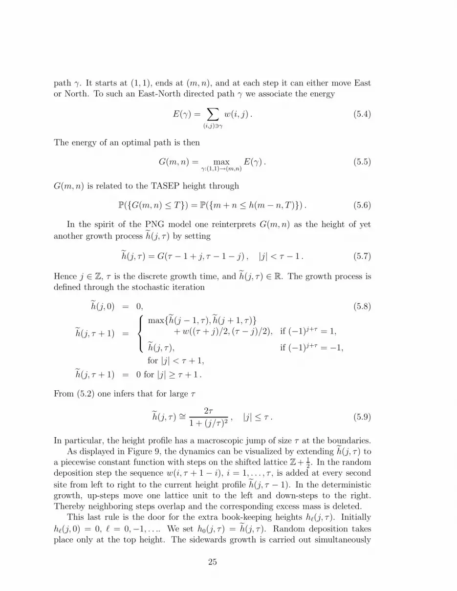
In particular, the height profile has a macroscopic jump of size τ at the boundaries.As displayed in Figure 9, the dynamics can be visualized by extending h(j, τ) to

a piecewise constant function with steps on the shifted lattice Z+ 12. In the random

deposition step the sequence w(i, τ + 1 − i), i = 1, . . . , τ , is added at every second

site from left to right to the current height profile h(j, τ − 1). In the deterministicgrowth, up-steps move one lattice unit to the left and down-steps to the right.Thereby neighboring steps overlap and the corresponding excess mass is deleted.

This last rule is the door for the extra book-keeping heights hℓ(j, τ). Initially

hℓ(j, 0) = 0, ℓ = 0,−1, . . .. We set h0(j, τ) = h(j, τ). Random deposition takesplace only at the top height. The sidewards growth is carried out simultaneously

25

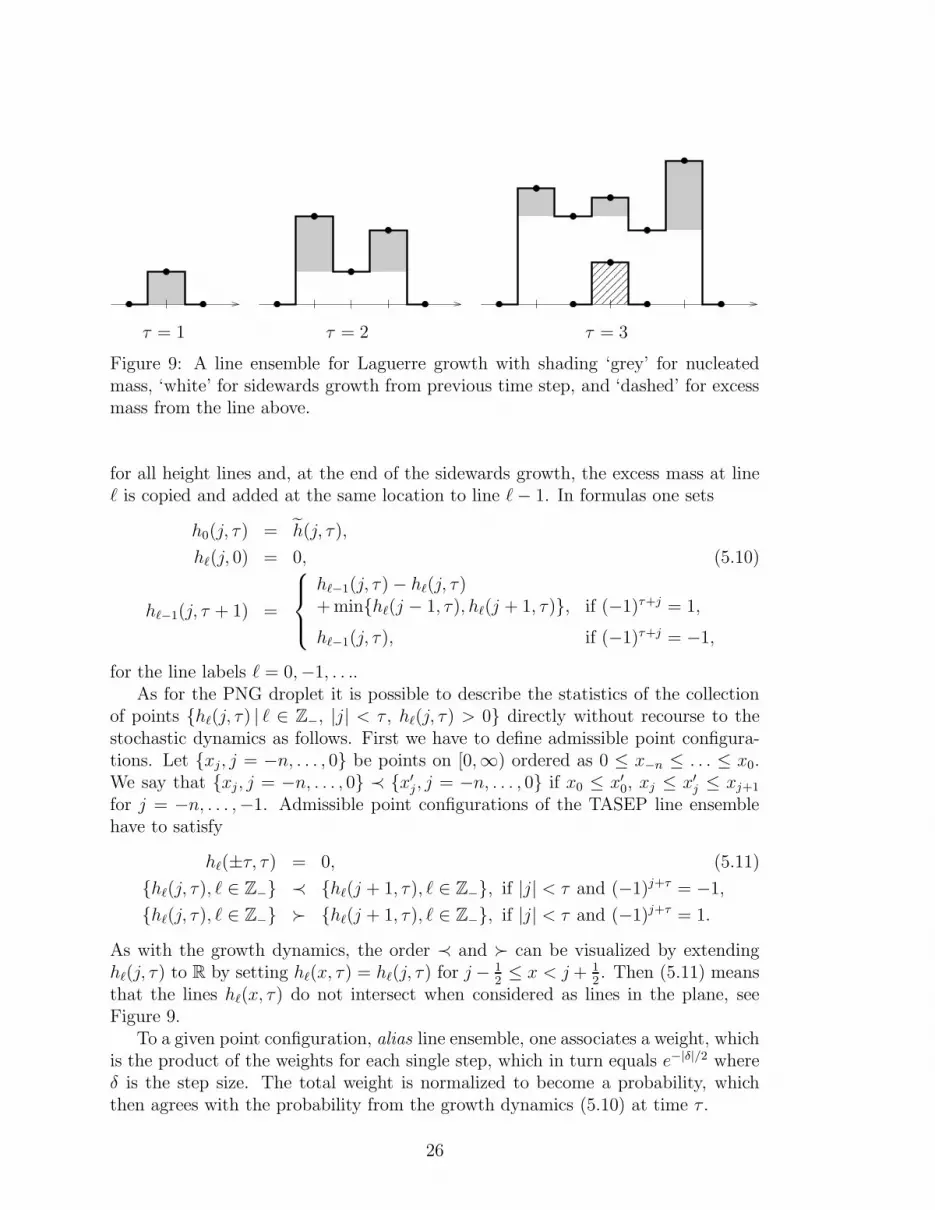
τ = 1 τ = 2 τ = 3

Figure 9: A line ensemble for Laguerre growth with shading ‘grey’ for nucleatedmass, ‘white’ for sidewards growth from previous time step, and ‘dashed’ for excessmass from the line above.

for all height lines and, at the end of the sidewards growth, the excess mass at lineℓ is copied and added at the same location to line ℓ− 1. In formulas one sets

h0(j, τ) = h(j, τ),

hℓ(j, 0) = 0, (5.10)

hℓ−1(j, τ + 1) =

hℓ−1(j, τ) − hℓ(j, τ)+ minhℓ(j − 1, τ), hℓ(j + 1, τ), if (−1)τ+j = 1,

hℓ−1(j, τ), if (−1)τ+j = −1,

for the line labels ℓ = 0,−1, . . ..As for the PNG droplet it is possible to describe the statistics of the collection

of points hℓ(j, τ) | ℓ ∈ Z−, |j| < τ , hℓ(j, τ) > 0 directly without recourse to thestochastic dynamics as follows. First we have to define admissible point configura-tions. Let xj, j = −n, . . . , 0 be points on [0,∞) ordered as 0 ≤ x−n ≤ . . . ≤ x0.We say that xj, j = −n, . . . , 0 ≺ x′j , j = −n, . . . , 0 if x0 ≤ x′0, xj ≤ x′j ≤ xj+1

for j = −n, . . . ,−1. Admissible point configurations of the TASEP line ensemblehave to satisfy

hℓ(±τ, τ) = 0, (5.11)

hℓ(j, τ), ℓ ∈ Z− ≺ hℓ(j + 1, τ), ℓ ∈ Z−, if |j| < τ and (−1)j+τ = −1,

hℓ(j, τ), ℓ ∈ Z− ≻ hℓ(j + 1, τ), ℓ ∈ Z−, if |j| < τ and (−1)j+τ = 1.

As with the growth dynamics, the order ≺ and ≻ can be visualized by extendinghℓ(j, τ) to R by setting hℓ(x, τ) = hℓ(j, τ) for j − 1

2≤ x < j+ 1

2. Then (5.11) means

that the lines hℓ(x, τ) do not intersect when considered as lines in the plane, seeFigure 9.

To a given point configuration, alias line ensemble, one associates a weight, whichis the product of the weights for each single step, which in turn equals e−|δ|/2 whereδ is the step size. The total weight is normalized to become a probability, whichthen agrees with the probability from the growth dynamics (5.10) at time τ .

26

To the line ensemble one associates the point process

ητ (y, j) =∑

ℓ≤0

δ(hℓ(j, τ) − y) , y > 0 , (5.12)

where j ∈ Z refers to time and y ∈ R+ to space. According to our construction, aty = 0 there are an infinite number of points. The point process ητ refers howeveronly to points with a strictly positive y coordinate. ητ is determinantal with acorrelation kernel Rτ , which is displayed in Proposition 3.3 of [16]. For j = 0,τ = 2m+ 1, the correlation kernel simplifies to

Rτ (0, y; 0, y′) = KL

m(y, y′) , (5.13)

where KLm is the Laguerre kernel of order m. In terms of the standard Laguerre

polynominals Ln of order 0, see [1], it is defined through

KLm(y, y′) =

m−1∑

n=0

Ln(y)Ln(y′)e−y/2e−y′/2 . (5.14)

In analogy, the line ensemble hℓ(j, τ) , ℓ ∈ Z− , j ∈ Z is called the Laguerre lineensemble.

Not to our surprise we have found again a disordered and an ordered zone sep-arated by the line (5.9) on the macroscopic scale. Only in this growth model thelower border is trivially the line y = 0.

There are two obvious questions.

(1) Could one choose for w(i, j) a distribution which is different from the exponen-tial without losing the determinantal property? One can, but the only admissiblemodification is w(i, j) to have a geometric distribution, P(w(i, j) = n) = (1 − q)qn,0 < q < 1, n ∈ N, compare with example (iv) of the addendum to Section 2. Notethat thereby one has constructed a family of growth models, mostly referred to asdiscrete time TASEP, which interpolate between PNG and TASEP. In the limit ofrare events, q → 0, the w(i, j) turn into a Poisson process on R

2+ with constant

intensity, while for q → 1, and proper rescaling, the geometric distribution turnsinto the exponential one.

(2) Assuming that w(i, j) is exponential, is it required that they all have the samemean? In fact not, but the determinantal property requires a product structure.More concretely, we assume that w(i, j) are independent exponentials with mean〈w(i, j)〉 = (aij)

−1. Then it is required that

aij = ai + bj > 0 . (5.15)

Before we discussed the special case ai = 12, bj = 1

2. Our construction of the line

ensemble can be repeated in general, only the weights of the line ensemble have tobe modified. The up-steps are ordered from right to left and the j-th up-step hasweight e−aj |δ|, δ the step size, while the down-steps are ordered from left to rightwith the j-th down-step having weight e−bj |δ|.

27

6 Random matrices and Dyson’s Brownian mo-

tion

Random matrices is the most unlikely, and at first sight unexpected, item in our list.In retrospect the dynamic exponent z = 3/2 of the KPZ equation in one dimension isthe “same” as the exponent 1/2 for the edge of the density of states according to theWigner semicircle law. A clear evidence for the link was established by Johansson[21]. He proved that, in the droplet geometry, the TASEP height above the originhas a scaling function given by the Tracy-Widom distribution, which was obtainedprior by Tracy and Widom [44] as the scaling function for the location of the largesteigenvalue of the Gaussian unitary ensemble (GUE). Historically, it was a big riddlewhy the same scaling function appears in such a diverse context. Our resolutionis on the mathematical side. Largest eigenvalue and height above the origin resultfrom the edge scaling of a determinantal space-time process.

The GUE of random matrices is a Gaussian probability distribution for N ×Ncomplex hermitian matrices defined through

Z−1N exp[−trA2/2N ] . (6.1)

Here A = A∗ is a N×N complex hermitian matrix. (6.1) is understood as a densityrelative to the flat measure dA on the independent coefficients of A,

dA =N∏

i=1

dAii

∏

1≤i<j≤N

dR(Aij)dI(Aij) , (6.2)

and ZN is the normalizing partition function. In convential random matrix theorythe factor 1/2N in the exponential is taken to be 1. Our units are such that thetypical spacing between eigenvalues is of order 1, in accordance with our previous ex-amples of point processes. Let λ1, . . . , λN be the eigenvalues of A. As a consequenceof (6.1) their joint probability density is given by

Z−1N |∆N (λ)|2

N∏

j=1

e−λ2j/2N (6.3)

with the Vandermonde determinant

∆N(λ) = det((λi)j−1)1≤i,j≤N =

∏

1≤i<j≤N

(λj − λi) . (6.4)

We regard λ1, . . . , λN as point process by setting

ηN(x) =N∑

j=1

δ(x− λj) . (6.5)

28

ηN(x) is determinantal with correlation kernel given by the Hermite kernel (2.24)with t = 2N .

To make contact with line ensembles one has to advance from the static dis-tribution (6.1) to dynamics. A natural candidate is the linear Langevin equation,

d

dtA(t) = − 1

2NA(t) + B(t) , (6.6)

where B(t) is N × N complex hermitian matrix-valued Brownian motion. To say,B(0) = 0, 〈B(t)〉 = 0, and Bij(t) are complex-valued Gaussian processes withBij(t)

∗ = Bji(t) and independent increments,

〈Bij(s)Bi′j′(t)∗〉 = δ(t− s)δii′δjj′ , (6.7)

i, j, i′, j′ = 1, . . . , N . Clearly, if in (6.6) A(0) is Gaussian, then so is A(t).The stationary distribution for (6.6) is the GUE probability measure (6.1). Thus

a natural choice is to consider the stationary process for (6.6). The eigenvaluesλ1(t), . . . , λN(t) of A(t) never intersect and form a determinantal line ensemble withcorrelation kernel

RN(x, t; x′, t′) =

〈x|e−tHNPNe

t′HN |x′〉 for t ≥ t′ ,

−〈x|e−tHN (1 − PN)et′HN |x′〉 for t < t′ .(6.8)

Here HN is the harmonic oscillator Hamiltonian with frequency 1/2N ,

HN =1

2

(− d

dx2+

1

(2N)2x2 − 1

2N

)(6.9)

and PN is the Hermite kernel, i.e., PN is the projection onto the first N eigenstatesof HN .

As in the previous models, the same line ensemble can be constructed statically.One starts with N independent Ornstein-Uhlenbeck processes governed by

d

dtyj(t) = − 1

2Nyj(t) + bj(t) , (6.10)

j = 1, . . . , N , with bj(t) , j = 1, . . . , N a collection of N independent white noises.In the time window t ∈ [−τ, τ ] one conditions on the yj(t)’s not to intersect. The

resulting process is denoted by y(τ)j (t). Taking the limit τ → ∞ one arrives at the

by construction stationary diffusion process y(∞)j (t) , j = 1, . . . , N , t ∈ R. It is

indeed determinantal with correlation kernel (6.8).From the perspective of the PNG droplet, stationarity looks unnatural. Closer

to PNG would be the watermelon ensemble from Section 2. In terms of randommatrices one sets

A(t) = B(t) − t

TB(T ) , (6.11)

i.e., each matrix element is a Brownian bridge, in particular A(0) = 0 = A(T ). Theeigenvalues λ1(t), . . . , λN(t) of A(t) are determinantal with correlation kernel (2.28).

29

7 Boundary sources

From the perspective of growth processes the method developed so far has twodrawbacks. Firstly, while we have rather concise formulas for spatial correlationsat fixed growth time T , there is no information on correlations in growth time.This limitation is intrinsic, since the line ensemble is constructed separately for eachT . Secondly, one can allow only for very special initial conditions which result insurfaces with a nonvanishing macroscopic curvature. While there is some interest,for example the Eden growth starting from a single seed builds up an essentiallycircular shape, in most computer simulations the initial condition is a flat surface,which then stays flat on average.

The restriction to curved profiles can be overcome, at least partially throughthe method of boundary sources, which covers several cases of interest. Boundarysources can be introduced for PNG, TASEP, and GUE. To avoid repetition weexplain only the PNG model, which happens to be the most transparent case. Moredetails are provided in the recent survey [13]. The flat initial height has been resolvedonly recently [40], see also [10, 17]. It is tricky with extra ideas and therefore slightlyoutside this overview.

We start with the PNG droplet, as explained in Section 4, and add additionalnucleation events at the two borders of the sample, i.e., at x = ±T . The sourcesare Poisson in time with left rate α− and right rate α+. Clearly, the sources willmodify the macroscopic shape. But this is not yet on the agenda. Rather, wewant to understand how the extra sources modify the line ensemble. Switching tothe directed polymer, the sources generate additional nucleation events on the linev = 0 with the intensity α+ and on the line u = 0 with the intensity α−.In the discrete setting, see Section 5, the exponential random variables would bemodified such that 〈w(i, 1)〉 = α+, 〈w(1, j)〉 = α−, and 〈w(i, j)〉 = 1 otherwise.

Note that this modification respects the product form, if the vectors ~a, ~b are alteredonly in their first entry from 1

2to a1 = α−1

+ − 12, b1 = α−1

− − 12. Hence 〈w(1, 1)〉 =

(α+ + α− −α+α−)/α+α−. Taking the limit of rare events we conclude that the lineensemble for the PNG model with boundary sources is still determinantal, providedthere is an extra nucleation event at (0, 0) with geometric weight of parameter α+α−.

A further, physically natural choice would be to place a single source with inten-sity β at x = 0. In terms of the directed polymer there are now additional Poissonpoints along the diagonal u = v, which should be viewed as a random pinningpotential. For large β the directed polymer stays order 1 close to the diagonal. Anydeviation would be too costly energy-wise. As β is decreased there will be longerand longer excursions away from the diagonal until the critical point βc, when thedirected polymer depins. It is conjectured that βc = 0 [20, 7], but there are coun-terclaims mostly based on numerical simulations of the TASEP [18]. Unfortunatelythe source at x = 0 is not covered by our methods, since it does not respect theproduct structure. To have a determinantal line ensemble one can allow for a generalintensity ρ(u, v) of nucleation events provided it is of the form ρ(u, v) = ρ+(u)ρ−(v),

30

which can be satisfied for the boundary sources but not for the centered source.For the PNG model with boundary sources the line ensemble hℓ(x, T ), ℓ =

0,−1, . . ., |x| ≤ T is constructed according to the rules of Section 4. Since thesource is in operation only for h0, one still has hℓ(±T, T ) = ℓ, ℓ = −1,−2, . . ..If h0(±T, T ) = n±, then the corresponding weight is (α+)n+(α−)n−. This looksdiverging for α+, α− ≥ 1. However the up-steps and down-steps still carry a dxvolume element. Since they are ordered, one obtains a factor 1/n! in the partitionfunction which makes the total weight finite for all α+, α− ≥ 0.

We do not provide the details for computing the correlation kernel, see [16] forthe TASEP. There is however one element which we want to point out. In thefermion formalism one has a product of transfer matrices, e−tG, and a few numberoperators, like a∗(j)a(j), sandwiched between the right and left vectors Ω+,Ω−.If α+ = α− = 0, the boundary conditions are hℓ(±T, T ) = ℓ which translate toΩ+ = Ω, Ω− = Ω, where Ω is the state with sites j ≤ 0 occupied and sites j > 0empty. If α+ > 0, then only the right end point of the top line h0 is lifted upwards.Thus the boundary state becomes

Ω+ = a∗(ψ+)Ω , a∗(ψ) =∑

j∈Z

ψja∗(j) , ψ+

j = (α+)j , (7.1)

correspondingly for −, where Ω is the state with sites j < 0 occupied and sites j ≥ 0empty. For the PNG model the generator G is the second quantization of nearestneigbor hopping, which implies that

e−tGa∗(ψ+)etG = et(α++α−1+ )a∗(ψ+) . (7.2)

Hence the boundary creation operator can be moved from the border to the numberoperator a∗(j)a(j).

Let us illustrate this simplification by computing the correlation kernel Rα+,α−

at t = 0. From Section 4 we know that for α+ = 0 = α−

R0,0(j, j′) = BT (j, j′) (7.3)

with BT the Bessel kernel. In general one has to compute expectations of the form

Z−1〈Ω|e−TGa(ψ−)

m∏

k=1

a∗(jk)a(jk)a∗(ψ+)e−TG|Ω〉F ,

Z = 〈Ω|e−TGa(ψ−)a∗(ψ+)e−TG|Ω〉F . (7.4)

This results in a determinantal point process with correlation kernel

Rα+,α−(j, j′) = BT (j, j′)

+(α+α−〈ψ−|(1 −BT )|ψ+〉

)−1((1 −BT )ψ−)j((1 − BT )ψ+)j′ . (7.5)

31

The boundary sources modify the correlation kernel through a one-dimensional pro-jection operator. Thus computationally the resulting difficulties are increased onlyslightly.

Even without computation one can guess typical configurations of the line en-semble. To compute h0(±T, T ) in terms of the directed polymer, it has to reach(2T, 0), resp. (0, 2T ). Therefore h0(±T, T ) ≃ α±T . For the line with label −1, justbelow the top line, we need the extra information on how h−1(x, T ) translates to thedirected polymer. It turns out that for h0(x, T ) + h−1(x, T ) one needs to considertwo directed polymers, both starting at (0, 0) and ending at (x + T, x − T ). Theyare required to visit disjoint Poisson points. Then

h0(x, T ) + h−1(x, T ) = maxγ1 6=γ2

γ1:(0,0)→(x+T,x−T )γ2:(0,0)→(x+T,x−T )

(E(γ1) + E(γ2)

). (7.6)

An according formula holds for h0(x, T ) + . . . + hℓ(x, T ). If x is near ±T , thesecond directed polymer has almost no Poisson points to visit. Thus h−1(x, T ) ≃2T (1 − (x/T )2)1/2 and the lines with ℓ ≤ −1 form a disordered zone as before.If α+, α− are small, then h0(x, T ) will follow closely h−1(x, T ) in such a way asto join tangentially the droplet. On the other hand for α+, α− large, h0(x, T ) ≃((α+−α−)x+(α+ +α−)T )/2. Clearly the most intriguing case occurs when h0(x, T )is still a line segment but touches tangentially the droplet. At the touching point,x = xm, h(xm, T ) is expected to have unusual fluctuations. In the picture of thedirected polymer, it chooses either one of the two boundaries and the fluctuationsfrom the boundary portions are comparable in size to the ones coming from thebulk. Such fluctuation properties are studied for PNG in [39] and for the TASEPin [16].

8 Edge scaling

For growth processes the physical height corresponds to the top line of the lineensemble. Similarly, the facet edge of the Ising corner is encoded by the top gradientline, see Figure 6. Thus our task is to understand the statistical properties of h0. Themost basic information is the size of typical fluctuations of h0 for large T , whichdefines the scaling exponents, and more precisely the scale invariant probabilitydistributions for large T , which defines the scaling functions. Of course, the hopeis that these quantities do not depend on the details of the line ensemble and thusare valid for all line ensembles discussed so far. This is not so unlikely, since the topline has a lot of space for fluctuations, which tend to wash out microscopic details.As guiding example serves a general step random walk, which on a large scale lookslike Brownian motion with the variance of the step distribution retained as onlyinformation on the random walk. Even more ambitiously we expect that, e.g., inthe case of growth models, the scaling exponents and the scaling functions computed

32

here are valid for all growth models in the KPZ universality class. This is in completeanalogy to critical phenomena, where models fall into distinct universality classes.As a rather common feature, concrete computations can be carried out only for onespecific member of a class.

The finite T , resp. finiteN , line ensemble is determinantal. If we consider T → ∞and focus our attention on a domain close to the edge, the line statistics there mustbe still determinantal. In other words, we only have to study the limit T → ∞ ofthe correlation kernel with an appropriate scaling of its arguments. Through thedeterminantal property one deduces the limiting probability distributions from thelimiting correlation kernel.

To illustrate how the scheme works let us consider the PNG model in the dropletgeometry. The starting point is the discrete Bessel kernel (4.4) which is the projec-tion onto all negative energy states of hT from (4.3). For simplicity let us study thedroplet close to x = 0. Then 〈h(0, T )〉 = 2T for large T and in the line ensemble weconsider the window j = 2T + yT β and t = τT α with y, τ of order one and α, β tobe determined. Inserting in (4.4) and switching to the variable y one arrives at

(hTψ)(y) = −ψ(y + T−β) − ψ(y − T−β) +1

T(2T + yT β)ψ(y) . (8.1)

To have a limit one must set

β =1

3(8.2)

and obtains for T → ∞

T 2/3hTψ(y) =(− d2

dy2+ y

)ψ(y) . (8.3)

Thus under edge scaling T 2/3hT goes over to the Airy operator

HAi = − d2

dy2+ y . (8.4)

The Airy operator has R as spectrum with the Airy function Ai as generalizedeigenfunctions

HAiAi(y − λ) = λAi(y − λ) , (8.5)

see [1]. In particular the projection onto the eigenstates with negative energies isthe Airy kernel

KAi(y, y′) =

∫ ∞

0

dλAi(y + λ)Ai(y′ + λ) . (8.6)

As established with rigor in [38], one concludes that

limT→∞

T 1/3BT ([2T + yT 1/3], [2T + y′T 1/3]) = KAi(y, y′) (8.7)

pointwise.

33

To have the extended kernel, see (4.6), one needs the scaling limit of e−tg witht = τT α. Since by the argument above the spatial scale is fixed as T 1/3, one infers

α = 23, exp[−tg] ∼= exp[τ(d2/dy2)] . (8.8)

While the value for α is correct, the complete asymptotic analysis shows that thetime propagation is governed by the Airy operator,

limT→∞

T 1/3BT

([2T + T 1/3(y − τ 2)] , T 2/3τ ; [2T + T 1/3(y′ − τ ′2)] , T 2/3τ ′

)

=

〈y|e−τHAiKAie

τ ′HAi|y′〉 for τ ≥ τ ′ ,

−〈y|e−τHAi(1 −KAi)eτ ′HAi|y′〉 for τ < τ ′

= KAi(y, τ ; y′, τ ′) . (8.9)

The right hand side of (8.9) is the extended correlation kernel of a determinantalprocess, which we denote by ξ(y, τ). ξ(y, τ) for fixed τ is concentrated on a discreteset of points, whose density vanishes as

〈ξ(y, τ)〉 =17

96πy−1/2 exp[−4y3/2/3] (8.10)

for y → ∞ and increases as

〈ξ(y, τ)〉 ≃ 1

π|y|1/2 − 1

4π|y| cos(4|y|3/2/3) (8.11)

for y → −∞. As a function of τ , ξ(y, τ) is concentrated on non-intersecting contin-uous lines, i.e.,

ξ(y, τ) =0∑

j=−∞

δ(y − yj(τ)

)(8.12)

with τ 7→ yj(τ) continuous. Since [HAi, KAi] = 0, ξ(y, τ) and the yj(τ)’s are stochas-tic processes stationary in τ .

The convergence in (8.9) to the extended kernel carries over to the convergenceof the height h(x, T ) of the PNG droplet. One infers that

limT→∞

T−1/3(h(τT 2/3, T ) − 2T

)= y0(τ) − τ 2 . (8.13)

Since Airy functions are all over, y0(τ) is baptized as Airy process [38] and denoted byA(τ). Some of its properties will be discussed in Section 9. At the moment we recallthat τ refers to physical space and T to growth time. h(0, T ) increases linearly andhas fluctuations of size T 1/3. In the spacial domain of size τT 2/3 the height statisticsis governed by the Airy process plus a systematic downward bending as −τ 2. Sincethe propagator on the right hand side of (8.9) and the static kernel are given throughHAi, the process A(τ) is stationary. This is physically quite reasonable. In every

34

small region of the droplet one has the same fluctuation statistics, provided the localcurvature (and possibly linear pieces) are properly subtracted.

For the Ising corner one also obtains the Airy process for edge fluctuations, asanticipated. But no simple short cut as for PNG seems to be available.

It is instructive to repeat the heuristic PNG argument for stationary Dyson’sBrownian motion (6.6). The confining potential is V (x) = x2/2N , which translatesto the potential U(x) = (x/2N)2/2 on the level of the Hamiltonian HN , see (6.9).Its first N levels are filled up which yields the Fermi energy EF = 1/2. The largesteigenvalue of Dyson’s Brownian motion is determined by balancing potential andFermi energy. Hence

U(λ1) = EF , i.e., λ1 = 2N , (8.14)

which is in agreement with the Wigner semicircle law asserting the asymptotic den-

sity of states as π−1(1− (x/2N)2

)1/2, |x| ≤ 2N . The determinantal process close to

the edge is governed by the Hamiltonian (6.9) linearized at λ1, i.e., by

Hl = −1

2

d2

dx2+

1

2Nx . (8.15)

Scaling as in (8.1), one concludes that β = 1/3. The time direction has correlationson the scale N2/3. By stationarity of Dyson’s Brownian motion, the edge eigenvaluesare thus governed by (8.9) in the scaling limit N → ∞.

If instead of the potential 12x2 we choose some other potential V (x), the GUE

generalizes to

Z−1N exp

[−Ntr(V (A/N))

], (8.16)

where V is taken as even polynomial with positive leading coefficient. As before,the distance between eigenvalues is of order 1. (6.6) becomes

d

dtA(t) = −1

2V ′(A/N) + B(t) (8.17)

and (6.9) is modified to

HN = −1

2

d2

dx2+ UN (x/N) . (8.18)

UN has to be chosen such that V = − logψg, where ψg is the ground state of HN . UN

depends only weakly on N . For the construction of the determinantal process onefills the first N levels of HN , which results in a Fermi energy EF = O(1). The edge,xe, is determined through U(xe/N) = EF. If U ′(xe) 6= 0, then the edge statistics isgoverned by the Airy operator. It may happen that U ′(xe) = 0, but U ′′(xe) 6= 0,say. Then the edge statistics changes and is governed by the Pearcey process, see[45] for a detailed study.

35

β = 1β = 2β = 4

s

F′ β(s

)

0

0.1

0.2

0.3

0.4

0.5

0.6

−6 −4 −2 0 2 4

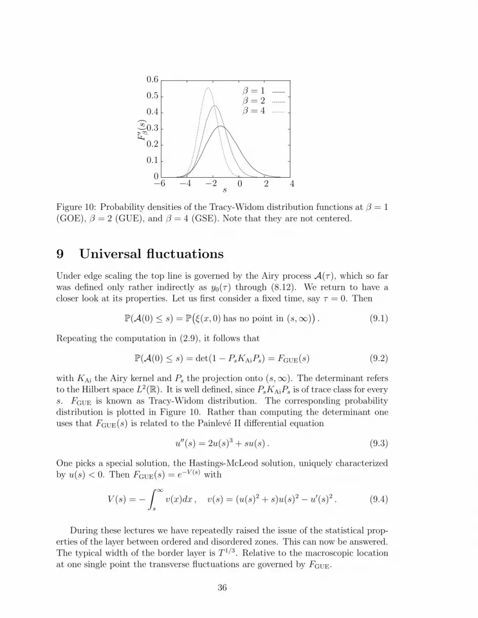
Figure 10: Probability densities of the Tracy-Widom distribution functions at β = 1(GOE), β = 2 (GUE), and β = 4 (GSE). Note that they are not centered.

9 Universal fluctuations

Under edge scaling the top line is governed by the Airy process A(τ), which so farwas defined only rather indirectly as y0(τ) through (8.12). We return to have acloser look at its properties. Let us first consider a fixed time, say τ = 0. Then

P(A(0) ≤ s) = P(ξ(x, 0) has no point in (s,∞)

). (9.1)

Repeating the computation in (2.9), it follows that

P(A(0) ≤ s) = det(1 − PsKAiPs) = FGUE(s) (9.2)

with KAi the Airy kernel and Ps the projection onto (s,∞). The determinant refersto the Hilbert space L2(R). It is well defined, since PsKAiPs is of trace class for everys. FGUE is known as Tracy-Widom distribution. The corresponding probabilitydistribution is plotted in Figure 10. Rather than computing the determinant oneuses that FGUE(s) is related to the Painleve II differential equation

u′′(s) = 2u(s)3 + su(s) . (9.3)

One picks a special solution, the Hastings-McLeod solution, uniquely characterizedby u(s) < 0. Then FGUE(s) = e−V (s) with

V (s) = −∫ ∞

s

v(x)dx , v(s) = (u(s)2 + s)u(s)2 − u′(s)2 . (9.4)

During these lectures we have repeatedly raised the issue of the statistical prop-erties of the layer between ordered and disordered zones. This can now be answered.The typical width of the border layer is T 1/3. Relative to the macroscopic locationat one single point the transverse fluctuations are governed by FGUE.

36

The Tracy-Widom distribution was first established in the context of randommatrix theory [44]. It then appeared in a, at first sight purely combinatorial prob-lem, namely Ulam’s problem, which poses the question to determine the length ofthe longest increasing subsequence of a random permutation [4], see also [3] for asurvey. In fact, this problem is identical to the height h(0, T ) of the PNG model.To understand the connection let us return to the directed polymer, see end of Sec-tion 4, with starting point (0, 0) and end point (T, T ). Let ω = (ω1, . . . , ωn) be arealization of Poisson points in [0, T ]2. We label their 1-coordinates, xj , in increas-ing order. Labeling their 2-coordinates, yj, also in increasing order yields ω =((x1, yσ(1)), . . . , (xn, yσ(n))) and thus a permutation (σ(1), . . . , σ(n)) of (1, . . . , n).

Clearly, n is distributed as (n!)−1T 2ne−T 2

and for prescribed n every permutationhas the same probability. For given permutation σ we define ℓT as the length of itslongest increasing subsequence, e.g., the permutation (6, 2, 5, 1, 4, 8, 7, 3) has ℓT = 3.From the geometry of the directed polymer it follows that ℓT = e(T, T ), see (4.8),and hence ℓT = h(0, T ). Thus objects from random matrix theory made their ap-pearance in growths problems first through the height above the origin in the PNGmodel [36] and independently for the TASEP [21], both in continuous and discretetime.

More ambitiously, we step to several space points of the PNG droplet for largeT , which means several fermionic times, τ1 < . . . < τm, for the Airy process andconsider

P(A(τ1) ≤ s1, . . . ,A(τm) ≤ sm)

= P(ξ(xj, τj) has no points in (sj,∞) , j = 1, . . . , m

). (9.5)

Let KAi be the extended Airy kernel of (8.9) and consider

θ(y − si)KAi(τi, y; τj, y′)θ(y − sj) = Aij(y, y

′) (9.6)

as a kernel in L2(R) ⊗ Cm. Then, again by repeating the computation leading to(2.9),

P(A(τ1) ≤ s1, . . . ,A(τm) ≤ sm) = det(1 − A) . (9.7)

Even form = 2 the determinant in (9.7) cannot be computed in the simple form as in(9.3) and (9.4), see however [2, 47], and to extract information requires considerableeffort.

Physically the most robust information is the two-point function

C(τ) = 〈(A(τ) −A(0)

)2〉 . (9.8)

For small τ Brownian motion dominates and

C(τ) = 2|τ |, for τ → 0 . (9.9)

For large τ one finds a decay as |τ |−2. In [2, 47] partial differential equations forthe multi-time distributions of (9.7) are derived, which can be thought of as a

37

generalization of (9.3). As one consequence

C(τ) = 2a2 − 2|τ |−2 , τ ≫ 1 , (9.10)

with a2 = 0.813... the variance of FGUE.

10 What have we learned?

One-dimensional growth models in the KPZ universality class. We have recoveredthe dynamical exponent z = 3/2, which comes hardly as a surprise, since it iswell established through theoretical arguments and Monte-Carlo simulations. Novelis the computation of scaling functions along with the insight that they dependon the geometry of the growth process [37]. If there is a non-zero curvature onthe macroscopic scale, the height fluctuations are governed by the GUE Tracy-Widom distribution. On the other hand for a macroscopically flat surface, thescaling function depends on how flat the surface is prepared initially. The flatsurface, no fluctuations at all initially, has a scaling function different from a surfacewhere initially the height differences are shortly correlated [38, 40]. It may happenthat a flat piece of the surface joins a curved one. The height fluctuations preciselyat the junction are governed by yet another scaling function. If the surface is semi-infinite, bordered by a hard wall, the scaling function changes [19]. In this way onerealizes the GOE and GSE random matrix edge scaling distributions, see Figure 10,and many more.

Facet edge. In the scaling limit the fluctuations of the facet edge are identical to thefluctuations in a growth process with rounded profile. The linear size of the facettakes here the role of the growth time T . As argued in [14], the Ising model withvolume constraint and at a temperature below roughening should have the samefacet edge fluctuations. In fact any model with short range interactions and a non-zero facet edge curvature is expected to be in the universality class discussed here.There are other surface models which are still determinantal and exhibit facets inequilibrium [33, 31]. To establish that their fluctuation properties are determinedby GUE random matrix theory remains as a task for the future.

References

[1] M. Abramowitz and I.A. Stegun, Pocketbook of Mathematical Functions, Ver-lag Harri Deutsch, Thun-Frankfurt am Main, 1984.

[2] M. Adler and P. van Moerbeke, PDEs for the joint distributions of the Dyson,Airy and Sine processes, Ann. Probab. 33, 1326–1361 (2005).

[3] D. J. Aldous and P. Diaconis, Longest increasing subsequences: from patiencesorting to the Baik-Deift-Johansson theorem, Bull. Amer. Math. Soc. 36, 413–432 (1999).

38

[4] J. Baik, P.A. Deift, and K. Johansson, On the distribution of the length of thelongest increasing subsequence of random permutations, J. Amer. Math. Soc.12, 1119–1178 (1999).

[5] J. Baik and E.M. Rains, Limiting distributions for a polynuclear growth modelwith external sources, J. Stat. Phys. 100, 523–542 (2000).

[6] R.J. Baxter, Exactly Solved Models in Statistical Mechanics, Academic Press,London, 1982.

[7] V. Beffara, V. Sidoravicius, H. Spohn, and M.E. Vares, Polymer pinning as aninfluence percolation problem, to be published in IMS Lecture Notes - Mono-graph Series.

[8] J. Cardy, SLE for theoretical physicists, arXiv:cond-mat/0503313.

[9] R. Cerf and R. Kenyon, The low-temperature expansion of the Wulff crystal inthe 3D-Ising model, Comm. Math. Phys. 222, 147–179 (2001).

[10] P. Ferrari, Polynuclear growth on a flat substrate and edge scaling of GOEeigenvalues, Comm. Math. Phys. 252, 77–109 (2004).

[11] P. Ferrari, Shape fluctuations of crystal facets and surface growth in one di-mension, Ph. D. thesis, TU Munchen, 2004, available athttp://tumb1.ub.tum.de/publ/diss/ma/2004/ferrari.html.

[12] P. Ferrari, private communication, 2005.

[13] P. Ferrari and M. Prahofer, One-dimensional stochastic growth and Gaussianensembles of random matrices, arXiv:math-ph/0505038.

[14] P. Ferrari, M. Prahofer, and H. Spohn, Fluctuations of an atomic ledge border-ing a crystalline facet, Phys. Rev. E 69, 035102(R) (2004).

[15] P. Ferrari and H. Spohn, Step fluctuations for a faceted crystal, J. Stat. Phys.113, 1–46 (2003).

[16] P. Ferrari and H. Spohn, Scaling limit for the space-time covariance of thestationary totally asymmetric simple exclusion process, to appear in Comm.Math. Phys., arXiv:math-phys/0504041.

[17] P. Ferrari and H. Spohn, A determinantal formula for the GOE Tracy-Widomdistribution, J. Phys. A 38, L557–L561 (2005).

[18] M. Ha, J. Timonen, and M. den Nijs, Queuing transitions in the asymmetricsimple exclusion process, Phys. Rev. E 68, 056122–056132, (2003).

39

[19] T. Imamura and T. Sasamoto, Fluctuations of a one-dimensional polynucleargrowth model in half space, J. Stat. Phys. 115, 749–803 (2004).

[20] S. Janowsky and J.L. Lebowitz, Exact results for the asymmetric simple exclu-sion process with a blockage, J. Stat. Phys. 77, 35–51 (1994).

[21] K. Johansson, Shape fluctuations and random matrices, Comm. Math. Phys.209, 437–476 (2000).

[22] K. Johansson, Non-intersecting paths, random tilings, and random matrices,Prob. Theor. Rel. Fields 123, 225–280 (2002).

[23] K. Johansson, Discrete polynuclear growth and determinantal processes,Comm. Math. Phys. 242, 277–329 (2003).

[24] K. Johansson, The arctic circle boundary and the Airy process, Ann. Probab.33, 1-30 (2005).

[25] K. Johansson, Random matrices and determinantal processes,arXiv:math-phys/0510038.

[26] M. Kardar, G. Parisi, and Y.Z. Zhang, Dynamic scaling of growing interfaces,Phys. Rev. Lett. 56, 889–892 (1986).

[27] S. Karlin and G. McGregor, Coincidence probabilities, Pacific J. Math. 9, 1141–1164 (1959).

[28] P. Kasteleyn, Graph theory and crystal physics, Graph Theory and TheoreticalPhysics, pp. 43–110, Academic Press, London, 1967.

[29] M. Katori and H. Tanemura, Symmetry of matrix-valued stochastic processesand noncolliding diffusion particle systems, J. Math. Phys. 45, 3058–3085(2004).

[30] R. Kenyon, Dominos and the Gaussian free field, Ann. Probab. 29, 1-30 (2001)

[31] R. Kenyon, A. Okounkov, and S. Sheffield, Dimers and amoebae, Ann. Math.,to appear (2005), arXiv:math-phys/0311005.

[32] E.H. Lieb and F.Y. Wu, Two dimensional ferroelectric models, in: Phase Tran-sitions and Critical Phenomena, C. Domb and N.S. Green eds, Vol. 1, pp.331-490, Academic Press, London, 1972.

[33] B. Nienhuis, H.J. Hilhorst, and H.W.J. Blote, Triangular SOS models and cubic-crystal shapes, J. Phys. A 17, 3559–3581 (1984).

[34] V.L. Pokrovsky and A.L. Talapov, Ground state, spectrum, and phase diagramof two-dimensional incommensurate crystals, Phys. Rev. Lett. 42, 65–68 (1978).

40

[35] M. Prahofer, Stochastic surface growth, Ph. D. thesis, LMU Munchen, 2003,available at http://edoc.ub.uni-muenchen.de/archive/00001381.

[36] M. Prahofer and H. Spohn, Statistical self-similarity of one-dimensional growthprocesses, Physica 279, 342–352 (2000).

[37] M. Prahofer and H. Spohn, Universal distributions for growth processes in 1+1dimension and random matrices, Phys. Rev. Lett. 84, 4882–4885 (2000).

[38] M. Prahofer and H. Spohn, Scale invariance of the PNG droplet and the Airyprocess, J. Stat. Phys. 108, 1071–1106 (2002).

[39] M. Prahofer and H. Spohn, Exact scaling function for one-dimensional station-ary KPZ growth, J. Stat. Phys. 115, 255–279 (2002).

[40] T. Sasamoto, Spatial correlations of the 1D KPZ surface on a flat substrate, J.Phys. A 38, L549–L556 (2005).

[41] T.D. Schultz, D.C. Mattis, and E.H. Lieb, Two-dimensional Ising model as asoluble problem of many fermions, Rev. Mod. Phys. 36, 856-871 (1964).

[42] A. Soshnikov, Determinantal random point fields, Russian Math. Surveys 55,923–975 (2000).

[43] J.R. Stembridge, Nonintersecting paths, Pfaffians, and plane partitions, Adv.in Math. 83, 96–131 (1990).

[44] C.A. Tracy and H. Widom, Level-spacing distributions and the Airy kernel,Comm. Math. Phys. 159, 151–174 (1994).

[45] C. Tracy and H. Widom, The Pearcey process, Comm. Math. Phys., to appear,(2005).

[46] J. Villain and P. Bak, Two-dimensional Ising model with competing interac-tions: floating phase, walls and dislocations, J. Physique 42, 657–668 (1981).

[47] H. Widom, On asymptotics for the Airy process, J. Stat. Phys. 115, 1129–1134(2004).

41