Investigation of Numerical Hydrodynamic Performance of

414 Noh Zainal Abidin et al.: Investigation of Numerical Hydrodynamic Performance of Deformable Hydrofoil (Applied on Blade Propeller)

a. Universiti Pertahanan Nasional Malaysia, Kuala Lumpur, Malaysia

e-mail: [email protected]

b. Naval Group/Ecole Centrale de Nantes, France

e-mail: ?

The hydrofoil is a hydro-lifting surface that significantly contributes to marine transportation such as a boat, ship, and submarine for its movement and maneuverability. The existing hydrofoils are in fixed-shaped National Advisory Committee for Aeronautics (NACA) profiles, depending merely on the variation of Angle of Attack (AOA) such as rudder, hydroplane, and propeller blade. This research is concerned with the deformable hydrofoil that aims at modifying its NACA profile rather than its AOA. However, there is still a lack of knowledge about designing an appropriate deformable hydrofoil. Therefore, a numerical

Investigation of Numerical Hydrodynamic Performance of Deformable Hydrofoil (Applied on Blade Propeller) Noh Zainal Abidina, Cédric Leblondb, Mohd Najib Abdul Ghani Yolhamida, Mohamad Abu Ubaidah Amir Abu Zarima, Farizha Ibrahima, Ameer Suhela

KEY WORDS ~ CFD ~ NACA ~ Numerical analysis ~ Hydrodynamic ~ Potential flow ~ Finite volume

1. INTRODUCTION

Hydrodynamic effects are the fluid interaction with the moving bodies, which is the backbone of designing the hydrofoil for marine vehicles such as ships (L.Birk, 2019). Commonly, the vessel has a rudder, propeller, and fin stabilizer that apply the advantages of hydrodynamic effects on itself. The airfoil design

This work is licensed under

doi: 10.7225/toms.v10.n02.012

Received on: ?

investigation of hydrodynamic characteristics for selected hydrofoils was conducted. After undergoing the 2D numerical analysis (potential flow method) at specific conditions, several NACA profiles were chosen based on the performance of NACA profiles. NACA 0017 was selected as the initial shape for this research before it deformed to the optimized NACA profiles, NACA 6417, 8417, and 9517. The 3D CFD simulations using the finite volume method to obtain hydrodynamic characteristics at 0 deg AOA with a constant flow rate. The mesh sensitivity and convergence study are carried out to get consistent, validated, and reliable results. The final CFD modeled for propeller VP 1304 for open water test numerically. The results found that the performance of symmetry hydrofoil NACA 0017 at maximum AOA is not the highest compared to the other deformed NACA profiles at 0 deg AOA. The numerical open water test showed that the error obtained on K.T., K.Q., and efficiency is less than 8% compared to the experimental results. It shows that the results were in good agreement, and the numerical CFD setting can be used for different deformed profiles in the future.

TRANSACTIONS ON MARITIME SCIENCE 415Trans. marit. sci. 2021; 02: 414-438

and analysis were carried out to increase lift characteristics and decrease drag characteristics as much as possible. In general, when the fluid strikes the airfoil, it results in two components of forces: one in the perpendicular direction and the other in the horizontal direction.

The vertical force represents the lifting force, while the horizontal force represents a drag force. Lift is caused by a pressure difference between the upper and lower surfaces. It is different from drag caused by pressure distribution at the leading and trailing edge (pressure drag), and viscous resistance occurred at the wall surface of the airfoil (viscous or friction drag) (Sun, Mao and Fan, 2020). Concerning this hydrodynamic potential, the deformable hydrofoil design should have the features to change the original foil's shape into the different NACA profiles. The concept can also be beneficial for other applications: dive bars of submarines and propeller blades. For instance, the ability to deform a propeller blade to maintain optimal propulsive performance for different speeds is technically fascinating.

Thus, the best possible design is formulated based on the application required. It is essential to have an accurate and trustworthy estimation of the hydrofoil performance at the design stage. Here, the CFD analysis is used to estimate the fundamental hydrodynamic characteristic, including drag, lifting, pressure distribution, vortices, and velocity profile. The disadvantages are the modeling errors occurring due to the simplified flow physics.

Thus, the CFD results need to be compared with the experimental results for validation (Seo et al., 2013).

1.1. What is Hydrofoil?

The development of marine knowledge in ship design and construction, one of the valuable inventions in the shipping industry, is the hydrofoil. Generally, a hydrofoil is a lifting surface like a foil but operated in the water (submerged) to create lift when mounted at the hull of a boat or ship. In the shipping industry, hydrofoils are mainly used for rudder, fin stabilizer, and propeller (Mahmud, 2015), while for the propeller, the blade itself uses the concept of hydrofoil to create lift, and the resultant force will generate thrust when rotating the blade (IV, 2012).

1.2. Deformable Hydrofoil

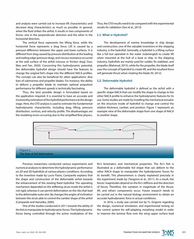
The deformable hydrofoil is defined as the airfoil with a specific shape NACA that can modify the shape to change to the other NACA profile to enhance the hydrodynamic features for its use. Some studies are made by installing the mechanical actuator on the structure inside of hydrofoil to change and control the relative thickness, camber, and position. Figure 1 represents an example view of the deformable shape from one shape of NACA to another shape.

Figure 1.The flow of foil deformation.

Previous researchers conducted various experiments and numerical analyses to determine the hydrodynamic performance on 2D and 3D hydrofoils at various physics conditions. According to the invention made by Lucio Flavio, Campanile explains that the shape and construction of the deformable airfoil towards the enhancement of the existing fixed hydrofoil. The operating mechanism depended on the stiffening struts inside the airfoil is not rigid, whereas it can permit deformation on the ribs that lead to the deformable outer skin. By changes the angles of inclination between the struts able to control the camber shape of the airfoil (Campanile and Hanselka, 2000).

One of the studies conducted in 2011 towards the ability of the fish to manipulate its hydrodynamic forces. The hydrodynamic forces being controlled through the active modulation of the

fin's kinematics and mechanical properties. The fin's fish is illustrated as a deformable foil shape that can deform to the other NACA shape to manipulate the hydrodynamic forces for its benefit. This phenomenon is clearly explained precisely in the experiment made by (Tangorra et al., 2011). As a result, the forces' magnitudes depend on the fin's stiffness and the direction of forces. Therefore, the variation in magnitude of the thrust, lift, and others components occur. Future research needs to be carried out in the natural biology environment to obtain an accurate hydrodynamic force in actual conditions.

In 2016, a study was carried out by T.L Grigorie regarding the design, numerical simulation, and experimental testing on the control system for self-adapting morphing model in order to improve the laminar flow over the wing upper surface lead


to the reduction of drag (Grigorie, Botez and Popov, 2016). Eventually, the morphing motion is successfully obtained and can be controlled for beneficial aerodynamic characteristics. Nevertheless, this study is still in progress to achieve the aim of this project: promoting large laminar regions on the wing surface, which reduces the drag.

Rediniotis et al. (2002) developed a shape-memory-alloy actuated bio-mimetic hydrofoil in order to achieve a submerged hydrofoil with high controllability. This hydrofoil shape can be deformed to different NACA shapes mimicking aquatic animals swimming to increase its performance. The numerical procedure based on the potential flow approach applied to analyze the hydrodynamic performance of the 3D NACA 4412 under the free surface was developed by Xie and Vassalos, 2007; Ghassemi, Iranmanesh, and Ardeshir, 2010; Ghassemi and Kohansal, 2013. They determined pressure distribution, lift, drag, and wave generated profiles to analyze various conditions of the 3D hydrofoil near the free surface. The hydrofoil's hydrodynamic performance was numerically studied using the Finite Volume Approach (Djavareshkian and Esmaeili, 2013).

Nowruzi, Ghassemi, and Ghiasi (2017) study the hydrodynamic performance in 2D and 3D of NACA0012, and NACA0015 hydrofoils were performed. Based on the cited works, a lack of study related to the comprehensive investigation on the hydrodynamic performance of submerged 2D and 3D hydrofoils under different geometrical and physics conditions is detectable. Besides that, CFD analysis of flow over 2D and 3D hydrofoils under different environmental and geometrical conditions has a reasonable computational cost. The CFD data for predicting hydrofoil performance with high accuracy and low computational cost. Therefore, the 2D and 3D analyses will be carried out in this research on the initial hydrofoil NACA 0017 and expected deformed shape NACA 6417, 8417, and 9517 to obtain the hydrodynamic performance and characteristic.

1.3. Application in this Project (Deformable Hydrofoil)

The hydrofoil is designed and modeled by the Fabrication and Material Department (FMD), Naval Group. The concept applied to the deformation is quite similar to Grigorie, Botez, and Popov (2016) study. However, in this project, the deformation ability was applied on the upper and lower part of hydrofoil and application of the flexible skin surface on both parts. The mechanical parts that control the deformation are the volume of compressed air injected inside the foil's vicinity and the material composite's ability for skin and middle support plate to control deformation to the specific NACA profile required.

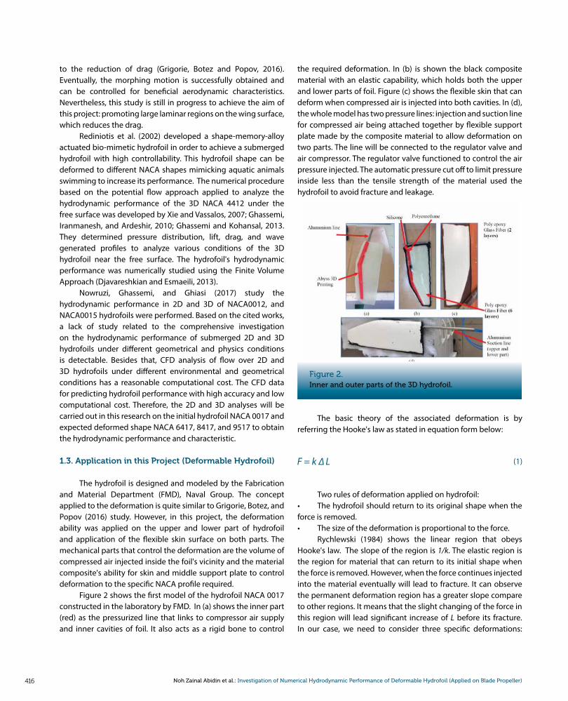
Figure 2 shows the first model of the hydrofoil NACA 0017 constructed in the laboratory by FMD. In (a) shows the inner part (red) as the pressurized line that links to compressor air supply and inner cavities of foil. It also acts as a rigid bone to control

the required deformation. In (b) is shown the black composite material with an elastic capability, which holds both the upper and lower parts of foil. Figure (c) shows the flexible skin that can deform when compressed air is injected into both cavities. In (d), the whole model has two pressure lines: injection and suction line for compressed air being attached together by flexible support plate made by the composite material to allow deformation on two parts. The line will be connected to the regulator valve and air compressor. The regulator valve functioned to control the air pressure injected. The automatic pressure cut off to limit pressure inside less than the tensile strength of the material used the hydrofoil to avoid fracture and leakage.

Figure 2.Inner and outer parts of the 3D hydrofoil.

The basic theory of the associated deformation is by referring the Hooke's law as stated in equation form below:

F = k ∆ L (1)

Two rules of deformation applied on hydrofoil:• The hydrofoil should return to its original shape when the force is removed.• The size of the deformation is proportional to the force.

Rychlewski (1984) shows the linear region that obeys Hooke's law. The slope of the region is 1/k. The elastic region is the region for material that can return to its initial shape when the force is removed. However, when the force continues injected into the material eventually will lead to fracture. It can observe the permanent deformation region has a greater slope compare to other regions. It means that the slight changing of the force in this region will lead significant increase of L before its fracture. In our case, we need to consider three specific deformations:


Table 1.The material for the structure of hydrofoil (given from FMD).

tension and compression, shear stress, and changes in volume. The others deformations explain in the form of the equation below.

∆ L = L0

σ =

ε =

∆ x = L0

∆ V = V0

(2)

(3)

(4)

(5)

(6)

1

Y

σ

Y

1

S

1

B

F

A

F

A

F

A

F

A

Equation (2) is the relationship between the deformation and the applied force. Y is Young's Modulus which depends on the material of the foil. A is the cross-sectional area, and L0 is the original length. When the material has a considerable Y value, significant tensile stiffness will have minor deformation when it exerts tension and compression. The ratio of force to the area is defined as stress measured in N/m2. The ratio of the change in length to original length is defined as strain (dimensionless). The relationship of strain with stress is presented in equation (4). The expression for shear deformation is showing in equation (5).

Where S is shear modulus, F is the force applied perpendicular to L0 and parallel surface. In our case, the foil volume will change when the compression and expansion are exerted inside the inner structure. The relationship of the change in volume to other physics quantities is stated as:

Where B is the bulk modulus, V0 is the original volume, while the F is the force per unit area applied uniformly on the surface. The deformation process and whole theory involved in the 3D point of view will detail by FMD. Eventually, the hydrofoil needs to undergo fatigue testing to plan the structure's lifetime to be less than the failure point on the S - N Curve. The fatigue test on the structure or flexible skin can be referred to Richard and Sander (2016). The parameters of substances used for inner and outer structure showed in Figure 2 are mentioned in Table 1.

Material Layer Skin Young Modulus (GPa) Thickness (mm)

Glass fiber reinforced plastic (polyepoxy matrix) 2 outer 3.1 0.71

Glass fiber reinforced plastic (polyepoxy matrix) 6 Inner 9.2 1.61

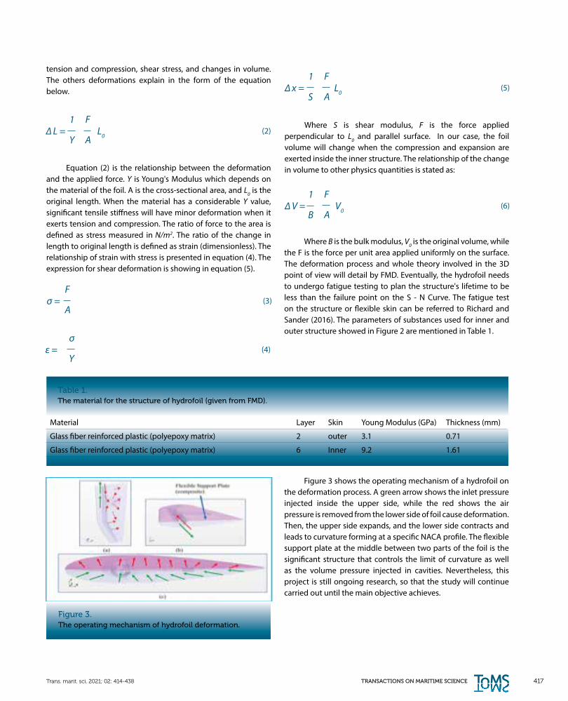
Figure 3.The operating mechanism of hydrofoil deformation.

Figure 3 shows the operating mechanism of a hydrofoil on the deformation process. A green arrow shows the inlet pressure injected inside the upper side, while the red shows the air pressure is removed from the lower side of foil cause deformation. Then, the upper side expands, and the lower side contracts and leads to curvature forming at a specific NACA profile. The flexible support plate at the middle between two parts of the foil is the significant structure that controls the limit of curvature as well as the volume pressure injected in cavities. Nevertheless, this project is still ongoing research, so that the study will continue carried out until the main objective achieves.


D = ex . ∫ σ(n) dA = ∫(-p+τrr ) (-cosθ ) + τrθ sin θ dA

L= ∫ (-p+τrr ) (sin θ)+ τrθ cos θ dA

(7)

(8)

1.4. Application on this Project (Deformable Hydrofoil)

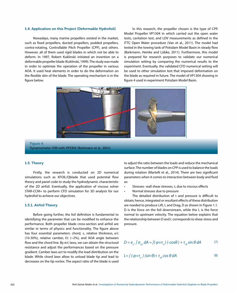
Nowadays, many marine propellers existed in the market, such as fixed propellers, ducted propellers, podded propellers, contra-rotating, Controllable Pitch Propeller (CPP), and others. However, all of them used rigid blades in which not be able to deform. In 1997, Robert Kuklinski initiated an invention on a deformable propeller blade (Kuklinski, 1999). The study was made in order to optimize the operation of the propeller in various AOA. It used heat elements in order to do the deformation on the flexible skin of the blade. The operating mechanism is in the figure below.

In this research, the propeller chosen is the type of CPP, Model Propeller VP1304 in which carried out the open water tests, cavitation test, and LDV measurements as defined in the ITTC Open Water procedure (Van et al., 2011). The model had tested in the towing tank of Potsdam Model Basin in steady flow (Barkmann, Heinke and Lübke, 2011). Furthermore, this model is prepared for research purposes to validate our numerical simulation setting by comparing the numerical results to the experiment. Eventually, the validated CFD numerical setting will be used to other simulation test that imposed deformation on the blade as required in future. The model of VP1304 showing in figure 4 used in experiment Potsdam Model Basin.

Figure 4.Dynamometer H39 with VP1304 (Barkmann et al., 2011).

1.5. Theory

Firstly, the research is conducted on 2D numerical simulations such as XFOIL/Qblade that used potential flow theory and panel code to study the hydrodynamic characteristic of the 2D airfoil. Eventually, the application of viscous solver STAR-CCM+ to perform CFD simulation for 3D analysis for our hydrofoil to achieve our objectives.

1.5.1. Airfoil Theory

Before going further, the foil definition is fundamental to identifying the parameter that can be modified to enhance the performance. Both propeller blade cross-section and airfoil are similar in terms of physics and functionality. The figure above has four essential parameters: chord, c, relative thickness, e/c (10-30%), relative camber, f/c (~2%), and AOA angle between flow and the chord line. By e/c laws, we can obtain the structural resistance and adjust the performances based on the pressure gradient. Camber laws act to modify the load distribution on the blade. While chord laws allow to unload blade tip and lead to decreases on the tip vortex. The aspect ratio of the blade is used

to adjust the ratio between the loads and reduce the mechanical surface. The number of blades on CPP is used to balance the loads during rotation (Martelli et al., 2014). There are two significant parameters when it comes to interaction between body and fluid as:• Stresses- wall shear stresses, τ, due to viscous effects• Normal stresses due to pressure

The detailed distribution of τ and pressure is difficult to obtain; hence, integrated or resultant effects of these distribution are needed to produce Lift, L and Drag, D as shown in Figure 1.1. D is the force on the foil downstream, while the L is the force normal to upstream velocity. The equation below explains that the relationship between D and L corresponds to shear stress and pressure.


Where τ and p are in N/m 2, therefore, the widely alternative way to define the dimensionless lift and drag coefficients to approximate values through simplified analysis, numerical technique, and appropriate experiment (Sun, Mao and Fan, 2020):

(9)(14)

(10)

(11)

(12)

(13)

CL = L

ρSV 21

2

CD = D

ρSV 21

2

Performance =L

D

Cf = τ

ρV 21

2

Cp = p-p0

ρ V∞21

2

Where; S = the projected area by c and span, s (m2) V= Velocity of the fluid (m/s) ρ = density of the fluid (kg/m3) Cf= Frictional coefficient p0 = Reference pressureCf and Cp are the essential parameters that identify the

location and the flow detachment and regime along the chord. It shows the boundary layer detachment happened earlier on the low Re number than the turbulent boundary layer. It means that the laminar boundary layer has less energy than the turbulent boundary layer, and flow separation occurs quickly.

1.5.2. Airfoil Theory

In our research, the NACA profile chosen is NACA 0017 as the initial shape profile. The four digits mean as follows:• 00 = there is no camber and symmetric• 17 = profile have a maximum thickness of 17% relative to the chord

The half-thickness equation of NACA 00xx is given by:

yt = c [ 0.2969 √ -0.1260 ( )

- 0.3516 ( )2+ 0.2843( )3- 0.1015( )4 ]

t

0.2

x

c

x

c

x

c

x

c

x

c

Where:c is the chordx is the position along with the c and 0y is the half-thickness for a given xt is the max thickness relative to the chordThe non-symmetric NACA profile used for the expected

deformable profile as presented in Section 3 is four digits. The same type of Equation 14 but with a cambered line:

m [2p - ]x

p2

x

c

m [1+ - -2p ]c-x

1- p2

x

c{yc = (15)

0≤x ≤pcpc≤x ≤c

• m is the maximum camber relative to chord (first digit)• p is the position of the max camber for leading-edge• Mainly for four digits non-symmetry, the maximum thickness is located at 30% of the chord from the leading edge.

1.5.3. Propeller Definition Diagram

The CPP chosen will undergo the CFD simulation in the open water test domain to obtain the significance parameter corresponding to propeller performance and efficiency. This study confronts the forces and moments acting on the propeller when operating in a constant fluid stream at the same RPM. The forces and moments produced by the propeller will be expressed in non-dimensional terms are as follows:

(16)Advance Coefficient: J = Vα

nD

(17)Thrust Coefficient: KT = T

ρn 2 D 4


(19)Propeller efficiency: η0 =T.Va

2πnQ

η0 =Rt .Vs

2πnQ(20)Propulsive efficiency:

(18)Torque Coefficient: KQ = Q

ρn 2 D 5

All the parameters of the non-dimensional term in Equation 16 – 20 will be obtained by using CFD simulation. The results obtained will be compared to the experimental results to check the validity and use in the subsequent research.

1.5.4. 2D Panel Method (XFOIL)

The 2D numerical simulation conducted using QBlade (2013) developed by David Marten integrates with XFOIL (1986) written by Mark Drela to compute the flow around subsonic isolated airfoils. This integration, which is also being improved, allows the fast design of custom airfoils and computation of their lift and drag polar (Marten and Wendler, 2013). Our attention is on the XFOIL code because it is the central part for 2D numerical analysis on the airfoil selected. XFOIL code applied the 2D panel method, and an integral boundary layer formulation is combined to analyze potential flow around the airfoils.

XFOIL code applied the 2D potential code to predict stationary flow and performance over an airfoil. It used the panel method with the distribution of source and vortex along the discretized chord. Equation closed with Kutta condition (Drela, 1989). The potential method is coupled with a boundary later code to get the viscous boundary layer. It allows analyzing the boundary layer regime accurately. Streamline function, as illustrates above, is a superposition of a vortex, a source, and a uniform flow. The equation form is as follows;

(21)ψ (x,y)=u∞ y- v∞ x+ π ∫γ (s) lnr ( s; x, y ) 1

2

ds + ∫ σ (s) θ ( s; x, y ) ds

1.5.5. CFD Modelling

The main objective of this research is to model the CFD simulation on the hydrofoil. This section will explain some

background of the CFD method used. Most natural fluid flow applications involve turbulent flow that provides the unsteady, three-dimensional, and presents significant spatial and temporal variations. These will lead to the formation of large eddies, transferring their energy to somewhat smaller eddies. This energy will cascade in which the energy is transferred to successively smaller and smaller eddies. In the end, the kinetic energy of turbulence is converted into heat. Kromolgorov's theorem in the figure below explains the energy transferred from larger to smaller eddies until energy dissipation. The turbulence model is the most crucial parameter in CFD simulation (Ducoin et al., 2009).

1.5.5.1. RANSE

The RANSE principle is based on the Reynolds decomposition. It means that all the quantities on Navier-Stokes (N.S.) equation will be written as a summation of a mean and fluctuating quantity. The decomposition made on velocity and pressure is written below.

(22)V = V + v- ~

(23)P = P + p- ~

Where V and P are mean quantity while v and p are the fluctuating quantity. The initial mass and momentum conservation equations of N.S. are as below:

~ ~

(24)∂Vk

∂xk

(25) + Vk = - + ( )+fi

∂Vi

∂t

∂2Vi

∂xk ∂xk

∂Vi

∂xk

∂P

∂xi

1

ρ

μ

ρ

Then, average the NS Equation 26 and 27 in which the Reynold decomposition used to produce the RANSE as below:

(26)∂Vk

∂xk


(27) + Vk = - - + ( )+fi

∂Vi

∂t

∂2Vi

∂xk ∂xk

∂Vi Vk

∂xk

∂Vi

∂xk

∂P

∂xi

1

ρ

μ

ρ

In Equation 27, after applying the Reynold decomposition method in Equation 25, a new term appears called as Reynold stress tensor at the right-hand side as:

(28)Rij = - ρ (Vi Vk ) ~ ~

Due to the minimal fluctuations in Equation 28, the turbulence modeling techniques based on the Boussinesq hypothesis were applied. This hypothesis is to link the Reynold stresses and velocity gradients through eddy viscosity.

(29)Rij = μt ( + )- ρkδij

∂Vi

∂xj

∂Vj

∂xi

2

3

μt is eddy viscosity while k is turbulent kinetic energy to be determined using various models (Rumsey et al., 2018). Some of them are:• 0 equation model: Mixing length, Cebeci-Smitch, Baldwin-Lomax, etc.• 1 equation model: Spalart-Allmaras, Wolfstein, k-model, etc.• Two equations model: k-ε, k-ω, k-τ, k-L, etc.

2. METHODOLOGY

In this study, the number of different 2D NACA profiles will be conducted in XFOIL code numerically. Then, some NACA profiles will be selected according to the highest hydrodynamic performance characteristics at the turbulence flow condition. The selected 2D NACA profiles will be designed for 3D NACA hydrofoil before undergoing the Finite Volume Analysis in CFD. The hydrodynamic performance on each 3D NACA hydrofoil will be collected and analyzed at this research's end. As for the podded propeller chosen, the CFD analysis will be conducted to obtain the hydrodynamic coefficients and be compared to the experiment results for validation. All of the numerical CFD setups will be used for the subsequent research for optimization.

2.1. The Scope of the Work

The detailed explanations of the work involved are as follows:• List all the possibilities foil shapes from NACA profiles 0012 to 0017 that are possible to deform.• Conducted the 2D numerical analysis) on several NACA profiles at Re= 35 x 106 to obtain the dimensionless hydrodynamic coefficient.• Choose the best NACA profiles with the highest performance at 0 deg AOA to design the 3D hydrofoil using CATIA software to evaluate the design. The selection process used a genetic Method shown using Pareto Front Diagram.• Construct the design using CATIA with the full-scale model to fabricate and will be computed numerically using Viscous Solver STAR-CCM+ and test experimentally in the future.• Ensure the meshing rule will obey the viscous and sub-viscous layer. The value of y+ should be less than two at the viscous layer around the foil surface.• Identify the physics model and turbulence model used in the simulation.• Do the 3D simulation using STAR-CCM+ on the selected hydrofoil.• The simulation is conducted at the same speed, Vs= 6 m/s at 0 deg AOA at the steady-state.• Observe all the hydrodynamic characteristics produced during simulation, such as lift and drag forces, wall shear stress, and Pressure distribution along hydrofoil.• Observe the vortices and detachment produced, which lead to the loss of performance. All the results will be compared to the experimental result in the future by FMD.• Study the advantages of the deformable hydrofoil on the results obtained being applied to the propeller blade in terms of thrust, maintaining the optimal propulsive performance for different speeds, flexibility, and efficiency in the future.

2.2. Selection of Several Possible Shapes of NACA to Deform (2D Analysis)

In this study, to analyze the different NACA profiles quickly, the QBlade that used XFOIL code was utilized. XFOIL is a program used to simulate and study subsonic isolated airfoils that take the 2D airfoil properties, Reynolds number, and Mach number and calculate global and local performances. XFOIL uses the potential flow theory, the boundary layer code, as explained in a viscous flow. In this way, the streamlines induced by the viscous flow can be modified. Here, the 2D foil analysis with Re= 35x 106

(turbulent) conducted on several NACA 6412 to 9517 is given by FMD.


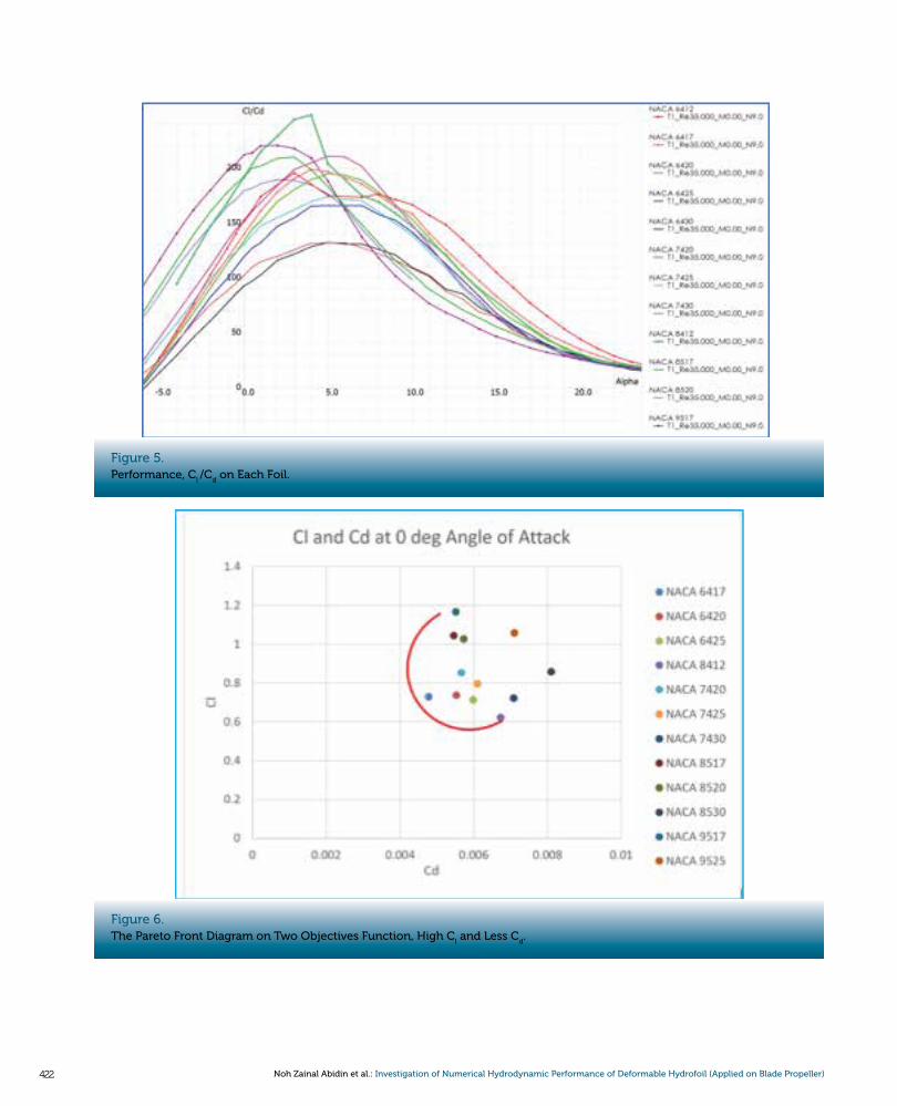
Figure 5.Performance, C

l /C

d on Each Foil.

Figure 6.The Pareto Front Diagram on Two Objectives Function, High C

l and Less C

d.


Figure 5 shows the best performance at 0 deg Angle of Attack (AOA) as required in the objective of this project. The results will compile and combine using the Stochastic Method to identify the best range of deformable NACA. According to Figure 5, the performance was obtained at the 0 deg AOA on different Non-Symmetry NACA profiles. The objectives function at 0 deg AOA at the constant Re= 35 x 106 are stated as follows:• High Lift, Cl

• Less Drag, Cd

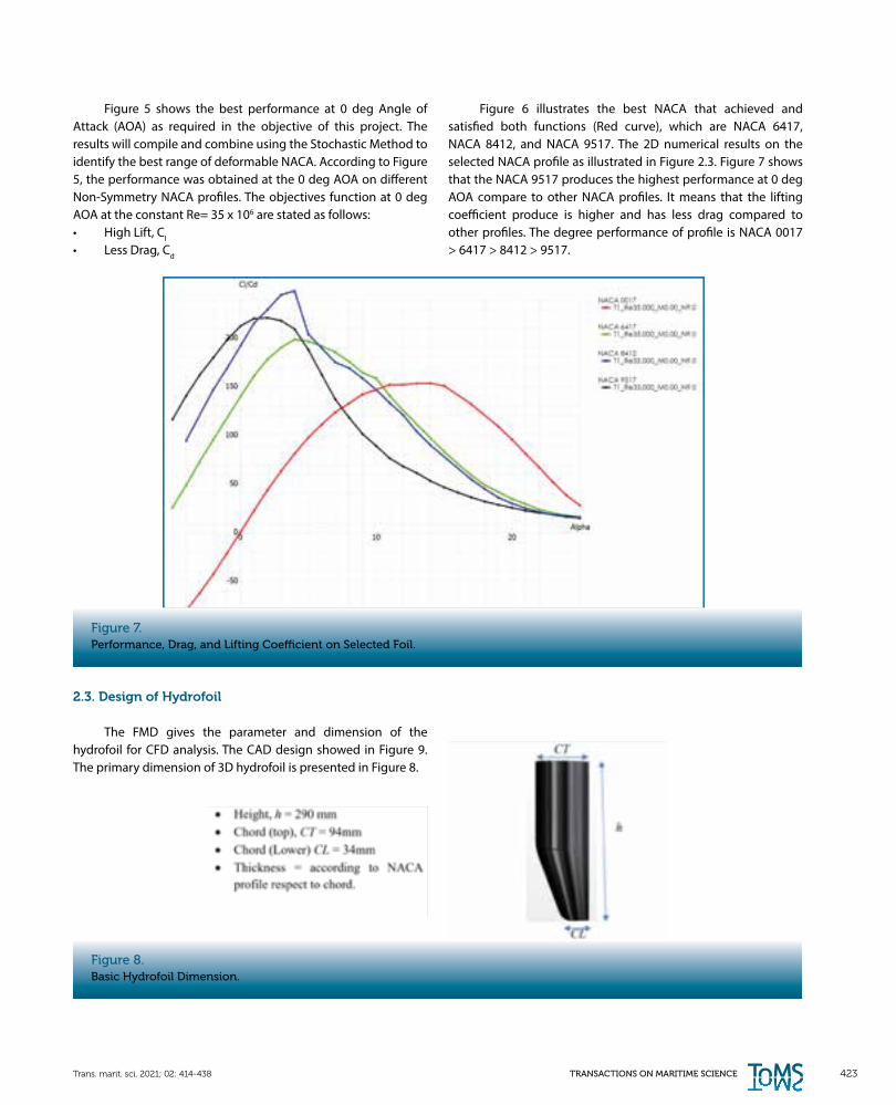
Figure 6 illustrates the best NACA that achieved and satisfied both functions (Red curve), which are NACA 6417, NACA 8412, and NACA 9517. The 2D numerical results on the selected NACA profile as illustrated in Figure 2.3. Figure 7 shows that the NACA 9517 produces the highest performance at 0 deg AOA compare to other NACA profiles. It means that the lifting coefficient produce is higher and has less drag compared to other profiles. The degree performance of profile is NACA 0017 > 6417 > 8412 > 9517.

Figure 7.Performance, Drag, and Lifting Coefficient on Selected Foil.

Figure 8.Basic Hydrofoil Dimension.

2.3. Design of Hydrofoil

The FMD gives the parameter and dimension of the hydrofoil for CFD analysis. The CAD design showed in Figure 9. The primary dimension of 3D hydrofoil is presented in Figure 8.


Table 2.Physics Value for CFD Simulation.

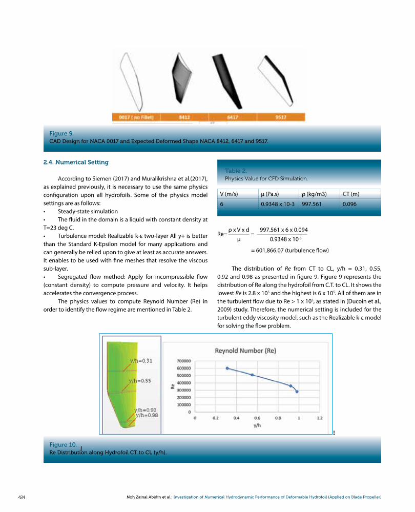
Figure 10.Re Distribution along Hydrofoil CT to CL (y/h).

Figure 9.CAD Design for NACA 0017 and Expected Deformed Shape NACA 8412, 6417 and 9517.

2.4. Numerical Setting

According to Siemen (2017) and Muralikrishna et al.(2017), as explained previously, it is necessary to use the same physics configuration upon all hydrofoils. Some of the physics model settings are as follows:• Steady-state simulation• The fluid in the domain is a liquid with constant density at T=23 deg C.• Turbulence model: Realizable k-ε two-layer All y+ is better than the Standard K-Epsilon model for many applications and can generally be relied upon to give at least as accurate answers. It enables to be used with fine meshes that resolve the viscous sub-layer.• Segregated flow method: Apply for incompressible flow (constant density) to compute pressure and velocity. It helps accelerates the convergence process.

The physics values to compute Reynold Number (Re) in order to identify the flow regime are mentioned in Table 2.

V (m/s) μ (Pa.s) ρ (kg/m3) CT (m)

6 0.9348 x 10-3 997.561 0.096

Re= =

= 601,866.07 (turbulence flow)

ρ x V x d

μ

997.561 x 6 x 0.094

0.9348 x 10-3

The distribution of Re from CT to CL, y/h = 0.31, 0.55, 0.92 and 0.98 as presented in figure 9. Figure 9 represents the distribution of Re along the hydrofoil from C.T. to CL. It shows the lowest Re is 2.8 x 105 and the highest is 6 x 105. All of them are in the turbulent flow due to Re > 1 x 105, as stated in (Ducoin et al., 2009) study. Therefore, the numerical setting is included for the turbulent eddy viscosity model, such as the Realizable k-ε model for solving the flow problem.

!

!


2.5. Domain

The domain of the simulation is the spatial region in which the simulation takes place. The shape of the domain is a rectangular box. The domain can be seen in Figure 11. The boundary condition is shown in Table 3.

Figure 11.The domain of The Hydrofoil From Inlet To Outlet.

Table 3.Boundaries and Boundary Conditions of the CFD Setup.

Table 4.Refinements Zones of the CFD Setup.

Name of Boundary Boundary Condition

Inlet Velocity Inlet, prescribed with V

Outlet Pressure Outlet

Hydrofoil Wall (No slip)

Top Wall (Slip)

Bottom Wall (Slip)

Side Wall (Slip)

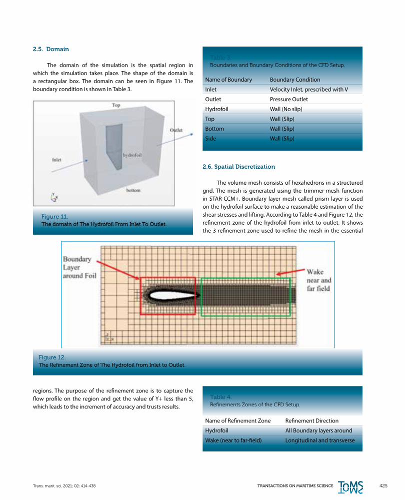
2.6. Spatial Discretization

The volume mesh consists of hexahedrons in a structured grid. The mesh is generated using the trimmer-mesh function in STAR-CCM+. Boundary layer mesh called prism layer is used on the hydrofoil surface to make a reasonable estimation of the shear stresses and lifting. According to Table 4 and Figure 12, the refinement zone of the hydrofoil from inlet to outlet. It shows the 3-refinement zone used to refine the mesh in the essential

Name of Refinement Zone Refinement Direction

Hydrofoil All Boundary layers around

Wake (near to far-field) Longitudinal and transverse

regions. The purpose of the refinement zone is to capture the flow profile on the region and get the value of Y+ less than 5, which leads to the increment of accuracy and trusts results.

Figure 12.The Refinement Zone of The Hydrofoil from Inlet to Outlet.


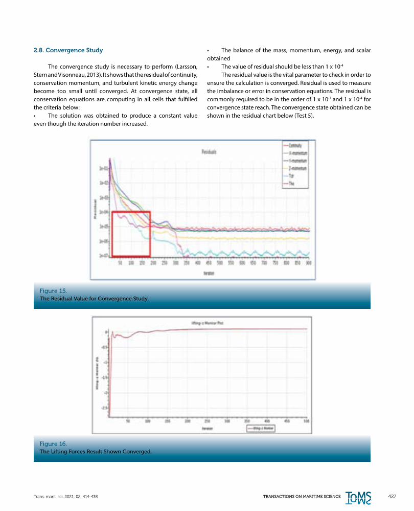
Table 5.The Summary of No of Cells Generated in Mesh Sensitivity.

Figure 14.Mesh Sensitivity Test Results Against the Number (No.) of Cells.

2.7. Meshing Sensitivity

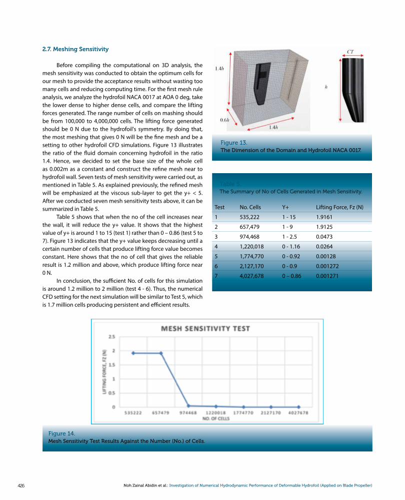
Before compiling the computational on 3D analysis, the mesh sensitivity was conducted to obtain the optimum cells for our mesh to provide the acceptance results without wasting too many cells and reducing computing time. For the first mesh rule analysis, we analyze the hydrofoil NACA 0017 at AOA 0 deg, take the lower dense to higher dense cells, and compare the lifting forces generated. The range number of cells on mashing should be from 100,000 to 4,000,000 cells. The lifting force generated should be 0 N due to the hydrofoil's symmetry. By doing that, the most meshing that gives 0 N will be the fine mesh and be a setting to other hydrofoil CFD simulations. Figure 13 illustrates the ratio of the fluid domain concerning hydrofoil in the ratio 1.4. Hence, we decided to set the base size of the whole cell as 0.002m as a constant and construct the refine mesh near to hydrofoil wall. Seven tests of mesh sensitivity were carried out, as mentioned in Table 5. As explained previously, the refined mesh will be emphasized at the viscous sub-layer to get the y+ < 5. After we conducted seven mesh sensitivity tests above, it can be summarized in Table 5.

Table 5 shows that when the no of the cell increases near the wall, it will reduce the y+ value. It shows that the highest value of y+ is around 1 to 15 (test 1) rather than 0 – 0.86 (test 5 to 7). Figure 13 indicates that the y+ value keeps decreasing until a certain number of cells that produce lifting force value becomes constant. Here shows that the no of cell that gives the reliable result is 1.2 million and above, which produce lifting force near 0 N.

In conclusion, the sufficient No. of cells for this simulation is around 1.2 million to 2 million (test 4 - 6). Thus, the numerical CFD setting for the next simulation will be similar to Test 5, which is 1.7 million cells producing persistent and efficient results.

Figure 13.The Dimension of the Domain and Hydrofoil NACA 0017.

Test No. Cells Y+ Lifting Force, Fz (N)

1 535,222 1 - 15 1.9161

2 657,479 1 - 9 1.9125

3 974,468 1 - 2.5 0.0473

4 1,220,018 0 - 1.16 0.0264

5 1,774,770 0 - 0.92 0.00128

6 2,127,170 0 - 0.9 0.001272

7 4,027,678 0 – 0.86 0.001271


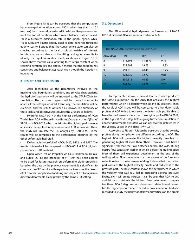
2.8. Convergence Study

The convergence study is necessary to perform (Larsson, Stern and Visonneau, 2013). It shows that the residual of continuity, conservation momentum, and turbulent kinetic energy change become too small until converged. At convergence state, all conservation equations are computing in all cells that fulfilled the criteria below:• The solution was obtained to produce a constant value even though the iteration number increased.

• The balance of the mass, momentum, energy, and scalar obtained• The value of residual should be less than 1 x 10-4

The residual value is the vital parameter to check in order to ensure the calculation is converged. Residual is used to measure the imbalance or error in conservation equations. The residual is commonly required to be in the order of 1 x 10-3 and 1 x 10-4 for convergence state reach. The convergence state obtained can be shown in the residual chart below (Test 5).

Figure 15.The Residual Value for Convergence Study.

Figure 16.The Lifting Forces Result Shown Converged.


Table 6.The NACA 0017 Performance on Each AOA.

From Figure 15, it can be observed that the computation has converged at iteration around 180 in which less than 1 x 10-4 (red box) then the residual reduced little bit and keep on constant until the end of iterations which mean balance state achieved. Tdr is a turbulent dissipation rate in the graph legend, while Tke is turbulent kinetic energy used to determine the turbulent eddy viscosity. Besides that, the convergence state can also be checked according to the local or global variable of interest. In this case, we can check on the lifting or drag force results to identify the equilibrium state reach, as shown in Figure 16. It shows above that the value of lifting force keeps constant when reaching iteration 180 and above. It means that the solution has converged and balance states reach even though the iteration is increasing.

3. RESULT AND DISCUSSION

After identifying all the parameters involved in the meshing rule, boundaries condition, and physics characteristic, the hydrofoil geometry will be imported to the STAR-CCM+ for simulation. The parts and regions will be created in order to adapt all the settings required. Eventually, the simulation will be executed, and the results obtained as follows. The summary of these tasks and objectives to simulate the CFD are as follows:• Hydrofoil NACA 0017 at the highest performance of AOA: The highest AOA will be estimated from 2D analysis using QBlade/XFOIL on NACA 0017, which contributes the highest performance at specific Re applied in experiment and CFD simulation. Then, the study will simulate the 3D analysis by STAR-CCM+. These results will be compared to the performance obtained by the other deformable hydrofoil.• Deformable Hydrofoil of NACA 6417, 8412, and 9517: The results obtained will be compared to NACA 0017 at AOA (highest performance – 2D analysis). • Open Water Test on Propeller VP 1304 (Barkmann, Heinke and Lübke, 2011): The propeller of VP 1304 has been agreed to be used for future research on deformable blade propellers based on the data by the previous experiment. It is significant to compare the CFD results with experimental to ensure the results of CFD solver is applicable for doing subsequent CFD analysis on different deformable blade profile by the same CFD setting.

AOA (deg) L(N) D(N) L/D

2 111.393 11.3873 9.78

8 223.593 19.73 11.33

9 291.91 28.49 10.25

12 321.539 32.77 9.81

14 359.516 40.23 8.94

16 362.36 49.78 7.28

As represented above, it proved that Re chosen produces the same assumption on the AOA that achieves the highest performance, which is 8 deg between 2D and 3D solutions. Then, the result of AOA 8 deg will be compared to other deformable profiles at AOA 0 deg to observe the deformable profile able to have the performance more than the original profile (NACA 0017) at the highest AOA 8 deg. Before going further on simulation to another deformable hydrofoil, we can observe the differences in the velocity vector at the plane (y/h= 0.31).

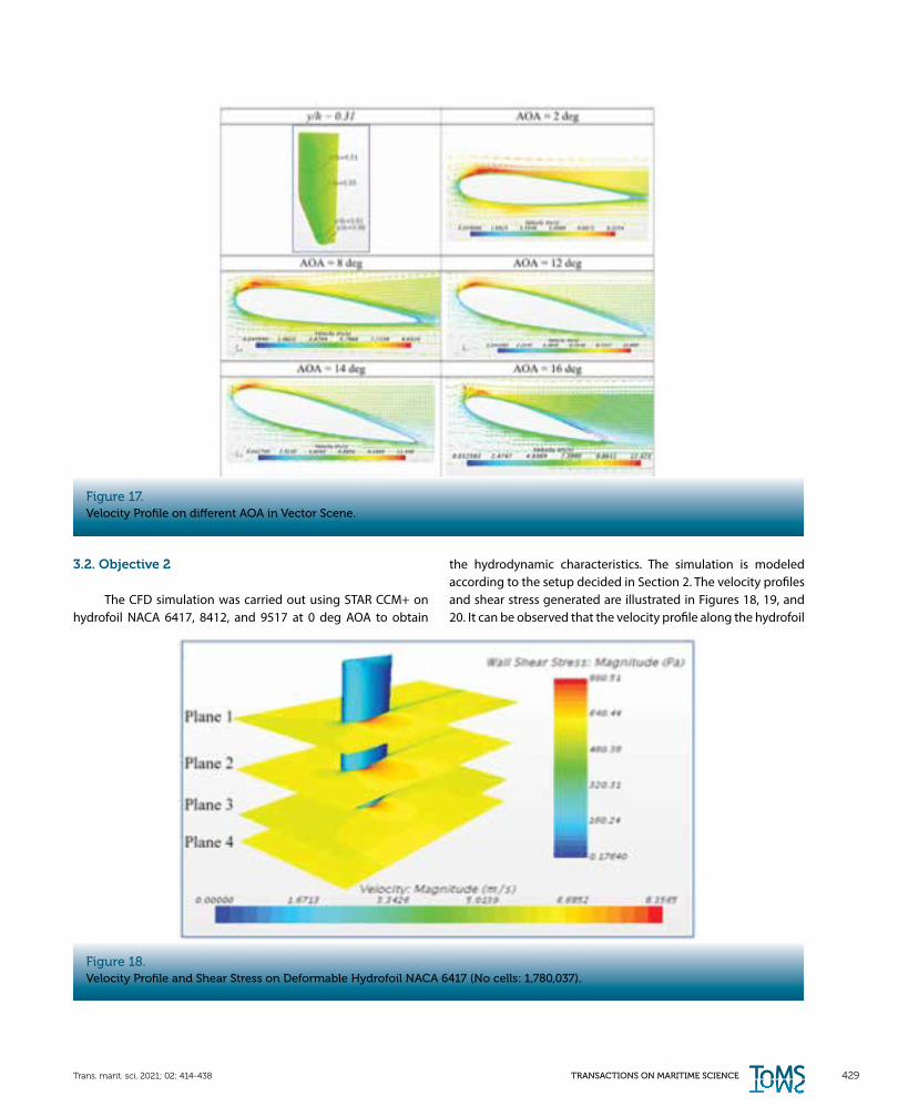
According to Figure 17, it can be observed that the velocity profiles along the hydrofoil are different according to AOA. The highest AOA will generate the highest velocity flow lead to generating higher lift more than others. However, it will have a significant risk that the flow detaches earlier. The AOA 16 deg occurs flow separation earlier in which before the trailing edge. Most of them will experience detachment at the end of the trailing edge. Flow detachment is the source of performance reduction due to the increment of drag. It shows that the suction part contains the highest velocity profile and reduces it to the pressure part. The blue contour shows the detachment in which the velocity near wall is 0, led to increasing adverse pressure. Eventually, it will create vortices. It can be seen that AOA 16 deg and 14 deg contribute the highest flow detachment compare to others. AOA 8 deg does not show much detachment caused has the higher performance. The video flow simulation had also recorded to study the behavior of flow and vortices on the profile

3.1. Objective 1

The 2D numerical hydrodynamic performances of NACA 0017 at different AOA are summarized in Table 6.


Figure 17.Velocity Profile on different AOA in Vector Scene.

Figure 18.Velocity Profile and Shear Stress on Deformable Hydrofoil NACA 6417 (No cells: 1,780,037).

3.2. Objective 2

The CFD simulation was carried out using STAR CCM+ on hydrofoil NACA 6417, 8412, and 9517 at 0 deg AOA to obtain

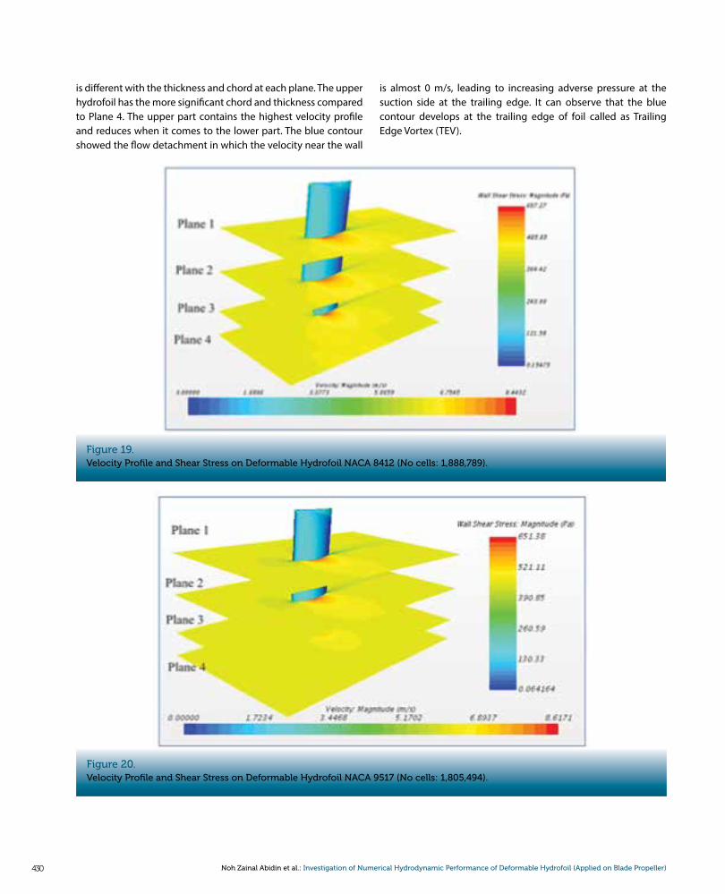
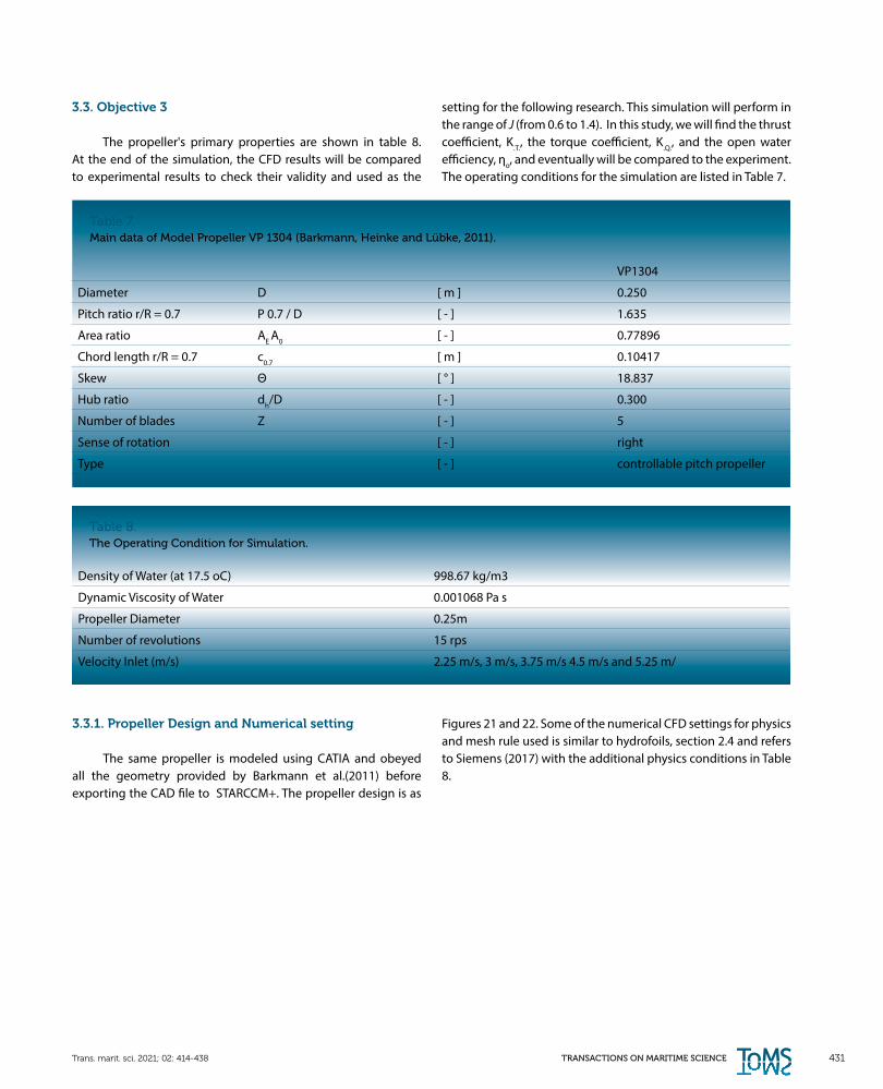
the hydrodynamic characteristics. The simulation is modeled according to the setup decided in Section 2. The velocity profiles and shear stress generated are illustrated in Figures 18, 19, and 20. It can be observed that the velocity profile along the hydrofoil




is different with the thickness and chord at each plane. The upper hydrofoil has the more significant chord and thickness compared to Plane 4. The upper part contains the highest velocity profile and reduces when it comes to the lower part. The blue contour showed the flow detachment in which the velocity near the wall

is almost 0 m/s, leading to increasing adverse pressure at the suction side at the trailing edge. It can observe that the blue contour develops at the trailing edge of foil called as Trailing Edge Vortex (TEV).


Table 7.Main data of Model Propeller VP 1304 (Barkmann, Heinke and Lübke, 2011).

Table 8.The Operating Condition for Simulation.

3.3. Objective 3

The propeller's primary properties are shown in table 8. At the end of the simulation, the CFD results will be compared to experimental results to check their validity and used as the

setting for the following research. This simulation will perform in the range of J (from 0.6 to 1.4). In this study, we will find the thrust coefficient, K.T., the torque coefficient, K.Q., and the open water efficiency, ηo, and eventually will be compared to the experiment. The operating conditions for the simulation are listed in Table 7.

VP1304

Diameter D [ m ] 0.250

Pitch ratio r/R = 0.7 P 0.7 / D [ - ] 1.635

Area ratio AE A0 [ - ] 0.77896

Chord length r/R = 0.7 c0.7 [ m ] 0.10417

Skew Θ [ ° ] 18.837

Hub ratio dh/D [ - ] 0.300

Number of blades Z [ - ] 5

Sense of rotation [ - ] right

Type [ - ] controllable pitch propeller

Density of Water (at 17.5 oC) 998.67 kg/m3

Dynamic Viscosity of Water 0.001068 Pa s

Propeller Diameter 0.25m

Number of revolutions 15 rps

Velocity Inlet (m/s) 2.25 m/s, 3 m/s, 3.75 m/s 4.5 m/s and 5.25 m/

3.3.1. Propeller Design and Numerical setting

The same propeller is modeled using CATIA and obeyed all the geometry provided by Barkmann et al.(2011) before exporting the CAD file to STARCCM+. The propeller design is as

Figures 21 and 22. Some of the numerical CFD settings for physics and mesh rule used is similar to hydrofoils, section 2.4 and refers to Siemens (2017) with the additional physics conditions in Table 8.


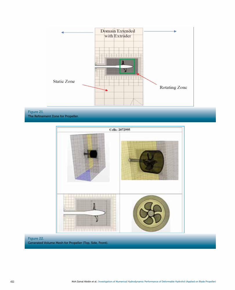
Figure 21.The Refinement Zone for Propeller.

Figure 22.Generated Volume Mesh for Propeller (Top, Side, Front).


3.3.2. Mesh Rule

The mesh setting for this simulation is different compared to the setting used for hydrofoil. In this case, the propeller's rotation will be modeled using Moving Reference Frame (MRF). It has two regions which are for the rotating region and static region. The zones involved are as follows:

For this simulation, the value of y+ is outside the buffer layer 5 to 30. Here we aim the wall y+ value greater than 30. The small y+ less than 5 is not applicable to use it due to involved the MRF. Otherwise, the number of cells increased and increased the computation time. Considering the refinement zone involved, the number of cells used is not much and is applicable to simulation. Therefore, the All Y+ Wall Treatment Approach was chosen to have better configurations that emulate the low y+ wall treatment for fine meshes and the high y+ wall treatment for coarse mesh. Due to the y+ value is more than 30, then the high y+ wall treatment option will automatically be activated in which the treatment does not resolve the viscous sub-layer. Therefore, it used the wall shear stress, turbulent production, and turbulent

dissipation are derived from equilibrium turbulent boundary layer theory.

3.3.3. Scalar Scene

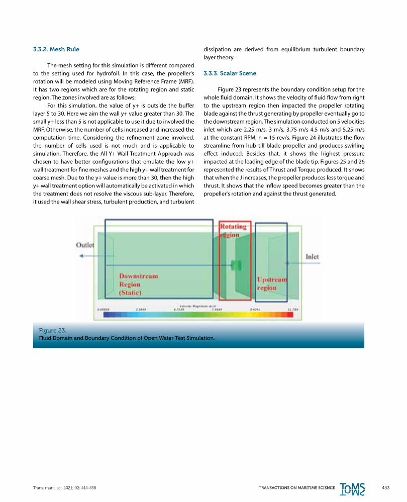
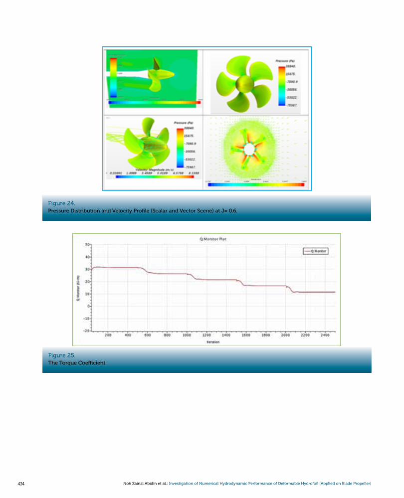
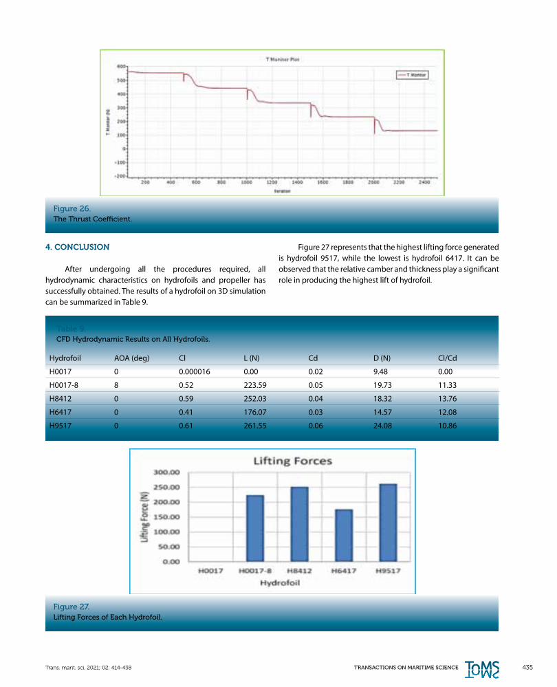
Figure 23 represents the boundary condition setup for the whole fluid domain. It shows the velocity of fluid flow from right to the upstream region then impacted the propeller rotating blade against the thrust generating by propeller eventually go to the downstream region. The simulation conducted on 5 velocities inlet which are 2.25 m/s, 3 m/s, 3.75 m/s 4.5 m/s and 5.25 m/s at the constant RPM, n = 15 rev/s. Figure 24 illustrates the flow streamline from hub till blade propeller and produces swirling effect induced. Besides that, it shows the highest pressure impacted at the leading edge of the blade tip. Figures 25 and 26 represented the results of Thrust and Torque produced. It shows that when the J increases, the propeller produces less torque and thrust. It shows that the inflow speed becomes greater than the propeller's rotation and against the thrust generated.

Figure 23.Fluid Domain and Boundary Condition of Open Water Test Simulation.


Figure 24.Pressure Distribution and Velocity Profile (Scalar and Vector Scene) at J= 0.6.

Figure 25.The Torque Coefficient.


Figure 26.The Thrust Coefficient.

Figure 27.Lifting Forces of Each Hydrofoil.

4. CONCLUSION

After undergoing all the procedures required, all hydrodynamic characteristics on hydrofoils and propeller has successfully obtained. The results of a hydrofoil on 3D simulation can be summarized in Table 9.

Table 9.CFD Hydrodynamic Results on All Hydrofoils.

Hydrofoil AOA (deg) Cl L (N) Cd D (N) Cl/Cd

H0017 0 0.000016 0.00 0.02 9.48 0.00

H0017-8 8 0.52 223.59 0.05 19.73 11.33

H8412 0 0.59 252.03 0.04 18.32 13.76

H6417 0 0.41 176.07 0.03 14.57 12.08

H9517 0 0.61 261.55 0.06 24.08 10.86

Figure 27 represents that the highest lifting force generated is hydrofoil 9517, while the lowest is hydrofoil 6417. It can be observed that the relative camber and thickness play a significant role in producing the highest lift of hydrofoil.


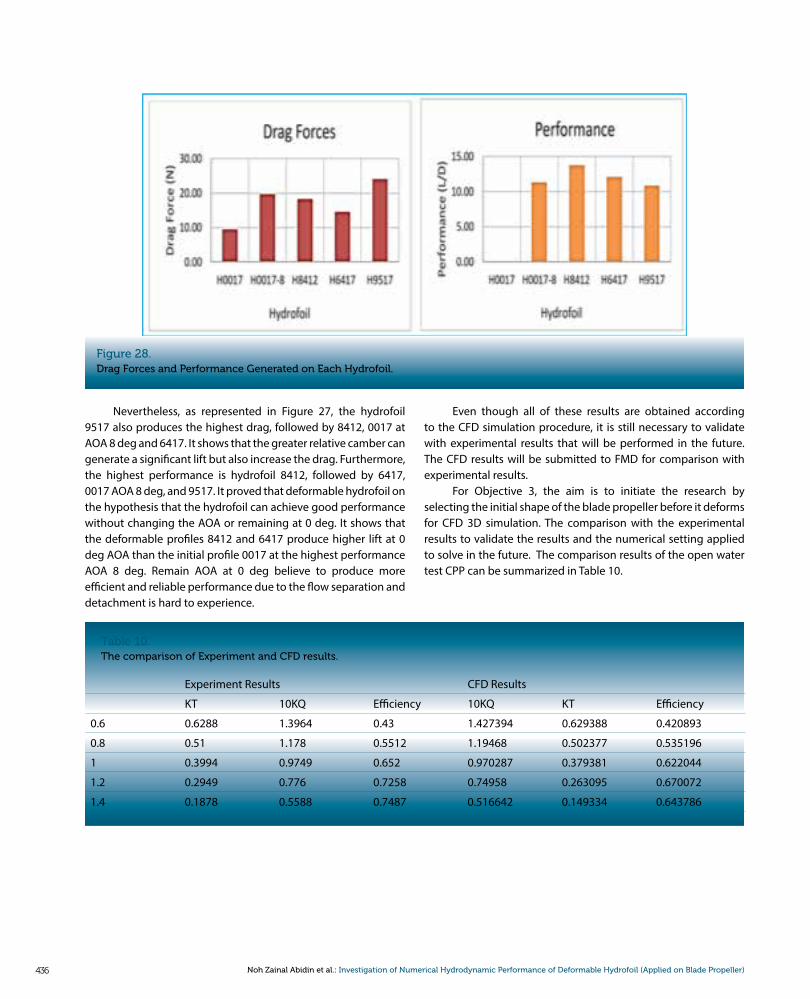
Figure 28.Drag Forces and Performance Generated on Each Hydrofoil.

Table 10.The comparison of Experiment and CFD results.

Nevertheless, as represented in Figure 27, the hydrofoil 9517 also produces the highest drag, followed by 8412, 0017 at AOA 8 deg and 6417. It shows that the greater relative camber can generate a significant lift but also increase the drag. Furthermore, the highest performance is hydrofoil 8412, followed by 6417, 0017 AOA 8 deg, and 9517. It proved that deformable hydrofoil on the hypothesis that the hydrofoil can achieve good performance without changing the AOA or remaining at 0 deg. It shows that the deformable profiles 8412 and 6417 produce higher lift at 0 deg AOA than the initial profile 0017 at the highest performance AOA 8 deg. Remain AOA at 0 deg believe to produce more efficient and reliable performance due to the flow separation and detachment is hard to experience.

Even though all of these results are obtained according to the CFD simulation procedure, it is still necessary to validate with experimental results that will be performed in the future. The CFD results will be submitted to FMD for comparison with experimental results.

For Objective 3, the aim is to initiate the research by selecting the initial shape of the blade propeller before it deforms for CFD 3D simulation. The comparison with the experimental results to validate the results and the numerical setting applied to solve in the future. The comparison results of the open water test CPP can be summarized in Table 10.

Experiment Results CFD Results

KT 10KQ Efficiency 10KQ KT Efficiency

0.6 0.6288 1.3964 0.43 1.427394 0.629388 0.420893

0.8 0.51 1.178 0.5512 1.19468 0.502377 0.535196

1 0.3994 0.9749 0.652 0.970287 0.379381 0.622044

1.2 0.2949 0.776 0.7258 0.74958 0.263095 0.670072

1.4 0.1878 0.5588 0.7487 0.516642 0.149334 0.643786


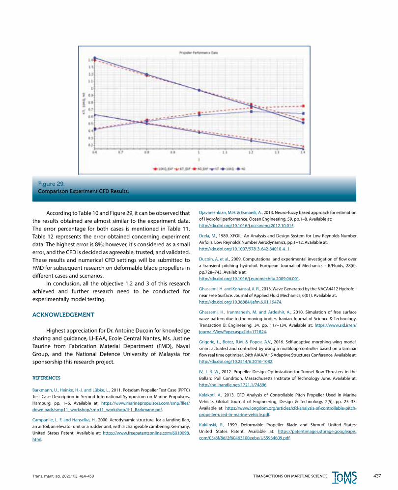
Figure 29.Comparison Experiment CFD Results.

According to Table 10 and Figure 29, it can be observed that the results obtained are almost similar to the experiment data. The error percentage for both cases is mentioned in Table 11. Table 12 represents the error obtained concerning experiment data. The highest error is 8%; however, it's considered as a small error, and the CFD is decided as agreeable, trusted, and validated. These results and numerical CFD settings will be submitted to FMD for subsequent research on deformable blade propellers in different cases and scenarios.

In conclusion, all the objective 1,2 and 3 of this research achieved and further research need to be conducted for experimentally model testing.

ACKNOWLEDGEMENT

Highest appreciation for Dr. Antoine Ducoin for knowledge sharing and guidance, LHEAA, Ecole Central Nantes, Ms. Justine Taurine from Fabrication Material Department (FMD), Naval Group, and the National Defence University of Malaysia for sponsorship this research project.

REFERENCES

Barkmann, U., Heinke, H.-J. and Lübke, L., 2011. Potsdam Propeller Test Case (PPTC) Test Case Description in Second International Symposium on Marine Propulsors. Hamburg, pp. 1–6. Available at: https://www.marinepropulsors.com/smp/files/downloads/smp11_workshop/smp11_workshop/II-1_Barkmann.pdf.

Campanile, L. F. and Hanselka, H., 2000. Aerodynamic structure, for a landing flap, an airfoil, an elevator unit or a rudder unit, with a changeable cambering. Germany: United States Patent. Available at: https://www.freepatentsonline.com/6010098.html.

Djavareshkian, M.H. & Esmaeili, A., 2013. Neuro-fuzzy based approach for estimation of Hydrofoil performance. Ocean Engineering, 59, pp.1–8. Available at: http://dx.doi.org/10.1016/j.oceaneng.2012.10.015.

Drela, M., 1989. XFOIL: An Analysis and Design System for Low Reynolds Number Airfoils. Low Reynolds Number Aerodynamics, pp.1–12. Available at: http://dx.doi.org/10.1007/978-3-642-84010-4_1.

Ducoin, A. et al., 2009. Computational and experimental investigation of flow over a transient pitching hydrofoil. European Journal of Mechanics - B/Fluids, 28(6), pp.728–743. Available at: http://dx.doi.org/10.1016/j.euromechflu.2009.06.001.

Ghassemi, H. and Kohansal, A. R., 2013. Wave Generated by the NACA4412 Hydrofoil near Free Surface. Journal of Applied Fluid Mechanics, 6(01). Available at: http://dx.doi.org/10.36884/jafm.6.01.19474.

Ghassemi, H., Iranmanesh, M. and Ardeshir, A., 2010. Simulation of free surface wave pattern due to the moving bodies. Iranian Journal of Science & Technology, Transaction B: Engineering, 34, pp. 117–134. Available at: https://www.sid.ir/en/journal/ViewPaper.aspx?id=171824.

Grigorie, L., Botez, R.M. & Popov, A.V., 2016. Self-adaptive morphing wing model, smart actuated and controlled by using a multiloop controller based on a laminar flow real time optimizer. 24th AIAA/AHS Adaptive Structures Conference. Available at: http://dx.doi.org/10.2514/6.2016-1082.

IV, J. R. W., 2012. Propeller Design Optimization for Tunnel Bow Thrusters in the Bollard Pull Condition. Massachusetts Institute of Technology June. Available at: http://hdl.handle.net/1721.1/74896.

Kolakoti, A., 2013. CFD Analysis of Controllable Pitch Propeller Used in Marine Vehicle, Global Journal of Engineering, Design & Technology, 2(5), pp. 25–33. Available at: https://www.longdom.org/articles/cfd-analysis-of-controllable-pitch-propeller-used-in-marine-vehicle.pdf.

Kuklinski, R., 1999. Deformable Propeller Blade and Shroud' United States: United States Patent. Available at: https://patentimages.storage.googleapis.com/03/8f/8d/2f60463100eebe/US5934609.pdf.


Larsson, L., Stern, F. and Visonneau, M., 2013. CFD in Ship Hydrodynamics — Results of the Gothenburg 2010 Workshop in MARINE 2011, IV International Conference on Computational Methods in Marine Engineering, pp. 237–259. Available at: http://dx.doi.org/10.1007/978-94-007-6143-8.

Lothar Birk, 2019. Fundamentals of Ship Hydrodynamics: Fluid Mechanics, Ship Resistance and Propulsion John Wiley & Sons Ltd. Available at: www.wiley.com/go/birk/hydrodynamics.

Mahmud, M.S., 2015. The applicability of hydrofoils as a ship control device. Journal of Marine Science and Application, 14(3), pp.244–249. Available at: http://dx.doi.org/10.1007/s11804-015-1314-x.

Martelli, M. et al., 2013. Controllable pitch propeller actuating mechanism, modelling and simulation. Proceedings of the Institution of Mechanical Engineers, Part M: Journal of Engineering for the Maritime Environment, 228(1), pp.29–43. Available at: http://dx.doi.org/10.1177/1475090212468254.

Marten, D. and Wendler, J., 2013. QBlade Guidelines.

Muralikrishna, I.V. & Manickam, V., 2017. Principles and Design of Water Treatment. Environmental Management, pp.209–248. Available at: http://dx.doi.org/10.1016/b978-0-12-811989-1.00011-7.

Nowruzi, H., Ghassemi, H. & Ghiasi, M., 2017. Performance predicting of 2D and 3D submerged hydrofoils using CFD and ANNs. Journal of Marine Science and Technology, 22(4), pp.710–733. Available at: http://dx.doi.org/10.1007/s00773-017-0443-0.

Rediniotis, O.K. et al., 2002. Development of a Shape-Memory-Alloy Actuated Biomimetic Hydrofoil. Journal of Intelligent Material Systems and Structures, 13(1), pp.35–49. Available at: http://dx.doi.org/10.1177/1045389x02013001534.

Richard, H.A. & Sander, M., 2016. Fatigue Crack Growth. Solid Mechanics and Its Applications. Available at: http://dx.doi.org/10.1007/978-3-319-32534-7.

Rumsey, C., Smith, B., and Huang, G., (2019). Turbulence modeling resource. http://turbmodels.larc.nasa.gov. Last visited December 1, 2019.

Rychlewski, J., 1984. On Hooke's law, Journal of Applied Mathematics and Mechanics, 48(3), pp. 303–314. Available at: https://doi.org/10.1016/0021-8928(84)90137-0.

Seo, J.H. et al., 2010. Flexible CFD meshing strategy for prediction of ship resistance and propulsion performance. International Journal of Naval Architecture and Ocean Engineering, 2(3), pp.139–145. Available at: http://dx.doi.org/10.2478/ijnaoe-2013-0030.

Shih, T.-H. et al., 1995. A new k-Є eddy viscosity model for high reynolds number turbulent flows. Computers & Fluids, 24(3), pp.227–238. Available at: http://dx.doi.org/10.1016/0045-7930(94)00032-t.

Siemens, 2017. STAR-CCM+® Documentation Version 12.06. Availkable at: https://www.plm.automation. siemens.com/global/en/products/simcenter/STAR-CCM.html.

Sun, Z., Mao, Y. & Fan, M., 2021. Performance optimization and investigation of flow phenomena on tidal turbine blade airfoil considering cavitation and roughness. Applied Ocean Research, 106, p.102463. Available at: http://dx.doi.org/10.1016/j.apor.2020.102463.

Tangorra, J. et al., 2011. Use of Biorobotic Models of Highly Deformable Fins for Studying the Mechanics and Control of Fin Forces in Fishes. Integrative and Comparative Biology, 51(1), pp.176–189. Available at: http://dx.doi.org/10.1093/icb/icr036.

Van, S.-H. et al., 2011. The Propulsion Committee in Proceedings of 26th ITTC – Volume I, pp. 61–121. Available at: https://ittc.info/media/5518/04.pdf.

Xie, N. & Vassalos, D., 2007. Performance analysis of 3D hydrofoil under free surface. Ocean Engineering, 34(8-9), pp.1257–1264. Available at: http://dx.doi.org/10.1016/j.oceaneng.2006.05.008.

Xu, G.D. et al., 2020. The free surface effects on the hydrodynamics of two-dimensional hydrofoils in tandem. Engineering Analysis with Boundary Elements, 115, pp.133–141. Available at: http://dx.doi.org/10.1016/j.enganabound.2020.03.014.

Documents

Investigation of Numerical Hydrodynamic Performance of