1

Forthcoming Applied Economics

Exchange-Rate Volatility and Trade: A Semiparametric Approach

Debasri Mukherjee1 Susan Pozo

Assistant Professor Professor

Department of Economics Department of Economics

Western Michigan University Western Michigan University

Kalamazoo, MI 49008 Kalamazoo, MI 49008

Abstract:

We use a gravity model to analyze the impact of exchange-rate volatility on the volume of

bilateral international trade. Semiparametric regression methods are applied to pooled

data for over 200 countries. Our results indicate that volatility affects trade negatively

although at very high level of volatility the effect diminishes and eventually becomes

statistically indistinguishable from zero. Countries apparently find avenues to mitigate

the detrimental impact of exchange rate uncertainty when volatility attains very high

levels. These results help reconcile the contradictory findings often found in the literature

on the impact of exchange-rate uncertainty on trade volume.

Keywords: international trade, semiparametric regression, volatility

JEL Classification: F40, C14

June 29, 2007

1 Corresponding author: Debasri Mukherjee, Economics Department, Western Michigan University,

Kalamazoo, MI 49008. Fax: (269)3875637. Email: debasri.mukherjee@wmich.edu

2

1. Introduction:

Despite the completion of a great number of studies on the impact of exchange-

rate volatility on the volume of international trade, there is still little consensus on how

uncertainty in currency values affects trade flows. Theoretical and empirical studies can

be cited to support a host of conclusions; that exchange-rate volatility depresses trade,

that it induces increases in the level of international trade, or that it has no impact on

trade flows. Researches have tried to reconcile these differences by slicing the data in a

myriad of ways. Our own solution to the reconciliation of the numerous results on the

impact of exchange-rate volatility on trade is to use a gravity equation and apply a

semiparametric regression technique because it does not superimpose any a priori

functional form restriction on the relationship under scrutiny. We examine (1) whether

the trade-volatility relation is negative; (2) whether the rate at which volatility affects

trade is constant; (3) and if not, at what levels of volatility it is nonlinear/non-constant;

and finally (4) whether we can derive any meaningful economic conclusion from these

statistical estimates.

Using a pooled sample for over 200 countries (with a total of 121,501

observations) we find that exchange-rate volatility affects trade negatively and the effect

remains more or less constant for a wide range of values of exchange-rate volatility.

However, at relatively high levels of volatility, the negative effect becomes very strong,

then subsequently weakens and finally gradually adjusts to zero. What may explain this

behavior? Countries may respond to higher levels of volatility by reducing their volume

of trade but after a certain point the countries find avenues to mitigate the harmful impact

of exchange-rate uncertainty. For example countries might informally dollarize when

3

exchange-rate volatility attains “unbearably” high levels, thereby insulating the country

from most of the harmful impacts of very high volatility. Section 2 provides background

and a literature review, section 3 explains the methodology used and section 4 describes

the data. Results are analyzed in section 5 while section 6 discusses the implications and

limitations of our findings.

2. Background and Literature Review

While most inquiries into the effects of exchange-rate volatility on trade conclude

that uncertainty reduces trade, there are enough exceptions to raise doubts with respect to

the universality of this conclusion. The lack of consensus exists with respect to both

theoretical and empirical studies. While theoretical models were derived early on

showing that increases in currency volatility will induce risk-averse traders to reduce the

level of international trade that takes place (e.g. Hooper and Kohlhagen, 1978), later

models demonstrated the possibility of the converse. Firms might reorganize production

and ultimately increase their share of international trade in response to increases in

exchange risk (e.g. De Grauwe, 1988). Lack of consensus on the impact of exchange-rate

volatility also arises with respect to the numerous empirical studies that have been

conducted. While many studies link exchange-rate volatility to decreases in the level of

trading (e.g. Kenen and Rodrik, 1986; Dell’Ariccia, 1999), others fail to find conclusive

evidence that volatility negatively impacts on trade flows (e.g. Hooper and Kolhagen,

1978; Tenreyro, 2004) and a few concur with the theoretical models attributing increased

trade to increases in volatility in exchange rates (e.g. Baum, et al, 2004).

Several avenues have been pursued in an attempt to reconcile the differing

conclusions about exchange-rate uncertainty on trade. One approach has been to

4

disaggregate trade by type of good traded. Differentiated products are found to be much

more susceptible to exchange-rate volatility relative to less differentiated products or

commodities (Broda and Romalis, 2004). Other attempts have been made by considering

the development status of trading partners, or the region in which trade is taking place.

Sauer and Bohara (2001) find that while developing countries’ exports fall with

exchange-rate volatility, the exports of developed countries’ are not affected. They also

find regional variations in the effect of exchange risk, with Africa and Latin America

displaying high susceptibility and Asia no susceptibility to exchange-rate risk. But these

disaggregations have not led to a consistent generalization aside from concluding that

whether exchange-rate volatility's impact is negative or not "depends" on specific

circumstances. As such these disaggregations have not succeeded in bringing us any

closer to a comprehensive understanding of the impact of exchange-rate volatility on

trade.

Alternative approaches to obtaining consistent results revolve around correcting

for econometric problems and experimenting with alternative specifications. Export

supply and import demand functions (e.g. Cushman, 1983) have given way to the gravity

model (e.g. Rose, 2000). Studies have also tended to move from focusing on a relatively

small number of countries (e.g. Thursby and Thursby, 1987 with a sample of 17

countries) to studies consisting of very large samples (e.g. Rose, 2000 and Sauer and

Bohara, 2001 with 186 and 91 countries respectively). Pozo (1992) examined historical

data from the early 1900s and Dell’Ariccia (1999) experimented with different

specifications for the volatility variable. In addition to using both nominal and real

exchange rates, he constructed proxies for exchange-rate instability using the standard

5

deviation of returns, the sum of squares of the forward errors, and the range of the

nominal spot exchange rate. Baum, Caglayan and Ozkan (2004) introduce dynamics to

the relationship between volatility and trade by applying various lag structures to

volatility.

Our paper offers an alternative approach to the empirical literature on the impact

of exchange-rate volatility on trade by using a semiparametric model of trade flows. This

model considers a general nonlinear (nonparametric) relationship between volatility and

trade, avoiding the need to superimpose any linearity restriction on the underlying

relationship between exchange-rate volatility and trade. Hence our approach is free from

any bias due to misspecification of the functional form in the aforementioned

relationship. The results indicate that increase in the level of volatility depresses trade.

We also find that although the rate at which volatility depresses trade is more or less

constant for a wide range of volatility, the rate changes very substantially at very high

levels of volatility. While the negative effect increases when the volatility is very high,

after a point the negative impact actually weakens. At the highest levels of volatility we

find no significant effect of volatility on trade. We offer explanations for why this non-

linear impact is observed and for why the impact fades to zero as volatility rises. The

non-linear nature of the impact of exchange risk on trade that we uncover provides an

explanation for some of the contradictory findings present in the literature.

3. Methodology

The overall plan for tracking how volatility impacts trade is to use a gravity model

of international trade. Gravity models have been very successful at explaining trade

6

volume and as discussed earlier have been increasing in popularity when testing for the

impact of exchange risk on said flows. The gravity model specifies that the log of the

value of real bilateral trade at time t between countries i and j (Tijt) can be expressed as:

ln(Tijt) = α1 + α2 ln (GDPi*GDPj)t +α3 ln((GDPi/Popi)(GDPj/Popj))t

+ α4ln(Dij) + εijt (1)

Popi and Popj are populations in i and j and Dij is the distance between i and j. The

product of real GDP and real GDP per capita are presumed to positively impact trade

volume.

As has been common in the literature, this equation has been augmented with a

series of dummy variables that are thought to further explain variations in the level of

trade.

ln(Tijt)= α1 + α2 ln (GDPi*GDPj)t +α3 ln((GDPi/Popi)(GDPj/Popj))t + α4ln(Dij) +

α5Borderij + α6ComLangij + α7Regionalij + α8Colonyij + α9CUStrictij + εijt (2)

Countries sharing borders (Borderij = 1) or languages (ComLangij = 1) are expected to

trade more with one another. Countries in the some trade integration arrangement

(Regionalij = 1) and countries who are either currently in a colonial relationship or in the

past maintained a colonial relationship (Colonyij = 1) are also expected to engage in more

trade. Trade is expected to be enhanced when the trading partners share a single currency

7

(CUStrictij=1), and trade is expected to be disrupted and diminshed when either partner

experiences a currency crisis (Crisis=1).2

To test for the impact of exchange rate uncertainty, the gravity equation is

augmented once more with a continuous variable that proxies for uncertainty in the

exchange rate and is denoted as σijt.

ln(Tijt)= α1 + α2 ln (GDPi*GDPj)t +α3 ln((GDPi/Popi)(GDPj/Popj))t + α4ln(Dij)

+α5Borderij + α6ComLangij + α7Regionalij + α8Colonyij + α9CUStrictij + α10Crisisijt

+α11σijt + εijt (3)

Unlike the dummy variables we do not have a prior expectation on the sign of the

coefficient α11. There has been much discussion in the literature on the methodology that

should be employed to measure the latent exchange rate uncertainty variable (e.g. Pozo,

1992; Dell’Arricia, 1999). Following Rose (2000), we take a simple approach,

computing the standard deviation of monthly real exchange rate returns over the

preceding year to construct the volatility of the exchange-rate (σijt) -- exchange-rate

volatility in the period before t. One may be concerned with the potential issue of

endogeneity between exchange-rate volatility and trade volume. Using disaggregated data

on bilateral trade for different types of products, Broda and Romalis (2004) find evidence

of endogeneity by reporting a substantial impact of trade on exchange-rate volatility.

2 In this paper we consider four different currency crisis episodes. The Asian currency crisis is presumed to

have taken place during 1997 and 1998. All trade flows including an Asian country are assigned a crisis

dummy value of 1 in 1997 and in 1998. We assign a crisis dummy variable value of 1 to any trading pair

that includes a Latin American nation during 1981 through 1986 and again in 1994 through 1998 to capture

the 2 currency crises believed to have impacted the Latin American nations and their trading partners.

Finally, we assigned a dummy variable value of 1 for all trade taking place from 1971 through 1974 to

account for the breakdown of the Bretton Woods Monetary system.

8

Rose (2000) addresses this issue by using instrumental variables to account for the

possible issue of endogeneity, and has shown that correcting for the endogeneity of

exchange-rate volatility does not change the results (as long as volatility itself is

measured with a one period lag). We follow Rose and use a one period lagged volatility

variable to account for the possible endogeneity of exchange rate volatility and trade.

The novelty in our estimation is to use semiparametric methods to explain the

effect of volatility (our main variable of interest) on trade volume. This is justified given

that Ramsey’s RESET test rejects linearity in the overall model with an associated p-

value of 0.000. It is well known that misspecification of the functional relationship can

lead to biased estimation and hypothesis testing. It is in this regard, that nonparametric

regression, which does not impose functional form restrictions, has been increasingly

popular in studying economic phenomena.

However, a pure nonparametric approach has several costs (sometimes double-

edged) associated with it. The computational problem, on the one hand, and the problem

of dimensionality, on the other, are major concerns. A fully nonparametric regression

technique that incorporates both continuous and categorical variables has been discussed

in the classic paper by Racine and Li (2004), where they also discuss the well known

computational challenge of any fully nonparametric technique. Given our sample size of

121,501 observations and given our rich set of explanatory variables we too face a

computational challenge, given that the challenge increases not only with the sample size,

but also with the number of regressors modeled nonparametrically.3 However our focus is

to use as much information as possible in terms of the sample size and we do not want to

9

reduce the number of regressors as this may possibly result in an omitted variable bias

problem. Thus we resort to a simple, more conventional and easily computable partially

linear (semiparametric) framework with only volatility (our main variable of interest)

being treated nonparametrically.4

One might be concerned with the possible remaining bias in the estimated

semiparametric coefficient of the exchange-rate volatility variable (our main variable of

interest) due to the linearity assumptions in the other variables, which could be

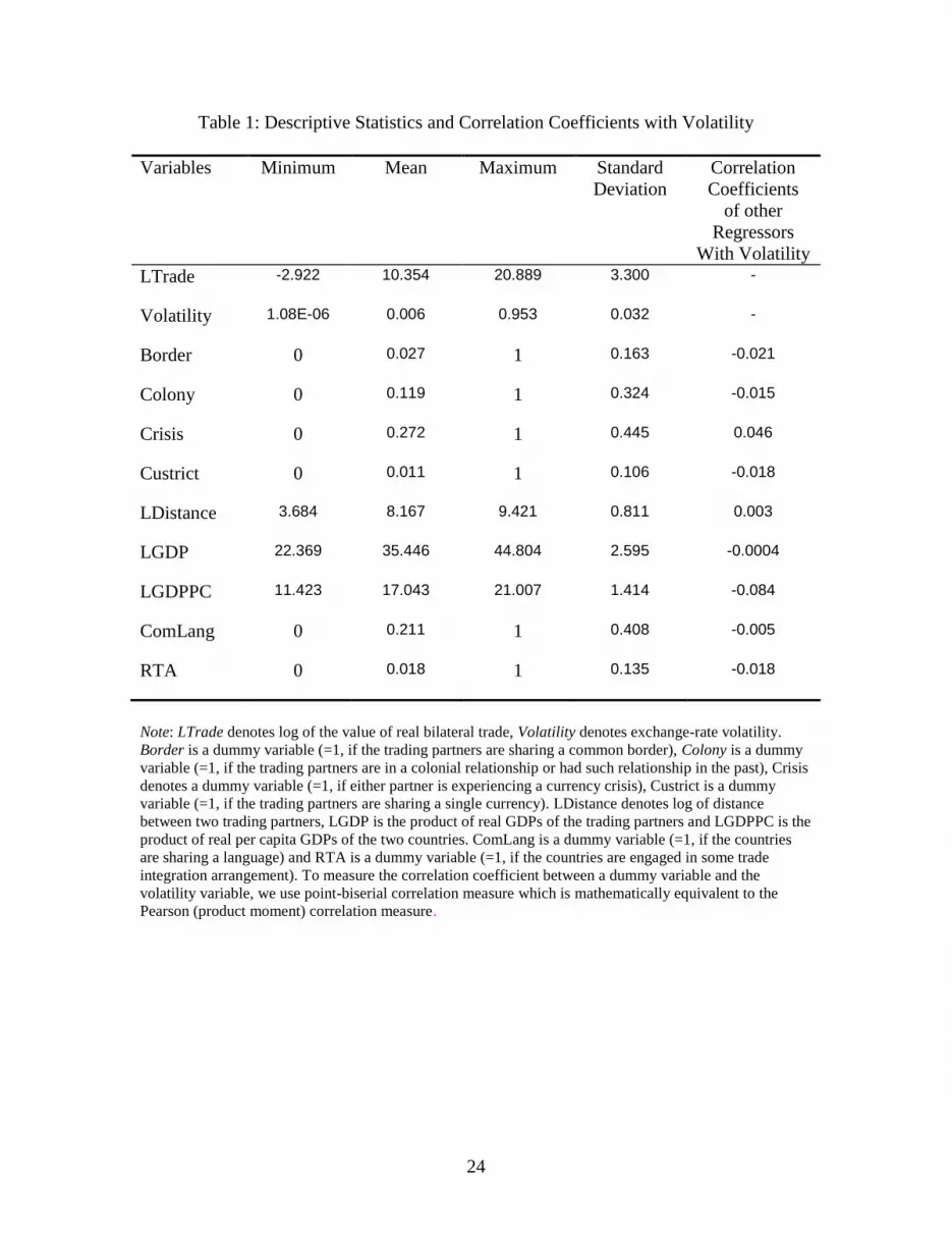
misspecified as well. However, we find that the correlation coefficients between

exchange-rate volatility and the other regressors are very low in our sample. (See Table 1

for details.) Therefore, any possible misspecification due to a linearity assumption for the

other regressors would not considerably impact the coefficient on volatility -- our main

variable of interest. However, in an attempt to provide some robustness testing we also

consider a randomly chosen sub-sample from our sample and estimate and compare the

results from a fully nonparametric model (see, Racine and Li (2004)) and a partially

linear model with only volatility being modeled nonparametrically (as in ours). The

goodness of fit gain turns out to be less than half of a percent - 68% for our partially

3 Henderson and Millimet (forthcoming),mentions about the same computational challenges in the context

of a fully nonparametric model. In order to deal with the problem they consider a much smaller sub-sample

from Rose’s data set and use a limited number of regressors. 4 Interestingly, Henderson and Millimet (forthcoming) does not find any evidence of nonlinearity in their

gravity equation itself, although they do not include the exchange-rate volatility variable in their

framework. Using a fully nonparametric model, they conclude that gravity is mostly linear. However, in

our case, when we include the volatility variable, trade-volatility relation not only displays some

nonlinearity (as clearly shown by the plots at the end of the paper), but the pattern of nonlinearity is

consistent with an interesting economic phenomenon. Note that Herwartz (2003) also considers nonlinearity

in trade flows and exchange-rate volatility relation among the Group of Seven.

10

linear model with only volatility being nonlinear (equation 4 below), as opposed to

68.22% for a fully nonparametric model.5

One may also be concerned with the effects of time invariant country specific

heterogeneities in the regression. To our knowledge, fixed effect unbalanced panel

regression results are not yet developed for the nonparametric/semiparametric

framework. A Hausman-type test that would help one choose between fixed vs. random

effects in a semiparametric framework has not yet been developed. As mentioned earlier,

our objective is to use as much data information as possible. Hence we estimate an

unbalanced panel. Otherwise, the loss of observations will be quite substantial. We have

used Li and Stengos (1996) type pooled semiparametric regression (without any fixed or

random effect heterogeneity) technique. The Li and Stengos (1996) approach

incorporates both predetermined and strictly exogenous regressors which is compatible

with our set of covariates. To compensate for the inability to estimate a fixed effects

regression, we augment the gravity models one additional time with region specific

dummy variables. Based on economic and geographical criteria, we consider seven broad

regional categories in our sample, namely Africa, Asia, the former socialist countries,

Latin America, Middle East, Oceania, and OECD. There are two sets of regional

dummies for each country pair. Thus we have two sets of regressions, one with, and one

without the regional dummies. Our main conclusion is however, quite robust to the use of

regional dummies.6 We also have six other dummy variables, (as discussed earlier) which

are mainly time invariant in nature. We reason that these regional and the other dummy

variables should capture the country specific characteristics to a considerable extent.

While Herwartz also uses a semiparametric approach to explore how exchange-

rate volatility impacts trade, our approach and his differ in a variety of ways. Most

importantly, he uses mainly time series data, while we use pooled data with large n

5 The in-sample average prediction error shows the same picture as well. This is consistent with Henderson

et al (forthcoming) finding in the sense that the other regressors do not have significantly nonlinear impact

on trade. 6 We get similar coefficients for the continuous as well as for the other dummy variables, as far as the signs

and the significances are concerned. The graphs depicting the relationship between volatility and trade (to

be discussed later) look very similar as well.

11

(number of cross sectional observations) and small T (time dimension). In this respect,

our approach is similar to Rose (2000) who also considers a pooled sample with large n

and small T. Herwartz estimates export supply and import demand equations separately

while in our approach we employ the gravity model. Herwartz (2003) concentrates on the

growth of trade among the Group of Seven while we use trade flows from over 200

countries. He constructs exchange-rate volatility by using a GARCH (1,1) model while

we use the standard deviation of exchange rate movement over the previous year. Our

intent in the paper is to focus on the nonlinear relationship using a very large pooled data

with a fixed time period (small yearly observations) with the number of cross sections

going to infinity7.

The details of our approach are as follows. First we assume that our true model is

a pooled partially linear semiparametric model. We allow our primary variable of

interest, (exchange-rate volatility) to affect trade volume in a general nonlinear fashion

(nonparametrically, so that there is no pre-assigned functional form) whereas the other

control covariates are assumed to affect the dependent variable in a linear fashion. The

partially linear (semiparametric) model that we have used can be written as

Yijt =Xijt+g(Zijt)+ijt (4)

Where Yijt denotes the dependent variable (ln(Tijt)), Zijt denotes our main variable of

interest, (σijt), Xijt captures all other control variables (as listed in (3)), and g(.) denotes the

7 A recent paper by Silva and Tenreyro (2006) criticizes the existing approaches for estimating a log-linear

gravity model. They suggest an alternative estimation approach - Poisson pseudo maximum likelihood

(PML) – even if the dependent variable is not strictly discrete. Using a RESET test they show that the PML

is appropriate, though OLS and parametric nonlinear least squares are not adequate for modeling a gravity

equation. Following their suggestion, we also use PML estimation for our data and perform the same

RESET test as they recommend. But we strongly reject the null hypothesis of PML being appropriate and

the corresponding RESET test p-values turn out to be 0.000 for both of our regression models (with and

without regional dummies). Hence PML, as suggested by Silva et al (2006) is not suitable for our dataset

and the variables.

12

unknown (nonparametric) functional form. The basic estimation method is a standard

kernel based semiparametric estimation (as described below). It is similar to that in Li

and Stengos (1996) which is similar to the one in Robinson (1988) and the approach is

summarized in Pagan and Ullah (1999).

From (4) we get:

Yijt –E(Yijt|Zijt) =[Xijt – E(Xijt|Zijt)]+ [g(Zijt) – E(g(Zijt)|Zijt)]+[ijt –E(ijt|Zijt)] (5)

Let 1ˆijtm and 2ˆ

ijtm denote the kernel based estimators of E(Yijt|Zijt) and E(Xijt|Zijt)

respectively and E(ijt|Zijt) = 0. Also note that [g(Zijt) – E(g(Zijt)|Zijt)]=0.

Rewriting (5) in matrix form we can then present the typical semiparametric

estimator of as

= )]ˆ)ˆ)]ˆˆ - [( 12122 m(Y - m[(X - m(X - )mX -

Where Y is an nT 1 vector of Yijt , X is an nT K matrix capturing the control variables

(K being the number of control variables) and 1m and

2m are the vector and matrix

generated from 1ˆijtm and 2ˆ

ijtm respectively.

After obtaining , we can then rewrite (4) as

(Yijt -Xijt )= Yijt* =g(Zijt)+ijt (6)

It is now a pure nonparametric regression model and we apply nonparametric kernel

weighted least square regression estimation at this final stage.8 Following the usual

practice, Z

g

can be interpreted as the point wise partial effect of exchange-rate volatility

8 See Robinson, 1988, Pagan and Ullah, 1999 and Fan and Yao (2003) and Li and Racine (2007) for more

details on such semiparametric and nonparametric regressions, their asymptotic properties as well as some

applications. We have used standard Gaussian kernel, exact binning and optimal as well as cross validated

bandwidths. Our conclusion is robust to the choice of bandwidths.

13

on trade volume. Our final stage of estimation is similar to the final stage estimation in

Herwartz (2003) in the sense that he also uses nonparametric kernel weighted least square

regression method to estimate the effect of volatility on export/import. Overall,

Herwartz’s approach can tease out variations in the response across countries as countries

may respond differently to exchange-rate risk. In our case, we derive an overall

conclusion backed by the results from a large number of countries. As such we are able to

better generalize about the impact of exchange risk on trade.

Our partially linear model will not only take care of any possible functional-form

misspecification in our main variable of interest; but will also shed some lights on how

volatility affects trade at various levels of volatility. Importantly, the model provides

information on the extent to which the underlying relationship between these two

variables is linear. This can only be achieved by using a general functional form.

4. Data

The data set used in this estimation is very large. We began with the data

compiled and used by Rose (2004) to study the impact of WTO membership on trade

stability. While many follow-ups to Rose’s (2000) widely cited study of the currency

union effect have been undertaken using Rose’s currency union database, it only contains

5-year intervals of data. We wished to use annual data to better capture the nonlinearities

in functional form that may be present in the data. We supplemented Rose's WTO

database with annual observations for real exchange-rate volatility. The volatility of the

exchange rate is constructed by first constructing monthly real exchange rate returns.

These returns are computed as log differences in the month to month exchange rate.

Twelve monthly returns are then used to compute a standard deviation for the year.

14

These standard deviations are then matched to the appropriate yearly observation so that

the volume of trade between two countries is presumed to be influenced by the previous

year’s real exchange-rate volatility. International Financial Statistics data on bilateral

exchange rates with their appropriate CPIs are used to construct the real exchange rates

used in the computation.

The original Rose data set includes observations, when available, from 1948 to

2000. Monthly exchange rate data were available in an easily accessible format only

since 1957, hence our database does not contain observations earlier than 1957. There are

a total of 214 countries in our sample and we use yearly data. Since all countries do not

trade with one another and since there are some missing observations our sample consists

of a total of 121501 observations.9

5. Results

We present the results with and without regional dummies for both parametric and

semiparametric regressions in Table 2. It is clear that the results are robust to the use of

regional dummies. These results are, broadly speaking, in line with results from Rose

(2000). The forces of attraction -- the product of real GDPs and of GDP per capita --

increase trade, as do the various dummy variables specifying the existence of common

borders, current or former colonial ties, trade integration agreements, and common

language. In contrast and as expected, the log of distance reduces trade flows while the

common currency variable promotes trade. The estimated value of the coefficient on the

common currency variable is similar to Rose's value of 1.25 implying that countries with

15

common currencies trade about 3 times more than do countries that do not share common

currencies (exp(1.1) = 2.99). The coefficient of the crisis variable turns out to be negative

and significant, as expected.

Of particular interest to us is the coefficient associated with the exchange-rate

volatility variable. As in any typical semiparametric regression, we obtain point wise

partial effects of volatility on trade (the conditional first derivatives or g(Zijt)/Zijt). The

median of these point wise partial effects are reported in Table 2.10

These median values

(-0.87 for the regression without regional dummies and -1.46 for the regression with

regional dummies) indicates that on an average11

real exchange-rate volatility depresses

the volume of trade, thereby concurring with the segment of the empirical and theoretical

literature that concludes that uncertainty in the exchange rate will depress the amount of

trade taking place. However, more comprehensive are the plots of these partial effects,

i.e., the plot of the conditional first derivatives (measured on the vertical axis) against

volatility (measured on the horizontal axis) as shown in Figure 1 and Figure A (in the

Appendix) for the entire range of observations on volatility. Figure 1 corresponds to the

semiparametric regression without the regional dummies. The corresponding plot is very

similar for the regression with the regional dummies, as is shown in Appendix Figure A.

While such plots allow us to observe how the partial effects vary with the level of

volatility, it is important to recall that not all levels of volatility are equally represented.

9 Note that our data set is a pooled one with large cross sections. The time dimension varies from about 10

to 40 annual observations per cross section. Thus the nonstationarity issues are not of major concern for us

because our data set, although pooled, contains large n. See Phillips and Moon (1999). 10

We have used STATA, Gauss and Nonparametric software NP package at various stages of our

computations. For more information on NP package, see http://www.mcmaster.ca/economics/racine/ 11

The mean values are also negative and larger than the median values.

16

In fact most of the values of volatility (97.4%) are between 0 and 0.05 and are thus

clustered in the first section of the graphs12

.

To better understand how trade, in practice, is impacted by exchange-rate

volatility, we focus on different ranges of volatility separately. We first “blow up” the

initial segment which contains 97.4% of total observations and display it in Figure 2.

Interestingly, we find that when volatility assumes values from around 0 to 0.025 the

plotted values appear almost as a horizontal line (though slightly downward sloping). As

volatility increases, trade seems to be depressed at a fairly constant rate.13

However, at

higher volatility (above 0.025 and up to about 0.05, containing about 3000 observations),

the relationship becomes noticeably nonlinear. The partial effects drop sharply implying

that volatility’s detrimental impacts become noticeably greater. Hence we can conclude

that exchange-rate volatility does depress trade and the depressing impact increases with

the level of volatility. Furthermore, at very high levels of volatility the “penalty”

increases at a rapidly increasing rate, practically pushing the volume of trade towards

zero.

In Figure 3 we plot how volatility impacts trade when volatility assumes even

greater values, specifically values between 0.05 and 0.07. This range contains about 750

12

It is noteworthy that we observe a sharp and large hump (for volatility level roughly around 0.025-0.07).

This hump does not disappear even if we use much larger bandwidths. We have tried up to 12 times larger

than the optimal (mean-square error minimizing bandwidth which is usually the default bandwidth) one.

However, the other relatively smaller humps appearing to the right (beyond this volatility level) gets

smoothened out when we use larger bandwidths. The coefficients associated with this large hump are

always highly significant. This hump can also be explained by an interesting economic phenomenon. We

therefore, focus on this part of the graph in Figures 2 and 3. 13

However, this rate is not really constant. A distinction between the partial effects for nonparametric vs.

parametric (constant partial effect, hence horizontal) regressions is shown in Figure 5 (for the range of

volatility up to 0.015) which depicts a steadily downward sloping partial effects for the nonparametric

model as opposed to the parametric model

17

observations.14

Here we observe a curious phenomenon. As volatility grows further, the

detrimental impact on trade weakens. Greater exchange-rate uncertainty no longer elicits

an even greater penalty on trade volume. Instead the detrimental impact weakens (though

it is still negative.) What might explain such? We argue that after some point, as the

level of exchange-rate uncertainty grows, countries learn to adapt to volatility, lessening

its harmful impacts. Countries employ hedging strategies that might otherwise be too

expensive to employ when volatility is relatively low. But when volatility surpasses a

point (and our data seem to indicate that point to be approximately a level of volatility of

0.05) it becomes cost-effective to employ these strategies15

. Eventually (when volatility

reaches about 0.07 or 0.08) trade is no longer depressed by exchange-rate volatility.

When volatility is this high countries have fully adjusted to the volatility employing one

means or another to mitigate its effect on trade.

In Figure 4 we show that at the highest range of volatility (around 0.07 and above)

the partial effect becomes noisy around the value zero.16

This noisy range contains about

2% percent of the observations. It is difficult to know exactly what is taking place in this

“noisy tail region”17

but it is noteworthy that almost all the insignificant coefficients fall

in this range.

Overall these plots seem to be suggesting that for the most part exchange-rate

volatility depresses trade and that the negative impact grows with the level of volatility.

14

Pakistan falls consistently in this range for the year 1973. This is basically the year after Bangladesh

gained its independence from Pakistan (the official date of independence was December 16th

1971). So it is

natural to observe some unusual exchange rate and trading behavior for Pakistan economy which just

experienced a considerable partitioning during that time. 15

As shown in Appendix Figure B, the story remains almost same for the regression with the regional

dummies as far as the shape of the graph and its location (values in the horizontal axis) is concerned,

although the steepness of the graphs differs. 16

It is 0.08 and above for the regressions with the regional dummies. 17

This may simply be the noisy tail behavior.

18

However, after a point countries seem to get a handle on the volatility and in one way or

another learn to diminish its impact. Figure 3 shows the weakening impact and suggests

that by the time exchange-rate volatility reaches around 0.07 countries have learned to

totally mitigate volatility’s negative impact on trade. How might this happen? Take for

example the case of trade between say the U.S. and the Dominican Republic (DR).

Suppose that exchange-rate volatility between the peso and the dollar becomes very

large. This will result in diminished trade. But over time with increasing levels and

persistence of volatility traders may protect themselves by informally dollarizing,

defining all of their transactions and assets in dollars, creating a mini "dollar economy."

Official levels of exchange-rate volatility will be recorded as high given our tracking of

the peso/dollar exchange rate, when in fact these traders are not affected to a great extent

by the peso/dollar exchange rate due to their operations in a "dollar" economy. This is

one manner by which traders may be mitigating the harmful impacts of exchange-rate

volatility and may explain what we are observing in the highest volatility ranges.

An examination of observations in the region of volatility running from roughly

0.0488 and 0.07/0.08 (where countries impact of volatility is weakening with greater

volatility) is supportive of this supposition. While a large cross-section of countries is

represented, ten countries show up repeatedly (with each consisting from 2.5 to 6 percent

of total observations). These are Argentina, Bolivia, Chile, Costa Rica, Ethiopia,

Guatemala, Pakistan, Nigeria, Sri Lanka, and Uruguay. We examined inflation series for

these countries in relation to the other countries in their respective geographic region. In

the case of the Latin American nations, all of these countries have experienced inflation

rates well in excess of the average for the region over extended periods of time. The

19

incidence of informal (and formal) dollarization for many of these countries is well

known (e.g. Argentina, Uruguay, and Bolivia). The Asian nations represented in this

group have also experienced relatively high inflation rates (in relation to neighboring

nations) over various periods in time. Nigeria has experiences periods of run-away

inflation, and Ethiopia’s inflation series is noteworthy in its variability, from high

inflation to deflation. As such, for each of these nations, domestic money, as a unit of

account, has suffered. Over time, countries that suffer from declines in the usefulness of

money tend to develop alternative methods to effectuate and to define transactions

including informal dollarization. It is conceivable that this region of observations is

picking up some of that adjustment to high and variable inflation which accompanies

very high exchange-rate volatility.

The question then arises, how do our results compare with Herwartz (2003)? He

finds that the impact of exchange-rate volatility on trade (growth) is non-linear and as

such our findings coincide. However, Herwartz does not find that trade is as consistently

negatively impacted as we find. The seven countries that he examines appear in some

cases to experience positive growth in trade on account of increased uncertainty, while

other countries experience the converse. His results appear to be country-specific. Our

larger sample, on the other hand, seems to point to an overall negative impact of volatility

on trade volume.

6. Discussions and Limitations:

To our knowledge, this is the first attempt to explore the relationship between exchange-

rate volatility and trade using a very large sample in a semiparametric framework. A fully

linear parametric model is a special case of a partially linear model, i.e., our

20

semiparametric model is a more generic one. Unless one estimates a more general model

it is not possible to assess to what extent a linear model is an appropriate one. Using a

data-driven estimation strategy (where we do not superimpose any a priori functional

form restriction in the trade-volatility relation), we try to investigate (1) if there is any

non-constancy in the rate at which volatility affects trade; (2) if so, at what levels of

volatility; (3) and whether we can derive any meaning economic conclusion from there.

We find that the detailed expositions of the relationship reveals nonlinearities and

those nonlinearities seem to get accentuated at higher levels of volatility (see Figures 2,3

and 5). This observed “U” (at a high level of volatility as shown in Figures 2 and 3)

remains present even if we use different bandwidths and try to smooth it out. Although

our parametric and semiparametric results are quite similar for the other control variables,

our semiparametric model gives us some additional economic information on how

volatility affects trade at various levels of volatility and this information has an intuitive

appeal.18

Overall our results can be interpreted as a reconciliation of the alternative findings

on the impact of exchange-rate volatility on trade volume. We find that by and large

exchange-rate volatility depresses trade, which is in accord with what has been found in

the bulk of the empirical literature. We also find that the negative impact of volatility on

trade strengthens as the level of uncertainty increases. Greater uncertainty increases the

costs of trade (and hedging) and in accordance the volume of trade is further reduced.

That is, there is some nonlinearity in the way that volatility impacts trade. More

interesting however, is our finding that at very high levels of exchange-rate volatility the

18

In particular, the behavior of the data around the "U" (Figures 2 and 3) could never be revealed in a linear

framework where we just obtain a single coefficient.

21

impact of uncertainty on trade volume fades and eventually trade volumes are unaffected

by increases in volatility. This provides us with an explanation for the less common, yet

bothersome occasional result in the empirical literature suggesting no impact of volatility

on trade. We find that at very high levels of volatility countries adjust or somehow

eliminate the harmful impact of volatility on trade. Informal dollarization is suggested as

one avenue that traders may be using to mitigate high levels of volatility.

22

References

Baum, Christopher F., Mustafa Caglayan and Neslihan Ozkan, “Nonlinear Effects of

Exchange-Rate Volatility on the Volume of Bilateral Exports,” Journal of Applied

Econometrics, 19, 2004, pp. 1-23.

Broda, Christian and John Romalis, “Identifying the Relationship between Trade and

Exchange Rate Volatility,” FRBNY working paper, February 2004.

Clark, Peter, Natalia Tamirisa, and Shang-Jin Wei, “Exchange Rate Volatility and Trade

Flows- Some New Evidence,” IMF Working Paper, May 2004.

Cushman, David O., “The Effects of Real Exchange Rate Risk on International Trade,”

Journal of International Economics, 15, 1983, pp. 45-63.

De Grauwe, Paul, 1988, “Exchange Rate Variability and the Slowdown in Growth of

International Trade,” IMF Staff Papers, 35, pp. 63-84.1988

Dell’Ariccia, Giovanni, “Exchange Rate Fluctuations and Trade Flows: Evidence from

the European Union,” IMF Staff Papers, Vol. 46, No. 3 (September/December 1999) pp.

315-334).

Fan, Jianqing and Irene Gijbels, Local Polynomial Modelling and its Applications, 1996,

Chapman and Hall.

Fan, Jianqing and QiweiYao, Nonlinear Time Series, 2003, Springer Series in Statistics.

Hayfield T. and Jeffrey S. Racine, 2007, np: Nonparametric kernel smoothing methods

for mixed datatypes. R package version 0.13-1.

Henderson, Daniel and Daniel Millimet, “Is Gravity Linear?” Journal of Applied

Econometrics, forthcoming.

Herwartz, Helmut, “On the (Nonlinear) Relationship between Exchange Rate Uncertainty

and Trade – An Investigation of US Trade Figures in the Group of Seven,” Review of

World Economics, 2003,139, 4, pp. 650- 682.

Hooper, Peter and Steven Kohlhagen, “The Effect of Exchange Rate Uncertainty on the

Prices and Volume of International Trade,” Journal of International Economics, 1978,

Vol. 8, 99. pp. 483-511.

Kenen Peter B. and Dani Rodrik, “Measuring and Analyzing the Effects of Short-Term

Volatility in Real Exchange Rates, “Review of Economics and Statistics, Vol. 68, No. 2,

May 1986, pp. 311-315.

23

Li, Qi and Thanasis Stengos, "Semiparametric Estimation of Partially Linear Panel Data

Models", Journal of Econometrics, 1996, 71, pp. 389-397.

Li, Qi and Jeffrey S. Racine, Nonparametric Econometrics: Theory and Practice, 2007,

Princeton University Press.

Nitsch, Volker, “Honey, I Shrunk the Currency Union Effect on Trade,” The World

Economy, 2002, 25, 4, pp. 457-474.

Pagan, Adrian and Aman Ullah, Nonparametric Econometrics, 1999, Cambridge

University Press.

Phillips P.C.B. and H.R. Moon, “Linear Regression Limit Theory for Nonstationary

Panel Data”, Econometrica, 1999, 67, 5, pp.1057-1111.

Pozo, Susan, "Conditional Exchange Rate Volatility and the Volume of International

Trade: Evidence from the Early 1900s," Review of Economics and Statistics, 1992, 74,

pp. 325-9.

Racine, Jeffrey.S. and Qi. Li (2004), “Nonparametric Estimation of Regression Functions

with both Categorical and Continuous Data”, Journal of Econometrics, 119, 99-130.

Robinson, Peter M., "Root-N-Consistent Semiparametric Regression", Econometrica,

1988, 56, pp. 931-954.

Rose, Andrew K., “One Money, One Market: The Effect of Common Currencies on

Trade.” Economic Policy, April 2000, p. 9-45.

Rose, Andrew K., “Does the WTO Make Trade More Stable?” University of California,

Berkeley working paper, January 13, 2004.

Sauer, Christine and Alok K. Bohara, “Exchange Rate Volatitliy and Exports: Regional

Differences between Developing and Industrialized Countries,” Review of International

Economics, Vol. 9, No. 1, 2001, pp. 133-52.

Silva Santos J.M.C. and Silvana Tenreyro, “Log of Gravity”, Review of Economics and

Statistics, 88(4), 2006, pp. 641-658.

Tenreyro, Silvana, “On the Trade Impact of Nominal Exchange Rate Volatility,” Federal

Reserve Bank of Boston working paper, April 2004.

Thursby, Jerry G. and Marie C. Thursby, "Bilateral Trade Flows, The Linder Hypothesis

and Exchange Risk," Review of Economics and Statistics, Vol. 69, No. 3, 1987 pp. 488-

495.

24

Table 1: Descriptive Statistics and Correlation Coefficients with Volatility

Variables Minimum Mean Maximum Standard

Deviation

Correlation

Coefficients

of other

Regressors

With Volatility

LTrade -2.922

10.354

20.889

3.300

-

Volatility 1.08E-06

0.006

0.953

0.032

-

Border 0 0.027

1 0.163

-0.021

Colony 0 0.119

1 0.324

-0.015

Crisis 0 0.272

1 0.445

0.046

Custrict 0 0.011

1 0.106

-0.018

LDistance 3.684

8.167

9.421

0.811

0.003

LGDP 22.369

35.446

44.804

2.595

-0.0004

LGDPPC 11.423

17.043

21.007

1.414

-0.084

ComLang 0 0.211

1 0.408

-0.005

RTA 0 0.018

1 0.135

-0.018

Note: LTrade denotes log of the value of real bilateral trade, Volatility denotes exchange-rate volatility.

Border is a dummy variable (=1, if the trading partners are sharing a common border), Colony is a dummy

variable (=1, if the trading partners are in a colonial relationship or had such relationship in the past), Crisis

denotes a dummy variable (=1, if either partner is experiencing a currency crisis), Custrict is a dummy

variable (=1, if the trading partners are sharing a single currency). LDistance denotes log of distance

between two trading partners, LGDP is the product of real GDPs of the trading partners and LGDPPC is the

product of real per capita GDPs of the two countries. ComLang is a dummy variable (=1, if the countries

are sharing a language) and RTA is a dummy variable (=1, if the countries are engaged in some trade

integration arrangement). To measure the correlation coefficient between a dummy variable and the

volatility variable, we use point-biserial correlation measure which is mathematically equivalent to the

Pearson (product moment) correlation measure.

25

Table 2: Parametric and Semiparametric Results

Variables Parametric

Coefficients

Semiparametric

Coefficients

Parametric

Coefficients

Semiparametric

Coefficients

Constant -21.423

(<0.000) -21.117

(<0.000) -15.404

(<0.0000) 10.431

(<0.000)

Volatility -1.759

(<0.000) -0.873

(<0.000) -0.634

(<0.000) -1.461

(<0.000)

Border 0.465

(<0.000) 0.472

(<0.000) 0.432

(<0.000) 0.436

(<0.000)

Colony 0.848

(<0.000) 0.844

(<0.000) 0.747

(<0.000) 0.751

(<0.000)

Crisis -0.136

(<0.000) -0.149

(<0.000) -0.117

(<0.000) -0.124

(<0.000)

Custrict 1.097

(<0.000) 1.053

(<0.000) 1.166

(<0.000) 1.143

(<0.000)

LDistance -1.116

(<0.000) -1.116

(<0.000) -1.215

(<0.000) -1.214

(<0.000)

LGDP 0.883

(<0.000) 0.884

(<0.000) 0.807

(<0.000) 0.809

(<0.000)

LGDPPC 0.554

(<0.000) 0.544

(<0.000) 0.465

(<0.000) 0.462

(<0.000)

ComLang 0.341

(<0.000) 0.341

(<0.000) 0.332

(<0.000) 0.331

(<0.000)

RTA 0.606

(<0.000) 0.592

(<0.000) 0.227

(<0.000) 0.218

(<0.000)

Regional

dummies

No No Yes Yes

Observations 121501 121501 121501 121501

Note: Dependent variable is the log of real bilateral trade. P-values are in the parentheses. All the

coefficients are significant at 1% level. Note, for the nonparametric part, medians of the nonparametric

point-wise estimates are reported. For details about nonparametric conditional first derivatives (partial

effects of volatility on logarithm of trade volume), refer to the graphs. For variable descriptions, refer to

Table 1.

26

27

28

Note: The Horizontal straight line represents the constant partial effects (-1.76)

from the parametric regression. The downward sloping curve represents the

varying partial effects from the semiparametric regression.

29

Appendix:

Figure A

Figure B

Note: In all these graphs we have not presented the upper and the lower confidence intervals because

they were very close to each other (small confidence intervals) and especially with too many

observations, it was heard to distinguish them visually in some regions. However for volatility level up to

0.08, all the coefficients are significant at 1% level.