Temi di discussione(Working papers)

Ap

ril

2008

660

Num

ber

Real exchange rate volatility and disconnect: An empirical investigation

by Riccardo Cristadoro, Andrea Gerali, Stefano Neri and Massimiliano Pisani

The purpose of the Temi di discussione series is to promote the circulation of working papers prepared within the Bank of Italy or presented in Bank seminars by outside economists with the aim of stimulating comments and suggestions.

The views expressed in the articles are those of the authors and do not involve the responsibility of the Bank.

Editorial Board: Domenico J. Marchetti, Patrizio Pagano, Ugo Albertazzi, Michele Caivano, Stefano Iezzi, Paolo Pinotti, Alessandro Secchi, Enrico Sette, Marco Taboga, Pietro Tommasino.Editorial Assistants: Roberto Marano, Nicoletta Olivanti.

REAL EXCHANGE RATE VOLATILITY AND DISCONNECT: AN EMPIRICAL INVESTIGATION

by Riccardo Cristadoro*, Andrea Gerali*, Stefano Neri* and Massimiliano Pisani*

Abstract

A two-country model that incorporates many features proposed in the New Open Economy Macroeconomics literature is developed in order to replicate the volatility of the real exchange rate and its disconnect with macroeconomic variables. The model is estimated using data for the euro area and the U.S. and Bayesian methods. The analysis delivers the following results: (a) international price discrimination, home bias and shocks to the uncovered interest rate parity (UIRP) condition are key features to replicate the variance of the real exchange rate; (b) home bias, shocks to the UIRP condition and to production technologies help replicating the disconnect; (c) distribution services intensive in local nontradeables are an important source of international price discrimination.

JEL Classification: F32, F33, F41, C11. Keywords: international economic cycle, real exchange-rate volatility, pass-through, international transmission of shocks.

Contents

1. Introduction.......................................................................................................................... 3 2. The model............................................................................................................................ 5

2.1 Firms............................................................................................................................. 6 2.1.1 International price discrimination....................................................................... 6 2.1.2 Nontradeable sector ............................................................................................ 8

2.2 Households ................................................................................................................... 9 2.2.1 Intratemporal preferences and the real exchange rate ......................................... 9 2.2.2 Intertemporal preferences and financial structure ............................................. 11

2.3 Monetary policy.......................................................................................................... 13 2.4 Market clearing conditions ......................................................................................... 14 2.5 Equilibrium................................................................................................................. 15

3. Bayesian estimation ........................................................................................................... 15 3.1 Data............................................................................................................................. 15 3.2 Prior distributions and calibrated parameters ............................................................. 16 3.3 Posterior distributions................................................................................................. 17 3.4 Model fit ..................................................................................................................... 18

4. What explains the real exchange rate volatility and disconnect........................................ 19 5. Impulse responses and variance decomposition ................................................................ 22 6. Concluding remarks........................................................................................................... 24 Appendix: The Bayesian estimation procedure...................................................................... 25 References .............................................................................................................................. 28 Tables and Figures.................................................................................................................. 32 _______________________________________ * Bank of Italy, Economic Outlook and Monetary Policy Department.

1 Introduction

While the real exchange rate plays an important role in the allocation of resources andexpenditures across countries, its short run movements are much less linked with pricesand quantities than one would expect (real exchange rate disconnect). On the one hand,the high volatility displayed by the exchange rate has little impact on that of othermacroeconomic variables such as output and consumption. On the other hand, this highvolatility does not seem to be induced by changes in fundamental determinants of theexchange rate (as it is the case for other macroeconomic variables).

One explanation of the puzzle is based on price rigidities and on the implications ofinternational price discrimination. Given the compelling case against the law of one priceand the evidence of a relative stability of import and consumer prices vis-a-vis nomi-nal exchange rate fluctuations (imperfect pass-through), several papers in the New OpenEconomy Macroeconomics (NOEM) framework have relaxed the producer currency pric-ing assumption (PCP) of the seminal Obstfeld and Rogoff’s (1995) Redux model.1 Amongothers, Chari et al. (2002) show that a high degree of price stickiness is necessary to repro-duce the volatility of the real exchange rate when the economy is hit by monetary policyand technology shocks. Devereux and Engel (2002) study the conditions under whicha model with local currency pricing (LCP), heterogeneity in international price-setting,incomplete international financial markets and shocks to the uncovered interest parity(UIRP) can generate large exchange rate volatility that, in addition, does not influencethe volatility of other macroeconomic variables.2 The implied international segmentationin product markets and incomplete risk sharing eliminate the equality between relativeprices and marginal rates of substitution. Therefore, changes in real exchange rate arenot linked to changes in the product market and the former can be driven by shocks tothe UIRP condition without significant spillover to other macroeconomic variables. Morerecently, Corsetti et al. (2005) show that, independently of nominal frictions, incompleteexchange rate pass-through and sticky prices can result from endogenous price discrimina-tion in presence of a large component of nontradable goods and services in the consumerprice of tradable goods.

Another explanation is based on quantities and looks at ways to introduce differencesin the consumption bundles consumed in each country. It amounts to relaxing the as-

We owe a special thank to Kosuke Aoki, Gianluca Benigno, Fabio Canova and Giancarlo Corsetti.We also thanks Pierpaolo Benigno, Paul Bergin, Leif Brubakk, Gunter Coenen, Luca Dedola, GabrielFagan, Fabio Ghironi, Frank Smets, Mattias Villani and participants at the workshops “New Modelsfor Forecasting and Policy Analysis” hosted by the Bank of Italy, “Recent Developments in Macroeco-nomic Modelling” hosted by the South African Reserve Bank, “Dynamic Macroeconomics” hosted bythe University of Bologna, “Estimation and Empirical Validation of Structural Models for Business Cy-cle Analysis” organized by the EABCN/CEPR and the Swiss National Bank, at the macroeconomicsseminars organized by Harvard University, Boston College, Federal Reserve Bank of Boston.

1See Devereux and Engel (2003).2See also Betts and Devereux (2000). Devereux and Engel (2002) motivate the shocks to the UIRP by

assuming the presence of foreign currency traders with biased expectations about future exchange rates.Duarte (2003) and Kollmann (2005) analyze the relationship between exchange rate regimes and businesscycle in models featuring LCP and a UIRP shock. See also Jeanne and Rose (2002).

3

sumption of symmetric preferences across countries, on the one hand, and that of fulltradeability of all goods, on the other. These two assumptions, in fact, when coupledwith the absence of international price discrimination are enough to ensure that the pur-chasing power parity condition holds and hence that the real exchange rate is constant.The assumption of symmetric preferences is relaxed by introducing home bias. The fulltradeability of all goods is relaxed by introducing nontradeable goods. As for the role ofhome bias, Warnock (2003) shows that when preferences are biased toward domestically-produced goods there are wealth transfers across countries and large short-run devia-tions from consumption-based purchasing power parity. The role of nontradable goodshas been studied by Stockman and Tesar (1995), Hau (2000), Benigno and Thoenissen(2006), Burstein, Eichenbaum and Rebelo (2006) and Dootsey and Duarte (2007). Themain result from these contributions is that nontraded goods increase the volatility of thereal exchange rates relative to its volatility in the model without nontraded goods andlowers the cross-correlation of exchange rates with other variables.

In this paper we provide an empirical and systematic assessment of the implicationsof several economic features that have been introduced in the literature to explain thereal exchange rate volatility and disconnect. To that purpose, we estimate a two-countrystochastic general equilibrium model for the U.S. and the euro area with Bayesian tech-niques.

We assume home bias, sticky import prices in the currency of the buyer (LCP), dis-tribution services along the lines of Corsetti et al. (2005), nontradeability of some goods.The presence of a distribution sector allows to distinguish between pass-through at theborder and at consumer level, the latter being usually lower than the former, and helps infurther breaking the link between real exchange rate and other macroeconomic variables.3

We allow for wage and nontradeables price stickiness as additional tools to insulate fun-damentals from real exchange rate fluctuations and assume labor-based production (thereis no capital accumulation). We characterize the behaviour of the central banks througha modified Taylor rule. International financial markets are incomplete (a riskless bond isinternationally traded) and there are shocks to the UIRP.

Several interesting results emerge from the analysis. First, relaxing in turn some of theabove mentioned features we prove that many combinations of the rigidities introducedin the model are sufficient to replicate the volatility of the real exchange rate and itsdisconnect with fundamentals, but they do so through different mechanisms. Second,the presence of nontradeables is what allows the model(s) to replicate the real exchangerate stylized facts without resorting to economically extreme outcomes. In fact, when weconsider only tradables in the model, the home bias estimate increases to one. Anothergeneral lesson is that home bias, international price discrimination and UIRP shock areall essential ingredients to generate high volatility. Home bias and technology shocks arecrucial to generate the disconnect since they help limiting the transmission of wide andpersistent real exchange rate fluctuations to consumer prices and consumption. Finally,

3See Kollman (2001) for a quantitative analysis of the relation between real exchange rate volatilityand staggered price and wage setting in a dynamic model. See Campa and Goldberg (2008) for empiricalevidence on the role of the distribution sector in reducing the sensitivity of consumer prices to exchangerate fluctuations.

4

the distribution sector is a key feature of international price discrimination. Interestingly,the degree of import price stickiness is not extremely high at the border and allows togenerate a positive correlation between real exchange rate and terms of trade. This isconsistent with the empirical evidence given by Obstfeld and Rogoff (2000) in favor ofthe expenditure-switching effect of nominal exchange rate acting at the border and notat the consumer level.

Our work can be related to recent contributions that exploit advances in Bayesian es-timation to empirically analyze NOEM models.4 Adolfson et al. (2007) estimate an openeconomy model featuring incomplete pass-through using euro area data (they take therest of the world as exogenous). Lubik and Schorfheide (2005), De Walque and Wouters(2004) and Rabanal and Tuesta (2006) estimate two-country models on euro area andU.S. data focusing on the role of import price stickiness and incomplete pass-through forinternational spillover and real exchange rate fluctuations. Rabanal and Tuesta (2007)analyze the role of nontradables and distribution services.5 We deviate from those contri-butions by empirically and systematically assessing the whole set of determinants of thereal exchange rate fluctuations (home bias, international price discrimination due to pricestickiness and distribution services, nontradables, UIP shocks).

The paper is organized as follows. Section 2 describes the model. Section 3 reportsthe estimates and the empirical validation of the model. Section 4 analyses the sources ofthe real exchange rate volatility and disconnect. Section 5 reports impulse responses andvariance decomposition analyses. Section 6 concludes.

2 The model

There are two countries of equal size (normalized to one), denominated home and for-eign. In each country there is a continuum of agents on the unit interval. We allow forhome bias in consumption preferences. Each country is specialized in the production oftradeable and nontradeable goods (the two sectors have equal size, normalized to one).Each sector is characterized by monopolistic competition. Consistently with most of theNOEM literature we abstract from capital accumulation and assume that labor is theonly input and that the production function is shifted by random variations in technol-ogy. Firms producing tradeables are engaged in international price discrimination. Thisfeature is the combination of the LCP assumption and distribution services which are in-tensive in local nontradeables. International financial markets are incomplete. A risklessbond is internationally traded and a modified uncovered interest parity condition linksthe expected nominal exchange rate depreciation to the interest rate differential and astochastic risk premium. Wages and prices are sticky. Finally, interest rates are set by

4See Bergin (2003, 2004) for a maximum likelihood approach to estimate NOEM models. See Smetsand Wouters (2003) for a Bayesian neo-keynesian closed economy model of the euro area.

5De Walque and Wouters (2004) also have a distribution sector. However, it is not intensive in localnontradeables and it is not a source of international price discrimination. Lubik and Schorfeide (2005)have complete pass-through at the border, but not at consumer level thanks to price stickiness. Rabanaland Tuesta (2006) have incomplete pass-through at the border but do not distinguish between borderand consumer levels. Justiniano and Preston (2006) estimate a small open economy model.

5

the monetary authorities according to feedback rules.

In what follows we report the equilibrium conditions of the home country. Thosereferring to the foreign country are similar. Variables with a star (∗) refer to the foreigncountry.

2.1 Firms

There are three categories of firms in the economy: producers of tradeables, of nontrade-ables, and of distribution services. The two former producers are monopolistic suppliersof their specific brand. The latter acts under perfect competition.

2.1.1 International price discrimination

Following Corsetti et al. (2005), we assume that firms producing tradeables need dis-tribution services intensive in local nontradeables to deliver their products to final con-sumers. This implies that the elasticity of demand for any brand is not necessarily thesame across markets and, as a consequence, it is optimal to price discriminate markets.Firms in the distribution sector are perfectly competitive. They purchase home and for-eign tradeable goods and distribute them in the home country using η ≥ 0 units of theconstant-elasticity-of-substitution basket η of nontradeable brands n:

η ≡[∫ 1

0

η (n)θN−1

θN dn

] θNθN−1

θN > 1 (1)

The parameter θN measures the elasticity of substitution among the different brands.

The distribution sector introduces a wedge η between wholesale and consumer prices.Denoting with p (h) and with p∗ (h) the wholesale price of the generic home brand re-spectively in the home and foreign markets and assuming η = η∗ we get the consumerprices:

pt(h) = pt(h) + ηPN,t , p∗t (h) = p∗t (h) + ηP ∗N,t (2)

where PN (P ∗N) is the price of the home (foreign) composite basket η. The price index

PN :

PN =

[∫ 1

0

p (n)1−θN dn

] 1θN−1

(3)

is defined as the minimum expenditure necessary to buy one unit of the basket η.

The second key assumption is that prices are sticky in the currency of the buyer (LCPassumption). Each firm, when adjusting prices, has to pay a cost by purchasing the CESaggregated basket (CH in the home market and C∗

H in the foreign market, defined later)

6

of all the brands produced in the sector:

ACpH,t (h) ≡ κp

H

2

(pt (h)

pt−1 (h)− 1

)2

CH,t κpH ≥ 0

ACp∗H,t (h) ≡ κp∗

H

2

(p∗t (h)

p∗t−1 (h)− 1

)2

C∗H,t κp∗

H ≥ 0 (4)

where κpH and κp∗

H measure the degree of nominal price rigidity.6

We assume that the generic firm produces its tradeable brand using the following CEStechnology:

yt (h) + y∗t (h) = ZH,tLH,t (h) (5)

LH,t (h) ≡[∫ 1

0

LH,t (h, j)θL−1

θL dj

] θLθL−1

θL > 1

where LH,t (h, j) is the labor input supplied by the generic domestic agent j ∈ (0, 1), θL

is the elasticity of substitution between labor varieties and yt (h) and y∗t (h) the outputsold respectively in the home and foreign markets.7 The term ZH,t is a sector-specifictechnology shock that follows a stationary autoregressive process of the form:

ln ZH,t = ρH ln ZH,t−1 + εZH,t

where 0 < ρH < 1 and the innovation εZHis an identically independently distributed

(i.i.d.) normal variable with mean and variance equal respectively to 0 and σ2H .8 Firms

take wages as given when minimizing their production cost. The implied marginal costis:

MCH,t =Wt

ZH,t

(6)

where the wage index of the economy is defined as Wt =[∫ 1

0Wt (j)1−θL dj

] 11−θL . Wages

are set by households who are monopolistic competitive in the labor market (see later).Concerning optimal prices, in each period the firm producing the brand h chooses pt (h)and p∗t (h) to maximize the expected flow of profits:

Et

∞∑τ=t

Λt,τ [pτ (h) yτ (h) + Sτ p∗τ (h) y∗τ (h)−MCH,τ (yτ (h) + y∗τ (h))]

6 See Rotemberg (1982) and Dedola and Leduc (2001).7The implied demand of labor variety j is

LH,t (h, j) =(

Wt (j)Wt

)−θL

LH,t (h)

8In the foreign country, the corresponding law of motion is:

ln Z∗F,t = ρ∗F ln Z∗F,t−1 + ε∗ZF,t

7

subject to price adjustment costs (4) and standard demand constraints. The term Et

denotes the expectation operator conditional on the information set at time t and Λt,τ

is the households’ intertemporal marginal rate of substitution in consumption (definedlater). The nominal exchange rate S is expressed as the number of home currency unitsper unit of foreign currency. In a symmetric equilibrium p(h) is equal to the price indexof the home composite tradeable PH,t (defined below) and, similarly, p∗t (h) is equal to thecomposite index P ∗

H,t. The first order conditions with respect to PH,t and to P ∗H,t can be

written as:

PH,t = θHPH,t − θHMCH,t + AH,t, P ∗H,t = θHP ∗

H,t − θHMCH,t

RSt

+ A∗H,t (7)

where AH,t and A∗H,t involve terms related to the presence of price adjustment costs and

θH and RSt are the elasticity of substitution between home tradeable brands and thehome real exchange rate, respectively (see below). A crucial implication of internationalprice discrimination is that at the border the nominal exchange rate pass-through intoimport prices is not complete (∂ log p∗t (h) /∂ log St < 1). The higher is pass-through themore fluctuations in the nominal exchange rate are transmitted to import prices. Inthe limiting case, when the pass-through is complete exchange rate movements are fullytransmitted. In our case, complete pass-through can happen only if there are neitherdistribution services (η = 0 and PH = PH) nor nominal rigidities (κp∗

H = 0). The aboveequations would collapse to the standard pricing rule of constant markup over marginalcost.

2.1.2 Nontradeable sector

Firms in the nontradeable sector solve a similar problem. Nontradeable goods do notneed distribution services (pt(n) = pt(n)) and the good is produced, as for tradeables,using a CES production function having labor varieties as inputs:

y (n) = ZN,tLN,t (n) (8)

LN,t (n) ≡[∫ 1

0

LN,t (n, j)θL−1

θL dj

] θLθL−1

θL > 1

ZN is a sector specific technology shock that follows a stationary autoregressive process:

ln ZN,t = ρN ln ZN,t−1 + εZN,t

where 0 < ρN < 1 and the innovation εZNis an i.i.d. normal random variable with mean

and variance equal respectively to 0 and σ2N .

Each firm, when adjusting prices, has to pay a cost by purchasing the CES aggregatedbasket (CN , defined later) of all the brands produced in the sector:

ACpN,t (n) ≡ κp

N

2

(pt (n)

pt−1 (n)− 1

)2

CN,t κpN ≥ 0

8

where κpN measures the degree of price stickiness. In each period, the firm producing

the brand n chooses pt(n) to maximize the expected flow of profits subject to the aboveadjustment costs and demand constraint (that includes demand for nontradeables usedin the domestic distribution sector).

In a symmetric equilibrium (p(n) = PN) the first-order condition is:

PN,t (1− θN) = −θNMCN,t + AN,t (9)

where AN,t contains terms related to the presence of price adjustment costs and θN andMCN,t = Wt/ZN,t are the elasticity of substitution between nontradable brands and thesector-specific marginal cost, respectively. If prices were flexible, they would be equal toa constant markup over marginal costs.

2.2 Households

There is a continuum of households which attain utility from consumption and leisure.Preferences are symmetric across countries, with the notable exception of home bias.Nominal and relative price indices are derived from them.

2.2.1 Intratemporal preferences and the real exchange rate

The aggregate consumption basket, Ct, is defined as:

Ct ≡[a

1ρ

T CT,t

ρ−1ρ + (1− aT )

1ρ CN,t

ρ−1ρ

] ρρ−1

ρ > 0 (10)

where ρ is the elasticity of substitution, CT is the bundle of tradeables and the parameteraT (0 < aT < 1) is its share, CN the basket of nontradeables.

The consumption index of traded goods CT is:

CT,t ≡[a

1φ

HCH,t

φ−1φ + (1− aH)

1φ CF,t

φ−1φ

] φφ−1

φ > 0 (11)

where the parameter φ is the elasticity of substitution,the parameter aH (0 < aH < 1) isthe share of domestic tradeables, CH and CF are the baskets of, respectively, home andforeign tradeables brands:9

CH,t ≡[∫ 1

0

ct (h)θH−1

θH dh

] θHθH−1

, CF,t ≡[∫ 1

0

ct (f)θF−1

θF df

] θFθF−1

CN,t ≡[∫ 1

0

ct (n)θN−1

θN dn

] θNθN−1

9C∗F and C∗H are similarly defined.

9

We assume that preferences are symmetric across countries (a∗T = aT , φ∗ = φ, θ∗H =θH = θ∗F = θF , θ∗N = θN) with the only exception of home bias. In each country,households have a strong preference for the domestic tradeable good (aH > 0.5). Assumingsymmetric home bias (a∗H = 1− aH), the foreign consumption index of traded goods is:

C∗T,t ≡

[(1− aH)

1φ C∗

H,t

φ−1φ + a

1φ

HC∗F,t

φ−1φ

] φφ−1

(12)

Distribution services introduce a wedge between the elasticity of substitution of tradeablegoods at the consumer and producer levels. The latter is given by:

φ

(1− η

PN

p (h)

)(13)

where PN and p (h) are set at their steady state values. The lower elasticity of substitutionat producer level contributes to increasing the volatility of relative prices and the realexchange rate. From the definition of the consumption bundles we can derive price indexes.In the home country the consumption-based price index:

Pt =[aT P 1−ρ

T,t + (1− aT ) P 1−ρN,t

] 11−ρ

(14)

The price index PT of the tradeable bundle is:10

PT,t =[aHP 1−φ

H,t + (1− aH) P 1−φF,t

] 11−φ

(15)

The symmetric home bias assumption implies the following foreign price index of trade-ables:

P ∗T,t =

[(1− aH) P ∗1−φ

H,t + aHP ∗1−φF,t

] 11−φ

. (16)

Given the above indexes, it is possible to define the real exchange rate and the terms oftrade. The first is given by:

RSt =StP

∗t

Pt

that measures the relative price of foreign consumption in terms of home consumption. Adepreciation (appreciation) of the real exchange rate corresponds to an increase (decrease)in RS. The terms of trade of the home economy at the producer and consumer levels arerespectively:

TOT t =P F,t

StP∗

H,t

, TOTt =PF,t

StP ∗H,t

and two expression differ because of distribution services at the consumer level.

10 The price index PH is equal to PH,t =[∫ 1

0pt (h)1−θH dh

] 11−θH . Price indexes PF,t and PN,t and

their foreign counterparts are similarly defined.

10

2.2.2 Intertemporal preferences and financial structure

Households receive utility from consuming the basket Ct of goods and disutility fromworking Lt hours. The expected value of household j lifetime utility is given by:

E0

{ ∞∑t=0

βtξt

[Ct (j)1−σ

1− σ− κ

τLt (j)τ

]}

where E0 denotes the expectation conditional on information set at date 0, β is thediscount factor, 1/σ is the elasticity of intertemporal substitution and 1/ (τ − 1) is thelabor Frish elasticity. The preference shifter ξ is common to all households and followsan autoregressive process of order one:

ln ξt = ρξ ln ξt−1 + εξ,t

where 0 < ρξ < 1 and the innovation εξ,t is an i.i.d. normal random variable with meanand variance equal, respectively, to 0 and σ2

ξ .11

Households in the home country can invest their wealth in two risk-free bonds with aone-period maturity. One is denominated in domestic currency and the other in foreigncurrency. In contrast, foreign households can allocate their wealth only in the bonddenominated in the foreign currency.12

The budget constraint of household j in the home country is:

BH,t (j)

Rt

+StBF,t (j)

R∗t Φ(

StBF,t

Pt− b)µt

−BH,t−1 (j)− StBF,t−1 (j)

≤∫ 1

0

Πt (h, j) dh +

∫ 1

0

Πt (n, j) dn + Wt (j) Lt (j)− PtCt (j)−WtACWt (j) (17)

BH (j) is household holding of the one-period risk-free nominal bond, denominated inunits of home currency, that pays a gross nominal interest rate Rt. BF (j) is the holdingof the risk-free one-period nominal bond denominated in units of foreign currency, thatpays R∗

t . Both Rt and R∗t are paid at the beginning of period t + 1 and are known at

time t. The function Φ(StBF,t

Pt− b), that captures the costs of undertaking positions in the

international asset market and pins down a well-defined steady-state, has the followingfunctional form:

Φ

(StBF,t

Pt

− b

)≡ exp

(φb

(StBF,t

Pt

− b

))φB ≥ 0

The parameter φB controls the speed of convergence to the non-stochastic steady state.13

The payment of this cost is rebated in a lump-sum fashion to foreign agents. Households

11 We do not include money explicitly and interpret this model as a cash-less limiting economy in thespirit of Woodford (1998).

12 See Benigno (2001) for a similar financial structure.13 The function Φ (.) depends on real holdings of the foreign assets in the entire home economy. Hence,

domestic households take it as given when deciding on the optimal holding of the foreign bond. Werequire that Φ(0) = 1 and that Φ(.) = 1 only if StBF,t/Pt = b, where b is the steady state real holdingsof the foreign assets in the entire home economy. The function Φ(.) is assumed to be differentiable anddecreasing at least in the neighborhood of the steady state. See Turnovsky (1985) and Schmitt-Groheand Uribe (2003).

11

derive income from two sources: nominal wage income Wt (j) Lt (j) and profits of do-

mestic tradeable and nontradeable firms, respectively∫ 1

0Πt (h) dh and

∫ 1

0Πt (n) dn. Each

household is a monopolistic supplier of one type of labor Lt (j) and sets the nominal wageWt(j) taking into account the demand for her type of labor by domestic firms. Wagesetting is subject to quadratic adjustment costs which are measured in terms of the totalwage bill:

ACWt (j) ≡ κW

2

(Wt (j)

Wt−1 (j)− 1

)2

Lt κW > 0 (18)

where the parameter κW measures the degree of nominal wage rigidity.

The first order conditions with respect to BH,t (j) and BF,t (j) are:

C−σt (j) ξt = RtβEt

[C−σ

t+1 (j) ξt+1Pt

Pt+1

](19)

C−σt (j) ξt = R∗

t Φ(StBF,t

Pt

− b)µtEt

[C−σ

t+1 (j) ξt+1Pt

Pt+1

St+1

St

](20)

Combination of the log-linearized versions of the two above equations yields the followingmodified UIRP condition:14

Rt −(R∗

t − φbbF,t

)− µt = ∆St+1 (21)

where ∆S > 0 is depreciation rate of the nominal exchange rate, Y bF,t ≡ (StBF,t/Pt − b)where Y is the steady state value of total home output. The shock µt follows an AR(1)process:

ln µt = ρµ ln µt−1 + εµ,t

where 0 < ρµ < 1 and the innovation εµ is an i.i.d. normal random variable with meanand variance equal respectively to 0 and σ2

µ. The shock can be justified on the basis of thewell known weak empirical support in favour of the uncovered interest parity condition.From a theoretical point of view, it can be seen as one shortcut for “noise traders” thathave biased expectations on the exchange rate or for “information shocks” that affect therisk premia required by foreign-exchange markets.15

The assumption of incomplete international financial markets is crucial for fitting thereal exchange rate dynamics. When a complete set of state contingent nominal assets istraded the following log-linearized risk-sharing condition holds in every state of nature:

RSt = σ(Ct (j)− C∗t (j)) (22)

according to which the real exchange rate is proportional to the relative marginal utilitiesof consumption, and hence, given the specification of preferences we adopt, to the relativeconsumption. The drawback is that it is hard to replicate the exchange rate volatilitywithout assuming a sufficiently high level of the coefficient of risk aversion σ (i.e., arelatively low intertemporal elasticity of substitution). To weak the risk-sharing condition

14 Variables are defined as Xt = lnXt − lnX, where lnX is the steady-state value.15 See Devereux and Engel (2002) and Duarte and Stockman (2005).

12

we assume incomplete international financial markets. In this case the relation betweenthe real exchange rate and the marginal utilities holds only in expected values. Hence,expectations introduce a wedge between relative consumption and real exchange rate.Combining the home and foreign agent’s log-linearized first order conditions with respectto the internationally traded bond BF,t gives:

Et

(RSt+1 − RSt

)= Et

[σ

(Ct+1 (j)− Ct (j)

)− (ξt+1 − ξt)

]− (23)

Et

[σ(C∗

t+1 (j)− C∗t (j))− (

ξ∗t+1 − ξ∗t)]

+ φBbF,t − µt

The assumption of incomplete markets has two other advantages. First, shocks leadto wealth redistribution across countries and hence increase in the persistence of the realexchange rate. Second, under risk sharing, the correlation between real exchange rate andrelative consumption is, counterfactually, positive (Backus-Smith puzzle).16 This is notnecessarily the case under incomplete markets: since the international bond is traded onlyafter shocks are realized the above equation does not necessarily hold in the first period.Consequently, the correlation between real exchange rate and relative consumption canbe negative, in line with the empirical evidence. The preference shocks ξt and ξ∗t andthe UIRP shock also contribute to break the link between real exchange rate and relativemarginal utility.17

Finally, the first order condition with respect to wages is:

Wt (j)

Pt

= AW,tθL

(θL − 1)κLτ−1

t (j)Cσ

t (j)

ξt

(24)

The real wage is equal to the marginal rate of substitution between consumption andleisure times the term θL/ (θL − 1), which measures the markup in the labour market anda term that takes into account the adjustment costs, AW,t. Absent these costs, the realwage would be equal to a constant markup over the marginal rate of substitution betweenconsumption and leisure.

2.3 Monetary policy

Home monetary authority sets the short-term nominal interest according to the followinglog-linear feedback rule:

Rt = ρRRt−1 + (1− ρR)ρππt + (1− ρR)ρyyt + (1− ρR)ρs∆St + εt (25)

where Rt is the short-term nominal interest rate, πt is the consumer price inflation rate, yt

is obtained by log-linearizing the sum of home tradable and nontradable output around thesteady state (see below) and ∆S is the nominal exchange rate percent variation (∆S > 0is a depreciation). The parameter ρR (0 < ρR < 1) captures inertia in interest rate setting.The monetary policy shock is denoted with εt and follows an i.i.d. normal process withmean and variance equal respectively to 0 and σ2

R. A similar monetary policy functionholds in the foreign country.

16 See Backus and Smith (1993).17 Stockman and Tesar (1995) also consider preference shocks.

13

2.4 Market clearing conditions

Market clearing conditions are defined as:

yt (h) = aHaT

(pt (h)

PH,t

)−θH(

PH,t

PT,t

)−φ (PT,t

Pt

)−ρ ∫ 1

0

Ct (j) dj (26)

+

(pt (h)

PH,t

)−θH∫ 1

0

ACH,t (x) dx

y∗t (h) = (1− aH)aT

(p∗t (h)

P ∗H,t

)−θH(

P ∗H,t

P ∗T,t

)−φ (P ∗

T,t

P ∗t

)−ρ ∫ 1

0

Ct (j∗) dj∗ (27)

+

(p∗t (h)

P ∗H,t

)−θH ∫ 1

0

AC∗H,t (x) dx

yt (f) = (1− aH)aT

(pt (f)

PF,t

)−θH(

PF,t

PT,t

)−φ (PT,t

Pt

)−ρ ∫ 1

0

Ct (j) dj (28)

+

(pt (f)

PF,t

)−θH∫ 1

0

ACF,t (x) dx

yt (n) = (1− aT )

(pt (n)

PN,t

)−θN(

PN,t

Pt

)−ρ ∫ 1

0

Ct (j) dj (29)

+

(pt (n)

PN,t

)−θN

η

(∫ 1

0

CH,t (j) dj +

∫ 1

0

CF,t (j) dj

)

+

(pt (n)

PN,t

)−θN∫ 1

0

ACN,t (x) dx

The firs two equations are the market clearing conditions of the generic home tradeablebrand h in the home and foreign market, respectively. The third equation is the clearingcondition of home imports of the generic brand f produced in the foreign country. Thelast one is the condition of home nontradable goods, that are bought by the domestichouseholds and distribution sector. In each market clearing there is also the demandcomponent implied by the price adjustment costs of firms x. As for financial markets, thefollowing market clearing conditions hold:

∫ 1

0

BH,t (j) dj = 0,

∫ 1

0

BF,t (j) dj +

∫ 1

0

B∗F,t (j∗) dj∗ = 0. (30)

The market clearing condition of the labor variety supplied by agent j is:

Lt (j) =

(Wt (j)

Wt

)−θL∫ 1

0

LH,t (h) dh +

∫ 1

0

LN,t (n) dn

From the budget constraint (17) and the above conditions we can derive the following

14

equation for the home trade balance:

TBt =

∫ 1

0StBF,t (j) dj

R∗t Φ(

StBF,t

Pt)µt

−∫ 1

0

StBF,t−1 (j) dj

= St

∫ 1

0

p∗t (h) y∗t (h) dh−∫ 1

0

pt (f) yt (f) df (31)

which is equal to the difference between total export and import.

2.5 Equilibrium

We make two assumptions. First, firms belonging to the same sector set the same price(hence pt(h) = PH,t, p∗t (h) = P ∗

H,t and pt(n) = PN,t). Second, households belonging tothe same country have the same initial level of wealth and share the profits of domesticfirms in equal proportion. Hence, within a country all the households face the samebudget constraint. In their optimal decisions, they will choose the same path of bonds,consumption and wages. The equilibrium is a sequence of allocations and prices such that,given the initial conditions, in each country the representative agent and the representativefirms satisfy their respective first order conditions and the market clearing conditions hold.

Since a closed form solution is not possible, the behaviour of the economy is studiedby taking at a loglinear approximation to the model equations in the neighbourhood of adeterministic steady state. In this steady state shocks are set to their mean values, priceinflation, wage inflation and the exchange rate depreciation are set to zero, interest ratesare equal to the agents’ discount rate, consumption is equalized across countries, the tradebalance and the net foreign asset position are zero. Given the presence of distributioncosts, the price of nontradeables is different from that of tradeables. However, prices aresymmetric between countries and the real exchange rate is one.

3 Bayesian estimation

In this Section we first presents the results of the estimation and then we assess the fit ofthe model by computing in-sample prediction errors for the observables and simulatingsecond moments.

3.1 Data

We interpret the model as representing the euro area and the U.S. economies. The homecountry is the euro area. In estimating the model we use data for the period 1983:1-2005:2on 14 variables: real consumptions C and C∗, consumer prices inflation rates π and π∗,nontradeable inflation rates πN and π∗N , domestic tradeable inflation rates πH and π∗F ,wage inflation rates πW and π∗W , the euro-dollar real exchange rate RS and the tradebalance TB. Inflation rates are constructed as quarterly changes in the corresponding

15

price indexes. We use the inflation rate in the manufacturing and services sector for,respectively, domestic tradeables and for nontradeables. The real exchange rate is basedon consumer price indices. The trade balance series is the bilateral net export seriesbetween the U.S. and the euro area. More details on data can be found in the Appendix.

3.2 Prior distributions and calibrated parameters

The Bayesian estimation technique allows us to use the prior information from earliermicro and macro studies. In particular, we choose priors as close as possible to those ofAdolfson et al. (2007), Lubik and Schorfheide (2005) and Rabanal and Tuesta (2006). Weuse the beta distribution for all parameters between 0 and 1, the gamma for those boundedon the set of positive numbers and the normal for the unbounded ones. We assume alldistributions to be a priori independent. Table 1 reports the mean and standard deviationof these distributions.

Priors on preferences are standard. The mean of home bias, aH , is set at 0.95 (standarddeviation 0.1) and the mean of the share of tradeables, aT , at 0.45 (0.1).18 The mean ofintratemporal elasticity of substitution between home and foreign tradeables, φ, is set at1.14 (0.1), while that of intratemporal elasticity of substitution between tradeables andnon tradeables, ρ, at 0.74 (0.1).19 The mean of the risk aversion coefficient, σ, is set at2.0 (0.2). The elasticity of the net foreign asset position to the premium, φb, has a meanequal to 0.01.

As far as the coefficients of monetary policy rules are concerned, we chose standardvalues for their prior distributions: a relatively high mean, 1.5, on the inflation coefficientsρπ and ρ∗π (standard deviation 0.1) helps to guarantee a unique solution of the model. Themeans of the coefficients on the lag of the interest rate, ρR and ρ∗R, are set at 0.8 (standarddeviation 0.1), those of the output coefficients, ρy and ρ∗y, and exchange rate depreciationcoefficients, ρs and ρ∗s, respectively at 0.1 and 0 (in all cases, the standard deviation is0.1).

Parameters measuring price stickiness (ki and k∗i , with i = H, F, N, N∗) have thesame mean value, set at 5.6 (standard deviation 10). This value is consistent with microevidence of Bils and Klenow (2002) for the U.S. and by Fabiani et al. (2005) for the euroarea. Parameters measuring wage stickiness (kW and k∗W ), which are chosen on the basisof the results by Smets and Wouters (2005), have a mean value equal to 63 (standarddeviation 40), that corresponds to an average contract length of 5 quarters. We set themean of the parameter η of distribution services at 1.2 (0.1).20

The autoregressive parameters of shocks have a mean value set at 0.9 (standard devi-

18 Stockman and Tesar (1995) find that aN is around 0.5 for the major OECD countries. Corsetti etal. (2005) calibrate aH to 0.72.

19 Corsetti et al. (2005) calibrate ρ at 0.74, consistently with empirical evidence in Mendoza (1991),while Bergin (2004) estimate for φ is equal to 1.13.

20 Corsetti et al. (2005), following Burstein et al. (2003) set η to a value that matches the share ofthe retail price of tradables accounted for by the local distribution services in the U.S. (approximately50 percent).

16

ation is 0.05). The standard deviations of all shocks have a prior mean equal to 0.01.

A very small number of parameters is calibrated.21 The discount factor β is set at 0.99.The Frish labor elasticity, 1/(τ − 1), is set at 1. The elasticity of substitution betweenlabour varieties, θW , is set at 4.3. The elasticity of substitution between nontradeablevarieties, θN , is set at 6 while the elasticity between tradeable varieties, θH , is endogenouslyset to satisfy the equality θH = θN (1 + η), which assures that markups are equal acrosssectors. The prior mean of η and the value of θN imply that θH is equal to 13.2. Thesevalues are similar to those used by Corsetti et al. (2005).

3.3 Posterior distributions

The technical details of the Bayesian estimation procedure are provided in the Appendix.In the following we comment on some features of the estimated posterior distributionsof the parameters, and also try to ascertain whether the data were informative or notabout our parameters, by comparing marginal priors and marginal posteriors. Table 1reports some percentiles from the posteriors (2.5th, 50th and 97.5th) as well as meanand standard deviations of priors and posteriors. A look at the table suggests that ourdata were informative about home bias aH , whose posterior mean and median (0.92) arelower than the prior mean.22 Data are also informative on the share of tradeables in theconsumption basket aT . Prior and posterior means are similar, but the posterior varianceis lower than its prior counterpart. The posterior mean of the consumer elasticity ofsubstitution between tradeables φ is higher (1.47) than the prior mean (1.14). Estimationdrives the mean of η to 1.0, only marginally below the mean of the prior. The previoustwo estimates imply that the mean of the elasticity of substitution between tradeablesat producer level is 0.7. Data are not informative about the degree of substitutabilitybetween tradeables and nontradeables ρ and the coefficient of relative risk aversion σ.23

In order to comment on the parameters measuring the degrees of price stickyness andto allow for a better comparison with other empirical analyses, it is useful to transformthem into probability of not adjusting prices and frequency of adjustments. Table 2,which reports these results, suggests that in each country wages are the most rigid prices,followed by those of nontradeables and tradeables. As we’ll see, these two features allowfitting the real exchange rate and the inflation rates without the need of having extremelyhigh values of import price stickiness or home bias to insulate stable domestic nominalprices from highly volatile international relative prices.24 Overall, the results are consistent

21 Calibration can be seen as chosing a prior with infinite precision.22 Estimates in the literature are quite similar. Rabanal and Tuesta (2006) report, depending on the

estimated model, 0.92 and 0.98, Lubik and Schorfheide (2005) equal to 0.8 and 0.9.23 Lubik and Schorfheide (2005) estimate a posterior mean value of σ slightly below 4.0. Rabanal and

Tuesta (2006) assume log utility.24 Rabanal and Tuesta (2006) find that firms adjust prices once every 4 and 5 quarters respectively

in the euro area and in the U.S., Lubik and Schorfheide (2005) find values between 1 and 7 quarters forimport prices, depending on the estimated model. Eichenbaum and Fisher (2005) find that U.S. firmsreoptimize prices at least once every two quarters. Adolfson et al. (2007) find that import prices adjustonce every 2-3 quarters in the euro area. Ortega and Rebei (2006) use Canadian data to estimate a smallopen NOEM economy model with, as in our case, sticky wages and nontradables. Their estimates are

17

with much of the evidence based on microdata, which suggests that the main source ofstickiness in the industrialized economies are not prices, but wages. Obstfeld and Rogoff(2000) emphasize this point when they say that models of incomplete pass-through basedonly on high import price rigidities hardly replicate the positive correlation between termsof trade and real exchange rate. In the next section we show that our model is able toreplicate this stylized fact.

The parameters of the monetary policy rules are rather similar in the two countries.Both rules are relatively inertial and aggressive against inflation, while there seems not tobe a significant reaction to exchange rate fluctuations. The high inertia contributes to thefit of the observables by increasing the endogenous persistence of the model.25 The esti-mates of the autoregressive coefficients of the shock processes are high, but not extremelyso. The more persistent shocks are those to the UIRP condition, to the technology of theeuro area nontradeables and of the U.S. economy. The data are not informative aboutthe persistence of the shock to the technology of the euro area tradeables and to U.S.preferences.

Finally, we find that the adjustment cost of the net foreign asset position, φb, is around0.01, in line with estimates of Rabanal and Tuesta (2006).

3.4 Model fit

Following Adolfson et al. (2007) in Figure 1 we assess the fit of the model by computing theKalman filtered one-sided estimates (thick line) of the observed variables at the posteriormode and comparing them with the actual data (thin lines). The fit of the real exchangerate, consumption levels, interest rates and inflation rates is satisfactory. The model facessome difficulty in fitting nominal wage inflation rates and the bilateral trade balance, thatin the data are more volatile than predicted in the model. However, these two variablesare likely to be measured with large errors.

We also assess the explanatory power of the model by simulating second moments andcomparing them with those in the data. To this end we draw 500 vectors of parametersfrom their posterior distribution and for each of them we generate 100 times series for themain variables. Each of them is 292 periods long. We discard the first 200 observationsto work with a number of periods equal to that of the actual series. Their business cyclecomponent is extracted using the Hodrick-Prescott (HP) filter. Statistics are computedusing all the simulated time series. Table 3 reports the 2.5, 50, 97.5 percentiles of the stan-dard deviation and first order autocorrelation. The volatility of the real exchange rate ishigher in the data (8.40) than in the model (95% of the posterior distribution lies between4.84 and 8.58), confirming the well-known difficulty in replicating the high volatility ofinternational relative prices. However, the magnitudes of actual and simulated volatilitiesare not too different. At the same time, the model is able to replicate the volatility of

close to ours: Canadian import have a posterior median duration of two quarters, nontradeables of threequarters, wages of five quarters.

25 See Benigno (2004) for the role of inertial monetary policy rules in matching the high persistence ofthe real exchange rate.

18

the fundamentals, which is much lower than that of the real exchange rate, both in themodel and in the data.26 The model has a hard time in matching the persistence of thereal exchange rate (0.66 the posterior median of the autocorrelation coefficient), comingslightly below the value in the data (0.81). Regarding other observables, the persistenceof the CPI inflations (π and π∗), and U.S. domestic tradable prices (π∗F ) as well as that ofeuro area nominal interest rate (R) is relatively well matched. The persistence of otherinflation rates (euro area and U.S. nontradable prices, i.e. πN and π∗N) is overstated, thatof consumptions (C and C∗) is instead underestimated.

Table 4 reports cross-correlations. The model replicates the low cross-correlation be-tween real exchange rate, the various inflation rates, nominal interest rates and the levelsof home and foreign consumption (disconnect). Hence, the large and volatile fluctuationsof the real exchange rate are not transmitted to nominal prices. Consumer relative prices,interest rates and consumptions do not greatly vary. As we show in the next session,nontradables and home bias are mainly responsible for matching these moments. Themodel is also able to replicate the correlations of the real exchange rate with relative con-sumption (the so-called Backus-Smith puzzle), the countercyclical behavior of the tradebalance (cross correlation between trade balance and euro area consumption) and thenegative cross-correlation of consumptions.

The overall message is that the model is able to account sufficiently well for thedynamics of the data and, thus, can be used in the next Section to understand whichfeatures contribute to the real exchange rate disconnect.

4 What explains the real exchange rate volatility and

disconnect

In this Section we investigate the role of the various features in accounting for the discon-nect. As a starting point, we decompose the variance of the change in the real exchangerate on the basis of the following equation (obtained by log-differencing the real exchangerate and consumer price definitions):

∆RSt = (1− aT )(π∗N,t − π∗T,t)− (1− aT )(πN,t − πT,t) + · · · (32)

+(2aH − 1)(πF,t − πH,t) + · · ·+aH

(∆St + π∗F,t − πF,t

)+ (1− aH)

(∆St + π∗H,t − πH,t

)

where ∆RSt and ∆St are the percentage change in the real and nominal exchange ratebetween period t and t−1, πT,t, πH,t, πF,t, πN,t denote the home country inflation rates ofrespectively tradeable, home tradeable, foreign tradeable and nontradeable goods. Vari-ables with a star refer to their foreign counterparts. The first two terms in equation (32)are referred to as the “real internal real exchange rate”while the term in the second row is

26 The volatility of the CPI inflation rate is matched in the euro area, underestimated in the U.S.Nontradables inflation rates and consumption volatilities are instead matched. As for nominal interestrates, the model matches the euro area data, while understates the volatility of U.S. data.

19

captures the role of home-bias. Finally, the last two terms show the deviations from theinternational law of one price for, respectively, the foreign and home tradeables. Absentnon tradeable goods (aT = 1), home bias (aH = 1

2) and assuming that the law of one

price holds (there is no market segmentation ∆St + π∗F,t = πF,t and ∆St + π∗H,t = πH,t),the purchasing power parity would hold and the real exchange rate would be constant.Variances and covariance terms are obtained by simulation as described in the previoussection. The results, which are reported in Table 5, suggest that international price dis-crimination is an important source of the real exchange fluctuations, followed by homebias. The contribution of the internal real exchange rate is negligible, indicating thatthe relative price of nontradeables does not matter for real exchange rate fluctuations.However, the role of nontradables for real exchange rate fluctuations cannot be dismissedsince they are an important source of international pricing discrimination.

Figure 2 reports the decomposition of the actual real exchange rate based on equation(32) and the mean of the posterior distribution of the parameters aT and aH . The graphconfirms that international price discrimination and home bias play a crucial role inshaping the dynamics of the real exchange rate as it can be seen by the fact that thesecomponents track pretty well its time series.

To further assess the importance of nontradeables, home bias and international pricediscrimination we estimate variants of the benchmark model that differ for the featuresthat we include. The columns of Table 6 report the mode of parameter vector (and themarginal likelihood) of the following models: i) without nontradeables (no NT); ii) withouthome bias (no HB); iii) without price discrimination and with prices set in the producercurrency (producer currency assumption, PCP); iv) without distribution services (i.e.setting η = 0) and with LCP being the only source of international price discrimination(LCP); v) without the UIRP shock. For comparison purposes the mode of the benchmarkmodel (LCP-DC) is also reported in the first column.

The comparison between the first and second column shows that, absent nontradeables,the mode of home bias aH approaches one. In this case the model fits the observables byclosing the two economies and thus letting the coincidence between consumer and domestictradeable prices to insulate consumers from real exchange rate fluctuations. When thereis no home bias (aH is calibrated at 0.5, see the third column), the share of nontradables(1− aT ) increase to one, so as to close the two economies in a way similar to the case ofno nontradables (no NT); in each country domestic nontradeables and consumer pricescoincide, insulating the latter from the instability of international relative prices. ThePCP column shows the implications of (the absence of) price discrimination. Under thisassumption, the international law of one price holds and pass-through of exchange rateonto import price is complete. Higher values of home bias aH and share of nontradeables(1 − aT ) allow fitting both fundamentals and the real exchange rate, so to compensatefor the lack of international price discrimination and its insulating properties. A similarmessage comes out from the next to the last column, that shows estimates when thereis no distribution sector. In this case the distinction between wholesale and retailingprices does not hold and local currency pricing is the only source of international pricediscrimination. To fit the observables, home bias, share of nontradeables (as in the PCP)and import prices nominal rigidities, all increase. The LCP and PCP models, given the

20

absence of the distribution sector, cannot rely upon a low elasticity of substitution between

tradeables at the producer level (given by φ(1− η PN

PH

), see equation (13)) to improve the

fit. Hence, they exploit the insulating properties of home bias, nontradables and pricestickiness. Finally, when the UIRP shock is not in the model, the share of tradeablesincreases, while the degree of import price rigidity goes down. This model is not able toreplicate the high volatility of the real exchange (see below)27, and hence has no need toinsulate the real side of the economy using nontradeables or import price stickiness. Notealso that the model’s fit is relatively low. Overall, the results of the sensitivity analysispresented in Table 6 suggests that nontradeables, price discrimination and UIRP shockare key features to fit our observables and in particular the real exchange rate.

To draw further evidence about the role of the various features in matching the data,we also computed the marginal likelihood of the model, a measure of aggregate fit thatis obtained by integrating the posterior density over the parameter set.28 The resultingnumber is a summary statistic measuring the probability of having observed the dataunder the proposed model independently of any particular parameter configuration. Thelast row of Table 6 presents the marginal likelihood for a set of alternative specificationsof our model (to be discussed in the next session) with the ”benchmark” model discussedso far in the LCP-DC column. Although, according to this criterion, the LCP model(where we shut down the distribution sectors by setting η = 0) produces the best fit(better: the highest marginal likelihood), the benchmark model is among the best fittersand, more importantly, there is a strong deterioration in the fitting ability of any modellacking home bias, a shock to the UIRP and/or nontradable goods, suggesting that thesefeatures are crucial for the empirical fit of our dataset.29

We further investigate this result by turning off these features one at a time and usingthe median of the posterior distribution of the benchmark model to simulate the secondmoments. The results are reported in Tables 7-9.30 Each of the features contributesto the real exchange rate volatility, in particular distribution services, home bias andnontradeables (Table 7). Distribution services and nontradeables are also important tomatch the volatility of the fundamentals. The volatilities of inflation rates, interest ratesand consumptions are larger when the nontradeables channel is shut down. Similarly,distribution services allow matching the volatility of CPI and tradeables inflation rates.The latter indeed increases when η is set to zero. No single feature plays a predominantrole in affecting the persistence of the observables (Table 8). Simulated values are rathersimilar across the various model specifications. We’ll see below that exogenous shocks

27 The measurement error of the real exchange rate, not reported, is much higher than in the LCP-DCmodel.

28 The marginal likelihood is numerically computed using the modified harmonic estimator in Geweke(1999) and 300,000 draws from the Metropolis algorithm.

29 To guarantee a fair comparison, the marginal likelihood of the LCP-noNT model is compared withthe “concentrated” marginal likelihood of the LCP-DC. This statistics is obtained by fitting the LCP-DCmodel to all the observables with the exception of nontradeables inflation rates. The LCP-noNT modelfits slightly better this reduced set of observables. The “cost” to pay, however, is the home bias equal toone.

30The no-NT case is obtained by setting aT , the weight of tradable goods in the consumption bundle,close to one.

21

play a key role in replicating first order autocorrelations. Cross-correlations between theexchange rate and fundamentals, in particular inflation rates and consumptions, increasewhen home bias is switched off (Table 9). The remaining specifications have similarimplications. As expected, the model with only tradable goods does not replicate thecross-correlation between real exchange rate and nontradeables inflation rates.

The next step is to understand the role of each shocks in explaining the dynamics ofthe real exchange rate. To this end, we simulate the LCP-DC model assuming: (a) onlyUIRP shocks; (b) shocks to the UIRP and to technology; (c) shocks to UIRP, technologyand monetary; (d) shocks to UIRP, technology, monetary and preferences. The results arereported in Tables 10-12. UIRP shocks are clearly necessary to generate high volatilityin the real exchange rate (Table 10). However, they do not reproduce the volatilitiesof fundamentals, for which fundamental shocks are necessary. In particular, technologyshocks match the inflation rates volatilities, preference shocks match the consumptionsvolatilities. Monetary shocks allow matching the volatilities of interest rates. The UIRPshocks play also a significant role in matching the persistence of the real exchange rate(Table 11), while the contribution of other shocks is negligible. Technology and monetarypolicy shocks improve the matching of the persistence of, respectively, interest rates andU.S. inflation rates. Preferences play only a marginal role. Finally, Table 12 showshow the different shocks contribute to the real exchange rate disconnect. Technologyshocks play the largest role while monetary shocks improve the matching of the cross-correlations of euro area consumption on one side and real exchange and trade balance onthe other. Preference shocks help matching the cross-correlations between consumptionsand between consumptions and real exchange rate (Backus-Smith puzzle).31 Either shocksto the UIRP condition or shocks to preferences are needed to match this stylised fact.

Overall, the analysis suggests that home bias, distribution services, nontradeables andUIRP shocks are key features of a model that aims to match the real exchange ratevolatility and its disconnect. Without these features and shocks, the volatility would betoo low. Distribution services and nontradeable goods contribute to match the volatilityof the fundamentals. The UIRP shock is important to induce persistence in the realexchange rate. Finally, home bias and technology shocks reduce the cross-correlationsbetween the real exchange rate and fundamentals, thus allowing the model to replicatethe disconnect. These results are similar to those in Devereux and Engel (2002). The mainimprovement to those authors’ analysis is that our assessment of the role of the differentfeatures and shocks is based on an estimated model that has proved to be able to replicatethe main empirical facts concerning the real exchange rate and its determinants.

5 Impulse responses and variance decomposition

In this Section we document the dynamic properties of our estimated economies (byshowing the impulse responses), and study the relative importance of different shocks

31 Chari et al. (2002) show that a two country model is able to replicate the volatility and persistenceof the exchange rate with only monetary shocks only when the coefficient of risk aversion is relativelylarge. They also show that the model is not able to replicate the Backus-Smith puzzle.

22

(by reporting the variance decomposition). Figures 3 and 5 to 7 report the median andthe 0.95 probability interval at each step of the impulse horizon. The percentiles arecomputed using the draws from the posterior distribution of the parameters from theMetropolis algorithm. The variance decomposition (Table 13) is computed on the basisof the median of the posterior distribution.

Figure 3 reports the responses of inflation rates, consumption levels and the interestrates to a positive one standard deviation UIRP shock. The strong increase in the euroarea import price inflation does not translates into an equally large increase in the euroarea CPI inflation rate (the same is true for the U.S.). The high values of the homebias and the share of nontradables allow to disconnect consumer prices from the largemovements of the real exchange rate. The shock induces a decrease in consumption anda deterioration of the euro area terms of trade. As a consequence, through a standardsubstitution effect, there is a shift of world demand towards the euro area tradable goods.The decrease in the euro area interest rate is hardly significant. Similarly, the responsesof U.S. consumption and interest rate are smaller than the response of import prices.All these responses can be used to study the implications of distribution services for theexchange rate pass-through. Figure 4 reports the median of the pass-through coefficients,both at the border and at the consumer level for the benchmark, the LCP and the PCPmodel.32 Import prices increase in the euro area while they decrease in the U.S. economy.The magnitude of the variation is roughly one half of the impact response of the exchangerate, implying a pass-through at the border of 0.5 both in the euro area and the U.S.economy. These values are sufficiently high to guarantee a deterioration of the terms oftrade in line with the results of Choudhri et al.(2005) and the empirical evidence reportedby Obstfeld and Rogoff (2000). At the consumer level, given the presence of distributionservices, the response of terms of trade is negative consistently with the low degree ofpass-through which on impact is equal to 0.25 in both economies.

Figure 5 reports the responses to a positive one standard deviation preference shock inthe euro area. The positive response of consumption induces an increase in domestic CPIinflation and the interest rate. The latter, through the UIRP condition, determines anappreciation of the euro area real exchange rate. The large degree of price stickiness andshare of nontradeables in the consumption bundle limit the response of consumer priceinflation. The burden of the equilibrium adjustment, therefore, relies upon internationalrelative prices, which are relatively flexible and whose responses become large. Note that,consistently with the disconnect, U.S. consumption, CPI inflation rate and interest rateare only slightly affected by the shock.

The responses to technology and monetary shocks in the euro area, which are reportedin Figures 6 and 7, all have the expected signs. After the positive technology shock, do-mestic CPI inflation rate and nominal interest rate decrease, while consumption increasesand the real exchange rate depreciates. After the restrictive monetary shock, the domes-tic inflation rate and consumption decrease and the real exchange rate appreciates. Thereaction of international relative prices is stronger than that of fundamentals, as in theUIRP and preference shocks cases. However, in contrast to the UIRP shock, the difference

32Pass-through is measured as the ratio between the response of nominal prices in each period and theinitial response of nominal exchange rate.

23

in the magnitude of responses between the real exchange rate and import prices, on oneside, and euro area consumption and CPI inflation rate, on the other, are not large. Thisresult is in line with those of the analysis of second moments discussed in Section 3.4 andsuggests that shocks to the UIRP condition are crucial for replicating the volatility of thereal exchange rate.

As a final remark, notice that the disconnect should imply that (a) shocks with im-portant effects on key macroeconomic variables do not explain a large fraction of thevariation in exchange rates, and (b) shocks that explain a sizable share of exchange ratevolatility do not explain a large share of the variation in other macroeconomic variables.And the results from the asymptotic variance decomposition, reported in Table 13, sup-port this conclusion. Each of the two economies is driven primarily by domestic shocks,in particular technology and preferences, while the real exchange rate by the shock to theUIRP condition, which accounts for more than three quarters of its variance.

6 Concluding remarks

In this paper, we have investigated the dynamics of the real exchange rate in the contextof an estimated model that incorporates many features proposed in the NOEM literature.The model replicates the volatility of the real exchange rate and its disconnect withfundamentals relying on home bias, international price discrimination and shocks to theUIRP condition. Nontradeable goods also play an important role since they are relativelysticky and represent a nontrivial component of consumer prices. They also contributeto match the volatility of inflation rates and consumption levels and allow the model toreplicate the real exchange rate stylized facts without resorting to extremely high (andimplausible) values for the home bias (when we drop them, home bias estimates increaseto one).

The presence of a distribution sector, a key feature to induce international price dis-crimination, allows to reduce the pass-through of exchange rate variations onto importand consumer prices. Pass-through at the border is, instead, relatively high (the degreeof import price stickiness is low) and guarantees a deterioration of the terms of tradewhen the nominal exchange rate depreciates, consistently with the evidence in Obstfeldand Rogoff (2000).

Several extension to the model are worth mentioning. First, the accumulation of physi-cal capital can be introduced in the model in order to enhance the propagation mechanismof the shocks. Second, the model can be estimated along the lines suggested by Corsetti etal. (2006), i.e. assuming alternative prior means for the elasticity of substitution betweentradeables and alternative specifications for the technology processes. In this way, it willbe possible to quantify the separate contributions of the wealth and substitution effectsassociated to changes in relative prices to the dynamics of the real exchange rate and thefundamentals. Finally, a welfare analysis could be conducted, given the extremely differ-ent implications that alternative sources of incomplete pass-through - nominal rigiditieson the one hand and real frictions, such as distribution services, on the other - have forthe optimal conduct of monetary policy.

24

Appendix: The Bayesian estimation procedure

The Bayesian approach starts form the assertion that both the data Y and of theparameters Θ are random variables. Starting from their joint probability distributionP (Y, Θ) one can derive the fundamental relationship between their marginal and condi-tional distributions known as Bayes theorem:

P (Θ|Y ) ∝ P (Y |Θ) ∗ P (Θ)

Reinterpreting these distributions, the Bayesian approach reduces to a procedure for com-bining the a priori information we have on the model, as summarized in the prior dis-tributions for the parameters P (Θ), with the information that comes from the data, assummarized in the likelihood function for the observed time series P (Y |Θ). The resultingposterior density of the parameters P (Θ|Y ) can then be used to draw statistical inferenceeither on the parameters themselves or on any function of them or of the original data.

Sources and treatment of the data

We use quarterly data on 14 macro variables over the period 1983:1-2005:2 from theArea Wide Model (AWM) and Bureau of Economic Analysis (BEA) databases:

Variable Content Source & NotesEuro area

real consumption National accounts def. AWMconsumer prices HICP AWMnontradeable prices HICP service prices AWMdomestic tradeables prices HICP manufactured goods AWMwages nominal wages AWMshort-term interest rate 3-months nominal rate AWM

euro-U.S. real exchange rate nom. exch. rate deflated using CPI’strade balance bilateral net trade

U.S.real consumption National accounts def. BEAconsumer prices CPI BEAnontradeable prices service prices BEAdomestic tradables prices manufactured goods BEAwages nominal wages BEAshort-term interest rate 3-months nominal rate BEA

(33)

We estimate the model in stationary form (i.e. exploiting its implications only for thelog deviations from steady state, and not for the trend, of the variables) and therefore

25

we pre-treat the data prior to estimation in order to achieve stationary. We demeanedall inflation rates, the interest rates and the real exchange rate; we remove a linear trendfrom the real consumptions, and a quadratic trend from the trade balance series.33

The series for tradeable inflation in the euro area has a strong seasonal componentstarting from 2001:1 (due to a change in the methodology and composition of the un-derlying data). We removed the resulting structural break by applying two differentseasonal adjustments to this series, one before and one after the break date. The seasonalcomponents were removed by regressing this variable on a set of seasonal dummies. Forconsistency we applied the same procedure to all inflation series in the euro area (andsimply removed the seasonal components from the U.S. ones). We also tried not to do so(i.e. treating for seasonality only the euro area tradeable inflation series) but the resultsare not affected in a substantive matter.

The stochastic part of the model features 9 structural shocks and 10 measurementerrors. The structural shocks are illustrated in the text. They follow an autoregressiveprocess of order one except the two i.i.d. monetary policy shocks. All measurement errorsare i.i.d.. With regard to the number of structural vs measurement errors, our choice hasbeen to use as many structural shocks as we deemed necessary for the economic issue wewanted to study and to deal with stochastic singularity by adding measurement errorsto all observed variables. This choice has the main advantage of keeping separate theeconomic intuition behind the model from the technical details of the estimation proce-dure. Moreover, the size of the variances estimated for the measurement errors providesus with an important insight about the dimensions along which the structural model ismost likely ill-specified. In the results presented we have a total of 12 measurement errors(one for each observable, with the exception of the two interest rates). Given that theseseries are already very smooth, the estimated variances for their measurement errors werealways negligeable and we decided to leave them out in order to increase the precision ofthe other estimates. Figure 1 gives a visual appreciation of the fit of the LCP-DC modelat the posterior mean values of the parameters.

Simulating the posterior distribution of the parameters

We use a standard Metropolis-Hastings algorithm in order to obtain a sample of drawsfrom the posterior distribution.34 The algorithm was started from a neighborhood of theposterior mode (found by maximizing the kernel of the posterior using a numerical routine)and then instructed to move around the parameter space using a multivariate normal ran-dom walk whose covariance matrix was a scaled variant of the inverse Hessian estimatedat the posterior mode. The scale parameter was set to achieve an efficient explorationof the space. This algorithm defines a Markov Chain which eventually generates drawscoming from the posterior distribution. Since these draws can (and will in general) beautocorrelated, we run long chains (typically of one million draws), check for convergenceof the chain to the posterior distribution (using cumulative plots statistics) and them

33Using a linear trend for the trade balance does not alter substantially any of the results, but doesnot completely remove the trend in the resulting series.

34 See An and Schorfheide (2005) for a review of Bayesian methods for estimation of DSGE models.

26

kept one every 100th draws. This procedure results in a sub-sample of almost uncorre-lated draws from the posterior, which can then be used to approximate all moments andquantities of interest.35

35Geweke (1999) reviews regularity conditions that guarantee the convergence to the posterior distri-bution of the Markov chains generated by the Metropolis-Hastings algorithm. More details on bayesiantechniques and DSGE models are in Del Negro et al. (2004), Schorfheide (2000), DeJong et al. (2000).For an applicaton of maximum likelihood methods see Ireland (2004) and Kim (2000).

27

References

[1] An, Sungbae, and Frank Schorfheide (2005). “Bayesian Analysis of DSGE Models”,University of Pennsylvania, unpublished.

[2] Adolfson, Malin, Stefan Laseen, Jesper Linde, and Mattias Villani (2007). “BayesianEstimation of an Open Economy DSGE Model with Incomplete Pass-Through”,Journal of International Economics, forthcoming.

[3] Backus, David K., and Gregory W. Smith (1993). “Consumption and Real ExchangeRate in Dynamic Economies with Non Traded Goods”, Journal of InternationalEconomics, 35, 297-316.

[4] Benigno Gianluca (2004). “Real Exchange Rate Persistence and Monetary PolicyRules”, Journal of Monetary Economics, 51, 473-502.

[5] Benigno, Gianluca, and Christoph Thoenissen (2006). “Consumption and Real Ex-change Rates with Incomplete Markets and Non-Traded Goods”, CEP DiscussionPapers.

[6] Benigno, Pierpaolo (2001). “Price Stability with Imperfect Financial Integration”,New York University, unpublished.

[7] Bergin, Paul R. (2003). “Putting the ‘New Open Economy Macroeconomics’ to aTest”, Journal of International Economics, 60, 3-34.

[8] Bergin, Paul R. (2004). “How Well Can the New Open Economy MacroeconomicsExplain the Exchange Rate and the Current Account?”, Journal of InternationalMoney and Finance.

[9] Betts, Caroline, and Michael B. Devereux (2000). “Exchange Rate Dynamics in aModel of Pricing to Market”, Journal of International Economics, 50,1 (2000) 215-244

[10] Bils, Mark, and Peter J. Klenow (2002). “Some Evidence on the Importance of StickyPrices”, NBER Working Paper no. 9069, July.

[11] Burstein, Ariel, Martin Eichenbaum, and Sergio Rebelo (2006). “The Importance ofNontradable Goods’ Prices in Cyclical Real Exchange Rate Fluctuations”, Japan andthe World Economy, 18 (3), August, 247-253.

[12] Burstein, Ariel T., Joao Neves, and Sergio Rebelo (2003). “Distribution Costs andReal Exchange Rate Dynamics During Exchange-Rate-Based Stabilizations”, Journalof Monetary Economics, 50, 1189-1214.

[13] Campa, Jose M., and Linda S. Goldberg (2008). “The Insensitivity of the CPI toExchange Rates: Distribution Margins, Imported Inputs, and Trade Exposure”, un-published, New York: Federal Reserve Bank of New York.

28

[14] Chari, V.V., Patrick Kehoe, and Ellen McGrattan (2002). “Can Sticky Price ModelsGenerate Volatile and Persistent Real Exchange Rate”, Review of Economic Studies,69, 533-563.

[15] Choudhri, Ehsan, Hamid Faruqee, and Dalia S. Hakura (2005). “Explaining theexchange rate pass-through in different prices”, Journal of International Economics,65, 349-374.

[16] Corsetti, Giancarlo, Luca Dedola, and Sylvain Leduc (2005). “DSGE models withhigh exchange rate volatility and low pass-through”, International Finance DiscussionPapers of the Federal Reserve Board, no. 845, November.

[17] Corsetti, Giancarlo, Luca Dedola, and Sylvain Leduc (2006). “International Risk-Sharing and The Transmission of Productivity Shocks”, Manuscript, European Uni-versity Institute.

[18] Dedola, Luca, and Sylvain Leduc (2001). “Why Is the Business-Cycle Behavior ofFundamentals Alike across Exchange-Rate Regimes?”, International Journal of Fi-nance & Economics, 6(4), 401-19.

[19] DeJong, David N., Beth F. Ingram, and Charles H. Whiteman (2000). “A BayesianApproach to Dynamic Macroeconomics”, Journal of Econometrics 98, 203-223.

[20] Del Negro, Marco, Frank Schorfheide, Frank Smets, and Raf Wouters (2004). “Onthe Fit and Forecasting Performance of New-Keynesian Models”, Federal ReserveBank of Atlanta, manuscript.

[21] Devereux, Michael B., and Charles Engel (2002). “Exchange Rate Pass-Though, Ex-change Rate Volatility and Exchange Rate Disconnect”, Journal of Monetary Eco-nomics, 49, 913-940.

[22] Devereux, Michael B., and Charles Engel (2003). ”Monetary Policy in the Open Econ-omy Revisited: Price Setting and Exchange Rate Flexibility” Review of EconomicStudies, 70, 765-783.

[23] De Walque, Gregory, and Raf Wouters (2004), ”An Open Economy DSGE ModelLinking the Euro Area and the US Economy”, October, mimeo.

[24] Duarte, Margarida (2003). “Why don’t macroeconomic quantities respond to ex-change rate variability”, Journal of Monetary Economics, 50, 889-913.

[25] Duarte, Margarida, and Alan Stockman (2005). “Rational Speculation and ExchangeRates”, Journal of Monetary Economics, 52, 3-29.

[26] Dootsey, Michael and Margarida Duarte (2007). “Nontraded Goods, Market Segmen-tation, and Exchange Rates”, mimeo.

[27] Eichenbaum, Martin, and Jonas D.M. Fisher (2005). ”Evaluating Calvo-Style StickyPrice Models”, mimeo, March.

29

[28] Fabiani Silvia, Martine Druant, Ignacio Hernando, Claudia Kwapil, Bettina Landau,Claire Loupias, Fernando Martins, Thomas Y. Matha, Roberto Sabbatini, HaraldStahl and Ad C. J. Stokman (2005). “The Pricing Behavior of Firms in the EuroArea. Some New Evidence”, ECB Working Paper, 535, October.

[29] Geweke, John (1999). “Using Simulation Methods for Bayesian Econometric Models:Inference, Development and Communication”, Econometric Reviews, 18, 1-126.

[30] Hau, Harald (2000). “Exchange Rate Determination under Factor Price Rigidities”,Journal of International Economics, 50(2), 421-447.

[31] Ireland, Peter (2004). “A Method for Taking Models to the Data”, Journal of Eco-nomic Dynamics and Control, 28(6), 1205-1226.

[32] Jeanne, Olivier, and Andrew Rose (2002). “Noise Trading and Exchange RateRegimes”, Quarterly Journal of Economics, May, 117(2), 537-569.

[33] Justiniano, Alejandro and Bruce Preston (2006). “Monetary Policy and Uncertaintyin an Empirical Small Open Economy Model ”, Manuscript, Columbia University.

[34] Kim, Jinill (2000). “Constructing and estimating a realistic optimizing model ofmonetary policy”, Journal of Monetary Economics, 45, 329-359.

[35] Kollmann, Robert (2001). “The exchange rate in a dynamic-optmizing business cyclemodel with nominal rigidities: a quantitative investigation”, Journal of InternationalEconomics, 55, 243-262.

[36] Kollmann, Robert (2005). “Macroeconomic effects of nominal exchange rate regimes:new insights into the role of price dynamics”, Journal of International Money andFinance, 24, 275-292.

[37] Lubik, Thomas, and Frank Schorfheide (2005). “A Bayesian Look at New OpenEconomy Macroeconomics”, NBER Macroeconomics Annual.

[38] Mendoza, Enrique (1991). “Real Business Cycles in a Small Open Economy”, Amer-ican Economic Review, 81(4), 797-818.

[39] Obstfeld, Maurice and Kenneth Rogoff (1995). “Exchange Rate Dynamics Redux,”Journal of Political Economy 103 (June): 624-60.

[40] Obstfeld, Maurice, and Kenneth Rogoff (2000). “New directions for stochastic openeconomy models”, Journal of International Economics, 50, 117–153.

[41] Ortega, Eva, and Nooman Rebei (2006). “The Welfare Implications of Inflation versusPrice-Level Targeting in a Two-Sector, Small Open Economy”, Bank of Canada 2006-12.

[42] Rabanal, Pau and Vicente Tuesta (2006). “Euro-Dollar Real Exchange Rate Dynam-ics in an Estimated Two-Country Model: What Is Important and What Is Not”,International Monetary Fund Working Paper No. 06/177, July.

30

[43] Rabanal, Pau and Vicente Tuesta (2007). “Non Tradable Goods and the Real Ex-change Rate”, La Caixa Working Paper No. 03/2007.

[44] Rotemberg, Julio (1982). “Monopolistic Price Adjustment and Aggregate Output”,Review of Economic Studies, 49, 517-31.

[45] Schmitt-Grohe, Stephanie, and Martin Uribe (2003). “Closing small open economymodels”, Journal of International Economics, 61, 163-185.

[46] Schorfheide, Frank (2000). “Loss Function-Based Evaluation of DSGE Models”, Jour-nal of Applied Econometrics, 15, 645-670.

[47] Smets, Frank and Raf Wouters (2003). “An Estimated Stochastic Dynamic GeneralEquilibrium Model for the euro area”, Journal of the European Economic Association,1, 1123-1175.

[48] Smets, Frank and Raf Wouters (2005). “Comparing Shocks and Frictions in U.S.and euro area Business Cycles: A Bayesian DSGE Approach”, Journal of AppliedEconometrics, 20, 161-183.

[49] Stockman, Alan C., and Linda Tesar (1995). “Tastes and Technology in a Two-Country Model of the Business Cycle: Explaining International Comovements”,American Economic Review, 83, 473-86.

[50] Turnovsky, S.J. (1985). “Domestic and Foreign Disturbances in an Optimizing Modelof Exchange-Rate Determination”, Journal of International Money and Finance,4(1), 151-171.

[51] Warnock, Francis (2003). “Exchange rate dynamics and the welfare effects of mone-tary policy in a two-country model with home-product bias”, Journal of InternationalMoney and Finance, 22, 343-363.

[52] Woodford, Michael (1998). “Doing without Money: Controlling Inflation in a Post-monetary World”, Review of Economic Dynamics, 1, 173-219.

31

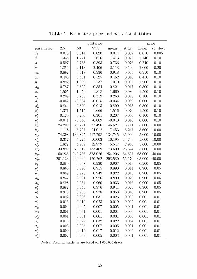
Table 1. Estimates: prior and posterior statistics

posterior priorparameter 2.5 50 97.5 mean st.dev mean st. dev.φb 0.010 0.014 0.020 0.014 0.002 0.010 0.005φ 1.336 1.471 1.616 1.473 0.072 1.140 0.10ρ 0.597 0.733 0.893 0.736 0.076 0.740 0.10σ 1.856 2.113 2.406 2.118 0.140 2.000 0.20aH 0.897 0.918 0.936 0.918 0.063 0.950 0.10aT 0.400 0.461 0.525 0.462 0.010 0.450 0.10η 0.892 1.009 1.137 1.010 0.032 1.200 0.10ρR 0.787 0.822 0.854 0.821 0.017 0.800 0.10ρπ 1.505 1.659 1.818 1.660 0.080 1.500 0.10ρy 0.209 0.263 0.319 0.263 0.028 0.100 0.10ρs -0.052 -0.034 -0.015 -0.034 0.009 0.000 0.10ρ∗R 0.864 0.890 0.913 0.890 0.013 0.800 0.10ρ∗π 1.371 1.515 1.666 1.516 0.076 1.500 0.10ρ∗y 0.120 0.206 0.301 0.207 0.046 0.100 0.10ρ∗s -0.071 -0.040 -0.009 -0.040 0.016 0.000 0.10κH 24.209 43.721 77.496 45.527 13.711 5.600 10.00κF 1.118 5.727 24.012 7.453 6.247 5.600 10.00κN 74.398 130.845 217.798 134.745 36.900 5.600 10.00κ∗H 0.337 5.225 50.003 10.195 13.733 5.600 10.00κ∗F 1.827 4.909 12.979 5.547 2.940 5.600 10.00κ∗N 33.899 70.012 133.469 73.609 25.624 5.600 10.00κW 160.236 249.736 373.026 254.206 54.507 63.000 40.00κ∗W 201.123 294.269 420.262 298.580 56.176 63.000 40.00ρξ 0.880 0.908 0.930 0.907 0.013 0.900 0.05ρ∗ξ 0.860 0.890 0.915 0.890 0.014 0.900 0.05ρµ 0.889 0.923 0.949 0.922 0.015 0.900 0.05ρH 0.847 0.891 0.926 0.890 0.020 0.900 0.05ρN 0.898 0.934 0.960 0.933 0.016 0.900 0.05ρ∗F 0.887 0.945 0.976 0.941 0.023 0.900 0.05ρ∗N 0.918 0.955 0.978 0.953 0.016 0.900 0.05σξ 0.022 0.026 0.031 0.026 0.002 0.001 0.01σ∗ξ 0.016 0.019 0.023 0.019 0.002 0.001 0.01σµ 0.004 0.005 0.007 0.005 0.001 0.001 0.01σR 0.001 0.001 0.001 0.001 0.000 0.001 0.01σ∗R 0.001 0.001 0.001 0.001 0.000 0.001 0.01σH 0.015 0.022 0.032 0.022 0.004 0.001 0.01σN 0.003 0.005 0.007 0.005 0.001 0.001 0.01σ∗F 0.009 0.012 0.017 0.012 0.002 0.001 0.01σ∗N 0.002 0.003 0.005 0.003 0.001 0.001 0.01

Notes: Posterior statistics are based on 1,000,000 draws.

32

Table 2. Estimates: nominal rigidities

Nominal rigidities Cost Probability Frequency

euro area

import (border) 5.73 0.27 1.37domestic tradeable (wholesale) 43.72 0.61 2.56nontradeable 130.84 0.83 5.88wages 249.73 0.90 10.00

U. S.

import (border) 5.23 0.26 1.35domestic tradeable (wholesale) 4.91 0.25 1.33nontradeable 70.01 0.77 4.35wages 294.27 0.90 10.00

Notes: The column denoted with cost reports the parameter measuring the cost for adjustingprices (posterior median values). The column denoted with probability reports the implicitCalvo probability for a firm of not being able to reset prices optimally. The column denotedwith frequency reports the average duration of prices, computed on the basis of the Calvoprobability.

33

Table 3. Goodness of fit: selected second moments

volatility persistence

Data 2.5 50 97.5 Data 2.5 50 97.5

real exchange rate RS 8.40 4.84 6.43 8.58 0.81 0.46 0.66 0.79

euro area CPI inflation π 0.21 0.15 0.20 0.26 0.20 0.33 0.54 0.70

U.S. CPI inflation π∗ 0.31 0.17 0.21 0.27 0.17 0.12 0.35 0.55

EA wholesale domestic tradable infl. πH 0.61 0.44 0.56 0.71 0.66 0.29 0.50 0.66

U.S. wholesale domestic tradable infl. π∗F 0.68 0.57 0.70 0.85 0.17 0.00 0.24 0.45

EA nontradable inflation πN 0.21 0.10 0.15 0.20 0.30 0.45 0.65 0.78

U.S. nontradable inflation π∗N 0.17 0.09 0.13 0.18 0.09 0.42 0.62 0.76

EA nominal interest rate R 0.19 0.13 0.19 0.27 0.87 0.64 0.79 0.88

U.S. nominal interest rate R∗ 0.25 0.11 0.14 0.20 0.88 0.51 0.69 0.81

EA consumption C 0.80 0.56 0.73 0.96 0.77 0.41 0.60 0.74

U.S. consumption C∗ 0.75 0.56 0.74 0.97 0.80 0.41 0.60 0.75

Notes: Results are on 500 draws from the posterior distribution and 100 time series of the variables.

Table 4. Goodness of fit: cross-correlations

Data 2.5 50 97.5RS, π 0.29 -0.29 0.05 0.38RS, π? -0.03 -0.41 -0.13 0.17RS, πH 0.21 -0.36 -0.05 0.26RS, π?

F -0.13 -0.25 0.01 0.26RS, πN 0.00 -0.47 -0.13 0.25RS, π?

N -0.02 -0.33 0.02 0.37RS, R 0.21 -0.55 -0.19 0.24RS, R? 0.21 -0.21 0.20 0.55RS, C -0.29 -0.55 -0.26 0.09RS, C? 0.25 -0.23 0.13 0.46RS, C − C? -0.37 -0.56 -0.27 0.09C, C? -0.09 -0.38 -0.05 0.29TB, C -0.34 -0.65 -0.41 -0.10

Notes: Results are on 500 draws from the posterior distri-bution and 100 time series of the variables.

34

Table 5. Real exchange rate fluctuations(Percentage of variance of the real exchange rate)

component 2.5 50 97.5

. . .σ2(IRS) 0.1 0.19 0.34

σ2(HB) 2.3 5.93 11.86

σ2(IPD) 41.6 58.75 76.54

cov(IPD, HB) -0.1 0.63 1.86

cov(IRS, IPD) 1.3 3.34 5.66

cov(HB, IPD) 18.2 31.14 41.44

Notes: Results are on 500 draws from the posteriordistribution and 100 time series of the variables. 2.5,50, 97.5 are percentiles of the draws. IRS is for in-ternal real exchange rate (it includes both euro areaand US terms), HB for home bias, IPD is for inter-national price discrimination (it includes both euroarea and U.S. terms).

35

Table 6. Sensitivity analysis: comparison of modes

parameter LCP-DC no NT no HB PCP LCP no UIRPφb 0.014 0.010 0.013 0 014 0.013 0.008φ 1.474 1.160 0.998 1 173 1.184 1.368ρ 0.734 - 0.574 0 745 0.746 0.764σ 2.117 2.120 1.985 2 096 2.095 2.143η 1.008 - - - - 1.060

aH 0.917 0.990 0.5 0 970 0.968 0.871aT 0.462 - 0.040 0 262 0.264 0.494ρR 0.821 0.830 0.770 0 823 0.825 0.828ρπ 1.657 2.030 1.677 1 672 1.672 1.666ρy 0.262 0.210 0.231 0 260 0.262 0.257ρs -0.034 -0.030 -0.032 -0 035 -0.028 -0.055ρ∗R 0.889 0.890 0.876 0 899 0.891 0.898ρ∗π 1.513 1.570 1.534 1 508 1.503 1.539ρ∗y 0.203 0.200 0.184 0 143 0.206 0.221ρ∗s -0.041 -0.030 -0.040 -0 040 -0.031 0.0κH 45.071 61.910 86.323 35 564 39.647 35.372κF 6.003 6.920 2.578 - 11.368 0.769κN 131.794 - 161.421 118 951 119.300 124.388κ∗H 5.144 8.630 0.519 - 11.326 1.382κ∗F 4.973 4.210 6.402 3.746 3.932 5.189κ∗N 71.690 - 78.991 73 063 74.695 74.739κW 252.705 169.840 167.896 245 236 246.065 226.283κ∗W 291.599 278.040 279.910 295 232 295.940 306.976ρ∗ξ 0.907 0.910 0.885 0 908 0.909 0.903ρξ 0.890 0.900 0.895 0 893 0.891 0.907ρu 0.920 0.920 0.918 0 922 0.923 -ρH 0.888 0.930 0.926 0 893 0.886 0.903ρN 0.933 - 0.933 0 937 0.938 0.933ρ∗F 0.943 0.940 0.927 0 952 0.950 0.940ρ∗N 0.954 - 0.927 0 947 0.946 -σξ 0.026 0.030 0.023 0 026 0.026 0.030σ∗ξ 0.019 0.020 0.018 0 020 0.019 0.020σu 0.005 0.000 0.005 0 005 0.005 0.000σ∗R 0.001 0.000 0.001 0 001 0.001 0.000σ∗R 0.001 0.000 0.001 0 001 0.001 0.000σ∗H 0.022 0.010 0.028 0 018 0.020 0.010σ∗N 0.005 - 0.004 0 005 0.005 -σ∗F 0.012 0.000 0.013 0 010 0.010 0.000σ∗N 0.003 - 0.004 0 003 0.003 -ML 4607.000 - 4548.000 4621 000 4625.000 4503.000

Concentrated ML 3807.000 3811.000 - - - -

Notes: Each column report the posterior mode. ML denotes the marginal likelihood.

36

Table 7. Sensitivity analysis with respect to selected featuresVolatility

Data LCP-DC LCP PCP no-HB no-NT

RS 8.40 6.43 4.80 4.61 4.48 3.74π 0.21 0.20 0.42 0.44 0.33 0.90π∗ 0.31 0.21 0.44 0.47 0.35 0.95πH 0.61 0.56 0.83 0.83 0.57 0.93π∗F 0.68 0.70 0.89 0.91 0.71 0.96πN 0.21 0.15 0.16 0.16 0.15 0.24π∗N 0.17 0.13 0.14 0.15 0.13 0.20R 0.19 0.19 0.24 0.25 0.19 0.44R∗ 0.25 0.14 0.16 0.17 0.15 0.26C 0.80 0.73 0.85 0.86 0.92 1.16C∗ 0.75 0.74 0.80 0.73 0.86 0.99

Notes: median values. Results are on 500 draws from the posterior distri-bution and 100 time series of the variables.

Table 8. Sensitivity analysis with respect to selected featuresPersistence

Data LCP-DC LCP PCP no-HB no-NT

RS 0.81 0.66 0.65 0.66 0.63 0.64π 0.20 0.54 0.43 0.38 0.30 0.42π∗ 0.17 0.35 0.18 0.15 0.27 0.17πH 0.66 0.50 0.43 0.43 0.50 0.44π∗F 0.17 0.24 0.16 0.16 0.24 0.17πN 0.30 0.65 0.67 0.67 0.65 0.70π∗N 0.09 0.62 0.64 0.65 0.62 0.68R 0.87 0.79 0.80 0.80 0.78 0.81R∗ 0.88 0.69 0.71 0.72 0.71 0.74C 0.77 0.60 0.63 0.63 0.64 0.70C∗ 0.80 0.60 0.62 0.61 0.64 0.66

Notes: median values. Results are on 500 draws from the posterior distri-bution and 100 time series of the variables.

37

Table 9. Sensitivity analysis with respect to selected featuresCross-correlations

Data LCP-DC LCP PCP no-HB no-NTRS, π 0.29 0.05 0.11 0.12 0.49 0.07RS, π? -0.03 -0.13 -0.18 -0.19 -0.50 -0.17RS, πH 0.21 -0.05 -0.02 -0.03 -0.01 -0.04RS, π?

F -0.13 0.01 -0.04 -0.04 -0.03 -0.07RS, πN 0.00 -0.13 -0.01 -0.01 0.07 0.16RS, π?

N -0.02 0.02 -0.10 -0.11 -0.22 -0.25RS, R 0.21 -0.19 0.05 0.10 0.39 0.18RS, R? 0.21 0.20 -0.01 -0.10 -0.24 -0.20RS, C -0.29 -0.26 -0.41 -0.42 -0.56 -0.30RS, C? 0.25 0.13 0.27 0.41 0.39 0.29RS, C/C? -0.37 -0.27 -0.46 -0.54 -0.58 -0.41C, C? -0.09 -0.05 -0.11 -0.17 -0.33 -0.06TB, C -0.34 -0.41 -0.44 -0.46 -0.65 -0.38

Notes: median values. Results are on 500 draws from the posterior distributionand 100 time series of the variables.

38

Table 10. Sensitivity analysis with respect to shocksVolatility

Data UIRP UIRP+tech UIRP+tech+mon All

RS 8.40 6.22 6.24 6.29 6.43π 0.21 0.05 0.19 0.19 0.20π∗ 0.31 0.05 0.20 0.20 0.21πH 0.61 0.00 0.55 0.55 0.56π∗F 0.68 0.00 0.69 0.69 0.70πN 0.21 0.00 0.12 0.12 0.15π∗N 0.17 0.00 0.11 0.11 0.13R 0.19 0.02 0.09 0.13 0.19R∗ 0.25 0.02 0.06 0.13 0.14C 0.80 0.09 0.2 0.27 0.73C∗ 0.75 0.08 0.15 0.36 0.74

Notes: median values. Results are on 500 draws from the posterior distributionand 100 time series of the variables.

Table 11. Sensitivity analysis with respect to shocksPersistence

Data UIRP UIRP+tech UIRP+tech+mon All

RS 0.81 0.65 0.66 0.65 0.66π 0.20 0.23 0.31 0.51 0.54π∗ 0.17 0.23 0.49 0.32 0.35πH 0.66 0.79 0.23 0.50 0.50π∗F 0.17 0.80 0.62 0.23 0.24πN 0.30 0.86 0.59 0.62 0.65π∗N 0.09 0.83 0.84 0.60 0.62R 0.87 0.44 0.8 0.69 0.79R∗ 0.88 0.53 0.84 0.63 0.69C 0.77 0.81 0.83 0.71 0.60C∗ 0.80 0.83 0.55 0.64 0.60

Notes: median values. Results are on 500 draws from the posterior distributionand 100 time series of the variables.

39

Table 12. Sensitivity analysis with respect to shocksCross-correlations

Data UIRP UIRP+tech UIRP+tech+mon AllRS, π 0.29 0.54 0.13 0.13 0.05RS, π? -0.03 -0.55 -0.15 -0.17 -0.13RS, πH 0.21 -0.96 -0.02 -0.02 -0.05RS, π?

F -0.13 0.92 0.00 -0.01 0.01RS, πN 0.00 -0.67 -0.03 -0.03 -0.13RS, π?

N -0.02 0.10 0.00 -0.03 0.02RS, R 0.21 -0.55 -0.12 -0.12 -0.19RS, R? 0.21 0.76 0.20 0.18 0.20RS, C -0.29 -0.94 -0.39 -0.25 -0.26RS, C? 0.25 0.91 0.42 0.08 0.13RS, C/C? -0.37 -0.93 -0.57 -0.22 -0.27C, C? -0.09 -0.99 0.04 0.02 -0.05TB, C -0.34 -0.87 -0.42 -0.30 -0.41

Notes: median values. Results are on 500 draws from the posterior distribution and 100 timeseries of the variables.

40

Table 13. Asymptotic forecast error variance decomposition

Variable zH z∗F zN z∗N zR z∗R zξ z∗ξ zµ ME Total

euro-area

C 4.6 0.2 7.5 0.0 3.7 0.0 79.6 0.2 4.2 0.0 100π 32.4 0.1 24.8 0.0 0.2 0.0 20.0 0.1 3.3 19.0 100πH 89.7 0.0 3.8 0.0 0.1 0.0 6.1 0.0 0.3 0.0 100πN 12.7 0.0 34.0 0.0 0.2 0.0 23.1 0.1 1.5 28.4 100πW 5.3 0.0 6.2 0.0 0.2 0.0 12.9 0.0 0.6 74.7 100TB 0.0 0.0 0.0 0.0 0.0 0.0 2.6 1.2 20.4 75.7 100R 9.7 0.0 11.1 0.0 7 0.0 70.9 0.1 1.2 0 100RS 0.1 0.1 0.3 0.2 0.1 0.4 6.8 2.5 89.5 0 100

U.S.

C 0.3 5.3 0.0 6.1 0.0 16.1 0.5 67.8 3.9 0.0 100π∗ 0.3 38.3 0.0 18.4 0.0 2.5 0.2 8.5 3.2 28.5 100π∗F 0.0 94.5 0.0 2.1 0.0 0.6 0.0 2.4 0.3 0.0 100π∗N 0.0 18.9 0.0 35.3 0.0 3.5 0.3 13.4 2.1 26.6 100π∗W 0.0 9.1 0.0 8.1 0.0 2.7 0.1 10.6 1.0 68.4 100R∗ 0.1 13.2 0.0 12.9 0.0 28.1 0.3 43.1 2.4 0.0 100

Notes: Each figure in the table is computed using the median of the marginal posterior distribution ofthe parameters. ME is for measurement errors.

41

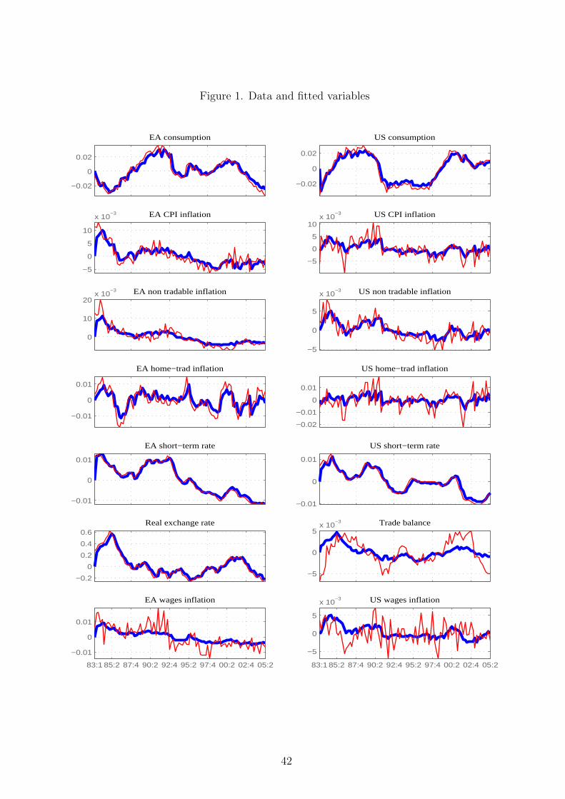
Figure 1. Data and fitted variables

−0.02

0

0.02

EA consumption

−0.02

0

0.02

US consumption

−5

0

5

10

x 10−3 EA CPI inflation

−5

0

5

10x 10

−3 US CPI inflation

0

10

20x 10

−3 EA non tradable inflation

−5

0

5

x 10−3 US non tradable inflation

−0.01

0

0.01

EA home−trad inflation

−0.02

−0.01

0

0.01

US home−trad inflation

−0.01

0

0.01

EA short−term rate

−0.01

0

0.01

US short−term rate

−0.2

0

0.2

0.4

0.6Real exchange rate

−5

0

5x 10

−3 Trade balance

83:1 85:2 87:4 90:2 92:4 95:2 97:4 00:2 02:4 05:2

−0.01

0

0.01

EA wages inflation

83:1 85:2 87:4 90:2 92:4 95:2 97:4 00:2 02:4 05:2

−5

0

5

x 10−3 US wages inflation

42

Figure 2. Decomposition of the euro-dollar real exchange rate

1983Q1 1985Q2 1987Q4 1990Q2 1992Q4 1995Q2 1997Q4 2000Q2 2002Q4 2005Q2

−0.5

−0.4

−0.3

−0.2

−0.1

0

0.1

0.2

0.3

price discriminationinternal RERhome biastotal RER

43

Figure 3. Impulse response analysis: UIRP shock

0 2 4 6 8 10 12 14 16 18 20−0.02

0

0.02

0.04Real Exchange Rate

0 2 4 6 8 10 12 14 16 18 20−0.02

0

0.02

0.04Change in Nominal Exch. Rate

0 2 4 6 8 10 12 14 16 18 20−0.01

0

0.01

0.02

0.03EA Import Inflation (border)

0 2 4 6 8 10 12 14 16 18 20−0.03

−0.02

−0.01

0

0.01US Import Inflation (border)

0 2 4 6 8 10 12 14 16 18 20−2

0

2

4

6x 10

−4 EA CPI Inflation

0 2 4 6 8 10 12 14 16 18 20−6

−4

−2

0

2x 10

−4 US CPI Inflation

0 2 4 6 8 10 12 14 16 18 20−2

−1

0

1

2x 10

−4 EA Interest Rate

0 2 4 6 8 10 12 14 16 18 20−1

0

1

2

3x 10

−4 US Interest Rate

0 2 4 6 8 10 12 14 16 18 20−6

−4

−2

0x 10

−4 EA Consumption

quarters0 2 4 6 8 10 12 14 16 18 20

0

2

4

6x 10

−4 US Consumption

quarters

44

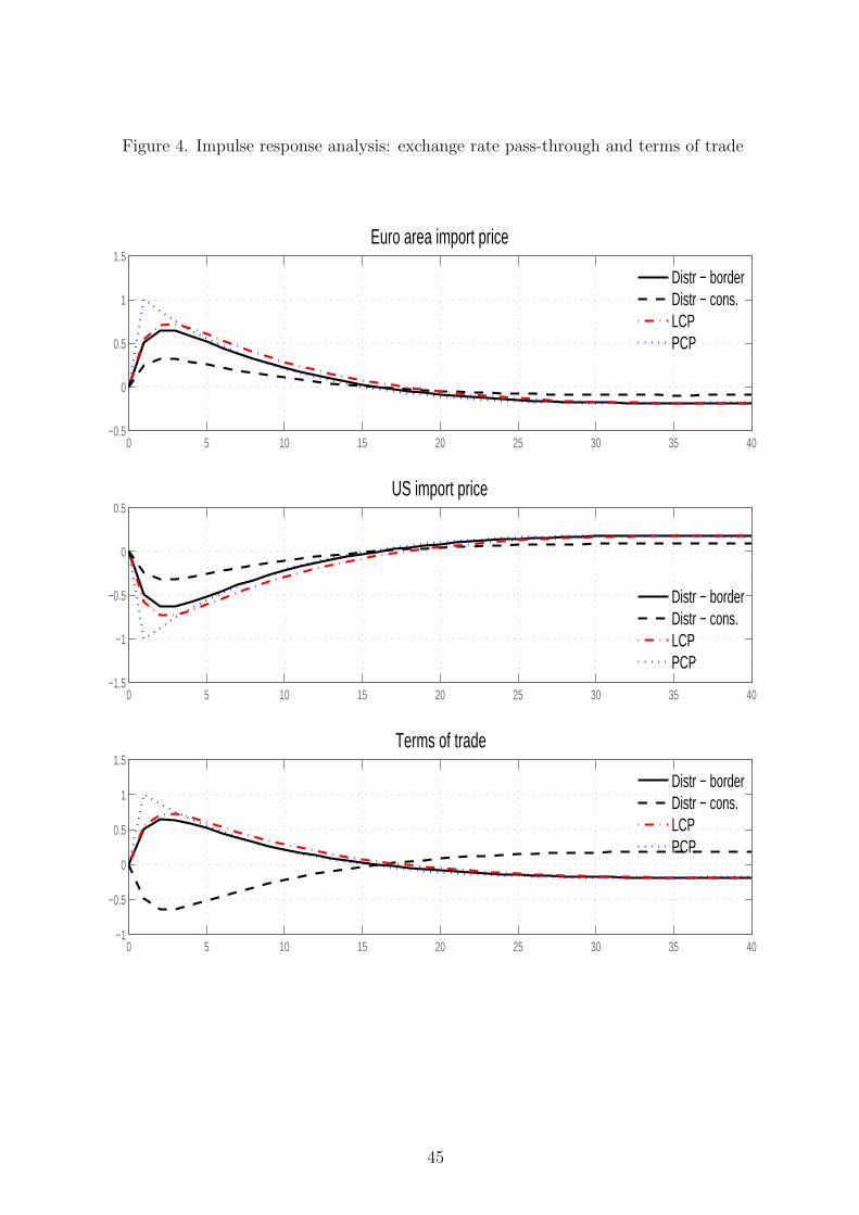
Figure 4. Impulse response analysis: exchange rate pass-through and terms of trade

0 5 10 15 20 25 30 35 40−0.5

0

0.5

1

1.5Euro area import price

Distr − borderDistr − cons.LCPPCP

0 5 10 15 20 25 30 35 40−1.5

−1

−0.5

0

0.5US import price

Distr − borderDistr − cons.LCPPCP

0 5 10 15 20 25 30 35 40−1

−0.5

0

0.5

1

1.5Terms of trade

Distr − borderDistr − cons.LCPPCP

45

Figure 5. Impulse response analysis: euro area preference shock

0 2 4 6 8 10 12 14 16 18 20−0.04

−0.02

0

0.02Real Exchange Rate

0 2 4 6 8 10 12 14 16 18 20−0.04

−0.02

0

0.02Change in Nominal Exch. Rate

0 2 4 6 8 10 12 14 16 18 20−0.02

−0.01

0

0.01EA Import Inflation (border)

0 2 4 6 8 10 12 14 16 18 20−0.01

0

0.01

0.02

0.03US Import Inflation (border)

0 2 4 6 8 10 12 14 16 18 200

0.5

1

1.5

2x 10

−3 EA CPI Inflation

0 2 4 6 8 10 12 14 16 18 20−2

0

2

4

6x 10

−4 US CPI Inflation

0 2 4 6 8 10 12 14 16 18 200

1

2

3

4x 10

−3 EA Interest Rate

0 2 4 6 8 10 12 14 16 18 20−2

−1

0

1

2x 10

−4 US Interest Rate

0 2 4 6 8 10 12 14 16 18 200

0.005

0.01

0.015

0.02EA Consumption

quarters0 2 4 6 8 10 12 14 16 18 20

−10

−5

0

5x 10

−4 US Consumption

quarters

46

Figure 6. Impulse response analysis: euro area tradable technology shock

0 2 4 6 8 10 12 14 16 18 20−2

0

2

4

6x 10

−3 Real Exchange Rate

0 2 4 6 8 10 12 14 16 18 20−3

−2

−1

0

1x 10

−3 Change in Nominal Exch. Rate

0 2 4 6 8 10 12 14 16 18 20−2

−1

0

1x 10

−3 EA Import Inflation (border)

0 2 4 6 8 10 12 14 16 18 20−0.06

−0.04

−0.02

0

0.02US Import Inflation (border)

0 2 4 6 8 10 12 14 16 18 20−6

−4

−2

0

2x 10

−3 EA CPI Inflation

0 2 4 6 8 10 12 14 16 18 20−15

−10

−5

0

5x 10

−4 US CPI Inflation

0 2 4 6 8 10 12 14 16 18 20−2

−1.5

−1

−0.5

0x 10

−3 EA Interest Rate

0 2 4 6 8 10 12 14 16 18 20−2

−1.5

−1

−0.5

0x 10

−4 US Interest Rate

0 2 4 6 8 10 12 14 16 18 200

1

2

3

4x 10

−3 EA Consumption

quarters0 2 4 6 8 10 12 14 16 18 20

0

0.5

1

1.5x 10

−3 US Consumption

quarters

47

Figure 7. Impulse response analysis: euro area monetary policy shock

0 2 4 6 8 10 12 14 16 18 20−4

−2

0

2x 10

−4 Real Exchange Rate

0 2 4 6 8 10 12 14 16 18 20−4

−2

0

2x 10

−4 Change in Nominal Exch. Rate

0 2 4 6 8 10 12 14 16 18 20−4

−2

0

2x 10

−4 EA Import Inflation (border)

0 2 4 6 8 10 12 14 16 18 20−2

0

2

4x 10

−4 US Import Inflation (border)

0 2 4 6 8 10 12 14 16 18 20−1.5

−1

−0.5

0x 10

−5 EA CPI Inflation

0 2 4 6 8 10 12 14 16 18 20−2

0

2

4

6x 10

−6 US CPI Inflation

0 2 4 6 8 10 12 14 16 18 20−5

0

5

10x 10

−5 EA Interest Rate

0 2 4 6 8 10 12 14 16 18 20−2

−1

0

1x 10

−6 US Interest Rate

0 2 4 6 8 10 12 14 16 18 20−2

−1

0

1

2x 10

−4 EA Consumption

quarters0 2 4 6 8 10 12 14 16 18 20

−2

−1

0

1x 10

−6 US Consumption

quarters

48

(*) Requestsforcopiesshouldbesentto:Bancad’Italia–ServizioStudidistrutturaeconomicaefinanziaria–DivisioneBibliotecaeArchiviostorico–ViaNazionale,91–00184Rome–(fax00390647922059).TheyareavailableontheInternetwww.bancaditalia.it.

RECENTLYPUBLISHED“TEMI”(*)

N. 634 – Prezzi delle esportazioni, qualità dei prodotti e caratteristiche di impresa: un’analisi su un campione di imprese italiane,byMatteoBugamelli(June2007).

N. 635 – Openness to trade and industry cost dispersion: Evidence from a panel of Italian firms,byMassimoDelGatto,GianmarcoI.P.OttavianoandMarcelloPagnini(June2007).

N. 636 – The weighting process in the SHIW,byIvanFaiellaandRominaGambacorta(June2007).

N. 637 – Emerging markets spreads and global financial conditions, byAlessio Ciarlone,PaoloPiselliandGiorgioTrebeschi(June2007).

N. 638 – Comparative advantage patterns and domestic determinants in emerging countries: An analysis with a focus on technology, by Daniela Marconi and Valeria Rolli(September2007).

N. 639 – The generation gap: Relative earnings of young and old workers in Italy,byAlfonsoRosoliaandRobertoTorrini(September2007).

N. 640 – The financing of small innovative firms: The Italian case,bySilviaMagri(September2007).

N. 641 – Assessing financial contagion in the interbank market: Maximum entropy versus observed interbank lending patterns,byPaoloEmilioMistrulli(September2007).

N. 642 – Detecting long memory co-movements in macroeconomic time series, by GianlucaMoretti(September2007).

N. 643 – The producer service sector in Italy: Long-term growth and its local determinants,byValterDiGiacintoandGiacintoMicucci(September2007).

N. 644 – Aggregazioni bancarie e specializzazione nel credito alle PMI: peculiarità per area geografica,byEnricoBerettaandSilviaDelPrete(November2007).

N. 645 – Costs and benefits of creditor concentration: An empirical approach, byAmandaCarmignaniandMassimoOmiccioli(November2007).

N. 646 – Does the underground economy hold back financial deepening? Evidence from the Italian credit market,byGiorgioGobbiandRobertaZizza(November2007).

N. 647 – Optimal monetary policy under low trend inflation, byGuidoAscari andTizianoRopele(November2007).

N. 648 – Indici di bilancio e rendimenti di borsa: un’analisi per le banche italiane,byAngelaRomagnoli(November2007).

N. 649 – Bank profitability and taxation, by Ugo Albertazzi and Leonardo Gambacorta(November2007).

N. 650 – Modelling bank lending in the euro area: A non-linear approach, by LeonardoGambacortaandCarlottaRossi(November2007).

N. 651 – Revisiting poverty and welfare dominance, byGianMariaTomat(November2007).N. 652 – The general equilibrium effects of fiscal policy: Estimates for the euro area, by

LorenzoForni,LiberoMonteforteandLucaSessa(November2007).N. 653 – Securitisation and the bank lending channel, by Yener Altunbas, Leonardo

GambacortaandDavidMarqués(November2007).N.654 – The cyclical response of fiscal policies in the euro area. Why do results of empirical

research differ so strongly?, by Roberto Golinelli and Sandro Momigliano(January2008).

N. 655 – What’s behind “inflation perceptions”? A survey-based analysis of Italian consumers,byPaoloDelGiovane,SilviaFabianiandRobertoSabbatini(January2008).

N. 656 – The effects of fiscal policy in Italy: Evidence from a VAR model,byRaffaelaGiordano,SandroMomigliano,StefanoNeriandRobertoPerotti(January2008).

N. 657 – Excess money growth and inflation dynamics,byBarbaraRoffiaandAndreaZaghini(January2008).

N. 658 – R&D and market structure in a horizontal differentiation framework, by DavideFantino(January2008).

N. 659 – Housing market spillovers: Evidence from an estimated DSGE model, byMatteoIacovielloandStefanoNeri(January2008).

"TEMI" LATER PUBLISHED ELSEWHERE

2005

L. DEDOLA and F. LIPPI, The monetary transmission mechanism: Evidence from the industries of 5 OECD countries, European Economic Review, 2005, Vol. 49, 6, pp. 1543-1569, TD No. 389 (December 2000).

D. Jr. MARCHETTI and F. NUCCI, Price stickiness and the contractionary effects of technology shocks. European Economic Review, Vol. 49, 5, pp. 1137-1164, TD No. 392 (February 2001).

G. CORSETTI, M. PERICOLI and M. SBRACIA, Some contagion, some interdependence: More pitfalls in tests of financial contagion, Journal of International Money and Finance, Vol. 24, 8, pp. 1177-1199, TD No. 408 (June 2001).

GUISO L., L. PISTAFERRI and F. SCHIVARDI, Insurance within the firm. Journal of Political Economy, Vol. 113, 5, pp. 1054-1087, TD No. 414 (August 2001)

R. CRISTADORO, M. FORNI, L. REICHLIN and G. VERONESE, A core inflation indicator for the euro area, Journal of Money, Credit, and Banking, Vol. 37, 3, pp. 539-560, TD No. 435 (December 2001).

F. ALTISSIMO, E. GAIOTTI and A. LOCARNO, Is money informative? Evidence from a large model used for policy analysis, Economic & Financial Modelling, Vol. 22, 2, pp. 285-304, TD No. 445 (July 2002).

G. DE BLASIO and S. DI ADDARIO, Do workers benefit from industrial agglomeration? Journal of regional Science, Vol. 45, (4), pp. 797-827, TD No. 453 (October 2002).

G. DE BLASIO and S. DI ADDARIO, Salari, imprenditorialità e mobilità nei distretti industriali italiani, in L. F. Signorini, M. Omiccioli (eds.), Economie locali e competizione globale: il localismo industriale italiano di fronte a nuove sfide, Bologna, il Mulino, TD No. 453 (October 2002).

R. TORRINI, Cross-country differences in self-employment rates: The role of institutions, Labour Economics, Vol. 12, 5, pp. 661-683, TD No. 459 (December 2002).

A. CUKIERMAN and F. LIPPI, Endogenous monetary policy with unobserved potential output, Journal of Economic Dynamics and Control, Vol. 29, 11, pp. 1951-1983, TD No. 493 (June 2004).

M. OMICCIOLI, Il credito commerciale: problemi e teorie, in L. Cannari, S. Chiri e M. Omiccioli (eds.), Imprese o intermediari? Aspetti finanziari e commerciali del credito tra imprese in Italia, Bologna, Il Mulino, TD No. 494 (June 2004).

L. CANNARI, S. CHIRI and M. OMICCIOLI, Condizioni di pagamento e differenziazione della clientela, in L. Cannari, S. Chiri e M. Omiccioli (eds.), Imprese o intermediari? Aspetti finanziari e commerciali del credito tra imprese in Italia, Bologna, Il Mulino, TD No. 495 (June 2004).

P. FINALDI RUSSO and L. LEVA, Il debito commerciale in Italia: quanto contano le motivazioni finanziarie?, in L. Cannari, S. Chiri e M. Omiccioli (eds.), Imprese o intermediari? Aspetti finanziari e commerciali del credito tra imprese in Italia, Bologna, Il Mulino, TD No. 496 (June 2004).

A. CARMIGNANI, Funzionamento della giustizia civile e struttura finanziaria delle imprese: il ruolo del credito commerciale, in L. Cannari, S. Chiri e M. Omiccioli (eds.), Imprese o intermediari? Aspetti finanziari e commerciali del credito tra imprese in Italia, Bologna, Il Mulino, TD No. 497 (June 2004).

G. DE BLASIO, Credito commerciale e politica monetaria: una verifica basata sull’investimento in scorte, in L. Cannari, S. Chiri e M. Omiccioli (eds.), Imprese o intermediari? Aspetti finanziari e commerciali del credito tra imprese in Italia, Bologna, Il Mulino, TD No. 498 (June 2004).

G. DE BLASIO, Does trade credit substitute bank credit? Evidence from firm-level data. Economic notes, Vol. 34, 1, pp. 85-112, TD No. 498 (June 2004).

A. DI CESARE, Estimating expectations of shocks using option prices, The ICFAI Journal of Derivatives Markets, Vol. 2, 1, pp. 42-53, TD No. 506 (July 2004).

M. BENVENUTI and M. GALLO, Il ricorso al "factoring" da parte delle imprese italiane, in L. Cannari, S. Chiri e M. Omiccioli (eds.), Imprese o intermediari? Aspetti finanziari e commerciali del credito tra imprese in Italia, Bologna, Il Mulino, TD No. 518 (October 2004).

L. CASOLARO and L. GAMBACORTA, Redditività bancaria e ciclo economico, Bancaria, Vol. 61, 3, pp. 19-27, TD No. 519 (October 2004).

F. PANETTA, F. SCHIVARDI and M. SHUM, Do mergers improve information? Evidence from the loan market, CEPR Discussion Paper, 4961, TD No. 521 (October 2004).

P. DEL GIOVANE and R. SABBATINI, La divergenza tra inflazione rilevata e percepita in Italia, in P. Del Giovane, F. Lippi e R. Sabbatini (eds.), L'euro e l'inflazione: percezioni, fatti e analisi, Bologna, Il Mulino, TD No. 532 (December 2004).

R. TORRINI, Quota dei profitti e redditività del capitale in Italia: un tentativo di interpretazione, Politica economica, Vol. 21, 1, pp. 7-41, TD No. 551 (June 2005).

M. OMICCIOLI, Il credito commerciale come “collateral”, in L. Cannari, S. Chiri, M. Omiccioli (eds.), Imprese o intermediari? Aspetti finanziari e commerciali del credito tra imprese in Italia, Bologna, il Mulino, TD No. 553 (June 2005).

L. CASOLARO, L. GAMBACORTA and L. GUISO, Regulation, formal and informal enforcement and the development of the household loan market. Lessons from Italy, in Bertola G., Grant C. and Disney R. (eds.) The Economics of Consumer Credit: European Experience and Lessons from the US, Boston, MIT Press, TD No. 560 (September 2005).

S. DI ADDARIO and E. PATACCHINI, Lavorare in una grande città paga, ma poco, in Brucchi Luchino (ed.), Per un’analisi critica del mercato del lavoro, Bologna , Il Mulino, TD No. 570 (January 2006).

P. ANGELINI and F. LIPPI, Did inflation really soar after the euro changeover? Indirect evidence from ATM withdrawals, CEPR Discussion Paper, 4950, TD No. 581 (March 2006).

S. FEDERICO, Internazionalizzazione produttiva, distretti industriali e investimenti diretti all'estero, in L. F. Signorini, M. Omiccioli (eds.), Economie locali e competizione globale: il localismo industriale italiano di fronte a nuove sfide, Bologna, il Mulino, TD No. 592 (October 2002).

S. DI ADDARIO, Job search in thick markets: Evidence from Italy, Oxford Discussion Paper 235, Department of Economics Series, TD No. 605 (December 2006).

2006

F. BUSETTI, Tests of seasonal integration and cointegration in multivariate unobserved component models, Journal of Applied Econometrics, Vol. 21, 4, pp. 419-438, TD No. 476 (June 2003).

C. BIANCOTTI, A polarization of inequality? The distribution of national Gini coefficients 1970-1996, Journal of Economic Inequality, Vol. 4, 1, pp. 1-32, TD No. 487 (March 2004).

L. CANNARI and S. CHIRI, La bilancia dei pagamenti di parte corrente Nord-Sud (1998-2000), in L. Cannari, F. Panetta (a cura di), Il sistema finanziario e il Mezzogiorno: squilibri strutturali e divari finanziari, Bari, Cacucci, TD No. 490 (March 2004).

M. BOFONDI and G. GOBBI, Information barriers to entry into credit markets, Review of Finance, Vol. 10, 1, pp. 39-67, TD No. 509 (July 2004).

FUCHS W. and LIPPI F., Monetary union with voluntary participation, Review of Economic Studies, Vol. 73, pp. 437-457 TD No. 512 (July 2004).

GAIOTTI E. and A. SECCHI, Is there a cost channel of monetary transmission? An investigation into the pricing behaviour of 2000 firms, Journal of Money, Credit and Banking, Vol. 38, 8, pp. 2013-2038 TD No. 525 (December 2004).

A. BRANDOLINI, P. CIPOLLONE and E. VIVIANO, Does the ILO definition capture all unemployment?, Journal of the European Economic Association, Vol. 4, 1, pp. 153-179, TD No. 529 (December 2004).

A. BRANDOLINI, L. CANNARI, G. D’ALESSIO and I. FAIELLA, Household wealth distribution in Italy in the 1990s, in E. N. Wolff (ed.) International Perspectives on Household Wealth, Cheltenham, Edward Elgar, TD No. 530 (December 2004).

P. DEL GIOVANE and R. SABBATINI, Perceived and measured inflation after the launch of the Euro: Explaining the gap in Italy, Giornale degli economisti e annali di economia, Vol. 65, 2 , pp. 155-192, TD No. 532 (December 2004).

M. CARUSO, Monetary policy impulses, local output and the transmission mechanism, Giornale degli economisti e annali di economia, Vol. 65, 1, pp. 1-30, TD No. 537 (December 2004).

A. NOBILI, Assessing the predictive power of financial spreads in the euro area: does parameters instability matter?, Empirical Economics, Vol. 31, 1, pp. 177-195, TD No. 544 (February 2005).

L. GUISO and M. PAIELLA, The role of risk aversion in predicting individual behavior, In P. A. Chiappori e C. Gollier (eds.) Competitive Failures in Insurance Markets: Theory and Policy Implications, Monaco, CESifo, TD No. 546 (February 2005).

G. M. TOMAT, Prices product differentiation and quality measurement: A comparison between hedonic and matched model methods, Research in Economics, Vol. 60, 1, pp. 54-68, TD No. 547 (February 2005).

F. LOTTI, E. SANTARELLI and M. VIVARELLI, Gibrat's law in a medium-technology industry: Empirical evidence for Italy, in E. Santarelli (ed.), Entrepreneurship, Growth, and Innovation: the Dynamics of Firms and Industries, New York, Springer, TD No. 555 (June 2005).

F. BUSETTI, S. FABIANI and A. HARVEY, Convergence of prices and rates of inflation, Oxford Bulletin of Economics and Statistics, Vol. 68, 1, pp. 863-878, TD No. 575 (February 2006).

M. CARUSO, Stock market fluctuations and money demand in Italy, 1913 - 2003, Economic Notes, Vol. 35, 1, pp. 1-47, TD No. 576 (February 2006).

S. IRANZO, F. SCHIVARDI and E. TOSETTI, Skill dispersion and productivity: An analysis with matched data, CEPR Discussion Paper, 5539, TD No. 577 (February 2006).

R. BRONZINI and G. DE BLASIO, Evaluating the impact of investment incentives: The case of Italy’s Law 488/92. Journal of Urban Economics, Vol. 60, 2, pp. 327-349, TD No. 582 (March 2006).

R. BRONZINI and G. DE BLASIO, Una valutazione degli incentivi pubblici agli investimenti, Rivista Italiana degli Economisti , Vol. 11, 3, pp. 331-362, TD No. 582 (March 2006).

A. DI CESARE, Do market-based indicators anticipate rating agencies? Evidence for international banks, Economic Notes, Vol. 35, pp. 121-150, TD No. 593 (May 2006).

L. DEDOLA and S. NERI, What does a technology shock do? A VAR analysis with model-based sign restrictions, Journal of Monetary Economics, Vol. 54, 2, pp. 512-549, TD No. 607 (December 2006).

R. GOLINELLI and S. MOMIGLIANO, Real-time determinants of fiscal policies in the euro area, Journal of Policy Modeling, Vol. 28, 9, pp. 943-964, TD No. 609 (December 2006).

P. ANGELINI, S. GERLACH, G. GRANDE, A. LEVY, F. PANETTA, R. PERLI,S. RAMASWAMY, M. SCATIGNA and P. YESIN, The recent behaviour of financial market volatility, BIS Papers, 29, QEF No. 2 (August 2006).

2007

L. CASOLARO. and G. GOBBI, Information technology and productivity changes in the banking industry, Economic Notes, Vol. 36, 1, pp. 43-76, TD No. 489 (March 2004).

M. PAIELLA, Does wealth affect consumption? Evidence for Italy, Journal of Macroeconomics, Vol. 29, 1, pp. 189-205, TD No. 510 (July 2004).

F. LIPPI. and S. NERI, Information variables for monetary policy in a small structural model of the euro area, Journal of Monetary Economics, Vol. 54, 4, pp. 1256-1270, TD No. 511 (July 2004).

A. ANZUINI and A. LEVY, Monetary policy shocks in the new EU members: A VAR approach, Applied Economics, Vol. 39, 9, pp. 1147-1161, TD No. 514 (July 2004).

R. BRONZINI, FDI Inflows, agglomeration and host country firms' size: Evidence from Italy, Regional Studies, Vol. 41, 7, pp. 963-978, TD No. 526 (December 2004).

L. MONTEFORTE, Aggregation bias in macro models: Does it matter for the euro area?, Economic Modelling, 24, pp. 236-261, TD No. 534 (December 2004).

A. DALMAZZO and G. DE BLASIO, Production and consumption externalities of human capital: An empirical study for Italy, Journal of Population Economics, Vol. 20, 2, pp. 359-382, TD No. 554 (June 2005).

M. BUGAMELLI and R. TEDESCHI, Le strategie di prezzo delle imprese esportatrici italiane, Politica Economica, v. 3, pp. 321-350, TD No. 563 (November 2005).

L. GAMBACORTA and S. IANNOTTI, Are there asymmetries in the response of bank interest rates to monetary shocks?, Applied Economics, v. 39, 19, pp. 2503-2517, TD No. 566 (November 2005).

S. DI ADDARIO and E. PATACCHINI, Wages and the city. Evidence from Italy, Development Studies Working Papers 231, Centro Studi Luca d’Agliano, TD No. 570 (January 2006).

P. ANGELINI and F. LIPPI, Did prices really soar after the euro cash changeover? Evidence from ATM withdrawals, International Journal of Central Banking, Vol. 3, 4, pp. 1-22, TD No. 581 (March 2006).

A. LOCARNO, Imperfect knowledge, adaptive learning and the bias against activist monetary policies, International Journal of Central Banking, v. 3, 3, pp. 47-85, TD No. 590 (May 2006).

F. LOTTI and J. MARCUCCI, Revisiting the empirical evidence on firms' money demand, Journal of Economics and Business, Vol. 59, 1, pp. 51-73, TD No. 595 (May 2006).

P. CIPOLLONE and A. ROSOLIA, Social interactions in high school: Lessons from an earthquake, American Economic Review, Vol. 97, 3, pp. 948-965, TD No. 596 (September 2006).

A. BRANDOLINI, Measurement of income distribution in supranational entities: The case of the European Union, in S. P. Jenkins e J. Micklewright (eds.), Inequality and Poverty Re-examined, Oxford, Oxford University Press, TD No. 623 (April 2007).

M. PAIELLA, The foregone gains of incomplete portfolios, Review of Financial Studies, Vol. 20, 5, pp. 1623-1646, TD No. 625 (April 2007).

K. BEHRENS, A. R. LAMORGESE, G.I.P. OTTAVIANO and T. TABUCHI, Changes in transport and non transport costs: local vs. global impacts in a spatial network, Regional Science and Urban Economics, Vol. 37, 6, pp. 625-648, TD No. 628 (April 2007).

G. ASCARI and T. ROPELE, Optimal monetary policy under low trend inflation, Journal of Monetary Economics, v. 54, 8, pp. 2568-2583, TD No. 647 (November 2007).

R. GIORDANO, S. MOMIGLIANO, S. NERI and R. PEROTTI, The Effects of Fiscal Policy in Italy: Evidence from a VAR Model, European Journal of Political Economy, Vol. 23, 3, pp. 707-733, TD No. 656 (December 2007).

2008

S. MOMIGLIANO, J. Henry and P. Hernández de Cos, The impact of government budget on prices: Evidence from macroeconometric models, Journal of Policy Modelling, v. 30, 1, pp. 123-143 TD No. 523 (October 2004).

P. DEL GIOVANE, S. FABIANI and R. SABATINI, What’s behind “inflation perceptions”? A survey-based analysis of Italian consumers, in P. Del Giovane e R. Sabbatini (eds.), The Euro Inflation and Consumers’ Perceptions. Lessons from Italy, Berlin-Heidelberg, Springer, TD No. 655 (January

2008).

FORTHCOMING

S. SIVIERO and D. TERLIZZESE, Macroeconomic forecasting: Debunking a few old wives’ tales, Journal of Business Cycle Measurement and Analysis, TD No. 395 (February 2001).

P. ANGELINI, Liquidity and announcement effects in the euro area, Giornale degli economisti e annali di economia, TD No. 451 (October 2002).

S. MAGRI, Italian households' debt: The participation to the debt market and the size of the loan, Empirical Economics, TD No. 454 (October 2002).

P. ANGELINI, P. DEL GIOVANE, S. SIVIERO and D. TERLIZZESE, Monetary policy in a monetary union: What role for regional information?, International Journal of Central Banking, TD No. 457 (December 2002).

L. MONTEFORTE and S. SIVIERO, The Economic Consequences of Euro Area Modelling Shortcuts, Applied Economics, TD No. 458 (December 2002).

L. GUISO and M. PAIELLA,, Risk aversion, wealth and background risk, Journal of the European Economic Association, TD No. 483 (September 2003).

G. FERRERO, Monetary policy, learning and the speed of convergence, Journal of Economic Dynamics and Control, TD No. 499 (June 2004).

F. SCHIVARDI e R. TORRINI, Identifying the effects of firing restrictions through size-contingent Differences in regulation, Labour Economics, TD No. 504 (giugno 2004).

C. BIANCOTTI, G. D'ALESSIO and A. NERI, Measurement errors in the Bank of Italy’s survey of household income and wealth, Review of Income and Wealth, TD No. 520 (October 2004).

D. Jr. MARCHETTI and F. Nucci, Pricing behavior and the response of hours to productivity shocks, Journal of Money Credit and Banking, TD No. 524 (December 2004).

L. GAMBACORTA, How do banks set interest rates?, European Economic Review, TD No. 542 (February 2005).

P. ANGELINI and A. Generale, On the evolution of firm size distributions, American Economic Review, TD No. 549 (June 2005).

R. FELICI and M. PAGNINI,, Distance, bank heterogeneity and entry in local banking markets, The Journal of Industrial Economics, TD No. 557 (June 2005).

M. BUGAMELLI and R. TEDESCHI, Le strategie di prezzo delle imprese esportatrici italiane, Politica Economica, TD No. 563 (November 2005).

S. DI ADDARIO and E. PATACCHINI, Wages and the city. Evidence from Italy, Labour Economics, TD No. 570 (January 2006).

M. BUGAMELLI and A. ROSOLIA, Produttività e concorrenza estera, Rivista di politica economica, TD No. 578 (February 2006).

PERICOLI M. and M. TABOGA, Canonical term-structure models with observable factors and the dynamics of bond risk premia, TD No. 580 (February 2006).

E. VIVIANO, Entry regulations and labour market outcomes. Evidence from the Italian retail trade sector, Labour Economics, TD No. 594 (May 2006).

S. FEDERICO and G. A. MINERVA, Outward FDI and local employment growth in Italy, Review of World Economics, Journal of Money, Credit and Banking, TD No. 613 (February 2007).

F. BUSETTI and A. HARVEY, Testing for trend, Econometric Theory TD No. 614 (February 2007). V. CESTARI, P. DEL GIOVANE and C. ROSSI-ARNAUD, Memory for Prices and the Euro Cash Changeover: An

Analysis for Cinema Prices in Italy, In P. Del Giovane e R. Sabbatini (eds.), The Euro Inflation and Consumers’ Perceptions. Lessons from Italy, Berlin-Heidelberg, Springer, TD No. 619 (February 2007).

B. ROFFIA and A. ZAGHINI, Excess money growth and inflation dynamics, International Finance, TD No. 629 (June 2007).

M. DEL GATTO, GIANMARCO I. P. OTTAVIANO and M. PAGNINI, Openness to trade and industry cost dispersion: Evidence from a panel of Italian firms, Journal of Regional Science, TD No. 635 (June 2007).

A. CIARLONE, P. PISELLI and G. TREBESCHI, Emerging Markets' Spreads and Global Financial Conditions, Journal of International Financial Markets, Institutions & Money, TD No. 637 (June 2007).

S. MAGRI, The financing of small innovative firms: The Italian case, Economics of Innovation and New Technology, TD No. 640 (September 2007).