Multiphase Science and Technology, Vol. 17, Nos. 1-2, pp. 147-168, 2005

EXPERIMENTAL AND ANALYTICAL STUDIES OF GAS

ENTRAINMENT PHENOMENA IN SLUG FLOW IN HORIZONTAL AND NEAR HORIZONTAL PIPES

C. P. Hale, G. F. Hewitt, I. G. Manolis, M. A. Mendes, S. M. Richardson and W. L. Wong Dept. of Chemical Engineering, Imperial College, London, UK

Abstract. For analysing cases of slug flow in which the slug body

contains gas bubbles, a common assumption is that the liquid and gas enter the slug to form a homogeneous mixture which passes through the slug and discharges at the tail. The liquid holdup in the slug calculated by this assumption is simply the ratio of the liquid volume flowrate entering the slug divided by the sum of the gas and liquid flowrates entering the slug.

In this paper the validity of the homogeneous assumption in the prediction of the liquid holdup within the slug body has been examined by conducting several campaigns of experiments in horizontal and 10 upwardly inclined test-sections. A special (“push-in”) experiment is also described which allows an objective measurement of the gas entrainment rate.

Comparisons between the predictions of the homogeneous “unit cell” model and the experimental data showed good agreement at superficial mixture velocities above 6 ms1. However, the model under-predicts the experimental holdup values at lower superficial mixture velocities. Gamma tomographic measurements of gas content distributions in the liquid slugs show that the gas tends to separate towards the top of the tube at lower flowrate. A two-fluid type model for the slug body is described for a stratified flow consisting of a bubbly layer at the top of the tube flowing over a pure liquid layer at the bottom. This appears to match the experimental observations.

148 C. P. HALE, et al.

1. BACKGROUND In modelling slug flow with gas entrainment into the slug body, a possible simplifying assumption is that a homogeneous mixture (with no difference in velocity between the gas and liquid phases) exists in the slug body. By applying the homogeneous model, the

pickup rate of gas at the slug front, V , is implicitly calculated by the pickup rate of

liquid at the slug front, V , and the liquid holdup in the slug body, ε

GP

•

LP

•

LS, by Eq. (1).

( )

LS

LSLPGP

VV

εε−

=

•• 1

(1)

LPV•

is calculated from the film velocity and holdup immediately downstream from the front of the slug body.The model of Taitel and Barnea [1,2] takes account of slip in the slug body through the use of the classical drift flux model (and hence a non-homogeneous flow through the slug); however, they suggest that (in the absence of any other information) a zero drift velocity and a distribution parameter of unity be assumed for horizontal flows. This would result in their model being equivalent to one in which the homogeneous assumption is made.

Gamma tomography studies, carried out at Imperial College (Wong [3]), show that, in fact, the gas phase is not distributed uniformly in the slug body, particularly for lower mixture superficial velocities. This maldistribution makes it very unlikely that Eq. (1)

(based in homogeneous distribution of the gas in the slug body) is valid. Thus, V cannot reliably be estimated from Eq. (1) and an alternative approach is required.

GP

•

Direct measurements of V were made in a special experiment (the “Push-in” experiment) by Manolis [4]. This is described briefly in Section 2. A correlation was

produced which allows calculation of V in terms of slug translational velocity and film height and velocity immediately downstream of the slug front. Using this

correlation, it is possible to calculate V and to check the validity of Eq 1. This was done for both horizontal data (Section 3.2) and for the inclined data of Hale [5] (Section 3.3). As expected, the homogeneous slug body assumption was found not to apply at mixture superficial velocities smaller than around 4–6 ms

GP

•

GP

•

GP•

-1, with the measured holdup being higher than that estimated from the homogeneous assumption.

Section 4 presents a model in which the slug body is assumed to consist of two layers, the upper one being a gas-liquid dispersion and the lower layer being liquid only. This is reasonably representative of the structures found in the tomographic studies (Wong [3]). The parallel flow in the two layers was modelled using a two-fluid model and the predictions were consistent with the experimental results.

GAS ENTRAINMENT PHENOMENA 149

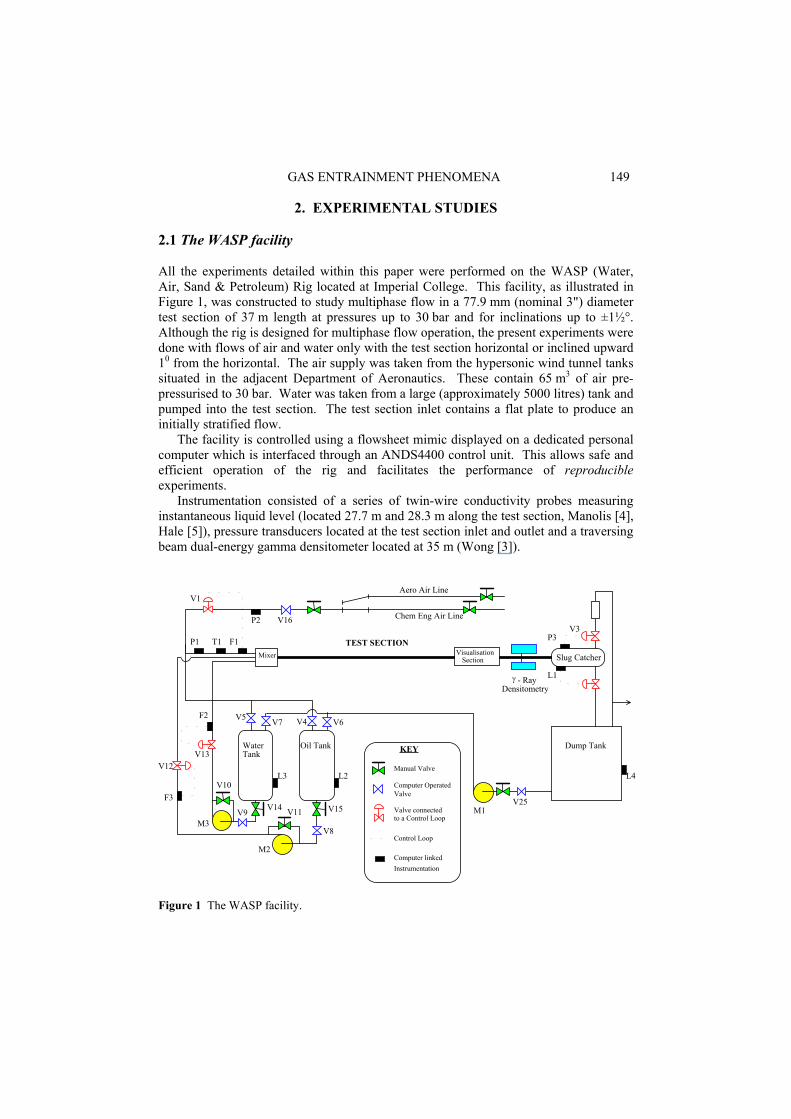
2. EXPERIMENTAL STUDIES 2.1 The WASP facility All the experiments detailed within this paper were performed on the WASP (Water, Air, Sand & Petroleum) Rig located at Imperial College. This facility, as illustrated in Figure 1, was constructed to study multiphase flow in a 77.9 mm (nominal 3") diameter test section of 37 m length at pressures up to 30 bar and for inclinations up to ±1½°. Although the rig is designed for multiphase flow operation, the present experiments were done with flows of air and water only with the test section horizontal or inclined upward 10 from the horizontal. The air supply was taken from the hypersonic wind tunnel tanks situated in the adjacent Department of Aeronautics. These contain 65 m3 of air pre-pressurised to 30 bar. Water was taken from a large (approximately 5000 litres) tank and pumped into the test section. The test section inlet contains a flat plate to produce an initially stratified flow.

The facility is controlled using a flowsheet mimic displayed on a dedicated personal computer which is interfaced through an ANDS4400 control unit. This allows safe and efficient operation of the rig and facilitates the performance of reproducible experiments.

Instrumentation consisted of a series of twin-wire conductivity probes measuring instantaneous liquid level (located 27.7 m and 28.3 m along the test section, Manolis [4], Hale [5]), pressure transducers located at the test section inlet and outlet and a traversing beam dual-energy gamma densitometer located at 35 m (Wong [3]).

Aero Air Line

Chem Eng Air Line

Mixer Slug Catcher

Dump TankOil TankWaterTank

V1

V16V3

P3

L1

L2L3 L4

V25M1

M2

M3V8

V9

P2

T1 F1P1

F2

F3

V13V12

V4V5

TEST SECTIONVisualisation

Section

γ - RayDensitometry

KEY

Manual Valve

Computer OperatedValve

Valve connectedto a Control Loop

Control Loop

Computer linkedInstrumentation

V7 V6

V14 V15V11

V10

Figure 1 The WASP facility.

150 C. P. HALE, et al.

2.2 Measurement of slug characteristics in air-water flows The WASP facility was used to investigate the characteristics of air-water flows in a horizontal pipe and a pipe inclined at 1° upwards. Further details of measurements are reported by Hale [5] and Wong [3] and will be the subject of further publications. From the wide range of data obtained in these studies, the parameters used in the work described here were as follows: 1. Slug translational velocity, measured by time of passage of the slugs between

successive transducers (twin wire conductance probes in the work of Hale [5] and gamma densitometers in the work of Wong [3]).

2. Measurements of the holdup in the liquid film immediately in front of the slugs

using gamma densitometry (Hale [5] and Wong [3]). 3. Measurements of mean slug body holdup and distribution of slug holdup using

conditional sampling of the output of a traversing beam gamma densitometry. Tomographic imaging was used to obtain cross sectional distributions of the phases.

2.3 Gas entrainment ("push-Iin") experiment The objective of the “push-in” experiment is to measure independently the rate of gas entrainment at the front of a single liquid slug propagated along the channel into a stratified layer of liquid flowing down the (inclined) channel towards the slug front. The experiments were carried out in the WASP facility with the test-section inclined upwards at 1o. The stages in the experiment were as follows: (a) The upstream part of the test-section was filled with a stationary slug of water by

introducing water at the downstream end of the test-section and allowing this water to collect at the inlet end. The water flowing from the downstream end of the test-section towards the stationary slug formed a stratified layer of known (measured) thickness and velocity.

(b) When the stationary slug reached a sufficient length (typically 10m), gas was

introduced at the upstream end of the test-section at a precisely known mass flowrate, forming a large bubble which pushed the stationary slug in the downstream direction. If the relative velocity between the advancing slug front and the descending stratified layer was sufficient, then gas bubbles were entrained at the slug front and joined the slug body. An essential feature of the methodology was that these bubbles did not reach the slug tail before the front of the slug reached the downstream end of the test-section.

(c) The position of the front and tail of the single slug induced in the test-section was

measured as a function of time elapsed from initiation of slug motion.

GAS ENTRAINMENT PHENOMENA 151

The velocity of the slug front (UT) is given by the sum of the superficial velocity (U) in the upstream (liquid filled) part of the liquid slug and the rates of accretion of gas and liquid per unit slug front area:

(1 ) (1 )

GPLFT

LF LF

VVU

A Aε ε= +

− −U+ (2)

where: is the (known) volumetric liquid flowrate flowing down towards the slug

front from the upstream end of the test-section, A is the pipe cross sectional area, is the fraction of the channel cross-section occupied by the liquid layer downstream of the slug front (calculated from the measured thickness of the liquid layer), and V is the (unknown) volumetric flowrate of gas entering the slug front. Thus, V can be calculated from the measured value of U

LFV

LFε

GP

GP

T provided that U is known. In the calculation of U at the time that UT is meaured, allowance has to be made for the compressibility of the gas upstream of the slug. U is given by V where V is the rate at which the upstream gas volume is increasing. V is given by:

/ A

( / )Gd MdVV

dt dtρ

= = (3)

where V is the upstream gas volume, M the mass of gas in the upstream zone and ρG is the gas density. In turn we have (assuming an ideal gas behaviour):

( / ) (1/ ) 1G G

G

d M Md dM V dp Mpdt dt dt p dt RT

ρ ρρ

= + = − +

M

(4)

where is the mass rate of flow of the gas entering the test section, p the pressure, R the gas constant and T the absolute temperature. Since the flow of gas at entry is critical,

is constant (and known). The upstream volume V at the time of measurement of U

M

T can be estimated knowing the position of the slug tail (entering bubble front); an allowance is made for the (relatively small) amount of liquid shed by the advancing slug tail. Using a pressure transducer in the upstream region and recording pressure (p) continuously, the values of p and (dp/dt) at the time of the UT measurement can be determined. Thus, from the measurements and from the above equations, the required value of V can be obtained. GP

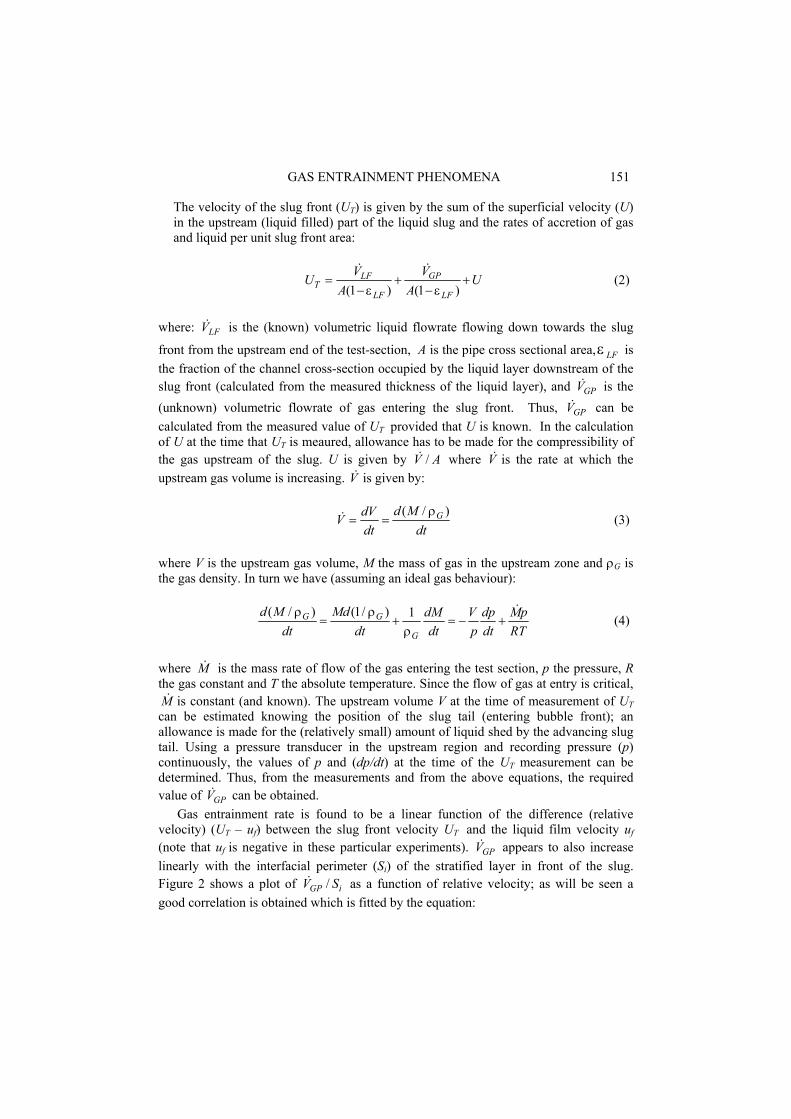
Gas entrainment rate is found to be a linear function of the difference (relative velocity) (UT – uf) between the slug front velocity UT and the liquid film velocity uf

(note that uf is negative in these particular experiments). V appears to also increase linearly with the interfacial perimeter (S

GP

i) of the stratified layer in front of the slug. Figure 2 shows a plot of V as a function of relative velocity; as will be seen a good correlation is obtained which is fitted by the equation:

/GP iS

152 C. P. HALE, et al.

( ) ( )1i

GP M T f T f MIN

SV k A U u U u

D= − − −

(5)

where is the net gas volumetric entrainment rate and kGPV M1 is a constant given by linear regression as k . Si is the interfacial width given as a function of the measured height of the liquid film (h

146.01M =

f) just downstream of the slug front:

2

1 2 1Fi

hS D

D = − −

(6)

Assuming a flat interface the film holdup εLF is related to the film height by:

2

1 2 2 211 cos 1 1 1 1f f fLF

h h hD D D

επ

− = − − − − − −

(7)

The minimum relative velocity for gas entrainment is (UT – uf)MIN ≈ 2.13 m/s. This value is close to that found by Nydal & Andreussi [6] and also to the value of 2m/s obtained by Bos & Du Chatinier [7] in experiments on sphere-propelled liquid slugs performed in a 26m long, 50mm diameter test section. Further details of this work are given by Manolis [4].

0.00

0.01

0.02

0.03

0.04

0.05

2.0 2.5 3.0 3.5 4.0 4.5 5.0 5.5 6.0 6.5 7.0

Relative velocity (m/s)

Entr

aine

d Vo

lum

etric

Vol

umet

ric F

low

rate

/ In

terf

acia

l per

imet

er

Elf = 0.0441Elf = 0.0650Elf = 0.1008Elf = 0.1403

Figure 2 Gas entrainment rate as a function of relative velocity.

GAS ENTRAINMENT PHENOMENA 153

3. A TEST OF THE VALIDITY OF THE HOMOGENEOUS ASSUMPTION

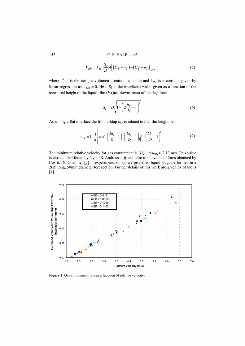
3.1 Calculation of pickup rate of liquid and gas This section outlines the equations used for the calculation of the pickup rates of gas and liquid to obtain the liquid holdup in a homogeneous slug body by Eq. (1).

Figure 3 shows a schematic of a slug unit cell. The bold arrows illustrate the pickup of gas and liquid, V and V respectively, at the slug front and the shedding of gas and liquid, V and V respectively, at the slug tail. For a steady state slug the shedding rate and pickup rate of a given phase is the same, thus, V = V and V = V . A liquid mass balance across the slug front gives the pickup rate of liquid as a function of the velocity (u

GP

LS

LP

GS

GP GS LP LS

f) and holdup (εLF) of the film immediately upstream of the slug front and the slug translational velocity (UT) as follows: (8) (LP LF T fV A U uε= − )

)

where A is the cross-sectional area of the pipe. An overall volumetric flow balance gives the following expression relating the pickup rate of gas and liquid. (9) (LP GP T MIXV V A U U+ = − where UMIX is the superficial mixture velocity. The pickup rate of gas at the slug front is given by in Eq. (5).

Knowing Si, εLF, UT and UMIX, Eq. (5) and Eqs. (8)-(9) have three- remaining unknowns (namely uf, V and V ) which can be obtained by simultaneous solution of the three equations. For example, by elimination of V and V Eq. (8) gives (following rearrangement)

GP LP

GP LP

Figure 3 Illustration of slug unit cell.

154 C. P. HALE, et al.

( ) ( )1 0.146 2.12

0.146

iT LF MIX T

fi

LF

SU U UDu

SD

ε

ε

− + + −=

+

(10)

The value of uf calculated from Eq. (8) is then substituted back into Eq. (8) and Eq. (5) to yield V and V . LP GP

Using values of UT and hf (thus εLF) measured in experiments, V and V can be

estimated as indicated above. An alternative would be to obtain UGP LP

T from a correlation and hf from a momentum balance over the slug tail region (see Taitel and Barnea [1]). Since the objective was to investigate the validity of Eq. (1), we preferred to use the experimental values rather than introduce a further source of uncertainty. The value of εLS expected if homogeneous flow occurred in the slug body can be calculated from these values by rearranging Eq. (1) and compared with the actual measured values.

For these comparisons two sets of data were used as discussed in Section 3.2 and Section 3.3 below.

3.2 Two-phase air-water data in a horizontal test section Further details of these experiments can be found in Wong [3]. From the plots of holdup as a function of time, obtained by a traversing beam gamma densitometer near the end of the WASP test section, the average film height, hf, immediately downstream of the slug front as well as the slug translational velocity was measured.

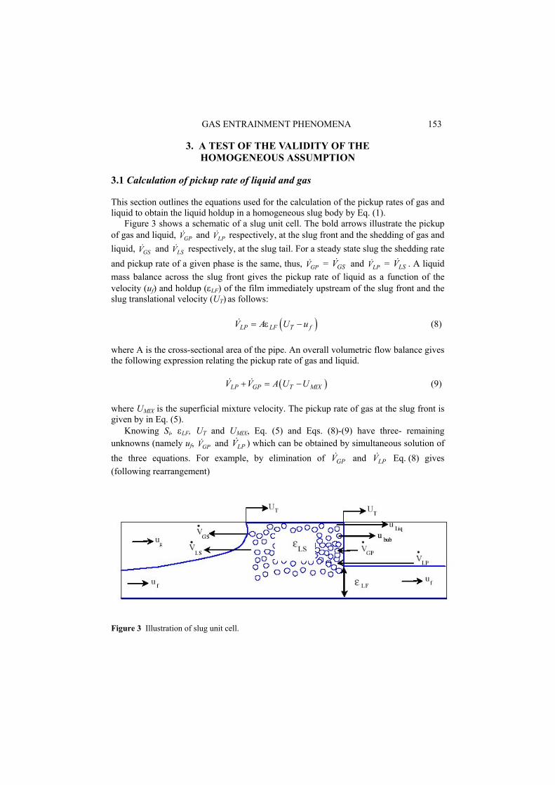
Figure 4 compares the measured values of slug body holdup obtained in the present work with values predicted from Eq. (1), Eqs. (5)-(10). From this graph, it appears that whilst the predicted values agree well with the experimental measurements at mixture

Figure 4 Comparison between measured two-phase slug body holdup data and predicted values assuming a homogeneous mixture in the slug body.

GAS ENTRAINMENT PHENOMENA 155

velocities above 6 ms-1, an underprediction is evident at the lower mixture velocities of less than 6 ms-1.

As is seen below, this trend is consistent with the gas separation effect seen in the tomographs presented in Section 4. 3.3 Two-phase air-water data in a 1o upwardly inclined test section The test of homogeneity was also applied to air-water data obtained by Hale [5] with the WASP test section upwardly inclined at 1°. This particular pipe configuration is of interest since the “Push-in” experiments carried out by Manolis [4] to investigate gas entrainment rates, resulting in Eq. (10), were also carried out with a 1° upwardly inclined pipe. In the calculations described in Section 3.2 above, it was assumed that the Manolis [4] correlation also applied to the horizontal case but the Hale [5] data is more directly consistent.

Measurements obtained by Hale [5] on the 1° upwardly inclined WASP test section included slug translational velocity and film holdup data averaged over the length of the film region behind the slug tail. These film holdup measurements are not immediately suitable for use in the analysis described in Section 3.1, for which the film height or holdup immediately downstream of the slug front is required. However, as described below, the method of Taitel and Barnea [1,2] can be used to establish values for the ratio of mean to slug front film holdup values and thus allow an estimate of slug front values from the mean value. Relationship between average film region holdup and holdup immediately downstream of the slug front. Taitel and Barnea [1,2] developed a model for the height profile of the film region from the tail of the leading slug to the front of the following slug. Their model involved manipulation of the one-dimensional mass and momentum balances as illustrated in Figure 3. The equation derived by Taitel and Barnea [1,2] for the change of film height with distance was as follows:

k

kF

BA

dzdh

=−

(11a)

( ) βρρτττ sin11 g

AAS

AS

ASA GL

GFII

G

GG

F

FFK −+

+−−= (11b)

( )

( ) ( )

( ) ( )( )

( )

2

2

cos

1

1

f liqT T LS LFK L G LLFLF

g T bub LST LFG

LFLF

U u U u dB gdh

U uU u ddh

ε ερ ρ β ρ

εε ε

ρε

− −= − −

− −−−

−

(11c)

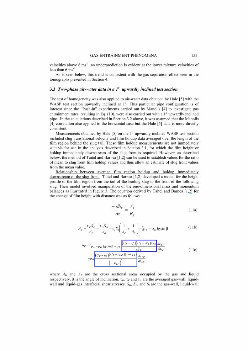
where AG and AF are the cross sectional areas occupied by the gas and liquid respectively. β is the angle of inclination. τG, τF and τi, are the averaged gas-wall, liquid-wall and liquid-gas interfacial shear stresses. SG, SF, and Si are the gas-wall, liquid-wall

156 C. P. HALE, et al.

and gas-liquid interfacial perimeters. ρG and ρL are respectively the gas and liquid densities. ubub and uliq are respectively the gas and liquid velocities within the slug body.

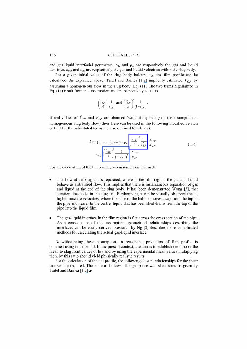
For a given initial value of the slug body holdup, εLS, the film profile can be calculated. As explained above, Taitel and Barnea [1,2] implicitly estimated V by assuming a homogeneous flow in the slug body (Eq. (1)). The two terms highlighted in Eq. (11) result from this assumption and are respectively equal to

GP

21LP

LF

VA ε

and ( )

21

1GP

LF

VA ε

−

.

If real values of V and V are obtained (without depending on the assumption of homogeneous slug body flow) then these can be used in the following modified version of Eq 11c (the substituted terms are also outlined for clarity):

GP LP

( )

( )

2

3

2

3

1cos

1

1

LP LFK L G LLF LF

GP LFG

LF LF

V dB g A dh

V dA dh

ερ ρ β ρ

ε

ερ

ε

= − −

−

−

(12c)

For the calculation of the tail profile, two assumptions are made

• The flow at the slug tail is separated, where in the film region, the gas and liquid behave as a stratified flow. This implies that there is instantaneous separation of gas and liquid at the end of the slug body. It has been demonstrated Wong [3], that aeration does exist in the slug tail. Furthermore, it can be visually observed that at higher mixture velocities, where the nose of the bubble moves away from the top of the pipe and nearer to the centre, liquid that has been shed drains from the top of the pipe into the liquid film.

• The gas-liquid interface in the film region is flat across the cross section of the pipe.

As a consequence of this assumption, geometrical relationships describing the interfaces can be easily derived. Research by Ng [8] describes more complicated methods for calculating the actual gas-liquid interface.

Notwithstanding these assumptions, a reasonable prediction of film profile is

obtained using this method. In the present context, the aim is to establish the ratio of the mean to slug front values of hLF and by using the experimental mean values multiplying them by this ratio should yield physically realistic results.

For the calculation of the tail profile, the following closure relationships for the shear stresses are required. These are as follows. The gas phase wall shear stress is given by Taitel and Barnea [1,2] as:

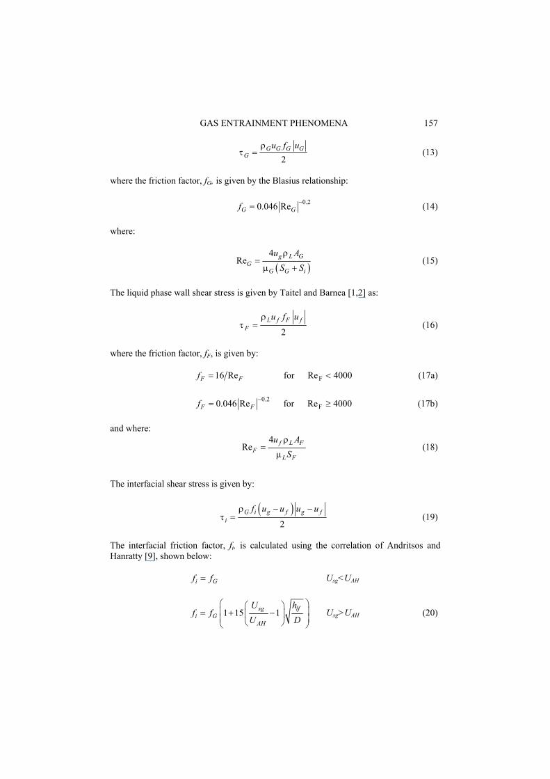
GAS ENTRAINMENT PHENOMENA 157

2

G G G GG

u f uρτ = (13)

where the friction factor, fG, is given by the Blasius relationship: 0.20.046 ReGf

−= G

)

(14) where:

(

4Re g L G

GG G i

u AS Sρ

µ=

+ (15)

The liquid phase wall shear stress is given by Taitel and Barnea [1,2] as:

2

L f F fF

u f uρτ = (16)

where the friction factor, fF, is given by: 16 ReFf = F for (17a) 4000ReF < 0.20.046 ReFf

−= F for (17b) 4000ReF ≥ and where:

4

Re f L FF

L F

u AS

ρ

µ= (18)

The interfacial shear stress is given by:

( )

2G i g f g f

i

f u u u uρτ

− −= (19)

The interfacial friction factor, fi, is calculated using the correlation of Andritsos and Hanratty [9], shown below: Uif f= G sg<UAH

1 15 1sg lfi G

AH

U hf f

U

= + − D

Usg>UAH (20)

158 C. P. HALE, et al.

where UAH is approximately 5 ms-1, which is the critical velocity for waves to affect the shear stress on the interface. Alternative correlations have been reviewed by Khor [10] and Srichai [11]. In the experiments of Hale [5], the slug body and tail region lengths were not measured directly. However,a reasonable assumption for slug body length was 15 diameters (consistent to the earlier experimental data of Manolis[4]); using this value, the Taitel and Barnea model predicts values of the slug tail region lengths which vary with feed flow rates but which were not very sensitive to the assumed slug body length for the conditions examined.

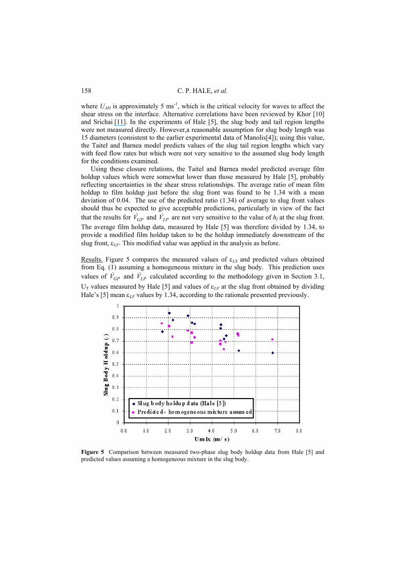
Using these closure relations, the Taitel and Barnea model predicted average film holdup values which were somewhat lower than those measured by Hale [5], probably reflecting uncertainties in the shear stress relationships. The average ratio of mean film holdup to film holdup just before the slug front was found to be 1.34 with a mean deviation of 0.04. The use of the predicted ratio (1.34) of average to slug front values should thus be expected to give acceptable predictions, particularly in view of the fact that the results for V and V are not very sensitive to the value of hGP LP f at the slug front. The average film holdup data, measured by Hale [5] was therefore divided by 1.34, to provide a modified film holdup taken to be the holdup immediately downstream of the slug front, εLF. This modified value was applied in the analysis as before. Results. Figure 5 compares the measured values of εLS and predicted values obtained from Eq. (1) assuming a homogeneous mixture in the slug body. This prediction uses values of V and V calculated according to the methodology given in Section 3.1, U

GP LP

T values measured by Hale [5] and values of εLF at the slug front obtained by dividing Hale’s [5] mean εLF values by 1.34, according to the rationale presented previously.

Figure 5 Comparison between measured two-phase slug body holdup data from Hale [5] and predicted values assuming a homogeneous mixture in the slug body.

GAS ENTRAINMENT PHENOMENA 159

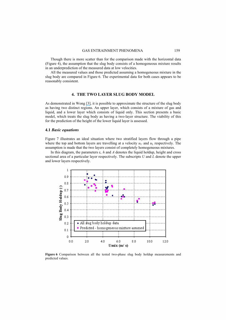
Though there is more scatter than for the comparison made with the horizontal data (Figure 4), the assumption that the slug body consists of a homogeneous mixture results in an underprediction of the measured data at low velocities.

All the measured values and those predicted assuming a homogeneous mixture in the slug body are compared in Figure 6. The experimental data for both cases appears to be reasonably consistent.

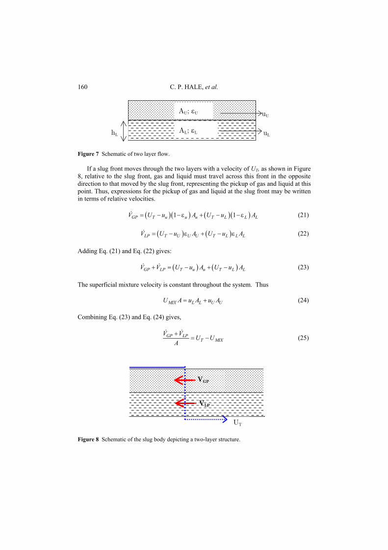
4. THE TWO LAYER SLUG BODY MODEL As demonstrated in Wong [3], it is possible to approximate the structure of the slug body as having two distinct regions. An upper layer, which consists of a mixture of gas and liquid, and a lower layer which consists of liquid only. This section presents a basic model, which treats the slug body as having a two-layer structure. The viability of this for the prediction of the height of the lower liquid layer is assessed. 4.1 Basic equations Figure 7 illustrates an ideal situation where two stratified layers flow through a pipe where the top and bottom layers are travelling at a velocity uU and uL respectively. The assumption is made that the two layers consist of completely homogeneous mixtures.

In this diagram, the parameters ε, h and A denotes the liquid holdup, height and cross sectional area of a particular layer respectively. The subscripts U and L denote the upper and lower layers respectively.

Figure 6 Comparison between all the tested two-phase slug body holdup measurements and predicted values.

160 C. P. HALE, et al.

uL hL AL; εL

AU; εU uU Figure 7 Schematic of two layer flow.

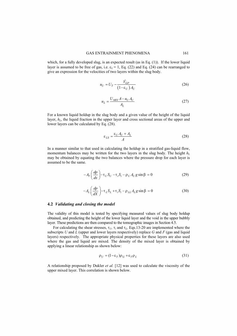
If a slug front moves through the two layers with a velocity of UT, as shown in Figure 8, relative to the slug front, gas and liquid must travel across this front in the opposite direction to that moved by the slug front, representing the pickup of gas and liquid at this point. Thus, expressions for the pickup of gas and liquid at the slug front may be written in terms of relative velocities. (21) ( ) ( ) ( )( )1 1GP T u u u T L L LV U u A U uε= − − + − − Aε

A (22) ( ) ( )LP T U U U T L L LV U u A U uε ε= − + − Adding Eq. (21) and Eq. (22) gives: (23) ( ) ( )GP LP T u u T L LV V U u A U u A+ = − + − The superficial mixture velocity is constant throughout the system. Thus (24) MIX L L U UU A u A u A= + Combining Eq. (23) and Eq. (24) gives,

GP LPT MI

V VU U

A+

= − X (25)

VLP

VGP

UT

Figure 8 Schematic of the slug body depicting a two-layer structure.

GAS ENTRAINMENT PHENOMENA 161

which, for a fully developed slug, is an expected result (as in Eq. (1)). If the lower liquid layer is assumed to be free of gas, i.e. εL = 1, Eq. (22) and Eq. (24) can be rearranged to give an expression for the velocities of two layers within the slug body.

( )1

GPU T

U U

Vu U

Aε= −

− (26)

MIX U UL

L

U A u Au

A−

= (27)

For a known liquid holdup in the slug body and a given value of the height of the liquid layer, hL, the liquid fraction in the upper layer and cross sectional areas of the upper and lower layers can be calculated by Eq. (28).

U U LLS

A AA

εε

+= (28)

In a manner similar to that used in calculating the holdup in a stratified gas-liquid flow, momentum balances may be written for the two layers in the slug body. The height hL may be obtained by equating the two balances where the pressure drop for each layer is assumed to be the same.

sin 0T U U i i U UdpA S S A gdx

τ τ ρ β − − − −

= (29)

sin 0L L L i i LL LdpA S S A gdX

τ τ ρ β − − + −

=

Lρ

(30)

4.2 Validating and closing the model The validity of this model is tested by specifying measured values of slug body holdup obtained, and predicting the height of the lower liquid layer and the void in the upper bubbly layer. These predictions are then compared to the tomographic images in Section 4.5.

For calculating the shear stresses, τU, τi and τL, Eqs.13-20 are implemented where the subscripts U and L (upper and lower layers respectively) replace G and F (gas and liquid layers) respectively. The appropriate physical properties for these layers are also used where the gas and liquid are mixed. The density of the mixed layer is obtained by applying a linear relationship as shown below: (31) (1 )U T G Tρ ε ρ ε= − + A relationship proposed by Dukler et al. [12] was used to calculate the viscosity of the upper mixed layer. This correlation is shown below.

162 C. P. HALE, et al.

( )( )

( )( )( )

1

1 1L q GG q L

Uq L q G q L q G

xx

x x x x

µ ρµ ρµ

ρ ρ ρ ρ

−= +

+ − + − (32)

where xq is the quality and is calculated by the following.

( )

( )1

1u G

qu G u L

xε ρ

ε ρ ε ρ

−=

− + (33)

Gas and liquid pickup rates, V and V , are calculated, as before, by implementing Eq. (8)-(10).Experimental values of U

GP LP

T and εLF at the slug front are input into these equations to calculate the pickup rates of the two phases.

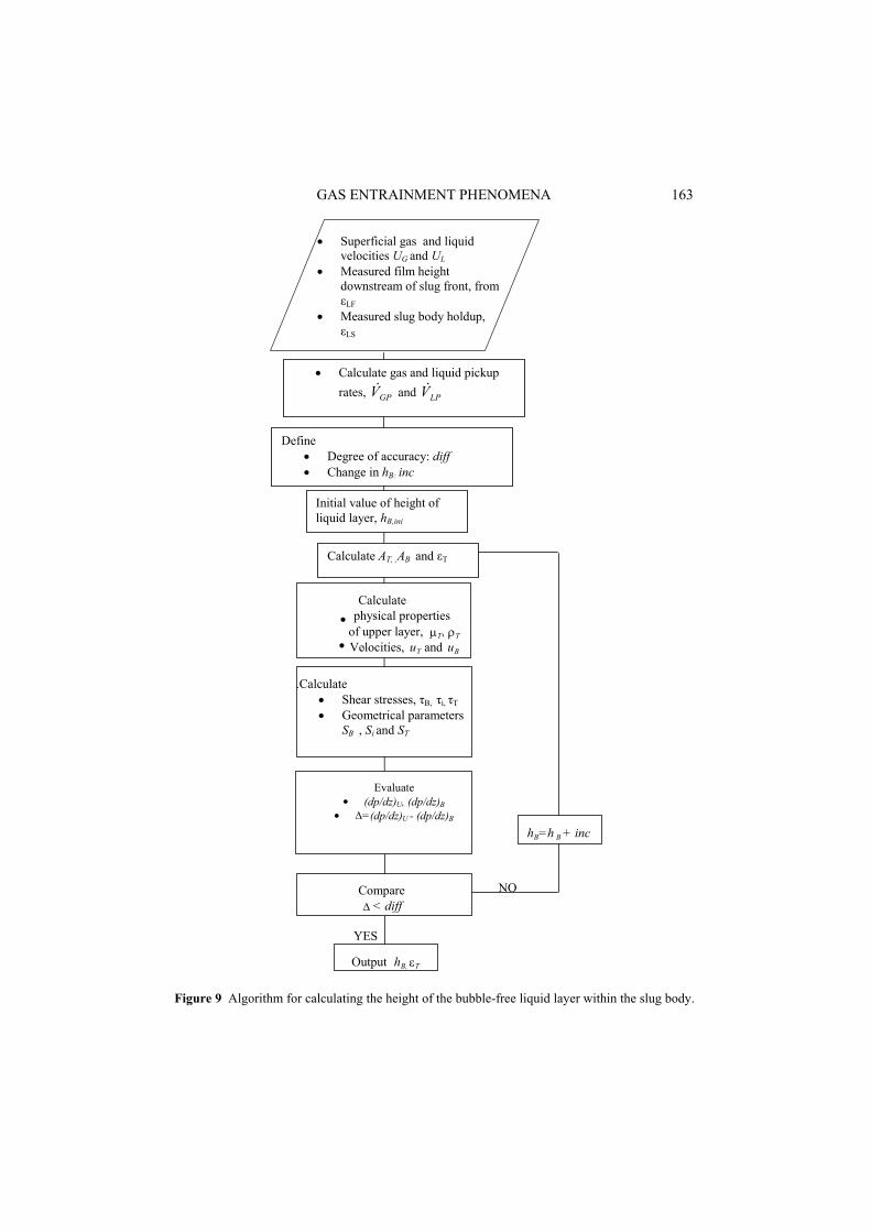
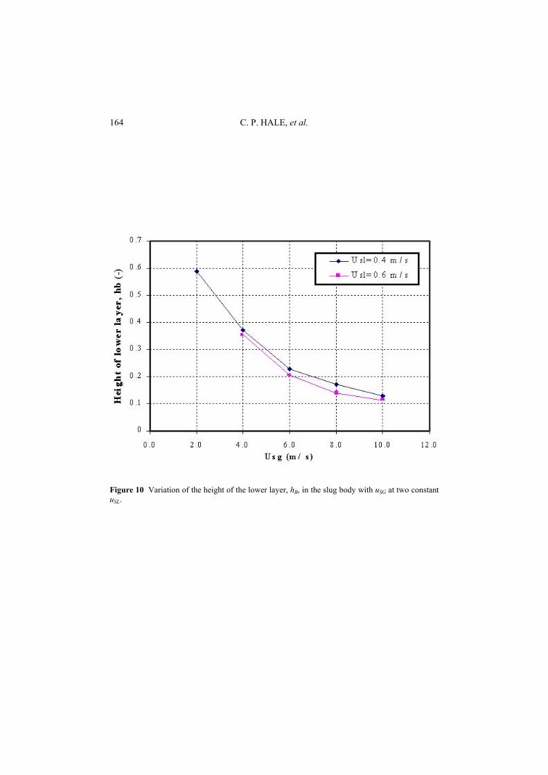
The flow diagram for the calculations is shown in Figure 9. 4.3 Results The height hL of the lower layer calculated by the procedure described in Sections 4.1 and 4.2 is shown as a function of Us,l and Us,g in Figure 10.

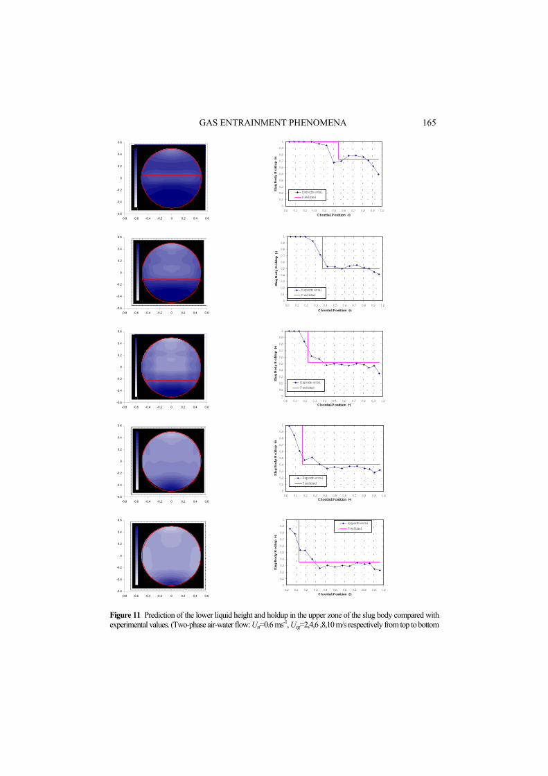
Figure 11 also illustrates predictions of the height of the lower liquid zone by the two-layer slug body model and compares these values with two-phase air-water tomographs obtained as part of the horizontal campaign of experiments for a range of superficial gas velocities and at a constant superficial liquid velocity. Here, the red lines superimposed onto the tomographic images represent the predicted values of hL. There is good qualitative agreement between the positions of these lines and the approximate position where the two regions are divided in the tomographs. The graphs shown alongside the tomographs compare the holdup values for the chordal positions in the upper aerated zone and again, the height of the lower layer predicted by model to data obtained experimentally. From Figure 11, it appears that the model slightly over predicts the height of the liquid zone. However, the position of the boundary between the two layers correctly coincides with the sudden drop in holdup in the slug body, where the holdup in the upper region is predicted moderately well. Overall, the comparisons shown in this figure demonstrate that the two-layer slug body model can be used to obtain an approximate idealised structure of the slug body.

5. CONCLUSION From the analysis given in Section 2 - 3, it is demonstrated that the homogeneous model does not predict the liquid holdup in the slug body at lower mixture velocities. For the case of the WASP test section, agreement is poor for velocities less than 6 ms-1. Furthermore, the results shown here are consistent with the experimental air-water tomographs shown in Figure 11. A two-fluid model for the liquid slugs was developed and gave a better representation of the data.

GAS ENTRAINMENT PHENOMENA 163

.Calculate • Shear stresses, τB, τi, τT • Geometrical parameters

SB , Si and ST

Calculate • physical properties

of upper layer, µ T , ρ T • . Velocities, u T and u B

Evaluate • (dp/dz) U , (dp/dz) B

• ∆ =(dp/dz) U - (dp/dz) B

Compare ∆ < diff

YES

Output h B, ε T

NO

• Superficial gas and liquid velocities UG and UL

• Measured film height downstream of slug front, from εLF

• Measured slug body holdup, εLS

h B =h B + inc

• Calculate gas and liquid pickup rates, GPV and LPV

Define • Degree of accuracy: diff • Change in hB: inc

Initial value of height of liquid layer, hB,ini

Calculate AT, ,AB and εT

Figure 9 Algorithm for calculating the height of the bubble-free liquid layer within the slug body.

164 C. P. HALE, et al.

Figure 10 Variation of the height of the lower layer, hB, in the slug body with uSG at two constant uSL.

GAS ENTRAINMENT PHENOMENA 165

-1 -0.5 0 0.5 1

-1

-0.5

0

0.5

1

-0.6

-0.4

-0.2

0

0.2

0.4

0.6

-0.8 -0.6 -0.4 -0.2 0 0.2 0.4 0.6

0

0.1

0.2

0.3

0.4

0.5

0.6

0.7

0.8

0.9

1

0.0 0.1 0.2 0.3 0.4 0.5 0.6 0.7 0.8 0.9 1.

Chordal Position (-)

Slug Body Holdup (-)

0

Experim ental

Predicted

-0.6

-0.4

-0.2

0

0.2

0.4

0.6

-0.8 -0.6 -0.4 -0.2 0 0.2 0.4 0.6

0

0.1

0.2

0.3

0.4

0.5

0.6

0.7

0.8

0.9

1

0.0 0.1 0.2 0.3 0.4 0.5 0.6 0.7 0.8 0.9 1.0

Chordal Position (-)

Slug Body Holdup (-)

Experim ental

Predicted

-1 -0.5 0 0.5 1

-1

-0.5

0

0.5

1

-0.6

-0.4

-0.2

0

0.2

0.4

0.6

-0.8 -0.6 -0.4 -0.2 0 0.2 0.4 0.6

0

0.1

0.2

0.3

0.4

0.5

0.6

0.7

0.8

0.9

1

0.0 0.1 0.2 0.3 0.4 0.5 0.6 0.7 0.8 0.9 1.Chordal Position (-)

Slug Body Holdup (-)

0

Experim ental

Predicted

-0.6

-0.4

-0.2

0

0.2

0.4

0.6

-0.8 -0.6 -0.4 -0.2 0 0.2 0.4 0.6

0

0.1

0.2

0.3

0.4

0.5

0.6

0.7

0.8

0.9

1

0.0 0.1 0.2 0.3 0.4 0.5 0.6 0.7 0.8 0.9 1.0Chordal Position (-)

Slug Body Holdup (-)

Experim ental

Predicted

-0.6

-0.4

-0.2

0

0.2

0.4

0.6

-0.8 -0.6 -0.4 -0.2 0 0.2 0.4 0.6

0

0.1

0.2

0.3

0.4

0.5

0.6

0.7

0.8

0.9

1

0.0 0.1 0.2 0.3 0.4 0.5 0.6 0.7 0.8 0.9 1.

Chordal Position (-)

Slug Body Holdup (-)

0

Experim ental

Predicted

Figure 11 Prediction of the lower liquid height and holdup in the upper zone of the slug body compared with experimental values. (Two-phase air-water flow: Usl=0.6 ms-1, Usg=2,4,6 ,8,10 m/s respectively from top to bottom

166 C. P. HALE, et al.

NOMENCLATURE A Pipe cross-sectional area m2 AF Cross-sectional area of film m2 AG Cross-sectional area of gas in film region m2 AL Cross-sectional area of lower layer m2 Au Cross-sectional area of upper layer m2 D Pipe diameter. m fF Liquid-wall friction factor in the film region - fG Gas-wall friction factor - fi Gas-liquid interface friction factor - g Acceleration due to gravity m/s2 hf Film thickness m hL Thickness of lower layer m hU Thickness of lower layer m kM1 Manolis [4] constant - n Blasius friction factor coefficient - p Pressure Pa R Gas constant J/kg K ReF Reynolds number for the film region - ReG Reynolds number for gas phase - SF Wetted perimeter of film m SG Wetted perimeter of gas m SI Wetted perimeter of the interface m SL Wetted perimeter of lower layer m SU Wetted perimeter of upper layer m t Time s T Temperature K uAH Andritsos & Hanratty [9] critical velocity m/s ubub Average velocity of dispersed bubbles in liquid slug m/s uf Liquid velocity in the film region m/s uG Gas velocity in the bubble in the film region m/s uGS Superficial gas velocity m/s uL Liquid velocity in the lower fluid layer m/s uliq Average liquid velocity in the liquid slug m/s uLS Superficial liquid velocity m/s uMIX Superficial mixture velocity m/s uT Translational velocity of the slug unit m/s

GAS ENTRAINMENT PHENOMENA 167

uU Liquid velocity in the upper fluid layer m/s

GPV Volumetric gas pick-up rate at the slug front m3/s

GSV Volumetric liquid shedding rate at the slug tail m3/s

LPV Volumetric liquid pick-up rate at the slug front m3/s

LSV Volumetric liquid shedding rate at the slug tail m3/s z Position from the rear of the slug body m β Angle of inclination from the horizontal - εL Liquid holdup in the lower region - εLF Liquid holdup in the film region - εLS Liquid holdup in the slug body - εU Liquid holdup in the upper region - ρG Gas density kg/m3 ρL Liquid density kg/m3 ρU Fluid density of the upper zone kg/m3 µG Dynamic viscosity of the gas Ns/m2 µL Dynamic viscosity of the liquid Ns/m2 µU Dynamic viscosity of the upper zone fluid Ns/m2 τF Liquid-wall shear stress Pa τG Gas-wall shear stress Pa τi Interfacial gas-liquid shear stress Pa τL Lower layer fluid-wall shear stress Pa τU Upper layer fluid-wall shear stress Pa

REFERENCES 1. Taitel, Y. and Barnea, D. (1990) Two-phase slug flow, Advances in Heat Transfer,

vol. 20, pp. 83-132. 2. Taitel, Y. and Barnea, D. (1990) A consistent approach for calculating pressure drop

in inclined slug flow, Chem. Engng Science, vol. 45, no. 5, pp. 1199-1206. 3. Wong, W. L. (2003) Flow development and mixing in three phase slug flow, PhD

Thesis, Department of Chemical Engineering, Imperial College London, England, October 2003.

4. Manolis, I. G. (1995) High pressure gas-liquid slug flow, PhD Thesis, Department of Chemical Engineering, Imperial College London, England, pp. 1-359, October 1995.

5. Hale, C. P. (2000) Slug formation, growth and decay in gas-liquid flows, PhD Thesis, Department of Chemical Engineering, Imperial College London, England, pp. 1-653, December 2000.

168 C. P. HALE, et al.

6. Nydal, O. J. and Andreussi, P. (1991) Gas entrainment in a long liquid slug advancing in a near horizontal pipe, I.J.M.F, vol. 17, no. 2, pp. 179-189.

7. Bos, A. and Du Chatinier, J. G. (1994) The Front of a Sphere-Propelled Liquid Slug in a Natural-Gas Pipeline, I.J.M.F, vol. 20, pp. 535-546.

8. Ng, T. S. (2002) Interfacial structure of stratified pipe flow, PhD Thesis, Department of Chemical Engineering, Imperial College London, England, October 2002.

9. Andritsos, N. and Hanratty, T. J. (1987) Interfacial instabilities for horizontal gas-liquid flows in pipelines, I.J.M.F., vol. 13, no. 5, pp. 583-603.

10. Khor, S. H. (1998) Three phase liquid-liquid-gas stratified flow in pipelines, PhD Thesis, Department of Chemical Engineering, Imperial College London, England, pp. 1-360, January 1998.

11. Srichai, S. (1994) High pressure separated two-phase flow., PhD Thesis, Department of Chemical Engineering, Imperial College London, England, pp. 1-261, September 1994

12. Dukler, A. E., Moye Wicks, III and Cleveland, R. G. (1964) Frictional pressure drop in two-phase flow: A. a comparison of existing correlations for pressure loss and holdup, AIChE J., vol. 10, no. 1, p. 38.