Embed Size (px)
Citation preview
ISSN 0965�5425, Computational Mathematics and Mathematical Physics, 2011, Vol. 51, No. 8, pp. 1339–1352. © Pleiades Publishing, Ltd., 2011.Original Russian Text © L.M. Skvortsov, 2011, published in Zhurnal Vychislitel’noi Matematiki i Matematicheskoi Fiziki, 2011, Vol. 51, No. 8, pp. 1434–1448.
1339
INTRODUCTION
Consider the Cauchy problem for the system of ordinary differential equations (ODEs)
,
where y is the vector of variables, f is a vector function, and t is an independent variable.
We first consider a linear problem; that is, . Assume that it is solved by a conventionalexplicit method. If varies fairly slowly and the spectral radius of the matrix J is sufficiently large( ), then the computational effort to construct the numerical solution can be estimated by the value
. This is a rough estimate for the number of evaluations of the right�hand side required for obtaining a
qualitatively correct solution. For nonlinear problems, an analogous estimate is , where
is the spectral radius of the Jacobian matrix on the solution trajectory. Among the problems for which, one can distinguish stiff and oscillation problems.
Stiff problems are characterized by the property of the Jacobian matrix to have eigenvalues with largenegative real parts. The corresponding components of the solution quickly die down and are negligiblysmall with the exception of small regions (called boundary layers). Stiff problems are usually solved usingimplicit methods, which ensure stable integration with a large step size. However, implicit methods havetheir own drawbacks; first of all, they are difficult to implement, and the Jacobian matrix must be calcu�lated. If the right�hand side has discontinuities or logical conditions, the calculation of the Jacobianmatrix can be a complex and not at all trivial problem. Note also that implicit methods yield unsatisfactoryand, sometimes, even qualitatively wrong results for some stiff problems (examples of such problems weregiven in [1]). Consequently, along with implicit methods, special explicit methods suitable for stiff prob�lems are also developed (see [1–17]).
Oscillation problems have some of their eigenvalues near the imaginary axis, and their solutions areoscillation processes with slowly varying amplitudes. The difficulty of solving such problems is explainedby the necessity to ensure correct values of the amplitude and phase over many periods. To efficiently solveoscillation problems, implicit symmetric methods, as well as special methods (including explicit ones), areapplied (see [3, 18–21]).
The choice of a numerical method should be based on the type of problem (stiff, nonstiff, oscillation,unstable). However, the type of problem can vary in the course of integration; it can also be different fordifferent components. A promising approach to solving such problems is when the integration formulatunes itself on the basis of estimates for certain parameters of the problem. As the parameters to be esti�mated, it is reasonable to use the dominant eigenvalues of the Jacobian matrix. The corresponding esti�
( ) ( ) 0' , , 0 , 0t t T= = ≤ ≤y f y y y
( ) ( ),t t= +f y Jy g( )tg ρ
1 Tρ �
Tρ
( )0
TT t dtρ = ρ∫
( )tρ
1Tρ �
Explicit Adaptive Runge–Kutta Methodsfor Stiff and Oscillation Problems
L. M. Skvortsov Bauman State Technical University, Vtoraya Baumanskaya ul. 5, Moscow, 105005 Russia
e�mail: [email protected] Received October 30, 2010; in final form, January 17, 2011
Abstract—Explicit Runge–Kutta methods with the coefficients tuned to the problem of interest areexamined. The tuning is based on estimates for the dominant eigenvalues of the Jacobian matrixobtained from the results of the preliminary stages. Test examples demonstrate that methods of thistype can be efficient in solving stiff and oscillation problems.
DOI: 10.1134/S0965542511080173
Keywords: explicit Runge–Kutta methods, stiff problems, oscillation problems, Cauchy problem fora system of first�order ordinary differential equations.
1340
COMPUTATIONAL MATHEMATICS AND MATHEMATICAL PHYSICS Vol. 51 No. 8 2011
SKVORTSOV
mates can easily be obtained from the results of the preliminary stages of explicit Runge–Kutta methods,and almost no additional calculations are required to this end.
The indicated approach was implemented in explicit nonlinear methods specially designed for solvingstiff problems (see [1–16]). The method proposed in [2] is especially noticeable because, for the first time,the stage where estimates for the eigenvalues are obtained was clearly separated from the subsequent useof these estimates for stabilizing the computational scheme. A critical analysis of the older explicit non�linear methods was given in [5, 6]. The conclusion there was that these methods are only suitable for thelow�accuracy solution of a very narrow class of problems.
More efficient explicit nonlinear methods were proposed in [1, 13–16]. These methods are calledadaptive because they tune to the problem of interest. The tuning is based on the componentwise estimatesfor the eigenvalues. These estimates can be complex, which makes it possible to apply explicit adaptivemethods to both stiff and oscillation problems. In this paper, we present the principles of the design ofadaptive methods based on explicit Runge–Kutta stages. Second� and third�order methods are con�structed. The accuracy and stability of the proposed methods is examined, and the results of solving testproblems are given.
1. CONSTRUCTION OF ADAPTIVE METHODS
1.1. Integration Formula
Let be the numerical solution obtained at the current point . In an explicit s�stage Runge–Kutta method, the stages of the next step are performed according to the formulas
.
Assume that the coefficients of the method satisfy the first�stage�order condition
, .
Using , find vectors so that the equalities
, (1.1)
are fulfilled for the maximum possible when the linear system is solved. If ( ),then and the vectors are uniquely determined by the relations
, (1.2)
where are the coefficients of the inner stability functions
.
For the explicit methods, these functions can be written in the form
.
We also examine methods for which (then, ). In this case, are not determineduniquely by relations (1.2) because . For a nonlinear problem with a smoothfunction , equalities (1.1) are fulfilled approximately, and is the Jacobian matrix calculated at ,
. Relations (1.1) allow us to use the power method for obtaining the vector of componentwise estimates
for the dominant eigenvalue of the matrix . This is the vector
. (1.3)
ny nt t=
( )1
1
, , , 1,2, ,i
i n ij j i n i i
j
h a t c h i s−
=
= + = + =∑Y y k k f Y …
1
1
i
ij i
j
a c−
=
=∑ 1,2, ,i s= …
1 2, , , sk k k… 1 2, , , ru u u…
( )1 , 1,2, ,ii nh h i r−
= =u J y …
r ' =y Jy , 1 0i ia−
≠ 2,3, ,i s= …
r s= 1 2, , , su u u…
1
1 1
1
, 1,2, ,i
i ij j
j
i s−
+
=
= + β =∑k u u …
ijβ
( )1
1
1i
ji ij
j
R z z−
=
= + β∑
( ) ( ) ( )[ ] [ ] [ ]1
1 2
1
, , , , 1, ,1 ,s
i is ij s s
i
R z R z R z z a−
×
=
= + = =∑e A e e A… …
т т
32 0a = 1r s= − 1 2 1, , , s−u u u…
32 43 , 1 0s s−β = β = = β =�
f J nt t=
ny y=
hJ
1 1r r−=z u u
COMPUTATIONAL MATHEMATICS AND MATHEMATICAL PHYSICS Vol. 51 No. 8 2011
EXPLICIT ADAPTIVE RUNGE–KUTTA METHODS FOR STIFF 1341
(It is assumed that all the operations with vectors are performed componentwise.) For the integration step, we use the formula
, (1.4)
where is the vector of adjustable parameters. In view of (1.3), this formula can be written as
, (1.5)
where . In what follows, we use formula (1.5), which contains fewer terms than (1.4)and is less sensitive to round�off errors. The components of are chosen to ensure the required stabilityand accuracy; they depend on the corresponding components of . Thus, the adaptive methods performthe componentwise tuning of the coefficients of the integration formula.
1.2. Stability Function
Consider the scalar equation
. (1.6)
Applying an adaptive method, we obtain the exact estimate for the eigenvalue, as well as thenumerical solution in the form , where
.
Choose the adjustable parameter from the condition , where is the given functioncalled a scalar stability function. Then, can be calculated using the recursion
. (1.7)
For a system of equations, these operations are performed componentwise. Then, for a linear autonomoussystem, we obtain , where
(1.8)
is a matrix stability function, , and .
For the conventional (that is, linear) Runge–Kutta methods, the scalar and matrix stability functionsare identical; however, they are different for nonlinear methods, including adaptive ones. A virtually arbi�trary function can be prescribed as the scalar stability function of an adaptive method. By contrast, the sta�bility function of a linear method must be linear fractional, and it must be a polynomial if the method isexplicit.
The simplest two�stage nonlinear method can be written as
(1.9)
where is the result of the componentwise application of the scalar function to the vector z.
The function should be chosen so as to ensure the accuracy of the nonstiff components and thestability of stiff components. For instance, one may require that method (1.9) solve scalar equation (1.6)exactly, which yields
. (1.10)
Methods of this type (usually called exponential methods) were examined in [3–7].
1
1
1
!r
n n i r r
i
h i−
+
=
⎛ ⎞= + +⎜ ⎟
⎜ ⎟⎝ ⎠∑y y u d u
rd
2
1 1 1
1
!r
n n i r r
i
h i−
+ − −
=
⎛ ⎞= + +⎜ ⎟
⎜ ⎟⎝ ⎠∑y y u d u
( )1 11 !r rr−
= − +d e d z
1r−d
1z
( )0 0' ,y y y t y= λ =
1z h= λ
( )1 1n ny R z y+=
( ) ( )2 1
11 2 !r rrR z z z r d z− −
−
= + + + − +�
1rd−
( ) ( )1 1R z Q z= ( )Q z
1rd−
( ) ( )0 1 1 1, 1 ! , 0,1, , 2i id Q z d d i z i r+
= = − = −…
1 ( )n nh+=y R J y
( ) ( )2 112 !r r
rr− −
−
= + + + − +R Z I Z Z D Z�
( )=I ediag ( )1 1r r− −
=D ddiag
( )( )
( ) ( )
2 11 1 1 1 1 1 1
1
1 2 1
, , ,
, , , ,
n n
n n n n
h Q
t t h h
+
−= + = − =
β
= = + β + β
k ky y d k d z e z z
k
k f y k f y k
( )Q z
( )Q z
( )( )1 1 1exp= −d z e z
1342
COMPUTATIONAL MATHEMATICS AND MATHEMATICAL PHYSICS Vol. 51 No. 8 2011
SKVORTSOV
A different way of determining is obtained if is chosen as the stability function of an implicitRunge–Kutta method. For instance, if , we have
.
A variety of similar formulas can be obtained by using various linear fractional approximations to theexponential function. The methods based on such formulas are called rational; methods of this type wereanalyzed in [8–12]. Note that these methods usually contain a disguised procedure for estimating thedominant eigenvalue.
Let us discuss the choice of the function . The best choice based on the accuracy of solving modelequation (1.6) is determined by the exponential fitting condition. However, in this case, there is a dangerof overflows caused by large components of the vector z1. For this reason, formula (1.9) is used in [2] onlyfor negative components; if , then one sets , which corresponds to the function
. An analysis of the results of numerous experiments made it possible to formulate the following require�
ments for the scalar stability function :
1. For nonstiff components corresponding to values of z with small moduli, must ensure that theexponential function is approximated with an order at least as high as the desired order of the method.
2. It is necessary to ensure that the stiff components corresponding to large negative z rapidly die down.This leads to the condition for such values. Here, the order of consistency with the exponentialfunction is not important.
3. One must ensure a qualitatively correct behavior of the unstable components corresponding to largepositive z. For these values, the condition must be fulfilled. This condition is not satisfied for lin�ear fractional methods in which not only stiff but also unstable components die down quickly.
4. The value of given by formula (1.7) must be bounded for all z1; otherwise, a loss of accuracy andstability is possible if is found inaccurately. Moreover, this allows one to avoid overflows and divisionsby zero when calculating the adjustable parameters. For the methods proposed here, we have
It is desirable that be a continuous and monotone function.
Let give a few examples of the functions used for constructing adaptive methods (in the parenthe�ses, we indicate the values of for which these functions are recommended):
(1.11)
(1.12)
The design of methods in which two dominant eigenvalues are estimated for each component is dis�cussed in Section 4.
2. ACCURACY AND STABILITY
In [14, 15], the author proposed explicit adaptive methods with the stages performed by the formulas
(2.1)
1d ( )Q z( ) ( )1 1Q z z= −
( )
21
11 21
n n h+
β= +
+ β −
ky y
k k
( )Q z
1 0iz ≥ 1 11 2i id z= +
( ) 21 2Q z z z= + +
( )Q z
( )Q z
( ) 1Q z �
( ) 1Q z �
1rd−
1z
( )10 1 1 !rd r−
≤ ≤ − ( )Q z
( )Q zr
( ) ( ) ( )
( )
( )
( )
2
2 3
2
1 2 1
1 1 1 2,3 ,
1 1.5 1,
1 2 6 1 6
0 1 6 3,4 ,
1 23 30 1 6,
z z z ,
Q z z z r
z z
z z z z .
Q z z . r
z z z .
⎧ + + ≤⎪
= − < − =⎨⎪ + >⎩
⎧ + + + ≤⎪
= < − =⎨⎪ + + >⎩
,
,
,
, ,
,
,
( ) ( ) ( )
2 3 4
2 3
1 2 6 24 2
1 1 2 4,5 .
1 2 4 2,
z z z z z
Q z z z r
z z z z
⎧ + + + + ≤⎪
= − < − =⎨⎪ + + + >⎩
, ,
,
,
( ) ( )
( )[ ] ( )1 2 1 2 2
1 1
, , , , ,
, , , 3,4, , .n n n n
i n i i n i
t h t h
h t h i s−
= = + β = + β
= + β − α + α = + β =
k f y Y y k k f Y
Y y k k k f Y …
COMPUTATIONAL MATHEMATICS AND MATHEMATICAL PHYSICS Vol. 51 No. 8 2011
EXPLICIT ADAPTIVE RUNGE–KUTTA METHODS FOR STIFF 1343
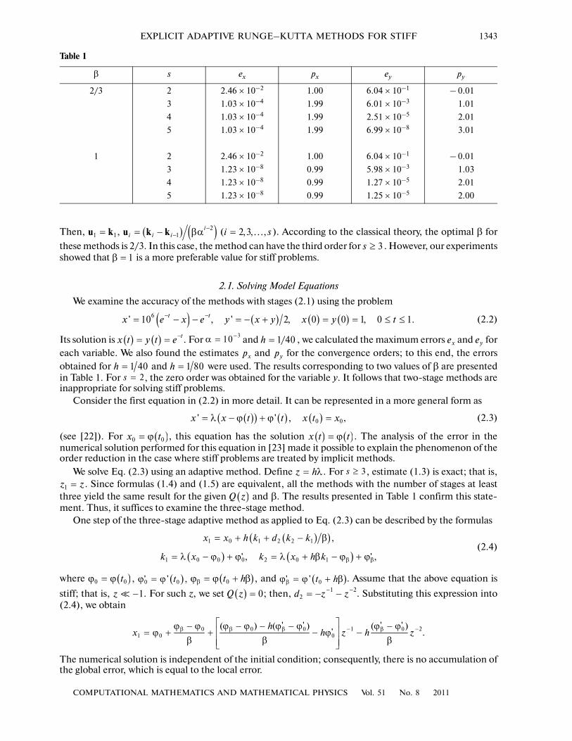
Then, , ( ). According to the classical theory, the optimal β for
these methods is 2/3. In this case, the method can have the third order for . However, our experimentsshowed that is a more preferable value for stiff problems.
2.1. Solving Model Equations
We examine the accuracy of the methods with stages (2.1) using the problem
(2.2)
Its solution is . For and , we calculated the maximum errors and foreach variable. We also found the estimates and for the convergence orders; to this end, the errorsobtained for and were used. The results corresponding to two values of β are presentedin Table 1. For , the zero order was obtained for the variable y. It follows that two�stage methods areinappropriate for solving stiff problems.
Consider the first equation in (2.2) in more detail. It can be represented in a more general form as
, (2.3)
(see [22]). For , this equation has the solution . The analysis of the error in thenumerical solution performed for this equation in [23] made it possible to explain the phenomenon of theorder reduction in the case where stiff problems are treated by implicit methods.
We solve Eq. (2.3) using an adaptive method. Define . For , estimate (1.3) is exact; that is,. Since formulas (1.4) and (1.5) are equivalent, all the methods with the number of stages at least
three yield the same result for the given and β. The results presented in Table 1 confirm this state�ment. Thus, it suffices to examine the three�stage method.
One step of the three�stage adaptive method as applied to Eq. (2.3) can be described by the formulas
(2.4)
where and . Assume that the above equation is
stiff; that is, . For such z, we set ; then, . Substituting this expression into(2.4), we obtain
.
The numerical solution is independent of the initial condition; consequently, there is no accumulation ofthe global error, which is equal to the local error.
1 1=u k ( ) ( )21
ii i i
−
−
= − βαu k k 2,3, ,i s= …
3s ≥1β =
( ) ( ) ( ) ( )6' 10 , ' 2, 0 0 1, 0 1.t tx e x e y x y x y t− −
= − − = − + = = ≤ ≤
( ) ( )tx t y t e−
= =
310−
α = 1 40h = / xe ye
xp yp1 40h = 1 80h =
2s =
( )( ) ( ) ( )0 0' ' ,x x t t x t x= λ − ϕ + ϕ =
( )0 0x t= ϕ ( ) ( )x t t= ϕ
z h= λ 3s ≥
1z z=
( )Q z
( )( )
( ) ( )
1 0 1 2 2 1
1 0 0 0 2 0 1
,
, ,' '
x x h k d k k
k x k x h k β β
= + + − β
= λ − ϕ + ϕ = λ + β − ϕ + ϕ
( )0 0 ,tϕ = ϕ ( )0 0' ,' tϕ = ϕ ( )0 ,t hβϕ = ϕ + β ( )0'' t hβϕ = ϕ + β
1z −� ( ) 0Q z =
1 22d z z− −
= − −
1 20 0 0 01 0 0
' ' ' '( ) ( ) ( )'
hx h z h z− −β β β β
⎡ ⎤ϕ − ϕ ϕ − ϕ − ϕ − ϕ ϕ − ϕ= ϕ + + − ϕ −⎢ ⎥
β β β⎢ ⎥⎣ ⎦
Table 1
β s ex px ey py
2/3 2 2.46 × 10⁻² 1.00 6.04 × 10⁻¹ – 0.01
3 1.03 × 10⁻⁴ 1.99 6.01 × 10⁻³ 1.01
4 1.03 × 10⁻⁴ 1.99 2.51 × 10⁻⁵ 2.01
5 1.03 × 10⁻⁴ 1.99 6.99 × 10⁻⁸ 3.01
1 2 2.46 × 10⁻² 1.00 6.04 × 10⁻¹ – 0.01
3 1.23 × 10⁻⁸ 0.99 5.98 × 10⁻³ 1.03
4 1.23 × 10⁻⁸ 0.99 1.27 × 10⁻⁵ 2.01
5 1.23 × 10⁻⁸ 0.99 1.25 × 10⁻⁵ 2.00
1344
COMPUTATIONAL MATHEMATICS AND MATHEMATICAL PHYSICS Vol. 51 No. 8 2011
SKVORTSOV
The error of the numerical solution can be written in the form
(2.5)
It is evident from (2.5) that, for , the error is proportional to h2. This explains the second order ofconvergence with respect to the variable x in Table 1. The error can be considerably reduced if we set
(then, the error is proportional to ). In this case, the error in , even though it is of the firstorder, is very small. As a result, the error in y dominates for , and this error determines the actual orderof the method. Thus, when the methods based on stages (2.1) are applied to solving stiff problems, theactual order cannot be higher than two irrespective of β.
2.2. Optimal α and β
The results presented in Table 1 show that is a slightly preferable value and the methods with thenumber of stages three or four are of practical interest.
The coefficient α virtually does not affect the accuracy and stability of solving linear problems. How�ever, when stiff nonlinear systems are integrated, a large deviation from the exact solution at the prelimi�nary stages may result in that uncertain estimates for the eigenvalues are obtained and the numerical solu�
tion is unstable. Therefore, a sufficiently small α (say, ) should be chosen. For many stiff problems,this is quite a reasonable value; however, for some problems, a finer tuning is significantly more advanta�geous.
The deviation of the solution at the preliminary stages is characterized by the inner stability functions
(2.6)
The choice of α should be based on the minimization of these functions at the points of the stiff spectrum,
which are determined by the vector . For a scalar equation, the best choice is ; then, functions(2.6) alternatively take the values 1 and 1 + . For a system of equations, we are guided by the worstcase, that is, by the dominant value among the negative components of . Using the vector from thepreceding step (we denote this vector by ), we can choose α as the minimum among the positive com�
ponents of the vector . It is recommended that α be bounded above by the value (we can set at the first step).
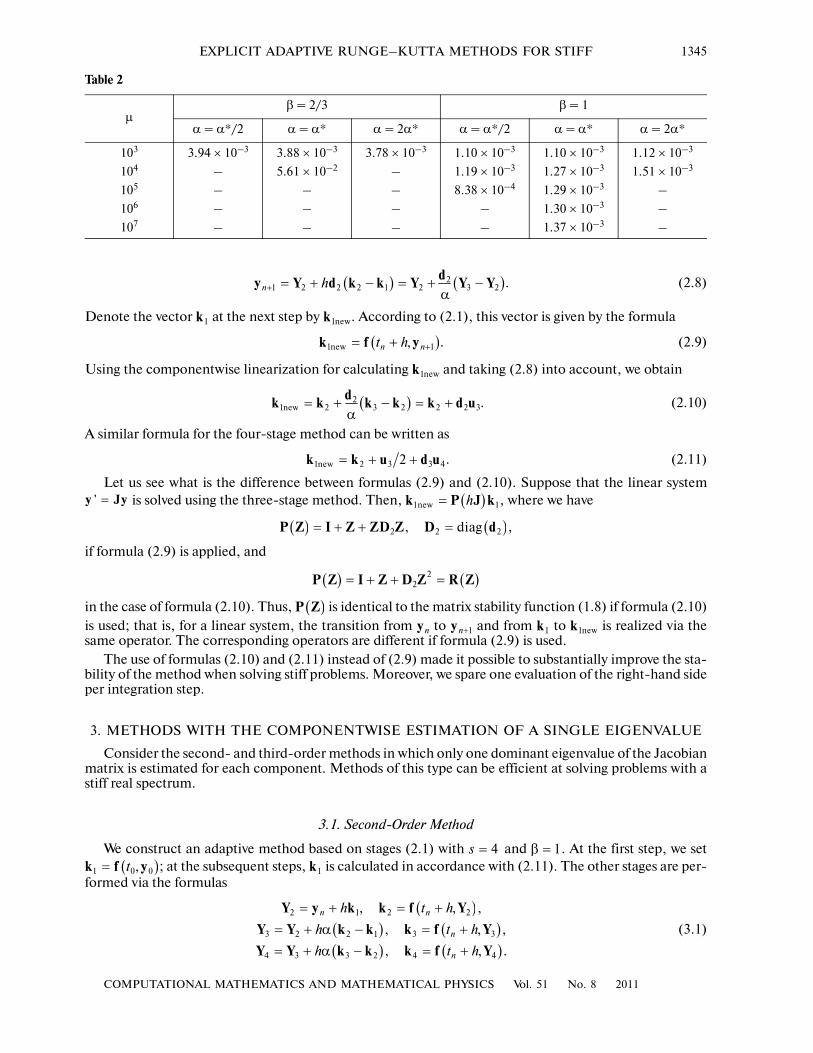
We demonstrate how the choice of α and β affects the accuracy and stability of the numerical solutionusing the problem
(2.7)
It has the eigenvalues and the solution , . For large μ, thisproblem is stiff and heavily nonlinear. The expected optimal for this problem is
.
In Table 2, we present the Euclidean norm of the error obtained at the endpoint for , , andvarious μ, α, and β (a dash indicates the divergence of the numerical solution). It is apparent from theseresults that and are indeed optimal values. Similar results were obtained for .
2.3. Stabilization of the First Stage
The stability of a method can be improved by using a different way of calculating . If , then theformula for one integration step of the three�stage method takes the form
( ) ( ) ( )
( ) ( ) ( )
− −
− −
⎡ ⎤ϕ + − = − β + − β + ϕ⎣ ⎦
⎡ ⎤+ − β + β − β + β ϕ +⎣ ⎦
21 2
0 1 0
32 1 2 4
0
''1 2 22
'''1 3 3 .6
ht h x z z
hz z O h
2 3β =1β =
2 1h z h−
= λ x3s ≥
1β =
410 −
( ) ( ) ( )
( )
21 2 3
2 2 34
1, 1 , 1 ,
1 , .
R z R z z R z z z
R z z z z
= = + β = + β + αβ
= + β + αβ + α β …
1z 11z −
α = −
11 z+ β
1z 1z
1z old
( )1
1 h h−
− z old old max 1 2α =
maxα = α
( ) ( )
( ) ( )
2 21 2 1 1 2 1
2 22 1 2 1 2 2
' 1 , 0
' 1 , 0 1, 0 2 .
y y y y y y
y y y y y y t
= − μ + − =
= − − μ + − = ≤ ≤ π
0,
21,2 1λ = −μ μ −∓ 1( ) sin( )y t t= 2( ) cos( )y t t=
α
( ) ( )1
1 21* 1h h
−
− ⎡ ⎤α = − λ = μ + μ −⎣ ⎦
3s = 2 400h = π
α = α* 1β = 4s =
1k 1β =
COMPUTATIONAL MATHEMATICS AND MATHEMATICAL PHYSICS Vol. 51 No. 8 2011
EXPLICIT ADAPTIVE RUNGE–KUTTA METHODS FOR STIFF 1345
. (2.8)
Denote the vector at the next step by . According to (2.1), this vector is given by the formula
. (2.9)
Using the componentwise linearization for calculating and taking (2.8) into account, we obtain
. (2.10)
A similar formula for the four�stage method can be written as
. (2.11)
Let us see what is the difference between formulas (2.9) and (2.10). Suppose that the linear system is solved using the three�stage method. Then, , where we have
, ,
if formula (2.9) is applied, and
in the case of formula (2.10). Thus, is identical to the matrix stability function (1.8) if formula (2.10)is used; that is, for a linear system, the transition from to and from to is realized via thesame operator. The corresponding operators are different if formula (2.9) is used.
The use of formulas (2.10) and (2.11) instead of (2.9) made it possible to substantially improve the sta�bility of the method when solving stiff problems. Moreover, we spare one evaluation of the right�hand sideper integration step.
3. METHODS WITH THE COMPONENTWISE ESTIMATION OF A SINGLE EIGENVALUE
Consider the second� and third�order methods in which only one dominant eigenvalue of the Jacobianmatrix is estimated for each component. Methods of this type can be efficient at solving problems with astiff real spectrum.
3.1. Second�Order Method
We construct an adaptive method based on stages (2.1) with and . At the first step, we set; at the subsequent steps, is calculated in accordance with (2.11). The other stages are per�
formed via the formulas
(3.1)
( ) ( )21 2 2 2 1 2 3 2n h
+= + − = + −
α
dy Y d k k Y Y Y
1k 1k new
( )1 1,n nt h+
= +k f ynew
1k new
( )21 2 3 2 2 2 3= + − = +
α
dk k k k k d unew
1 2 3 3 42= + +k k u d unew
' =y Jy ( )1 1h=k P J knew
( ) 2= + +P Z I Z ZD Z ( )2=D d2 diag
( ) ( )2
2= + + =P Z I Z D Z R Z
( )P Z
ny 1n+y 1k 1k new
4s = 1β =
( )1 0 0,t=k f y 1k
( )
( ) ( )
( ) ( )
2 1 2 2
3 2 2 1 3 3
4 3 3 2 4 4
, , ,
, , ,
, , .
n n
n
n
h t h
h t h
h t h
= + = +
= + α − = +
= + α − = +
Y y k k f Y
Y Y k k k f Y
Y Y k k k f Y
Table 2
μβ = 2/3 β = 1
α = α*/2 α = α* α = 2α* α = α*/2 α = α* α = 2α*
103 3.94 × 10⁻³ 3.88 × 10⁻³ 3.78 × 10⁻³ 1.10 × 10⁻³ 1.10 × 10⁻³ 1.12 × 10⁻³
104 – 5.61 × 10⁻² – 1.19 × 10⁻³ 1.27 × 10⁻³ 1.51 × 10⁻³
105 – – – 8.38 × 10⁻⁴ 1.29 × 10⁻³ –
106 – – – – 1.30 × 10⁻³ –
107 – – – – 1.37 × 10⁻³ –
1346
COMPUTATIONAL MATHEMATICS AND MATHEMATICAL PHYSICS Vol. 51 No. 8 2011
SKVORTSOV
Then, we calculate
. (3.2)
The scalar stability function is chosen in form (1.11). The ith component of the vector is calculated inaccordance with (1.7). If , we set ; otherwise,
This arrangement of calculations eliminates the possibility of overflows or divisions by zero. The integra�tion step is governed by the formula
.
If the integration is performed with an automatic step size control, then a nested formula is used forcalculating the value , which yields the norm of the vector as an error estimate. We choose
the nested formula , where the components of the vector are determined by (1.7) and
the scalar stability function of the nested method is used. The requirements for are the same as
for . In addition, we require that and differ for with small moduli and for positive z (oth�erwise, the error control for nonstiff and unstable components gets worse). Setting
= , we obtain
3.2. Third�Order Method
The design of adaptive methods that actually have the third order when applied to stiff problems ishampered by the low stage order and the instability of the inner stages of explicit Runge–Kutta schemes.It is practically impossible to define the stages so that all of them are stable. However, this stability require�ment is not mandatory; it suffices to restrict the growth of the inner stability functions, as was done in thesecond�order method by choosing an appropriate . However, this is not easy to do for the methods oforder three or higher.
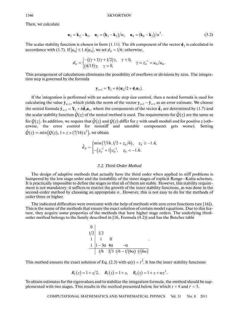
The indicated difficulties were overcome with the help of methods with zero error functions (see [16]).This is the name of the methods that ensure the exact solution of certain model equations. Due to this fea�ture, they acquire some properties of the methods that have higher stage orders. The underlying third�order method belongs to the family described in [16, Formula (4.2)] and has the Butcher table
.
This method ensures the exact solution of Eq. (2.3) with . It has the inner stability functions
.
To obtain estimates for the eigenvalues and to stabilize the integration formula, the method should be sup�plemented with two stages. This results in the method presented below, for which and .
( ) ( )2
2 2 1 3 3 2 4 4 3, ,= − = − α = − αu k k u k k u k k
3d
4 31.6i iu u≤ 3 1 6id =
( )( )
( )1
3 1 3 4
1 1 2 0.
4 15 0,i i i id z u u−
− γ + γ + γ γ <⎧= γ = =⎨
γ γ >⎩
, ,
,
( )1 2 2 3 32n h+= + +y Y u d u
1ˆ n+y 1 1ˆn n+ +−y y
1 2 2 2ˆˆ n h
+= +y Y d u 2d̂
( )Q̂ z ( )Q̂ z
( )Q z ( )Q̂ z ( )Q z z
( )Q̂ z ( ) ( )( )2min , 1 7 16Q z z z+ +
( )
( )1 1
2 1 11 1 1
min 7 16,1 2 6 , 1.6,ˆ
1 , 1.6.
i i
ii i i
z zd
z z z− −
+ ≥ −⎧⎪= ⎨
− + < −⎪⎩
α
( ) ( )
0
1 2 1 2
1 1 0
1 1 3 4
1 6 2 3 1 6 1 6 1 6
− α α −α
− α α
( ) 2t tϕ =
( ) ( ) ( )2
2 3 41 2, 1 , 1R z z R z z R z z z= + = + = + + α
6s = 5r =
COMPUTATIONAL MATHEMATICS AND MATHEMATICAL PHYSICS Vol. 51 No. 8 2011
EXPLICIT ADAPTIVE RUNGE–KUTTA METHODS FOR STIFF 1347
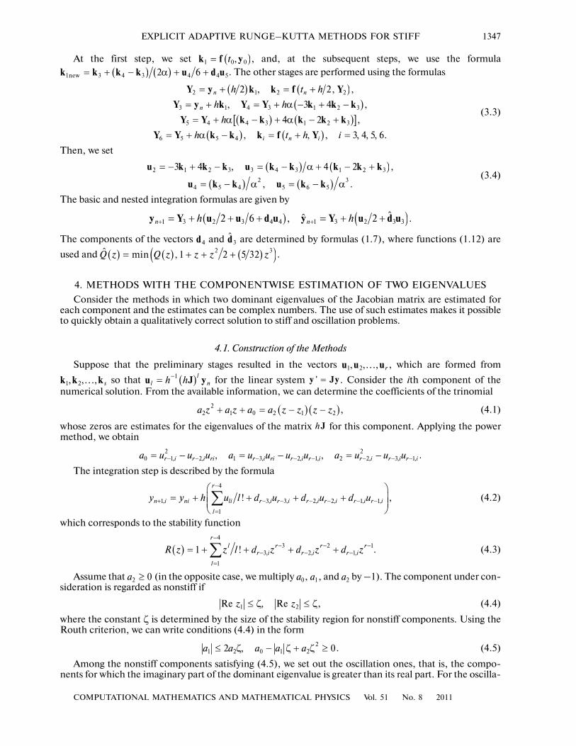
At the first step, we set , and, at the subsequent steps, we use the formula. The other stages are performed using the formulas
(3.3)
Then, we set
(3.4)
The basic and nested integration formulas are given by
The components of the vectors and are determined by formulas (1.7), where functions (1.12) are
used and .
4. METHODS WITH THE COMPONENTWISE ESTIMATION OF TWO EIGENVALUES
Consider the methods in which two dominant eigenvalues of the Jacobian matrix are estimated foreach component and the estimates can be complex numbers. The use of such estimates makes it possibleto quickly obtain a qualitatively correct solution to stiff and oscillation problems.
4.1. Construction of the Methods
Suppose that the preliminary stages resulted in the vectors , which are formed from
so that for the linear system . Consider the ith component of thenumerical solution. From the available information, we can determine the coefficients of the trinomial
, (4.1)
whose zeros are estimates for the eigenvalues of the matrix for this component. Applying the powermethod, we obtain
.
The integration step is described by the formula
, (4.2)
which corresponds to the stability function
. (4.3)
Assume that (in the opposite case, we multiply , , and by –1). The component under con�sideration is regarded as nonstiff if
, (4.4)
where the constant ζ is determined by the size of the stability region for nonstiff components. Using theRouth criterion, we can write conditions (4.4) in the form
. (4.5)
Among the nonstiff components satisfying (4.5), we set out the oscillation ones, that is, the compo�nents for which the imaginary part of the dominant eigenvalue is greater than its real part. For the oscilla�
( )1 0 0,t=k f y( ) ( )3 4 3 4 4 52 6= + − α + +k k k k u d u1new
( ) ( )
( )
( ) ( )[ ]
( ) ( )
2 1 2 2
3 1 4 3 1 2 3
5 4 4 3 1 2 3
6 5 5 4
2 , 2, ,
, 3 4 ,
4 2 ,
, , , 3, 4, 5, 6.
n n
n
i n i
h t h
h h
h
h t h i
= + = +
= + = + α − + −
= + α − + α − +
= + α − = + =
Y y k k f Y
Y y k Y Y k k k
Y Y k k k k k
Y Y k k k f Y
( ) ( )
( ) ( )
2 1 2 3 3 4 3 1 2 3
2 34 5 4 5 6 5
3 4 , 4 2 ,
, .
= − + − = − α + − +
= − α = − α
u k k k u k k k k k
u k k u k k
( ) ( )1 3 2 3 4 4 1 3 2 3 3ˆˆ2 6 , 2 .n nh h
+ += + + + = + +y Y u u d u y Y u d u
4d 3d̂
( ) ( ) ( )( )2 3ˆ min , 1 2 5 32Q z Q z z z z= + + +
1 2, , , ru u u…
1 2, , , sk k k… ( )1 ll nh h−
=u J y ' =y Jy
( ) ( )2
2 1 0 2 1 2a z a z a a z z z z+ + = − −
hJ
2 20 1, 2, 1 3, 2, 1, 2 2, 3, 1,, ,r i r i ri r i ri r i r i r i r i r ia u u u a u u u u a u u u
− − − − − − − −
= − = − = −
4
1, 3, 3, 2, 2, 1, 1,
1
!r
n i ni li r i r i r i r i r i r i
l
y y h u l d u d u d u−
+ − − − − − −
=
⎛ ⎞= + + + +⎜ ⎟
⎜ ⎟⎝ ⎠∑
( )4
3 2 13, 2, 1,
1
1 !r
l r r rr i r i r i
l
R z z l d z d z d z−
− − −
− − −
=
= + + + +∑
2 0a ≥ 0a 1a 2a
1 2Re , Rez z≤ ζ ≤ ζ
21 2 0 1 22 , 0a a a a a≤ ζ − ζ + ζ ≥
1348
COMPUTATIONAL MATHEMATICS AND MATHEMATICAL PHYSICS Vol. 51 No. 8 2011
SKVORTSOV
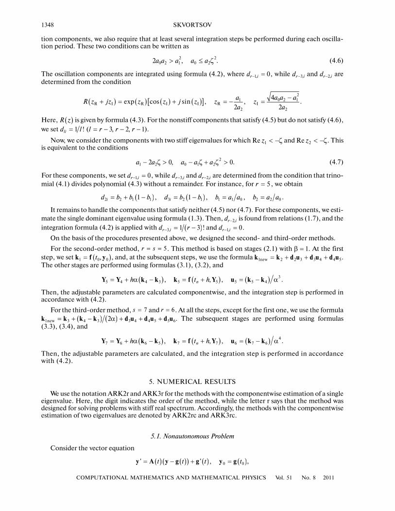
tion components, we also require that at least several integration steps be performed during each oscilla�tion period. These two conditions can be written as
. (4.6)
The oscillation components are integrated using formula (4.2), where , while and aredetermined from the condition
.
Here, is given by formula (4.3). For the nonstiff components that satisfy (4.5) but do not satisfy (4.6),we set ( ).
Now, we consider the components with two stiff eigenvalues for which and . Thisis equivalent to the conditions
. (4.7)
For these components, we set , while and are determined from the condition that trino�mial (4.1) divides polynomial (4.3) without a remainder. For instance, for , we obtain
.
It remains to handle the components that satisfy neither (4.5) nor (4.7). For these components, we esti�mate the single dominant eigenvalue using formula (1.3). Then, is found from relations (1.7), and theintegration formula (4.2) is applied with and .
On the basis of the procedures presented above, we designed the second� and third�order methods.
For the second�order method, . This method is based on stages (2.1) with . At the firststep, we set , and, at the subsequent steps, we use the formula .The other stages are performed using formulas (3.1), (3.2), and
.
Then, the adjustable parameters are calculated componentwise, and the integration step is performed inaccordance with (4.2).
For the third�order method, and . At all the steps, except for the first one, we use the formula. The subsequent stages are performed using formulas
(3.3), (3.4), and
.
Then, the adjustable parameters are calculated, and the integration step is performed in accordancewith (4.2).
5. NUMERICAL RESULTS
We use the notation ARK2r and ARK3r for the methods with the componentwise estimation of a singleeigenvalue. Here, the digit indicates the order of the method, while the letter r says that the method wasdesigned for solving problems with stiff real spectrum. Accordingly, the methods with the componentwiseestimation of two eigenvalues are denoted by ARK2rc and ARK3rc.
5.1. Nonautonomous Problem
Consider the vector equation
,
2 20 2 1 0 22 ,a a a a a> ≤ ζ
1, 0r id−
= 3,r id− 2,r id
−
( ) ( ) ( ) ( )[ ]2
0 2 11
2 2
4exp cos sin , ,
2 2
a a aaR z jz z z j z z z
a a
−+ = + = − =R I R I I R I
( )R z1 !lid l= 3, 2, 1l r r r= − − −
1Re z < −ζ 2Re z < −ζ
21 2 0 1 22 0, 0a a a a a− ζ > − ζ + ζ >
1, 0r id−
= 3,r id− 2,r id
−
5r =
( ) ( )2 2 1 1 3 2 1 1 1 0 2 2 01 , 1 , ,i id b b b d b b b a a b a a= + − = − = =
2,r id−
( )3, 1 3 !r id r−
= − 1, 0r id−
=
5r s= = 1β =
( )1 0 0,t=k f y 1 2 2 3 3 4 4 5= + + +k k d u d u d unew
( ) ( ) ( )3
5 4 4 3 5 5 5 5 4, , ,nh t h= + α − = + = − αY Y k k k f Y u k k
7s = 6r =
( ) ( )3 4 3 3 4 4 5 5 62= + − α + + +k k k k d u d u d u1new
( ) ( ) ( )4
7 6 6 5 7 7 6 7 6, , ,nh t h= + α − = + = − αY Y k k k f Y u k k
( ) ( )( ) ( ) ( )0 0' ' ,t t t t= − + =y A y g g y g
COMPUTATIONAL MATHEMATICS AND MATHEMATICAL PHYSICS Vol. 51 No. 8 2011
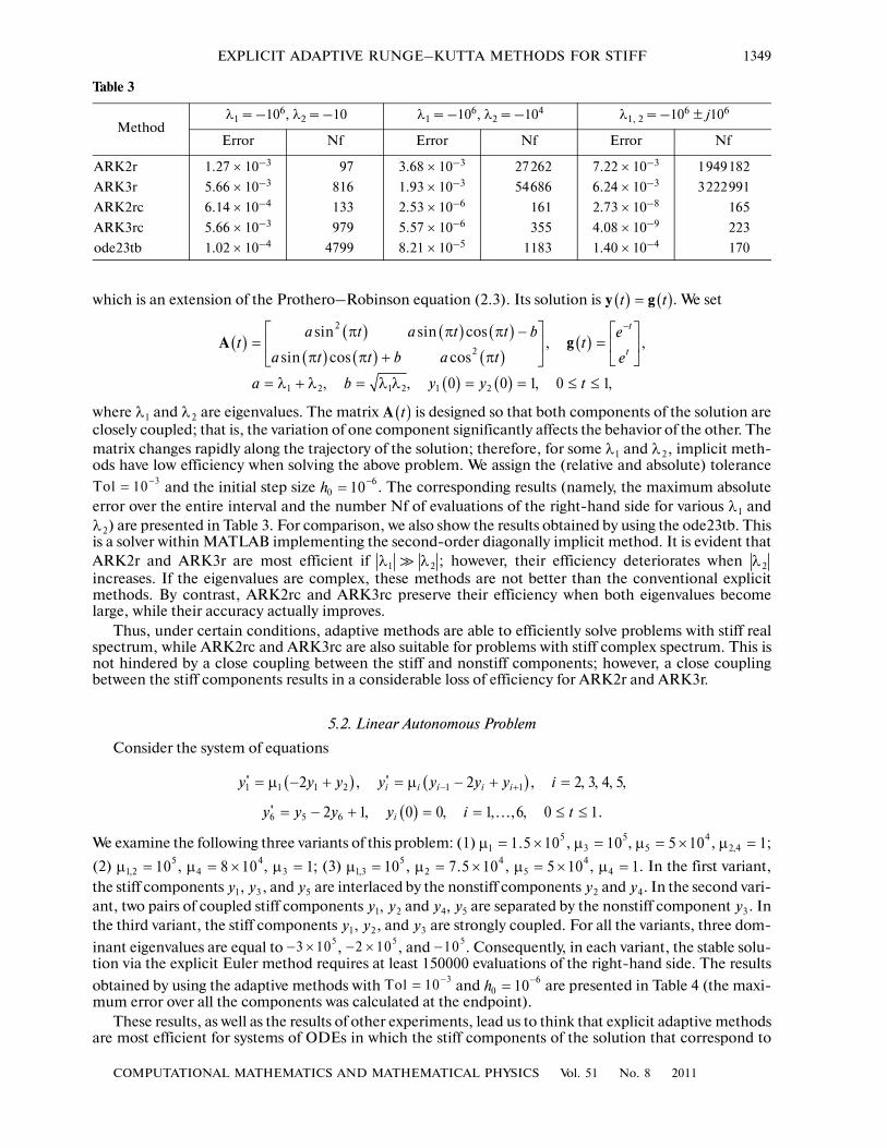
EXPLICIT ADAPTIVE RUNGE–KUTTA METHODS FOR STIFF 1349
which is an extension of the Prothero–Robinson equation (2.3). Its solution is . We set
where and are eigenvalues. The matrix is designed so that both components of the solution areclosely coupled; that is, the variation of one component significantly affects the behavior of the other. Thematrix changes rapidly along the trajectory of the solution; therefore, for some and , implicit meth�ods have low efficiency when solving the above problem. We assign the (relative and absolute) tolerance
and the initial step size . The corresponding results (namely, the maximum absoluteerror over the entire interval and the number Nf of evaluations of the right�hand side for various and
) are presented in Table 3. For comparison, we also show the results obtained by using the ode23tb. Thisis a solver within MATLAB implementing the second�order diagonally implicit method. It is evident thatARK2r and ARK3r are most efficient if ; however, their efficiency deteriorates when increases. If the eigenvalues are complex, these methods are not better than the conventional explicitmethods. By contrast, ARK2rc and ARK3rc preserve their efficiency when both eigenvalues becomelarge, while their accuracy actually improves.
Thus, under certain conditions, adaptive methods are able to efficiently solve problems with stiff realspectrum, while ARK2rc and ARK3rc are also suitable for problems with stiff complex spectrum. This isnot hindered by a close coupling between the stiff and nonstiff components; however, a close couplingbetween the stiff components results in a considerable loss of efficiency for ARK2r and ARK3r.
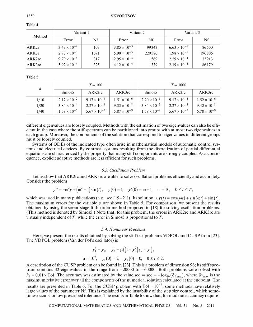
5.2. Linear Autonomous Problem
Consider the system of equations
We examine the following three variants of this problem: (1) , , , ;
(2) , , ; (3) , , , . In the first variant,the stiff components , , and are interlaced by the nonstiff components and . In the second vari�ant, two pairs of coupled stiff components and are separated by the nonstiff component . Inthe third variant, the stiff components , , and are strongly coupled. For all the variants, three dom�
inant eigenvalues are equal to , , and . Consequently, in each variant, the stable solu�tion via the explicit Euler method requires at least 150000 evaluations of the right�hand side. The results
obtained by using the adaptive methods with and are presented in Table 4 (the maxi�mum error over all the components was calculated at the endpoint).
These results, as well as the results of other experiments, lead us to think that explicit adaptive methodsare most efficient for systems of ODEs in which the stiff components of the solution that correspond to
( ) ( )t t=y g
( )( ) ( ) ( )
( ) ( ) ( )( )
( ) ( )
2
2
1 2 1 2 1 2
sin sin cos, ,
sin cos cos
, , 0 0 1, 0 1,
t
t
a t a t t b et t
a t t b a t e
a b y y t
−⎡ ⎤ ⎡ ⎤π π π −= =⎢ ⎥ ⎢ ⎥
π π + π ⎣ ⎦⎣ ⎦
= λ + λ = λ λ = = ≤ ≤
A g
1λ 2λ ( )tA
1λ 2λ
310−
=Tol 60 10h −
=
1λ
2λ
1 2λ λ� 2λ
( ) ( )
( )
1 1 1 2 1 1
6 5 6
' '2 , 2 , 2, 3, 4, 5,
' 2 1, 0 0, 1, ,6, 0 1.
i i i i i
i
y y y y y y y i
y y y y i t
− +
= μ − + = μ − + =
= − + = = ≤ ≤…
51 1.5 10µ = ×
53 10µ =
45 5 10µ = × 2,4 1µ =
51,2 10µ =
44 8 10µ = × 3 1µ =
51,3 10µ =
42 7.5 10µ = ×
45 5 10µ = × 4 1µ =
1y 3y 5y 2y 4y
1 2,y y 4 5,y y 3y
1y 2y 3y53 10− ×
52 10− ×
510−
310−
=Tol 60 10h −
=
Table 3
Methodλ1 = –106, λ2 = –10 λ1 = –106, λ2 = –104
λ1, 2 = –106 ± j106
Error Nf Error Nf Error Nf
ARK2r 1.27 × 10⁻³ 97 3.68 × 10⁻³ 27262 7.22 × 10⁻³ 1949182
ARK3r 5.66 × 10⁻³ 816 1.93 × 10⁻³ 54686 6.24 × 10⁻³ 3222991
ARK2rc 6.14 × 10⁻⁴ 133 2.53 × 10⁻⁶ 161 2.73 × 10⁻⁸ 165
ARK3rc 5.66 × 10⁻³ 979 5.57 × 10⁻⁶ 355 4.08 × 10⁻⁹ 223
ode23tb 1.02 × 10⁻⁴ 4799 8.21 × 10⁻⁵ 1183 1.40 × 10⁻⁴ 170
1350
COMPUTATIONAL MATHEMATICS AND MATHEMATICAL PHYSICS Vol. 51 No. 8 2011
SKVORTSOV
different eigenvalues are loosely coupled. Methods with the estimation of two eigenvalues can also be effi�cient in the case where the stiff spectrum can be partitioned into groups with at most two eigenvalues ineach group. Moreover, the components of the solution that correspond to eigenvalues in different groupsmust be loosely coupled.
Systems of ODEs of the indicated type often arise in mathematical models of automatic control sys�tems and electrical devices. By contrast, systems resulting from the discretization of partial differentialequations are characterized by the property that many stiff components are strongly coupled. As a conse�quence, explicit adaptive methods are less efficient for such problems.
5.3. Oscillation Problem
Let us show that ARK2rc and ARK3rc are able to solve oscillation problems efficiently and accurately.Consider the problem
,
which was used in many publications (e.g., see [19–21]). Its solution is .The maximum errors for the variable are shown in Table 5. For comparison, we present the resultsobtained by using the seven�stage fifth�order method proposed in [18] for solving oscillation problems.(This method is denoted by Simos5.) Note that, for this problem, the errors in ARK2rc and ARK3rc arevirtually independent of , while the error in Simos5 is proportional to .
5.4. Nonlinear Problems
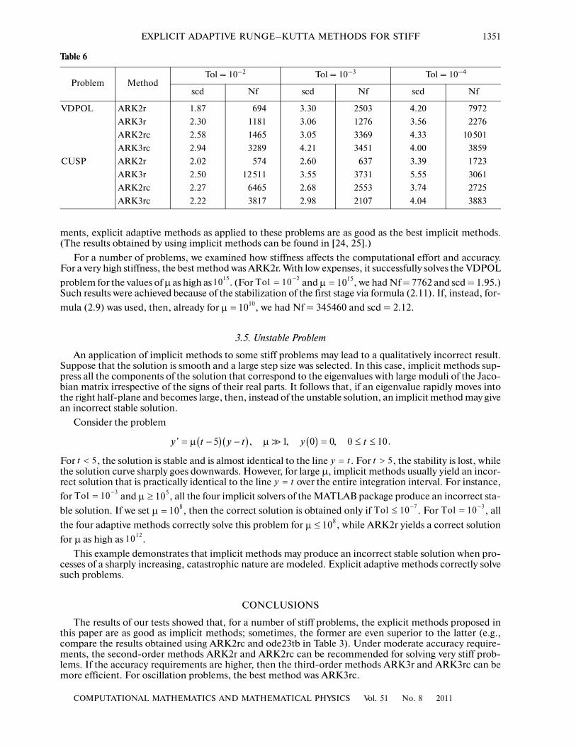
Here, we present the results obtained by solving the stiff test problems VDPOL and CUSP from [23].The VDPOL problem (Van der Pol’s oscillator) is
A description of the CUSP problem can be found in [23]. This is a problem of dimension 96; its stiff spec�trum contains 32 eigenvalues in the range from –20000 to –60000. Both problems were solved with
. The accuracy was estimated by the value scd = , where is themaximum relative error over all the components of the numerical solution calculated at the endpoint. The
results are presented in Table 6. For the CUSP problem with , some methods have relativelylarge values of the parameter Nf. This is explained by the instability of the step size control, which some�times occurs for low prescribed tolerance. The results in Table 6 show that, for moderate accuracy require�
( ) ( ) ( ) ( )2 2'' 1 sin , 0 1, ' 0 1, 10, 0y y t y y t T= −ω + ω − = = ω+ ω = ≤ ≤
( ) ( ) ( ) ( )cos sin siny t t t t= ω + ω +
y
T T
( )( )( ) ( )
21 2 2 1 2 1
61 2
' ', 1 ,
10 , 0 2, 0 0, 0 2.
y y y y y y
y y t
= = μ − −
μ = = = ≤ ≤
0 0.01h = × Tol ( )10 maxlog y= − δscd maxyδ
210−
=Tol
Table 4
MethodVariant 1 Variant 2 Variant 3
Error Nf Error Nf Error Nf
ARK2r 3.43 × 10⁻⁴ 103 3.85 × 10⁻⁵ 99343 6.63 × 10⁻⁶ 86500
ARK3r 2.73 × 10⁻³ 1671 5.90 × 10⁻⁵ 220586 1.98 × 10⁻⁵ 196806
ARK2rc 9.79 × 10⁻⁴ 317 2.95 × 10⁻³ 569 2.29 × 10⁻⁴ 23213
ARK3rc 5.92 × 10⁻⁴ 325 4.12 × 10⁻⁴ 379 2.19 × 10⁻⁴ 86179
Table 5
hT = 100 T = 1000
Simos5 ARK2rc ARK3rc Simos5 ARK2rc ARK3rc
1/10 2.17 × 10⁻² 9.17 × 10⁻⁴ 1.51 × 10⁻⁶ 2.20 × 10⁻¹ 9.17 × 10⁻⁴ 1.52 × 10⁻⁶
1/20 3.84 × 10⁻⁴ 2.27 × 10⁻⁴ 9.33 × 10⁻⁸ 3.84 × 10⁻³ 2.27 × 10⁻⁴ 9.42 × 10⁻⁸
1/40 1.58 × 10⁻⁵ 5.67 × 10⁻⁵ 5.87 × 10⁻⁹ 1.58 × 10⁻⁴ 5.67 × 10⁻⁵ 6.78 × 10⁻⁹
COMPUTATIONAL MATHEMATICS AND MATHEMATICAL PHYSICS Vol. 51 No. 8 2011
EXPLICIT ADAPTIVE RUNGE–KUTTA METHODS FOR STIFF 1351
ments, explicit adaptive methods as applied to these problems are as good as the best implicit methods.(The results obtained by using implicit methods can be found in [24, 25].)
For a number of problems, we examined how stiffness affects the computational effort and accuracy.For a very high stiffness, the best method was ARK2r. With low expenses, it successfully solves the VDPOL
problem for the values of µ as high as . (For and , we had Nf = 7762 and scd = 1.95.)Such results were achieved because of the stabilization of the first stage via formula (2.11). If, instead, for�
mula (2.9) was used, then, already for , we had Nf = 345460 and scd = 2.12.
3.5. Unstable Problem
An application of implicit methods to some stiff problems may lead to a qualitatively incorrect result.Suppose that the solution is smooth and a large step size was selected. In this case, implicit methods sup�press all the components of the solution that correspond to the eigenvalues with large moduli of the Jaco�bian matrix irrespective of the signs of their real parts. It follows that, if an eigenvalue rapidly moves intothe right half�plane and becomes large, then, instead of the unstable solution, an implicit method may givean incorrect stable solution.
Consider the problem
.
For , the solution is stable and is almost identical to the line . For , the stability is lost, whilethe solution curve sharply goes downwards. However, for large µ, implicit methods usually yield an incor�rect solution that is practically identical to the line over the entire integration interval. For instance,
for and , all the four implicit solvers of the MATLAB package produce an incorrect sta�
ble solution. If we set , then the correct solution is obtained only if . For , all
the four adaptive methods correctly solve this problem for , while ARK2r yields a correct solution
for µ as high as .
This example demonstrates that implicit methods may produce an incorrect stable solution when pro�cesses of a sharply increasing, catastrophic nature are modeled. Explicit adaptive methods correctly solvesuch problems.
CONCLUSIONS
The results of our tests showed that, for a number of stiff problems, the explicit methods proposed inthis paper are as good as implicit methods; sometimes, the former are even superior to the latter (e.g.,compare the results obtained using ARK2rc and ode23tb in Table 3). Under moderate accuracy require�ments, the second�order methods ARK2r and ARK2rc can be recommended for solving very stiff prob�lems. If the accuracy requirements are higher, then the third�order methods ARK3r and ARK3rc can bemore efficient. For oscillation problems, the best method was ARK3rc.
1510 210−
=Tol 1510µ =
1010µ =
( ) ( ) ( )' 5 , 1, 0 0, 0 10y t y t y t= μ − − μ = ≤ ≤�
5t < y t= 5t >
y t=
310−
=Tol 510μ ≥
810μ =710−
≤Tol 310−
=Tol810μ ≤
1210
Table 6
Problem MethodTol = 10–2 Tol = 10–3 Tol = 10–4
scd Nf scd Nf scd Nf
VDPOL ARK2r 1.87 694 3.30 2503 4.20 7972
ARK3r 2.30 1181 3.06 1276 3.56 2276
ARK2rc 2.58 1465 3.05 3369 4.33 10501
ARK3rc 2.94 3289 4.21 3451 4.00 3859
CUSP ARK2r 2.02 574 2.60 637 3.39 1723
ARK3r 2.50 12511 3.55 3731 5.55 3061
ARK2rc 2.27 6465 2.68 2553 3.74 2725
ARK3rc 2.22 3817 2.98 2107 4.04 3883
1352
COMPUTATIONAL MATHEMATICS AND MATHEMATICAL PHYSICS Vol. 51 No. 8 2011
SKVORTSOV
REFERENCES
1. L. M. Skvortsov, “Explicit Multistep Method for the Numerical Solution of Stiff Differential Equations,” Com�put. Math. Math. Phys. 47, 915–923 (2007).
2. M. E. Fowler and R. M. Warten, “A Numerical Integration Technique for Ordinary Differential Equations withWidely Separated Eigenvalues,” IBM J. Research Development 11 (5), 537–543 (1967).
3. S. O. Fatunla, “Numerical Integrators for Stiff and Highly Oscillatory Differential Equations,” Math. Comput.34 (150), 373–390 (1980).
4. V. V. Bobkov, “A Technique for the Construction of Methods for the Numerical Solution of Differential Equa�tions,” Differ. Uravn. Ikh Primen. 19 (7), 1115–1122 (1983).
5. A. N. Zavorin, “Application of Nonlinear Methods for the Calculation of Transient Processes in Electric Cir�cuits,” Izv. Vyssh. Uchebn. Zaved., Radioelektronika 26 (3), 35–41 (1983).
6. A. N. Saworin, “Über die Effektivitat Einiger Nichtlinearer Verfahren bei der Numerischen Behandlung SteiferDifferentialgleichungssysteme,” Numer. Math. 40, 169–177 (1982).
7. S. S. Ashour and O. T. Hanna, “Explicit Exponential Method for the Integration of Stiff Ordinary DifferentialEquations,” J. of Guidance, Control and Dynamics 14 (6), 1234–1239 (1991).
8. J. D. Lambert, “Nonlinear Methods for Stiff Systems of Ordinary Differential Equations,” Lect. Notes Math.363, 75–88 (1974).
9. A. Wambecq, “Rational Runge�Kutta Methods for Solving Systems of Ordinary Differential Equations,” Com�puting 20 (4), 333–342 (1978).
10. V. V. Bobkov, “New Explicit A�Stable Methods for the Numerical Solution of Differential Equations,” Differ.Uravn. 14 (12), 2249–2251 (1978).
11. X. Y. Wu and J. L. Xia, “Two Low Accuracy Methods for Stiff Systems,” Appl. Math. Comput. 123 (2), 141–153 (2001).
12. H. Ramos, “A Non�Standard Explicit Integration Scheme for Initial�Value Problems,” Appl. Math. Comput.189 (1), 710–718 (2007).
13. L. M. Skvortsov, “Adaptive Methods for the Digital Modeling of Dynamical Systems,” Izv. Ross. Akad. Nauk,Teor. Sist. Upr., No. 4, 180–190 (1995).
14. L. M. Skvortsov, “Adaptivnye metody chislennogo integrirovaniya v zadachakh modelirovaniya dinamicheskikhsistem,” J. Comput. Syst. Sci. Int. 38, 573–579 (1999).
15. L. M. Skvortsov, “Explicit Adaptive Methods for the Numerical Solution of Stiff Systems,” Matem. Modelir. 12(12), 97–107 (2000).
16. L. M. Skvortsov, “Explicit Runge–Kutta Methods for Moderately Stiff Problems,” Comput. Math. Math. Phys.45, 1939–1951 (2005).
17. V. I. Lebedev, “How to Solve Stiff Systems of Differential Equations Using Explicit Methods,” in Vychislitel’nyeprotsessy i sistemy (Nauka, Moscow, 1991), No. 8, pp. 237–291 [in Russian].
18. T. E. Simos, “A Modified Runge�Kutta Method for the Numerical Solution of ODE’S with Oscillation Solu�tions,” Appl. Math. Lett. 9 (6), 61–66 (1996).
19. J. M. Franco, “Runge�Kutta Methods Adapted to the Numerical Integration of Oscillatory Problems,” Appl.Numer. Math. 50, 427–443 (2004).
20. Y. Fang, Y. Song, and X. Wu, “New Embedded Pairs of Explicit Runge�Kutta Methods with FSAL PropertiesAdapted to the Numerical Integration of Oscillatory Problems,” Phys. Lett. A 372, 6551–6559 (2008).
21. A. A. Kosti, Z. A. Anastassi, and T. E. Simos, “An Optimized Explicit Runge�Kutta Method with IncreasedPhase�Lag Order for the Numerical Solution of the Schrodinger Equation and Related Problems,” J. Math.Chem. 47 (1), 315–330 (2010).
22. A. Prothero and A. Robinson, “On the Stability and Accuracy of One�Step Methods for Solving Stiff Systemsof Ordinary Differential Equations,” Math. Comput. 28 (1), 145–162 (1974).
23. E. Hairer and G. Wanner, Solving Ordinary Differential Equations, Vol. 2: Stiff and Differential�Algebraic Prob�lems (Springer, Berlin, 1987–1991; Mir, Moscow, 1999).
24. F. Mazzia and C. Magherini, “Test Set for Initial Value Problem Solvers,” Release, 4 (2008); http://pitag�ora.dm.uniba.it/~testset/reprt/testset.pdf.
25. http://web.math.unifi.it/users/brugnano/BiM/BiMD/index_BiMD.htm.


