Embed Size (px)
Citation preview
BIT Numerical Mathematics 43: 21–39, 2003.© 2003 Kluwer Academic Publishers. Printed in The Netherlands
21
PARTITIONED RUNGE–KUTTA METHODS INLIE-GROUP SETTING∗
KENTH ENG؆
Department of Informatics, University of Bergen, P.O. Box 7800
N-5020 Bergen, Norway. email: [email protected]
Abstract.
We introduce partitioned Runge–Kutta (PRK) methods as geometric integratorsin the Runge–Kutta–Munthe-Kaas (RKMK) method hierarchy. This is done by firstnoticing that tangent and cotangent bundles are the natural domains for the differentialequations to be solved. Next, we equip the (co)tangent bundle of a Lie group with agroup structure and treat it as a Lie group. The structure of the differential equationson the (co)tangent-bundle Lie group is such that partitioned versions of the RKMKmethods are naturally introduced. Numerical examples are included to illustrate thenew methods.
AMS subject classification: 65L06, 34C40
Key words: Partitioned Runge–Kutta method, RKMK method, geometric integra-tion, tangent bundle of Lie group, semidirect product, differential equations on mani-folds
1 Introduction.
The Runge–Kutta–Munthe-Kaas (RKMK) method was introduced in [17] tosolve differential equations on homogeneous spaces, that is, differential equationsin the form of an infinitesimal generator of the Lie-group action. The idea behindthe approach is simple and is essentially to solve a differential equation in theLie algebra of the Lie group, instead of the original differential equation on thehomogeneous space. The differential equation in the Lie algebra evolves in avector space and any classical Runge–Kutta (RK) method can be used to solveit. Coordinatizing the Lie group with different local coordinates corresponds todifferent differential equations on the Lie algebra, as shown in [5]. Hence, thechoice of coordinates in the RKMK method is a variable to be considered whensolving differential equations on a homogeneous space.Classical partitioned Runge–Kutta (PRK) methods can of course be intro-
duced in the RKMK method in a straight forward and naive way. Just apply aPRK method directly to the differential equation in the Lie algebra instead of
∗Received September 2000. Revised October 2002. Communicated by Christian Lubich.†This work was sponsored by the Norwegian Research Council under contract no.
113492/420.1New affiliation: Telenor R&D, Snarøyveien 30, 1331 Fornebu, Norway. New email address:
22 KENTH ENGØ
the RK method. We believe, however, that this approach is not the right one forgeneralizing the classical PRK methods to Lie groups. Recall that PRK methodsare used to solve systems of differential equations that naturally separate intotwo sets of equations [7]. Examples of problems in this form are Hamiltonianproblems and second order differential equations2. In the context of manifoldsthese problems generalize to Hamiltonian problems on cotangent bundles, andsprays on tangent bundles, respectively. Thus, we will in this paper consider(co)tangent bundles of Lie groups as an appropriate domain for partitioned dif-ferential equations.The present idea is to equip the (co)tangent bundle of the Lie group with a
group structure turning it into another continuous group. Doing this, we canutilize the RKMK approach directly. However, the (co)tangent bundle of a Liegroup can be represented in several different ways. In the subsequent section wewill investigate three representations, and explore some of their implications.The rest of the paper is organized as follows: In Section 2 we discuss the dif-
ferent representations of the tangent bundle of a Lie group in detail. Then thesubsequent section discusses some examples of differential equations naturallyevolving on the tangent bundle. Section 4 introduces the partitioned Runge–Kutta–Munthe-Kaas method as a generalization of the PRK method to cotan-gent bundles and tangent bundles of Lie groups. This is followed by numericalexperiments in Section 5, and the paper is concluded in Section 6.
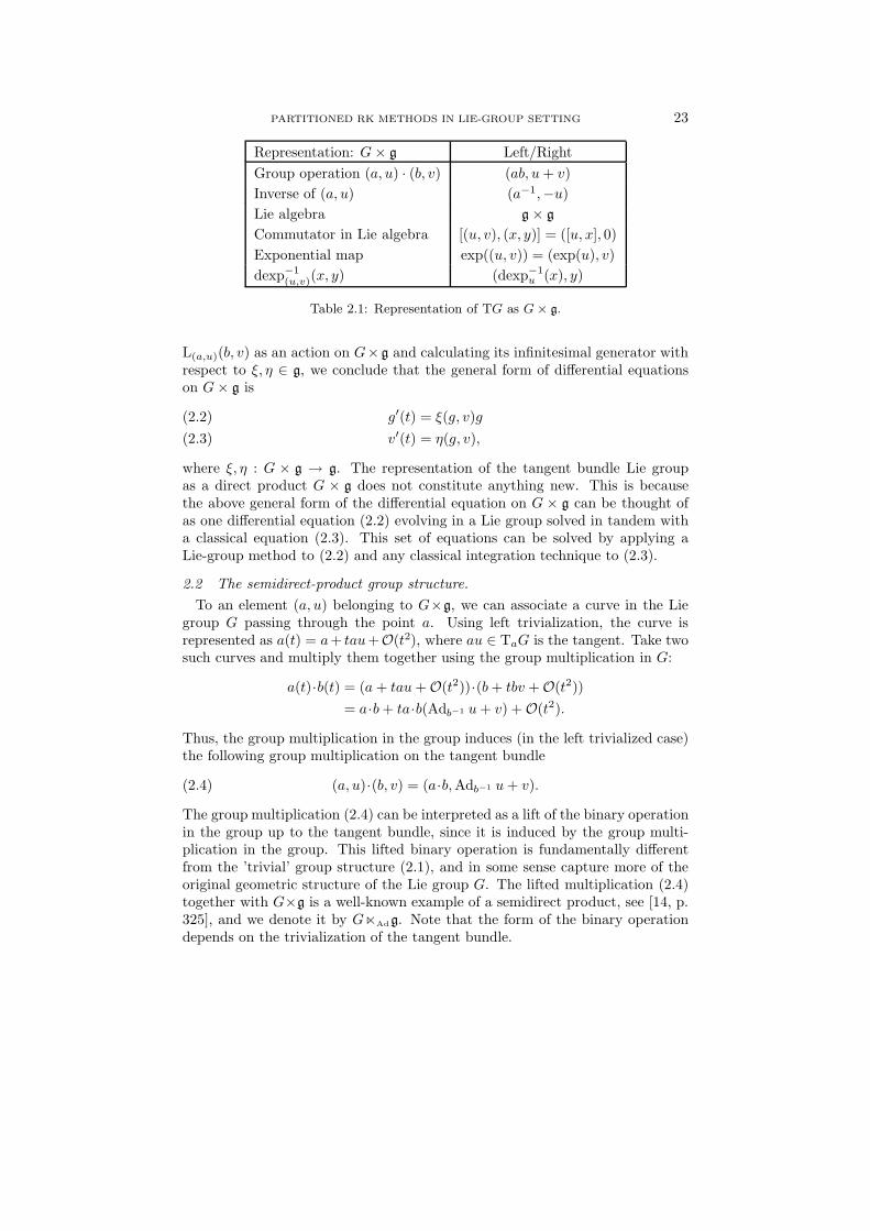
2 On representing the tangent bundle of a Lie group.First we make precise the meaning of trivialization. The term will refer to how
to translate a Lie algebra element out to the tangent space at a specific pointon the Lie group. This can be done in two ways; by either the lifted left or rightmultiplication. Left multiplication is defined as La(b) = µ(a, b) = a·b, and rightmultiplication is defined as Ra(b) = µ(b, a) = b·a, where µ is group multiplication.Hence, we will speak of left and right trivializations of the tangent bundle, andby ‘body’ and ‘space’ coordinates we understand coordinates obtained throughleft and right trivialization, respectively. See [2, p. 15] or [14] for details.
2.1 The direct-product group structure.Considered as a manifold, the tangent bundle of a Lie group is diffeomorphic
to the direct product of the Lie group with its Lie algebra; that is TG ≈ G×g.This representation implies a very simple tangent Lie-group structure; For twopairs of elements (a, u), (b, v) ∈ G×g, just choose group multiplication for thegroup elements, and vector addition for the algebra elements; i.e.
(2.1) (a, u)·(b, v) = (a·b, u+ v).
Relevant constructs for this representation of the tangent bundle of a Lie groupis summarized in Table 2.1. In this representation the left and right trivializedversions of the tangent bundle coincide. Following [5], using left multiplication
2Second order differential equations can be solved by a Runge–Kutta–Nystrom method,but this method is in fact just a partitioned Runge–Kutta method in disguise [7].
PARTITIONED RK METHODS IN LIE-GROUP SETTING 23
Representation: G× g Left/RightGroup operation (a, u) · (b, v) (ab, u+ v)Inverse of (a, u) (a−1,−u)Lie algebra g × g
Commutator in Lie algebra [(u, v), (x, y)] = ([u, x], 0)Exponential map exp((u, v)) = (exp(u), v)dexp−1
(u,v)(x, y) (dexp−1u (x), y)
Table 2.1: Representation of TG as G × g.
L(a,u)(b, v) as an action on G×g and calculating its infinitesimal generator withrespect to ξ, η ∈ g, we conclude that the general form of differential equationson G× g is
g′(t) = ξ(g, v)g(2.2)v′(t) = η(g, v),(2.3)
where ξ, η : G × g → g. The representation of the tangent bundle Lie groupas a direct product G × g does not constitute anything new. This is becausethe above general form of the differential equation on G × g can be thought ofas one differential equation (2.2) evolving in a Lie group solved in tandem witha classical equation (2.3). This set of equations can be solved by applying aLie-group method to (2.2) and any classical integration technique to (2.3).
2.2 The semidirect-product group structure.To an element (a, u) belonging to G×g, we can associate a curve in the Lie
group G passing through the point a. Using left trivialization, the curve isrepresented as a(t) = a+ tau+O(t2), where au ∈ TaG is the tangent. Take twosuch curves and multiply them together using the group multiplication in G:
a(t)·b(t) = (a+ tau+O(t2))·(b+ tbv +O(t2))= a·b+ ta·b(Adb−1 u+ v) +O(t2).
Thus, the group multiplication in the group induces (in the left trivialized case)the following group multiplication on the tangent bundle
(2.4) (a, u)·(b, v) = (a·b,Adb−1 u+ v).
The group multiplication (2.4) can be interpreted as a lift of the binary operationin the group up to the tangent bundle, since it is induced by the group multi-plication in the group. This lifted binary operation is fundamentally differentfrom the ’trivial’ group structure (2.1), and in some sense capture more of theoriginal geometric structure of the Lie group G. The lifted multiplication (2.4)together with G×g is a well-known example of a semidirect product, see [14, p.325], and we denote it by GAdg. Note that the form of the binary operationdepends on the trivialization of the tangent bundle.
24 KENTH ENGØ
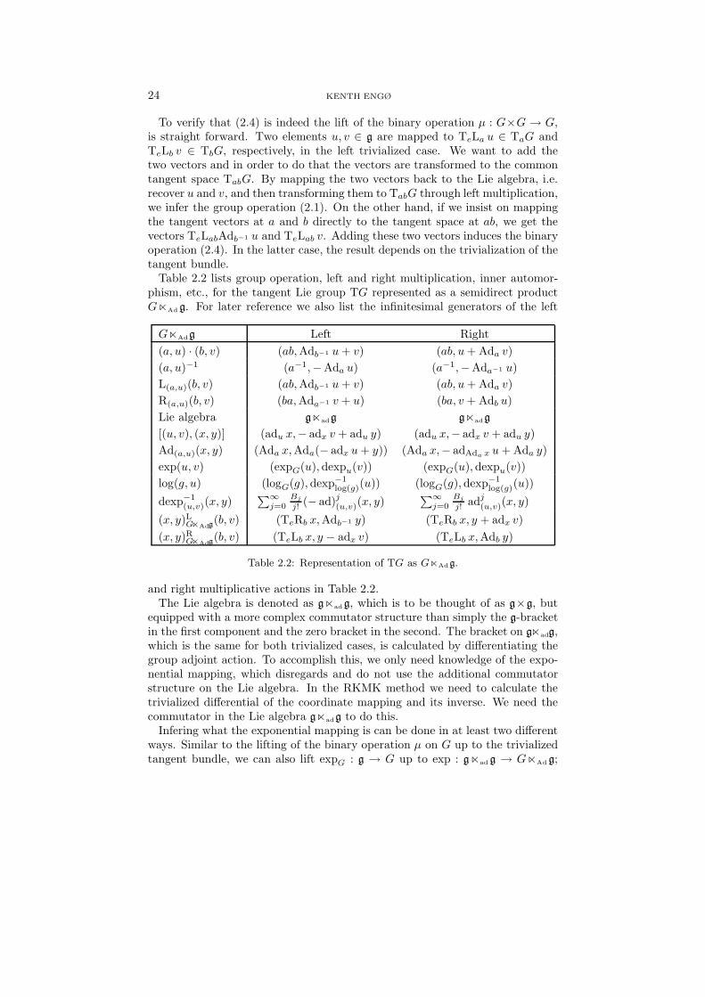
To verify that (2.4) is indeed the lift of the binary operation µ : G×G → G,is straight forward. Two elements u, v ∈ g are mapped to TeLa u ∈ TaG andTeLb v ∈ TbG, respectively, in the left trivialized case. We want to add thetwo vectors and in order to do that the vectors are transformed to the commontangent space TabG. By mapping the two vectors back to the Lie algebra, i.e.recover u and v, and then transforming them to TabG through left multiplication,we infer the group operation (2.1). On the other hand, if we insist on mappingthe tangent vectors at a and b directly to the tangent space at ab, we get thevectors TeLabAdb−1 u and TeLab v. Adding these two vectors induces the binaryoperation (2.4). In the latter case, the result depends on the trivialization of thetangent bundle.Table 2.2 lists group operation, left and right multiplication, inner automor-
phism, etc., for the tangent Lie group TG represented as a semidirect productGAd g. For later reference we also list the infinitesimal generators of the left
GAdg Left Right(a, u) · (b, v) (ab,Adb−1 u+ v) (ab, u+Ada v)(a, u)−1 (a−1,−Ada u) (a−1,−Ada−1 u)L(a,u)(b, v) (ab,Adb−1 u+ v) (ab, u+Ada v)R(a,u)(b, v) (ba,Ada−1 v + u) (ba, v + Adb u)Lie algebra gadg gadg
[(u, v), (x, y)] (adu x,− adx v + adu y) (adu x,− adx v + adu y)Ad(a,u)(x, y) (Ada x,Ada(− adx u+ y)) (Ada x,− adAda x u+Ada y)exp(u, v) (expG(u), dexpu(v)) (expG(u), dexpu(v))log(g, u) (logG(g), dexp
−1log(g)(u)) (logG(g), dexp
−1log(g)(u))
dexp−1(u,v)(x, y)
∑∞j=0
Bj
j! (− ad)j(u,v)(x, y)∑∞
j=0Bj
j! adj(u,v)(x, y)
(x, y)LGAdg(b, v) (TeRb x,Adb−1 y) (TeRb x, y + adx v)
(x, y)RGAdg(b, v) (TeLb x, y − adx v) (TeLb x,Adb y)
Table 2.2: Representation of TG as GAdg.
and right multiplicative actions in Table 2.2.The Lie algebra is denoted as gadg, which is to be thought of as g×g, but
equipped with a more complex commutator structure than simply the g-bracketin the first component and the zero bracket in the second. The bracket on gadg,which is the same for both trivialized cases, is calculated by differentiating thegroup adjoint action. To accomplish this, we only need knowledge of the expo-nential mapping, which disregards and do not use the additional commutatorstructure on the Lie algebra. In the RKMK method we need to calculate thetrivialized differential of the coordinate mapping and its inverse. We need thecommutator in the Lie algebra gadg to do this.Infering what the exponential mapping is can be done in at least two different
ways. Similar to the lifting of the binary operation µ on G up to the trivializedtangent bundle, we can also lift expG : g → G up to exp : gad g → GAd g;
PARTITIONED RK METHODS IN LIE-GROUP SETTING 25
(u, v) → (expG(u), dexpu(v)), where dexpu is the trivialized differential of expG
(different in the left and right cases). Alternatively, the same result can beobtained through solving the differential equation
σ′(t) = Xw(σ(t)) = Te Lσ(t) w,
with initial condition σ(0) = e. In the right trivialized case this ODE looks like
a′(t) = a(t)uv′(t) = Ada(v),
where (a(0), v(0)) = (e, 0), and w(t) = (a(t), v(t)).The general form of differential equations on GAdg depends on the trivializa-
tion of the tangent bundle. For a left trivialized tangent bundle, any ODE canbe phrased (matrix notation) as
g′(t) = a(g, v, t)gv′(t) = Adg(t)−1(γ(g, v, t)),
for suitable functions a, γ : G×g×R → g. For the right trivialized tangentbundle, with the same functions a and γ as above, any ODE is of the form
g′(t) = a(g, v, t)gv′(t) = ada(g,v,t) v + γ(g, v, t).
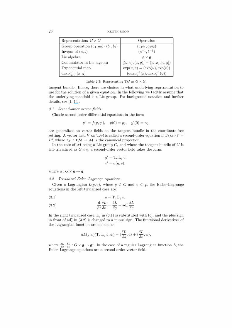
2.3 The Cartesian-product representation.In the literature on the discretization of variational principles, e.g. [18], we
find that it is convenient to represent the tangent bundle of the Lie group G asthe Cartesian product G×G. This representation of the tangent bundle mightat first sight appear awkward, since the tangent (velocity) of a group elementis now represented by another group element. But on the other hand, this isreally the same as finite differences. The benefit of this approach is that onecan construct discrete versions of the continuous Euler–Lagrange and Euler–Poincare equations that preserve discrete analogous of the geometric propertiesof the continuous equations [13].The representation of the tangent bundle of a Lie group G as a Cartesian
product G×G implies the operations listed in Table 2.3. Defining the left andright actions and other types of hybrid actions is straight forward, as findingtheir infinitesimal generators. We will see in Section 3.3 that the symmetricrigid body equations is an example where the representation of TG as G × Goccurs naturally.
3 Differential equations on the tangent bundle of a Lie group.The purpose of this section is to give a few examples of differential equations
that naturally evolve on tangent bundles. The equations will be written out intrivialized form to emphasize their partitioned structure. Note that the equa-tions are defined irrespectively of the underlying group structure modeling the
26 KENTH ENGØ
Representation: G×G OperationGroup operation (a1, a2) · (b1, b2) (a1b1, a2b2)Inverse of (a, b) (a−1, b−1)Lie algebra g × g
Commutator in Lie algebra [(u, v), (x, y)] = ([u, x], [v, y])Exponential map exp(u, v) = (exp(u), exp(v))dexp−1
(u,v)(x, y) (dexp−1u (x), dexp−1
v (y))
Table 2.3: Representing TG as G × G.
tangent bundle. Hence, there are choices in what underlying representation touse for the solution of a given equation. In the following we tacitly assume thatthe underlying manifold is a Lie group. For background notation and furtherdetails, see [1, 14].
3.1 Second-order vector fields.Classic second order differential equations in the form
y′′ = f(y, y′), y(0) = y0, y′(0) = u0,
are generalized to vector fields on the tangent bundle in the coordinate-freesetting. A vector field V on TM is called a second-order equation if TτM V =Id, where τM : TM → M is the canonical projection.In the case of M being a Lie group G, and where the tangent bundle of G is
left-trivialized as G× g, a second-order vector field takes the form:
g′ = Te Lg v,
v′ = a(g, v),
where a : G× g → g.
3.2 Trivialized Euler–Lagrange equations.Given a Lagrangian L(g, v), where g ∈ G and v ∈ g, the Euler–Lagrange
equations in the left trivialized case are:
g = Te Lg v,(3.1)ddt
δL
δv=
δL
δg+ ad∗v
δL
δv.(3.2)
In the right trivialized case, Lg in (3.1) is substituted with Rg, and the plus signin front of ad∗v in (3.2) is changed to a minus sign. The functional derivatives ofthe Lagrangian function are defined as
dL(g, v)(Te Lg u,w) = 〈δLδg
, u〉+ 〈δLδv
, w〉,
where δLδg ,
δLδv : G × g → g∗. In the case of a regular Lagrangian function L, the
Euler–Lagrange equations are a second-order vector field.
PARTITIONED RK METHODS IN LIE-GROUP SETTING 27
The unreduced rigid body equations: Choosing L(g,Ω) = 12Ω · IΩ as our
Lagrangian function, we obtain the unreduced version of the rigid body equationson the full tangent bundle TG. Furthermore, we consider left trivialization of thetangent bundle, since we want the equations represented in body coordinates,where g is the current configuration and Ω is the body angular velocity.The functional derivatives are easily checked to equal
δL
δg= 0,
δL
δΩ= Π,
where Π = IΩ is the body angular momentum. Putting this into (3.1-3.2), theunreduced rigid body equations in body coordinates are
g′(t) = Te Lg ΩΠ′(t) = ad∗ΩΠ.
Specifying G = SO(3), the equations reduce to
g′(t) = gΩΠ′(t) = Π× Ω,
which are the familiar unreduced Euler equations.
3.3 The symmetric rigid body equations.
An interesting rewriting of the rigid body equations in the case G = SO(n)give rise to a set of equivalent equations on SO(n)×SO(n) called the symmetricrigid body equations [3]. The body version of these equations are
Q′ = QΩP ′ = PΩ,
(3.3)
where Q,P ∈ SO(n), Ω = I−1M ∈ so(n), and M = QTP − PTQ is the mo-mentum. By differentiation the symmetric rigid body equations reduce to theunreduced rigid body equation on SO(n). That is,
Q′ = QΩM ′ = [M,Ω].
In [4] it is shown that a discretization of the symmetric rigid body equationscoincide with the discrete Moser–Veselov rigid body equations [15]. Integratorsderived from this approach conserve momentum and are symplectic.
4 Partitioned Runge–Kutta methods in Lie group setting.
We will now adapt the classical partitioned Runge–Kutta methods to thesetting developed in Section 2. We briefly recall the classical methods beforeintroducing the new methods.
28 KENTH ENGØ
4.1 Classical partitioned Runge–Kutta methods.
Consider a partitioned ordinary differential equation in R2n of the form
(4.1)dp
dt= f(p, q),
dq
dt= g(p, q),
where p, q ∈ Rn and f, g : R
2n → Rn. The classical partitioned Runge–Kutta
method consists of choosing the method coefficients aij , bi and aij , bi of twoRunge–Kutta methods. Use the first Runge–Kutta method to advance the so-lution of p and the second Runge–Kutta method to advance the solution of q in(4.1). This can be stated in algorithmic form as
Algorithm 4.1 (Classic r’th order partitioned Runge–Kutta met-
hod). Given the method coefficients aij , bi and aij , bi of two r’th order s-stageRunge–Kutta methods that also satisfy the necessary coupling conditions [8]. Thefollowing is an r’th order update of the solution of (4.1) from t = tn to t = tn+1:
Given pn = p(tn) and qn = q(tn).for i = 1, 2, . . . , s
ui = pn + h∑s
j=1 aijkj
vi = qn + h∑s
j=1 aij lj
ki = f(ui, vi)li = g(ui, vi)
endpn+1 = pn + h
∑si=1 biki
qn+1 = qn + h∑s
i=1 bili
Partitioned Runge–Kutta methods generalize the Runge–Kutta methods. Fur-ther, the PRKmethods show favorable features when applied to separable Hamil-tonian problems with Hamiltonian function H(p, q) = K(p) + V (q). Methodscan be constructed that are both explicit and symmetric, or both explicit andsymplectic. The celebrated Stormer–Verlet method and the symplectic Eulermethod are examples of explicit and symplectic partitioned Runge–Kutta meth-ods. A natural question to investigate is if we can construct methods in the newproposed family – to be introduced in the next section – that share the samedesirable features of the classical versions.
4.2 Partitioned Runge–Kutta–Munthe-Kaas methods.
In Section 2 we equipped the tangent bundle of the Lie group G with a groupstructure, thus, turning it into a continuous group. As we saw, the natural rep-resentation of any differential equation on the trivialized tangent bundle of a Liegroup, as a pair of two differential equations, should motivate the introductionand use of partitioned Runge–Kutta methods in the Lie group setting.Next, we apply the approach of [17] to transform the differential equation
on the Lie group TG into a differential equation in the Lie algebra Te(TG) of
PARTITIONED RK METHODS IN LIE-GROUP SETTING 29
TG. The transformed equation df−1(u,w)(ξ, η) in the Lie algebra is naturally in
partitioned form, and we apply a classical PRK method to solve this differentialequation. The situation is summarized in the following commutative diagram [5].
TTe(TG) Tf−−−−→ T(TG)
df−1(u,w)(ξ,η)
TeRf(u,w)(ξ,η)
Te(TG) −−−−→f
TG
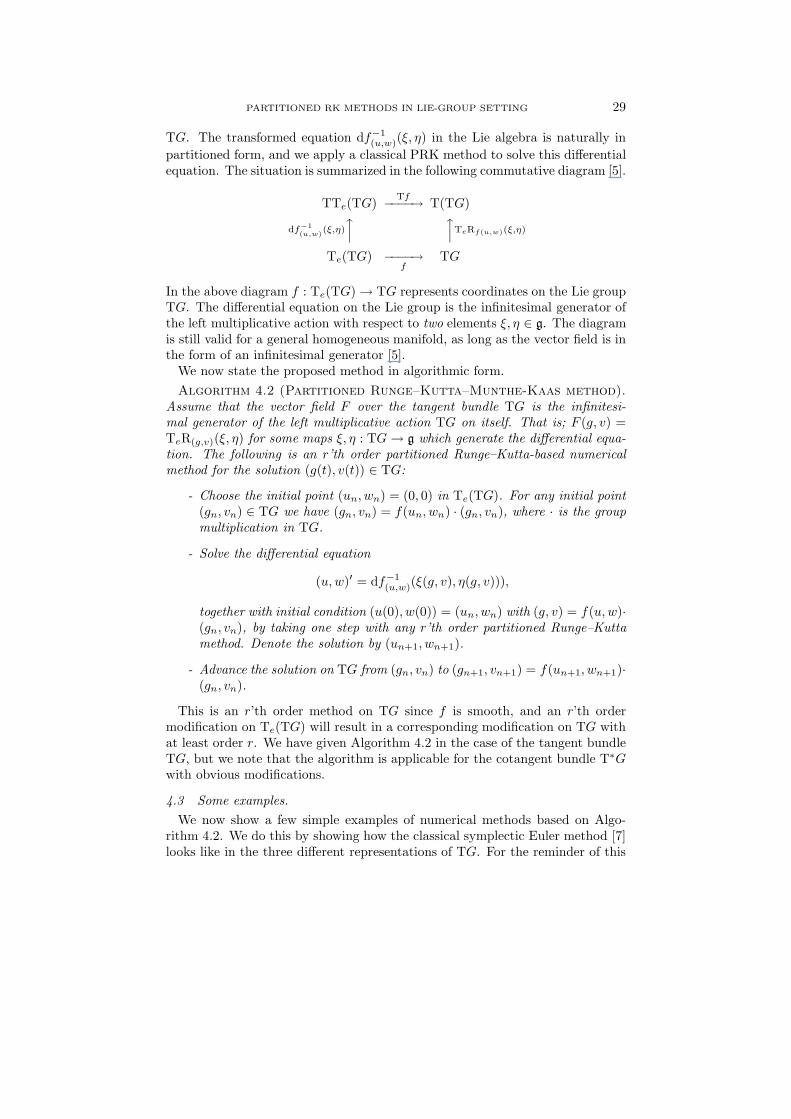
In the above diagram f : Te(TG) → TG represents coordinates on the Lie groupTG. The differential equation on the Lie group is the infinitesimal generator ofthe left multiplicative action with respect to two elements ξ, η ∈ g. The diagramis still valid for a general homogeneous manifold, as long as the vector field is inthe form of an infinitesimal generator [5].We now state the proposed method in algorithmic form.Algorithm 4.2 (Partitioned Runge–Kutta–Munthe-Kaas method).
Assume that the vector field F over the tangent bundle TG is the infinitesi-mal generator of the left multiplicative action TG on itself. That is; F (g, v) =TeR(g,v)(ξ, η) for some maps ξ, η : TG → g which generate the differential equa-tion. The following is an r’th order partitioned Runge–Kutta-based numericalmethod for the solution (g(t), v(t)) ∈ TG:
- Choose the initial point (un, wn) = (0, 0) in Te(TG). For any initial point(gn, vn) ∈ TG we have (gn, vn) = f(un, wn) · (gn, vn), where · is the groupmultiplication in TG.
- Solve the differential equation
(u,w)′ = df−1(u,w)(ξ(g, v), η(g, v))),
together with initial condition (u(0), w(0)) = (un, wn) with (g, v) = f(u,w)·(gn, vn), by taking one step with any r’th order partitioned Runge–Kuttamethod. Denote the solution by (un+1, wn+1).
- Advance the solution on TG from (gn, vn) to (gn+1, vn+1) = f(un+1, wn+1)·(gn, vn).
This is an r’th order method on TG since f is smooth, and an r’th ordermodification on Te(TG) will result in a corresponding modification on TG withat least order r. We have given Algorithm 4.2 in the case of the tangent bundleTG, but we note that the algorithm is applicable for the cotangent bundle T∗Gwith obvious modifications.
4.3 Some examples.We now show a few simple examples of numerical methods based on Algo-
rithm 4.2. We do this by showing how the classical symplectic Euler method [7]looks like in the three different representations of TG. For the reminder of this
30 KENTH ENGØ
section we treat Algorithm 4.2 in exponential coordinates, only. The first ordersymplectic Euler method is given by the two Butcher tableaus
(4.2)1 1
10 0
1.
The direct product G×g: Recall equations (2.2-2.3):
g′ = ξ(g, w)g,w′ = η(g, w),
g(0) = g0,
w(0) = w0.(4.3)
Then (4.3) transforms to the equivalent equation
(4.4) (u′, v′) = dexp−1(u,v)(ξ(g, w), η(g, w)), (u(0), v(0)) = (0, 0),
in the Lie algebra g × g. This equation separates into
u′ = dexp−1u (ξ(g, w)),
v′ = η(g, w),
u(0) = 0,v(0) = 0,
(4.5)
where (g, w) = (exp(u)g0, v+w0). The symplectic Euler method is of first order,hence the equations in (4.5) are truncated to yield the following set of equations.
u′ = ξ(exp(u)g0, v + w0),v′ = η(exp(u)g0, v + w0),
u(0) = 0,v(0) = 0.
(4.6)
Applying the symplectic Euler method (4.2) to (4.6) yields the following PRKMK-SE1 method. Solve
u1 = hξ(exp(u1)g0, w0)v1 = hη(exp(u1)g0, w0)
(4.7)
for u1 and v1, and update the solution in the group by
g1 = exp(u1)g0w1 = v1 + w0.
(4.8)
This method is in general implicit for the u-variable, and explicit for the v-variable.The semidirect product GAdg: In the following we will only consider the
left trivialized case, but remark that everything can be appropriately rephrasedfor the right trivialized case. The starting point now is the following set ofequations on the group GAdg.
g′ = ξ(g, w)g,w′ = Adg−1 η(g, w),
g(0) = g0,
w(0) = w0.
In the Lie algebra gadg we formally get the same equation (4.4) as in the abovecase. But, now since the commutator is different, (4.4) separates into the two
PARTITIONED RK METHODS IN LIE-GROUP SETTING 31
equations
u′ = dexp−1u (ξ(g, w)),
v′ = ddexp−1(u,v)(ξ(g, w), η(g, w)),
u(0) = 0,v(0) = 0,
(4.9)
where (g, w)= (exp(u)g0,Adg−10(dexpu(v))+w0), and ddexp−1 can be thought of
as the inverse differential of dexp, as defined in equations (30-31) in [6, AppendixA]. Next, the equations (4.9) are truncated to yield the following set of equations.
u′ = ξ(exp(u)g0,Adg−10(dexpu(v)) + w0),
v′ = η(exp(u)g0,Adg−10(dexpu(v)) + w0),
u(0) = 0,v(0) = 0.
The PRKMK-SE1 method is now formulated as follows. Solve
u1 = hξ(exp(u1)g0, w0)v1 = hη(exp(u1)g0, w0)
(4.10)
for u1 and v1, and update the solution in the group by
g1 = exp(u1)g0w1 = Adg−1
0(dexpu1
(v1)) + w0.(4.11)
This method is in general implicit for the u-variable, and explicit for the v-variable.The Cartesian product G×G: Finally, we will now consider the Cartesian
product formulation G × G. The general form of differential equations on thisgroup are
g′ = ξ(g, p)g,p′ = η(g, p)p,
g(0) = g0 ∈ G,
p(0) = p0 ∈ G.
These two equations formally transform into (4.4), but separate into differentequations than in the previous cases because the commutator is different.
u′ = dexp−1u (ξ(g, p)),
v′ = dexp−1v η(g, p)),
u(0) = 0,v(0) = 0,
(4.12)
where (g, p) = (exp(u)g0, exp(v)p0). Again, truncating (4.12) we obtain
u′ = ξ(exp(u)g0, exp(v)p0),v′ = η(exp(u)g0, exp(v)p0),
u(0) = 0,v(0) = 0.
The PRKMK-SE1 method obtained this way is: Solve
u1 = hξ(exp(u1)g0, p0)v1 = hη(exp(u1)g0, p0)
(4.13)
for u1 and v1, and update the solution in the group by
g1 = exp(u1)g0p1 = exp(v1)p0.
(4.14)
32 KENTH ENGØ
This method is in general implicit for the u-variable, and explicit for the v-variable.General remarks: The reader should have the followings facts in mind when
studying the above examples of methods: The coordinate map is chosen to bethe exponential mapping in all the examples, and we have used the same firstorder method in the discretization of the equations in the algebra. The readermust not be misled to conclude that the truncated equations are always equal forthe three different representations, albeit that is the case above (See equations(4.7), (4.10), and (4.13).) This is a coincidence, and is a consequence of the firstorder method used in the discretization. A higher order method will in generalgive rise to quite different truncated equations in the three representations. Thedifference of the above three methods becomes clear in the updating of the groupelement, which is apparent from (4.8), (4.11), and (4.14).All the three proposed methods are implicit in the solution of the first trun-
cated equation in the algebra3. We get a similar situation as for classical sep-arable Hamiltonian problems if the two generator maps ξ and η depend on thegroup variables as
ξ = ξ(w)η = η(g)
— function of “velocity” only,— function of “position” only.
(4.15)
Plugging these generator maps into either of the above three methods will pro-duce explicit schemes. The same effect is also obtained if one discretizes theequations in the algebra with the Stormer–Verlet method.
4.4 Other types of coordinates.As shown in [5] the continuous group can be coordinatized by different co-
ordinates yielding different vector fields df−1 in the algebra. Hence, we canobtain different realizations of the RKMK method based on different coordinatemappings. Illustrating this point in the current partitioned setting we will co-ordinatize the group by the Cayley mapping cay : g → G, defined for quadraticLie groups [9];
cay(u) =1 + 1
2u
1− 12u
= 1 +∞∑
i=1
12i−1
ui.
We emphasize that in the rest of this section we are restricting our attention tomatrices only, and that the multiplications below are really nothing else thanordinary matrix multiplications.What we need to find is expressions for the Cayley mapping and
dcay−1(u,v)(x, y)
in the different representations of the tangent bundle group. In order to do thisit is important to realize how to multiply two elements in the Lie algebra. Think
3It is essential that one considers the truncated equations, because the full equations willgenerally introduce dependences on both group variables through e.g. the dexp−1 function.One way to circumvent this dependence in the full equations, is in addition to (4.15), to imposea commutativity condition on ξ and/or η.
PARTITIONED RK METHODS IN LIE-GROUP SETTING 33
of the following multiplication of two algebra elements as an infinitesimal versionof the group multiplication4.
(4.16) (u, v) · (x, y) = d2
dtds
∣∣∣∣t=s=0
exp(tu, tv) · exp(sx, sy).
The direct product G×g: Simple calculations give the following not surpris-ing results, where we have used the multiplication rule (u, v) · (x, y) = (ux, 0):
cay(u, v) = (e, 0) + 12(u, v) · (e, 0)− 1
2(u, v)−1
= (e, 0) +∞∑
i=1
12i−1
(u, v)i.
= (cay(u), v),
and
dcay−1(u,v)(x, y) = (e, 0)− 1
2(u, v) · (x, y) · (e, 0) + 1
2(u, v)
= ((e− 12u)x(e+
12u), y)
= (dcay−1u (x), y).
Compared to (4.5), replacing the exponential coordinates with the above Cayleycoordinates will result in the simplification that the infinite sum in the firstequation is replaced by a three term sum. The second equation remains thesame. It is now straight forward to construct an integrator in Cayley coordinatesbased on e.g. the symplectic Euler method (4.2).The Cartesian product G×G: For this representation a natural duplication
of the operations occur since the multiplication in the algebra is (u, v) · (x, y) =(ux, vy), and hence we get
cay(u, v) = (e, e) + 12(u, v) · (e, e)− 1
2(u, v)−1
= (cay(u), cay(v))
for the Cayley map, and the vector field
dcay−1(u,v)(x, y) = (e, e)− 1
2(u, v) · (x, y) · (e, e) + 1
2(u, v)
= ((e− 12u)x(e+
12u), (e− 1
2v)y(e+
12v))
= (dcay−1u (x), dcay−1
v (y))
in the algebra g × g.4We note that we are using the existence of a universal enveloping algebra to the Lie
algebra, and all the elements (u, v)n are really elements of this algebra. For more information,see e.g. [16].
34 KENTH ENGØ
The semidirect product GAdg: Starting from the left trivialized groupmultiplication (a, u) · (b, v) = (ab,Adb−1 u + v), we end up with (u, v) · (x, y) =(ux,− adx v) as multiplication in the algebra. A simple induction argumentyields
(u, v)n = (un, (− adu)n−1v.
To prove correctness we now find the exponential mapping from the algebra tothe group.
exp(u, v) =∞∑
n=0
(u, v)n
n!
=( ∞∑
n=0
un
n!,
∞∑n=0
(−1)n(n+ 1)!
adnu v
)
= (exp(u),exp(− adu)− I
− aduv)
= (exp(u), dexpu(v)).
In a similar way we can now find the expression for the Cayley coordinates.
cay(u, v) = (I, 0) + (u, v) +12(u2,− adu v) +
14(u3, (− adu)2v) + · · ·
=(cay(u),
∞∑n=0
(−1)n2n
adnu v
)
= (cay(u),cay(− adu)− I
− aduv)
= (cay(u),I
I + 12 adu
v).
In the above formulae, notice that
dcayu(v) = (I + u/2)−1v(I − u/2)−1 = cay(− adu)− I
− aduv.
For the exponential coordinates, however, we have the equality
dexpu(v) =exp(− adu)− I
− aduv.
The vector field dcay−1(u,v)(x, y) is given as
dcay−1(u,v)(x, y) = (x, y)− 1
2ad(u,v)(x, y)−
14(u, v) · (x, y) · (u, v)
= (dcay−1u (x), y − 1
2([u, y] + [v, x])− 1
4[u, [x, v]]).
Further avenues to explore would be canonical coordinates of the second kind,higher order Pade approximants, etc.
PARTITIONED RK METHODS IN LIE-GROUP SETTING 35
5 Numerical examples.
In the numerical examples below we tested two PRKMK methods. Onemethod is based on the coefficients of the symplectic Euler method (4.2), whilethe second is based on the second order Stormer–Verlet method:
0 0 01 1/2 1/2
1/2 1/2
1/2 1/2 01/2 1/2 0
1/2 1/2
5.1 Symmetric rigid body in body coordinates.
Recall the symmetric rigid body equations (3.3). The solution evolves on thedirect product SO(3)×SO(3), given initial conditions in SO(3). We have solvedequations (3.3) by first generating a random matrix Q0 in SO(3). The bodyangular momentum vector is initially
(5.1) M0 = [0.250 0.625 0.875]T ,
and the inertia tensor in body coordinates is
(5.2) I = diag(7/8, 5/8, 1/4).
Finding the second initial condition P0, given Q0 and M0 is done by exploitingthe identity
M = QTP − PTQ
= 2 sinh(sinh−1(M/2))= exp(sinh−1(M/2))− exp(− sinh−1(M/2)),
where we locally get the following expression
P0 = Q0 exp(sinh−1(M0/2)).
Further, the body angular velocity Ω is calculated as
Ω = I−1M = I−1(QTP − PTQ).
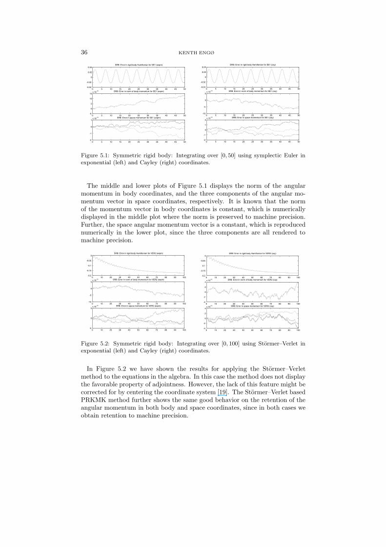
In all the numerical experiments we have used the stepsize h = 1/10.In Figure 5.1 we have shown the results for applying the symplectic Euler
method to the equations in the algebra. By construction all the iterates Pn andQn are elements of the group SO(3), and the numerical method respects theunderlying domain manifold by default. What is interesting is to check how wellthis method preserves other known conserved quantities. In the upper plot ofFigure 5.1 we have plotted the error of the Hamiltonian. It is clear that the erroroscillates in a constant band, and does not increase in magnitude. The trend isthe same for integration over longer time intervals. This feature of a numericalmethod is typical for self-adjoint (symmetric) methods applied to Hamiltonianproblems. Self-adjoint Lie group methods are discussed at length in [19].
36 KENTH ENGØ
Figure 5.1: Symmetric rigid body: Integrating over [0, 50] using symplectic Euler inexponential (left) and Cayley (right) coordinates.
The middle and lower plots of Figure 5.1 displays the norm of the angularmomentum in body coordinates, and the three components of the angular mo-mentum vector in space coordinates, respectively. It is known that the normof the momentum vector in body coordinates is constant, which is numericallydisplayed in the middle plot where the norm is preserved to machine precision.Further, the space angular momentum vector is a constant, which is reproducednumerically in the lower plot, since the three components are all rendered tomachine precision.
Figure 5.2: Symmetric rigid body: Integrating over [0, 100] using Stormer–Verlet inexponential (left) and Cayley (right) coordinates.
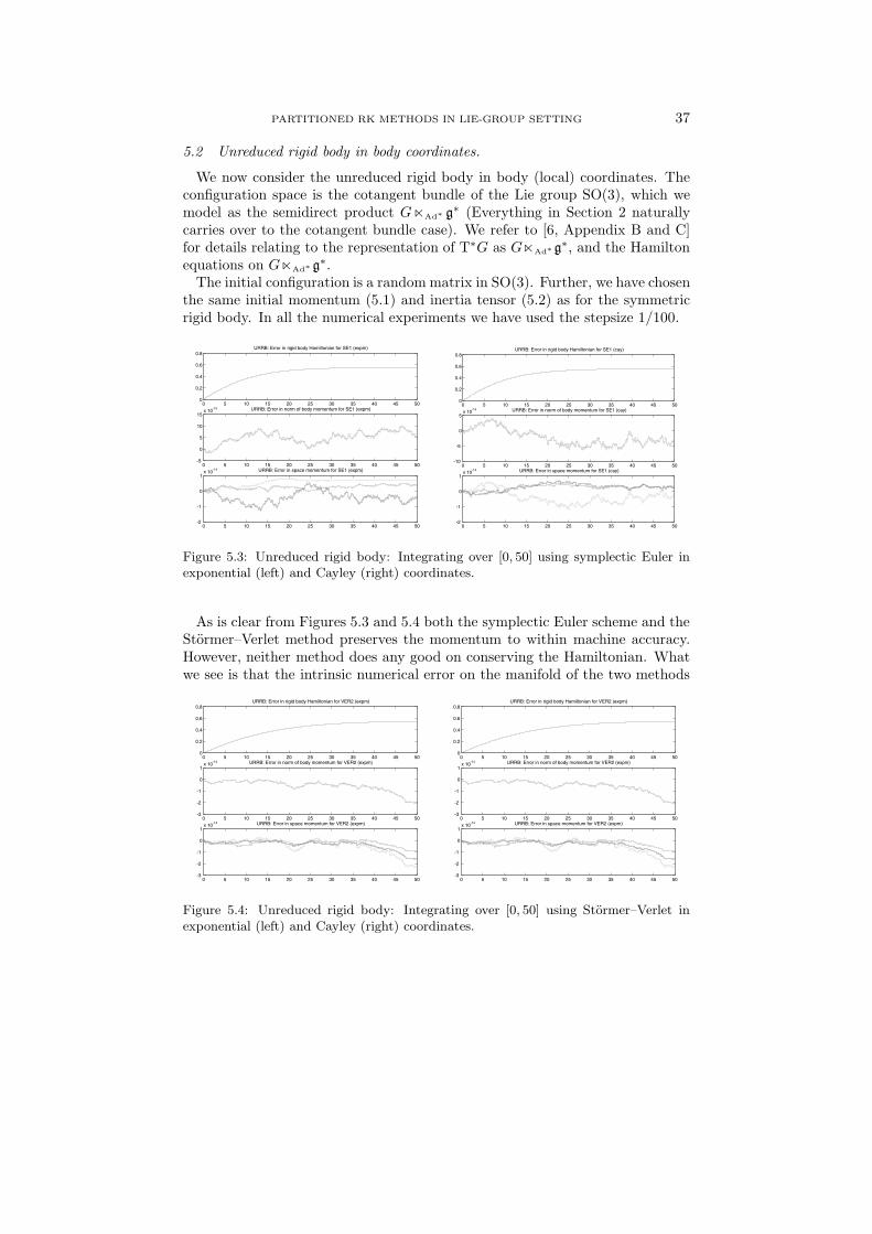
In Figure 5.2 we have shown the results for applying the Stormer–Verletmethod to the equations in the algebra. In this case the method does not displaythe favorable property of adjointness. However, the lack of this feature might becorrected for by centering the coordinate system [19]. The Stormer–Verlet basedPRKMK method further shows the same good behavior on the retention of theangular momentum in both body and space coordinates, since in both cases weobtain retention to machine precision.
PARTITIONED RK METHODS IN LIE-GROUP SETTING 37
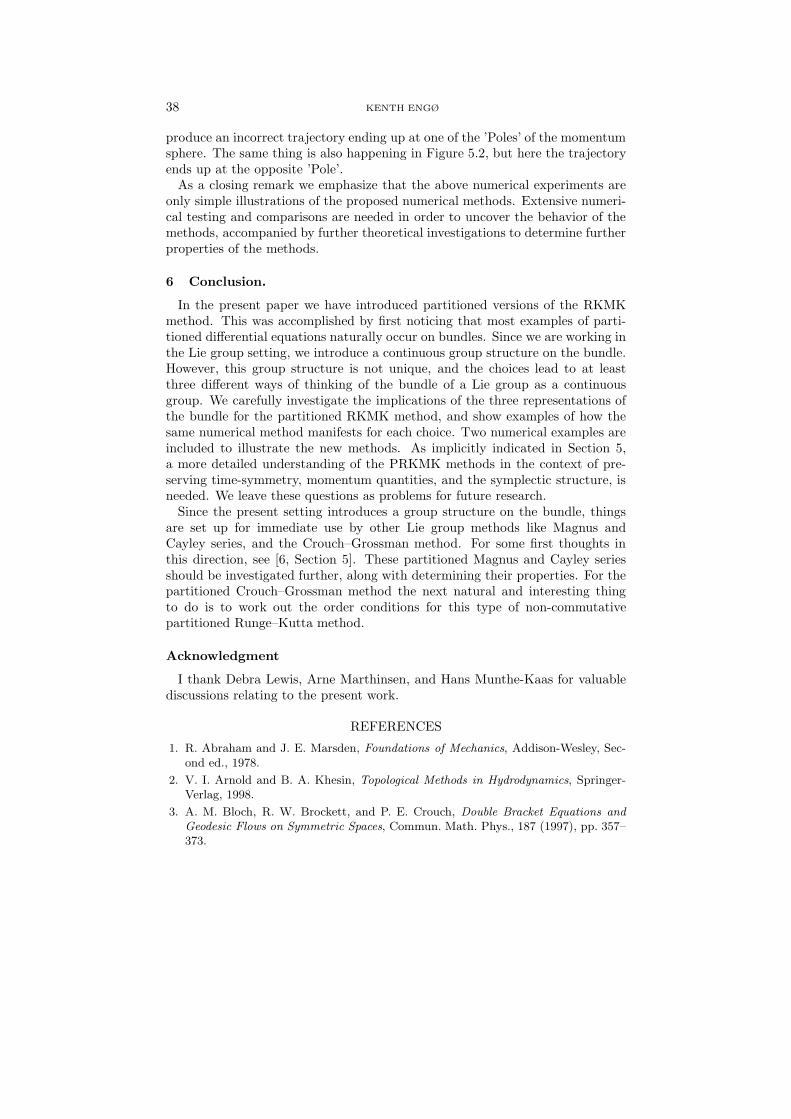
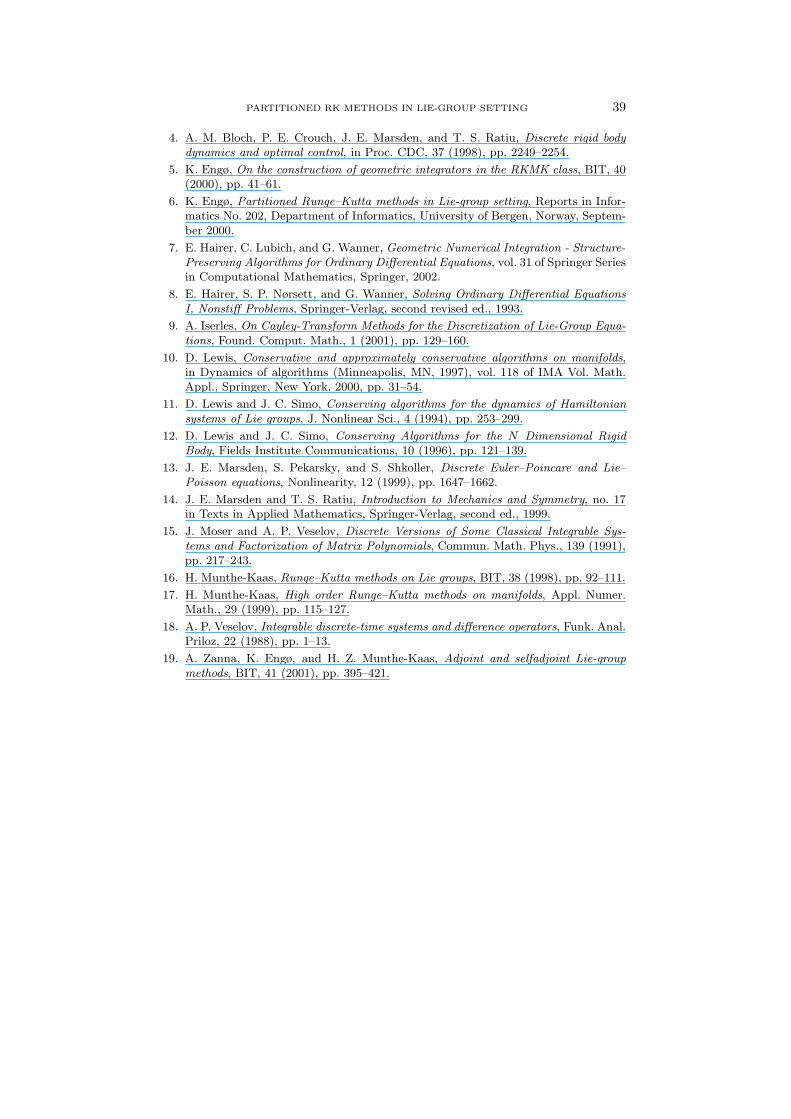
5.2 Unreduced rigid body in body coordinates.
We now consider the unreduced rigid body in body (local) coordinates. Theconfiguration space is the cotangent bundle of the Lie group SO(3), which wemodel as the semidirect product GAd∗ g∗ (Everything in Section 2 naturallycarries over to the cotangent bundle case). We refer to [6, Appendix B and C]for details relating to the representation of T∗G as GAd∗g∗, and the Hamiltonequations on GAd∗ g∗.The initial configuration is a random matrix in SO(3). Further, we have chosen
the same initial momentum (5.1) and inertia tensor (5.2) as for the symmetricrigid body. In all the numerical experiments we have used the stepsize 1/100.
Figure 5.3: Unreduced rigid body: Integrating over [0, 50] using symplectic Euler inexponential (left) and Cayley (right) coordinates.
As is clear from Figures 5.3 and 5.4 both the symplectic Euler scheme and theStormer–Verlet method preserves the momentum to within machine accuracy.However, neither method does any good on conserving the Hamiltonian. Whatwe see is that the intrinsic numerical error on the manifold of the two methods
Figure 5.4: Unreduced rigid body: Integrating over [0, 50] using Stormer–Verlet inexponential (left) and Cayley (right) coordinates.
38 KENTH ENGØ
produce an incorrect trajectory ending up at one of the ’Poles’ of the momentumsphere. The same thing is also happening in Figure 5.2, but here the trajectoryends up at the opposite ’Pole’.As a closing remark we emphasize that the above numerical experiments are
only simple illustrations of the proposed numerical methods. Extensive numeri-cal testing and comparisons are needed in order to uncover the behavior of themethods, accompanied by further theoretical investigations to determine furtherproperties of the methods.
6 Conclusion.
In the present paper we have introduced partitioned versions of the RKMKmethod. This was accomplished by first noticing that most examples of parti-tioned differential equations naturally occur on bundles. Since we are working inthe Lie group setting, we introduce a continuous group structure on the bundle.However, this group structure is not unique, and the choices lead to at leastthree different ways of thinking of the bundle of a Lie group as a continuousgroup. We carefully investigate the implications of the three representations ofthe bundle for the partitioned RKMK method, and show examples of how thesame numerical method manifests for each choice. Two numerical examples areincluded to illustrate the new methods. As implicitly indicated in Section 5,a more detailed understanding of the PRKMK methods in the context of pre-serving time-symmetry, momentum quantities, and the symplectic structure, isneeded. We leave these questions as problems for future research.Since the present setting introduces a group structure on the bundle, things
are set up for immediate use by other Lie group methods like Magnus andCayley series, and the Crouch–Grossman method. For some first thoughts inthis direction, see [6, Section 5]. These partitioned Magnus and Cayley seriesshould be investigated further, along with determining their properties. For thepartitioned Crouch–Grossman method the next natural and interesting thingto do is to work out the order conditions for this type of non-commutativepartitioned Runge–Kutta method.
Acknowledgment
I thank Debra Lewis, Arne Marthinsen, and Hans Munthe-Kaas for valuablediscussions relating to the present work.
REFERENCES
1. R. Abraham and J. E. Marsden, Foundations of Mechanics, Addison-Wesley, Sec-ond ed., 1978.
2. V. I. Arnold and B. A. Khesin, Topological Methods in Hydrodynamics, Springer-Verlag, 1998.
3. A. M. Bloch, R. W. Brockett, and P. E. Crouch, Double Bracket Equations andGeodesic Flows on Symmetric Spaces, Commun. Math. Phys., 187 (1997), pp. 357–373.
PARTITIONED RK METHODS IN LIE-GROUP SETTING 39
4. A. M. Bloch, P. E. Crouch, J. E. Marsden, and T. S. Ratiu, Discrete rigid bodydynamics and optimal control, in Proc. CDC, 37 (1998), pp. 2249–2254.
5. K. Engø, On the construction of geometric integrators in the RKMK class, BIT, 40(2000), pp. 41–61.
6. K. Engø, Partitioned Runge–Kutta methods in Lie-group setting, Reports in Infor-matics No. 202, Department of Informatics, University of Bergen, Norway, Septem-ber 2000.
7. E. Hairer, C. Lubich, and G. Wanner, Geometric Numerical Integration - Structure-Preserving Algorithms for Ordinary Differential Equations, vol. 31 of Springer Seriesin Computational Mathematics, Springer, 2002.
8. E. Hairer, S. P. Nørsett, and G. Wanner, Solving Ordinary Differential EquationsI, Nonstiff Problems, Springer-Verlag, second revised ed., 1993.
9. A. Iserles, On Cayley-Transform Methods for the Discretization of Lie-Group Equa-tions, Found. Comput. Math., 1 (2001), pp. 129–160.
10. D. Lewis, Conservative and approximately conservative algorithms on manifolds,in Dynamics of algorithms (Minneapolis, MN, 1997), vol. 118 of IMA Vol. Math.Appl., Springer, New York, 2000, pp. 31–54.
11. D. Lewis and J. C. Simo, Conserving algorithms for the dynamics of Hamiltoniansystems of Lie groups, J. Nonlinear Sci., 4 (1994), pp. 253–299.
12. D. Lewis and J. C. Simo, Conserving Algorithms for the N Dimensional RigidBody, Fields Institute Communications, 10 (1996), pp. 121–139.
13. J. E. Marsden, S. Pekarsky, and S. Shkoller, Discrete Euler–Poincare and Lie–Poisson equations, Nonlinearity, 12 (1999), pp. 1647–1662.
14. J. E. Marsden and T. S. Ratiu, Introduction to Mechanics and Symmetry, no. 17in Texts in Applied Mathematics, Springer-Verlag, second ed., 1999.
15. J. Moser and A. P. Veselov, Discrete Versions of Some Classical Integrable Sys-tems and Factorization of Matrix Polynomials, Commun. Math. Phys., 139 (1991),pp. 217–243.
16. H. Munthe-Kaas, Runge–Kutta methods on Lie groups, BIT, 38 (1998), pp. 92–111.
17. H. Munthe-Kaas, High order Runge–Kutta methods on manifolds, Appl. Numer.Math., 29 (1999), pp. 115–127.
18. A. P. Veselov, Integrable discrete-time systems and difference operators, Funk. Anal.Priloz, 22 (1988), pp. 1–13.
19. A. Zanna, K. Engø, and H. Z. Munthe-Kaas, Adjoint and selfadjoint Lie-groupmethods, BIT, 41 (2001), pp. 395–421.