Exploiting 3D Spatial Sampling in Inverse Modeling of Thermochronological Data

14Reviews in Mineralogy & GeochemistryVol. 58, pp. 375-387, 2005Copyright © Mineralogical Society of America

1529-6466/05/0058-0014$05.00 DOI: 10.2138/rmg.2005.58.14

Exploiting 3D Spatial Sampling in Inverse Modeling of Thermochronological Data

Kerry Gallagher1, John Stephenson1, Roderick Brown2, Chris Holmes3, Pedro Ballester1

1Dept. of Earth Sciences and EngineeringImperial College London

South Kensington, London, SW7 2AS, England2Division of Earth Sciences

Gregory BuildingUniversity of Glasgow

Glasgow, G12 8QQ, Scotland3Dept. of Statistics

University of Oxford1 South Parks Road

Oxford, OX1 3TG, England

INTRODUCTION

The development of quantitative models for fi ssion track annealing (Laslett et al. 1987; Carlson 1990; Laslett and Galbraith 1996; Ketcham et al. 1999) and more recently, helium diffusion in apatite (Wolf et al. 1996; Farley 2000), has allowed direct inference of the temperature history of the host rocks, and a more indirect inference of denudation chronologies (see Kohn et al. this volume, and references therein). An example of a model prediction of AFT parameter and (U-Th)/He age for a specifi ed thermal history is given in Figure 1. Various approaches exist to extract a thermal history model directly from the data, and these focus around inverse modeling (Corrigan 1991; Gallagher 1995; Issler 1996; Willett 1997; Ketcham et. al. 2000). The user specifi es some constraints on the thermal history (e.g., upper and lower bounds on the temperature time, and heating/cooling rate), and then typically some form of stochastic sampling is adopted to infer either the most likely thermal history (ideally with some measure of the uncertainty of the solution), and/or a family of acceptable thermal histories. In both the forward and inverse approaches, the thermal history is typically parameterized as nodes in time-temperature space, with some form of interpolation between the nodes.

Over recent years, one of the major applications of low temperature thermochronology has been the study of long term denudation as recorded in the cooling history of surface samples. More recently, some studies have specifi cally tried to link relatively short term, local estimates of denudation (e.g., from cosmogenic surface exposure dating) to these longer term estimates (Cockburn et al. 2000; Brown et al. 2001; Reiners et al. 2003). The step from the thermal history to denudation chronology is less direct that inferring the thermal history from the data, in that we need to make some assumptions in order to convert temperature to depth. This may involve an assumption that a 1D steady state with a constant temperature gradient over time is appropriate, or alternatively that a full 3D diffusion-advection model is required. The latter situation is not particularly amenable to an inversion approach, although recent applications have been made with a restricted number of parameters, to identify plausible solutions to relatively specifi c questions, such as the timing of relief development (Braun

376 Gallagher, Stephenson, Brown, Holmes & Ballester

2005). In practice, heat transfer can vary spatially (in both horizontal and vertical dimemsions) as a consequence of variations in thermal properties, in the mode of heat transfer (conduction and advection) and spatial variations in erosion rate and surface topography.

In the simplest case, assuming a constant gradient, it is common to adopt a “representative” geotherm of around 25–30 °C and to additionally specify that this is constant over time. Often, we do not know the present day gradient in crystalline basement areas, although it may be possible to adopt a local value from a global heat fl ow database (Pollack et al. 1993), which may also require assumptions regarding the thermal conductivity of the material that that has been removed by erosion. The role of thermal conductivity is often neglected, but the importance lies in the fact that thermal conductivities of common rocks can vary by a factor of 2–3 (Somerton 1992), and so for a constant heat fl ow, the geothermal gradient will vary by a similar factor. However, the thermal conductivity or rocks is reasonably predictable, in terms of lithology, mineralogy and porosity. Consequently, if it is possible to infer the nature of the eroded material, then it is possible to make an informed judgement of the thermal conductivity.

Here we consider some aspects related to inverse modeling of the thermal history and describe a strategy which aims to identify good, but simple, thermal history models. Such models are found by jointly fi tting data from multiple samples, rather than taking each data set independently. The method has been developed to identify spatial variations in the thermal history, particularly in the context of identifying boundaries (such as faults), across which the thermal history may vary signifi cantly.

What is a good but simple thermal history model?

Although it is relatively straightforward to fi nd a thermal history that fi ts the observed thermochronological data, a more diffi cult, but signifi cant stage in modeling is to understand how good this thermal history is. Intuitively, we can argue a good model is one that fi ts the observations satisfactorily without being overly complex, i.e., having structure that is not supported or required by the available data. Thus, the important criteria are the measure of the

Figure 1. A typical forward model—the thermal history is specifi ed, and having chosen and annealing/diffusion model, we can predict the apatite fi ssion track parameters (age, length distribution), and (U-Th)/He data. PRZ and PAZ are the partial retention zone, and partial annealing zones, over which the He and AFT systems are most sensitive on geological timescales.

3D Spatial Sampling in Inverse Modeling 377

data fi t and also a measure of the model complexity. For fi ssion track data, a natural choice of data fi t is the log likelihood function given by Gallagher (1995). This is defi ned in terms of the observed spontaneous and induced track counts, Ns

j and Nij for each crystal j of a total of Nc,

and the Nt individual track length measurements, lk, k = 1,Nt and is given as

L N N P lsj

ij

j

N

kk

Nc t= + −{ } +

= =∑ ∑ln( ) ln( ) ln[ ( )] ( )θ θ1 1

1 1

where θ is a function of the predicted spontaneous and induced track densities (ρs, ρi), given as

θ ρρ ρ

=+

s

s i( )2

P(lk) is the probability of having a track of length lk in the observed distribution, given that we have predicted the track lengths distribution for a particular thermal history (for details see Gallagher 1995). A common form of likelihood function, probably appropriate for (U-Th)/He dating, is based on a sum of squares statistic between observed and predicted ages, weighted by the error, which for N (U-Th)/He ages, is given as

L t tiobs

ipred

ij

N= −⎛

⎝⎜

⎞

⎠⎟

⎛

⎝⎜⎜

⎞

⎠⎟⎟=

∑ln ( )σ1

2

3

where tobs and tpred are the observed and predicted He ages. This form, interpreted as a log-likelihood, implicitly assumes normally distributed errors.

In practice, the log-likelihood is a negative number, and we look for the thermal history that produces the maximum value of the log-likelihood (i.e., closest to zero), This is equivalent to the thermal history that has the maximum probability of producing the observed data. It is clear from Equation (1), that the value of the log-likelihood will depend on the number of data. As already alluded to above, the likelihood value will also depend on the complexity of the model in that we expect a model with more parameters to provide a better fi t to the observed data. However, the issue then is whether the improvement in the data fi t is suffi cient to justify the additional model parameters. One straightforward way of assessing this is through the Bayesian Information Criterion (Schwartz 1978), which is defi ned for a model, mi, as

BIC m L m Ni i mi( ) = − ( ) +2 4ν log( ) ( )

where L is the log-likelihood, νmi is the number of model parameters in the current model, and N is the number of data (observations). The second term in Equation (4) penalizes the improvement in the data fi t as a consequence of increasing the complexity of the model. If we consider two models, m1 and m2, where m2 has more model parameters than m1, then if BIC(m1) < BIC(m2), then we infer that model m1 is preferable to m2. The BIC is useful for model choice when we use the same number of data for all models and an implicit assumption is that the true model is contained in all the models we consider.

Figure 2 shows three thermal history models inferred from the same set of synthetic data in which the parameterization captures the true model (which has 5 parameters, 3 temperatures and 2 times—we know the present day time). The fi rst model is under-parameterized (3 parameters), and the third model is over-parameterized (7 parameters). As we expect, the 7 parameter model provides the best fi t to the data, but the BIC implies that the improvement over the 5 parameter model is not signifi cant, while the 5 parameter model is signifi cantly better than the 3 parameter model. Heuristically, we could infer this by looking at the form of the thermal histories. The 7 parameter model does not really introduce any signifi cantly


new features compared with the 5 parameter model, in that the extra time-temperature node effectively falls on the cooling trajectory from the maximum temperature to the present day for the 5 parameter model.

Another aspect of modeling that is relevant to the approach advocated in this contribution is the role of the number of data used. Although there is likely to be redundancy in thermochronological data, incorporating more data to constrain a thermal history model generally leads to less variability in the acceptable solutions, or smaller confi dence regions about the inferred thermal history. This is illustrated in Figure 3 where 2 synthetic data sets were generated by sampling the predicted parameters for the same thermal history shown in Figure 2. We calculated the 95% confi dence regions about the best thermal history using the methods outlined in Gallagher (1995), and the results show that the inferred thermal history is better constrained with a larger amount of data than with relatively few data. This then implies that if we can group the data from multiple samples and model them jointly with a common thermal history, then the resolution of the inferred thermal history should be better than if we model each sample independently. The likelihood function for the collective samples is just the sum of the log-likelihoods for the individual samples, each calculated using the same, common thermal history. This approach will also tend to produce simpler models, as there will be a degree of compromise in jointly fi tting multiple data sets.

The philosophy behind our preferred strategy to modeling thermochronological data can be summarized as follows: we aim to incorporate multiple data sets into a common model, and try to fi nd the simplest thermal history models that can satisfy the observed data. The BIC can be used to address the second aspect, but a remaining issue in addressing the fi rst aspect is how best to group data together from a suite of irregularly distributed spatial samples. In some cases, there are natural groupings. For example, a suite of samples from a borehole, or vertical profi les, in which a suite of samples is collected over a range of elevation at effectively on location. In these cases, the spatial relationship between the samples is the vertical offset and this can be regarded as a 1D geometry (i.e., the vertical dimension). Provided there have not been thermal perturbations within the section (e.g., due to fl uid fl ow or faulting), this can be directly translated into a temperature offset, such that samples at great depth in a borehole,

Figure 2. Thermal histories (black lines) derived from fi tting AFT synthetic data and ν is the number of model parameters (time and temperature nodes). The original thermal history has ν = 5 and is shown as the grey line (BIC = 1129.4). The shaded regions are the approximate 95% confi dence regions (see Gallagher 1995 for details). L is the log-likelihood, and although the model with ν = 7 yields the maximum likelihood, the BIC of 1140.0 implies the improvement over the model with ν = 5 does not warrant the extra model parameters. The model with ν = 3 has BIC = 1142.7.


or shallower elevation for a vertical profi le, will have been at higher temperatures than the shallower depth (or higher elevation) samples. In practice, the thermochronological defi nition of a vertical profi le does not require the samples to be aligned vertically, but does imply that the dominant direction of heat transfer is vertical. This means that factors such as spatial variations in thermal properties, erosion rate or surface topography, leading to lateral heat transfer, do not signifi cantly infl uence the thermal history of the samples (vertical profi le) being considered. When dealing with sedimentary basins, there may also be complications in terms of preserving provenance signatures (refl ecting the pre-depositional thermal history of detrital grains), which can complicate the inference of the post-depositional thermal history (Carter and Gallagher 2004). However, it is straightforward to allow for this, by incorporating extra model parameters to account for the pre-depositional thermal history (which may or may not be specifi ed to be independent between samples).

When dealing with samples irregularly distributed in two spatial dimensions (e.g., latitude and longitude), there is not such an obvious way to group samples in order to share a common thermal histories. One approach, that underlies the geostatistical method of kriging (e.g., Isaaks and Srivastava 1989), is to assume that samples which are close in space will have experienced similar thermal histories. As the distance between samples becomes greater, this requirement is relaxed. One problem with this assumption is that two nearby samples may be separated by a fault (which is a spatial discontinuity). Furthermore, such a fault may or may not have been active over the time span of the thermal history retrievable from the data, or the presence of a discontinuity may not have even been recognized. The most general case, in 3D, incorporates the features of the 1D vertical offset case, and the irregularly distributed 2D samples, which may be separated by unknown discontinuities.

In the next sections, we review a general strategy to deal with these situations, and demonstrate the application to synthetic apatite fi ssion track data, although the basic approach is completely general in terms of application to other thermochronological systems, and to combinations of different types of data, provided suitable likelihood functions can be defi ned. In all cases, we parameterize the thermal history as a series of time-temperature nodes, and specify bounds on the possible values of the temperature and time as described earlier. To fi nd the thermal history models, we use stochastic sampling methods, primarily genetic algorithms

Figure 3. Inferred thermal histories based on different amounts of AFT data. The left panel has 10 track lengths and 5 single grain, ages, the central panel 200 lengths and 30 single grain ages, and the right panel has 500 lengths and 50 single grain ages. The absolute value of the likelihood depends on the number of data. The approximate 95% confi dence regions are based on differences in the likelihood and, when more data are used, these are smaller (i.e., the thermal history is more well resolved).


(GA) and Markov chain Monte Carlo (MCMC). The former method is an effi cient optimizer, i.e., for rapidly identifying the better data fi tting models. The latter method provides reliable estimates of the joint and marginal probability density functions of the model parameters, from which it is to examine correlation between parameters, and to quantify the uncertainty in terms of, for example, the 95% credible range on individual model parameters. More detail on the methodology and applications to real data sets can be found in Gallagher et al. (2005) and Stephenson et al. (2005). We fi rst consider the 1D vertical profi le case, then the 2D case with an unknown number of spatial discontinuities, and fi nally demonstrate the generalization to 3D.

1D modeling

Here we want to exploit the spatial relationship of samples in the vertical dimension, in which we implicitly assume the lowermost sample was always the hottest and the uppermost sample was always the coolest. The situation we consider is shown in Figure 4 where samples are collected from a vertical profi le (e.g., a borehole or up the side of a valley). We specifi ed a thermal history and generated synthetic data for a suite of such samples. These “synthetic samples” were fi rst modeled independently and then modeled jointly. In the second case, the parameters for the thermal history model were specifi ed in the same way as adopted for modeling the samples independently, with additional model parameters which deal with the temperature offset between the upper and lower samples. We consider two cases in which we use a constant temperature offset and a time-varying offset. In both cases, we choose the pale-offset to be independent of the present day offset as many vertical profi les are collected on surface samples which are often at similar present day temperatures (or the temperature offset is effectively the atmospheric temperature lapse rate, typically 5–6 °C/km).

The results are shown in Figure 5. Modeling the samples independently leads to a better log-likelihood (L = 7514.60), as we expect, but there are 72 model parameters required (9 parameters for 8 samples). There are some common features, such as the rapid cooling recorded in the deepest samples, but generally the individual thermal histories show little coherence. When treating the samples jointly, and assuming a constant temperature offset, the inferred thermal history model is much simpler, with only 11 model parameters, and the

Figure 4. A vertical profi le is obtained by sampling from different depths in a borehole, or different elevations in a valley. The distribution of fi ssion track age and mean length with elevation is characteristic of the thermal history.


95% credible regions about each time-temperature point imply the thermal history is well resolved. While we do not fi t the data quite as well (L = −7539.60), the BIC tells us that this simpler model is readily acceptable (the difference in log-likelihood is 25). In fact the difference in the log-likelihood would need to be about an order of magnitude greater before we reject the simpler model. Allowing for a variable temperature gradient over time produces a slightly better model (L = −7539.04), the incorporation of the 3 extra model parameters is not warranted, based on the BIC.

As part of the model formulation, we infer the temperature offset over time, which then gives a estimate of the temperature gradient directly from the thermochronological data. Moreover, as we use MCMC to characterize the model parameter space, we also obtain the probability distribution on the temperature gradient (Fig. 6). As mentioned earlier, the

Figure 5. (a) Results for modeling a synthetic vertical profi le. The “observed” data and the predictions are shown as symbols, and lines, respectively as a function of elevation. The solid lines are the predictions when modeling each sample independently, and the dashed lines are the predictions when the samples are modeled jointly (on this scale there is no difference between the predictions from the models shown in panels c and d). (b) Inferred thermal histories when modeling the samples independently, labeled according to the present day elevation (BIC = 15569.5). The true thermal history for the uppermost and lowermost samples are shown as the dashed lines, and the intermediate samples are all parallel to these. (c) Thermal histories inferred by modeling the samples jointly, with a constant temperature offset over time (BIC = 15161.9). The grey shaded areas around each time-temperature point are the distributions obtained from MCMC sampling and approximate the 95% confi dence regions. The lighter grey regions (around the lower temperature thermal history) incorporate the uncertainty on the temperature offset between the 2 thermal histories. (d) Thermal histories inferred by modeling the samples jointly, but allowing the temperature offset to vary over time (BIC=15175.9). This model is only marginally better than the constant offset model in terms of the likelihood, but the extra model parameters are not justifi ed when assessed with the BIC.


temperature gradient is a key requirement to convert the thermal history to a equivalent depth or denudation chronology. The probability distributions on the thermal history and the temperature offset can be readily sampled to construct the probability distribution of the denudation estimates. If the temperature gradient changed over time, as a consequence of rapid denudation, and there is information in the thermochronological data, then this approach should extract that information (and the uncertainty). However, from our experience, introducing a time-varying offset tends to introduce too much variation, and we would certainly recommend exploring whether the difference in data fi t in comparison with a constant offset model is justifi ed.

2D modeling

In this situation, the spatial relationship is nearness, i.e., samples close together are likely to have similar thermal histories. As mentioned earlier, in the real world, there are discontinuities (e.g., faults). The problem then is how to group samples spatially, allowing for the presence of unknown discontinuities. Here we classify the samples into different sub-groups defi ned by discrete spatial regions or partitions,, such that the thermal history is the same for a given partition,, but varies between partitions. Also, we do not know how many partitions we should look for, i.e., one of the unknown parameters is the number of parameters. The problem as formulated here does not allow for lateral variations in the thermal history within a partition, although this is not a major problem to implement (it just requires some form of interpolation across a partition). Another requirement is that samples do not move laterally relative to each other, which may limit the application to active mountain belts involving large scale lateral transfer (e.g., the southern Alps in New Zealand).

This is solved with a form of Bayesian Partition Modeling (BPM), which is more formally described by Denison et al. (2002). In essence, BPM provides a method for spatial clustering of different samples, according to the spatial structure of the data. In our case, we have an additional complication in that we are interesting in spatial clustering based on the thermal history inferred from the data for particular samples. The 2D space is parameterized with a Voronoi tessellation (Okabe et al. 2000), which are polygonal regions defi ned by an internal point, such that any sample location that falls within a given Voronoi cell is closer to that internal point. The boundaries of the Voronoi cells are drawn as the perpendicular bisectors of the internal points in each cell (Fig. 7). It is the boundaries of the partitions that are our proxy for geological discontinuities, such as faults, where the thermal history may change rapidly over a small distance.

22 24 26 28 30 32 34 36

Temperature Gradient (°C/km)

P(dT/dz)

Palaeogradient

22 24 26 28 30 32 34 36

Present gradient

Temperature Gradient (°C/km)

P(dT/dz)

Figure 6. Distributions on the temperature gradient for the model shown in Figure 5c, which assumes a constant palaeogradient. The true solution for both the present and palaeogradient is ~28.6 °C km−1. These distributions can be sampled to produce uncertainty estimates for denudation.


The implementation of BPM we adopt uses a dimension changing version of MCMC, known as Reversible Jump (RJ) MCMC (Green 1995), as we need to deal with an unknown number of partitions. In this approach, we can specify the minimum and maximum number of partitions we allow a priori. The maximum range is from 1 to the number of samples, but we typically choose to set the maximum number to value less than the number of samples. Otherwise, we can just model all the samples independently. In order to deal with the unknown thermal histories in each partition, we use the GA described by Ballester and Carter (2004) to fi nd the optimal thermal history with each partition for a given partition confi guration generated during the MCMC run. When a given partition confi guration is repeated during the MCMC (in that the sample groupings have previously been considered), we take the earlier best GA thermal history model for the partitions in that confi guration. This particular approach can lead to the algorithm becoming somewhat static and sub-optimal. However, we can modify the algorithm to run another MCMC run on the thermal history in each partition, for a given partition confi guration, which improves the combined sampling of the model space for the thermal histories and partitions (Stephenson et al. 2005). The examples we consider in this paper are based on synthetic data, and here the resolution on the thermal history is not our primary objective. Rather we want to demonstrate the concept of implementing the partition model approach to irregularly distributed spatial samples.

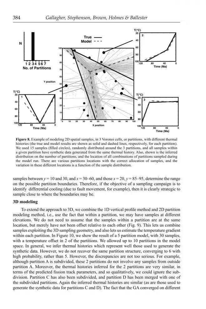
Figure 8 shows the method applied to a 3 partition problem, with 15 sample locations, where the RJ-MCMC was run allowing for up to 7 partitions. The results show that we can recover the correct number of partitions with high probability, with the correct allocation of samples in each partition, and also a good representation of the thermal history within each partition. Note that here we chose thermal histories for each partition that are distinct and relatively easy for the method to identify, as our aim is to demonstrate the ability of the methodology to identify the form and spread in the inferred partition structure. The spread in the solutions for 3 partitions is also an indication of the uncertainty about the location of the partition boundaries. With the implementation we have used here, all partitions geometries that correctly allocate the samples will use the same thermal histories (and have the same likelihood), then it is clear that the range of the location of the boundaries is determined by the location of the sample locations, subject to the requirement that the boundaries are straight. So in the top right of Figure 8. there is a relatively large spread in the location of the boundaries, as there are no sample locations there, but the spread is constrained by the samples around x = 50, and y = 70–80. Similarly, the

Figure 7. The geometry of 2D Voronoi cells, and their centers (indicated by the stars). The boundaries of each cell is defi ned as the perpendicular bisectors of the lines joining its centre to all other centers. Any sample location (fi lled circles) that falls within a given cell is closer to the centre of that cell than any other centre. The linear boundaries are used in our modeling approach to characterize spatial discontinuities, although their number and positions are unknown.


samples between y = 10 and 30, and x = 30–60, and those x = 20, y = 85–95, determine the range on the possible partition boundaries. Therefore, if the objective of a sampling campaign is to identify differential cooling (due to fault movement, for example), then it is clearly strategic to sample close to where the boundaries may be.

3D modeling

To extend the approach to 3D, we combine the 1D vertical profi le method and 2D partition modeling method, i.e., use the fact that within a partition, we may have samples at different elevations. We do not need to assume that the samples within a partition are at the same location, but merely have not been offset relative to each other (Fig. 9). This lets us combine samples exploiting the 3D sampling geometry, and also lets us estimate the temperature gradient within each partition. In Figure 10, we show the result of a 5 partition model, with 30 samples, with a temperature offset in 2 of the partitions. We allowed up to 10 partitions in the model space. In general, we infer thermal histories which represent well those used to generate the synthetic data. However, we do not recover the same partition structure, converging to 6 with high probability, rather than 5. However, the discrepancies are not too serious. For example, although partition A is subdivided, these 2 partitions do not involve any samples from outside partition A. Moreover, the thermal histories inferred for the 2 partitions are very similar, in terms of the predicted fi ssion track parameters, and so qualitatively, we could ignore the sub-division. Partition C has also been subdivided, and partition D has been merged with one of the subdivided partitions. Again the inferred thermal histories are similar (as are those used to generate the synthetic data for partitions C and D). The fact that the GA converged on different

Figure 8. Example of modeling 2D spatial samples, in 3 Voronoi cells, or partitions, with different thermal histories (the true and model results are shown as solid and dashed lines, respectively, for each partition). We used 15 samples (fi lled circles), randomly distributed around the 3 partitions, and all samples within a given partition have synthetic data generated from the same thermal history. Also, shown is the inferred distribution on the number of partitions, and the location of all combinations of partitions sampled during the model run. There are various partitions locations with the correct allocation of samples, and the variation in these different locations is a function of the sample distribution.


Figure 9. The geometry of the 3D modeling approach which uses 2D Voronoi cells, and within a cell, the 1D vertical profi le approach (a temperature offset as a function of sample elevation).

Figure 10. Example of the 3D modeling, with 5 partitions, different thermal histories (the true and model results are shown for each partition and 30 samples (fi lled circles), randomly distributed around the 5 partitions. Partitions A and E have temperature offsets, while B, C and D do not. The model infers 6 partitions and does not always correctly allocate the samples within partitions. However, this refl ects the fact that the thermal histories are similar, and we select optimal thermal histories for a given partition confi guration (see the text for details).


solutions in these situations and did not subsequently move appears to be a consequence of this particular implementation not allowing new thermal history models for a given partition confi guration (although this is a relatively straightforward modifi cation; see Stephenson et al. 2005). However, the other partition boundaries are well identifi ed (given the distribution of sample locations). For example, the boundary that runs SW-NW is well resolved as there are several samples located close to the boundary. The same comments about the resolution of the boundaries made for the 2D case also applies in 3D. Thus, the boundaries between A and E, and B and D, are as well resolved as they can be, given the sample distributions.

SUMMARY

We have given an overview of a modeling strategy aimed at exploiting the spatial geometry of the sample distributions in order to maximize the retrieval of thermal history information from thermochronological data. Philosophically, we aim to fi nd thermal history solutions that fi t the observations well, but do not have unwarranted complexity. These two requirements are quantifi ed through the Bayesian Information Criterion, which combines the data likelihood and the number of model parameters. The overall approach relies on exploiting the spatial geometry of the sample locations to combine data from individual samples and identify a common thermal history. The combination of different data sets has the advantage of improving the resolution on the inferred thermal history, and also reducing the complexity. Markov chain Monte Carlo sampling provides a means of constructing reliable representations on the probability distributions for the model parameters. 1D modeling is relevant to vertical profi les, and provides an estimate of the paleotemperature gradient directly from the data. The 2D approach relies on a partition model, in which each partition contains a subgroup of the samples with a common thermal history. The partition model approach allows for an unknown number of discontinuities, whose locations are also unknown. The extension to 3D combines the 1D and 2D approaches to fi nd partitions in which samples at different elevations have experienced a common form of thermal history, but the actual temperatures depend on the elevation. As presented here, it is implicit that the spatial relationship between samples has not changed over time, at least not in a way that will lead to different thermal histories.

The approach presented here is different to 3D thermal models (Braun 2003, 2005; Ehlers 2005) but complementary. Thus, we infer the thermal history directly from the data, while the other 3D models are specifi ed and certain parameters are adjusted to match the observed data. Both approaches assume that the predictive models for fi ssion track annealing or helium diffusion in apatite are correct. In principle, this assumption can be relaxed and appropriate predictive model parameters can be estimated as part of the modeling process. However, this will lead to signifi cant trade-off between annealing of diffusion parameters and the thermal history (Gallagher and Evans 1991). Future modifi cations to this approach will include more generalized sampling of the thermal histories during the MCMC sampling of the partition structure, incorporation of multiple data types (e.g., apatite fi ssion track and (U-Th)/He data) and potentially allowing for irregularly shaped partition boundaries.

REFERENCES Ballester PJ, Carter JN (2004) “An Effective Real-Parameter Genetic Algorithms with Parent Centric Normal

Crossover for Multimodal Optimization.” Genetic and Evolutionary Computation Conference (GECCO-04, Seattle, USA). Lecture Notes in Computer Science 3102, Springer, p. 901-91

Braun J (2003) Pecube: a new fi nite element code to solve the 3D heat transport equation including the effects of a time-varying, fi nite amplitude surface topography. Comp Geosci 29:787-794


Braun J (2005) Quantitative constraints on the rate of landform evolution derived from low-temperature thermochrohonology. Rev Mineral Geochem 58:351-374

Brown RW, Summerfi eld MA, Gleadow AJW (2002) Denudational history along a transect across the Drakensberg Escarpment of southern Africa derived from apatite fi ssion track thermochronology. J Geophys Res 107(B12):2350, doi:10.1029/2001JB000745

Carlson WD (1990) Mechanisms and kinetics of apatite fi ssion-track annealing. Am Mineral 75:1120-1139Carter A, Gallagher K (2004) Provenance signatures and the inference of thermal history models from apatite

fi ssion track data – A synthetic data study. Geol Soc Am Spec Publ 378:7-23Cockburn HAP, Brown RW, Summerfi eld MA, Seidl MA (2000) Quantifying passive margin denudation

and landscape development using a combined fi ssion-track thermochronology and cosmogenic isotope analysis approach. Earth Planet Sci Lett 179:429-435

Corrigan J (1991) Inversion of apatite fi ssion track data for thermal history information. J Geophys Res 96(B6):10347–10360, doi:10.1029/91JB00514

Denison DGT, Holmes CC, Mallick BK, Smith AFM (2000) Bayesian Methods for Nonlinear Classifi cation and Regression. John Wiley & Sons, Chichester

Ehlers TA (2005) Crustal thermal processes and the interpretation of thermochronometer data. Rev Mineral Geochem 58:315-350

Farley KA (2000) Helium diffusion from apatite I: General behavior as illustrated by Durango fl uorapatite. J Geophys Res 105:2903-2914

Gallagher K (1995) Evolving thermal histories from fi ssion track data. Earth Planet Sci Lett 136:421-435 Gallagher K, Evans E (1991) Estimating kinetic parameters for organic reactions from geological data: an

example from the Gippsland Basin, Australia. Appl Geochem 6:653-664Gallagher K, Stephenson J, Brown R, Holmes C, Fitzgerald P (2005) Low temperature thermochronology and

strategies for multiple samples. 1 : vertical profi les, Earth Planet Sci Lett, in pressGreen PJ (1995) Reversible jump Markov chain Monte Carlo computation and Baeysin model determination.

Biometrika 82:711-732Isaaks EH, Srivastava RM (1989) Introduction to Applied Geostatistics. Oxford University Press, OxfordIssler DR (1996) An inverse model for extracting thermal histories from apatite fi ssion track data: Instructions

and software for the Windows 95 environment. Geological Survey of Canada, Open File Report 2325Ketcham RA (2005) Forward and inverse modeling of low-temperature thermochronometry data. Rev Mineral

Geochem 58:275-314Ketcham R, Donelick R, Carlson W (1999) Variability of apatite fi ssion-track annealing kinetics: III.

Extrapolation to geological timescales. Am Mineral 84:1235-1255Ketcham R, Donelick R, Donelick M (2000) AFTSolve: a program for multi-kinetic modeling of apatite fi ssion

track data. Geol Mater Res 2:1-32Laslett GM, Galbraith R (1996) Statistical modeling of thermal annealing of fi ssion tracks in apatite. Geochim

Cosmochim Acta 60:5117-5131Laslett GM, Green PF, Duddy IR, Gleadow AJW (1987) Thermal annealing of fi ssion tracks in apatite. 2. A

quantitative analysis. Chem Geol (Isot. Geosci. section) 65:1-13Okabe A, Boots B, Sugihara K, Chin S-N (2000) Spatial Tessellations: Concepts and Applications of Voronoi

Diagrams, 2nd edition. John Wiley & Sons, ChichesterPollack HN, Hurter SJ, Johnson JR (1993) Heat fl ow from the earth’s interior: analysis of the global data set.

Rev Geophys 31(3):267-280 Reiners PW, Zuyi Z, Elhers TA, Xu C, Brandon MT, Donelick RA, Nicolescu S (2003) Post-orogenic evolution

of the Dabie Shan, eastern China, from (U-Th)/He and fi ssion-track thermochronology. Am J Sci 303:489-518

Schwartz G (1978) Estimating the dimension of a model. Ann Statistics 6:461-646Somerton WH (1992) Thermal Properties and Temperature-related Behaviour of Fluid Rock Systems. Elsevier,

AmsterdamStephenson J, Gallagher K, Holmes C (2005) Low temperature thermochronology and strategies for multiple

samples 2: partition modeling for 2/3D distributions with disontinuities. To be submitted to Earth Planet Sci Lett

Willett SD (1997) Inverse modeling of annealing of fi ssion tracks in apatite 1: A Controlled Random Search method. Am J Sci 297:939-969

Wolf RA, Farley KA, Silver LT (1996) Helium diffusion and low temperature thermchrononmetry of apatite. Geochim Cosmochim Acta 60:4231-4240

Documents

Exploiting 3D Spatial Sampling in Inverse Modeling of Thermochronological Data