1

Exploration of RaPiD-style Pipelined FPGA Interconnects

Akshay Sharma1, Katherine Compton2, Carl Ebeling3, Scott Hauck1

1 University of Washington, Dept. of EE, Seattle, WA, {akshay, hauck}@ee.washington.edu 2 University of Wisconsin – Madison, Dept. of ECE, Madison, WI, kati@engr.wisc.edu

3 University of Washington, Dept. of CSE, Seattle, WA, ebeling@cs.washington.edu

Abstract

Pipelined FPGAs promise high performance for reconfigurable computing. However, the architectural design of these systems is complex, involving the optimization of numerous features. In this work, we parameterize and explore the interconnect structure of pipelined FPGAs. Specifically, we explore the effects of interconnect register population, length of registered routing track segments, registered I/O terminals of logic units, and the flexibility of the interconnect structure on the performance of a pipelined FPGA. Our experiments with the RaPiD architecture identify tradeoffs in pipelined interconnect design. After quantifying these effects, we were able to design an architecture with a 19% improvement over RaPiD in area-delay product.

1. Introduction Over the last few years, reconfigurable technologies have made remarkable progress. Today, state-of-the-art devices from FPGA vendors provide a wide range of functionalities. Coupled with gate-counts in the millions, these devices can be used to implement entire systems at a time. However, improvements in FPGA clock cycle times have consistently lagged behind advances in device functionalities and capacities. Even the simplest circuits cannot be clocked at more than a few hundred megahertz.

A number of research groups have tried to improve clock cycle times by proposing pipelined FPGA architectures. Some examples of pipelined architectures are HSRA [Tsu99], RaPiD [Cronquist99, Ebeling96], and the architecture proposed in [Singh01]. The key issues in designing a pipelined interconnect are the number and location of registers in the architecture. Pipelined FPGAs provide a relatively large number of registers, both in the logic and interconnect structures. Applications that are mapped to pipelined FPGAs are often retimed to take advantage of abundant, easily available registers.

Pipelined FPGA architecture design poses a number of challenges, not the least of which is the composition of the interconnect structure. Earlier work [Betz99, Betz99a] has shown that the design of traditional FPGA interconnect structures involves tradeoffs amongst different parameters like segment-length, switch-box types, and layout considerations. The design of a pipelined FPGA’s interconnect structure involves each of these issues, plus the possible inclusion of a large number of registers. The number and location of interconnect registers plays an important role in determining the performance of applications mapped to pipelined FPGAs. If the number of interconnect registers is too few, the benefits of pipelining may get lost in long, circuitous routes. On the other hand, the area penalty due to too many interconnect registers may reduce the impact of improvements in clock cycle time.

The objective of this paper is to parameterize and explore the performance of pipelined interconnect structures. Specifically, we try to answer the following questions:

• What are the benefits of registering the I/O terminals of logic units? • How many sites in the interconnect structure should be registered, and how many registers should there be at

each site? • How long should the segments of registered routing tracks be? • How does the flexibility of the interconnect structure affect the performance of pipelined FPGAs?

2

We first give some important background on pipelining and pipelined FPGAs. We then discuss the RaPiD architecture, a pipelined FPGA used as the target architecture in this work. We also discuss the CAD tool flow and benchmarks used in this work. Then, we present our work on optimizing RaPiD’s interconnect structure.

2. Pipelining One of the most common techniques for achieving high performance hardware designs is pipelining – breaking a single computation up into multiple stages by inserting registers into the datapath. This has the advantage of boosting throughput, since a computation broken into N equal stages might run at approximately N times the clock rate. However, this transformation is typically not good for latency, since the added registers and mismatch in stage delay increases the time it takes to perform a single complete computation. Also, it changes the I/O protocol of the computation since the result is available N-1 cycles later than in the unpipelined circuit. Finally, in circuits with sequential dependencies pipelining can be complex, or impossible. Thus pipelining can be of limited benefit for general circuit design, and many FPGA mappings are only lightly pipelined.

For reconfigurable computing [Hauck98, Compton02] things are fairly different – in this case computation is typically done on streaming computations, with significant data parallelism, and where throughput is more important than latency. Thus, in many uses of FPGAs for high-performance computation we can add as many pipeline stages to a computation as we desire, providing an opportunity for significantly higher clock rates.

OA

CB

OA

CB

OA

CB

OAA

CCBB

BO

A

CBB

OA

CC

OA

CB

OAA

CCBB

OA

CB

OAA

CCBB

(a) (b) (c) (d) (e)

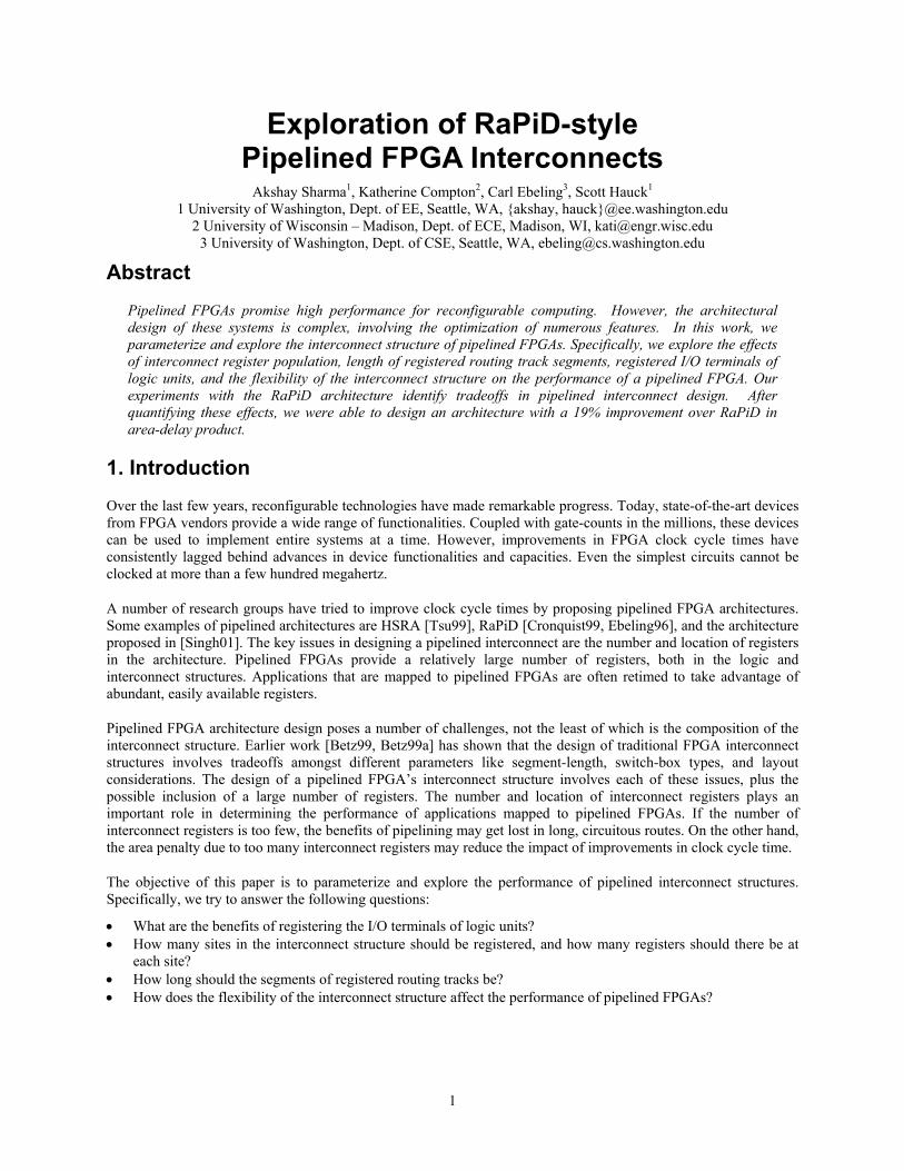
Figure 1. Original circuit (a) with clock cycle of 3 gate delays is pipelined by adding registers to the inputs and outputs (b). The circuit is then retimed (c) to a clock cycle of 2 gate delays. A 2-slowing (d) is then retimed to 1 gate delay (e).

Addition of registers gives rise to retiming [Leiserson91], the movement of registers to speed up execution without changing functionality. For example, in Figure 1(a) we have a circuit with a clock cycle of 3 gate delays (assuming for now that registers have no delay, and all combinational gates have the same delay). We pipeline it by adding registers to the inputs and to the outputs in Figure 1(b), but the delay stays the same. However, retiming says that we can add a register to every output of a gate by removing one from every input, or vice-versa, and have a functionally equivalent circuit. Thus, we retime the example circuit by moving registers from the inputs to the output of the top gate as shown in Figure 1(c), achieving a clock cycle of 2 gate delays.

Note that “classical” retiming has a significant limitation: we cannot add or subtract registers from a cycle. This means the fastest rate to which a circuit can be classically retimed is limited by the maximum average-weight cycle [Papaefthymiou91], where the average-weight of a cycle is the total delay divided by the number of registers. For

3

the circuit in Figure 1, there is a cycle of two gate delays, with a single register, meaning the fastest retimed circuit has a clock cycle of 2/1=2 gate delays. Thus, Figure 1(c) is the fastest circuit possible via classical retiming.

A technique called C-slowing [Leiserson91, Tsu99, Weaver03] can overcome this limit. It replaces the registers of a circuit by a set of C registers to increase retiming. Specifically, the pipelined circuit of Figure 1(b) is 2-slowed in Figure 1(d), and then retimed to 1 gate delay in Figure 1(e). Note that C-slowing changes the behavior of the circuit. The computation takes C times as many clock cycles to compute, taking inputs and producing outputs every C cycles. However, we can provide new data every cycle, interleaving C separate computations on the same logic. Thus, computations working on multiple independent datasets can do productive work every cycle, improving the throughput by up to C times. However, the independent data-set requirement often cannot be met. For example, consider an encryption chip. Ciphers can be chained, which increases security by making the encryption of block I depend on that of block I-1. Obviously, the encryption of a single stream can be C-slowed if the blocks are not chained, but cannot be C-slowed if the cipher is in a more secure chained mode.

S

K2 K3K1

S

K2 K3K1

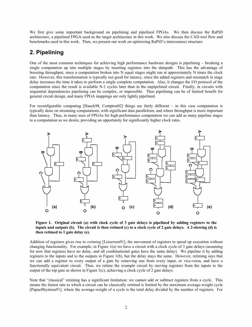
Figure 2. A multi-terminal pipelined signal.

Due to retiming and the style of circuits created, netlists that are mapped to pipelined FPGAs generally contain a significant number of pipelined signals. A pipelined signal is a signal that must go through registers in the interconnect structure. An example of a pipelined signal is shown in Figure 2. In this case, there must be three registers between S and K1, four registers between S and K2 and five registers between S and K3.

3. Recent Work on Pipelined FPGAs There have been several efforts to harness pipelining in reconfigurable systems. However, most restrict the types of circuits mapped to these devices, or have significant overheads when used to implement general-purpose circuits. For example, the HSRA architecture [Tsu99] achieves a 250MHz clock cycle by radically pipelining the system, including inserting registers throughout the logic block and interconnect structure. However, this degree of pipelining requires that the circuit be amenable to C-slow retiming, which often is not achievable. Also, the architecture pays approximately a 2x area penalty, 2x power penalty, and can increase the single-stream latency by up to 5x.

Some architectures do not require circuits be heavily pipelined, but provide registers in their interconnects to support whatever pipelining is needed. RaPiD [Ebeling96, Cronquist99] is a reconfigurable device optimized for signal processing tasks, and provides up to three levels of registers at the programmable connection points in the interconnect. Similarly, the Chess architecture [Marshall98, Marshall99, Stansfield02] from H.P./Elixent augments their switchboxes with registers. In each of these cases the computations do not need to be pipelined to be implemented efficiently, but the chips do make use of the pipelining available in the input mappings.

A final architecture uses heavy pipelining somewhat as a byproduct of its fast reconfiguration support. In the PipeRench Project [Schmit97, Goldstein00] the chip is broken into rows, and the device reconfigures one row each cycle to overlap computation with reconfiguration. The hardware emulates a much larger structure, similar in concept to virtual memory. To support this computation mechanism each row is pipelined, and cycles are restricted to remain within one row (i.e. a single level of logic) of the device.

Each of these designs has sacrificed some of the flexibility of general-purpose FPGAs for greater optimization for some class of computations. There has been some work on using general-purpose FPGAs [Singh02, Singh02a], perhaps with minor modifications [Singh01a], to support retiming and pipelining. While these efforts have shown promise in improving circuit performance, there is significant work left to do. For example, while they consider the

4

impact of registers in the interconnect structure [Singh01a], this is done with a very simplistic router which cannot consider the pipelining effects of different paths.

4. The RaPiD Architecture

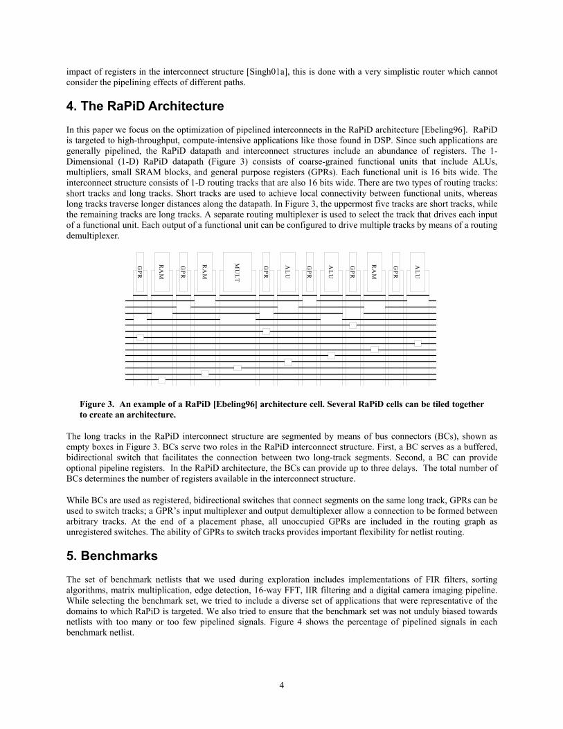
In this paper we focus on the optimization of pipelined interconnects in the RaPiD architecture [Ebeling96]. RaPiD is targeted to high-throughput, compute-intensive applications like those found in DSP. Since such applications are generally pipelined, the RaPiD datapath and interconnect structures include an abundance of registers. The 1-Dimensional (1-D) RaPiD datapath (Figure 3) consists of coarse-grained functional units that include ALUs, multipliers, small SRAM blocks, and general purpose registers (GPRs). Each functional unit is 16 bits wide. The interconnect structure consists of 1-D routing tracks that are also 16 bits wide. There are two types of routing tracks: short tracks and long tracks. Short tracks are used to achieve local connectivity between functional units, whereas long tracks traverse longer distances along the datapath. In Figure 3, the uppermost five tracks are short tracks, while the remaining tracks are long tracks. A separate routing multiplexer is used to select the track that drives each input of a functional unit. Each output of a functional unit can be configured to drive multiple tracks by means of a routing demultiplexer.

GPR

GPR

RA

M

RA

M

MU

LT

AL

U

GPR

AL

U

GPR

GPR

RA

M

AL

U

GPR

Figure 3. An example of a RaPiD [Ebeling96] architecture cell. Several RaPiD cells can be tiled together to create an architecture.

The long tracks in the RaPiD interconnect structure are segmented by means of bus connectors (BCs), shown as empty boxes in Figure 3. BCs serve two roles in the RaPiD interconnect structure. First, a BC serves as a buffered, bidirectional switch that facilitates the connection between two long-track segments. Second, a BC can provide optional pipeline registers. In the RaPiD architecture, the BCs can provide up to three delays. The total number of BCs determines the number of registers available in the interconnect structure.

While BCs are used as registered, bidirectional switches that connect segments on the same long track, GPRs can be used to switch tracks; a GPR’s input multiplexer and output demultiplexer allow a connection to be formed between arbitrary tracks. At the end of a placement phase, all unoccupied GPRs are included in the routing graph as unregistered switches. The ability of GPRs to switch tracks provides important flexibility for netlist routing.

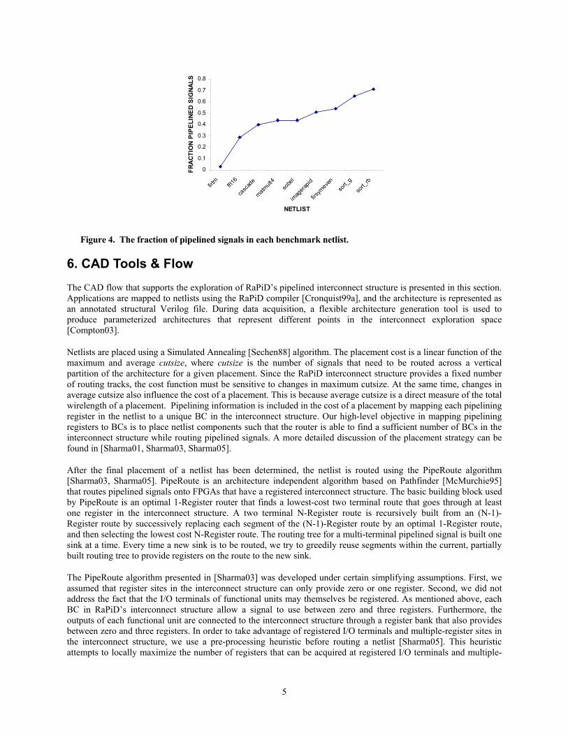
5. Benchmarks The set of benchmark netlists that we used during exploration includes implementations of FIR filters, sorting algorithms, matrix multiplication, edge detection, 16-way FFT, IIR filtering and a digital camera imaging pipeline. While selecting the benchmark set, we tried to include a diverse set of applications that were representative of the domains to which RaPiD is targeted. We also tried to ensure that the benchmark set was not unduly biased towards netlists with too many or too few pipelined signals. Figure 4 shows the percentage of pipelined signals in each benchmark netlist.

5

0

0.1

0.2

0.3

0.4

0.5

0.6

0.7

0.8

firtm

fft16

casc

ade

matmult

4so

bel

imag

erapid

firsym

even

sort_

g

sort_

rb

NETLIST

FRAC

TIO

N PI

PELI

NED

SIG

NALS

Figure 4. The fraction of pipelined signals in each benchmark netlist.

6. CAD Tools & Flow

The CAD flow that supports the exploration of RaPiD’s pipelined interconnect structure is presented in this section. Applications are mapped to netlists using the RaPiD compiler [Cronquist99a], and the architecture is represented as an annotated structural Verilog file. During data acquisition, a flexible architecture generation tool is used to produce parameterized architectures that represent different points in the interconnect exploration space [Compton03].

Netlists are placed using a Simulated Annealing [Sechen88] algorithm. The placement cost is a linear function of the maximum and average cutsize, where cutsize is the number of signals that need to be routed across a vertical partition of the architecture for a given placement. Since the RaPiD interconnect structure provides a fixed number of routing tracks, the cost function must be sensitive to changes in maximum cutsize. At the same time, changes in average cutsize also influence the cost of a placement. This is because average cutsize is a direct measure of the total wirelength of a placement. Pipelining information is included in the cost of a placement by mapping each pipelining register in the netlist to a unique BC in the interconnect structure. Our high-level objective in mapping pipelining registers to BCs is to place netlist components such that the router is able to find a sufficient number of BCs in the interconnect structure while routing pipelined signals. A more detailed discussion of the placement strategy can be found in [Sharma01, Sharma03, Sharma05].

After the final placement of a netlist has been determined, the netlist is routed using the PipeRoute algorithm [Sharma03, Sharma05]. PipeRoute is an architecture independent algorithm based on Pathfinder [McMurchie95] that routes pipelined signals onto FPGAs that have a registered interconnect structure. The basic building block used by PipeRoute is an optimal 1-Register router that finds a lowest-cost two terminal route that goes through at least one register in the interconnect structure. A two terminal N-Register route is recursively built from an (N-1)-Register route by successively replacing each segment of the (N-1)-Register route by an optimal 1-Register route, and then selecting the lowest cost N-Register route. The routing tree for a multi-terminal pipelined signal is built one sink at a time. Every time a new sink is to be routed, we try to greedily reuse segments within the current, partially built routing tree to provide registers on the route to the new sink.

The PipeRoute algorithm presented in [Sharma03] was developed under certain simplifying assumptions. First, we assumed that register sites in the interconnect structure can only provide zero or one register. Second, we did not address the fact that the I/O terminals of functional units may themselves be registered. As mentioned above, each BC in RaPiD’s interconnect structure allow a signal to use between zero and three registers. Furthermore, the outputs of each functional unit are connected to the interconnect structure through a register bank that also provides between zero and three registers. In order to take advantage of registered I/O terminals and multiple-register sites in the interconnect structure, we use a pre-processing heuristic before routing a netlist [Sharma05]. This heuristic attempts to locally maximize the number of registers that can be acquired at registered I/O terminals and multiple-

6

register sites. By doing so, we try to reduce the total number of register sites that have to be found in the interconnect structure during pipelined routing.

A last, albeit important, feature that we added to the PipeRoute algorithm was to make it timing-aware [Sharma05]. Since the primary objective of pipelined FPGAs is the reduction of clock cycle time, it is imperative that a pipelined routing algorithm maintains control over the criticality of pipelined signals during routing. In making PipeRoute timing-aware, we drew inspiration from the Pathfinder algorithm. While routing a signal, Pathfinder uses the criticality of the signal in determining the relative contributions of the congestion and delay terms to the cost of routing resources. However, in the special case of a pipelined signal, the signal’s route may contain multiple interconnect registers and hence different segments on the route may be at different criticalities. Furthermore, the signal’s route may go through different interconnect registers from one routing iteration to the next. Thus, before routing a pipelined signal, we are faced with making an intelligent guess about the overall criticality of a pipelined signal. Our solution is to make a pessimistic choice and assign the criticality of the most critical segment to the criticality of the pipelined signal.

7. Characterizing Pipelined Interconnect Structures

Before presenting our results, we briefly explain the effects of certain important interconnect features on the area and delay of a netlist:

• Track Count: The track count of a netlist is the minimum number of tracks required to route the netlist. Track count directly affects area in two ways. First, the area of the I/O multiplexers and demultiplexers depends on the number of tracks that connect to them. Second, the number of BCs in the architecture is directly proportional to the number of tracks.

• BCs: The frequency and number of BCs in the interconnect structure affects both area and delay. A large number of BCs provide an abundance of interconnect register sites. Consequently, a BC-rich interconnect structure improves the routability of pipelined signals. Routability improvements generally result in track count reductions, and if the area benefit due to such reductions is greater than the area penalty of a large number of BCs, an overall area win may result. The number and location of BCs in the interconnect structure also influences the delay characteristics of a netlist. One reason is the effects of segmentation on the critical path delay of a netlist [Betz99]. Another reason is that the number of BCs determines the quality of the routes of pipelined signals. Recall that the number of BCs is a direct measure of the number of interconnect registers. In BC-poor architectures, the pipelined router finds long, circuitous routes for heavily pipelined signals. Such poor-quality routes result in a deterioration of the delay characteristics of a netlist.

Based on our observations on the impact of track count and BCs on area and delay, we identified the following parameters that may play an important role in determining the overall performance of RaPiD’s pipelined interconnect structure:

• Registered I/O Terminals – The number of registers that can be locally acquired at the I/O terminals of logic units directly affects the number of registers that need to be located in the interconnect structure. The ability to acquire registers at I/O terminals may reduce the overall routing effort expended in locating pipelining registers.

• Bus Connectors – The number of BCs in the interconnect structure directly impacts both area and delay. As mentioned earlier in this section, a large number of BCs might improve track count and delay. However, the area hit due to too many BCs might offset improvements due to track count and delay reductions.

• Multiple-Register Bus Connectors – The number of registers in a BC is a measure of the number of pipelining registers that can be acquired at a single pipelining site. Increasing the number of registers that can be acquired at a BC reduces the total number of BCs that have to be found when routing pipelined signals.

• Short / Long Track Ratio – Since BCs can only be found on long tracks, the ratio between the number of short and long tracks affects the total number of BCs that can be found in the interconnect structure. Further, if there

7

are too many short tracks compared to long tracks, then long connections that would have otherwise used long tracks may be forced to use short track segments. This might adversely affect track counts and delay.

• Datapath Registers (GPRs) – The GPRs provided in the RaPiD datapath structure offer an important degree of flexibility. Any unoccupied GPRs in the datapath can be used to switch tracks during routing. The ability to switch tracks might improve routability.

We now present our interpretation and analysis of the trends that we observed while exploring RaPiD’s pipelined interconnect structure. We first sought the best possible architecture by iteratively varying each of the architectural parameters considered in this paper. Then, in order to demonstrate each parameter’s importance, we present graphs of the impact of varying each parameter away from this optimized architecture’s settings. Our primary measure of the quality of a given point in the exploration space is the post place-and-route geometric mean of the area-delay product across the benchmark set. Netlists are placed using the placement algorithm described above, and routed using timing-aware PipeRoute. The area-delay product of a netlist is measured from the minimum number of RaPiD cells required to route a netlist in less than thirty-two tracks. Area models for the RaPiD architecture are derived from a combination of the current layout of the RaPiD cell and transistor-count models. The delay model is extrapolated from SPICE simulations.

0

1000000

2000000

3000000

4000000

5000000

6000000

7000000

8000000

9000000

Unregistered Reg Inputs Reg Outputs

Registered IO Terminals

AREA

(um

2 )

0

2

4

6

8

10

12

DELA

Y (n

s)

AREA DELAY

0

5

10

15

20

25

Unregistered Reg Inputs Reg Outputs

REGISTERED IO

TRAC

K C

OUN

T

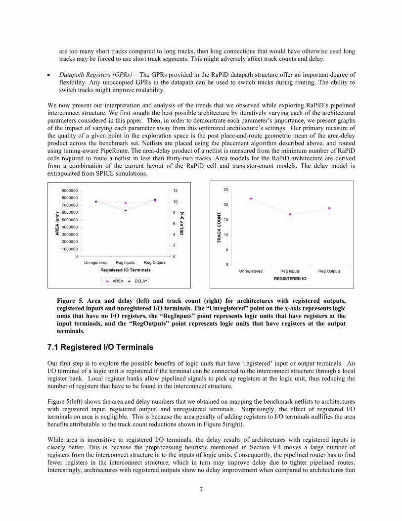
Figure 5. Area and delay (left) and track count (right) for architectures with registered outputs, registered inputs and unregistered I/O terminals. The “Unregistered” point on the x-axis represents logic units that have no I/O registers, the “RegInputs” point represents logic units that have registers at the input terminals, and the “RegOutputs” point represents logic units that have registers at the output terminals.

7.1 Registered I/O Terminals

Our first step is to explore the possible benefits of logic units that have ‘registered’ input or output terminals. An I/O terminal of a logic unit is registered if the terminal can be connected to the interconnect structure through a local register bank. Local register banks allow pipelined signals to pick up registers at the logic unit, thus reducing the number of registers that have to be found in the interconnect structure.

Figure 5(left) shows the area and delay numbers that we obtained on mapping the benchmark netlists to architectures with registered input, registered output, and unregistered terminals. Surprisingly, the effect of registered I/O terminals on area is negligible. This is because the area penalty of adding registers to I/O terminals nullifies the area benefits attributable to the track count reductions shown in Figure 5(right).

While area is insensitive to registered I/O terminals, the delay results of architectures with registered inputs is clearly better. This is because the preprocessing heuristic mentioned in Section 9.4 moves a large number of registers from the interconnect structure in to the inputs of logic units. Consequently, the pipelined router has to find fewer registers in the interconnect structure, which in turn may improve delay due to tighter pipelined routes. Interestingly, architectures with registered outputs show no delay improvement when compared to architectures that

8

have unregistered I/O. This is probably because the number of interconnect registers that are moved in to the outputs of logic units is an insignificant fraction of the total number of interconnect registers that have to be found during pipelined routing. Overall, architectures with registered input terminals proved to be the best choice in terms of area-delay product.

7.2 Bus Connectors (BCs)

BCs serve as buffered registered switches in the RaPiD interconnect structure The total number of BCs in the interconnect structure plays a major role in determining the overall area and delay of a netlist mapped to the RaPiD architecture. Since a single BC may provide multiple registers, the number of BCs directly impacts the number of pipelining registers available in the interconnect structure.

GPR

GPR

RA

M

RA

M

MU

LT

AL

U

GPR

AL

U

GPR

GPR

RA

M

AL

U

GPR

G

PR

GPR

RA

M

RA

M

MU

LT

AL

U

GPR

AL

U

GPR

GPR

RA

M

AL

U

GPR

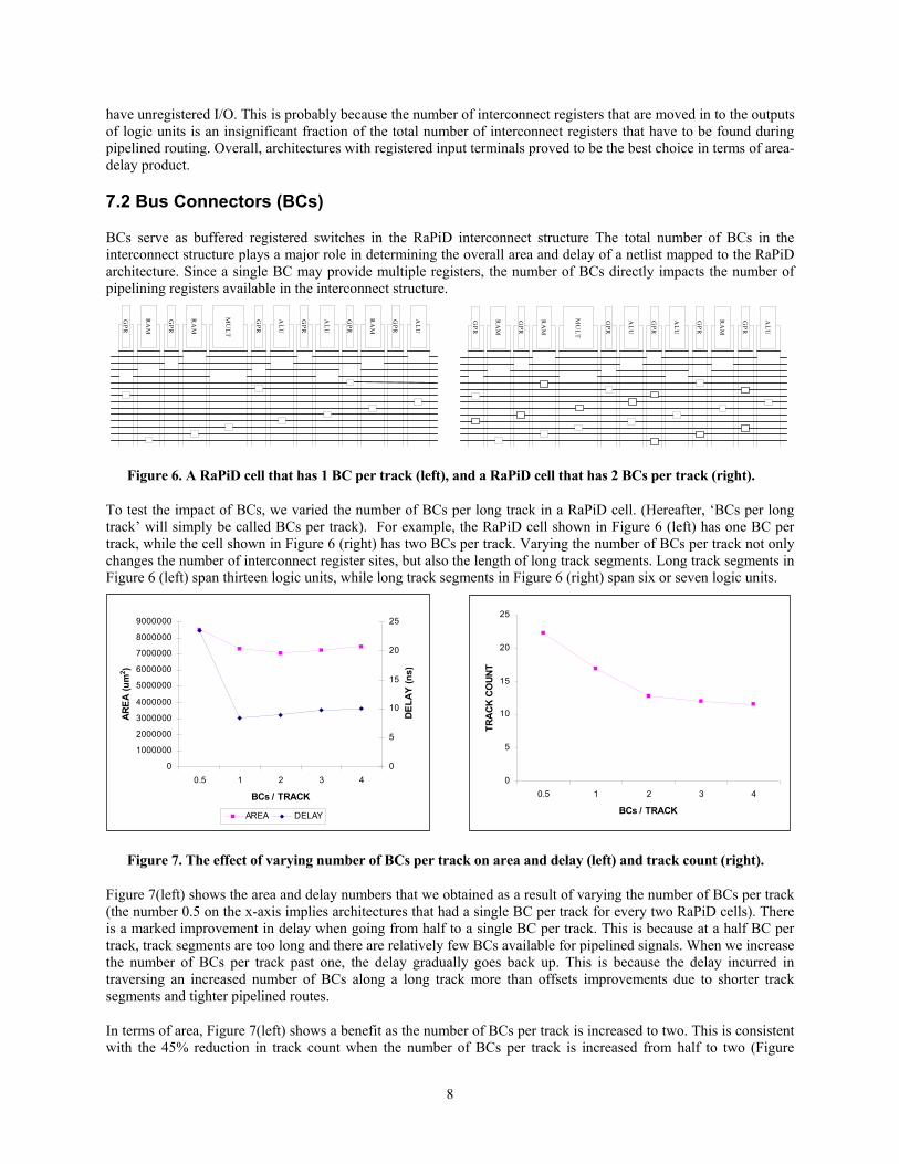
Figure 6. A RaPiD cell that has 1 BC per track (left), and a RaPiD cell that has 2 BCs per track (right).

To test the impact of BCs, we varied the number of BCs per long track in a RaPiD cell. (Hereafter, ‘BCs per long track’ will simply be called BCs per track). For example, the RaPiD cell shown in Figure 6 (left) has one BC per track, while the cell shown in Figure 6 (right) has two BCs per track. Varying the number of BCs per track not only changes the number of interconnect register sites, but also the length of long track segments. Long track segments in Figure 6 (left) span thirteen logic units, while long track segments in Figure 6 (right) span six or seven logic units.

0

1000000

2000000

3000000

4000000

5000000

6000000

7000000

8000000

9000000

0.5 1 2 3 4

BCs / TRACK

ARE

A (u

m2 )

0

5

10

15

20

25

DEL

AY (n

s)

AREA DELAY

0

5

10

15

20

25

0.5 1 2 3 4

BCs / TRACK

TRAC

K CO

UNT

Figure 7. The effect of varying number of BCs per track on area and delay (left) and track count (right).

Figure 7(left) shows the area and delay numbers that we obtained as a result of varying the number of BCs per track (the number 0.5 on the x-axis implies architectures that had a single BC per track for every two RaPiD cells). There is a marked improvement in delay when going from half to a single BC per track. This is because at a half BC per track, track segments are too long and there are relatively few BCs available for pipelined signals. When we increase the number of BCs per track past one, the delay gradually goes back up. This is because the delay incurred in traversing an increased number of BCs along a long track more than offsets improvements due to shorter track segments and tighter pipelined routes.

In terms of area, Figure 7(left) shows a benefit as the number of BCs per track is increased to two. This is consistent with the 45% reduction in track count when the number of BCs per track is increased from half to two (Figure

9

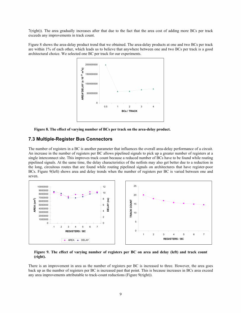
7(right)). The area gradually increases after that due to the fact that the area cost of adding more BCs per track exceeds any improvements in track count.

Figure 8 shows the area-delay product trend that we obtained. The area-delay products at one and two BCs per track are within 1% of each other, which leads us to believe that anywhere between one and two BCs per track is a good architectural choice. We selected one BC per track for our experiments.

0

50000000

100000000

150000000

200000000

0.5 1 2 3 4

BCs / TRACK

AREA

*DEL

AY (x

10 -2

1 m2 s)

Figure 8. The effect of varying number of BCs per track on the area-delay product.

7.3 Multiple-Register Bus Connectors

The number of registers in a BC is another parameter that influences the overall area-delay performance of a circuit. An increase in the number of registers per BC allows pipelined signals to pick up a greater number of registers at a single interconnect site. This improves track count because a reduced number of BCs have to be found while routing pipelined signals. At the same time, the delay characteristics of the netlists may also get better due to a reduction in the long, circuitous routes that are found while routing pipelined signals on architectures that have register-poor BCs. Figure 9(left) shows area and delay trends when the number of registers per BC is varied between one and seven.

0100000020000003000000400000050000006000000700000080000009000000

10000000

1 2 3 4 5 6 7

REGISTERS / BC

AREA

(um

2 )

0

2

4

6

8

10

12

DELA

Y (n

s)

AREA DELAY

0

5

10

15

20

25

1 2 3 4 5 6 7

REGISTERS / BC

TRAC

K CO

UNT

Figure 9. The effect of varying number of registers per BC on area and delay (left) and track count (right).

There is an improvement in area as the number of registers per BC is increased to three. However, the area goes back up as the number of registers per BC is increased past that point. This is because increases in BCs area exceed any area improvements attributable to track-count reductions (Figure 9(right)).

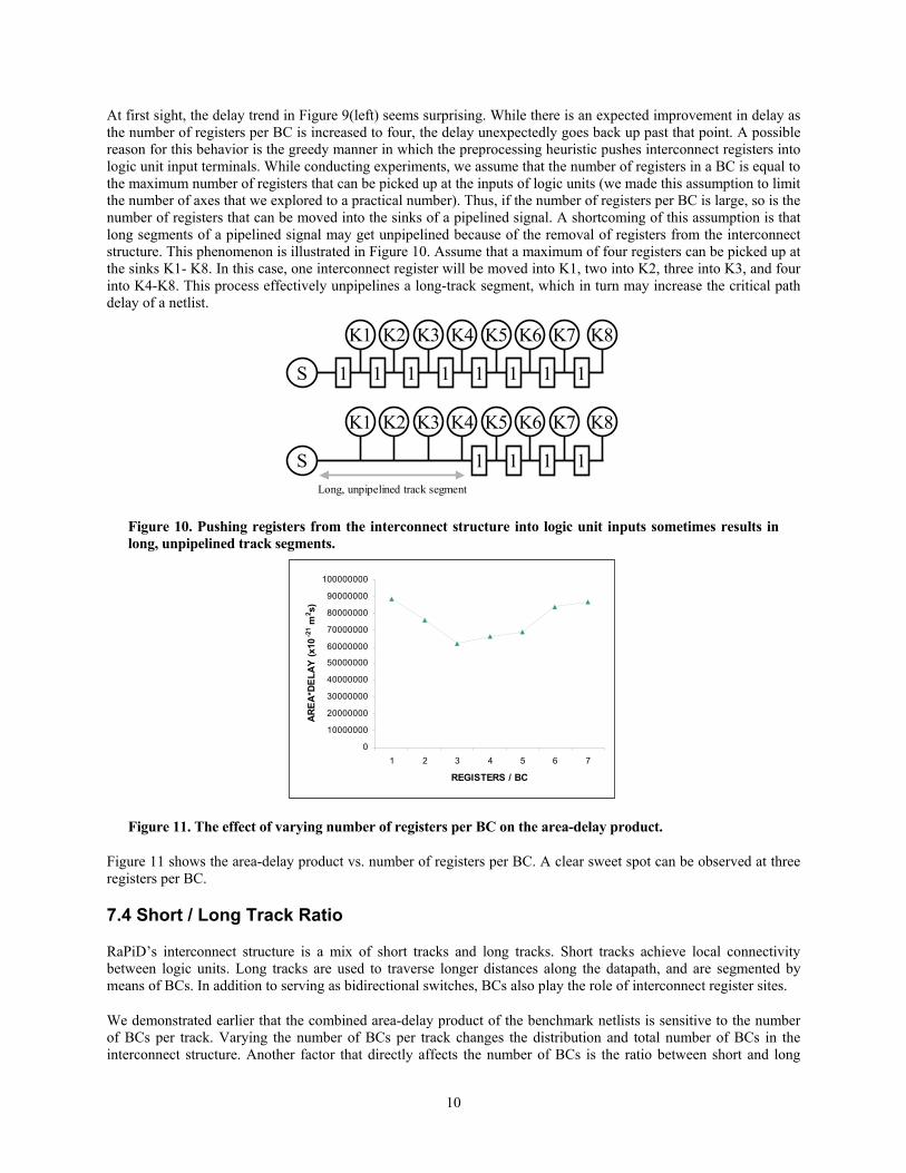
10

At first sight, the delay trend in Figure 9(left) seems surprising. While there is an expected improvement in delay as the number of registers per BC is increased to four, the delay unexpectedly goes back up past that point. A possible reason for this behavior is the greedy manner in which the preprocessing heuristic pushes interconnect registers into logic unit input terminals. While conducting experiments, we assume that the number of registers in a BC is equal to the maximum number of registers that can be picked up at the inputs of logic units (we made this assumption to limit the number of axes that we explored to a practical number). Thus, if the number of registers per BC is large, so is the number of registers that can be moved into the sinks of a pipelined signal. A shortcoming of this assumption is that long segments of a pipelined signal may get unpipelined because of the removal of registers from the interconnect structure. This phenomenon is illustrated in Figure 10. Assume that a maximum of four registers can be picked up at the sinks K1- K8. In this case, one interconnect register will be moved into K1, two into K2, three into K3, and four into K4-K8. This process effectively unpipelines a long-track segment, which in turn may increase the critical path delay of a netlist.

S 1 1 1 1 1 1 1 1

K1 K2 K3 K4 K5 K6 K7 K8

1 1 1 1

K1 K2 K3 K4 K5 K6 K7 K8

Long, unpipelined track segment

S

Figure 10. Pushing registers from the interconnect structure into logic unit inputs sometimes results in long, unpipelined track segments.

0

10000000

20000000

30000000

40000000

50000000

60000000

70000000

80000000

90000000

100000000

1 2 3 4 5 6 7

REGISTERS / BC

AREA

*DEL

AY (x

10 -2

1 m2 s)

Figure 11. The effect of varying number of registers per BC on the area-delay product.

Figure 11 shows the area-delay product vs. number of registers per BC. A clear sweet spot can be observed at three registers per BC.

7.4 Short / Long Track Ratio

RaPiD’s interconnect structure is a mix of short tracks and long tracks. Short tracks achieve local connectivity between logic units. Long tracks are used to traverse longer distances along the datapath, and are segmented by means of BCs. In addition to serving as bidirectional switches, BCs also play the role of interconnect register sites.

We demonstrated earlier that the combined area-delay product of the benchmark netlists is sensitive to the number of BCs per track. Varying the number of BCs per track changes the distribution and total number of BCs in the interconnect structure. Another factor that directly affects the number of BCs is the ratio between short and long

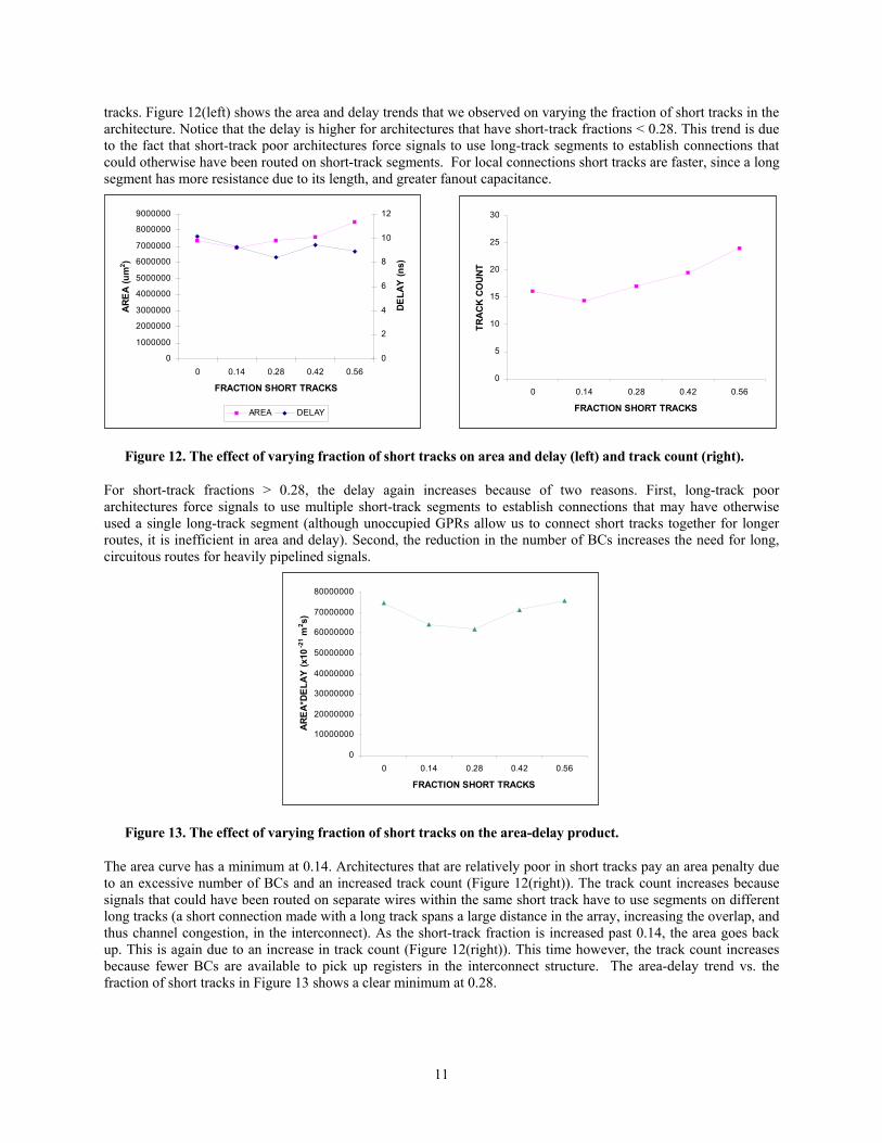
11

tracks. Figure 12(left) shows the area and delay trends that we observed on varying the fraction of short tracks in the architecture. Notice that the delay is higher for architectures that have short-track fractions < 0.28. This trend is due to the fact that short-track poor architectures force signals to use long-track segments to establish connections that could otherwise have been routed on short-track segments. For local connections short tracks are faster, since a long segment has more resistance due to its length, and greater fanout capacitance.

0

1000000

2000000

3000000

4000000

5000000

6000000

7000000

8000000

9000000

0 0.14 0.28 0.42 0.56

FRACTION SHORT TRACKS

ARE

A (u

m2 )

0

2

4

6

8

10

12

DELA

Y (n

s)AREA DELAY

0

5

10

15

20

25

30

0 0.14 0.28 0.42 0.56

FRACTION SHORT TRACKS

TRA

CK C

OUN

T

Figure 12. The effect of varying fraction of short tracks on area and delay (left) and track count (right).

For short-track fractions > 0.28, the delay again increases because of two reasons. First, long-track poor architectures force signals to use multiple short-track segments to establish connections that may have otherwise used a single long-track segment (although unoccupied GPRs allow us to connect short tracks together for longer routes, it is inefficient in area and delay). Second, the reduction in the number of BCs increases the need for long, circuitous routes for heavily pipelined signals.

0

10000000

20000000

30000000

40000000

50000000

60000000

70000000

80000000

0 0.14 0.28 0.42 0.56

FRACTION SHORT TRACKS

AREA

*DEL

AY (x

10 -2

1 m2 s)

Figure 13. The effect of varying fraction of short tracks on the area-delay product.

The area curve has a minimum at 0.14. Architectures that are relatively poor in short tracks pay an area penalty due to an excessive number of BCs and an increased track count (Figure 12(right)). The track count increases because signals that could have been routed on separate wires within the same short track have to use segments on different long tracks (a short connection made with a long track spans a large distance in the array, increasing the overlap, and thus channel congestion, in the interconnect). As the short-track fraction is increased past 0.14, the area goes back up. This is again due to an increase in track count (Figure 12(right)). This time however, the track count increases because fewer BCs are available to pick up registers in the interconnect structure. The area-delay trend vs. the fraction of short tracks in Figure 13 shows a clear minimum at 0.28.

12

0

1000000

2000000

3000000

4000000

5000000

6000000

7000000

8000000

5 6 7 8 9 10

GPRs / CELL

AREA

(um

2 )

0

2

4

6

8

10

12

DELA

Y (n

s)

AREA DELAY

0

5

10

15

20

25

5 6 7 8 9 10

GPRs / CELL

TRA

CK

CO

UNT

Figure 14. The effect of increasing the number of extra GPRs / RaPiD cell on area and delay (left) and track count (right).

7.5 Datapath Registers (GPRs)

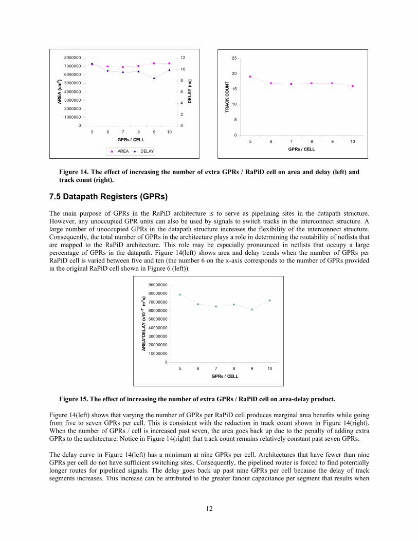
The main purpose of GPRs in the RaPiD architecture is to serve as pipelining sites in the datapath structure. However, any unoccupied GPR units can also be used by signals to switch tracks in the interconnect structure. A large number of unoccupied GPRs in the datapath structure increases the flexibility of the interconnect structure. Consequently, the total number of GPRs in the architecture plays a role in determining the routability of netlists that are mapped to the RaPiD architecture. This role may be especially pronounced in netlists that occupy a large percentage of GPRs in the datapath. Figure 14(left) shows area and delay trends when the number of GPRs per RaPiD cell is varied between five and ten (the number 6 on the x-axis corresponds to the number of GPRs provided in the original RaPiD cell shown in Figure 6 (left)).

0

10000000

20000000

30000000

40000000

50000000

60000000

70000000

80000000

90000000

5 6 7 8 9 10

GPRs / CELL

ARE

A*D

ELA

Y (x

10 -2

1 m2 s)

Figure 15. The effect of increasing the number of extra GPRs / RaPiD cell on area-delay product.

Figure 14(left) shows that varying the number of GPRs per RaPiD cell produces marginal area benefits while going from five to seven GPRs per cell. This is consistent with the reduction in track count shown in Figure 14(right). When the number of GPRs / cell is increased past seven, the area goes back up due to the penalty of adding extra GPRs to the architecture. Notice in Figure 14(right) that track count remains relatively constant past seven GPRs.

The delay curve in Figure 14(left) has a minimum at nine GPRs per cell. Architectures that have fewer than nine GPRs per cell do not have sufficient switching sites. Consequently, the pipelined router is forced to find potentially longer routes for pipelined signals. The delay goes back up past nine GPRs per cell because the delay of track segments increases. This increase can be attributed to the greater fanout capacitance per segment that results when

13

the number of GPRs per cell is increased. Figure 15 shows that the area-delay product is minimum for architectures that have nine GPRs per RaPiD cell.

7.6 Quantitative Evaluation

In this section we quantify the benefits of exploring RaPiD’s pipelined interconnect structure. The RaPiD cell in Figure 6 (left) has registered outputs, a single BC per track, three registers per BC and 28% short tracks.

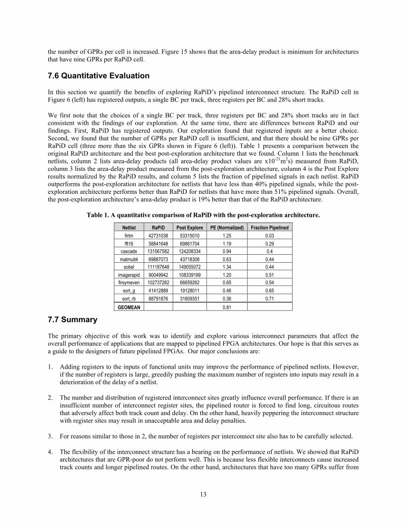
We first note that the choices of a single BC per track, three registers per BC and 28% short tracks are in fact consistent with the findings of our exploration. At the same time, there are differences between RaPiD and our findings. First, RaPiD has registered outputs. Our exploration found that registered inputs are a better choice. Second, we found that the number of GPRs per RaPiD cell is insufficient, and that there should be nine GPRs per RaPiD cell (three more than the six GPRs shown in Figure 6 (left)). Table 1 presents a comparison between the original RaPiD architecture and the best post-exploration architecture that we found. Column 1 lists the benchmark netlists, column 2 lists area-delay products (all area-delay product values are x10-21m2s) measured from RaPiD, column 3 lists the area-delay product measured from the post-exploration architecture, column 4 is the Post Explore results normalized by the RaPiD results, and column 5 lists the fraction of pipelined signals in each netlist. RaPiD outperforms the post-exploration architecture for netlists that have less than 40% pipelined signals, while the post-exploration architecture performs better than RaPiD for netlists that have more than 51% pipelined signals. Overall, the post-exploration architecture’s area-delay product is 19% better than that of the RaPiD architecture.

Table 1. A quantitative comparison of RaPiD with the post-exploration architecture.

Netlist RaPiD Post Explore PE (Normalized) Fraction Pipelined firtm 42731038 53315010 1.25 0.03 fft16 58841648 69861704 1.19 0.29

cascade 131567582 124208334 0.94 0.4 matmult4 69887073 43718308 0.63 0.44

sobel 111187648 149055072 1.34 0.44 imagerapid 90049942 108339199 1.20 0.51 firsymeven 102737262 66659262 0.65 0.54

sort_g 41412889 19128011 0.46 0.65 sort_rb 88791876 31809351 0.36 0.71

GEOMEAN 0.81

7.7 Summary

The primary objective of this work was to identify and explore various interconnect parameters that affect the overall performance of applications that are mapped to pipelined FPGA architectures. Our hope is that this serves as a guide to the designers of future pipelined FPGAs. Our major conclusions are:

1. Adding registers to the inputs of functional units may improve the performance of pipelined netlists. However, if the number of registers is large, greedily pushing the maximum number of registers into inputs may result in a deterioration of the delay of a netlist.

2. The number and distribution of registered interconnect sites greatly influence overall performance. If there is an insufficient number of interconnect register sites, the pipelined router is forced to find long, circuitous routes that adversely affect both track count and delay. On the other hand, heavily peppering the interconnect structure with register sites may result in unacceptable area and delay penalties.

3. For reasons similar to those in 2, the number of registers per interconnect site also has to be carefully selected.

4. The flexibility of the interconnect structure has a bearing on the performance of netlists. We showed that RaPiD architectures that are GPR-poor do not perform well. This is because less flexible interconnects cause increased track counts and longer pipelined routes. On the other hand, architectures that have too many GPRs suffer from

14

an excessive area-penalty. Although GPRs are RaPiD-specific, many other FPGAs have interconnect structures called “track graphs” which limit the ability of a signal to switch tracks. In a pipelined interconnect track graph structures may be more problematic than in standard FPGAs because of the added requirements on the interconnect.

There are several open questions left in pipelined FPGA development. First, although we have developed an efficient router for pipelined FPGAs, the timing optimization within this router is greedy and simplistic. Algorithms that more effectively incorporate timing into the router may provide a significant improvement. Second, current pipelined FPGA architectures generally pay a significant penalty for providing those pipelining resources, particularly when implementing unpipelined circuits. For example, some architectures radically increase the area and latency of mappings in order to support heavy pipelining. An architectural and CAD approach that provides high-quality unpipelined implementations, yet can sacrifice area to support pipelining, may be more practical. For example, one early work [Herzen97] used commodity FPGAs to achieve very high performance (for the time) by using only a small portion of the logic blocks for computation; other unused locations were used as pipelining registers only. This approach, where only the beneficiaries of heavy pipelining pay a significant area penalty, may be the most commercially viable approach to high-performance computing on FPGAs. In much the same vein, it would be useful to explore the area and delay performance of island-style, pipelined FPGA architectures.

8. Acknowledgements

We would like to thank Chris Fisher for providing us with a set of benchmark netlists. Thanks are also due to Ken Eguro and Shawn Phillips for the area and delay models. This work was supported by grants from the NSF. Scott Hauck was supported in part by an NSF Career Award and an Alfred P. Sloan Fellowship.

References [Betz99] V. Betz and J. Rose, “FPGA Routing Architecture: Segmentation and Buffering to Optimize

Speed and Density”, ACM/SIGDA Seventh International Symposium on Field-Programmable Gate Arrays, pp 59-68, 1999.

[Betz99a] V. Betz and J. Rose, “Circuit Design, Transistor Sizing and Wire Layout of FPGA Interconnect”, IEEE Custom Integrated Circuits Conference, pp 171 - 174, 1999.

[Compton02] K. Compton, S. Hauck, “Reconfigurable Computing: A Survey of Systems and Software”, ACM Computing Surveys, Vol. 34, No. 2, pp. 171-210. June 2002.

[Compton03] K. Compton, Architecture Generation of Customized Reconfigurable Hardware, Ph.D. Thesis, Northwestern University, Dept. of ECE, 2003.

[Cronquist99] D. C. Cronquist, P. Franklin, C. Fisher, M. Figueroa, C. Ebeling, "Architecture Design of Reconfigurable Pipelined Datapaths", Conference on Advanced Research in VLSI, pp. 23-40, 1999.

[Cronquist99a] Darren C. Cronquist, Paul Franklin, Stefan Berg, Carl Ebeling, “Specifying and Compiling Applications to RaPiD”, Field-Programmable Custom Computing Machines, 1999.

[Ebeling96] C. Ebeling, D. C. Cronquist, P. Franklin, "RaPiD - Reconfigurable Pipelined Datapath", International Workshop on Field-Programmable Logic and Applications, pp. 126-135, 1996.

[Goldstein00] S. C. Goldstein, H. Schmit, M. Budiu, S. Cadambi, M. Moe, R. R. Taylor, "PipeRench: A Reconfigurable Architecture and Compiler”, IEEE Computer, Vol. 33, No. 4, pp. 70-77, April, 2000.

15

[Hauck98] S. Hauck, “The Roles of FPGAs in Reprogrammable Systems”, Proceedings of the IEEE, Vol. 86, No. 4, pp. 615-639, April 1998.

[Herzen97] B. Von Herzen, “Signal Processing at 250MHz using High-Performance FPGA’s”, ACM International Symposium on FPGAs, pp. 62-68, 1997.

[Leiserson91] C. E. Leiserson, J. B. Saxe, “Retiming Synchronous Circuitry”, Algorithmica, Vol. 6, pp. 5-35, 1991.

[Marshall98] A. Marshall, “A Reconfigurable Computing Architecture for the Masses”, Configurable Computing Workshop, 1998.

[Marshall99] A. Marshall, T. Stansfield, I. Kostarnov, J. Vuillemin, B. Hutchings, “A Reconfigurable Arithmetic Array for Multimedia Applications”, ACM International Symposium on FPGAs, pp. 135-143, 1999.

[McMurchie95] L. McMurchie, C. Ebeling, “PathFinder: A Negotiation-Based Performance-Driven Router for FPGAs”, ACM International Symposium on Field-Programmable Gate Arrays, pp 111-117, 1995.

[Papaefthymiou91] M. C. Papaefthymiou, “Understanding Retiming through Maximum Average-Weight Cycles”, ACM Symposium on Parallel Algorithms and Architectures, pp. 338-348, 1991.

[Schmit97] H. Schmit, "Incremental Reconfiguration for Pipelined Applications", IEEE Symposium on FPGAs for Custom Computing Machines, pp. 47-55, 1997.

[Sechen88] C. Sechen, VLSI Placement and Global Routing Using Simulated Annealing, Kluwer Academic Publishers, Boston, MA: 1988.

[Sharma01] A. Sharma, Development of a Place and Route Tool for the RaPiD Architecture, Master’s Thesis, University of Washington, Dept. of EE, 2001.

[Sharma03] A. Sharma, C. Ebeling, S. Hauck, “PipeRoute: A Pipelining-Aware Router for FPGAs”, ACM/SIGDA Symposium on Field-Programmable Gate Arrays, pp. 68-77, 2003.

[Sharma05] A. Sharma, Place and Route Techniques for FPGA Architecture Advancement, Ph.D. Thesis, University of Washington, Dept. of EE, 2005.

[Singh01] A. Singh, A. Mukherjee, M. Marek-Sadowska, “Interconnect Pipelining in a Throughput-Intensive FPGA Architecture”, ACM International Symposium on FPGAs, pp. 153-160, 2001.

[Singh01a] D. P. Singh, S. D. Brown, “The Case for Registered Routing Switches in Field Programmable Gate Arrays”, ACM International Symposium on FPGAs, pp. 161-169, 2001.

[Singh02] D. P. Singh, S. D. Brown, “Integrated Retiming and Placement for Field Programmable Gate Arrays”, ACM International Symposium on FPGAs, pp. 67-76, 2002.

[Singh02a] D. P. Singh, S. D. Brown, “Constrained Clock Shifting for Field Programmable Gate Arrays”, ACM International Symposium on FPGAs, pp. 121-126, 2002.

[Tsu99] W. Tsu, K. Macy, A. Joshi, R. Huang, N. Walker, T. Tung, O. Rowhani, V. George, J. Wawrzynek, A. DeHon, “HSRA: High-Speed, Hierarchical Synchronous Reconfigurable Array”, ACM International Symposium on FPGAs, pp. 125-134, 1999.

16

[Weaver03] N. Weaver, Y. Markovskiy, Y. Patel, J. Wawrzynek, “Post-Placement C-slow Retiming for the Xilinx Virtex FPGA”, ACM International Symposium on FPGAs, pp. 185-194, 2003.