Fast approximate computation of a time-harmonic scattered field using the on-surface radiation condition method

IMA Journal of Applied Mathematics (2001) 66, 83–110

Fast approximate computation of a time-harmonic scatteredfield using the on-surface radiation condition method

XAVIER ANTOINE†

Laboratoire de Mathematiques pour l’Industrie et la Physique, MIP CNRSUMR 5640, Universite P. Sabatier, Toulouse III, Complexe Scientifique de Rangueil,

118 route de Narbonne, 31062 Toulouse Cedex 4, France

[Received 27 November 1998 and in revised form 20 March 2000]

The numerical study of the on-surface radiation condition method applied to two- andthree-dimensional time-harmonic scattering problems is examined. This approach allowsus to quickly compute an approximate solution to the initial exact boundary-value problem.A general background for the numerical treatment of arbitrary convex-shaped objectsis stated. New efficient on-surface radiation conditions leading in a natural way to asymmetrical boundary variational formulation are introduced. The approximation is basedupon boundary finite-element methods. Moreover, this study requires a specific numericaltreatment of the curvature operator. To this end, a numerical procedure using some resultsabout the theory of local approximation of surfaces is described. Finally, the effectivenessand generality of the approach is numerically tested for several scatterers.

Keywords: scattering; Helmholtz equation; surface radiation condition; boundary finiteelement method; curvature operator approximation; radar cross-section.

1. Introduction

We investigate the development of a reliable and fast computational method called the on-surface radiation condition method to compute an approximate solution to the scatteringproblem of a time-harmonic electromagnetic or acoustic field by an obstacle. It is wellknown that these problems require the solution of a boundary-value problem in an openregion (Bowman et al., 1969; Chen & Zhou, 1992; Jin, 1993). Clearly, the unboundedcharacteristic of the domain is in conflict with the usual finite computational domaininvolved in numerical methods like finite-difference or finite-element methods (Ciarlet,1991; Jin, 1993). Therefore, an efficient process must be introduced to reduce the initialexterior problem to a boundary-value problem well-posed in a bounded domain.

Among the most widely used approaches are the boundary integral equation methods(BIEM) (Antoine, 1997; Chen & Zhou, 1992). The main idea of their derivation lies inthe writing of an equivalent field integral equation posed on the finite boundary of thescatterer. The robustness and efficiency of this class of methods for far-field calculationsis now proved. The equations arising in the formulations of such approaches involvenon-local pseudodifferential operators. The non-local particularity of these operators isin contrast with the local property of finite-difference or finite-element methods. From acomputational viewpoint, this implies that the resulting linear system involves a full matrix

†E-mail: [email protected]

c© Oxford University Press 2001

84 X. ANTOINE

and not the broadly sparse one met, for example, in finite-element methods. As a result,huge memory storage and an expensive use of CPU time is required to compute the solutionof the diffraction problem. This limits the ability to treat high-frequency problems and/orthree-dimensional problems.

A second approach consists of introducing a fictitious boundary enclosing the scattererwhich has to be endowed with an exact transparent boundary condition. Such a condition,usually called non-reflecting in scattering problems, may be implicitly defined by the so-called Dirichlet-to-Neumann (DtN) non-local pseudodifferential operator (Antoine, 1997;Antoine et al., 1999; Bielak et al., 1997; Givoli et al., 1997; Halpern & Rauch, 1995).The resulting mixed bounded problem is then equivalent to the initial exterior boundary-value problem. Unfortunately, the discretization schemes associated to the non-local DtNoperator generally yield non-sparse systems (Givoli et al., 1997). Furthermore, we wishto have a fictitious boundary as ‘close’ as possible to the scatterer to minimize the sizeof the computational bounded domain. This problem is closely related to the design ofappropriate local conditions. To overcome these difficulties, one usually introduces localapproximations of the DtN operator which are often called absorbing boundary conditionsor radiation conditions at infinity. This viewpoint has been initiated by the work of Engquist& Majda (1977). Many authors have afterwards generalized the latter approach or adoptedother methods to obtain efficient conditions. We refer to Antoine (1997), Antoine et al.(1999), Bayliss et al. (1982), Bayliss & Turkel (1980), Bielak et al. (1997), Jones (1988),Mittra & Ramahi (1990), Moore et al. (1988), Senior & Volakis (1995), Senior et al. (1997)and references therein for further details. Despite the efficiency of the radiation conditionmethods, limitations are still generated by the size of the data. Hence, the conception andstudy of fast and cheap approximate computational methods is justified.

The on-surface radiation condition (OSRC) method presents an interesting alternativeto both BIEM and radiation condition methods. This method was introduced byKriegsmann et al. (1987) for the radar cross-section calculations in two-dimensionalelectromagnetic wave scattering. Many authors have extended its application range to otherproblems, see, for example (Ammari, 1998; Janaswamy, 1991; Jin, 1993; Jones, 1988,1992; Jones & Kriegsmann, 1990; Moore et al., 1988; Murch, 1993). The principle of thisapproach is based on the determination of an approximation of the Cauchy data; in otherwords, of the two first-traces of the scattering problem solution, through a local relationon the boundary of the scatterer. To derive local relations, Kriegsmann et al. use radiationconditions at infinity which are directly imposed on the scatterer’s surface following anheuristic process. The conditions obtained are called on-surface radiation conditions. Froma computational point of view, the approximate problem leads to the calculation of thesolution of a differential equation on the boundary of the scatterer which can be computedquickly. As a consequence, the OSRC solution can be seen as a good approximation to thescattered field and should be useful in iterative algorithms. In particular, we think that theOSRC method provides an accurate ‘initial guess’ well-suited to fast multipole methods.

Therefore, the OSRC method can be seen as an approach combining two interestingaspects of BIEM and radiation conditions methods, that is,

• solving a problem which is, as in BIEM, reduced to the computation of an equation onthe boundary of the scatterer,

• inversing only a differential operator (and not a non-local one as in BIEM).

COMPUTATIONAL SCATTERING BY THE OSRC METHOD 85

The aim of this work is to show how a general approach to the OSRC method fortwo- and three-dimensional scattering problems can be stated involving suitable boundaryfinite-element methods. Moreover, we give new on-surface radiation conditions that aremore accurate than those in current use.

After a brief statement of the problem in Section 2, we recall the integral representationof the radar cross-section given from the Cauchy data. This property leads to severalnumerical methods and in particular to the OSRC method which is studied in Section 3for two-dimensional electromagnetic field computations. A review of the principle anddesign of the most commonly used OSRC is described following the Kriegsmann et al.heuristic procedure for convex obstacles. To our knowledge, previous numerical studies ofOSRC methods are always based upon the construction of approximations for canonicalobstacles and explicitly known geometries, see, for example (Ammari, 1998; Janaswamy,1991; Jin, 1993; Jones & Kriegsmann, 1990; Kriegsmann et al., 1987). These limitations tothe method of simple geometrical configurations motivate the search for a general approachfor convex scatterers with arbitrarily-shaped boundaries. Thus, we propose a variationalformulation of the OSRC problem. Next, we approximate it using a boundary finite-element method. To take into account general boundaries, we recall an approximationprocess to the curvature at the degrees of freedom of the surface finite-element mesh.Illustrative numerical examples validate our approach. We next introduce new on-surfaceradiation conditions incorporating the curvature variation effects. We test them for differentconvex geometries and conclude that they improve the numerical accuracy of the method.Finally, several limitations of OSRC methods are recorded.

Whereas numerous papers deal with the OSRC method for two-dimensional scattering,the three-dimensional case has given rise to only a few theoretical and numerical works.Jones (1988, 1992) and Teymur (1996) study scattering from the sphere with impedanceconditions, Murch (1993) and Roxburgh (1997) for perfectly conducting bodies ofrevolution and Kriegsmann & Moore (1988) for the scattering of acoustic waves by areactively loaded sphere. We present in Section 4 the unconventional extension of ourapproach to three-dimensional acoustic problems. We begin by recalling new accuratesecond-order on-surface radiation conditions derived in some previous works (Antoine,1997; Antoine et al., 1999). These OSRC are then written variationally. The associatedboundary finite-element methods are introduced next. This allows us to focus on the twomain new difficulties arising in the three-dimensional case. First, we derive an efficientscheme to approximate the curvature operator at the points of the finite-element mesh. Asecond difficulty is related to the implementation of the approximate curvature operator inthe finite-element context. This leads us to describe the elementary contribution comingfrom each triangular element involved in the assembly process of the finite-elementmethod. Finally, several illustrative examples bear out the efficiency of our approach.This study demonstrates that the OSRC approximate solution might be a very useful toolto reduce the computational cost of more efficient but at the same time more expensivemethods like, for example, BIEM.

2. The model problem

Let Ω− be an obstacle, that is, Ω− is a C∞ compact manifold of the N -dimensional spaceR

N (N = 2, 3) with Γ = ∂Ω− as a closed boundary; we define Ω+ to be the unbounded

86 X. ANTOINE

n

x

k

−

+

x

x

1

2

3

ϕθ

γ

FIG. 1. Scattering from a three-dimensional object surrounded by a fluid.

space of propagation that is the complementary set of Ω− in RN (see Fig. 1). We consider

a time-harmonic incident (plane) wave u inc. The wave number in the surrounding mediumΩ+ is k. The exterior boundary-value problem governing the scattering problem of u inc byΩ− is stated as follows: find the diffracted field u solution to the Helmholtz equation in theunbounded domain Ω+

∆u + k2u = 0, in Ω+, (2.1)

satisfying a non-homogeneous Dirichlet or Neumann boundary condition

u = −u inc = g or ∂nu = −∂nu inc = g, on Γ . (2.2)

The Sommerfeld radiation condition at infinity (Chen & Zhou, 1992) is added to selectthe physical outgoing solution to (2.1) and (2.2), that is, to ensure the uniqueness of thesolution to the exterior boundary-value problem. In the previous equations, we denoteby ∆ = ∑N

i=1 ∂2xi

the Laplacian operator, where x = t (x1, . . . , xN ) is the spacevariable. The vector n is the outwardly directed unit normal to Γ . The two-dimensionalproblem is generated by a transverse magnetic (TM) or transverse electric (TE) polarizedincident wave for the time-harmonic Maxwell system illuminating a perfectly conductingcylinder (Jin, 1993). The Dirichlet (resp. Neumann) boundary-value problem is connectedto the TM (resp. TE) case. The three-dimensional case is related to acoustics (Bowmanet al., 1969). The Dirichlet (resp. Neumann) boundary condition is usually referred asthe sound-soft (resp. sound-hard) obstacle problem.

We are interested in the computation of the radiated wave in the far-field zone. Thebehaviour of the scattered field for an incident plane wave u inc is generally described by theradar cross-section (RCS) (Bowman et al., 1969). More precisely, in the two-dimensional


case, we define the RCS (in decibels) by

RCS(θ) = 10 log10(2π |a0(θ)|2) (db),

where (r, θ) stands for the polar coordinate system. The asymptotic behaviour of thescattered field gives (Bowman et al., 1969) the r -independant scattering amplitude a0(θ)

in the direction θ as

a0(θ) = exp(−iπ/4)

(8πk)1/2

∫Γ

∂n(y)u(y) − ikθ · n(y)u(y)

exp(−ikθ · y) dΓ (y), (2.3)

where θ = t (cos θ, sin θ). For the three-dimensional case, we compute the RCS (Bowmanet al., 1969)

RCS(θ) = 10 log10(4π |a0(θ)|2) (db),

a0(θ) = 1

4π

∫Γ

∂n(y)u(y) − ikθ · n(y)u(y)

exp(−ikθ · y) dΓ (y).

(2.4)

In the above equation, we set a0(θ) as the scattering amplitude of the radiated fieldfollowing the θ = t (cos θ cos ϕ, sin θ cos ϕ, sin ϕ) diffusion direction. We denote by(r, θ, ϕ) the spherical coordinates system.

3. The on-surface radiation condition method for two-dimensional electromagneticfield computations

Clearly, (2.3) and (2.4) show that the RCS can be determined in terms of the Cauchy data(u|Γ , ∂nu|Γ ). The OSRC method (Kriegsmann et al., 1987) is based on the determinationof the two a priori unknowns u|Γ and ∂nu|Γ through the exact non-local operator Λ linkingthe Cauchy data, the so-called Dirichlet-to-Neumann (DtN) operator, cf. (Antoine, 1997;Antoine et al., 1999; Halpern & Rauch, 1995). Combined with the boundary condition,the DtN operator allows us to reduce the boundary-value problem (2.1) and (2.2) to thefollowing system: find the Cauchy data (u|Γ , ∂nu|Γ ) such that

u = g or ∂nu = g and ∂nu = Λu on Γ . (3.1)

Nevertheless, the DtN operator is non-local in space. From a numerical viewpoint, thecomputation of (3.1) leads to the inversion of a full linear system. To reduce thiscomputational cost, Kriegsmann et al. use a local approximation to the DtN operatorby the introduction of a differential operator. To this end, radiation conditions at infinityare directly imposed on the scatterer’s surface. The resulting local approximate equationlinking u|Γ and ∂nu|Γ is called an OSRC.

3.1 On-surface radiation conditions for the two-dimensional Helmholtz equation

3.1.1 The Kriegsmann, Taflove and Umashankar principle for the design of OSRC. Werecall briefly the derivation of the most classical radiation conditions given in the literatureand the associated OSRC following the Kriegsmann et al. method. We refer to Mittra &

88 X. ANTOINE

Ramahi (1990), Moore et al. (1988), Senior & Volakis (1995), Senior et al. (1997) for anextended survey of radiation boundary conditions.

The first radiation conditions considered have been derived by Engquist & Majda(1977) for a circular boundary using the theory of pseudodifferential operators. The firstcondition is given by the following relation:

∂r u − iku + 1

2Ru = 0, on CR, (3.2)

and the second one by

∂r u − iku + 1

2Ru +

(1

2ik− 1

2k2 R

)1

R2∂2θ u = 0, on CR, (3.3)

where CR is the circular boundary of radius R centred at the origin. Althrough condition(3.3) seems to be more accurate than (3.2), each of them is a first-order condition (Antoine,1997). Indeed, generally speaking, a condition given by an operator P is said to be oforder l (see, for example, Antoine et al., 1999; Bayliss & Turkel, 1980) if the followingapproximation holds: Pu = O(R−1/2−2l) on CR . It can be shown (Antoine, 1997) using,for example, the approach of Mittra & Ramahi (1990) that each of these conditions satisfiesan estimation Pu = O(R−5/2), and hence, gives rise to a first-order condition.

The applicability of such conditions is restricted to circular boundaries. To extend themto arbitrary-shaped objects, Kriegsmann et al. propose the following formal substitutions:

∂r → ∂n, R−1 → κ(s), R−2∂2θ → ∂2

s . (3.4)

The variable s is the arc-length measured along the curve Γ . The curvature of Γ at s is κ(s).The symbol → designates the transport of operators for CR to the associated operators onΓ . The use of the radiation condition directly on the scatterer’s surface implies that theOSRC approach is restricted to convex-shaped objects.

Substitutions (3.4) yield the two on-surface radiation conditions

∂nu − iku + 12κu = 0, on Γ , (3.5)

and

∂nu − iku + κ

2u +

(1

2ik− κ

2k2

)∂2

s u = 0, on Γ . (3.6)

A second-order OSRC coming from the Bayliss et al. radiation condition can be stated as

∂nu − iku + κ

2u − κ2

8(κ − ik)u − 1

2(κ − ik)∂2

s u = 0, on Γ . (3.7)

Another second-order condition has been devised by Mittra & Ramahi (1990):

∂nu − iku + κ

2u + κ2

8iku − κ3

8k2u +

(1

2ik− κ

2k2

)∂2

s u = 0, on Γ . (3.8)

Hereafter, we will call EM1 (resp. EM2, BGT and MR) condition (3.5) (resp. conditions(3.6), (3.7) and (3.8)).


3.1.2 Jones’s on-surface radiation condition. It seems quite natural that the efficiencyof an OSRC is directly linked to the method of incorporating geometrical information.Hence, an improvement of the on-surface radiation condition method should be obtainedtaking into account the curvature variation ∂sκ . As far as we know, only Jones (1988)considers this point of view constructing some OSRC by the WKB method. The second-order radiation boundary condition is then stated as

∂nu − iku + κ

2u − κ2

8(κ − ik)u − 1

2(κ − ik)∂2

s u + i

2k(κ − ik)

(∂2

s κ

4u + ∂sκ∂su

)= 0,

on Γ . (3.9)

3.2 Computational aspects

To the best of our knowledge, numerical approaches developed in the literature (see, forexample, Ammari, 1998; Janaswamy, 1991; Jones & Kriegsmann, 1990; Kriegsmann etal., 1987) to solve an OSRC problem are elaborated for some canonical geometries suchas a circular cylinder, an elliptical surface, etc. Here, we adopt a finite-element methodviewpoint to approximate the solution for an arbitrarily-shaped object. To this end, weformulate the OSRC in a variational way. Denoting conditions (3.5)–(3.9) as

γ ∂nu = −∂2s u + α∂su + βu, on Γ ,

we conclude that a weak formulation is: find (u|Γ , ∂nu|Γ ) satisfying

∫Γ

∂su∂sv + α∂suv + βuv dΓ =∫Γ

γ ∂nuv dΓ , (3.10)

for every test function v in an appropriate space (Antoine, 1997).

REMARK Formulation (3.10) is symmetrical except in the case of Jones’s condition (3.9).

Let us consider a Dirichlet boundary-value problem (TM polarization case). Then,formulation (3.10) can be reduced to the problem: find the normal derivative ∂nu|Γsatisfying the equation

∫Γ

γ ∂nuv dΓ =∫Γ

∂s g∂sv + α∂s gv + βgv dΓ , (3.11)

for every test function v. For a Neumann boundary condition (TE polarization case), wehave to solve the integral formulation: determine u|Γ such that

∫Γ

∂su∂sv + α∂suv + βuv dΓ =∫Γ

γ gv dΓ . (3.12)

The numerical solution to (3.11) and (3.12) is computed by a one-dimensional finite-element method. The first step consists in the approximation of the curve Γ by anapproximate polygonal boundary Γh . We denote by Th = ∪M

j=1 K j the disjoint union ofsegments K j which is assumed to satisfy a uniform regularity condition (Ciarlet, 1991).

90 X. ANTOINE

Next, a choice of the boundary finite-element space has to be made to compute the Cauchydata (uh|Γh , ∂nh uh|Γh ) on Γh . Let us define the two spaces

Mh = ψh ∈ L2(Γh) ; ψK = ψh|K ∈ P0, ∀K ∈ Th (3.13)

and

Vh = ψh ∈ C0(Γh) ; ψK = ψh|K ∈ P1, ∀K ∈ Th, (3.14)

where Pm designates the space of polynomials of degree m. In the sequel, we refer to(Chazarain & Piriou, 1982) for the definition of the different functional spaces. Then, anatural approximation of (uh|Γh , ∂nuh|Γh ) is searched for Vh × Mh and approximate testfunctions are in Vh . The solution to the Dirichlet boundary-value problem leads to thediscrete formulation: find ∂nh uh|Γh in Mh such that

∫Γh

γh∂nh uhvh dΓh =∫Γh

∂s gh∂svh + αh∂s ghvh + βh ghvh dΓh, (3.15)

where gh and vh are the Vh-approximates of g and v. From a matricial point of view,it is equivalent to compute the approximate normal trace ∂nh uh|Γh given by: Ah gh|Γh =∂nh uh|Γh , where Ah is the M × M sparse matrix with 3N non-null coefficients comingfrom formulation (3.15). So, the solution to the Dirichlet problem amounts to calculatingthe product of an M × M sparse matrix Ah by a vector gh|Γh . Let us now consider aNeumann condition. Then, we compute uh in Vh a solution to the discrete equation∫

Γh

∂suh∂svh + αh∂suhvh + βhuhvh dΓh =∫Γh

γh ghvh dΓh, (3.16)

where the test-function vh is in Vh and the datum gh is the Mh approximation of g. So, thecomputation of uh is given by the inversion of an M × M sparse linear system defined byAh . The interesting property of matrix Ah of being sparse directly results from the localcharacter of an on-surface radiation condition. This is a decisive advantage of the OSRCmethod on boundary integral equation methods. Indeed, usual BIEMs for a Dirichlet orNeumann problem require the inversion of an M×M non-sparse symmetrical linear system(Antoine, 1997; Chen & Zhou, 1992). Using higher-order finite elements does not increasethe accuracy of the OSRC method since the main discrepancy of the approximation isdue to the localization of the DtN pseudodifferential operator by a differential operator(Antoine, 1997; Antoine et al., 1999). We must impose the meshsize h λ/10 to achievethe maximal accuracy, where λ = 2π/k is the wavelength. In terms of CPU time, thecomputation of the approximate solution with the OSRC method is approximately onehundred time less expensive than with the BIEM, especially as k grows larger.

To consider general convex-shaped objects, we have to describe an approximation ofthe curvature κ at the meshpoints with only the knowledge of the finite-element mesh. Tothis end, we use the following result (Goldberg, 1991; Spivak, 1979).

PROPOSITION 3.1 Let K = (ABC) be a triangle with any vertex A, B or C on Γh ; then,the curvature can be approximated at point B by

κ(B) 4 area(K )

abc.


Real numbers a, b and c are the different side lengths of K satisfying a b c. The areaof K is evaluated by the formula

area(K ) = ((a + (b + c))(a + (b − c))(c + (a − b))(c − (a − b)))1/2/4.

In the case of polygonal scatterers like the square cylinder, the numerical curvatureeffect reproduces in a heuristic way scattering coming from the corners (Antoine, 1997).

REMARK In the case of a TM polarized wave, the normal derivative of the scatteredfield is given from the knowledge of its trace on Γ . So, this and the Helmholtz integralrepresentation of the exterior field directly yields an approximation of the exterior fieldin Ω+. Hence, a suitable approximation of the resulting integral equation gives anapproximate cross-section. For a TE polarized wave, the OSRC solution requires us tosolve an ordinary differential equation on Γ . In the two-dimensional case, other numericalschemes than finite elements may be used. However, as seen in Section 4, this will not carryover to the three-dimensional problem where finite elements provide a very well-adaptedgeneral framework.

3.3 Numerical experiments

We consider an incident plane wave. Benchmark computations are given by a BIEM(Antoine, 1997). The first example consists of a TE incident plane wave illuminatingthe unit circular cylinder. In Fig. 2 we compare the bistatic RCS for the EM1 (3.5) andBGT (3.7) on-surface radiation conditions (k = 1). As we readily see, the use of theBGT condition induces a gain in the RCS prediction (althrough the EM1 condition givesquite accurate results). Now, we report in Fig. 3 the bistatic RCS for a TM polarized wave(k = 14 and θ inc = 45) for the unit square cylinder. We observe the improvement ofthe accuracy using the BGT condition versus the MR (and EM2) condition. Finally, wepresent in Fig. 4 the scattering of a TM incident plane wave (k = 30 and θ inc = 90) ona triangular cylinder. Only the BGT OSRC solution is given. The main discrepancies forcertain angles of incidence are linked to the problem of modelling creeping and grazingrays (see also p. 97).

More intensive computations for a wide range of frequencies, angles of incidence andobjects (Antoine, 1997) show that the BGT condition is the most efficient condition. Fromnow on, this condition plays the role of reference condition.

3.4 Improvement of on-surface radiation conditions

One apparently surprisingly remark is that Jones’s condition (3.9) is not the most accuratecondition and even may yield a loss of accuracy in cases (Antoine, 1997). This results froman unsuitable way of incorporating the curvature variation effects. Indeed, the derivativeof the curvature may not be defined for some geometries as, for instance, in the squarecylinder case. Furthermore, this condition does not leads to a symmetrical variationalformulation. These remarks lead us to construct new OSRCs such that

(i) they are symmetrical in the sense of the L2(Γ ) scalar product,(ii) they implicitly handle the curvature variation effects.

92 X. ANTOINE

30 60 90 120 150 180

− 2

− 1

0

1

2

3

4

5

BIEMOSRC using BGTOSRC using EM1

x 1

θ

2x

u inc

k = 1

θ (deg.)

RC

S (d

b)

FIG. 2. Bistatic RCS of the unit circular cylinder: TE polarization.

60 90 120 150 180 210

− 10

− 5

0

5

10

15

20

θ

1

inc

k = 14

u

x

θ inc= 45°

θ (deg.)

RC

S (d

b)

2xBIEMOSRC using MR (or EM2)OSRC using BGT

FIG. 3. Bistatic RCS of the unit square cylinder: TE polarization.


0 60 120 180 240 300 360

−20

−10

0

10

20

30

θ (deg.)

RC

S (

db)

BIEM OSRC using BGT

θ

u inc

k = 30

θ inc

0 60 120 180 240 300 360

0

10

20

30

(deg.)

RC

S (

db)

BIEM OSRC using BGT

θ

u inc

k = 30

θ inc = 90˚

x

x

1

2

− 40

− 30

FIG. 4. Bistatic RCS of the unit triangular cylinder: TM polarization.

3.4.1 Formal derivation of new OSRCs. Let us choose the on-surface radiationcondition EM2

∂r u − iku + 1

2Ru +

(1

2ik− 1

2k2 R

)1

R2∂2θ u = 0, on CR .

Multiplying this equation by a test-function v and an integrating by parts along the circularboundary CR , we can write the following variational equation:

∫CR

(1

2ik− 1

2k2 R

)(R−1∂θ u)(R−1∂θv) +

(ik − 1

2R

)uv

dCR =

∫CR

∂r uv dCR .

(3.17)

This formulation is obviously symmetrical. Next, to extend it to an arbitrarily-shapedboundary Γ , we use the above mentioned procedure. Equation (3.17) becomes

∫Γ

(1

2ik− κ

2k2

)∂su∂sv +

(iku − κ

2

)uv

dΓ =

∫Γ

∂nuv dΓ . (3.18)

Finally, integration by parts gives the following OSRC:(∂n − ik + κ

2

)u − ∂s

(1

2ik− κ

2k2

)∂su = 0, on Γ (3.19)

94 X. ANTOINE

and satisfies both conditions (i) and (ii).Following the same principle, we derive from the Bayliss et al. (1982), Bayliss &

Turkel (1980) and the Mittra & Ramahi (1990) conditions the two OSRCs(

∂n − ik + κ

2− κ2

8(κ − ik)

)u − ∂s

(1

2(κ − ik)∂s

)u = 0, on Γ (3.20)

and(

∂n − ik + κ

2+ κ2

8ik− κ3

8k2

)u − 1

2ik∂s

((1 − iκ

k

)∂s

)u = 0, on Γ . (3.21)

In the sequel, we will denote by EM3 (resp. CBGT and CMR) condition (3.19) (resp.conditions (3.20) and (3.21)).

REMARK As seen above, all the previous OSRCs have been designed following a heuristicprinciple applied to some radiation conditions at infinity. In Antoine (1997) and Antoine etal. (1999), a rigorous and precise process to construct these conditions has been given.

3.4.2 Numerical performance of the new OSRCs. The four following examples wellillustrate the improvement gained by the new OSRC. We depict in Fig. 5 the bistaticRCS of a conesphere for a TE polarized wave (k = 1 and θ inc = 180). A gain ofaccuracy is obtained by conditions EM3, CBGT and CMR compared to the conditionBGT. Furthermore, it appears that the CBGT condition is the most accurate new on-surface radiation condition. Two other examples are given in Figs 6 and 7 for a wavein TE polarization. Once again, we observe in these two cases the improvement resultingfrom the use of the CBGT condition. To see how the approximation behaves betweenthe two operators BGT and CBGT, we compute the monostatic backscattering RCS (seeFig. 8) of the square cylinder illuminated by an incident plane wave in TM polarization.As can be seen, the use of the CBGT condition globally leads to a better approximation.Moreover, an interesting gain of accuracy is obtained for a wave number k 6. Morenumerical experiments (Antoine, 1997) lead to the conclusion that the CBGT conditiongenerally improves the computation of the RCS compared to any other previous condition,particularly for polygonal convex scatterers such as the triangular cylinder case. From nowon, we retain the CBGT condition as the reference OSRC and numerical tests will beprovided for this condition.

3.5 Some numerical remarks on the OSRC approach

Several examples are now presented to show the capability of the OSRC to treat differentscattering problems but also to stress some of its limitations. As seen before, the curvatureapproximation is well suited to corner-like singularities. Nevertheless, radiation comingfrom a strong singularity is less efficiently reproduced. To illustrate it, we compute in Fig. 9the bistatic RCS for an elliptical cylinder. The incident TE polarized wave is characterizedby a wave number k = 30 and a null incidence θ inc. Clearly, scattering from the points(−1, 0) and (1, 0) is not completely modelled. Numerical efficiency of the OSRC methodtends to be improved when θ inc gets nearer to 90 (see Fig. 10). Let us now consider the


30 60 90 120 150

− 35

− 30

− 25

−20

− 15

− 10

− 5 OSRC using BGT

OSRC using CMR (or EM3)OSRC using CBGT

BIEM

RC

S (d

b)

θ (deg.)

θ

x 2

x1

θinc= 180˚k = 1

u inc

FIG. 5. Bistatic RCS of a conesphere: TE polarization.

60 120 180 240 300 360

− 20

− 10

0

10

θ (deg.)

RC

S (d

b)

x 1

θ

x2

uinc

k = 5θ

inc= 90˚

OSRC using CMR (or EM3)OSRC using CBGTOSRC using BGTBIEM

FIG. 6. Bistatic RCS of the unit triangular cylinder: TE polarization.

96 X. ANTOINE

30 60 90 120 150 180

− 20

− 10

0

10

20 BIEMOSRC using BGTOSRC using CBGTOSRC using CMR(or EM3)

θ (deg.)

θ

x 1

2x

u inc

k = 20θ inc = 45˚

RC

S (d

b)

FIG. 7. Bistatic RCS of the unit triangular cylinder: TE polarization.

0 2 4 6 8 10 12 14 16 18 204

6

8

10

12

14

16

18

20

k

RC

S (

db)

BIEM OSRC using BGT OSRC using CBGT

FIG. 8. Monostatic backscattering RCS of the triangular cylinder: TM polarization.


30 60 90 120 150 180

− 20

− 15

− 10

− 5

0

5

1

θ (deg.)

RC

S (d

b)

0.1θ

x 1

x 2

k = 30

u inc

BIEMOSRC using CBGT

FIG. 9. Bistatic RCS of an elliptical cylinder: TE polarization.

case of a conesphere. A degeneracy of the OSRC approach in the high-frequency domaincan be noticed if θ inc is close to the null-angle or 180. This is still due to the singularityproblem. However, for incidence angles not too close to these two directions, the OSRCapproximate solution gives quite accurate results (see Fig. 11).

One of the problems of OSRC concerns the computation of grazing rays but also ofcreeping rays in the shadow zone. The OSRC approach has the very important abilityto partly model scattered rays in the non-illuminating zone which is not the case forthe physical optic theory, see, for example (Kriegsmann et al., 1987). To emphasize thisremark, we depict in Fig. 12 the scattered field from the unit square cylinder for a TMincident (k = 14 and θ inc = 0). We observe that radiation is correctly reproduced even ifsome discrepancies appear for a diffusion angle θ in the range of 40–160 degrees. Indeed,the contribution of grazing rays along the part of the surface parallel to the Ox1-axis isincompletely taken into account by the OSRC approach (Antoine, 1997; Antoine et al.,1999). In the case for example of the triangular cylinder case, a more precise domain ofvalidity of the OSRC method (Antoine, 1997) can be stated using the geometric theoryof diffraction. This leads to an analysis of the participation of each ray to the scatteringphenomenon and gives a better comprehension of the application range of the OSRCmethod. In Antoine (1997), the case of the triangular cylinder is treated in detail.

4. The on-surface radiation condition method for three-dimensional acoustic fieldcomputations

We now examine the OSRC approach applied to the three-dimensional acoustic. This is nota straightforward extension of the two-dimensional case. New investigations on theoreticaland numerical aspects are needed.

98 X. ANTOINE

60 120 180 240 300 360

−20

−10

0

10

20

θ (deg.)

RC

S (d

b)BIEMOSRC using CBGT

θ

x1

x2

u inc

k = 150θ inc = 25˚

FIG. 10. Bistatic RCS of an elliptical cylinder: TE polarization.

0 60 120 180 240 300 360− 40

− 30

− 20

− 10

0

10

20

30

θ (deg.)

RC

S (

db)

BIEM OSRC using CBGT

k = 20, = 135˚ inc θ

FIG. 11. Bistatic RCS of a conesphere: TE polarization.


30 60 90 120 150 180

− 5

0

5

10

15

20

θ (deg.)

RC

S (d

b) θ

x 1

x 2

u inc

= 14k

BIEMOSRC using CBGT

FIG. 12. Bistatic RCS of the unit square cylinder: TM polarization.

4.1 On-surface radiation conditions for the three-dimensional Helmholtz equation

We have developed in Antoine (1997) and Antoine et al. (1999) a high-frequency analysisof a local approximation of the non-local DtN operator (considering 1/k as a smallparameter). This allows us to construct a hierarchy of complete OSRCs whose accuracyis given by their order (in a precise way). In the sequel, we recall these conditions withoutany detail.

The first-order complete OSRC is the extension of the EM1 condition to the three-dimensional scattering problem

∂nu − iku + Hu = 0, on Γ . (4.1)

If the principal curvatures of Γ are called κ1 and κ2 (with κ1 κ2), the mean curvature Hof Γ is expressed as H = (κ1 + κ2)/2. A second complete condition of order 3/2 can bewritten as

∂nu − iku + Hu + i

2k(K − H2)u + 1

2ik∆Γ u = 0, on Γ . (4.2)

In this relation, K = κ1κ2 stands for the Gauss curvature of Γ and ∆Γ is the LaplaceBeltrami operator on Γ . A condition of type (4.1) has already been obtained in Jones(1992, 1988) and (4.2) in Jones (1992). Furthermore, an incomplete radiation condition oforder 3/2 splitting the term (K − H2) in (4.2) is stated in Jones (1988).

Unlike the two above conditions, there is no single way for designing complete second-order OSRCs. Indeed, three conditions can be constructed following (Antoine, 1997;Antoine et al., 1999). They possess the particularities of generalizing properties (i) and (ii)

100 X. ANTOINE

(see p. 91). More precisely, we get the first condition called a Mittra–Ramahi-like radiationcondition:


2k

(1 − i

2Hk

)(K − H2)u − ∆ΓH

4k2u

+ divΓ

(1

2ik

(I − i

kR

)∇Γ

)u = 0, on Γ . (4.3)

The operator R is the self-adjoint curvature operator of the tangent plane to the surfaceΓ and divΓ is the surface divergence operator of a tangent vector field on Γ . The surfaceoperator ∇Γ is the surface gradient. Condition (4.3) can be seen as the three-dimensionalextension of the symmetrical MR condition (3.21) up to the ∆ΓH term (to be convinced,take κ1 = κ and κ2 = 0 in equation (4.3)). We can establish another complete second-orderradiation condition, called a Bayliss–Turkel-like radiation condition:


2k

(1 + i

2Hk

)−1

(K − H2)u − ∆ΓH4k2

u

+ divΓ

(1

2ik

(I + i

kR

)−1

∇Γ

)u = 0, on Γ . (4.4)

This condition exactly coincides with the radiation condition of Bayliss & Turkel (1980)for a sphere. After some simplifications, we again find the CBGT condition (3.20) in thetwo-dimensional case (neglecting the ∆ΓH term). Since the CBGT condition is the mostefficient two-dimensional condition, it seems quite realistic to expect the same conclusionin the three-dimensional case. Finally, the last elaborated complete second-order radiationcondition is


2k

(1 + i

2Hk

)−1

(K − H2)u − ∆ΓH4k2

u

− divΓ

(1

2ik

(1 + 2i

Hk

)−1(n ×

(I + i

kR

)(n × ∇Γ )

))u = 0, on Γ . (4.5)

Here, × stands for the usual cross product. In the spherical case, this latter condition isanalogous to the radiation condition developed by Stupfel (1994) and will be called aStupfel-like radiation condition. Some simplications occur in the two-dimensional caseand (4.5) leads to the CBGT radiation condition.

For the sake of brevity, we will denote by OSRC1 and OSRC3/2 conditions (4.1)and (4.2). For the second-order conditions, the notation CMRL, CBGTL and CSL willcorrespond to the OSRC (4.3), (4.4) and (4.5).

4.2 Computational aspects

The symmetrical weak formulation required for the boundary finite-element method is∫Γ

AΓ∇Γ u · ∇Γ v + βuv dΓ =∫Γ

∂nuv dΓ , (4.6)


xy

z

1.0

0.0

− 0.5

− 1.0− 1.0

− 0.5

0.0

0.5

1.0

0.5

− 1.0

− 0.50.0

0.5

0

FIG. 13. A mesh of the unit sphere involving 80 triangular elements K , 42 vertices and 120 edges.

for any test-function v in a suitable space (Antoine, 1997). Here, AΓ is a tensorial operatorof the tangent plane and β is a complex-valued function depending of the principalcurvatures defined by the above OSRC (except for the CSL condition (4.5) where a similarapproach can be adopted).

A polyhedral surface Γh interpolating Γ and satisfying the usual overlappingconditions for a finite-element method (Ciarlet, 1991) is first introduced. Let us callTh = ∪NT

i=1 Ki the disjoint union of the NT triangular finite elements Ki (cf. Fig. 13) and letNV be the number of vertices of the approximate surface Γh . It follows that an approximateequation of (4.6) can be stated as

∫Γh

AΓh ∇Γh uh · ∇Γh vh + βhuhvh dΓh =∫Γh

∂nh uhvh dΓh . (4.7)

In view of (4.7), a natural choice of the spaces of boundary finite elements are Mh (3.13) toapproximate the normal derivative trace and Vh (3.14) for both the trace and test functions.

Since linear boundary finite elements arise in the left-hand side of equation (4.7), anapproximation process of the curvature operator at the vertices of Γh has to be constructed.From this observation, the problem of integrating the approximation of this operator in avariational and finite-element context has to be solved.

4.2.1 Approximation of the curvature operator. The development of numericalmethods to approximate the scalar principal curvatures κ1 and κ2 associated to a surfaceΓ has been investigated using numerous techniques. Among the most widely used are

102 X. ANTOINE

the Beziers and B-splines methods (Hagen, 1994; Jones, 1994) and the Gordons–Coonssurfaces type (Hagen, 1994; Hagen & Schulze, 1987). Nevertheless, none of these differentstandpoints seems to be completely in accordance with our problem. Indeed, we want togive an approximation of the curvature operator at a meshpoint in a known basis of thetangent plane given at this point with only knowledge of the finite-element mesh. In ouropinion, one well-suited approach to our problem has been developed by Hamman (1993),where a local description of the principal curvatures is investigated. We state here anotherapproach to this method establishing an approximation of the second fundamental form ofthe approximate surface Γh at a given vertex.

Let Γ be a regular surface of class Cm , m 2, and consider (V,Ψ) as a coordinatepatch of Γ such that Ψ : V ⊂ R

2 → Γ . Let p = Ψ(s) be a point of Ψ(V) ⊂ Γ , withs = (s1, s2) ∈ V . It is possible to define the tangent plane Tp(Γ ) (Do Carmo, 1976) atpoint p of Γ . The associated basis of tangent vectors (τ1, τ2) is defined by the relation:τ j = ∂s j Ψ , j = 1, 2. This choice implies that the normal vector n to Γ at point p isdefined by (cf. Fig. 14)

n(p) = τ1 × τ2

|τ1 × τ2| . (4.8)

We now introduce the quadratic form II p : Tp(Γ ) → Tp(Γ ) as the secondfundamental form of the surface Γ at point p (Do Carmo, 1976). From now on, we supposethat (τ1, τ2) is an orthonormalized basis of Tp(Γ ). Let Vp be a neighbourhood of p. Then,if x ∈ Vp, we designate by dTp(Γ )(x) the distance from the point x to the tangent planeTp(Γ ). Using this notation, the following result (Antoine, 1997) holds.

PROPOSITION 4.1 Let x ∈ Vp. Then, we have the second-order approximation to thesecond fundamental form II p

limh→0

|h|−2|dTp(Γ )(x) − 12II p(h)| = 0, x ∈ Vp, (4.9)

where h = t (h1, h2) is the projection of x onto the tangent plane Tp(Γ ) and whosecoordinates are h1 and h2 in the local orthonormal coordinate system (τ1, τ2) with p fixedas the origin.

Let us define A as the representative self-adjoint symmetrical matrix of the curvatureoperator at the point p in (τ1, τ2). We can check (Antoine, 1997) that we have

II p(h) = − t hAh.

It follows from (4.9) that a second-order approximation to R at the point p is obtainedsolving the problem

find the self-adjoint symmetrical matrix Ap such that12

t hAph + dTp(Γ )(x) = 0, x ∈ Vp, (4.10)

where Vp is a choosen neighbourhood of a given point p.Now, we focus on the numerical computation of Ap at a meshpoint p. Let us define

VNpp as the local neighbourhood of p constructed from the collection of the Np triangular


a

aj

j

1

2

(a )

aj+1

n (p)

Tp

d KΓ

pj

( )

FIG. 14. Computation of the curvature operator at a point p of the mesh.

elements of the mesh Th such that one of the vertices is p. We designate bya j

Np

j=1 theset of these points (excluding p). The overlapping condition imposed on the mesh forceseach point a j to be on both Γ and Γh . Hence, the approximate problem (4.10) is solved bythe discrete overdetermined system

find the self-adjoint symmetrical matrix ANpp such that

12

t a jANpp a j + dTp(Γ )(a j ) = 0, j = 1, . . . , Np. (4.11)

The vector a j is the projection on Tp(Γ ) of the vector a j expressed in (p, τ1, τ2, n),j = 1, . . . , Np. Finally, a least-squares algorithm (Antoine, 1997) is used to solve (4.11).This leads to an approximation of the curvature operator at the point p ∈ Γh and, by

diagonalization of ANpp , also to the computation of the principal curvatures.

4.2.2 Boundary finite-element context and integration of the curvature operatorapproximation. We can now focus on the computation of the elementary elementinvolved in the assembly process. Let us choose K as a triangular element of the surfacemesh Th and let a j , j ∈ I3 = 1, 2, 3, be its vertices. These points are counterclockwisedirected in the plane K with outwardly directed unit normal vector n. We use theconvention concerning the circular permutation of the indices for values greater than 3.

104 X. ANTOINE

Letλ j

j∈I3

be the j th barycentric coordinate relative to the triangle K . Since the NV

vertices are the degrees of freedom, the elementary contribution u = t (u1, u2, u3) of atriangle K to the final NV×NV linear system is given by

[A]u = b.

The coefficients of the 3 × 3 matrix [A] are

[A]l, j =∫

KA∇K λ j · ∇K λl dK +

∫K

βλ jλl dK , j, l ∈ I3. (4.12)

The vector b satisfies

bl =∫

K∂nu|K λl dK , l ∈ I3,

where ∂nu|K is the P0 -approximation of the normal derivative trace on the element K . Wedo not describe here the implementation of the vector b nor the second integral of (4.12);they are quite usual in finite-element methods (Antoine, 1997).

We now focus on the first term of the right-hand side of equation (4.12). For the sake ofclarity, we study the case where A is the P1-approximation of the curvature operator on K .Let us define ei as the unit edge vector and li as the length of the edge ai ai+1 (see Fig. 15).Then, the surface gradient on K of a barycentric coordinate λ j , j ∈ I3, may be written inthe basis E j = (e j , e j+2) as

∇K λ j = ε j e j + ε j+2e j+2 = t (ε j , ε j+2), (4.13)

where the coordinates ε j and ε j+2 are expressed (Antoine, 1997) as

ε j = − (l j+2 + l j (e j · e j+2))

l j l j+2(1 − (e j · e j+2)2), ε j+2 = − (l j + l j+2(e j · e j+2))

l j l j+2(1 − (e j · e j+2)2), j ∈ I3.

Let us define Ti = (τ1,i , τ2,i ) as an orthonormal basis of the tangent plane Tai (Γ )

checking the compatibility assumption (4.8) with the unit normal ni = n(ai ). As seenabove, an approximation Ri of the curvature operator R at a meshpoint ai can be derivedin the basis Ti . From now on, we distinguish the basis in which a matrix B is describedsetting BE→F for two given bases E and F . Let us define PEl→Ti as the 2×2 passagematrix from the bases El to Ti . Then, the following relation holds:

Ri,El→E j = PTi →E jRi PEl→Ti , i, j, l ∈ I3.

A P1-approximation of the curvature operator on each triangle K can be computed as

REl→E j =3∑

i=1

Ri,El→E j λi , j, l ∈ I3.

Since the surface gradient is constant on K , we have

[A]l, j = area(K )

3

3∑i=1

t (εl , εl+2)Ri,El→E j (ε j , ε j+2), j, l ∈ I3.

This formula gives the elementary contribution coming from the CMRL condition. Anyother condition can be treated with similar arguments (Antoine, 1997).


T ( )

n

a

a

a

+ 1

e en

Ki

i

i+ 2i

1, i

2, i

i

i

ia

+ 2

FIG. 15. Geometric configuration for the integration of the curvature operator approximation on a triangle K ofthe finite-element mesh Th .

REMARK The tangent plane Tai (Γ ) and the triangle K are not a priori identical (cf.Fig. 15). As a consequence, an approximation error comes from the projection from thebasis El onto Ti since el and el+2 are not vectors of the tangent plane Tai (Γ ).

As in the TM polarized two-dimensional case, the approximate cross-section forthe acoustically soft body may be computed directly combining the OSRC and theHelmholtz integral representation and next using a suitable approximation scheme. Forthe acoustically hard body, the OSRC solution needs to solve a partial differential equationon Γ . Compared to the TE polarized two-dimensional problem where other numericalmethods may be used, the three-dimensional finite-element method provides a very well-adapted approximate solution. This approach allows us to treat very general scatteringproblems with complex boundary conditions (Antoine, 1998).

4.3 Numerical experiments

We now illustrate the efficiency of the above approach giving some numerical examples.Test that incident waves u inc are planar

u inc(x) = exp(−ik(x1 cos θ inc cos ϕ inc + x2 sin θ inc cos ϕ inc + x3 sin ϕ inc)).

The angles ϕ inc and θ inc are expressed in the spherical coordinates system. All benchmarkcomputations are obtained via a development in Mie series or a BIEM.

As in the two-dimensional case, the product of a NV × NV highly sparse matrixby a NV-dimensional vector is needed for the sound-soft obstacle problem whereas the

106 X. ANTOINE

TABLE 1Memory storage requirement and CPU time for BIEM and OSRC methods for thesound-hard unit sphere problem on a quadriprocessor Digital AlphaServer 8200

5/622 workstation

BIEM OSRCNENV NC CPU (secs) NV NC Sparsity (%) CPU (secs)

120 42 903 0·71 42 162 82 0·04480 162 13 203 5·30 162 642 95 0·11750 252 31 878 12·32 252 1002 96 0·21

1080 362 65 703 25·75 362 1442 97 0·311920 642 206 403 93·77 642 2562 98 0·68

60 120 180 240 300 360

− 25

− 20

− 15

− 10

− 5

0

θ (deg.)

BIEM

OSRC using CMRLOSRC using CBGTLOSRC using CSL

RCS( ,0) (db)

Ellipsoid

a = 1= 0.85= 0.85

bc

x

x

uk = 1

inc

1

2

incθ = 45˚

ϕ = 0˚inc

OSRC using OSRC 3/2

FIG. 16. Bistatic RCS: sound-hard ellipsoidal scatterer.

computation of a NV × NV sparse linear system is required for the sound-hard scatterer.The symmetric matrix is renumbered using a minimum degree reordering algorithm andthe system is solved by an LU factorization method. Let us consider the sound-hard unitsphere problem. We report in Table 1 the number of vertices NV and the number of storedcoefficients (NC) of the upper triangular part of the symmetric matrix involved in the BIEMor OSRC method compared to the number of edges NE. We also present the density of nullcoefficients for the OSRC approach. We show the CPU times required for the assemblyprocess and computation of the linear system for the BIEM and the OSRC method. Aswe can readily observe, the OSRC method is a cheap memory storage and fast CPU timecomputational method.


60 90 120 150 180 210

− 20

− 10

0

10

20

x

u

k = 5

θ = 45˚ϕ = 0˚

inc

inc

inc1

2x

θ (deg.)

BIEMOSRC using Sommerfeld’s conditionOSRC using CBGTL

RC

S(,0

) (d

b)

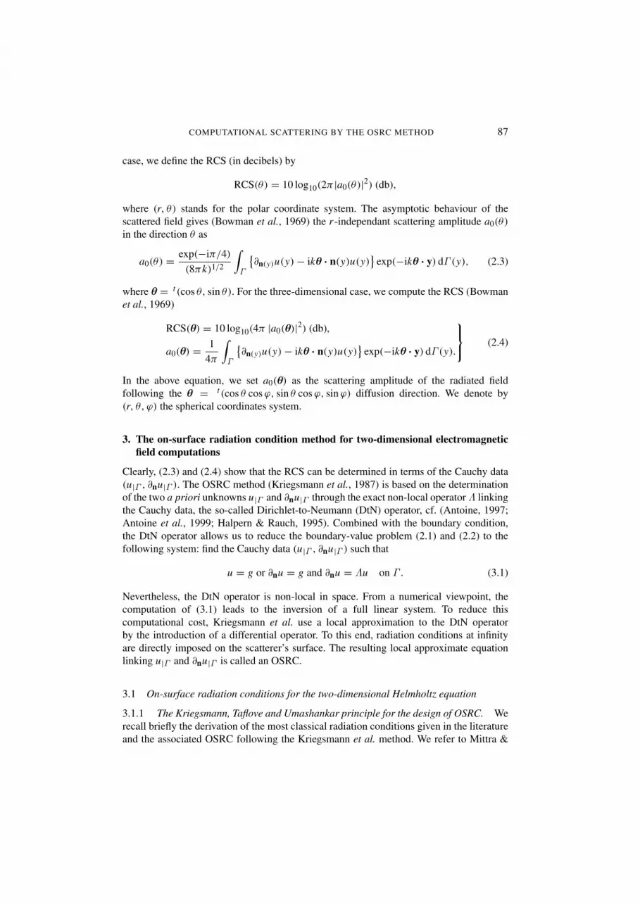
FIG. 17. Bistatic RCS: sound-hard unit cubic scatterer.

30 60 90 120 150 180

− 5

0

5

10

15

20

25

x

x

u

k = 10

ϕ inc = 0˚

1

2

inc

θ (deg.)

RC

S(,0

) (d

b)

OSRC using CBGTLMie series

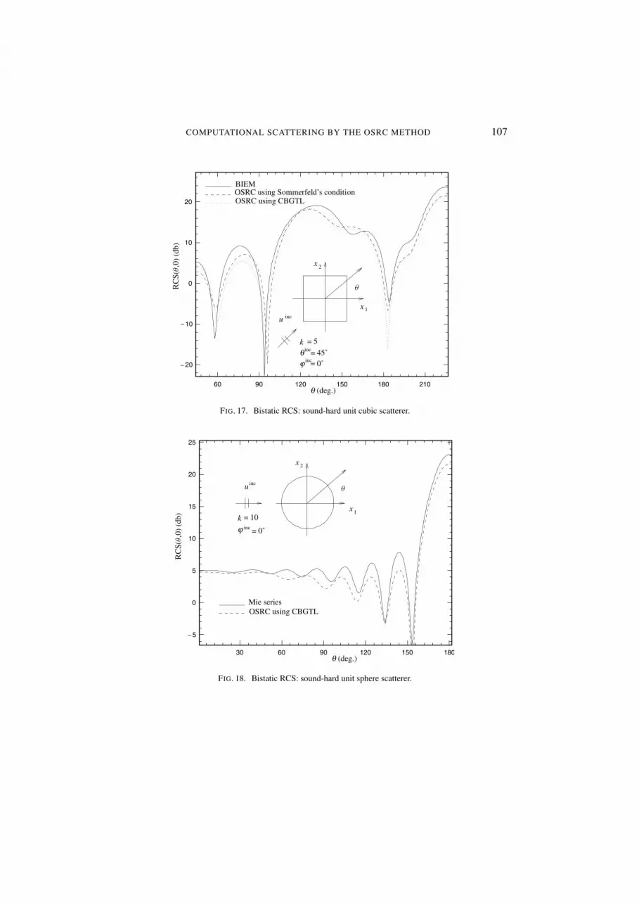
FIG. 18. Bistatic RCS: sound-hard unit sphere scatterer.

108 X. ANTOINE

60 120 180 240 300 360

− 20

− 10

0

10

a

b

c

= 1

= 0.5

= 0.5

Ellipsoid

x

x

u

ϕ

k

θ

1

2

inc

inc

inc = 10

= 45˚= 0˚

BIEMOSRC using CMRL (or CBGTL)

RC

S(,0

) (d

b)

θ (deg.)

FIG. 19. Bistatic RCS: sound-hard ellipsoidal scatterer.

To check that the greater the order the better the approximation, we compute the RCSof an ellipsoidal scatterer characterized by a semi-axis a (resp. b and c) along the Ox1-axis(resp. Ox2 and Ox3). We set here a = 1, b = 0·85 and c = 0·85. The bistatic RCS for ϕ =0 depicted in Fig. 16 illustrates the property that the improvement of numerical efficiencyof the OSRC method is due to the use of higher-order conditions. The best calculations areobtained for the CMRL, CBGTL and CSL conditions. Other numerical experiments lead usto the same conclusion as in the two-dimensional case: the second-order conditions yieldthe best approximations. Moreover, unlike the two-dimensional scattering, the CMRL andCBGTL conditions seem to have the same efficiency even for wave numbers k satisfyingk 1.

From our viewpoint, the main difference between the two- and three-dimensional casesis that we very often have a similar good accuracy for any condition of any order when thewave number k is such that k 3 (although the second-order conditions are the mostaccurate OSRCs in some experiments) (cf. Fig. 17). Finally, we give in Figs 18 and 19 twolast examples showing the effectiveness of OSRC methods for different parameters andscattering objects.

REFERENCES

AMMARI, H. 1998 Scattering of waves by thin periodic layers at high frequencies using the on-surface radiation condition method. IMA J. Appl. Math. 60, 199–215.

ANTOINE, X. 1997 Conditions de Radiation sur le Bord, Ph.D. Thesis, Universite de Pau et des Paysde l’Adour.


ANTOINE, X. 1998 A numerical study of a scattering problem involving a generalized impedanceboundary condition using the on-surface radiation condition method. Mathematical andNumerical Aspects of Wave Propagation (J. DoSanto ed). Philadelphia: SIAM, pp 287–291.

ANTOINE, X., BARUCQ, H., & BENDALI, A. 1999 Bayliss-and-Turkel-like radiation conditions onsurface of arbitrary shape. J. Math. Anal. Appl. 229, 184–211.

BAYLISS, A. & TURKEL, E. 1980 Radiation boundary conditions for wave-like equations. Commun.Pure Appl. Math. 23, 707–725.

BAYLISS, A., GUNZBURGER, M., & TURKEL, E. 1982 Boundary conditions for the numericalsolution of elliptic equations in exterior regions. SIAM J. Appl. Math. 42, 430–451.

BIELAK, J., KALLIVOLAS, L. F., & MAC CAMY, R. C. 1997 A simple impedance-infinite elementfor the finite element solution of the three-dimensional wave equation in unbounded domains.Comput. Methods Appl. Mech. Eng. 147, 235–262.

BOWMAN, J. J., SENIOR, T. B. A., & USLENGHI, P. L. E., eds 1969 Electromagnetic and AcousticScattering by Simple Shape. Amsterdam: North–Holland.

CHAZARAIN, J. & PIRIOU, A. 1982 Introduction to the Theory of Linear Partial DifferentialEquations. Amsterdam: North–Holland.

CHEN, G. & ZHOU, J. 1992 Boundary Element Methods. New York: Academic Press.CIARLET, P. G. 1991 Handbook of Numerical Analysis, Vol. II, Finite Element Methods (Part I) (P.

G. Ciarlet & J. L. Lions eds). Amsterdam: North–Holland.DO CARMO, M. P. 1976 Differential Geometry of Curves and Surfaces. Englewood Cliffs, NJ:

Prentice Hall.ENGQUIST, B. & MAJDA, A. 1977 Absorbing boundary conditions for the numerical simulation of

waves. Math. Comput. 31, 629–651.GIVOLI, D., KELLER, J. B., & PATLASHENKO, I. 1997 High order boundary conditions and finite

elements for infinite domains. Comput. Methods Appl. Mech. Eng. 143, 13–39.GOLDBERG, D. 1991 What every computer scientist should know about floating point arithmetic.

ACM Comput. Surv. 23.HAGEN, H. 1994 Twist estimation for smooth surface design. The Mathematics of Surface IV

(A. Bowyer ed). The IMA Conference Series (NS), New York: Oxford University Press, 48,pp 285–293.

HAGEN, H. & SCHULZE, G. 1987 Automatic smoothing with geometric surface patches. Comput.Aided Design 4, 231–235.

HALPERN, L. & RAUCH, J. 1995 Absorbing boundary conditions for diffusion equations. Numer.Math. 71, 185–224.

HAMMAN, B. 1993 Curvature approximation for triangulated surfaces. Comput. Suppl. 8, 139–153.JANASWAMY, R. 1991 On the applicability of OSRC method to homogeneous scatterers. IEEE

Trans. Antennas Prop. 39, 862–867.JIN, J. M. 1993 The Finite Element Method in Electromagnetics. New York: Wiley.JONES, A. K. 1994 Curvature interpolation through constrained optimization. Shape Quality in

Geometric Modelling and Computer-Aided Design. Philadelphia: SIAM, pp 29–44.JONES, D. S. 1988 Surface radiation conditions. IMA J. Appl. Math. 41, 21–30.JONES, D. S. 1992 An improved surface radiation condition. IMA J. Appl. Math. 48, 163–193.JONES, D. S. 1988 An approximate boundary condition in acoustics. J. Sound and Vibration 121,

37–45.JONES, D. S. & KRIEGSMANN, G. A. 1990 Note on surface radiation conditions. SIAM J. Appl.

Math. 50, 559–568.KRIEGSMANN, G. A. & MOORE, T. G. 1988 An application of the OSRC method to the scattering

110 X. ANTOINE

of acoustic waves by a reactively loaded sphere. Wave Motion 10, 277–284.KRIEGSMANN, G. A., TAFLOVE, A., & UMASHANKAR, K. R. 1987 A new formulation of

electromagnetic wave scattering using the on-surface radiation condition approach. IEEE Trans.Antennas Prop. 35, 153–161.

MITTRA, R. & RAMAHI, O. 1990 Absorbing boundary conditions for the direct solutionof partial differential equations arising in electromagnetic scattering problems. Progress inElectromagnetic Research: Finite Element and Finite Difference Methods in ElectromagneticScattering, Chapter 4 (M. A. Morgan ed). Newark: Elsevier.

MOORE, T. G., BLASCHAK, J. G., TAFLOVE, A., & KRIEGSMANN, G. A. 1988 Theory andapplication of radiation boundary operators. IEEE Trans. Antennas Prop. 36, 1797–1811.

MURCH, R. D. 1993 The on-surface radiation condition applied to three-dimensional convex objects.IEEE Trans. Antennas Prop. 41, 651–658.

ROXBURGH, R. G. 1997 Electromagnetic scattering from a rightcircular cylinder using a surfaceradiation condition. IMA J. Appl. Math. 59, 221–230.

SENIOR, T. B. A. & VOLAKIS, J. L. 1995 Approximate Boundary Conditions in Electromagnetics,Electromagnetic Waves Series 41. London: IEE.

SENIOR, T. B. A., VOLAKIS, J. L., & LEGAULT, R. 1997 Higher order impedance and absorbingboundary conditions. IEEE Trans. Antennas Prop. 45, 107–114.

SPIVAK, M. 1979 A Comprehensive Introduction to Differential Geometry. Berkely: Publish orPerish.

STUPFEL, B. 1994 Absorbing boundary conditions on arbitrary boundaries for the scalar and vectorwave equations. IEEE Trans. Antennas Prop. 42, 773–780.

TEYMUR, M. 1996 A note on higher-order surface radiation conditions. IMA J. Appl. Math. 57,137–163.

Documents

Fast approximate computation of a time-harmonic scattered field using the on-surface radiation condition method