Embed Size (px)
Citation preview

Financial Economics, Fat-tailed Distributions∗
Markus Haas†
Christian Pigorsch‡
First version: April 13, 2007This version : September 21, 2007
∗We are grateful to Bruce Mizrach for his helpful comments. The research of Haas was supportedby the German Research Foundation.
†Department of Statistics, University of Munich (LMU), D-80799 Munchen, Akademiestr 1/I. E-mail:[email protected]. Phone: +49 (0) 89 21 80 - 25 70.
‡Department of Economics, University of Bonn, D-53113 Bonn, Adenauerallee 24-42. E-mail:[email protected]. Phone: +49 (0) 228 73 - 39 20.

Article Outline
1 Glossary 2
2 Definition of the Subject and Its’ Importance 2
3 Introduction 3
4 Defining Fat–tailedness 6
5 Empirical Evidence about the Tails 9
6 Some Specific Distributions 156.1 Alpha Stable and Related Distributions . . . . . . . . . . . . . . . . . . . 156.2 The Generalized Hyperbolic Distribution . . . . . . . . . . . . . . . . . . 21
6.2.1 The Hyperbolic Distribution . . . . . . . . . . . . . . . . . . . . . 266.2.2 The Normal Inverse Gaussian Distribution . . . . . . . . . . . . . 276.2.3 The Student t distribution . . . . . . . . . . . . . . . . . . . . . . 286.2.4 The Variance Gamma Distribution . . . . . . . . . . . . . . . . . 296.2.5 The Cauchy distribution . . . . . . . . . . . . . . . . . . . . . . . 306.2.6 The Normal Distribution . . . . . . . . . . . . . . . . . . . . . . . 30
6.3 Finite Mixtures of Normal Distributions . . . . . . . . . . . . . . . . . . 306.4 Empirical Comparison . . . . . . . . . . . . . . . . . . . . . . . . . . . . 31
7 Volatility Clustering and Fat Tails 32
8 Application to Value–at–Risk 40
9 Future Directions 42
A Literature 42A.1 Primary Literature . . . . . . . . . . . . . . . . . . . . . . . . . . . . . . 42A.2 Books and Reviews . . . . . . . . . . . . . . . . . . . . . . . . . . . . . . 56
1

1 Glossary
LeptokurtosisA distribution is leptokurtic if it is more peaked in the center and thicker tailedthan the normal distribution with the same mean and variance. Occasionally,leptokurtosis is also identified with a moment–based kurtosis measure larger thanthree, see Section 3.
ReturnLet St be the price of a financial asset at time t. Then the continuous return, rt,is rt = log(St/St−1). The discrete return, Rt, is Rt = St/St−1 − 1. Both are rathersimilar if −0.15 < Rt < 0.15, because rt = log(1 + Rt). See Section 3.
TailThe (upper) tail, denoted by F (x) = P (X > x), characterizes the probability thata random variable X exceeds a certain “large” threshold x. For analytical purposes,“large” is often translated with “as x →∞”. For financial returns, a daily changeof 5% is already infinitely large. A Gaussian model essentially excludes such anevent.
Tail indexThe tail index, or tail exponent, α, charcaterizes the rate of tail decay if the tailgoes to zero, in essence, like a power function, i.e., F (x) = x−αL(x), where L isslowly varying. Moments of order lower (higher) than α are (in)finite.
2 Definition of the Subject and Its’ Importance
Have a look at Figure 1. Its top plot shows the daily percentage changes, or returns, ofthe S&P500 index ranging from January 2, 1985 to December 29, 2006, a total of 5550daily observations. We will use this data set throughout the article to illustrate someof the concepts and models to be discussed. Two observations are immediate. The firstis that both small and large changes come clustered, i.e., there are periods of low andhigh volatility. The second is that, from time to time, we observe rather large changeswhich may be hard to reconcile with the standard distributional assumption in statisticsand econometrics, that is, normality. The most outstanding return certainly occurredon October 19, 1987, the “Black Monday”, where the index lost more than 20% of itsvalue, but the phenomenon is chronic. For example, if we fit a normal distribution tothe data, the resulting model predicts that we observe an absolute daily change largerthan 5% once in approximately 1860 years, whereas we actually encountered that 13times during our 22–year sample period. This suggests that, compared to the normaldistribution, the distribution of the returns is fat–tailed, i.e., the probability of largelosses and gains is much higher than would be implied by a time–invariant unconditionalGaussian distribution. The latter is obviously not suitable for describing the booms,busts, bubbles, and bursts of activity which characterize financial markets, and whichare apparent in Figure 1.
2

The two aforementioned phenomena, i.e., volatility clustering and fat tails, have beendetected in almost every financial return series that was subject to statistical analysissince the publication of Mandelbrot’s [154] seminal study of cotton price changes, andthey are of paramount importance for any individual or institution engaging in the fi-nancial markets, as well as for financial economists trying to understand their mode ofoperation. For example, investors holding significant portions of their wealth in riskyassets need a realistic assessment of the likelihood of severe losses. Similarly, economiststrying to learn about the relation between risk and return, the pricing of financial deriva-tives, such as options, and the inherent dynamics of financial markets, can only benefitfrom building their models on adequate assumptions about the stochastic properties ofthe variables under study, and they have to reconcile the predictions of their models withthe actual facts.
This article reviews some of the most important concepts and distributional modelsthat are used in empirical finance to capture the (almost) ubiquitous stochastic proper-ties of returns as indicated above. Section 3 defines in a somewhat more precise mannerthan above the central variable of interest, the return of a financial asset, and gives abrief account of the early history of the problem. Section 4 discusses various operational-izations of the term “fat–tailedness”, and Section 4 summarizes what is or is at leastwidely believed to be known about the tail characteristics of typical return distributions.Popular parametric distributional models are discussed in Section 6. The alpha stablemodel as the archetype of a fat–tailed distribution in finance is considered in detail, asis the generalized hyperbolic distribution, which provides a convenient framework fordiscussing, as special or limiting cases, many of the important distributions employed inthe literature. An empirical comparison using the S&P500 returns is also included. InSection 7, the relation between the two “stylized facts” mentioned above, i.e., clusters ofvolatility and fatness of the tails, is highlighted, where we concentrate on the GARCHapproach, which has gained outstanding popularity among financial econometricians.This model has the intriguing property of producing fat–tailed marginal distributionseven with light–tailed innovation processes, thus emphasizing the role of the marketdynamics. In Section 8, we compare both the unconditional parametric distributionalmodels introduced in Section 6 as well as the GARCH model of Section 7 on an economicbasis by evaluating their ability to accurately measure the Value-at-Risk, which is animportant tool in risk management. Finally, Section 9 identifies some open issues.
3 Introduction
To fix notation, let St be the price of an asset at time t, e.g., a stock, a market index,or an exchange rate. The continuously compounded or log return from time t to timet + ∆t, rt,t+∆t, is then defined as
rt,t+∆t = log St+∆t − log St. (1)
Often the quantity defined in (1) is also multiplied by 100, so that it can be interpretedin terms of percentage returns, see Figure 1. Moreover, in applications, ∆t is usually setequal to one and represents the horizon over which the returns are calculated, e.g., a day,
3

-25
-20
-15
-10
-5
0
5
10
1986 1988 1990 1992 1994 1996 1998 2000 2002 2004 2006
1e-04
0.001
0.01
0.1
1
0.001 0.01 0.1 1 10 100
1
1.5
2
2.5
3
3.5
4
50 100 150 200 250 300 350 400 450 500
0
0.1
0.2
0.3
0.4
0.5
0.6
-3 -2 -1 0 1 2 3
1e-05
1e-04
0.001
0.01
0.1
1
-4 -2 0 2 4
date
r t
xx
x
f(x
)
f(x
)α
H
k
P(|r t
|>
x)
kernel
kernel
normal
normal
empnormalfit
linear
Figure 1: The top plot shows the S&P500 percentage returns, rt, from January 1985 toDecember 2006, i.e., rt = 100× log(St/St−1), where St is the index level at time t. Theleft plot of the middle panel shows a nonparametric density estimate (solid), along withthe fitted normal density (dotted); the right graph is similar but shows the respectivelog–densities in order to better visualize the tail regions. The bottom left plot representsa Hill plot for the S&P500 returns, i.e., it displays αk,n defined in (11) for k ≤ 500. Thebottom right plot shows the complementary cdf, F (x), on a log–log scale, see Section 5for discussion.
4

week, or month. In this case, we drop the first subscript and define rt := log St−log St−1.The log returns (1) can be additively aggregated over time, i.e.,
rt,t+τ =τ∑
i=1
rt+i. (2)
Empirical work on the distribution of financial returns is usually based on log returns.In some applications a useful fact is that, over short intervals of time, when returns tendto be small, (1) can also serve as a reasonable approximation to the discrete return,Rt,t+∆t := St+∆t/St − 1 = exp (rt,t+∆t) − 1. For further discussion of the relationshipbetween continuous and discrete returns and their respective advantages and disadvan-tages, see, e.g., [46, 76].
The seminal work of [155], to be discussed in Section 6.1, is often viewed as thebeginning of modern empirical finance. As reported in [74], “[p]rior to the work ofMandelbrot the usual assumption ... was that the distribution of price changes in aspeculative series is approximately Gaussian or normal”. The rationale behind thisprevalent view, which was explicitly put forward as early as 1900 by Bachelier [14], wasclearly set out in [178]: If the log–price changes (1) from transaction to transactionare independently and identically distributed with finite variance, and if the number oftransactions is fairly uniformly distributed in time, then (2) along with the central limittheorem (CLT) implies that the return distribution over longer intervals, such as a day,a week, or a month, approaches a Gaussian shape.
However, it is now generally acknowledged that the distribution of financial returnsover horizons shorter than a month is not well described by a normal distribution. In par-ticular, the empirical return distributions, while unimodal and approximately symmetric,are typically found to exhibit considerable leptokurtosis, i.e., they are more peaked inthe center and have fatter tails than the Gaussian with the same variance. Althoughthis has been occasionally observed in the pre–Mandelbrot literature (e.g., [6]), the firstsystematic account of this phenomenon appeared in [154] and the follow–up papers byFama [74, 75] and Mandelbrot [156], and it was consistently confirmed since then. Thetypical shape of the return distribution, as compared to a fitted Gaussian, is illustratedin the middle panel of Figure 1 for the S&P500 index returns, where a nonparamet-ric kernel density estimator (e.g., [198]) is superimposed on the fitted Gaussian curve(dashed line). Interestingly, this pattern has been detected not only for modern financialmarkets but also for those of the eighteenth century [103].
The (location and scale–free) standardized fourth moment, or coefficient of kurtosis,
K [X] =E [(X − µ)4]
σ4, (3)
where µ and σ are the mean and the standard deviation of X, respectively, is sometimesused to assess the degree of leptokurtosis of a given distribution. For the normal distri-bution, K = 3, and K > 3, referred to as excess kurtosis, is taken as an indicator of aleptokurtic shape (e.g., [164], p. 429). For example, the sample analogue of (3) for theS&P500 returns shown in Figure 1 is 47.9, indicating very strong excess kurtosis. A for-mal test could be conducted using the fact that, under normality, the sample kurtosis is
5

asymptotically normal with mean 3 and standard deviation√
24/T (T being the samplesize), but the result can be anticipated.
As is well–known, however, such moment–based summary measures have to be in-terpreted with care, because a particular moment need not be very informative about adensity’s shape. We know from Finucan [82] that if two symmetric densities, f and g,have common mean and variance and finite fourth moment, and if g is more peaked andhas thicker tails than f , then the fourth moment (and hence K) is greater for g thanfor f , provided the densities cross exactly twice on both sides of the mean. However,the converse of this statement is, of course, not true, and a couple of (mostly somewhatartificial) counterexamples can be found in [16, 68, 121]. [158] provides some intuition byrelating density crossings to moment crossings. For example, (only) if the densities crossmore than four times, it may happen that the fourth moment is greater for f , but thesixth and all higher moments are greater for g, reflecting the thicker tails of the latter.Nevertheless, Finucan’s result, along with his (in some respects justified) hope that wecan view “this pattern as the common explanation of a high observed kurtosis”, mayserve to argue for a certain degree of usefulness of the kurtosis measure (3), provided thefourth moment is assumed to be finite. However, a nonparametric density estimate willin any case be more informative. Note that the density crossing condition in Finucan’stheorem is satisfied for the S&P500 returns in Figure 1.
4 Defining Fat–tailedness
The notion of leptokurtosis as discussed so far is rather vague, and both financial marketresearchers as well as practitioners, such as risk managers, are interested in a moreprecise description of the tail behavior of financial variables, i.e., the laws governingthe probability of large gains and losses. To this end, we define the upper tail of thedistribution of a random variable (rv) X as
F (x) = P (X > x) = 1− F (x), (4)
where F is the cumulative distribution function (cdf) of X. Consideration of the uppertail is the standard convention in the literature, but it is clear that everything could bephrased just as well in terms of the lower tail.
We are interested in the behavior of (4) as x becomes large. For our benchmark, i.e.,the normal distribution with (standardized) density (pdf) φ(x) = (2π)−1/2 exp (−x2/2),we have (cf. [79], p. 131)
F (x) ∼=1√2πx
exp
(−x2
2
)=
φ(x)
xas x →∞, (5)
where the notation f(x) ∼= g(x) as x → ∞ means that limx→∞ f(x)/g(x) = 1. Thus,the tails of the normal tend to zero faster than exponentially, establishing its very lighttails.
To appreciate the difference between the general concept of leptokurtosis and the ap-proach that focuses on the tails, consider the class of finite normal mixtures as discussed
6

in Section 6.3. These a leptokurtic in the sense of peakedness and tailedness (comparedto the normal), but are light–tailed according to the tail–based perspective.
While it is universally accepted in the literature that the Gaussian is too light–tailedto be an appropriate model for the distribution of financial returns, there is no completeagreement with respect to the actual shape of the tails. This is not surprising becausewe cannot reasonably expect to find a model that accurately fits all markets at anytime and place. However, the current mainstream opinion is that the probability for theoccurrence of large (positive and negative) returns can often appropriately be describedby Pareto–type tails. Such tail behavior is also frequently adopted as the definition offat–tailedness per se, but the terminology in the literature is by no means unique.
A distribution has Pareto–type tails if they decay essentially like a power functionas x becomes large, i.e., F is regularly varying (at infinity) with index −α (writtenF ∈ RV−α), meaning that
F (x) = x−αL(x), α > 0, (6)
where L > 0 is a slowly varying function, which can be interpreted as “slower than anypower function” (see [34, 188, 195] for a technical treatment of regular variation). Thedefining property of a slowly varying function is limx→∞ L(tx)/L(x) = 1 for any t > 0,and the aforementioned interpretation follows from the fact that, for any γ > 0, we have(cf. [195], p. 18)
limx→∞
xγL(x) = ∞, limx→∞
x−γL(x) = 0. (7)
Thus, for large x, the parameter α in (6), called the tail index or tail exponent, controlsthe rate of tail decay and provides a measure for the fatness of the tails.
Typical examples of slowly varying functions include L(x) = c, a constant, L(x) =c + o(1), or L(x) = (log x)k, x > 1, k ∈ R. The first case corresponds to strictPareto tails, while in the second the tails are asymptotically Paretian in the sense thatF (x) ∼= cx−α, which includes as important examples in finance the (nonnormal) sta-ble Paretian (see (13) in Section 6.1) and the Student’s t distribution considered inSection 6.2.3, where the tail index coincides with the characteristic exponent and thenumber of degrees of freedom, respectively. As an example for both, the Cauchy dis-tribution with density f(x) = [π(1 + x2)]−1 has cdf F (x) = 0.5 + π−1 arctan(x). Asarctan(x) =
∑∞0 (−1)ix2i+1/(2i + 1) for |x| < 1, and arctan(x) = π/2− arctan(1/x) for
x > 0, we have F (x) ∼= (πx)−1.For the distributions mentioned in the previous paragraph, it is known that their
moments exist only up to (and excluding) their tail indices, α. This is generally truefor rvs with regularly varying tails and follows from (7) along with the well–knownconnection between moments and tail probabilities, i.e., for a nonnegative rv X, andr > 0, E [Xr] = r
∫∞0
xr−1F (x)dx (cf. [95], p. 75). The only possible minor variation
is that, depending on L, E [Xα] may be finite. For example, a rv X with tail F (x) =cx−1(log x)−2 has finite mean. The property that moments greater than α do not existprovides further intuition for α as a measure of tail–fatness.
As indicated above, there is no universal agreement in the literature with respect tothe definition of fat–tailedness. For example, some authors (e.g., [72, 196]) emphasize the
7

class of subexponential distributions, which are (although not exclusively) characterizedby the property that their tails tend to zero slower than any exponential, i.e., for any γ >0, limx→∞ eγxF (x) = ∞, implying that the moment generating function does not exist.Clearly a regularly varying distribution is also subexponential, but further members ofthis class are, for instance, the lognormal as well as the stretched exponential, or heavytailed Weibull, which has a tail of the form
F (x) = exp(−xb), 0 < b < 1. (8)
The stretched exponential has recently been considered by [134, 152, 153] as an alter-native to the Pareto–type distribution (6) for modeling the tails of asset returns. Notethat, as opposed to (6), both the lognormal as well as the stretched exponential possesspower moments of all orders, although no exponential moment.
In addition, [24] coined the term semi–heavy tails for the generalized hyperbolic (GH)distribution, but the label may be employed more generally to refer to distributions withslower tails than the normal but existing moment generating function. The GH, which isnow very popular in finance and nests many interesting special cases, will be examinedin detail in Section 6.2.
As will be discussed in Section 5, results of extreme value theory (EVT) are oftenemployed to identify the tail shape of return distributions. This has the advantagethat it allows to concentrate fully on the tail behavior, without the need to model thecentral part of the distribution. To sketch the idea behind this approach, suppose weattempt to classify distributions according to the limiting behavior of their normalizedmaxima. To this end, let {Xi, i ≥ 1} be an iid sequence of rvs with common cdf F ,Mn = max{X1, . . . , Xn}, and assume there exist sequences an > 0, bn ∈ R, n ≥ 1, suchthat
P
(Mn − bn
an
≤ x
)= F n(anx + bn)
n→∞−→ G(x), (9)
where G is assumed nondegenerate. To see that normalization is necessary, note thatlimn→∞ P (Mn ≤ x) = limn→∞ F n(x) = 0 for all x < xM := sup{x : F (x) < 1} ≤ ∞, sothat the limiting distribution is degenerate and of little help. If the above assumptionsare satisfied, then, according to the classical Fisher–Tippett theorem of extreme valuetheory (cf. [188]), the limiting distribution G in (9) must be of the following form:
Gξ(x) = exp(−(1 + ξx)−1/ξ
), 1 + ξx > 0, (10)
which is known as the generalized extreme value distribution (GEV), or von Mises repre-sentation of the extreme value distributions (EV). The latter term can be explained bythe fact that (10) actually nests three different types of EV distributions, namely
(i) the Frechet distribution, denoted by G+ξ , where ξ > 0 and x > −1/ξ,
(i) the so–called Weibull distribution of EVT, denoted by G−ξ , where ξ < 0 andx < −1/ξ, and
(iii) the Gumbel distribution, denoted by G0, which corresponds to the limiting case asξ → 0, i.e., G0(x) = exp(−e−x), where x ∈ R.
8

A cdf F belongs to the maximum domain of attraction (MDA) of one of the extremevalue distributions nested in (10), written F ∈ MDA(Gξ), if (9) holds, i.e., classifyingdistributions according to the limiting behavior of their extrema amounts to figuring outthe MDAs of the extreme value distributions. It turns out that it is the tail behavior ofa distribution F that accounts for the MDA it belongs to. In particular, F ∈ MDA(G+
ξ )
if and only if its tail F ∈ RV−α, where α = 1/ξ. As an example, for a strict Paretodistribution, i.e., F (x) = 1 − (u/x)α, x ≥ u > 0, with an = n1/αu/α and bn = n1/αu,we have limn→∞ F n(anx + bn) = limx→∞(1 − n−1(1 + x/α)−α)n = G+
1/α(x). Distribu-
tions in MDA(G−ξ ) have a finite right endpoint, while, roughly, most of the remainingdistributions, such as the normal, the lognormal and (stretched) exponentials, belongto MDA(G0). The latter also accommodates a few distributions with finite right end-point. See [188] for precise conditions. The important case of non–iid rvs is discussedin [136]. A central result is that, rather generally, vis–a–vis an iid sequence with thesame marginal cdf, the maxima of stationary sequences converge to the same type oflimiting distribution. See [63] and [166] for an application of this theory to ARCH(1)and GARCH(1,1) processes (see Section 7), respectively
One approach to exploit the above results, referred to as the method of block maxima,is to divide a given sample of return data into subsamples of equal length, pick themaximum of each subsample, assume that these have been generated by (10) (enrichedwith location and scale parameters to account for the unknown an and bn), and findthe maximum–likelihood estimate for ξ, location, and scale. Standard tests can thenbe conducted to assess, e.g., whether ξ > 0, i.e., the return distribution has Pareto–type tails. An alternative but related approach, which is based on further theoreticaldevelopments and often makes more efficient use of the data, is the peaks over thresholds(POT) method. See [72] for a critical discussion of these and alternative techniques.
We finally note that 1 − G+1/α(α(x − 1)) ∼= x−α, while 1 − G0(x) ∼= e−x, i.e., for the
extremes, we have asymptotically a Pareto and an exponential tail, respectively. Thismay provide, on a meta–level, a certain rationale for reserving the notion of genuinefat–tailedness for the distributions with regularly varying tails.
5 Empirical Evidence about the Tails
The first application of power tails in finance appeared in Mandelbrot’s [154] study ofthe log–price changes of cotton. Mandelbrot proposed to model returns with nonnormalalpha stable, or stable Paretian, distributions, the properties of which will be discussedin some detail in Section 6.1. For the present discussion, it suffices to note that forthis model the tail index α in (6), also referred to as characteristic exponent in thecontext of stable distributions, is restricted to the range 0 < α < 2, and that much ofits theoretical appeal derives from the fact that, due to the generalized CLT, “Mandel-brot’s hypothesis can actually be viewed as a generalization of the central–limit theoremarguments of Bachelier and Osborne to the case where the underlying distributions ofprice changes from transaction to transaction ... have infinite variances” [75]. For thecotton price changes, Mandelbrot came up with a tail index of about 1.7, and his workwas subsequently complemented by Fama [75] with an analysis of daily returns of the
9

stocks belonging to the Dow Jones Industrial Average. [75] came to the conclusion thatMandelbrot’s theory was supported by these data, with an average estimated α close to1.9.
The findings of Mandelbrot and Fama initiated an extensive discussion about theappropriate distributional model for stock returns, partly because the stable model’simplication that the tails are so fat that even the variance is infinite appeared to be tooradical to many economists used to work with models built on the assumption of finitesecond moments. The evidence concerning the stable hypothesis gathered in the courseof the debate until the end of the eighties was not ultimately conclusive, but there weremany papers reporting mainly negative results [4, 28, 36, 40, 54, 67, 98, 99, 109, 135,176, 180, 184].
From the beginning of the nineties, a number of researchers have attempted to esti-mate the tail behavior of asset returns directly, i.e., without making specific assumptionsabout the entire distributional shape. [86, 115, 142, 143] use the method of block maxima(see Section 4) to identify the maximum domain of attraction of the distribution of stockreturns. They conclude that the Frechet distribution with a tail index α > 2 is mostlikely, implying Pareto–type tails which are thinner than those of the stable Paretian.
A second strand of literature assumes a priori the presence of a Pareto–type tail andfocuses on the estimation of the tail index α. If, as is often the case, a power tail isdeemed adequate, an explicit estimate of α is of great interest both from a practical andan academic viewpoint. For example, investors want to assess the likelihood of largelosses of financial assets. This is often done using methods of extreme value theory,which require an accurate estimate of the tail exponent. Such estimates are also im-portant because the properties of statistical tests and other quantities of interest, suchas empirical autocorrelation functions, frequently depend on certain moment conditions(e.g., [144, 166]). Clearly the desire to figure out the actual tail shape has also an in-trinsic component, as is reflected in the long–standing debate on the stable Paretianhypothesis. People simply wanted to know whether this distribution, with its appealingtheoretical properties, is consistent with actual data. Moreover, empirical findings mayguide economic theorizing, as they can help both in assessing the validity of certain ex-isting models as well as in suggesting new explanations. Two examples will briefly bediscussed at the end of the present section.
Within this second strand of literature, the Hill estimator [106] has become the mostpopular tool. It is given by
αk,n =
(1
k − 1
k−1∑j=1
log Xj,n − log Xk,n
)−1
, (11)
where Xi,n denotes the ith upper order statistic of a sample of length n, i.e., X1,n ≥X2,n ≥ · · · ≥ Xn,n. See [64, 72] for various approaches to deriving (11). If the tail is notregularly varying, the Hill estimator does not estimate anything.
A crucial choice to be made when using (11) is the selection of the threshold valuek, i.e., the number of order statistics to be included in the estimation. Ideally, onlyobservations from the tail region should be used, but choosing k to small will reducethe precision of the estimator. There exist various methods for picking k optimally in a
10

mean–squared error sense [62, 61], but much can be learned by looking at the Hill plot,which is obtained by plotting αk,n against k. If we can find a range of k–values wherethe estimate is approximately constant, this can be taken as a hint for where the “true”tail index may be located. As illustrated in [189], however, the Hill plot may not alwaysbe so well–behaved, and in this case the semiautomatic methods mentioned above willpresumably also be of little help.
The theoretical properties of (11), along with technical conditions, are summarizedin [72, 189]. Briefly, for iid data generated from a distribution with tail F ∈ RV−α,the Hill estimator has been shown to be consistent [159] and asymptotically normalwith standard deviation α/
√k [100]. Financial data, however, are usually not iid but
exhibit considerable dependencies in higher–order moments (see Section 7). In thissituation, i.e., with ARCH–type dynamics, (11) will still be consistent [190], but littleis known about its asymptotic variance. However, simulations conducted in [123] withan IGARCH model, as defined in Section 7, indicate that, under such dependencies, theactual standard errors may be seven to eight times larger than those implied by theasymptotic theory for iid variables.
The Hill estimator was introduced into the econometrics literature in the series ofarticles [107, 113, 125, 126]. [125, 126], using weekly observations, compare the tails ofexchange rate returns in floating and fixed exchange rate systems, such as the BrettonWoods period and the EMS. They find that for the fixed systems, most tail index esti-mates are below 2, i.e., consistent with the alpha stable hypothesis, while the estimatesare significantly larger than 2 (ranging approximately from 2.5 to 4) for the float. [126]interpret these results in the sense that “a float lets exchange rates adjust more smoothlythan any other regime that involves some amount of fixity”. Subsequent studies of float-ing exchange rates using data ranging from weekly [107, 110, 111] over daily [58, 89, 144]to very high–frequency [59, 62, 170] have confirmed the finding of these early papersthat the tails are not fat enough to be compatible with the stable Paretian hypothesis,with estimated tail indices usually somewhere in the region 2.5–5. [58] is the first toinvestigate the tail behavior of the euro against the US dollar, and finds that it is similarboth to the German mark in the pre–euro era as well as to the yen and the Britishpound, with estimated exponents hovering around 3–3.5.
Concerning estimation with data at different time scales, a comparison of the resultsreported in the literature reveals that the impact on the estimated tail indices appearsto be moderate. [59] observe an increase in the estimates when moving from 30–minuteto daily returns, but they argue that these changes, due to the greater bias at thelower frequencies, are small enough to be consistent with α being invariant under timeaggregation.
Note that if returns were independently distributed, their tail behavior would in factbe unaffected by time aggregation. This is a consequence of (2) along with Feller’s ([80],p. 278) theorem on the convolution of regularly varying distributions, stating that anyfinite convolution of a regularly varying cdf F (x) has a regularly varying tail with thesame index. Thus, in principle, the tail survives forever, but, as long as the varianceis finite, the CLT ensures that in the course of aggregation an increasing probabilityweight is allocated to the center of the distribution, which becomes closer to a Gaussianshape. The probability of observing a tail event will thus decrease. However, for fat–
11

tailed distributions, the convergence to normality can be rather slow, as reflected in theobservation that pronounced nonnormalities in financial returns are often observed evenat a weekly and (occasionally) monthly frequency. See [41] for an informative discussionof these issues. The fact that returns are, in general, not iid makes the interpretation ofthe approximate stability of the tail index estimates observed across papers employingdifferent frequencies not so clear–cut, but Feller’s theorem may nevertheless provide someinsight.
There is also an extensive literature reporting tail index estimates of stock returns,mostly based on daily [2, 89, 92, 112, 113, 144, 145, 146, 177] and higher frequencies[2, 91, 92, 147, 181]. The results are comparable to those for floating exchange ratesin that the tenor of this literature, which as a whole covers all major stock markets, isthat most stock return series are characterized by a tail index somewhere in the region2.5–5, and most often below 4. That is, the tails are thinner than expected under thestable Paretian hypothesis, but the finiteness of the third and in particular the fourthmoments (and hence kurtosis) may already be questionable. Again, the results appear tobe relatively insensitive with respect to the frequency of the data, indicating a rather slowconvergence to the normal distribution. Moreover, most authors do not find significantdifferences between the left and the right tail, although, for stock returns, the pointestimates tend to be somewhat lower for the left tail (e.g., [115, 145]).
Applications to the bond market appear to be rare, but see [201], who report tailindex estimates between 2.5 and 4.5 for 5–minute and 1–hour Bund future returns andsomewhat higher values for daily data.
[160] compare the tail behaviors of spot and future prices of various commodities(including cotton) and find that, while future prices resemble stock prices with tail indicesin the region 2.5–4, spot prices are somewhat fatter tailed with α hovering around 2.5and, occasionally, smaller than 2.
Summarizing, it is now a widely held view that the distribution of asset returnscan typically be described as fat–tailed in the power law sense but with finite variance.Thus, currently there seems to exist a far reaching consensus that the stable Paretianmodel is not adequate for financial data, but see [163, 202] for a different viewpoint.A consequence of the prevalent view is that asset return distributions belong to theGaussian domain of attraction, but that the convergence appears to be very slow.
To illustrate typical findings as reported above, let us consider the S&P500 returnsdescribed in Section 2. A first informal check of the appropriateness of a power law can beobtained by means of a log–log plot of the empirical tail, i.e., if 1−F (x) = F (x) ≈ cx−α
for large x, then a plot of the log of the empirical complementary cdf, F (x), againstlog x should display a linear behavior in its outer part. For the data at hand, sucha plot is shown in the bottom right panel of Figure 1. Assuming homogeneity acrossthe tails, we pool negative and positive returns by first removing the sample mean andthen taking absolute values. We have also multiplied (1) by 100, so that the returnsare interpretable in terms of percentage changes. The plot suggests that a power lawregime may be starting from approximately the 90% quantile. Included in Figure 1 isalso a regression line (“fit”) fitted to the log–tail using the 500 upper (absolute) returnobservations. This yields, as a rough estimate for the tail index, a slope of α = 3.13,with a coefficient of determination R2 = 0.99. A Hill plot for k ≤ 500 in (11) is shown in
12

1.5
2
2.5
3
3.5
4
4.5
5
5.5
6
6.5
7
50 100 150 200 250 300 350 400 450 500
αH
klinear
Figure 2: Shown are, for k ≤ 500, the 95%, 50%, and 5% quantiles of the distribution ofthe Hill estimator αk,n, as defined in (11), over 176 stocks included in the S&P500 stockindex.
the bottom left panel of Figure 1. The estimates are rather stable over the entire regionand suggest an α somewhere in the interval (3,3.5), which is reconcilable with the resultsin the literature summarized above. A somewhat broader picture can be obtained byconsidering individual stocks. Here we consider the 176 stocks that were listed in theS&P500 from January 1985 to December 2006. Figure 2 presents, for each k ≤ 500, the5%, 50%, and 95% quantiles of the distribution of (11) over the different stocks. Themedian is close to 3 throughout, and it appears that an estimate in (2.5, 4.5) would bereasonable for most stocks.
At this point, it may be useful to note that the issue is not whether a power law is truein the strict sense but only if it provides a reasonable approximation in the relevant tailregion. For example, it might be argued that asset returns actually have finite support,implying finiteness of all moments and hence inappropriateness of a Pareto–type tail.However, as concisely pointed out in [144], “saying that the support of an empiricaldistribution is bounded says very little about the nature of outlier activity that mayoccur in the data”.
We clearly cannot expect to identify the “true” distribution of financial variables.For example, [153] have demonstrated that by standard techniques of EVT it is virtuallyimpossible, even in rather large samples, to discriminate between a power law and astretched exponential (8) with a small value of b, thus questioning, for example, theconclusiveness of studies relying on the block maxima method, as referred to above. Asimilar point was made in [137], who showed by simulation that a three–factor stochasticvolatility model, with a marginal distribution known to have all its moments finite, cangenerate apparent power laws in practically relevant sample sizes. As put forward in[152], “for most practical applications, the relevant question is not to determine whatis the true asymptotic tail, but what is the best effective description of the tails in thedomain of useful applications”.
As is evident in Figure 1, a power law may (and often does) provide a useful approx-
13

1e-05
1e-04
0.001
0.01
0.1
1
1 10
x
P(|r t
|>
x)
S&P500DAX
linear fit
Figure 3: The figure shows, on a log-log scale, the complementary cdf, F (x), for thelargest 500 absolute return observations both for the daily S&P500 returns from January1985 to December 2006 and the daily DAX returns from July 1987 to July 2007.
imation to the tail behavior of actual data, but there is no reason to expect that it willappear in every market, and a broad range of heavy and semi–heavy tailed distributions(such as the GH in Section 6.2) may provide adequate fit. For instance, [93] investigatethe tail behavior of high–frequency returns of one of the most frequently traded stockson the Paris Stock Exchange (Alcatel) and conclude that the tails decay at an exponen-tial rate, and [197] and [119] obtain similar results for daily returns of the Nikkei 225index and various individual US stocks, respectively. As a further illustration, withoutrigorous statistical testing, Figure 3 shows the log–log tail plot for daily returns of theGerman stock market index DAX from July 3, 1987 to July 4, 2007 for the largest 500out of 5218 (absolute) return observations, along with a regression–based linear fit. Forpurpose of comparison, the corresponding figure for the S&P500 has also been repro-duced from Figure 1. While the slopes of the fitted power laws exhibit an astonishingsimilarity (in fact, the estimated tail index of the DAX is 2.93), it is clear from Figure3 that an asymptotic power law, although not necessarily inconsistent with the data, ismuch less self–evident for the DAX than for the S&P500, due to the apparent curvatureparticularly in the more extreme tail.
It is finally worthwhile to mention that financial theory in general, although some ofits models are built on the assumption of a specific distribution, has little to say aboutthe distribution of financial variables. For example, according to the efficient markets
14

paradigm, asset prices change in response to the arrival of relevant new information,and, consequently, the distributional properties of returns will essentially reflect those ofthe news process. As noted by [148], an exception to this rule is the model of rationalbubbles of [35]. [148] show that this class of processes gives rise to an (approximate)power law for the return distribution. However, the structure of the model, i.e., theassumption of rational expectations, restricts the tail exponent to be below unity, whichis incompatible with observed tail behaviors.
More recently, prompted by the observation that estimated tail indices are oftenlocated in a relatively narrow interval around 3, [84, 85, 83] have developed a model toexplain a hypothesized “inverse cubic law for the distribution of stock price variations“[91], valid for highly developed economies, i.e., a power law tail with index α = 3. Thismodel is based on Zipf’s law for the size of large institutional investors and the hypothesisthat large price movements are generated by the trades of large market participants viaa square–root price impact of volume, V , i.e., r ∼= h
√V , where r is the log return
and h is a constant. Putting these together with a model for profit maximizing largefunds, which have to balance between trading on a perceived mispricing and the priceimpact of their actions, leads to a power law distribution of volume with tail index1.5, which by the square–root price impact function and simple power law accountingthen produces the “cubic law”. See [78, 182] for a discussion of this model and thevalidity of its assumptions. In a somewhat similar spirit, [161] find strong evidence forexponentially decaying tails of daily Indian stock returns and speculate about a generalinverse relationship between the stage of development of an economy and the closenessto Gaussianity of its stock markets, but it is clear that this is really just a speculation.
6 Some Specific Distributions
6.1 Alpha Stable and Related Distributions
As noted in Section 5, the history of heavy tailed distributions in finance has its origin inthe alpha stable model proposed by Mandelbrot [154, 155]. Being the first alternative tothe Gaussian law, the alpha stable distribution has a long history in financial economicsand econometrics, resulting in a large number of books and review articles.
Apart from its good empirical fit the stable distribution has also some attractive the-oretical properties such as the stability property and domains of attraction. The stabilityproperty states that the index of stability (or shape parameter) remains the same underscaling and addition of different stable rv with the same shape parameter. The conceptof domains of attraction is related to a generalized CLT. More specifically, dropping theassumption of a finite variance in the classical CLT, the domains of attraction states,loosely speaking, that the alpha stable distribution is the only possible limit distribu-tion. For a more detailed discussion of this concept we refer to [169], who also providean overview over alternative stable schemes. While the fat–tailedness of the alpha stabledistributions makes it already an attractive candidate for modeling financial returns, theconcept of the domains of attraction provides a further argument for its use in finance,as under the relaxation of the assumption of a finite variance of the continuously arrivingreturn innovations the resulting return distribution at lower frequencies is generally an
15

alpha stable distribution.Although the alpha stable distribution is well established in financial economics and
econometrics, there still exists some confusion about the naming convention and param-eterization. Popular terms for the alpha stable distribution are the stable Paretian, Levystable or simply stable laws. The parameterization of the distribution in turn variesmostly with its application. For instance, to numerically integrate the characteristicfunction, it is preferable to have a continuous parameterization in all parameters.
The numerical integration of the alpha stable distributions is important, since withthe exception of a few special cases, its pdf is unavailable in closed form. However, thecharacteristic function of the standard parameterization is given by
E [exp (itX)] =
{exp
(−cα |t|α
(1− iβsign (t) tan
(πα2
))+ iτ t
)α 6= 1
exp(−c |t|
(1 + iβ 2
πsign (t) ln (|t|)
)+ iτ t
)α = 1,
(12)
where sign (·) denotes the sign function, which is defined as
sign (x) =
−1 x < 0
0 x = 01 x > 0,
0 < α ≤ 2 denotes the shape parameter, characteristic exponent or index of stability,−1 ≤ β ≤ 1 is the skewness parameter, and τ ∈ R and c ≥ 0 are the location and scaleparameters, respectively.
Figure 4 highlights the impact of the parameters α and β. β controls the skewnessof the distribution. The shape parameter α controls the behavior of the tails of thedistribution and therefore the degree of leptokurtosis. For α < 2 moments only up to(and excluding) α exist, and for α > 1 we have E [X] = τ . In general, for α ∈ (0, 1) andβ = 1 (β = −1) the support of the distribution is the set (τ,∞) (or (−∞, τ)) ratherthan the whole real line. In the following we call this stable distribution with α ∈ (0, 1),τ = 0 and β = 1 the positive alpha stable distribution.
Moreover, for α < 2 the stable law has asymptotically power tails,
F (x) = P (X > x) ∼= cαd(1 + β)x−α
fS(x, α, β, c, τ) ∼= αcαd(1 + β)x−α+1
with d = sin(
πα2
)Γ(α)/π.
For α = 2 the stable law is equivalent to the normal law with variance 2c2, for α = 1and β = 0 the Cauchy distribution is obtained, and for α = 1/2, β = 1 and τ = 0 thestable law is equivalent to the Levy distribution, with support over the positive real line.
An additional property of the stable laws is that they are closed under convolutionfor constant α, i.e., for two independent alpha stable rvs X1 ∼ S(α, β1, c1, τ1) and X2 ∼S(α, β2, c2, τ2) with common shape parameter α we have
X1 + X2 ∼ S
(α,
β1cα1 + β2c
α2
cα1 + cα
2
, (cα1 + cα
2 )1/α , τ1 + τ2
)and
aX1 + b ∼{
S(α, sign (a) β, |a| c, aτ + b) α 6= 1S(1, sign (a) β, |a| c, aτ + b− 2
πβca log |a|) α = 1.
16

0
0.1
0.2
0.3
0.4
0.5
0.6
-4 -2 0 2 4
1e-04
0.001
0.01
0.1
1
-4 -2 0 2 4
0
0.1
0.2
0.3
0.4
0.5
0.6
-4 -2 0 2 4
1e-05
1e-04
0.001
0.01
0.1
1
-4 -2 0 2 4
xx
xx
fS(x
;α,β
∗,c
,τ)
fS(x
;α,β
∗,c
,τ)
fS(x
;α∗,β
,c,τ
)
fS(x
;α∗,β
,c,τ
)
β∗ = −0.9
β∗ = −0.9
β∗ = 0.9
β∗ = 0.9
β∗ = 0.0
β∗ = 0.0
α∗ = 1.2
α∗ = 1.2
α∗ = 1.6
α∗ = 1.6
α∗ = 2.0
α∗ = 2.0
linear
Figure 4: Density function (pdf) of the alpha stable distribution for different parametervectors. The right panel plots the log–densities to better visualize the tail behavior. Theupper (lower) section present the pdf for different values of β (α).
17

These results can be extended to n stable rvs. The closedness under convolution im-mediately implies the infinite divisibility of the stable law. As such every stable lawcorresponds to a Levy process. A more detailed analysis of alpha stable processes in thecontext of Levy processes is given in [192, 193].
The computation and estimation of the alpha stable distribution is complicated bythe aforementioned non–existence of a closed form pdf. As a consequence, a number ofdifferent approximations for evaluating the density have been proposed, see e.g. [65, 175].Based on these approximations, parameter estimation is facilitated using for example themaximum–likelihood estimator, see [66], or other estimation methods. As maximum–likelihood estimation relies on computationally demanding numerical integration meth-ods, the early literature focused on alternative estimation methods. The most importantmethods include the quantile estimation suggested by [77, 162], which is still heavily ap-plied in order to obtain starting values for more sophisticated estimation procedures, aswell as the characteristic function approach proposed by [127, 131, 186]. However, basedon its nice asymptotic properties and the nowadays available computational power, themaximum–likelihood approach is preferable.
Many financial applications also involve the simulation of a return series. In derivativepricing, for example, the computation of an expectation is oftentimes impossible asthe financial instrument is generally a highly nonlinear function of asset returns. Acommon way to alleviate this problem is to apply Monte Carlo integration, which inturn requires quasi rvs drawn from the respective return distribution, i.e. the alphastable distribution. A useful simulation algorithm for alpha stable rvs is proposed by[49], which is a generalization of the algorithm of [120] to the non–symmetric case. Arandom variable X distributed according to the stable law, S(α, β, c, τ), can be generatedas follows:
1. draw a rv U , uniformly distributed over the interval (−π/2, π/2), and an (inde-pendent) exponential rv E with unit mean,
2. if α 6= 1, compute
X = cSsin (α (U + B))
cos1/α (U)
(cos (U − α(U + B))
E
)(1−α)/α
+ τ
where
B :=arctan
(β tan
(πα2
))α
S :=(1 + β2 tan2
(πα
2
))1/(2α)
for α = 1 compute
X = c2
π
((π
2+ βU
)tan (U)− β log
((π/2)E cos (U)
(π/2) + βU
))+
2
πβc log (c) + τ.
18

Interestingly, for α = 2 the algorithm collapses to the Box–Muller method [42] to generatenormally distributed rvs.
As further discussed in Section 6.2, the mixing of normal distributions allows toderive interesting distributions having support over the real line and exhibiting heaviertails than the Gaussian. While generally any distribution with support over the positivereal line can be used as the mixing distribution for the variance, transformations of thepositive alpha stable distribution are often used in financial modeling.
In this context the symmetric alpha stable distributions have a nice representation.In particular, if X ∼ S(α∗, 0, c, 0) and A (independent of X) is an α/α∗ positive alphastable rv with scale parameter cosα∗/α
(πα2α∗
)then
Z = A1/α∗X ∼ S(α, 0, c, 0).
For α∗ = 2 this property implies that every symmetric alpha stable distribution, i.e.an alpha stable distribution with β = 0, can be viewed as being conditionally normallydistributed, i.e., it can be represented as a continuous variance normal mixture distribu-tion.
Generally, the tail behavior of the resulting mixture distribution is completely de-termined by the (positive) tails of the variance mixing distribution. In the case of thepositive alpha stable distribution this implies that the resulting symmetric stable dis-tribution exhibits very heavy tails, in fact the second moment does not exist. As theliterature is controversial on the adequacy of such heavy tails (see Section 5), trans-formations of the positive alpha stable distribution are oftentimes considered to weightdown the tails. The method of exponential tilting is very useful in this context. In ageneral setup the exponential tilting of a rv X with respect to a rv Y (defined on thesame probability space) defines a new rv X, which pdf can be written as
fX(x; θ) = fX(x)E [exp (θY ) |X = x]
E [exp (θY )],
where the parameter θ determines the “degree of dampening”. The exponential tiltingof a rv X with respect to itself, known as Esscher transformation, is widely used infinancial economics and mathematics, see e.g. [88]. In this case the resulting pdf is givenby
fX(x; θ) =exp (θx)
E [exp (θX)]fX(x) = exp (θx−K(θ))fX(x), (13)
with K(·) denoting the cumulant generating function, K(θ) := log (E [exp (θX)]).The tempered stable (TS) laws are given by an application of the Esscher transform
(13) to a positive alpha stable law. Note that the Laplace transform E [exp (−tX)],t ≥ 0, of a positive alpha stable rv is given by exp (−δ(2t)α), where δ = cα/(2α cos(πα
2)).
Thus, with θ = −(1/2)γ1/α ≤ 0, the pdf of the tempered stable law is given by
fTS(x; α, δ, γ) =exp
(−(1/2)γ1/αx
)E [exp (−(1/2)γ1/αX)]
fS(x; α, 1, c(δ, α), 0)
= exp
(δγ − 1
2γ1/αx
)fS(x; α, 1, c(δ, α), 0)
19
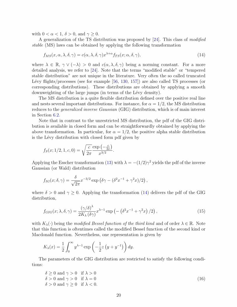
with 0 < α < 1, δ > 0, and γ ≥ 0.A generalization of the TS distribution was proposed by [24]. This class of modified
stable (MS) laws can be obtained by applying the following transformation
fMS(x, α, λ, δ, γ) = c(α, λ, δ, γ)xλ+αfTS(x; α, δ, γ), (14)
where λ ∈ R, γ ∨ (−λ) > 0 and c(α, λ, δ, γ) being a norming constant. For a moredetailed analysis, we refer to [24]. Note that the terms “modified stable” or “temperedstable distribution” are not unique in the literature. Very often the so called truncatedLevy flights/processes (see for example [56, 130, 157]) are also called TS processes (orcorresponding distributions). These distributions are obtained by applying a smoothdownweighting of the large jumps (in terms of the Levy density).
The MS distribution is a quite flexible distribution defined over the positive real lineand nests several important distributions. For instance, for α = 1/2, the MS distributionreduces to the generalized inverse Gaussian (GIG) distribution, which is of main interestin Section 6.2.
Note that in contrast to the unrestricted MS distribution, the pdf of the GIG distri-bution is available in closed form and can be straightforwardly obtained by applying theabove transformation. In particular, for α = 1/2, the positive alpha stable distributionis the Levy distribution with closed form pdf given by
fS(x; 1/2, 1, c, 0) =
√c
2π
exp(− c
2x
)x3/2
.
Applying the Esscher transformation (13) with λ = −(1/2)γ2 yields the pdf of the inverseGaussian (or Wald) distribution
fIG(x; δ, γ) =δ√2π
x−3/2 exp(δγ − (δ2x−1 + γ2x)/2
),
where δ > 0 and γ ≥ 0. Applying the transformation (14) delivers the pdf of the GIGdistribution,
fGIG(x; λ, δ, γ) =(γ/δ)λ
2Kλ (δγ)xλ−1 exp
(−(δ2x−1 + γ2x
)/2), (15)
with Kλ(·) being the modified Bessel function of the third kind and of order λ ∈ R. Notethat this function is oftentimes called the modified Bessel function of the second kind orMacdonald function. Nevertheless, one representation is given by
Kλ(x) =1
2
∫ ∞
0
yλ−1 exp
(−1
2z(y + y−1
))dy.
The parameters of the GIG distribution are restricted to satisfy the following condi-tions:
δ ≥ 0 and γ > 0 if λ > 0δ > 0 and γ > 0 if λ = 0δ > 0 and γ ≥ 0 if λ < 0.
(16)
20

Importantly, in contrast to the positive alpha stable law, all moments exist and are givenby
E [Xr] =
(δ
γ
)rKλ+r(δγ)
Kλ(δγ)(17)
for all r > 0. For a very detailed analysis of the GIG distribution we refer to [117].The GIG distribution nests several positive distributions as special cases and as limitdistributions. Since all of these distributions belong to a special class of the generalizedhyperbolic distribution, we proceed with a discussion of the latter, thus providing abroad framework for the discussion of many important distributions in finance.
6.2 The Generalized Hyperbolic Distribution
The mixing of normal distributions is well suited for financial modeling, as it allows toconstruct very flexible distributions. For example, the normal variance–mean mixture,given by
X = µ + βV +√
V Z, (18)
with Z being normally distributed and V a positive random variable, generally exhibitsheavier tails than the Gaussian distribution. Moreover, this mixture possesses interest-ing properties, for an overview see [22]. First, similarly to other mixtures, the normalvariance–mean mixture is a conditional Gaussian distribution with conditioning on thevolatility states, which is appealing when modeling financial returns. Second, if themixing distribution, i.e. the distribution of V , is infinitely divisible, then X is likewiseinfinitely divisible. This implies that there exists a Levy process with support over thewhole real line, which is distributed at time t = 1 according to the law of X. As thetheoretical properties of Levy processes are well established in the literature (see e.g.[26, 194]), this result immediately suggests to formulate financial models in terms of thecorresponding Levy process.
Obviously, different choices for the distribution of V result in different distributionsof X. However, based on the above property, an infinitely divisible distribution is mostappealing. For the MS distributions discussed in Section 6.1, infinite divisibility is notyet established, although [24] strongly surmise so. However, for some special casesinfinite divisibility has been shown to hold. The most popular is the GIG distributionyielding the generalized hyperbolic (GH) distribution for X. The latter distribution wasintroduced by [17] for modeling the distribution of the size of sand particles. The infinitedivisibility of the GIG distribution was shown by [21].
To derive the GH distribution as a normal variance–mean mixture, let V ∼ GIG(λ, δ, γ)as in (15), with γ =
√α2 − β2, and Z ∼ N(0, 1) independent of V . Applying (18) yields
21

the GH distributed rv X ∼ GH(λ, α, β, µ, δ) with pdf
fGH(x; λ, α, β, µ, δ) =(δγ)λ (δα)1/2−λ
√2πδKλ(δγ)
(1 +
(x− µ)2
δ2
)λ/2−1/4
Kλ−1/2
(αδ
√1 +
(x− µ)2
δ2
)exp (β(x− µ))
for µ ∈ R and
δ ≥ 0 and |β| < α if λ > 0δ > 0 and |β| < α if λ = 0δ > 0 and |β| ≤ α if λ < 0,
which are the induced parameter restrictions of the GIG distribution given in (16).Note that, based on the mixture representation (18), the existing algorithms for
generating GIG distributed rvs can be used to draw rvs from the GH distribution, see[12, 60].
For |β + u| < α, the moment generating function of the GH distribution is given by
E [exp (uX)] = exp (µu)
(α2 − β2
α2 − (β + u)2
)λ/2 Kλ
(δ√
α2 − (β + u)2)
Kλ
(δ√
α2 − β2) . (19)
As the moment generating function is infinitely differentiable in the neighborhood ofzero, moments of all orders exist and have been derived in [27]. In particular, the meanand the variance of a GH rv X are given by
E [X] = µ +βδ√
α2 − β2
Kλ+1(δ√
α2 − β2)
Kλ(δ√
α2 − β2)
= µ + βE [XGIG]
V [X] =δ√
α2 − β2
Kλ+1(δ√
α2 − β2)
Kλ(δ√
α2 − β2)
+β2δ2
α2 − β2
(Kλ+2(δ
√α2 − β2)
Kλ(δ√
α2 − β2))−
K2λ+1(δ
√α2 − β2)
K2λ(δ√
α2 − β2)
)= E [XGIG] + β2V [XGIG] ,
with XGIG ∼ GIG(λ, δ, γ) denoting a GIG distributed rv. Skewness and kurtosis can bederived in a similar way using the third and fourth derivative of the moment generatingfunction (19). However, more information on the tail behavior is given by
fGH(x; λ, α, β, µ, δ) ∼= |x|λ−1 exp ((∓α + β)x) ,
which shows that the GH distribution exhibits semi–heavy tails, see [24].
22

The moment generating function (19) also shows that the GH distribution is gener-ally not closed under convolution. However, for λ ∈ {−1/2, 1/2}, the modified Besselfunction of the third kind satisfies
K− 12(x) = K 1
2(x) =
√π
2xexp(−x),
yielding the following form of the moment generating function for λ = −1/2
E [exp (uX) |λ = −1/2] = exp (µu)exp
(δ√
α2 − β2)
exp(δ√
α2 − (β + u)2) ,
which is obviously closed under convolution. This special class of the GH distributionis called normal inverse Gaussian distribution and is discussed in more detail in Section6.2.2. The closedness under convolution is an attractive property of this distribution asit facilitates forecasting applications.
Another very popular distribution that is nested in the GH distribution is the hyper-bolic distribution given by λ = 1 (see the discussion in Section 6.2.1). Its popularity isprimarily based on its pdf, which can (except for the norming constant) be expressed interms of elementary functions allowing for a very fast numerical evaluation. However,given the increasing computer power and the slightly better performance in reproducingthe unconditional return distribution, the normal inverse Gaussian distribution is nowthe most often used subclass.
Interestingly, further well–known distributions can be expressed as limiting cases ofthe GH distribution, when certain of its parameters approach their extreme values. Tothis end, the following alternative parametrization of the GH distribution turns out to
be useful. Setting ξ = 1/√
1 + δ√
α2 − β2 and χ = ξβ/α renders the two parameters
invariant under location and scale transformations. This is an immediate result of thefollowing property of the GH distribution. If X ∼ GH(λ, α, β, µ, δ), then
a + bX ∼ GH
(λ,
α
|b|,
β
|b|, a + bµ, δ|b|
).
Furthermore, the parameters are restricted by 0 ≤ |χ| < ξ < 1, implying that theyare located in the so–called shape triangle introduced by [20]. Figure 5 highlights theimpact of the parameters in the GH distribution in terms of χ, ξ and λ. Obviously, χcontrols the skewness and ξ the tailedness of the distribution. The impact of λ is not soclear–cut. The lower panels in figure 5 depict the pdfs for different values of λ wherebythe first two moments and the values of χ and ξ are kept constant to show the “partial”influence.
As pointed out by [71], the limit distributions can be classified by the values of ξ andχ as well as by the values % and ζ of a second location and scale invariant parametrizationof the GH, given by % = β/α and ζ = δ
√α2 − β2, as follows:
• ξ = 1 and −1 ≤ χ ≤ 1: The resulting limit distributions depend here on thevalues of λ. Note, that in order to reach the boundary either δ → 0 or |β| → α.
23

0
0.1
0.2
0.3
0.4
0.5
0.6
0.7
-4 -2 0 2 4
1e-04
0.001
0.01
0.1
1
-4 -2 0 2 4
0
0.1
0.2
0.3
0.4
0.5
0.6
0.7
0.8
-4 -2 0 2 4
1e-05
1e-04
0.001
0.01
0.1
1
-4 -2 0 2 4
0
0.1
0.2
0.3
0.4
0.5
0.6
-4 -2 0 2 4
1e-05
1e-04
0.001
0.01
0.1
1
-4 -2 0 2 4
xx
xx
xx
fG
H(x
;λ∗,α
λ∗,β
λ∗,µ
λ∗,δ
λ∗)
fG
H(x
;λ∗,α
λ∗,β
λ∗,µ
λ∗,δ
λ∗)
fG
H(x
;λ,α
ξ∗,β
ξ∗,µ
,δ)
fG
H(x
;λ,α
ξ∗,β
ξ∗,µ
,δ)
fG
H(x
;λ,α
χ∗,β
χ∗,µ
,δ)
fG
H(x
;λ,α
χ∗,β
χ∗,µ
,δ)
λ∗ = −4
λ∗ = −4
λ∗ = −1
λ∗ = −1
λ∗ = 2
λ∗ = 2
ξ∗ = 0.5
ξ∗ = 0.5
ξ∗ = 0.7
ξ∗ = 0.7
ξ∗ = 0.9
ξ∗ = 0.9
χ∗ = −0.8
χ∗ = −0.8
χ∗ = 0.0
χ∗ = 0.0
χ∗ = 0.8
χ∗ = 0.8
linear
Figure 5: Density function (pdf) of the GH distribution for different parameter vectors.The right panel plots the log–densities to better visualize the tail behavior. The upperand middle section present the pdf for different values of χ and ξ. Note that thesecorrespond to different values of α and β. The lower panel highlights the influence of λif the the first two moments, as well as χ and ξ, are held fixed. This implies that α, β, µand δ have to be adjusted accordingly.
24

– For λ > 0 and |β| → α no limit distribution exists, but for δ → 0 the GHdistribution converges to the distribution of a variance gamma rv (see Section6.2.4). However, note that |β| < α implies |χ| < ξ and so the limit distributionis not valid in the corners. For these cases, the limit distributions are givenby ξ = |χ| and 0 < ξ ≤ 1, i.e. the next case.
– For λ = 0 there exists no proper limit distribution.
– For λ < 0 and δ → 0 no proper distribution exists but for β → ±α the limitdistribution is given in [185] with pdf
2λ+1(δ2 + (x− µ)2)(λ−1/2)/2
√2πΓ(−λ)δ2λαλ−1/2
Kλ−1/2
(α√
δ2 + (x− µ)2)
exp (±α(x− µ)) ,
(20)
which is the limit distribution of the corners, since β = ±α is equivalent toχ = ±ξ. This distribution was recently called the GH skew t distribution by[1]. Assuming additionally that α → 0 and β = %α → 0 with % ∈ (−1, 1)yields the limit distribution in between
Γ (−λ + 1/2)√πδ2Γ(−λ)
(1 +
(x− µ)2
δ2
)λ−1/2
,
which is the scaled and shifted Student’s t distribution with −2λ degrees offreedom, expectation µ and variance 4λ2ν/(ν−2), for more details see Secion6.2.3.
• ξ = |χ| and 0 < ξ ≤ 1: Except for the upper corner the limit distribution of theright boundary can be derived for
β = α− φ
2; α →∞; δ → 0; αδ2 → τ
with φ > 0 and is given by the µ-shifted GIG distribution GIG(λ,√
τ ,√
φ). Thedistribution for the left boundary is the same distribution but mirrored at x = 0.Note that the limit behavior does not depend on λ. However, to obtain the limitdistributions for the left and right upper corners we have to distinguish for differentvalues of λ. Recall that for the regime ξ = 1 and −1 ≤ χ ≤ 1 the derivation wasnot possible.
– For λ > 0 the limit distribution is a gamma distribution.
– For λ = 0 no limit distribution exists.
– For λ < 0 the limit distribution is the reciprocal gamma distribution.
• ξ = χ = 0: This is the case for α →∞ or δ →∞. If only α →∞ then the limitdistribution is the Dirac measure concentrated in µ. If in addition δ → ∞ andδ/α → σ2 then the limit distribution is a normal distribution with mean µ + βσ2
and variance σ2.
25

-7620
-7600
-7580
-7560
-7540
-7520
-7500
-7480
-7460
-4 -3 -2 -1 0 1 2 3
-7486
-7485
-7484
-7483
-7482
-7481
-7480
-7479
-2 -1.5 -1 -0.5 0
max
α,β
,µ,δ
∑lo
gf
GH
(x)
λλlinear
Figure 6: Partially maximized log likelihood, estimated maximum log likelihood valuesof the GH distribution for different values of λ.
As pointed out by [185] applying the unrestricted GH distribution to financial dataresults in a very flat likelihood function especially for λ. This characteristic is illustratedin Figure 6, which plots the maximum of the log likelihood for different values of λusing our sample of the S&P500 index returns. This implies that the estimate of λis generally associated with a high standard deviation. As a consequence, rather thanusing the GH distribution directly, the finance literature primarily predetermines thevalue of λ, resulting in specific subclasses of the GH distribution, which are discussed inthe sequel. However, it is still interesting to derive the general results in terms of theGH distribution (or the corresponding Levy process) directly and to restrict only theempirical application to a subclass. For example [191] derived a diffusion process withGH marginal distribution, which is a generalization of the result of [33], who proposeda diffusion process with hyperbolic marginal distribution.
6.2.1 The Hyperbolic Distribution
Recall, that the hyperbolic (HYP) distribution can be obtained as a special case of theGH distribution by setting λ = 1. Thus, all properties of the GH law can be applied tothe HYP case. For instance the pdf of the HYP distribution is straightforwardly givenby (19) setting λ = 1
fH(x; α, β, µ, δ) := fGH(x; 1, α, β, µ, δ)
=
√α2 − β2
2αδK1(δ√
α2 − β2)e−α
√δ2+(x−µ)2+β(x−µ), (21)
where 0 ≤ |β| < α are the shape parameter and µ ∈ R and δ > 0 are the location andscale parmeter, respectively.
The distribution was applied to stock return data by [69, 70, 132] while [33] derived adiffusion model with marginal distribution belonging to the class of HYP distributions.
26

6.2.2 The Normal Inverse Gaussian Distribution
The normal inverse Gaussian (NIG) distribution is given by the GH distribution withλ = −1/2 and has the following pdf
fNIG(x; α, β, µ, δ) := fGH(x;−1
2, α, β, µ, δ)
=αδK1
(α√
δ2 + (x− µ)2)
π√
δ2 + (x− µ)2eδγ+β(x−µ) (22)
with 0 < |β| ≤ α, δ > 0 and µ ∈ R. The moments of a NIG distributed rv canbe obtained from the moment generating function of the GH distribution (19) and aregiven by
E [X] = µ +δβ√
α2 − β2and V [X] =
δα2√α2 − β2
3
S [X] = 3β
α√
δ√
α2 − β2
and K [X] = 3α2 + 4β2
δα2√
α2 − β2.
This distribution was heavily applied in financial economics for modeling the uncondi-tional as well as the conditional return distribution, see e.g. [19, 23, 185]; as well as[10, 18, 114], respectively. Recently, [57] used the NIG distribution for modeling real-ized variance and found improved forecast performance relative to a Gaussian model.A more realistic modeling of the distributional properties is not only important for riskmanagement or forecasting, but also for statistical inference. For example the efficientmethod of moments, proposed by [87] requires the availability of an highly accurate aux-iliary model, which provide the objective function to estimate a more structural model.Recently, [39] provide such an auxiliary model, which uses the NIG distribution andrealized variance measures.
Recall that for λ = −1/2 the mixing distribution is the inverse Gaussian distribution,which facilitates the generation of rvs. Hence, rvs with NIG distribution can be generatedin the following way
1. draw a chi-square distributed rv C with one degree of freedom and a uniformlydistributed rv over the intervall (0, 1) U
2. compute
X1 =δ
γ+
1
2δγ
(δC
γ−√
4δ3C/γ + δ2C2/γ2
)3. if U < δ/(γ(δ/γ + X1)) return X1 else return δ2/(γ2X1).
As pointed out by [187] the main difference between the HYP and NIG distribution:“Hyperbolic log densities, being hyperbolas, are strictly concave everywhere. Thereforethey cannot form any sharp tips near x = 0 without loosing too much mass in the tails... In contrast, NIG log densities are concave only in an intervall around x = 0, andconvex in the tails.” Moreover, [18] concludes, “It is, moreover, rather typical that assetreturns exhibit tail behaviour that is somewhat heavier than log linear, and this furtherstrengthens the case for the NIG in the financial context”.
27

6.2.3 The Student t distribution
Next to the alpha stable distribution Student’s t (t thereafter) distribution has the longesthistory in financial economics. One reason is that although the nonnormality of assetreturns is widely accepted, there still exists some discussion on the exact tail behavior.While the alpha stable distribution implies extremely slowly decreasing tails for α 6= 2,the t distribution exhibits power tails and existing moments up to (and excluding) ν.As such, the t distribution might be regarded as the strongest competitor to the alphastable distribution, shedding also more light on the empirical tail behavior of returns.The pdf for the scaled and shifted t distribution is given by
ft(x; ν, µ, σ) =Γ((ν + 1)/2)√
νπΓ(ν/2)σ
(1 +
1
ν
(x− µ
σ
)2)−(ν+1)/2
(23)
for ν > 0, σ > 0 and µ ∈ R. For µ = 0 and σ = 1 the well–known standard t distributionis obtained. The shifted and scaled t distribution can also be interpreted as a mean-variance mixture (18) with a reciprocal gamma distribution as a mixing distribution.The mean, variance, and kurtosis (3) are given by µ, σ2ν/(ν − 2), and 3(ν − 2)/(ν − 4),provided that ν > 1, ν > 2, and ν > 4, respectively. The tail behavior is
ft(x, ν, µ, σ) ∼= cx−ν−1.
The t distribution is one of the standard nonnormal distribution in financial economics,see e.g. [36, 38, 184]. However, as the unconditional return distribution may exhibitskewness, a skewed version of the t distribution might be more adequate in some cases.In fact, several skewed t distributions were proposed in the literature, for a short overviewsee [1]. The following special form of the pdf was considered in [81, 102]
ft,FS(x; ν, µ, σ, β) =2β
β2 + 1
Γ(
ν+12
)Γ (ν/2)
√πνσ(
1 +1
ν
(x− µ
σ
)2(1
β2I(X ≥ µ) + β2I(x < µ)
))− ν+12
with β > 0. For β = 1 the pdf reduces to the pdf of the usual symmetric scaled andshifted t distribution. Another skewed t distribution was proposed by [116] with pdf
ft,JF (x, ν, µ, σ, β) =Γ(ν + β)21−ν−β
Γ(ν/2)Γ(ν/2 + β)√
ν + βσ
1 +x−µ
σ√ν + β +
(x−µ
σ
)2(ν+1)/2
1−x−µ
σ√ν + β +
(x−µ
σ
)2β+(ν+1)/2
for β > −ν/2. Again, the usual t distribution can be obtained as a special case forβ = 0. A skewed t distribution in terms of the pdf and cdf of the standard t distribution
28

ft(x; ν, 0, 1) and Ft(x; ν, 0, 1) is given by [13, 43]
ft,AC(x; ν, µ, σ, β) =2
σft
(x− µ
σ, ν, 0, 1
)Ft
(β
(x− µ
σ
)√ν + 1
ν +(
x−µσ
)2 , ν + 1, 0, 1
)for β ∈ R.
Alternatively, a skewed t distribution can also be obtained as a limit distribution ofthe GH distribution. Recall that for λ < 0 and β → α the limit distribution is given by(20) as
ft,GH(x; λ, µ, δ, α) =2λ+1(δ2 + (x− µ)2)(λ−1/2)/2
√2πΓ(−λ)δ2λαλ−1/2
Kλ−1/2
(α√
δ2 + (x− µ)2)
exp (α(x− µ)) .
for α ∈ R. The symmetric t distribution is obtained for α → 0. The distribution wasintroduced by [185] and a more detailed examination was recently given in [1].
6.2.4 The Variance Gamma Distribution
The variance gamma (VG) distribution can be obtained as mean–variance mixture withgamma mixing distribution. Note that the gamma distribution is obtained in the limitfrom the GIG distribution for λ > 0 and δ → 0. The pdf of the VG distribution is givenby
fV G(x; µ, α, β, λ) := limδ→0
fGH(x; λ, α, β, δ, µ)
=γ2λ|x− µ|λ−1/2Kλ−1/2 (α|x− µ|)√
πΓ(λ)(2α)λ−1/2eβ(x−µ). (24)
Note, the usual parameterization of the VG distribution
f ∗V G(x; σ∗, θ∗, ν∗, µ∗) =2 exp (θ∗(x− µ∗)/σ∗2)
ν∗1/ν∗√
2πσ∗2Γ(1/ν∗)
((x− µ∗)2
2σ∗2/ν∗ + θ∗2
) 12ν∗−
14
K 1ν∗−
12
(√(x− µ∗)2(2σ∗2/ν∗ + θ∗2)
σ∗2
)is different from the one used here, however the parameters can be transformed betweenthese repesentation in the following way
σ∗ =
√2λ
α2 − β2; θ∗ =
2βλ
α2 − β2; ν∗ =
1
λ; µ∗ = µ.
This distribution was introduced by [149, 150, 151]. For λ = 1 (the HYP case) we obtaina skewed, shifted and scaled Laplace distribution with pdf
fL(x; α, β, µ) := limδ→0
fGH(x; 1, α, β, δ, µ)
=α2 − β2
2αexp (−α|x− µ|+ β(x− µ)) .
A generalization of the VG distribution to the so called CGMY distribution was proposedby [48].
29

6.2.5 The Cauchy distribution
Setting λ = −1/2, β → 0 and α → 0 the GH distribution converges to the Cauchydistribution with parameters µ and δ. Since the Cauchy distribution belongs to the classof symmetric alpha stable (α = 1) and symmetric t distributions (ν = 1) we refer toSection 6.1 and 6.2.3 for a more detailed discussion.
6.2.6 The Normal Distribution
For α →∞, β = 0 and δ = 2σ2 the GH distribution converges to the normal distributionwith mean µ and variance σ2.
6.3 Finite Mixtures of Normal Distributions
The density of a (finite) mixture of k normal distributions is given by a linear combinationof k Gaussian component densities, i.e.,
fNM(x; θ) =k∑
j=1
λjφ(x; µj, σ2j ), φ(x; µ, σ2) =
1√2πσ
exp
(−(x− µ)2
2σ2
), (25)
where θ = (λ1, . . . , λk−1, µ1, . . . , µk, σ21, . . . , σ
2k), λk = 1 −
∑k−1j=1 λj, λj > 0, µj ∈ R,
σ2j > 0, j = 1, . . . , k, and (µi, σ
2i ) 6= (µj, σ
2j ) for i 6= j. In (25), the λj, µj, and σ2
j arecalled the mixing weights, component means, and component variances, respectively.
Finite mixtures of normal distributions have been applied as early as 1886 in [174] tomodel leptokurtic phenomena in astrophysics. A voluminous literature exists, see [165]for an overview. In our discussion, we shall focus on a few aspects relevant for appli-cations in finance. In this context, (25) arises naturally when the component densitiesare interpreted as different market regimes. For example, in a two–component mixture(k = 2), the first component, with a relatively high mean and small variance, may beinterpreted as the bull market regime, occurring with probability λ1, whereas the secondregime, with a lower expected return and a greater variance, represents the bear market.This (typical) pattern emerges for the S&P500 returns, see Table 1. Clearly (25) canbe generalized to accommodate nonnormal component densities; e.g., [104] model stockreturns using mixtures of generalized error distributions of the form (40). However, itmay be argued that in this way much of the original appeal of (25), i.e., within–regimenormality along with CLT arguments, is lost.
The moments of (25) can be inferred from those of the normal distribution, withmean and variance given by
E [X] =k∑
j=1
λjµj, and V [X] =k∑
j=1
λj(σ2j + µ2
j)−
(k∑
j=1
λjµj
)2
, (26)
respectively. The class of finite normal mixtures is very flexible in modeling the lep-tokurtosis and, if existent, skewness of financial data. To illustrate the first property,consider the scale normal mixture, where, in (25), µ1 = µ2 = · · · = µk := µ. Infact, when applied to financial return data, it is often found that the market regimes
30

differ mainly in their variances, while the component means are rather close in value,and often their differences are not significant statistically. This reflects the observa-tion that excess kurtosis is a much more pronounced (and ubiquitous) property of as-set returns than skewness. In the scale mixture case, the density is symmetric, butwith higher peaks and thicker tails than the normal with the same mean and variance.To see this, note that
∑j(λj/σj) > (
∑j λjσ
2j )−1/2 ⇔ (
∑j λjσ
2j )
1/2 > [∑
j(λj/σj)]−1.
But (∑
j λjσ2j )
1/2 >∑
j λjσj > [∑
j(λj/σj)]−1 by Jensen’s and the arithmetic–harmonic
mean inequality, respectively. This shows fNM(µ; θ) > φ(µ; µ,∑
j λjσ2j ), i.e., peaked-
ness. Tailedness follows from the observation that the difference between the mixtureand the mean–variance equivalent normal density is asymptotically dominated by thecomponent with the greatest variance. Moreover, the densities of the scale mixture andthe mean–variance equivalent Gaussian intersect exactly two times on both sides of themean, so that the scale mixture satisfies the density crossing condition in Finucan’s the-orem mentioned in Section 3 and observed in the center panel of Figure 1. This followsfrom the fact that, if a1, . . . , an and γ1 < · · · < γn are real constants, and N is thenumber of real zeros of the function ϕ(x) =
∑i aie
γix, then W − N is a nonnegativeeven integer, where W is the number of sign changes in the sequence a1, . . . , an [183].Skewness can be incorporated into the model when the component means are allowedto differ. For example, if, in the two–component mixture, the high–variance componenthas both a smaller mean and mixing weight, then the distribution will be skewed to theleft.
Due to their flexibility and the aforementioned economic interpretation, finite normalmixtures have been frequently used to model the unconditional distribution of assetreturns [40, 44, 129, 179], and they have become rather popular since the publicationof Hamilton’s [101] paper on Markov–switching processes, where the mixing weights areassumed to be time–varying according to a k–state Markov chain; see, e.g., [200] for anearly contribution in this direction.
However, although a finite mixture of normals is a rather flexible model, its tails decayeventually in a Gaussian manner, and therefore, according to the discussion in Section 5,it may often not be appropriate to model returns at higher frequencies unconditionally.Nevertheless, when incorporated into a GARCH structure (see Section 7), it provides aboth useful and intuitively appealing framework for modeling the conditional distributionof asset returns, as in [5, 96, 97]. These papers also provide a discussion of alternativeinterpretations of the mixture model (25), as well as an overview over the extensiveliterature.
6.4 Empirical Comparison
In the following we empirically illustrate the adequacy of the various distributions dis-cussed in the previous sections for modeling the unconditional return distribution. Table1 presents the estimation results for the S&P500 index assuming iid returns. The loglikelihood values clearly indicate the inadequacy of the normal, Cauchy and stable dis-tributions. This is also highlighted in the upper panel of Figure 7, which clearly showsthat the tails of the Cauchy and stable distributions are too heavy, whereas those of thenormal distribution are too weak. To distinguish the other distributions in more detail,
31

the lower left panel is an enlarged display of the shadowed box in the upper panel. Itillustrates nicely that the two component mixture, VG and HYP distribution exhibitsemiheavy tails, which are probably a little bit to weak for an adequate modeling asis indicated by the log likelihood values. Similarly, the two–component finite normalmixture, although much better than the normal, cannot keep up with most of the othermodels, presumably due to its essentially Gaussian tails. Although the pdf of the NIGdistribution lies somewhere in between the pdfs of the HYP and the different t distri-butions, the log likelihood value clearly indicates that this distribution is in a statisticalsense importantly closer to the t distributions. A further distinction between the otherdistributions including all kinds of t distributions and the GH distribution is nearly im-possible, as can be seen from the lower right plot, which is an enlarged display of thelower left panel. The log likelihood values also do not allow for a clear distinction. Notealso that the symmetric t distribution performs unexpectedly well. In particular, its loglikelihood is almost indistinguishable from those of the skewed versions. Also note that,for all t distributions, the estimated tail index, ν, is close to 3.5, which is in accordancewith the results from semiparametric tail estimation in Section 5.
The ranking of the distributions in terms of the log likelihood depends of courseheavily on the dataset, and different return series may imply different rankings. However,Table 1 also highlights some less data–dependent results, which are more or less acceptedin the literature, e.g., the tails of the Cauchy and stable distributions are too heavy, andthose of the HYP and VG are too light for the unconditional distribution. This needsof course no longer be valid in a different modeling setup. Especially in a GARCHframework the conditional distribution don’t need to imply such heavy tails because themodel itself imposes fatter tails.
In Section 8, the comparison of the models will be continued on the basis of theirability the measure the Value–at–Risk, an important concept in risk management.
7 Volatility Clustering and Fat Tails
It has long been known that the returns of most financial assets, although close to beingunpredictable, exhibit significant dependencies in measures of volatility, such as absoluteor squared returns. Moreover, the empirical results based on the recent availability ofmore precise volatility measures, such as the realized volatility, which is defined as thesum over the squared intradaily high–frequency returns (see e.g. [7] and [25]), alsopoint towards the same direction. In particular, the realized volatility has been found toexhibit strong persistence in its autocorrelation function, which shows a hyperbolic decayindicating the presence of long memory in the volatility process. In fact, this finding aswell as other stylized features of the realized volatility have been observed across differentdata sets and markets and are therefore by now widely acknowledged and establishedin the literature. For a more detailed and originating discussion on the stylized facts ofthe high–frequency based volatility measures for stock returns and exchange returns werefer to [9] and [8], respectively.
The observed dependence of time–varying pattern of the volatility is usually referredto as volatility clustering. It is also apparent in the top panel of Figure 1 and was alreadyobserved by Mandelbrot [154], who noted that “‘large changes tend to be followed by
32

Table 1: Maximum–likelihood parameter estimates of the iid model.distribution parameters loglik
GHλ µ α β δ
-7479.2−1.422(0.351)
0.087(0.018)
0.322(0.222)
−0.046(0.022)
1.152(0.139)
tGHµ δ λ α
-7479.70.084(0.018)
1.271(0.052)
3.445(0.181)
−0.041(0.021)
tJFν µ σ β
-7480.03.348(0.179)
0.098(0.025)
0.684(0.012)
0.091(0.049)
tACν µ σ β
-7480.13.433(0.180)
0.130(0.042)
0.687(0.013)
−0.123(0.068)
tFSν µ σ β
-7480.33.432(0.180)
0.085(0.020)
0.684(0.012)
0.972(0.017)
symmetric tν µ σ
-7481.73.424(0.179)
0.056(0.011)
0.684(0.012)
NIGµ α β δ
-7482.00.088(0.018)
0.784(0.043)
−0.048(0.022)
0.805(0.028)
HYPµ α β δ
-7499.50.090(0.018)
1.466(0.028)
−0.053(0.023)
0.176(0.043)
VGµ α β λ
-7504.20.092(0.013)
1.504(0.048)
−0.054(0.019)
1.115(0.054)
alpha stableα β c τ
-7522.51.657(0.024)
−0.094(0.049)
0.555(0.008)
0.036(0.015)
finite mixture (k = 2)λ1 µ1 µ2 σ1
2 σ22
-7580.80.872(0.018)
0.063(0.012)
−0.132(0.096)
0.544(0.027)
4.978(0.530)
Cauchyµ σ
-7956.60.060(0.010)
0.469(0.008)
normalµ σ
-8168.90.039(0.014)
1.054(0.010)
Shown are maximum likelihood estimates for iid models with different assumptions about thedistribution of the innovations. Standard errors are given in parentheses. “loglik” is the valueof the maximized log likelihood function.
33

1e-22
1e-20
1e-18
1e-16
1e-14
1e-12
1e-10
1e-08
1e-06
1e-04
0.01
1
-10 -5 0 5 10
1e-05
1e-04
-9 -8.5 -8 -7.5 -7
1e-04
-9 -8.9 -8.8 -8.7 -8.6 -8.5
xx
x
f(x
)
f(x
)f(x
)
finite mixture
alpha stableCauchynormal
NIGHYP
VG
GHtGH
tJF
tAC
tFS
sym. t
linear
Figure 7: Plot of the estimated pdfs of the different return distributions assuming iidreturns.
34

large changes—of either sign—and small changes tend to be followed by small changes”.It is now well understood that volatility clustering can explain at least part of the fat–tailedness of the unconditional return distribution, even if the conditional distribution isGaussian. This is also supported by the recent observation that if the returns are scaledby the realized volatility then the distribution of the resulting series is approximatelyGaussian (see [9] and [8]). To illustrate, consider a time series {εt} of the form
εt = ηtσt, (27)
where {ηt} is an iid sequence with mean zero and unit variance, with ηt being independentof σt, so that σ2
t is the conditional variance of εt. With respect to the kurtosis measureK in (3), it has been observed by [108], and earlier by [31] in a different context, that, aslong as σ2
t is not constant, Jensen’s inequality implies E [ε4t ] = E [η4
t ] E [σ4t ] > E [η4
t ] E2[σ2t ],
so that the kurtosis of the unconditional distribution exceeds that of the innovationprocess. Clearly K provides only limited information about the actual shape of thedistribution, and more meaningful results can be obtained by specifying the dynamics ofthe conditional variance, σ2
t . A general useful result [166] for analyzing the tail behaviorof processes such as (27) is that, if ξt and σt are independent nonnegative randomvariables with σt regularly varying, i.e., P (σt > x) = L(x)x−α for some slowly varyingL, and E
[ξα+δt
]< ∞ for some δ > 0, then ξtσt is likewise regularly varying with tail
index α, namely,
P (ξtσt > x) ∼= E [ξα] P (σt > x) as x →∞. (28)
Arguably the most popular model for the evolution of σ2t in (27) is the generalized
autoregressive conditional heteroskedasticity process of orders p and q, or GARCH(p, q),as introduced by [73, 37], which specifies the conditional variance as
σ2t = α0 +
q∑i=1
αiε2t−i +
p∑i=1
βiσ2t−i. (29)
The case p = 0 in (29) is referred to as an ARCH(q) process, which is the specificationconsidered in [73]. To make sure that the conditional variance remains positive forall t, appropriate restrictions have to be imposed on the parameters in (29), i.e., αi,i = 0, . . . , q, and βi, i = 1, . . . , p. It is clearly sufficient to assume that α0 is positive andall the other parameters are nonnegative, as in [37], but these conditions can be relaxedsubstantially if p, q > 0 and p + q > 2 [173].
[37] has shown that the process defined by (27) and (29) is covariance stationary iff
P (z) = zm −m∑
i=1
(αi + βi)zm−i = 0 ⇒ |z| < 1, (30)
where m = max{p, q}, and αi = 0 for i > q, and βi = 0 for i < p, which boils downto∑
i αi +∑
i βi < 1 in case the nonnegativity restrictions of [37] are imposed. Thesituation
∑i αi +
∑i βi = 1 is referred to as an integrated GARCH (IGARCH) model,
and in applications it is often found that the sum is just below unity. This indicates a
35

high degree of volatility persistence, but the interpretation of this phenomenon is not soclear–cut [167]. If (30) holds, the unconditional variance of the process defined by (27)and (29) is given by
E[ε2t
]=
α0
1−∑q
i=1 αi −∑p
i=1 βi
. (31)
In practice, the GARCH(1,1) specification is of particular importance, and it will be thefocus of our discussion too, i.e., we shall concentrate on the model (27) with
σ2t = α0 + (α1η
2t−1 + β1)σ
2t−1, α0 > 0, α1 > 0, 1 > β1 ≥ 0. (32)
The case α1 = 0 corresponds to a model with constant variance, which is of no interestin the current discussion.
An interesting property of the GARCH process is that its unconditional distributionis fat–tailed even with light–tailed (e.g., Gaussian) innovations, i.e., the distributionalproperties of the returns will not reflect those of the innovation (news) process. This hasbeen known basically since [73, 37], who showed that, even with normally distributedinnovations, (G)ARCH processes do not have all their moments finite. For example,for the GARCH(1,1) model, [37] showed that, with m ∈ N, the unconditional (2m)thmoment of εt in (27) is finite if and only if
E[(α1η
2t + β1)
m]
< 1, (33)
which, as long as α1 > 0, will eventually be violated for all practically relevant distribu-tions. The argument in [37] is based on the relation
E[σ2m
t
]=
m∑i=0
(m
i
)αi
0E[(α1η
2t−1 + β1)
m−i]E[σ
2(m−i)t−1
], (34)
which follows from (32). The coefficient of E[σ2m
t−1
]on the right–hand side of (34) is just
the expression appearing in (33), and consequently the (2m)th unconditional momentcannot be finite if this exceeds unity. The heavy–tailedness of the GARCH process issometimes also exemplified by means of its unconditional kurtosis measure (3), which isfinite for the GARCH(1,1) model with Gaussian innovations iff 3α2
1 + 2α1β1 + β21 < 1.
Writing (34) down for m = 2, using (31) and substituting into (3) gives
K [εt] =3[1− (α1 + β1)
2]
1− (α1 + β1)2 − 2α21
> 3,
as E [ε4t ] = 3E [σ4
t ]. [73] notes that “[m]any statistical procedures have been designed tobe robust to large errors, but ... none of this literature has made use of the fact thattemporal clustering of outliers can be used to predict their occurrence and minimize theireffects. This is exactly the approach taken by the ARCH model”. Conditions for theexistence of and expressions for higher–order moments of the GARCH(p, q) model canbe found in [50, 105, 122, 139]. The relation between the conditional and unconditionalkurtosis of GARCH models was investigated in [15], see also [47] for related results.
36

A more precise characterization of the tails of GARCH processes has been developedby applying classical results about the tail behavior of solutions of stochastic differenceequations as, for example, in [124]. We shall continue to concentrate on the GARCH(1,1)case, which admits relatively explicit results, and which has already been written as afirst–order stochastic difference equation in (32). Iterating this,
σ2t = σ2
0
t∏i=1
(α1η2t−i + β1) + α0
[1 +
t−1∑k=1
k∏i=1
(α1η2t−i + β1)
]. (35)
[171] has shown that the GARCH(1,1) process (32) has a strictly stationary solution,given by
σ2t = α0
[1 +
∞∑k=1
k∏i=1
(α1η2t−i + β1)
], (36)
if and only if
E[log(α1η
2t + β1)
]< 0. (37)
The keynote of the argument in [171] is the application of the strong law of large num-bers to the terms of the form
∏ki=1(α1η
2t−i + β1) = exp{
∑k1 log(α1η
2t−i + β1)} in (35),
revealing that (35) converges almost surely if (37) holds. Note that E [log(α1η2t + β1)] <
log E [α1η2t + β1] = log(α1 + β1), i.e., stationary GARCH processes need not be covari-
ance stationary. Using (36) and standard moment inequalities, [171] further establishedthat, in case of stationarity, E [|εt|p], p > 0, is finite if and only if E
[(α1η
2t + β1)
p/2]
< 1,which generalizes (33) to noninteger moments. It may now be supposed, and, buildingon the results of [124, 90], has indeed been established by [166], that the tails of themarginal distribution of εt generated by a GARCH(1,1) process decay asymptotically ina Pareto–type fashion, i.e.,
P (|εt| > x) ∼= cx−α as x →∞, (38)
where the tail index α is the unique positive solution of the equation
h(α) := E[(α1η
2t + β1)
α/2]
= 1. (39)
This follows from (28) along with the result that the tails of σ2t and σt are asymptot-
ically Paretian with tail indices α/2 and α, respectively. For a discussion of technicalconditions, see [166]. [166] also provides an expression for the constant c in (38), whichis difficult to calculate explicitly, however. For the ARCH(1) model with Gaussianinnovations, (39) becomes (2α1)
α/2Γ[(α + 1)/2]/√
π = 1, which has already been ob-tained by [63] and was foreshadowed in the work of [168]. The results reported abovehave been generalized in various directions, with qualitatively similar conclusions. TheGARCH(p, q) case is treated in [29], while [140, 141] consider various extensions of thestandard GARCH(1,1) model.
Although the unconditional distribution of a GARCH model with Gaussian innova-tions has genuinely fat tails, it is often found in applications that the tails of empirical
37

return distributions are even fatter than those implied by fitted Gaussian GARCH mod-els, indicating that the conditional distribution, i.e., the distribution of ηt in (27), islikewise fat–tailed. Therefore, it has become standard practice to assume that the in-novations ηt are also heavy tailed, although it has been questioned whether this is thebest modeling strategy [199]. The most popular example of a heavy tailed innovationdistribution is certainly the t considered in Section 6.2.3, which was introduced by [38]into the GARCH literature. Some authors have also found it beneficial to let the degreesof freedom parameter ν in (23) be time–varying, thus obtaining time–varying conditionalfat–tailedness [45].
In the following, we shall briefly discuss a few GARCH(1,1) estimation results for theS&P500 series in order to compare the tails implied by these models with those from thesemiparametric estimation procedures in Section 5. As distributions for the innovationprocess {ηt}, we shall consider the Gaussian, t, and the generalized error distribution(GED), which was introduced by [172] into the GARCH literature, see [128] for a recentcontribution and asymmetric extensions. It has earlier been used in an unconditionalcontext by [94] for the S&P500 returns. The density of the GED with mean zero andunit variance is given by
fGED(x; ν) =λν
21/ν+1Γ(1/ν)exp
(−|λx|ν
2
), ν > 0, (40)
where λ = 21/ν√
Γ(3/ν)/Γ(1/ν). Parameter ν in (40) controls the thickness of the tails.For ν = 2, we get the normal distribution, and a leptokurtic shape is obtained for ν < 2.In the latter case, the tails of (40) are therefore thicker than those of the Gaussian,but they are not fat in the Pareto sense. However, even if one argues for Pareto tailsof return distributions, use of (40) may be appropriate as a conditional distribution inGARCH models, because the power law already accompanies the volatility dynamics.To make the estimates of the parameter α1 in (32) comparable, we also use the unitvariance version of the t, which requires multiplying X in (23) by
√(ν − 2)/ν. Returns
are modeled as rt = µ + εt, where µ is a constant mean and εt is generated by (27) and(32). Parameter estimates, obtained by maximum–likelihood estimation, are provided inTable 2. In addition to the GARCH parameters in (32) and the shape parameters of theinnovation distributions, Table 2 reports the log likelihood values and the implied tailindices, α, which are obtained by solving (39) numerically. First note that all the GARCHmodels have considerably higher likelihood values than the iid models in Table 1, whichhighlights the importance of accounting for conditional heteroskedasticity. We can alsoconclude that the Gaussian assumption is still inadequate as a conditional distribution inGARCH models, as both the t and the GED achieve significantly higher likelihood values,and their estimated shape parameters indicate pronounced nonnormalities. However, thedegrees of freedom parameter of the t, ν, is somewhat increased in comparison to Table1, as part of the leptokurtosis is now explained by the GARCH effects.
Compared to the nonparametric tail estimates obtained in Section 5, the tail indeximplied by the Gaussian GARCH(1,1) model turns out to be somewhat too high, whilethose of the more flexible models are both between 3 and 4 and therefore more in linewith what has been found in Section 5. However, for all three models, the confidenceintervals for α, as obtained from 1000 simulations from the respective estimated GARCH
38

Table 2: GARCH parameter estimates
distribution µ α0 α1 β1 ν α logliknormal 0.059
(0.011)0.012(0.002)
0.080(0.008)
0.911(0.009)
− 4.70(3.20,7.22)
–7271.7
GED 0.063(0.010)
0.007(0.002)
0.058(0.007)
0.936(0.008)
1.291(0.031)
3.95(2.52,6.95)
–7088.2
symmetric t 0.063(0.010)
0.006(0.002)
0.051(0.006)
0.943(0.007)
6.224(0.507)
3.79(2.38,5.87)
–7068.1
Shown are maximum–likelihood estimation results for GARCH(1,1) models, as givenby (27) and (32), with different assumptions about the distribution of the innovationsηt in (27). Standard errors for the model parameters and 95% confidence intervalsfor the implied tail indices, α, are given in parentheses. “loglik” is the value of themaximized log likelihood function.
0.96
0.98
1
1.02
1.04
1.06
1.08
1.1
0 1 2 3 4 5 6 7 8
α
β = 0.911β = 0.9β = 0.92
h(α
)=
E
[ (α1η
2 t+
β1)α
/2
]
linear
Figure 8: The figure displays the function h(α), as defined in (39), for Gaussian ηt,
α = 0.0799 and various values of β1. Note that α1 = 0.0799 and β1 = 0.911 are themaximum likelihood estimates for the S&P500 returns, as reported in Table 2.
processes, are rather wide, so that we cannot conclusively rule out the existence of theunconditional fourth (and even fifth) moment. The width of the confidence intervalsreflects the fact that the implied tail indices are very sensitive to small variations in theunderlying GARCH parameters. For example, if, in the GARCH model with conditionalnormality, we replace the estimate β1 = 0.911 with 0.9, the implied tail index is 7.31,and with β1 = 0.92, we get α = 2.05, which is close to an infinite variance. The situationis depicted in Figure 8, showing h(α) in (39) for the different values of β1. The shapeof h follows generally from h(0) = 1, h′(0) < 0 by (37), h′′ > 0, i.e., h is convex, andlimα→∞ h(α) = ∞ as long as P [(α1η
2t + β1) > 1] > 0, so that h(α) = 1 has a unique
positive solution. Note that both 0.9 and 0.92 are covered by 0.911 ± 2 × 0.009, i.e.,a 95% confidence interval for β1. This shows that the GARCH–implied tail indices arerather noisy.
Alternatively, we may avoid precise assumptions about the distribution of the inno-
39

vation process {ηt} and rely on quasi maximum–likelihood results [138]. That is, weestimate the innovations by ηt = εt/σt, t = 1, . . . , 5550, where {σt} is the sequence ofconditional standard deviations implied by the estimated Gaussian GARCH model, andthen solve the sample analogue of (39), i.e., T−1
∑Tt=1(α1η
2t + β1)
α/2 = 1, a proceduretheoretically justified in [32]. Doing so, we obtain α = 2.97, so that we recover the “uni-versal cubic law”. However, the 95% confidence interval, calculated from 1000 GARCHsimulations, where the innovation sequences are obtained by sampling with replacementfrom the ηt–series, is (1.73, 4.80), which is still reconcilable with a finite fourth moment,and even with an infinite second moment. These results clearly underline the caveatbrought out by [72] (p. 349), that “[t]here is no free lunch when it comes to [tail index]estimation”.
8 Application to Value–at–Risk
In this section, we compare the models discussed in Sections 6 and 7 on an economicbasis by employing the Value–at–Risk (VaR) concept, which is a widely used measureto describe the downside risk of a financial position both in industry and in academia[118]. Consider a time series of portfolio returns, rt, and an associated series of ex–anteVaR measures with target probability ξ, VaRt(ξ). The VaRt(ξ) implied by a model Mis defined by
PrMt−1(rt < −VaRt(ξ)) = ξ, (41)
where PrMt−1(·) denotes a probability derived from model M using the information upto time t − 1, and the negative sign in (41) is due to the convention of reporting VaRas a positive number. For an appropriately specified model, we expect 100× ξ% of theobserved return values not to exceed the (negative of the) respective VaR forecast. Thus,to assess the performance of the different models, we examine the percentage shortfallfrequencies,
Uξ = 100× x
T= 100× ξ, (42)
where T denotes the number of forecasts evaluated, x is the observed shortfall frequency,i.e., the number of days for which rt < −VaRt(ξ), and ξ = x/T is the empirical shortfallprobability. If ξ is significantly less (higher) than ξ, then model M tends to overestimate(underestimate) the risk of the position. In the present application, in order to captureeven the more extreme tail region, we focus on the target probabilities ξ = 0.001, 0.0025,0.005, 0.01, 0.025, and 0.05.
To formally test whether a model correctly estimates the risk (according to VaR)inherent in a given financial position, that is, whether the empirical shortfall probability,ξ, is statistically indistinguishable from the nominal shortfall probability, ξ, we use thelikelihood ratio test [133]
LRTVaR = −2{x log(ξ/ξ) + (T − x) log[(1− ξ)/(1− ξ)]} asy∼ χ2(1). (43)
Based on the first 1000 return observations, we calculate one–day–ahead VaR mea-sures based on parameter estimates obtained from an expanding data window, where the
40
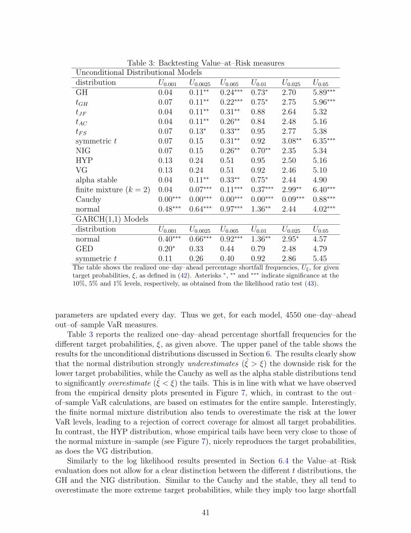
Table 3: Backtesting Value–at–Risk measuresUnconditional Distributional Modelsdistribution U0.001 U0.0025 U0.005 U0.01 U0.025 U0.05
GH 0.04 0.11∗∗ 0.24∗∗∗ 0.73∗ 2.70 5.89∗∗∗
tGH 0.07 0.11∗∗ 0.22∗∗∗ 0.75∗ 2.75 5.96∗∗∗
tJF 0.04 0.11∗∗ 0.31∗∗ 0.88 2.64 5.32tAC 0.04 0.11∗∗ 0.26∗∗ 0.84 2.48 5.16tFS 0.07 0.13∗ 0.33∗∗ 0.95 2.77 5.38symmetric t 0.07 0.15 0.31∗∗ 0.92 3.08∗∗ 6.35∗∗∗
NIG 0.07 0.15 0.26∗∗ 0.70∗∗ 2.35 5.34HYP 0.13 0.24 0.51 0.95 2.50 5.16VG 0.13 0.24 0.51 0.92 2.46 5.10alpha stable 0.04 0.11∗∗ 0.33∗∗ 0.75∗ 2.44 4.90finite mixture (k = 2) 0.04 0.07∗∗∗ 0.11∗∗∗ 0.37∗∗∗ 2.99∗∗ 6.40∗∗∗
Cauchy 0.00∗∗∗ 0.00∗∗∗ 0.00∗∗∗ 0.00∗∗∗ 0.09∗∗∗ 0.88∗∗∗
normal 0.48∗∗∗ 0.64∗∗∗ 0.97∗∗∗ 1.36∗∗ 2.44 4.02∗∗∗
GARCH(1,1) Modelsdistribution U0.001 U0.0025 U0.005 U0.01 U0.025 U0.05
normal 0.40∗∗∗ 0.66∗∗∗ 0.92∗∗∗ 1.36∗∗ 2.95∗ 4.57GED 0.20∗ 0.33 0.44 0.79 2.48 4.79symmetric t 0.11 0.26 0.40 0.92 2.86 5.45
The table shows the realized one–day–ahead percentage shortfall frequencies, Uξ, for giventarget probabilities, ξ, as defined in (42). Asterisks ∗, ∗∗ and ∗∗∗ indicate significance at the10%, 5% and 1% levels, respectively, as obtained from the likelihood ratio test (43).
parameters are updated every day. Thus we get, for each model, 4550 one–day–aheadout–of–sample VaR measures.
Table 3 reports the realized one–day–ahead percentage shortfall frequencies for thedifferent target probabilities, ξ, as given above. The upper panel of the table shows theresults for the unconditional distributions discussed in Section 6. The results clearly showthat the normal distribution strongly underestimates (ξ > ξ) the downside risk for thelower target probabilities, while the Cauchy as well as the alpha stable distributions tendto significantly overestimate (ξ < ξ) the tails. This is in line with what we have observedfrom the empirical density plots presented in Figure 7, which, in contrast to the out–of–sample VaR calculations, are based on estimates for the entire sample. Interestingly,the finite normal mixture distribution also tends to overestimate the risk at the lowerVaR levels, leading to a rejection of correct coverage for almost all target probabilities.In contrast, the HYP distribution, whose empirical tails have been very close to those ofthe normal mixture in–sample (see Figure 7), nicely reproduces the target probabilities,as does the VG distribution.
Similarly to the log likelihood results presented in Section 6.4 the Value–at–Riskevaluation does not allow for a clear distinction between the different t distributions, theGH and the NIG distribution. Similar to the Cauchy and the stable, they all tend tooverestimate the more extreme target probabilities, while they imply too large shortfall
41

probabilities at the five percent quantile.The fact that most unconditional distributional models tend to overestimate the risk
at the lower target probabilities may be due to our use of an expanding data windowand the impact of the “Black Monday”, where the index decreased by more than 20%,at the beginning of our sample period. In this regard, the advantages of accountingfor time–varying volatility via a GARCH(1,1) structure may become apparent, as thismodel allows the more recent observations to have much more impact on the conditionaldensity forecasts.
In fact, by inspection of the results for the GARCH models, as reported in thelower part of Table 3, it turns out that the GARCH(1,1) model with a normal distribu-tion strongly underestimates the empirical shortfall probabilities at all levels except thelargest (5%). However, considering a GED or t distribution for the return innovationswithin the GARCH model provides accurate estimates of downside risks.
To further discriminate between the GARCH processes and the iid models, tests forconditional coverage may be useful, which are discussed in the voluminous VaR literature(e.g., [53]).
Finally, we point out that the current application is necessarily of an illustrativenature. In particular, if the data generating process is not constant but evolves slowlyover time and/or is subject to abrupt structural breaks, use of a rolling data windowwill be preferred to an expanding window.
9 Future Directions
As highlighted in the previous sections, there exists a plethora of different and well–established approaches for modeling the tails of univariate financial time series. How-ever, on the multivariate level the number of models and distributions is still very limited,although the joint modeling of multiple asset returns is crucial for portfolio risk manage-ment and allocation decisions. The problem is then to model the dependencies betweenfinancial assets. In the literature, this problem has been tackled, for example, by meansof multivariate extensions of the mean–variance mixture (18) [18], multivariate GARCHmodels [30], regime–switching models [11], and copulas [51]. The problem is particularlyintricate if the number of assets to be considered is large, and much work remains tounderstand and properly model their dependence structure.
It is also worth mentioning that the class of GARCH processes, due to its interestingconditional and unconditional distributional properties, has been adopted, for example,in the signal processing literature [52, 55, 3], and it is to be expected that it will beapplied in other fields in the future.
A Literature
A.1 Primary Literature
[1] K. Aas and I. H. Haff. The generalized hyperbolic skew Student’s t-distribution.Journal of Financial Econometrics, 4:275–309, 2006. [25, 28, 29]
42

[2] A. Abhyankar, L. S. Copeland, and W. Wong. Moment condition failure in highfrequency financial data: Evidence from the S&P 500. Applied Economics Letters,2:288–290, 1995. [12]
[3] A. Abramson and I. Cohen. State smoothing in Markov-switching time-frequencyGARCH models. IEEE Signal Processing Letters, 13:377–380, 2006. [42]
[4] V. Akgiray and G. G. Booth. The stable-law model of stock returns. Journal ofBusiness & Economic Statistics, 6:51–57, 1988. [10]
[5] C. Alexander and E. Lazar. Normal mixture GARCH(1,1). Applications to ex-change rate modelling. Journal of Applied Econometrics, 21:307–336, 2006. [31]
[6] S. S. Alexander. Price movements in speculative markets: Trends or random walks.Industrial Management Review, 2:7–25, 1961. [5]
[7] T. G. Andersen and T. Bollerslev. Answering the skeptics: Yes, standard volatilitymodels do provide accurate forecasts. International Economic Review, 39:885–905,1998. [32]
[8] T. G. Andersen, T. Bollerslev, F. X. Diebold, and H. Ebens. The distribution ofrealized stock return volatility. Journal of Financial Economics, 61:43–76, 2001.[32, 35]
[9] T. G. Andersen, T. Bollerslev, F. X. Diebold, and P. Labys. The distribution ofrealized exchange rate volatility. Journal of the American Statistical Association,96:42–55, 2001. [32, 35]
[10] J. Andersson. On the normal inverse Gaussian stochastic volatility model. Journalof Business & Economic Statistics, 19:44–54, 2001. [27]
[11] A. Ang and J. Chen. Asymmetric correlations of equity portfolios. Journal ofFinancial Economics, 63:443–494, 2002. [42]
[12] A. C. Atkinson. The simulation of generalized inverse Gaussian and hyperbolicrandom variables. SIAM Journal on Scientific and Statistical Computing, 3:502–515, 1982. [22]
[13] A. Azzalini and A. Capitanio. Distributions generated by perturbation of symmetrywith emphasis on a multivariate skew t-distribution. Journal of the Royal StatisticalSociety. Series B, 65:367–389, 2003. [29]
[14] L. Bachelier. Theory of speculation. In P. H. Cootner, editor, The Random Char-acter of Stock Market Prices, pages 17–75. MIT Press, 1964. [5]
[15] X. Bai, J. R. Russell, and G. C. Tiao. Kurtosis of GARCH and stochastic volatilitymodels with non–normal innovations. Journal of Econometrics, 114:349–360, 2003.[36]
43

[16] K. P. Balanda and H. L. MacGillivray. Kurtosis: A critical review. The AmericanStatistician, 42:111–119, 1988. [6]
[17] O. E. Barndorff-Nielsen. Exponentially decreasing distributions for the logarithmof particle size. Proceedings of the Royal Society of London. Series A, 353:401–419,1977. [21]
[18] O. E. Barndorff-Nielsen. Normal inverse Gaussian distributions and stochasticvolatility modelling. Scandinavian Journal of Statistics, 24:1–13, 1997. [27, 42]
[19] O. E. Barndorff-Nielsen. Processes of normal inverse Gaussian type. Finance andStochastics, 2:41–68, 1998. [27]
[20] O. E. Barndorff-Nielsen, P. Blæsild, J. L. Jensen, and M. Sørensen. The fascinationof sand. In A. C. Atkinson and S. E. Fienberg, editors, A Celebration of Statistics,pages 57–87. Springer, 1985. [23]
[21] O. E. Barndorff-Nielsen and C. Halgreen. Infinite divisibility of the hyperbolic andgeneralized inverse Gaussian distributions. Probability Theory and Related Fields,38:309–311, 1977. [21]
[22] O. E. Barndorff-Nielsen, J. Kent, and M. Sørensen. Normal variance-mean mix-tures and z distributions. International Statistical Review, 50:145–159, 1982. [21]
[23] O. E. Barndorff-Nielsen and K. Prause. Apparent scaling. Finance and Stochastics,5:103–113, 2001. [27]
[24] O. E. Barndorff-Nielsen and N. Shephard. Normal modified stable processes. The-ory of Probability and Mathematical Statistics, 65:1–19, 2001. [8, 20, 21, 22]
[25] O. E. Barndorff-Nielsen and N. Shephard. Estimating quadratic variation usingrealized variance. Journal of Applied Econometrics, 17:457–477, 2002. [32]
[26] O. E. Barndorff-Nielsen and N. Shephard. Financial Volatility in Continuous Time.Cambridge University Press, 2007. [21]
[27] O. E. Barndorff-Nielsen and R. Stelzer. Absolute moments of generalized hy-perbolic distributions and approximate scaling of normal inverse Gaussian Levyprocesses. Scandinavian Journal of Statistics, 32:617–637, 2005. [22]
[28] A. Barnea and D. H. Downes. A reexamination of the empirical distribution ofstock price changes. Journal of the American Statistical Association, 68:348–350,1973. [10]
[29] B. Basrak, R. A. Davis, and T. Mikosch. Regular variation of GARCH processes.Stochastic Processes and their Applications, 99:95–115, 2002. [37]
[30] L. Bauwens, S. Laurent, and J. V. K. Rombouts. Multivariate GARCH models:A survey. Journal of Applied Econometrics, 21:79–109, 2006. [42]
44

[31] E. M. L. Beale and C. L. Mallows. Scale mixing of symmetric distributions withzero mean. Annals of Mathematical Statistics, 30:1145–1151, 1959. [35]
[32] I. Berkes, L. Horvath, and P. Kokoszka. Estimation of the maximal momentexponent of a GARCH(1,1) sequence. Econometric Theory, 19:565–586, 2003. [40]
[33] B. M. Bibby and M. Sørensen. A hyperbolic diffusion model for stock prices.Finance and Stochastics, 1:25–41, 1997. [26]
[34] N. H. Bingham, C. M. Goldie, and J. L. Teugels. Regular Variation. CambridgeUniversity Press, 1987. [7]
[35] O. J. Blanchard and M. W. Watson. Bubbles, rational expectations, and financialmarkets. In P. Wachtel, editor, Crises in the Economic and Financial Structure,pages 295–315. Lexington Books, 1982. [15]
[36] R. C. Blattberg and N. J. Gonedes. A comparison of the stable and Studentdistributions as statistical models for stock prices. Journal of Business, 47:244–280, 1974. [10, 28]
[37] T. Bollerslev. Generalized autoregressive conditional heteroskedasticity. Journalof Econometrics, 31:307–327, 1986. [35, 36]
[38] T. Bollerslev. A conditionally heteroskedastic time series model for speculativeprices and rates of return. Review of Economics and Statistics, 69:542–547, 1987.[28, 38]
[39] T. Bollerslev, U. Kretschmer, C. Pigorsch, and G. Tauchen. A discrete-time modelfor daily S&P500 returns and realized variations: Jumps and leverage effects. Jour-nal of Econometrics, forthcoming, 2007. [27]
[40] P. Boothe and D. Glassman. The statistical distribution of exchange rates. Journalof International Economics, 22:297–319, 1987. [10, 31]
[41] J.-P. Bouchaud and M. Potters. Theory of Financial Risks. From Statistical Physicsto Risk Management. Cambridge University Press, 2000. [12]
[42] G. E. P. Box and M. E. Muller. A note on the generation of random normaldeviates. Annals of Mathematical Statistics, 29:610–611, 1958. [19]
[43] M. D. Branco and D. K. Dey. A general class of multivariate skew-elliptical distri-butions. Journal of Multivariate Analysis, 79:99–113, 2001. [29]
[44] D. S. Broca. Mixture distribution models of Indian stock returns: An empiricalcomparison. Indian Journal of Economics, 84:525–535, 2004. [31]
[45] C. Brooks, S. P. Burke, S. Heravi, and G. Persand. Autoregressive conditionalkurtosis. Journal of Financial Econometrics, 3:399–421, 2005. [38]
[46] J. Campbell, A. W. Lo, and A. C. MacKinlay. The Econometrics of FinancialMarkets. Princeton University Press, 1997. [5]
45

[47] M. A. Carnero, D. Pena, and E. Ruiz. Persistence and kurtosis in GARCH andstochastic volatility models. Journal of Financial Econometrics, 2:319–342, 2004.[36]
[48] P. Carr, H. Geman, D. B. Madan, and M. Yor. The fine structure of asset returns:An empirical investigation. Journal of Business, 75:305–332, 2002. [29]
[49] J. M. Chambers, C. L. Mallows, and B. W. Stuck. A method for simulating stablerandom variables. Journal of the American Statistical Association, 71:340–344,1976. [18]
[50] M. Chen and H. Z. An. A note on the stationarity and the existence of momentsof the GARCH model. Statistica Sinica, 8:505–510, 1998. [36]
[51] U. Cherubini, E. Luciano, and W. Vecchiato. Copula Methods in Finance. JohnWiley & Sons, 2004. [42]
[52] Y. M. Cheung and L. Xu. Dual multivariate auto-regressive modeling in statespace for temporal signal separation. IEEE Transactions on Systems, Man, andCybernetics—Part B: Cybernetics, 33:386–398, 2003. [42]
[53] P. F. Christoffersen and D. Pelletier. Backtesting value–at–risk: A duration–basedapproach. Journal of Financial Econometrics, 2:84 – 108, 2004. [42]
[54] P. K. Clark. A subordinated stochastic process model with finite variance forspeculative prices. Econometrica, 41:135–155, 1973. [10]
[55] I. Cohen. Modeling speech signals in the time-frequency domain using GARCH.Signal Processing, 84:2453–2459, 2004. [42]
[56] R. Cont and P. Tankov. Financial Modelling with Jump Processes. Chapman &Hall, 2004. [20]
[57] F. Corsi, S. Mittnik, C. Pigorsch, and U. Pigorsch. The volatility of realizedvolatility. Working Paper, Center for Financial Studies, 2007. [27]
[58] J. Cotter. Tail behaviour of the euro. Applied Economics, 37:827–840, 2005. [11]
[59] M. M. Dacorogna, U. A. Muller, O. V. Pictet, and C. G. de Vries. Extremal forexreturns in extremely large data sets. Extremes, 4:105–127, 2001. [11]
[60] J. S. Dagpunar. An easily implemented generalised inverse Gaussian generator.Communications in Statistics: Simulations, 18:703–710, 1989. [22]
[61] J. Danıelsson, L. de Haan, L. Peng, and C. G. de Vries. Using a bootstrap methodto choose the sample fraction in tail index estimation. Journal of MultivariateAnalysis, 76:226–248, 2001. [11]
[62] J. Danıelsson and C. G. de Vries. Tail index and quantile estimation with veryhigh frequency data. Journal of Empirical Finance, 4:241–257, 1997. [11]
46
[63] L. de Haan, S. I. Resnick, H. Rootzen, and C. G. de Vries. Extremal behaviour ofsolutions to a stochastic difference equation with applications to ARCH processes.Stochastic Processes and their Applications, 32:213–234, 1989. [9, 37]
[64] C. G. de Vries. Stylized facts of nominal exchange rate returns. In F. V. D. Ploeg,editor, The Handbook of International Macroeconomics, pages 348–389. Blackwell,1994. [10]
[65] T. Doganoglu and S. Mittnik. An approximation procedure for asymmetric stableParetian densities. Computational Statistics, 13:463–475, 1998. [18]
[66] W. H. DuMouchel. On the asymptotic normality of the maximum-likelihood es-timate when sampling from a stable distribution. Annals of Statistics, 1:948–957,1973. [18]
[67] W. H. DuMouchel. Estimating the stable index α in order to measure tail thickness:A critique. Annals of Statistics, 11:1019–1031, 1983. [10]
[68] F. J. Dyson. A note on kurtosis. Journal of the Royal Statistical Society, 106:360–361, 1943. [6]
[69] E. Eberlein and U. Keller. Hyperbolic distributions in finance. Bernoulli, 1:281–299, 1995. [26]
[70] E. Eberlein, U. Keller, and K. Prause. New insights into smile, mispricing, andvalue at risk: The hyperbolic model. Journal of Business, 71:371–405, 1998. [26]
[71] E. Eberlein and E. A. von Hammerstein. Generalized hyperbolic and inverse Gaus-sian distributions: Limiting cases and approximation of processes. In R. Dalang,M. Dozzi, and F. Russo, editors, Seminar on Stochastic Analysis, Random Fieldsand Applications IV, pages 221–264. Birkhauser, 2004. [23]
[72] P. Embrechts, C. Kluppelberg, and T. Mikosch. Modelling Extremal Events forInsurance and Finance. Springer, 1997. [7, 9, 10, 11, 40]
[73] R. F. Engle. Autoregressive conditional heteroscedasticity with estimates of thevariance of United Kingdom inflation. Econometrica, 50:987–1006, 1982. [35, 36]
[74] E. F. Fama. Mandelbrot and the stable Paretian hypothesis. Journal of Business,36:420–429, 1963. [5]
[75] E. F. Fama. The behavior of stock market prices. Journal of Business, 38:34–105,1965. [5, 9, 10]
[76] E. F. Fama. Foundations of Finance. Basic Books, 1976. [5]
[77] E. F. Fama and R. Roll. Parameter estimates for symmetric stable distributions.Journal of the American Statistical Association, 66:331–338, 1971. [18]
[78] J. D. Farmer and F. Lillo. On the origin of power-law tails in price fluctuations.Quantitative Finance, 4:C7–C11, 2004. [15]
47

[79] W. Feller. An Introduction to Probability Theory and its Applications I. JohnWiley & Sons, 1950. [6]
[80] W. Feller. An Introduction to Probability Theory and its Applications II. JohnWiley & Sons, 1971. [11]
[81] C. Fernandez and M. F. Steel. On Bayesian modeling of fat tails and skewness.Journal of the American Statistical Association, 93:359–371, 1998. [28]
[82] H. M. Finucan. A note on kurtosis. Journal of the Royal Statistical Society. SeriesB, 26:111–112, 1964. [6]
[83] X. Gabaix, P. Gopikrishnan, V. Plerou, and E. Stanley. A unified econophysicsexplanation for the power-law exponents of stock market activity. Physica A,382:81–88, 2007. [15]
[84] X. Gabaix, P. Gopikrishnan, V. Plerou, and H. E. Stanley. A theory of power-lawdistributions in financial market fluctuations. Nature, 423:267–270, 2003. [15]
[85] X. Gabaix, P. Gopikrishnan, V. Plerou, and H. E. Stanley. Institutional investorsand stock market volatility. Quarterly Journal of Economics, 121:461–504, 2006.[15]
[86] J. W. Galbraith and S. Zernov. Circuit breakers and the tail index of equityreturns. Journal of Financial Econometrics, 2:109–129, 2004. [10]
[87] A. R. Gallant and G. Tauchen. Which moments to match? Econometric Theory,12:657–681, 1996. [27]
[88] H. U. Gerber and E. S. W. Shiu. Option pricing by Esscher transforms. Transac-tions of Society of Actuaries, 46:99–140, 1994. [19]
[89] D. Ghose and K. F. Kroner. The relationship between GARCH and symmetricstable processes: Finding the source of fat tails in financial data. Journal ofEmpirical Finance, 2:225–251, 1995. [11, 12]
[90] C. M. Goldie. Implicit renewal theory and tails of solutions of random equations.Annals of Applied Probability, 1:126–166, 1991. [37]
[91] P. Gopikrishnan, M. Meyer, L. A. N. Amaral, and H. E. Stanley. Inverse cubiclaw for the distribution of stock price variations. European Physical Journal B,3:139–140, 1998. [12, 15]
[92] P. Gopikrishnan, V. Plerou, L. A. N. Amaral, M. Meyer, and H. E. Stanley. Scalingof the distribution of fluctuations of financial market indices. Physical Review E,60:5305–5316, 1999. [12]
[93] C. Gourieroux and J. Jasiak. Truncated maximum likelihood, goodness of fit testsand tail analysis. Working Paper, CREST, 1998. [14]
48

[94] J. B. Gray and D. W. French. Empirical comparisons of distributional modelsfor stock index returns. Journal of Business Finance and Accounting, 17:451–459,1990. [38]
[95] A. Gut. Probability: A Graduate Course. Springer, 2005. [7]
[96] M. Haas, S. Mittnik, and M. S. Paolella. Mixed normal conditional heteroskedas-ticity. Journal of Financial Econometrics, 2:211–250, 2004. [31]
[97] M. Haas, S. Mittnik, and M. S. Paolella. A new approach to Markov–switchingGARCH models. Journal of Financial Econometrics, 2:493–530, 2004. [31]
[98] R. L. Hagerman. More evidence on the distribution of security returns. Journalof Finance, 33:1213–1221, 1978. [10]
[99] J. A. Hall, W. Brorsen, and S. H. Irwin. The distribution of futures prices: A testof the stable Paretian and mixture of normals hypotheses. Journal of Financialand Quantitative Analysis, 24:105–116, 1989. [10]
[100] P. Hall. On some simple estimates of an exponent of regular variation. Journal ofthe Royal Statistical Society. Series B, 44:37–42, 1982. [11]
[101] J. D. Hamilton. A new approach to the economic analysis of nonstationary timeseries and the business cycle. Econometrica, 57:357–384, 1989. [31]
[102] B. E. Hansen. Autoregressive conditional density estimation. International Eco-nomic Review, 35:705–730, 1994. [28]
[103] P. Harrison. Similarities in the distribution of stock market price changes betweenthe eighteenth and twentieth centuries. Journal of Business, 71:55–79, 1996. [5]
[104] A. Hazan, Z. Landsman, and U. E. Makov. Robustness via a mixture of exponen-tial power distributions. Computational Statistics and Data Analysis, 42:111–121,2003. [30]
[105] C. He and T. Terasvirta. Fourth moment structure of the GARCH(p, q) process.Econometric Theory, 15:824–846, 1999. [36]
[106] B. M. Hill. A simple general approach to inference about the tail of a distribution.Annals of Statistics, 3:1163–1174, 1975. [10]
[107] M. C. A. B. Hols and C. G. de Vries. The limiting distribution of extremal exchangerate returns. Journal of Applied Econometrics, 6:287–302, 1991. [11]
[108] D. A. Hsieh. Modeling heteroskedasticity in daily foreign-exchange rates. Journalof Business & Economic Statistics, 7:307–317, 1989. [35]
[109] D.-A. Hsu, R. B. Miller, and D. W. Wichern. On the stable Paretian behavior ofstock-market prices. Journal of the American Statistical Association, 69:108–113,1974. [10]
49

[110] R. Huisman, K. G. Koedijk, C. J. M. Kool, and F. Palm. Tail-index estimates insmall samples. Journal of Business & Economic Statistics, 19:208–216, 2001. [11]
[111] R. Huisman, K. G. Koedijk, C. J. M. Kool, and F. Palm. The tail-fatness of FXreturns reconsidered. De Economist, 150:299–312, 2002. [11]
[112] N. Hyung and C. G. de Vries. Portfolio diversification effects of downside risk.Journal of Financial Econometrics, 3:107–125, 2005. [12]
[113] D. W. Jansen and C. G. de Vries. On the frequency of large stock returns: Puttingbooms and busts into perspective. Review of Economics and Statistics, 73:18–24,1991. [11, 12]
[114] M. B. Jensen and A. Lunde. The NIG-S&ARCH model: A fat-tailed, stochas-tic, and autoregressive conditional heteroskedastic volatility model. EconometricsJournal, 4:319–342, 2001. [27]
[115] E. Jondeau and M. Rockinger. Testing for differences in the tails of stock-marketreturns. Journal of Empirical Finance, 10:559–581, 2003. [10, 12]
[116] M. C. Jones and M. J. Faddy. A skew extension of the t-distribution, with ap-plications. Journal of the Royal Statistical Society. Series B, 65:159–174, 2003.[28]
[117] B. Jørgensen. Statistical Properties of the Generalized Inverse Gaussian Distribu-tion. Springer, 1982. [21]
[118] P. Jorion. Value at Risk: The New Benchmark for Controlling Derivatives Risk.McGraw-Hill, 2006. [40]
[119] T. Kaizoji and M. Kaizoji. Empirical laws of a stock price index and a stochasticmodel. Advances in Complex Systems, 6:303–312, 2003. [14]
[120] M. Kanter. Stable densities under change of scale and total variation inequalities.Journal of the American Statistical Association, 3:697–707, 1975. [18]
[121] I. Kaplansky. A common error concerning kurtosis. Journal of the AmericanStatistical Association, 40:259, 1945. [6]
[122] M. Karanasos. The second moment and the autocovariance function of the squarederrors of the GARCH model. Journal of Econometrics, 90:63–76, 1999. [36]
[123] P. Kearns and A. Pagan. Estimating the density tail index for financial time series.Review of Economics and Statistics, 79:171–175, 1997. [11]
[124] H. Kesten. Random difference equations and renewal theory for products of randommatrices. Acta Mathematica, 131:207–248, 1973. [37]
[125] K. G. Koedijk, M. M. A. Schafgans, and C. G. de Vries. The tail index of exchangerate returns. Journal of International Economics, 29:93–108, 1990. [11]
50

[126] K. G. Koedijk, P. A. Stork, and C. G. de Vries. Differences between foreignexchange rate regimes: The view from the tails. Journal of International Moneyand Finance, 11:462–473, 1992. [11]
[127] S. M. Kogon and D. B. Williams. Characteristic function based estimation ofstable distribution parameters. In R. J. Adler, R. E. Feldman, and M. S. Taqqu,editors, A Practical Guide to Heavy Tails: Statistical Techniques and Applications,pages 311–335. Birkhauser, 1998. [18]
[128] I. Komunjer. Asymmetric power distribution: Theory and applications to riskmanagement. Journal of Applied Econometrics, 22:891–921, 2007. [38]
[129] S. J. Kon. Models of stock returns: A comparison. Journal of Finance, 39:147–165,1984. [31]
[130] I. Koponen. Analytic approach to the problem of convergence of truncated Levyflights towards the Gaussian stochastic process. Physical Review E, 52:1197–1199,1995. [20]
[131] I. A. Koutrouvelis. Regression-type estimation of the parameters of stable laws.Journal of the American Statistical Association, 75:918–928, 1980. [18]
[132] U. Kuchler, K. Neumann, M. Sørensen, and A. Streller. Stock returns and hyper-bolic distributions. Mathematical and Computer Modelling, 29:1–15, 1999. [26]
[133] P. H. Kupiec. Techniques for verifying the accuracy of risk management models.Journal of Derivatives, 3:73–84, 1995. [40]
[134] J. Laherrere and D. Sornette. Stretched exponential distributions in nature andeconomy: “fat tails” with characteristic scales. European Physical Journal B,2:525–539, 1998. [8]
[135] A. H.-L. Lau, H.-S. Lau, and J. R. Wingender. The distribution of stock returns:New evidence against the stable model. Journal of Business & Economic Statistics,8:217–223, 1990. [10]
[136] M. R. Leadbetter, G. Lindgren, and H. Rootzen. Extremes and Related Propertiesof Random Sequences and Processes. Springer, 1983. [9]
[137] B. LeBaron. Stochastic volatility as a simple generator of apparent financial powerlaws and long memory. Quantitative Finance, 1:621–631, 2001. [13]
[138] S.-W. Lee and B. E. Hansen. Asymptotic theory for the GARCH(1,1) quasi-maximum likelihood estimator. Econometric Theory, 10:29–52, 1994. [40]
[139] S. Ling and M. McAleer. Necessary and sufficient moment conditions for theGARCH(r, s) and asymmetric power GARCH(r, s) models. Econometric Theory,18:722–729, 2002. [36]
51

[140] J.-C. Liu. On the tail behaviors of a family of GARCH processes. EconometricTheory, 22:852–862, 2006. [37]
[141] J.-C. Liu. On the tail behaviors of Box-Cox transformed threshold GARCH(1,1)processes. Statistics and Probability Letters, 76:1323–1330, 2006. [37]
[142] F. M. Longin. The asymptotic distribution of extreme stock market returns. Jour-nal of Business, 69:383–408, 1996. [10]
[143] F. M. Longin. The choice of the distribution of asset returns: How extreme valuetheory can help? Journal of Banking and Finance, 29:1017–1035, 2005. [10]
[144] M. Loretan and P. C. B. Phillips. Testing the covariance stationarity of heavy-tailed time series. Journal of Empirical Finance, 1:211–248, 1994. [10, 11, 12,13]
[145] T. Lux. The stable Paretian hypothesis and the frequency of large returns: Anexamination of major German stocks. Applied Financial Economics, 6:463–475,1996. [12]
[146] T. Lux. On moment condition failure in German stock returns: An applicationof recent advances in extreme value statistics. Empirical Economics, 25:641–652,2000. [12]
[147] T. Lux. The limiting extremal behaviour of speculative returns: An analysis ofintra-daily data from the Frankfurt stock exchange. Applied Financial Economics,11:299–315, 2001. [12]
[148] T. Lux and D. Sornette. On rational bubbles and fat tails. Journal of Money,Credit and Banking, 34:589–610, 2002. [15]
[149] D. B. Madan, P. P. Carr, and E. C. Chang. The variance gamma process andoption pricing. European Finance Review, 2:79–105, 1998. [29]
[150] D. B. Madan and F. Milne. Option pricing with v.g. martingale components.Mathematical Finance, 1:39–55, 1991. [29]
[151] D. B. Madan and E. Seneta. The variance gamma (v.g.) model for share marketreturns. Journal of Business, 63(4):511–524, 1990. [29]
[152] Y. Malevergne, V. Pisarenko, and D. Sornette. Empirical distributions of stockreturns: Between the stretched exponential and the power law? QuantitativeFinance, 5:379–401, 2005. [8, 13]
[153] Y. Malevergne, V. Pisarenko, and D. Sornette. On the power of generalized extremevalue (GEV) and generalized Pareto distribution (GDP) estimators for empiricaldistributions of stock returns. Applied Financial Economics, 16:271–289, 2006. [8,13]
52
[154] B. Mandelbrot. New methods in statistical economics. Journal of Political Econ-omy, 71:421–440, 1963. [3, 5, 9, 15, 32]
[155] B. Mandelbrot. The variation of certain speculative prices. Journal of Business,36:394–419, 1963. [5, 15]
[156] B. Mandelbrot. The variation of some other speculative prices. Journal of Business,40:393–413, 1967. [5]
[157] R. N. Mantegna and H. E. Stanley. Stochastic process with ultraslow convergenceto a Gaussian: The truncated Levy flight. Physical Review Letters, 73:2946–2949,1994. [20]
[158] G. Marsaglia, A. W. Marshall, and F. Proschan. Moment crossings as relatedto density crossings. Journal of the Royal Statistical Society. Series B, 27:91–93,1965. [6]
[159] D. M. Mason. Laws of large numbers for sums of extreme values. Annals ofProbability, 10:754–764, 1982. [11]
[160] K. Matia, L. A. N. Amaral, S. P. Goodwin, and H. E. Stanley. Different scalingbehaviors of commodity spot and future prices. Physical Review E, 66:045103,2002. [12]
[161] K. Matia, M. Pal, H. Salunkay, and H. E. Stanley. Scale-dependent price fluctua-tions for the Indian stock market. Europhysics Letters, 66:909–914, 2004. [15]
[162] J. H. McCulloch. Simple consistent estimators of stable distribution parameters.Communications in Statistics - Simulations, 15:1109–1136, 1986. [18]
[163] J. H. McCulloch. Measuring tail thickness to estimate the stable index α: Acritique. Journal of Business & Economic Statistics, 15:74–81, 1997. [12]
[164] J. B. McDonald. Probability distributions for financial models. In G. S. Maddalaand C. R. Rao, editors, Handbook of Statistics 14: Statistical Methods in Finance,pages 427–461. Elsevier, 1996. [5]
[165] G. J. McLachlan and D. Peel. Finite Mixture Models. John Wiley & Sons, 2000.[30]
[166] T. Mikosch and C. Starica. Limit theory for the sample autocorrelations andextremes of a GARCH(1,1) process. Annals of Statistics, 28:1427–1451, 2000. [9,10, 35, 37]
[167] T. Mikosch and C. Starica. Nonstationarities in financial time series, the long-range dependence, and the IGARCH effects. Review of Economics and Statistics,86:378 – 390, 2004. [36]
[168] A. Milhøj. The moment structure of ARCH processes. Scandinavian Journal ofStatistics, 12:281–292, 1985. [37]
53

[169] S. Mittnik and S. T. Rachev. Modeling asset retunrs with alternative stable dis-tributions. Econometric Reviews, 12:261–330, 1993. [15]
[170] T. Mizuno, S. Kurihara, M. Takayasu, and H. Takayasu. Analysis of high-resolutionforeign exchange data of USD-JPY for 13 years. Physica A, 324:296–302, 2003.[11]
[171] D. B. Nelson. Stationarity and persistence in the GARCH(1,1) model. EconometricTheory, 6:318–334, 1990. [37]
[172] D. B. Nelson. Conditional heteroskedasticity in asset returns: A new approach.Econometrica, 59:347–370, 1991. [38]
[173] D. B. Nelson and C. Q. Cao. Inequality constraints in the univariate GARCHmodel. Journal of Business & Economic Statistics, 10:229–235, 1992. [35]
[174] S. Newcomb. A generalized theory of the combination of observations so as toobtain the best result. In S. M. Stigler, editor, American Contributions to Mathe-matical Statistics in the Nineteenth Century, volume 2, pages 343–366. Arno Press,1980. [30]
[175] J. P. Nolan. Numerical calculation of stable densities and distribution functions.Communications in Statistics - Stochastic Models, 13:759–774, 1997. [18]
[176] R. R. Officer. The distribution of stock returns. Journal of the American StatisticalAssociation, 67:807–812, 1972. [10]
[177] M. F. Omran. Moment condition failure in stock returns: UK evidence. AppliedMathematical Finance, 4:201–206, 1997. [12]
[178] M. F. M. Osborne. Brownian motion in the stock market. Operations Research,7:145–173, 1959. [5]
[179] A. Peiro. The distribution of stock returns: International evidence. Applied Fi-nancial Economics, 4:431–439, 1994. [31]
[180] P. R. Perry. More evidence on the nature of the distribution of security returns.Journal of Financial and Quantitative Analysis, 18:211–221, 1983. [10]
[181] V. Plerou, P. Gopikrishnan, L. A. N. Amaral, M. Meyer, and H. E. Stanley. Scalingof the distribution of price fluctuations of individual companies. Physical ReviewE, 60:6519–6529, 1998. [12]
[182] V. Plerou, P. Gopikrishnan, X. Gabaix, and E. Stanley. On the origin of power-lawfluctuations in stock prices. Quantitative Finance, 4:C11–C15, 2004. [15]
[183] G. Polya and G. Szego. Problems and Theorems in Analysis II. Springer, 1976.[31]
[184] P. D. Praetz. The distribution of share price changes. Journal of Business, 45:49–55, 1972. [10, 28]
54

[185] K. Prause. The Generalized Hyperbolic Model: Estimation, Financial Derivatives,and Risk Measures. PhD thesis, Albert-Ludwigs-Universitat Freiburg i. Br., 1999.[25, 26, 27, 29]
[186] S. J. Press. Estimation in univariate and multivariate stable distributions. Journalof the American Statistical Association, 67:842–846, 1972. [18]
[187] S. Raible. Levy Processes in Finance: Theory, Numerics, and Empirical Facts.PhD thesis, Albert-Ludwigs-Universitat Freiburg i. Br., 2000. [27]
[188] S. I. Resnick. Extreme Values, Regular Variation, and Point Processes. Springer,1987. [7, 8, 9]
[189] S. I. Resnick. Heavy tail modeling and teletraffic data. Annals of Statistics,25:1805–1849, 1997. [11]
[190] S. I. Resnick and C. Starica. Tail index estimation for dependent data. Annals ofApplied Probability, 8:1156–1183, 1998. [11]
[191] T. H. Rydberg. Generalized hyperbolic diffusion processes with applications infinance. Mathematical Finance, 9:183–201, 1999. [26]
[192] G. Samorodnitsky and M. S. Taqqu. Stable Non-Gaussian Random Processes:Stochastic Models with Infinite Variance. Chapman & Hall, 1994. [18]
[193] K.-I. Sato. Levy Processes and Infinitely Divisible Distributions. Cambridge Uni-versity Press, 1999. [18]
[194] W. Schoutens. Levy Processes in Finance: Pricing Financial Derivatives. JohnWiley & Sons, 2003. [21]
[195] E. Seneta. Regularly Varying Functions. Springer, 1976. [7]
[196] K. Sigman. Appendix: A primer on heavy-tailed distributions. Queueing Systems,33:261–275, 1999. [7]
[197] A. C. Silva, R. E. Prange, and V. M. Yakovenko. Exponential distribution offinancial returns at mesoscopic time lags: A new stylized fact. Physica A, 344:227–235, 2004. [14]
[198] B. W. Silverman. Density Estimation for Statistics and Data Analysis. Chapman& Hall, 1986. [5]
[199] I. Tsiakas. Periodic stochastic volatility and fat tails. Journal of Financial Econo-metrics, 4:90–135, 2006. [38]
[200] C. M. Turner, R. Startz, and C. R. Nelson. A Markov model of heteroskedasticity,risk, and learning in the stock market. Journal of Financial Economics, 25:3–22,1989. [31]
55

[201] T. Werner and C. Upper. Time variation in the tail behavior of bund futurereturns. Journal of Futures Markets, 24:387–398, 2004. [12]
[202] R. Weron. Levy-stable distributions revisited: Tail index > 2 does not exclude theLevy-stable regime. International Journal of Modern Physics C, 12:209–223, 2001.[12]
A.2 Books and Reviews
[203] T. Bollerslev, R. F. Engle, and D. B. Nelson. ARCH models. In R. F. Engleand D. L. McFadden, editors, Handbook of Econometrics IV, pages 2959–3038.Elsevier, 1994.
[204] S. Borak, W. Hardle, and R. Weron. Stable distributions. In P. Cizek, W. Hardle,and R. Weron, editors, Statistical Tools for Finance and Insurance, pages 21–44.Springer, 2005.
[205] A. Janicki and A. Weron. Simulation and Chaotic Behavior of α-Stable StochasticProcesses. Marcel Dekker, 1993.
[206] J. H. McCulloch. Financial applications of stable distributions. In G. S. Maddalaand C. R. Rao, editors, Handbook of Statistics 14: Statistical Methods in Finance,pages 393–425. Elsevier, 1996.
[207] T. Mikosch. Modeling dependence and tails of financial time series. InB. Finkenstadt and H. Rootzen, editors, Extreme Values in Finance, Telecom-munications, and the Environment, pages 185–286. Chapman & Hall, 2004.
[208] S. Mittnik, S. T. Rachev, and M. S. Paolella. Stable Paretian modeling in fi-nance: Some empirical and theoretical aspects. In R. J. Adler, R. E. Feldman, andM. S. Taqqu, editors, A Practical Guide to Heavy Tails: Statistical Techniques andApplications, pages 79–110. Birkhauser, 1998.
[209] R. B. Nelsen. An Introduction to Copulas. Springer, 2nd edition, 2006.
[210] A. Pagan. The econometrics of financial markets. Journal of Empirical Finance,3:15–102, 1996.
[211] F. C. Palm. GARCH models of volatility. In G. S. Maddala and C. R. Rao, editors,Handbook of Statistics 14, pages 209–240. Elsevier, 1996.
[212] S. T. Rachev and S. Mittnik. Stable Paretian Models in Finance. John Wiley &Sons, 2000.
[213] V. M. Zolotarev. One-Dimensional Stable Distributions. American MathematicalSociety, 1986.
56


