TI 2014-073/IV Tinbergen Institute Discussion Paper

New HEAVY Models for Fat-Tailed Returns and Realized Covariance Kernels Pawel Janus1

André Lucas2

Anne Opschoor2

1 UBS Global Asset Management; 2 Faculty of Economics and Business Administration, VU University Amsterdam, and Tinbergen Institute.

Tinbergen Institute is the graduate school and research institute in economics of Erasmus University Rotterdam, the University of Amsterdam and VU University Amsterdam. More TI discussion papers can be downloaded at http://www.tinbergen.nl Tinbergen Institute has two locations: Tinbergen Institute Amsterdam Gustav Mahlerplein 117 1082 MS Amsterdam The Netherlands Tel.: +31(0)20 525 1600 Tinbergen Institute Rotterdam Burg. Oudlaan 50 3062 PA Rotterdam The Netherlands Tel.: +31(0)10 408 8900 Fax: +31(0)10 408 9031

Duisenberg school of finance is a collaboration of the Dutch financial sector and universities, with the ambition to support innovative research and offer top quality academic education in core areas of finance.

DSF research papers can be downloaded at: http://www.dsf.nl/ Duisenberg school of finance Gustav Mahlerplein 117 1082 MS Amsterdam The Netherlands Tel.: +31(0)20 525 8579

New HEAVY Models for Fat-Tailed

Returns and Realized Covariance Kernels∗

Pawel Janusa, Andre Lucasb, Anne Opschoorb

a UBS Global Asset Management

b VU University Amsterdam and Tinbergen Institute

This version: June 19, 2014

Abstract

We develop a new model for the multivariate covariance matrix dynamics based on

daily return observations and daily realized covariance matrix kernels based on intra-

day data. Both types of data may be fat-tailed. We account for this by assuming

a matrix-F distribution for the realized kernels, and a multivariate Student’s t dis-

tribution for the returns. Using generalized autoregressive score dynamics for the

unobserved true covariance matrix, our approach automatically corrects for the ef-

fect of outliers and incidentally large observations, both in returns and in covariances.

Moreover, by an appropriate choice of scaling of the conditional score function we are

able to retain a convenient matrix formulation for the dynamic updates of the covari-

ance matrix. This makes the model highly computationally efficient. We show how

the model performs in a controlled simulation setting as well as for empirical data. In

our empirical application, we study daily returns and realized kernels from 15 equi-

ties over the period 2001-2012 and find that the new model statistically outperforms

(recently developed) multivariate volatility models, both in-sample and out-of-sample.

We also comment on the possibility to use composite likelihood methods for estimation

if desired.

Keywords: realized covariance matrices; heavy tails; (degenerate) matrix-F distri-

bution; generalized autoregressive score (GAS) dynamics.

Classification codes: C32, C58.

∗Lucas and Opschoor thank the Dutch Science Foundation (NWO, grant VICI453-09-005) for financialsupport. The views expressed herein are those of the authors and not necessarily those of UBS, which doesnot accept any responsibility for the contents and opinions expressed in this paper. Email correspondence:pawel.janus@ubs.com, a.lucas@vu.nl, a.opschoor@vu.nl.

1

1 Introduction

There is a substantial body of literature for modeling volatilities and correlations of financial

asset returns.; see Bauwens et al. (2006) and Asai et al. (2006) for surveys. Such models are

crucial for risk management, asset allocation, and option pricing. The increasing availability

of intraday financial data has led to the introduction of new types of volatility models that

include so called ’realized measures’ of variances and covariances. These new models lead to

more accurate measures and forecasts of the conditional variance of daily financial returns;

see for example Andersen et al. (2003). Examples in the univariate case of such models are

the MEM model (Engle and Gallo, 2006), the HEAVY (High-frEquency-bAsed VolatilitY)

model (Shephard and Sheppard, 2010), and the Realized GARCH model (Hansen et al.,

2012). These models propose a joint model for the returns and a the realized (variance)

measure. For the multivariate context, Noureldin et al. (2012) propose a multivariate version

of the HEAVY model. Another example is the model for (multivariate) realized measures

of Chiriac and Voev (2011); Bauer and Vorkink (2011), which discard the daily return

observations.

A key feature of financial data is the presence of fat-tails and outliers. This might

effect both the daily return observations as well as the realized measures. Depending on

the chosen estimator for the realized measure, the estimator measures either integrated

variance, or both integrated variance and variation due to jumps. The latter may obviously

substantially inflate realized measures occasionally whenever jumps occur; see for example

Lee and Mykland (2008) on the estimation of spot variances in the presence of jumps. Huang

and Tauchen (2005) show the importance of jumps and argue that they account for up to

7% of S&P cash index variation. Hence both large returns and large values of (multivariate)

realized measures may impact the dynamics of the recently proposed volatility models.

In this paper we develop a new dynamic model for the joint evolution of daily return

covariance matrices and intraday-based realized covariance matrices allowing for fat tails in

both the returns and the realized (co)variance kernels. We do so in an observation driven

framework, thus allowing for easy likelihood evaluation, estimation, and inference. We

describe the dynamics of the unobserved true daily return covariance matrix by adopting

the generalized autoregressive score framework (GAS) of Creal et al. (2011, 2013); see also

2

Harvey (2013). The GAS framework uses the score of the conditional density function to

drive the dynamics of the time-varying parameters, in our case, the covariance matrix. The

framework has been successfully applied in the recent literature to a variety of different

areas. For example, Creal et al. (2011) use the GAS framework to model volatilities and

correlations in stock returns; Lucas et al. (2014) develop new dynamic copula models under

skewness and fat tails and apply this to systemic risk measurement, Harvey and Luati

(2014) describe a new framework for dynamic local level models and state filtering based

on scores, Creal et al. (2014) introduce observation driven mixed measurement dynamic

factor models to describe default and loss-given-default dynamics, Andres (2014) studies

score driven models for positive random variables, and Oh and Patton (2013) studies high

dimensional factor copula models based on GAS dynamics.

The key distributional assumption in our current model is that of a matrix-F distribution

for the realized covariance matrix measures, and a multivariate Student’s t distribution

for the daily returns. For an introduction to the matrix-F distribution, see for example

Konno (1991). This joint distribution for the Student’s t returns and matrix-F realized

kernels provides the basis for computing a score with respect to the unobserved underlying

true covariance matrix. The fat-tailed nature of the F and Student’s t distribution are

particularly convenient in our setting. Fat tails give rise to incidental large observations

that may easily corrupt the estimated dynamic pattern of the underlying covariance matrix

using regular models; see Creal et al. (2011), Janus et al. (2011), Harvey (2013), and Lucas

et al. (2014). The GAS framework based on the matrix-F and multivariate Student’s t

automatically introduces a robust weighting scheme for new return observations and realized

covariance matrices. We show that the weighting induced by our new model takes a highly

intuitive form and automatically downweights the impact of tail observations.

One of the main challenges for matrix-valued random variables and distributions is effi-

ciency of computation and parsimony of the postulated model. In this respect, the HEAVY

models of Noureldin et al. (2012) perform very well. GAS models typically work with the

score of the conditional observation density with respect to a vectorized version of the under-

lying covariance matrix. See for example the paper by Hansen et al. (2014), which models

the vectorized Choleski decomposition of the covariance matrix by a (heavy-tailed but not

fat-tailed) Wishart distribution. Their model is used as a benchmark in our analysis, but is

3

computationally cumbersome in high dimensions k, because it involves the construction of

k2 × k2 matrices for each time t. A second important contribution of our paper, therefore,

is that we introduce a different scaling for the scores that allows us to preserve the matrix

format for the transition dynamics of the unobserved true daily covariance matrix. Our

method thus becomes computationally efficient, while allowing for new robust score driven

transition dynamics. The conditions under which the model is stationary are intuitive and

in line with the familiar multivariate GARCH literature.

As a third contribution, we provide a composite likelihood (CL) scheme for estimation.

Though maximum likelihood estimation is feasible for dimensions up to at least k = 15,

in higher dimensions CL methods might become preferable. Moreover, as argued in Engle

et al. (2008), maximum likelihood methods may suffer from severe biases due to incidental

parameter problems. In such cases, CL methods may provide a better and less biased

alternative estimation methodology. Though we expect the bias problems to be less severe in

our context due to the presence of realized measures, the problem might still play a role. We

show the severity of the problem in a simulation setting and in an empirical application, and

confirm that CL estimation offers a partial solution at the cost of a reduction in estimation

efficiency.

We illustrate the performance of the new method in both a controlled simulation en-

vironment and in an empirical application. In our empirical application, we use the new

Student’s t matrix-F HEAVY type model (HEAVY GAS tF hereafter) to describe daily

returns and daily realized kernels of fifteen equities from the Dow Jones Industrial Aver-

age over the period January 2001 to December 2012. Based on two loss functions, we find

evidence that the in-sample fit improves compared to the normal Wishart GAS model of

Hansen, Janus and Koopman (2014) and the familiar EMWA methodology. We show that

the volatilities and correlations estimated by our new model produce less spikes due to in-

cidentally large tail observations. The differences follow directly from the fat-tailed nature

of the observation densities we assume, and the GAS transition dynamics used to drive the

time variation in the true daily covariance matrices. We also show that the new model

performs better than its competitors out of sample when estimating the model up to the

financial crisis, and using the estimated parameters to forecast volatilities and covariances

afterwards.

4

The rest of this paper is set up as follows. In Section 2, we introduce the new GAS model

for multivariate returns and realized covariance matrices under fat-tails. In Section 3, we

study the performance of the model in a simulation setting. In Section 4, we apply the model

to a panel of 15 daily equity returns and daily realized kernels from the Dow Jones index.

We conclude in Section 5. The appendix gathers some of the more technical derivations.

2 Modeling Framework

2.1 The model

Let yt ∈ Rk denote the vector of (demeaned) asset returns over period t, t = 1, . . . , T , and

let RKt ∈ Rk×k denote the realized covariance matrix over period t, where RKt is computed

using high-frequency data, e.g., a standard realized covariance matrix estimator based on 5

minute return intervals. We allow both yt and RKt to be fat-tailed. For yt, we assume a

standardized Student’s t distribution with ν0 degrees of freedom and time varying covariance

matrix Vt. The observation for density yt reads

py(yt|Vt,Ft−1; ν0) =Γ((ν0 + k)/2)

Γ(ν0/2)[(ν0 − 2)π]k/2|Vt|1/2×

(

1 +ytV

−1t yt

ν0 − 2

)

−(ν0+k)/2

, (1)

where Vt ∈ Rk×k is the positive definite covariance matrix of yt, and Ft is the information

set containing all returns and realized covariances up to time t. We assume that ν0 > 2,

such that the covariance matrix exists. For the realized covariance matrix RKt, we assume

a matrix-F distribution with ν1 and ν2 degrees of freedom. The corresponding observation

density is

pRK(RKt|Vt,Ft−1; ν1, ν2) = K(ν1, ν2)×

∣

∣

∣

ν1ν2−k−1

V −1t

∣

∣

∣

ν1

2

|RKt|(ν1−k−1)/2

∣

∣

∣Ik +

ν1ν2−k−1

V −1t RKt

∣

∣

∣

(ν1+ν2)/2, (2)

5

with positive definite expectation Et[RKt|Ft−1] = Vt, the degrees of freedom ν1, ν2 > k − 1,

and

K(ν1, ν2) =Γk((ν1 + ν2)/2)

Γk(ν1/2)Γk(ν2/2), (3)

where Γk(x) is the multivariate Gamma function

Γk(x) = πk(k−1)/4 ·k∏

i−1

Γ(x+ (1− i)/2); (4)

see for example Konno (1991). We follow Tan (1969) and Gupta and Nagar (2000), and

restrict ν1 and ν2 to be greater than (k − 1) rather than (k + 1) as in Konno (1991). The

matrix-F distribution is the multivariate analogue of the univariate F distribution, which is

in turn a quotient of two χ2 distributions. When ν2 → ∞, the matrix-F distribution degen-

erates and becomes a Wishart distribution (the multivariate analogue of a χ2 distribution)

with ν1 degrees of freedom.

The observation densities for both yt and RKt depend on the common time varying

covariance matrix Vt. We assume that conditional on Vt and Ft−1, returns yt and realized

covariances RKt are independent. There is no obvious way to include dependence between

the multivariate yt and the matrix variate RKt. We therefore leave such extensions to a

future paper.

To describe the dynamics of the unobserved matrix Vt, we use the generalized autore-

gressive score (GAS) framework of Creal et al. (2011, 2013); see also Harvey (2013), Creal

et al. (2014), Lucas et al. (2014), and Hansen et al. (2014). The approach is observation

driven in the classification of Cox (1981). A main advantage of this approach over for

example the parameter driven approach is that the likelihood function is known in closed

form, and therefore estimation and inference by means of maximum likelihood methods is

straightforward.

As mentioned in the introduction, we want to retain the computational efficiency of

matrix recursions. Therefore, instead of the vectorization approach adopted in for example

Lucas et al. (2014) and Hansen et al. (2014), we compute the scores of the conditional

observation density at time t with respect to the matrix variable Vt. We adopt the scaling

6

of the score accordingly. Using a score of the observation density to drive the updates of

the unobserved covariance matrix Vt can be seen as a steepest-ascent step using the time

t predictive likelihood as the criterion function. Score steps can also directly be motivated

from an information theoretic perspective or an optimal mean-squared error perspective

for possibly misspecified filters; see Blasques et al. (2014a) and Nelson and Foster (1994),

respectively.

Rather than taking a steepest-ascent step by taking a derivative on the manifold of

positive definite symmetric matrices, we take the derivative over the simpler manifold of

real, possibly asymmetric matrices. Even though this derivative does not a priori force

the next covariance matrix Vt+1 to be positive definite, we show that the recursions take

such a form that all matrices Vt are positive definite almost surely for all times t under

appropriate parameter restrictions. Further local gains at each time could be obtained by

taking steepest-ascent steps over the more restricted manifold of positive definite symmetric

matrices, but only at the cost of a substantial loss in computational efficiency. As one of

the main aims in this paper is to construct a numerically efficient approach that can also be

used in higher dimensions k, we adopt our current approach of taking scores with respect

to general matrices Vt.

The score with respect to Vt can be found by adding the scores of (1) and (2). The GAS

recursion for our HEAVY model in its basic set-up is given by

Vt+1 = ω + Ast +BVt, (5)

where st is the scaled score, A and B are scalars, and ω ∈ Rk×k is a matrix of intercepts. An

possible extension is to let A and B be diagonal matrices, however we stick to the basic set-

up in this paper. The recursion in (5) is reminiscent of the dynamic conditional correlation

(DCC) recursion of Engle (2002). The main difference is that we use the scaled score st

rather than outer products yty′

t of past returns. Unlike Lucas et al. (2014), and Hansen

et al. (2014), our score is a matrix rather than a vector valued variable. Further lags of Vt

and st can be added on the right-hand side of (5), as can be more complicated dynamics

such as fractionally integrated dynamics; see Creal et al. (2013) and Janus et al. (2011).

Given the two observation densities and the conditional independence assumption, we

7

have the predictive log likelihood and the scores

Lt = log py(yt|Vt,Ft−1; ν0) + log pRK(RKt|Vt,Ft−1; ν1, ν2), (6)

∇t = ∂Lt/∂Vt = ∇y,t +∇RK,t, (7)

∇y,t = ∂ log py(yt|Vt,Ft−1; ν0)/∂Vt,

∇RK,t = ∂ log pRK(RKt|Vt,Ft−1; ν1, ν2)/∂Vt.

This leads to the following result, which is proved in the Appendix A.

Proposition 1 For the Student’s t density (1) and the matrix-F distribution (2), the cor-

responding k × k score matrices ∇y,t and ∇RK,t are

∇y,t =1

2V −1t [wtyty

′

t − Vt]V−1t (8)

∇RK,t =ν12V −1t

ν1 + ν2ν2 − k − 1

RKt

(

Ik +ν1

ν2 − k − 1V −1t RKt

)

−1

− Vt

V −1t (9)

where wt = (ν0 + k)/(ν0 − 2 + y′tV−1t yt), and where derivatives have been taken with respect

to a general non-symmetric matrix Vt rather than a positive definite symmetric matrix Vt.

Equation (8) reveals two important features, which are also put forward in Creal et al.

(2011). First, Vt is driven by the deviations of the weighted outer product wtyty′

t from the

local covariance matrix Vt. When ν0 → ∞, i.e the Student’s t distribution becomes a normal

distribution, the weight equals one and the dynamics of Vt resemble the covariance dynamics

of a multivariate GARCH model. Second, the impact of ‘large values’ yty′

t on Vt is tempered

by wt if the density for y is heavy-tailed, i.e., if 1/ν0 > 0. Put differently, wt decreases when

y′tV−1t yt explodes. The interpretation is that if yt is drawn from a heavy-tailed distribution,

large values of yty′

t could arise as a result of the heavy-tailed nature of the distribution

rather than from a substantial change in the covariance matrix.

The second part of the score presented is new and due to the matrix-F distribution. The

expression in (9) has a similar interpretation as that for the Student’s t distribution, but

for matrix valued random variables. Due to the fat-tailedness of the matrix-F distribution,

‘large’ values of RKt do not automatically lead to a substantial change in the covariance

8

matrix Vt. Instead, the inverse of (Ik + ν1V−1t RKt/(ν2 − k− 1))−1 takes the same role as wt

in (8) and downweights the impact of a large RKt on future values of Vt. When ν2 → ∞,

the matrix-F distribution collapses to the Wishart distribution with ν1 degrees of freedom

and the score in (9) collapses to

∇RK,t =ν12V −1t [RKt − Vt]V

−1t .

The parameter ν2 thus takes the same robustification role for the realized covariance mea-

sures RKt as the parameter ν0 takes for the returns yt.

We emphasize that the results in Proposition 1 differ in an important way from the GAS

models for multivariate volatilities and correlations developed recently by Creal et al. (2011),

Lucas et al. (2014), and Hansen et al. (2014). These earlier models use a vectorized version

of the covariance matrix Vt or of its Choleski decomposition as the time varying parameter.

This vector score is scaled subsequently by the inverse of its conditional variance, or a

similarly sized matrix. This scaling results in matrix multiplications involving matrices of

the order k2 × k2, which typically becomes computationally cumbersome if k increases. For

example, for k = 15, these models typically take a long time to be estimated.

The scores in Proposition 1 clearly need some type of scaling, as the scores and therefore

the transition dynamics explode if the matrix Vt becomes nearly singular. This is the same in

the univariate GARCH context. Looking at the format of the scores, however, the solution

is straightforward. Let G⋆ denote the pseudo inverse of some generic matrix G. In earlier

papers, score for the vectorized covariance matrix were typically scaled by a scaling matrix

of the type((

V−1/2t ⊗ V

−1/2t

)

G(

V−1/2t ⊗ V

−1/2t

))⋆

,

for some fixed matrix G that depends on the distribution of yt, and where ⊗ denotes the

Kronecker product; see for example Creal et al. (2011) and Lucas et al. (2014). Rather

than deriving the matrix G from the distribution of yt, we adopt a simpler approach and

set G = g · Ik2 for a scalar g. As a result, our scaling matrix for the vectorized covariance

matrix becomes 2 Vt ⊗ Vt. Using a matrix rather than a vector format for the derivatives of

9

the predictive likelihood, we can then easily rewrite the scaled scores

st =Vt(∇y,t +∇RK,t)Vt

ν1 + 1, (10)

where we chose g = (ν1 + 1)/2. The pre and post-multiplication by the matrix Vt directly

offsets the instability caused by the inverses V −1t in equations (8) and (9). It does so, while

retaining the efficient form of the matrix recursion. As a result, matrix multiplications only

involve k× k matrices, rather than k2× k2 matrices as in the approaches mentioned earlier.

The division by g = (ν1+1)/2 is performed for similar reasons as in Hansen et al. (2014): it

emerges from the expression for the conditional Fisher information matrix for the limiting

case ν0, ν2 → ∞. The factor can also be omitted and integrated into the parameter A.

However, the factor nicely balances with the value of ν1 in front of ∇RK,t. As a result, the

Student’s t score in the square brackets in (8) receives weight (ν1 + 1)−1, and the F score

in the square brackets in (9) receives weight ν1(ν1 + 1)−1. These weighs naturally add up

to one. If ν1 is large, the signal in RKt about the unobserved Vt is relatively much more

precise than in yty′

t. Therefore, the score due to yty′

t receives a correspondingly lower weight

than that of RKt in the transition dynamics of Vt.

We note that even though we have taken derivatives over the general space of k × k

matrices rather than the manifold of positive definite symmetric matrices, all of the matrices

coming from the recursion (5) are positive definite symmetric as long as A,B > 0, and ω

is positive definite symmetric. Though this is not easy to see directly, we can check that

the matrix-F scaled score steps Vt∇RK,tVt are symmetric and positive definite. The current

modeling framework is thus both computationally efficient, and internally consistent in the

sense that the dynamics for Vt always produce appropriate covariance matrices under the

parameter restrictions mentioned above.

2.2 Stationarity and ergodicity

A useful feature of score based dynamics is that under the assumption of correct specification

the scores ∇y,t and ∇RK,t are martingale differences and have conditional expectation 0. To

study the probabilistic properties of the new fat-tailed score driven HEAVY model, we

10

rewrite the scaled score as

V−1/2t st (V

′

t )−1/2 =

(ν0 + k)

(ν1 + 1)(ν0 − 2)εy,tεy,t

(

1 +1

ν0 − 2ε′y,tεy,t

)

−1

+ (11)

ν1 (ν1 + ν2)

(ν1 + 1)(ν2 − k − 1)εRK,t

(

Ik +ν1

ν2 − k − 1εRK,t

)

−1

− Ik,

where εy,t has Student’s t distribution with mean zero, covariance matrix I, and degrees

of freedom ν0, and εRK,t has a matrix-F distribution with expectation Ik, and degrees of

freedom parameters ν1 and ν2. The right-hand side of (11) does not depend on Vt. Moreover,

the terms on the right-hand side are transformations of (matrix) Beta distributed random

variables; see Tan (1969). They thus have finite expectation and variance if 2 < ν0 < ∞,

k − 1 < ν1 < ∞, and k − 1 < ν2 < ∞. We have the following result.

Proposition 2 If 0 < B < 1, the process generated by the HEAVY GAS tF model is

stationary and ergodic and β-mixing.

Proof: We note that the recursion in (5) can be written as

Vt+1 = ω +BVt +A(Vt)1/2V

−1/2t st (V

′

t )−1/2(V ′

t )1/2.

Using (11), the recursion is then directly of the multivariate GARCH form studied in Boussama (n.d.), and

the result follows directly by Theorem 2 in his paper, accounting for the different parameterization of the

GAS model vis-a-vis the standard multivariate GARCH (BEKK) model.

For the new score driven HEAVY model to be stationary and ergodic, the model thus has

to satisfy the easy and intuitive condition 0 < B < 1. Inspecting the proof of Proposition 2

and of Theorem 2 in Boussama (n.d.), we see that it is straightforward to generalize the

result to models with dynamics of the type

Vt+1 = ω + AstA′ +B VtB

′, (12)

for k×k matrices A and B, which allows for possible volatility spillover effects. It is also clear

from (11) that we can establish the existence of moments for Vt using the feature that the

(matrix) Beta random variates are ‘bounded’ in the appropriate matrix sense. In particular,

for 0 < B < 1, we easily obtain the unconditional first moment E[Vt] = (1−B)−1ω. Many of

11

these features are discussed elaborately for the univariate case in Harvey (2013), including

the feature of the Beta distributed scores and the existence of univariate moments. Our

results provide a multivariate extension of these results.

We note that establishing stationarity and ergodicity of the HEAVY GAS process is

just a first step in establishing the consistency and asymptotic normality of the maximum

likelihood estimator (MLE) for the new model; see also the Section 2.3 about estimation.

Two important additional steps need to be taken as well, namely proving that the model

is identified and that the model is invertible; see the detailed discussions in for example

Straumann and Mikosch (2006) and Wintenberger (2013). Though we conjecture that both

features can be proven for our new model, a full proof goes beyond the scope of the present

paper. We do note that a proof for the univariate case without the realized measures has

been provided by Blasques et al. (2014b). We leave a multivariate extension of this result,

including the use of realized measures, to a future paper.

2.3 Estimation

We collect the parameters in ω,A,B, ν0, ν1, and ν2 into the static parameter vector θ and

estimate θ by maximum likelihood. To do so, we maximize the log-likelihood LT (θ) =∑T

t=1 Lt, where Lt was defined in equation (6). The starting value V1 can be either estimated

or set equal to RK1. We further reduce the number of parameters following Hansen et al.

(2014) by using a covariance targeting approach to estimate ω. As ω = (1 − B)E[Vt] for

0 < B < 1, we replace ω in during estimation by (1 − B) times the sample mean of RKt,

which should be a consistent estimator for the expectation under an ergodicity assumption.

The resulting maximum likelihood estimation procedure is fast and numerically efficient. In

our empirical section, we use it to estimate the parameters of dynamic systems with up to

15 dimensions. Proceeding to even higher dimensional systems should be feasible as well.

Although estimation by maximum likelihood methods is relatively fast in our setting,

the evaluation of the inverse of the k×k matrix Vt for each time t in the score and evaluation

of the likelihood may become time consuming for very large k. As an alternative, we briefly

discuss how to apply composite likelihood (CL) methods for our HEAVY GAS tF model.

CL methods were proposed in contexts like these by Engle, Shephard and Sheppard (2008).

12

They introduced the method to circumvent the incidental parameter problem due to the

estimation of ω in the context of the DCC model of Engle (2002). In particular, they

showed that the maximum likelihood estimator for A, but also for B, is severely biased

towards zero in moderate to large dimensions k. Though we expect that the bias problem is

much less pronounced in the context of HEAVY models due to the availability of accurate

measurements RKt, composite likelihood methods might still provide a useful alternative

estimation method.

To operationalize a CL approach, we have to derive the appropriate likelihood expressions

for pairs of elements from the general observations yt and RKt. Let Mm,t denote a 2 × 2

submatrix extracted from the k × k square matrix Mt, with m = (i, j) a possible pair i, j

(i < j) out of k assets. For the Student’s t distribution, we directly obtain that the bivariate

likelihood for (yi,t, yj,t) is a bivariate Student’s t distribution with ν0 degrees of freedom, and

covariance matrix

Vm,t =

Vii,t Vij,t

Vji,t Vjj,t

.

For the matrix-F distribution, we have the following result due to Gupta and Nagar (2000)

Result 1 (Gupta and Nagar, 2000) If a k × k matrix Vt is matrix-F distributed, i.e.,

RKt ∼ F (ν1, ν2, Vt), then RKm,t ∼ F (ν1, ν2 − (k − 2), Vm,t).

Result 1 directly allows us to obtain a bivariate Student’s t and matrix-F likelihood

for a pair m. In particular, the 2 × 2 submatrix RKm,t also has a matrix-F likelihood,

but with a lower second degrees of freedom parameter ν2 − k + 2 with k ≥ 2. We can

now obtain a CL estimator of θ by maximizing the sum of n∗ bivariate Student’s t and

matrix-F log-likelihoods with respect to θ, where n∗ denotes the number of bivariate pairs

taken into consideration. As suggested by Engle et al. (2008), we only take contigious pairs

m = (i, i+1) into account. The objective function is then computed as follows. For a given

θ, we first compute the full k × k covariance matrices Vt, t = 1, . . . , T . Next, we compute

the appropriate submatrices Vm,t for m = 1, . . . , n∗, and evaluate the bivariate likelihoods

for each pair. The CL objective function is found by taking the sum of all the bivariate

likelihoods over all time periods t and pairs m.

13

3 Simulation experiment

3.1 DGP from the GAS model

We now perform a Monte Carlo study to investigate the statistical properties of the max-

imum likelihood estimator for θ. We simulate time series of T daily returns and daily

realized covariances of dimension k. We use T = 250, 500, 1000, and k = 5, 15. We generate

data using the HEAVY GAS tF model as the true data generating process (DGP) and set

A = α = 0.8, B = β = 0.97, ν0 = 12, ν1 = 22, ad ν2 = 35. In addition, V0 is a matrix with

Vjj = 4 (j = 1, . . . , k) and Vij = 4ρ (i 6= j) with ρ = 0.7. The parameters resemble values

found in the empirical application of Section 4. For each simulated series, we estimate θ

by maximum likelihood. For k = 15, we also use composite likelihood estimation as an

alternative method.

Table 1 shows results of the estimated parameters. The upper panel presents the results

for maximum likelihood estimation. All parameters are estimated near their true values.

Standard deviations shrink as either the sample size T or the dimension k grows. Interest-

ingly, there appears to be a small bias in A for larger dimensions k = 15, especially when

the sample size is small. This could be due to the incidental parameter problem, as shown

by Engle, Shephard and Sheppard (2008) for the DCC model. The composite likelihood

method works well to solve this issue. This is shown in the lower part of the table. The

smaller bias, however, comes at the cost of a larger standard deviation for the estimates, as

expected.

3.2 Filtering results

One of the main aims of the model is to obtain estimates of the unobserved Vt. Given θ

such estimates follow directly from the recursion (5) of the GAS model. To see how well

the model does in capturing unknown dynamics of the (co)variances Vt, we perform the

following experiment. Consider the bivariate deterministic process for the daily volatilities

14

Table 1: Parameter estimations of HEAVY GAS DGPThis table shows Monte Carlo averages and standard deviations (in parentheses) of parameter estimatesfrom simulated HEAVY GAS processes using (5) with k = 5, 15, and T = 250, 500, 1000. For k = 15,the lower panel of the table shows the results of composite likelihood estimation. The true values of theparameters are A = 0.8, B = 0.97, ν0 = 12, ν1 = 22, and ν2 = 35. The table reports the mean andthe standard deviation in parentheses based on 4000 (maximum likelihood) or 1000 (composite likelihood)replications.

k = 5 k = 15Coef. T = 500 T = 1000 T = 500 T = 1000

Maximum LikelihoodA 0.797 (0.036) 0.798 (0.025) 0.787 (0.010) 0.792 (0.007)B 0.966 (0.005) 0.968 (0.004) 0.967 (0.003) 0.969 (0.002)ν0 12.419 (2.233) 12.179 (1.460) 12.178 (1.147) 12.096 (0.805)ν1 22.063 (0.794) 22.037 (0.559) 21.998 (0.129) 21.997 (0.092)ν2 35.127 (2.049) 35.054 (1.435) 35.040 (0.374) 35.012 (0.267)

Composite Likelihoodα 0.794 (0.036) 0.797 (0.026)β 0.964 (0.008) 0.967 (0.004)ν0 12.517 (2.475) 12.364 (1.681)ν1 21.960 (1.018) 21.990 (0.707)ν2 35.067 (1.436) 35.030 (0.891)

and correlation

yi,ti.i.d.∼ N(0, Vt/n),

σt = 4 + sin(2πt), ρt = 0.5 sin(2πt), ,

where σ2t and ρtσ

2t are the variance and covariance at day t = 1, . . . , T . Over the t-th day,

we simulate n intra-day returns yi,t, i = 1, . . . , n. The returns are i.i.d. with covariance

matrix Vt/n. Using the intra-day returns, we construct the daily return yt and the realized

covariance matrix RCOVt (computed as∑n

i=1 yi,ty′

i,t), which is set equal to RKt in this

experiment. We set T and n equal to 1000 and 50, respectively.

In a second experiment, we let the (co)variances vary in a stochastic, rather than a

deterministic way. This DGP combines the fat-tailedness of returns and realized covariance

matrices with stochastic volatility dynamics for the covariance matrix Vt. It does so in the

15

following way:

yt|Ft−1 ∼ t(ν0, Vt), RKt|Ft−1 ∼ F (ν1, ν2, Vt),

Vt = V + γVt−1 + ηt, ηt ∼ SW (V0,w/νw, νw), V0 = 4

1 0.7

0.7 1

,

with ηt a k × k matrix drawn from a standard Wishart distribution with mean V0,η =

κ(1 − γ)V0, and νη degrees of freedom. We set ν0 = 14, ν1 = 30, ν2 = 40, γ = 0.98,

T = 1000, k = 2, νη = 4, κ = 15, and V = (1/10)V0. All these values are chosen such that

we obtain reasonable volatility and correlation patterns.

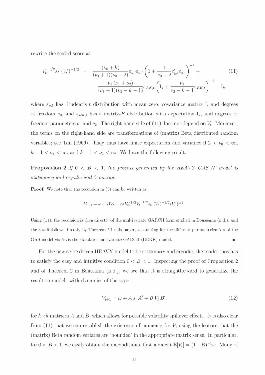
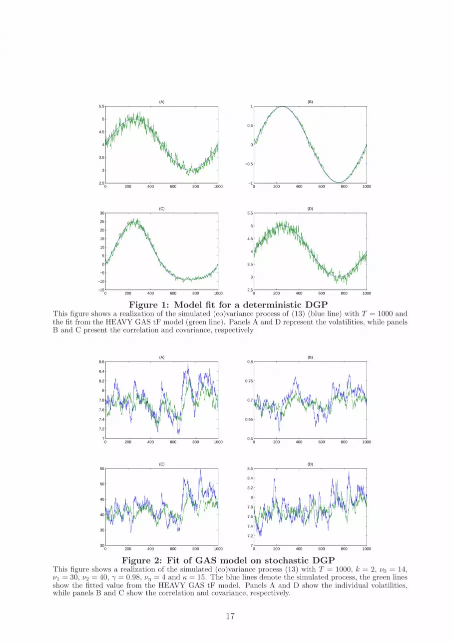
Figures 1 and 2 present the results, each for one particular realization of the DGP. The

blue lines represents the true values of the volatility, correlation, or covariance. The green

lines denote the fitted values corresponding with the estimated HEAVY GAS tF model.

For the deterministic case in Figure 1, the new model easily recovers the patterns for the

volatility, correlation, and covariance. For the stochastic (co)variance case in Figure 2, the

overall fit is also good. The estimated Vt from the HEAVY GAS recursions mimic the

peaks and troughs of the true process, with the exception that some of the larger swings

are somewhat smoothed out. The model works well for both variances, covariances, and

correlations.

4 Empirical application: U.S. equity returns

4.1 Data

We apply the HEAVY GAS tF model to daily returns and daily covariances of 15 equities

from the Dow Jones Industrial Average with the following ticker symbols: AA, AXP, BA,

CAT, GE, HD, HON, IBM, JPM, KO, MCD, PFE, PG, WMT and XOM. The data spans

the period January 2, 2001 until December 31, 2012, or T = 3017 trading days. We

observe consolidated trades (transaction prices) extracted from the Trade and Quote (TAQ)

database with a time-stamp precision of one second. We first clean the high-frequency data

following the guidelines of Brownlees and Gallo (2006) and Barndorff-Nielson et al. (2009).

Second, we construct realized kernels using refresh-time-sampling methods of Barndorff-

16

0 200 400 600 800 10002.5

3

3.5

4

4.5

5

5.5(A)

0 200 400 600 800 1000−1

−0.5

0

0.5

1(B)

0 200 400 600 800 1000−15

−10

−5

0

5

10

15

20

25

30(C)

0 200 400 600 800 10002.5

3

3.5

4

4.5

5

5.5(D)

Figure 1: Model fit for a deterministic DGPThis figure shows a realization of the simulated (co)variance process of (13) (blue line) with T = 1000 andthe fit from the HEAVY GAS tF model (green line). Panels A and D represent the volatilities, while panelsB and C present the correlation and covariance, respectively

0 200 400 600 800 10007

7.2

7.4

7.6

7.8

8

8.2

8.4

8.6(A)

0 200 400 600 800 10000.6

0.65

0.7

0.75

0.8(B)

0 200 400 600 800 100030

35

40

45

50

55(C)

0 200 400 600 800 10007

7.2

7.4

7.6

7.8

8

8.2

8.4

8.6(D)

Figure 2: Fit of GAS model on stochastic DGPThis figure shows a realization of the simulated (co)variance process (13) with T = 1000, k = 2, ν0 = 14,ν1 = 30, ν2 = 40, γ = 0.98, νη = 4 and κ = 15. The blue lines denote the simulated process, the green linesshow the fitted value from the HEAVY GAS tF model. Panels A and D show the individual volatilities,while panels B and C show the correlation and covariance, respectively.

17

Nielson et al. (2011) with the same hyper-parameters as used by Hansen et al. (2014).

4.2 In-sample performance

Using all 3017 trading days, we estimate the HEAVY GAS tF model and compare the

in-sample fit with two alternative models: the HEAVY GAS NW model of Hansen, Janus

and Koopman (2014), and the classical Exponentially Weighted Moving Average (EWMA)

model applied to the constructed realized kernels. Recall that the Hansen, Janus and

Koopman (2014) model uses the vech-torized form of the Cholesky decomposition of Vt and

assumes a conditional normal distribution for the daily returns yt, and aWishart distribution

for the daily realized kernels RKt. The EWMA model uses

Vt+1 = bVt + (1− b)RKt, (13)

where the fixed smoothing parameter b is set equal to 0.96 by practitioners.

We compare the in-sample fit of the models by computing the quasi-likelihood loss

function and the root mean squared error based on the matrix norm

QLIK(Vt, RKt) = log |Vt|+ tr(V −1t RKt), (14)

RMSE(Vt, RKt) = ||RKt − Vt||1/2 =

[

∑

i,j

(RKij,t − Vij,t)2

]1/2

, (15)

with Vt the model based covariance matrix estimate. As Vt is known at time t − 1, the

criteria can also be interpreted as one-step-ahead forecasting criteria.

Table 2 shows parameter estimates and standard errors based on the inverse hessian of

the likelihood evaluated at the optimum. We show the results for two selections of k = 5

stocks, as well as for the complete set of all 15 equities. In addition, we presents the total and

individual log-likelihood values corresponding with the GAS models as well as the average

loss functions for all competing models.

The results in Table 2 suggest that allowing for fat tails in the distribution of both the

returns and realized covariances improves the fit substantially. For example, the RMSE

value decreases by almost 12% when k = 15. We obtain further evidence from the log-

likelihood values of both GAS models. The values show that most of the gain comes from

18

Table 2: Parameter estimates, likelihoods and loss functionsThis table reports maximum likelihood parameter estimates of the HEAVY GAS tF and the HAEVY GAS NW model, applied to daily equity returns anddaily realized kernels of 5 and 15 assets. In case of 15 assets, the table also shows parameter estimates obtained by the Composite Likelihood (CL) method.Standard errors are provided in parenthesis. For both GAS models, the total log-likelihood as well as the individual log-likelihoods corresponding to thereturn and covariance densities are reported. The QLIK and RMSE loss functions are defined in (14) and (15) and are also computed for the EWMAmodel with b = 0.96. The sample is January 2, 2001 until December 31, 2012 (3017 observations).

BA/HD/JPM/PFE/PG GE/IBM/JPM/PG/XOM All equitiesCoef. GAS tF GAS NW EMWA GAS tF GAS NW EMWA GAS tF GAS tF (CL) GAS NW EMWAA 1.349 0.052 1.407 0.056 0.777 0.968 0.026

(0.027) (0.001) (0.025) (0.001) (0.006) (0.008) (0.000)B 0.988 0.974 0.989 0.971 0.991 0.996 0.982

(0.001) (0.001) (0.000) (0.001) (0.000) (0.000) (0.000)ν0 9.969 9.625 11.61 9.468

(0.477) (0.460) (0.377) (0.188)ν1 49.44 17.52 49.56 18.98 66.66 14.95 30.41

(0.975) (0.103) (0.927) (0.113) (0.391) (0.082) (0.056)ν2 36.22 42.17 61.16 77.48

(0.527) (0.671) (0.324) (0.636)

L -42880 -50029 -29745 -36888 -7569 -47560Ly -25766 -26323 -23859 -24430 -72343 -74173LRK -17113 -23706 -5886 -12458 64774 26613QLIK 7.372 7.455 7.590 6.294 6.375 6.575 19.132 19.254 19.192 19.476RMSE 4.889 5.535 5.812 4.809 5.666 5.995 12.923 13.775 14.610 14.903

19

modeling RKt by the matrix-F distribution instead of the Wishart distribution. This is

confirmed by the significant coefficient ν2. Recall that the matrix-F distribution converges

to the Wishart distribution if ν2 → ∞. Finally both HEAVY GAS models outperform the

EMWA model. This is consistent with the findings of Hansen, Janus and Koopman (2014).

Looking at the individual parameter estimates, we first not that the estimates of A

cannot be compared between the HEAVY GAS tF and the HEAVY GAS NW model. This

is due to the fact that the former takes the time varying parameter to be directly Vt,

whereas the latter takes the vech of the Choleski decomposition of Vt as the time varying

parameter. Also the scaling approach for the score differs between the two models, as do

the distributional assumptions. Both models show a high degree of persistence in Vt via

the estimate of B, which is close to 1. The high degrees of freedom ν2 may seem surprising

at first sight. One should note, however, that the matrix-F distribution requires ν2 > k.

On top of that, already moderately large values of ν2 cause a substantial moderation of the

effect of incidentally large observations RKt in (9).

For k = 15, we can also compare the maximum likelihood and composite likelihood

estimation results. Estimating the model by CL shows an increase of A from 0.78 to 1.00

for the HEAVY GAS tF model. This could indicate a bias due to an incidental parameter

problem may be present if we estimate the GAS model by maximum likelihood, similar to

the findings in Engle, Shephard and Sheppard (2008). In contrast to the results based on

the ML estimator, the HEAVY GAS tF model estimated by CL no longer outperforms the

HEAVY GAS NW model in terms of QLIK. The CL results are still better, however, in

terms of RMSE.

Figure 3 plots some of the fitted volatilities and correlations. We show the results for

HD, PG and PFE, according to the for HEAVY GAS NW model (blue line) and the HEAVY

GAS tF model (red line). The left panels in the figure show the estimated volatilities, while

the right panels present the estimated (implied) correlations from the Vt matrices.

The figure shows that the robust transition scheme based on the matrix-F GAS dynamics

is successful in mitigating the impact of temporary RKt observations on the estimates of Vt.

The HEAVY GAS NW, being based on thin-tailed densities, is much more sensitive to such

observations. Important episodes where we see large differences are at the start of 2005 for

Pfizer (PFE), or around the May 2010 flash crash for Procter & Gamble (PG). For Home

20

2001 2003 2005 2007 2009 2011 20130

1

2

3

4

5

6

Volatility of HD

2001 2003 2005 2007 2009 2011 2013

0

0.2

0.4

0.6

Correlation between HD and PFE

2001 2003 2005 2007 2009 2011 20130

1

2

3

4

5

Volatility of PFE

2001 2003 2005 2007 2009 2011 2013

0

0.1

0.2

0.3

0.4

0.5

0.6

0.7Correlation between HD and PG

2001 2003 2005 2007 2009 2011 20130

1

2

3

4

5Volatility of PG

2001 2003 2005 2007 2009 2011 2013

−0.2

0

0.2

0.4

0.6

Correlation between PFE and PG

Figure 3: Estimated volatilities and correlationsThis figure depicts estimated volatilities of HD, PFE and PG at the left side and their pairwise correlationsat the right side, estimated by the HEAVY GAS NW and HEAVY GAS tF model. The blue line correspondswith the HEAVY GAS NW model, while the red line denotes the fit from the HEAVY GAS tF model. Theestimation is based on the full sample, which runs from January 2, 2001 until December 31, 2012 (2017observations).

21

Depot (HD), the differences are less visible and the two models produce similar results.

Interestingly, apart from the main striking differences for Pfizer and Procter & Gamble, we

also see a range of other days where the HEAVY GAS NW model produces a short-lived

spike in the estimated Vt, whereas the fat-tailed HEAVY GAS tF model is much more stable

around those times.

The patterns for the correlations reveals similar features. The two models give roughly

similar patterns for the correlations between HD and PFE, and HD and PG. The correlation

pair between PFE and PG, however, clearly displays sudden incidental drops in correlations,

for example around 2005, during the flash crash of May 2010, but also at the start of 2003,

the end of 2006, and the start of 2011. Again, the robust HEAVY GAS tF model results in

a much more stable correlation pattern that is filtered from the data.

4.3 Out-of-sample performance

We assess the short-term forecasting performance of the GAS model by considering 1-step

ahead forecasts. Similar to the in-sample analysis of the previous subsection, we compare the

HEAVY GAS tF model with the HEAVY GAS NW model and the EWMA approach using

the QLIK and RMSE loss functions in equations (14) and (15). The first 1900 observations

are taken as an in-sample period to estimate the model parameters. This corresponds to the

period January, 2001 until July 2008. Hence the out-of-sample period starts just before the

heat of the financial crisis (October 2008) and consists of roughly 1100 observations. This

therefore constitutes an important test for the robustness of the model.

Table 3 shows the values of the loss functions over the out-of-sample period for all assets

and for two pairs of five assets considered earlier. We perform our forecasts with and without

incorporating the May 2010 Flash Crash. The results confirm our earlier analysis in an out-

of-sample setting. The HEAVY GAS tF model outperforms the HEAVY GAS NW and the

EMWA models on both criteria over the evaluation period. Especially in terms of RMSE

reductions, the HEAVY GAS model based on fat-tailed distributions performs well and

results in decreases in RMSE with 11%, 17%, and 11% respectively. Removing the Flash

Crash from the out-of-sample period leads to smaller gains (especially when k = 5), as the

RMSE decreases now by 4%, 5% and 9%. Our model deals adequately with large outliers in

22

Table 3: Out-of-sample loss functionsThis table shows loss functions, defined in (14) and (15) based on 1-step ahead predictions of the covariancematrix, according to the HEAVY GAS tF, HEAVY GAS NW and the EMWA model for two pairs of fiveassets and for all equities (k = 15). The Table shows results with and without including May 2010 FlashCrash. The prediction period runs from August, 2008 until December, 2012 (1100 observations).

GAS tF GAS NW EMWA2010 Flash Crash included

BA/HD/JPM/PFE/PG QLIK 7.582 7.684 7.860RMSE 6.463 7.254 7.884

GE/IBM/JPM/PG/XOM QLIK 6.739 6.879 7.146RMSE 7.045 8.476 9.041

All equities QLIK 18.96 19.09 19.45RMSE 18.00 20.15 21.16

2010 Flash Crash excludedBA/HD/JPM/PFE/PG QLIK 7.493 7.555 7.725

RMSE 6.343 6.646 7.753GE/IBM/JPM/PG/XOM QLIK 6.638 6.692 6.963

RMSE 6.959 7.268 8.824All equities QLIK 18.76 18.82 19.17

RMSE 17.64 19.30 20.78

the data, as the RMSE values of the HEAVY GAS tF model decrease considerably less than

the RMSE values of the HEAVY GAS NW model. In addition, excluding this event does

not change our main result: allowing for fat tails in both the distribution of the returns and

realized kernels improves the forecasts of the covariance matrix. The gain is achieved by

adding only two parameters (ν0 and ν2) to the HEAVY GAS NW specification and comes

on top of the gain of the HEAVY GAS NW model vis-a-vis earlier models in the literature;

see the discussion in Hansen et al. (2014).

5 Conclusions

We have introduced a new multivariate HEAVY model that combines return observations

and (ex-post) observed realized covariance matrices to estimate the unobserved common

underlying covariance matrices. The model we proposed explicitly acknowledges that both

returns and realized covariance matrices for financial data are typically fat-tailed. Using the

GAS dynamics of Creal et al. (2011, 2013) based on a Student’s t distribution for the returns,

and a matrix-F distribution for the realized covariance matrices, we derived an observation

23

driven model for the unobserved covariances with robust propagation dynamics.

An important feature of our model is that it retains the matrix format for the transition

dynamics of the covariance matrices, unlike earlier GAS models proposed in the literature.

This makes the model computationally efficient. We showed that the model adequately

captures both deterministic and stochastic volatility (SV) dynamics. Finally, we showed that

the model substantially improves both the in-sample and out-of-sample fit of the covariance

matrices for fifteen equity returns from the Dow Jones Industrial Average during 2001-2012.

The improvements include the period of the recent financial crisis.

References

Abadir, K.M. and J.R. Magnus (2005), Matrix Algebra, Cambridge University Press.

Andersen, T., T. Bollerslev, F.X. Diebold and P. Labys (2003), Modeling and forecasting

realized volatility, Econometrica 71, 529–626.

Andres, P. (2014), Computation of Maximum Likelihood Estimates for Score Driven Models

for Positive Valued Observations, Computational Statistics and Data Analysis (forthcom-

ing) .

Asai, Manabu, Michael McAleer and Jun Yu (2006), Multivariate stochastic volatility: a

review, Econometric Reviews 25(2-3), 145–175.

Barndorff-Nielson, O.E., P.R. Hansen, A. Lunde and N. Shephard (2009), Realized kernels

in practice: trades and quotes, Econometrics Journal 12, 1–32.

Barndorff-Nielson, O.E., P.R. Hansen, A. Lunde and N. Shephard (2011), Multivariate

realized kernels: Consistent positive semi-definite estimators of the covariation of equity

prices with noise and non-synchronous trading, Journal of Econometrics 12, 1–32.

Bauer, G.H. and K. Vorkink (2011), Forecasting multivariate realized stock market volatility,

Journal of Econometrics 160, 93–101.

Bauwens, Luc, Sebastien Laurent and Jeroen VK Rombouts (2006), Multivariate GARCH

models: a survey, Journal of applied econometrics 21(1), 79–109.

24

Blasques, C., S.J. Koopman and A. Lucas (2014a), ”Information Theoretic Optimality of

Observation Driven Time Series Models, Tinbergen Institute Discussion Paper, TI 14-

046/III.

Blasques, C., S.J. Koopman and A. Lucas (2014b), Maximum Likelihood Estimation for

Generalized Autoregressive Score Models, Tinbergen Institute Discussion Paper, TI 14-

029/III.

Boussama, Farid (n.d.), Ergodicite des chaınes de Markov a valeurs dans une variete

algebrique: application aux modeles GARCH multivaries, Comptes Rendus Mathema-

tique, Academie Science Paris, Serie I .

Brownlees, C.T. and G.M. Gallo (2006), Financial econometric analysis at ultra-high fre-

quency: Data handling concerns, Computational Statistics and Data Analysis 51, 2232–

2245.

Chiriac, R. and V. Voev (2011), Modelling and forecasting multivariate realized volatility,

Journal of Applied Econometrics 26, 922–947.

Cox, David R. (1981), Statistical analysis of time series: some recent developments, Scan-

dinavian Journal of Statistics 8, 93–115.

Creal, D., S.J. Koopman and A. Lucas (2011), A dynamic Multivariate Heavy-Tailed Model

for Time-Varying Volatilities and Correlations, Journal of Business and Economic Statis-

tics 29, 552–563.

Creal, D., S.J. Koopman and A. Lucas (2013), Generalized Autoregressive Score Models

with Applications, Journal of Applied Econometrics 28, 777–795.

Creal, D., S.J. Koopman, A. Lucas and B. Schwaab (2014), Observation Driven Mixed-

Measurement Dynamic Factor Models with an Application to Credit Risk, Review of

Economics and Statistics (forthcoming) .

Engle, R.F. and G.M. Gallo (2006), A multiple indicators model for volatility using intra-

daily data, Journal of Econometrics 131, 3–27.

25

Engle, R.F, N. Shephard and K. Sheppard (2008), Fitting and testing vast dimensional

time-varying covariance models, Working Paper.

Engle, Robert (2002), Dynamic conditional correlation: A simple class of multivariate gen-

eralized autoregressive conditional heteroskedasticity models, Journal of Business and

Economic Statistics 20(3), 339–350.

Gupta, A.K. and D.K. Nagar (2000), Matrix Variate Distributions, Chapman & Hall/CRC.

Hansen, P.R., P. Janus and S.J. Koopman (2014), Modeling Daily Covariance: A Joint

Framework for Low and High-frequency Based Measures, Working Paper.

Hansen, P.R., Z. Huang and H.H. Shek (2012), Realized GARCH: A joint model for returns

and realized measures of volatility, Journal of Applied Econometrics 27, 877–906.

Harvey, A.C. (2013), Dynamic Models for Volatility and Heavy Tails: With Applications to

Financial and Economic Time Series, Cambridge University Press.

Harvey, A.C. and A. Luati (2014), Filtering with heavy tails, Journal of the American

Statistical Association (forthcoming) .

Huang, X. and G. Tauchen (2005), The relative contribution of mumps to total price vari-

ance, Journal of Financial Econometrics 3, 456–499.

Janus, P., S.J. Koopman and A. Lucas (2011), ”Long Memory Dynamics for Multivariate De-

pendence under Heavy Tails, Tinbergen Institute Discussion Paper, TI 11-175/2/DSF28.

Konno, Y. (1991), A Note on Estimating Eigenvalues of Scale Matrix of the Multivariate

F-distribution, Annals of the Institute of Statistical Mathematics 43, 157–165.

Lee, S. and P.A. Mykland (2008), Jumps in financial markets: A new nonparametric test

and jump dynamics, Review of Financial Studies 21, 2535–2563.

Lucas, A., B. Schwaab and X. Zhang (2014), Conditional Euro Area Sovereign Default Risk,

Journal of Business and Economic Statistics (forthcoming) .

Nelson, Daniel B. and Dean P. Foster (1994), Asymptotic filtering theory for univariate

ARCH models, Econometrica pp. 1–41.

26

Noureldin, D., N. Shephard and K. Sheppard (2012), Multivariate high-frequency-based

volatility (HEAVY) models, Journal of Applied Econometrics 27, 907–933.

Oh, D.H. and A.J. Patton (2013), Time-Varying Systemic Risk: Evidence from a Dynamic

Copula Model of CDS Spreads, Duke University Working Paper.

Shephard, N. and K. Sheppard (2010), Realising the future: forecasting with high-frequency-

based volatility (heavy) models, Journal of Applied Econometrics 25, 197–231.

Straumann, Daniel and Thomas Mikosch (2006), Quasi-Maximum-Likelihood Estimation

in Conditionally Heteroeskedastic Time Series: A Stochastic Recurrence Equations Ap-

proach, The Annals of Statistics 34(5), 2449–2495.

Tan, W.Y. (1969), Note on the multivariate and the generalized multivariate beta distribu-

tions, Journal of the American Statistical Association 64(325), 230–241.

Wintenberger, Olivier (2013), Continuous invertibility and stable QML estimation of the

EGARCH(1, 1) model, Scandinavian Journal of Statistics 40(4), 846–867.

A Technical derivations

A.1 Proofs

We use the following matrix calculus results for a general matrix X ,

dX−1 = −X−1(dX)X−1,

d log |X| = tr(X−1 dX),

trA′B = vec(A)′ vec(B),

vec(ABC) = (C ′ ⊗A) vecB,

b⊗ a = vec(a′b) (a, b k × 1 vectors);

see Abadir and Magnus (2005).

27

Proof of Proposition 1: The general form of the score is given by (8) and (9). The

relevant parts of the log-likelihood that depend on Vt are

ℓy,t = −1

2log |Vt| −

ν0 + k

2log

(

1 +ytV

−1t yt

ν0 − 2

)

ℓRK,t = −ν12log |Vt| −

ν1 + ν22

log

∣

∣

∣

∣

Ik +ν1

ν2 − k − 1V −1t RKt

∣

∣

∣

∣

Using the matrix calculus results above, we obtain

d ℓy,t = −1

2tr(V −1

t dVt)−ν0 + k

2

1

1 +y′tV −1

tyt

ν0−2

d

(

1 +ytV

−1t yt

ν0 − 2

)

= −1

2tr(V −1

t dVt)−ν0 + k

2

1

1 +y′tV −1

tyt

ν0−2

dy′tV

−1t yt

ν0 − 2

= −1

2

(

vec V −1t

)′

d vec Vt +ν0 + k

2

1

1 +y′tV −1

tyt

ν0−2

1

ν0 − 2y′tV

−1t dVtV

−1t yt

= −1

2

(

vec V −1t

)′

d vec Vt +1

2

[

ν0 + k

ν0 − 2 + y′tV−1t yt

y′tV−1t ⊗ y′tV

−1t

]

d vec Vt

= −1

2

(

vec V −1t

)′

d vec Vt +1

2

[

ν0 + k

ν0 − 2 + y′tV−1t yt

vec(V −1t yty

′

tV−1t )

′

]

d vec Vt,

such that

∂ℓy,t∂ vec Vt

= −1

2vec V −1

t +1

2

[

ν0 + k

ν0 − 2 + y′tV−1t yt

vec(V −1t yty

′

tV−1t )

]

.

Note that we have dealt with Vt in the above derivations as a general rather than a symmetric

matrix, for reasons explained in the main text. Omitting the vec operator and rewriting

28

yields the desired result. For d ℓRK,t we have

d ℓRK,t = −ν12tr(V −1

t dVt)−ν1 + ν2

2

tr

[

(

Ik +ν1

ν2 − k − 1V −1t RKt

)

−1

d

(

Ik +ν1

ν2 − k − 1V −1t RKt

)

]

= −ν12

(

vec V −1t

)′

d vec Vt +ν1 + ν2

2

tr

[

(

Ik +ν1

ν2 − k − 1V −1t RKt

)

−1ν1

ν2 − k − 1V −1t dVtV

−1t RKt

]

= −ν12

(

vec V −1t

)′

d vec Vt +ν1 + ν2

2

tr

[

ν1ν2 − k − 1

V −1t RKt

(

Ik +ν1

ν2 − k − 1V −1t RKt

)

−1

V −1t dVt

]

= −ν12

(

vec V −1t

)′

d vec Vt +ν1 + ν2

2

vec

(

ν1ν2 − k − 1

V −1t RKt

(

Ik +ν1

ν2 − k − 1V −1t RKt

)

−1

V −1t

)′

d vec Vt.

Consequently,

∂ℓRK,t

∂ vec Vt= −

ν12vec V −1

t +ν1 + ν2

2

vec

(

ν1ν2 − k − 1

V −1t RKt

(

Ik +ν1

ν2 − k − 1V −1t RKt

)

−1

V −1t

)

.

Again, removing the vec operator yields the desired result.

29