Fiscal and Trade Balances in a Model withSticky Prices and Distortionary Taxes

Guay C. Lim∗and Paul D. McNelis†

August 5, 2005

Abstract

This paper examines the interaction of fiscal and trade balances inopen economices subject to monopolistic competition with sticky price-setting behavior and distortionary taxes. We find that the elasticity of netexports with respect to the real exchange rate can influence the correlationbetween the balances. In particular, following a shock to productivity, wefind a positive correlation between trade and fiscal balances, when exportelasticity is high, but a negative correlation when export elasticity is low.

Key words : sticky price setting, fiscal and trade balancesJEL Classificaltion: E52, E62,F41

∗Department of Economics & the Melbourne Institute, University of Melbourne, Parkville,Australia. Email: g.lim@unimelb.edu.au.

†Department of Finance, Graduate School of Business Administration at Lincoln Center,Fordham University, New York 10211. Email: mcnelis@fordham.edu

1

1 IntroductionThe relationship between trade and fiscal balances is of more than academicinterest. For example, Bradford De Long (2004) notes that "we have a largetrade deficit now—and did not back in 1997, because the federal budget deficitis much larger now than it was then." In contrast, former Undersecretary ofthe Treasury John Taylor (2004) argues that the trade deficit simply reflects thegrowth of productivity in the United States, leading to capital formation growingfaster than U.S. saving. The aim of the paper is to examine the behaviourof fiscal and trade balances in an open economy subject to the distortions ofmonopolistic competition, sticky price setting behavior, and income taxes, withrecurring productivity shocks.In our model, the monetary authority simply targets inflation. This is con-

sistent with recent work on monetary and fiscal interaction in open economies.Razin (2005) has argued that optimal monetary policy should put progressivelymore weight on inflation and less weight (or no weight) on output-gap targetsas economies become more open in trade and capital flows. However, Razineliminated the steady-state distortion of monopolistic competition by a systemof taxes and subsidies, and he did not incorporate distortionary taxes and otherforms of fiscal policy in his analysis. Kollmann (2004) argues for monetaryrules which just respond to inflation and for a tax rate on household incomethat responds to public debt. He finds that this monetary/fiscal configurationyields welfare results quite close to more elaborate rules. Schmidt-Grohé andUribe (2004) find that further emphasis on inflation by the monetary author-ity, beyond what is required for determinacy makes little difference for welfare,while a muted monetary response to output, with passive fiscal rules are bestfor welfare. Like us, Schmidt-Grohé and Uribe (2004) fully incorporate thedistortionary steady-state effects of monopolistic competition in their analysisof monetary and fiscal rules.To anticipate results, we find that the sensitivity of export demands to real

exchange rate changes influences the relationship between fiscal and trade bal-ances. In particular, in the presence of continuing productivity shocks, fiscalbalances and current accounts are "twins", or positively correlated, when ex-port demand is highly elastic; otherwise, the fiscal and current account balancesare negatively correlated . In the latter case, trade deficits simply reflect theresponse of foreign capital to changes in domestic productivity, while fiscal bal-ances increase with the higher tax revenue generated by rising labor income.Our finding, that correlations of fiscal and trade balances may be positive

or negative is consistent with recent work by Bussière, Fratzscher, and Müller(2005). These authors could not detect any robust empirical link betweengovernment deficits and the current account in time series studies of serveralEuropean countries. Given that the structure of exports markets are beyondthe policy scope of a small or medium size country, and that these markets arein a process of change, it should not be surprising that the link between fiscaland current account deficits change through time as well.Erceg, Guerrieri and Gust (2004) also note that the empirical literature

2

gives divergent estimates about the effects of fiscal deficits on the trade deficit.Like Bussière, Fratzscher, and Müller, they realized that this issue will notbe settled by econometric regression results. Like us, they make use of astochastic dynamic general equilibrium model, embedding sticky prices as wellas other rigidities, to investigate the fiscal/current account linkages. They find,not surprisingly, that the trade price elasticity makes the trade balances moreresponsive to changes in fiscal balances, but they find that the elasticity has tobe implausibly high in order for it to generate a higher response that 0.2% for agiven one percent change in the fiscal deficit. Their model is more complex thatthe one we use here, since it contains many more distortions and rigidies that wehave used. But, in contrast to their approach, we treat both fiscal and currentaccount deficits as endogenous variables and we examine their adjustment andco-movement in response to exogenous productivity changes.The next section describes the model as well as the monetary/fiscal policy

regimes, with calibration based on Smets and Wouters (2002) open-economyversion of the Euro-Area model. In section 3 we evaluate the performanceof the model with impulse response function for alternative export demandregimes, one with relatively high and one with relatively low elasticity withrespect to the real exchange rate. Section 4 presents accuracy tests and welfarecomparisons of regimes with high and relatively low export demand. The finalsection concludes.

2 An Open-Economy Model with Sticky PricesThis section presents a simple model of a small open economy. It containshouseholds which are assumed to follow the standard optimizing behavior char-acterized in dynamic stochastic general equilibrium models; firms with Calvo-style price-setting behavior and a monetary authority which sets the interestrate using a simple linear Taylor rule.

2.1 Households - Consumption and Labor

A representative household, at period 0, optimizes the intertemporal welfarefunction:

V = E0

∞Xt=0

βtUt(Ct, Lt) (1)

Ut(.) =C1−σt

1− σ− L1+t1 +

(2)

where β is the discount factor, Ct is an index of consumption goods, Lt is labourservices, σ is the coefficient of relative risk aversion and is the elasticity ofmarginal disutility with respect to labour supply.The household is assumed to consume only domestically produced goods

and to aggregate the bundle of differentiated goods j using a Dixit-Stiglitz

3

aggregator:

Ct =

∙Z 1

0

(Cj,t)d−1d dj

¸ dd−1

where j denotes the domestic goods and the elasticity of substitution is givenby d > 1. Standard cost-minimization yields demand functions:

Cjt =

ÃP jt

Pt

!−dCt

where P jt is the price of each differentiated good and Pt, the aggregate price

level is given by

Pt =

∙Z 1

0

(Pj,t)1−ddj

¸ 11−d

2.2 Firms - Production and Pricing

We follow Smets and Wouters (2002) in assuming that each firm j producesdifferentiated goods using a Leontief technology:

Yj,t = min

½υtLj,t(1− α)

,Kj,t

α

¾(3)

where υt is the aggregate productivity shock, which follows the following au-toregressive process (in log terms):

log(υt) = ρ · log(υt−1) + t (4)

t ∼ N(0, σ2)

The symbol Lj denotes the labor services hired by the firm and Kj representsthe imported intermediate good which is a fixed proportion α of output. Ag-gregating over all firms yields aggregate supply as:

Yt = min

½υtLt1− α

,Kt

α

¾

Yt =

∙Z 1

0

(Yj,t)d−1d dj

¸ dd−1

Lt =

Z 1

0

Lj,tdj

Kt =

Z 1

0

Kj,tdj

where Y is the aggregate domestic output comprising the composite bundle ofdifferentiated goods produced by monopolistically competitive producers. Thedemand for good Yj,t is given by the following expression:

Yj,t =

µPj,tPt

¶−dYt

4

2.2.1 Price dispersion index and Resource Cost

Both Schmidt-Grohe and Uribe (2004) and Yun (2004) note that sticky pricemodels with staggered pricing, creates a wedge between aggregate supply Y andaggregate demand. To see this, note first that the demand for good i is the sumof domestic and foreign demand:

Yj,t = Cj,t +Xj,t +Gj,t

Aggregating this over the monopolistic domestic goods producers gives the fol-lowing relationship between overall output, price dispersion, and the compo-nents of aggregate demand, consumption (Ct), exports (Xt) and governmentexpenditure (Gt):

Yt = ∆t(Ct +Xt +Gt) (5)

∆t =

Z µPj,tPt

¶−ddj

∆t ≥ 1

where ∆t ≥ 1 is a measure of relative price dispersion; with Pj,t/P the relativeprice of firm j at time t.Overall, the major implication of price stickiness is that it creates distor-

tion. It generates real resource allocation costs leading to an overall reductionin production (and demand for labour services). Furthermore, the greater thedispersion of price in the economy, the lower the level of consumption for a givenlevel of aggregate output and export demand. Alternatively, to maintain con-sumption at a particular level (for given exports and government expenditure)the greater the dispersion the greater the demand for labor and intermediategoods:

Lt =(1− α)Yt∆tυt

Kt = αYt∆t

which in turn implies increases in disutility (reduction in welfare) and increasesin the current account (and foreign debt).

5

2.2.2 Calvo Price Setting and Markup Distortion

We adopt a version of the Calvo (1983) staggered price system which is sum-marized in the equations below:

P 1j,t =

µPj,t−1Pj,t−2

¶κPj,t−1, 0 ≤ κ ≤ 1 (6)

P 2j,t = Ψ

Yj,tMCj,t +P∞

j=1

µ1Qj−1

k=0(1+Rt+k)

¶ξjY i

j,t+jMCj,t+j

Yj,t +P∞

j=1

µ1Qj−1

k=0(1+Rt+k)

¶ξjY i

j,t+j

(7)

where MCj,t = (1− α)Wt

υt+ αPF

t

Ψ =d

d− 1

Equation (6) describes the backward pricing behavior of firms which did notreceive a price-signal. For simplicity, we set the indexation parameter κ = 0,that is, firms simply keep the price level at the previous period’s level. Equation(7) is based on Calvo (1983). It describes the forward pricing behavior of theremaining firms. This framework was applied by Yun (1996) to business cycles.It represents a first-order condition from maximizing a profit function, in whicha supplier will change its price at time t to maximize expected profits, basedon the expected duration of the price as well as on expected demand and costs[see Woodford (2003): p. 173-203] for an extensive discussion of this framework.The term MCt represents marginal cost which is identical across firms, PF

t isthe price of the imported intermediate goods PF

t = P∗

t St where P∗t describes

the price set by foreigners which is fully "passed-through" to domestic pricesof imported goods. We assume an identical wage Wt, productivity factor υt,foreign price PF

t , and production technology across all firms, MCj,t = MCt.The optimal markup factor, Ψ, equal to d

d−1 , is derived from maximizing thefollowing profit function of firm j, Πj,t, with respect to the price Pj,t :

Πj,t = Pj,t

µPj,tPt

¶−dYt −

µPj,tPt

¶−dYt

∙1− α)

Wt

υt+ αPF

t

¸Canzoneri, Cumby and Diba (2004) note, marginal revenue divided by price,

d [Pj,tYj,t] /Pj,t, is equal to [(d− 1)/d]dYj,t, less than dYj,t, with d representingthe total differential operator for revenue [Pj,tYj,t] and output Yj,t. The factor[d/(d− 1)] is called the markup distortion created by monopolistic competition,and leads firms to produce too little.The domestic price level for each of the differentiated goods, Pj,t is a weighted

average of a backward-looking price, P 1j,t with imperfect indexation, and aforward-looking component and P 2j,t with respective weights of ξ and (1− ξ),with ξ representing the fraction of goods prices which are expected to remainunchanged; alternatively that a fraction (1 − ξ) of firms are forward-looking.

6

For simplicity, the likelihood that any price will be changed in a given periodis (1 − ξ) and it is independent of the length of time since the price was setand the level of the current price. As Woodford (2003, p. 177) notes, whilethese assumptions are unrealistic, they drastically simplify equilibrium inflationdynamics as well as reduce the state-space required to solve for the dynamics.The aggregate price index is given by the following Dixit-Stiglitz aggregator:

Pt =hξ (Pt−1)

1−d + (1− ξ)¡P 2t¢1−di 1

1−d(8)

Note that the lagged aggregate price Pt−1 in equation (8) replaces Pj,t−1, whichappears in equation (6).Equation (8) may also be expressed in the following way:

1 = ξ [1 + πt]d−1 + (1− ξ) [p∗t ]

1−d

where p∗t is the relative price (P2j,t/Pt), and πt = ((Pt − Pt−1)/Pt−1) is the ag-

gregate inflation between periods t−1 and t. Yun (2004) rewrites the dispersionindex, in terms of Calvo relative prices, as the following law of motion:

∆t = (1− ξ)hpj∗t

i−d+ ξ [1 + πt]

d ·∆t−1 (9)

where pj∗t is the relative price (P j2t /Pt), and πt = ((Pt − Pt−1)/Pt−1) is the

aggregate inflation between periods t− 1 and t.Goodfriend and King (1997) point out that monetary policy cannot elimi-

nate distortions caused by Ψ, since it is a steady state effect. Studies of optimalmonetary policy, evaluating monetary policy rules which compare the dynamicsof the model under sticky prices with the dynamics and welfare effects underflexible prices, follow the common practice of eliminating this steady-state dis-tortion by assuming an optimal tax/subsidy scheme to offset the markup effecton pricing and production, in other word, Ψ = 1. However in this paper,following Schmitt-Grohé and Uríbe (2004), we do not eliminate this distortion.The challenge facing us is to incorporate the forward pricing equation and

the law of motion describing price dispersion (9) into the solution of the modelThe former implies that we need to devise a way to handle the sum of an infinitenumber of forward-looking variables and the later implies that we need to allowfor the cost of price stickiness to affect production. Rather than work withinfinite forward sums, following Schmidt-Grohé and Uribe (2004), we can retainthe non-linear structure of the pricing system, while making use of a recursive

7

framework with two auxiliary variables V Nt and V Dt, in the following way:

V Nt = YtMCt +∞Xj=1

Ã1Qj−1

k=0(1 +Rt+k)

!ξjYt+jMCt+j

= YtMCt +1

(1 +Rt+1)ξV Nt+1 (10)

V Dt = Yt +∞Xj=1

Ã1Qj−1

k=0(1 +Rt+k)

!ξjYt+j

= Yt +1

(1 +Rt+1)ξV Dt+1 (11)

This simplification also allows us to write the first order Calvo-pricing equa-tion in a form similar to the Euler equations as follows.

V Nt

V Dt=

d

d− 1 •

hYtMCt +

1(1+Rt+1)

ξV Nt+1

ihYt +

1(1+Rt+1)

ξV Dt+1

i (12)

2.3 Closure Conditions and Foreign Debt

The demand for exports is modelled as:

log(Xt) = log(X) + χ[log(St/Pt)− log(S/P )] (13)

where X,S, and P are the steady state values of exports, the nominal exchangerate, and the price level, and χ is the elasticity of aggregate exports (relativeto steady state levels) with respect to the real exchange rate, St/Pt, relative toits steady state level. Exports thus depend on the current value of the realexchange rate, St/Pt. We could, of course, incorporate J-curve dynamics byputting in lags for the real exchange-rate effect on exports. Given the value ofexports (Xt) and the imports of intermediate goods (Kt) the change in foreigndebt Ft evolves as follows:

(PtXt − PFt Kt) = −St

£Ft − Ft−1(1 +R∗t−1 +Φ(Ft−1))

¤(14)

As Schmidt-Grohé and Uribe (2003) note, without any further modification,the random walk property of this type of models implies an infinite unconditionalvariance for variables such as F and C. To induce stationarity in these variables,several options are available: endogenous discounting, adjustment costs for theaccumulation of foreign debt, or the specification of debt-elastic risk premia.Schmidt-Grohé and Uribe find that all of the options deliver "virtually identical"results at business-cycle frequencies.In this paper we induce stationarity by introducing an asset-elastic interest

rate, that is we augment the interest on international asset R∗t with a riskpremium term Φt which has the following symmetric functional form:

Φt = sign(Ft)ϕ[exp(|Ft|− F ] (15)

8

where F represents the steady-state value of the international asset. If thedebt is greater (less) than the steady state, we assume that foreign lendersexact an international risk premium (discount). Note when Ft = F then

Φ(Ft) = ϕheFt−F − 1

i= 0. As Schmidt-Grohé and Uribe (2003) note, the

value of the coefficient ϕ directly affects the volatility of the current account toGDP ratio, as well as consumption volatility.Introducing a risk premium term which is a function of debt Φ(Ft) =

ϕheFt−F − 1

ialters the typical Euler equations. In particular, the intertem-

poral budget equation becomes:

−StFt(1 +R∗t − Φ(Ft))

+Bt

(1 +Rt)= −StFt−1 +Bt−1 +WtLt − PtCt − Taxt (16)

where F is a one-period foreign bonds, B is one-period domestic bonds, S is thenominal exchange rate (defined as the home currency per unit of foreign), W isthe wage rate, P is the overall price index, R∗ is the foreign interest rate, R thedomestic interest rate.

2.4 Monetary and Fiscal Policy

We assume that the central bank follows a very simple Taylor (1993) rule aimedsolely at inflation stabilization:

R = R∗ + φπ(πt − eπ), φπ > 1

and actual interest rate follows the following partial adjustment mechanism:

Rt = θRt−1 + (1− θ)R (17)

The target rate of inflation, is simply zero, eπ = 0.We also assume that government expenditures are pre-set, with G = G and

taxes are levied and collected on labor income at each period t:

Taxt = τ ·WtLt (18)

where τ is the tax rate on labor income. Government debt hence evolves ac-cording to the following equation:

PtG− Taxt = Bt −Bt−1(1 +Rt−1) (19)

Maximizing utility subject to the budget constraint, with respect toCt, Lt, Bt,and Ft yields the aggregate first-order Euler equations:

C−σt

Pt= λt (20)

βEtλt+1 =λt

(1 +Rt)(21)

λtSt(1 +R∗t − Φ(Ft))

"(1 +R∗t +Φ(Ft))− FtΦ

0(Ft)

(1 +R∗t − Φ(Ft))

#= βEt (λt+1St+1)(22)

[1− τ ]λtWt = Lt (23)

9

where Et is the expectations operator conditional on information available attime t.

3 Model SolutionTo solve the model, we need to determine decision rules for consumption Ct,exchange rate St, as well as for the numerator and denominator of the forward-looking Calvo price, V Nt and V Dt such that the three intertemporal Eulerequation errors, given below are minimised:

Ct =

C−σt

Pt(1 +Rt)− βE

ÃC−σt+1

Pt+1

!

St =

C−σt StPt(1 +R∗t +Φ(Ft))

"(1 +R∗t +Φ(Ft))− FtΦ

0(Ft)

(1 +R∗t +Φ(Ft))

#− βE

ÃC−σt+1

Pt+1St+1

!

Pt =

V Nt

V Dt−Ψ

hYtMCt +

1(1+Rt+1)

ξV Nt+1

ihYt +

1(1+Rt+1)

ξV Dt+1

i3.1 Parameters and steady-state initial values

The calibrated values are:

σ = 1.5 β = 0.99 = 0.25 α = 0.15 ϕ = .001ξ = .85 d = 6 θ = 0.95 φπ = 1.2

The values for σ, β, , α and ϕ are the values suggested by Smets andWouters (2002). The Calvo pricing parameters imply a gross mark-up rate of1.2. The Taylor rule parameters are within the range typically used.Using the normalisation, (υ = 1, S = 1.0), the pre-set foreign variables

(P ∗ = 1.0, R∗= 0.04) and the exogenous variable, (G = 0.15), we solve for the

initial steady state values of the other variables (C, Y,K,L,W,P,R), the impliedtax rates (τ) and export value X so that initial values of foreign and domesticdebt are zero (F = B = 0) and so that the Euler equations are satisfied.The initial values of the variables appear below:

C =0.7392 Y =1.0656 K =0.1598 L =0.9058W =0.7116 P =0.9058 R =0.01 τ =0.2108

We can, of course, normalize on other initial conditions. In the fully sto-chastic simulations, in which we examine welfare based on consumption andlabor, the effect of initialization is mitigated by discarding the first 25% of thesample size. We note too that this model is specified and calibrated for thecase where the steady-state inflation rate is assumed to be zero.

10

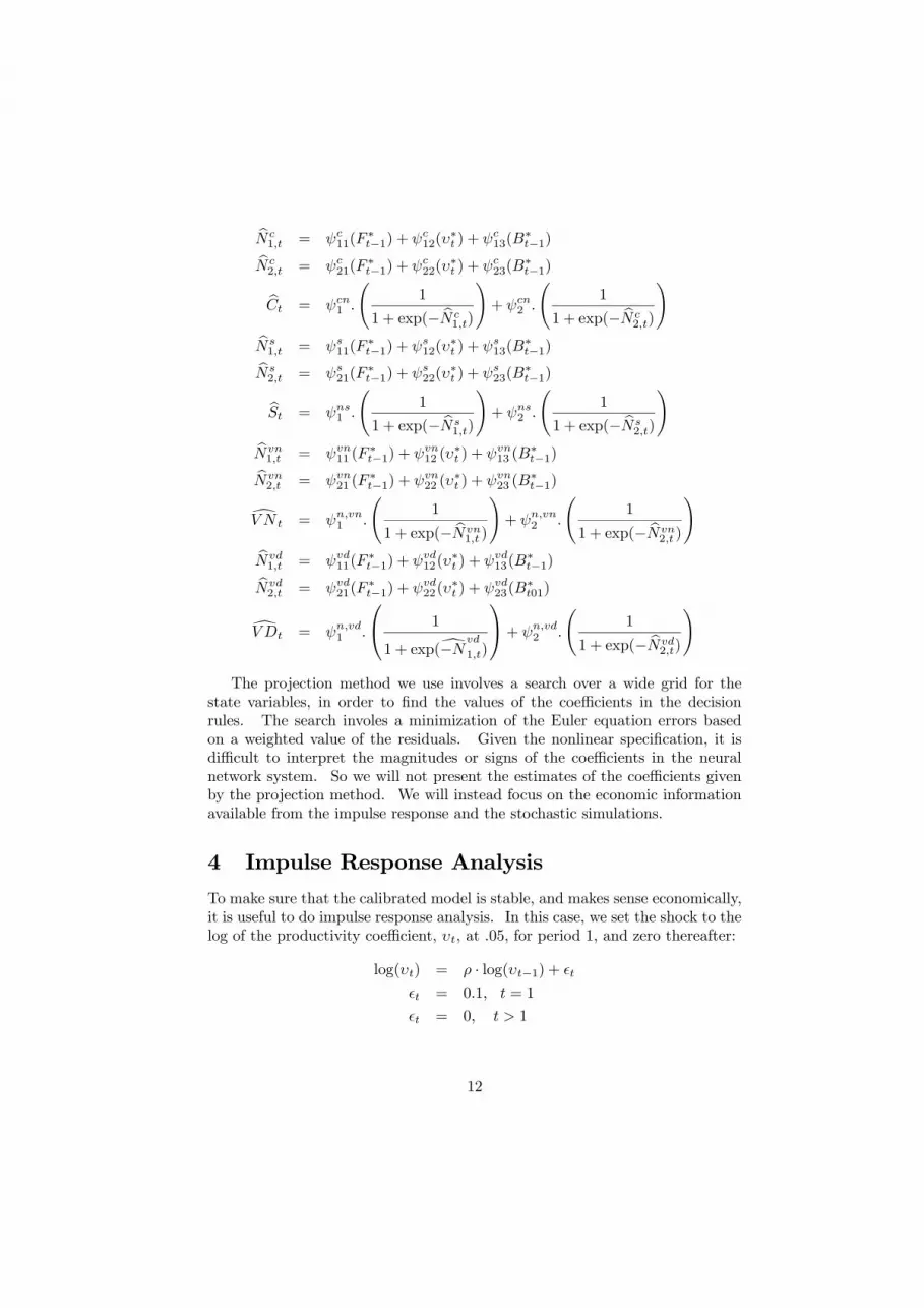
3.2 Solution Algorithm and Decision Rules

We choose to solve the above model with a nonlinear global solution algorithm,based on the collocation projection method. We do not linearize the model,nor do we make use of first or second-order Taylor methods in the popular andwidely used perturbation methods [see Collard and Julliard (2001a, 2001b) andSchmidt-Grohé and Uribe (2004a)]. There methods make use of the method ofBlanchard and Khan (1985) for rational expectations models with forward andbackward-looking variables. As such, they are local solutions while we use aglobal search method.In this model we have five state variables, productivity index, foreign debt,

the price dispersion index, domestic government debt, and the interest rate.However, some state variables are more important than others. Given the lowinflation in our model, the interest rate and the price dispersion index do notchange very much. We found that it makes little difference if we omit them asarguments in the decision rule.We have the choice of specifying the decision rules for the four forward-

looking variables, C, E, V N , and V D, either as a Chebyshev polynimal or asa neural netowrk. Using a Chebyshev second-order polynomial expansion, forthree state variables, we have 32 parameters (= ndchebnstate.ndecision.rule),wherendcheb, nstate, and ndecision.rule represent the degree of the Chebyshev poly-nomial, the number of state variables, and the number of decision rules, respec-tively. For the neural network, with two neurons for each decision rule, therealso 32 parameters (= nneuron.nstate.ndecisionrule+nneuron.ndecisionrule),where nnuron represents the number of neurons for each decision rule. Inthis case the number of parameters is the same, given the neural network withtwo neurons and a second-order polynomial expansion with three state vari-ables. However, as the number of state variables increases, the advantage ofthe neural network specification over the Chebyshev orthogonal polynomial be-comes more apparent. In this paper, we use the neural network specificationfor the functional form of the decision rules. The advanage, as noted by Sir-akaya, Turnovsky, and Alemdar (2005), is that such networks, with logsigmoidfunctions, easily deliver control bounds on endogenous variables.The network specification implies the following functional forms for the de-

cision rules for C, S, V N , and V D :

11

bNc1,t = ψc11(F

∗t−1) + ψc12(υ

∗t ) + ψc13(B

∗t−1)bNc

2,t = ψc21(F∗t−1) + ψc22(υ

∗t ) + ψc23(B

∗t−1)

bCt = ψcn1 .

Ã1

1 + exp(− bNc1,t)

!+ ψcn2 .

Ã1

1 + exp(− bN c2,t)

!bNs1,t = ψs11(F

∗t−1) + ψs12(υ

∗t ) + ψs13(B

∗t−1)bNs

2,t = ψs21(F∗t−1) + ψs22(υ

∗t ) + ψs23(B

∗t−1)

bSt = ψns1 .

Ã1

1 + exp(− bNs1,t)

!+ ψns2 .

Ã1

1 + exp(− bNs2,t)

!bNvn1,t = ψvn11 (F

∗t−1) + ψvn12 (υ

∗t ) + ψvn13 (B

∗t−1)bNvn

2,t = ψvn21 (F∗t−1) + ψvn22 (υ

∗t ) + ψvn23 (B

∗t−1)

dV N t = ψn,vn1 .

Ã1

1 + exp(− bNvn1,t )

!+ ψn,vn2 .

Ã1

1 + exp(− bNvn2,t )

!bNvd1,t = ψvd11(F

∗t−1) + ψvd12(υ

∗t ) + ψvd13(B

∗t−1)bNvd

2,t = ψvd21(F∗t−1) + ψvd22(υ

∗t ) + ψvd23(B

∗t01)

dV Dt = ψn,vd1 .

⎛⎝ 1

1 + exp(d−Nvd

1,t)

⎞⎠+ ψn,vd2 .

Ã1

1 + exp(− bNvd2,t)

!

The projection method we use involves a search over a wide grid for thestate variables, in order to find the values of the coefficients in the decisionrules. The search involes a minimization of the Euler equation errors basedon a weighted value of the residuals. Given the nonlinear specification, it isdifficult to interpret the magnitudes or signs of the coefficients in the neuralnetwork system. So we will not present the estimates of the coefficients givenby the projection method. We will instead focus on the economic informationavailable from the impulse response and the stochastic simulations.

4 Impulse Response AnalysisTo make sure that the calibrated model is stable, and makes sense economically,it is useful to do impulse response analysis. In this case, we set the shock to thelog of the productivity coefficient, υt, at .05, for period 1, and zero thereafter:

log(υt) = ρ · log(υt−1) + t

t = 0.1, t = 1

t = 0, t > 1

12

0 50 1001

1.1

1.2Prod. Index

0 50 1000.72

0.74

0.76Consumption

0 50 1001.1

1.2

1.3Real Ex. Rate

0 50 100−0.01

0

0.01Trade & Fiscal Bal

0 50 1000.03

0.04

0.05Interest Rate

0 50 1000.75

0.8

0.85Real Wage

Trade

Fiscal

Figure 1: Impulse Response Paths with High Export Elasticity

0 50 1001

1.1

1.2Prod. Index

0 50 1000.72

0.74

0.76Consumption

0 50 1001.1

1.2

1.3Real Ex. Rate

0 50 100−0.01

0

0.01Trade & Fiscal Bal

Trade

Fiscal

0 50 1000.03

0.04

0.05Interest Rate

0 50 1000.75

0.8

0.85Real Wage

Figure 2: Impulse Response Paths with Low Export Price Elasticity

13

4.1 Response with High Export Elasticity

Figure (1) pictures the paths of consumption, the real exchange rate, the tradebalance (exports less imports) and fiscal balance (revenue less expenditure), theinterest rate and the real wages, for a 10 percent productivity shock, underthe assumption of relatively high elasticity of exports with respect to the realexchange rate (χ = 2.0). We see familiar results. A temporary increase inthe productivity index leads to a temporary increase in consumption, the realexchange rate and real wages, a fall in the interest rate and a rise in the fiscalbalance. We see that the trade balance also rises. With a relatively strong realexchange rate elasticity, exports rise more than the imports (due to the risingoutput), so that the current and fiscal accounts become positively correlated.

4.2 Response with Low Export Elasticity

Figure (2) pictures the same variables under the assumption of a relatively lowexport elasticity (χ = 0.2). We see one major difference between (2) and (1).The trade balance now falls after the productivity shock. The rise in importedintermediate goods, K, is no longer offset by an increase in export demand,so that the productivity increase generates opposite reactions in the fiscal andcurrent-account balances.The quantitative differences between the two cases are shown in Figure (3).

We see that real wages and the fiscal balance are slightly higher when exportshave a very high real exchange-rate elasticity.

0 5 10 15 20 25 30 35 400.78

0.79

0.8

0.81

0.82Real Wages

0 5 10 15 20 25 30 35 40−5

0

5

10x 10

−3 Fiscal Balance

high elasticitylow elasticity

Figure 3: Real Wage and Fiscal Balances Under Alternative Assumptions

14

5 Stochastic SimulationsThis section takes up the accuracy measures of the model, the correlationsamong key macroeconomic variables, and the welfare consequences of havingexports with a relatively high or relatively low exchange rate elasticity.

5.1 Accuracy Assessment

Before proceeding to our analysis of the correlations of key macroeconomic in-dicators, we first take up the accuracy of our simulations. We make use ofthe Judd-Gaspar mean absolute error measures, as well as the Den-Haan andMarcet distributions.Judd and Gaspar (1997) suggest a transformation of the Euler equation

errors in the following way:

L(Ct) =

¯̄Ct

¯̄Ct

L(St) =

¯̄St

¯̄Ct

L(Pt) =

¯̄Pt

¯̄Ct

If the mean absolute values of the errors, deflated by consumption, is 10−2, Juddand Gaspar note that the Euler equation is accurate to within a penny per dollarof expenditure. Figure (4) pictures the distribution of the Judd-Gaspar errormeasures for 1000 simulations of sample length 200, under the assumption of arelatively high export price elasticity, with χ = 2.0 We see that the mean errormeasures are less than one cent per dollar of consumption expenditure. Figure(5) pictures the corresponding error distributions for the case of χ = 0.2. Wesee that the distributions are not markedly different.A drawback of the Judd and Gaspar criterion is that it is not based on

any statistical distribution. For this reason, we use another commonly usedcriterion, due to den Haan and Marcet (1994). This test is denoted DM(m)and is defined as:

DM(m) = TB0A−1B ∼ χ2(m)

B =1

T(y0X)

A =1

T

XXtX

0

tε2t

where the vector y represent the stacked Euler equation errors (for consumption,exchange rate and price), X is the instrument matrix with m columns. Underthe null hypothesis of an accurate solution, the E(y0X) = 0. The authors

15

recommend the following procedure for implementing this test: calculate theDM statistics repeatedly, and compute the percentage of the DM statisticswhich are below the lower or above the upper five percent critical values of theχ2(m) distribution. If these fractions are noticeably different from the expectedfive percent, then we have evidence for an inaccurate solution. Figure (6) and(7) shows the calculated and theoretical cumulative density function of the Den-Haan Marcet Statistics for the case of high and low elasticity of export demand.The upper and lower rejection regions are 0.01/0.08 for both cases.

5.2 Correlations

How do the correlations between key macroeconomic variables change with thevalue of the export price elasticity? Figure (8) pictures the corelations betweenfiscal and trade balances, between the real exchange rate and the trade balance,between the interest rate and the real exchange rate, and between the interestrate and fiscal balances under the assumption of a relatively high export priceelasticity. We see in the lower two quadrants that the correlations are negative:high interest rates are correlated with real exchange appreciations while fiscalsurpluses are correlated with falling interest rates. The upper two quadrantsshow relatively high positive correlations. Given the high export price elasticity,a real exchange rate depreciation leads to a higher trade balance. The fiscaland trade balances are now positively correlated. Given that positive fiscalbalances lower interest rates, which in turn lead to a real depreciation, a fiscalsurplus goes hand in hand with a trade or current-account surplus.Figure (9), which gives the corresponding correlations under a relatively

low export price elasticity, tells another story. While the correlations in thelower two quadrants remain negative, as above, the correlations between thereal exchange rate and trade balance and the correlations between the fiscaland trade balances are now negative. The key reason is that a real exchangeincrease, or depreciation, leads to a deterioration in the trade balance. Thedepreciation in the real exchange rate increases the cost of the imports, sincethey are used as intermediate goods to produce domestic goods, while the exportdemand changes little. Thus, a fiscal surplus, which lowers interest rates andleads to a depreciation, actually worsens the current account.

5.3 Welfare Comparisons

Figure (10) pictures the welfare distributions under the assumptions of relativelyhigh or relatively low export price elasticity. We see that the variability ofthe welfare distribution is higher when exports are more price elastic than lessprice elastic. There is opportunity for welfare gain as well as welfare loss ifthe exports become more price elastic, due to structural change in foreign ordomestic markets.One well-known way to evaluate alternative price elastic or price-inelastic

regimes is to compare the welfare of the sticky-price and tax distorted economy

16

1.4 1.5 1.6 1.7 1.8 1.9 2 2.1 2.2 2.3

x 10−3

0

50

100Consumption Error

2.2 2.4 2.6 2.8 3 3.2 3.4 3.6 3.8 4

x 10−3

0

100

200Exchange Rate Error

2 3 4 5 6 7 8 9 10 11

x 10−3

0

100

200Calvo Pricing Error

Figure 4: Judd-Gaspar Errors Statistics for High Export Price Elasticity

1.4 1.5 1.6 1.7 1.8 1.9 2 2.1 2.2 2.3

x 10−3

0

100

200Consumption Error

2.2 2.4 2.6 2.8 3 3.2 3.4 3.6

x 10−3

0

100

200Exchange Rate Error

3 4 5 6 7 8 9 10

x 10−3

0

50

100Calvo Pricing Error

Figure 5: Judd-Gaspar Error Statistics for Low Export Price Elasticity

17

5 10 15 20 25 30 35 40 450

0.1

0.2

0.3

0.4

0.5

0.6

0.7

0.8

0.9

1

x

F(x

)

CDF of the DM test statistic

Figure 6: Case of High Export Elasticity

0 5 10 15 20 25 30 35 40 450

0.1

0.2

0.3

0.4

0.5

0.6

0.7

0.8

0.9

1

x

F(x

)

CDF of the DM test statistic

Figure 7: Case of Low Export Elasticity

18

0.4 0.6 0.8 10

200

400

600Fiscal/Trade Balance Correlation

0 0.5 10

200

400

600Real Ex. Rate/Trade Balance Correlation

−1 −0.5 00

200

400

600Interest/Real Exchange Rate Correlation

−1 −0.5 0 0.50

200

400

600Interest/Fiscal Balance Correlation

Figure 8: Macroeconomic Correlations Under High Export Price Elasticity

−1 −0.5 0 0.50

200

400

600Fiscal/Trade Balance Correlation

−1 −0.5 0 0.50

200

400

600Real Ex. Rate/Trade Balance Correlation

−1 −0.5 00

200

400

600Interest/Real Exchange Rate Correlation

−1 −0.8 −0.6 −0.4 −0.20

200

400

600Interest/Fiscal Balance Correlation

Figure 9: Macroeconomic Correlations Under Low Export Price Elasticity

19

−250.3 −250.2 −250.1 −250 −249.9 −249.80

100

200

300Welfare: High Elasticity

−250.3 −250.2 −250.1 −250 −249.9 −249.80

100

200

300Welfare: Low Elasticity

Figure 10: Welfare Distributions Under Alternative Export Price Elasticities

to the welfare of a reference regime r. The loss function of regime i can bewritten in the following way:

it =

V i0 − V r

0

V r0

(24)

where V r0 represents welfare in the reference regime r, and V i

0 the welfare inpolicy regime i. This loss function, of course, is measured in terms of a utilityfunction. Following Schmitt-Grohé, Stephanie and Uribe (2004) , the differencesin the two welfare indices may be re-expressed as the percentage of consumptionthat the household in regime i should be compensated, in order to make thehousehold indifferent between the policy regimes i and r. With our utility func-tion, we calculate this consumption compensation percentage in the followingway:

20

C,i0 = 100

"1−

µV i0 − V r

0eCr+ 1

¶ 11−σC

#(25)

eCr =1

1− σE0

∞Xt=0

βt (Crt )1−σ

Figure (11) pictures the implied consumption compensation between the wel-fare distributions given in Figure (10). The value are computed with equation(25). We see that the differences amount to at most 0.3% of a unit of consump-tion in the reference regime of low export price elasticity. Thus the potentialgains or losses are not very large if the structure of the export market changesfrom a relatively low to a relatively high price elasticity.

−0.3 −0.2 −0.1 0 0.1 0.2 0.3 0.40

10

20

30

40

50

60

70

80

Figure 11: Percentage Consumption Compensation for Welfare Equalization

6 ConclusionThe simulations in this chapter brought up a number of interesting issues thatare worthy of further exploration. First we see that fiscal and current accountdeficits may or may not be twins. If there is strong productivity growth and lowexport-price sensitivity, the current account deficit will likely increase, while thefiscal deficit will shrink. With a high export price elasticity, however, the current

21

account deficit will shrink in tandem with the fiscal deficit as the exchange ratedepreciates.The model incorporates many of the distortions and stickiness popular in the

"new neoclassical synthesis" or "new open economy macroeconomics", such asmonopolistic competition, sticky price setting behavior, and distortionary taxes.However, we could have added further sources of stickiness, such as imperfectexchange-rate pass through, and sticky wage setting behavior, as well as habitpersistence in consumption. We could even allow a given percentage of con-sumers to be non-Ricardian rule-of-thumb consumers. All of these assumptionswould lower welfare but allow more scope for monetary or fiscal stabilizationpolicy.When all is said and done, it is better to have exports which have a high

or a low price elasticity in foreign markets? In this simple setting, we assumethat the export growth or volatility does not feed back into any productivitychange for the home country. We assume the same structure of underlyingproductivity shocks driving the model, whether exports are fixed or variable.This is a drawback, of course, since exporting does generate learning effectswhich improve domestic productivity.We conclude with a recurring theme. As an economy becomes more open,

there are opportunities for foreign borrowing or lending, by which consumersmay offset the losses of domestic distortions. We see in this paper anotherbenefit of increasing openness or globalization. By exporting to markets wheredemand is highly price elastic, an economy may be able to import a degree ofprice flexibility through trade. This price flexibility can, of course, feed backinto greater flexibility in domestic markets and thereby further improve welfare.In short, the monopolistic markup factors and the degree of price stickiness maybecome endogenous. Exporting to a market with greater price flexibility maybe a backdoor way to import greater price flexibility and lower monopolisticdistortions in the domestic market.

22

References[1] Angeloni, Ignazio, Günter Coenen, and Frank Smets (2003), "Persistence,

The Transmission Mechanism, and Robust Monetary Policy". ScottishJournal of Political Economy 50: 527-549.

[2] Benigno, Pierpaolo and Michael Woodford (2004), "Optimal Monetary andFiscal Policy: A Linear Quadratic Approach". Working Paper 345,European Central Bank.

[3] Blanchard, Olivier and Charles Khan (1985), "The Solution of Linear Dif-ference Equation Models Under Rational Expectations", Econometrica45, 1305-1311.

[4] Bussière, Matthiew, Marcel Fratzscher, and Gernot J. Müller (2005), "Pro-ductivity Shocks, Budget Deficits and the Current Account". WorkingPaper, European Central Bank.

[5] Calvo, Guillermo (1983), "Staggered prices in a utility maximising frame-work", Journal of Monetary Economics, 12, 383-398.

[6] Collard, F. and M. Julliard (2001a), Perturbation Methods for RationalExpectations Models. Manuscript: CEPREMAP, Paris.

[7] __________ (2001b), "Accuracy of Stochastic Perturbation Methodsin the Case of Asset Pricing Models", Journal of Economic Dynamicsand Control 25, 979-999.

[8] Den Haan. W. and Marcet, Albert (1990), “Solving the Stochastic GrowthModel by Parameterizing Expectations”, Journal of Business and Eco-nomic Statistics 8, 31-34.

[9] Hughes Hallet, Andrew (2005), "Fiscal Policy Coordination with Indepen-dent Monetary Policies: Is It Possible"?". Working Paper, Departmentof Economics, Vanderbilt University.

[10] Judd, K. and Jess Gaspar (1996), "Solving Large Scale Rational Expecta-tions Models", Macroeconomic Dynamics 1, 45-75.

[11] Judd, John F. and Glenn D. Rudebusch (1998), "Taylor’s Rule and theFed: 1970-1997". Federal Reserve Bank of San Francisco EconomicReview 3, 3-16.

[12] Kim, Junill and Sunghyun Henry Kim (2004), "Welfare Effects of TaxPolicy in Open Economies: Stabilization and Cooperation". WorkingPaper, Department of Economics, Tufts University.

[13] Kollmann, Robert (2004), "Welfare-Maximizing Operational Monetary andTax Policy Rules". Working Paper 4782, Center for Economic PolicyResearch.

[14] Orphanides, Athanasios and John G. Williams (2002), "Robust MonetaryPolicy Rules with Unknown Natural Rates". Brookings Papers on Eco-nomic Activity 2002, 63-118.

23

[15] Razin, Asaf (2005), "Globalization and Disinflation: A Note". WorkingPaper No. 4826, Center for Economic Policy Research.

[16] Schmidt-Grohé, Stephanie and Martin Uribe (2004a), "Solving DynamicGeneral Equilibrium Models Using a Second Order Approximation tothe Policy Function", Journal of Economic Dynamics and Control 28,755-775.

[17] __________ (2004b), "Optimal Simple and Implementable Monetaryand Fiscal Rules" Web page: /www.econ.duke.edu/uribe.

[18] Smets, Frank and Raf Wouters (2003), "An Estimated Stochastic DynamicGeneral EquilibriumModel of the Euro Area". European Central Bank,Working Paper 171.

[19] Taylor, John B. (1993), ”Discretion vs. Policy Rules in Practice”. Carnegie-Rochester Conference Series on Public Policy 39, 195-214.

[20] __________ (1999), Monetary policy rules, NBER and University ofChicago Press, Chicago.

24