Embed Size (px)
Citation preview

Frequency domain modelling of transients in pipe networks with
compound nodes using a Laplace-domain admittance matrix
by
Zecchin, A.C., Lambert, M.F., White, L.B., and Simpson, A.R.
Journal of Hydraulic Engineering
Citation: Zecchin, A.C., Lambert, M.F., White, L.B., and Simpson, A.R. (2010). “Frequency domain modelling of transients in pipe networks with compound nodes using a Laplace-domain admittance matrix.” Journal of Hydraulic Engineering, 136 (10), 739-755. Published Online: 07 April 2010. ISSN (print): 0733-9429, ISSN (online): 1943-7900.
For further information about this paper please email Angus Simpson at [email protected]

FREQUENCY-DOMAIN MODELING OF TRANSIENTSIN PIPE NETWORKS WITH COMPOUND NODES USING
A LAPLACE-DOMAIN ADMITTANCE MATRIX
Aaron C. Zecchina, Martin F. Lambertb, Angus R. Simpsonb, and Langford B. Whitec
aLecturer, School of Civil, Environmental, and Mining Engineering, The University of Adelaide, Adelaide, South Australia,
5005. Email: [email protected] (corresponding author)
bProfessor, School of Civil, Environmental, and Mining Engineering, The University of Adelaide, Adelaide, South Australia,
5005. Email: [email protected]
cProfessor, School of Civil, Environmental, and Mining Engineering, The University of Adelaide, Adelaide, South Australia,
5005. Email: [email protected]
dProfessor, School of Electrical and Electronic Engineering, The University of Adelaide, Adelaide, South Australia, 5005.
Email: [email protected]
Abstract
An alternative to modeling the transient behavior of pipeline systems in the time-domain is to model these
systems in the frequency-domain using Laplace transform techniques. A limitation with traditional frequency-
domain pipeline models is that they are only able to deal with systems of a limited class of configuration. Despite
the development of a number of recent Laplace-domain network models for arbitrarily configured systems, the
current formulations are designed for systems comprised only of pipes and simple node types such as reser-
voirs and junctions. This paper presents a significant generalization of existing network models by proposing a
framework that allows not only complete flexibility with regard to the topological structure of a network, but also,
encompasses nodes with dynamic components of a more general class (such as air vessels, valves and capacitance
elements). This generalization is achieved through a novel decomposition of the nodal dynamics for inclusion into
a Laplace-domain network admittance matrix. A symbolic example is given demonstrating the development of the
network admittance matrix and numerical examples are given comparing the proposed method to the method of
characteristics for 11-pipe and 51-pipe networks.
1

INTRODUCTION
Networks of interlinked fluid lines occur in many different instances, examples of which are material transport
systems (e.g. water, gas and petroleum [Fox, 1977; Chaudhry, 1987; Wylie and Streeter, 1993]), control systems
(e.g. hydraulic and pneumatic [Stecki and Davis, 1986; Barber, 1989]), and biological systems (e.g. arterial blood
flow [John, 2004]). Given the far reaching nature of these systems, the ability to model the transient response
of these networks subjected to boundary perturbations is of broad interest and is fundamental for the purposes of
analysis and design.
A particular application of transient network modelling is water hammer analysis in distribution systems. Tra-
ditionally, the approach for modelling water hammer within distribution systems is via the use of time-domain
approximate discrete methods such as the method of characteristics [Wylie and Streeter, 1993]. However, re-
cently alternative Laplace-domain models have been proposed [Kim, 2007; Zecchin et al., 2009] where classical
frequency-domain models [Chaudhry, 1987; Wylie and Streeter, 1993] have been extended to handle arbitrarily
configured networks.
The Laplace-domain network admittance formulation from Zecchin et al. [2009] was designed for systems
comprised of pipes, reservoirs and junctions. Despite the capacity to deal with networks of arbitrary configuration,
the formulation is still limited in its application as real world networks contain many other types of hydraulic
components such as valves, emitters, surge tanks (accumulators), pumps, and other components. This paper
presents a new and extended formulation that is able to deal with, not only arbitrarily configured networks, but
also pipe networks containing a general class of hydraulic components. The class of components that can be
incorporated into the proposed framework is the extremely general class whose dynamic state equations yield
an admittance representation, that is, there exists a definable map from the components state variables to the
components connection flows (discussed later ). The incorporation of these arbitrary components is achieved by a
novel nodal expansion method that enables the inclusion of the nodal dynamics into the network admittance matrix
structure. These arbitrary components from hereon are referred to as compound nodes, which references the fact
that these elements represent dynamic systems in conjunction with the nodal-like property of being a connection
point for pipes.
The paper is structured as follows. Firstly, the background is given including current methods for modeling
pipe networks and a mathematical formulation of the network equations as well as a brief background to Laplace-
domain representations of the fluid network equations. This is followed by a comprehensive mathematical frame-
work for the compound node type. The formulation of the Laplace-domain model for an arbitrarily configured
network comprised of arbitrary node types is then presented , where a brief review of the work of Zecchin et al.
2

[2009] is given followed by a staged generalization. This section highlights the concepts and definitions that are
required to deal with arbitrary node types within a network setting. Numerical examples are then given for two
case studies, a 11-pipe network and a 51-pipe network, followed by the conclusions.
BACKGROUND
Modelling the Transient Behaviour of Pipe Networks
Pipe networks can essentially be viewed as systems comprised of dynamic interacting elements. These networks
are comprised of two types of elements, namely distributed elements (e.g. pipes) and lumped elements (e.g. junc-
tions, air vessels and valves). The fluid variables of each of the hydraulic elements interact with their neighboring
components according to the physical laws of conservation of mass, momentum and energy. The network problem
involves defining a computable model that can deal with an arbitrary structure of connected hydraulic elements,
and determine the value of the associated fluid variables that satisfy the system of underlying equations.
Modeling an arbitrary network in the time-domain has been broadly addressed within the research literature
(e.g. [Karney, 1984; Chaudhry, 1987; Wylie and Streeter, 1993; Axworthy, 1997; Izquierdo and Iglesias, 2004]),
and, within industry, there exist many commercial software packages for the purpose of water hammer analysis
within water distribution systems. For these time-domain models, the distributed components are discretized
in space and time and modeled using hyperbolic partial differential equation (PDE) solvers [Chaudhry, 1987;
Wylie and Streeter, 1993], and the lumped components are modeled by simultaneous equations solvers, which
are computed at each time point. The distributed nature of the pipelines means that there is a time delay in the
wave propagation of the fluid variables. This time delay means that the network variables are not required to be
solved simultaneously, but that, at each time step, the interior points of each fluid line can be computed explicitly
in isolation [Wylie and Streeter, 1993], and only the fluid variables at the endpoints of the pipes, incident on
common nodes, require simultaneous solving, thus greatly reducing the problem complexity. The fluid variables
at the pipes endpoints then serve as the boundary condition to the interior points at the following time step.
Laplace-domain modelling is significantly different to this. The underlying fluid equations of the hydraulic el-
ements (pipelines and lumped components) are first linearised, then transformed using the Laplace transform, and
finally solved to yield analytic transfer relationships between the points at which the element connects to other ele-
ments within the network [Chaudhry, 1987; Wylie and Streeter, 1993] (e.g. pipeline end points). The construction
of a full network model from the individual element transfer relationships involves solving the simultaneous set of
complex valued equations that arise from the hydraulic elements and their interactions with other elements that are
3

incident to similar nodes. What this means is that as the transformed fluid variables are in the Laplace-domain, the
temporal delays are replaced by algebraic operations, and consequently the fluid variables for all components must
be solved simultaneously for every frequency point of interest. Interestingly, in this regard the Laplace-domain
model is similar to steady-state models for solving the flows and pressures in a water distribution system [Todini
and Pilati, 1988], in that there is a direct dependence of one network variable on another.
The classical methods for Laplace-domain modelling of pipe networks are the impedance method [Wylie,
1965; Wylie and Streeter, 1993] and the transfer matrix method [Chaudhry, 1970, 1987]. Both these methods
have their origins in Laplace-domain transmission line theory, where pipes are described by their wave propagation
characteristics [Brown and Nelson, 1965; Stecki and Davis, 1986] . Within the impedance method, a pipe network
is characterised by the distribution of hydraulic impedance throughout the network and impedance relationships
are derived to relate the hydraulic impedance values across an element (note that Hydraulic impedance refers to
the ratio of transformed pressure to transformed flow). Within the transfer matrix method, each hydraulic element
is expressed as a 2 × 2 transfer matrix relating the upstream and downstream transformed variables of pressure
and flow, whereby a network model can be created by an ordered multiplication of these matrices.
The advantages of these methods are that they are able to deal with systems comprised of pipes and lumped
hydraulic components. The major disadvantage, however, is that such methods are not able to deal with an arbitrary
network configuration, but are limited to simple first order looped systems [Fox, 1977] (structural reasons for the
transfer matrix method, and practical reasons for the impedance method). Many authors have utilised different
methods to achieve a frequency-domain representation of complex networks (e.g. Ogawa [1980]; Margolis and
Yang [1985]; Boucher and Kitsios [1986]; John [2004]; Kim [2007, 2008a,b]). However, these methods were
designed simply for networks with junctions and reservoir node types only, with the exception of Kim [2007,
2008a,b] who included an emitter elements and some surge protection devices in his formulation.
An alternative method for modelling systems comprised of pipes, junctions and reservoirs was proposed in
Zecchin et al. [2009] in which an admittance matrix expression relating the nodal pressures to the nodal outflows
was derived from the basic fluid equations using graph theory concepts. The significance of this is twofold, (i) the
network matrix was shown to have an intuitive and simple structure for which analogies with admittance matrices
in electrical circuits was made apparent [Desoer and Kuh, 1969], and (ii) it showed that the entire network state
was a function of the reduced variable set of nodal pressures and flows. The focus of this paper is the development
of a new model to deal with networks than include compound nodes in addition to pipes, junctions and reservoirs.
4

Problem Definition
The development of a network model not only involves modelling the dynamics of each individual component,
but it also involves accounting for the continuity of the fluid variables of the hydraulic elements at their connection
points. Before outlining the network equations, some notation is defined below, and the general framework for a
node is given.
To facilitate the discussion of the network connectivity equations, it is convenient to describe a network as a
connected graph G (N ,Λ) [Diestel, 2000] consisting of the node set N = {1, 2, ..., nn}, and the link set Λ =
{λ1, λ2, ..., λnΛ} and where λj = (iu,j , id,j) where iuj , idj ∈ N are the upstream and downstream nodes of
link j respectively. Each node is associated with a lumped hydraulic component that is connected to a number of
links, and each link is associated with a distributed pipe element where the directed nature of the link describes
the positive flow direction sign convention of the element. There are two link sets associated with each node,
these are Λui and Λdi which correspond to the set of links directed from and to node i respectively, that is
Λui = {(i, k) , k ∈ N : (i, k) ∈ Λ} and Λdi = {(k, i) , k ∈ N : (k, i) ∈ Λ}). Note that the first set corresponds
to the links whose upstream node is i and the second set correspond to the links whose downstream node is i.
Compound Node Equations
Previous work has presented a methodology that included a specific class of node that describes junctions, demand
nodes and reservoirs. This nodal type is called a simple node and is defined as a point with an infinitely small
volume that has a lossless connection to one or more fluid lines. The infinitely small volume implies that there is
no variation of pressure or accumulation of mass, and the lossless connection implies that the pressure at the ends
of the fluid line connected to the node are equal. The main contribution of this paper is that it presents a novel way
to include a completely general node type into the network equations. The node types considered in this paper are
of a much more general class encompassing any hydraulic element whose dynamics can be exactly represented
(or adequately approximated) by a passive, time-invariant linear system, as is the case for most hydraulic elements
such as valves, emitters, and surge tanks (see Desoer and Vidyasagar [1975] for a discussion on passivity). These
nodes are referred to as compound nodes and are defined and discussed below.
The equations describing the dynamic behaviour of a compound node are derived from the physical laws of
mass and momentum conservation. In the general case, the dynamic behaviour of a compound node is given by
the vector equation
φi (pi, qi,ui, ui, t) = 0 (1)
5

where φi is the vector valued operator describing the compound node dynamics, ui(t) is the set of controlled state
variables for the node (i.e. valve opening, demand etc.), ui is the set of response state variables (e.g. pressure,
volume and inflow for a surge tank, or pressure and outflow for an emitter) and pi and qi are the sets of pressures
and flows of the pipes incident to node i. That is, pi and qi are vector organisations of the sets
{pj(0, ·) : λj ∈ Λui} ∪ {pj(lj , ·) : λj ∈ Λdi}
{qj(0, ·) : λj ∈ Λui} ∪ {qj(lj , ·) : λj ∈ Λdi}
respectively, where pj and qj are the distributions of pressure and flow along pipe j, and lj is the length of pipe j.
Mathematically, the difference between the controlled states and the response states is that the controlled states are
inputs that require specification to compute (1), and the dependent states are outputs that are computed from (1).
It is important to note that the compound node framework (1) encompasses basic nodes, such as junctions with
emitters, and also nodes of complex configurations involving multiple equations for different elements within the
compound node. This is demonstrated in the following example.
Example 1. Consider the compound node configuration in Figure 1(a) consisting of a closed branch and a con-
trolled demand bounded by valves A and B. Pipe [a] is incident to valve A and pipes [b] and [c] are incident to
valve B. The nodal states can be taken as the internal pressure ψo, the capacitive inflow into the closed branch
θo, and the controlled flow injection (or demand) θd. Labeling this node with i, the nodal vectors are
pi(t) =
pa(la, t)
pb(lb, t)
pc(0, t)
, qi(t) =
qa(la, t)
qb(lb, t)
qc(0, t)
, ui(t) = θd(t), ui(t) =
ψo(t)
θo(t)
. (2)
The vector equation φi for compound node is
φi(pi, qi,ui, ui, t) =
pb(lb, t)− ψo(t)− fB (qb(lb, t)− qc(0, t)) = 0 pressure change across valve B
qa(la, t) + qb(lb, t)− qc(0, t)− θo(t) + θd(t) = 0 continuity within node
pb(lb, t)− pc(0, t) = 0 connectivity of links b and c
VoKe
dψo(t)
dt− θo(t) = 0
capacitance equation
for branch
pa(la, t)− ψo(t)− fA (qa(la, t)) = 0 pressure change across valve A
(3)
6

where Vo and Ke are volume and effective modulus of the branch, and
fX(q) =ρ
2
|q|q(CdXAvX)
2
is the valve pressure change where CdX andAvX are the valve coefficient and valve cross-sectional area for valve
X for subscripts X = A,B.
Network Equations
With the given notation, a compound node network can be defined as the triple
(G(N ,Λ),P, C)
where G(N ,Λ) is the network graph of nodesN and links Λ, P = {Pj : λj ∈ Λ} is the set of pipeline properties
where Pj are the properties for pipe j (i.e. lj , diameter, roughness etc.), and C = {φi : i ∈ Nc} is the set of
compound node functions for the set of compound nodesNc ⊂ N . The state space of the network (G(N ,Λ),P, C)
is given by the distributions of pressure and flow along each line of the network, and the compound node response
states, which are given by
p (x, t) =
p1 (x1, t)
...
pnΛ (xnΛ , t)
, q (x, t) =
q1 (x1, t)
...
qnΛ (xnΛ , t)
, u(t) =
u1(t)
...
unc(t)
, (4)
respectively, where x = [x1 · · ·xnΛ ]T is the vector of spatial coordinates, (i.e. x ∈ X = X1 × · · · XnΛ where
Xj = [0, lj ]), t ∈ R is time, nΛ is the number of links, and nc is the number of compound nodes.
For a given network (G(N ,Λ),P, C), the network modeller is interested in the transient response of the states
(4) for a specific hydraulic scenario, where hydraulic scenario is defined by a set of specified initial and boundary
conditions. In addition to the compound node controls ui, i ∈ Nc, each simple node either has controlled nodal
pressure (as in the case of a reservoir) or a controlled nodal flow (as in the case of a demand node or a junction).
Therefore, partitioning the set of simple nodes Ns = N/Nc as Ns = NJ ∪ Nd ∪ Nr where NJ is the set of
junctions, Nd is the set of demand nodes, and Nr is the set of reservoir nodes, the system of dynamic equations
7

governing the network states (4) is
∂qj∂t
+Ajρ
∂pj∂x
+qjAj
∂qj∂x
+πDj
ρτj = 0, x ∈ Xj , λj ∈ Λ, (5)
∂pj∂t
+ρc2jAj
∂qj∂x
+qjAj
∂pj∂x
= 0, x ∈ Xj , λj ∈ Λ, (6)
pj(ϕji, t)− pk(ϕki, t) = 0, λj , λk ∈ Λi, i ∈ NJ ∪Nd (7)
pj(ϕji, t)− ψri(t) = 0, λj ∈ Λi, i ∈ Nr, (8)∑λj∈Λdi
qj(lj , t)−∑
λj∈Λui
qj(0, t) = 0, i ∈ NJ (9)
θdi(t) +∑
λj∈Λdi
qj(lj , t)−∑
λj∈Λui
qj(0, t) = 0, i ∈ Nd (10)
φi (pi, qi,ui, ui, t) = 0, i ∈ Nc (11)
pj(x, 0) = p0j (x), qj(x, 0) = q0
j (x), x ∈ Xj , λj ∈ Λ (12)
ui(0) = u0i , i ∈ Nc (13)
where the symbols are defined as follows: for the fluid lines ρ is the fluid density, cj , Aj , Dj and τj = τj(qj)
are the fluid line wavespeed, the cross-sectional area, the diameter and the cross sectional shear stress for pipe
j respectively; for the nodes ψri is the controlled temporally varying reservoir pressure for the reservoir nodes
in the reservoir node set Nr, θdi is the controlled temporally varying nodal demand for the demand nodes in the
demand node set Nd; p0j and q0
j are the initial distribution of pressure and flow in each pipe λj ∈ Λ; u0i are the
initial values for the compound node response states; and ϕji = lj if λj ∈ Λdi and 0 otherwise.
The network equations (5)-(13) can be divided into five groups: (5) and (6) are the unsteady equations of
motion and mass continuity for each fluid line; (7) and (8) are the nodal equations of equal pressures in pipe ends
connected to the same node for junctions (nodes for which the inline pressure is the free variable) and reservoirs
(nodes for which the nodal flow is the free variable) respectively; (9) and (10) are the nodal equations of mass
conservation for junctions and demand nodes; (11) is the vector equation governing the behaviour of the compound
nodes; (12)-(13) are the initial conditions for the link states and node states.
Laplace-Domain Representation of Fluid Equations
The Laplace transform is a useful tool in dealing with partial differential equations as it removes the time-
dependency of the variables and yields a simpler ordinary differential equation [Kreyszig, 1999]. Via the Laplace
transform, the real variable p(x, t) becomes the complex Laplace-domain variable P (x, s), where s ∈ C, and all
8

differential operations involving t become algebraic operations involving s. An important property of the Laplace
transform is that the frequency-domain behaviour of a variable is given by the value of the Laplace-domain vari-
able restricted to the positive imaginary axis, that is s = iω where i is the imaginary unit, and ω is the radial
frequency [Franklin et al., 2001].
The Laplace-domain representation of the network equations (5)-(13) requires (i) the linearisation of (5)-(10)
in pj , qj , and ui and (ii) the assumption of homogeneous initial conditions. The standard approach to satisfy both
these requirements is to linearise the system (5)-(11) about the initial conditions (12) and consider the transient
fluctuations in pj , qj and ui about these values [Chaudhry, 1987; Wylie and Streeter, 1993]. For the application
of transient modelling within water distribution systems, it is common to take the initial conditions as the steady
state conditions. The assumption with this approach is that the unsteadiness of the flow during normal operation
is negligible and the system is approximately at steady-state conditions. This assumption is typically adequate
as the transient events to be simulated are orders of magnitude greater than background transients caused by the
mild unsteadiness within the system. For the nodal conditions (7)-(10), no approximation is required, as these
equations are linear, but linearisation is required for the unsteady fluid equations (5) and (6) and the compound
node equation (11).
For small Mach number flows the convective terms in (5) and (6) maybe neglected, and the Laplace transform
of these PDEs becomes
∂Pj∂x
= − ρ
Aj
[s+
πDj
ρL{τj} (s)
]Qj , (14)
∂Qj∂x
= −s Ajρc2j
Pj , (15)
on x ∈ Xj , s ∈ C where Pj and Qj are the transformed pressure and flow, the operator τj = τj(qj) is a
linear approximation of the nonlinear operator τj , and L{f} denotes the Laplace transform of the function f .
For turbulent flow τj(qj) = τj(qj) + O{(qj − q0
j
)2}but for unsteady formulations with terms in τj involving
convolution operations on qj (e.g. Zielke [1968]; Vardy and Brown [2003, 2004]), τj exactly captures the unsteady
effects as a convolution is a linear operation (see Stecki and Davis [1986] for more detail). Note that in the case
of nonhomogeneous initial conditions, Pj and Qj are taken as the Laplace transform of the transient fluctuations
about these initial conditions.
The solution to the linearised equations (5) and (6) is given by the standard solution to a constant coefficient
9

first order ordinary differential equation [Kreyszig, 1999], that is
Pj(x, s)Qj(x, s)
= B−j (s)e−Γj(s)x
1
Z−1c,j (s)
+B+j (s)eΓj(s)x
1
−Z−1c,j (s)
, (16)
on x ∈ Xj , s ∈ C where B−j and B+j are arbitrary functions dependent on the boundary conditions of pipe j, and
Γj and Zc,j are the propagation operator and the characteristic impedance, respectively, for pipe j and are given
by
Γj(s) =s
cj
√1 +
πDj
ρ
L{τj} (s)
s, Zc,j(s) =
cjρ
Aj
√1 +
πDj
ρ
L{τj} (s)
s.
The propagation operator Γj describes the rate of attenuation and phase change experienced by a propagating wave
within a pipeline, and the series impedance Zc,j describes the amplitude and phase coupling between a pressure
wave and its associated flow perturbation.
With respect to the hydraulic component, to be able to apply the Laplace transform, the equations (1) must
be approximated by a linear, time-invariant system. The method of constructing this approximation is dependent
on the nature of the nonlinearities in the node equation φ. A standard property of the nonlinearities within many
hydraulic components is that they are memoryless, that is the integrodifferential and delay terms are linear in the
nodal variables. For these circumstances, the linear time-invariant approximation is constructed by taking only
the linear terms in a Taylor series approximation about a selected operating point. Performing such a linearization
about a selected operating point and taking the Laplace-transform of (1) leads to the following expression for the
dynamics of the i-th hydraulic component
Φi(s)
P i(s)
Qi(s)
U i(s)
U i(s)
= 0 (17)
where Φj(s) is the matrix Laplace-transform of the linear approximation of the vector function φj , and P i, Qi,
U i and U i are the Laplace transforms of their lower case counterparts (note that in the case were pi, qi, ui and
ui have nonhomogeneous initial conditions, the Laplace variables are taken as the transient fluctuations about the
initial values). Consider the following example.
Example 2. Revisiting the compound node from Figure 1(a) in Example 1. Linearising the valve pressure loss
functions of (3), as in Wylie and Streeter [1993], and taking the Laplace transform leads to the (17)-type repre-
10

sentation where
Φi(s) =
0 1 0 0 −cB cB 0 −1 0
0 0 0 1 1 −1 1 0 −1
0 1 −1 0 0 0 0 0 0
0 0 0 0 0 0 0 c(s) −1
1 0 0 −cA 0 0 0 −1 0
(18)
where c(s) = V0s/Ke, cX = 2ρ|qoX |/(CdXAvX)2, X = A,B where the qoX are the operating points for the
linearisation of the valve headloss functions and P i,Qi,U i, and, U i, are the Laplace transforms of the transient
fluctuation of the variables (2) about the initial values. The partitions of (18) correspond to the matrix sections
that act on the node states P i,Qi, U i, and, U i, respectively.
MATHEMATICAL FRAMEWORK FOR COMPOUND NODE
For a compound node element to be incorporated within a network model, a special representation of the com-
pound node equation (17) must be determined. In a network context, a compound node is comprised of a hydraulic
component and a number of connection points (i.e. junctions between the compound node component and the in-
cident pipes). The hydraulic component is the physical structure of the compound node that governs the dynamic
behaviour of the node, and the connections are the junctions through which the compound node interacts with
the network. Formally, a connection for a compound node is defined as an interface between one or more links
and the compound node’s component, within which there is no accumulation of fluid or change in pressure. The
significance of a connection is that as the link end pressures and flows are uncoupled, the component experiences
the aggregated effect of all links incident to a connection and does not differentiate between the contributions to
the connection flow from individual links. Consider the following example.
Example 3. The compound node in Figure 1(a) used in Examples 1 and 2 has two connections, each just exterior
to the valvesA andB, and the component of the compound node includes the valves and everything in between the
valves. Figure 1(b) demonstrates the connectivity of the compound node with the link [a] incident to connection
A, and links [b] and [c] both incident to the connection at B. Figure 1(c) demonstrates the fluid states of pressure
and flow at the connections, where the pressures PciA and PciB are the pressures at the end point of the links, and
the inflows QciA and QciB are the aggregated link flows into the component.
In general, for a compound node i with nsi connections, the connection states of pressure and flow are given
11

by the vectors
Pci(s) =
Pci1(s)
...
Pcinsi(s)
, Qci(s) =
Qci1(s)
...
Qcinsi(s)
, (19)
where Pcik is the common pressure shared at all link ends incident to the k-th connection of compound node i, and
Qcik is the aggregated flow from the links incident to the k-th connection of compound node i into the component.
With this notation, the desired admittance representation of the compound node dynamics from (17) is given by
Yci(s)Pci(s)− Yui(s)U i(s) = Qci(s) (20)
where Yci and Yui are stable transfer matrices of size nsi × nsi and nsi × nui respectively. Technically, a
stable transfer function is one for which all poles (singularities) are located in the right hand plane of the complex
domain [Franklin et al., 2001]. Practically, stability is a property of most physical systems, and is observed as the
temporal decay in the system response when subject to transient inputs. This canonical representation of the node
dynamics is interpreted as a hydraulic admittance as Yci(s) is the admittance transfer matrix from the connection
pressures to the connection flows, and Yui(s) is the admittance transfer matrix from the controlled nodal states to
the connection flows.
The derivation of (20) from (17) involves three steps: (i) the expression of the nodal equations in terms of
the compound node variables U i and U i, and the connection variables (19), (ii) the decoupling of the nodal
equations from U i, and (iii) the extraction of the form (20). Details of these steps are omitted here, but are given
in the Appendix , where the criteria for the existence of such a representation is also given. Continuing on from
Example 6 in the Appendix , the following example gives the form of (20) for the compound node in Figure 1(a).
Example 4. Consider the compound node from Figure 1(a). Example 2 showed that the controlled state is U i =
Θd, and Example 3 demonstrated that the connection states of pressure and flow are
Pci(s) =
PciA(s)
PciB(s)
, Qci(s) =
QciA(s)
QciB(s)
. (21)
Following the three step process outlined in Appendix , the matrices of the admittance form for this compound
12
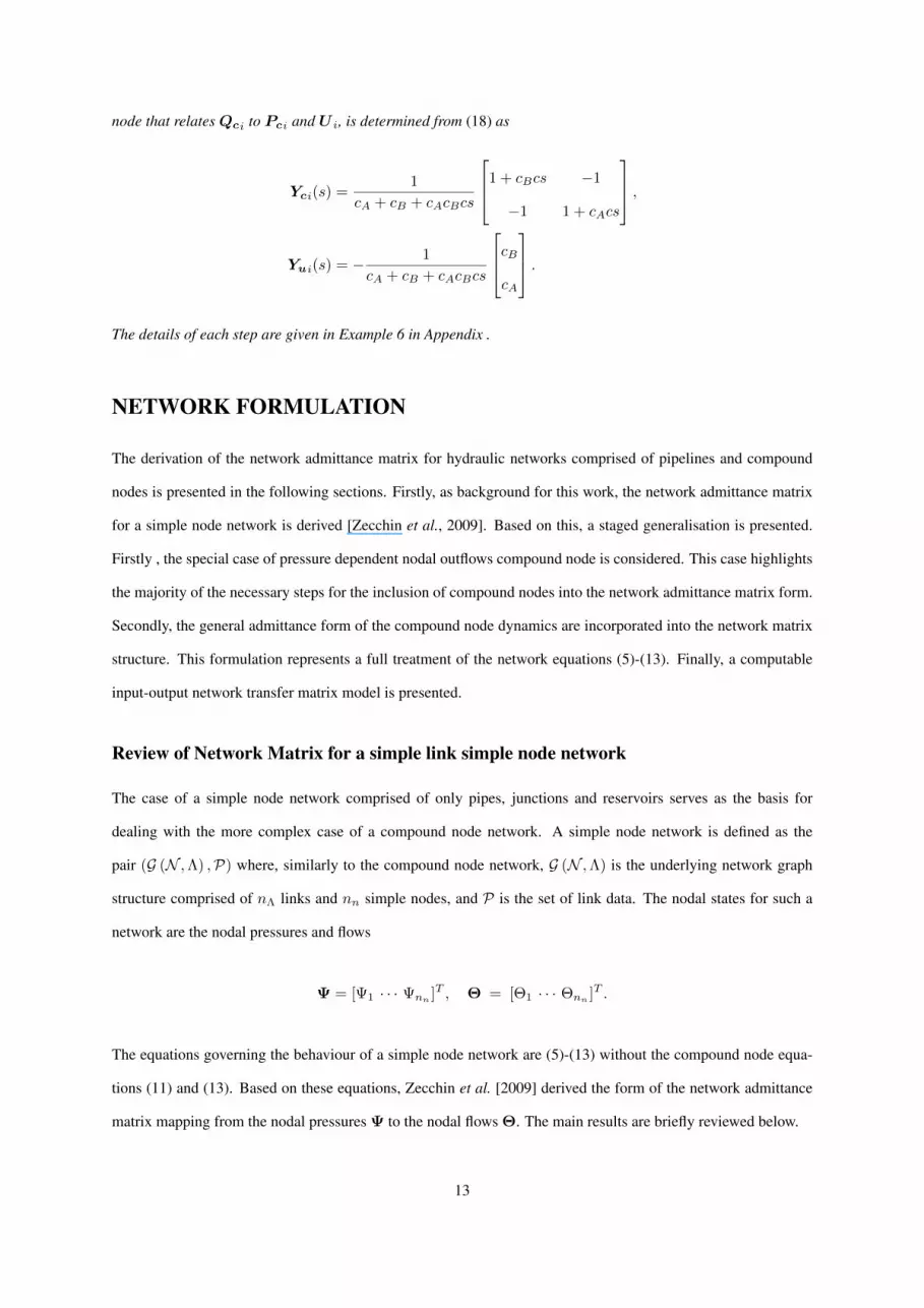
node that relatesQci to Pci and U i, is determined from (18) as
Yci(s) =1
cA + cB + cAcBcs
1 + cBcs −1
−1 1 + cAcs
,
Yui(s) = − 1
cA + cB + cAcBcs
cBcA
.The details of each step are given in Example 6 in Appendix .
NETWORK FORMULATION
The derivation of the network admittance matrix for hydraulic networks comprised of pipelines and compound
nodes is presented in the following sections. Firstly, as background for this work, the network admittance matrix
for a simple node network is derived [Zecchin et al., 2009]. Based on this, a staged generalisation is presented.
Firstly , the special case of pressure dependent nodal outflows compound node is considered. This case highlights
the majority of the necessary steps for the inclusion of compound nodes into the network admittance matrix form.
Secondly, the general admittance form of the compound node dynamics are incorporated into the network matrix
structure. This formulation represents a full treatment of the network equations (5)-(13). Finally, a computable
input-output network transfer matrix model is presented.
Review of Network Matrix for a simple link simple node network
The case of a simple node network comprised of only pipes, junctions and reservoirs serves as the basis for
dealing with the more complex case of a compound node network. A simple node network is defined as the
pair (G (N ,Λ) ,P) where, similarly to the compound node network, G (N ,Λ) is the underlying network graph
structure comprised of nΛ links and nn simple nodes, and P is the set of link data. The nodal states for such a
network are the nodal pressures and flows
Ψ = [Ψ1 · · · Ψnn ]T , Θ = [Θ1 · · · Θnn ]T .
The equations governing the behaviour of a simple node network are (5)-(13) without the compound node equa-
tions (11) and (13). Based on these equations, Zecchin et al. [2009] derived the form of the network admittance
matrix mapping from the nodal pressures Ψ to the nodal flows Θ. The main results are briefly reviewed below.
13

The Laplace-domain description of transient fluid lines (16) can be organised into the end-to-end transfer
matrix admittance form [Goodson and Leonard, 1972]
Qj(s, 0)
−Qj(s, lj)
=1
Zcj(s)
coth Γj(s) −cschΓj(s)
−cschΓj(s) coth Γj(s)
Pj(s, 0)
Pj(s, lj)
,
where Γj = ljΓj . The admittance matrix functions for each link λ ∈ Λ can be organised into the matrix form
Q(s,0)
−Q(s, l)
=
Zc−1(s) coth Γ(s) −Zc
−1(s)cschΓ(s)
−Zc−1(s)cschΓ(s) Zc
−1(s) coth Γ(s)
P (s,0)
P (s, l)
with link state vectors
P (s,x) = [P1(s, x1), . . . , PnΛ(s, xnΛ
)]T, Q(s,x) = [Q1(s, x1), . . . , QnΛ
(s, xnΛ)]T,
and the diagonal link function matrices
Γ(s) = diag {Γ1(s), . . . ,ΓnΛ(s)} ,Zc(s) = diag {Zc1(s), . . . , ZcnΛ
(s)} ,
where x = [x1, . . . , xnΛ ]T is the vector of spatial coordinates, and x = 0 (x = l) corresponds to all coordinates
set at their start (end) points. Defining the upstream and downstream node incidence matrices as
{Nu}i,j =
1 if λj ∈ Λu,i
0 otherwise
, {Nd}i,j =
1 if λj ∈ Λd,i
0 otherwise
,
the upstream and downstream pressure and flow link variables can be related to the pressure and flow nodal
variables by the matrix equations
P (s,0)
P (s, l)
=
[Nu Nd
]TΨ (s) ,
[Nu Nd
] Q(s,0)
−Q(s, l)
= Θ (s) ,
which are expressions of the pressure preservation, and mass conservation of a simple node, respectively (i.e.
matrix versions of equations (7) and (9) respectively). Combining these link and node relationship expressions
14

with the link functions (22) yields an admittance matrix expression for the network dynamics
Y (s)Ψ(s) = Θ(s)
where Y (s) is the symetric nn × nn admittance matrix given by
Y (s) =
[Nu Nd
] Zc−1(s) coth Γ(s) −Zc
−1(s)cschΓ(s)
−Zc−1(s)cschΓ(s) Zc
−1(s) coth Γ(s)
[ Nu Nd
]T(22)
which posesses the elementwise representation
{Y (s)}i,k =
∑λj∈Λi
coth Γj(s)
Zcj(s)if k = i
−cschΓj(s)
Zcj(s)if λj ∈ Λi ∩ Λk
0 otherwise
. (23)
Despite the fact that (23) represents a solution for a simple node network only, it provides the basis and framework
within which to include the compound node dynamics.
Network Matrix for a Network with Pressure Dependent Nodal Flows
The first extension to the work outlined above is the consideration of the case of compound nodes consisting of
only one connection, that is, compound nodes consisting of a hydraulic component connected to a single junction.
Examples of such components are emitters, scour valves, surge tanks or pressure relief valves. The flow into the
hydraulic component is clearly pressure dependent, but to generalise slightly further, it is assumed to be influenced
by a control action Ui (e.g. time varying valve opening, or fluctuating air volume). For a network with such node
types, a general expression for the flow into the compound node’s component is
Qci(s) = Yci(s)Pci(s)− Yui(s)Ui(s) (24)
where the first term on the right side of (24) represents the pressure dependent flow with admittance function Yci
and connection pressure Pci, and the second term represents the controlled flow with admittance function Yui and
control Ui. Note that (24) is simple a scalar version of (20).
Consider a network (G(N ,Λ), C,P) with nc such compound nodes collected into the set Nc, with Ns as the
15

set of remaining simple nodes (N = Ns ∪ Nc). Ordering the nodal states with the Nc nodes first, a network
admittance expression can be derived
Y (s)
Ψc(s)
Ψs(s)
=
Θc(s)
Θs(s)
(25)
where Y is the admittance matrix (23) for the simple node network given by (G(N ,Λ),P), Ψc and Ψs are the
nodal pressures at the compound junction and simple nodes respectively, and Θc and Θs are the nodal flows
at the compound junction and simple nodes respectively. In the expression (25), Θc corresponds to the flow
that enters the network (G(N ,Λ),P) from the compound nodes component, which is external to the network
(G(N ,Λ),P), and as such, the component dynamics are not directly incorporated in (25). To incorporate the
component dynamics the relationship between each Θci and Qci from (24) must be used. Given that Θci is the
flow at the junction into the network, and Qci is the flow at the junction into the component, for continuity it is
required that Θci +Qci = 0. Therefore, infact
Θc(s) = −Qc(s)
= −diag {Yc1(s), . . . , Ycnc(s)}Ψc(s) + diag {Yu1(s), . . . , Yunc
(s)}U(s)
(26)
whereQc andU are vector organisations of the compound node connection flows and controlled states. Combin-
ing (26) with (25) yields the admittance form for the compound node network as
Y (s) +
diag {Yc1(s), . . . , Ycnc(s)} 0
0 0
Ψc(s)
Ψs(s)
=
diag {Yu1(s), . . . , Yunc(s)} 0
0 I
U(s)
Θs(s)
(27)
where, using the identity for Y from (23) for the simple node network (G(N ,Λ),P), the elementwise expression
for (27) is,
{Y (s) + diag {diag {Yc1(s), . . . , Ycnc(s)} ,0}}i,k =
∑j∈Λi
coth Γj(s)
Zj(s)if k = i ∈ Ns
∑j∈Λi
coth Γj(s)
Zj(s)+ Yci(s) if k = i ∈ Nc
−cschΓj(s)
Zj(s)if λj = Λi ∩ Λj
0 otherwise
. (28)
where the diagonalisation refers to a block matrix organisation. Note that in (28), only the diagonal terms in the
16

upper left block of the original network matrix are altered, that is, the terms that correspond to a nodal’s pressure
influence on its nodal flow.
Admittance Matrix for a General Compound Node Network
In this section, the admittance matrix for a compound node network (G(N ,Λ),P, C) comprised of compound
nodes of a general type is derived. Before this can be done, an important preliminary concept must be introduced.
Given a compound node network (G(N ,Λ),P, C) with compound nodesNc and simple nodesNs, the associated
simple node expanded network is given by the simple node network (G(No,Λo),Po) where the node set is given
as the union of the simple node set Ns and the compound node connection sets Ni, that is
No = Ns ∪⋃i∈Nc
Ni,
where Ni is the set of connections for compound node i (as defined in Appendix ), the link set Λo is given by a
relabelling of the original link set Λ to the nodes in No, which is given by
Λo = {〈λ〉o : λ ∈ Λ}
where the function 〈λ〉o : N ×N 7→ No ×No is the relabelling function given by
〈(i, j)〉o =
(i, j) if i, j ∈ Ns
(i, l) if i ∈ Ns and (i, j) ∈ Λdjl, l ∈ Nj , j ∈ Nc
(k, j) if (i, j) ∈ Λuik, k ∈ Ni, i ∈ Nc and j ∈ Ns
(k, l) if (i, j) = Λuik ∪ Λdjl, k ∈ Ni, l ∈ Nj , i, j ∈ Nc
∅ otherwise
, (29)
and Po is the link data set P for the relabeled links [note that, as defined in Appendix , Λujk ⊂ Λuj (Λdjk ⊂ Λdj)
in (29) are defined as the set of links whose upstream (downstream) node is the k-th connection of compound
node j]. This concept of a simple node expanded network is fundamental to the developments within this section
as it provides the basic framework within which to include compound nodes. An example of the expanded simple
connection network for a given compound node network in Figure 2(a) is given in Figure 2(b), this is studied in
greater depth later.
17

The nodal states for an expanded simple node network are given as
Ψ(s) =
Ψ1(s)
...
Ψnc(s)
Ψs(s)
, Θ(s) =
Θ1(s)
...
Θnc(s)
Θs(s)
, (30)
where Ψi(s),Θi(s) are the pressures and flows associated with the simple connections inNi for each i ∈ Nc and
Ψs(s), and Θs(s) are the pressures and flows associated with the simple nodes Ns. As in the previous section, it
is important to explain the meaning of the Θi, i ∈ Nc. These variables correspond to nodal flow injections that
enter the network (G(No,Λo),Po) through the connections from a compound node’s component. The primary
motivation for the construction of the simple node expanded network is that the connection states (30) can be
related by the admittance relationship
Yo(s)
Ψ1(s)
...
Ψnc(s)
Ψs(s)
=
Θ1(s)
...
Θnc(s)
Θs(s)
, (31)
where Yo is the network admittance matrix (23) for the simple node network (G(No,Λo),Po). As with (25) for
the special case of pressure dependent flows, (31) deals only with the flow into the network (G(No,Λo),Po) and
does not directly incorporate the dynamics of the compound node’s component. To incorporate the component
dynamics, the flows into the network Θi are related to the compound node connection flows Qci by applying
continuity at the connections. This yields Θi +Qci = 0 (as explained in the previous section for the special case
of compound nodes with only a single connection). Given this relationship, by (20), the following relationship
between the nodal flows and the admittance form of the compound node can be derived
Θ1(s)
...
Θnc(s)
= −
Yc1(s)
. . .
Ycnc(s)
Ψ1(s)
...
Ψnc(s)
+
Yu1(s)
. . .
Yunc(s)
U1(s)
...
Unc(s)
(32)
18

where the first term on the righthand side of (32) is the pressure dependent term and the second term corresponds
to the connection flows associated with the controlled nodal states. Substituting (32) into (31) provides the full
expression relating the nodal pressures to the controlled nodal states and simple node flows
Yo(s) +
Yc1(s)
. . .
Ycnc(s)
0
Ψ1(s)
...
Ψnc(s)
Ψs(s)
=
Yu1(s)
. . .
Yunc(s)
I
U1(s)
...
Unc(s)
Θs(s)
(33)
where the elementwise expression for the admittance matrix acting on the simple connection pressures can be
derived as
{Yo (s) + diag {Yc1, . . . ,Ycnc,0}}
i,k=
∑j∈Λi
coth Γj(s)
Zj(s)if k = i ∈ Ns
∑j∈Λi
coth Γj(s)
Zj(s)+ {Yci(s)}〈i,i〉l if k = i ∈ Nc and i ∈ Nl, l ∈ Nc
−cschΓj(s)
Zj(s)if λj ∈ Λi ∩ Λk, i, k ∈ Ns
{Yci(s)}〈i,k〉l if i, k ∈ Nl, l ∈ Nc
0 otherwise
,(34)
where Nl is the l-th compound node connection set, and 〈·〉l maps from the ordering in the state vectors to the
local ordering for the connections at compound node l ∈ Nc. Here, unlike the pressure dependent outflow, off
diagonal terms in the admittance matrix are changed in addition to the diagonal terms. The structure of (34) is
consistent with that of (23) where the diagonal terms are comprised of sums of transfer functions, each associated
with the connection between a node and its neighboring nodes, and the off-diagonal terms are comprised of single
transfer functions, each associated with the connection between two nodes.
The matrix equation (33) represents the network admittance matrix for a compound node network of arbitrary
configuration and is the main result of the paper. The following example demonstrates the construction process
for the network in Figure 2(a).
19

Example 5. Consider the network (G(N ,Λ),P, C) in Figure 2(a), with
N = {1, 2, 3, 4, 5, 6} , as the set of nodes
Λ = {(1, 2), (2, 3), (2, 4), (3, 4), (3, 5), (4, 5), (5, 6)} , as the set of links
P = {P1,P2,P3,P4,P5,P6,P7} , as the set of link functions, and
C = {φ2,φ3,φ5} , as the set of compound node functions,
where the compound node set is Nc = {2, 3, 5} and the simple node set is Ns = {1, 4, 6}. Given the compound
node realisation in Figure 2(b), the connection sets for the compound nodes can be expressed as N2 = {21, 22},
N3 = {31, 32, 33}, andN5 = {51}, which leads to the expanded simple node network (G(No,Λo),Po) in Figure
2(c) defined by the following network sets
No = {1, 21, 22, 31, 32, 33, 4, 51, 6} ,
Λo = {(1, 21), (22, 31), (22, 4), (32, 4), (33, 51), (4, 51), (51, 6)} ,
Po = {Po1,Po2,Po3,Po4,Po5,Po6,Po7}
where Λo is constructed from Λ according to the relabeling function (29), and Po is the relabeled elements of P ,
associated with Λo. For the expanded simple node network (G(No,Λo),Po), the nodal states, ordered as in (30),
are
Ψ(s) =
Ψ21(s)
Ψ22(s)
Ψ31(s)
Ψ32(s)
Ψ33(s)
Ψ51(s)
Ψ1(s)
Ψ4(s)
Ψ6(s)
, Θ(s) =
Θ21(s)
Θ22(s)
Θ31(s)
Θ32(s)
Θ33(s)
Θ51(s)
Θ1(s)
Θ4(s)
Θ6(s)
. (35)
Given (23), the network admittance matrix Y o for the expanded simple node network (G(No,Λo),Po) can be
20

expressed as
Yo(s) =
t1 0 0 0 0 0 −s1 0 0
0∑
j=2,3 tj −s2 0 0 0 0 −s3 0
0 −s2 t2 0 0 0 0 0 0
0 0 0 t4 0 0 0 −s4 0
0 0 0 0 t5 −s5 0 0 0
0 0 0 0 −s5∑
j=5,6,7 tj 0 −s6 −s7
−s1 0 0 0 0 0 t1 0 0
0 −s3 0 −s4 0 −s6 0∑
j=3,4,6 tj 0
0 0 0 0 0 −s7 0 0 t7
(36)
where tj = tj(s) = Z−1c (s) coth Γj(s) and sj = sj(s) = Z−1
c (s)cschΓj(s). Note that as (36) is a network
admittance matrix, it is a square symmetric matrix, and the row and colum partitions of (36) correspond to the
partitions of the state vectors in (35). Assuming that node 2 has one controlled state, node 3 has two and node 5
has none, the admittance forms (20) of the compound node functions φ2, φ3, and φ5 are
Qc21(s)
Qc22(s)
= Yc2(s)
Pc21(s)
Pc22(s)
− Yu2(s)U2(s),
Qc31(s)
Qc32(s)
Qc33(s)
= Yc3(s)
Pc31(s)
Pc32(s)
Pc33(s)
− Yu3(s)
U31(s)
U32(s)
, (37)
Qc51(s) = Yc5(s)Pc51(s).
21

The pressure dependent term in the compound node network admittance matrix (33) can be constructed as
diag {Yc2(s),Yc3(s),Yc5(s),0} =
{Yc2}1,1 {Yc2}1,2 0 0 0 0 0 0 0
{Yc2}2,1 {Yc2}2,2 0 0 0 0 0 0 0
0 0 {Yc3}1,1 {Yc3}1,2 {Yc3}1,3 0 0 0 0
0 0 {Yc3}2,1 {Yc3}2,2 {Yc3}2,3 0 0 0 0
0 0 {Yc3}3,1 {Yc3}3,2 {Yc3}3,3 0 0 0 0
0 0 0 0 0 Yc5 0 0 0
0 0 0 0 0 0 0 0 0
0 0 0 0 0 0 0 0 0
0 0 0 0 0 0 0 0 0
0 0 0 0 0 0 0 0 0
and organising the state vector on the right side of (33) as
[U21(s) U31(s) U32(s) Θ1(s) Θ4(s) Θ6(s)
]T,
the matrix operator on this state vector is given as
diag {Yu2(s),Yu3(s),Yu5(s), I} =
{Yu2}1,1 0 0 0 0 0
{Yu2}2,1 0 0 0 0 0
0 {Yu3}1,1 {Yu3}1,2 0 0 0
0 {Yu3}2,1 {Yu3}2,2 0 0 0
0 {Yu3}3,1 {Yu3}3,2 0 0 0
0 0 0 0 0 0
0 0 0 1 0 0
0 0 0 0 1 0
0 0 0 0 0 1
,
(i.e. as there are no controlled states for compound node 5, Yu5 is a matrix of one row and zero columns). Given
these matrix identities, the network admittance equation (33) for the compound node network (G(N ,Λ),P, C)
can be constructed.
22

Formulation of a Computable Model
Despite the qualitative understanding enabled by the representation (33), it is not suitable for numerical imple-
mentation. The computational utility of the compound node network model requires a mapping from the inputs
(known nodal states) to the outputs (unknown nodal states). Consider the network (G(N ,Λ),P, C) with com-
pound nodes Nc, and simple nodes Ns that can be partitioned as Ns = NJ ∪ Nd ∪ Nr where NJ are junctions,
Nd are the demand nodes (flow control nodes) and Nr are the reservoirs (pressure control nodes). The inputs for
such a setup are the controlled node statesU i for each i ∈ Nc, the controlled nodal demands Θdi for each i ∈ Nd
and the known reservoir pressures Ψri for each i ∈ Nr. Defining the nodal set
ND =⋃i∈Nc
Ni ∪NJ ∪Nd (38)
(33) can be expressed as
Y DD(s) YoDr(s)
YorD(s) Yorr(s)
ΨD(s)
Ψr(s)
=
Yu(s)
I
I
I
U(s)
ΘJ (s)
Θd(s)
Θr(s)
(39)
where Yu = diag {Yu1, . . . ,Yunc}, U is the vector concatenation of the U i vectors, YorD, YoDr, and Yorr are
the partitions of Yo corresponding to the node sets ND and Nr, that is
YoDD(s) YoDr(s)
YorD(s) Yorr(s)
= Yo(s),
and Y DD incorporates the compound node dynamics and is given by
Y DD(s) = YoDD(s) + diag {Yc1(s), . . . ,Ycnc(s),0} .
Noting that the nodal flow for junctions ΘJ = 0, (39) can be reorganised to map from the input to the output as
ΨD(s)
Θr(s)
= H(s)
U(s)
Θd(s)
Ψr(s)
, (40)
23

whereH is given by
H(s) =
ZDu(s)Yu(s) ZDd(s) −ZDD(s)YoDr(s)
YorD(s)ZDu(s)Yu(s) YorD(s)ZDd(s) Yorr(s)− YorD(s)ZDD(s)Y Dr(s)
where ZDD is an impedance matrix given by ZDD = Y −1
DD and is partitioned as
ZDD(s) =
[ZDu(s) ZDJ(s) ZDd(s)
]
where each partition corresponds to the nodes of the sets⋃i∈Nc
Ni, NJ and Nd, respectively.
NUMERICAL EXAMPLES
Two example networks are considered in the following. Network-1 (Figure 2) is a 7-pipe/6-node network adapted
from Zecchin et al. [2009], and Network-2 (Figure 3) is a 51-pipe/34-node network adapted from Vıtkovsky
[2001]. The numerical experiments compare the frequency responses as calculated by the proposed admittance
matrix method, and that calculated from the discrete time-domain method of characteristics (MOC) model via
the discrete Fourier transform (DFT). As expected, and verified by many experiments, the admittance matrix
methodology yields the exact solution for linear networks. Hence, comparisons involving linear networks are not
presented. A question of greater practical interest is how well does the method approximate systems comprised
of nonlinear components? It is for this reason that the results presented are for numerical experiments performed
on nonlinear systems. The MOC results for network-1 were obtained from a frequency sweep, where the system
was excited into a steady oscillatory state, one frequency at a time. In contrast, the MOC results for network-2
were obtained from a transient excitation, where the frequency response was computed using the entire transient
response.
Network-1 in Steady-Oscillatory State
For the numerical study of network-1 (Figure 2), the network parameters are as follows; pipe diameters =
{60, 50, 35, 50, 35, 50, 60} mm, pipe lengths = {31, 52, 34, 41, 26, 57, 28} m, the wavespeeds and the Darcy-
Weisbach friction factors were set to 1000 m/s and 0.02, respectively, for all pipes, and the compound node details
are given in Tables 1 and 2. The demand at node 1 was taken as a sinusoidal form of amplitude 0.2 L/s about a
base demand level of 10 L/s. For the MOC model, a frequency sweep was performed for 200 frequencies up to
24
20 Hz. Figure 4 presents the amplitude of the sinusoidal pressure fluctuations observed at node 6 as computed by
the Laplace-domain admittance matrix and the DFT of the MOC in steady oscillatory state. Figure 5 presents the
same results for the sinusoidal flow fluctuations into the reservoir at node 1. Within both figures, the error between
the Laplace-domain and MOC approaches is presented in the bottom subfigure.
Despite the nonlinearities of pipe friction and the valve pressure loss, extremely good matches between the
two methods are observed as the errors for both the pressure and flow are more than three orders of magnitude
less than the amplitude of the response oscillations (as seen in Figures 4 and 5). The larger errors occur at the
networks harmonic frequencies, where the linear admittance matrix model slightly over estimates the amplitude
of the nonlinear MOC model.
Network-2 in Transient State
The original formulation for network-2 in Vıtkovsky [2001] was modified as follows: pipe lengths were rounded
to the nearest meter and the wavespeeds were all made to be 1000 m/s to ensure a Courant number of 1, which
was required to preserve the accuracy of the MOC; the nodal demands were doubled to increase the flow through
the network; nodes 7, 9, 11, 19, 22, 23, 25, and 34 were converted to compound nodes, the details of which are
given in Tables 1 and 2. For brevity, the network details are not given here, but the range of network parameters
are [450, 895] m for pipe lengths, [304, 1524] mm for pipe diameters, and [80, 280] L/s for nodal demands (for
case study details, the reader is referred to [Vıtkovsky, 2001]).
In order to avoid burdensome computational requirements, network-2 was analyzed in the transient state as
opposed to the steady-oscillatory state used for network-1. This meant that the frequency response was computed
from a single MOC simulation of the system for the entire response time of the system. The network was excited
into a transient state by a perturbing the flow at nodes {14, 17, 28}. Results for two types of excitations are
presented. The first type of excitation involved a pulse perturbation, which was achieved by reducing the nodal
flows by a magnitude of {70, 50, 100} L/s for a duration {0.055, 0.025, 0.075} s only. The second involved a step
perturbation, which was achieved by reducing the nodal flows by a magnitude of {70, 50, 100} L/s.
A plot of the frequency response at nodes 14 and 18 for network-2 with the pulse perturbation is given in
Figures 6 and 7 where the top subfigure gives the frequency response of the Laplace-domain method, and the
bottom subfigure shows the magnitude of the error between the Laplace-domain method and the MOC. Due to the
densely distributed harmonics, only the range 0 - 4 Hz is shown.
Figures 6 and 7 show that the error between the DFT of the MOC and the proposed Laplace-domain admittance
matrix method is small in comparison to the spectral amplitude of the frequency response. This illustrates that even
25

for a network of a large size containing nonlinear elements such as emitters, valves, and accumulators, the linear
admittance matrix model provides an extremely good approximation of the nonlinear MOC model. Similarly
with network-1, the larger errors occur at the networks harmonics. There is also a slight trend of increasing in
magnitude with increasing frequency. Despite this, the matches are excellent.
A plot of the frequency response at nodes 14 and 18 for the step excitation is given in Figures 8 and 9, where
the top subfigure gives the frequency response and the bottom subfigure shows the magnitude of the error between
the two methods. The plots are presented with a log scale on the vertical axis as the excitation energy for a step
input reduces rapidly for increasing frequency.
It is observed from Figures 8 and 9 that the error between the methods is over an order of magnitude less than
the spectral amplitude of the frequency response. This error is surprisingly low, given that for the step input the
operating point of the linearization for the Laplace-domain model (i.e. the initial steady-state) is different to the
final operating position of the network due to the permanent change in the nodal flows. The change of the steady-
state operating point is the cause for the error peak near the zero frequency point. The linear Laplace-domain
model is seen to yield a good approximation of the nonlinear system even when the operating point for the system
shifts.
CONCLUSIONS
Existing methods for modeling the frequency-domain behavior of a transient fluid line system have either been
limited by the configuration of network types that they can model, or are limited by the hydraulic element types that
they can encompass. Within this paper, a completely new formulation is derived that is able to deal with networks
of an arbitrary configuration containing an extremely broad class of hydraulic elements, termed compound nodes,
namely those that yield an admittance type representation.
An analytic representation of the network admittance matrix has been presented in this paper, which not only
yields significant qualitative information about the network, but also serves as a basis for numerical implemen-
tation of the proposed method. An interesting finding presented in this paper is that the admittance matrix for a
compound node network can be expressed as the addition of two matrix terms, one pertaining to its simple node
network structure, and the other containing the compound node dynamics.
The proposed new method has been verified by numerical examples with a 7-pipe network, and a 51-pipe
network. For these case studies, the proposed method provided excellent agreement with the frequency response
as calculated by the method of characteristics. This result was particularly interesting as the networks contained
26

nonlinear elements (emitters, valves, accumulators, and turbulent pipes).
This proposed new approach allows complete flexibility with regard to the topological structure of a network
and the types of hydraulic elements. As such, it overcomes previous limitations in frequency-domain modeling of
pipe networks, and provides general basis for future research utilizing the Laplace-domain representation of fluid
line systems.
References
Axworthy, D. (1997) Water Distribution Network Modelling from Steady State to Waterhammer PhD thesis Uni-
versity of Toronto, Canada.
Barber, A. (1989) Pneumatic handbook 7th edn. Trade and Technical Press, Morden, England.
Boucher, R.F. and Kitsios, E.E. (1986) “Simulation of fluid network dynamics by transmission-line modeling”
Proceedings of the Institution of Mechanical Engineers Part C-Journal of Mechanical Engineering Science
200(1), 21–29.
Brown, F. and Nelson, S. (1965) “Step responses of liquid lines with frequency-dependent effects of viscosity”
Journal of Basic Engineering, ASME 87(June), 504–510.
Chaudhry, M. (1970) “Resonance in pressurized piping systems” Journal of the Hydraulics Division, ASCE
96(HY9, September), 1819–1839.
Chaudhry, M. (1987) Applied Hydraulic Transients 2nd edn. Van Nostrand Reinhold Co., New York, USA.
Desoer, C.A. and Kuh, E.S. (1969) Basic Circuit Theory McGraw-Hill, New York.
Desoer, C.A. and Vidyasagar, M. (1975) Feedback Systems: Input-Output Properties Electrical Science Academic
Press Inc., New York.
Diestel, R. (2000) Graph Theory electronic edition edn. Springer-Verlag, New York, USA.
Fox, J. (1977) Hydraulic Analysis of Unsteady Flow in Pipe Networks The Macmillan Press Ltd., London, UK.
Franklin, G.F., Powell, J.D., and Emami-Naeini, A. (2001) Feedback Control of Dynamic Systems 4th edn. Prentice
Hall PTR, Upper Saddle River, N.J. London.
Goodson, R. and Leonard, R. (1972) “A survey of modeling techniques for fluid line transient” Journal of Basic
Engineering, ASME 94, 474–482.
27

Izquierdo, J. and Iglesias, P.L. (2004) “Mathematical modelling of hydraulic transients in complex systems” Math-
ematical and Computer Modelling 39(4-5), 529–540.
John, L.R. (2004) “Forward electrical transmission line model of the human arterial system” Medical and Biolog-
ical Engineering and Computing 42(3), 312–321.
Karney, B. (1984) Analysis of Fluid Transients in Large Distribution Networks PhD thesis The University of
British Columbia, Canada.
Kim, S.H. (2007) “Impedance matrix method for transient analysis of complicated pipe networks” Journal of
Hydraulic Research 45(6), 818–828.
Kim, S.H. (2008a) “Address-oriented impedance matrix method for generic calibration of heterogeneous pipe
network systems” Journal of Hydraulic Engineering, ASCE 134(1), 66–75.
Kim, S.H. (2008b) “Impulse response method for pipeline systems equipped with water hammer protection de-
vices” Journal of Hydraulic Engineering, ASCE 134(7), 916–924.
Kreyszig, E. (1999) Advanced Engineering Mathematics 8th edn. John Wiley, New York.
Margolis, D.L. and Yang, W.C. (1985) “Bond graph models for fluid networks using modal approximation” Jour-
nal of Dynamic Systems Measurement and Control-Transactions of the ASME 107(3), 169–175.
Ogawa, N. (1980) “A study on dynamic water pressure in underground pipelines of water supply system dur-
ing earthquakes” Recent Advances in Lifeline Earthquake Engineering in Japan, vol. 43, eds. H. Shibata,
T. Katayma, and T. Ariman 55–60 ASME.
Stecki, J.S. and Davis, D.C. (1986) “Fluid transmission-lines - distributed parameter models .1. A review of the
state-of-the-art” Proceedings of the Institution of Mechanical Engineers Part A-Journal of Power and Energy
200(4), 215–228.
Todini, E. and Pilati, S. (1988) “A gradient algorithm for the analysis of pipe networks” Computer Applications in
Water Supply, eds. B. Coulbeck and C.H. Orr 1–20 Research Studies Press, Letchworth, Hertfordshire, UK.
Vardy, A. and Brown, J. (2003) “Transient turbulent friction in smooth pipe flows” Journal of Sound and Vibration
259(5, January), 1011–1036.
Vardy, A. and Brown, J. (2004) “Transient turbulent friction in fully-rough pipe flows” Journal of Sound and
Vibration 270, 233–257.
28

Vıtkovsky, J. (2001) Inverse Analysis and Modelling of Unsteady Pipe Flow: Theory, Applications and Experi-
mental Verification PhD thesis Adelaide University, Australia.
Wylie, E. (1965) “Resonance in pressurized piping systems” Journal of Basic Engineering, Transactions of the
ASME (December), 960–966.
Wylie, E. and Streeter, V. (1993) Fluid Transients in Systems Prentice-Hall Inc., Englewood Cliffs, New Jersey,
USA.
Zecchin, A.C., Simpson, A., Lambert, M., White, L.B., and Vitkovsky, J.P. (2009) “Transient modelling of arbi-
trary pipe networks by a Laplace-domain admittance matrix” Journal of Engineering Mechanics, ASCE 135(6),
538–547.
Zielke, W. (1968) “Frequency-dependent friction in transient pipe flow” Journal of Basic Engineering, ASME
90(1), 109–115.
29

CAPTIONS FOR FIGURES AND TABLES
Figures
30

Example of a compound node consisting of a capacitive dead end branch and an offtake bounded by valves A
and B. (a) The physical layout demonstrating the link end states of pressure and flow for links [a], [b], and [c],
and the internal node states of the internal pressure ψo, the capacitive flow θo and the offtake flow θd. (b)The
simple connection configuration, where the compound node is observed to have two simple connections with
[a] incident to one and [b], and [c] incident to another. (c) The transformed simple connection states, where
PciA and PciB are the pressures at connections A and B, and QciA and QciB are the aggregated flows into
connections A and B. (d) The expanded simple node network representation of the compound node with simple
node pressures ΨA and ΨB , and flows ΘA and ΘB . For this example, the variables are related as follows:
PciA(s) = ΨA(s) = Pa(la, s); QciA(s) = −ΘA(s) = Qa(la, s);, PciB(s) = ΨB(s) = Pb(lb, s) = Pc(lc, s) and
QciB(s)−ΘB(s) = Qb(lb, s)−Qc(0, s).
31

[c][c]
[b][b]
[a][a]
[c][c]
[b][b]
[a][a] i
[b]
[c]
θd (t)
[a]
A B
A B
(a)
(b)
A B
(c)
QciA(s)
pa(la,t), qa(la,t)
pb(lb,t), qb(lb,t)
pc(0,t), qc(0,t)
ψo(t), θo(t)
PciA(s)
A B
(d)
ΘB(s)ΘA(s)
ΨA(s) ΨB(s)
PciB(s)
QciB(s)i
Figure 1: Caption
32

Example network-1 adapted from Zecchin et al. [2009], with controlled demand as node 1, a single valve at
node 2, two valves at node 3 and capacitance branch at node 5. (a) The physical configuration of the system.
(b) The compound nodes’ connection configurations. (c) The simple connection expanded network, where the
denoted Θi’s are the flows into the simple connection expanded network from the compound nodes.
33

Θ33(s)
Θ22(s)
Θ31(s)
[4][4]
[5][5]
(b)
[1][1]
[2][2]
[6][6][3][3]
[7][7]22
1
1
51
(c)
331
2
4
[4][4]
[5][5][1][1]
[2][2]
[6][6][3][3]
[7][7]2221
1
51
3331
32
4
(c)
Θ51(s)Θ21(s)Θ32(s)
[4][4]
[5][5]
(a)
[1][1] [2][2]
[6][6][3][3]
[7][7]2
1
5
3
4
1
6
6
6
θ1(t)valve
dead end
Figure 2: Caption
34

[1][1]
[3][3] [6][6]
[9][9] [10][10]
[12][12]
[15][15]
[17][17][20][20]
[21][21]
[23][23][25][25]
[2][2]
[5][5]
[26][26][24][24]
[29][29][22][22]
[7][7]
[11][11]
[14][14]
[13][13]
[31][31][30][30]
[8][8]
[4][4]
[27][27]
[33][33]
[16][16]
[19][19]
[34][34]
[28][28]
[32][32]
5
20
17
16
1514
1312
6
10
43
2
[18][18]
8
[41][41]
[43][43]
[46][46]
[39][39]
[40][40]
[42][42][45][45]
[47][47][48][48]
[44][44]
[49][49]
[51][51]
[36][36]
[50][50]
[35][35]
[37][37] [38][38] 272624
31
3332
30
28
18
21
9
25
34
19
11
22 35
21
29
23
(a)
7
[1][1]
[3][3] [6][6]
[9][9][10][10]
[12][12]
[15][15]
[17][17] [20][20]
[21][21]
[23][23][25][25]
[2][2]
[5][5]
[26][26]
[24][24]
[29][29][22][22]
[7][7]
[11][11]
[14][14]
[13][13]
[31][31][30][30]
[8][8]
[4][4]
[27][27]
[33][33][16][16]
[19][19]
[34][34]
[28][28]
[32][32]
5
20
17
16
1514
1312
6
10
43
2
[18][18]
8
[41][41]
[43][43]
[46][46]
[39][39]
[40][40]
[42][42][45][45]
[47][47][48][48]
[44][44]
[49][49]
[51][51]
[36][36]
[50][50]
[35][35]
[37][37] [38][38] 272624
31
3332
30
28
182
9
1
4 2
3
25
1
34
1
2
3
191
11 1
222
1
29
2231
(b)
1
721
35
2
1
θ28(t)
θ17(t)θ14(t)
air chamber
emitter
Figure 3: Caption
Example network-2, adapted from Vıtkovsky [2001], with compound nodes as described in Table 1. (a) The
physical layout of the network, and (b) shows the compound nodes’ connection configurations.
35

Oscillation
Amplitude(kPa)
Error
(kPa)
Frequency (Hz)
0 2 4 6 8 10 12 14 16 18 20-3
-2
-1
0
1
200
400
600
800
1000
Figure 4: Caption
Sinusoidal pressure amplitude response for network-1 at node 6 for the admittance matrix model (continuous
line) and the method of characteristics in steady oscillatory state (◦ points). The error between the two methods is
given in the bottom figure.
36

Oscillation
Amplitude(L
/s)
Error
(L/s)
Frequency (Hz)
0 2 4 6 8 10 12 14 16 18 20
-0.004
-0.002
0
0
0.5
1
1.5
2
Figure 5: Caption
Sinusoidal flow amplitude response for network-1 at node 1 for the admittance matrix model (continuous line)
and the method of characteristics in steady oscillatory state (◦ points). The error between the two methods is given
in the bottom figure.
37

SpectralAmplitude(kPa·s)
Error
(kPa·s)
Frequency (Hz)
0 0.5 1 1.5 2 2.5 3 3.5 40
0.5
1
1.5
2
10
20
30
40
50
Figure 6: Caption
Pressure frequency response magnitudes for network-2 at node 14 for the admittance matrix model pulse
perturbation. The lower figure gives the magnitude of the error between the admittance matrix and MOC methods
(the admittance matrix minus the DFT of the MOC).
38

SpectralAmplitude(kPa·s)
Error
(kPa·s)
Frequency (Hz)
0 0.5 1 1.5 2 2.5 3 3.5 40
0.5
1
1.5
2
10
20
30
40
50
Figure 7: Caption
Pressure frequency response magnitudes for network-2 at node 18 for the admittance matrix model for the
pulse perturbation. The lower figure gives the magnitude of the error between the admittance matrix and MOC
methods (the admittance matrix minus the DFT of the MOC).
39

SpectralAmplitude(kPa·s)
Error
(kPa·s)
Frequency (Hz)
0 0.5 1 1.5 2 2.5 3 3.5 4
10−1
100
101
102
10−1
100
101
102
103
Figure 8: Caption
Pressure frequency response magnitudes for network-2 at node 14 for the admittance matrix model for the step
perturbation. The lower figure gives the magnitude of the error between the admittance matrix and MOC methods
(the admittance matrix minus the DFT of the MOC).
40

SpectralAmplitude(kPa·s)
Error
(kPa·s)
Frequency (Hz)
0 0.5 1 1.5 2 2.5 3 3.5 4
10−1
100
101
102
10−1
100
101
102
103
Figure 9: Caption
Pressure frequency response magnitudes for network-2 at node 18 for the admittance matrix model for the step
perturbation. The lower figure gives the magnitude of the error between the admittance matrix and MOC methods
(the admittance matrix minus the DFT of the MOC).
41

Table Captions
Table 1: Compound element parameters for numerical studies for networks 1 and 2. Capacitors are physical
models for short dead end sections, and accumulators are the models for air chambers.
Table 2: Compound node element details. All elements are discussed at greater depth in Wylie and Streeter
[1993].
42

NOMENCLATURE
C Set of compound node functions
H(s) Transfer function matrix for the input/output network model
nc Number of compound nodes
nd Number of demand (flow controlled) nodes
nr Number of reservoir (pressure controlled) nodes
nsi Number of simple connections for compound node i
nΛ Number of links
Nd Incidence matrix for downstream nodes
Nu Incidence matrix for upstream nodes
Ndi Compound node incidence matrix for downstream nodes
Nui Incidence matrix for upstream nodes
N Set of nodes
Nc Set of compound nodes
Nd Set of demand (flow controlled) nodes
ND Set of flow controlled nodes within the simple node expanded network, see
(38)
Ni Set of connections for compound node i
NJ Set of junctions
No Set of nodes for the simple node expanded network
Nr Set of reservoir (pressure controlled) nodes
Ns Set of simple nodes
pi(x, t) Pressure for pipe i
p(x, t) Vector of pipeline pressures
Pi(x, s) Laplace transform of pressure for pipe i
P (x, s) Vector of Laplace transform of pipeline pressures
Pci(s) Vector of Laplace transform of connection pressures for compound node i
Pd(s) Vector of pipeline pressures at upstream point
Pu(s) Vector of pipeline pressures at downstream point
P Set of pipeline functions
qi(x, t) Axial flow rate for pipe i
43

q(x, t) Vector of pipeline axial flow rates
Qi(x, s) Laplace transform of axial flow rate for pipe i
Q(x, s) Vector of Laplace transform of pipeline axial flow rates
Qci(s) Vector of Laplace transform of connection flows for compound node i
Qd(s) Vector of pipeline axial flow rates at upstream point
Qu(s) Vector of pipeline axial flow rates at downstream point
ui(t) Controlled internal nodal states for compound node i
ui(t) Dependent internal nodal states for compound node i
U i(s) Laplace transform of ui(t)
U i(s) Laplace transform of ui(t)
Y (s) Network admittance transfer matrix
Y j(s) Admittance transfer matrix for hydraulic element j
Yci(s) Admittance matrix operating on the compound node connection pressures
for canonical form of compound node dynamics
Yui(s) Admittance matrix operating on the compound node controlled states for
canonical form of compound node dynamics
Zc(s) Series impedance
φ, [Φ(s)] Compound node equation [and its Laplace transform]
Λ Set of links within a graph or network
Λi Set of links incident to node i
Λdi Set of links for which the downstream node is node i
Λui Set of links for which the upstream node is node i
ψ(t) Nodal pressure
ψr(t) Nodal pressure at reservoir node
Ψ(s) Vector of Laplace transformed network nodal pressures
Ψd(s) Vector of Laplace transformed network demand (flow control) node pres-
sures
ΨD(s) Vector of Laplace transformed node pressures for flow controlled nodes
within the simple node expanded network
Ψi(s) Vector of Laplace transformed of nodal pressures for compound node i for
the simple node expanded network
44

Ψr(s) Vector of Laplace transformed network reservoir pressures
θ(t) Nodal flows (flow injections)
θd(t) Nodal flows at demand nodes
Θ(s) Vector of Laplace transformed network nodal flows
Θd(s) Vector of Laplace transformed network demand node flows
Ψi(s) Vector of Laplace transformed of nodal flows for compound node i for the
simple expanded node network
Θr(s) Vector of Laplace transformed network reservoir flows
Γ(s) Fluid line propagation operator
Γ(s) Fluid line propagation operator matrix for hydraulic network
45

APPENDIX: ADMITTANCE REPRESENTATION OF A COMPOUND
NODE
The three phased derivation of the compound node admittance form (20) from the Laplace-transform of the lin-
earised original compound node equation (17) is outlined below, followed by an example.
Connection representation of a Compound Node
The representation of a compound node as a hydraulic component with connections is a fundamental representa-
tion of the compound node, and is independent of the connectivity of the compound node with the wider network.
It is convenient to denote the set of connections for compound node i ∈ Nc by Ni. As with a simple node, each
connection k ∈ Ni has two states, the nodal pressure Pcik, and the nodal flow into the compound nodes compo-
nent Qcik, where, as stated above, the pressure Pcik is the common pressure shared by all link ends incident to the
connection, and the flow Qcik is the aggregated flow into the component from all links incident to the connection.
Organising these states as (19), they can be related to the incident link states P i andQi, from (17) by
P i(s) = [Nui +Ndi]TPci(s), Qci(s) = [Nui −Ndi]Qi(s) (41)
whereNui andNdi are compound node incidence matrices, describing the topology of the node, and are defined
by
{Nui}kj =
1 if j-th link in Λui is in Λuik
0 otherwise
,
{Ndi}kj =
1 if j-th link in Λdi is in Λdik
0 otherwise
,
where the link sets Λuik and Λdik are associated with the sets Λui and Λdi, respectively, and contain the upstream
and downstream links that are incident to the connection k. The equations (41) are analogous to the simple node
constraints for networks (7) and (9), and are explained as follows. Concerning the connection pressure Pcik, as
there is no pressure variation within a connection, the pressure of any links incident to the same connection k will
be equal. Concerning the connection flow Qcik, as there is no accumulation of mass within a connection, the total
flow through the connection k is equal to the sum of the inflows from the links in Λdik minus the outflows from
46

the links in Λuik.
The existence of the relationships (41) implies that there exists a lower dimensional form of Φi incorporating
the component dynamics that is just dependent on the connection states Pci and Qci. This lower dimensional
form can be expressed as
Φsi(s)
Pci(s)
Qci(s)
U i(s)
U i(s)
= 0 (42)
where Φsi is a (nsi + nui)× (2nsi + nui + nui) matrix of stable transfer functions. The matrix system Φsi
has (nsi + nui) rows as it must contain enough equations to determine one state at each connection, and all the
internal response states.
Decoupled nodal equations
By definition, as ui is a nodal response variable, it can be uniquely determined from the other nodal states. Hence
there exists a stable Laplace-domain transfer function mapping from the transformed connection pressures and
flows (Pci, Qci) and the transformed controlled nodal states (U i) to the transformed nodal response states U i.
That is, Φsi can be partitioned as
Φsi(s) =
Φopi(s) Φoqi(s) Φoui(s) Φoui(s)
Φ1pi(s) Φ1qi(s) Φ1ui(s) Φ1ui(s)
(43)
where the blocks correspond to their subscripted variables, and Φ1ui is a nui × nui matrix that possesses a
stable inverse. Formally, the matrix function A(s) : C 7→ Cn×n possesses a stable inverse if detA(s) > 0 for
Re {s} ≥ 0. Therefore, a nsi order system exists that relates the states Pci, Qci and U i can be decoupled from
U i, which can be expressed as
Φci(s)
Pci(s)
Qci(s)
U i(s)
= 0 (44)
47

where Φci is an nsi × (2nsi + nui) matrix of stable complex functions, given by
Φci(s) =
[Φcpi(s) Φcqi(s) Φcui(s)
]=
[Φopi(s) Φoqi(s) Φoui(s)
]−Φoui(s)Φ1u
−1i (s)
[Φ1pi(s) Φ1qi(s) Φ1ui(s)
] . (45)
The matrix Φci represents a minimal state matrix for the compound node i as it yields equivalent dynamics to Φsi
but with a reduced number of states. An example of the derivation of the form of (45) is given in Example 6.
Admittance Representation of Φci(s)
Given the decoupled connection representation (45), the criteria for the existence of the admittance representation
(20) can be precisely stated as
rank{Φcqi(s)
}= nsi for Re {s} ≥ 0. (46)
The significance of (46) is that it defines the criteria under which the compound nodes simple connection flows
Qci can be resolved from the simple connection pressures Pci and the compound nodes controlled states Uci.
The transfer matrix Φcqi is nsi × nsi, therefore, the constraint (46) can be interpreted as Φcqi begin full rank
without diminishing rank on Re {s} ≥ 0. In this instance Φcqi is a nsi×nsi transfer matrix with a stable inverse,
and the admittance matrices from (20) can be given as
Yci(s) = −[Φcqi(s)
]−1Φcpi(s), Yui(s) =
[Φcqi(s)
]−1Φcui(s). (47)
It turns out that (46) is not a very restrictive, but that all components considered within this research adhere to this
requirement. Consider the following example.
Example 6. Revisiting the compound node from Figure 1 in Examples 1 and 2, it is recognised that there are
nλi = 3 links, nui = 1 controlled node state, nui = 2 response node states, where the order of the φ is clearly
5. This compound node is recognised as having two connections (i.e. nsi = 2), one just outside valve A and the
other outside valve B. Denoting these connections as A and B, the connection states are as given in (21), and the
topological matrices are
Nui =
0 0 0
0 0 1
, Ndi =
1 0 0
0 1 0
.
48

By identifying and removing the connection equations (41), (18) can be converted into the form (42) as
Φi(s) =
0 1 0 −cB 0 −1 0
0 0 1 1 1 0 −1
0 0 0 0 0 cs −1
1 0 −cA 0 0 −1 0
(48)
where the partitions correspond to those in (43), where
[Φu1i(s)]−1
=
cs −1
−1 0
−1
= −
0 1
1 cs
(49)
clearly exists for Re {s} ≥ 0. Given the expressions in (45), the decoupled representation (44) is given by
Φci(s) =
−1 1 cA −cB 0
−cs 0 1 + cAcs 1 1
where the partitions are according to (45). Recognising from (50) that
Φcqi(s) =
cA −cB
1 + cAcs 1
the criteria (46) holds if
det{Φcqi(s)
}= cA + cB + cAcBcs 6= 0, on Re {s} ≥ 0.
This clearly holds as c,cA, and cB are all positive real numbers. Therefore, it can be demonstrated from (47) that
the admittance matrices for (20) are given by
Yci(s) =1
det{Φcqi(s)
}1 + cBcs −1
−1 1 + cAcs
, Yui(s) = − 1
det{Φcqi(s)
}cBcA
.
49

TABLES FOR MANUSCRIPT
50
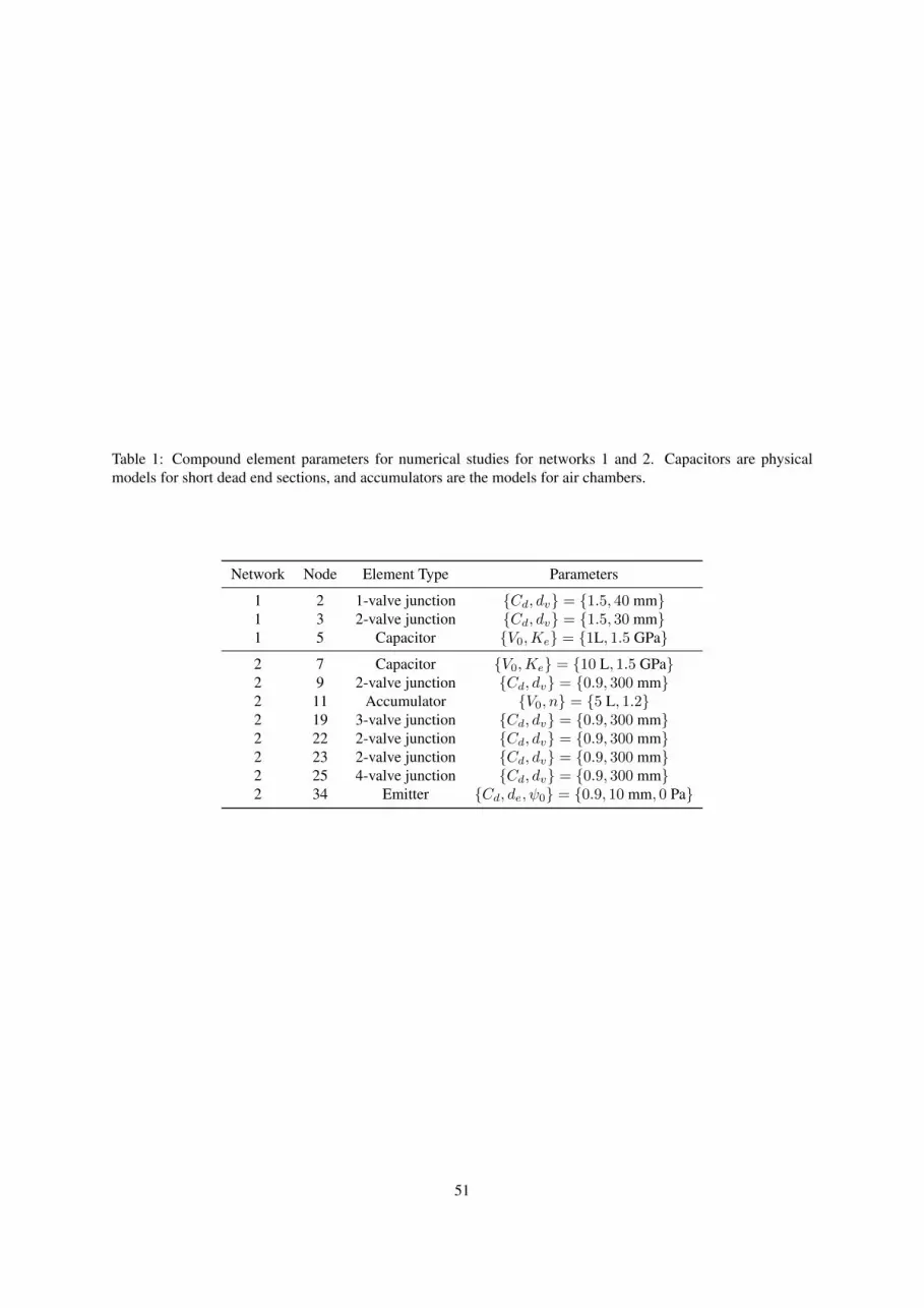
Table 1: Compound element parameters for numerical studies for networks 1 and 2. Capacitors are physicalmodels for short dead end sections, and accumulators are the models for air chambers.
Network Node Element Type Parameters
1 2 1-valve junction {Cd, dv} = {1.5, 40 mm}1 3 2-valve junction {Cd, dv} = {1.5, 30 mm}1 5 Capacitor {V0,Ke} = {1L, 1.5 GPa}2 7 Capacitor {V0,Ke} = {10 L, 1.5 GPa}2 9 2-valve junction {Cd, dv} = {0.9, 300 mm}2 11 Accumulator {V0, n} = {5 L, 1.2}2 19 3-valve junction {Cd, dv} = {0.9, 300 mm}2 22 2-valve junction {Cd, dv} = {0.9, 300 mm}2 23 2-valve junction {Cd, dv} = {0.9, 300 mm}2 25 4-valve junction {Cd, dv} = {0.9, 300 mm}2 34 Emitter {Cd, de, ψ0} = {0.9, 10 mm, 0 Pa}
51

Table 2: Compound node element details. All elements are discussed at greater depth in Wylie and Streeter [1993].
Element States, u Parameter Set Equations comprising φ
Emitter [ψ θ]T {Cd, de, ψ0} θ(t)− CdAe
√ψ(t)− ψ0
ρ
Capacitor [ψ θ]T {V0,Ke} θ(t)− V0
Ke
dψ
dt
Accumulator [ψ θ V ]T {V0, n}[ψ(t)V n(t)− Caθ(t)− dV
dt
]
Valvea [ψu ψd θ]T {Cd, dv} θ(t)− sign {∆ψ(t)}CdAv
√|∆ψ(t)|
ρ
a Note that ∆ψ(t) = ψu(t)− ψd(t).
52