Embed Size (px)
Citation preview


FROM HOW MUCH TO HOW MANY
Managing Complexity in Routine Design
Automation
PROEFSCHRIFT
ter verkrijging vande graad van doctor aan de Universiteit Twente,
op gezag van de rector magnificus,prof. dr. H. Brinksma,
volgens besluit van het College voor Promotiesin het openbaar te verdedigen
op donderdag 29 April 2010 om 16.45 uur
door
Juan Manuel Jauregui Beckergeboren op 20 May 1980
te Merida, Venezuela

Dit proefschrift is goedgekeurd door:
Prof. dr. ir. F.J.A.M. van Houten promotor

FROM HOW MUCH TO HOW MANY
Managing Complexity in Routine Design
Automation
PhD Thesis
By Juan Manuel Jauregui Becker at the Faculty of Engineering Technology(CTW) of the University of Twente, Enschede, the Netherlands.Enschede, 29 April 2010

De promotiecommissie:
Prof. dr. F. Eising Universiteit Twente, voorzitter, secretarisProf. dr. ir. F.J.A.M. van Houten Universiteit Twente, promotorDr. ir. G. Still Universiteit TwenteProf. dr. ir. R. Akkerman Universiteit TwenteProf. dr. ir. J. van Hillegersberg Universiteit TwenteProf. dr. ir. F.W. Jansen Technische Universiteit DelftProf. dr. T. Tomiyama Technische Universiteit DelftProf. dr. ir. A.C. Brombacher Technische Universiteit EindhovenProf. dr. T. Kjellberg KTH Royal Institute of Technology
Keywords: Computational Design Synthesis, Routine Design, Complexity Management
ISBN 978-90-365-2989-1
Copyright © Juan Manuel Jauregui Becker, 2010Cover design by Diruji Dugarte ManoukianPrinted by Gildeprint, EnschedeAll rights reserved.

A Diru,
a mis papas y hermanos

Summary
Advances in technology and competitive markets are driving the development ofproducts with shorter times to market. In addition to this, products are becomingmore complex, with more functionality, and yet lower prices. This has motivatedthe development of computer systems that support different phases of the designprocess, one of which is the synthesis process. This process consists of generatingcandidate design solutions to design problems.
This thesis researches the development of software that supports synthesisprocesses. This type of software is denoted in this thesis as Computer AidedSynthesis, or CAS. The scope lies within the boundaries of routine design problemsof artifacts. In such problems, designers have all knowledge available about thecomponents, parameters, relations and constrains that are used for solving them.
Synthesis processes for generating solutions to routine design problems consistof two tasks: (1) generating networks of components and (2) attributing valuesto unknown parameters. The exact strategy determining how these tasks areperformed depends on the distribution of requirements throughout the differentlevels of detail of the problem, e.g. only on top, only at the bottom or as amix. However, this relation is not known a priori and is different for differentdistributions of design requirements. From here that complexity in routine de-sign is attributed to the distribution of design requirements along the differentabstractions of the problem. Determining the dependency between design com-plexity and synthesis strategies is the main challenge of this research. The resultis a new complexity management approach: Computational Design Synthesis byComplexity Management. This approach integrates six methods, which have allbeen developed during this research.
The first step of this approach consists in formulating a design problem us-ing the FBS based Formulation method. This method uses FBS representationsto aid designers in the process of determining which are the exact components,parameters, relations and constraints playing a role in the design problem.
The formal design problem is then decomposed by applying the ADT based
VII

Decomposition method. This results in a new problem formulation consistingdifferent levels of abstraction. The decomposition is both functional and physi-cal and is based in the structure of the functions, components, parameters andrelations in the problem.
The decomposed model is then translated into a Topology Abstraction Repre-sentation Diagram (TARD). TARD consists of four building blocks: Elements,C-relations, H-relations and ACO-relations. Elements represent individual com-ponents of the design problem, and group the set of parameters used in its de-scription. C-relations represent the connectedness of the elements in the topology.H-relations model how a group of C-relations are related to describe the composi-tion of a higher level element. ACO-relations are used to model analysis relations,physical coherence constraints and objective functions. The two most importantcharacteristics of TARD are: it supports the representation of different distri-butions of design requirements for one problem, and it supports top-down andbottom-up synthesis strategies.
The next step in the approach is to determine the Topology System of Equa-tions (ToSE) of the TARD model. ToSE consists of algebraic equations thatdefine how the instantiation of one component is constrained by the instantiationof other components. These equations model the relation between componentswithin one level of detail (balance equations), as well as between different levels ofdetail (vertical equations) in one TARD model. This method was developed in thisresearch with the goal of translating topology characteristics of design problemsinto equations that can be handled by existing constraint solving algorithms.
Determining a synthesis strategy is done in this approach by applying the Lo-cal Grammar Method and the KGM Solving Algorithm. The first method specifieshow to generate networks of components in one level of detail. The second algo-rithm determines how to proceed within different levels of abstraction by solvingToSE. Furthermore, this algorithm also determines the order in which the designparameters are solved.
Several examples describe the application of these techniques, while two soft-ware implementations demonstrate how the collaborative usage of these tech-niques leads to the automation of a routine design problem. The first imple-mentation automates the design of cooling systems for injection molding. Bycombining these methods with specialized algorithms, the software is capable ofautomatically generating cooling systems for a given mold. A user interface de-veloped with SolidWorks© API allows users to input their problems by specifyingthe geometry of the mold and its characteristics. The second implementation isa toolbox that implements TARD, ToSE, the Local Grammar Method and theKGM Solving Algorithm in a generic fashion. After entering the TARD modelof a given design problem, this toolbox is capable of automatically generatingcandidate solutions.
The developed approach has the advantage that it permits the reuse of existingproblem formulations, the use of standard solving methods, and the developmentof computer based design tools.
VIII

Samenvatting
Technologische ontwikkelingen en economische concurrentie zijn de aanjagers vaneen verkorting van de time to market. Daarnaast krijgen producten meer func-tionaliteit, stijgt hun complexiteit en staan prijzen onder druk. Deze tendensenzijn de drijfveren voor de ontwikkeling van computersystemen die verschillendefasen van het ontwerpproces ondersteunen. Een van die fasen is het syntheseproces, waarin kandidaat-oplossingen voor ontwerpproblemen worden ontworpen.
Dit proefschrift onderzoekt de ontwikkeling van software die synthese pro-cessen ondersteunt. Dit type software wordt in dit proefschrift aangeduid alsComputer Aided Synthesis, of CAS. Het toepassingsgebied ligt binnen de grenzenvan het routinematige ontwerpen van artefacten. In dergelijke problemen hebbenontwerpers alle kennis beschikbaar over te gebruiken componenten, parameters,relaties en de beperkingen die gelden voor het toepassen.
Synthese processen voor het genereren van oplossingen voor problemen inroutine-ontwerp bestaat uit twee taken: (1) het genereren de relaties tussen com-ponenten in de vorm van netwerken en (2) het toe kennen vaan waarden aanonbekende parameters. De strategie voor de uitvoering van deze taken hangt afvan de verdeling van de eisen en randvoorwaarden over de verschillende detail-niveaus van het probleem, bijv. alleen globale eisen, alleen op het laagste detailniveau of als een mix. Deze verhouding is echter niet a priori bekend, en ver-schillend voor verschillende verdelingen van randvoorwaarden over het ontwerp.Van daar, dat de complexiteit in de routine ontwerp wordt veroorzaakt door deverdeling van de ontwerpeisen over de verschillende abstracties van het probleem.Het bepalen van de afhankelijkheid tussen ontwerp de complexiteit en de syn-these strategien is de belangrijkste uitdaging van dit onderzoek. Het resultaatis een aanpak, de zogenaamde Computational Design Synthesis by ComplexityManagement, waarin zes methoden worden gentegreerd.
De eerste stap van deze aanpak is het formuleren van een ontwerpprobleem metde FBS based Formulation methode. Deze methode maakt gebruik van FBS rep-resentaties om ontwerpers te steunen bij het bepalen van de exacte componenten,
IX

parameters, relaties en beperkingen die een rol spelen in het ontwerpprobleem.Het geformuleerde probleem wordt vervolgens opgedeeld door het toepassen
van de ADT based Decomposition methode. Dit resulteert in een nieuwe prob-leemformulering, bestaande uit verschillende niveaus van abstractie. De ontledingis zowel functioneel als fysiek en wordt beschreven met een structuur van functies,onderdelen, parameters en relaties uit het probleem.
Het ontlede model wordt vervolgens vertaald in een Topology Abstraction Rep-resentation Diagram (TARD). TARD bestaat uit vier bouwstenen: Elementen,C-relaties, H-relaties en ACO-relaties. Elementen vormen de afzonderlijke on-derdelen van het ontwerpprobleem en groeperen de parametersets van het prob-leem. C- relaties modeleren de verbondenheid van de elementen in de topologie.H-relaties beschrijven hoe C-relaties zijn gerelateerd aan de samenstelling vaneen hoger niveau element. ACO-relaties worden gebruikt om analysemethoden,fysieke beperkingen en de samenhang met doelfuncties te modeleren. De tweebelangrijkste kenmerken van TARD zijn: het ondersteunt de beschrijving van deverschillende eisenverdelingen van het ontwerpprobleem en helpt het definiren vantop-down en bottom-up synthesestrategien.
De volgende stap in de aanpak is het bepalen van het Topology System ofEquations (ToSE) van de TARD model. ToSE bestaat uit algebrasche vergeli-jkingen die bepalen hoe de instantiering van een component is gerelateerd aan deinstantiering van andere componenten. Deze vergelijkingen modeleren de relatiestussen de componenten op n detailniveau (balansvergelijkingen), alsmede tussende verschillende detailniveaus (verticale vergelijkingen) in een TARD model. Dezemethode maakt het mogelijk om de topologie van het ontwerpprobleem te ver-talen in vergelijkingen die vervolgens kunnen worden behandeld door bestaandeconstraint solving algoritmen.
Het bepalen van een synthesestrategie wordt gedaan door de toepassing vande Local Grammar methode en de KGM Solving algoritme. De eerste methodebeschrijft hoe netwerken van componenten gegenereerd worden. Het tweede algo-ritme bepaalt hoe binnen verschillende abstractieniveaus verder wordt gegaan methet oplossen van ToSE. Bovendien bepaalt dit algoritme ook de volgorde waarinontwerpparameters worden opgelost.
Verschillende voorbeelden beschrijven de toepassing van deze technieken entwee software-implementaties laten zien hoe deze technieken leiden tot de au-tomatisering van ontwerpproblemen. De eerste implementatie automatiseert hetontwerpen van koelsystemen voor spuitgietmatrijzen. Door het combineren van demethoden met gespecialiseerde algoritmen, is de software in staat om automatischkoelsystemen te genereren voor een bepaalde matrijs. Een gebruikersinterface isontwikkeld met de SolidWorks© API waarmee gebruikers in staat zijn om hunproblemen te definiren door de geometrie in te voeren en de eigenschappen ervan.De tweede uitvoering is een gereedschapskist die implementeert TARD, ToSE ,de Local Grammar methode en het oplossen van KGM Solving algoritme op eengenerieke manier. Na het invoeren van een TARD model van een bepaald on-twerpprobleem, is de toolbox geschikt om kandidaat-oplossingen te genereren.
X

Table of Contents
Summary VII
Samenvatting IX
Table of Contents XI
List of Figures XVII
List of Tables XXI
List of Abbreviations XXI
I Research Introduction 1
1 Vision and Research Description 31.1 Context: Computers in Engineering Design . . . . . . . . . . . . . 3
1.1.1 The Engineering Design Process . . . . . . . . . . . . . . . 41.1.2 The Role of Computers in Design . . . . . . . . . . . . . . . 6
1.2 Focus: Computer Aided Synthesis . . . . . . . . . . . . . . . . . . 61.2.1 Story Board: Designing Wind Turbines with CAS . . . . . 71.2.2 CAS Properties . . . . . . . . . . . . . . . . . . . . . . . . . 81.2.3 CAS Development Challenges . . . . . . . . . . . . . . . . . 10
1.3 Scope: Artifactual Routine Design . . . . . . . . . . . . . . . . . . 101.3.1 FBS model . . . . . . . . . . . . . . . . . . . . . . . . . . . 101.3.2 Classification of Design Problem . . . . . . . . . . . . . . . 11
1.4 Vision: Bottom-up Approach to CAS . . . . . . . . . . . . . . . . . 131.5 Challenge: Complexity in Routine Design . . . . . . . . . . . . . . 14
1.5.1 Modeling Design Artifacts . . . . . . . . . . . . . . . . . . . 14
XI

TABLE OF CONTENTS
1.5.2 Modeling Design Problems . . . . . . . . . . . . . . . . . . 151.5.3 Synthesis in Routine Design . . . . . . . . . . . . . . . . . . 151.5.4 Complexity in Routine Design Problems . . . . . . . . . . . 16
1.6 Research: Managing Complexity In Routine Design . . . . . . . . . 171.6.1 Hypothesis . . . . . . . . . . . . . . . . . . . . . . . . . . . 171.6.2 Case Study . . . . . . . . . . . . . . . . . . . . . . . . . . . 171.6.3 Complexity Management Approach . . . . . . . . . . . . . . 18
2 Research Positioning 192.1 Field: Computational Design Synthesis . . . . . . . . . . . . . . . . 19
2.1.1 General Method . . . . . . . . . . . . . . . . . . . . . . . . 202.1.2 Grammars . . . . . . . . . . . . . . . . . . . . . . . . . . . . 212.1.3 Agent Based Design . . . . . . . . . . . . . . . . . . . . . . 222.1.4 Evolutionary Approaches . . . . . . . . . . . . . . . . . . . 232.1.5 PaRC . . . . . . . . . . . . . . . . . . . . . . . . . . . . . . 24
2.2 The Problem: Complexity Management . . . . . . . . . . . . . . . 252.2.1 Complexity in Axiomatic Design . . . . . . . . . . . . . . . 262.2.2 Completeness of Information . . . . . . . . . . . . . . . . . 272.2.3 Complexity of Multi-disciplinarity . . . . . . . . . . . . . . 282.2.4 Large Parametric Spaces . . . . . . . . . . . . . . . . . . . . 29
2.3 Case Study: CSIM Design . . . . . . . . . . . . . . . . . . . . . . . 302.3.1 Cooling Design . . . . . . . . . . . . . . . . . . . . . . . . . 302.3.2 Related Work . . . . . . . . . . . . . . . . . . . . . . . . . . 32
II Founding Frameworks 33
3 Information and Models 353.1 Introduction . . . . . . . . . . . . . . . . . . . . . . . . . . . . . . . 353.2 Types of Information . . . . . . . . . . . . . . . . . . . . . . . . . . 353.3 Problem Formulation . . . . . . . . . . . . . . . . . . . . . . . . . . 38
3.3.1 Example: CSIM Design . . . . . . . . . . . . . . . . . . . . 393.4 Models in Artifactual Routine Design . . . . . . . . . . . . . . . . 40
3.4.1 Models of Descriptions . . . . . . . . . . . . . . . . . . . . . 403.4.2 Models of Relations . . . . . . . . . . . . . . . . . . . . . . 43
3.5 Common Design Problem Formulations . . . . . . . . . . . . . . . 443.5.1 Parametric Design . . . . . . . . . . . . . . . . . . . . . . . 443.5.2 Configuration Design . . . . . . . . . . . . . . . . . . . . . . 443.5.3 Layout Design . . . . . . . . . . . . . . . . . . . . . . . . . 453.5.4 Shaping . . . . . . . . . . . . . . . . . . . . . . . . . . . . . 453.5.5 Topology Generation . . . . . . . . . . . . . . . . . . . . . . 45
XII

TABLE OF CONTENTS
4 Design Structure and Complexity 474.1 Introduction . . . . . . . . . . . . . . . . . . . . . . . . . . . . . . . 474.2 Structuring Routine Design Problems . . . . . . . . . . . . . . . . 48
4.2.1 Structuring Framework . . . . . . . . . . . . . . . . . . . . 494.2.2 Example: Spring Design . . . . . . . . . . . . . . . . . . . . 51
4.3 Complexity in Routine Design . . . . . . . . . . . . . . . . . . . . . 534.3.1 Translating ADT Terms . . . . . . . . . . . . . . . . . . . . 534.3.2 Model of Complexity . . . . . . . . . . . . . . . . . . . . . . 534.3.3 Complexity of Problem Classes . . . . . . . . . . . . . . . . 544.3.4 Complexity of Problem Instances . . . . . . . . . . . . . . . 564.3.5 Example: CSIM Design . . . . . . . . . . . . . . . . . . . . 58
III Theories and Methods 59
5 Managing Complexity I: Information Contents 615.1 Introduction . . . . . . . . . . . . . . . . . . . . . . . . . . . . . . . 615.2 Method 1: FBS based Formulation . . . . . . . . . . . . . . . . . . 61
5.2.1 Example: CSIM Design . . . . . . . . . . . . . . . . . . . . 635.3 Method 2: ADT based Decomposition . . . . . . . . . . . . . . . . 69
5.3.1 Functional Domain . . . . . . . . . . . . . . . . . . . . . . . 695.3.2 Physical Domain . . . . . . . . . . . . . . . . . . . . . . . . 715.3.3 Example: CSIM Design . . . . . . . . . . . . . . . . . . . . 72
6 Managing Complexity II: Representations 796.1 Introduction . . . . . . . . . . . . . . . . . . . . . . . . . . . . . . . 79
6.1.1 Multi-level Networks . . . . . . . . . . . . . . . . . . . . . . 806.1.2 Graph Grammars . . . . . . . . . . . . . . . . . . . . . . . . 80
6.2 Theory 1: TARD Model . . . . . . . . . . . . . . . . . . . . . . . . 816.2.1 Base definitions . . . . . . . . . . . . . . . . . . . . . . . . . 836.2.2 Building Blocks . . . . . . . . . . . . . . . . . . . . . . . . . 836.2.3 Types of abstraction-groups . . . . . . . . . . . . . . . . . . 88
6.3 Example: Belt System Design . . . . . . . . . . . . . . . . . . . . . 906.3.1 Proximity Relation . . . . . . . . . . . . . . . . . . . . . . . 92
7 Managing Complexity III: Manipulating Elements 937.1 Introduction . . . . . . . . . . . . . . . . . . . . . . . . . . . . . . . 937.2 Theory 2: Topology System of Equations . . . . . . . . . . . . . . 94
7.2.1 Balance Equations . . . . . . . . . . . . . . . . . . . . . . . 947.2.2 Vertical Equations . . . . . . . . . . . . . . . . . . . . . . . 96
7.3 Method 4: The Local Grammar Method . . . . . . . . . . . . . . . 987.3.1 Grammar Rules and their Application . . . . . . . . . . . . 997.3.2 Adding Complementary Rules . . . . . . . . . . . . . . . . . 997.3.3 Guiding the Search Process . . . . . . . . . . . . . . . . . . 100
XIII

TABLE OF CONTENTS
7.3.4 Creation vs. recognition . . . . . . . . . . . . . . . . . . . . 1017.4 Example: XRF Optical Path Design . . . . . . . . . . . . . . . . . 102
7.4.1 TARD Model . . . . . . . . . . . . . . . . . . . . . . . . . . 1027.4.2 Assembling ToSE . . . . . . . . . . . . . . . . . . . . . . . . 1037.4.3 Generating Sequences . . . . . . . . . . . . . . . . . . . . . 105
8 Managing Complexity IV: Manipulating Parameters 1078.1 Introduction . . . . . . . . . . . . . . . . . . . . . . . . . . . . . . . 107
8.1.1 Knowledge Graphs (KG) . . . . . . . . . . . . . . . . . . . 1078.2 Method 5: KGM Solving Algorithm . . . . . . . . . . . . . . . . . 108
8.2.1 Knowledge Graph Matrix (KGM) . . . . . . . . . . . . . . . 1098.2.2 Effort and Influence . . . . . . . . . . . . . . . . . . . . . . 1098.2.3 Parameter States . . . . . . . . . . . . . . . . . . . . . . . . 1108.2.4 KGM Transformations . . . . . . . . . . . . . . . . . . . . . 1118.2.5 Identifying Driver and Driven . . . . . . . . . . . . . . . . . 1128.2.6 The Algorithm . . . . . . . . . . . . . . . . . . . . . . . . . 113
8.3 Benchmarking . . . . . . . . . . . . . . . . . . . . . . . . . . . . . . 1158.4 Example: Compression Spring . . . . . . . . . . . . . . . . . . . . . 115
IV Results and Conclusions 121
9 Integration and Implementation 1239.1 Introduction . . . . . . . . . . . . . . . . . . . . . . . . . . . . . . . 1239.2 Methodology: CDS-Complexity Management . . . . . . . . . . . . 123
9.2.1 Initialization Phase . . . . . . . . . . . . . . . . . . . . . . . 1249.2.2 Generation Process . . . . . . . . . . . . . . . . . . . . . . . 1259.2.3 Generic Implementation . . . . . . . . . . . . . . . . . . . . 1279.2.4 Example: Drive train Design . . . . . . . . . . . . . . . . . 127
9.3 Automating CSIM Design . . . . . . . . . . . . . . . . . . . . . . . 1329.3.1 Synthesis Strategy . . . . . . . . . . . . . . . . . . . . . . . 1329.3.2 Results . . . . . . . . . . . . . . . . . . . . . . . . . . . . . 139
10 Conclusions & Recommendations 14110.1 Conclusions . . . . . . . . . . . . . . . . . . . . . . . . . . . . . . . 14110.2 Recommendations . . . . . . . . . . . . . . . . . . . . . . . . . . . 146
Acknowledgments 149
List of References 151
XIV
TABLE OF CONTENTS
V Appendices 159
A TARD and ToSE Example 161A.1 Equation Generator . . . . . . . . . . . . . . . . . . . . . . . . . . 161A.2 TARD Model . . . . . . . . . . . . . . . . . . . . . . . . . . . . . . 161A.3 ToSE Equations . . . . . . . . . . . . . . . . . . . . . . . . . . . . 162A.4 Generating Solutions . . . . . . . . . . . . . . . . . . . . . . . . . . 163
B ToSE for CSIM 165B.1 TARD Model . . . . . . . . . . . . . . . . . . . . . . . . . . . . . . 165
B.1.1 Elements . . . . . . . . . . . . . . . . . . . . . . . . . . . . 165B.1.2 C-Relations . . . . . . . . . . . . . . . . . . . . . . . . . . . 165B.1.3 Abstraction-groups . . . . . . . . . . . . . . . . . . . . . . . 165
B.2 Balance equations . . . . . . . . . . . . . . . . . . . . . . . . . . . 166B.3 Vertical equations . . . . . . . . . . . . . . . . . . . . . . . . . . . 170B.4 Summary . . . . . . . . . . . . . . . . . . . . . . . . . . . . . . . . 170
C Generic CDS-CS Implementation 171C.1 TARD Implementation . . . . . . . . . . . . . . . . . . . . . . . . . 171C.2 ToSE Implementation . . . . . . . . . . . . . . . . . . . . . . . . . 173
XV


List of Figures
1.1 Models of the design process . . . . . . . . . . . . . . . . . . . . . . 51.2 Photo and topologic diagram of a wind turbine . . . . . . . . . . . 71.3 FBS example of a crank compression mechanism. . . . . . . . . . . 121.4 Design problem classification. . . . . . . . . . . . . . . . . . . . . . 121.5 Bottom-up approach to computational synthesis research. . . . . . 141.6 The pyramid of Gerrit Muller [48] to model artifacts . . . . . . . . 151.7 Modeling design problems as incomplete representations of artifacts 161.8 Synthesis: from incomplete to complete descriptions . . . . . . . . 16
2.1 Computational design synthesis diagram [8]. . . . . . . . . . . . . . 202.2 Grammar of truss design. . . . . . . . . . . . . . . . . . . . . . . . 212.3 CDS and agents in A-Design [7]. . . . . . . . . . . . . . . . . . . . 232.4 Genetic algorithm and the computational synthesis method. . . . . 242.5 PaRC: Knowledge engineering method, from [57]. . . . . . . . . . . 252.6 Complexity as function of knowledge completeness, from [80]. . . . 282.7 Complexity from the viewpoint of knowledge structure [78]. . . . . 292.8 Injection mold example. . . . . . . . . . . . . . . . . . . . . . . . . 302.9 Example of a cooling System for injection molding. . . . . . . . . . 31
3.1 Types of information in routine design. . . . . . . . . . . . . . . . . 363.2 Information flow in analysis and synthesis processes . . . . . . . . 373.3 Problem formulation of CSIM design. . . . . . . . . . . . . . . . . 403.4 Example of a field attribute. . . . . . . . . . . . . . . . . . . . . . . 413.5 Super quadric of a toroid, from [26]. . . . . . . . . . . . . . . . . . 423.6 Example shape graph of electric resistor symbol. . . . . . . . . . . 43
4.1 Structure of problems in modeling natural phenomena. . . . . . . . 494.2 Framework to structure design problem. . . . . . . . . . . . . . . . 50
XVII

LIST OF FIGURES
4.3 Problem structure dependencies. . . . . . . . . . . . . . . . . . . . 514.4 structure of spring design example. . . . . . . . . . . . . . . . . . . 524.5 Complexity map for routine design problems. . . . . . . . . . . . . 544.6 Three states of problem classes according to its complexity. . . . . 55
5.1 The FBS based design formulation method. . . . . . . . . . . . . . 625.2 Overview of the design exploration method in the design of cooling
systems for injection molding. . . . . . . . . . . . . . . . . . . . . . 645.3 FBS description of CSIM design. . . . . . . . . . . . . . . . . . . . 655.4 Embodiment definition in FBS based formulation method. . . . . . 675.5 The ADT based decomposition method. . . . . . . . . . . . . . . . 705.6 Problem formulation of CSIM design. . . . . . . . . . . . . . . . . 725.7 Reformulation of CSIM. . . . . . . . . . . . . . . . . . . . . . . . . 745.8 Resulting decomposed problem formulations. . . . . . . . . . . . . 755.9 Primitives in functional element “Absorber Channel”. . . . . . . . 765.10 Results of decomposing the CSIM design problem. . . . . . . . . . 78
6.1 Vertical assembly relation in a multilevel network. . . . . . . . . . 806.2 Example of horizontal grammar representation. . . . . . . . . . . . 816.3 Example for the general usage of Elements, C-relation and H-
relations on two levels of detail. . . . . . . . . . . . . . . . . . . . . 826.4 Design problem structure using TARD. . . . . . . . . . . . . . . . 826.5 Example of bi-level TARD Diagram. . . . . . . . . . . . . . . . . . 846.6 Connectivity relations. . . . . . . . . . . . . . . . . . . . . . . . . . 856.7 C-relations: class and instance. . . . . . . . . . . . . . . . . . . . . 866.8 Parametric rules in the C-relation relate the parameters of the con-
nected Elements. . . . . . . . . . . . . . . . . . . . . . . . . . . . . 866.9 H-relations: class and instance. . . . . . . . . . . . . . . . . . . . . 886.10 Simple and complex abstraction-groups. . . . . . . . . . . . . . . . 896.11 Example of representation of a pulley transmission system. . . . . 906.12 Topological network of the belt system with two levels of detail. . . 916.13 A conceptual double belt transmission: one input, two outputs. . . 92
7.1 Two abstraction-groups. . . . . . . . . . . . . . . . . . . . . . . . . 957.2 Example of complex abstraction group. . . . . . . . . . . . . . . . 967.3 Relational paths of vertical equations in a two level TARD model. 987.4 Local grammar rules for the elements in Figure 6.10(b). . . . . . . 997.5 Example of an adding a grammar rule in the local grammar method.1007.6 Class and instance representations of an abstraction-group. . . . . 1027.7 Schematic of the optical path design of an XRF spectrometer. . . . 1037.8 TARD model of XRF optical path design. . . . . . . . . . . . . . . 1037.9 Complementary grammar rule in XRF design. . . . . . . . . . . . . 1057.10 Example generation of a sequence for the XRF optical Path design. 106
XVIII

LIST OF FIGURES
8.1 Knowledge graph of equation 8.1 and equation 8.2. . . . . . . . . . 1088.2 KGM solving algorithm. . . . . . . . . . . . . . . . . . . . . . . . . 1138.3 Example of strategy. . . . . . . . . . . . . . . . . . . . . . . . . . . 1148.4 Knowledge graph of spring design. . . . . . . . . . . . . . . . . . . 1178.5 Instantiating order of parameters in spring example. . . . . . . . . 119
9.1 General procedures in CDS by Complexity Management. . . . . . . 1249.2 Choosing abstraction groups. . . . . . . . . . . . . . . . . . . . . . 1269.3 Generation algorithm for local grammar method. . . . . . . . . . . 1269.4 Identifying and solving parameter values. . . . . . . . . . . . . . . 1279.5 Sketch of a drivetrain in a car. . . . . . . . . . . . . . . . . . . . . 1289.6 TARD representation of drive train example. . . . . . . . . . . . . 1299.7 The resulting 2nd order instantiated network representing a so-
lution of the generation process (generated automatically by theimplementation.) . . . . . . . . . . . . . . . . . . . . . . . . . . . . 131
9.8 TARD model of CSIM problem. . . . . . . . . . . . . . . . . . . . . 1339.9 Method for automating CSIM design. . . . . . . . . . . . . . . . . 1349.10 Mold of telephone used as example. . . . . . . . . . . . . . . . . . . 1359.11 Sections of the telephone voxel mesh model. . . . . . . . . . . . . . 1369.12 Section of telephone mold with points. . . . . . . . . . . . . . . . . 1379.13 Group of aleatory selected absorber channels in the telephone mold. 1389.14 Solution space of CSIM design for telephone mold. . . . . . . . . . 1399.15 CSIM design solutions for telephone mold. . . . . . . . . . . . . . . 140
10.1 Integrated approach to complexity management. . . . . . . . . . . 143
A.1 TARD model of the design of equations . . . . . . . . . . . . . . . 162A.2 Rues in equation generator grammar . . . . . . . . . . . . . . . . . 164A.3 Example sequence generation . . . . . . . . . . . . . . . . . . . . . 164
B.1 TARD model of CSIM problem. . . . . . . . . . . . . . . . . . . . . 167
C.1 Architecture of the computer implementation of TARD buildingblocks: class and instance. . . . . . . . . . . . . . . . . . . . . . . . 172
C.2 UML diagram of basic TARD building blocks. . . . . . . . . . . . . 172C.3 Class structure of TARD building blocks . . . . . . . . . . . . . . . 173C.4 Diagrams of the equation and cardinality classes . . . . . . . . . . 174C.5 Object references (pointers) for ToSE equations. . . . . . . . . . . 175
XIX


List of Tables
3.1 Common artifactual routine design problems. . . . . . . . . . . . . 44
5.1 State based performance and scenario mapping. . . . . . . . . . . . 665.2 Design parameters in CSIM . . . . . . . . . . . . . . . . . . . . . . 685.3 Logic relations determining the color of Points. . . . . . . . . . . . 77
8.1 Efforts and influences at problem class. . . . . . . . . . . . . . . . . 1108.2 Efforts and influences for problem instance with D known . . . . . 1128.3 Result of KGM transformations in example. . . . . . . . . . . . . . 1148.4 Parameters considered in compression spring design. . . . . . . . . 1168.5 KGM of compression spring design. . . . . . . . . . . . . . . . . . . 1188.6 Initial efforts and influences. . . . . . . . . . . . . . . . . . . . . . . 1188.7 Problem instance of spring design example. . . . . . . . . . . . . . 1198.8 Results of KGM transformation in example. . . . . . . . . . . . . . 120
9.1 List of attributes of a voxel element. . . . . . . . . . . . . . . . . . 1359.2 Logic relations defining the color of points. . . . . . . . . . . . . . 137
XXI


List of Abbreviations
CAS Computer Aided SynthesisDPD Digital Product DevelopmentCAD Computer Aided DesignCAE Computer Aided EngineeringFEA Finite Element AnalysisCFD Computational Fluid DynamicsMES Mechanical Event SimulationsCAM Computer Aided ManufacturingPDM Product Data ManagementCDS Computational Design SynthesisADT Axiomatic Design TheoryCDS Computational Design SynthesisFBS Functional Behavior/State StructureFBPSS Function Behavior Principle State StructureFRs Functional RequirementsDPs Design ParametersCSIM Cooling System design for Injection MoldingATC Advanced Technology CenterGA Genetic AlgorithmsPaRC Parameters, Resolve rules and Constrain rulesADT Axiomatic Design TheoryTARD Topology Abstraction Representational DiagramToSE Topology System of EquationsDM Design MatrixCDS-CM Computational Design Synthesis by Complexity Management//
XXIII


Part I
Research Introduction
1


Chapter 1Vision and ResearchDescription
This thesis presents the results of researching the complexity of artifactualroutine design problems. The main motivation is the future developmentof general purpose design automation systems. Design complexity is re-searched as a means of developing methods to automate design problems.This chapter introduces the research by describing its context, focus andscope. It finalizes with a brief description of the research approach.
1.1 Context: Computers in Engineering Design
From paperclips to digital folders, dwellings to skyscrapers, bicycles to airplanes;the world we live in is constantly being reshaped by design. But, what is itmeant by design? First of all, depending on whether “design” is used as a nounor as a verb it gets different meanings. When used as a noun, different peopleunderstand it in different ways, like for example wallpapers, buildings, clothes,coffee machines or cars. But when it is used as a verb, most people would agreethat it is a process of human creation. In fact, Bruce Archer [3] stated that“design is a human activity concerned with the ability to mold the environmentto suit material and spiritual needs”. So, to design is a process. However, thecharacteristics of this process depend on what the purpose of design is. Whendesigning a building, architectural design processes are used; while designing anairplane requires engineering design processes. Furthermore, designers do not onlydeal with the design of “new artifacts”, but also with understating the rationales oftheir design processes. By doing so, improved design processes have emerged thatare capable of designing better artifacts, more efficiently and using less resources.
3

Chapter 1. Vision and Research Description
1.1.1 The Engineering Design Process
Since the early ’60s, the design community has made important improvementsin the understanding and systematization of the engineering design process [52].These have resulted in different theories and methodologies, which have enabledthe design of artifacts as complex as spaceships and airplanes. The most ac-cepted design methods nowadays are: (1) The Theory of Technical Systems byV. Hubka and E. Eder [25], (2) A Systematic Approach to Engineering Designby G. Pahl and W. Beitz [52], (3) Axiomatic Design Theory by N. Suh [72], (4)Product Design and Development by K. Ulrich and S. Eppinger [83], (5) TheMechanical Design Process by D. Ullman [81], (6) The General Design Theory byT. Tomiyama and H. Yoshikawa [79, 86] and (7) C-K Theory of Design by A.Hatchuel and B. Weil [24]. Figure 1.1(a) shows the design process according toPahl and Beitz [52]. This process is divided into four main phases. In order toexplain these phases, lets consider the design of a bicycle:
1. Planning and clarifying the task: A market study determines the preferenceson the types of bicycles, colors, prices, costumers characteristics, etc. Thesepreferences are transformed into a set product requirements: mountain bike,red, not larger than 2 meters, etc.
2. Conceptual design: The requirements are used to design a conceptual de-scription that includes the components and principles of the bicycle. Forexample, the shape of its frame, the choice of having an electric engine, thenumber and shape of the seats.
3. Embodiment design: The conceptual design is further detailed by choosingmaterials, the size of the wheels, the length and diameter of the bars, etc.
4. Detail design: The results are documented and manufacturing processes areplaned. For the bicycle this means to determine the number and type ofmanufacturing machines, assembling order, etc.
The first phase of this process regards the problem statement, while the fourthphase aims at planning the manufacturing. So, both are organizational processes.The phases where the artifact is designed occurs in the second and the thirdphase, namely, the conceptual and embodiment design phases. Both phases areaccomplished by following the processes depicted in Figure 1.1(b). This model,presented by Schotborgh et al. [59], shows that a synthesis process transformsthe set of input requirements into a candidate solution. This solution is thenanalyzed to obtain measures of its performance. Resulting performances areevaluated, to decide whether to modify (path 1), reject (path 2) or accept (path3) the candidate solution. In case the quality of a candidate solution can beimproved by small modifications, an adjustment process is followed. This thesisfocuses on the synthesis process.
4

1.1 Context: Computers in Engineering Design
Plan and clarify the task
Develop the principle solution
Develop the construction
structure
Define the construction
structure
Prepare production and
operating documents
Task
Market, company, economy
Requirements list
(Design specification)
Concept
(Principle solution)
Preliminary layout
Definitive layout
Product documentation
Solution
Up
gra
de
an
d im
pro
ve
Pla
nn
ing
an
d
cla
rify
ing
th
e ta
sk
Co
nce
ptu
al
de
sig
nE
mb
od
ime
nt d
esig
nD
eta
il d
esig
n
(a) The engineering design process according toPahl and Beitz [52].
Synthesis
Analysis
Evaluation
Candidate solution
performance
Adjustment
12
3
solutionsrequirements
(b) Steps of the conceptual and embodiment de-sign processes [59].
Figure 1.1: Models of the design process5

Chapter 1. Vision and Research Description
1.1.2 The Role of Computers in Design
Ever since the emergence of computers, design researchers and practitioners havedeveloped computer based systems to support engineering design tasks. Withmodern advances in technology, computers have become faster, more accessibleand capable of handling increasing amounts of data, information and knowledge.This has transformed the design process, leading to the progressive substitutionof paper based techniques by Digital Product Development (DPD) approaches.Nowadays, DPD is mainly supported by the following types of systems:
• Computer Aided Design (CAD): Is used to represent geometries and ma-terial properties of artifacts. Support the representation of conceptual andembodiment solutions that resulted from a synthesis process.
• Computer Aided Engineering (CAE): Supports the analysis of design so-lutions by simulating the artifact under working circumstances. Typicalmethods are based on Finite Element Analysis (FEA), Computational FluidDynamics (CFD) and Mechanical Event Simulations (MES). In some cases,optimization tasks are also supported, which enables the adjustment processin Figure 1.1(b).
• Computer Aided Manufacturing (CAM): Assists the fourth phase of thedesign process, by supporting the development of manufacturing plans andprocess.
• Product Data Management (PDM): Supports the exchange and organizationof information during the whole design process. Aids the communicationbetween different design departments and keeps databases consistent.
These systems aid engineers in the design of complex products. However,advances in technology and competitive markets are driving modern products to-wards further miniaturization, better quality, more functionality and yet lowerprices [45]; imposing a great challenge on product development. This has moti-vated the need for computer systems that support the synthesis process as well [4].As a response, academia has researched and developed methods and tools to sup-port the synthesis activity. In this context, the research presented in this thesisdeals with the development of methods to automate the synthesis process of ar-tifactual design.
1.2 Focus: Computer Aided Synthesis
In this thesis, Computer Aided Synthesis (CAS) is defined as software that au-tomates, partially or entirely, the activity of design synthesis. The input of suchsystems are under-constrained design problems and its output a set of design
6

1.2 Focus: Computer Aided Synthesis
candidate solutions. The development of CAS systems is the result of the inte-gration of different scientific disciplines, and its formal field of study and researchis Computational Design Synthesis (CDS), presented in Chapter 2. This sectiondescribes the expected functionality of future CAS systems. This is done by pre-senting in subsection 1.2.1 a fictional story about the design of wind turbines withCAS. Subsection 1.2.2 describes some properties that CAS systems should havein order to reproduce this functionality. Subsection 1.2.3 positions this thesis inrelation to the challenges posed by these properties on the development of CAS.
1.2.1 Story Board: Designing Wind Turbines with CAS
Wind Turbine Design
Wind turbines, as for example the one shown in Figure 1.2, are rotating machinesthat transform kinetic energy of the wind into electricity. The main componentsof a wind turbine are a tower, a rotor, a gear box, an electric generator, a con-troller, a brake and an anemometer. According to geographic characteristics andgovernmental regulations, wind turbines are designed using different materials,configurations and shapes. For example, a wind turbine to be placed off-shore(e.g. wind farms in the North Sea) requires a special coating material to preventit from corrosion. On the other hand, its allowable noise levels are probably muchhigher than those of wind turbines placed in urban areas.
Wind turbine
components:
A: Rotor
B: Gearbox
C: Generator
D: Control system
E: Anemometer
F: Tower
G: Brakes
BA
C
D
E
F
G
Figure 1.2: Photo and topologic diagram of a wind turbine
Design Session with CAS
A team of designers of an important energy company has a new project: designa wind turbine for skyscrapers. The two major specifications are to produce lownoise levels and to minimize weight. Physical constraints regarding the turbineplacement and assembly represent two of the main challenges of this project. Theteam has been using a special CAS system over the past years, which will enablethe usage of libraries containing previously designed components and turbines.
7

Chapter 1. Vision and Research Description
The libraries also contain a knowledge base of wind turbine functions, behaviorsand design rules.
The designers proceed by specifying the problem characteristics in their CASsystem, as for example spatial, behavioral and manufacturing requirements. Byaccessing the CAS libraries, the designers are capable of selecting previously usedfunctionalities and components they want to include in the new design. Once thisis done, the system starts generating candidate solutions.
The CAS system generates solutions by applying different mechanisms. First,a design management routine recognizes the building blocks required for gener-ating solutions, and decomposes the overall problem into problem chunks. Themanager engine also decides in which order each problem should be solved anddetermines which expert algorithm should solve which problem. After this, ex-pert algorithms continue by generating candidate solutions to their subproblems,which are later integrated to form the problem’s overall candidate solutions.
Once a number of candidate solutions has been generated, the design teamgathers around a screen and explores the automatically generated wind turbinedesigns. CAS has a special solution exploration tool to do this. The designersexplore the performances of all generated solutions using a graphical solutionexplorer view. This tool is used to compare the different performances of differentcandidate solutions easily and relatively fast. The designers decide to select anumber of solutions with low costs and low manufacturing efforts. A CAD moduleis then used to generate the 3D models and to allow the visualization of theturbines’ geometry and configuration.
Although the solutions meet the initial requirements, the team of designerswants to explore the possibility of generating solutions based on different princi-ples. For this purpose, the CAS system has an Internet based synthesis enginethat searches a universal library of functions, behaviors and components. Thislibrary has been fed by thousands of designers around the world, and containsproduct independent design knowledge. As the designers are interested in in-novative principles, they use as input an incomplete functional network. Afterwaiting a couple of seconds, a number of solutions appear on screen. The foundsolutions are analyzed by both the computer and the designers. A large por-tion of the Internet found design principles are dismissed, leaving a few feasiblesolutions. These candidate solutions are further detailed by the CAS system inanother design session. The solutions are compared to the ones generated in theprevious session. Although the innovative solutions result in lower noise levels,its elevated cost and complexity persuade the design team to select one of theinitially generated wind turbine concepts.
1.2.2 CAS Properties
This subsection describes some of the properties of CAS systems that would enablethe functionality described in the previous story. This list is inspired in: (a) theresearch project Smart Synthesis Tools carried out by the University of Twente
8

1.2 Focus: Computer Aided Synthesis
and the University of Delft presented in [60], of which this research is part of;(b) the reflections “Intelligent computer-aided design systems: Past 20 years andfuture 20 years” presented by T. Tomiyama in [78] and (c) the paper presentedby D. Ullman entitled “Toward the ideal mechanical engineering design supportsystem” [82]. Although this list is not exhaustive, it provided the guidelinesdriving the research presented in this thesis.
Drawing your own problems
CAS systems should be capable of solving design problem structures rather thanspecific design problems cases. Instead of developing one system for individualdesign problems, there should be one system for design problem families. Further-more, problems modeled in CAS should be stored in libraries for their reusability.
Domain knowledge independence
Generation strategies and algorithms have to be uncoupled from specific problemdomain knowledge. However, there should be the possibility of using domainknowledge to steer the solution generation process. An example of the latter ispresented by W. Schotborgh in [58].
Distribution of Requirements
CAS should generate solutions independent of the distributions of requirementsin the problem, which implies:
• Configuration of the requirements: The system should be capable of han-dling different requirement configurations for a given specific problem. Forexample, when designing a compression spring, requirements can be set ona given wire diameter or on the spring constant or on both. In any case,the software should be capable of generating solutions.
• Requirements at different levels of detail: Setting requirements should bepossible at different levels of detail. To illustrate this, lets consider the de-sign of a computer. On the one hand, the user of a CAS system should becapable of defining the functionality network of the system, thus, the upperabstraction level. On the other hand, he/she should also be capable of defin-ing the capacity of a Hard Disk Drive (HDD), thus, the lower abstractionlevels.
Internet integration
Internet serves as a large pool of knowledge. By integrating CAS with Internet,these knowledge can be made available for the generation of design solutions. Thefirst steps towards this goal have been achieved by the NIST Design Repository
9

Chapter 1. Vision and Research Description
Project [75]. NIST is a framework where component information in the form offunctions, behaviors and flows can be stored.
Integration with existing systems
The successful implementation of future CAS systems requires a sound integrationwith existing CAD, CAE, CAM and PDM systems. As this integration willprobably change the “classical” way in which designers approach their designprocesses, new types of User Interfaces (UI) have to be researched and developed.Two examples can be found in [61] and [69].
1.2.3 CAS Development Challenges
These properties pose a number of challenges on the development of CAS. Theresearch presented in this thesis focuses on the following:
• Domain knowledge independence: Formalizing a generic framework for mod-eling design problems.
• Drawing your own problems: Developing standard building blocks for rep-resenting both specific components and specific behaviors.
• Distribution of Requirements: Determining the dependency between a syn-thesis process and the distribution of requirements.
1.3 Scope: Artifactual Routine Design
The scope of this thesis lies within the field of engineering artifactual routinedesign. This section explain what is meant by this at the hand of the FBS model.
1.3.1 FBS model
FBS models a design artifact by distinguishing the following levels of object rep-resentation: Function, Behavior/State and Structure, as shown in Figure 1.3.The basis of the FBS model is that the transition from function to structure isperformed via the synthesis of physical behaviors. Therefore, behavior allowscharacterizing the implementation of a function. As many different views of theFBS model have been developed and researched, this thesis adopts the unifiedFBPSS model presented by Zhang [87]. This model is based on the analysis andgeneralization of the Japanese [84, 85], European [52], American [11] and Aus-tralian [19] schools of design modeling. The FBPSS model uses the followingdefinitions:
• Structure: Is a set of entities and relations among entities connected ina meaningful way. Entities are perceived in the form of their attributes
10

1.3 Scope: Artifactual Routine Design
when the system is in operation. For example, in Figure 1.3 the Structureis represented by an electric motor and a crank mechanism. Here, the twopossible entities (structures) are the lengths of the bars L1 and L2.
• States: Are quantities (numerical or categorical) of the Behavioral domain(e.g. heat transfer, fluid dynamics, psychology). States change with respectto time, implying the dynamics of the system. For example, in Figure 1.3,the states of the structure are represented by the distance L0 between theelectric motor and the piston, the torque T of the electric motor, or thedisplacement of the piston s.
• Principle: Is the fundamental law that allows the development of a quan-titative relation of the States variables. It governs Behavior as the relation-ships among a set of State variables. For the example in Figure 1.3, twopossible principles are electromagnetism ruling the operation of the electricmotor, and solid mechanics ruling the function of the crank mechanism.
• Behavior: Represents the response of the structure when it receives stim-uli. Since the Structure is represented by States and Structure variables,Behaviors are quantified by the values of these variables. In the case pre-sented in Figure 1.3, the two Behaviors are Generate torque and Converttorque into force.
• Function: It is about the context sensitive usefulness of a system for itsexistence. For example, in Figure 1.3, one possible function of this systemis to compress gas.
1.3.2 Classification of Design Problem
If one considers a design artifact as an object with a complete FBS description,a design problem can be defined as one with an incomplete set of descriptions.Different classifications of design problems can be formulated from the FBS model.In this thesis, the classification is chosen according to the types of incompleterepresentations and according to the types of behavior. As shown in Figure 1.4,according to the types of incomplete representations design is classified in:
• Routine design: One in which the space of functions, behaviors and struc-tures is known, and the problem consists of instantiating structure variables.
• Innovative design: One in which the functions and behaviors are known,and the design consist of generating new structures that satisfy them.
• Creative design: One in which the functions are known, and the prob-lem consists in determining the structures and behaviors required to satisfythem.
11

Chapter 1. Vision and Research Description
Generate
torque
Convert torque
into force
Compress gasFunction
Behavior
Electric
motorPiston
L2 (Sv)L1 (Sv)Θ (Stv)
L0 (Stv)
S (Stv)
Structure
Structure variables (Sv)State variables (Stv)
Solid MechanicsElectromagnetism Principles
......
Figure 1.3: FBS example of a crank compression mechanism.
Known
Function
Known
Behavior
Known
Structure
New values of
Structure variables
Known
Function
New
Behaviors
New
Structure
New values of
Structure variables
Known
Function
Known
Behavior
New
Structure
New values of
Structure variables
Routine Design
Innovative Design
Creative Design
Figure 1.4: Design problem classification.
12

1.4 Vision: Bottom-up Approach to CAS
Nature encompasses a vast variety of behaviors (physical, chemical, human,etc). Considering physical and human behaviors, design can be classified in:
• Engineering design: Behaviors are characterized by principles stated inthe laws of physics. Depending on the discipline of study, engineering designcan be further classified into mechanical, electrical, chemical, geological, etc.
• Human centered design: behaviors are characterized by physiologic, psy-chological and emotional human reactions. Two examples are architecturaldesign and industrial design.
Under these definitions, the scope of this thesis lies within the boundaries ofengineering routine design problems. Furthermore, emphasis is set on problemscomposed of parametric and topologic models, as it will be described in Chapter3.
1.4 Vision: Bottom-up Approach to CAS
Figure 1.5 shows how routine, innovative and creative design are performed withindifferent dimensions of design representations. The figure also shows that inno-vative design encompasses routine design, and creative design encompasses bothinnovative and routine design. From this perspective, understanding the ratio-nales of creative design requires the previous understanding of innovative design,and likewise the understanding of innovative design requires the previous under-standing of routine design. For the development of CAS, this means that beforeassisting creative and innovate design activities, first a sound comprehension ofthe automation of routine design needs to be developed. Moreover, C. Wynnestates in [12] that “routineness is an individuals standard, measured in the brainof the beholder”. In other words, what one designer perceives as creative, an-other more experienced designer regards as routine. Therefore, the routinenessof a design problem depends on the available knowledge designers have on func-tions, behaviors and structures. In this sense, it is expected that having librariesof routine design problems will enable, after further research, the automation ofmore innovative and creative problems.
Although CDS in routine design has been broadly researched in academia [12],most methods have been developed for specific applications [4]. Moreover, Caganet al. [4] stated that the initialization of CDS has not received enough attentionin literature, and that this might be the reason why it has not been widely im-plemented in industry. While it is true that advances in CDS have enabled thedevelopment of design automation methods for specific routine design problems,few methods describe how to do so from a general perspective [4]. Therefore, thiswork investigates the development of generic methods to automate the synthesisprocess of routine design problems.
13

Chapter 1. Vision and Research Description
Functions Behaviors Structures
Creative
Innovative
Routine
Figure 1.5: Bottom-up approach to computational synthesis research.
1.5 Challenge: Complexity in Routine Design
Although routine design occurs within a well defined domain of knowledge, sev-eral industrial cases clearly demonstrate the complexity that such problems canexhibit. Consider for example the design of injection molds. The first injectionmolds were designed and developed in 1868 by John Wesley Hyatt, who injectedhot cellulose into a mold for producing billiard balls [15]. Much later, in 1946,James Hendry built the first screw injection molding machine, giving birth tothe machines and processes we know nowadays. Since then, much knowledge oninjection mold design has emerged and been formalized in books (e.g. [15, 44]),expert systems (e.g. [46, 10]) and Internet. However, given the amount of compo-nents, physical phenomena and processes involved, the design of injection moldsis still considered a complex task. As one may imagine, automating the synthesisprocess of mold design, though being routine, is not straightforward. Given thataround 80% of design at industry is routine [43], a proper understanding of itscomplexity is a relevant topic in the field of design theory and methodology.
1.5.1 Modeling Design Artifacts
Artifacts, e.g. an injection mold, can be modeled as a hierarchical multi-layerednetwork of interrelated components and parameters that resemble the structureof the pyramid of Gerrit Muller [48], as shown in Figure 1.6. In this model, thetop layers represent functional requirements, the in-between levels represent com-ponents, and the lower levels represent design parameters of these components.Functional requirements specify the characteristics of an artifact’s function, as forexample the power of an electric engine. Furthermore, in this model componentsare composed of networks of other sub-components, and so forth. For example,sliders in injection molds are composed of mechanical linkages, which are simulta-neously composed of rigid links and joints. It is characteristic to complex artifactsto have a large number of interconnected networks of components, as well as alarge number of parameters, relations and constraints.
14

1.5 Challenge: Complexity in Routine Design
Core
Cavity 2
Melt
Slider
Linkage mechanisms
Gate
Ejector pin 1
Cycle Time
Part deformation
Costs
Link Joint
Ejector pin 2Cavity 1
Cooling system
Channel 1
Channel nChannel 2
Diameter Length
Material Width
Length
Material
LengthP P
P PP
P
P
PP
P P
P
P
P
P
P
P
P
PP P
P PP
P
PP
P P
P
P
P
P
P
P
P
P P P PP
P
PP
P
P
P
P
P
P
P
P
P
P
P
PP P
PP
P
P P
P
P
PP P
P
P
PP
PP
P
Functional
requirements
Design
parameters
Design
Components
107
103
102
101
100
Number of Items
Link Link
Joint
Joint
The pyramid of Gerrit Muller Model of a mold
Figure 1.6: The pyramid of Gerrit Muller [48] to model artifacts
1.5.2 Modeling Design Problems
An artifactual design problem can be modeled as an incomplete description of anartifact, as it is shown in Figure 1.7. The descriptions known on forehand areregarded as the design requirements, and these must be satisfied by candidatesolutions. Design requirements can be functional requirements, components, pa-rameter values or combinations thereof. Creative, innovative and routine designproblems can be represented using this model, as the differences among themreside in the amount and type of knowledge available for generating candidatesolutions.
In routine design there is knowledge available about:
• the types of components that can be used to generate candidate solutions,
• how components are allowed to be connected among each others,
• parametric descriptions of each component, and
• relations and constraints that relate parameters and components to func-tional requirements.
Furthermore, designing one type of artifact can be the subject of different typesof problems, as several combinations of design requirements can be formulated.
1.5.3 Synthesis in Routine Design
As Figure 1.8 indicates, moving from an incomplete representation to a completedescription is done by a synthesis process. Synthesis processes in routine de-sign are performed by two types of tasks: (1) generating networks of componentsand (2) attributing values to unknown parameters. The exact strategy determin-ing how these tasks are performed depends on the distribution of requirements
15

Chapter 1. Vision and Research Description
Slider
Linkage mechanisms
Cycle Time
Part
deformation
Costs
Link Joint
Diameter
value
Length
value
Link Link
P
P
P P
PP
P
P
PP P
PP
P
Core
Cycle Time
Part
deformation
Costs
Cavity 1
Cooling system
Channel 1
Channel nChannel 2
Diameter Length
Material
Abstract representation of the
design problem of an artifactExample 2 of abstract representation
of the problem of mold design
Example 1 of abstract representation of
the problem of mold design
Figure 1.7: Modeling design problems as incomplete representations of artifacts
throughout the different levels of detail of the problem, e.g. only on top, onlyat the bottom or as a mix. However, this relation is not known a priori and isdifferent for different distributions of design requirements.
1.5.4 Complexity in Routine Design Problems
Complexity in routine design problems is attributed to the distribution of designrequirements along the different abstractions of the problem. Determining thedependency between design complexity and a synthesis strategy is the challengethis research deals with.
P P
P PP
P
P
PP
P P
P
P
P
P
P
P
P
PP P
P PP
P
PP
P P
P
P
P
P
P
P
P
P P P PP
P
PP
P
P
P
P
P
P
P
P
P
P
P
PP PP
P
P
P P
P
P
PP PP
P
PP
PP
PP P
P PP
P
P
PP
P P
P
P
P
P
P
P
P
PP P
P PP
P
PP
P P
P
P
P
P
P
P
P
P P P PP
P
PP
P
P
P
P
P
P
P
P
P
P
P
PP PP
P
P
P P
P
P
PP PP
P
PP
PP
P
P P PP
Design problem:
incomplete description of an artifact
Design solutions:
complete description of an artifact
Generate
networks of
components
Attribute values
to parameters
Synthesis
process
Figure 1.8: Synthesis: from incomplete to complete descriptions
16
1.6 Research: Managing Complexity In Routine Design
1.6 Research: Managing Complexity In RoutineDesign
The work presented in this thesis proposes the management of complexity asmeans of determining synthesis strategies to solve routine design problems. Theresearch approach consisted in: identifying different types of complexity in routinedesign, developing methods to manage each type of complexity, and integratingthe methods into one methodology that determines the synthesis strategy forsolving a routine design problem. By implementing the resulting methodologyinto computer programs, routine design problems are automated.
1.6.1 Hypothesis
The research presented in this thesis is founded on three hypothesis:
A routine design problem can be characterizedby a finite number of complexity types.
A method can be found to manage each complexity type.
A generic method to determine the synthesis strategy of routine design problemscan be found by determining the types of complexity in the problem and applying
methods for their management.
This under the assumption that:
• complexity in routine design is related to the distribution of design require-ments throughout the different levels of detail of the problem, and
• synthesis strategies depend on the complexity of the problem.
The results of investigating the first hypothesis are presented in Part I. Theresult is a model of complexity in routine design. Part II presents methods thatwere developed during this research for managing the previously identified typesof complexities. Part III integrates these complexity management methods intoone methodology for determining synthesis strategies for routine design problems.
1.6.2 Case Study
The research presented in this thesis is part of the project Smart Synthesis Toolsbeing developed at the University of Twente in cooperation with Delft Universityof Technology, both in The Netherlands. The project researches the developmentprocess of CAS systems. The aim is to deliver generic development methodologiesfor dedicated synthesis tools supporting engineering design processes [60]. Thecase study assigned to this research project is the design of Cooling Systems forInjection Molding (CSIM). The Advanced Technology Center (ATC) departmentof PHILIPS has provided the knowledge about this design problem. Chapter 2presents a brief description of the characteristics CSIM design.
17

Chapter 1. Vision and Research Description
1.6.3 Complexity Management Approach
The approach proposed in this thesis for managing design complexity, as meansof determining synthesis strategies for routine design problems, consists of thefollowing steps:
1. Determine a formal model of the components, parameters and relations ofthe design problem to automate. This is done by applying the FBS baseddesign formulation method described in Chapter 5.
2. Decompose the design problem into different levels of detail by analyzingits functional and physical structure. The ADT based design decompositionmethod described in Chapter 5 is proposed for this end.
3. Translate the obtained problem model into a TARD representation. TARDrepresentations are maps that describe which components, relations andparameters can be used for designing an artifact. Chapter 6 describes therationals of TARD.
4. Determine the Topology System of Equations (ToSE) of the model, followingthe method in Chapter 7. ToSE are algebraic relations that determine howthe instantiation of one component is constrained by the instantiation ofother components. These equations relate components within one level ofdetail (balance equations), and between different levels of detail (verticalequations).
5. Apply a constraint solving algorithm (Chapter 8) and a grammar gen-eration method (Chapter 7) to determine the design’s problem synthesisstrategy. The constraint solving algorithm determines which componentsto instantiate by solving the ToSE equations. The grammar method fur-ther specifies how to generate a network of components. Furthermore, theconstraint solving algorithm also determines the order in which the designparameters are solved.
The last two steps of this approach have been implemented into software appli-cations. One tool is an specific software implementation for the design problem ofcooling systems for injection molding. This tool is capable of determining synthe-sis strategies, which in combination with other algorithms, allows the automaticgeneration of cooling systems. The second implementation is rather generic. Here,a designer enters as input a TARD model of a routine design problem and thesystem, in combination with a random generation algorithm, generates candidatesolutions. The effectiveness of this implementation can be improved by usingbetter algorithms.
18

Chapter 2Research Positioning
The following review is a collection of accepted literature associated with theproposed research into complexity management for routine design automa-tion. Its purpose is to establish a background for the reader regarding theareas of computational synthesis and complexity in design. It also showshow previous research is incorporated in this thesis. A short description ofCSIM design is also presented.
2.1 Field: Computational Design Synthesis
Research in Computational Design Synthesis (CDS) studies algorithmic proce-dures to automate the generation of designs [2]. The idea is that by com-bining “low-level” building blocks, “high level” functionalities can be achieved.CDS methods vary from straight forward implementation of artificial-intelligence(e.g. [56]), constraint solving (e.g. [33, 16]) and optimization techniques (e.g. [89])down to much more specialized approaches, as for example engineering shapegrammars ( [41] ) and function-based synthesis methods ( [70] ). CDS is a multi-disciplinary science integrating knowledge from diverse disciplines, among which:
• Design theory, cognitive science and artificial intelligence: have developedprescriptive and descriptive methods to model design processes; have re-sulted in better understandings of the types of design problems, reasoningapproaches, problem structures, design rationales and representations.
• Optimization, constraint solving and operations research: have providedstrategies, algorithms and methods for the automatic generation and eval-uation of design solutions.
• Knowledge engineering: has allowed the usage of knowledge to structuredesign problems and aid the process of synthesis. Other contributions are
19
Chapter 2. Research Positioning
knowledge elicitation techniques, knowledge representation methods andframeworks, as well as knowledge based expert systems.
• Computer science: has provided software languages, information models,algorithmic procedures and practical techniques for the implementation ofcomputer systems.
The following subsections describe how these disciplines have been integratedinto methods for CDS.
2.1.1 General Method
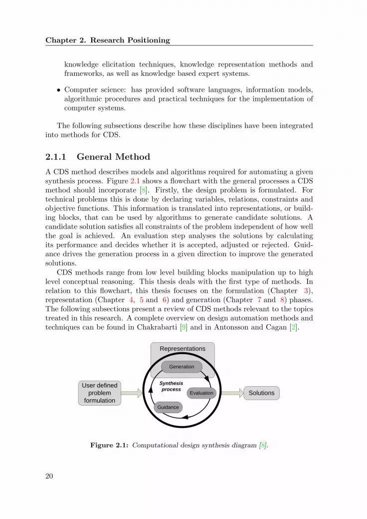
A CDS method describes models and algorithms required for automating a givensynthesis process. Figure 2.1 shows a flowchart with the general processes a CDSmethod should incorporate [8]. Firstly, the design problem is formulated. Fortechnical problems this is done by declaring variables, relations, constraints andobjective functions. This information is translated into representations, or build-ing blocks, that can be used by algorithms to generate candidate solutions. Acandidate solution satisfies all constraints of the problem independent of how wellthe goal is achieved. An evaluation step analyses the solutions by calculatingits performance and decides whether it is accepted, adjusted or rejected. Guid-ance drives the generation process in a given direction to improve the generatedsolutions.
CDS methods range from low level building blocks manipulation up to highlevel conceptual reasoning. This thesis deals with the first type of methods. Inrelation to this flowchart, this thesis focuses on the formulation (Chapter 3),representation (Chapter 4, 5 and 6) and generation (Chapter 7 and 8) phases.The following subsections present a review of CDS methods relevant to the topicstreated in this research. A complete overview on design automation methods andtechniques can be found in Chakrabarti [9] and in Antonsson and Cagan [2].
Representations
Evaluation
Guidance
Solutions
Generation
User defined
problem
formulation
Synthesis
process
Figure 2.1: Computational design synthesis diagram [8].
20

2.1 Field: Computational Design Synthesis
2.1.2 Grammars
Using grammars for CDS consists in translating knowledge about a design prob-lem (e.g. from experienced designers) into a set of transformation rules describinghow an initial incomplete design can be transformed into a complete one. Here,algorithms generate solutions by applying the rules to an initial design. Gram-mars are used both as representations (e.g. [54, 51]) and as generation systems(e.g. [35, 64, 68, 71]. As generative systems, grammars have been typically usedin architecture (e.g. [17]) and in mechanical design (e.g. [68]).
A grammar is defined by a 4-tuple G = (V,X,R, S) , where V is the set ofobjects that are manipulated by the grammar, X is a set of terminal and non-terminal symbols, S is the initial symbol and R is a set of rules of the formoutlined above. The language of the grammar G is the set of all results producedfrom the start symbol that consists of only terminal symbols.
Figure 2.2 shows a set of exemplary transformation rules referring to shapegrammars for a planar truss design [63]. Accordingly, the first rule of the illustra-tion states that a given triangular truss can be divided into two triangles, whereasthe second rule states the inverse transformation. Rule 3 applies on a slightly dif-ferent structure as rule 1 (a triangle with a fixed point) and consequently proposesan appropriate transformation, while rule 4 also allows this transformation in areverse fashion. A structure composed of multiple triangular truss features cansuccessively be transformed by applying these rules.
There are three possible tasks for programs that implement grammars [20].The most common task, and perhaps the first that comes to mind, is to aid inthe generation of designs at the hand of a known grammar. Here, grammar rulesare combined using special algorithms to generate a new design. A second typeof program is a parsing program. A parsing program is given a grammar anda design, and the program determines if the design is in the language generatedby the grammar and, if so, gives the sequence of rules that produces the shape.A third type of program is an inference program. The grammatical inferenceproblem is: given a set of designs, construct a grammar that generates the designsolutions.
This thesis researches the applicability of grammar approaches as function ofthe type of requirements and available resources in a design problem. A generativeapproach based on grammars in presented in Chapter 7.
Rule 2Rule 1 Rule 3 Rule 4
2f ff f f f
f
3
1
f
3
21 4
f
3
142
f
3
2 1
Figure 2.2: Grammar of truss design.
21

Chapter 2. Research Positioning
2.1.3 Agent Based Design
Agent based design is inspired in how multiple members of a design team con-tribute to generate design solutions. Here, individual designers (agents) work in-dividually in their specific problems coordinated by a manager that keeps controlof the overall design process. In agent based design, components are synthesizedbased on the physical interactions between them [76].
Agents are meta-heuristics which have been used to solve a wide variety ofoptimization and constraint satisfaction problems [47]. It is based in encapsulatingsoftware modules into agents which can then be organized into teams. The agentscollaborate with each other by communicating results via shared memories. A-Teams can handle multiple objectives and constraints naturally, and do not requirea set of weighting functions a-priori, allowing the user to select from a set of paretoequivalent solutions at the end of the solution process.
A-design, proposed by M. Campbell et al. in [7], is a CDS method in whichagents modify design candidates and are themselves modified in order to createbetter results. The basic subsystems of the A-Design theory are (1) an agentarchitecture that is responsible for creating and improving design alternatives,(2) a representation of the conceptual design problem that is comprehended bythe agents in order to create design concepts, (3) a scheme for multi-objectivedecision making that retains solutions exhibiting different patterns of strengthsand weaknesses in order to accommodate change in user preferences, and (4) anevaluation-based iterative algorithm for improving basic design concepts towardssuccessful solutions.
M. Campbell et al. present in [6] the application of this theory to the configu-ration problem of electro-mechanical devices. As shown in Figure 2.3, it uses fourtypes of computational agents. C-agents construct conceptual candidate solu-tions using a library of component types. I-agents generate conceptual solutionswith values obtained from a catalog of components. Each I-agent has a differentpreference, e.g. low costs of high performance. M-agents receive good designsand produce feedback to control the other agents in the system. F-agents alsoreceive good designs, but their function is to modify solutions with expectationof improving them.
The solutions generated by I-agents are classified into three groups: poordesigns, good designs and pareto designs. Poor designs are discarded by an eval-uation algorithm. Good designs are modified by M- and F-agents. Pareto designsare added to a “hit list” and simultaneously used by modification agents in thesearch of better designs. Each iteration step yields a new “best” design. Afterthe iterations ends, the “best of the best” is presented to the user as the solution.
From the perspective of A-Design, this thesis sets the focus on the developmentof a manager agent. The goal is to have one generic manager agent which candetermine synthesis strategies for routine design in general.
22

2.1 Field: Computational Design Synthesis
F-Agents
C-Agents
I-AgentsManager-
Agent
Calculate
objectives
Sort
Feedback
Fragmented
designs
Design
configuration
Completed
designPareto and
good designs
Poor designs
discardedFinal designs
Generate
Evaluate
Guide
Problem description
and representation
User
Figure 2.3: CDS and agents in A-Design [7].
2.1.4 Evolutionary Approaches
Evolutionary approaches are based on the principles of biological evolution, andencompass a broad range of search techniques, among which the most prevalentare genetic algorithms (e.g. [32]), evolutionary programming (e.g. [18]) and evo-lution strategies (e.g. [88]).
The search algorithms of evolutionary approaches are based on genetic adap-tive operators, namely, mutation and recombination. The selection is based onDarwinian selection, or selection of the fittest. A characteristic of these methodsis that they employ sets of solutions (populations) represented by vectors. Anyparticular solution is written as a string of objects called chromosomes, and eachcomponent is regarded as a gene. All three methods consist of maintaining apopulation of competing candidate solutions. The first population of solutionsis randomly generated. Then, new populations are created by bringing randomalteration to the solutions in the previous population. The performance of a solu-tion determines how fit it is. A selection mechanism determines which solutionsto combine for generating new solutions, and which ones to exclude.
The main differences between these techniques are their representation andselection methods, which are:
• Genetic algorithms: The representation is done in the form of string ofnumbers, which are often binary. The selection is done by calculating afitness based on an analysis.
• Genetic programming: uses lisp-like trees as representation of the solutions,resulting in computer program like solutions. The fitness is determined bythe ability of the generated program to solve a computational problem.
23

Chapter 2. Research Positioning
• Evolutionary programming: the structure of the program is fixed, being theparameters the ones allowed to change. Evolutionary programming usesvectors of real numbers for the representation of solutions. The selectionhas the characteristic that the results of mutations are considered in futuregenerations only if their fitness is higher than in other found solutions.
Evolutionary approaches incorporate the processes of Synthesis, Analysis,Evaluation and Adjustment required in CDS as it is shown in Figure 2.4. Thischaracteristic makes the implementations of such approaches relatively straight-forward for CDS.
2 3
1
requirements
Synthesis
(Population Initialization)
Analysis
(Fitness Calculation)
Evaluation
(Selection Operation)
Adjustment
(Mutation Operation,
Crossover Operation)
Embodiment
(Initial Population)
Solution
Performances
(Fitness of each solution)
Embodiment
(New population)
Figure 2.4: Genetic algorithm and the computational synthesis method.
2.1.5 PaRC
PaRC (acronym for Parameters, Resolved rules and Constrain rules) is a knowl-edge engineering methodology for design automation [57]. PaRC prescribes theautomation of parametric routine design problem by proposing a framework forrepresenting knowledge and methods for automating the design problem. Themajor characteristic of PaRC in relation to other CDS methodologies, is that itcovers the path from a knowledge source (e.g. an expert with a design problem)up to the development of software tools (see Figure 2.5)
PaRC distinguishes two types of design knowledge: (1) knowledge that defineswhat the design problem is, and (2) knowledge that defines how the design prob-lem can be solved. Design problem knowledge is represented by parameters andtopological elements. Knowledge for solving the problem is represented by resolverules (R-rules) and constraint rules (C-rules). A generation algorithm, generic todesign problem formulated with the PaRC representation, enables the synthesis
24

2.2 The Problem: Complexity Management
Knowledge
source
Design
automation
software
deco
mpo
sitio
n
know
ledg
e
acqu
isition
mod
eling
auto
mat
ion
gene
ric sof
twar
e
deve
lopm
ent
user
inte
raction
Figure 2.5: PaRC: Knowledge engineering method, from [57].
activity. PaRC prescribes two methods for translating a parametric routine de-sign problem into software for automatic design generation. On the one hand,a knowledge elicitation method targets the acquisition of problem and problemsolving knowledge. On the other hand, a method for developing the software toolis presented. Software development is supported by a generic software frameworkthat facilitates the codifications of new design automation tools.
In relation to PaRC, the long term goal of this research is to automate thedevelopment of CDS methods at the hand of the structure of the problem. Theresults of PaRC have served in envisioning the development process of computa-tional synthesis systems. Furthermore, this thesis builds up the model of infor-mation classification presented in PaRC.
2.2 The Problem: Complexity Management
Complexity in design has been studied from two different perspectives: the physi-cal domain and the functional domain [73]. In the physical domain -which includesmost engineers, physicists and mathematicians- complexity is seen as an inherentcharacteristic of physical things, including algorithms, products, processes, andmanufacturing systems. This kind of thinking leads to the idea that systems withmany parts are inherently more complex than those with less. In the functionaldomain, complexity is seen as a relative concept that evaluates how well we cansatisfy “what we want to achieve” with “what is achievable”. This view is usedin this thesis to develop a model of complexity for routine design problems.
This section aims at presenting a short overview of studies on design complex-ity that are the most relevant to this work. From the functional perspective, thetheories of axiomatic design, incompleteness of information and multi-disciplinarycomplexity are described. From the physical perspective, complexity in largeparametric spaces is described.
Complexity in design can be attributed to the different stages of the designprocess. In this sense, there is complexity of synthesis, complexity of analysis,complexity of evaluations, complexity of the design solutions, complexity of man-aging the design process. Here, I will only present complexity of the synthesisprocess.
25

Chapter 2. Research Positioning
2.2.1 Complexity in Axiomatic Design
ADT is based on the hypothesis that there are fundamental principles that governgood designs [72]. Its two founding axioms are:
1. Maintain the independence of the Functional Requirements (FRs)
2. Minimize the information of the Design Parameters (DPs).
FRs are the set of requirements that characterize the needs of the artifact inthe functional domain, while DPs are the variables that characterize the design inthe physical domain. The relation between the FRs and the DPs is representedin equation form as:
FR = [A]DP (2.1)
where A is the Design Matrix (DM) of the problem. Depending on the DM, adesign can be coupled, decoupled or uncoupled. Consider for example a problemwith two FRs and two DPs. When the design is coupled, the FRs cannot besatisfied independently because of the interdependence with both DPs, as shownin Equation 2.2. In a decoupled design, shown in Equation 2.3, the DPs haveto be solved in a particular order so that FRs are achieved. In uncoupled designs(Equation 2.4), the FRs are independent from each others, and no particularorder is required for solving the DPS.
Coupled :{FR1FR2
}=[x xx x
]{DP1DP2
}(2.2)
Decoupled :{FR1FR2
}=[x 0x x
]{DP1DP2
}(2.3)
Uncoupled
{FR1FR2
}=[x 00 x
]{DP1DP2
}(2.4)
In ADT, complexity is defined as “the measure of uncertainty in achieving thefunctional requirements of a system within their specified design range”. Whenthe range of a system changes as function of time, it is regarded as a systemwith time-dependent complexity. When the range does not change as function oftime, it has a time-independent complexity. “Time” is used in a general sense,signifying progression of “events”.
Time-independent complexity is classified into time-independent real complex-ity and time-independent imaginary complexity. The former is a consequence ofthe system range not being inside the design range. The latter occurs when thereare many FRs and the design is a decoupled design. It is called imaginary becausethis corresponds to a situation in which the different orders in solving the designmatrix have different attributed levels of difficulty. A system with imaginarycomplexity can satisfy the FRs at all times if we vary DPs in the right order.
26

2.2 The Problem: Complexity Management
Time-dependent complexity is the uncertainty caused by the increase or de-crease of the number and types of DPs during the design process itself. ADTclassifies time-dependent complexity into combinatorial and periodic complexity.Design problems with combinatorial complexity experience a continued growth oftheir DPs in time. For example, constructing a sentence by the combination ofwords has combinatorial complexity. As the number of words (the DPs in thiscase) increases, keeping semantic and syntactic consistency among them becomesmore difficult. On the other hand, periodic complexity is the case in which the in-crease of parameters is restarted after a period of time (or succession of actions).An example described in [74] is air traffic control. Air traffic in large airportsfollows wave pattern that depends on the time of the day. When the traffic is atits peak, air controllers deal with very complex situations. However, at low traffictimes their task becomes significantly more simple.
ADT suggests three main strategies for managing design complexity:
• Minimize the number of FRs
• Eliminate time-independent real complexity and time-independent imagi-nary complexity,
• Transform a system with time-dependent combinatorial complexity into asystem with time dependent periodic complexity
This thesis adopts this model of design complexity, and explores its char-acteristics for routine design problems. The developed complexity managementmethods are based on the three previously suggested strategies.
2.2.2 Completeness of Information
As presented by Ueda [80], complexity of emergent systems can be categorizedin three classes with respect to incompleteness of information about the artifactsenvironment and/or the specification of the problem. Figure 2.6 shows how thecomplexity of a design problem increases as function of the incompleteness ofinformation for different domain.
The three classes pointed out in [80] are:
• Class 1: Problems with complete descriptions. Are those where the envi-ronment information and the problem descriptions are given wholly. In thiscase it is often difficult to find the optimal solution.
• Class 2: Problems with incomplete environment descriptions. The difficultyin these problems is characterized by uncertainties in modeling the dynamicbehavior of the system.
• Class 3: Problem with incomplete specifications. Environment and problemspecifications are both incomplete. Difficulty resides in the ambiguity of theproblem, having human interaction as the most significant aspects.
27

Chapter 2. Research Positioning
Complexity of system
Problem domain
Uncertainty of information
Increasingly
difficult
Problem Class III: Incomplete specifications
Problem Class II: Incomplete environment descriptions
Problem Class I: complete descriptions
Design
Manufacturing
Utilization
Figure 2.6: Complexity as function of knowledge completeness, from [80].
In this research the focus is set on complexity class 2. For this type of problems,there are many candidate solutions, which lead to a combinatorial explosion ofthe space of solutions. Here, Ueda has pointed out the need to develop efficientand robust methods to find optimal solutions. Typical problem solvers here areevolutionary algorithms, genetic programming methods, and genetic algorithm,among others. The preference on choosing one technique or another dependson the characteristics of the problem, e.g., purely parametric, topologies, layouting, etc [27]. For complex routine design, where the problems usually presenta mixed combination of characteristics, collaborative usage of different techniquesis preferred. The difficulty here lies in the proper management of techniques andsolutions though the generation process.
2.2.3 Complexity of Multi-disciplinarity
Tomiyama [77, 78] researched design complexity resulting from the involvementof multiple disciplines. He examined the structure of knowledge represented byrelationships among theories. Consider the design of an electromechanical en-gine, where the mechanism dynamics and electromagnetism are integrated by themulti-disciplinary character of the artifact. In this case, two independent theo-ries become relevant to the instantiation of a variable -e.g. length, width, depth-common to both theories, as indicated in Figure 2.7. These type of complexityis regarded as Complexity by Design, being commonly found in multidisciplinarydesign problems (MDDP). Intrinsic complexity of multidisciplinary is also iden-tified as a second type of complexity arising from MDDP. Here, two theories getintegrated through one common concept as an interface between them, as shownin Figure 2.7.
28

2.2 The Problem: Complexity Management
Intrinsic complexity of multidisciplinaryComplexity by Design
Figure 2.7: Complexity from the viewpoint of knowledge structure [78].
2.2.4 Large Parametric Spaces
An important source of complexity in design is attributed to large amountsof inter-constrained parameters. To cope with these types of complexity, de-sign problems are usually partitioned into smaller and easier to solve sub prob-lems, which are latter solved towards optimal solutions in a coordinated fashion.One category of decomposition methods is Multidisciplinary Design Optimization(MDO) [53]. Here, systems are partitioned along discipline boundaries, which areoften dictated by the design organization structure or available analysis tools.The focus lies in dividing the optimization into the sub-optimizations within eachmodule and a coordinating optimization at the system level place.
MDO methods can be subdivided into single-level and multilevel. The formercentralizes all design decision in one optimizer, while the latter distribute decisionmaking throughout the system by providing design groups with some autonomyand ability to utilize existing design tools. Notable multilevel MDO techniques areCollaborative Optimization (CO) [1] and Bi-Level Integrated System Synthesis(BLISS) [66]. Another category of decomposition methods is Analytic TargetCascading (ATC) [1]. Here, the problem is partitioned in a hierarchical formaround the components composing it. The method consists in specifying top leveltargets (performances to achieve) and cascading the targets to the lower levelcomponents design.
In order to use these methods, it is necessary to already have a first bestguess initial design, which is refined to produce optimal designs. However, thesetypes of methods is applicable for redesign proposes rather than for CDS of newsolutions. Therefore, this type of complexity is not regarded in this study. As itwill be discussed in Chapter 4, this type of complexity is rather attributed to thesolution space than to the problem space.
29

Chapter 2. Research Positioning
2.3 Case Study: CSIM Design
Injection molding is an important manufacturing technique for producing plasticparts. This technique consists of injecting a hot polymer into the impression of amold. Figure 2.8 shows an exploited view of a mold. A mold is composed of twobasic parts, namely, a core and a cavity. Here, the plastic is cooled down to a solidstate by a series of cooling channels drilled into the mold. The cooling stage is ofgreat importance in the injection molding process, as it affects the productivityand the quality of the final part.
Mold cavity
Mold core
Product
Figure 2.8: Injection mold example.
2.3.1 Cooling Design
Cooling systems for injection molding are defined as the set of components thatenable heat transfer between a hot melt contained in a mold and a coolant sub-stance flowing within it. Cooling systems allow reducing the time required forsolidifying the plastic melt, which is translated in manufacturing cost reduction.In addition, cooling systems should be capable of delivering uniform tempera-tures on the plastic part so that unwanted effects, such as differential shrinkageand warpage, can be minimized. A cooling system for injection molding is com-posed of a temperature-controlling unit, a pump, coolant supply manifold, hoses,cooling channels, and collection manifold. For the present case study, the cooling
30
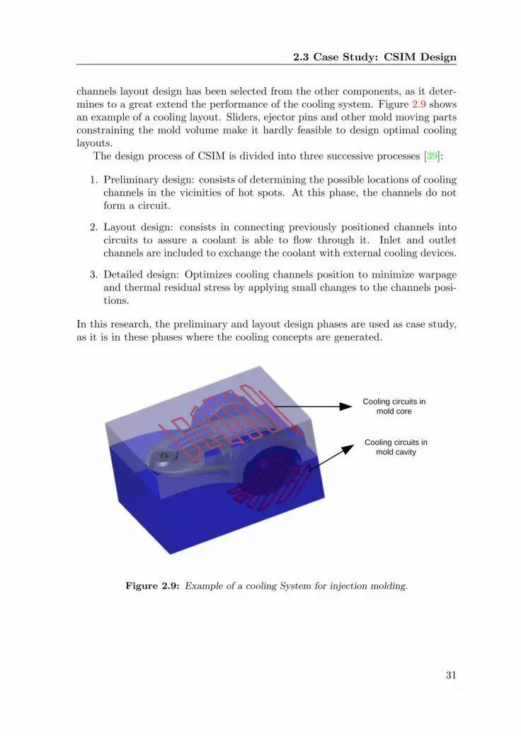
2.3 Case Study: CSIM Design
channels layout design has been selected from the other components, as it deter-mines to a great extend the performance of the cooling system. Figure 2.9 showsan example of a cooling layout. Sliders, ejector pins and other mold moving partsconstraining the mold volume make it hardly feasible to design optimal coolinglayouts.
The design process of CSIM is divided into three successive processes [39]:
1. Preliminary design: consists of determining the possible locations of coolingchannels in the vicinities of hot spots. At this phase, the channels do notform a circuit.
2. Layout design: consists in connecting previously positioned channels intocircuits to assure a coolant is able to flow through it. Inlet and outletchannels are included to exchange the coolant with external cooling devices.
3. Detailed design: Optimizes cooling channels position to minimize warpageand thermal residual stress by applying small changes to the channels posi-tions.
In this research, the preliminary and layout design phases are used as case study,as it is in these phases where the cooling concepts are generated.
Cooling circuits in
mold core
Cooling circuits in
mold cavity
Figure 2.9: Example of a cooling System for injection molding.
31
Chapter 2. Research Positioning
2.3.2 Related Work
At present, most academic research in injection molding cooling design has focusedon developing detailed analysis and optimization strategies. The former simulatethe cooling phase of the injection molding process and has resulted in ComputerAided Engineering (CAE) systems as MoldFlow [67] and Moldex3D [40]. Thelatter uses heat transfer analysis to minimize cooling time and temperature dis-tributions of the plastic part. However, a human designer has to create the initialdesign from where CAE and optimization methods can be applied. In fact, opti-mizing cooling channels placement and diameter results in local optimum, giventhat the initial design limits the possibility of finding global optima. Therefore,in order to achieve complete automation, the problem of generating the initialdesign must be solved.
Although automating design problems has been extensively investigated overthe past 30 years [37], not much literature addresses the problem of injectionmolding cooling design. The most relevant to this thesis is the research devel-oped by Li et al. [37, 39, 38], which has resulted in a method for automatingthe design of cooling circuits for injection molding. In short, the method con-sists of decomposing the part geometry into several predefined shapes. Then,three techniques are collaboratively used for candidate solution generation: (1)case-based design, (2) graph-based search and (3) heuristic search. Case-baseddesign maps the shape features to predefined solutions, obtaining a preliminarydesign that is captured in a graph model. A graph based transversal algorithm isemployed to search for candidate cooling circuits. Heuristic search develops thecandidate solutions into layout designs that contemplate tentative manufacturingplans. Although this approach has demonstrated to be capable of automating thegeneration of cooling solutions, it suffers from the drawback that the design hasa strong dependency on the accuracy of the shape recognition algorithm as wellas on the quality of the sub-solution predefined for each shape feature. Further-more, complex algorithms are required to solve geometric constraints and keepthe physical consistency of the cooling solutions (e.g. make sure cooling channelsare connected to form a circuit).
32

Part II
Founding Frameworks
33


Chapter 3Information and Models
This chapter explores the entities and types of information in artifactualdesign required to formulate routine problems. As the focus is computationalsynthesis, mathematical models and relations used in design automationare presented. The chapter finishes by presenting a classification of designproblems as function of the types of information.
3.1 Introduction
Design artifacts are described by three different types of entities: (a) vocabularyof elements, (b) descriptions of elements and (c) the configuration of elements.Consider the case of the gear device shown in Figure 3.1. Here, the vocabulary ofelements is two gears and two shafts. Descriptions determine the attributes of theartifact, like the diameter (D) and angular velocity (w). Configurations determinethe disposition of the elements in the structure, as for example the connectednessbetween elements represented by the relations in the figure. Configurations canbe classified into topologic relations and physical coherence constraints. Whilethe former define the topology of the elements in the structure, the latter is usedto assure no physical impossibilities are committed by the artifact being designed.For example, two gears cannot share the same place in space.
The following sections describe types of information in routine design problemsand a scheme for their formulation. This scheme is used in Chapter 4 to identifydifferent types of complexity.
3.2 Types of Information
As proposed by Schotborgh et al [59], the information flow of an analysis andsynthesis process can be classified in three groups: embodiment, scenario andperformance, as shown in Figure 3.2. According to this model, analysis allows the
35

Chapter 3. Information and Models
Relations
Element
Description
Scenario
Mass
Shape
Velocity
Force
Cost
Position
Force
Cost
Mass
Force
Cost
MassEqual velocities
Diameter = i x Diameter
Velocity = i x Velocity
DiameterMass
shape
Velocity
Force
CostPosition
Diameter
Equal Velocities
Velocity
Velocity
Input Shaft
Output Shaft
Input Gear
Output Gear
Color
Mass
etc
Shape
Position
Color
Speed
Mass
etc
ShapePosition
Objective
Function
Connectedness
Force
Force
Speed
Color
Mass
Force
Speed
Position
Shape
Law of Physics
Aesthetics
Cost
Cost
Embodiment
Figure 3.1: Types of information in routine design.
36

3.2 Types of Information
quantification of the performances of an embodiment undergoing a given scenario(Figure 3.2(a)), while synthesis consists of specifying an embodiment undergoinga given scenario such that performances are satisfied (Figure 3.2(b)). Thus, twoopposing processes handling the same types of information.
AnalysisScenario
Embodiment
Performance
(a) Information flow in analysis process,from [59].
SynthesisScenario
Embodiment
Performance
(b) Information flow in synthesis process in-formation
Figure 3.2: Information flow in analysis and synthesis processes
Embodiment
Embodiment is here defined as the subset of descriptions of an artifact upon whichinstances are created to generate design solutions. In Figure 3.1 this is shown forthe case of the gear device, where the embodiment is composed of two elements(one input gear and one output gear), and its descriptions (diameter and velocity).
Scenario
An artifact’s ability to accomplish its function is affected by its interaction withits environment. The subset of environment variables, attributed to elementsin the natural world and considered in measuring a design artifact’s ability toaccomplish its function, is here defined as scenario. Scenarios are also specifiedby descriptions. For the case of the gear device in Figure 3.2, a possible scenariois one shaft attached to the input gear and one connected to the output gear.
Performance and Goals
Given that design functions are expressed in abstract terms, it is necessary to usemeasurable descriptions to express and asses its goals. Goals are commonly rep-resented by objective functions, where performance indicators are weighted andadded to compute the overall performance of the design. Performances are calcu-lated by analysis relations using instantiated embodiments and scenarios. Analy-sis relations use known principles -as for example laws of physics and economics-
37
Chapter 3. Information and Models
to model the interaction of the design artifact with its environment and predictits behavior.
Goals can be expressed by defining requirements on the objective functions andperformance parameters and assessed by calculating -using analysis relations- theperformances and objective function of an instantiated artifact. Two types of goalsare often found in design problems: constraint satisfaction and optimization. Inconstraint satisfaction, the objective is finding instances of design artifacts withinthe allowed topology relations and confinement constraints. Here, performancesare used as means of assessing the behavior of the design. For optimization,maximizing or minimizing performances is added to the constraint satisfactionproblem. Performances are used to express the desired quality of the designartifact.
Analysis in design is often done analytically, by simulation, or by a combi-nation of both. They can vary from algebraic equations to complex differentialequations. Finite element methods, computational fluid dynamics, circuit simula-tion, and other computational analysis tools offer accurate and robust analyses [4].For the case of the gear device in Figure 3.1, a performance indicator could be therotational speed of the output shaft. The objective function could be expressedby this performance, reducing the goal to that of the output rotational speed.The goal can then be expressed by a required rotational speed, while it can beassessed by an analysis technique for an instantiated design.
Design Rules
Design rules determine values of embodiment descriptions as function of scenarioand performances descriptions. These rules are the result of experience, andconstrain the ranges of permitted values parameters. Design rules aid the gen-eration, evaluation and guidance processes by providing shortcuts to values thathave proven to be successful.
3.3 Problem Formulation
Deriving methods and schemes for formulating design problems has been an im-portant subject of research in the field of Problem Solving Theory (PST) [65,22, 21] as well as in the field of CDS [57, 5]. From the perspective of PST, Si-mon [65] has defined problem structuring as the process of drawing upon ourknowledge to compensate for missing information, and using this knowledge toconstruct the problem space. Here, design problems whose problem space arecompletely defined are regarded as well-defined, while those which are not areregarded as ill-defined. Well-defined problems can be solved using generally ap-plicable problem-solving mechanisms, whereas ill-defined problems require otherapproaches [21]. As routine design problems proceed within a known space offunctions, expected behaviors and structure variables and the problem is one of
38

3.3 Problem Formulation
instantiating structure variables [19], it is regarded as well-defined. Accordingto PST [22], well-defined problems are formulated as function of a known initialstate, a clear goal state, a constrained set of logical states and constraint pa-rameters. Using this formulation structure, the following scheme is proposed forformulating routine design problems:
• Embodiment and scenario to describe the initial state of the design.
• Objective function, performance indicators and analysis relationsto express and assess the goal of the design artifact.
• Topological relations and physical coherence constraints indicate theset of logical states that have to hold for the design artifact to exist.
• Confinement constraints indicating the values embodiment, scenario andperformance descriptions are allowed to get.
This scheme is used by the knowledge elicitation method presented by Olthofet al. [50]. The method allows identifying and formalizing routine design problemsat industrial settings.
3.3.1 Example: CSIM Design
Figure 3.3 graphically represents the problem formulation of CSIM design byrepresenting elements by nodes and relations by arcs. Labels specify the modelsof the elements and relations. For explanatory reasons, not all descriptions andrelations have been included.
In the figure, Channel is regarded as embodiment element, while Mold Partand Plastic Part are regarded as scenario elements. The goal of the design, ex-pressed by the objective function, is to minimize the cooling time and to minimizethe temperature differences in the plastic part. Cooling time and temperature dis-tribution are therefore regarded as performances. Analysis is represented by theequation of Laplace, and allows the calculation of the performances (temperaturedistributions and cooling time). Detailed information on the analysis methods canbe found in [62]. Topology relations specify that Channel elements are connectedto each other inside the mold and are not allowed to share its space with thePlastic Part element. Physical coherence constraints are used to define: (a) theminimum distance between Channel and Plastic Part (PCC-1), (b) the minimumdistance between Channel (PCC-2), (c) the diameter values of the Channel (PCC-3) and (d) the allowed distance between Channels and the Mold Parts (PCC-4).In [44], knowledge from expert designers has been used to formulate these threequantities as a function of the plastic part thickness. Furthermore, other physicalcoherence constraints, such as non-drillable surfaces and inlet/outlet surfaces, arealso described. As the model is used for explanatory reasons, the latter have beenkept out of the formulation.
39

Chapter 3. Information and Models
Channel
Mold Part(Core, Cavity)
Plastic Part
Geometry,
Material Type,
Temperature
Geometry,
Material Type,
Temperature
Diameter,Position,
length,
Minimal & Maximal
Distance to product
(PCC-1)
Scenario Embodiment
Equation: Laplace
thermal equilibriumPerformances:
Cooling Time
Temp. DistributionDisconnected
Distance between channel (PCC-2)
Diameter (PCC-3)
Maximize (heat transfer),
Minimize (temperature distribution)
Objective function
Analysis
Relation
Physical
Coherence Topologic
Relation
Distance to mold part
(PCC-4)
Connected
Inside of
Figure 3.3: Problem formulation of CSIM design.
3.4 Models in Artifactual Routine Design
This section presents models to represent descriptions and relations used in thecomputational synthesis of artifactual routine design. The aim is to classify theinformation contents by using common data models, which can be regarded asbasic building blocks for formulating artifactual routine design problems. Doingso facilitates the development of abstract formulations from where to differentiatefamilies of design problems, and later develop algorithms to automate them.
3.4.1 Models of Descriptions
Design descriptions have been classified in five model categories: parametric,fields, space, shapes and topologies. Each category represents a different problemdomain, as different problem solving approaches are used to generate solutions. Inthis sense, design problems comprehending several dimension have higher degreesof complexity and require a combination of methods for its automation. The workpresented in this thesis mainly focuses on the domains Parametric and Topology.
Parametric
Parameters model properties valid for the entire element. They are used to rep-resent attributes as material properties, color, weight, density, etc. These can beof different nature, as for example numeric, symbolic, logic, predicate, and com-binations among them. For numeric parameters, confinement constraints define acontinuous or discrete space of possible values. For symbolic, predicate and logic
40

3.4 Models in Artifactual Routine Design
ones, all possible values have to be specified. That is for every Ai =(A1...An)exists an Ai such that:
Ai ∈ (N,Z,Q,R,C) (3.1)Ai = {true, false} (3.2)
Ai = Symbol (3.3)
Spaces
Describe positional attributes of elements in a topology. Positional descriptionsdepend on the chosen coordinate system -Cartesian, Cylindrical of Spherical- andthe dimensions of interest -1D, 2D, or 3D. These can be considered as numericparameters related by a model that is determined by the chosen coordinate system.Values can either be continuous or discrete.
Fields
Use parameters and geometric vectors to describe properties that are valid inspecific regions of the elements. Fields are specified together with an incidentzone, shown in the Figure 3.4 as cubic. Incident zone is the spatial place wherethe field influences an element. An incident zone can be a volume, an area, a lineor a point. Meshed CAD models are used in Computer Aided Engineering (CAE)software to specify incident zones. Vectors and parameters can then be attributedto each mesh-element. In Figure 3.4 an example illustrates how a parameters andvectors are related with their incident zones
Figure 3.4: Example of a field attribute.
41

Chapter 3. Information and Models
Shapes
Describe the form of the elements -or groups of elements- present in the designstructure. Commonly used models are based on geometric relations and graphs.Geometry models the form by means of mathematic equations. Models are definedwith parameters related by geometric functions, the latest being usually algebraicor differential. When the geometric function is known, parameters are instantiatedto produce new shapes. When not known, the problem becomes one of findingthe correct geometric relations. Polynomials are often used for this purpose,having the polynomial degree and its coefficients as unknowns. Depending on thecase, confinement constraints are set either to parameters or geometric functions.Furthermore, perimeters, areas and volumes can also be subject of restriction.
Super quadrics [26] have been broadly used for this purpose. Super quadricsare polynomials whose degrees and coefficients values vary depending on the shapebeing modeled. In Figure 3.5 a toroid super quadric shape is shown together withits polynomial equation. By changing the values of the polynomial coefficient, theshape of the toroid can be changed.
Figure 3.5: Super quadric of a toroid, from [26].
Attributed Graphs model shapes using nodes (representing shape primitives)and arcs (representing the connection within primitives). Primitives might befurther decomposed into sub graphs, obtaining shape models with several levelsof abstraction. When the shape graph is specified, design generation consist ininstantiating attributes related to the graph’s nodes and arcs. When the graphis not specified, but its primitives and relations are, shapes are generated byconstructing new graphs. Confinement constraints can be set to both, the numberand the types of primitives and relations. In Figure 3.6, a handmade symbol ofan electrical resistor shape is modeled using such an attributed graph. Arcs of thegraph represent segments, while the nodes are used to represent vertices. Labelsare used to further specify the arcs.
Topologies
For design problems whose elements can be instantiated several times, its cardi-nality can be defined as a topology description. It reflects the number of instances
42

3.4 Models in Artifactual Routine Design
(a) Handmade resistor symbol. (b) Graph representation of resistorsymbol.
Figure 3.6: Example shape graph of electric resistor symbol.
of one element in the artifact. This variable allows controlling the instantiationof elements when the problem is one of generating topologic structures. The con-cept of cardinality also applies to topology relations. In this case, the number ofallowable relations is determined by its cardinality.
3.4.2 Models of Relations
Different types of models are used in design to describe relations. Their character-istics determine the approaches required to handle them, and are here restrictedto three basic types: algebraic, differential and logic models. However, this set isnot restrictive as others can also be considered.
Physical Coherence and Objective Functions
Are commonly modeled with algebraic relations. In some cases, when the descrip-tions are symbolic rather than numeric, logic models can be assembled. First orderlogic and propositional logic models are the most common types of logic modelsin design.
Analysis
These relations are often modeled by a combination of all three types. Analyticmethods are usually a combination of algebraic and logic models, while simulationsmake use of numeric methods to solve differential equations.
Topology
Topology is often modeled with set theory. One framework for doing so is RegionConnection Calculus (RCC) [13], which in a qualitative fashion describes therelation among euclidean or topological regions. It allows the formalization ofconcepts as convergence, connectedness and continuity.
43
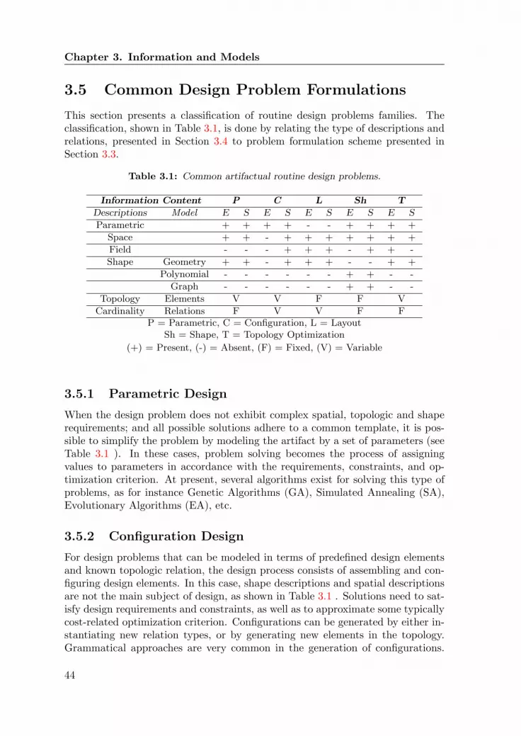
Chapter 3. Information and Models
3.5 Common Design Problem Formulations
This section presents a classification of routine design problems families. Theclassification, shown in Table 3.1, is done by relating the type of descriptions andrelations, presented in Section 3.4 to problem formulation scheme presented inSection 3.3.
Table 3.1: Common artifactual routine design problems.
Information Content P C L Sh T
Descriptions Model E S E S E S E S E S
Parametric + + + + - - + + + +
Space + + - + + + + + + +
Field - - - + + + - + + -
Shape Geometry + + - + + + - - + +
Polynomial - - - - - - + + - -
Graph - - - - - - + + - -
Topology Elements V V F F V
Cardinality Relations F V V F FP = Parametric, C = Configuration, L = Layout
Sh = Shape, T = Topology Optimization
(+) = Present, (-) = Absent, (F) = Fixed, (V) = Variable
3.5.1 Parametric Design
When the design problem does not exhibit complex spatial, topologic and shaperequirements; and all possible solutions adhere to a common template, it is pos-sible to simplify the problem by modeling the artifact by a set of parameters (seeTable 3.1 ). In these cases, problem solving becomes the process of assigningvalues to parameters in accordance with the requirements, constraints, and op-timization criterion. At present, several algorithms exist for solving this type ofproblems, as for instance Genetic Algorithms (GA), Simulated Annealing (SA),Evolutionary Algorithms (EA), etc.
3.5.2 Configuration Design
For design problems that can be modeled in terms of predefined design elementsand known topologic relation, the design process consists of assembling and con-figuring design elements. In this case, shape descriptions and spatial descriptionsare not the main subject of design, as shown in Table 3.1 . Solutions need to sat-isfy design requirements and constraints, as well as to approximate some typicallycost-related optimization criterion. Configurations can be generated by either in-stantiating new relation types, or by generating new elements in the topology.Grammatical approaches are very common in the generation of configurations.
44
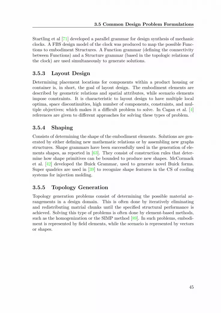
3.5 Common Design Problem Formulations
Startling et al [71] developed a parallel grammar for design synthesis of mechanicclocks. A FBS design model of the clock was produced to map the possible Func-tions to embodiment Structures. A Function grammar (defining the connectivitybetween Functions) and a Structure grammar (based in the topologic relations ofthe clock) are used simultaneously to generate solutions.
3.5.3 Layout Design
Determining placement locations for components within a product housing orcontainer is, in short, the goal of layout design. The embodiment elements aredescribed by geometric relations and spatial attributes, while scenario elementsimpose constraints. It is characteristic to layout design to have multiple localoptima, space discontinuities, high number of components, constraints, and mul-tiple objectives; which makes it a difficult problem to solve. In Cagan et al. [4]references are given to different approaches for solving these types of problem.
3.5.4 Shaping
Consists of determining the shape of the embodiment elements. Solutions are gen-erated by either defining new mathematic relations or by assembling new graphsstructures. Shape grammars have been successfully used in the generation of ele-ments shapes, as reported in [63]. They consist of construction rules that deter-mine how shape primitives can be bounded to produce new shapes. McCormacket al. [42] developed the Buick Grammar, used to generate novel Buick forms.Super quadrics are used in [39] to recognize shape features in the CS of coolingsystems for injection molding.
3.5.5 Topology Generation
Topology generation problems consist of determining the possible material ar-rangements in a design domain. This is often done by iteratively eliminatingand redistributing matrial chunks until the specified structural performance isachieved. Solving this type of problems is often done by element-based methods,such as the homogenization or the SIMP method [89]. In such problems, embodi-ment is represented by field elements, while the scenario is represented by vectorsor shapes.
45


Chapter 4Design Structure andComplexity
This Chapter presents a framework to structure routine design problems anddevelops a model of its complexity. The results are positioned in relation tothe model of complexity of Axiomatic Design Theory.
4.1 Introduction
In design, structure and complexity are two closely related concepts. Complexityis a property related to the degree of difficulty or uncertainty for finding a solutionto a design problem. In order to analyze design complexity, it is necessary tounderstand the structure of the problem. The structure of a design problem hastwo important aspects to be studied:
• The distribution of design parameters along the problem model: all param-eters concentrated in one element vs. several parameters scattered thoroughseveral elements; one level of detail vs. several levels of detail.
• The relation between what is known (design requirements) and what is un-known: scattered along the problem model, concentrated in problem chunks,at the top (only functional requirements), at the bottom (only design pa-rameters) or as mix of all these possibilities.
From this perspective, design complexity depends on the structure of the prob-lem. This chapter describes different types of complexity that have been identifiedroutine design problem structures. This has been done by relating ADT’s com-plexity theory to the design formulation scheme presented in Chapter 3 and thestructuring framework presented in Section 4.2.1 of this chapter.
47
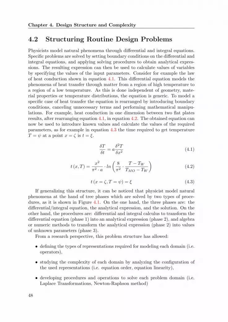
Chapter 4. Design Structure and Complexity
4.2 Structuring Routine Design Problems
Physicists model natural phenomena through differential and integral equations.Specific problems are solved by setting boundary conditions on the differential andintegral equations, and applying solving procedures to obtain analytical expres-sions. The resulting expression can then be used to calculate values of variablesby specifying the values of the input parameters. Consider for example the lawof heat conduction shown in equation 4.1. This differential equation models thephenomena of heat transfer through matter from a region of high temperature toa region of a low temperature. As this is done independent of geometry, mate-rial properties or temperature distributions, the equation is generic. To model aspecific case of heat transfer the equation is rearranged by introducing boundaryconditions, canceling unnecessary terms and performing mathematical manipu-lations. For example, heat conduction in one dimension between two flat platesresults, after rearranging equation 4.1, in equation 4.2. The obtained equation cannow be used to introduce known values and calculate the values of the requiredparameters, as for example in equation 4.3 the time required to get temperatureT = ψ at a point x = ζ is t = ξ.
δT
δt= a
δ2T
δx2(4.1)
t (x, T ) =x2
π2 · a· ln
(8π2· T − TW
TMO − TW
)(4.2)
t (x = ζ, T = ψ) = ξ (4.3)
If generalizing this structure, it can be noticed that physicist model naturalphenomena at the hand of tree phases which are solved by two types of proce-dures, as it is shown in Figure 4.1. On the one hand, the three phases are: thedifferential/integral equation, the analytical expression, and the solution. On theother hand, the procedures are: differential and integral calculus to transform thedifferential equation (phase 1) into an analytical expression (phase 2), and algebraor numeric methods to transform the analytical expression (phase 2) into valuesof unknown parameters (phase 3).
From a research perspective, this problem structure has allowed:
• defining the types of representations required for modeling each domain (i.e.operators),
• studying the complexity of each domain by analyzing the configuration ofthe used representations (i.e. equation order, equation linearity),
• developing procedures and operations to solve each problem domain (i.e.Laplace Transformations, Newton-Raphson method)
48

4.2 Structuring Routine Design Problems
y = -0.25 3
1 , 0 dy
x xdx
44
1 50 1
4 4
5 11 1
4 4 4
C C
xy x
x = 0 1 0 x y
Differential
equation
Analytical
Model
Analytical
Solution
Figure 4.1: Structure of problems in modeling natural phenomena.
• identifying common problem structures ( i.e. Poisson’s equation, Laplaceequation)
On the other hand, some of the major advantages from an application per-spective are:
• reusing existing problem formulation,
• utilization of standard solving methods,
• development of computer based simulation tools.
Structuring design problems as done in natural sciences is likely to drive theautomation of design problems toward more generic approaches, with advantagesin both research and application. For this research, such an structure would allowthe identification of features causing complexity, and do so independent from theproblem semantics. Furthermore, strategies for managing design complexity canbe formulated as function of problem structures.
4.2.1 Structuring Framework
By making an analogy between the information contents presented in Chapter 3and the structure described in the previous section, it is proposed to structureroutine design problems at three different abstraction: problem class, probleminstance and problem solution. This is shown in Figure 4.2. Problem classes aretransformed into problem instances by specifying its requirements. Requirementsare specified by instantiating descriptions. Problem instances are transformedinto problem solutions by algorithms that generate instances to the unknown de-scriptions. Therefore, one problem class can represent many problem instances,and one problem instance can have many problem solutions, as indicated in Fig-ure 4.3. Under this view, solving routine design is analogues to solving problemswith known differential equations.
49

Chapter 4. Design Structure and Complexity
This structure can also be used to structure innovative and creative designproblems. Solving innovative design is analogous to combining different differen-tial equations to model various interrelated physical phenomena. Solving creativedesign problems is analogous to developing new differential equations.
Problem
Class
Problem
Instance
Problem
Solution
Requirements
Placement
Requirements
Specification
Figure 4.2: Framework to structure design problem.
Problem Class
A problem class is structured in:
• Elements: are considered class descriptions, and are used to represent both,embodiment and scenario elements. As it will be described in Chapter 5,Element can also be differentiated by assessing the functions and types ofdescriptors modeling a component.
• Relations: are considered class descriptions and are of different types, namely,topology, physical coherence, design rules, analysis relations and objectivefunctions. Their descriptions can be declared within the scope of the relationor by pointing towards descriptions of embodiment and scenario elements.
• Descriptions: are variables that characterize elements and relations by math-ematic models.
Problem Instance
A problem instance is structured by:
• Instantiated scenario: represent scenario specifications,
• Partially instantiated embodiment elements or parameters: represent em-bodiment requirements, and impose constraints to the space of possiblesolutions.
• Instantiated performance parameters: represent the performance specifica-tions the embodiment has to meet.
50

4.2 Structuring Routine Design Problems
Problem Solution
Consist of fully instantiated elements, relations and parameters. For under-constrained problem-instances, many solutions may exist for one problem in-stance. This depends on how constrained the problem is. An underconstrainedwill allow for multiple solutions, while a systems of equation type of problem willhave a limited number of solutions.
PC
PI PI PI PI PI
PS
PS
PS
PS
PS
Problem solutionPS
Problem instancePI
Problem classPC
Figure 4.3: Problem structure dependencies.
The mayor consequence of utilizing this structure in the development of CASsystems, is that generation algorithms and software architectures have to be ca-pable of handling different types of problem instances and problem classes. Devel-oping methods for automating specific routine design problems have to be validfor a design problem class, rather than for specific problem instance.
4.2.2 Example: Spring Design
Consider for example the spring design formulation shown in Figure 4.4(a). Fig-ure 4.4(b) shows that the problem class corresponds to the declaration of thedifferent types of parameters of the problem formulation. By setting require-ments, the problem class is transformed into one problem instance. However, byrequirements to other parameters, another problem instance is obtained.
51

Chapter 4. Design Structure and Complexity
gObject
kLc
M
L0
Fspring
Fo
scenario
embodiment
performance
embodiment
scenario
scenario
performance
gravity constant
spring constantcompressed length
mass
free length
compression force spring
force object
Fg = m g
Parameters
Analysis relation
Fspring - Lc)(L0= k
spring
Fo
Fg
Fg scenarioforce ground
Fspring = Fg = Fobject
Topology relation
Spring EC Object Spring EC Ground
(a) Spring design problem formulation.
Object Spring Ground
M
k
Lc
L0
Fspring
FoFg
Lc
L0
Object Spring Ground
M = 5 Kgk
Lc
L0 = 8cm
Fspring
FoFg
Object Spring Ground
M = 5 KgK = 12.5 cm/Nm
Lc = 4cm
L0 = 8cm
Fo = 50 Nm Fg = 50 Nm
Problem Class
Problem Instance
Problem Solution
(b) structure of spring design example.
Figure 4.4: structure of spring design example.
52
4.3 Complexity in Routine Design
4.3 Complexity in Routine Design
Complexity of systems can be studied from different points of view. This thesisis based on the notions of design complexity stated in Axiomatic Design Theory(ADT) [74], explained in Chapter 2. The basic idea of this model is that withoutdifficulty in understanding (or making, operating, etc.), a system is not complex.In this sense, complexity is the property of a system that makes it difficult tounderstand with the available knowledge about its constituents parts. Tomiyamafurther elaborates this view, by stating that complexity can be studied from theview point of knowledge structure (see Section 2.2.3), identifying two types ofcomplexity: complexity by design and intrinsic complexity of multi-disciplinarity.The former is attributed to the structure of the design problem, while the latterdeals with behavioral characteristics.
This thesis adopts ADT definition of complexity, and focuses on complexity bydesign. The three main reasons why this model has been chosen as framework inthis research are: (1) complexity is regarded as a relative property, (2) complexityis the consequence of engineering activities, and (3) it is assumed that complexitycan be managed. ADT model of complexity is used to identify different types ofcomplexities in routine design.
4.3.1 Translating ADT Terms
In order to apply ADT theory of complexity to routine design, it is first requiredto relate the terms in both theories:
• Functional Requirements (FR’s): correspond to the functions, per-formances and scenario descriptions proposed as information contents inChapter 3. FR’s model either elements or parameters.
• Design Parameters (DP’s): correspond to the embodiment descriptionsin the routine design formulation, and model elements and parameters.
• Design Matrix (DM): is formed by the analysis, topology and physicalcoherence constraints.
In order to facilitate the analysis of complexity, ADT terms are interchangedwith the design formulation terms in in the following sections.
4.3.2 Model of Complexity
Figure 4.5 shows the identified complexity types in routine design. As subse-quent subsections will explain, complexity of problem classes deals with incorrectproblem formulations, while complexity in problem instances deals with derivingstrategies for solving it. Complexity of design solutions is related to the numberof elements, parameters and relations of the design solution. Physical domain
53

Chapter 4. Design Structure and Complexity
Time-independent
imaginary complexity
Time-dependent
combinatorial
complexity
Time-independent
Imaginary complexity
Characteristic
Inconsistent or incomplete
problem model
No separation of information
types
Unknown cardinalities
Instantiated vs. non instantiated
elements
Problem
Class
Problem
instance
Type
Problem
Solution
Physical domain
complexity
Large numbers of instantiated
elements, parameters and
relations
Structure Dimention
Instantiated vs. non instantiated
parameters
Figure 4.5: Complexity map for routine design problems.
complexity is out of the scope of this research, as this work focuses on solvingproblems rather than understanding complex solutions.
4.3.3 Complexity of Problem Classes
Time-independent complexity captures the complexity of a system in which thetime dimension does not limit achieving its functional requirements. In otherwords, the range of the system does not change in time. In routine design, theprocess of moving from problem classes to problem instances is not a synthesisprocess by itself. This is rather a human process that involves specifying whichare the parameters and elements characterizing the input of the problem. There-fore, complexity here is related to how well the problem has been formulated,and regards two types of uncertainties. One is the uncertainty of having all therequired information in the problem formulation. The second is the lack of dif-ferentiation between problem chunks and its interrelations. Figure 4.6 illustratesthis by sketching three possible states of a problem class according to its level ofcomplexity. The result of both uncertainties result in incomplete and unorganizedinformation contents. So, both aspects are caused by the lack of knowledge, orignorance, in formulating the design problem.
Ignorance of FRs and DPs is related to the failure to properly understandthem in a design task. This is caused by a faulty or incomplete description
54

4.3 Complexity in Routine Design
E3
E1
E2
E4 P12
R1
P9
P8
P4
P5
P6
P7P1
P2
P3
P11
P16
P14
P17
P18
P19P13
P15
R3
R2P
R
E Element
Parameter
Relation
Pn
Non
considered
Parameter
PnPn1
Pn2
(a) Inconsistent and unstructured design problem.
E3
E1
E2
E4 P12
R1 P8
P4
P5
P6
P1
P2
P11
P14
P19
R3
R2
Embodiment
Scenario
Topology
Objective
Analysis
Coherence
(b) Consistent and unstructured design problem.
H
E1
P8P5
P1E3
P19
E2
P4 P11E4 P12
P6
R1
R3
C
R2
E42
P14
E41
P2
H
C
Embodiment
Scenario
Has a
ACO-Objective
ACO-Analysis
ACO-Coherence
Is connected
(c) Consistent and structured design problem.
Figure 4.6: Three states of problem classes according to its complexity.
55

Chapter 4. Design Structure and Complexity
of the functions, performances and scenarios in the problem formulation. Asresult, one would be addressing a wrong problem. Complexity emerging fromincomplete problem formulations is time-independent imaginary complexity. InADT, imaginary complexity is defined as the uncertainty that arises because ofthe designer’s lack of knowledge and understanding of a specific design itself [74].In order to solve this, the FRs of the problem have to be identified and relatedto the problem’s DPs. Then, the problem can be reformulated in terms of theemerging relations between FRs and DPs. By doing so, the imaginary componentof the complexity can be managed. Two methods have been developed in thiswork to manage time-independent imaginary complexity in problem classes:
• FBS based formulation: is presented in Chapter 5, Section 5.2. This methodaids the exploration of the information required to formulate a given designproblem. The goal of the method is to obtain a consistent mapping betweena problem’s function, its behaviors, and the parameters and relation in itsformulation. The last ones following the scheme presented in Chapter 3.
• ADT based decomposition: is described in Chapter 5, Section 5.3. Thismethod deals with the decomposition of the problem into smaller problemchunks. The goal is to distribute the information of the problem amongdifferent abstraction levels.
4.3.4 Complexity of Problem Instances
Time-independent Real Complexity
Real complexity appears in multi-objective problems, where one parameter has tosatisfy contradicting objectives. This is caused when several disciplines determinean artifacts behavior. For example, the more lanes a highway has, the moretraffic it can accommodate. At the same time, as the number of lanes increases,the number of accidents also increase. Designing highways with the objectives oftraffic maximization and accidents minimization has a contradiction, and thereforeis a problem with time-independent real complexity. This type of complexity issolved in routine design using constrain satisfaction and optimization techniques.Therefore, this type of complexity is not further treated in this work.
Time-independent Imaginary Complexity
Imaginary complexity originates from the fact that design requirements are setat different combinations of parameters and elements. As consequence, it is notknown a priori in which order the problem will be solved. Furthermore, when theDM is uncoupled, a particular order is required for solving the problem. Imaginarycomplexity depends on the relations between known ad unknown cardinalities aswell as on the relation between instantiated and non instantiated elements and
56

4.3 Complexity in Routine Design
parameters. The former is regarded in this work as knowledge distribution, whilethe latter is regarded as requirements distribution.
From a knowledge distribution viewpoint, the more cardinalities that areknown in a problem instance, the lower its uncertainty is regarding the numberof elements to instantiate. Moreover, as the cardinalities of elements are ofteninterrelated among each other, modifying one automatically leads to the modifi-cation of others. In this sense, knowledge distribution refers to the distributionof known cardinalities among the elements of the problem.
Requirements distribution, on the other hand, refers to the distribution of in-stantiated and non instantiated elements and parameters. For elements, complex-ity regards the uncertainty of having to apply bottom-up or top-down approaches,while for parameters it regards the uncertainty of knowing in which order to solvethe constrained system.
Time-dependent Combinatorial Complexity
For problem instances, combinatorial complexity occurs when the design problemconsists in generating complex topologies or shapes in which embodiment elementsare instantiated several times within one design solution (for example, the numberof gears required in a gear box). This results in a DM with time-dependent varyingsize and terms. When no knowledge is available about the number of instancesrequired to satisfy the FRs, the problem presents time-dependent combinatorialcomplexity. One way of recognizing this type of complexity is by assessing thecardinalities of the elements in the problem formulation. When the ranges ofcardinalities are not known, or cannot be written as function of other parameters,the design problems has combinatorial complexity.
Complexity Management
Complexity management of problem instances is limited to the domains of para-metric and topology models, as addressed in Chapter 3, Subsection 3.4.1. Theresearch on complexity management for the domains of space, shapes and fieldsis subject of further research.
Complexity management is performed from three different perspectives: rep-resentations, manipulating building blocks, and manipulating parameters. Chap-ter 6 proposes a generic model for representing design problem structures. Thismodel is used in Chapter 7 to develop a method for translating the topologycharacteristics of a design problem into a algebraic model. This permits solvingtopologies by using algebraic solving procedures. Furthermore, a design gram-mars method is described for managing the combinatorial complexity of designproblems. Chapter 8 presents a constraint solving algorithm for deriving solvingorders of non-instantiated elements and parameters. Chapter 9 integrates thesemethods into a new method for CDS, which allows automating in a generic fashionproblems with parametric and topology models.
57

Chapter 4. Design Structure and Complexity
4.3.5 Example: CSIM Design
According to this model of complexity, the design of CSIM has the following typesof complexity:
1. Problem class, time-independent imaginary: Is caused by an inconsistentformulation. Literature does not present exact problem formulations. Noseparation of information contents. Furthermore, all information content isattributed to one element type channel.
2. Problem instance, time-independent imaginary: Different ways of solvingDM, with different levels of difficulty. There are different approaches forplacing and configuring channels.
3. Problem instance, time dependent combinatorial: Number of DPs explodesas function of time. The number of channels and its configuration is notknown a priori, and changes as the design is being solved. The placementand instantiation of one channel determines the number and position ofother channels.
58

Part III
Theories and Methods
59


Chapter 5Managing Complexity I:Information Contents
This Chapter describes two methods that aim at managing complexity ofproblem classes. The first method focuses on how to formulate the infor-mation contents and the second on decomposing the problem into differentlevels of detail.
5.1 Introduction
The first challenge encountered when developing methods for CDS is the for-mulation of the design problem and definition of its building blocks; thus thedevelopment of the model of the artifact upon which designs can be generated.This chapter presents two methods to define a design problem’s building blocks.While the first method deals with formulating “good” problems, the second dealswith the distribution of the building blocks in different levels of abstraction. Bothmethods are paper based, and are meant to be applied previous to the develop-ment of strategies and algorithms for synthesis automation.
5.2 Method 1: FBS based Formulation
Design formulation is the active process through which a routine design problemis formally identified and described. The result is a set of representations thatmodel the problem class. The description of the problem should explicitly reflectthe structure and relations of the design problem. Therefore, the goal of FBSbased formulation is to explore the set of elements, description and configura-tion (as defined in Chapter 3) required for formalizing a given artifactual routinedesign problem. The methodology, which consists of the four steps shown in Fig-
61

Chapter 5. Managing Complexity I: Information Contents
1st step
FBS Formulation
2nd step
Performance & Scenario Exploration
3rd step
Analysis Technique Exploration
4th step
Embodiment Exploration
Information for an FBS model
Information contents for a routine design problem
- Behavior
- States
- Performance parameters
- Scenario
parameters
- Embodiment parameters
- Element
Constraints
- Topologic
Relations
- Analysis
- Elements
- Function
- Principle
- Structure
Vocabulary of
elements
Description of the
elements
Configuration of
elements
Figure 5.1: The FBS based design formulation method.
ure 5.1, uses FBS modeling for assessing the function, behavior, principle, stateand structure representation of the design object in question. States are used forderiving performance and scenario parameters, while embodiment parameters aredefined by relating performances and scenario to a given analysis technique. Thismethod is used in M. Olthof [49] to determine the model of the design problemof a clock and the design problem of a runner gate system for injection molding.Subsection 5.2.1 demonstrated the method at the hand of CSIM design.
Step 1: FBS Formulation
The first step consists of defining the functions, structure elements and principlesof the design problem in question, given that these are known entities when dealingwith routine design. This input is used to formalize the behaviors that support thefunctions. The (sequence of) states that the structure is meant to experience aredescribed by relating the design structure elements and the derived behaviors toprinciples. Topology relations can be identified by formalizing the connectednessof the elements in the structure.
Step 2: Performance and scenario exploration
Parameters describing the properties of states or sequence of states can now bederived from the FBS formulation. For this purpose, the parameters present in
62

5.2 Method 1: FBS based Formulation
both principle and state serve as entities representing performance and scenarioparameters. The dynamics implied by the sequence of states is also translatedinto a performance parameter.
Step 3: Analysis Technique Identification
The analysis technique can now be identified by assessing the principles ruling thebehavior of the design artifact. This is done by assessing existent techniques (e.g.literature, CAE, expert knowledge) or by deriving a new method. In either case,the analysis method has to integrate the performance and scenario parametersidentified in the third step of the method. Furthermore, depending on the desiredlevel of detail -or abstraction-, different analysis techniques can be used.
Step 4: Embodiment Definition
The analysis technique can now be used to define the parameters describing theembodiment for the chosen abstraction level. This is done by identifying the setof parameters present in the analysis technique describing the characteristics ofthe artifacts structure.
Step 5: Design Rules and constraints
Once the performance, embodiment and scenario parameters have been identi-fied, the constraints and design rules can be formalized. Element constraints cannow be represented mathematically by relating the found parameters. Confine-ment constraints are stated by defining the ranges of values of each embodimentparameter. Confinement constraints are meant to avoid physical impossibilitiesby confining the parameters between limits the designers considers appropriate,depending often on experience. To specify design rules, knowledge has to beassessed. Having the parametric descriptions and constraints can aid the pro-cess of extracting knowledge from diverse sources, like design books, experts andInternet. In appendix a method for eliciting expert knowledge is presented.
5.2.1 Example: CSIM Design
Figure 5.2 shows an overview of the information flow of this method for CSIMdesign. The following subsections further detail its application.
Step 1: FBS Formulation
Consider the design of cooling systems for injection molding shown in Figure 5.3.Here, the cooling system functions are mapped to behaviors that allow the re-quired function to exist. For example, the function ‘Cool Down Plastic Part’ ismapped to the behavior ’Extract Heat From Plastic Part’. The figure also showshow structure and behavior are related to the states by means of a principle, in
63
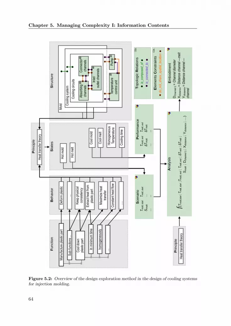
Chapter 5. Managing Complexity I: Information Contents
Beh
avio
r
….
Sta
tes
Hom
ogen
eous
Te
mpe
ratu
re
Coo
l mo
ld
Hot
mol
d
Coo
l me
lt
Hot
mel
t
Prin
cip
le
Hea
t tra
nsfe
r th
eory
Coo
ling
time
Str
uctu
re
M
old
Coo
ling
syst
em
Pum
p Te
mpe
ratu
re
cont
rol u
nit
Coo
ling
circ
uits
Abs
orbi
ng
chan
nels
C
onne
ctor
ch
anne
ls
Inle
t/ou
tlet c
hann
els
Fun
ction
In m
inim
um
tim
e
hom
ogen
eous
ly
Coo
l dow
n
plas
tic p
art
Man
ufac
ture
pla
stic
par
t
Sub
-fun
ctio
ns ..
.
...
Em
bod
imen
t
Dcha
nne
l 1 =
Cha
nnel
dia
met
er
Xd
ista
nce
= D
ista
nce
cha
nnel
—m
elt
Yd
ista
nce
= D
ista
nce
chan
nel —
chan
nel
Scen
ario
Tm
old,
sta
rt T
mel
t, st
art
S
melt
…
…
...
Perf
orm
an
ce
T
mol
d, e
nd
Tm
elt,
end
Δ
Tm
old
ΔT
me
lt
…
...
An
aly
sis
f(
Tm
old,
star
t ; T
mel
t, st
art ;
T mol
d, e
nd ; T
mel
t, en
d ; Δ
Tm
elt ; Δ
Tm
elt ;
Sm
elt ;
Dcha
nne
l 1 ;
Xd
ista
nce
; Y
dis
tance
; …
)
Top
olo
gic
Rela
tion
s
is_c
ompo
sed_
of
is_c
onne
cted
_to
Ele
men
ts C
on
stra
ints
do_n
ot_s
hare
_spa
tial_
loca
tion
Prin
cip
le
Hea
t tra
nsfe
r th
eory
...
Def
orm
pla
stic
Kee
p ph
ysic
al
cons
iste
ncy
Ext
ract
hea
t fro
m
plas
tic p
art
Max
imiz
e he
at
tran
sfer
Con
stan
t hea
t flo
w
Figure 5.2: Overview of the design exploration method in the design of cooling systemsfor injection molding.
64

5.2 Method 1: FBS based Formulation
Function Behavior State Structure
Principle
Cool down the plastic part
Cool in minimum time
Cool homogeneously
Simple
Channels Baffles
Bubblers
Cooling circuits
Part with constant
temperature
Cool Mold
Heat Transfer Theory
Extract Heat from Plastic
Part
Extract Heat at Constant Heat flow
Maximize Heat Transfer
Flow Pump Temperature control unit
Hot Mold
Coolant supply
manifolds
Collection manifolds
Cool Melt
Hot Melt
Figure 5.3: FBS description of CSIM design.
this case heat transfer theory. The structure is composed of several components.However, for explanation purposes, only cooling channel layout design is takeninto consideration. Examples of topology relations are:
• cooling circuit is composed of cooling channels
• one cooling channel is connected to one cooling channel
Examples of physical coherence constraints are:
• cooling channel does not share spatial location with melt.
• cooling channel starts at mold surface
• cooling channel ends at mold surface
• cooling channel is confined in mold
Step 2: Performance and Scenario Exploration
Table 5.1 presents a generalized summary of performance and scenario parame-ters. The dynamics implied by the sequence of states is also translated into aperformance parameter. In the case of cooling system design, the difference intime between both states is one performance parameter that describes the time re-quired to change from one state (hot melt) to the other(cold melt). The completedescription of performance and scenario parameters is presented in Table 5.1.
65

Chapter 5. Managing Complexity I: Information Contents
Table 5.1: State based performance and scenario mapping.
State Sequence State variables TypeHot Mold First Temperature Mold ScenarioHot Melt First Temperature Melt ScenarioCool Mold Second Temperature Mold PerformanceCool Melt Second Temperature Melt PerformancePart constantTemperature
Second Temperature Differ-ence in Part
Performance
Step 3: Analysis Technique Identification
Consider the case of the cooling system design for injection molding. A simpleanalysis has been chosen from [62]. The analysis is derived from the equation ofheat transfer by conduction for a substance in rest under several assumptions.The analysis consists of the following calculation:
1. Calculate heat transfer from the melt to the cooling medium using equa-tion 5.1.
2. Calculate the shape factor (Se), Reynolds (Re) number, the coolant heattransfer coefficient (α) and the thermal diffusivity of the melt (a) usingequations 5.2, 5.3, 5.4 and 5.5 respectively.
3. Consider Qabs = Qm, and use results of 5.2, 5.3, 5.4 and 5.5 to solve thesystem composed by equations 5.6 and 5.7.
The set of equations 5.1 to 5.7 represent the analysis technique that has beenchosen for the purpose of demonstrating the methodology. Each one follows fromdifferent partitions, obtaining that different parameters appear in different anal-ysis equations. The analysis has been formulated in such a way that it holds atboth sides of the axes of symmetry shown in Figure 5.4. This allows assessing thetemperature difference between the two sides of the mold, which was selected asperformance parameters in the second step of the method. It is worth mentioningthat 3D analysis formulation is better suited for the performance calculation ofthis type of problems. However, to describe the performance and scenario param-eters so far considered, the analysis technique here presented suffices. Table 5.2presents a list with the description of the used symbols.
Qabs = 10−3 · [(TM − TE)Cps + im] · ςm ·s
2· x (5.1)
Se =2πx4·[ln(
2 · x · sinh(
2 · π · yx
)/π · d
)]−1
(5.2)
66
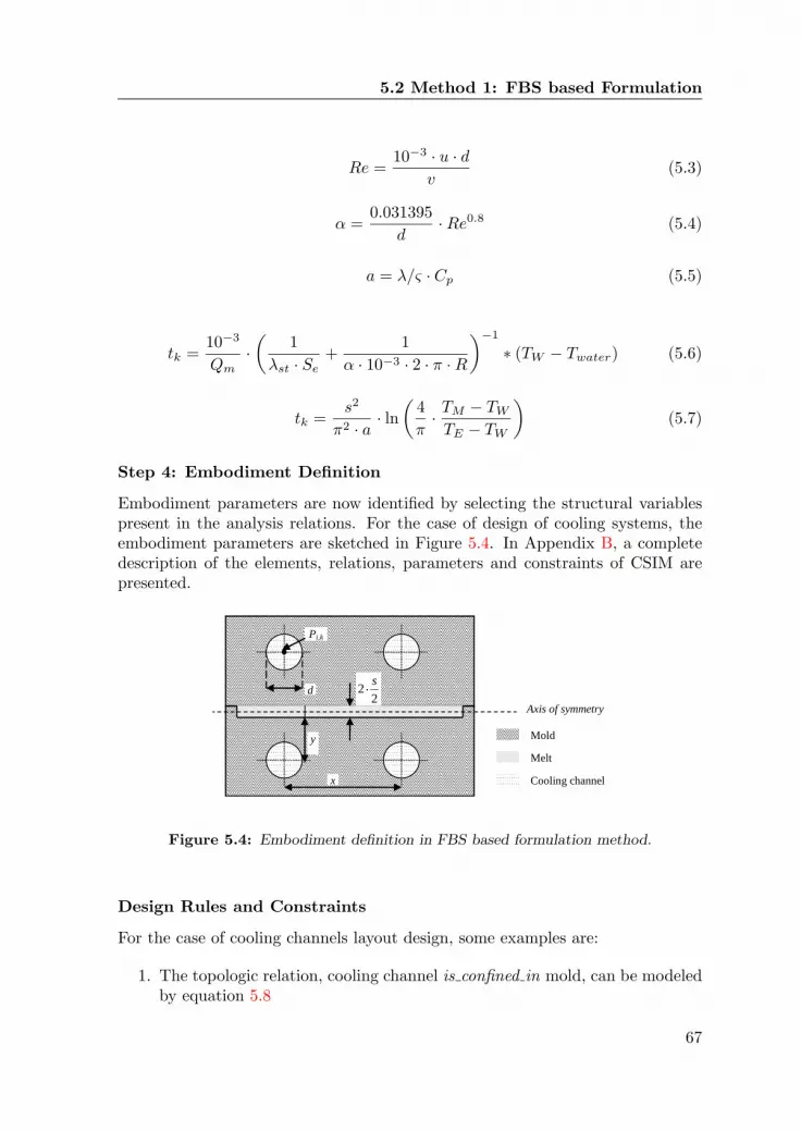
5.2 Method 1: FBS based Formulation
Re =10−3 · u · d
v(5.3)
α =0.031395
d·Re0.8 (5.4)
a = λ/ς · Cp (5.5)
tk =10−3
Qm·(
1λst · Se
+1
α · 10−3 · 2 · π ·R
)−1
∗ (TW − Twater) (5.6)
tk =s2
π2 · a· ln(
4π· TM − TW
TE − TW
)(5.7)
Step 4: Embodiment Definition
Embodiment parameters are now identified by selecting the structural variablespresent in the analysis relations. For the case of design of cooling systems, theembodiment parameters are sketched in Figure 5.4. In Appendix B, a completedescription of the elements, relations, parameters and constraints of CSIM arepresented.
d
y
x
Mold
Melt
Cooling channel
Axis of symmetry 2
2s
Pi,k
Figure 5.4: Embodiment definition in FBS based formulation method.
Design Rules and Constraints
For the case of cooling channels layout design, some examples are:
1. The topologic relation, cooling channel is confined in mold, can be modeledby equation 5.8
67

Chapter 5. Managing Complexity I: Information Contents
Table 5.2: Design parameters in CSIM
Symbol Units Description ClassificationQabs KJ/m Heat content of melt ScenarioQm KJ/m Heat absorbed by coolant Performancetk s Cooling time PerformanceS mm Part thickness ScenarioX mm Distance X EmbodimentY mm Distance Y EmbodimentD mm Diameter of cooling channel EmbodimentR mm Radius of cooling channel EmbodimentPi,k (mm,mm) Point i of cooling channel k Embodimenti No Index: 1 is start and 2 is end
point of cooling channelEmbodiment
k No Index: 1. . . N cooling channel EmbodimentTM
0C Melt (Molding) temperature ScenarioTE
0C De-molding temperature PerformanceTW
0C Temperature of mold PerformanceTwater
0C Temperature of cooling water Scenarioim KJ/Kg Latent heat of fusion of the
polymerScenario
Cps KJ/KgK Specific heat of the polymer Scenarioς g/cm3 Melt density Scenarioa cm2/s Thermal diffusivity of the melt ScenarioV m2/s Kinematics viscosity of water ScenarioU m/s Velocity of cooling water Scenarioλst W/mK Thermal conductivity of mold
steelScenario
Cp KJ/KgK) Specific heat of water Scenarioλ W/mK Thermal conductivity of water Scenarioα W/m2 Heat transfer coefficient Scenariotk s Cooling time Performance
68

5.3 Method 2: ADT based Decomposition
2. Element constraint avoiding two cooling channels sharing the same space inequation 5.9
3. Design rule defining the diameter of the cooling channel as function of thepart thickness in equation 5.10
Pi,k ∈Mold (5.8)√(xi,k − xi,k+1)2 + (yi,k − yi,k+1)2 − (DK +Dk+1)
2≤ ζ1 (5.9)
ζ2 ≤ D ≤ ζ3 (5.10)Note that the symbol ζi is used for representing a border value, while the wordMold represents the element mold.
5.3 Method 2: ADT based Decomposition
The goal of this method is to decompose the design problem class into severalindependent levels of abstraction. Decomposing the design into smaller chunks -adivide and conquer strategy- is often used to reduce complexity [77], as for examplein ADT [73] and MDO [1]. However, the resulting chunks are required to haveclear boundaries and governing principles. According to Goel et al. [21], designdecomposition has to be based on problem structure. This avoids unwanted sideeffects, such as multiple interdependencies among sub-problems and disjointedsub-problems. Therefore, the method presented decomposes the problem at thehand of the problem structure. The method (applied both in the functionaldomain and in the physical domain) consists of the three steps shown in Figure 5.5:
• Identification: determines the space of FRs and classifies the types of DPsinvolved in the problem.
• Reformulation: assembles the obtained FRs and DPs into a new decomposedproblem model
• Separation: separates the reformulated problem in abstraction groups ac-cording to the problem’s DM.
In Subsection 5.3.3 the method is applied to the design CSIM. In JaureguiBecker et al. [29] the method is applied to the design of Printed Circuit Boards.
5.3.1 Functional Domain
In the functional domain, the method consists of identifying functional elements,identifying its instantiation order and encapsulating the resulting structures intonew problem formulations. Functional elements are considered high level DPrelated to one (or a group of) FR(s).
69
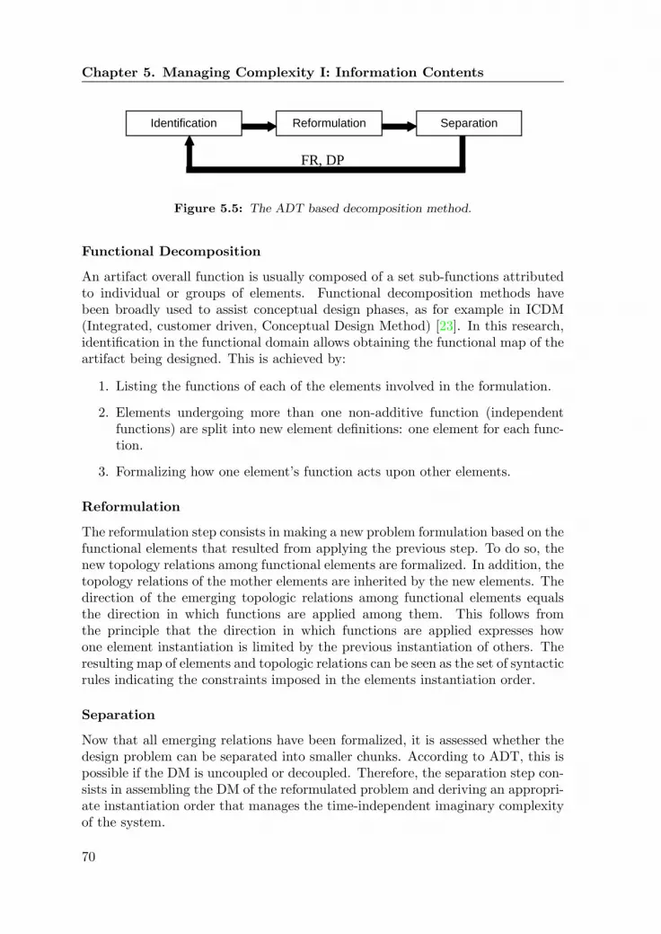
Chapter 5. Managing Complexity I: Information Contents
Identification Reformulation Separation
FR, DP
Figure 5.5: The ADT based decomposition method.
Functional Decomposition
An artifact overall function is usually composed of a set sub-functions attributedto individual or groups of elements. Functional decomposition methods havebeen broadly used to assist conceptual design phases, as for example in ICDM(Integrated, customer driven, Conceptual Design Method) [23]. In this research,identification in the functional domain allows obtaining the functional map of theartifact being designed. This is achieved by:
1. Listing the functions of each of the elements involved in the formulation.
2. Elements undergoing more than one non-additive function (independentfunctions) are split into new element definitions: one element for each func-tion.
3. Formalizing how one element’s function acts upon other elements.
Reformulation
The reformulation step consists in making a new problem formulation based on thefunctional elements that resulted from applying the previous step. To do so, thenew topology relations among functional elements are formalized. In addition, thetopology relations of the mother elements are inherited by the new elements. Thedirection of the emerging topologic relations among functional elements equalsthe direction in which functions are applied among them. This follows fromthe principle that the direction in which functions are applied expresses howone element instantiation is limited by the previous instantiation of others. Theresulting map of elements and topologic relations can be seen as the set of syntacticrules indicating the constraints imposed in the elements instantiation order.
Separation
Now that all emerging relations have been formalized, it is assessed whether thedesign problem can be separated into smaller chunks. According to ADT, this ispossible if the DM is uncoupled or decoupled. Therefore, the separation step con-sists in assembling the DM of the reformulated problem and deriving an appropri-ate instantiation order that manages the time-independent imaginary complexityof the system.
70

5.3 Method 2: ADT based Decomposition
5.3.2 Physical Domain
The application of the method in the physical domain is based on the design de-scriptions classification presented in 3.4.1. This classification is used to decomposeelements in different primitives, where each primitive encapsulates attributes thatcorrespond to one type of description. By doing so, building blocks with focusedsearch ranges are found. Furthermore, the method manages imaginary complexityby firstly integrating physical coherence constraints into the resulting primitiveelements, and secondly by introducing periodicity in the system.
Identification
First, embodiment and scenario parameters are classified in one of the followinggroups:
• Parameter: models the properties applicable to a whole element. These canbe of different nature, as for example numeric, symbolic, logic, predicateand combinations among them.
• Space: describes the position of the elements and depends on the chosencoordinate system (Cartesian, Cylindrical of Spherical) and the dimensionsof interest (1D, 2D, or 3D).
• Field: uses parameters and geometric vectors to describe properties thathold for specific regions of the elements. Fields are specified together withan incident zone, which is the spatial place where the field influences anelement. An incident zone can be a volume, an area, a line or a point.
• Shape: describes the form of an element or groups of elements. Commonlyused models are based on geometry and shape graphs.
• Topology: uses topology relations to describe the disposition of elements indesign. Cardinality is used to measure the number of times an element isinstantiated in the topology.
For example, the layout design of boxes would have spatial descriptions (itsposition) and shape descriptions (the length, width and depth of the boxes).
Reformulation
Reformulation consists of encapsulating each of the identified description dimen-sions into a new primitive element and formalizing the physical coherence con-straint among them. In this way, a new problem formulation is obtained. Inthe previous example this would mean that a box is composed out of a primitiveelement shape and a primitive element position.
71

Chapter 5. Managing Complexity I: Information Contents
Separation
This step consists of separating the reformulated problem into smaller chunksby assessing the DM of the resulting problem. As the interest here lays in thephysical domain, the DM has to describe the interrelations among the primitiveelements, or DPs, of the problem. As result, primitive elements are set to differentlevels of abstraction.
5.3.3 Example: CSIM Design
The example here presented is based on the model present in Figure 5.6, which isa simplification of the results gotten in the previous example.
Channel
Mold Part(Core, Cavity)
Plastic Part
Geometry,
Material Type,
Temperature
Geometry,
Material Type,
Temperature
Diameter,Position,
length,
Minimal & Maximal
Distance to product
(PCC-1)
Scenario Embodiment
Equation: Laplace
thermal equilibriumPerformances:
Cooling Time
Temp. DistributionDisconnected
Distance between channel (PCC-2)
Diameter (PCC-3)
Maximize (heat transfer),
Minimize (temperature distribution)
Objective function
Analysis
Relation
Physical
Coherence Topologic
Relation
Distance to mold part
(PCC-4)
Connected
Inside of
Figure 5.6: Problem formulation of CSIM design.
Functional Domain: Decomposition
Consider the case of injection molding cooling systems. To decompose the elementChannels we start by listing its functions:
• Function 1: to cool down the melt. Channels are placed close to the part ge-ometry and arranged such that heat is transferred in a homogeneous mannerfrom the melt to the coolant flowing through it.
• Function 2: to transport the coolant. Coolant is transported between chan-nels absorbing heat (function 1) to constitute cooling circuits.
• Function 3: to exchange coolant with the environment. Channels are usedto connect the cooling circuits with the external surface of the mold.
72

5.3 Method 2: ADT based Decomposition
As these functions are not additive but complementary, the element channelis decomposed into three different elements: (a) Absorber channels to fulfill func-tion 1; (b) Exchanger channels to fulfill function 2; (c) Connector channels tofulfill function 3. Figure 5.7(a) presents the resulting channels and their func-tions assembled in a model. As shown, the new element Absorber channel appliesits function to the scenario element Plastic Part, Connector channels apply theirfunction to the element Absorber channel, and the Exchanger channel applies itsfunction to both the Connector channel and the Absorber channel.
Functional Domain: Reformulation
In Figure 5.7(b) the reformulated CSIM is presented. The figure shows both thefunctional elements and the topology relations that have emerged. Here, eachchannel element type can be connected to another channel element of the sametype (relations 3, 5 and 9). Connector channel elements can be connected toAbsorber channels (relation 12). However, the relation does not work in theopposite direction. This is because Connector channels function is constrained bythe previous existence of an arrangement of Absorber channels, as indicated inFigure 5.7. A similar situation occurs for the relation between Exchanger channelsand the partial circuits formed by the arrangement of Absorber and Connectorchannels (relations 6 and 8): the existence of the former is constrained by theprevious existence of the latter.
Functional Domain: Separation
For the case of CSIM, a DM is assembled by considering the relations betweenthe FRs and the DPs shown in Figure 5.7, obtaining:
FRs DM DPs Cool MeltTransport CoolantExchange Coolant
=
9 − −12 5 −6 8 3
Absorber ChannelConnector ChannelExchanger Channel
(5)
As shown, the DM is decoupled and square, and can be separated into threeindependent problem formulations. The first is shown in Figure 5.8(a). Here, Ab-sorber channels are first instantiated by taking into considerations the relationsshown in the figure. In a similar manner, Connector channel are designed con-sidering the Absorber channel as scenario elements, shown in Figure 5.8(b). Theformulation in Figure 5.8(c) is assembled for the design of Exchanger channels. Ifthe number of FRs does not match the number of DPs, the resulting DM is notsquare. In such a case, a DM of the relation among the DPs is better suited fordetermining the appropriate instantiation orders.
73

Chapter 5. Managing Complexity I: Information Contents
Absorber
channels
Exchanger
channels
Connector
channels
Supply coolant Exchange coolant
Exchange coolant
Plastic
Part/Melt
Cool melt
(a) Functional elements in cooling layout design.
Absorber Channels
Exchanger
Channels
Connector
Channels
Plastic Part/
Melt
Is_connected_toIs_connected_to
Is_connected_to Is_connected_to
Is_connected_to
Inside of
Mold Part
(Core, Cavity)
Inside of
Inside of
Disconnected
Disconnected
Disconnected
1
2
3 5
6
7
9
10
11
12
4
Is_connected_to
8
(b) Decomposed cooling layout design.
Figure 5.7: Reformulation of CSIM.
Physical Domain: Identification
In this step, descriptions are categorized around the five attributive dimensions.In the case study of CSIM design, the identification of primitive elements is doneby analyzing the type of description used to model them. As the elements Ab-sorber channels, Connector channels and Exchanger channels are modeled withthe same descriptions, the identification has been generalized in an element Chan-nel, which represents either one of the three before mentioned types. Channelshave attributes in two domains:
• Space: models the position of a channel inside the mold. The position ismodeled by three coordinates in the Cartesian coordinate system.
• Shape: models the geometry of a channel by the descriptions diameter (D)and length (L).
74

5.3 Method 2: ADT based Decomposition
Absorber Channels
Plastic
Part/Melt
Cool melt
Is_connected_to
Mold Part
(Core, Cavity)
Is inside
Absorber
Channels
Connectors
Channels
Supply coolant
Is_connected_to
Is_connected_to
Mold Part
(Core, Cavity)
Is inside
Absorber Channels
Exchanger
Channels
Connectors Channels
Exchange coolantExchange coolant
Is_connected_toIs_connected_to
Is_connected_to
Mold Part
(Core, Cavity)
Is inside
Scenario
EmbodimentFunction
Topologic relation
(a) Sub-Problem 1: Absorber channels design (b) Sub-Problem 2: Connectors channels design
(c) Sub-Problem 3: Exchanger channels design
Disconnected Plastic
Part/Melt
Disconnected
Plastic
Part/Melt
Disconnected
(a) Sub-problem 1: absorber channel design.
Absorber Channels
Plastic
Part/Melt
Cool melt
Is_connected_to
Mold Part
(Core, Cavity)
Is inside
Absorber
Channels
Connectors
Channels
Supply coolant
Is_connected_to
Is_connected_to
Mold Part
(Core, Cavity)
Is inside
Absorber Channels
Exchanger
Channels
Connectors Channels
Exchange coolantExchange coolant
Is_connected_toIs_connected_to
Is_connected_to
Mold Part
(Core, Cavity)
Is inside
Scenario
EmbodimentFunction
Topologic relation
(a) Sub-Problem 1: Absorber channels design (b) Sub-Problem 2: Connectors channels design
(c) Sub-Problem 3: Exchanger channels design
Disconnected Plastic
Part/Melt
Disconnected
Plastic
Part/Melt
Disconnected
(b) Sub-problem 2: connector channel de-sign.
Absorber Channels
Plastic
Part/Melt
Cool melt
Is_connected_to
Mold Part
(Core, Cavity)
Is inside
Absorber
Channels
Connectors
Channels
Supply coolant
Is_connected_to
Is_connected_to
Mold Part
(Core, Cavity)
Is inside
Absorber Channels
Exchanger
Channels
Connectors Channels
Exchange coolantExchange coolant
Is_connected_toIs_connected_to
Is_connected_to
Mold Part
(Core, Cavity)
Is inside
Scenario
EmbodimentFunction
Topologic relation
(a) Sub-Problem 1: Absorber channels design (b) Sub-Problem 2: Connectors channels design
(c) Sub-Problem 3: Exchanger channels design
Disconnected Plastic
Part/Melt
Disconnected
Plastic
Part/Melt
Disconnected
(c) Sub-problem 3: Exchanger channel de-sign.
Absorber Channels
Plastic
Part/Melt
Cool melt
Is_connected_to
Mold Part
(Core, Cavity)
Is inside
Absorber
Channels
Connectors
Channels
Supply coolant
Is_connected_to
Is_connected_to
Mold Part
(Core, Cavity)
Is inside
Absorber Channels
Exchanger
Channels
Connectors Channels
Exchange coolantExchange coolant
Is_connected_toIs_connected_to
Is_connected_to
Mold Part
(Core, Cavity)
Is inside
Scenario
EmbodimentFunction
Topologic relation
(a) Sub-Problem 1: Absorber channels design (b) Sub-Problem 2: Connectors channels design
(c) Sub-Problem 3: Exchanger channels design
Disconnected Plastic
Part/Melt
Disconnected
Plastic
Part/Melt
Disconnected
(d) Legend
Figure 5.8: Resulting decomposed problem formulations.
The scenario element Mold Parts can be modeled in different dimensions:Shape, Fields and Parameter. As Mold Parts are not subject of design and itsshape and parametric representation are fixed, it is chosen to use the representa-tional dimension Fields.
Physical Domain: Reformulation
For the case of CSIM shown in Figure 5.9, the following primitive elements arederived:
• Points: encapsulate the Space dimension of the representations. A Pointcontains a description about its position (x,y,z). Points are related to thescenario elements by the physical coherence constraints PCC-1 and PCC-4.A set of Points indicates the path followed by the channel.
• Segments: encapsulate the Shape dimension. A Segment contains the de-scriptions diameter (D) and length (L). The physical coherence relationPCC-2 determines the minimum allowed distance between two points toavoid break of the mold, while the relation PCC-3 determines the diameterof the channel as function of the distance between a Point and Mold Partor Plastic Part.
75

Chapter 5. Managing Complexity I: Information Contents
Channel
Cardinality Segment
Diameter DLength L
Cardinality C
Point
Position (x,y,z)
TypeCardinality
Voxels
Plastic Part/
Melt
Voxels
Mold Part
(Core, Cavity)
PCC-1
PCC-4PCC-2
Is
Is composed of
Is inside of
Disconnected
PCC-3
1
2
3
4
5
6
7
Figure 5.9: Primitives in functional element “Absorber Channel”.
Given that the three functional elements are decomposed into the same prim-itives, the following notation is used to differentiate among them:
• Absorber channels have primitives Blue Points and Blue segments.
• Connector channels have primitives Green Points and Green segments.
• Exchanger channels have primitives Brown Points and Brown segments.
These six primitive elements define the information contents of the DPs of theproblem. On the other hand, the element Mold Parts is also decomposed intoprimitives. Here, the dimension of concern is Fields and, as such, voxel elementsare chosen. Voxels are cubic units and can be used to describe a mold’s shapeand position.
Physical Domain: Separation
For the case of CSIM design, the resulting DM becomes:
Points
SegmentsMoldPartP lasticPart
=
2 0 5, 6 4, 7
3, 1 0 0 00 0 0 00 0 0 0
PointsSegmentsMoldPartP lasticPart
(6)
According to this, Points have to be instantiated firstly and Segments sec-ondly. Now that the problem has been separated, the combinatorial aspect ofthe complexity is tackled. In the case study of CSIM, combinatorial complexityarises from the uncertainty of how many Channels are required and how theyshould be connected. This is managed by predefining a 3D grid of points without“color” within the voxel mesh. By doing so, periodicity is brought in the systemas suggested in ADT. By setting the distance between Points according to relation
76

5.3 Method 2: ADT based Decomposition
Table 5.3: Logic relations determining the color of Points.
Point ID Logic relation with scenario elementsBlue C1 Surrounded by [(core voxels) OR (cavity voxels)]
AND [product voxels]Green C2 Surrounded by [(core voxels) OR (cavity voxels)]Brown C3 Surrounded by [(core voxels) OR (cavity voxels)]
AND [exchanger voxels]Black C4 Surrounded by [non drillable voxels]
PCC-2, imaginary complexity is also removed from the system, as relation 2 canbe removed from the DM shown in equation 6. In order to integrate the physicalcoherence constraints PCC-1 and PCC-4 into DPs, one extra type of Points isdeclared, namely, Black Points. Black points define the positions where channelscannot be placed to avoid mold breakage. In Table 5.3, the logic relations thatdetermine the colors of Points are presented.
Results
Figure 5.10 shows the results of applying this method. A hierarchical model con-sisting of three levels of abstraction (Points design, Segment design and Channeldesign) is obtained. Each element in the model is considered a DP , while thetopology relations among them represent the syntactic rules determining theirstructure. Physical coherence constraints represent semantic rules assuring nophysical inconsistencies occur. The complexity of the system has been reducedby specifying the ranges of each DP : Points as function of the scenario elementsPlastic Part and Mold Parts, Segments as function of Points, and Channels asfunction of Segments. Furthermore, the order of instantiation was determined foreach abstraction level at the hand of its DM.
The representations in Figure 5.10 can now be used for automating the designof CSIM. Chapter 9 describes the implementation of this method to automateCSIM design using these representations.
77

Chapter 5. Managing Complexity I: Information Contents
Absorber Channel
Length
Cardinality
Blue Segment
Diameter DCardinality C
Blue Point
Position (x,y,z)
Cardinality
Plastic Part/
Melt
Mold Part
(Core, Cavity)
PCC-2
Is composed of
Is composed of
Exchanger Channel
Length
Cardinality
Green SegmentDiameter D
Cardinality C
Green PointPosition (x,y,z)
Cardinality
PCC-2
Is composed of
Is composed of
Connector Channel
Length
Cardinality
Brown SegmentDiameter D
Cardinality C
Brown Point
Position (x,y,z)
Cardinality
PCC-2
Is composed of
Is composed of
C1
C2 C3
Is_connected_to Is_connected_to
Black Point
Position (x,y,z)
Cardinality
C4
Discretization
into voxels
PointDesign
Segment
design
Channel
design
Figure 5.10: Results of decomposing the CSIM design problem.
78

Chapter 6Managing Complexity II:Representations
This Chapter presents a framework for representing artifactual routine de-sign problems according to the structure described in Chapter 4. First, thefour basic building blocks (Elements, ACO-relations, C-relations and H-relations) are proposed. Later, an example describing how to translate aroutine design problem into this framework is presented.
6.1 Introduction
A great diversity of representation schemes can be found in CDS literature. Whilesome representations are specific for one domain (e.g. super quadric for shapedesign), other representation schemes, like grammars and parametric models, haveproven to be of a more generic character. For example, design grammars have beensuccessfully used in computational synthesis methods for shapes design (e.g. [42,51]), product design configurations (e.g. [71]) and conceptual design (e.g. [34]).However, these representations are specific to the problem formulation model andits automation approach. In order to be capable of developing methodologiesfor complexity management, standard representation are required. The buildingblocks should be capable of representing different levels of detail independentfrom each others, and supporting the instantiation of elements, parameters andrelations independent from hierarchical dependencies.
Considering these requirements, a framework to represent the structure ofartifactual routine design problems has been developed. The framework is namedTopology Abstraction Representation Diagram (TARD), as the focus is set on thetopology characteristics of design problems. As this thesis concerns computationaldesign synthesis, software implementation aspects have been considered. The
79

Chapter 6. Managing Complexity II: Representations
framework is founded upon two existing representation models, namely, multi-level networks and graph grammars. This section describes the generalities ofthese models as well as its shortcomings for representing different types of designproblems.
6.1.1 Multi-level Networks
Nested topologies require an approach for separating different levels of designdetail. Johnson et al. [31] does so by presenting a multilevel network for relatingelements in a topology. This network distinguishes parts and its components atdifferent levels of abstraction. Components at level N are related by an assemblyrelation R to one component at level N + 1. By doing so, the component on thehigher level N + 1 can be represented as function of the components on the lowerlevel N and the assembly relation R, as shown in the example in Figure 6.1. Here,an arch is represented as function of the blocks b1, b2, b3 and the relation R. Thismakes the components of the multilevel network highly dependent across levelsof abstraction, thus in a vertical direction. As a consequence, the componentswithin a level are not directly related with each other in a horizontal manner.This multilevel network only uses an implicit assembly relation between the levelsof detail. In order to obtain an explicit relation between detail levels, the assemblyhas to be managed autonomously in the lower level, requiring another method forthe establishment of topological relations.
b1b2
b3
R (assemble)
Level N+1
Level NBlocks
Arch
<b1,b2,b3;R>
Figure 6.1: Vertical assembly relation in a multilevel network.
6.1.2 Graph Grammars
As described in Chapter 2, grammars make use of rules to produce networks ofelements by either modifying existing graphs or expanding an initial single elementgraph. A grammar rule, as shown in Figure 6.2, specifies how one sub-graph can bereplaced by another sub-graph. By applying grammar rules, different components
80

6.2 Theory 1: TARD Model
can be inserted to form a design topology. The example in Figure 6.2 illustratesa simple transmission system. As shown, rule R1 describes the connection ofelement inputshaft and gear1, rule R2 describes the connection of element gear1with element gear2 and rule R3 describe the connection of the lement gear2with the element outputshaft. Grammars make use of “horizontal” relationsin opposition to the multilevel network representation, which uses a “vertical”relation. In other words, grammars describe the relation of elements at one levelof detail, while multilevel networks describe the relation between elements atdifferent levels of detail. For the case of example in Figure 6.2, the transmissionsystem is represented explicitly by the components and their connectivity relationsand not by a single implicit assembly relation like in the multilevel network.
R1
Inputshaft Gear1 Gear2 Outputshaft
R2 R3
1 2 1 2 3
RR R
Grammar rule
Figure 6.2: Example of horizontal grammar representation.
6.2 Theory 1: TARD Model
The Topology Abstraction Representation Diagram, or TARD, integrates explicitrelations to model both the connectedness among elements in one abstraction leveland the inter-dependency of elements at different abstraction levels. By doing so,characteristics of grammar, parametric and multi-level networks representationsare resembled by a small set of generic building blocks: Elements, C-relations,H-relations and ACO-Relations. Elements represent individual components ofthe design problem, and group the set of parameters used in its description. Forexample, in Figure 6.3 the components E1, E2 and E3 represent an engine, agear box and a wheel respectively. C-relations represent the connectedness ofthe elements in the topology, which is described in Figure 6.3 by the relationsC. H-relations model how a group of C-relations are related to describe thecomposition of a higher level element. This group of C-relations, together withtheir corresponding Elements is denoted here as abstraction-group. ACO-relationsare used to model analysis relations, physical coherence constraints and objectivefunctions.
81

Chapter 6. Managing Complexity II: Representations
E3
Wheel
E2
Gear Box
E1
Engine
E6
Gear 3
E5Gear 2
E4
Gear 1
H
C C
C C
Level 1
Level 2
Horizontal direction
Vert
ica
l d
ire
ctio
n
Figure 6.3: Example for the general usage of Elements, C-relation and H-relations ontwo levels of detail.
Using these building blocks to represent a problem structure results in a hor-izontal and vertical connected network, as shown in Figure 6.3. By consideringexplicit -instead of implicit- relations, TARD supports the creation of problem so-lutions at one level of detail topologically independent from other levels of detail.The last is required for supporting bottom-up and top-down design strategies si-multaneously. TARD reassembles the design structure presented in Chapter 4, asshown in Figure 6.4. In this sense, the building blocks in TARD have both a classrepresentation and an instance representation. The problem class is constructedat the hand of Elements, C-relations, H-relations and ACO-relations classes. Aproblem instance is defined by partiality instantiating these building blocks.
Problem
Class
Problem
Instance
Problem
Solution
Figure 6.4: Design problem structure using TARD.
82

6.2 Theory 1: TARD Model
6.2.1 Base definitions
Cardinality
In order to control the number of instances of each building block, TARD usescardinalities. Two types of cardinalities are distinguished: local and global. Whilelocal cardinalities describe the number of instances in a relative fashion (e.g. C-relation in relation to an Element), global cardinalities model the total numberof instances of a certain element class in the complete design problem.
References
A reference is a pointer to another class or object instance. It is used to define howone building block is related to another. Relations also use references to elementparameters to define its form. Depending on the direction of the association,the reference is of the type owned or the type owner. Owner references followthe hierarchical structure from top to bottom, while owned references do it frombottom to top. References are required to enable communication among thebuilding blocks classes and instances.
6.2.2 Building Blocks
Elements, C-relations and H-relations are used at the three levels of problemstructure: problem class, problem instance and problem solution. At the problemclass level, these building blocks describe the blueprint of an artifact. At a probleminstance level, a combination of class and instance descriptions is used, while atthe problem solution, only instances of these building blocks are used. From thisperspective, the problem instance can be seen as a partially instantiated problemsolution. The following subsections present a detailed description of each buildingblock of TARD.
Elements
An Element represents a class description of a component in a design problem.For example, the transmission system in Figure 6.3 contains four Element blocks:inputshaft, gear1, gear2 and outputshaft. Each Element class is described inTARD by the following information:
• Parameters: Describe the class by modeling its characteristics. At theproblem class, parameters are only declared. Values are attributed eitherby setting the requirements at the problem instance level, or by a generationalgorithm to create problem solutions.
• Cardinalities: The total cardinality e describes the amount of Elementsof a type in the design solution, while the local cardinality el describes thetotal amount of Elements within one abstraction-group. Cardinality can be
83

Chapter 6. Managing Complexity II: Representations
BA C
Z
C1
i j
C2
i j
l l
Level 1
Level 0
Figure 6.5: Example of bi-level TARD Diagram.
either known or unknown. Depending on whether cardinalities are knownor unknown, the problem exhibits different complexities, as described inChapter 5.
• References: owner-reference to a H-relations and owned-reference to a C-relation.
Elements can be classified according to their absolute position or relative po-sition in the topology diagram. From an absolute perspective, three types ofElements are distinguished:
• Zero Elements: Each network formulated by the representation of thisframework has a hierarchical structure topped by a single Element repre-senting the structure as a whole. In Figure 6.5, the zero level Element isdenoted as Element Z. The cardinality of Zero Elements equals one (1) andno C-relations are connected to them.
• Abstract Elements: Are those with a subordinate abstraction-group, andare found between Zero Elements and Base Elements. In Figure 6.5, Z isboth a Zero-element and an abstract element.
• Base Elements: Are those at the bottom of each network path, and donot have lower abstraction level dependencies. In Figure 6.5, elements A,Band C are all base elements, as none of them has a lower abstraction-group.
On the other hand, from a relative perspective elements can be classified inparent or son elements. For example, in Figure 6.5 the element Z is the parentelement of A, B and C; while element B is the son of element Z.
84

6.2 Theory 1: TARD Model
Engine
GearBox
Wheel
S
Engine GearBox WheelC1 C2
(a) 3 Elements connected by two 1-simplices.
Engine
GearBox
Wheel
S
Engine GearBox WheelC C
(b) 3 Elements connected byone 2-simplex.
Figure 6.6: Connectivity relations.
C-Relations
C-relations are used to determine the connection between two element classesin an abstraction-group. Having explicit connective relations makes it possibleto assemble sequences of Elements independent of the previous existence of in-stantiated parent elements. Elements are horizontally related to C-relations byreferences, which allows its instantiation in two ways: by instantiating the rela-tions and later their referenced Elements (a top-down strategy), or by matchingpreviously instantiated Elements and then instantiate the C-relation accordingly(a bottom-up strategy). Consider the example shown in Figure 6.3. Here, theElement engine can exist without the need for an Element wheel or even withoutthe need for a C-relation C.
Furthermore, C-relations support the generation of topologies by generatingsequences, enabling the application of grammar approaches for design synthesis.In contrast to the multidimensional representation, the grammar approach withthe rule in Figure 6.6(a) relates two Element classes with each other using a 1-simplex to describe the relation. By an iterative repetition of the rule, a multitudeof C-relations can be created. TARD only supports the representation of 1-simplexC-relations, thus, it only relates two elements. Higher dimensional simplices areindirectly supported by the H-relation, as it it described in Subsection 6.2.2. C-relations are modeled using the following descriptions:
• Direction: Indicates how one Element is related to other Elements of an-other class.
• Cardinalities: C-relations have two local cardinalities, namely, cardinalityi and cardinality j. These cardinalities define the number i of instancesof an Element type that can be connected with a number j of instances toanother element. As the framework is decided to suport 1-simplex relations,i has a constant value of 1. The example shown in Figure 6.7(a) illustrates aC-relation class C that relates the Element classes A and B with i = 1 andj = 4. The instanced C-relations in Figure 6.7(b) shows that one instanceof A is connected to four instances of B.
85

Chapter 6. Managing Complexity II: Representations
• References: Owner-reference to an element, owned-reference to a H-relation
• Parametric models: Are rules concerning the constitution of the con-nected Element instances. These rules, in the form of equation, relate pa-rameters of the two Element classes involved in the relation. Figure 6.8shows an example, where the parameters defined within the two Elementclasses are related to each other by a set of rules in the C-relation. Accord-ingly, the instantiation process of Element 2 has to consider the parametricrelations defined with respect to the prior Element.
Note: It is important to notice that although C connects one Element A withfour Elements B, it does not connect the instances of B (b1,b2,b3,b4) among eachothers. So, even if C-relations relate more than two Element instances, as in theexample, they do not model multidimensional simpleces.
A B
C
i=1 j=4
a1
b1
b2
b3
b4
c1
instanceclass(a) C-relation class connected to two El-ement classes.
A B
C
i=1 j=4
a1
b1
b2
b3
b4
c1
class
(b) C-relation instance connected to fiveElement instances.
Figure 6.7: C-relations: class and instance.
Element 1
C-relation
Element 2parameters:
p1p2
p3..
parameters:
pApB
pC..
rules:
p1 < 2 pAP2 = pB
P3 >= pC2
.
.
Figure 6.8: Parametric rules in the C-relation relate the parameters of the connectedElements.
86

6.2 Theory 1: TARD Model
H-relations
H-relations connect the model in a vertical direction, thus they relate two lev-els of detail with each other. More precisely, a H-relation connects an abstractElement in a level N with an abstraction-group on a more detailed level N + 1.Abstraction-groups describe topology compositions on an abstract Element, andare analoguos to the assembly relation of the multilayer network [28]. However,while assembly relations in the multilayer network relates a set of componentsto a single component on a higher level, the H-relation relates the C-relations ofabstraction-group at level N with its parental Element on level N − 1.
A topological diagram according to TARD is composed of elements connectedby relations. These relations represent the possible topological dependencies ofa design problem. By referencing H-relation to C-relations instead of directly toElements, the combination of the H-relations and C-relations establishes a selfcontained definition of the structure of each abstraction-group. By doing so, Ele-ments and topology relations can be uncoupled, and the description provided bythe relations yields a valid description of the abstraction-group, even without anyknowledge about the actual Element instances. On the other hand, this obligesa problem solution to represent both the Elements and their connection in anabstraction-group. The C-relations and H-relations create an explicitly formu-lated skeleton in which, by the means of generation or recognition algorithms,Element instances are created.
A H-relations contains the following information:
• Cardinalities: Each reference from an H-relation class to a C-relation classis associated with a total cardinality lc. This cardinality models the amountof instances of C-relations in an abstraction-group. In the example shownin Figure 6.9, a C-relation C connects one Element A with one Element B.In order to connect 3 element instances A with 3 element instances of B,three C-relations C are required, which results in l = 3.
• Sequence: The second type of information stored within the H-relation iscalled sequence. A sequence is a list of successive relations that in essenceresembles a plan for the instantiation order.
• Constraining rules: Constrained combination of C-relations by specify-ing required combinations or not allowed combinations. Constraining rulesare formulated in the form of sequence fragments. This type of rules areformulated using references to both C-relations and Elements classes andinstances and logic operators.
• Reference: Owner-reference to C-relations, owned-reference to an Ele-ment.
It is interesting to note that the sequence and constraining rules indicate themanaging role the H-relation has over an abstraction-group. As H-relations are
87

Chapter 6. Managing Complexity II: Representations
A B
C
H lc=3
i=1 j=1
P
e=3 e=3
a1 b1
c1
a2 b2
c2
a3 b3
c3
p
h
(a) Class representation with lC = 3.
A B
C
H lc=3
i=1 j=1
P
e=3 e=3
a1 b1
c1
a2 b2
c2
a3 b3
c3
p
h
(b) Instance representation with C-relation instances.
Figure 6.9: H-relations: class and instance.
always related to parental Element on a one to one basis, they are coupled tocardinalities. According to this, an Element instance can only have one type ofH-relation in the topology domain. However, multiple domains of an element canbe represented by different types of H-relations.
ACO-Relations
ACO relations represent the non-topology relations of a design problem formula-tion: Analysis relations, physical Coherence constraints and Objective functions.ACO-relations have the following type of information:
• References: owner references are used to parameters declared in Elements,C-relations and H-rations. In this context, cardinalities are also regardedas parameters.
• Parameters: model the parameters that not attributed to other elements.For example, an the weight parameters of an objective function.
• Model: The model uses references, parameters and operators to describethe nature of the relation.
6.2.3 Types of abstraction-groups
Creating solutions to problem instances consists in instantiating C-relations andElements in abstraction-groups, which results in a collection of m elements con-nected by successive m − 1 C-relations. This collection is regarded as sequence,and determines the time dependency of a problem. Abstraction-groups with one
88
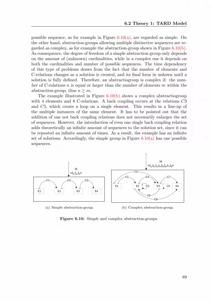
6.2 Theory 1: TARD Model
possible sequence, as for example in Figure 6.10(a), are regarded as simple. Onthe other hand, abstraction-groups allowing multiple distinctive sequences are re-garded as complex, as for example the abstraction-group shown in Figure 6.10(b).As consequence, the degree of freedom of a simple abstraction-group only dependson the amount of (unknown) cardinalities, while in a complex one it depends onboth the cardinalities and number of possible sequences. The time dependencyof this type of problems draws from the fact that the number of elements andC-relations changes as a solution is created, and its final form in unkown until asolution is fully defined. Therefore, an abstractiogroup is complex if: the num-ber of C-relations n is equal or larger than the number of elements m within theabstraction-group, thus n ≥ m.
The example illustrated in Figure 6.10(b) shows a complex abstractiogroupwith 4 elements and 8 C-relations. A back coupling occurs at the relations C3and C5, which create a loop on a single element. This results in a line-up ofthe multiple instances of the same element. It has to be pointed out that theaddition of one not back coupling relations does not necessarily enlarges the setof sequences. However, the introduction of even one single back coupling relationadds theoretically an infinite amount of sequences to the solution set, since it canbe repeated an infinite amount of times. As a result, the example has an infiniteset of solutions. Accordingly, the simple group in Figure 6.10(a) has one possiblesequences.
E1 E2 E3
C1
C3
C4
C2
C8
C6
C7
C5 E4E1 E2 E3 E4
C1 C2 C3
H <l1,l2,l3>
H <l1,l2,l3,l4,l5,l6,l7,l8>
(a) Simple abstraction-group.
E1 E2 E3
C1
C3
C4
C2
C8
C6
C7
C5 E4E1 E2 E3 E4
C1 C2 C3
H <l1,l2,l3>
H <l1,l2,l3,l4,l5,l6,l7,l8>
(b) Complex abstraction-group.
Figure 6.10: Simple and complex abstraction-groups.
89

Chapter 6. Managing Complexity II: Representations
6.3 Example: Belt System Design
The following example illustrates the concepts discussed above. Figure 6.11 showsa sketch of a conceptual belt system. The embodiment of the belt system includesan input shaft (IS), an input pulley (IP ), a belt (B), an output pulley (OP ) andan output shaft (OS). The components within the embodiment are arranged inorder to serve the main functionality of the system, which is transferring force andmomentum. This type of problem can be regarded as a topologic design problem,as it concerns the configuration of different types of components. In other words,the topology has to make sense from a functional point of view. This impliesthat the C-relations are established within the functional domain of transferringenergy.
Figure 6.11(b) presents a straightforward topological diagram on the basisof the framework. It is composed of just one level containing all componentsfrom Figure 6.11(b) translated into Elements. These Elements are related to eachother by the means of four C-relations (C1,C2,C3,C4) in such a manner that itresembles the path of the energy flow from input to output. Due to the fact thateach component only appears once, all C-relations are one by one relations, withi and j equal to one. A further consequence is that the cardinalities l containedwithin the H-relation, which is connected to the zero level Element BS (Beltsystem), are equal to one as well.
inputshaft
inputpulley
outputshaft
belt
outputpulley
(a) A conceptual single belt transmission.
inputshaft
inputpulley
outputpulley
outputshaft
belt
IPIS B
BS
C1
1 1
C2
1 1
OP OS
C3
1 1
C4
1 1
H0
1 1 1 1
(b) Topological network of the belt system with a single level of detail.
Figure 6.11: Example of representation of a pulley transmission system.
The values of the cardinalities are fixed due to the fact that the artifacts’
90
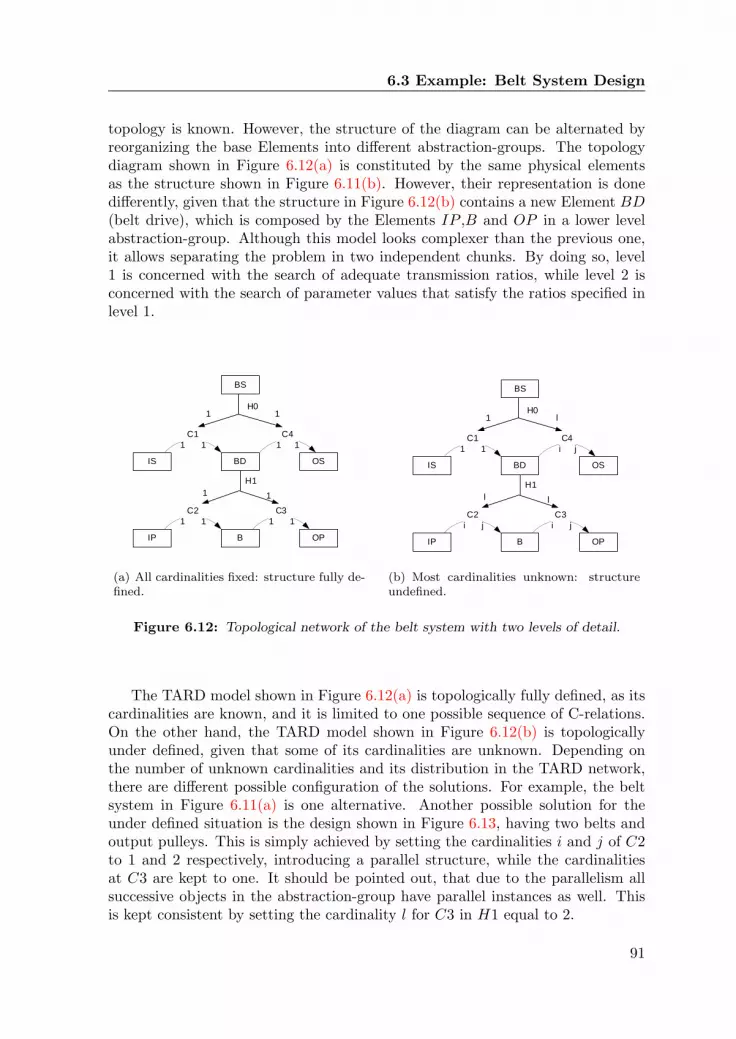
6.3 Example: Belt System Design
topology is known. However, the structure of the diagram can be alternated byreorganizing the base Elements into different abstraction-groups. The topologydiagram shown in Figure 6.12(a) is constituted by the same physical elementsas the structure shown in Figure 6.11(b). However, their representation is donedifferently, given that the structure in Figure 6.12(b) contains a new Element BD(belt drive), which is composed by the Elements IP ,B and OP in a lower levelabstraction-group. Although this model looks complexer than the previous one,it allows separating the problem in two independent chunks. By doing so, level1 is concerned with the search of adequate transmission ratios, while level 2 isconcerned with the search of parameter values that satisfy the ratios specified inlevel 1.
IP B OP
BDIS OS
BS
C1
1 1
C4
1 1
C2
1 1
C3
1 1
H01 1
1 1
H1
IP B OP
BDIS OS
BS
C1
1 1
C4
i j
C2
i j
C3
i j
H01 l
l l
H1
(a) All cardinalities fixed: structure fully de-fined.
IP B OP
BDIS OS
BS
C1
1 1
C4
1 1
C2
1 1
C3
1 1
H01 1
1 1
H1
IP B OP
BDIS OS
BS
C1
1 1
C4
i j
C2
i j
C3
i j
H01 l
l l
H1
(b) Most cardinalities unknown: structureundefined.
Figure 6.12: Topological network of the belt system with two levels of detail.
The TARD model shown in Figure 6.12(a) is topologically fully defined, as itscardinalities are known, and it is limited to one possible sequence of C-relations.On the other hand, the TARD model shown in Figure 6.12(b) is topologicallyunder defined, given that some of its cardinalities are unknown. Depending onthe number of unknown cardinalities and its distribution in the TARD network,there are different possible configuration of the solutions. For example, the beltsystem in Figure 6.11(a) is one alternative. Another possible solution for theunder defined situation is the design shown in Figure 6.13, having two belts andoutput pulleys. This is simply achieved by setting the cardinalities i and j of C2to 1 and 2 respectively, introducing a parallel structure, while the cardinalitiesat C3 are kept to one. It should be pointed out, that due to the parallelism allsuccessive objects in the abstraction-group have parallel instances as well. Thisis kept consistent by setting the cardinality l for C3 in H1 equal to 2.
91

Chapter 6. Managing Complexity II: Representations
inputshaft
inputpulley
belt
belt
outputpulley
outputshaft
outputpulley
Figure 6.13: A conceptual double belt transmission: one input, two outputs.
6.3.1 Proximity Relation
One special case of ACO-relations is the proximity relation. Although abstraction-group are in principle treated independently, Elements between different abstraction−groups might be physically connected too. Usually, this relationship exist betweenthe first and last Elements of an abstraction-group. These elements are regardedin TARD as boundary Elements. Boundary Elements might be physically con-nected to components in Elements in other neighboring abstraction− groups.
Consider the example in Figure 6.11. Here, the transmission system consistsof physically connected parts. Figure 6.12 shows that the Elements of the beltsystem can be divided into two abstraction-groups. Although the output pulleyOP and the outputshaft OS are physically connected, they are allocated intodifferent abstraction-group. If there are two instances of Element OP , there haveto be two instances of OS as well and vice versa. The resulting physical modelis shown in Figure 6.13. The same is true for the Elements IS and IP , howeverthe cardinalities remain 1 in this case. The correlation between those Elementsis called proximity relation. In the example, the local cardinalities of IP and OPare set equal to the local cardinalities of IS and OS respectively, resulting in theproximity relations: e < IP >= e < IS > and e < OP >= e < OS >, withe1e2
= p, where p is called proximity constraint. The choice of which Elements tobind by a proximity relation is highly dependent on the problem and its boundaryconditions.
92

Chapter 7Managing Complexity III:Manipulating Elements
Two techniques to manage problem instance complexity are proposed in thisChapter. One technique manages complexity arising from requirements dis-tribution, while a second technique manages complexity arising from knowl-edge distribution.
7.1 Introduction
Solving design problem instances can be regarded as a two folded process. Firstly,depending on the distribution of known and unknown entities, a design strategy isdeveloped. Secondly, specialized algorithms instantiate the elements, parametersand relations such that the goal of the design is achieved. While the formerprocess aims at determining the solving order of a problem instance, the latteris concerned with the attribution of values that meet the design goals of theproblem. Under the model of complexity presented in Chapter 4, complexity inproblem instances appears from uncertainties in defining solving strategies ratherthan the process of attributing values to design parameters. Therefore, the resultof managing complexity of problem instances are methods determining the order(which elements are instantiated when) and directions (e.g. top-down, bottom-up,combinations) in which a design solution can be generated.
This chapter proposes two approaches for managing the complexity of prob-lem instances from the viewpoint of element manipulations. Both approachesare based on the TARD framework. The first approach is a model that relatesthe cardinalities of the elements with algebraic equations. By doing so, con-straint solving algorithms can be implemented to determine the order in whichabstraction-groups have to be solved. The second determines the generation ap-
93

Chapter 7. Managing Complexity III: Manipulating Elements
proach as a function of the distribution of design requirements. This method de-termines which strategies to use for solving an abstraction-group. In other words,the first is concerned with the relation among different abstraction-groups, whilethe second is concerned with the internal process within an abstraction-group.
Section 7.4 demonstrates the use of both methods in the design of the opticalpath of an XRF device. Appendix A presents how these methods have been usedfor an equation generation tool.
7.2 Theory 2: Topology System of Equations
The Topology System of Equations (ToSE) is a set of algebraic equations that linkthe cardinalities attributed to the building blocks in TARD: e,el, i, j, l. Theseequations can be seen as the bounds keeping Elements, C-relations and H-relationsof a design problem tied together. ToSE enables managing both combinatorial andimaginary complexity of problem instances. Combinatorial complexity is managedby incorporating relations among cardinalities that do not change as the designprocess progresses (not function of time). Imaginary complexity management isachieved by constituting a set of equation that can be used to determine thetype of problem: under constrained, over constrained or system of equation. Byapplying, for example, a constrain solving algorithm, the topologic problem canbe solved. ToSE consists of two types of equations, namely, balance equationsand vertical equations. While the former describe the relations in one abstraction-group, the latter express the relation among all the abstraction-groups. ToSE alsoallows determining how changes in one abstraction-group affect other abstraction-groups.
7.2.1 Balance Equations
The example in Figure 7.1(a) shows a simple TARD model composed of oneabstract element and one abstraction-group. At the top, the parent element classP at level N is related to the C-relation C in the subgroup at level N + 1 by themeans of the H-relation H. The element classes A and B are connected by C.Calculating the local cardinalities of A and B is in this case simply done by thefollowing equations:
eA loc = ic · lc (7.1)
eB loc = jc · lc (7.2)
Where i and j are the cardinalities in the C-relation and l denotes the cardinalityof C in H. This equation states that the amount of instances of element A is the
94

7.2 Theory 2: Topology System of Equations
A B
C
H <lc>
i j
P
eA eB
ep
N+1eA_loc eB_loc
N
(a) Simple abstraction-group.
B
P
A C
C1 C3
C2
H <lC1,lC2,lC3>
N+1
N
(b) Complex abstraction-group.
Figure 7.1: Two abstraction-groups.
product of the amount of instances of relation C by the amount of instances ofelement A that have to be connected to a single relation C.
Figure 7.1(b) shows a TARD model that introduces a third element and twoC-relations to the previous one. Here, equations 7.1 and 7.2 are no longer valid.Given that there are three relations interfering with this element, another ap-proach is required for calculating the local catrdinalities elocal. This can be doneby classifying C-relations in two types: incoming CI and outgoing CO. Usingthis definition, the cardinality of an element el can be calculated using either itsincoming C-relations or using its outgoing C-relations as follows:
elocal =∑
jCI · lCI (7.3)
elocal =∑
iCO · lCO (7.4)
Given that the cardinalities of the incoming and outgoing relation have to beequal in order to have consistency, both relations can be integrated to result inthe equation: ∑
jCIE· lCIE
=∑
iCOE· lCOE
(7.5)
where CIE and COE being the C-relations connected to element E. This equa-tion is regarded as the balance equation of an element. Balance equations canbe assembled for each of the elements in a TARD model.
Consider now the example of the abstraction-group shown in Figure 7.2. Thebalance equations for element E2 is expressed by equation 7.6 and for elementE3 by equation 7.7. However, elements E1 and E4 are not related to any in-coming or outgoing relations. This is because of the fact that boundary elementsare connected to other element in other abstraction-group. Therefore, proximity
95

Chapter 7. Managing Complexity III: Manipulating Elements
E1 E2 E3
C1
C3
C4
C2
C8
C6
C7
C5 E4E1 E2 E3 E4
C1 C2 C3
H <l1,l2,l3>
H
<l1,l2,l3,l4,l5,l6,l7,l8>
Figure 7.2: Example of complex abstraction group.
equations are used to formulate the balance equation of boundary elements. Inthe case of the first element of an abstraction-group, the contribution of the prox-imity equation has to be added to the side of the incoming relations. In the caseit is the last element, the proximity equation is added to the side of the outgoingrelation. Following these remarks, the balance equations for the elements E1 andE4 are equation 7.8 and equation 7.9, respectively.
jC1 · lC1 + jC3 · lC3 + jC6 · lC6 = iC3 · lC3 + iC4 · lC4 + iC8 · lC8 (7.6)
jC2 · lC2 + jC4 · lC4 + jC5 · lC5 = iC5 · lC5 + iC6 · lC6 + iC7 · lC7 (7.7)
eproxE1 = iC1 · lC1 + iC2 · lC2 (7.8)
jC7 · lC7 + jC8 · lC8 = eproxE4 (7.9)
Where eproxE denotes the proximity relation of element E
7.2.2 Vertical Equations
Vertical equations are used to relate cardinalities across abstractiongroups in aTARD model. To explain the concept of vertical equations, consider the TARDmodel shown in Figure 7.1(b). Here, for each instance of the element P existsone corresponding instance of abstraction-group containing instances of A and B.
96

7.2 Theory 2: Topology System of Equations
In this case, the global cardinalities of the elements A and B keep track of theamount of element instances in all abstraction-groups, which can be expressed bythe following expression:
eB = eP ·∑
jCI · lCI (7.10)
eB = eP ·∑
jCO · lCO (7.11)
The equation for calculating the global cardinality of an element is based onlevel N and level N + 1. The equation for element P (ep) can be derived in thesame fashion, relating the to the level N − 1. By following this pattern until thezero-element (level N−N), the equations connect all related elements successivelyacross from level N+1 until the zero level into a single relationship. The resultingequation, is regarded as the elements vertical equation. The vertical equationstates that a change in the value of an element’s cardinality on a high level has adirect effect on the cardinality of an element on a lower level and vice versa. Ageneral expression of a vertical equation can be written as follows:
eEN=
m=1∏m=N
∑[(i, j)CI;O
· lCI;O
]m
(7.12)
Where eENdenotes the global cardinality of element Eon level N . Either
incoming or outgoing C-relations can be used.Figure 7.3 shows an example of a TARD model with two levels. The lines indicatethe how the cardinalities of different elements are related by vertical equations.In this example, two alternative but equally valid vertical equations for elementF are:
eF =(jCE−F ·lCEF
)·(jCA−B ·lCAB
)(7.13)
eF =(iCF−G·lCFG
)·(iCB−C ·lCBC
)(7.14)
The path used for formulating Equation 7.13 is indicated by the dotted linein Figure 7.3, while the path used for equation 7.14 is indicated by dashed line.Two more valid equations can be formulated:
eF =(jCE−F ·lCEF
)·(jCB−C ·lCBC
)(7.15)
eF =(iCH−I ·lCHI
)·(iCA−B ·lCAB
)(7.16)
In contrast, element H only has one possible vertical equation:
eH =(iCH−I ·lCHI
)·(jCC−D·lCCD
)(7.17)
97

Chapter 7. Managing Complexity III: Manipulating Elements
F
BN=1
E G
C DA
0
N=2
N=0
IH
Figure 7.3: Relational paths of vertical equations in a two level TARD model.
As it can be seen, the number of valid vertical equations of a given elementdepends on the incoming and outgoing C-relations in the path. The purpose of thevertical equations is to relate the model mathematically across the levels of detail.In order to take all elements into account by vertical equations, it is sufficient toformulate one vertical equation for each base element in a TARD diagram. Forthe example in Figure 7.3 this means that abstract elements B and D are alreadycovered by the equations of the elements E, F , G, H and I. In this example, 7vertical equations are sufficient to relate all abstraction-groups.
7.3 Method 4: The Local Grammar Method
As described in Chapter 4, a problem instance is the result of setting embodiment,scenario and performance requirements. Requirements are set by instantiating el-ements, relations, or parameters of the problem class. Depending on which entitiesare instantiated in one abstraction-group, two different types of complexity arise:
• Time-dependent periodic complexity : is the uncertainty of knowinghow many and in which order the C-relations are instantiated to producea problem solution. This type of complexity in attributed in TARD tocomplex abstraction-groups, described in Subsection 6.2.3.
• Time-independent imaginary complexity : is the uncertainty of know-ing if solutions are created bottom-up, top-down manner or as combinationsof both. In TARD, this type of complexity is found in problems where re-
98

7.3 Method 4: The Local Grammar Method
E1 E2
C1
E1
E2 E3
C4
E2
E1 E3
C2
rule 1 rule 2
E2 E4
C8
E2 C3
rule 3
E3 E2
C6
E3 E3 E4
C7
E3 C5
Figure 7.4: Local grammar rules for the elements in Figure 6.10(b).
quirements are set by instantiating elements at different levels of abstrac-tion. This type of complexity is independent of the type of abstraction-group(complex or simple).
The local grammar method aims at managing these complexities by presentinga formalism for grammar generation that depends on the allocation of the designrequirements.
7.3.1 Grammar Rules and their Application
In order to apply grammar theory in TARD models, a C-relation class relatingtwo element classes is considered as a grammar rule. The advantage of C-relationsis that it can represent various grammar rules at once: IC instantiated and OCnot instantiated, IC and OC not instantiated, and OC-instantiated and IC in-stantiated. As the instantiation of C-relations depend on the direct neighbors ofan element, this procedure is referred to as the local grammar method.
Figure 7.4 shows the local rules of the elements E1, E2 and E3 in Figure 7.2.Generating a network of components starts by applying one of the two rulesavailable for element E1. If rule 2 is chosen, an instance of C2 that connectselement E1 to E3 is created. Done this, the algorithm continues by checkingwhich rules are available to connect element E3 and then selecting one rule. Thisprocess continues iteratively, until an end element (here E4) or end criterion isreached, with a sequence as a result. Specialized algorithms can be used to drivethe search process.
7.3.2 Adding Complementary Rules
Complimentary rules can be defined within an H-relation to constrain the gen-eration of sequences. These rules are used to model design rules and reduce the
99

Chapter 7. Managing Complexity III: Manipulating Elements
solution space of a problem. For example, for the case of CSIM design, com-plementary rules can be used to model how expert designers alternate betweendifferent types of cooling channels when constructing cooling circuits.
When a sequence fragment matches an already made sub-sequence, the com-plementary rule is applied. This is particularly useful to constrain the generationof known infeasible combinations and the infinite usage of rules. For example, arepetition of a certain element can be constrained in this way, by defining a rule,stating that after a C-relation has been used for a given number of times, it hasto be excluded from the following set of local grammar rules. Figure 7.5 showssuch a rule, where C2 is excluded from the local grammar iteration after usingit twice. As a result, three instances of E are chained up and C3 remains as theonly choice for the next iteration.
E
C1 C3C2
C2-C2 exclude C2
Additional rule
(a)
E
C1 C3C2
C2-C2 exclude C2
Additional rule
(b)
Figure 7.5: Example of an adding a grammar rule in the local grammar method.
7.3.3 Guiding the Search Process
A sequence has been described as one possible combination of the elements in anabstraction-group. This combination is stored in the form of a list of successiveC-relations (a string), which starts and finishes with an C-relations. In order tomanage the generation of sequences, a factor kC associated to each C-relation Cinstance in the string has been defined. This factor denotes the amount of relationinstances at a given position in the sequence. Thus, the total amount of instanceslC of the C-relation in a sequence C is given by the sum of its factors kC . Byrelating both terms, an expression termed as sequence equation is derived to aidthe management of complex abstraction-groups:
lc =∑
Kc (7.18)
In a complex abstraction-group, algorithms iteratively connect elements usingC-relations. While this is done, a sequence is generated and expanded, whichin turn is used as guidance by the complementary rules. By adding each of thefactors kC , a comparison can be made to the sequence equations. This enablesmaking predictions over which relation to choose in the next iteration step or,if no alternative can be found, to stop. Thus, the sequence equation provides aguidance to the assembly processes in order to end up with a consistent sequence.
100

7.3 Method 4: The Local Grammar Method
7.3.4 Creation vs. recognition
Within one abstraction-group, the concepts of top-down and bottom-up are re-lated to mechanisms used in the instantiation of Elements and C-relations . Intop-down approaches, instantiated upper layers determine the creation of thelower level. For example, an instantiated C-relation determines the instantiationof an element. In a bottom-up approach occurs the opposite: instantiated lowerlayers are used to recognize upper non instantiated levels. For example, recog-nize if two instantiated elements can be related by one of the C-relations in theabstraction-group. Determining which of these processes -creation or recognition-is to be applied is a function of which elements and relation have been previouslyinstantiated. Its instantiation is the consequence of how the requirements aredistributed in the problem class.
The left side of Figure 7.6 shows an example of an abstraction-group describedby the element classes A, B and C, while the right side shows a pool of elementinstances a, b and c. The number of instances of each type in the pool is rep-resented by Xa, Xb and Xc respectively. Furthermore, the amount of instancesrequired in a solution is denoted by the element cardinalities. The number ofelement instances that result from a recognition process or a creation process isdenoted as fx and fg, respectively. Element cardinalities that exclusively resultfrom a generation process are given by e = fg and those resulting from recognitionare given by e = fx. In order to determine which approach should be used, thefollowing relations have been determined:
• System type 1: A creation mechanism is used, as no elements have beeninstantiated yet. It has the following characteristics:
x = 0, e = f(g)
• System type 2: Instances are only created for element classes that haveno existing instances. Recognition is used to determine how to connectedexisting instances. It has the following characteristics:
x > 0, x < e, e = f(g)
• System type 3: Instances are only created for element classes that have noexisting instances. C-relations are recognized for instantiated elements, andcreated for non instantiated elements. It has the following characteristics:
x > 0, x < e, e = f(g) + f(x)
• System type 4: C-relations are only recognized. It has the following char-acteristics:
x > 0, X = e, e = f(x)
101

Chapter 7. Managing Complexity III: Manipulating Elements
B C
C2
A
C1
P a
a a
a
ab
b
b
b
cc
a
a
Problem InstanceProblem Class
Xa=amount of instances of type A
Xb= “ B
Xc= “ C
eA=element cardinality of element A
eB= “ B
eC= “ C
Figure 7.6: Class and instance representations of an abstraction-group.
7.4 Example: XRF Optical Path Design
This example deals with the design of an optical chamber of an x-ray fluorescencespectrometer (XRF spectrometer), described in [57]. An XRF spectrometer is aninstrument capable of determining the chemical composition of material samples.This is done by radiating a sample with a high-energy x-ray. The radiation causesthe sample to expel photons which are absorbed by an energy dispersive detector.By analyzing the wave lengths of the energy absorbed by the detector, differentmaterial compositions can be identified. The arrangement of the components inthe optical chamber of an XRF spectrometer are shown in Figure 7.7, consistingof: the x-ray tube, the sample, the detector and some diaphragms.
7.4.1 TARD Model
The function of the device is primarily determined by the path of the radiationfrom the x-ray tube to the detector. Therefore, the components in the TARDare arranged according to the path followed by the beam, as this one determinesthe flow of energy in the artifact. For this example, components like the cas-ing or electrical circuits are not taken into account, since they are allocated indifferent functional domains. The five base element classes are: X-ray tube, di-aphragm type 1, sample, diaphragm type 2 and detector. As consequence, onlyone abstraction-group is defined. The C-relations are formalized according tothe fashion in which the element functions act upon each others (as describedin Subsection 5.3.1). The H-relation relates the group of C-relations to the zerolevel element “optical chamber”. All proximity relations equal one. The resulting
102

7.4 Example: XRF Optical Path Design
x-ray tube
diaphragm
detector
sample
Figure 7.7: Schematic of the optical path design of an XRF spectrometer.
TARD model is shown in Figure 7.8. This model represents the problem class ofthe problem.
X-ray tubeDiaphragm
type 1Sample
C1 C3
Optical
chamber
Diaphragm
type 2Detector
C4 C6
C2 C5
H : <lC1,lC2,lC3,lC4,lC5,lC6>
1 1 1 1 1 1 1 1
11 11
Figure 7.8: TARD model of XRF optical path design.
7.4.2 Assembling ToSE
To construct the problem instance, requirements are set by specifying which el-ements are instantiated and which cardinalities are known. The global elementcardinalities of the x-ray tube, the sample and the detector are set equal to one(1), given that only one of each component is used in the optical chamber. Ad-
103

Chapter 7. Managing Complexity III: Manipulating Elements
ditionally, as each component is only related to one other component, the valuesof the cardinalities i and j of all C-relation equals one. At the hand of the in-formation gathered in the diagram, the vertical and balance equations are nowformulated. Given that all elements are base elements, the ToSE of this problemconsists of 5 vertical and 5 balance equations.The vertical equations are:
etube = [iC1 · lC1] · e0 =⇒ 1 = [1 · lC1] · 1 =⇒ lC1 = 1
edia1 = [jC1 · lC1 + jC2 · lC2] · e0 =⇒ edia1 = [1 · 1 + 1 · lc2] · 1 =⇒ edia1 = 1 + lC2
esample = [jC3 · lC3] · e0 =⇒ 1 = [1 · lC3] · 1 =⇒ lC3 = 1
edia2 = [jC4 · lC4 + jC5 · lC5] · e0 =⇒ edia2 = [1 · 1 + 1 · lc5] · 1 =⇒ edia2 = 1 + lC5
edetector = [jC6 · lC6] · e0 =⇒ 1 = [1 · lC6] · 1 =⇒ lC6 = 1
The balance equations are:
eproxtube = iC1 · lC1 =⇒ 1 = 1 · lC1 =⇒ lC1 = 1
jC1 · lC1 + jC2 · lC2 = iC2 · lC2 + iC3 · lC3 =⇒ lC2 = lC2
jC3 · lC3 = iC4 · lC4 =⇒ 1 = 1
jC4 · lC4 + jC5 · lC5 = iC5 · lC5 + iC6 · lC6 =⇒ lC5 = lC5
eproxdetector = jC6 · lC6 =⇒ 1 = 1 · lC6 =⇒ lC6 = 1
In this example, the balance equations cannot be used to solve implicit car-dinalities. However, they confirm the consistency of the model. There are twounknown cardinalities values subject to design.
104

7.4 Example: XRF Optical Path Design
7.4.3 Generating Sequences
In this example, the recursive relations C2 and C5 can be repeated an arbitraryamount of times in the process of generating a sequence. By defining an additionalgrammar rule in the H-relation, the number of C-relations can be constrained. Forexample, if the maximum number of diaphragms type 1 is considered to be three,a maximum of two C2 can be used. Figure 7.9 shows two complementary rules,one regarding the C-relation C2 and another regarding the C-relation C5.
Sequence fragment
C2-C2 C2
C5-C5 C5
exclude
1.
2.
Figure 7.9: Complementary grammar rule in XRF design.
In this example, no instances are provided as requirements in the problem in-stance. Therefore, it is considered to be a type 1 problem (creation, as described inSubsection 7.3.4). The problem is solved by applying the local grammar method.Figure 7.10 shows an example of the steps followed for generating a possiblesequence. The figure shows which are the possible rules to use, and which ruleswhere selected, for each generation step. Which rule to select should be performedby a decision making algorithm. The latter being either a simple random selec-tion algorithm or a sophisticated algorithm, like for example genetic algorithm.In either case, the sequence is expanded at each iteration step until the processreaches the last element or an end criteria based on the design performances.
The resulting sequence for the abstraction-group determines the remaining twodegrees of freedom by adding two sequence equations to the system of equations,one for C2 and one for C5:
lC2 =∑
kC2 = 1 + 1 = 2
lC5 =∑
kC5 = 0
By substituting these equations in the vertical equations, the cardinalities canbe calculated:
edia1 = 1 + lC2 = 1 + 2 = 3
edia2 = 1 + lC5 = 1 + 0 = 1
105
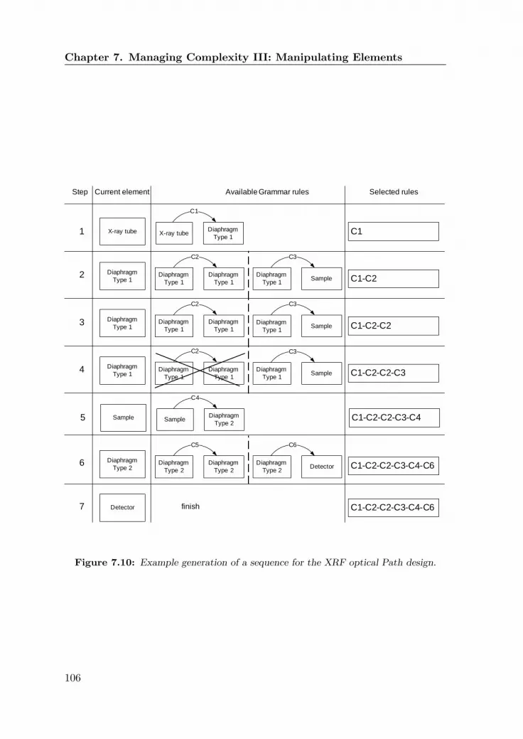
Chapter 7. Managing Complexity III: Manipulating Elements
Current element Available Grammar rules Selected rules
X-ray tube
Step
1 X-ray tubeDiaphragm
Type 1
C1
C1
Diaphragm
Type 12 Diaphragm
Type 1
Diaphragm
Type 1
C2
C1-C2Diaphragm
Type 1Sample
C3
Diaphragm
Type 13 Diaphragm
Type 1
Diaphragm
Type 1
C2
C1-C2-C2Diaphragm
Type 1Sample
C3
Diaphragm
Type 14 Diaphragm
Type 1
Diaphragm
Type 1
C2
C1-C2-C2-C3Diaphragm
Type 1Sample
C3
Sample5 SampleDiaphragm
Type 2
C4
C1-C2-C2-C3-C4
Diaphragm
Type 26 Diaphragm
Type 2
Diaphragm
Type 2
C5
C1-C2-C2-C3-C4-C6Diaphragm
Type 2Detector
C6
Detector7 finish C1-C2-C2-C3-C4-C6
Figure 7.10: Example generation of a sequence for the XRF optical Path design.
106

Chapter 8Managing Complexity IV:Manipulating Parameters
This chapter presents a method for determining appropriate solving ordersof networks of parameters in problem instances. In terms of ADT, thealgorithm determines the order in which the DM of a problem instance canbe solved.
8.1 Introduction
As it was described in Chapter 7, time-independent imaginary complexity in prob-lem instances originates from uncertainties in knowing the order in which DPs canbe solved. When the problem has many DPs, choosing a solving path at the handof the problem’s DM is not straight forward. While Chapter 7 described methodsfor determining how to instantiate elements, this chapter focuses on parametersrelated by analysis, physical coherence constrains, and knowledge rules relations.These relations can be explicitly written as mathematical models, but can alsobe graphically represented using knowledge graphs, as proposed by [57]. In thischapter, these directed graphs are used to represent the network of parametersand relations, and explain the basis of the algorithm.
8.1.1 Knowledge Graphs (KG)
Knowledge Graphs represent the network of deterministic knowledge and the pos-sible paths through the network to resolve all parameters and find a solution.Knowledge graphs (KG) consist of nodes and directed edges. Nodes representparameters and the directed edges describe the relations among each parameter.The directions of the edges are pointed toward the parameter to resolve. Forexample, if node D has N ingoing edges, the parameter represented by node D
107

Chapter 8. Managing Complexity IV: Manipulating Parameters
2 2
2
1 1
1
dwire
w
D
Lc
n
Figure 8.1: Knowledge graph of equation 8.1 and equation 8.2.
requires N other parameters to be known in order to resolve it. The knowledgegraphs edges are labeled according to the relations to which they belong. Anexample of such a knowledge graph is shown in Figure 8.1. This graph representsequation 8.1 and equation 8.2, used in the design of a compression spring. Thefirst equation describes the winding ratio w as a fraction of the spring diame-ter D and the wire diameter dwire. The second describes the maximum springcompression Lc as function of the number of coils n and the wire diameter dwire.
w =D
dwire(8.1)
Lc = n · dwire (8.2)
Node w has two edges directed toward it, meaning that its value can be re-solved if the values of D and dwire are known. As shown in Figure 8.1, theparameter value of dwire has no edges toward it. This means dwire cannot beresolved with this equation. The reason is that the allowed values of dwire arediscontinuous (specified by a DIN standard), and a calculated value from equa-tion (1) is not guaranteed to be exactly a DIN value. Therefore, dwire has to beresolved by another rule before equation (1) can be used to resolve either w orLc.
8.2 Method 5: KGM Solving Algorithm
The KGM algorithm aims at determining orders in which parameters related byACO-relations can be solved. It does so at the hand of two complexity measuresthat can be calculated for each of the parameters in the problem, namely, theeffort E and the influence Inf. The effort measures the number of parametersthat have to be known in order to resolve a parameter with a certain equation.The influence measures the number of parameter that can be solved by solving thisparameter. Furthermore, the algorithm is also based on four states a parametercan have: unknown, known, driver and driven. At the beginning of the problem,
108

8.2 Method 5: KGM Solving Algorithm
all parameters have the state unknown. Then, as the designers set requirements onthe problem, some parameter take the state known. A driver state corresponds toparameters that are instantiated by an algorithm (e.g. randomly) or by a designdecision, while a driven state defines a parameter that can be calculated in arelation where the values of all other parameters are known. By assessing thevalues of the effort and the influence of each parameter, the algorithm chooseswhich parameter should become driver and which becomes driven as consequenceof that decision.
8.2.1 Knowledge Graph Matrix (KGM)
The first step in the method consists in assembling the Knowledge Graph Matrix(KGM) of the problem. The adjacency matrix of a directed G on n vertices isthe n × n matrix where the non diagonal entry aij is the number of edges fromvertex i to vertex j, and the diagonal entry aii is number of loops at vertex.However, given the form of knowledge graphs (KG), no loops are present andtherefore the diagonal entries remain empty. Furthermore, each entry in thematrix is accompanied by the equation id related to that entry. For the case ofthe knowledge graph in Figure 8.1, the corresponding adjacency matrix wouldtake the following form:
KGM =
dwire D w Lc n
dwire 0 1(1) 1(1) 1(2) 1(2)D 0 0 1(1) 0 0w 0 1(1) 0 0 0Lc 0 0 0 0 1(2)n 0 0 0 1(2) 0
(8.3)
8.2.2 Effort and Influence
Two measures are used to assess how each node of the knowledge graph is relatedto the others. These two measures are used to determine which parameters are“easier” to solve and which will help solving most of the left unknown parameters.The first case corresponds to the parameter with the lowest effort, while the secondcorresponds to those with the largest influence.
Effort
Each node, or parameter, has an effort (E ) for each of the relations in which it isincluded. The effort represents the number of parameters that have to be knownin order to resolve a parameter with a certain equation. In a knowledge graph,the effort in one relation of one parameter corresponds to the sum of all the edgespointing towards that node.
109

Chapter 8. Managing Complexity IV: Manipulating Parameters
Using the matrix representation, the effort of a parameter p in a relation n iscalculated by:
Ep,n =l∑
i=1
KGM (i, p) (8.4)
where l equals the number of rows of the KGM. Furthermore, if one column of thematrix has entries that relate this one to others, the effort of the correspondingparameter is set to 1,which represents the effort the parameter requires for solvingitself.
Influence
Each node, or parameter, has an influence (I ) that measures the number of rela-tions in which this parameter is present. This equals the sum of all relation presentin the row corresponding to a given parameter and is calculated as follows:
Inp =l∑
i=1
KGM (p, i) (8.5)
where l equals the number of columns of the KGM. If one row does not containentries, the parameter related to it has an influence equal to zero. This meansthat this parameter cannot be used to solve others.
Parameter dwire D w n LoEffort 1 2(1) 2(1) 2(2) 2(2)Influence 4 1 1 1 1
Table 8.1: Efforts and influences at problem class.
In Table 8.1 the efforts and influences of the KGM shown in equation 8.3 arepresented. As the table shows, the parameters D, w, n and Lc have all effortequal to 2 and influence equal to 1, while the parameter dwire has an effort equalto 1 (which is the effort of solving itself) and an influence equal to 4. This suggestthat for this case dwire is the easiest variable to solve as well as it is the parameterthat if solved will help the most parameters to be solved.
8.2.3 Parameter States
In a design problem, a parameter can have two states, namely, known and un-known. In the first case, the parameter has been instantiated, and its valueimposes a requirement on the problem. The second case corresponds to the pa-rameters the designer is interested in solving.
110
8.2 Method 5: KGM Solving Algorithm
A parameter can become known according to two possibilities:
1. As a design decision of the designer or, in the case of automated design, byan algorithm (e.g. randomly).
2. By calculating it from with a relation where precisely one parameter isunknown.
In this method, these cases are regarded as two more states possibilities of aparameter. The first one is termed as driver state, as the parameter being instan-tiated will drive the calculation of other unknown parameter. The second caseis termed driven state, as the instantiation is driven by the previous algorithmicinstantiation of other parameters. According to this, the four states a parametercan have in this approach are: known, unknown, driver and driven.
In these terms, the goal of solving a design problem is to transform parameterwith unknown states into known, driver and driven states such that valid solu-tions are found or a certain objective function is maximized or minimized. It isimportant to differentiate between the optimization or constrain solving problemand the one this method aims at. As this is concerned with defining the orderin which parameter have to be instantiated, the optimization or constrain solvingalgorithm for solving the values of the parameters are not further studied. Thethree possible types of state transition are:
1. Unknown-known: occurs when the problem statement is being made byattributing a value to one parameter as a requirement the design has tosatisfy. Is attributed to the change from problem class to problem instance.
2. Unknown-driver: occurs by attributing a value to a parameter accordingto a design decision or an algorithmic step (e.g. by randomly attributinga value). Is attributed to the change from problem instance to problemsolution.
3. Unknown-driven: occurs when the effort of a parameter becomes zero afterKGM recalculation. This means that this variable can be calculated by usingthe relation attributed to the effort that became zero. Is also attributed tothe change from problem instance to problem solution.
8.2.4 KGM Transformations
As it will be explained later, each time a state transition occurs, the KGM changesand has to be recalculated. Recalculating the KGM is performed by:
1. Eliminating all entries in the row and the column that corresponds to thatparameter from the KGM.
2. Recalculating all efforts and influences according to equations 8.4 and 8.5.
111

Chapter 8. Managing Complexity IV: Manipulating Parameters
Parameter dwire D w n LoEffort 1 0 1(1) 2(2) 2(2)Influence 3 0 0 1 1
Table 8.2: Efforts and influences for problem instance with D known
Consider the example of the KGM in equation 8.3. If one assumes that theparameter D (spring diameter) is set as known and all the others are unknown, theKGM is transformed as shown in equation 8.6, obtaining the efforts and influencesshown in Table 8.2.
KGM =
dwire D w Lc n
dwire 0 0 1(1) 1(2) 1(2)D 0 0 0 0 0w 0 0 0 0 0Lc 0 0 0 0 1(2)n 0 0 0 1(2) 0
(8.6)
8.2.5 Identifying Driver and Driven
The essence of the KGM algorithm resides in choosing drivers and identifyingwhich parameter becomes driven as consequence of the that decision. Driversare identified by choosing the parameter with the lowest effort. If the value ofthe minimum effort is shared by more than one parameter, then the parameterwith the highest influence among them is chosen. By doing so, it is avoided thattwo parameter become over constrained as the algorithm progresses. This alsominimizes the effort of other parameters. In the case that the minimum effortand the highest influence are shared by more than one parameter, either one ofthe parameters can be chosen as driver parameter.
Consider the efforts and influences in Table 8.2. As it can be seen, the pa-rameter dwire has the lowest effort. As no other parameter has an effort equal tothat of dwire, this parameter becomes automatically a driver parameter.
Drivens are identified as those parameters whose effort becomes 0 (zero) aftera KGM transformation has taken place. In this case, this parameter can becalculated by using the relation corresponding to the effort that became 0 (zero).
112

8.2 Method 5: KGM Solving Algorithm
Identified
knowns? Transform KGMyes
Identified
drivens?
Identified
drivers?
yes yes
Assemble KGMCalculate Efforts
and Influences
no
no
no
finished
Identify knowns
Identify drivens
Identify drivers
Figure 8.2: KGM solving algorithm.
8.2.6 The Algorithm
Having presented the KGM, its transformations and a method for identifyingdrivers and drivens, the algorithm for recognizing the sequence in which to solvea parametric design problem is presented in Figure 8.2.The steps in the algorithmare the following:
1. Make a knowledge graph including all relations and parameters.
2. Assemble the KGM and calculate efforts and influences.
3. Identify which parameters have been attributed as known and transformthe KGM.
4. Identify if any variable has changed it state from unknown to driven. If thisis the case, perform a KGM transformation. This step is continued until noparameter change to driven state.
5. Identify one driver parameter and transform the KGM.
6. Repeat steps 3, 4 and 5 until all parameters are changed to the state driven,driven or known.
Table 8.3 shows the results of applying the algorithm on the example shown inTable 8.2. As the table shows, the state transition occurs when setting the valueof D to known in step 1. In step 2, the recalculated efforts and influences areshown. Here, the variable dwire is identified as the best to be changed into driver.
113

Chapter 8. Managing Complexity IV: Manipulating Parameters
Table 8.3: Result of KGM transformations in example.
Parameter dwire D w n LoStep 1 Effort 1 2(1)* 2(1) 2(2) 2(2)
Influence 4 1 1 1 1Step 2 Effort 1** 0 1(1) 2(2) 2(2)
Influence 3 0 0 1 1Step 3 Effort 0 0 0*** 1(2) 1(2)
Influence 0 0 0 1 1Step 4 Effort 0 0 0 1(2)** 1(2)
Influence 0 0 0 1 1Step 4 Effort 0 0 0 0 0***
Influence 0 0 0 0 0State transition: * unknown-known, ** unknown-driver, *** unknown-driven
Fix
D
Set Dwire
as driver
Driven w with
relation 1
Set n
as driver
Drive Lo with
relation 2
Figure 8.3: Example of strategy.
It can also be seen that the variable w gets an influence of zero, as this parametercannot influence solving others. In step 3, the recalculated KGM measurementsindicate that w becomes driven, as its effort drops to zero. As w is only containedin relation 1, its effort only depends on this equation. Therefore, the value of wcan be calculated by using equation 1 in combination with the previously definedvalues of D and dwire. In step 2, the parameter n is chosen as driver, as no otherparameter became driven. However, parameter Lo could have also be chosen,as its effort and influence values equals the one of n. As result of a new KGMtransformation, parameter Lo becomes driven with equation (2).
The result of applying the algorithm is a sequence of proposed parameters statetransitions. The sequence can be outlined by keeping track on the order in whichparameter states change from unknown to known, drivers and driven. In the caseof driven, the relations through which they are calculated have to be recordedtoo. After this algorithm is applied to a given parametric design problem, theresulting sequence can be used by a constraint solving or optimization algorithmto search for the numerical solution of the problem. For the example in Table 8.3,the resulting sequence is shown in Figure 8.3.
114

8.3 Benchmarking
8.3 Benchmarking
In [30] a survey of decomposition methods for constraint systems is presented.Here, decomposition methods have been investigated from different perspectives,and compared against each others. One consists in identifying subsystem as an in-teresting (i.e., solvable) subsystem. A second approach aims at identifying pointsof weakness in the constraint system for partitioning the problem. A third oneconsists in identifying subsystems as solvable provided that the complementarysubsystem is solvable as well. The fourth, denominated recursive division meth-ods, works by iteratively splitting the constraint system into components, them-selves subject to further splitting. The review finishes by proposing two propertiesthat are desirable to meet real-life applicative requirements: generality and relia-bility.
This algorithm differentiates from the ones presented in [30] as follows:
1. The directed graph consists of nodes denoting the parameters, and arcsdenoting its relations, while the adjacency graph of the methods in [30] iscomposed of nodes that represent both the parameters and the relations.Arcs are used to describe which parameters are involved in which relations.The adjacency matrix of this graph allows solving asymmetric problems.Asymmetric problems are those in which at least one relation contains aparameter that is not solvable as function of the others.
2. The decomposition is based on two complexity measurements, namely, theeffort and the influence. Because of the generality of the approach, thealgorithm can be used in different types of CS problems, as for example,geometric and topological problems.
3. The KGM algorithm does not recognizes systems of equations, and is there-fore limited to be used in under-constrained problems. Other algorithmsdiscussed in [30] do have the capability of recognizing systems of equationsand over-constrained problems.
8.4 Example: Compression Spring
The parametric design of a compression spring is used to demonstrate the algo-rithm at the hand of one combination of known and unknown parameters. Acompression spring is modeled as a single element with 11 parameters and 6 re-lations (material is kept constant). The parameters are stated in Table 8.4 andthe relations in equation 8.7 - 8.12. An ID has been attributed to each relation.Figure 8.4 shows the KG of this example with the IDs of each relation appearingalong the arcs. At the hand of the KG, the KGM is assembled and the effortsand influences of each parameter are calculated, as shown in Table 8.5 and 8.6respectively.
115

Chapter 8. Managing Complexity IV: Manipulating Parameters
Table 8.4: Parameters considered in compression spring design.
Parameter DescriptionD mean diameterd wire diametern number of coilsA space between coilsL0 uncompressed lengthLs compressed lengthLc maximum compressed lengths compressionsc maximum compressionR spring constant (stiffness)F force at compression
R =G
8· d4
D3 · n7→ ID = 1 (8.7)
F = R · s 7→ ID = 2 (8.8)
L0 = s+ Ls 7→ ID = 3 (8.9)
L0 = sc+ Lc 7→ ID = 4 (8.10)
Lc = n · d 7→ ID = 5 (8.11)
L0 = n · (A+ d) 7→ ID = 6 (8.12)
The combinations of known and unknown that have been used to demonstratethe algorithm is shown in Table 8.7.
In Table 8.8 the efforts and influences that result from applying the algorithmare presented, while Figure 8.5 shows the resulting sequence. As it can be seen,some parameters have more than one effort value attributed. This is the con-sequence of having some parameters present in more than one equation. Thetable also shows that the parameter sc becomes driven with equation 8.10 afterrecalculating the KGM for the known parameters. This is due to the fact thatall parameters in relation 8.10, except sc, have an attributed value. In step 4, itcan be seen that although the parameters s, R and Ls have the same minimumvalue of the effort (effort = 1), the parameter s is chosen as driver. The reason fordoing so is that the influence of s is larger than that of the parameters R andLo,which means that attributing a value to this parameter will reduce the effort oftwo other parameters, speeding the course of the algorithm.
116

8.4 Example: Compression Spring
Figure 8.4: Knowledge graph of spring design. 117

Chapter 8. Managing Complexity IV: Manipulating Parameters
Table 8.5: KGM of compression spring design.
D d n A Lo Ls Lc s sc R FD 1(1) 1(1) 1(1)d 1(1) 1(1)
1(5)1(6)
1(6) 1(6) 1(5) 1(1)
n 1(1) 1(1)1(5)1(6)
1(6) 1(6) 1(5) 1(1)
A 1(6) 1(6) 1(6)Lo 1(6) 1(6) 1(6) 1(3) 1(4) 1(3) 1(4)Ls 1(3) 1(3)Lc 1(5) 1(5) 1(4) 1(4)S 1(3) 1(3) 1(2) 1(2)Sc 1(4) 1(4)R 1(1) 1(1) 1(1) 1(2) 1(2)F 1(2) 1(2)
Table 8.6: Initial efforts and influences.
Parameters D d n A Lo Ls Lc s sc R FStart E 3(1) 3(1)
3(6)2(5)
3(1)3(6)2(5)
3(6) 3(6)2(4)2(3)
2(3) 2(5)2(4)
2(2)2(3)
2(4) 2(2)3(1)
2(2)
Inf 3 8 8 3 7 2 4 4 2 5 2
118

8.4 Example: Compression Spring
Table 8.7: Problem instance of spring design example.
Parameter StateD unknownd unknownn unknownA unknownL0 KnownLs unknownLc Knowns unknownsc unknownR unknownF Known
Lo Lc F Sc
ndAD0
R s Ls
Dv
Dr
K
Known
Parameter
Driver
Parameter
Driven
Parameter
K K
Dr
Dv
DvDv
Dv Dv Dv
Dr
K
Figure 8.5: Instantiating order of parameters in spring example.
119

Chapter 8. Managing Complexity IV: Manipulating Parameters
Table 8.8: Results of KGM transformation in example.
D d n A Lo Ls Lc s sc R FStep 1 E 3(1) 3(1)
2(6)1(5)
3(1)2(6)1(5)**
2(6) 0*
1(3) 0*
2(2)1(3)
0(4) 2(2)3(1)
0*
Inf 3 6 6 2 0 1 0 2 0 4 0Step 2 E 2(1) 2(1)
1(6)0(5)***
0 1(6) 0 1(3) 0 1(2)1(3)
0 1(2)2(1)
0
Inf 2 3 0 1 1 0 2 0 3 0Step 3 E 1(1) 0 0 0(6)
***0 1(3) 0 1(2)
1(3)0 1(2)
1(1)0
Inf 1 0 0 0 0 1 0 2 0 2 0Step 4 E 1(1) 0 0 0 0 1(3) 0 1(2)
1(3)*
0 1(2)1(1)
0
Inf 1 0 0 0 0 1 0 2 0 2 0Step 5 E 1(1) 0 0 0 0 0(3)
***0 0 0 0(2)
1(1)***
0
1. Inf 1 0 0 0 0 0 0 0 0 0 0Step 6 E 0(1)
***0 0 0 0 0(3)
***0 0 0 0(2)
1(1)***
0
Inf 0 0 0 0 0 0 0 0 0 0 0State transition: * unknown-known, ** unknown-driver, *** unknown-driven
120

Part IV
Results and Conclusions
121


Chapter 9Integration andImplementation
This Chapter discusses the integration of the methods discussed in Chapters5, 6, 7 and 8. Two computer implementations demonstrating the resultingmethod are presented: one generic toolbox to test the proposed methods andone specific implementation that automates CSIM design.
9.1 Introduction
This chapter explains how the methods proposed for complexity managementare integrated into a methodology for CDS. The resulting methodology is namedCDS by Complexity Management (CDS-CM). A preliminary generic software im-plementation of this methodology has been developed, and is described in Ap-pendix C. The design of a transmission system, presented in Subsection 9.2.4, isused as example to demonstrate it. Section 9.3 presents an specific implementa-tion of this methodology to CSIM design.
9.2 Methodology: CDS-Complexity Management
The flow chart in Figure 9.1 shows how the techniques proposed in this thesis canbe integrated to result in a methodology for CDS: CDS by Complexity Manage-ment (CDS-CM). The methodology consists of two general phases: initializationand generation. The initialization phase consists of transforming the design prob-lem into a formal model of a problem class. The generation phase takes over theautomatic generation of design solutions.
123

Chapter 9. Integration and Implementation
Decompose
problem
Assemble
ToSE equations
Find implicit
cardinalities
Select abstraction
group to solve
Generate
sequence
Generation Phase (Problem Instance)
Initialization Phase (Problem Class)
Make TARD
model
Identify parameters of
instantiated elements
Assemble and solve KGM
for identified parameters
Check
consistency
Formulate
problem
Set and specify
requirements
Solutions
FBS problem
formulation
ADT based
decomposition
Local Grammar
Method
Figure 9.1: General procedures in CDS by Complexity Management.
9.2.1 Initialization Phase
The initialization aims at developing formal and consistent design problem mod-els. This is achieved by:
1. Problem formulation: consists in obtaining a consistent model of the in-formation contents of the problem as proposed in Chapter 3. This thesisproposes FBS design formulation as means of performing this task.
2. Problem decomposition: consists in reducing the dimensionality of the prob-lem by decomposing it into smaller problem chunks with lower degrees ofcomplexity. By doing so, search processes in the generation phase can fo-cus on specific levels of abstraction. This thesis proposed ADT problemdecomposition as a method for doing so.
3. Making the TARD model: consists of representing a problem class by meansof the four types of building blocks in TARD: Elements, C-relations, H-relations and ACO-relations. Once the problem is translated into its TARDform, its formulation can be reused for different problem instances. Further-more, the model can be integrated into other TARD models to be reused inother design problem formulations.
4. Assembling ToSE equations: Is done as explained in Chapter 7. These
124

9.2 Methodology: CDS-Complexity Management
equations allow setting requirements on the problem’s topology. During thegeneration phase, ToSE equations allow controlling the generation of designsolutions.
9.2.2 Generation Process
Once the initialization phase is completed, a generation phase determines how toinstantiate the elements and relations in the problem. It is important to noticethat the method only determines strategies, or orders, in which the problemscan be solved. The algorithms for instantiating these building blocks have beenkept out of the scope of this research. The generation procedure consists of fouractivities: (1) checking the consistency and calculating implicit cardinalities, (2)selecting an abstraction-groups, (3) solving that abstraction-group by generatingsequences, and (4) solving the values of the parameters contained in each element.
Checking Consistency
After ToSE is derived, the first operation performed is to check for inconsistenciesin the cardinality values. A consistent set of equations is required for determiningvalid solutions. There are two consistency rules that have hold:
1. Balance equations have to meet equality.
2. The value of each cardinality has to be a positive integer.
In case that not all cardinalities are known, the ToSE equations are usedto determine if any other cardinality can be directly computed. This operationreduces the degree of freedom of the problem.
Identifying Abstraction-group to Solve
The KGM algorithm described in Chapter 8 is applied to ToSE to identify whichabstraction-group to solve, as indicated in Figure 9.2(a). The ToSE equations andthe cardinalities values are fed into the KGM algorithm, obtaining a list of drivercardinalities. The cardinality with the lowest effort determines the abstraction-group to solve. As the successive generation of a sequence will fix the cardinalitiesof other elements and relations, the KGM algorithm has to be applied recursivelyafter obtaining the solution of one abstraction-group, as indicated in Figure 9.2(b).
Generating Sequences
Simple abstraction-groups are solved by attributing values to the elements car-dinalities according to the order prescribed by the KGM algorithm. In complexabstraction-groups, sequences are generated using the Local Grammar methoddescribed in Section 7.3.
125

Chapter 9. Integration and Implementation
BalanceEquations
VerticalEquations
Input Output
Strategy List
(Driver/Driven)
Cardinalities
effort
cardinalities
ca
rdin
alit
ies
KGM Algorithms
(a) KGM input and output.
Find implicitly
given cardinalities
Decide which
Abstraction-group
to solve
Generate
sequence
KGM
(b) Abstraction-group selection algorithm.
Figure 9.2: Choosing abstraction groups.
Identify first
element
Identify local rules
of element
Evaluate
complementary rules
Select rule
to apply
Instantaite rule Identify edge elementFinish ?
NO
YES
Figure 9.3: Generation algorithm for local grammar method.
Figure 9.3 shows a simple algorithm for generating sequences using this method.The local grammar rules are selected by checking the references to outgoing C-relations of the element at hand. Thereafter, it is checked if any complementaryrules can be applied. The choice of which of the remaining rules to choose isdone by following a certain algorithm, e.g. randomly. If the cardinalities i andj of the chosen C-relation are not known yet, they have to be generated. Gen-erated sequences are stored as a sequence object in the corresponding H-relationinstance. The corresponding cardinalities are calculated according to the sequenceequations. If the KGM analysis does not result in any more drivers or drivens,the topology of the problem is completely defined and is not subject of furthergeneration.
126

9.2 Methodology: CDS-Complexity Management
Identify
instantiated
elements
Identify ACO-
relationsAssemble KGM
Solve KGMInstantiate
Parameters
New
Cardinalities
values?
NO
YES Finish
Figure 9.4: Identifying and solving parameter values.
Identifying and Solving Parameter Values
Instantiated elements have parameters with no values assigned. These steps con-sists in identifying which parameters appear as consequence of instantiating el-ements, and attributing them with values, as indicated in Figure 9.4. In orderto do so, the ACO-relations in which the parameters are present are listed too.This information is then used to assemble a KGM and determine the order inwhich they can be solved. In case the proximity relations (also an ACO-relation)determines the instantiation of an element, the procedure is repeated taking intoaccount the parameters of the instantiated elements.
9.2.3 Generic Implementation
The method described in Section 9.2 has been implemented into a generic soft-ware toolbox. The software automatically generates solutions for design problemsrepresented by a TARD model. Appendix C describes the generalities of the im-plementation of the TARD building blocks and the construction of the ToSEequations.
9.2.4 Example: Drive train Design
This example considers a schematic composition of a vehicle drivetrain, as forexample the one shown in Figure 9.5. The goal of this example is to show thecollaborative integration of TARD, the Local Grammar method, ToSE and theKGM algorithm by the implemented toolbox. For explanatory reasons, paramet-ric descriptions of the elements have not been taken into account.
Problem class
The TARD model of this example is shown in Figure 9.6. It consists of 16 el-ements (in addition to the zero-level element) and three abstraction-groups formore detailed levels. The only complex abstraction-group corresponds to H1.
127

Chapter 9. Integration and Implementation
Motor
Gearbox
Differential
Figure 9.5: Sketch of a drivetrain in a car.
Depending on the amount and position of known cardinalities, the solution spaceand shape changes and expands.
Problem instance
The objective of this problem instance is to generate a topology that does notviolate the constrains imposed by the specified cardinalities, which are:
• One motor, connected to one axle1: eMotor = iC1 = jC1 = 1.
• One input shaft and one output shaft per gearbox:eGearinputShaftlocal = eGearoutputShaftlocal = 1.
• Due to their functions, the components of the differential are all connectedone-on-one, with the exception of the one-on-two connection between theplanetGear and sideGear: (i, j) C12 = C13 = C15 = iC14 = 1 andjC14 = 2
• A two-on-one C-relation for C3: iC3 = 2 and jC3 = 1.
• Two wheel axes connected to the differential: iC5 = 1 and jC5 = 2.
The last point poses an interesting test for the application: there should betwice as many instances of the element differential as of the element axle2. Thenext step is to feed this graphical network together with the defined cardinalityvalues into the application in order to obtain a 1st order representation com-posed of 1st order elements, C-relations and H-relations object instances. This isachieved by hard coding the data into the application by means of an input class.On the basis of this input, the algorithm is able to derive a solution in the formof a 2nd order network.
128

9.2 Methodology: CDS-Complexity Management
Moto
r
C1
Axle
1G
ea
rbo
xA
xle
2D
iffe
rential
Axle
3W
heel
Gearinput
shaft
Gearo
utp
ut
shaft
Gears
haft
Gear
C7
C9
C11
C8
C10
H1
C2
C3
C4
C5
C6
DiffI
nput
shaft
Rin
gG
ear
Pla
netG
ear
Sid
eG
ear
DiffO
utp
ut
shaft
C12
C13
C14
C15
H2
DriveT
rain H0
0
Figure 9.6: TARD representation of drive train example.
129

Chapter 9. Integration and Implementation
Problem solution
Figure 9.7 shows one of the automatically generated solutions for the probleminstance descrived before. This solution demonstrates the functionality of theimplementation, especially in the treatment of the system of equations. The 2nd
order network resulting from the determination of the cardinalities representsthe topological solution for a drivetrain design. Here, the names of the elementinstances are followed by an index starting at zero, which serves as ID for identi-fying different instances of the same element class. For example, gearbox00 andgerbox01 resemble the first and the second instance of the type gearbox. Thesolid arrows represent C-relation instances connecting the element instances. AC-relation connecting one to two elements and vice versa is represented by two sep-arate arrows, as for example between elements Axle1 and Gearbox. Accordingly,the dotted curved arrows indicate the H-relation instances, which are pointingtowards the C-relation instances in the respective abstraction-groups.
The design solution generated by the method consists of a single motor con-nected to two gearboxes via a single axle. There are two gearboxes connected toa single axle, which in turn drives two differentials. Finally, the two axles behindeach differential are connected to a single wheel. It is worth mentioning that themultiple existence of the abstract elements gearbox and differential have resultedin two independent instances of their abstraction-groups. Proof of a correct ex-ecution is the existence of twice as much gearbox instances as Axle2 instances.As the network is consistently connected, it is demonstrated that all unspecifiedcardinalities are properly calculated or generated according to the theory.
The generated solution (single motor, double gearbox and double differential)is analogous to the drivetrain of four-wheel drive vehicles having a normal andlow range gearbox with differential at each axle.
130

9.2 Methodology: CDS-Complexity Management
Figure 9.7: The resulting 2nd order instantiated network representing a solution of thegeneration process (generated automatically by the implementation.)
131

Chapter 9. Integration and Implementation
9.3 Automating CSIM Design
Applying the complexity management techniques to CSIM design has resultedin a a bottom-up recognition approach (see Subsection 7.3.4). The methodand algorithms for cooling generation have been implemented using C#© [55].SolidWorks© [14] is used as interface for modeling the 3D mold parts. Further-more, a User Interface (UI) was developed using SolidWorks© API [14]. Thissection presents the automation method from a general point of view, and theresults from its implementation into a software tool.
The first and second steps of the initialization phase have been performed inthe examples shown in Chapter 5. This result is used to build the TARD modelpresented in Figure 9.8. The considerations taken for making the TARD modeland the ToSE equations that follow from this model are presented in AppendixB.
9.3.1 Synthesis Strategy
Figure 9.9 presents a summary of the steps in the CSIM design automation strat-egy that follow from the TARD model and ToSE equations. The method consistsof:
1. Making a voxel model of the solid parts Mold Part and Plastic Parts. Thisstep consists in transforming the requirements from the shape model intofields, as indicated in Chapter 5, Subsection 5.3.3.
2. The second step consists in generating a mesh of Points on top of the voxelmodel and attributing color to the points according to the relations shownin Table 5.3. By doing so, a pool of elements Points is obtained. As con-sequence, the abstraction-groups absorberChannels, connectorChannel, in-putSegment and outputSegments, are generated by using a recognition ap-proach, as indicated in Subsection 7.3.4.
3. Generating absorberChannels by connecting points using the Local Gram-mar method and a recognition approach.
4. Generating cooling circuits by connecting Absorber channels with Connectorchannels. The later are generated by assembling pairs of green points alsousing the Local Grammar method and a recognition approach. Furthermore,by connecting Absorber channels and Connector channels to inputSegmentand outputSegments fully defined circuits are obtained.
5. Generating cooling systems is performed by assembling combinations of thepreviously generated cooling circuits. Here again, all obtained circuits forma pool of elements from where a recognition approach determines possiblecooling system configurations.
132

9.3 Automating CSIM Design
Inp
utS
eg
me
nt
C1
Blu
eP
oin
t
H1
C11
Co
olin
gS
yste
m
H0
Co
olin
gC
ircu
it
Ab
so
rbe
rCh
an
ne
lC
on
ne
cto
rCh
an
ne
lO
utp
utS
eg
me
nt
C2
C3 C4
C6
C5C7
C8
C9
Gre
en
Po
int
Bro
wn
Po
int
C10
Blu
eP
oin
tG
ree
nP
oin
tB
row
nP
oin
t
C17
C16
Blu
eP
oin
t
C12
Blu
eP
oin
tG
ree
nP
oin
t
C14
C13
H2
H3
H4
H5
Le
ve
l 0
Le
ve
l 1
Le
ve
l 3
Le
ve
l 2
C15
Figure 9.8: TARD model of CSIM problem.
133

Chapter 9. Integration and Implementation
The initial state of the problem
consist of mold parts
Mold parts and plastic parts are
discretized into voxels.
A grid of points is generated on top
of the voxel mesh. Each point gets a color that
determines its functionality.
Blue points are connected creating
Absorber Channels.Connection channels and
Exchanger form circuits.
Figure 9.9: Method for automating CSIM design.
134

9.3 Automating CSIM Design
Figure 9.10: Mold of telephone used as example.
Table 9.1: List of attributes of a voxel element.
Attributes Description ModelCore Identifies the core of the mold Boolean
Cavity Identifies the cavity of the mold BooleanProduct Identifies the product or plastic part of the mold Boolean
Inlet/outlet Identifies if a surface is used for inlets or outlets BooleanNon drillable Identifies if a surfaces cannot be drilled Boolean
Size Defines the size of the vertices of the voxel BooleanPosition Defines the position of the voxel double [i,j,k]
The ToSE (shown in appendix B) equations are used to keep topological con-sistency of the resulting solutions. The following sections explain each of the stepof the method at the hand of telephone mold example shown in Figure 9.10.
Voxel Mesh Generation
Creating a mesh of voxels is the first step of this method. By using voxels, thegeometric model can be transformed into a logic one. The idea of using voxelsresulted from applying the ADT Based Decomposition to the physical domain.Although this transformation results in a loss of geometric information, it alsoeases solving spatial constraints. Table 9.1 summarizes the attributes of a voxelobject. Figure 9.11 shows two sections of the voxel mesh of the telephone moldshown in Figure 9.10. Here, the core is indicated in dark green, the cavity in lightgreen and the part in red.
135

Chapter 9. Integration and Implementation
Horizontal section
Vertical section
Figure 9.11: Sections of the telephone voxel mesh model.
Points Generation
After making the voxel mesh, a 3D grid of points is generated. This grid is setinside the voxel mesh model of the mold. The distance between points in thegrid is based on relation PCC-2, whos values can be found in [28]. The objectiveof this step is to define the spatial locations in the mold where cooling channelscan eventually be placed as well as those places where it cannot. To do so, a“color” is attributed to each point in the grid. This assigned attribute is used tocharacterize the function of the point. These are:
• Blue: defines points that can be used to create an Absorber channel.
• Green: defines points that can be used to create a Connector channels.
• Brown: defines points on the surface of a core and cavity where Exchangerchannels can be placed.
• Grey points: define points nearby the melt where channels cannot be placedto overcome mold break.
• Black points: define points where channels cannot be placed to avoid moldbreak.
136
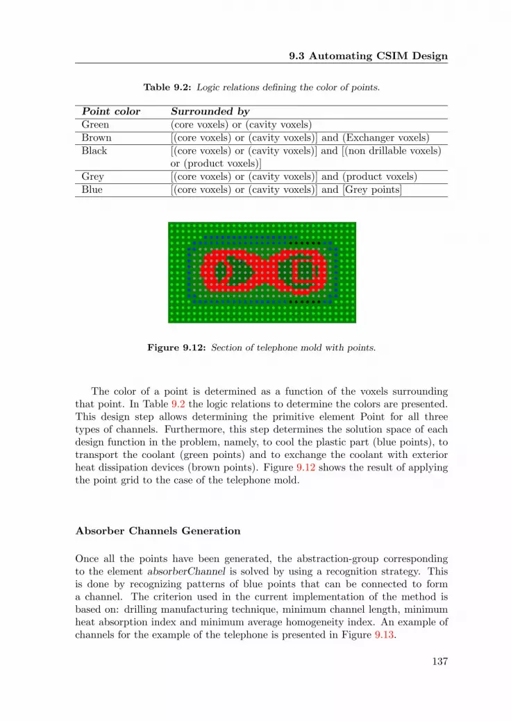
9.3 Automating CSIM Design
Table 9.2: Logic relations defining the color of points.
Point color Surrounded byGreen (core voxels) or (cavity voxels)Brown [(core voxels) or (cavity voxels)] and (Exchanger voxels)Black [(core voxels) or (cavity voxels)] and [(non drillable voxels)
or (product voxels)]Grey [(core voxels) or (cavity voxels)] and (product voxels)Blue [(core voxels) or (cavity voxels)] and [Grey points]
Figure 9.12: Section of telephone mold with points.
The color of a point is determined as a function of the voxels surroundingthat point. In Table 9.2 the logic relations to determine the colors are presented.This design step allows determining the primitive element Point for all threetypes of channels. Furthermore, this step determines the solution space of eachdesign function in the problem, namely, to cool the plastic part (blue points), totransport the coolant (green points) and to exchange the coolant with exteriorheat dissipation devices (brown points). Figure 9.12 shows the result of applyingthe point grid to the case of the telephone mold.
Absorber Channels Generation
Once all the points have been generated, the abstraction-group correspondingto the element absorberChannel is solved by using a recognition strategy. Thisis done by recognizing patterns of blue points that can be connected to forma channel. The criterion used in the current implementation of the method isbased on: drilling manufacturing technique, minimum channel length, minimumheat absorption index and minimum average homogeneity index. An example ofchannels for the example of the telephone is presented in Figure 9.13.
137

Chapter 9. Integration and Implementation
Section showing cooling channels
Non-overlapping cooling channels
Figure 9.13: Group of aleatory selected absorber channels in the telephone mold.
Circuits Generation
Cooling circuits are designed by combining absorberChannels capable of forminga circuit. This is done by defining sequences of C-relations in the abstraction cor-responding to the element circuit. A recognition strategy is used, following theindications presented in Chapter 7. Knowledge about the construction of feasablesequences are based on knowledge rules of expert designers at Philips ATC. TheA∗ algorithm [36] is used as recognition algorithm that determines paths of con-nectorChannels between absorberChannels. The resulting path determines thelayout of the connectorChannels. Furthermore, inputSegements and outputSege-ments are generated by recognizing which brownPoints are closer to the obtainedcircuits.
Cooling Systems Generation
Cooling systems are generated by recognizing combinations or coolingCircuitssatisfying the physical coherence constrains of the problem. In the implementationdeveloped in this work, this is performed by randomly combining coolingCircuisand assessing if they violate any of the constraints.
138
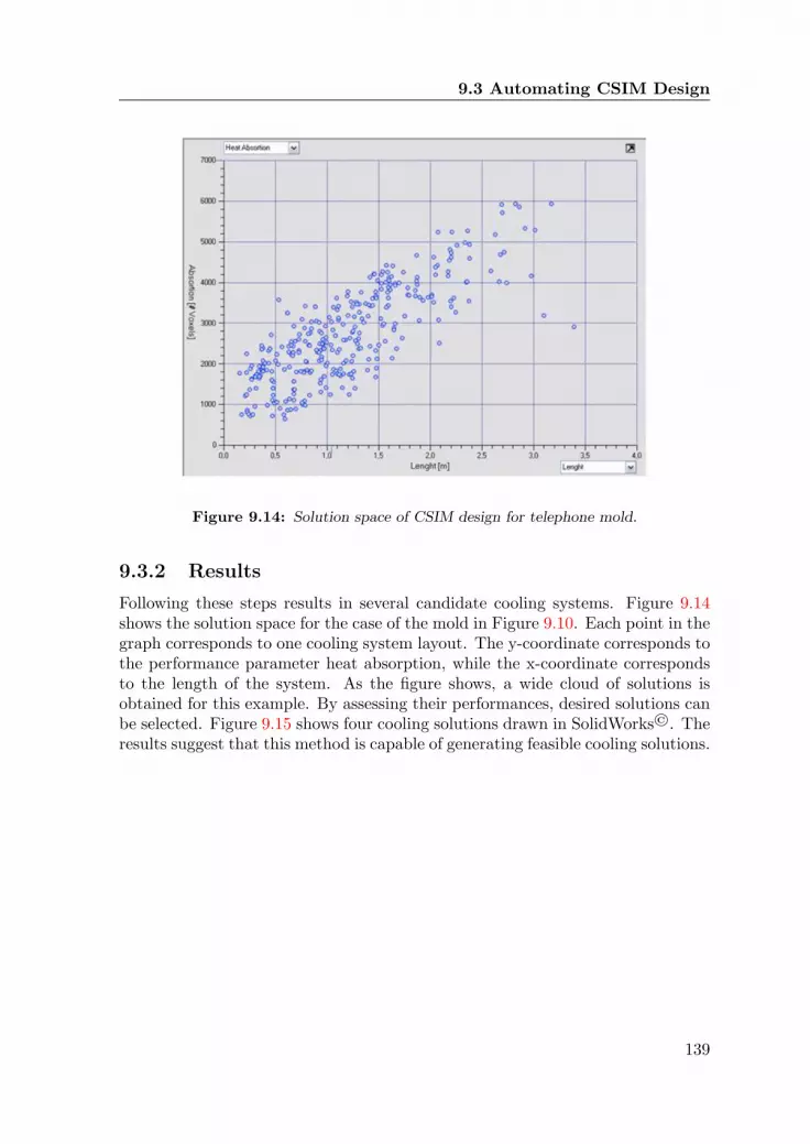
9.3 Automating CSIM Design
Figure 9.14: Solution space of CSIM design for telephone mold.
9.3.2 Results
Following these steps results in several candidate cooling systems. Figure 9.14shows the solution space for the case of the mold in Figure 9.10. Each point in thegraph corresponds to one cooling system layout. The y-coordinate corresponds tothe performance parameter heat absorption, while the x-coordinate correspondsto the length of the system. As the figure shows, a wide cloud of solutions isobtained for this example. By assessing their performances, desired solutions canbe selected. Figure 9.15 shows four cooling solutions drawn in SolidWorks©. Theresults suggest that this method is capable of generating feasible cooling solutions.
139

Chapter 9. Integration and Implementation
Figure 9.15: CSIM design solutions for telephone mold.
140

Chapter 10Conclusions &Recommendations
This chapter presents a discussion on the usage of complexity managementin the development of methods for computational design synthesis. Themain issue is whether such techniques can support the generic developmentof Computer Aided Synthesis tools. The chapter finishes presenting recom-mendations for further research.
10.1 Conclusions
In general terms, automating routine design problems can be performed in twodifferent fashions: developing specific methods for specific problems, or developinggeneric methods for problem families. It is the second approach which can enablethe future development of CAS systems, and the one this thesis dealt with. Suchan approach is confronted with three main challenges. Firstly, design problemshave to be translated into terms that allow their study independent of its semanticcontents, thus to define a common language. Secondly, basic problem character-istics have to be identified, which consists in finding the common ground of theseproblems. And thirdly, general problem solving approaches have to be developed.This thesis contributed to solving these challenges by investigating complexity indesign. Its result is a generic approach for automating artifactual routine designproblems. Its computer implementation demonstrates the method can be usedfor automating such problems. However, further research is required to achievea true generic software for design automation, as it is explained in Section 10.2.The following sections present a discussion on these issues.
141

Chapter 10. Conclusions & Recommendations
First challenge: a common language for routine design
The first challenge has been solved by developing a scheme for formulating arti-factual routine design problems, described in Chapter 3. The scheme has beendeveloped by mapping models of information types found in design literature toschemes for formulating problems found in problem solving theory. The informa-tion contents has been further characterized by classifying commonly used mathe-matical models in design automation in the following groups: parametric, spatial,shapes, fields and topology. This has enabled benchmarking design problems thatat first sight seem very different. The results represent a common language forunderstanding the similarities and differences of between routine design problems.Furthermore, the solution approach to one given problem can be extrapolated toothers, as long as both formulations are equal.
Second challenge: a generic structure for design problem
By making an analogy to the structure of analysis problems (which deal withunderstanding the behavior of “things”), this thesis presents a new frameworkfor structuring design problems. The structure consists of three levels of ab-straction: the problem class, the problem instance, and the problem solution. Aproblem class is formed by non instantiated elements, parameters and relations.A problem instance has partially instantiated elements, parameters and relations,which represent the requirements of the problem. Problem solutions are formedby fully instantiated elements, parameters and relations. This structure allowsgeneralizing design problems by:
• defining the types of representations required for modeling each abstraction,
• studying the complexity of each abstraction by analyzing the configurationof the used representations,
• developing procedures and operations to solve each problem domain, and
• identifying common problem structures.
This framework, described in Chapter 4, constitutes one of the main contri-butions of this work, as it allows studying design problems in abstract terms andidentifying the characteristics of design problems from where complexity arises.
Mapping the structuring framework to ADT model of complexity, has resulteda new model of design complexity for routine design. It has been found that thecomplexity of problem classes is related to the consistency of the information con-tents and the problem formulation. One cause of complexity results from havinga less suitable problem formulation. Another is the lack of differentiation betweenproblem chunks and its interrelations. In this sense, in complex problem classesthe design problem is not addressed correctly and it has a high dimensionality(few levels of abstraction).
Complexity in problem instances depends on:
142

10.1 Conclusions
1. The distribution of the requirements: concentrated in the top abstractionlayers, in the bottom layers or a mix of both.
2. The constrains imposed to the cardinalities of elements. Cardinality is avariable that defines the number of times an element can be instantiated.If cardinalities are unknown and unbounded, the number of instantiatedelements (and therefore the number of parameters) explodes.
As these complexities can be identified independently of problem specific se-mantics, they represent a generic approach for determining what the problem tobe solved is. This brings the issues of solving routine design problems to that ofmanaging their complexity, which verifies the first hypothesis of this research.
Third challenge: generic solving approaches
Different complexity management methods have been developed. Figure 10.1presents an overview of these methods.
Build TARD
model
Assemble ToSE
equations
Elem
ents
C-relat
ions
H-relat
ion
ACO-relat
ions
Pam
eter
sBalan
ce e
quat
ion
Ver
tical e
quat
ions
Car
dina
ities
Loca
l gra
mm
ar m
etho
d
KGM
Solving
algor
ithm
Formulate design
problem
Decompose
design problem
FBS b
ased
form
ulat
ion
ADT b
ased
dec
ompo
sitio
n
Organizing information contents
(Problem class)
Manipulating building blocks
(Problem instance)
Determine
generation
strategy
Representations
Figure 10.1: Integrated approach to complexity management.
Information ContentsA first group consists of two methods that aim at organizing the informationcontents. One method targets the development of consistent problem formula-tions, while the second focuses on decomposing a problem into different levelsof abstraction. Both methods target complexity of problem classes. By usingthe FBS model, the first method is capable of keeping a detailed track of therelations among the information contents of the problem. The second methodis founded upon ADT’s axioms ruling good designs, which sets a formal criteriafor decomposing design problems. The application of these methods enable theinitialization of a synthesis process, which according to Cagan et al. [4] has notreceived enough attention in literature. The result of applying these two methodsis a well organized design problem with low dimensionality.
143

Chapter 10. Conclusions & Recommendations
RepresentationsThe second group consists of a new framework for the computational represen-tation of design problems named TARD. TARD integrates four types of buildingblocks (elements, C-relations, H-relations and ACO-relations) to support mathe-matical models for design automation by exhibiting the characteristics of the de-sign formulation scheme and problem structure previously described. In TARD,elements group parameters, ACO-relations determine relations between param-eters, C-relation describe how different elements types can be connected, andH-relations describe the relations between different levels of abstraction. Thisconfiguration has number of advantages:
1. allows developing solving strategy methods as function of the organizationof building blocks,
2. abstraction groups can be solved independent from others,
3. several domains can easily be represented (juts adding extra H-relations),
4. it enables both bottom-up and top-down design strategies, and
5. solutions can be generated by using either parametric or grammar ap-proaches.
Building Blocks ManipulationThe third group of methods developed in this research relates the structure of aproblem instance to a strategy for solving it. This part of the research focused onparametric and topology models. The result is a theory about the parametrizationof topologies represented in TARD, and two methods for manipulating buildingblocks. One method deals with elements, while the second does it with parame-ters.
ToSE, or the Topology Systems of Equations, represents topologies in theform of algebraic equations. These equations have three specific functions: keepconsistency of the topology, identify distributions of requirements, and control theinstantiation of elements. Furthermore, ToSE equations are assembled for a givenTARD model following strict rules, which allows for a straightforward computerimplementation. The main advantage of ToSE is that topologies can be solvedusing known constraint solving methods.
This thesis developed the Local Grammar method as means of solving TARDinstance problems with under constrained ToSE equations. This method is anadaptation of the grammar approaches described in Chapter 2. However, it dif-ferentiates from them in two aspects:
• the generation of solutions is controlled by the cardinalities in ToSE, and
• it integrates functions that determine if the generation algorithms shouldexhibit creation or recognition characteristics.
144

10.1 Conclusions
Creation corresponds to a top-down approach, for example, assessing first thetypes of elements that can be connected, and then instantiating and connectingthem. Recognition, on the other hand, corresponds to a bottom-up approach. Forexample, a pool of instantiated elements exists, and its characteristics determinehow they can be connected. This characteristic, and the fact that it is genericto problems represented by TARD, opens a new way of solving design problems.For example, assessing the differences in the design solutions of problems that arespecified in terms of what we want (requirements at the top abstraction levels) vs.those specified in terms of what we have (requirements set at the bottom levelsof abstraction). This moves the task of designers from finding solutions towardsdesigning the right problems.
The KGM solving algorithm is proposed for determining the order in whichparameters can be instantiated. The algorithm gets its name from the KnowledgeGraph Matrix used for representing the structure of parameters and relations. Thealgorithm is based on two complexity measures that can be calculated for eachparameter, namely, the effort and the influence. The effort relates to the numberof parameters that have to be known in order to solve another parameter. Theinfluence is related to the number of parameters that can be solved if a givenparameter is known. The algorithm finds a solving order by assessing whichparameters have low efforts and high influences. The algorithm has demonstratedto be effective in underconstrained problems.
By integrating all these methods, a new Computational Design Synthesismethodology is presented: CDS by Complexity Management. The methodologyis demonstrated by two implementations. One is the case study of this research:design of cooling systems for injection molding (termed CSIM design). The sec-ond is a preliminary generic implementation. The latter permits automating adesign problem by entering the TADD model of a problem instance.
Final Remarks
From a general point of view, two types of methods are required for automatingdesign problems:
• Solving strategy: focus on determining road maps indicating the order inwhich elements and parameters are instantiated.
• Instantiating elements and parameters: regard instantiation of elements andparameters such that the goals of the design are meet. Examples are randomgeneration, case based selection, optimization techniques, etc.
Furthermore, automating methods can also be classified into static or dynamic.Static methods consist in solving first the strategy, and latter the instantiation.For example, evolutionary methods (described in Chapter 2) consist of a fixedstrategy, having a random instantiation of parameters. Dynamic methods de-termine the strategy as the elements and parameters of the problem are being
145

Chapter 10. Conclusions & Recommendations
instantiated, thus, in an integrated fashion. For example, A-based design (de-scribed in Chapter 2) is a dynamic method, as both the solving strategy andinstantiation of elements and parameters occurs as the problem is being solved.
Using these classifications, the work on complexity management presented inthis thesis focused on determining solving strategies using a static approach. Themain contribution is that it provides a generic approach for automating artifac-tual design problem. The integration of these methods has the advantage thatit permits the reuse of existing problem formulation, the use of standard solvingmethods, and the development of computer based design tools. Furthermore, ithas been demonstrated that these techniques can be used in a collaborative fash-ion for automating the generation of solutions by managing design complexities,corroborating the third hypothesis driving the research presented in this thesis.
10.2 Recommendations
Two main lines of further research have been identified: one is towards the devel-opment of CAS, and another deals with the automation of CSIM design. In thissection, the recommendations firstly focus on the development of generic methodsfor design automation, and secondly on transforming the existing CSIM designerprototype into a tool for standard usage.
Towards CAS
In order to achieve full automation of artifactual routine design, it is required toresearch the complexity of problems that are represented in the domain of fields,spatial and shapes. A possible approach for doing so consists in collecting problemswith such characteristics and assembling its corresponding TARD models. AsTARD is based on an ontology that considers these domains of representations,it can now also be used for understanding its complexity characteristics. Thereis also a need to understand the relations between algorithms for instantiatingelements/parameters and the domains of design representations.
From the point of view of developing general propose CAS systems, the fol-lowing road map is proposed:
1. At present, TARD models are implemented in programming time. A userinterface for implementing TARD models would lower the human effortrequired for implementing new problems. The resulting software wouldserve as experimental setup for testing new methods and algorithms.
2. Integrate functional representations into TARD to enable high level abstrac-tion reasoning for engineering design problems.
3. Develop a software architecture that permits plugging-in new algorithms forboth solving strategies and instantiating elements and parameters.
146

10.2 Recommendations
4. Explore the possibility of using TARD to represent functions and behav-iors. This could be used as framework for researching methods for automat-ing innovative and creative designs. This would also enable Internet basedsearches for components, constraints, and analysis relations.
This road map represents an exiting field of further research, with a possiblelarge impact in current design practice.
CSIM Design
The current implementation of CSIM design generates solutions that cover a largeportion of the solution space. However, many of the generated solutions are notrealistic in terms of its applicability. This problem has three causes. One is thelack of constrains imposed to the instantiation process. Another is the types ofinstantiating algorithm used for the automatic generation. The third cause is thatthe analysis of solutions is based on a qualitative method. It is recommended totackle these problems by:
1. Introducing new pattern based rules by further assessing the knowledge usedby expert designers.
2. Implementing other instantiating algorithms, as for example Genetic Algo-rithms. The idea is to let GA identify combinations of absorber channelsthat maximizes the heat abortion of the cooling system while minimizingtemperature differences in the part.
3. Developing a new analysis method. At the moment this thesis is being writ-ten, an analysis method based on a multigrid approach is being developedto solve this problem.
By researching these issues, a new tool can be obtained that fully automatesthe design of CSIM.
147


Acknowledgments
In the last four years, I think the most difficult question somebody could makeme was “and tell me, what are you doing?” I never knew how to answer itcorrectly. On the one hand, if I would say “I am doing a PhD”, people wouldrespond “so, you are still studying”. On the other hand, if I would answer “I workas researcher”, people would say “doing what?”, and I would respond “doing aPhD”, getting again the answer “ah, so..., you are still studying”.
Knowing I am about to finish my PhD made me feel relived I will finally stopbeing a “student”. One less in the list of difficult questions to answer. However,I have been confronted now with an even more difficult question: “how can Iacknowledge all the people that have given me their support during these lastfour years in one or two pages?” A fair answer would be saying that this is notpossible. However, now that I will officially become a researcher, I cannot saythis without having given it a try.
This thesis is part of the research project “Smart Synthesis Tools”, started in2005. The author gratefully acknowledges the support of the Dutch InnovationOriented Research Program ”Integrated Product Creation and Realization (IOP-IPCR)” of the Dutch Ministry of Economic Affairs.
Professor Fred van Houten, thanks for the nice discussions and for helping meunderstand the world of design from a more general perspective. Thank you alsofor your confidence in my research and in me.
Professor Tomiyama, in one of our first meetings you described my researchas translating design problems from how much statements to how many ones. Asthe title of this thesis suggests, I still believe this is the best way to describe it.Thanks you for sharing your insights in the field of design research.
Begeleidingscommissie, thank you for showing me the realities of the designprocesses at industry.
Mi Linda (Diru), siempre me has apoyado y motivado a cumplir mis suenos.Gracias por querer entender siempre que es lo que estaba investigando. Graciaspor mostrarme otras perspectivas, y hacerme preguntas difıciles. Gracias por
149

Chapter 10. Conclusions & Recommendations
acompanarme en las noches de trasnocho. Por eso, y mucho mas, este nuevologro es tan tuyo como mıo. Te agradezco todo el amor y la paciencia que me hasbrindado en nuestros anos juntos. Gracias.
Papa y mama, ustedes han sido el mejor ejemplo de que con principios, trabajo,esfuerzo y motivacion se es capaz de alcanzar cualquier meta. Les agradezco elsiempre haber estado con nosotros, sin necesariamente estar fısicamente . Austedes tambien, muchısimas gracias.
Hermanos, Maite y Rudy, gracias a ambos por estar siempre pendientes de suhermano. A pesar de la distancia no hemos dejado de compartir muchos momentosbonitos.
Opa, Oma, grote Rudy, Monique, Marion, Ron, Nahidu en Demi, bedanktvoor alle steun en gezelligheid in de afgelopen jaren. Het is heel fijn om ookfamilie in Nederland te hebben.
Sra. Siran y Sr. Victor, les agradezco mucho la confianza que siempre handepositado en mı.
Gracias a todos mis tıos y primos en Venezuela.I would like to personally thank my direct tutor, Hans. Thank you for guiding
me during this academic journey. Your pragmatism really helped me developingthis research. Furthermore, the Friday’s afternoon wine was a good source ofinspiration and motivation.
Fokke, I really enjoyed discussing with you my ideas. I enjoyed even moregetting your feedback.
Frans, Georg and Sipke, thank you for showing me the power of exchangingknowledge and techniques from one field to another to find easy ways to solvewhat might seem as a difficult problem. You were good Friday’s afternoon winecompanions.
Inge and Ans, thank you for your guidance and support. Thanks you also forshowing me the insights of the UT, CTW and OPM organizations.
Two important people I also have and want to thank are Wouter and Wessel.Thank you for the nice discussions, your jokes, and most importantly, thank youfor offering me your friendship.
Maarten, Matteijs and Valentina, I really enjoyed working with you in thisproject. Robert, thanks for always being creative. Boris, thanks for all the nicesmoking moments and chats. Thanks to all the department’s colleges for thenice chats and cakes. Jorge y Nestor, gracias por las largas horas de amenasdiscusiones, y por mantener nuestra amistad. Martijn, thanks for offering meyour friendship in these years. A los venezolanos en Holanda, Mariana, Ivan yAna Maria, gracias por todos los momentos cheveres. Gert Jan, Marco, Klass Janand Stefan, thank you taking part in my research project and for delivering suchgood results.
I could continue this list for pages and pages, but unfortunately I have to putnow an end to it. However, to finish, I want to thank all the people who onceasked me what was that what I was doing. Searching constantly for an answerhelped me understand what is that what I have done.
150

List of References
[1] J. Allison, M. Kokkolaras, M. Zawislak, and P. Y. Papalambros. On theuse of analytical target cascading and collaborative optimization for complexsystem design, 2005.
[2] E. K. Antonsson and J. Cagan. Formal Engineering Design Synthesis. Cam-bridge University Press, 2001.
[3] L. B. Archer. The need for design education. Royal College of Art, 1973.
[4] J. Cagan, M. I. Campbell, S. Finger, and T. Tomiyama. A framework forcomputational design synthesis: Model and applications. Journal of Com-puting and Information Science in Engineering, 5(3):171–181, 2005.
[5] J. Cagan, I. E. Grossmann, and Hooker. A conceptual framework for com-bining artificial intelligence and optimization in engineering design. Researchin Engineering Design, 9:20–34, 1997.
[6] M. I. Campbell, J. Cagan, and K. Kotovsky. Agent-based synthesis of electro-mechanical design configurations. Journal of Mechanical Design, 122(61),2000.
[7] M. I. Campbell, J. Cagan, and K. Kotovsky. The a-design approach to man-aging automated design synthesis. Research in Engineering Design, 14:12–24,2003.
[8] M. I. Campbell and R. Rai. A generalization of computational synthesismethods in engineering design. AAAI Spring Symposium Series, 2003.
[9] A. Chakrabarti. Engineering Design Synthesis: Understanding, Approachesand Tools. Springer Verlag, London, 2002.
151

LIST OF REFERENCES
[10] W. M. Chan, L. Yan, W. Xiang, and B. T. Cheok. A 3d cad knowledge-based assisted injection mould design system. The International Journal ofAdvanced Manufacturing Technology, 22(5):387–395, 2003.
[11] B. Chandrasekaran, A. Goel, and Y. Iwasaki. Functional representation asdesign rationale. IEEE Compute, 26:48–56, 1993.
[12] L. D. Clive. Engineering design: a synthesis of views. Cambridge UniversityPress, 1995.
[13] A. G. Cohn and S. M. Hazarika. Qualitative spatial representation and rea-soning: An overview. Fundam. Inf., 46(1-2):1–29, 2001.
[14] SolidWorks Corporation. SolidWorks 2007 API Documentation. SolidWorksCorporation, 2007.
[15] M. B. Douglas. Plastic Injection Molding: Manufacturing Startup And Man-agement, volume 4. Sme, 1999.
[16] H. Draijer and F. G. M. Kokkeler. Heron’s synthesis engine applied to link-age design- the philosophy of watt software. In Design Engineering TechnicalConferences and Computer and Information in Engineering Conference, vol-ume DETC2002/MECH-34373, Montreal, 2002.
[17] J. Duarte. Customizing mass housing: a discursive grammar for Siza’sMalagueira houses. Massachusetts Institute of Technology, 2000.
[18] Z. Fan, J. Wang, K. Seo, J. Hu, R. Rosenberg, J. Terpenny, and E. Good-man. Automating the hierarchical synthesis of mems using evolutionary ap-proaches. Evolvable Machines, pages 129–149, 2005.
[19] J. S. Gero and U. Kannengiesser. The situated function-behaviour-structureframework. Design Studies, 25:373–391, 2004.
[20] J. Gips. Computer implementation of shape grammars. NSF/MIT Workshopon Shape Computation, 1999.
[21] V. Goel and P. Pirolli. The structure of design problem spaces. CognitiveScience: A Multidisciplinary Journal, 16(3):395 – 429, 1992.
[22] J. Greeno. Natures of problem-solving ability. Handbook of learning andcognitive processes, 5:239–270, 1978.
[23] Weiss M.P. Hari A. Icdm an integrated methodology for the conceptualdesign of new systems. In Systems Engineering / Test and Evaluation Con-ference, 2004.
[24] A. Hatchuel and B. Weil. C-k design theory: An advanced formulation.Research in Engineering Design, 19(4):181–192, 2009.
152

LIST OF REFERENCES
[25] V. Hubka and E. W. Eder. Theory of Technical Systems: A Total ConceptTheory for Engineering Design. Springer, 1988.
[26] A. Jaklic, A. Leonardis, and F. Solina. Segmentation and recovery of su-perquadrics series. Computational Imaging and Vision, 20:12–39, 2001.
[27] J. M. Jauregui-Becker, H. Tragter, and F.J.A.M. van Houten. Structuringand modeling routine design problems for computational synthesis develop-ment. In CIRP Design Conference on Design Synthesis 2008, 2008.
[28] J. M. Jauregui-Becker, H. Tragter, and F.J.A.M. van Houten. Toward abottom-up approach to automate the design of cooling systems for injectionmolding. In CAD09, Reno, Nevada, USA, 2009.
[29] J. M. Jauregui-Becker, W. W. Wits, and F.J.A.M van Houten. Reducingdesign complexity of multidisciplinary domain integrated products: a casestudy. In 41st CIRP Conference on Manufacturing Systems, volume 1, pages149–154, 2008.
[30] C. Jermann, G.Trombettoni, B. Neveu, and P. Mathis. Decomposition ofgeometric constraint systems: a survey. Int. J. Comput. Geometry Appl.,16(5-6):379–414, 2006.
[31] J. H Johnson. Multidimensional networks in the science of the design ofcomplex systems. In ECCS 2005 Satellite Workshop: Embracing Complexityin Design, pages 33–48, 2005.
[32] J. R. Koza, M. J. Streeter, and M. A. Keane. Automated synthesis by meansof genetic programming of human-competitive designs employing reuse, hier-archies, modularities, development, and parameterized topologies. In The2003 AAAI Spring Symposioum: Computational Synthesis: From BasicBuilding Blocks to High Level Functionality, 2003.
[33] V. Kumar. Algorithms for constraint satisfaction problems: a survey. AImagazine, 13(1):32–44, 1992.
[34] T. Kurtoglu and M. I. Campbell. A graph grammar based framework forautomated concept generation. In The International Design Conference 2006,pages 61–68, Paris, 2006.
[35] T. Kurtoglu and M. I. Campbell. Automated synthesis of electromechanicaldesign configurations from empirical analysis of function to form mapping.Journal of Engineering Design, 20(1):83–104, 2009.
[36] H. Y. Lee and T. H. Cho. A* - based layout design for gratings allocation.Computer-Aided Design, 40(4):455–464, 2008.
153

LIST OF REFERENCES
[37] C. L. Li and C. G. Li. Manufacturable and functional layout design of coolingsystem for plastic injection mould. In International conference on manufac-turing automation, pages 47–54, 2004.
[38] C. L. Li and C. G. Li. Plastic injection mould cooling system design by theconfiguration space method. Computer-Aided Design, 40(3):334–349., 2008.
[39] C. L. Li, C. G. Li, and A. C. K. Mok. Automated layout design of plasticmold cooling system. Computer Aided Design, 37:645–662, 2005.
[40] CoreTech System Co. Ltd. Moldex3d/solid-rim reference manual,, 2003.
[41] A. Manish and C. Jonathan. On the use of shape grammars as expert systemsfor geometry-based engineering design. Artifitial Intelligence in EngineeringDesign and Manufacturing, 14(5):431–439, 2000.
[42] J. P. McCormack, J. Cagan, and C. M. Vogel. Speaking the buick language:capturing, understanding, and exploring brand identity with shape gram-mars. Design Studies, 25(1):1–29, 2004.
[43] Moka consortium Melody Stokes. Managing Engineering Knowledge:MOKA. Professional Engineering Publication, 2001.
[44] M. Menges. How to make injection molds. Hanser, 1986.
[45] S. Minderhoud and P. Fraser. Shifting paradigms of product developmentin fast and dynamic markets. Reliability Engineering & System Safety,88(2):127–135, 2005.
[46] C. K. Mok, K. S. Chin, and John K. L. Ho. An interactive knowledge-based cad system for mould design in injection moulding processes. TheInternational Journal of Advanced Manufacturing Technology, 17(1):27–38,2001.
[47] J. Moss, J. Cagan, and K. Kotovsky. Learning from design experience in anagent-based design system. Research in Engineering Design, 15:77–92, 2004.
[48] G.J. Muller. Design objectives and design understandability, 2007.
[49] M. M. Olthof. Identifying and formalizing routine design problems in in-dustrial settings. PhD thesis, University of Twente, Faculty of EngineeringDesign, OPM-877, 2008.
[50] M. M. Olthof, J.M. Jauregui-Becker, H. Tragter, and F.J.A.M. van Houten.Knowledge acquisition of routine design problems in industrial settings. In10th European Conference on Knowledge Management, Vicenza, Italy., 2009.
154

LIST OF REFERENCES
[51] S. Orsborn, J. Cagan, R. Pawlicki, and R. Smith. Creating cross-over vehi-cles: defining and combining vehicle classes using shape grammars. ArtificialIntelligence in Engineering Design and Manufacturing, 20(3):217–246, 2006.
[52] G. Pahl, W. Beitz, J. Feldhusen, and K. H. Grote. Engineering Design: ASystematic Approach. Springer, 2007.
[53] P. Y. Papalambros and D. J. Wilde. Principles of Optimal Design- Modelingand Computation. Cambridge University press, 2000.
[54] Van Parunak. Case grammar: A linguistic tool for engineering agent-basedsystems. Unpublished white paper at http://www.iti.org/ van/ asegram.ps,1995.
[55] C. Petzold. Programming Microsoft Windows with C#. Microsoft Press,2002.
[56] S. S. Rao, A. Nahm, S. Zhengzhong, X. Deng, and A. Syamil. Artificialintelligence and expert systems applications in new product development- asurvey. Kluwer Academic Publishers, 1999.
[57] W. O. Schotborgh. Knowledge engineering for design automation. Universityof Twente, 2009.
[58] W. O. Schotborgh, F. G. M. Kokkeler, H. Tragter, M. J. Bommhoff, andFjam van Houten. A generic synthesis algorithm for well-defined parametricdesign. Proceedings of the 18th CIRP Design Conference, 2008.
[59] W. O. Schotborgh, F. G. M. Kokkeler, H. Tragter, and Fjam van Houten. Abottom-up approach for automated synthesis tools in the engineering designprocess. Proceedings of International Design Conference 2006, pp. 349-356,2006.
[60] W. O. Schotborgh, H. Tragter, F. G. M. Kokkeler, Fjam van Houten, andT. Tomiyama. Towards a generic model of smart synthesis tools. Proceedingsof the CIRP Design Seminar 2007, 2007.
[61] W.O. Schotborgh, M.H.L. Roring, D.R. Grigoras, H. Tragter, F.G.M.Kokkeler, and F.J.A.M. van Houten. A development methodology for para-metric synthesis tools. In ASME IDETC&CIE, 2007.
[62] R. N.S. Schumacher. Design formulas for plastic engineers. Hanser Publish-ers, 2004.
[63] K. Shea and J. Cagan. The design of novel roof trusses with shape annealing:assessing the ability of a computational method in aiding structural designerswith varying design intent. Design Studies, 20:3–23, 1999.
155

LIST OF REFERENCES
[64] K. Shea and J. Cagan. Languages and semantics of grammatical discretestructures. AI EDAM, 13(4):241–251, 1999.
[65] H. Simon. The structure of ill structured problems. Artificial Intelligence,4(3):181–201, 1973.
[66] Jaroslaw Sobieszczanski, S. Emiley Mark, S. Agte Jeremy, and R. SanduskyJr Robert. Advancement of bi-level integrated system synthesis (bliss). Tech-nical report, NASA Langley Technical Report Server, 2000.
[67] Autodesk Software. http://www.moldflow.com/stp/, 2009.
[68] A. Soman, S. Padhye, and M.I. Campbell. Toward an automated approachto the design of sheet metal components. AI EDAM, 17(03):187–204, 2003.
[69] B. Spence, L. Tweedle, and H. Dawkes. Visualisation - enhancing qualitativedesign. In CHI ’95, 1995.
[70] P. Sridharan and M. I. Campbell. A grammar for function structures. Pro-ceedings of the ASME Design Engineering Technical Conference, 3:41–55,2004.
[71] A. C. Startling and K. Shea. A parallel grammar for simulation-driven me-chanical design synthesis. International Design Engineering Technical Con-ferences 2005, 2(A):427–426, 2005.
[72] N. P. Suh. Axiomatic design theory for systems. Research in EngineeringDesign, 10, pp 189-209, 1998.
[73] N. P. Suh. Complexity in engineering. Annals of CIRP, 54(2): 581-598, 2005.
[74] N. P. Suh. Complexity: Theory And Applications. Mit-Pappalardo Series inMechanical Engineering. Oxford University Press, 2005.
[75] S. Szykman and R. D. Sriram. Design and implementation of the web-enablednist design repository. ACM Trans. Internet Technol., 6(1):85–116, 2006.
[76] S. N. Talukdar, S. Sachdev, and E. Camponogara. A collaboration strategyfor autonomous, highly specialized agents. Proceedings of the SPIE, Sympo-sium on Intelligent Systems & Advanced Manufacturing, 1997.
[77] T. Tomiyama. Dealing with complexity in design: A knowledge point ofview. Design Methods for Practice, pages 137–146, 2006.
[78] T. Tomiyama. Intelligent computer-aided design systems: Past 20 years andfuture 20 years. Artificial Intelligence for Engineering Design, Analysis, andManufacturing, 21:27–29, 2007.
156

LIST OF REFERENCES
[79] T. Tomiyama and H. Yoshikawa. Extended general design. Centre For Math-ematics and Computer Science, Technical Report CS-R8604, 1986.
[80] K. Ueda. Synthesis and emergence - research overview. Artificial Intelligencein Engineering, 15:321–327, 2001.
[81] D. G. Ullman. The Mechanical Design Process. McGraw-Hill, 1992.
[82] D. G. Ullman. Toward the ideal mechanical engineering design support sys-tem. Research in Engineering Design, 13(2):55–64, 2002.
[83] K. Ulrich and S. Eppinger. Product Design and Development. McGraw-Hill,2008.
[84] Y. Umeda and T. Tomiyama. Fbs modeling: Modeling scheme of functionfor conceptual design. In Working Papers of the 9th Int. Workshop on Qual-itative Reasoning About Physical Systems, pages 271–278, Amsterdam, 1995.
[85] Y. Umeda and T. Tomiyama. Functional reasoning in design. AI in Design,12(2):41–48, 1997.
[86] H. Yoshikawa. General design theory and a cad system. Man-Machine Com-munication in CAD/CAM, 1981.
[87] W. J. Zhang, Y. Lin, and N. Sinha. On the function-behavior-structure modelfor design, 2005.
[88] Y. Zhang, E. K. Antonsson, and A. Martinoli. Evolutionary engineering de-sign synthesis of on-board traffic monitoring sensors. Research in EngineeringDesign, 19(2):113–125, 2008.
[89] L. Zhen, T. Liyong, W. Michael Yu, and W. Shengyin. Shape and topol-ogy optimization of compliant mechanisms using a parameterization level setmethod. Journal of Computation in Physics, 227(1):680–705, 2007.
157


Part V
Appendices
159


Appendix ATARD and ToSE Example
A.1 Equation Generator
This example concerns the generation of equations. The idea is to have a TARDmodel capable of deriving expressions like the following:
a+ b · c− d = e/f
p1 + p2 ≥ p3 · p4 − p5
One application of this model is the development of algebraic equations match-ing a predefined data set.
A.2 TARD Model
The appearance of an equation directly resembles its topology, which consistsof variables that are related by operators. Therefore, the TARD model can beassembled by defining a single element class which represents all variables. Dueto the fact that the operators relate two variables with each other, the choice is todenote a C-relation for each of the different operators. In a simple structure likethis, the proximity relations deduce their contribution to the boundary elementsfrom the element cardinality of the parent element, which is here equal to one.
eproxL = eprox
R = eeq = 1
Because the operators relate the variables in a one on one fashion, the car-dinalities i and j are equal to one in each relation. All other cardinalities areunknown. This can be avoided by splitting the element denoting the variablesinto two elements, representing the parameters on the left and right hand side of
161
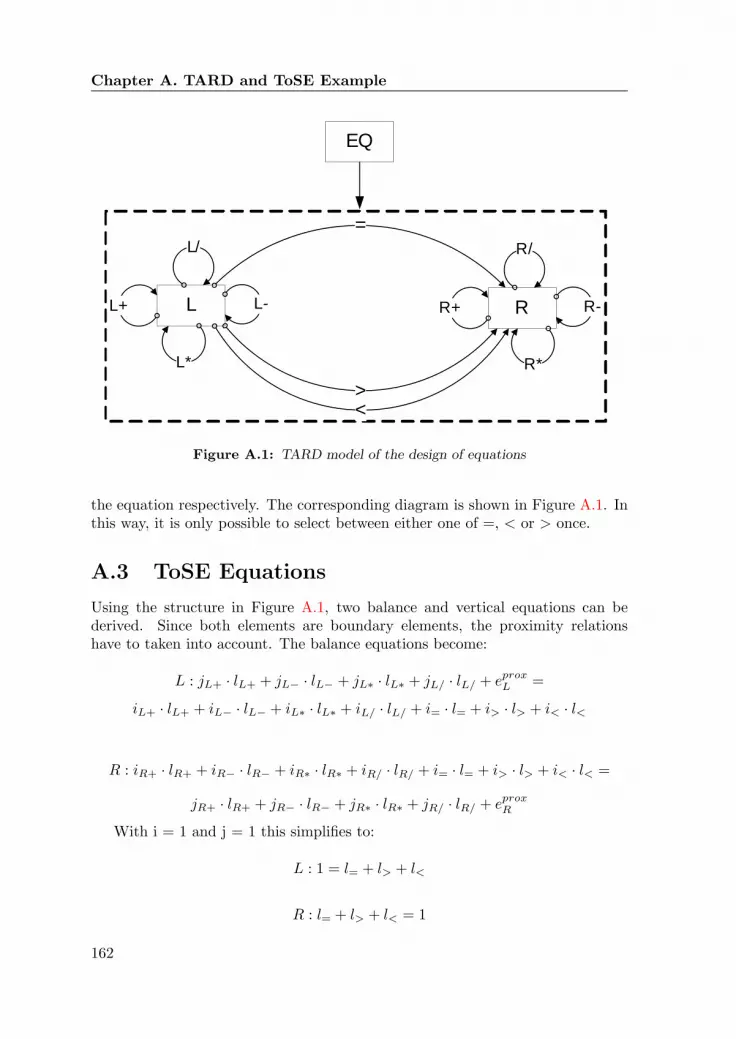
Chapter A. TARD and ToSE Example
L
=
EQ
L-
L*
L+
L/
R R-
R*
R+
R/
><
P
=
EQ
-
*
+
/
>
<
Figure A.1: TARD model of the design of equations
the equation respectively. The corresponding diagram is shown in Figure A.1. Inthis way, it is only possible to select between either one of =, < or > once.
A.3 ToSE Equations
Using the structure in Figure A.1, two balance and vertical equations can bederived. Since both elements are boundary elements, the proximity relationshave to taken into account. The balance equations become:
L : jL+ · lL+ + jL− · lL− + jL∗ · lL∗ + jL/ · lL/ + eproxL =
iL+ · lL+ + iL− · lL− + iL∗ · lL∗ + iL/ · lL/ + i= · l= + i> · l> + i< · l<
R : iR+ · lR+ + iR− · lR− + iR∗ · lR∗ + iR/ · lR/ + i= · l= + i> · l> + i< · l< =
jR+ · lR+ + jR− · lR− + jR∗ · lR∗ + jR/ · lR/ + eproxR
With i = 1 and j = 1 this simplifies to:
L : 1 = l= + l> + l<
R : l= + l> + l< = 1
162

A.4 Generating Solutions
These balance equations resemble the limitations in using the operators =, >and <. This proves the correct integration of the contains into the diagram bysplitting the system into two elements. Accordingly, the vertical equations for Land R are:
eL = [iL+ · lL+ + iL− · lL− + iL∗ · lL∗ + iL/ · lL/ + i= · l= + i> · l> + i< · l<] · eEQ
eR = [jR+ · lR+ + jR− · lR− + jR∗ · lR∗ + jR/ · lR/ + j= · l= + j> · l> + j< · l<] · eEQ
With i , j and eEQ equal to 1, this simplifies to:
eL = lL+ + lL− + lL∗ + lL/ + l= + l> + l<
eR = lR+ + lR− + lR∗ + lR/ + l= + l> + l<
The result is a set of 3 equations (the balance equations are the identical) and13 unknowns. However, since all cardinalities l=, l> or l< can be equal to 1, thebalance equation can be used to calculate two cardinalities if one is known. Thus,this is an under-constraint with 8 degrees of freedom.
A.4 Generating Solutions
As shown to Figure A.3, a sequence can be generated with the Local GrammarMethod. Accordingly, the values for all cardinalities l of each C-relation arecalculated by using the sequence equations. Figure A.2 shows the available rulesfor the local grammar generation, where rule 1 to 7 apply for the element L andrule 8 to 11 for element R. Figure A.3 shows the stepwise generation of a possiblesolution.
The resulting sequence of the example gives results in:
lL+ = 1, lL− = 2, lL∗ = 1, lL/ = 2, lR+ = 0, lR− = 0
lR∗ = 1, lR/ = 0, l= = 1, l< = 1, l> = 1
By denoting the instances of both, L and R, as equation parameters p, theequation generated by this example yields:
p1 · p2 + p3 · p4 = p5 · p6
In case p1 = p2 = a, p3 = p4 = b and p5 = p6 = c, this equation becomes theequation of Pythagoras:
a2 + b2 = c2
163

Chapter A. TARD and ToSE Example
L+
L LL-
L LL*
L LL/
L L
=
L R>
L R
<
L Lrule 7:L+
R RL-
R RL*
R RL/
R R
rule 8:
rule 9:
rule 10:
rule 11:
rule 1:
rule 2:
rule 3:
rule 4:
rule 5:
rule 6:
Figure A.2: Rues in equation generator grammar
Current element Grammar rules Sequence
L
Step
1 L*1 , 2 , 3 , 4 , 5 , 6 , 7
L2 L*-L+1 , 2 , 3 , 4 , 5 , 6 , 7
L3 L*-L+-L*1 , 2 , 3 , 4 , 5 , 6 , 7
L4 L*-L+-L*-=1 , 2 , 3 , 4 , 5 , 6 , 7
R5 L*-L+-L*-=-R*8 , 9 , 10 , 11
R6 finish
Figure A.3: Example sequence generation
164
Appendix BToSE for CSIM
B.1 TARD Model
B.1.1 Elements
The base elements of this TARD model are the point elements: blue, green andbrown. Combination of these points are used to create absorber channel, connec-tor channel or input-/output channel. Channel elements are connected to amongeach others to form the abstraction-group cooling circuit. Finally, the entire cool-ing system is represented by the zero level element.
B.1.2 C-Relations
The first C-relation represents the connection of multiple cooling circuits into asingle cooling system. The abstractiongroup described by channels is significantlymore complex. The assembly of each circuit begins with an input channel. How-ever, this channel can either be connected to a connector channel or directly toan absorber channel, represented by C2 and C3. For the output channel, thesituation is the other way round, because it is connected from either of the twochannels, as constituted by C8 and C9. The two channel elements might be eitherconnected to itself respectively or with each other in both directions, ensuring alimitless variety of possible combinations.
B.1.3 Abstraction-groups
The abstraction-group describing the assembly of an input channel element con-tains two alternative c-relations connecting the brown point to a green or bluepoint. The c-relation in the abstraction-group of the absorber channel only con-nects to blue points, since all parts of this channel type fulfill the task of heat
165

Chapter B. ToSE for CSIM
absorption. Connector channel are assembled by connecting green points or greenpoints with a blue point. Finally, the assembly of the output channel can startwith a blue or green point, which is connected to a brown point by C16 or C17.
In summary, the network is composed of 6 complex abstractiongroups. Thesegroups are distributed over 3 levels of abstraction and contain 14 element classes.All cardinalities i and j are equal to 1.
B.2 Balance equations
The proximity relations for the local cardinality of each boundary element is 1.This indicates that the sequence of each abstraction-group begins with a single,non-parallel element instance. Five balance equations can be established for thelevels 1 and 2:
CoolingCircuit:eprox + jC1 · lC1 = iC1 · lC1 + eprox
InputSegment:eprox = iC2 · lC2 + iC3 · lC3
AbsorberChannel:
jC2 · lC2 + jC4 · lC4 + jC7 · lC7 = iC4 · lC4 + iC5 · lC5 + iC9 · lC9
ConnectorChannel:
jC3 · lC3 + jC5 · lC5 + jC6 · lC6 = iC6 · lC6 + iC7 · lC7 + iC8 · lC8
Outputsegement:jC8 · lC8 + jC9 · lC9 = eprox
With eprox = 1 and i = j = 1, these equations can be writen as:
CoolingCircuit:lC1 = lC1
InputSegment:1 = lC2 + lC3
AbsorberChannel:
lC2 + lC4 + lC7 = lC4 + lC5 + lC9
ConnectorChannel:
lC3 + lC5 + lC6 = lC6 + lC7 + lC8
166

B.2 Balance equations
Inp
utS
eg
me
nt
C1
Blu
eP
oin
t
H1
C11
Co
olin
gS
yste
m
H0
Co
olin
gC
ircu
it
Ab
so
rbe
rCh
an
ne
lC
on
ne
cto
rCh
an
ne
lO
utp
utS
eg
me
nt
C2
C3 C4
C6
C5C7
C8
C9
Gre
en
Po
int
Bro
wn
Po
int
C10
Blu
eP
oin
tG
ree
nP
oin
tB
row
nP
oin
t
C17
C16
Blu
eP
oin
t
C12
Blu
eP
oin
tG
ree
nP
oin
t
C14
C13
H2
H3
H4
H5
Le
ve
l 0
Le
ve
l 1
Le
ve
l 3
Le
ve
l 2
C15
Figure B.1: TARD model of CSIM problem.
167

Chapter B. ToSE for CSIM
Outputsegement:lC8 + lC9 = 1
The determination of the balance equation for the 3rd level requires extra atten-tion:
• Given that the three different point types are repeated in different abstraction-groups, each point type is treated as a different element class.
• As the abstraction-groups H2 and H5 connect blue or green points withbrown points, each of these requires two proximity relations. For abstractiongroup H2 this is:
eproxblue = 1− lC11
andeproxgreen = 1− lC10
For abstraction-group H5 this is:
eproxblue = 1− lC17
andeproxgreen = 1− lC16
• As H4 is a complex abstraction-group, and the sequences can either begin orend with any of the elements, it is not possible to define proximity relations.This increases the uncertainty of the design problem by adding an unknowncardinality.
By taking this considerations, the balance equation of H2 are:
BrownPoint:eprox = iC10 · lC10 + iC11 · lC11
BluePoint:jC10 · lC10 = e(bp)prox
GreenPoint:jC11 · lC11 = eprox
gp
With eprox = 1, eproxgp − lC10 = 1, eprox
bp − lC11 = 1, and i = j = 1, these equationsbecome:
168

B.2 Balance equations
BrownPoint:1 = lC10 + lC11
BluePoint:lC10 = 1− lC11
GreenPoint:lC11 = 1− lC10
As it can be noticed, this equations are equivalent, which results in one equationrepresenting the balance equation for all this elements.
For H3, the balance equation is:
BluePoint:
eprox + jC12 · lC12 = iC12 · iC12 + eprox ⇒ 1 + l12 = l12 + 1
Taking into consideration the 3rd aspect mentioned above, the balance equationsof the abstraction-group H4 are:
BluePoint:
eproxbp + jC15 · lC15 = iC13 · lC13 ⇒ eprox
bp + lC15 = lC13
GreenPoint:
eproxgp +jC13·lC13+jC14·lC14 = iC14·lC14+iC15·lC15 ⇒ eprox
gp +lC13+lC14 = lC14+lC15
The balance equations of H5 are:
BluePoint:eproxbp = iC16 · lC16 ⇒ 1− l17 = l16
GreenPoint:eproxgp = iC17 · lC17 ⇒ 1− l16 = l17
BrownPoint:iC16 · lC16 + iC17 · lC17 = eprox ⇒ l16 + l17 = 1
Again here, all three equations are the same.
169

Chapter B. ToSE for CSIM
B.3 Vertical equations
The vertical are assembled for the base elements by considering that for all c-relations i = j = 1.
In abstraction-group H2:
ebrownPointH2 = (lC10 + lC12) · (lC2 + lC3) · lC1
egreenPointH2 = lC11 · (lC2 + lC3) · lC1
ebluePointH2 = lC10 · (lC2 + lC3) · lC1
In abstraction-group H3:
ebluePointH3 = lC12 · (lC4 + lC5 + lC9) · lC1
In abstraction-group H4:
ebluePointH4 = lC13 · (lC8 + lC6 + lC7) · lC1
egreenPointH4 = (lC14 + lC15) · (lC8 + lC6 + lC7) · lC1
In abstraction-group H5:
ebrownPointH5 = (lC16 + lC17) · (lC8 + lC9) · lC1
egreenPointH5 = lC17 · (lC8 + lC9) · lC1
ebluePointH5 = lC16 · (lC8 + lC9) · lC1
B.4 Summary
The ToSE consists of 18 equations, composed of 9 balances equations and 9 verti-cal equations. There are 28 cardinalities (17 l, 2 proximity relations and 9 elementglobal cardinalities). As this design problem has 10 degrees of freedom and 2 com-plex abstract groups, it presents both time-dependent combinatorial complexityand time-independent imaginary complexity.
170

Appendix CGeneric CDS-CSImplementation
C.1 TARD Implementation
The architecture of the TARD implementation consist of two types of classes foreach of the building block, namely, a building block class and a building block-instance class. For example, Figure C.1 shows that the building block elementis implemented by an element class and an element-instance class. By doing so,elements in the problem class are instances of the generic elements class (1st orderinstances), while elements in the problem solution are instances of the element-instance class (2nd order instances). Furthermore, each of this classes has variablesdescribing the building blocks cardinalities, references and parameters. This isshown in Figure C.2, where a simple UML diagram of the six topology classesis presented. As shown, an super class “ModelComponent” accommodates thebuilding blocks classes. Figure C.3 shows the class description of these buildingblocks.
By using this architecture, a problem class is represented by making a 1st
order network, while problem instances and problem solutions are instances ofthe 2nd order network. For the elements this means that the amount of 1st orderinstances equals the amount of component types and abstraction-groups, whereasthe amount of 2nd order instances equals the sum of all element cardinalitieswithin the 1st order instances.
171

Chapter C. Generic CDS-CS Implementation
elementElement
class 1
Element
class n...
Element
instance 1 ...Element
instance m
instantiation
instantiation
element instance
class
C# class
component types
1st
order instances
2nd
order instances
Figure C.1: Architecture of the computer implementation of TARD building blocks:class and instance.
-e
-e_local
-C-in-C-out
-H-rel
-parameterTypes
Element
-E_in
-E_out
-i
-j-relations
C-relation
-E_parent
-c_list
-l_list
-sequence-rules
H-relation
-name
ModelComponent
-c_inst_in
-c_inst_out
-h_inst-parameterValues
Element_instance
-E_inst_in
-E_inst_out
-relations
C-relation_instance
-E_inst_parent
-c_inst_list
H-relation_instance
Figure C.2: UML diagram of basic TARD building blocks.
172

C.2 ToSE Implementation
element
C-relation
H-relation
Element
class 1
Element
class n...
C-relation
class 1C-relation
class n...
H-relation
class 1
H-relation
class n...
Element
instance 1 ...Element
instance m
C-relation instance 1 ...
C-relation
instance m
H-relation
instance 1 ...H-relation
instance m
building blocks structure classes structure instances
instantiation instantiation
Figure C.3: Class structure of TARD building blocks
C.2 ToSE Implementation
ToSE is implemented at the hand of three classes, which are shown in Figure C.4.These classes are:
• LocalCardinalityFunction: Objects of this class model the local cardi-nality of an element. A variable identifies if the cardinality is derived usingincoming (IN) or outgoing (OUT) C-relations. It has a list with referencesthat allows it to calculate the local cardinality of an element.
• BalanceEquation: Objects of this class point to elements. It has two in-stances of the localCardinalityEquation, one based on incoming C-relationsand another based on outgoing C-relations.
• VerticalEquation : Models the global cardinality of an element. It has alist of localCardinalityFunctions. The number of entries in that list dependson the level of abstraction of its element. It has a method to determine itsvalue at the hand of this list.
In order to illustrate how this classes allow the implementation of ToSE, Fig-ure C.5 shows the ToSE objects of element E of the TARD model shown inthe same figure. The localCardinalityFunction relates the balanceEquation andverticalEquation to the cardinalities e,el, i, j, l, which are defined in their corre-sponding building blocks (element, C-relations and H-relations).
173

Chapter C. Generic CDS-CS Implementation
verticalEquation
ElementCardinality
List : LocalCardinalityEquations
localCardinalityFunction
element
Side (IN/OUT)
List : cardinalities
balanceEquation
element
left_LocalCardFunction
right_LocalCardFunction
Figure C.4: Diagrams of the equation and cardinality classes
174

C.2 ToSE Implementation
11
33
44
EC
CC
CC
Ce
jl
jl
jl
33
44
44
55
CC
CC
CC
CC
jl
jl
il
il
4Ci
4Cl
3Cj
3Cl
1Cj
1Cl
Fe5
Ci5
Cl4
Cj4
Cl
f(e
E)IN
f(e
E)O
UT
f(e
B)IN
Ca
rdin
alit
y
ob
jects
Lo
ca
l ca
rdin
alit
y
fnc. o
bje
cts
Ba
lan
ce
-,V
ert
ica
l
eq
ua
tio
n o
bje
cts
ve
rtE
q(E
)b
alE
q(E
)
refe
ren
ce
co
rre
sp
on
ds
Eq
ua
tio
ns
EB1
D
C3
F
C5
C
C2
A
C1
0
20
C4
Figure C.5: Object references (pointers) for ToSE equations.
175