Generalized Calderon-Zygmund operators over

spaces of homogeneous type ∗

Songbai Wang1 and Yinsheng Jiang

(1,College of Mathematics and statistics, Hubei Normal University, Huangshi 435000, P. R. China)

(2,College of Mathematics and System Sciences, Xinjiang University, Urumqi 830046, P. R. China)

Abstract. We study the generalized Calderon-Zygmund operators with non-smooth ker-nel,whose kernels satisfy regularity conditions significantly weaker than those of the standardCalderon-Zygmund kernels, on the RD-spaces which which are spaces of homogeneous type e-quipped with doubling measures satisfying a reverse doubling condition. The endpoint estimatesand strong type estimates for this operator are obtained by Calderon-Zygmund decompositionand multilinear interpolation. And the pointwise estimate for sharp function acting on the gen-eralized Calderon-Zygmund operators are be established. As a consequence, the multiple-weightboundedness of them are valid.

Key Words: Generalized Calderon-Zygmund operators, A~P condition, space of homoge-neous type.

AMS(2000) subject classification: 47B47, 42B20, 42B25

1 Introduction

The theory of multilinear analysis related to the Calderon-Zygmund program originated in

the work of Coifman and Meyer [1, 2, 3]. Its study has been attracting a lot of attention in

the last few decades. A series of papers on this topic enriches this program, for example Christ

and Journe [4], Kenig and Stein [20], and Grafakos and Torres [14, 15]. The authors [21] built

a theory of wight (called multiple weight) adapted to the multilinear setting and developed the

weighted multilnear Calderon-Zygmund theory.

It is worth to point out that one of the earliest examples of multilinear operators in classical

harmonic analysis are the commutators of Calderon appearing in a series representation of the

Cauchy integral along Lipschitz curves, which could be assigned to a class of m-linear operators

whose kernels have regularity significantly weaker than that of the standard Calderon- Zygmund

kernels. We refer readers to [8, 7, 13].

The theory of function spaces on spaces of homogeneous type has been developed by many

authors: Coifman and Weiss [5, 6], Macıas and Segovia [22], Han and Sawyer [19], etc. The mul-

tilinear Calderon-Zygmund theory, and more the weighted theory, were developed by Grafakos,

Liu, Maldonado and Yang [12] underlying the metric spaces endowed with a Randon measure

∗Supported by NSF of China (No.11161044,No.11261055)1

satisfying a doubling condition and a reverse doubling condition. Plenty of the references in [12]

are convenient to ask for more information about this space for readers.

The main purpose of this paper is to study boundedness properties of m-linear operators

whose kernels have regularity significantly weaker than that of the standard Calderon- Zygmund

kernels over the metric spaces of homogeneous type. The motivated idea comes from [14, 8, 21,

12].

2 Some definitions and lemmas

We will work on the spaces of homogeneous type which provide a general framework where

the real-variable approach in the study of singular integrals of Calderon-Zygmund can be carried

out. It begins with some necessary notations and results related to the spaces of homogeneous

type and the so-called RD-spaces by the same statements with the text [12].

Definition 2.1 (Quasi-metric spaces). Let X be a set. A binary function d : X × X → R+ iscalled a quasi-metric if(i) d(x, y) = d(y, x) for all x, y ∈ X ,(ii) d(x, y) = 0 if and only if x = y, and(iii) there exists a constant K ∈ [1,∞) such that d(x, y) ≤ K[d(x, z) + d(z, y)] for all x, y, z ∈ X .In this case we call (X , d) a quasi-metric space. In particular, when K = 1, we call d a metricand (X , d) a metric space.

For any x ∈ X and r > 0, the set B(x, r) := y ∈ X : d(x, y) < r is the ball with center x

and radius r.

Definition 2.2 (Spaces of homogeneous type and RD-spaces). Let (X , d) be a metric space andthe balls B(x, r) : r > 0 form a basis of open neighborhoods of the point x ∈ X . Suppose thatµ is a regular Borel measure defined on a σ-algebra which contains all Borel sets induced by theopen balls B(x, r) : x ∈ X , r > 0, and that 0 < µ(B(x, r)) < 1 for all x ∈ X and r > 0. Thetriple (X , d, µ) is called a space of homogeneous type if there exists a constant C1 ∈ [1,∞) suchthat, for all x ∈ X and r > 0,

µ(B(x, 2r)) ≤ C1µ(B(x, r)). (1)

Remark 2.1. In some sense, the doubling order n of µ measures the “dimension” of X . For aspace of homogeneous type (X , d, µ), µ(X ) <∞ if and only if there exists a positive number R0

such that X = B(x,R0) for all x ∈ X . From (1), there exist C2 ∈ [1,∞) and n ∈ (0,∞) suchthat, for all x ∈ X , r > 0 and λ > 1,

µ(B(x, λr)) ≤ C2λnµ(B(x, r)).

It also follows from the doubling condition that there exist C3 and N, 0 ≤ N ≤ n so that

µ(B(x, r)) ≤ C3

(1 +

d(x, y)

r

)Nµ(B(y, r)).

In cases such as the Euclidean space Rn or Lie groups of polynomial growth, N can be chosento be 0. If N = 0, we can get that it is normal, i.e., there are two positive constants C4 and C5

such thatC4r

n ≤ µ(B(x, r)) ≤ C5rn.

2

Definition 2.3. The triple (X , d, µ) is called an RD-space if it is a space of homogeneous typeand there exist constants κ ∈ [0,∞) and C6 ∈ (0, 1] such that, for all x ∈ X , 0 < r < 2diam(X )and 1 ≤ λ < 2diam(X )/r,

C6λκµ(B(x, r)) ≤ µ(B(x, λr)), (2)

where and in what follows, diam(X ) := supx,y∈X

d(x, y).

Remark 2.2. When X is an RD-space, we obviously have n ≥ κ, and µ(x) = 0 for allx ∈ X , which is said to be non-atomic. Throughout this paper, we always assume that (X , d, µ)is a normal RD-space and µ(X ) = ∞, unless it is clearly stated that (X , d, µ) is a space ofhomogeneous type.

Set Vr(x) := µ(B(x, r)) and V (x, y) := µ(B(x, d(x, y))) for all x, y ∈ X and r > 0. It follows

from (1) that V (x, y) ∼ V (y, x). Denote by supp f the closure of the set x ∈ X : f(x) 6= 0 in

X .For any f ∈ L1

loc(X ), the Hardy-Littlewood maximal function Mf is defined by

Mf(x) := supB3x

1

µ(B)

∫B

|f(y)|dµ(y), for any x ∈ X , (3)

where the supremum is taken over all balls B ⊂ X containing x. It is easy to see that the

function Mf is lower semi-continuous (hence µ-measurable) for every f ∈ L1loc(X ). Using the

Vitali-Wiener type covering lemma, Coifman and Weiss [5] proved that M is bounded from

L1(X ) to L1,∞(X ) and bounded on Lp(X ) for all p ∈ (1,∞]. Also, by an argument similar to

Grafakos [11], we know that M is bounded on Lp,∞(X ) for p ∈ (1,∞). The operator norms

‖M‖L1(X )→L1,∞(X ), ‖M‖Lp(X )→Lp(X ) and ‖M‖Lp,∞(X )→Lp,∞(X )

all depend only on C1 and p.

Denote by Cb(X) the space of all continuous functions on X with bounded supports (namely,

contained in a ball of (X , d)). As in Definition 2.2 we are assuming that µ is a regular Borel

measure on the metric space (X , d), which means that µ has the outer and inner regularity, so

Cb(X ) is dense in Lp(X ) for all p ∈ [1,∞). This, combined with the weak type (1, 1) boundedness

of M and a standard argument (see [17]), implies the differentiation theorem for integrals: for

all f ∈ L1loc(X ) and almost every x ∈ X ,

limB3x,µ(B)→0

1

µ(B)

∫B

f(y)dµ(y) = f(x),

and

limB3x,µ(B)→0

1

µ(B)

∫B

|f(y)− f(x)|dµ(y) = 0.

A consequence of the current Whitney covering lemma and the differentiation theorem for inte-

grals on (X , d, µ) as well as the weak-(1, 1) boundedness ofM is the celebrated Calderon-Zygmund

decomposition process for integrable functions; see Coifman and Weiss [5, 6].

3

Lemma 2.1 (Calderon-Zygmund decomposition of X ). Let f ∈ L1(X ). Then, for every λ >‖f‖L1(X )/µ(X ), there exists a sequence of balls, Bkk∈I , where I is some index set, such that

(i) 14Bkk∈I are pairwise disjoint,(ii) |f(x)| ≤ Cλ for almost every x ∈ X\ ∪k∈I Bk,(iii) for any k ∈ I,

1

µ(Bk)

∫Bk

|f(y)|dµ(y) > Cλ,

(iv) ∑k∈I

µ(Bk) ≤ C‖f‖L1(X )/λ,

where the positive constant C depends only on C1.

Lemma 2.2 (Calderon-Zygmund decomposition for function). Let f ∈ L1(X ). For every λ >‖f‖L1(X )/µ(X ), let Bkk∈I be the sequence of balls provided by Lemma 2.1. Then, there existfunctions g and bkk∈I such that(i)

f = g +∑k∈I

bk,

(ii) ‖g‖L∞(X ) ≤ Cλ,(iii) for every k ∈ I, supp bk ⊂ Bk, and ∫

Xbkdµ = 0,

(iv)

‖g‖L1(X ) ≤ C‖f‖L1(X ), and∑k∈I

‖bk‖L1(X ) ≤ C‖f‖L1(X ),

where C is a positive constant depending only on C1.

For any η ∈ (0, 1], let Cη(X ) be the set of all functions f : X → C such that

‖f‖Cη(X ) := supx 6=y

|f(x)− f(y)|d(x, y)η

<∞.

Define

Cηb (X ) := f ∈ Cη(X ) : f has bounded support.

Then Cηb (X ) ⊂ L∞(X ) and the norm on Cηb (X ) is given by

‖f‖Cη(X ) := ‖f‖L∞(X ) + ‖f‖Cη(X ).

In what follows, we endow Cηb (X ) with the strict inductive limit topology (see [23]) arising from

the sequence of spaces, (Cηb (Bn), ‖ · ‖Cη(X )), where Bnn∈Z is any given increasing sequence of

balls with the same center such that X = supn∈NBn and

Cηb (Bn) := f ∈ Cηb (X ) : supp f ⊂ Bn.

Denote by (Cηb (X ))′ the dual space of Cηb (X ), namely, the collection of all continuous linear

functionals on Cηb (X ). The space (Cηb (X ))′ is endowed with the weak*-topology.4

Lemma 2.3. [12] Let µ(X ) =∞, η ∈ (0, 1] and f ∈ Cηb (X ). For any λ > 0, f has the decompo-sition

f = g +

∞∑k=1

bk;

where g, bkk∈I and∑k∈I bk are functions in Cηb (X ) satisfying (i)-(iv) of Lemma 2.2.

3 Endpoint estimates for generalized Calderon-Zygmundoperators

The authors extended the the multilinear Calderon-Zygmund theory in the Euclidean case,

as stemed from the work of Coifman and Meyer in [1, 2, 3] and developed by Grafakos and Torres

in [14], to the context of the RD-spaces (X , d, µ) ∈ [12].

Definition 3.1 (Multlinear Calderon-Zygmund kernel). Given m ∈ N, set

Ωm := Xm+1(y0, y1, · · · , ym) : y0 = y1 = · · · = ym.

Suppose that K : Ωm → C is locally integrable. The function K is called a Calderon-Zygmundkernel if there exist constants CK ∈ (0,∞) and δ ∈ (0, 1] such that, for all (y0, y1, · · · , ym) ∈ Ωm,

|K(y0, y1, · · · , ym)| ≤ CK1

[∑ml=1 V (y0, yl)]m

, (4)

and that, for all k ∈ 0, 1, · · · ,m,

|K(y0, y1, · · · , yk, · · · , ym)−K(y0, y1, · · · , y′k, · · · , ym)|

≤ CK[

d(yk, y′k)

max1≤l≤m d(y0, yl)

]δ1

[∑ml=1 V (y0, yl)]m

, (5)

whenever d(yk, y′k) ≤ max1≤l≤m d(y0, yl)/2. Briefly write K ∈ Ker(m,CK , δ).

Definition 3.2 (Multilinear Calderon-Zygmund operators). Let η ∈ (0, 1].Anm-linear Calderon-Zygmund operator is a continuous operator

T :

m times︷ ︸︸ ︷Cηb (X )× · · · × Cηb (X )→ (Cηb (X ))′,

such that, for all f1, · · · , fm ∈ Cηb (X ) and x /∈ ∩ml=1 supp fl,

T (f1, · · · , fm)(x) =

∫Xm

K(x, y1, · · · , ym)

m∏l=1

fl(yl)dµ(y1) · · · dµ(ym), (6)

where the kernel K ∈ Ker(m,CK , δ) for some CK > 0 and δ ∈ (0, 1].

As an m-linear operator, T has m formal transposes. The j-th transpose T ∗,j of T is defined

by

〈T ∗,j(f1, · · · , fm), g〉 = 〈T (f1, · · · , fj−1, g, fj+1, · · · , fm), fj〉,5

for all f1, · · · , fm, g in Cηb (X ). The kernel K∗,j of T ∗,j is related to the one of T by

K∗,j(x, y1, · · · , yj−1, yj , yj+1, · · · , ym) = K(yj , y1, · · · , yj−1, x, yj+1, · · · , ym).

To maintain uniform notation, we may occasionally denote T by T ∗,0 and K by K∗,0.

The authors established the endpoint weak-type estimate for m-linear Calderon-Zygmund

operators over the RD-Spaces in [12], and also see [14] for the Euclidean space.

Theorem 3.1 (Endpoint weak-type estimate for m-linear Calderon-Zygmund operators). LetT be an m-linear Calderon-Zygmund operator associated with a kernel K ∈ Ker(m,CK , δ).Assume that, for some 1 ≤ q1, q2, · · · , qm ≤ ∞ and some 0 < q <∞ with

∑mj=1

1qj

= 1q , T maps

Lq1(X )×· · ·×Lqm(X )→ Lq,∞(X ). Then T can be extended to a bounded m-linear operator fromthe m-fold product L1(X )× · · · × L1(X )→ L1/m,∞(X ) and

‖T‖L1(X )×···×L1(X )→L1/m,∞(X ) ≤ C[CK + ‖T‖Lq1 (X )×···×Lqm (X )→Lq,∞(X )],

for some positive constant C that depends only on C1, C2, δ and m.

We will consider a weak regularity condition of kernel associated with a family integral op-

erators, introduced by Duong and McIntosh [9] in Euclidean setting, which plays the role of

approximations to the identity.

Definition 3.3 (Approximation of the identity). A family of operators At, t > 0 is saidto be an “approximation of the identity”, if for every t > 0, At is represented by the kernelat(x, y), which is a measurable function defined on X × X , in the following sense: for everyf ∈ Lp(X ), p ≥ 1,

Atf(x) =

∫Xat(x, y)f(y)dµ(y),

and the following condition holds:

|at(x, y)| ≤ ht(x, y) =1

Vt1/s(x)h

(d(x, y)

t1/s

), (7)

where s is a positive fixed constant and h is a positive, bounded, decreasing function verifying

limr→∞

rn+τh(rs) = 0, (8)

for some τ > κ. These conditions imply that for some C ′ > 0 and all 0 < τ ′ ≤ τ, the kernelsat(x, y) satisfy

|at(x, y)| ≤ C ′Vt1/s(x)−1(1 + t−1/sd(x, y))−n−τ′.

Now, let T be a multilinear operator associated with a kernel K(x, y1, · · · , ym) in the sense

of (6). The basic assumptions we are going to be making concerning T are the following.

Assumption 3.1. Assume that for each j = 1, 2, · · · ,m, there exist operators A(j)t t>0 with

kernels a(j)t (x, y) that satisfy conditions (7) and (8) with constants s and τ and there exist kernels

K(j)t (x, y1, · · · , ym) such that

〈T (f1, · · · , A(j)t fj , · · · , fm), g〉

=

∫X

∫Xm

K(j)t (x, y1, · · · , ym)f1(y1) · · · fm(ym)g(x)dµ(y1) · · · dµ(ym)dµ(x), (9)

for all f1, · · · , fm, g ∈ Cηb (X ) with ∩ml=1 supp fl ∩ g = ∅.6

Assumption 3.2. There exist a function ϕ ∈ C(R) with suppϕ ⊂ [−1, 1] and a constant δ > 0so that for all x, y1, · · · , ym ∈ X and t > 0 we have

|K(x, y1, · · · , ym)−K(j)t (x, y1, · · · , ym)|

≤ A

[∑ml=1 V (x, yl)]m

m∑k=1k 6=j

ϕ

(d(yj , yk)

t1/s

)+

[t1/s

max1≤l≤m d(x, yl)

]δA

[∑ml=1 V (x, yl)]m

, (10)

for some A > 0, whenever t1/s ≤ d(x, yj)/2.

Under Assumptions 3.1 and 3.2 we say that T is an m-linear operator with generalized

Calderon-Zygmund kernel K. The collection of functions K satisfying (9) and (10) with param-

eters m,A, s, τ and δ will be denoted by m-GKer0(A, s, τ, δ).

Before stating our main theorem in this section, an important lemma will be used as follows.

Lemma 3.1. For any δ > 0, there exists positive constant C, depending only on C1, δ and m,such that, for all i ∈ 1, · · · ,m and all x, yk ∈ X with k 6= i,∫

X

1

[max1≤k≤m d(x, yk)]δ1∑m

k=1 V (x, yk)dµ(yi) ≤ C

1

[max1≤k≤m,k 6=i d(x, yk)]δ.

We obtain the endpoint boundedness of T associated with generalized Calderon-Zygmund

kernels provided these operators are bounded on a single product of Lebesgue spaces. A similar

result refers to [8] underlying the Euclidean space.

Theorem 3.2. Let T be an m-linear operator associated with a kernel K ∈ m-GKer0(A, s, τ, δ).Assume that, for some 1 ≤ q1, q2, · · · , qm ≤ ∞ and some 0 < q <∞ with

1

q1+ · · ·+ 1

qm=

1

q. (11)

T maps Lq1(X ) × · · · × Lqm(X ) → Lq,∞(X ). Then T can be extended to a bounded m-linearoperator from the m-fold product L1(X ) × · · · × L1(X ) → L1/m,∞(X ). Precisely, there exists apositive constant C that depends only on s, τ, δ and m,

‖T‖L1(X )×···×L1(X )→L1/m,∞(X ) ≤ C[A+ ‖T‖Lq1 (X )×···×Lqm (X )→Lq,∞(X )].

Proof. Set B = ‖T‖L1(X )×···×L1(X )→L1/m,∞(X ). Since the space Cηb (X ) is dense in L1(X ) for anyη ∈ (0, 1] (see [18]), it suffices to prove the theorem for functions fj ∈ Cηb (X ), and by the linearityof the operator, we may assume that ‖fj‖L1(X ) = 1 j = 1, · · · ,m. For any α > 0, let

Eα := x ∈ X : |T (f1, · · · , fm)(x)| > α,

We only need to show thatµ(Eα) ≤ C(A+B)1/mα−1/m.

Let λ > 0 be a constant to be determined later. For all j ∈ 1, · · · ,m, apply the Calderon-Zygmund decomposition (Lemma 2.3) to fj at height (αλ)1/m to obtain good and bad functionsgj and bj and families of balls, Bj,kjkj∈Ij , such that

fj = gj + bj = gj +∑kj∈Ij

bj,kj

7

and for all kj ∈ Ij and q ∈ [1,∞],(i) supp bj,kj ⊂ Bj,kj and ∫

Xbj,kj (x)dµ(x) = 0.

(ii)‖bj,kj‖L1(X ) ≤ C(αλ)1/mµ(Bj,kj ),

(iii) ∑kj∈Ij

µ(Bj,kj ) ≤ C(αλ)−1/m,

(iv)

‖gj‖Lq(X ) ≤ C(αλ)1/m(1−1/q) and ‖bj‖L1(X ) ≤∑kj∈Ij

‖bj,kj‖L1(X ) ≤ C.

For q > 1, from ‖gj‖L∞(X ) < (αλ)1/m, it is easy to get that ‖gj‖Lq(X ) ≤ C(αλ)1/m(1−1/q). Also,notice that gj and bj as above are functions in Cηb (X ) by Lemma 2.3.

Now, let

E1α = x ∈ X : |T (g1, · · · , gm)(x)| > α/2m

E2α = x ∈ X : |T (g1, b2, · · · , gm)(x)| > α/2m

E1α = x ∈ X : |T (b1, g2, · · · , gm)(x)| > α/2m· · ·

E2m

α = x ∈ X : |T (b1, · · · , bm)(x)| > α/2m

where each Esα = x ∈ X : |T (h1, h2, · · · , hm)(x)| > α/2m with hj ∈ gj , bj and all the sets

Esλ are distinct. Since µ(x ∈ X : |T (f1, f2, · · · , fm)(x)| > α) ≤∑2m

s=1 µ(Esα), it will suffice toprove estimate for all s ∈ 1, 2, · · · , 2m such that

µ(Esα) ≤ C(A+B)1/mα−1/m.

Chebychev’s inequality and the Lq1(X )× · · · × Lqm(X )→ Lq,∞(X ) boundedness of T give

µ(E1α) ≤

(2mB

α

)q‖g1‖qLq1q(X ) · · · ‖gm‖

qLqm (X )

≤ C(B

α

)q m∏j=1

(αλ)q/(mq′j)

≤ CBqα1/mλq−1/m.

Consider now the term Esα as above with s = 2, 3, · · · , 2m. We will show that

µ(Esα) ≤ Cα−1/m[λ−1/m + λ−1/m(λA)1/l],

where l is the number of bad functions appearing in T (h1, · · · , hm). Let rj,kj and cj,kj be theradius and the center of the ball Bj,kj , respectively. Set B∗j,kj = Bj,kj (cj,kj , 5rj,kj ), since

µ

( m⋃j=1

⋃kj∈Ij

B∗j,kj

)≤ C(αλ)−1/m.

8

It turns to prove that

µ

(x /∈

m⋃j=1

⋃kj∈Ij

B∗j,kj : |T (h1, · · · , hm)(x)| > α

)≤ Cα−1/mλ−1/m(λA)1/l.

For matters of simplicity, we assume that the bad functions appear at the entries 1, 2, · · · , l. Fixan x /∈ ∪lj=1 ∪kj∈Ij B∗j,kj , one has

T (b1, · · · , bl, gl+1, · · · , gm)(x)

=∑

k1,k2,··· ,kl

T (b1,k1 , b2,k2 , · · · , bl,kl , gl+1, · · · , gm)(x)

=

l∑j=1

∑k1,··· ,kj−1,kj+1,··· ,kl

∑kj :rj,kj

≤ri,kifor all i6=j,i∈1,··· ,l

T (b1,k1 , b2,k2 , · · · , bl,kl , gl+1, · · · , gm)(x)

:=

l∑j=1

T (j)(b1,k1 , b2,k2 , · · · , bl,kl , gl+1, · · · , gm)(x).

For every T (j)(b1, · · · , bl, gl+1, · · · , gm), we will approximate each bj,kj byAtj,kj bj,kj , where tj,kj =

rsj,kj and s is the constant appearing in (7). For example,

T (1)(b1,k1 , b2,k2 , · · · , bl,kl , gl+1, · · · , gm)(x)

=∑

k2,··· ,kl

∑k1:r1,k1

≤ri,kii=2,··· ,l

T (b1,k1 −At1,k1 b1,k1 , b2,k2 , · · · , bl,kl , gl+1, · · · , gm)(x)

+∑

k2,··· ,kl

∑k1:r1,k1

≤ri,kii=2,··· ,l

T (At1,k1 b1,k1 , b2,k2 , · · · , bl,kl , gl+1, · · · , gm)(x)

:= T (11)(b1,k1 , b2,k2 , · · · , bl,kl , gl+1, · · · , gm)(x) + T (12)(b1,k1 , b2,k2 , · · · , bl,kl , gl+1, · · · , gm)(x).

Since x /∈ ∪lj=1 ∪kj∈Ij B∗j,kj , by condition (10) we have

|T (11)(b1,k1 , b2,k2 , · · · , bl,kl , gl+1, · · · , gm)(x)|

≤ CA∣∣∣∣ ∑k2,··· ,kl

∑k1:r1,k1

≤ri,kii=2,··· ,l

∫Xm

rδ1,k1∏lj=1 bj,kj (yj)

[max1≤l≤m d(x, yl)]δ[∑ml=1 V (x, yl)]m

m∏j=l+1

g(yj)

m∏j=1

dµ(yj)

∣∣∣∣+ CA

∣∣∣∣ m∑u=2

∑k2,··· ,kl

∑k1:r1,k1

≤ri,kii=2,··· ,l

∫Xm

∏lj=1 bj,kj (yj)

[∑ml=1 V (x, yl)]m

ϕ

(d(y1, yu)

r1,k1

) m∏j=l+1

g(yj)

m∏j=1

dµ(yj)

∣∣∣∣:= |T (11)

1 (b1,k1 , b2,k2 , · · · , bl,kl , gl+1, · · · , gm)(x)|+ |T (11)2 (b1,k1 , b2,k2 , · · · , bl,kl , gl+1, · · · , gm)(x)|.

It is a known fact by integrating with respect to every yi with i /∈ 1, · · · , l and using Lemma3.1 (m− l) times and the assumption r1,k1 ≤ ri,ki , i = 2, · · · , l,∫

Xm−l

∣∣∣∣ ∫B∗1,k1

rδ1,k1b1,k1(y1)

[max1≤l≤m d(x, yl)]δ[∑ml=1 V (x, yl)]m

dµ(y1)

∣∣∣∣ m∏i=l+1

dµ(i)

≤ Cl∏i=1

[ri,ki

d(x, ci,ki)

]δ/l1

V (x, ci,ki).

9

‖g‖L∞(X ) ≤ C(αλ)1/m, together with property (ii) of the Calderon-Zygmund decomposition,imply that

|T (11)1 (b1,k1 , b2,k2 , · · · , bl,kl , gl+1, · · · , gm)(x)|

≤ CA∑

k2,··· ,kl

∑k1:r1,k1

≤ri,kii=2,··· ,l

∫Xm−1

∣∣∣∣ ∫B∗1,k1

rδ1,k1b1,k1(y1)

[max1≤i≤m d(x, yi)]δ[∑mi=1 V (x, yi)]m

dµ(y1)

∣∣∣∣×

l∏j=2

|bj,kj (yj)|m∏

j=l+1

|g(yj)|m∏j=2

dµ(yj)

≤ CA∑

k2,··· ,kl

∑k1:r1,k1

≤ri,kii=2,··· ,l

(αλ)(m−l)/m‖b1,k1‖L1(X )

×l∏i=1

[ri,ki

d(x, ci,ki)

]δ/l1

V (x, ci,ki)

∫X l−1

l∏i=2

|bi,ki(yi)|dµ(yi)

≤ CA∑

k2,··· ,kl

∑k1:r1,k1

≤ri,kii=2,··· ,l

(αλ)(m−l)/ml∏i=1

[ri,ki

d(x, ci,ki)

]δ/l ‖bi,ki‖L1(X )

V (x, ci,ki)

≤ CA∑

k2,··· ,kl

∑k1:r1,k1

≤ri,kii=2,··· ,l

(αλ)

l∏i=1

[ri,ki

d(x, ci,ki)

]δ/lµ(Bi,ki)

V (x, ci,ki)

≤ CA(αλ)

l∏i=1

( ∑ki∈Ii

[ri,ki

d(x, ci,ki)

]δ/lµ(Bi,ki)

V (x, ci,ki)

)

≤ CA(αλ)

l∏i=1

∑ki∈Ii

[M(χBi,ki )(x)]1+δ/(nl),

With L1+δ/(nl)(X )-boundedness of M and Holder’s inequality, this gives that

µ

(x /∈

m⋃j=1

⋃kj

Bj,kj∗ : |T (11)1 (b1,k1 , b2,k2 , · · · , bl,kl , gl+1, · · · , gm)(x)| > α/2m

)

≤ C(α)1/l∫X\∪mj=1∪kjBj,kj ∗

|T (11)1 (b1,k1 , b2,k2 , · · · , bl,kl , gl+1, · · · , gm)(x)|1/ldµ(x)

≤ C(λ)1/ll∏

j=1

∑kj∈Ij

∫X

[M(χBj,kj )(x)

]1+δ/(nl)dµ(x)

1/l

≤ C(λ)1/ll∏

j=1

( ∑kj∈Ij

µ(Bj,kj∗))1/l

≤ C(λ)1/l(αλ)−1/m

For the term T(11)2 . Employing the fact ϕ is supported in [−1, 1], ‖bj,kj‖L1(X ) ≤ C(αλ)1/mµ(Bj,kj )

10

and the assumption r1,k1 ≤ ri,ki , i = 2, · · · , l, we deduce that

|T (11)2 (b1,k1 , b2,k2 , · · · , bl,kl , gl+1, · · · , gm)(x)|

≤ CA(αλ)1/ml∑

u=2

∑k1

∫Xm−1

l∏j=2j 6=u

(∑kj

µ(Bj,kj )1/(m−1)|bj,kj (yj)|

[∑ml=1 V (x, yl)]m/(m−1)

)

×m∏

j=l+1

(∑kj

µ(B1,k1)1/(m−1)|gj,kj (yj)|[∑ml=1 V (x, yl)]m/(m−1)

)

×(∑

ku

µ(B1,k1)1/(m−1)|bu,ku(u)|[∑ml=1 V (x, yl)]m/(m−1)

χB1,k1(yu)

) m∏j=2

dµ(yj)

+ CA(αλ)1/ml∑

u=2

∑k1

∫Xm−1

l∏j=2

(∑kj

µ(Bj,kj )1/(m−1)|bj,kj (yj)|

[∑ml=1 V (x, yl)]m/(m−1)

)

×m∏

j=l+1j 6=u

(∑kj

µ(B1,k1)1/(m−1)|gj,kj (yj)|[∑ml=1 V (x, yl)]m/(m−1)

)

×(∑

ku

µ(B1,k1)1/(m−1)|gu,ku(u)|[∑ml=1 V (x, yl)]m/(m−1)

χB1,k1(yu)

) m∏j=2

dµ(yj)

≤ CA(αλ)l/mm∑

u=l+1

l∏j=2

Jj, 1m−1

(x)

m∏j=l+1

M(gj)(x)(M(gu)(x) + (αλ)1/mJ1, 1m−1

(x)),

where

Jj,ε(x) =∑kj

µ(Bj,kj )1+ε

(µ(Bj,kj )) + V (x, cj,kj ))1+ε

, (12)

it is similar to the statement [10] to verify that for p > 1/(1 + ε)

‖Jj,kj (x)‖Lp(X ) ≤ C(∑

kj

µ(Bj,kj )

)1/p

≤ C(αλ)−1/mp. (13)

Chebychev’s inequality tells us

µ

(x /∈

m⋃j=1

⋃kj

Bj,kj∗ : |T (11)2 (b1,k1 , b2,k2 , · · · , bl,kl , gl+1, · · · , gm)(x)| > α/2m

)≤ Cα−1/m(λ−1/m +Bλ1−1/m).

Selecting λ = (A+B)−1 and a similar argument to [8] concludes the proof of the theorem.

To obtain strong type Lp1(X )× · · · × Lpm(X ) → Lp(X ) boundedness results for multilinear

operators of generalized Calderon- Zygmund type, we will impose restrictions on their adjoint

operators.

Assumption 3.3. Assume that for each i = 1, 2, · · · ,m, there exist operators A(i)t t>0 with

kernels a(i)t (x, y) that satisfy conditions (7) and (8) with constants s and τ, and for every j =

11

0, 1, · · · ,m there exist kernels K∗,j,(i)t (x, y1, · · · , ym) such that

〈T ∗,j(f1, · · · , A(i)t fj , · · · , fm), g〉

=

∫X

∫Xm

K(∗,j,(i))t (x, y1, · · · , ym)f1(y1) · · · fm(ym)g(x)dµ(y1) · · · dµ(ym)dµ(x), (14)

for all f1, · · · , fm, g ∈ Cηb (X ) with ∩ml=1 supp fl ∩ g = ∅.

Assumption 3.4. There exist a function ϕ ∈ C(R) with suppϕ ⊂ [−1, 1] and a constant ε > 0so that for every j = 0, 1, · · · ,m and i = 1, · · · ,m, we have

|K∗,j(x, y1, · · · , ym)−K∗,j,(i)t (x, y1, · · · , ym)|

≤ A

[∑ml=1 V (x, yl)]m

m∑k=1k 6=j

ϕ

(d(yj , yk)

t1/s

)+

[t1/s

max1≤l≤m d(x, yl)

]δA

[∑ml=1 V (x, yl)]m

, (15)

for some A > 0, whenever t1/s ≤ d(x, yj)/2.

Under Assumptions 3.3 and 3.4 we will say that T is an m-linear operator with general-

ized Calderon-Zygmund kernel K. The collection of functions K satisfying (14) and (15) with

parameters m,A, s, τ and δ will be denoted by m- GKer(A, s, τ, δ). A kernel K belongs to m-

GKer(A, s, τ, δ) exactly when it belongs to m-GKer0(A, s, τ, δ) and all of its adjoints also belong

to m-GKer0(A, s, τ, δ). We say that T is of class m-GCZO(A, s, τ, δ) if T is associated with a

kernel K in m-GKer(A, s, τ, δ).

We have the strong estimates for generalized Calderon-Zygmund operators with kernel K ∈GKer(A, s, τ, δ) and still put down the proof although the process is very similar to that of

Theorem 3.1 [8].

Theorem 3.3. Let T be a multilinear operator in m-GCZO(A, s, τ, δ). Given 1 < q1, q2, · · · , qm, q <∞ with 1/q1 + · · · + 1/qm = 1/q. Assume that T maps Lq1(X ) × · · · × Lqm(X ) to Lq(X ). Letp, pj be numbers satisfying 1/m ≤ p < ∞, 1 ≤ pj ≤ ∞ and 1/p = 1/p1 + · · · + 1/pm. Then allstatements below are valid,(i) when all pj > 1, then T can be extended to be a bounded operator from the m-fold productLp1(X )× · · · × Lpm(X ) to Lp(X ),(ii) when some pj = 1, then T can be extended to be a bounded operator from the m-fold productLp1(X )× · · · ×Lpm(X ) to Lp,∞(X ). Moreover, there exists a constant C such that the followingestimate holds

‖T‖L1(X )×···×L1(X )→L1/m,∞(X ) ≤ C(A+ ‖T‖Lq1 (X )×···×Lqm (X )→Lq(X )).

Proof. We also prove it for the case m = 2 in details. It begin with the first part (i) nat-urally. Since T : Lq1(X ) × Lq2(X ) → Lq(X ), it follows that the adjoint with respect to thefirst variable T ∗,1 : Lq

′(X ) × Lq2(X ) → Lq1(X ). But then Theorem 3.2 yields that T ∗,1 :

L1(X ) × L1(X ) → L1/2,∞(X ). Interpolation (in the complex way) between these estimatesyields that T ∗,1 : Lr1(X ) × Lr2(X ) → Lr,∞(X ) for some 1/r1 + 1/r2 = 1/r, where r > 1since q′1 > 1. Duality implies that T : Lr,∞(X ) × Lr2(X ) → Lr1(X ). Theorem 3.2 yieldsthat T : L1(X ) × L1(X ) → L1/2,∞(X ). Interpolating between this estimate and the estimatesT : Lr,∞(X ) × Lr2(X ) → Lr1(X ) and T : Lq1(X ) × Lq2(X ) → Lq(X ) yields boundedness for

12

T in the interior of an open triangle. (Here we use the bilinear Marcinkiewicz interpolationtheorem that yields strong-type bounds in the interior of the convex hull of three points at whichLorentz space estimates are known; see [16].) Bootstrapping this argument and using dualityand interpolation, we fill in the entire convex region 1 < p1, p2 ≤ ∞.

Now we turn to prove the part (ii). We may assume that pj = 1. It follows from (i) that

T : Lp(X ) × L∞(X ) → Lp(X ) with 1 < p < ∞. Fix a function f2 ∈ L∞(X ), we set K(x, y) =∫X K(x, y, z)f2(z)dµ(z), and define the operator T as follows

T (f1)(x) = T (f1, f2)(x) =

∫X

∫XK(x, y, z)f2(z)dµ(z)f1(y)dµ(y)

:=

∫XK(x, y)f1(y)dµ(y).

The same argument to [8] working on normal RD-spaces goes on that T maps Lp(X ) to Lp(X )for 1 < p < ∞ and L1(X ) to L1,∞(X ). Thus, T maps L1(X ) × L∞(X ) to L1,∞(X ) with thenorm

‖T‖L1(X )×L∞(X )→L1,∞(X ) = Cn,q1,q2,p(A+ ‖T‖Lq1 (X )×Lq2 (X )→Lq(X )).

Since T : L1(X ) × L1(X ) → L1/2,∞(X ), it follows by (linear) interpolation that T : L1(X ) ×Lp2(X )→ Lp,∞(X ), where p = p2/(p2 + 1).

4 Weighted estimates for generalized Calderon-Zygmundoperators

A multiple-weight theory adapted to the multilinear Calderon-Zygmund theory introduced

by Lerner, Ombrosi, Perez, Torres, and Trujillo-Gonzalez [21] developed the weighted multilinear

Calderon-Zygmund theory. Grafakos, Liu, Maldonado and Yang [12] extended it to the context

of of spaces of homogeneous type.

If the measure v is absolutely continuous with respect to µ and if there exists a nonnegative

locally integrable function ω such that dν(x) = ω(x)dµ(x), we say that ν is a weighted measure

with respect to µ and that ω is a weight. We also denote that ν(B) =∫Bω(x)dµ(x) and the

weighted Lebesgue spaces as

Lp(ν) :=

f is measurable : ‖f‖Lp(ν) =

(∫X|f(x)|pν(x)dµ(x)

)1/p.

Definition 4.1 (Ap weight). A weight ω is said to be in Ap(1 < p <∞) on X , if there exists aconstant C such that for every ball B ⊂ X ,(

1

µ(B)

∫B

ω(x)dµ(x)

)(1

µ(B)

∫B

ω(x)1−p′dµ(x)

)p−1≤ C.

For p = 1, we say that ω ∈ A1 if there is a constant C such that for every ball B ⊂ X ,(1

|B|

∫B

ω(x)dµ(x)

)(essinfx∈B

ω(x)

)−1≤ C.

We set A∞ = ∪p≥1Ap. 13

The reverse Holder classes are defined in the following way: ω ∈ RHq, 1 < q <∞, if there is

a constant C such that for any ball B ⊂ X ,(1

µ(B)

∫B

ω(x)qdµ(x)

)1/q

≤ C 1

µ(B)

∫B

ω(x)dµ(x).

It is checked that RH∞ ⊂ RHq ⊂ RHp for 1 < p ≤ q < ∞ in [24] . And some of the standard

properties of classes of weights are listed in the following lemma which will be used later on.

Lemma 4.1. [24] (i) If ω ∈ Ap, 1 < p <∞, then there exists 1 < r < p <∞ such that ω ∈ Ar,(ii) If ω ∈ Ap, 1 ≤ p <∞, then there exists some r > 1 such that ω−1/(p−1) ∈ RHr.(iii) If ω ∈ Ap, 1 ≤ p < ∞, then there exists a constant C such that for any ball B and anymeasurable set S ⊂ B

ω(S)

ω(B)≤ C

(µ(S)

µ(B)

)1/p

.

(iv) If ω ∈ A∞, then dµ(x) = ω(x)dµ(x) be a doubling measure.

Definition 4.2 (Multiple weights). Let ~P = (p1, · · · , pm) and 1/p = 1/p1 + · · · + 1/pm with1 ≤ p1, · · · , pm <∞. We say the vector of wights ~ω = (ω1, · · · , ωm) belongs to A~P , if there is aconstant C such that for all balls B ⊂ X ,(

1

µ(B)

∫B

ν~ω(x)dµ(x)

)1/p m∏j=1

(1

µ(B)

∫B

ω(x)1−p′jdµ(x)

)p/p′j≤ C,

where ν~ω =∏mj=1 ω

p/pjj , when pj = 1, ( 1

µ(B)

∫Bω(x)1−p

′jdµ(x))p/p

′j is understood as [essinfB ω(x)]−p.

From Proposition 4.3 in [12], the class of multiple weights possesses the following same prop-

erties with them in the Euclidean spaces. (i)

m∏j=1

Apj ⊂ A~P .

(ii) ~ω = (ω1, · · · , ωm) ∈ A~P if and only if ω1−p′jj ∈ Amp′j for all j = 1, · · · ,m and ν~ω∈Amp .

From Lemma 4.1 and the above property (ii), A similar lemma to Lemma 6.1 in [21] can be

formulated as follows,

Lemma 4.2. Assume that ~P = (p1, · · · , pm) and ~ω = (ω1, · · · , ωm) satisfies the A~P condition.Then there exists a finite constant 1 < γ ≤ min1≤j≤m pj such that ω ∈ A~P/γ .

Proof. The statement of the proof for Lemma 6.1 in [21] can be removed here without anymodification except replacing Theorem 3.6 by the above property (ii), so we omit it.

Definition 4.3 (Multi-sublinear maximal function). Given ~f = (f1, · · · , fm) with f1, · · · , fm ∈L1loc(X ), we define the maximal function for any r > 0

Mγ(~f)(x) := supB3x

m∏j=1

(1

µ(B)

∫B

|fj(yj)|γdµ(yj)

)1/γ

14

and for 1 ≤ l < m, σ = j1, j2, · · · , jl ⊂ 1, · · · ,m and σ′ = 1, 2, · · · ,m\σ, we define

Mσ,γ(~f)(x) := supB3x

∞∑k=0

2−knl∏j∈σ

(1

µ(B)

∫B

|fj(yj)|γdµ(yj)

)1/γ ∏j∈σ′

(1

µ(2kB)

∫2kB

|fj(yj)|γdµ(yj)

)1/γ

where the supremum is taken over all balls B ∈ X containing x. For γ = 1, we denote byM andMσ respectively.

In [12], the authors have the following equivalent relationship between the boundedness Mon the m-product weighted Lebesgue spaces and A~P condition.

Theorem 4.1. Let 1 ≤ p1, · · · , pm <∞ and 1/p = 1/p1+· · ·+1/pm. If ~ω = (ω1, · · · , ωm) ∈ A~P ,then(i) when every pj > 1 for j = 1, · · · ,m,M is bounded from Lp1(ω1)× · · · ×Lpm(ωm) to Lp(ν~ω);(ii) when some pj = 1,M is bounded from Lp1(ω1)× · · · × Lpm(ωm) to Lp,∞(ν~ω);holds true for all (f1, · · · , fm) ∈ Lp1(ω1)× · · · × Lpm(ωm).

The reverse is also right.

We extend the necessary part of the above theorem to the case γ > 1 for Mγ and Mσ,γ .

Theorem 4.2. Let 1 < p1, · · · , pm < ∞, 1/p = 1/p1 + · · · + 1/pm, ~P = (p1, · · · , pm), and~ω ∈ A~P . Let 1 ≤ l < m and σ = j1, · · · , jl ⊂ 1, · · · ,m. Then for some γ > 1 (γ dependingonly on ~ω), Mγ and Mσ,γ is bounded from Lp1(ω1)× · · · × Lpm(ωm) to Lp(ν~ω).

Proof. Firstly we prove it for Mγ . To prove that

‖Mγ(~f)‖Lp(ν~ω) ≤ Cm∏j=1

‖fj‖Lpj (ωj),

is equivalent to prove

‖M(~f)‖Lp/γ(ν~ω) ≤ Cm∏j=1

‖fj‖Lpj/γ(ωj),

By Theorem 4.1, this is equivalent to showing that ~ω ∈ A~P/γ and Lemma 4.2 tells us there existsa γ to ensure it.

For Mσ,γ , we may assume σ = 1, ..., l without loss of generality. Also there exists a γ > 1

such that ~ω ∈ A~P/γ , since ~ω ∈ A~P . Consequently, ω−1/(pj/γ−1)j ∈ Am(pj/γ)′ and then by Lemma

4.1, there exists a u > 1 such that(1

µ(B)

∫B

ω(x)−u/(pj/γ−1)dµ(x)

)1/u

≤ C

µ(B)

∫B

ω(x)−1/(pj/γ−1)dµ(x). (16)

Set bj = pj/γ and b = p/γ, then 1/b = 1/b1 + · · ·+ 1/bm. And let

t = max1≤j≤m

bm

bm+ (1− 1/u)(bj − 1)

Observe that t < 1 and tbj > 1 for all j = 1, · · · ,m. By the Holder inequality, we have for any x

15

and any ball B 3 x,∫B

|f(yj)|γdµ(yj)

≤(∫

B

|fj(yj)|rbjtωtj(yj)ν~ω(yj)1−tdµ(yj)

)1/(bjt)(∫B

(ωtjν1−t~ω )(yj)

−1/(bjt−1)dµ(yj)

)1−1/(bjt)

≤ CM cν~ω

([|fj |rbjω/ν~ω]t)(x)

1/bjt

ν~ω(B)1/bj(∫

B

ωj(yj)−b′j/bjdµ(yj)

)1/b′j

,

where M cν~ω

denotes the weighted centered Hardy-Littlewood maximal function, that is,

M cν~ω

(f)(x) := supr>0

1

ν~ω(B(x, r))

∫B(x,r)

|f(y)|ν~ω(y)dy.

From Lemma 4.1 (iv), we know that M cν~ω

is bounded from Lp(ν~ω) to Lp(ν~ω) for p > 1 andfrom L1(ν~ω) to L1,∞(ν~ω). And the second inequality depends on the following estimates. Let

ξj =tbj−1

(1−t)(bm−1) , by the definition of t, we can check that ξj > 1. And using the Holder inequalityagain, we get∫B

(ωtjν1−t~ω )(yj)

−1/(bjt−1)dµ(yj) ≤(∫

B

ωj(yj)−tξ′j/(bjt−1)dµ(yj)

)1/ξ′j(∫

B

ν~ω(yj)−1/(bm−1)dµ(yj)

)1/ξj

.

(17)Note that for any j,

t(bj − 1)ξ′jtbj − 1

=t(bj − 1)

t(bj − 1)− (1− t)bm≤ u,

Therefore, by (16), it immediately deduces that∫B

ωj(yj)−tξ′j/(bjt−1)dµ(yj) ≤ Cµ(B)1−(tbj−1)ξ

′j/(tbj−1)

(∫B

ωj(yj)−1/(bj−1)dµ(yj)

)(tbj−1)ξ′j/(tbj−1)

.

(18)The second inequality above follows from (17), (18) and the fact ν~ω ∈ Amp.

Hence,(1

µ(B)

∫B

|f(yj)|γdµ(yj)

)1/γ

≤ CM cν~ω

([|fj |pjω/ν~ω]t)(x)

1/pjt(ν~ω(B)

µ(B)

)1/(bjγ)( 1

µ(B)

∫B

ωj(yj)−b′j/bjdµ(yj)

)1/(γb′j)

,

16

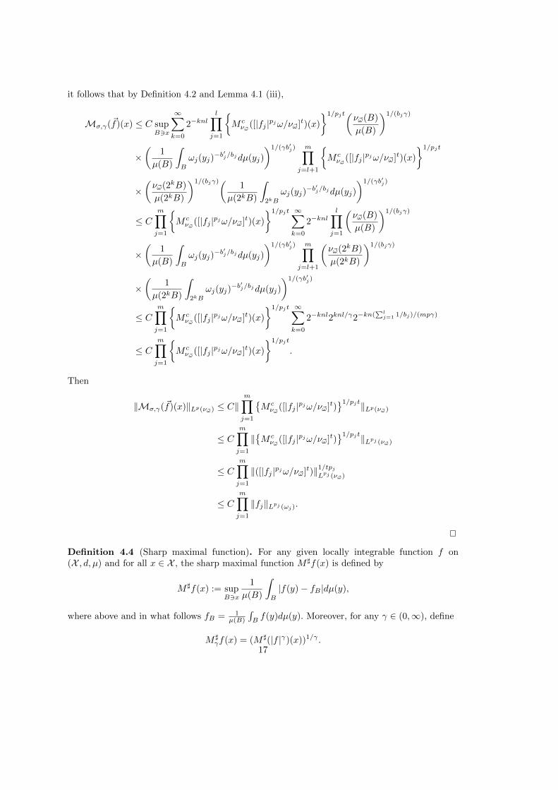
it follows that by Definition 4.2 and Lemma 4.1 (iii),

Mσ,γ(~f)(x) ≤ C supB3x

∞∑k=0

2−knll∏

j=1

M cν~ω

([|fj |pjω/ν~ω]t)(x)

1/pjt(ν~ω(B)

µ(B)

)1/(bjγ)

×(

1

µ(B)

∫B

ωj(yj)−b′j/bjdµ(yj)

)1/(γb′j) m∏j=l+1

M cν~ω

([|fj |pjω/ν~ω]t)(x)

1/pjt

×(ν~ω(2kB)

µ(2kB)

)1/(bjγ)( 1

µ(2kB)

∫2kB

ωj(yj)−b′j/bjdµ(yj)

)1/(γb′j)

≤ Cm∏j=1

M cν~ω

([|fj |pjω/ν~ω]t)(x)

1/pjt ∞∑k=0

2−knll∏

j=1

(ν~ω(B)

µ(B)

)1/(bjγ)

×(

1

µ(B)

∫B

ωj(yj)−b′j/bjdµ(yj)

)1/(γb′j) m∏j=l+1

(ν~ω(2kB)

µ(2kB)

)1/(bjγ)

×(

1

µ(2kB)

∫2kB

ωj(yj)−b′j/bjdµ(yj)

)1/(γb′j)

≤ Cm∏j=1

M cν~ω

([|fj |pjω/ν~ω]t)(x)

1/pjt ∞∑k=0

2−knl2knl/γ2−kn(∑lj=1 1/bj)/(mpγ)

≤ Cm∏j=1

M cν~ω

([|fj |pjω/ν~ω]t)(x)

1/pjt

.

Then

‖Mσ,γ(~f)(x)‖Lp(ν~ω) ≤ C‖m∏j=1

M cν~ω

([|fj |pjω/ν~ω]t)1/pjt‖Lp(ν~ω)

≤ Cm∏j=1

‖M cν~ω

([|fj |pjω/ν~ω]t)1/pjt‖Lpj (ν~ω)

≤ Cm∏j=1

‖([|fj |pjω/ν~ω]t)‖1/tpjLpj (ν~ω)

≤ Cm∏j=1

‖fj‖Lpj (ωj).

Definition 4.4 (Sharp maximal function). For any given locally integrable function f on(X , d, µ) and for all x ∈ X , the sharp maximal function M ]f(x) is defined by

M ]f(x) := supB3x

1

µ(B)

∫B

|f(y)− fB |dµ(y),

where above and in what follows fB = 1µ(B)

∫Bf(y)dµ(y). Moreover, for any γ ∈ (0,∞), define

M ]γf(x) = (M ](|f |γ)(x))1/γ .

17

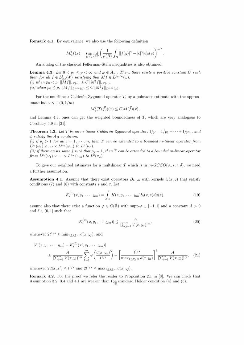
Remark 4.1. By equivalence, we also use the following definition

M ]γf(x) = sup

B3xinfc∈C

(1

µ(B)

∫B

||f(y)|γ − |c|γ |dµ(y)

)1/γ

.

An analog of the classical Fefferman-Stein inequalities is also obtained.

Lemma 4.3. Let 0 < p0 ≤ p < ∞ and ω ∈ A∞. Then, there exists a positive constant C suchthat, for all f ∈ L1

loc(X ) satisfying that Mf ∈ Lp0,∞(ω),(i) when p0 < p, ‖Mf‖Lp(ω) ≤ C‖M ]f‖Lp(ω).(ii) when p0 ≤ p, ‖Mf‖Lp,∞(ω) ≤ C‖M ]f‖Lp,∞(ω).

For the multilinear Calderon-Zygmund operator T, by a pointwise estimate with the approx-

imate index γ ∈ (0, 1/m)

M ]γ(T (~f))(x) ≤ CM(~f)(x),

and Lemma 4.3, ones can get the weighted boundedness of T, which are very analogous to

Corollary 3.9 in [21].

Theorem 4.3. Let T be an m-linear Calderon-Zygmund operator, 1/p = 1/p1 + · · ·+ 1/pm, and~ω satisfy the A~P condition.(i) if pj > 1 for all j = 1, · · · ,m, then T can be extended to a bounded m-linear operator fromLp1(ω1)× · · · × Lpm(ωm) to Lp(ν~ω).(ii) if there exists some j such that pj = 1, then T can be extended to a bounded m-linear operatorfrom Lp1(ω1)× · · · × Lpm(ωm) to Lp(ν~ω).

To give our weighted estimates for a multilinear T which is in m-GCZO(A, s, τ, δ), we need

a further assumption.

Assumption 4.1. Assume that there exist operators Btt>0 with kernels bt(x, y) that satisfyconditions (7) and (8) with constants s and τ. Let

K(0)t (x, y1, · · · , ym) =

∫XK(z, y1, · · · , ym)bt(x, z)dµ(z), (19)

assume also that there exist a function ϕ ∈ C(R) with suppϕ ⊂ [−1, 1] and a constant A > 0and δ ∈ (0, 1] such that

|K(0)t (x, y1, · · · , ym)| ≤ A

[∑mj=1 V (x, yj)]m

, (20)

whenever 2t1/s ≤ min1≤j≤m d(x, yj), and

|K(x, y1, · · · , ym)−K(0)t (x′, y1, · · · , ym)|

≤ A

[∑ml=1 V (x, yl)]m

m∑k=1

ϕ

(d(x, yk)

t1/s

)+

[t1/s

max1≤l≤m d(x, yl)

]δA

[∑ml=1 V (x, yl)]m

, (21)

whenever 2d(x, x′) ≤ t1/s and 2t1/s ≤ max1≤j≤m d(x, yj).

Remark 4.2. For the proof we refer the reader to Proposition 2.1 in [8]. We can check thatAssumption 3.2, 3.4 and 4.1 are weaker than the standard Holder condition (4) and (5).

18

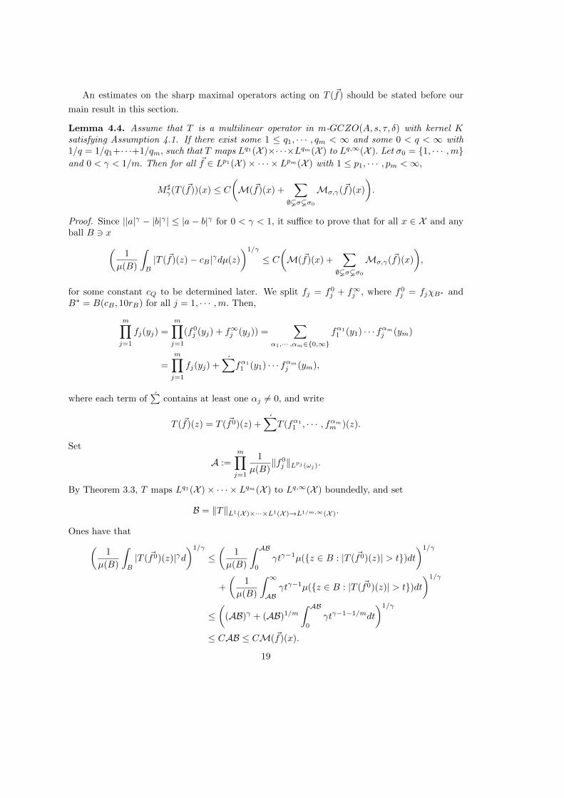
An estimates on the sharp maximal operators acting on T (~f) should be stated before our

main result in this section.

Lemma 4.4. Assume that T is a multilinear operator in m-GCZO(A, s, τ, δ) with kernel Ksatisfying Assumption 4.1. If there exist some 1 ≤ q1, · · · , qm < ∞ and some 0 < q < ∞ with1/q = 1/q1+· · ·+1/qm, such that T maps Lq1(X )×· · ·×Lqm(X ) to Lq,∞(X ). Let σ0 = 1, · · · ,mand 0 < γ < 1/m. Then for all ~f ∈ Lp1(X )× · · · × Lpm(X ) with 1 ≤ p1, · · · , pm <∞,

M ]γ(T (~f))(x) ≤ C

(M(~f)(x) +

∑∅ σ σ0

Mσ,γ(~f)(x)

).

Proof. Since ||a|γ − |b|γ | ≤ |a− b|γ for 0 < γ < 1, it suffice to prove that for all x ∈ X and anyball B 3 x(

1

µ(B)

∫B

|T (~f)(z)− cB |γdµ(z)

)1/γ

≤ C(M(~f)(x) +

∑∅ σ σ0

Mσ,γ(~f)(x)

),

for some constant cQ to be determined later. We split fj = f0j + f∞j , where f0j = fjχB∗ andB∗ = B(cB , 10rB) for all j = 1, · · · ,m. Then,

m∏j=1

fj(yj) =

m∏j=1

(f0j (yj) + f∞j (yj)) =∑

α1,··· ,αm∈0,∞

fα11 (y1) · · · fαmj (ym)

=

m∏j=1

fj(yj) +∑

fα11 (y1) · · · fαmj (ym),

where each term of∑

contains at least one αj 6= 0, and write

T (~f)(z) = T ( ~f0)(z) +∑

T (fα11 , · · · , fαmm )(z).

Set

A :=

m∏j=1

1

µ(B)‖f0j ‖Lpj (ωj).

By Theorem 3.3, T maps Lq1(X )× · · · × Lqm(X ) to Lq,∞(X ) boundedly, and set

B = ‖T‖L1(X )×···×L1(X )→L1/m,∞(X ).

Ones have that(1

µ(B)

∫B

|T ( ~f0)(z)|γd)1/γ

≤(

1

µ(B)

∫ AB0

γtγ−1µ(z ∈ B : |T ( ~f0)(z)| > t)dt)1/γ

+

(1

µ(B)

∫ ∞AB

γtγ−1µ(z ∈ B : |T ( ~f0)(z)| > t)dt)1/γ

≤(

(AB)γ + (AB)1/m∫ AB0

γtγ−1−1/mdt

)1/γ

≤ CAB ≤ CM(~f)(x).

19

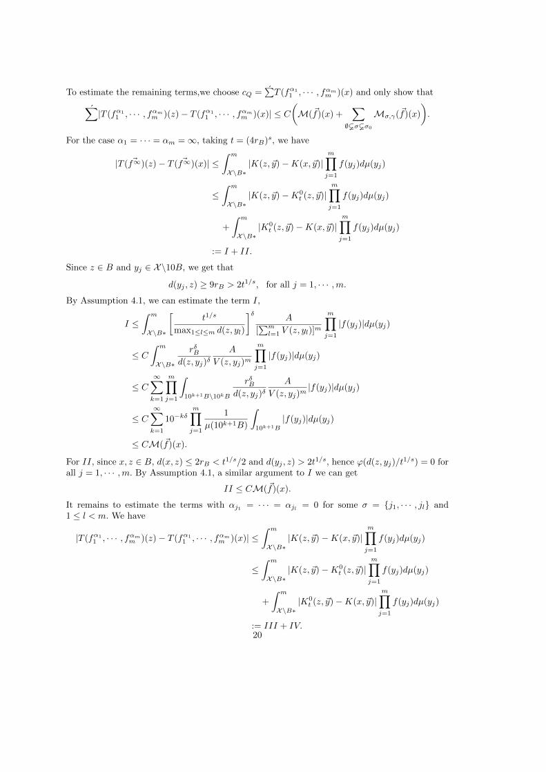
To estimate the remaining terms,we choose cQ =∑T (fα1

1 , · · · , fαmm )(x) and only show that∑|T (fα1

1 , · · · , fαmm )(z)− T (fα11 , · · · , fαmm )(x)| ≤ C

(M(~f)(x) +

∑∅ σ σ0

Mσ,γ(~f)(x)

).

For the case α1 = · · · = αm =∞, taking t = (4rB)s, we have

|T ( ~f∞)(z)− T ( ~f∞)(x)| ≤∫ m

X\B∗|K(z, ~y)−K(x, ~y)|

m∏j=1

f(yj)dµ(yj)

≤∫ m

X\B∗|K(z, ~y)−K0

t (z, ~y)|m∏j=1

f(yj)dµ(yj)

+

∫ m

X\B∗|K0

t (z, ~y)−K(x, ~y)|m∏j=1

f(yj)dµ(yj)

:= I + II.

Since z ∈ B and yj ∈ X\10B, we get that

d(yj , z) ≥ 9rB > 2t1/s, for all j = 1, · · · ,m.

By Assumption 4.1, we can estimate the term I,

I ≤∫ m

X\B∗

[t1/s

max1≤l≤m d(z, yl)

]δA

[∑ml=1 V (z, yl)]m

m∏j=1

|f(yj)|dµ(yj)

≤ C∫ m

X\B∗

rδBd(z, yj)δ

A

V (z, yj)m

m∏j=1

|f(yj)|dµ(yj)

≤ C∞∑k=1

m∏j=1

∫10k+1B\10kB

rδBd(z, yj)δ

A

V (z, yj)m|f(yj)|dµ(yj)

≤ C∞∑k=1

10−kδm∏j=1

1

µ(10k+1B)

∫10k+1B

|f(yj)|dµ(yj)

≤ CM(~f)(x).

For II, since x, z ∈ B, d(x, z) ≤ 2rB < t1/s/2 and d(yj , z) > 2t1/s, hence ϕ(d(z, yj)/t1/s) = 0 for

all j = 1, · · · ,m. By Assumption 4.1, a similar argument to I we can get

II ≤ CM(~f)(x).

It remains to estimate the terms with αj1 = · · · = αjl = 0 for some σ = j1, · · · , jl and1 ≤ l < m. We have

|T (fα11 , · · · , fαmm )(z)− T (fα1

1 , · · · , fαmm )(x)| ≤∫ m

X\B∗|K(z, ~y)−K(x, ~y)|

m∏j=1

f(yj)dµ(yj)

≤∫ m

X\B∗|K(z, ~y)−K0

t (z, ~y)|m∏j=1

f(yj)dµ(yj)

+

∫ m

X\B∗|K0

t (z, ~y)−K(x, ~y)|m∏j=1

f(yj)dµ(yj)

:= III + IV.20

Since x, z ∈ B and yj ∈ X\B∗, we have that d(x, yj) ∼ d(z, yj) ∼ d(cB , yj) and V (x, yj) ∼V (z, yj) ∼ V (cB , yj). Set σ′ = σ0\σ, by Assumption 4.1 we can deduce that

III ≤ C∏j∈σ

∫B∗|fj(yj)|dµ(yj)

(∫X\B∗

tδ

d(x, yj)δA

V (x, yj)m

∏j∈σ′|fj(yj)|dµ(yj)

+

∫X\B∗

A

V (x, yj)m

∏j∈σ′|fj(yj)|dµ(yj)

)

≤ C∏j∈σ

∫B∗|fj(yj)|dµ(yj)

( ∞∑k=1

∏j∈σ′

∫2k+1B∗\2kB∗

rBd(cB , y)

1

V (cB , yj)m|f(yj)|dµ(yj)

+

∞∑k=1

∏j∈σ′

∫2k+1B∗\2kB∗

1

V (cB , yj)m|f(yj)|dµ(yj)

)

≤ C( ∞∑k=1

2−kδm∏j=1

1

µ(2kB∗)

∫2kB∗

|fj(yj)|dµ(yj)

+

∞∑k=1

2−knl∏j∈σ

1

µ(B∗)

∫B∗|fj(yj)|dµ(yj)

∏j∈σ′

1

µ(2kB∗)

∫2kB∗

|fj(yj)|dµ(yj)

)

≤ C(M(~f)(x) +Mσ,γ(~f)(x)

).

Similarly,

IV ≤ C(M(~f)(x) +Mσ,γ(~f)(x)

).

This finishes the proof of Lemma 4.4.

Our main theorem in this section is formulated as follows.

Theorem 4.4. Assume that T is a multilinear operator in m-GCZO(A, s, τ, δ) with kernel Ksatisfying Assumption 4.1. If there exist some 1 ≤ q1, · · · , qm < ∞ and some 0 < q < ∞with 1/q = 1/q1 + · · · + 1/qm, such that T maps Lq1(X ) × · · · × Lqm(X ) to Lq,∞(X ), then for

1/m < p <∞, 1 ≤ p1, · · · , pm <∞ with 1/p = 1/p1+ · · ·+1/pm, ~P = (p1, · · · , pm), and ~ω ∈ A~P ,(i) if pj > 1 for all j = 1, · · · ,m, then T can be extended to a bounded m-linear operator fromLp1(ω1)× · · · × Lpm(ωm) to Lp(ν~ω).(ii) if there exists some j such that pj = 1, then T can be extended to a bounded m-linear operatorfrom Lp1(ω1)× · · · × Lpm(ωm) to Lp(ν~ω).

Proof. The fact is that ω ∈ A~p implies that ν~ω ∈ Amp. Therefore Lemma 4.4 and Theorem 4.2leads us to

‖T (~f)‖Lp(ν~ω) ≤ C(‖M(~f)‖Lp(ν~ω) + ‖Mσ,γ‖Lp(ν~ω))≤ C‖fj‖Lpj (ωj).

Thus it completes our proof.

References

[1] R. Coifman, Y. Meyer, On commutators of singular integral and bilinear singular integrals,

Trans. Amer. Math. Soc., 212 (1975), 315-331.21

[2] R. Coifman, Y. Meyer, Au dela des operateurs pseudo-differentiels, Asterisque, 57 (1978).

[3] R. Coifman, Y. Meyer, Ondelettes et operateurs, III, Hermann, Paris, 1990.

[4] M. Christ, J. L. Journe, Polynomial growth estimates for multilinear singular integral oper-

ators, Acta Math. 159 (1987) 51-80.

[5] R. R. Coifman et G. Weiss, Analyse harmonique non-commutative sur certains espaces

homogenes, Lecture Notes in Math. 242, Springer, Berlin, 1971.

[6] R. R. Coifman et G. Weiss, Extensions of Hardy spaces and their use in analysis, Bull.

Amer. Math. Soc. 83 (1977), 569-645.

[7] X. T. Duong, R. Gong, L. Grafakos, J. Li and L. Yan, Maximal operator for multilinear

singular integrals with non-smooth kernels, Indiana Univ. Math. J. 58 (2009) 2517-2541.

[8] X. T. Duong, L. Grafakos, L.X. Yan, Multilinear operators with non-smooth kernels and

commutators of singular integrals, Trans. Amer. Math. Soc. 362 (4) (2010) 2089-2113.

[9] X. T. Duong, A. McIntosh, Singular integral operators with non-smooth kernels on irregular

domains. Rev. Mat. Iberoam. 15, (1999) 233-265.

[10] C. Fefferman and E.M. Stein, Some maximal inequalities, Amer. J. Math., 93 (1971), 107-

115.

[11] L. Grafakos, Classical Fourier Analysis, 2nd edition, Graduate Texts in Mathematics 249,

Springer, New York, 2008.

[12] L. Grafakos, L. Liu, D. Maldonado and D. Yang, Multilinear analysis on metric spaces,

http://www.math.ksu.edu/ dmaldona/papers/glmy(DM704).pdf.

[13] L. Grafakos, L. Liu, D. Yang, Multiple weighted norm inequalities for maximal multilinear

singular integrals with non-smooth kernels, Proc. Roy. Soc. Edinburgh Sect. A 141A (2011)

755-775.

[14] L. Grafakos, R. H. Torres, Multilinear Calderon-Zygmund theory, Adv. Math. 165 (1) (2002)

124-164.

[15] L. Grafakos, R. H. Torres, Maximal operator and weighted norm inequalities for multilinear

singular integrals, Indiana Univ. Math. J. 51 (5) (2002) 1261-1276.

[16] L. Grafakos, N. Kalton, Some remarks on multilinear maps and interpolation, Math. Ann.,

319 (2001), 151-180.

[17] J. Heinonen, Lectures on Analysis on Metric Spaces, Springer-Verlag, New York, 2001.

22

[18] Y. Han, D. Muller, D. Yang, A theory of Besov and Triebel-Lizorkin spaces on metric

measure spaces modeled on Carnot-Caratheodory spaces, Abstr. Appl. Anal. 2008, Art. ID

893409, 250 pp.

[19] Y. Han and E. Sawyer, LittlewoodCPaley theory on spaces of homogeneous type and the

classical function spaces, Mem. Amer. Math. Soc. 110 (1994), no. 530.

[20] C. E. Kenig, E. M. Stein, Multilinear estimates and fractional integration, Math. Res. Lett.

6 (1999) 1-15.

[21] A. K. Lerner, S. Ombrosi, C. Perez, R. H. Torres, R. Trujillo-Gonzalez, New maximal

functions and multiple weights for the multilinear Calderon-Zygmund theory, Adv. Math.

220 (2009) 1222-1264.

[22] R. A. Macıas, C. Segovia, Lipschitz functions on spaces of homogeneous type, Adv. Math.

33 (1979), 257-270.

[23] R. A. Macıas, C. Segovia, A decomposition into atoms of distributions on spaces of homo-

geneous type, Adv. Math. 33 (1979), 271-309.

[24] J. Stromberg, A. Torchinsky, Weighted Hardy spaces. Lecture Notes in Math., vol. 1381.

Springer, Berlin (1989).

23