Generating interest-rate scenarios for fixed-income portfolio optimisation

© Actuarial Society of South Africa | 1

SOUTH AFRICA ACTUARIAL JOURNALSAAJ 10 (2010) 1–42

GENERATING INTEREST-RATE SCENARIOS FOR FIXED-INCOME PORTFOLIO OPTIMISATION

By H Raubenheimer and MF Kruger

ABSTRACTOne of the main sources of uncertainty in the analysis of the risk and return properties of a portfolio of fixed-income securities is the stochastic evolution of the shape of the yield curve. The authors have estimated a model that fits the South African yield curve, using a Kalman filter. The model includes four latent factors and three observable macroeconomic variables (capacity utilisation, inflation and the repo rate). The goal is to capture the dynamic interactions between the macroeconomy and the yield curve in such a way that the resulting model can be used to generate interest-rate scenario trees that are suitable for fixed-income portfolio optimisation. An important input into the scenario generator is the investor’s view on the future evolution of the repo rate. In this paper, details of the model are provided and the results of the estimation and scenario generation are reported.

KEYWORDSTerm structure; yield curve; Kalman filter; macroeconomic; scenario generation; Nelson–Siegel curve; Svensson curve

CONTACT DETAILSMr Helgard Raubenheimer, Centre for Business Mathematics and Informatics, North-West University (Potchefstroom Campus), Private Bag X6001, Potchefstroom, 2520, South Africa; Tel: +27(0)18 299 2565; Fax: +27(0)18 299 2584; E-mail: [email protected]

1. INTRODUCTION1.1 One of the main sources of uncertainty in the analysis of the risk and return properties of a portfolio of fixed-income securities is the stochastic evolution of the shape of the yield curve. Many yield-curve models (e.g. Knez et al., 1994, Duffie & Kan,

SAAJ 10 (2010)

2 | GENERATING INTEREST-RATE SCENARIOS FOR FIXED-INCOME PORTFOLIO OPTIMISATION

1996 and Dai & Singleton, 2000) consider models in which unobserved factors explain the entire set of yields. (In this paper ‘yield’ means the yield to maturity on a zero-coupon bond.) These factors are often given the labels ‘level’, ‘slope’ and ‘curvature’. The factors in these models are however not linked to macroeconomic variables. Examples where a latent-factor model is used to characterise the yield curve and that explicitly include macroeconomic factors can be found in Ang & Piazzesi (2003), Hördahl et al. (unpublished) and Wu (unpublished). These examples, however, only consider a unidirectional linkage between the macroeconomy and the yield curve. Kozicki & Tinsley (2001), Dewachter & Lyrio (unpublished) and Rudebusch & Wu (unpublished) allow for implicit feedback. Tilley (1992) provides an actuarial layperson’s guide to building stochastic interest-rate generators.

1.2 Bernaschi et al. (2008) shows that, besides the relation with the official interest rate of the European Central Bank, it is extremely difficult to find, using simple linear regression analysis, a convincing relation among the parameters that describe the Italian yield curve and macroeconomic variables that drive the dynamics of the yield curve itself. Bernaschi et al. (op. cit.) concludes that a possible solution is to resort to more complex interaction models based on non-linear impulse-response functions. Ang & Piazzesi (op. cit.) further argue the importance of describing the joint behaviour of the yield curve and macroeconomic variables for bond pricing, investment decisions and public policy. They state that although many yield-curve models use latent factors to explain yield-curve movements and may afford some interpretation of the meaning of these factors (e.g. level, slope and curvature), the factors do not correspond explicitly to macroeconomic variables. These models describe the effect the latent factors have on the yield curve rather than describing the economic sources of the shocks. Ang & Piazzesi (op. cit.) consider a unidirectional linkage between the macroeconomy and the yield curve.

1.3 De Pooter et al. (unpublished) argues that models that include macroeconomic variables seem more accurate in sub-periods where there is substantial uncertainty about the future path of interest rates. Furthermore, models that do not include information about the macroeconomy perform well in sub-periods where the yield curve has a more stable pattern.

1.4 Inspired by the research of Diebold, Rudebusch & Aruoba (2006), the authors estimate a model that fits the South African yield curve, using a Kalman filter approach. Diebold, Rudebusch & Aruoba (op. cit.) characterise the yield curve using three latent factors, namely level, slope and curvature. To model the dynamic interactions between the macroeconomy and the yield curve, they also included observable macroeconomic variables, specifically real activity, inflation and a monetary-policy instrument.

1.5 To capture the dynamics of the yield curve, Diebold, Rudebusch & Aruoba (op. cit.) do not use a no-arbitrage factor representation such as the typically used affine

SAAJ 10 (2010)

GENERATING INTEREST-RATE SCENARIOS FOR FIXED-INCOME PORTFOLIO OPTIMISATION | 3

no-arbitrage models (see e.g. Duffee, 2002 and Brousseau, unpublished) or canonical affine no-arbitrage models (see e.g. Rudebusch & Wu, op. cit.). Instead of using a no-arbitrage representation Diebold, Rudebusch & Aruoba (op. cit.) suggest using a three-factor yield-curve model based on the yield-curve model of Nelson & Siegel (1987), as used in Diebold & Li (2006), and interpret these factors as level, slope and curvature. Diebold & Li (op. cit.) propose a two-step procedure to estimate the dynamics of the yield curve. The procedure firstly estimates the three latent factors and secondly estimates an autoregressive model for these factors. Diebold & Li (op. cit.) use these models to forecast the yield curve. Diebold, Rudebusch & Aruoba (op. cit.) propose a one-step approach by introducing an integrated state-space modelling approach which is preferred over the two-step Diebold–Li approach. This Kalman-filter approach allows for a bidirectional linkage between the macroeconomy and the yield curve and simultaneously fits the yield curve and estimates the underlying dynamics of these factors. The model also incorporates the estimation of the macroeconomic factors and the link between the macroeconomy and the latent factors driving the yield curve.

1.6 In the South African yield curve context, Maitland (2002) provides principle-component analysis to interpolate the South African yield curve. The method proposed by Maitland (op. cit.) provides a way in which the yield curve can be interpolated from a restricted number of modelled yields, and at the same time minimises the number of yields from which to estimate the remainder of the curve. Given the first and second principal components, Maitland (op. cit.) shows that the short rate and the long-bond yield could be used to reconstruct the South African yield curve. Stander (unpublished) discusses bond indices in South Africa. Using a survey, Stander (op. cit.) establishes inadequacies in the indices as well as possible changes that should be considered. Stander (op. cit.) further addresses criticism of the Bond Exchange–Actuaries yield curve and presents alternative empirical yield-curve models and equilibrium models. These contributions focus on the characterisation of the yield curve and do not consider forecasting or scenario generation.

1.7 In Section 2, the authors describe Kalman-filter state-space modelling for the basic three-factor ‘yields-only model’ (YO3F) proposed by Diebold, Rudebusch & Aruoba (op. cit.). Their model uses only three latent factors of the yield curve and does not include macroeconomic factors. The model estimation for the South African yield curve is described and a four-factor model (YO4F) based on the Svensson (1994) yield curve model is introduced. It is shown that the Nelson & Siegel (op. cit.) model is not flexible enough to get an acceptable fit to the South African yield curve and a four-factor model is therefore introduced.

1.8 In Section 3, macroeconomic variables (capacity utilisation, inflation and repo-rate) are incorporated into the ‘yields-macro model’ (YM4F). The goal is to capture the dynamic interactions between the macroeconomy and the yield curve in such a way that the resulting model can be used to generate interest-rate scenario trees that are suitable

SAAJ 10 (2010)


for fixed-income portfolio optimisation. Section 4 describes the approach adopted. An important input into the scenario generator is the investor’s view on the future evolution of the repo rate. In practice these views are produced by means of an economic scenario generator (ESG) or expert opinion. The existence of arbitrage in the scenario trees is discussed and a method to eliminate arbitrage opportunities is proposed. Concluding remarks are offered in Section 5.

2. YIELDS-ONLYMODEL In this section the factor model representation of the yield curve is introduced. Following Diebold, Rudebusch & Aruoba (op. cit.), the discussion starts with the YO3F model using the three-factor representation of Nelson & Siegel (op. cit.) and this is used as a benchmark for the four factor representation of Svensson (op. cit.). By using the more flexible four-factor model, a better cross-sectional fit of the South African yield curve is obtained. Since all the models that are described in this section are fitted using a Kalman filter, this section starts with an overview of the Kalman filter.

2.1 THE KALMAN FILTER2.1.1 The Kalman filter, introduced by Kalman (1960), is a popular

technique used in signal processing, control engineering and other fields. The main idea is to represent a dynamic system in terms of states (the unobserved underlying Markov process). The ‘state equation’ (or ‘transition equation’) describes the dynamics of this process while the ‘observation equation’ (or ‘measurement equation’) relates the observables to the unobserved states. The advantage of using a state-space representation (defined below) is that it allows the modeller to infer the properties of the unobserved yield-curve drivers from the observed yields.

2.1.2 Following Hamilton (1994: Chapter 13), let yt denote a vector of variables (yields in our case) observed at date t that can be described in terms of ft, a vector of unobservable states. The ‘state-space representation’ of the dynamics of y is then given by the following system of equations: ft = Aft–1+ t (1) yt = Bxt + Λft + εt (2)

where the matrices A, B and Λ have appropriate dimensions and xt is a vector of exogenous variables. Equation (1) is the transition equation and equation (2) is the measurement equation. The disturbances t and εt are vector white-noise processes such that:

( )for

0 otherwise; andt

tE τ

τηη

=′ =

Q

( )for

0 otherwise;t

tE τ

τε ε

=′ =

H

where the matrices Q and H have appropriate dimensions. The disturbances t and εt are also assumed to be uncorrelated at all lags:

SAAJ 10 (2010)


( ) 0, forall and .tE tτη ε τ=

2.1.3 TheKalmanfilterisasequentialalgorithmthatcalculatesthebestpre-dictoroftheunobservedstates,givenallpreviousobservations—seedetailsbelow.

2.2 FACTORREPRESENTATION2.2.1 Themainaimof the factormodel is to represent theyieldcurve (a

largesetofyieldswithvariousmaturities)asafunctionofasmallersetofunobservablefactors. TheNelson–Siegel (op. cit.) representation produces reliable and reasonableestimation results and has becomeone of the popular approaches adopted by centralbanksforyieldcurveestimation.1TheNelson–Siegelmodel,derivedfromaparametricfunctionalformfortheforwardrates,usesonlyfourparameterstodefineaparsimoniousandstablerepresentationofthewholeyieldcurve:

,

( ) 1 2 31 1e ey e

λτ λτλττ β β β

λτ λτ

− −− − −

= + + −

wherey(τ)istheyieldwithmaturityτandβ1,β2,β3andλarethemodelparameters.AsdemonstratedbyDiebold&Li (op. cit.), theparametersβ1,β2andβ3of theNelson–Siegelrepresentationoftheyieldcurve,canbeinterpretedaslevel,slopeandcurvature;the terms thatmultiply these factorsarecalled the ‘factor loadings’.Theparameterλdeterminestheshapeofthecurveanddoesnothaveadirecteconomicinterpretation.To givemeaning to the parametersβ1,β2andβ3,Diebold&Li (op. cit.) rewrite therepresentationas

( ) 1 1

t t t te ey L S C e

λτ λτλττ

λτ λτ

− −− − −

= + + −

whereLt ,StandCtare the time-varyingparameters,andβ1,β2andβ3areconsideredunobservedfactors.

2.2.2 Diebold, Rudebusch & Aruoba (op. cit.) describe the state-spacesystemasfollows.ThedynamicsoftheunobservablefactorsLt ,StandCtaremodelledasavectorautoregressiveprocessofthefirstorder(a‘VAR(1)’process),whichformsastate-spacesystem.Theautoregressivemoving-averagestate-vectordynamicsmaybeofanyorder,buttheVAR(1)assumptionismaintainedfortransparencyandparsimony.Thedynamicsofthestatevectorisgovernedbythetransitionequation:

( )( )( )

111 12 13

21 22 23 1

31 32 33 1

tt L t L

t S t S t

t C t C t

LL La a aS a a a S S

a a aC C C

ηµ µµ µ ηµ µ η

−

−

−

− − − = − +

− −

;

wheret=1,…,T.

1 Zero-couponyieldcurves:technicaldocumentation.BankforInternationalSettlements,Switzerland,1999

SAAJ 10 (2010)


2.2.3 Forafixedvalueoftheparameterλ(specifiedbelow),themeasurementequation,whichrelatesasetofNyieldsoftheyieldcurve,withmaturitiesτ1,…τN,tothethreeunobservedfactors,are:

;

1 11

2 22

1 11 1

2 22 2

1 11

1 11

1 11N N

N

t tt

t tt

tt N t N

N N

e e ey

Le e eySC

ye e e

wheret=1,…,T.Thestate-spacesystemcanbewritteninmatrixnotationas ,

1t t tf f A

yt =Λft +εt .Thewhite-noisedisturbancesinthetransitionandmeasurementequationsarerequiredtobeorthogonaltoeachotherandtotheinitialstateforthelinearleast-squaresoptimalityoftheKalmanfilter:

;

0 0~ ,

0 0t

t

QWN

Hηε

( )0 0tE f η′ = ;and ( )0 0tE f ε ′ = .

2.2.4 Diebold,Rudebusch&Aruoba(op. cit.)assumethattheQmatrixisnon-diagonaltoallowtheshockstothethreeyield-curvefactorstobecorrelated.TheHmatrixisassumedtobediagonal,whichimpliesthatthedeviationsoftheyieldsofvariousmaturitiesfromtheyieldcurveareuncorrelated.Thisisquitestandardand,asinestimatingno-arbitrageyieldcurvemodels,independentlyandidenticallydistributed(i.i.d.)‘measurementerrors’areaddedtotheobservedyields.Giventhelargenumberof observed yields, this is required for computational tractability as well (Diebold,Rudebusch&Aruoba,op. cit.).

2.3 THREE-FACTORMODELESTIMATION2.3.1 Weuse the‘perfectfitbondcurves’,oneof thefiveBEASSAzero-

couponyield-curveseries,2withmaturities1,2,3,6,9,12,15,18,21,24,36,48,60,72,84,96,108,120,132,144,156,168,180,192,204,216and228months.Theyields

2 AnintroductiontotheBEASSAzerocouponyieldcurves.BondExchangeofSouthAfrica,Johannesburg,2003

SAAJ 10 (2010)


curves are compounded semi-annually. For the purposes of analysis the yields are converted to continuously compounded yields. The curves are derived from government-bond data.3 End-of-month data are used from August 1999 to February 2009. Figure 1 plots the yield-curve data.

2.3.2 The variation in the level of the yield curve is visually apparent, as is the variation in its slope and curvature. Descriptive statistics for the yields (mean, standard deviation, minimum, maximum and autocorrelations for 1, 12 and 30 months) are provided in Table 1. It is clear that the typical yield curve is hump-shaped with a negative hump at about 20 months and a positive hump at about 120 months. The short rates are less volatile than the long rates but comparison of the autocorrelation with a lag of 12 months shows that they are less persistent. This is opposite to the U.S. yield curve (see Diebold & Li, op. cit.). The level is persistent and varies moderately relative to its mean and the slope and the curvature are the least persistent. The slope is highly variable relative to its mean, as is its curvature. In Figure 2 the median yield curve together with point-wise interquartile ranges are displayed. The hump-shaped pattern, with short rates less volatile than long rates, is apparent.

3 For technical specifications, see The BEASSA zero coupon yield curves: technical specifications. Bond Exchange of South Africa, Johannesburg, 2003

Figure 1: Yields curves, August 1999 to February 2009

SAAJ 10 (2010)


Table 1: Descriptive statistics of the yield curveMaturity Mean

(%)Standard deviation

(%)

Minimum (%)

Maximum (%) ( )ˆ 1ρ ( )ˆ 12ρ ( )ˆ 30ρ

1 9,225 1,835 6,542 12,437 0,974 0,272 –0,3352 9,215 1,806 6,554 12,383 0,975 0,271 –0,3373 9,199 1,774 6,565 12,329 0,974 0,269 –0,3346 9,127 1,672 6,604 12,223 0,968 0,268 –0,3019 9,054 1,586 6,574 12,092 0,956 0,268 –0,24212 9,003 1,533 6,531 12,058 0,945 0,272 –0,17515 8,981 1,509 6,509 12,024 0,936 0,280 –0,11318 8,977 1,499 6,385 11,989 0,931 0,293 –0,05821 8,987 1,498 6,347 11,954 0,928 0,309 –0,01124 9,005 1,502 6,295 11,918 0,927 0,327 0,03036 9,108 1,546 6,638 12,107 0,930 0,403 0,14248 9,219 1,606 6,912 12,615 0,937 0,463 0,19460 9,311 1,660 6,980 12,959 0,943 0,501 0,21972 9,381 1,702 7,026 13,190 0,946 0,524 0,23284 9,432 1,733 7,055 13,350 0,948 0,538 0,23796 9,466 1,756 7,072 13,466 0,949 0,548 0,236108 9,483 1,773 7,076 13,553 0,950 0,554 0,231120 9,481 1,789 7,069 13,621 0,950 0,560 0,225132 9,462 1,805 7,051 13,676 0,950 0,565 0,216144 9,427 1,823 7,023 13,721 0,951 0,570 0,207156 9,380 1,842 6,987 13,759 0,951 0,574 0,197168 9,325 1,863 6,945 13,792 0,952 0,579 0,186180 9,266 1,885 6,898 13,820 0,952 0,583 0,174192 9,204 1,907 6,847 13,845 0,953 0,588 0,162204 9,141 1,931 6,794 13,866 0,953 0,591 0,150216 9,077 1,956 6,698 13,886 0,954 0,594 0,138228 9,015 1,981 6,581 13,903 0,954 0,597 0,126Level 9,232 1,571 6,818 12,821 0,958 0,575 0,138Slope 0,184 2,140 –3,760 4,093 0,965 0,261 –0,336Curvature –0,204 1,376 –5,409 2,847 0,852 0,016 –0,102

2.3.3 As in Diebold, Rudebusch & Aruoba (op. cit.), the YO3F model forms a state-space system, with a VAR(1) transition equation summarising the dynamics of the vector of latent variables, and a linear measurement equation relating the observed yields to the state vector as described above. In the entire model there are 46 parameters that need to be estimated by the numerical optimisation of the relevant likelihood function. Let ψ be the vector of all parameters that need to be estimated. These parameters are the nine parameters contained in transition matrix A, the three parameters contained in the

SAAJ 10 (2010)


mean state vector μ, and the one parameter λ contained in the measurement matrix Λ. Furthermore, the transition-disturbance covariance matrix Q contains six parameters, and the measurement-disturbance covariance matrix H contains 27 parameters (one variance for each of the 27 yields). Given that the matrices A and Λ are affine and assuming that the distributions of t , εt and f0 are normal, the model is referred to as a ‘linear Gaussian state-space model’ (Lemke, 2006). The Kalman-filter algorithm is provided in Appendix A.

2.3.4 The parameters are estimated by maximising the log-likelihood function (see Appendix A), using either the Nelder–Mead simplex or Newton–Raphson algorithm. For more details on Kalman filtering see Harvey (1989) and Lemke (op. cit.). Non-negativity constraints are imposed on all the variances. As in Diebold, Rudebusch & Aruoba (op. cit.), starting parameters are obtained using the two-step Diebold–Li method and initialising the variances to 1,0. As in Diebold & Li (op. cit.) the value of λ is initialised at 0,0609 to maximise the loading on the curvature factor at exactly 30 months, i.e. the maturity at which the hump occurs in the yield curve.

2.3.5 Tables 2 and 3 show the estimation results for the YO3F model. In those tables bold entries denote parameters estimates significant at 5% and standard errors appear in parentheses. In Table 2 the estimate of the A matrix indicates the highly persistent dynamics of Lt , St and Ct , the estimated own-lag coefficients being 0,945, 0,987 and 0,953 respectively. Cross-factor dynamics between St and Lt and between St and Ct appear to be important with statistically significant effects. The mean of the level is approximately 8,5%. The means of the slope and of the curvature do not seem statistically significant different from zero and appear to be reasonable in comparison with the mean values of the empirical estimates in Table 1. The largest eigenvalue of the A matrix is 0,96, which ensures the stationarity of the system. In Table 3 the estimates

Figure 2: Median yield curve with the point-wise interquartile range

6

7

8

9

10

11

12

0 50 100 150 200 250

Yie

lds (

per c

ent)

Maturity (months)

first quartilemedianthird quartile

SAAJ 10 (2010)


of the Q matrix indicate that transitional shock volatility increases as we move from Lt to St to Ct as measured by the diagonal elements. There are no significant covariance terms in the Q matrix. The estimate for λ is 0,0916, which implies that the loading on the curvature factor is maximised at a maturity of 19,85 months. This can be seen in Figure 2, where the first (inverted) hump occurs near the maturity of 20 months.

Table 2: YO3F: model estimates

Lt–1 St–1 Ct–1 μLt 0,945

(0,026)0,007

(0,020)–0,022(0,014)

8,568(0,886)

St 0,091(0,033)

0,987(0,025)

0,110(0,018)

0,039(0,723)

Ct –0,137(0,078)

–0,213(0,059)

0,953(0,043)

–0,988(0,597)

Table 3: YO3F: estimated Q matrix

Lt St Ct

Lt 0,161(0,021)

–0,163(0,024)

0,003(0,046)

St 0,265(0,035)

–0,015(0,059)

Ct 1,476(0,196)

2.3.6 Table 4 shows the means and standard deviations of the predicted errors (also called measurement errors, which are measured as the excess of the actual yields over the predicted model yields) for the yields-only model and the yields-macro model (presented in section 3 below). The YO3F model fits the yield curve reasonably well in the short maturities but less so in the longer maturities, the standard deviation also increasing for longer maturities. The results are similar to the yields-only model of Diebold, Rudebusch & Aruoba (op. cit.).

2.3.7 The Kalman-filter fixed-interval smoothing algorithm (see Appendix A) is used to obtain optimal extractions of the latent level, slope and curvature factors. Figure 3 plots the three smoothed estimated factors together and Figures 4 to 6 plot the three factors together with various empirical proxies and related macroeconomic variables. The level factor in Figure 3 is in the neighbourhood of 8% and displays persistence. The slope and the curvature factors vary around zero with positive and negative values and appear less persistent. The slope factor is more persistent than the curvature factor but has a lower variance. This seems consistent with the mean and autocorrelation values of the empirical estimates in Table 1.

SAAJ 10 (2010)


Table 4: Summary of statistics for predicted errors of yields (%)

MaturityYO3F YO4F YM3F YM4F

Mean Standard deviation




1 –0,052 0,377 –0,048 0,491 0,000 0,431 –0,008 0,3992 –0,011 0,358 –0,008 0,449 0,004 0,438 0,003 0,4103 0,017 0,359 0,020 0,430 0,010 0,317 0,021 0,3116 0,047 0,385 0,054 0,431 –0,011 0,338 0,030 0,3189 0,037 0,407 0,051 0,462 0,006 0,323 0,026 0,313

12 0,023 0,432 0,044 0,499 0,016 0,321 0,022 0,31515 0,018 0,456 0,045 0,528 0,026 0,337 0,013 0,33618 0,019 0,476 0,048 0,550 0,020 0,357 0,009 0,36221 0,023 0,493 0,052 0,566 0,015 0,377 0,009 0,38324 0,030 0,506 0,055 0,576 0,014 0,393 0,011 0,40036 0,064 0,537 0,049 0,594 0,016 0,408 0,014 0,41548 0,104 0,551 0,027 0,596 0,019 0,421 0,017 0,42860 0,141 0,556 0,002 0,597 0,024 0,432 0,019 0,44072 0,168 0,557 –0,018 0,604 0,049 0,466 0,023 0,47584 0,186 0,558 –0,028 0,612 0,083 0,487 0,017 0,49396 0,195 0,560 –0,028 0,619 0,118 0,496 0,010 0,498

108 0,192 0,560 –0,021 0,623 0,149 0,500 0,006 0,499120 0,174 0,560 –0,013 0,627 0,170 0,501 0,007 0,499132 0,141 0,559 –0,007 0,629 0,180 0,502 0,013 0,498144 0,095 0,560 –0,005 0,632 0,177 0,503 0,020 0,499156 0,038 0,565 –0,005 0,634 0,159 0,504 0,026 0,501168 –0,025 0,574 –0,005 0,636 0,128 0,505 0,029 0,503180 –0,091 0,589 –0,005 0,638 0,085 0,509 0,030 0,506192 –0,160 0,608 –0,004 0,639 0,033 0,518 0,030 0,509204 –0,229 0,633 –0,002 0,641 –0,024 0,532 0,029 0,511216 –0,298 0,661 0,000 0,644 –0,085 0,553 0,028 0,514228 –0,365 0,693 0,004 0,647 –0,146 0,579 0,029 0,517

2.3.8 Figure 4 displays the estimated level factor and two related comparison series. The first one is a commonly used empirical proxy for the level factor, namely the average of the short-, medium- and long-term yields:

( ) ( ) ( )( )3 24 228 / 3y y y+ + .

The second is the annual percentage change in the consumer price index. There is a high correlation of 0,89 between the level factor and the empirical proxy. The correlation between the level factor and the inflation rate is 0,51. As stated by Diebold, Rudebusch & Aruoba (op. cit.) this is consistent with the Fisher equation, which suggests a link between the level of the yield curve and inflation expectations.

SAAJ 10 (2010)


2.3.9 In the estimates of the empirical level, slope and curvature the228-monthyieldwasusedandnot the120-monthyieldas inDiebold,Rudebusch&Aruoba(op. cit.).Thishasverylittleeffectontheresults.

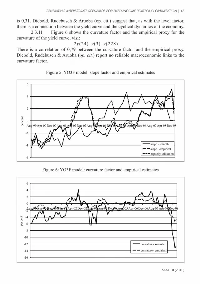
2.3.10 Figure 5 also displays the estimated slope factor and two relatedcomparisonseries.Thefirstistheempiricalproxyfortheslopefactor,namelytheexcessoftheshort-termyieldoverthelong-termyield:

y(3)–y(228).Thesecondisanindicatorofmacroeconomicactivity,namelythedemeanedmanufac-turingcapacityutilisation.Thereisahighcorrelationof0,97betweentheslopefactorandtheempiricalproxy.Thecorrelationbetweentheslopefactorandcapacityutilisation

Figure3:YO3Fmodel:estimatesofthelevel,slopeandcurvaturefactors

Figure4:YO3Fmodel:levelfactorandempiricalestimates

-15

-10

-5

0

5

10

15

20

Aug-99Apr-00Dec-00Aug-01Apr-02Dec-02Aug-03Apr-04Dec-04Aug-05Apr-06Dec-06Aug-07Apr-08Dec-08

percent

level- smoothslope- smoothcurvature- smooth

0

2

4

6

8

10

12

14

16

Aug-99Apr-00 Dec-00Aug-01Apr-02 Dec-02Aug-03Apr-04 Dec-04Aug-05Apr-06 Dec-06Aug-07Apr-08 Dec-08

percent

level- smoothlevel- empiricalinflation

SAAJ 10 (2010)


is 0,31. Diebold, Rudebusch & Aruoba (op. cit.) suggest that, as with the level factor, there is a connection between the yield curve and the cyclical dynamics of the economy.

2.3.11 Figure 6 shows the curvature factor and the empirical proxy for the curvature of the yield curve, viz.: 2y(24)–y(3)–y(228).There is a correlation of 0,79 between the curvature factor and the empirical proxy. Diebold, Rudebusch & Aruoba (op. cit.) report no reliable macroeconomic links to the curvature factor.

Figure 5: YO3F model: slope factor and empirical estimates

Figure 6: YO3F model: curvature factor and empirical estimates

-6

-4

-2

0

2

4

6

Aug-99 Apr-00 Dec-00Aug-01 Apr-02 Dec-02Aug-03 Apr-04 Dec-04Aug-05 Apr-06 Dec-06Aug-07 Apr-08 Dec-08per c

ent

slope - smoothslope - empiricalcapacity utilisation

-16

-14

-12

-10

-8

-6

-4

-2

0

2

4

6

Aug-99 Apr-00 Dec-00Aug-01 Apr-02 Dec-02Aug-03 Apr-04 Dec-04Aug-05 Apr-06 Dec-06Aug-07 Apr-08 Dec-08

per c

ent

curvature - smooth

curvature - empirical

SAAJ 10 (2010)


2.4 FOUR-FACTORMODELESTIMATION2.4.1 Table4 shows that theYO3Fmodelfits theyield curve reasonably

wellintheshortmaturitiesbutlesswellatthelongermaturities.TheYO3Fmodelisextendedtoafour-factormodelusingtheSvensson(op. cit.)representationoftheyieldcurve:

( )1 1 2

1 21 2 3 4

1 1 2

1 1 1e e ey e eλ τ λ τ λ τ

λ τ λ ττ β β β βλτ λτ λ τ

− − −− − − − −

= + + − + −

;

wherey(τ)istheyieldtomaturityτandβ1,β2,β3,β4,λ1andλ2aremodelparameters.Figure7illustratesafitofboththeNelson–SiegelcurveandtheSvenssoncurveonanarbitraryyieldcurveinthedataset.ItisclearlyvisiblethattheSvenssoncurveismoreflexibleandprovidesabetterfittotheSouthAfricanyieldcurvethantheNelson–Siegelcurve.

2.4.2 AsfortheNelson–Siegelparameterisation,theSvenssonrepresenta-tionmayberewrittenas:

( )1 1 2

1 21 2

1 1 2

1 1 1t t t t t

e e ey L S C e C eλ τ λ τ λ τ

λ τ λ ττλτ λτ λ τ

− − −− − − − −

= + + − + −

;

whereLt ,St ,1tC and 2

tC arethetime-varyingparametersβ1,β2,β3andβ4respectively.ThefactorsLt ,St ,1tC and 2

tC areinterpretedaslevel,slope,curvature1andcurvature2respectively.Thestate-spacesystemcanbeextendedas: ;

t t tf f A

yt =Λft +εt , and

Figure7:Nelson–SiegelfitversusSvenssonfitoftheyieldcurve

8.0

8.5

9.0

9.5

10.0

10.5

11.0

0 50 100 150 200 250

percent

maturity(months)

actualNelson–SiegelSvensson

SAAJ 10 (2010)


0 0

~ ,0 0

t

t

WNηε

QH

;

where ( )1 2, , ,t t t t tf L S C C ′= . The dimensions of A, μ, t and Q are increased as appropriate. Λ is changed to be

.

1 1 1 1 1 21 1 1 2

2 1 2 1 2 22 1 2 2

1 1 21 2

1 1 1 1 1 2

2 1 2 1 2 2

1 1 2

1 1 11

1 1 11

1 1 11N N N

N N

N N N

e e ee e

e e ee e

e e ee e

Λ

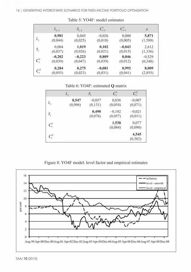
2.4.3 Tables 5 and 6 show the estimation results for the YO4F model. As before, bold entries denote parameters estimates significant at 5% and standard errors appear in parentheses. In Table 6 the estimate of the A matrix indicates high persistent dynamics of Lt, St,

1tC and 2

tC , the estimated own-lag coefficients being 0,981, 1,019, 0,809 and 0,992 respectively. Some cross-factor dynamics seem significantly important. As with the YO3F model (see Table 2) the level of persistence is higher in St than in Lt and 1

tC . Also we see that the level of persistence is higher in 2tC than in Lt and 1

tC . The mean of the level is approximately 5.9 percent and is statistically significant different from zero. The mean of the slope is 2.612 percent, the mean of the first curvature factor is –0.529 percent, which is not statistically significant different from zero. The mean of the second curvature factor 8.009 percent and is statistically significant different from zero. The largest eigenvalue of the A matrix is 0.986 and ensures the stationarity of the system. In Table 6 the estimates indicate an increase in the transitional shock volatility as we move from Lt to St to 1

tC to 2tC . The estimate for λ1 is 0.088 which implies that the

loading on the first curvature factor is maximised at a maturity of 20.38 months and the estimate for λ2 is 0.015 which implies that the loading on the second curvature factor is maximised at a maturity of 119.55 months. Again in Figure 2 it can be seen that the first hump is at about 20 months and the second hump at 120 months.

2.4.4 As shown in Table 4, the YO4F model improves on the means of the predicted errors, especially for the long maturities. Figures 8 and 9 plot the estimated smoothed level and slope factors against empirical proxies and macroeconomic factors. The curvature factors are omitted as there is no reliable macroeconomic link to them. Figure 8 plots the estimated level factor against the empirical proxy and annual percentage change in the inflation index. There is a correlation of 0,67 between the estimated level factor and the empirical proxy. The correlation between the estimated level and the inflation rate is 0,28, which again suggests that inflation is linked to the dynamics of the yield curve. Figure 9 shows the estimated slope curve together with the empirical proxy

SAAJ 10 (2010)


Figure 8: YO4F model: level factor and empirical estimates

Table 5: YO4F: model estimates

Lt–1 St–11

1tC −2

1tC − μ

Lt0,981

(0,044)0,045

(0,025)–0,026(0,018)

0,000(0,005)

5,871(1,588)

St0,004

(0,037)1,019

(0,026)0,102

(0,021)–0,043(0,015)

2,612(1,336)

1tC

–0,202(0,039)

–0,223(0,047)

0,809(0,039)

0,046(0,012)

–0,529(0,348)

0,284(0,055)

0,275(0,023)

–0,081(0,031)

0,992(0,041)

8,009(2,855)

Table 6: YO4F: estimated Q matrix

Lt St1tC 2

tC

Lt0,547

(0,096)–0,057(0,131)

0,036(0,054)

–0,007(0,071)

St0,490

(0,076)–0,102(0,057)

–0,021(0,011)

1tC 1,538

(0,084)0,077

(0,090)

2tC 4,545

(0,382)

2tC

0

2

4

6

8

10

12

14

16

Aug-99 Apr-00 Dec-00Aug-01 Apr-02 Dec-02Aug-03 Apr-04 Dec-04Aug-05 Apr-06 Dec-06Aug-07 Apr-08 Dec-08

per c

ent

inflationlevel - smoothlevel - empirical

SAAJ 10 (2010)


and demeaned manufacturing capacity utilisation. There is a 0,84 correlation between the estimated slope factor and the empirical proxy, and a 0,30 correlation between the estimated slope factor and capacity utilisation. This also suggests a link between capacity utilisation and the dynamics of the yield curve.

3. MACROECONOMIC MODEL In this section we relate the four unobserved factors, level, slope and the two curvature factors, which provide a good representation of the yield curve, to macroeconomic variables. This can be done by extending the state-space model in the previous section. We also present out-of-sample forecasting results to assess how well the YM4F model forecast the dynamics of the yield curve.

3.1 YIELDS-MACRO MODEL3.1.1 The following three macroeconomic variables are included:

– manufacturing capacity utilisation (CUt), which represents the level of real economic activity relative to potential;

– the annual percentage change in the inflation index (IFt), which represents the inflation rate; and

– the repo rate (RRt), which represents the South African monetary-policy instrument.According to Diebold, Rudebusch & Aruoba (op. cit.) these three macroeconomic variables are considered to be the minimum set of fundamentals needed to capture the basic macroeconomic dynamics (see also Rudebusch & Svensson, 1999 and Kozicki & Tinsley, op. cit.).

3.1.2 We extend the YO4F model, to the YM4F model, to incorporate the three macroeconomic variables. This is done by adding the macroeconomic variables to the set of state variables. The state-space system is extended as follows:

Figure 9: YO4F model: slope factor and empirical estimates

-6

-4

-2

0

2

4

6

8

10

12

Aug-99Apr-00 Dec-00Aug-01Apr-02 Dec-02Aug-03Apr-04 Dec-04Aug-05Apr-06 Dec-06Aug-07Apr-08 Dec-08

per c

ent

capacity utilisationslope - smoothslope - empirical

SAAJ 10 (2010)


( )( )

( )( )

( )( )

11 1 12 1

21 1 22 1

t t t t

tt t t

f f x

x f x

µ µ ν ηγν µ ν

− −

− −

− − − = + + − − −

A A

A A;

yt =Λft +εt ;and

;

0 0~ 0 , 0

0 0 0

t

t

t

WNηγε

′

Q KK J

H

where ( )1 2, , ,t t t t tf L S C C ′= andxt=(CUt , IFt , RRt)'.WhereA11,A12,A21,A22,μ,ν,t ,γt ,Q,KandJhaveappropriatedimensions.Λstaysunchanged.Thisisconsistentwiththeview thatonly four factorsareneeded todistil the information in theyieldcurve(Diebold,Rudebusch&Aruoba,op. cit.).IntheYM4Fmodelthematrix

′

Q KK J

isassumedtobenon-diagonalandHisassumedtobediagonal.3.1.3 The extension of theKalman-filter algorithm to include themacro-

economicvariablesispresentedinAppendixB.3.1.4 Tables7and8showtheestimationresultsfortheYM4Fmodel.The

estimateoftheAmatrixagainindicateshighpersistentdynamicsforSt ,1tC , 2

tC ,CUtandIFt .Someofthecross-factordynamicsaresignificantlyimportantformostfactors.TheestimatesalsoindicateanincreaseinthetransitionalshockvolatilityaswemovefromLttoStto

1tC to 2

tC allbeingstatisticallysignificantlydifferentfromzero,andadecreaseinthetransitionalshockvolatilityaswemovefromCUt toIFt toRRt ,allbeingstatistically significantlydifferent fromzero.Thereare small changes in themeanoftheslopeandthetwocurvaturefactorsincomparisonwiththeyields-onlymodel.ThelargesteigenvalueoftheAmatrixis0,98,whichensuresthestationarityofthesystem.NoneofthecovariancetermsintheQmatrixaresignificantlydifferentfromzero.

3.1.5 As shown inTable 4 theYM4Fmodel reducesmost of themeansslightlyornotatall,butitdoesreducethestandarddeviationsofthepredictederrors,indicatingabetterfit.ThemeansandstandarddeviationsofthepredictederrorsfortheYM3Fmodelarealsoshown;againtheYM4Fmodelfitstheyieldcurvebetterthanthethree-factoryields-macromodel.Theestimates for the level,slopeand twocurvaturefactorsoftheYM4FmodelareverysimilartothoseoftheYO4Fmodel.

3.1.6 Figure10 shows themeanpredicted error and the associatedupperand lower95%confidencebands for theYO4Fand theYM4Fmodels.Herewecanclearlyseethatthereislittledifferenceinthemeansofthetwomodels.Butasmentionedbefore,thereislessvarianceintheyields-macromodel,especiallyinlongermaturities,indicatingabetterfit.TheanalysisbelowusestheYM4Fmodel.

SAAJ 10 (2010)


Table 7: YM4F: model estimates

Lt–1 St–1 C1t–1 C2t–1 CUt–1 IFt–1 RRt–1 μ

Lt0,516

(0,036)–0,369(0,034)

0,002(0,033)

–0,020(0,024)

0,044(0,061)

0,109(0,092)

0,288(0,097)

6,427(2,318)

St0,503

(0,114)1,303

(0,084)0,116

(0,040)0,018

(0,028)–0,046(0,071)

–0,018(0,109)

–0,353(0,060)

2,746(2,535)

C1t 0,250

(0,079)0,217

(0,044)0,867

(0,066)0,030

(0,048)–0,045(0,116)

–0,037(0,161)

–0,303(0,177)

0,785(1,546)

C2t1,622

(0,045)1,534

(0,102)0,098

(0,082)0,907

(0,079)–0,533(0,168)

–0,245(0,303)

–1,543(0,298)

7,747(3,771)

CUt0,163

(0,120)0,108

(0,091)0,014

(0,023)0,019

(0,016)0,938

(0,041)–0,086(0,062)

–0,119(0,048)

83,127(1,067)

IFt0,416

(0,037)0,261

(0,045)0,057

(0,023)0,032

(0,014)0,053

(0,038)0,953

(0,060)–0,206(0,075)

6,387(1,427)

RRt0,503

(0,062)0,324

(0,060)0,130

(0,019)0,019

(0,012)–0,029(0,033)

0,103(0,050)

0,534(0,071)

10,013(1,091)

Table 8: YM4F: estimated Q matrix

Lt St C1t C2t CUt IFt RRt

Lt0,5250,005

–0,0010,036

0,0000,087

0,0000,112

0,0000,077

0,0000,019

0,0000,042

St0,6330,096

0,0000,060

0,0000,171

0,0000,036

0,0000,051

0,0000,011

C1t1,5120,148

0,0000,167

0,0000,097

0,0000,198

0,0000,150

C2t4,9321,249

0,0000,100

0,0000,195

0,0000,165

CUt0,2100,031

0,0000,021

–0,0010,011

IFt0,1990,036

0,0010,010

RRt0,1010,013

3.2 OUT-OF-SAMPLE TESTING3.2.1 For scenario generation it is important not only to capture the dynamics

of the yield curve well in-sample, but also to forecast the dynamics of the yield curve well out-of-sample. For this reason the YM4F model is estimated on truncated or curtailed datasets. Using the estimated parameters the yield curve is forecast repeatedly for one, two, three and four years ahead over the period of February 2004 to February 2009, using monthly intervals. For the purpose of asset and liability management it would be of importance to use longer periods for out-of-sample testing, but the lack of data for model fitting restricts this period. Diebold & Li (op. cit.) model and forecast the Nelson–Siegel

SAAJ 10 (2010)


factors as univariate AR(1) processes for one month, six months and twelve months ahead. The model proposed by Diebold & Li (op. cit.) outperforms other models for yield-curve forecasting at all maturities. Thus the Svensson factors are modelled and forecast as univariate AR(1) processes in order to compare their model against the YM4F model in this paper.

3.2.2 Tables 9 to 12 show the out-of-sample forecasting results for maturities 3, 12, 36, 60, 120, 180 and 288 months. The forecast errors at time t + h are defined to be:

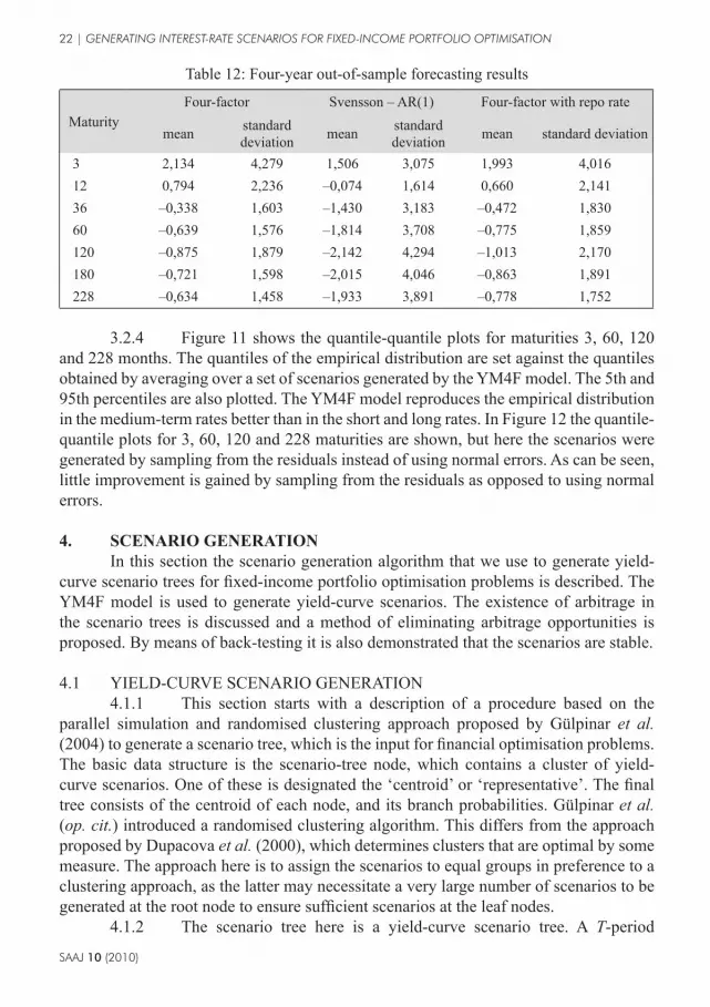
( ) ( )ˆt h t hy yτ τ+ +− ;where t is the time of parameter estimation and h the length of the period forecast. The mean and standard deviation of the forecast errors are reported. The YM4F model outperforms the AR(1) model. The standard deviations for the AR(1) model are also larger than those of the YM4F model. In particular, the four-year-ahead forecast of the YM4F model is better than that of the AR(1) model.

3.2.3 In practice most financial institutions have views on the macro-economy. These views are produced by means of an ESG or expert opinion. These ESGs produce forecasts only for macroeconomic variables, for example the repo rate, and not a complete yield curve. By using the Kalman filter to model the yield curve bidirectionally, as mentioned in the introduction, it is possible to close this loop and to produce a full yield curve given a set of macroeconomic forecasts. This is done by including the macroeconomic forecasts produced by such an ESG in the forecasting of the yield curve rather than the forecast macroeconomic variables of the model. Either all three macroeconomic variables or only a selection of them can be replaced. Because of the lack of real ESG forecasts for the repo rate the actual repo rate is included. Tables 9 to 12 out-of-sample forecasting results are also shown, where the actual repo rate was included in the forecasting instead of the forecast repo rate from the model. As can be

Figure 10: Mean predicted errors and confidence bands at 5% and 95%

-1.5

-1.0

-0.5

0.0

0.5

1.0

1.5

0 12 24 36 48 60 72 84 96 108 120 132 144 156 168 180 192 204 216 228

erro

r

maturity (months)

mean error - YO4F 95% band - YO4Fmean error - YM4F 95% band - YM4F

SAAJ 10 (2010)


seen, the forecasting error reduces, especially for the longer maturities, in comparison with the other models. Thus, by including these forecasts, a better yield-curve forecast can be made.

Table 9: One-year out-of-sample forecast results

MaturityFour-factor Svensson – AR(1) Four-factor with repo rate

mean standard deviation mean standard

deviation mean standard deviation

3 –1,053 1,562 –1,338 2,213 –0,395 1,16412 –0,686 1,103 –1,281 1,909 –0,021 0,74236 –0,706 0,605 –1,666 1,417 –0,046 0,40860 –0,929 0,593 –2,036 1,166 –0,276 0,573120 –1,009 0,741 –2,277 0,972 –0,364 0,837180 –0,932 0,649 –2,292 0,969 –0,291 0,752228 –0,854 0,524 –2,274 1,022 –0,217 0,621

Table 10: Two-year out-of-sample forecast results




3 0,710 1,973 0,451 2,350 0,804 1,50512 0,342 1,411 –0,091 1,734 0,466 1,21236 –0,430 1,081 –1,075 1,520 –0,288 1,00060 –0,914 1,032 –1,652 1,653 –0,773 0,846120 –1,243 1,129 –2,085 1,828 –1,106 0,931180 –1,110 1,085 –2,010 1,795 –0,982 0,869

228 –0,941 1,004 –1,880 1,706 –0,820 0,792

Table 11: Three-year out-of-sample forecast results




3 1,489 2,187 0,939 1,805 1,451 1,98812 0,727 1,503 –0,019 1,218 0,703 1,48236 –0,283 1,131 –1,233 1,710 –0,305 1,18960 –0,782 1,200 –1,811 2,182 –0,806 1,189120 –1,169 1,521 –2,284 2,681 –1,199 1,488180 –1,019 1,395 –2,171 2,570 –1,055 1,354228 –0,858 1,251 –2,031 2,416 –0,899 1,214

SAAJ 10 (2010)


Table 12: Four-year out-of-sample forecasting results




3 2,134 4,279 1,506 3,075 1,993 4,01612 0,794 2,236 –0,074 1,614 0,660 2,14136 –0,338 1,603 –1,430 3,183 –0,472 1,83060 –0,639 1,576 –1,814 3,708 –0,775 1,859120 –0,875 1,879 –2,142 4,294 –1,013 2,170180 –0,721 1,598 –2,015 4,046 –0,863 1,891228 –0,634 1,458 –1,933 3,891 –0,778 1,752

3.2.4 Figure 11 shows the quantile-quantile plots for maturities 3, 60, 120 and 228 months. The quantiles of the empirical distribution are set against the quantiles obtained by averaging over a set of scenarios generated by the YM4F model. The 5th and 95th percentiles are also plotted. The YM4F model reproduces the empirical distribution in the medium-term rates better than in the short and long rates. In Figure 12 the quantile-quantile plots for 3, 60, 120 and 228 maturities are shown, but here the scenarios were generated by sampling from the residuals instead of using normal errors. As can be seen, little improvement is gained by sampling from the residuals as opposed to using normal errors.

4. SCENARIO GENERATIONIn this section the scenario generation algorithm that we use to generate yield-

curve scenario trees for fixed-income portfolio optimisation problems is described. The YM4F model is used to generate yield-curve scenarios. The existence of arbitrage in the scenario trees is discussed and a method of eliminating arbitrage opportunities is proposed. By means of back-testing it is also demonstrated that the scenarios are stable.

4.1 YIELD-CURVE SCENARIO GENERATION4.1.1 This section starts with a description of a procedure based on the

parallel simulation and randomised clustering approach proposed by Gülpinar et al. (2004) to generate a scenario tree, which is the input for financial optimisation problems. The basic data structure is the scenario-tree node, which contains a cluster of yield-curve scenarios. One of these is designated the ‘centroid’ or ‘representative’. The final tree consists of the centroid of each node, and its branch probabilities. Gülpinar et al. (op. cit.) introduced a randomised clustering algorithm. This differs from the approach proposed by Dupacova et al. (2000), which determines clusters that are optimal by some measure. The approach here is to assign the scenarios to equal groups in preference to a clustering approach, as the latter may necessitate a very large number of scenarios to be generated at the root node to ensure sufficient scenarios at the leaf nodes.

4.1.2 The scenario tree here is a yield-curve scenario tree. A T-period

SAAJ 10 (2010)


scenario tree structure is represented as a ‘tree string’, which is a string of integers specifying for each stage s = 1,2,…,T the number of branches (or branching factors) for each node in that stage (see Dempster et al., 2006). This gives rise to balanced scenario trees, in which each sub-tree in the same period has the same number of branches. Let ks denote the branching factor for stage s. Then Figure 13 illustrates a scenario tree with a (3, 2) tree string, i.e. k1 = 3 and k2 = 2.

4.1.3 The generated trees are non-recombining. Given that four latent factors and three macroeconomic factors are used in the yield-curve model, it is very difficult to construct a recombining tree. Even with only three latent factors it is notoriously difficult

Figure 11: Quantile-quantile plots for maturities 3, 60, 120 and 228 months

3

5

7

9

11

13

15

17

5 7 9 11 13 15

Qua

ntile

s of t

he si

mul

ated

serie

s

Quantiles of the empirical series

3 Months

3

5

7

9

11

13

15

17

5 7 9 11 13 15

Qua

ntile

s of t

he si

mul

ated

serie

s


60 Months

3

5

7

9

11

13

15

17

5 7 9 11 13 15

Qua

ntile

s of t

he si

mul

ated

serie

s


180 Months

3

5

7

9

11

13

15

17

5 7 9 11 13 15

Qua

ntile

s of t

he si

mul

ated

serie

s


228 Months

SAAJ 10 (2010)


to construct a recombining tree. Furthermore, non-recombining trees are used in fixed-income portfolio optimisation problems as the portfolio composition is path-dependent.

4.1.4 Figure 14 illustrates the methods of scenario simulation, namely parallel and sequential. The parallel method for simulation is used here as this method produces more realistic extreme events in the scenario tree. The reason for this is that, with the number of simulations growing smaller down the tree in the parallel method, the centroids that eventually represent the scenario groups are drawn from a smaller sample size. In the sequential method, at every stage the simulated scenarios in all of the clusters

Figure 12: Quantile-quantile plots for maturities 3, 60, 120 and 228 months, sampling from errors

3

5

7

9

11

13

15

17

5 7 9 11 13 15

Qua

ntile

s of t

he si

mul

ated

serie

s


3 Months

3

5

7

9

11

13

15

17

5 7 9 11 13 15

Qua

ntile

s of t

he si

mul

ated

serie

s


60 Months

3

5

7

9

11

13

15

17

5 7 9 11 13 15

Qua

ntile

s of t

he si

mul

ated

serie

s


180 Months

3

5

7

9

11

13

15

17

5 7 9 11 13 15

Qua

ntile

s of t

he si

mul

ated

serie

s


228 Months

SAAJ 10 (2010)


Figure 14: Two methods of simulating scenarios

Parallel simulation Sequential simulation

t = 0 t = 2t = 1

Entity6.5

7

7.5

8

0 5 10 15 20

Entity6.5

7

7.5

8

8.5

0 5 10 15 20

Entity6.5

7.5

8.5

9.5

0 5 10 15 20

Entity6.5

7.5

8.5

9.5

0 5 10 15 20

Entity6.5

7.5

8.5

9.5

0 5 10 15 20

Entity6.5

7

7.5

8

8.5

0 5 10 15 20

Entity6.5

7

7.5

8

0 5 10 15 20

Entity6.5

7

7.5

8

8.5

0 5 10 15 20

Entity6.5

7

7.5

8

0 5 10 15 20

Entity6.5

7

7.5

8

8.5

0 5 10 15 20

S0

0

S1

0

S2

0

S2

1

S2

1

S2

1

Figure 13: Graphic representation of scenarios

SAAJ 10 (2010)


are discarded, and the next simulation restarted from the centroid, which will prevent any extreme variation (Gülpinar et al., op. cit.).

4.1.5 In order to group the scenarios a measure of relative position is used. The ‘distance’ between the discounting factors of the yield curve and that of the average is calculated as:

; ( )( ) ( )( )

1 11 1 M

Dy y

τ ττ τ τ

= − + +

∑

where y(τ) is the yield to maturity τ and yM(τ) the average yield to maturity τ. Note that the relative distance D can be negative or positive, which means that a yield curve can be positioned to the left or to the right of the average yield curve. This is to ensure realistic extreme events. Chueh (2002) discusses several other distance methods for interest-rate sampling. The relative distance method used here relates closely to the relative present value distance method in that paper.

4.1.6 It is necessary to represent each group of scenarios with a single point, which becomes the datum in the scenario tree. Gülpinar et al. (op. cit.) argue that to prevent the scenario tree from containing scenarios that are not consistent with the simulation parameters, the centroid should not be taken to be the centre of the group, but rather the simulated scenario closest to the centre. The mean of the group is used here as the notion of the centre; other notions of the centre that can be used are the median and the mode.

4.1.7 The main steps of the algorithm used are as follows:Step 1: At s = 0 create a root node group containing N scenarios. Generate all the

scenarios using Monte Carlo simulation and the YM4F model. Each scenario is equally likely and consists of T + 1 sequential yield curves with the same starting point, the current yield curve (in total (T + 1) × N yield curves are generated).

Step 2: Set s = s + 1 and for each group in the previous stage, calculate the average scenario and calculate the distance (i.e. the relative position as defined above) of each scenario with respect to the average.

Step 3: For each group, sort the scenarios in descending order by the distance and group them into ks equal-sized groups.

Step 4: For each new group, find the scenario closest (in absolute value) to the average of the group, and designate it as the centroid. To each centroid assign the probability:

( ) 11

1

sii

k−−

=∏ .

Step 5: If s < T, go to step 2; otherwise stop.

4.2 ARBITRAGE4.2.1 Filipović (1999) and other researchers such as Diebold, Rudebusch

& Aruoba (op. cit.) show that the Nelson–Siegel family of yield-curve models does not impose absence of arbitrage, although these models estimate and forecast the yield

SAAJ 10 (2010)


curve better than arbitrage-free models. (Duffee (op. cit.) noted that canonical affine arbitrage-free models demonstrate poor out-of-sample performance.) In light of this, the scenarios generated are not arbitrage-free. Klaassen (2002) shows that arbitrage opportunities can either be detected ex post by checking for solutions to a set of linear constraints, or be excluded by including non-linear constraints in the scenario generation process. Christensen et al. (unpublished a, unpublished b) derive a class of arbitrage-free affine dynamic yield-curve models that approximate the Nelson–Siegel yield-curve specification. They extend these models to include the Svensson extension of the Nelson–Siegel yield curves.

4.2.2 In this article the authors propose a method of reducing the presence of arbitrage ex post, without extending their models to the class of arbitrage-free models. They reduce the presence of arbitrage ex post, as opposed to excluding it by means of including non-linear constraints during the scenario generation process. This approach has no additional effect on the computational difficulty of the model estimation process and the data requirements. As the scenario generation process is a discrete approximation of the continuous evolution of the yield curve, the extension of the models, used in the simulation process, to a class of arbitrage-free models would not ensure the exclusion of arbitrage in the generated scenarios.

4.2.3 Klaassen (op. cit.) proposes linear constraints for two types of arbitrage. Ingersoll (1987) distinguishes these two types of arbitrage. The first type is an opportunity to construct a zero-investment portfolio that has non-negative payoffs in all states of the world, and a strictly positive payoff in at least one state. The second type is an opportunity to construct a negative investment portfolio (i.e. providing an immediate positive cash flow) that generates a non-negative payoff in all future states of the world.

4.2.4 Following the notation of Klaassen (op. cit.), let , 1n

k tr + be the return on

asset class k (k = 1,…,K) between times t and t + 1 if state n (n = 1,…,N ) of the world

materialises at time t + 1. Klaassen (op. cit.) mentions a useful result, that if the set of equations ( ), 11

1 1N nn k tn

v r +=+ =∑ for all k = 1,…,K

has a strictly positive solution vn for all n, then no arbitrage opportunities of the first or second type exist (see also Ingersoll, op. cit.). Taking , 1

ntrτ + to be the yield to maturity

k = τ, then: ;

( )( )

1, 1

11

ntn

tt

Pr

Pτ

ττ

++

−+ =

where ( ) ( )tytP e τ ττ −=

is the price at time t of a zero-coupon bond with maturity τ. Thus if the set of equations

( ) ( )1( 1) 1

1

nt tN y y

nnv e eτ τ τ τ+− − − −

==∑ for all maturities τ,

has a strictly positive solution vn for all n, then no arbitrage opportunities of the first or second type exist in these yield-curve scenarios. 4.2.5 The class of arbitrage-free affine dynamic yield-curve models that Christensen et al. (unpublished a, unpublished b) derive, for the Nelson–Siegel family

SAAJ 10 (2010)


of yield curves, differs from the Diebold, Rudebusch & Aruoba (op. cit.) models only in the inclusion of an additional yield-adjustment term, which depends only on the maturity of the zero-coupon bond. As this term is dependent on the maturity of the bond, it can be seen as a shift in the slope of the yield curve. Now let

for all n (n = 1,…,N ) .

( )1ty

nev

N

−

=

Then, if we can find yield curve shifts ct+1(τ) such that

( ) ( )( ) ( )

( )1 1( 1) 1

11

1 tnt t

t

yy cN

yn

eeN e

τ ττ τ τ+ +

−− − − +

−==∑ for all maturities τ,

then no arbitrage opportunities exist in the yield-curve scenarios. Thus, if, for every maturity τ, the mean of the calculated values of a zero-coupon bond with that maturity, using different scenarios, equals the price, then no arbitrage opportunity exists in the yield-curve scenarios. (This is consistent with the no-arbitrage literature.)

4.2.6 Given the small size of the branching factors of the scenario trees generated it may not be possible to find realistic solutions to the yield-curve shifts ct+1(τ). Thus, to eliminate most of the arbitrage opportunities in the scenario trees the following algorithm is proposed:Step 1: At the root node create a group of N scenarios. Generate all the scenarios using

Monte Carlo simulation and the YM4F model (as for the scenario tree). Each scenario is equally likely and consists of T sequential yield curves.

Step 2: At each branching time of the scenario tree calculate the average of the N generated scenarios (at the root node the current yield curve is used).

Step 3: Then for each average yield curve and the corresponding one-period-ahead scenarios solve

( ) ( )( ) ( )

( )1 1( 1) 1

11

1 tnt t

t

yy cN

yn

eeN e

τ ττ τ τ+ +

−− − − +

−==∑

for all maturities, to obtain the yield curve shifts ct+1(τ).Step 4: Add the amount ct+1(τ) to the original scenario-tree yield curves.

4.2.7 The described method removes most of the arbitrage opportunities in the scenario tree, with a few opportunities left in sub-trees. For scenario trees with a short horizon all opportunities may be removed. This reduction of arbitrage opportunities is considered sufficient, since portfolio constraints in optimisation problems, such as the restriction of short-selling and the inclusion of bid–ask spreads, will eliminate the remaining arbitrage opportunities.

4.3 BACK-TESTING4.3.1 To test their scenario generation method, the authors implemented

the multi-stage stochastic optimisation problem described by Dempster et al. (op. cit.). In that paper an asset- and liability-management framework is proposed and numerical results are given for a simple example of a closed-end guaranteed fund where no

SAAJ 10 (2010)


contributions are allowed after the initial cash outlay. The design of investment products with a guaranteed minimum rate of return focusing on the liability side of the product is demonstrated in that paper. A detailed discussion of the asset- and liability-management framework is beyond the scope of this paper. The multi-period stochastic programming model of Dempster et al. (op. cit.) is included in Appendix C. In this paper the authors’ scenario generation approach is used to generate the input scenarios for the optimisation problem. The YM4F model is fitted to market data up to an initial decision time t and scenario trees are generated from time t to some chosen horizon t + T. The optimal first-stage or root node decision is then implemented at time t and the success of the portfolio implementation is measured by its performance with historical data up to time t + 1. This whole procedure is rolled forward for T trading times. At each decision time t, the parameters of the YM4F model are re-estimated using the historical data up to and including that time.

4.3.2 Back-tests were performed over a period of five years, from February 2004 to February 2009, and different tree structures were used with approximately the same number of scenarios. The tree structures are defined in Table 13. Bonds with 5, 7, 10, 15 and 19 year maturities as well as the FTSE–JSE Top-40 index are included in the portfolio. (Dempster et al. (op. cit.) include bonds with different maturities and an equity index.) In order to generate scenarios for the Top-40 index, the index is modelled using a simple linear regression model incorporating the three macroeconomic variables. The expected average shortfall is minimised for an annual guarantee of 9% and transaction costs are included.

Table 13: Tree structure for different back-tests

Year Set 1 Set 2 Set 3April 2003 5.5.5.5.5 = 3 125 13.4.4.4.4=3 328 200.2.2.2.2 = 3 200April 2004 8.8.8.8 = 4 096 15.6.6.6 = 3 240 400.2.2.2 = 3 200April 2005 15.15.15 = 3 375 30.10.10 = 3 000 400.3.3 = 3 600April 2006 56.56 = 3 136 160.20 = 3 200 800.4 = 3 200April 2007 3 125 3 328 3 200

4.3.3 Figure 15 illustrates the back-testing portfolio values and the minimum guarantee for all three scenario sets. The results are consistent with those in Dempster et al. (op. cit.). In that paper the expected average shortfall is minimised and the expected terminal wealth of the portfolio is maximised, optimality being achieved with reference to a risk-aversion parameter. The model performs well, staying above the guarantee at all times, although the system involves the inclusion of transaction costs, which puts downward pressure on the portfolio wealth.

4.3.4 Table 14 shows back-testing stability statistics. The model was solved for 100 different scenario sets, with a tree string of 40,3 (120 scenarios) using all available data for model fitting. The table shows the mean, standard deviation, minimum and maximum of the objective function and the first-stage portfolio allocations. The first-

SAAJ 10 (2010)


stage portfolio allocation seems consistent with low standard deviation. The objective function also has low standard deviations, and the minima and maxima show no outliers, further indicating the stability of the scenario generation.

Table 14: Macroeconomic portfolio allocation: stability statistics

Objective function Top-40 5-year bond 7-year bond 10-year

bond17-year

bond19-year

bond

Mean –0,3246 0,0135 0,9619 0,0018 0,0000 0,0000 0,0051

Standard deviation 0,0024 0,0000 0,0003 0,0001 0,0000 0,0000 0,0000

Maximum –0,4970 0,0057 0,8945 0,0000 0,0000 0,0000 0,0000

Minimum –0,2143 0,0248 0,9990 0,0808 0,0000 0,0000 0,0228

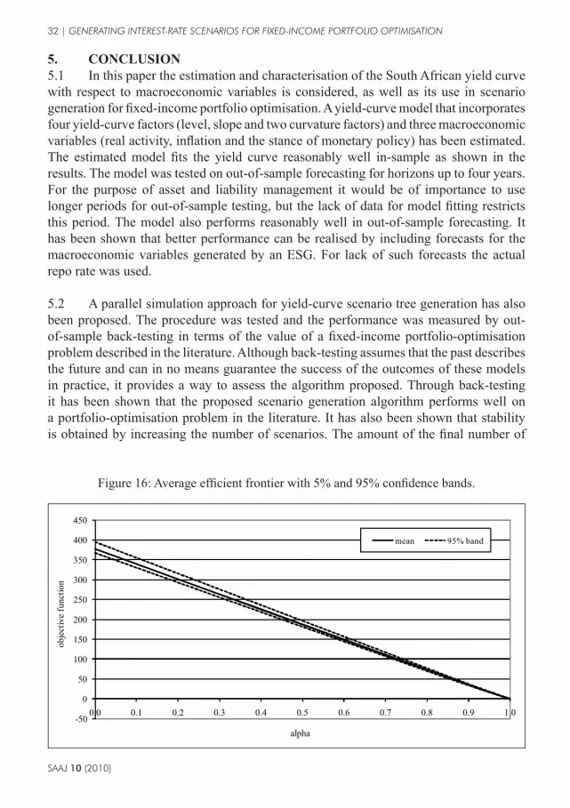
4.3.5 The scenario generation is further tested by again solving the model for 100 different scenario sets and for different number of final nodes, 120, 500, 1000 and 2000. Dempster et al. (op. cit.) minimises the expected average shortfall and maximises the expected terminal wealth of the portfolio, and distinguishes between them using a risk aversion parameter (‘alpha’). For each scenario set the model is solved ranging the risk aversion parameter from 0 to 1 in steps of 0,1 (1 being the most risk-averse). Table 15 shows the mean and standard deviation for each number of final nodes. Figure 16 shows the mean frontier, derived by averaging the objective function obtained over the 100 different scenario sets, and the confidence bands covering 95% of the results. (Kaut

Figure 15: Scenario back-test results

160

170

140

150

160

170

120

130

140

150

160

170

G t

90

100

110

120

130

140

150

160

170

GuaranteeSet 1Set 2Set 3

90

100

110

120

130

140

150

160

170

Feb-04 Aug-04 Mar-05 Sep-05 Apr-06 Oct-06 May-07 Dec-07 Jun-08 Jan-09

GuaranteeSet 1Set 2Set 3

SAAJ 10 (2010)


et al. (2007) and Consiglio & Staino (unpublished) display similar results for scenario and model stability testing.) The frontier is a decreasing function of the risk-aversion parameter alpha. If the value of alpha is closer to 1, more importance is given to the shortfall of the portfolio and less to the expected wealth, and hence a more risk-averse portfolio allocation strategy will be taken, and vice versa. In the extreme case where alpha is 1, only the shortfall will be minimised and the expected wealth will be ignored, and where alpha is 0, the unconstrained case only maximises the wealth. For 1000 final nodes the 95% region, at its maximum (alpha at 0), is 4,9% wide (a reduction of 2% from 500 final nodes), ensuring that the randomisation error is bounded enough. From Table 15 it may also be observed that the standard deviation reduces as the number of final nodes increases. The reduction is less or none at all when the number of final nodes is increased from 1000 to 2000, again ensuring that the randomisation error is bounded enough, and achieves stability.

Table 15: Macroeconomic efficient frontier: stability statistics

Alpha120 scenarios 500 scenarios 1000 scenarios 2000 scenarios

Mean Standard deviation Mean Standard

deviation Mean Standard deviation Mean Standard

deviation

0,0 377,92 8,11 376,75 7,58 377,27 5,38 377,17 5,51

0,1 339,80 7,35 338,75 6,87 339,22 4,88 339,13 4,99

0,2 301,69 6,59 300,74 6,16 301,17 4,38 301,09 4,48

0,3 263,58 5,83 262,73 5,45 263,12 3,88 263,06 3,96

0,4 225,47 5,07 224,73 4,74 225,08 3,38 225,02 3,45

0,5 187,36 4,31 186,72 4,04 187,03 2,88 186,98 2,94

0,6 149,26 3,56 148,72 3,33 148,99 2,39 148,95 2,42

0,7 111,16 2,81 110,72 2,63 110,95 1,90 110,92 1,91

0,8 73,08 2,05 72,73 1,94 72,91 1,41 72,89 1,41

0,9 35,21 1,11 34,90 1,10 34,97 0,84 34,94 0,80

1,0 –0,32 0,05 –0,37 0,05 –0,37 0,04 –0,39 0,03

4.3.6 Although back-testing assumes that the past describes the future and can in no means guarantee the success of the outcomes of these models in practice, it provides a way to assess the algorithm proposed. Through back-testing it may be seen that the proposed scenario generation algorithm performs well on a portfolio optimisation problem in the literature; similar results are obtained to those of Dempster et al. (op. cit.). It may also be seen that stability in the objective is obtained by increasing the number of scenarios. The amount of the final number of scenarios necessary to achieve this stability may depend on the optimisation problem in question.

SAAJ 10 (2010)


5. CONCLUSION5.1 In this paper the estimation and characterisation of the South African yield curve with respect to macroeconomic variables is considered, as well as its use in scenario generation for fixed-income portfolio optimisation. A yield-curve model that incorporates four yield-curve factors (level, slope and two curvature factors) and three macroeconomic variables (real activity, inflation and the stance of monetary policy) has been estimated. The estimated model fits the yield curve reasonably well in-sample as shown in the results. The model was tested on out-of-sample forecasting for horizons up to four years. For the purpose of asset and liability management it would be of importance to use longer periods for out-of-sample testing, but the lack of data for model fitting restricts this period. The model also performs reasonably well in out-of-sample forecasting. It has been shown that better performance can be realised by including forecasts for the macroeconomic variables generated by an ESG. For lack of such forecasts the actual repo rate was used.

5.2 A parallel simulation approach for yield-curve scenario tree generation has also been proposed. The procedure was tested and the performance was measured by out-of-sample back-testing in terms of the value of a fixed-income portfolio-optimisation problem described in the literature. Although back-testing assumes that the past describes the future and can in no means guarantee the success of the outcomes of these models in practice, it provides a way to assess the algorithm proposed. Through back-testing it has been shown that the proposed scenario generation algorithm performs well on a portfolio-optimisation problem in the literature. It has also been shown that stability is obtained by increasing the number of scenarios. The amount of the final number of

Figure 16: Average efficient frontier with 5% and 95% confidence bands.

-50

0

50

100

150

200

250

300

350

400

450

0.0 0.1 0.2 0.3 0.4 0.5 0.6 0.7 0.8 0.9 1.0

obje

ctiv

e fu

nctio

n

alpha

mean 95% band

SAAJ 10 (2010)


scenarios necessary to achieve this stability may depend on the optimisation problem in question.

5.3 The existence of arbitrage in the scenario trees has been discussed and a method of eliminating arbitrage opportunities ex post has been proposed. Consideration may be given to other methods of eliminating arbitrage opportunities either during simulation or ex post. This is left to future research.

ACKNOWLEDGEMENTSThe research was supported by the National Research Foundation (NRF grant number FA2006022300018 and THRIP project ID TP2006050800003) and by industry (Absa and SAS Institute). The authors would like to thank Professor Hennie Venter for his help with the statistics on the Kalman filter. Secondly, thanks are extended to the Editor and the three anonymous scrutineers for their valuable input.

REFERENCESAng, A & Piazzesi, M (2003). A no-arbitrage vector autoregression of term structure dynamics

with macroeconomic and latent variables. Journal of Monetary Economics 50, 745–87Bernaschi, M, Tacconi, E & Vergni, D (2008). A parametric study of the term structure dynamics.

Physica A, 387:1264–72Brousseau, V (unpublished). The functional form of yield curves. Working Paper 148, European

Central Bank, 2002Christensen, JH, Diebold, FX & Rudebusch, GD (unpublished a). The affine arbitrage-free class

of Nelson–Siegel term structure models. NBER working paper, No. 13611, November, 2007Christensen, JH, Diebold, FX & Rudebusch, GD (unpublished b). An arbitrage-free generalized

Nelson–Siegel term structure model. Reserve Bank of San Francisco, Working Paper 08-07, 2008

Chueh, YCM (2002). Efficient stochastic modelling for large and consolidated insurance business: interest rate sampling algorithms. North American Actuarial Journal 6, 88–103

Consiglio, A & Staino, A (unpublished). A stochastic programming model for the optimal insurance of government bonds. SSRN eLibrary, DSSM working paper, No. 15, 2008

Dai, Q & Singleton, K (2000). Specification analysis of affine term structure models. Journal of Finance 55, 1943–78

De Pooter, M, Ravazzolo, F & van Dijk, D (unpublished). Predicting the term structure of interest rates: incorporating parameter uncertainty, model uncertainty and macroeconomic information. MPRA Paper 2512, University Library of Munich, Germany, 2007

Dempster, MAH, Germano, M, Madova, EA, Rietbergen, MI, Sandrini, F & Scrowston, M (2006). Managing guarantees. The Journal of Portfolio Management 32, 51–61

SAAJ 10 (2010)


Dewachter, H & Lyrio, M (unpublished). Macroeconomic factors in the term structure of interest rates. Manuscript, Catholic University Leuven, Erasmus University, Rotterdam, 2002

Diebold, FX, & Li, C (2006). Forecasting the term structure of government bond yields. Journal of Econometrics 130, 337–64

Diebold, FX, Rudebusch, GD & Aruoba, SB (2006). The macroeconomy and the yield curve: a dynamic latent factor approach. Journal of Econometrics 131, 309–38

Duffee, GR (2002). Term premia and interest rate forecasts in affine models. Journal of Finance 57, 405–43

Duffie, D & Kan, R (1996). A yield-factor model of interest rates. Mathematical Finance 6, 379–406

Dupacova, J, Consigli, G & Wallace, SW (2000). Scenarios for multi-stage stochastic programs. Annals of Operations Research 100, 25–53

Filipović, D (1999). A note on the Nelson–Siegel family. Mathematical Finance 9, 349–59Gülpinar, N, Rustem, B & Settergren, R (2004). Simulation and optimization approaches to

scenario tree generation. Journal of Economic Dynamics & Control 28, 1291–315Hamilton, JD (1994). Time Series Analysis. Princeton University Press, Princeton, New JerseyHarvey, AC (1989). Forecasting, Structural Time Series Models and the Kalman Filter. Cambridge

University Press, CambridgeHördahl, P, Tristani, O & Vestin, D (unpublished). A joint econometric model of macroeconomic

and term structure dynamics. Manuscript, European Central Bank, 2002Ingersoll, Jr., JE (1987). Theory of Financial Decision Making. Rowman & Littlefield, Totowa, NJKalman, RE (1960). A new approach to linear filtering and prediction problems. Journal of Basic

Engineering, Transactions ASME, Series D 83, 35–45Kaut, M, Wallace, SW, Vladimirou, H & Zenios, SA (2007). Stability analysis of a portfolio

management model based on the conditional value-at-risk measure. Quantitative Finance 7(4), 397–409

Klaassen, P (2002). Comment on “Generating scenario trees for multistage decision problems”. Management Science 48, 1512–16

Knez, P, Litterman, R & Scheinkman, J (1994). Exploration into factors explaining money market returns. Journal of Finance 49, 1861–82

Kozicki, S & Tinsley, PA (2001). Shifting endpoints in the term structure of interest rates. Journal of Monetary Economics 47, 613–52

Lemke, W (2006). Term Structure Modelling and Estimation in a State Space Framework. Springer-Verlag, Berlin

Nelson, CR & Siegel, AF (1987). Parsimonious modeling of yield curves. Journal of Business 60, 473–89

Maitland, AJ (2002). Interpolating the South African yield curve using a principal-component analysis: a descriptive approach. South African Actuarial Journal 2, 129–45

Rudebusch, GD & Svensson, LEO (1999). Policy rules for inflation targeting. In Taylor (1999: 203–46)

Rudebusch, GD & Wu, T (unpublished). A macro-finance model of the term structure, monetary policy, and the economy. Manuscript, Federal Reserve Bank of San Francisco, 2003

SAAJ 10 (2010)


Stander, Y (unpublished). Bond Indices in South Africa. Unpublished dissertation for M.Sc. at the University of the Witwatersrand, Johannesburg, 2000

Svensson, LEO (1994). Estimating and interpreting forward rates: Sweden 1992–4. CEPR Discussion Paper Series No. 1051, October

Taylor, JB (ed.) (1999). Monetary Policy Rules. University of Chicago Press, ChicagoTilley, JA (1992). An actuarial layman’s guide to building stochastic interest rate generators.

Transactions of the Society of Actuaries 34, 421–59Wu, T (unpublished). Monetary policy and the slope factors in empirical term structure estimations.

Federal Reserve Bank of San Francisco, Working Paper 02-07, 2002

SAAJ 10 (2010)


APPENDIX A

THE KALMAN-FILTER ALGORITHM

A.1 InthisappendixtheKalman-filteralgorithmanditsassumptionsarepresented.

A.2 It follows by assumption that the transition density ( )1 |t tp f f+ and themeasurementdensity ( )|t tp y f arejointlynormal.Thisimpliesthatthepredictionandfilteringdensitiesarenormal;i.e.: ( )1 | 1 | 1

ˆ| Y ~ ,t t t t t tf N f− − −Σ ;

( )| |ˆ| Y ~ ,t t t t t tf N f Σ ;and

( )1 | 1ˆ| Y ~ ,t t t t ty N y F− − ;

whereYt=y1,…,ytistakentobethesequenceofobservationsavailableforestimationandft|t–1, tf , | 1ˆt ty − and | 1t t−Σ , |t tΣ ,Ft arethesequencesofconditionalmeansandcovariancematrices.ThesequantitiescanbeobtainedbyemployingtheKalmanfilterforagivensetofparametersψ.

A.3 TheKalman-filteralgorithmmaybedescribedasfollows(seeLemke,op. cit.):

Step1: Set 0|0 0f f= , 0|0 0Σ = Σ andt=0.

Step2: 1| 1t tf − − and 1| 1t t− −Σ aregivenvalues,butythasnotbeenobservedyet.Compute: ( ) ( )| 1 1| 1

ˆ ˆt t t tf fµ µ− − −− = −A ;

| 1 1| 1t t t t− − − ′Σ = Σ +A A Q

| 1 | 1ˆˆt t t ty f Λ ;and

Ft=ΛΣt|t–1Λ' + H.

Step3: ythasbeenobserved.Compute: 1

| 1t t t tK F −− ′= Σ Λ ;

( )| | 1 | 1ˆ ˆ ˆt t t t t t t tf f K y y− −= + − ;and

| | 1 | 1t t t t t t tK− −Σ = Σ − ΛΣ .

Step4: Ift<T,sett=t +1,andgotostep2;otherwise,stop.

SAAJ 10 (2010)


A.4 HencetheKalmanfilterdeliversthesequenceofmeansandcovariancematricesfortheconditionaldistributionsofinterestforagivensetofparametersψ.TheKalmanfilter is initialised by setting 0f and 0Σ to the unconditionalmean and unconditionalcovariancematrixofthestatevectorrespectively.Underthenormalityassumption,thedistributionofytconditionalonYt–1istheN-dimensionalnormaldistributionwithmean

| 1ˆt ty − andcovariancematrixFt .TheconditionaldensityofytgivenYt–1andψcanbewrittenas(seeLemke,op. cit.):

1/ 2 11

1 | 1 | 12 ˆ ˆ| Y ; 2 expNt t t t t t t t t tp y F y y F y y

.

Accordingly,thelog-likelihoodfunctionbecomes

( ) 1

1 1

1 1ln log 2 log2 2 2

T Tt t t tt t

NTL F v F vψ π −= =

′= − − −∑ ∑ ,

where ( )| 1ˆt t t tv y y −= − isthevectorofpredictionerrors.

A.5 Foragivensetofparametersψ,theKalmanfilterisusedtocomputethepredictionerrors vt and their covariance matrix Ft, after which the log-likelihood function iscomputed.

A.6 TheKalman-filterfixed-intervalsmoothingalgorithmisusedtoobtainoptimalextractionsofthelatentlevel,slopeandcurvaturefactors.Thealgorithmconsistsofasetofrecursions,whichstartwiththefinalquantitiesgivenbytheKalmanfilterandworkbackwards(Harvey,op. cit.).Theequationsare

( )*

| | 1| 1|ˆ ˆ ˆ ˆt T t t t t T t tf f f f+ += + Σ − ;and

( )* *| | 1| 1|t T t t t t T t t t+ +

′Σ = Σ +Σ Σ −Σ Σ ;

where * 1| 1|t t t t tA −

+′Σ = Σ Σ .

SAAJ 10 (2010)


APPENDIX B

EXTENDED KALMAN-FILTER ALGORITHM INCLUDING MACROECONOMIC VARIABLES

B.1 In this appendix the extension of the Kalman filer algorithm to includethe macroeconomic variables is presented. The extension of the algorithm is notstraightforwardandisomittedinmanyarticles.Itisforthisreasonthattheextensionishereincluded.

B.2 Asstatedaboveitfollowsbyassumptionthatthetransitiondensity ( )1 |t tp f f+ and ( )1 |t tp x x+ andthemeasurementdensity ( )|t tp y f arejointlynormal.Thisimpliesthatthepredictionandfilteringdensitiesarenormal,i.e.:

| 1 | 1 | 1 | 1

1 | 1 | 1 | 1 | 1

| 1 | 1 | 1 | 1

ˆ

ˆ~ ,ˆ

ff fx fyt t t t t t t t t

xf xx xyt t t t t t t t t t

yf yx yyt t t t t t t t t

f fx G N xy y

− − − −

− − − − −

− − − −

Σ Σ Σ Σ Σ Σ Σ Σ Σ

;and

( )| |ˆ| ~ , ff

t t t t t tf G N f Σ ;

whereGt=y1,…,yt,x1,…xtistakentobethesequenceofobservationsavailableforestimation.ThesequantitiescanbeobtainedbyemployingtheKalmanfilterforagivensetofparametersψ.

B.3 TheKalman-filteralgorithmisupdatedasfollows:

Step1: Set 0|0 0f f= , 0|0 0ffΣ = Σ andt=0.

Step2: 1| 1t tf − −

and 1| 1fft t− −Σ are given values, but yt and xt has not been observed yet.

Compute:

( ) ( ) ( )| 1 11 1| 1 12 1ˆ ˆt t t t tf f xµ µ ν− − − −− = − + −A A ;

( ) ( ) ( )| 1 11 1| 1 12 1

ˆˆt t t t tx f xµ µ ν− − − −− = − + −A A;

| 1 | 1ˆˆt t t ty f Λ ;

| 1 11 1| 1 11ff fft t t t− − − ′Σ = Σ +A A Q;

| 1 21 1| 1 21xx fft t t t− − − ′Σ = Σ +A A J;

| 1 | 1yy fft t t t Λ Λ H ;

SAAJ 10 (2010)


| 1 11 1| 1 21fx fft t t t− − − ′Σ = Σ +A A K ;

| 1 | 1fy fft t t t Λ

; and

| 1 | 1xy fxt t t t Λ

.

Step 3: yt and xt have been observed. Compute:

( )

1| 1| 1 | 1

| | 1 | 1 | 1| 1| 1 | 1

ˆˆ ˆˆ

xx xyt t tt t t tfx fy

t t t t t t t t yx yyt t tt t t t

y yf f

x x

−

−− −− − −

−− −

− ∑ ∑ = + ∑ ∑ −∑ ∑

; and

( )1

| 1 | 1 | 1| | 1 | 1 | 1

| 1 | 1 | 1

xx xy fxt t t t t tff ff fx fy

t t t t t t t t yx yy fyt t t t t t

−

− − −− − −

− − −

∑ ∑ ∑Σ = Σ − ∑ ∑ ∑ ∑ ∑

.

Step 4: If t < T, set t = t + 1, and go to step 2; otherwise, stop.

B.4 Accordingly, the log-likelihood function becomes:

( )1

| 1 | 1 | 1 | 11 1

| 1 | 1 | 1 | 1

1 1ln log 2 log ;2 2 2

xx xy xx xyT Tt t t t t t t t

t tyx yy yx yyt tt t t t t t t t

NTL v vψ π−

− − − −

= =− − − −

∑ ∑ ∑ ∑′= − − − ∑ ∑ ∑ ∑ ∑ ∑

where | 1

| 1

ˆˆ

t t tt

t t t

y yv

x x−

−

− = −

is the vector of prediction errors.

SAAJ 10 (2010)


APPENDIX C

MINIMUM GUARANTEE STOCHASTIC PROGRAMMING FORMULATION

In this appendix the multi-period stochastic programming model of Dempster et al. (op. cit.) for minimum guarantees is presented. Given a set of scenarios the stochastic program results in a large linear program.

C1. VARIABLE PARAMETERS OF THE MODEL

The variable parameters of the model are defined as shown in Tables C.1 to C.4

Table C.1: Time sets

1 212 120, , , ,totalT T

: set of all times considered in the stochastic program;

0,1,2, , 1dT T : set of decision times;

\i total dT T T= : set of intermediate times;

31 12 2 2, , ,cT T : set of coupon payment time between decision times;

Table C.2: Instruments

: Stock index level at time t in scenario ω;

( )TtB ω : Treasury security with maturity T at time t in scenario ω;

( )TBtδ ω : coupon rate of Treasury security with maturity T at time t in scenario ω;

TBF : face value of Treasury security with maturity T

( )tZ ω : zero-coupon Treasury security price at time t in scenario ω;

( )tS ω

SAAJ 10 (2010)


Table C.3: Risk-management barrier

( ),ty τ ω : zero-coupon Treasury yield with maturity T at time t in scenario ω;

G : annual guaranteed return;

( )tL ω : barrier at time t in scenario ω;

Table C.4: Portfolio evolution

A : set of all assets;

P Pt a

buy

t a

sell

, ,( (

: buy/sell price of asset a A at time t in scenario ω;

f / g : transaction costs of buying and selling;

xt,a (ω) : quantity held of asset a A between time t and t + 1 in scenario ω;

x+t,a (ω) / x–t,a (ω) : quantity bought/sold of asset a A at time t in scenario ω;

stW : portfolio wealth at time t T total in scenario ω;

( ) ( ) ( )( ): max 0,t t th L Wω ω ω= − : shortfall at time t in scenario ω;

C2. MODEL FORMULATION

The model is formulated as:

( ) ( ) ( )

( ) ( ) ( )

( ) ( ) , , ,, , :

, ,

max 1d dt a t a t a

d

tt totalx x x t T T t T T

a A t T T

hp W p

Tω ω ω ω ωω

ωα ω ω α ω

+ − ∈Ω ∈Ω∈ ∪ ∈ ∪ ∈ ∈Ω ∈ ∪

− − ∑ ∑ ∑ ∑

subject to:( ) ( ) ( )0, 0, 0 for buy

a aa A

fP x Wω ω ω ω+

∈

= ∈Ω∑ ;

( ) ( )

( ) ( ) ( ) ( ) 11 , , , , 0,2

\ for , \ 0 ;a a sell buy d

t t a t a t a t a aa A S a A a A

F x gP x fP x t Tδ ω ω ω ω ω ω ω− − +−

∈ ∈ ∈

+ = ∈Ω ∈∑ ∑ ∑

( ) ( ) ( )

,

,

,

0 for , , \ ;

0 for , , \ ;

0 for , , \ 0 ;

totalt a

totalt a

totalt a

x a A t T T

x a A t T T

x a A t T

ω ω

ω ω

ω ω

+

−

≥ ∈ ∈Ω ∈

≥ ∈ ∈Ω ∈

≥ ∈ ∈Ω ∈

SAAJ 10 (2010)


( ) ( ) ( ) , , for , \buy totalt t a t a

a AW fP x t T Tω ω ω ω

∈

= ∈Ω ∈∑ ;

( ) ( ) ( ) ( )

1 112 12

1, 1, ,2

\ for sell a a

T T a TT a T aa A a A S

W gP x F xω ω ω δ ω ω−− −∈ ∈

= + ∈Ω∑ ∑ ;

( ) ( )0, 0, for ,a ax x a Aω ω ω+= ∈ ∈Ω ;

( ) ( ) ( ) ( ) 112, , ,, for , , \ 0total

t a t a t at ax x x x a A t Tω ω ω ω ω+ −−= + − ∈ ∈Ω ∈ ;

( ) ( ), , 0 for , , \i ct a t ax x a A t T Tω ω ω+ −= = ∈ ∈Ω ∈ ;

( )( ) ( )

( )

( ) ( ) ( )

112

12 ,

,,

,

, ,

for \ , , ;

0 for \ , , ;

0 for \ , , ;

a at t a c

t a buyt a

ct a

ct S t S

F xx a A S t T

fP

x a A S t T

x x a A S t T

δ ω ωω ω

ω

ω ω

ω ω ω

−+

−

+ −

= ∈ ∈Ω ∈

= ∈ ∈Ω ∈

= = ∈ ∈Ω ∈

( ) ( ) ( )( )

for , ;

0 for , ;

totalt t t

totalt

h W L t T

h t T

ω ω ω ω

ω ω

+ ≥ ∈Ω ∈

≥ ∈Ω ∈

( ) ( ) ( )( ) ( )( ),

0

0

1 Z

1 for , ; andt T

Tt t

T y T t total

L W G

W G e t Tω

ω ω

ω− −

= +

= + ∈Ω ∈0 1α≤ ≤ .

Documents

Generating interest-rate scenarios for fixed-income portfolio optimisation