Embed Size (px)
Citation preview
Springer Geochemistry
Geochemical Modelling of Igneous Processes –Principles And Recipes in R Language
Vojtěch JanoušekJean-François MoyenHervé MartinVojtěch ErbanColin Farrow
Bringing the Power of R to a Geochemical Community

Springer Geochemistry

More information about this series at http://www.springer.com/series/13486
Vojtěch Janoušek • Jean-François MoyenHervé Martin • Vojtěch ErbanColin Farrow
Geochemical Modellingof Igneous Processes –Principles And Recipesin R LanguageBringing the Power of R to a GeochemicalCommunity
123
Vojtěch JanoušekCzech Geological SurveyPragueCzech Republic
Jean-François MoyenUniversité Jean-MonnetSaint-EtienneFrance
Hervé MartinUniversité Blaise-PascalClermont-FerrandFrance
Vojtěch ErbanCzech Geological SurveyPragueCzech Republic
Colin FarrowGlasgowScotland
Springer GeochemistryISBN 978-3-662-46791-6 ISBN 978-3-662-46792-3 (eBook)DOI 10.1007/978-3-662-46792-3
Library of Congress Control Number: 2015937379
Springer Heidelberg New York Dordrecht London© Springer-Verlag Berlin Heidelberg 2016This work is subject to copyright. All rights are reserved by the Publisher, whether the whole or partof the material is concerned, specifically the rights of translation, reprinting, reuse of illustrations,recitation, broadcasting, reproduction on microfilms or in any other physical way, and transmissionor information storage and retrieval, electronic adaptation, computer software, or by similar or dissimilarmethodology now known or hereafter developed.The use of general descriptive names, registered names, trademarks, service marks, etc. in thispublication does not imply, even in the absence of a specific statement, that such names are exempt fromthe relevant protective laws and regulations and therefore free for general use.The publisher, the authors and the editors are safe to assume that the advice and information in thisbook are believed to be true and accurate at the date of publication. Neither the publisher nor theauthors or the editors give a warranty, express or implied, with respect to the material contained herein orfor any errors or omissions that may have been made.
Printed on acid-free paper
Springer-Verlag GmbH Berlin Heidelberg is part of Springer Science+Business Media(www.springer.com)
Preface
Because I have known the torment of thirst, I would build a well where others may drink.
––– Ernest Thompson Seton
The goal of generations of igneous geochemists is to use mineralogical and chemical laws in an attempt to explain the geological processes they are investi-gating. This scientific approach is both simple and rigorous. Initially it consists of highlighting magmatic differentiation trends and determining the possible underly-ing petrogenetic mechanism(s). Then, the major elements are used to establish the nature and the modal composition of the fractionating mineral assemblage respon-sible for the differentiation trends; its temporal evolution is also addressed. Finally all these data are fed into models calculating the behaviour of trace elements (and possibly isotopes), in order to account for the chemistry of the investigated igne-ous rocks and evolution of the parental magma.
Such methodology is very powerful; not only because it is consistent with field geological data but also it is based on several independent methods. Indeed, major elements, trace elements and isotopes are governed by different principles. Thus any model predicting the coherent behaviour of these three independent parts of the dataset would possess a high internal consistency, making the modelled sce-nario robust.
Indeed, graphical and numerical methods remain the alpha and omega of mod-ern igneous geochemistry. The problem is how to implement the necessary dia-grams or formulae so that the code can be understood and used by an ordinary
v
Everyone, needing to interpret whole-rock geochemical data from igneous rocks, faces the same problem. Regardless of whether he/she has to calculate some simple indexes, more complex norms, plot a diagram for a paper or model effects of some petrogenetic will end up using a computer. He would be certainly delighted to find that several programs exist designed specifically for this purpose. At first glance, most look useful with a plethora of built-in functions, but after a second look, he realizes that they are essentially black boxes, in which he soon loses track of exactly what is happening with his precious data. Worse still, there could be something missing or not quite appropriate to the required task. The code is difficult or impossible to alter (many geochemical programs are commercial). And even when the required diagram is plotted correctly, it may need to be altered extensively before reaching publication quality.
process, he
geochemist. We strongly believe that this knowledge can be mediated in the form of simple numerical recipes in a high-level programming language that includes built-in mathematical and statistical functionality, matrix manipulation tools and be capable of generating publication-quality graphics. There are currently avail-able several potentially suitable environments, but only one of them—the R lan-
there already exists an R package GCDkit (www.gcdkit.org)1, containing most of
Book structure—how to read? This textbook gives a detailed overview of modelling approaches to petrogenesis of igneous rocks using whole-rock geochemical data. The theoretical chapters are followed by their implementation using R/GCDkit, and by numerous exercises, mostly based on real-life problems.
The text is divided into six parts, and three appendices. Part I gives a short but comprehensive introduction to R (with, or without GCDkit), the implementation of simple geochemical computations, calculation of norms, statistical evaluation of complex data sets, and plotting the most common diagrams. In all cases, the geo-
on radiogenic isotope data interpretation is presented. For newbies, the fundamen-tals and syntax of the R language are explained in Appendix A, and an introduc-tion to the GCDkit system is given in Appendix B.
The core of the book (parts II–IV) is dedicated to modelling of the main proc-esses in igneous petrogenesis using various types of geochemical data. These in-clude major elements (treated by the concept of mass balance), trace elements (modelling based on solid/liquid partitioning or saturation concepts) and radio-
assimilation or giving direct information on the source). The principles of forward and reverse numerical techniques are presented and explained, as is the underlying mathematical apparatus; the R code necessary for their implementation is also given. The specific problem of solving sets of linear equations is outli-ned in Appendix C
logical and geochemical backgrounds are briefly discussed. Moreover, a refresher
genic isotopic data (either constraining open-system processes such as mixing and
the required geochemical calculation procedures and graphics. Furthermore , the underlying code can be easily viewed, modified or extended.
algebraic.
In the realm of geochemical modelling, there does not exist any prescribed sce- nario. In fact, the modelling strategy not only depends on the geological problem, but also on the nature of the available data: hence the approach must be adapted and optimized to each individual case. The purpose of this book is to show, using many concrete examples, how a researcher can proceed in developing a realistic model tailored to his questions. It is in this investigative adventure that the authors of this book invite you. Let’s embark on a scientific journey in the intimacy ofpetrogenetic modelling!
guage (www.r-project.org) has the advantage of being freely available for all the
1 Natively for Windows, but can be run on other platforms with a suitable emulator environment.
Prefacevi
main platforms (MS Windows, Mac OS and various dialects of Linux). Moreover, —
Part V provides a practical guide on how to formulate and run a sensible petrogenetic model simulating natural systems. It stresses the fundamental signifi-cance of additional information coming, e.g., from field relations, petrology or physics. Above all, the importance of critical thinking is underlined.
The text is supplemented by numerous solved exercises. It is crowned by two worked real-world problems (Part VI) that illustrate the complex approach to petrogenetic modelling based on the techniques described in this book.
On the other hand, intentionally omitted are most of the more sophisticated sta-tistical methods as these have been dealt with by other, more competent authors. This is also the case for detailed mathematical derivations of laws governing geo-chemical variations in complex petrogenetic scenarios.
The book is intended for senior undergraduate and postgraduate courses, as well as all potential users of R/GCDkit interested in the implementation of graphi-cal, statistical and numerical methods. The prerequisite is a sound knowledge of secondary school maths as well as of basic principles of solid-rock geochemistry.
Most of the exercises in this book are designed to run in an interactive mode. To adopt them for batch use, the contents of any variable should be disp-
print or cat (see AppenThe code supplied, obviously, will run only if the current R directory is that in
which the data file(s) reside. The best is probably to save all the needed files in a directory of your choice and, before starting, set the working directory either from the GUI (File|Change dir…), or with a command such as: GCDkit->Rbook.dir<-"C:/user/my_name/Documents/Rbook"2
GCDkit->setwd(Rbook.dir)
of the R language. Plain R will
2 Backslash is an escape character in R, so it would need to be preceded by another one, i.e.: "C:\\user\\my_name\\Documents\\Rbook".
viiPreface
dix A, Sect. 3.1).
This text is based on version 2.13 of R for Windows, 4.0 of GCDkit. It con-
layed using the functions
run on other systems, including Linux and Mac OS, but the current GCDkit will require a suitable emulation environment, e.g. Wine on Linux. The code, relying on GCDkit functions, will be displayed with the namesake prompt, GCDkit->.
centrates on MS Windows implementation
Electronic supplementary material Errata, code to the exercises and data sets are available on:
. It is supplied purely for the saketerested reader. They are unlikely to
http://book.gcdkit.org this book from
. Moreover, this web site also contains the scripts used toproduce many of the figures. However, insimple and easy to comprehend by a beginner
the latter case the code is not always
of curiosity, and in order to stimulate the inwork without at least some adaptations. If reading an electronic version of thisbook, the exercises, dataset icons and relevant figures are clickable.
Acknowledgements
Prefaceviii
We would like to thank several people without whom this book would have hardly
originated. First of all Robert Gentleman and Ross Ihaka, as well as members of the
R Development Core Group, for their ideas and sterling efforts in developing the R
language. In particular, Friedrich Leisch (Technische Universität, Vienna) provided
valuable consultations on the development of R packages.
This book builds on hand-outs used for workshops given in Prague and Helsinki
(2011), Stellenbosch, South Africa (2012) and Hyderabad, India (2013) by VJ and
JFM. The authors are indebted to many people without whom these events would
not materialize, especially Tapani Ramö (Helsinki), Gary Stevens (Stellenbosch)
and Santosh Kumar (Nainital, India). VJ is grateful to Graeme Rogers, once
supervisor of his PhD. thesis, who has taught him to ask the basic petrogenetic ques-
tions, why and how much, Francis Albarède for his excellent book and a motivating
course of geochemical modelling and Milan Novák (Brno, Czech Republic) with
František V. Holub (Prague), who requested, in 2000, a practical course on interpre-
tation of geochemical data in R that is running ever since.
GCDkit originated during a post-doctoral stay of VJ at University of Salzburg
(FWF Project 15133–GEO to F. Finger). The work was, over the years, supported
by several projects from the Czech Grant Agency (GACR), Czech Geological
Survey (3314, 336200) and Ministry of Education of the Czech Republic
(LK11202 to K. Schulmann). The scientifi c exchanges were facilitated by the
French–Czech programme Mobility 7AMB13FR026.
Régis Doucelance (Clermont-Ferrand, France) brought to our attention a great
reverse mixing hyperbola example from Martinique, and other papers on mantle
geochemistry that escaped our attention. Nice photos were contributed by Gerhard
Wörner (Göttingen, Germany), Christian Nicollet (Clermont-Ferrand), Ewa Słaby
(Warsaw, Poland) and S. Hidalgo (Quito, Ecuador). Didier Laporte (Clermont-
Ferrand) supplied an original version of his fi gure on wetting angles (Fig. 24.1).
Leon Bagas (Crawley, Australia) provided dataset for the anomaly plot.
Oscar Laurent (Liège, Belgium) and Arnaud Villaros (Orléans, France) —in
addition to always being pleasant company—are responsible for many good ideas
and suggestions, which eventually helped to develop the existing code. We are also
grateful to the many students and GCDkit users, whose requests, in the course of
time, led to more software development, clever ideas and debugging.
We are thankful to people from Springer, Annett Buettner, Ulrike Stricker and
Chris Bendall, for their hard work and patience with which they have guided us
through the dire straits of preparing and publishing this monograph. The Czech
brewing industry was a source of inspiration during late-night coding sessions.
In Prague, St. Etienne, Clermont-Ferrand and Glasgow, Christmas 2014
Vojt ch Janou ek ([email protected]) Jean-Francoi Moyen ([email protected])
Hervé Martin ([email protected]) Erban ([email protected])
Colin Farrow ([email protected])
ě
Vojt chě
š
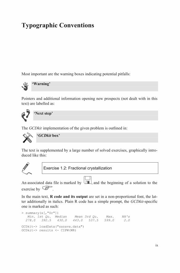
Typographic Conventions
‘Warning’
Pointers and additional information opening new prospects (not dealt with in this text) are labelled as:
‘Next step’
‘GCDkit box’
The text is supplemented by a large number of solved exercises, graphically intro-duced like this:
Exercise 1.2: Fractional crystallization
exercise by .
In the main text, R code and its output are set in a non-proportional font, the lat-ter additionally in italics. Plain R code has a simple prompt, the GCDkit-specific one is marked as such: > summary(x[,"Sr"]) Min. 1st Qu. Median Mean 3rd Qu. Max. NA's 278.0 392.5 430.0 443.0 537.5 599.0 2.0
GCDkit-> loadData("sazava.data") GCDkit-> results <- CIPW(WR)
Most important are the warning boxes indicating potential pitfalls:
An associated data file is marked by , and the beginning of a solution to the
The GCDkit implementation of the given problem is outlined in:
ix
GCDkit-> plot(WR[,"SiO2"), + pch="*",col="khaki")
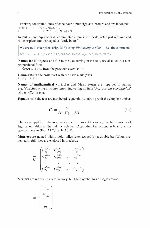
In Part VI and Appendix A, commented chunks of R code, often just outlined and displayed as “code boxes”:
We create Harker plots (Fig. 25.3) using Plot|Multiple plots…, i.e. the command:
GCDkit-> multiple("SiO2","Al2O3,Fe2O3,MgO,CaO,Na2O,K2O")
Names for R objects and file names, occurring in the text, are also set in a non-proportional font: … factor silica from the previous exercise …
Comments in the code start with the hash mark (“#”): # Fig. 4.2.1
of the ‘Misc’ menu.
Equations in the text are numbered sequentially, starting with the chapter number:
0
(1 )LCC
D F D (5.1)
The same applies to figures, tables, or exercises. Otherwise, the first number of figures or tables is that of the relevant Appendix; the second refers to a se-
sented in full, they are enclosed in brackets:
2 2 2
2 2 2
2 5 2 5 2 5
SiO SiO SiOPl Opx nTiO TiO TiOPl Opx n
P O P O P OPl Opx n
C C CC C C
C C C
C
Vectors are written in a similar way, but their symbol has a single arrow:
x
Broken, continuing lines of code have a plus sign as a prompt and are indented:
Typographic Conventions
Names of mathematical variables Menu items are type set in italics, e.g. Misc|Stop current computation, indicating an item ‘Stop current computation’
quence there in (Fig. A1.2; Table A3.5).
Matrices are named with a bold italics letter topped by a double bar. When pre-
and
not complete, are
Pl
Opx
n
mm
m
m
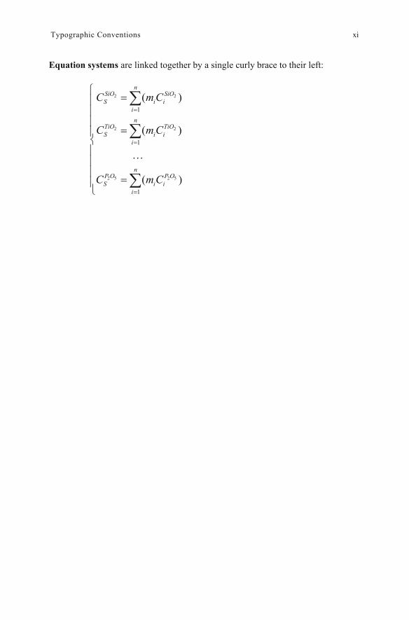
Equation systems are linked together by a single curly brace to their left:
2 2
2 2
2 5 2 5
1
1
1
( )
( )
( )
nSiO SiOS i i
in
TiO TiOS i i
i
nP O P OS i i
i
C m C
C m C
C m C
xiTypographic Conventions
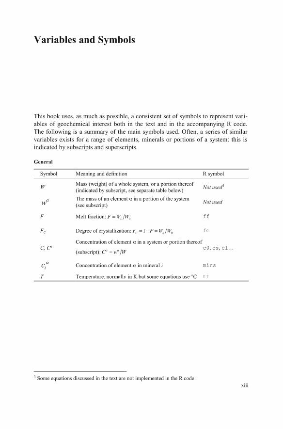
Variables and Symbols
This book uses, as much as possible, a consistent set of symbols to represent vari-ables of geochemical interest both in the text and in the accompanying R code. The following is a summary of the main symbols used. Often, a series of similar variables exists for a range of elements, minerals or portions of a system: this is indicated by subscripts and superscripts.
General
Symbol Meaning and definition R symbol
W Mass (weight) of a whole system, or a portion thereof (indicated by subscript, see separate table below) Not used3
w (see subscript) Not used
F Melt fraction: 0LF W W ff
FC Degree of crystallization: 01 SCF F W W fc
C, C (subscript): C w W
c0, cs, cl…
ic mins
T Temperature, normally in K but some equations use °C tt
3 Some equations discussed in the text are not implemented in the R code.
xiii
The mass of an element in a portion of the system
Concentration of element in a system or portion thereof
Concentration of element in mineral i
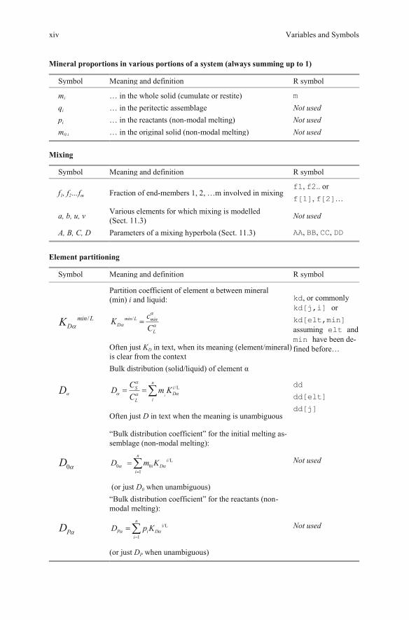
Mineral proportions in various portions of a system (always summing up to 1)
Symbol Meaning and definition R symbol
mi … in the whole solid (cumulate or restite) m
qi … in the peritectic assemblage Not used pi … in the reactants (non-modal melting) Not used m0,i … in the original solid (non-modal melting) Not used
Mixing
Symbol Meaning and definition R symbol
f1, f2…fm Fraction of end-members 1, 2, …m involved in mixing f1, f2.. or f[1], f[2]…
a, b, u, v Various elements for which mixing is modelled (Sect. 11.3) Not used
A, B, C, D Parameters of a mixing hyperbola (Sect. 11.3) AA, BB, CC, DD
Element partitioning
Symbol Meaning and definition R symbol
:
/min L minD
L
cKC
Often just KD in text, when its meaning (element/mineral) is clear from the context
kd, or commonly kd[j,i] or kd[elt,min] assuming elt and min have been de-fined before…
Bulk distribution (solid/liquid) of element
/Li
niD
S
L i
CD m KC
Often just D in text when the meaning is unambiguous
dd
dd[elt]
dd[j]
“Bulk distribution coefficient” for the initial melting as-semblage (non-modal melting):
1
/L0 0
n
ii
iDD m K
(or just D0 when unambiguous)
Not used
“Bulk distribution coefficient” for the reactants (non-modal melting):
L
1
i/P i
iD
n
D p K
(or just DP when unambiguous)
Not used
xiv Variables and Symbols
Partition coefficient of element between mineral (min) i and liquid
/min LDK
D
0D
PD
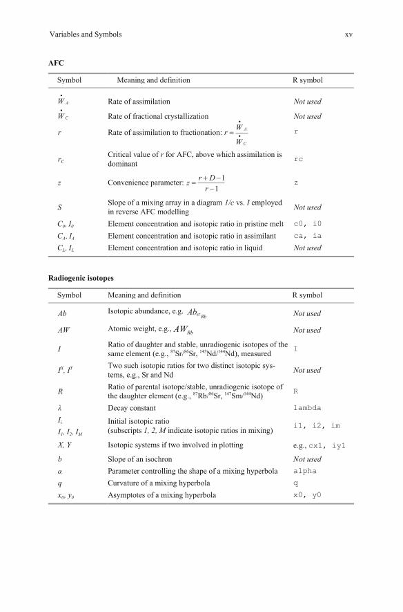
AFC
Symbol Meaning and definition R symbol
AW Rate of assimilation Not used
CW Rate of fractional crystallization Not used
r Rate of assimilation to fractionation: A
C
WrW
r
rC Critical value of r for AFC, above which assimilation is dominant rc
z Convenience parameter: 11
r Dzr
z
S Slope of a mixing array in a diagram 1/c vs. I employed in reverse AFC modelling Not used
C0, I0 Element concentration and isotopic ratio in pristine melt c0, i0
CA, IA Element concentration and isotopic ratio in assimilant ca, ia
CL, IL Element concentration and isotopic ratio in liquid Not used
Radiogenic isotopes
Symbol Meaning and definition R symbol
Ab Isotopic abundance, e.g. 87Rb
Ab Not used
AW Atomic weight, e.g., RbAW Not used
I Ratio of daughter and stable, unradiogenic isotopes of the same element (e.g., 87Sr/86Sr, 143Nd/144Nd), measured I
IX, IY Two such isotopic ratios for two distinct isotopic sys-tems, e.g., Sr and Nd Not used
R Ratio of parental isotope/stable, unradiogenic isotope ofthe daughter element (e.g., 87Rb/86Sr, 147Sm/144Nd) R
Decay constant lambda
Ii
I1, I2, IM Initial isotopic ratio (subscripts 1, 2, M indicate isotopic ratios in mixing) i1, i2, im
X, Y Isotopic systems if two involved in plotting e.g., cx1, iy1
b Slope of an isochron Not usedParameter controlling the shape of a mixing hyperbola alpha
q Curvature of a mixing hyperbola q
x0, y0 Asymptotes of a mixing hyperbola x0, y0
xvVariables and Symbols
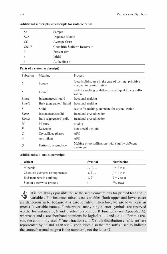
Additional subscripts/superscripts for isotopic ratios
SA DM CC CHUR 0
t
Sample Depleted Mantle Average Crust Chondritic Uniform Reservoir Present-day Initial At the time t
Parts of a system (subscript)
Subscript Meaning Process
0 Source [zero] solid source in the case of melting, primitive magma for crystallization
L Liquid melt for melting or differentiated liquid for crystalli-zation
S Solid restite for melting, cumulate for crystallization S.inst Instantaneous solid fractional crystallization S.bulk Bulk (aggregated) solid fractional crystallization M Mixture mixing P Reactants non-modal melting C Crystallized phases AFC A Assimilant AFC
Q Peritectic assemblage Melting or crystallization (with slightly different meanings)
Additional sub- and superscripts
Object Symbol Numbering
Minerals A, B… i = 1 to n Chemical elements (components) j = 1 to p End-members in a mixing 1, 2… k = 1 to m Step of a stepwise process t Not used
It is not always possible to use the same conventions for printed text and R variables. For instance, mixed case variables (both upper and lower case)
are dangerous in R, because it is case sensitive. Therefore, we use lower case in (most) R variable names. Furthermore, many single-letter symbols are reserved words: for instance c, D and t refer to common R functions (see Appendix ),
son, the commonly used F (melt fraction) and D (bulk distribution coefficient) are
the source/parental magma is the number 0, not the letter O!
xvi Variables and Symbols
…
represented by ff and dd in our R code. Note also that the suffix used to indicate
whereas T and F are shorthand notations for logical TRUE FALSE. For this rea- and
,
i
A
L.inst Instantaneous liquid fractional melting L.bulk Bulk (aggregated) liquid fractional melting
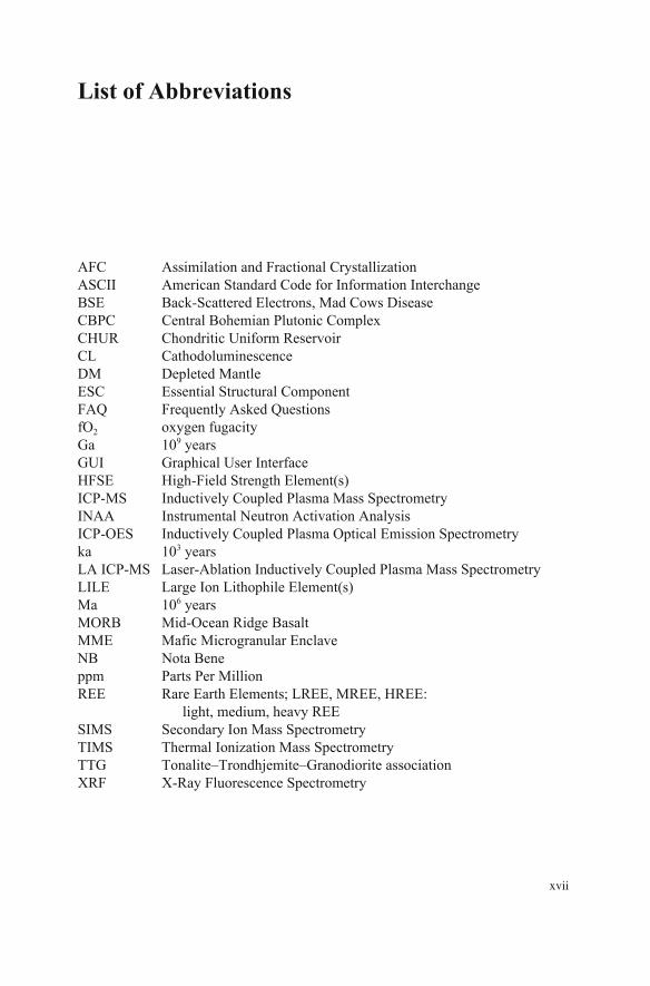
List of Abbreviations
AFC Assimilation and Fractional Crystallization ASCII American Standard Code for Information Interchange BSE Back-Scattered Electrons, Mad Cows Disease CBPC Central Bohemian Plutonic Complex CHUR Chondritic Uniform Reservoir CL Cathodoluminescence DM Depleted Mantle ESC Essential Structural Component FAQ Frequently Asked Questions fO2 oxygen fugacity Ga 109 years GUI Graphical User Interface HFSE High-Field Strength Element(s) ICP-MS Inductively Coupled Plasma Mass Spectrometry INAA Instrumental Neutron Activation Analysis ICP-OES Inductively Coupled Plasma Optical Emission Spectrometry ka 103 years LA ICP-MS Laser-Ablation Inductively Coupled Plasma Mass Spectrometry LILE Large Ion Lithophile Element(s) Ma 106 years MORB Mid-Ocean Ridge Basalt MME Mafic Microgranular Enclave NB Nota Bene ppm Parts Per Million REE Rare Earth Elements; LREE, MREE, HREE:
light, medium, heavy REE SIMS Secondary Ion Mass Spectrometry TIMS Thermal Ionization Mass Spectrometry TTG Tonalite–Trondhjemite–Granodiorite association XRF X-Ray Fluorescence Spectrometry
xvii
Abbreviations of Mineral Names
Symbols for mineral names mostly follow Kretz (1983):
Ab Albite All Allanite Amp Amphibole An Anorthite Ap Apatite Bt Biotite Cpx Clinopyroxene Crd Cordierite Di Diopside En Enstatite Fo Forsterite Grt Garnet Hbl Hornblende Ilm Ilmenite Kfs Potassium feldspar Mnz Monazite Ms Muscovite Mt Magnetite Ol Olivine Opx Orthopyroxene Phl Phlogopite Pl Plagioclase Qtz Quartz Rt Rutile Sil Sillimanite Spl Spinel Zrn Zircon
xix
ReferenceKretz R (1983) Symbols for rock-forming minerals. Amer Miner 68:277-279.
Contents
xxi
1 Introduction
1.1 Causes of Whole-Rock Chemical Variation in Igneous Suites .............. 1 1.2 Conventional Software for Igneous Geochemistry ................................. 3
1.2.1 Spreadsheets ............................................................................. 3 1.2.2 Dedicated Programs (PC Compatibles) .................................... 4
1.3 A Revolution? The R Language ............................................................. 4 1.3.1 What is R? ................................................................................ 4 1.3.2 Geochemical Data Toolkit (GCDkit) ....................................... 5
Part I R/GCDkit at Work 2 Data Manipulation and Simple Calculations............................................... 11
2.1 Loading and Manipulating Data ........................................................... 112.2 Linking Whole-Rock Chemistry with Mineral Stoichiometry ............. 13
2.2.1 Basic Indexes .......................................................................... 14 2.2.2 Cationic Parameters ................................................................ 16 2.2.3 Normative Calculations and Classification
2.3 Statistics ............................................................................................... 182.4 Classification and Grouping—Using Factors ....................................... 19
2.4.1 Statistical Examination of Complex Data Sets ....................... 20 2.4.2 Conversion of Numeric Vectors to Factors ............................ 22 2.4.3 Frequency (Contingency) Tables ........................................... 23
3 Classical Plots 3.1 Binary Plots .......................................................................................... 27
3.1.1 Plotting Simple Binary Plots .................................................. 27 3.1.2 Constant Sum Effect (Closure) ............................................... 30
3.2 Harker Plots and Other Basic Multiple Plots ........................................ 313.3 Ternary Plots ........................................................................................ 323.4 Classification Plots in GCDkit . ............................................................ 343.5 Geotectonic Diagrams .......................................................................... 353.6 Spiderplots ............................................................................................ 363.7 Multiple Plots by Groups ...................................................................... 40
References........ ..................................................................................................6
References........ ... ............................................................................................. 24
References........ ... ............................................................................................. 41
........................ ....... ............. ....................................................27
...................................................................................................... 1
of Igneous Rocks..................................................................... 17
xxii Contents
4 Specialized Plots ............................................................................................. 454.1 Log–Log Binary Plots .......................................................................... 454.2 Specialized Spiderplots ........................................................................ 46
4.2.1 Double-Normalized Spiderplots ............................................. 47 4.2.2 Spider Boxplots, Spider Box and Percentile Plots .................. 47
Contour Plots .............. .......................................................................... 48Anomaly Plots............... ........................................................................ 49Stripplots and Strip Boxplots.............. .................................................. 50
5 Radiogenic Isotopes ....................................................................................... 535.1 Recalculation of Elemental to Isotopic Ratios ...................................... 535.2 Calculation of Initial Ratios or Ages .................................................... 555.3 Epsilon, Delta and Gamma Values ....................................................... 575.4 Model Ages .......................................................................................... 60
5.4.1 Single-Stage Model Ages ................................................ 60 5.4.2 Two-Stage Nd Model Ages .................................................... 61
5.5 Isochron Ages ....................................................................................... 63References........................................................................................................ 65
Part II Modelling Major Elements 6 Direct Models ..................................................................................................69
6.1 Mass Balance During Crystallization ................................................... 69 6.1.1 Graphical Solutions ................................................................ 70 6.1.2 Cumulate Composition ........................................................... 71 6.1.3 Analytical Formulation ........................................................... 72 6.1.4 Generating a Magmatic Series Through Crystallization ......... 73
6.2 Partial Melting ...................................................................................... 756.3 Peritectic Reactions .............................................................................. 766.4 Mixing6.5 Crystallization and Partial Melting—Are These Just Special
7 Reverse Models .............................................................................................. 817.1 An Under-Determined Problem ............................................................ 817.2 Least-Square Solution to Crystallization/Melting Problems ................ 827.3 Least-Square Solution to Mixing Problems .......................................... 83
8 Forward Modelling in R ............................................................................... 85
9 Reverse Modelling in R . ................................................................................ 93
References........ ... ............................................................................................. 51
Reference ....................................................................................................... 80
References........................................................................................................ 83
References........................................................................................................ 92
................................................................................................... 78
Cases of Mixing?................................................................................. 79..
4.34.44.5
Nd .
xxiiiContents
Part III Modelling Trace Elements 10 Dilute Trace Elements: Partition Coefficients ........................................... 101
10.1 Crystal Networks and Substitutions ................................................... 10110.2 Partition Coefficients .......................................................................... 10110.3 Controls on the Values of Partition Coefficients .................................10210.4 Bulk Distribution Coefficients ........................................................... 103
11 Direct (Dilute) Trace-Element Models11.1 Crystallization ................................................................................... 106
11.1.1 Batch Crystallization .......................................................... 106 11.1.2 Fractional Crystallization ................................................... 106 11.1.3 Comparing Different Models..............................................109
11.2 Melting................................................................................................110 11.2.1 Batch Melting ....................................................................... 110 11.2.2 Fractional Melting ................................................................ 110 11.2.3 Comparing Different 11.2.4 Alternative Formulations of the Melting Equations ............. 111
11.3 Mixing.................................................................................................114 11.3.1 Ratio of Two Elements During Binary Mixing .................... 114 11.3.2 Mixing Hyperbolae in Ratio–Ratio Plots ............................. 114
11.4 Assimilation and Fractional Crystallization (AFC) ............................ 11711.5 Composite Models .............................................................................. 119 11.5.1 Crystallization with Incomplete Crystal Separation (Batch
Crystallization + Binary Mixing) ......................................... 120 11.5.2 Fluxed Melting (Binary Mixing + Batch Melting) ............... 121
12 Reverse (Dilute) Trace-Element Models .................................................. 12512.1 Reverse Fractional Crystallization (Using Rayleigh’s Law) .............. 12512.2 Reverse Batch Partial Melting ............................................................ 12712.3 Reverse Mixing .................................................................................. 128
13 Trace Elements as Essential Structural Constituents of Accessory Minerals: the Solubility Concept.................................................................12913.1 Solubility Formulae for Common Accessory Minerals ...................... 129
Zircon, ZrSiO4 ...................................................................... 129 13.1.2 Monazite, (LREE)PO4 .......................................................... 131 13.1.3 Apatite, Ca5(PO4)3(F,Cl,OH) ................................................ 134
13.2 Evolution Through Saturation ............................................................ 136
14 Forward Modelling in R ............................................................................. 141
References........ ... ........................................................................................... 104
References........ ... ........................................................................................... 123...
References........ ... ........................................................................................... 128
References........ ... ........................................................................................... 139
References........ ... ........................................................................................... 152References........ ... ........................................................................................... 15215 Reverse Modelling in R................................................................................ 153
....................................................... 105
Models................................................ 111
13.1.1
xxiv Contents
Part IV Radiogenic Isotopes 16 Direct Models ................................................................................................ 159
16.1 Binary Mixing .................................................................................... 159 16.1.1 Single Isotopic Ratio ............................................................ 159 16.1.2 Pair of Isotopic Ratios .......................................................... 161
16.2 AFC Formulation for Isotopes ............................................................ 163
17 Reverse Models ............................................................................................ 16717.1 Binary Mixing .................................................................................... 16717.2 AFC 167
18 Forward Modelling in R . ............................................................................ 16918.1 Binary Mixing .................................................................................... 16918.2 AFC 173
19 Reverse Modelling in R ............................................................................... 175
Reference. ............................................................................................... 177
Part V Practical Modelling 20 Choosing an Appropriate Model ................................................................ 181
20.1 Evidence for Crystallization ............................................................... 181 20.1.1 Final Solidification During Emplacement ............................ 181 20.1.2 Fractional Crystallization at Depth ....................................... 182
20.2 Evidence For Melting ......................................................................... 183 20.2.1 Crustal Anatexis ................................................................... 183 20.2.2 Melting of the Mantle ........................................................... 184
20.3 Magma Mixing and Assimilation ....................................................... 185 20.3.1 Mixing and Mingling of Magmas ......................................... 185 20.3.2 Assimilation.......................................................................... 186
21 Semi-Quantitative Geochemical Approach ............................................... 19121.1 Assessing Trace-Element Compatibility ............................................ 19121.2 Order of (In)Compatibility ................................................................. 19221.3 Process Identification ......................................................................... 195
21.3.1 Mixing vs. Crystallization/Melting ....................................... 195 21.3.2 Crystallization vs. Melting in a Log–Log Diagram ............. 195 21.3.3 Crystallization vs. Melting Using Incompatible Elements ... 198
21.4 Mixing Test ........................................................................................ 19921.5 Identifying Fractionating Minerals Using Log–Log Plots .................. 202
22 Constraining a Model . ................................................................................. 20522.1 Choosing an Appropriate Strategy...................................................... 205
.....................................................................................................
References........ ... ........................................................................................... 166
.....................................................................................................References........ ... ........................................................................................... 168
.......
References........ ... ........................................................................................... 187
References........ ... ........................................................................................... 203
22.2.3 Composition of the Solid Phases (Cumulate/Restite)........... 208 22.2.4 Partition Coefficients ............................................................ 211
22.3 Dealing with Accessory Minerals ....................................................... 212 22.3.1 Assessing the Role of Accessory Minerals ........................... 212 22.3.2 Modelling with Accessories ................................................. 214
22.4 Constraining the End-Members of a Mixing Model ........................... 221
23 Numerical Tips and Tricks ......................................................................... 22523.1 The Size of the Geochemical Space ................................................... 22523.2 Reducing the System .......................................................................... 22723.3 Colinearity .......................................................................................... 22723.4 Breaking Minerals into End Members ............................................... 22823.5 Coupling Majors and Traces .............................................................. 22823.6 This pace Left Blank for Your Own Tricks ..................................... 229
24 Common Sense in Action . ........................................................................... 23124.1 Physical Constraints ........................................................................... 231
24.1.1 Thermodynamic Constraints ................................................ 231Mechanical (Rheological) Constraints ................................. 232
24.2 Scale nd Speed f Processes—Approach o Equilibrium .............. 23424.3 Is Your Model Worth Your Efforts? .................................................. 235
24.3.1 How Well Can We Discriminate Between Models? ............ 236 24.3.2 Dangerous Projections .......................................................... 237
KD vs. C0—What Should You Improve First? ..................... 23824.4 Back to the Field! ................................................................................ 239References...................................................................................................... 240
Part VI Worked Examples 25 Differentiation of a Calc-Alkaline Series: Example of the
Atacazo-Ninahuilca volcanoes, Ecuador . ................................................... 245 25.1 Geological Setting .............................................................................. 24525.2 Data Exploration and Implications ..................................................... 246
25.2.1 Isotopic Data ........................................................................ 246 25.2.2 Major Elements .................................................................... 247 25.2.3 Trace Elements ..................................................................... 248
25.3 Geochemical Modelling ..................................................................... 250 25.3.1 First Step: Atacazo ............................................................... 252 25.3.2 Second Step: Ninahuilca ...................................................... 256
25.4 Summary ............................................................................................ 258
xxvContents
References...................................................................................................... 222
References...................................................................................................... 229
References...................................................................................................... 260
a o t ...
22.2 Constraining a Fractionation or Melting Model ................................. 206The Differentiated Liquid(s)/Melt: C L .................................206
22.2.2 The Primitive Liquid/Source: C0 .......................................... 20622.2.1
24.3.3
24.1.2
S
xxvi Contents
26.3.1 Mode Evolution During melting .......................................... 265 26.3.2 Major and Trace Elements .................................................... 268 26.3.3 Zircon ................................................................................... 271
References...................................................................................................... 275
Appendix A R Syntax in a Nutshell 1 Direct Mode
1.1 Basic Operations ................................................................................. 277 1.1.1 Starting and Terminating the R Session ............................... 277 1.1.2 Seeking Help and Documentation ........................................ 278
1.2 Fundamental Objects of the R Language ............................................ 279 1.2.1 Commands ............................................................................ 279
1.2.2 Handling Objects in Memory ...............................................2811.2.3 Attributes to Objects ............................................................. 282
1.3 Numeric Vectors ................................................................................. 282 1.3.1 Assignment ........................................................................... 282
1.3.2 Vector Arithmetic ................................................................. 2821.3.3 Names ................................................................................... 2831.3.4 Generating Regular Sequences ............................................. 2831.3.5 Functions to Manipulate Numeric Vectors ........................... 284
1.4 Character Vectors ............................................................................... 2841.5 Logical Vectors .................................................................................. 285
1.5.1 Logical Operators ................................................................. 285 1.5.2 Missing Values (NA, NaN) .................................................. 286
1.6 Arrays, Matrices, Data Frames ........................................................... 286 1.6.1 Matrix/Data Frame Operations ............................................. 287
1.7 Indexing/Subsetting of Vectors, Arrays and Data Frames .................. 288 1.7.1 Vectors ................................................................................. 289 1.7.2 Matrices/Data Frames ........................................................... 289
1.8 Lists ....................................................................................................2901.9 Coercion of Individual Object Types ................................................. 2911.10 Factors.................................................................................................292
1.10.1 Basic Usage of Factors ......................................................... 292 1.10.2 Conversion of Numeric Vectors to Factors .......................... 292 1.10.3 Frequency Tables ................................................................. 293 1.10.4 Using Factors to Handle Complex Datasets ......................... 293
1.11 Data Input/Output, Files ..................................................................... 293 1.11.1 Reading Data ........................................................................ 293 1.11.2 Sample Data Sets .................................................................. 295 1.11.3 Saving Data .......................................................................... 295
.................................................................................................. 277
26.2 Major and Trace Elements .................................................................. 26226.3 Geochemical Modelling ..................................................................... 264
26 Progressive Melting of a Metasedimentary Sequence: the Saint-Malo Migmatitic Complex, France ...................................................................... 261 26.1 Geological Setting .............................................................................. 261
xxviiContents
2 Graphics 2.1 Obtaining and Annotating Binary Plots .............................................. 2952.2 Additional High-Level Plotting Functions ......................................... 3022.3 Creating Custom Layouts and Axes ................................................... 3052.4 Exporting Graphs from R and Graphical Devices .............................. 3082.5 Interaction with Plots .......................................................................... 308
3 Programming in R.........................................................................................3093.1 Input and Output ................................................................................. 3093.2 Conditional Execution ........................................................................ 3103.3 Loops.................................................................................................. 3103.4 User-Defined Functions...................................................................... 311
3 .4.2 Assignments in Functions .................................................... 312
3.5 An Alternative to Loops— . ...................................................... 313References........ .............................................................................................. 313
Appendix B Introduction to GCDkit
1 First Steps with GCDkit .............................................................................. 315 1.1 Installation .......................................................................................... 3151.2 GCDkit Overview: The User Interface ............................................... 3161.3 Working with Data ............................................................................. 318
1.3.1 Data Format .......................................................................... 3181.3.2 Loading Data ........................................................................ 3191.3.3 Merging Data ....................................................................... 321
1.3.4 Choosing Data ...................................................................... 3221.3.5 Grouping............................................................................... 322
1.4 Plotting................................................................................................ 3231.4.1 Plot Settings ......................................................................... 3261.4.2 Single Plot Editing ............................................................... 3271.4.3 Plates and 1.4.4 Spiderplots ............................................................................ 3281.4.5 Classification and
1.5 Calculations ........................................................................................ 3291.6 Exporting from GCDkit . ..................................................................... 331
2 Under the Bonnet: GCDkit Internals........................................................2.1 R language and GCDkit . .....................................................................2.2 Data Variables .................................................................................... 3332.3 System Variables ................................................................................ 2.4 Tailoring GCDkit to Suit your Needs.................................................. 3342.5 Plugins.................................................................................................334 References..................................................................................................... ...3 36
...................................................................................................... .. 295
Plate Editing ........................................................ 328
Geotectonic Diagrams ............................ 329
3.4.1 Arguments to Functions........................................................311
sapply
. 332
333
332

xxviii Contents
Appendix C Solving Systems of Linear Algebraic Equations in R 1.1 Linear Algebraic le Solution) ....................... 3371.2 Overdetermined Systems (Unconstrained Least-Square Method)...... 3381.3 Constrained Least-Square Method ..................................................... 339References...................................................................................................... 340
Equation Systems (Sing
................................................................................................................... 341Index
Chapter 1 Introduction
Very soon after the birth of igneous geochemistry, geologists like Alfred Harker (Harker 1909) recognized the existence of igneous rock “series”, i.e. rock suites sharing common geochemical features and having progressively changing compo-sitions. Such variation was, and still frequently is, ascribed to evolution by frac-tional crystallization at depth, in a putative magma chamber. Research over the following century, however, has demonstrated that the chemistry of magmatic suites may in fact be shaped by many contrasting petrogenetic processes. Geo-chemistry, especially in combination with petrology, represents a powerful tool for deciphering and parameterizing of such processes.
1.1 Causes of Whole-Rock Chemical Variation in Igneous Suites
Human beings—and geologists in particular—have always been fascinated by magmas. Due to the well-known increase of temperature with depth, it was be-lieved for a long time that there is a planetary-scale reservoir of molten rocks beneath the crust (e.g., Kircher 1664; Moro 1740; Cordier 1827). This archaic concept has long been abandoned as seismic data demonstrated that, apart from the outer core, the interior of the Earth is solid (Oldham 1906; Gutenberg 1914; Jeffreys 1926, among others). Suddenly a more complex picture has arisen—that of vigorous deep interactions between solid and liquid materials, including at least two successive petrogenetic processes: melting and crystallization. Of course, these mechanisms are inaccessible to direct observation, which is why their inves-tigation has been mainly indirect, based on petrological and geochemical methods.
In the beginning of the 20th century, two distinct and complementary ap-proaches to the problem emerged. The first one, based on experiments, was devel-oped by Bowen (1912, 1928) who demonstrated the existence of mineral reaction series in magmatic systems. Indeed, during the crystallization of magma, minerals do not grow simultaneously but, as the magma cools, the individual mineral phases appear in a succession determined by their crystallization temperature. This concept showed crystallization as a dynamic process with a certain temporal
1© Springer-Verlag Berlin Heidelberg 2016 V. Janoušek et al., Geochemical Modelling of Igneous Processes – Principles And Recipes in R Language, Springer Geochemistry, DOI 10.1007/978-3-662-46792-3_1
development. Thus, the evolution is not linear, but it can take different directions in response to the changes in physico–chemical parameters and, in turn, of mineral chemistry of crystallizing assemblages.
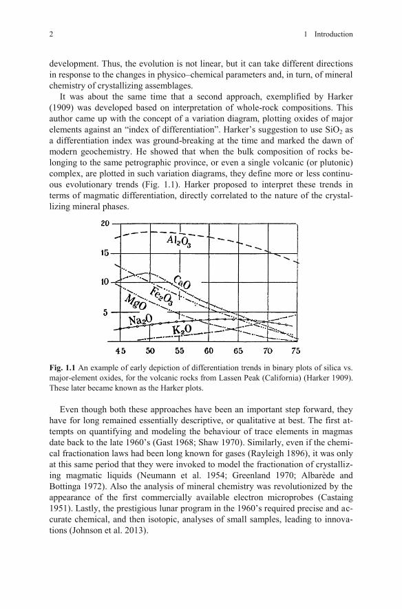
It was about the same time that a second approach, exemplified by Harker (1909) was developed based on interpretation of whole-rock compositions. This author came up with the concept of a variation diagram, plotting oxides of major elements against an “index of differentiation”. Harker’s suggestion to use SiO2 as a differentiation index was ground-breaking at the time and marked the dawn of modern geochemistry. He showed that when the bulk composition of rocks be-longing to the same petrographic province, or even a single volcanic (or plutonic) complex, are plotted in such variation diagrams, they define more or less continu-ous evolutionary trends (Fig. 1.1). Harker proposed to interpret these trends in terms of magmatic differentiation, directly correlated to the nature of the crystal-lizing mineral phases.
Fig. 1.1 An example of early depiction of differentiation trends in binary plots of silica vs. major-element oxides, for the volcanic rocks from Lassen Peak (California) (Harker 1909).These later became known as the Harker plots.
Even though both these approaches have been an important step forward, they have for long remained essentially descriptive, or qualitative at best. The first at-tempts on quantifying and modeling the behaviour of trace elements in magmas date back to the late 1960’s (Gast 1968; Shaw 1970). Similarly, even if the chemi-cal fractionation laws had been long known for gases (Rayleigh 1896), it was only at this same period that they were invoked to model the fractionation of crystalliz-ing magmatic liquids (Neumann et al. 1954; Greenland 1970; Albarède and Bottinga 1972). Also the analysis of mineral chemistry was revolutionized by the appearance of the first commercially available electron microprobes (Castaing 1951). Lastly, the prestigious lunar program in the 1960’s required precise and ac-curate chemical, and then isotopic, analyses of small samples, leading to innova-tions (Johnson et al. 2013).
2 1 Introduction
A further boost to geochemical modelling came with the advancement of radio-genic isotope methods (originally Thermal-Ionization Mass Spectrometry, TIMS, and from late 1990’s also Inductively Coupled Mass Spectrometry, ICP-MS). In 1970’s analytical techniques became available revolutionising whole-rock trace-element determinations, providing precise and reproducible data needed for petro-genetic modelling (e.g., X-Ray Fluorescence Spectrometry, XRF; Instrumental Neutron Activation Analysis, INAA) later joined by Inductively Coupled Plasma Optical Emission Spectrometry, ICP-OES and, in particular, ICP-MS (Potts 1987; Sylvester 2001). Obviously related was the development of the theoretical princi-ples, including new geochemical projections (see Rollinson 1993 and references therein) or innovative approaches to numerical description and modelling of petrogenetic processes (summarized, above all, in excellent monographs of Albarède 1995 and Shaw 2006).
This revolution in whole-rock geochemistry has been joined, especially in the last twenty years, by novel and cost-effective methods for in situ determinations of mineral composition, most importantly Secondary Ion Mass Spectrometry (SIMS) and Laser-Ablation Inductively Coupled Plasma Mass Spectrometry (LA ICP-MS). This advancement is ongoing, and seems to be accelerating nowadays.
1.2 Conventional Software for Igneous Geochemistry
With the modern analytical techniques has inevitably arrived a flood of precise geochemical data on major- and trace elements, as well as a seemingly endless number of isotope systems. This technical progress goes hand in hand with the in-creasing accessibility of data over the Internet, in the form of online publications, their supplementary datasets, or web-based databases such as EarthChem (www.earthchem.org) or GeoRoc (georoc.mpch-mainz.gwdg.de/georoc).
Quick and efficient handling of such large datasets represents a true challenge in modern geochemistry. This is routinely achieved by personal computers, also enabling the calculation of rather complicated thermodynamic and petrogenetic models in the comfort of one’s own office.
1.2.1 Spreadsheets
The most accessible and generally available are the spreadsheets. They belong to basic software preloaded on many computers, thus requiring no extra costs. Even though relatively easy to use, they are not very suitable for geochemical calcula-tions. Dedicated geochemical tools, mostly designed for Microsoft Excel aided by VBA macros, are rather scarce, and their functionality rudimentary (Sidder 1994; Su et al. 2003; Zhou and Li 2006; Wang et al. 2008) even though some more so-phisticated tools for petrogenetic modelling are also available (Ersoy 2013; Keskin 2013). Moreover, spreadsheets endure low efficiency for repeated tasks as well as limited protection of the primary data; for more complicated calculations the
1.1 Causes of Whole-Rock Chemical Variation in Igneous Suites 3
worksheet becomes too complex and prone to errors. The graphical output is poor and requires much tweaking to become truly of publication quality. In our view, spreadsheets are useful only for organization of the data (although databases are superior for the task) and production of tables for final publication.
1.2.2 Dedicated Programs (PC Compatibles)1
A number of dedicated software tools have been written in a variety of program-ming languages that PC users could employ. Some of them were designed for DOS or 16-bit versions of Windows and thus became obsolete, such as MinCalc (Melín and Kunst 1992), NewPet (Clarke et al. 1994), MinPet (Richard 1995), or Norman (Janoušek 2001). Others are more recent and still being continuously de-veloped, most notably IgPet (Carr 2014; www.rockware.com), PetroGraph (Petrelli et al. 2005), accounts.unipg.it/~maurip/SOFTWARE.htm) and WinRock (Kanen 2004, www.geologynet.com/winrock.htm).
Unfortunately, it is often difficult to figure out exactly which algorithms have been employed by a given program. The documentation is never detailed enough and it is not a common practice to make the source code available. Even if it is, any modifications or additions to the original program could be tedious, or impos-sible for legal reasons, or merely because the user may not be a skilled program-mer. Moreover, many of the programs require complex formatting of the input data, and/or fail to produce high-quality graphical output. Of concern to many col-leagues also is that some of the applications are rather costly and/or have a pecu-liar user interface.
1.3 A Revolution? The R Language
Clearly the best approach to many problems outlined above would be to write our own software. But we suggest that it would not be wise to develop it from scratch; much better is to employ a comprehensive computing environment such as Mathematica or Matlab, with a built-in computational, graphical and input/output functionality. However, also these packages are commercial, hindering the distri-bution of any product to potential users, especially in economically challenged countries.
1.3.1 What is R?
Fortunately, with the appearance of the R language at the turn of millennium, we now have a powerful, yet simple and free, open-source toolbox, ideal for devel-opment of geochemical packages. Put in simple terms, R is an environment for efficient data processing, their visualization and statistical analysis as well as a
1 Apart from thermodynamic software, dealt with in one of the Next step boxes in Chap. 22.
4 1 Introduction
high-level functional/object-oriented programming language. It was developed originally by Ihaka and Gentleman (1996) from the University of Auckland. Sub-sequently an open group of experts formed the R Development Core Team who continue to oversee the development of the project (www.r-project.org)1.00 was released in 2000; the current one at the time of writing this book is 3.1.2 (Pumpkin Helmet).
The syntax of R (see Appendix A) is based on, and largely compatible with, its successful predecessor, the S language. The latter was developed in Bell Laborato-ries in 1975, and followed by The New S Language in late 1980’s (Becker et al. 1988). The commercial version, S-PLUS, is currently being distributed by TIBCO Software (www.tibco.com).
The chief advantage of R is—apart from a somewhat more efficient implemen-tation—that it is freely available, with all the source code, for all the main plat-forms (MS Windows, Unix/Linux and Mac OS). The R language includes arith-metic and database functions (plus data import in many formats, also via SQL and ODBC), functions for matrix manipulation/arithmetic and a large number of statis-tical tools.
The graphic output is publication-quality, including mathematical symbols. It can be exported into a number of data formats (PostScript, WMF, PDF, TIFF, PNG…), for incorporation into DTP programs and word processors or for further editing in graphical packages such Corel Draw or Adobe Illustrator.
R allows interactive as well as batch use (as a true programming language). For the latter, it enables writing user-defined functions involving conditions or loops. R is easily extensible with user-contributed packages. Apart from this, an over-whelming majority of programs designed originally for S/S-PLUS work—directly or after cosmetic changes—in R. Most of the R system is written in R; for compu-tationally intensive tasks, C, C++, and FORTRAN code can be linked and called at run time.
1.3.2 Geochemical Data Toolkit (GCDkit)
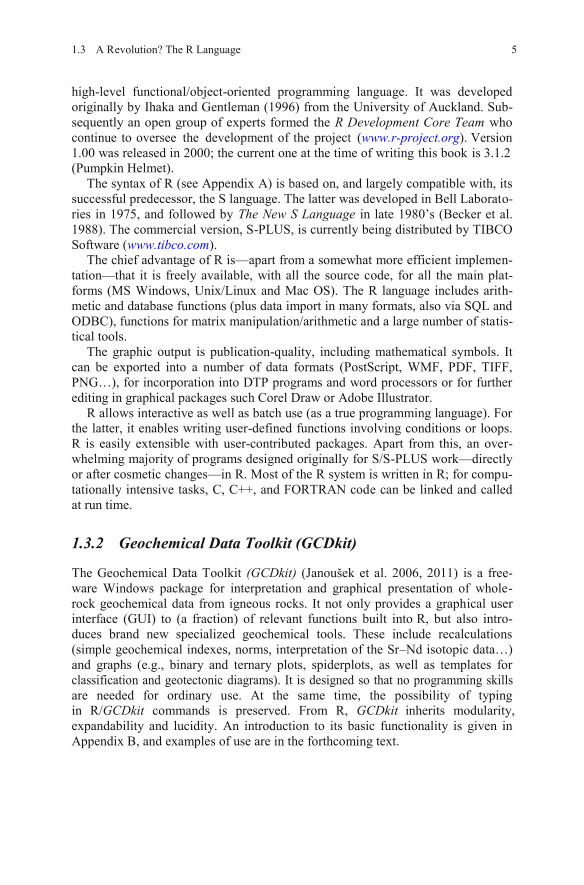
The Geochemical Data Toolkit (GCDkit) (Janoušek et al. 2006, 2011) is a free-ware Windows package for interpretation and graphical presentation of whole-rock geochemical data from igneous rocks. It not only provides a graphical user interface (GUI) to (a fraction) of relevant functions built into R, but also intro-duces brand new specialized geochemical tools. These include recalculations (simple geochemical indexes, norms, interpretation of the Sr–Nd isotopic data…) and graphs (e.g., binary and ternary plots, spiderplots, as well as templates for classification and geotectonic diagrams). It is designed so that no programming skills are needed for ordinary use. At the same time, the possibility of typing in R/GCDkit commands is preserved. From R, GCDkit inherits modularity,expandability and lucidity. An introduction to its basic functionality is given in Appendix B, and examples of use are in the forthcoming text.
1.3 A Revolution? The R Language 5
. Version
6 1 Introduction
References
Albarède F (1995) Introduction to geochemical modeling. Cambridge University Press, Cambridge
Albarède F, Bottinga Y (1972) Kinetic disequilibrium in trace element partitioning between phe-nocrysts and host lava. Geochim Cosmochim Acta 36:141–156
Becker RA, Chambers JM, Wilks AR (1988) The new S language. Chapman & Hall, LondonBowen NL (1912) The order of crystallization in igneous rocks. J Geol 20:457–468Bowen NL (1928) The evolution of the igneous rocks. Princeton University Press, Princeton
Castaing R (1951) Application des sondes électroniques à une méthode d’analyse ponctuelle chimique et cristallographique. Publication ONERA, vol 55. University of Paris, Paris (PhD Thesis)
Clarke D, Mengel F, Coish RA, Kosinowski MHF (1994) NewPet for DOS, version 94.01.07. Department of Earth Sciences, Memorial University of Newfoundland, Canada
Cordier PLA (1827) Essai sur la température de l’intérieur de la Terre. Mémoires de l’Académie des sciences de l’Institut de France 7:473–556
Ersoy Y (2013) PETROMODELER (Petrological Modeler): a Microsoft® Excel© spreadsheet program for modelling melting, mixing, crystallization and assimilation processes in mag-matic systems. Turkish J Earth Sci 22:115–125
Gast PW (1968) Trace element fractionation and the origin of tholeiitic and alkaline magma types. Geochim Cosmochim Acta 32:1057–1086
Greenland LP (1970) An equation of trace element distribution during magmatic crystallization. Amer Miner 55:455–465
Gutenberg B (1914) Über Erdbenwellen VIIA. Beobachtungen an Registrierungen von Fernbeben in Göttingen und Folgerungen über die Konstitution des Erdkörpers. Nachr d Kön Ges d Wiss Göttingen, math-phys Kl 125–176
Harker A (1909) The natural history of igneous rocks. Methuen & Co., LondonIhaka R, Gentleman R (1996) R: a language for data analysis and graphics. J Comp Graph Stat
5:299–344Janoušek V (2001) Norman, a QuickBasic programme for petrochemical re-calculation of whole-
rock major-element analyses on IBM PC. J Czech Geol Soc 46:9–13Janoušek V, Farrow CM, Erban V (2006) Interpretation of whole-rock geochemical data in igne-
ous geochemistry: introducing Geochemical Data Toolkit (GCDkit). J Petrol 47:1255–1259Janoušek V, Farrow CM, Erban V, Trubač J (2011) Brand new Geochemical Data Toolkit
(GCDkit 3.0)—is it worth upgrading and browsing documentation? (Yes!). Geol výzk Mor Slez 18:26–30
Jeffreys H (1926) The rigidity of the Earth’s central core. Monthly Notices of the Royal Astronomical Society, Geophysical Supplement 1:371–383
Johnson CM, McLennan SM, McSween HY, Summons RE (2013) Smaller, better, more: five decades of advances in geochemistry. In: Bickford ME (ed) The web of geological sciences: advances, impacts, and interactions. Geological Society of America Special Papers, vol 500, pp 259–302
Kanen (2004) WinRock (a manual). MinServ, ISBN 0 9756723 8 XKeskin M (2013) AFC-Modeler: a Microsoft® Excel© workbook program for modelling assimi-
lation combined with fractional crystallization (AFC) process in magmatic systems by using equations of DePaolo (1981). Turkish J Earth Sci 22:304–319
Kircher A (1664) Mundus subterraneus, Tomus 1–2. Apud Joannem Janssonium & Elyseum Weyerstraten, Amsterdam
Melín M, Kunst M (1992) MINCALC Development Kit 2.1. Geological Institute of the Czech Academy of Sciences, Prague
Carr M (2014) IgPet, a graphics and modeling program for igneous petrology. Terra Softa, Somerset, New Jersey, U.S.A.
References 7
Moro AL (1740) De crostacei e degli altri marini corpi che si truovano su’ monti. Appresso Stefano Monti, Venezia
Neumann H, Mead J, Vitaliano CJ (1954) Trace element variation during fractional crystalliza-tion as calculated from the distribution law. Geochim Cosmochim Acta 6:90–99
Oldham RD (1906) The constitution of the interior of the Earth, as revealed by earthquakes. Q J Geol Soc Lond 62:456–475
Petrelli M, Poli G, Perugini D, Peccerillo A (2005) PetroGraph: a new software to visualize, model, and present geochemical data in igneous petrology. Geochem Geophys Geosyst 6: Q07011
Potts PJ (1987) A Handbook of silicate rock analysis. Blackie & Son Ltd., Glasgow and LondonRayleigh L (1896) Theoretical considerations respecting the separation of gases by diffusion and
similar processes. Philosophical Magazine Series 5 42:493–498Richard LR (1995) MinPet: mineralogical and petrological data processing system, version 2.02.
MinPet Geological Software, Québec, CanadaRollinson HR (1993) Using geochemical data: evaluation, presentation, interpretation. Longman,
LondonShaw DM (1970) Trace element fractionation during anatexis. Geochim Cosmochim Acta
34:237–243Shaw DM (2006) Trace elements in magmas. A theoretical treatment. Cambridge University
Press, CambridgeSidder GB (1994) Petro.calc.plot, Microsoft Excel macros to aid petrologic interpretation.
Comput and Geosci 20:1041–1061Su YJ, Langmuir CH, Asimow PD (2003) PetroPlot: A plotting and data management tool set for
Microsoft Excel. Geochem Geophys Geosyst 4:1030, doi:10.1029/2002GC000323Sylvester P (ed) (2001) Laser ablation-ICPMS in the Earth sciences: principles and applications.
Mineralogical Association of Canada Short Course Series, vol 29Wang X, Ma W, Gao S, Ke L (2008) GCDPlot: An extensible Microsoft Excel VBA program for
geochemical discrimination diagrams. Comput and Geosci 34:1964–1969Zhou J, Li X (2006) GeoPlot: an Excel VBA program for geochemical data plotting. Comput and
Geosci 32:554–560

Part I R/GCDkit at Work
In this section we will demonstrate practical use of the R language to solve com-mon problems in igneous geochemistry. The text usually starts with a brief discus-sion of the geological background, followed by a R code (see Appendix A for an overview of R syntax) and its equivalent (or more elegant ) solution in GCDkit (for introduction to the system or for reference, see Appendix B).
Chapter 2 Data Manipulation and Simple Calculations
2.1 Loading and Manipulating Data
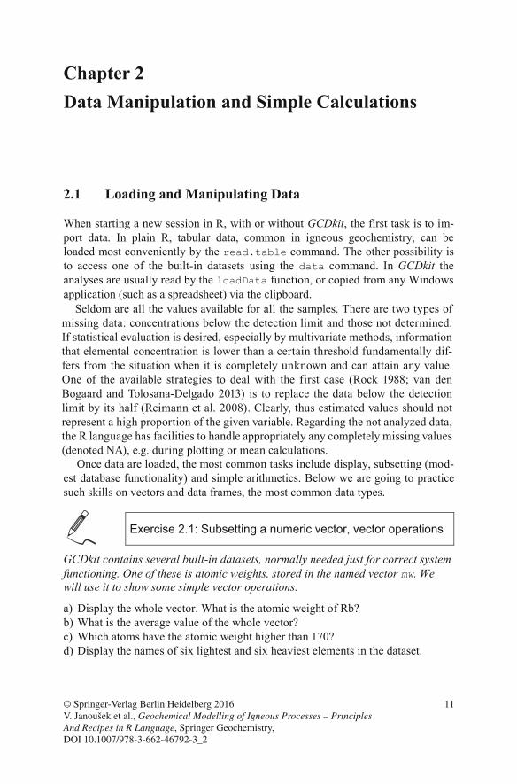
When starting a new session in R, with or without GCDkit, the first task is to im-port data. In plain R, tabular data, common in igneous geochemistry, can be loaded most conveniently by the read.table command. The other possibility is to access one of the built-in datasets using the data command. In GCDkit the analyses are usually read by the loadData function, or copied from any Windows application (such as a spreadsheet) via the clipboard.
Once data are loaded, the most common tasks include display, subsetting (mod-est database functionality) and simple arithmetics. Below we are going to practice such skills on vectors and data frames, the most common data types.
Exercise 2.1: Subsetting a numeric vector, vector operations
GCDkit contains several built-in datasets, normally needed just for correct system functioning. One of these is atomic weights, stored in the named vector mw. We will use it to show some simple vector operations.
a) Display the whole vector. What is the atomic weight of Rb? b) What is the average value of the whole vector? c) Which atoms have the atomic weight higher than 170? d) Display the names of six lightest and six heaviest elements in the dataset.
© Springer-Verlag Berlin Heidelberg 2016 V. Janoušek et al., Geochemical Modelling of Igneous Processes – Principles And Recipes in R Language, Springer Geochemistry, DOI 10.1007/978-3-662-46792-3_2
11
Seldom are all the values available for all the samples. There are two types of
missing data: concentrations below the detection limit and those not determined.
If statistical evaluation is desired, especially by multivariate methods, information
that elemental concentration is lower than a certain threshold fundamentally dif-
fers from the situation when it is completely unknown and can attain any value.
One of the available strategies to deal with the first case (Rock 1988; van den
Bogaard and Tolosana-Delgado 2013) is to replace the data below the detection
limit by its half (Reimann et al. 2008). Clearly, thus estimated values should not
represent a high proportion of the given variable. Regarding the not analyzed data,
the R language has facilities to handle appropriately any completely missing values
(denoted NA), e.g. during plotting or mean calculations.
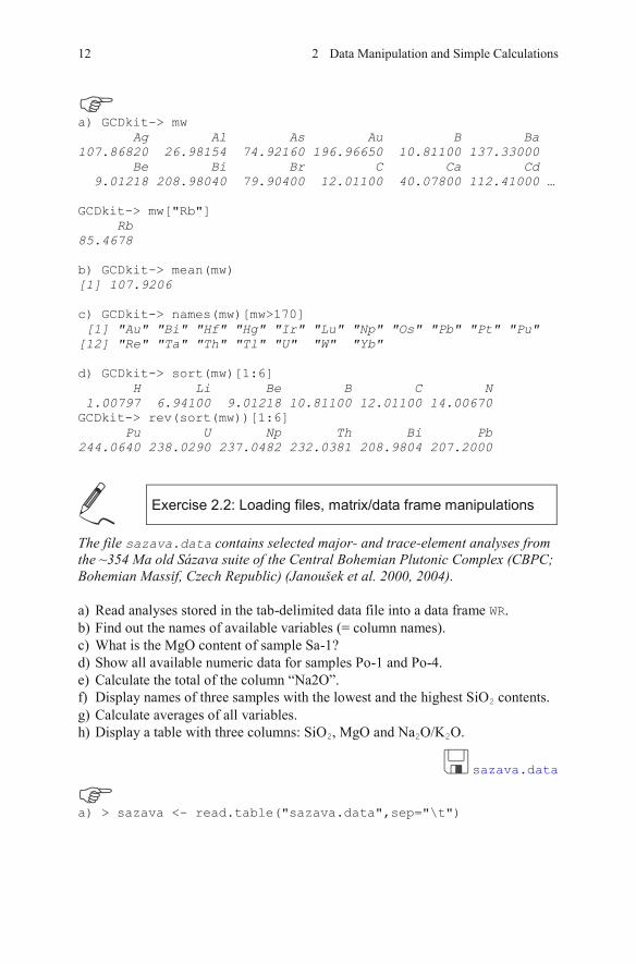
a) GCDkit-> mw Ag Al As Au B Ba 107.86820 26.98154 74.92160 196.96650 10.81100 137.33000 Be Bi Br C Ca Cd 9.01218 208.98040 79.90400 12.01100 40.07800 112.41000 … GCDkit-> mw["Rb"] Rb 85.4678 b) GCDkit-> mean(mw) [1] 107.9206 c) GCDkit-> names(mw)[mw>170] [1] "Au" "Bi" "Hf" "Hg" "Ir" "Lu" "Np" "Os" "Pb" "Pt" "Pu" [12] "Re" "Ta" "Th" "Tl" "U" "W" "Yb" d) GCDkit-> sort(mw)[1:6] H Li Be B C N 1.00797 6.94100 9.01218 10.81100 12.01100 14.00670 GCDkit-> rev(sort(mw))[1:6] Pu U Np Th Bi Pb 244.0640 238.0290 237.0482 232.0381 208.9804 207.2000
Exercise 2.2: Loading files, matrix/data frame manipulations
The file sazava.data contains selected major- and trace-element analyses from the ~354 Ma old Sázava suite of the Central Bohemian Plutonic Complex (CBPC; Bohemian Massif, Czech Republic) (Janoušek et al. 2000, 2004).
a) Read analyses stored in the tab-delimited data file into a data frame WR.b) Find out the names of available variables (= column names). c) What is the MgO content of sample Sa-1?d) Show all available numeric data for samples Po-1 and Po-4. e) Calculate the total of the column “Na2O”.f) Display names of three samples with the lowest and the highest SiO2 contents. g) Calculate averages of all variables. h) Display a table with three columns: SiO2, MgO and Na2O/K2O.
sazava.data
a) > sazava <- read.table("sazava.data",sep="\t")
12 2 Data Manipulation and Simple Calculations
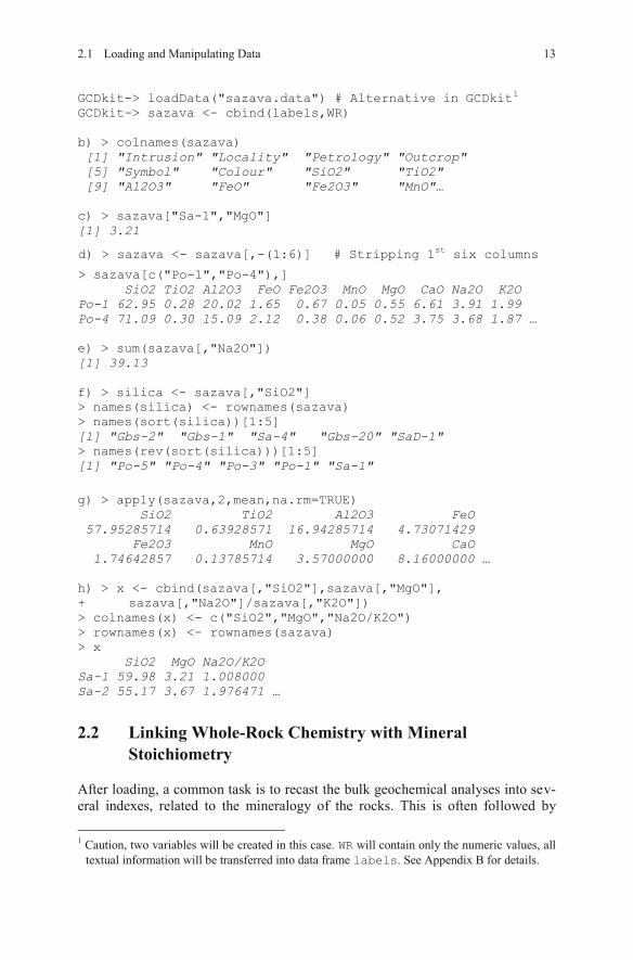
GCDkit-> loadData("sazava.data") # Alternative in GCDkit 1
GCDkit-> sazava <- cbind(labels,WR) b) > colnames(sazava) [1] "Intrusion" "Locality" "Petrology" "Outcrop" [5] "Symbol" "Colour" "SiO2" "TiO2" [9] "Al2O3" "FeO" "Fe2O3" "MnO"… c) > sazava["Sa-1","MgO"] [1] 3.21
> sazava[c("Po-1","Po-4"),] SiO2 TiO2 Al2O3 FeO Fe2O3 MnO MgO CaO Na2O K2O Po-1 62.95 0.28 20.02 1.65 0.67 0.05 0.55 6.61 3.91 1.99 Po-4 71.09 0.30 15.09 2.12 0.38 0.06 0.52 3.75 3.68 1.87 … e) > sum(sazava[,"Na2O"]) [1] 39.13 f) > silica <- sazava[,"SiO2"] > names(silica) <- rownames(sazava) > names(sort(silica))[1:5] [1] "Gbs-2" "Gbs-1" "Sa-4" "Gbs-20" "SaD-1" > names(rev(sort(silica)))[1:5] [1] "Po-5" "Po-4" "Po-3" "Po-1" "Sa-1"
st six columns
SiO2 TiO2 Al2O3 FeO 57.95285714 0.63928571 16.94285714 4.73071429 Fe2O3 MnO MgO CaO 1.74642857 0.13785714 3.57000000 8.16000000 … h) > x <- cbind(sazava[,"SiO2"],sazava[,"MgO"], + sazava[,"Na2O"]/sazava[,"K2O"]) > colnames(x) <- c("SiO2","MgO","Na2O/K2O") > rownames(x) <- rownames(sazava) > x SiO2 MgO Na2O/K2O Sa-1 59.98 3.21 1.008000 Sa-2 55.17 3.67 1.976471 …
2.2 Linking Whole-Rock Chemistry with Mineral Stoichiometry
After loading, a common task is to recast the bulk geochemical analyses into sev-eral indexes, related to the mineralogy of the rocks. This is often followed by 1 Caution, two variables will be created in this case. WR will contain only the numeric values, all
textual information will be transferred into data frame labels. See Appendix B for details.
2.1 Loading and Manipulating Data 13
d) > sazava <- sazava[,-(1:6)] # Stripping 1
g) > apply(sazava,2,mean,na.rm=TRUE)
normative recalculations. The aim is to better understand the modal chemistry, classification and, together with statistical methods, the distribution of elements within the dataset. R, as a statistical language, is well suited to such a task. Fur-thermore, user-defined functions serve to add new features tailored to our needs.
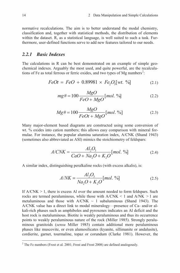
2.2.1 Basic Indexes
The calculations in R can be best demonstrated on an example of simple geo-chemical indexes. Arguably the most used, and quite powerful, are the recalcula-tions of Fe as total ferrous or ferric oxides, and two types of Mg numbers : 2
2 30.89981 [ . %]FeOt FeO Fe O wt (2.1)
# 100 [ . %]MgOmg molFeO MgO
(2.2)
# 100 [ . %]MgOMg molFeOt MgO
(2.3)
Many major-element based diagrams are constructed using some conversion of wt. % oxides into cation numbers; this allows easy comparison with mineral for-mulae. For instance, the popular alumina saturation index, A/CNK (Shand 1943) (sometimes also abbreviated as ASI) mimics the stoichiometry of feldspars:
2 3
2 2
/ [ . %]Al OA CNK molCaO Na O K O
(2.4)
A similar index, distinguishing peralkaline rocks (with excess alkalis), is:
2 3
2 2
/ [ . %]Al OA NK molNa O K O
(2.5)
If A/CNK > 1, there is excess Al over the amount needed to form feldspars. Such rocks are termed peraluminous, while those with A/CNK < 1 and A/NK
<
1 are metaluminous and those with A/CNK ~ 1 subaluminous (Shand 1943). The A/CNK value has a direct link to modal mineralogy—presence of Ca- and/or al-kali-rich phases such as amphiboles and pyroxenes indicates an Al deficit and the host rock is metaluminous. Biotite is weakly peraluminous and thus its occurrence points to weakly peraluminous nature of the rock (Miller 1985). Strongly peralu-minous granitoids (sensu Miller 1985) contain additional more peraluminous phases like muscovite, or even alumosilicates (kyanite, sillimanite or andalusite), cordierite, garnet, tourmaline, topaz or corundum (Clarke 1981). However, the 2 The Fe numbers (Frost et al. 2001; Frost and Frost 2008) are defined analogously.
14 2 Data Manipulation and Simple Calculations
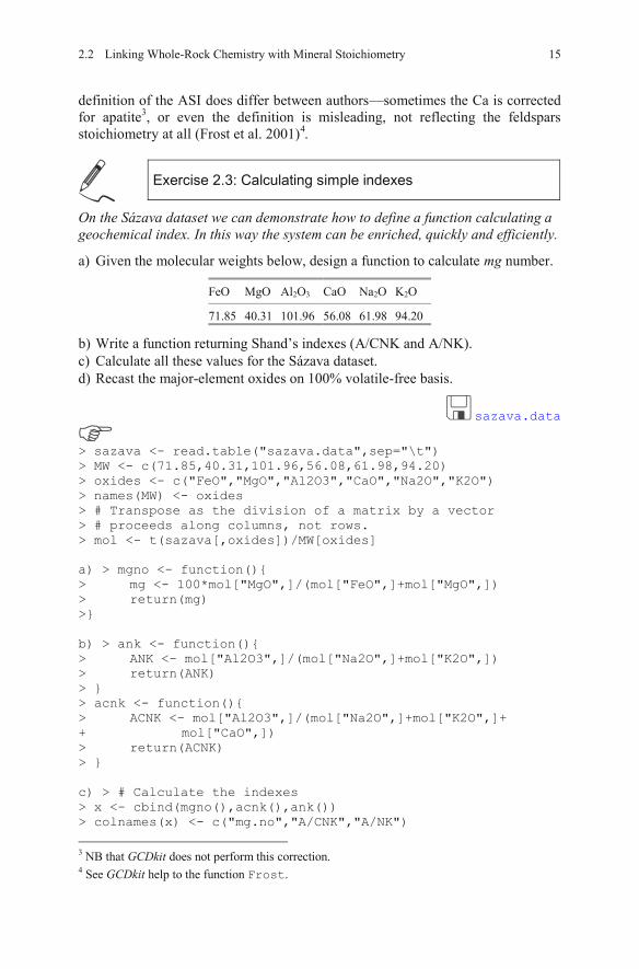
definition of the ASI does differ between authors—sometimes the Ca is corrected for apatite , or even the definition is misleading, not reflecting the feldspars stoichiometry at all (Frost et al. 2001) .
3
4
Exercise 2.3: Calculating simple indexes
On the Sázava dataset we can demonstrate how to define a function calculating a geochemical index. In this way the system can be enriched, quickly and efficiently.
a) Given the molecular weights below, design a function to calculate mg number.
FeO MgO Al2O3 CaO Na2O K2O
71.85 40.31 101.96 56.08 61.98 94.20
b) Write a function returning Shand’s indexes (A/CNK and A/NK). c) Calculate all these values for the Sázava dataset. d) Recast the major-element oxides on 100% volatile-free basis.
sazava.data
> sazava <- read.table("sazava.data",sep="\t") > MW <- c(71.85,40.31,101.96,56.08,61.98,94.20) > oxides <- c("FeO","MgO","Al2O3","CaO","Na2O","K2O") > names(MW) <- oxides > # Transpose as the division of a matrix by a vector > # proceeds along columns, not rows. > mol <- t(sazava[,oxides])/MW[oxides]
a) > mgno <- function(){ > mg <- 100*mol["MgO",]/(mol["FeO",]+mol["MgO",]) > return(mg) >} b) > ank <- function(){ > ANK <- mol["Al2O3",]/(mol["Na2O",]+mol["K2O",]) > return(ANK) > } > acnk <- function(){ > ACNK <- mol["Al2O3",]/(mol["Na2O",]+mol["K2O",]+ + mol["CaO",]) > return(ACNK) > } c) > # Calculate the indexes > x <- cbind(mgno(),acnk(),ank()) > colnames(x) <- c("mg.no","A/CNK","A/NK")
3 NB that GCDkit does not perform this correction. 4 See GCDkit help to the function Frost.
2.2 Linking Whole-Rock Chemistry with Mineral Stoichiometry 15
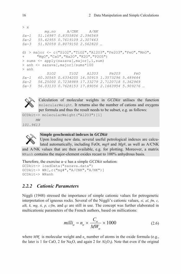
> x mg.no A/CNK A/NK Sa-1 51.16987 0.8355806 2.396569 Sa-2 55.42955 0.7619109 2.307463 Sa-3 51.92059 0.8079150 2.562820 … d) > major <- c("SiO2","TiO2","Al2O3","Fe2O3","FeO","MnO", + "MgO","CaO","Na2O","K2O","P2O5") > sums <- apply(sazava[,major],1,sum) > anh <- sazava[,major]/sums*100 > anh SiO2 TiO2 Al2O3 Fe2O3 FeO Sa-1 60.30565 0.6334205 16.50915 1.3573296 5.489644 Sa-2 56.25000 0.7238989 17.33279 2.7120718 5.362969 Sa-3 56.03133 0.7628153 17.89056 2.1663954 5.909276 …
Calculation of molecular weights in GCDkit utilises the function molecularWeight. It returns also the number of cations and oxygens per formula and thus the result needs to be subset, e.g. as follows:
GCDkit-> molecularWeight("Al2O3")[1] MW 101.9613
Simple geochemical indexes in GCDkitUpon loading new data, several useful petrological indexes are calcu-lated automatically, including FeOt, mg# and Mg#, as well as A/CNK
and A/NK values that are then available, e.g. for plotting. Moreover, a matrix WRanh contains the major-element oxides recast to 100% anhydrous basis.
Therefore, the exercise a–c has a simple GCDkit solution: GCDkit-> loadData("sazava.data") GCDkit-> WR[,c("mg#","A/CNK","A/NK")] GCDkit-> WRanh
2.2.2 Cationic Parameters
Niggli (1948) stressed the importance of simple cationic values for petrogenetic interpretation of igneous rocks. Several of the Niggli’s cationic values, si, al, fm, c,alk, k, mg, ti, p, c/fm, and qz are still in use. The concept was further elaborated in multicationic parameters of the French authors, based on millications:
1000Cmilli nMW
(2.6)
where MW is molecular weight and n number of atoms in the oxide formula (e.g., 2O, and again 2 for Al2O3). Note that even if the original
16 2 Data Manipulation and Simple Calculations
the later is 1 for CaO, 2 for Na
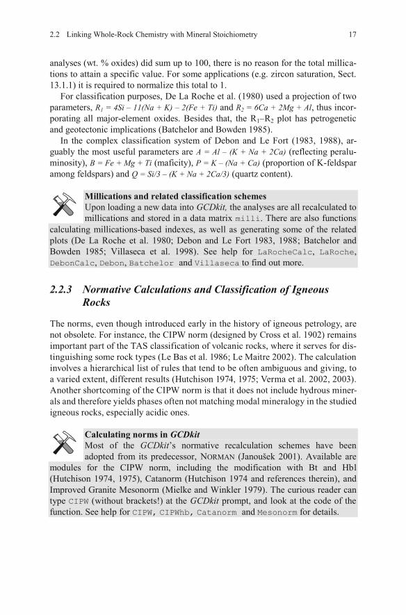
analyses (wt. % oxides) did sum up to 100, there is no reason for the total millica-tions to attain a specific value. For some applications (e.g. zircon saturation, Sect. 13.1.1) it is required to normalize this total to 1.
For classification purposes, De La Roche et al. (1980) used a projection of two parameters, R1 = 4Si – 11(Na + K) – 2(Fe + Ti) and R2 = 6Ca + 2Mg + Al, thus incor-porating all major-element oxides. Besides that, the R1–R2 plot has petrogenetic and geotectonic implications (Batchelor and Bowden 1985).
In the complex classification system of Debon and Le Fort (1983, 1988), ar-guably the most useful parameters are A = Al – (K + Na + 2Ca) (reflecting peralu-minosity), B = Fe + Mg + Ti (maficity), P = K – (Na + Ca) (proportion of K-feldspar among feldspars) and Q = Si/3 – (K + Na + 2Ca/3) (quartz content).
Millications and related classification schemesUpon loading a new data into GCDkit, the analyses are all recalculated to millications and stored in a data matrix milli. There are also functions
calculating millications-based indexes, as well as generating some of the related plots (De La Roche et al. 1980; Debon and Le Fort 1983, 1988; Batchelor and Bowden 1985; Villaseca et al. 1998). See help for LaRocheCalc, LaRoche,DebonCalc, Debon, Batchelor and Villaseca to find out more.
2.2.3 Normative Calculations and Classification of Igneous Rocks
Calculating norms in GCDkitMost of the GCDkit’s normative recalculation schemes have been adopted from its predecessor, NORMAN (Janoušek 2001). Available are
modules for the CIPW norm, including the modification with Bt and Hbl(Hutchison 1974, 1975), Catanorm (Hutchison 1974 and references therein), and Improved Granite Mesonorm (Mielke and Winkler 1979). The curious reader can type CIPW (without brackets!) at the GCDkit prompt, and look at the code of the function. See help for CIPW, CIPWhb, Catanorm and Mesonorm for details.
172.2 Linking Whole-Rock Chemistry with Mineral Stoichiometry
The norms, even though introduced early in the history of igneous petrology, are
not obsolete. For instance, the CIPW norm (designed by Cross et al. 1902) remains
important part of the TAS classification of volcanic rocks, where it serves for dis-
tinguishing some rock types (Le Bas et al. 1986; Le Maitre 2002). The calculation
involves a hierarchical list of rules that tend to be often ambiguous and giving, to
a varied extent, different results (Hutchison 1974, 1975; Verma et al. 2002, 2003).
Another shortcoming of the CIPW norm is that it does not include hydrous miner-
als and therefore yields phases often not matching modal mineralogy in the studied
igneous rocks, especially acidic ones.
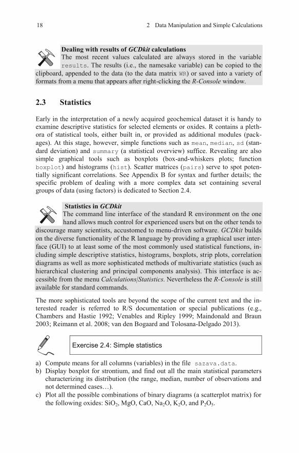
Dealing with results of GCDkit calculationsThe most recent values calculated are always stored in the variable results. The results (i.e., the namesake variable) can be copied to the
clipboard, appended to the data (to the data matrix WR) or saved into a variety of formats from a menu that appears after right-clicking the R-Console window.
2.3 Statistics
Early in the interpretation of a newly acquired geochemical dataset it is handy to examine descriptive statistics for selected elements or oxides. R contains a pleth-ora of statistical tools, either built in, or provided as additional modules (pack-ages). At this stage, however, simple functions such as mean, median, sd (stan-dard deviation) and summary (a statistical overview) suffice. Revealing are also simple graphical tools such as boxplots (box-and-whiskers plots; function boxplot) and histograms (hist). Scatter matrices (pairs) serve to spot poten-tially significant correlations. See Appendix B for syntax and further details; the specific problem of dealing with a more complex data set containing several groups of data (using factors) is dedicated to Section 2.4.
Statistics in GCDkit
The more sophisticated tools are beyond the scope of the current text and the in-terested reader is referred to R/S documentation or special publications (e.g., Chambers and Hastie 1992; Venables and Ripley 1999; Maindonald and Braun 2003; Reimann et al. 2008; van den Bogaard and Tolosana-Delgado 2013).
Exercise 2.4: Simple statistics
a) Compute means for all columns (variables) in the file sazava.data.b) Display boxplot for strontium, and find out all the main statistical parameters
characterizing its distribution (the range, median, number of observations and not determined cases…).
c) Plot all the possible combinations of binary diagrams (a scatterplot matrix) for the following oxides: SiO2, MgO, CaO, Na2O, K2O, and P2O5.
18 2 Data Manipulation and Simple Calculations
The command line interface of the standard R environment on the one
hand allows much control for experienced users but on the other tends to
discourage many scientists, accustomed to menu-driven software. GCDkit builds
on the diverse functionality of the R language by providing a graphical user inter-
face (GUI) to at least some of the most commonly used statistical functions, in-
cluding simple descriptive statistics, histograms, boxplots, strip plots, correlation
diagrams as well as more sophisticated methods of multivariate statistics (such as
hierarchical clustering and principal components analysis). This interface is ac-
cessible from the menu Calculations|Statistics. Nevertheless the R-Console is still
available for standard commands.
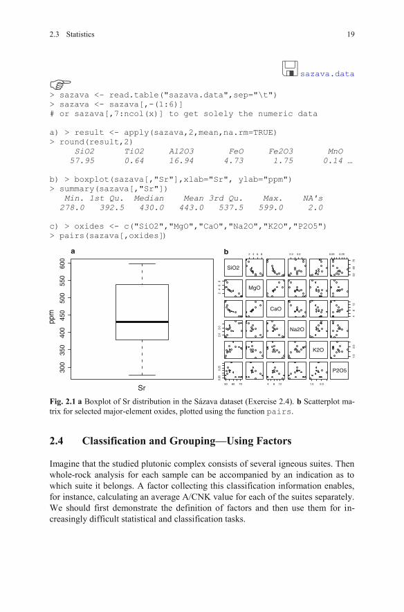
sazava.data
> sazava <- read.table("sazava.data",sep="\t") > sazava <- sazava[,-(1:6)] # or sazava[,7:ncol(x)] to get solely the numeric data a) > result <- apply(sazava,2,mean,na.rm=TRUE) > round(result,2) SiO2 TiO2 Al2O3 FeO Fe2O3 MnO 57.95 0.64 16.94 4.73 1.75 0.14 … b) > boxplot(sazava[,"Sr"],xlab="Sr", ylab="ppm") > summary(sazava[,"Sr"]) Min. 1st Qu. Median Mean 3rd Qu. Max. NA's 278.0 392.5 430.0 443.0 537.5 599.0 2.0 c) > oxides <- c("SiO2","MgO","CaO","Na2O","K2O","P2O5") > pairs(sazava[,oxides]
Fig. 2.1 Boxplot of Sr distribution in the Sázava dataset (Exercise 2.4). b Scatterplot ma-trix for selected major-element oxides, plotted using the function pairs.
2.4 Classification and Grouping—Using Factors
Imagine that the studied plutonic complex consists of several igneous suites. Then whole-rock analysis for each sample can be accompanied by an indication as to which suite it belongs. A factor collecting this classification information enables, for instance, calculating an average A/CNK value for each of the suites separately. We should first demonstrate the definition of factors and then use them for in-creasingly difficult statistical and classification tasks.
300
350
400
450
500
550
600
Sr
ppm
SiO2
2 4 6 8 2.0 3.0 0.05 0.25
5060
70
24
68
MgO
CaO
48
12
2.0
3.0
Na2O
K2O1.
02.
0
50 60 70
0.05
0.25
4 8 12 1.0 2.0
P2O5
a b
2.3 Statistics 19
)
a
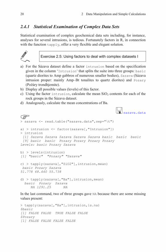
2.4.1 Statistical Examination of Complex Data Sets
Statistical examination of complex geochemical data sets including, for instance, analyses for several intrusions, is tedious. Fortunately factors in R, in connection with the function tapply, offer a very flexible and elegant solution.
Exercise 2.5: Using factors to deal with complex datasets I
a) For the Sázava dataset define a factor intrusion based on the specification given in the column ‘Intrusion’ that splits the suite into three groups: basic(quartz diorites to Amp gabbros of numerous smaller bodies), Sazava (Sázava intrusion proper: mainly Amp–Bt tonalites to quartz diorites) and Pozary(Požáry trondhjemite).
b) Display all possible values (levels) of this factor. c) Using the factor intrusion, calculate the mean SiO2 contents for each of the
rock groups in the Sázava dataset. d) Analogously, calculate the mean concentrations of Ba.
sazava.data
> sazava <- read.table("sazava.data",sep="\t") a) > intrusion <- factor(sazava[,"Intrusion"]) > intrusion [1] Sazava Sazava Sazava Sazava Sazava basic basic basic [9] basic basic Pozary Pozary Pozary Pozary Levels: basic Pozary Sazava b) > levels(intrusion) [1] "basic" "Pozary" "Sazava" c) > tapply(sazava[,"SiO2"],intrusion,mean) basic Pozary Sazava 51.778 68.440 55.738 d) > tapply(sazava[,"Ba"],intrusion,mean) basic Pozary Sazava NA 1291.25 NA
In the last command, two of three groups gave NA because there are some missing values present:
> tapply(sazava[,"Ba"],intrusion,is.na) $basic [1] FALSE FALSE TRUE FALSE FALSE $Pozary [1] FALSE FALSE FALSE FALSE
20 2 Data Manipulation and Simple Calculations
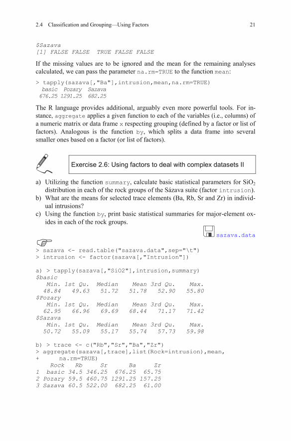
$Sazava [1] FALSE FALSE TRUE FALSE FALSE
If the missing values are to be ignored and the mean for the remaining analyses calculated, we can pass the parameter na.rm=TRUE to the function mean: > tapply(sazava[,"Ba"],intrusion,mean,na.rm=TRUE) basic Pozary Sazava 676.25 1291.25 682.25
The R language provides additional, arguably even more powerful tools. For in-stance, aggregate applies a given function to each of the variables (i.e., columns) of a numeric matrix or data frame x respecting grouping (defined by a factor or list of factors). Analogous is the function by, which splits a data frame into several smaller ones based on a factor (or list of factors).
Exercise 2.6: Using factors to deal with complex datasets II
a) Utilizing the function summary, calculate basic statistical parameters for SiO2distribution in each of the rock groups of the Sázava suite (factor intrusion).
b) What are the means for selected trace elements (Ba, Rb, Sr and Zr) in individ-ual intrusions?
c) Using the function by, print basic statistical summaries for major-element ox-ides in each of the rock groups.
sazava.data
> sazava <- read.table("sazava.data",sep="\t") > intrusion <- factor(sazava[,"Intrusion"]) a) > tapply(sazava[,"SiO2"],intrusion,summary) $basic Min. 1st Qu. Median Mean 3rd Qu. Max. 48.84 49.63 51.72 51.78 52.90 55.80 $Pozary Min. 1st Qu. Median Mean 3rd Qu. Max. 62.95 66.96 69.69 68.44 71.17 71.42 $Sazava Min. 1st Qu. Median Mean 3rd Qu. Max. 50.72 55.09 55.17 55.74 57.73 59.98 b) > trace <- c("Rb","Sr","Ba","Zr") > aggregate(sazava[,trace],list(Rock=intrusion),mean, + na.rm=TRUE) Rock Rb Sr Ba Zr 1 basic 34.5 346.25 676.25 65.75 2 Pozary 59.5 460.75 1291.25 157.25 3 Sazava 60.5 522.00 682.25 61.00
2.4 Classification and Grouping—Using Factors 21
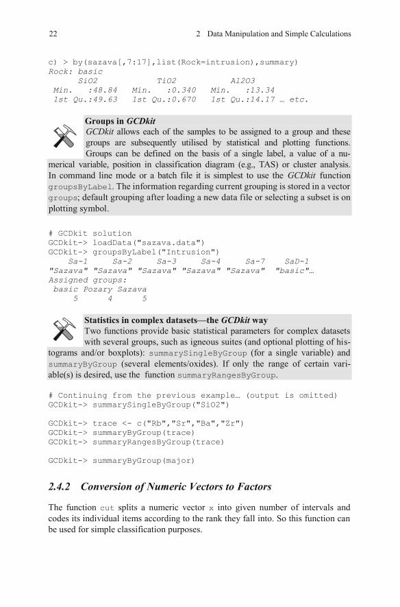
c) > by(sazava[,7:17],list(Rock=intrusion),summary) Rock: basic SiO2 TiO2 Al2O3 Min. :48.84 Min. :0.340 Min. :13.34 1st Qu.:49.63 1st Qu.:0.670 1st Qu.:14.17 … etc.
Groups in GCDkit
# GCDkit solution GCDkit-> loadData("sazava.data") GCDkit-> groupsByLabel("Intrusion") Sa-1 Sa-2 Sa-3 Sa-4 Sa-7 SaD-1 "Sazava" "Sazava" "Sazava" "Sazava" "Sazava" "basic"… Assigned groups: basic Pozary Sazava 5 4 5
Statistics in complex datasets—the GCDkit wayTwo functions provide basic statistical parameters for complex datasets with several groups, such as igneous suites (and optional plotting of his-
tograms and/or boxplots): summarySingleByGroup (for a single variable) and summaryByGroup (several elements/oxides). If only the range of certain vari-able(s) is desired, use the function summaryRangesByGroup.
# Continuing from the previous example… (output is omitted) GCDkit-> summarySingleByGroup("SiO2") GCDkit-> trace <- c("Rb","Sr","Ba","Zr") GCDkit-> summaryByGroup(trace) GCDkit-> summaryRangesByGroup(trace) GCDkit-> summaryByGroup(major)
2.4.2 Conversion of Numeric Vectors to Factors
The function cut splits a numeric vector x into given number of intervals and codes its individual items according to the rank they fall into. So this function can be used for simple classification purposes.
22 2 Data Manipulation and Simple Calculations
GCDkit allows each of the samples to be assigned to a group and these
groups are subsequently utilised by statistical and plotting functions.
Groups can be defined on the basis of a single label, a value of a nu-
merical variable, position in classification diagram (e.g., TAS) or cluster analysis.
In command line mode or a batch file it is simplest to use the GCDkit. The information regarding current grouping is stored in a vector
function
groupsByLabelgroups; default grouping after loading a new data file or selecting a subset is on
plotting symbol.
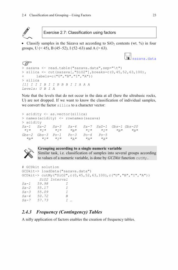
Exercise 2.7: Classification using factors
Classify samples in the Sázava set according to SiO2 contents (wt. %) in four groups, U (< 45), B (45–52), I (52–63) and A (> 63).
sazava.data
> sazava <- read.table("sazava.data",sep="\t") > silica <- cut(sazava[,"SiO2"],breaks=c(0,45,52,63,100), + labels=c("U","B","I","A")) > silica [1] I I I B I I B B B I I A A A Levels: U B I A
Note that the levels that do not occur in the data at all (here the ultrabasic rocks, U) are not dropped. If we want to know the classification of individual samples, we convert the factor silica to a character vector:
> acidity <- as.vector(silica) > names(acidity) <- rownames(sazava) > acidity Sa-1 Sa-2 Sa-3 Sa-4 Sa-7 SaD-1 Gbs-1 Gbs-20 "I" "I" "I" "B" "I" "I" "B" "B" Gbs-2 Gbs-3 Po-1 Po-3 Po-4 Po-5 "B" "I" "I" "A" "A" "A"
Grouping according to a single numeric variableSimilar task, i.e. classification of samples into several groups according to values of a numeric variable, is done by GCDkit function cutMy.
# GCDkit solution GCDkit-> loadData("sazava.data") GCDkit-> cutMy("SiO2",c(0,45,52,63,100), c("U","B","I","A")) SiO2 Interval Sa-1 59.98 I Sa-2 55.17 I Sa-3 55.09 I Sa-4 50.72 B Sa-7 57.73 I …
2.4.3 Frequency (Contingency) Tables A nifty application of factors enables the creation of frequency tables.
232.4 Classification and Grouping—Using Factors
a) Using the factor intrusion, count the number of analyses obtained from each of the rock groups in the Sázava dataset.
b) Analogously, count the number of ultrabasic, basic, intermediate and acid rocks (factor silica from the previous exercise).
c) Set up a frequency table showing the dependence of silica on the rock type.
sazava.data
> intrusion <- factor(sazava[,"Intrusion"]) a) > table(intrusion) intrusion basic Pozary Sazava 5 4 5 b) > table(silica) silica U B I A 0 4 7 3 c) > table(intrusion,silica) silica intrusion U B I A basic 0 3 2 0 Pozary 0 0 1 3 Sazava 0 1 4 0
24 2 Data Manipulation and Simple Calculations
Exercise 2.8: Frequency tables
Continuing from the previous exercise, we demonstrate making frequency tables.
References
Batchelor RA, Bowden P (1985) Petrogenetic interpretation of granitoid rock series using multi-cationic parameters. Chem Geol 48:43–55
Chambers JM, Hastie TJ (1992) Statistical models in S. Chapman & Hall, LondonClarke DB (1981) The mineralogy of peraluminous granites; a review. Canad Mineral 19:3–17Cross W, Iddings JP, Pirsson LV, Washington HS (1902) A quantitative chemico-mineralogical
classification and nomenclature of igneous rocks. J Geol 10:555–690De La Roche H, Leterrier J, Grandclaude P, Marchal M (1980) A classification of volcanic and
plutonic rocks using R1R2–diagram and major element analyses—its relationships with cur-rent nomenclature. Chem Geol 29:183–210
Debon F, Le Fort P (1983) A chemical-mineralogical classification of common plutonic rocks and associations. Trans Roy Soc Edinb, Earth Sci 73:135–149
Debon F, Le Fort P (1988) A cationic classification of common plutonic rocks and their mag-matic associations: principles, method, applications. Bull Minéral 111:493–510
Frost BR, Frost CD (2008) A geochemical classification for feldspathic igneous rocks. J Petrol 49:1955–1969
Frost BR, Barnes CG, Collins WJ, Arculus RJ, Ellis DJ, Frost CD (2001) A geochemical classifi-cation for granitic rocks. J Petrol 42:2033–2048
References 25
Hutchison CS (1974) Laboratory handbook of petrographic techniques. John Wiley & Sons, New York
Hutchison CS (1975) The norm, its variations, their calculation and relationships. Schweiz min-eral petrogr Mitt 55:243–256
Janoušek V (2001) Norman, a QuickBasic programme for petrochemical re-calculation of whole-rock major-element analyses on IBM PC. J Czech Geol Soc 46:9–13
Janoušek V, Bowes DR, Rogers G, Farrow CM, Jelínek E (2000) Modelling diverse processes in the petrogenesis of a composite batholith: the Central Bohemian Pluton, Central European Hercynides. J Petrol 41:511–543
Janoušek V, Braithwaite CJR, Bowes DR, Gerdes A (2004) Magma-mixing in the genesis of Hercynian calc-alkaline granitoids: an integrated petrographic and geochemical study of the Sázava intrusion, Central Bohemian Pluton, Czech Republic. Lithos 78:67–99
Le Bas MJ, Le Maitre RW, Streckeisen A, Zanettin B (1986) A chemical classification of vol-canic rocks based on the total alkali-silica diagram. J Petrol 27:745–750
Le Maitre RW (2002) Igneous rocks: a classification and glossary of terms: recommendations of the International Union of Geological Sciences, Subcommission on the Systematics of Igneous Rocks. Cambridge University Press, Cambridge
Maindonald J, Braun J (2003) Data analysis and graphics using R. Cambridge University Press, Cambridge
Mielke P, Winkler HGF (1979) Eine bessere Berechnung der Mesonorm für granitische Gesteine. Neu Jb Mineral, Mh 471–480
Miller CF (1985) Are strongly peraluminous magmas derived from pelitic sources? J Geol 93:673–689
Niggli P (1948) Gesteine und Minerallagerstätten. Birkhäuser, BaselReimann C, Filzmoser P, Garrett R, Dutter R (2008) Statistical data analysis explained: applied
environmental statistics with R. John Wiley & Sons, ChichesterRock NMS (1988) Numerical geology. A source guide, glossary and selective bibliography
to geological uses of computers and statistics. Lecture Notes in Earth Sciences, vol 18. Springer, Berlin
Shand SJ (1943) Eruptive rocks. Their genesis, composition, classification, and their relation to ore-deposits with a chapter on meteorite. John Wiley & Sons, New York
van den Bogaard P, Tolosana-Delgado R (2013) Analyzing compositional data with R. Springer, Berlin
Venables WN, Ripley BD (1999) Modern applied statistics with S-Plus. Springer, BerlinVerma SP, Torres-Alvarado IS, Sotelo-Rodriguez ZT (2002) SINCLAS: standard igneous norm
and volcanic rock classification system. Comput and Geosci 28:711–715Verma SP, Torres-Alvarado IS, Velasco-Tapia F (2003) A revised CIPW norm. Schweiz mineral
petrogr Mitt 83:197–216Villaseca C, Barbero L, Herreros V (1998) A re-examination of the typology of peraluminous
granite types in intracontinental orogenic belts. Trans Roy Soc Edinb, Earth Sci 89:113–119
Chapter 3 Classical Plots
In this chapter, R recipes are presented to produce the most common graphs used in igneous geochemistry, such as binary plots (simple and multiple, e.g. Harker plots), ternary plots, spiderplots, classification and geotectonic diagrams. Espe-cially for the latter two types, the text does not intend to be exhaustive. A compre-hensive review can be found in Rollinson (1993) and in documentation/help to the GCDkit package (especially the file diagrams.pdf).
3.1 Binary Plots
The most common graph used in igneous geochemistry is a binary plot of two variables, linear or logarithmic. Often, as x axis serves some fractionation index, i.e. a chemical species mimicking the progressive development of the igneous suite studied (e.g., SiO2 for felsic, and MgO or mg# for mafic rock associations).
3.1.1 Plotting Simple Binary Plots
We shall demonstrate here the use of the basic plotting and annotation capabilities of R. Appendix A contains all the necessary details, including the explanation of function expression, as well as of abline and curve that can be used for add-ing simple trends to the graphs.
Exercise 3.1: Simple binary plots
In this exercise we focus on graphical analysis of the Sázava dataset.
a) Build a binary plot SiO2–CaO. Choose suitable ranges for the axes, label them and annotate data points by sample names. Assign the plotting symbols ac-cording to individual rock types (utilizing the pre-defined column “Symbol”).
b) Plot a line SiO2/CaO = 10 passing through origin [0,0]. c) Plot a diagram log Zr–log Ba and fit the data points, using the least-square lin-
ear regression, by a straight line.
© Springer-Verlag Berlin Heidelberg 2016 V. Janoušek et al., Geochemical Modelling of Igneous Processes – Principles And Recipes in R Language, Springer Geochemistry, DOI 10.1007/978-3-662-46792-3_3
27
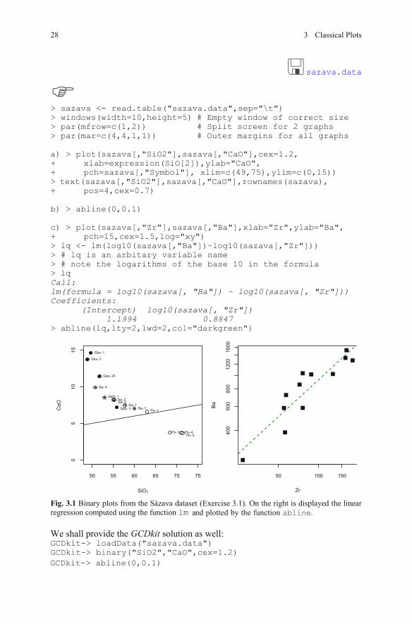
sazava.data
> sazava <- read.table("sazava.data",sep="\t") > windows(width=10,height=5) # Empty window of correct size > par(mfrow=c(1,2)) # Split screen for 2 graphs > par(mar=c(4,4,1,1)) # Outer margins for all graphs a) > plot(sazava[,"SiO2"],sazava[,"CaO"],cex=1.2, + xlab=expression(SiO[2]),ylab="CaO", + pch=sazava[,"Symbol"], xlim=c(49,75),ylim=c(0,15)) > text(sazava[,"SiO2"],sazava[,"CaO"],rownames(sazava), + pos=4,cex=0.7) b) > abline(0,0.1) c) > plot(sazava[,"Zr"],sazava[,"Ba"],xlab="Zr",ylab="Ba", + pch=15,cex=1.5,log="xy") > lq <- lm(log10(sazava[,"Ba"])~log10(sazava[,"Zr"])) > # lq is an arbitary variable name > # note the logarithms of the base 10 in the formula > lq Call: lm(formula = log10(sazava[, "Ba"]) ~ log10(sazava[, "Zr"])) Coefficients: (Intercept) log10(sazava[, "Zr"]) 1.1994 0.8847 > abline(lq,lty=2,lwd=2,col="darkgreen")
Fig. 3.1 Binary plots from the Sázava dataset (Exercise 3.1). On the right is displayed the linear regression computed using the function lm
We shall provide the GCDkit solution as well: GCDkit-> loadData("sazava.data") GCDkit-> binary("SiO2","CaO",cex=1.2)
50 55 60 65 70 75
05
10
15
SiO2
Ca
O
Sa- 1
Sa- 2Sa- 3
Sa- 4
Sa- 7
SaD- 1
Gbs- 1
Gbs- 20
Gbs- 2
Gbs- 3Po- 1
Po- 3 Po- 4Po- 5
50 100 150
40
06
00
80
01
20
01
60
0
Zr
Ba
28 3 Classical Plots
and plotted by the function .
GCDkit-> abline(0,0.1)
abline
Plot editing from the command prompt
1
On our Zr–Ba graph we can demonstrate post-processing of a single GCDkit plot: GCDkit-> binary("Zr","Ba",log="xy",pch=15,cex=1.5, + col="black",fit=TRUE) GCDkit-> figMain("Demonstration") # Add main title GCDkit-> figXlab("Zirconium (ppm)") # Modify x axis label GCDkit-> figCol("darkred") # Colour of symbols GCDkit-> figCex(2) # Size of symbols GCDkit-> figCexLab(0.8) # Scaling of axes labels GCDkit-> figCexMain(1.5) # Size of main title GCDkit-> figXlim(c(10,300)) # Limits of the x axis GCDkit-> figUser("pch=\"+\"") # Plotting symbol GCDkit-> figUser("main=\"My plot\";las=2;bg=\"khaki\"; + font.main=4;cex.main=2;col.main=\"blue\"") GCDkit-> figBw() # Set everything to black and white
Annotating plots in GCDkit GCDkit provides a function annotate “guessing” the correct format-ting of axis labels or of other text strings. It is called silently by many
functions in the system; see, for instance: GCDkit-> binary("K2O/Na2O","Al2O3")
Plotting results of numeric calculations So far we have plotted only numeric data stored internally by the GCDkit
able WR. In fact, it is also rather simple to plot the results of calculations (such as the output of a normative scheme). This involves three steps: cal-
culation, appending the results to the data (using function addResults) and plot-ting as usual.
NB that the argument to 1 figUser is a single text string. Thus any quotation marks therein
have to be preceded by an escape character, i.e. the backslash.
3.1 Binary Plots 29
Owing to the fact that most of the single plots in GCDkit are in fact
Figaro templates (see Appendix B), they can be post-processed, i.e. many
of their properties altered using functions from the menu Plot editing.
They can also be modified directly from a command line or batch file. Moreover,
function figUser nables setting several graphical parameters at once (that
“ ” commands are available (see ?par for their meaning). In addi-
For a list of further available functions and more detailed explanation, see
help pages to figEdit, figColours, figScale, figZoom and figUser.
plotting
v ari
figSomethingtion, figIdentify
are to be separated by semicolons) , including those for which no separate
e
can be used to (interactively) label the datapoints on theactive graph. Do not forget to click on “Stop” when you are done.
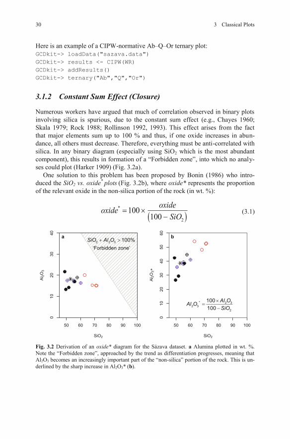
Here is an example of a CIPW-normative Ab–Q–Or ternary plot: GCDkit-> loadData("sazava.data") GCDkit-> results <- CIPW(WR) GCDkit-> addResults() GCDkit-> ternary("Ab","Q","Or")
3.1.2 Constant Sum Effect (Closure)
Numerous workers have argued that much of correlation observed in binary plots involving silica is spurious, due to the constant sum effect (e.g., Chayes 1960; Skala 1979; Rock 1988; Rollinson 1992, 1993). This effect arises from the fact that major elements sum up to 100 % and thus, if one oxide increases in abun-dance, all others must decrease. Therefore, everything must be anti-correlated with silica. In any binary diagram (especially using SiO2 which is the most abundant component), this results in formation of a “Forbidden zone”, into which no analy-ses could plot (Harker 1909) (Fig. 3.2a).
One solution to this problem has been proposed by Bonin (1986) who intro-duced the SiO2 vs. oxide* plots (Fig. 3.2b), where oxide* represents the proportion of the relevant oxide in the non-silica portion of the rock (in wt. %):
*
2
100100
oxideoxideSiO
(3.1)
Fig. 3.2 Derivation of an oxide* diagram for the Sázava dataset. a Alumina plotted in wt. %. Note the “Forbidden zone”, approached by the trend as differentiation progresses, meaning that Al2O3 becomes an increasingly important part of the “non-silica” portion of the rock. This is un-derlined by the sharp increase in Al2O3* (b).
a b
50 60 70 80 90 100
010
20
30
40
SiO2
Al 2
O3
50 60 70 80 90 100
010
20
30
40
50
60
SiO2
Al 2
O3∗
�
�
�
* 2 3
2 3
2
100
100
Al OAl O
SiO
� �2 2 3
100%SiO Al O
ʻ ’Forbidden zone
30 3 Classical Plots
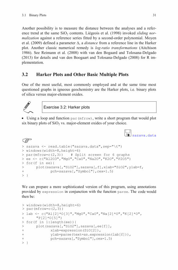
Another possibility is to measure the distance between the analyses and a refer-ence trend at the same SiO2 contents. Liégeois et al. (1998) invoked sliding nor-malization against a reference series fitted by a second-order polynomial. Moyen et al. (2009) defined a parameter , a distance from a reference line in the Harker plot. Another classic numerical remedy is log-ratio transformations (Aitchison 1986). See Reimann et al. (2008) with van den Bogaard and Tolosana-Delgado (2013) for details and van den Boogaart and Tolosana-Delgado (2008) for R im-plementation.
3.2 Harker Plots and Other Basic Multiple Plots
One of the most useful, most commonly employed and at the same time most questioned graphs in igneous geochemistry are the Harker plots, i.e. binary plots of silica versus major-element oxides.
Exercise 3.2: Harker plots
Using a loop and function par(mfrow), write a short program that would plot six binary plots of SiO2 vs. major-element oxides of your choice.
sazava.data
> sazava <- read.table("sazava.data",sep="\t") > windows(width=8,height=6) > par(mfrow=c(2,3)) # Split screen for 6 graphs > ee <- c("Al2O3","MgO","CaO","Na2O","K2O","P2O5") > for(f in ee){ > plot(sazava[,"SiO2"],sazava[,f],xlab="SiO2",ylab=f, + pch=sazava[,"Symbol"],cex=1.5) > }
We can prepare a more sophisticated version of this program, using annotations provided by expression in conjunction with the function parse. Thethen be:
> lab <- c("Al[2]*O[3]","MgO","CaO","Na[2]*O","K[2]*O", + "P[2]*O[5]") > for(f in 1:length(ee)){ > plot(sazava[,"SiO2"],sazava[,ee[f]], + xlab=expression(SiO[2]), + ylab=parse(text=as.expression(lab[f])), + pch=sazava[,"Symbol"],cex=1.5) > }
31 3.1 Binary Plots
code would
> par(mfrow=c(2,3))> windows(width=8,height=6)
GCDkit-> loadData("sazava.data") GCDkit-> multiple("SiO2","Al2O3,MgO,CaO,Na2O,K2O,P2O5")
Fig. 3.3 Selected Harker plots from the Sázava dataset (Exercise 3.2).
3.3 Ternary Plots
Ternary plots rank among important and widely used geochemical tools. Setting the sides of the triangle to equating a unity, its vertices (bottom-left, top, and bot-tom-right) have [x,y] coordinates of A[0,0], B[0.5, ] and C[1,0]. The ternary coordinates [a,b,c] of a data point X can be transformed to binary ones [x,y] (Fig. 3.4) as follows:
12bx a and
32
y b . (3.2)
50 55 60 65 70
14
16
18
20
SiO2
Al 2
O3
50 55 60 65 70
24
68
SiO2
Mg
O
50 55 60 65 70
46
81
01
21
4
SiO2
CaO
50 55 60 65 70
2.0
2.5
3.0
3.5
SiO2
Na
2O
50 55 60 65 70
1.0
1.5
2.0
2.5
SiO2
K2O
50 55 60 65 70
0.0
50
.10
0.1
50
.20
0.2
50
.30
0.3
5
SiO2
P2O
5
32 3 Classical Plots
GCDkit solution is: And a
3/2
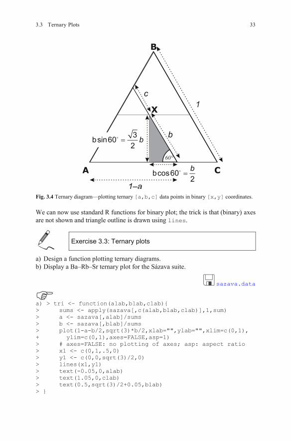
Fig. 3.4 Ternary diagram—plotting ternary [a,b,c] data points in binary [x,y] coordinates.
We can now use standard R functions for binary plot; the trick is that (binary) axes are not shown and triangle outline is drawn using lines.
Exercise 3.3: Ternary plots
a) Design a function plotting ternary diagrams. b) Display a Ba–Rb–Sr ternary plot for the Sázava suite.
sazava.data
a) > tri <- function(alab,blab,clab){ > sums <- apply(sazava[,c(alab,blab,clab)],1,sum) > a <- sazava[,alab]/sums > b <- sazava[,blab]/sums > plot(1-a-b/2,sqrt(3)*b/2,xlab="",ylab="",xlim=c(0,1), + ylim=c(0,1),axes=FALSE,asp=1) > # axes=FALSE: no plotting of axes; asp: aspect ratio > x1 <- c(0,1,.5,0) > y1 <- c(0,0,sqrt(3)/2,0) > lines(x1,y1) > text(-0.05,0,alab) > text(1.05,0,clab) > text(0.5,sqrt(3)/2+0.05,blab) > }
A
X
B
C
b
c
1–a
1
60°
bcos602
b
3bsin60
2b
33 3.3 Ternary Plots
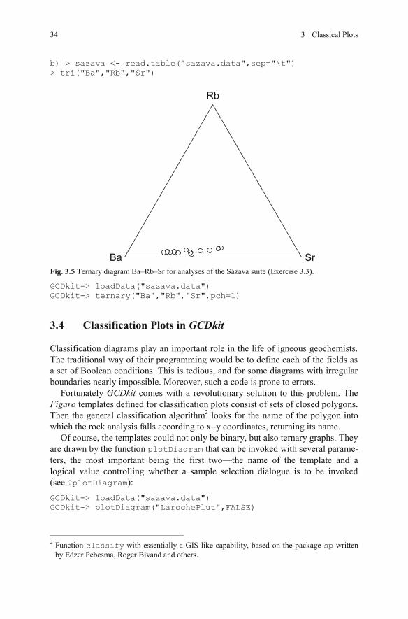
b) > sazava <- read.table("sazava.data",sep="\t") > tri("Ba","Rb","Sr")
Fig. 3.5 Ternary diagram Ba–Rb–Sr for analyses of the Sázava suite (Exercise 3.3).
GCDkit-> loadData("sazava.data") GCDkit-> ternary("Ba","Rb","Sr",pch=1)
3.4 Classification Plots in GCDkit
Classification diagrams play an important role in the life of igneous geochemists. The traditional way of their programming would be to define each of the fields as a set of Boolean conditions. This is tedious, and for some diagrams with irregular boundaries nearly impossible. Moreover, such a code is prone to errors.
Fortunately GCDkit comes with a revolutionary solution to this problem. The Figaro templates defined for classification plots consist of sets of closed polygons. Then the general classification algorithm looks for the name of the polygon into which the rock analysis falls according to x–y coordinates, returning its name.
2
Of course, the templates could not only be binary, but also ternary graphs. They are drawn by the function plotDiagram that can be invoked with several parame-ters, the most important being the first two—the name of the template and a logical value controlling whether a sample selection dialogue is to be invoked (see ?plotDiagram): GCDkit-> loadData("sazava.data") GCDkit-> plotDiagram("LarochePlut",FALSE)
Function2 classify with essentially a GIS-like capability, based on the package sp written by Edzer Pebesma, Roger Bivand and others.
Ba Sr
Rb
34 3 Classical Plots
Classification on the basis of the current diagram can be requested from menu Plot editing|Classify or, if the template name is specified as an argument, by the func-tion classify: GCDkit-> classify("LarochePlut") Samples classified by: R1 - R2 (De la Roche et al. 1980) diorite gabbro gabbro-norite 4 1 1 gabbrodiorite granodiorite ultramafic rock 3 2 1 unclassified 2 LarochePlut Sa-1 "diorite" Sa-2 "gabbrodiorite" Sa-3 "gabbrodiorite" … etc.
A vector of resulting rock names is stored in a variable results. The analyses falling outside the defined polygons are labelled as ‘unclassified’.
Needless to say that the classification diagrams are often misused—and it is a responsibility of each user to become familiar with the original work and
use the given scheme as appropriate.
3.5 Geotectonic Diagrams
Deciphering the tectonic setting of ancient igneous suites is of great scientific and practical interest. One of the key tools, geotectonic diagrams, gained popularity with improving analytical facilities in 1970–1980’s (e.g., Pearce and Cann 1973; Pearce and Norry 1979; Wood 1980; Shervais 1982; Mullen 1983; Pearce et al. 1984; Meschede 1986 – see Rollinson 1993 for review). Originally the diagrams were largely empirical and the discrimination boundaries fitted by eye, but rigor-ous statistical treatment including (linear or quadratic) discriminant analysis has become increasingly popular (Vermeesch 2006).
Geotectonic diagrams tend to work because rocks from similar tectonic settings are likely to have formed by the same combination of sources and processes. The problem is that several prior assumptions have to be made (often silently):
the studied suite had a geotectonic position that can be compared with some ofsimple settings predicted by the global tectonics paradigm (thus the diagrams are not usable for Archaean rocks or suites from complex settings),
its geochemical signature has not been significantly modified by processes such as fractional crystallization, crystal accumulation or magma mixing,
elemental mobility during alteration/weathering can be neglected, analytical determinations are precise enough, often at sub-ppm level.
3.4 Classification Plots in 35GCDkit
After the initial adoration, geotectonic diagrams became evil for many colleagues, while others proposed schemes in which the geochemical rationale vanished to be replaced by abstract, and rather mechanical, statistical treatment (Verma and Rivera-Gómez 2013; Verma et al. 2013 and references therein).
In our view, some classic diagrams are useful, especially if the original defini-tion and scope are strictly adhered to. Fruitful seems the concept of spiderplot-based geochemical proxies (elemental ratios), advocated by J. Pearce. These may constrain, for instance, the depth of melting, the degree of mantle enrichment, or of contamination by subduction-related fluids/melts. For example of application to back-arcs and ophiolites, see Pearce and Stern (2006) and Pearce (2008, 2014).
Selected, presumably little mobile elements from basic lavas are the most valu-able, as the parental magmas come from a primary source (mantle) and do not originate by recycling of crustal material (Pearce 1996a). On the other hand, acid igneous rocks—especially collisional granitoids—are often generated from several times recycled crustal materials and may inherit the signature of the older source(s) (Arculus 1987; Förster et al. 1997). Any danger of misinterpretation can be minimized if the geology, petrology, age and whole geochemical signature are all taken into account (Barbarin 1990; Bonin 1990; Pearce 1996b; Clemens 2012).
GCDkit comes with many geotectonic diagrams (see diagrams.pdf in the help system for their overview). Please note that these templates are
somewhat restricted in use, e.g. they cannot be employed for classification.
3.6 Spiderplots
36 3 Classical Plots
Geochemists often like to express the compositional differences between the stud-
ied sample and given geochemical reservoir in the form of so-called spiderplots
(also known as spiderdiagrams/spidergrams or (better) multi-element diagrams).
Spiderplots allow representing much of the sample’s composition on a single
graph. Technically these are logarithmic plots of elemental concentrations (allow-
ing comparison of concentrations that differ by several orders of magnitude) in
the sample divided (normalized) by those in the selected standard. The order of
the elements along the axis is critical as it can by itself generate artificial anom-
alies (Dupré et al. 1994). Normally, the elements are arranged in a logical se-
quence according to their geochemical behaviour (often based on bulk distribution
coefficients, with the more incompatible ones on the left) (Hofmann 1988)
(see also Sect. 21.2).
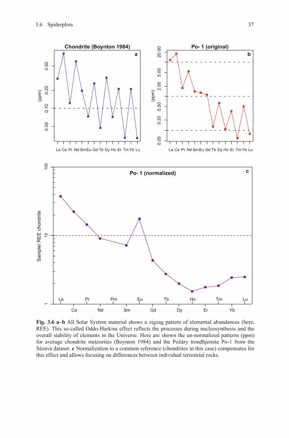
3.6 Spiderplots 37
Fig. 3.6 a–b All Solar System material shows a zigzag pattern of elemental abundances (here, REE). This so-called Oddo-Harkins effect reflects the processes during nucleosynthesis and the overall stability of elements in the Universe. Here are shown the un-normalized patterns (ppm) for average chondrite meteorites (Boynton 1984) and the Požáry trondhjemite Po-1 from the Sázava dataset. c Normalization to a common reference (chondrites in this case) compensates for this effect and allows focusing on differences between individual terrestrial rocks.
La Pr Pm Eu Tb Ho Tm Lu
Ce Nd Sm Gd Dy Er Yb
110
100
Sam
ple
/ R
EE
chondri
te
Chondrite (Boynton 1984)
(ppm
)
La Ce Pr Nd SmEu Gd Tb Dy Ho Er Tm Yb Lu
0.0
50.1
00.2
00.5
0Po 1 (original)-
(ppm
)La Ce Pr Nd SmEu Gd Tb Dy Ho Er Tm Yb Lu
0.0
50
.20
0.5
02
.00
5.0
02
0.0
0
Po 1 (normalized)-
a
c
b
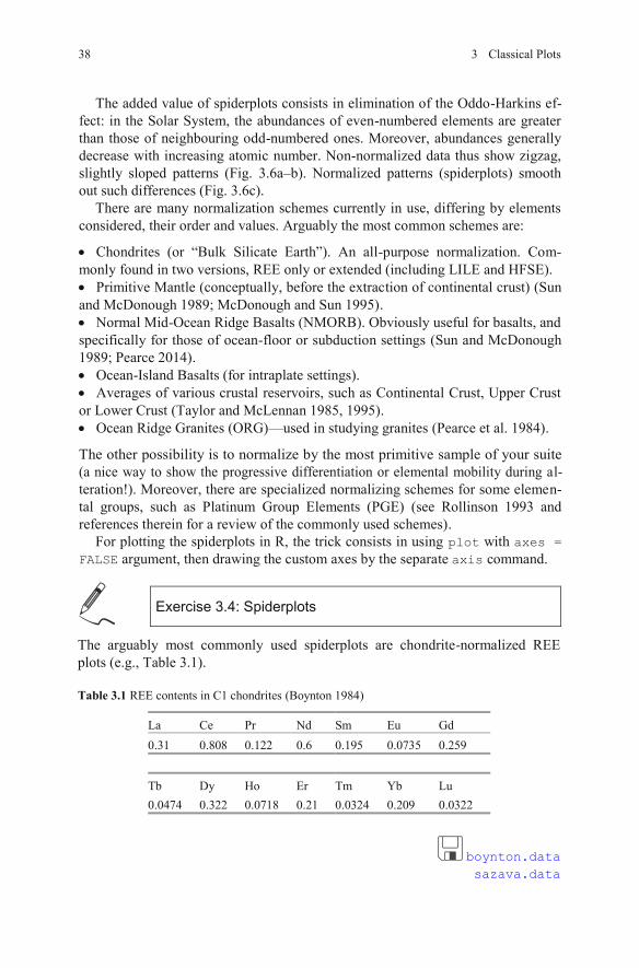
38 3 Classical Plots
The added value of spiderplots consists in elimination of the Oddo-Harkins ef-fect: in the Solar System, the abundances of even-numbered elements are greater than those of neighbouring odd-numbered ones. Moreover, abundances generally decrease with increasing atomic number. Non-normalized data thus show zigzag, slightly sloped patterns (Fig. 3.6a–b). Normalized patterns (spiderplots) smooth out such differences (Fig. 3.6c).
There are many normalization schemes currently in use, differing by elements considered, their order and values. Arguably the most common schemes are:
Chondrites (or “Bulk Silicate Earth”). An all-purpose normalization. Com-monly found in two versions, REE only or extended (including LILE and HFSE).
Primitive Mantle (conceptually, before the extraction of continental crust) (Sun and McDonough 1989; McDonough and Sun 1995).
Normal Mid-Ocean Ridge Basalts (NMORB). Obviously useful for basalts, and specifically for those of ocean-floor or subduction settings (Sun and McDonough 1989; Pearce 2014).
Ocean-Island Basalts (for intraplate settings). Averages of various crustal reservoirs, such as Continental Crust, Upper Crust
or Lower Crust (Taylor and McLennan 1985, 1995). Ocean Ridge Granites (ORG)—used in studying granites (Pearce et al. 1984).
The other possibility is to normalize by the most primitive sample of your suite
teration!). Moreover, there are specialized normalizing schemes for some elemen-tal groups, such as Platinum Group Elements (PGE) (see Rollinson 1993 and references therein for a review of the commonly used schemes).
For plotting the spiderplots in R, the trick consists in using plot with axes = FALSE argument, then drawing the custom axes by the separate axis command.
(a nice way to show the progressive differentiation or elemental mobility during al-
Exercise 3.4: Spiderplots
The arguably most commonly used spiderplots are chondrite-normalized REE plots (e.g., Table 3.1).
Table 3.1 REE contents in C1 chondrites (Boynton 1984)
La Ce Pr Nd Sm Eu Gd0.31 0.808 0.122 0.6 0.195 0.0735 0.259
Tb Dy Ho Er Tm Yb Lu0.0474 0.322 0.0718 0.21 0.0324 0.209 0.0322
boynton.data sazava.data
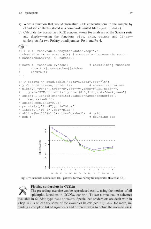
a) Write a function that would normalize REE concentrations in the sample by chondritic contents (stored in a comma-delimited file boynton.data).
b) Calculate the normalized REE concentrations for analyses of the Sázava suite and display—using the functions plot, axis, points and lines—spiderplots for two Požáry trondhjemites, Po-1 and Po-4.
a) > x <- read.table("boynton.data",sep=",") > chondrite <- as.numeric(x) # conversion to numeric vector > names(chondrite) <- names(x) > norm <- function(x,chon){ # normalizing function > z <- t(x[,names(chon)])/chon > return(z) > } b) > sazava <- read.table("sazava.data",sep="\t") > y <- norm(sazava,chondrite) # normalized values > plot(y[,"Po-1"],type="o",log="y",axes=FALSE,xlab="", + ylab="REE/chondrite",ylim=c(0.1,100),col="darkgreen") > axis(1,1:length(chondrite),labels=names(chondrite), + cex.axis=0.75) > axis(2,cex.axis=0.75) > points(y[,"Po-4"],col="blue") > lines(y[,"Po-4"],col="blue") > abline(h=(10^(-1:3)),lty="dashed") # grid > box() # bounding box
393.6 Spiderplots
Fig. 3.7 Chondrite-normalized REE patterns for two Požáry trondhjemites (Exercise 3.4).
RE
E/c
hondri
te
La Ce Pr Nd Sm Eu Gd Tb Dy Ho Er Tm Yb Lu
0.1
0.5
1.0
5.0
50.0
Plotting spiderplots in GCDkitThe preceding exercise can be reproduced easily, using the mother-of-all spiderplot functions in GCDkit, spider. To see normalization schemes
available in GCDkit, type ?selectNorm. Specialized spiderplots are dealt with in Chap. 4.2. You can try some of the examples below (see ?spider for more, in-cluding a complete list of arguments and different ways to define the norm to use).
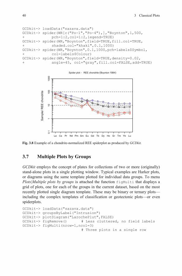
GCDkit-> loadData("sazava.data") GCDkit-> spider(WR[c("Po-1","Po-4"),],"Boynton",1,500, + pch=1:2,col=1:2,legend=TRUE) GCDkit-> spider(WR,"Boynton",field=TRUE,fill.col=TRUE, + shaded.col="khaki",0.1,1000) GCDkit-> spider(WR,"Boynton",0.1,1000,pch=labels$Symbol, + col=labels$Colour) GCDkit-> spider(WR,"Boynton",field=TRUE,density=0.02, + angle=45, col="gray",fill.col=FALSE,add=TRUE)
Fig. 3.8 Example of a chondrite-normalized REE spiderplot as produced by GCDkit.
Spider plot � REE chondrite �Boynton 1984�
Sa
mp
le/
RE
E c
ho
nd
rite
La Ce Pr Nd Pm Sm Eu Gd Tb Dy Ho Er Tm Yb Lu
0.1
11
01
00
10
00
40 3 Classical Plots
3.7 Multiple Plots by Groups
GCDkit employs the concept of plates for collections of two or more (originally) stand-alone plots in a single plotting window. Typical examples are Harker plots, or diagrams using the same template plotted for individual data groups. To menuPlots|Multiple plots by groups is attached the function figMulti that displays a grid of plots, one for each of the groups in the current dataset, based on the most recently plotted single diagram template. These may be binary or ternary plots—including the complex templates of classification or geotectonic plots—or even spiderplots. GCDkit-> loadData("sazava.data") GCDkit-> groupsByLabel("Intrusion") GCDkit-> plotDiagram("LarochePlut",FALSE) GCDkit-> figRemove() # Less cluttered, no field labels GCDkit-> figMulti(nrow=1,ncol=3) # Three plots in a single row
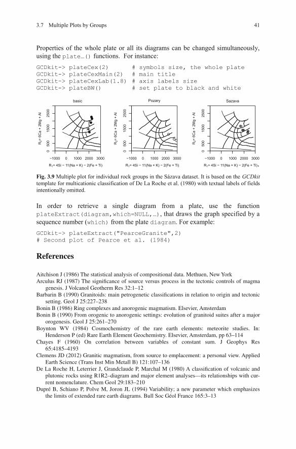
Properties of the whole plate or all its diagrams can be changed simultaneously, using the plate…() functions. For instance: GCDkit-> plateCex(2) # symbols size, the whole plate GCDkit-> plateCexMain(2) # main title GCDkit-> plateCexLab(1.8) # axis labels size GCDkit-> plateBW() # set plate to black and white
Fig. 3.9 Multiple plot for individual rock groups in the Sázava dataset. It is based on the GCDkit template for multicationic classification of De La Roche et al. (1980) with textual labels of fields intentionally omitted.
In order to retrieve a single diagram from a plate, use the function plateExtract(diagram,which=NULL,…), that draws the graph specified by a sequence number (which) from the plate diagram. For example: GCDkit-> plateExtract("PearceGranite",2) # Second plot of Pearce et al. (1984)
−1000 0 1000 2000 3000
05
00
15
00
25
00
basic
R1= 4Si 11(Na + K) 2(Fe + Ti)− −
R2=
6C
a +
2M
g +
Al
−1000 0 1000 2000 3000
05
00
15
00
25
00
Pozary
R1= 4Si 11(Na + K) 2(Fe + Ti)− −
R2=
6C
a +
2M
g +
Al
−1000 0 1000 2000 3000
05
00
15
00
25
00
Sazava
R1= 4Si 11(Na + K) 2(Fe + Ti)− −
R2=
6C
a +
2M
g +
Al
3.7 Multiple Plots by Groups 41
References
Aitchison J (1986) The statistical analysis of compositional data. Methuen, New YorkArculus RJ (1987) The significance of source versus process in the tectonic controls of magma
genesis. J Volcanol Geotherm Res 32:1–12Barbarin B (1990) Granitoids: main petrogenetic classifications in relation to origin and tectonic
setting. Geol J 25:227–238Bonin B (1986) Ring complexes and anorogenic magmatism. Elsevier, AmsterdamBonin B (1990) From orogenic to anorogenic settings: evolution of granitoid suites after a major
orogenesis. Geol J 25:261–270Boynton WV (1984) Cosmochemistry of the rare earth elements: meteorite studies. In:
Henderson P (ed) Rare Earth Element Geochemistry. Elsevier, Amsterdam, pp 63–114Chayes F (1960) On correlation between variables of constant sum. J Geophys Res
65:4185–4193Clemens JD (2012) Granitic magmatism, from source to emplacement: a personal view. Applied
Earth Science (Trans Inst Min Metall B) 121:107–136De La Roche H, Leterrier J, Grandclaude P, Marchal M (1980) A classification of volcanic and
plutonic rocks using R1R2–diagram and major element analyses—its relationships with cur-rent nomenclature. Chem Geol 29:183–210
Dupré B, Schiano P, Polve M, Joron JL (1994) Variability; a new parameter which emphasizes the limits of extended rare earth diagrams. Bull Soc Géol France 165:3–13
42 3 Classical Plots
Förster H-J, Tischendorf G, Trumbull RB (1997) An evaluation of the Rb vs. (Y + Nb) discrimi-nation diagram to infer tectonic setting of silicic igneous rocks. Lithos 40:261–293
Harker A (1909) The natural history of igneous rocks. Methuen & Co., LondonHofmann AW (1988) Chemical differentiation of the Earth: the relationship between mantle, con-
tinental crust, and oceanic crust. Earth Planet Sci Lett 90:297–314Liégeois J-P, Navez J, Hertogen J, Black R (1998) Contrasting origin of post-collisional high-K
calc-alkaline and shoshonitic versus alkaline and peralkaline granitoids. Lithos 45:1–28McDonough WF, Sun S (1995) The composition of the Earth. Chem Geol 120:223–253Meschede M (1986) A method of discriminating between different types of mid-ocean ridge
basalts and continental tholeiites with the Nb–Zr–Y diagram. Chem Geol 56:207–218Moyen JF, Champion D, Smithies RH (2009) The geochemistry of Archaean plagioclase-rich
granites as a marker of source enrichment and depth of melting. Earth Environ Sci Trans R Soc Edinb 100:35–50
Mullen ED (1983) MnO/TiO2/P2O5: a minor element discriminant for basaltic rocks of oceanic environments and its implications for petrogenesis. Earth Planet Sci Lett 62:53–62
Pearce JA (1996a) A user’s guide to basalt discrimination diagrams. In: Wyman DA (ed) Trace element geochemistry of volcanic rocks: applications for massive sulphide exploration. Geological Association of Canada, Short Course Notes, vol 12, pp 79–113
Pearce JA (1996b) Sources and settings of granitic rocks. Episodes 19:120–125Pearce JA (2008) Geochemical fingerprinting of oceanic basalts with applications to ophiolite
classification and the search for Archean oceanic crust. Lithos 100:14–48Pearce JA (2014) Immobile element fingerprinting of ophiolites. Elements 10:101–108Pearce JA, Cann JR (1973) Tectonic setting of basic volcanic rocks determined using trace ele-
ment analyses. Earth Planet Sci Lett 19:290–300Pearce JA, Norry MJ (1979) Petrogenetic implications of Ti, Zr, Y, and Nb variations in volcanic
rocks. Contrib Mineral Petrol 69:33–47Pearce JA, Stern RJ (2006) Origin of back-arc basin magmas: trace element and isotope perspec-
tives. In: Christie DM, Fisher CR, Lee S-M, Givens S (eds) Back-arc spreading systems: geo-logical, biological, chemical, and physical interactions. Geophysical Monograph Series, vol 166. American Geophysical Union, pp 63–86
Pearce JA, Harris NBW, Tindle AG (1984) Trace element discrimination diagrams for the tec-tonic interpretation of granitic rocks. J Petrol 25:956–983
Reimann C, Filzmoser P, Garrett R, Dutter R (2008) Statistical data analysis explained: applied environmental statistics with R. John Wiley & Sons, Chichester
Rock NMS (1988) Numerical geology. A source guide, glossary and selective bibliography to geological uses of computers and statistics. Lecture Notes in Earth Sciences, vol 18. Springer, Berlin
Rollinson HR (1992) Another look at the constant sum problem in geochemistry. Mineral Mag 56:469–475
Rollinson HR (1993) Using geochemical data: evaluation, presentation, interpretation. Longman, London
Shervais JW (1982) Ti–V plots and the petrogenesis of modern and ophiolitic lavas. Earth Planet Sci Lett 59:101–118
Skala W (1979) Some effects of the constant-sum problem in geochemistry. Chem Geol 27:1–9Sun SS, McDonough WF (1989) Chemical and isotopic systematics of oceanic basalts: implica-
tions for mantle composition and processes. In: Saunders AD, Norry M (eds) Magmatism in the ocean basins. Geological Society of London Special Publications, vol 42, pp 313–345
Taylor SR, McLennan SM (1985) The continental crust: its composition and evolution. Blackwell, Oxford
Taylor SR, McLennan SM (1995) The geochemical evolution of the continental crust. Rev Geophys 33:241–265
van den Boogaart KG, Tolosana-Delgado R (2008) “compositions”: a unified R package to ana-lyze compositional data. Comput and Geosci 34:320–338

References 43
van den Bogaard P, Tolosana-Delgado R (2013) Analyzing compositional data with R. Springer, Berlin
Verma SP, Rivera-Gómez MA (2013) New computer program TecD for tectonomagmatic dis-crimination from discriminant function diagrams for basic and ultrabasic magmas and its application to ancient rocks. J Iber Geol 39:167–179
Verma SP, Pandarinath K, Verma SK, Agrawal S (2013) Fifteen new discriminant-function-based multi-dimensional robust diagrams for acid rocks and their application to Precambrian rocks. Lithos 168–169:113–123
Vermeesch P (2006) Tectonic discrimination diagrams revisited. Geochem Geophys Geosyst 7:Q06017
Wood DA (1980) The application of a Th–Hf–Ta diagram to problems of tectonomagmatic clas-sification and to establishing the nature of crustal contamination of basaltic lavas of the British Tertiary volcanic province. Earth Planet Sci Lett 50:11–30
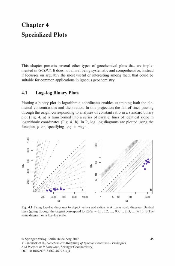
Chapter 4 Specialized Plots
This chapter presents several other types of geochemical plots that are imple-mented in GCDkit. It does not aim at being systematic and comprehensive; instead it focusses on arguably the most useful or interesting among them that could be suitable for common applications in igneous geochemistry.
4.1 Log–log Binary Plots
Plotting a binary plot in logarithmic coordinates enables examining both the ele-mental concentrations and their ratios. In this projection the fan of lines passing through the origin corresponding to analyses of constant ratio in a standard binary plot (Fig. 4.1a) is transformed into a series of parallel lines of identical slope in logarithmic coordinates (Fig. 4.1b). In R, log–log diagrams are plotted using the function plot, specifying log = "xy".
Fig. 4.1 Using log–log diagrams to depict values and ratios. a A linear scale diagram. Dashed lines (going through the origin) correspond to Rb/Sr = 0.1, 0.2, …, 0.9, 1, 2, 3, … to 10. b The same diagram on a log–log scale.
200 400 600 800 1000
200
400
600
800
1000
Sr
Rb
1 5 10 50 500
15
10
50
500
Sr
Rb
a b
© Springer-Verlag Berlin Heidelberg 2016 V. Janoušek et al., Geochemical Modelling of Igneous Processes – Principles And Recipes in R Language, Springer Geochemistry, DOI 10.1007/978-3-662-46792-3_4
45
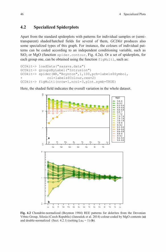
4.2 Specialized Spiderplots
Apart from the standard spiderplots with patterns for individual samples or (semi-transparent) shaded/hatched fields for several of them, GCDkit produces also some specialized types of this graph. For instance, the colours of individual pat-terns can be coded according to an independent conditioning variable, such as SiO2 or MgO (function spider.contour, Fig. 4.2a). Or a set of spiderplots, for each group one, can be obtained using the function figMulti, such as:
GCDkit-> loadData("sazava.data") GCDkit-> groupsByLabel("Intrusion") GCDkit-> spider(WR,"Boynton",1,100,pch=labels$Symbol, + col=labels$Colour,cex=2) GCDkit-> figMulti(nrow=1,ncol=3,plot.symb=TRUE)
Here, the shaded field indicates the overall variation in the whole dataset.
Fig. 4.2 Chondrite-normalized (Boynton 1984) REE patterns for dolerites from the Devonian Vrbno Group, Silesia (Czech Republic) (Janoušek et al. 2014) colour-coded by MgO contents (a)and double-normalized (Sect. 4.2.1) (setting LuN = 1) (b).
La Pr Pm Eu Tb Ho Tm Lu
Ce Nd Sm Gd Dy Er Yb
0.1
110
100
MgO
5.8- 66- 6.26.2- 6.46.4- 6.66.6- 6.86.8- 77- 7.27.2- 7.47.4- 7.67.6- 7.87.8- 88- 8.28.2- 8.48.4- 8.68.6- 8.88.8- 99- 9.29.2- 9.49.4- 9.6
La Ce Pr Nd Pm Sm Eu Gd Tb Dy Ho Er Tm Yb Lu
0.1
11
0
a
b
46 4 Specialized Plots
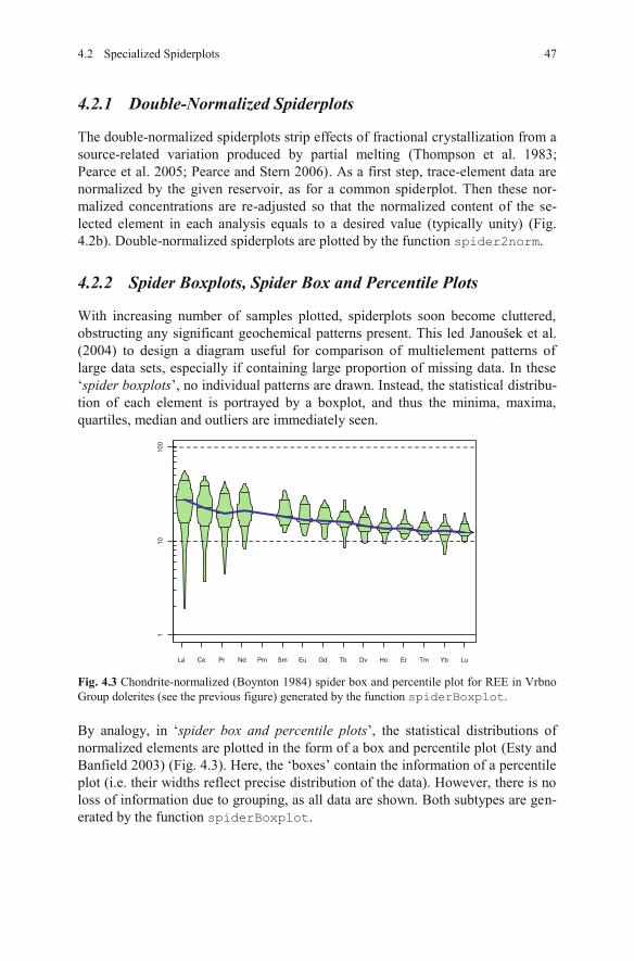
4.2.1 Double-Normalized Spiderplots
The double-normalized spiderplots strip effects of fractional crystallization from a source-related variation produced by partial melting (Thompson et al. 1983; Pearce et al. 2005; Pearce and Stern 2006). As a first step, trace-element data are normalized by the given reservoir, as for a common spiderplot. Then these nor-malized concentrations are re-adjusted so that the normalized content of the se-lected element in each analysis equals to a desired value (typically unity) (Fig. 4.2b). Double-normalized spiderplots are plotted by the function spider2norm.
4.2.2 Spider Boxplots, Spider Box and Percentile Plots
With increasing number of samples plotted, spiderplots soon become cluttered, obstructing any significant geochemical patterns present. This led Janoušek et al. (2004) to design a diagram useful for comparison of multielement patterns of large data sets, especially if containing large proportion of missing data. In these ‘spider boxplots’, no individual patterns are drawn. Instead, the statistical distribu-tion of each element is portrayed by a boxplot, and thus the minima, maxima, quartiles, median and outliers are immediately seen.
La Ce Pr Nd Pm Sm Eu Gd Tb Dy Ho Er Tm Yb Lu
110
100
Fig. 4.3 Chondrite-normalized (Boynton 1984) spider box and percentile plot for REE in Vrbno Group dolerites (see the previous figure) generated by the function spiderBoxplot.
By analogy, in ‘spider box and percentile plots’, the statistical distributions of normalized elements are plotted in the form of a box and percentile plot (Esty and Banfield 2003) (Fig. 4.3). Here, the ‘boxes’ contain the information of a percentile plot (i.e. their widths reflect precise distribution of the data). However, there is no loss of information due to grouping, as all data are shown. Both subtypes are gen-erated by the function spiderBoxplot.
4.2 Specialized Spiderplots 47
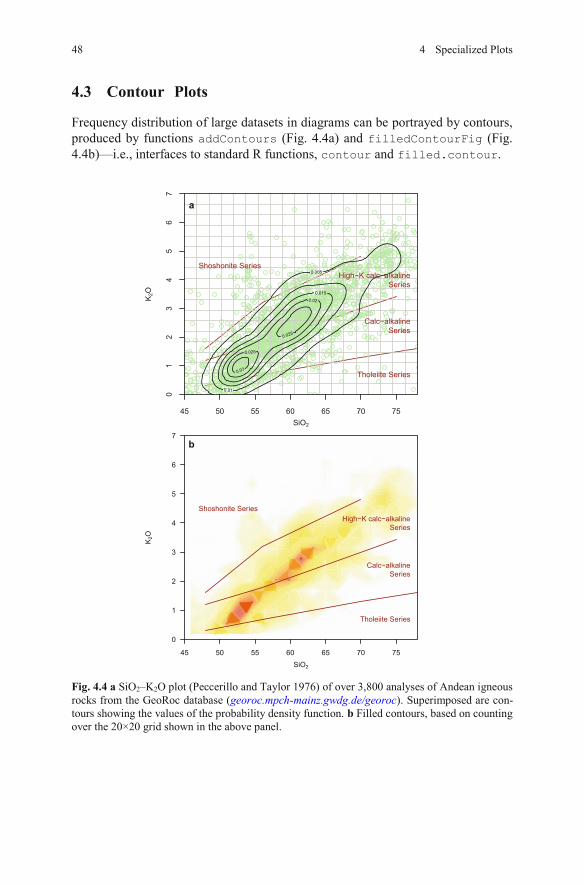
Frequency distribution of large datasets in diagrams can be portrayed by contours, produced by functions addContours (Fig. 4.4a) and filledContourFig (Fig. 4.4b)—i.e., interfaces to standard R functions, contour and filled.contour.
Fig. 4.4 a SiO2–K2O plot (Peccerillo and Taylor 1976) of over 3,800 analyses of Andean igneous rocks from the GeoRoc database (georoc.mpch-mainz.gwdg.de/georoc). Superimposed are con-tours showing the values of the probability density function. b Filled contours, based on counting over the 20×20 grid shown in the above panel.
45 50 55 60 65 70 75
01
23
45
67
SiO2
K2O
0.005
0.01
0.015
0.02
0.025
0.025
0.03
Shoshonite Series
High K calc alkaline− −
Series
Calc alkaline−
Series
Tholeiite Series
45 50 55 60 65 70 75
0
1
2
3
4
5
6
7
Tholeiite Series
Calc alkaline−
Series
High K calc alkaline− −
Series
Shoshonite Series
SiO2
K2O
a
b
48 4 Specialized Plots
4.3 Contour Plots
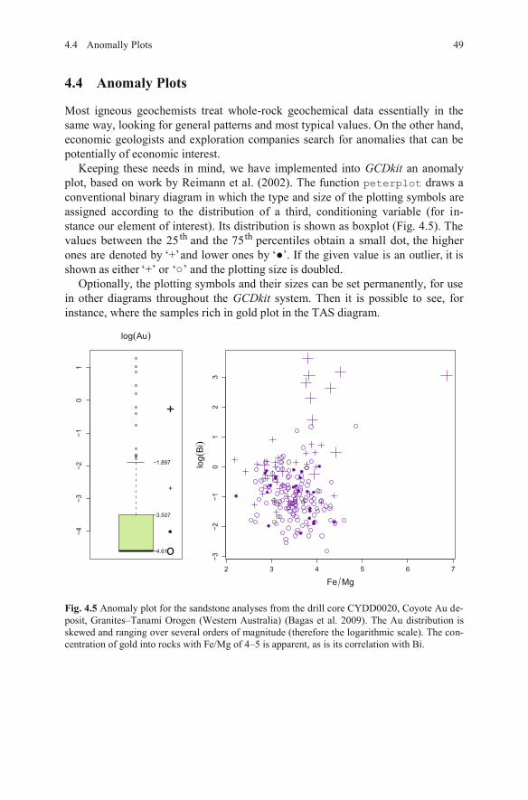
4.4 Anomaly Plots
Most igneous geochemists treat whole-rock geochemical data essentially in the same way, looking for general patterns and most typical values. On the other hand, economic geologists and exploration companies search for anomalies that can be potentially of economic interest.
Keeping these needs in mind, we have implemented into GCDkit an anomaly plot, based on work by Reimann et al. (2002). The function peterplot draws a conventional binary diagram in which the type and size of the plotting symbols are assigned according to the distribution of a third, conditioning variable (for in-stance our element of interest). Its distribution is shown as boxplot (Fig. 4.5). The values between the 25th and the 75 percentiles obtain a small dot, the higher
’. If the given value is an outlier, it is
or ‘ ’ and the plotting size is doubled. Optionally, the plotting symbols and their sizes can be set permanently, for use
in other diagrams throughout the GCDkit system. Then it is possible to see, for instance, where the samples rich in gold plot in the TAS diagram.
Fig. 4.5 Anomaly plot for the sandstone analyses from the drill core CYDD0020, Coyote Au de-posit, Granites–Tanami Orogen (Western Australia) (Bagas et al. 2009). The Au distribution is skewed and ranging over several orders of magnitude (therefore the logarithmic scale). The con-centration of gold into rocks with Fe/Mg of 4–5 is apparent, as is its correlation with Bi.
−4
−3
−2
−1
01
log�Au�
−4.61
−3.507
−1.897
o
+
+
2 3 4 5 6 7
−3
−2
−1
01
23
Fe Mg
log�B
i�
494.4 Anomally Plots
ones are denoted by and lower ones by ‘‘+’‘+’shown as either
th
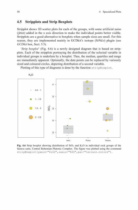
4.5 Stripplots and Strip Boxplots
‘Strip boxplot’ (Fig. 4.6) is a newly designed diagram that is based on strip-plots. Each of the stripplots portraying the distribution of the selected variable in individual groups is underlain by a boxplot. Thus, the median, quartiles and range are immediately apparent. Optionally, the data points can be replaced by variously sized and coloured circles, depicting distribution of a second variable.
Plotting of this type of diagrams is done by the function stripBoxplot.
Fig. 4.6 Strip boxplot showing distribution of SiO2 and K2O in individual rock groups of the Sázava suite, Central Bohemian Plutonic Complex. The figure was plotted using the command stripBoxplot(yaxis="SiO2",zaxis="K2O",pal="terrain.colors").
K2O
0.5 1-
1 1.5-
1.5 2-
2 2.5-
basic Pozary Sazava
50
55
60
65
70
SiO
2
50 4 Specialized Plots
Stripplot shows 1D scatter plots for each of the groups, with some artificial noise
(jitter) added in the x axis direction to make the individual points better visible.
Stripplots are a good alternative to boxplots when sample sizes are small. For this
reason, they are implemented mainly in GCDkit’s isotope (SrNd.r) plugin (see
GCDkit box, Sect. 5.5).
References 51
References
Bagas L, Anderson JAC, Bierlein FP (2009) Palaeoproterozoic evolution of the Killi Killi Formation and orogenic gold mineralization in the Granites-Tanami Orogen, Western Australia. Ore Geol Rev 35:47–67
Boynton WV (1984) Cosmochemistry of the rare earth elements: meteorite studies. In: Henderson P (ed) Rare Earth Element Geochemistry. Elsevier, Amsterdam, pp 63–114
Esty WW, Banfield JD (2003) The box-percentile plot. J Stat Softw 8:1–14Janoušek V, Finger F, Roberts MP, Frýda J, Pin C, Dolejš D (2004) Deciphering the petrogenesis
of deeply buried granites: whole-rock geochemical constraints on the origin of largely unde-pleted felsic granulites from the Moldanubian Zone of the Bohemian Massif. Trans Roy Soc Edinb, Earth Sci 95:141–159
Janoušek V, Aichler J, Hanžl P, Gerdes A, Erban V, Pecina V, Žácek V, Pudilová M, Hrdlicková K, Mixa P, Žácková E (2014) Constraining genesis and geotectonic setting of metavolcanic complexes: a multidisciplinary study of the Devonian Vrbno Group (Hrubý Jeseník Mts., Czech Republic). Int J Earth Sci 103:455–483
Pearce JA, Stern RJ (2006) Origin of back-arc basin magmas: trace element and isotope perspec-tives. In: Christie DM, Fisher CR, Lee S-M, Givens S (eds) Back-arc spreading systems: geo-logical, biological, chemical, and physical interactions. Geophysical Monograph Series, vol 166. American Geophysical Union, pp 63–86
Pearce JA, Stern RJ, Bloomer SH, Fryer P (2005) Geochemical mapping of the Mariana arc-basin system: implications for the nature and distribution of subduction components. Geochem Geophys Geosyst 6:Q07006
Peccerillo A, Taylor SR (1976) Geochemistry of Eocene calc-alkaline volcanic rocks from the Kastamonu area, Northern Turkey. Contrib Mineral Petrol 58:63–81
Reimann C, Filzmoser P, Garrett RG (2002) Factor analysis applied to regional geochemical data: problems and possibilities. Appl Geochem 17:185–206
Thompson RN, Morrison MA, Dickin AP, Hendry GL (1983) Continental flood basalts… Arachnids rule OK? In: Hawkesworth CJ, Norry MJ (eds) Continental basalts and mantle Xenoliths. Shiva, Nantwich, pp 158–185
Chapter 5 Radiogenic Isotopes
In contrast to the light stable isotopes (e.g., O, H, Li, C), the utility of the rela-tively heavy radiogenic isotopes (e.g., Sr, Nd, Pb, Hf) consists in the fact that they should not be fractionated by equilibrium, closed-system processes (so named, as no components external to the magmatic system are involved) such as partial melt-ing, fractional crystallization or crystal accumulation. In these cases the radiogenic isotopes enable us to fingerprint the magma sources. Alternatively, these ratios may be used to prove the operation of open-system processes, for instance magma mixing or crustal assimilation. Subsequently, compositions and proportions of end-members involved can often be constrained.
The aim of this chapter is to explain basic numerical approaches in interpreting radiogenic isotope data in igneous geochemistry, with a particular emphasis on Sr–Nd–Hf–Os isotopes. The text is concerned with calculation of initial ratios, ages, and values, single- and two-stage model ages and fitting of isochrons. Theoretical background is explained only briefly as detailed accounts are readily available in several textbooks (Geyh and Schleicher 1990; Faure and Mensing 2004; Dickin 2005; Allègre 2008 to name just a few).
5.1 Recalculation of Elemental to Isotopic Ratios
Many of the parent–daughter dating methods are based on similar principles. The parent (radioactive) isotope (e.g., 87Rb, 147Sm or 176Lu) decays to the daughter (ra-diogenic) isotope (e.g., 87Sr, 143Nd or 176Hf):
87 87Rb Sr , 147 143Sm Nd , 176 176Lu Hf , 187 187Re Os (5.1)
As the mass spectrometer is only capable of measuring isotopic ratios, the content of daughter isotope is expressed as a ratio to a stable, non-radiogenic isotope, whose natural abundance does not change with time (for simplicity termed here I; e.g., 87Sr/86Sr, 143Nd/144Nd or 176Hf/177Hf). Age calculation also requires the amount of the parental isotope to be expressed as a ratio to the same non-radiogenic stable isotope of the daughter element (R; e.g., 87Rb/86Sr, 147Sm/144Nd
© Springer-Verlag Berlin Heidelberg 2016 V. Janoušek et al., Geochemical Modelling of Igneous Processes – Principles And Recipes in R Language, Springer Geochemistry, DOI 10.1007/978-3-662-46792-3_5
53
or 176Lu/177Hf). Whereas the I ratios are measured directly with the mass spectrome-
ter (TIMS or ICP-MS), R ratios must be calculated from elemental concentrations obtained by isotope dilution, ICP-MS, XRF or other analytical methods.
The concept behind the derivation of the conversion formulae is illustrated here using the Rb–Sr system. Combining the relation between atomic weight and molar abundance we obtain (Faure 1986):
87
86
87
86Rb Rb Sr
Rb Sr Sr
C Ab AWRbSr AW C Ab
(5.2)
where CSr, CRb are concentrations (ppm), Ab = isotopic abundances, AW = atomic weights. The problem is that both SrAW and 87Sr
Ab are a function of the isotopiccomposition of the sample, and thus depend on its 87Sr/86Sr ratio. If the atomicweight is expressed as a sum of weights of individual isotopes multiplied by their abundances, the right-hand side of Eq. (5.2) can be rewritten as:
87
87
87 85
86 86
85
RbSr Sr
SrRb
RbC Sr Sr RbAW AWC Sr Sr Rb AW
Rb
(5.3)
where the sums refer to all non-radiogenic isotopes of Sr ( = 84, 86, 88) and all isotopes of Rb ( = 85, 87), respectively. All Sr ratios are expressed relative to 86Sr; both Rb ratios relative to 85Rb. The 87Sr/86Sr values (i.e. I), CRb and CSr are to be determined; the rest are constants that can be obtained from literature (e.g., Audi et al. 2003; Berglund and Wieser 2011 and references therein). The third term may be substituted by simpler, yet less precise ratio 87 / RbRb
Ab AW . The literaturedata vary slightly; based on those from Faure (1986), we obtain:
87 87
86 862.6939 0.2832Rb
Sr
CRb SrSr C Sr
(5.4)
Similarly, for the 147Sm/144Nd isotopic ratio can be derived:
147 143
144 1440.53151 0.14252Sm
Nd
CSm NdNd C Nd
(5.5)
using Nd stable isotopic ratios from Wasserburg et al. (1981), renormalized to 146Nd/144Nd = 0.7219. For whole-rock samples, especially if the fractionation be-tween Sm and Nd is small and thus the variability of the 143Nd/144Nd can be ne-glected (relatively to the precision of concentrations), the term in square brackets in Eq. (5.5) collapses to 0.6047.
54 5 Radiogenic Isotopes
For the Lu–Hf system, the relevant equation is:
176 176
177 1770.13517 0.02613Lu
Hf
CLu HfHf C Hf
(5.6)
If the 176Hf/177Hf ratio is close to that of CHUR (‘normal’ whole-rock samples), the expression in square brackets collapses to 0.142 (Faure and Mensing 2004).
Lastly, 178Re/188Os can be calculated as follows, provided that the 186Os is not in-fluenced by the decay of 190Pt:
187 187Re
188 188
Re 4.7393 0.6285Os
C OsOs C Os
(5.7)
5.2 Calculation of Initial Ratios or Ages
Using our notation, an equation between I, R and age t (in years) can be written as:
1tI R e (5.8)
Where is the relevant decay constant (see Ickert 2013 for discussion):
Equation (5.8) assumes that initially, t years ago, there was no daughter isotope present. This can be (nearly) justified for some minerals, forming so-called (par-ent-) rich systems (Allègre 2008). As an example may serve a Li-mica that is Rb rich and whose Sr will soon become dominated by the radiogenic component. However, generally there is always some common Sr, Nd or Hf present. Assuming that its composition (initial ratio) is Ii, Eq. (5.8) changes into:
1tiI I R e (5.9)
If the age is known, the isotopic ratios can be easily ‘age-corrected’ (i.e. initial ra-tios back-calculated) and used in petrogenetic considerations.
On the other hand, knowing the initial ratio, e.g. by analysis of a (parent-) poor system (e.g., Sr in apatite that contains little Rb and thus its 87Sr/86Sr is nearly con-
5.1 Recalculation of Elemental to Isotopic Ratios 55
87Rbλ = 1.42 × 10⁻¹¹y–1 (Steiger and Jäger 1977) (old but still widely used value)
87Rbλ = 1.3968 × 10⁻¹¹ y–1 (Rotenberg et al. 2012) (new determination)
147Smλ = 6.54 × 10⁻¹² y–1 (Lugmair and Marti 1978)
176Luλ = 1.867 × 10⁻¹¹ y–1 (Söderlund et al. 2004)
187Reλ = 1.6668 × 10⁻¹¹ y–1 (Selby et al. 2007)
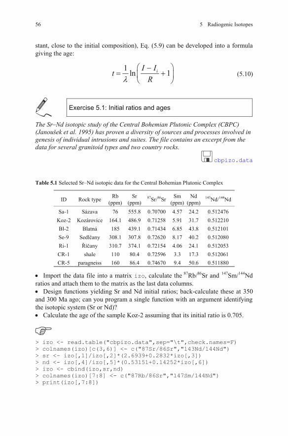
stant, close to the initial composition), Eq. (5.9) can be developed into a formula giving the age:
1 ln 1iI ItR
(5.10)
Exercise 5.1: Initial ratios and ages
The Sr–Nd isotopic study of the Central Bohemian Plutonic Complex (CBPC) (Janoušek et al. 1995) has proven a diversity of sources and processes involved in genesis of individual intrusions and suites. The file contains an excerpt from the data for several granitoid types and two country rocks.
cbpizo.data
Table 5.1 Selected Sr–Nd isotopic data for the Central Bohemian Plutonic Complex
ID Rock type Rb(ppm)
Sr(ppm)
87Sr/86Sr Sm(ppm)
Nd(ppm)
143Nd/144Nd
Sa-1 Sázava 76 555.8 0.70700 4.57 24.2 0.512476Koz-2 Kozárovice 164.1 486.9 0.71258 5.91 31.7 0.512210Bl-2 Blatná 185 439.1 0.71434 6.85 43.8 0.512101Se-9 Sedl any 308.1 307.8 0.72620 8.17 40.2 0.512080Ri-1 í any 310.7 374.1 0.72154 4.06 24.1 0.512053CR-1 shale 110 80.4 0.72596 3.3 17.3 0.512061CR-5 paragneiss 160 86.4 0.74670 9.4 50.6 0.511880
Import the data file into a matrix izo, calculate the 87Rb/86Sr and 147Sm/144Nd ratios and attach them to the matrix as the last data columns.
Design functions yielding Sr and Nd initial ratios; back-calculate these at 350 and 300 Ma ago; can you program a single function with an argument identifying the isotopic system (Sr or Nd)?
Calculate the age of the sample Koz-2 assuming that its initial ratio is 0.705.
> izo <- read.table("cbpizo.data",sep="\t",check.names=F) > colnames(izo)[c(3,6)] <- c("87Sr/86Sr","143Nd/144Nd") > sr <- izo[,1]/izo[,2]*(2.6939+0.2832*izo[,3]) > nd <- izo[,4]/izo[,5]*(0.53151+0.14252*izo[,6]) > izo <- cbind(izo,sr,nd) > colnames(izo)[7:8] <- c("87Rb/86Sr","147Sm/144Nd") > print(izo[,7:8])
56 5 Radiogenic Isotopes
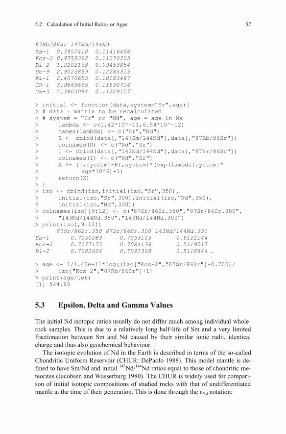
Sa-1 0.3957418 0.11416466 Koz-2 0.9759392 0.11270205 Bl-2 1.2202168 0.09453854 Se-9 2.9023859 0.12285315 Ri-1 2.4070655 0.10183487 CR-1 3.9669665 0.11530714 CR-5 5.3803064 0.11229157 > initial <- function(data,system="Sr",age){ > # data = matrix to be recalculated > # system = "Sr" or "Nd", age = age in Ma > lambda <- c(1.42*10^-11,6.54*10^-12) > names(lambda) <- c("Sr","Nd") > R <- cbind(data[,"147Sm/144Nd"],data[,"87Rb/86Sr"]) > colnames(R) <- c("Nd","Sr") > I <- cbind(data[,"143Nd/144Nd"],data[,"87Sr/86Sr"]) > colnames(I) <- c("Nd","Sr") > X <- I[,system]-R[,system]*(exp(lambda[system]* > age*10^6)-1) > return(X) > } > izo <- cbind(izo,initial(izo,"Sr",350), > initial(izo,"Sr",300), initial(izo,"Nd",350), > initial(izo,"Nd",300)) > colnames(izo)[9:12] <- c("87Sr/86Sr.350","87Sr/86Sr.300", > "143Nd/144Nd.350","143Nd/144Nd.300") > print(izo[,9:12]) 87Sr/86Sr.350 87Sr/86Sr.300 143Nd/144Nd.350 Sa-1 0.7050283 0.7053105 0.5122144 Koz-2 0.7077175 0.7084136 0.5119517 Bl-2 0.7082604 0.7091308 0.5118844 … > age <- 1/1.42e-11*log((izo["Koz-2","87Sr/86Sr"]-0.705)/ > izo["Koz-2","87Rb/86Sr"]+1) > print(age/1e6) [1] 544.85
5.3 Epsilon, Delta and Gamma Values
The initial Nd isotopic ratios usually do not differ much among individual whole-rock samples. This is due to a relatively long half-life of Sm and a very limited fractionation between Sm and Nd caused by their similar ionic radii, identical charge and thus also geochemical behaviour.
The isotopic evolution of Nd in the Earth is described in terms of the so-called Chondritic Uniform Reservoir (CHUR: DePaolo 1988). This model mantle is de-fined to have Sm/Nd and initial 143Nd/144Nd ratios equal to those of chondritic me-teorites (Jacobsen and Wasserburg 1980). The CHUR is widely used for compari-son of initial isotopic compositions of studied rocks with that of undifferentiated mantle at the time of their generation. This is done through the Nd notation:
5.2 Calculation of Initial Ratios or Ages 57
87Rb/86Sr 147Sm/144Nd
143
1444
143
144
1 10
SA
i iNd CHUR
i
NdNd
NdNd
(5.11)
Where: t = intrusion age, indexes i decipher initial isotopic ratios [Eq.(5.9)], SA =sample. The present-day composition of the CHUR is 147Sm/144NdCHUR = 0.1967 and 143Nd/144NdCHUR = 0.512638 (Jacobsen and Wasserburg 1980) or 147Sm/144NdCHUR = 0.1960 and 143Nd/144NdCHUR = 0.512630 (Bouvier et al. 2008).For an overview of alternatives, as well as of error propagation, see Ickert (2013).
This notation makes it much easier to compare the initial Nd isotope ratios of samples of different ages. In earlier days, it also removed the effects of the differ-ent fractionation corrections employed during analysis in individual laboratories (Faure 1986). Note that all Nd isotopic data and formulae presented in this text are based on normalization to 146Nd/144Nd = 0.7219, a common practice nowadays.
As Nd is more incompatible than Sm, partial melting of a mantle peridotite would produce melts with Sm/Nd ratios lower than the source. On the other hand, the residue would be enriched in Sm and yield a higher Sm/Nd ratio (Fig. 5.1a). Thus old crustal rocks formed originally by CHUR-like mantle melting should have present-day 143Nd/144Nd lower than CHUR ( < 0) and mantle domains with long-term depletion will, over time, develop higher 143Nd/144Nd ( > 0).
Comparable geochemical behaviour is shown also by the Hf isotopes, for which we can define Hf values by analogy to Eq. (5.11). The present-day composition of the CHUR is 176Lu/177HfCHUR = 0.0336 and 176Hf/177HfCHUR = 0.282785 (Bouvier et al. 2008). Again, for an overview of alternatives, see Ickert (2013).
On the other hand, the Rb–Sr system behaves in an opposite way. Rubidium is more incompatible than Sr in the course of mantle melting and thus the crust is characterized by high Rb/Sr producing, over the time, high 87Sr/86Sr ratios. The values, even though seldom used for the Sr isotopes, would be strongly positive.
The geochemical-reservoir normalized compositions can be also expressed as values , as is customary for the Re–Os system: 1
187
1882
187
188
1 10
SA
i iOs Mantle
i
OsOs
OsOs
(5.12)
1 The notation, used for stable isotopes, is analogous (just multiply by 103 rather than 102).
58 5 Radiogenic Isotopes
Nd
Nd
In fact, this forms a logic system, whereby 10n is expressed by (n+1 th) letter in the Greek alphabet.
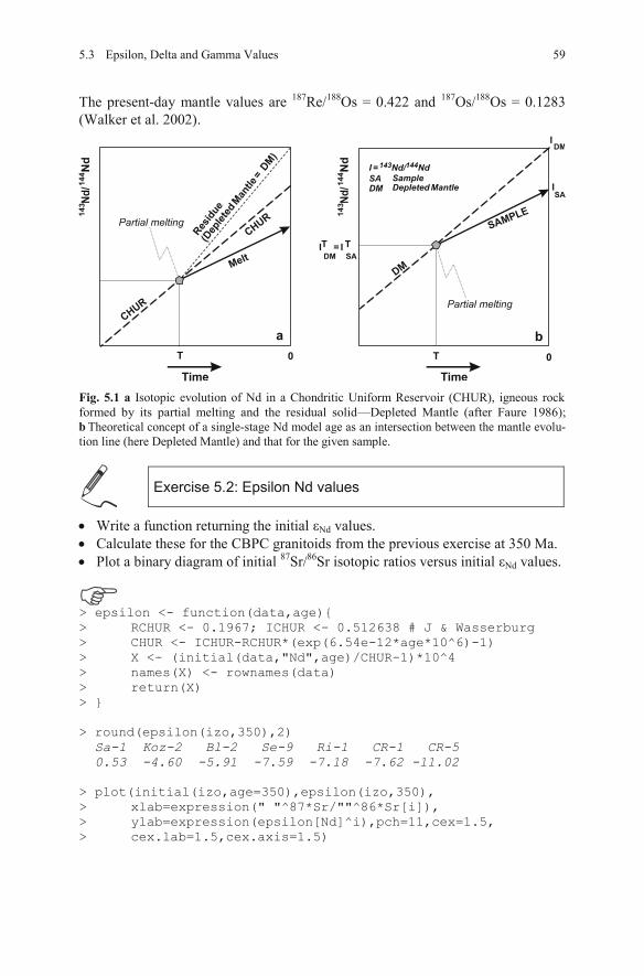
The present-day mantle values are 187Re/188Os = 0.422 and 187Os/188Os = 0.1283 (Walker et al. 2002).
Fig. 5.1 a Isotopic evolution of Nd in a Chondritic Uniform Reservoir (CHUR), igneous rock formed by its partial melting and the residual solid—Depleted Mantle (after Faure 1986);b Theoretical concept of a single-stage Nd model age as an intersection between the mantle evolu-tion line (here Depleted Mantle) and that for the given sample.
Exercise 5.2: Epsilon Nd values
Write a function returning the initial Nd values. Calculate these for the CBPC granitoids from the previous exercise at 350 Ma. Plot a binary diagram of initial 87Sr/86Sr isotopic ratios versus initial Nd values.
> epsilon <- function(data,age){ > RCHUR <- 0.1967; ICHUR <- 0.512638 # J & Wasserburg > CHUR <- ICHUR-RCHUR*(exp(6.54e-12*age*10^6)-1) > X <- (initial(data,"Nd",age)/CHUR-1)*10^4 > names(X) <- rownames(data) > return(X) > } > round(epsilon(izo,350),2) Sa-1 Koz-2 Bl-2 Se-9 Ri-1 CR-1 CR-5 0.53 -4.60 -5.91 -7.59 -7.18 -7.62 -11.02 > plot(initial(izo,age=350),epsilon(izo,350), > xlab=expression(" "^87*Sr/""^86*Sr[i]), > ylab=expression(epsilon[Nd]^i),pch=11,cex=1.5, > cex.lab=1.5,cex.axis=1.5)
Melt
CHUR
CHUR
Res
idue
(Dep
lete
dM
antle
=DM
)
T 0
Time Time
Partial melting
a b
SAMPLE
DM
T 0
IT = I T
DM SA
ISA
IDM
Partial melting
I = Nd/ Nd143 144
SA SampleDM Depleted Mantle
5.3 Epsilon, Delta and Gamma Values 59
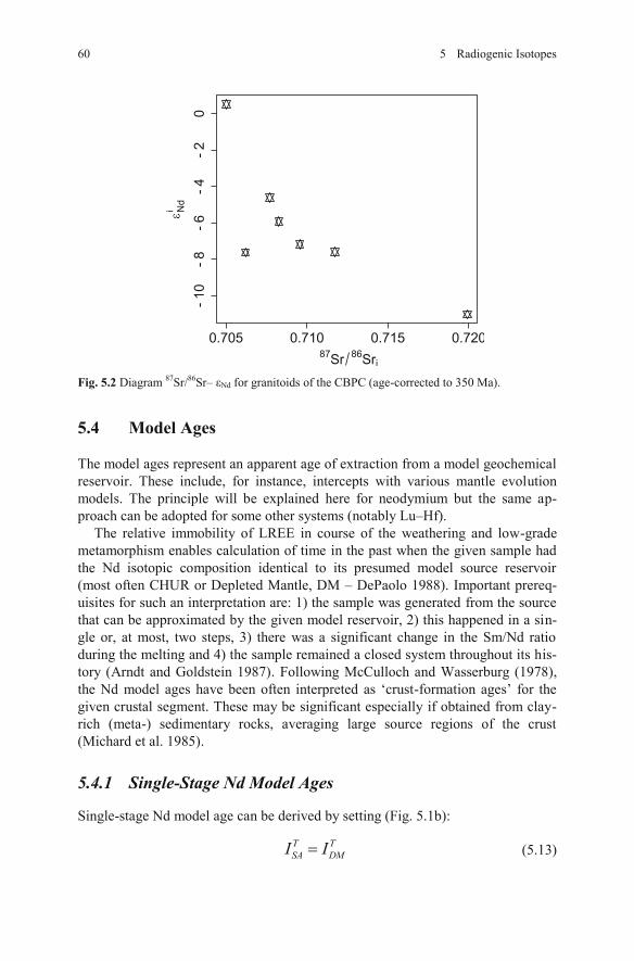
Fig. 5.2 Diagram 87Sr/86Sr– Nd for granitoids of the CBPC (age-corrected to 350 Ma).
5.4 Model Ages
The model ages represent an apparent age of extraction from a model geochemical reservoir. These include, for instance, intercepts with various mantle evolution models. The principle will be explained here for neodymium but the same ap-proach can be adopted for some other systems (notably Lu–Hf).
The relative immobility of LREE in course of the weathering and low-grade metamorphism enables calculation of time in the past when the given sample had the Nd isotopic composition identical to its presumed model source reservoir (most often CHUR or Depleted Mantle, DM – DePaolo 1988). Important prereq-uisites for such an interpretation are: 1) the sample was generated from the source that can be approximated by the given model reservoir, 2) this happened in a sin-gle or, at most, two steps, 3) there was a significant change in the Sm/Nd ratio during the melting and 4) the sample remained a closed system throughout its his-tory (Arndt and Goldstein 1987). Following McCulloch and Wasserburg (1978),the Nd model ages have been often interpreted as ‘crust-formation ages’ for the given crustal segment. These may be significant especially if obtained from clay-rich (meta-) sedimentary rocks, averaging large source regions of the crust (Michard et al. 1985).
5.4.1 Single-Stage Nd Model Ages
Single-stage Nd model age can be derived by setting (Fig. 5.1b):
T TSA DMI I (5.13)
0.705 0.710 0.715 0.720
-10
-8
-6
-4
-2
0
87Sr
86Sri
Nd
i
60 5 Radiogenic Isotopes
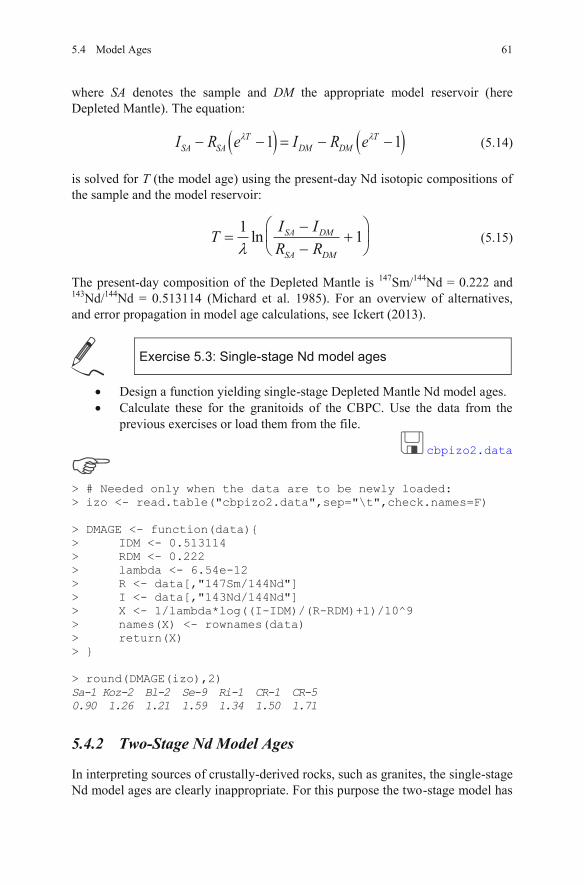
where SA denotes the sample and DM the appropriate model reservoir (here Depleted Mantle). The equation:
1 1T TSA SA DM DMI R e I R e (5.14)
is solved for T (the model age) using the present-day Nd isotopic compositions of the sample and the model reservoir:
1 ln 1SA DM
SA DM
I ITR R
(5.15)
The present-day composition of the Depleted Mantle is 147Sm/144Nd = 0.222 and 143Nd/144Nd = 0.513114 (Michard et al. 1985). For an overview of alternatives, and error propagation in model age calculations, see Ickert (2013).
Exercise 5.3: Single-stage Nd model ages
Design a function yielding single-stage Depleted Mantle Nd model ages. Calculate these for the granitoids of the CBPC. Use the data from the previous exercises or load them from the file.
cbpizo2.data
> # Needed only when the data are to be newly loaded: > izo <- read.table("cbpizo2.data",sep="\t",check.names=F) > DMAGE <- function(data){ > IDM <- 0.513114 > RDM <- 0.222 > lambda <- 6.54e-12 > R <- data[,"147Sm/144Nd"] > I <- data[,"143Nd/144Nd"] > X <- 1/lambda*log((I-IDM)/(R-RDM)+1)/10^9 > names(X) <- rownames(data) > return(X) > } > round(DMAGE(izo),2) Sa-1 Koz-2 Bl-2 Se-9 Ri-1 CR-1 CR-5 0.90 1.26 1.21 1.59 1.34 1.50 1.71
5.4.2 Two-Stage Nd Model Ages
In interpreting sources of crustally-derived rocks, such as granites, the single-stage Nd model ages are clearly inappropriate. For this purpose the two-stage model has
5.4 Model Ages 61
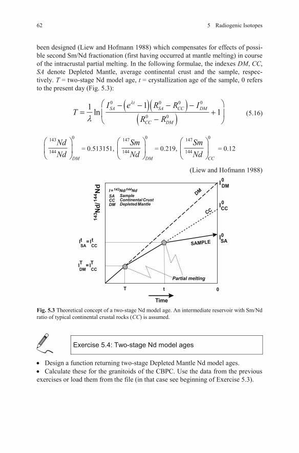
been designed (Liew and Hofmann 1988) which compensates for effects of possi-ble second Sm/Nd fractionation (first having occurred at mantle melting) in course of the intracrustal partial melting. In the following formulae, the indexes DM, CC,SA denote Depleted Mantle, average continental crust and the sample, respec-tively. T = two-stage Nd model age, t = crystallization age of the sample, 0 refers to the present day (Fig. 5.3):
0 0 0 0
0 0
11 ln 1t
SA SA CC DM
CC DM
I e R R IT
R R (5.16)
0143
144DM
NdNd
= 0.513151,
0147
144DM
SmNd
= 0.219,
0147
144CC
SmNd
= 0.12
(Liew and Hofmann 1988)
Fig. 5.3 Theoretical concept of a two-stage Nd model age. An intermediate reservoir with Sm/Nd ratio of typical continental crustal rocks (CC) is assumed.
Exercise 5.4: Two-stage Nd model ages
Design a function returning two-stage Depleted Mantle Nd model ages. Calculate these for the granitoids of the CBPC. Use the data from the previous
exercises or load them from the file (in that case see beginning of Exercise 5.3).
SAMPLE
CC
DM
T t 0
It = I tSA CC
IT
= IT
DM CC
I0SA
I0
CC
I0
DM
Partial melting
I = Nd/ Nd 143 144
SACCDM
SampleContinental CrustDepleted Mantle
Time
62 5 Radiogenic Isotopes
cbpizo2.data
> DMLHAGE <- function(data,age){ > R <- data[,"147Sm/144Nd"] > I <- data[,"143Nd/144Nd"] > IDM <- 0.513151 > RDM <- 0.219 > RCC <- 0.12 > lambda <- 6.54e-12 > A <- I-(exp(lambda*age*1e6)-1)*(R-RCC)-IDM > B <- RCC-RDM > X <- 1/lambda*log(A/B+1)/10^9 > names(X) <- rownames(data) > return(X) > } > round(DMLHAGE(izo,350),2) Sa-1 Koz-2 Bl-2 Se-9 Ri-1 CR-1 CR-5 1.02 1.42 1.52 1.66 1.62 1.66 1.92
5.5 Isochron Ages
An elegant remedy to the problem of unknown initial ratio in the geochronological calculations is to use a cogenetic suite of whole-rock or mineral samples. In fact, Eq. (5.9) corresponds to a straight line in the isochron diagrams R e.g.,87Rb/86Sr vs 87Sr/86Sr:
y a bx (5.17) where a is an intercept (initial isotopic ratio), and b the slope of the isochron:
1tb tg e (5.18)
giving a formula for the isochron age: 1 ln 1t b (5.19)
The isochrons are usually fitted using dedicated software, most frequently Isoplot (Ludwig 2003). The algorithm utilizes weighted linear regression (York 1969).This means that it takes into account the errors in both coordinates at each indi-vidual data point (Provost 1990; Kullerud 1991 and references therein).
Exercise 5.5: Isochrons
The file acari.data contains Rb–Sr isotopic data for granite Serra do Acari (Brazil) (Provost 1990 and references therein). On this example, we will demon-strate the use of simple (i.e. not weighted) linear regression in fitting isochrons.
5.4 Model Ages 63
I,vs
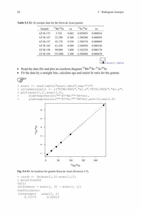
Table 5.2 Rb–Sr isotopic data for the Serra do Acari granite
Sample 87Rb/86Sr 1 87Sr/86Sr 1AT-R-173 5.743 0.062 0.858993 0.000034AT-R-167 22.290 0.280 1.290200 0.000050AT-R-157 42.170 0.530 1.760370 0.000069AT-R-165 61.230 0.980 2.248950 0.000140AT-R-158 99.000 1.800 3.182530 0.000170AT-R-169 232.000 3.300 6.548880 0.000470
acari.data
Read the data file and plot an isochron diagram 87Rb/86Sr–87Sr/86Sr Fit the data by a straight line, calculate age and initial Sr ratio for the granite
> acari <- read.table("acari.data",sep="\t") > colnames(acari) <- c("87Rb/86Sr","er.x","87Sr/86Sr","er.y") > plot(acari[,1],acari[,3], > xlab=expression(""^87*Rb/""^86*Sr), > ylab=expression(""^87*Sr/""^86*Sr),pch=15,cex=1.5)
Fig. 5.4 Rb–Sr isochron for granite Serra do Acari (Exercise 5.5).
> izoch <- lm(acari[,3]~acari[,1]) > print(izoch) Call: lm(formula = acari[, 3] ~ acari[, 1])
0 50 100 150 200
12
34
56
87Rb
86Sr
87S
r86S
r
64 5 Radiogenic Isotopes
(Intercept) acari[, 1] 0.71171 0.02513
Coefficients:
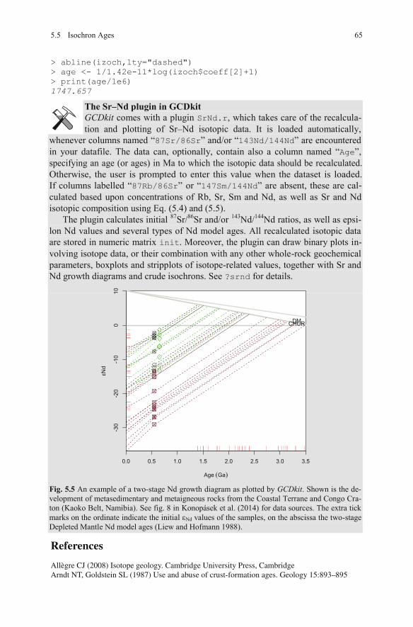
> abline(izoch,lty="dashed") > age <- 1/1.42e-11*log(izoch$coeff[2]+1) > print(age/1e6) 1747.657
The Sr–Nd plugin in GCDkitGCDkit comes with a plugin SrNd.r, which takes care of the recalcula-tion and plotting of Sr–Nd isotopic data. It is loaded automatically,
whenever columns named “87Sr/86Sr” and/or “143Nd/144Nd” are encountered in your datafile. The data can, optionally, contain also a column named “Age”,
isotopic data should be recalculated.wise, the user is prompted to enter this value when the dataset is loaded.
87Rb/86Sr” or “147Sm/144Nd” are absent, these are caland Nd, as well as S
The plugin calculates initial 87Sr/86Sr and/or 143Nd/144Nd ratios, as well as epsi-lon Nd values and several types of Nd model ages. All recalculated isotopic data are stored in numeric matrix init. Moreover, the plugin can draw binary plots in-volving isotope data, or their combination with any other whole-rock geochemical parameters, boxplots and stripplots of isotope-related values, together with Sr and Nd growth diagrams and crude isochrons. See ?srnd for details.
Fig. 5.5 An example of a two-stage Nd growth diagram as plotted by GCDkit. Shown is the de-velopment of metasedimentary and metaigneous rocks from the Coastal Terrane and Congo Cra-ton (Kaoko Belt, Namibia). See fig. 8 in Konopásek et al. (2014) for data sources. The extra tick marks on the ordinate indicate the initial Nd values of the samples, on the abscissa the two-stage Depleted Mantle Nd model ages (Liew and Hofmann 1988).
CHURDM
0.0 0.5 1.0 1.5 2.0 2.5 3.0 3.5
-30
-20
-10
010
Age �Ga�
εN
d
5.5 Isochron Ages 65
specifying an age (or ages) in Ma to which the Other
columns labelled “If -culated based upon concentrations of Rb, Sr, Sm isotopic composition using Eq. (5.4) and (5.5).
r and Nd
References
Allègre CJ (2008) Isotope geology. Cambridge University Press, CambridgeArndt NT, Goldstein SL (1987) Use and abuse of crust-formation ages. Geology 15:893–895
66 5 Radiogenic Isotopes
Audi G, Wapstra AH, Thibault C (2003) The Ame2003 atomic mass evaluation: (II). Tables, graphs and references. Nucl Phys A 729:337–676
Berglund M, Wieser M E (2011) Isotopic compositions of the elements 2009 (IUPAC Technical Report). Pure App Chem 83:397–410
Bouvier A, Vervoort JD, Patchett PJ (2008) The Lu–Hf and Sm–Nd isotopic composition of CHUR: constraints from unequilibrated chondrites and implications for the bulk composition of terrestrial planets. Earth Planet Sci Lett 273:48–57
DePaolo DJ (1988) Neodymium isotope geochemistry. Springer, BerlinDickin AP (2005) Radiogenic isotope geology. Cambridge University Press, CambridgeFaure G (1986) Principles of isotope geology. John Wiley & Sons, ChichesterFaure G, Mensing TM (2004) Isotopes: principles and applications. Wiley, New JerseyGeyh MA, Schleicher H (1990) Absolute age determination. Springer, BerlinIckert RB (2013) Algorithms for estimating uncertainties in initial radiogenic isotope ratios and
model ages. Chem Geol 340:131–138Jacobsen SB, Wasserburg GJ (1980) Sm–Nd isotopic evolution of chondrites. Earth Planet Sci
Lett 50:139–155Janoušek V, Rogers G, Bowes DR (1995) Sr–Nd isotopic constraints on the petrogenesis of the
Central Bohemian Pluton, Czech Republic. Geol Rundsch 84:520–534Konopásek J, Košler J, Sláma J, Janoušek V (2014) Timing and sources of pre-collisional
Neoproterozoic sedimentation along the SW margin of the Congo Craton (Kaoko Belt, NW Namibia). Gondwana Res 26:386–401
Kullerud L (1991) On the calculation of isochrons. Chem Geol (Isot Geosci Sect) 87:115–124Liew TC, Hofmann AW (1988) Precambrian crustal components, plutonic associations, plate
environment of the Hercynian Fold Belt of Central Europe: indications from a Nd and Sr iso-topic study. Contrib Mineral Petrol 98:129–138
Ludwig KR (2003) Isoplot/Ex version 3.00. A geochronological toolkit for Microsoft Excel, User’s Manual. Berkeley Geochronology Center Special Publications, vol 4, pp 1–70
Lugmair GW, Marti K (1978) Lunar initial 143Nd/144Nd: differential evolution line of the lunar crust and mantle. Earth Planet Sci Lett 39:349–357
McCulloch MT, Wasserburg GJ (1978) Sm–Nd and Rb–Sr chronology of the continental crust formation. Science 200:1003–1011
Michard A, Gurriet P, Soudant M, Albarède F (1985) Nd isotopes in French Phanerozoic shales: external vs. internal aspects of crustal evolution. Geochim Cosmochim Acta 49:601–610
Provost A (1990) An improved diagram for isochron data. Chem Geol (Isot Geosci Sect) 80:85–99
Rotenberg E, Davis DW, Amelin Y, Ghosh S, Bergquist BA (2012) Determination of the decay-constant of 87Rb by laboratory accumulation of 87Sr. Geochim Cosmochim Acta 85:41–57
Selby D, Creaser RA, Stein HJ, Markey RJ, Hannah JL (2007) Assessment of the 187Re decay constant by cross calibration of Re–Os molybdenite and U–Pb zircon chronometers in mag-matic ore systems. Geochim Cosmochim Acta 71:1999–2013
Söderlund U, Patchett PJ, Vervoort JD, Isachsen CE (2004) The 176Lu decay constant determined by Lu–Hf and U–Pb isotope systematics of Precambrian mafic intrusions. Earth Planet Sci Lett 219:311–324
Steiger RH, Jäger E (1977) Subcommission on Geochronology; convention on the use of decay constants in geo- and cosmochronology. Earth Planet Sci Lett 36:359–362
Walker RJ, Horan MF, Morgan JW, Becker H, Grossman JN, Rubin AE (2002) Comparative 187Re–187Os systematics of chondrites: implications regarding early solar system processes. Geochim Cosmochim Acta 66:4187–4201
Wasserburg GJ, Jacobsen SB, DePaolo DJ, McCulloch MT, Wen T (1981) Precise determina-tion of Sm/Nd ratios, Sm and Nd isotopic abundances in standard solutions. Geochim Cosmochim Acta 45:2311–2324
York D (1969) Least-squares fitting of a straight line with correlated errors. Earth Planet Sci Lett 5:320–324
Part II Modelling Major Elements
In igneous geochemistry it is customary to discriminate between major (> ca. 1 wt. %) and trace (< ca. 0.1 wt. %) elements, with minor elements falling in between. However, no exact cut-off values have been codified separating these three groups. In the current book, we distinguish majors (occurring in large concentra-tions and combining to the main rock-forming minerals), dilute traces (that substi-tute only in very low concentrations in crystal lattice of other phases) and essential structural components (with low whole-rock contents but crystallizing own acces-sory minerals as soon as saturation is reached—see Part III). The main reason for such a division is that the approach to modelling of igneous processes does differ fundamentally among these three elemental groups.
This definition can lead to slightly unexpected results, whereby elements such as K would be regarded as traces in mafic/ultramafic systems, whereas Cr in ul-tramafic rocks or Zr or even REE in high-silica alkali magmas are major elements. Although somewhat unusual, this approach actually allows for a better description of the relevant systems.
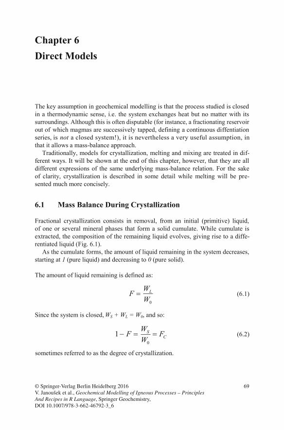
Chapter 6 Direct Models
The key assumption in geochemical modelling is that the process studied is closed in a thermodynamic sense, i.e. the system exchanges heat but no matter with its surroundings. Although this is often disputable (for instance, a fractionating reservoirout of which magmas are successively tapped, defining a continuous diffentiationseries, is notthat it allows a mass-balance approach.
Traditionally, models for crystallization, melting and mixing are treated in dif-ferent ways. It will be shown at the end of this chapter, however, that they are all different expressions of the same underlying mass-balance relation. For the sake of clarity, crystallization is described in some detail while melting will be pre-sented much more concisely.
6.1 Mass Balance During Crystallization
Fractional crystallization consists in removal, from an initial (primitive) liquid, rm a solid cumulate. While cumulate is
uid evolves, giving rise to a diffe-
As the cumulate forms, the amount of liquid remaining in the system decreases, starting at 1 (pure liquid) and decreasing to 0 (pure solid). The amount of liquid remaining is defined as:
0
LWFW
(6.1)
Since the system is closed, WS + WL = W0, and so:
0
1 SC
WF FW
(6.2)
© Springer-Verlag Berlin Heidelberg 2016 V. Janoušek et al., Geochemical Modelling of Igneous Processes – Principles And Recipes in R Language, Springer Geochemistry, DOI 10.1007/978-3-662-46792-3_6
69
of one or several mineral phases that foextracted, the composition of the remaining liqrentiated liquid (Fig. 6.1).
sometimes referred to as the degree of crystallization.
a closed system!), it is nevertheless a very useful assumption, in
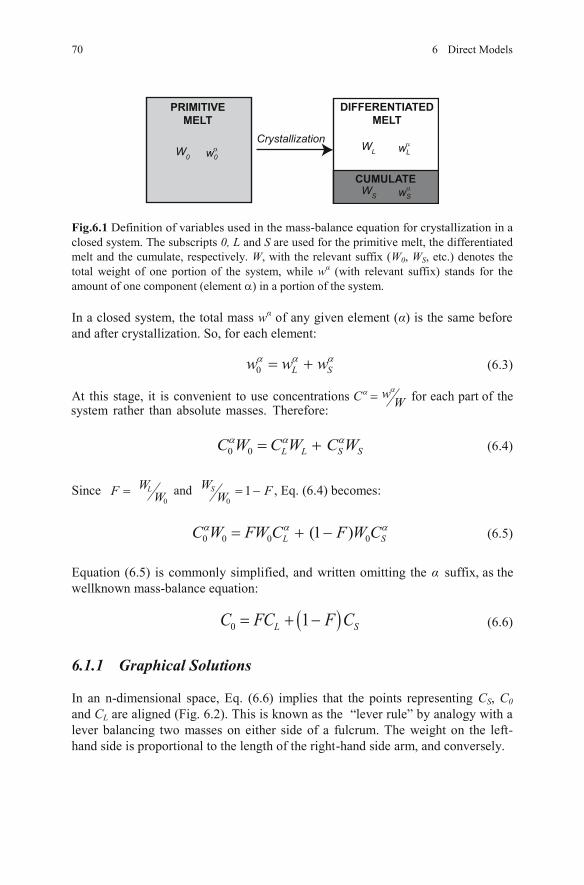
Fig.6.1 Definition of variables used in the mass-balance equation for crystallization in aclosed system. The subscripts 0, L and S are used for the primitive melt, the differentiated melt and the cumulate, respectively. W, with the relevant suffix (W0, WS, etc.) denotes the total weight of one portion of the system, while w (with relevant suffix) stands for the amount of one component (element ) in a portion of the system.
In a closed system, the total mass w of any given element ( ) is the same before and after crystallization. So, for each element:
0 L Sw w w (6.3)
At this stage, it is convenient to use concentrationsrather than absolute masses system herefore:
0 0 L S SLWC W C C W (6.4)
Since 0
LWF W and 0
1SW FW , Eq. (6.4) becomes:
0 0 0 0 (1 ) L SC W FW C F W C (6.5)
Equation (6.5) is commonly simplified, and written omitting the suffix, as the
0 1L SC FC F C (6.6)
6.1.1 Graphical Solutions
In an n-dimensional space, Eq. (6.6) implies that the points representing CS, C0and CL are aligned (Fig. 6.2). This is known as the “lever rule” by analogy with a lever balancing two masses on either side of a fulcrum. The weight on the left-hand side is proportional to the length of the right-hand side arm, and conversely.
PRIMITIVE
MELT
DIFFERENTIATED
MELT
CUMULATE
Crystallization
WS wS
W0WLw0
wL
70 6 Direct Models
. T
wellknown mass-balance equation:
wC W for each part of the
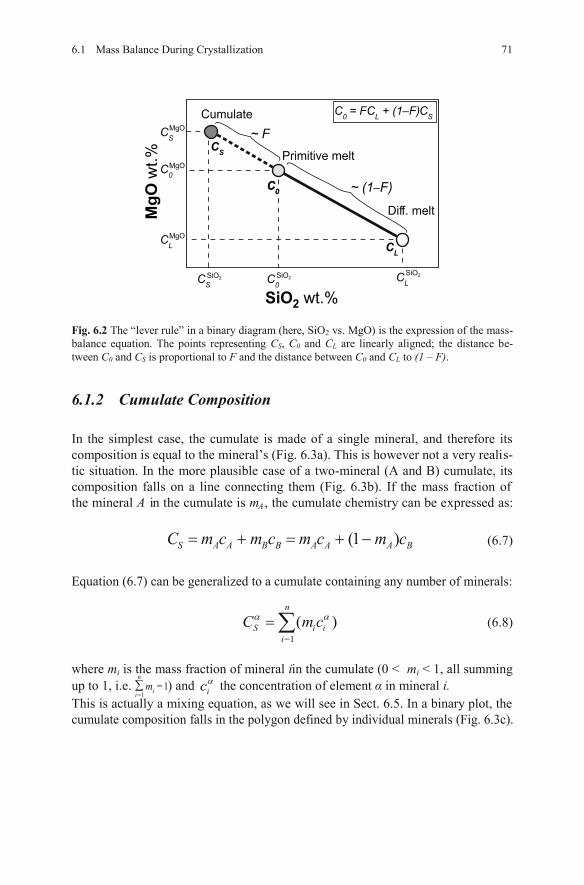
Fig. 6.2 The “lever rule” in a binary diagram (here, SiO2 vs. MgO) is the expression of the mass-balance equation. The points representing CS, C0 and CL are linearly aligned; the distance be-tween C0 and CS is proportional to F and the distance between C0 and CL to (1 – F).
6.1.2 Cumulate Composition
In the simplest case, the cumulate is made of a single mineral, and therefore its composition is equal to the mineral’s (Fig. 6.3a). This is however not a very realis-tic situation. In the more plausible case of a two-mineral (A and B) cumulate, its composition falls on a line connecting them (Fig. 6.3b). If the mass fraction ofthe mineral A in the cumulate is mA, the cumulate chemistry can be expressed as:
(1 )S A A B A BAB AC m c m c m c m c (6.7)
Equation (6.7) can be generalized to a cumulate containing any number of minerals:
( )n
S i ii
C cm (6.8)
where mi is the mass fraction of mineral i in the cumulate (0 < mi < 1, all summing up to 1, i.e.
n
i im ) and ic the concentration of element in mineral i.This is actually a mixing equation, as we will see in Sect. 6.5. In a binary plot, the cumulate composition falls in the polygon defined by individual minerals (Fig. 6.3c).
MgO
wt.%
SiO2 wt.%
CS
CL
Primitive melt
Diff. melt
Cumulate
MgOCL
SiO2CL
C0MgO
C0SiO2
CSMgO
CSSiO2
C0 = F CL + (1–F) CS
~ F
~ (1–F)CC00
6.1 Mass Balance During Crystallization 71
=1=1
=1
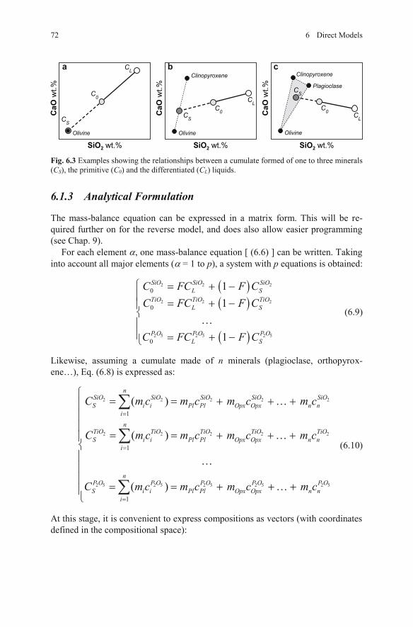
Fig. 6.3 Examples showing the relationships between a cumulate formed of one to three minerals (CS), the primitive (C0) and the differentiated (CL) liquids.
6.1.3 Analytical Formulation
The mass-balance equation can be expressed in a matrix form. This will be re-quired further on for the reverse model, and does also allow easier programming (see Chap. 9).
For each element , one mass-balance equation [ (6.6) ] can be written. Taking = 1 to p), a system with p equations is obtained:
2 2 2
2 2 2
2 5 2 5 2 5
0
0
0
1 1
1
SiO SiO SiOL S
TiO TiO TiOL S
P O P O P OL S
C FC F CC FC F C
C FC F C
(6.9)
Likewise, assuming a cumulate made of n minerals (plagioclase, orthopyrox-ene…), Eq. (6.8) is expressed as:
2 2 2 2 2
2 2 2 2 2
2 5 2 5 2 5 2 5 2 5
1
1
1
( )
( )
( )
nSiO SiO SiO SiO SiOS i i Opx Opx n n
in
TiO TiO TiO TiO TiOS i i O
Pl Pl
Pl px Opx n ni
nP O P O P O P O P OS i i Op
Pl
Pl P xl Opx n ni
C m c m c m c m c
C m c m c m c m c
C m c m c m c m c
(6.10)
At this stage, it is convenient to express compositions as vectors (with coordinates defined in the compositional space):
CaO
wt.%
SiO2 wt.%
CS
C0
CL
Olivine
CaO
wt.%
SiO2 wt.%
CaO
wt.%
SiO2 wt.%
CS
C0
CL
Olivine
Clinopyroxene
C0 CL
Olivine
Clinopyroxene
PlagioclaseCS
a b c
72 6 Direct Models
into account all major elements (
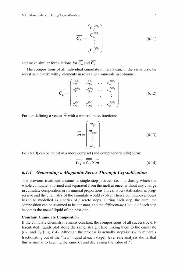
(6.11)
and make similar formulations for and .The compositions of all individual cumulate minerals can, in the same way, be
recast as a matrix with p elements in rows and n minerals in columns:
(6.12)
Further defining a vector with n mineral mass fractions:
(6.13)
Eq. (6.10) can be recast in a more compact (and computer-friendly) form:
(6.14)
6.1.4 Generating a Magmatic Series Through Crystallization The previous treatment assumes a single-step process, i.e. one during which the whole cumulate is formed and separated from the melt at once, without any change
has to be modelled as a series of discrete steps. During each step, the cumulate composition can be assumed to be constant, and the differentiated becomes the initial liquid of the next one.
Constant Cumulate Composition If the cumulate chemistry remains constant, the compositions of all successive dif-ferentiated liquids plot along the same, straight line linking them to the cumulate (CS) and C0 (Fig. 6.4). Although the process is actually stepwise (with minerals
6.1 Mass Balance During Crystallization 73
in cumulate composition or its mineral proportions. In reality, crystallization is prog-ould evolve. Then a continuous process ressive and the chemistry of the cumulate w
fractionating out of the “new” liquid at each stage), lever rule analysis shows that this is similar to keeping the same C0 and decreasing the value of F.
0C LC
m
C=SC C m
liquid of each step
2
2
2 5
SiOSTiOS
P OS
CC
C
SC
2 2 2
2 2 2
2 5 2 5 2 5
SiO SiO SiOPl Opx nTiO TiO TiOPl Opx n
P O P O P OPl Opx n
c c cc c c
c c c
CC
Pl
Opx
n
mm
m
m
×
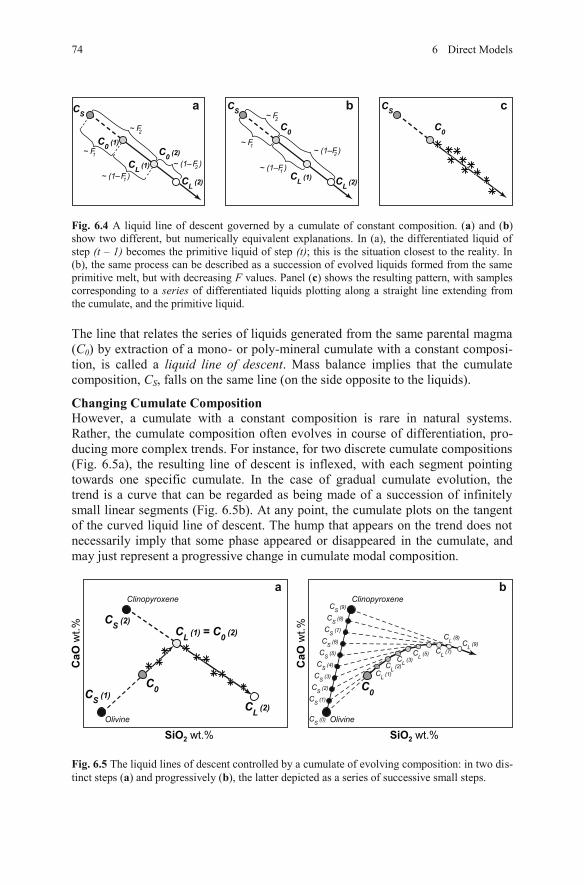
Fig. 6.4 A liquid line of descent governed by a cumulate of constant composition. (a) and (b)show two different, but numerically equivalent explanations. In (a), the differentiated liquid of step (t – 1) becomes the primitive liquid of step (t); this is the situation closest to the reality. In (b), the same process can be described as a succession of evolved liquids formed from the same primitive melt, but with decreasing F values. Panel (c) shows the resulting pattern, with samples corresponding to a series of differentiated liquids plotting along a straight line extending from the cumulate, and the primitive liquid.
The line that relates the series of liquids generated from the same parental magma (C0) by extraction of a mono- or poly-mineral cumulate with a constant composi-tion, is called a liquid line of descent. Mass balance implies that the cumulate composition, CS, falls on the same line (on the side opposite to the liquids).
Changing Cumulate Composition However, a cumulate with a constant composition is rare in natural systems. Rather, the cumulate composition often evolves in course of differentiation, pro-ducing more complex trends. For instance, for two discrete cumulate compositions (Fig. 6.5a), the resulting line of descent is inflexed, with each segment pointing towards one specific cumulate. In the case of gradual cumulate evolution, the trend is a curve that can be regarded as being made of a succession of infinitely small linear segments (Fig. 6.5b). At any point, the cumulate plots on the tangent of the curved liquid line of descent. The hump that appears on the trend does not necessarily imply that some phase appeared or disappeared in the cumulate, and may just represent a progressive change in cumulate modal composition.
Fig. 6.5 The liquid lines of descent controlled by a cumulate of evolving composition: in two dis-tinct steps (a) and progressively (b), the latter depicted as a series of successive small steps.
CS
C0 (1)~ F1
~ (1–F1 )
C0 (2)
CL (1)
CL (2)
~ F2
~ (1–F2 )
~ F1
~ (1–F1 )
~ F2
~ (1–F2 )
CS
C0
CL (1) CL (2)
CS
C0
a b c
CaO
wt.%
SiO2 wt.%Olivine
Clinopyroxene
= C0 (2)CL (1)
CL (2)
C0
CaO
wt.%
SiO2 wt.%Olivine
Clinopyroxene
C0
CL (2)CL (1)
CL (3)CL (5) CL (7)
CL (9)
CS (1)
CS (2)
CS (3)
CS (4)
CS (5)
CS (6)
CS (7)
CS (0)
CS (8)
CS (9)
CL (8)
a b
CS (1)
CS (2)
74 6 Direct Models
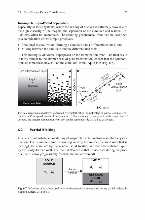
Incomplete Liquid/Solid Separation Especially in felsic systems, where the settling of crystals is extremely slow due to the high viscosity of the magma, the separation of the cumulate and residual liq-uids may often be incomplete. The resulting geochemical trend can be described as a combination of two simple processes:
Fractional crystallization, forming a cumulate and a differentiated melt, and Mixing between the cumulate and the differentiated melt.
This mixing is, of course, superposed on the fractionation trend. The final result is fairly similar to the simpler case of pure fractionation, except that the composi-tions of some rocks now fall on the cumulate–initial liquid join (Fig. 6.6).
Fig. 6.6 Geochemical patterns generated by crystallization, complicated by partial cumulate ex-traction. a Conceptual sketch of this situation. b Since mixing is superposed on the liquid line of descent, the magma compositions can plot on the cumulate side of the line of descent.
6.2 Partial Melting
In terms of mass-balance modelling of major elements, melting resembles crystal-lization. The primitive liquid is now replaced by the source (the solid rock that is melting), the cumulate by the residual solid (restite) and the differentiated liquid by the newly-formed melt. The main difference is that F increases during the proc-ess (melt is now progressively formed, and not consumed).
Fig. 6.7 Definition of variables used to write the mass-balance equation during partial melting in a closed system. Cf. Fig 6.1.
CaO
wt.%
SiO2 wt.%
C0
Pure differentiated liquid
Liquid+
Crystals
Pure cumulate CS
CL
Purecumulate
Puredifferentiated
liquid
Crystal-ric
h
mixtures
Liquid-rich
mixtures
a b
SOLIDSOURCE
MELT
RESIDUALSOLID
Partialmelting
WS wSα
W0
WL
w0α
wLα
6.1 Mass Balance During Crystallization 75
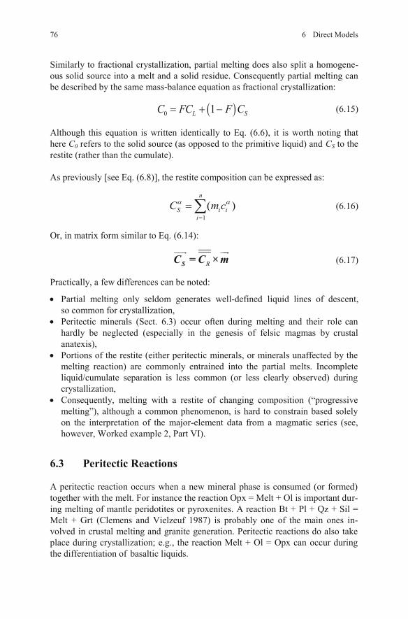
Similarly to fractional crystallization, partial melting does also split a homogene-ous solid source into a melt and a solid residue. Consequently partial melting can be described by the same mass-balance equation as fractional crystallization:
0 1L SC FC F C (6.15)
Although this equation is written identically to Eq. (6.6), it is worth noting that here C0 refers to the solid source (as opposed to the primitive liquid) and CS to the restite (rather than the cumulate).
As previously [see Eq. (6.8)], the restite composition can be expressed as:
( )n
S i ii
C m c (6.16)
Or, in matrix form similar to Eq. (6.14):
(6.17)
Practically, a few differences can be noted:
Partial melting only seldom generates well-defined liquid lines of descent,
Peritectic minerals (Sect. 6.3) occur often during melting and their role canhardly be neglected (especially in the genesis of felsic magmas by crustalanatexis), Portions of the restite (either peritectic minerals, or minerals unaffected by the melting reaction) are commonly entrained into the partial melts. Incomplete
Consequently, melting with a restite of changing composition (“progressive melting”), although a common phenomenon, is hard to constrain based solely on the interpretation of the major-element data from a magmatic series (see, however, Worked example 2, Part VI).
6.3 Peritectic Reactions
A peritectic reaction occurs when a new mineral phase is consumed (or formed) together with the melt. For instance the reaction Opx = Melt + Ol is important dur-ing melting of mantle peridotites or pyroxenites. A reaction Bt + Pl + Qz + Sil = Melt + Grt (Clemens and Vielzeuf 1987) is probably one of the main ones in-volved in crustal melting and granite generation. Peritectic reactions do also take place during crystallization; e.g., the reaction Melt + Ol = Opx can occur during
76 6 Direct Models
so common for crystallization,
liquid/cumulate separation is less common (or less clearly observed) duringcrystallization,
the differentiation of basaltic liquids.
=1
RSC = C ×m
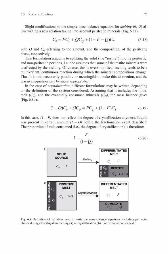
Slight modifications to the simple mass-balance equation for melting (6.15) al-low writing a new relation taking into account peritectic minerals (Fig. 6.8a):
0 (1 )L Q SC FC QC F Q C (6.18)
with Q and CQ referring to the amount, and the composition, of the peritectic phase, respectively.
This formulation amounts to splitting the solid (the “restite”) into its peritectic, and non-peritectic portions, i.e. one assumes that some of the restite minerals were unaffected by the melting. Of course, this is oversimplified; melting tends to be a multivariant, continuous reaction during which the mineral compositions change. Thus it is not necessarily possible or meaningful to make this distinction, and the classical equation may be more appropriate.
In the case of crystallization, different formulations may be written, depending on the definition of the system considered. Assuming that it includes the initial melt (C0), and the eventually consumed minerals (CQ), the mass balance gives (Fig. 6.8b):
0(1 ) (1 )Q L SQ C QC FC F C (6.19)
In this case, (1 – F) does not reflect the degree of crystallization anymore. Liquid was present in certain amount (1 – Q) before the fractionation event described. The proportion of melt consumed (i.e., the degree of crystallization) is therefore:
1(1 )
FQ
(6.20)
Fig. 6.8 Definition of variables used to write the mass-balance equations including peritectic phases during closed-system melting (a) or crystallization (b). For explanation, see text.
PRIMITIVEMELT
DIFFERENTIATEDMELT
CUMULATE
Crystallization
CS
C0CL
F
1–F
Q1–Q
CQ
PER
ITEC
TIC
MIN
ERA
L
SOLIDSOURCE
DIFFERENTIATEDMELT
RESTITE
Melting
CS
C0
CLF
1–F–QQ
1 CQ
PER
I. M
IN
a
b
6.3 Peritectic Reactions 77
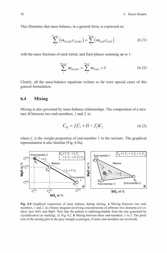
This illustrates that mass balance, in a general form, is expressed as:
START ENDn n
START START END ENDi i
m c m c (6.21)
with the mass fractions of each initial, and final phases summing up to 1:
1START ENDn n
START ENDi i
m m (6.22)
Clearly, all the mass-balance equations written so far were special cases of this general formulation.
6.4 Mixing
Mixing is also governed by mass-balance relationships. The composition of a mix-ture M between two end-members, 1 and 2, is:
1 1 1 2(1 )MC f C f C (6.23)
Fig. 6.9 Graphical expression of mass balance during mixing. a Mixing between two end-members, 1 and 2, in a binary diagram involving concentrations of arbitrary two elements (or ox-ides), here SiO2 and MgO. Note that the pattern is indistinguishable from the one generated by crystallization (or melting), cf. Fig. 6.2. b Mixing between three end-members, 1 to 3. The prod-ucts of the mixing plot in the grey triangle (a polygon, if more end-members are involved).
MgO
wt.%
SiO2 wt.%
C2
CM
C1
Mixture
End-member 2
MgOC1
SiO2C1
CMMgO
CMSiO2
C2MgO
C2SiO2
CM= f1 C1 + f2 C2 = f1 C1 + (1–f1 ) C2~ f 1
~ f2 = 1–f1
End-member 1
End-memberEnd-member MgO
wt.%
SiO2 wt.%
C1
CM
C2
Mixture
End-member 1CM = f1 C1 + f2 C2 + f3 C3
~ 1–
~ 1–
~ 1–
33
End-member 2End-member 3C3
~ 1–~ 1–~ 1–ff11
~ 1–~ 1–~ 1–ff22
a b
ff
78 6 Direct Models
1 is the weight proportion of end-member 1 in the mixture. The graphical representation is also familiar (Fig. 6.9a).
fwhere
where Ck is the concentration in component k that enters the mixing in proportion
fk (0 < fk < 1; 1=
1k
m
k
f ).
This is nothing else than a weighted average of individual components, and the binary mixing Eq. (6.23) is its special case. In a binary diagram, the components of the mixing define a polygon (Fig. 6.9b), and the mixture is located therein (spe-cifically at the center of mass, assuming the weight of each apex is fk). In three-dimensional diagrams, the mixing region is a polyhedron with m apices (and in a p-dimension diagram, a hyper-volume with m apices).
As discussed in Sect. 6.1.3, this equation can also be written in a matrix form, with the concentration of the mixture expressed as a vector of p (elements) length and the mass fractions of each end-member forming a vector of m
(elements) rows and
(6.25)
6.5 Crystallization and Partial Melting—Are These Just Special Cases of Mixing?
By now it should be clear that the mass-balance formulations used for crystalliza-tion, melting and mixing are effectively the same. Indeed, generating a differenti-ated melt CL from a parental melt C0, with a cumulate made of n minerals is equivalent to mixing the cumulate minerals with the differentiated liquid in order to recover the composition of the parental liquid. In this case, if F is the melt frac-tion, and m the mineral proportions in the cumulate, the proportions in the mixing are F for the melt and (1 – F) × mi for each mineral i. The mass-balance equation can be expressed as:
01
(1 ) ( )n
L i ii
cF FC C m (6.26)
which we can recast in a matrix form:
(6.27)
6.4 Mixing 79
If m components (m 2) are involved (e.g., Fig. 6.9b), the equation becomes:
1
( )m
M k kk
C f C (6.24)
(end members) length. Moreover, the compositions of the end-members are recastof pEC
0C = C × f
fMC
(6.24) becomes, in matrix form: m
=
=
(end members) columns. Equation
EMC = C × f
as a matrix
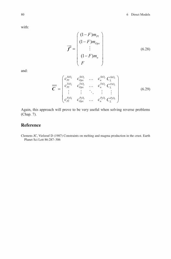
with:
(6.28)
and:
(6.29)
Again, this approach will prove to be very useful when solving reverse problems (Chap. 7).
Reference
Clemens JC, Vielzeuf D (1987) Constraints on melting and magma production in the crust. Earth Planet Sci Lett 86:287–306
80 6 Direct Models
(1 )(1 )
(1 )
Pl
Opx
n
F mF m
F mF
f
2 2 2 2
2 2 2 2
2 5 2 5 2 5 2 5
Pl
Pl L
Pl
SiO SiO SiO SiOOpx n L
TiO TiO TiO TiOOpx n
P O P O P O PO L
Opx n
c c c Cc c c C
c c c C
C
Chapter 7 Reverse Models
Although direct approach can be used to predict the compositions generated by a certain well-defined process, and compare them with observations, the real geolo-
1
7.1 An Under-Determined Problem
In the case of fractional crystallization, examining Eq. (6.27) reveals that the fol-lowing parameters remain to be determined (assuming the composition LC of the differentiated lava is known from sampled rocks):
composition 0C of the primitive magma (for the p elements considered), composition SC of the cumulate, itself a function of: – compositions ic of all n cumulate minerals i, – mineral mass fractions mi in the cumulate,
degree of fractionation ( 1– F ).
In a system with p elements and n possible cumulate minerals, there is therefore a total of p×n (cumulate mineral compositions) + p (primitive liquid) + n + 1 (min-eral proportions and F) –1 (because all the mi sum up to 1) variables. On the other hand, the matrix equation (6.27) represents a system of only p equations. It is therefore clear that some of the variables must be constrained using realistic geo-logical assumptions, whereas others can be calculated from these hypotheses (Sect. 22.1).
1 The following discussion is written for crystallization but the same logic can be applied to melt-
ing. Mixing is slightly different and thus it is addressed separately in Sect. 7.3.
© Springer-Verlag Berlin Heidelberg 2016 V. Janoušek et al., Geochemical Modelling of Igneous Processes – Principles And Recipes in R Language, Springer Geochemistry, DOI 10.1007/978-3-662-46792-3_7
81
gical problems are seldom soluble in this way. Geochemists more generally face areverse problem in which only the differentiated liquid compositions are observed(e.g., as a series of lavas from a volcano or igneous province), while the other para-meters such as the composition of the primitive melt, or the nature of the cumulatecontrolling the liquid line of descent, are not known.
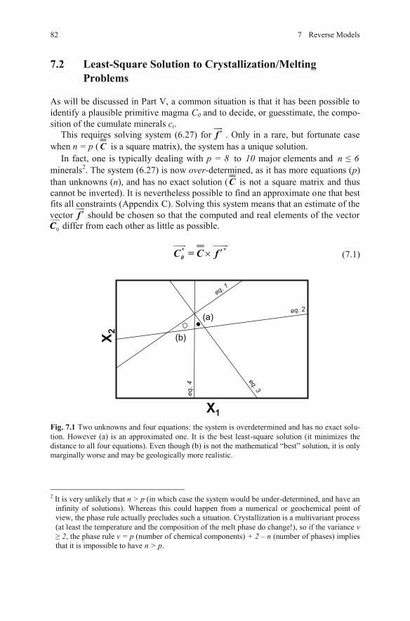
7.2 Least-Square Solution to Crystallization/Melting Problems
As will be discussed in Part V, a common situation is that it has been possible to identify a plausible primitive magma C0 and to decide, or guesstimate, the compo-sition of the cumulate minerals ci.
This requires solving system (6.27) for ff . Only in a rare, but fortunate case when n = p (C is a square matrix), the system has a unique solution.
p = 8 to 10 major elements and n 6minerals2. The system (6.27) is now over-determined, as it has more equations (p)than unknowns (n), and has no exact solution ( is not a square matrix and thus cannot be inverted). It is nevertheless possible to find an approximate one that best fits all constraints (Appendix C). Solving this system means that an estimate of the vector should be chosen so that the computed and real elements of the vector
0CC differ from each other as little as possible.
(7.1)
Fig. 7.1 Two unknowns and four equations: the system is overdetermined and has no exact solu-tion. However (a) is an approximated one. It is the best least-square solution (it minimizes the distance to all four equations). Even though (b) is not the mathematical “best” solution, it is only marginally worse and may be geologically more realistic.
2 It is very unlikely that n > p (in which case the system would be under-determined, and have an
infinity of solutions). Whereas this could happen from a numerical or geochemical point of view, the phase rule actually precludes such a situation. Crystallization is a multivariant process (at least the temperature and the composition of the melt phase do change!), so if the variance v
2, the phase rule v = p (number of chemical components) + 2 – n (number of phases) implies that it is impossible to have n > p.
X 2
X1
(a)
(b)
eq. 2
eq. 1
eq. 4
eq. 3
82 7 Reverse Models
* *0C = C f
In fact, one is typically dealing with
ff
C
This is commonly solved by the least-square approximation:
0
T T* -1f = (C ×C C ×C×) (7.2)
The sum of squares of residuals R2 is a useful quantifier for the goodness of fit:
*0
22
0R *2
C C (7.3)
For further details on the least-square method and its implementation in R, see Appendix C, Albarède (1995) and Janoušek and Moyen (2014).
7.3 Least-Square Solution to Mixing Problems In a mixing problem, geological constraints are different. Typically, the possible end-members are known or at least can be assumed. The questions that can be an-swered by modelling are:
Can the observed ‘hybrid’ composition be explained as a mixture of the as-sumed end-members? If so, what is the proportion of each of them?
This amounts to solving Eq. (6.25) for ff .
A general solution for mixing of an arbitrary number of components3 can be again
T T* -1
E E MEf = (C ×C ) C ×C× (7.4)
As previously, R2 gives an estimate of the quality of the model, i.e. whether the composition observed can really be explained in terms of mixing.
A special case of such reverse mixing is that of the modal recalculations. Knowing the mineral compositions, it is possible to recast them into the composition of any given rock. This approach is used routinely in experimental petrology to obtain the likely mode (in wt. %) from run-product analyses.
7.2 Least-Square Solution to Crystallization/Melting … 83
obtained by least-square method (Appendix C):
References
Albarède F (1995) Introduction to geochemical modeling. Cambridge Univ Press, CambridgeFourcade S, Allègre CJ (1981) Trace-elements behavior in granite genesis—a case-study the
calc-alkaline plutonic association from the Querigut Complex (Pyrenées, France). Contrib Mineral Petrol 76:177–195
Janoušek V, Moyen J-F (2014) Mass balance modelling of magmatic processes in GCDkit. In: Kumar S, Singh RN (eds) Modelling of magmatic and allied processes. The Society of Earth Scientists Series, vol 83. Springer, Berlin, pp 225–238
3 In the case of a binary mixing, the problem can be simplified and a graphical method known as the “mixing test” (Fourcade and Allègre 1981) applied (Sect. 21.4).
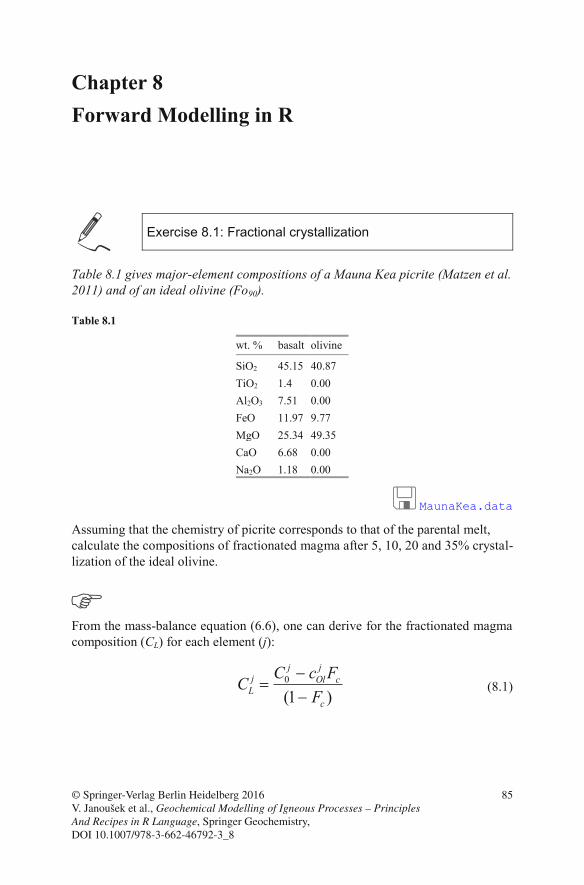
Chapter 8 Forward Modelling in R
Exercise 8.1: Fractional crystallization
Table 8.1 gives major-element compositions of a Mauna Kea picrite (Matzen et al. 2011) and of an ideal olivine (Fo90).
Table 8.1
wt. % basalt olivine
SiO2 45.15 40.87 TiO2 1.4 0.00 Al2O3 7.51 0.00 FeO 11.97 9.77 MgO 25.34 49.35 CaO 6.68 0.00 Na2O 1.18 0.00
MaunaKea.data
Assuming that the chemistry of picrite corresponds to that of the parental melt, calculate the compositions of fractionated magma after 5, 10, 20 and 35% crystal-lization of the ideal olivine.
From the mass-balance equation (6.6), one can derive for the fractionated magma composition (CL) for each element (j):
0
)(1
j jj Ol c
Lc
C c FCF
(8.1)
© Springer-Verlag Berlin Heidelberg 2016 V. Janoušek et al., Geochemical Modelling of Igneous Processes – Principles And Recipes in R Language, Springer Geochemistry, DOI 10.1007/978-3-662-46792-3_8
85
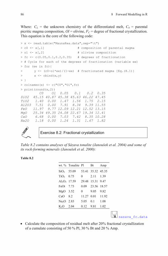
Where: CL = the unknown chemistry of the differentiated melt, C0 = parental picritic magma composition, Ol = olivine, FC = degree of fractional crystallization. This equation is the core of the following code:
> x <- read.table("MaunaKea.data",sep="\t")
> c0 <- x[,1] # composition of parental magma
> ol <- x[,2] # olivine composition
> fc <- c(0.05,0.1,0.2,0.35) # degrees of fractionation
> # Cycle for each of the degrees of fractionation (variable ee)
> for (ee in fc){
> y <- (c0-ol*ee)/(1-ee) # fractionated magma [Eq.(8.1)]
> x <- cbind(x,y)
> }
> colnames(x) <- c("C0","Ol",fc)
> print(round(x,2)) C0 Ol 0.05 0.1 0.2 0.35 SiO2 45.15 40.87 45.38 45.63 46.22 47.45 TiO2 1.40 0.00 1.47 1.56 1.75 2.15 Al2O3 7.51 0.00 7.91 8.34 9.39 11.55 FeO 11.97 9.77 12.09 12.21 12.52 13.15 MgO 25.34 49.35 24.08 22.67 19.34 12.41 CaO 6.68 0.00 7.03 7.42 8.35 10.28 Na2O 1.18 0.00 1.24 1.31 1.47 1.82
Exercise 8.2: Fractional crystallization
Table 8.2 contains analyses of Sázava tonalite (Janoušek et al. 2004) and some of its rock-forming minerals (Janoušek et al. 2000):
Table 8.2
wt. % Tonalite Pl Bt Amp
SiO2 55.09 53.41 35.32 45.35TiO2 0.75 0 2.11 1.39Al2O3 17.59 29.48 15.31 9.47FeOt 7.73 0.09 23.56 18.57MgO 3.52 0 9.05 9.82CaO 8.2 11.27 0.01 11.92Na2O 2.83 5.05 0.1 1.08K2O 2.04 0.12 9.81 1.02
sazava_fc.data
Calculate the composition of residual melt after 20% fractional crystallization of a cumulate consisting of 50 % Pl, 30 % Bt and 20 % Amp.
86 8 Forward Modelling in R
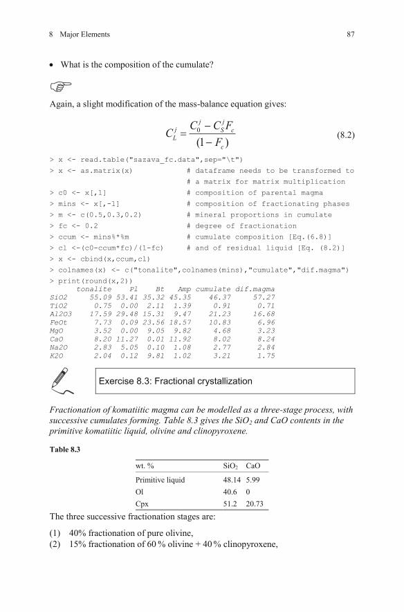
What is the composition of the cumulate?
Again, a slight modification of the mass-balance equation gives:
0
)(1
j jj S c
Lc
C C FCF
(8.2)
> x <- read.table("sazava_fc.data",sep="\t")
> x <- as.matrix(x) # dataframe needs to be transformed to
# a matrix for matrix multiplication
> c0 <- x[,1] # composition of parental magma
> mins <- x[,-1] # composition of fractionating phases
> m <- c(0.5,0.3,0.2) # mineral proportions in cumulate
> fc <- 0.2 # degree of fractionation
> ccum <- mins%*%m # cumulate composition [Eq.(6.8)]
> cl <-(c0-ccum*fc)/(1-fc) # and of residual liquid [Eq. (8.2)]
> x <- cbind(x,ccum,cl)
> colnames(x) <- c("tonalite",colnames(mins),"cumulate","dif.magma")
> print(round(x,2)) tonalite Pl Bt Amp cumulate dif.magma SiO2 55.09 53.41 35.32 45.35 46.37 57.27 TiO2 0.75 0.00 2.11 1.39 0.91 0.71 Al2O3 17.59 29.48 15.31 9.47 21.23 16.68 FeOt 7.73 0.09 23.56 18.57 10.83 6.96 MgO 3.52 0.00 9.05 9.82 4.68 3.23 CaO 8.20 11.27 0.01 11.92 8.02 8.24 Na2O 2.83 5.05 0.10 1.08 2.77 2.84 K2O 2.04 0.12 9.81 1.02 3.21 1.75
Exercise 8.3: Fractional crystallization
Fractionation of komatiitic magma can be modelled as a three-stage process, with successive cumulates forming. Table 8.3 gives the SiO2 and CaO contents in the primitive komatiitic liquid, olivine and clinopyroxene.
Table 8.3
wt. % SiO2 CaO
Primitive liquid 48.14 5.99 Ol 40.6 0 Cpx 51.2 20.73
The three successive fractionation stages are:
(1) 40% fractionation of pure olivine, (2) 15% fractionation of 60 % olivine + 40 % clinopyroxene,
878 Major Elements
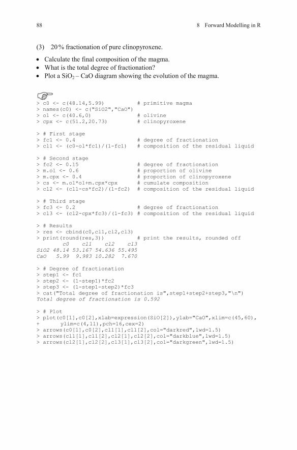
(3) 20 % fractionation of pure clinopyroxene.
Calculate the final composition of the magma. What is the total degree of fractionation? Plot a SiO2 – CaO diagram showing the evolution of the magma.
> c0 <- c(48.14,5.99) # primitive magma > names(c0) <- c("SiO2","CaO") > ol <- c(40.6,0) # olivine > cpx <- c(51.2,20.73) # clinopyroxene > # First stage > fc1 <- 0.4 # degree of fractionation > cl1 <- (c0-ol*fc1)/(1-fc1) # composition of the residual liquid > # Second stage > fc2 <- 0.15 # degree of fractionation > m.ol <- 0.6 # proportion of olivine > m.cpx <- 0.4 # proportion of clinopyroxene > cs <- m.ol*ol+m.cpx*cpx # cumulate composition > cl2 <- (cl1-cs*fc2)/(1-fc2) # composition of the residual liquid > # Third stage > fc3 <- 0.2 # degree of fractionation > cl3 <- (cl2-cpx*fc3)/(1-fc3) # composition of the residual liquid > # Results > res <- cbind(c0,cl1,cl2,cl3) > print(round(res,3)) # print the results, rounded off c0 cl1 cl2 cl3 SiO2 48.14 53.167 54.636 55.495 CaO 5.99 9.983 10.282 7.670 > # Degree of fractionation > step1 <- fc1 > step2 <- (1-step1)*fc2 > step3 <- (1-step1-step2)*fc3 > cat("Total degree of fractionation is",step1+step2+step3,"\n") Total degree of fractionation is 0.592 > # Plot > plot(c0[1],c0[2],xlab=expression(SiO[2]),ylab="CaO",xlim=c(45,60), + ylim=c(4,11),pch=16,cex=2) > arrows(c0[1],c0[2],cl1[1],cl1[2],col="darkred",lwd=1.5) > arrows(cl1[1],cl1[2],cl2[1],cl2[2],col="darkblue",lwd=1.5) > arrows(cl2[1],cl2[2],cl3[1],cl3[2],col="darkgreen",lwd=1.5)
88 8 Forward Modelling in R
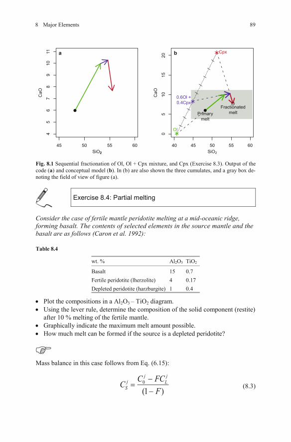
Fig. 8.1 Sequential fractionation of Ol, Ol + Cpx mixture, and Cpx (Exercise 8.3). Output of the code (a) and conceptual model (b). In (b) are also shown the three cumulates, and a gray box de-noting the field of view of figure (a).
Exercise 8.4: Partial melting
Consider the case of fertile mantle peridotite melting at a mid-oceanic ridge, forming basalt. The contents of selected elements in the source mantle and the
Table 8.4
wt. % Al2O3 TiO2
Basalt 15 0.7 Fertile peridotite (lherzolite) 4 0.17 Depleted peridotite (harzburgite) 1 0.4
Plot the compositions in a Al2O3 – TiO2 diagram. Using the lever rule, determine the composition of the solid component (restite)
after 10 % melting of the fertile mantle. Graphically indicate the maximum melt amount possible. How much melt can be formed if the source is a depleted peridotite?
Mass balance in this case follows from Eq. (6.15):
0
(1 )
j jj L
SC FCC
F (8.3)
40 45 50 55 60
05
10
15
20
SiO2C
aO
0.6Ol +
0.4Cpx
Cpx
Primary
melt
Fractionated
melt
b ∗
Ol
2
45 50 55 60
45
67
89
10
11
SiO2
CaO
a
∗
∗
898 Major Elements
basalt are as follows (Caron et al. 1992):
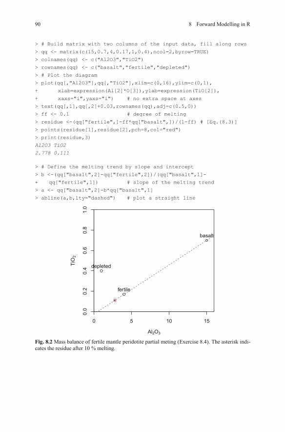
> # Build matrix with two columns of the input data, fill along rows
> qq <- matrix(c(15,0.7,4,0.17,1,0.4),ncol=2,byrow=TRUE)
> colnames(qq) <- c("Al2O3","TiO2")
> rownames(qq) <- c("basalt","fertile","depleted")
> # Plot the diagram
> plot(qq[,"Al2O3"],qq[,"TiO2"],xlim=c(0,16),ylim=c(0,1),
+ xlab=expression(Al[2]*O[3]),ylab=expression(TiO[2]),
+ xaxs="i",yaxs="i") # no extra space at axes
> text(qq[,1],qq[,2]+0.03,rownames(qq),adj=c(0.5,0))
> ff <- 0.1 # degree of melting
> residue <-(qq["fertile",]-ff*qq["basalt",])/(1-ff) # [Eq.(8.3)]
> points(residue[1],residue[2],pch=8,col="red")
> print(residue,3)
Al2O3 TiO2
2.778 0.111
> # Define the melting trend by slope and intercept
> b <-(qq["basalt",2]-qq["fertile",2])/(qq["basalt",1]-
+ qq["fertile",1]) # slope of the melting trend
> a <- qq["basalt",2]-b*qq["basalt",1]
> abline(a,b,lty="dashed") # plot a straight line
Fig. 8.2 Mass balance of fertile mantle peridotite partial meting (Exercise 8.4). The asterisk indi-cates the residue after 10 % melting.
0 5 10 15
0.0
0.2
0.4
0.6
0.8
1.0
Al2O3
TiO
2
basalt
fertile
depleted
90 8 Forward Modelling in R
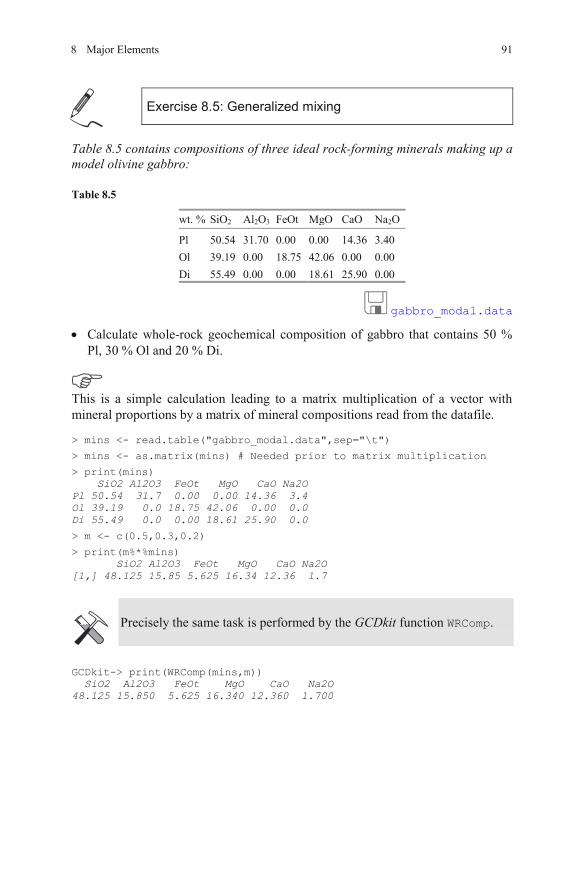
Exercise 8.5: Generalized mixing
Table 8.5 contains compositions of three ideal rock-forming minerals making up a model olivine gabbro:
Table 8.5
wt. % SiO2 Al2O3 FeOt MgO CaO Na2O
Pl 50.54 31.70 0.00 0.00 14.36 3.40 Ol 39.19 0.00 18.75 42.06 0.00 0.00 Di 55.49 0.00 0.00 18.61 25.90 0.00
gabbro_modal.data
Calculate whole-rock geochemical composition of gabbro that contains 50 % Pl, 30 % Ol and 20 % Di.
This is a simple calculation leading to a matrix multiplication of a vector with mineral proportions by a matrix of mineral compositions read from the datafile.
> mins <- read.table("gabbro_modal.data",sep="\t")
> mins <- as.matrix(mins) # Needed prior to matrix multiplication
> print(mins) SiO2 Al2O3 FeOt MgO CaO Na2O Pl 50.54 31.7 0.00 0.00 14.36 3.4 Ol 39.19 0.0 18.75 42.06 0.00 0.0 Di 55.49 0.0 0.00 18.61 25.90 0.0
> m <- c(0.5,0.3,0.2)
> print(m%*%mins) SiO2 Al2O3 FeOt MgO CaO Na2O [1,] 48.125 15.85 5.625 16.34 12.36 1.7
Precisely the same task is performed by the GCDkit function WRComp.
GCDkit-> print(WRComp(mins,m)) SiO2 Al2O3 FeOt MgO CaO Na2O 48.125 15.850 5.625 16.340 12.360 1.700
918 Major Elements

92 8 Forward Modelling in R
References
Caron J-M, Gauthier A, Schaaf A, Ulysse J, Wozniak J (1992) Comprendre et enseigner la Planète Terre. Ophrys, Paris
Janoušek V, Bowes DR, Rogers G, Farrow CM, Jelínek E (2000) Modelling diverse processes in the petrogenesis of a composite batholith: the Central Bohemian Pluton, Central European Hercynides. J Petrol 41:511–543
Janoušek V, Braithwaite CJR, Bowes DR, Gerdes A (2004) Magma-mixing in the genesis of Hercynian calc-alkaline granitoids: an integrated petrographic and geochemical study of the Sázava intrusion, Central Bohemian Pluton, Czech Republic. Lithos 78:67–99
Matzen AK, Baker MB, Beckett JR, Stolper EM (2011) Fe–Mg partitioning between olivine and high-magnesian melts and the nature of Hawaiian parental liquids. J Petrol 52:1243–1263
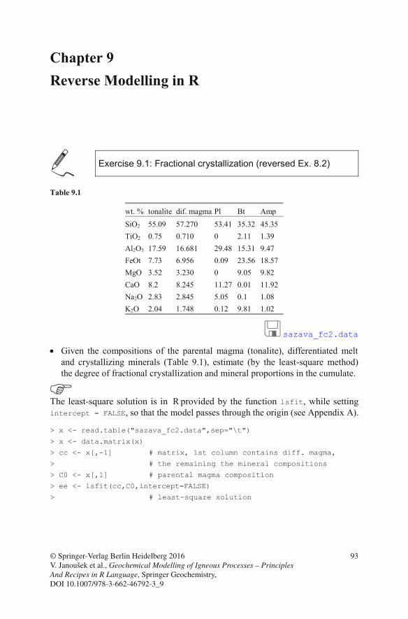
Chapter 9 Reverse Modelling in R
Exercise 9.1: Fractional crystallization (reversed Ex. 8.2)
Table 9.1
wt. % tonalite dif. magma Pl Bt Amp SiO2 55.09 57.270 53.41 35.32 45.35 TiO2 0.75 0.710 0 2.11 1.39 Al2O3 17.59 16.681 29.48 15.31 9.47 FeOt 7.73 6.956 0.09 23.56 18.57 MgO 3.52 3.230 0 9.05 9.82 CaO 8.2 8.245 11.27 0.01 11.92 Na2O 2.83 2.845 5.05 0.1 1.08 K2O 2.04 1.748 0.12 9.81 1.02
sazava_fc2.data
Given the compositions of the parental magma (tonalite), differentiated melt and crystallizing minerals (Table 9.1), estimate (by the least-square method) the degree of fractional crystallization and mineral proportions in the cumulate.
The least-square solution is in R provided by the function lsfit, so that the model passes through the origin (see Appendix A).
> x <- read.table("sazava_fc2.data",sep="\t")
> x <- data.matrix(x)
> cc <- x[,-1] # matrix, 1st column contains diff. magma,
> # the remaining the mineral compositions
> C0 <- x[,1] # parental magma composition
> ee <- lsfit(cc,C0,intercept=FALSE)
> # least-square solution
© Springer-Verlag Berlin Heidelberg 2016 V. Janoušek et al., Geochemical Modelling of Igneous Processes – Principles And Recipes in R Language, Springer Geochemistry, DOI 10.1007/978-3-662-46792-3_9
93
, while setting intercept = FALSE
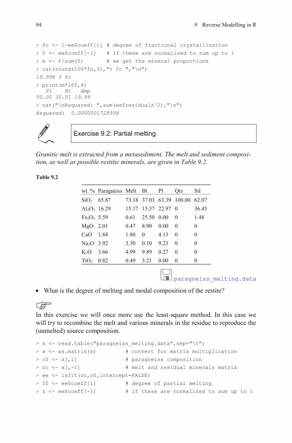
> fc <- 1-ee$coeff[1] # degree of fractional crystallization
> f <- ee$coeff[-1] # if these are normalized to sum up to 1
> m <- f/sum(f) # we get the mineral proportions
> cat(round(100*fc,3),"% fc ","\n")
19.996 % fc
> print(m*100,4) Pl Bt Amp 50.00 30.01 19.99
> cat("\nRsquared: ",sum(ee$residuals^2),"\n")
Rsquared: 0.0000001728938
Exercise 9.2: Partial melting
Granitic melt is extracted from a metasediment. The melt and sediment composi-tion, as well as possible restitic minerals, are given in Table 9.2.
Table 9.2
wt. % Paragneiss Melt Bt Pl Qtz SilSiO2 65.87 73.18 37.03 63.39 100.00 62.07Al2O3 16.29 15.17 15.37 22.97 0 36.45Fe2O3 5.59 0.61 25.50 0.00 0 1.48MgO 2.01 0.47 8.90 0.00 0 0CaO 1.84 1.80 0 4.13 0 0Na2O 3.92 3.30 0.10 9.23 0 0K2O 3.66 4.99 9.89 0.27 0 0TiO2 0.82 0.49 3.21 0.00 0 0
paragneiss_melting.data
What is the degree of melting and modal composition of the restite?
In this exercise we will once more use the least-square method. In this case we will try to recombine the melt and various minerals in the residue to reproduce the (unmelted) source composition.
> x <- read.table("paragneiss_melting.data",sep="\t")
> x <- as.matrix(x) # convert for matrix multiplication
> c0 <- x[,1] # paragneiss composition
> cc <- x[,-1] # melt and residual minerals matrix
> ee <- lsfit(cc,c0,intercept=FALSE)
> ff <- ee$coeff[1] # degree of partial melting
> z <- ee$coeff[-1] # if these are normalized to sum up to 1
94 9 Reverse Modelling in R
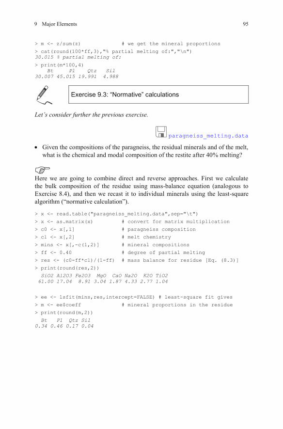
> m <- z/sum(z) # we get the mineral proportions
> cat(round(100*ff,3),"% partial melting of:","\n") 30.015 % partial melting of:
> print(m*100,4) Bt Pl Qtz Sil 30.007 45.015 19.991 4.988
Exercise 9.3: “Normative” calculations
Let’s consider further the previous exercise.
paragneiss_melting.data
Given the compositions of the paragneiss, the residual minerals and of the melt, what is the chemical and modal composition of the restite after 40% melting?
Here we are going to combine direct and reverse approaches. First we calculate the bulk composition of the residue using mass-balance equation (analogous to Exercise 8.4), and then we recast it to individual minerals using the least-square algorithm (“normative calculation”).
> x <- read.table("paragneiss_melting.data",sep="\t")
> x <- as.matrix(x) # convert for matrix multiplication
> c0 <- x[,1] # paragneiss composition
> cl <- x[,2] # melt chemistry
> mins <- x[,-c(1,2)] # mineral compositions
> ff <- 0.40 # degree of partial melting
> res <- (c0-ff*cl)/(1-ff) # mass balance for residue [Eq. (8.3)]
> print(round(res,2))
SiO2 Al2O3 Fe2O3 MgO CaO Na2O K2O TiO2 61.00 17.04 8.91 3.04 1.87 4.33 2.77 1.04
> ee <- lsfit(mins,res,intercept=FALSE) # least-square fit gives
> m <- ee$coeff # mineral proportions in the residue
> print(round(m,2))
Bt Pl Qtz Sil 0.34 0.46 0.17 0.04
95Major Elements9
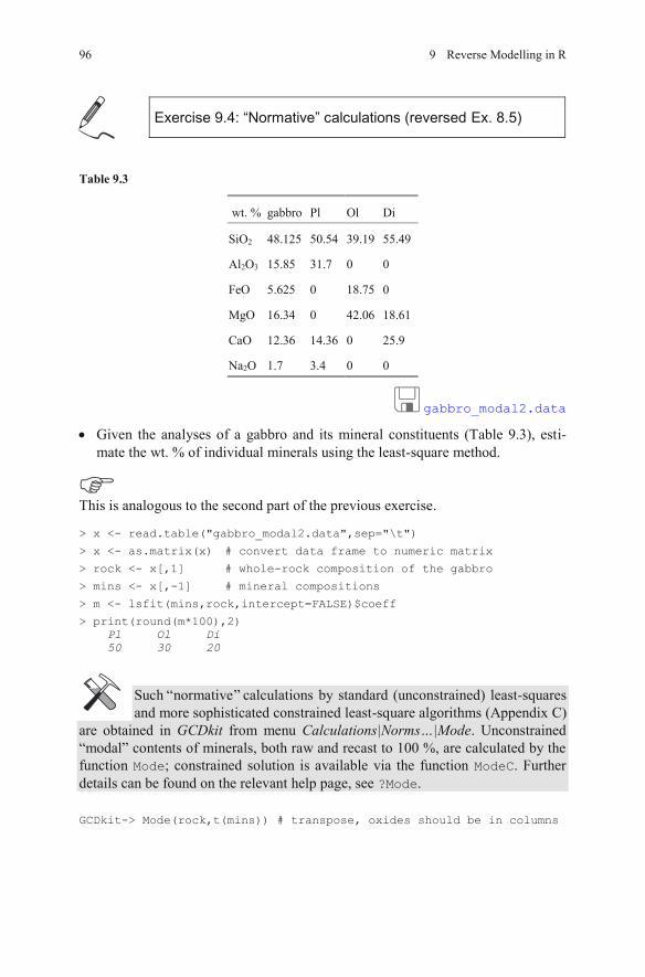
Exercise 9.4: “Normative” calculations (reversed Ex. 8.5)
Table 9.3
wt. % gabbro Pl Ol Di
SiO2 48.125 50.54 39.19 55.49
Al2O3 15.85 31.7 0 0
FeO 5.625 0 18.75 0
MgO 16.34 0 42.06 18.61
CaO 12.36 14.36 0 25.9
Na2O 1.7 3.4 0 0
gabbro_modal2.data
Given the analyses of a gabbro and its mineral constituents (Table 9.3), esti-mate the wt. % of individual minerals using the least-square method.
This is analogous to the second part of the previous exercise.
> x <- read.table("gabbro_modal2.data",sep="\t")
> x <- as.matrix(x) # convert data frame to numeric matrix
> rock <- x[,1] # whole-rock composition of the gabbro
> mins <- x[,-1] # mineral compositions
> m <- lsfit(mins,rock,intercept=FALSE)$coeff
> print(round(m*100),2) Pl Ol Di 50 30 20
Such normative calculations by standard (unconstrained) least-squares and more sophisticated constrained least-square algorithms (Appendix C)
are obtained in GCDkit from menu Calculations|Norms…|Mode. Unconstrained “modal” contents of minerals, both raw and recast to 100 %, are calculated by the function Mode; constrained solution is available via the function ModeC. Further details can be found on the relevant help page, see ?Mode.
GCDkit-> Mode(rock,t(mins)) # transpose, oxides should be in columns
96 9 Reverse Modelling in R
“ ”
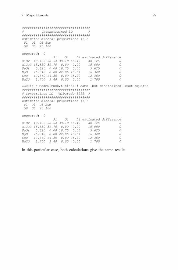
################################### # Unconstrained LQ # ################################### Estimated mineral proportions (%): Pl Ol Di Sum 50 30 20 100 Rsquared: 0 Pl Ol Di estimated difference SiO2 48.125 50.54 39.19 55.49 48.125 0 Al2O3 15.850 31.70 0.00 0.00 15.850 0 FeOt 5.625 0.00 18.75 0.00 5.625 0 MgO 16.340 0.00 42.06 18.61 16.340 0 CaO 12.360 14.36 0.00 25.90 12.360 0 Na2O 1.700 3.40 0.00 0.00 1.700 0
################################### # Constrained LQ (Albarede 1995) # ################################### Estimated mineral proportions (%): Pl Ol Di Sum 50 30 20 100 Rsquared: 0 Pl Ol Di estimated difference SiO2 48.125 50.54 39.19 55.49 48.125 0 Al2O3 15.850 31.70 0.00 0.00 15.850 0 FeOt 5.625 0.00 18.75 0.00 5.625 0 MgO 16.340 0.00 42.06 18.61 16.340 0 CaO 12.360 14.36 0.00 25.90 12.360 0 Na2O 1.700 3.40 0.00 0.00 1.700 0
97
GCDkit-> ModeC(rock,t(mins)) # same, but constrained least-squares
Major Elements9
In this particular case, both calculations give the same results.
Part III Modelling Trace Elements
Equilibrium (the underlying assumption to most petrological and geochemical modelling) is attained when the activities of all components in the geological sys-tem become equal (Spear 1994). In magma, such equilibrium should govern the partitioning of an element between the crystal and surrounding liquid. However, the relationships between activities and concentrations are not straightforward, as it is difficult, if not impossible, to express them in a rigorous form for all elements and minerals present in the system. Hence, geochemical modelling relies on sev-eral simplifying assumptions.
For major elements, the mineral chemistry is generally nearly constant during melting or crystallization. Thus the easiest approach is to ignore the activities al-together, and measure, or assume, the mineral chemistries. Note, however, that even in this case activities and equilibria can be calculated (Holland and Powell 1998).
Trace elements1 pose a different challenge. With a few exceptions (Kelsey and Powell 2011), no activity–composition models are available. Also, the trace-element contents in minerals are highly variable, and usually poorly constrained. It is, therefore, generally not possible to use the same mass-balance approach as for major elements.
In the case of trace elements that occur in small amounts in the crystal lattice (so are sufficiently ‘dilute’), the activity should be proportional to their concentra-tion (Henry 1803). The coefficient of proportionality depends on the nature of the mineral but not on the concentration of the element. Consequently, activities can be again ignored and replaced by the simpler concept of element partitioning be-tween different phases (in igneous petrology, a liquid and crystal(s)). Whereas the major-element modelling relies on the absolute concentrations in the solid phase, the key parameter for the trace elements is the ratio of their concentrations in the solid phases and the liquid (Chap. 10).
1 In this text the term “trace element” implies low whole-rock content. However, such an element
can still be the main component of an accessory mineral, as is the case for Zr in zircon (ZrSiO4).
This approach, however, fails when dealing with trace-element-rich phases. Some elements, termed essential structural constituents (ESC) (Hanson and Langmuir 1978), form a substantial part of the crystal lattice of certain accessory minerals. These are e.g., Zr in zircon, P in apatite or P, Th and LREE in monazite. Henry’s Law is not applicable anymore and the strategy based on partition coefficients is inappropriate. Furthermore, activity–composition relationships are not perfectly, or not at all, established. The best approach is therefore largely em-pirical, based on experiments and on the notion of the mineral solubility in a sili-cate melt (Chap. 13).
100 PART III Modelling Trace Elements
Hanson GN, Langmuir CH (1978) Modelling of major elements in mantle–melt systems using trace element approaches. Geochim Cosmochim Acta 42:725–741
Henry W (1803) Experiments on the quantity of gases absorbed by water, at different temperatures, and under different pressures. Phil Trans R Soc London 93:29–274
Holland TJB, Powell R (1998) An internally consistent thermodynamic dataset for phases of petrological interest. J Metamorph Geol 16:309–343
Kelsey DE, Powell R (2011) Progress in linking accessory mineral growth and breakdown to major mineral evolution in metamorphic rocks: a thermodynamic approach in the Na2O–CaO–K2O–FeO–MgO–Al2O3–SiO2–H2O–TiO2–ZrO2 system. J Metamorph Geol 29:151–166
Spear FS (1994) Metamorphic phase equilibria and pressure–temperature–time paths. Mineralogical Society of America Monographs. Mineralogical Society of America, Washington
References
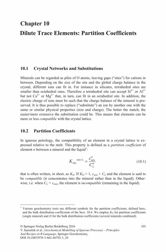
Chapter 10 Dilute Trace Elements: Partition Coefficients
10.1 Crystal Networks and Substitutions
Minerals can be regarded as piles of O atoms, leaving gaps (“sites”) for cations in between. Depending on the size of the site and the global charge balance in the crystal, different ions can fit in. For instance in silicates, tetrahedral sites are smaller than octahedral ones. Therefore a tetrahedral site can accept Si4+ or Al3+ but not Ca2+ or Mg2+ that, in turn, can fit in an octahedral site. In addition, the electric charge of ions must be such that the charge balance of the mineral is pre-served. It is thus possible to replace (“substitute”) an ion by another one with the same or similar physical properties (size and charge). The better the match, the easier/more extensive the substitution could be. This means that elements can be more or less compatible with the crystal lattice.
10.2 Partition Coefficients
In igneous petrology, the compatibility of an element in a crystal lattice is ex-pressed relative to the melt. This property is defined as a partition coefficient of element between a mineral and the liquid : 1
/min L minD
L
cKC
(10.1)
that is often written, in short, as KD. If KD > 1, cmin > CL and the element is said to be compatible (it concentrates into the mineral rather than in the liquid). Other-wise, i.e. when CL > cmin, the element is incompatible (remaining in the liquid).
1 Various geochemistry texts use different symbols for the partition coefficients, defined here,
and the bulk distribution coefficients of the Sect. 10.4. We employ KD for partition coefficients (single mineral) and D for the bulk distribution coefficients (several minerals combined).
© Springer-Verlag Berlin Heidelberg 2016 V. Janoušek et al., Geochemical Modelling of Igneous Processes – Principles And Recipes in R Language, Springer Geochemistry, DOI 10.1007/978-3-662-46792-3_10
101
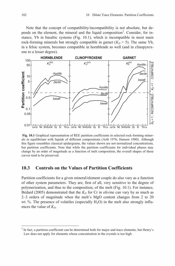
Note that the concept of compatibility/incompatibility is not absolute, but de-pends on the element, the mineral and the liquid composition . Consider, for in-stance, Yb in basaltic systems (Fig. 10.1), which is incompatible in most main rock-forming minerals but strongly compatible in garnet (KD > 5). The same Yb, in a felsic system, becomes compatible in hornblende as well (and in clinopyrox-ene to a lesser degree).
2
Fig. 10.1 Graphical representation of REE partition coefficients in selected rock-forming miner-als in equilibrium with liquids of different compositions (Arth 1976; Hanson 1980). Although this figure resembles classical spidergrams, the values shown are not normalized concentrations, but partition coefficients. Note that while the partition coefficients for individual phases may change by an order of magnitude as a function of melt composition, the overall shapes of these curves tend to be preserved.
10.3 Controls on the Values of Partition Coefficients
Partition coefficients for a given mineral/element couple do also vary as a function of other system parameters. They are, first of all, very sensitive to the degree of polymerization, and thus to the composition, of the melt (Fig. 10.1). For instance, Bédard (2005) demonstrated that the KD for Cr in olivine can vary by as much as 2–3 orders of magnitude when the melt’s MgO content changes from 2 to 20 wt. %. The presence of volatiles (especially H2O) in the melt also strongly influ-ences the value of KD.
2 In fact, a partition coefficient can be determined both for major and trace elements, but Henry’s
Law does not apply for elements whose concentration in the crystals is too high.
rhyolite
dacite
basalt
rhyolite
dacite
basalt
rhyolite
dacite
basalt
0.01
1
0.1
0.5
10
LaCe Nd SmEuGd Dy Er YbLu
5
10050
0.05
LaCe Nd SmEuGd Dy Er YbLu LaCe Nd SmEuGd Dy Er YbLu
Part
ition
coe
ffici
ent
K
HORNBLENDEDhbl/L K
CLINOPYROXENEDcpx/L K
GARNETDgrt/L
K D >
1 :
CO
MPA
TIBL
EK D
< 1
: IN
COM
PATI
BLE
102 10 Dilute Trace Elements: Partition Coefficients
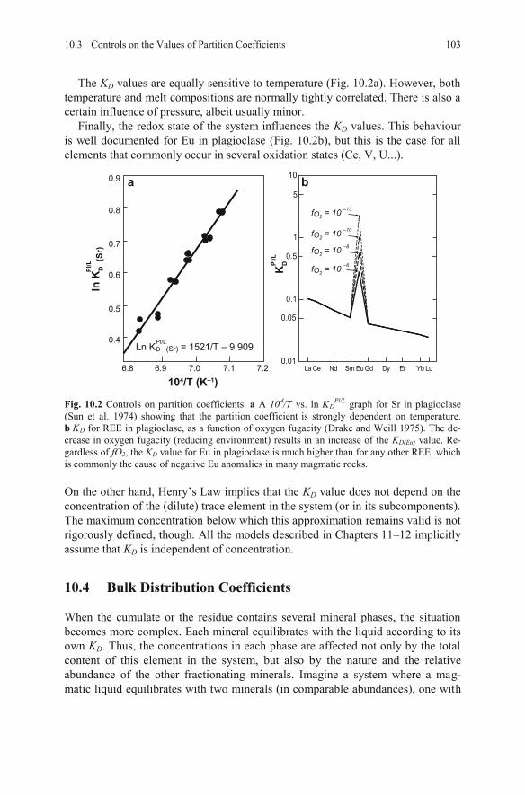
The KD values are equally sensitive to temperature (Fig. 10.2a). However, both temperature and melt compositions are normally tightly correlated. There is also a certain influence of pressure, albeit usually minor.
Finally, the redox state of the system influences the KD values. This behaviour is well documented for Eu in plagioclase (Fig. 10.2b), but this is the case for all elements that commonly occur in several oxidation states (Ce, V, U...).
Fig. 10.2 Controls on partition coefficients. a A 104/T vs. ln KDPl/L graph for Sr in plagioclase
(Sun et al. 1974) showing that the partition coefficient is strongly dependent on temperature. b KD for REE in plagioclase, as a function of oxygen fugacity (Drake and Weill 1975). The de-crease in oxygen fugacity (reducing environment) results in an increase of the KD(Eu) value. Re-gardless of fO2, the KD value for Eu in plagioclase is much higher than for any other REE, which is commonly the cause of negative Eu anomalies in many magmatic rocks.
On the other hand, Henry’s Law implies that the KD value does not depend on the concentration of the (dilute) trace element in the system (or in its subcomponents). The maximum concentration below which this approximation remains valid is not rigorously defined, though. All the models described in Chapters 11–12 implicitly assume that KD is independent of concentration.
10.4 Bulk Distribution Coefficients
When the cumulate or the residue contains several mineral phases, the situation becomes more complex. Each mineral equilibrates with the liquid according to its own KD. Thus, the concentrations in each phase are affected not only by the total content of this element in the system, but also by the nature and the relative abundance of the other fractionating minerals. Imagine a system where a mag-matic liquid equilibrates with two minerals (in comparable abundances), one with
10.3 Controls on the Values of Partition Coefficients 103
0.01
1
0.1
0.5
10
La Ce Nd Sm EuGd Dy Er Yb Lu
5
0.05
0.4
0.5
0.6
0.7
0.8
0.9
6.8 6.9 7.0 7.1 7.2
Ln K (Sr) = 1521/T – 9.909 Pl/L
D
a b
104/T (K–1)
(Sr)
ln K
DPl/
L
KDP
l/L
fO2 = 10 –13
fO2 = 10 –10
fO2 = 10 –8
fO2 = 10 –6
high KD, and another with low KD. The high-KD phase would extract from the liq-uid almost all the element—leaving even less available for the low-KD one.
This leads to the concept of a “bulk distribution coefficient”, D, that accounts for the behaviour of the solid phases as a whole. It can be expressed as the ratio of the concentration in the bulk solid (CS) and in the liquid (CL):
(10.2)
Contrarily to CL that is a single phase, CS refers to the bulk solid, which is typi-cally made of several minerals. Consequently, the trace-element content in the cumulate (or residue) can be expressed as a mixture of n mineral phases. There-fore, the mass-balance reads:
n
S i ii
C m c (10.3)
Combination of previous equations yields:
(10.4)
In this way, D is expressed as a function of the partition coefficients for individual minerals. In petrogenetic modelling, D is a key parameter, exerting strong influ-ence on trace-element behaviour.
References
Arth JG (1976) Behavior of trace elements during magmatic processes: a summary of theoretical models and their applications. J Res US Geol Surv 4:41–47
Bédard J (2005) Partitioning coefficients between olivine and silicate melts. Lithos 83:394–419Drake MJ, Weill DF (1975) Partition of Sr, Ba, Ca, Y, Eu2+, Eu3+ and other REE between pla-
gioclase feldspar and magmatic liquid: an experimental study. Geochim Cosmochim Acta 39:689–712
Hanson GN (1980) Rare earth elements in petrogenetic studies of igneous systems. Ann Rev Earth Planet Sci 8:371–406
Sun C-O, Williams RJ, Sun S-S (1974) Distribution coefficients of Eu and Sr for plagioclase–liquid and clinopyroxene–liquid equilibria in oceanic ridge basalt: an experimental study. Geochim Cosmochim Acta 38:1415–1433
104 10 Dilute Trace Elements: Partition Coefficients
/Li
niD
im K α= ∑
/ S
L
S L CDC
/S LD
=1
=1
Chapter 11 Direct (Dilute) Trace-Element Models
Trace-element modelling of crystallization or melting involves a balance between solid phases and melt assessed by the partitioning concept. Most geochemists use different equations for melting (batch melting) and crystallization (fractional crys-tallization). We will show, however, that this choice of models—warranted as it may be—is not the only option available. Deciding between batch and fractional processes can be critical in choosing a correct modelling strategy.
In batch (closed-system) processes, the direction of evolution (melting or frac-tionation) is irrelevant, and the numerical expression identical, since they are both governed exclusively by the mass balance between the solid and the liquid. On the other hand, the formulation is distinct for fractional melting and crystallization, as these represent essentially open systems.
The logic for mixing modelling is rather different. Partitioning between liquid and solid phases is not a factor anymore. Mixing is, normally, treated in the same way for the whole range of elements although it will be shown that certain ap-proaches—seldom used for majors—may be more useful for trace elements.
Equilibrium, batch, fractional—a matter of terminology In the geochemical literature, several terms are deeply ingrained. Melting is
described as “batch” or “fractional”, whereas crystallization is “equilibrium” (rarely) or “fractional” (more commonly, to the point that sometimes “fractiona-tion” is used as a synonym for “crystallization”).
The term “equilibrium” is somewhat misleading—as fractional processes also involve equilibrium between the melt and crystals, albeit an infinitesimal one (see Part V, Sect. 24.2). In addition, “batch” melting and “equilibrium” crystallization refer to very similar processes, i.e. those without separation of the liquid from the solid before their completion.
We therefore decided to use “batch” and “fractional” qualifiers for both melt-ing and crystallization—which in this book results in the absence of the term “equilibrium crystallization” and its replacement by the (so far) uncommon ex-pression “batch crystallization”.
© Springer-Verlag Berlin Heidelberg 2016 V. Janoušek et al., Geochemical Modelling of Igneous Processes – Principles And Recipes in R Language, Springer Geochemistry, DOI 10.1007/978-3-662-46792-3_11
105
11.1 Crystallization
11.1.1 Batch Crystallization
During batch crystallization, newly crystallizing phases remain in the system (the crystals are not removed from the melt) until the process is complete. Such a situ-ation resembles that of experimental capsules (closed system). The liquid–relations can be described in terms of the mass balance:
0 (1 )L SC FC CF (11.1)
and Cs can be deduced from Eq. (10.2):
S LC DC (11.2)
thus giving:
0
(1 )LCC
D F D (11.3)
Although known as the “batch melting” equation (Gast 1968; Shaw 1970), it does also apply to batch crystallization.
11.1.2 Fractional Crystallization
In this scenario, the crystals are immediately removed from the system as they form. Therefore, the equilibrium defined by Eq. (10.2) exists only for infinitesimal crystal (or melt) amounts. The differential expression linking the liquid composi-tion with its amount, F, is:
( 1) L
L
dCdFDF C
(11.4)
In order to get a general expression, Eq. (11.4) must be integrated over the whole range of relevant F values. As demonstrated e.g. in Albarède (1995) or Zou (2007), for constant D this leads to the equation:
( 1)
0
DLC FC
(11.5)
known as Rayleigh’s fractionation law, initially established for gas fractionation (Rayleigh 1896). For strongly incompatible elements (D ~ 0), it changes to:
106 11 Direct (Dilute) Trace-Element Models
solid
0
1LCC F
(11.6)
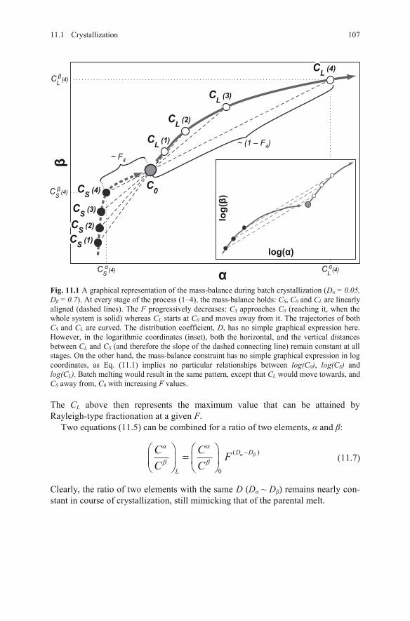
Fig. 11.1 A graphical representation of the mass-balance during batch crystallization (D = 0.05, D = 0.7). At every stage of the process (1–4), the mass-balance holds: CS, C0 and CL are linearly aligned (dashed lines). The F progressively decreases: CS approaches C0 (reaching it, when the whole system is solid) whereas CL starts at C0 and moves away from it. The trajectories of both CS and CL are curved. The distribution coefficient, D, has no simple graphical expression here. However, in the logarithmic coordinates (inset), both the horizontal, and the vertical distances between CL and CS (and therefore the slope of the dashed connecting line) remain constant at all stages. On the other hand, the mass-balance constraint has no simple graphical expression in log coordinates, as Eq. (11.1) implies no particular relationships between log(C0), log(CS) and log(CL). Batch melting would result in the same pattern, except that CL would move towards, and CS away from, C0 with increasing F values.
The CL above then represents the maximum value that can be attained by Rayleigh-type fractionation at a given F.
Two equations (11.5) can be combined for a ratio of two elements, and :
( )
0
D D
L
C C FC C
(11.7)
Clearly, the ratio of two elements with the same D (D ~ D ) remains nearly con-stant in course of crystallization, still mimicking that of the parental melt.
C0
CL (4)
~ F4
~ (1 – F4)
CS (4)CS (4)CS (4)
CS (3)CS (3)CS (3)
CS (2)CS (2)CS (2)
CS (1)CS (1)CS (1)
CL (4)CL (4)CL (4)
CL (3)CL (3)CL (3)
CL (2)CL (2)CL (2)
CL (1)CL (1)CL (1)
α
β
α
CL (4)β
CS (4)α
CS (4)β
log(α)
log(
β)
11.1 Crystallization 107
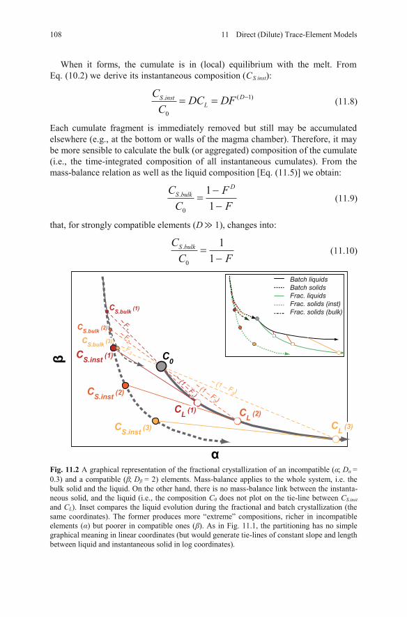
When it forms, the cumulate is in (local) equilibrium with the melt. From
( 1).
0
DS instL
C D DFC
C (11.8)
Each cumulate fragment is immediately removed but still may be accumulated elsewhere (e.g., at the bottom or walls of the magma chamber). Therefore, it may be more sensible to calculate the bulk (or aggregated) composition of the cumulate (i.e., the time-integrated composition of all instantaneous cumulates). From the mass-balance relation as well as the liquid composition [Eq. (11.5)] we obtain:
.
0
11
DS bulkC FC F
(11.9)
that, for strongly compatible elements (D 1), changes into:
.
0
11
S bulkCC F
(11.10)
Fig. 11.2 A graphical representation of the fractional crystallization of an incompatible ( D =0.3) and a compatible ( D = 2) elements. Mass-balance applies to the whole system, i.e. the bulk solid and the liquid. On the other hand, there is no mass-balance link between the instanta-neous solid, and the liquid (i.e., the composition C0 does not plot on the tie-line between CS.instand CL). Inset compares the liquid evolution during the fractional and batch crystallization (the same coordinates). The former produces more “extreme” compositions, richer in incompatibleelements ( ) but poorer in compatible ones ( ). As in Fig. 11.1, the partitioning has no simple graphical meaning in linear coordinates (but would generate tie-lines of constant slope and length between liquid and instantaneous solid in log coordinates).
~ (1 – F3 )
~ (1 – F3 )
~ (1 – F3 )
CS.inst (1)CS.inst (1)CS.inst (1)
CS.inst (2)CS.inst (2)CS.inst (2)
CS.inst (3)CS.inst (3)CS.inst (3)
CL (1)CL (1)CL (1) CL (2)CL (2)CL (2)
CL (3)CL (3)CL (3)
CS.bulk (1)CS.bulk (1)CS.bulk (1)
CS.bulk (2)CS.bulk (2)CS.bulk (2)
CS.bulk (3)CS.bulk (3)CS.bulk (3)
~ F1
~ F1
~ F1
~ (1 – F1 )
~ (1 – F1 )
~ (1 – F1 )
~ F2
~ F2
~ F2
~ (1 – F2 )
~ (1 – F2 )
~ (1 – F2 )
α
β C0
~ F3
~ F3
~ F3
Batch liquidsBatch solidsFrac. liquidsFrac. solids (inst)Frac. solids (bulk)
108 11 Direct (Dilute) Trace-Element Models
Eq. (10.2) we derive its instantaneous composition (CS.inst):
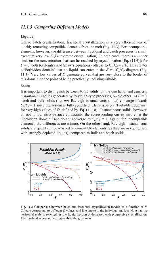
11.1.3 Comparing Different Models
Liquids Unlike batch crystallization, fractional crystallization is a very efficient way of quickly removing compatible elements from the melt (Fig. 11.3). For incompatible elements, however, the difference between fractional and batch processes is small, except at very low F (i.e. extreme crystallization). In both cases, there is an upper limit on the concentration that can be reached by crystallization [Eq. (11.6)]: for D = 0, both Rayleigh’s and Shaw’s equations collapse to CL/C0 = 1/F. This creates a ‘Forbidden domain’ that no liquid can enter in the F vs. CL/C0 diagram (Fig. 11.3). Very low values of D generate curves that are very close to the border of this domain, to the point of being practically undistinguishable.
Solids It is important to distinguish between batch solids, on the one hand, and bulk and instantaneous solids generated by Rayleigh-type processes, on the other. At F = 0, batch and bulk solids (but not Rayleigh instantaneous solids) converge towards Cs/C0 = 1 since the system is fully solidified. There is also a ‘Forbidden domain’, for very high values of D, defined by Eq. (11.10). Instantaneous solids, however,do not follow mass-balance constraints; the corresponding curves may enter the‘Forbidden domain’, and do not converge to elements, the differences are minute. On the other hand, Rayleigh instantaneous solids are quickly impoverished in compatible elements (as they are in equilibriumwith strongly depleted liquids), compared to bulk and batch solids.
Fig. 11.3 Comparison between batch and fractional crystallization models as a function of F.Colours correspond to different D values, and line stroke to the individual models. Note that the horizontal scale is reverted, as the liquid fraction F decreases with progressive crystallization. The ‘Forbidden domain’ corresponds to the grey areas.
a – Liquids
1.0 0.8 0.6 0.4 0.2 0.0F
0.001
0.01
0.1
110
100
1.0 0.8 0.6 0.4 0.2 0.0F
0.001
0.01
0.1
110
100
Batch crystallization (or melting)Batch crystallization (or melting)Batch crystallization (or melting)Rayleigh crystallizationRayleigh crystallizationRayleigh crystallization
b – Solids
CL/
C0
CS/C
0
D = 0.01D = 0.5D = 2D = 5
Forbidden domain(above D = 0)
Forbidden domain(above D = 0)
Batch crystallization (or melting)Batch crystallization (or melting)Batch crystallization (or melting)Rayleigh crystal. – instantaneous solidRayleigh crystal. – instantaneous solidRayleigh crystal. – instantaneous solidRayleigh crystallization – bulk solidRayleigh crystallization – bulk solidRayleigh crystallization – bulk solid
D = 0.01D = 0.5D = 2D = 5
11.1 Crystallization 109
CL/C0 = 1. Again, for incompatible
11.2 Melting
11.2.1 Batch Melting
Batch melting can be described by the same equation as the batch crystallization [Eq. (11.3)]:
0
(1 )LCC
D F D(11.11)
In the batch melting equation, D corresponds to the bulk distribution coef-ficient of the solid residue after melting (so not of the original source). Ex-
pressions using the mode of the original source are given in Sect. 11.2.4.
11.2.2 Fractional Melting
When the melt is progressively extracted, the system behaves symmetrically to the fractional crystallization. In this case, the phase leaving is the melt, and that stay-ing behind the solid residue. Similarly to the Rayleigh-type fractional crystalliza-tion [Eq. (11.5)], integrating the instantaneous mass-balance equation gives:
1 1
0
(1 ) DSC FC
(11.12)
Note the symmetry of this formulation with Eq. (11.5), if substituting F by 1 – Fand D by 1/D. Both equations refer to the composition of the non-extracted phase, i.e. CL for fractional crystallization, but CS for fractional melting.
As, at any moment, the instantaneous liquid equilibrates with the solid, the combination of equations (10.2) and (11.12) gives the composition of a single melt increment at a given melt fraction F:
(11.13)
This equation describes the evolution of each (infinitesimally small) drop of melt as it forms, just before it is extracted from the source. Actually, each successive melt increment is likely to be collected, mixed with the previously formed melt, and re-homogenized, but not necessarily at the melting site. The mass-balance re-lation holds between the source, the aggregated liquid and the solid, allowing derivation of the equation for fractional melting with accumulation (also known as aggregated melting). Again, note that the form of this equation resembles
110 11 Direct (Dilute) Trace-Element Models
1 1.
0
(1 )1 DL instC FC D
⎛ ⎞−⎜ ⎟⎝ ⎠= −
Eq. (11.9):
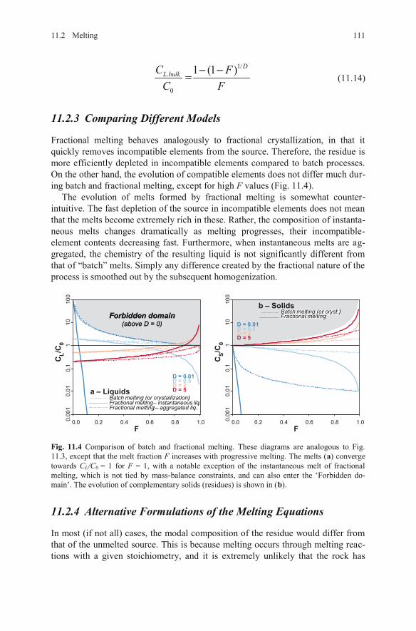
(11.14)
11.2.3 Comparing Different Models
Fractional melting behaves analogously to fractional crystallization, in that it quickly removes incompatible elements from the source. Therefore, the residue is more efficiently depleted in incompatible elements compared to batch processes. On the other hand, the evolution of compatible elements does not differ much dur-ing batch and fractional melting, except for high F values (Fig. 11.4).
The evolution of melts formed by fractional melting is somewhat counter-intuitive. The fast depletion of the source in incompatible elements does not mean that the melts become extremely rich in these. Rather, the composition of instanta-neous melts changes dramatically as melting progresses, their incompatible-element contents decreasing fast. Furthermore, when instantaneous melts are ag-gregated, the chemistry of the resulting liquid is not significantly different from that of “batch” melts. Simply any difference created by the fractional nature of the process is smoothed out by the subsequent homogenization.
Fig. 11.4 Comparison of batch and fractional melting. These diagrams are analogous to Fig. 11.3, except that the melt fraction F increases with progressive melting. The melts (a) converge towards CL/C0 = 1 for F = 1, with a notable exception of the instantaneous melt of fractional melting, which is not tied by mass-balance constraints, and can also enter the ‘Forbidden do-main’. The evolution of complementary solids (residues) is shown in (b).
11.2.4 Alternative Formulations of the Melting Equations
In most (if not all) cases, the modal composition of the residue would differ from that of the unmelted source. This is because melting occurs through melting reac-tions with a given stoichiometry, and it is extremely unlikely that the rock has
a – Liquids
Batch melting (or cryst.)Batch melting (or cryst.)Fractional meltingFractional melting
0.0 0.2 0.4 0.6 0.8 1.0
F
0.001
0.01
0.1
110
100
0.0 0.2 0.4 0.6 0.8 1.0
F
0.001
0.01
0.1
110
100
CL/C0
CS/C0
Forbidden domain(above D = 0)
Forbidden domain(above D = 0)
b – Solids
Batch melting (or crystallization)Batch melting (or crystallization)Fractional melting– instantaneous liq.Fractional melting– instantaneous liq.Fractional melting– aggregated liq.Fractional melting– aggregated liq.
D = 0.01D = 0.5D = 2D = 5
D = 0.01D = 0.5D = 2D = 5
11.2 Melting 111
1/.
0
1 (1 ) D
L bulkC FC F
− −=
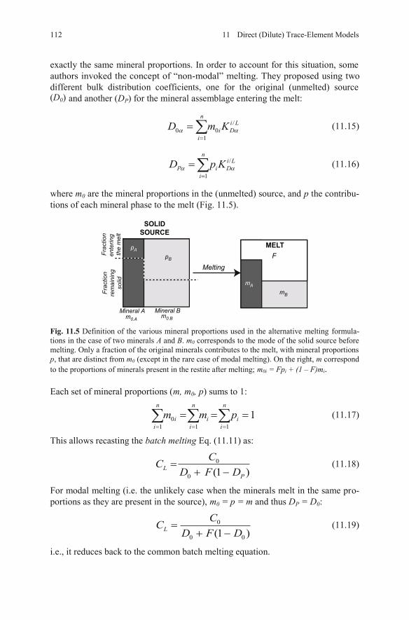
pt of “non-modal” melting. They proposed using two
and another (DP) for the mineral assemblage entering the melt:
0 01
/in
ii
LDD m K (11.15)
/
1
n
P Di
i LiD p K (11.16)
where m0 are the mineral proportions in the (unmelted) source, and p the contribu-tions of each mineral phase to the melt (Fig. 11.5).
Fig. 11.5 Definition of the various mineral proportions used in the alternative melting formula-tions in the case of two minerals A and B. m0 corresponds to the mode of the solid source before melting. Only a fraction of the original minerals contributes to the melt, with mineral proportions p, that are distinct from m0 (except in the rare case of modal melting). On the right, m correspond to the proportions of minerals present in the restite after melting; m0i = Fpi + (1 – F)mi.
Each set of mineral proportions (m, m0, p) sums to 1:
01 1 1
1n n n
i i ii i i
m m p (11.17)
This allows recasting the batch melting Eq. (11.11) as:
0
0
(1 )L
P
CCD F D
(11.18)
For modal melting (i.e. the unlikely case when the minerals melt in the same pro-portions as they are present in the source), m0 = p = m and thus DP = D0:
0
0 0(1 )LCC
D F D(11.19)
i.e., it reduces back to the common batch melting equation.
PRIMITIVEMELT
MELT
C0
F
1-p
SOLIDSOURCE
Melting
Frac
tion
ente
ring
the
mel
t
Frac
tion
rem
aini
ngso
lid
Mineral A Mineral Bm0.A m0.B
mA
mB
pA
pB
112 11 Direct (Dilute) Trace-Element Models
exactly the same mineral proportions. In order to account for this situation, someauthors invoked the concedifferent bulk distribution coefficients, one for the original (unmelted) source(D0)
Analogous notation can be used to describe fractional melting:
(11.20)
and fractional melting with accumulation:
(11.21)
Whether these formulations are more useful than the ones using the D based on the solid residue depends on the specific problem.
In all the models proposed above, D is taken as a constant throughout the fractionation/melting history. This is actually highly unlikely, because, in natural systems, (1) the proportions of the crystallizing phases may change,
abruptly or gradually, during fractionation (e.g., amphibole replaces pyroxene dur-ing the fractional crystallization of a calc-alkaline magma) as may the stoichio-metry of the melting reactions, and (2) the K D values depend on the compositionof the liquid, as well as P–T conditions. This issue can be tackled by two methods:
Analytical approachEquation (11.5) can be adapted to the case of variable D. For instance, when D is
F, D a bF , it becomes (Greenland 1970):
( 1)L
L
dC dFa FF
bC
(11.22)
which integrates to:
1 ln ( 1)0
F b FL
aC C e (11.23)
11311.2 Melting
1 1
0.
0 0
1PD
PL inst
C D FCD D
⎛ ⎞−⎜ ⎟
⎝ ⎠⎛ ⎞−⎜ ⎟
⎝ ⎠=
0
1
0.
0
1 1D
PL bulk
C D FCF D
⎛ ⎞⎛ ⎞⎜ ⎟= − −⎜ ⎟⎜ ⎟⎝ ⎠⎜ ⎟⎝ ⎠
The original definition of the batch melting equation [Eq. (11.11)] may be superior in that it takes into account modal proportions after melting. Thus
it can be applied universally, for modal as well as non-modal melting. On the other hand, it requires knowledge (or assumptions) of the modal composition of the restite that may or may not be easier to obtain than the initial modal composi-tion of the source prior to melting.
a linear function of
Note that if b = 0, D is constant and the equation collapses to Rayleigh’s law.It is possible to derive analogous, or even more complex equations (Zou 2007), by putting other constraints on the evolution of D during fractionation (or by writing similar equations for melting). However, one is limited to cases when it is possible to express D evolution using a (reasonably simple) mathematical function1.
Numerical approachA more empirical approach consists in breaking down the melting (or crystalliza-tion) process into several successive steps, during each of which D can be as-sumed to be constant. For each stage t, C0(t) is taken as being the end-product of the previous one (CL(t–1)); thus D is calculated using the modal composition of the cumulate/residue stable during the specific step. This modal composition can be constrained by petrology, experimental data or otherwise [Worked Example 2].
11.3 Mixing
The mixing equation for individual (major or trace) elements relies on a simple mass balance, and consequently, it does not invoke any partitioning at all. There-fore, Eq. 6.24 established for the major-elements is also applicable for traces, and the graphical representation remains the same (cf. Fig. 6.9):
1
( )m
M k kk
C f C (11.24)
11.3.1 Ratio of Two Elements During Binary Mixing
When two components (1 and 2) mix in proportions f such that f1 + f2 = 1, the rela-tion between two elements ( and ) in the mixture can be established as follows:
1 1 1 2
1 1 1 2
(1 )(1 )
MM
M
C f C f CRC f C f C
(11.25)
11.3.2 Mixing Hyperbolae in Ratio–Ratio Plots
The treatment of binary mixing in a ratio–ratio plot of four trace elements (a, b, u and v) (Fig. 11.6) stems from Vollmer (1976) and Langmuir et al. (1978) with
2
1 Specifically, one that can be integrated symbolically. Of course, it is always possible to inte-
grate any differential equation using numerical methods such as finite differences implemented in R, for instance in the package RootSolve.
2 Ratios between two major elements, or a major and a trace element, would behave in the same way but are seldom used.
114 11 Direct (Dilute) Trace-Element Models
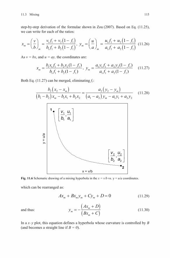
step-by-step derivation of the formulae shown in Zou (2007). Based on Eq. (11.25),
1 1 2 1
1 1 2 1
1
1mm
v f v fvxb b f b f
, 1 1 2 1
1 1 2 1
1
1mm
u f u fuya a f a f
(11.26)
As v = bx, and u = ay, the coordinates are:
1 1 1 2 2 1
1 1 2 1
(1 )(1 )m
b x f b x fxb f b f
, 1 1 1 2 2 1
1 1 2 1
(1 )(1 )m
a y ya
f a fyf a f
(11.27)
Both Eq. (11.27) can be merged, eliminating f1:
2 2 2 2
1 2 1 1 2 2 1 2 1 1 2 2
m m
m m
b x x ab b x b x b x a a
yy
yy a a y
(11.28)
Fig. 11.6 Schematic drawing of a mixing hyperbola in the x = v/b vs. y = u/a coordinates.
which can be rearranged as:
0m m m mAx Bx y Cy D (11.29)
and thus: mm
m
Axy
x CD
B(11.30)
In a x–y plot, this equation defines a hyperbola whose curvature is controlled by B(and becomes a straight line if B = 0).
1
x = v/b
y =
u/a
2
1 1
1 1
,v u
b a
� �
� �
� �
2 2
2 2
,v u
b a
� �
� �
� �
11511.3 Mixing
we can write for each of the ratios:
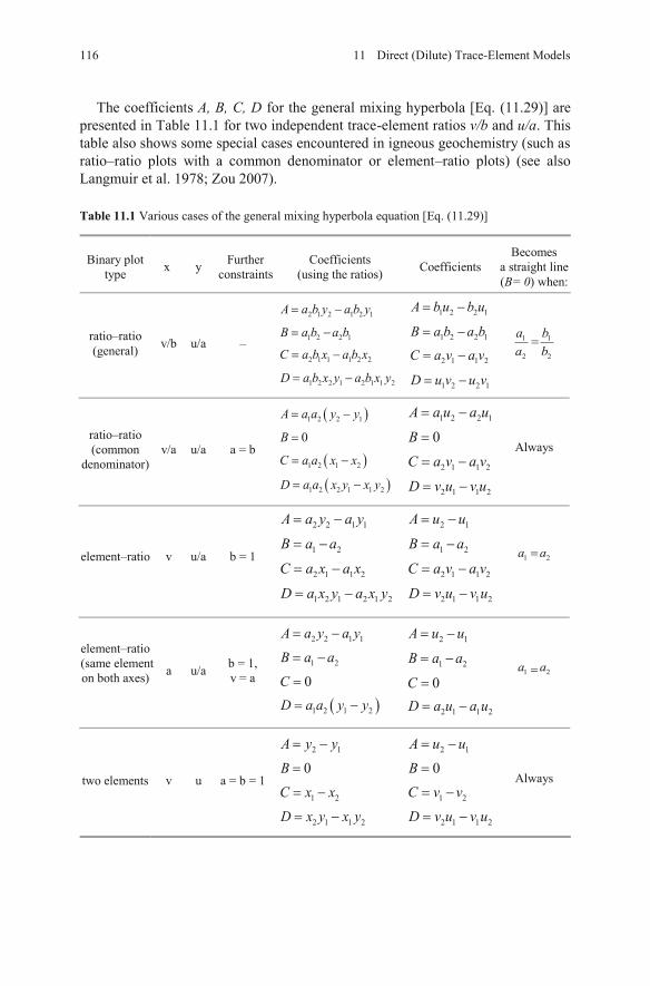
The coefficients A, B, C, D for the general mixing hyperbola [Eq. (11.29)] are presented in Table 11.1 for two independent trace-element ratios v/b and u/a. This table also shows some special cases encountered in igneous geochemistry (such as ratio–ratio plots with a common denominator or element–ratio plots) (see also Langmuir et al. 1978; Zou 2007).
Table 11.1 Various cases of the general mixing hyperbola equation [Eq. (11.29)]
Binary plot type x y Further
constraintsCoefficients
(using the ratios) CoefficientsBecomes
a straight line (B= 0) when:
ratio–ratio(general) v/b u/a –
2 1 2 1 2 1
1 2 2 1
2 1 1 1 2 2
1 2 2 1 2 1 1 2
A a b y a b y
B a b a b
C a b x a b x
D a b x y a b x y
1 2 2 1
1 2 2 1
2 1
2 11 2
1 2
u u
v v
A b b
B a b a b
C a a
D u uv v
1 1
2 2
a ba b
ratio–ratio (common
denominator)v/a u/a a = b
1 2 2 1
1 2 1
1 2 2 1 1
2
2
0
A a a y y
B
C a a x x
D a a x y x y
1 2 2
2 1 2
2 1 1 2
1
1
0
v
A a u a u
B
C a a
D
v
v u v u
Always
element–ratio v u/a b = 1
2 2 1 1
1 2
2 1 1 2
1 2 1 2 1 2
A a y a y
B a a
C a x a x
D a x y a x y
2 1
1 2
2 1 1 2
2 1 1 2
v
A u u
B a a
C a a
D v
v
v u u
1 2 a a
element–ratio (same elementon both axes) a u/a b = 1,
v = a
2 2 1 1
1 2
1 2 1 2
0
A a y a y
B a a
CD a a y y
2 1
1 2
2 1 1 2
0
A u u
B a a
CD a u a u
1 2 a a
two elements v u a = b = 1
2 1
1 2
2 1 1 2
0
A y y
BC x x
D x y x y
2 1
1 2
2 1 1 2
0
A u u
BC v v
D v u v u
Always
116 11 Direct (Dilute) Trace-Element Models
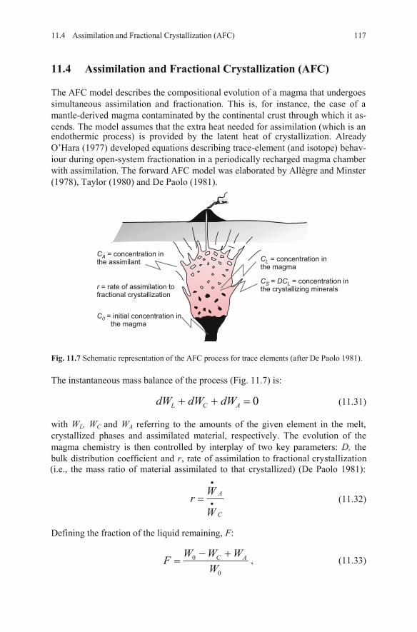
endothermic process) is provided by the latent heat of crystallization. AlreadyO’Hara (1977) developed equations describing trace-element (and isotope) behav-iour during open-system fractionation in a periodically recharged magma chamber with assimilation. The forward AFC model was elaborated by Allègre and Minster (1978), Taylor (1980) and De Paolo (1981).
Fig. 11.7 Schematic representation of the AFC process for trace elements (after De Paolo 1981).
The instantaneous mass balance of the process (Fig. 11.7) is:
0L C AdW dW dW (11.31)
with WL, WC and WA referring to the amounts of the given element in the melt, crystallized phases and assimilated material, respectively. The evolution of the magma chemistry is then controlled by interplay of two key parameters: D, the bulk distribution coefficient and r, rate of assimilation to fractional crystallization (i.e., the mass ratio of material assimilated to that crystallized) (De Paolo 1981):
A
C
WrW
(11.32)
Defining the fraction of the liquid remaining, F:
0
0
C AW W WFW
, (11.33)
11.4 Assimilation and Fractional Crystallization (AFC) 117
11.4 Assimilation and Fractional Crystallization (AFC)
The AFC model describes the compositional evolution of a magma that undergoes simultaneous assimilation and fractionation. This is, for instance, the case of a mantle-derived magma contaminated by the continental crust through which it as-cends. The model assumes that the extra heat needed for assimilation (which is an
r = rate of assimilation tofractional crystallization
CA = concentration inthe assimilant CL = concentration in
the magma
CS = DCL = concentration inthe crystallizing minerals
C0 = initial concentration inthe magma
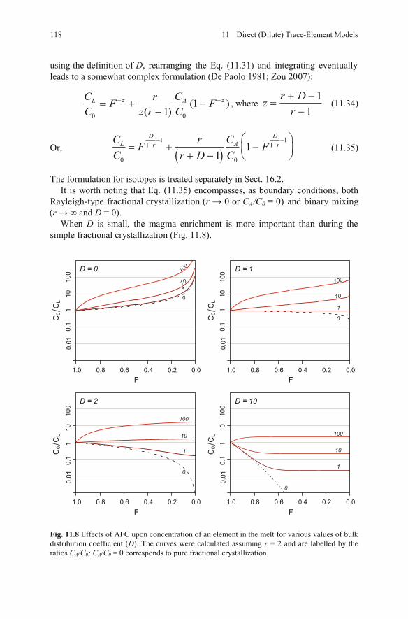
Or, 1 1
1
00
111
D DL Ar rC CrF F
C r D C (11.35)
The formulation for isotopes is treated separately in Sect. 16.2. It is worth noting that Eq. (11.35) encompasses, as boundary conditions, both
Rayleigh-type fractional crystallization (r 0 or CA/C0 = 0) and binary mixing and D = 0).
When D is small, the magma enrichment is more important than during the simple fractional crystallization (Fig. 11.8).
Fig. 11.8 Effects of AFC upon concentration of an element in the melt for various values of bulk distribution coefficient (D). The curves were calculated assuming r = 2 and are labelled by the ratios CA/C0; CA/C0 = 0 corresponds to pure fractional crystallization.
C0
CL
C0
CL
0.1
0.0
11
10
10
0
0.1
0.0
11
10
10
0
C0
CL
C0
CL
0.1
0.0
11
10
10
0
0.1
0.0
11
10
10
0
D = 0 D = 1
D = 10D = 2
1.0 0.8 0.6 0.4 0.2 0.0
F
1.0 0.8 0.6 0.4 0.2 0.0
F
1.0 0.8 0.6 0.4 0.2 0.0
F
1.0 0.8 0.6 0.4 0.2 0.0
F
0
10
100
1
0
0
0
1
1
1
10
10
10
100
100
100
118 11 Direct (Dilute) Trace-Element Models
using the definition of D, rearranging the Eq. (11.31) and integrating eventuallyleads to a somewhat complex formulation (De Paolo 1981; Zou 2007):
0 0
(1 )( 1)
z zL AC CrF FC z r C
, where 1
1r Dz
r (11.34)
(r
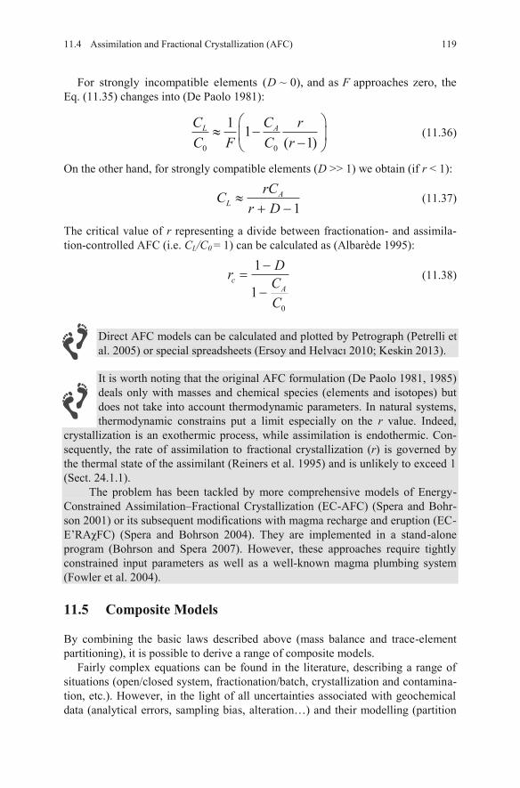
0 0
1 1( 1)
L AC C rC F C r
(11.36)
On the other hand, for strongly compatible elements (D >> 1) we obtain (if r < 1):
1A
LrCC
r D(11.37)
The critical value of r representing a divide between fractionation- and assimila-tion-controlled AFC (i.e. CL/C0 = 1) can be calculated as (Albarède 1995):
0
1
1c
A
Dr CC
(11.38)
Direct AFC models can be calculated and plotted by Petrograph (Petrelli et al. 2005) or special spreadsheets (Ersoy and Helvacı 2010; Keskin 2013).
It is worth noting that the original AFC formulation (De Paolo 1981, 1985) deals only with masses and chemical species (elements and isotopes) but does not take into account thermodynamic parameters. In natural systems, thermodynamic constrains put a limit especially on the r value. Indeed,
crystallization is an exothermic process, while assimilation is endothermic. Con-sequently, the rate of assimilation to fractional crystallization (r) is governed by the thermal state of the assimilant (Reiners et al. 1995) and is unlikely to exceed 1(Sect. 24.1.1).
The problem has been tackled by more comprehensive models of Energy-Constrained Assimilation–Fractional Crystallization (EC-AFC) (Spera and Bohr-son 2001) or its subsequent modifications with magma recharge and eruption (EC-E’RA FC) (Spera and Bohrson 2004). They are implemented in a stand-alone program (Bohrson and Spera 2007). However, these approaches require tightly constrained input parameters as well as a well-known magma plumbing system (Fowler et al. 2004).
11.5 Composite Models
By combining the basic laws described above (mass balance and trace-element partitioning), it is possible to derive a range of composite models.
Fairly complex equations can be found in the literature, describing a range of situations (open/closed system, fractionation/batch, crystallization and contamina-tion, etc.). However, in the light of all uncertainties associated with geochemical data (analytical errors, sampling bias, alteration…) and their modelling (partition
11911.4 Assimilation and Fractional Crystallization (AFC)
For strongly incompatible elements (D ~ 0), and as F approaches zero, the.35) changes into (De Paolo 1981): Eq. (11
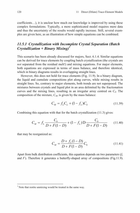
coefficients…), it is unclear how much our knowledge is improved by using these complex formulations. Typically, a more sophisticated model requires more data and thus the uncertainty of the results would rapidly increase. Still, several exam-ples are given here, as an illustration of how simple equations can be combined.
11.5.1 Crystallization with Incomplete Crystal Separation (Batch Crystallization + Binary Mixing) 3
This scenario has been already discussed for majors, Sect. 6.1.4. Similar equations can be derived for trace elements by coupling batch crystallization (the crystals are not separated from the residual melt!) and mixing equations. For major elements, both equations are expressed in terms of mass balance, and therefore identical, which in binary diagrams results in overlapping straight lines.
However, this does not hold for trace elements (Fig. 11.9). In a binary diagram, the liquid and cumulate compositions plot along curves, while mixing results in straight lines. So, contrary to major elements, both trends are not superposed. The mixtures between crystals and liquid plot in an area delimited by the fractionation curves and the mixing lines, resulting in an irregular array centred on C0. The composition of the mixture, CM, is given by the mass balance:
(1 )M SL LLC f C f C (11.39)
Combining this equation with that for the batch crystallization (11.3) gives:
0 0(1 )D(1 ) (1 )LM L
C CC f fD F D D F D
(11.40)
that may be reorganized as:
0(1 )(1 )M
LD f DC CD F D
(11.41)
3 Note that restite unmixing would be treated in the same way.
120 11 Direct (Dilute) Trace-Element Models
Apart from bulk distribution coefficients, this equation depends on two parameters (fLand F ). Therefore it generates a butterfly-shaped array of compositions (Fig.11.9).
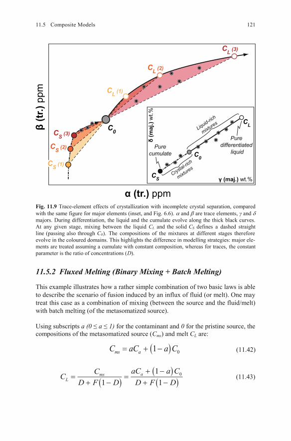
Fig. 11.9 Trace-element effects of crystallization with incomplete crystal separation, compared with the same figure for major elements (inset, and Fig. 6.6). and are trace elements, and majors. During differentiation, the liquid and the cumulate evolve along the thick black curves. At any given stage, mixing between the liquid CL and the solid CS defines a dashed straight line (passing also through C0). The compositions of the mixtures at different stages thereforeevolve in the coloured domains. This highlights the difference in modelling strategies: major ele-ments are treated assuming a cumulate with constant composition, whereas for traces, the constant parameter is the ratio of concentrations (D).
11.5.2 Fluxed Melting (Binary Mixing + Batch Melting)
This example illustrates how a rather simple combination of two basic laws is able to describe the scenario of fusion induced by an influx of fluid (or melt). One may treat this case as a combination of mixing (between the source and the fluid/melt) with batch melting (of the metasomatized source).
Using subscripts a (0 a 1) for the contaminant and 0 for the pristine source, the compositions of the metasomatized source (Cms) and melt CL are:
0 1ms aC aC a C (11.42)
C0 CS (3)CS (3)CS (3)
CS (2)CS (2)CS (2)
CS (1)CS (1)CS (1)
CL (3)CL (3)CL (3)
CL (2)CL (2)CL (2)
CL (1)CL (1)CL (1)
δ (m
aj.)
wt.%
γ (maj.) wt.%
C0
CS
CL
Purecumulate
Puredifferentiated
liquid
Crystal-ric
h
mixtures
Liquid-rich
mixtures
α (tr.) ppm
β (tr
.) pp
m12111.5
0 11 1
amsL
aC a CCCD F D D F D
(11.43)
Composite Models
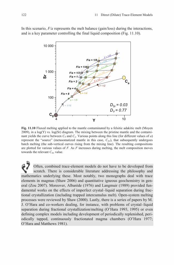
Fig. 11.10 Fluxed melting applied to the mantle contaminated by a felsitic adakitic melt (Moyen 2009), in a log(Y) vs. log(Sr) diagram. The mixing between the pristine mantle and the contami-nant yields the curve between C0 and Ca. Various points along this line (for different values of a)represent the “source” (metasomatized mantle in this case, Cms), that subsequently undergoes batch melting (the sub-vertical curves rising from the mixing line). The resulting compositions are plotted for various values of F. As F increases during melting, the melt composition moves towards the relevant Cms value.
In this scenario, F/a represents the melt balance (gain/loss) during the interactions, and is a key parameter controlling the final liquid composition (Fig. 11.10).
Often, combined trace-element models do not have to be developed from scratch. There is considerable literature addressing the philosophy and
mathematics underlying these. Most notably, two monographs deal with trace elements in magmas (Shaw 2006) and quantitative igneous geochemistry in gen-eral (Zou 2007). Moreover, Albarède (1976) and Langmuir (1989) provided fun-damental works on the effects of imperfect crystal–liquid separation during frac-tional crystallization (including trapped intercumulus melt). Open-system melting processes were reviewed by Shaw (2000). Lastly, there is a series of papers by M. J. O’Hara and co-workers dealing, for instance, with problems of crystal–liquid separation during fractional crystallization/melting (O’Hara 1993, 1995) or even defining complex models including development of periodically replenished, peri-odically tapped, continuously fractionated magma chambers (O’Hara 1977; O’Hara and Matthews 1981).
4 10
100
1 000
10 000
DSr = 0.03DY = 0.77
a = 1/2
a = 1/4
a = 1/8
a = 1/16
F = 1/2
F = 1/4
F = 1/8
Sr
F = 1/16F = 1/32
F/a = 1F/a = 1/2
F/a = 2
F/a = 4
F/a = 8
F/a = 1/4
F/a = 1/8
C0
Ca
Y
122 11 Direct (Dilute) Trace-Element Models
References 123
References
Albarède F (1976) Some trace element relationships among liquid and solid phases in the course of the fractional crystallization of magmas. Geochim Cosmochim Acta 40:667–673
Albarède F (1995) Introduction to geochemical modeling. Cambridge Univ Press, CambridgeAllègre CJ, Minster JF (1978) Quantitative models of trace-element behavior in magmatic pro-
cesses. Earth Planet Sci Lett 38:1–25Bohrson WA, Spera FJ (2007) Energy-Constrained Recharge, Assimilation, and Fractional
Crystallization (EC-RAχFC): a Visual Basic computer code for calculating trace element and isotope variations of open-system magmatic systems. Geochem Geophys Geosyst 8:Q11003
De Paolo DJ (1981) Trace element and isotopic effects of combined wallrock assimilation and fractional crystallization. Earth Planet Sci Lett 53:189–202
De Paolo DJ (1985) Isotopic studies of processes in mafic magma chambers: I. The Kiglapait Intrusion, Labrador. J Petrol 26:925–951
Ersoy Y, Helvacı C (2010) FC–AFC–FCA and mixing modeler: a Microsoft© Excel® spreadsheet program for modeling geochemical differentiation of magma by crystal fractionation, crustal assimilation and mixing. Comput Geosci 36:383–390
Fowler SJ, Bohrson WA, Spera FJ (2004) Magmatic evolution of the Skye Igneous Centre, Western Scotland: modelling of assimilation, recharge and fractional crystallization. J Petrol 45:2481–2505
Gast PW (1968) Trace element fractionation and the origin of tholeiitic and alkaline magma type. Geochim Cosmochim Acta 32:1057–1086
Greenland LP (1970) An equation of trace element distribution during magmatic crystallization. Amer Miner 55:455–465
Keskin M (2013) AFC-Modeler: a Microsoft® Excel© workbook program for modelling assimi-lation combined with fractional crystallization (AFC) process in magmatic systems by using equations of DePaolo (1981). Turkish J Earth Sci 22:304–319
Langmuir CH (1989) Geochemical consequences of in situ crystallization. Nature 340:199–205Langmuir CH, Vocke RD, Hanson GN (1978) A general mixing equation with application to
Icelandic basalts. Earth Planet Sci Lett 37:380–392Moyen J-F (2009) High Sr/Y and La/Yb ratios: the meaning of the “adakitic signature”. Lithos
112:556–574.
O’Hara MJ (1977) Geochemical evolution during fractional crystallisation of a periodically refilled magma chamber. Nature 266:503–507
O’Hara MJ (1993) Trace element geochemical effects of imperfect crystal–liquid separation. In: Prichard HM, Alabaster T, Harris NBW, Neary CR (eds) Magmatic processes and plate tec-tonics. Geological Society of London Special Publications, vol 76, pp 39–59
O’Hara MJ (1995) Imperfect melt separation, finite increment size and source region flow during fractional melting and the generation of reversed or subdued discrimination of incompatible trace elements. Chem Geol 121:27–50
O’Hara MJ, Matthews RE (1981) Geochemical evolution in an advancing, periodically replen-ished, periodically tapped, continuously fractionated magma chamber. J Geol Soc London 138:237–277
Petrelli M, Poli G, Perugini D, Peccerillo A (2005) PetroGraph: a new software to visualize, model, and present geochemical data in igneous petrology. Geochem Geophys Geosyst 6:Q07011
Rayleigh JWS (1896) Theoretical considerations respecting the separation of gases by diffusion and similar processes. Phil Mag 42:77–107
Reiners PW, Nelson BK, Ghiorso MS (1995) Assimilation of felsic crust by basaltic magma: thermal limits and extents of crustal contamination of mantle-derived magmas. Geology 23:563–566
Shaw DM (1970) Trace element fractionation during anatexis. Geochim Cosmochim Acta 34:237–243

124 11 Direct (Dilute) Trace-Element Models
Shaw DM (2000) Continuous (dynamic) melting theory revisited. Canad Mineral 38:1041–1063Shaw DM (2006) Trace elements in magmas: a theoretical treatment. Cambridge University
Press, CambridgeSpera FJ, Bohrson WA (2001) Energy constrained open-system magmatic processes I: general
model and Energy-Constrained Assimilation and Fractional Crystallization (EC-AFC) formu-lation. J Petrol 42:999–1018
Spera FJ, Bohrson WA (2004) Open-system magma chamber evolution: an Energy-Constrained geochemical model incorporating the effects of concurrent Eruption, Recharge, variable Assimilation and Fractional Crystallization (EC-E’RAχFC). J Petrol 45:2459–2480
Taylor HP (1980) The effects of assimilation of country rocks on 18O/16O and 87Sr/86Sr systematics in igneous rocks. Earth Planet Sci Lett 47:243–254
Vollmer R (1976) Rb–Sr and U–Th–Pb systematics of alkaline rocks: the alkaline rocks from Italy. Geochim Cosmochim Acta 40:283–295
Zou H (2007) Quantitative geochemistry. Imperial College Press, London
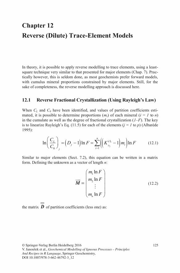
Chapter 12 Reverse (Dilute) Trace-Element Models
In theory, it is possible to apply reverse modelling to trace elements, using a least-square technique very similar to that presented for major elements (Chap. 7). Prac-tically however, this is seldom done, as most geochemists prefer forward models, with cumulus mineral proportions constrained by major elements. Still, for the sake of completeness, the reverse modelling approach is discussed here.
12.1 Reverse Fractional Crystallization (Using Rayleigh’s Law)
When CL and C0 have been identified, and values of partition coefficients esti-mated, it is possible to determine proportions (mi) of each mineral (i = 1 to n) in the cumulate as well as the degree of fractional crystallization (1–F). The key is to linearize Rayleigh’s Eq. (11.5) for each of the elements (j = 1 to p) (Albarède 1995):
i/L
10
ln 1 ln 1 lnD j
nL
j iij
C D F K m FC
(12.1)
Similar to major elements (Sect. 7.2), this equation can be written in a matrix form. Defining the unknown as a vector of length n:
(12.2)
the matrix D of partition coefficients (less one) as:
© Springer-Verlag Berlin Heidelberg 2016 V. Janoušek et al., Geochemical Modelling of Igneous Processes – Principles And Recipes in R Language, Springer Geochemistry, DOI 10.1007/978-3-662-46792-3_12
125
1
2
ln
ln
lnn
m F
m F
m F
=M
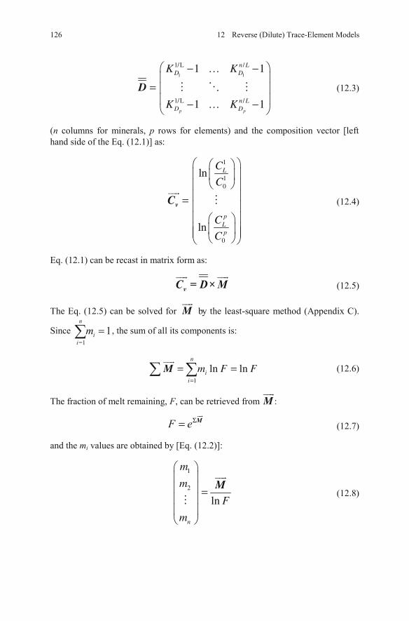
(12.3)
(n columns for minerals, p rows for elements) and the composition vector [left hand side of the Eq. (12.1)] as:
(12.4)
Eq. (12.1) can be recast in matrix form as:
(12.5)
The Eq. (12.5) can be solved for by the least-square method (Appendix C).
Since 1n
ii
m , the sum of all its components is:
(12.6)
The fraction of melt remaining, F, can be retrieved from :
(12.7)
and the mi values are obtained by [Eq. (12.2)]:
(12.8)
126 12 Reverse (Dilute) Trace-Element Models
1 1
1/L /
1/L /
1 1
1 1p p
n LD D
n LD D
K K
K K
− … −
=− … −
D
1
10
0
ln
ln
L
pLp
C
C
C
C
=vC
M
M
1
2
ln
n
m
m
F
m
= M
1
n lnln
ii
m FF=
= =M
v D×C = M
F eΣ= M
=1
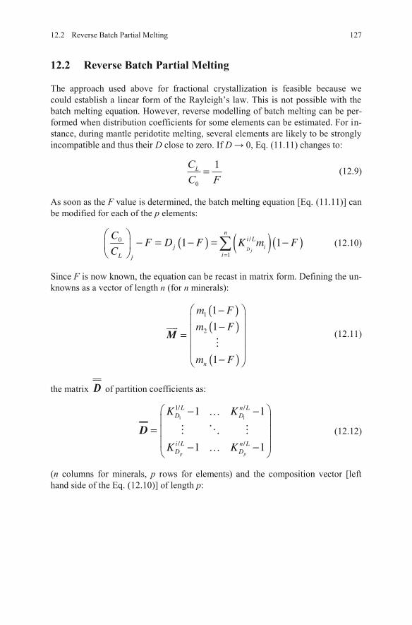
12.2 Reverse Batch Partial Melting
The approach used above for fractional crystallization is feasible because we could establish a linear form of the Rayleigh’s law. This is not possible with the batch melting equation. However, reverse modelling of batch melting can be per-formed when distribution coefficients for some elements can be estimated. For in-stance, during mantle peridotite melting, several elements are likely to be strongly incompatible and thus their D close to zero. If D 0, Eq. (11.11) changes to:
0
1LCC F
(12.9)
As soon as the F value is determined, the batch melting equation [Eq. (11.11)] can be modified for each of the p elements:
(12.10)
Since F is now known, the equation can be recast in matrix form. Defining the un-knowns as a vector of length n (for n minerals):
(12.11)
the matrix D of partition coefficients as:
(12.12)
(n columns for minerals, p rows for elements) and the composition vector [left hand side of the Eq. (12.10)] of length p:
12.2 Reverse Batch Partial Melting 127
( ) ( )( )/0
1
1 1D j
ni L
j iiL j
CF D F K m F
C =
− = − = −
( )( )
( )
1
2
1
1
1n
F
F
F
m
m
m
=
−−
−
M
1 1
1/ /
/ /
1 1
1 1p p
L n LD D
i L n LD D
K K
K K
− … −
=− … −
D
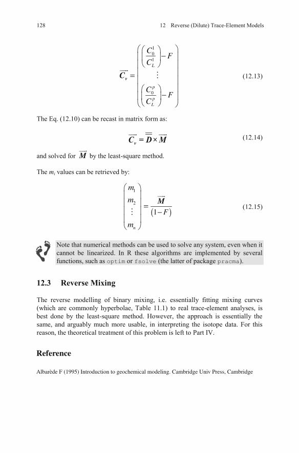
(12.13)
The Eq. (12.10) can be recast in matrix form as:
(12.14)
and solved for by the least-square method.
The mi values can be retrieved by:
(12.15)
Note that numerical methods can be used to solve any system, even when it cannot be linearized. In R these algorithms are implemented by several functions, such as optim or fsolve (the latter of package pracma).
12.3 Reverse Mixing
The reverse modelling of binary mixing, i.e. essentially fitting mixing curves (which are commonly hyperbolae, Table 11.1) to real trace-element analyses, is best done by the least-square method. However, the approach is essentially the same, and arguably much more usable, in interpreting the isotope data. For this reason, the theoretical treatment of this problem is left to Part IV.
128 12 Reverse (Dilute) Trace-Element Models
101
0
L
p
Lp
CF
C
CF
C
−
=
−
vC
( )
1
2
1
n
m
m
F
m
=−M
M
Reference
Albarède F (1995) Introduction to geochemical modeling. Cambridge Univ Press, Cambridge
v D×C = M
Chapter 13 Trace Elements as Essential Structural Constituents of Accessory Minerals: the Solubility Concept
13.1 Solubility Formulae for Common Accessory Minerals
13.1.1 Zircon, ZrSiO4
The zircon solubility in felsic silicate melts has attracted special attention because of the importance of this mineral in geochronology:
(1) Based on experimental calibration, the Zr saturation level has been expressed as (Watson and Harrison 1983):
© Springer-Verlag Berlin Heidelberg 2016 V. Janoušek et al., Geochemical Modelling of Igneous Processes – Principles And Recipes in R Language, Springer Geochemistry, DOI 10.1007/978-3-662-46792-3_13
129
Accessory minerals such as zircon, monazite or apatite have annoying proper-
ties in terms of geochemical modelling. Some elements that appear only as traces
in a rock can be stoichiometric components of such minerals. As a consequence,
their activity–composition relationships do not obey Henry’s Law, i.e. KD values
are not independent of the concentration anymore. Neither can be such cases treated
using a mass-balance approach (applied for ‘proper’ major elements) as the whole-
rock abundance is low and we lack information on exact distribution of the given
essential structural constituents (ESC) among all phases in the system.
The preferred modelling approach is based on the solubility of a relevant
accessory phase into the melt. Let’s take zircon and fractional crystallization as an
example. This mineral crystallizes when the Zr concentration in the melt exceeds
a certain threshold, called saturation level, which mainly depends on the melt tem-
perature and composition. When the melt is saturated, any excess Zr is incorporated
in newly formed zircon crystals. Knowing the zircon stoichiometry, it is possible to
use the saturation level to constrain the amount of zircon in the cumulate. Thus the
effect of this accessory mineral on the whole trace-element budget can be modelled.
12900 3.80 0.85( 1)ZrZrnZrL sat
cln MTC
(13.1)
where T is temperature in K, Zrzirconc = 497644 ppm (49.7 wt. %) is the
stoichiometric amount of Zr in an ideal (substitution-free) zircon, and M is a whole-rock chemical parameter based on cation fractions : 1
2Na K CaMAl Si
(13.2)
Equation (13.1) was determined for a normal peraluminous granite having M 1.3, and applies in the range 0.9 < M < 1.7 (Fig. 13.1).
Reversing Eq. (13.1), the zircon saturation temperature can be expressed as:
12900
497644ln 3.80 0.85 1ZrL sat
T
MC
(13.3)
(2) A revised formulation based on the linear regression of the same experimental data has been proposed by Kelsey et al. (2008):
11 574 0.679 1.7965ZrZrnZrL sat
c FMTC
(13.4)
Where FM is defined, again using cation fractions, as:
2( )Na K Ca Fe MgFMAl Si
(13.5)
1 These are cation fractions, i.e. the sum of all major cations, including those not involved in this
equation (Fe, Mg…) must equal 1. Consequently, these values differ from e.g. millications [Sect. 2.2.2] that are not normalized. Practically, this means that M cannot be calculated with-out knowing the composition of the magmatic liquid for all major elements.
130 13 Trace Elements as Essential Structural Constituents …
ln
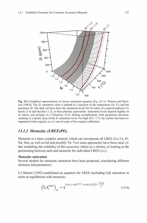
Fig. 13.1 Graphical representation of zircon saturation equation [Eq. (13.1), Watson and Harri-son (1983)]. The Zr saturation value is plotted as a function of the temperature (in °C) and the parameter M. The dark red lines show the saturation levels for M values of a typical andesite (2), dacite (1.5) and rhyolite (1.3), or their plutonic equivalents. Saturation levels depend slightly on M values, and strongly on T (Exercise 14.5). During crystallization, both parameters decrease, resulting in a drastic drop of the Zr saturation level. For high M (> 1.7), the surface has been ex-trapolated (white region), as it is out of scope of the original calibration.
13.1.2 Monazite, (LREE)PO4
Monazite is a more complex mineral, which can incorporate all LREE (La, Ce, Pr, Nd, Sm), as well as Gd and possibly Th. Two main approaches have been used, ei-ther modelling the solubility of this accessory (taken as a whole), or looking at the partitioning between melt and monazite for individual LREE (s.l.).
Monazite saturation Several models for monazite saturation have been proposed, considering different elements and parameters:
(1) Montel (1993) established an equation for LREE (including Gd) saturation in melts in equilibrium with monazite:
2133189.50 2.34 0.3879
eMontelD HLREE T
L sa
O
tA (13.6)
13.1 Solubility Formulae for Common Accessory Minerals 131
M
1.0
1.2
1.4
1.6
1.8
2.0
T(°C)
600
700
800
900
1000
Zr
(pp
m)
0
200
400
600
800
1000
M =
1.3
M =
1.5
M =
2
where H2O is expressed in wt. % and T in K. In this equation, LREELA is the
sum of the atomic amounts of LREE from La to Gd (excluding Eu):
jREEGdLREE LL sat
j La j
CA (13.7)
with j being the atomic weight of REE j and jREELC the concentration in ppm.
DMontel is defined as (in cation fractions):
( 2 ) 1( )
Montel Na K Li CaDAl Al Si
(13.8)
The monazite saturation temperature can be derived from Eq. (13.6) as:
2
133189.5 2.34 0.3879 lnMontel LREE
L sat
TO AD H
(13.9)
(2) Monazite is however a solid solution that can include Th and U besides LREE. Hence, Eq. (13.6) must be multiplied by
4
MnzREEPOX , which is the molar proportion
of the REE-bearing monazite:
4
CorrLREE Mnz LREEL REEPO Lsat sat
A X A (13.10)
If unknown, a typical value of 4
MnzREEPOX is 0.83 (Montel 1993).
This set of equations must not be used for Ca-rich magmas, where allanite is likely to be the main LREE-bearing mineral. In addition, the Fe and Mg contents of the magma should be low. For granitic compositions, typical DMontel values range from 0.9 to 1.1.
(3) Kelsey et al. (2008) established a different formula, resembling their Eq. (13.4) used for zircon:
The stoichiometric amount of LREE in monazite, (LREE)PO4,LREEMnzc , is 566,794
ppm and FM is defined by Eq. (13.5). Unlike in Eq. (13.6), the REE are expressed here in ppm (i.e. weight units).
310 1.324 7.5852L sat
LREEMnzLREE
c FMTC
(13.11)
132 13 Trace Elements as Essential Structural Constituents …
AW
AW
ln
(13.12)
where only the concentrations (in ppm) of the light REE (La to Sm) H2O is in wt. %, T temperature in K and P pressure in kbar.
Partitioning of various LREE in monazite Monazite/melt partitioning of each REE (and Th) can be, for each element, ex-pressed as (Montel 1993, 1996):
2
2
4
133189.50 2.34 0.3879e
j Montelj
D HREE Mnz RT TL REEPO
WO
A X e (13.13)
where jREELA represents the atomic amount of element REEj in the melt, i.e.:
jj
REE
jL
REELCA (13.14)
and 4
MnzREEPOX is the proportion of the REE-bearing end-member in the monazite.
Wj/R is a constant depending on the element (Wj = molar energy in J.mol–1, R =8.31 J/mol–1K–1):
Element Th La Ce Pr Nd Sm GdWj/R –520 –260 –116 31 177 460 750
Note that Eq. (13.11) is not equivalent to Eq. (13.6), and both models predict (slightly) different total REE in the melt (Fig. 13.2):
jREELREEL L
Gd
j asat
LA A (13.15)
2 Thorium is not a REE, but Montel (1996) proposed to treat it in the same way.
13.1 Solubility Formulae for Common Accessory Minerals 133
(4) A new calibration accounts for the effects of pressure (Stepanov et al. 2012):
4211494ln( ) 16.16 0.23 19.4 lnLREE
mM
enzREEPOlt
PC H OT
XT Σ
Σ = + − − +
are considered,
AW
universal gas constant,
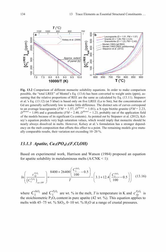
Fig. 13.2 Comparison of different monazite solubility equations. In order to make comparison possible, the “total LREE” of Montel’s Eq. (13.6) has been converted to weight units (ppm), as-suming that the relative proportions of REE are the same as calculated by Eq. (13.11). Stepanov et al.’s Eq. (13.12) (at 5 kbar) is based only on five LREE (La to Sm), but the concentrations of Gd are generally sufficiently low to make little difference. The distinct sets of curves correspond to an average leucogranite (FM = 1.57, DMontel = 1.01), a S-type biotite granite (FM = 2.23, DMontel = 1.09) and a granodiorite (FM = 2.40, DMontel = 1.23, probably out of the application field
of the models because of its significant Ca contents). As pointed out by Stepanov et al. (2012), Kel-sey’s equation predicts very high saturation values, which would imply that monazite should be nearly always dissolved in melts. However, Kelsey at al.’s formulation has a stronger depend-ency on the melt composition that offsets this effect to a point. The remaining models give mutu-ally comparable results, their variation not exceeding 10–20 %.
13.1.3 Apatite, Ca5(PO4)3(F,Cl,OH)
Based on experimental work, Harrison and Watson (1984) proposed an equation for apatite solubility in metaluminous melts (A/CNK < 1):
(13.16)
where 2SiOLC and 2 5P O
LC are wt. % in the melt, T is temperature in K and 2 5P OApc is
T (°C)T (°C)
[CL
] sat(p
pm
)LREE
7.0 7.5 8.0 8.5 9.0 9.5 10.0
10
02
00
50
02
00
05
00
01100 1000 900 800 700
10000/T (K)
600 650 700 750 800 850 900
01
00
20
03
00
40
05
00
60
0
aa bb
T (°C)
Approx. extentof panel (b)
Leucogranite (D = 1.01, FM = 1.57)Granite (D = 1.09, FM = 2.23)Granodiorite (D = 1.23, FM = 2.40)
Montel (1993) [all REE]Montel (1993) [REE partitionning]
Kelsey et al. (2008)
Stepanov et al. (2012)
[CL
] sat(p
pm
)LREE
134 13 Trace Elements as Essential Structural Constituents …
( )
2
2 5 2
2 5
.
8400 26400 0.5100
3.1 12.4 0.100
5
SiOL
P OA
SiOLp
P
sa W
OL t H
Cc Cln
TC
+ −= − + −
the stoichiometric P2O5 content in pure apatite (42 wt. %). This equation applies to melts with 45–75 wt. % SiO2, 0–10 wt. % H2O at a range of crustal pressures.
2
2
2 5
.
0.5840100
0.51
0 26400
42ln 3.1 1 40
2.0
SiOL
SiOL
L sat W
P
H
O
C
CC
T (13.17)
However, peraluminous melts (A/CNK > 1) are able to dissolve much more apa-tite than predicted by Harrison and Watson’s (1984) equation. This is due to the formation of aluminium–phosphate complexes in peraluminous aluminosilicate melts, in which P5+ is bonded with Al3+ to form AlPO4 species (Mysen et al. 1999 and references therein). Three strategies were proposed to tackle the effect of en-hanced solubility in peraluminous melts (Fig. 13.3):
(1) Bea et al. (1992)—based on experiments of Holtz and Johannes (1991), they
proposed correcting the saturation values 2 5
.L s
O
at W
P
HC of Harrison and Watson
(1984) as follows:
2 5 2 5
6429 / 1273.15
.
A CNKT
L Lsat sat HW
P O P OC C e (13.18)
(2) Pichavant et al. (1992) —experimental correction, at 750–1000 °C, 2–5 kbar:
2
2 5 2 5
5900 3.22 9.31100
./ 1
SiOL
P O PC
TL Lsat sat HW
OC C A CNK e (13.19)
(3) Wolf and London (1994) —experimental, at 750 °C and 200 MPa only:
2 5 3.4 /3.1L sat
P OC A CNK (13.20)
Saturnin and solubility models in GCDkitGCDkit comes with a plugin Saturation.r containing a set of functions to calculate the zircon, monazite, and apatite saturation levels/temperatures.
This plugin is based on a previous standalone R script Saturnin, documented in Janoušek (2006).
13.1 Solubility Formulae for Common Accessory Minerals 135
The apatite saturation temperature can be expressed from Eq. (13.16) as:
The GCDkit functions performing the saturation calculations are named
zrSaturation, mzSaturation apSaturation. See the respective help
pages for references and further details.
and
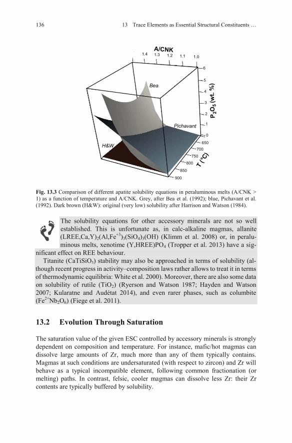
Fig. 13.3 Comparison of different apatite solubility equations in peraluminous melts (A/CNK > 1) as a function of temperature and A/CNK. Grey, after Bea et al. (1992); blue, Pichavant et al. (1992). Dark brown (H&W): original (very low) solubility after Harrison and Watson (1984).
(LREE,Ca,Y)2(Al,Fe+3)3(SiO4)3(OH) (Klimm et al. 2008) or, in peralu-minous melts, xenotime (Y,HREE)PO4 (Tropper et al. 2013) have a sig-
nificant effect on REE behaviour.
on solubility of rutile (TiO2) (Ryerson and Watson 1987; Hayden and Watson 2007; Kularatne and Audétat 2014), and even rarer phases, such as columbite (Fe2+Nb2O6) (Fiege et al. 2011).
13.2 Evolution Through Saturation
The saturation value of the given ESC controlled by accessory minerals is strongly dependent on composition and temperature. For instance, mafic/hot magmas can dissolve large amounts of Zr, much more than any of them typically contains. Magmas at such conditions are undersaturated (with respect to zircon) and Zr will behave as a typical incompatible element, following common fractionation (or melting) paths. In contrast, felsic, cooler magmas can dissolve less Zr: their Zr contents are typically buffered by solubility.
A/CNK1.5
P 2O
5 (w
t. %
)
T (°C
)
1.4 1.3 1.2 1.1 1.0
0
1
2
3
4
5
6
650700
800
850
900
750
Bea
Pichavant
H&W
13 13 Trace Elements as Essential Structural Constituents …6
The solubility equations for other accessory minerals are not so well
established. This is unfortunate as, in calc-alkaline magmas, allanite
Titanite (CaTiSiO5) stability may also be approached in terms of solubility (al-
though recent progress in activity–composition laws rather allows to treat it in terms
of thermodynamic equilibria: White et al. 2000). Moreover, there are also some data
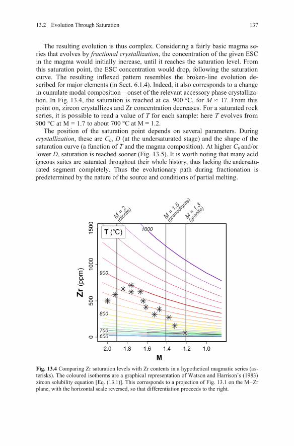
The resulting evolution is thus complex. Considering a fairly basic magma se-ries that evolves by fractional crystallization, the concentration of the given ESC in the magma would initially increase, until it reaches the saturation level. From this saturation point, the ESC concentration would drop, following the saturation curve. The resulting inflexed pattern resembles the broken-line evolution de-scribed for major elements (in Sect. 6.1.4). Indeed, it also corresponds to a change in cumulate modal composition—onset of the relevant accessory phase crystalliza-tion. In Fig. 13.4, the saturation is reached at ca. 900 °C, for M 1.7. From this point on, zircon crystallizes and Zr concentration decreases. For a saturated rock
series, it is possible to read a value of T for each sample: here T evolves from 900 °C at M = 1.7 to about 700 °C at M = 1.2.
The position of the saturation point depends on several parameters. During crystallization, these are C0, D (at the undersaturated stage) and the shape of the saturation curve (a function of T and the magma composition). At higher C0 and/or lower D, saturation is reached sooner (Fig. 13.5). It is worth noting that many acid igneous suites are saturated throughout their whole history, thus lacking the undersatu-rated segment completely. Thus the evolutionary path during fractionation is
predetermined by the nature of the source and conditions of partial melting.
Fig. 13.4 Comparing Zr saturation levels with Zr contents in a hypothetical magmatic series (as-terisks). The coloured isotherms are a graphical representation of Watson and Harrison’s (1983)
M2.0 1.8 1.6 1.4 1.2 1.0
0500
1000
1500
M = 1.3
(gran
ite)
M = 1.5
(gran
odior
ite)
M = 2
(diori
te)
900900900
800800800
700700700600600600
T (°C) 100010001000
Zr (ppm)
13.2 Evolution Through Saturation 137
zircon solubility equation [Eq. (13.1)]. This corresponds to a projection of Fig. 13.1 on the M–plane, with the horizontal scale reversed, so that differentiation proceeds to the right.
Zr
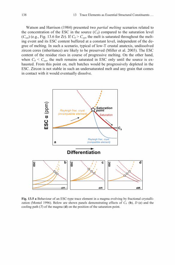
Watson and Harrison (1984) presented two partial melting scenarios related to the concentration of the ESC in the source (C0) compared to the saturation level (Csat) (e.g., Fig. 13.6 for Zr). If C0 > Csat, the melt is saturated throughout the melt-ing event and its ESC content buffered at a constant level, independent of the de-gree of melting. In such a scenario, typical of low-T crustal anatexis, undissolved zircon cores (inheritance) are likely to be preserved (Miller et al. 2003). The ESC content of the residue rises in course of progressive melting. On the other hand, when C0 < Csat, the melt remains saturated in ESC only until the source is ex-hausted. From this point on, melt batches would be progressively depleted in the ESC. Zircon is not stable in such an undersaturated melt and any grain that comesin contact with it would eventually dissolve.
Fig. 13.5 a Behaviour of an ESC-type trace element in a magma evolving by fractional crystalli-zation (Montel 1996). Below are shown panels demonstrating effects of C0 (b), D (c) and the cooling path (T) of the magma (d) on the position of the saturation point.
Differentiation
ESC
α (ppm)
C0
Rayleigh frac. cryst.(incompatible element) Saturation
Saturationpoint
a
b c d
Rayleigh frac. cryst.(compatible element)
diff.diff.diff.
ESC
ESC
diff.diff.diff.
ESC
ESC
diff.diff.
ESC
ESC
138 13 Trace Elements as Essential Structural Constituents …
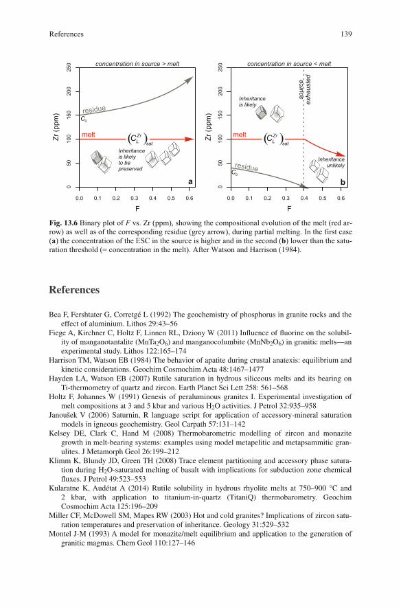
Fig. 13.6 Binary plot of F vs. Zr (ppm), showing the compositional evolution of the melt (red ar-row) as well as of the corresponding residue (grey arrow), during partial melting. In the first case (a) the concentration of the ESC in the source is higher and in the second (b) lower than the satu-ration threshold (= concentration in the melt). After Watson and Harrison (1984).
a b
0.0 0.1 0.2 0.3 0.4 0.5 0.6
05
01
00
15
02
00
25
0
F
Zr
(pp
m)
Zr
(pp
m)
0.0 0.1 0.2 0.3 0.4 0.5 0.6
05
01
00
15
02
00
25
0
F
residue
melt melt
resid eu
concentration in source > melt concentration in source < melt
Inheritance
is likely
to be
preserved
Inheritance
is likely
Inheritance
unlikely
source
exhausted
0C
0C
� Zr
Lsat
C � Zr
Lsat
C
References
References 139
Bea F, Fershtater G, Corretgé L (1992) The geochemistry of phosphorus in granite rocks and the effect of aluminium. Lithos 29:43–56
Fiege A, Kirchner C, Holtz F, Linnen RL, Dziony W (2011) Influence of fluorine on the solubil-ity of manganotantalite (MnTa2O6) and manganocolumbite (MnNb2O6) in granitic melts—an experimental study. Lithos 122:165–174
Harrison TM, Watson EB (1984) The behavior of apatite during crustal anatexis: equilibrium and kinetic considerations. Geochim Cosmochim Acta 48:1467–1477
Hayden LA, Watson EB (2007) Rutile saturation in hydrous siliceous melts and its bearing on Ti-thermometry of quartz and zircon. Earth Planet Sci Lett 258: 561–568
Holtz F, Johannes W (1991) Genesis of peraluminous granites I. Experimental investigation of melt compositions at 3 and 5 kbar and various H2O activities. J Petrol 32:935–958
Janoušek V (2006) Saturnin, R language script for application of accessory-mineral saturation models in igneous geochemistry. Geol Carpath 57:131–142
Kelsey DE, Clark C, Hand M (2008) Thermobarometric modelling of zircon and monazite growth in melt-bearing systems: examples using model metapelitic and metapsammitic gran-ulites. J Metamorph Geol 26:199–212
Klimm K, Blundy JD, Green TH (2008) Trace element partitioning and accessory phase satura-tion during H2O-saturated melting of basalt with implications for subduction zone chemical fluxes. J Petrol 49:523–553
Kularatne K, Audétat A (2014) Rutile solubility in hydrous rhyolite melts at 750–900 °C and 2 kbar, with application to titanium-in-quartz (TitaniQ) thermobarometry. Geochim Cosmochim Acta 125:196–209
Miller CF, McDowell SM, Mapes RW (2003) Hot and cold granites? Implications of zircon satu-ration temperatures and preservation of inheritance. Geology 31:529–532
Montel J-M (1993) A model for monazite/melt equilibrium and application to the generation of granitic magmas. Chem Geol 110:127–146
140 13 Trace Elements as Essential Structural Constituents …
Pichavant M, Montel J-M, Richard LR (1992) Apatite solubility in peraluminous liquids—exper-imental data and an extension of the Harrison–Watson model. Geochim Cosmochim Acta 56:3855–3861
Ryerson FJ, Watson EB (1987) Rutile saturation in magmas; implications for Ti–Nb–Ta deple-tion in island-arc basalts. Earth Planet Sci Lett 86: 225–239
Stepanov AS, Hermann J, Rubatto D, Rapp RP (2012) Experimental study of monazite/melt par-titioning with implications for the REE, Th and U geochemistry of crustal rocks. Chem Geol 300:200–220
Tropper P, Manning C, Harlov D (2013) Experimental determination of CePO4 and YPO4 solu-bilities in H2O–NaF at 800° C and 1 GPa: implications for rare earth element transport in high‐grade metamorphic fluids. Geofluids 13:372–380
Watson EB, Harrison TM (1983) Zircon saturation revisited: temperature and composition effects in a variety of crustal magmas types. Earth Planet Sci Lett 64:295–304
Watson EB, Harrison TM (1984) Accessory minerals and the geochemical evolution of crustal magmatic systems: a summary and prospectus of experimental approaches. Phys Earth Planet Inter 35:19–30
White RW, Powell R, Holland TJB, Worley B (2000) The effect of TiO2 and Fe2O3 on metape-litic assemblages at greenschist and amphibolite facies conditions: mineral equilibria calcu-lations in the system K2O–FeO–MgO–Al2O3–SiO2–H2O–TiO2–Fe2O3. J Metamorph Geol 18:497–511
Wolf MB, London D (1994) Apatite dissolution into peraluminous haplogranitic melts: an exper-imental study of solubilities and mechanisms. Geochim Cosmochim Acta 58:4127–4145
Montel J-M (1996) Géochimie de la fusion de la croûte continentale. Mémoire d’habilitation à diriger des recherches (= habilitation thesis), Université Blaise-Pascal, Clermont-Ferrand
Mysen BO, Holtz F, Pichavant M, Beny JM, Montel J-M (1999) The effect of temperature and bulk composition on the solution mechanism of phosphorus in peraluminous haplogranitic magma. Amer Miner 84:1336–1345
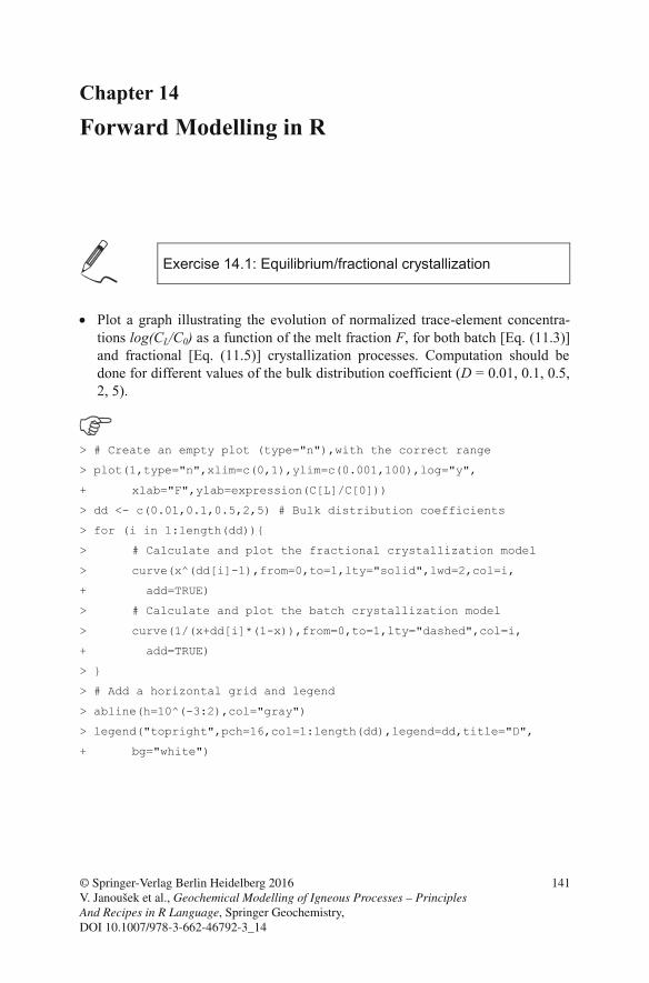
Chapter 14
Forward Modelling in R
Exercise 14.1: Equilibrium/fractional crystallization
Plot a graph illustrating the evolution of normalized trace-element concentra-tions log(CL/C0) as a function of the melt fraction F, for both batch [Eq. (11.3)] and fractional [Eq. (11.5)] crystallization processes. Computation should be done for different values of the bulk distribution coefficient (D = 0.01, 0.1, 0.5, 2, 5).
> # Create an empty plot (type="n"),with the correct range
> plot(1,type="n",xlim=c(0,1),ylim=c(0.001,100),log="y",
+ xlab="F",ylab=expression(C[L]/C[0]))
> dd <- c(0.01,0.1,0.5,2,5) # Bulk distribution coefficients
> for (i in 1:length(dd)){
> # Calculate and plot the fractional crystallization model
> curve(x^(dd[i]-1),from=0,to=1,lty="solid",lwd=2,col=i,
+ add=TRUE)
> # Calculate and plot the batch crystallization model
> curve(1/(x+dd[i]*(1-x)),from=0,to=1,lty="dashed",col=i,
+ add=TRUE)
> }
> # Add a horizontal grid and legend
> abline(h=10^(-3:2),col="gray")
> legend("topright",pch=16,col=1:length(dd),legend=dd,title="D",
+ bg="white")
© Springer-Verlag Berlin Heidelberg 2016 V. Janoušek et al., Geochemical Modelling of Igneous Processes – Principles And Recipes in R Language, Springer Geochemistry, DOI 10.1007/978-3-662-46792-3_14
141
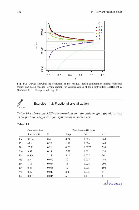
Fig. 14.1 Curves showing the evolution of the residual liquid composition during fractional (solid) and batch (dashed) crystallization for various values of bulk distribution coefficient D(Exercise 14.1). Compare with Fig. 11.3.
Exercise 14.2: Fractional crystallization
Table 14.1 shows the REE concentrations in a tonalitic magma (ppm), as well as the partition coefficients for crystallizing mineral phases.
Table 14.1
Concentration Partition coefficientsSource H34 Pl Amp Ilm All
La 32.04 0.4 0.74 0.005 960Ce 61.9 0.27 1.52 0.006 940Nd 25.75 0.21 4.26 0.0075 750Sm 3.97 0.13 7.77 0.01 620Eu 0.966 2.15 5.14 0.007 56Gd 2.3 0.097 10 0.017 440Dy 1.16 0.064 13 0.028 200Er 0.46 0.055 12 0.035 100Yb 0.37 0.049 8.4 0.075 54Lu 0.057 0.046 6 0.1 41
ttg.data
0.0 0.2 0.4 0.6 0.8 1.0
0.0
01
0.1
00
10.0
00
F
CL
C0
D
0.01
0.1
0.5
2
5
142 14 Forward Modelling in R
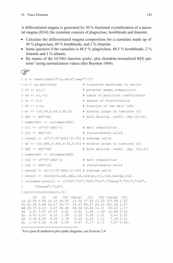
> x <- read.table("ttg.data",sep="\t")
> x <- as.matrix(x) # transform dataframe to matrix
> c0 <- x[,1] # parental magma composition
> kd <- x[,-1] # table of partition coefficients
> fc <- 0.3 # degree of fractionation
> ff <- 1-fc # fraction of the melt left
> m1 <- c(0.49,0.49,0.02,0) # mineral props in cumulate (1)
> dd1 <- kd%*%m1 # bulk distrib. coeff. [Eq.(10.4)]
> names(m1) <- colnames(dd1)
> cl1 <- c0*ff^(dd1-1) # melt composition
> cs1 <- dd1*cl1 # instantaneous solid
> csavg1 <- c0*(1-ff^dd1)/(1-ff) # average solid
> m2 <- c(0.485,0.485,0.02,0.01) # mineral props in cumulate (2)
> dd2 <- kd%*%m2 # bulk distrib. coeff. [Eq. (10.4)]
> names(m2) <- colnames(dd2)
> cl2 <- c0*ff^(dd2-1) # melt composition
> cs2 <- dd2*cl2 # instantaneous solid
> csavg2 <- c0*(1-ff^dd2)/(1-ff) # average solid
> result <- cbind(c0,dd1,dd2,cs1,csavg1,cl1,cs2,csavg2,cl2)
> colnames(result) <- c("C0","D1","D2","CS1","CSavg1","CL1","CS2",
+ "CSavg2","CL2")
> print(round(result,2))
C0 D1 D2 CS1 CSavg1 CL1 CS2 cSavg2 CL2 La 32.04 0.56 10.15 20.95 19.30 37.50 12.43 103.94 1.22 Ce 61.90 0.88 10.27 56.73 55.43 64.67 23.31 201.04 2.27 Nd 25.75 2.19 9.67 36.89 46.54 16.84 11.31 83.10 1.17 Sm 3.97 3.87 10.03 5.52 9.91 1.43 1.59 12.86 0.16 Eu 0.97 3.57 4.10 1.38 2.32 0.39 1.31 2.47 0.32 Gd 2.30 4.95 9.30 2.78 6.35 0.56 1.11 7.39 0.12 Dy 1.16 6.40 8.34 1.08 3.47 0.17 0.71 3.67 0.08
1 For a pure R method to plot spider diagrams, see Exercise 3.4
14314 Trace Elements
A differentiated magma is generated by 30 % fractional crystallization of a paren-tal magma (H34); the cumulate consists of plagioclase, hornblende and ilmenite.
Calculate the differentiated magma composition for a cumulate made up of 49 % plagioclase, 49 % hornblende, and 2 % ilmenite. Same question if the cumulate is 48.5 % plagioclase, 48.5 % hornblende, 2 % ilmenite and 1 % allanite. By means of the GCDkit function spider, plot chondrite-normalized REE pat-terns (using normalization values after Boynton 1984). 1
...
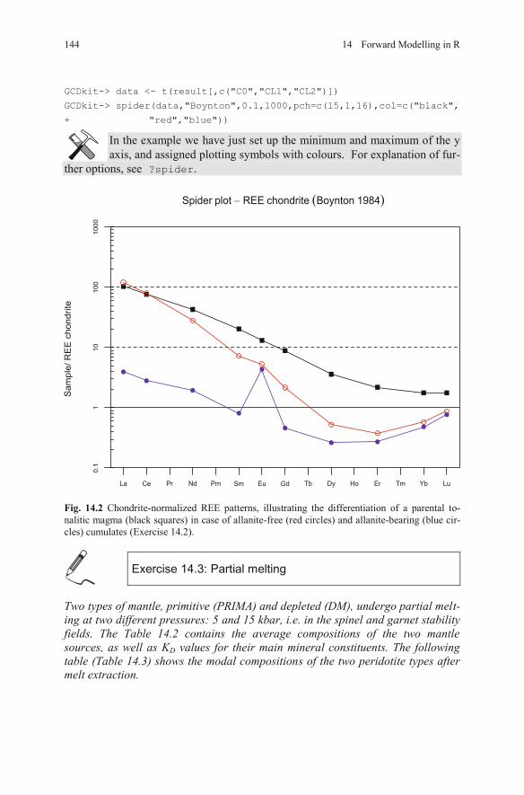
GCDkit-> data <- t(result[,c("C0","CL1","CL2")])
GCDkit-> spider(data,"Boynton",0.1,1000,pch=c(15,1,16),col=c("black",
+ "red","blue"))
In the example we have just set up the minimum and maximum of the y axis, and assigned plotting symbols with colours. For explanation of fur-
ther options, see ?spider.
Fig. 14.2 Chondrite-normalized REE patterns, illustrating the differentiation of a parental to-nalitic magma (black squares) in case of allanite-free (red circles) and allanite-bearing (blue cir-cles) cumulates (Exercise 14.2).
Exercise 14.3: Partial melting
Two types of mantle, primitive (PRIMA) and depleted (DM), undergo partial melt-ing at two different pressures: 5 and 15 kbar, i.e. in the spinel and garnet stability fields. The Table 14.2 contains the average compositions of the two mantle sources, as well as KD values for their main mineral constituents. The following table (Table 14.3) shows the modal compositions of the two peridotite types after melt extraction.
La Ce Pr Nd Pm Sm Eu Gd Tb Dy Ho Er Tm Yb Lu
0.1
11
01
00
10
00
Spider plot REE chondrite �Boynton 1984
Sa
mp
le/
RE
E c
ho
nd
rite
144 14 Forward Modelling in R
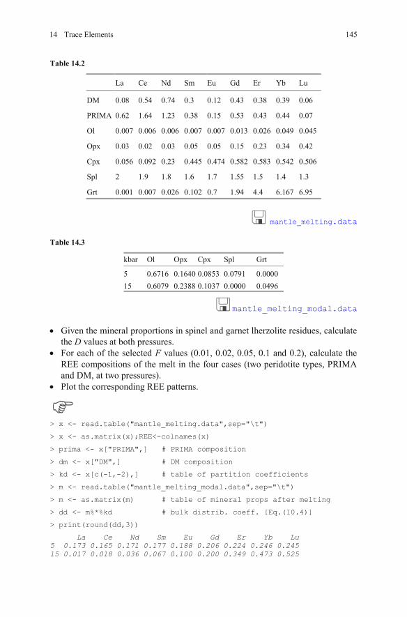
Table 14.2
La Ce Nd Sm Eu Gd Er Yb Lu
DM 0.08 0.54 0.74 0.3 0.12 0.43 0.38 0.39 0.06
PRIMA 0.62 1.64 1.23 0.38 0.15 0.53 0.43 0.44 0.07
Ol 0.007 0.006 0.006 0.007 0.007 0.013 0.026 0.049 0.045
Opx 0.03 0.02 0.03 0.05 0.05 0.15 0.23 0.34 0.42
Cpx 0.056 0.092 0.23 0.445 0.474 0.582 0.583 0.542 0.506
Spl 2 1.9 1.8 1.6 1.7 1.55 1.5 1.4 1.3
Grt 0.001 0.007 0.026 0.102 0.7 1.94 4.4 6.167 6.95
mantle_melting.data
Table 14.3
kbar Ol Opx Cpx Spl Grt
5 0.6716 0.1640 0.0853 0.0791 0.0000 15 0.6079 0.2388 0.1037 0.0000 0.0496
mantle_melting_modal.data Given the mineral proportions in spinel and garnet lherzolite residues, calculate
the D values at both pressures. For each of the selected F values (0.01, 0.02, 0.05, 0.1 and 0.2), calculate the
REE compositions of the melt in the four cases (two peridotite types, PRIMA and DM, at two pressures).
Plot the corresponding REE patterns.
> x <- read.table("mantle_melting.data",sep="\t")
> x <- as.matrix(x);REE<-colnames(x)
> prima <- x["PRIMA",] # PRIMA composition
> dm <- x["DM",] # DM composition
> kd <- x[c(-1,-2),] # table of partition coefficients
> m <- read.table("mantle_melting_modal.data",sep="\t")
> m <- as.matrix(m) # table of mineral props after melting
> dd <- m%*%kd # bulk distrib. coeff. [Eq.(10.4)]
> print(round(dd,3))
La Ce Nd Sm Eu Gd Er Yb Lu 5 0.173 0.165 0.171 0.177 0.188 0.206 0.224 0.246 0.245 15 0.017 0.018 0.036 0.067 0.100 0.200 0.349 0.473 0.525
14514 Trace Elements
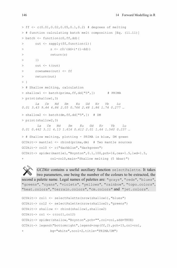
> ff <- c(0.01,0.02,0.05,0.1,0.2) # degrees of melting
> # function calculating batch melt composition [Eq. (11.11)]
> batch <- function(c0,ff,dd){
> out <- sapply(ff,function(i){
> z <- c0/(dd+i*(1-dd))
> return(z)
> })
> out <- t(out)
> rownames(out) <- ff
> return(out)
> # Shallow melting, calculation
> shallow1 <- batch(prima,ff,dd["5",]) # PRIMA
> print(shallow1,3)
La Ce Nd Sm Eu Gd Er Yb Lu 0.01 3.43 9.44 6.86 2.05 0.766 2.48 1.86 1.74 0.277 … > shallow2 <- batch(dm,ff,dd["5",]) # DM
> print(shallow2,3)
La Ce Nd Sm Eu Gd Er Yb Lu 0.01 0.442 3.11 4.13 1.616 0.612 2.01 1.64 1.540 0.237 … > # Shallow melting, plotting - PRIMA is blue, DM green
GCDkit-> mantle1 <- rbind(prima,dm) # Two mantle sources
GCDkit-> col0 <- c("darkblue","darkgreen")
GCDkit-> spider(mantle1,"Boynton",0.1,100,pch=16,cex=1.5,lwd=1.5,
+ col=col0,main="Shallow melting (5 kbar)")
GCDkit contains a useful auxiliary function selectPalette. It takes two parameters, one being the number of the colours to be extracted, the
second a palette name. Legal names of palettes are: "grays", "reds", "blues","greens", "cyans", "violets", "yellows", "rainbow", "topo.colors","heat.colors", "terrain.colors", "cm.colors" and "jet.colors".
GCDkit-> col1 <- selectPalette(nrow(shallow1),"blues")
GCDkit-> col2 <- selectPalette(nrow(shallow2),"greens")
GCDkit-> shallow <- rbind(shallow1,shallow2)
GCDkit-> col <- c(col1,col2)
GCDkit-> spider(shallow,"Boynton",pch="",col=col,add=TRUE)
GCDkit-> legend("bottomright",legend=rep(ff,2),pch=15,col=col,
+ bg="white",ncol=2,title="PRIMA/DM")
146 14 Forward Modelling in R
> }
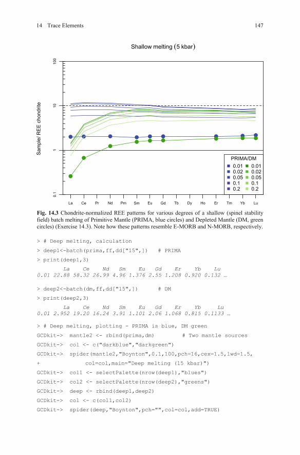
Fig. 14.3 Chondrite-normalized REE patterns for various degrees of a shallow (spinel stability field) batch melting of Primitive Mantle (PRIMA, blue circles) and Depleted Mantle (DM, green circles) (Exercise 14.3). Note how these patterns resemble E-MORB and N-MORB, respectively.
> # Deep melting, calculation
> deep1<-batch(prima,ff,dd["15",]) # PRIMA
> print(deep1,3)
La Ce Nd Sm Eu Gd Er Yb Lu 0.01 22.88 58.32 26.99 4.96 1.376 2.55 1.208 0.920 0.132 …
> deep2<-batch(dm,ff,dd["15",]) # DM
> print(deep2,3)
La Ce Nd Sm Eu Gd Er Yb Lu 0.01 2.952 19.20 16.24 3.91 1.101 2.06 1.068 0.815 0.1133 … > # Deep melting, plotting - PRIMA is blue, DM green
GCDkit-> mantle2 <- rbind(prima,dm) # Two mantle sources
GCDkit-> col <- c("darkblue","darkgreen")
GCDkit-> spider(mantle2,"Boynton",0.1,100,pch=16,cex=1.5,lwd=1.5,
+ col=col,main="Deep melting (15 kbar)")
GCDkit-> col1 <- selectPalette(nrow(deep1),"blues")
GCDkit-> col2 <- selectPalette(nrow(deep2),"greens")
GCDkit-> deep <- rbind(deep1,deep2)
GCDkit-> col <- c(col1,col2)
GCDkit-> spider(deep,"Boynton",pch="",col=col,add=TRUE)
14714
La Ce Pr Nd Pm Sm Eu Gd Tb Dy Ho Er Tm Yb Lu
0.1
110
10
0
Shallow melting 5 kbar
Sa
mp
le/
RE
E c
ho
nd
r ite
PRIMA/DM
0.010.020.050.10.2
0.010.020.050.10.2
Trace Elements
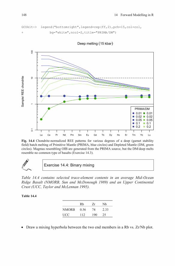
GCDkit-> legend("bottomright",legend=rep(ff,2),pch=15,col=col,
+ bg="white",ncol=2,title="PRIMA/DM")
Fig. 14.4 Chondrite-normalized REE patterns for various degrees of a deep (garnet stability field) batch melting of Primitive Mantle (PRIMA, blue circles) and Depleted Mantle (DM, green circles). Magmas resembling OIB are generated from the PRIMA source, but the DM/deep melts resemble no common type of basalts (Exercise 14.3).
Exercise 14.4: Binary mixing
Table 14.4 contains selected trace-element contents in an average Mid-Ocean Ridge Basalt (NMORB, Sun and McDonough 1989) and an Upper Continental Crust (UCC, Taylor and McLennan 1995).
Table 14.4
Rb Zr NbNMORB 0.56 74 2.33UCC 112 190 25
Draw a mixing hyperbola between the two end members in a Rb vs. Zr/Nb plot.
148
La Ce Pr Nd Pm Sm Eu Gd Tb Dy Ho Er Tm Yb Lu
0.1
110
100
Deep melting 15 kbar
Sa
mp
le/
RE
E c
ho
nd
rite
PRIMA/DM
0.010.020.050.10.2
0.010.020.050.10.2
14 Forward Modelling in R
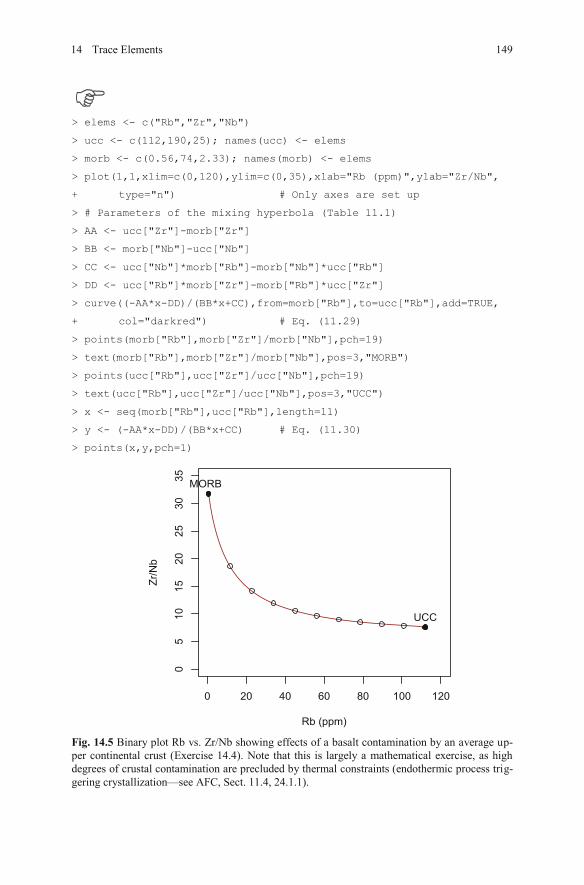
> elems <- c("Rb","Zr","Nb")
> ucc <- c(112,190,25); names(ucc) <- elems
> morb <- c(0.56,74,2.33); names(morb) <- elems
> plot(1,1,xlim=c(0,120),ylim=c(0,35),xlab="Rb (ppm)",ylab="Zr/Nb",
+ type="n") # Only axes are set up
> # Parameters of the mixing hyperbola (Table 11.1)
> AA <- ucc["Zr"]-morb["Zr"]
> BB <- morb["Nb"]-ucc["Nb"]
> CC <- ucc["Nb"]*morb["Rb"]-morb["Nb"]*ucc["Rb"]
> DD <- ucc["Rb"]*morb["Zr"]-morb["Rb"]*ucc["Zr"]
> curve((-AA*x-DD)/(BB*x+CC),from=morb["Rb"],to=ucc["Rb"],add=TRUE,
+ col="darkred") # Eq. (11.29)
> points(morb["Rb"],morb["Zr"]/morb["Nb"],pch=19)
> text(morb["Rb"],morb["Zr"]/morb["Nb"],pos=3,"MORB")
> points(ucc["Rb"],ucc["Zr"]/ucc["Nb"],pch=19)
> text(ucc["Rb"],ucc["Zr"]/ucc["Nb"],pos=3,"UCC")
> x <- seq(morb["Rb"],ucc["Rb"],length=11)
> y <- (-AA*x-DD)/(BB*x+CC) # Eq. (11.30)
> points(x,y,pch=1)
Fig. 14.5 Binary plot Rb vs. Zr/Nb showing effects of a basalt contamination by an average up-per continental crust (Exercise 14.4). Note that this is largely a mathematical exercise, as high degrees of crustal contamination are precluded by thermal constraints (endothermic process trig-gering crystallization—see AFC, Sect. 11.4, 24.1.1).
0 20 40 60 80 100 120
05
10
15
20
25
30
35
Rb (ppm)
Zr/
Nb
MORB
UCC
14914 Trace Elements
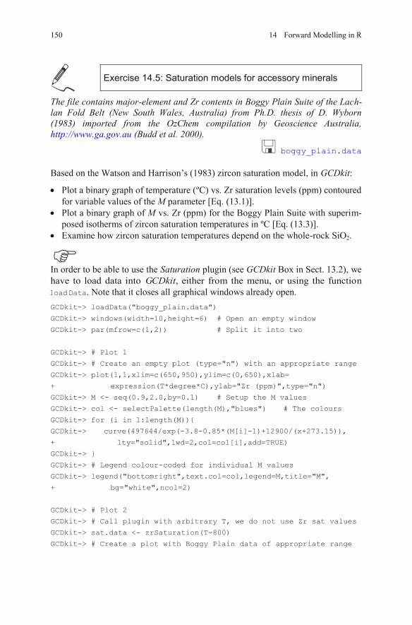
Exercise 14.5: Saturation models for accessory minerals
The file contains major-element and Zr contents in Boggy Plain Suite of the Lach-lan Fold Belt (New South Wales, Australia) from Ph.D. thesis of D. Wyborn (1983) imported from the OzChem compilation by Geoscience Australia, http://www.ga.gov.au (Budd et al. 2000).
boggy_plain.data
Based on the Watson and Harrison’s (1983) zircon saturation model, in GCDkit:
Plot a binary graph of temperature (ºC) vs. Zr saturation levels (ppm) contoured for variable values of the M parameter [Eq. (13.1)].Plot a binary graph of M vs. Zr (ppm) for the Boggy Plain Suite with superim-posed isotherms of zircon saturation temperatures in ºC [Eq. (13.3)].Examine how zircon saturation temperatures depend on the whole-rock SiO2.
In order to be able to use the Saturation plugin (see GCDkit Box in Sect. 13.2), we have to load data into GCDkit, either from the menu, or using the functionloadData. Note that it closes all graphical windows already open. GCDkit-> loadData("boggy_plain.data")
GCDkit-> windows(width=10,height=6) # Open an empty window
GCDkit-> par(mfrow=c(1,2)) # Split it into two
GCDkit-> # Plot 1
GCDkit-> # Create an empty plot (type="n") with an appropriate range
GCDkit-> plot(1,1,xlim=c(650,950),ylim=c(0,650),xlab=
+ expression(T*degree*C),ylab="Zr (ppm)",type="n")
GCDkit-> M <- seq(0.9,2.0,by=0.1) # Setup the M values
GCDkit-> col <- selectPalette(length(M),"blues") # The colours
GCDkit-> for (i in 1:length(M)){
GCDkit-> curve(497644/exp(-3.8-0.85*(M[i]-1)+12900/(x+273.15)),
+ lty="solid",lwd=2,col=col[i],add=TRUE)
GCDkit-> }
GCDkit-> # Legend colour-coded for individual M values
GCDkit-> legend("bottomright",text.col=col,legend=M,title="M",
+ bg="white",ncol=2)
GCDkit-> # Plot 2
GCDkit-> # Call plugin with arbitrary T, we do not use Zr sat values
GCDkit-> sat.data <- zrSaturation(T=800)
GCDkit-> # Create a plot with Boggy Plain data of appropriate range
150 14 Forward Modelling in R
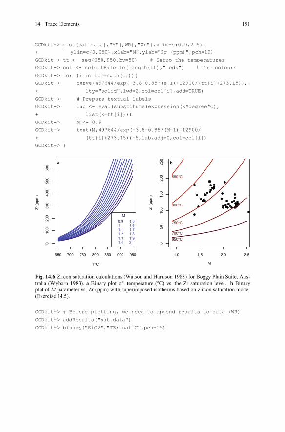
+ ylim=c(0,250),xlab="M",ylab="Zr (ppm)",pch=19)
GCDkit-> tt <- seq(650,950,by=50) # Setup the temperatures
GCDkit-> col <- selectPalette(length(tt),"reds") # The colours
GCDkit-> for (i in 1:length(tt)){
GCDkit-> curve(497644/exp(-3.8-0.85*(x-1)+12900/(tt[i]+273.15)),
+ lty="solid",lwd=2,col=col[i],add=TRUE)
GCDkit-> # Prepare textual labels
GCDkit-> lab <- eval(substitute(expression(x*degree*C),
+ list(x=tt[i])))
GCDkit-> M <- 0.9
GCDkit-> text(M,497644/exp(-3.8-0.85*(M-1)+12900/
+ (tt[i]+273.15))-5,lab,adj=0,col=col[i])
GCDkit-> }
Fig. 14.6 Zircon saturation calculations (Watson and Harrison 1983) for Boggy Plain Suite, Aus-tralia (Wyborn 1983). a Binary plot of temperature (ºC) vs. the Zr saturation level. b Binary plot of M parameter vs. Zr (ppm) with superimposed isotherms based on zircon saturation model(Exercise 14.5).
GCDkit-> # Before plotting, we need to append results to data (WR)
GCDkit-> addResults("sat.data")
GCDkit-> binary("SiO2","TZr.sat.C",pch=15)
15114
GCDkit-> plot(sat.data[,"M"],WR[,"Zr"],xlim=c(0.9,2.5),
650 700 750 800 850 900 950
01
00
20
03
00
40
05
00
60
0
T�C
Zr
(pp
m)
M
0.9
1
1.1
1.2
1.3
1.4
1.5
1.6
1.7
1.8
1.9
2
1.0 1.5 2.0 2.5
05
01
00
15
02
00
25
0
M
Zr
(pp
m)
650�C
700�C
750�C
800�C
850�C
ba
Trace Elements
Fig. 14.7 Binary plot of whole-rock silica contents (wt. %) vs. zircon saturation temperatures (Watson and Harrison 1983) for Boggy Plain Suite, Australia (Wyborn 1983) (Exercise 14.5).
50 55 60 65 70 75
550
600
650
700
750
800
SiO2
Zircon s
atu
ration
T(°
C)
References
Boynton WV (1984) Geochemistry of the rare-earth elements: meteorite studies. In: Henderson P (ed) Rare Earth Element Geochemistry. Elsevier, Amsterdam, pp 63–114
Budd AR, Hazell MS, Sedgmen A, Sedgmen L, Wyborn LAI, Ryburn R (2000) OZCHEM data-set release 1 documentation: AGSO’s national whole rock geochemistry database. Australian Geological Survey Organisation, Canberra
Sun SS, McDonough WF (1989) Chemical and isotopic systematics of oceanic basalts: implica-tions for mantle composition and processes. In: Saunders AD, Norry MJ (eds) Magmatism in ocean basins. Geological Society of London Special Publications, vol 42, pp 313–345
Taylor SR, McLennan SM (1995) The geochemical evolution of the continental crust. Rev Geophys 33:241–265
Watson EB, Harrison TM (1983) Zircon saturation revisited: temperature and composition effects in a variety of crustal magmas types. Earth Planet Sci Lett 64:295–304
Wyborn D (1983) Fractionation processes in the Boggy Plain zoned pluton. Unpublished Ph.D. thesis, Australian National University, Canberra
152 14 Forward Modelling in R
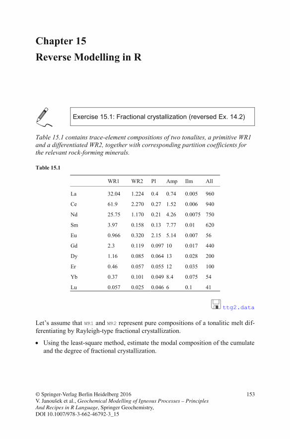
Chapter 15 Reverse Modelling in R
Exercise 15.1: Fractional crystallization (reversed Ex. 14.2)
Table 15.1 contains trace-element compositions of two tonalites, a primitive WR1 and a differentiated WR2, together with corresponding partition coefficients for the relevant rock-forming minerals.
Table 15.1
WR1 WR2 Pl Amp Ilm All
La 32.04 1.224 0.4 0.74 0.005 960
Ce 61.9 2.270 0.27 1.52 0.006 940
Nd 25.75 1.170 0.21 4.26 0.0075 750
Sm 3.97 0.158 0.13 7.77 0.01 620
Eu 0.966 0.320 2.15 5.14 0.007 56
Gd 2.3 0.119 0.097 10 0.017 440
Dy 1.16 0.085 0.064 13 0.028 200
Er 0.46 0.057 0.055 12 0.035 100
Yb 0.37 0.101 0.049 8.4 0.075 54
Lu 0.057 0.025 0.046 6 0.1 41
ttg2.data Let’s assume that WR1 and WR2 represent pure compositions of a tonalitic melt dif-ferentiating by Rayleigh-type fractional crystallization.
Using the least-square method, estimate the modal composition of the cumulate and the degree of fractional crystallization.
© Springer-Verlag Berlin Heidelberg 2016 V. Janoušek et al., Geochemical Modelling of Igneous Processes – Principles And Recipes in R Language, Springer Geochemistry, DOI 10.1007/978-3-662-46792-3_15
153
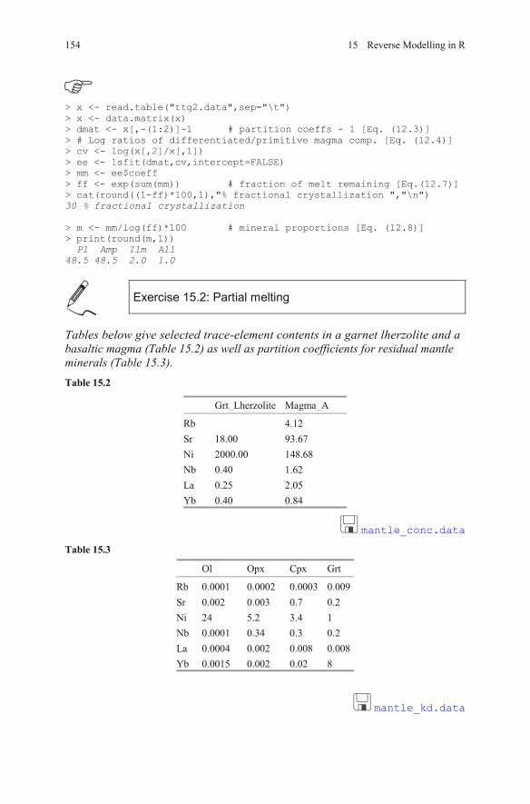
> x <- read.table("ttg2.data",sep="\t") > x <- data.matrix(x) > dmat <- x[,-(1:2)]-1 # partition coeffs - 1 [Eq. (12.3)] > # Log ratios of differentiated/primitive magma comp. [Eq. (12.4)] > cv <- log(x[,2]/x[,1]) > ee <- lsfit(dmat,cv,intercept=FALSE) > mm <- ee$coeff > ff <- exp(sum(mm)) # fraction of melt remaining [Eq.(12.7)] > cat(round((1-ff)*100,1),"% fractional crystallization ","\n") 30 % fractional crystallization > m <- mm/log(ff)*100 # mineral proportions [Eq. (12.8)] > print(round(m,1)) Pl Amp Ilm All 48.5 48.5 2.0 1.0
Exercise 15.2: Partial melting
Tables below give selected trace-element contents in a garnet lherzolite and apartition coefficients for residual mantle
minerals (Table 15.3). Table 15.2
Grt_Lherzolite Magma_A
Rb 4.12Sr 18.00 93.67Ni 2000.00 148.68Nb 0.40 1.62La 0.25 2.05Yb 0.40 0.84
mantle_conc.data
Table 15.3
Ol Opx Cpx Grt
Rb 0.0001 0.0002 0.0003 0.009Sr 0.002 0.003 0.7 0.2Ni 24 5.2 3.4 1Nb 0.0001 0.34 0.3 0.2La 0.0004 0.002 0.008 0.008Yb 0.0015 0.002 0.02 8
mantle_kd.data
154 15 Reverse Modelling in R
basaltic magma (Table 15.2) as well as
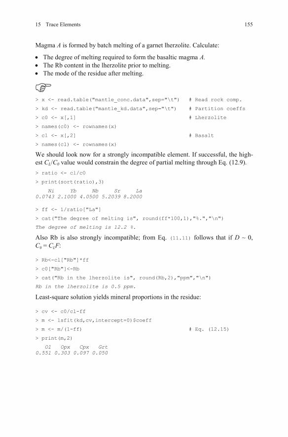
Magma A is formed by batch melting of a garnet lherzolite. Calculate:
The degree of melting required to form the basaltic magma A. The Rb content in the lherzolite prior to melting. The mode of the residue after melting.
> x <- read.table("mantle_conc.data",sep="\t") # Read rock comp.
> kd <- read.table("mantle_kd.data",sep="\t") # Partition coeffs
> c0 <- x[,1] # Lherzolite
> names(c0) <- rownames(x)
> cl <- x[,2] # Basalt
> names(cl) <- rownames(x)
We should look now for a strongly incompatible element. If successful, the high-est CL/C0 value would constrain the degree of partial melting through Eq. (12.9). > ratio <- cl/c0
> print(sort(ratio),3)
Ni Yb Nb Sr La 0.0743 2.1000 4.0500 5.2039 8.2000 > ff <- 1/ratio["La"]
> cat("The degree of melting is", round(ff*100,1),"%.","\n")
The degree of melting is 12.2 %.
Also Rb is also strongly incompatible; from Eq. (11.11) follows that if D ~ 0, C0 = CLF:
> Rb<-cl["Rb"]*ff
> c0["Rb"]<-Rb
> cat("Rb in the lherzolite is", round(Rb,2),"ppm","\n")
Rb in the lherzolite is 0.5 ppm.
Least-square solution yields mineral proportions in the residue:
> cv <- c0/cl-ff
> m <- lsfit(kd,cv,intercept=0)$coeff
> m <- m/(1-ff) # Eq. (12.15)
> print(m,2)
Ol Opx Cpx Grt 0.551 0.303 0.097 0.050
15515 Trace Elements
Part IV Radiogenic Isotopes
As shown in the preceding text, a suite of magmas affected by an open-system process, i.e. interaction with a compositionally dissimilar external component (magma mixing, AFC, hydrothermal alteration, metasomatism…), will generally display regular geochemical patterns. However, such trace-element evidence is of-ten, and major-element variation always, equivocal. The best proofs for operation of open-system processes remain radiogenic isotope ratios which are generally not fractionated during closed-system processes such as melting or crystallization. The magmas formed should preserve the isotopic characteristics of their source. In other words, the radiogenic isotope data are totally transparent to mechanisms of
closed-system magmatic differentiation but are very sensitive to mixing tamination.
or con-
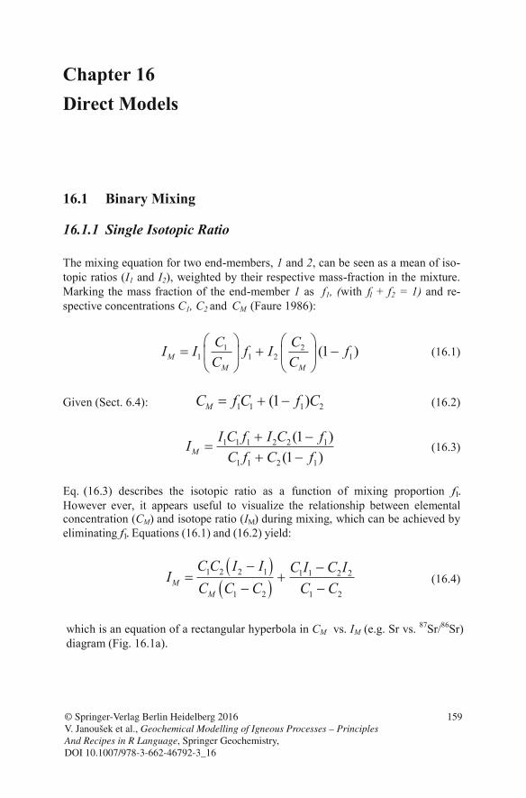
Chapter 16 Direct Models
16.1 Binary Mixing
16.1.1 Single Isotopic Ratio
The mixing equation for two end-members, 1 and 2, can be seen as a mean of iso-topic ratios (I1 and I2), weighted by their respective mass-fraction in the mixture. Marking the mass fraction of the end-member 1 as f1, (with f1 + f2 = 1) and re-spective concentrations C1, C2 and CM (Faure 1986):
1 21 1 2 1(1 )M
M M
C CI I f I fC C
(16.1)
Given (Sect. 6.4): 1 1 1 2(1 )MC f C f C (16.2)
1 1 1 2 2 1
1 1 2 1
(1 )(1 )M
I C f I C fIC f C f
(16.3)
1 2 2 1 1 1 2 2
1 2 1 2M
M
C C I I C I C IIC C C C C
(16.4)
© Springer-Verlag Berlin Heidelberg 2016 V. Janoušek et al., Geochemical Modelling of Igneous Processes – Principles And Recipes in R Language, Springer Geochemistry, DOI 10.1007/978-3-662-46792-3_16
159
which is an equation of a rectangular hyperbola in CM vs. IM (e.g. Sr vs. 87Sr/86Sr)diagram (Fig. 16.1a).
Eq. (16.3) describes the isotopic ratio as a function of mixing proportion f1.However ever, it appears useful to visualize the relationship between elementalconcentration (CM) and isotope ratio (IM) during mixing, which can be achieved byeliminating f1. Equations (16.1) and (16.2) yield:
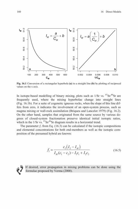
Fig. 16.1 Conversion of a rectangular hyperbola (a) to a straight line (b) by plotting of reciprocal values on the x axis.
In isotope-based modelling of binary mixing, plots such as 1/Sr vs. 87Sr/86Sr are frequently used, where the mixing hyperbolae change into straight lines (Fig. 16.1b). For a suite of cogenetic igneous rocks, when the slope of this line dif-fers from zero, it indicates the involvement of an open-system process, such as magma mixing or wall-rock assimilation (Briqueu and Lancelot 1979) (Fig. 16.2). On the other hand, samples that originated from the same source by various de-grees of closed-system fractionation preserve identical initial isotopic ratios, which in the 1/Sr vs. 87Sr/86Sr diagram results in a horizontal trend.
The parameter f1 from Eq. (16.3) can be calculated if the isotopic compositions and elemental concentrations for both end-members as well as the isotopic com-position of the presumed hybrid are known:
2 21
1 2 1 1 2 2( )M
M
c I If
I c c I c I c(16.5)
100 200 300 400 500 600
50.2
50.4
50.6
50.8
51.0
0.002 0.004 0.006 0.008 0.01050.2
50.4
50.6
50.8
51.0
a b
CM
IM IM
1/CM
M
M
aI b
C�
1M
M
I a bC
� �
� � �
� �
160 16 Direct Models
If desired, error propagation in mixing problems can be done using the formulae proposed by Verma (2000).
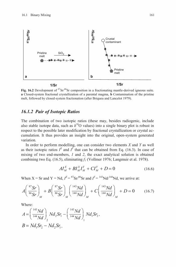
Fig. 16.2 Development of 87Sr/86Sr composition in a fractionating mantle-derived igneous suite. a Closed-system fractional crystallization of a parental magma, b Contamination of the pristine melt, followed by closed-system fractionation (after Briqueu and Lancelot 1979).
16.1.2 Pair of Isotopic Ratios
The combination of two isotopic ratios (these may, besides radiogenic, include also stable isotope data, such as 18O values) into a single binary plot is robust in respect to the possible later modification by fractional crystallization or crystal ac-cumulation. It thus provides an insight into the original, open-system generated variation.
In order to perform modelling, one can consider two elements X and Y as well as their isotopic ratios IX and IY that can be obtained from Eq. (16.3). In case of mixing of two end-members, 1 and 2, the exact analytical solution is obtained combining two Eq. (16.5), eliminating f1 (Vollmer 1976; Langmuir et al. 1978).
0X X Y YM M M MAI BI I CI D (16.6)
When X = Sr and Y = Nd, IX = 87Sr/86Sr and IY = 143Nd/144Nd, we arrive at:
87 87 143 143
86 86 144 144 0M M M M
Sr Sr Nd NdA B C DSr Sr Nd Nd
(16.7)
Where: 143 143
2 1 1 2144 1442 1
Nd NdA Nd Sr Nd SrNd Nd
,
1 2 2 1B Nd Sr Nd Sr ,
1/Sr1/Sr
87S
r/
Sr
86
87S
r/
Sr
86
Pristinemelt
Crustalcontaminant
Pristinemelt
SiO2
a b
16.1 Binary Mixing 161
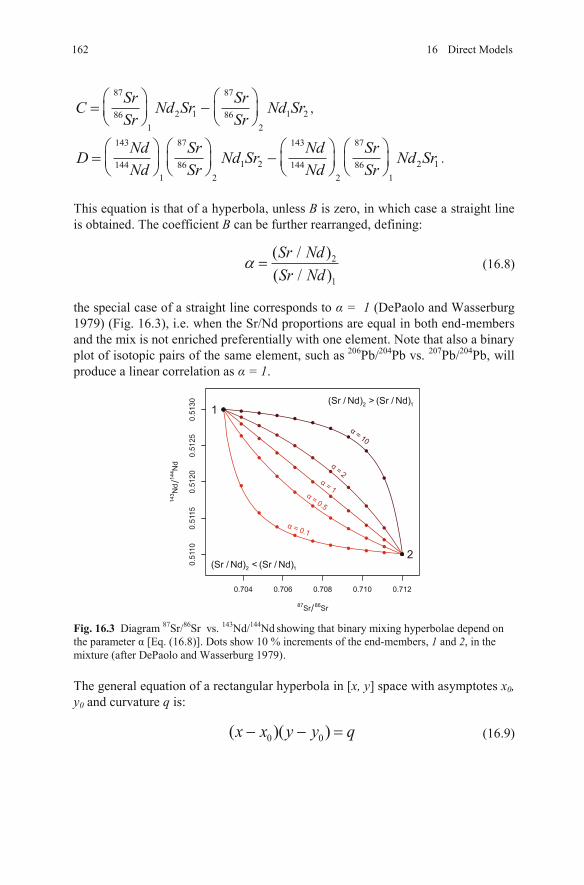
87 87
2 1 1 286 861 2
Sr SrC Nd Sr Nd SrSr Sr
,
143 87 143 87
1 2 2 1144 86 144 861 2 2 1
Nd Sr Nd SrD Nd Sr Nd SrNd Sr Nd Sr
.
This equation is that of a hyperbola, unless B is zero, in which case a straight line is obtained. The coefficient B can be further rearranged, defining:
2
1
( / )( / )Sr NdSr Nd
(16.8)
the special case of a straight line corresponds to = 1 (DePaolo and Wasserburg 1979) (Fig. 16.3), i.e. when the Sr/Nd proportions are equal in both end-members
plot of isotopic pairs of the same element, such as 206Pb/204Pb vs. 207Pb/204Pb, will produce a linear correlation as = 1.
Fig. 16.3 Diagram 87Sr/86Sr vs. 143Nd/144Nd showing that binary mixing hyperbolae depend on the parameter [Eq. (16.8)]. Dots show 10 % increments of the end-members, 1 and 2, in the mixture (after DePaolo and Wasserburg 1979).
The general equation of a rectangular hyperbola in [x, y] space with asymptotes x0,y0 and curvature q is:
0 0( )( )x x y y q (16.9)
0.704 0.706 0.708 0.710 0.712
0.5
110
0.5
115
0.5
120
0.5
125
0.5
130
87Sr
86Sr
14
3Nd
14
4Nd
α=
10
α=
2
α=
1α
=0.5
α = 0.1
2 1(Sr / Nd) > (Sr / Nd)
2 1(Sr / Nd) < (Sr / Nd)
1
2
162 16 Direct Models
and the mix is not enriched preferentially with one element. Note that also a binary
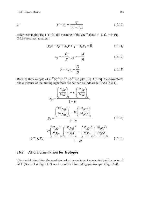
or 00( )
qy yx x
(16.10)
After rearranging Eq. (16.10), the meaning of the coefficients A, B, C, D in Eq. (16.6) becomes apparent:
0 0 0 0 0y x xy x y q x y (16.11)
0CxB
, 0AyB
(16.12)
0 0Dq x yB
(16.13)
Back to the example of a 87Sr/86Sr–143Nd/144Nd plot [Eq. (16.7)], the asymptotes and curvature of the mixing hyperbola are defined as (Albar de 1995) ( 1):
87 87
86 861 2
0 1
Sr SrSr Sr
x ,
143 143
144 1442 1
0 1
Nd NdNd Nd
y (16.14)
87 143 87 143
86 144 86 1442 1 1 2
0 0 1
Sr Nd Sr NdSr Nd Sr Nd
q x y (16.15)
16.2 AFC Formulation for Isotopes
The model describing the evolution of a trace-element concentration in course of AFC (Sect. 11.4, Fig. 11.7) can be modified for radiogenic isotopes (Fig. 16.4).
16316.1 Binary Mixing
è
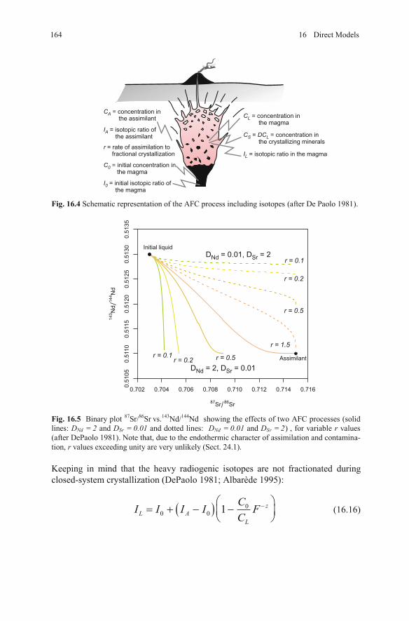
Fig. 16.4 Schematic representation of the AFC process including isotopes (after De Paolo 1981).
Fig. 16.5 Binary plot 87Sr/86Sr vs.143Nd/144Nd showing the effects of two AFC processes (solid lines: DNd = 2 and DSr = 0.01 and dotted lines: DNd = 0.01 and DSr = 2) , for variable r values (after DePaolo 1981). Note that, due to the endothermic character of assimilation and contamina-tion, r values exceeding unity are very unlikely (Sect. 24.1).
Keeping in mind that the heavy radiogenic isotopes are not fractionated during
00 0 1 z
L AL
CI I I I FC
(16.16)
0.702 0.704 0.706 0.708 0.710 0.712 0.714 0.716
0.5
105
0.5
110
0.5
115
0.5
120
0.5
125
0.5
130
0.5
135
87Sr
86Sr
14
3Nd
14
4Nd
Assimilant
Initial liquid
D = 2, D = 0.01Nd Sr
D = 0.01, D = 2Nd Sr
r = 0.1
r = 0.1
r = 0.2
r = 0.2
r = 0.5
r = 0.5
r = 1.5
164 16 Direct Models
closed-system crystallization (DePaolo 1981; Albar de 1995):è
r = rate of assimilation tofractional crystallization
CA = concentration inthe assimilant CL = concentration in
the magma
CS = DCL = concentration inthe crystallizing minerals
IL = isotopic ratio in the magma
C0 = initial concentration inthe magma
I0 = initial isotopic ratio ofthe magma
IA = isotopic ratio ofthe assimilant
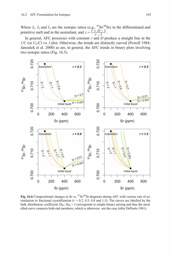
Where IL, I0 and IA are the isotopic ratios (e.g., 87Sr/86Sr) in the differentiated and primitive melt and in the assimilant, and 1
1r Dz r .
In general, AFC processes with constant r and D produce a straight line in the 1/C (or C0/C) vs. I plot. Otherwise, the trends are distinctly curved (Powell 1984; Janoušek et al. 2000) as are, in general, the AFC trends in binary plots involving two isotopic ratios (Fig. 16.5).
Fig. 16.6 Compositional changes in Sr vs. 87Sr/86Sr diagrams during AFC with various rate of as-similation to fractional crystallization (r = 0.2, 0.5, 0.8 and 1.5). The curves are labelled by the bulk distribution coefficient D D = 1 corresponds to simple binary mixing and thus the mod-elled curve connects both end members, which is otherwise not the case (after DePaolo 1981).
D=
1
D=
1
D=
2
D=
2
D =
2
D =
0.9
D =
0.9
D = 0.7
D=
0.7
D = 0.001D = 0.001
D = 0.001
D = 0.01
D = 0.01
r = 0.2 r = 0.5
r = 0.8 r = 1.5
D=
1
D=
0.7
D=
0.5
D=
1
D =
2
D=
0.0
01
D=
0.0
1
0 200 400 600
0.7
00
0.7
10
0.7
20
Sr (ppm)
87Sr
86Sr
Assimilant
Initial liquid
0 200 400 600
0.7
00
0.7
10
0.7
20
Sr (ppm)
87Sr
86Sr
Assimilant
Initial liquid
0 200 400 600
0.7
00
0.7
10
0.7
20
Sr (ppm)
87Sr
86Sr
87Sr
86Sr
Assimilant
Initial liquid
0 200 400 600
0.7
00
0.7
10
0.7
20
Sr (ppm)
Assimilant
Initial liquid
16.2 AFC Formulation for Isotopes 165
;Sr Sr
It is worth noting that even a massive assimilation may lead to very limited changes in the isotopic composition of an incompatible element in the melt. In contrast, compatible elements may record large isotopic shifts already at modest assimilation rates (Fig. 16.6). A characteristic feature of AFC is that the composi-tion of the resulting magma does not generally plot onto a tie line between both
166 16 Direct Models
end members, unlike in the case of binary mixing.
References
Albarède F (1995) Introduction to geochemical modeling. Cambridge University Press, Cambridge
Briqueu L, Lancelot J (1979) Rb–Sr systematics and crustal contamination trends for calc-alka-line igneous rocks. Earth Planet Sci Lett 43:385–396
DePaolo DJ (1981) Trace element and isotopic effects of combined wallrock assimilation and fractional crystallization. Earth Planet Sci Lett 53:189–202
DePaolo DJ, Wasserburg GJ (1979) Petrogenetic mixing models and Nd–Sr isotopic patterns. Geochim Cosmochim Acta 43:615–627
Faure G (1986) Principles of isotope geology. John Wiley & Sons, ChichesterJanoušek V, Bowes DR, Rogers G, Farrow CM, Jelínek E (2000) Modelling diverse processes in
the petrogenesis of a composite batholith: the Central Bohemian Pluton, Central European Hercynides. J Petrol 41:511–543
Langmuir CH, Vocke RD, Hanson GN, Hart SR (1978) A general mixing equation with applica-tions to Icelandic basalts. Earth Planet Sci Lett 37:380–392
Powell R (1984) Inversion of the assimilation and fractional crystallization (AFC) equations; characterization of contaminants from isotope and trace element relationships in volcanic suites. J Geol Soc London 141:447–452
Verma SP (2000) Error propagation in equations for geochemical modeling of radiogenic iso-topes in two-component mixing. J Earth Syst Sci 109:79–88
Vollmer R (1976) Rb–Sr and U–Th–Pb systematics of alkaline rocks: the alkaline rocks from Italy. Geochim Cosmochim Acta 40:283–295
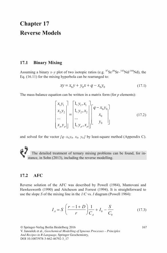
Chapter 17 Reverse Models
17.1 Binary Mixing
Assuming a binary x–y plot of two isotopic ratios (e.g. 87Sr/86Sr–143Nd/144Nd), the Eq. (16.11) for the mixing hyperbola can be rearranged to:
0 0 0 0xy x y y x q x y (1 .1)
The mass-balance equation can be written in a matrix form (for p elements):
1 1 1 10 0
2 2 2 20
0
1, ,1, ,
... ...1, ,p p p p
x y y xq x y
x y y xxy
x y y x
(17.2)
and solved for the vector [q– x0 y0, x0, y0 ] by least-square method (Appendix C).
The detailed treatment of ternary mixing problems can be found, for in-stance, in Sohn (2013), including the reverse modelling.
17.2 AFC
Reverse solution of the AFC was described by Powell (1984), Mantovani and Hawkesworth (1990) and Aitcheson and Forrest (1994). It is straightforward to use the slope S of the mixing line in the 1/C vs. I diagram (Powell 1984):
© Springer-Verlag Berlin Heidelberg 2016 V. Janoušek et al., Geochemical Modelling of Igneous Processes – Principles And Recipes in R Language, Springer Geochemistry, DOI 10.1007/978-3-662-46792-3_17
167
7
00
1 1A
A
r D SI S Ir C C
(17.3)
This can be solved for r:
00
1
A A
S Dr
SS I I CC
(17.4)
For reverse AFC modelling there is a specialized R package AFC3D using an innovative graphical approach (Guzmán et al. 2014).
168 17 Reverse Models
References
Aitcheson SJ, Forrest AH (1994) Quantification of crustal contamination in open magmatic sys-tems. J Petrol 35:461–488
Guzmán S, Carniel R, Caffe PJ (2014) AFC3D: a 3D graphical tool to model Assimilation and Fractional Crystallization with and without recharge in the R environment. Lithos 190–191:264–278
Mantovani MSM, Hawkesworth CJ (1990) An inversion approach to assimilation and fractional crystallisation processes. Contrib Mineral Petrol 105:289–302
Powell R (1984) Inversion of the assimilation and fractional crystallization (AFC) equations; characterization of contaminants from isotope and trace element relationships in volcanic suites. J Geol Soc London 141:447–452
Sohn RA (2013) A method for inverting ratio-ratio data to estimate end-member compositions in mixing problems. Chem Geol 352:63–69
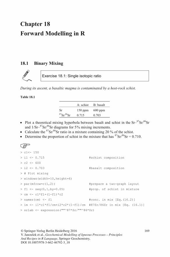
Chapter 18 Forward Modelling in R
18.1 Binary Mixing
Exercise 18.1: Single isotopic ratio
During its ascent, a basaltic magma is contaminated by a host-rock schist.
Table 18.1
A: schist B: basalt Sr 150 ppm 600 ppm 87Sr/86Sr 0.715 0.703
Plot a theoretical mixing hyperbola between basalt and schist in the Sr–87Sr/86Srand 1/Sr–87Sr/86Sr diagrams for 5 % mixing increments.
Calculate the 87Sr/86Sr ratio in a mixture containing 20 % of the schist. Determine the proportion of schist in the mixture that has 87Sr/86Sr = 0.710.
> c1<- 150
> i1 <- 0.715 #schist composition
> c2 <- 600
> i2 <- 0.703 #basalt composition
> # Plot mixing
> windows(width=10,height=6)
> par(mfrow=c(1,2)) #prepare a two-graph layout
> f1 <- seq(0,1,by=0.05) #prop. of schist in mixture
> cm <- c1*f1+(1-f1)*c2
> names(cm) <- f1 #conc. in mix [Eq.(16.2)]
> im <- i1*c1*f1/cm+i2*c2*(1-f1)/cm #87Sr/86Sr in mix [Eq. (16.1)]
> srlab <- expression(""^87*Sr/""^86*Sr)
© Springer-Verlag Berlin Heidelberg 2016 V. Janoušek et al., Geochemical Modelling of Igneous Processes – Principles And Recipes in R Language, Springer Geochemistry, DOI 10.1007/978-3-662-46792-3_18
169
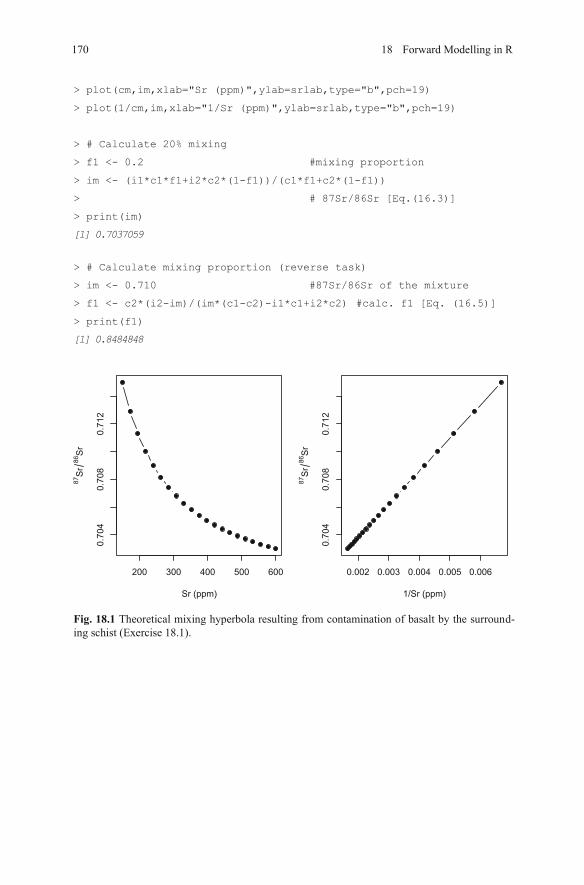
> plot(cm,im,xlab="Sr (ppm)",ylab=srlab,type="b",pch=19)
> plot(1/cm,im,xlab="1/Sr (ppm)",ylab=srlab,type="b",pch=19)
> # Calculate 20% mixing
> f1 <- 0.2 #mixing proportion
> im <- (i1*c1*f1+i2*c2*(1-f1))/(c1*f1+c2*(1-f1))
> # 87Sr/86Sr [Eq.(16.3)]
> print(im)
[1] 0.7037059
> # Calculate mixing proportion (reverse task)
> im <- 0.710 #87Sr/86Sr of the mixture
> f1 <- c2*(i2-im)/(im*(c1-c2)-i1*c1+i2*c2) #calc. f1 [Eq. (16.5)]
> print(f1)
[1] 0.8484848
Fig. 18.1 Theoretical mixing hyperbola resulting from contamination of basalt by the surround-ing schist (Exercise 18.1).
200 300 400 500 600
0.7
04
0.7
08
0.7
12
Sr (ppm)
87S
r8
6S
r
0.002 0.003 0.004 0.005 0.006
0.7
04
0.7
08
0.7
12
1/Sr (ppm)
87S
r8
6S
r
170 18 Forward Modelling in R
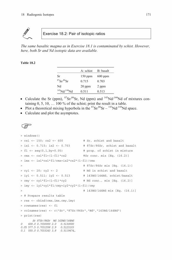
Table 18.2
A: schist B: basaltSr 150 ppm 600 ppm87Sr/86Sr 0.715 0.703Nd 20 ppm 2 ppm143Nd/144Nd 0.511 0.513
Calculate the Sr (ppm), 87Sr/86Sr, Nd (ppm) and 143Nd/144Nd of mixtures con-taining 0, 5, 10, … 100 % of the schist; print the result in a table. Plot a theoretical mixing hyperbola in the 87Sr/86Sr – 143Nd/144Nd space. Calculate and plot the asymptotes.
18 Radiogenic Isotopes 171
Exercise 18.2: Pair of isotopic ratios
The same basaltic magma as in Exercise 18.1 is contaminated by schist. However, here, both Sr and Nd isotopic data are available.
> windows()
> cx1 <- 150; cx2 <- 600 # Sr, schist and basalt
> ix1 <- 0.715; ix2 <- 0.703 # 87Sr/86Sr, schist and basalt
> f1 <- seq(0,1,by=0.05) # prop. of schist in mixture
> cmx <- cx1*f1+(1-f1)*cx2 #Sr conc. mix [Eq. (16.2)]
> imx <- ix1*cx1*f1/cmx+ix2*cx2*(1-f1)/cmx
> # 87Sr/86Sr mix [Eq. (16.1)]
> cy1 <- 20; cy2 <- 2 # Nd in schist and basalt
> iy1 <- 0.511; iy2 <- 0.513 # 143Nd/144Nd, schist/basalt
> cmy <- cy1*f1+(1-f1)*cy2 # Nd conc., mix [Eq. (16.2)]
> imy <- iy1*cy1*f1/cmy+iy2*cy2*(1-f1)/cmy
> # 143Nd/144Nd mix [Eq. (16.1)]
> # Prepare results table
> res <- cbind(cmx,imx,cmy,imy)
> rownames(res) <- f1
> colnames(res) <- c("Sr","87Sr/86Sr","Nd","143Nd/144Nd")
> print(res)
Sr 87Sr/86Sr Nd 143Nd/144Nd 0 600.0 0.7030000 2.0 0.5130000 0.05 577.5 0.7031558 2.9 0.5123103 0.1 555.0 0.7033243 3.8 0.5119474…
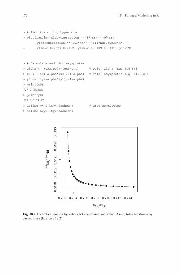
Fig. 18.2 Theoretical mixing hyperbola between basalt and schist. Asymptotes are shown by dashed lines (Exercise 18.2).
0.702 0.704 0.706 0.708 0.710 0.712 0.714
0.5
11
00
.511
50
.51
20
0.5
12
50
.51
30
87Sr
86Sr
14
3N
d1
44N
d
172 18 Forward Modelling in R
> # Plot the mixing hyperbola
> plot(imx,imy,xlab=expression(""^87*Sr/""^86*Sr),
+ ylab=expression(""^143*Nd/" "^144*Nd),type="b",
+ xlim=c(0.7023,0.7152),ylim=c(0.5109,0.5131),pch=19)
> # Calculate and plot asymptotes
> alpha <- (cx2/cy2)/(cx1/cy1) # calc. alpha [Eq. (16.8)]
> x0 <- (ix1-alpha*ix2)/(1-alpha) # calc. asymptotes [Eq. (16.14)]
> y0 <- (iy2-alpha*iy1)/(1-alpha)
> print(x0)
[1] 0.7026923
> print(y0)
[1] 0.5109487
> abline(v=x0,lty="dashed") # draw asymptotes
> abline(h=y0,lty="dashed")
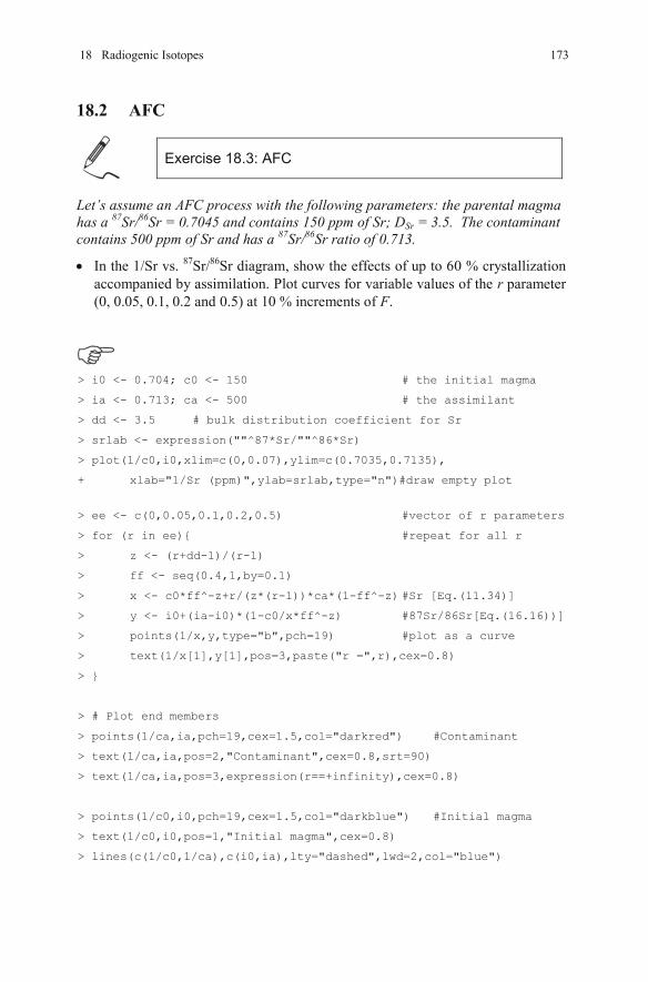
> i0 <- 0.704; c0 <- 150 # the initial magma
> ia <- 0.713; ca <- 500 # the assimilant
> dd <- 3.5 # bulk distribution coefficient for Sr
> srlab <- expression(""^87*Sr/""^86*Sr)
> plot(1/c0,i0,xlim=c(0,0.07),ylim=c(0.7035,0.7135),
+ xlab="1/Sr (ppm)",ylab=srlab,type="n")#draw empty plot
> ee <- c(0,0.05,0.1,0.2,0.5) #vector of r parameters
> for (r in ee){ #repeat for all r
> z <- (r+dd-1)/(r-1)
> ff <- seq(0.4,1,by=0.1)
> x <- c0*ff^-z+r/(z*(r-1))*ca*(1-ff^-z) #Sr [Eq.(11.34)]
> y <- i0+(ia-i0)*(1-c0/x*ff^-z) #87Sr/86Sr[Eq.(16.16))]
> points(1/x,y,type="b",pch=19) #plot as a curve
> text(1/x[1],y[1],pos=3,paste("r =",r),cex=0.8)
> }
> # Plot end members
> points(1/ca,ia,pch=19,cex=1.5,col="darkred") #Contaminant
> text(1/ca,ia,pos=2,"Contaminant",cex=0.8,srt=90)
> text(1/ca,ia,pos=3,expression(r==+infinity),cex=0.8)
> points(1/c0,i0,pch=19,cex=1.5,col="darkblue") #Initial magma
> text(1/c0,i0,pos=1,"Initial magma",cex=0.8)
> lines(c(1/c0,1/ca),c(i0,ia),lty="dashed",lwd=2,col="blue")
173
18.2 AFC
Exercise 18.3: AFC
Let’s assume an AFC process with the following parameters: the parental magma has a 87Sr/86Sr = 0.7045 and contains 150 ppm of Sr; DSr = 3.5. The contaminant contains 500 ppm of Sr and has a 87Sr/86Sr ratio of 0.713.
In the 1/Sr vs. 87Sr/86Sr diagram, show the effects of up to 60 % crystallization accompanied by assimilation. Plot curves for variable values of the r parameter (0, 0.05, 0.1, 0.2 and 0.5) at 10 % increments of F.
18 Radiogenic Isotopes
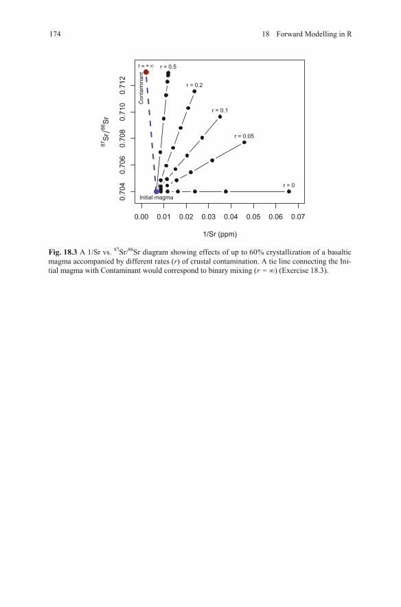
Fig. 18.3 A 1/Sr vs. 87Sr/86Sr diagram showing effects of up to 60% crystallization of a basaltic magma accompanied by different rates (r) of crustal contamination. A tie line connecting the Ini-tial magma with Contaminant would correspond to binary mixing (r = ) (Exercise 18.3).
0.00 0.01 0.02 0.03 0.04 0.05 0.06 0.07
0.7
04
0.7
06
0.7
08
0.7
10
0.7
12
1/Sr (ppm)
87S
r86S
r
r = 0
r = 0.05
r = 0.1
r = 0.2
r = 0.5
Co
nta
min
an
t
r = +
Initial magma
174 18 Forward Modelling in R
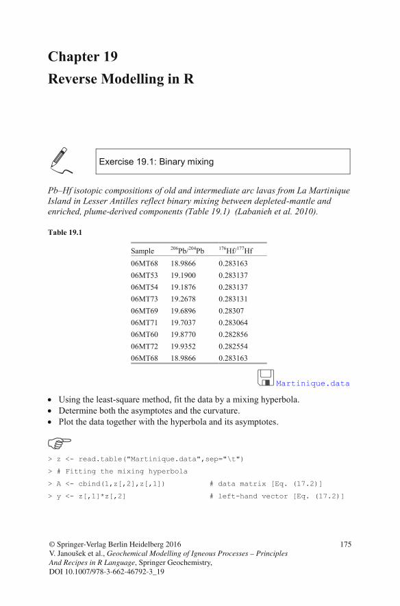
Chapter 19 Reverse Modelling in R
Exercise 19.1: Binary mixing
Pb–Hf isotopic compositions of old and intermediate arc lavas from La MartiniqueIsland in Lesser Antilles reflect binary mixing between depleted-mantle and enriched, plume-derived components (Table 19.1) (Labanieh et al. 2010).
Table 19.1
Sample 206Pb/204Pb 176Hf/177Hf 06MT68 18.9866 0.283163 06MT53 19.1900 0.283137 06MT54 19.1876 0.283137 06MT73 19.2678 0.283131 06MT69 19.6896 0.28307 06MT71 19.7037 0.283064 06MT60 19.8770 0.282856 06MT72 19.9352 0.282554 06MT68 18.9866 0.283163
Martinique.data
Using the least-square method, fit the data by a mixing hyperbola. Determine both the asymptotes and the curvature. Plot the data together with the hyperbola and its asymptotes.
> z <- read.table("Martinique.data",sep="\t")
> # Fitting the mixing hyperbola
> A <- cbind(1,z[,2],z[,1]) # data matrix [Eq. (17.2)]
> y <- z[,1]*z[,2] # left-hand vector [Eq. (17.2)]
© Springer-Verlag Berlin Heidelberg 2016 V. Janoušek et al., Geochemical Modelling of Igneous Processes – Principles And Recipes in R Language, Springer Geochemistry, DOI 10.1007/978-3-662-46792-3_19
175
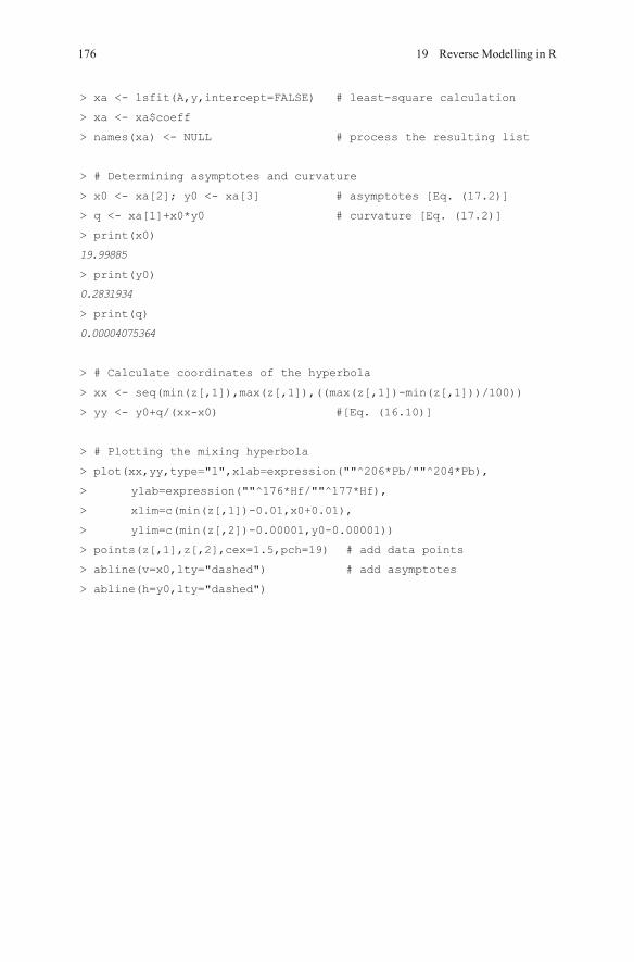
> xa <- lsfit(A,y,intercept=FALSE) # least-square calculation
> xa <- xa$coeff
> names(xa) <- NULL # process the resulting list
> # Determining asymptotes and curvature
> x0 <- xa[2]; y0 <- xa[3] # asymptotes [Eq. (17.2)]
> q <- xa[1]+x0*y0 # curvature [Eq. (17.2)]
> print(x0)
19.99885
> print(y0)
0.2831934
> print(q)
0.00004075364
> # Calculate coordinates of the hyperbola
> xx <- seq(min(z[,1]),max(z[,1]),((max(z[,1])-min(z[,1]))/100))
> yy <- y0+q/(xx-x0) #[Eq. (16.10)]
> # Plotting the mixing hyperbola
> plot(xx,yy,type="l",xlab=expression(""^206*Pb/""^204*Pb),
> ylab=expression(""^176*Hf/""^177*Hf),
> xlim=c(min(z[,1])-0.01,x0+0.01),
> ylim=c(min(z[,2])-0.00001,y0-0.00001))
> points(z[,1],z[,2],cex=1.5,pch=19) # add data points
> abline(v=x0,lty="dashed") # add asymptotes
> abline(h=y0,lty="dashed")
176 19 Reverse Modelling in R
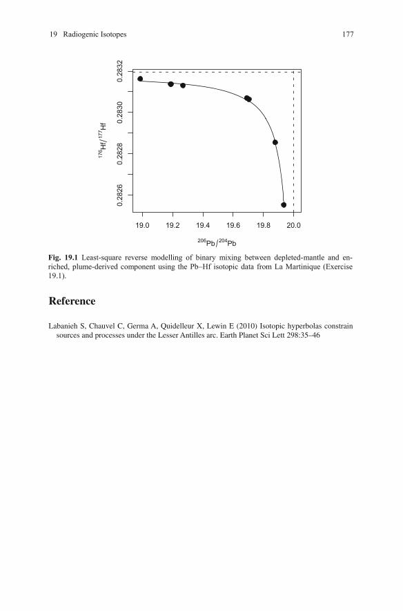
Fig. 19.1 Least-square reverse modelling of binary mixing between depleted-mantle and en-riched, plume-derived component using the Pb–Hf isotopic data from La Martinique (Exercise 19.1).
19.0 19.2 19.4 19.6 19.8 20.0
0.2
826
0.2
828
0.2
830
0.2
832
206Pb
204Pb
176H
f1
77H
f
Reference
Labanieh S, Chauvel C, Germa A, Quidelleur X, Lewin E (2010) Isotopic hyperbolas constrain sources and processes under the Lesser Antilles arc. Earth Planet Sci Lett 298:35–46
17719 Radiogenic Isotopes
Part V Practical Modelling
In previous chapters, we have seen numerous formulae describing the composi-tional evolution of a magma undergoing different petrogenetic processes. From a purely mathematical point of view, these equations are relatively simple. How-ever, in any igneous system, there are many unknowns, and several of them must be set or estimated using geological constraints before attempting to (numerically) solve the modelling equations.
It is important to bear in mind that a geochemical model can only test specific hypotheses—i.e., the geologist has to decide on the question to ask, while being aware that the only answer that the model can provide is “yes” (from a geochemi-cal point of view, this mechanism can account for the observed data) or “no” (it is unable to reproduce the dataset). Modelling does not provide answers to “open” questions; thus we can ask, for instance:
Is it possible to generate this dacite from that basalt, by fractional crystalliza-tion of a cumulate made up of amphibole and plagioclase? If so, what is the modal composition of that cumulate?
Could this granite be derived by partial melting of that sediment? What was the maximum degree of melting allowed by such a source?
Could assimilation of lower continental crust by ascending basalt yield an an-desitic magma of the given composition?
Could the compositional range observed in this igneous suite be the result of fractionation from a common parent?
Often, a negative answer is actually more useful, as it definitely rules out an assumption. In contrast, a positive answer just indicates that the proposed
process is not impossible—it does not demonstrate that it actually happened!
Although there is no universal recipe, a set of tricks can be used. Frequently, there is no pure mathematical solution, and assumptions have to be made. These typically relate to the composition of the primitive magma, or the fractionating mineral phases. Often, a composite approach combining calculations and educated
that would help in determining what processes were possible or not, and so start constraining them.
Build a full model, which in turn implies:
– Choose the process to be modelled: mixing, melting, crystallization… – Decide on key variants thereof: modal or non-modal, fractional or batch… – Set the key input parameters: composition of the primitive liquid, fraction-
ating phases and their chemistry, partition coefficients… – Perform the actual calculations.
Test the model, i.e. compare the computed result with real data (including all the other available information, such as that coming from geology and petrol-ogy). Most often, this leads to refining the existing model.
Reiterate until the model fits the data satisfactorily.
As a word of caution, one cannot stress strongly enough that it is unsafe to rely on the purely mathematical “best fit”. It is indeed possible that it does
not make geological sense, whereas a slightly worse fit (from a numerical perspec-tive) may be more realistic. For instance, modelling can predict the crystallization of an Ol + Qtz cumulate. Such a result is geologically meaningless. On the other hand, an Opx-bearing one is more plausible, even if the numerical fit is worse.
guesses must be employed. In general, the following steps will be implemented:
After having demonstrated the existence of a differentiation series (e.g. plottingtrends in binary plots), identify and further constrain the process(es) that could have shaped the composition of the suite. This can be done on the basis of:
– Previous knowledge (literature), analogy with similar occurrences else-where, relevant experiments or personal experience.
– Geological evidence in general, e.g. field relations or petrology. – Geochemical evidence, such as interpretation of variation diagrams or iso-
topic constraints. At this point, one may also apply semi-quantitative tests (e.g. mixing test, determination of compatibility of elements—Chap. 21)
180 PART V Practical Modelling
Chapter 20 Choosing an Appropriate Model
Geochemical modelling described in this book is primarily concerned with the in-terpretation of natural igneous suites. Therefore, any geochemical study must rest upon a sound understanding of their field
ribe all the relevant tools, but
20.1 Evidence for Crystallization
20.1.1 Final Solidification During Emplacement
In lava sequences, final solidification after eruption is typically fast and does not affect the chemistry of the suite. However, in low-viscosity magmas such as ko-matiites, there are well-documented examples of intra-flow differentiation (Arndt 1994) driven by gravity settling of crystals at the bottom of the lava flow (Fig. 20.1a). This process could be adequately modelled using the incomplete crystal separation scenario of Sect. 6.1.4 and 11.5.1.
In plutonic complexes, cooling is slower and may be accompanied by segrega-tion of the fractionated liquids from the mush of already formed crystals (Fig. 20.1b), a process that can be enhanced by syn-magmatic deformation (“filter-pressing”, e.g. Sisson and Bacon 1999). One may describe the slow solidification of a pluton in terms of batch crystallization (preserving the mass balance, but with changing phase compositions), or of incomplete crystal separation.
© Springer-Verlag Berlin Heidelberg 2016 V. Janoušek et al., Geochemical Modelling of Igneous Processes – Principles And Recipes in R Language, Springer Geochemistry, DOI 10.1007/978-3-662-46792-3_20
181
relations and petrological features. As thistext is not a manual of petrology, we will not descrather point out a few features that may help in deciding on the process to bemodelled, even constraining it to some point.
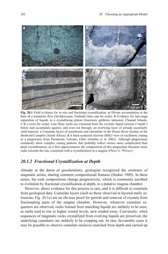
Fig. 20.1 Field evidence for in situ and fractional crystallization. a Olivine accumulation at the base of a komatiite flow (Sivikkovaara, Finland) (lens cap for scale). b Evidence for late-stage separation of liquids in a crystallizing pluton (Guernsey gabbroic intrusion, Channel Islands, U.K.) (coin for scale). Late felsic melts are extracted from the crystals–liquid mixture (“mush”) below and accumulate against, and even cut through, an overlying layer of already essentially solid material. c Cumulate layers of anorthosite and chromitite in the Dwars River locality of the Bushveld Complex (South Africa). d A back-scattered electron (BSE) view of oscillatory zoning in a plagioclase from Parinacota Volcano, Chile (Ginibre et al. 2002). Although plagioclases commonly show complex zoning patterns that probably reflect stories more complicated than plain crystallization, as a first approximation the composition of this plagioclase becomes more sodic towards the rim, consistent with a crystallization in a magma (Photo G. Wörner).
20.1.2 Fractional Crystallization at Depth
Already at the dawn of geochemistry, geologists recognized the existence of magmatic series, sharing common compositional features (Harker 1909). In these series, the rock compositions change progressively, which is commonly ascribed to evolution by fractional crystallization at depth, in a putative magma chamber.
However, direct evidence for this process is rare, and it is difficult to constrain from geological data. Cumulate layers (such as those observed in layered mafic in-trusions; Fig. 20.1c) are an obvious proof for growth and removal of crystals from fractionating parts of the magma chamber. However, whenever cumulate se-quences are observed, rocks formed from matching liquids are unlikely to be seen, as melts tend to rise to higher crustal levels, now eroded away. Conversely, when sequences of magmatic rocks crystallized from evolving liquids are preserved, the underlying cumulates are unlikely to be cropping out. In rare, favourable cases it may be possible to observe cumulate enclaves snatched from depth and carried up
a b
c
≈ 20 cm
300 μm
d
182 20 Choosing an Appropriate Model
by the ascending differentiated magma. Phenocrysts in lava are generally taken as evidence for early fractionation. In particular, their oscillatory or simple continuous zoning patterns (Fig. 20.1d) are an indication for fractional crystallization from agradually evolving magma.
20.2 Evidence for Melting
The mere presence of igneous rock that had to crystallize from magma is evidence for melting. In that sense every geochemical model should include a stage of par-tial melting. However, melting processes generally take place at great depth, much deeper than the place where magmas crystallize. Consequently, melting sites can be poorly (if at all) documented at the current exposure level. Therefore, decipher-ing melting is often tricky and indirect.
20.2.1 Crustal Anatexis
Partially molten upper crustal rocks (migmatites) are frequently observed (Fig. 20.2a–c), and there is ample literature describing and interpreting these rocks in terms of field relations, rheology or petrology: see for instance Mehnert (1968) or the reviews in Brown (2007) or Sawyer (2008). A batch melting model may seem adequate, and direct observation of the restitic assemblage should make modelling relatively easy.
However, geochemical modelling of migmatites has many pitfalls. One of the critical issues is that the leucosomes seldom have pure melt compositions. Several explanations have been proposed, including reequilibration by diffusion (Fourcade et al. 1992) or “back-reactions” with the melanosome (Kriegsman and Hensen 1998). Alternatively, the leucosomes may be interpreted as early cumulate layers left behind after melt removal (Taylor et al. 2014) or even injected foreign melts (Hasalová et al. 2008). All these processes can be modelled—at the cost of in-creased complexity.
In addition, the mere existence of felsic intrusions demonstrates that melt has been extracted from migmatites (Brown 2004; Yakymchuk and Brown 2014). There-fore, it is likely that many of them are melt-depleted and thus poorly represent the state of the source during anatexis.
Yet, the presence of migmatites in the right place at the right time does indeed provide crucial evidence for crustal melting processes that could have been poten-tially involved in the generation of nearby, contemporaneous felsic suites.
20.1 Evidence for Crystallization 183
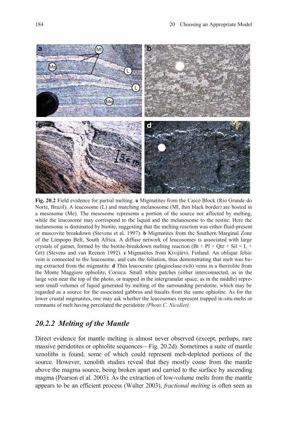
Fig. 20.2 Field evidence for partial melting. a Migmatites from the Caicó Block (Rio Grande do Norte, Brazil). A leucosome (L) and matching melanosome (Ml, thin black border) are hosted in a mesosome (Me). The mesosome represents a portion of the source not affected by melting, while the leucosome may correspond to the liquid and the melanosome to the restite. Here the melanosome is dominated by biotite, suggesting that the melting reaction was either fluid-present or muscovite breakdown (Stevens et al. 1997). b Migmatites from the Southern Marginal Zone of the Limpopo Belt, South Africa. A diffuse network of leucosomes is associated with large crystals of garnet, formed by the biotite-breakdown melting reaction (Bt + Pl + Qtz + Sil = L + Grt) (Stevens and van Reenen 1992). c Migmatites from Kivijärvi, Finland. An oblique felsic vein is connected to the leucosome, and cuts the foliation, thus demonstrating that melt was be-ing extracted from the migmatite. d Thin leucocratic (plagioclase-rich) veins in a lherzolite from the Monte Maggiore ophiolite, Corsica. Small white patches (either interconnected, as in the large vein near the top of the photo, or trapped in the intergranular space, as in the middle) repre-sent small volumes of liquid generated by melting of the surrounding peridotite, which may be regarded as a source for the associated gabbros and basalts from the same ophiolite. As for the lower crustal migmatites, one may ask whether the leucosomes represent trapped in-situ melts or remnants of melt having percolated the peridotite (Photo C. Nicollet).
20.2.2 Melting of the Mantle
Direct evidence for mantle melting is almost never observed (except, perhaps, rare massive peridotites or ophiolite sequences—Fig. 20.2d). Sometimes a suite of mantle xenoliths is found, some of which could represent melt-depleted portions of the source. However, xenolith studies reveal that they mostly come from the mantle above the magma source, being broken apart and carried to the surface by ascending magma (Pearson et al. 2003). As the extraction of low-volume melts from the mantle appears to be an efficient process (Walter 2003), fractional melting is often seen as
a b
c d
L
Ml
Me
L
Me
184 20 Choosing an Appropriate Model
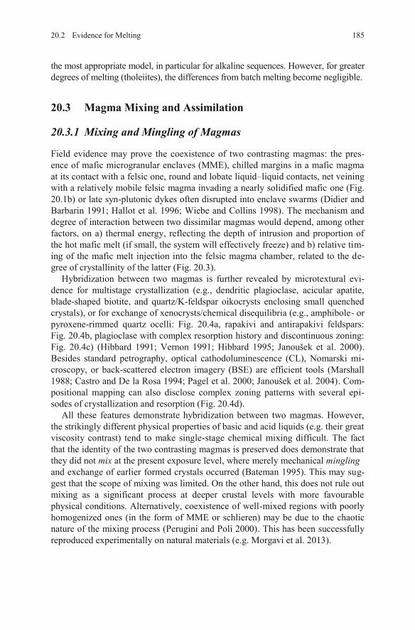
the most appropriate model, in particular for alkaline sequences. However, for greater degrees of melting (tholeiites), the differences from batch melting become negligible.
20.3 Magma Mixing and Assimilation
20.3.1 Mixing and Mingling of Magmas
Field evidence may prove the coexistence of two contrasting magmas: the pres-ence of mafic microgranular enclaves (MME), chilled margins in a mafic magma at its contact with a felsic one, round and lobate liquid–liquid contacts, net veining with a relatively mobile felsic magma invading a nearly solidified mafic one (Fig. 20.1b) or late syn-plutonic dykes often disrupted into enclave swarms (Didier and Barbarin 1991; Hallot et al. 1996; Wiebe and Collins 1998). The mechanism and degree of interaction between two dissimilar magmas would depend, among other factors, on a) thermal energy, reflecting the depth of intrusion and proportion of the hot mafic melt (if small, the system will effectively freeze) and b) relative tim-ing of the mafic melt injection into the felsic magma chamber, related to the de-gree of crystallinity of the latter (Fig. 20.3).
Hybridization between two magmas is further revealed by microtextural evi-dence for multistage crystallization (e.g., dendritic plagioclase, acicular apatite, blade-shaped biotite, and quartz/K-feldspar oikocrysts enclosing small quenched crystals), or for exchange of xenocrysts/chemical disequilibria (e.g., amphibole- or pyroxene-rimmed quartz ocelli: Fig. 20.4a, rapakivi and antirapakivi feldspars: Fig. 20.4b, plagioclase with complex resorption history and discontinuous zoning: Fig. 20.4c) (Hibbard 1991; Vernon 1991; Hibbard 1995; Janoušek et al. 2000).Besides standard petrography, optical cathodoluminescence (CL), Nomarski mi-croscopy, or back-scattered electron imagery (BSE) are efficient tools (Marshall 1988; Castro and De la Rosa 1994; Pagel et al. 2000; Janoušek et al. 2004). Com-positional mapping can also disclose complex zoning patterns with several epi-sodes of crystallization and resorption (Fig. 20.4d).
All these features demonstrate hybridization between two magmas. However, the strikingly different physical properties of basic and acid liquids (e.g. their great viscosity contrast) tend to make single-stage chemical mixing difficult. The fact that the identity of the two contrasting magmas is preserved does demonstrate that they did not mix at the present exposure level, where merely mechanical mingling and exchange of earlier formed crystals occurred (Bateman 1995). This may sug-gest that the scope of mixing was limited. On the other hand, this does not rule out mixing as a significant process at deeper crustal levels with more favourable physical conditions. Alternatively, coexistence of well-mixed regions with poorly homogenized ones (in the form of MME or schlieren) may be due to the chaotic nature of the mixing process (Perugini and Poli 2000). This has been successfully reproduced experimentally on natural materials (e.g. Morgavi et al. 2013).
20.2 Evidence for Melting 185
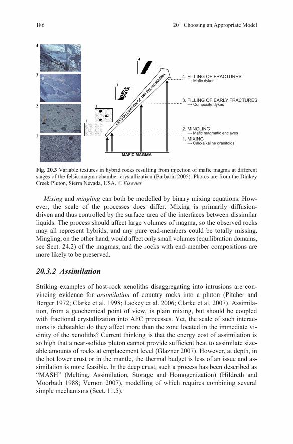
Fig. 20.3 Variable textures in hybrid rocks resulting from injection of mafic magma at different stages of the felsic magma chamber crystallization (Barbarin 2005). Photos are from the Dinkey Creek Pluton, Sierra Nevada, USA. © Elsevier
Mixing and mingling can both be modelled by binary mixing equations. How-ever, the scale of the processes does differ. Mixing is primarily diffusion-
ace area of the interfaces between dissimilarliquids. The process should affect large volumes of magma, so the observed rocksmay all represent hybrids, and any pure end-members could be totally missing.Mingling, on the other hand, would affect only small volumes (equilibration domains,see Sect. 24.2) of the magmas, and the rocks with end-member compositions aremore likely to be preserved.
4. FILLING OF FRACTURES → Mafic dykes
3. FILLING OF EARLY FRACTURES → Composite dykes
2. MINGLING → Mafic magmatic enclaves1. MIXING → Calc-alkaline granitoids
MAFIC MAGMA
CRYSTALL
IZATIO
N OF T
HE FELS
IC M
AGMA
20.3.2 Assimilation
Striking examples of host-rock xenoliths disaggregating into intrusions are con-vincing evidence for assimilation of country rocks into a pluton (Pitcher and Berger 1972; Clarke et al. 1998; Lackey et al. 2006; Clarke et al. 2007). Assimila-tion, from a geochemical point of view, is plain mixing, but should be coupled with fractional crystallization into AFC processes. Yet, the scale of such interac-tions is debatable: do they affect more than the zone located in the immediate vi-cinity of the xenoliths? Current thinking is that the energy cost of assimilation is so high that a near-solidus pluton cannot provide sufficient heat to assimilate size-able amounts of rocks at emplacement level (Glazner 2007). However, at depth, in the hot lower crust or in the mantle, the thermal budget is less of an issue and as-similation is more feasible. In the deep crust, such a process has been described as “MASH” (Melting, Assimilation, Storage and Homogenization) (Hildreth and Moorbath 1988; Vernon 2007), modelling of which requires combining several simple mechanisms (Sect. 11.5).
186 20 Choosing an Appropriate Model
driven and thus controlled by the surf
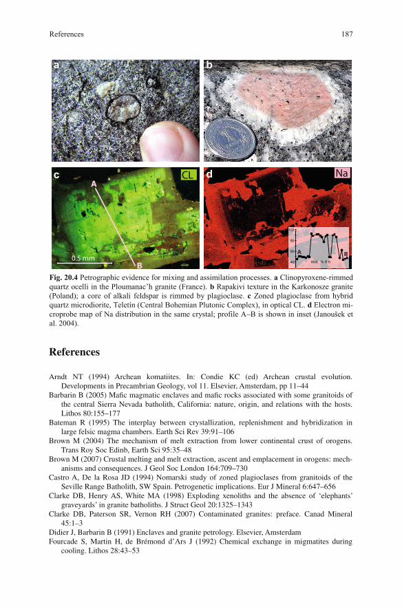
Fig. 20.4 Petrographic evidence for mixing and assimilation processes. a Clinopyroxene-rimmed quartz ocelli in the Ploumanac’h granite (France). b Rapakivi texture in the Karkonosze granite (Poland); a core of alkali feldspar is rimmed by plagioclase. c Zoned plagioclase from hybrid quartz microdiorite, Teletín (Central Bohemian Plutonic Complex), in optical CL. d Electron mi-croprobe map of Na distribution in the same crystal; profile A–B is shown in inset (Janoušek et al. 2004).
a b
mol. % A n40
60
80
100
Nac.A
B0.5 mm
CL dc
References
References 187
Arndt NT (1994) Archean komatiites. In: Condie KC (ed) Archean crustal evolution. Developments in Precambrian Geology, vol 11. Elsevier, Amsterdam, pp 11–44
Barbarin B (2005) Mafic magmatic enclaves and mafic rocks associated with some granitoids of the central Sierra Nevada batholith, California: nature, origin, and relations with the hosts. Lithos 80:155–177
Bateman R (1995) The interplay between crystallization, replenishment and hybridization in large felsic magma chambers. Earth Sci Rev 39:91–106
Brown M (2004) The mechanism of melt extraction from lower continental crust of orogens. Trans Roy Soc Edinb, Earth Sci 95:35–48
Brown M (2007) Crustal melting and melt extraction, ascent and emplacement in orogens: mech-anisms and consequences. J Geol Soc London 164:709–730
Castro A, De la Rosa JD (1994) Nomarski study of zoned plagioclases from granitoids of the Seville Range Batholith, SW Spain. Petrogenetic implications. Eur J Mineral 6:647–656
Clarke DB, Henry AS, White MA (1998) Exploding xenoliths and the absence of ‘elephants’ graveyards’ in granite batholiths. J Struct Geol 20:1325–1343
Clarke DB, Paterson SR, Vernon RH (2007) Contaminated granites: preface. Canad Mineral 45:1–3
Didier J, Barbarin B (1991) Enclaves and granite petrology. Elsevier, AmsterdamFourcade S, Martin H, de Brémond d’Ars J (1992) Chemical exchange in migmatites during
cooling. Lithos 28:43–53
188 20 Choosing an Appropriate Model
Ginibre C, Wörner G, Kronz A (2002) Minor- and trace-element zoning in plagioclase: implica-tions for magma chamber processes at Parinacota volcano, northern Chile. Contrib Mineral Petrol 143:300–315
Glazner AF (2007) Thermal limitations on incorporation of wall rock into magma. Geology 35:319–322
Hallot E, Davy P, de Brémond d’Ars J, Auvray B, Martin H, van Damme H (1996) Non-Newtonian effects during injection in partially crystallised magmas. J Volcanol Geotherm Res 71:31–44
Harker A (1909) A natural history of igneous rocks. Methuen and Co., LondonHasalová P, Janoušek V, Schulmann K, Štípská P, Erban V (2008) From orthogneiss to migma-
tite: geochemical assessment of the melt infiltration model in the Gföhl Unit (Moldanubian Zone, Bohemian Massif). Lithos 102:508–537
Hibbard MJ (1991) Textural anatomy of twelve magma-mixed granitoid systems. In: Didier J, Barbarin B (eds) Enclaves and granite petrology. Elsevier, Amsterdam, pp 431–444
Hibbard MJ (1995) Mixed magma rocks. In: Petrography to petrogenesis. Prentice Hall, New Jersey, pp 242–260
Hildreth W, Moorbath S (1988) Crustal contributions to arc magmatism in the Andes of central Chile. Contrib Mineral Petrol 98:455–489
Janoušek V, Bowes DR, Braithwaite CJR, Rogers G (2000) Microstructural and mineralogical evidence for limited involvement of magma mixing in the petrogenesis of a Hercynian high-K calc-alkaline intrusion: the Kozárovice granodiorite, Central Bohemian Pluton, Czech Republic. Trans Roy Soc Edinb, Earth Sci 91:15–26
Janoušek V, Braithwaite CJR, Bowes D, Gerdes A (2004) Magma-mixing in the genesis of Hercynian calc-alkaline granitoids: an integrated petrographic and geochemical study of the Sázava intrusion, Central Bohemian Pluton, Czech Republic. Lithos 78:67–99
Kriegsman LM, Hensen BJ (1998) Back reaction between restite and melt: implications for geo-thermobarometry and pressure–temperature paths. Geology 26:1111–1114
Lackey JS, Valley JW, Hinke HJ (2006) Deciphering the source and contamination history of per-aluminous magmas using δ18O of accessory minerals: examples from garnet-bearing plutons of the Sierra Nevada Batholith. Contrib Mineral Petrol 151:20–44
Marshall DJ (1988) Cathodoluminescence of geological materials. Unwin Hyman, BostonMehnert KR (1968) Migmatites and the origin of granitic rocks. Elsevier, AmsterdamMorgavi D, Perugini D, de Campos CP, Ertel-Ingrisch W, Dingwell DB (2013) Morphochemistry
of patterns produced by mixing of rhyolitic and basaltic melts. J Volcanol Geotherm Res 253:87–96
Pagel M, Barbin V, Blanc P, Ohnenstetter D (2000) Cathodoluminescence in geosciences. Springer, Berlin
Pearson D, Canil D, Shirey S (2003) Mantle samples included in volcanic rocks: xenoliths and diamonds. In: Carlson R (ed) The mantle and core. Treatise on Geochemistry, vol 2. Elsevier, Amsterdam, pp 171–275
Perugini D, Poli G (2000) Chaotic dynamics and fractals in magmatic interaction processes: a different approach to the interpretation of mafic microgranular enclaves. Earth Planet Sci Lett 175:93–103
Pitcher WS, Berger AR (1972) The geology of Donegal: a study of granite emplacement and unroofing. Wiley-Interscience, New York
Sawyer EW (2008) Atlas of migmatites. The Canadian Mineralogist Special Publication, vol 9. NRC Research Press, Ottawa
Sisson TW, Bacon CR (1999) Gas-driven filter pressing in magmas. Geology 27:613–616Stevens G, van Reenen D (1992) Partial melting and the origin of metapelitic granulites in the
Southern Marginal Zone of the Limpopo Belt, South Africa. Precambr Res 55:303–319Stevens G, Clemens JD, Droop GTR (1997) Melt production during granulite-facies anatexis: exper-
imental data from ‘primitive’ metasedimentary protoliths. Contrib Mineral Petrol 128:352–370

189References
Taylor J, Nicoli G, Stevens G, Frei D, Moyen JF (2014) The processes that control leucosome compositions in metasedimentary granulites: perspectives from the Southern Marginal Zone migmatites, Limpopo Belt, South Africa. J Metam Geol 32:713–742
Vernon RH (1991) Interpretation of microstructures of microgranitoid enclaves. In: Didier J, Barbarin B (eds) Enclaves and granite petrology. Elsevier, Amsterdam, pp 277–291
Vernon RH (2007) Problems in identifying restite in S-type granites of southeastern Australia, with speculations on sources of magma and enclaves. Canad Mineral 45:147–178
Walter M (2003) Melt extraction and compositional variability in mantle lithosphere. In: Carlson R (ed) The mantle and core. Treatise on Geochemistry, vol 2. Elsevier, Amsterdam, pp 363–394
Wiebe RA, Collins WJ (1998) Depositional features and stratigraphic sections in granitic plu-tons: implications for the emplacement and crystallization of granitic magma. J Struct Geol 20:1273–1289
Yakymchuk C, Brown M (2014) Consequences of open-system melting in tectonics. J Geol Soc London 171:21–40
Chapter 21 Semi-Quantitative Geochemical Approach
Even without embarking on developing a proper geochemical model, it is possible to devise several geochemical tests that can help in selecting a model, or in con-straining some of its parameters.
21.1 Assessing Trace-Element Compatibility
As noted already in Sect. 10.2, the concept of compatibility and incompatibility of a trace element is a relative one. For instance, let’s consider the behaviour of Yb. During peridotite melting, leaving a residue made of olivine ( /
Yb
Ol LDK = 0.00151 ),
orthopyroxene ( /Yb
Opx LDK = 0.05) and clinopyroxene ( /
Yb
Cpx LDK = 0.28), DYb << 1 and Yb
would show a strongly incompatible behaviour. In contrast, for eclogite meltingthe residue consists of clinopyroxene ( /
Yb
Cpx LDK = ~1.0) and garnet ( /
Yb
Grt LDK = 21); con-
sequently, DYb >> 1 and Yb would be strongly compatible as soon as more than 5% garnet is present.
In silica-rich magmas, most elements tend to become compatible due to the complex main rock-forming and accessory mineral assemblages involved. Even elements such as REE (strongly incompatible in basic magmas) are hosted by ac-cessory minerals (allanite, monazite, xenotime, etc.). Of course, this effect is taken to the extreme in highly differentiated systems, such as pegmatites.
The first step in any study is, therefore, to assess the behaviour of each element in the system. The simplest approach is to plot binary diagrams of a differentiation index vs. the investigated elements. A positive correlation characterizes incom-patible, and a negative one compatible elements. In basic suites, commonly used differentiation indexes are MgO, Cr, Ni or mg#, while in intermediate to acid as-sociations, SiO2 is preferred. Still, it must be kept in mind that diagrams involving major elements, especially SiO2, suffer from the constant sum effect (Sect. 3.1.2).
1 KD values are from Rollinson (1993).
© Springer-Verlag Berlin Heidelberg 2016 V. Janoušek et al., Geochemical Modelling of Igneous Processes – Principles And Recipes in R Language, Springer Geochemistry, DOI 10.1007/978-3-662-46792-3_21
191
21.2 Order of (In)Compatibility
Regardless of the process involved, the largest changes in elemental concentra-tions are observed for D values very different from 1. This idea was developed for incompatible elements by Schiano et al. (1993). In a suite of rocks related by a single petrogenetic process (such as fractional crystallization or partial melting), there is a correlation between D and the variability of the dataset, defined as:
( ) V (21.1)
with ( ) and referring respectively to the standard deviation, and the mean of the concentrations, of the element .
For incompatible elements, the order of increasing variability then mimics the increasing incompatibility of individual elements (i.e. the smaller D, the higher the variability). Likewise for compatible elements, variability correlates with com-patibility (large D results in high variabilities): elements with D very different from 1 (very compatible or very incompatible) have highest variabilities2. Several applications of this approach can be found in Schiano et al. (1993). For instance, one may plot the variability of a dataset against that in a reference rock suite (typi-cally MORBs). Elements plotting away from the 1:1 line have D values different in the two sets (often because other minerals were involved, in the melting source
plotting a spidergram normalized to the likely source, if all the elements are arranged in the order of compatibility estab-lished from the dataset, any anomalies reveal deviation of the source composition from the normalization values.
Exercise 21.1: Order of (in)compatibility
chpuy.data hofmann.data
2 Thus, this approach originally developed for incompatible elements will also work for compati-ble ones, but the two groups must be treated independently.3 Major elements were corrected for reequilibration with the host olivine.
192 21 Semi-Quantitative Geochemical Approach
crystallizing assemblage). Similarly, when
File chpuy.data contains analyses3 for melt inclusions in olivine crystals from the Chaîne des Puys Quaternary volcanoes of central France (Jannot 2005). We shall investigate the genesis of these magmas from their mantle source; we focus on the set of elements present in Hofmann’s (1988) Primitive Mantle composition, for which the variability in MORBs was calculated by Schiano et al. (1993).
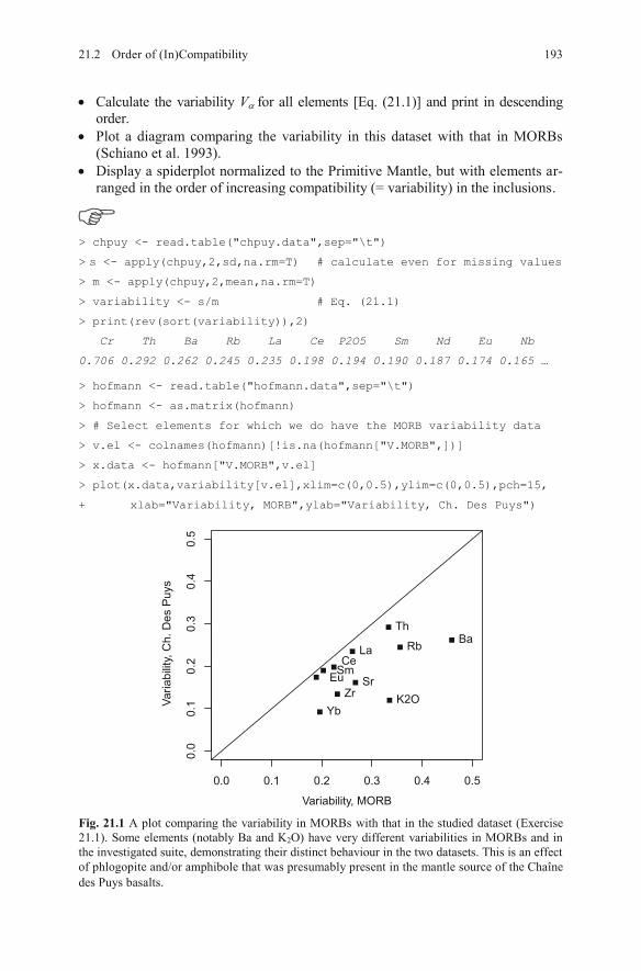
Calculate the variability V for all elements [Eq. (21.1)] and print in descending order. Plot a diagram comparing the variability in this dataset with that in MORBs (Schiano et al. 1993). Display a spiderplot normalized to the Primitive Mantle, but with elements ar-ranged in the order of increasing compatibility (= variability) in the inclusions.
> chpuy <- read.table("chpuy.data",sep="\t")
> s <- apply(chpuy,2,sd,na.rm=T) # calculate even for missing values
> m <- apply(chpuy,2,mean,na.rm=T)
> variability <- s/m # Eq. (21.1)
> print(rev(sort(variability)),2)
Cr Th Ba Rb La Ce P2O5 Sm Nd Eu Nb
0.706 0.292 0.262 0.245 0.235 0.198 0.194 0.190 0.187 0.174 0.165 …
> hofmann <- read.table("hofmann.data",sep="\t")
> hofmann <- as.matrix(hofmann)
> # Select elements for which we do have the MORB variability data
> v.el <- colnames(hofmann)[!is.na(hofmann["V.MORB",])]
> x.data <- hofmann["V.MORB",v.el]
> plot(x.data,variability[v.el],xlim=c(0,0.5),ylim=c(0,0.5),pch=15,
+ xlab="Variability, MORB",ylab="Variability, Ch. Des Puys")
Fig. 21.1 A plot comparing the variability in MORBs with that in the studied dataset (Exercise 21.1). Some elements (notably Ba and K2O) have very different variabilities in MORBs and in the investigated suite, demonstrating their distinct behaviour in the two datasets. This is an effect of phlogopite and/or amphibole that was presumably present in the mantle source of the Chaîne
0.0 0.1 0.2 0.3 0.4 0.5
0.0
0.1
0.2
0.3
0.4
0.5
Variability, MORB
Vari
ability, C
h. D
es P
uys
Th
BaRbLa
Ce
Eu Sr
ZrK2O
Yb
21. y 1932 Order of (In)Compatibilit
des Puys basalts.
Sm
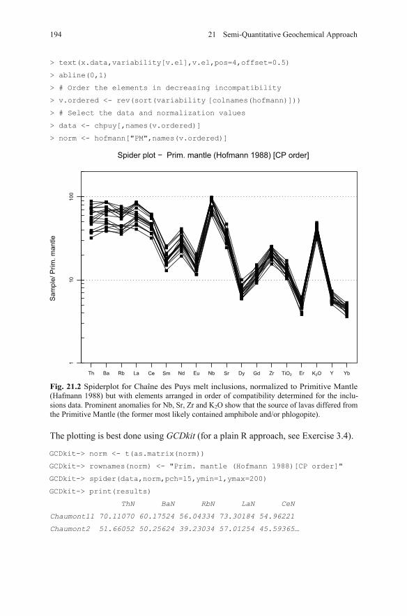
> text(x.data,variability[v.el],v.el,pos=4,offset=0.5)
> abline(0,1)
> # Order the elements in decreasing incompatibility
> v.ordered <- rev(sort(variability [colnames(hofmann)]))
> # Select the data and normalization values
> data <- chpuy[,names(v.ordered)]
> norm <- hofmann["PM",names(v.ordered)]
Fig. 21.2 Spiderplot for Chaîne des Puys melt inclusions, normalized to Primitive Mantle
ogopite).
The plotting is best done using GCDkit (for a plain R approach, see Exercise 3.4). GCDkit-> norm <- t(as.matrix(norm))
GCDkit-> rownames(norm) <- "Prim. mantle (Hofmann 1988)[CP order]"
GCDkit-> spider(data,norm,pch=15,ymin=1,ymax=200)
GCDkit-> print(results)
ThN BaN RbN LaN CeN
Chaumont11 70.11070 60.17524 56.04334 73.30184 54.96221
Chaumont2 51.66052 50.25624 39.23034 57.01254 45.59365…
Th Ba Rb La Ce Sm Nd Eu Nb Sr Dy Gd Zr TiO2 Er K2O Y Yb
110
100
Spider plot − Prim. mantle (Hofmann 1988) [CP order]
Sam
ple/
Prim
. man
tle
194 21 Semi-Quantitative Geochemical Approach
(Hafmann 1988) but with elements arranged in order of compatibility determined for the inclu-
the Primitive Mantle (the former most likely contained amphibole and/or phl2O show that the source of lavas differed fromsions data. Prominent anomalies for Nb, Sr, Zr and K
21.3 Process Identification
For major elements, the three main petrogenetic processes (melting, crystallization and mixing) are governed by mass-balance relationships (Sect. 6.5). This results in a linear trend in any binary plot of major-element compositions.
A linear trend in a binary plot of two major elements, or their oxides (in-cluding Harker plots), indicates no specific petrogenetic process! This can
be generalized, in p-dimensional space, for p major elements.
For trace elements, melting is commonly regarded as a batch process and crystal-lization as fractional. Mixing, on the other hand, still follows linear laws. As shown in Part III, these three processes are described by contrasting equations:
0 (1 )L
CCD F D
, ( 1)
0
DLC FC
and 1 1 1 21LC f C f C .
In a binary plot of two trace elements, the resulting curves have different shapes4.
21.3.1 Mixing vs. Crystallization/Melting
Recognition of mixing is, theoretically, straightforward. Mixing is controlled by mass balance and yields linear trends in any element vs. element diagram (and hy-perbolae in plots involving at least one ratio, see Table 11.1), whereas the two other processes generate curved trends (except in a major major plot) . A straight
4 But see Sect. 24.3.1 for a discussion on the feasibility of distinguishing between processes.
21.3 Process Identification 195
no indicator of fractiona-D e fractio-
0 LCC F , i.e. a straight line).
Obviously, isotopes are the tool of choice to spot mixing—at least between two isotopically contrasting compositions. However, open-system processes such as magma mixing or assimilation are frequently accompanied with, or followed by, fractional crystallization/accumulation that modifies the binary mixing-related elemental distribution, often beyond recognition. Even in such cases, the isotope ratios should escape unaffected, still ‘seeing through’ such modifications (Part IV).
21.3.2 Crystallization vs. Melting in a Log–Log Diagram
In Chap. 11, it has been shown that the behaviour of incompatible elements during both crystallization and melting is roughly similar. Indeed, they are all expressed
line in a trace-trace (or major-trace) diagram is therefore tion, but rather points to mixing (unless is close to 0, in which case thnation/batch curves both collapse to
–
by equations such that when D 0, then CL C0/F. On the other hand, fractional crystallization is extremely efficient at depleting compatible elements in a magma, whereas partial melting has little effect on these.
This relation is usually described in a log( ) vs. log( ) diagram, where is in-compatible and compatible. From Rayleigh’s Law we derive for each element:
(21.2)
(21.3)
Combining two Eq. (21.3), for and , gives:
(21.4)
(21.5)
Since D ~ 0 and D 1, the slope is steep negative5, close to –D .
Likewise, the fractional melting equation (instantaneous liquids, Eq. 11.13) can be expressed for elements and , transformed in log coordinates and combined into:
(21.6)
The result is again a straight line, whose slope is:
11
D DD D
(21.7)
5 Note that
196 21 Semi-Quantitative Geochemical Approach
0log log 1 logLC C D F
0log loglog1
LC CFD
0 0
1log log log C log C
111L L
D DC C
D D
In a log(C ) vs. log(C ) diagram, this is a straight line whose slope is:
11
DD
0
0
1 1log log log log 1
1 1log log1
L L
D DC C C
D D D
D DC
D D D
the slope of the line is distorted. the scales should be the same on both axes; indeed when the scales are too dissimilar
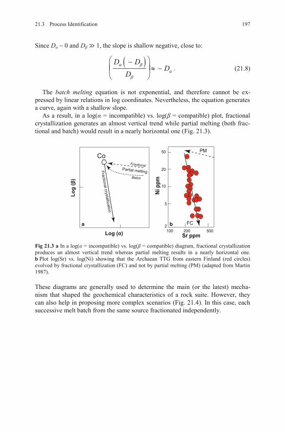
Since D ~ 0 and D 1, the slope is shallow negative, close to:
D D
DD
. (21.8)
The batch melting equation is not exponential, and therefore cannot be ex-pressed by linear relations in log coordinates. Nevertheless, the equation generates a curve, again with a shallow slope.
As a result, in a log( = incompatible) vs. log( = compatible) plot, fractional crystallization generates an almost vertical trend while partial melting (both frac-tional and batch) would result in a nearly horizontal one (Fig. 21.3).
Fig 21.3 a In a log( = incompatible) vs. log( = compatible) diagram, fractional crystallization produces an almost vertical trend whereas partial melting results in a nearly horizontal one. b Plot log(Sr) vs. log(Ni) showing that the Archaean TTG from eastern Finland (red circles) evolved by fractional crystallization (FC) and not by partial melting (PM) (adapted from Martin 1987).
These diagrams are generally used to determine the main (or the latest) mecha-nism that shaped the geochemical characteristics of a rock suite. However, they can also help in proposing more complex scenarios (Fig. 21.4). In this case, each successive melt batch from the same source fractionated independently.
Log
(β)
Log (α)
Partial meltingFractional crystallization
Co
100 200 500
50
20
10
5
2
Sr ppm
Ni p
pm
FC
PM
Fractional
Batch
a b
19721.3 Process Identification
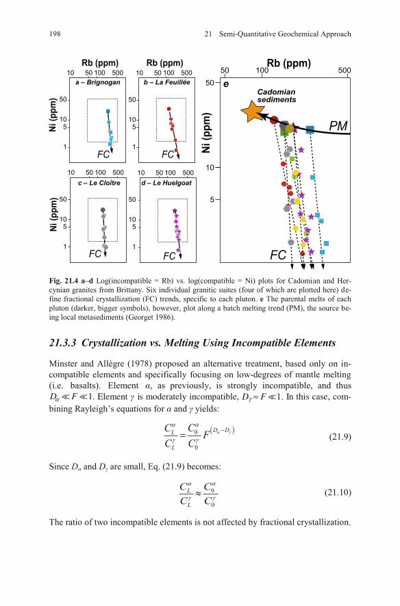
Fig. 21.4 a–d Log(incompatible = Rb) vs. log(compatible = Ni) plots for Cadomian and Her-cynian granites from Brittany. Six individual granitic suites (four of which are plotted here) de-fine fractional crystallization (FC) trends, specific to each pluton. e The parental melts of each pluton (darker, bigger symbols), however, plot along a batch melting trend (PM), the source be-ing local metasediments (Georget 1986).
21.3.3 Crystallization vs. Melting Using Incompatible Elements
Minster and Allègre (1978) proposed an alternative treatment, based only on in-compatible elements and specifically focusing on low-degrees of mantle melting (i.e. basalts). Element , as previously, is strongly incompatible, and thus
r and yields:
0
0
D DL
L
CC FC C
(21.9)
Since D and D are small, Eq. (21.9) becomes:
0
0
L
L
CCC C
(21.10)
The ratio of two incompatible elements is not affected by fractional crystallization.
198 21 Semi-Quantitative Geochemical Approach
50
10
1
5
5001005010
b – La Feuillée
1
5
5001005010
Rb (ppm)
a – Brignogan
50
10
1
5
5001005010
d – Le Huelgoatc – Le Cloître
50
10
1
5
5001005010
Ni (p
pm
)
50
10
5
50010050
PM
FC
50
10
FC FC
FC FC
Cadomiansediments
Rb (ppm)N
i (p
pm
)
Ni (p
pm
)
Rb (ppm)
e
1D Fα . Element is moderately incompatible, 1.D Fγ ≈ In this case, com-bining Rayleigh’s equations fo
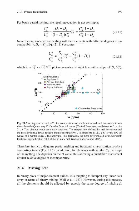
For batch partial melting, the resulting equation is not so simple:
0
0 0
1(1 ) 1
LL
L
D CC CC C
DC D
DD
(21.11)
Nevertheless, since we are dealing with two elements with different degrees of in-compatibility, , Eq. (21.11) becomes:
0
0 0
1LL
L
D CC C DC C C
(21.12)
which in a LC vs. /L LC C plot represents a straight line with a slope of 0/D C .
Fig. 21.5 A diagram La vs. La/Yb for compositions of whole rocks and melt inclusions in oli-vines from the Quaternary Chaîne des Puys volcanoes (Central France) (same dataset as Exercise 21.1). Two distinct trends are clearly apparent. The steeper line, defined by melt inclusions and the most primitive lavas, reflects mantle melting (PM). Its intercept at La0/Yb0 is very low (as
Therefore, in such a diagram, partial melting and fractional crystallization produce contrasting trends (Fig. 21.5). In addition, for elements with similar C0, the slope of the melting line depends on the D value, thus allowing a qualitative assessment of their relative degree of incompatibility.
21.4 Mixing Test
In binary plots of major-element oxides, it is tempting to interpret any linear data array in terms of binary mixing (Wall et al. 1987). However, during this process, all the elements should be affected by exactly the same degree of mixing f1.
0
10
20
30
40
100
La/Y
b
La (ppm)0 20 40 60 80
Puy Beaunit
Puy ChaumontPuy des Trois Sols
Puy de la Vache
Melt inclusions
Chaîne des Puys lavas
FC
PM
19921.3 Process Identification
Dα Dγ
typical of a mantle source). The horizontal line, formed by the more differentiated lavas, represents fractional crystallization (FC) of the primary melt (redrawn after Jannot 2005).
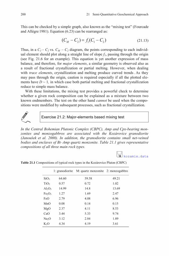
the “mixing test” (Fourcade and Allègre 1981). Equation (6.23) can be rearranged as:
2 1 1 2( ) ( )MC C f C C (21.13)
Thus, in a C1 – C2 vs. CM – C2 diagram, the points corresponding to each individ-ual element should plot along a straight line of slope f1, passing through the origin (see Fig. 21.6 for an example). This equation is yet another expression of mass balance, and therefore, for major elements, a similar geometry is observed also as a result of fractional crystallization or partial melting. However, when dealing with trace elements, crystallization and melting produce curved trends . As they may pass through the origin, caution is required especially if all the plotted ele-ments have D ~ 1, in which case both partial melting and fractional crystallization reduce to simple mass balance.
cannot be used when the compo-
Exercise 21.2: Major-elements based mixing test
kozamix.data
Table 21.1 Compositions of typical rock types in the Kozárovice Pluton (CBPC)
1: granodiorite M: quartz monzonite 2: monzogabbro
SiO2 64.60 59.58 49.21TiO2 0.57 0.72 1.02Al2O3 14.99 14.8 13.69Fe2O3 1.27 1.69 2.47FeO 2.79 4.08 6.96MnO 0.08 0.14 0.15MgO 2.37 4.11 8.53CaO 3.44 5.33 9.74Na2O 3.12 2.84 1.89K2O 4.34 4.19 3.61
200 21 Semi-Quantitative Geochemical Approach
This can be checked by a simple graph, also known as
With these limitations, the mixing test provides a powerful check to determine whether a given rock composition can be explained as a mixture between two known endmembers. The test on the other hand sitions were modified by subsequent processes, such as fractional crystallization.
In the Central Bohemian Plutonic Complex (CBPC), Amp and Cpx-bearing mon-zonites and monzogabbros are associated with the Kozárovice granodiorite (Janoušek et al. 2000). In addition, the granodiorite contains small net-veined bodies and enclaves of Bt–Amp quartz monzonite. Table 21.1 gives representative compositions of all three main rock types.
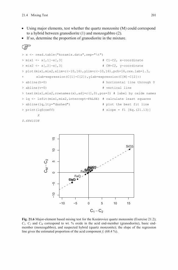
Using major elements, test whether the quartz monzonite (M) could correspond to a hybrid between granodiorite (1) and monzogabbro (2).
If so, determine the proportion of granodiorite in the mixture.
> x <- read.table("kozamix.data",sep="\t")
> mix1 <- x[,1]-x[,3] # C1-C2, x-coordinate
> mix2 <- x[,2]-x[,3] # CM-C2, y-coordinate
> plot(mix1,mix2,xlim=c(-10,16),ylim=c(-10,16),pch=16,cex.lab=1.3,
+ xlab=expression(C[1]-C[2]),ylab=expression(C[M]-C[2]))
> abline(h=0) # horizontal line through 0
> abline(v=0) # vertical line
> text(mix1,mix2,rownames(x),adj=c(1,0),pos=3) # label by oxide names
> lq <- lsfit(mix1,mix2,intercept=FALSE) # calculate least squares
> abline(lq,lty="dashed") # plot the best fit line
> print(lq$coeff) # slope = f1 [Eq.(21.13)]
X
0.6841038
Fig. 21.6 Major-element based mixing test for the Kozárovice quartz monzonite (Exercise 21.2); C1, C2 and CM correspond to wt. % oxide in the acid end-member (granodiorite), basic end-member (monzogabbro), and suspected hybrid (quartz monzonite); the slope of the regression line gives the estimated proportion of the acid component f1 (68.4 %).
−10 −5 0 5 10 15
−1
0−
50
51
01
5
C1 C2
CM
C
2
SiO2
TiO2
Al2O3
FeO
Fe2O3MnO
MgOCaO
Na2OK2O
21.4 Mixing Test 201
21.5 Identifying Fractionating Minerals Using Log–Log Plots
For Rayleigh-type fractionation, one may identify controlling phases using log–log plots of whole-rock trace-element concentrations, in which the originally ex-ponential trends are converted to linear ones [Eq. (21.2)]. This enables plotting fractionation vectors, either for pure mineral phases, or any combination thereof.
A clever choice consists in using compatible elements, whose content sharply decreases during fractional crystallization. Of course, such an approach requires the prior determination, for the investigated system, of the compati-ble/incompatible character of all elements (see Sect. 21.1).
Exercise 21.3: Fractionation vectors
Table 21.2 Partition coefficients for selected minerals in dacitic to rhyolitic melts (Hanson 1978)
Mineral Sr BaAmp 0.22 0.044Bt 0.12 6.36Kfs 3.87 6.12Pl 4.4 0.31
blatna.data hanson.data
Plot the analyses in a binary graph of Ba vs. Sr (with logarithmic coordinates).
rock-forming mineral.
> WR <- read.table("blatna.data",sep="\t") # Read whole-rock data
> kd <- read.table("hanson.data",sep="\t") # Partition coefficients
> # Binary plot (plain R)
> plot(WR[,"Ba"],WR[,"Sr"],xlab="Ba",ylab="Sr",log="xy",pch=15,
+ ylim=c(250,550))
202 21 Semi-Quantitative Geochemical Approach
The file blatna.data contains Ba and Sr concentrations (ppm) from granodioritic rocks of the Blatná suite, Central Bohemian Plutonic Complex (Janoušek et al. 2010). Table 21.2 summarizes partition coefficients between amphibole, biotite, K-feldspar and plagioclase and dacitic to rhyolitic melts (Hanson 1978).
Superimpose vectors portraying 10 % fractional crystallization of each individual
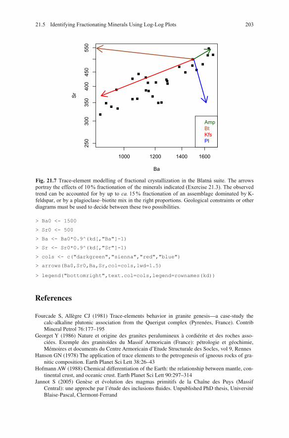
Fig. 21.7 Trace-element modelling of fractional crystallization in the Blatná suite. The arrows portray the effects of 10 % fractionation of the minerals indicated (Exercise 21.3). The observed trend can be accounted for by up to ca. 15 % fractionation of an assemblage dominated by K-feldspar, or by a plagioclase–biotite mix in the right proportions. Geological constraints or other diagrams must be used to decide between these two possibilities.
> Ba0 <- 1500
> Sr0 <- 500
> Ba <- Ba0*0.9^(kd[,"Ba"]-1)
> Sr <- Sr0*0.9^(kd[,"Sr"]-1)
20321.5 Identifying Fractionating Minerals Using Log-Log Plots
References
Fourcade S, Allègre CJ (1981) Trace-elements behavior in granite genesis—a case-study the calc-alkaline plutonic association from the Querigut complex (Pyrenées, France). Contrib Mineral Petrol 76:177–195
Georget Y (1986) Nature et origine des granites peralumineux à cordiérite et des roches asso-ciées. Exemple des granitoïdes du Massif Armoricain (France): pétrologie et géochimie, Mémoires et documents du Centre Armoricain d’Etude Structurale des Socles, vol 9, Rennes
Hanson GN (1978) The application of trace elements to the petrogenesis of igneous rocks of gra-nitic composition. Earth Planet Sci Lett 38:26–43
Hofmann AW (1988) Chemical differentiation of the Earth: the relationship between mantle, con-tinental crust, and oceanic crust. Earth Planet Sci Lett 90:297–314
Jannot S (2005) Genèse et évolution des magmas primitifs de la Chaîne des Puys (Massif Central): une approche par l’étude des inclusions fluides. Unpublished PhD thesis, Université Blaise-Pascal, Clermont-Ferrand
> cols <- c("darkgreen","sienna","red","blue")
> arrows(Ba0,Sr0,Ba,Sr,col=cols,lwd=1.5)
> legend("bottomright",text.col=cols,legend=rownames(kd))
1000 1200 1400 1600
250
300
350
400
450
550
Ba
Sr
AmpBtKfsPl
204 21 Semi-Quantitative Geochemical Approach
Janoušek V, Bowes DR, Braithwaite CJR, Rogers G (2000) Microstructural and mineralogical evidence for limited involvement of magma mixing in the petrogenesis of a Hercynian high-K calc-alkaline intrusion: the Kozárovice granodiorite, Central Bohemian Pluton, Czech Republic. Trans Roy Soc Edinb, Earth Sci 91:15–26
Janoušek V, Wiegand BA, Žák J (2010) Dating the onset of Variscan crustal exhumation in the core of the Bohemian Massif: new U–Pb single zircon ages from the high-K calc-alkaline granodiorites of the Blatná suite, Central Bohemian Plutonic Complex. J Geol Soc London 167:347–360
Martin H (1987) Petrogenesis of Archaean trondhjemites, tonalites and granodiorites from east-ern Finland; major and trace element geochemistry. J Petrol 28:921–953
Minster J, Allègre C (1978) Systematic use of trace elements in igneous processes. Part III: inverse problem of batch partial melting in volcanic suites. Contrib Mineral Petrol 68:37–52
Rollinson HR (1993) Using geochemical data: evaluation, presentation, interpretation. Longman, London
Schiano P, Allègre CJ, Dupré B, Lewin E, Joron J-L (1993) Variability of trace elements in basal-tic suites. Earth Planet Sci Lett 119:37–51
Wall VJ, Clemens JD, Clarke DB (1987) Models for granitoid evolution and source composi-tions. J Geol 95:731–749
Chapter 22 Constraining a Model
After completing the previous tasks, enough information should have been gath-ered to decide on the likely processes shaping the composition of the suite. This chapter will discuss setting different parameters for subsequent calculations.
22.1 Choosing an Appropriate Strategy
First of all, one has to decide on “variants” of the model, e.g., batch vs. fractional processes. The choice between these will be based on a balance between added complexity (related to the number of free parameters that will have to be set), and geological realism. Quite possibly, the best strategy is to test several variants of the models, and see (i) whether they produce results that are significantly differ-ent, and (ii) which one provides a better match with the data.
After that, a correct treatment has to be chosen for each element. Is it a major (mass balance only), a dilute trace (partition coefficient) or an ESC-type (solubil-ity-controlled) element? Again, the choice will be guided primarily by petrology, especially by the nature of the minerals present. For instance, when a system only
amounts of K2O, e.g. during a partial melting of a phlogopite-bearing 2O behaves as a major element since it is a
stoichiometric component in phlogopite. However, this would imply knowing the phlogopite composition, which may be difficult to constrain. On the other hand, K2O can be treated as a trace element, by assuming that
2
/K O
Phl LDK is constant. This
scenario leads to fewer assumptions and simplifies the computing procedure (for instance by ignoring major elements and focussing on traces). We shall return to this question in Exercise 22.1 and compare the results of different equations when dealing with accessory minerals.
Finally, one must decide on the use of a forward or reverse approach. The un-derlying logic is not the same. A forward model will be handy to test a hypothesis (“can this cumulate account for the liquid line of descent as observed in the host lavas?”). Reverse models would rather help in constraining an otherwise poorly known process (“which cumulate modal composition may generate such trends?”).
© Springer-Verlag Berlin Heidelberg 2016 V. Janoušek et al., Geochemical Modelling of Igneous Processes – Principles And Recipes in R Language, Springer Geochemistry, DOI 10.1007/978-3-662-46792-3_22
205
contains smallsperidotite, it is possible to consider that K
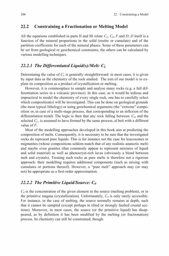
22.2 Constraining a Fractionation or Melting Model
All the equations established in parts II and III relate CL, C0, F and D; D itself is a function of the mineral proportions in the solid (restite or cumulate) and of the partition coefficients for each of the mineral phases. Some of these parameters can be set from geological or geochemical constraints; the others can be calculated by various modelling techniques.
22.2.1 The Differentiated Liquid(s)/Melt: CL
Determining the value of CL is generally straightforward: in most cases, it is given by input data as the chemistry of the rock studied. The aim of our model is to ex-plain its composition as a product of crystallization or melting.
However, it is commonplace to sample and analyse many rocks (e.g. a full dif-ferentiation series in a volcanic province). In this case, as it would be tedious and impractical to model the chemistry of every single rock, one has to carefully selectwhich composition(s) will be investigated. This can be done on geological grounds (the most typical lithology) or using geochemical arguments (the “sition or, in case of a multi-stage process, that corresponding to an inflexion of the differentiation trend). The logic is then that any rock falling between selected CL, is assumed to have formed by the same process, al
-
value of F. Most of the modelling approaches developed in this book aim at predicting the
composition of melts. Consequently, it is necessary to be sure that the investigated rocks do represent pure liquids. This is for instance not the case for leucosomes in migmatites (whose compositions seldom match that of any realistic anatectic melt) and maybe even granites (that commonly appear to represent mixtures of liquid and solid material) as well as phenocryst-rich lavas (obviously a blend between melt and crystals). Treating such rocks as pure melts is therefore not a rigorous approach: their modelling requires additional components (such as mixing with cumulates or portions thereof). However, a “pure melt” approach may (or may not) be appropriate as a first-order approximation.
22.2.2 The Primitive Liquid/Source: C0
C0 is the concentration of the given element in the source (melting problem), or in the primitive magma (crystallization). Unfortunately, C0 is only rarely accessible. For instance, in the case of melting, the source normally remains at depth, such that it cannot be sampled (except perhaps in tilted or strongly faulted crustal sec-tions). Moreover, in most cases, the source (or the primitive liquid) has disap-peared, as by definition it has been modified by the melting (or fractionation) process. Its chemistry can still be constrained, though.
206 22 Constraining a Model
extreme” compo
C0, and thebeit with a different
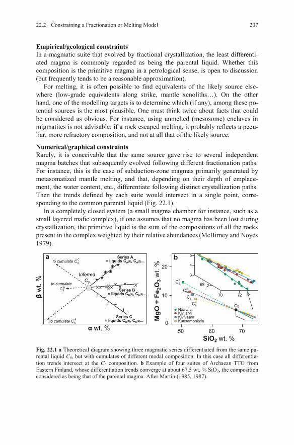
Empirical/geological constraints In a magmatic suite that evolved by fractional crystallization, the least differenti-ated magma is commonly regarded as being the parental liquid. Whether this composition is the primitive magma in a petrological sense, is open to discussion (but frequently tends to be a reasonable approximation).
For melting, it is often possible to find equivalents of the likely source else-where (low-grade equivalents along strike, mantle xenoliths…). On the other hand, one of the modelling targets is to determine which (if any), among these po-tential sources is the most plausible. One must think twice about facts that could be considered as obvious. For instance, using unmelted (mesosome) enclaves in migmatites is not advisable: if a rock escaped melting, it probably reflects a pecu-liar, more refractory composition, and not at all that of the likely source.
Numerical/graphical constraints Rarely, it is conceivable that the same source gave rise to several independent magma batches that subsequently evolved following different fractionation paths. For instance, this is the case of subduction-zone magmas primarily generated by metasomatized mantle melting, and that, depending on their depth of emplace-ment, the water content, etc., differentiate following distinct crystallization paths. Then the trends defined by each suite would intersect in a single point, corre-sponding to the common parental liquid (Fig. 22.1).
In a completely closed system (a small magma chamber for instance, such as a small layered mafic complex), if one assumes that no magma has been lost during crystallization, the primitive liquid is the sum of the compositions of all the rocks present in the complex weighted by their relative abundances (McBirney and Noyes
Fig. 22.1 a Theoretical diagram showing three magmatic series differentiated from the same pa-rental liquid C0, but with cumulates of different modal composition. In this case all differentia-tion trends intersect at the C0 composition. b Example of four suites of Archaean TTG from Eastern Finland, whose differentiation trends converge at about 67.5 wt. % SiO2, the composition considered as being that of the parental magma. After Martin (1985, 1987).
β w
t. %
α wt. %
InferredC0
Series A= liquids CA(1), CA(2)...
Series B= liquids CB(1), CB(2)...
Series C= liquids CC(1), CC(2)...to cumulate CS
A
to cumulate CS
B
to cumulate CSC
10
50 60 700
20
Cs1
Cs2
Cs3
Cs4
C0
7270
68
4
5
3
2
KuusamonkylaKivivaaraKivijärviNaavala
SiO2 wt. %
MgO
+ F
e 2O
3 w
t. %
a b
22.2 Constraining a Fractionation or Melting Model 207
1979).
22.2.3 Composition of the Solid Phases (Cumulate/Restite)
The nature of the solid phases involved in melting or crystallization is critical. However, these may be the most difficult parameters to determine: the number of possible minerals and the range of their compositions are vast.
Geological constraints Often, geological information can be incorporated into the model:
In the most favourable case, remnants of the solid (i.e., cumulate enclaves or fragments of the restite) can be found, and their compositions (and maybe min-eral chemistries and proportions) directly measured. In lavas, the compositions of phenocrysts in the less differentiated members of the fractionation series are commonly regarded as a good approximation of the chemistries of the crystallizing phases. Sometimes, ideal minerals, or minerals with an arbitrary composition from the literature, can be used. This applies mostly to simple phases: e.g., the composi-tion of plagioclase will be similar in all andesitic magmas. Experimental data on systems of relevant composition may constrain the chemical/modal compositions of the solid phases in equilibrium with the melt. Phase-equilibrium modelling predicts the composition of all the phases stable in the system (melt and solid). Of course, this approach solves the whole prob-lem (if P, T and the system’s chemistry are fixed, the proportions and composi-tions of all phases are calculated). Then there is no need for further mass-balance modelling of major elements (see Next step box below).
Crystallization and melting result from changing intensive parameters, es-pecially temperature. Recent thermodynamic models are able to predict the amount and composition of all phases, including melt, in a system of given bulk composition and P–T conditions. Thus, instead of guessing or geo-
chemically constraining the composition of solid phases, it is possible to use more realistic models, assessing more precisely the nature, chemistry and amount of solid phases. Gone also is the assumption of a constant composition (mode and mineral chemistry) of the cumulate (respectively restite) during fractionation or melting—an unlikely, if not impossible proposition in a multivariant system, in which by definition a change in e.g. T is accompanied by changes in composition.Technically, the most commonly used thermodynamic databases are:
MELTS (Ghiorso and Sack 1995) and pMELTS (Ghiorso and Sack 1995; Ghiorso et al. 2002) are able to deal with mafic liquids (komatiites to basalts), at mantle conditions. They do not predict realistic compositions for water-present systems, shallow depths (crustal) or felsic liquids. Rhyolite-MELTS (Gualda et al. 2013) is identical to MELTS, but has been adjusted to model K-feldspar and quartz. However, it is not able to assess equilibria involving large amounts of hydrous phases (e.g. biotite or amphibole) and should therefore be used primarily for differentiation of rhyolites or dry basalts (MORBs).
208 22 Constraining a Model
THERMOCALC (Holland and Powell 1998, 2011), initially developed for(high-T) metamorphic equilibria in the continental crust; a melt model (White etal. 2001, 2007) has been added, which provides modest, but improving, providesmodest, but improving, abilities to deal with crustal melting and granitic liquids.itic liquids.
Several programs are available to perform such calculations. They differ in terms of their minimization strategies, the databases and mineral models they incorpo-rate, and the output format. The most commonly used software includes:
MELTS, bundled with its own database. This programme is effective for pre-dicting the evolution of a liquid composition along a given P–T path, including options for fractionation, etc. (melts.ofm-research.org).THERMOCALC also relies on its own database. It is designed to draw pseudo-sections and phase diagrams, but retrieving the phase compositions is a bit more difficult (www.metamorph.geo.uni-mainz.de/thermocalc).PERPLE_X (Connolly and Petrini 2002) can use any mineral model, and many of them are bundled in the default distribution (e.g. Berman 1990; Taj manová et al. 2009), including THERMOCALC models. PERPLE_X is very good at generating gridded output mapping the system properties (phase proportions, phase compositions…) in P–T space. On the other hand, modelling fractiona-tion along a P–T path is more involved (www.perplex.ethz.ch).Theriak/Domino (de Capitani and Petrakakis 2010) is similar to PERPLE_Xalbeit with slightly less accessible output (phase compositions) and fewer calculation options. It can also use all sorts of models but the set coded in the existing data files is restricted to a handful of databases. Preparing new models is fairly difficult (titan.minpet.unibas.ch/minpet/theriak/theruser.html).
In fractional crystallization (respectively melting), the geometric relations im-posed by the lever rule imply that the cumulate (respectively restite), the initial liquid (respectively source) and the fractionated liquids (respectively melt) must be linearly aligned in any n-dimensional space (2 n number of major ele-ments). Therefore, we know in which portion of the diagram(s) the solid composi-tion lies. In the common situation when CL is known and C0 inferred, C0, CS and CL are aligned on the linear trend, and CS plots on the opposite side from CL.
This approach can be used to rule out one phase. In Fig. 22.2, the fractionation trend points towards hornblende, whereas biotite plots far away. Therefore, it is very unlikely that biotite played any significant role in shaping this trend.
A more elaborate analysis is illustrated in Fig. 22.3, where the composition of the primitive and most differentiated liquids are assessed graphically. We can con-strain the position of the cumulate as being on the left-hand side of the best-fit trends, between the most basic composition and the intersection with the horizon-tal axes. The strongest constraint is provided by the SiO2–K2O diagram; there the intersection with the x-axis occurs at SiO2 = 50 %, further restricting the range of permissible cumulate compositions. As the lavas are basalts to basaltic andesites, the fractionating phases were probably plagioclase, amphibole and/or pyroxene(s)
20922.2 Constraining a Fractionation or Melting Model
Geochemical constraints
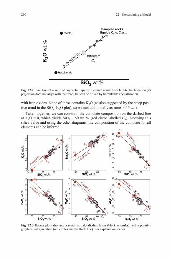
Fig. 22.2 Evolution of a suite of cogenetic liquids. It cannot result from biotite fractionation (its projection does not align with the trend) but can be driven by hornblende crystallization.
with iron oxides. None of these contains K2O (as also suggested by the steep posi-tive trend in the SiO2–K2O plot), so we can additionally assume 2 0K O
SC . Taken together, we can constrain the cumulate composition on the dashed line
at K2O = 0, which yields SiO2 ~ 50 wt. % (red circle labelled CS). Knowing this silica value and using the other diagrams, the composition of the cumulate for all elements can be inferred.
Fig. 22.3 Harker plots showing a series of calc-alkaline lavas (black asterisks), and a possible graphical interpretation (red circles and the thick line). For explanation see text.
K2O
wt.%
SiO2 wt.%
InferredC0
Sampled rocks= liquids CL(1), CL(2)...
to cumulate C S
Biotite
Hornblende
CaO
wt.%
SiO2 wt.%50 55 60
0.0
1.0
2.0
3.0
50 55 60
01
23
4
50 55 60
34
56
78
910
50 55 60
34
56
78
910
50 55 60
12
34
56
78
50 55 60
1516
1718
1920
SiO2 wt.% SiO2 wt.%
SiO2 wt.% SiO2 wt.% SiO2 wt.%
K2O
wt.%
Na 2
O w
t.%M
gO w
t.%
FeO
T wt.%
Al 2O
3 wt.%
C0
CL
Possib
le C S
CS
Possible C S
C0
CL
CS
Possible CS
Possible CS
Possible CS
C0
CL
CSCS
Possible CS
C0
CL
CSCSCS
Possible CS
C0
CS
Possible CS
C0
CL
CS
CL
210 22 Constraining a Model
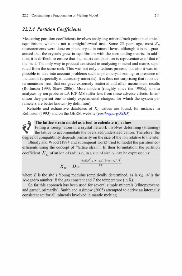
22.2.4 Partition Coefficients
Measuring partition coefficients involves analysing mineral/melt pairs in chemical equilibrium, which is not a straightforward task. Some 25 years ago, most KDmeasurements were done on phenocrysts in natural lavas, although it is not guar-anteed that the crystals grew in equilibrium with the surrounding matrix. In addi-tion, it is difficult to ensure that the matrix composition is representative of that of the melt. The only way to proceed consisted in analysing mineral and matrix sepa-rated from the same rock. This was not only a tedious process, but also it was im-possible to take into account problems such as phenocrysts zoning, or presence of inclusions (especially of accessory minerals). It is thus not surprising that most de-terminations from that era gave extremely scattered and often inconsistent results (Rollinson 1993; Shaw 2006). More modern (roughly since the 1990s), in-situ analyses by ion probe or LA ICP-MS suffer less from these adverse effects. In ad-dition they permit one to study experimental charges, for which the system pa-rameters are better known (by definition).
Reliable and exhaustive databases of KD values are found, for instance in Rollinson (1993) and on the GERM website (earthref.org/KDD).
The lattice strain model as a tool to calculate KD valuesFitting a foreign atom in a crystal network involves deforming (straining) the lattice to accommodate the oversized/undersized cation. Therefore, the
degree of compatibility depends primarily on the size of the ion relative to the site.Blundy and Wood (1994 and subsequent work) tried to model the partition co-
efficients using the concept of “lattice strain”. In their formulation, the partition coefficient
iDK of an ion of radius ri, in a site of size r0, can be expressed as:
where E is the site’s Young modulus (empirically determined, as is r0), is the Avogadro number, R the gas constant and T the temperature (in K).
So far this approach has been used for several simple minerals (clinopyroxene and garnet, primarily). Smith and Asimow (2005) attempted to derive an internally consistent set for all minerals involved in mantle melting.
21122.2 Constraining a Fractionation or Melting Model
2 30 0 04 ( ) /2 ( ) /3
0
i i
i
r
R
E r r
DT
r r
K D eπ− − + −
=
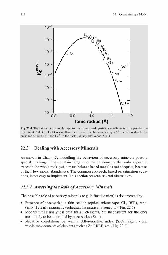
Fig 22.4 The lattice strain model applied to zircon–melt partition coefficients in a peralkaline rhyolite at 700 °C. The fit is excellent for trivalent lanthanides, except Ce3+, which is due to the presence of both Ce3+ and Ce4+ in the melt (Blundy and Wood 2003)
22.3 Dealing with Accessory Minerals
As shown in Chap. 13, modelling the behaviour of accessory minerals poses a special challenge. They contain large amounts of elements that only appear in traces in the whole rock; yet, a mass-balance based model is not adequate, because of their low modal abundances. The common approach, based on saturation equa-tions, is not easy to implement. This section presents several alternatives.
22.3.1 Assessing the Role of Accessory Minerals
The possible role of accessory minerals (e.g. in fractionation) is documented by:
Presence of accessories in thin section (optical microscope, CL, BSE), espe-cially if clearly magmatic (euhedral, magmatically zoned…) (Fig. 22.5).Models fitting analytical data for all elements, but inconsistent for the ones most likely to be controlled by accessories (Zr…).Negative correlations between a differentiation index (SiO2, mg#…) and whole-rock contents of elements such as Zr, LREE, etc. (Fig. 22.6).
10 –4
10 –3
10 –2
10 –1
10 0
1.21.11.00.90.8
10 +1
10 +2
10 +3
Ionic radius (Å)
K D min
/L
La
Pr
Nd
Sm
Sc
Lu
EuGd
TbDy
HoY
YbTm
Ce3+
212 22 Constraining a Model
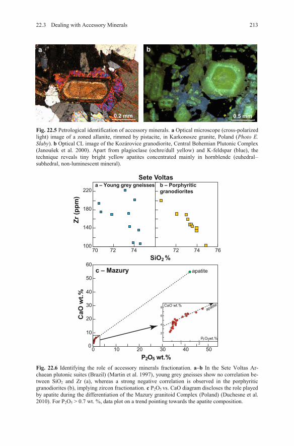
Fig. 22.5 Petrological identification of accessory minerals. a Optical microscope (cross-polarized light) image of a zoned allanite, rimmed by pistacite, in Karkonosze granite, Poland (Photo E. S aby). b Optical CL image of the Kozárovice granodiorite, Central Bohemian Plutonic Complex (Janoušek et al. 2000). Apart from plagioclase (ochre/dull yellow) and K-feldspar (blue), the technique reveals tiny bright yellow apatites concentrated mainly in hornblende (euhedral–subhedral, non-luminescent mineral).
Fig. 22.6 Identifying the role of accessory minerals fractionation. a–b In the Sete Voltas Ar-chaean plutonic suites (Brazil) (Martin et al. 1997), young grey gneisses show no correlation be-tween SiO2 and Zr (a), whereas a strong negative correlation is observed in the porphyritic granodiorites (b), implying zircon fractionation. c P2O5 vs. CaO diagram discloses the role played by apatite during the differentiation of the Mazury granitoid Complex (Poland) (Duchesne et al. 2010). For P2O5 > 0.7 wt. %, data plot on a trend pointing towards the apatite composition.
0.5 mm
ba
0.2 mm
72 74SiO %2
100
140
180
220
7670 72 74
Zr (p
pm)
a – Young grey gneisses b – Porphyriticgranodiorites
00
10
20
30
40
50
60
10 20 30 40 50P2O5 wt.%
CaO
wt.%
apatite
2
4
6
8
1 2P2O5 wt.%
CaO wt.%apatite
c – Mazury
Sete Voltas
22.3 Dealing with Accessory Minerals 213
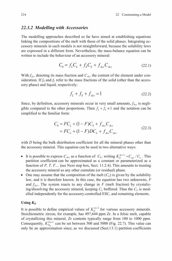
22.3.2 Modelling with Accessories
The modelling approaches described so far have aimed at establishing equations linking the compositions of the melt with those of the solid phases. Integrating ac-cessory minerals in such models is not straightforward, because the solubility laws are expressed in a different form. Nevertheless, the mass-balance equation can be written to include the behaviour of an accessory mineral:
0 L L S S AcAcc cC f C f C f C (22.1)
With fAcc denoting its mass fraction and CAcc the content of the element under con-sideration. If fS and fL refer to the mass fractions of the solid (other than the acces-sory phase) and liquid, respectively:
1L S Accf f f (22.2)
Since, by definition, accessory minerals occur in very small amounts, fAcc is negli-gible compared to the other proportions. Then 1L Sf f and the notation can be simplified to the familiar form:
0 (1 )(1 )
L S AccAcc
L L Acc Acc
C FC F C f CFC F DC f C
(22.3)
with D being the bulk distribution coefficient for all the mineral phases other than the accessory mineral. This equation can be used in two alternative ways:
It is possible to express CAcc as a function of CL, writing / /Acc LD Acc LK C C
partition coefficient can be approximated as a constant or parameterized as a function of P, T, F…the accessory mineral as any other cumulate (or residual) phase. One may assume that the composition of the melt (CL) is given by the solubility law, and it is therefore known. In this case, the equation has two unknowns, Fand fAcc. The system reacts to any change in F (melt fraction) by crystaliz-ing/dissolving the accessory mineral, keeping CL buffered. Thus the CL is mod-elled independently for the accessory-controlled ESC, and remaining elements.
Using KD
It is possible to define empirical values of / Acc LDK for various accessory minerals.
Stoichiometric zircon, for example, has 497,644 ppm Zr. In a felsic melt, capable of crystallizing this mineral, Zr contents typically range from 100 to 1000 ppm. Consequently, /
Zr
Zrn LDK can be set between 500 and 5000 (Fig. 22.7). This value can
only be an approximation since, as we discussed (Sect.1 3.1) partition coefficients
214 22 Constraining a Model
(see Next step box, Sect. 11.2.4). This amounts to treating
. This
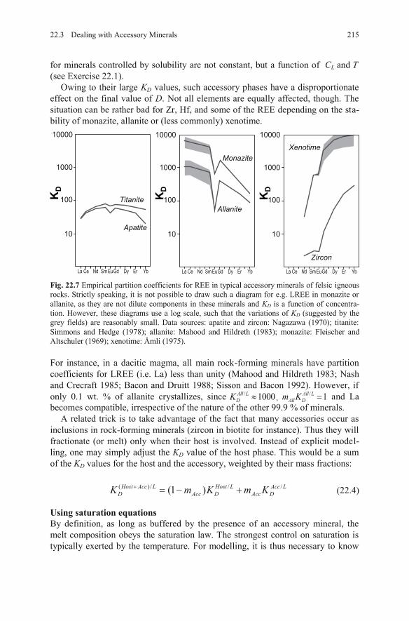
for minerals controlled by solubility are not constant, but a function of (see Exercise 22.1).
Owing to their large KD values, such accessory phases have a disproportionate effect on the final value of D. Not all elements are equally affected, though. The situation can be rather bad for Zr, Hf, and some of the REE depending on the sta-bility of monazite, allanite or (less commonly) xenotime.
Fig. 22.7 Empirical partition coefficients for REE in typical accessory minerals of felsic igneous rocks. Strictly speaking, it is not possible to draw such a diagram for e.g. LREE in monazite or allanite, as they are not dilute components in these minerals and KD is a function of concentra-tion. However, these diagrams use a log scale, such that the variations of KD (suggested by the grey fields) are reasonably small. Data sources: apatite and zircon: Nagazawa (1970); titanite: Simmons and Hedge (1978); allanite: Mahood and Hildreth (1983); monazite: Fleischer and
For instance, in a dacitic magma, all main rock-forming minerals have partition coefficients for LREE (i.e. La) less than unity (Mahood and Hildreth 1983; Nash
/ 1000All LDK ,
/ 1All LAll Dm K and La
A related trick is to take advantage of the fact that many accessories occur as inclusions in rock-forming minerals (zircon in biotite for instance). Thus they will fractionate (or melt) only when their host is involved. Instead of explicit model-ling, one may simply adjust the KD value of the host phase. This would be a sum of the KD values for the host and the accessory, weighted by their mass fractions:
(22.4)
Using saturation equations By definition, as long as buffered by the presence of an accessory mineral, the melt composition obeys the saturation law. The strongest control on saturation is typically exerted by the temperature. For modelling, it is thus necessary to know
KD
10000
1000
100
10
Titanite
Apatite
La Ce Nd Sm EuGd Dy Er Yb
KD
10000
1000
100
10
Monazite
Allanite
La Ce Nd Sm EuGd Dy Er YbK
D
10000
1000
100
10
Xenotime
Zircon
La Ce Nd Sm EuGd Dy Er Yb
21522.3 Dealing with Accessory Minerals
CL and T
and Crecraft 1985; Bacon and Druitt 1988; Sisson and Bacon 1992). However, ifonly 0.1 wt. % of allanite crystallizes, sincebecomes compatible, irrespective of the nature of the other 99.9 % of minerals.
( )/ / /(1 ) Host Acc L Host L Acc LD Acc D Acc DK mm K K
Altschuler (1969); xenotime: Åmli (1975).
how T varies as a function of F, or conversely. This is where coupling thermody-namic and geochemical models (Next step box, Sect. 22.2.3) is of particular use.
Alternatively, one can assume that the liquid was saturated throughout its evo-lution (or a relevant portion thereof) (Evans and Hanson 1993; Hoskin et al. 2000). Then, the saturation temperature of individual samples can be calculated, and curves of T vs. chemical parameters established.
Effects on other elements Another issue with accessory minerals such as zircon is that the KD values are high not only for their stoichiometric components, but also for a range of other ele-ments. For instance, zircon (ZrSiO4) can form solid solution with hafnon (HfSiO4), thorite (ThSiO4), coffinite (USiO4), but it is also able to contain up to 4.4 wt. % REE2O3 or 10 wt. % Y2O3 (Hoskin and Schaltegger 2003). This trans-lates to a very high KD (although Henry’s law is not applicable in this situation): ca. 1000 for Hf, and exceeding 100 for HREE (Fig. 22.7), higher than in most rock-forming minerals (even garnet has KD for HREE lower than 50). This effect must also be taken into account, by adding to the cumulate (or restite) the relevant amount of accessory minerals for further trace-element based calculations.
For zircon, knowing the whole-rock concentration 0ZrC and the saturation value
ZrL sat
C , the mass-balance relationship holds between C0, CL and the zircon crystals.con crystals. The excess Zr, available to form zircon grains, is 0
ZrL sat
C C . Themass proportion of zircon crystallizing is then:
0Zr Zr
L satZrn Zr
Zrn
C Cm
c(22.5)
with ZrZrnc = 497,644 ppm in stoichiometric zircon. The resulting mZrn value (typi-
cally small) should be integrated into the calculation of D for other elements.
The situation is more complex when several accessory minerals play a role (e.g., monazite and zircon) as they will “compete” for the trace elements available! The solubility equations must then be solved simultaneously.
Exercise 22.1: Modelling with accessory minerals
We shall develop a (forward) model accounting for the evolution of a rock suite undergoing fractional crystallization. The concentration of Zr (and potentially any other trace element hosted by zircon) will be modelled using several approaches (solubility or ad-hoc values of KD), that will be compared.
216 22 Constraining a Model
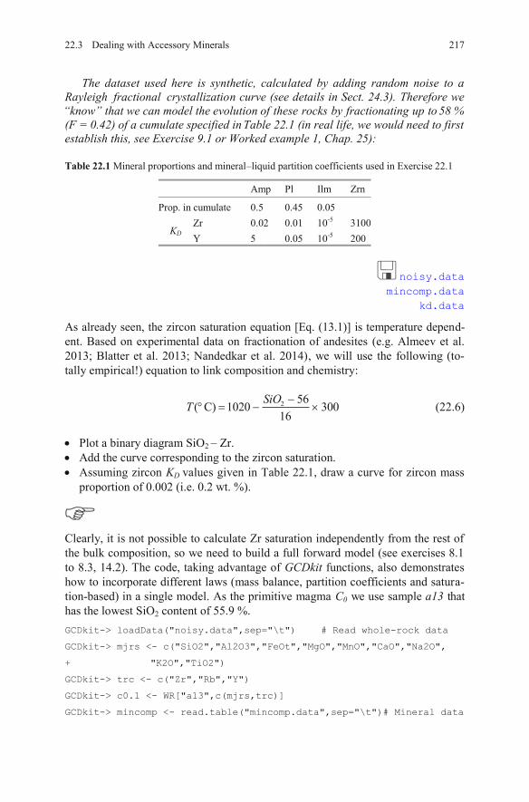
The dataset used here is synthetic, calculated by adding random noise to a Rayleigh fractional crystallization curve (see details in Sect. 24.3). Therefore we “know” that we can model the evolution of these rocks by fractionating up to (F = 0.42) of a cumulate specified in Table 22.1 (in real life, we would need to first establish this, see Exercise 9.1 or Worked example 1, Chap. 25):
Table 22.1 Mineral proportions and mineral–liquid partition coefficients used in Exercise 22.1
Amp Pl Ilm Zrn
Prop. in cumulate 0.5 0.45 0.05
KD Zr 0.02 0.01 10-5 3100 Y 5 0.05 10-5 200
noisy.data mincomp.data
kd.data
As already seen, the zircon saturation equation [Eq. (13.1)] is temperature depend-ent. Based on experimental data on fractionation of andesites (e.g. Almeev et al. 2013; Blatter et al. 2013; Nandedkar et al. 2014), we will use the following (to-tally empirical!) equation to link composition and chemistry:
2 56( C) 1020 30016
SiOT (22.6)
Plot a binary diagram SiO2 – Zr. Add the curve corresponding to the zircon saturation. Assuming zircon KD values given in Table 22.1, draw a curve for zircon mass
proportion of 0.002 (i.e. 0.2 wt. %).
Clearly, it is not possible to calculate Zr saturation independently from the rest of the bulk composition, so we need to build a full forward model (see exercises 8.1 to 8.3, 14.2). The code, taking advantage of GCDkit functions, also demonstrates how to incorporate different laws (mass balance, partition coefficients and satura-tion-based) in a single model. As the primitive magma C0 we use sample a13 that has the lowest SiO2 content of 55.9 %. GCDkit-> loadData("noisy.data",sep="\t") # Read whole-rock data
GCDkit-> mjrs <- c("SiO2","Al2O3","FeOt","MgO","MnO","CaO","Na2O",
+ "K2O","TiO2")
GCDkit-> trc <- c("Zr","Rb","Y")
GCDkit-> c0.1 <- WR["a13",c(mjrs,trc)]
GCDkit-> mincomp <- read.table("mincomp.data",sep="\t")# Mineral data
21722.3 Dealing with Accessory Minerals
58 %
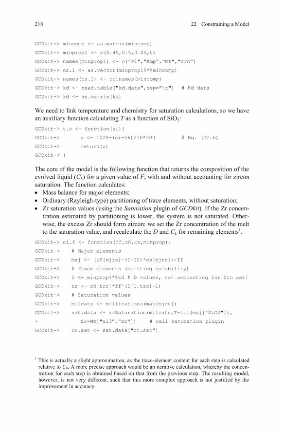
GCDkit-> mincomp <- as.matrix(mincomp)
GCDkit-> minprop1 <- c(0.45,0.5,0.05,0)
GCDkit-> names(minprop1) <- c("Pl","Amp","Mt","Zrn")
GCDkit-> cs.1 <- as.vector(minprop1%*%mincomp)
GCDkit-> names(cs.1) <- colnames(mincomp)
GCDkit-> kd <- read.table("kd.data",sep="\t") # Kd data
GCDkit-> kd <- as.matrix(kd)
We need to link temperature and chemistry for saturation calculations, so we have an auxiliary function calculating T as a function of SiO2: GCDkit-> t.c <- function(si){
GCDkit-> z <- 1020-(si-56)/16*300 # Eq. (22.6)
GCDkit-> return(z)
GCDkit-> }
The core of the model is the following function that returns the composition of the evolved liquid (CL) for a given value of F, with and without accounting for zircon saturation. The function calculates:
Mass balance for major elements; Ordinary (Rayleigh-type) partitioning of trace elements, without saturation; Zr saturation values (using the Saturation plugin of GCDkit). If the Zr concen-tration estimated by partitioning is lower, the system is not saturated. Other-wise, the excess Zr should form zircon: we set the Zr concentration of the melt to the saturation value, and recalculate the D and CL for remaining elements .1
GCDkit-> cl.f <- function(ff,c0,cs,minprop){
GCDkit-> # Major elements
GCDkit-> maj <- (c0[mjrs]-(1-ff)*cs[mjrs])/ff
GCDkit-> # Trace elements (omitting solubility)
GCDkit-> D <- minprop%*%kd # D values, not accounting for Zrn sat!
GCDkit-> tr <- c0[trc]*ff^(D[1,trc]-1)
GCDkit-> # Saturation values
GCDkit-> milcats <- millications(maj[mjrs])
GCDkit-> sat.data <- zrSaturation(milcats,T=t.c(maj["SiO2"]),
+ Zr=WR["a13","Zr"]) # call Saturation plugin
GCDkit-> Zr.sat <- sat.data["Zr.sat"]
1 This is actually a slight approximation, as the trace-element content for each step is calculated relative to C0. A more precise approach would be an iterative calculation, whereby the concen-tration for each step is obtained based on that from the previous step. The resulting model, however, is not very different, such that this more complex approach is not justified by the improvement in accuracy.
218 22 Constraining a Model
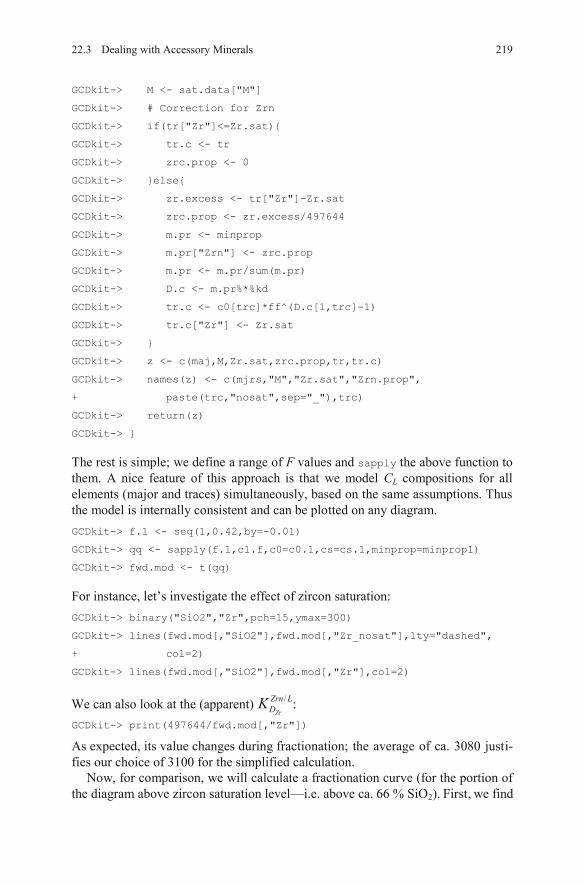
GCDkit-> M <- sat.data["M"]
GCDkit-> # Correction for Zrn
GCDkit-> if(tr["Zr"]<=Zr.sat){
GCDkit-> tr.c <- tr
GCDkit-> zrc.prop <- 0
GCDkit-> }else{
GCDkit-> zr.excess <- tr["Zr"]-Zr.sat
GCDkit-> zrc.prop <- zr.excess/497644
GCDkit-> m.pr <- minprop
GCDkit-> m.pr["Zrn"] <- zrc.prop
GCDkit-> m.pr <- m.pr/sum(m.pr)
GCDkit-> D.c <- m.pr%*%kd
GCDkit-> tr.c <- c0[trc]*ff^(D.c[1,trc]-1)
GCDkit-> tr.c["Zr"] <- Zr.sat
GCDkit-> }
GCDkit-> z <- c(maj,M,Zr.sat,zrc.prop,tr,tr.c)
GCDkit-> names(z) <- c(mjrs,"M","Zr.sat","Zrn.prop",
+ paste(trc,"nosat",sep="_"),trc)
GCDkit-> return(z)
GCDkit-> }
The rest is simple; we define a range of F values and sapply the above function to them. A nice feature of this approach is that we model CL compositions for all elements (major and traces) simultaneously, based on the same assumptions. Thus the model is internally consistent and can be plotted on any diagram. GCDkit-> f.1 <- seq(1,0.42,by=-0.01)
GCDkit-> qq <- sapply(f.1,cl.f,c0=c0.1,cs=cs.1,minprop=minprop1)
GCDkit-> fwd.mod <- t(qq)
For instance, let’s investigate the effect of zircon saturation:GCDkit-> binary("SiO2","Zr",pch=15,ymax=300)
GCDkit-> lines(fwd.mod[,"SiO2"],fwd.mod[,"Zr_nosat"],lty="dashed",
+ col=2)
GCDkit-> lines(fwd.mod[,"SiO2"],fwd.mod[,"Zr"],col=2)
We can also look at the (apparent) :GCDkit-> print(497644/fwd.mod[,"Zr"])
As expected, its value changes during fractionation; the average of ca. 3080 justi-fies our choice of 3100 for the simplified calculation.
Now, for comparison, we will calculate a fractionation curve (for the portion of the diagram above zircon saturation level—i.e. above ca. 66 % SiO2). First, we find
21922.3 Dealing with Accessory Minerals
/Zr
Zrn LDK
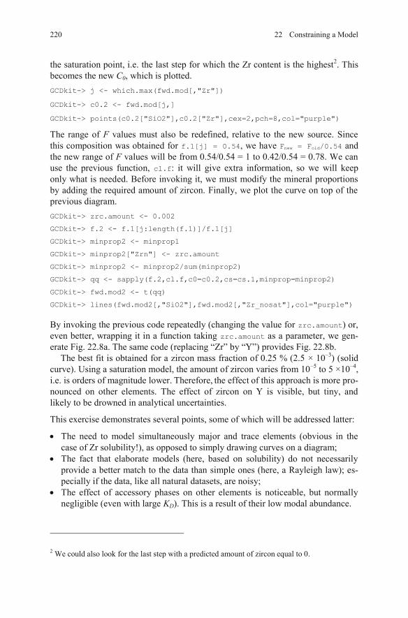
the saturation point, i.e. the last step for which the Zr content is the highest . This becomes the new C0, which is plotted.
2
GCDkit-> j <- which.max(fwd.mod[,"Zr"])
GCDkit-> c0.2 <- fwd.mod[j,]
GCDkit-> points(c0.2["SiO2"],c0.2["Zr"],cex=2,pch=8,col="purple")
The range of F values must also be redefined, relative to the new source. Since this composition was obtained for f.1[j] = 0.54, we have Fnew = Fold/0.54 and the new range of F values will be from 0.54/0.54 = 1 to 0.42/0.54 = 0.78. We can use the previous function, cl.f: it will give extra information, so we will keep only what is needed. Before invoking it, we must modify the mineral proportions by adding the required amount of zircon. Finally, we plot the curve on top of the previous diagram. GCDkit-> zrc.amount <- 0.002
GCDkit-> f.2 <- f.1[j:length(f.1)]/f.1[j]
GCDkit-> minprop2 <- minprop1
GCDkit-> minprop2["Zrn"] <- zrc.amount
GCDkit-> minprop2 <- minprop2/sum(minprop2)
GCDkit-> qq <- sapply(f.2,cl.f,c0=c0.2,cs=cs.1,minprop=minprop2)
GCDkit-> fwd.mod2 <- t(qq)
GCDkit-> lines(fwd.mod2[,"SiO2"],fwd.mod2[,"Zr_nosat"],col="purple")
By invoking the previous code repeatedly (changing the value for zrc.amount) or, even better, wrapping it in a function taking zrc.amount as a parameter, we gen-erate Fig. 22.8a. The same code (replacing “Zr” by “Y”) provides Fig. 22.8b.
The best fit is obtained for a zircon mass fraction of 0.25 % (2.5 × 10⁻³) (solid curve). Using a saturation model, the amount of zircon varies from 10–5 to 5 ×10⁻⁴,i.e. is orders of magnitude lower. Therefore, the effect of this approach is more pro-nounced on other elements. The effect of zircon on Y is visible, but tiny, and likely to be drowned in analytical uncertainties.
This exercise demonstrates several points, some of which will be addressed latter:
The need to model simultaneously major and trace elements (obvious in the case of Zr solubility!), as opposed to simply drawing curves on a diagram; The fact that elaborate models (here, based on solubility) do not necessarily provide a better match to the data than simple ones (here, a Rayleigh law); es-pecially if the data, like all natural datasets, are noisy; The effect of accessory phases on other elements is noticeable, but normally
KD). This is a result of their low modal abundance.
We could also look for the last step with a predicted amount of zircon equal to 0. 2
220 22 Constraining a Model
negligible (even with large
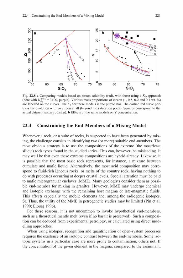
Fig. 22.8 a Comparing models based on zircon solubility (red), with those using a KD approach (here with = 3100, purple). Various mass proportions of zircon (1, 0.5, 0.2 and 0.1 wt. %) are labelled on the curves. The C0 for these models is the purple star. The dashed red curve por-trays the evolution with no zircon at all (beyond the saturation point). Squares correspond to the actual dataset ( ). b Effects of the same models on Y concentration.
22.4 Constraining the End-Members of a Mixing Model
Whenever a rock, or a suite of rocks, is suspected to have been generated by mix-ing, the challenge consists in identifying two (or more) suitable end-members. The most obvious strategy is to use the compositions of the extreme (the most/least silicic) rock types found in the studied series. This can, however, be misleading. It may well be that even these extreme compositions are hybrid already. Likewise, it is possible that the most basic rock represents, for instance, a mixture between cumulate and mafic liquid. Alternatively, the most acid composition may corre-spond to fluid-rich igneous rocks, or melts of the country rock, having nothing to do with processes occurring at deeper crustal levels. Special attention must be paid to mafic microgranular enclaves (MME). Many geologists consider them as possi-ble end-member for mixing in granites. However, MME may undergo chemical and isotopic exchange with the remaining host magma or late-magmatic fluids. This affects especially the mobile elements and, among the radiogenic isotopes, Sr. Thus, the utility of the MME in petrogenetic studies may be limited (Pin et al. 1990; Elburg 1996).
For these reasons, it is not uncommon to invoke hypothetical end-members, such as a theoretical mantle melt (even if no basalt is preserved). Such a composi-tion can be deduced from experimental petrology, or calculated using direct mod-elling approaches.
When using isotopes, recognition and quantification of open-system processes requires the existence of an isotopic contrast between the end-members. Some iso-topic systems in a particular case are more prone to contamination, others not. If the concentration of the given element in the magma, compared to the assimilant,
55 60 65 70 75
5010
015
020
025
030
0Zr
55 60 65 70 75
05
1015
2025
YSiO2 SiO2
a b
1 %1 %1 %
0.5 %0.5 %0.5 %
0.25 %0.25 %0.25 %
0.1 %0.1 %0.1 %
0.1 %0.1 %0.1 %0.25 %0.25 %0.25 %0.5 %0.5 %0.5 %1 %1 %1 %
22.4 Constraining the End-Members of a Mixing Model 221
/Zr
Zrn LDK
noisy.data
is high, the isotopic composition will be essentially buffered until high degrees of contamination. For example, Bohemian Variscan lamprophyres and ultrapotassic intrusions have high Sr and Nd contents that rendered them resistant to crustal as-similation during intrusion. For this reason, their crust-like Sr–Nd isotopic signa-ture must reflect enriched mantle source or its contamination by a deeply sub-ducted felsic crust (Janoušek et al. 2010).
222 22 Constraining a Model
References
Almeev R, Holtz F, Ariskin AA, Kimura JI (2013) Storage conditions of Bezymianny Volcano parental magmas: results of phase equilibria experiments at 100 and 700 MPa. Contrib Mineral Petrol 166:1389–1414
Åmli R (1975) Mineralogy and rare earth geochemistry of apatite and xenotime from the Gloserheia granite pegmatite, Froland, southern Norway. Amer Miner 60:607–620
Bacon CR, Druitt TH (1988) Compositional evolution of the zoned calc-alkaline magma cham-ber of Mount Mazama, Crater Lake, Oregon. Contrib Mineral Petrol 98:224–256
Berman RG (1990) Mixing properties of Ca − Mg − Fe − Mn garnets. Amer Miner 75:238–344Blatter DL, Sisson TW, Hankins WB (2013) Crystallization of oxidized, moderately hydrous arc
basalt at mid- to lower-crustal pressures: implications for andesite genesis. Contrib Mineral Petrol 166:861–886
Blundy J, Wood B (1994) Prediction of crystal melt partition coefficients from elastic moduli. Nature 372:452–454
Blundy J, Wood B (2003) Mineral–melt partitioning of uranium, thorium and their daughters.
Connolly JAD, Petrini K (2002) An automated strategy for calculation of phase diagram sec-tions and retrieval of rock properties as a function of physical conditions. J Metamorph Geol 20:697–708
de Capitani C, Petrakakis K (2010) The computation of equilibrium assemblage diagrams with Theriak/Domino software. Amer Miner 95:1006–1016
Duchesne J-C, Martin H, Bagiński B, Wiszniewska J, Vander Auwera J (2010) The origin of ferroan–potassic A-type granitoids: the case of the hornblende–biotite granite suite of the Mesoproterozoic Mazury Complex, northeastern Poland. Canad Mineral 48:947–968
Elburg MA (1996) Evidence of isotopic equilibration between microgranitoid enclaves and host granodiorite, Warburton Granodiorite, Lachlan Fold Belt, Australia. Lithos 38:1–22
Evans OC, Hanson GN (1993) Accessory-mineral fractionation of rare-earth element (REE) abundances in granitoid rocks. Chem Geol 110:69–93
Fleischer M, Altschuler ZS (1969) The relationship of the rare earth composition of minerals to geological environment. Geochim Cosmochim Acta 33:725–732
Ghiorso MS, Sack RO (1995) Chemical mass-transfer in magmatic processes. 4. A revised and internally consistent thermodynamic model for the interpolation and extrapolation of liquid–solid equilibria in magmatic systems at elevated temperatures and pressures. Contrib Mineral Petrol 119:197–212
Ghiorso MS, Hirschmann MM, Reiners PW, Kress VC (2002) The pMELTS: a revision of MELTS for improved calculation of phase relations and major element partitioning related to partial melting of the mantle to 3 GPa. Geochem Geophys Geosyst 3:1–35
Gualda GAR, Ghiorso MS, Lemons RV, Carley TL (2013) Rhyolite-MELTS: a modified cali-bration of MELTS optimized for silica-rich, fluid-bearing magmatic systems. J Petrol 53:875–890
In: Bourdon B, Henderson GM, Lundstrom CC, Turner SP (eds) Uranium-series geochemistry. Mineralogical Society of America Reviews in Mineralogy and Geochemistry, vol 52, pp 59–123
References 223
Holland TJB, Powell R (1998) An internally consistent thermodynamic dataset for phases of pet-rological interest. J Metamorph Geol 16:309–343
Holland TJB, Powell R (2011) An improved and extended internally consistent thermodynamic dataset for phases of petrological interest, involving a new equation of state for solids. J Metamorph Geol 29:333–383
Hoskin PWO, Schaltegger U (2003) The composition of zircon and igneous and metamorphic petrogenesis. In: Hanchar JM, Hoskin PWO (eds) Zircon. Mineralogical Society of America and Geochemical Society Reviews in Mineralogy and Geochemistry, vol 53, pp 27–62
Hoskin PWO, Kinny PD, Wyborn D, Chappell BW (2000) Identifying accessory mineral satura-tion during differentiation in granitoid magmas: an integral approach. J Petrol 41:1365–1396
Janoušek V, Bowes DR, Braithwaite CJR, Rogers G (2000) Microstructural and mineralogical evidence for limited involvement of magma mixing in the petrogenesis of a Hercynian high-K calc-alkaline intrusion: the Kozárovice granodiorite, Central Bohemian Pluton, Czech Republic. Trans Roy Soc Edinb, Earth Sci 91:15–26
Janoušek V, Holub FV, Magna T, Erban V (2010) Isotopic constraints on the petrogenesis of the Variscan ultrapotassic magmas from the Moldanubian Zone of the Bohemian Massif. Mineral Spec Pap 37:32–36
Mahood GA, Hildreth EW (1983) Large partition coefficients for trace elements in high-silica rhyolites. Geochim Cosmochim Acta 47:11–30
Martin H (1985) Nature, origine et évolution d’un segment de croûte continentale archée-nne: contraintes chimiques et isotopiques. Exemple de la Finlande orientale. Mémoires et Documents du Centre Armoricain d’Etude Structurale des Socles, vol 1, Rennes
Martin H (1987) Petrogenesis of Archaean trondhjemites, tonalites and granodiorites from east-ern Finland; major and trace element geochemistry. J Petrol 28:921–953
Martin H, Sabaté P, Peucat J-J, Cunha JC (1997) Crustal evolution in the early Archaean of South America: example of the Sete Voltas Massif, Bahia state, Brazil. Precambr Res 83:35–62
McBirney AR, Noyes RM (1979) Crystallization and layering of the Skaergaard intrusion. J Petrol 20:487–554
Nagazawa H (1970) Rare Earth concentrations in zircon and apatite and their host dacite and granites. Earth Planet Sci Lett 9:359–364
Nandedkar R, Ulmer P, Müntener O (2014) Fractional crystallization of primitive, hydrous arc magmas: an experimental study at 0.7 GPa. Contrib Mineral Petrol 167:1–27
Nash WP, Crecraft HR (1985) Partition coefficients for trace elements in silicic magmas. Geochim Cosmochim Acta 49:2309–2322
Pin C, Binon M, Belin JM, Barbarin B, Clemens JD (1990) Origin of microgranular enclaves in granitoids—equivocal Sr–Nd evidence from Hercynian rocks in the Massif Central (France). J Geophys Res 95:17821–17828
Rollinson HR (1993) Using geochemical data: evaluation, presentation, interpretation. Longman, London
Shaw DM (2006) Trace elements in magmas: a theoretical treatment. Cambridge University Press, Cambridge
Simmons EC, Hedge CE (1978) Minor-element and Sr-isotope geochemistry of Tertiary stocks, Colorado mineral belt. Contrib Mineral Petrol 67:379–396
Sisson TW, Bacon CR (1992) Garnet/high-silica rhyolite trace element partition coefficients measured by ion microprobe. Geochim Cosmochim Acta 56:2133–2136
Smith P, Asimow P (2005) Adiabat_1ph: a new public front-end to the MELTS, pMELTS, and pHMELTS models. Geochem Geophys Geosyst 6: doi: 10.1029/2004GC000816
Tajčmanová L, Connolly J, Cesare B (2009) A thermodynamic model for titanium and ferric iron solution in biotite. J Metamorph Geol 27:153–165
White RW, Powell R, Holland TJB (2001) Calculation of partial melting equilibria in the sys-tem CaO–Na2O–K2O–FeO–MgO–Al2O3–SiO2–H2O (CNKFMASH). J Metamorph Geol 19:139–153
White RW, Powell R, Holland TJB (2007) Progress relating to calculation of partial melting equilibria for metapelites. J Metamorph Geol 25:511–527
Chapter 23 Numerical Tips and Tricks
Geochemical modelling is an art as much as a science. In many cases, in addition to the geological constraints discussed above, some numerical tricks—mostly re-lated to the behaviour of the compositional space—may provide substantial help.
23.1 The Size of the Geochemical Space It is vital to remember that a 2D graphical representation (such as a binary diagram) is a projection of the p-dimensional space onto a plane. An important skill for geochemists is to find the right viewing angle (projection) that best emphasizes thefeatures of interest.
As an illustration, let’s consider a binary diagram, where the geochemical data define a straight or a curved trend. Without further examination of the data (in the full p-dimensional space), it is not possible to decide whether this corresponds to an actual evolution (Fig. 23.1a), or to an artefact resulting from the projection of a more or less flat cloud of data onto the X–Y plane (Fig. 23.1b). By the same logic we can interpret a triangular data array on the X–Y plane. If, in 2D, data points fall in a small section of a plane (a triangle) defined by three end-members, it may correspond to a legitimate ternary mixing (Fig. 23.1c). Or it reflects a meaning-less, essentially random 3D distribution (Fig. 23.1d).
Clearly, there are better viewing angles. In Fig. 23.1b for instance, projecting the data in an X–Z or Y–Z plane, or even better, from a direction perpendicular to the data plane, would reveal the whole compositional range. On the other hand, looking at the same data “from the top” (projected on the X–Y plane) makes them appear as a line. This notion underlies the concept of Principal Component Analy-sis (PCA), which is essentially a numerical technique that defines the directions in the geochemical space in which the dataset has the highest variance. These direc-tions are called the first, second etc. principal components, and each of them is asso-
Principal component analysis (PCA) in R/GCDkit GCDkit can calculate and plot PCA for the current dataset, from the menu Calculations|Statistics|Principal components. Several other op-
tions for statistical treatment of the dataset are present in the same menu; the un-derlying R functions are described in Reimann et al. (2008).
© Springer-Verlag Berlin Heidelberg 2016 V. Janoušek et al., Geochemical Modelling of Igneous Processes – Principles And Recipes in R Language, Springer Geochemistry, DOI 10.1007/978-3-662-46792-3_23
225
ciated with a proportion of the total variance of the data.
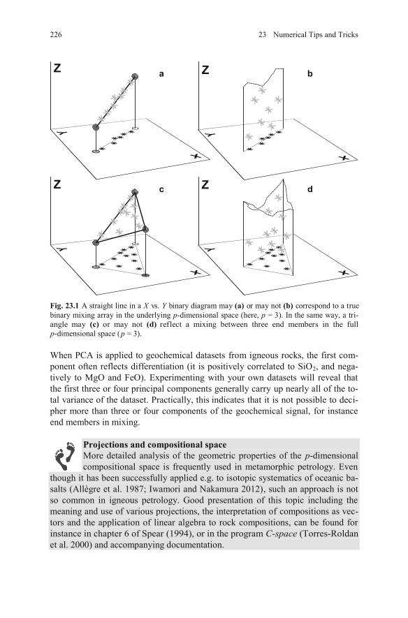
Fig. 23.1 A straight line in a X vs. Y binary diagram may (a) or may not (b) correspond to a true binary mixing array in the underlying p-dimensional space (here, p = 3). In the same way, a tri-angle may (c) or may not (d) reflect a mixing between three end members in the full p-dimensional space (p = 3).
When PCA is applied to geochemical datasets from igneous rocks, the first com-ponent often reflects differentiation (it is positively correlated to SiO2, and nega-tively to MgO and FeO). Experimenting with your own datasets will reveal that the first three or four principal components generally carry up nearly all of the to-tal variance of the dataset. Practically, this pher more than three or four components of the geochemical signal, for instance end members in mixing.
Projections and compositional spaceMore detailed analysis of the geometric properties of the p-dimensional compositional space is frequently used in metamorphic petrology. Even
though it has been successfully applied e.g. to isotopic systematics of oceanic ba-salts (Allègre et al. 1987; Iwamori and Nakamura 2012), such an approach is not so common in igneous petrology. Good presentation of this topic including the meaning and use of various projections, the interpretation of compositions as vec-tors and the application of linear algebra to rock compositions, can be found for instance in chapter 6 of Spear (1994), or in the program C-space (Torres-Roldan
a bZ Z
ZZ c d
226 23 Numerical Tips and Tricks
indicates that it is not possible to deci-
et al. 2000) and accompanying documentation.
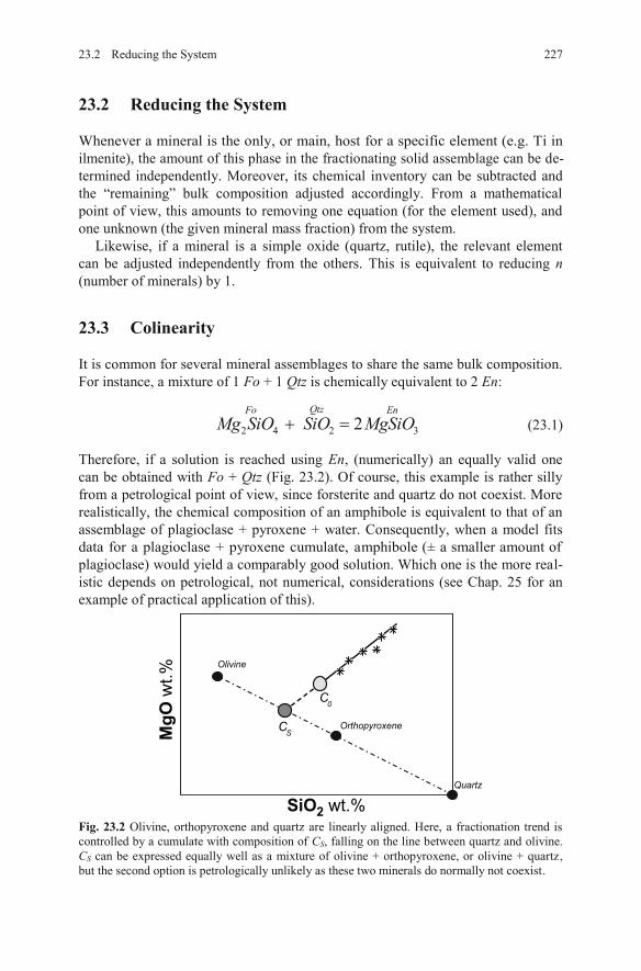
23.2 Reducing the System
Whenever a mineral is the only, or main, host for a specific element (e.g. Ti in
termined independently. Moreover, its chemical inventory can be subtracted and the “remaining” bulk composition adjusted accordingly. From a mathematical point of view, this amounts to removing one equation (for the element used), and one unknown (the given mineral mass fraction) from the system.
Likewise, if a mineral is a simple oxide (quartz, rutile), the relevant element can be adjusted independently from the others. This is equivalent to reducing n (number of minerals) by 1.
23.3 Colinearity
It is common for several mineral assemblages to share the same bulk composition. For instance, a mixture of 1 Fo + 1 Qtz is chemically equivalent to 2 En:
2 4 2 32QtzFo En
SiOMg SiO MgSiO (23.1)
Therefore, if a solution is reached using En, (numerically) an equally valid one can be obtained with Fo + Qtz (Fig. 23.2). Of course, this example is rather silly from a petrological point of view, since forsterite and quartz do not coexist. More realistically, the chemical composition of an amphibole is equivalent to that of an assemblage of plagioclase + pyroxene + water. Consequently, when a model fits data for a plagioclase + pyroxene cumulate,plagioclase) would yield a comparably good solution. Which one is the more real-istic depends on petrological, not numerical, considerations (see Chap. 25 for an example of practical application of this).
Fig. 23.2 Olivine, orthopyroxene and quartz are linearly aligned. Here, a fractionation trend is controlled by a cumulate with composition of CS, falling on the line between quartz and olivine. CS can be expressed equally well as a mixture of olivine + orthopyroxene, or olivine + quartz, but the second option is petrologically unlikely as these two minerals do normally not coexist.
MgO
wt.%
SiO2 wt.%Quartz
CS
C0
Olivine
Orthopyroxene
23.2 Reducing the System 227
amphibole (± a smaller amount of
ilmenite), the amount of this phase in the fractionating solid assemblage can be de-
23.4 Breaking Minerals into End Members
When modelling major-element behaviour, a common trick involves breaking down minerals into their end-members. For instance plagioclase is treated as two phases (pure Ab and An); similarly titanomagnetite is considered as a mixture of pure magnetite and rutile. This approach removes the need to make an assumption on the composition of the solid solution as this will come out as a result of the model (see Chap. 25 for an application). An additional benefit pertains to overde-termined systems, i.e. when there are more equations (p) than unknowns (n)
n = p for which there is an exact solution . However, this app-1
23.5 Coupling Majors and Traces
A common issue related to geochemical modelling as presented in many papers, is that they are based on a restricted number of elements. Most often the computed model really boils down to a curve on a diagram. In this case, the model satisfac-torily predicts the behaviour of the elements or isotopic systems taken into ac-count, but does not provide any information on the remaining ones. Thus it is im-possible to assess the internal consistency of the proposed scenario.
For instance, modelling based solely on isotopes could lead to a conclusion that a basalt has been contaminated by ~50 % of continental crust, but this is unrealis-tic because such a magma would not be basaltic anymore. Another classical ex-ample is that of trace-element modelling indicating that a parental magma differ-entiated by e.g. 50% fractional crystallization of amphibole. However, parental magma containing 5 % MgO cannot crystallize 50 % amphibole containing 15 % MgO (the computed value for MgO
LC would be negative, here –5 %). In other words, the system does not contain enough MgO to precipitate 50 % of amphibole. Thisissue is not obvious from trace elements alone (as the laws are multiplicative), but becomes clear from major elements (that use subtractive equations).
On the other hand, we have also discussed the fact that major and trace ele-ments carry different information. Most importantly, processes cannot be distin-guished using majors only (Sect. 21.3). Therefore, it is vital to build internally-consistent models accounting for the largest possible range of elements (and iso-tope ratios). Major and trace elements should be coupled. For instance, a forward model should calculate simultaneously the composition in major (via mass bal-ance) and trace elements, using the same mineral proportions in both cases.
1 Note that the phase rule is not violated, as the increase in number of components is a pure nu-merical exercise—physically, the phases were solid solutions.
228 23 Numerical Tips and Tricks
(Sec. 7.2). This trick artificially increases the number of unknowns, bringing thesystem closer to roach is limited by the fact that if the number of unknowns exceeds that of
), the system becomes underdetermined and cannot be solvedn > pequations ((Appendix C).
A common strategy involves a mixed approach, solving the reverse problem for major elements (least-square method), and using the mineral proportions as the in-put into a forward model for traces (see Martin 1987 for an example of this approach, or the Part VI).
This Space Left Blank for Your Own Tricks
23.5 Coupling Majors and Traces 229
References
Allègre CJ, Hamelin B, Provost A, Dupré B (1987) Topology in isotopic multispace and origin of mantle chemical heterogeneities. Earth Planet Sci Lett 81:319–337
Iwamori H, Nakamura H (2012) East–west mantle geochemical hemispheres constrained from independent component analysis of basalt isotopic compositions. Geochem J 46:e39–e46
Martin H (1987) Petrogenesis of Archaean trondhjemites, tonalites and granodiorites from east-ern Finland; major and trace element geochemistry. J Petrol 28:921–953
Reimann C, Filzmoser P, Garrett R, Dutter R (2008) Statistical data analysis explained: applied environmental statistics with R. Wiley, Chichester
Spear FS (1994) Metamorphic phase equilibria and pressure–temperature–time paths. Mineralogical Society of America Monographs. Mineralogical Society of America, Washington
Torres-Roldan RL, Garcia-Casco A, Garcia-Sanchez PA (2000) CSpace: an integrated workplace for the graphical and algebraic analysis of phase assemblages on 32-bit Wintel platforms. Comput Geosci 26:779–793
Chapter 24 Common Sense in Action
One of the most commonly heard complaints about geochemical modelling—and indeed, one of the worst problems of this approach—is that it is very easy to get bogged down in numerical subtleties and lose touch with the underlying geologi-cal reality. Most importantly, a geochemical model is developed in order to under-stand and quantify a geological process. Thus any sound model must rest on a solid geological understanding of the problems involved. In here, we disuss someof the limitations of geochemical modelling applied to geological problems.
24.1 Physical Constraints
Modelling based on mass balance describes the evolution of igneous rocks in purely chemical terms—i.e. focussing on conservation of mass. Equally important, however, is the conservation of energy, in other words, physical constraints. Cur-rently, comprehensive models coupling chemical and physical models are not rou-tinely used; yet one should, at least, make sure that a proposed geochemical model is not grossly inconsistent with physics.
24.1.1 Thermodynamic Constraints
Thermodynamic constraints are probably some of the most often ignored physical controls in geochemical modelling.
Melting, for instance, is a strongly endothermic process, such that its magnitude (F) is strongly controlled by the available heat supply (Thompson and Connolly 1995; Henk et al. 2000; Annen et al. 2006; Sawyer et al. 2011; Bea 2012).
Assimilation involves physical disruption of the assimilated rock, and its subse-quent melting. Both are very expensive processes in terms of energy. The sophis-ticated AFC equations with many parameters can be easily tweaked to yield solu-tions nicely reproducing the observed variation. Still, they may be geologically
sically permissible parameters during e Next step boxes). The rate of assimilation
© Springer-Verlag Berlin Heidelberg 2016 V. Janoušek et al., Geochemical Modelling of Igneous Processes – Principles And Recipes in R Language, Springer Geochemistry, DOI 10.1007/978-3-662-46792-3_24
231
unrealistic (Roberts and Clemens 1995), as they ignore the constraints imposed byconservation of energy. In fact, the range of phyAFC is restricted (see Sect. 11.4, including th
to fractional crystallization (r) is governed by the thermal state of the assimilant (Reiners et al. 1995); it tends to be low for cold upper crustal rocks and higher for hotter deeper ones. Nevertheless, r is unlikely to be higher than about 1, as the amount of heat required in order to melt a mass of country rock roughly equals the
24.1.2 Mechanical (Rheological) Constraints
There are also several mechanical issues related to the rheology of partially molten system (Arzi 1978; Rosenberg 2001). Depending on the interplay between the many parameters such as viscosity, temperature, strain rate and melt fraction, solid–liquid segregation may be more or less efficient. Note also that most of these parameters are not independent of each other, but are somehow related to the chemi-cal properties we are trying to model! This has important implications for the fea-sibility of generating differentiated magmas (Vigneresse and Burg 2004).
Crystallization In a liquid-dominated system (Newtonian viscous medium), the speed of gravita-tional settling of particles (crystals) is expressed by Stokes’ (1901) law:
229
ps
rv
g (24.1)
where vs is the sinking velocity, rp the particle’s radius, g gravitational constant, the density difference between the particle and the melt, and the viscosity. In a non-Newtonian fluid, the critical radius below which a crystal would not
sink solely under the effect of gravity is (McBirney and Noyes 1979):
3 ycritr
g (24.2)
where y is the yield strength of the fluid. In a typical felsic magma, = 105 Pa.s, y
= 10 Pa and magma = 2300 kg.m–3 (Turcotte and Schubert 1982). The critical radius for a zircon ( = 4650 kg.m–3: Anthony et al. 2014) is ca. 1.3 mm: it is unlikely that it would reach this size. Therefore, gravitational settling is unable to extract this mineral out of the magma from which it crystallized. A biotite has a lower density ( = 3000 kg.m–3; Anthony et al. 2014), but typically a larger size; its critical radius is 4.4 mm, a perfectly feasible size for a biotite in a felsic magma. The sinking velocity of a 5 mm biotite is, from Eq. (24.1), 3.8 × 10⁻⁷ m.s–1 (ca. 12 m/yr). Crystal/liquid segregation
A mafic or ultramafic melt has a much lower viscosity: ca. 1 Pa.s in komatiites, 50–100 Pa.s in basalts (Spera 2000). Under these conditions, a 1 mm olivine
232 24 Common Sense in Action
heat released by crystallization of the same mass of magma (De Paolo 1981; Taylorand Sheppard 1986).
would be possible but sluggish.
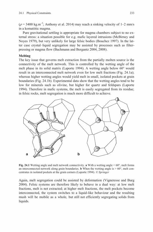
( = 3400 kg.m–3; Anthony et al. 2014) may reach a sinking velocity of 1–2 mm/s in a komatiitic magma.
Pure gravitational settling is appropriate for magma chambers subject to no ex-ternal stress: a situation possible for e.g. mafic layered intrusions (McBirney and Noyes 1979), but very unlikely for large felsic bodies (Bouchez 1997). In the lat-ter case crystal–liquid segregation may be assisted by processes such as filter-pressing or magma flow (Bachmann and Bergantz 2004, 2008).
Melting The key issue that governs melt extraction from the partially molten source is the connectivity of the melt network. This is controlled by the wetting angle of the melt phase in its solid matrix (Laporte 1994). A wetting angle below 60° would result in an interconnected melt network even for low melt fractions (Fig. 24.1a); whereas higher wetting angles would yield melt in small, isolated pockets at grain boundaries (Fig. 24.1b). Experimental data show that the wetting angles tend to be low for minerals such as olivine, but higher for quartz and feldspars (Laporte 1994). Therefore in mafic systems, the melt is easily segregated from its residue; in felsic rocks, melt segregation is much more difficult to achieve.
Fig. 24.1 Wetting angle and melt network connectivity. a With a wetting angle < 60°, melt forms an interconnected network along grain boundaries. b When the wetting angle is > 60°, melt con-centrates in isolated pockets at the grain corners (Laporte 1994). © Springer
Again, melt segregation could be assisted by deformation (Vigneresse and Burg 2004). Felsic systems are therefore likely to behave in a dual way: at low melt fractions, melt is not extracted; at higher melt fractions, the melt pockets become interconnected, the system switches to a liquid-like behaviour and the resulting
t still not efficiently segregating solids from liquids.
ba
24.1 Physical Constraints 233
mush will be mobile as a whole, bu
In summary, for mafic systems it is very easy to achieve melt/crystal separa-tion, be it during crystallization or melting. Fractional processes are perfectly fea-sible, and low-melt fraction (F) liquids may exist. In felsic systems, liquid/solid segregation is more difficult, and may only exist if assisted by deformation. Low-F liquids are less likely to be observed, and batch processes are more feasible.
24.2 Scale and Speed of Processes—Approach to Equilibrium
Chemical equilibrium is attained when the reactants and products of a reaction are present in concentrations that do not change with time. Thermal equilibrium oc-curs when there are no temperature changes in the system. In both cases, this does not preclude a dynamic balance of heat or material fluxes between components of the system.
Perfect equilibrium is never achieved in nature. It is however possible to break down a continuous process into a succession of infinitesimal equilibrium states, between which parameters (temperature, concentration…) vary For each step, the system can be treated as in equilibrium, which implicitly as-sumes that it reacts sufficiently fast to the changes.
In geochemical modelling, the term “equilibrium” is used to imply such a situa-tion, i.e. a system reacts to (temperature-induced mostly) changes more quicklythan is the rate of heating or cooling. This tends to be a sound assumption, because heat diffusion is sluggish in natural materials (e.g. Turcotte and Schubert 1982),whereas the kinetics of mineral reactions is strongly temperature-dependent, and therefore reasonably fast at igneous temperatures (Spear 1994). However, there may be situations where this assumption fails—in particular when the anatexis was short-lived, the system dry or cold, the source infertile and/or some of its components incapable of equilibrating with the melt. Some minerals are refractory and difficult to re-equilibrate; others may have failed to communicate with the melt, having been shielded by such refractory, or newly grown peritectic, phases (Watson and Harrison 1984). Also the solubility of accessories, often hosting a significant proportion of trace elements and radiogenic isotopes, is limited (Chap. 13). This is shown e.g., by the common occurrence of inherited zircon in low-T, anatectic granites (Miller et al. 2003).
1
In all these scenarios, equilibrium is not attained, primarily because the chemi-cal process is slower than the rate of temperature change. However, one may note that this definition largely relies on equilibration time, itself a function of the sys-tem size. From this observation is derived the concept of “equilibration volume”, i.e. the portion of a system that is small enough to allow equilibrium. This notion, although not new (Blackburn 1968) is increasingly used as a tool to decipher complex metamorphic textures, such as partially reacted assemblages or
1 Of course, if heat advection or convection are significant, disequilibrium, in the sense discussed here, is much more likely.
234 24 Common Sense in Action
only slightly.
phenocrysts preserved from igneous protolith (e.g. Tinkham and Ghent 2005amongst others). In effect, a very similar approach is used for igneous rocks. In a “non-modal” melting model, one assumes that only a part of the system (although its spatial extent is not explicitly specified) was involved in melting. “Disequilib-rium” approaches (i.e. models based on melting or crystallization affecting only a portion of a rock) have been successfully used to account for trace-element (Barbero et al. 1995; Villaros et al. 2009) or isotopic (Knesel and Davidson 1996; Farina and Stevens 2011; McLeod et al. 2012) characteristics of melts, primarily during (relatively low-T) crustal melting.
2
From this it is clear that the notion of equilibrium (from an igneous perspective) is very strongly dependent on the scale of observation. Pushing the reasoning to the absurd, it is clear that equilibrium is not attained at the scale of the whole man-tle (melts generated there are not in equilibrium with a bulk mantle composition). As one looks at smaller volumes, equilibrium becomes more likely. On the other hand, there is in general little point in considering equilibrium volumes that are too small (a few grains). The resulting melts are likely to be eventually mixed and homogenised, and any such subtle chemical variations erased.
The size of the equilibration volume to consider for geochemical modelling of magmatic rocks has to be decided on a case-by-case basis. Depending on the tem-perature of the processes studied, duration, presence of fluids etc., it may range from a few mm3 (similar to equilibration domains in metamorphic petrology), through a hand-specimen, to that of a rock unit.
24.3 Is Your Model Worth Your Efforts?
In general, the more complex the model, the longer it will take to develop. It is, therefore, important to think beforehand whether it is worth the added complexity, and how precise or detailed an answer is needed. In addition, complex models tend to require more input data: fewer parameters of a simple scenario are likely to be much better constrained that many of a complex one. Finally, a model is not built for its own sake, but for comparison with real data. If they are of poor quality (be it for analytical problems, or limited understanding of the geology involved), modelling will fail to discriminate between possible solutions.
2 Depending on the context, the opposite to “equilibrium” can be either “disequilibrium” or“fractional”, which is why the term “equilibrium” is not used in this book to describe a class of models (see Warning box at beginning of Chap. 11). Fractional melting (or crystallization) is not a disequilibrium process, as the system still reacts sufficiently fast to the changes to be re-garded as in equilibrium at any point in time!
24.2 Scale and Speed of Processes ... 235
24.3.1 How Well Can We Discriminate Between Models?
In the preceding text, different equations were written in order to describe various situations that are encountered during melting, crystallization or mixing. In theory, individual processes do produce distinct trends in geochemical plots. However, in many cases the difference is less than the scatter in the dataset. All natural datasets are intrinsically noisy due to: a) analytical errors, b) variable alteration of individualsamples, that is hard to totally avoid, c) limited sample size vs. that of possible
and/or d) multistage, complex genesis. The latter may reflect superposition ofseveral processes, such as melting of different portions of a source, crystallization, variable contamination, crystal accumulation or metasomatic redistribution ofelements by fluids.
In general, geochemists try to model only the dominant process(es), thus sim-plifying the problem by ignoring the other mechanisms. However, all of them af-fect to varying degrees the whole-rock compositions, and introduce some addi-tional variability in the dataset. When these variations are large, they are easily recognizable and we try to incorporate them in a more complex model. When they
In order to discuss whether it is practicable to distinguish between different models, we have built a synthetic dataset (the same as used for Exercise 22.1) .The advantage is that, unlike for natural data, the true evolution line is known, and it is possible to compare models against it. This dataset has been generated by cal-culating the theoretical evolution of a calc-alkaline basaltic magma, crystallizing Pl + Amp + Mt, with Zrn added using the saturation concept. “Sample” composi-tions were obtained by randomly modifying the ideal composition based on a normal distribution (2 = 5 % for majors and 10 % for traces). These computed values scatter around the actual model curve like natural datasets do.
3
Figure 24.2 compares the difference between three principal petrogenetic mod-els (fractional crystallization, melting and mixing), with the noise of our synthetic dataset. Clearly, processes are efficiently distinguished only when considering elements with contrasting behaviour and with D values very different from 1 (if D= 1, all equations collapse to linear). Even so, the fit between the true model (Rayleigh fractionation) and the data is satisfactory, but not great—there is sig-nificant scatter around the curve. The use of a log scale does not make a differ-ence: Rayleigh curves are linearized (cf. Fig. 24.2c and f), but when the D values are too similar or too close to 1 (cf. Fig. 24.2a–b with d–e), this does not help.
In the light of this, one may question the use of elaborate models such as AFC or fractional melting. While they may be intellectually satisfying, in that they ar-guably incorporate geologically more realistic processes, they may not be distin-guishable on geochemical grounds, and may actually bring no further insight! Likewise, the use of complex solubility equations (Sect. 22.3) may, or may not
3 The code generating this dataset is given in full on the Web site.
236 24 Common Sense in Action
heterogeneities (accumulated crystals, incompletely mixed magma batches, etc.),
are small, they are easily considered as natural noise and overlooked.
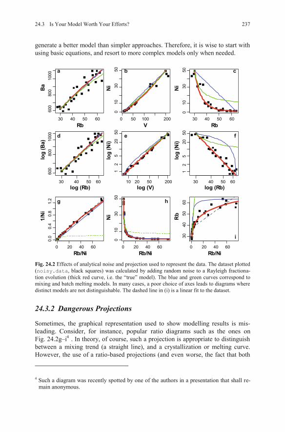
generate a better model than simpler approaches. Therefore, it is wise to start with using basic equations, and resort to more complex models only when needed.
Fig. 24.2 Effects of analytical noise and projection used to represent the data. The dataset plotted (noisy.data, black squares) was calculated by adding random noise to a Rayleigh fractiona-tion evolution (thick red curve, i.e. the “true” model). The blue and green curves correspond to mixing and batch melting models. In many cases, a poor choice of axes leads to diagrams where distinct models are not distinguishable. The dashed line in (i) is a linear fit to the dataset.
24.3.2 Dangerous Projections
Sometimes, the graphical representation used to show modelling results is mis-leading. Consider, for instance, popular ratio diagrams such as the ones onFig. 24.2g–i . In theory, of course, such a projection is appropriate to distinguish between a mixing trend (a straight line), and a crystallization or melting curve. However, the use of a ratio-based projections (and even worse, the fact that both
4
4 Such a diagram was recently spotted by one of the authors in a presentation that shall re-main anonymous.
30 40 50 60
600
800
1000
Rb
Ba
0 50 100 2000
1030
50
V
Ni
30 40 50 60
010
3050
Rb
Ni
30 40 50 60
600
800
1000
log (Rb)
log
(Ba)
10 20 50 200
12
520
50
log (V)
log
(Ni)
30 40 50 601
25
2050
log (Rb)
log
(Ni)
0 20 40 60
0.0
0.4
0.8
1.2
Rb/Ni
1/N
i
0 20 40 60
010
3050
Rb/Ni
Ni
0 20 40 60
3040
5060
Rb/Ni
Rb
a b c
d e f
g h
i
24.3 Is Your Model Worth Your Efforts? 237
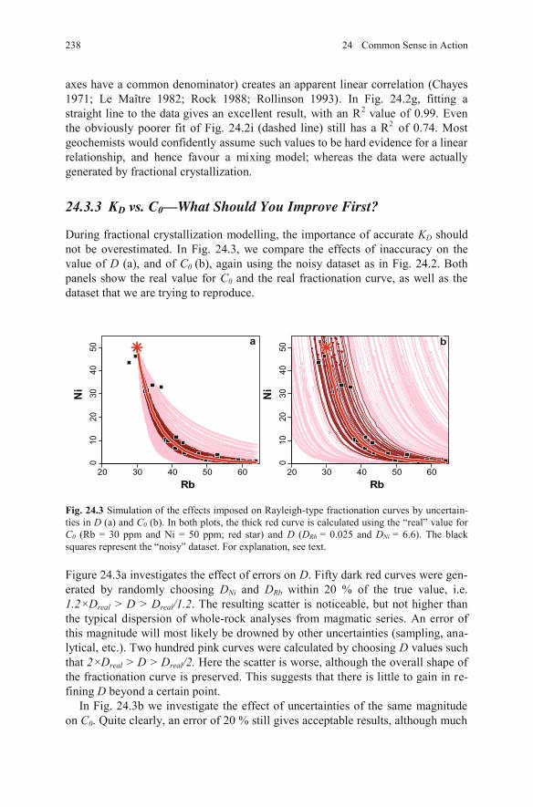
axes have a common denominator) creates an apparent linear correlation (Chayes 1971; Le Maître 1982; Rock 1988; Rollinson 1993). In Fig. 24.2g, fitting a straight line to the data gives an excelthe obviously poorer fit of Fig. 24.2i geochemists would confidently assume relationship, and hence favour a mixgenerated by fractional crystallization.
24.3.3 KD vs. C0—What Should You Improve First?
During fractional crystallization modelling, the importance of accurate KD should not be overestimated. In Fig. 24.3, we compare the effects of inaccuracy on the value of D (a), and of C0 (b), again using the noisy dataset as in Fig. 24.2. Both panels show the real value for C0 and the real fractionation curve, as well as the dataset that we are trying to reproduce.
Fig. 24.3 Simulation of the effects imposed on Rayleigh-type fractionation curves by uncertain-ties in D (a) and C0 (b). In both plots, the thick red curve is calculated using the “real” value for C0 (Rb = 30 ppm and Ni = 50 ppm; red star) and D (DRb = 0.025 and DNi = 6.6). The black squares represent the “noisy” dataset. For explanation, see text.
Figure 24.3a investigates the effect of errors on D. Fifty dark red curves were gen-erated by randomly choosing DNi and DRb within 20 % of the true value, i.e. 1.2×Dreal > D > Dreal/1.2. The resulting scatter is noticeable, but not higher than the typical dispersion of whole-rock analyses from magmatic series. An error of this magnitude will most likely be drowned by other uncertainties (sampling, ana-lytical, etc.). Two hundred pink curves were calculated by choosing D values such that 2×Dreal > D > Dreal/2. Here the scatter is worse, although the overall shape of the fractionation curve is preserved. This suggests that there is little to gain in re-fining D beyond a certain point.
In Fig. 24.3b we investigate the effect of uncertainties of the same magnitude on C0. Quite clearly, an error of 20 % still gives acceptable results, although much
20 30 40 50 60
010
2030
4050
Rb
Ni
20 30 40 50 60
010
2030
4050
Rb
Ni
a bbb
238 24 Common Sense in Action
lent result, with an R2 value of 0.99. Even(dashed line) still has a R2 of 0.74. Mostsuch values to be hard evidence for a linear
ing model; whereas the data were actually
worse than in Fig. 24.3a. On the other hand, curves generated by an error of a fac-tor of two cover the whole diagram.
In general, it must be kept in mind that the composition of a melt is also a func-tion of the source (or primitive liquid) composition (C0) and F—parameters for which there are considerable uncertainties. Even though KD is a source of error, it is perhaps not the worst offender in most models. It seems more important to en-sure that the ratios between individual KD are right, as this would eventually con-trol the ratio in the melt. Indeed, many geochemists would rely more on ratios (such as Zr/Nb, Nb/Ta, etc.) than on absolute values. On the other hand, a good determination of C0 is more crucial, as it can easily lead to meaningless results. This is perhaps more important during partial melting, as modelling relies on a se-lection of a possible, although rarely of a fractionating series is generally observed. In other words, the most importantaspect of modelling is to get the geology right, and to understand what is actuallymelting (or fractionating)!
24.4 Back to the Field!
In a sense, the most critical input parameter in any model remains the geological understanding. There is, for instance, little point in trying to build a model for a dataset that includes rock units of distinct ages. Therefore, modelling should be endured on a well-designed dataset, including only relevant data. This may in-volve heart-breaking decisions, such as discarding some of your precious analyses. In any case, such a judgement can only be made on the basis of geological under-standing of the studied region.
Finally, one cannot stress strongly enough that the ultimate test for a model is its geological consistency. Therefore, models that invoke sources absent from the studied area; that predict volumes of rocks not matching the observed distribution; that require thermal regimes totally at odds with the local record, or impossibly high melt amounts are of no use. Although such models may pass the geochemical tests, reproduce observed compositions and otherwise seem satisfactory at first glance, one must keep in mind that geological data in the broadest sense are just as valuable as geochemical ones. Indeed, the ultimate goal of modelling is to provide an explanation for all the observations, regardless of their origin, and shed some light onto the evolution of existing rocks in their geological context.
And so, as a final word of caution, perhaps unexpected in a text on geochemical modelling, we would like to encourage you to return again and again to the obser-vation of field relationships, geological maps, samples and thin sections…
If you don’t understand it—map it! ––– An anonymous geologist
23924.3 Is Your Model Worth Your Efforts?
known, source; whereas the primitive liquid
240 24 Common Sense in Action
References
Annen C, Blundy JD, Sparks RSJ (2006) The sources of granitic melt in Deep Hot Zones. Trans Roy Soc Edinb, Earth Sci 97:297–309
Anthony JW, Bideaux RA, Bladh KW, Nichols MC (2014) Handbook of Mineralogy (web ver-sion). Mineralogical Society of America. http://www.handbookofmineralogy.org
Arzi AA (1978) Critical phenomena in the rheology of partially melted rocks. Tectonophysics 44:173–184
Bachmann O, Bergantz GW (2004) On the origin of crystal-poor rhyolites: extracted from batho-lithic crystal mushes. J Petrol 45:1565
Bachmann O, Bergantz GW (2008) Rhyolites and their source mushes across tectonic settings. J Petrol 49:2277–2285
Barbero L, Villaseca C, Rogers G, Brown P (1995) Geochemical and isotopic disequilibrium in crustal melting: an insight from the anatectic granitoids from Toledo, Spain. J Geophys Res 100:15745–15765
Bea F (2012) The sources of energy for crustal melting and the geochemistry of heat-producing elements. Lithos 153:278–291
Blackburn W (1968) The spatial extent of chemical equilibrium in some high-grade metamorphic rocks from the Grenville of southeastern Ontario. Contrib Mineral Petrol 19:72–92
Bouchez J-L (1997) Granite is never isotropic: an introduction to AMS studies of granitic rocks. In: Bouchez J-L, Hutton DHW, Stephens WE (eds) Granite: from segregation of melt to emplacement fabrics. Kluwer Academic Publications, Dordrecht, pp 95–112
Chayes F (1971) Ratio correlation: a manual for students of petrology and geochemistry. University of Chicago Press, Chicago
De Paolo DJ (1981) Trace element and isotopic effects of combined wallrock assimilation and fractional crystallization. Earth Planet Sci Lett 53:189–202
Farina F, Stevens G (2011) Source controlled 87Sr/86Sr isotope variability in granitic magmas: the inevitable consequence of mineral-scale isotopic disequilibrium in the protolith. Lithos 122:189–200
Henk A, von Blanckenburg F, Finger F, Schaltegger U, Zulauf G (2000) Syn-convergent high-temperature metamorphism and magmatism in the Variscides: a discussion of potential heat sources. In: Franke W, Haak V, Oncken O, Tanner D (eds) Orogenic processes: quantification and modelling in the Variscan Belt. Geological Society of London Special Publications, vol 179, pp 387–399
Knesel KM, Davidson JP (1996) Isotopic disequilibrium during melting of granite and implica-tions for crustal contamination of magmas. Geology 24:243–246
Laporte D (1994) Wetting behavior of partial melts during crustal anatexis: the distribution of hydrous silicic melts in polycrystalline aggregates of quartz. Contrib Mineral Petrol 116:486–499
Le Maître RW (1982) Numerical petrology. Elsevier, AmsterdamMcBirney AR, Noyes RM (1979) Crystallization and layering of the Skaergaard intrusion.
J Petrol 20:487–554McLeod CL, Davidson JP, Nowell GM, de Silva SL (2012) Disequilibrium melting during crus-
tal anatexis and implications for modeling open magmatic systems. Geology 40:435–438Miller CF, McDowell SM, Mapes RW (2003) Hot and cold granites? Implications of zircon satu-
ration temperatures and preservation of inheritance. Geology 31:529–532Reiners PW, Nelson BK, Ghiorso MS (1995) Assimilation of felsic crust by basaltic magma:
thermal limits and extents of crustal contamination of mantle-derived magmas. Geology 23:563–566
Roberts MP, Clemens JD (1995) Feasibility of AFC models for the petrogenesis of calc-alkaline magma series. Contrib Mineral Petrol 121:139–147
References 241
Rock NMS (1988) Numerical geology. A source guide, glossary and selective bibliography to geological uses of computers and statistics. Lecture Notes in Earth Sciences, vol 18. Springer, Berlin
Rollinson HR (1993) Using geochemical data: evaluation, presentation, interpretation. Longman, London
Rosenberg CL (2001) Deformation of partially molten granite: a review and comparison of experimental and natural case studies. Int J Earth Sci 90:60–76
Sawyer EW, Cesare B, Brown M (2011) When the continental crust melts. Elements 7:229–234Spear FS (1994) Metamorphic phase equilibria and pressure–temperature–time paths.
Mineralogical Society of America Monographs. Mineralogical Society of America, Washington
Spera FJ (2000) Physical properties of magma. In: Sigurdsson (ed) Encyclopedia of volcanoes. Academic Press, San Diego, pp 171–189
Stokes GG (1901) Mathematical and physical papers, vol 3. Cambridge University Press, Cambridge
Taylor HP, Jr, Sheppard SMF (1986) Igneous rocks: I. Processes of isotopic fractionation and isotope systematics. In: Valley JW, Taylor HP, Jr, O’Neil JR (eds) Stable isotopes in high temperature geological processes. Mineralogical Society of America Reviews in Mineralogy, vol 16, pp 227–271
Thompson AB, Connolly JAD (1995) Melting of the continental crust: some thermal and pet-rological constraints on anatexis in continental collision zones and other tectonic settings. J Geophys Res 100:15565–15579
Tinkham DK, Ghent ED (2005) Estimating PT conditions of garnet growth with isochemi-cal phase-diagram sections and the problem of effective bulk-composition. Canad Mineral 43:35–50
Turcotte DL, Schubert G (1982) Geodynamics: applications of continuum physics to geological problems. John Wiley and Sons, New York
Vigneresse JL, Burg J-P (2004) Strain-rate dependent rheology of partially molten rocks. In: Grocott J, McCaffrey KJW, Taylor G, Tikoff B (eds) Vertical coupling and decoupling in the lithosphere. Geological Society of London Special Publications, vol 227, pp 327–336
Villaros A, Stevens G, Moyen J-F, Buick IS (2009) The trace element composition of S-type granites: evidence for disequilibrium melting and accessory phase entrainment in the source. Contrib Mineral Petrol 158:543–561
Watson EB, Harrison TM (1984) Accessory minerals and the geochemical evolution of crustal magmatic systems: a summary and prospectus of experimental approaches. Phys Earth Planet Inter 35:19–30
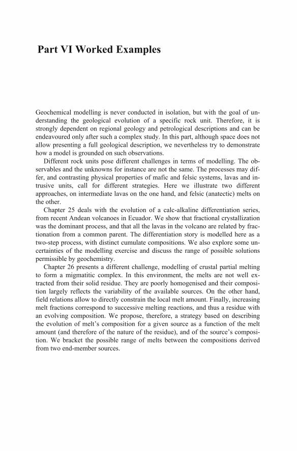
Part VI Worked Examples
Geochemical modelling is never conducted in isolation, but with the goal of un-derstanding the geological evolution of a specific rock unit. Therefore, it is strongly dependent on regional geology and petrological descriptions and can be endeavoured only after such a complex study. In this part, although space does not allow presenting a full geological description, we nevertheless try to demonstrate how a model is grounded on such observations.
Different rock units pose different challenges in terms of modelling. The ob-servables and the unknowns for instance are not the same. The processes may dif-fer, and contrasting physical properties of mafic and felsic systems, lavas and in-trusive units, call for different strategies. Here we illustrate two different approaches, on intermediate lavas on the one hand, and felsic (anatectic) melts on the other.
Chapter 25 deals with the evolution of a calc-alkaline differentiation series, from recent Andean volcanoes in Ecuador. We show that fractional crystallization was the dominant process, and that all the lavas in the volcano are related by frac-tionation from a common parent. The differentiation story is modelled here as a two-step process, with distinct cumulate compositions. We also explore some un-certainties of the modelling exercise and discuss the range of possible solutions permissible by geochemistry.
Chapter 26 presents a different challenge, modelling of crustal partial melting to form a migmatitic complex. In this environment, the melts are not well ex-tracted from their solid residue. They are poorly homogenised and their composi-tion largely reflects the variability of the available sources. On the other hand, field relations allow to directly constrain the local melt amount. Finally, increasing melt fractions correspond to successive melting reactions, and thus a residue with an evolving composition. We propose, therefore, a strategy based on describing the evolution of melt’s composition for a given source as a function of the melt amount (and therefore of the nature of the residue), and of the source’s composi-tion. We bracket the possible range of melts between the compositions derived from two end-member sources.
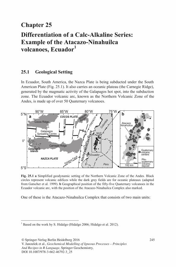
Chapter 25 Differentiation of a Calc-Alkaline Series: Example of the Atacazo-Ninahuilca volcanoes, Ecuador1
25.1 Geological Setting
In Ecuador, South America, the Nazca Plate is being subducted under the South American Plate (Fig. 25.1). It also carries an oceanic plateau (the Carnegie Ridge), generated by the magmatic activity of the Galapagos hot spot, into the subduction zone. The Ecuador volcanic arc, known as the Northern Volcanic Zone of the
Fig. 25.1 a Simplified geodynamic setting of the Northern Volcanic Zone of the Andes. Black circles represent volcanic edifices while the dark grey fields are for oceanic plateaux (adapted from Gutscher et al. 1999). b Geographical position of the fifty-five Quaternary volcanoes in the Ecuador volcanic arc, with the position of the Atacazo-Ninahuilca Complex also marked.
One of these is the Atacazo-Ninahuilca Complex that consists of two main units:
1 Based on the work by S. Hidalgo (Hidalgo 2006; Hidalgo et al. 2012).
TREN
CH
Carnegie RidgeGalapagosGalapagos
IslandsIslands
Malpelo
RidgeCocos Ridge
GalapagosSpreading Centre
Ecuador
Peru
Colombia
COCOS PLATE
NAZCA PLATE
Grijalva Fault
80°W 75°W85°W90°W
5°S
0°
5°N
AtacazoNinahuilca
100 km
a b
NVZNVZNVZ
Plio-quaternaryvolcanicdeposit
Quaternaryvolcaniccenters
SOUT
H AM
ERIC
AN P
LATE
SOUT
H AM
ERIC
AN P
LATE
SOUT
H AM
ERIC
AN P
LATE
© Springer-Verlag Berlin Heidelberg 2016 V. Janoušek et al., Geochemical Modelling of Igneous Processes – Principles And Recipes in R Language, Springer Geochemistry, DOI 10.1007/978-3-662-46792-3_25
245
Andes, is made up of over 50 Quaternary volcanoes.
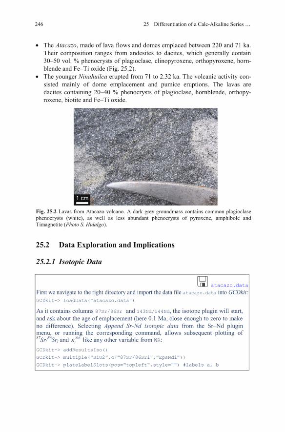
The Atacazo, made of lava flows and domes emplaced between 220 and 71 ka. Their composition ranges from andesites to dacites, which generally contain 30–50 vol. % phenocrysts of plagioclase, clinopyroxene, orthopyroxene, horn-blende and Fe–Ti oxide (Fig. 25.2). The younger Ninahuilca erupted from 71 to 2.32 ka. The volcanic activity con-sisted mainly of dome emplacement and pumice eruptions. The lavas are dacites containing 20–40 % phenocrysts of plagioclase, hornblende, orthopy-roxene, biotite and Fe–Ti oxide.
Fig. 25.2 Lavas from Atacazo volcano. A dark grey groundmass contains common plagioclase phenocrysts (white), as well as less abundant phenocrysts of pyroxene, amphibole and
Photo S. Hidalgo).
25.2 Data Exploration and Implications
25.2.1 Isotopic Data
atacazo.data
First we navigate to the right directory and import the data file atacazo.data into GCDkit:GCDkit-> loadData("atacazo.data")
As it contains columns 87Sr/86Sr and 143Nd/144Nd, the isotope plugin will start, and ask about the age of emplacement (here 0.1 Ma, close enough to zero to make no difference). Selecting Append Sr-Nd isotopic data from the Sr–Nd plugin menu, or running the corresponding command, allows subsequent plotting of 87Sr/86Sri and Nd
i like any other variable from WR: GCDkit-> addResultsIso()
GCDkit-> multiple("SiO2",c("87Sr/86Sri","EpsNdi"))
GCDkit-> plateLabelSlots(pos="topleft",style="") #labels a, b
1 cm
246 25 Differentiation of a Calc-Alkaline Series …
Timagnetite (
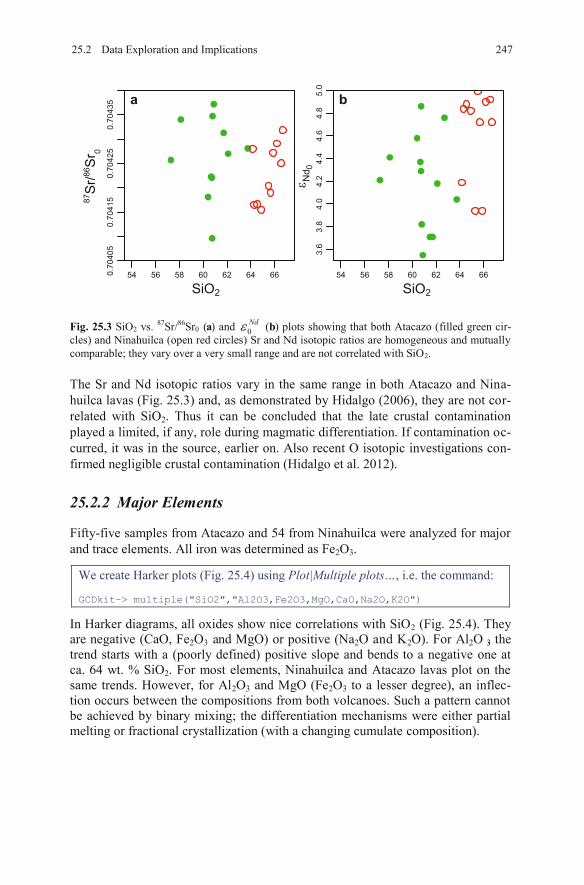
Fig. 25.3 SiO2 vs. 87Sr/86Sr0 (a) and 0Nd (b) plots showing that both Atacazo (filled green cir-
cles) and Ninahuilca (open red circles) Sr and Nd isotopic ratios are homogeneous and mutually comparable; they vary over a very small range and are not correlated with SiO2.
The Sr and Nd isotopic ratios vary in the same range in both Atacazo and Nina-huilca lavas (Fig. 25.3) and, as demonstrated by Hidalgo (2006), they are not cor-related with SiO2. Thus it can be concluded that the late crustal contamination played a limited, if any, role during magmatic differentiation. If contamination oc-curred, it was in the source, earlier on. Also recent O isotopic investigations con-firmed negligible crustal contamination (Hidalgo et al. 2012).
25.2.2 Major Elements
Fifty-five samples from Atacazo and 54 from Ninahuilca were analyzed for major and trace elements. All iron was determined as Fe2O3.
We create Harker plots (Fig. 25.4) using Plot|Multiple plots…, i.e. the command:
GCDkit-> multiple("SiO2","Al2O3,Fe2O3,MgO,CaO,Na2O,K2O")
In Harker diagrams, all oxides show nice correlations with SiO2 (Fig. 25.4). They are negative (CaO, Fe2O3 and MgO) or positive (Na2O and K2O). For Al2O 3, the trend starts with a (poorly defined) positive slope and bends to a negative one at ca. 64 wt. % SiO2. For most elements, Ninahuilca and Atacazo lavas plot on the same trends. However, for Al2O3 and MgO (Fe2O3 to a lesser degree), an inflec-tion occurs between the compositions from both volcanoes. Such a pattern cannot be achieved by binary mixing; the differentiation mechanisms were either partial melting or fractional crystallization (with a changing cumulate composition).
54 56 58 60 62 64 660.70405
0.70415
0.70425
0.70435
54 56 58 60 62 64 66
3.6
3.8
4.0
4.2
4.4
4.6
4.8
5.0
a b
SiO2SiO2
87Sr/86Sr 0
Nd0
25.2 Data Exploration and Implications 247
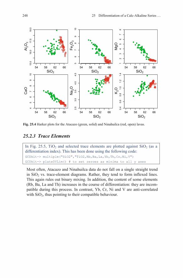
Fig. 25.4 Harker plots for the Atacazo (green, solid) and Ninahuilca (red, open) lavas.
25.2.3 Trace Elements
In Fig. 25.5, TiO2 and selected trace elements are plotted against SiO2 (as a differentiation index). This has been done using the following code: GCDkit-> multiple("SiO2","TiO2,Rb,Ba,La,Yb,Th,Cr,Ni,V")
GCDkit-> plate0YLim() # to set zeroes as minima to all y axes
Most often, Atacazo and Ninahuilca data do not fall on a single straight trend in SiO2 vs. trace-element diagrams. Rather, they tend to form inflexed lines.This again rules out binary mixing. In addition, the content of some elements (Rb, Ba, La and Th) increases in the course of differentiation: they are incom-patible during this process. In contrast, Yb, Cr, Ni and V are anti-correlated with SiO2, thus pointing to their compatible behaviour.
54 58 62 66
15.0
16.0
17.0
18.0
54 58 62 66
56
78
910
54 58 62 66
12
34
56
78
54 58 62 66
45
67
89
10
54 58 62 66
2.5
3.0
3.5
4.0
4.5
54 58 62 66
0.4
0.6
0.8
1.0
1.2
1.4
Al 2O
3
Fe2O
3
MgO
CaO
Na 2
O
K2O
SiO2 SiO2 SiO2
SiO2 SiO2 SiO2
248 25 Differentiation of a Calc-Alkaline Series …
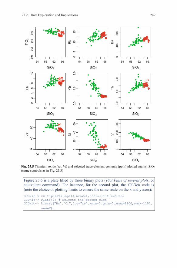
Fig. 25.5 Titanium oxide (wt. %) and selected trace-element contents (ppm) plotted against SiO2
(same symbols as in Fig. 25.3)
Figure 25.6 is a plate filled by three binary plots (Plot|Plate of several plots, or equivalent command). For instance, for the second plot, the GCDkit code is (note the choice of plotting limits to ensure the same scale on the x and y axes): GCDkit-> multiplePerPage(3,nrow=1,ncol=3,title=NULL) GCDkit-> Plate(2) # Selects the second slot GCDkit-> binary("Ba","Cr",log="xy",xmin=5,ymin=5,xmax=1100,ymax=1100,
+ new=F)…
54 58 62 66
0.0
0.2
0.4
0.6
SiO2
TiO
2
54 58 62 66
05
1525
SiO2R
b
54 58 62 66
040
080
0
SiO2
Ba
54 58 62 66
02
46
812
SiO2
La
54 58 62 66
0.0
1.0
2.0
SiO2
Yb
54 58 62 66
0.0
1.0
2.0
SiO2Th
54 58 62 66
SiO2
Zr
54 58 62 66
020
4060
SiO2
Ni
54 58 62 66
010
020
030
0
SiO2
V
040
80
25.2 Data Exploration and Implications 249
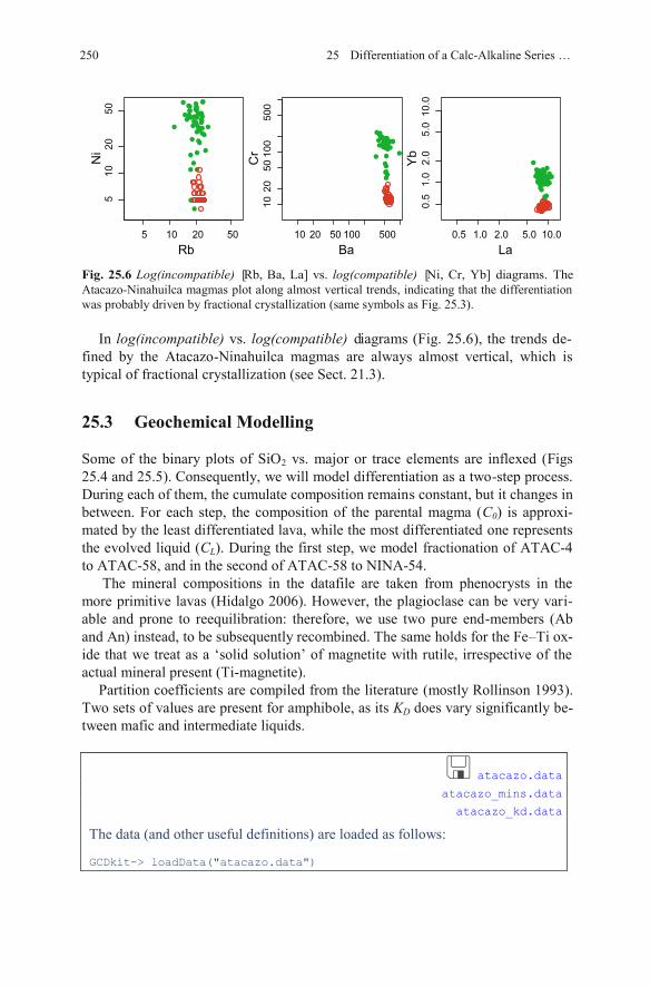
Fig. 25.6 Log(incompatible) [Rb, Ba, La] vs. log(compatible) [Ni, Cr, Yb] diagrams. The
In log(incompatible) vs. log(compatible) diagrams (Fig. 25.6), the trends de-fined by the Atacazo-Ninahuilca magmas are always almost vertical, which is typical of fractional crystallization (see Sect. 21.3).
25.3 Geochemical Modelling
Some of the binary plots of SiO2 vs. major or trace elements are inflexed (Figs 25.4 and 25.5). Consequently, we will model differentiation as a two-step process. During each of them, the cumulate composition remains constant, but it changes in between. For each step, the composition of the parental magma (C0) is approxi-mated by the least differentiated lava, while the most differentiated one represents the evolved liquid (CL). During the first step, we model fractionation of ATAC-4to ATAC-58, and in the second of ATAC-58 to NINA-54.
The mineral compositions in the datafile are taken from phenocrysts in the more primitive lavas (Hidalgo 2006). However, the plagioclase can be very vari-able and prone to reequilibration: therefore, we use two pure end-members (Ab and An) instead, to be subsequently recombined. The same holds for the Fe–Ti ox-ide that we treat as a ‘solid solution’ of magnetite with rutile, irrespective of the actual mineral present (Ti-magnetite).
Partition coefficients are compiled from the literature (mostly Rollinson 1993).Two sets of values are present for amphibole, as its KD does vary significantly be-tween mafic and intermediate liquids.
atacazo.data
atacazo_mins.data
atacazo_kd.data
The data (and other useful definitions) are loaded as follows:
GCDkit-> loadData("atacazo.data")
5 10 20 50
510
2050
10 20 50 100 500
1020
5010
050
0
0.5 1.0 2.0 5.0 10.0
0.5
1.0
2.0
5.0
10.0
Ni
Cr
Yb
Rb Ba La
250 25 Differentiation of a Calc-Alkaline Series …
Atacazo-Ninahuilca magmas plot along almost vertical trends, indicating that the differentiationwas probably driven by fractional crystallization (same symbols as Fig. 25.3).
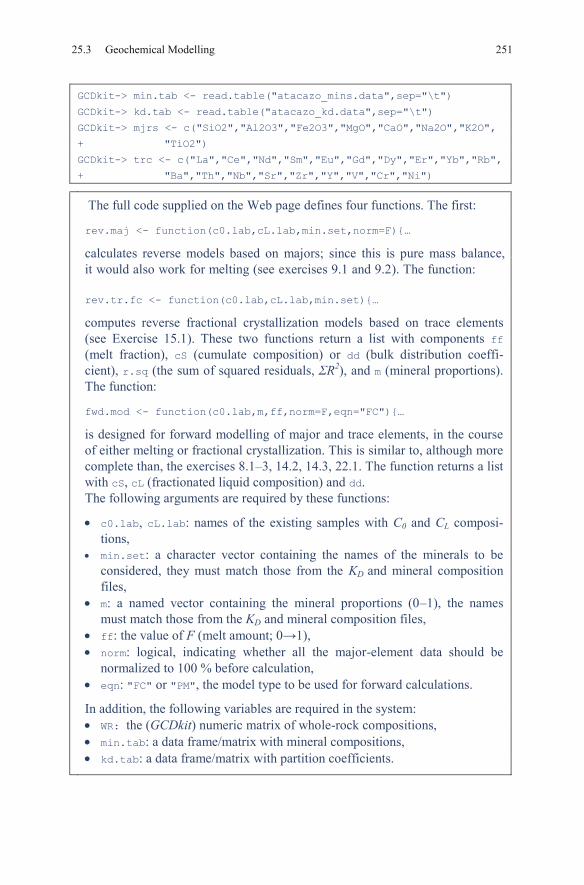
GCDkit-> min.tab <- read.table("atacazo_mins.data",sep="\t")
GCDkit-> kd.tab <- read.table("atacazo_kd.data",sep="\t")
GCDkit-> mjrs <- c("SiO2","Al2O3","Fe2O3","MgO","CaO","Na2O","K2O",
+ "TiO2")
GCDkit-> trc <- c("La","Ce","Nd","Sm","Eu","Gd","Dy","Er","Yb","Rb",
+ "Ba","Th","Nb","Sr","Zr","Y","V","Cr","Ni")
The full code supplied on the Web page defines four functions. The first:
rev.maj <- function(c0.lab,cL.lab,min.set,norm=F){…
calculates reverse models based on majors; since this is pure mass balance, it would also work for melting (see exercises 9.1 and 9.2). The function:
rev.tr.fc <- function(c0.lab,cL.lab,min.set){…
computes reverse fractional crystallization models based on trace elements (see Exercise 15.1). These two functions return a list with components ff(melt fraction), cS (cumulate composition) or dd (bulk distribution coeffi-cient), r.sq (the sum of squared residuals, R2), and m (mineral proportions). The function:
fwd.mod <- function(c0.lab,m,ff,norm=F,eqn="FC"){…
is designed for forward modelling of major and trace elements, in the course of either melting or fractional crystallization. This is similar to, although more complete than, the exercises 8.1–3, 14.2, 14.3, 22.1. The function returns a list with cS, cL (fractionated liquid composition) and dd. The following arguments are required by these functions:
c0.lab, cL.lab: names of the existing samples with C0 and CL composi-tions, min.set: a character vector containing the names of the minerals to be considered, they must match those from the KD and mineral composition files, m: a named vector containing the mineral proportions (0–1), the names must match those from the KD and mineral composition files, ff: the value of F (melt amount; 0 1), norm: logical, indicating whether all the major-element data should be normalized to 100 % before calculation, eqn: "FC" or "PM", the model type to be used for forward calculations.
In addition, the following variables are required in the system: WR: the (GCDkit) numeric matrix of whole-rock compositions, min.tab: a data frame/matrix with mineral compositions, kd.tab: a data frame/matrix with partition coefficients.
25.3 Geochemical Modelling 251
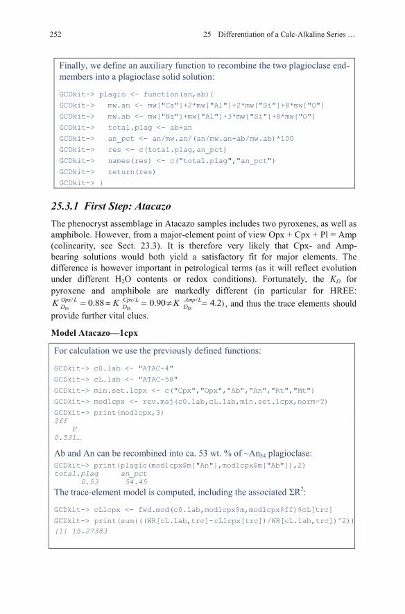
Finally, we define an auxiliary function to recombine the two plagioclase end-members into a plagioclase solid solution:
GCDkit-> plagio <- function(an,ab){
GCDkit-> mw.an <- mw["Ca"]+2*mw["Al"]+2*mw["Si"]+8*mw["O"]
GCDkit-> mw.ab <- mw["Na"]+mw["Al"]+3*mw["Si"]+8*mw["O"]
GCDkit-> total.plag <- ab+an
GCDkit-> an_pct <- an/mw.an/(an/mw.an+ab/mw.ab)*100
GCDkit-> res <- c(total.plag,an_pct)
GCDkit-> names(res) <- c("total.plag","an_pct")
GCDkit-> return(res)
GCDkit-> }
25.3.1 First Step: Atacazo The phenocryst assemblage in Atacazo samples includes two pyroxenes, as well as amphibole. However, from a major-element point of view Opx + Cpx + Pl = Amp (colinearity, see Sect. 23.3). It is therefore very likely that Cpx- and Amp- bearing solutions would both yield a satisfactory fit for major elements. The difference is however important in petrological terms (as it will reflect evolution under different H2O contents or redox conditions). Fortunately, the KD for pyroxene and amphibole are markedly different (in particular for HREE:
/ / /0.88 0.90 4.2Yb Yb Yb
Opx L Cpx L Amp LD D DK K K ) , and thus the trace elements should
provide further vital clues.
Model Atacazo—1cpx
For calculation we use the previously defined functions:
GCDkit-> c0.lab <- "ATAC-4"
GCDkit-> cL.lab <- "ATAC-58"
GCDkit-> min.set.1cpx <- c("Cpx","Opx","Ab","An","Rt","Mt")
GCDkit-> mod1cpx <- rev.maj(c0.lab,cL.lab,min.set.1cpx,norm=T)
GCDkit-> print(mod1cpx,3) $ff F 0.531…
Ab and An can be recombined into ca. 53 wt. % of ~An54 plagioclase: GCDkit-> print(plagio(mod1cpx$m["An"],mod1cpx$m["Ab"]),2) total.plag an_pct 0.53 54.45
The trace-element model is computed, including the associated R2:
GCDkit-> cL1cpx <- fwd.mod(c0.lab,mod1cpx$m,mod1cpx$ff)$cL[trc]
GCDkit-> print(sum(((WR[cL.lab,trc]-[1] 15.27383
252
25 Differentiation of a Calc-Alkaline Series …
cL1cpx[trc])/WR[cL.lab,trc])^2))
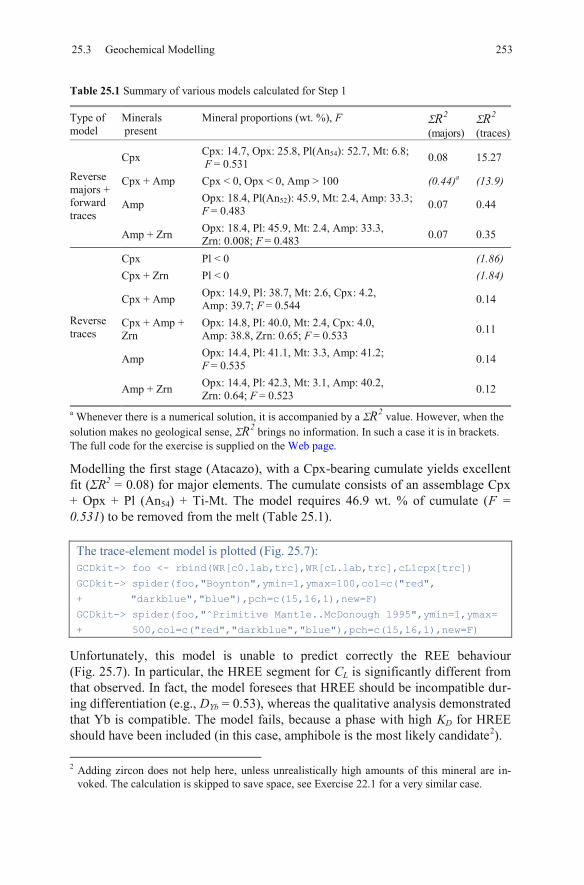
Table 25.1 Summary of various models calculated for Step 1
Type of model
Mineralspresent
Mineral proportions (wt. %), F(majors) (traces)
Reverse majors + forward traces
Cpx Cpx: 14.7, Opx: 25.8, Pl(An54): 52.7, Mt: 6.8;F = 0.531 0.08 15.27
Cpx + Amp Cpx < 0, Opx < 0, Amp > 100 (0.44)a (13.9)
Amp Opx: 18.4, Pl(An52): 45.9, Mt: 2.4, Amp: 33.3; F = 0.483 0.07 0.44
Amp + Zrn Opx: 18.4, Pl: 45.9, Mt: 2.4, Amp: 33.3, Zrn: 0.008; F = 0.483 0.07 0.35
Reverse traces
Cpx Pl < 0 (1.86)Cpx + Zrn Pl < 0 (1.84)
Cpx + Amp Opx: 14.9, Pl: 38.7, Mt: 2.6, Cpx: 4.2, Amp: 39.7; F = 0.544 0.14
Cpx + Amp +Zrn
Opx: 14.8, Pl: 40.0, Mt: 2.4, Cpx: 4.0, Amp: 38.8, Zrn: 0.65; F = 0.533 0.11
Amp Opx: 14.4, Pl: 41.1, Mt: 3.3, Amp: 41.2; F = 0.535 0.14
Amp + Zrn Opx: 14.4, Pl: 42.3, Mt: 3.1, Amp: 40.2, Zrn: 0.64; F = 0.523 0.12
a Whenever there is a numerical solution, it is accompanied by a value. However, when the solution makes no geological sense, brings no information. In such a case it is in brackets. The full code for the exercise is supplied on the Web page.
Modelling the first stage (Atacazo), with a Cpx-bearing cumulate yields excellent fit ( R2 = 0.08) for major elements. The cumulate consists of an assemblage Cpx + Opx + Pl (An54) + Ti-Mt. The model requires 46.9 wt. % of cumulate (F = 0.531) to be removed from the melt (Table 25.1).
The trace-element model is plotted (Fig. 25.7):GCDkit-> foo <- rbind(WR[c0.lab,trc],WR[cL.lab,trc],cL1cpx[trc])
GCDkit-> spider(foo,"Boynton",ymin=1,ymax=100,col=c("red",
+ "darkblue","blue"),pch=c(15,16,1),new=F)
GCDkit-> spider(foo,"^Primitive Mantle..McDonough 1995",ymin=1,ymax=
+ 500,col=c("red","darkblue","blue"),pch=c(15,16,1),new=F)
Unfortunately, this model is unable to predict correctly the REE behaviour (Fig. 25.7). In particular, the HREE segment for CL is significantly different from that observed. In fact, the model foresees that HREE should be incompatible dur-ing differentiation (e.g., DYb = 0.53), whereas the qualitative analysis demonstrated that Yb is compatible. The model fails, because a phase with high KD for HREE should have been included (in this case, amphibole is the most likely candidate2). 2 Adding zircon does not help here, unless unrealistically high amounts of this mineral are in-
voked. The calculation is skipped to save space, see Exercise 22.1 for a very similar case.
25325.3 Geochemical Modelling
R2 R2
R2R2
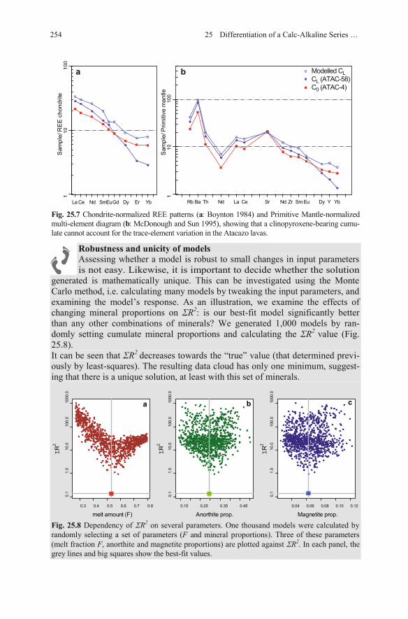
Fig. 25.7 Chondrite-normalized REE patterns (a: Boynton 1984) and Primitive Mantle-normalized multi-element diagram (b: McDonough and Sun 1995), showing that a clinopyroxene-bearing cumu-late cannot account for the trace-element variation in the Atacazo lavas.
Robustness and unicity of modelsAssessing whether a model is robust to small changes in input parameters is not easy. Likewise, it is important to decide whether the solution
generated is mathematically unique. This can be investigated using the Monte Carlo method, i.e. calculating many models by tweaking the input parameters, and examining the model’s response. As an illustration, we examine the effects of changing mineral proportions on R2: is our best-fit model significantly better than any other combinations of minerals? We generated 1,000 models by ran-domly setting cumulate mineral proportions and calculating the R2 value (Fig. 25.8).It can be seen that R2 decreases towards the “true” value (that determined previ-ously by least-squares). The resulting data cloud has only one minimum, suggest-
Fig. 25.8 Dependency of R2 on several parameters. One thousand models were calculated by randomly selecting a set of parameters ( ). Three of these parameters (melt fraction F, anorthite and magnetite proportions) are plotted against R2. In each panel, the grey lines and big squares show the best-fit values.
Rb Ba Th Nd La Ce Sr Nd Zr Sm Eu Dy Y Yb
110
100
Sam
ple/
Prim
itive
man
tle
La Ce Nd SmEuGd Dy Er Yb
110
100
Sam
ple/
RE
E c
hond
rite
Modelled CLCL (ATAC-58)C0 (ATAC-4)
a b
254 25 Differentiation of a Calc-Alkaline Series …
F and minera l proportions
0.3 0.4 0.5 0.6 0.7 0.8
0.1
1.0
10.0
100.
010
00.0
melt amount (F)
R2
R2
R2
0.15 0.25 0.35 0.45
0.1
1.0
10.0
100.
010
00.0
Anorthite prop.0.04 0.06 0.08 0.10 0.12
0.1
1.0
10.0
100.
010
00.0
Magnetite prop.
a b c
ing that there is a unique solution, at least with this set of minerals.
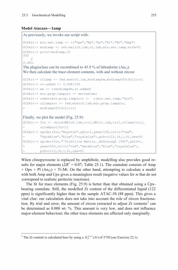
Model Atacazo—1ampAs previously, we invoke our script with:
GCDkit-> min.set.1amp <- c("Opx","Ab","An","Rt","Mt","Amp")
GCDkit-> mod1amp <- rev.maj(c0.lab,cL.lab,min.set.1amp,norm=T)
GCDkit-> print(mod1amp,3) $ff F 0.483… The plagioclase can be recombined to 45.9 % of labradorite (An52).We then calculate the trace-element contents, with and without zircon:
GCDkit-> cL1amp <- fwd.mod(c0.lab,mod1amp$m,mod1amp$ff)$cL[trc]
GCDkit-> zr.added <- 0.008/100
GCDkit-> ee <- c(mod1amp$m,zr.added)
GCDkit-> min.prop.1ampzrc <- ee/sum(ee)
GCDkit-> names(min.prop.1ampzrc) <- c(min.set.1amp,"Zrn")
GCDkit-> cL1ampzrc <- fwd.mod(c0.lab,min.prop.1ampzrc,
+ mod1amp$ff)$cL[trc]
Finally, we plot the model (Fig. 25.9):GCDkit-> foo <- rbind(WR[c0.lab,trc],WR[cL.lab,trc],cL1amp[trc],
+ cL1ampzrc[trc])
GCDkit-> spider(foo,"Boynton",ymin=1,ymax=100,col=c("red",
+ "darkblue","blue","royalblue"),pch=c(15,16,1,6),new=F)
GCDkit-> spider(foo,"^Primitive Mantle..McDonough 1995",ymin=1,
+ ymax=500,col=c("red","darkblue","blue","royalblue"),
+ pch=c(15,16,1,6),new=F)
When clinopyroxene is replaced by amphibole, modelling also provides good re-sults for major elements ( R2 = 0.07; Table 25.1). The cumulate consists of Amp + Opx + Pl (An52) + Ti-Mt. On the other hand, attempting to calculate a model with both Amp and Cpx gives a meaningless result (negative values for m
The fit for trace elements (Fig. 25.9) is better than that obtained using a Cpx-bearing cumulate. Still, the modelled Zr content of the differentiated liquid (122 ppm) is significantly higher than in the sample ATAC-58 (88 ppm). This gives a vital clue: our calculation does not take into account the role of zircon fractiona-tion. By trial and error, the amount of zircon extracted to adjust Zr contents3 can be determined as 0.008 wt. %. This amount is very low, and does not influence major-element behaviour; the other trace elements are affected only marginally.
3 The Zr content is calculated here by using a / ( )Zrn L
D ZrK of 3750 (see Exercise 22.1).
25525.3 Geochemical Modelling
that do notcorrespond to realistic peritectic reactions).
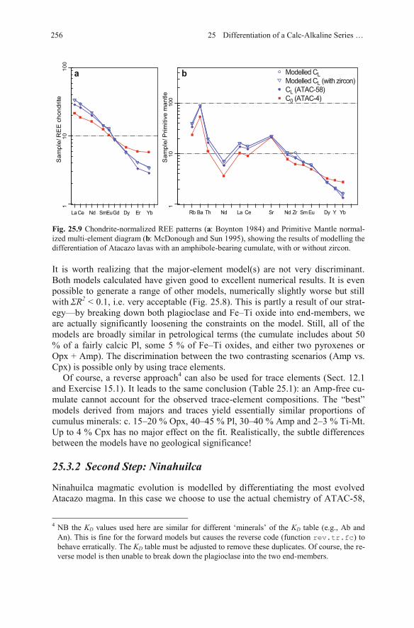
Fig. 25.9 Chondrite-normalized REE patterns (a: Boynton 1984) and Primitive Mantle normal-ized multi-element diagram (b: McDonough and Sun 1995), showing the results of modelling the differentiation of Atacazo lavas with an amphibole-bearing cumulate, with or without zircon.
It is worth realizing that the major-element model(s) are not very discriminant. Both models calculated have given good to excellent numerical results. It is even possible to generate a range of other models, numerically slightly worse but still with R2 < 0.1, i.e. very acceptable (Fig. 25.8). This is partly a result of our strat-egy—by breaking down both plagioclase and Fe–Ti oxide into end-members, we are actually significantly loosening the constraints on the model. Still, all of the models are broadly similar in petrological terms (the cumulate includes about 50 % of a fairly calcic Pl, some 5 % of Fe–Ti oxides, and either two pyroxenes or Opx + Amp). The discrimination between the two contrasting scenarios (Amp vs. Cpx) is possible only by using trace elements.
Of course, a reverse approach4 can also be used for trace elements (Sect. 12.1 and Exercise 15.1). It leads to the same conclusion (Table 25.1): an Amp-free cu-mulate cannot account for the observed trace-element compositions. The “best” models derived from majors and traces yield essentially similar proportions of cumulus minerals: c. 15–20 % Opx, 40–45 % Pl, 30–40 % Amp and 2–3 % Ti-Mt. Up to 4 % Cpx has no major effect on the fit. Realistically, the subtle differences between the models have no geological significance!
25.3.2 Second Step: Ninahuilca
Ninahuilca magmatic evolution is modelled by differentiating the most evolved Atacazo magma. In this case we choose to use the actual chemistry of ATAC-58,
4 NB the KD values used here are similar for different ‘minerals’ of the KD table (e.g., Ab and
An). This is fine for the forward models but causes the reverse code (function rev.tr.fc) to behave erratically. The KD table must be adjusted to remove these duplicates. Of course, the re-verse model is then unable to break down the plagioclase into the two end-members.
Rb Ba Th Nd La Ce Sr Nd Zr Sm Eu Dy Y Yb
110
100
Sam
ple/
Prim
itive
man
tle
La Ce Nd SmEuGd Dy Er Yb
110
100
Sam
ple/
RE
E c
hond
rite
Modelled CLModelled CL (with zircon)CL (ATAC-58)C0 (ATAC-4)
a b
256 25 Differentiation of a Calc-Alkaline Series …
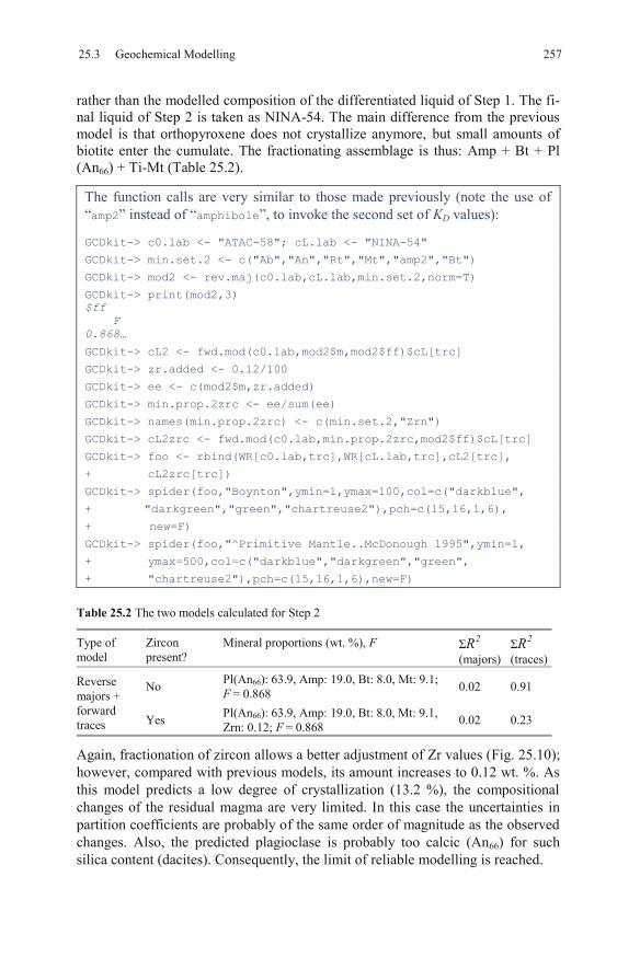
rather than the modelled composition of the differentiated liquid of Step 1. The fi-nal liquid of Step 2 is taken as NINA-54. The main difference from the previous model is that orthopyroxene does not crystallize anymore, but small amounts of biotite enter the cumulate. The fractionating assemblage is thus: Amp + Bt + Pl (An66) + Ti-Mt (Table 25.2).
The function calls are very similar to those made previously (note the use of “amp2” instead of “amphibole”, to invoke the second set of KD values):
GCDkit-> c0.lab <- "ATAC-58"; cL.lab <- "NINA-54"
GCDkit-> min.set.2 <- c("Ab","An","Rt","Mt","amp2","Bt")
GCDkit-> mod2 <- rev.maj(c0.lab,cL.lab,min.set.2,norm=T)
GCDkit-> print(mod2,3) $ff F 0.868… GCDkit-> cL2 <- fwd.mod(c0.lab,mod2$m,mod2$ff)$cL[trc]
GCDkit-> zr.added <- 0.12/100
GCDkit-> ee <- c(mod2$m,zr.added)
GCDkit-> min.prop.2zrc <- ee/sum(ee)
GCDkit-> names(min.prop.2zrc) <- c(min.set.2,"Zrn")
GCDkit-> cL2zrc <- fwd.mod(c0.lab,min.prop.2zrc,mod2$ff)$cL[trc]
GCDkit-> foo <- rbind(WR[c0.lab,trc],WR[cL.lab,trc],cL2[trc],
+ cL2zrc[trc])
GCDkit-> spider(foo,"Boynton",ymin=1,ymax=100,col=c("darkblue",
+ "darkgreen","green","chartreuse2"),pch=c(15,16,1,6), + new=F) GCDkit-> spider(foo,"^Primitive Mantle..McDonough 1995",ymin=1,
+ ymax=500,col=c("darkblue","darkgreen","green",
+ "chartreuse2"),pch=c(15,16,1,6),new=F)
Table 25.2 The two models calculated for Step 2
Type of model
Zirconpresent?
Mineral proportions (wt. %), F R2
(majors)R2
(traces)
Reverse majors + forward traces
No Pl(An66): 63.9, Amp: 19.0, Bt: 8.0, Mt: 9.1; F = 0.868 0.02 0.91
Yes Pl(An66): 63.9, Amp: 19.0, Bt: 8.0, Mt: 9.1, Zrn: 0.12; F = 0.868 0.02 0.23
Again, fractionation of zircon allows a better adjustment of Zr values (Fig. 25.10); however, compared with previous models, its amount increases to 0.12 wt. %. As this model predicts a low degree of crystallization (13.2 %), the compositional changes of the residual magma are very limited. In this case the uncertainties inpartition coefficients are probably of the same order of magnitude as the observed changes. Also, the predicted plagioclase is probably too calcic (An66) for such silica content (dacites). Consequently, the limit of reliable modelling is reached.
25725.3 Geochemical Modelling
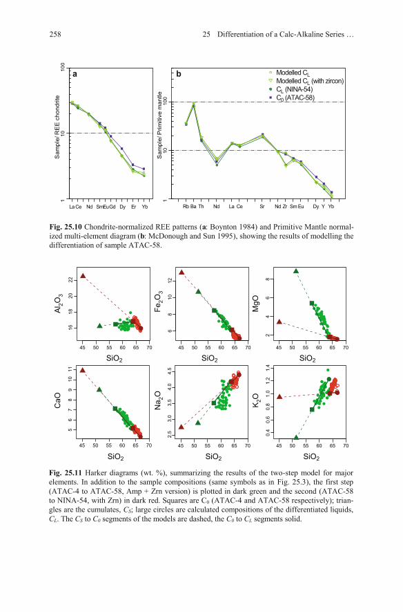
Fig. 25.10 Chondrite-normalized REE patterns (a: Boynton 1984) and Primitive Mantle normal-ized multi-element diagram (b: McDonough and Sun 1995), showing the results of modelling the differentiation of sample ATAC-58.
Rb Ba Th Nd La Ce Sr Nd Zr Sm Eu Dy Y Yb
110
100
Sam
ple/
Prim
itive
man
tle
La Ce Nd SmEuGd Dy Er Yb
110
100
Sam
ple/
RE
E c
hond
rite
Modelled CLModelled CL (with zircon)CL (NINA-54)C0 (ATAC-58)
a b
258 25 Differentiation of a Calc-Alkaline Series …
Fig. 25.11 Harker diagrams (wt. %), summarizing the results of the two-step model for major elements. In addition to the sample compositions (same symbols as in Fig. 25.3), the first step (ATAC-4 to ATAC-58, Amp + Zrn version) is plotted in dark green and the second (ATAC-58 to NINA-54, with Zrn) in dark red. Squares are C0 (ATAC-4 and ATAC-58 respectively); trian-gles are the cumulates, CS; large circles are calculated compositions of the differentiated liquids, CL. The CS to C0 segments of the models are dashed, the C0 to CL segments solid.
Al 2O
3
Fe2O
3
MgO
CaO
Na 2
O
K2O
SiO2 SiO2 SiO2
SiO2SiO2 SiO2
45 50 55 60 65 70
68
1012
45 50 55 60 65 70
24
68
45 50 55 60 65 70
56
78
910
11
45 50 55 60 65 70
2.5
3.0
3.5
4.0
4.5
45 50 55 60 65 70
0.4
0.6
0.8
1.0
1.2
1.4
45 50 55 60 65 70
1618
2022
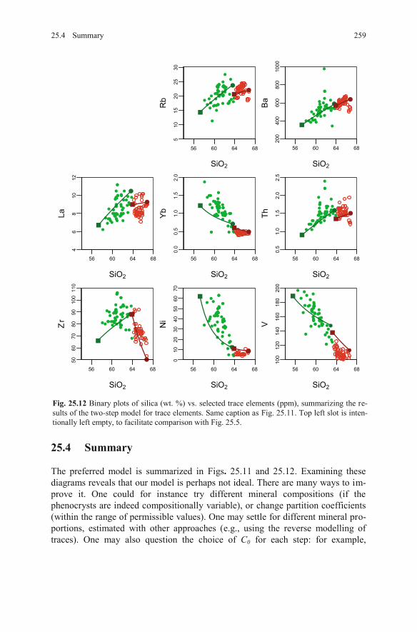
25.4 Summary 259
Fig. 25.12 Binary plots of silica (wt. %) vs. selected trace elements (ppm), summarizing the re-sults of the two-step model for trace elements. Same caption as Fig. 25.11. Top left slot is inten-tionally left empty, to facilitate comparison with Fig. 25.5.
56 60 64 68
510
1520
2530
56 60 64 68
200
400
600
800
1000
56 60 64 68
46
810
12
56 60 64 68
0.0
0.5
1.0
1.5
2.0
56 60 64 68
0.5
1.0
1.5
2.0
2.5
56 60 64 68
5060
7080
9010
011
0
56 60 64 68
010
2030
4050
6070
56 60 64 68
100
120
140
160
180
200
SiO2R
bSiO2
Ba
SiO2
La
SiO2
Yb
SiO2
Th
SiO2
Zr
SiO2
Ni
SiO2
V
25.4 Summary
The preferred model is summarized in Figs. 25.11 and 25.12. Examining these diagrams reveals that our model is perhaps not ideal. There are many ways to im-prove it. One could for instance try different mineral compositions (if the phenocrysts are indeed compositionally variable), or change partition coefficients (within the range of permissible values). One may settle for different mineral pro-portions, estimated with other approaches (e.g., using the reverse modelling of traces). One may also question the choice of C0 for each step: for example,
260 25 Differentiation of a Calc-Alkaline Series …
References
Boynton WV (1984) Geochemistry of the rare-earth elements: meteorite studies. In: Henderson P (ed) Rare Earth Element geochemistry. Elsevier, Amsterdam, pp 63–114
Gutscher MA, Malavieille J, Lallemand S, Collot J-Y (1999) Tectonic segmentation of the North Andean margin: impact of the Carnegie Ridge collision. Earth Planet Sci Lett 168:255–270
Hidalgo S (2006) Les interactions entre magmas calco-alcalins “classiques” et adakitiques: exemple du complexe volcanique Atacazo-Ninahuilca (Equateur). Unpublished PhD. thesis, Université Blaise-Pascal, Clermont-Ferrand
Hidalgo S, Gerbe MC, Martin H, Samaniego P, Bourdon E (2012) Role of crustal and slab com-ponents in the Northern Volcanic Zone of the Andes (Ecuador) constrained by Sr–Nd–O iso-topes. Lithos 132:180–192
McDonough WF, Sun SS (1995) The composition of the Earth. Chem Geol 120:223–253Rollinson HR (1993) Using geochemical data: evaluation, presentation, interpretation. Longman,
London
ATAC-4 has the lowest SiO2, but is out of the main trend for Zr and Yb. Finally, one could also build the model for the second stage using as a primitive magma, C0(2), the outcome of the first step (CL(1)) rather than an existing composition. The tools provided here will allow the critical readers to investigate these options, and many more, for themselves!
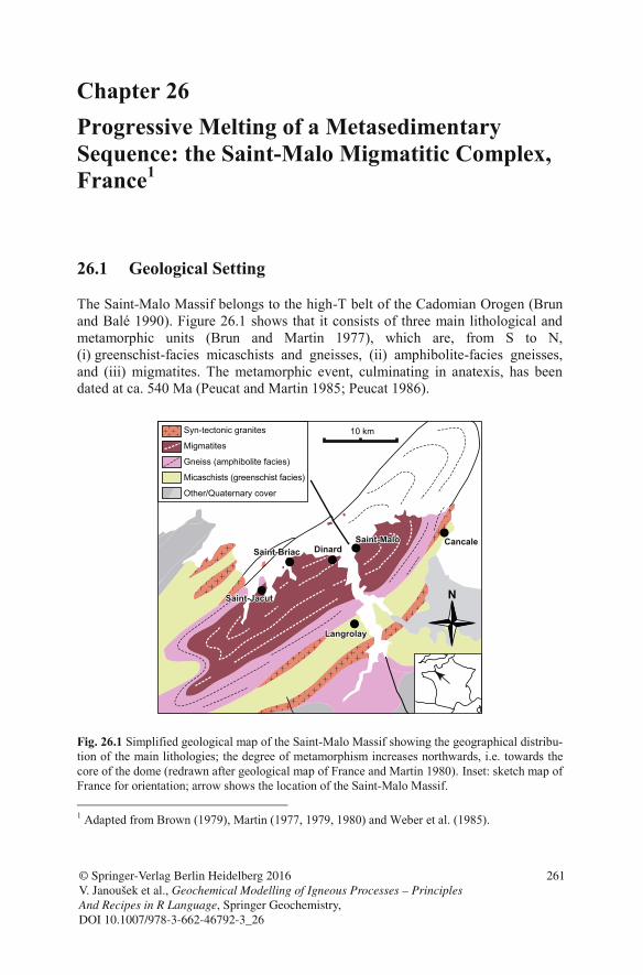
Chapter 26 Progressive Melting of a Metasedimentary Sequence: the Saint-Malo Migmatitic Complex, France 1
26.1 Geological Setting
The Saint-Malo Massif belongs to the high-T belt of the Cadomian Orogen (Brun and Balé 1990). Figure 26.1 shows that it consists of three main lithological and metamorphic units (Brun and Martin 1977), which are, from S to N, (i) greenschist-facies micaschists and gneisses, (ii) amphibolite-facies gneisses, and (iii) migmatites. The metamorphic event, culminating in anatexis, has been dated at ca. 540 Ma (Peucat and Martin 1985; Peucat 1986).
Fig. 26.1 Simplified geological map of the Saint-Malo Massif showing the geographical distribu-tion of the main lithologies; the degree of metamorphism increases northwards, i.e. towards the core of the dome (redrawn after geological map of France and Martin 1980). Inset: sketch map of France for orientation; arrow shows the location of the Saint-Malo Massif. Adapted from Brown (1 1979), Martin (1977, 1979, 1980) and Weber et al. (1985).
Syn-tectonic granites
Migmatites
Gneiss (amphibolite facies)
Micaschists (greenschist facies)
Other/Quaternary cover
10 km
Saint-MaloSaint-MaloSaint-MaloDinardDinardDinardSaint-BriacSaint-BriacSaint-Briac
Saint-JacutSaint-JacutSaint-Jacut
CancaleCancaleCancale
LangrolayLangrolayLangrolay
N
© Springer-Verlag Berlin Heidelberg 2016 V. Janoušek et al., Geochemical Modelling of Igneous Processes – Principles And Recipes in R Language, Springer Geochemistry, DOI 10.1007/978-3-662-46792-3_26
261
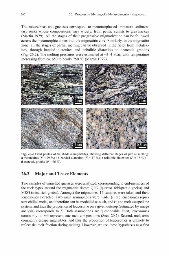
The micaschists and gneisses correspond to metamorphosed immature sedimen-tary rocks whose compositions vary widely, from pelitic schists to graywackes (Martin 1979). All the stages of their progressive migmatization can be followed across the metamorphic zones into the migmatitic core. Similarly, in the migmatite zone, all the stages of partial melting can be observed in the field, from metatex-ites, through banded diatexites and nebulitic diatexites to anatectic granites (Fig. 26.2). The melting pressures were estimated at ~3–4 kbar, with temperature increasing from ca. 650 to nearly 750 °C (Martin 1979).
Fig. 26.2 Field photos of Saint-Malo migmatites, showing different stages of partial melting: a metatexites (F 29 %) ; b banded diatexites (F 47 %); c nebulitic diatexites (F 76 %);d anatectic granite (F 96 %).
26.2 Major and Trace Elements
Two samples of unmelted gneisses were analyzed, corresponding to end-members of the rock types around the migmatitic dome: QFG (quartzo–feldspathic gneiss) and MRG (mica-rich gneiss). Amongst the migmatites, 17 samples were taken and their leucosomes extracted. Two main assumptions were made: (i) the leucosomes repre-sent chilled melts, and therefore can be modelled as such, and (ii) no melt escaped the system, and thus the proportion of leucosome on a given outcrop (estimated by image analysis) corresponds to F. Both assumptions are questionable. First, leucosomes commonly do not represent true melt compositions (Sect. 20.2). Second, melt doescommonly escape migmatites, and thus the proportion of leucosomes is unlikely to reflect the melt fraction during melting. However, we use these hypotheses as a first
a b
c d
2 cm 2 cm
5 cm 0.5 cm
262 26 Progressive Melting of a Metasedimentary Sequence …
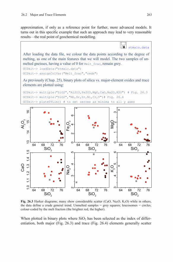
approximation, if only as a reference point for further, more advanced models. It turns out in this specific example that such an approach may lead to very reasonable results—the real point of geochemical modelling.
stmalo.data
After loading the data file, we colour the data points according to the degree of melting, as one of the main features that we will model. The two samples of un-melted gneisses, having a value of 0 for Melt_frac, remain grey.GCDkit-> loadData("stmalo.data")
GCDkit-> assignColVar("Melt_frac","reds")
As previously (Chap. 25), binary plots of silica vs. major-element oxides and trace elements are plotted using:
GCDkit-> multiple("SiO2","Al2O3,Fe2O3,MgO,CaO,Na2O,K2O") # Fig. 26.3
GCDkit-> multiple("SiO2","Rb,Sr,Zr,Ni,Cr,V")# Fig. 26.4
GCDkit-> plate0YLim() # to set zeroes as minima to all y axes
Fig. 26.3 Harker diagrams; many show considerable scatter (CaO, Na2O, K2O) while in others, the data define a crude general trend. Unmelted samples = grey squares; leucosomes = circles, colour-coded by the melt fraction (the brighter red, the higher).
When plotted in binary plots where SiO2 has been selected as the index of differ-entiation, both major (Fig. 26.3) and trace (Fig. 26.4) elements generally scatter
●●
●●
●
●
●
●●
●●
●
●
●●●●
●●●●● ●●●●
●●●
●●
●●●
●●●●● ●●
●
●●●●
●●●●●
●
●
●
●●
●
●●
●
●
●
●
●
●
●●●
●
●●
●
● ●●●
●
●●
●●●
●●●
●●
●●●
●●
●●
●●●●●●●●
SiO2
Al 2O
3
MgO
CaO
Na 2O
K2O
64 68 72 76SiO2
64 68 72 76
SiO2
64 68 72 76SiO2
64 68 72 76
SiO2
64 68 72 76
SiO2
64 68 72 76
1314
1516
1.1
1.0
1.2
1.3
1.4
1.5
02
46
23
45
01
23
34
56
Fe2O
3
26.2 Major and Trace Elements 263
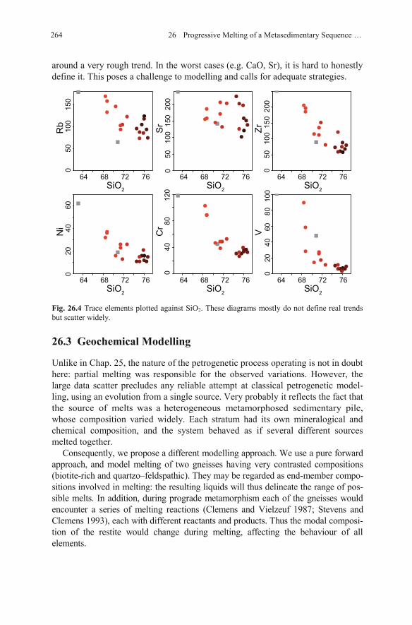
around a very rough trend. In the worst cases (e.g. CaO, Sr), it is hard to honestly define it. This poses a challenge to modelling and calls for adequate strategies.
Fig. 26.4 Trace elements plotted against SiO2. These diagrams mostly do not define real trends but scatter widely.
26.3 Geochemical Modelling
Unlike in Chap. 25, the nature of the petrogenetic process operating is not in doubt here: partial melting was responsible for the observed variations. However, the large data scatter precludes any reliable attempt at classical petrogenetic model-ling, using an evolution from a single source. Very probably it reflects the fact that the source of melts was a heterogeneous metamorphosed sedimentary pile, whose composition varied widely. Each stratum had its own mineralogical and chemical composition, and the system behaved as if several different sources melted together.
Consequently, we propose a different modelling approach. We use a pure forward approach, and model melting of two gneisses having very contrasted compositions (biotite-rich and quartzo–feldspathic). They may be regarded as end-member compo-sitions involved in melting: the resulting liquids will thus delineate the range of pos-sible melts. In addition, during prograde metamorphism each of the gneisses would encounter a series of melting reactions (Clemens and Vielzeuf 1987; Stevens and Clemens 1993), each with different reactants and products. Thus the modal composi-tion of the restite would change during melting, affecting the behaviour of all elements.
●●
●
●●
●●●●
●●
●●
●●
●
●
●●
●●
●
●
●●
●●
●●
●●
●●
●
●●●●
● ●●●
●●
●
●●●
●●●
●●●●●●
●
●●●
●●●
●
●●●
●●
●●● ●●●
●
●●●●●
●●●
●●●●● ●●●●
●●
●●●
●
●
●
Rb
Sr Zr
Ni
Cr V
SiO2
64 68 72 76
SiO2
64 68 72 76
SiO2
64 68 72 76SiO2
64 68 72 76
SiO2
64 68 72 76SiO2
64 68 72 76
050
100
150
020
4060
040
8012
0
040
8010
020
60
010
020
050
150
010
020
050
150
264 26 Progressive Melting of a Metasedimentary Sequence …
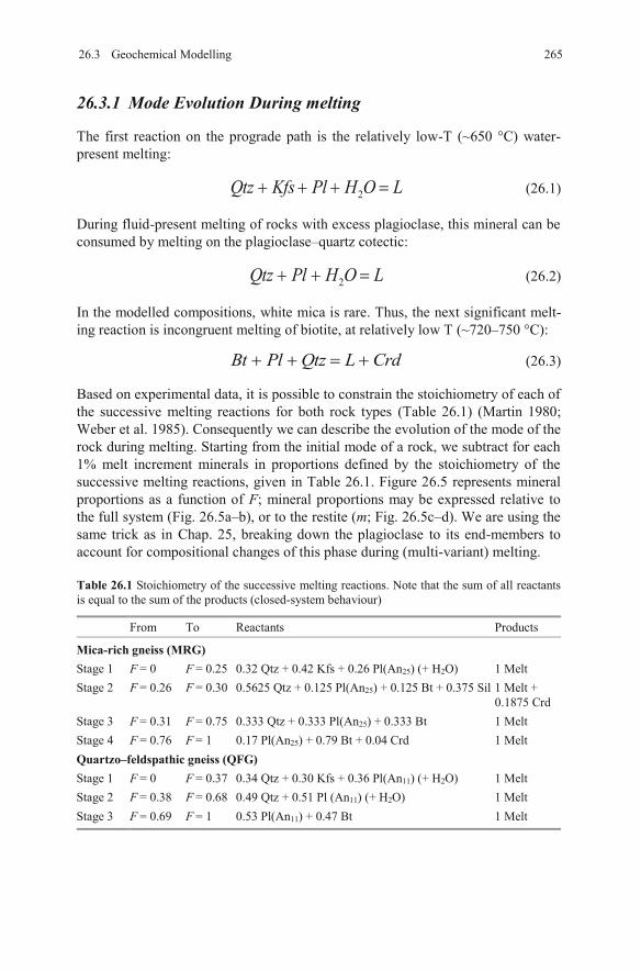
26.3.1 Mode Evolution During melting
The first reaction on the prograde path is the relatively low-T (~650 °C) water-present melting:
2Qtz Kfs P Ol LH (26.1)
During fluid-present melting of rocks with excess plagioclase, this mineral can be consumed by melting on the plagioclase–quartz cotectic:
2Qtz Pl LH O (26.2)
In the modelled compositions, white mica is rare. Thus, the next significant melt-ing reaction is incongruent melting of biotite, at relatively low T (~720–750 °C):
Bt Pl Qtz L Crd (26.3)
Based on experimental data, it is possible to constrain the stoichiometry of each of the successive melting reactions for both rock types (Table 26.1) (Martin 1980;Weber et al. 1985). Consequently we can describe the evolution of the mode of the rock during melting. Starting from the initial mode of a rock, we subtract for each 1% melt increment minerals in proportions defined by the stoichiometry of the successive melting reactions, given in Table 26.1. Figure 26.5 represents mineral proportions as a function of F; mineral proportions may be expressed relative to the full system (Fig. 26.5a–b), or to the restite (m; Fig. 26.5c–d). We are using the same trick as in Chap. 25, breaking down the plagioclase to its end-members to account for compositional changes of this phase during (multi-variant) melting.
Table 26.1 Stoichiometry of the successive melting reactions. Note that the sum of all reactants is equal to the sum of the products (closed-system behaviour)
From To Reactants Products
Mica-rich gneiss (MRG)Stage 1 F = 0 F = 0.25 0.32 Qtz + 0.42 Kfs + 0.26 Pl(An25) (+ H2O) 1 MeltStage 2 F = 0.26 F = 0.30 0.5625 Qtz + 0.125 Pl(An25) + 0.125 Bt + 0.375 Sil 1 Melt +
0.1875 CrdStage 3 F = 0.31 F = 0.75 0.333 Qtz + 0.333 Pl(An25) + 0.333 Bt 1 MeltStage 4 F = 0.76 F = 1 0.17 Pl(An25) + 0.79 Bt + 0.04 Crd 1 MeltQuartzo–feldspathic gneiss (QFG)Stage 1 F = 0 F = 0.37 0.34 Qtz + 0.30 Kfs + 0.36 Pl(An11) (+ H2O) 1 MeltStage 2 F = 0.38 F = 0.68 0.49 Qtz + 0.51 Pl (An11) (+ H2O) 1 MeltStage 3 F = 0.69 F = 1 0.53 Pl(An11) + 0.47 Bt 1 Melt
26.3 Geochemical Modelling 265
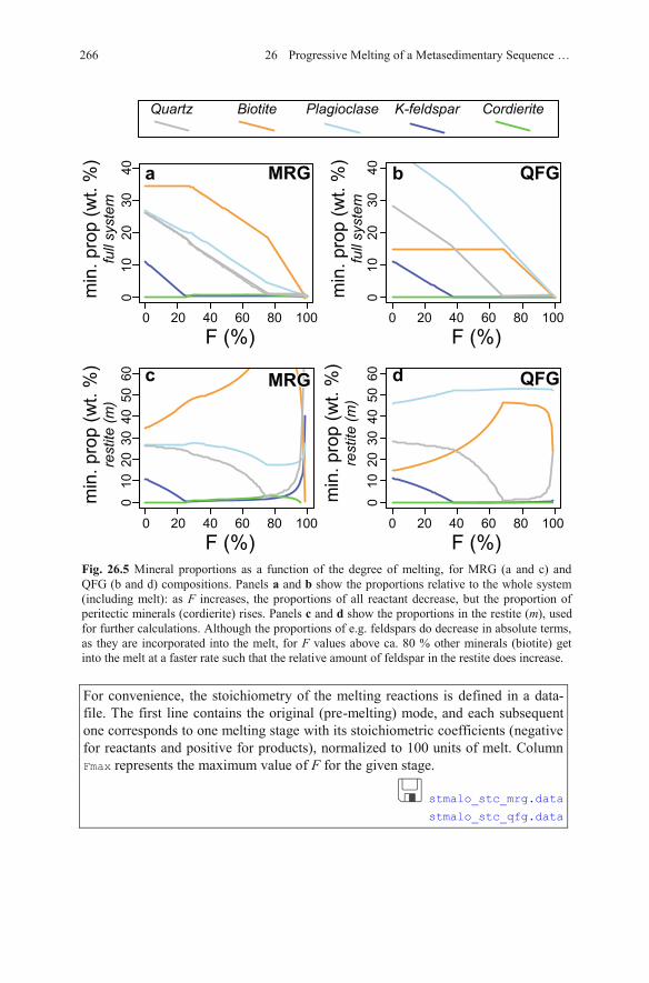
Fig. 26.5 Mineral proportions as a function of the degree of melting, for MRG (a and c) and QFG (b and d) compositions. Panels a and b show the proportions relative to the whole system (including melt): as F increases, the proportions of all reactant decrease, but the proportion of peritectic minerals (cordierite) rises. Panels c and d show the proportions in the restite (m), used for further calculations. Although the proportions of e.g. feldspars do decrease in absolute terms, as they are incorporated into the melt, for F values above ca. 80 % other minerals (biotite) get into the melt at a faster rate such that the relative amount of feldspar in the restite does increase.
For convenience, the stoichiometry of the melting reactions is defined in a data-file. The first line contains the original (pre-melting) mode, and each subsequent one corresponds to one melting stage with its stoichiometric coefficients (negative for reactants and positive for products), normalized to 100 units of melt. Column Fmax represents the maximum value of F for the given stage.
stmalo_stc_mrg.data stmalo_stc_qfg.data
266 26 Progressive Melting of a Metasedimentary Sequence …
Biotite Plagioclase K-feldspar Cordierite
F (%)0 20 40 60 80 100
F (%)0 20 40 60 80 100
F (%)0 20 40 60 80 100
F (%)0 20 40 60 80 100
min
. p
rop
(w
t. %
)full system
min
. p
rop
(w
t. %
)restite
(m)
min
. p
rop
(w
t. %
)full system
min
. p
rop
(w
t. %
)restite
(m)
a b
c d
QFGMRG
QFG1
02
03
04
00
10
20
30
40
0
10
20
30
40
50
60
0
10
20
30
40
50
60
0
Quartz
MRGMRGMRG
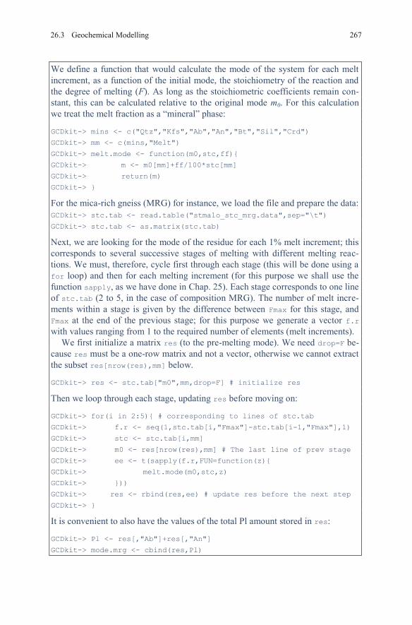
We define a function that would calculate the mode of the system for each melt increment, as a function of the initial mode, the stoichiometry of the reaction and the degree of melting (F). As long as the stoichiometric coefficients remain con-stant, this can be calculated relative to the original mode m0. For this calculation we treat the melt fraction as a “mineral” phase:
GCDkit-> mins <- c("Qtz","Kfs","Ab","An","Bt","Sil","Crd")
GCDkit-> mm <- c(mins,"Melt")
GCDkit-> melt.mode <- function(m0,stc,ff){
GCDkit-> m <- m0[mm]+ff/100*stc[mm]
GCDkit-> return(m)
GCDkit-> }
For the mica-rich gneiss (MRG) for instance, we load the file and prepare the data: GCDkit-> stc.tab <- read.table("stmalo_stc_mrg.data",sep="\t")
GCDkit-> stc.tab <- as.matrix(stc.tab)
Next, we are looking for the mode of the residue for each 1% melt increment; this corresponds to several successive stages of melting with different melting reac-tions. We must, therefore, cycle first through each stage (this will be done using a for loop) and then for each melting increment (for this purpose we shall use the function sapply, as we have done in Chap. 25). Each stage corresponds to one line of stc.tab (2 to 5, in the case of composition MRG). The number of melt incre-ments within a stage is given by the difference between Fmax for this stage, and Fmax at the end of the previous stage; for this purpose we generate a vector f.rwith values ranging from 1 to the required number of elements (melt increments).
We first initialize a matrix res (to the pre-melting mode). We need drop=F be-cause res must be a one-row matrix and not a vector, otherwise we cannot extract the subset res[nrow(res),mm] below.
GCDkit-> res <- stc.tab["m0",mm,drop=F] # initialize res
Then we loop through each stage, updating res before moving on:
GCDkit-> for(i in 2:5){ # corresponding to lines of stc.tab
GCDkit-> f.r <- seq(1,stc.tab[i,"Fmax"]-stc.tab[i-1,"Fmax"],1)
GCDkit-> stc <- stc.tab[i,mm]
GCDkit-> m0 <- res[nrow(res),mm] # The last line of prev stage
GCDkit-> ee <- t(sapply(f.r,FUN=function(z){
GCDkit-> melt.mode(m0,stc,z)
GCDkit-> }))
GCDkit-> res <- rbind(res,ee) # update res before the next step
GCDkit-> }
It is convenient to also have the values of the total Pl amount stored in res:
GCDkit-> Pl <- res[,"Ab"]+res[,"An"]
GCDkit-> mode.mrg <- cbind(res,Pl)
26726.3 Geochemical Modelling
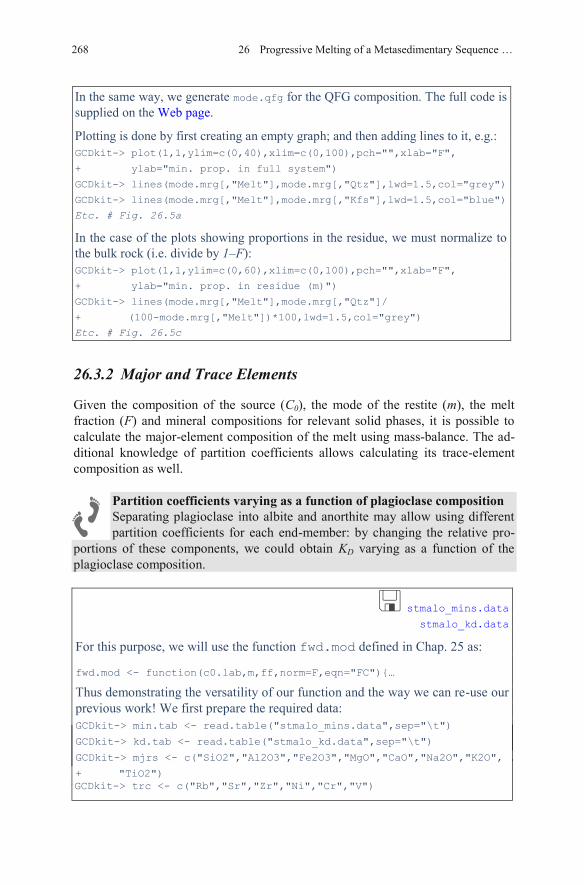
In the same way, we generate mode.qfg for the QFG composition. The full code is supplied on the Web page.
Plotting is done by first creating an empty graph; and then adding lines to it, e.g.: GCDkit-> plot(1,1,ylim=c(0,40),xlim=c(0,100),pch="",xlab="F",
+ ylab="min. prop. in full system")
GCDkit-> lines(mode.mrg[,"Melt"],mode.mrg[,"Qtz"],lwd=1.5,col="grey")
GCDkit-> lines(mode.mrg[,"Melt"],mode.mrg[,"Kfs"],lwd=1.5,col="blue")
Etc. # Fig. 26.5a
In the case of the plots showing proportions in the residue, we must normalize to the bulk rock (i.e. divide by 1–F):GCDkit-> plot(1,1,ylim=c(0,60),xlim=c(0,100),pch="",xlab="F",
+ ylab="min. prop. in residue (m)")
GCDkit-> lines(mode.mrg[,"Melt"],mode.mrg[,"Qtz"]/
+ (100-mode.mrg[,"Melt"])*100,lwd=1.5,col="grey") Etc. # Fig. 26.5c
26.3.2 Major and Trace Elements
Given the composition of the source (C0), the mode of the restite (m), the melt fraction (F) and mineral compositions for relevant solid phases, it is possible to calculate the major-element composition of the melt using mass-balance. The ad-ditional knowledge of partition coefficients allows calculating its trace-element composition as well.
Partition coefficients varying as a function of plagioclase compositionSeparating plagioclase into albite and anorthite may allow using different partition coefficients for each end-member: by changing the relative pro-
portions of these components, we could obtain KD varying as a function of the plagioclase composition.
stmalo_mins.data stmalo_kd.data
For this purpose, we will use the function fwd.mod defined in Chap. 25 as:
fwd.mod <- function(c0.lab,m,ff,norm=F,eqn="FC"){… Thus demonstrating the versatility of our function and the way we can re-use our previous work! We first prepare the required data: GCDkit-> min.tab <- read.table("stmalo_mins.data",sep="\t")
GCDkit-> kd.tab <- read.table("stmalo_kd.data",sep="\t")
GCDkit-> mjrs <- c("SiO2","Al2O3","Fe2O3","MgO","CaO","Na2O","K2O",
+ "TiO2")
268 26 Progressive Melting of a Metasedimentary Sequence …
GCDkit-> trc <- c("Rb","Sr","Zr","Ni","Cr","V")
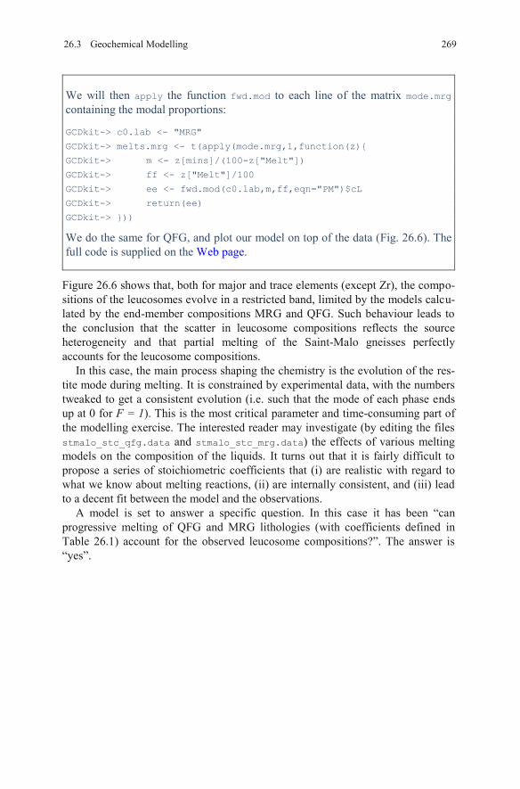
We will then apply the function fwd.mod to each line of the matrix mode.mrgcontaining the modal proportions:
GCDkit-> c0.lab <- "MRG"
GCDkit-> melts.mrg <- t(apply(mode.mrg,1,function(z){
GCDkit-> m <- z[mins]/(100-z["Melt"])
GCDkit-> ff <- z["Melt"]/100
GCDkit-> ee <- fwd.mod(c0.lab,m,ff,eqn="PM")$cL
GCDkit-> return(ee)
GCDkit-> }))
We do the same for QFG, and plot our model on top of the data (Fig. 26.6). The full code is supplied on the Web page.
Figure 26.6 shows that, both for major and trace elements (except Zr), the compo-sitions of the leucosomes evolve in a restricted band, limited by the models calcu-lated by the end-member compositions MRG and QFG. Such behaviour leads to the conclusion that the scatter in leucosome compositions reflects the source heterogeneity and that partial melting of the Saint-Malo gneisses perfectly accounts for the leucosome compositions.
In this case, the main process shaping the chemistry is the evolution of the res-tite mode during melting. It is constrained by experimental data, with the numbers tweaked to get a consistent evolution (i.e. such that the mode of each phase ends up at 0 for F = 1). This is the most critical parameter and time-consuming part of the modelling exercise. The interested reader may investigate (by editing the files stmalo_stc_qfg.data and stmalo_stc_mrg.data) the effects of various melting models on the composition of the liquids. It turns out that it is fairly difficult to propose a series of stoichiometric coefficients that (i) are realistic with regard to what we know about melting reactions, (ii) are internally consistent, and (iii) lead to a decent fit between the model and the observations.
A model is set to answer a specific question. In this case it has been “can progressive melting of QFG and MRG lithologies (with coefficients defined in Table 26.1) account for the observed leucosome compositions?”. The answer is “yes”.
26926.3 Geochemical Modelling
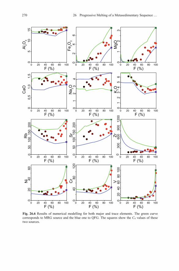
Fig. 26.6 Results of numerical modelling for both major and trace elements. The green curve corresponds to MRG source and the blue one to QFG. The squares show the C0 values of these two sources.
270 26 Progressive Melting of a Metasedimentary Sequence …
● ●●●●●
●●●
●●●●●●●●
● ●●●●● ●
●●
●●●●●
●●●
● ●●●●● ●
●
●●●●
●●●●●
●
●●●●● ●●●
●●
●
●●●●●
●
●●●
●● ●●●
●●●●●
●●
● ●●●
●● ●●●
●●●●●●●
Al 2O
3
MgO
CaO
Na 2O
K2O
F (%)0 20 40 60 80 100
F (%)0 20 40 60 80 100
F (%)0 20 40 60 80 100
F (%)0 20 40 60 80 100
F (%)0 20 40 60 80 100
F (%)0 20 40 60 80 100
05
1015
00.
51.
01.
5
02
34
1
02
13
45
60
23
1
02
46
Fe2O
3
●●●
●●●
●●●
●●
●●
●●
●
●
●●
●●
●
●
●●
● ●
●●
●●●●
●
● ●●●●● ●●● ●
●●●●●●●
● ●●●●
●●
●● ●
●●●
●
●●●
● ●●●●● ●●●
●●●●●
●●●
● ●●●●● ●●●
●●
●●●●
●
●
Rb Sr Zr
Ni
Cr
V
F (%)0 20 40 60 80 100
F (%)0 20 40 60 80 100
F (%)0 20 40 60 80 100
F (%)0 20 40 60 80 100
F (%)0 20 40 60 80 100
F (%)0 20 40 60 80 100
010
020
050
150
040
8010
020
60
040
8012
0
020
4060
060
012
0030
090
0
050
100
150
200
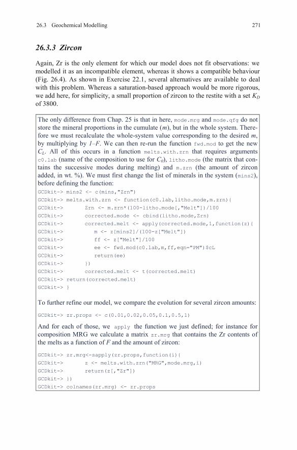
26.3.3 Zircon
Again, Zr is the only element for which our model does not fit observations: we modelled it as an incompatible element, whereas it shows a compatible behaviour (Fig. 26.4). As shown in Exercise 22.1, several alternatives are available to deal with this problem. Whereas a saturation-based approach would be more rigorous, we add here, for simplicity, a small proportion of zircon to the restite with a set KDof 3800.
The only difference from Chap. 25 is that in here, mode.mrg and mode.qfg do not store the mineral proportions in the cumulate (m), but in the whole system. There-fore we must recalculate the whole-system value corresponding to the desired m,by multiplying by 1–F. We can then re-run the function fwd.mod to get the new CL. All of this occurs in a function melts.with.zrn that requires arguments c0.lab (name of the composition to use for C0), litho.mode (the matrix that con-tains the successive modes during melting) and m.zrn (the amount of zircon added, in wt. %). We must first change the list of minerals in the system (mins2), before defining the function:GCDkit-> mins2 <- c(mins,"Zrn")
GCDkit-> melts.with.zrn <- function(c0.lab,litho.mode,m.zrn){
GCDkit-> Zrn <- m.zrn*(100-litho.mode[,"Melt"])/100
GCDkit-> corrected.mode <- cbind(litho.mode,Zrn)
GCDkit-> corrected.melt <- apply(corrected.mode,1,function(z){
GCDkit-> m <- z[mins2]/(100-z["Melt"])
GCDkit-> ff <- z["Melt"]/100
GCDkit-> ee <- fwd.mod(c0.lab,m,ff,eqn="PM")$cL
GCDkit-> return(ee)
GCDkit-> })
GCDkit-> corrected.melt <- t(corrected.melt)
GCDkit-> return(corrected.melt)
GCDkit-> }
To further refine our model, we compare the evolution for several zircon amounts:
GCDkit-> zr.props <- c(0.01,0.02,0.05,0.1,0.5,1)
And for each of those, we apply the function we just defined; for instance for composition MRG we calculate a matrix zr.mrg that contains the Zr contents of the melts as a function of F and the amount of zircon:
GCDkit-> zr.mrg<-sapply(zr.props,function(i){
GCDkit-> z <- melts.with.zrn("MRG",mode.mrg,i)
GCDkit-> return(z[,"Zr"])
GCDkit-> })
GCDkit-> colnames(zr.mrg) <- zr.props
27126.3 Geochemical Modelling
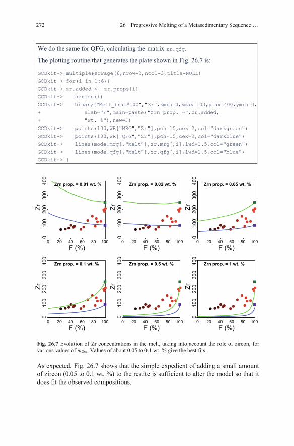
We do the same for QFG, calculating the matrix zr.qfg.
The plotting routine that generates the plate shown in Fig. 26.7 is:
GCDkit-> multiplePerPage(6,nrow=2,ncol=3,title=NULL)
GCDkit-> for(i in 1:6){
GCDkit-> zr.added <- zr.props[i]
GCDkit-> screen(i)
GCDkit-> binary("Melt_frac*100","Zr",xmin=0,xmax=100,ymax=400,ymin=0,
+ xlab="F",main=paste("Zrn prop. =",zr.added,
+ "wt. %"),new=F)
GCDkit-> points(100,WR["MRG","Zr"],pch=15,cex=2,col="darkgreen")
GCDkit-> points(100,WR["QFG","Zr"],pch=15,cex=2,col="darkblue")
GCDkit-> lines(mode.mrg[,"Melt"],zr.mrg[,i],lwd=1.5,col="green")
GCDkit-> lines(mode.qfg[,"Melt"],zr.qfg[,i],lwd=1.5,col="blue")
GCDkit-> }
Fig. 26.7 Evolution of Zr concentrations in the melt, taking into account the role of zircon, for various values of mZrn. Values of about 0.05 to 0.1 wt. % give the best fits.
As expected, Fig. 26.7 shows that the simple expedient of adding a small amount of zircon (0.05 to 0.1 wt. %) to the restite is sufficient to alter the model so that it does fit the observed compositions.
● ●●●●● ●●
●●
●
●●●
●●●
● ●●●●● ●●
●●
●
●●●
●●●
● ●●●●● ●●
●●
●
●●●
●●●
● ●●●●● ●●
●●
●
●●●
●●●
● ●●●●● ●●
●●
●
●●●
●●●
● ●●●●● ●●
●●
●
●●●
●●●
Zr Zr Zr
Zr Zr Zr
F (%)0 20 40 60 80 100
F (%)0 20 40 60 80 100
F (%)0 20 40 60 80 100
F (%)0 20 40 60 80 100
F (%)0 20 40 60 80 100
F (%)0 20 40 60 80 100
Zrn prop. = 0.05 wt. %Zrn prop. = 0.02 wt. %Zrn prop. = 0.01 wt. %Zrn prop. = 0.01 wt. %Zrn prop. = 0.01 wt. %Zrn prop. = 0.01 wt. %
Zrn prop. = 1 wt. %Zrn prop. = 0.5 wt. %Zrn prop. = 0.1 wt. %
020
040
010
030
00
200
400
100
300
020
040
010
030
00
200
400
100
300
020
040
010
030
00
200
400
100
300
272 26 Progressive Melting of a Metasedimentary Sequence …
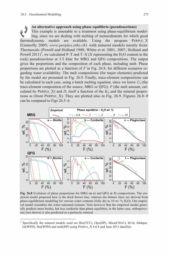
An alternative approach using phase equilibria (pseudosections) This example is amenable to a treatment using phase-equilibrium model-ling, since we are dealing with melting of metasediments for which good
thermodynamic models are available. Using the program PERPLE_X ( www.perplex.ethz.ch) with mineral models mostly from
Powell 2011) , we calculated P–T and T–X (X representing the H2O content in the rock) pseudosections at 3.5 kbar for MRG and QFG compositions. The output gives the proportions and the composition of each phase, including melt. Phase proportions are plotted as a function of F in Fig. 26.8, for different scenarios re-garding water availability. The melt compositions (for major elements) predicted by the model are presented in Fig. 26.9. Finally, trace-element compositions can be calculated in each case, using a batch melting equation, since we know C0 (the trace-element composition of the source, MRG or QFG); F (the melt amount, cal-culated by PERPLE_X) and D, itself a function of the KD and the mineral propor-tions m (from PERPLE_X). They are plotted also in Fig. 26.9. Figures 26.8–9
–6.
2
Fig. 26.8 Evolution of phase proportions for MRG (a–c) and QFG (e–f) compositions. The em-pirical model proposed here is the thick brown line, whereas the thinner lines are derived from phase-equilibrium modelling for various water contents (fully dry to 10 wt. % H2O). Our empiri-cal model resembles the water-saturated systems. Note however that the empirical model gener-ally predicts more biotite, but less cordierite than phase equilibria; in the latter case, orthopyrox-ene (not shown) is also predicted as a peritectic mineral.
Specifically the mineral models used are Bio(TCC), Opx(HP), Mica(CHA1), hCrd, feldspar, Gt(WPH), Ilm(WPH) and melt(HP) using PERPLE_X 6.6.8 and June 2013 datafiles.
2
Empirical Phase equilibria – H2O wt. %
0.4 1 2 5 10
a — Biotite b — Cordierite c — Plagioclase
f — Plagioclasee — Cordierited — Biotited — Biotited — Biotite
MRG
QFGF (%)
wt.
%
F (%)
wt.
%
F (%)
wt.
%
F (%)
wt.
%
01
23
F (%)
wt.
%
F (%)
wt.
%
0 20 40 60 80 100
0 20 40 60 80 100
0 20 40 60 80 100
0 20 40 60 80 100
0 20 40 60 80 100
0 20 40 60 80 100
1020
3040
500
510
1520
250
510
150
1020
300
24
68
1012
0
27326.3 Geochemical Modelling
Connolly 2005;
can be compared to Figs 26.5
Thermocalc (Powell and Holland 1988; White et al. 2001, 2007; Holland and
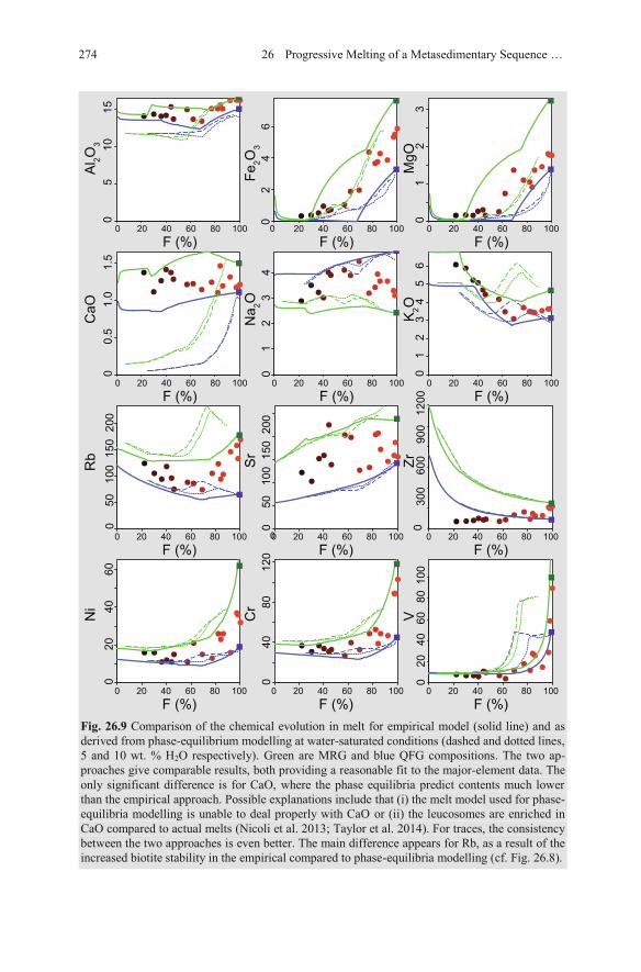
Fig. 26.9 Comparison of the chemical evolution in melt for empirical model (solid line) and as derived from phase-equilibrium modelling at water-saturated conditions (dashed and dotted lines,5 and 10 wt. % H2O respectively). Green are MRG and blue QFG compositions. The two ap-proaches give comparable results, both providing a reasonable fit to the major-element data. The only significant difference is for CaO, where the phase equilibria predict contents much lower than the empirical approach. Possible explanations include that (i) the melt model used for phase-equilibria modelling is unable to deal properly with CaO or (ii) the leucosomes are enriched in CaO compared to actual melts (Nicoli et al. 2013; Taylor et al. 2014). For traces, the consistency between the two approaches is even better. The main difference appears for Rb, as a result of the increased biotite stability in the empirical compared to phase-equilibria modelling (cf. Fig. 26.8).
● ●●●●●
●●●
●●●●●●●●
● ●●●●● ●
●●
●●●●
●
●●●
● ●●●●● ●
●
●●●●
●●●●●
●
●●●●
● ●●●●●
●
●●●●●
●
●●●
●● ●●●
●●●●●
●●
● ●●●
●● ●●
●●●●●●●●
F (%)0 20 40 60 80 100
F (%)0 20 40 60 80 100
F (%)20 40 60 80 100
F (%)0 20 40 60 80 100
F (%)0 20 40 60 80 100
F (%)0 20 40 60 80 100
Al 2O
3
MgO
CaO
Na 2O
K2O
0
05
1015
00.
51.
01.
5
02
34
1
02
13
45
60
23
1
02
46
Fe2O
3
●●●
●●●
●●●
●●
●●
●●●
●
●●
●●
●
●
●●
● ●
●●
●●●
●●
● ●●●●● ●●● ●●●●●
●●●
● ●●●●
●●
●● ●
●●●
●
●●●
● ●●●●● ●●
●
●●●●●
●●●
● ●●●●● ●●●
●●
●●●●
●
●
F (%)0 20 40 60 80 100
F (%)0 20 40 60 80 100
F (%)0 20 40 60 80 100
F (%)0 20 40 60 80 100
F (%)0 20 40 60 80 100
F (%)0 20 40 60 80 100
Rb Sr Zr
Ni
Cr
V
0
010
020
050
150
040
8010
020
60
040
8012
0
020
4060
050
100
150
200
060
012
0030
090
0
274 26 Progressive Melting of a Metasedimentary Sequence …
References 275
References
Brown M (1979) The petrogenesis of the St. Malo migmatite belt, Armorican Massif, France, with particular reference to the diatexites. Neu Jb Mineral, Abh 135:48–74
Brun J-P, Balé P (1990) Cadomian tectonics in Northern Brittany. In: D’Lemos RS, Strachan RA, Topley CG (eds) The Cadomian Orogeny. Geological Society of London Special Publications, vol 55, pp 95–114
Brun JP, Martin H (1977) Relations métamorphisme-déformation au cours de l’évolution dynam-ique d’un dôme migmatitique: le Massif de Saint-Malo (France). Bull Soc Géol France 20:91–101
Clemens JC, Vielzeuf D (1987) Constraints on melting and magma production in the crust. Earth Planet Sci Lett 86:287–306
Connolly JAD (2005) Computation of phase equilibria by linear programming: a tool for geody-namic modeling and its application to subduction zone decarbonation. Earth Planet Sci Lett 236:524–541
Holland TJB, Powell R (2011) An improved and extended internally consistent thermodynamic dataset for phases of petrological interest, involving a new equation of state for solids. J Metamorph Geol 29:333–383
Martin H (1977) Contribution à l’étude de l’anatexie: le Massif de Saint-Malo (Massif armoric-ain). Mobilisation des éléments durant la fusion. Proposition d’un modèle. Unpublished PhD thesis, Université de Rennes I, Rennes
Martin H (1979) Geochemical behaviour of major and trace elements during incongruent melting of biotite in the Saint-Malo migmatites. Neu Jb Mineral, Mh 509–524
Martin H (1980) Comportement de quelques éléments en traces au cours de l’anatexie: exemple du Massif de Saint-Malo (Bretagne, France). Can J Earth Sci 17:927–941
Nicoli G, Stevens G, Moyen J-F, Taylor J (2013) Leucosome formation by disequilibrium melt-ing and melt loss: perspectives from the South Marginal Zone (SMZ) of the Limpopo Belt, South Africa. Mineral Mag 77:1846
Peucat J-J (1986) Behavior of Rb–Sr whole rock and U–Pb zircon systems during partial melting as shown in migmatitic gneisses from the St-Malo Massif, N.E. Brittany, France. J Geol Soc London 143:875–886
Peucat J-J, Martin H (1985) Are Rb–Sr thin slab migmatite ages meaningful? Neu Jb Mineral, Abh 152:1–21
Powell R, Holland TJB (1988) An internally consistent thermodynamic dataset with uncertain-ties and correlations: 3. Applications to geobarometry, worked examples and a computer pro-gram. J Metamorph Geol 6:173–204
Stevens G, Clemens J (1993) Fluid-absent melting and the roles of fluids in the lithosphere: a slanted summary? Chem Geol 108:1–17
Taylor J, Nicoli G, Stevens G, Frei D, Moyen JF (2014) The processes that control leucosome compositions in metasedimentary granulites: perspectives from the Southern Marginal Zone migmatites, Limpopo Belt, South Africa. J Metamorph Geol 32:713–742
Weber C, Barbey P, Cuney M, Martin H (1985) Trace element behaviour during migmatization. Evidence for a complex melt–residuum fluid interaction in the St-Malo migmatitic dome (France). Contrib Mineral Petrol 90:52–62
White RW, Powell R, Holland TJB (2001) Calculation of partial melting equilibria in the sys-tem CaO–Na2O–K2O–FeO–MgO–Al2O3–SiO2–H2O (CNKFMASH). J Metamorph Geol 19:139–153
White RW, Powell R, Holland T (2007) Progress relating to calculation of partial melting equilibria for metapelites. J Metamorph Geol 25:511–527
Appendix A
Here we give an overview of the syntax and basic usage of the R language. We describe how to start and stop an R session, obtain help and find documentation. An account of the main object types and their manipulation in direct (i.e. com-mand line) mode is followed by text on arguably the strongest point—graphics. The Appendix is closed by a section on writing true R programs (batch mode). The text is partly based on the pdf file ‘An Introduction to R’, available from the Help menu.
This text does not intend to be a replacement for a proper R course. Apart from the help system and pdf manuals included with the R distribution, the reader can find additional information in an increasing number of books and web sites.
Importantly, information concerning the current state of the R project, binaries, source codes and documentation are obtainable from the dedicated website (www.r-project.org) and the Comprehensive R Archive Network (CRAN, cran.r-project.org). CRAN, which is mirrored at many servers worldwide, also provides a distribution channel for user-contributed packages that add new functionality to the core of the R system.
Chapter 1 Direct Mode
1.1 Basic Operations
1.1.1 Starting and Terminating the R Session
© Springer-Verlag Berlin Heidelberg 2016 V. Janoušek et al., Geochemical Modelling of Igneous Processes – Principles And Recipes in R Language, Springer Geochemistry, DOI 10.1007/978-3-662-46792-3
277
R Syntax in a Nutshell
In Windows, double clicking the file RGUI.EXE or the associated shortcut opens
the , a text window for the entry of commands and display of textual
output (Fig. A1.1). The system prints a number of messages, the most important of
which is the last line with a prompt, showing that the R environment is awaiting
commands. Apart from the R Console, one or more windows for graphical output
and help pages may be displayed.
“R Console”
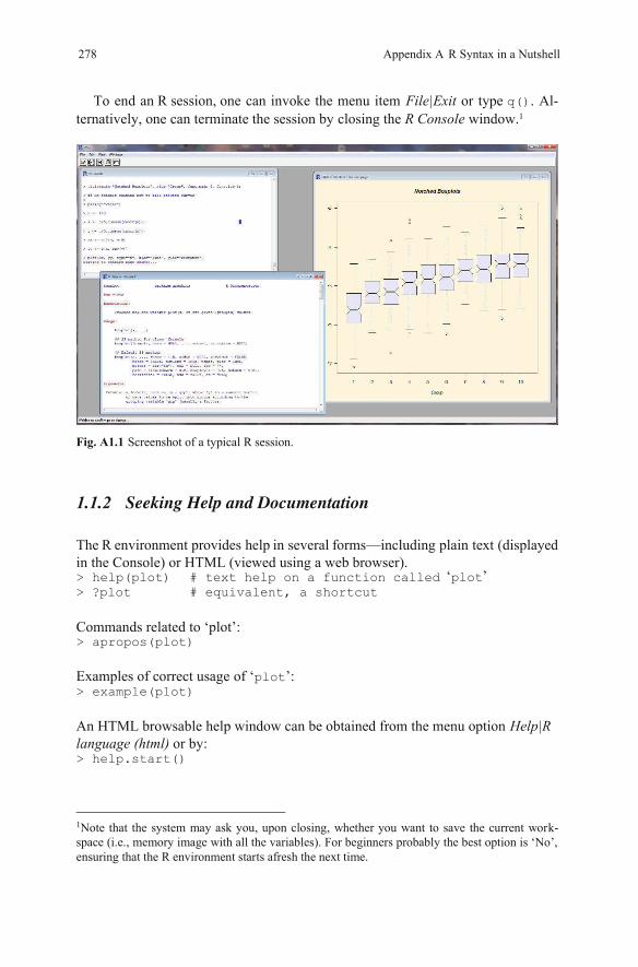
To end an R session, one can invoke the menu item File|Exit or type q(). Al-ternatively, one can terminate the session by closing the R Console window.1
Fig. A1.1 Screenshot of a typical R session.
1.1.2 Seeking Help and Documentation
The R environment provides help in several forms—including plain text (displayed in the Console) or HTML (viewed using a web browser). > help(plot) # text help on a function called plot > ?plot # equivalent, a shortcut Commands related to ‘plot’: > apropos(plot) Examples of correct usage of ‘plot’: > example(plot) An HTML browsable help window can be obtained from the menu option elp|R language (html) or by: > help.start()
1Note that the system may ask you, upon closing, whether you want to save the current work-space (i.e., memory image with all the variables). For beginners probably the best option is ‘No’,
278 Appendix A R Syntax in a Nutshell
H
‘ ’
ensuring that the R environment starts afresh the next time.
R is distributed together with PDF documents, which can be invoked from the menu item Help|Manuals. There are several documents available, including ‘Writ-ing R Extensions’, ‘R Data Import/Export’, ‘The R Language Definition’ and ‘R Installation and Administration’. At this stage the most appropriate will be ‘An In-troduction to R’ which outlines the basics of the R language.
Other good sources of information are the many books about R (e.g., Maindonald and Braun 2003; Murrell 2005; Crawley 2007; Chambers 2009; Adler 2012; van den Bogaard and Tolosana-Delgado 2013), or the related S language (Becker et al. 1988; Chambers and Hastie 1992; Chambers 1998) as the two lan-guages share most of their syntax. CRAN contains a list of published monographs (www.r-project.org/doc/bib/R-books.html) as well as links to numerous contrib-uted documents or manuals, both general and specific. The R Journal, an open-ac-cess refereed journal, features short to medium length articles on various R appli-cations, R programming and add-on packages. The community meets at annual useR! conferences. Moreover, there exist e-mail discussion groups dedicated to help users (R-help), to announce new versions and further progress in the R pro-ject (R-announce, R-packages) and to facilitate communication among developers (R-devel). Further information, including the archive of the e-mail discussion groups, is available on CRAN.
Lastly, there exist numerous blogs dedicated to the R project, most of them ac-cessible from the R-bloggers web page, www.r-bloggers.com. A useful starting point to search for a topic is RSeek, www.rseek.org.
1.2 Fundamental Objects of the R Language
1.2.1 Commands
The R environment can be utilized in direct mode, typing commands straight into the Console and getting an immediate response. Alternatively, the whole R code can be prepared in advance as a plain text file and run at once in batch mode. The commands (functions) in R are entered either individually, each on a single line,
lines of code are enclosed in braces {}. Each command is followed by brackets with parameters (or empty, if none are required or default values are desired). Typing just the command name returns a listing of the function’s definition.
It is also important to note that several words are reserved by the system and cannot be used as variable names. For details, see ?Reserved.
Appendix A R Syntax in a Nutshell 279
The R language is case sensitive. Commands are typed in lowercase and
the environment distinguishes between lower and upper case letters in
variable names. The latter cannot start with a digit and may contain any symbols
stance, accented characters.
or are separated by a semicolon (;). More complex statements consisting of several
apart from the hash mark (“#”). Note however that it is not wise to use, for in-
Direct Mode
In the simplest case, commands are entered and the result displayed: > (15+6)*3 [1] 63
The numerical values can be assigned to a named variable. Perhaps confusingly, R does not use “=” as an assignment operator. Instead, an arrow “<–” is imple-mented, corresponding to a combination of “<” (less than) and “-” (minus) char-acters2: x <- 5
In direct mode, the content of a variable is displayed by typing its name: x [1] 5
If an incomplete command is entered, R displays a prompt “+” giving the oppor-tunity to add what is needed. > (15+6 + )*3 [1] 63
The R environment automatically records a command history. The previous com-mands can be recalled using the vertical arrow keys, edited and re-used, as de-sired. The history can be displayed by the namesake function: history()
Batch Mode
A sequence of R commands or program can also be prepared beforehand in the form of a plain text file. This can be written by any editor ranging from Notepad, to more sophisticated word processors. In the latter case the file may need to be ex-ported as Plain/ASCII text. However, the most useful seem to be text editors de-signed especially for programmers as they often provide extra functionality such as line numbering, syntax checking/highlighting and brackets matching (WinEdt, Tinn-R, Notepad++, etc.)
Commonly used suffixes for R program scripts are “r” or “R”. The script can be run from the menu File|Source R code or using the command source: > source("myprogram.r")3
The program can be stopped by pressing the Esc key or from the menu Misc|Stop current computation. Optional comments start with a hash mark: > # My comment
2 In fact the “=” the code readability. We prefer using the arrow notation throughout the book. 3 Assuming that the code resides in the current working directory; otherwise the full path needs to be specified or directory changed.
280 Appendix A R Syntax in a Nutshell
also works as an assignment operator, however it is considered to degrade
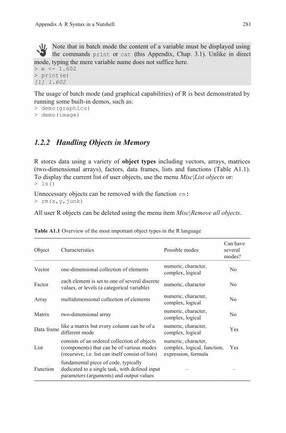
Appendix A R Syntax in a Nutshell 281
Table A1.1 Overview of the most important object types in the R language
Object Characteristics Possible modes Can have several modes?
Vector one-dimensional collection of elements numeric, character, complex, logical No
Factor each element is set to one of several discrete values, or levels (a categorical variable) numeric, character No
Array multidimensional collection of elements numeric, character, complex, logical No
Matrix two-dimensional array numeric, character, complex, logical No
like a matrix but every column can be of a different mode
numeric, character, complex, logical Yes
List consists of an ordered collection of objects (components) that can be of various modes (recursive, i.e. list can itself consist of lists)
numeric, character, complex, logical, function, expression, formula
Yes
Function fundamental piece of code, typically dedicated to a single task, with defined input parameters (arguments) and output values
– –
Data frame
Note that in batch mode the content of a variable must be displayed using the commands print or cat (this Appendix, Chap. 3.1). Unlike in direct
mode, typing the mere variable name does not suffice here. > e <- 1.602 > print(e) [1] 1.602
The usage of batch mode (and graphical capabilities) of R is best demonstrated by running some built-in demos, such as: > demo(graphics) > demo(image)
1.2.2 Handling Objects in Memory
R stores data using a variety of object types including vectors, arrays, matrices (two-dimensional arrays), factors, data frames, lists and functions (Table A1.1). To display the current list of user objects, use the menu or: > ls() Unnecessary objects can be removed with the function rm: > rm(x,y,junk)
All user R objects can be deleted using the menu item Misc|Remove all objects.
Misc|List objects
1.3 Numeric Vectors
1.3.1 Assignment
Assignment of several items to a vector is done using the combine function c: > x <- c(10.4, 5.6, 3.1, 6.4, 21.7) > y <- c(x, 0, x) > y [1] 10.4 5.6 3.1 6.4 21.7 0.0 10.4 5.6 3.1 6.4 21.7
1.3.2 Vector Arithmetic
For vectors, calculations are made using basic arithmetic operators: + - * / ^. The use of these operators for two vectors of the same length is intuitive. In other cases, the elements of the shorter vector are recycled as often as necessary. For in-stance, for the x vector defined above, we can calculate:
282 Appendix A R Syntax in a Nutshell
1.2.3 Attributes to
Every object possesses several properties, called attributes. The two most im-portant of these are length and mode. Some object types, or in R jargon classes, can have more modes. For the given object, the mode (logical, numeric, complex or character) can be displayed using the namesake function: > mode(10) [1] "numeric"
Objects
All the objects are stored in memory, and not automatically saved to disc. When quitting the R environment, you are given the opportunity to save the current workspace, i.e. all the objects created during the given session. If you accept, they are written to a .RData in the current directory and reloaded automatically the next time R is started. Different R sessions may therefore be maintained in separatedirectories.
file
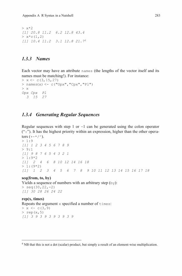
> x*2 [1] 20.8 11.2 6.2 12.8 43.4 > x*c(1,2) [1] 10.4 11.2 3.1 12.8 21.74
1.3.3 Names
Each vector may have an attribute names (the lengths of the vector itself and its names must be matching!). For instance: > x <- c(3,15,27) > names(x) <- c("Opx","Cpx","Pl") > x Opx Cpx Pl 3 15 27
1.3.4 Generating Regular Sequences
Regular sequences with step 1 or -1 can be generated using the colon operator (“:”). It has the highest priority within an expression, higher than the other opera-tors (+-*/^). > 1:9 [1] 1 2 3 4 5 6 7 8 9 > 9:1 [1] 9 8 7 6 5 4 3 2 1 > 1:9*2 [1] 2 4 6 8 10 12 14 16 18 > 1:(9*2) [1] 1 2 3 4 5 6 7 8 9 10 11 12 13 14 15 16 17 18
seq(from, to, by) Yields a sequence of numbers with an arbitrary step (by): > seq(30,22,-2) [1] 30 28 26 24 22
rep(x, times) Repeats the argument x specified a number of times: > x <- c(3,9) > rep(x,5)[1] 3 9 3 9 3 9 3 9 3 9
4 NB that this is not a dot (scalar) product, but simply a result of an element-wise multiplication.
Appendix A R Syntax in a Nutshell 283
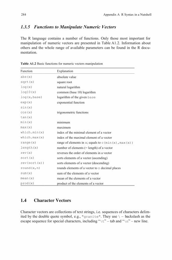
1.3.5 Functions to Manipulate Numeric Vectors
The R language contains a number of functions. Only those most important for manipulation of numeric vectors are presented in Table A1.2. Information about others and the whole range of available parameters can be found in the R docu-mentation.
Table A1.2 Basic functions for numeric vectors manipulation
Function Explanation
abs(x) absolute value sqrt(x) square root log(x) natural logarithm log10(x) common (base 10) logarithm log(x,base) logarithm of the given base exp(x) exponential function sin(x)
cos(x)
tan(x) trigonometric functions
min(x) minimum max(x) maximum which.min(x) index of the minimal element of a vector which.max(x) index of the maximal element of a vector range(x) range of elements in x; equals to c(min(x),max(x)) length(x) number of elements (= length) of a vector rev(x) reverses the order of elements in a vector sort(x) sorts elements of a vector (ascending) rev(sort(x)) sorts elements of a vector (descending) round(x,n) rounds elements of a vector to n decimal places sum(x) sum of the elements of a vector mean(x) mean of the elements of a vector prod(x) product of the elements of a vector
1.4 Character Vectors
Character vectors are collections of text strings, i.e. sequences of characters delim-ited by the double quote symbol, e.g., "granite". They use \ – backslash as the escape sequence for special characters, including “\t” – tab and “\n” – new line.
284 Appendix A R Syntax in a Nutshell
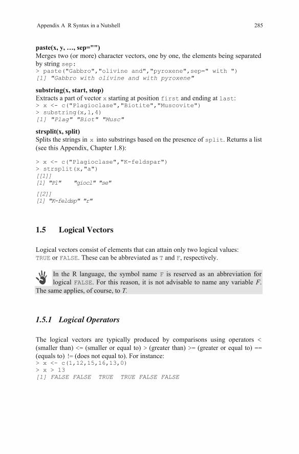
paste(x, y, …, sep="") Merges two (or more) character vectors, one by one, the elements being separated by string sep: > paste("Gabbro","olivine and","pyroxene",sep=" with ") [1] "Gabbro with olivine and with pyroxene"
substring(x, start, stop) Extracts a part of vector x starting at position first and ending at last: > x <- c("Plagioclase","Biotite","Muscovite") > substring(x,1,4) [1] "Plag" "Biot" "Musc"
strsplit(x, split) Splits the strings in into substrings based on the presence of split. Returns a list (see this Appendix, Chapter 1.8): > x <- c("Plagioclase","K-feldspar") > strsplit(x,"a") [[1]] [1] "Pl" "giocl" "se"
[[2]] [1] "K-feldsp" "r"
1.5 Logical Vectors
Logical vectors consist of elements that can attain only two logical values: TRUE or FALSE. These can be abbreviated as T and F, respectively.
In the R language, the symbol name F is reserved as an abbreviation for logical FALSE. For this reason, it is not advisable to name any variable F.
The same applies, of course, to T.
1.5.1 Logical Operators
The logical vectors are typically produced by comparisons using operators <(smaller than) <= (smaller or equal to) > (greater than) >= (greater or equal to) == (equals to) != (does not equal to). For instance: > x <- c(1,12,15,16,13,0) > x > 13 [1] FALSE FALSE TRUE TRUE FALSE FALSE
Appendix A R Syntax in a Nutshell 285
x
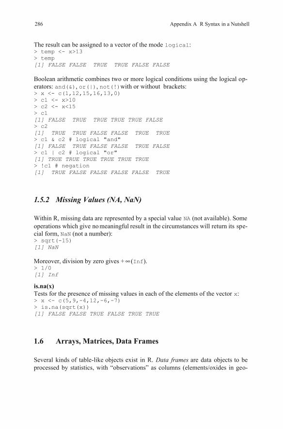
The result can be assigned to a vector of the mode logical: > temp <- x>13 > temp [1] FALSE FALSE TRUE TRUE FALSE FALSE Boolean arithmetic combines two or more logical conditions using the logical op-erators: and(&), or(|), not(!)with or without brackets: > x <- c(1,12,15,16,13,0) > c1 <- x>10 > c2 <- x<15 > c1 [1] FALSE TRUE TRUE TRUE TRUE FALSE > c2 [1] TRUE TRUE FALSE FALSE TRUE TRUE > c1 & c2 # logical "and" [1] FALSE TRUE FALSE FALSE TRUE FALSE > c1 | c2 # logical "or" [1] TRUE TRUE TRUE TRUE TRUE TRUE > !c1 # negation [1] TRUE FALSE FALSE FALSE FALSE TRUE
1.5.2 Missing Values (NA, NaN)
Within R, missing data are represented by a special value NAoperations which give no meaningful result in the circumstances will return its spe-cial form, (not a number): > sqrt(-15) [1] NaN Moreover, division by zero gives + (Inf). > 1/0 [1] Inf
is.na(x) Tests for the presence of missing values in each of the elements of the vector x: > x <- c(5,9,-4,12,-6,-7) > is.na(sqrt(x)) [1] FALSE FALSE TRUE FALSE TRUE TRUE
1.6 Arrays, Matrices, Data Frames
Several kinds of table-like objects exist in R. Data frames are data objects to be processed by statistics, with “observations” as columns (elements/oxides in geo-
286 Appendix A R Syntax in a Nutshell
(not available). Some
NaN
∞
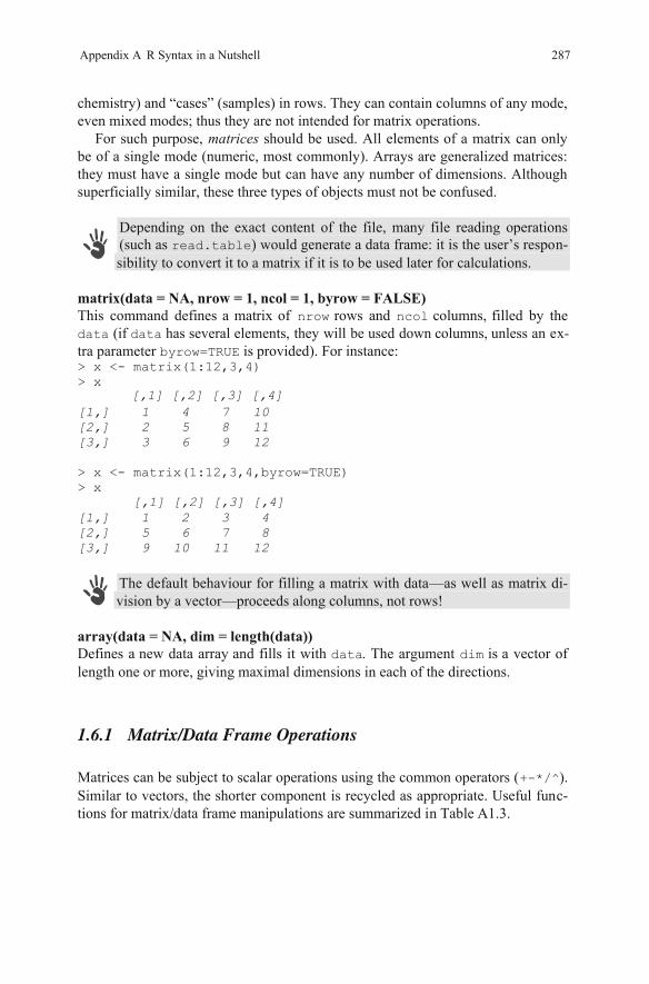
chemistry) and “cases” (samples) in rows. They can contain columns of any mode, even mixed modes; thus they are not intended for matrix operations.
For such purpose, matrices should be used. All elements of a matrix can only be of a single mode (numeric, most commonly). Arrays are generalized matrices: they must have a single mode but can have any number of dimensions. Although superficially similar, these three types of objects must not be confused.
Depending on the exact content of the file, many file reading operations (such as read.table) would generate a data frame: it is the user’s respon-sibility to convert it to a matrix if it is to be used later for calculations.
matrix(data = NA, nrow = 1, ncol = 1, byrow = FALSE) This command defines a matrix of nrow rows and ncol columns, filled by the data data has several elements, they will be used down columns, unless an ex-tra parameter byrow=TRUE is provided). For instance: > x <- matrix(1:12,3,4) > x
[,1] [,2] [,3] [,4] [1,] 1 4 7 10 [2,] 2 5 8 11 [3,] 3 6 9 12 > x <- matrix(1:12,3,4,byrow=TRUE) > x
[,1] [,2] [,3] [,4] [1,] 1 2 3 4 [2,] 5 6 7 8 [3,] 9 10 11 12
The default behaviour for filling a matrix with data—as well as matrix di-vision by a vector—proceeds along columns, not rows!
array(data = NA, dim = length(data)) Defines a new data array and fills it with data. The argument dim is a vector of length one or more, giving maximal dimensions in each of the directions.
1.6.1 Matrix/Data Frame Operations
Matrices can be subject to scalar operations using the common operators (+-*/^). Similar to vectors, the shorter component is recycled as appropriate. Useful func-tions for matrix/data frame manipulations are summarized in Table A1.3.
Appendix A R Syntax in a Nutshell 287
(if
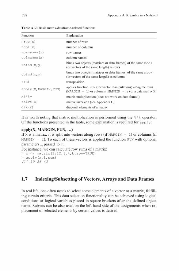
Table A1.3 Basic matrix/dataframe-related functions
Function Explanation
nrow(x) number of rows ncol(x) number of columns rownames(x) row names colnames(x) column names
rbind(x,y) binds two objects (matrices or data frames) of the same ncol (or vectors of the same length) as rows
cbind(x,y) binds two objects (matrices or data frames) of the same nrow (or vectors of the same length) as columns
t(x) transposition
apply(X,MARGIN,FUN) applies function FUN
) or columns ( ) of a data matrix x%*%y matrix multiplication (does not work on data frame!) solve(A) matrix inversion (see Appendix C) dix(x) diagonal elements of a matrix
Of the functions presented in the table, some explanation is required for apply:
apply(X, MARGIN, FUN, …) If X is a matrix, it is split into vectors along rows (if MARGIN = 1) or columns (if MARGIN = 2). To each of these vectors is applied the function FUN with optional parameters ... passed to it.For instance, we can calculate row sums of a matrix: > x <- matrix(1:12,3,4,byrow=TRUE) > apply(x,1,sum) [1] 10 26 42
1.7 Indexing/Subsetting of Vectors, Arrays and Data Frames
In real life, one often needs to select some elements of a vector or a matrix, fulfill-ing certain criteria. This data selection functionality can be achieved using logical conditions or logical variables placed in square brackets after the defined object name. Subsets can be also used on the left hand side of the assignments when re-placement of selected elements by certain values is desired.
288 Appendix A R Syntax in a Nutshell
(for vector manipulations) along the rows ( MARGIN = 2MARGIN = 1
It is worth noting that matrix multiplication is performed using the %*%
X
operator.
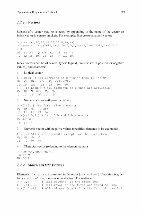
1.7.1 Vectors
Subsets of a vector may be selected by appending to the name of the vector an le, first create a named vector:
> x <- c(1,12,15,NA,16,13,0,NA,NA) > names(x) <- c("Pl","Bt","Mu","Q","Kfs","Ky","Ol","Px","C")
Pl Bt Mu Q Kfs Ky Ol Px C 1 12 15 NA 16 13 0 NA NA Index vectors can be of several types: logical, numeric (with positive or negative values), and character:
1. Logical vector > x[x>10] # all elements of x higher than 10 (or NA)Bt Mu <NA> Kfs Ky <NA> <NA>
12 15 NA 16 13 NA NA > x[!is.na(x)] # all elements of x that are available Pl Bt Mu Kfs Ky Ol
1 12 15 16 13 0
2. Numeric vector with positive values > x[1:5] # the first five elements Pl Bt Mu Q Kfs 1 12 15 NA 16 > x[c(1,5,7)] # 1st, 5th and 7th elements
1 16 0
3. Numeric vector with negative values (specifies elements to be excluded) > x[-(1:5)] # all elements except for the first five
13 0 NA NA
4. Character vector (referring to the element names) > x[c("Q","Bt","Mu")] Q Bt Mu
NA 12 15
1.7.2 Matrices/Data Frames
Elements of a matrix are presented in the order [row,column]. If nothing is given for a row or column, it means no restriction. For instance: > x[1,] # (all columns) of the first row > x[,c(1,3)] # (all rows) of the first and third columns > x[1:3,-2] # all columns (apart from the 2nd) of rows 1–3
Appendix A R Syntax in a Nutshell 289
index vector in square brackets. For examp
> x
Pl Kfs Ol
Ky Ol Px C
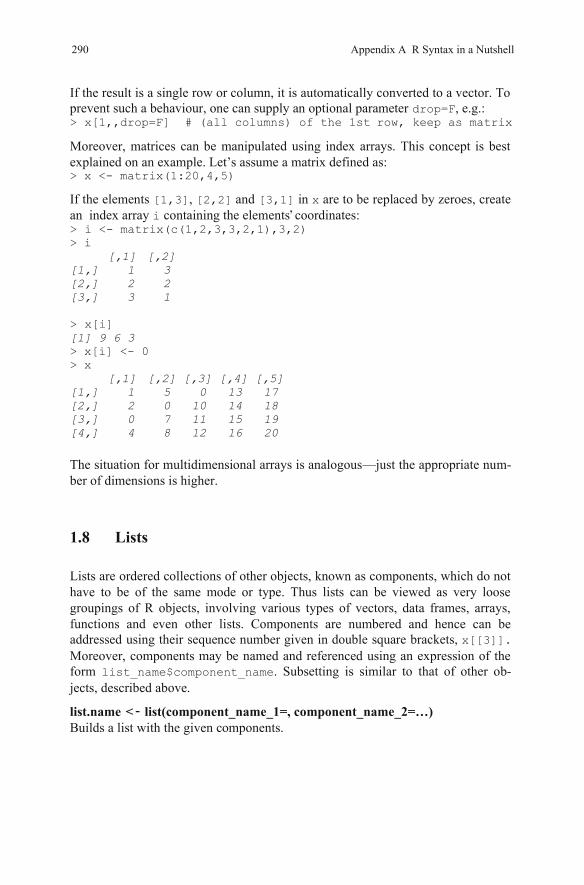
If the result is a single row or column, it is automatically converted to a vector. To prevent such a behaviour, one can supply an optional parameter drop=F, e.g.: > x[1,,drop=F] # (all columns) of the 1
Moreover, matrices can be manipulated using index arrays. This concept is best explained on an example. Let’s assume a matrix defined as: > x <- matrix(1:20,4,5)
If the elements [1,3], [2,2] and [3,1] in x are to be replaced by zeroes, create an index array i containing the elements coordinates: > i <- matrix(c(1,2,3,3,2,1),3,2) > i
[,1] [,2] [1,] 1 3 [2,] 2 2 [3,] 3 1 > x[i] [1] 9 6 3 > x[i] <- 0 > x
[,1] [,2] [,3] [,4] [,5] [1,] 1 5 0 13 17 [2,] 2 0 10 14 18 [3,] 0 7 11 15 19 [4,] 4 8 12 16 20 The situation for multidimensional arrays is analogous—just the appropriate num-ber of dimensions is higher.
1.8 Lists
Lists are ordered collections of other objects, known as components, which do not have to be of the same mode or type. Thus lists can be viewed as very loose groupings of R objects, involving various types of vectors, data frames, arrays, functions and even other lists. Components are numbered and hence can be addressed using their sequence number given in double square brackets, x[[3]].Moreover, components may be named and referenced using an expression of the form list_name$component_name. Subsetting is similar to that of other ob-jects, described above.
list.name Builds a list with the given components.
290 Appendix A R Syntax in a Nutshell
< -
st row, keep as matrix
list(component_name_1=, component_name_2=…)
’
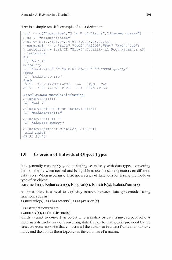
> x1 <- c("Luckovice","9 km E of Blatna","disused quarry") > x2 <- "melamonzonite" > x3 <- c(47.31,1.05,14.94,7.01,8.46,10.33) > names(x3) <- c("SiO2","TiO2","Al2O3","FeO","MgO","CaO") > luckovice <- list(ID="Gbl-4",Locality=x1,Rock=x2,major=x3) > luckovice $ID [1] "Gbl-4" $Locality [1] "Luckovice" "9 km E of Blatna" "disused quarry" $Rock [1] "melamonzonite" $major SiO2 TiO2 Al2O3 Fe2O3 FeO MgO CaO 47.31 1.05 14.94 2.23 7.01 8.46 10.33
As well as some examples of subsetting: > luckovice[[1]] [1] "Gbl-4"
> luckovice$Rock # or luckovice[[3]] [1] "melamonzonite"
> luckovice[[2]][3] [1] "disused quarry"
> luckovice$major[c("SiO2","Al2O3")] SiO2 Al2O3 47.31 14.94
1.9 Coercion of Individual Object Types
R is generally reasonably good at dealing seamlessly with data types, converting them on the fly when needed and being able to use the same operators on different data types. When necessary, there are a series of functions for testing the mode or type of an object: is.numeric(x), is.character(x), is.logical(x), is.matrix(x), is.data.frame(x)
At times there is a need to explicitly convert between data types/modes using functions such as: as.numeric(x), as.character(x), as.expression(x)
Less straightforward are: as.matrix(x), as.data.frame(x) which attempt to convert an object x to a matrix or data frame, respectively. A more user-friendly way of converting data frames to matrices is provided by the function data.matrix that converts all the variables in a data frame x to numeric mode and then binds them together as the columns of a matrix.
Appendix A R Syntax in a Nutshell 291
Here is a simple real-life example of a list definition:
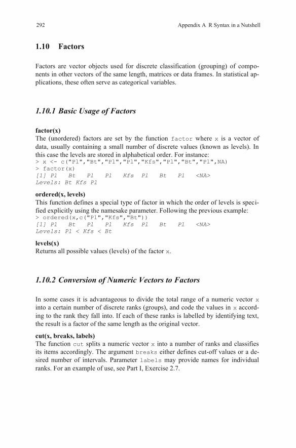
1.10 Factors
Factors are vector objects used for discrete classification (grouping) of compo-nents in other vectors of the same length, matrices or data frames. In statistical ap-plications, these often serve as categorical variables.
1.10.1 Basic Usage of Factors
factor(x) The (unordered) factors are set by the function factor where x is a vector of data, usually containing a small number of discrete values (known as levels). In this case the levels are stored in alphabetical order. For instance: > x <- c("Pl","Bt","Pl","Pl","Kfs","Pl","Bt","Pl",NA) > factor(x) [1] Pl Bt Pl Pl Kfs Pl Bt Pl <NA> Levels: Bt Kfs Pl
ordered(x, levels) This function defines a special type of factor in which the order of levels is speci-fied explicitly using the namesake parameter. Following the previous example: > ordered(x,c("Pl","Kfs","Bt")) [1] Pl Bt Pl Pl Kfs Pl Bt Pl <NA> Levels: Pl < Kfs < Bt
levels(x) Returns all possible values (levels) of the factor x.
1.10.2 Conversion of Numeric Vectors to Factors
In some cases it is advantageous to divide the total range of a numeric vector x into a certain number of discrete ranks (groups), and code the values in x accord-ing to the rank they fall into. If each of these ranks is labelled by identifying text, the result is a factor of the same length as the original vector.
cut(x, breaks, labels) The function cut splits a numeric vector x into a number of ranks and classifies its items accordingly. The argument breaks either defines cut-off values or a de-sired number of intervals. Parameter labels may provide names for individual ranks. For an example of use, see Part I, Exercise 2.7.
292 Appendix A R Syntax in a Nutshell
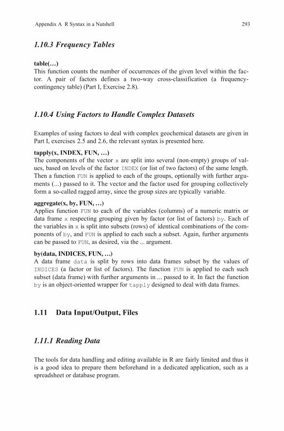
1.10.3 Frequency Tables
table(…) This function counts the number of occurrences of the given level within the fac-tor. A pair of factors defines a two-way cross-classification (a frequency-contingency table) (Part I, Exercise 2.8).
1.10.4 Using Factors to Handle Complex Datasets
Examples of using factors to deal with complex geochemical datasets are given in Part I, exercises 2.5 and 2.6, the relevant syntax is presented here.
The components of the vector x are split into several (non-empty) groups of val-ues, based on levels of the factor INDEX (or list of two factors) of the same length. Then a function FUN is applied to each of the groups, optionally with further argu-ments (...) passed to it. The vector and the factor used for grouping collectivelyform a so-called ragged array, since the group sizes are typically variable.
aggregate(x, by, FUN, )Applies function FUNdata frame x respecting grouping given by factor (or list of factors) by. Each of the variables in x is split into subsets (rows) of identical combinations of the com-ponents of by, and FUN is applied to each such a subset. Again, further arguments can be passed to FUN, as desired, via the ... argument.
by(data, INDICES, FUN, )A data frame data is split by rows into data frames subset by the values of INDICES (a factor or list of factors). The function FUN is applied to each such subset (data frame) with further arguments in ... passed to it. In fact the functionby is an object-oriented wrapper for tapply designed to deal with data frames.
1.11 Data Input/Output, Files
1.11.1 Reading Data
The tools for data handling and editing available in R are fairly limited and thus it is a good idea to prepare them beforehand in a dedicated application, such as a spreadsheet or database program.
Appendix A R Syntax in a Nutshell 293
tapply(x, INDEX, FUN, …)
…
…
to each of the variables (columns) of a numeric matrix or
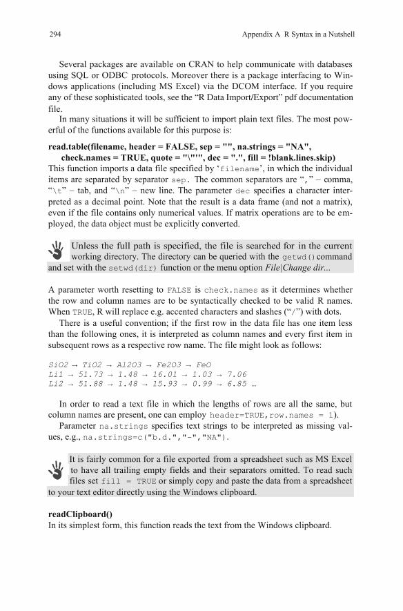
read.table(filename, header = FALSE, sep = "", na.strings = "NA", check.names = TRUE, quote = "\"'", dec = ".", fill = !blank.lines.skip)
This function imports a data file specified by ‘filename’, in which the individual items are separated by separator sep. The common separators are “,” – comma, “\t” – tab, and “\n” – new line. The parameter dec specifies a character inter-preted as a decimal point. Note that the result is a data frame (and not a matrix), even if the file contains only numerical values. If matrix operations are to be em-ployed, the data object must be explicitly converted.
Unless the full path is specified, the file is searchedgetwd()
setwd(dir) function or the menu option File|Change dir...
A parameter worth resetting to FALSE is check.names as it determines whether the row and column names are to be syntactically checked to be valid R names. When TRUE, R will replace e.g. accented characters and slashes (“/”) with dots.
There is a useful convention; if the first row in the data file has one item less than the following ones, it is interpreted as column names and every first item in subsequent rows as a respective row name. The file might look as follows: SiO2 TiO2 Al2O3 Fe2O3 FeO Li1 51.73 1.48 16.01 1.03 7.06 Li2 51.88 1.48 15.93 0.99 6.85 …
In order to read a text file in which the lengths of rows are all the same, but column names are present, one can employ header=TRUE,row.names = 1).
Parameter na.strings specifies text strings to be interpreted as missing val-ues, e.g., na.strings=c("b.d.","-","NA").
It is fairly common for a file exported from a spreadsheet such as MS Excel to have all trailing empty fields and their separators omitted. To read such files set fill = TRUE or simply copy and paste the data from a spreadsheet
to your text editor directly using the Windows clipboard.
readClipboard() In its simplest form, this function reads the text from the Windows clipboard.
294 Appendix A R Syntax in a Nutshell
Several packages are available on CRAN to help communicate with databases using SQL or ODBC
see the “R Data Import/Export” pdf documentation
In many situations it will be sufficient to import plain text files. The most pow-erful of the functions available for this purpose is:
dows applications (including MS Excel) via the DCOM interface. If you requireprotocols. Moreover there is a package interfacing to Win-
any of these sophisticated tools, file.
for in the currentworking directory. The directory can be queried with the
and set with the command
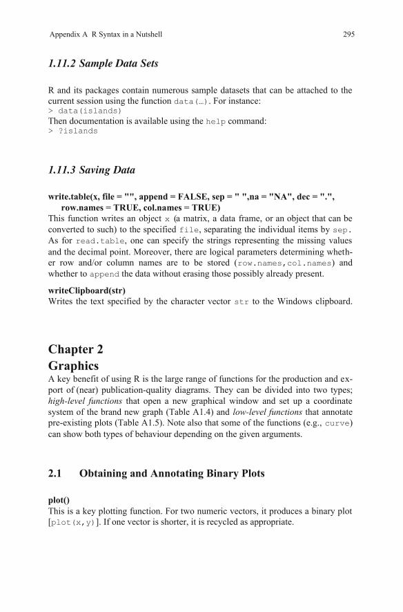
1.11.2 Sample Data Sets
R and its packages contain numerous sample datasets that can be attached to the current session using the function data(…). For instance: > data(islands) Then documentation is available using the help command: > ?islands
1.11.3 Saving Data
write.table(x, file = "", append = FALSE, sep = " ",na = "NA", dec = ".", row.names = TRUE, col.names = TRUE)
This function writes an object x or an object that can be converted to such) to the specified file, separating the individual items by sep. As for read.table, one can specify the strings reand the decimal point. Moreover, there are logical parameters determining wheth-er row and/or column names are to be stored (row.names,col.names) and whether to append the data without erasing those possibly already present.
writeClipboard(str) Writes the text specified by the character vector str to the Windows clipboard.
Chapter 2 Graphics A key benefit of using R is the large range of functions for the production and ex-port of (near) publication-quality diagrams. They can be divided into two types; high-level functions that open a new graphical window and set up a coordinate system of the brand new graph (Table A1.4) and low-level functions that annotate pre-existing plots (Table A1.5). Note also that some of the functions (e.g., curve) can show both types of behaviour depending on the given arguments.
2.1 Obtaining and Annotating Binary Plots
plot() This is a key plotting function. For two numeric vectors, it produces a binary plot [plot(x,y)]. If one vector is shorter, it is recycled as appropriate.
Appendix A R Syntax in a Nutshell 295
presenting the missing values
(a matrix, a data frame,
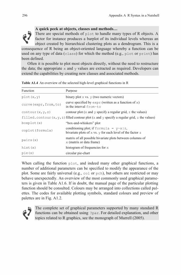
A quick peek at objects, classes and methods… There are special methods of plot to handle many types of R objects. A factor for instance produces a barplot of its individual levels whereas an object created by hierarchical clustering plots as a dendrogram. This is a
consequence of R being an object-oriented language whereby a function can be used on any type of data (class) for which the method (e.g., or print) has been defined.
Often it is possible to plot most objects directly, without the need to restructure the data; the appropriate x and y values are extracted as required. Developers can extend the capabilities by creating new classes and associated methods.
Table A1.4 An overview of the selected high-level graphical functions in R
Function Purpose plot(x,y) binary plot x vs. y (two numeric vectors)
curve(expr,from,to) curve specified by expr (written as a function of x) in the interval from–to
contour(x,y,z) contour plot (x and y specify a regular grid, z the values) filled.contour(x,y,z)filled contour plot (x and y specify a regular grid, z the values) boxplot(x) “box-and-whiskers” plot
coplot(formula) conditioning plot; if formula = y~x|z, bivariate plots of x vs. y for each level of the factor z
pairs(x) matrix of all possible bivariate plots between columns of x
hist(x) histogram of frequencies for x pie(x) circular pie-chart When calling the function plot, and indeed many other graphical functions, a number of additional parameters can be specified to modify the appearance of the plot. Some are fairly universal (e.g., col or pch), but others are restricted or may behave unexpectedly. An overview of the most commonly used graphical parame-ters is given in Table A1.6. If in doubt, the manual page of the particular plotting function should be consulted. Colours may be arranged into collections called pal-ettes. The codes for available plotting symbols, standard colours and preview of palettes are in Fig. A1.2.
The complete set of graphical parameters supported by many standard R functions can be obtained using . For detailed explanation, and other topics related to R graphics, see the monograph of Murrell (2005).
296 Appendix A R Syntax in a Nutshell
plot
(matrix or data frame)
?par
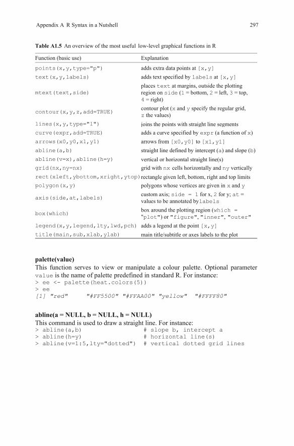
Table A1.5 An overview of the most useful low-level graphical functions in R
Function (basic use) Explanation
points(x,y,type="p") adds extra data points at [x,y] text(x,y,labels) adds text specified by labels at [x,y]
mtext(text,side) places text at margins, outside the plotting region on side 1 = bottom, 2 = left, 3 = top, 4 = right)
contour(x,y,z,add=TRUE) contour plot (x and y specify the regular grid, z the values)
lines(x,y,type="l") joins the points with straight line segments curve(expr,add=TRUE) adds a curve specified by expr x) arrows(x0,y0,x1,y1) arrows from [x0,y0] to [x1,y1] abline(a,b) straight line defined by intercept (a) and slope (b) abline(v=x),abline(h=y) vertical or horizontal straight line(s) grid(nx,ny=nx) grid with nx cells horizontally and ny vertically rect(xleft,ybottom,xright,ytop) rectangle given left, bottom, right and top limits polygon(x,y) polygons whose vertices are given in and y
axis(side,at,labels) custom axis; side = 1 for x, 2 for y; at = values to be annotated bylabels
box(which) box around the plotting region (which = "plot") or "figure", "inner",
legend(x,y,legend,lty,lwd,pch) adds a legend at the point [x,y] title(main,sub,xlab,ylab) main title/subtitle or axes labels to the plot
palette(value) This function serves to view or manipulate a colour palette. Optional parameter value is the name of palette predefined in standard R. For instance: > ee <- palette(heat.colors(5)) > ee [1] "red" "#FF5500" "#FFAA00" "yellow" "#FFFF80"
abline(a = NULL, b = NULL, h = NULL) This command is used to draw a straight line. For instance: > abline(a,b) # slope b, intercept a > abline(h=y) # horizontal line(s) > abline(v=1:5,lty="dotted") # vertical dotted grid lines
Appendix A R Syntax in a Nutshell 297
(
(a function of
x
"outer"
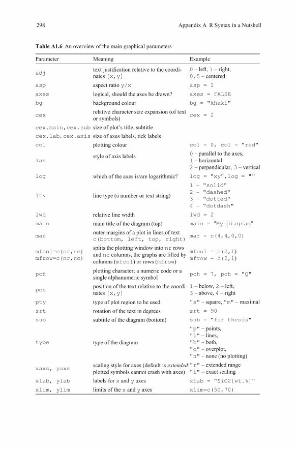
Table A1.6 An overview of the main graphical parameters
Parameter Meaning Example
adj text justification relative to the coordi-nates [x,y]
0 – left, 1 – right, 0.5 – centered
aspect ratio y/x asp = 1
logical, should the axes be drawn? axes = FALSE
background colour bg = "khaki"
relative character size expansion (of text or symbols) cex = 2
cex.main,cex.sub size of plot title, subtitle
cex.lab,cex.axis size of axes labels, tick labels
plotting colour col = 0, col = "red"
style of axis labels
0 –1 –2 – 3 – vertical
which of the axes is/are logarithmic? log = "xy",log = ""
line type (a number or text string)
1 – "solid" 2 – "dashed" 3 – "dotted" 4 – "dotdash"
relative line width lwd = 2 main title of the diagram (top) main = "My diagram" outer margins of a plot in lines of text c(bottom, left, top, right) mar = c(4,4,0,0)
mfcol=c(nr,nc) mfrow=c(nr,nc)
splits the plotting window into nr rows and nc columns, the graphs are filled by columns (mfcol) or rows (mfrow)
mfcol = c(2,1) mfrow = c(2,1)
plotting character; a numeric code or a single alphanumeric symbol pch = 7, pch = "Q"
position of the text relative to the coordi-nates [x,y]
1 – below, 2 – left, 3 – above, 4 – right
type of plot region to be used "s" – square, "m" – maximal rotation of the text in degrees srt = 90
subtitle of the diagram (bottom) sub = "for thesis"
type of the diagram
"p" – points, "l" – lines, "b" – both, "o" – overplot, "n" – none (no plotting)
xaxs, yaxs scaling style for axes (default is extended: plotted symbols cannot crash with axes)
"r" – extended range "i" – exact scaling
xlab, ylab labels for x and y axes xlab = "SiO2[wt.%]"
xlim, ylim limits of the x and y axes xlim=c(50,70)
298 Appendix A R Syntax in a Nutshell
asp
axes
bg
cex
col
las
log
lty
lwd
main
mar
pch
pos
pty
srt
sub
type
’ s
parallel to the axes, horizontal perpendicular,
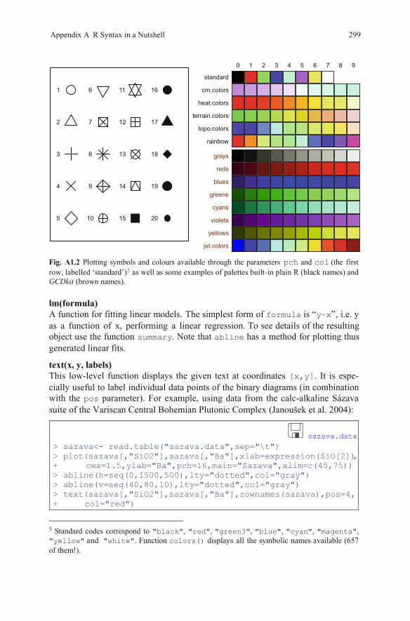
Fig. A1.2 Plotting symbols and colours available through the parameters pch and col (the first row, labelled ‘standard’)5 as well as some examples of palettes built-in plain R (black names) and GCDkit (brown names).
lm(formula) A function for fitting linear models. The simplest form of formula is “y~x”, i.e. y as a function of x, performing a linear regression. To see details of the resulting
summary. Note that abline has a method for plotting thus generated linear fits.
text(x, y, labels) This low-level function displays the given text at coordinates [x,y]. It is espe-cially useful to label individual data points of the binary diagrams (in combination with the pos parameter). For example, using data from the calc-alkaline Sázava suite of the Variscan Central Bohemian Plutonic Complex (Janoušek et al. 2004):
sazava.data > sazava<- read.table("sazava.data",sep="\t") > plot(sazava[,"SiO2"],sazava[,"Ba"],xlab=expression(SiO[2]),+ cex=1.5,ylab="Ba",pch=16,main="Sazava",xlim=c(45,75)) > abline(h=seq(0,1500,500),lty="dotted",col="gray") > abline(v=seq(40,80,10),lty="dotted",col="gray") > text(sazava[,"SiO2"],sazava[,"Ba"],rownames(sazava),pos=4,+ col="red")
5 Standard codes correspond to "black", , "green3", "blue", "cyan", "magenta", "yellow" . Function colors() displays all the symbolic names available (657
Appendix A R Syntax in a Nutshell 299
1
2
3
4
5
6
7
8
9
10
11
12
13
14
15
16
17
18
19
20
standard
cm.colors
heat.colors
terrain.colors
topo.colors
rainbow
grays
reds
blues
greens
cyans
violets
yellows
jet.colors
0 1 2 3 4 5 6 7 8 9
object use the function
"red" and "white"
of them!).
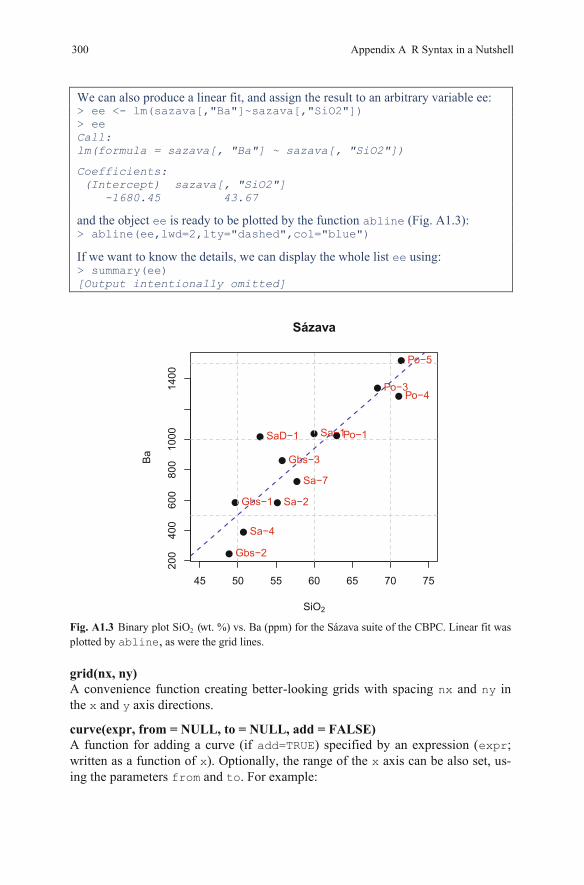
We can also produce a linear fit, and assign the result to an arbitrary variable ee: > ee <- lm(sazava[,"Ba"]~sazava[,"SiO2"]) > ee Call: lm(formula = sazava[, "Ba"] ~ sazava[, "SiO2"])
Coefficients: (Intercept) sazava[, "SiO2"] -1680.45 43.67
and the object ee is ready to be plotted by the function abline (Fig. A1.3): > abline(ee,lwd=2,lty="dashed",col="blue")
If we want to know the details, we can display the whole list ee using: > summary(ee) [Output intentionally omitted]
Fig. A1.3 Binary plot SiO2 (wt. %) vs. Ba (ppm) for the Sázava suite of the CBPC. Linear fit was plotted by abline, as were the grid lines.
grid(nx, ny) A convenience function creating better-looking grids with spacing nx and ny in the x and y axis directions.
curve(expr, from = NULL, to = NULL, add = FALSE) A function for adding a curve (if add=TRUE) specified by an expression (expr; written as a function of x). Optionally, the range of the x axis can be also set, us-ing the parameters from and to. For example:
45 50 55 60 65 70 75
20
04
00
60
08
00
10
00
14
00
Sázava
SiO2
Ba
Sa−1
Sa−2
Sa−4
Sa−7
SaD−1
Gbs−1
Gbs−2
Gbs−3
Po−1
Po−3Po−4
Po−5
300 Appendix A R Syntax in a Nutshell
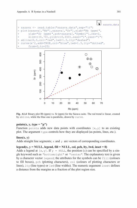
sazava.data > sazava <- read.table("sazava.data",sep="\t") > plot(sazava[,"Rb"],sazava[,"Sr"],xlab="Rb (ppm)", + ylab="Sr (ppm)",pch=sazava[,"Symbol"],cex=2, + xlim=c(0,70),ylim=c(0,650),xaxs="i",yaxs="i") > abline(0,5,col="red",lwd=1.5,lty="dashed") > curve(x^2,add=TRUE,col="blue",lwd=1.5,lty="dotted", + from=0,to=25)
Fig. A1.4 Binary plot Rb (ppm) vs. Sr (ppm) for the Sázava suite. The red trend is linear, created by abline, while the blue one is parabolic, drawn by curve.
points(x, y, type = "p") Function points adds new data points with coordinates [x,y] to an existing plot. The argument type controls how they are displayed (as points, lines, etc.).
lines(x, y) Adds straight line segments; and y are vectors of corresponding coordinates.
legend(x, y = NULL, legend, fill = NULL, col, pch, lty, lwd, inset = 0) Adds a legend at [x,y]. If y = NULL, the position (x) can be specified by a sin-gle keyword such as "bottomright" . The explanatory text is given by a character vector legend; the attributes for the symbols can be fill (colours to fill boxes), pch (plotting characters), col (colours of plotting characters or lines), lty (line types) or lwd (line widths). The numeric argument inset defines a distance from the margins as a fraction of the plot region size.
0 10 20 30 40 50 60 70
0100
200
300
400
500
600
Rb (ppm)
Sr
(ppm
)
Appendix A R Syntax in a Nutshell 301
x
"center" or
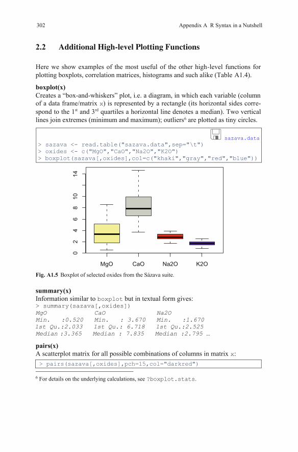
2.2 Additional High-level Plotting Functions
Here we show examples of the most useful of the other high-level functions for plotting boxplots, correlation matrices, histograms and such alike (Table A1.4).
boxplot(x) Creates a “box-and-whiskers” plot, i.e. a diagram, in which each variable (column of a data frame/matrix x) is represented by a rectangle (its horizontal sides corre-spond to the 1st and 3rd quartiles a horizontal line denotes a median). Two vertical lines join extremes (minimum and maximum); outliers6 are plotted as tiny circles.
sazava.data > sazava <- read.table("sazava.data",sep="\t") > oxides <- c("MgO","CaO","Na2O","K2O") > boxplot(sazava[,oxides],col=c("khaki","gray","red","blue"))
Fig. A1.5 Boxplot of selected oxides from the Sázava suite.
summary(x) Information similar to boxplot but in textual form gives: > summary(sazava[,oxides]) MgO CaO Na2O Min. :0.520 Min. : 3.670 Min. :1.670
1st Qu.:2.033 1st Qu.: 6.718 1st Qu.:2.525 Median :3.365 Median : 7.835 Median :2.795 …
pairs(x) A scatterplot matrix for all possible combinations of columns in matrix x: > pairs(sazava[,oxides],pch=15,col="darkred")
6 For details on the underlying calculations, see ?boxplot.stats.
MgO CaO Na2O K2O
02
46
810
14
302 Appendix A R Syntax in a Nutshell
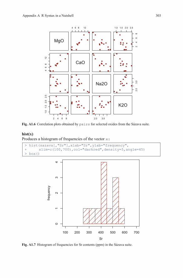
Fig. A1.6 Correlation plots obtained by pairs for selected oxides from the Sázava suite.
hist(x) Produces a histogram of frequencies of the vector x: > hist(sazava[,"Sr"],xlab="Sr",ylab="frequency", + xlim=c(100,700),col="darkred",density=5,angle=45) > box()
Fig. A1.7 Histogram of frequencies for Sr contents (ppm) in the Sázava suite.
MgO
4 6 8 12 1.0 1.5 2.0 2.5
24
68
46
812
CaO
Na2O
2.0
3.0
2 4 6 8
1.0
1.5
2.0
2.5
2.0 3.0
K2O
Sr
fre
qu
en
cy
100 200 300 400 500 600 700
01
23
4
Appendix A R Syntax in a Nutshell 303
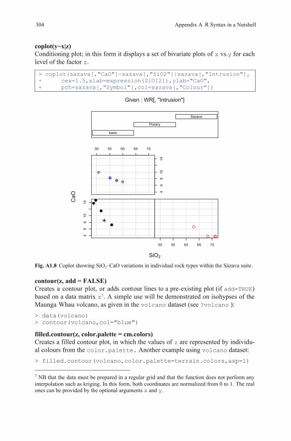
coplot(y~x|z) Conditioning plot; in this form it displays a set of bivariate plots of x vs.y for each level of the factor z.
> coplot(sazava[,"CaO"]~sazava[,"SiO2"]|sazava[,"Intrusion"],
Fig. A1.8 Coplot showing SiO2–CaO variations in individual rock types within the Sázava suite.
contour(z, add = FALSE) Creates a contour plot, or adds contour lines to a pre-existing plot (if add=TRUE) based on a data matrix z7. A simple use will be demonstrated on isohypses of the Maunga Whau volcano, as given in the volcano dataset (see ?volcano ): > data(volcano) > contour(volcano,col="blue")
filled.contour(z, color.palette = cm.colors) Creates a filled contour plot, in which the values of z are represented by individu-al colours from the color.palette. Another example using volcano dataset: > filled.contour(volcano,color.palette=terrain.colors,asp=1)
7 NB that the data must be prepared in a regular grid and that the function does not perform any interpolation such as kriging. In this form, both coordinates are normalized from 0 to 1. The real ones can be provided by the optional arguments x and y.
46
810
14
50 55 60 65 70
50 55 60 65 70
46
810
14
SiO2
Ca
O
basic
Pozary
Sazava
Given : WR[, "Intrusion"]
304 Appendix A R Syntax in a Nutshell
+ cex=1.5,xlab=expression(SiO[2]),ylab="CaO", + pch=sazava[,"Symbol"],col=sazava[,"Colour"])
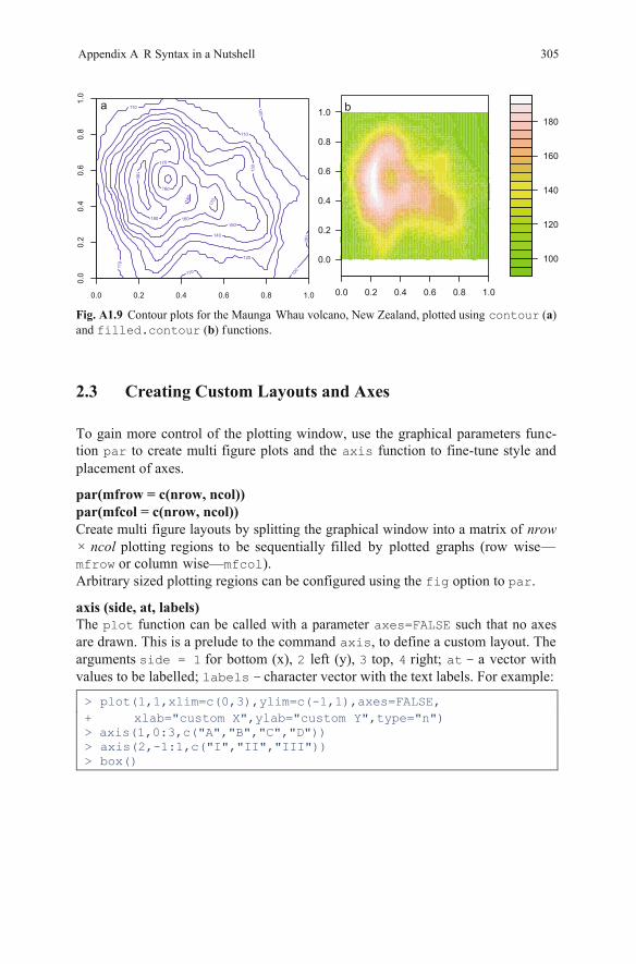
Fig. A1.9 Contour plots for the Maunga Whau volcano, New Zealand, plotted using contour (a) and filled.contour b) functions.
2.3 Creating Custom Layouts and Axes
To gain more control of the plotting window, use the graphical parameters func-tion par to create multi figure plots and the axis function to fine-tune style and placement of axes.
par(mfrow = c(nrow, ncol)) par(mfcol = c(nrow, ncol)) Create multi figure layouts by splitting the graphical window into a matrix of nrow × ncol plotting regions to be sequentially filled by plotted graphs (row wise—mfrow or column wise—mfcol). Arbitrary sized plotting regions can be configured using the fig option to par.
axis (side, at, labels) The plot function can be called with a parameter axes=FALSE such that no axes are drawn. This is a prelude to the command axis, to define a custom layout. The arguments side = 1 for bottom (x), 2 left (y), 3 top, 4 right; at – a vector with values to be labelled; labels – character vector with the text labels. For example:
> plot(1,1,xlim=c(0,3),ylim=c(-1,1),axes=FALSE, + xlab="custom X",ylab="custom Y",type="n") > axis(1,0:3,c("A","B","C","D")) > axis(2,-1:1,c("I","II","III")) > box()
100
120
140
160
180
0.0 0.2 0.4 0.6 0.8 1.0
0.0
0.2
0.4
0.6
0.8
1.0
100
100
10
0
110
110
110
110
120
13
0
140
150
160
160
170
170
180
180
19
0
0.0 0.2 0.4 0.6 0.8 1.0
0.0
0.2
0.4
0.6
0.8
1.0
a b
Appendix A R Syntax in a Nutshell 305
(
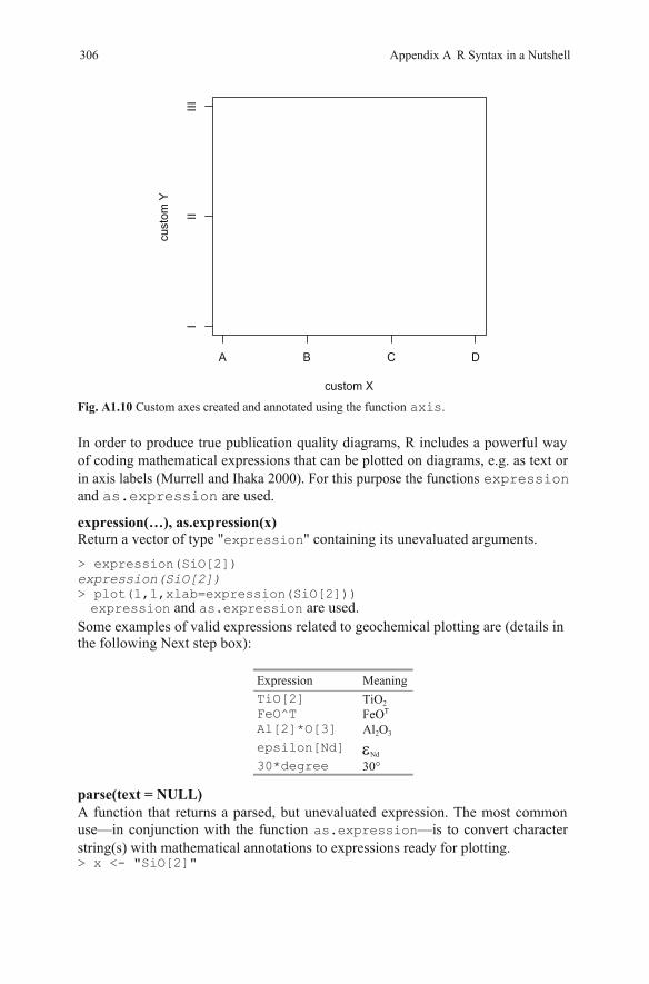
Fig. A1.10 Custom axes created and annotated using the function axis.
In order to produce true publication quality diagrams, R includes a powerful way of coding mathematical expressions that can be plotted on diagrams, e.g. as text or
expression and as.expression are used.
expression(…), as.expression(x) Return a vector of type "expression" containing its unevaluated arguments. > expression(SiO[2]) expression(SiO[2]) > plot(1,1,xlab=expression(SiO[2])) Some examples of valid expressions related to geochemical plotting are (details in the following Next step box):
Expression Meaning TiO[2] TiO2 FeO^T FeOT
Al[2]*O[3] Al2O3
epsilon[Nd] Nd
30*degree 30°
parse(text = NULL) A function that returns a parsed, but unevaluated expression. The most common use—in conjunction with the function as.expression—is to convert character string(s) with mathematical annotations to expressions ready for plotting. > x <- "SiO[2]"
custom X
A B C D
III
III
306 Appendix A R Syntax in a Nutshell
in axis labels (Murrell and Ihaka 2000). For this purpose the functions expressionand as.expression are used.
custo
m Y
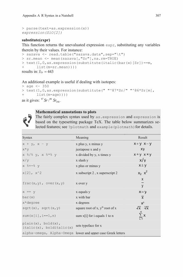
> parse(text=as.expression(x)) expression(SiO[2])
substitute(expr) This function returns the unevaluated expression expr, substituting any variables therein by their values. For instance: > sazava <- read.table("sazava.data",sep="\t") > sr.mean <- mean(sazava[,"Sr"],na.rm=TRUE) > text(1,0,as.expression(substitute(italic(bar(x)[Sr])==m, + list(m=sr.mean)))) results in: 443Srx An additional example is useful if dealing with isotopes: > age <- 350 > text(1,0,as.expression(substitute(" "^87*Sr/" "^86*Sr[m], + list(m=age))))
as it gives: 87 86350/Sr Sr .
Appendix A R Syntax in a Nutshell 307
Mathematical annotations to plots The fairly complex syntax used by as.expression and expression is based on the typesetting package TeX. The table below summarizes se-lected features; see ?plotmath and example(plotmath)for details.
Syntax Meaning Result x + y, x – y x plus y, x minus y x*y juxtapose x and y x %/% y, x %*% y x divided by y, x times y x/y x slash y x %+-% y x plus or minus y
x[2], x^2 x subscript 2 , x superscript 2
frac(x,y), over(x,y) x over y
x == y x equals y bar(x) x with bar x*degree x degrees sqrt(x), sqrt(x,y) square root of x, yth root of x
sum(x[i],i==1,n) sum x[i] for i equals 1 to n
plain(x), bold(x), italic(x), bolditalic(x) sets typeface for x
alpha–omega, Alpha–Omega
x y x y
xy
x ÷ y x × y
x yx y
x2 x2
x
y
x y
x
xx
yx
i 1
n
xi
lower and upper case Greek letters
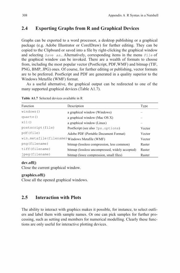
2.4 Exporting Graphs from R and Graphical Devices
Graphs can be exported to a word processor, a desktop publishing or a graphical package (e.g. Adobe Illustrator or CorelDraw) for further editing. They can be copied to the Clipboard or saved into a file by right-clicking the graphical window and selecting Save as… Alternatively, corresponding items in the menu File of the graphical window can be invoked. There are a wealth of formats to choose from, including the most popular vector (PostScript, PDF,WMF) and bitmap (TIF, PNG, BMP, JPG) ones. Of course, for further editing or publishing, vector formats are to be preferred. PostScript and PDF are generated in a quality superior to the Windows Metafile (WMF) format.
As a useful alternative, the graphical output can be redirected to one of the many supported graphical devices (Table A1.7).
Table A1.7 Selected devices available in R
Function Description Type windows() a graphical window (Windows) – quartz() a graphical window (Mac OS X) – x11() a graphical window (Linux) – postscript(file) PostScript (see also ?ps.options) Vector pdf(file) Adobe PDF (Portable Document Format) Vector win.metafile(filename)Windows Metafile (WMF) Vector png(filename) bitmap (lossless compression, less common) Raster tiff(filename) bitmap (lossless uncompressed, widely accepted) Raster jpeg(filename) bitmap (lossy compression, small files) Raster
dev.off() Close the current graphical window.
graphics.off() Close all the opened graphical windows.
2.5 Interaction with Plots
The ability to interact with graphics makes it possible, for instance, to select outli-ers and label them with sample names. Or one can pick samples for further pro-cessing, such as setting end members for numerical modelling. Clearly these func-tions are only useful for interactive plotting devices.
308 Appendix A R Syntax in a Nutshell
locator() The locator returns the coordinates of one or more points clicked on by the left mouse button. Identification is stopped by pressing the right mouse button and se-lecting Stop.
identify(x, y, labels) This function annotates the plot with labels for each given [x,y] coordinate. Usually only useful when there are a small number of data points.
Chapter 3 Programming in R This chapter deals with preparing R scripts to be run in batch mode. We shall learn to control the output to the screen and input from the keyboard, to build condition-al statements and loops as well as to program simple user-defined functions.
3.1 Input and Output
print(x) Prints the contents of an object x, nicely formatted.
cat(…, file="", sep="") This function displays the contents of one or more R objects in a less sophisticated way, but enabling much more control over the output format8: > x <- 5.8 > cat("The result is ",x," N/m.\n") The result is 5.8 N/m.
readline(prompt) Displays the prompt and then reads input from the keyboard: > x <- readline("Enter x:\n") Enter x: > 5.8 > x [1] "5.8"
This example shows that keyboard input is always in the form of a character vec-tor of length 1. If required it has to be coerced to a numeric value using the func-tion as.numeric: > x <- as.numeric(x) > x [1] 5.8
8Note that this function does not append a newline character that must be added explicitly to the output string as "\n".
Appendix A R Syntax in a Nutshell 309
3.2 Conditional Execution
Conditional execution of R code can be achieved using:
if(condition) expression1 else expression2 If condition evaluates to TRUE, expression1expression2 is run. Complicated commands may be grouped together in braces:
> x <- 6 > y <- 0.5 > if(x>2 & y<1){ > print(x) > print(y) > }else{ > cat("Warning, x<=2 or y>=1!\n") >}
3.3 Loops
Sometimes it is useful to run some chunk of code repetitively in a loop. Due to the powerful indexing in R, loops are needed considerably less often than in any con-ventional programming language. They can be built using the statement:
for(variable in expression1) expression2 expression2 is a chunk of R code, usually grouped in braces to be executed once for each of the values of the control variable. The range of possible values for the variable is specified by a vector, expression1. See the example, which calculates and prints the square roots of the sequence of numbers 1, 3, 5, 7, and 9:
> for(f in seq(1,10,by=2)){ > cat("Square root of",f,"is",sqrt(f),"\n") > } Square root of 1 is 1 Square root of 3 is 1.732051 Square root of 5 is 2.236068 Square root of 7 is 2.645751 Square root of 9 is 3
Try to avoid loops if possible. Their execution in R tends to be time con-suming and there are, usually, other alternatives. For instance here, thanks
to the recycling rules in R, we can write: > x <- seq(1,10,by=2) > ee <- paste("Square rootof",x,"is",sqrt(x),"\n") > cat(ee) Commands apply, tapply sapply (below) are commonly a better approach.
310 Appendix A R Syntax in a Nutshell
or
is executed, otherwise
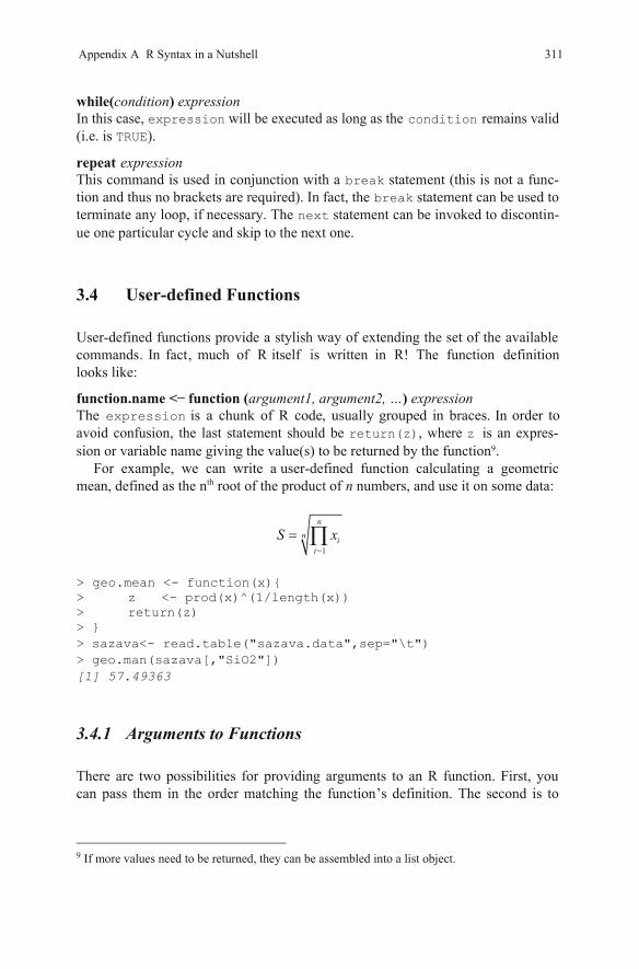
while(condition) expression In this case, expression will be executed as long as the condition remains valid (i.e. is TRUE).
repeat expression This command is used in conjunction with a break statement (this is not a func-tion and thus no brackets are required). In fact, the break statement can be used to terminate any loop, if necessary. The next statement can be invoked to discontin-ue one particular cycle and skip to the next one.
3.4 User-defined Functions
User-defined functions provide a stylish way of extending the set of the available commands. In fact, much of R itself is written in R! The function definitionlooks like:
function.name <– argument1, argument2, …) expression The expression is a chunk of R code, usually groupe d i n braces. order to avoid confusion, the last statement should be return(z), where z is an expres-sion or variable name giving the value(s) to be returned by the function9.
For example, we can write a user-defined function calculating a geometric mean, defined as the nth root of the product of n numbers, and use it on some data:
n
n ii
S x
> geo.mean <- function(x){ > z <- prod(x)^(1/length(x)) > return(z) > }
[1] 57.49363
3.4.1 Arguments to Functions
There are two possibilities for providing arguments to an R function. First, you can pass them in the order matching the function’s definition. The second is to
9 If more values need to be returned, they can be assembled into a list object.
Appendix A R Syntax in a Nutshell 311
> sazava<- read.table("sazava.data",sep="\t") > geo.man(sazava[,"SiO2"])
=1
In function (
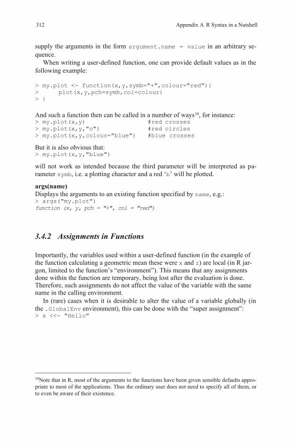
supply the arguments in the form argument.name = value in an arbitrary se-quence.
When writing a user-defined function, one can provide default values as in the following example:
> my.plot <- function(x,y,symb="+",colour="red"){ > plot(x,y,pch=symb,col=colour) > } And such a function then can be called in a number of ways10, for instance: > my.plot(x,y) #red crosses > my.plot(x,y,"o") #red circles > my.plot(x,y,colour="blue") #blue crosses
But it is also obvious that: > my.plot(x,y,"blue")
will not work as intended because the third parameter will be interpreted as pa-rameter symb, i.e. a plotting character and a red ‘b’ will be plotted.
args(name) Displays the arguments to an existing function specified by name, e.g.: > args("my.plot") function (x, y, pch = "+", col = "red")
3.4.2 Assignments in Functions
Importantly, the variables used within a user-defined function (in the example of the function calculating a geometric mean these were x and z) are local (in R jar-gon, limited to the function’s “environment”). This means that any assignments done within the function are temporary, being lost after the evaluation is done. Therefore, such assignments do not affect the value of the variable with the same name in the calling environment.
In (rare) cases when it is desirable to alter the value of a variable globally (in the .GlobalEnv environment), this can be done with the “super assignment”: > x <<- "Hello"
10Note that in R, most of the arguments to the functions have been given sensible defaults appro-priate to most of the applications. Thus the ordinary user does not need to specify all of them, or to even be aware of their existence.
312 Appendix A R Syntax in a Nutshell
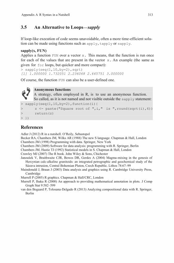
3.5 An Alternative to Loops
If loop-like execution of code seems unavoidable, often a motion can be made using functions such as apply,tapply or sapply.
sapply(x, FUN) Applies a function FUN over a vector x. This means, that the function is run once for each of the values that are present in the vector x. An example (the same asgiven for for > sapply(seq(1,10,by=2),sqrt) [1] 1.000000 1.732051 2.236068 2.645751 3.000000
Of course, the function FUN can also be a user-defined one.
Anonymous functions A strategy, often employed in R, is to use an anonymous function.
sapply statement: > sapply(seq(1,10,by=2),function(i){ > z <- paste("Square root of ",i," is ",round(sqrt(i),6)) > return(z) > })
Adler J (2012) R in a nutshell. O’Reily, Sebastopol Becker RA, Chambers JM, Wilks AR (1988) The new S language. Chapman & Hall, London Chambers JM (1998) Programming with data. Springer, New York Chambers JM (2009) Software for data analysis: programming with R. Springer, Berlin Chambers JM, Hastie TJ (1992) Statistical models in S. Chapman & Hall, London Crawley MJ (2007) The R book. John Wiley & Sons, Chichester Janoušek V, Braithwaite CJR, Bowes DR, Gerdes A (2004) Magma-mixing in the genesis of
Hercynian calc-alkaline granitoids: an integrated petrographic and geochemical study of the Sázava intrusion, Central Bohemian Pluton, Czech Republic. Lithos 78:67–99
Maindonald J, Braun J (2003) Data analysis and graphics using R. Cambridge University Press, Cambridge
Murrell P (2005) R graphics. Chapman & Hall/CRC, London Murrell P, Ihaka R (2000) An approach to providing mathematical annotation in plots. J Comp
Graph Stat 9:582–599 van den Bogaard P, Tolosana-Delgado R (2013) Analyzing compositional data with R. Springer,
Berlin
Appendix A R Syntax in a Nutshell 313
References
re time-efficient solu-
So called, as it is not named and not visible outside the
sapply—
loops, but quicker and more compact):
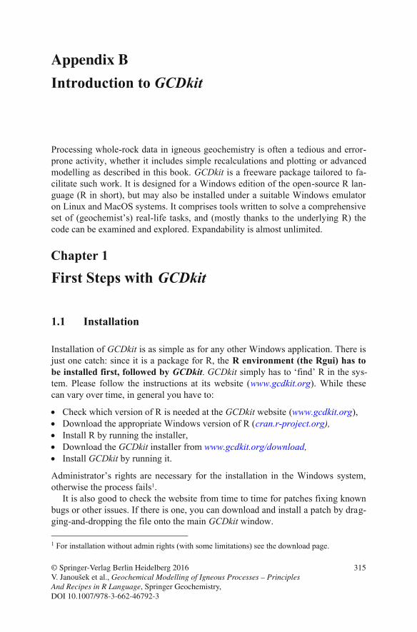
Appendix B
Processing whole-rock data in igneous geochemistry is often a tedious and error-prone activity, whether it includes simple recalculations and plotting or advanced modelling as described in this book. GCDkit is a freeware package tailored to fa-cilitate such work. It is designed for a Windows edition of the open-source R lan-guage (R in short), but may also be installed under a suitable Windows emulator on Linux and MacOS systems. It comprises tools written to solve a comprehensive set of (geochemist’s) real-life tasks, and (mostly thanks to the underlying R) the code can be examined and explored. Expandability is almost unlimited.
Chapter 1
First Steps with GCDkit
1.1 Installation
Installation of GCDkit is as simple as for any other Windows application. There is just one catch: since it is a package for R, the R environment (the Rgui) has to be installed first, followed by GCDkit. GCDkit simply has to ‘find’ R in the sys-tem. Please follow the instructions at its website (www.gcdkit.org). While these can vary over time, in general you have to:
Check which version of R is needed at the GCDkit website (www.gcdkit.org), Download the appropriate Windows version of R (cran.r-project.org), Install R by running the installer, Download the GCDkit installer from www.gcdkit.org/download, Install GCDkit by running it.
Administrator’s rights are necessary for the installation in the Windows system, otherwise the process fails1.
It is also good to check the website from time to time for patches fixing known bugs or other issues. If there is one, you can download and install a patch by drag-ging-and-dropping the file onto the main GCDkit window. 1 For installation without admin rights (with some limitations) see the download page.
© Springer-Verlag Berlin Heidelberg 2016 V. Janoušek et al., Geochemical Modelling of Igneous Processes – Principles And Recipes in R Language, Springer Geochemistry, DOI 10.1007/978-3-662-46792-3
315
Introduction to GCDkit
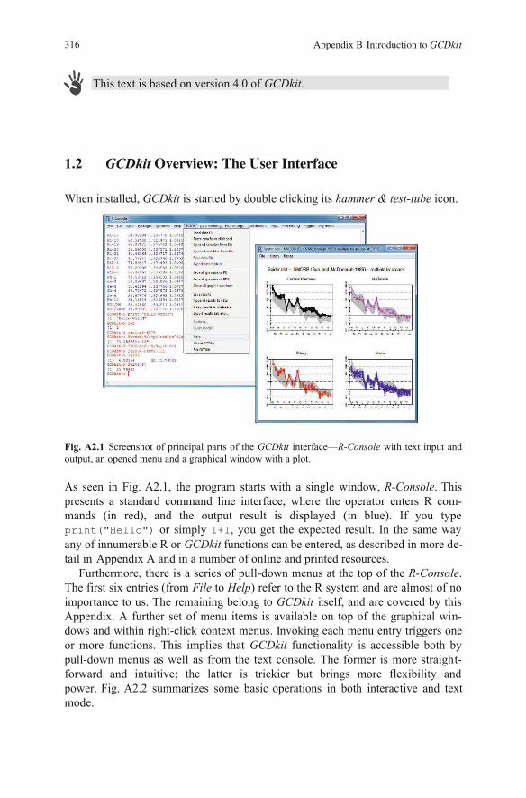
This text is based on version 4.0 of GCDkit.
1.2 GCDkit Overview: The User Interface
When installed, GCDkit is started by double clicking its hammer & test-tube icon.
Fig. A2.1 Screenshot of principal parts of the GCDkit interface—R-Console with text input and output, an opened menu and a graphical window with a plot.
As seen in Fig. A2.1, the program starts with a single window, . This presents a standard command line interface, where the operator enters R com-mands (in red), and the output result is displayed (in blue). If you type print("Hello") or simply 1+1, you get the expected result. In the same way any of innumerable R or functions can be entered, as described in more de-tail in Appendix A and in a number of online and printed resources.
Furthermore, there is a series of pull-down menus at the top of the R-Console. The first six entries (from File to Help) refer to the R system and are almost of no importance to us. The remaining belong to GCDkit itself, and are covered by this Appendix. A further set of menu items is available on top of the graphical win-dows and within right-click context menus.or more functions. This implies that GCDkit functionality is accessible both by pull-down menus as well as from the text console. The former is more straight-forward and intuitive; the latter is trickier but brings more flexibility and power. Fig. A2.2 summarizes some basic operations in both interactive and text mode.
316 Appendix B Introduction to GCDkit
R-Console
GCDkit
Invoking each menu entry triggers one
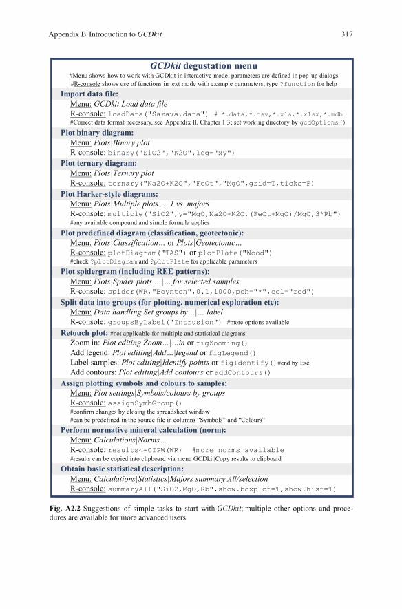
Fig. A2.2 Suggestions of simple tasks to start with GCDkit; multiple other options and proce-dures are available for more advanced users.
GCDkit degustation menu
#Menu shows how to work with GCDkit in interactive mode; parameters are defined in pop-up dialogs
#R-console shows use of functions in text mode with example parameters; type ?function for help
Import data file:
Menu: GCDkit|Load data file
R-console: loadData("Sazava.data") # *.data,*.csv,*.xls,*.xlsx,*.mdb
#Correct data format necessary, see Appendix II, Chapter 1.3; set working directory by gcdOptions()
Plot binary diagram:
Menu: Plots|Binary plot
R-console: binary("SiO2","K2O",log="xy")
Plot ternary diagram:
Menu: Plots|Ternary plot
R-console: ternary("Na2O+K2O","FeOt","MgO",grid=T,ticks=F)
Plot Harker-style diagrams:
Menu: Plots|Multiple plots …|1 vs. majors
R-console: multiple("SiO2",y="MgO,Na2O+K2O,(FeOt+MgO)/MgO,3*Rb")
#any available compound and simple formula applies
Plot predefined diagram (classification, geotectonic):
Menu: Plots|Classification… or Plots|Geotectonic…
R-console: plotDiagram("TAS") or plotPlate("Wood")
#check ?plotDiagram and ?plotPlate for applicable parameters
Plot spidergram (including REE patterns):
Menu: Plots|Spider plots …|… for selected samples
R-console: spider(WR,"Boynton",0.1,1000,pch="*",col="red")
Split data into groups (for plotting, numerical exploration etc):
Menu: Data handling|Set groups by…|… label
R-console: groupsByLabel("Intrusion") #more options available
Retouch plot: #not applicable for multiple and statistical diagrams
Zoom in: Plot editing|Zoom…|…in or figZooming()
Add legend: Plot editing|Add…|legend or figLegend()
Label samples: Plot editing|Identify points or figIdentify()#end by Esc
Add contours: Plot editing|Add contours or addContours()
Assign plotting symbols and colours to samples:
Menu: Plot settings|Symbols/colours by groups
R-console: assignSymbGroup()
#confirm changes by closing the spreadsheet window
#can be predefined in the source file in columns “Symbols” and “Colours”
Perform normative mineral calculation (norm):
Menu: Calculations|Norms…
R-console: results<-CIPW(WR) #more norms available
#results can be copied into clipboard via menu GCDkit|Copy results to clipboard
Obtain basic statistical description:
Menu: Calculations|Statistics|Majors summary All/selection
R-console: summaryAll("SiO2,MgO,Rb",show.boxplot=T,show.hist=T)
317Appendix B Introduction to GCDkit
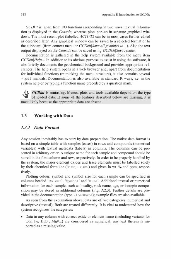
GCDkit is (apart from I/O functions) responding in two ways: textual informa-tion is displayed in the Console, whereas plots pop-up in separate graphical win-dows. The most recent plot (labelled ACTIVE) can be in most cases further edited as described later. Any graphical window can be saved to a selected format or to the clipboard (from context menu or GCDkit|Save all graphics to…). Also the text output displayed on the Console can be saved using GCDkit|Save results.
Documentation is gathered in the help system available from the menu item GCDkit|Help… In addition to its obvious purpose to assist in using the software, it also briefly documents the geochemical background and provides appropriate ref-erences. The help system opens in a web browser an from documentationfor individual functions (mimicking the menu structure), it also contains several *.pdf manuals. Documentation is also available in standard R ways, i.e. in the system help or by typing a function name preceded by a question mark.
GCDkit is mutating. Menus, plots and tools available depend on the type of loaded data. If some of the features described below are missing, it is
most likely because the appropriate data are absent.
1.3 Working with Data
1.3.1 Data Format
As seen from the explanation above, data are of two categories: numerical and descriptive (textual). Both are treated differently. It is vital to understand how the system recognizes the categories:
Data in any column with correct oxide or element name (including variants for total Fe, H2O+, Mg#...) are considered as numerical; any text therein is im-ported as a missing value.
318 Appendix B Introduction to GCDkit
d, apart
Any session inevitably has to start by data preparation. The native data format is based on a simple table with samples (cases) in rows and compounds (numerical variables) with textual metadata (labels) in columns. The columns can be pre-sented in arbitrary order. A unique name for each sample and compound should be stored in the first column and row, respectively. In order to be properly handled by the system, the major-element oxides and trace elements must be labelled solely by their chemical formulae (SiO2, Sr etc.) and given in wt. % and ppm, respec-tively.
Plotting colour, symbol and symbol size for each sample can be specified in columns headed ‘Colour’, ‘Symbol’ and ‘Size’. Additional textual or numerical information for each sample, such as locality, rock name, age, or isotopic compo-sition may be stored in additional columns (Fig. A2.3). Further details are pro-vided in the documentation (type ?loadData); example files are also available.
Data in columns labelled ‘Symbol’, ‘Colour’ and ‘Size’ are considered as
Data in any other column containing at least some text (except permitted strings for missing values) are treated as textual (descriptive). Data in any other column containing strictly numbers (with, or without, permit-ted strings for missing values) are treated as numerical.
Fig. A2.3 Commented example of a correctly formatted input file.
Some common formatting mistakes are highlighted in Fig. A2.4. There are no doubt many more possibilities to spoil the input; this is a field of unlimited crea-tivity.
In the following text and in GCDkit, Variable refers to the name of a col-umn (and the data within it) recognized as numerical. Label is a term re-
served for names of the remaining descriptive columns.
1.3.2 Loading Data
There are several ways of introducing data into GCDkit. The basic one leads through menu GCDkit|Load data file, which invokes a file selection dialogue to find the desired *.data file (and other formats). However, more popular has
Major elements
(oxide
w ight percent)e
Labels for
·
structurally
bound water:
H2O.PLUS, H2OPLUS,
H2O_PLUS,H2OP, H2O+
Other
numerical data
(numbers only)
#
comment sign:
whole row will
be ignored
Unique names
of columns
(numerical
and descriptive)
Unique sample
names
(all allowed
characters)
Descriptive
properties
(at least
some text)
Plotting symbol
properties
(Symbol,
Colour, Size)
total Fe
as ferrous oxide:
· FeOt or FeO*‘ ’ ‘ ’
values below
detection limit:
<0.1
-0.1 (optionally)
Other
numerical data
(not used
internally as total)
All allowed
expressions
of missing
value
Special
symbols in texts
not recommended
Trace elements
(ppm)
319Appendix B Introduction to GCDkit
symbol plotting parameters (this Appendix, Sect.1.4.1).
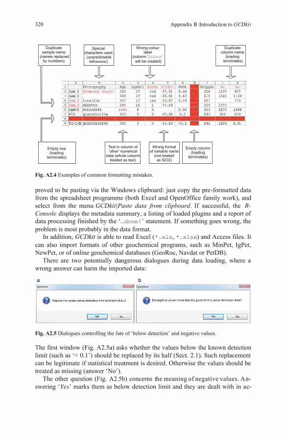
Fig. A2.4 Examples of common formatting mistakes. proved to be pasting via the Windows clipboard: just copy the pre-formatted data from the spreadsheet programme (both Excel and OpenOffice family work), and
GCDkit|Paste data from clipboard. If successful, the R-Console displays the metadata summary, a listing of loaded plugins and a report of data processing finished by the ‘…done!’ statement. If something goes wrong, the problem is most probably in the data format.
In addition, GCDkit is able to read Excel (*.xls, *.xlsx) and Access files. It can also import formats of other geochemical programs, such as MinPet, IgPet, NewPet, or of online geochemical databases (GeoRoc, Navdat or PetDB).
There are two potentially dangerous dialogues during data loading, where a wrong answer can harm the imported data:
Fig. A2.5 Dialogues controlling the fate of ‘below detection’ and negative values.
The first window (Fig. A2.5a) asks whether the values below the known detection limit (such as ‘< 0.1’) should be replaced by its half (Sect. 2.1). Such replacement can be legitimate if statistical treatment is desired. Otherwise the values should be treated as missing (answer ‘No’).
The other question (Fig. A2.5b) concernsswering ‘ ’ marks them as below detection limit and they are dealt with in ac-
Duplicate
column name
(loading
terminates)
Empty row
(loading
terminates)
Empty column
(loading
terminates)
Wrong format
of variable name
(not treated
as SiO2)
Special
characters used
(unpredictable
behaviour)
Wrong colour
label
(column ’ ’
will be created)
Colour
Text in column of
‘other’ numerical
data (whole column
treated as text)
Duplicate
sample name
(names replaced
by numbers)
320 Appendix B Introduction to GCDkit
select from the menu
Yes the meaning of negative values. An-
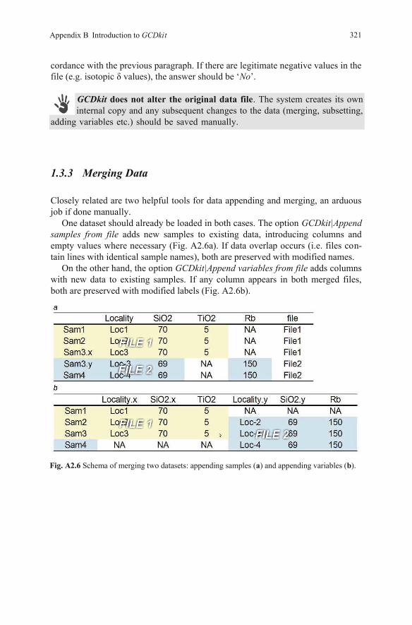
cordance with the previous paragraph. If there are legitimate negative values in the file (e.g. isotopic ), the answer should be ‘No’.
GCDkit does not alter the original data file. The system creates its own internal copy and any subsequent changes to the data (merging, subsetting,
adding variables etc.) should be saved manually.
1.3.3 Merging Data
Closely related are two helpful tools for data appending and merging, an arduous job if done manually.
One dataset should already be loaded in both cases. The option GCDkit|Append samples from file adds new samples to existing data, introducing columns and empty values where necessary (Fig. A2.6a). If data overlap occurs (i.e. files con-tain lines with identical sample names), both are preserved with modified names.
On the other hand, the option GCDkit|Append variables from file adds columns with new data to existing samples. If any column appears in both merged files, both are preserved with modified labels (Fig. A2.6b).
321
Fig. A2.6 Schema of merging two datasets: appending samples (a) and appending variables (b).
Appendix B Introduction to GCDkit
values
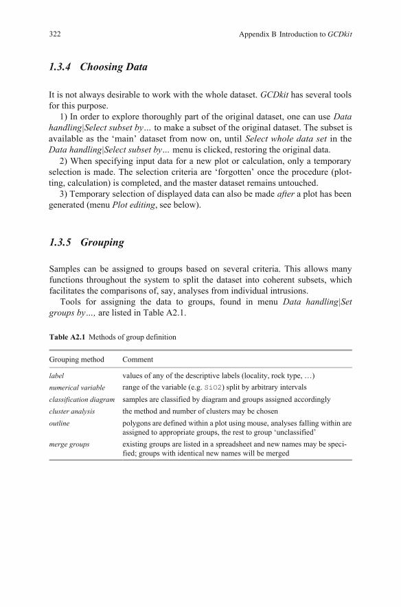
1.3.5 Grouping
Samples can be assigned to groups based on several criteria. This allows many functions throughout the system to split the dataset into coherent subsets, which facilitates the comparisons of, say, analyses from individual intrusions.
Tools for assigning the data to groups, found in menu Data handling|Set groups by…, are listed in Table A2.1.
Table A2.1 Methods of group definition
Grouping method Comment
label values of any of the descriptive labels (locality, rock type, …) numerical variable range of the variable (e.g. SiO2) split by arbitrary intervals classification diagram samples are classified by diagram and groups assigned accordingly cluster analysis the method and number of clusters may be chosen outline polygons are defined within a plot using mouse, analyses falling within are
assigned to appropriate groups, the rest to group ‘unclassified’ merge groups existing groups are listed in a spreadsheet and new names may be speci-
fied; groups with identical new names will be merged
322
1.3.4 Choosing Data
It is not always desirable to work with the whole dataset. GCDkit has several tools for this purpose.
1) In order to explore thoroughly part of the original dataset, one can use Data handling|Select subset by… to make a subset of the original dataset. The subset is
available as the ‘main’ dataset from now on, until Select whole data set in the Data handling|Select subset by… menu is clicked, restoring the original data.
2) When specifying input data for a new plot or calculation, only a temporary selection is made. The selection criteria are ‘forgotten’ once the procedure (plot-ting, calculation) is completed, and the master dataset remains untouched.
3) Temporary selection of displayed data can also be made after a plot has been generated (menu Plot editing, see below).
Appendix B Introduction to GCDkit
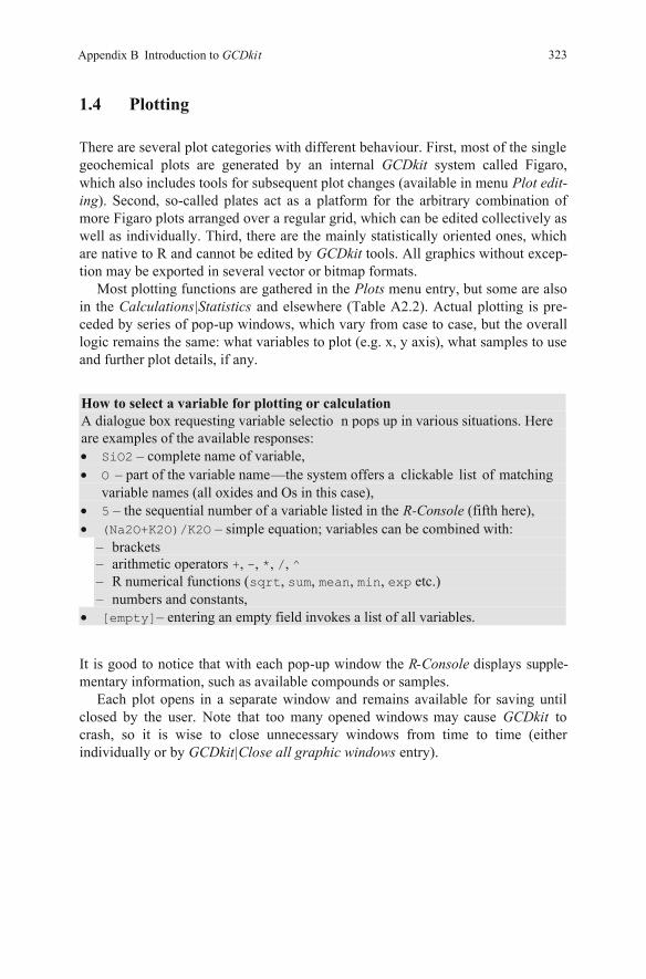
which also includes tools for subsequent plot changes (available in menu Plot edit-ing). Second, so-called plates act as a platform for the arbitrary combination of more Figaro plots arranged over a regular grid, which can be edited collectively as well as individually. Third, there are the mainly statistically oriented ones, which are native to R and cannot be edited by GCDkit tools. All graphics without excep-tion may be exported in several vector or bitmap formats.
Most plotting functions are gathered in the Plots menu entry, but some are also in the Calculations|Statistics and elsewhere (Table A2.2). Actual plotting is pre-ceded by series of pop-up windows, which vary from case to case, but the overall logic remains the same: what variables to plot (e.g. x, y axis), what samples to use and further plot details, if any.
How to select a variable for plotting or calculation A dialogue box requesting variable selectio n pops up in various situations. Here are examples of the available responses:
SiO2 – complete name of variable, O – part of the variable name—the system offers a clickable list of matching variable names (all oxides and Os in this case), 5 – the sequential number of a variable listed in the R-Console (fifth here), (Na2O+K2O)/K2O – simple equation; variables can be combined with:
– brackets – arithmetic operators +, -, *, /, ^ – R numerical functions (sqrt, sum, mean, min, exp etc.) – numbers and constants, [empty]– entering an empty field invokes a list of all variables.
It is good to notice that with each pop-up window the R -Console displays supple-mentary information, such as available compounds or samples.
Each plot opens in a separate window and remains available for saving until closed by the user. Note that too many opened windows may cause GCDkit to crash, so it is wise to close unnecessary windows from time to time (either individually or by GCDkit|Close all graphic windows entry).
323Appendix B Introduction to GCDkit
1.4 Plotting
There are several plot categories with different behaviour. First, most of the single geochemical plots are generated by an internal GCDkit system called Figaro,
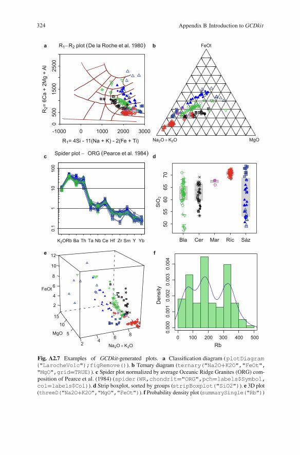
324 Appendix B Introduction to GCDkit
-1000 0 1000 2000 3000
050
015
0025
00R1 R2 plot De la Roche et al. 1980
R1= 4Si - 11(Na + K) - 2(Fe + Ti)
R2=
6C
a +
2Mg
+Al
2O K2O MgONa
FeOt
Spider plot ORG Pearce et al. 1984
K2ORb Ba Th Ta Nb Ce Hf Zr Sm Y Yb
0.1
110
100
Bla Cer Mar Ríc Sáz
5055
6065
70Si
O2
24 6 85
10
15
2
4
6
8
10
12
2O K2O
MgO
Na
FeOt
Rb
Den
sity
0 100 200 300 400 500
0.00
00.
001
0.00
20.
003
0.00
4
a b
dc
fe
("LarocheVolc"); move()). b ternary("Na2O+K2O","FeOt","MgO",grid=TRUE)). c Spider plot normalized by average Oceanic Ridge Granites (ORG) com-position of Pearce et al. (1984) (spider(WR,chondrit="ORG",pch=labels$Symbol,col=labels$Col)). d Strip boxplot, sorted by groups (stripBoxplot("SiO2")). e 3D plot(threeD("Na2O+K2O","MgO","FeOt")). f Probability density plot (summarySingle("Rb"))
figRe Ternary diagram (Fig. A2.7 Examples of GCDkit-generated plots. a plotDiagramClassification diagram (
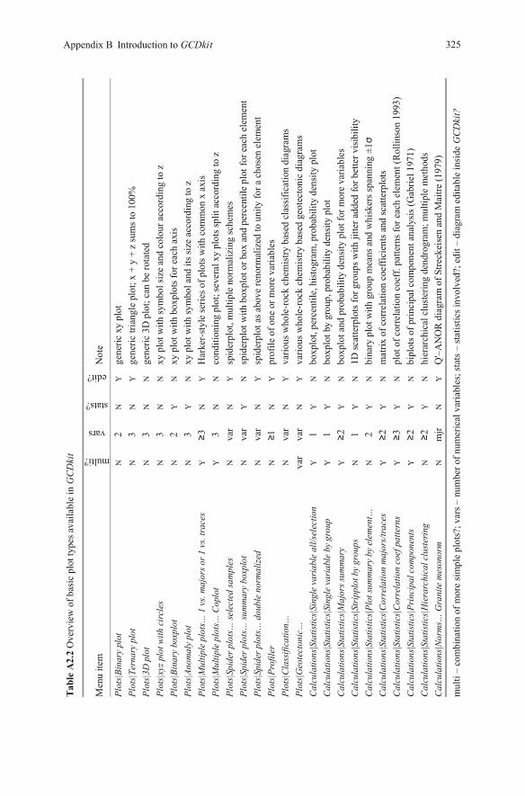
Ta
ble
A2.
2 O
verv
iew
of b
asic
plo
t typ
es a
vaila
ble
in G
CD
kit
Men
u ite
m
multi?
vars
stats?
edit?
Not
e
Plot
s|Bin
ary
plot
N
2
N
Y
gene
ric x
y pl
ot
Plot
s|Ter
nary
plo
t N
3
N
Y
gene
ric tr
iang
le p
lot;
x +
y +
z su
ms t
o 10
0%
Plot
s|3D
plo
t N
3
N
N
gene
ric 3
D p
lot;
can
be ro
tate
d Pl
ots|x
yz p
lot w
ith c
ircl
es
N
3 N
N
xy
plo
t with
sym
bol s
ize
and
colo
ur a
ccor
ding
to z
Pl
ots|B
inar
y bo
xplo
t N
2
Y
N
xy p
lot w
ith b
oxpl
ots f
or e
ach
axis
Pl
ots|A
nom
aly
plot
N
3
Y
N
xy p
lot w
ith sy
mbo
l and
its s
ize
acco
rdin
g to
z
Plot
s|Mul
tiple
plo
ts… 1
vs.
maj
ors o
r 1 v
s. tr
aces
Y
3
N
Y
Har
ker-
styl
e se
ries o
f plo
ts w
ith c
omm
on x
axi
s Pl
ots|M
ultip
le p
lots…
Cop
lot
Y
3 N
N
co
nditi
onin
g pl
ot; s
ever
al x
y pl
ots s
plit
acco
rdin
g to
z
Plot
s|Spi
der p
lots…
sele
cted
sam
ples
N
va
r N
Y
sp
ider
plot
, mul
tiple
nor
mal
izin
g sc
hem
es
Plot
s|Spi
der p
lots…
sum
mar
y bo
xplo
t N
va
r Y
N
sp
ider
plot
with
box
plot
or b
ox a
nd p
erce
ntile
plo
t for
eac
h el
emen
t Pl
ots|S
pide
r plo
ts… d
oubl
e no
rmal
ized
N
va
r N
Y
sp
ider
plot
as a
bove
reno
rmal
ized
to u
nity
for a
cho
sen
elem
ent
Plot
s|Pro
filer
N
1
N
Y
prof
ile o
f one
or m
ore
varia
bles
Pl
ots|C
lass
ifica
tion…
N
va
r N
Y
va
rious
who
le-r
ock
chem
istry
bas
ed c
lass
ifica
tion
diag
ram
s Pl
ots|G
eote
cton
ic…
va
r va
r N
Y
va
rious
who
le-r
ock
chem
istry
bas
ed g
eote
cton
ic d
iagr
ams
Cal
cula
tions
|Sta
tistic
s|Sin
gle
varia
ble
all/s
elec
tion
Y
1 Y
N
bo
xplo
t, pe
rcen
tile,
his
togr
am, p
roba
bilit
y de
nsity
plo
t C
alcu
latio
ns|S
tatis
tics|S
ingl
e va
riabl
e by
gro
up
Y
1 Y
N
bo
xplo
t by
grou
p, p
roba
bilit
y de
nsity
plo
t C
alcu
latio
ns|S
tatis
tics|M
ajor
s sum
mar
y Y
2
Y
N
boxp
lot a
nd p
roba
bilit
y de
nsity
plo
t for
mor
e va
riabl
es
Cal
cula
tions
|Sta
tistic
s|Str
ippl
ot b
y gr
oups
N
1
Y
N
1D sc
atte
rplo
ts fo
r gro
ups w
ith ji
tter a
dded
for b
ette
r vis
ibili
ty
Cal
cula
tions
|Sta
tistic
s|Plo
t sum
mar
y by
ele
men
t…
N
2 Y
N
bi
nary
plo
t with
gro
up m
eans
and
whi
sker
s spa
nnin
g ±1
C
alcu
latio
ns|S
tatis
tics|C
orre
latio
n m
ajor
s/tra
ces
Y
2 Y
N
m
atrix
of c
orre
latio
n co
effic
ient
s and
scat
terp
lots
C
alcu
latio
ns|S
tatis
tics|C
orre
latio
n co
ef p
atte
rns
Y
3 Y
N
pl
ot o
f cor
rela
tion
coef
f. pa
ttern
s for
eac
h el
emen
t (R
ollin
son
1993
) C
alcu
latio
ns|S
tatis
tics|
Prin
cipa
l com
pone
nts
Y
2 Y
N
bi
plot
s of p
rinci
pal c
ompo
nent
ana
lysi
s (G
abrie
l 197
1)
Cal
cula
tions
|Sta
tistic
s|Hie
rarc
hica
l clu
sterin
g N
2
Y
N
hier
arch
ical
clu
ster
ing
dend
rogr
am; m
ultip
le m
etho
ds
Cal
cula
tions
|Nor
ms…
Gra
nite
mes
onor
m
N
mjr
N
Y
Q'–
AN
OR
dia
gram
of S
treck
eise
n an
d M
aitre
(197
9)
mul
ti –
com
bina
tion
of m
ore
sim
ple
plot
s?; v
ars –
num
ber o
f num
eric
al v
aria
bles
; sta
ts –
stat
istic
s inv
olve
d?; e
dit –
dia
gram
edi
tabl
e in
side
GCD
kit?
325Appendix B Introduction to GCDkit
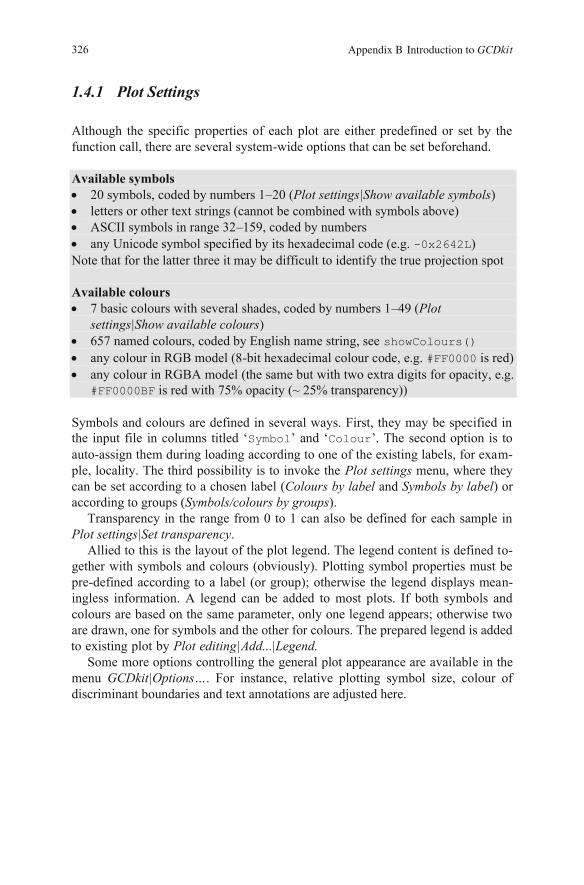
1.4.1 Plot Settings
Although the specific properties of each plot are either predefined or set by the function call, there are several system-wide options that can be set beforehand.
Available symbols 20 symbols, coded by numbers 1–20 (Plot settings|Show available symbols) letters or other text strings (cannot be combined with symbols above) ASCII symbols in range 32–159, coded by numbers any Unicode symbol specified by its hexadecimal code (e.g. -0x2642L)
Note that for the latter three it may be difficult to identify the true projection spot Available colours
7 basic colours with several shades, coded by numbers 1–49 (Plot settings|Show available colours) 657 named colours, coded by English name string, see showColours() any colour in RGB model (8-bit hexadecimal colour code, e.g. #FF0000 is red) any colour in RGBA model (the same but with two extra digits for opacity, e.g. #FF0000BF is red with 75% opacity (~ 25% transparency))
Symbols and colours are defined in several ways. First, they may be specified in the input file in columns titled ‘Symbol’ and ‘Colour’. The second option is to auto-assign them during loading according to one of the existing labels, for exam-ple, locality. The third possibility is to invoke the Plot settings menu, where they can be set according to a chosen label (Colours by label and Symbols by label) or according to groups (Symbols/colours by groups).
Transparency in the range from 0 to 1 can also be defined for each sample in Plot settings|Set transparency.
Allied to this is the layout of the plot legend. The legend content is defined to-gether with symbols and colours (obviously). Plotting symbol properties must be pre-defined according to a label (or group); otherwise the legend displays mean-ingless information. A legend can be added to most plots. If both symbols and colours are based on the same parameter, only one legend appears; otherwise two are drawn, one for symbols and the other for colours. The prepared legend is added
Some more options controlling the general plot appearance are available in the menu GCDkit Options…. For instance, relative plotting symbol size, colour of discriminant boundaries and text annotations are adjusted here.
326 Appendix B Introduction to GCDkit
to existing plot by lot editing Add... Legend.P | |
|
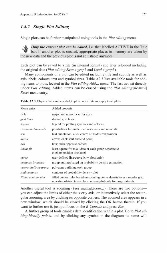
1.4.2 Single Plot Editing
Single plots can be further manipulated using tools in the Plot editing menu.
Only the current plot can be edited, i.e. that labelled ACTIVE in the Title bar. If another plot is created, appropriate places in memory are taken by
the new data and the previous plot is not adjustable anymore.
Each plot can be saved to a file (in internal format) and later reloaded including the original data (Plot editing|Save a graph and Load a graph).
Many components of a plot can be edited including title and subtitle as well as axis labels, colours, text and symbol sizes. Table A2.3 lists available tools for add-ing items to plots, located in the Plot editing|Add… menu. The last two sit directly under Plot editing. Added items can be erased using the Plot editing RedrawReset menu entry.
Table A2.3 Objects that can be added to plots; not all items apply to all plots
Menu entry Added property
ticks major and minor ticks for axes grid lines dashed grid lines legend legend for plotting symbols and colours reservoirs/minerals points/lines for predefined reservoirs and minerals text text annotation; click centre of its desired position arrow arrow; click start and end point box box; click opposite corners linear fit least-square fit; to all data or each group separately;
click to position line label curve user-defined line/curve (x–y plots only) contours by group group outlines based on probability density estimation convex hulls by group polygons outlining each group Add contours contours of probability density plot Filled contour plot filled contour plot based on counting points density over a regular grid;
no extrapolation takes place; meaningful only for large datasets
Another useful tool is zooming (Plot editing|Zoom…). There are two options—you can adjust the limits of either the x or y axis, or interactively select the rectan-gular zooming area by clicking its opposite corners. The zoomed area appears in a new window, which should be closed by clicking the OK button therein. If you want to further use it, just put focus on the R-Console and press Esc.
A further group of tools enables data identification within a plot. Go to Plot ed-iting|Identify points, and by clicking any symbol in the diagram its name will
327Appendix B Introduction to GCDkit
| |
show up. The Select samples and Highlight multiple points selections in turn show (or highlight) points chosen by the standard selection procedure.
1.4.3 Plates and Plate Editing
Plates are collections of plots in a single window/on a single sheet. Their charm rests in the fact that plots can be created and edited individually as well as collec-tively.
Whereas plates can be built automatically, as are, for example, most geotec-tonic diagrams or all Harker plots, they can also easily be constructed from scratch. Menu entry Plots|Plate of several plots defines an empty grid of rows and col-umns. Right-clicking the context menu GCDkit plate|Select slot activates a red rectangle highlighting the “active” slot, which moves together with the cursor. The selection is confirmed with a left-click, and the rectangle colour becomes ochre. Fill the slot with the desired graphics from the GCDkit plate|Introduce plot menu option. Several plots are available (Binary plot, Ternary plot, Spiderplot and Clas-sification diagram); a particularly convenient technique here is to introduce a pre-viously prepared and saved plot in internal format (Load a saved graph).
The existing plate can be further edited, either each plot individually using tools described above (accessed by the Plot editing entry in the context menu), or all plots together (Plate editing). The latter entry contains several exporting op-tions, tools for axis, plotting symbol and colours editing (and unification) and for text annotations removal.
1.4.4 Spiderplots
Apart from the standard multi-element diagram (spiderplot) there are several ad-vanced variants (Sect. 4.2). Instead of individual samples, fields for predefined groups, spider boxplots or spider box and percentile plots can be drawn. Also double-normalized plots are available: once normalized data are re-normalizedby the content of one—normally the least incompatible—element, and all the patterns intercept here. Further options, such as combination of shaded fields with individual patterns, can be set up from the command line. See exam-and help(spider). Normalization data can be inspected and edited in a text file,see this Appendix, Sect. 2.4 for details. The usage of standard spiderplots is discussedin Sect. 3.6. of the main text.
Another useful option is to normalize using a sample chosen from the dataset or average of selected samples.
328 Appendix B Introduction to GCDkit
ple(spider)
1.4.5 Classification and Geotectonic Diagrams
Descriptive geochemistry of igneous rocks traditionally employs numerous classi-fication diagrams. Whereas some are easy to implement numerically (i.e. Shand’s AN/K–ACN/K diagram), other use empirical or even curved field boundaries and a graphical approach is the only feasible solution.
GCDkit contains a series of Figaro-based classification templates, which can be employed for plotting as well as (automatic) sample classification. The list of available diagrams is accessible from Plots|Classification… (the actual possibili-ties depending on available data). The classification is to be found at Data han-dling|Classify… Results can be appended to labels or treated otherwise as de-scribed later (Sect. 1.6, this Appendix). Classification may also be used for data grouping (Data handling|Set groups by… |… diagram).
Furthermore, GCDkit also contains a set of geotectonic diagrams, available from menu Plots|Geotectonic…. Whereas these may resemble classification plots, there is one crucial difference: geotectonic diagrams are in all cases designed as a hint for geotectonic considerations rather than for authoritative determination of palaeotectonic setting. This is why the option for ‘classification’ using geotectonic diagrams is (intentionally) disabled. Both types of diagrams are also discussed in
Read the original paper. This general rule is particularly important here: each classification diagram has its limits and application rules specified.
These guidelines cannot be fully followed by the classification routine, and the results can thus be misleading albeit numerically correct. References for each dia- gram can be found in GCDkit help, or in the file GCDkit/doc/diagrams.pdf
library folder.
1.5 Calculations
Numerous calculation routines are the real core of GCDkit. Calculated data are displayed in the Console and stored internally (in the variable results). From here they can be inspected, exported or appended to data (GCDkit|Append results to data), i.e. stored for any subsequent calculations and plotting.
Some calculations are performed automatically during data loading. Depending on the data available in the file, some elemental abundances and basic indexes are computed (K, Ti, P, FeOt, mg#, Mg#, A/NK, A/CNK, K2O/Na2O). All are ap-pended to the main data table WR. Majors recalculated to anhydrous basis are stored in WRanh, and recast to millications (milli; Sect. 2.2.2, main text).
329Appendix B Introduction to GCDkit
your R
the main text (sections 3.4 and 3.5).
in
Within the Calculation menu are available several normative and related schemes as summarized in Table A2.4. Calculations|Statistics offers several vari-ants of descriptive statistics together with graphical presentation.
Table A2.4 Main calculation routines
Required action Solution Summary statistics* for one variable Calculations|Statistics…|Single variable… Compare summary statistics* of single Calculations|Statistics…|Single variable by group
Compare data ranges between groups Calculations|Statistics…|Ranges by groups Summary statistics* for more variables Calculations|Statistics…|Majors summary Compare summary statistics* of more Calculations|Statistics…|Majors summary by group
Correlation coefficients matrix Calculations|Statistics…|Correlation: majors (in graphical form)
Principal components Calculations|Statistics…|Principal components CIPW norm Calculations|Norms…|CIPW CIPW norm with hornblende and biotite Calculations|Norms…|CIPWhb Granite mesonorm Calculations|Norms…|Granite mesonorm Catanorm Calculations|Norms…|Catanorm Least -square calculation of modal Calculations|Norms…|Mode (both constrained and
unconstrained variants are calculated) Niggli’s cationic parameters Calculations|Norms…|Niggli Coefficients of De la Roche et al. (1980) Calculations|Norms…|De la Roche Coefficients of Debon and Fort (1983) Calculations|Norms…|Debon and Le Fort Larsen’s, Kuno’s, Agpaitic indexes Calculations|Norms…|Miscellany Data normalization used for spiderplots Plots|Spider plots… User-defined, new variable Calculations|Calculate a new variable
*Summary statistics here means number of observations, mean, median, standard deviation, minimum, maximum and quartiles
As already mentioned in Sect. 1.4 of this Appendix, dialogues prompting for a variable selection in course of plot preparation also accept simple formulae. Varia-
combined with numbers (3, pi), brackets, arithmetic numerical functions (sum, mean, sin etc. ).
The same calculation routine can also be called on demand at Calcula-tions|Calculate a new variable and the result appended to the internal data. More complicated expressions can be also saved for later use in a text file as R code us-ing Calculations|Add a new variable to a script.
330 Appendix B Introduction to GCDkit
bles ( SiO2, La etc.) can be operators (+, -, *, /, ^) and
variable between groups
variables respecting groups
composition
1.6 Exporting from GCDkit
The system would be of little use without a method to get data and results out of it, either numerical or graphical.
If the dataset was modified within GCDkit, for example by merging, subsetting, or direct editing, it is necessary and wise to save it occasionally (yes, the system can crash unexpectedly). The menu entry GCDkit|Save data
GCDkit|Export data table formats (*.html, , *.xlsx, , ).
es routines for sample and ed. This is
table for presentation. Apart from raw data, each computation as well as many plots produce numeri-
cal output, displayed in the and stored in variable results. These val-ues can be saved or exported in the same formats as the dataset (GCDkit|Save re-sults and GCDkit|Export results table to…, respectively). Alternatively, perhaps more handy is to export via the system clipboard (GCDkit|Copy results to clip- board).
Do not copy results directly from the console. This is particularly incon-venient, as the output is usually poorly formatted and contains unnecessary
symbols. Use one of the exporting options outlined above instead.
Any graphical window may be saved to one of several formats; vector files as well as bitmaps (raster). Both vector and bitmap images can also be transferred via the Windows clipboard. Exporting options are available in the title bar of each graphi-cal window (File|Save as…); a somewhat limited set of options is also accessible in the right-click context menu. Moreover, all opened graphical windows can be saved en bloc via GCDkit|Save all graphics to… option.
Export to vector graphics for further editing. Using a vector format fa-cilitates further modification of GCDkit plots with graphical programs such as Adobe Illustrator or Corel Draw. Available formats are Windows
metafile (*.wmf), postscript (*.eps) and Adobe’s portable format (*.pdf), the last one usually giving the best results.
331Appendix B Introduction to GCDkit
*.xls *.mdb *.dbf
R-Console
stores the data in GCDkitto... offers several alternative The HTML option is of particular interest, as it featurvariable selection, computes the sum and rounds off the data if requirthe best option to obtain a quick and well formatted data
native format (Appendix B, sect. 1.3.1), whereas
Chapter 2
Under the Bonnet: GCDkit Internals Chapter one introduced the reader into using GCDkit with few details of the pro-gramme’s internal design or binding to the R environment. The dark side of such an approach is obvious—a substantial part of the functionality and flexibility re-mains hidden. Here we try to go into more detail, explaining the structure of the data, further tools available via the command line and ways to extend the system.
2.1 R Language and GCDkit
R language is an open-source project developed in a public, collaborative manner.Apart from the team of core developers, a large community is producing special-ized code organized in packages. Both R-core and contributed packages are avail-able from the CRAN repository at cran.r-project.org. GCDkit is one such package.However, as it does not follow the strict rules for official packages (most impor-tantly, it is so far Windows only), it is not included in the official repository. The main download hub remains its own home page www.gcdkit.org/download.
The GCDkit functions are available through a clickable menu interface or in command line mode. In the former approach, input data and other necessary pa-rameters are supplied to functions via pop-up dialogues. This is user-friendly but tedious and the range of variants is limited. Command line mode on the other hand offers much more flexibility but is more demanding. Advanced users can type commands directly into the R-Console or run a plain text file with a script .
To facilitate a user’s transition from menu to console approach, GCDkit dis-plays the appropriate function in the console (in red) each time a menu is called. This statement is however without used parameters. Many functions do not need any; these can be re-typed in the same form. Otherwise it is necessary to explore the help system (type ?function_name), which lists the proper syntax, all pa-rameters, detailed description and examples for each function. In particular the abundant examples can provide inspiration for more creative uses of the functions.
Where to find GCDkit within Windows folder structure As for any R package, GCDkit files are stored in the library folder of the R in-stallation. It resides in the default Windows folder (if not specified otherwise dur-ing installation). So, the complete path to GCDkit root should be something like: C:\Program Files\R\R-3.1.0\library\GCDkit
A working directory containing the data can be set in menu GCDkit|Options…
332 Appendix B Introduction to GCDkit
GCDkit or R
2.2 Data Variables
GCDkit stores the geochemical data in several variables. These can be accessed directly from the R-Console or used in batch mode (e.g. in plugins):
WR – matrix with all loaded and appended numerical data, as well as some variables calculated during sample loading (A/CNK, Ti, FeOt…),
labels – a dataframe with the rest of the information. Columns contain all the textual data, as well as plotting attributes ‘Colour’, ‘Symbol’ and ‘Size’,
WRanh – matrix with oxides recalculated to 100 % anhydrous basis, milli – matrix of molar proportions of the elements (see ?millications), groups vector of group ‘levels’ assigned to each sample (i.e., if groups are
defined by locality, vector groups contains locality name for each sample), results – an object (most typically, a matrix) containing the outcome of the
last calculation, including the auxiliary data of some plotting functions.
All variables can be accessed and manipulated just like any other R object, for in-stance WR[,"SiO2"]will return a named vector containing the silica contents of your samples. Furthermore, WR, labels, WRanh and milli all carry sample IDs as rownames, and the same holds for the groups attribute name. Thanks to this the variables can be matched or indexed by sample names.
2.3 System Variables
Moreover, GCDkit defines some useful system variables. Vectors major, REE, HFSE and LILE contain eponymous species , and can be used as a nickname throughout the system (try multiple("SiO2",LILE)vector ‘mw’ containing atomic weights is obvious (try mw["La"] or mw[LILE]). Variable Comment
SiO2, TiO2, Al2O3, Fe2O3, FeO, MnO, MgO, CaO, Na2O, K2O, P2O5 REE La, Ce, Pr, Nd, Sm, Eu, Gd, Tb, Dy, Ho, Er, Tm, Yb, Lu LILE Rb, Sr, Ba, K, Cs, Li
HFSE Zr, Hf, Nb, Ta, Ti, La, Ce, Y, Ga, Sc, Th, U MW, mw vector of molar/atomic weights of oxides and elements, respectively mol.wt matrix of molar weights, number of cations and of O for all oxides
name (including path) of last loaded or appended file data.dir path to default data folder gcdx.dir path to GCDkit system folder
2 NB that these three variables store the list of relevant elements that are present in your file.
333Appendix B Introduction to GCDkit
–
major
filename
). Use of 2
as an example
2.4 Tailoring GCDkit to Suit Your Needs
GCDkit includes several built-in datasets used for internal purposes. These are stored in plain text files and can be edited manually, though care should be taken to maintain the formatting.
Data for normalization within spider diagrams are retrieved from a file spider.data in the GCDkit library root folder (see gcdx.dirzation series is defined in triplet of text lines, with individual elements separa- ted by commas: MORB (Pearce 1996) Th,Nb,Ce,Zr,Ti,Y 0.2,2.7,10,90,8692.75,30 The first line contains the title and reference, the second element names and the third normalizing values. The element order matters as it determines sorting of the spidergram. There is an empty row between the adjacent normalization schemes. As the file spider.data is read only when it is needed, the user can add or delete normalization schemes at will using a text editor. See also help to selectNorm.
Similar format and location apply to the reservoir.data file, which is used by the Plot editing|Add…|Reservoirs/Minerals option. However, the elemental or-der does not matter here, as this function only adds items to an existing plot. The same routine also invokes the file idealmins.data to get mineral compositions. The format is tab-delimited table in this case, which may add both rows and col-umns in units corresponding to the data loaded in GCDkit (i.e. wt. % and ppm).
The templates for classification and geotectonic diagrams are also stored as plain text files in the Diagram folder of the GCDkit root. This allows an R-literate user to explore, edit (translation being the most likely reason) or even create a new template (with a little more effort). Although there is not space to explain the for-mat in detail, it is fairly self-explanatory. In short, the template defines an R list, which is assigned to the variable sheet. The boundaries and texts for the plot are each defined as one list item, the item clssf carries parameters for classification, item GCDkit and arguments written in the sheet assignment define the parame-ters determining the plot appearance.
2.5 Plugins
The previous section shows some options to adjust built-in data and templates used for standard GCDkit functionality. Users can go further, by creating a plugin to add new functions. In outline, after successfully loading a datafile the system executes any R code (recognized by a suffix of .r or .R) found in the
334 Appendix B Introduction to GCDkit
). Each normali-
\Plugin subdirectory of your GCDkit installation. The plugin mechanism thus enables GCDkit to be expanded without tweaking or breaking the whole system.
Plugins should include one or more functions that combine R and/or GCDkit commands and manipulate any of the geochemical data or system variables (this Appendix, sections 2.2 and 2.3). These functions can be integrated into the menu structure and invoked by other users. By convention, plugins should be called from the Plugins menu.
In the Windows version of R, there are two functions for defining the menu structure:
winMenuAdd("Plugins/submenu") – creates a new menu group, winMenuAddItem("Plugins/submenu","Name",function())– defines a
new menu item and links it to the corresponding function.
The plugin can also employ dialogue boxes (see help for list of their parameters):
winDialog()– returning value of pressed button, such as ‘Ok’ or ‘No’ winDialogString()– returning entered string, select.list()– returning one or more selected values, choose.files()– a file selection dialogue.
A minimalistic plugin can look as follows: newPlugin<-function(){ myString<-winDialog("yesno",
"Print available compounds?") if (myString=="YES") cat(colnames(WR), "\n") } winMenuAdd("Plugins/New") winMenuAddItem("Plugins/New","Run plugin","newPlugin()")
There are some general rules especially important if the new plugin is in-tended for sharing with other users (which we recommend):
do integrate the plugin into the appropriate menu, i.e. Plugins, do not rewrite any existing objects, in order to maintain data integrity, do not alter existing GCDkit variables di-
rectly; create a new variable or use dedicated functions instead, use comments in the code to explain its functionality, write documentation.
Standard plugins, in the Plugin directory, can serve as an inspiration. Further de-tails/hints for plugin programming were given by Janoušek and Moyen (2014).
335Appendix B Introduction to GCDkit
De la Roche H, Leterrier J, Grandclaude P, Marchal,M (1980) A classification of volcanic and plutonic rocks using R1R2 —its relationships with cur-rent nomenclature. Chem Geol 29:183–210
Debon F, Le Fort P (1983) A chemical–mineralogical classification of common plutonic rocks and associations. Trans Roy Soc Edinburgh, Earth Sci 73:135–149
Gabriel K (1971) The biplot graphic display of matrices with application to principal component analysis. Biometrika 58: 453–467
Janoušek V, Moyen J-F (2014) Mass balance modelling of magmatic processes in GCDkit. In: Kumar S, Singh RN (eds) Modelling of magmatic and allied processe of Earth Scientists Series, vol 83. Springer, Berlin, pp 225–238
Rollinson H (1993) Using geochemical data: evaluation, presentation, interpretation. Longman, Harlow
Streckeisen A, Le Maitre R (1979) A chemical approximation to the modal QAPF classification of the igneous rocks. Neu Jb Mineral, Abh 136: 169–206
336
References
Appendix B Introduction to GCDkit
– diagram and major-element analyses
s. Society
Pearce JA, Harris NBW, Tindle AG (1984) Trace element discrimination diagrams for the tectonic interpretation of granitic rocks. J Petrol 25:956 983–
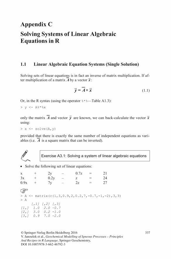
Appendix C
1.1 Linear Algebraic Equation Systems (Single Solution)
Solving sets of linear equations is in fact an inverse of matrix multiplication. If af-ter multiplication of a matrix A by a vector :
(1.1)
Or, in the R syntax (using the operator %*%—Table A1.3): > y <- A%*%x
using: > x <- solve(A,y)
provided that there is exactly the same number of independent equations as vari-ables (i.e. is a square matrix that can be inverted).
Exercise A3.1: Solving a system of linear algebraic equations
Solve the following set of linear equations:
x + 2y – 0.7z = 21 3x + 0.2y – z = 24 0.9x + 7y – 2z = 27
> A <- matrix(c(1,3,0.9,2,0.2,7,-0.7,-1,-2),3,3) > A [,1] [,2] [,3] [1,] 1.0 2.0 -0.7 [2,] 3.0 0.2 -1.0 [3,] 0.9 7.0 -2.0
© Springer-Verlag Berlin Heidelberg 2016 V. Janoušek et al., Geochemical Modelling of Igneous Processes – Principles And Recipes in R Language, Springer Geochemistry, DOI 10.1007/978-3-662-46792-3
337
Solving Systems of Linear Algebraic Equations in R
x
= × xy A
only the matrix and vector are known, we can back-calculate the vector A y
A
x
> x <- solve(A,y) > x [1] 30 20 70 > # checking the result > A%*%x [,1] [1,] 21 [2,] 24 [3,] 27
1.2 Overdetermined Systems ( nconstrained Least-Square
If there are more independent equations than variables, the system is overdeter-mined. The matrix is not square, and thus cannot be inverted. But we can cal-culate an approximate estimate of the vector (denoted here ). Defining:
(1.2)
we must find the value of such that the computed and real elements of the vec-tor differ as little as possible. The most common approach is to minimize the sum of the squares of the differences between each element of and (so-called least-square method: Bryan et al. 1969; Albarède and Provost 1977; Al-barède 1995):
(1.3)
It can be demonstrated that the best least-square solution is then:
(1.4)
By analogy with Eq. (1.1), 1T T
A × A × A is referred to as the (Moore–Penrose) “pseudo inverse” of matrix (it serves the same purpose as an inverse).
338 Appendix C Solving Systems of Linear Algebraic ...
Method) U
> y <- c(21,24,27)
Ax x
xy
y y
= Ay × x
22 minR y y
1T Tyx = A × A × A ×
AAlbarède (1995) discussed in a detail all the necessary mathematical apparatus
that is behind the solution. Janoušek and Moyen (2014) have shown implementa-tion of (unconstrained) least-square method in R and its utilization for solving simple geochemical problems, such as modal calculations or reverse mass-balance modelling of fractional crystallization. The least-squares are implemented by the R function:
lsfit(A, y, intercept = FALSE1) The outcome of this function is a list, of which the most interesting is the compo-nent $coefficients, corresponding to the vector as defined above, and a component $residuals with deviations between the calculated ( ) and ob-served ( ) compositions.
The sum of squares of residuals R2 [Eq. (1.3)] is an useful quantifier for the goodness of fit. Even though it shows a marked tendency to decrease with increas-ing number of variables involved in the calculation, as a rule of thumb it should not greatly exceed one. R2 >> 1 means that the model is not acceptable: the pro-posed geological hypotheses (i.e. composition of the primitive liquid, nature or composition of the cumulate minerals, or even the process itself) do not explain the observed variation. Note that the error is absolute, and it is therefore always wise to examine the residuals for individual elements or oxides.
1.3 Constrained Least-Square Method
In geochemistry are very often examined some variables that have to fulfil some condition. Most commonly they sum up to a certain value (e.g., unity or 100 %). The ordinary least-square method generally does not produce such normalized so-lutions, though. Albarède (1995) presented the necessary equations for modified, ‘constrained’ least squares defining the Lagrange multiplier as:
(1.5)
where stands for an ordinary least-square solution 2 and is a vector whose all elements are 1. The constrained least-squares solution is then given by:
1 Note that the parameter intercept needs to be set to FALSE for the solution to pass through the origin. 2 Obtained by lsfit as above.
339Appendix C Solving Systems of Linear Algebraic ...
(1.6)
a worked example of least-squares implementation, both unconstrained and con-strained, for ‘normative’ calculations (in wt. %) is given in Exercise 9.4.
xy
y
11 T
TT
x
A
J
J JA ×
1
ˆT
A × A+xx = J
Jx
The so-called generalized mixing problems in igneous or metamorphic geochemistry (including chemical mode computations, magma mixing,
liquid line of descent or batch partial melting modelling, end-member calculations and balancing of mineral reactions) are indeed the most commonly solved by the classic least-square techniques (Bryan et al. 1969; Albarède and Provost 1977; Stormer and Nicholls 1978; Le Maitre 1979, 1981). However,these mass-balance problems can be approached also by other minimalization algorithms such aslinear programming (Wright and Doherty 1970).
The standard least-square method does not permit constraining the sign of the coefficients of the solution, even when all-positive/all-negative or even mixed signs do not make a petrological sense3. This in fact provides an independent check on the feasibility of the solution. The linear programming, on the other hand, allows much easier forcing all-positive coefficients in the problem. This can be a dubious advantage, however (Rock 1988).
Albarède F (1995) Introduction to geochemical modeling. Cambridge University Press, Cambridge
Albarède F, Provost A (1977) Petrological and geochemical mass-balance equations: an algorithm for least-square fitting and general error analysis. Comput and Geosci 3:309–326
Bryan WB, Finger LW, Chayes F (1969) Estimating proportions in petrographic mixing equations by least-squares approximation. Science 163:926–927
Janoušek V, Moyen JF (2014) Mass balance modelling of magmatic processes in GCDkit. In: Kumar S, Singh RN (eds) Modelling of magmatic and allied processes. Society of Earth Scientists Series, vol 83. Springer, Berlin, pp 225–238
Le Maitre RW (1979) A new generalised petrological mixing model. Contrib Mineral Petrol 71:133–137
Le Maitre RW (1981) GENMIX—a generalized petrological mixing model program. Comput and Geosci 7:229–247
Rock NMS (1988) Numerical Geology. A source guide, glossary and selective bibliography to geological uses of computers and statistics. Lecture Notes in Earth Sciences, vol 18. Springer, Berlin
Stormer JC, Nicholls J (1978) XLFRAC: a program for the interactive testing of magmatic differentiation models. Comput and Geosci 4:143–159
Wright TL, Doherty PC (1970) A linear programming and least squares computer method for solving petrologic mixing problems. Geol Soc Amer Bull 81:1995–2008
3 But one needs to be aware of the problem of peritectic minerals, for which a negative coefficient
340
References
Appendix C Solving Systems of Linear Algebraic ...
is meaningful. See Sect. 6.3.
Index
A A/CNK-A/NK, 14 Accessory minerals, 212
allanite, 215 apatite, 134 exercise, 150, 216 inclusions, 215 monazite, 131, 215 saturation thermometry, 130, 132, 135, 216 solid solutions, 216 solubility, 129 xenotime, 215 zircon, 129, 214, 217, 255, 271
Activity, 99 AFC, 117, 163
energy constraints, 119, 186, 231 exercise, 173 reverse solution, 167 software, 119, 168
Amphibole, 102 Anatexis. See Melting Apatite, 134 Assimilation, 160, 186 Assimilation and fractional
crystallization. See AFC Atacazo-Ninahuilca Complex, 245 B Basic geochemical indexes, 14 Binary mixing, 159, 186
binary isotopic plot, 161 concentration vs. isotopes plot, 159 equation in x-y plot, 114, 161 error propagation, 160 exercise, 148, 169, 171 major elements, 78
mixing test (incl. exercise), 199 reverse model, 128, 167
exercise, 175 trace elements, 114
Binary plot constant sum effect, 30 lever rule, 71log log
element ratio, 45 fractionation vectors, 202 incompatible vs.
compatible elements, 195, 250
mixing, 78 mixing hyperbola, 114 mixing test, 199 two incompatible elements, 198
Biotite, 232 Bowen’s reaction scheme, 1 Bulk distribution coefficient, 103
non constant, 113
C Classification diagrams, 34 Clinopyroxene, 102Closure effect. See Binary plot,
constant sum effect Compatibility of elements, 101, 109
order of compatibility (incl. exercise), 192
Crystallization, 105 batch, 106 deep-level, 182 equation, 76equilibrium. See Batch evolving cumulate, 74
© Springer-Verlag Berlin Heidelberg 201 V. Janoušek et al., Geochemical Modelling of Igneous Processes – Principles And Recipes in R Language, Springer Geochemistry, DOI 10.1007/978-3-662-46792-3
341
–
6
final liquid composition selection, 206 fractional, 106
exercise, 85, 86, 87, 141, 142
fractional, reverse model, 82, 125
exercise, 93, 153 fractionating mineral identification, 202 identification, 195 incomplete crystal separation, 75, 120, 181 mechanical constraints, 232 peritectic phase, 76shallow-level, 181 source composition selection, 206 terminology, 70, 77 worked example, 245
Cumulate, 69, 71, 182 aggregated composition, 108 evolving, 74 incomplete separation, 75
D Degree of crystallization, Descriptive statistics, 18
exercise, 18, 21 Dilute trace elements. See Trace
elements E Equilibrium, 99, 105, 234 Essential structural components
(ESC), 100, 129. See also Accessory minerals
F Filter pressing, 180Fractional crystallization. See
Crystallization Fractionation vectors (incl.
Exercise), 202 G Garnet, 102 GCDkit, 5
anomaly plot, 49 basic indexes, 16exercise, 15
calculation results, further use,
calculations, 329 built-in routines, 330
classification diagrams, 34, 329, 334 contour plot, 48 data format, 318 descriptive statistics, 22, 330 direct access to data, exercise, 12 documentation, 318 double-normalized spiderplots, 47 export data, 331 export graphics, 331 export results, 331 Figaro, 29, 34, 323files localization, 332 geotectonic diagrams, 329 groups, 22, 23, 40, 322 help system, 332 installation, 315 internal variables, 333
idealmins.data 334labels, 318milli, 17, 329
, 11reservoir.data 334results, 329spider.data 334 WR, 318WRanh, 329
loading data, 319 merging data, 321 new variable, 330 personalization, 334 plate, 41, 323, 328 plot, 323
adding properties, 327 annotation, 29 colours, 326 contours, 327 curve, 327 editing, 29, 327 legend, 326, 327 symbols, 326
342 Index
file,
file,
file,
69
18, 29
mw
zoom, 327plots available, 325plotted variables specification, 323plugins, 334sample session, 317
135spider boxplots, 47spiderplots, 40, 46, 328, 334SrNd plugin, 65, 246stripplot, 50subsetting data, 322user interface, 316, 332
GCDkit function
, 319
, 46, 328
, 22,
22,
22, 34, 325
, 17, 91
, 135
H
Harker plots, 2exercise, 31
Henry’s Law, 99, 103Hornblende. See Amphibole Hybridization. See Mixing
I Incompatible elements. See
Compatibility of elements Isotopes, 53
epsilon notation (incl. Exercise), 57initial ratio (incl. Exercise), 55isochron (incl. Exercise), 63mixing, 159model ages, 60
exercise, 61, 62parent/daughter ratio, 53
K Kd. See Partition coefficient
LLattice strain model, 211Least-square method. See Linear
equations Leucosome, 183Lever rule, 71Linear equations
exact solution, 337exercise, 337least-square method, 82, 338
constrained, 339linear programming, 340over-determined system, 338under-determined system, 81
Liquid line of descent, 74, 76Liquid remaining, 69
Index 343
addContours()addResults()annotate()apSaturation()Batchelor()binary()Catanorm()CIPW()classify() cutMy()Debon()figMulti()figRemove()figUser() and similafilledContourFig()groupsByLabel()LaRoche()loadData()Mesonorm()milli()Mode()molecularWeight()multiple()mzSaturation()peterplot()plateCex() and similar, plateExtract()plotDiagram()prComp()selectNorm()selectPalette()spider()spider.contour()spider2norm()spiderBoxplot()
, 35
, 48, 29
, 29, 135
, 17, 28
, 17, 17
, 23, 17
, 40, 40
, 48, 22
, 17, 11, 17
, 17, 96
, 16, 32
, 135, 49
, 34, 225
, 39, 146
, 40, 46
, 47, 47
, 41
summaryByGroup()summaryRangesByGroup()
summarySingleByGroup()
ternary()Villaseca()WRComp()zrSaturation()
stripBoxplot(), 50
Geotectonic diagrams, 35
r, 29
41
, 325
Saturation plugin,
M Mafic microgranular enclaves
(MME), Magma mixing. See Mixing Major elements, 67 Mass balance, 69
accessory minerals, 214 equation, 70 generalized form, 79 matrix formulation, 72
Melting, 105 aggregated, 110 batch, 110 batch, reverse model, 127 crustal anatexis, 183 disequilibrium, energy constraints, 231 equation, 76, 77 fluxed, 121 fractional, 110 fractional with accumulation, 110 fractional, reverse model, 82 geological evidence, 183 identification, 195 mantle, 184 melt composition selection, 206 non-modal, 111 partial exercise, 89, 144 partial, reverse model
exercise, 94, 154 peritectic phase, 76, 265 prograde metamorphism, 265 progressive, 76 segregation, 233 source composition selection, 206 terminology, 75, 77 worked example, 261
Migmatite, 183 Millications, 16 Mingling, 185 Mixing, 105, 114
binary. See Binary mixing end-member constraining, 221 equation, 71 exercise, 91 field evidence, 185 generalized form, 79
identification, trace elements, 195 reverse model, 83
Mixing hyperbola, asymptotes, 162
Modelling choosing strategy, 181 colinearity, 227, 252 compositional space, 225 data resources, 3 element compatibility, 191 equilibration volume, 234 internal consistency, 228 mechanical constraints, 232 mineral as solid solution, 228, 250 model constraining, 205 Monte Carlo check, 254 phase equilibria, 273 process identification, 160, 195, 236 robustness, 254 software, 3, 208, 273, 320 system reduction, 227 thermodynamic constraints, 231
Monazite, 131 Multi-element diagram. See
Spiderplots N Niggli’s values, 16 Normative calculation
exercise, 95, 96 Norms, 17 O Olivine, 102, 232
P Partial melting. See Melting Partition coefficient, 101
calculation, 211 controlling physical factors, 102 resources, 211
Peraluminosity, 14 Peritectic reactions, 76 Phase rule, 228
344 Index
185, 221114, 161
234
Phlogopite, 205Plagioclase, 103Principal component analysis, 225
R Rayleigh’s fractionation law, 106Reverse models, 81R-function
%*% operator, 288, 299
aggregate() 293apply()args() 312array()as matrix()
axis(), 302
c()cat()
colnames()contour() , 304coplot()curve()cut()data()expression()factor()filled.contour() , 304for loopfunction()
grid()help()hist()identify()if-else conditiois.matrix() and
is.na()legend()levels()lines()list()lm()locator()ls()lsfit() , 175, 339matrix() 286
pairs() 302palette()par() , 298, 305parse()paste()plot()points()print() 309
, 294
readline()rep()
rm()
sapply() , 313
solve() , 337source() strsplit()
summary()t()
tapply() , 293text()
R-language, 4array, 282, 286batch mode, 280, 309Boolean operators, 285box-and-whiskers plot, 302conditions, 310data frame. See Matrix
difference from matrix,28 , 286
direct mode, 280documentation, 278export graphics, 308factor, 281, 292
exercise, 20, 21, 23frequency table, 293
Index 345
, 288,
, , 287
, 282,
, 305
309
, 288, 48
, 304, 300
, 292, 295
, 306, 292
, 48, 310
, 311
, 300, 278, 303
, 309 310
, 286, 301, 292
, 301, 290
, 299, 309
, 281, 93
,
, 294getwd()
, 288
, 293by()
abline(), 297
boxplot()
,, 297
, 296, 306, 285
, 295, 301
,, 288
, 309, 283
, 281
, 219
, 288, 280
, 285
, 302, 288
, 20, 299
rbind()read.table(), 11readClipboard(), 294
repeat-break loop, 311
rownames(), 288
seq(), 283setwd(), 294
substitute(), 307substring(), 285
table()
while loo 311winDialog() and popups, winMenuAdd(), 335write.table(), 295writeClipboard(), 295
similar 291
ordered(), 292
similar, 291
, 293
cbind()
and,
n,
p,335
1
frequency table (incl. Exercise), 23
function, 282anonymous, 313arguments, 311user-defined, 311
graphics, 295graphical parameters,
298high-level, 296low-level, 297
histogram, 303installation, 277, 315list, 281, 290load data, 11, 287, 293logical operators, 285loop alternatives. SeeVectorization loops, 310matrix, 281, 287
operations, 287subsetting, 289
missing values, 11, 286numerical functions, 284object, 282, 296
attributes, 282coercing, 291
packages, 332plot, 295
annotation, 297, 306creating, 296customization, 305exercise, 27export, 308interactive functions, 308linear fit, 299
parameters, 298save data, 295scripts. See Batch mode start Console, 277syntactic rules, 279table-like objects, 286variable assignment, 280vector, 282
assignment, 282character, 284logical, 285named, 283regular sequence, 283subsetting, 289substring, 285
vectorization, 282, 284, 293, 313working directory, 294
S Saint-Malo Massif, 261Saturation temperature, 136
exercise, 150Solubility. See Accessory mineralsSpiderplots, 36
exercise, 38
TTernary plot (incl. Exercise), 32Trace elements, 67, 101
V Visualization of data
projection, 225
ZZircon, 129, 232
exercise, 150
Index346