Gillibrand, P.A. and T.L. Aumdrud, 2007. A numerical study of the tidal circulation and buoyancy effects in a Scottish fjord: Loch Torridon

A numerical study of the tidal circulation and buoyancy effects

in a Scottish fjord: Loch Torridon

Philip A. Gillibrand1 and Trisha L. Amundrud2

Received 7 July 2006; revised 10 October 2006; accepted 16 November 2006; published 16 May 2007.

[1] The tidal and buoyancy-driven circulation in Loch Torridon, a Scottish fjord, isinvestigated using a three-dimensional, hydrostatic, primitive equationmodel. The predictionsfrom the model have been quantitatively compared to available data gathered between1998 and 2001. The model performed well in reproducing the tidal characteristics and densityevolution of the fjord over the 3-month simulation period. Results show that tidal currentsare dominated by the constraint imposed on the flow by the shallow sill separating theupper and middle basins: the flow is strongly accelerated during flood and ebb tides, andsignificant residual currents are generated that may influence exchange and residence times ofthe middle basin. A strong baroclinic response to the flow over the sill is predictedthroughout the fjord, with a propagating linear M2 tide displacing isopycnals vertically by upto 32 m. At the sill the formation of stationary lee waves on both flood and ebb tides ispredicted, with the wave generated during flood tide being notably larger as the growth of theebb wave is inhibited by deep dense water. This allows more energy to transfer into theseaward propagating internal tide. As the tidal flowweakens, the lee waves propagate over thesill and upstream. Estimates of the total vertical turbulent buoyancy flux in the fjord aremade, and the distribution of mixing over a tidal cycle is shown; vertical mixing is seen to behighly spatially and temporally variable and strongly linked to the presence and dissipationof lee waves near the sill.

Citation: Gillibrand, P. A., and T. L. Amundrud (2007), A numerical study of the tidal circulation and buoyancy effects in a Scottish

fjord: Loch Torridon, J. Geophys. Res., 112, C05030, doi:10.1029/2006JC003806.

1. Introduction

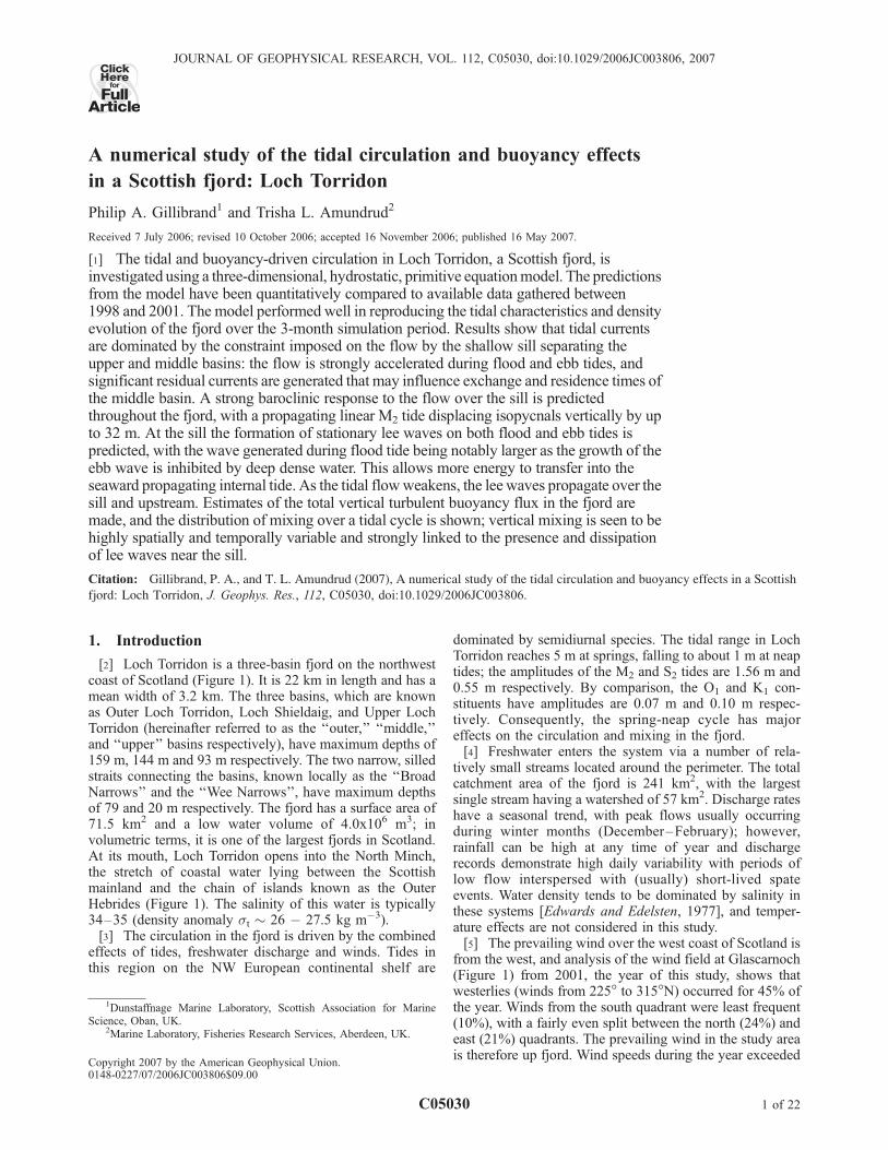
[2] Loch Torridon is a three-basin fjord on the northwestcoast of Scotland (Figure 1). It is 22 km in length and has amean width of 3.2 km. The three basins, which are knownas Outer Loch Torridon, Loch Shieldaig, and Upper LochTorridon (hereinafter referred to as the ‘‘outer,’’ ‘‘middle,’’and ‘‘upper’’ basins respectively), have maximum depths of159 m, 144 m and 93 m respectively. The two narrow, silledstraits connecting the basins, known locally as the ‘‘BroadNarrows’’ and the ‘‘Wee Narrows’’, have maximum depthsof 79 and 20 m respectively. The fjord has a surface area of71.5 km2 and a low water volume of 4.0x106 m3; involumetric terms, it is one of the largest fjords in Scotland.At its mouth, Loch Torridon opens into the North Minch,the stretch of coastal water lying between the Scottishmainland and the chain of islands known as the OuterHebrides (Figure 1). The salinity of this water is typically34–35 (density anomaly st � 26 � 27.5 kg m�3).[3] The circulation in the fjord is driven by the combined

effects of tides, freshwater discharge and winds. Tides inthis region on the NW European continental shelf are

dominated by semidiurnal species. The tidal range in LochTorridon reaches 5 m at springs, falling to about 1 m at neaptides; the amplitudes of the M2 and S2 tides are 1.56 m and0.55 m respectively. By comparison, the O1 and K1 con-stituents have amplitudes are 0.07 m and 0.10 m respec-tively. Consequently, the spring-neap cycle has majoreffects on the circulation and mixing in the fjord.[4] Freshwater enters the system via a number of rela-

tively small streams located around the perimeter. The totalcatchment area of the fjord is 241 km2, with the largestsingle stream having a watershed of 57 km2. Discharge rateshave a seasonal trend, with peak flows usually occurringduring winter months (December–February); however,rainfall can be high at any time of year and dischargerecords demonstrate high daily variability with periods oflow flow interspersed with (usually) short-lived spateevents. Water density tends to be dominated by salinity inthese systems [Edwards and Edelsten, 1977], and temper-ature effects are not considered in this study.[5] The prevailing wind over the west coast of Scotland is

from the west, and analysis of the wind field at Glascarnoch(Figure 1) from 2001, the year of this study, shows thatwesterlies (winds from 225� to 315�N) occurred for 45% ofthe year. Winds from the south quadrant were least frequent(10%), with a fairly even split between the north (24%) andeast (21%) quadrants. The prevailing wind in the study areais therefore up fjord. Wind speeds during the year exceeded

JOURNAL OF GEOPHYSICAL RESEARCH, VOL. 112, C05030, doi:10.1029/2006JC003806, 2007ClickHere

for

FullArticle

1Dunstaffnage Marine Laboratory, Scottish Association for MarineScience, Oban, UK.

2Marine Laboratory, Fisheries Research Services, Aberdeen, UK.

Copyright 2007 by the American Geophysical Union.0148-0227/07/2006JC003806$09.00

C05030 1 of 22

http://dx.doi.org/10.1029/2006JC003806

10 m s�1 for only 5% of the time, reaching a peak of 20 ms�1; the mean wind speed was 4.2 m s�1.[6] In narrow fjords, where the width of the fjord is

typically less than the baroclinic Rossby radius of deforma-tion, variability across the fjord is weak and this obviatesthe need to consider lateral variability in the circulationfield. Numerous studies have appeared in the literaturereporting the application of two-dimensional, depth-resolving, width-averaged models to fjords. Earlier models[e.g., Lavelle et al., 1991; Gillibrand et al., 1995; Staceyet al., 1995, 2002] were hydrostatic and used to investigateprocesses such as deep water renewal. More recently,nonhydrostatic models [e.g., Vlasenko et al., 2002;Cummins et al., 2003; Xing and Davies, 2006] have beendeveloped in order to explore the hydraulics of flows oversills, where large vertical velocities invalidate the hydro-static assumption.[7] In Loch Torridon, the baroclinic Rossby radius is of

the order 1–3 km depending on the strength of the strati-fication. Since the outer basin has a width of �4 km, thefjord lies in the ‘‘intermediate’’ category between broad andnarrow fjords, where both Coriolis and wall-to-wall effectsare likely to influence the circulation [Cushman-Roisin etal., 1994]. In this case, lateral variability in the circulationcannot be neglected and a three-dimensional model isrequired. Although there have been numerous publicationsin the peer-reviewed literature over the past twenty yearsdescribing the application of three-dimensional hydrody-

namic models to shallow estuaries [e.g., Oey et al., 1985a,1985b; Galperin and Mellor, 1990a, 1990b; Zheng et al.,2003; Zheng and Weisberg, 2004], there are far fewerreports of applications of such models to study watercirculation in fjordic estuaries. A variety of finite elementand finite difference 3-D models have been used to studythe circulation [Utnes and Brors, 1993; Eliassen et al.,2001], upwelling [Cushman-Roisin et al., 1994] and plank-ton and fish larvae transport [Asplin et al., 1999] inNorwegian fjords and, recently, Foreman et al. [2006]applied a finite volume model, ELCIRC, to the BroughtonArchipelago in British Columbia which includes KnightInlet.[8] In this paper, we employ a three-dimensional, prim-

itive equation, finite difference circulation model to inves-tigate the tidal and buoyancy-driven circulation in LochTorridon. Like many of the fjordic sea lochs in Scotland, thepristine waters of Loch Torridon have been exploited inrecent years for farmed salmon production and this study ofthe water circulation in the fjord was motivated by the needto understand the dispersal of sea lice larvae from fish farmsites in the loch. The coupling of the hydrodynamic modelwith a larval transport model and the initial results ofthat study have been described elsewhere [Murray andGillibrand, 2006]. Here we exploit the development of thehydrodynamic model to investigate features of the tidal anddensity-driven circulation and cross-sill exchange in thefjord. In subsequent sections, the model and its validation

Figure 1. The bathymetry (shaded) of Loch Torridon and its location in the northwest of Scotland(inset). The locations of CTD profiles (lettered dots), water level recorders (inverted triangles), and theSC-ADCP (triangle) are shown, including those providing boundary forcing data, which are shown in theinset. Multiple CTD station numbers occur when profiles were collected at a location on more than oneoccasion. The six freshwater sources to the model are indicated by the black arrows; wind data were takenfrom the Glascarnoch meteorological station (inset). The dashed line indicates the section along whichmodel predictions are discussed in sections 4 and 5. The mesh indicates the resolution of the model grid.

C05030 GILLIBRAND AND AMUNDRUD: FJORD CIRCULATION AND BUOYANCY EFFECTS

2 of 22

C05030

against available data are described and results from simu-lations from the period April–June 2001 presented.

2. Model Description and Calibration

2.1. Model Equations, Domain, and Solution Method

[9] We use the three-dimensional baroclinic coastal oceanmodel previously described by Stronach et al. [1993],Saucier and Chasse [2000] and Saucier et al. [2003]. Thismodel is derived from the hydrostatic solution with theBousinesq approximation to the equations of mass, momen-tum and density conservation first presented by Backhaus[1985] for application to the North Sea. A modified versionof the model was then developed for the strongly tidalwaters of the Strait of Georgia by Stronach et al. [1993].The mathematical framework and solution methods of themodel are described in detail in those papers and are notrepeated here. The development of the model code sawapplications to the St. Lawrence Estuary and Gulf bySaucier and Chasse [2000] and Saucier et al. [2003]. Theversion of the model used here is similar to that of Saucieret al. [2003].[10] The governing equations are solved by finite differ-

ence approximations on an Arakawa C grid. The prognosticvariables are the sea surface elevation h, the water density r,and the three components of velocity u, v, w along thehorizontal axes x and y and the vertical axis z (positiveupward) respectively. A two-time-level scheme is used,representing ‘‘present’’ and ‘‘future,’’ and the prognosticvariables are stepped forward in time. The external (baro-tropic) mode is treated implicitly, thus avoiding the Cou-rant-Friedrichs-Lewy stability constraint imposed onexplicit schemes. The internal (baroclinic) component istreated explicitly. The implicit solution for the domain-widesea surface elevation is obtained by solving the verticallyintegrated continuity equation by successive overrelaxation(SOR) iteration [Backhaus, 1985; Stronach et al., 1993].The equation for density is treated explicitly, except for thevertical diffusion term which is solved implicitly using aCrank-Nicholson solution. The advection of density usesthe method of characteristics in the horizontal and a second-order Lax-Wendroff type scheme in the vertical [Stronach etal., 1993].[11] The model domain for the present study is shown in

Figure 1. The grid is a staggered Cartesian grid with ahorizontal grid spacing of Dx = Dy = 100 m throughout thedomain, and is rotated by 49� so that the x axis is orientatedtoward 139�N. There are up to 40 layers in the vertical,with layer bases regularly spaced at 4 m intervals from 4 mto 160 m depth. The thickness of the bottom cell in eachgrid column is adjusted so that the water depth in the modelcorresponds to the real depth. The thickness of the surfacelayer varies with the displacement of the sea surface from itsmean height. The minimum allowed water depth in themodel is 8 m (i.e., there is a minimum of two cells in eachgrid column).[12] Horizontal viscosity and diffusion are treated follow-

ing Smagorinsky [1963], i.e.,

AH ¼ KH ¼ gDx2@u

@x

� �2

þ @v

@y

� �2

þ 0:5@u

@yþ @v

@x

� �2" #0:5

ð1Þ

with g = 0.2. The value of g was chosen to be as small aspossible while retaining numerical stability. Vertical turbu-lent viscosities, AV, and diffusivities, KV, are calculatedusing the so-called ‘‘level 2.2’’ Mellor-Yamada turbulenceclosure [Mellor and Yamada, 1982; Kantha and Clayson,1994; Saucier et al., 2003]; the level 2.2 scheme includesvertical diffusion but not horizontal or vertical advection ofthe turbulent kinetic energy (TKE). Simulations thatincluded advection of TKE did not produce noticeabledifferences to the results, but did incur a significantcomputational cost; as such, we chose to use the moreefficient level 2.2 algorithm. The vertical turbulent eddycoefficients are defined as

KV ¼ qlSs þ KVb ð2Þ

AV ¼ qlSM þ AVb ð3Þ

where Ss and SM are stability functions for density andmomentum, calculated following Kantha and Clayson[1994]. The turbulent kinetic energy, k = q2/2, is calculatedfrom

@k

@t¼ @

@zAV

@k

@z

� �þ P þ B� e ð4Þ

where

P ¼ AV

@u

@z

� �2

þ @v

@z

� �2" #

ð5Þ

and

B ¼ �KVN2 ð6Þ

represent turbulence production by velocity shear andbuoyancy respectively. N is the buoyancy frequency givenby N2 = �(g/r)@r/@z. Dissipation, e, is given by

e ¼ q3

B1lð7Þ

where B1 = 16.6. For the turbulence length scale, l, we use alaw of the wall algebraic formulation, lW, bounded by theOzmidov scale, lO, i.e.

l ¼ min lW ; lOð Þ ð8Þ

where

lW zð Þ ¼ k z0t � zð Þ 1þ z0b þ zð Þ=h½ � ð9Þ

lO ¼ 0:53q

Nð10Þ

Here k = 0.4 is the von Karman constant, h is the waterdepth, and z0t and z0b are roughness lengths at the surfaceand bottom respectively, computed from Charnock’sformulae z0 = au*

2 /g, where u* is the friction velocity.The value of the constant a used here is 0.011. Equations (8)and (10) ensure that the length scale is constrained bystratification, a limitation that has been widely employed inshelf and coastal models [e.g., Galperin et al., 1988; Kanthaand Clayson, 1994; Holt and James, 2001; Stacey et al.,2002; Warner et al., 2005].


3 of 22

C05030

[13] Like other authorsmodeling fjordic environments [e.g.,Stacey et al., 1995, 2002], we found it necessary to supplementthe vertical eddy diffusivity and viscosity terms with a ‘‘back-ground’’ mixing term. The requirement for this additionalmixing arises from the active internal wavefield found inmanyfjords [e.g., Stigebrandt and Aure, 1989; Inall and Rippeth,2002; Inall et al., 2004], which supplies energy from gener-ation zones at sills to the deep basins [Stacey et al., 2002].Sporadic wind forcing may also generate near-inertial internalwaves in stratified coastal waters [Xing and Davies, 2004].WefollowGargett and Holloway [1984] to stipulate an additionalmixing term based on the stability of the water column, i.e.,

AVb ¼ KVb ¼ a0N�1 ð11Þ

Following a series of trial simulations, a0 was specifiedas 10�6 m2 s�2. Under weak stratification conditions (N =10�2 s�1), the background mixing term had a value ofKVb = 1.0 10�4 m2 s�1; for stronger stratification in thepycnocline (N = 10�1 s�1), KVb = 1.0 10�5 m2 s�1.

2.2. Initial Conditions and Boundary Forcing

[14] The model simulation described here is from 9 April to18 July 2001. This period coincided with an observationalprogram during which a moored 300 kHz RDI ADCP andAanderaa bottom pressure sensors were deployed, and surveysof water temperature and salinity conducted with a SeabirdSBE25 Sealogger CTD. These data are used to calibrate andvalidate the model performance. Details of the mooringdeployments and CTD casts used to assess model performanceare given in Tables 1a and 1b. Three CTD surveys wereconducted on 9 April, 7–10 July, and 18 July 2001.[15] Tidal forcing at the open boundary was provided by

37 tidal constituents derived from observations of bottom pres-sure at a location 9 km west of the entrance to Loch Torridon(ref. 661W, Figure 1, insert, and Tables 1a and 1b). Harmonicanalysis captured 99% of the variance of the observed seasurface height. The reconstructed water level, h0 (Figure 2),was specified at the central grid cell along the open boundary;water levels, hb, to either side of this central location wereallowed to deviate from h0, on both flooding and ebbing tides,by assuming a geostrophic balance along the boundary i.e.,

g@hb@y

¼ �fU ð12Þ

where U is the depth mean velocity normal to the openboundary (calculated by the model at the first grid columnsinside the open boundary), f is the Coriolis parameter and g isthe gravitational acceleration. Equation (12) allows bothincoming and outgoing surface waveforms to propagatethrough the boundary as Kelvin waves [Stronach et al.,

1993], and successfully prevented wave energy becomingtrapped in the model domain. During flood tides, a zero-gradient condition across the boundary is applied to bothcomponents of velocity, while density is relaxed to aspecified coastal ocean profile. During ebb flows, the radiationcondition

@ u; v; rð Þ@t

þ u@ u; v; rð Þ

@x¼ 0 ð13Þ

is applied to both velocity components and density.[16] Wind forcing was applied as a surface stress with

tX ¼ raircs WX � uSð ÞW ð14aÞ

tY ¼ raircs WY � vSð ÞW ð14bÞ

where rair = 1.2 kg m�3 is the density of air, WX(Y) is thealong-loch (across-loch) wind velocity, and us (vs) is thealong-loch (across-loch) current velocity in the surfacelayer, and W = (WX

2 + WY2 )1/2 is the wind speed. The use of

the surface current velocity in equations (14a) and (14b)ensures that the surface stress was zero when the windvelocity equaled the surface water velocity [Stacey et al.,1995; Yeremy and Stacey, 1998]. The surface dragcoefficient is given by [Atakturk and Katsaros, 1999]

cS ¼ 0:87þ 0:078Wð Þ 10�3 ð15Þ

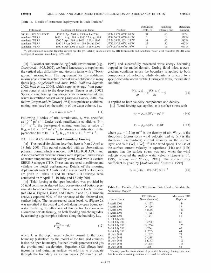
Table 1a. Details of Instrument Deployments in Loch Torridona

Instrument Deployment Times and Dates PositionInstrumentDepth, m

SamplingInterval, min

ReferenceNumber

300 kHz RDI SC-ADCP 1700 9 Apr 2001 to 1300 6 Jun 2001 57034.15�N, 05043.80�W 94 60 662AAanderaa WLR5 1600 11 Aug 1998 to 1100 27 Aug 1998 57034.26�N, 05046.81�W 5 5 578WAanderaa WLR5 1200 7 Apr 1999 to 1600 10 Nov 1999 57 34.33�N, 05041.23�W 38 60 583WAanderaa WLR5 1500 15 Apr 2000 to 1000 20 Jul 2000 57032.03�N, 05041.62�W 25 30 642WAanderaa WLR5 1000 9 Apr 2001 to 1200 17 July 2001 57034.63�N, 05058.16�W 5 15 661W

aA self-contained acoustic Doppler current profiler (SC-ADCP) manufactured by RD Instruments and Aanderaa water level recorders (WLR) weredeployed at various times during 1998–2001.

Table 1b. Details of the CTD Station Data Used to Validate the

Numerical Modela

Cruise DatesCTD Station

Name (Number)Maximum CTD

Depth, m

9 April 2001 A (127) 1449 April 2001 D (126) 879 April 2001 F (123) 1239 April 2001 H (125) 429 April 2001 I (124) 517–10 July 2001 - -7–10 July 2001 B (266) 867–10 July 2001 G (256) 1257–10 July 2001 I (254) 677–10 July 2001 J (257) 6418 July 2001 A (267) 7518 July 2001 C (288) 7718 July 2001 E (280) 10518 July 2001 G (278) 11318 July 2001 I (276) 62

aDensity profiles from station A provided boundary forcing data, anddata from the remaining stations were used for validation.


4 of 22

C05030

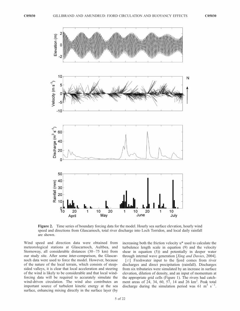
Wind speed and direction data were obtained frommeteorological stations at Glascarnoch, Aultbea, andStornoway, all considerable distances (30–75 km) fromour study site. After some inter-comparison, the Glascar-noch data were used to force the model. However, becauseof the nature of the local terrain, which consists of steep-sided valleys, it is clear that local acceleration and steeringof the wind is likely to be considerable and that local wind-forcing data will be required to accurately simulate thewind-driven circulation. The wind also contributes animportant source of turbulent kinetic energy at the seasurface, enhancing mixing directly in the surface layer (by

increasing both the friction velocity u* used to calculate theturbulence length scale in equation (9) and the velocityshear in equation (5)) and potentially in deeper waterthrough internal wave generation [Xing and Davies, 2004].[17] Freshwater input to the fjord comes from river

discharges and direct precipitation (rainfall). Dischargesfrom six tributaries were simulated by an increase in surfaceelevation, dilution of density, and an input of momentum atthe appropriate grid cells (Figure 1). The rivers had catch-ment areas of 24, 34, 60, 57, 14 and 26 km2. Peak totaldischarge during the simulation period was 61 m3 s�1.

Figure 2. Time series of boundary forcing data for the model. Hourly sea surface elevation, hourly windspeed and directions from Glascarnoch, total river discharge into Loch Torridon, and local daily rainfallare shown.


5 of 22

C05030

Discharge data were based on observed data from the RiverCarron (Figure 1) and calculated for each tributary bycatchment weighting. Direct precipitation was modeled asan increase in elevation and a dilution of surface layerdensity in all ‘‘wet’’ model cells. Data came from observedrainfall values at Torridon.[18] At solid lateral boundaries, normal flow is set to

zero, ensuring no loss of volume, momentum or mass. Atthe seabed, a quadratic slip condition is applied, with thebottom stress given by

tb ¼ r0CDubjubj ð16Þ

where r0 is a reference density and ub is the velocity inthe bottom grid cell. The drag coefficient, CD, was variedduring the calibration process to find the optimum value.In reality, the drag coefficient is likely to vary over thedomain in response to variable bed types and frictionalcharacteristics of the seafloor, and could be related to abed roughness length [e.g., Xing and Davies, 2001];however, we do not have sufficient data to calibrate themodel to that extent, and have therefore used a constantvalue of CD.[19] The model elevation, velocity and density fields were

prepared by ramping up the model from rest over the period1 March to 9 April using observed sea surface elevation dataand a stationary boundary density profile taken from CTDcast 127, obtained on 9 April. The internal model fieldstherefore evolved such that on 9 April they were consistentwith all boundary data. The simulation proper then began,again using observed boundary data and an ocean densityprofile that evolved linearly in time from the profile on9 April to that on 18 July.

2.3. Skill Assessment

[20] The ability of the model to reproduce the observa-tions is tested quantitatively, using methods described by

Willmott et al. [1985]. We calculate the root mean squareerror between model and data, given by

ERMS ¼ 1

N

XNj¼1

pj � oj� �2 !" #1=2

ð17Þ

where pj and oj are predicted and observed valuesrespectively and N is the number of data points in thecalculation. Model skill is estimated from

d2 ¼ 1�XNj¼1

pj � oj� �2" #, XN

j¼1

jpj � oj þ joj � oj� �2" #

ð18Þ

where o is the arithmetic mean of the observed data. A per-fect agreement between model and data would give d2 = 1,with decreasing values indicating declining performance.

3. Model Calibration

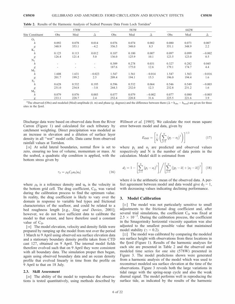
[21] The model was not particularly sensitive to smalladjustments to the frictional drag coefficient and, afterseveral trial simulations, the coefficient CD was fixed at2.5 10�3. During the calibration process, the coefficientin the Smagorinsky horizontal viscosity equation was alsoadjusted to the smallest possible value that maintainedmodel stability (g = 0.2).[22] The model was calibrated by comparing the modeled

sea surface height with observations from three locations inthe fjord (Figure 1). Results of the harmonic analyses foreach site are presented in Table 2 and the observed andmodeled time series for one site (578W) presented inFigure 3. The model predictions shown were generatedfrom a harmonic analysis of the model which was used toreconstruct modeled sea surface elevation at the time of theobservations. Figure 3 reveals both the large variations intidal range with the spring-neap cycle and also the weakdiurnal signal. The model performs well in reproducing thesurface tide, as indicated by the results of the harmonic

Table 2. Results of the Harmonic Analysis of Seabed Pressure Data From Loch Torridona

Site Constituent

578W 583W 642W

Obs Mod D Obs Mod D Obs Mod D

O1

h 0.092 0.078 0.014 0.076 0.074 0.002 0.080 0.073 0.007g 348.9 353.1 �4.2 356.5 348.0 8.5 351.1 348.9 2.2

K1

h 0.125 0.113 0.012 0.107 0.100 0.007 0.097 0.099 �0.002g 126.4 121.4 5.0 136.0 125.9 10.1 123.5 123.0 0.5

N2

h - - - 0.309 0.278 0.031 0.327 0.282 0.045g - - - 187.6 175.0 12.6 179.1 174.7 4.4

M2

h 1.608 1.631 �0.023 1.547 1.561 �0.014 1.547 1.563 �0.016g 201.7 199.2 2.5 209.4 194.1 15.3 196.0 194.4 1.6

S2h 0.628 0.532 0.195 0.596 0.532 0.064 0.546 0.549 �0.003g 231.0 234.8 �3.8 244.3 232.0 12.3 232.8 231.2 1.6

M4

h 0.079 0.076 0.003 0.077 0.079 �0.002 0.077 0.080 �0.003g 233.1 228.7 2.4 252.4 220.8 31.6 225.5 221.6 3.9

aThe observed (Obs) and modeled (Mod) amplitude (h, m) and phase (g, degrees) and the difference between them (D = hobs � hmod) are given for threesites in the fjord.


6 of 22

C05030

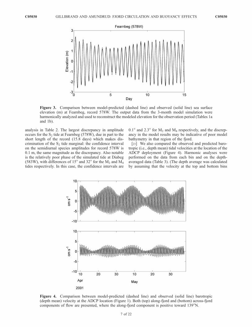
analysis in Table 2. The largest discrepancy in amplitudeoccurs for the S2 tide at Fearnbeg (578W), due in part to theshort length of the record (15.8 days) which makes dis-crimination of the S2 tide marginal: the confidence intervalon the semidiurnal species amplitudes for record 578W is0.1 m, the same magnitude as the discrepancy. Also notableis the relatively poor phase of the simulated tide at Diabeg(583W), with differences of 15� and 32� for the M2 and M4

tides respectively. In this case, the confidence intervals are

0.1� and 2.3� for M2 and M4 respectively, and the discrep-ancy in the model results may be indicative of poor modelbathymetry in that region of the fjord.[23] We also compared the observed and predicted baro-

tropic (i.e., depth mean) tidal velocities at the location of theADCP deployment (Figure 4). Harmonic analyses wereperformed on the data from each bin and on the depth-averaged data (Table 3). (The depth average was calculatedby assuming that the velocity at the top and bottom bins

Figure 3. Comparison between model-predicted (dashed line) and observed (solid line) sea surfaceelevation (m) at Fearnbeg, record 578W. The output data from the 3-month model simulation wereharmonically analyzed and used to reconstruct the modeled elevation for the observation period (Tables 1aand 1b).

Figure 4. Comparison between model-predicted (dashed line) and observed (solid line) barotropic(depth mean) velocity at the ADCP location (Figure 1). Both (top) along-fjord and (bottom) across-fjordcomponents of flow are presented, where the along-fjord component is positive toward 139�N.


7 of 22

C05030

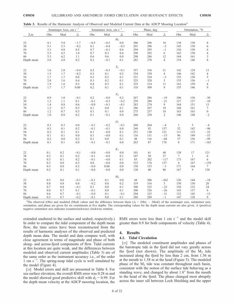
extended unaltered to the surface and seabed, respectively.)In order to compare the tidal component of the depth meanflow, the time series have been reconstructed from theresults of harmonic analyses of the observed and predicteddepth mean data. The model and data compare well, withclose agreement in terms of magnitude and phase of bothalong- and across-fjord components of flow. Tidal currentsat this location are quite weak, and the differences betweenmodeled and observed current amplitudes (Table 3) are ofthe same order as the instrument accuracy i.e., of the order1 cm s�1. The spring-neap tidal cycle is well simulated bythe model (Figure 4).[24] Model errors and skill are presented in Table 4. For

sea surface elevation, the overall RMS error was 0.28 m andthe model showed good predictive skill with d2 = 0.99. Forthe depth mean velocity at the ADCP mooring location, the

RMS errors were less than 1 cm s�1 and the model skillgreater than 0.9 for both components of velocity (Table 4).

4. Results

4.1. Tidal Circulation

[25] The modeled constituent amplitudes and phases ofthe barotropic tide in the fjord did not vary greatly acrossthe fjord (not shown). The amplitude of the M2 tideincreased along the fjord by less than 2 cm, from 1.56 mat the mouth to 1.58 m at the head (Figure 5). The modeledphase of the M2 tide was constant throughout each basin,consistent with the notion of the surface tide behaving as astanding wave, and changed by about 1.8� from the mouthto the head of the fjord. The phase changed most abruptlyacross the inner sill between Loch Shieldaig and the upper

Table 3. Results of the Harmonic Analysis of Observed and Modeled Current Data at the ADCP Mooring Locationa

Z,m

Semimajor Axis, cm s�1 Semiminor Axis, cm s�1 Phase, deg Orientation, �N

Obs Mod D Obs Mod D Obs Mod D Obs Mod D

M2

22 4.1 5.8 �1.7 �0.5 �0.5 0.0 306 296 10 138 130 838 5.1 5.3 �0.2 0.1 �0.4 �0.3 291 296 �5 145 139 654 5.3 4.8 0.5 0.7 �0.1 0.6 294 295 �1 156 150 670 5.5 4.5 1.0 0.7 0.3 0.4 298 292 6 162 158 486 5.3 4.2 1.1 0.6 0.6 0.0 298 286 12 164 161 3Depth mean 5.0 4.8 0.2 0.2 �0.1 0.1 282 278 4 154 146 8

S222 1.6 2.0 �0.4 0.2 �0.3 �0.1 357 336 21 142 129 1338 1.5 1.7 �0.2 0.3 0.1 0.2 334 330 4 146 142 454 1.7 1.7 0.0 0.3 0.2 0.1 321 324 �3 155 150 570 2.0 1.6 0.4 0.3 0.2 0.1 325 320 5 155 156 �186 1.9 1.6 0.3 0.4 0.3 0.1 325 314 11 162 158 4Depth mean 1.7 1.7 0.00 0.2 0.1 0.1 318 309 9 155 146 9

N2

22 0.9 1.0 �0.1 0.2 �0.0 0.2 267 286 �19 106 136 �3038 1.2 1.1 0.1 �0.1 �0.3 �0.2 259 280 �21 127 137 �1054 1.4 0.8 0.6 �0.0 �0.1 �0.1 283 274 9 164 151 1370 1.2 0.7 0.5 0.1 0.0 0.1 286 267 19 168 161 786 1.2 0.7 0.5 0.1 0.1 0.0 275 257 18 163 163 0Depth mean 1.0 0.8 0.2 0.1 �0.1 0.0 260 258 2 146 148 �2

O1

22 0.3 0.3 0.0 �0.1 �0.2 �0.1 260 264 �4 1 5 �438 0.3 0.1 0.2 �0.1 �0.1 0.0 249 92 157 52 142 �9054 0.2 0.1 0.1 0.1 �0.0 0.1 251 130 121 111 133 �2270 0.1 0.1 0.0 0.1 �0.0 0.1 116 131 �15 96 149 �5386 0.2 0.0 0.2 0.1 0.0 0.1 48 116 �68 57 156 �99Depth mean 0.1 0.1 0.0 �0.1 �0.1 0.0 263 87 176 8 171 �163

K1

22 0.1 0.2 �0.1 �0.0 �0.0 0.0 101 61 40 138 17 12138 0.3 0.1 0.2 �0.1 �0.0 0.1 107 50 57 7 1 654 0.3 0.1 0.2 �0.1 �0.0 0.1 85 202 �117 173 167 670 0.3 0.0 0.3 0.0 �0.0 0.0 333 176 157 8 167 �15986 0.3 0.0 0.3 �0.0 0.00 0.0 150 153 �3 171 164 7Depth mean 0.2 0.1 0.1 �0.0 �0.0 0.0 120 40 80 167 9 158

M4

22 0.5 0.6 �0.1 �0.1 0.1 0.0 44 306 �262 126 144 �1838 0.8 0.8 0.0 �0.2 0.0 0.2 319 316 3 150 130 2054 0.7 0.8 �0.1 0.1 0.0 0.1 300 323 �23 156 132 2470 0.8 0.7 0.1 �0.1 0.0 0.1 300 326 �26 143 137 686 0.6 0.7 �0.1 �0.0 0.1 �0.1 294 325 �31 132 145 �13Depth mean 0.5 0.7 �0.2 �0.1 0.0 0.1 288 289 �1 147 138 9

aThe observed (Obs) and modeled (Mod) values and the difference between them (D = jObsj � jModj) of the semimajor axis, semiminor axis,orientation, and phase are given for six constituents at five depths. The corresponding values for the depth mean currents are also given. A (positive)negative semiminor axis indicates (counterclockwise) clockwise rotation.


8 of 22

C05030

basin, where a lag of 1.6� was introduced. This lag indicatesa loss of barotropic energy at the sill, which may result fromenhanced dissipation by boundary friction, form drag andbaroclinic wave drag [Stigebrandt, 1999]; such processeshave been widely observed in many other fjords [e.g.,Farmer and Freeland, 1983; Farmer and Armi, 1999;Arneborg et al., 2004; Inall et al., 2004, 2005].

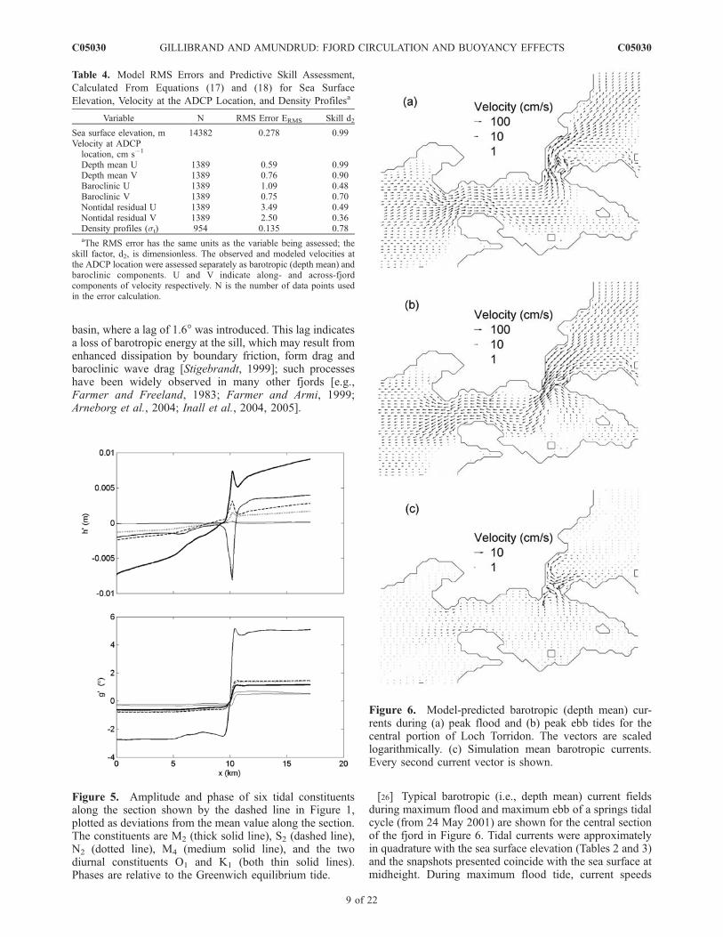
[26] Typical barotropic (i.e., depth mean) current fieldsduring maximum flood and maximum ebb of a springs tidalcycle (from 24 May 2001) are shown for the central sectionof the fjord in Figure 6. Tidal currents were approximatelyin quadrature with the sea surface elevation (Tables 2 and 3)and the snapshots presented coincide with the sea surface atmidheight. During maximum flood tide, current speeds

Table 4. Model RMS Errors and Predictive Skill Assessment,

Calculated From Equations (17) and (18) for Sea Surface

Elevation, Velocity at the ADCP Location, and Density Profilesa

Variable N RMS Error ERMS Skill d2

Sea surface elevation, m 14382 0.278 0.99Velocity at ADCPlocation, cm s�1

Depth mean U 1389 0.59 0.99Depth mean V 1389 0.76 0.90Baroclinic U 1389 1.09 0.48Baroclinic V 1389 0.75 0.70Nontidal residual U 1389 3.49 0.49Nontidal residual V 1389 2.50 0.36Density profiles (st) 954 0.135 0.78aThe RMS error has the same units as the variable being assessed; the

skill factor, d2, is dimensionless. The observed and modeled velocities atthe ADCP location were assessed separately as barotropic (depth mean) andbaroclinic components. U and V indicate along- and across-fjordcomponents of velocity respectively. N is the number of data points usedin the error calculation.

Figure 5. Amplitude and phase of six tidal constituentsalong the section shown by the dashed line in Figure 1,plotted as deviations from the mean value along the section.The constituents are M2 (thick solid line), S2 (dashed line),N2 (dotted line), M4 (medium solid line), and the twodiurnal constituents O1 and K1 (both thin solid lines).Phases are relative to the Greenwich equilibrium tide.

Figure 6. Model-predicted barotropic (depth mean) cur-rents during (a) peak flood and (b) peak ebb tides for thecentral portion of Loch Torridon. The vectors are scaledlogarithmically. (c) Simulation mean barotropic currents.Every second current vector is shown.


9 of 22

C05030

were typically O(0.1) m s�1 in the deeper central parts ofthe basins (Figure 6a). Some acceleration on the flood tidewas apparent through the outer narrows, but accelerationwas much stronger through the inner narrows, with currentspeeds reaching �1.2 m s�1 over the inner sill. On enteringthe upper basin, the inflowing jet hugged the left-hand(northwest) coastline, entraining basin water and settingup an anticyclonic vortex to the southeast. Within about1.5 km of the sill, current speeds had returned to typically0.1 m s�1. Predicted flows in the bays to either side of thecentral channel were weak.

[27] During the ebb tide (Figure 6b), the barotropic flowaccelerated from speeds of O(0.1) m s�1 in the upper basinto about 1.2 m s�1 over the inner sill. The jet currentpenetrated into the centre of the Loch Shieldaig basin, fromwhere it was steered northwestward through the outernarrows, maintaining speeds of about 0.3 m s�1. Entrain-ment into this surface jet created a cyclonic circulation inthe Loch Shieldaig basin, whereby water from the head ofthe basin was drawn toward the inner narrows beforejoining the ebbing jet. Once through the outer narrows,the flow broadened and weakened as the fjord width

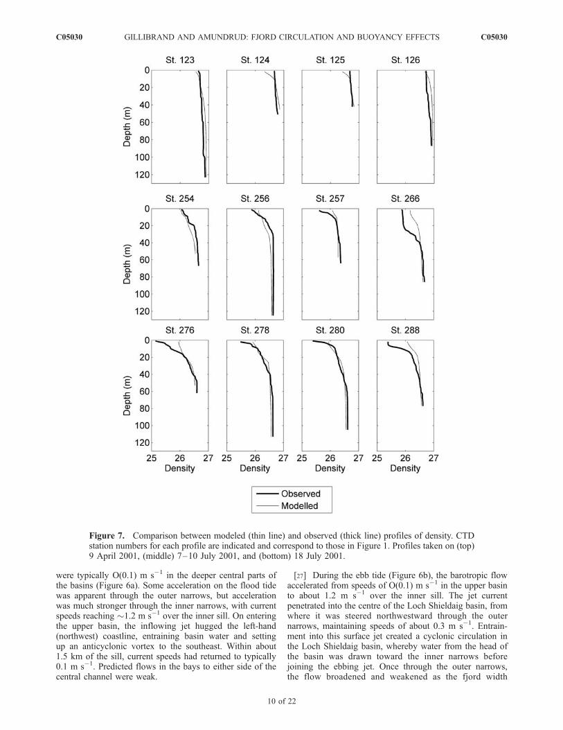
Figure 7. Comparison between modeled (thin line) and observed (thick line) profiles of density. CTDstation numbers for each profile are indicated and correspond to those in Figure 1. Profiles taken on (top)9 April 2001, (middle) 7–10 July 2001, and (bottom) 18 July 2001.


10 of 22

C05030

increased. Again, predicted flow outside the central channelregion was weak. The tidal flow over the inner sill wasweakly asymmetric, with the flood currents lasting typically6 hours compared to 6.4 hours for the ebb.[28] Tidal residual vectors are mapped in Figure 6c.

Residuals were generally weak (O(0.1) m s�1) except inthe region of the inner narrows and immediately off theheadlands that surround the outer narrows. On the upperbasin side of the inner narrows, an anticyclonic residualcirculation cell is evident; on the Loch Shieldaig side, acyclonic cell is partly discernible, although not fullyformed. These cells may have some retentive effect on theexchange of water between the basins but, beyond theimmediate vicinity of the sills, tidal currents appeared tointroduce only a very weak net transport.

4.2. Modeled Density and Density-Driven Circulation

[29] Modeled density was compared with profilesobtained during three CTD surveys of the fjord duringApril and July 2001. Four representative density profilesfrom each survey, the locations of which are shown in

Figure 1, are presented in Figure 7. The profiles show goodagreement between model and data, with the model repro-ducing the freshening of the entire water column thatoccurred between April and July. The model did not capturethe lowest densities found at the surface, which mayindicate that the freshwater input to the fjord was under-represented. The water density below 20 m depth was wellsimulated, and these results suggest that the model should becapable of simulating the major features of the barocliniccirculation in the fjord. The average RMS error for modeleddensity was 0.135, and the predictive skill was 0.78 (Table 4).[30] The simulation mean surface layer density is pre-

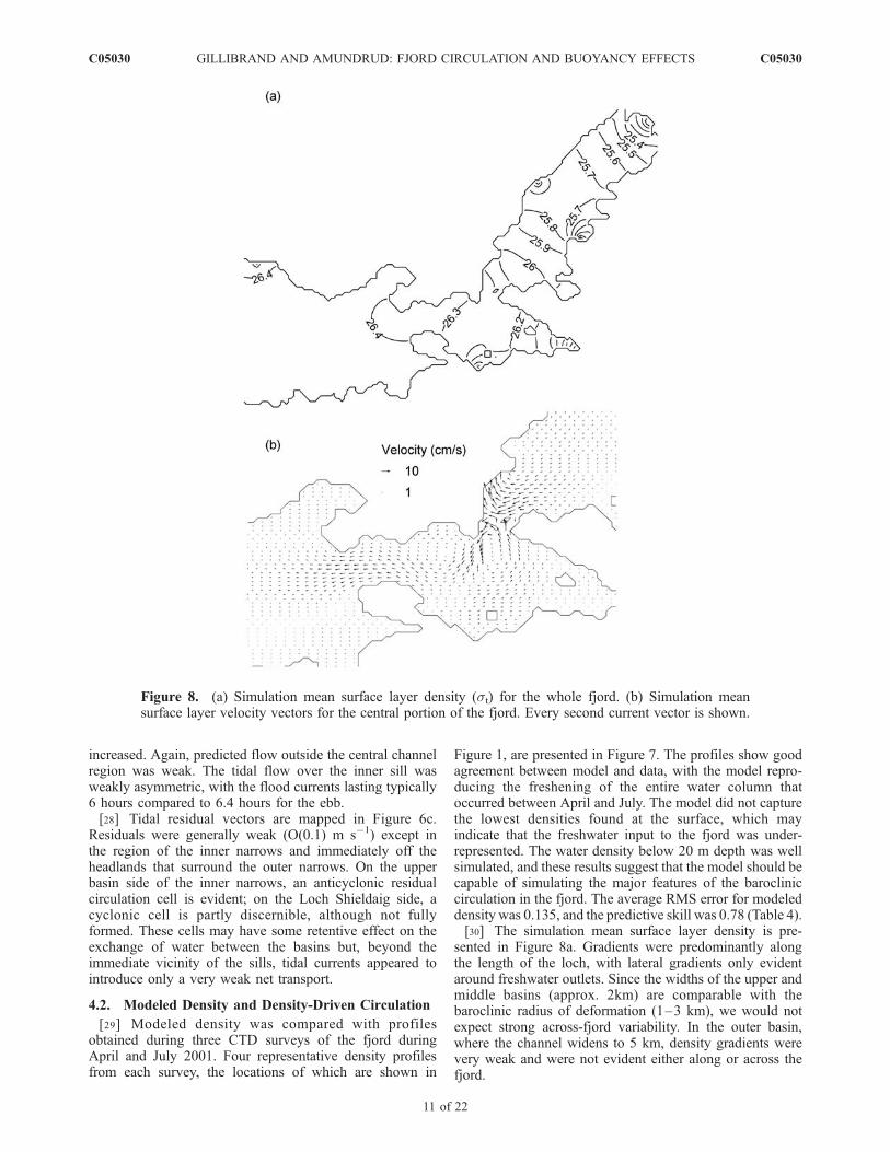
sented in Figure 8a. Gradients were predominantly alongthe length of the loch, with lateral gradients only evidentaround freshwater outlets. Since the widths of the upper andmiddle basins (approx. 2km) are comparable with thebaroclinic radius of deformation (1–3 km), we would notexpect strong across-fjord variability. In the outer basin,where the channel widens to 5 km, density gradients werevery weak and were not evident either along or across thefjord.

Figure 8. (a) Simulation mean surface layer density (st) for the whole fjord. (b) Simulation meansurface layer velocity vectors for the central portion of the fjord. Every second current vector is shown.


11 of 22

C05030

[31] The simulation mean surface layer circulation for thecentral section of the fjord (Figure 8b) features some notablechanges from the tidal residual circulation shown inFigure 6. The mean flow fields were still dominated bythe strong tidal residuals on either side of the inner sill, butsurface layer flow in the upper and outer basins was nowgenerally seaward, with speeds of 3–5 cm s�1, a result ofthe gravitational circulation driven by the buoyancy input.Under the influence of the seaward surface flow, the tidallygenerated residual vortex in the upper basin had degener-ated and was no longer closed. Conversely, in the middlebasin, the cyclonic circulation had strengthened, and asecond, anticyclonic, vortex formed in the northern part ofthe middle basin. Both cells introduced landward residualflow in the surface layer over a significant portion of thebasin, which would inhibit horizontal exchange and in-crease residence times in the basin. In deeper water, as thenarrower channel topography exerts more influence, vorti-ces in the mean flow were less evident (not shown) than inthe surface layer.[32] The seaward directed mean flow extended from the

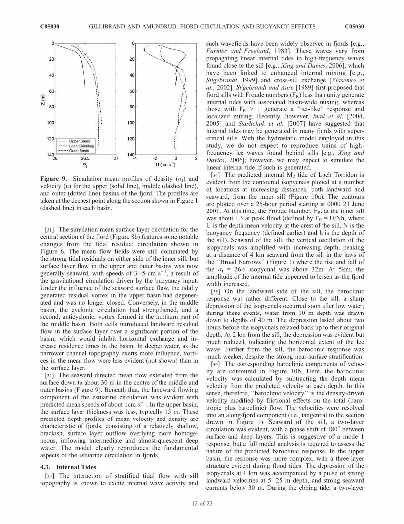
surface down to about 30 m in the centre of the middle andouter basins (Figure 9). Beneath that, the landward flowingcomponent of the estuarine circulation was evident withpredicted mean speeds of about 1cm s�1. In the upper basin,the surface layer thickness was less, typically 15 m. Thesepredicted depth profiles of mean velocity and density arecharacteristic of fjords, consisting of a relatively shallow,brackish, surface layer outflow overlying more homoge-neous, inflowing intermediate and almost-quiescent deepwater. The model clearly reproduces the fundamentalaspects of the estuarine circulation in fjords.

4.3. Internal Tides

[33] The interaction of stratified tidal flow with silltopography is known to excite internal wave activity and

such wavefields have been widely observed in fjords [e.g.,Farmer and Freeland, 1983]. These waves vary frompropagating linear internal tides to high-frequency wavesfound close to the sill [e.g., Xing and Davies, 2006], whichhave been linked to enhanced internal mixing [e.g.,Stigebrandt, 1999] and cross-sill exchange [Vlasenko etal., 2002]. Stigebrandt and Aure [1989] first proposed thatfjord sills with Froude numbers (FR) less than unity generateinternal tides with associated basin-wide mixing, whereasthose with FR > 1 generate a ‘‘jet-like’’ response andlocalized mixing. Recently, however, Inall et al. [2004,2005] and Stashchuk et al. [2007] have suggested thatinternal tides may be generated in many fjords with super-critical sills. With the hydrostatic model employed in thisstudy, we do not expect to reproduce trains of high-frequency lee waves found behind sills [e.g., Xing andDavies, 2006]; however, we may expect to simulate thelinear internal tide if such is generated.[34] The predicted internal M2 tide of Loch Torridon is

evident from the contoured isopycnals plotted at a numberof locations at increasing distances, both landward andseaward, from the inner sill (Figure 10a). The contoursare plotted over a 25-hour period starting at 0000 23 June2001. At this time, the Froude Number, FR, at the inner sillwas about 1.5 at peak flood (defined by FR = U/Nh, whereU is the depth mean velocity at the crest of the sill, N is thebuoyancy frequency (defined earlier) and h is the depth ofthe sill). Seaward of the sill, the vertical oscillation of theisopycnals was amplified with increasing depth, peakingat a distance of 4 km seaward from the sill in the jaws ofthe ‘‘Broad Narrows’’ (Figure 1) where the rise and fall ofthe st = 26.6 isopycnal was about 32m. At 5km, theamplitude of the internal tide appeared to lessen as the fjordwidth increased.[35] On the landward side of the sill, the baroclinic

response was rather different. Close to the sill, a sharpdepression of the isopycnals occurred soon after low water;during these events, water from 10 m depth was drawndown to depths of 40 m. The depression lasted about twohours before the isopycnals relaxed back up to their originaldepth. At 2 km from the sill, the depression was evident butmuch reduced, indicating the horizontal extent of the leewave. Further from the sill, the baroclinic response wasmuch weaker, despite the strong near-surface stratification.[36] The corresponding baroclinic components of veloc-

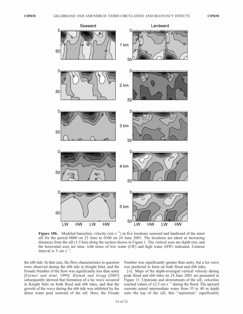
ity are contoured in Figure 10b. Here, the baroclinicvelocity was calculated by subtracting the depth meanvelocity from the predicted velocity at each depth. In thissense, therefore, ‘‘baroclinic velocity’’ is the density-drivenvelocity modified by frictional effects on the total (baro-tropic plus baroclinic) flow. The velocities were resolvedinto an along-fjord component (i.e., tangential to the sectiondrawn in Figure 1). Seaward of the sill, a two-layercirculation was evident, with a phase shift of 180� betweensurface and deep layers. This is suggestive of a mode 1response, but a full modal analysis is required to assess thenature of the predicted baroclinic response. In the upperbasin, the response was more complex, with a three-layerstructure evident during flood tides. The depression of theisopycnals at 1 km was accompanied by a pulse of stronglandward velocities at 5–25 m depth, and strong seawardcurrents below 30 m. During the ebbing tide, a two-layer

Figure 9. Simulation mean profiles of density (st) andvelocity (u) for the upper (solid line), middle (dashed line),and outer (dotted line) basins of the fjord. The profiles aretaken at the deepest point along the section shown in Figure 1(dashed line) in each basin.


12 of 22

C05030

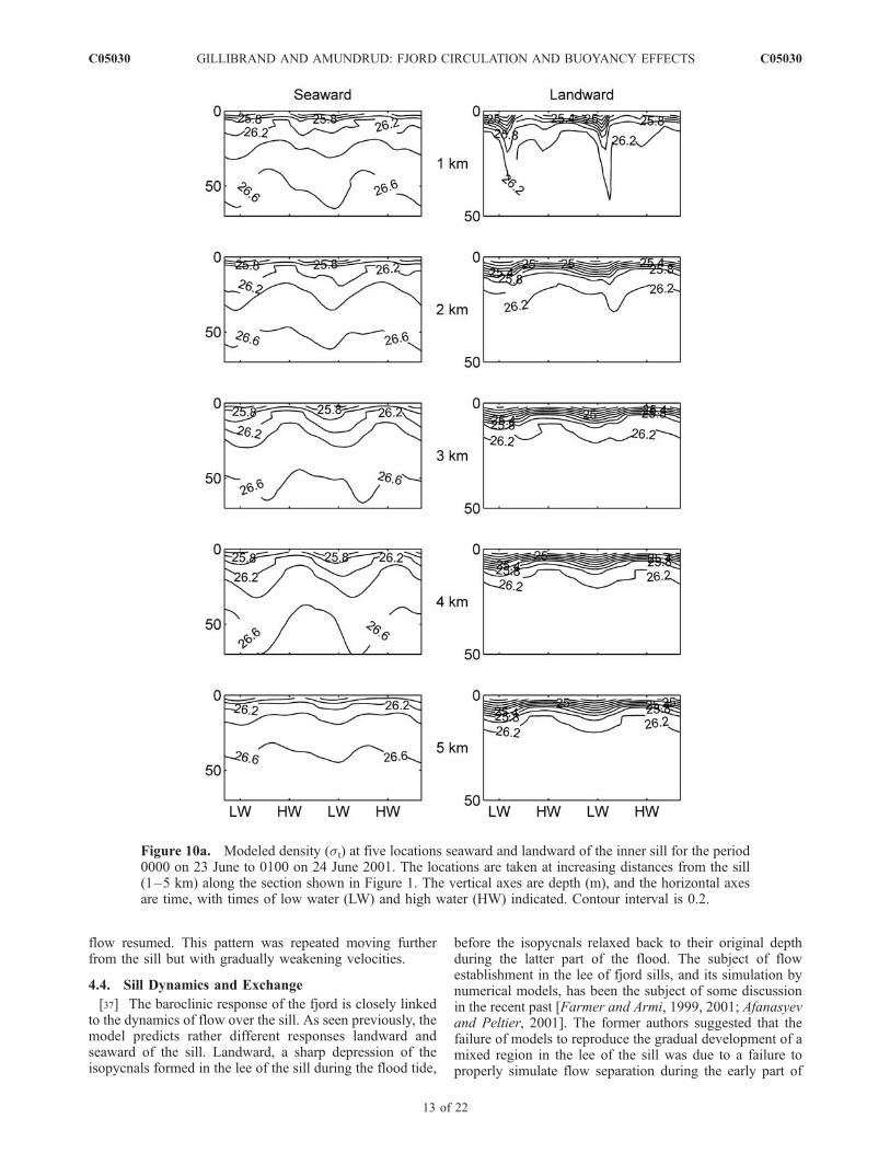
flow resumed. This pattern was repeated moving furtherfrom the sill but with gradually weakening velocities.

4.4. Sill Dynamics and Exchange

[37] The baroclinic response of the fjord is closely linkedto the dynamics of flow over the sill. As seen previously, themodel predicts rather different responses landward andseaward of the sill. Landward, a sharp depression of theisopycnals formed in the lee of the sill during the flood tide,

before the isopycnals relaxed back to their original depthduring the latter part of the flood. The subject of flowestablishment in the lee of fjord sills, and its simulation bynumerical models, has been the subject of some discussionin the recent past [Farmer and Armi, 1999, 2001; Afanasyevand Peltier, 2001]. The former authors suggested that thefailure of models to reproduce the gradual development of amixed region in the lee of the sill was due to a failure toproperly simulate flow separation during the early part of

Figure 10a. Modeled density (st) at five locations seaward and landward of the inner sill for the period0000 on 23 June to 0100 on 24 June 2001. The locations are taken at increasing distances from the sill(1–5 km) along the section shown in Figure 1. The vertical axes are depth (m), and the horizontal axesare time, with times of low water (LW) and high water (HW) indicated. Contour interval is 0.2.


13 of 22

C05030

the ebb tide. In that case, the flow characteristics in questionwere observed during the ebb tide in Knight Inlet, and theFroude Number of the flow was significantly less than unity[Farmer and Armi, 1999]. Klymak and Gregg [2003]subsequently showed that formation of a lee wave occurredin Knight Inlet on both flood and ebb tides, and that thegrowth of the wave during the ebb tide was inhibited by thedense water pool seaward of the sill. Here, the Froude

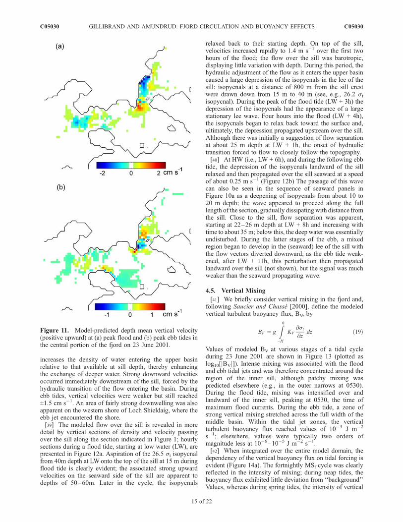
Number was significantly greater than unity, but a lee wavewas predicted to form on both flood and ebb tides.[38] Maps of the depth-averaged vertical velocity during

peak flood and ebb tides on 24 June 2001 are presented inFigure 11. Upstream and downstream of the sill, velocitiesreached values of ±2.5 cm s�1 during the flood. The upwardcurrents raised intermediate water from 35 to 40 m depthonto the top of the sill; this ‘‘aspiration’’ significantly

Figure 10b. Modeled baroclinic velocity (cm s�1) at five locations seaward and landward of the innersill for the period 0000 on 23 June to 0100 on 24 June 2001. The locations are taken at increasingdistances from the sill (1-5 km) along the section shown in Figure 1. The vertical axes are depth (m), andthe horizontal axes are time, with times of low water (LW) and high water (HW) indicated. Contourinterval is 5 cm s�1.


14 of 22

C05030

increases the density of water entering the upper basinrelative to that available at sill depth, thereby enhancingthe exchange of deeper water. Strong downward velocitiesoccurred immediately downstream of the sill, forced by thehydraulic transition of the flow entering the basin. Duringebb tides, vertical velocities were weaker but still reached±1.5 cm s�1. An area of fairly strong downwelling was alsoapparent on the western shore of Loch Shieldaig, where theebb jet encountered the shore.[39] The modeled flow over the sill is revealed in more

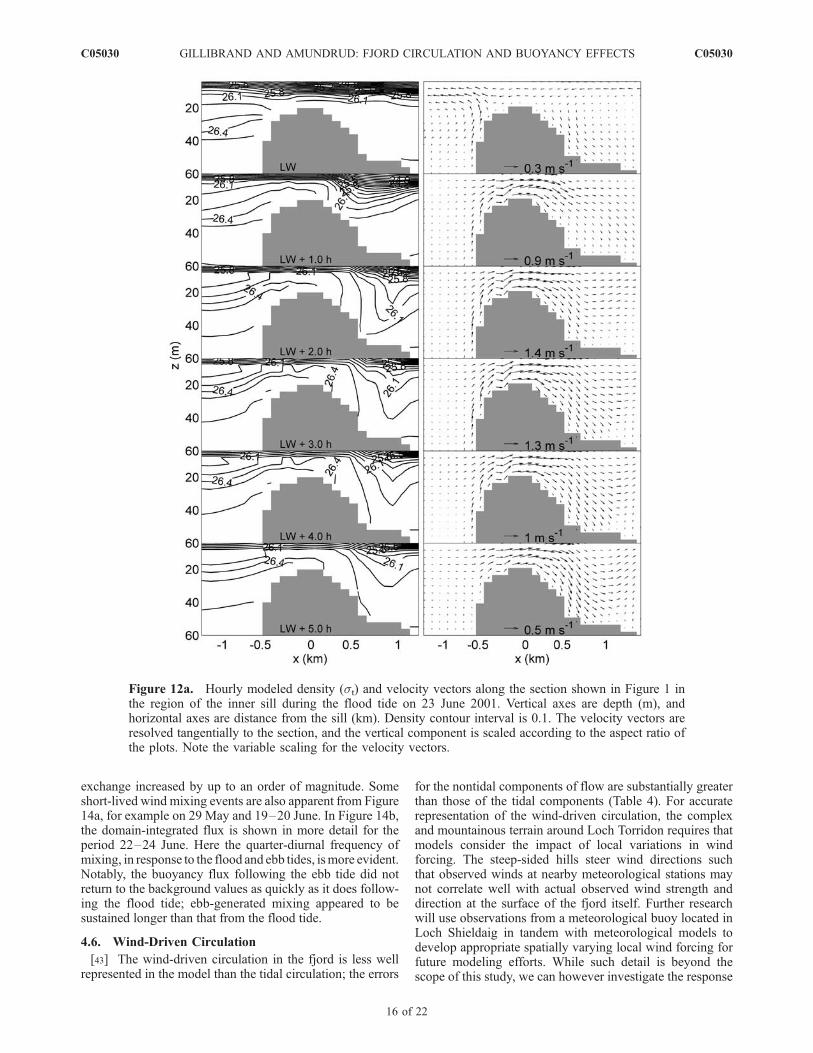
detail by vertical sections of density and velocity passingover the sill along the section indicated in Figure 1; hourlysections during a flood tide, starting at low water (LW), arepresented in Figure 12a. Aspiration of the 26.5 st isopycnalfrom 40m depth at LWonto the top of the sill at 15 m duringflood tide is clearly evident; the associated strong upwardvelocities on the seaward side of the sill are apparent todepths of 50–60m. Later in the cycle, the isopycnals

relaxed back to their starting depth. On top of the sill,velocities increased rapidly to 1.4 m s�1 over the first twohours of the flood; the flow over the sill was barotropic,displaying little variation with depth. During this period, thehydraulic adjustment of the flow as it enters the upper basincaused a large depression of the isopycnals in the lee of thesill: isopycnals at a distance of 800 m from the sill crestwere drawn down from 15 m to 40 m (see, e.g., 26.2 stisopycnal). During the peak of the flood tide (LW + 3h) thedepression of the isopycnals had the appearance of a largestationary lee wave. Four hours into the flood (LW + 4h),the isopycnals began to relax back toward the surface and,ultimately, the depression propagated upstream over the sill.Although there was initially a suggestion of flow separationat about 25 m depth at LW + 1h, the onset of hydraulictransition forced to flow to closely follow the topography.[40] At HW (i.e., LW + 6h), and during the following ebb

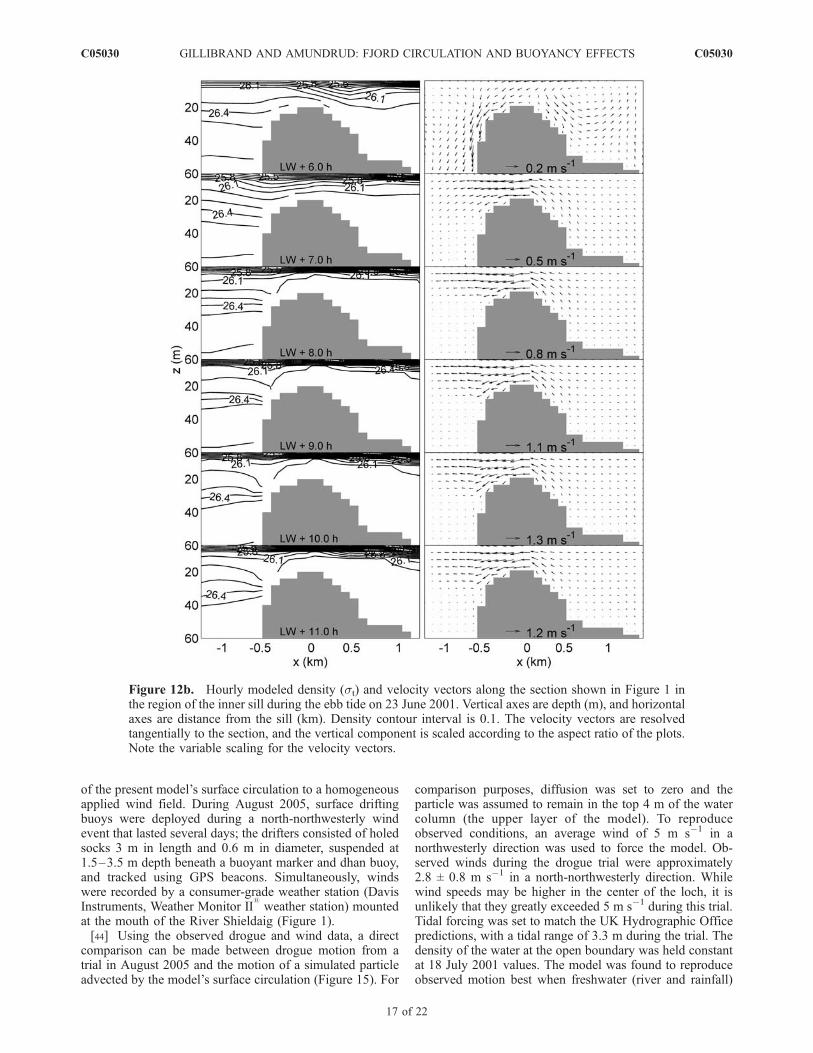
tide, the depression of the isopycnals landward of the sillrelaxed and then propagated over the sill seaward at a speedof about 0.25 m s�1 (Figure 12b) The passage of this wavecan also be seen in the sequence of seaward panels inFigure 10a as a deepening of isopycnals from about 10 to20 m depth; the wave appeared to proceed along the fulllength of the section, gradually dissipating with distance fromthe sill. Close to the sill, flow separation was apparent,starting at 22–26 m depth at LW + 8h and increasing withtime to about 35 m; below this, the deep water was essentiallyundisturbed. During the latter stages of the ebb, a mixedregion began to develop in the (seaward) lee of the sill withthe flow vectors diverted downward; as the ebb tide weak-ened, after LW + 11h, this perturbation then propagatedlandward over the sill (not shown), but the signal was muchweaker than the seaward propagating wave.

4.5. Vertical Mixing

[41] We briefly consider vertical mixing in the fjord and,following Saucier and Chasse [2000], define the modeledvertical turbulent buoyancy flux, BV, by

BV ¼ g

Z0�H

KV

@st

@z:dz ð19Þ

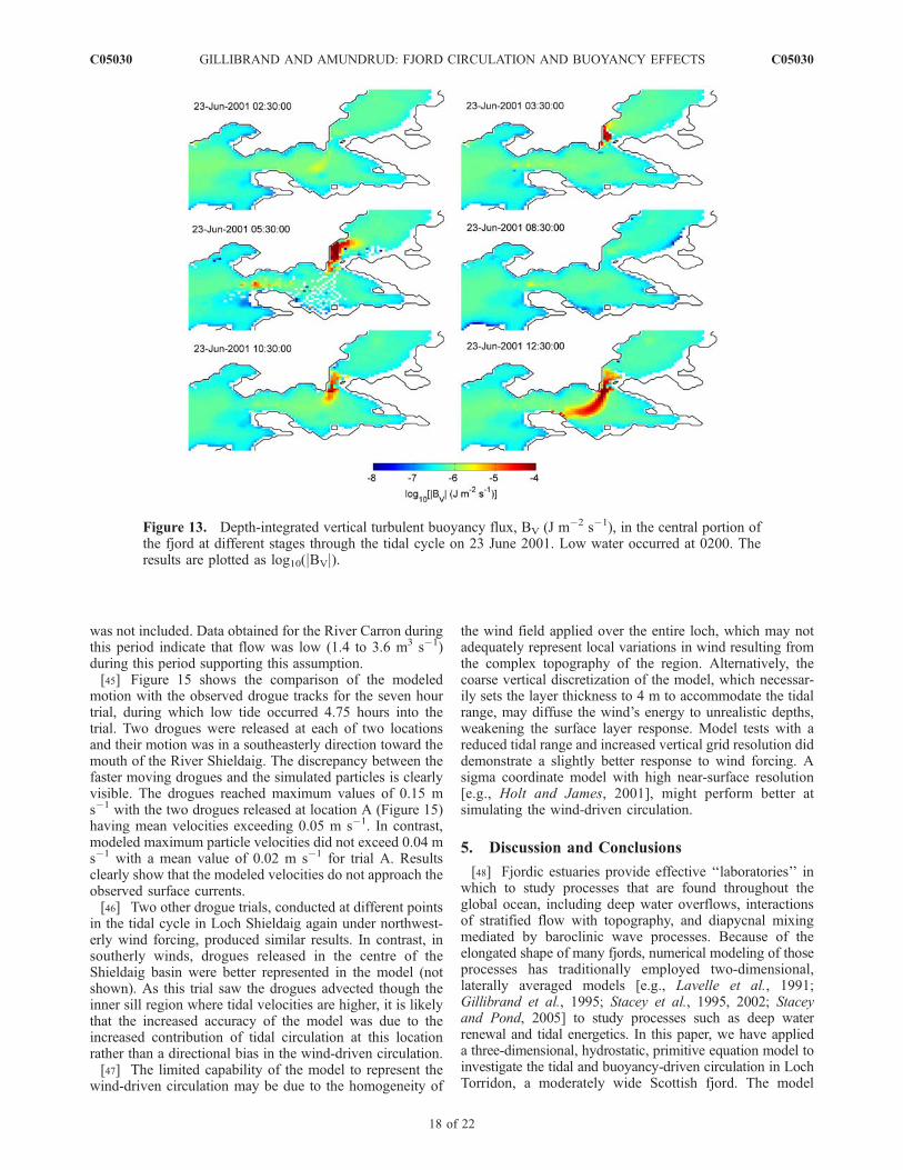
Values of modeled BV at various stages of a tidal cycleduring 23 June 2001 are shown in Figure 13 (plotted aslog10[jBVj]). Intense mixing was associated with the floodand ebb tidal jets and was therefore concentrated around theregion of the inner sill, although patchy mixing waspredicted elsewhere (e.g., in the outer narrows at 0530).During the flood tide, mixing was intensified over andlandward of the inner sill, peaking at 0530, the time ofmaximum flood currents. During the ebb tide, a zone ofstrong vertical mixing stretched across the full width of themiddle basin. Within the tidal jet zones, the verticalturbulent buoyancy flux reached values of 10�3 J m�2

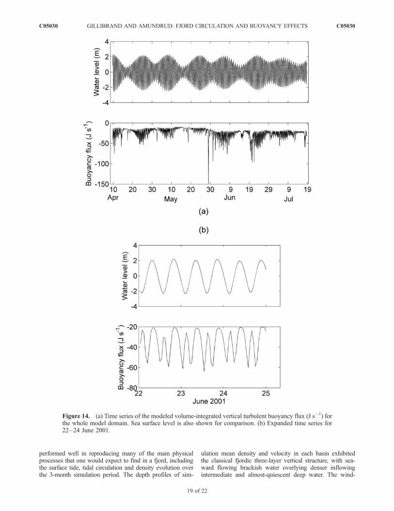
s�1; elsewhere, values were typically two orders ofmagnitude less at 10�6–10�5 J m�2 s�1.[42] When integrated over the entire model domain, the

dependency of the vertical buoyancy flux on tidal forcing isevident (Figure 14a). The fortnightly MSf cycle was clearlyreflected in the intensity of mixing; during neap tides, thebuoyancy flux exhibited little deviation from ‘‘background’’Values, whereas during spring tides, the intensity of vertical

Figure 11. Model-predicted depth mean vertical velocity(positive upward) at (a) peak flood and (b) peak ebb tides inthe central portion of the fjord on 23 June 2001.


15 of 22

C05030

exchange increased by up to an order of magnitude. Someshort-lived wind mixing events are also apparent from Figure14a, for example on 29 May and 19–20 June. In Figure 14b,the domain-integrated flux is shown in more detail for theperiod 22–24 June. Here the quarter-diurnal frequency ofmixing, in response to the flood and ebb tides, ismore evident.Notably, the buoyancy flux following the ebb tide did notreturn to the background values as quickly as it does follow-ing the flood tide; ebb-generated mixing appeared to besustained longer than that from the flood tide.

4.6. Wind-Driven Circulation

[43] The wind-driven circulation in the fjord is less wellrepresented in the model than the tidal circulation; the errors

for the nontidal components of flow are substantially greaterthan those of the tidal components (Table 4). For accuraterepresentation of the wind-driven circulation, the complexand mountainous terrain around Loch Torridon requires thatmodels consider the impact of local variations in windforcing. The steep-sided hills steer wind directions suchthat observed winds at nearby meteorological stations maynot correlate well with actual observed wind strength anddirection at the surface of the fjord itself. Further researchwill use observations from a meteorological buoy located inLoch Shieldaig in tandem with meteorological models todevelop appropriate spatially varying local wind forcing forfuture modeling efforts. While such detail is beyond thescope of this study, we can however investigate the response

Figure 12a. Hourly modeled density (st) and velocity vectors along the section shown in Figure 1 inthe region of the inner sill during the flood tide on 23 June 2001. Vertical axes are depth (m), andhorizontal axes are distance from the sill (km). Density contour interval is 0.1. The velocity vectors areresolved tangentially to the section, and the vertical component is scaled according to the aspect ratio ofthe plots. Note the variable scaling for the velocity vectors.


16 of 22

C05030

of the present model’s surface circulation to a homogeneousapplied wind field. During August 2005, surface driftingbuoys were deployed during a north-northwesterly windevent that lasted several days; the drifters consisted of holedsocks 3 m in length and 0.6 m in diameter, suspended at1.5–3.5 m depth beneath a buoyant marker and dhan buoy,and tracked using GPS beacons. Simultaneously, windswere recorded by a consumer-grade weather station (DavisInstruments, Weather Monitor II

1

weather station) mountedat the mouth of the River Shieldaig (Figure 1).[44] Using the observed drogue and wind data, a direct

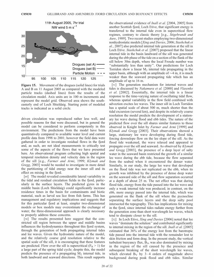
comparison can be made between drogue motion from atrial in August 2005 and the motion of a simulated particleadvected by the model’s surface circulation (Figure 15). For

comparison purposes, diffusion was set to zero and theparticle was assumed to remain in the top 4 m of the watercolumn (the upper layer of the model). To reproduceobserved conditions, an average wind of 5 m s�1 in anorthwesterly direction was used to force the model. Ob-served winds during the drogue trial were approximately2.8 ± 0.8 m s�1 in a north-northwesterly direction. Whilewind speeds may be higher in the center of the loch, it isunlikely that they greatly exceeded 5 m s�1 during this trial.Tidal forcing was set to match the UK Hydrographic Officepredictions, with a tidal range of 3.3 m during the trial. Thedensity of the water at the open boundary was held constantat 18 July 2001 values. The model was found to reproduceobserved motion best when freshwater (river and rainfall)

Figure 12b. Hourly modeled density (st) and velocity vectors along the section shown in Figure 1 inthe region of the inner sill during the ebb tide on 23 June 2001. Vertical axes are depth (m), and horizontalaxes are distance from the sill (km). Density contour interval is 0.1. The velocity vectors are resolvedtangentially to the section, and the vertical component is scaled according to the aspect ratio of the plots.Note the variable scaling for the velocity vectors.


17 of 22

C05030

was not included. Data obtained for the River Carron duringthis period indicate that flow was low (1.4 to 3.6 m3 s�1)during this period supporting this assumption.[45] Figure 15 shows the comparison of the modeled

motion with the observed drogue tracks for the seven hourtrial, during which low tide occurred 4.75 hours into thetrial. Two drogues were released at each of two locationsand their motion was in a southeasterly direction toward themouth of the River Shieldaig. The discrepancy between thefaster moving drogues and the simulated particles is clearlyvisible. The drogues reached maximum values of 0.15 ms�1 with the two drogues released at location A (Figure 15)having mean velocities exceeding 0.05 m s�1. In contrast,modeled maximum particle velocities did not exceed 0.04 ms�1 with a mean value of 0.02 m s�1 for trial A. Resultsclearly show that the modeled velocities do not approach theobserved surface currents.[46] Two other drogue trials, conducted at different points

in the tidal cycle in Loch Shieldaig again under northwest-erly wind forcing, produced similar results. In contrast, insoutherly winds, drogues released in the centre of theShieldaig basin were better represented in the model (notshown). As this trial saw the drogues advected though theinner sill region where tidal velocities are higher, it is likelythat the increased accuracy of the model was due to theincreased contribution of tidal circulation at this locationrather than a directional bias in the wind-driven circulation.[47] The limited capability of the model to represent the

wind-driven circulation may be due to the homogeneity of

the wind field applied over the entire loch, which may notadequately represent local variations in wind resulting fromthe complex topography of the region. Alternatively, thecoarse vertical discretization of the model, which necessar-ily sets the layer thickness to 4 m to accommodate the tidalrange, may diffuse the wind’s energy to unrealistic depths,weakening the surface layer response. Model tests with areduced tidal range and increased vertical grid resolution diddemonstrate a slightly better response to wind forcing. Asigma coordinate model with high near-surface resolution[e.g., Holt and James, 2001], might perform better atsimulating the wind-driven circulation.

5. Discussion and Conclusions

[48] Fjordic estuaries provide effective ‘‘laboratories’’ inwhich to study processes that are found throughout theglobal ocean, including deep water overflows, interactionsof stratified flow with topography, and diapycnal mixingmediated by baroclinic wave processes. Because of theelongated shape of many fjords, numerical modeling of thoseprocesses has traditionally employed two-dimensional,laterally averaged models [e.g., Lavelle et al., 1991;Gillibrand et al., 1995; Stacey et al., 1995, 2002; Staceyand Pond, 2005] to study processes such as deep waterrenewal and tidal energetics. In this paper, we have applieda three-dimensional, hydrostatic, primitive equation model toinvestigate the tidal and buoyancy-driven circulation in LochTorridon, a moderately wide Scottish fjord. The model

Figure 13. Depth-integrated vertical turbulent buoyancy flux, BV (J m�2 s�1), in the central portion ofthe fjord at different stages through the tidal cycle on 23 June 2001. Low water occurred at 0200. Theresults are plotted as log10(jBVj).


18 of 22

C05030

performed well in reproducing many of the main physicalprocesses that one would expect to find in a fjord, includingthe surface tide, tidal circulation and density evolution overthe 3-month simulation period. The depth profiles of sim-

ulation mean density and velocity in each basin exhibitedthe classical fjordic three-layer vertical structure, with sea-ward flowing brackish water overlying denser inflowingintermediate and almost-quiescent deep water. The wind-

Figure 14. (a) Time series of the modeled volume-integrated vertical turbulent buoyancy flux (J s�1) forthe whole model domain. Sea surface level is also shown for comparison. (b) Expanded time series for22–24 June 2001.


19 of 22

C05030

driven circulation was reproduced rather less well, andpossible reasons for that were discussed, but in general themodel can be considered to perform competently in thisenvironment. The predictions from the model have beenquantitatively compared to available water level and currentprofile data from 1998 to 2001; however the field data weregathered in order to investigate residual flows in the fjordand, as such, are not ideal measurements to critically testsome of the aspects of the flows that we have presentedhere. An observational program collecting high spatial andtemporal resolution density and velocity data in the regionof the sill [e.g., Farmer and Armi, 1999; Klymak andGregg, 2003] would be needed to investigate in more detailthe partitioning of tidal energy near the inner sill and itseffect on mixing in the fjord.[49] The model revealed considerable lateral variability in

the tidal and residual circulation fields in the fjord, partic-ularly in the surface layers. The predicted gyres in themiddle basin (Loch Shieldaig) could significantly increaseresidence times in the basin for contaminants and bioticmaterial, such as larval sea lice from fish farms. This hasmanagement and regulatory implications and suggests thatfor this particular fjord at least, simpler two-dimensionalmodels or box models may overestimate the exchange ofwater; the three-dimensional approach is clearly necessaryto properly address these concerns.[50] The results presented here suggest that the con-

stricted sill region between the upper and middle basinsinfluences the hydrodynamics throughout this fjord system,through the generation of both propagating internal tidesand lee waves. Given the hydrostatic nature of the model,and the relatively coarse grid resolution relative to thespatial scale of the sill, it is encouraging that these featuresare predicted. Flow over the sill is supercritical (FR > 1) fora large part of the spring tidal cycle; despite this, the modelpredicts the presence of a propagating M2 internal tide, inboth landward and seaward directions. This result supports

the observational evidence of Inall et al. [2004, 2005] fromanother Scottish fjord, Loch Etive, that significant energy istransferred to the internal tide even in supercritical flowregimes, contrary to classic theory [e.g., Stigebrandt andAure, 1989]. Two recent studies employing two-dimensionalnonhydrostatic models [Xing and Davies, 2006; Stashchuk etal., 2007] also predicted internal tide generation at the sill inLoch Etive. Stashchuk et al. [2007] proposed that the linearinternal tide in the basin landward of the sill was generatedduring the ebb phase of the tide on a section of the flank of thesill below 30m depth, where the local Froude number was‘‘substantially less than unity’’. Our predictions for LochTorridon show a linear M2 internal tide propagating in theupper basin, although with an amplitude of �4 m, it is muchweaker than the seaward propagating tide which has anamplitude of up to 16 m.[51] The generation mechanism for internal waves and

tides is discussed by Nakamura et al. [2000] and Vlasenkoet al. [2002]. Essentially, the internal tide is a linearresponse to the time-varying nature of oscillating tidal flow,whereas spatial variability in the flow field combined withadvection excites lee waves. The inner sill in Loch Torridonhas a spatial scale of about 500 m, much shorter than thetidal excursion (several km), and despite its relatively coarseresolution the model predicts the development of a station-ary lee wave during flood and ebb tides. The nature of thepredicted flow over the sill shares similar features to thoseobserved in Knight Inlet by Farmer and Armi [1999] andKlymak and Gregg [2003]. Their observations showed alarge, stationary lee wave developing during flood tide,forcing downslope flow on the lee slope of the sill. As theflood tide weakened, the wave relaxed and appeared topropagate over the sill and seaward. As observed by Klymakand Gregg [2003], the presence of a deep layer of saltywater in the seaward basin restricted the growth of a similarlee wave during the ebb tide, because the flow separatedfrom the seabed when it encountered the denser water.Similarly, in our study, the large lee wave that developedon the flood tide was not replicated on the ebb, when itsgrowth was inhibited by the presence of dense deep wateron the seaward side of the sill and flow separation occurredat a depth of about 25 m. The net effect was that duringflood tide, energy from the tide passed into the lee wave andonly a weak internal tide was produced; in contrast, on theebb, more energy passed into the internal tide, which wasgenerated on the flank of the sill where the pycnoclineseparating the surface layers and the deep salty poolintersected the topography. This has implications for mixingin the fjord, since internal tides radiate energy further fromthe generation zone than short wavelength lee waves, whichtend to dissipate closer to the sill.[52] In Loch Etive, Xing and Davies [2006] noted that lee

waves ‘‘dominate the solution’’ and contributed significantlyto internal mixing in the region of the sill. Inall et al. [2005]estimated that 36% of the energy lost from the barotropictide passed into the internal tide with the remainder lost toskin friction and form drag. In the present study, the verticalturbulent buoyancy flux, BV, was also dominated by mixingin the region of the sill caused by the presence andsubsequent breaking of the short wavelength lee waves,which elevated BV by 3–4 orders of magnitude abovebackground during peak flood and ebb tides. Similar

Figure 15. Movement of the drogues (solid lines) for trialsA and B on 11 August 2005 as compared with the modeledparticle tracks (dashed lines) from the results of thecirculation model. Axis units are in 100 m increments andrepresent the model grid. Observed area shows the south-easterly end of Loch Shieldaig. Starting point of modeledtracks is indicated as a solid circle.


20 of 22

C05030

enhancement of the vertical diffusivities by large unsteadylee waves was predicted by Nakamura et al. [2000] for theKuril Straits sill.[53] The domain-integrated vertical buoyancy flux pre-

dicted by the model exhibited a strong temporal variabilitylinked to the spring-neap tidal cycle. The flux increased by afactor of four at springs relative to neaps. Superimposed onthis tidal mixing, are several transient events of intensemixing, for example on 2 May, 29 May, and 19–20 June.We have not investigated this mixing in detail, because ofthe uncertainty over the accuracy of the wind-forcing dataand the resulting velocity fields; however, a preliminaryinspection of the results suggests that these events coincidewith short-lived bursts of westerly winds, which are alignedwith the upper basin. Mixing may result directly from thesurface input of turbulent kinetic energy, or through wind-induced internal waves that can be generated in stratifiedcoastal waters [Xing and Davies, 2004]. The role of windmixing in the fjord needs further investigation.[54] Because the present model is hydrostatic, it is limited

in its ability to simulate the large vertical velocities evidentin the flow over the sill and the nonlinear waves and mixingthat result. Although the model predicts the development ofa large stationary lee wave, the hydrostatic assumption maylead to errors in the detailed characteristics of the wave. Inaddition, the sensitivity of the nonlinear generating mech-anism to small-scale topography in the sill region makes itessential that accurate detailed topography is resolved bythe model if small-scale baroclinic features are to beaccurately simulated [Xing and Davies, 2006]; the 100 mresolution used here captures the overall topographic gra-dients but will miss some of the fine detail. Also, internalwave breaking in hydrostatic models leads to staticallyunstable water columns, which are resolved by convectiveadjustment of the density profile; this process may enhancevertical mixing unrealistically. All these problems havebeen overcome previously by utilizing high-resolution,two-dimensional, nonhydrostatic models, which have illus-trated the generation of large-amplitude unsteady lee wavesbehind sills that subsequently propagate upstream as thetidal flow slackens and turns [e.g., Vlasenko et al., 2002;Cummins et al., 2003]. Vlasenko et al. [2002] demonstratedthe formation of large unsteady lee waves in the Trond-heimfjord and showed, through simulation of a passivetracer, that the nonlinearity of the waves enhances exchangethrough the sill region. Cummins et al. [2003] reproducedobservations of trains of solitary-like internal waves prop-agating upstream, and the model of Xing and Davies [2006]also predicted a train of unsteady lee waves which propa-gated toward the sill when the tide reversed.[55] These models offer great insights into the excitation

and propagation of nonlinear waves near supercritical flowregimes, but neglect three-dimensional aspects of the flowswhich observations suggest are important for energy parti-tioning and dissipation [e.g., Klymak and Gregg, 2001; Inallet al., 2005]. Three-dimensional, nonhydrostatic modelswith the capability to simulate stratified flow processes inrealistic (nonidealized) environments are now becomingavailable to the research community [e.g., Marshall et al.,1997], and should be exploited to explore these problems.Fjords make ideal numerical laboratories for this effort,

offering varying flow regimes and a steadily expandingarchive of observations against which to test and refine ourmodels and understanding.

[56] Acknowledgments. We are grateful to F.J. Saucier for makingthe GFX code available and are greatly indebted to J.-F. Dumais for hisefforts in developing and configuring the initial version of the Torridonmodel. S. Hughes and G. Slesser processed the ADCP, CTD, and WLRdata. J. Beaton and D. Lichtman assisted with the drogue field experiment.We thank two reviewers for their very helpful comments, which improvedthis paper. The wind data from Glascarnoch and rainfall data from Torridonwere supplied by the UK Met Office through the British Atmospheric DataCentre, and the flow data from the River Carron were provided by theScottish Environment Protection Agency (SEPA).

ReferencesAfanasyev, Y. D., and W. R. Peltier (2001), On breaking internal wavesover the sill in Knight Inlet, Proc. R. Soc. London, Ser. A, 457, 2799–2825.

Arneborg, L., C. Janzen, B. Liljebladh, T. P. Rippeth, J. H. Simpson, andA. Stigebrandt (2004), Spatial variability of diapycnal mixing and turbu-lent dissipation rates in a stagnant fjord basin, J. Phys. Oceanogr., 34,1679–1691.

Asplin, L., A. G. V. Salvanes, and J. B. Kristoffersen (1999), Nonlocalwind-driven fjord-coast advection and its potential effect on planktonand fish recruitment, Fish. Oceanogr., 8, 255–263.

Atakturk, S. S., and K. B. Katsaros (1999), Wind stress and surface wavesobserved on Lake Washington, J. Phys. Oceanogr., 29, 633–650.

Backhaus, J. O. (1985), A three-dimensional model for the simulation ofshelf sea dynamics, Dtsch. Hydrogr. Z., 38, 165–187.

Cummins, P. F., S. Vagle, L. Armi, and D. M. Farmer (2003), Stratified flowover topography: Upstream influence and generation of nonlinear internalwaves, Proc. R. Soc. London, Ser. A, 459, 1467–1487.

Cushman-Roisin, B., L. Asplin, and H. Svendsen (1994), Upwelling inbroad fjords, Cont. Shelf Res., 14, 1701–1721.

Edwards, A., and D. Edelsten (1977), Deep water renewal of Loch Etive: Athree basin Scottish fjord, Estuarine Coastal Mar. Sci., 5, 575–595.

Eliassen, I. K., Y. Heggelund, and M. Haakstad (2001), A numerical studyof the circulation in Saltfjorden, Saltstraumen and Skjerstadfjorden, Cont.Shelf Res., 21, 1669–1689.

Farmer, D. M., and L. Armi (1999), Stratified flow over topography: Therole of small-scale entrainment and mixing in flow establishment, Proc.R. Soc. London, Ser. A, 455, 3221–3258.

Farmer, D. M., and L. Armi (2001), Stratified flow over topography: Mod-els versus observations, Proc. R. Soc. London, Ser. A, 457, 2827–2830.

Farmer, D., and H. Freeland (1983), The physical oceanography of fjords,J. Phys. Oceanogr., 12, 147–220.

Foreman, M. G. G., D. J. Stucchi, Y. Zhang, and A. M. Baptista (2006),Estuarine and tidal currents in the Broughton Archipelago, Atmos. Ocean,44, 47–63.

Galperin, B., and G. L. Mellor (1990a), A time-dependent, three-dimensional model of the Delaware Bay and River system. part 2:Three-dimensional flow fields and residual circulation, Estuarine CoastalShelf Sci., 31, 255–281.

Galperin, B., andG. L.Mellor (1990b), A time-dependent, three-dimensionalmodel of the Delaware Bay and River system. part I: Description of themodel and tidal analysis, Estuarine Coastal Shelf Sci., 31, 231–253.

Galperin, B., L. H. Kantha, S. Hassid, and A. Rosati (1988), A quasi-equilibrium turbulent energy model for geophysical flows, J. Atmos.Sci., 45, 55–62.

Gargett, A. E., and G. Holloway (1984), Dissipation and diffusion byinternal wave breaking, J. Mar. Res., 42, 15–27.

Gillibrand, P. A., W. R. Turrell, and A. J. Elliott (1995), Deep-water renewalin the upper basin of Loch Sunart, a Scottish fjord, J. Phys. Oceanogr., 25,1488–1503.

Holt, J. T., and I. D. James (2001), An s coordinate density evolving modelof the northwest European continental shelf: 1. Model description anddensity structure, J. Geophys. Res., 106, 14,015–14,034.

Inall, M. E., and T. P. Rippeth (2002), Dissipation of tidal energy andassociated mixing in a wide fjord, Environ. Fluid Mech., 2, 219–240.

Inall, M. E., F. R. Cottier, C. Griffiths, and T. P. Rippeth (2004), Silldynamics and energy transformation in a jet fjord, Ocean Dyn., 54,307–314.

Inall, M., T. Rippeth, C. Griffiths, and P. Wiles (2005), Evolution anddistribution of TKE production and dissipation within stratified flow overtopography, Geophys. Res. Lett. , 32 , L08607, doi:10.1029/2004GL022289.


21 of 22

C05030

Kantha, L., and C. A. Clayson (1994), An improved mixed layer model forgeophysical applications, J. Geophys. Res., 99, 25,235–25,266.

Klymak, J. M., and M. C. Gregg (2001), Three-dimensional nature of flownear a sill, J. Geophys. Res., 106, 22,295–22,311.

Klymak, J. M., and M. C. Gregg (2003), The role of upstream waves and adownstream density pool in the growth of lee waves: Stratified flow overthe Knight Inlet sill, J. Phys. Oceanogr., 33, 1446–1461.

Lavelle, J. W., E. D. Cokelet, and G. A. Cannon (1991), A model study ofdensity intrusions and circulation within a deep, silled estuary: PugetSound, J. Geophys. Res., 96, 16,779–16,800.

Marshall, J., C. Hill, L. Perelman, and A. Adcroft (1997), Hydrostatic,quasi-hydrostatic, and nonhydrostatic ocean modeling, J. Geophys.Res., 102, 5733–5752.

Mellor, G. L., and T. Yamada (1982), Development of a turbulence closuremodel for geophysical fluid problems, Rev. Geophys., 20, 851–875.

Murray, A. G., and P. A. Gillibrand (2006), Modelling salmon lice dispersalin Loch Torridon, Scotland, Mar. Pollut. Bull., 53, 128–135.

Nakamura, T., T. Awaji, T. Hatayama, and K. Akitomo (2000), The gen-eration of large-amplitude unsteady lee waves by subinertial K1 tidalflow: A possible vertical mixing mechanism in the Kuril Straits, J. Phys.Oceanogr., 30, 1601–1621.

Oey, L. Y., G. L. Mellor, and R. I. Hires (1985a), A 3-dimensional simula-tion of the Hudson-Raritan Estuary. 1. Description of the model andmodel simulations, J. Phys. Oceanogr., 15, 1676–1692.

Oey, L. Y., G. L. Mellor, and R. I. Hires (1985b), A 3-dimensional simula-tion of the Hudson-Raritan Estuary. 2. Comparison with observation,J. Phys. Oceanogr., 15, 1693–1709.

Saucier, F. J., and J. Chasse (2000), Tidal circulation and buoyancy effectsin the St. Lawrence Estuary, Atmos. Ocean, 38, 505–556.

Saucier, F. J., F. Roy, D. Gilbert, P. Pellerin, and H. Ritchie (2003), Model-ing the formation and circulation processes of water masses and sea ice inthe Gulf of St. Lawrence, Canada, J. Geophys. Res., 108(C8), 3269,doi:10.1029/2000JC000686.

Smagorinsky, J. (1963), General circulation experiments with primitiveequations. I. The basic experiment, Mon. Weather Rev., 91, 99–164.

Stacey, M. W., and S. Pond (2005), Energy fluxes due to the surface andinternal tides in Knight Inlet, British Columbia, J. Phys. Oceanogr., 35,2219–2227.

Stacey, M. W., S. Pond, and Z. P. Nowak (1995), A numerical model of thecirculation in Knight Inlet, British Columbia, Canada, J. Phys. Ocea-nogr., 25, 1038–1062.

Stacey, M. W., R. Pieters, and S. Pond (2002), The simulation of deep waterexchange in a fjord: Indian Arm, British Columbia, Canada, J. Phys.Oceanogr., 32, 2753–2765.

Stashchuk, N., M. E. Inall, and V. Vlasenko (2007), Analysis of super-critical stratified tidal flow in a Scottish fjord, J. Phys. Oceanogr., inpress.

Stigebrandt, A. (1999), Resistance to barotropic tidal flow in straits bybaroclinic wave drag, J. Phys. Oceanogr., 29, 191–197.

Stigebrandt, A., and J. Aure (1989), Vertical mixing in basin waters offjords, J. Phys. Oceanogr., 19, 917–926.

Stronach, J. A., J. O. Backhaus, and T. S. Murty (1993), An update on thenumerical simulation of oceanographic processes in the waters betweenVancouver Island and the mainland: The GF8 model, Oceanogr. Mar.Biol., 31, 1–86.

Utnes, T., and B. Brors (1993), Numerical modelling of 3-D circulation inrestricted waters, Appl. Math. Modell., 17, 522–535.

Vlasenko, V., N. Stashchuk, and K. Hutter (2002), Water exchange in fjordsinduced by tidally generated internal lee waves, Dyn. Atmos. Oceans, 35,63–89.

Warner, J. C., C. R. Sherwood, H. G. Arango, and R. P. Signell (2005),Performance of four turbulence closure models implemented using ageneric length scale method, Ocean Modell., 8, 81–113.

Willmott, C. J., S. G. Ackleson, R. E. Davis, J. J. Feddema, K. M. Klink,D. R. Legates, J. O0Donnell, and C. M. Rowe (1985), Statistics forevaluation and comparison of models, J. Geophys. Res., 90, 8995–9005.

Xing, J., and A. M. Davies (2001), A three-dimensional baroclinic model ofthe Irish Sea: Formation of the thermal fronts and associated circulation,J. Phys. Oceanogr., 3, 94–114.

Xing, J., and A. M. Davies (2004), On the influence of a surface coastalfront on near-inertial wind-induced internal wave generation, J. Geophys.Res., 109, C01023, doi:10.1029/2003JC001794.

Xing, J., and A. M. Davies (2006), Processes influencing tidal mixing in theregion of sills, Geophys. Res. Lett., 33, L04603, doi:10.1029/2005GL025226.

Yeremy, M. L., and M. W. Stacey (1998), A two-dimensional numericalmodel which simulates the temperature, salinity and velocity fields inKnight Inlet, British Columbia, Atmos. Ocean, 36, 1–27.

Zheng, L., and R. H. Weisberg (2004), Tide, buoyancy, and wind-drivencirculation of the Charlotte Harbor estuary: A model study, J. Geophys.Res., 109, C06011, doi:10.1029/2003JC001996.

Zheng, L., C. Chen, and H. Liu (2003), A modeling study of the SatillaRiver Estuary, Georgia, part I: Flooding/drying process and waterexchanges over the salt marsh-estuary-shelf complex, Estuaries, 26,651–669.

��T. L. Amundrud, Marine Laboratory, Fisheries Research Services,

Victoria Road, Aberdeen AB11 9DB, UK.P. A. Gillibrand, Dunstaffnage Marine Laboratory, Scottish Association

for Marine Science, Oban, Argyll PA37 1QA, UK.


22 of 22

C05030

Documents

Gillibrand, P.A. and T.L. Aumdrud, 2007. A numerical study of the tidal circulation and buoyancy effects in a Scottish fjord: Loch Torridon