Grid-Connected PV Plants • Ángel Molina-García and Rosa Anna M

astromauro

Grid-Connected PV Plants

Printed Edition of the Special Issue Published in Energies

www.mdpi.com/journal/energies

Ángel Molina-García and Rosa Anna MastromauroEdited by

Grid-Connected PV Plants

Grid-Connected PV Plants

Editors

Angel Molina-Garcıa

Rosa Anna Mastromauro

MDPI • Basel • Beijing • Wuhan • Barcelona • Belgrade • Manchester • Tokyo • Cluj • Tianjin

Rosa Anna Mastromauro University of Florence Italy

EditorsAngel Molina-Garcıa Universidad Politecnica de Cartagena

Spain

Editorial Office

MDPISt. Alban-Anlage 66

4052 Basel, Switzerland

This is a reprint of articles from the Special Issue published online in the open access journal Energies

(ISSN 1996-1073) (available at: https://www.mdpi.com/journal/energies/special issues/GC PVP).

For citation purposes, cite each article independently as indicated on the article page online and as

indicated below:

LastName, A.A.; LastName, B.B.; LastName, C.C. Article Title. Journal Name Year, Article Number,

Page Range.

ISBN 978-3-03936-848-8 (Hbk) ISBN 978-3-03936-849-5 (PDF)

c© 2020 by the authors. Articles in this book are Open Access and distributed under the Creative

Commons Attribution (CC BY) license, which allows users to download, copy and build upon

published articles, as long as the author and publisher are properly credited, which ensures maximum

dissemination and a wider impact of our publications.

The book as a whole is distributed by MDPI under the terms and conditions of the Creative Commons

license CC BY-NC-ND.

Contents

About the Editors . . . . . . . . . . . . . . . . . . . . . . . . . . . . . . . . . . . . . . . . . . . . . . vii

Preface to ”Grid-Connected PV Plants” . . . . . . . . . . . . . . . . . . . . . . . . . . . . . . . . . ix

Tekai Eddine Khalil Zidane, Mohd Rafi Adzman, Mohammad Faridun Naim Tajuddin,

Samila Mat Zali, Ali Durusu and Saad Mekhilef

Optimal Design of Photovoltaic Power Plant Using Hybrid Optimisation: A Case ofSouth AlgeriaReprinted from: Energies 2020, 13, 2776, doi:10.3390/en13112776 . . . . . . . . . . . . . . . . . . . 1

Massimiliano Chiandone, Riccardo Campaner, Daniele Bosich and Giorgio Sulligoi

A Coordinated Voltage and Reactive Power Control Architecture for Large PV Power PlantsReprinted from: Energies 2020, 13, 2441, doi:10.3390/en13102441 . . . . . . . . . . . . . . . . . . . 29

Giuseppe Schettino, Filippo Pellitteri, Guido Ala, Rosario Miceli, Pietro Romano and Fabio Viola

Dynamic Reconfiguration Systems for PV Plant: Technical and Economic AnalysisReprinted from: Energies 2020, 13, 2004, doi:10.3390/en13082004 . . . . . . . . . . . . . . . . . . . 51

Yujia Huo, Simone Barcellona, Luigi Piegari, Giambattista Gruosso

Reactive Power Injection to Mitigate Frequency Transients Using Grid Connected PV SystemsReprinted from: Energies 2020, 13, 1998, doi:10.3390/en13081998 . . . . . . . . . . . . . . . . . . . 73

Sheesh Ram Ola, Amit Saraswat, Sunil Kumar Goyal, Virendra Sharma, Baseem Khan, Om Prakash Mahela, Hassan Haes Alhelou and Pierluigi Siano

Alienation Coefficient and Wigner Distribution Function Based Protection Scheme for Hybrid Power System Network with Renewable Energy PenetrationReprinted from: Energies 2020, 13, 1120, doi:10.3390/en13051120 . . . . . . . . . . . . . . . . . . . 97

Roshan Sharma and Masoud Karimi-Ghartemani

Addressing Abrupt PV Disturbances, and Mitigating Net Load Profile’s Ramp and PeakDemands, Using Distributed Storage DevicesReprinted from: Energies 2020, 13, 1024, doi:10.3390/en13051024 . . . . . . . . . . . . . . . . . . . 123

Riyad Mubarak, Eduardo Weide Luiz and Gunther Seckmeyer

Why PV Modules Should Preferably No Longer Be Oriented to the South in the Near FutureReprinted from: Energies 2019, 12, 4528, doi:10.3390/en12234528 . . . . . . . . . . . . . . . . . . . 145

Rosa Anna Mastromauro

Grid Synchronization and Islanding Detection Methods for Single-Stage Photovoltaic SystemsReprinted from: Energies 2020, 13, 3382, doi:10.3390/en13133382 . . . . . . . . . . . . . . . . . . . 161

v

About the Editors

Angel Molina-Garcıa received a degree in electrical engineering from the Universidad Politecnica

de Valencia, Spain, in 1998, and a Ph.D. in electrical engineering from the Universidad Politecnica de

Cartagena, Spain, in 2003, where he is currently Full Professor. His research interests include wind

power generation, PV power plants, energy efficiency, and renewable integration into power systems.

Rosa Anna Mastromauro received M.Sc. and Ph.D. degrees in electrical engineering from the

Politecnico di Bari, Bari, Italy, in 2005 and 2009, respectively. Since 2005, she has been with the Power

Converters, Electrical Machines, and Drives Research Team, Politecnico di Bari, where she was an

Assistant Professor. Currently she is an Associate Professor at the University of Florence, Florence,

Italy, and is engaged in teaching courses in power electronics and electrical machines. Her research

interests include power converters and control techniques for distributed power generation systems,

renewable energies, and transportation applications.

vii

Preface to ”Grid-Connected PV Plants”

This Special Issue discusses different aspects of the increasing presence of nonprogrammable

renewable energy sources (RESs) in current power systems, mainly focused on photovoltaic (PV)

power plants connected to the grid. Under this framework, coordinated voltage and reactive

power control analysis are discussed and evaluated, as well as technical and economic PV studies.

In addition, some contributions regarding hybrid solutions considering the variable nature of RES

and discussion of grid synchronization and PV module orientation are included in this Special Issue,

where PV power plant integration is approached from a transversal perspective.

Angel Molina-Garcıa, Rosa Anna Mastromauro

Editors

ix

energies

Article

Optimal Design of Photovoltaic Power Plant UsingHybrid Optimisation: A Case of South Algeria

Tekai Eddine Khalil Zidane 1,*, Mohd Rafi Adzman 1,2, Mohammad Faridun Naim Tajuddin 1,

Samila Mat Zali 1, Ali Durusu 3 and Saad Mekhilef 4,5,6

1 School of Electrical Systems Engineering, Universiti Malaysia Perlis, Arau 02600, Malaysia;mohdrafi@unimap.edu.my (M.R.A.); faridun@unimap.edu.my (M.F.N.T.); samila@unimap.edu.my (S.M.Z.)

2 Centre of Excellence for Renewable Energy (CERE), School of Electrical Systems Engineering,Universiti Malaysia Perlis, Arau 02600, Malaysia

3 Department of Electrical Engineering, Davutpasa Campus, Yildiz Technical University,Istanbul 34220, Turkey; adurusu@yildiz.edu.tr

4 Power Electronics and Renewable Energy Research Laboratory (PEARL),Department of Electrical Engineering, University of Malaya, Kuala Lumpur 50603, Malaysia;saad@um.edu.my

5 School of Software and Electrical Engineering, Swinburne University of Technology, Victoria 3122, Australia6 Center of Research Excellence in Renewable Energy and Power Systems, King Abdulaziz University,

Jeddah 21589, Saudi Arabia* Correspondence: zidanetekai@hotmail.fr

Received: 5 March 2020; Accepted: 30 April 2020; Published: 1 June 2020

Abstract: Considering the recent drop (up to 86%) in photovoltaic (PV) module prices from 2010 to2017, many countries have shown interest in investing in PV plants to meet their energy demand.In this study, a detailed design methodology is presented to achieve high benefits with lowinstallation, maintenance and operation costs of PV plants. This procedure includes in detailthe semi-hourly average time meteorological data from the location to maximise the accuracy anddetailed characteristics of different PV modules and inverters. The minimum levelised cost ofenergy (LCOE) and maximum annual energy are the objective functions in this proposed procedure,whereas the design variables are the number of series and parallel PV modules, the number of PVmodule lines per row, tilt angle and orientation, inter-row space, PV module type, and inverterstructure. The design problem was solved using a recent hybrid algorithm, namely, the grey wolfoptimiser-sine cosine algorithm. The high performance for LCOE-based design optimisation ineconomic terms with lower installation, maintenance and operation costs than that resulting from theuse of maximum annual energy objective function by 12%. Moreover, sensitivity analysis showed thatthe PV plant performance can be improved by decreasing the PV module annual reduction coefficient.

Keywords: optimal design; photovoltaic power plants; hybrid optimisation; LCOE; PV modulereduction

1. Introduction

Nowadays, solar photovoltaic energy is being utilised in electrical energy generation to meetthe quick-growing consumption and the urgent need for power [1]. Grid-connected photovoltaic(PV) systems with a capacity of 3 kW PV modules could meet the electric demand of a 60–90 m2 forresidential building [2]. By contrast, large-scale PV power plants face some major challenges for the useof vast amounts of components in relation to the cost, reliability, and efficiency, requiring an optimaldesign of the PV power plant. Recently, the drop in PV module prices of up to 86% from 2010 to2017 [3] resulted in a decrement in the levelised cost of energy (LCOE) of large-scale PV power plantsreaching 0.03 ($) [4].

Energies 2020, 13, 2776; doi:10.3390/en13112776 www.mdpi.com/journal/energies1

Energies 2020, 13, 2776

TRNSYS software has been used to determine the optimum PV inverter sizing ratios [5].The simulation has been carried out using three types of inverters with low, medium and high efficiencyto determine the maximum total output of the PV system. Furthermore, the PV inverter sizing ratio ofthe grid-connected has been investigated for eight European locations. Mondol et al. suggested that theinstallation of a PV system with high-efficiency inverter in the sizing of PV and inverter is more flexiblethan that of a low-efficiency inverter. Artificial intelligence (AI) methods have also been used to optimisethe grid-connected PV power plant, as presented in [6], whereas the PV plant global solution is solvedthrough particle swarm optimisation technique (PSO) and compared with a genetic algorithm (GA), basedon the total net economic benefit. However, the PSO algorithm showed better performance than the GAapproach used in this study. The optimisation design of the grid-connected PV system is introduced in [7].The decision variables of the proposed methodology are the type of PV modules, inverter, and tilt angle.The study supports the mathematical models of the PV array, inverter and solar irradiance on tilt PVmodules surface. The optimisation process considered three types of inverter, four types of PV modulesand seven values of tilt angle, as well as the hourly solar irradiance and ambient temperature. As a result,the optimal design of the system is selected based on maximum efficiency.

In 2012 [8], Sulaiman, S.I., et al. proposed a sizing methodology by using an evolutionaryprogramming sizing algorithm. The optimisation procedure supports all possible combinations ofPV modules and inverters considering different types of PV modules and inverters. The technicaland economic aspects are included in this method, and both the maximum yield factor and the netpresent value of the PV system were calculated. Chen et al. have proposed an iterative method forthe optimal size of inverter for PV systems with maximum savings in nine locations in the USA [9].The optimisation procedure has selected the gainful inverter size for each location. Additionally,optimum inverter size lower than or the same as that of PV array rated size can be installed, due to theinverter intrinsic parameters, economic and weather considerations. In 2014, Perez-Gallardo proposedan optimal configuration of the grid-connected PV power plant of different PV technologies by usingthe GA technique, by considering economic, technical and environmental criteria [10]. This study aimsto maximise annual energy generation. Another methodology was proposed in [11] to design a PVplant for the self-consumption mechanism for different capacities in the range of 450–1250 kWp for theuniversity campus. The simulation was performed using PV*SOL software.

A study in [12] investigated the selection and configuration of inverter and PV modules for a PVsystem for minimising costs. The purchasing costs can be reduced by 16.45% of 10 kW by using this model.However, this evaluation model is applicable only at the lowest price and cannot be applied to achieve thehighest efficiency in power production. A mathematical procedure is presented in [13–15] to determinethe optimal number of rows and a PV module tilt angle for maximising the profit during PV plant lifetime,by considering the effect of shading on the PV module output power. A work in [16] investigated thedesign of PV systems grid-connected, considering the PV module degradation rate, to select the optimuminverter size for increased energy and reduced cost. Actual inverters with high efficiency offer a widerrange than inverter with low-efficiency for sizing factor to increase the energy generation. Researchpresented in [17] proposed an eco-design for grid-connected PV systems, on the basis of the combinationof multi-objective optimisation and other software. The techno-economic and environmental criteria wereoptimised simultaneously. The installation of thin-film PV modules in PV systems show an advantageover crystalline silicon ones. A methodology for achieving the optimal configuration of large-scale PVpower plants to improve its performance is presented in [18]. The optimisation process was performedusing different algorithms and is considered to minimise the LCOE by using crystalline silicon andthin-film cadmium telluride PV module technology. According to this study, the proposed technique ofgrey wolf optimiser showed improved results compared with the other methods in solving the optimaldesign of the PV power plant. The PV plant LCOE with the thin film had a lower value than crystallinesilicon and is more productive. The work reported in [19] proposed a method to convert the design of PVpower plants to binary linear programming to achieve an economical design. However, in this method,only the number of inverters and PV modules connected in series and parallel were considered as the

2

Energies 2020, 13, 2776

design variables. Some other methods have also been employed and published by researchers in thistopic to propose a suitable configuration and determine the best solution that considers the environment,economic and technical aspects of the PV system [20–36]. Additionally, references [37–41] reviewed thegrid-connected PV system optimisation and challenges.

The average time for the input meteorological data is an essential factor in PV system design,because the monthly and daily average time of the meteorological data fails to determine an optimumdesign, resulting in the oversizing system and high energy losses and increasing the financial riskof the PV plant. Additionally, the geographic latitude of the PV plant installation site can lead toa significant variation of the PV module optimal tilt angle from one location to another, to convertmaximum solar irradiance into electricity and make the PV system more profitable [42].

This paper intends to present a methodology for designing PV power plants by consideringsemi-hourly time-resolution (i.e., 30 min-average) to address the accuracy of the meteorologicaldata variation, and thus determine the PV plant optimal design and increase its performance.The procedure considers the detailed specifications of the different alternatives of PV modules andinverters to determine the optimum component and system topology for the location under study.Three meteorological parameters of solar irradiation, wind speed, and ambient temperature weremeasured for 1 year at the installation field are considered. Hybrid grey wolf optimiser-sine cosinealgorithm (HGWOSCA) [43] and sine cosine algorithm (SCA) [44] were applied as optimisationtechniques to solve the PV plant design problem for two different objectives, including minimumlevelised cost of energy (LCOE) and maximum annual energy, while considering many design variablesfor improving the system performance. The contributions of this article to the book of knowledge inthis research field are described below.

• The proposed methodology is suitable to be executed using semi-hourly time-resolution(i.e., 30 min-average) values of the meteorological input data in designing the PV power plantand by introducing an actual PV plant field model, by considering the shape and size of the PVpower plant installation area, to arrange all the existing components properly.

• The application of a HGWOSCA optimisation approach after the consideration of two objectivefunctions to design the PV power plant was presented.

• A sensitivity study was performed to investigate the effect of the annual PV module reductioncoefficient on PV plant performance.

• A review of the Algerian renewable energy target and its integration was presented.

This paper is organised as follows: Section 2 presents an overview of the renewable energypotential of Algeria, and Section 3 presents the work methodology, including the formulation ofthe design problem, the PV system description and meteorological data and, the proposed designoptimization. In Section 4, the HGWOSCA algorithm is described. Section 5 presents the obtainedresults with the sensitivity study. Finally, Section 6 presents the conclusions of the paper.

2. The Renewable Energy Potential of Algeria

Algeria has an important potential for electricity generation from renewable energy sources,as performed in several recent studies. However, according to reference [45], approximately 0.415% ofelectricity in Algeria is generated from renewable energy sources in 2014. The diesel generator is thedominant energy source in rural and Saharan regions in Algeria [46].

2.1. Solar Energy

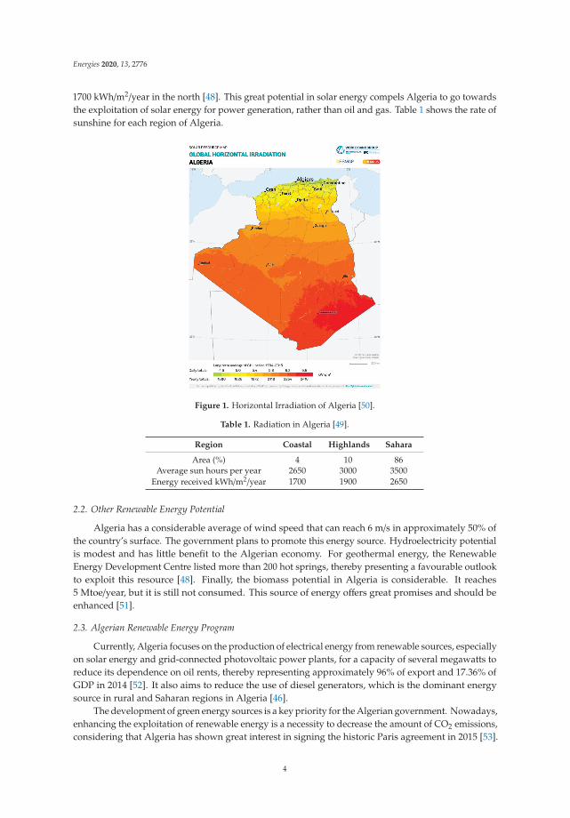
The potential of solar energy in southern Algeria is the largest in all Mediterranean basins,with 1,787,000 km2 of Sahara desert, according to the German Aerospace Centre (DLR). The insolationtime of almost all the national territory exceeds 2000 h annually and reaches 3900, as shown inFigure 1 (high plains and Sahara) [47]. Over most of the country and during the day, the energyobtained on a horizontal surface of 1 m2 is nearly 5 kWh or about 2263 kWh/m2/year in the south and

3

Energies 2020, 13, 2776

1700 kWh/m2/year in the north [48]. This great potential in solar energy compels Algeria to go towardsthe exploitation of solar energy for power generation, rather than oil and gas. Table 1 shows the rate ofsunshine for each region of Algeria.

Figure 1. Horizontal Irradiation of Algeria [50].

Table 1. Radiation in Algeria [49].

Region Coastal Highlands Sahara

Area (%) 4 10 86Average sun hours per year 2650 3000 3500

Energy received kWh/m2/year 1700 1900 2650

2.2. Other Renewable Energy Potential

Algeria has a considerable average of wind speed that can reach 6 m/s in approximately 50% ofthe country’s surface. The government plans to promote this energy source. Hydroelectricity potentialis modest and has little benefit to the Algerian economy. For geothermal energy, the RenewableEnergy Development Centre listed more than 200 hot springs, thereby presenting a favourable outlookto exploit this resource [48]. Finally, the biomass potential in Algeria is considerable. It reaches5 Mtoe/year, but it is still not consumed. This source of energy offers great promises and should beenhanced [51].

2.3. Algerian Renewable Energy Program

Currently, Algeria focuses on the production of electrical energy from renewable sources, especiallyon solar energy and grid-connected photovoltaic power plants, for a capacity of several megawatts toreduce its dependence on oil rents, thereby representing approximately 96% of export and 17.36% ofGDP in 2014 [52]. It also aims to reduce the use of diesel generators, which is the dominant energysource in rural and Saharan regions in Algeria [46].

The development of green energy sources is a key priority for the Algerian government. Nowadays,enhancing the exploitation of renewable energy is a necessity to decrease the amount of CO2 emissions,considering that Algeria has shown great interest in signing the historic Paris agreement in 2015 [53].

4

Energies 2020, 13, 2776

Furthermore, with such a measure, the government can save conventional resources, which are used togenerate electricity. The renewable sources showed a poor share in the total energy compared with theconventional sources [54]. The residential electricity sector reached approximately 42% of the totalenergy consumption [55]. However, the ambitious national renewable energy program allowed one toreach 27% of renewable energy in the national energy mix [56].

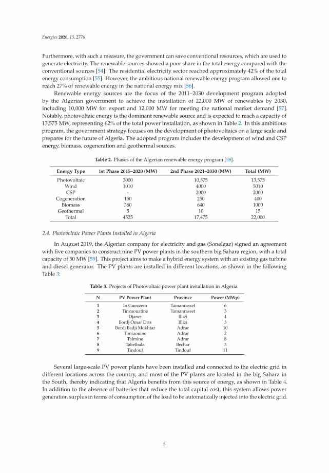
Renewable energy sources are the focus of the 2011–2030 development program adoptedby the Algerian government to achieve the installation of 22,000 MW of renewables by 2030,including 10,000 MW for export and 12,000 MW for meeting the national market demand [57].Notably, photovoltaic energy is the dominant renewable source and is expected to reach a capacity of13,575 MW, representing 62% of the total power installation, as shown in Table 2. In this ambitiousprogram, the government strategy focuses on the development of photovoltaics on a large scale andprepares for the future of Algeria. The adopted program includes the development of wind and CSPenergy, biomass, cogeneration and geothermal sources.

Table 2. Phases of the Algerian renewable energy program [58].

Energy Type 1st Phase 2015–2020 (MW) 2nd Phase 2021–2030 (MW) Total (MW)

Photovoltaic 3000 10,575 13,575Wind 1010 4000 5010CSP - 2000 2000

Cogeneration 150 250 400Biomass 360 640 1000

Geothermal 5 10 15Total 4525 17,475 22,000

2.4. Photovoltaic Power Plants Installed in Algeria

In August 2019, the Algerian company for electricity and gas (Sonelgaz) signed an agreementwith five companies to construct nine PV power plants in the southern big Sahara region, with a totalcapacity of 50 MW [59]. This project aims to make a hybrid energy system with an existing gas turbineand diesel generator. The PV plants are installed in different locations, as shown in the followingTable 3:

Table 3. Projects of Photovoltaic power plant installation in Algeria.

N PV Power Plant Province Power (MWp)

1 In Guezzem Tamanrasset 62 Tinzaouatine Tamanrasset 33 Djanet Illizi 44 Bordj Omar Dris Illizi 35 Bordj Badji Mokhtar Adrar 106 Timiaouine Adrar 27 Talmine Adrar 88 Tabelbala Bechar 39 Tindouf Tindouf 11

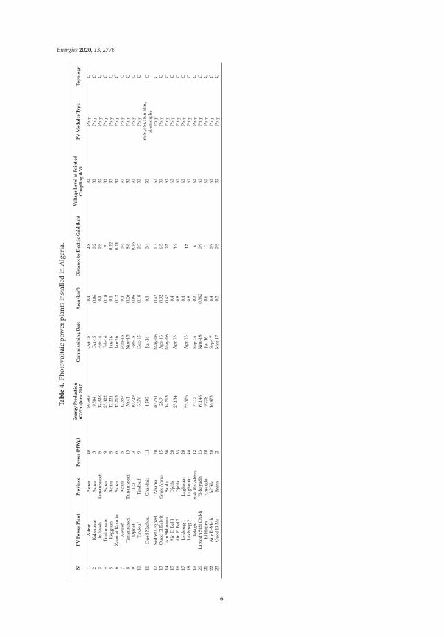
Several large-scale PV power plants have been installed and connected to the electric grid indifferent locations across the country, and most of the PV plants are located in the big Sahara inthe South, thereby indicating that Algeria benefits from this source of energy, as shown in Table 4.In addition to the absence of batteries that reduce the total capital cost, this system allows powergeneration surplus in terms of consumption of the load to be automatically injected into the electric grid.

5

Energies 2020, 13, 2776

Ta

ble

4.

Phot

ovol

taic

pow

erpl

ants

inst

alle

din

Alg

eria

.

NP

VP

ow

er

Pla

nt

Pro

vin

ceP

ow

er

(MW

p)

En

erg

yP

rod

uct

ion

(GW

h)-

Jun

e2

01

7C

om

mis

sin

ing

Da

teA

rea

(km

2)

Dis

tan

ceto

Ele

ctri

cG

rid

(km

)V

olt

ag

eL

ev

el

at

Po

int

of

Co

up

lin

g(k

V)

PV

Mo

du

les

Ty

pe

To

po

log

y

1A

drar

Adr

ar20

59.5

85O

ct-1

50.

42.

830

Poly

C2

Kab

ertè

neA

drar

39.

584

Oct

-15

0.06

0.2

30Po

lyC

3In

Sala

hTa

man

rass

et5

12.3

28Fe

b-16

0.1

0.5

30Po

lyC

4Ti

mim

oune

Adr

ar9

23.8

22Fe

b-16

0.18

930

Poly

C5

Reg

guen

Adr

ar5

12.2

21Ja

n-16

0.1

0.22

30Po

lyC

6Z

aoui

atK

ount

aA

drar

615

.213

Jan-

160.

120.

2430

Poly

C7

Aou

lef

Adr

ar5

12.5

57M

ar-1

60.

10.

430

Poly

C8

Tam

anra

sset

Tam

anra

sset

1336

.41

Nov

-15

0.26

8.8

30Po

lyC

9D

jane

tIl

izi

310

.729

Feb-

150.

060.

3530

Poly

C10

Tind

ouf

Tind

ouf

96.

376

Dec

-15

0.18

0.3

30Po

lyC

11O

ued

Nec

hou

Gha

rdai

a1.

14.

593

Jul-

140.

10.

430

m-S

i,c-S

i,Thi

nfil

m,

si-a

mor

phe

C

12Se

dret

Legh

zel

Naâ

ma

2040

.751

May

-16

0.42

1.3

60Po

lyC

13O

ued

ElK

ebri

tSo

ukA

hras

1528

.9A

pr-1

60.

326.

530

Poly

C14

Ain

Skho

una

Said

a30

14.2

13M

ay-1

60.

4212

60Po

lyC

15A

inEl

Bel1

Dje

lfa

2025

.134

Apr

-16

0.4

3.9

60Po

lyC

16A

inEl

Bel2

Dje

lfa

330.

860

Poly

C17

Lekh

neg

1La

ghou

at20

53.5

76A

pr-1

60.

412

60Po

lyC

18Le

khne

g2

Lagh

ouat

400.

860

Poly

C19

Tela

ghSi

di-B

el-A

bbes

127.

417

Sep-

160.

36

60Po

lyC

20La

biod

hSi

diC

hikh

El-B

ayad

h23

19.1

46N

ov-1

80.

392

0.9

60Po

lyC

21El

Hdj

ira

Oua

rgla

309.

738

Jul-

160.

61

60Po

lyC

22A

in-E

l-M

elh

M’S

ila20

16.4

73Se

p-17

0.4

0.9

60Po

lyC

23O

ued

ElM

aBa

tna

2-

Mar

-17

0.3

0.5

30Po

lyC

6

Energies 2020, 13, 2776

3. Methodology

3.1. Formulation of the Design Problem

The single objective optimisation function is used to find the optimum solution correspondingto the minimum or maximum value defined by the objective function. In contrast, multi-objectiveoptimisation combines two or more individual objective functions to determine a set of trade-offsolutions, which allow decision makers to select the most suitable solution based on the problemrequirements [60]. In this study, in sizing optimisation methodology depending on the requirements ofthe power plant designer, each of the two objectives can be used to produce an optimal design for thePV power plant. In addition, for comparison purposes, the optimum values are calculated by usingeach objective function individually to evaluate the PV power plant performance.

Furthermore, multi-objective optimisation can be used in the design of PV systems with a smallcapacity in the range of kW, with a small number of PV modules and inverters or in hybrid renewableenergy systems for example (PV-wind) or (PV-diesel denerator-battery). However, in large scale PVpower plants (i.e., >200 kW nominal power rating—the largest plants reaching several tens of MW ofcapacity), with a considerable number of components required in PV plant installation, it is well-knownthat the levelised cost of energy (LCOE) is applied to enable the reduction of the PV plant cost perwatt of nominal power that is installed [61,62], for this reason, single objective optimisation is used.Additionally, a recent study is presented in [63] to investigate the LCOE of large scale PV power plantsat 8 PV plants ranging from 1 to 46 MWp and many similar studies can be found in the literature.

In this section, two objective functions are considered to evaluate the PV power plant performanceand to solve its complex design problem. The design variables and constraints of the proposedmethodology are also explained.

3.1.1. Objective Function

In this work, the LCOE and maximum annual energy were set as objective functions to determinethe optimal solution of the PV plant design. These two objective functions can be combined to form asingle optimisation function.

The first part presents the LCOE which is calculated on the basis of the sum of maintenance,operation and installation costs of the plant divided by the total energy generation of the plant duringits lifetime. The LCOE method is generally applied to compare power plants with different energygeneration sources, by considering the appropriate cost structures. However, the best LCOE for powerplants presents the lowest possible investment with high annual energy production. The second partpresents the maximum amount of annual energy that can be captured by the PV modules duringthe PV plant in its lifetime, which is 25 years. The single optimisation function is expressed by thefollowing equation:

minX

[(Cc(X) + CM(X)

Etot(X)

)·a−

((1− a)·

(Pplant(X)·ns·EAF

))](1)

where ns is equal to 1 year.The optimum values are calculated by using each objective function individually. In other words,

in the objective function, a is a binary number; if a is equal to 0, the target of the objective function ismaximum energy and, if a is equal to 1, the objective function target is minimum LCOE.

3.1.2. Design Variables

The proposed optimisation algorithm was used for the calculation of all the decision variables,to determine the optimum design of the PV power plant. The chosen optimisation algorithm shouldhave high performance in determining the best design variables and solving the design problem.In this methodology, the proposed decision variables, including the number of PV modules connected

7

Energies 2020, 13, 2776

in series (Ns) and parallel (Np), number of PV module lines per row (Nr), the distance between twoadjacent rows (Fy), the tilt angle of the PV module (β), the orientation of PV modules (PVorien), that canbe installed vertically or horizontally, optimum PV module (PVi), and inverter (INi), can be selectedon the basis of several alternatives from a list of possible candidates.

The vector of the decision variables are summarized as given by the following expression:

X =[Ns Np Nr β FyPVorien PVi INi

](2)

3.1.3. Constraints

During the design of the PV power plant, many constraints are considered to account for thelimits of the different parameters of the whole system. The following expression shows the limitationof some variables:

Ns,min ≤ Ns ≤ Ns,max (3)

1 ≤ Np ≤ Np,max (4)

1 ≤ Nr ≤ Nr,max (5)

0 ≤ β ≤ 90 (6)

Socupied ≤ Avalaiblearea (7)

The following equality constraint expressions were used to select the PV module and inverterfrom the list of candidates:

PV1 + PV2 + . . . = 1 (8)

INV1 + INV2 + . . . = 1 (9)

3.2. System Description and Meteorological Data

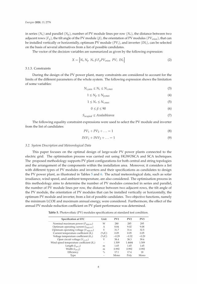
This paper focuses on the optimal design of large-scale PV power plants connected to theelectric grid. The optimisation process was carried out using HGWOSCA and SCA techniques.The proposed methodology supports PV plant configurations for both central and string topologiesand the arrangement of the components within the installation area. Moreover, it considers a listwith different types of PV modules and inverters and their specifications as candidates to designthe PV power plant, as illustrated in Tables 5 and 6. The actual meteorological data, such as solarirradiance, wind speed, and ambient temperature, are also considered. The optimisation process inthis methodology aims to determine the number of PV modules connected in series and parallel,the number of PV module lines per row, the distance between two adjacent rows, the tilt angle ofthe PV module, the orientation of PV modules that can be installed vertically or horizontally, theoptimum PV module and inverter, from a list of possible candidates. Two objective functions, namelythe minimum LCOE and maximum annual energy, were considered. Furthermore, the effect of theannual PV module reduction coefficient on PV plant performance was determined.

Table 5. Photovoltaic (PV) modules specifications at standard test condition.

Specification at STC Unit PV1 PV2 PV3

Nominal maximum power (Pmpp,stc) W 280 285 295Optimum operating current (Impp,stc) A 8.84 9.02 9.08Optimum operating voltage (Vmpp,stc) V 31.7 31.6 32.5Current temperature coefficient (Ki) (%/C) 0.05 0.05 0.05Voltage temperature coefficient (Kv) (%/C) −0.29 −0.32 −0.29

Open circuit voltage (Voc,stc) V 38.4 38.3 39.6Wind speed temperature coefficient (Kr) - 1.509 1.4684 1.509

Length (Lpv,1) m 1.65 1.65 1.65Width (Lpv,2) m 0.992 0.992 0.992

Efficiency % 17.1 17.4 18Type - Mono Poly Mono

8

Energies 2020, 13, 2776

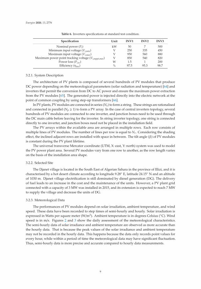
Table 6. Inverters specifications at standard test condition.

Specification Unit INV1 INV2 INV3

Nominal power (Pi) kW 50 7 500Minimum input voltage (Vi,min) V 250 335 450Maximum input voltage (Vi,max) V 950 560 880

Maximum power point tracking voltage (Vi,mppt,max) V 850 540 820Power loss (Pi,sc) W 1.5 1 200Efficiency (ηinv) % 97.5 95.3 98.7

3.2.1. System Description

The architecture of PV plants is composed of several hundreds of PV modules that produceDC power depending on the meteorological parameters (solar radiation and temperature) [64] andinverters that permit the conversion from DC to AC power and ensure the maximum power extractionfrom the PV modules [65]. The generated power is injected directly into the electric network at thepoint of common coupling by using step-up transformers [66].

In PV plants, PV modules are connected in series (Ns) to form a string. These strings are rationalisedand connected in parallel (Np ≥ 1) to form a PV array. In the case of central inverters topology, severalhundreds of PV modules are connected to one inverter, and junction boxes need to be used throughthe DC main cable before leaving for the inverter. In string inverter topology, one string is connecteddirectly to one inverter, and junction boxes need not be placed in the installation field.

The PV arrays within the available area are arranged in multiple rows. Each row consists ofmultiple lines of PV modules. The number of lines per row is equal to Nr. Considering the shadingeffect, the inclined adjacent rows are installed with space in between. The tilt angle (β) of PV modulesis constant during the PV plant lifetime.

The universal transverse Mercator coordinate (UTM, X: east, Y: north) system was used to modelthe PV power plant area. Several PV modules vary from one row to another, as the row length varieson the basis of the installation area shape.

3.2.2. Selected Site

The Djanet village is located in the South East of Algerian Sahara in the province of Illizi, and it ischaracterised by a hot desert climate according to longitude 9.28◦ E, latitude 24.15◦ N and an altitudeof 1030 m. Djanet village electrification is still dominated by diesel generation (DG). The deliveryof fuel leads to an increase in the cost and the maintenance of the units. However, a PV plant gridconnected with a capacity of 3 MW was installed in 2015, and its extension is expected to reach 7 MWto supply the village and decrease the units of DG.

3.2.3. Meteorological Data

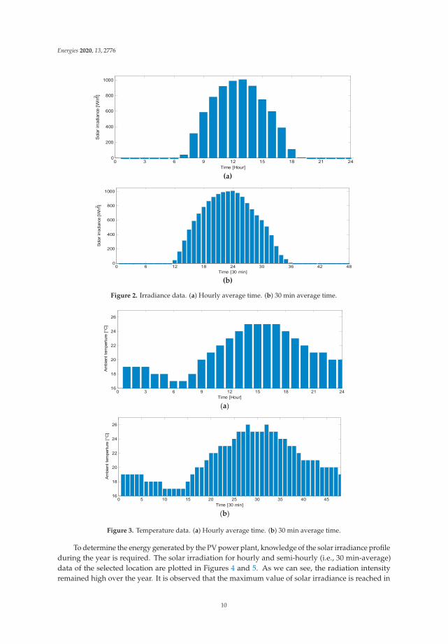
The performances of PV modules depend on solar irradiation, ambient temperature, and windspeed. These data have been recorded to step times of semi-hourly and hourly. Solar irradiation isexpressed in Watts per square meter (W/m2). Ambient temperature is in degrees Celsius (◦C). Windspeed is in m/s. Figures 2 and 3 show the daily assessment of the meteorological characteristics.The semi-hourly data of solar irradiance and ambient temperature are observed as more accurate thanthe hourly data. That is because the peak values of the solar irradiance and ambient temperaturemay not be recorded in the hourly data. This happens because the data only records point values forevery hour, while within a period of time the meteorological data may have significant fluctuation.Thus, semi-hourly data is more precise and accurate compared to hourly data measurements.

9

Energies 2020, 13, 2776

(a)

(b)

Figure 2. Irradiance data. (a) Hourly average time. (b) 30 min average time.

(a)

(b)

Figure 3. Temperature data. (a) Hourly average time. (b) 30 min average time.

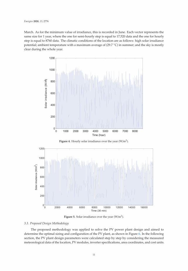
To determine the energy generated by the PV power plant, knowledge of the solar irradiance profileduring the year is required. The solar irradiation for hourly and semi-hourly (i.e., 30 min-average)data of the selected location are plotted in Figures 4 and 5. As we can see, the radiation intensityremained high over the year. It is observed that the maximum value of solar irradiance is reached in

10

Energies 2020, 13, 2776

March. As for the minimum value of irradiance, this is recorded in June. Each vector represents thesame size for 1 year, where the one for semi-hourly step is equal to 17,520 data and the one for hourlystep is equal to 8760 data. The climatic conditions of the location are as follows: high solar irradiancepotential; ambient temperature with a maximum average of (29.7 ◦C) in summer; and the sky is mostlyclear during the whole year.

Figure 4. Hourly solar irradiance over the year (W/m2).

Figure 5. Solar irradiance over the year (W/m2).

3.3. Proposed Design Methodology

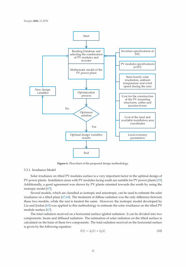
The proposed methodology was applied to solve the PV power plant design and aimed todetermine the optimal sizing and configuration of the PV plant, as shown in Figure 6. In the followingsection, the PV plant design parameters were calculated step by step by considering the measuredmeteorological data of the location, PV modules, inverter specifications, area coordinates, and cost units.

11

Energies 2020, 13, 2776

Start

Inverters specifications at STC

PV modules specifications at STC

Semi-hourly solar irradiation, ambient

temperature and wind speed during the year

Cost for the construction of the PV mounting

structures, cables and junction boxes

Cost of the land and available installation area

coordinates

Local economy parameters

Reading Database and selecting the combination

of PV modules and inverter

Mathematic model of the PV power plant

New design variables

Optimal design variables results

End

Optimum solution

Optimization process

Yes

No

Figure 6. Flowchart of the proposed design methodology.

3.3.1. Irradiance Model

Solar irradiance on tilted PV modules surface is a very important factor in the optimal design ofPV power plants. Installation areas with PV modules facing south are suitable for PV power plants [35].Additionally, a good agreement was shown by PV plants oriented towards the south by using theisotropic model [67].

Several models, which are classified as isotropic and anisotropic, can be used to estimate the solarirradiance on a tilted plane [67,68]. The treatment of diffuse radiation was the only difference betweenthese two models, while the rest is treated the same. However, the isotropic model developed byLiu and Jordan [69] was applied to this methodology to estimate the solar irradiance on the tilted PVmodule surface [67].

The total radiation received on a horizontal surface (global radiation: I) can be divided into twocomponents: beam and diffused radiation. The estimation of solar radiation on the tilted surface iscalculated on the basis of these two components. The total radiation received on the horizontal surfaceis given by the following equation:

I(t) = Ib(t) + Id(t) (10)

12

Energies 2020, 13, 2776

The index of transparency of the atmosphere or the clearness index kT of the sky is an essentialfactor. The clearness index is the function of the ratio between the extraterrestrial and horizontalradiation, as expressed by the following equation:

kT(t) =I(t)I0(t)

(11)

The diffuse fraction of total horizontal radiation depends on the clearness index of the sky [67]and is expressed by the following equation:

Id(t)I(t)

=

⎧⎪⎪⎪⎨⎪⎪⎪⎩1.0− 0.09kT(t), kT(t) ≤ 0.22

0.9511− 0.1604kT(t)+4.388(t)k2T−16.638k3

T(t)+12.336k4T(t), 0.22 <kT(t) ≤ 0.8

0.165, kT(t) ≤ 0.80(12)

manipulating Equation (10), the beam radiation is given by the following expression:

Ib(t) = I(t) − Id(t) (13)

The total incident solar radiation on tilted surface is the sum of three components, namely, beamradiation from direct radiation of the inclined surface, diffuse radiation and reflected radiation.

IT(t, β) = IB(t) + ID(t) + IR(t) (14)

The beam irradiance on an inclined surface can be calculated on the basis of multiplicationbetween beam horizontal irradiance and beam ratio factor Rb, as shown in the following expression:

IB(t) = Ib(t)Rb(t, β) (15)

where the beam ratio factor Rb is a function of the ratio between beam irradiance on the inclined surfaceand horizontal irradiance, as expressed in the Equation (18).

The first component is the incidence angle cos(t, β), which can be derived as follows:

cos(t, β) = sin δ(t) sinϕ cos β− sin δ(t) cosϕ sin β cosγ+ cos δ(t) cosϕ cos β cosω(t)+ cos δ(t) sinϕ sin β cosγ cosω(t)+ cos δ(t) sin β sinγ sinω(t)

(16)

where δ is the solar declination angle, ϕ is the location latitude, γ is the surface azimuth angle, and ω isthe hour angle. The global radiation on the inclined surface calculation model’s error was lower than3% [70].

The second component deals with solar zenith angle cosθz and can be calculated using thefollowing equation:

cosθz(t, β) = cosγ cos δ(t) cosω(t) + sinϕ sin δ(t) (17)

Rb(t, β) =cos(t, β)

cosθz(t, β)(18)

Diffuse irradiance on an inclined surface is computed on the basis of the isotropic sky model.A well-known isotropic model was introduced by Liu and Jordan (1963). This model is simple,and the diffuse radiation has a uniform distribution over the skydome. The diffuse radiation on theinclined surface increases with an increasing amount of seen by the inclined surface, as expressed inEquation (19).

ID(t) = Id(t)(

1 + cosβ2

)(19)

13

Energies 2020, 13, 2776

where β is the surface tilt angle and considered as a design variable. Its optimal values are computedby the optimisation algorithm.

The reflected irradiance on an inclined surface is expressed by Equation (20) and depends on thetransposition factor for ground reflection Rr given by Equation (21) and the reflectivity of the ground ρthat is equal to 0.2 [68].

IR(t) = I(t)ρRr (20)

Rr(t) =1− cosβ

2(21)

3.3.2. Area Calculation Model

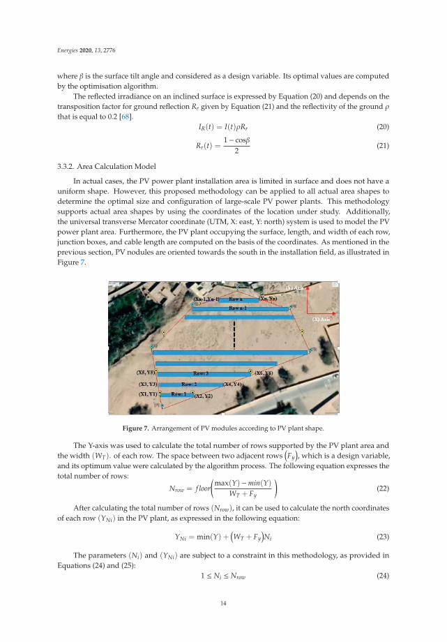
In actual cases, the PV power plant installation area is limited in surface and does not have auniform shape. However, this proposed methodology can be applied to all actual area shapes todetermine the optimal size and configuration of large-scale PV power plants. This methodologysupports actual area shapes by using the coordinates of the location under study. Additionally,the universal transverse Mercator coordinate (UTM, X: east, Y: north) system is used to model the PVpower plant area. Furthermore, the PV plant occupying the surface, length, and width of each row,junction boxes, and cable length are computed on the basis of the coordinates. As mentioned in theprevious section, PV nodules are oriented towards the south in the installation field, as illustrated inFigure 7.

Figure 7. Arrangement of PV modules according to PV plant shape.

The Y-axis was used to calculate the total number of rows supported by the PV plant area andthe width (WT). of each row. The space between two adjacent rows

(Fy

), which is a design variable,

and its optimum value were calculated by the algorithm process. The following equation expresses thetotal number of rows:

Nrow = f loor(

max(Y) −min(Y)WT + Fy

)(22)

After calculating the total number of rows (Nrow), it can be used to calculate the north coordinatesof each row (YNi) in the PV plant, as expressed in the following equation:

YNi = min(Y) +(WT + Fy

)Ni (23)

The parameters (Ni) and (YNi) are subject to a constraint in this methodology, as provided inEquations (24) and (25):

1 ≤ Ni ≤ Nrow (24)

14

Energies 2020, 13, 2776

min(Y) < YNi < max(Y) (25)

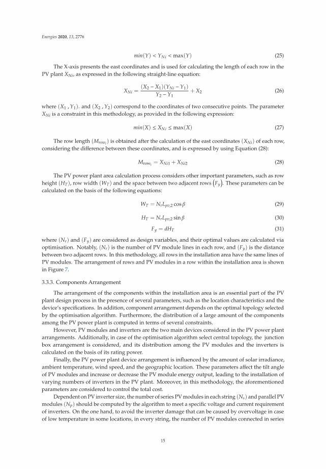
The X-axis presents the east coordinates and is used for calculating the length of each row in thePV plant XNi, as expressed in the following straight-line equation:

XNi =(X2 −X1)(YNi −Y1)

Y2 −Y1+ X2 (26)

where (X1 , Y1). and (X2 , Y2) correspond to the coordinates of two consecutive points. The parameterXNi is a constraint in this methodology, as provided in the following expression:

min(X) ≤ XNi ≤ max(X) (27)

The row length (Mrowi) is obtained after the calculation of the east coordinates (XNi) of each row,considering the difference between these coordinates, and is expressed by using Equation (28):

Mrowi = XNi1 + XNi2 (28)

The PV power plant area calculation process considers other important parameters, such as rowheight (HT), row width (WT) and the space between two adjacent rows

(Fy

). These parameters can be

calculated on the basis of the following equations:

WT = NrLpv,2 cos β (29)

HT = NrLpv,2 sin β (30)

Fy = dHT (31)

where (Nr) and (Fy) are considered as design variables, and their optimal values are calculated viaoptimisation. Notably, (Nr) is the number of PV module lines in each row, and (Fy) is the distancebetween two adjacent rows. In this methodology, all rows in the installation area have the same lines ofPV modules. The arrangement of rows and PV modules in a row within the installation area is shownin Figure 7.

3.3.3. Components Arrangement

The arrangement of the components within the installation area is an essential part of the PVplant design process in the presence of several parameters, such as the location characteristics and thedevice’s specifications. In addition, component arrangement depends on the optimal topology selectedby the optimisation algorithm. Furthermore, the distribution of a large amount of the componentsamong the PV power plant is computed in terms of several constraints.

However, PV modules and inverters are the two main devices considered in the PV power plantarrangements. Additionally, in case of the optimisation algorithm select central topology, the junctionbox arrangement is considered, and its distribution among the PV modules and the inverters iscalculated on the basis of its rating power.

Finally, the PV power plant device arrangement is influenced by the amount of solar irradiance,ambient temperature, wind speed, and the geographic location. These parameters affect the tilt angleof PV modules and increase or decrease the PV module energy output, leading to the installation ofvarying numbers of inverters in the PV plant. Moreover, in this methodology, the aforementionedparameters are considered to control the total cost.

Dependent on PV inverter size, the number of series PV modules in each string (Ns) and parallel PVmodules (Np) should be computed by the algorithm to meet a specific voltage and current requirementof inverters. On the one hand, to avoid the inverter damage that can be caused by overvoltage in caseof low temperature in some locations, in every string, the number of PV modules connected in series

15

Energies 2020, 13, 2776

has to be optimally computed. On the other hand, the number of parallel-connected PV modules (Np)

multiplied by its current is equal to the input current of the inverter. To avoid the inverter damagecreated by the overcurrent locations with high solar irradiance, a limited number of PV modulesconnected in parallel (Np) should be addressed.

The first part handles PV modules distribution among the inverters and their arrangement withinthe PV plant area. The number of series (Ns) and parallel (Np) PV modules are computed in accordancewith the optimum selected inverter by the optimisation process. In this proposed methodology,the number of PV modules connected in series (Ns) and parallel (Np) were considered as the designvariables, and their optimum values were calculated using the optimisation algorithm. The (Ns)

design variable involves a number of minimum (Ns,min) and maximum (Ns,max) PV modules, and theselimitations can be calculated on the basis of the inverter input voltage range in [11,22], as expressed inthe following equations:

Ns,min =Vi,min

Vmpp,min(32)

Ns,min =Vi,max

Voc,max(33)

Nsm,2 =Vi,mpptmax

Vmpp,max(34)

Ns,max =

{Nsm,1, Nsm,1 ≤ Nsm,2

Nsm,2, Nsm,2 < Nsm,1(35)

The maximum number of PV modules connected in parallel (Np) was calculated according tothe selected inverter by using the nominal power (Pi), and the PV module maximum output power(Pmpp,max) was selected with respect to the optimum number of PV modules connected in series (Ns) [22],as provided in the following expression:

Np,max =Pi

NsPmpp,max(36)

As mentioned in the previous section, the arrangement of PV modules in the PV plant arearequires the use of the length of each row in the PV plant to determine the optimum number of PVmodules installed in each line (Nci) and the total number in each row (Nrowi, pv ). The total number ofPV modules installed in each line (Nci) of rows, which are described as the function ratio betweenthe length of each row

(Mrowi

)and the length of the optimum PV modules

(Lpv,1

), is given in the

following equation:

Nci =Mrowi

Lpv,1(37)

The total number of PV modules installed in each row(Nrow,pv

)depends on the number of PV

module lines (Nr), which is a design variable in this methodology, and its optimum value is computedby the optimisation algorithm.

Nrowi,pv = NrNci (38)

The sum of PV modules in each row of the PV plant results in their total number in the installationarea as expressed in the following equation:

NI =i∑1

Nrowi,pv (39)

16

Energies 2020, 13, 2776

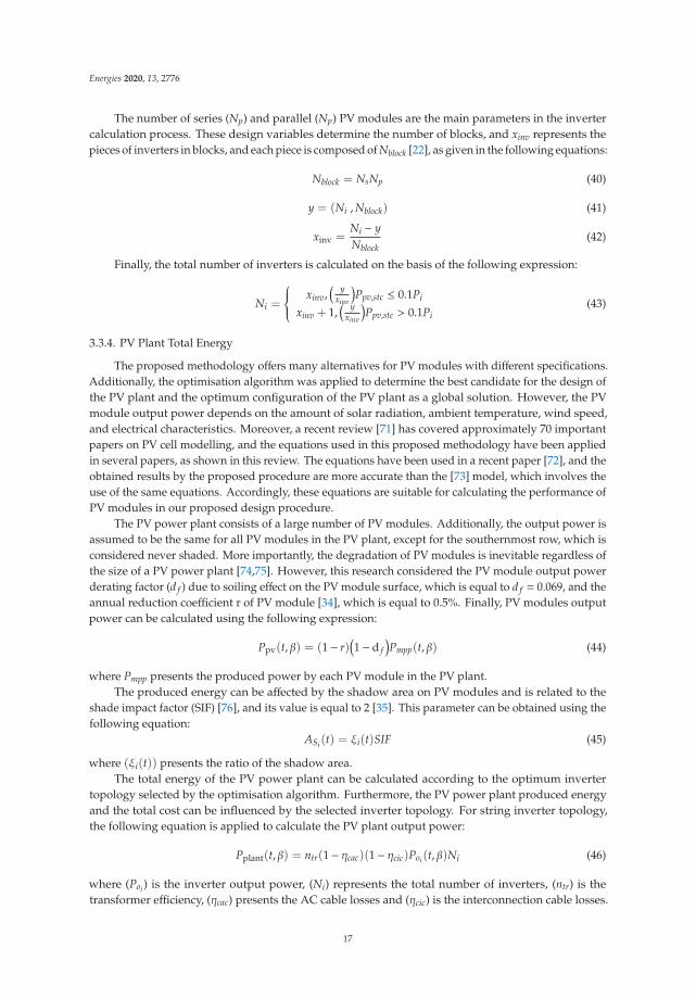
The number of series (Np) and parallel (Np) PV modules are the main parameters in the invertercalculation process. These design variables determine the number of blocks, and xinv represents thepieces of inverters in blocks, and each piece is composed of Nblock [22], as given in the following equations:

Nblock = NsNp (40)

y = (Ni , Nblock) (41)

xinv =Ni − yNblock

(42)

Finally, the total number of inverters is calculated on the basis of the following expression:

Ni =

⎧⎪⎪⎨⎪⎪⎩xinv,

( yxinv

)Ppv,stc ≤ 0.1Pi

xinv + 1,( y

xinv

)Ppv,stc > 0.1Pi

(43)

3.3.4. PV Plant Total Energy

The proposed methodology offers many alternatives for PV modules with different specifications.Additionally, the optimisation algorithm was applied to determine the best candidate for the design ofthe PV plant and the optimum configuration of the PV plant as a global solution. However, the PVmodule output power depends on the amount of solar radiation, ambient temperature, wind speed,and electrical characteristics. Moreover, a recent review [71] has covered approximately 70 importantpapers on PV cell modelling, and the equations used in this proposed methodology have been appliedin several papers, as shown in this review. The equations have been used in a recent paper [72], and theobtained results by the proposed procedure are more accurate than the [73] model, which involves theuse of the same equations. Accordingly, these equations are suitable for calculating the performance ofPV modules in our proposed design procedure.

The PV power plant consists of a large number of PV modules. Additionally, the output power isassumed to be the same for all PV modules in the PV plant, except for the southernmost row, which isconsidered never shaded. More importantly, the degradation of PV modules is inevitable regardless ofthe size of a PV power plant [74,75]. However, this research considered the PV module output powerderating factor (d f ) due to soiling effect on the PV module surface, which is equal to d f = 0.069, and theannual reduction coefficient r of PV module [34], which is equal to 0.5%. Finally, PV modules outputpower can be calculated using the following expression:

Ppv(t, β) = (1− r)(1− d f

)Pmpp(t, β) (44)

where Pmpp presents the produced power by each PV module in the PV plant.The produced energy can be affected by the shadow area on PV modules and is related to the

shade impact factor (SIF) [76], and its value is equal to 2 [35]. This parameter can be obtained using thefollowing equation:

ASi(t) = ξi(t)SIF (45)

where (ξi(t)) presents the ratio of the shadow area.The total energy of the PV power plant can be calculated according to the optimum inverter

topology selected by the optimisation algorithm. Furthermore, the PV power plant produced energyand the total cost can be influenced by the selected inverter topology. For string inverter topology,the following equation is applied to calculate the PV plant output power:

Pplant(t, β) = ntr(1− ηcac)(1− ηcic)Poi(t, β)Ni (46)

where (Poi) is the inverter output power, (Ni) represents the total number of inverters, (ntr) is thetransformer efficiency, (ηcac) presents the AC cable losses and (ηcic) is the interconnection cable losses.

17

Energies 2020, 13, 2776

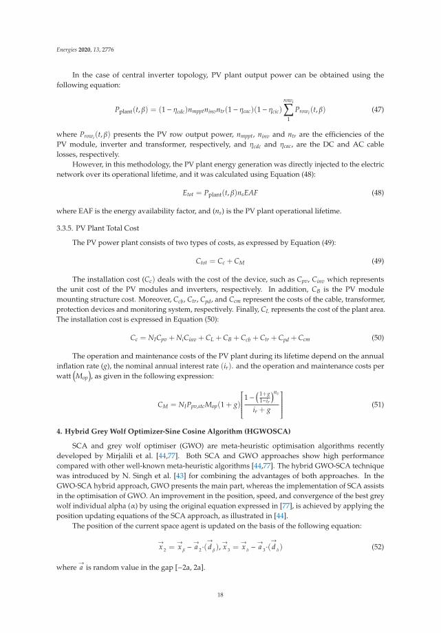
In the case of central inverter topology, PV plant output power can be obtained using thefollowing equation:

Pplant(t, β) = (1− ηcdc)nmpptninvntr(1− ηcac)(1− ηcic)

rowi∑1

Prowi(t, β) (47)

where Prowi(t, β) presents the PV row output power, nmppt, ninv and ntr are the efficiencies of thePV module, inverter and transformer, respectively, and ηcdc and ηcac, are the DC and AC cablelosses, respectively.

However, in this methodology, the PV plant energy generation was directly injected to the electricnetwork over its operational lifetime, and it was calculated using Equation (48):

Etot = Pplant(t, β)nsEAF (48)

where EAF is the energy availability factor, and (ns) is the PV plant operational lifetime.

3.3.5. PV Plant Total Cost

The PV power plant consists of two types of costs, as expressed by Equation (49):

Ctot = Cc + CM (49)

The installation cost (Cc) deals with the cost of the device, such as Cpv, Cinv which representsthe unit cost of the PV modules and inverters, respectively. In addition, CB is the PV modulemounting structure cost. Moreover, Ccb, Ctr, Cpd, and Ccm represent the costs of the cable, transformer,protection devices and monitoring system, respectively. Finally, CL represents the cost of the plant area.The installation cost is expressed in Equation (50):

Cc = NICpv + NiCinv + CL + CB + Ccb + Ctr + Cpd + Ccm (50)

The operation and maintenance costs of the PV plant during its lifetime depend on the annualinflation rate (g), the nominal annual interest rate (ir). and the operation and maintenance costs perwatt

(Mop

), as given in the following expression:

CM = NIPpv,stcMop(1 + g)

⎡⎢⎢⎢⎢⎢⎢⎢⎣1−

( 1+g1−ir

)ns

ir + g

⎤⎥⎥⎥⎥⎥⎥⎥⎦ (51)

4. Hybrid Grey Wolf Optimizer-Sine Cosine Algorithm (HGWOSCA)

SCA and grey wolf optimiser (GWO) are meta-heuristic optimisation algorithms recentlydeveloped by Mirjalili et al. [44,77]. Both SCA and GWO approaches show high performancecompared with other well-known meta-heuristic algorithms [44,77]. The hybrid GWO-SCA techniquewas introduced by N. Singh et al. [43] for combining the advantages of both approaches. In theGWO-SCA hybrid approach, GWO presents the main part, whereas the implementation of SCA assistsin the optimisation of GWO. An improvement in the position, speed, and convergence of the best greywolf individual alpha (α) by using the original equation expressed in [77], is achieved by applying theposition updating equations of the SCA approach, as illustrated in [44].

The position of the current space agent is updated on the basis of the following equation:

→x 2 =

→x β −

→a 2 ·(

→d β),

→x 3 =

→x δ −

→a 3 ·(

→d δ) (52)

where→a is random value in the gap [−2a, 2a].

18

Energies 2020, 13, 2776

The position of→Xβ,

→Xδ. and

→Xα. is updated using the following equation:

→x 1 +

→x 2 +

→x 3

3(53)

Details and description of the HGWOSCA approach can be found in reference [43]. Furthermore,the computational procedure of the HGWOSCA approach is illustrated in Figure 8.

1. Begin of Algorithm 2. Initialize the grey wolf population xi = 1,2,…..,n 3. Initialize the parameters A, a and C 4. Calculate the fitness of each search agent 5. = the best search agent 6. the second best search agent 7. = the third best search agent 8. While t < Max_generation 9. For search space 10. Update the position of the current space agent in the basis of equation (53) 11. End 12. Update the parameters a, A and C 13. Calculate the fitness of search agent 14. Update the , by equation (52) and as below 15. if rand() < 5 16. then 17. 18. else 19. 20. 21. end if 22. end else 23. end while 24. Return

Figure 8. Pseudo-code of the hybrid grey wolf optimiser-sine cosine algorithm (HGWOSCA).

Although the GWO and SCA are able to expose an efficient accuracy in comparison with otherwell-known swarm intelligence optimisation techniques, it is not fitting for highly complex functionsand may still face the difficulty of getting trapped in local optima [43]. Thus, a new hybrid variantbased on GWO and SCA is used to solve recent real-life problems.

5. Results and Discussion

The proposed methodology has been implemented in MATLAB software and applied to thedevelopment of the optimal design of a PV plant connected to the electric grid. Solar irradiance,ambient temperature, and wind speed data for 1 year from the installation field are required. The effectof minimum LCOE and maximum annual energy objective functions on the PV plant design wasdetermined. The HGWOSCA optimisation technique and a single SCA algorithm were applied with400 search agents and 30 iterations to solve the design problem.

According to the results presented in Table 7, the PV plant optimal design variables dependon the selected objective function. The minimum LCOE and maximum annual energy result intwo completely different optimal PV plant structures. PV power plant results are presented in

19

Energies 2020, 13, 2776

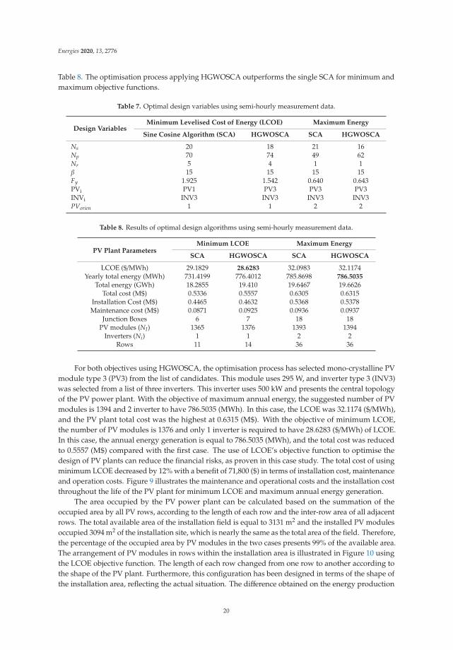
Table 8. The optimisation process applying HGWOSCA outperforms the single SCA for minimum andmaximum objective functions.

Table 7. Optimal design variables using semi-hourly measurement data.

Design VariablesMinimum Levelised Cost of Energy (LCOE) Maximum Energy

Sine Cosine Algorithm (SCA) HGWOSCA SCA HGWOSCA

Ns 20 18 21 16Np 70 74 49 62Nr 5 4 1 1β 15 15 15 15Fy 1.925 1.542 0.640 0.643PVi PV1 PV3 PV3 PV3INVi INV3 INV3 INV3 INV3PVorien 1 1 2 2

Table 8. Results of optimal design algorithms using semi-hourly measurement data.

PV Plant ParametersMinimum LCOE Maximum Energy

SCA HGWOSCA SCA HGWOSCA

LCOE ($/MWh) 29.1829 28.6283 32.0983 32.1174Yearly total energy (MWh) 731.4199 776.4012 785.8698 786.5035

Total energy (GWh) 18.2855 19.410 19.6467 19.6626Total cost (M$) 0.5336 0.5557 0.6305 0.6315

Installation Cost (M$) 0.4465 0.4632 0.5368 0.5378Maintenance cost (M$) 0.0871 0.0925 0.0936 0.0937

Junction Boxes 6 7 18 18PV modules (NI) 1365 1376 1393 1394

Inverters (Ni) 1 1 2 2Rows 11 14 36 36

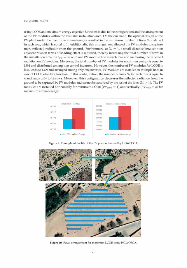
For both objectives using HGWOSCA, the optimisation process has selected mono-crystalline PVmodule type 3 (PV3) from the list of candidates. This module uses 295 W, and inverter type 3 (INV3)was selected from a list of three inverters. This inverter uses 500 kW and presents the central topologyof the PV power plant. With the objective of maximum annual energy, the suggested number of PVmodules is 1394 and 2 inverter to have 786.5035 (MWh). In this case, the LCOE was 32.1174 ($/MWh),and the PV plant total cost was the highest at 0.6315 (M$). With the objective of minimum LCOE,the number of PV modules is 1376 and only 1 inverter is required to have 28.6283 ($/MWh) of LCOE.In this case, the annual energy generation is equal to 786.5035 (MWh), and the total cost was reducedto 0.5557 (M$) compared with the first case. The use of LCOE’s objective function to optimise thedesign of PV plants can reduce the financial risks, as proven in this case study. The total cost of usingminimum LCOE decreased by 12% with a benefit of 71,800 ($) in terms of installation cost, maintenanceand operation costs. Figure 9 illustrates the maintenance and operational costs and the installation costthroughout the life of the PV plant for minimum LCOE and maximum annual energy generation.

The area occupied by the PV power plant can be calculated based on the summation of theoccupied area by all PV rows, according to the length of each row and the inter-row area of all adjacentrows. The total available area of the installation field is equal to 3131 m2 and the installed PV modulesoccupied 3094 m2 of the installation site, which is nearly the same as the total area of the field. Therefore,the percentage of the occupied area by PV modules in the two cases presents 99% of the available area.The arrangement of PV modules in rows within the installation area is illustrated in Figure 10 usingthe LCOE objective function. The length of each row changed from one row to another according tothe shape of the PV plant. Furthermore, this configuration has been designed in terms of the shape ofthe installation area, reflecting the actual situation. The difference obtained on the energy production

20

Energies 2020, 13, 2776

using LCOE and maximum energy objective functions is due to the configuration and the arrangementof the PV modules within the available installation area. On the one hand, the optimal design of thePV plant under the maximum annual energy resulted in the minimum number of lines Nr installedin each row, which is equal to 1. Additionally, this arrangement allowed the PV modules to capturemore reflected radiation from the ground. Furthermore, at Nr = 1, a small distance between twoadjacent rows in terms of shading effect is required, thereby increasing the total number of rows inthe installation area to Drow = 36 with one PV module line in each row and increasing the reflectedradiation on PV modules. Moreover, the total number of PV modules for maximum energy is equal to1394 and distributed among two central inverters. However, the number of PV modules for LCOE isless, leads to 1379 and arranged among only one inverter. PV modules are installed in multiple lines incase of LCOE objective function. In this configuration, the number of lines Nr for each row is equal to4 and leads only to 14 rows. Moreover, this configuration decreases the reflected radiation from theground to be captured by PV modules and cannot be absorbed by the rest of the lines (Nr > 1). The PVmodules are installed horizontally for minimum LCOE (PVorien = 1) and vertically (PVorien = 2) formaximum annual energy.

Figure 9. Throughout the life of the PV plant optimised by HGWOSCA.

Figure 10. Rows arrangement for minimum LCOE using HGWOSCA.

21

Energies 2020, 13, 2776

Figure 11 illustrates the monthly energy generation by the PV power plant for the LCOE objectivefunction. The PV plant energy generation remained high over the year, with an energy average of65 (MWh) per month. The highest value of the energy generated by the PV power plant is obtained inMarch, because this condition is due to the high solar irradiance in this period.

Figure 11. PV plant energy generation (MWh).

For comparison, the semi-hourly average time was compared with the hourly average timemeteorological data to examine the step time effect on the PV plant performance. The peaks of themeteorological data can influence the design solution. Therefore, the usage of annual semi-hourlyaverage time rather than monthly, daily and hourly is recommended, as semi-hourly data containthe troughs and peaks of solar irradiation, ambient temperature, and wind speed. According to theresults presented in Tables 9 and 10, the step time data can affect the objective functions. The LCOE forsemi-hourly average time is 28.6283 ($/MWh), and that obtained for hourly average time is higher andequal to 28.637 ($/MWh). The use of semi-hourly average time meteorological data in designing the PVplant can increase the financial benefits.

Table 9. Optimal design variables using hourly measurement data.

Design VariablesMinimum LCOE Maximum Energy

SCA HGWOSCA SCA HGWOSCA

Ns 19 18 22 14Np 70 74 42 47Nr 5 4 1 1β 15 15 15 15Fy 1.925 1.540 0.64 0.64PVi PV3 PV3 PV3 PV3INVi INV3 INV3 INV3 INV3PVorien 1 1 2 2

Table 10. Results of optimal design algorithms using hourly measurement data.

PV Plant ParametersMinimum LCOE Maximum Energy

SCA HGWOSCA SCA HGWOSCA

LCOE ($/MWh) 28.6622 28.6370 32.0983 32.1552Yearly total energy (MWh) 770.0032 776.1651 785.6774 786.2915

Total energy (GWh) 19.2501 19.4041 19.6419 19.6573Total cost (M$) 0.5517 0.5557 0.6305 0.6321

Installation Cost (M$) 0.4600 0.4632 0.5368 0.5384Maintenance cost (M$) 0.0917 0.0925 0.0936 0.0937

Junction Boxes 6 7 18 18PV modules (NI) 1365 1376 1393 1394

Inverters (Ni) 1 1 2 2Rows 11 14 36 36

22

Energies 2020, 13, 2776

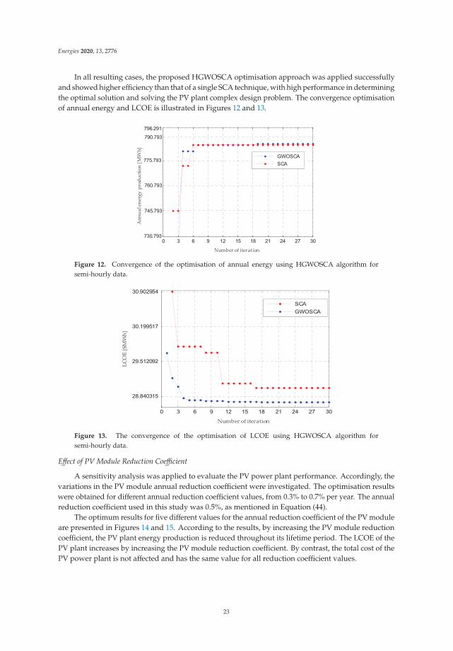
In all resulting cases, the proposed HGWOSCA optimisation approach was applied successfullyand showed higher efficiency than that of a single SCA technique, with high performance in determiningthe optimal solution and solving the PV plant complex design problem. The convergence optimisationof annual energy and LCOE is illustrated in Figures 12 and 13.

Number of iteration

Ann

ual e

nerg

y pr

oduc

tion

[MW

h]

Figure 12. Convergence of the optimisation of annual energy using HGWOSCA algorithm forsemi-hourly data.

Number of iteration

LCO

E [$

MW

h]

Figure 13. The convergence of the optimisation of LCOE using HGWOSCA algorithm forsemi-hourly data.

Effect of PV Module Reduction Coefficient

A sensitivity analysis was applied to evaluate the PV power plant performance. Accordingly, thevariations in the PV module annual reduction coefficient were investigated. The optimisation resultswere obtained for different annual reduction coefficient values, from 0.3% to 0.7% per year. The annualreduction coefficient used in this study was 0.5%, as mentioned in Equation (44).

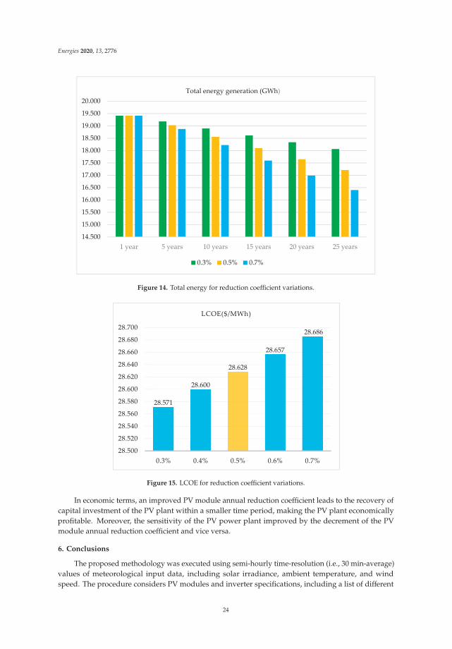
The optimum results for five different values for the annual reduction coefficient of the PV moduleare presented in Figures 14 and 15. According to the results, by increasing the PV module reductioncoefficient, the PV plant energy production is reduced throughout its lifetime period. The LCOE of thePV plant increases by increasing the PV module reduction coefficient. By contrast, the total cost of thePV power plant is not affected and has the same value for all reduction coefficient values.

23

Energies 2020, 13, 2776

14.500

15.000

15.500

16.000

16.500

17.000

17.500

18.000

18.500

19.000

19.500

20.000

1 year 5 years 10 years 15 years 20 years 25 years

Total energy generation (GWh)

0.3% 0.5% 0.7%

Figure 14. Total energy for reduction coefficient variations.

28.571

28.600

28.628

28.657

28.686

28.500

28.520

28.540

28.560

28.580

28.600

28.620

28.640

28.660

28.680

28.700

0.3% 0.4% 0.5% 0.6% 0.7%

LCOE($/MWh)

Figure 15. LCOE for reduction coefficient variations.

In economic terms, an improved PV module annual reduction coefficient leads to the recovery ofcapital investment of the PV plant within a smaller time period, making the PV plant economicallyprofitable. Moreover, the sensitivity of the PV power plant improved by the decrement of the PVmodule annual reduction coefficient and vice versa.

6. Conclusions

The proposed methodology was executed using semi-hourly time-resolution (i.e., 30 min-average)values of meteorological input data, including solar irradiance, ambient temperature, and windspeed. The procedure considers PV modules and inverter specifications, including a list of different

24

Energies 2020, 13, 2776

commercially available PV modules and inverter technologies as candidates. The optimisation processselects only one PV module and inverter from a list of several alternatives, presenting the optimumcombination. The proposed PV plant area model considers the shape and size of the installation fieldto properly arrange all the existing components.

The minimum LCOE and maximum annual energy objective functions were used to design the PVpower plant. On the basis of the optimal results, the total cost of using the minimum LCOE objectivefunction decreased by 12% with a benefit of 71,800 ($), including installation cost and maintenance andoperation costs compared with the maximum annual energy. In this methodology, the HGWOSCAoptimisation technique and a single SCA algorithm were applied. The optimum design solution showsthat the proposed HGWOSCA is more efficient. Additionally, the PV plant optimal design variablesdepend on the selected objective function. The minimum LCOE and maximum annual energy resultin two different optimal PV plant structures. LCOE improved with the use of semi-hourly averagetime meteorological data for designing the PV plant and can increase the financial benefits. Moreover,the sensitivity analysis shows that the PV power plant can be improved by the decrement of the PVmodule annual reduction coefficient and makes the PV plant economically more profitable.

Author Contributions: T.E.K.Z. contributed theoretical approaches, simulation, and preparing the article; M.R.A.,M.F.N.T., S.M.Z. and A.D. contributed to supervision; M.R.A., A.D. and S.M. contributed to article editing.All authors have read and agreed to the published version of the manuscript.

Funding: This research was funded by the School of Electrical System Engineering Research Fund(SESERF), UniMAP.

Acknowledgments: We gratefully acknowledge the support of the Algerian company of electricity SONELGAZ,for providing the measurement data.

Conflicts of Interest: The authors declare no conflict of interest.

References

1. Mohammadi, K.; Naderi, M.; Saghafifar, M. Economic feasibility of developing grid-connected photovoltaicplants in the southern coast of Iran. Energy 2018, 156, 17–31. [CrossRef]

2. Zou, H.; Du, H.; Brown, M.A.; Mao, G. Large-scale PV power generation in China: A grid parity andtechno-economic analysis. Energy 2017, 134, 256–268. [CrossRef]

3. Feldman, D.; Margolis, R. Q2/Q3 2018 Solar Industry Update 2018; Technical Report; National RenewableEnergy Lab. (NREL): Golden, CO, USA, 2018.

4. Comello, S.; Reichelstein, S.; Sahoo, A. The road ahead for solar PV power. Renew. Sustain. Energy Rev. 2018,92, 744–756. [CrossRef]

5. Mondol, J.D.; Yohanis, Y.G.; Norton, B. Optimal sizing of array and inverter for grid-connected photovoltaicsystems. Sol. Energy 2006, 80, 1517–1539. [CrossRef]

6. Kornelakis, A.; Marinakis, Y. Contribution for optimal sizing of grid-connected PV-systems using PSO.Renew. Energy 2010, 35, 1333–1341. [CrossRef]

7. Notton, G.; Lazarov, V.; Stoyanov, L. Optimal sizing of a grid-connected PV system for various PV moduletechnologies and inclinations, inverter efficiency characteristics and locations. Renew. Energy 2010, 35,541–554. [CrossRef]

8. Sulaiman, S.I.; Rahman, T.K.A.; Musirin, I.; Shaari, S.; Sopian, K. An intelligent method for sizing optimizationin grid-connected photovoltaic system. Sol. Energy 2012, 86, 2067–2082. [CrossRef]

9. Chen, S.; Li, P.; Brady, D.; Lehman, B. Determining the optimum grid-connected photovoltaic inverter size.Sol. Energy 2013, 87, 96–116. [CrossRef]

10. Perez-Gallardo, J.R.; Azzaro-Pantel, C.; Astier, S.; Domenech, S.; Aguilar-Lasserre, A. Ecodesign ofphotovoltaic grid-connected systems. Renew. Energy 2014, 64, 82–97. [CrossRef]

11. Senol, M.; Abbasoglu, S.; Kukrer, O.; Babatunde, A. A guide in installing large-scale PV power plant for selfconsumption mechanism. Sol. Energy 2016, 132, 518–537. [CrossRef]

12. Báez-Fernández, H.; Ramirez-Beltran, N.D.; Méndez-Piñero, M.I. Selection and configuration of invertersand modules for a photovoltaic system to minimize costs. Renew. Sustain. Energy Rev. 2016, 58, 16–22.[CrossRef]

25

Energies 2020, 13, 2776

13. Topic, D.; Kneževic, G.; Fekete, K. The mathematical model for finding an optimal PV system configurationfor the given installation area providing a maximal lifetime profit. Sol. Energy 2017, 144, 750–757. [CrossRef]

14. Durusu, A.; Erduman, A. An improved methodology to design large-scale photovoltaic power plant. J. Sol.Energy Eng. 2017, 140, 011007. [CrossRef]

15. Zidane, T.E.K.; Adzman, M.R.; Zali, S.M.; Mekhilef, S.; Durusu, A.; Tajuddin, M.F.N. Cost-effective topologyfor photovoltaic power plants using optimization design. In Proceedings of the 2019 IEEE 7th Conference onSystems, Process and Control (ICSPC), Malacca, Malaysia, 13–14 December 2019; pp. 210–215.

16. Wang, H.; Muñoz-García, M.; Moreda, G.; Alonso-Garcia, C. Optimum inverter sizing of grid-connectedphotovoltaic systems based on energetic and economic considerations. Renew. Energy 2018, 118, 709–717.[CrossRef]

17. Perez-Gallardo, J.R.; Azzaro-Pantel, C.; Astier, S. Combining multi-objective optimization, principalcomponent analysis and multiple criteria decision making for ecodesign of photovoltaic grid-connectedsystems. Sustain. Energy Technol. Assess. 2018, 27, 94–101. [CrossRef]

18. Zidane, T.E.K.; Adzman, M.R.; Tajuddin, M.F.N.; Zali, S.M.; Durusu, A. Optimal configuration of photovoltaicpower plant using grey wolf optimizer: A comparative analysis considering CdTe and c-Si PV modules.Sol. Energy 2019, 188, 247–257. [CrossRef]

19. Bakhshi-Jafarabadi, R.; Sadeh, J.; Soheili, A. Global optimum economic designing of grid-connectedphotovoltaic systems with multiple inverters using binary linear programming. Sol. Energy 2019, 183,842–850. [CrossRef]

20. Sulaiman, S.I.; Rahman, T.K.A.; Musirin, I.; Shaari, S. Sizing grid-connected photovoltaic system usinggenetic algorithm. In Proceedings of the 2011 IEEE Symposium on Industrial Electronics and Applications,Langkawi, Malaysia, 25–28 September 2011; pp. 505–509. [CrossRef]

21. Al-Sabounchi, A.M.; Yalyali, S.A.; Al-Thani, H.A. Design and performance evaluation of a photovoltaicgrid-connected system in hot weather conditions. Renew. Energy 2013, 53, 71–78. [CrossRef]

22. Kornelakis, A.; Koutroulis, E. Methodology for the design optimisation and the economic analysis ofgrid-connected photovoltaic systems. IET Renew. Power Gener. 2009, 3, 476. [CrossRef]

23. Koutroulis, E.; Yang, Y.; Blaabjerg, F. Co-Design of the PV array and DC/AC inverter for maximizing theenergy production in grid-connected applications. IEEE Trans. Energy Convers. 2018, 34, 509–519. [CrossRef]

24. Moradi-Shahrbabak, Z.; Tabesh, A.; Yousefi, G.R. Economical design of utility-scale photovoltaic powerplants with optimum availability. IEEE Trans. Ind. Electron. 2013, 61, 3399–3406. [CrossRef]

25. Okido, S.; Takeda, A. Economic and environmental analysis of photovoltaic energy systems via robustoptimization. Energy Syst. 2013, 4, 239–266. [CrossRef]

26. Paravalos, C.; Koutroulis, E.; Samoladas, V.; Kerekes, T.; Sera, D.; Teodorescu, R. Optimal design ofphotovoltaic systems using high time-resolution meteorological data. IEEE Trans. Ind. Inform. 2014, 10,2270–2279. [CrossRef]

27. Ramli, M.; Hiendro, A.; Sedraoui, K.; Twaha, S. Optimal sizing of grid-connected photovoltaic energy systemin Saudi Arabia. Renew. Energy 2015, 75, 489–495. [CrossRef]

28. Rodrigo, P.M. Improving the profitability of grid-connected photovoltaic systems by sizing optimization.In Proceedings of the 2017 IEEE Mexican Humanitarian Technology Conference (MHTC), Puebla, Mexico,29–31 March 2017; pp. 1–6.

29. Arefifar, S.A.; Paz, F.; Ordonez, M. Improving solar power PV plants using multivariate design optimization.IEEE J. Emerg. Sel. Top. Power Electron. 2017, 5, 638–650. [CrossRef]

30. Camps, X.; Velasco, G.; De La Hoz, J.; Martín, H. Contribution to the PV-to-inverter sizing ratio determinationusing a custom flexible experimental setup. Appl. Energy 2015, 149, 35–45. [CrossRef]

31. Demoulias, C. A new simple analytical method for calculating the optimum inverter size in grid-connectedPV plants. Electr. Power Syst. Res. 2010, 80, 1197–1204. [CrossRef]

32. Fernández-Infantes, A.; Contreras, J.; Bernal-Agustín, J.L. Design of grid connected PV systems consideringelectrical, economical and environmental aspects: A practical case. Renew. Energy 2006, 31, 2042–2062.[CrossRef]

33. Gemignani, M.; Rostegui, G.; Salles, M.B.C.; Kagan, N. Methodology for the sizing of a solar PV plant:A comparative case. In Proceedings of the 2017 6th International Conference on Clean Electrical Power(ICCEP), Santa Margherita Ligure, Italy, 27–29 June 2017; pp. 7–13.

26

Energies 2020, 13, 2776

34. Kerekes, T.; Koutroulis, E.; Sera, D.; Teodorescu, R.; Katsanevakis, M. An optimization method for designinglarge PV Plants. IEEE J. Photovoltaics 2012, 3, 814–822. [CrossRef]

35. Kerekes, T.; Koutroulis, E.; Eyigun, S.; Teodorescu, R.; Katsanevakis, M.; Sera, D. A practical optimizationmethod for designing large PV plants. In Proceedings of the 2011 IEEE International Symposium on IndustrialElectronics, Gdansk, Poland, 27–30 June 2011; pp. 2051–2056. [CrossRef]

36. Kornelakis, A. Multiobjective particle swarm optimization for the optimal design of photovoltaicgrid-connected systems. Sol. Energy 2010, 84, 2022–2033. [CrossRef]

37. Alsadi, S.; Khatib, T. Photovoltaic power systems optimization research status: A review of criteria, constrains,models, techniques, and software tools. Appl. Sci. 2018, 8, 1761. [CrossRef]

38. Baños, R.; Manzano-Agugliaro, F.; Montoya, F.; Gil, C.; Alcayde, A.; Gómez, J. Optimization methods appliedto renewable and sustainable energy: A review. Renew. Sustain. Energy Rev. 2011, 15, 1753–1766. [CrossRef]

39. Eltawil, M.A.; Zhao, Z. Grid-connected photovoltaic power systems: Technical and potentialproblems—A review. Renew. Sustain. Energy Rev. 2010, 14, 112–129. [CrossRef]

40. Khatib, T.; Mohamed, A.; Sopian, K. A review of photovoltaic systems size optimization techniques.Renew. Sustain. Energy Rev. 2013, 22, 454–465. [CrossRef]

41. Mellit, A.; Kalogirou, S.; Hontoria, L.; Shaari, S. Artificial intelligence techniques for sizing photovoltaicsystems: A review. Renew. Sustain. Energy Rev. 2009, 13, 406–419. [CrossRef]

42. Maatallah, T.; El Alimi, S.; Ben Nassrallah, S. Performance modeling and investigation of fixed, singleand dual-axis tracking photovoltaic panel in Monastir city, Tunisia. Renew. Sustain. Energy Rev. 2011, 15,4053–4066. [CrossRef]

43. Singh, N.; Singh, S. A novel hybrid GWO-SCA approach for optimization problems. Eng. Sci. Technol. Int. J.2017, 20, 1586–1601. [CrossRef]

44. Mirjalili, S. SCA: A sine cosine algorithm for solving optimization problems. Knowl.-Based Syst. 2016, 96,120–133. [CrossRef]

45. Energy Information Administration (EIA) USA. Total Electricity Net Generation. 2014. Available online:https://www.eia.gov/beta/international/data/browser (accessed on 30 March 2015).

46. Fodhil, F.; Hamidat, A.; Nadjemi, O. Potential, optimization and sensitivity analysis ofphotovoltaic-diesel-battery hybrid energy system for rural electrification in Algeria. Energy 2019, 169,613–624. [CrossRef]

47. Saiah, S.B.D.; Stambouli, A.B. Prospective analysis for a long-term optimal energy mix planning in Algeria:Towards high electricity generation security in 2062. Renew. Sustain. Energy Rev. 2017, 73, 26–43. [CrossRef]

48. Alegria CDER. 2010. Available online: http://www.cder.dz (accessed on 12 April 2010).49. Abada, Z.; Bouharkat, M. Study of management strategy of energy resources in Algeria. Energy Rep. 2018, 4,

1–7. [CrossRef]50. Solar Resource Maps and GIS Data for 200+ Countries. Available online: https://solargis.com/maps-and-gis-

data/download/algerian.d. (accessed on 7 June 2017).51. Stambouli, A.B. Promotion of renewable energies in Algeria: Strategies and perspectives. Renew. Sustain.

Energy Rev. 2011, 15, 1169–1181. [CrossRef]52. World Bank. World Development Indicators. 2017. Available online: http://data.worldbank.org/data-catalog/

world-development-indicators (accessed on 1 March 2017).53. Bouznit, M.; Pablo-Romero, M.D.P. CO2 emission and economic growth in Algeria. Energy Policy 2016, 96,

93–104. [CrossRef]54. Boukhelkhal, A.; Bengana, I. Cointegration and causality among electricity consumption, economic, climatic

and environmental factors: Evidence from North-Africa region. Energy 2018, 163, 1193–1206. [CrossRef]55. Laib, I.; Hamidat, A.; Haddadi, M.; Ramzan, N.; Olabi, A. Study and simulation of the energy performances

of a grid-connected PV system supplying a residential house in north of Algeria. Energy 2018, 152, 445–454.[CrossRef]

56. Mihoub, S.; Chermiti, A.; Beltagy, H. Methodology of determining the optimum performances of futureconcentrating solar thermal power plants in Algeria. Energy 2017, 122, 801–810. [CrossRef]

57. Ministry of Energy Algeria. Algerian Energy Review N4. May 2015; ISSN 2437-0479. Available online:www.mem-algeria.org (accessed on 15 July 2015).

58. Ministry of Energy Algeria. Objectives New Renewable Energies Program in Algeria (2015-2020-2030). 2015.Available online: www.mem-algeria.org (accessed on 5 September 2015).

27

Energies 2020, 13, 2776

59. The Weekend Read: Sustainable Finance—Reassessing Risk, Purpose. Available online: https://www.pv-magazine.com/2019/08/16/algerian-diesel-solar-tender-concludes-with-lowest-bid-of-11-cents/n.d.(accessed on 16 August 2019).

60. Fadaee, M.; Radzi, M.A.M. Multi-objective optimization of a stand-alone hybrid renewable energy system byusing evolutionary algorithms: A review. Renew. Sustain. Energy Rev. 2012, 16, 3364–3369. [CrossRef]

61. Panchula, A.F.; Hayes, W.; Bilash, J.; Kimber, A.; Graham, C. First year performance of a 20 MWac PV powerplant. In Proceedings of the 2011 37th IEEE Photovoltaic Specialists Conference, Washington, DC, USA,19–24 June 2011; p. 001993.

62. Krishnamoorthy, H.S.; Essakiappan, S.; Enjeti, P.N.; Balog, R.; Ahmed, S. A new multilevel converter forMegawatt scale solar photovoltaic utility integration. In Proceedings of the 2012 Twenty-Seventh AnnualIEEE Applied Power Electronics Conference and Exposition (APEC), Orlando, FL, USA, 5–9 February 2012;pp. 1431–1438.

63. Marcos, J.; De La Parra, I.; García, M.; Marroyo, L.; Cirés, E. The potential of forecasting in reducing theLCOE in PV plants under ramp-rate restrictions. Energy 2019, 188, 116053. [CrossRef]

64. Sharma, V.; Kumar, A.; Sastry, O.S.; Chandel, S. Performance assessment of different solar photovoltaictechnologies under similar outdoor conditions. Energy 2013, 58, 511–518. [CrossRef]

65. Cabrera-Tobar, A.; Bullich-Massagué, E.; Aragüés-Peñalba, M.; Gomis-Bellmunt, O. Topologies for largescale photovoltaic power plants. Renew. Sustain. Energy Rev. 2016, 59, 309–319. [CrossRef]

66. Testa, A.; De Caro, S.; La Torre, R.; Scimone, T. A probabilistic approach to size step-up transformers for gridconnected PV plants. Renew. Energy 2012, 48, 42–51. [CrossRef]

67. Noorian, A.M.; Moradi, I.; Kamali, G.A. Evaluation of 12 models to estimate hourly diffuse irradiation oninclined surfaces. Renew. Energy 2008, 33, 1406–1412. [CrossRef]

68. Demain, C.; Journée, M.; Bertrand, C. Evaluation of different models to estimate the global solar radiation oninclined surfaces. Renew. Energy 2013, 50, 710–721. [CrossRef]

69. Liu, B.Y.H.; Jordan, R.C. A rational procedure for predicting the long-term average performance of flat-platesolar-energy collectors with design data for the U. S., its outlying possessions and Canada. Sol. Energy 1963,7, 53–74. [CrossRef]

70. Ayaz, R.; Durusu, A.; Akca, H. Determination of optimum tilt angle for different photovoltaic technologiesconsidering ambient conditions: A case study for Burdur, Turkey. J. Sol. Energy Eng. 2017, 139, 041001.[CrossRef]

71. Chin, V.J.; Chin, V.J.; Ishaque, K. Cell modelling and model parameters estimation techniques for photovoltaicsimulator application: A review. Appl. Energy 2015, 154, 500–519. [CrossRef]

72. Orioli, A.; Di Gangi, A. A procedure to evaluate the seven parameters of the two-diode model for photovoltaicmodules. Renew. Energy 2019, 139, 582–599. [CrossRef]

73. Elbaset, A.A.; Ali, H.; Sattar, M.A.-E.; Elbaset, A.A. Novel seven-parameter model for photovoltaic modules.Sol. Energy Mater. Sol. Cells 2014, 130, 442–455. [CrossRef]

74. Dhoke, A.; Sharma, R.; Saha, T.K. PV module degradation analysis and impact on settings of overcurrentprotection devices. Sol. Energy 2018, 160, 360–367. [CrossRef]

75. Rosillo, F.G.; Alonso-Garcia, C. Evaluation of color changes in PV modules using reflectance measurements.Sol. Energy 2019, 177, 531–537. [CrossRef]

76. Deline, C.; Deline, C. Partially shaded operation of a grid-tied PV system. In Proceedings of the 2009 34thIEEE Photovoltaic Specialists Conference (PVSC), Philadelphia, PA, USA, 7–12 June 2009; pp. 001268–001273.[CrossRef]

77. Mirjalili, S.; Mirjalili, S.M.; Lewis, A. Grey Wolf Optimizer. Adv. Eng. Softw. 2014, 69, 46–61. [CrossRef]

© 2020 by the authors. Licensee MDPI, Basel, Switzerland. This article is an open accessarticle distributed under the terms and conditions of the Creative Commons Attribution(CC BY) license (http://creativecommons.org/licenses/by/4.0/).

28

energies

Article

A Coordinated Voltage and Reactive Power ControlArchitecture for Large PV Power Plants

Massimiliano Chiandone, Riccardo Campaner, Daniele Bosich * and Giorgio Sulligoi

Department of Engineering and Architecture, University of Trieste, 34127 Trieste, Italy;mchiandone@units.it (M.C.); riccardo.campaner@gmail.com (R.C.); gsulligoi@units.it (G.S.)* Correspondence: dbosich@units.it

Received: 11 April 2020; Accepted: 9 May 2020; Published: 13 May 2020

Abstract: The increasing presence of nonprogrammable renewable energy sources (RES) forcestowards the development of new methods for voltage control. In the case of centralized generation,the hierarchical regulation or secondary voltage regulation (SVR) is guaranteed by coordinated voltageand reactive power controls in transmission systems. This type of regulation loses effectiveness whenthe generation becomes distributed and based on small and medium sized generators. To overcomethis problem, it is important that also distributed generators, typically based on RES, participatein the voltage regulation. By starting from the methodologies already applied, this work wantsto present a new method for involving distributed generators in SVR. The novelty is given by theapplication of an existing methodology to the new configuration of electrical grids characterized by arelevant distributed generation. The aim is to control the distributed generators (DGs) as coordinatedsources of reactive power for conveniently supporting the voltage regulation. In this paper, a reallarge photovoltaic (PV) plant is considered. The power plant is composed of several PV generatorsconnected through a distribution network. With the algorithm proposed, the set of generators can betreated as a single traditional power plant that can participate in the hierarchical voltage regulation.The reactive power of each single generator is coordinated in a way similar to the SVR used in severalnational systems.

Keywords: distribution network; hierarchical voltage control; reactive power control; RES; SVR; PV

1. Introduction

As well known in electrical engineering, user appliances work in the best conditions(i.e., performance, efficiency, and lifetime) when fed at a rated voltage or within a small voltagedeviation from that value [1]. Not only the loads’ section but similar considerations can also be drawnfor production, transmission, and distribution systems (e.g., generators, transformers, lines, reactors,and shunt capacitors). Indeed, also in these cases, the voltage on components is to be maintainedwithin a limited range for avoiding various negative effects on the system operation [2,3].

During a standard operative scenario in transmission grids, undesired voltage fluctuations at thegrid nodes are mainly caused by variations in absorbed power, which is variously requested fromthe different loads connected to the network [4]. On the other hand, temporary out of service of anynetwork component (lines, transformers, etc.) are responsible for significant variations in suppliedvoltage and even the loads’ disconnection [4]. For the reasons expressed so far, the transmission systemoperator (TSO) must guarantee an adequate voltage control service, i.e., a complex of measures forachieving a suitable voltage control in the different network nodes [4]. Clearly, each TSO operatingon a specific grid can implement a peculiar voltage control service, which is definitely not stifflyestablished. Being the high voltage (HV) nodes mainly influenced by the flows of reactive power [4],the voltage control is typically performed by regulating the reactive power flows by means of

Energies 2020, 13, 2441; doi:10.3390/en13102441 www.mdpi.com/journal/energies29

Energies 2020, 13, 2441

different reactive power resources. For giving some examples, it possible to mention FACT devices,synchronous generators, synchronous condenser, transformer tap changers, static VAR compensators,capacitor banks, and capacitance of lines and cables [5].

During the last decades, several countries have implemented hierarchical voltage control systems,practically based on the reactive power provided by conventional large power plants [6]. In this regard, areview of the adopted systems is reported in [5]. As a matter of fact, the standard voltage control systemshave been designed and developed for traditional electric power grids, which are characterized by aunidirectional energy flow (from large production centers up to the loads). Nowadays, this assumptionis not valid anymore, where the electric power systems are experimenting a great structural change bymoving from the centralized production paradigm to the distributed generation model [7,8]. The latteris characterized by small–medium size generation centers, typically based on renewable energy sources(RES), which are conveniently (sometime randomly) distributed throughout the territory. The largepenetration of RES leads relevant consequences on several aspects (power quality, power losses,and voltage profiles), as discussed in [9–11].

The RES scenario in EU-28 is constantly evolving [12]. Just to give some data [12], at the endof 2014, the installed RES power has been equal to 369,511 GW, more than a third of total installedpower (37.8%). In detail, RES power plants are capable of contributing to the production of 930 TWh,another time almost one-third of the total production (29.2%). This data can be summarized not only inthe significant growth rate of RES in the last years but also in the fact that RES growth is the only onehaving a positive index among the different resources. There are several technologies that contributeto renewable generation: among others, hydroelectric, wind, biomass, and photovoltaic [12–14].Particularly, the last references provide some important reports for the context frame.

Nowadays, the secondary voltage regulation (SVR) for HV networks is based on traditional fossilpower plants and large hydroelectric power plants, while most of the new renewable energy plantsare not taking part in this task [5]. By considering this aspect, the existing voltage control systemsare experiencing a decrease in the control capability, especially when the power of conventionalthermal plants is replaced by the one produced by distributed generators (DGs) [5]. For what concernsthe connection, medium voltage (MV) and low voltage (LV) distribution networks are the standardend-point for RES power plants, whilst the HV transmission system represents the future connectingpoint for high-power renewable sources. In this regard, the Italian case represents an interestingexample, where 6.4% of PV plants are directly connected to the HV grid by the end of 2014 [15].The Italian case is noteworthy also for the high presence of nonprogrammable RES power plants,whereas the Italian TSO implements a hierarchical voltage control by adopting the production plantsas actuators [5].

Independently from the voltage level of interconnection, the introduction of RES technologycan determine important consequences on the voltage control [16]. The RES operation outside theconstant unitary power factor is commonly accepted as a standard requirement, independently fromthe interconnection at transmission or distribution level [17–20]. Particularly, last references are aimedat defining regulations and guidelines for network code.

In this regard, the authors have largely studied the contribution of photovoltaic (PV) plants insupporting the network voltage: in [21], the voltage control functionality is guaranteed by modulatingthe reactive power and bounding the injected ramp of active power, while PV power plants areregulated for behaving as STATCOM devices in [22]. As proposed in [23], PV units can provide reactivepower compensation as ancillary service, whilst the dynamic reactive power compensation can beobtained by suitably controlling power electronics devices [24]. By regulating active and reactivepower of PV systems, the adaptive droop-based control algorithms are useful to minimize losses andincrease the capacity installation, while avoiding overvoltage [25]. For what concerns the integration ofPV systems into a residential area, the papers [26] and [27] offer some interesting proposals, while themix of RES and electrical storage is conversely described in [21,28–30]. Extending the concept of RESaway from the PV power plants, several voltage controls have been proposed in literature [31–35] for

30

Energies 2020, 13, 2441

the wind farms. Particularly, [36] provides important considerations on how to regulate the windgenerators for emulating a hierarchical voltage control. A similar perspective is the one provided bythe so-called virtual power plants (VPP) [37]. In such a case, multiple distributed generation plants areconnected and managed for behaving as a virtual smart network (VSN). For the electrical grid point ofview, the VSN constitutes a single provider of main services (energy and capacity) and auxiliary ones(regulations, reserves, etc.) [38–41].

The present paper wants to analyze an innovative control strategy to conveniently integrate RESpower plants (i.e., large PV) into the voltage control system of the transmission network. Such a strategyis based on a hierarchical control architecture, successfully implemented in several countries [6,42–44].A crucial device for this control system is the reactive power regulator (RPR), which is implementedin the so-called SART (in Italian language “Sistema Automatico per la Regolazione della Tensione”,translated as “Automatic Voltage and Reactive Power Regulator”) [45] in the Italian Grid Code. In thispaper, the algorithm adopted by the control system is extended to coordinate the reactive powers ofall generators that participate in the voltage control, despite their size and position in the network(and therefore applicable also to distribution networks). The final effect is the control of the voltageof the bus connecting the power plant to the rest of the system, through the reactive power of thegenerators. By comparing simulations and data from measurement campaigns on conventionaloperating power plants, the paper is initially aimed at validating the proposed methodology. Once themethodology is proved on standard cases, the control strategy can be proficiently transferred to the PVtest case.

The paper is organized as follows. Section 2 describes the proposed architecture for the voltagecontrol, while Section 3 is focused on modeling aspects, particularly on the differences in representingRES (where large PV power plant is a particular case) and traditional power plants. Then Section 4discusses the main topic. Once demonstrated, the validity of the proposed methodology by comparingsimulation results and measurements data from traditional power plants, such a methodology willbe proficiently extended to the PV case. Finally, Section 5 provides a discussion about the obtainedresults, while Section 6 outlines the conclusions.

2. Hierarchical Voltage Control Architecture

In this paper, the voltage control strategy is based on a hierarchical architecture (Figure 1),where the main controller has been already proposed and utilized in several countries [46,47].Therefore, the proposed strategy is based on an already implemented algorithm. Indeed, in the last30 years this algorithm has proved its simple implementation, while at the same time it is scalable totransmission networks of different size and topology. For all these reasons, the application of suchan algorithm has been extended to HV networks populated by nonprogrammable energy resources.The proposed architecture presents an external loop and a cluster of internal controllers, where theRPR behaves as a central control unit for coordinating the reactive power from each generator. Such aregulation is therefore adopted to obtain the voltage control on a peculiar pilot bus, named point ofconnection (POC). By implementing this control structure, the so-obtained reactive power regulation isactually similar to what is achieved by the SVR on transmission grids [48].

The control structure is explained in the scheme of Figure 1. Particularly, the network operatorforwards the voltage reference to the control system, while the POC of the RES generation plant isoperating as a pilot bus (as defined in SVR). In traditional fossil fuel power plants, all the generatorsare normally connected through a busbar, while in a more general case all generators are connectedthrough any kind of grid, thus without any topology regularity. In the proposed architecture, the busbarvoltage regulator (BVR) plays a crucial role, being responsible for the pilot bus voltage control (timeconstant Tb near ten seconds). Based on a classical PI (proportional-integral) functionality, the BVRcan impose a level of reactive power qliv (between −1 and +1) to be applied by each generator [48]for getting the requested voltage regulation. For particular cases in which the TSO implements aremote regional voltage control architecture, the TSO excludes the BVR function by directly sending

31

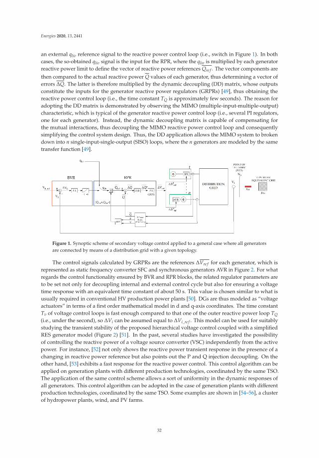
Energies 2020, 13, 2441

an external qliv reference signal to the reactive power control loop (i.e., switch in Figure 1). In bothcases, the so-obtained qliv signal is the input for the RPR, where the qliv is multiplied by each generatorreactive power limit to define the vector of reactive power references Qre f . The vector components arethen compared to the actual reactive power Q values of each generator, thus determining a vector oferrors ΔQ. The latter is therefore multiplied by the dynamic decoupling (DD) matrix, whose outputsconstitute the inputs for the generator reactive power regulators (GRPRs) [49], thus obtaining thereactive power control loop (i.e., the time constant TQ is approximately few seconds). The reason foradopting the DD matrix is demonstrated by observing the MIMO (multiple-input-multiple-output)characteristic, which is typical of the generator reactive power control loop (i.e., several PI regulators,one for each generator). Instead, the dynamic decoupling matrix is capable of compensating forthe mutual interactions, thus decoupling the MIMO reactive power control loop and consequentlysimplifying the control system design. Thus, the DD application allows the MIMO system to brokendown into n single-input-single-output (SISO) loops, where the n generators are modeled by the sametransfer function [49].

Figure 1. Synoptic scheme of secondary voltage control applied to a general case where all generatorsare connected by means of a distribution grid with a given topology.

The control signals calculated by GRPRs are the references ΔVre f for each generator, which isrepresented as static frequency converter SFC and synchronous generators AVR in Figure 2. For whatregards the control functionality ensured by BVR and RPR blocks, the related regulator parameters areto be set not only for decoupling internal and external control cycle but also for ensuring a voltagetime response with an equivalent time constant of about 50 s. This value is chosen similar to what isusually required in conventional HV production power plants [50]. DGs are thus modeled as “voltageactuators” in terms of a first order mathematical model in d and q-axis coordinates. The time constantTv of voltage control loops is fast enough compared to that one of the outer reactive power loop TQ(i.e., under the second), so ΔVi can be assumed equal to ΔVi_re f . This model can be used for suitablystudying the transient stability of the proposed hierarchical voltage control coupled with a simplifiedRES generator model (Figure 2) [51]. In the past, several studies have investigated the possibilityof controlling the reactive power of a voltage source converter (VSC) independently from the activepower. For instance, [52] not only shows the reactive power transient response in the presence of achanging in reactive power reference but also points out the P and Q injection decoupling. On theother hand, [53] exhibits a fast response for the reactive power control. This control algorithm can beapplied on generation plants with different production technologies, coordinated by the same TSO.The application of the same control scheme allows a sort of uniformity in the dynamic responses ofall generators. This control algorithm can be adopted in the case of generation plants with differentproduction technologies, coordinated by the same TSO. Some examples are shown in [54–56], a clusterof hydropower plants, wind, and PV farms.

32

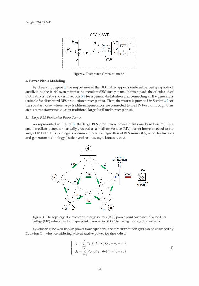
Energies 2020, 13, 2441

Figure 2. Distributed Generator model.

3. Power Plants Modeling

By observing Figure 1, the importance of the DD matrix appears undeniable, being capable ofsubdividing the initial system into n independent SISO subsystems. In this regard, the calculation ofDD matrix is firstly shown in Section 3.1 for a generic distribution grid connecting all the generators(suitable for distributed RES production power plants). Then, the matrix is provided in Section 3.2 forthe standard case, where large traditional generators are connected to the HV busbar through theirstep-up transformers (i.e., as in traditional large fossil fuel power plants).

3.1. Large RES Production Power Plants

As represented in Figure 3, the large RES production power plants are based on multiplesmall–medium generators, usually grouped as a medium voltage (MV) cluster interconnected to thesingle HV POC. This topology is common in practice, regardless of RES source (PV, wind, hydro, etc.)and generators technology (static, synchronous, asynchronous, etc.).

Figure 3. The topology of a renewable energy sources (RES) power plant composed of a mediumvoltage (MV) network and a unique point of connection (POC) to the high voltage (HV) network.

By adopting the well-known power flow equations, the MV distribution grid can be described byEquation (1), when considering active/reactive power for the node k:

⎧⎪⎪⎪⎪⎪⎨⎪⎪⎪⎪⎪⎩Pk =

n∑i=1

Vk·Vi·Yki· cos(θk − θi − γki)

Qk =n∑

i=1Vk·Vi·Yki· sin(θk − θi − γki)

(1)

33

Energies 2020, 13, 2441

where Pk and Qk are the active/reactive power at the node k, while Vk and Vi are the RMS voltage,respectively, at the node k and node i. The magnitude of admittance coefficients in branch ik isrepresented by Yki, whereas θk and θi are the voltage phase angle at node k and node i. Finally, γkiis the admittance phase of branch ik, whereas n the total number of nodes constituting the analyzedgrid. By considering the per-unit notation (i.e., rated values are the basis) and linearizing (1) at a givenoperating point, the Jacobian matrix is defined as in Equation (2):

⎡⎢⎢⎢⎢⎢⎢⎢⎢⎣[Δp]

[Δq]

⎤⎥⎥⎥⎥⎥⎥⎥⎥⎦ =⎡⎢⎢⎢⎢⎢⎢⎢⎢⎢⎢⎢⎢⎣

[dpdθ

]|

[dp∂v

]− −[dqdθ

]|

[dqdv

]⎤⎥⎥⎥⎥⎥⎥⎥⎥⎥⎥⎥⎥⎦·⎡⎢⎢⎢⎢⎢⎢⎢⎢⎣[Δθ]

[Δv]

⎤⎥⎥⎥⎥⎥⎥⎥⎥⎦ (2)

By taking into account a behavior around the operating point, the partial derivatives matrices[dpdv

],[

dpdϑ

],[

dqdv

],[

dqdϑ

]are the link between active/reactive power and magnitude/phase angle of voltage

at buses. As a matter of fact, such matrix coefficients embed the information about the characteristicparameters of the network lines. For the purposes of voltage control, the last equation is to beparticularized as in Equation (3), neglecting the active power variations ([Δp] = 0) and assuming theonly reactive power sources as actuators [57]:

[Δq] =

⎡⎢⎢⎢⎢⎣[

dqdv

]−

[dqdθ

]·[

dpdθ

]−1

·[

dpdv

]⎤⎥⎥⎥⎥⎦[Δv] (3)

By setting a system-operating point, the power flow problem is solved, thus deducing the followingequations for the linearized system:

[Δq] = [A]·[Δv] (4)

where [Δq] and [Δv] are the vectors (n,1) of reactive power/voltage variations, whilst the (n,n) matrix [A]

models the electric coupling between reactive powers and voltage magnitudes. Hence, the generatorsare electrically coupled according to the coefficients (5):

[dqdv

]−

[dqdθ

]·[

dpdθ

]−1

·[

dpdv

](5)

In other words, a voltage variation at every network node causes a reactive power variation in allthe n nodes, according to the matrix [A] coefficients, as expressed in Equation (6):

⎡⎢⎢⎢⎢⎢⎢⎢⎢⎣Δq1

ΔqiΔqn

⎤⎥⎥⎥⎥⎥⎥⎥⎥⎦ =⎡⎢⎢⎢⎢⎢⎢⎢⎢⎣

a11 a1i a1nai1 aii ainan1 ani ann

⎤⎥⎥⎥⎥⎥⎥⎥⎥⎦·⎡⎢⎢⎢⎢⎢⎢⎢⎢⎣

Δv1

ΔviΔvn

⎤⎥⎥⎥⎥⎥⎥⎥⎥⎦ (6)

It is remarkable to notice that [A] is considered full rank in the most practical applications, while thediscussion of idiosyncratic cases (i.e., [A] singular) is beyond the study aims. Finally, Equation (7) iscapable of modeling the voltage at the POC, where [S] is the vector (1,n) of the sensitivity coefficientsdv/dq for combining the POC to the network nodes:

Δvb = [S]·[Δq] =n∑

i=1

si ∗ Δqi (7)

Depending on the relative coefficients dv/dq, the reactive power variation achieved at different gridnodes thus produces at the POC the voltage variation as in Equation (7). The matrix [A] (n,n) and thevector [S] (1,n) can also be determined by a numerical sensitivity analysis. Indeed, once all the networkparameters are established and the reactive power of each DG plant is increased, the consequent voltage

34

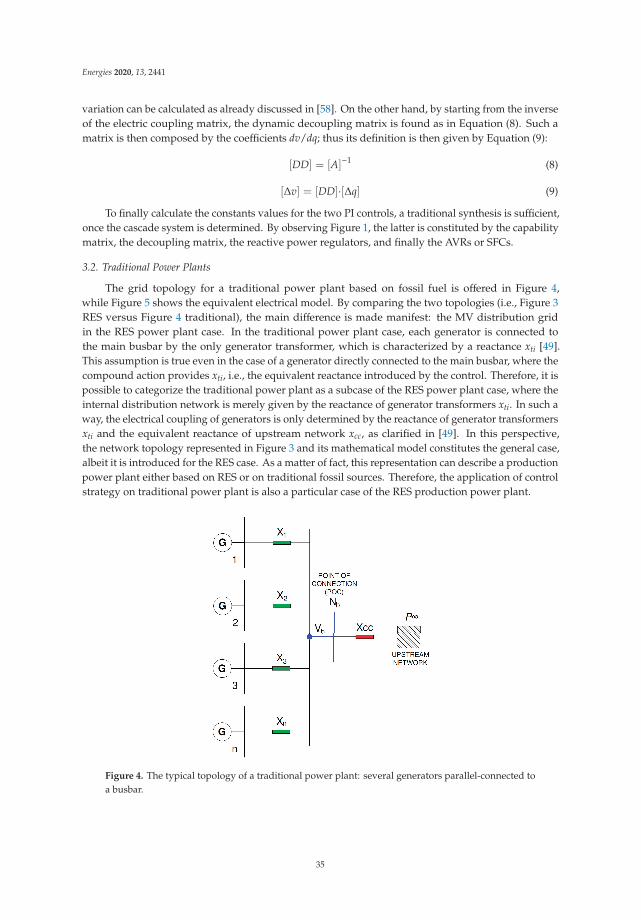
Energies 2020, 13, 2441

variation can be calculated as already discussed in [58]. On the other hand, by starting from the inverseof the electric coupling matrix, the dynamic decoupling matrix is found as in Equation (8). Such amatrix is then composed by the coefficients dv/dq; thus its definition is then given by Equation (9):

[DD] = [A]−1 (8)

[Δv] = [DD]·[Δq] (9)

To finally calculate the constants values for the two PI controls, a traditional synthesis is sufficient,once the cascade system is determined. By observing Figure 1, the latter is constituted by the capabilitymatrix, the decoupling matrix, the reactive power regulators, and finally the AVRs or SFCs.

3.2. Traditional Power Plants

The grid topology for a traditional power plant based on fossil fuel is offered in Figure 4,while Figure 5 shows the equivalent electrical model. By comparing the two topologies (i.e., Figure 3RES versus Figure 4 traditional), the main difference is made manifest: the MV distribution gridin the RES power plant case. In the traditional power plant case, each generator is connected tothe main busbar by the only generator transformer, which is characterized by a reactance xti [49].This assumption is true even in the case of a generator directly connected to the main busbar, where thecompound action provides xti, i.e., the equivalent reactance introduced by the control. Therefore, it ispossible to categorize the traditional power plant as a subcase of the RES power plant case, where theinternal distribution network is merely given by the reactance of generator transformers xti. In such away, the electrical coupling of generators is only determined by the reactance of generator transformersxti and the equivalent reactance of upstream network xcc, as clarified in [49]. In this perspective,the network topology represented in Figure 3 and its mathematical model constitutes the general case,albeit it is introduced for the RES case. As a matter of fact, this representation can describe a productionpower plant either based on RES or on traditional fossil sources. Therefore, the application of controlstrategy on traditional power plant is also a particular case of the RES production power plant.

Figure 4. The typical topology of a traditional power plant: several generators parallel-connected toa busbar.

35

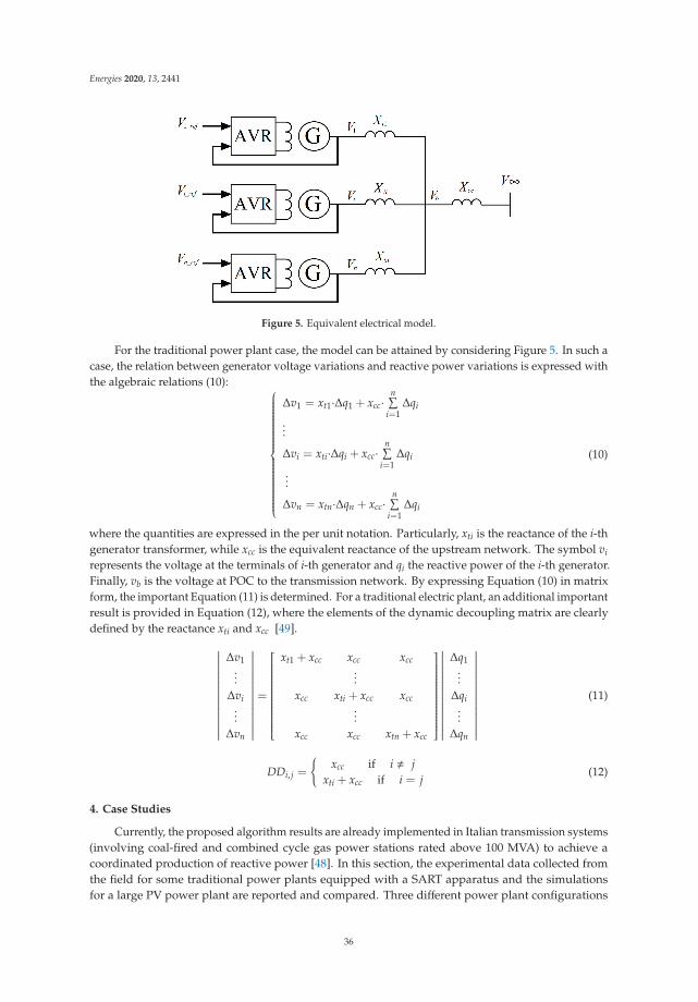
Energies 2020, 13, 2441

Figure 5. Equivalent electrical model.

For the traditional power plant case, the model can be attained by considering Figure 5. In such acase, the relation between generator voltage variations and reactive power variations is expressed withthe algebraic relations (10): ⎧⎪⎪⎪⎪⎪⎪⎪⎪⎪⎪⎪⎪⎪⎪⎪⎪⎨⎪⎪⎪⎪⎪⎪⎪⎪⎪⎪⎪⎪⎪⎪⎪⎪⎩

Δv1 = xt1·Δq1 + xcc·n∑

i=1Δqi

...

Δvi = xti·Δqi + xcc·n∑

i=1Δqi

...

Δvn = xtn·Δqn + xcc·n∑

i=1Δqi

(10)

where the quantities are expressed in the per unit notation. Particularly, xti is the reactance of the i-thgenerator transformer, while xcc is the equivalent reactance of the upstream network. The symbol virepresents the voltage at the terminals of i-th generator and qi the reactive power of the i-th generator.Finally, vb is the voltage at POC to the transmission network. By expressing Equation (10) in matrixform, the important Equation (11) is determined. For a traditional electric plant, an additional importantresult is provided in Equation (12), where the elements of the dynamic decoupling matrix are clearlydefined by the reactance xti and xcc [49].

∣∣∣∣∣∣∣∣∣∣∣∣∣∣∣∣∣

Δv1...

Δvi...

Δvn

∣∣∣∣∣∣∣∣∣∣∣∣∣∣∣∣∣=

⎡⎢⎢⎢⎢⎢⎢⎢⎢⎢⎢⎢⎢⎢⎢⎢⎢⎢⎢⎢⎢⎢⎣

xt1 + xcc xcc xcc...

xcc xti + xcc xcc...

xcc xcc xtn + xcc

⎤⎥⎥⎥⎥⎥⎥⎥⎥⎥⎥⎥⎥⎥⎥⎥⎥⎥⎥⎥⎥⎥⎦

∣∣∣∣∣∣∣∣∣∣∣∣∣∣∣∣∣

Δq1...

Δqi...

Δqn

∣∣∣∣∣∣∣∣∣∣∣∣∣∣∣∣∣(11)

DDi, j =

{xcc if i � j

xti + xcc if i = j(12)

4. Case Studies

Currently, the proposed algorithm results are already implemented in Italian transmission systems(involving coal-fired and combined cycle gas power stations rated above 100 MVA) to achieve acoordinated production of reactive power [48]. In this section, the experimental data collected fromthe field for some traditional power plants equipped with a SART apparatus and the simulationsfor a large PV power plant are reported and compared. Three different power plant configurations

36

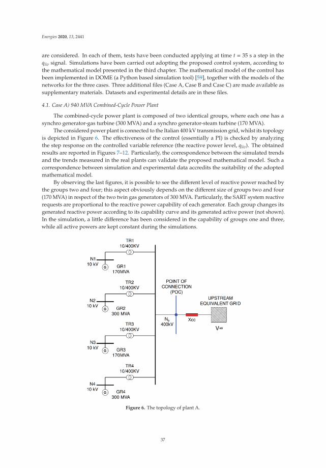
Energies 2020, 13, 2441

are considered. In each of them, tests have been conducted applying at time t = 35 s a step in theqliv signal. Simulations have been carried out adopting the proposed control system, according tothe mathematical model presented in the third chapter. The mathematical model of the control hasbeen implemented in DOME (a Python based simulation tool) [59], together with the models of thenetworks for the three cases. Three additional files (Case A, Case B and Case C) are made available assupplementary materials. Datasets and experimental details are in these files.

4.1. Case A) 940 MVA Combined-Cycle Power Plant

The combined-cycle power plant is composed of two identical groups, where each one has asynchro generator-gas turbine (300 MVA) and a synchro generator-steam turbine (170 MVA).

The considered power plant is connected to the Italian 400 kV transmission grid, whilst its topologyis depicted in Figure 6. The effectiveness of the control (essentially a PI) is checked by analyzingthe step response on the controlled variable reference (the reactive power level, qliv). The obtainedresults are reported in Figures 7–12. Particularly, the correspondence between the simulated trendsand the trends measured in the real plants can validate the proposed mathematical model. Such acorrespondence between simulation and experimental data accredits the suitability of the adoptedmathematical model.

By observing the last figures, it is possible to see the different level of reactive power reached bythe groups two and four; this aspect obviously depends on the different size of groups two and four(170 MVA) in respect of the two twin gas generators of 300 MVA. Particularly, the SART system reactiverequests are proportional to the reactive power capability of each generator. Each group changes itsgenerated reactive power according to its capability curve and its generated active power (not shown).In the simulation, a little difference has been considered in the capability of groups one and three,while all active powers are kept constant during the simulations.

Figure 6. The topology of plant A.

37

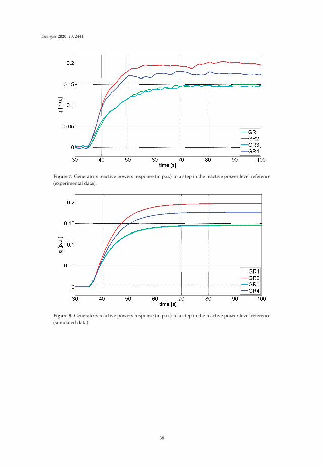
Energies 2020, 13, 2441

Figure 7. Generators reactive powers response (in p.u.) to a step in the reactive power level reference(experimental data).

Figure 8. Generators reactive powers response (in p.u.) to a step in the reactive power level reference(simulated data).

38

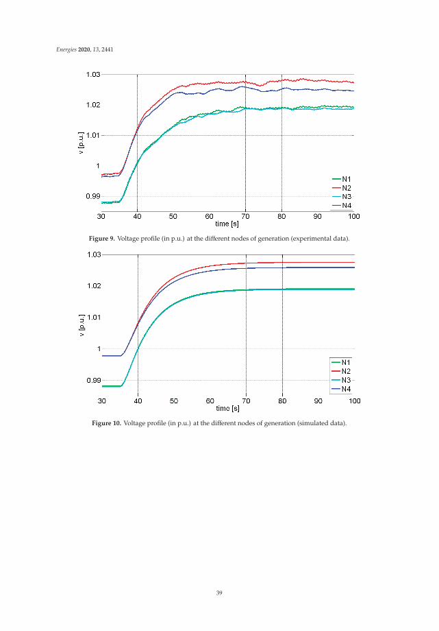
Energies 2020, 13, 2441

Figure 9. Voltage profile (in p.u.) at the different nodes of generation (experimental data).

Figure 10. Voltage profile (in p.u.) at the different nodes of generation (simulated data).

39

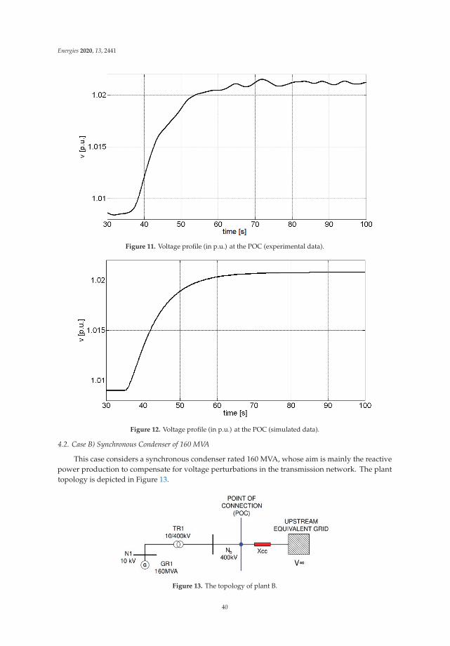
Energies 2020, 13, 2441

Figure 11. Voltage profile (in p.u.) at the POC (experimental data).

Figure 12. Voltage profile (in p.u.) at the POC (simulated data).

4.2. Case B) Synchronous Condenser of 160 MVA

This case considers a synchronous condenser rated 160 MVA, whose aim is mainly the reactivepower production to compensate for voltage perturbations in the transmission network. The planttopology is depicted in Figure 13.

Figure 13. The topology of plant B.

40

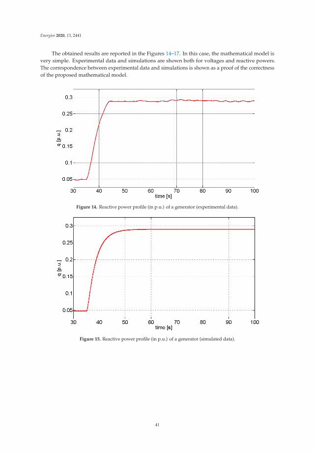
Energies 2020, 13, 2441

The obtained results are reported in the Figures 14–17. In this case, the mathematical model isvery simple. Experimental data and simulations are shown both for voltages and reactive powers.The correspondence between experimental data and simulations is shown as a proof of the correctnessof the proposed mathematical model.

Figure 14. Reactive power profile (in p.u.) of a generator (experimental data).

Figure 15. Reactive power profile (in p.u.) of a generator (simulated data).

41

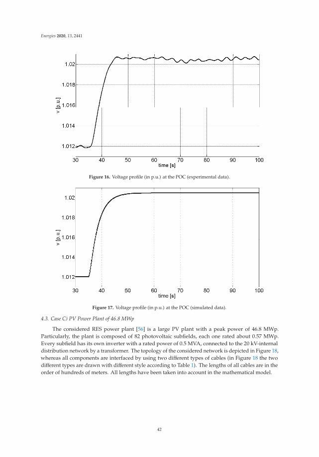
Energies 2020, 13, 2441

Figure 16. Voltage profile (in p.u.) at the POC (experimental data).

Figure 17. Voltage profile (in p.u.) at the POC (simulated data).

4.3. Case C) PV Power Plant of 46.8 MWp

The considered RES power plant [56] is a large PV plant with a peak power of 46.8 MWp.Particularly, the plant is composed of 82 photovoltaic subfields, each one rated about 0.57 MWp.Every subfield has its own inverter with a rated power of 0.5 MVA, connected to the 20 kV-internaldistribution network by a transformer. The topology of the considered network is depicted in Figure 18,whereas all components are interfaced by using two different types of cables (in Figure 18 the twodifferent types are drawn with different style according to Table 1). The lengths of all cables are in theorder of hundreds of meters. All lengths have been taken into account in the mathematical model.

42

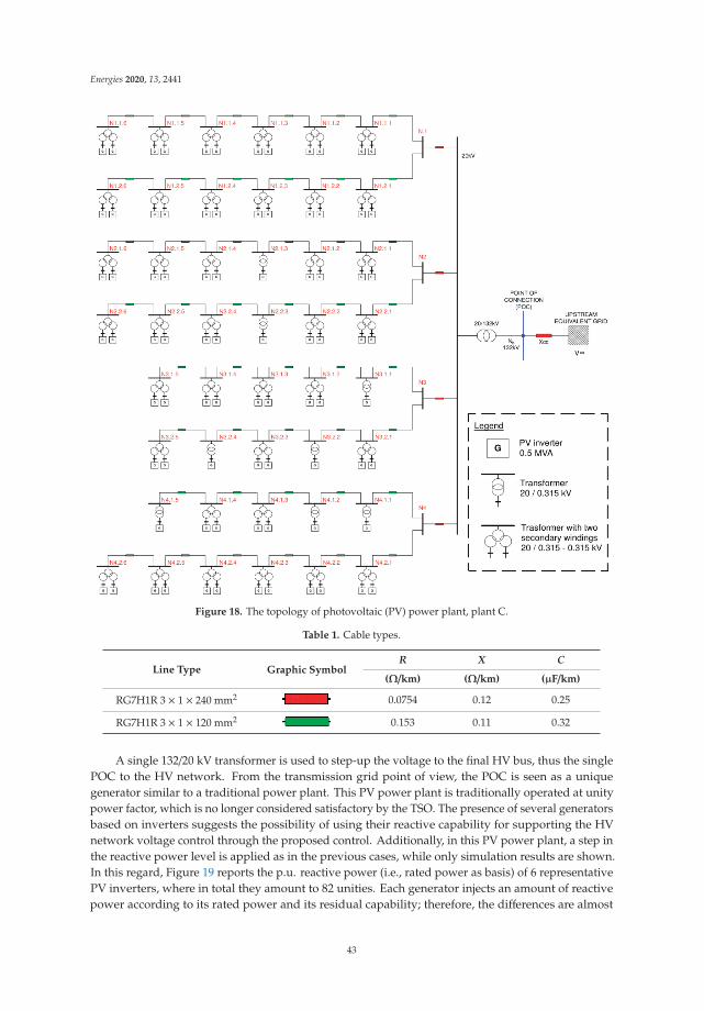
Energies 2020, 13, 2441

Figure 18. The topology of photovoltaic (PV) power plant, plant C.

Table 1. Cable types.

Line Type Graphic SymbolR X C

(Ω/km) (Ω/km) (μF/km)

RG7H1R 3 × 1 × 240 mm2 0.0754 0.12 0.25

RG7H1R 3 × 1 × 120 mm2 0.153 0.11 0.32

A single 132/20 kV transformer is used to step-up the voltage to the final HV bus, thus the singlePOC to the HV network. From the transmission grid point of view, the POC is seen as a uniquegenerator similar to a traditional power plant. This PV power plant is traditionally operated at unitypower factor, which is no longer considered satisfactory by the TSO. The presence of several generatorsbased on inverters suggests the possibility of using their reactive capability for supporting the HVnetwork voltage control through the proposed control. Additionally, in this PV power plant, a step inthe reactive power level is applied as in the previous cases, while only simulation results are shown.In this regard, Figure 19 reports the p.u. reactive power (i.e., rated power as basis) of 6 representativePV inverters, where in total they amount to 82 unities. Each generator injects an amount of reactivepower according to its rated power and its residual capability; therefore, the differences are almost

43

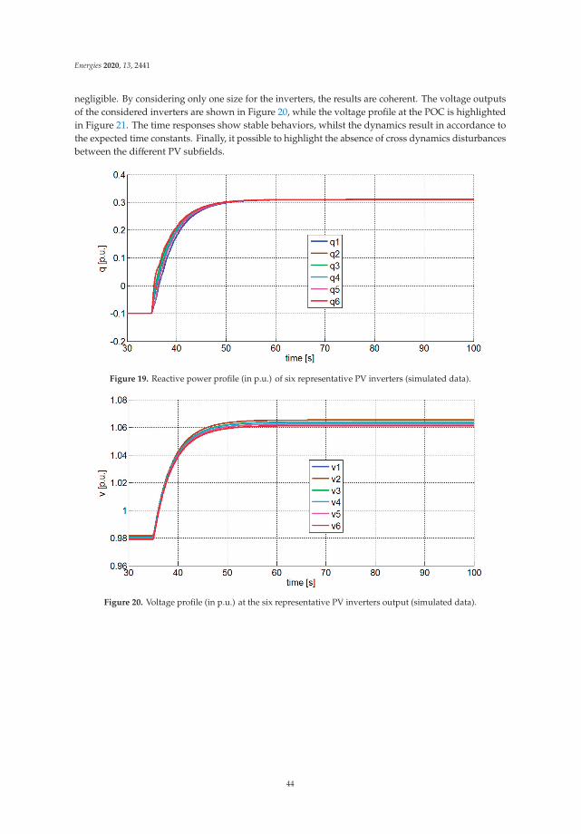
Energies 2020, 13, 2441

negligible. By considering only one size for the inverters, the results are coherent. The voltage outputsof the considered inverters are shown in Figure 20, while the voltage profile at the POC is highlightedin Figure 21. The time responses show stable behaviors, whilst the dynamics result in accordance tothe expected time constants. Finally, it possible to highlight the absence of cross dynamics disturbancesbetween the different PV subfields.

Figure 19. Reactive power profile (in p.u.) of six representative PV inverters (simulated data).

Figure 20. Voltage profile (in p.u.) at the six representative PV inverters output (simulated data).

44

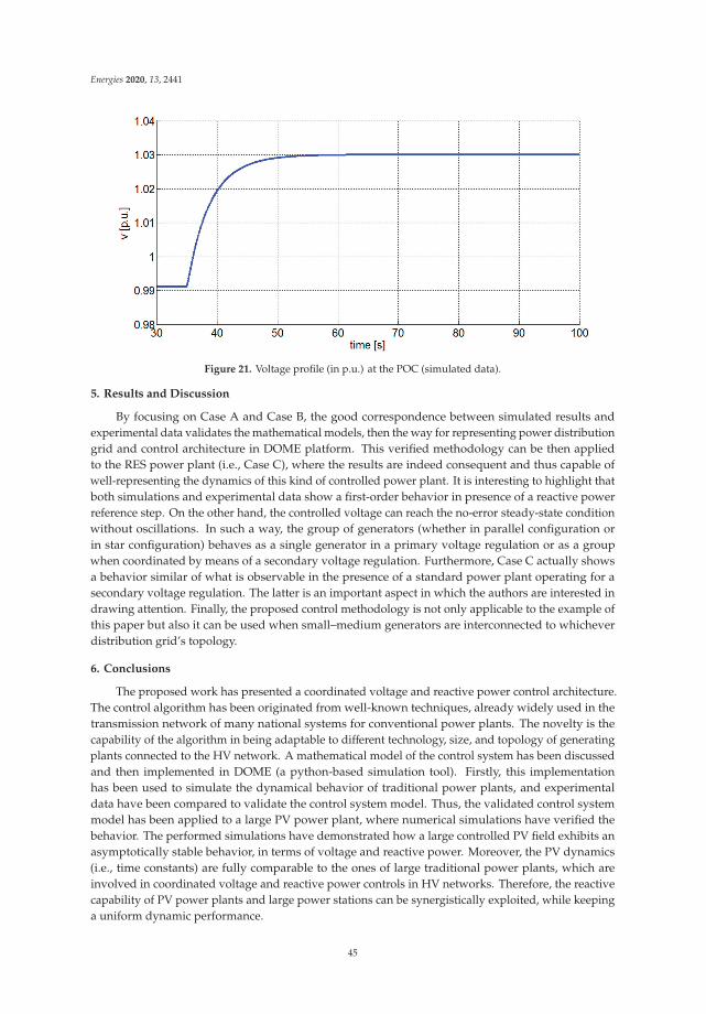
Energies 2020, 13, 2441

Figure 21. Voltage profile (in p.u.) at the POC (simulated data).

5. Results and Discussion

By focusing on Case A and Case B, the good correspondence between simulated results andexperimental data validates the mathematical models, then the way for representing power distributiongrid and control architecture in DOME platform. This verified methodology can be then appliedto the RES power plant (i.e., Case C), where the results are indeed consequent and thus capable ofwell-representing the dynamics of this kind of controlled power plant. It is interesting to highlight thatboth simulations and experimental data show a first-order behavior in presence of a reactive powerreference step. On the other hand, the controlled voltage can reach the no-error steady-state conditionwithout oscillations. In such a way, the group of generators (whether in parallel configuration orin star configuration) behaves as a single generator in a primary voltage regulation or as a groupwhen coordinated by means of a secondary voltage regulation. Furthermore, Case C actually showsa behavior similar of what is observable in the presence of a standard power plant operating for asecondary voltage regulation. The latter is an important aspect in which the authors are interested indrawing attention. Finally, the proposed control methodology is not only applicable to the example ofthis paper but also it can be used when small–medium generators are interconnected to whicheverdistribution grid’s topology.

6. Conclusions

The proposed work has presented a coordinated voltage and reactive power control architecture.The control algorithm has been originated from well-known techniques, already widely used in thetransmission network of many national systems for conventional power plants. The novelty is thecapability of the algorithm in being adaptable to different technology, size, and topology of generatingplants connected to the HV network. A mathematical model of the control system has been discussedand then implemented in DOME (a python-based simulation tool). Firstly, this implementationhas been used to simulate the dynamical behavior of traditional power plants, and experimentaldata have been compared to validate the control system model. Thus, the validated control systemmodel has been applied to a large PV power plant, where numerical simulations have verified thebehavior. The performed simulations have demonstrated how a large controlled PV field exhibits anasymptotically stable behavior, in terms of voltage and reactive power. Moreover, the PV dynamics(i.e., time constants) are fully comparable to the ones of large traditional power plants, which areinvolved in coordinated voltage and reactive power controls in HV networks. Therefore, the reactivecapability of PV power plants and large power stations can be synergistically exploited, while keepinga uniform dynamic performance.

45

Energies 2020, 13, 2441

The proposed control scheme is finally characterized by several advantages: it is capable ofensuring a fast response, while performing a perfect tracking of both the HV bus voltage and RESreactive powers. In addition, there is no steady-state error and the system dynamics does not highlightoscillations. Each generator participates in the control by sharing its reactive power (in absorptionor injection), where the provided quota is proportional to its capability at the point of operation.An important note to be highlighted regards the communication data. The proposed control strategy isbased on the communication of a single control signal (i.e., the reactive power level) to all the generatorsinvolved, thus making its implementation rather simple. The transmitted qliv value is coherent to thereactive power level’s control signal that is already in use in the coordinated voltage and reactive powercontrol of transmission networks. This makes the proposed control architecture fully compatible withexisting ones. As a further development, authors are investigating how this control architecture can bescaled and integrated into distribution networks. In a glance, the proposed control is characterized bythe two important pros: a) only one signal is requested for regulating multiple-generators and b) itis strictly alike to the secondary control already used in transmission system, thus consequently it iscompatible. The proposed solution is feasible when promoting the integration of large PV systems inthe HV networks’ control strategies (i.e., voltage and reactive power).

Supplementary Materials: The following are available online at http://www.mdpi.com/1996-1073/13/10/2441/s1,File S1: Case A.dm, File S2: Case B.dm, File S3: Case C.dm. Three additional files (Case A, Case B and Case C)are made available during the submission process. Full datasets and full experimental details are provided inthese three files. The three files are the inputs for performing simulations then reproducing the results in DOME,the Python based simulation tool used in this paper.

Author Contributions: Conceptualization, M.C., D.B. and G.S.; Data curation, M.C. and R.C.; Formal analysis,R.C.; Methodology, D.B. and G.S.; Software, M.C.; Supervision, G.S.; Validation, D.B.; Visualization, R.C.;Writing—original draft, R.C.; Writing—review & editing, M.C., D.B. and G.S. All authors have read and agreed tothe published version of the manuscript.

Funding: This research received no external funding.

Conflicts of Interest: The authors declare no conflict of interest.

Abbreviations

AVR Automatic Voltage RegulatorBVR Busbar Voltage RegulatorDD Dynamic DecouplingDGs Distributed GeneratorsGRPRs Generator Reactive Power RegulatorsHV High VoltageLV Low VoltageMIMO Multiple-Input-Multiple-OutputMV Medium VoltagePI Proportional-IntegralPOC Point Of ConnectionPV PhotovoltaicRES Renewable Energy SourcesRPR Reactive Power RegulatorSFC Static Frequency ConverterSISO Single-Input-Single-OutputSTATCOM Static Synchronous CompensatorSVR Secondary Voltage RegulationTSO Transmission System OperatorVPP Virtual Power PlantsVSC Voltage Source ConverterVSN Virtual Smart Network

46

Energies 2020, 13, 2441

References

1. van Wyk, A.A.L.; Khan, M.A.; Barendse, P. Impact of over/under and voltage unbalanced supplies onEnergy-Efficient motors. In Proceedings of the 2011 IEEE International Electric Machines & Drives Conference(IEMDC), Niagara Falls, ON, Canada, 15–18 May 2011; pp. 1380–1385.

2. Jahmeerbacus, I.; Bhurtun, C. Energy efficiency and power quality issues of AC voltage controllers in instantwater heaters. In Proceedings of the 2012 20th Domestic Use of Energy Conference, Cape Town, South Africa,3–4 April 2012; pp. 139–144.

3. Lipsky, A.; Braunstein, A.; Miteva, N.; Slonim, M. Electric power quality and efficiency of power supply.In Proceedings of the 21st IEEE Convention of the Electrical and Electronic Engineers in Israel. Proceedings(Cat. No.00EX377), Tel-Aviv, Israel, 11–12 April 2000; pp. 222–225.

4. Fusco, G.; Russo, M. Adaptive Voltage Control System; Springer: Berlin/Heidelberg, Germany, 2007.5. Chiandone, M.; Sulligoi, G.; Massucco, S.; Silvestro, F. Hierarchical voltage regulation of transmission systems

with renewable power plants: An overview of the Italian case. In Proceedings of the 3rd Renewable PowerGeneration Conference (RPG 2014), Naples, Italy, 24–25 September 2014; pp. 1–5.

6. Mousavi, O.A.; Cherkaoui, R. Literature Survey on Fundamental Issues of Voltage and Reactive Power Control;École polytechnique fédérale de Lausanne: Lausanne, Switzerland, 2011.

7. Mohandes, B.; el Moursi, M.S.; Hatziargyriou, N.D.; el Khatib, S. A review of power system flexibility withhigh penetration of renewables. IEEE Trans. Power Syst. 2019, 34, 3140–3155. [CrossRef]

8. Sun, H.; Guo, Q.; Qi, J.; Ajjarapu, V.; Bravo, R.; Chow, J.; Li, Z.; Moghe, R.; Nasr-Azadani, E.; Tamrakar, U.;et al. Review of challenges and research opportunities for voltage control in smart grids. IEEE Trans.Power Syst. 2019, 34, 2790–2801. [CrossRef]

9. Vita, V.; Alimardan, T.; Ekonomou, L. The impact of distributed generation in the distribution networks’voltage profile and energy losses. In Proceedings of the 9th IEEE European Modelling Symposium onMathematical Modelling and Computer Simulation, Madrid, Spain, 6–8 October 2015; pp. 260–265.

10. Ceaki, O.; Seritan, G.; Vatu, R.; Mancasi, M. Analysis of power quality improvement in smart grids.In Proceedings of the 10th International Symposium on Advanced Topics in Electrical Engineering (ATEE),Bucharest, Romania, 23–25 March 2017; pp. 797–801.

11. Nieto, A.; Vita, V.; Maris, T.I. Power quality improvement in power grids with the integration of energystorage systems. Int. J. Eng. Res. Technol. 2016, 5, 438–443.

12. European Commission. EU Energy in Figures—Statistical Pocketbook 2016; Publications Office of the EuropeanUnion: Brussels, Belgium, 2016.

13. The International Renewable Energy Agency. Renewable Energy Statistics 2016; IRENA: Abu Dhabi, UAE, 2016.14. Renewable Energy Policy Network for the 21st Century (REN21). Renewables 2014 Global Status Report;

REN21: Paris, France, 2014.15. GSE S.p.A. Rapporto Statistico 2014—Solare Fotovoltaico; GSE S.p.A.: Rome, Italy, 2015.16. Petinrin, J.O.; Shaaban, M. Impact of renewable generation on voltage control in distribution systems.

Renew. Sustain. Energy Rev. 2016, 65, 770–783. [CrossRef]17. Pfeiffer, R. Brief status on CENELEC standards related to Connection Network Code. In Proceedings of the

3rd Grid Connection Stakeholder Committee Meeting, Brussels, Belgium, 8 September 2016.18. Bründlinger, R. Advanced smart inverter and DER functions Requirements in latest European Grid Codes and

future trends. In Proceedings of the Solar Canada 2015 Conference, Toronto, ON, Canada, 7–8 December 2015.19. ENTSO-E. Implementation Guideline for Network Code “Requirements for Grid Connection Applicable to all

Generators”; ENTSO-E: Brussels, Belgium, 2013.20. The European Commission. Commission Regulation (EU) 2016/631 of 14 April 2016 Establishing a Network

Code on Requirements for Grid Connection of Generators; Official Journal of the European Union: Brussels,Belgium, 2016.

21. Arrinda, J.; Barrena, J.A.; Rodríguez, M.A.; Guerrero, A. Analysis of massive integration of renewable powerplants under new regulatory frameworks. In Proceedings of the 2014 International Conference on RenewableEnergy Research and Application (ICRERA), Milwaukee, WI, USA, 19–22 October 2014; pp. 462–467.

22. Varma, R.K.; Salama, M. Large-scale photovoltaic solar power integration in transmission and distributionnetworks. In Proceedings of the 2011 IEEE Power and Energy Society General Meeting, Detroit, MI, USA,24–28 July 2011; pp. 1–4.

47

Energies 2020, 13, 2441

23. Delfino, F.; Procopio, R.; Rossi, M.; Ronda, G. Integration of large-size photovoltaic systems into thedistribution grids: A P-Q chart approach to assess reactive support capability. IET Renew. Power Gener. 2010,4, 329–340. [CrossRef]

24. Tyll, H.K.; Schettle, F. Historical overview on dynamic reactive power compensation solutions from thebegin of AC power transmission towards present applications. In Proceedings of the 2009 IEEE/PES PowerSystems Conference and Exposition, Seattle, WA, USA, 15–18 March 2009; pp. 1–7.

25. Ghasemi, M.A.; Parniani, M. Prevention of distribution network overvoltage by adaptive droop-based activeand reactive power control of PV systems. Electric Power Syst. Res. 2016, 133, 313–327. [CrossRef]

26. Hashemi, M.; Agelidis, V. Evaluation of voltage regulation mitigation methods due to high penetration of PVgeneration in residential areas. In Proceedings of the 2013 International Conference on Renewable EnergyResearch and Applications (ICRERA), Madrid, Spain, 20–23 October 2013; pp. 1180–1189.

27. Hasheminamin, M.; Agelidis, V.G.; Ahmadi, A.; Siano, P.; Teodorescu, R. Single-point reactive power controlmethod on voltage rise mitigation in residential networks with high PV penetration. Renew. Energy 2018,119, 504–512. [CrossRef]

28. Rallabandi, V.; Akeyo, O.M.; Ionel, D.M. Modeling of a multi-megawatt grid connected PV system withintegrated batteries. In Proceedings of the 2016 IEEE International Conference on Renewable Energy Researchand Applications (ICRERA), Birmingham, UK, 20–23 November 2016; pp. 1146–1151.

29. Olival, P.C.; Madureira, A.G.; Matos, M. Advanced voltage control for smart microgrids using distributedenergy resources. Electr. Power Syst. Res. 2017, 146, 132–140. [CrossRef]

30. Jayasekara, N.; Wolfs, P.; Masoum, M.A.S. An optimal management strategy for distributed storages indistribution networks with high penetrations of PV. Electr. Power Syst. Res. 2014, 116, 147–157. [CrossRef]

31. Ko, H.; Bruey, S.; Jatskevich, J.; Dumont, G.; Moshref, A. A PI Control of DFIG-Based Wind Farm for VoltageRegulation at Remote Location. In Proceedings of the 2007 IEEE Power Engineering Society General Meeting,Tampa, FL, USA, 24–28 June 2007; pp. 1–6.

32. Baalbergen, F.; Gibescu, M.; van der Sluis, L. Voltage stability consequences of decentralized generation andpossibilities for intelligent control. In Proceedings of the 2010 IEEE PES Innovative Smart Grid TechnologiesConference Europe (ISGT Europe), Gothenburg, Sweden, 11–13 October 2010; pp. 1–8.

33. Zhao, J.; Li, X.; Hao, J.; Lu, J. Reactive power control of wind farm made up with doubly fed inductiongenerators in distribution system. Electr. Power Syst. Res. 2010, 80, 698–706. [CrossRef]

34. El-Fouly, T.H.M.; El-Saadany, E.F.; Salama, M.M.A. Voltage regulation of wind farms equipped withvariable-speed doubly-fed induction generators wind turbines. In Proceedings of the 2007 IEEE PowerEngineering Society General Meeting, Tampa, FL, USA, 24–28 June 2007; pp. 1–8.

35. Qin, N.; Bak, C.L.; Abildgaard, H. Automatic voltage control system with market price employing largewind farms. Electr. Power Syst. Res. 2018, 157, 93–105. [CrossRef]

36. Mastromauro, R.A.; Orlando, N.A.; Ricchiuto, D.; Liserre, M.; Dell’Aquila, A. Hierarchical control of asmall wind turbine system for active integration in LV distribution network. In Proceedings of the 2013International Conference on Clean Electrical Power (ICCEP), Alghero, Italy, 11–13 June 2013; pp. 426–433.

37. Koraki, D.; Strunz, K. Wind and solar power integration in electricity markets and distribution networksthrough service-centric virtual power plants. IEEE Trans. Power Syst. 2018, 33, 473–485. [CrossRef]

38. Unger, D.; Spitalny, L.; Myrzik, J.M.A. Voltage control by small hydro power plants integrated into a virtualpower plant. In Proceedings of the 2012 IEEE Energytech, Cleveland, OH, USA, 29–31 May 2012; pp. 1–6.

39. Dielmann, K.; van der Velden, A. Virtual power plants (VPP)—A new perspective for energy generation? InProceedings of the 9th International Scientific and Practical Conference of Students, Post-graduates ModernTechniques and Technologies, 2003, MTT 2003, Tomsk, Russia, 7–11 April 2003.

40. Pudjianto, D.; Ramsay, C.; Strbac, G. Virtual power plant and system integration of distributed energyresources. IET Renew. Power Gener. 2007, 1, 10–16. [CrossRef]

41. Ricerca Sistema Energetico (RSE). Definizione dei Concetti e Delle Architetture di Gestione, Controllo e Comunicazionedi Microreti e Virtual Power Plant; Progetto RdS—Trasmissione e Distribuzione; RSE: Milan, Italy, 2006.

42. Arcidiacono, V. Automatic Voltage and Reactive Power Control in Transmission Systems. In Proceedings ofthe 1983 CIGRE-IFAC Symposium, Florence, Italy, 26–28 September 1983. Survey paper.

43. Paul, J.P.; Leost, J.Y.; Tesseron, J.M. Survey of the Secondary Voltage Control in France: Present Realizationand Investigations. IEEE Trans. Power Syst. 1987, 2, 505–511. [CrossRef]

48

Energies 2020, 13, 2441

44. Sancha, J.L.; Fernandez, J.L.; Cortes, A.; Abarca, J.T. Secondary voltage control: Analysis, solutions andsimulation results for the Spanish transmission system. IEEE Trans. Power Syst. 1996, 11, 630–638. [CrossRef]

45. Automatic System for Voltage Regulation (SART) for Electric Power Plant, GRTN Document nr. DRRPX03019.Available online: http://www.terna.it/LinkClick.aspx?fileticket=irZ1FD%2BYxUE%3D&tabid=106&mid=468(accessed on 11 April 2020).

46. Lagonotte, P.; Sabonnadiere, J.C.; Leost, J.Y.; Paul, J.P. Structural analysis of the electrical system: Applicationto secondary voltage control in France. IEEE Trans. Power Syst. 1989, 4, 479–486. [CrossRef]

47. Sancha, J.L.; Fernandez, J.L.; Martinez, F.; Salle, C. Spanish practices in reactive power management andvoltage control. In Proceedings of the IEE Colloquium on International Practices in Reactive Power Control,London, UK, 7 April 1993; pp. 3/1–3/4.

48. Sulligoi, G.; Chiandone, M.; Arcidiacono, V. NewSART automatic voltage and reactive power regulator forsecondary voltage regulation: Design and application. In Proceedings of the 2011 IEEE Power and EnergySociety General Meeting, San Diego, CA, USA, 24–28 July 2011; pp. 1–7.

49. Arcidiacono, V.; Menis, R.; Sulligoi, G. Improving power quality in all electric ships using a voltage and VARintegrated regulator. In Proceedings of the 2007 IEEE Electric Ship Technologies Symposium, Arlington, VA,USA, 21–23 May 2007; pp. 322–327.

50. TERNA. Sistema Automatico per la Regolazione di Tensione (SART) per Centrali Elettriche di Produzione.Annex A16 to the National Grid Code, GRTN Document nr. DRRPX03019. Available online: http://collaudo.download.terna.it/terna/0000/0105/33.pdf(accessed on 11 April 2020).

51. Tamimi, B.; Cañizares, C.; Bhattacharya, K. Modeling and performance analysis of large solar photo-voltaicgeneration on voltage stability and inter-area oscillations. In Proceedings of the 2011 IEEE Power and EnergySociety General Meeting, San Diego, CA, USA, 24–28 July 2011; pp. 1–6.

52. Vasquez, J.C.; Mastromauro, R.A.; Liserre, J.M. Voltage support provided by a droop-controlledmultifunctional inverter. IEEE Trans. Ind. Electron. 2009, 56, 4510–4519. [CrossRef]

53. Cagnano, A.; De Tuglie, E.; Liserre, M.; Mastromauro, R.A. Online Optimal Reactive Power Control Strategyof PV Inverters. IEEE Trans. Ind. Electron. 2011, 58, 4549–4558. [CrossRef]

54. Campaner, R.; Chiandone, M.; Arcidiacono, V.; Sulligoi, G.; Milano, F. Automatic voltage control of a clusterof hydro power plants to operate as a virtual power plant. In Proceedings of the 2015 IEEE 15th InternationalConference on Environment and Electrical Engineering (EEEIC), Rome, Italy, 10–13 June 2015; pp. 2153–2158.

55. Chiandone, M.; Campaner, R.; Arcidiacono, V.; Sulligoi, G.; Milano, F. Automatic voltage and reactive powerregulator for wind farms participating to TSO voltage regulation. In Proceedings of the 2015 IEEE EindhovenPowerTech, Eindhoven, The Netherlands, 29 June–2 July 2015; pp. 1–5.

56. Chiandone, M.; Campaner, R.; Pavan, A.M.; Arcidiacono, V.; Milano, F.; Sulligoi, G. Coordinated voltagecontrol of multi-converter power plants operating in transmission systems. The case of photovoltaics.In Proceedings of the 2015 International Conference on Clean Electrical Power (ICCEP), Taormina, Italy,16–18 June 2015; pp. 506–510.

57. Gao, B.; Morison, G.K.; Kundur, P. Voltage Stability evaluation using modal analysis. IEEE Trans. Power Syst.1992, 7, 1529–1542. [CrossRef]

58. Carvalho, P.M.; Correia, P.F.; Ferreira, L.A. Distributed reactive power generation control for voltage risemitigation in distribution networks. IEEE Trans. Power Syst. 2008, 23, 766–772. [CrossRef]

59. Milano, F. A python-based software tool for power system analysis. In Proceedings of the IEEE PES GeneralMeeting, Vancouver, BC, Canada, 21–25 July 2013.

© 2020 by the authors. Licensee MDPI, Basel, Switzerland. This article is an open accessarticle distributed under the terms and conditions of the Creative Commons Attribution(CC BY) license (http://creativecommons.org/licenses/by/4.0/).

49

energies

Article

Dynamic Reconfiguration Systems for PV Plant:Technical and Economic Analysis

Giuseppe Schettino, Filippo Pellitteri, Guido Ala, Rosario Miceli, Pietro Romano and

Fabio Viola *

Department of Engineering, University of Palermo, 90128 Palermo, Italy; giuseppe.schettino@unipa.it (G.S.);filippo.pellitteri@unipa.it (F.P.); guido.ala@unipa.it (G.A.); rosario.miceli@unipa.it (R.M.);pietro.romano@unipa.it (P.R.)* Correspondence: fabio.viola@unipa.it

Received: 16 March 2020; Accepted: 15 April 2020; Published: 17 April 2020

Abstract: Solar plants suffer of partial shading and mismatch problems. Without considering thegeneration of hot spots and the resulting security issues, a monitoring system for the health of a PVplant should be useful to drive a dynamic reconfiguration system (DRS) to solve bottlenecks due todifferent panels’ shading. Over the years different DRS architectures have been proposed, but nosuggestions about costs and benefits have been provided. Starting from technical subjects such asdifferences of the topologies driving the hardware complexity and number of components, this paperidentifies the cost of DRS and its lifetime, and based on these issues it provides an economic analysisfor a 6 kWp PV plant in different European Union countries, in which the dissimilar incentive policieshave been considered.

Keywords: energy policies related to PV power plants; economic analyses; monitoring and case studies

1. Introduction

The trend of the last decade to reduce greenhouse gas emissions and decarbonize the energysources is mainly due to the increase of the temperature of the planet, has driven the development andimprovement of technologies for renewable energy sources. As well known, solar energy is the mostavailable renewable energy source in the world with respect to the other sources and an interestingtopic of research is the evaluation of its economic convenience. For this reason, in many studiesreported in literature, the economic convenience of grid-connected PV systems has been evaluatedwith respect to other technologies. The traditional approach is based on the use of the “levelized cost”method that represents the per unit value of total costs (i.e., capital, operation and maintenance, fuel)over the economic life of the power plant [1,2]. The notion of economic convenience of PV plantsemerged from these studies.

In the European Union (EU), the number of the PV plants is increasing significantly thanks tothe policies of the different countries that have led to economic benefits for private citizens and inparticular for small size PV plants called “residential plants” (from 1 kWp to 10 kWp) through diverseincentive systems. The international policies to encourage the installation of the PV plants usuallyconsist of an incentive for the total “green energy” produced and in an incentive for the energy injectedinto the grid only for the grid-connected plants.

As well known, a typical issue of PV plants is the power loss due to the differences of irradiation(partial shading or wrong design) among the cells of the same module or among different modules ofan array. This phenomenon, known as mismatch, can generate a considerable power loss of the totalsystem with a consequent economic loss. In [3] an interesting estimation of PV mismatch losses causedby moving clouds is reported. Moreover, this phenomenon can be caused from a fixed obstacle that

Energies 2020, 13, 2004; doi:10.3390/en13082004 www.mdpi.com/journal/energies51

Energies 2020, 13, 2004

may have appeared years after the installation of the PV plant. The presence of a fixed obstacle afterthe installation is a frequent case in residential PV plants.

In order to limit the mismatch phenomenon, monitoring systems are extensively used in renewableenergy applications to track the performance of the generation plant. A monitoring system for PVarrays is usually needed to collect power production and performance data as well as weather conditioninformation and relate them [4–6]. These systems allow detecting fault conditions, but they are noteffective for estimating the power reduction of a PV plant.

The issue of the different irradiation levels among the cells of a module has been studied in [7],where an investigation on partially shaded modules with different PV cell connections was reported.The authors compared five different connection configurations in order to find the best solution toincrease the maximum power production and the fill factor of a module. The same problem has beenstudied in [8] and [9].

The different irradiance causes also problems in maximum power point tracking (MPPT) algorithmsbecause the P-V curves of the PV module exhibit multiple maximum power points due to the bypassdiodes, which are used to exclude the module of an array. In [10], the authors classified MPPTtechniques for different PV array configurations. Obviously, each method presents advantages anddrawbacks. Again, an interesting MPPT strategy for PV arrays under uniform and non-uniformirradiance condition is described in [11].

A recent solution proposed in the literature to reduce the power losses is the use of a dynamicreconfiguration system (DRS). The DRS allows one to change the configuration of the PV plant in order toincrease the power production. Different solutions have been recently proposed in literature to optimizethe power output adopting dynamic reconfiguration systems for PV module interconnection [12–19].

An interesting topic about DRS concerns the economic benefits introduced by the use of thesesystems. In [20] a technical-economical evaluation on the use of a DRS in some EU countries for PVplants is reported. In particular, by considering the incentive policies and others technical aspects of a3 kW PV plant the NPV have been evaluated for each country taken into account. Nevertheless, inthis study the technical aspects and different configurations of the DRS were not considered. For thisreason, it is necessary to extend the economic analysis by introducing the real technical considerationsof the DRS for different configurations reported in literature.

The aim of this paper is to evaluate the economic benefits accrued by using a DRS in a residentialPV plant. First, an economic analysis of different DRSs according to the costs of the components and tothe adopted topological schemes, is carried out; to the authors’ knowledge, this issue has never beenaddressed in the technical literature. Architectures involve switching matrix, sensing network anddriving circuit, the choice of switches affects the electro-technical and, electrical endurance. As will beshown in the following sections, the choice of a more flexible DRS comprises higher initial cost due tothe number of switches required by the adopted architecture, but at the same time a less exploitationand therefore a longer useful life.

In particular, the study takes into account different technical and economic aspects of a PV plantin order to present a complete economic analysis. In other words, the study is focused on the useof different DRS configurations reported in literature, in some EU countries in order to evaluate theperformances of the investment. The economic tools are the net present value (NPV) and payback time.

This paper is organized as follows: Section 2 provides a brief description of the DRS topologytaken into account in this work and technical considerations to estimate the costs and lifetime ofDRS. Section 3 describes the experimental set-up to perform the evaluation of performance of DRSs.In Section 4 the economic data are reported and in Section 5 the economic results are presented. Finally,Section 6 concludes the paper.

2. Dynamic Reconfiguration Systems

A DRS allows changing the connections among PV modules in order to increase the total powerproduction from a PV plant under poor irradiance conditions or other situations, that determine the

52

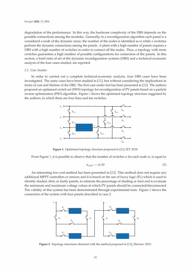
Energies 2020, 13, 2004

degradation of the performance. In this way, the hardware complexity of the DRS depends on thepossible connections among the modules. Generally, in a reconfiguration algorithm each panel is aconsidered a node of the dynamic array; the number of the nodes is identified as m while n switchesperform the dynamic connections among the panels. A plant with a high number of panels requires aDRS with a high number of switches in order to connect all the nodes. Thus, a topology with moreswitches guarantees a high number of possible configurations for connection of the panels. In thissection, a brief state of art of the dynamic reconfiguration systems (DRS) and a technical-economicanalysis of the four cases studied, are reported.

2.1. Case Studies

In order to carried out a complete technical-economic analysis, four DRS cases have beeninvestigated. The same cases have been studied in [21], but without considering the implications interms of cost and lifetime of the DRS. The first case under test has been presented in [22]. The authorsproposed an optimised switch set (SWS) topology for reconfiguration of PV panels based on a particleswarm optimization (PSO) algorithm. Figure 1 shows the optimised topology structure suggested bythe authors, in which there are four lines and ten switches.

Figure 1. Optimised topology structure proposed in [22], IET: 2018.

From Figure 1, it is possible to observe that the number of switches n for each node m, is equal to:

ncase1 = m·10 (1)

An interesting low-cost method has been presented in [23]. This method does not require anyadditional MPPT controllers or sensors and it is based on the use of fuzzy logic (FL) which is used toidentify shaded, dirty or faulty panels, to estimate the percentage of shading or dust and to evaluatethe minimum and maximum voltage values at which PV panels should be connected/disconnected.The validity of this system has been demonstrated through experimental tests. Figure 2 shows theconnection of the system with four panels described in case 2.

Figure 2. Topology structures obtained with the method proposed in [23], Elsevier: 2015.

53

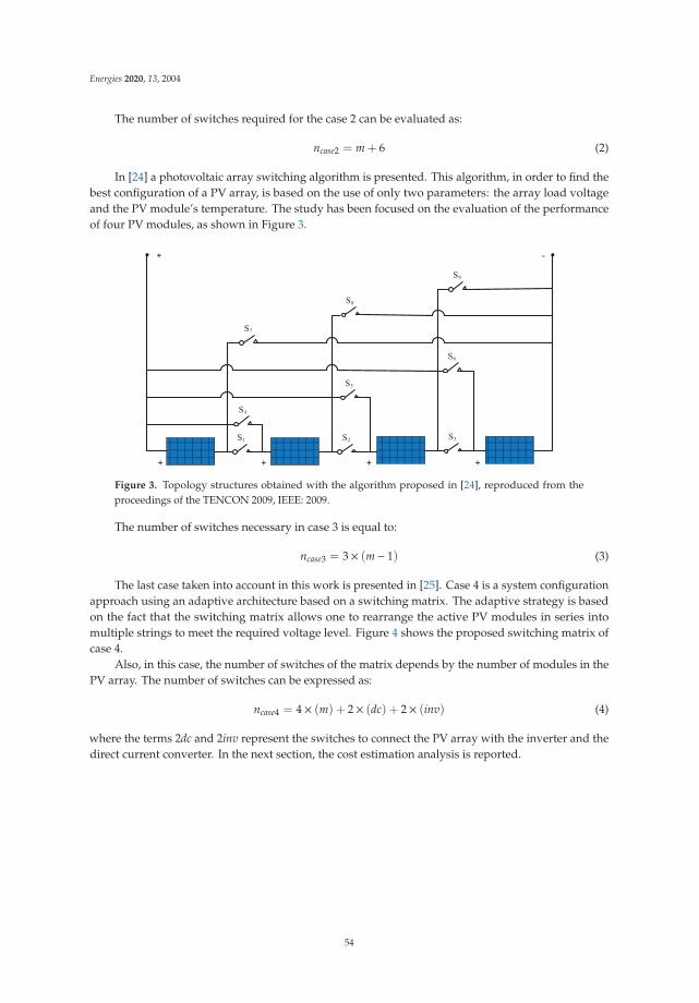
Energies 2020, 13, 2004

The number of switches required for the case 2 can be evaluated as:

ncase2 = m + 6 (2)

In [24] a photovoltaic array switching algorithm is presented. This algorithm, in order to find thebest configuration of a PV array, is based on the use of only two parameters: the array load voltageand the PV module’s temperature. The study has been focused on the evaluation of the performanceof four PV modules, as shown in Figure 3.

Figure 3. Topology structures obtained with the algorithm proposed in [24], reproduced from theproceedings of the TENCON 2009, IEEE: 2009.

The number of switches necessary in case 3 is equal to:

ncase3 = 3× (m− 1) (3)

The last case taken into account in this work is presented in [25]. Case 4 is a system configurationapproach using an adaptive architecture based on a switching matrix. The adaptive strategy is basedon the fact that the switching matrix allows one to rearrange the active PV modules in series intomultiple strings to meet the required voltage level. Figure 4 shows the proposed switching matrix ofcase 4.

Also, in this case, the number of switches of the matrix depends by the number of modules in thePV array. The number of switches can be expressed as:

ncase4 = 4× (m) + 2× (dc) + 2× (inv) (4)

where the terms 2dc and 2inv represent the switches to connect the PV array with the inverter and thedirect current converter. In the next section, the cost estimation analysis is reported.

54

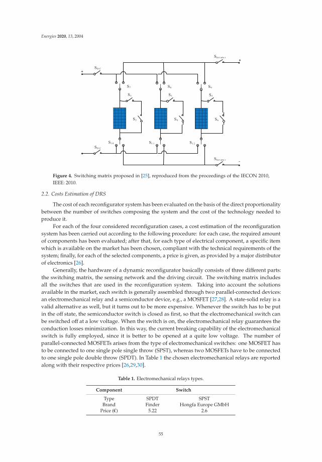
Energies 2020, 13, 2004

Figure 4. Switching matrix proposed in [25], reproduced from the proceedings of the IECON 2010,IEEE: 2010.

2.2. Costs Estimation of DRS

The cost of each reconfigurator system has been evaluated on the basis of the direct proportionalitybetween the number of switches composing the system and the cost of the technology needed toproduce it.

For each of the four considered reconfiguration cases, a cost estimation of the reconfigurationsystem has been carried out according to the following procedure: for each case, the required amountof components has been evaluated; after that, for each type of electrical component, a specific itemwhich is available on the market has been chosen, compliant with the technical requirements of thesystem; finally, for each of the selected components, a price is given, as provided by a major distributorof electronics [26].

Generally, the hardware of a dynamic reconfigurator basically consists of three different parts:the switching matrix, the sensing network and the driving circuit. The switching matrix includesall the switches that are used in the reconfiguration system. Taking into account the solutionsavailable in the market, each switch is generally assembled through two parallel-connected devices:an electromechanical relay and a semiconductor device, e.g., a MOSFET [27,28]. A state-solid relay is avalid alternative as well, but it turns out to be more expensive. Whenever the switch has to be putin the off state, the semiconductor switch is closed as first, so that the electromechanical switch canbe switched off at a low voltage. When the switch is on, the electromechanical relay guarantees theconduction losses minimization. In this way, the current breaking capability of the electromechanicalswitch is fully employed, since it is better to be opened at a quite low voltage. The number ofparallel-connected MOSFETs arises from the type of electromechanical switches: one MOSFET hasto be connected to one single pole single throw (SPST), whereas two MOSFETs have to be connectedto one single pole double throw (SPDT). In Table 1 the chosen electromechanical relays are reportedalong with their respective prices [26,29,30].

Table 1. Electromechanical relays types.

Component Switch

Type SPDT SPSTBrand Finder Hongfa Europe GMbH

Price (€) 5.22 2.6

55

Energies 2020, 13, 2004

In Table 2 the selected MOSFETs and drivers and respective prices are reported as well [26,31,32].

Table 2. MOSFET and driver taken into account.

Component MOSFET Driver

Type n-ch. IsolatedBrand IPB08CN10N MAX845

Price (€) 1.273 3.2

As far as the sensing network, three types of measurements are generally needed: voltage,current and temperature. In all four cases provided in this paper no irradiance sensor is required.The electronics involved in the voltage sensing circuit are normally very cheap, therefore voltagesensors are not considered in the hardware balance for the sake of simplicity. The selected sensors oftemperature and current and their price are reported in Table 3. Note that for the current measurement,the selected sensors are compliant with a 6A rated current [26,33,34].

Table 3. Selected sensors for current and temperature.

Component Sensors

Type Temperature CurrentBrand LM35 LEM

Price (€) 1.393 12.11

Table 4 provides the details concerning the number of the different components which should beused in the four considered reconfiguration cases: PV modules (Np), SPST and SPDT switches (NSPST

and NSPDT), MOSFETs, drivers and sensors. The total price has been calculated according to the costtables previously reported.

Table 4. Components considered for each case.

Cost of Components Case 1 Case 2 Case 3 Case 4

Np 20 20 20 20NSPST 200 26 57 44NSPDT 0 0 0 40

MOSFET 200 26 57 124Drivers 200 26 57 124

Current sensors 20 0 0 20Temperature sensors 0 0 20 20

Total price (€) 1 657 184 431 1 148

Note: Each driver is supposed to drive one MOSFET.

2.3. Lifetime Estimation of DRS

The lifetime of each reconfiguration solution has a significant contribution to the overall economicalimpact, even though in the scientific literature this aspect is generally neglected [35] Regarding this, themost important issue to be addressed is the lifetime of the relays, due to their mechanical characteristics.Both the electrical and the mechanical endurance are reported in the technical datasheets. Indeed,both the electrical and the mechanical behaviour of the relay are affected by the switching operations.More in detail, the electrical endurance, given by the maximum number of cycles recommended to notaffect the electrical behaviour of the relay, is usually much shorter than the maximum number of cyclesrecommended not to affect the mechanical behaviour. Therefore, being first in the time course, only theelectrical endurance has been considered in the overall lifetime estimation.

56

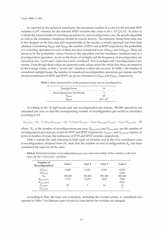
Energies 2020, 13, 2004

As reported in the technical datasheets, the maximum number of cycles for the selected SPSTswitches is 105, whereas for the selected SPDT switches this value is 60 × 103 [29,30]. In order toevaluate the actual number of switching operations for each reconfiguration case, the specific algorithmas well as the irradiance conditions should be exactly known. Nevertheless, being these data dueto the designer in the first case and unpredictable in the second, a simple approach has been hereadopted. Considering NSPST and NSPDT the number of SPST and of SPDT respectively, the probabilityof a switching operation for each of them has been considered to be 1/NSPST and 1/NSPDT. These aremeant to be the probability values whenever the algorithm and the irradiance condition lead to areconfiguration operation. As far as the hours of sunlight and the frequency of reconfiguration areconcerned, two “worst case” values have been considered: 16 h of sunlight and 1 reconfiguration everyminute. Even though these values are generally peak values across the whole day, these are meant tobe the average values, so that a “worst case” situation is taken into account. In Table 5, the number ofconsidered sunlight hours, the number of considered reconfiguration operations per minute and theelectrical endurance of SPST and SPDT are given, referenced as ESPST and ESPDT, respectively.

Table 5. Main characteristics of the proposed study case of reconfiguration.

Sunlight hours 16

Reconfigurations Per Minute 1ESPST 105

ESPDT 60 × 103

According to the 16 light hours and one reconfiguration per minute, 350,400 operations arecalculated per year, so that the corresponding number of reconfiguration per switch is calculated,according to (5):

Ryrsw,SPST = Ryr · (1/NSPST)Ryrsw,SPDT = Ryr · (1/NSPDT)Nyr,SPST = ESPST/Ryrsw,SPSTNyr,SPDT = ESPDT/Ryrsw,SPDT (5)

where: Ryr is the number of reconfigurations per year; Ryrsw,SPST and Ryrsw,SPDT are the number ofreconfigurations per year per switch for SPST and SPDT respectively; Nyr,SPST and Nyr,SPDT express, interms of number of years, the endurance of SPTS and SPDT switches respectively.

Table 6 reports the data referring to both types of switches and to the four considered casesof reconfiguration, obtained from (5). Note that the number of total reconfigurations Ryr has beenconsidered the same for all the cases.

Table 6. Estimated number of reconfigurations per year and endurability of the switches in the fourcases, for the “worst case” condition.

Number ofReconfigurations

Case 1 Case 2 Case 3 Case 4

1/NSPST 0.005 0.038 0.018 0.0231/NSPDT 0.025

Ryr 350,400 350,400 350,400 350,400Ryrsw,SPST 1752 13,477 6147 7964Ryrsw,SPDT 8760Nyr,SPST 57 7 16 13Nyr,SPDT 7

According to that, the total cost evaluation, including the overall system, is considered andreported in Table 7 for different cases of years to come before the switches are changed.

57

Energies 2020, 13, 2004

Table 7. Cost evaluation according to the estimated endurability, as reported in Table 6 in the fourcases, for the “worst case” condition.

After n YearsSwitches Cost Evaluation

Case 1 Case 2 Case 3 Case 4

n = 10 0 67.6 0 208.8n = 20 0 135.2 148.2 532n = 30 0 270.4 148.2 1064

After n YearsTotal Cost Evaluation

Case 1 Case 2 Case 3 Case 4

n = 10 1 657 € 251 € 431 € 1 357 €n = 20 1 657 € 319 € 579 € 1 680 €n = 30 1 657 € 454 € 579 € 2 212 €

The economical contributions concerning the switches and the overall system, as reported inTable 7, arise from the data reported in Tables 1 and 2, respectively. Note that the configurationswith the lowest number of switches are less convenient if only the price of the switches is considered,supposing that in the same number of years they require to be changed a higher number of times.On the contrary, if the total cost of the reconfigurator is considered, the cases with the lowest number ofswitches are the most convenient. Indeed, the initial price in terms of sensors, drivers and MOSFETs isgenerally higher if the number of mechanical switches is higher, due to the higher hardware complexity.Note as well as that if a low number of switches is associated to a more complex algorithm, so that thereconfiguration frequency is higher, the frequency of maintenance increases. As an example, Table 8refers to two reconfigurations per minute in case 2, whereas the number of reconfigurations per minutein the other cases is kept at 1.

Table 8. Cost evaluation if in case 2 (case of minimum number of switches) the number ofreconfigurations per minute is 2 instead of 1.

Total Cost for Years Case 1 Case 2 Case 3 Case 4

Reconfigurations per minute 1 2 1 1after n years Total cost evaluation

n = 10 1 657 € 319 € 431 € 1 357 €n = 20 1 657 € 522 € 579 € 1 680 €n = 30 1 657 € 725 € 579 € 2 212 €

One can see that in this case the most convenient solution, after 30 years, is the one corresponding tothe case 3. Although the obtained economical results of this comparison among different reconfigurationcases shall not be critically considered, what is significant in this paragraph is the proposed approachfor an economical estimation of the system lifetime.

3. Experimental Set-Up

Figure 5 sketches a realistic situation in which, during the day, a shadow overlays different panels.As a consequence, the shadowed panels disturb those connected in parallel: a decrease in voltage ofshadowed panel involves a decrease of not shadowed ones and a rise of current for the power balance.This rise of current is not constantly probable: if the not shadowed panels are in the area of maximumpower point, any decrease of voltage decreases the power.

58

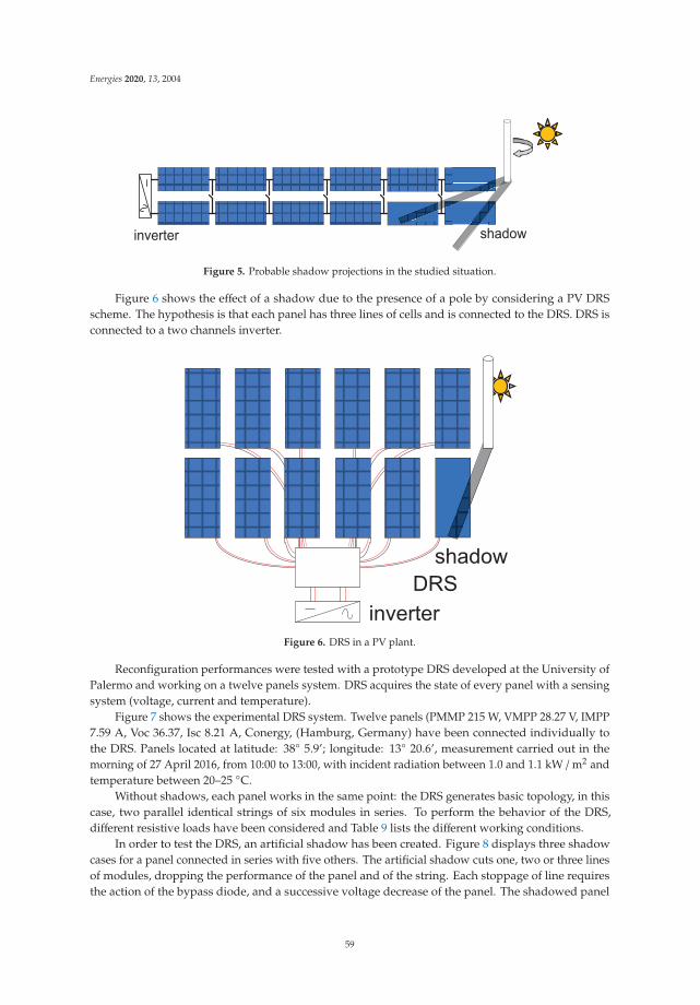
Energies 2020, 13, 2004

Figure 5. Probable shadow projections in the studied situation.

Figure 6 shows the effect of a shadow due to the presence of a pole by considering a PV DRSscheme. The hypothesis is that each panel has three lines of cells and is connected to the DRS. DRS isconnected to a two channels inverter.

Figure 6. DRS in a PV plant.

Reconfiguration performances were tested with a prototype DRS developed at the University ofPalermo and working on a twelve panels system. DRS acquires the state of every panel with a sensingsystem (voltage, current and temperature).

Figure 7 shows the experimental DRS system. Twelve panels (PMMP 215 W, VMPP 28.27 V, IMPP7.59 A, Voc 36.37, Isc 8.21 A, Conergy, (Hamburg, Germany) have been connected individually tothe DRS. Panels located at latitude: 38◦ 5.9’; longitude: 13◦ 20.6’, measurement carried out in themorning of 27 April 2016, from 10:00 to 13:00, with incident radiation between 1.0 and 1.1 kW /m2 andtemperature between 20–25 ◦C.

Without shadows, each panel works in the same point: the DRS generates basic topology, in thiscase, two parallel identical strings of six modules in series. To perform the behavior of the DRS,different resistive loads have been considered and Table 9 lists the different working conditions.

In order to test the DRS, an artificial shadow has been created. Figure 8 displays three shadowcases for a panel connected in series with five others. The artificial shadow cuts one, two or three linesof modules, dropping the performance of the panel and of the string. Each stoppage of line requiresthe action of the bypass diode, and a successive voltage decrease of the panel. The shadowed panel

59

Energies 2020, 13, 2004

has labelled with the number 6, so V1–V5 are the voltages of normally irradiated panels and V6 is theshadowed one; DRS evaluates the power of each panel and connects the panels into the string.

Figure 7. Experimental system with panels individually connected to DRS.

Table 9. Electrical characteristics in different load conditions evaluated by reconfigurator for each panel.

ElectricalCharacteristics

Load A Load B Load C Load D Load E

Voltage (V) 31.3 28.9 26.1 23.1 16.8Current (A) 1.9 4.0 6.0 7.0 7.4Power (W) 54.5 115.6 156.6 161.7 124.3String (W) 356.2 693.7 939.2 970.2 745.5

Figure 8. Shaded panel case 1, 2 and 3. In case 1 shadow can vary from 225 to 450 cm2; whichcorresponds to one interruption of a line of cells; in case 2 shadow varies from 450 to 900 cm2, whichcorresponds to two interruption of lines; case 3 corresponds to the interruption of the panel.

60

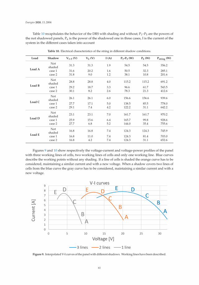
Energies 2020, 13, 2004

Table 10 recapitulates the behavior of the DRS with shading and without; P1–P5 are the powers ofthe not shadowed panels, P6 is the power of the shadowed one in three cases, I is the current of thesystem in the different cases taken into account

Table 10. Electrical characteristics of the string in different shadow conditions.

Load Shadow V1–5 (V) V6 (V) I (A) P1-P5 (W) P6 (W) Pstring (W)

Load A

Notshaded 31.3 31.3 1.9 54.5 54.5 356.2

case 1 31.6 20.2 1.6 50.5 32.3 285.1case 2 31.8 9.0 1.2 38.1 10.8 201.6

Load B

Notshaded 28.8 28.8 4.0 115.2 115.2 691.2

case 1 29.2 18.7 3.3 96.6 61.7 543.5case 2 30.1 8.2 2.6 78.3 21.3 412.6

Load C

Notshaded 26.1 26.1 6.0 156.6 156.6 939.6

case 1 27.7 17.1 5.0 138.5 85.5 778.0case 2 29.1 7.4 4.2 122.2 31.1 642.2

Load D

Notshaded 23.1 23.1 7.0 161.7 161.7 970.2

case 1 25.9 15.6 6.4 165.7 99.8 928.6case 2 27.7 6.8 5.2 144.0 35.4 755.6

Load E

Notshaded 16.8 16.8 7.4 124.3 124.3 745.9

case 1 16.8 11.0 7.4 124.3 81.4 703.0case 2 16.8 4.2 7.4 124.3 31.1 652.6

Figures 9 and 10 show respectively the voltage-current and voltage-power profiles of the panelwith three working lines of cells, two working lines of cells and only one working line. Blue curvesdescribe the working points without any shading. If a line of cells is shaded the orange curve has to beconsidered, maintaining a similar current and with a new voltage. When a shadow covers two lines ofcells from the blue curve the gray curve has to be considered, maintaining a similar current and with anew voltage.

Figure 9. Interpolated V-I curves of the panel with different shadows. Working lines have been described.

61

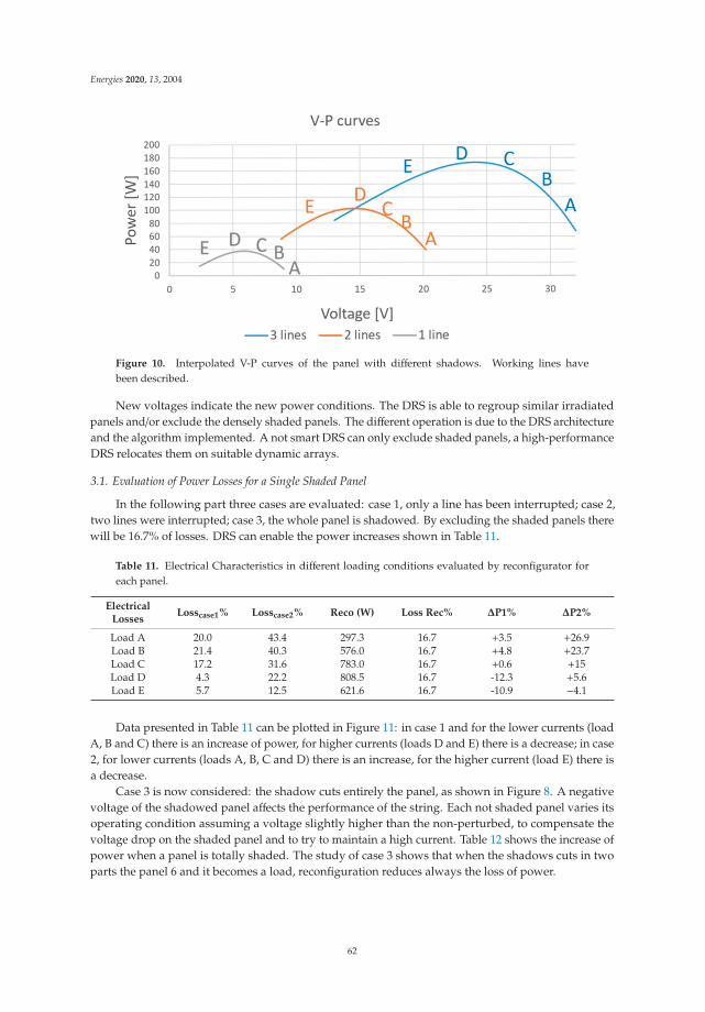
Energies 2020, 13, 2004

Figure 10. Interpolated V-P curves of the panel with different shadows. Working lines havebeen described.

New voltages indicate the new power conditions. The DRS is able to regroup similar irradiatedpanels and/or exclude the densely shaded panels. The different operation is due to the DRS architectureand the algorithm implemented. A not smart DRS can only exclude shaded panels, a high-performanceDRS relocates them on suitable dynamic arrays.

3.1. Evaluation of Power Losses for a Single Shaded Panel

In the following part three cases are evaluated: case 1, only a line has been interrupted; case 2,two lines were interrupted; case 3, the whole panel is shadowed. By excluding the shaded panels therewill be 16.7% of losses. DRS can enable the power increases shown in Table 11.

Table 11. Electrical Characteristics in different loading conditions evaluated by reconfigurator foreach panel.

ElectricalLosses

Losscase1% Losscase2% Reco (W) Loss Rec% ΔP1% ΔP2%

Load A 20.0 43.4 297.3 16.7 +3.5 +26.9Load B 21.4 40.3 576.0 16.7 +4.8 +23.7Load C 17.2 31.6 783.0 16.7 +0.6 +15Load D 4.3 22.2 808.5 16.7 -12.3 +5.6Load E 5.7 12.5 621.6 16.7 -10.9 −4.1

Data presented in Table 11 can be plotted in Figure 11: in case 1 and for the lower currents (loadA, B and C) there is an increase of power, for higher currents (loads D and E) there is a decrease; in case2, for lower currents (loads A, B, C and D) there is an increase, for the higher current (load E) there isa decrease.

Case 3 is now considered: the shadow cuts entirely the panel, as shown in Figure 8. A negativevoltage of the shadowed panel affects the performance of the string. Each not shaded panel varies itsoperating condition assuming a voltage slightly higher than the non-perturbed, to compensate thevoltage drop on the shaded panel and to try to maintain a high current. Table 12 shows the increase ofpower when a panel is totally shaded. The study of case 3 shows that when the shadows cuts in twoparts the panel 6 and it becomes a load, reconfiguration reduces always the loss of power.

62

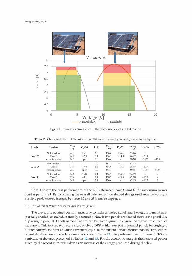
Energies 2020, 13, 2004

Figure 11. Zones of convenience of the disconnection of shaded module.

Table 12. Characteristics in different load conditions evaluated by reconfigurator for each panel.

Loads ShadowV1–5

(V)V6 (V) I (A)

P1–55

(W)P6 (W)

Pstring

(W)Loss% ΔP3%

Load C

Not shadow 26.1 26.1 6.0 156.6 156.6 939.6 - -Case 3 26.7 −2.9 5.1 136.1 −14.8 665.7 −29.1 -

reconfigurated 26.1 open 6.0 156.6 - 783.0 -16.7 +12.4

Load D

Not shadow 23.1 23.1 7.0 161.1 161.1 970.2 - -Case 3 23.7 −3.0 6.5 154.0 −19.5 750.7 −22.7 -

reconfigurated 23.1 open 7.0 161.1 - 808.5 -16.7 +6.0

Load E

Not shadow 16.8 16.8 7.4 124.3 124.3 745.9 - -Case 3 17.4 −3.1 7.4 128.7 −21.5 620.8 −16.7 -

reconfigurated 16.8 open 7.4 156.6 - 621.5 −16.7 0

Case 3 shows the real performance of the DRS. Between loads C and D the maximum powerpoint is performed. By considering the overall behavior of two shaded strings used simultaneously, apossible performance increase between 12 and 25% can be expected.

3.2. Evaluation of Power Losses for two shaded panels

The previously obtained performances only consider a shaded panel, and the logic is to maintain it(partially shaded) or exclude it (totally obscured). Now if two panels are shaded there is the possibilityof placing in parallel. Panels named 6 and 7, can be re-configured to ensure the maximum current ofthe arrays. This feature requires a more evolved DRS, which can put in parallel panels belonging todifferent arrays, the sum of which currents is equal to the current of not obscured panels. This featureis useful only when it considers case 2 as shown in Table 13. The performances of different DRS area mixture of the ones presented in Tables 12 and 13. For the economic analysis the increased powergiven by the reconfigurator is taken as an increase of the energy produced during the day.

63

Energies 2020, 13, 2004

Table 13. Electrical characteristic of the string in different shadow conditions.

ElectricalParameters

Load C Load D

Not Shaded Case 1 Case 2 Not Shaded Case 1 Case 2

V1–5 (V) 26.1 27.7 29.1 23.1 25.9 27.7V6–7 (V) 26.1 17.1 7.4 23.1 15.6 6.8

I (A) 6.0 5.0 4.2 7.0 6.4 5.2P1–5 (W) 156.6 138.5 122.2 161.7 165.7 144.0P6–7 (W) 156.6 85.5 31.1 161.7 99.8 35.4

Pstring (W) 1096 863.5 673.3 1132 1028 755.6Loss% - -21.2 -38.5 - -9.2 −33.2

V6–7 (V) - 19.3 6.2 - 15.0 5.0I6–7 (A) - 6.0 6.0 - 7.0 7.0P6–7 (W) 156.6 60 36.1 161.7 101.0 36.3

Pstring(W) 1096 903.3 909.2 970.2 1010 881.1ΔP% - +4.2 +21.4 - −1.5 +11.1

4. Economic Data

In order to carry out a complete study, the economic analysis presented in this paper takes intoaccount different aspects of a PV plant, such as PV technology, location of the installation, governmentincentives, component lifetime, aging and periodic maintenance costs.

This study is based on the use of economic a tool called net present value (NPV), in order toevaluate the benefits of an economic investment in PV field with innovative devices such as a DRS.The NPV allows to evaluate the economic convenience of an investment for a specific period froma sum of cash flows actualized at time zero. In (6) the mathematic expression to evaluate the NPVis reported:

NPV = −C0 +n∑

y=1

Cy

(1 + i)y (6)

With reference to expression (6), C0 is the cash flow at time zero, Cy is the cash flow at the year y,i is the interest rate and y is the year of investment. Thus, the sign of the NPV, positive or negative,indicates the infeasibility of the investment and therefore the economic convenience. The interest ratei% considered in this work is equal to 5%. In this study, the technical-economic analysis has beencarried out by considering an investment time equal to 20 years. In the following, detailed descriptionof different aspects taken into account for the economic analysis and economic data are reported.

4.1. PV Plant

Since the first PV plants became commercially available on the market the cost of PV components,installation and maintenance has changed notably. In particular, in the last years there has been aconstant decrease of the costs on the world market.

In this study, only residential PV systems with 6 kWp of power have been taken into account. Thischoice is motivated by the fact that the use of DRS is very interesting in residential PV plants, where theprobability of installation of a fixed obstacle is high in respect to other type of plants. Indeed, four yearsafter the installation, a fixed obstacle reducing by 35% the total power is assumed to appear. This valueof reduction has been demonstrated in study [20]. Moreover, in order to carry out a complete analysisamong different locations of installation taken into account, an installation of the PV plant between2013 and 2014 was assumed, considering that in those years there were incentives in all the countries.

Regarding the cost of the PV plant, the average estimated price for this type of plant is about2500 €/kWp (included installation). In Table 14 the economic data about the PV plant under testare summarized.

64

Energies 2020, 13, 2004

Table 14. PV plant data.

PV Plant Type Residential Grid Connected

Power 6 kWp

Number of modules 20

PV plant Cost (installation included) 15, 000€

Power reduction 35%

Year of installation 2013/2014

4.2. Location of Installation and Economic Aspects

The installation location represents an interesting point of analysis in terms of production capability,government incentives and payments to private citizens for the production of the energy. Moreover,also the lifestyle of people plays an important role and therefore the average consumption per capita ofthe electric energy. In order to extend the economic analysis Italy, Germany, France, Spain, Bulgaria,Romania, Greece and Croatia have been considered as reference countries. As well known, thesecountries have different PV plant performances, different policies to improve the use of electricitygenerated from renewable sources and different people’s lifestyle. In detail, the common strategy isbased on a feed-in tariff (FIT) system with different values and timing of the incentives.

The economic data for each country (average consumption per capita, production facility, energycost and incentives) have been referred of a PV plant installed in the capital of each countries. Moreover,has been considered a family composed by four people that lives in the capital of each countries.In Table 15 the considered economic data are reported.

Table 15. Economic data of the reference countries reproduced from [20], reproduced from proceedingsof the 2018 International Conference on Smart Grid, IEEE: 2018.

CountryAverage

Consumption perCapita kWh/year)

Production Facility(kWh/year)

Energy Cost(€/kWh)

Incentives perYears (€/kWh)

Incentive Duration(years)

Italy 3200 9900 0.200 0.208 20Germany 3512 6240 0.330 0.130 20

France 6343 7020 0.180 0.280 20Spain 4131 9960 0.280 0.340 20

Bulgaria 4640 9000 0.090 0.240 20Romania 2495 8400 0.125 0.160 15Greece 5029 11,100 0.180 0.140 20Croatia 3754 9600 0.132 0.150 14

These data are based on the following consideration:

• a family composed of four members and living in each capital of the considered countries;• the electrical energy produced per year by a 6 kWp PV plant has been taken into account.• the installation of the plant has been assumed between the year 2013 and 2014.

It should be noted that France has the highest value of average consumption per capita. This datais very high with respect to the production facility of the PV plant, so the analysis for the use of DRS isparticularly difficult. The higher value of the energy production is in Greece, whereas, Romania andCroatia only offer incentives for 15 and 12 years. It should be noted that these considerations haveinfluenced the economic results.

65

Energies 2020, 13, 2004

4.3. Inverter

The inverter represents the heart of the production from the solar energy. In particular, as wellknown, this system allows the electric energy conversion from DC to AC in order to inject the powersurplus into the grid. Therefore, in the case of inverter fault it is not possible to use the energy with aconsequence economic loss. From different studies, it is known that the inverter is the componentmore sensitive to failure. In [2], the authors considered an inverter life equal to 10 years. Nevertheless,it is not possible to estimate with accuracy the lifetime of an electronic component. For this reason, byconsidering a possible worst case, in this study it was assumed that the average lifetime of the inverteris equal to seven years. As far as the cost is concerned, according to [36] for a residential PV plant with6 kWp of power the average cost is equal to 1000 €.

4.4. Increase of Production by DRS

The purpose of a DRS system is to increase the power of a PV plant in the case of a reduction ofthe total power production. The increment of the power production is a parameter that depends onthe DRS topology and therefore hard to estimate. Indeed, the increment of power depends on the typeof DRS and therefore of the number of possible available configuration. Thus, the number of possiblereconfiguration available play an important role. By considering that a DRS with high number ofswitches allows many reconfigurations with respect to a DRS with a low number of switches, it issupposed to provide a higher increment of power. Nevertheless, this consideration is not enough toestimate the increment of power provided by a DRS with a defined number of switches, because it ispossible that a DRS with high number of switches has redundant configurations. For this reason, inthis work the same value of power increment has been considered for each DRS and fixed equal to10% for the sake of simplicity. This obviously represents an unfavourable condition for DRS with highnumber of switches and higher costs. Nevertheless, this choice allows to emphasize the effect on theeconomic analysis of the costs and lifetime for each DRS.

4.5. Aging and Maintenance of PV Plant

After the installation, a natural phenomenon is the aging of the PV components. This phenomenoncauses a reduction of the power and it increases over the time. Thus, in the economic analysis has beenconsidered a reduction of power after the first year of the installation equal to 3% and a reduction foreach year equal to 0.5%. Moreover, also a periodic maintenance has been considered with a cost equalto 100 €/year.

5. Economic Results and Discussion

As described above, the economic analysis of this study is focused on the evaluation of theeconomic benefits by using a DRS system four years after the installation of the PV plant with a powerreduction equal to 35%. In particular, four cases of DRS have been analysed in different EU countriesin order to extend the economic results. Figure 12 shows the NPV trend over the time of four cases ofDRS1-4 and without DRS for each country.

The best result has been obtained in Spain with the highest value of the NPV after 20 years due tothe incentives per year. Positive NPV values have been obtained in Italy, Bulgaria and Greece thanksto the high values of the production facility. Romania and Croatia have been penalized for a lowerduration of the incentives, whereas, France and Germany have been penalized for the lower values ofthe production facility. The values of the NPV for each country and for each DRS are summarizedin Table 16.

66

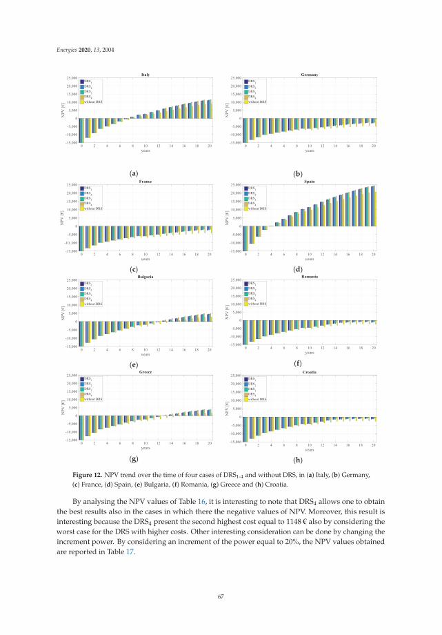
Energies 2020, 13, 2004

(a)

(b)

(c) (d)

(e) (f)

(g) (h)

Figure 12. NPV trend over the time of four cases of DRS1-4 and without DRS, in (a) Italy, (b) Germany,(c) France, (d) Spain, (e) Bulgaria, (f) Romania, (g) Greece and (h) Croatia.

By analysing the NPV values of Table 16, it is interesting to note that DRS4 allows one to obtainthe best results also in the cases in which there the negative values of NPV. Moreover, this result isinteresting because the DRS4 present the second highest cost equal to 1148 € also by considering theworst case for the DRS with higher costs. Other interesting consideration can be done by changing theincrement power. By considering an increment of the power equal to 20%, the NPV values obtainedare reported in Table 17.

67

Energies 2020, 13, 2004

Table 16. NPV values after 20 years (increment power 10%).

CountriesNPV After 20 Years (€)

DRS1 DRS2 DRS3 DRS4 Without

Italy 10,871 11,095 11,068 11,480 8723Germany −3298 −3075 −3101 −2689 −4991

France −2663 −2439 −2466 −2054 −4380Spain 23,633 23,856 23,830 24,241 20,349

Bulgaria 4076 4300 4274 4685 2497Romania −1601 −1377 −1403 −992 −2713Greece 3186 3410 3384 3795 1297Croatia −1646 −1423 −1449 −1038 −2873

Table 17. NPV values after 20 years (increment power 20%).

CountriesNPV After 20 Years (€)

DRS1 DRS2 DRS3 DRS4 Without

Italy 13,019 13,243 13,217 13,628 8723

Germany −1606 −1382 −1408 −997 −4991

France −946 −722 −748 −337 −4380

Spain 26,917 27,140 27,114 27,526 20,349

Bulgaria 5656 5879 5853 6265 2497

Romania −489 −265 −291 120 −2713

Greece 5075 5299 5273 5684 1297

Croatia −420 −196 −222 189 −2873

In respect to the previous case, the DRS4 with an increment of power equal to 20% allows to obtainpositive values of the NPV also for Romania and Croatia. This result is realistic because the DRS4,thanks to the high number of switches and thus the high number of the possible configurations, maygenerate an increment of power equal to 20%. Another interesting point of analysis is the paybacktime. In Table 18, the payback times for each country and for each DRS in two power increment casesare reported.

Table 18. Payback time for increment of power equal to 10% and 20%. In some cases the payback timeexceeds the reasonable time for the return on the investment, and it is not evaluated (n.e.).

Countries

Payback Time (Years)

DRS1 DRS2 DRS3 DRS4

10% 20% 10% 20% 10% 20% 10% 20%

Italy 8 8 8 8 8 8 8 8Germany n.e. 28 n.e. 27 n.e. 27 n.e 25

France n.e. 25 n.e. 24 n.e. 24 n.e. 23Spain 5 5 5 5 5 5 5 5

Bulgaria 13 12 13 12 13 12 13 12Romania n.e. n.e. n.e. 27 n.e. n.e. n.e. 20Greece 15 12 14 12 15 12 13 12Croatia n.e. n.e. n.e. n.e. n.e. n.e. n.e 19

Spain and Italy present the best results and it is interesting to note that the same values in thetwo cases of the increment of power have been obtained. In other countries (Germany, France andRomania), it was necessary to extend the duration of the investment in order to find the payback timebut in all cases the best results have been obtained with DRS4 and an increment of power equal to 20%.

68

Energies 2020, 13, 2004

Only in Bulgaria and Greece a reduction of the payback time has been obtained, an increment powerequal to 20%, 13 years to 12 years and from 15 years to 12 years, respectively.

6. Conclusions

This paper presents a complete analysis on the real benefits introduced by a DRS system in a PVplant after a considerable power reduction. In particular, in order to evaluate the overall economicimpact on the costs of a PV plant the technical and economic aspects about the DRS have beenconsidered. In the first part of the paper an economic analysis of different DRSs due to the costs ofthe components and to the adopted topological schemes, is carried out. Switching matrix, sensingnetwork and driving circuit constitute the architecture of DRS, the choice of switches and their numberaffects the electrical endurance. A more flexible DRS involves higher initial cost due to the number ofswitches required by the adopted architecture, but at the same time a less exploitation and therefore alonger useful life.

From the economic point of view, the analysis has been extended to different countries of EU inorder to considerate incentives policies, location of installation and lifestyles of the people, while, froma technical study, that takes into account the hardware complexity in terms of the components requiredand other technical aspects, the costs and lifetime of four DRS have been estimated. The economic toolused in this analysis is the NPV and the payback time.

Firstly, in all scenarios the analysis has demonstrated the positive economic impact on the useof a DRS in a PV plant with respect to the cases without DRS. The best results have been obtainedin Spain thanks to the higher value of the incentives per year in terms of NPV and payback time,whereas good results have been obtained for Italy, Bulgaria and Greece. The worst results have beenobtained for France and Germany due to the lower values of the production facility. Among the DRSconsidered in the economic analysis, the DRS4 option allows one to obtain the best results in all cases.The best performance of DRS4 is attributable to the high number of switches that allows it to increasethe lifetime of the system.

Author Contributions: Conceptualization, F.V.; methodology, F.V. and P.R.; software, G.S. and F.P.; validation,F.P. and G.S.; formal analysis, F.V. and G.S.; investigation, P.R. and F.V.; resources, R.M. and G.A.; data curation,G.S. and F.P.; writing—original draft preparation, F.P., G.S., and F.V.; writing—review and editing, G.A. and F.V.;visualization, G.A. and R.M.; supervision, G.A., R.M. and F.V. All authors have read and agreed to the publishedversion of the manuscript.

Funding: This research received no external funding. This work was financially supported by MIUR-Ministerodell’Istruzione, dell’Università e della Ricerca (Italian Ministry of Education, University and Research) andby SDESLab (Sustainable Development and Energy Saving Laboratory) and LEAP (Laboratory of ElectricalAPplications) of the University of Palermo.

Conflicts of Interest: The authors declare no conflict of interest.

References

1. Timilsina, G.R.; Kurdgelashvili, L.; Narbel, P.A. Solar energy: Markets, economics and policies. Renew.Sustain. Energy Rev. 2012, 16, 449–465. [CrossRef]

2. Branker, K.; Pathak, M.J.M.; Pearce, J.M. A review of solar photovoltaic levelized cost of electricity. Renew.Sustain. Energy Rev. 2011, 15, 4470–4482. [CrossRef]

3. Lappalainen, K.; Valkealahti, S. Photovoltaic mismatch losses caused by moving clouds. Sol. Energy 2017,158, 455–461. [CrossRef]

4. Zou, X.; Li, B.; Zhai, Y.; Liu, H. Performance monitoring and test system for GridConnected photovoltaicsystems. In Proceedings of the 2012 Asia-Pacific Power and Energy Engineering Conference, Shanghai,China, 27–29 March 2012.

5. Caruso, M.; Miceli, R.; Romano, P.; Schettino, G.; Spataro, C.; Viola, F. A low cost, Real-time monitoring systemfor PV plants based on ATmega 328P-PU Microcontroller. In Proceedings of the 2015 IEEE InternationalTelecommunications Energy Conference (INTELEC), Osaka, Japan, 18–22 October 2015.

69

Energies 2020, 13, 2004

6. Caruso, M.; Di Tommaso, A.O.; Miceli, R.; Ricco Galluzzo, G.; Romano, P.; Schettino, G.; Viola, F. Design andexperimental characterization of a low cost, real-time, wireless, AC monitoring system based on ATmega328P-PU microcontroller. In Proceedings of the 2015 AEIT International Annual Conference (AEIT), Naples,Italy, 14–16 October 2015; pp. 1–6.

7. Wang, Y.-J.; Hsu, P.-C. An investigation on partial shading of PV modules with different connectionconfigurations of PV cells. Energy 2011, 36, 3069–3078. [CrossRef]

8. Potnuru, S.R.; Pattabiraman, D.; Ganesan, S.I.; Chilakapati, N. Positioning of PV panels for reduction in linelosses and mismatch losses in PV array. Renew. Energy 2015, 78, 264–275. [CrossRef]

9. Wang, Y.J.; Lin, S.S. Analysis of a partially shaded PV array considering different module connection schemesand effects of bypass diodes. In Proceedings of the 2011 International Conference & Utility Exhibition onPower and Energy Systems: Issues and Prospects for Asia (ICUE), Pattaya City, Thailand, 28–30 September2011; pp. 1–7.

10. Kandemir, E.; Cetin, N.S.; Borekci, S. A comprehensive overview of maximum power extraction methods forPV systems. Renew. Sustain. Energy Rev. 2017, 78, 93–112. [CrossRef]

11. Kouchaki, A.; Iman-Eini, H.; Asaei, B. A new maximum power point tracking strategy for PV arrays underuniform and non-uniform insolation conditions. Sol. Energy 2013, 91, 221–232. [CrossRef]

12. Alahmad, M.; Chaaban, M.A.; Kit Lau, S.; Shi, J.; Neal, J. An adaptive utility interactive photovoltaic systembased on a flexible switch matrix to optimize performance in real-time. Sol. Energy 2012, 86, 951–963.[CrossRef]

13. Ramaprabha, R.; Mathur, B.L. A Comprehensive review and analysis of solar photovoltaic array configurationsunder partial shaded conditions. Int. J. Photoenergy 2012, 2012, 1–16. [CrossRef]

14. Candela, R.; Sanseverino, E.R.; Romano, P.; Cardinale, M.; Musso, D. A Dynamic electrical scheme for theoptimal reconfiguration of PV modules under non-homogeneous solar irradiation. Appl. Mech. Mater. 2012,197, 768–777. [CrossRef]

15. Sanseverino, E.R.; Ngoc, T.N.; Cardinale, M.; Romano, P.; LiVigni, V.; Musso, D.; Viola, F. Dynamicprogramming and Munkres algorithm for optimal photovoltaic arrays reconfiguration. Sol. Energy 2015, 122,347–358. [CrossRef]

16. Tian, H.; Mancilla–David, F.; Ellis, K.; Muljadi, K.; Jenkins, P. Determination of the optimal configuration fora photovoltaic array depending on the shading condition. Sol. Energy 2013, 95, 1–12. [CrossRef]

17. Balato, M.; Costanzo, L.; Vitelli, M. Series-parallel PV array re-configuration: Maximization of the extractionof energy and much more. Appl. Energy 2015, 159, 145–160. [CrossRef]

18. Chao, K.H.; Ho, S.H.; Wang, M.H. Modeling and fault diagnosis of a photovoltaic system. Electr. Power Syst.Res. 2008, 78, 97–105. [CrossRef]

19. Livreri, P.; Caruso, M.; Castiglia, V.; Pellitteri, F.; Schettino, G. Dynamic reconfiguration of electricalconnections for partially shaded PV modules: Technical and economical performances of an Arduino-basedprototype. Int. J. Renew. Energy Res. 2018, 8, 336–344.

20. Viola, F.; Romano, P.; Miceli, R.; Spataro, C.; Schettino, G. Technical and Economical Evaluation on the Use ofReconfiguration Systems in Some EU Countries for PV Plants. IEEE Trans. Ind. Appl. 2017, 53, 1308–1315.[CrossRef]

21. Caruso, M.; Miceli, R.; Romano, P.; Sanseverino, E.R.; Schettino, G.; Viola, F.; Ngoc, T.N. Comparison betweendifferent dynamic reconfigurations of electrical connections for partially shaded PV modules. In Proceedingsof the 2018 International Conference on Smart Grid (icSmartGrid), Nagasaki, Japan, 4–6 December 2018;pp. 220–227.

22. Iraji, F.; Farjah, E.; Ghanbari, T. Optimisation method to find the best switch set topology for reconfigurationof photovoltaic panels. IET Renew. Power Gener. 2018, 12, 374–379. [CrossRef]

23. Tabanjat, A.; Becherif, M.; Hissel, D. Reconfiguration solution for shaded PV panels using switching control.Renew. Energy 2015, 82, 4–13. [CrossRef]

24. Tria, L.A.R.; Escoto, M.T.; Odulio, C.M.F. Photovoltaic array reconfiguration for maximum power transfer. InProceedings of the TENCON 2009—2009 IEEE Region 10 Conference, Singapore, 23–26 January 2009; pp. 1–6.

25. Chaaban, M.A.; Alahmad, M.; Neal, J.; Shi, J.; Berryman, C.; Cho, Y.; Lau, S.; Li, H.; Schwer, A.; Shen, Z.;et al. Adaptive photovoltaic system. In Proceedings of the IECON 2010—36th Annual Conference on IEEEIndustrial Electronics, Glendale, AZ, USA, 7–10 November 2010; pp. 3192–3197.

26. RS Homepage. Available online: https://www.rs-online.com/ (accessed on 2 May 2019).

70

Energies 2020, 13, 2004

27. Balato, M.; Vitelli, M.; Femia, N.; Petrone, G.; Spagnuolo, G. Factors limiting the efficiency of DMPPT in PVapplications. In Proceedings of the 2011 International Conference on Clean Electrical Power (ICCEP), Ischia,Italy, 14–16 June 2011; pp. 604–608.

28. Spagnuolo, G.; Petrone, G.; Lehman, B.; Paja, C.A.R.; Zhao, Y.; Gutierrez, M.L.O. Control of photovoltaicarrays: Dynamical reconfiguration for fighting mismatched conditions and meeting load requests. IEEE Ind.Electron. Mag. 2015, 9, 62–76. [CrossRef]

29. HF41F. Subminiature Power Relay. Available online: https://docs-emea.rs-online.com/webdocs/14c6/0900766b814c652d.pdf (accessed on 2 May 2019).

30. Finder. Ultra-Slim PCB Relays (EMR or SSR) 0.1-0.2-2-6 A. Available online: https://docs-emea.rs-online.com/webdocs/16d4/0900766b816d4f36.pdf (accessed on 10 February 2020).

31. Infineon. OptiMOS®2 Power-Transistor. Available online: https://datasheet.octopart.com/IPP08CN10N-G-Infineon-datasheet-5315235.pdf (accessed on 17 February 2020).

32. MAXIM. Isolated Transformer Driver for PCMCIA Applications. Available online: https://datasheets.maximintegrated.com/en/ds/MAX845.pdf (accessed on 1 March 2020).

33. Texas Instruments. MAX 845. LM35 Precision Centigrade Temperature Sensors. Available online: http://www.ti.com/lit/ds/symlink/lm35.pdf (accessed on 5 March 2020).

34. LEM. Current Transducer LTS 25-NP. Available online: https://docs-emea.rs-online.com/webdocs/146d/0900766b8146d120.pdf (accessed on 7 March 2020).

35. La Manna, D.; Vigni, V.L.; Sanseverino, E.R.; Di Dio, V.; Romano, P. Reconfigurable electrical interconnectionstrategies for photovoltaic arrays: A review. Renew. Sustain. Energy Rev. 2014, 33, 412–426. [CrossRef]

36. Fu, R.; Feldman, D.; Margolis, R.; Woodhouse, M.; Ardani, K. U.S. Solar Photovoltaic System Cost Benchmark: Q12017; Technical Report No. NREL/TP-6A20-68925 7752; USDOE Office of Energy Efficiency and RenewableEnergy (EERE): Washington, DC, USA, 2017. [CrossRef]

© 2020 by the authors. Licensee MDPI, Basel, Switzerland. This article is an open accessarticle distributed under the terms and conditions of the Creative Commons Attribution(CC BY) license (http://creativecommons.org/licenses/by/4.0/).

71

energies

Article

Reactive Power Injection to Mitigate FrequencyTransients Using Grid Connected PV Systems

Yujia Huo, Simone Barcellona, Luigi Piegari and Giambattista Gruosso *

Politecnico di Milano, Dipartimento di Elettronica Informazione e Bioingegneria, Piazza Leonardo da Vinci 32,20133 Milano, Italy; yujia.huo@polimi.it (Y.H.); simone.barcellona@polimi.it (S.B.); luigi.piegari@polimi.it (L.P.)* Correspondence: giambattista.gruosso@polimi.it

Received: 22 January 2020; Accepted: 12 April 2020; Published: 17 April 2020

Abstract: The increasing integration of renewable energies reduces the inertia of power systems andthus adds stiffness to grid dynamics. For this reason, methods to obtain virtual inertia have beenproposed to imitate mechanical behavior of rotating generators, but, usually, these methods relyon extra power reserves. In this paper, a novel ancillary service is proposed to alleviate frequencytransients by smoothing the electromagnetic torque of synchronous generators due to change of activepower consumed by loads. Being implemented by grid-tied inverters of renewables, the ancillaryservice regulates the reactive power flow in response to frequency transients, thereby demandingno additional power reserves and having little impact on renewables’ active power generation.Differently from the active power compensation by virtual inertia methods, it aims to low-passfilter the transients of the active power required to synchronous generators. The proposed ancillaryservice is firstly verified in simulation in comparison with the virtual inertia method, and afterwardstested on processor by controller-hardware-in-the-loop simulation, analysing practical issues andproviding indications for making the algorithm suitable in real implementation. The ancillary serviceproves effective in damping frequency transients and appropriate to be used in grid with distributedpower generators.

Keywords: ancillary service; PV Plant; frequency-assisting; hardware-in-the-loop; Photovoltaic; DER

1. Introduction

Renewable energy sources (RESs) are of strategic importance and crucial to the sustainabilityof energy production from an environmental point of view. They are playing an important role indistribution networks [1,2] transforming them from passive to active [3], and representing a challengefor power planning and operation [4,5]. The increasing penetration of RESs, which are usuallyinterfaced with static power converters, reduces the inertia of the electric network, so issues relatedto stiff frequency transients and oscillations arise and the immunity against faults and disturbancesis weakened [6,7]. Nevertheless, RESs themselves are foreseen to play a major and decisive role inmaintaining the reliability and stability of the grid in the future [8]. Moreover, the idea to divide thedistribution networks in several small zones capable of self-regulating can help to overcome thoseissues. These kinds of partitioned networks, which are called microgrids, are well reviewed andclassified in [9]. The photovoltaic (PV) system is one of the most representative RESs, which takesan active part in the construction of these modern grids. Therefore, the grid codes of many countrieshave requested for PV systems’ cooperation in case of faults and transients [10,11]. Another importantaspect is related to the management of both active and reactive power among different sources andloads. This aspect is crucial for microgrids that can operate both in grid connected mode and inislanded mode [12]. In any case, among the most popular control strategies, which also help for thestability of the network, there are the well-known droop-based controls. These kinds of control are

Energies 2020, 13, 1998; doi:10.3390/en13081998 www.mdpi.com/journal/energies73

Energies 2020, 13, 1998

very powerful because they can deal with different sources; they are flexible and can be used bothin high voltage (HV) lines and low voltage (LV) distribution lines. In HV lines, it is well-know theassumption for which it is possible to decouple the frequency and voltage controls by acting on theactive power (P/f) and reactive power (Q/V), respectively. This assumption is valid because in HVlines the inductive effect is predominant on the resistive one. On the contrary, in LV lines, where theresistive effect is the predominant one, the two droop controls can be exchanged each other having theP/V control and Q/f control [13–16]. In general, both effects are coupled. In particular, in the mediumvoltage lines the inductive and resistive effects are comparable, therefore, it is not possible none ofthe two assumptions. In this case, to decouple the problem it is possible to use the orthogonal linearrotational transformation matrix from the active and reactive actual powers to the modified ones asreported in [17]. Another way to decouple the two droop-controls, also considering the harmoniccurrent in case of non linear loads, is through the usage of the virtual impedance [18–20].

Focusing, in particular, on the frequency stability of networks in which it is valid the assumptionof predominant inductive effect, several approaches and control techniques have been studied andproposed. They can be categorized into two main groups: active power based frequency controls andreactive power based frequency controls. The active power based frequency controls are the mostcommon used because they are related to the assumption itself of P/f and Q/V decoupling controls [21].In this case, static reserves such as battery storage units can be dispatched to provide fast responsewhen the system is under serious or peak load conditions [22,23]. Frequency-oriented advancedconverter control algorithms, such as the virtual synchronous generator (VSG), are also viable methodstackling those problems [4,24,25]. They can be either provided by specific equipment or integrated intoRES systems. In the former case, the energy reserve is utilized as a backup so it does not contributeto the nominal capacity. In the latter case, the availability of the VSG service could be restricted byambient conditions; therefore, in order to ensure the service in any condition, auxiliary battery energystorage systems can be added to the RES [26]. The presence of additional equipment implies increasedbudget and complexity. In [27], the frequency-active power curve is studied and integrated into PVsystems focusing on the curtailment, dead band and droop. Again, the droop-like control is limited bysolar radiation and the efficiency of the PV systems is reduced. Ochoa [28] proposes an innovativecontrol for wind system by shifting the maximum power point tracking (MPPT) to an optimized powerpoint tracking, so that the power generation curve versus the ambient condition is smoothed. In thisway, the wind farm contributes to the power grid capacity. Moreover, due to its self-regulating feature,it is not sensitive to grid conditions. All these methods present a common drawback related to thenecessity to have an energy reserve to be implemented. For this reason, even if the active power basedfrequency controls are the most studied for the above-mentioned reasons, also the reactive powerbased frequency controls have been analyzed as well. It is worth nothing that, even if we are in the casein which it is valid the P/f and Q/V controls for the steady state power management, it is possible touse the reactive power during the transients to dump and help the frequency stability [29–35]. The firstdeveloped tools were the so-called power system stabilizers (PSSs) that act directly on the exciters ofthe synchronous generators (SGs) damping both the local and inter-area frequency oscillations [29,35].Recently, thanks to the wide spread of the well-kwon flexible alternating current transmission systems(FACTSs) the supplementary damping controllers (SDCs) have also been developed [30–35]. Both thePSSs and SDCs provide an additional voltage signal to the voltage reference of the exciters of SGs orFACTSs. This signal is related to the frequency deviation. In order to avoid the influence of the voltagereference signal at the steady state regulation a washout filter is usually employed [34]. These methods,acting on the exciters of synchronous generators or on voltage references of FACTS are usually notreally fast and, mainly, can be implemented only in few points of the grid.

Unlike the aforementioned previous researches, in this paper it is proposed a method based on asimple reactive power based frequency control carried out by RESs without introducing any additionalreserve or reducing the active power efficiency. Moreover, no additional voltage reference is employed.

74

Energies 2020, 13, 1998

For this reason, the proposed method can be applied in any RES converter, spreading the service in thegrid and improving, in this way, its effectiveness.

Taking the PV system as an example, its excessive capacity design makes it possible to generate orabsorb a considerable amount of reactive power also at the peak hours. The capacity of the PV inverteris defined according to the maximum evaluated solar irradiance of the day. However, the inverter isnot used at its maximum power during the whole day. Indeed, it stands partially idling in most of thedaytime and completely idling after the sunset. Therefore, the active power produced by the PV can becontrolled according to MPPT while exchanging reactive power. For this reason, the proposed control,based on exchanging reactive power to smooth frequency transients can be implemented withoutaffecting the main PV control (i.e., MPPT). In the following, the proposed ancillary service will beshortly indicated as Q/f control.

In order to evaluate the effectiveness of the proposed ancillary service, it is firstly tested by meansof numerical simulations. Frequency transients and the consumed power for this service are illustrated.For proving the hypothesis based on which the ancillary service is proposed, significant internalvariables of the synchronous generator (SG) are shown as well. Moreover, a comparison between theproposed method and the VSG method is carried out focusing on the working principles, performance,cost effectiveness and practicability. Then a controller-hardware-in-the-loop (CHIL) platform is set upbased on which, the ancillary service is tested in real time.

The paper is organized as follows: Section 2 reports the theoretical aspects of the proposedancillary service; Section 3 demonstrates the effectiveness of the ancillary service in simulation andthe comparison with the VSG method; Section 4 describes the performance of the algorithm inCHIL highlighting the related issues and suggesting appropriate solutions; finally Section 5 drawsthe conclusions.

2. The Proposed Ancillary Service

2.1. Scope and Comparison with VSG

Advanced control strategies, such as virtual inertia generation, are studied and implemented ongrid-tied inverters to mitigate the stiffness caused by lack of inertia technologies. Virtual synchronousgenerators usually are implemented using a reference for the active power dependent on the virtualinertia, the virtual friction factor, the frequency and the rate of the frequency change (ROCOF) while theset point of the reactive power is obtained by the voltage regulator. This method partially compensatesthe fast active power variations of the loads during transients and thus gives less pressure to SG’sgovernor to recover the frequency. The differential component ROCOF makes the active power looprespond to the frequency change earlier; however, as a consequence, it can bring instability concerns.VSG can be carried out by the highly integrated RESs. RESs are expected to work at the MPPs whichare determined by ambient conditions and therefore, the MPPs can be taken as the output active powerof VSG at steady state. When frequency goes below the setpoint, VSG is required to provide fast activepower response greater than the MPP and the amount over MPP must be supported by other reserves.These reserves serve the transients but do not contribute to the capacity of the network.

The purpose of the proposed ancillary service is to alleviate frequency transients without eitherintroducing additional power reserves or sacrificing the maximum active power generation. This isachieved, in this paper, by relating the grid frequency to the reactive power Q exchanged by the RESinverter with the grid itself.

The main idea is to change the voltage across the terminals of the SG with a consequent variationof the electromagnetic torque developed by the machine. In order to achieve this objective, the reactivepower can be utilized. Indeed, while the excitation system fixes the rotor flux, controlling the reactivepower it is possible to change the stator flux and, consequently, the machine torque. Acting onthe torque, it is possible to modify the speed transient of the SG and, as a consequence, the gridfrequency transient. Therefore, a relationship between grid frequency and reactive power can beimplemented in the inverter control for a transient assisting purpose. Frequency transients are due to

75

Energies 2020, 13, 1998

unbalance between prime motor torque and electromagnetic torque. When electrical load increases,the electromagnetic torque increases and, while the prime motor adjust its torque, the machine speeddecreases and so does the frequency. For this reason, when, for example, the grid frequency dropsbelow its set point, the proposed ancillary service makes the inverter to absorb reactive power reducingthe stator flux and limiting the increasing of the electromagnetic torque mitigating the speed transient.Finally, the proposed service is implemented by means of a linear relationship between the reactivepower absorbed by the inverter and the frequency deviation from the rated value.

Table 1 summarizes and compares the features of the VSG method and the proposed Q/f method.J is the virtual moment of inertia; F is the virtual friction factor; ω is the electrical angular frequency;v is the voltage; p is the number of pole pairs. P∗ and Q∗ are the active and reactive power setpoints of the ancillary service control loops. In the VSG method, the fast change of the load power iscompensated by a third entity, i.e., the VSG.

Table 1. Features of VSG and the proposed Q/f method.

SG Model Based VSG Proposed Method

working principle P∗ = f (J, F, ωp , d(ω/p)

dt )Q∗ = 0 or Q∗ = f (v)

P∗ = MPPQ∗ = f (ω)

effective power P or P, Q Q

extra reserve? Yes No

expected effect compensating load power impeding voltage recovery

other featuresresponds to dω/dt, earlyinstability concerns

responds to ω, laterhigh loop speed required

In order to achieve a low-pass filtering effect on the change of the electromagnetic torque, theproposed method must be faster than the governing and excitation systems of the SG. Mostly, bothsystems are much slower than the power electronic devices.

It is worth noting that, in low voltage distribution grids with low X/R ratio it is not possibleto decouple the frequency and voltage regulation using active and reactive power respectively. Inthose cases, a cross-coupled regulation of active and reactive power is used to regulate frequency andvoltage [36]. Nevertheless, for grid connected PV plants, active power is usually injected to supportmicrogrids during frequency transients [37]. Moreover, it has to be highlighted that, the proposedservice is a fast-transient service. Indeed, the regulation proposed has its positive effect in the fasttransient when, usually, excitation systems of synchronous generators are not yet capable of working.A sort of secondary regulation leading the reactive power to zero after the frequency transient can bedesigned. In this paper, for sake of simplicity, this possibility has not been investigated.

2.2. Working Principle

Since the electrical frequency is set by the grid former which is usually a SG, the analysis is startedfrom the mechanical behavior of the SG. Under the assumption of the friction absence the rotationmotion of SG’s rotor can be expressed by:

Jdω

dt= Tm − Te, (1)

where Tm is the mechanical torque produced by the prime mover and Te is the electromagnetic torqueapplied to the rotor. From the Equation (1) it can be easily understood that the frequency transientdepends on the ratio between the torque difference and the inertia. Given a SG, the inertia is fixedand the mechanical torque is provided by a governor with a slow response. Therefore, during a loadchange which induces an abrupt variation of the electromagnetic torque, the frequency experiences

76

Energies 2020, 13, 1998

either an over-shooting or a drop in addition to a long recovery process usually accompanied byoscillations due to the low speed of the governor’s response.

The working principle of VSG is to compensate the slow response of the mechanical system byinjecting or absorbing active power to the grid. The motion equation of SG’s rotor is then changed into:

Jdω

dt= Tm +

ΔPVSGω

− Te = (Tm + ΔTm)− Te, (2)

where ΔPVSG is the compensating power injected by the VSG. This direct compensation is achieved byactive power control and the compensated power is then transformed into compensated torque.Consequently, there are three origins of torques influencing the motion of the rotor: the primemover torque, Tm, the virtual mechanical torque ΔTm resulted from the active power of VSG and theelectromagnetic torque Te given by electric loads.

Differently from VSG, the proposed method aims at damping the frequency oscillations duringthe transients by means of regulating the reactive power. The motion equation of SG’s rotor is thuschanged into:

Jdω

dt= Tm − fLPF(Pload)

ω= Tm − fLPF(Te), (3)

where the function fLPF() stands for low-pass filtering behaviour. The high-frequency attenuationis achieved by additional reactive power absorption or injection which smooths the change ofelectromagnetic torque.

Figure 1 shows the dynamic equivalent model of SG in the dq rotating frame. All the parametershave been transformed to the stator side. For clarity, the losses and the presence of dampers areignored. Subscripts d and q respectively represent the variables or parameters on d-axis and q-axis;Superscript r refers to the dq-frame; Vf and i f are the excitation voltage and current; v is the terminalvoltage of SG; i is the armature current; φ is the stator flux; Ll is the armature leakage inductance; Lm isthe magnetizing inductance and L f l is the field winding leakage inductance.

Llqr

Lmqr

iqr

vqr

dr

d-axis (rotor) equivalent circuit q-axis (rotor) equivalent circuit

Vf

Lldr

Lmdr

Lflidr if

vdr

qr

dr

qr

Figure 1. Equivalent dynamic model of SG seen at stator side in the dq frame set on the rotor.

As is known, the dq terminal voltages of SG are function of the stator flux, of its derivative andof the speed of the reference frame coinciding, at steady state, with the angular frequency. This isexpressed, under lossless condition, as:

{vd

r = dφdr

dt − ωφqr

vqr =

dφqr

dt + ωφdr

. (4)

Therefore, in symmetric situation, the instantaneous active electric power of SG can be derived as:

Pe =32

vdrid

r +32

vqriq

r =32

ω(φdriqr − φq

ridr) +

32(

dφdr

dtid

r +dφq

r

dtiqr), (5)

77

Energies 2020, 13, 1998

which indicates that the output active power of SG is a result of the developed torque and of the rateof change of magnetic stored energy. Hence in the rotating reference frame, the electromagnetic torquecan be expressed as:

Te =32

p(φdriq

r − φqrid

r), (6)

where p is the number of pole pairs. According to the equivalent circuit shown above, the flux isobtained as: {

φdr = Lmd

ri f − (Lldr + Lmd

r)idr

φqr = −(Llq

r + Lmqr)iqr . (7)

Based on (6) and (7) the electromagnetic torque can be rewritten as:

Te =32

p(

Lmdri f − ΔLmdq

ridr)iq

r, (8)

where ΔLmdqr = (Lmd

r − Lmqr). The high frequency part of Te can thus be expressed as:

Te =32

p((

Lmdri f − ΔLmdq

ridr)iq

r − ΔLmdqrid

r(iq

r+ iq

r))

, (9)

where the over-line symbol represents the low frequency component of the variable while the hatsymbol represents the high frequency component. The partial differentials of Te respecting to the highfrequency currents are: ⎧⎨

⎩∂Te=

∂idr = − 3

2 pΔLmdqrirq

∂Te=

∂iqr = 3

2 p(Lmdri f − ΔLmdq

ridr)

. (10)

Since in (10) the currents are the main variables, vector diagrams are drawn so that the internalcurrent of the SG can be associated to the current that is provided by the ancillary service actuator.

Figure 2a shows the vector diagram of the SG variables under normal generative operation. Twosets of dq-frames: r-dq-frame and c-dq-frame have been drawn respectively according to the rotorposition and the coupling point voltage. Therefore, in the following passage, r-d-axis, r-q-axis, c-d-axisand c-q-axis are used in short to refer to the d,q axes oriented on the rotor and on the grid voltagerespectively. E0 represents the no-load electromotive force lying on q-axis of rotor (r-q-axis). θ is thetorque angle and ϕ is the power angle. c-dq-frame leads r-dq-frame by (π/2 − θ) and, θ should be anacute angle under stable condition. In case of ohmic-inductive loads, ϕ should be an acute angle withthe armature current i lagging the terminal voltage v.

Back to the discussion of Te, as the magnetizing inductance is proportional to the reciprocalof the magnetic reluctance, the term ΔLmdq

r in a salient pole machine is positive while in a roundrotor machine it is close to zero. In normal generative operation, both iqr and (Lmd

ri f − ΔLmdqrid

r)

are positive. Referring to Equation (10), the partial differential of Te respecting to idr

is negative fora salient pole rotor and zero for round rotor while the partial differential of Te respecting to iq

ris

positive for both salient pole and round rotors. So if we are able to increase idr

and decrease iqr, we

can attenuate Te as long as the armature current is located in the first quadrant of r-dq-frame, i.e., r-I.In other words, the target variation of armature current Δi should be located in quadrant r-IV whenTe > 0 and in quadrant r-II when Te < 0. Without decreasing the active power of the ancillary serviceactuator, the reactive power can be utilized to provide the low-pass filtering of the electromagnetictorque. As the c-dq-frame is set by the voltage at the coupling point, the current which induces reactivepower flow should lie on the c-q-axis. As it is shown in Figure 2, the positive part of c-q-axis locates inquadrant r-II and the negative part in quadrant r-IV. So when a load is connected to the grid, Te > 0.To attenuate Te, the ancillary service actuator injects a positive c-q-axis current Δiinv to the grid andthus forces the SG to generate Δi, which is 180◦ shifted from Δiinv, as shown in Figure 2b. Projecting Δito r-dq-frame, we obtain:

78

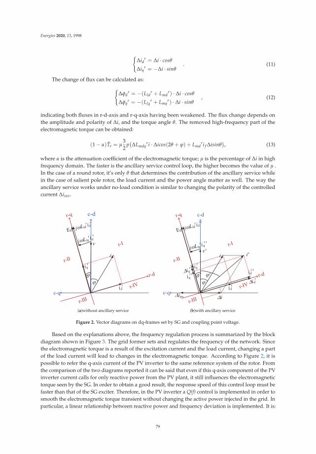
Energies 2020, 13, 1998

{Δid

r = Δi · cosθ

Δiqr = −Δi · sinθ

. (11)

The change of flux can be calculated as:

{Δφd

r = −(Lldr + Lmd

r) · Δi · cosθ

Δφqr = −(Llq

r + Lmqr) · Δi · sinθ

, (12)

indicating both fluxes in r-d-axis and r-q-axis having been weakened. The flux change depends onthe amplitude and polarity of Δi, and the torque angle θ. The removed high-frequency part of theelectromagnetic torque can be obtained:

(1 − α)Te = μ32

p(ΔLmdq

ri · Δicos(2θ + ϕ) + Lmdri f Δisinθ

), (13)

where α is the attenuation coefficient of the electromagnetic torque; μ is the percentage of Δi in highfrequency domain. The faster is the ancillary service control loop, the higher becomes the value of μ .In the case of a round rotor, it’s only θ that determines the contribution of the ancillary service whilein the case of salient pole rotor, the load current and the power angle matter as well. The way theancillary service works under no-load condition is similar to changing the polarity of the controlledcurrent Δiinv.

c-d

c-q

v

(a)without ancillary service

c-d

c-q

v'

iinv i

i'

'

(b)with ancillary service

Figure 2. Vector diagrams on dq-frames set by SG and coupling point voltage.

Based on the explanations above, the frequency regulation process is summarized by the blockdiagram shown in Figure 3. The grid former sets and regulates the frequency of the network. Sincethe electromagnetic torque is a result of the excitation current and the load current, changing a partof the load current will lead to changes in the electromagnetic torque. According to Figure 2, it ispossible to refer the q-axis current of the PV inverter to the same reference system of the rotor. Fromthe comparison of the two diagrams reported it can be said that even if this q-axis component of the PVinverter current calls for only reactive power from the PV plant, it still influences the electromagnetictorque seen by the SG. In order to obtain a good result, the response speed of this control loop must befaster than that of the SG exciter. Therefore, in the PV inverter a Q(f) control is implemented in order tosmooth the electromagnetic torque transient without changing the active power injected in the grid. Inparticular, a linear relationship between reactive power and frequency deviation is implemented. It is:

79

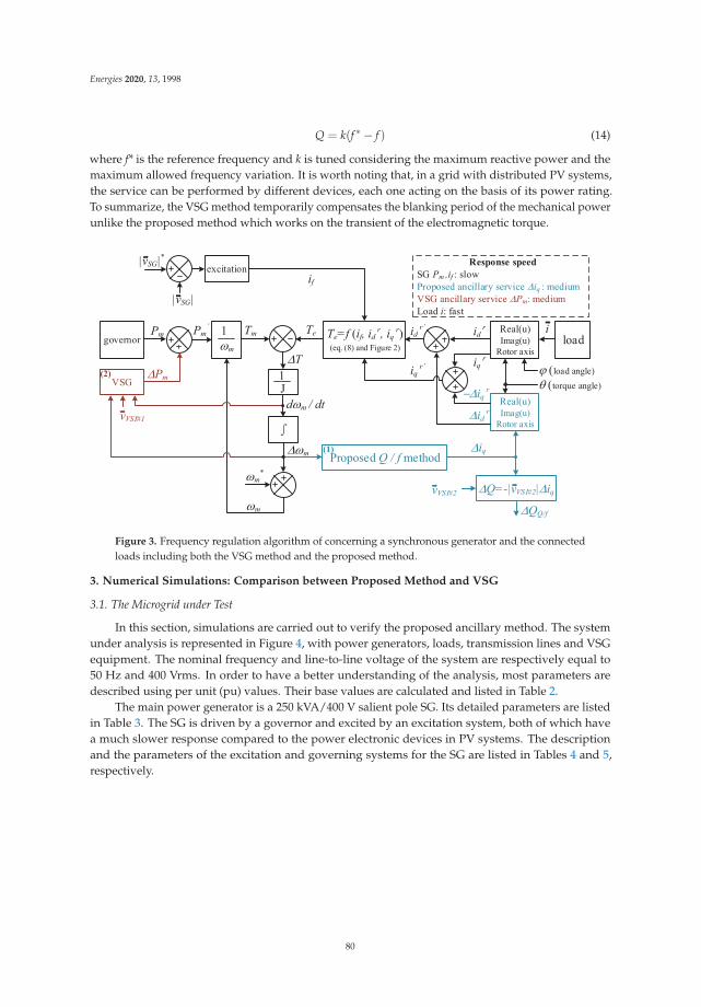
Energies 2020, 13, 1998

Q = k(f ∗ − f ) (14)

where f* is the reference frequency and k is tuned considering the maximum reactive power and themaximum allowed frequency variation. It is worth noting that, in a grid with distributed PV systems,the service can be performed by different devices, each one acting on the basis of its power rating.To summarize, the VSG method temporarily compensates the blanking period of the mechanical powerunlike the proposed method which works on the transient of the electromagnetic torque.

m

TmPm’Pm

Pm

J

governor

VSG

Te

T

d m / dt

m

m*

m

excitation|vSG|*

if

load

Proposed Q / f method

vVSI#1

Te=f (if, id r, iq

r)(eq. (8) and Figure 2)

|vSG|

(2)

(1)

QQ/f

iq

Real(u)Imag(u)

Rotor axis

torque angle)

i

iq r

id r

Real(u)Imag(u)

Rotor axis

load angle)

iq r

id r

id r’

iq r’

Q=-|vVSI#2| iq vVSI#2

Response speed SG Pm ,if : slow Proposed ancillary service iq

: medium VSG ancillary service Pm: medium Load i: fast

Figure 3. Frequency regulation algorithm of concerning a synchronous generator and the connectedloads including both the VSG method and the proposed method.

3. Numerical Simulations: Comparison between Proposed Method and VSG

3.1. The Microgrid under Test

In this section, simulations are carried out to verify the proposed ancillary method. The systemunder analysis is represented in Figure 4, with power generators, loads, transmission lines and VSGequipment. The nominal frequency and line-to-line voltage of the system are respectively equal to50 Hz and 400 Vrms. In order to have a better understanding of the analysis, most parameters aredescribed using per unit (pu) values. Their base values are calculated and listed in Table 2.

The main power generator is a 250 kVA/400 V salient pole SG. Its detailed parameters are listedin Table 3. The SG is driven by a governor and excited by an excitation system, both of which havea much slower response compared to the power electronic devices in PV systems. The descriptionand the parameters of the excitation and governing systems for the SG are listed in Tables 4 and 5,respectively.

80

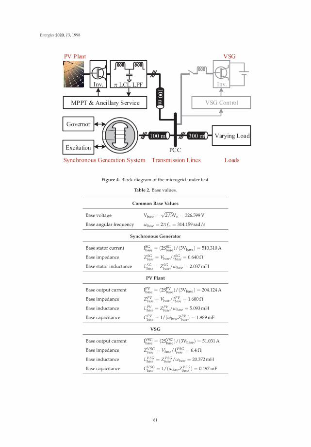
Energies 2020, 13, 1998

Inv.

VSG Control

Governor

Excitation

Varying Load

Transmission LinesSynchronous Generation System Loads

Inv. LCL LPF

PV Plant

MPPT & Ancillary Service

100 m

100 m

300 m

PCC

VSG

Figure 4. Block diagram of the microgrid under test.

Table 2. Base values.

Common Base Values

Base voltage Vbase =√

2/3Vn = 326.599 V

Base angular frequency ωbase = 2π fn = 314.159 rad/s

Synchronous Generator

Base stator current ISGbase = (2SSG

base)/(3Vbase) = 510.310 A

Base impedance ZSGbase = Vbase/ISG

base = 0.640 Ω

Base stator inductance LSGbase = ZSG

base/ωbase = 2.037 mH

PV Plant

Base output current IPVbase = (2SPV

base)/(3Vbase) = 204.124 A

Base impedance ZPVbase = Vbase/IPV

base = 1.600 Ω

Base inductance LPVbase = ZPV

base/ωbase = 5.093 mH

Base capacitance CPVbase = 1/(ωbaseZPV

base) = 1.989 mF

VSG

Base output current IVSGbase = (2SVSG

base)/(3Vbase) = 51.031 A

Base impedance ZVSGbase = Vbase/IVSG

base = 6.4 Ω

Base inductance LVSGbase = ZVSG

base /ωbase = 20.372 mH

Base capacitance CVSGbase = 1/(ωbaseZVSG

base ) = 0.497 mF

81

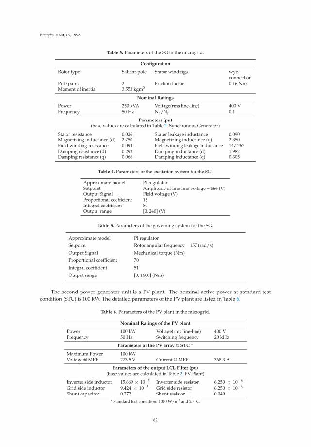
Energies 2020, 13, 1998

Table 3. Parameters of the SG in the microgrid.

Configuration

Rotor type Salient-pole Stator windings wyeconnection

Pole pairs 2 Friction factor 0.16 NmsMoment of inertia 3.553 kgm2

Nominal Ratings

Power 250 kVA Voltage(rms line-line) 400 VFrequency 50 Hz Ns/Nf 0.1

Parameters (pu)(base values are calculated in Table 2–Synchronous Generator)

Stator resistance 0.026 Stator leakage inductance 0.090Magnetizing inductance (d) 2.750 Magnetizing inductance (q) 2.350Field winding resistance 0.094 Field winding leakage inductance 147.262Damping resistance (d) 0.292 Damping inductance (d) 1.982Damping resistance (q) 0.066 Damping inductance (q) 0.305

Table 4. Parameters of the excitation system for the SG.

Approximate model PI regulatorSetpoint Amplitude of line-line voltage = 566 (V)Output Signal Field voltage (V)Proportional coefficient 15Integral coefficient 80Output range [0, 240] (V)

Table 5. Parameters of the governing system for the SG.

Approximate model PI regulator

Setpoint Rotor angular frequency = 157 (rad/s)

Output Signal Mechanical torque (Nm)

Proportional coefficient 70

Integral coefficient 51

Output range [0, 1600] (Nm)

The second power generator unit is a PV plant. The nominal active power at standard testcondition (STC) is 100 kW. The detailed parameters of the PV plant are listed in Table 6.

Table 6. Parameters of the PV plant in the microgrid.

Nominal Ratings of the PV plant

Power 100 kW Voltage(rms line-line) 400 VFrequency 50 Hz Switching frequency 20 kHz

Parameters of the PV array @ STC ∗

Maximum Power 100 kWVoltage @ MPP 273.5 V Current @ MPP 368.3 A

Parameters of the output LCL Filter (pu)(base values are calculated in Table 2–PV Plant)

Inverter side inductor 15.669 × 10−3 Inverter side resistor 6.250 × 10−6

Grid side inductor 9.424 × 10−3 Grid side resistor 6.250 × 10−6

Shunt capacitor 0.272 Shunt resistor 0.049∗ Standard test condition: 1000 W/m2 and 25 ◦C.

82

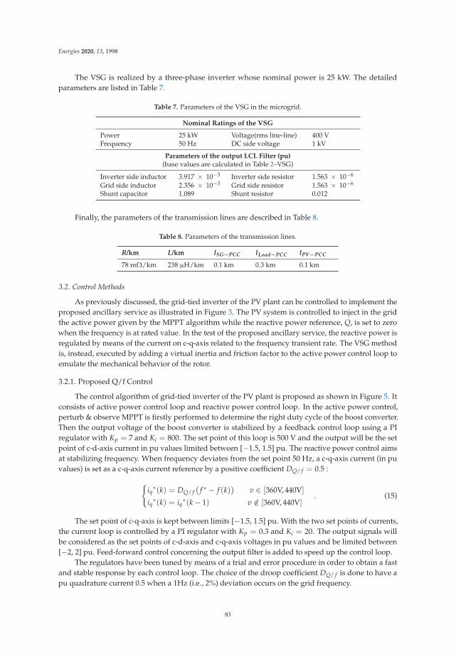
Energies 2020, 13, 1998

The VSG is realized by a three-phase inverter whose nominal power is 25 kW. The detailedparameters are listed in Table 7.

Table 7. Parameters of the VSG in the microgrid.

Nominal Ratings of the VSG

Power 25 kW Voltage(rms line-line) 400 VFrequency 50 Hz DC side voltage 1 kV

Parameters of the output LCL Filter (pu)(base values are calculated in Table 2–VSG)

Inverter side inductor 3.917 × 10−3 Inverter side resistor 1.563 × 10−6

Grid side inductor 2.356 × 10−3 Grid side resistor 1.563 × 10−6

Shunt capacitor 1.089 Shunt resistor 0.012

Finally, the parameters of the transmission lines are described in Table 8.

Table 8. Parameters of the transmission lines.

R/km L/km lSG−PCC lLoad−PCC lPV−PCC

78 mΩ/km 238 μH/km 0.1 km 0.3 km 0.1 km

3.2. Control Methods

As previously discussed, the grid-tied inverter of the PV plant can be controlled to implement theproposed ancillary service as illustrated in Figure 3. The PV system is controlled to inject in the gridthe active power given by the MPPT algorithm while the reactive power reference, Q, is set to zerowhen the frequency is at rated value. In the test of the proposed ancillary service, the reactive power isregulated by means of the current on c-q-axis related to the frequency transient rate. The VSG methodis, instead, executed by adding a virtual inertia and friction factor to the active power control loop toemulate the mechanical behavior of the rotor.

3.2.1. Proposed Q/f Control

The control algorithm of grid-tied inverter of the PV plant is proposed as shown in Figure 5. Itconsists of active power control loop and reactive power control loop. In the active power control,perturb & observe MPPT is firstly performed to determine the right duty cycle of the boost converter.Then the output voltage of the boost converter is stabilized by a feedback control loop using a PIregulator with Kp = 7 and Ki = 800. The set point of this loop is 500 V and the output will be the setpoint of c-d-axis current in pu values limited between [−1.5, 1.5] pu. The reactive power control aimsat stabilizing frequency. When frequency deviates from the set point 50 Hz, a c-q-axis current (in puvalues) is set as a c-q-axis current reference by a positive coefficient DQ/ f = 0.5 :

{iq∗(k) = DQ/ f

(f ∗ − f (k)

)v ∈ [360V, 440V]

iq∗(k) = iq∗(k − 1) v /∈ [360V, 440V]

. (15)

The set point of c-q-axis is kept between limits [−1.5, 1.5] pu. With the two set points of currents,the current loop is controlled by a PI regulator with Kp = 0.3 and Ki = 20. The output signals willbe considered as the set points of c-d-axis and c-q-axis voltages in pu values and be limited between[−2, 2] pu. Feed-forward control concerning the output filter is added to speed up the control loop.

The regulators have been tuned by means of a trial and error procedure in order to obtain a fastand stable response by each control loop. The choice of the droop coefficient DQ/ f is done to have apu quadrature current 0.5 when a 1Hz (i.e., 2%) deviation occurs on the grid frequency.

83

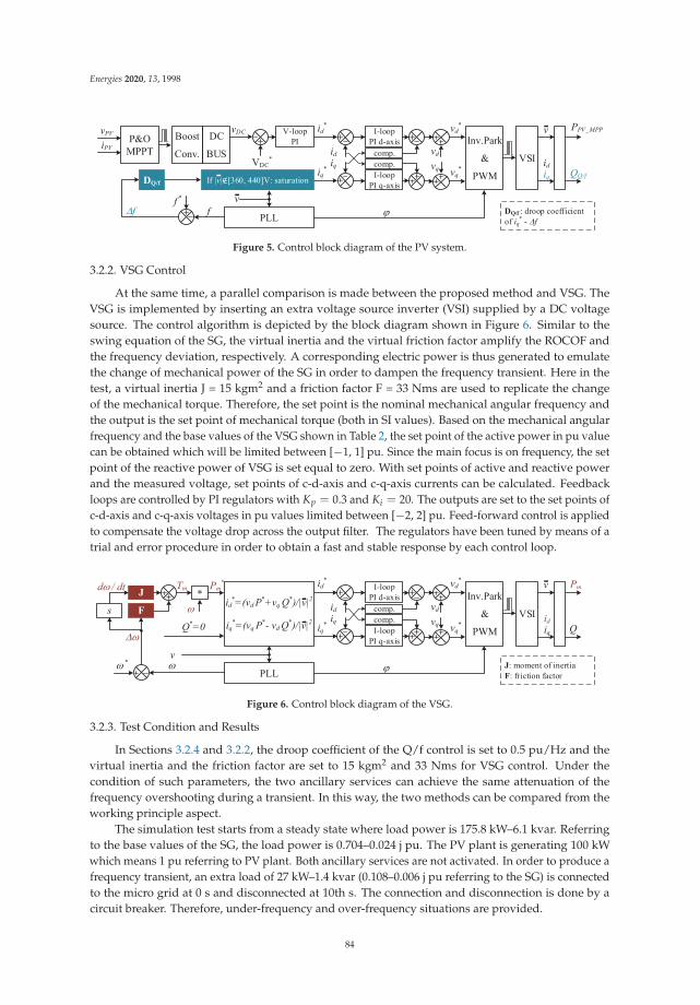
Energies 2020, 13, 1998

P&OMPPT

Boost

Conv.

DC

BUS

V-loopPI

VDC*

vDCvPV

iPV

f

v

id*

iq*

id

iq

I-loopPI d-axis

I-loopPI q-axis

comp.comp.

vd

vq

vd*

vq*

Inv.Park

&

PWM

PLL

VSI

v PPV_MPP

QQ/f

ff *

id

iq

DQ/f If |v|∉[360, 440]V: saturation

DQ/f : droop coefficient of iq

* - f

Figure 5. Control block diagram of the PV system.

3.2.2. VSG Control

At the same time, a parallel comparison is made between the proposed method and VSG. TheVSG is implemented by inserting an extra voltage source inverter (VSI) supplied by a DC voltagesource. The control algorithm is depicted by the block diagram shown in Figure 6. Similar to theswing equation of the SG, the virtual inertia and the virtual friction factor amplify the ROCOF andthe frequency deviation, respectively. A corresponding electric power is thus generated to emulatethe change of mechanical power of the SG in order to dampen the frequency transient. Here in thetest, a virtual inertia J = 15 kgm2 and a friction factor F = 33 Nms are used to replicate the changeof the mechanical torque. Therefore, the set point is the nominal mechanical angular frequency andthe output is the set point of mechanical torque (both in SI values). Based on the mechanical angularfrequency and the base values of the VSG shown in Table 2, the set point of the active power in pu valuecan be obtained which will be limited between [−1, 1] pu. Since the main focus is on frequency, the setpoint of the reactive power of VSG is set equal to zero. With set points of active and reactive powerand the measured voltage, set points of c-d-axis and c-q-axis currents can be calculated. Feedbackloops are controlled by PI regulators with Kp = 0.3 and Ki = 20. The outputs are set to the set points ofc-d-axis and c-q-axis voltages in pu values limited between [−2, 2] pu. Feed-forward control is appliedto compensate the voltage drop across the output filter. The regulators have been tuned by means of atrial and error procedure in order to obtain a fast and stable response by each control loop.

d / dt

Tm Pm*

Q*=0

id*

iq*

id

iq

I-loopPI d-axis

I-loopPI q-axis

comp.comp.

id*=(vd P*+vq Q*)/|v|2

iq*=(vq P*- vd Q*)/|v|2

vd

vq

vd*

vq*

Inv.Park

&

PWM

PLL

VSI

v Pm

Q

*

s

JF

id

iq

J: moment of inertiaF: friction factor

*

v

Figure 6. Control block diagram of the VSG.

3.2.3. Test Condition and Results

In Sections 3.2.4 and 3.2.2, the droop coefficient of the Q/f control is set to 0.5 pu/Hz and thevirtual inertia and the friction factor are set to 15 kgm2 and 33 Nms for VSG control. Under thecondition of such parameters, the two ancillary services can achieve the same attenuation of thefrequency overshooting during a transient. In this way, the two methods can be compared from theworking principle aspect.

The simulation test starts from a steady state where load power is 175.8 kW–6.1 kvar. Referringto the base values of the SG, the load power is 0.704–0.024 j pu. The PV plant is generating 100 kWwhich means 1 pu referring to PV plant. Both ancillary services are not activated. In order to produce afrequency transient, an extra load of 27 kW–1.4 kvar (0.108–0.006 j pu referring to the SG) is connectedto the micro grid at 0 s and disconnected at 10th s. The connection and disconnection is done by acircuit breaker. Therefore, under-frequency and over-frequency situations are provided.

84

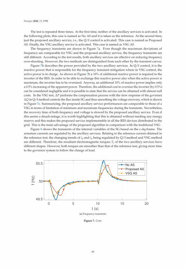
Energies 2020, 13, 1998

The test is repeated three times. At the first time, neither of the ancillary services is activated. Inthe following plots, this case is named as No AS and it is taken as the reference. At the second time,just the proposed ancillary service, i.e., the Q/f control is activated. This case is named as ProposedAS. Finally, the VSG ancillary service is activated. This case is named as VSG AS.

The frequency transients are shown in Figure 7a. Even though the maximum deviations offrequency are comparable for VSG and the proposed ancillary service, the frequency transients arestill different. According to the test results, both ancillary services are effective on reducing frequencyover-shooting. However, the two methods are distinguished from each other by the transient curves.

Figure 7b describes the power provided by the two ancillary services. In Q/f control, it is thereactive power that is responsible for the frequency transient mitigation where in VSG control, theactive power is in charge. As shown in Figure 7b a 10% of additional reactive power is required to theinverter of the RES. In order to be able to exchange this reactive power also when the active power ismaximum, the inverter has to be oversized. Anyway, an additional 10% of reactive power implies onlya 0.5% increasing of the apparent power. Therefore, the additional cost to oversize the inverter (by 0.5%)can be considered negligible and it is possible to state that the service can be obtained with almost nullcosts. In the VSG test, ΔP performs the compensation process with the slow response of the governer.ΔQ in Q/f method controls the flux inside SG and thus smoothing the voltage recovery, which is shownin Figure 7c. Summarizing, the proposed ancillary service performances are comparable to those of aVSG in terms of limitation of minimum and maximum frequencies during the transients. Nevertheless,the recovery time of both frequency and voltage is slowed by the proposed ancillary service. Even ifthis seems a disadvantage, it is worth highlighting that this is obtained without needing any energyreserve and this makes the proposed service implementable in all the RES devices distributed in thegrid. This is the main advantage of the proposed algorithm in comparison with the traditional VSG.

Figure 8 shows the transients of the internal variables of the SG based on the c-dq-frame. Thearmature currents are regulated by the ancillary services. Relating to the reference current obtained inthe reference test, the changing trends of id and iq being regulated by Q/f method and VSG methodare different. Therefore, the resultant electromagnetic torques Te of the two ancillary services havedifferent shapes. However, both torques are smoother than that of the reference test, giving more timeto the governor system to follow the change of load.

0 5 10 15 20

t (s)

49.5

50

50.5

f (H

z)

No ASProposed ASVSG AS

(a) Frequency transients;

Figure 7. Cont.

85

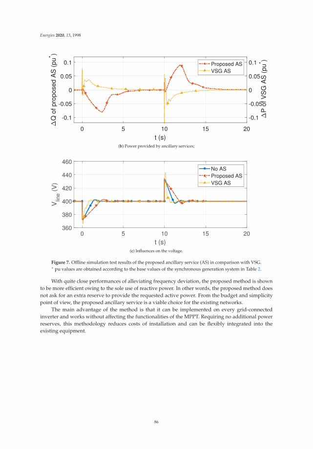
Energies 2020, 13, 1998

0 5 10 15 20

t (s)

-0.1

-0.05

0

0.05

0.1

Q o

f pro

pose

d A

S (

pu* )

-0.1

-0.05

0

0.05

0.1

P o

f VS

G A

S (

pu* )

Proposed ASVSG AS

(b) Power provided by ancillary services;

0 5 10 15 20

t (s)

360

380

400

420

440

460

Vlin

e (

V)

No ASProposed ASVSG AS

(c) Influences on the voltage.

Figure 7. Offline simulation test results of the proposed ancillary service (AS) in comparison with VSG.∗ pu values are obtained according to the base values of the synchronous generation system in Table 2.

With quite close performances of alleviating frequency deviation, the proposed method is shownto be more efficient owing to the sole use of reactive power. In other words, the proposed method doesnot ask for an extra reserve to provide the requested active power. From the budget and simplicitypoint of view, the proposed ancillary service is a viable choice for the existing networks.

The main advantage of the method is that it can be implemented on every grid-connectedinverter and works without affecting the functionalities of the MPPT. Requiring no additional powerreserves, this methodology reduces costs of installation and can be flexibly integrated into theexisting equipment.

86

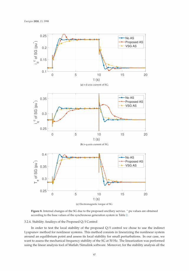
Energies 2020, 13, 1998

0 5 10 15 20

t (s)

0.1

0.15

0.2

0.25i d

c of S

G (

pu* )

No ASProposed ASVSG AS

(a) r-d-axis current of SG;

0 5 10 15 20

t (s)

0.25

0.3

0.35

i qc o

f SG

(pu

* )

No ASProposed ASVSG AS

(b) r-q-axis current of SG;

0 5 10 15 20

t (s)

0.25

0.3

0.35

0.4

Te o

f SG

(pu

* )

No ASProposed ASVSG AS

(c) Electromagnetic torque of SG.

Figure 8. Internal changes of the SG due to the proposed ancillary service. ∗ pu values are obtainedaccording to the base values of the synchronous generation system in Table 2.

3.2.4. Stability Analisys of the Proposed Q/f Control

In order to test the local stability of the proposed Q/f control we chose to use the indirectLyapunov method for nonlinear systems. This method consists in linearizing the nonlinear systemaround an equilibrium point and assess its local stability for small perturbations. In our case, wewant to assess the mechanical frequency stability of the SG at 50 Hz. The linearization was performedusing the linear analysis tool of Matlab/Simulink software. Moreover, for the stability analysis all the

87

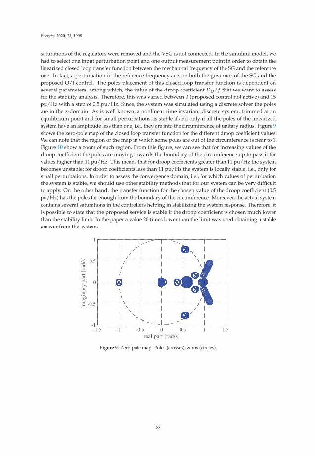
Energies 2020, 13, 1998

saturations of the regulators were removed and the VSG is not connected. In the simulink model, wehad to select one input perturbation point and one output measurement point in order to obtain thelinearized closed loop transfer function between the mechanical frequency of the SG and the referenceone. In fact, a perturbation in the reference frequency acts on both the governor of the SG and theproposed Q/f control. The poles placement of this closed loop transfer function is dependent onseveral parameters, among which, the value of the droop coefficient DQ/ f that we want to assessfor the stability analysis. Therefore, this was varied between 0 (proposed control not active) and 15pu/Hz with a step of 0.5 pu/Hz. Since, the system was simulated using a discrete solver the polesare in the z-domain. As is well known, a nonlinear time invariant discrete system, trimmed at anequilibrium point and for small perturbations, is stable if and only if all the poles of the linearizedsystem have an amplitude less than one, i.e., they are into the circumference of unitary radius. Figure 9shows the zero-pole map of the closed loop transfer function for the different droop coefficient values.We can note that the region of the map in which some poles are out of the circumference is near to 1.Figure 10 show a zoom of such region. From this figure, we can see that for increasing values of thedroop coefficient the poles are moving towards the boundary of the circumference up to pass it forvalues higher than 11 pu/Hz. This means that for droop coefficients greater than 11 pu/Hz the systembecomes unstable; for droop coefficients less than 11 pu/Hz the system is locally stable, i.e., only forsmall perturbations. In order to assess the convergence domain, i.e., for which values of perturbationthe system is stable, we should use other stability methods that for our system can be very difficultto apply. On the other hand, the transfer function for the chosen value of the droop coefficient (0.5pu/Hz) has the poles far enough from the boundary of the circumference. Moreover, the actual systemcontains several saturations in the controllers helping in stabilizing the system response. Therefore, itis possible to state that the proposed service is stable if the droop coefficient is chosen much lowerthan the stability limit. In the paper a value 20 times lower than the limit was used obtaining a stableanswer from the system.

-1.5 -1 -0.5 0 0.5 1 1.5real part [rad/s]

-1

-0.5

0

0.5

1

imag

inar

y pa

rt [

rad/

s]

Figure 9. Zero-pole map. Poles (crosses); zeros (circles).

88

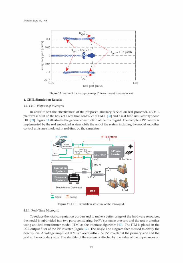
Energies 2020, 13, 1998

0.95 1 1.05real part [rad/s]

-0.15

-0.1

-0.05

0

0.05

0.1im

agin

ary

part

[ra

d/s]

DQ/f

DQ/f

DQ/f = 0.5 pu/HzDQ/f = 11.5 pu/Hz

Figure 10. Zoom of the zero-pole map. Poles (crosses); zeros (circles).

4. CHIL Simulation Results

4.1. CHIL Platform of Microgrid

In order to test the effectiveness of the proposed ancillary service on real processor, a CHILplatform is built on the basis of a real-time controller dSPACE [38] and a real-time simulator TyphoonHIL [39]. Figure 11 illustrates the general construction of the micro grid. The complete PV control isimplemented by the real embedded system while the rest of the system including the model and othercontrol units are simulated in real-time by the simulator.

Solar Farm

Load

300 m

400 V

100 mExcitationSystem

GovernorSystem

Synchronous Generator

300 m sw1

sw2

LCL Filter

RT Control RT Microgrid

3-PhaseInverter

InterfaceSoftware

PartHardware

Part

digital analog

RTS

ESPulse

Generation

PV Control

Figure 11. CHIL simulation structure of the microgrid.

4.1.1. Real-Time Microgrid

To reduce the total computation burden and to make a better usage of the hardware resources,the model is subdivided into two parts considering the PV system in one core and the rest in anotherusing an ideal transformer model (ITM) as the interface algorithm [40]. The ITM is placed in theLCL output filter of the PV inverter (Figure 12). The single-line diagram then is used to clarify thedescription. A voltage amplified ITM is placed within the PV inverter at the primary side and thegrid at the secondary side. The stability of the system is affected by the value of the impedances on

89

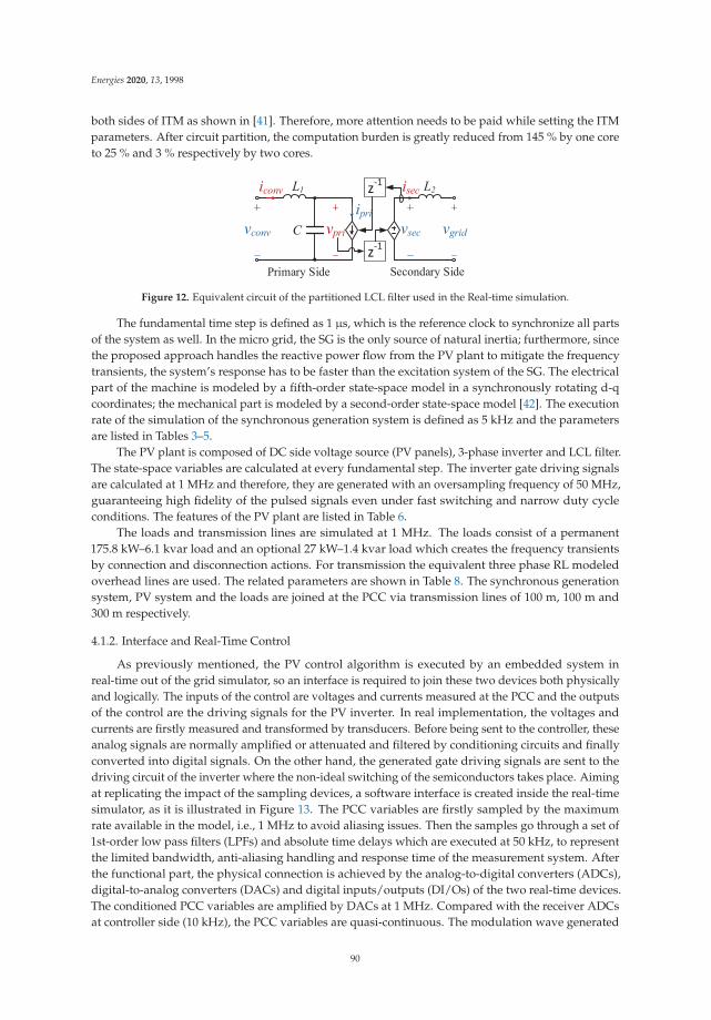
Energies 2020, 13, 1998

both sides of ITM as shown in [41]. Therefore, more attention needs to be paid while setting the ITMparameters. After circuit partition, the computation burden is greatly reduced from 145 % by one coreto 25 % and 3 % respectively by two cores.

vconv

iconv L1

Cipri

vpri

L2isecz-1

z-1vsec vgrid

Primary Side Secondary Side

Figure 12. Equivalent circuit of the partitioned LCL filter used in the Real-time simulation.

The fundamental time step is defined as 1 μs, which is the reference clock to synchronize all partsof the system as well. In the micro grid, the SG is the only source of natural inertia; furthermore, sincethe proposed approach handles the reactive power flow from the PV plant to mitigate the frequencytransients, the system’s response has to be faster than the excitation system of the SG. The electricalpart of the machine is modeled by a fifth-order state-space model in a synchronously rotating d-qcoordinates; the mechanical part is modeled by a second-order state-space model [42]. The executionrate of the simulation of the synchronous generation system is defined as 5 kHz and the parametersare listed in Tables 3–5.

The PV plant is composed of DC side voltage source (PV panels), 3-phase inverter and LCL filter.The state-space variables are calculated at every fundamental step. The inverter gate driving signalsare calculated at 1 MHz and therefore, they are generated with an oversampling frequency of 50 MHz,guaranteeing high fidelity of the pulsed signals even under fast switching and narrow duty cycleconditions. The features of the PV plant are listed in Table 6.

The loads and transmission lines are simulated at 1 MHz. The loads consist of a permanent175.8 kW–6.1 kvar load and an optional 27 kW–1.4 kvar load which creates the frequency transientsby connection and disconnection actions. For transmission the equivalent three phase RL modeledoverhead lines are used. The related parameters are shown in Table 8. The synchronous generationsystem, PV system and the loads are joined at the PCC via transmission lines of 100 m, 100 m and300 m respectively.

4.1.2. Interface and Real-Time Control

As previously mentioned, the PV control algorithm is executed by an embedded system inreal-time out of the grid simulator, so an interface is required to join these two devices both physicallyand logically. The inputs of the control are voltages and currents measured at the PCC and the outputsof the control are the driving signals for the PV inverter. In real implementation, the voltages andcurrents are firstly measured and transformed by transducers. Before being sent to the controller, theseanalog signals are normally amplified or attenuated and filtered by conditioning circuits and finallyconverted into digital signals. On the other hand, the generated gate driving signals are sent to thedriving circuit of the inverter where the non-ideal switching of the semiconductors takes place. Aimingat replicating the impact of the sampling devices, a software interface is created inside the real-timesimulator, as it is illustrated in Figure 13. The PCC variables are firstly sampled by the maximumrate available in the model, i.e., 1 MHz to avoid aliasing issues. Then the samples go through a set of1st-order low pass filters (LPFs) and absolute time delays which are executed at 50 kHz, to representthe limited bandwidth, anti-aliasing handling and response time of the measurement system. Afterthe functional part, the physical connection is achieved by the analog-to-digital converters (ADCs),digital-to-analog converters (DACs) and digital inputs/outputs (DI/Os) of the two real-time devices.The conditioned PCC variables are amplified by DACs at 1 MHz. Compared with the receiver ADCsat controller side (10 kHz), the PCC variables are quasi-continuous. The modulation wave generated

90

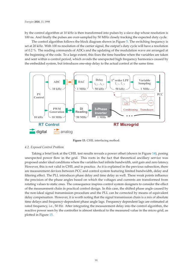
Energies 2020, 13, 1998

by the control algorithm at 10 kHz is then transformed into pulses by a slave dsp whose resolution is100 ns. And finally the pulses are over-sampled by 50 MHz closely tracking the expected duty cycle.

The control algorithm follows the block diagram shown in Figure 5. The switching frequency isset at 20 kHz. With 100 ns resolution of the carrier signal, the output’s duty cycle will have a resolutionof 0.2 %. The reading commands of ADCs and the updating of the modulation wave are arranged atthe beginning of the code. To a large extent, this fixes the time baseline when the variables are takenand sent within a control period, which avoids the unexpected high frequency harmonics caused bythe embedded system, but introduces one-step delay to the actual control at the same time.

CT

VT

Transducers

KLPF

Conditioning

Delaytd_I , td_V

Variable Sampling

1st order LPFfc_I , fc_V DAC

1 MHz50 kHz50 kHz1 MHz

PCCPV Control

PWMGeneration

ADC

10 kHz

10 kHz 10 MHz

DIReading50 MHz

3-PhaseInverter

1 MHz

RT Control RT Microgriddigital analog

Figure 13. CHIL interfacing method.

4.2. Exposed Control Problem

Taking a brief look at the CHIL test results reveals a power offset (shown in Figure 14), posingunexpected power flow in the grid. This roots in the fact that theoretical ancillary service wasproposed under ideal conditions where the variables had infinite bandwidth, unit gain and zero latency.However, this is not valid in CHIL and in practice. As it is explained in the previous subsection, thereare measurement devices between PCC and control system featuring limited bandwidth, delay andfiltering effect. The PLL introduces phase delay and time delay as well. These weak points influencethe precision of the phase angles based on which the voltages and currents are transformed fromrotating values to static ones. The consequence inspires control system designers to consider the effectof the measurement chain in practical control design. In this case, the shifted phase angle caused bythe non-ideal signal transmission procedure and the PLL can be corrected by means of equivalentdelay compensation. However, it is worth noting that the signal transmission chain is a mix of absolutetime delays and frequency-dependent phase angle lags. Frequency dependent lags are estimated atrated frequency, i.e., 50 Hz. After integrating the measurement delay into the control algorithm, thereactive power seen by the controller is almost identical to the measured value in the micro grid, asplotted in Figure 15.

91

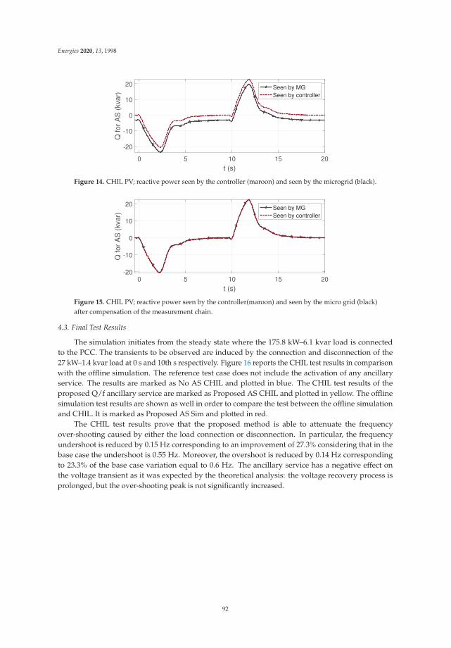
Energies 2020, 13, 1998

0 5 10 15 20

t (s)

-20

-10

0

10

20

Q fo

r A

S (

kvar

)

Seen by MGSeen by controller

Figure 14. CHIL PV; reactive power seen by the controller (maroon) and seen by the microgrid (black).

0 5 10 15 20

t (s)

-20

-10

0

10

20

Q fo

r A

S (

kvar

)

Seen by MGSeen by controller

Figure 15. CHIL PV; reactive power seen by the controller(maroon) and seen by the micro grid (black)after compensation of the measurement chain.

4.3. Final Test Results

The simulation initiates from the steady state where the 175.8 kW–6.1 kvar load is connectedto the PCC. The transients to be observed are induced by the connection and disconnection of the27 kW–1.4 kvar load at 0 s and 10th s respectively. Figure 16 reports the CHIL test results in comparisonwith the offline simulation. The reference test case does not include the activation of any ancillaryservice. The results are marked as No AS CHIL and plotted in blue. The CHIL test results of theproposed Q/f ancillary service are marked as Proposed AS CHIL and plotted in yellow. The offlinesimulation test results are shown as well in order to compare the test between the offline simulationand CHIL. It is marked as Proposed AS Sim and plotted in red.

The CHIL test results prove that the proposed method is able to attenuate the frequencyover-shooting caused by either the load connection or disconnection. In particular, the frequencyundershoot is reduced by 0.15 Hz corresponding to an improvement of 27.3% considering that in thebase case the undershoot is 0.55 Hz. Moreover, the overshoot is reduced by 0.14 Hz correspondingto 23.3% of the base case variation equal to 0.6 Hz. The ancillary service has a negative effect onthe voltage transient as it was expected by the theoretical analysis: the voltage recovery process isprolonged, but the over-shooting peak is not significantly increased.

92

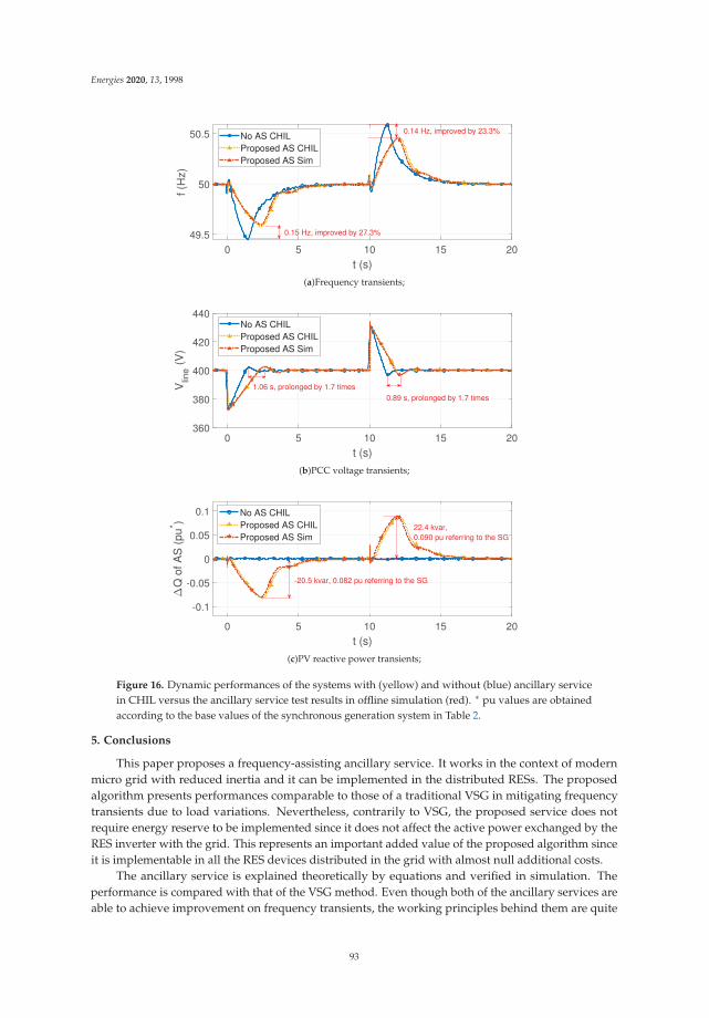
Energies 2020, 13, 1998

0 5 10 15 20

t (s)

49.5

50

50.5

f (H

z)

No AS CHILProposed AS CHILProposed AS Sim

0.15 Hz, improved by 27.3%

0.14 Hz, improved by 23.3%

(a)Frequency transients;

0 5 10 15 20

t (s)

360

380

400

420

440

Vlin

e (

V)

No AS CHILProposed AS CHILProposed AS Sim

1.06 s, prolonged by 1.7 times0.89 s, prolonged by 1.7 times

(b)PCC voltage transients;

0 5 10 15 20

t (s)

-0.1

-0.05

0

0.05

0.1

Q o

f AS

(pu

* )

No AS CHILProposed AS CHILProposed AS Sim

-20.5 kvar, 0.082 pu referring to the SG

22.4 kvar, 0.090 pu referring to the SG

(c)PV reactive power transients;

Figure 16. Dynamic performances of the systems with (yellow) and without (blue) ancillary servicein CHIL versus the ancillary service test results in offline simulation (red). ∗ pu values are obtainedaccording to the base values of the synchronous generation system in Table 2.

5. Conclusions

This paper proposes a frequency-assisting ancillary service. It works in the context of modernmicro grid with reduced inertia and it can be implemented in the distributed RESs. The proposedalgorithm presents performances comparable to those of a traditional VSG in mitigating frequencytransients due to load variations. Nevertheless, contrarily to VSG, the proposed service does notrequire energy reserve to be implemented since it does not affect the active power exchanged by theRES inverter with the grid. This represents an important added value of the proposed algorithm sinceit is implementable in all the RES devices distributed in the grid with almost null additional costs.

The ancillary service is explained theoretically by equations and verified in simulation. Theperformance is compared with that of the VSG method. Even though both of the ancillary services areable to achieve improvement on frequency transients, the working principles behind them are quite

93

Energies 2020, 13, 1998

distinct and thereby, the requested types of power used for the ancillary services differ as well. Finally,a CHIL micro grid system is constructed to test the algorithm in an embedded system. However, itwas noticed that without cautious consideration related to the non-ideal measurement and the delaycaused by data processing, the control algorithm heads toward the performance deterioration andunexpected power loss. After modification, the ancillary service on processor proves to be effective ondamping the over-shooting of frequency.

Author Contributions: Conceptualization, Y.H., S.B., L.P. and G.G.; methodology, Y.H., S.B., L.P. and G.G.;software, Y.H. and S.B.; validation, L.P. and G.G.; formal analysis, Y.H., S.B., L.P. and G.G.; investigation, Y.H.and S.B.; resources, L.P. and G.G.; data curation, Y.H. and S.B.; writing–original draft preparation, Y.H., S.B.;writing–review and editing, Y.H., S.B., L.P. and G.G.; supervision, L.P. and G.G.; All authors have read and agreedto the published version of the manuscript.

Funding: This research received no external funding.

Conflicts of Interest: The authors declare no conflict of interest.

References

1. Chicco, G.; Mancarella, P. Distributed multi-generation: A comprehensive view. Renew. Sustain. Energy Rev.2009, 13, 535–551. [CrossRef]

2. Llaria, A.; Curea, O.; Jiménez, J.; Camblong, H. Survey on microgrids: Unplanned islanding and relatedinverter control techniques. Renew. Energy 2011, 36, 2052–2061. [CrossRef]

3. Georgilakis, P.S.; Hatziargyriou, N.D. A review of power distribution planning in the modern power systemsera: Models, methods and future research. Electr. Power Syst. Res. 2015, 121, 89–100. [CrossRef]

4. D’Arco, S.; Suul, J.A.; Fosso, O.B. A Virtual Synchronous Machine implementation for distributed control ofpower converters in SmartGrids. Electr. Power Syst. Res. 2015, 122, 180–197. [CrossRef]

5. Lopes, J.P.; Hatziargyriou, N.; Mutale, J.; Djapic, P.; Jenkins, N. Integrating distributed generation intoelectric power systems: A review of drivers, challenges and opportunities. Electr. Power Syst. Res. 2007,77, 1189–1203. Distributed Generation. [CrossRef]

6. Carrasco, J.M.; Franquelo, L.G.; Bialasiewicz, J.T.; Galvan, E.; PortilloGuisado, R.C.; Prats, M.A.M.; Leon,J.I.; Moreno-Alfonso, N. Power-Electronic Systems for the Grid Integration of Renewable Energy Sources:A Survey. IEEE Trans. Ind. Electron. 2006, 53, 1002–1016. [CrossRef]

7. Blaabjerg, F.; Teodorescu, R.; Liserre, M.; Timbus, A.V. Overview of Control and Grid Synchronization forDistributed Power Generation Systems. IEEE Trans. Ind. Electron. 2006, 53, 1398–1409. [CrossRef]

8. Rocabert, J.; Luna, A.; Blaabjerg, F.; Rodríguez, P. Control of Power Converters in AC Microgrids. IEEETrans. Power Electron. 2012, 27, 4734–4749. [CrossRef]

9. Hossain, M.A.; Pota, H.R.; Hossain, M.J.; Blaabjerg, F. Evolution of microgrids with converter-interfacedgenerations: Challenges and opportunities. Int. J. Electr. Power Energy Syst. 2019, 109, 160–186. [CrossRef]

10. Yang, Y.; Blaabjerg, F.; Wang, H. Low-Voltage Ride-Through of Single-Phase Transformerless PhotovoltaicInverters. IEEE Trans. Ind. Appl. 2014, 50, 1942–1952. [CrossRef]

11. Stetz, T.; Marten, F.; Braun, M. Improved Low Voltage Grid-Integration of Photovoltaic Systems in Germany.IEEE Trans. Sustain. Energy 2013, 4, 534–542. [CrossRef]

12. Hossain, M.; Pota, H.; Hossain, M.; Haruni, A. Active power management in a low-voltage islandedmicrogrid. Int. J. Electr. Power Energy Syst. 2018, 98, 36–47. [CrossRef]

13. Engler, A.; Soultanis, N. Droop control in LV-grids. In Proceedings of the 2005 International Conference onFuture Power Systems, Amsterdam, NL, USA, 18 November 2005; p. 6. [CrossRef]

14. Yu, X.; Khambadkone, A.M.; Wang, H.; Terence, S.T.S. Control of Parallel-Connected Power Convertersfor Low-Voltage Microgrid—Part I: A Hybrid Control Architecture. IEEE Trans. Power Electron. 2010,25, 2962–2970. [CrossRef]

15. Moradi, M.H.; Eskandari, M.; Hosseinian, S.M. Cooperative control strategy of energy storage systems andmicro sources for stabilizing microgrids in different operation modes. Int. J. Electr. Power Energy Syst. 2016,78, 390–400. [CrossRef]

94

Energies 2020, 13, 1998

16. Vandoorn, T.L.; Kooning, J.D.D.; Meersman, B.; Zwaenepoel, B. Control of storage elements in an islandedmicrogrid with voltage-based control of DG units and loads. Int. J. Electr. Power Energy Syst. 2015, 64,996–1006. [CrossRef]

17. De Brabandere, K.; Bolsens, B.; Van den Keybus, J.; Woyte, A.; Driesen, J.; Belmans, R. A Voltage andFrequency Droop Control Method for Parallel Inverters. IEEE Trans. Power Electron. 2007, 22, 1107–1115.[CrossRef]

18. Guerrero, J.M.; De Vicuna, L.G.; Matas, J.; Castilla, M.; Miret, J. Output impedance design of parallel-connected UPS inverters with wireless load-sharing control. IEEE Trans. Ind. Electron. 2005, 52, 1126–1135.[CrossRef]

19. He, J.; Li, Y.W. Analysis, Design, and Implementation of Virtual Impedance for Power Electronics InterfacedDistributed Generation. IEEE Trans. Ind. Appl. 2011, 47, 2525–2538. [CrossRef]

20. Kim, J.; Guerrero, J.M.; Rodriguez, P.; Teodorescu, R.; Nam, K. Mode Adaptive Droop Control WithVirtual Output Impedances for an Inverter-Based Flexible AC Microgrid. IEEE Trans. Power Electron. 2011,26, 689–701. [CrossRef]

21. Anderson, P.M.; Fouad, A.A. Power System Control and Stability; IEEE Press: Piscataway, NJ, US, 2003.22. Pulendran, S.; Tate, J. Energy storage system control for prevention of transient under-frequency load

shedding. In Proceedings of the 2017 IEEE Power Energy Society General Meeting, Chicago, IL, USA, 16–20July 2017; p. 1. [CrossRef]

23. Wen, Y.; Li, W.; Huang, G.; Liu, X. Frequency dynamics constrained unit commitment with battery energystorage. In Proceedings of the 2017 IEEE Power Energy Society General Meeting, Chicago, IL, USA, 16–20July 2017; p. 1. [CrossRef]

24. Barcellona, S.; Huo, Y.; Niu, R.; Piegari, L.; Ragaini, E. Control strategy of virtual synchronous generatorbased on virtual impedance and band-pass damping. In Proceedings of the 2016 International Symposiumon Power Electronics, Electrical Drives, Automation and Motion (SPEEDAM), Anacapri, Italy, 22–24 June2016; pp. 1354–1362. [CrossRef]

25. Liu, J.; Hossain, M.; Lu, J.; Rafi, F.; Li, H. A hybrid AC/DC microgrid control system based on a virtualsynchronous generator for smooth transient performances. Electr. Power Syst. Res. 2018, 162, 169–182.[CrossRef]

26. Tan, J.; Zhang, Y. Coordinated Control Strategy of a Battery Energy Storage System to Support a WindPower Plant Providing Multi-Timescale Frequency Ancillary Services. IEEE Trans. Sustain. Energy 2017,8, 1140–1153. [CrossRef]

27. Johnson, J.; Neely, J.C.; Delhotal, J.J.; Lave, M. Photovoltaic Frequency–Watt Curve Design for FrequencyRegulation and Fast Contingency Reserves. IEEE J. Photovolt. 2016, 6, 1611–1618. [CrossRef]

28. Ochoa, D.; Martinez, S. Fast-Frequency Response Provided by DFIG-Wind Turbines and its Impact on theGrid. IEEE Trans. Power Syst. 2017, 32, 4002–4011. [CrossRef]

29. Schleif, F.R.; Hunkins, H.D.; Martin, G.E.; Hattan, E.E. Excitation Control to Improve Powerline Stability.IEEE Trans. Power Appar. Syst. 1968, PAS-87, 1426–1434. [CrossRef]

30. Larsen, E.V.; Chow, J.S. SVC Control Design Concepts for Dystem Dynamic Performance; IEEE Press: Piscataway,NJ, USA, 2003.

31. Zhao, Q.; Jiang, J. Robust SVC controller design for improving power system damping. IEEE Trans. PowerSyst. 1995, 10, 1927–1932. [CrossRef]

32. Noroozian, M.; Ghandhari, M.; Andersson, G.; Gronquist, J.; Hiskens, I. A robust control strategy for shuntand series reactive compensators to damp electromechanical oscillations. IEEE Trans. Power Deliv. 2001,16, 812–817. [CrossRef]

33. Liu, Q.; Vittal, V.; Elia, N. LPV supplementary damping controller design for a thyristor controlled seriescapacitor (TCSC) device. IEEE Trans. Power Syst. 2006, 21, 1242–1249. [CrossRef]

34. Zhang, S.; Vittal, V. Design of Wide-Area Power System Damping Controllers Resilient to CommunicationFailures. IEEE Trans. Power Syst. 2013, 28, 4292–4300. [CrossRef]

35. Moeini, A.; Kamwa, I. Analytical Concepts for Reactive Power Based Primary Frequency Control in PowerSystems. IEEE Trans. Power Syst. 2016, 31, 4217–4230. [CrossRef]

36. Li, Y.; Li, Y.W. Power Management of Inverter Interfaced Autonomous Microgrid Based on VirtualFrequency-Voltage Frame. IEEE Trans. Smart Grid 2011, 2, 30–40. [CrossRef]

95

Energies 2020, 13, 1998

37. Sun, M.; Jia, Q. A Novel Frequency Regulation Strategy for Single-Stage Grid-Connected PV Generation.In Proceedings of the 2018 2nd IEEE Conference on Energy Internet and Energy System Integration (EI2),Bejing, China, 20–22 October 2018; pp. 1–6. [CrossRef]

38. Dspace Manual. Available online: http://www.dspace.com. (accessed on 1 December 2019).39. Typhoon Hil manual. Available online: https://www.typhoon-hil.com. (accessed on 1 December 2019).40. Ren, W.; Steurer, M.; Baldwin, T.L. Improve the Stability and the Accuracy of Power Hardware-in-the-Loop

Simulation by Selecting Appropriate Interface Algorithms. IEEE Trans. Ind. Appl. 2008, 44, 1286–1294.[CrossRef]

41. Wang, J.; Song, Y.; Li, W.; Guo, J.; Monti, A. Development of a Universal Platform for Hardware In-the-LoopTesting of Microgrids. IEEE Trans. Ind. Inf. 2014, 10, 2154–2165. [CrossRef]

42. Fitzgerald, A.E. Electric Machinery, 6th ed.; McGraw-Hill: New York, NY, USA, 2002.

c© 2020 by the authors. Licensee MDPI, Basel, Switzerland. This article is an open accessarticle distributed under the terms and conditions of the Creative Commons Attribution(CC BY) license (http://creativecommons.org/licenses/by/4.0/).

96

energies

Article

Alienation Coefficient and Wigner DistributionFunction Based Protection Scheme for Hybrid PowerSystem Network with Renewable Energy Penetration

Sheesh Ram Ola 1, Amit Saraswat 1,*, Sunil Kumar Goyal 1, Virendra Sharma 2, Baseem Khan 3,

Om Prakash Mahela 4, Hassan Haes Alhelou 5,* and Pierluigi Siano 6,*

1 Department of Electrical Engineering, Manipal University Jaipur, Rajasthan 303007, India;sheeshola@gmail.com (S.R.O.); sunilkumar.goyal@jaipur.manipal.edu (S.K.G.)

2 Department of Electrical Engineering, Arya College of Engineering and Information Technology,Jaipur 302028, India; vsharmakiran@gmail.com

3 Department of Electrical Engineering, Hawassa University, Awasa P.O. Box 05, Ethiopia;baseem.khan04@gmail.com

4 Power System Planning Division, Rajasthan Rajya Vidhyut Prasaran Nigam Ltd., Jaipur 302005, India;opmahela@gmail.com

5 Department of Electrical Power Engineering, Faculty of Mechanical and Electrical Engineering,Tishreen University, 2230 Lattakia, Syria

6 Department of Management & Innovation Systems, University of Salerno, 84084 Fisciano (SA), Italy* Correspondence: amit.saraswat@jaipur.manipal.edu (A.S.); alhelou@tishreen.edu.sy (H.H.A.);

psiano@unisa.it (P.S.)

Received: 4 February 2020; Accepted: 25 February 2020; Published: 2 March 2020

Abstract: The rapid growth of grid integrated renewable energy (RE) sources resulted in developmentof the hybrid grids. Variable nature of RE generation resulted in problems related to the power quality(PQ), power system reliability, and adversely affects the protection relay operation. High penetrationof RE to the utility grid is achieved using multi-tapped lines for integrating the wind and solar energyand also to supply loads. This created considerable challenges for power system protection. Toovercome these challenges, an algorithm is introduced in this paper for providing protection to thehybrid grid with high RE penetration level. All types of fault were identified using a fault index(FI), which is based on both the voltage and current features. This FI is computed using element toelement multiplication of current-based Wigner distribution index (WD-index) and voltage-basedalienation index (ALN-index). Application of the algorithm is generalized by testing the algorithmfor the recognition of faults during different scenarios such as fault at different locations on hybridgrid, different fault incident angles, fault impedances, sampling frequency, hybrid line consistingof overhead (OH) line and underground (UG) cable sections, and presence of noise. The algorithmis successfully tested for discriminating the switching events from the faulty events. Faults wereclassified using the number of faulty phases recognized using FI. A ground fault index (GFI) computedusing the zero sequence current-based WD-index is also introduced for differentiating double phaseand double phase to ground faults. The algorithm is validated using IEEE-13 nodes test networkmodelled as hybrid grid by integrating wind and solar energy plants. Performance of algorithmis effectively established by comparing with the discrete wavelet transform (DWT) and Stockwelltransform based protection schemes.

Keywords: alienation coefficient; hybrid power system network; protection; power system fault;solar energy; wind energy; Wigner distribution function

Energies 2020, 13, 1120; doi:10.3390/en13051120 www.mdpi.com/journal/energies97

Energies 2020, 13, 1120

1. Introduction

Adverse environmental impacts of fossil fuel based power plants have forced the utilities tointegrate clean energy with the grid in order to meet future energy demands. Fast development ofrenewable technologies and government incentives to reduce carbon footprints have motivated theutilities to switch from the conventional power plants to the renewable energy (RE) generationsources [1]. This is achieved by forming the hybrid grid with multi-tapped transmission andsub-transmission lines to supply the loads and integrate RE sources such as wind and solar powerplants. Formation of hybrid grids using multi-tapped lines provide economic solutions for REintegration to the grid; however it creates protection challenges due to variable nature of RE generationand bidirectional flow of power in the lines. This resulted in the requirement of new protectionschemes, which can be deployed in the recent structure of hybrid grids for effective protection. Thesetechniques must be independent of direction of power flow, unbalanced nature of loads, fault currentand variable generation [2]. This can be effectively achieved by the use of machine learning andsignal processing techniques. Fang et al. [3], proposed an improved distance relay scheme using timedelay and zero-sequence impedance for the grid to which RE sources are integrated. This schemehas high reliability compared to the conventional relays and reduced risk of malfunction. A detailedstudy of challenges associated with the protection of grid integrated distributed generation (DG)and adaptive protection schemes for these systems are presented in [4]. A detailed study relatedto the application of signal processing techniques and intelligent methods such as artificial neuralnetwork (ANN), fuzzy set theory (FST), and expert system (ES) in the field of protection of DG sourcesintegrated power system is presented in [5]. A sensor based fault detection isolation scheme for thegrid, interfaced with RE sources and electric vehicles (EV) is introduced by authors in [6]. This caneffectively be deployed in eleven order multi-area smart dynamic power system interfacing RE and EV.In [7], authors introduced an algorithm based on the fast recursive discrete Fourier transform (FRDFT)for the protection of distribution system, integrated with DG. This is a novel, fast and adaptive relaytechnique for relay systems, which is effective for obtaining the optimal protection settings whensystem conditions are continuously changing. Application of the syntactic methods for identificationof power system signals by measuring the parameters is reported in [8,9]. This method has thecapability to provide syntactic and semantic information simultaneously. Nieto et al. [10], introduced adetailed study for improvement of quality of power in grid with integration of energy storage systems.This study helps to differentiate the power quality disturbances from the disturbances associatedwith the faulty events. In [11], a current-based transmission line protection scheme using Wignerdistribution function and alienation coefficient is introduced. However, this scheme fails to providedprotection to hybrid grids in the presence of both wind and solar energy penetration. Discrete wavelettransform was implemented for the identification of wind and solar energy penetration into the utilitygrid [12,13]. This method has the disadvantage of generating false tripping signals in the presence ofhigh noise level. Stockwell transform was implemented for the identification of wind and solar energypenetration into the utility grid [14,15]. This method overcomes the demerits of discrete wavelettransform (DWT) scheme; however, it has the disadvantage of slow speed of protection scheme dueto large data involved in the extraction of features from voltage and current signals. Therefore, newprotection scheme is designed to provide effective protection against various faults to the hybrid gridwith high RE penetration level. This protection scheme has merits, such as fast response (recognitionof fault in a time duration which is less than quarter cycle) and performance is not affected by presenceof high level of noise. Following are main contributions of the paper:

• An algorithm supported by the features of both voltage and current is introduced in this paper,which is effective to provide protection for the hybrid grid with RE penetration.

• A W-index is computed by processing the current signals using Wigner distribution function(WDF). Also an ALN-index is computed using sample-based alienation coefficients of voltagesignals. Furthermore, fault index (FI) is computed from these W-index and ALN-index, which iseffective for recognition of all the fault types incident on hybrid grid.

98

Energies 2020, 13, 1120

• The performance of the algorithm is not affected by the presence of high level of noise.• The proposed algorithm is effective to provide high speed protection of hybrid grid. Faults were

detected within a time less than (1/10)th cycle.• The algorithm is effective in discriminating switching transients from the faulty transients.• The fault type was recognized using the number of faulty phases and identified using FI. A GFI,

based on the processing of zero sequence currents using WDF is effective in differentiating thedouble phase (2P) and double phase to ground (2PG) faults.

• This algorithm works effectively and efficiently for the identification of faults on the hybridgrid during various operating scenarios such as fault location, various sampling frequencies,variations in the fault impedance, fault incidence angle and hybrid combination of the OH lineand UG cable.

Nine sections are used to arrange the contents in the article. A brief introduction to carry outresearch on the selected topic and main contributions is included in Section 1. Section 2 describes thehybrid grid test network incorporated with RE generators. The proposed algorithm implementedfor the protection of hybrid grid is described in Section 3. Section 4 demonstrates the simulationresults related to fault identification in the hybrid grid. This section also includes the simulationresults to highlight the requirements of protection scheme for the hybrid grid. Fault classificationresults are included in Section 5. Section 6 discusses the results of various case studies. Results for thediscrimination of switching events from the faulty events are discussed in Section 7. A brief commenton the results and performance comparison of the proposed protection scheme with other existedschemes in the presence of RE is detailed in Section 8, followed by the conclusions (Section 9).

2. The Proposed Test System

IEEE-13 node test network is modelled as hybrid grid by incorporating the wind and solarphotovoltaic (PV) generators. As specified by IEEE, the capacity of this network is equal to 5MVAand operated at frequency of 60 Hz and two voltage levels of 0.48 kV and 4.16 kV [16,17]. Doublyfed induction generator-based wind plant (WG) of capacity 1.5 MW is integrated at node 680 of testsystem using transformer TRFW. Also, PV plant of capacity 1 MW is integrated to test network at node680 using a transformer TRFS and an overhead line (5 km length) as described in Figure 1. Positiveand zero sequence resistances of this line are 0.1153 and 0.413 Ω/km respectively. Positive and zerosequence inductances of the same line are 1.05e−3 and 3.32e−3 H/km respectively. Positive and zerosequence capacitances of the same line are 11.33e−9 and 5.01e−9 F/km respectively. Since, wind andsolar PV plants are integrated at node 680, therefore this node is considered to be a point of commoncoupling (PCC).

The configurations of overhead (OH) lines and underground (UG) cables are considered sameas that provided in the original data as illustrated in Table 1. Impedance matrix (Z601) of the OHlines (configuration 601) is provided by the equation (1) where all the impedances are expressedin Ω/km. Impedance matrix (Z606) of UG cables (configuration 606) is provided by equation (2)where all impedances are expressed in Ω/km. Positive and zero sequence capacitance magnitudes of1.57199 nF/km and 1.3398nF/km, respectively are used for OH lines. Similarly, the parameters forUG cables (configuration 606) are taken as 15.96979 μF/km. All loads are assumed as 3φ balanced asdetailed in Table 2 [18,19].

Z601 =

⎡⎢⎣0.2153 + j0.6325 0.0969 + j0.3117 0.0982 + j0.2632

0.0969 + j0.3117 0.2097 + j0.6511 0.0954 + j0.23920.0982 + j0.2632 0.0954 + j0.2392 0.2121 + j0.6430

⎤⎥⎦ (1)

Z606 =

⎡⎢⎣0.4960 + j0.2773 0.1983 + j0.0204 0.1770 + j0.0089

0.1983 + j0.0204 0.4903 + j0.2511 0.1983 + j0.02040.1770 + j0.0089 0.1983 + j0.0204 0.4960 + j0.2773

⎤⎥⎦ (2)

99

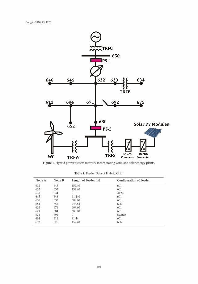
Energies 2020, 13, 1120

Figure 1. Hybrid power system network incorporating wind and solar energy plants.

Table 1. Feeder Data of Hybrid Grid.

Node A Node B Length of Feeder (m) Configuration of Feeder

632 645 152.40 601632 633 152.40 601633 634 0 XFM645 646 91.440 601650 632 609.60 601684 652 243.84 606632 671 609.60 601671 684 680.00 601671 692 0 Switch684 611 91.44 601692 675 152.40 606

100

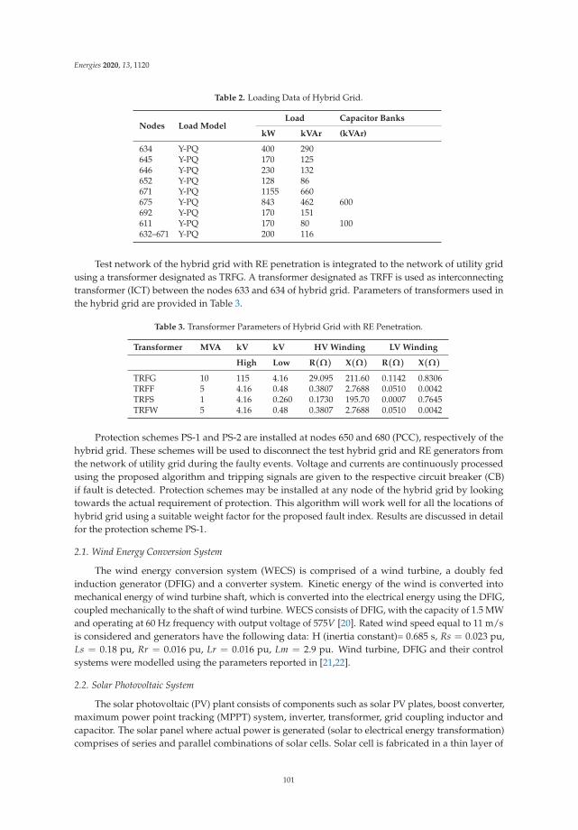
Energies 2020, 13, 1120

Table 2. Loading Data of Hybrid Grid.

Nodes Load ModelLoad Capacitor Banks

kW kVAr (kVAr)

634 Y-PQ 400 290645 Y-PQ 170 125646 Y-PQ 230 132652 Y-PQ 128 86671 Y-PQ 1155 660675 Y-PQ 843 462 600692 Y-PQ 170 151611 Y-PQ 170 80 100632–671 Y-PQ 200 116

Test network of the hybrid grid with RE penetration is integrated to the network of utility gridusing a transformer designated as TRFG. A transformer designated as TRFF is used as interconnectingtransformer (ICT) between the nodes 633 and 634 of hybrid grid. Parameters of transformers used inthe hybrid grid are provided in Table 3.

Table 3. Transformer Parameters of Hybrid Grid with RE Penetration.

Transformer MVA kV kV HV Winding LV Winding

High Low R(Ω) X(Ω) R(Ω) X(Ω)

TRFG 10 115 4.16 29.095 211.60 0.1142 0.8306TRFF 5 4.16 0.48 0.3807 2.7688 0.0510 0.0042TRFS 1 4.16 0.260 0.1730 195.70 0.0007 0.7645TRFW 5 4.16 0.48 0.3807 2.7688 0.0510 0.0042

Protection schemes PS-1 and PS-2 are installed at nodes 650 and 680 (PCC), respectively of thehybrid grid. These schemes will be used to disconnect the test hybrid grid and RE generators fromthe network of utility grid during the faulty events. Voltage and currents are continuously processedusing the proposed algorithm and tripping signals are given to the respective circuit breaker (CB)if fault is detected. Protection schemes may be installed at any node of the hybrid grid by lookingtowards the actual requirement of protection. This algorithm will work well for all the locations ofhybrid grid using a suitable weight factor for the proposed fault index. Results are discussed in detailfor the protection scheme PS-1.

2.1. Wind Energy Conversion System

The wind energy conversion system (WECS) is comprised of a wind turbine, a doubly fedinduction generator (DFIG) and a converter system. Kinetic energy of the wind is converted intomechanical energy of wind turbine shaft, which is converted into the electrical energy using the DFIG,coupled mechanically to the shaft of wind turbine. WECS consists of DFIG, with the capacity of 1.5 MWand operating at 60 Hz frequency with output voltage of 575V [20]. Rated wind speed equal to 11 m/sis considered and generators have the following data: H (inertia constant)= 0.685 s, Rs = 0.023 pu,Ls = 0.18 pu, Rr = 0.016 pu, Lr = 0.016 pu, Lm = 2.9 pu. Wind turbine, DFIG and their controlsystems were modelled using the parameters reported in [21,22].

2.2. Solar Photovoltaic System

The solar photovoltaic (PV) plant consists of components such as solar PV plates, boost converter,maximum power point tracking (MPPT) system, inverter, transformer, grid coupling inductor andcapacitor. The solar panel where actual power is generated (solar to electrical energy transformation)comprises of series and parallel combinations of solar cells. Solar cell is fabricated in a thin layer of

101

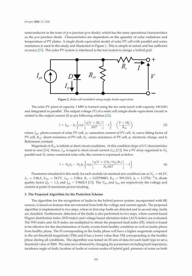
Energies 2020, 13, 1120

semiconductor in the form of p-n junction (p-n diode), which has the same operational characteristicsas the p-n junction diode. Characteristics are dependent on the quantity of solar radiations andtemperature of PV plates. A single diode equivalent model of solar PV cell with parallel and seriesresistances is used in this study and illustrated in Figure 2. This is simple in nature and has sufficientaccuracy [23]. This solar PV system is interfaced to the test system to design a hybrid grid.

Figure 2. Solar cell modelled using single diode equivalent.

The solar PV plant of capacity 1 MW is formed using the ten units (each with capacity 100 kW)and integrated in parallel. The output voltage (V) of a solar cell (single-diode equivalent circuit) isrelated to the output current (I) as per following relation [24].

I = Iph − I0

{exp

[q(V + IRs)

AkT

]− 1

}−

(V + IRs

Rsh

)(3)

where Iph: photo-current of solar PV cell, I0: saturation current of PV cell, A: curve fitting factor ofPV cell, Rsh: shunt resistance of PV cell, Rs: series resistance of PV cell, q: electronic charge, and k:Boltzmann constant.

Magnitude of Rsh is infinite at short circuit conditions. At this condition slope of I-V characteristicstends to zero [24]. Hence, Iph is equal to short circuit current (Isc) [23]. For a PV array organized in Np

parallel and Ns series connected solar cells, the current is expressed as below.

I = Np Isc − Np I0

{exp

[q(V + I(Ns/Np)Rs)

Ns AkT

]− 1

}(4)

Parameters simulated in this study for each module (at standard test condition) are as Voc = 64.2V,Isc = 5.96A, Vmp = 54.7V, Imp = 5.58A, Rs = 0.037998Ω, Rsh = 993.51Ω, I0 = 1.1753e−8 A, diodequality factor Qd = 1.3, and Iph = 5.9602A [25]. The Vmp and Imp are respectively the voltage andcurrent at point of maximum power tracking.

3. The Proposed Algorithm for the Protection Scheme

The algorithm for the recognition of faults in the hybrid power system, incorporated with REsources, is based on features that are extracted from both the voltage and current signals. The proposedalgorithm is implemented in two steps, where in first step faults are detected and in second step, faultsare classified. Furthermore, detection of the faults is also performed in two steps, where current-basedWigner distribution index (WD-index) and voltage-based alienation index (ALN-index) are evaluated.The WD-index and ALN-index are multiplied to obtain the proposed fault index (FI), which is foundto be effective for the discrimination of faulty events from healthy condition as well as faulty phasefrom healthy phase. The FI corresponding to the faulty phase will have a higher magnitude comparedto the set threshold magnitude (TM) and it has a lower value than TM corresponding to the healthyphase during all conditions. The algorithm was tested on 30 sets of data for each fault type to set athreshold value of 5000. The data set is obtained by changing the parameters including fault impedance,incidence angle of fault, location of faults at various nodes of hybrid grid, presence of noise on both

102

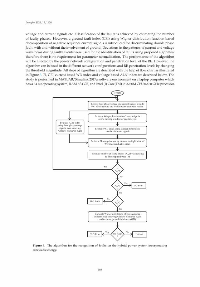
Energies 2020, 13, 1120

voltage and current signals etc. Classification of the faults is achieved by estimating the numberof faulty phases. However, a ground fault index (GFI) using Wigner distribution function baseddecomposition of negative sequence current signals is introduced for discriminating double phasefault, with and without the involvement of ground. Deviations in the patterns of current and voltagewaveforms during faulty events were used for the identification of faults using proposed algorithm;therefore there is no requirement for parameter normalization. The performance of the algorithmwill be affected by the power network configuration and penetration level of the RE. However, thealgorithm can be used in the different network configurations and RE penetration levels by changingthe threshold magnitude. All steps of algorithm are described with the help of flow chart as illustratedin Figure 3. FI, GFI, current-based WD-index and voltage-based ALN-index are described below. Thestudy is performed in MATLAB/Simulink 2017a software environment on a laptop computer whichhas a 64 bit operating system, RAM of 4 GB, and Intel (I) Core(TM) i5-3230M CPU@2.60 GHz processor.

START

Record three phase voltage and current signals at node650 of test system and evaluate zero sequence current

Evaluate Winger distribution of current signalsover a moving window of quarter cycle

Evaluate WD-index using Winger distributionmatrix of current signals

Evaluate FI using element by element multiplication ofWD-index and ALN-index

Estimate number of faulty phases (N ) by comparing

FI of each phase with TMFP

Is=0N

?FP

Is=2N

?FP

IsGFI>TMGFI

?

Is=1N

?FP

2P Fault2PG FaultYes

3PG FaultNo

No

No

PG FaultYes

No

Evaluate ALN-indexusing three phase voltage

signals over a movingwindow of quarter cycle

Yes

Compute Wigner distribution of zero sequencecurrents over a moving window of quarter cycle

and evaluate ground fault index (GFI)

Yes

Figure 3. The algorithm for the recognition of faults on the hybrid power system incorporatingrenewable energy.

103

Energies 2020, 13, 1120

3.1. Current Based Wigner Distribution Index

Wigner distribution function (WDF) is a phase space distribution function. This is effectivein description of signal in a space and frequency at the same time. This can be considered to be alocal frequency spectrum of the signal. This can be used for processing of both deterministic andstochastic signals. The WDF is effective in providing local frequency spectrum of the signal. Hence, itis most suitable for analysis of the faulty transients to identify the faulty events. The current signalscaptured at node 650 are processed using Wigner distribution function over a quarter cycle with asampling frequency (SF) of 3.84 kHz. Window moving by one sample step is used for the continuouscomputation of Wigner distribution. Absolute magnitude of the output is evaluated and designated asWD-index. Energy density of current signal is used by the WD-index for estimation of the faults. Thisis achieved by Bilinear analysis of current signal I(t) (in time domain ) twice. The WD-index has theadvantage of high concentration of energy as well as high resolution of time-frequency [26]. Followingrelation effectively illustrates the evaluation of WD-index by processing the current signal (I(t)) [27].

WDindex =∫ ∞

−∞I(t +

τ

2)I∗(t + τ

2)e−jωτdτ (5)

here representations of symbols are as follows t: time (sliding variable); ω: signal angular frequency; τ:time domain based signal function.

3.2. Voltage Based Alienation Index

Alienation index is computed using sample-based alienation coefficients of voltage signals at a SFof 3.84 kHz and designated as ALN-index. This index is evaluated using the correlation coefficient (r)between voltage magnitudes at two different time instants as detailed below.

ALNindex = 1 − r2 (6)

Here, r is the correlation coefficient between voltage variables x and y and can be expressed asdetailed below.

r =Ns ∑ xy − (∑ x)(∑ y)√

[Ns ∑ x2 − (∑ x)2][Ns ∑ y2 − (∑ y)2](7)

here Ns is the numbers considered in a cycle (in this study Ns=64 is considered), x is the voltagesamples measured at time t0, y is the voltage samples measured at −T + t0 time where T is time periodof voltage signal [28,29]. The ALN-index is evaluated with the help of moving window techniquefor the samples of quarter cycle. Implementation of this index is based on the comparison of data ofquarter cycle considered with the data of previous quarter cycle using a moving window (one samplestep). This index is effective in reducing the fault detection time because it has the merit of sharpchange at the time of fault incidence. This makes the protection scheme fast.

3.3. Fault Index Based on Voltage and Current Features

A fault index (FI), based on the features of both voltage and current is introduced for recognitionof faults in the hybrid power system with RE penetration. This index is computed using element toelement multiplication of ALN-index and WD-index as detailed in the following relation.

FI = (ALNindex)× (WDindex) (8)

The proposed FI effectively identifies the different nature of faults in the hybrid power networkwith RE penetration by good accuracy and minimum time. This is achieved by comparing themagnitude of FI with pre-set threshold magnitude (TM). Individual application of ALN-index will notdetect any type of fault due to its same value for all phases for all the events. However, application of

104

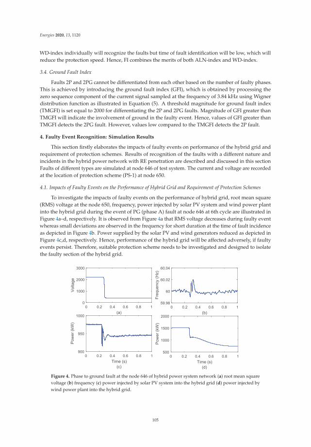
Energies 2020, 13, 1120

WD-index individually will recognize the faults but time of fault identification will be low, which willreduce the protection speed. Hence, FI combines the merits of both ALN-index and WD-index.

3.4. Ground Fault Index

Faults 2P and 2PG cannot be differentiated from each other based on the number of faulty phases.This is achieved by introducing the ground fault index (GFI), which is obtained by processing thezero sequence component of the current signal sampled at the frequency of 3.84 kHz using Wignerdistribution function as illustrated in Equation (5). A threshold magnitude for ground fault index(TMGFI) is set equal to 2000 for differentiating the 2P and 2PG faults. Magnitude of GFI greater thanTMGFI will indicate the involvement of ground in the faulty event. Hence, values of GFI greater thanTMGFI detects the 2PG fault. However, values low compared to the TMGFI detects the 2P fault.

4. Faulty Event Recognition: Simulation Results

This section firstly elaborates the impacts of faulty events on performance of the hybrid grid andrequirement of protection schemes. Results of recognition of the faults with a different nature andincidents in the hybrid power network with RE penetration are described and discussed in this sectionFaults of different types are simulated at node 646 of test system. The current and voltage are recordedat the location of protection scheme (PS-1) at node 650.

4.1. Impacts of Faulty Events on the Performance of Hybrid Grid and Requirement of Protection Schemes

To investigate the impacts of faulty events on the performance of hybrid grid, root mean square(RMS) voltage at the node 650, frequency, power injected by solar PV system and wind power plantinto the hybrid grid during the event of PG (phase A) fault at node 646 at 6th cycle are illustrated inFigure 4a–d, respectively. It is observed from Figure 4a that RMS voltage decreases during faulty eventwhereas small deviations are observed in the frequency for short duration at the time of fault incidenceas depicted in Figure 4b. Power supplied by the solar PV and wind generators reduced as depicted inFigure 4c,d, respectively. Hence, performance of the hybrid grid will be affected adversely, if faultyevents persist. Therefore, suitable protection scheme needs to be investigated and designed to isolatethe faulty section of the hybrid grid.

Figure 4. Phase to ground fault at the node 646 of hybrid power system network (a) root mean squarevoltage (b) frequency (c) power injected by solar PV system into the hybrid grid (d) power injected bywind power plant into the hybrid grid.

105

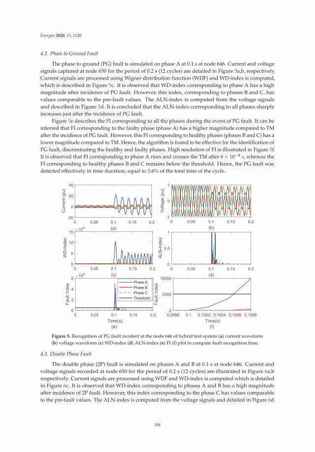
Energies 2020, 13, 1120

4.2. Phase to Ground Fault

The phase to ground (PG) fault is simulated on phase A at 0.1 s at node 646. Current and voltagesignals captured at node 650 for the period of 0.2 s (12 cycles) are detailed in Figure 5a,b, respectively.Current signals are processed using Wigner distribution function (WDF) and WD-index is computed,which is described in Figure 5c. It is observed that WD-index corresponding to phase A has a highmagnitude after incidence of PG fault. However, this index, corresponding to phases B and C, hasvalues comparable to the pre-fault values. The ALN-index is computed from the voltage signalsand described in Figure 5d. It is concluded that the ALN-index corresponding to all phases sharplyincreases just after the incidence of PG fault.

Figure 5e describes the FI corresponding to all the phases during the event of PG fault. It can beinferred that FI corresponding to the faulty phase (phase A) has a higher magnitude compared to TMafter the incidence of PG fault. However, this FI corresponding to healthy phases (phases B and C) has alower magnitude compared to TM. Hence, the algorithm is found to be effective for the identification ofPG fault, discriminating the healthy and faulty phases. High resolution of FI is illustrated in Figure 5f.It is observed that FI corresponding to phase A rises and crosses the TM after 6 × 10−4 s, whereas theFI corresponding to healthy phases B and C remains below the threshold. Hence, the PG fault wasdetected effectively in time duration, equal to 3.6% of the total time of the cycle.

Figure 5. Recognition of PG fault incident at the node 646 of hybrid test system (a) current waveform(b) voltage waveform (c) WD-index (d) ALN-index (e) FI (f) plot to compute fault recognition time.

4.3. Double Phase Fault

The double phase (2P) fault is simulated on phases A and B at 0.1 s at node 646. Current andvoltage signals recorded at node 650 for the period of 0.2 s (12 cycles) are illustrated in Figure 6a,brespectively. Current signals are processed using WDF and WD-index is computed which is detailedin Figure 6c. It is observed that WD-index corresponding to phases A and B has a high magnitudeafter incidence of 2P fault. However, this index corresponding to the phase C has values comparableto the pre-fault values. The ALN-index is computed from the voltage signals and detailed in Figure 6d.

106

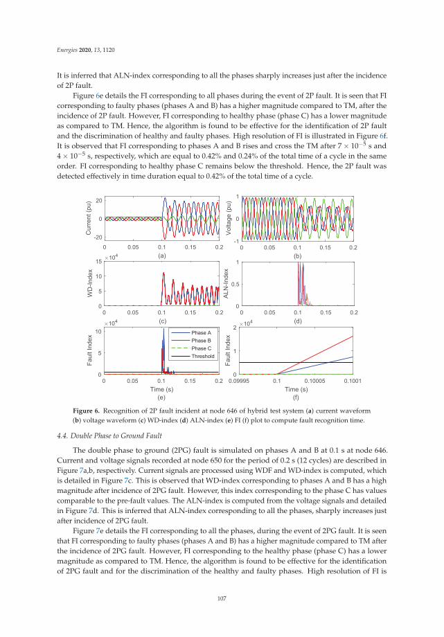
Energies 2020, 13, 1120

It is inferred that ALN-index corresponding to all the phases sharply increases just after the incidenceof 2P fault.

Figure 6e details the FI corresponding to all phases during the event of 2P fault. It is seen that FIcorresponding to faulty phases (phases A and B) has a higher magnitude compared to TM, after theincidence of 2P fault. However, FI corresponding to healthy phase (phase C) has a lower magnitudeas compared to TM. Hence, the algorithm is found to be effective for the identification of 2P faultand the discrimination of healthy and faulty phases. High resolution of FI is illustrated in Figure 6f.It is observed that FI corresponding to phases A and B rises and cross the TM after 7 × 10−5 s and4 × 10−5 s, respectively, which are equal to 0.42% and 0.24% of the total time of a cycle in the sameorder. FI corresponding to healthy phase C remains below the threshold. Hence, the 2P fault wasdetected effectively in time duration equal to 0.42% of the total time of a cycle.

Figure 6. Recognition of 2P fault incident at node 646 of hybrid test system (a) current waveform(b) voltage waveform (c) WD-index (d) ALN-index (e) FI (f) plot to compute fault recognition time.

4.4. Double Phase to Ground Fault

The double phase to ground (2PG) fault is simulated on phases A and B at 0.1 s at node 646.Current and voltage signals recorded at node 650 for the period of 0.2 s (12 cycles) are described inFigure 7a,b, respectively. Current signals are processed using WDF and WD-index is computed, whichis detailed in Figure 7c. This is observed that WD-index corresponding to phases A and B has a highmagnitude after incidence of 2PG fault. However, this index corresponding to the phase C has valuescomparable to the pre-fault values. The ALN-index is computed from the voltage signals and detailedin Figure 7d. This is inferred that ALN-index corresponding to all the phases, sharply increases justafter incidence of 2PG fault.

Figure 7e details the FI corresponding to all the phases, during the event of 2PG fault. It is seenthat FI corresponding to faulty phases (phases A and B) has a higher magnitude compared to TM afterthe incidence of 2PG fault. However, FI corresponding to the healthy phase (phase C) has a lowermagnitude as compared to TM. Hence, the algorithm is found to be effective for the identificationof 2PG fault and for the discrimination of the healthy and faulty phases. High resolution of FI is

107

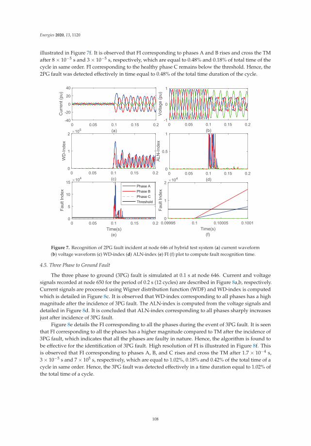
Energies 2020, 13, 1120

illustrated in Figure 7f. It is observed that FI corresponding to phases A and B rises and cross the TMafter 8 × 10−5 s and 3 × 10−5 s, respectively, which are equal to 0.48% and 0.18% of total time of thecycle in same order. FI corresponding to the healthy phase C remains below the threshold. Hence, the2PG fault was detected effectively in time equal to 0.48% of the total time duration of the cycle.

Figure 7. Recognition of 2PG fault incident at node 646 of hybrid test system (a) current waveform(b) voltage waveform (c) WD-index (d) ALN-index (e) FI (f) plot to compute fault recognition time.

4.5. Three Phase to Ground Fault

The three phase to ground (3PG) fault is simulated at 0.1 s at node 646. Current and voltagesignals recorded at node 650 for the period of 0.2 s (12 cycles) are described in Figure 8a,b, respectively.Current signals are processed using Wigner distribution function (WDF) and WD-index is computedwhich is detailed in Figure 8c. It is observed that WD-index corresponding to all phases has a highmagnitude after the incidence of 3PG fault. The ALN-index is computed from the voltage signals anddetailed in Figure 8d. It is concluded that ALN-index corresponding to all phases sharply increasesjust after incidence of 3PG fault.

Figure 8e details the FI corresponding to all the phases during the event of 3PG fault. It is seenthat FI corresponding to all the phases has a higher magnitude compared to TM after the incidence of3PG fault, which indicates that all the phases are faulty in nature. Hence, the algorithm is found tobe effective for the identification of 3PG fault. High resolution of FI is illustrated in Figure 8f. Thisis observed that FI corresponding to phases A, B, and C rises and cross the TM after 1.7 × 10−4 s,3 × 10−5 s and 7 × 105 s, respectively, which are equal to 1.02%, 0.18% and 0.42% of the total time of acycle in same order. Hence, the 3PG fault was detected effectively in a time duration equal to 1.02% ofthe total time of a cycle.

108

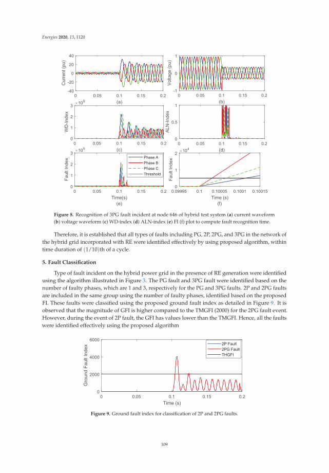
Energies 2020, 13, 1120

Figure 8. Recognition of 3PG fault incident at node 646 of hybrid test system (a) current waveform(b) voltage waveform (c) WD-index (d) ALN-index (e) FI (f) plot to compute fault recognition time.

Therefore, it is established that all types of faults including PG, 2P, 2PG, and 3PG in the network ofthe hybrid grid incorporated with RE were identified effectively by using proposed algorithm, withintime duration of (1/10)th of a cycle.

5. Fault Classification

Type of fault incident on the hybrid power grid in the presence of RE generation were identifiedusing the algorithm illustrated in Figure 3. The PG fault and 3PG fault were identified based on thenumber of faulty phases, which are 1 and 3, respectively for the PG and 3PG faults. 2P and 2PG faultsare included in the same group using the number of faulty phases, identified based on the proposedFI. These faults were classified using the proposed ground fault index as detailed in Figure 9. It isobserved that the magnitude of GFI is higher compared to the TMGFI (2000) for the 2PG fault event.However, during the event of 2P fault, the GFI has values lower than the TMGFI. Hence, all the faultswere identified effectively using the proposed algorithm

Figure 9. Ground fault index for classification of 2P and 2PG faults.

109

Energies 2020, 13, 1120

6. Implementation of the Algorithm to Recognize Faulty Events with Various Scenarios:Case Studies

To generalize the implementation of proposed protection scheme to provide effective protectionsfor hybrid grid with RE penetration, algorithm was tested for recognition of the faults during variousscenarios such as fault location at different nodes of the hybrid grid, variations in fault impedance,variations in fault incidence angle, effect of noise, effect of change in sampling frequency, effect oftransformers and effect of hybrid line with underground (UG) cable and overhead (OH) line sections.The algorithm was also tested for identification of the faulty events by measuring voltage and currentsignals at PCC. Detailed results for recognition of the PG fault during above mentioned scenarios arediscussed in following sections. The algorithm is equally applicable for all fault types.

6.1. Fault Location

Incidence of fault on a particular node/line of the hybrid grid affects the nature of faulty transients,which ultimately affects the performance of fault recognition algorithm. To investigate this effect,the algorithm was tested for the faults, simulated at various critical locations of the hybrid grid. FIcorresponding to all the phases during the PG fault event at various nodes of hybrid grid are tabulatedin Table 4.

Table 4. Fault Index at Different Nodes of Test System with PG Fault.

Test Node Fault Index Magnitude

Phase-A Phase-B Phase-C

646 5.055 × 104 332 1370632 1.138 × 105 645 1855634 5.001 × 104 348 998652 4.956 × 104 1170 439611 6.216 × 104 1491 1785671 6.234 × 104 2711 2886675 6.164 × 104 1529 2001

It can be observed from Table 4 that the FI corresponding to the faulty phase A is higher comparedto TM at all locations. However, healthy phases B and C have lower FI compared to TM. Hence,PG faulty is effectively recognized at all nodes of the test hybrid grid with RE penetration. Detaileddiscussion of PG fault at node 652 and 634 is presented in following subsections.

6.1.1. Fault on Node 652

The algorithm was tested for all the faulty events simulated at node 652 and found to be effectivefor the recognition of these events. Position of this node is critical because there is hybrid combinationof line between this node and node 650 (where current and voltage are recorded), which consists of UGcable and OH line sections. At the junction of UG cable and OH line, reflection of the faulty transient,carrying travelling wave may take place, which might affect the performance of algorithm. Results ofPG fault simulated on phase A at 0.1 s on node 652 are included in Figure 10. Current and voltagesignals captured on node 650 for a period of 0.2 s (12 cycles) are detailed in Figure 10a,b, respectively.Current signals are processed using WDF and WD-index is computed, which is described in Figure 10c.It is observed that WD-index corresponding to phase A has a high magnitude after the incidence ofPG fault. However, this index corresponding to the phases B and C has values comparable to thepre-fault values. The ALN-index is computed from the voltage signals and described in Figure 10d. Itis concluded that the ALN-index corresponding to all phases sharply increases just after the incidenceof PG fault.

Figure 5e describes the FI corresponding to all the phases during the event of PG fault. It can beinferred that FI corresponding to faulty phase (phase A) has a higher magnitude compared to TM

110

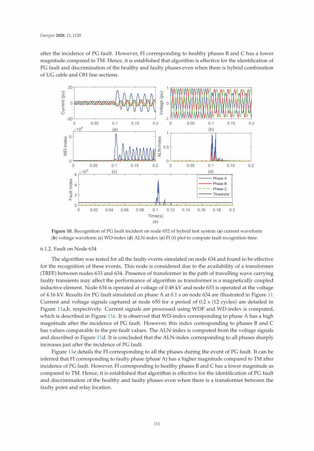
Energies 2020, 13, 1120

after the incidence of PG fault. However, FI corresponding to healthy phases B and C has a lowermagnitude compared to TM. Hence, it is established that algorithm is effective for the identification ofPG fault and discrimination of the healthy and faulty phases even when there is hybrid combinationof UG cable and OH line sections.

Figure 10. Recognition of PG fault incident on node 652 of hybrid test system (a) current waveform(b) voltage waveform (c) WD-index (d) ALN-index (e) FI (f) plot to compute fault recognition time.

6.1.2. Fault on Node 634

The algorithm was tested for all the faulty events simulated on node 634 and found to be effectivefor the recognition of these events. This node is considered due to the availability of a transformer(TRFF) between nodes 633 and 634. Presence of transformer in the path of travelling wave carryingfaulty transients may affect the performance of algorithm as transformer is a magnetically coupledinductive element. Node 634 is operated at voltage of 0.48 kV and node 633 is operated at the voltageof 4.16 kV. Results for PG fault simulated on phase A at 0.1 s on node 634 are illustrated in Figure 11.Current and voltage signals captured at node 650 for a period of 0.2 s (12 cycles) are detailed inFigure 11a,b, respectively. Current signals are processed using WDF and WD-index is computed,which is described in Figure 11c. It is observed that WD-index corresponding to phase A has a highmagnitude after the incidence of PG fault. However, this index corresponding to phases B and Chas values comparable to the pre-fault values. The ALN-index is computed from the voltage signalsand described in Figure 11d. It is concluded that the ALN-index corresponding to all phases sharplyincreases just after the incidence of PG fault.

Figure 11e details the FI corresponding to all the phases during the event of PG fault. It can beinferred that FI corresponding to faulty phase (phase A) has a higher magnitude compared to TM afterincidence of PG fault. However, FI corresponding to healthy phases B and C has a lower magnitude ascompared to TM. Hence, it is established that algorithm is effective for the identification of PG faultand discrimination of the healthy and faulty phases even when there is a transformer between thefaulty point and relay location.

111

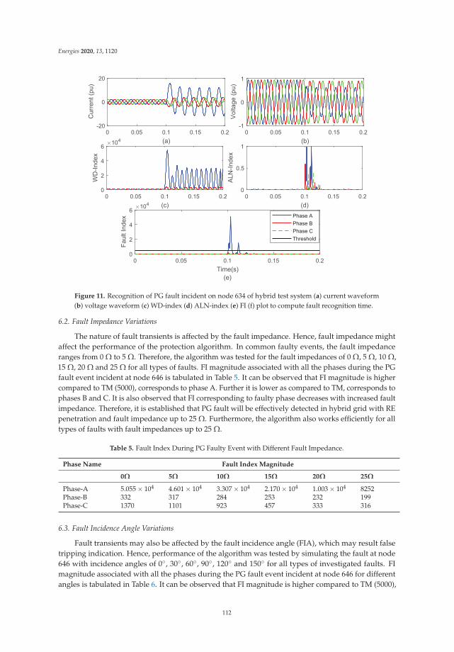
Energies 2020, 13, 1120

Figure 11. Recognition of PG fault incident on node 634 of hybrid test system (a) current waveform(b) voltage waveform (c) WD-index (d) ALN-index (e) FI (f) plot to compute fault recognition time.

6.2. Fault Impedance Variations

The nature of fault transients is affected by the fault impedance. Hence, fault impedance mightaffect the performance of the protection algorithm. In common faulty events, the fault impedanceranges from 0 Ω to 5 Ω. Therefore, the algorithm was tested for the fault impedances of 0 Ω, 5 Ω, 10 Ω,15 Ω, 20 Ω and 25 Ω for all types of faults. FI magnitude associated with all the phases during the PGfault event incident at node 646 is tabulated in Table 5. It can be observed that FI magnitude is highercompared to TM (5000), corresponds to phase A. Further it is lower as compared to TM, corresponds tophases B and C. It is also observed that FI corresponding to faulty phase decreases with increased faultimpedance. Therefore, it is established that PG fault will be effectively detected in hybrid grid with REpenetration and fault impedance up to 25 Ω. Furthermore, the algorithm also works efficiently for alltypes of faults with fault impedances up to 25 Ω.

Table 5. Fault Index During PG Faulty Event with Different Fault Impedance.

Phase Name Fault Index Magnitude

0Ω 5Ω 10Ω 15Ω 20Ω 25Ω

Phase-A 5.055 × 104 4.601 × 104 3.307 × 104 2.170 × 104 1.003 × 104 8252Phase-B 332 317 284 253 232 199Phase-C 1370 1101 923 457 333 316

6.3. Fault Incidence Angle Variations

Fault transients may also be affected by the fault incidence angle (FIA), which may result falsetripping indication. Hence, performance of the algorithm was tested by simulating the fault at node646 with incidence angles of 0◦, 30◦, 60◦, 90◦, 120◦ and 150◦ for all types of investigated faults. FImagnitude associated with all the phases during the PG fault event incident at node 646 for differentangles is tabulated in Table 6. It can be observed that FI magnitude is higher compared to TM (5000),

112

Energies 2020, 13, 1120

corresponds to phase A and lower compared to TM, corresponds to phases B and C for all types of faultincidence angles. It is also observed that FI corresponding to faulty phase is maximum for FIA of 90◦.Therefore, it is established that PG fault will be effectively detected in hybrid grid with RE penetrationand all types of fault incidence angle with respect to current and voltage waveforms. Furthermore, thealgorithm also works efficiently for all types of faults for different FIA.

Table 6. Fault Index During PG Faulty Event with Different Fault Incidence Angles.

Phase Name Fault Index Magnitude

0◦ 30◦ 60◦ 90◦ 120◦ 150◦

Phase-A 5.055 × 104 6.848 × 104 4.641 × 104 7.531 × 104 3.875 × 104 2.139 × 104

Phase-B 332 1107 621 1323 1146 704Phase-C 1370 1244 985 1327 156 75

6.4. Effect of Noise

There is a possibility of interference from external factors on the power system distribution andtransmission lines while passing through the terrain, which may superimpose noise on the faultytransients travelling from the faulty point to the location of PS. Noise may affect the performance ofthe protection schemes resulting in false tripping. To investigate the effect of noise on the performanceof algorithm, a noise level of 10 dB signal to noise ratio (SNR) is introduced on both the voltageand current signals. The algorithm was tested for all types of faults whereas the results of PG faultsimulated on phase A at 0.1 s on node 646 are illustrated in Figure 12, where superimposed noisecan be seen easily. Current and voltage signals captured at node 650 for a period of 0.2 s (12 cycles)are detailed in Figure 12a,b, respectively. Current signals are processed using WDF and WD-index iscomputed, which is described in Figure 12c. It is observed that the WD-index corresponding to phaseA has a higher magnitude after the incidence of PG fault. However, this index corresponding to thephases B and C has values comparable to the pre-fault values. Performance of the WD-index is notaffected by noise. The ALN-index is computed from the voltage signals and described in Figure 12d. Itis concluded that the ALN-index corresponding to all the phases has a high magnitude throughouttime range, indicating that performance of ALN-index will be affected by the noise.

Figure 12 details the FI corresponding to all the phases during the event of PG fault withsuperimposed noise on both voltage and current signals. It can be inferred that FI corresponding tothe faulty phase (phase A) has a higher magnitude compared to TM after the incidence of PG fault.However, FI corresponding to healthy phases B and C has a lower magnitude as compared to TM.Hence, it is established that algorithm is effective for the identification of PG fault and discriminationof the healthy and faulty phases even when there is high level noise (10 dB SNR) superimposed on thecurrent and voltage signals in the hybrid grid in the presence of RE generation. High resolution plot ofFI is illustrated in Figure 12f, where it can be seen that FI corresponding to phase A crosses the TMand FI for phases B & C is below the TM.

6.5. Sampling Frequency Variations

To investigate the effect of frequency used for sampling the voltage and current signals on theperformance of protection scheme, the algorithm was tested for different sampling frequencies. FIcorresponding to the faulty phase A during the event of PG fault is observed and equal to 3.981 × 104,5.055 × 104, and 5.170 × 104 while using the sampling frequencies of 1.92 kHz, 3.84 kHz and 7.68 kHz,respectively. Therefore, sampling frequency, lower than 3.84 kHz, reduces the peak magnitude of FI,which may also go lower compared to TM. Sampling frequency greater than 3.84 kHz increases thefault detection time due to large size of input data set. Hence, 3.84 kHz is observed to be the optimumSF for the protection scheme.

113

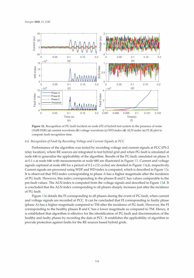
Energies 2020, 13, 1120

Figure 12. Recognition of PG fault incident on node 652 of hybrid test system in the presence of noise(10dB SNR) (a) current waveform (b) voltage waveform (c) WD-index (d) ALN-index (e) FI (f) plot tocompute fault recognition time.

6.6. Recognition of Fault by Recording Voltage and Current Signals at PCC

Performance of the algorithm was tested by recording voltage and current signals at PCC (PS-2relay location), where RE sources are integrated to test hybrid grid and when PG fault is simulated atnode 646 to generalize the applicability of the algorithm. Results of the PG fault, simulated on phase Aat 0.1 s at node 646 with measurements at node 680 are illustrated in Figure 13. Current and voltagesignals captured at node 680 for a period of 0.2 s (12 cycles) are detailed in Figure 13a,b, respectively.Current signals are processed using WDF and WD-index is computed, which is described in Figure 13c.It is observed that WD-index corresponding to phase A has a higher magnitude after the incidenceof PG fault. However, this index corresponding to the phases B and C has values comparable to thepre-fault values. The ALN-index is computed from the voltage signals and described in Figure 13d. Itis concluded that the ALN-index corresponding to all phases sharply increases just after the incidenceof PG fault.

Figure 13e details the FI corresponding to all phases during the event of PG fault, when currentand voltage signals are recorded at PCC. It can be concluded that FI corresponding to faulty phase(phase A) has a higher magnitude compared to TM after the incidence of PG fault. However, the FIcorresponding to the healthy phases B and C has a lower magnitude as compared to TM. Hence, itis established that algorithm is effective for the identification of PG fault and discrimination of thehealthy and faulty phases by recording the data at PCC. It establishes the applicability of algorithm toprovide protection against faults for the RE sources based hybrid grids.

114

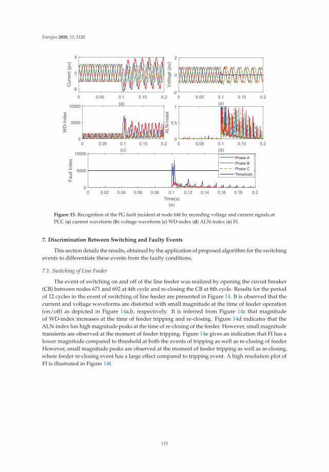
Energies 2020, 13, 1120

Figure 13. Recognition of the PG fault incident at node 646 by recording voltage and current signals atPCC (a) current waveform (b) voltage waveform (c) WD-index (d) ALN-index (e) FI.

7. Discrimination Between Switching and Faulty Events

This section details the results, obtained by the application of proposed algorithm for the switchingevents to differentiate these events from the faulty conditions.

7.1. Switching of Line Feeder

The event of switching on and off of the line feeder was realized by opening the circuit breaker(CB) between nodes 671 and 692 at 4th cycle and re-closing the CB at 8th cycle. Results for the periodof 12 cycles in the event of switching of line feeder are presented in Figure 14. It is observed that thecurrent and voltage waveforms are distorted with small magnitude at the time of feeder operation(on/off) as depicted in Figure 14a,b, respectively. It is inferred from Figure 14c that magnitudeof WD-index increases at the time of feeder tripping and re-closing. Figure 14d indicates that theALN-index has high magnitude peaks at the time of re-closing of the feeder. However, small magnitudetransients are observed at the moment of feeder tripping. Figure 14e gives an indication that FI has alower magnitude compared to threshold at both the events of tripping as well as re-closing of feeder.However, small magnitude peaks are observed at the moment of feeder tripping as well as re-closing,where feeder re-closing event has a large effect compared to tripping event. A high resolution plot ofFI is illustrated in Figure 14f.

115

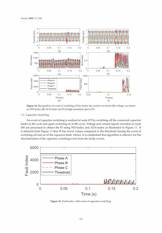
Energies 2020, 13, 1120

Figure 14. Recognition of event of switching of line feeder (a) current waveform (b) voltage waveform(c) WD-index (d) ALN-index (e) FI (f) high resolution plot of FI.

7.2. Capacitive Switching

An event of capacitor switching is realized at node 675 by switching off the connected capacitorbanks at 4th cycle and again switching on at 8th cycle. Voltage and current signals recorded on node650 are processed to obtain the FI using WD-index and ALN-index as illustrated in Figure 15. Itis inferred from Figure 15 that FI has lower values compared to the threshold during the event ofswitching off and on of the capacitor bank. Hence, it is established that algorithm is effective for thediscrimination of the capacitor switching event from the faulty events.

Figure 15. Fault index with event of capacitor switching.

116

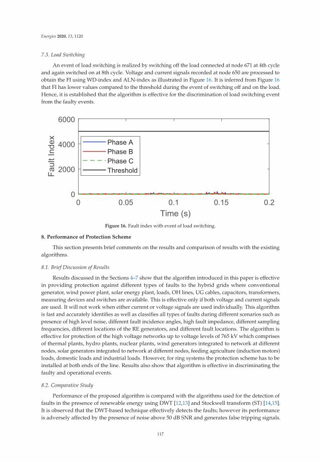
Energies 2020, 13, 1120

7.3. Load Switching

An event of load switching is realized by switching off the load connected at node 671 at 4th cycleand again switched on at 8th cycle. Voltage and current signals recorded at node 650 are processed toobtain the FI using WD-index and ALN-index as illustrated in Figure 16. It is inferred from Figure 16that FI has lower values compared to the threshold during the event of switching off and on the load.Hence, it is established that the algorithm is effective for the discrimination of load switching eventfrom the faulty events.

Figure 16. Fault index with event of load switching.

8. Performance of Protection Scheme

This section presents brief comments on the results and comparison of results with the existingalgorithms.

8.1. Brief Discussion of Results

Results discussed in the Sections 4–7 show that the algorithm introduced in this paper is effectivein providing protection against different types of faults to the hybrid grids where conventionalgenerator, wind power plant, solar energy plant, loads, OH lines, UG cables, capacitors, transformers,measuring devices and switches are available. This is effective only if both voltage and current signalsare used. It will not work when either current or voltage signals are used individually. This algorithmis fast and accurately identifies as well as classifies all types of faults during different scenarios such aspresence of high level noise, different fault incidence angles, high fault impedance, different samplingfrequencies, different locations of the RE generators, and different fault locations. The algorithm iseffective for protection of the high voltage networks up to voltage levels of 765 kV which comprisesof thermal plants, hydro plants, nuclear plants, wind generators integrated to network at differentnodes, solar generators integrated to network at different nodes, feeding agriculture (induction motors)loads, domestic loads and industrial loads. However, for ring systems the protection scheme has to beinstalled at both ends of the line. Results also show that algorithm is effective in discriminating thefaulty and operational events.

8.2. Comparative Study

Performance of the proposed algorithm is compared with the algorithms used for the detection offaults in the presence of renewable energy using DWT [12,13] and Stockwell transform (ST) [14,15].It is observed that the DWT-based technique effectively detects the faults; however its performanceis adversely affected by the presence of noise above 50 dB SNR and generates false tripping signals.

117

Energies 2020, 13, 1120

Hence, DWT-based technique is not effective for the detection of faults when high noise level of 10dB SNR is present. The Stockwell transform-based algorithm uses the patterns of various contoursand plots for the fault detection, which ranges from half cycle to one cycle. The protection schemebased on the application of proposed WD-index individually will be slow and fault detection timewill be high. However, its performance is least affected by the noise. The proposed ALN-index iseffective for reducing the fault detection time because it has the merit of sharp change at the time offault incidence. However, this cannot be used as a standalone protection scheme because at the timeof fault incidence, its magnitude increases for the faulty as well as healthy phases. Furthermore, theperformance of ALN-index-based method is adversely affected by the presence of high noise level.Therefore, proposed algorithm, obtained using WD-index and ALN-index has the combined merits ofthese indexes and provide fast performance of protection scheme, further it is not affected by the noise.Hence it is established that the performance of proposed algorithm is superior as compared to DWT,Stockwell transform, standalone WD-index and standalone ALN-index.

9. Conclusions

A method for the detection and classification of faults is presented in this paper to design aprotection scheme for hybrid grid system integrated with wind and solar energy plants. Various faulttypes such as PG, 2P, 2PG, and 3PG were successfully identified in the RE sources based hybrid gridusing proposed fault index. The FI is obtained using Wigner distribution function based decompositionof current signals (WD-index) sample with alienation coefficient of voltage signals (ALN-index). Faulttypes were classified using number of faulty phases and identified using proposed FI. A ground faultindex, based on the Wigner distribution function supported decomposition of negative sequencecurrent is proposed to differentiate the 2P and 2PG faults. It is concluded that the algorithm is fast andaccurate for detection of all the types of faults in the hybrid grid with RE penetration. Furthermore, thealgorithm was tested and effectively works in the presence of high level noise, different fault incidenceangles, high fault impedance and different fault locations. The algorithm is also effective for thediscrimination of switching events of capacitor, load and line feeder from faulty events. The algorithmis also effective in recognizing faults in the presence of transformers and hybrid lines consisting of OHline and UG cable sections. It is also established that the proposed algorithm obtained using WD-indexand ALN-index has the combined merits of these indexes and provide fast response protection schemewhose performance is not affected by the noise. Hence it is established that performance of proposedalgorithm is superior compared to DWT, ST, standalone WD-index and standalone ALN-index. As afuture enhancement, testing of performance of algorithm with data recorded on real time network ofthe utility grids may be considered before implementation in the protection schemes.

Author Contributions: Conceptualization, S.R.O., O.P.M., A.S., V.S. and S.K.G.; methodology, S.R.O. and O.P.M.;software, S.R.O. and O.P.M.; validation, S.R.O. and O.P.M.; formal analysis, S.R.O., B.K. and O.P.M.; investigation,S.R.O. and O.P.M.; resources, A.S., S.K.G., H.H.A. and P.S.; data curation, S.R.O., B.K. and O.P.M.; writing—originaldraft preparation, S.R.O., B.K. and O.P.M.; writing—review and editing, B.K., H.H.A. and P.S.; visualization, B.K.,H.H.A. and P.S.; supervision, A.S., S.K.G., H.H.A. and P.S. All authors have read and agreed to the publishedversion of the manuscript.

Funding: External funding is not received for this research.

Conflicts of Interest: The authors declare that they have no known conflicts of interest.

118

Energies 2020, 13, 1120

Abbreviations

Abbreviations used in this article are detailed below:

2P Double phase2PG Double phase to ground3PG Three phase to groundPG Phase to groundALN AlienationANN Artificial neural networkCB Circuit breakerDFIG Doubly fed induction generatorDG Distributed generationDWT Discrete Wavelet transformES Expert systemEV Electric vehicleFI Fault indexFIA Fault incidence angleFRDFT Fast recursive discrete Fourier transformFST Fuzzy set theoryGFI Ground fault indexICT Interconnecting transformerIEEE Institute of Electrical and Electronics EngineersOH OverheadMATLAB Matrix laboratoryMPPT Maximum power point trackingPCC Point of common couplingPQ Power qualityPS Protection schemePV PhotovoltaicRE Renewable energySF Sampling frequencySNR Signal to noise ratioST Stockwell transformTM Threshold magnitudeTMGFI Threshold magnitude of ground fault indexUG UndergroundWECS Wind energy conversion systemWD Wigner distributionWDF Wigner distribution function

References

1. Aftab, M.A.; Hussain, S.S.; Ali, I.; Ustun, T.S. Dynamic protection of power systems with high penetration ofrenewables: A review of the traveling wave based fault location techniques. Int. J. Electr. Power Energy Syst.2020, 114, 105410. doi:10.1016/j.ijepes.2019.105410. [CrossRef]

2. Eissa, M.; Awadalla, M.H. Centralized protection scheme for smart grid integrated with multiple renewableresources using Internet of Energy. Glob. Trans. 2019, 1, 50–60. doi:10.1016/j.glt.2019.01.002. [CrossRef]

3. Fang, Y.; Jia, K.; Yang, Z.; Li, Y.; Bi, T. Impact of Inverter-Interfaced Renewable Energy Generatorson Distance Protection and an Improved Scheme. IEEE Trans. Ind. Electron. 2019, 66, 7078–7088.doi:10.1109/TIE.2018.2873521. [CrossRef]

4. Barra, P.; Coury, D.; Fernandes, R. A survey on adaptive protection of microgrids and distribution systemswith distributed generators. Renew. Sustain. Energy Rev. 2020, 118, 109524. doi:10.1016/j.rser.2019.109524.[CrossRef]

5. Eissa, M. Protection techniques with renewable resources and smart grids—A survey. Renew. Sustain. EnergyRev. 2015, 52, 1645–1667. doi:10.1016/j.rser.2015.08.031. [CrossRef]

119

Energies 2020, 13, 1120

6. Alhelou, H.H.; Golshan, M.H.; Askari-Marnani, J. Robust sensor fault detection and isolation scheme forinterconnected smart power systems in presence of RER and EVs using unknown input observer. Int. J.Electr. Power Energy Syst. 2018, 99, 682–694. doi:10.1016/j.ijepes.2018.02.013. [CrossRef]

7. Kumar, D.S.; Srinivasan, D.; Reindl, T. A Fast and Scalable Protection Scheme for Distribution NetworksWith Distributed Generation. IEEE Trans. Power Deliv. 2016, 31, 67–75. doi:10.1109/TPWRD.2015.2464107.[CrossRef]

8. Pavlatos, C.; Vita, V.; Ekonomou, L. Syntactic pattern recognition of power system signals. In Proceedingsof the 19th WSEAS International Conference on Systems (Part of CSCC’15), Zakynthos Island, Greece,16–20 July 2015; pp. 16–20.

9. Pavlatos, C.; Vita, V. Linguistic representation of power system signals. In Electricity Distribution; Springer:Berlin, Germany, 2016; pp. 285–295.

10. Nieto, A.; Vita, V.; Maris, T.I. Power quality improvement in power grids with the integration of energystorage systems. Int. J. Eng. Res. Technol. 2016, 5, 438–443.

11. Sheesh, R.O.; Amit, S.; Sunil, K.G.; Jhajharia, S.K.; Bhuvnesh, R.; Om Prakash, M. Wigner DistributionFunction and Alienation Coefficient Based Transmission Line Protection Scheme. IET Gener. Transm. Distrib.2020, 14, 1–12.

12. Suman, T.; Mahela, O.P.; Ola, S.R. Detection of transmission line faults in the presence of wind powergeneration using discrete wavelet transform. In Proceeidngs of the 2016 IEEE 7th Power India InternationalConference (PIICON), Bikaner, India, 25–27 November 2016; pp. 1–6. doi:10.1109/POWERI.2016.8077174.[CrossRef]

13. Suman, T.; Mahela, O.P.; Ola, S.R. Detection of transmission line faults in the presence of solar PV generationusing discrete wavelet. In Proceeidngs of the 2016 IEEE 7th Power India International Conference (PIICON),Bikaner, India, 25–27 November 2016; pp. 1–6. doi:10.1109/POWERI.2016.8077203. [CrossRef]

14. Thukral, S.; Mahela, O.P.; Kumar, B. Detection of transmission line faults in the presence of solar PV systemusing stockwell’s transform. In Proceedings of the 2016 2016 IEEE 7th Power India International Conference(PIICON), Bikaner, India, 25–27 November 2016; pp. 1–6. doi:10.1109/POWERI.2016.8077304. [CrossRef]

15. Ola, S.; Saraswat, A.; Goyal, S.; Jhajharia, S.; Mahela, O.P. Detection and Analysis of Power SystemFaults in the Presence of Wind Power Generation Using Stockwell Transform Based Median. InIntelligent Computing Techniques for Smart Energy Systems; Lecture Notes in Electrical Engineering; KalamA., Niazi K., Soni A., Siddiqui S., Mundra A., Eds.; Springer: Singapore, 2020; Volume 607, pp. 319–330.doi:10.1007/978-981-15-0214-9_36. [CrossRef]

16. Kersting, W.H. Radial distribution test feeders. Power Syst. IEEE Trans. 1991, 6, 975–985.doi:10.1109/59.119237. [CrossRef]

17. Kersting, W. Radial distribution test feeders. In Proceedings of the Power Engineering Society WinterMeeting, Columbus, OH, USA, 1 February 2001; Volume 2, pp. 908–912. doi:10.1109/PESW.2001.916993.[CrossRef]

18. Mahela, O.P.; Shaik, A.G. Power quality improvement in distribution network using {DSTATCOM}with battery energy storage system. Int. J. Electr. Power Energy Syst. 2016, 83, 229–240.doi:10.1016/j.ijepes.2016.04.011. [CrossRef]

19. Paz, M.C.R.; Ferraz, R.G.; Bretas, A.S.; Leborgne, R.C. System unbalance and fault impedance effect onfaulted distribution networks. Comput. Math. Appl. 2010, 60, 1105–1114. doi:10.1016/j.camwa.2010.03.067.[CrossRef]

20. Shaik, A.G.; Mahela, O.P. Power quality assessment and event detection in hybrid power system. ElectricPower Syst. Res. 2018, 161, 26–44. doi:10.1016/j-eps-converted-to.pdfr.2018.03.026. [CrossRef]

21. Mahela, O.P.; Shaik, A.G. Power Quality Detection in Distribution System with Wind Energy PenetrationUsing Discrete Wavelet Transform. In Proceedings of the 2015 Second International Conference on Advancesin Computing and Communication Engineering (ICACCE), Dehradun, India, 1–2 May 2015; pp. 328–333.doi:10.1109/ICACCE.2015.52. [CrossRef]

22. Mahela, O.P.; Khan, B.; Alhelou, H.H.; Siano, P. Power Quality Assessment and Event Detection inDistribution Network with Wind Energy Penetration Using Stockwell Transform and Fuzzy Clustering.IEEE Trans. Ind. Inform. 2020, 1–10, In press. [CrossRef]

120

Energies 2020, 13, 1120

23. Kuo, C.L.; Lin, C.H.; Yau, H.T.; Chen, J.L. Using Self-Synchronization Error Dynamics Formulation BasedController for Maximum Photovoltaic Power Tracking in Micro-Grid Systems. Emerg. Sel. Top. Circ. Syst.IEEE J. 2013, 3, 459–467. doi:10.1109/JETCAS.2013.2272839. [CrossRef]

24. Ding, K.; Bian, X.; Liu, H.; Peng, T. A MATLAB-Simulink-Based PV Module Model and Its ApplicationUnder Conditions of Nonuniform Irradiance. Energy Convers. IEEE Trans. 2012, 27, 864–872.doi:10.1109/TEC.2012.2216529. [CrossRef]

25. Mahela, O.P.; Shaik, A.G. Power quality recognition in distribution system with solar energypenetration using S-transform and Fuzzy C-means clustering. Renew. Energy 2017, 106, 37–51.doi:10.1016/j.renene.2016.12.098. [CrossRef]

26. Khan, N.A.; Taj, I.A.; Jaffri, M.N.; Ijaz, S. Cross-term elimination in Wigner distribution based on 2D signalprocessing techniques. Signal Process. 2011, 91, 590–599. doi:10.1016/j.sigpro.2010.06.004. [CrossRef]

27. Cheng, J.Y.; Huang, S.J.; Hsieh, C.T. Application of Gabor–Wigner transform to inspect high-impedancefault-generated signals. Int. J. Electr. Power Energy Syst. 2015, 73, 192–199. doi:10.1016/j.ijepes.2015.05.010.[CrossRef]

28. Rathore, B. Alienation based fault detection and classification in transmission lines. In Proceedings ofthe 2015 Annual IEEE India Conference (INDICON), New Delhi, India, 17–20 December 2015; pp. 1–6.doi:10.1109/INDICON.2015.7443649. [CrossRef]

29. Rathore, B.; Shaik, A.G. Wavelet-alienation based protection scheme for multi-terminal transmission line.Electric Power Syst. Res. 2018, 161, 8–16. doi:10.1016/j-eps-converted-to.pdfr.2018.03.025. [CrossRef]

© 2020 by the authors. Licensee MDPI, Basel, Switzerland. This article is an open accessarticle distributed under the terms and conditions of the Creative Commons Attribution(CC BY) license (http://creativecommons.org/licenses/by/4.0/).

121

energies

Article

Addressing Abrupt PV Disturbances, and MitigatingNet Load Profile’s Ramp and Peak Demands, UsingDistributed Storage Devices

Roshan Sharma∗ and Masoud Karimi-Ghartemani

Department of Electrical and Computer Engineering, Mississippi State University, Starkville, MS 39762, USA;karimi@ece.msstate.edu* Correspondence: rs2142@msstate.edu

Received:10 January 2020; Accepted: 21 February 2020; Published: 25 February 2020

Abstract: At high penetration level of photovoltaic (PV) generators, their abrupt disturbances(caused by moving clouds) cause voltage and frequency perturbations and increase system losses.Meanwhile, the daily irradiation profile increases the slope in the net-load profile, for example,California duck curve, which imposes the challenge of quickly bringing on-line conventionalgenerators in the early evening hours. Accordingly, this paper presents an approach to achievetwo objectives: (1) address abrupt disturbances caused by PV generators, and (2) shape the net loadprofile. The approach is based on employing battery energy storage (BES) systems coupled with PVgenerators and equipped with proper controls. The proposed BES addresses these two issues byrealizing flexible power ramp-up and ramp-down rates by the combined PV and BES. This paperpresents the principles, modeling and control design aspects of the proposed system. A hybriddc/ac study system is simulated and the effectiveness of the proposed BES in reducing the impactsof disturbances on both the dc and ac subsystems is verified. It is then shown that the proposedPV-BES modifies the daily load profile to mitigate the required challenge for quickly bringing on-linesynchronous generators.

Keywords: PV generator; power ramping; battery energy storage; duck curve; hybrid dc/ac grids

1. Introduction

The limitations of fossil fuel reserves and environmental concerns have increased interest inrenewable energy resources [1]. Solar photovoltaic (PV) generation is one of the most promisingrenewable energy approaches. In recent years, PV power generation has increased significantlythanks to the development of cost-effective, higher efficiency semiconductor PV technology, as well asadvancements in related power electronics and controls. Solar PV is projected to contribute 16% ofthe world’s total electricity and 43% of the added electricity in the United States (US) by 2050 [2,3].However, the uncertainty and variability of PV sources constitute the main obstacles against their highlevel penetration. Furthermore, PV sources do not have inherent rotational inertia to support the gridduring the transients [4–6].

The power injected by PV can change suddenly due to cloud movements. In 2011, a study of threePV systems, located in Porterville, Palmdale, and Fontana, California, found that the power ramp ratewas as high as 90%, 93% and 75% per minute of their rated power, respectively [7]. The sudden changesin PV power can introduce voltage fluctuations in distribution system and frequency fluctuations inthe case of high PV penetration and weak grid, leading to grid stability issues [2,8–10]. Puerto RicoElectric Power Authority (PREPA) limits the ramp rate to 10%/minute of the rated capacity for bothwind and PV generation, and the Hawaiian Electric Company (HECO) limits its ramps at ±2 MW/min(even ±1 MW/min during some times) for wind generators under 50 MW [11]. According to IEEE

Energies 2020, 13, 1024; doi:10.3390/en13051024 www.mdpi.com/journal/energies123

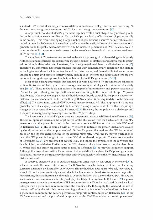
Energies 2020, 13, 1024

standard 1547, distributed energy resources (DERs) cannot cause voltage fluctuations exceeding 3%for a medium voltage interconnection and 5% for a low voltage interconnection [12].

A large number of distributed PV generators together create a duck-shaped daily net load profiledue to the variation in solar irradiation. The duck-shaped net load profile has steep slopes, especiallyin the evening. This requires bringing a large number of synchronous resources online within a shortperiod of time. Such changes in the net load profile cannot be easily addressed by slow conventionalgenerators and the problem becomes severe with the increased penetration of PVs. The existence of alarge number of PV generators also increases the chances of negative net load that requires curtailmentof PV power [8,13,14].

The number of PV generators connected to the electric power grid has been rising continuously.Authorities and researchers are considering the development of strategies and approaches to obtaingrid services, both transient and long-term, from the aggregation of these distributed resources [15].Therefore, PV generators have been coupled together with complementary generation and storagetechnologies to address the intermittencies and the disturbances, and these distributed resources areutilized to obtain grid services. Battery energy storage (BES) systems and super-capacitors are twoimportant energy storage approaches that can be coupled with PV generators [16–18].

Most of the existing approaches that combine BES with household PV-prosumers are concernedwith optimization of battery size, and energy management strategies to minimize electricitybills [19–21]. These methods do not address the impact of intermittency and power variation ofPVs on the grid. Moving average methods are used to mitigate the impact of abrupt PV powerdisturbances. However, moving average method does not directly control the ramp rate, depends onhistorical data, and operates the BES even though BES operation is not required due to the memoryeffect [22]. The direct ramp control of PV power is an effective method. The ramp-up of PV output isgenerally not a challenging issue, and it can be achieved using a proper controller without requiring astorage, at the expense of total extracted PV energy [23]. However, the ramp-down is a challenge, andit requires an energy storage to compensate for the PV power drop.

The fluctuations of wind/PV generators are compensated using the BES station in Reference [24].The control approach calculates the target power for the BES station from the fluctuations of wind/PVgenerators, and this power is shared by the constituting smaller BES units based on their SOC level.In Reference [22], a BES is coupled with a PV system to mitigate the power fluctuations causedby cloud passing using the ramping method. During PV power fluctuations, the BES is controlledbased on the inverse characteristics of the desired ramp-rate. Once the PV power fluctuation isover, the BES power is brought to zero using SOC droop-based ramp rate. The control strategiesof References [22,24] are presented at system level, and ignore the dynamics of the converter anddetails of the control design. Furthermore, the BES reference calculations involve complex algorithms.A hybrid BES and super-capacitor setup is used in Reference [25] to provide frequency support.Although this is combined with a PV generator, it does not directly address the PV power generationvariations. Moreover, the frequency does not directly and quickly reflect the PV disturbances at thedistribution level.

A battery is integrated in an ac-stack architecture in series with PV converters in Reference [26] toachieve the controlled ramp rate in power. The BES control uses the derivative of the rms of ac stringcurrent to determine the fluctuation in PV power. This method does not appear to be able to respond toabrupt PV fluctuations in a timely manner due to the limitations with a derivative operator in practice.Furthermore, this architecture is vulnerable to over-modulation that distorts the output. Finally, thestack architecture compromises the plug-and-play flexibility of the system. In Reference [27], a powermanagement strategy is proposed for a BES in connection to a PV and a local load. If the local loadis larger than a predefined minimum value, the combined PV-BES supply the load and the rest ofpower is offset by the grid. No power ramping is done in this mode. If the local load is less thana predefined minimum, the battery performs a ramp rate control, based on Reference [22], if thePV fluctuations exceed the predefined ramp rate; and the PV-BES operates in constant power feed

124

Energies 2020, 13, 1024

mode otherwise. Further details of the control design procedures are not presented. A PV-batterycombination connected to an ac grid is presented in Reference [28] where the PV operates at the MPP,a battery controls the dc bus voltage of the inverter and the inverter operates in constant power mode.If the reference power of the inverter is properly determined, it can realize ramping. However, this isnot discussed in Reference [28]. One limitation of this approach is that the BES cannot be used for analready operating inverter without altering the control system of the inverter. A similar approach isused in Reference [29] where the BES supplies/absorbs the difference of power between the desiredand the PV power. The controller in Reference [29] requires communication of an ac signal which is amajor limitation. In Reference [30], a 1 MW/2 MWh BES is connected with a multi-MW PV system toachieve (1) power smoothing using moving average and low pass filter, and (2) frequency regulationusing P-f droop control. The power smoothing method of Reference [30] has the disadvantages of themoving average approach mentioned earlier. Also, the frequency regulation may not be useful at thedistribution level.

Most of the aforementioned works that implement BES to smooth PV power treat the matterat the system level and ignore the dynamics at the converters level. There is a lack of systematicdesign of the local controls to accomplish the desired power ramps. This paper presents a BES controlsystem concept to address both the abrupt and daily variations of PV power. The proposed BESconnects at the terminals of the PV generator (without requiring a change in the PV inverter) andresponds to the disturbances to execute desired power ramp rates. The ramp rate signals are eithergenerated locally or received from the grid operator. The paper presents the complete mathematicalmodel of the system including the dynamics of the converter and provides systematic approach indesigning the control. Furthermore, if the BES is only used to filter the abrupt PV disturbances for ashort period, it results in low utilization of the BES. Therefore, the ramping capability of the PV-BESsystem has been utilized in this paper to improve the daily load profile. The grid operator can remotelycommand the distributed PV-BES units with the desired ramp rate, and the proposed control executesthe command. The aggregated effect of the distributed PV-BES units with the proposed rampingcapability significantly enhances the daily net load profile in terms of (1) reduced peak, (2) increasedminimum, and (3) reduced slopes. The proposed method also includes an outer loop that controlsthe SOC of the BES. The performance of the proposed system is verified using extensive computersimulation and a laboratory prototype.

The contributions of this paper may be summarized as follows: (1) A simple yet effectivebattery control philosophy to address both the abrupt and daily photovoltaic generation variations.The two set-points of the proposed controller can be generated locally or through communications forsystem-wide optimization; (2) Complete modeling and control design of the battery control system;(3) Verification of the proposed approach using simulations and laboratory tests.

The remainder of the paper is organized as follows. The power variabilities, abrupt and dailyprofile, originated from PV generators are discussed in Section 2. Section 3 presents a proposedbattery energy storage (BES) system, its mathematical model, and the proposed control to ramp theoutput power of the PV. Numerical designs and the results obtained both in simulation and laboratoryexperiment are presented in Section 4. The paper concludes with concluding remarks and limitationsof the proposed control in Section 5.

2. Power Variabilities of a PV Generator

2.1. Abrupt Disturbances in PV Generation

Cloud movements cause abrupt changes in solar irradiation, Figure 1. To study the impact ofthese abrupt power changes, a hybrid dc/ac system is considered in this paper as shown in Figure 2.The parameters of the dc microgrid and the ac system are shown in Tables 1 and 2, respectively.The details of the PV control used in this study are given in Section 4.1.1.

125

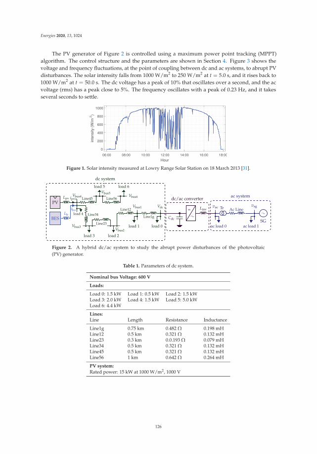
Energies 2020, 13, 1024

The PV generator of Figure 2 is controlled using a maximum power point tracking (MPPT)algorithm. The control structure and the parameters are shown in Section 4. Figure 3 shows thevoltage and frequency fluctuations, at the point of coupling between dc and ac systems, to abrupt PVdisturbances. The solar intensity falls from 1000 W/m2 to 250 W/m2 at t = 5.0 s, and it rises back to1000 W/m2 at t = 50.0 s. The dc voltage has a peak of 10% that oscillates over a second, and the acvoltage (rms) has a peak close to 5%. The frequency oscillates with a peak of 0.23 Hz, and it takesseveral seconds to settle.

06:00 08:00 10:00 12:00 14:00 16:00 18:00

Hour

0

200

400

600

800

1000

inte

nsity

(W

/m2)

Figure 1. Solar intensity measured at Lowry Range Solar Station on 18 March 2013 [31].

PVLpv ipvo

Vbus4

BESLb

iboload 4

Line45

Vbus5

load 5

Line56Vbus6

load 6

Line34

Vbus3

load 3

Line23

Vbus2

load 2

Line12Vbus1

load 1

Line1g

Vdc

load 0

Cdc

= Linvvac

ac load 0

Tr Ac Linevsg

ac load 1SG

dc system

ac systemdc/ac converter

Figure 2. A hybrid dc/ac system to study the abrupt power disturbances of the photovoltaic(PV) generator.

Table 1. Parameters of dc system.

Nominal bus Voltage: 600 V

Loads:

Load 0: 1.5 kW Load 1: 0.5 kW Load 2: 1.5 kWLoad 3: 2.0 kW Load 4: 1.5 kW Load 5: 5.0 kWLoad 6: 4.4 kW

Lines:Line Length Resistance Inductance

Line1g 0.75 km 0.482 Ω 0.198 mHLine12 0.5 km 0.321 Ω 0.132 mHLine23 0.3 km 0.0.193 Ω 0.079 mHLine34 0.5 km 0.321 Ω 0.132 mHLine45 0.5 km 0.321 Ω 0.132 mHLine56 1 km 0.642 Ω 0.264 mH

PV system:

Rated power: 15 kW at 1000 W/m2, 1000 V

126

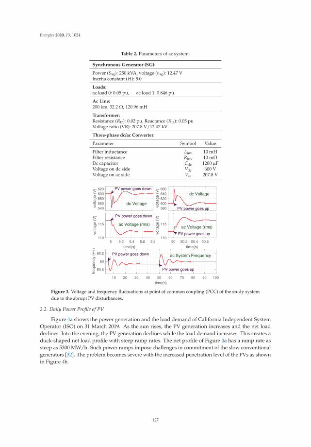
Energies 2020, 13, 1024

Table 2. Parameters of ac system.

Synchronous Generator (SG):

Power (Ssg): 250 kVA, voltage (vsg): 12.47 VInertia constant (H): 5.0

Loads:ac load 0: 0.05 pu, ac load 1: 0.846 pu

Ac Line:200 km, 32.2 Ω, 120.96 mH

Transformer:Resistance (Rtr): 0.02 pu, Reactance (Xtr): 0.05 puVoltage ratio (VR): 207.8 V/12.47 kV

Three-phase dc/ac Converter:

Parameter Symbol Value

Filter inductance Linv 10 mHFilter resistance Rinv 10 mΩDc capacitor Cdc 1200 μFVoltage on dc side Vdc 600 VVoltage on ac side Vac 207.8 V

540560580600620

volta

ge (

V)

dc Voltage580600620640660

volta

ge (

V)

dc Voltage

5 5.2 5.4 5.6 5.8

time(s)

110

115

volta

ge (

V)

ac Voltage (rms)

50 50.2 50.4 50.6

time(s)

110

115

volta

ge (

V)

ac Voltage (rms)

10 20 30 40 50 60 70 80 90 100

time(s)

59.8

60

60.2

freq

uenc

y (H

z)

ac System Frequency

PV power goes down

PV power goes up

PV power goes down

PV power goes up

PV power goes down

PV power goes up

Figure 3. Voltage and frequency fluctuations at point of common coupling (PCC) of the study systemdue to the abrupt PV disturbances.

2.2. Daily Power Profile of PV

Figure 4a shows the power generation and the load demand of California Independent SystemOperator (ISO) on 31 March 2019. As the sun rises, the PV generation increases and the net loaddeclines. Into the evening, the PV generation declines while the load demand increases. This creates aduck-shaped net load profile with steep ramp rates. The net profile of Figure 4a has a ramp rate assteep as 5300 MW/h. Such power ramps impose challenges in commitment of the slow conventionalgenerators [32]. The problem becomes severe with the increased penetration level of the PVs as shownin Figure 4b.

127

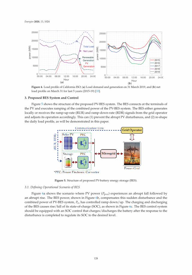
Energies 2020, 13, 1024

00:00 04:00 08:00 12:00 16:00 20:00 24:00

Hour

0

5000

10000

15000

20000

25000po

wer

(M

W)

PV Generation

Renewable Generation

Total Load

Net Load

(a)

00:00 04:00 08:00 12:00 16:00 20:00 24:00

Hour

0

5000

10000

15000

20000

25000

pow

er (

MW

)

20152016201720182019

(b)Figure 4. Load profile of California ISO; (a) Load demand and generation on 31 March 2019, and (b) netload profile on March 31 for last 5 years (2015-19) [33].

3. Proposed BES System and Control

Figure 5 shows the structure of the proposed PV-BES system. The BES connects at the terminals ofthe PV and executes ramping of the combined power of the PV-BES system. The BES either generateslocally or receives the ramp-up-rate (RUR) and ramp-down-rate (RDR) signals from the grid operatorand adjusts its operation accordingly. This can (1) prevent the abrupt PV disturbances, and (2) re-shapethe daily load profile, as will be demonstrated in this paper.

Figure 5. Structure of proposed PV-battery energy storage (BES).

3.1. Defining Operational Scenario of BES

Figure 6a shows the scenario where PV power (Ppvo) experiences an abrupt fall followed byan abrupt rise. The BES power, shown in Figure 6b, compensates this sudden disturbance and thecombined power of PV-BES system, Po, has controlled ramp down/up. The charging and dischargingof the BES causes rise/fall of its state-of-charge (SOC), as shown in Figure 6c. The BES control systemshould be equipped with an SOC control that charges/discharges the battery after the response to thedisturbance is completed to regulate its SOC to the desired level.

128

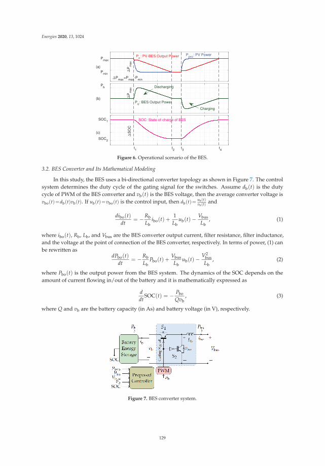
Energies 2020, 13, 1024

Ppvo: PV PowerPo: PV-BES Output PowerPmax

Pmin

ΔP

max

ΔPmax=Pmax-Pmin

(a)

Po: BES Output Power

Pb

ΔP

max

(b)

SOC: State-of-charge of BESSOC1

SOC2

ΔS

OC

t1 t2 t3 t4

(c)

Discharging

Charging

Figure 6. Operational scenario of the BES.

3.2. BES Converter and Its Mathematical Modeling

In this study, the BES uses a bi-directional converter topology as shown in Figure 7. The controlsystem determines the duty cycle of the gating signal for the switches. Assume db(t) is the dutycycle of PWM of the BES converter and vb(t) is the BES voltage, then the average converter voltage isvbo(t)=db(t)vb(t). If ub(t)=vbo(t) is the control input, then db(t)=

ub(t)vb(t)

and

dibo(t)dt

= −RbLb

ibo(t) +1Lb

ub(t)− VbusLb

, (1)

where ibo(t), Rb, Lb, and Vbus are the BES converter output current, filter resistance, filter inductance,and the voltage at the point of connection of the BES converter, respectively. In terms of power, (1) canbe rewritten as

dPbo(t)dt

= −RbLb

Pbo(t) +VbusLb

ub(t)−V2

busLb

, (2)

where Pbo(t) is the output power from the BES system. The dynamics of the SOC depends on theamount of current flowing in/out of the battery and it is mathematically expressed as

ddt

SOC(t) = − PboQvb

, (3)

where Q and vb are the battery capacity (in As) and battery voltage (in V), respectively.

Figure 7. BES converter system.

129

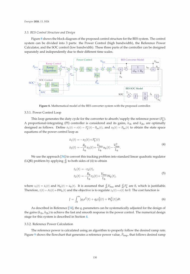
Energies 2020, 13, 1024

3.3. BES Control Structure and Design

Figure 8 shows the block diagram of the proposed control structure for the BES system. The controlsystem can be divided into 3 parts: the Power Control (high bandwidth), the Reference PowerCalculator, and the SOC control (low bandwidth). These three parts of the controller can be designedseparately and independently due to their different time scales.

RampAlgorithm

Ppvo +-

Prmp +

SOC∗ + ∫k1soc

-

k2soc

--

P∗soc

+

P∗b + ∫

k1b-

k2b

Pbo

--

-

Vbus

+ ÷ db

SOC

×

vb

+ - 1sLb + Rb

×ibo

Vbus

Pbo

÷vb

1Q

ib∫-1 +SOC

Ramp Control

SOC Control

Power Control BES Converter Model

BES SOC Model

Figure 8. Mathematical model of the BES converter system with the proposed controller.

3.3.1. Power Control Loop

This loop generates the duty cycle for the converter to absorb/supply the reference power (P∗b ).

A proportional-integrating (PI) controller is considered and its gains, k1b and k2b, are optimallydesigned as follows. Define x1(t) = e(t) = P∗

b (t)−Pbo(t), and x2(t) = Pbo(t) to obtain the state spaceequations of the power control loop as

x1(t) =−x2(t)+P∗b (t)

x2(t) =−RbLb

x2(t)+VbusLb

ub(t)−V2

busLb

.(4)

We use the approach [34] to convert this tracking problem into standard linear quadratic regulator(LQR) problem by applying d

dt to both sides of (4) to obtain

z1(t) =−z2(t),

z2(t) =−RbLb

z2(t)+VbusLb

Wb(t),(5)

where zi(t) = xi(t) and Wb(t) = ub(t). It is assumed that ddt Vbus and d

dt P∗b are 0, which is justifiable.

Therefore, z(t)=Az(t)+BWb(t) and the objective is to regulate z1(t)= e(t) to 0. The cost function is

J =∫ ∞

0[q1e2(t) + q2z2

2(t) + W2b(t)]dt. (6)

As described in Reference [34], the qi parameters can be systematically adjusted for the design ofthe gains (k1b, k2b) to achieve the fast and smooth response in the power control. The numerical designstage for this system is described in Section 4.

3.3.2. Reference Power Calculation

The reference power is calculated using an algorithm to properly follow the desired ramp rate.Figure 9 shows the flowchart that generates a reference power value, Prmp, that follows desired ramp

130

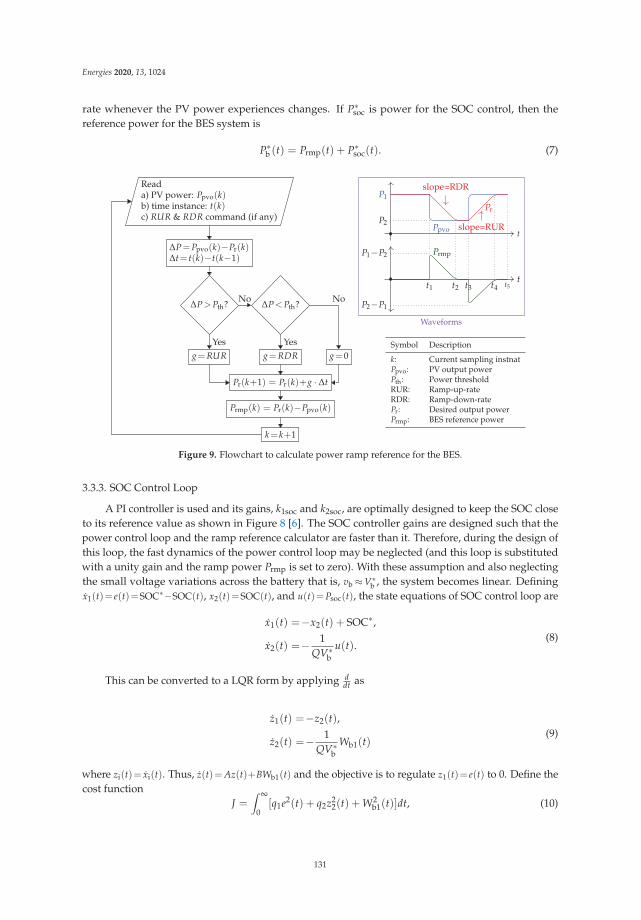
Energies 2020, 13, 1024

rate whenever the PV power experiences changes. If P∗soc is power for the SOC control, then the

reference power for the BES system is

P∗b (t) = Prmp(t) + P∗

soc(t). (7)

Reada) PV power: Ppvo(k)b) time instance: t(k)c) RUR & RDR command (if any)

ΔP=Ppvo(k)−Pr(k)Δt= t(k)−t(k−1)

ΔP>Pth? ΔP<Pth?No

g=RURYes

g=RDRYes

g=0

No

Pr(k+1) = Pr(k)+g · Δt

Prmp(k) = Pr(k)−Ppvo(k)

k= k+1

t

P1

PpvoP2

Pr

slope=RDR

slope=RUR

tt1

Prmp

t2 t3 t4 t5

P1−P2

P2−P1

Waveforms

Symbol Description

k: Current sampling instnatPpvo: PV output powerPth: Power thresholdRUR: Ramp-up-rateRDR: Ramp-down-ratePr: Desired output powerPrmp: BES reference power

Figure 9. Flowchart to calculate power ramp reference for the BES.

3.3.3. SOC Control Loop

A PI controller is used and its gains, k1soc and k2soc, are optimally designed to keep the SOC closeto its reference value as shown in Figure 8 [6]. The SOC controller gains are designed such that thepower control loop and the ramp reference calculator are faster than it. Therefore, during the design ofthis loop, the fast dynamics of the power control loop may be neglected (and this loop is substitutedwith a unity gain and the ramp power Prmp is set to zero). With these assumption and also neglectingthe small voltage variations across the battery that is, vb ≈V∗

b , the system becomes linear. Definingx1(t)= e(t)=SOC∗−SOC(t), x2(t)=SOC(t), and u(t)=Psoc(t), the state equations of SOC control loop are

x1(t) =−x2(t) + SOC∗,

x2(t) =− 1QV∗

bu(t).

(8)

This can be converted to a LQR form by applying ddt as

z1(t) =−z2(t),

z2(t) =− 1QV∗

bWb1(t)

(9)

where zi(t)= xi(t). Thus, z(t)=Az(t)+BWb1(t) and the objective is to regulate z1(t)= e(t) to 0. Define thecost function

J =∫ ∞

0[q1e2(t) + q2z2

2(t) + W2b1(t)]dt, (10)

131

Energies 2020, 13, 1024

and use the method of Reference [34] for the design of the gains (k1soc, k2soc) to achieve smooth responsein the SOC control. Numerical design is provided in Section 4.

3.4. Determining the BES Capacity

The battery capacity depends on the desired slowest power ramp of the PV and the BES combined.The minimum BES capacity (Qmin) is chosen such that during the maximum power disturbance (ΔPmax)the system operates at desired slowest power ramp (Rmin) keeping the SOC within the desired range(SOCmin, SOCmax) for all the time.

Figure 6 shows the typical desired response of the system. For maximum PV power fluctuationΔPmax (in W), the BES should be able to supply power with minimum ramp Rmin (in W/s) for the timeinterval T where T = ΔPmax

Rmin. Assuming that the battery voltage remains relatively constant at V∗

b (inV) during this period, the total charge supplied by the battery is 0.5TΔPmax

V∗b

(in As). If ΔSOCmax is themaximum permissible fluctuation in SOC from its nominal value, SOCn, during this period, then theminimum battery capacity required, Qmin (in As), is given by

Qmin =ΔP2

max2V∗

b RminΔSOCmax. (11)

4. Numerical Designs, Results, and Comparisons

This section presents some numerical designs of the proposed system and also investigates itsperformance in the context of both abrupt PV power variations and daily irradiation profile usingsimulations and laboratory-scale experimentation. The structure of the this section is as follows.(1) Section 4.1 studies the performance of proposed system in response to abrupt PV disturbancesin a simulated hybrid dc/ac system. (2) Section 4.2 shows the simulation results of applying theproposed system to address abrupt PV disturbances in a real irradiation profile data. (3) Section 4.3investigates the performance of the proposed method in mitigating the duck-curve phenomenon usingsimulations on practical data. (4) Section 4.4 shows the results of a laboratory-scale realization of theproposed method. (5) Section 4.5 shows the qualitative comparison of the proposed method withexisting methods to mitigate PV power fluctuations.

4.1. Abrupt Disturbances: Case Study 1

The proposed controller is applied to the study system of Figure 2 to study the impact of abruptPV disturbances. The design of system components are discussed first.

4.1.1. System and Control Parameters

Figure 10 and Table 3 show the PV system and its converter parameters. The controller gains ofthe PV system are designed using the method discussed in Reference [34]. The internal current loopis designed first, which gives k1pv and k2pv, and then the external loop is designed that includes thedesign of k3pv, k4pv,k5pv, and k6pv. In the design of the external loop, all the dynamics of the internalloop are carried along. Therefore, unlike common practice, the internal loop is not limited to be severaltimes faster than the external loop. In our study, the PV operates at MPPT using perturb and observe(P&O) algorithm [35]. However, this is not a requirement for the proposed BES controller.

132

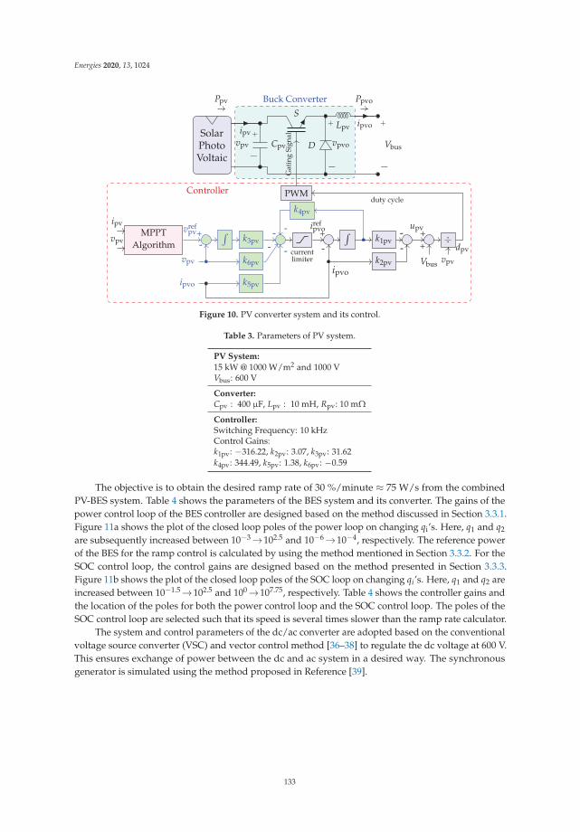
Energies 2020, 13, 1024

SolarPhotoVoltaic

Buck Converter

ipv

Cpv

+

−vpv

S

D

+

−

vpvo

Lpv ipvo +

−Vbus

Ppv Ppvo

MPPTAlgorithm

ipv

vpv

vrefpv+ ∫

k3pv-

k6pv

-vpv

-

k5pvipvo

- currentlimiter

+irefpvo ∫

k1pv

ipvo

--

k2pv

-+

upv

÷vpv

dpv

Vbus

+

k4pv

-

PWM

Gat

ing

Sign

al

duty cycleController

Figure 10. PV converter system and its control.

Table 3. Parameters of PV system.

PV System:

15 kW @ 1000 W/m2 and 1000 VVbus: 600 V

Converter:Cpv : 400 μF, Lpv : 10 mH, Rpv: 10 mΩ

Controller:Switching Frequency: 10 kHzControl Gains:k1pv: −316.22, k2pv: 3.07, k3pv: 31.62k4pv: 344.49, k5pv: 1.38, k6pv: −0.59

The objective is to obtain the desired ramp rate of 30 %/minute ≈ 75 W/s from the combinedPV-BES system. Table 4 shows the parameters of the BES system and its converter. The gains of thepower control loop of the BES controller are designed based on the method discussed in Section 3.3.1.Figure 11a shows the plot of the closed loop poles of the power loop on changing qi’s. Here, q1 and q2

are subsequently increased between 10−3→102.5 and 10−6→10−4, respectively. The reference powerof the BES for the ramp control is calculated by using the method mentioned in Section 3.3.2. For theSOC control loop, the control gains are designed based on the method presented in Section 3.3.3.Figure 11b shows the plot of the closed loop poles of the SOC loop on changing qi’s. Here, q1 and q2 areincreased between 10−1.5→102.5 and 100→107.75, respectively. Table 4 shows the controller gains andthe location of the poles for both the power control loop and the SOC control loop. The poles of theSOC control loop are selected such that its speed is several times slower than the ramp rate calculator.

The system and control parameters of the dc/ac converter are adopted based on the conventionalvoltage source converter (VSC) and vector control method [36–38] to regulate the dc voltage at 600 V.This ensures exchange of power between the dc and ac system in a desired way. The synchronousgenerator is simulated using the method proposed in Reference [39].

133

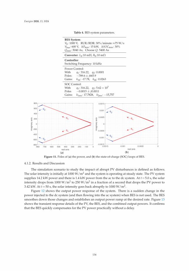
Energies 2020, 13, 1024

Table 4. BES system parameters.

BES System:Vb: 1000 V, RUR/RDR: 30%/minute ≈75 W/sVbus: 600 V, ΔPmax: 15 kW, ΔSOCmax: 30%Qmin: 5040 As, Choose Q: 5400 As

Converter: Lb:10 mH, Rb:10 mΩ

Controller:Switching Frequency: 10 kHz

Power Control:With q1: 316.22, q2: 0.0001Poles: −789.6 ± j665.9Gains: k1b: -17.78, k2b: 0.0263

SOC Control:With q1: 316.22, q2: 5.62 × 107

Poles −0.0015 ± j0.0011Gains: k1soc: 17.7828, k2soc: −15,757

-800 -700 -600 -500 -400 -300 -200 -100 0

real axis

-800

-600

-400

-200

0

200

400

600

800

imag

inar

y ax

is q1

q1

q2

q2

(a)

-0.0015 -0.001 -0.0005 0

real axis

-0.0015

-0.001

-0.0005

0

0.0005

0.001

0.0015

imag

inar

y ax

is q1

q1

q2

q2

(b)

Figure 11. Poles of (a) the power, and (b) the state-of-charge (SOC) loops of BES.

4.1.2. Results and Discussion

The simulation scenario to study the impact of abrupt PV disturbances is defined as follows.The solar intensity is initially at 1000 W/m2 and the system is operating at steady state. The PV systemsupplies 14.2 kW power and there is 1.4 kW power from the ac to the dc system. At t=5.0 s, the solarintensity drops from 1000 W/m2 to 250 W/m2 in a fraction of a second that drops the PV power to3.42 kW. At t=50 s, the solar intensity goes back abruptly to 1000 W/m2.

Figure 12 shows the output power response of the system. There is a sudden change in thepower injected to the dc system (and then flowing into the ac system) when BES is not used. The BESsmoothes down those changes and establishes an output power ramp at the desired rate. Figure 13shows the transient response details of the PV, the BES, and the combined output powers. It confirmsthat the BES quickly compensates for the PV power practically without a delay.

134

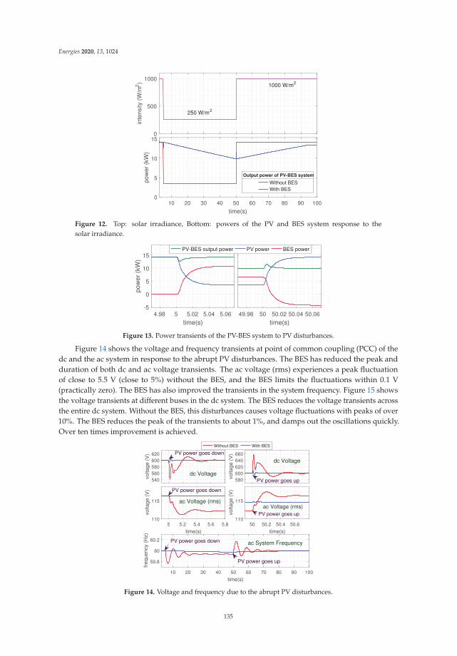
Energies 2020, 13, 1024

0

500

1000

inte

nsity

(W

/m2)

250 W/m2

1000 W/m2

10 20 30 40 50 60 70 80 90 100

time(s)

0

5

10

15po

wer

(kW

)

Without BESWith BES

Output power of PV-BES system

Figure 12. Top: solar irradiance, Bottom: powers of the PV and BES system response to thesolar irradiance.

4.98 5 5.02 5.04 5.06

time(s)

-5

0

5

10

15

pow

er (

kW)

49.98 50 50.02 50.04 50.06

time(s)

PV-BES output power PV power BES power

Figure 13. Power transients of the PV-BES system to PV disturbances.

Figure 14 shows the voltage and frequency transients at point of common coupling (PCC) of thedc and the ac system in response to the abrupt PV disturbances. The BES has reduced the peak andduration of both dc and ac voltage transients. The ac voltage (rms) experiences a peak fluctuationof close to 5.5 V (close to 5%) without the BES, and the BES limits the fluctuations within 0.1 V(practically zero). The BES has also improved the transients in the system frequency. Figure 15 showsthe voltage transients at different buses in the dc system. The BES reduces the voltage transients acrossthe entire dc system. Without the BES, this disturbances causes voltage fluctuations with peaks of over10%. The BES reduces the peak of the transients to about 1%, and damps out the oscillations quickly.Over ten times improvement is achieved.

540560580600620

volta

ge (

V)

dc Voltage580600620640660

volta

ge (

V)

dc Voltage

5 5.2 5.4 5.6 5.8

time(s)

110

115

volta

ge (

V)

ac Voltage (rms)

50 50.2 50.4 50.6

time(s)

110

115

volta

ge (

V)

ac Voltage (rms)

10 20 30 40 50 60 70 80 90 100

time(s)

59.8

60

60.2

freq

uenc

y (H

z)

ac System Frequency

Without BES With BES

PV power goes down

PV power goes up

PV power goes down

PV power goes up

PV power goes down

PV power goes up

Figure 14. Voltage and frequency due to the abrupt PV disturbances.

135

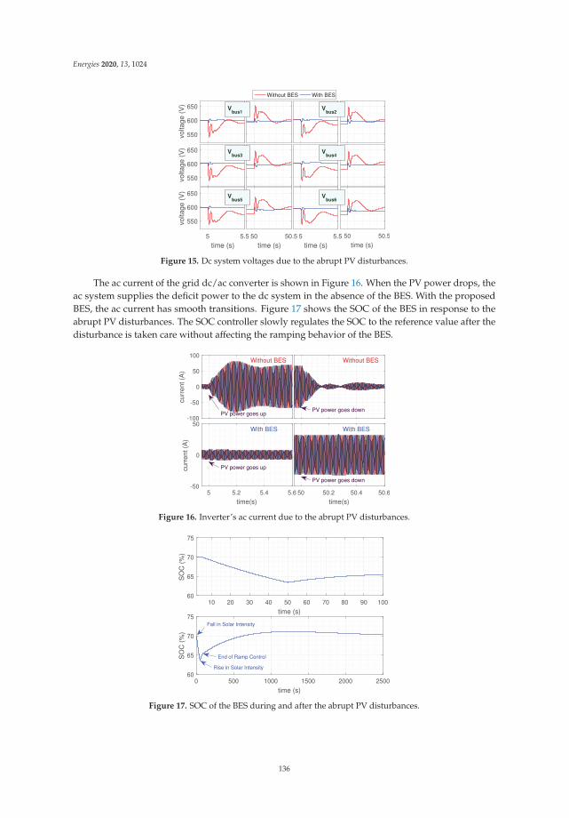
Energies 2020, 13, 1024

550

600

650

volta

ge (

V)

550

600

650

volta

ge (

V)

5 5.5

time (s)

550

600

650

volta

ge (

V)

50 50.5

time (s)5 5.5

time (s)50 50.5

time (s)

Without BES With BES

Vbus1

Vbus2

Vbus3

Vbus4

Vbus5

Vbus6

Figure 15. Dc system voltages due to the abrupt PV disturbances.

The ac current of the grid dc/ac converter is shown in Figure 16. When the PV power drops, theac system supplies the deficit power to the dc system in the absence of the BES. With the proposedBES, the ac current has smooth transitions. Figure 17 shows the SOC of the BES in response to theabrupt PV disturbances. The SOC controller slowly regulates the SOC to the reference value after thedisturbance is taken care without affecting the ramping behavior of the BES.

-100

-50

0

50

100

curr

ent (

A)

Without BES Without BES

5 5.2 5.4 5.6

time(s)

-50

0

50

curr

ent (

A)

With BES

50 50.2 50.4 50.6

time(s)

With BES

PV power goes upPV power goes down

PV power goes up

PV power goes down

Figure 16. Inverter’s ac current due to the abrupt PV disturbances.

10 20 30 40 50 60 70 80 90 100

time (s)

60

65

70

75

SO

C (

%)

0 500 1000 1500 2000 2500

time (s)

60

65

70

75

SO

C (

%)

Fall in Solar Intensity

Rise in Solar Intensity

End of Ramp Control

Figure 17. SOC of the BES during and after the abrupt PV disturbances.

136

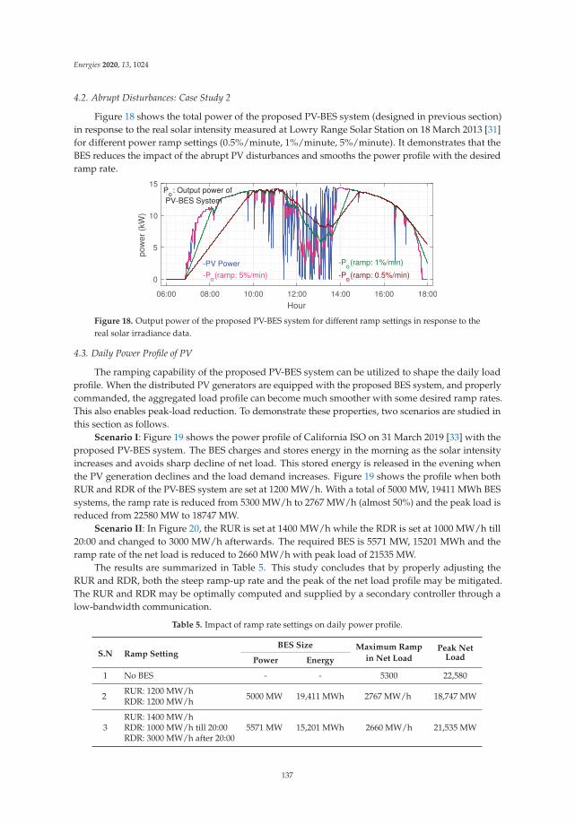
Energies 2020, 13, 1024

4.2. Abrupt Disturbances: Case Study 2

Figure 18 shows the total power of the proposed PV-BES system (designed in previous section)in response to the real solar intensity measured at Lowry Range Solar Station on 18 March 2013 [31]for different power ramp settings (0.5%/minute, 1%/minute, 5%/minute). It demonstrates that theBES reduces the impact of the abrupt PV disturbances and smooths the power profile with the desiredramp rate.

06:00 08:00 10:00 12:00 14:00 16:00 18:00

Hour

0

5

10

15

pow

er (

kW)

-PV Power

-Po(ramp: 5%/min)

-Po(ramp: 1%/min)

-Po(ramp: 0.5%/min)

Po: Output power of PV-BES System

Figure 18. Output power of the proposed PV-BES system for different ramp settings in response to thereal solar irradiance data.

4.3. Daily Power Profile of PV

The ramping capability of the proposed PV-BES system can be utilized to shape the daily loadprofile. When the distributed PV generators are equipped with the proposed BES system, and properlycommanded, the aggregated load profile can become much smoother with some desired ramp rates.This also enables peak-load reduction. To demonstrate these properties, two scenarios are studied inthis section as follows.

Scenario I: Figure 19 shows the power profile of California ISO on 31 March 2019 [33] with theproposed PV-BES system. The BES charges and stores energy in the morning as the solar intensityincreases and avoids sharp decline of net load. This stored energy is released in the evening whenthe PV generation declines and the load demand increases. Figure 19 shows the profile when bothRUR and RDR of the PV-BES system are set at 1200 MW/h. With a total of 5000 MW, 19411 MWh BESsystems, the ramp rate is reduced from 5300 MW/h to 2767 MW/h (almost 50%) and the peak load isreduced from 22580 MW to 18747 MW.

Scenario II: In Figure 20, the RUR is set at 1400 MW/h while the RDR is set at 1000 MW/h till20:00 and changed to 3000 MW/h afterwards. The required BES is 5571 MW, 15201 MWh and theramp rate of the net load is reduced to 2660 MW/h with peak load of 21535 MW.

The results are summarized in Table 5. This study concludes that by properly adjusting theRUR and RDR, both the steep ramp-up rate and the peak of the net load profile may be mitigated.The RUR and RDR may be optimally computed and supplied by a secondary controller through alow-bandwidth communication.

Table 5. Impact of ramp rate settings on daily power profile.

S.N Ramp SettingBES Size Maximum Ramp

in Net LoadPeak Net

LoadPower Energy

1 No BES - - 5300 22,580

2 RUR: 1200 MW/h 5000 MW 19,411 MWh 2767 MW/h 18,747 MWRDR: 1200 MW/h

3RUR: 1400 MW/h

5571 MW 15,201 MWh 2660 MW/h 21,535 MWRDR: 1000 MW/h till 20:00RDR: 3000 MW/h after 20:00

137

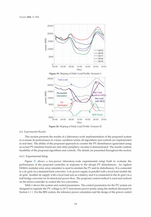
Energies 2020, 13, 1024

00:00 04:00 08:00 12:00 16:00 20:00 24:00

Hour

0

5000

10000

15000

20000

25000

pow

er (

MW

)

20152016201720182019

Figure 19. Shaping of Daily Load Profile: Scenario I.

00:00 04:00 08:00 12:00 16:00 20:00 24:00

Hour

-5000

0

5000

10000

15000

20000

25000

pow

er (

MW

)

PV Generation

Renewable Generation

Total Load

Net Load (without BES)

BES Power

Net Load (with BES)

Figure 20. Shaping of Daily Load Profile: Scenario II.

4.4. Experimental Results

This section presents the results of a laboratory-scale implementation of the proposed systemto evaluate its performance in a basic condition where all algorithms and controls are implementedin real time. The ability of the proposed approach to counter the PV disturbances (generated usingan actual PV emulator hardware and other periphery circuits) is demonstrated. The results confirmfeasibility of the proposed algorithms and controls. The details are presented throughout the section.

4.4.1. Experimental Setup

Figure 21 shows a low-power laboratory-scale experimental setup built to evaluate theperformance of the proposed controller in response to the abrupt PV disturbances. An AgilentE4360A modular solar array simulator is used to emulate the PV and its disturbances. It is connectedto a dc grid via a standard buck converter. A dc power supply in parallel with a local load models thedc grid. Another dc supply with a local load acts as a battery, and it is connected to the dc grid via ahalf-bridge converter for bi-directional power flow. The proposed control method is used and realizedon the micro-controller to control the two converters.

Table 6 shows the system and control parameters. The control parameters for the PV system aredesigned to regulate the PV voltage to 20 V (maximum power point) using the method discussed inSection 4.1.1. For the BES system, the reference power calculation and the design of the power control

138

Energies 2020, 13, 1024

parameters are done using the method in Section 3.3. We have ignored the SOC control and the acsystem due to limitations in experimental setup.

Figure 21. Experimental setup.

Table 6. Experimental setup parameters.

Modular Solar Array Simulator:PV Curve I: Vmp: 20.0 V, Imp: 0.3 A, Voc: 23.0 V, Isc: 0.5 APV Curve II: Vmp: 20.0 V, Imp: 2.0 A, Voc: 23.0 V, Isc: 2.5 A

PV converter: Lpv: 1 mH, Rpv: 0.2587 Ω, Cpv: 100μF

BES and converter: Vb: 30.0 V, Local Load: 30 Ω, Lb: 1 mH, Rb: 0.250 Ω

Dc bus: Vbus: 10.0 V, Local Load: 2 Ω

Controller:Switching Frequency: 32 kHzPV converter control gainsk1pv: −56.23, k2pv: 0.18, k3pv: 10.00, k4pv: 382.76, k5pv: 1.02, k6pv: −0.16BES controller settingsRUR & RDR: 1.0 W/s, Control Gains: k1b= −5.6234, k2b= 0.0189 (Power control)

4.4.2. Results

Figure 22a shows the response of the system for the ramp rate setting of 1.0 W/s (for both RDR &RUR). Abrupt PV disturbances are manually applied to the PV emulator by switching from PV Curve Ito PV Curve II and vice versa as specified in Table 6. When the PV conveter output increases, thebattery quickly intervenes to absorb the power. Similarly, the battery supplies power when there isabrupt fall in PV converter power. With the grid voltage of 10 V, the ramp rate of 0.1 A/s in current isobtained. Figure 23 shows the results when the PV power experiences random abrupt disturbances.The study presented in this section confirms that the proposed control system can be successfullyimplemented in real-time on a typical hardware platform and the desired ramping rates set by theuser are achieved by the combination of PV and proposed BES control system.

139

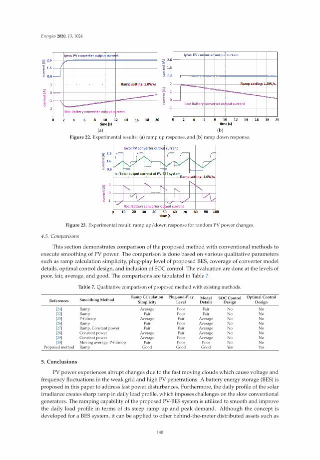
Energies 2020, 13, 1024

(a) (b)Figure 22. Experimental results: (a) ramp up response, and (b) ramp down response.

Figure 23. Experimental result: ramp up/down response for random PV power changes.

4.5. Comparisons

This section demonstrates comparison of the proposed method with conventional methods toexecute smoothing of PV power. The comparison is done based on various qualitative parameterssuch as ramp calculation simplicity, plug-play level of proposed BES, coverage of converter modeldetails, optimal control design, and inclusion of SOC control. The evaluation are done at the levels ofpoor, fair, average, and good. The comparisons are tabulated in Table 7.

Table 7. Qualitative comparison of proposed method with existing methods.

References Smoothing MethodRamp Calculation

Simplicity

Plug-and-Play

LevelModelDetails

SOC ControlDesign

Optimal Control

Design

[24] Ramp Average Poor Fair No No[22] Ramp Fair Poor Fair No No[25] P-f droop Average Fair Average No No[26] Ramp Fair Poor Average No No[27] Ramp, Constant power Fair Fair Average No No[28] Constant power Average Fair Average No No[29] Constant power Average Poor Average No No[30] Moving average, P-f droop Fair Poor Poor No No

Proposed method Ramp Good Good Good Yes Yes

5. Conclusions

PV power experiences abrupt changes due to the fast moving clouds which cause voltage andfrequency fluctuations in the weak grid and high PV penetrations. A battery energy storage (BES) isproposed in this paper to address fast power disturbances. Furthermore, the daily profile of the solarirradiance creates sharp ramp in daily load profile, which imposes challenges on the slow conventionalgenerators. The ramping capability of the proposed PV-BES system is utilized to smooth and improvethe daily load profile in terms of its steep ramp up and peak demand. Although the concept isdeveloped for a BES system, it can be applied to other behind-the-meter distributed assets such as

140

Energies 2020, 13, 1024

small gas turbine generators. The optimal computation and communication of the storage ramp ratesare the future directions of research. To mention a limitation, the proposed approach of this paperrequires the BES to be co-located with the PV and have access to its terminals in order to achieve thedesired power ramping of the combined PV-BES.

Author Contributions: Conceptualization, R.S. and M.K.-G.; Modeling and simulation, R.S.; Formal analysis, R.S.and M.K.-G.; Investigation, R.S.; Writing–original draft preparation, R.S. and M.K.-G.; Writing–review and editing,R.S. and M.K.-G.; Supervision, M.K.-G.; Funding acquisition, M.K.-G. All authors have read and agreed to thepublished version of the manuscript.

Funding: This research work was partially supported by National Science Foundation (NSF 1808368).

Conflicts of Interest: The authors declare no conflict of interest.

Abbreviations

PV Photovoltaic BES Battery Energy StorageDER Distributed Energy Resources LQR Linear quadratic regulatorMPPT Maximum power point tracking PCC Point of common couplingPI Proportional Integrator pu per unitRDR Ramp Down Rate RUR Ramp Up RateSG Synchronous generator SOC State of ChargeISO Independent System OperatorSymbols and Variables

t Time k Sampling instantΔt Change in time Ssg Synchronous generator powervsg Voltage of synchronous generator H Inertia constantRtr Resistance of transformer Xtr Reactance of transformerVR Transformer voltage ratio Vdc Dc voltage at the PCCVac L-L rms ac voltage at PCC Linv Filter inductance of dc/ac converterRinv Filter resistance of dc/ac converter Cdc Capacitor on dc side of dc/ac converterVbus Voltage at PV-BES connection Vbus i Voltage of ith busRUR Ramp up rate RDR Ramp down rateRmin Minimum ramp rate Ppv PV powerPpvo Output power of PV converter ΔP Change in PV powerPr Desired output power ΔPmax Maximum change in PV powerPo Total output power of PV-BES system Lpv Filter inductance of PV converterCpv Capacitor across PV terminals Rpv Filter resistance of PV converterki pv PV control ith gain ipv PV currentipvo Output current of PV converter vpv PV voltagevref

pv PV reference voltage Vmp PV voltage at maximum PV powerImp PV current at maximum PV power Voc Open-circuit voltage of PVIsc Short-circuit current of PV P∗

b BES reference powerP∗

soc Reference power for SOC control of BES Pb Battery PowerPbo Output power of BES converter ib Battery currentibo Output current of BES converter db Duty cycle for BES converterub Control input of BES converter vb Battery voltageV∗

b Nominal voltage of battery SOC State of charge of BESSOCn Nominal SOC of BES ΔSOC Change in SOC of BESΔSOCmax Maximum change in SOC Lb Filter inductance of BES converterRb Filter resistance of BES converter Q Battery capacityQmin Minimum battery capacity ki b BES power control ith gainki soc ith gain of SOC control J Cost functionqi ith weighting factor in cost function

141

Energies 2020, 13, 1024

References

1. Al-Hallaj, S. More than enviro-friendly: Renewable energy is also good for the bottom line. IEEE PowerEnergy Mag. 2004, 2, 16–22. [CrossRef]

2. Hu, J.; Li, Z.; Zhu, J.; Guerrero, J.M. Voltage Stabilization: A Critical Step Toward High PhotovoltaicPenetration. IEEE Ind. Electron. Mag. 2019, 13, 17–30. [CrossRef]

3. Administration, U.E.I. Annual Energy Outlook 2019: With Projections to 2050. 2019. Available online:https://www.eia.gov/outlooks/aeo/pdf/aeo2019.pdf (accessed on 8 April 2019).

4. Kroposki, B.; Johnson, B.; Zhang, Y.; Gevorgian, V.; Denholm, P.; Hodge, B.M.; Hannegan, B. Achieving a100% renewable grid: Operating electric power systems with extremely high levels of variable renewableenergy. IEEE Power Energy Mag. 2017, 15, 61–73. [CrossRef]

5. Silwal, S.; Karimi-Ghartemani, M. On Transient Responses of a Class of PV Inverters. IEEE Trans.Sustain. Energy 2019, 10, 311–314. [CrossRef]

6. Qunais, T.; Sharma, R.; Karimi-Ghartemani, M.; Silwal, S.; Khajehoddin, S.A. Application of BatteryStorage System to Improve Transient Responses in a Distribution Grid. In Proceedings of the 2019 IEEE28th International Symposium on Industrial Electronics (ISIE), Vancouver, BC, Canada, 12–14 June 2019;pp. 52–57.

7. Mather, B.A.; Shah, S.; Norris, B.L.; Dise, J.H.; Yu, L.; Paradis, D.; Katiraei, F.; Seguin, R.; Costyk, D.;Woyak, J.; et al. NREL/SCE High Penetration PV Integration Project: FY13 Annual Report; Technical Report;National Renewable Energy Lab. (NREL): Golden, CO, USA, 2014.

8. Katiraei, F.; Aguero, J.R. Solar PV integration challenges. IEEE Power Energy Mag. 2011, 9, 62–71. [CrossRef]9. Bueno, P.G.; Hernández, J.C.; Ruiz-Rodriguez, F.J. Stability assessment for transmission systems with large

utility-scale photovoltaic units. IET Renew. Power Gener. 2016, 10, 584–597. [CrossRef]10. Sakamuri, J.N.; Das, K.; Altin, M.; Cutululis, N.A.; Hansen, A.D.; Tielens, P.; Van Hertem, D. Improved

frequency control from wind power plants considering wind speed variation. In Proceedings of the 2016Power Systems Computation Conference (PSCC), Genoa, Italy, 20–24 June 2016; pp. 1–7.

11. Gevorgian, V.; Booth, S. Review of PREPA Technical Requirements for Interconnecting Wind and Solar Generation;Technical Report; National Renewable Energy Lab. (NREL): Golden, CO, USA, 2013.

12. IEEE Std 1547-2018 Standard for Interconnection and Interoperability of Distributed Energy Resources withAssociated Electric Power Systems Interfaces. 2018; pp. 1–138. Available online: https://ieeexplore.ieee.org/abstract/document/8332112 (accessed on 8 April 2019).

13. Denholm, P.; O’Connell, M.; Brinkman, G.; Jorgenson, J. Overgeneration from Solar Energy in California. A FieldGuide to the Duck Chart; Technical Report; National Renewable Energy Lab. (NREL): Golden, CO, USA, 2015.

14. Ghosh, S.; Rahman, S.; Pipattanasomporn, M. Distribution voltage regulation through active powercurtailment with PV inverters and solar generation forecasts. IEEE Trans. Sustain. Energy 2016, 8, 13–22.[CrossRef]

15. Xue, Y.; Guerrero, J.M. Smart Inverters for Utility and Industry Applications. In Proceedings of the PCIMEurope 2015; International Exhibition and Conference for Power Electronics, Intelligent Motion, RenewableEnergy and Energy Management, Nuremberg, Germany, 19–21 May 2015; pp. 1–8.

16. Bragard, M.; Soltau, N.; Thomas, S.; De Doncker, R.W. The balance of renewable sources and user demandsin grids: Power electronics for modular battery energy storage systems. IEEE Trans. Power Electron. 2010,25, 3049–3056. [CrossRef]

17. Teleke, S.; Baran, M.E.; Bhattacharya, S.; Huang, A.Q. Rule-based control of battery energy storage fordispatching intermittent renewable sources. IEEE Trans. Sustain. Energy 2010, 1, 117–124. [CrossRef]

18. Ceja-Espinosa, C.; Espinosa-Juárez, E. Smoothing of photovoltaic power generation using batteries as energystorage. In Proceedings of the 2017 IEEE PES—Innovative Smart Grid Technologies Conference-LatinAmerica (ISGT Latin America), Quito, Ecuador, 20–22 September 2017; pp. 1–6.

19. Lujano-Rojas, J.M.; Dufo-López, R.; Bernal-Agustín, J.L.; Catalão, J.P. Optimizing daily operation of batteryenergy storage systems under real-time pricing schemes. IEEE Trans. Smart Grid 2016, 8, 316–330. [CrossRef]

20. Hernández, J.; Sanchez-Sutil, F.; Muñoz-Rodríguez, F. Design criteria for the optimal sizing of a hybridenergy storage system in PV household-prosumers to maximize self-consumption and self-sufficiency.Energy 2019, 186, 115827. [CrossRef]

142

Energies 2020, 13, 1024

21. Gomez-Gonzalez, M.; Hernandez, J.; Vera, D.; Jurado, F. Optimal sizing and power schedule in PVhousehold-prosumers for improving PV self-consumption and providing frequency containment reserve.Energy 2020, 191, 116554. [CrossRef]

22. Alam, M.; Muttaqi, K.; Sutanto, D. A novel approach for ramp-rate control of solar PV using energy storageto mitigate output fluctuations caused by cloud passing. IEEE Trans. Energy Convers. 2014, 29, 507–518.

23. Sangwongwanich, A.; Yang, Y.; Blaabjerg, F. A cost-effective power ramp-rate control strategy forsingle-phase two-stage grid-connected photovoltaic systems. In Proceedings of the Energy ConversionCongress and Exposition (ECCE), Milwaukee, WI, USA, 18–22 September 2016; pp. 1–7.

24. Li, X.; Hui, D.; Lai, X. Battery energy storage station (BESS)-based smoothing control of photovoltaic (PV)and wind power generation fluctuations. IEEE Trans. Sustain. Energy 2013, 4, 464–473. [CrossRef]

25. Hernández, J.C.; Bueno, P.G.; Sanchez-Sutil, F. Enhanced utility-scale photovoltaic units with frequencysupport functions and dynamic grid support for transmission systems. IET Renew. Power Gener. 2017,11, 361–372. [CrossRef]

26. Kim, N.; Parkhideh, B. Control and Operating Range Analysis of AC-Stacked PV Inverter ArchitectureIntegrated with Battery. IEEE Trans. Power Electron. 2018, 33, 10032–10037. [CrossRef]

27. Tran, V.T.; Islam, M.R.; Sutanto, D.; Muttaqi, K.M. Mitigation of Solar PV Intermittency Using Ramp-RateControl of Energy Buffer Unit. IEEE Trans. Energy Convers. 2018, 34, 435–445. [CrossRef]

28. Saxena, N.; Hussain, I.; Singh, B.; Vyas, A.L. Implementation of a Grid-Integrated PV-Battery System forResidential and Electrical Vehicle Applications. IEEE Trans. Ind. Electron. 2018, 65, 6592–6601. [CrossRef]

29. Zhang, Q.; Sun, K. A Flexible Power Control for PV-Battery-Hybrid System Using Cascaded H-BridgeConverters. IEEE J. Emerg. Sel. Top. Power Electron. 2018, 7, 2184–2195. [CrossRef]

30. Rallabandi, V.; Akeyo, O.M.; Jewell, N.; Ionel, D.M. Incorporating Battery Energy Storage Systems IntoMulti-MW Grid Connected PV Systems. IEEE Trans. Ind. Appl. 2019, 55, 638–647. [CrossRef]

31. Yoder, M.; Andreas, A. Lowry Range Solar Station: Arapahoe County, Colorado (Data). Available online:https://data.nrel.gov/submissions/30 (accessed on 8 April 2019).

32. Lew, D.; Miller, N. Reaching new solar heights: integrating high penetrations of PV into the power system.IET Renew. Power Gener. 2017, 11, 20–26, doi:10.1049/iet-rpg.2016.0264. [CrossRef]

33. California ISO. Renewables and Emission Reports. Available online: http://www.caiso.com/market/Pages/ReportsBulletins/RenewablesReporting.aspx (accessed on 8 April 2019).

34. Karimi-Ghartemani, M.; Khajehoddin, S.A.; Jain, P.; Bakhshai, A. Linear quadratic output tracking anddisturbance rejection. Int. J. Control 2011, 84, 1442–1449. [CrossRef]

35. De Brito, M.A.G.; Galotto, L.; Sampaio, L.P.; e Melo, G.d.A.; Canesin, C.A. Evaluation of the main MPPTtechniques for photovoltaic applications. IEEE Trans. Ind. Electron. 2013, 60, 1156–1167. [CrossRef]

36. Kazmierkowski, M.P.; Malesani, L. Current control techniques for three-phase voltage-source PWMconverters: A survey. IEEE Trans. Ind. Electron. 1998, 45, 691–703. [CrossRef]

37. Blaabjerg, F.; Teodorescu, R.; Liserre, M.; Timbus, A.V. Overview of Control and Grid Synchronizationfor Distributed Power Generation Systems. IEEE Trans. Ind. Electron. 2006, 53, 1398–1409,doi:10.1109/TIE.2006.881997. [CrossRef]

38. Silwal, S.; Karimi-Ghartemani, M.; Sharma, R.; Karimi, H. Impact of Feed-forward andDecoupling Terms on Stability of Grid-Connected Inverters. In Proceedings of the 2019 IEEE 28thInternational Symposium on Industrial Electronics (ISIE), Vancouver, BC, Canada, 12–14 June 2019;pp. 2641–2646, doi:10.1109/ISIE.2019.8781454. [CrossRef]

39. Silwal, S.; Taghizadeh, S.; Karimi Ghartemani, M.; Hossain, J.; Davari, M. An Enhanced Control Systemfor Single-Phase Inverters Interfaced with Weak and Distorted Grids. IEEE Trans. Power Electron. 2019, 34,12538–12551, doi:10.1109/TPEL.2019.2909532. [CrossRef]

c© 2020 by the authors. Licensee MDPI, Basel, Switzerland. This article is an open accessarticle distributed under the terms and conditions of the Creative Commons Attribution(CC BY) license (http://creativecommons.org/licenses/by/4.0/).

143

energies

Article

Why PV Modules Should Preferably No Longer BeOriented to the South in the Near Future

Riyad Mubarak *, Eduardo Weide Luiz and Gunther Seckmeyer

Institute for Meteorology and Climatology, Leibniz Universität Hannover, Herrenhäuser Straße 2,30419 Hannover, Germany; luiz@muk.uni-hannover.de (E.W.L.); seckmeyer@muk.uni-hannover.de (G.S.)* Correspondence: mubarak@muk.uni-hannover.de

Received: 7 October 2019; Accepted: 25 November 2019; Published: 28 November 2019

Abstract: PV modules tilted and oriented toward east and west directions gain gradually moreimportance as an alternative to the presently-preferred south (north in the Southern Hemisphere)orientation and it is shown to become economically superior even under the reimbursement offeed-in tariff (FIT). This is a consequence of the increasing spread between the decreasing costs ofself-consumed solar power and the costs for power from the grid. One-minute values of irradiancewere measured by silicon sensors at different orientations and tilt angles in Hannover (Germany)over three years. We show that south-oriented collectors give the highest electrical power during theday, whereas combinations of east and west orientations (E-W) result in the highest self-consumptionrate (SC), and combinations of southeast and southwest (SE-SW) orientations result in the highestdegree of autarky (AD), although they reduce the yearly PV Power by 5–6%. Moreover, the economicanalysis of PV systems without FIT shows that the SE-SW and E-W combinations have the lowestelectricity cost and they are more beneficial in terms of internal rate of return (IRR), compared to the Sorientation at the same tilt. For PV systems with FIT, the S orientation presently provides the highesttransfer of money from the supplier. However, as a consequence of the continuing decline of FIT, theeconomic advantage of S orientation is decreasing. E-W and SE-SW orientations are more beneficialfor the owner as soon as FIT decreases to 7 Ct/kWh. East and west orientations of PV modules donot only have benefits for the individual owner but avoid high costs for storing energy—regardlesswho would own the storage facilities—and by avoiding high noon peaks of solar energy productionduring sunny periods, which would become an increasing problem for the grid if more solar power isinstalled. Furthermore, two types of commonly used PV software (PVSOL and PVsyst) were used tosimulate the system performance. The comparison with measurements showed that both PV softwareunderestimate SC and AD for all studied orientations, leading to the conclusion that improvementsare necessary in modelling.

Keywords: incident solar radiation; PV output power modelling; tilt angle; orientation; rooftop solar

1. Introduction

Decarbonization of our energy supply is an important component to fulfill pledges of the ParisAgreement to keep the global warming below 1.5 ◦C, because 65% of the world’s current CO2 emissionsare due to burning fossil fuels [1]. Renewable energy is one of the most cost-effective options to replacefossil fuels and to reduce electricity-related emissions. In recent years, many countries have begun atransition to more sustainable energy supply based on renewable energies. Solar energy represents themost abundant natural energy resource on the earth and has the potential to replace fossil fuels tosatisfy this clean energy demand of our society in future [2]. This exceptional energy source is the mostsimple and economic renewable energy technology available that can be easily installed, especially onrooftops of houses. The costs for solar modules, measured in $/Wp, have reduced by as much as 90%during the last decade and are expected to fall further in the future [3].

Energies 2019, 12, 4528; doi:10.3390/en12234528 www.mdpi.com/journal/energies145

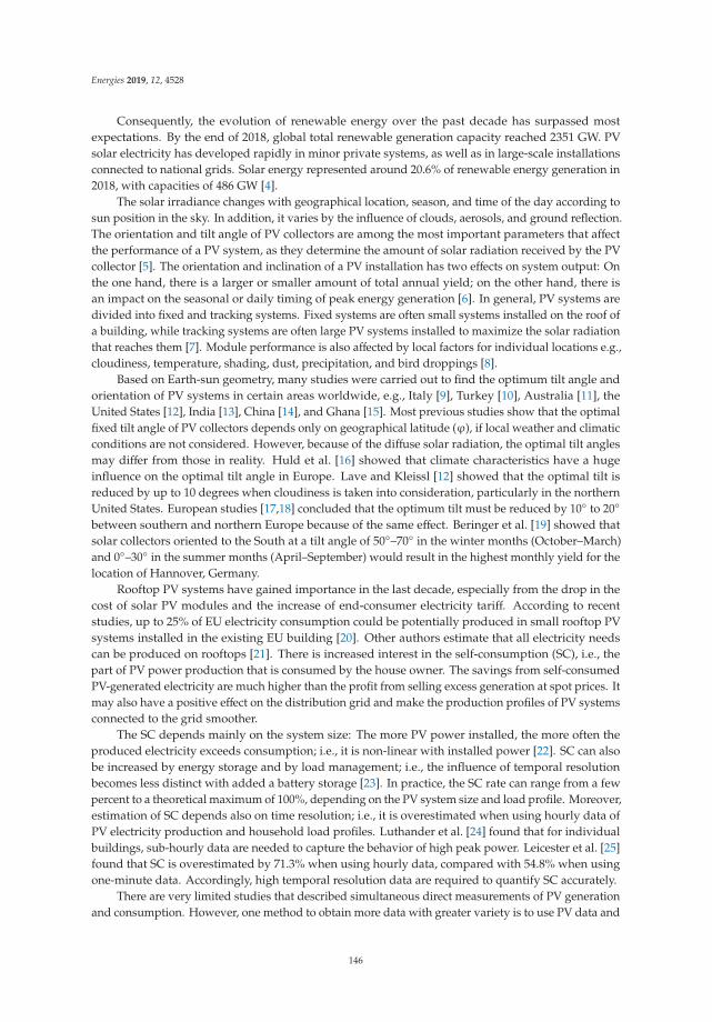
Energies 2019, 12, 4528

Consequently, the evolution of renewable energy over the past decade has surpassed mostexpectations. By the end of 2018, global total renewable generation capacity reached 2351 GW. PVsolar electricity has developed rapidly in minor private systems, as well as in large-scale installationsconnected to national grids. Solar energy represented around 20.6% of renewable energy generation in2018, with capacities of 486 GW [4].

The solar irradiance changes with geographical location, season, and time of the day according tosun position in the sky. In addition, it varies by the influence of clouds, aerosols, and ground reflection.The orientation and tilt angle of PV collectors are among the most important parameters that affectthe performance of a PV system, as they determine the amount of solar radiation received by the PVcollector [5]. The orientation and inclination of a PV installation has two effects on system output: Onthe one hand, there is a larger or smaller amount of total annual yield; on the other hand, there isan impact on the seasonal or daily timing of peak energy generation [6]. In general, PV systems aredivided into fixed and tracking systems. Fixed systems are often small systems installed on the roof ofa building, while tracking systems are often large PV systems installed to maximize the solar radiationthat reaches them [7]. Module performance is also affected by local factors for individual locations e.g.,cloudiness, temperature, shading, dust, precipitation, and bird droppings [8].

Based on Earth-sun geometry, many studies were carried out to find the optimum tilt angle andorientation of PV systems in certain areas worldwide, e.g., Italy [9], Turkey [10], Australia [11], theUnited States [12], India [13], China [14], and Ghana [15]. Most previous studies show that the optimalfixed tilt angle of PV collectors depends only on geographical latitude (ϕ), if local weather and climaticconditions are not considered. However, because of the diffuse solar radiation, the optimal tilt anglesmay differ from those in reality. Huld et al. [16] showed that climate characteristics have a hugeinfluence on the optimal tilt angle in Europe. Lave and Kleissl [12] showed that the optimal tilt isreduced by up to 10 degrees when cloudiness is taken into consideration, particularly in the northernUnited States. European studies [17,18] concluded that the optimum tilt must be reduced by 10◦ to 20◦between southern and northern Europe because of the same effect. Beringer et al. [19] showed thatsolar collectors oriented to the South at a tilt angle of 50◦–70◦ in the winter months (October–March)and 0◦–30◦ in the summer months (April–September) would result in the highest monthly yield for thelocation of Hannover, Germany.

Rooftop PV systems have gained importance in the last decade, especially from the drop in thecost of solar PV modules and the increase of end-consumer electricity tariff. According to recentstudies, up to 25% of EU electricity consumption could be potentially produced in small rooftop PVsystems installed in the existing EU building [20]. Other authors estimate that all electricity needscan be produced on rooftops [21]. There is increased interest in the self-consumption (SC), i.e., thepart of PV power production that is consumed by the house owner. The savings from self-consumedPV-generated electricity are much higher than the profit from selling excess generation at spot prices. Itmay also have a positive effect on the distribution grid and make the production profiles of PV systemsconnected to the grid smoother.

The SC depends mainly on the system size: The more PV power installed, the more often theproduced electricity exceeds consumption; i.e., it is non-linear with installed power [22]. SC can alsobe increased by energy storage and by load management; i.e., the influence of temporal resolutionbecomes less distinct with added a battery storage [23]. In practice, the SC rate can range from a fewpercent to a theoretical maximum of 100%, depending on the PV system size and load profile. Moreover,estimation of SC depends also on time resolution; i.e., it is overestimated when using hourly data ofPV electricity production and household load profiles. Luthander et al. [24] found that for individualbuildings, sub-hourly data are needed to capture the behavior of high peak power. Leicester et al. [25]found that SC is overestimated by 71.3% when using hourly data, compared with 54.8% when usingone-minute data. Accordingly, high temporal resolution data are required to quantify SC accurately.

There are very limited studies that described simultaneous direct measurements of PV generationand consumption. However, one method to obtain more data with greater variety is to use PV data and

146

Energies 2019, 12, 4528

separately-obtained load profile data, and estimate the SC fraction [25]. With the present reimbursementfor feed-in tariffs that value just the yearly sum fed into the grid, suitability studies focused for rooftophave just concentrated on the yearly yield. Many studies and online web tools concerning the suitabilityof the orientation of rooftop implicitly take only the yearly sum into account [26]. Calculations for thediurnal variability are lacking.

In this study, we use one-minute data to compare the outputs of 12 solar collectors at various tiltand azimuth angles in order to propose an alternative concept for increasing SC via non-south-orientedPV systems and investigate its potential. The calculations are based on measurements from siliconsensors with different orientations and tilt angles in Hannover (Germany). The SC of all orientationsis calculated by using a set of separately measured load profiles in order to evaluate the best andmore-economic orientations for rooftop PV systems. The results are also compared with the simulatedvalues of two widely used PV software packages, PVSOL [27] and PVsyst [28] to validate this software.Detailed information about the simulation parameters are listed in Tables.

2. Methodology

The input dataset used in this study is composed of one-minute output of 12 solar collectors(Figure 1) installed for three years (2016–2018) on the roof of the Institute for Meteorology andClimatology (IMUK) of the Leibniz Universität Hannover (Hannover, Germany; 52.23◦ N, 9.42◦ Eand 50 m above sea level). Measurements have been made, using crystalline silicon PV devices withindividual temperature sensors (Mencke and Tegtmeyer GmbH, Hameln, Germany). The PV deviceshave been calibrated by the manufacturer in November 2013 and they are cleaned regularly to preventthe accumulation of dirt and dust. In addition, all devices are compared after one year of measurementsby placing them side by side horizontally. These comparisons were performed under different weatherconditions and have showed an agreement within ±3%.

Figure 1. Set of solar PV devices based on silicon sensors mounted in several different tilt angles andorientations, operational at the IMUK (Institute for Meteorology and Climatology) [IMUK, 2017].

Two groups of identical devices are considered here: The first group consist of devices with 45◦tilt, oriented to S, E, W, SE, and SW; the second group consists of vertical devices, oriented to S, E, W,SE, SW, and N. The tilt angle for the first group (45◦) is chosen to represent the large number of roofpitches, where most residential houses in Germany were built with a tilted roof angle between 40◦ and45◦ [29]. According to the initial design of the measurement system, the S measurements are conductedat tilt angles of 40◦ and 50◦, therefore we take the average of both sensors (40◦ and 50◦) to represent thePV outputs at 45◦ tilt; the uncertainty resulting from this procedure and other orientation uncertaintiesare less than 1% according to PVGIS calculations. Table 1 shows an overview about the inclination

147

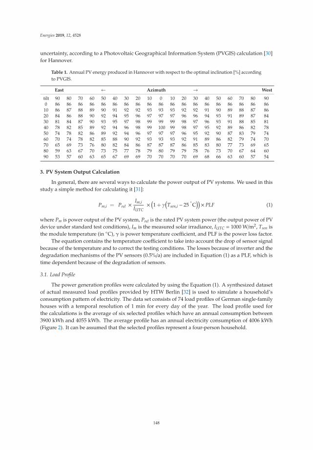
Energies 2019, 12, 4528

uncertainty, according to a Photovoltaic Geographical Information System (PVGIS) calculation [30]for Hannover.

Table 1. Annual PV energy produced in Hannover with respect to the optimal inclination [%] accordingto PVGIS.

East ← Azimuth → West

tilt 90 80 70 60 50 40 30 20 10 0 10 20 30 40 50 60 70 80 900 86 86 86 86 86 86 86 86 86 86 86 86 86 86 86 86 86 86 86

10 86 87 88 89 90 91 92 92 93 93 93 92 92 91 90 89 88 87 8620 84 86 88 90 92 94 95 96 97 97 97 96 96 94 93 91 89 87 8430 81 84 87 90 93 95 97 98 99 99 99 98 97 96 93 91 88 85 8140 78 82 85 89 92 94 96 98 99 100 99 98 97 95 92 89 86 82 7850 74 78 82 86 89 92 94 96 97 97 97 96 95 92 90 87 83 79 7460 70 74 78 82 85 88 90 92 93 93 93 92 91 89 86 82 79 74 7070 65 69 73 76 80 82 84 86 87 87 87 86 85 83 80 77 73 69 6580 59 63 67 70 73 75 77 78 79 80 79 79 78 76 73 70 67 64 6090 53 57 60 63 65 67 69 69 70 70 70 70 69 68 66 63 60 57 54

3. PV System Output Calculation

In general, there are several ways to calculate the power output of PV systems. We used in thisstudy a simple method for calculating it [31]:

Pm,i = Prel ×Im,i

IUTC×

(1 + γ

(Tsen,i − 25

◦C))× PLF (1)

where Pm is power output of the PV system, Prel is the rated PV system power (the output power of PVdevice under standard test conditions), Im is the measured solar irradiance, IUTC = 1000 W/m2, Tsen isthe module temperature (in ◦C), γ is power temperature coefficient, and PLF is the power loss factor.

The equation contains the temperature coefficient to take into account the drop of sensor signalbecause of the temperature and to correct the testing conditions. The losses because of inverter and thedegradation mechanisms of the PV sensors (0.5%/a) are included in Equation (1) as a PLF, which istime dependent because of the degradation of sensors.

3.1. Load Profile

The power generation profiles were calculated by using the Equation (1). A synthesized datasetof actual measured load profiles provided by HTW Berlin [32] is used to simulate a household’sconsumption pattern of electricity. The data set consists of 74 load profiles of German single-familyhouses with a temporal resolution of 1 min for every day of the year. The load profile used forthe calculations is the average of six selected profiles which have an annual consumption between3900 kWh and 4055 kWh. The average profile has an annual electricity consumption of 4006 kWh(Figure 2). It can be assumed that the selected profiles represent a four-person household.

148

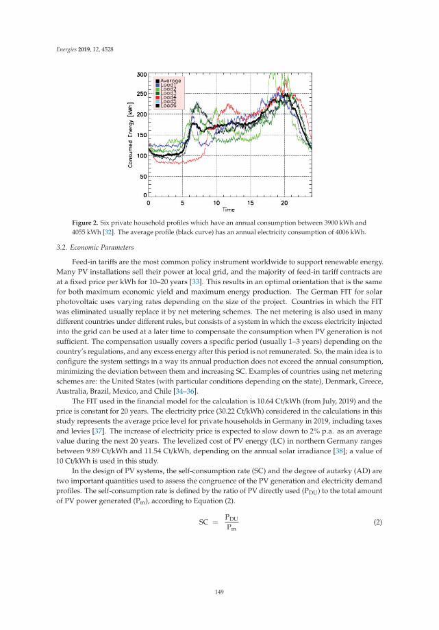
Energies 2019, 12, 4528

Figure 2. Six private household profiles which have an annual consumption between 3900 kWh and4055 kWh [32]. The average profile (black curve) has an annual electricity consumption of 4006 kWh.

3.2. Economic Parameters

Feed-in tariffs are the most common policy instrument worldwide to support renewable energy.Many PV installations sell their power at local grid, and the majority of feed-in tariff contracts areat a fixed price per kWh for 10–20 years [33]. This results in an optimal orientation that is the samefor both maximum economic yield and maximum energy production. The German FIT for solarphotovoltaic uses varying rates depending on the size of the project. Countries in which the FITwas eliminated usually replace it by net metering schemes. The net metering is also used in manydifferent countries under different rules, but consists of a system in which the excess electricity injectedinto the grid can be used at a later time to compensate the consumption when PV generation is notsufficient. The compensation usually covers a specific period (usually 1–3 years) depending on thecountry’s regulations, and any excess energy after this period is not remunerated. So, the main idea is toconfigure the system settings in a way its annual production does not exceed the annual consumption,minimizing the deviation between them and increasing SC. Examples of countries using net meteringschemes are: the United States (with particular conditions depending on the state), Denmark, Greece,Australia, Brazil, Mexico, and Chile [34–36].

The FIT used in the financial model for the calculation is 10.64 Ct/kWh (from July, 2019) and theprice is constant for 20 years. The electricity price (30.22 Ct/kWh) considered in the calculations in thisstudy represents the average price level for private households in Germany in 2019, including taxesand levies [37]. The increase of electricity price is expected to slow down to 2% p.a. as an averagevalue during the next 20 years. The levelized cost of PV energy (LC) in northern Germany rangesbetween 9.89 Ct/kWh and 11.54 Ct/kWh, depending on the annual solar irradiance [38]; a value of10 Ct/kWh is used in this study.

In the design of PV systems, the self-consumption rate (SC) and the degree of autarky (AD) aretwo important quantities used to assess the congruence of the PV generation and electricity demandprofiles. The self-consumption rate is defined by the ratio of PV directly used (PDU) to the total amountof PV power generated (Pm), according to Equation (2).

SC =PDU

Pm(2)

149

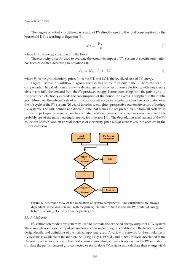
Energies 2019, 12, 4528

The degree of autarky is defined as a ratio of PV directly used to the total consumption by thehousehold [39], according to Equation (3).

AD =PDU

L(3)

where L is the energy consumed by the loads.The electricity price PE used to evaluate the economic impact of PV system at specific orientation

has been calculated according to Equation (4).

PE = (PG − PFi) + LC (4)

where PG is the grid electricity price, PFi is the FIT, and LC is the levelized cost of PV energy.Figure 3 shows a workflow diagram used in this study to calculate the SC with the feed-in

components. The calculations are always dependent on the consumption of electricity, with the primaryobjective to fulfil the demand from the PV produced energy, before purchasing from the public grid. Ifthe produced electricity exceeds the consumption of the house, the excess is supplied to the publicgrid. Moreover, the internal rate of return (IRR) for all available orientations has been calculated overthe life cycle of the PV system (20 years) in order to enlighten prospective owners/investors of rooftopPV systems. The IRR, defined as a discount rate that makes the net present value from all cash flowsfrom a project equal to zero, is used to evaluate the attractiveness of a project or investment, and it isprobably one of the most meaningful metric for investors [40]. The degradation mechanisms of the PVcollectors (0.5%/a) and an annual increase of electricity price (2%/a) were taken into account in theIRR calculations.

Figure 3. Schematic view of the calculation of system components. The calculations are alwaysdependent on the load demand, with the primary objective to fulfil it from the PV produced energy,before purchasing electricity from the public grid.

3.3. PV Software

PV estimation models are generally used to estimate the expected energy output of a PV system.These models need specific input parameters such as meteorological conditions of the location, systemdesign details, and definitions of the main components used. A variety of software for the simulation ofPV systems is available in the market, including PVsyst, PVSOL, and others. PVsyst, developed at theUniversity of Geneva, is one of the most common modeling software tools used in the PV industry tosimulate the performance of grid-connected or stand-alone PV systems and calculate their energy yield.

150

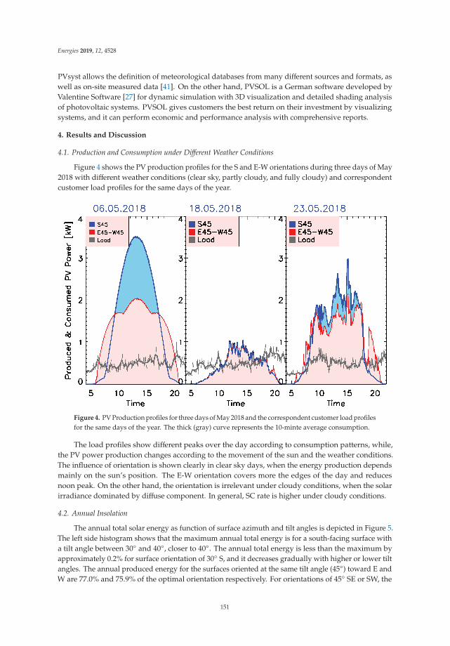
Energies 2019, 12, 4528

PVsyst allows the definition of meteorological databases from many different sources and formats, aswell as on-site measured data [41]. On the other hand, PVSOL is a German software developed byValentine Software [27] for dynamic simulation with 3D visualization and detailed shading analysisof photovoltaic systems. PVSOL gives customers the best return on their investment by visualizingsystems, and it can perform economic and performance analysis with comprehensive reports.

4. Results and Discussion

4.1. Production and Consumption under Different Weather Conditions

Figure 4 shows the PV production profiles for the S and E-W orientations during three days of May2018 with different weather conditions (clear sky, partly cloudy, and fully cloudy) and correspondentcustomer load profiles for the same days of the year.

Figure 4. PV Production profiles for three days of May 2018 and the correspondent customer load profilesfor the same days of the year. The thick (gray) curve represents the 10-minte average consumption.

The load profiles show different peaks over the day according to consumption patterns, while,the PV power production changes according to the movement of the sun and the weather conditions.The influence of orientation is shown clearly in clear sky days, when the energy production dependsmainly on the sun’s position. The E-W orientation covers more the edges of the day and reducesnoon peak. On the other hand, the orientation is irrelevant under cloudy conditions, when the solarirradiance dominated by diffuse component. In general, SC rate is higher under cloudy conditions.

4.2. Annual Insolation

The annual total solar energy as function of surface azimuth and tilt angles is depicted in Figure 5.The left side histogram shows that the maximum annual total energy is for a south-facing surface witha tilt angle between 30◦ and 40◦, closer to 40◦. The annual total energy is less than the maximum byapproximately 0.2% for surface orientation of 30◦ S, and it decreases gradually with higher or lower tiltangles. The annual produced energy for the surfaces oriented at the same tilt angle (45◦) toward E andW are 77.0% and 75.9% of the optimal orientation respectively. For orientations of 45◦ SE or SW, the

151

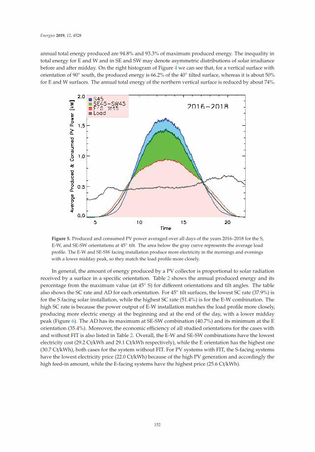
Energies 2019, 12, 4528

annual total energy produced are 94.8% and 93.3% of maximum produced energy. The inequality intotal energy for E and W and in SE and SW may denote asymmetric distributions of solar irradiancebefore and after midday. On the right histogram of Figure 4 we can see that, for a vertical surface withorientation of 90◦ south, the produced energy is 66.2% of the 40◦ tilted surface, whereas it is about 50%for E and W surfaces. The annual total energy of the northern vertical surface is reduced by about 74%.

Figure 5. Produced and consumed PV power averaged over all days of the years 2016–2018 for the S,E-W, and SE-SW orientations at 45◦ tilt. The area below the gray curve represents the average loadprofile. The E-W and SE-SW facing installation produce more electricity in the mornings and eveningswith a lower midday peak, so they match the load profile more closely.

In general, the amount of energy produced by a PV collector is proportional to solar radiationreceived by a surface in a specific orientation. Table 2 shows the annual produced energy and itspercentage from the maximum value (at 45◦ S) for different orientations and tilt angles. The tablealso shows the SC rate and AD for each orientation. For 45◦ tilt surfaces, the lowest SC rate (37.9%) isfor the S facing solar installation, while the highest SC rate (51.4%) is for the E-W combination. Thehigh SC rate is because the power output of E-W installation matches the load profile more closely,producing more electric energy at the beginning and at the end of the day, with a lower middaypeak (Figure 6). The AD has its maximum at SE-SW combination (40.7%) and its minimum at the Eorientation (35.4%). Moreover, the economic efficiency of all studied orientations for the cases withand without FIT is also listed in Table 2. Overall, the E-W and SE-SW combinations have the lowestelectricity cost (29.2 Ct/kWh and 29.1 Ct/kWh respectively), while the E orientation has the highest one(30.7 Ct/kWh), both cases for the system without FIT. For PV systems with FIT, the S-facing systemshave the lowest electricity price (22.0 Ct/kWh) because of the high PV generation and accordingly thehigh feed-in amount, while the E-facing systems have the highest price (25.6 Ct/kWh).

152

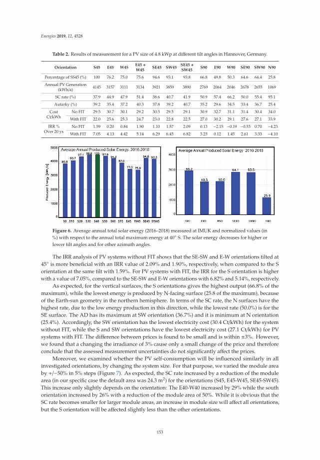
Energies 2019, 12, 4528

Table 2. Results of measurement for a PV size of 4.8 kWp at different tilt angles in Hannover, Germany.

Orientation S45 E45 W45E45 +W45

SE45 SW45SE45 +SW45

S90 E90 W90 SE90 SW90 N90

Percentage of SS45 (%) 100 76.2 75.0 75.6 94.6 93.1 93.8 66.8 49.8 50.3 64.6 64.4 25.8

Annual PV Generation(kWh/a) 4145 3157 3111 3134 3921 3859 3890 2769 2064 2046 2678 2655 1069

SC rate (%) 37.9 44.9 47.9 51.4 38.6 40.7 41.9 50.9 57.4 66.2 50.0 55.4 95.1

Autarky (%) 39.2 35.4 37.2 40.3 37.8 39.2 40.7 35.2 29.6 34.5 33.4 36.7 25.4

CostCt/kWh

No FIT 29.5 30.7 30.1 29.2 30.5 29.5 29.1 30.9 32.7 31.1 31.4 30.4 34.0

With FIT 22.0 25.6 25.3 24.7 23.0 22.8 22.5 27.0 30.2 29.1 27.6 27.1 33.9

IRR %Over 20 ys

No FIT 1.59 0.20 0.84 1.90 1.10 1.57 2.09 0.13 −2.15 −0.19 −0.53 0.70 −4.23

With FIT 7.05 4.13 4.42 5.14 6.29 6.45 6.82 3.23 0.12 1.45 2.61 3.33 −4.10

Figure 6. Average annual total solar energy (2016–2018) measured at IMUK and normalized values (in%) with respect to the annual total maximum energy at 40◦ S. The solar energy decreases for higher orlower tilt angles and for other azimuth angles.

The IRR analysis of PV systems without FIT shows that the SE-SW and E-W orientations tilted at45◦ is more beneficial with an IRR value of 2.09% and 1.90%, respectively, when compared to the Sorientation at the same tilt with 1.59%. For PV systems with FIT, the IRR for the S orientation is higherwith a value of 7.05%, compared to the SE-SW and E-W orientations with 6.82% and 5.14%, respectively.

As expected, for the vertical surfaces, the S orientations gives the highest output (66.8% of themaximum), while the lowest energy is produced by N-facing surface (25.8 of the maximum), becauseof the Earth-sun geometry in the northern hemisphere. In terms of the SC rate, the N surfaces have thehighest rate, due to the low energy production in this direction, while the lowest rate (50.0%) is for theSE surface. The AD has its maximum at SW orientation (36.7%) and it is minimum at N orientation(25.4%). Accordingly, the SW orientation has the lowest electricity cost (30.4 Ct/kWh) for the systemwithout FIT, while the S and SW orientations have the lowest electricity cost (27.1 Ct/kWh) for PVsystems with FIT. The difference between prices is found to be small and is within ±3%. However,we found that a changing the irradiance of 3% cause only a small change of the price and thereforeconclude that the assessed measurement uncertainties do not significantly affect the prices.

Moreover, we examined whether the PV self-consumption will be influenced similarly in allinvestigated orientations, by changing the system size. For that purpose, we varied the module areaby +/−50% in 5% steps (Figure 7). As expected, the SC rate increased by a reduction of the modulearea (in our specific case the default area was 24.3 m2) for the orientations (S45, E45-W45, SE45-SW45).This increase only slightly depends on the orientation: The E40-W40 increased by 29% while the southorientation increased by 26% with a reduction of the module area of 50%. While it is obvious that theSC rate becomes smaller for larger module areas, an increase in module size will affect all orientations,but the S orientation will be affected slightly less than the other orientations.

153

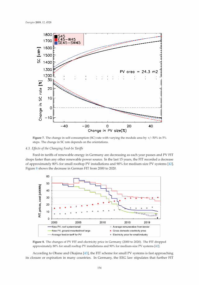
Energies 2019, 12, 4528

Figure 7. The change in self-consumption (SC) rate with varying the module area by +/−50% in 5%steps. The change in SC rate depends on the orientations.

4.3. Effects of the Changing Feed-In Tariffs

Feed-in tariffs of renewable energy in Germany are decreasing as each year passes and PV FITdrops faster than any other renewable power source. In the last 15 years, the FIT recorded a decreaseof approximately 80% for small rooftop PV installations and 90% for medium-size PV systems [42].Figure 8 shows the decrease in German FIT from 2000 to 2020.

Figure 8. The changes of PV FIT and electricity price in Germany (2000 to 2020). The FIT droppedapproximately 80% for small rooftop PV installations and 90% for medium-size PV systems [42].

According to Obane and Okajima [43], the FIT scheme for small PV systems is fast approachingits closure or expiration in many countries. In Germany, the EEG law stipulates that further FIT

154

Energies 2019, 12, 4528

systems will not be allowed, when the total PV installations reach 52 GW. At the end of April 2018, thecountry had 43.8 GW PV installed. With the current tenders of PV, this cap is expected to be reached in2020 [44]. However, the German government presently reconsidering this plan and is considering toallow FIT in future when the 52 GW is exceeded. With decreasing FIT self-consumption is gaininghigher importance, especially with increasing cost of delivering PV electricity and rapid decline inthe cost of solar PV modules. In addition, after 2020, the FIT will gradually expire for the oldest PVplants [42] and the produced PV power will be mainly used for SC. Thus, E-W and SE-SW orientationswill provide the highest SC rate and will be more beneficial for the householders. Our calculationshows that the higher benefit of south orientation is no longer existent if FIT decreases to 7.0 Ct/kWhor lower, where at least the SE-SW orientation will have a higher IRR that the S orientation.

The economic calculations above were done for the conditions of the present FIT in Germany.The major conclusions, however, can used for many countries around the world, which apply FIT orsimilar PV cost structures. The results are especially relevant for the countries, which offer a very lowFIT (e.g., New Zealand and Portugal) or for which eliminated the FIT scheme (e.g., UK, Spain, CzechRepublic, Italy).

4.4. Comparison with PV Software

For simulation of the IMUK measurement system, a fixed PV system configuration, consisting ofa 4.8 kWp is considered in the calculations, corresponding to the installation of 24 modules. Moreover,the same load profile that is used for the calculation of SC and AD at IMUK is also used in both models.Table 3 shows the important model parameters used in the simulation.

Table 3. Model parameters used in comparison.

Parameter Model (PVSol, PVSyst)

Modules 4.8 kWp, mono, 24 modulesInverter ABB, 4.6 kW

Climate data Meteonorm 7.2Transposition model Perez-Ineichen model

Diffuse radiation model Perez model

Both simulation programs have been run for each orientation separately. Table 4 shows thesimulated annually produced energies for all studied orientations and tilt angles. The programsoverestimate the south-tilted irradiance and most of the studied orientations. This may result fromthe use of an anisotropic model (Perez-Ineichen model) to calculate the tilted irradiance, where wefound in a previous study [45] that anisotropic models overestimate the south-tilted irradiance andmost vertical-tilted irradiances.

The table also shows the SC and AD fractions for each orientation. For the 45◦-tilt surfaces,the lowest SC (PVsyst = 32.9% and PVSOL = 32.3%) are for the S orientation, while the highest SC(PVsyst = 43.1% and PVSOL = 44.5%) is for the E-W combination, which agrees with the measuredresults. According to PVsyst, the AD has its maximum at E-W combination (37.4%) and at S orientation(34.7%) according to PVSOL calculations, while it is minimum at the W orientation for both models(PVsyst = 34.0%, PVSOL = 31.9).

For the vertical surfaces, the results of both programs show also that the S orientations gives thehighest output, while the lowest energy is produced by a N-facing surface. In terms of the SC rate, theN surface has the highest fractions (PVsyst = 85.7% and PVSOL = 89.0%), while the lowest (40.7%) arefor the S surfaces. The AD has its maximum for S surfaces (PVsyst = 31.8% and PVSOL = 30.6%) and itis minimum at the N orientation (PVsyst = 24.6% and PVSOL = 24.7). Table 4 also shows that bothPV programs overestimate the percentage of energy production at 45◦ in most orientations versus thesouthern maximum value.

155

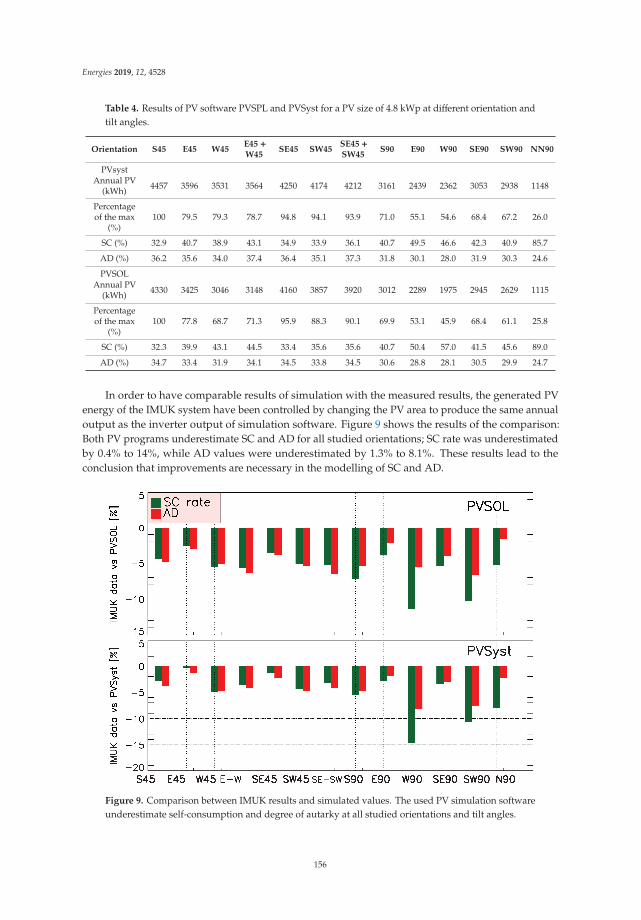
Energies 2019, 12, 4528

Table 4. Results of PV software PVSPL and PVSyst for a PV size of 4.8 kWp at different orientation andtilt angles.

Orientation S45 E45 W45E45 +W45

SE45 SW45SE45 +SW45

S90 E90 W90 SE90 SW90 NN90

PVsystAnnual PV

(kWh) 4457 3596 3531 3564 4250 4174 4212 3161 2439 2362 3053 2938 1148

Percentageof the max

(%)100 79.5 79.3 78.7 94.8 94.1 93.9 71.0 55.1 54.6 68.4 67.2 26.0

SC (%) 32.9 40.7 38.9 43.1 34.9 33.9 36.1 40.7 49.5 46.6 42.3 40.9 85.7

AD (%) 36.2 35.6 34.0 37.4 36.4 35.1 37.3 31.8 30.1 28.0 31.9 30.3 24.6

PVSOLAnnual PV

(kWh) 4330 3425 3046 3148 4160 3857 3920 3012 2289 1975 2945 2629 1115

Percentageof the max

(%)100 77.8 68.7 71.3 95.9 88.3 90.1 69.9 53.1 45.9 68.4 61.1 25.8

SC (%) 32.3 39.9 43.1 44.5 33.4 35.6 35.6 40.7 50.4 57.0 41.5 45.6 89.0

AD (%) 34.7 33.4 31.9 34.1 34.5 33.8 34.5 30.6 28.8 28.1 30.5 29.9 24.7

In order to have comparable results of simulation with the measured results, the generated PVenergy of the IMUK system have been controlled by changing the PV area to produce the same annualoutput as the inverter output of simulation software. Figure 9 shows the results of the comparison:Both PV programs underestimate SC and AD for all studied orientations; SC rate was underestimatedby 0.4% to 14%, while AD values were underestimated by 1.3% to 8.1%. These results lead to theconclusion that improvements are necessary in the modelling of SC and AD.

Figure 9. Comparison between IMUK results and simulated values. The used PV simulation softwareunderestimate self-consumption and degree of autarky at all studied orientations and tilt angles.

156

Energies 2019, 12, 4528

5. Conclusions

Using one-minute measured data of PV energy, the outputs of 12 solar collectors at various tilt andazimuth angles in Hannover (Germany) were analyzed. For validation, the results were also comparedwith the simulated values of two widely used PV software: PVSOL and PVsyst.

The measurements show that a south-oriented generator at about 40◦ gives the highest electricityprofile. For non-vertical devices, the combinations of E and W orientations result in the highest SC rateand combinations of SE and SW orientations result in the highest AD. E-W and SE-SW combinationshave the lowest electricity coast for PV systems without FIT, while the E orientation has the highest one.For PV systems with FIT, S orientation provides the highest transfer of money from the supplier. Theeconomic analysis using IRR of PV systems without FIT shows that the SE-SW and E-W orientationstilted at 45◦ is slightly more beneficial, while S orientation has higher IRR for PV systems with FIT.

However, in light of the continuing decline of FIT, the advantage of S orientation is decreasingand our results show that E-W and SE-SW orientations will be more beneficial if FIT is to 7 Ct/kWhor lower. East and west orientations of PV modules and not south orientations should be supportedbecause they would also reduce the economic costs for storing renewable energy—regardless whowould own the storage facilities—and avoid high noon peaks of solar energy production, which wouldbecome a problem for the grid for higher solar power penetrations levels.

Furthermore, the results show that the vertical tilted surfaces represent a high potential for PVenergy production and facade PV systems could be an alternative for many people, especially forthose who do not have access to a rooftop. So far, combinations of different vertically tilted modulesas well as the combinations between vertical and 45◦-tilted surfaces have not yet been taken intoaccount because of the problems with the standardization of shadows from nearby building, trees and,other obstacles.

The calculation in this study assumed a constant price for the FIT over the day. However, if weconsider the general trend to link the price of electricity with the spot market price, so that the price ofselling or feeding electricity to grid changes according to the production and demand, the E-W andSE-SW orientations might become even more beneficial against S-facing PV systems. In addition, thesuitability criteria for rooftops carrying solar modules must be questioned [26]. More roofs should betaken into account when diurnal variations are considered. Based on our measurements and analysiswe conclude that the yearly sum of produced electricity can no longer be the only criterion for theinstallation of PV modules. Instead, other orientations may be more beneficial for both the owner andthe society that uses solar power.

Regarding the model validation, both of the tested PV software overestimate the energy productionat most studied orientations and also overestimate the percentage of these orientations when comparedto the south-oriented generator. This result agrees with previous results [45], which showed thatanisotropic models overestimate the S-tilted irradiance and most vertical irradiances. The need toimprove existing modelling has also been shown in previous studies [46,47]. A major cause for thedeviation between models and measurements may be the oversimplified assumptions about the skyradiance, which can be overcome by new measurement techniques [48,49]. Moreover, the study showedthat the overestimation increases with increasing deviation from the south direction. In addition, bothPV programs underestimate SC rate and AD for all studied orientations. SC rate was underestimatedfrom 0.4% to 14%, while AD values were underestimated from 1.3% to 8.1%. These results lead to theconclusion that improvements are necessary when modelling SC and AD.

The amount of solar irradiance received by the surface of the PV collector is among the mostimportant parameters that affect the performance of a PV system. Therefore, high-resolution tiltedsolar irradiance data in various orientations and weather conditions are needed to feed the models forbetter simulation of PV Power.

157

Energies 2019, 12, 4528

Author Contributions: R.M. conceived and designed the study and wrote the draft paper; G.S. initiated theinvestigation on the performance of differently oriented PV modules. G.S. and E.W.L. contributed in the conceptionand design, analysis and interpretation of the data. All the authors significantly contributed to the final version ofthe manuscript.

Funding: The publication of this article was funded by the Open Access fund of Leibniz Universität Hannover”This is what we wrote in all our previous papers.

Acknowledgments: The publication of this article was funded by the Open Access fund of Leibniz UniversitätHannover. We are also grateful to Holger Schilke for his contribution in collecting the data and supervising themeasurements. Thanks also to Martin Hoffmann for his instruction in using PVSOL. Ben Liley from the NationalInstitute of Water and Atmospheric Research (NIWA), New Zealand for improving the English and providinghelpful comments on the clarity of the presentation.

Conflicts of Interest: The authors declare no conflict of interest.

Nomenclature

SC Self-consumptionAD Degree of autarkyPm Power output of the PV systemPrel Rated PV system powerIm Measured solar irradianceIUTC Solar irradiance at STC (1000 W/m2)Tsen Sensor temperatureγ Power temperature coefficientPdu PV directly used energyPLF Power loss factorϕ Geographical latitude ϕ

PVg Total PV generated energyPe Electricity pricePG Grid electricity pricePfi, FIT Feed-in tariffLC Levelized coast of PV energy

References

1. Jäger-Waldau, A. Snapshot of Photovoltaics 2018. EPJ Photovolt. 2018, 9, 6. [CrossRef]2. Ginley, D.; Green, M.A.; Collins, R. Solar energy conversion toward 1 TW. MRS Bull. 2008, 33, 355–364.

[CrossRef]3. Vartiainen, E.; Breyer, C.; Moser, D.; Medina, E.R. Impact of weighted average cost of capital, capital

expenditure, and other parameters on future utility-scale PV levelised cost of electricity. Prog. Photovolt. Res.Appl. 2019, 1–15. [CrossRef]

4. IRENA. Renewable Energy Statistics 2018, The International Renewable Energy Agency. Availableonline: https://www.irena.org//media/Files/IRENA/Agency/Publication/2019/Mar/RE_capacity_highlights_2019pdf?la=en&hash=BA9D38354390B001DC0CC9BE03EEE559C280013F (accessed on 26 October 2019).

5. Khoo, Y.S.; Nobre, A.; Malhotra, R.; Yang, D.; Ruther, R.; Reindl, T.; Aberle, A.G. Optimal orientation and tiltangle for maximizing in-plane solar irradiation for PV applications in Singapore. IEEE J. Photovolt. 2014, 4,647–653. [CrossRef]

6. Hartner, M.; Ortner, A.; Heisl, A.; Haas, R. East to west—The optimal tilt angle and orientation of photovoltaicpanels from an electricity system perspective. Appl. Energy 2015, 160, 94–107. [CrossRef]

7. Seme, S.; Krawczyk, A.; Łada, E.; Tondyra, Š.B.; Hadžiselimovic, M. The Efficiency of Different Orientationsof Photovoltaic Systems. Przeglad Elektrotechniczny 2017, 93, 201–204. [CrossRef]

8. Ghazi, S.; Ip, K. The effect of weather conditions on the efficiency of PV panels in southeast of UK. Renew.Energy 2014, 69, 50–59. [CrossRef]

9. Colli, A.; Zaaiman, W.J. Maximum-power-based PV performance validation method: Application tosingle-axis tracking and Fixed-Tilt c-Si systems in the Italian Alpine region. IEEE J. Photovolt 2012, 2, 555–563.[CrossRef]

158

Energies 2019, 12, 4528

10. Bakirci, K. General models for optimum tilt angles of solar panels: Turkey case study. Renew. Sustain. EnergyRev. 2012, 16, 6149–6159. [CrossRef]

11. Yan, R.; Saha, T.K.; Meredith, P.; Goodwin, S. Analysis of yearlong performance of differently tiltedphotovoltaic systems in Brisbane, Australia. Energy Convers. Manag. 2013, 74, 102–108. [CrossRef]

12. Lave, M.; Kleissl, J. Optimum fixed orientations and benefits of tracking for capturing solar radiation in thecontinental United States. Renew. Energy 2011, 36, 1145–1152. [CrossRef]

13. Agarwal, A.; Vashishtha, V.K.; Mishra, S.N. Comparative approach for the optimization of tilt angle to receivemaximum radiation. Int. J. Eng. Res. Technol. 2012, 1, 1–9.

14. Tang, R.; Wu, T. Optim. tilt-angles for solar collectors used in China. Appl. Energy 2004, 79, 239–248.[CrossRef]

15. Uba, F.A.; Sarsah, E.A. Optimization of tilt angle for solar collectors in WA, Ghana, Pelagia Research Library.Adv. Appl. Sci. Res. 2013, 4, 108–114.

16. Huld, T.; Šúri, M.; Dunlop, E.D. Comparison of potential solar electricity output from fixed-inclined andtwo-axis tracking photovoltaic modules in Europe. Prog. Photovolt. Res. Appl. 2008, 16, 47–59, ISSN 1099-159X.[CrossRef]

17. Huld, T.; Müller, R.; Gambardella, A. A new solar radiation database for estimating PV performance inEurope and Africa. Sol. Energy 2012, 86, 1803–1815. [CrossRef]

18. Quinn, S.W.; Lehman, B.A. Simple formula for the optimum tilt angles of photovoltaic panels. In Proceedingsof the IEEE 14th Workshop on Control and Modeling for Power Electronics (COMPEL), Salt Lake City, UT,USA, 23–26 June 2013; pp. 1–8.

19. Beringer, S.; Schilke, H.; Lohse, I.; Seckmeyer, G. Case study showing that the tilt angle of photovoltaic plantsis nearly irrelevant. Sol. Energy 2011, 85, 470–476. [CrossRef]

20. Bodis, K.; Kougias, I.; Jäger-Waldau, A.; Taylor, N.; Szabo, S. A high-resolution geospatial assessment of therooftop solar photovoltaic potential in the European Union. Renew. Sustain. Energy Rev. 2019, 114, 109309.[CrossRef]

21. Mertens, K. Photovoltaics: Fundamentals, Technology and Practice, 1st ed.; John Wiley & Sons, Ltd. Published:Hoboken, NJ, USA, 2014.

22. Luthander, R. Photovoltaic System Layout for Optimized Self-Consumption. Uppsala Universitet.2013. Available online: http://www.diva-portal.org/smash/get/diva2:637625/FULLTEXT01.pdf (accessed on26 November 2019).

23. Beck, T.; Kondziella, H.; Huard, G.; Bruckner, T. Assessing the influence of the temporal resolution ofelectrical load and PV generation profiles on self-consumption and sizing of PV-battery systems. Appl.Energy 2016, 173, 331–342. [CrossRef]

24. Luthander, R.; Widen, J.; Nilsson, D.; Palm, J. Photovoltaic self consumprion in buidings: A review. Appl.Energy 2015, 142, 80–94. [CrossRef]

25. Leicester, P.A.; Rowley, P.N.; Goodier, C.I. Probabilistic analysis of solar photovoltaic self-consumption usingBayesian network models. IET Renew. Power Gener. 2016, 10, 448–455. [CrossRef]

26. Martín, A.M.; Domínguez, J.; Amador, J. Applying LIDAR datasets and GIS based model to evaluate solarpotential over roofs: A review. AIMS Energy 2015, 3, 326–343. [CrossRef]

27. PVSOL. PV*SOL Online—A Free Tool Forsolar Power (PV) Systems. 2019. Available online: http://pvsol-online.valentin-software.com/#/ (accessed on 6 May 2019).

28. PVSyst, Version, 6.79; [Computer Software]; University of Geneva: Geneva, Switzerland, 2019.29. DGS. EnergyMap.info; Deutsche Gesellschaft für Sonnenenergie e.V.: Berlin, Germany, 2015.30. PVGIS. Overview of PVGIS data sources and calculation methods. European Commission. Available online:

http://re.jrc.ec.europa.eu/pvg_static/methods.html (accessed on 26 November 2019).31. Idoko, L.; Anaya-Lara, O.; McDonald, A. Enhancing PV modules efficiency and power output using

multi-concept cooling technique. Energy Rep. 2018, 4, 357–369. [CrossRef]32. Tjaden, T.; Bergner, J.; Weniger, J.; Quaschning, V. Repräsentative elektrische Lastprofile für Wohngebäude in

Deutschland auf 1-sekündiger Datenbasis. Technical report, Berlin, Germany. Hochschule für Technik undWirtschaft HTW Berlin. Available online: https://pvspeicher.htw-berlin.de/wp-content/uploads/2017/05/HTW-BERLIN-2015-Repr%C3%A4sentative-elektrische-Lastprofile-f%C3%BCr-Wohngeb%C3%A4ude-in-Deutschland-auf-1-sek%C3%BCndiger-Datenbasis.pdf (accessed on 26 November 2019).

159

Energies 2019, 12, 4528

33. Haysom, J.E.; Hinzer, K.; Wright, D. Impact of electricity tariffs on optimal orientation of photovoltaicmodules. Prog. Photovolt. Res. Appl. 2015, 24, 253–260. [CrossRef]

34. Jager-Waldau, A.; Bucher, C.; Frederiksen, K.H.B.; Guerro-Lemus, R.; Mason, G.; Mather, B.; Mayr, C.;Moneta, D.; Nikoletatos, J.; Roberts, M.B. Self-consumption of electricity produced from PV systems inapartment buildings—Comparison of the situation in Australia, Austria, Denmark, Germany, Greece, Italy,Spain, Switzerland and the USA. In Proceedings of the 2018 IEEE 7th World Conf. Photovolt. EnergyConversion, WCPEC 2018—A Jt. Conf. 45th IEEE PVSC, 28th PVSEC 34th EU PVSEC 1424–1430, WaikoloaVillage, HI, USA, 10–15 June 2018. [CrossRef]

35. Mojonero, D.H.; Villacorta, A.R.; Kuong, J.L. Impact assessment of net metering for residential photovoltaicdistributed generation in Peru. Int. J. Renew. Energy Res. 2018, 8, 1200–1207.

36. Pereira da Silva, P.; Dantas, G.; Pereira, G.I.; Câmara, L.; De Castro, N.J. Photovoltaic distributedgeneration—An international review on diffusion, support policies, and electricity sector regulatoryadaptation. Renew. Sustain. Energy Rev. 2019, 103, 30–39. [CrossRef]

37. BDEW. BDEW-Strompreisanalyse (Haushalte und Industrie). Available online: https://www.bdew.de/me-dia/documents/190115_BDEW-Strompreisanalyse_Januar-2019.pdf (accessed on 28 January 2019).

38. Fraunhofer Institute for Solar Energy Systems (ISE). Levelized Cost of Electricity Renewable Energy Technologies;Fraunhofer Institute for Solar Energy Systems (ISE): Freiburg, Germany, 2018.

39. Stenzel, P.; Linssen, J.; Fleer, J.; Busch, F. Impact of temporal resolution of supply and demand profiles onthe design of photovoltaic battery systems for increased self-consumption. In Proceedings of the 2016 IEEEInternational Energy Conference (ENERGYCON), Leuven, Belgium, 4–8 April 2016.

40. Talavera, D.L.; Nofuentes, G.; Aguilera, J. The Internal Rate of Return of Photovoltaic Grid-ConnectedSystems: A Comprehensive Sensitivity. Renew. Energy 2010, 35, 101–111. [CrossRef]

41. Tapia, M. Evaluation of Performance Models against Actual Performance of Grid Connected PV Systems.Master’s Thesis, Carl von Ossietzky Universität, Oldenburg, Germany, 2014.

42. Fraunhofer ISE. Recent Facts about Photovoltaics in Germany; Fraunhofer Institute for Solar Energy SystemsISE: Freiburg, Gemmary, 2019.

43. Obane, H.; Okajima, K. Extracting issues significant to valuing electricity from small photovoltaic systemsusing quantitative content analysis. Electr. J. 2019, 32, 106673. [CrossRef]

44. Solar Power Europe. Global Market Outlook for Solar Power 2018–2022; Solar Power Europe: Brussels, Belgium,2018.

45. Mubarak, R.; Hofmann, M.; Riechelmann, S.; Seckmeyer, G. Comparison of modelled and measured tiltedsolar irradiance for photovoltaic applications. Energies 2017, 10, 1688. [CrossRef]

46. Hofmann, M.; Seckmeyer, G. Influence of various irradiance models and their combination on simulationresults of photovoltaic systems. Energies 2017, 10, 1495. [CrossRef]

47. Hofmann, M.; Seckmeyer, G. A New Model for Estimating the Diffuse Fraction of Solar Irradiance for PVSystem Simulations. Energies 2017, 10, 248. [CrossRef]

48. Seckmeyer, G.; Lagos Rivas, L.; Gaetani, C.; Heinzel, J.W.; Schrempf, M. Biologische und medizinischeWirkungen solarer Strahlung (Biological and medical effects of solar radiation). In Promet, Heft 100Strahlungsbilanzen; Chapter 13; Deutscher Wetterdienst (DWD): Offenbach am Main, Germany, 2018.

49. Riechelmann, S.; Schrempf, M.; Seckmeyer, G. Simultaneous measurement of spectral sky radiance by anon-scanning multidirectional spectroradiometer (MUDIS). Meas. Sci. Technol. 2013, 24, 125501. [CrossRef]

© 2019 by the authors. Licensee MDPI, Basel, Switzerland. This article is an open accessarticle distributed under the terms and conditions of the Creative Commons Attribution(CC BY) license (http://creativecommons.org/licenses/by/4.0/).

160

energies

Review

Grid Synchronization and Islanding DetectionMethods for Single-Stage Photovoltaic Systems

Rosa Anna Mastromauro

Department of Information Engineering (DINFO), University of Florence, 50139 Florence, Italy;rosaanna.mastromauro@unifi.it; Tel.: +39-055-275-8650

Received: 29 April 2020; Accepted: 28 June 2020; Published: 1 July 2020

Abstract: Synchronization and islanding detection represent some of the main issues forgrid-connected photovoltaic systems (PVSs). The synchronization technique allows to achievePVS high power factor operation and it provides grid voltage monitoring. The islanding detectioncontrol function ensures safe operation of the PVS. Focusing on low-power single-stage PVSs, in thisstudy the most adopted and the highest performance synchronization and islanding detectionmethods are discussed. The role of the synchronization system is fundamental to detect the gridconditions, for the islanding detection purpose, and to manage the reconnection to the grid after aPVS trip. Hence a combined review is advantageous.

Keywords: photovoltaicsystems; synchronizationsystems; phase-lockedloops; islandingdetectionmethods

1. Introduction

At the end of 2018, the world had 152 GW of installed photovoltaic (PV) electricity capacity.The best PV markets in 2018 were China with 44.3 GW, India with 10.8 GW, USA with 10.7 GW, Japanwith 6.7 GW, Australia with 3.8 GW. The European Union (EU) has registered rise for the first time inyears with 8.4 GW, but this growth is far from the 23.2 GW registered in 2011. However, the growthcan be considered slow, some of the EU countries have already achieved high PV penetration due topast installations such as Germany with a PV overall capacity of 45.5 GW by the end of 2018, Italythat exceeds 20 GW, United Kingdom with 13 GW, Spain with 5.6 GW, Belgium with 4.3 GW andSwitzerland with 2.2 GW. It is estimated that overall, the PV systems (PVSs) had contributed to the2.9% of the global electricity demand in 2018 and that the climate change impact is of 590 millions oftons of CO2 saving every year [1–3].

Due to the photovoltaic prize reduction and availability of loan products, a significant portion ofPVSs have been recently installed also in absence of governments initiatives especially for residentialapplications. A performance evaluation of residential PVSs in some European countries is presentedin [4]. Considering the period 2014–2016, the highest specific yield in kWh/kWp has been registered inItaly in 2015.

The PVSs inverters price has diminished around 0.10 $/Wp in the last decade [5]. In addition,the design optimization of the PVS converters has facilitated the reduction of the total cost ofownership [6]. Nevertheless, the increase of PVS grid-connected installations implies severalmanagement challenges depending also on the point of interconnection between the PVS and thegrid [7–10]. In this scenario advanced control features of the PVS inverters can contribute to overcomesome of the grid management challenges due to high penetration [11–13].

Looking at the residential applications, the PVSs can be single-stage or double-stage. In case ofsingle-stage PVSs, the PV array is directly connected to the inverter avoiding a boost DC/DC converter.Single-stage transformerless PVSs represent the most promising technology due to lower weight,higher efficiency, smaller size and limited cost than double-stage PVSs or single-stage architectures

Energies 2020, 13, 3382; doi:10.3390/en13133382 www.mdpi.com/journal/energies161

Energies 2020, 13, 3382

coupled to low-frequency transformers [14–18]. Focusing on a single-stage PVS, a review about someof the main control issues is presented in [19], however the analysis is limited to current and voltagecontrol methods and maximum power point tracking (MPPT) techniques.

About the most important issues to be considered in grid-connected PVS there are thesynchronization with the grid and the detection of the islanding condition. Synchronization dealswith PVS high power factor operation, since the synchronization algorithms objective is to providegrid voltage information about amplitude, phase and frequency in order to generate a current/voltagereference which is in phase with the grid voltage [13,20–24].

Synchronization deals also with the grid voltage monitoring. According to the grid-connectionrequirements [25], the PVSs connected to the low-voltage distribution grid must operate withoutcausing step change in the RMS voltage at the point of common coupling (PCC) exceeding 5% of ratedvalue. In addition, the synchronization parameters limits for grid-connected PVS are: 0.3 Hz for thefrequency difference, 10% for the voltage difference. Abnormal conditions can arise on the utility gridwhich require a prompt response from the grid-connected PVS, hence the information provided by thesynchronization system are fundamental for this purpose [26–28].

Unintentional islanding phenomenon is verified in case of grid power outages when the PVScontinues to supply the local loads. Unintentional islanding can cause damages to the local electricalloads, to the grid-connected PVS inverter, to the technicians during the maintenance operations.Numerous improved islanding detection algorithms have been proposed in literature in the last yearsaiming to detect islanding phenomenon in all possible cases [29–35]. However, many these algorithmsare not designed peculiarly for PVS.

In case of low power residential PVSs and in particular in case of single-stage systems, the PVSinverter is commonly in charge of the islanding detection, hence the anti-islanding functionalityrepresents one of the main challenge in the PVS inverters design [18]. The anti-islanding protectionsmust be implemented on the basis of the international standards requirements for distributed powergeneration systems (DPGSs) [25,36–38]. In particular, it is required that unintentional islanding bedetected in less than two seconds as already established in the previous guidelines for PVSs [39–41].

After a disconnection due to the islanding detection an improper reconnection event is notimprobable if the PVS breaker connects the system to the grid when the PVS voltage is out of phase.In this hypothesis a second disconnection can occur due to the PVS protections action. Hence thereclosing procedure has to be managed in strict coordination with the PVS synchronization system.For this reason, synchronization and islanding detection issues must be analyzed together.

About synchronization systems some books have been published such as [42]. Few review paperscan be found in literature [23,43–46]. In [43] all the main families of synchronization techniques (alsoincluding the artificial intelligence techniques) are classified showing advantages and disadvantages.Basic concepts about phase-locked loop (PLL) techniques are explained in [44]. Reference [45] isdevoted to three-phase applications, reference [23] is devoted to single-phase application, while [46] isoriented to design issues.

About islanding detection methods many review papers have been published in literatureconsidering different DPGSs [47–57]. Reference [47] provides a review of the islanding detectionmethods for high power DPGSs. In [48] an extensive review of the islanding detection methods isprovided focusing on some performance indices evaluation and in particular on the detection time.Reference [49] is focused just on passive methods, reference [50] is focused just on active methods.In [51] the focus is on active and passive methods and a new active methods is proposed for athree-phase PVS. The same islanding detection methods are discussed also in [52] also including thehybrid detection methods. However, hybrid methods are categorized just as combination of active andpassive methods. In [53] some active islanding detection techniques are compared on the basis of anew index assessing the non-detection-zone (NDZ) size. In [54] the active techniques are classified intwo categories: techniques introducing positive feedback in the control of the inverter and techniquesbased on harmonics injection. In [55] the islanding detection methods based on different signal

162

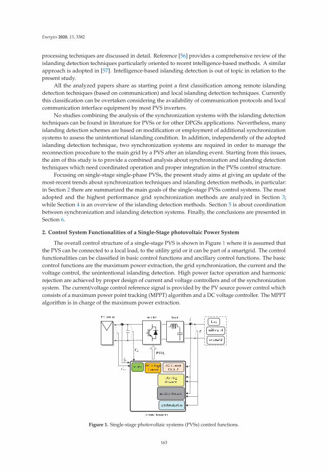
Energies 2020, 13, 3382

processing techniques are discussed in detail. Reference [56] provides a comprehensive review of theislanding detection techniques particularly oriented to recent intelligence-based methods. A similarapproach is adopted in [57]. Intelligence-based islanding detection is out of topic in relation to thepresent study.

All the analyzed papers share as starting point a first classification among remote islandingdetection techniques (based on communication) and local islanding detection techniques. Currentlythis classification can be overtaken considering the availability of communication protocols and localcommunication interface equipment by most PVS inverters.

No studies combining the analysis of the synchronization systems with the islanding detectiontechniques can be found in literature for PVSs or for other DPGSs applications. Nevertheless, manyislanding detection schemes are based on modification or employment of additional synchronizationsystems to assess the unintentional islanding condition. In addition, independently of the adoptedislanding detection technique, two synchronization systems are required in order to manage thereconnection procedure to the main grid by a PVS after an islanding event. Starting from this issues,the aim of this study is to provide a combined analysis about synchronization and islanding detectiontechniques which need coordinated operation and proper integration in the PVSs control structure.

Focusing on single-stage single-phase PVSs, the present study aims at giving an update of themost-recent trends about synchronization techniques and islanding detection methods, in particular:in Section 2 there are summarized the main goals of the single-stage PVSs control systems. The mostadopted and the highest performance grid synchronization methods are analyzed in Section 3;while Section 4 is an overview of the islanding detection methods. Section 5 is about coordinationbetween synchronization and islanding detection systems. Finally, the conclusions are presented inSection 6.

2. Control System Functionalities of a Single-Stage photovoltaic Power System

The overall control structure of a single-stage PVS is shown in Figure 1 where it is assumed thatthe PVS can be connected to a local load, to the utility grid or it can be part of a smartgrid. The controlfunctionalities can be classified in basic control functions and ancillary control functions. The basiccontrol functions are the maximum power extraction, the grid synchronization, the current and thevoltage control, the unintentional islanding detection. High power factor operation and harmonicrejection are achieved by proper design of current and voltage controllers and of the synchronizationsystem. The current/voltage control reference signal is provided by the PV source power control whichconsists of a maximum power point tracking (MPPT) algorithm and a DC voltage controller. The MPPTalgorithm is in charge of the maximum power extraction.

Figure 1. Single-stage photovoltaic systems (PVSs) control functions.

163

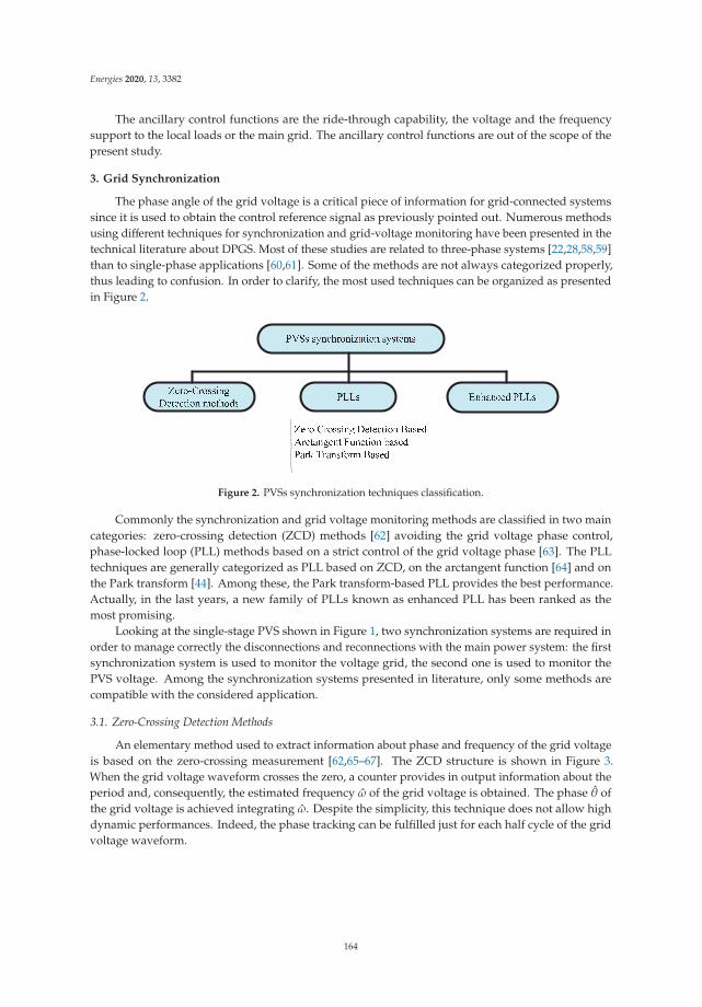
Energies 2020, 13, 3382

The ancillary control functions are the ride-through capability, the voltage and the frequencysupport to the local loads or the main grid. The ancillary control functions are out of the scope of thepresent study.

3. Grid Synchronization

The phase angle of the grid voltage is a critical piece of information for grid-connected systemssince it is used to obtain the control reference signal as previously pointed out. Numerous methodsusing different techniques for synchronization and grid-voltage monitoring have been presented in thetechnical literature about DPGS. Most of these studies are related to three-phase systems [22,28,58,59]than to single-phase applications [60,61]. Some of the methods are not always categorized properly,thus leading to confusion. In order to clarify, the most used techniques can be organized as presentedin Figure 2.

Figure 2. PVSs synchronization techniques classification.

Commonly the synchronization and grid voltage monitoring methods are classified in two maincategories: zero-crossing detection (ZCD) methods [62] avoiding the grid voltage phase control,phase-locked loop (PLL) methods based on a strict control of the grid voltage phase [63]. The PLLtechniques are generally categorized as PLL based on ZCD, on the arctangent function [64] and onthe Park transform [44]. Among these, the Park transform-based PLL provides the best performance.Actually, in the last years, a new family of PLLs known as enhanced PLL has been ranked as themost promising.

Looking at the single-stage PVS shown in Figure 1, two synchronization systems are required inorder to manage correctly the disconnections and reconnections with the main power system: the firstsynchronization system is used to monitor the voltage grid, the second one is used to monitor thePVS voltage. Among the synchronization systems presented in literature, only some methods arecompatible with the considered application.

3.1. Zero-Crossing Detection Methods

An elementary method used to extract information about phase and frequency of the grid voltageis based on the zero-crossing measurement [62,65–67]. The ZCD structure is shown in Figure 3.When the grid voltage waveform crosses the zero, a counter provides in output information about theperiod and, consequently, the estimated frequency ω of the grid voltage is obtained. The phase θ ofthe grid voltage is achieved integrating ω. Despite the simplicity, this technique does not allow highdynamic performances. Indeed, the phase tracking can be fulfilled just for each half cycle of the gridvoltage waveform.

164

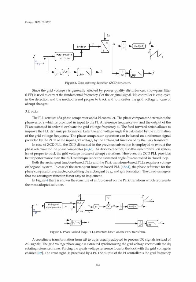
Energies 2020, 13, 3382

T

π

f

( )π

e dtT

⋅

s

πE

ω θ

θ

Figure 3. Zero-crossing detection (ZCD) structure.

Since the grid voltage e is generally affected by power quality disturbances, a low-pass filter(LPF) is used to extract the fundamental frequency f of the original signal. No controller is employedin the detection and the method is not proper to track and to monitor the grid voltage in case ofabrupt changes.

3.2. PLLs

The PLL consists of a phase comparator and a PI controller. The phase comparator determines thephase error ε which is provided in input to the PI. A reference frequency ωIC and the output of thePI are summed in order to evaluate the grid voltage frequency ω. The feed-forward action allows toimprove the PLL dynamic performance. Later the grid voltage angle θ is calculated by the informationof the grid voltage frequency. The phase comparator operation can be based on a reference signalprovided by the ZCD of the input grid voltage, by the arctangent function of by the Park transform.

In case of ZCD PLL, the ZCD discussed in the previous subsection is employed to extract thephase reference for the phase comparator [42,68]. As described before, also this synchronization systemis not proper to track the grid voltage in case of abrupt variations. However, the ZCD PLL providesbetter performance than the ZCD technique since the estimated angle θ is controlled in closed loop.

Both the arctangent function-based PLLs and the Park transform-based PLLs require a voltageorthogonal system. In case of the arctangent function-based PLL [42,64], the phase reference for thephase comparator is extracted calculating the arctangent by eα and eβ information. The disadvantage isthat the arctangent function is not easy to implement.

In Figure 4 there is shown the structure of a PLL-based on the Park transform which representsthe most adopted solution.

e qe

θ

f

( )π

α β+e e

e

ICω

s

πE

ω θ

θ

αe

βe

α β

d qde

Figure 4. Phase-locked loop (PLL) structure based on the Park transform.

A coordinate transformation from αβ to dq is usually adopted to process DC signals instead ofAC signals. The grid voltage phase angle is extracted synchronizing the grid voltage vector with the dqrotating reference frame. Forcing the q-axis voltage reference to zero, the lock with the grid voltage isensured [69]. The error signal is processed by a PI. The output of the PI controller is the grid frequency.

165

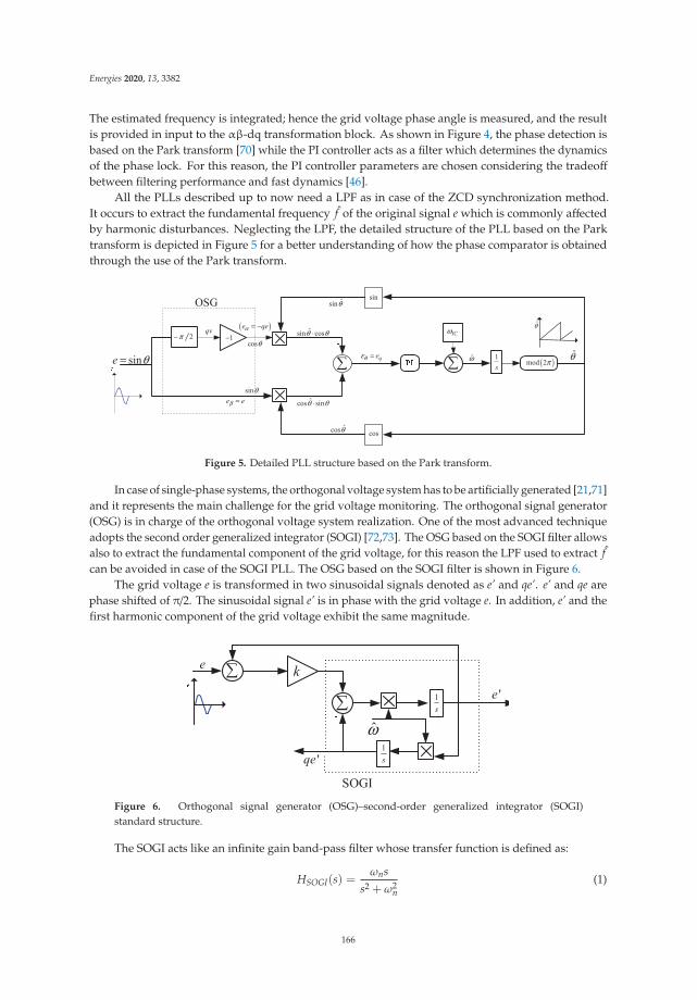
Energies 2020, 13, 3382

The estimated frequency is integrated; hence the grid voltage phase angle is measured, and the resultis provided in input to the αβ-dq transformation block. As shown in Figure 4, the phase detection isbased on the Park transform [70] while the PI controller acts as a filter which determines the dynamicsof the phase lock. For this reason, the PI controller parameters are chosen considering the tradeoffbetween filtering performance and fast dynamics [46].

All the PLLs described up to now need a LPF as in case of the ZCD synchronization method.It occurs to extract the fundamental frequency f of the original signal e which is commonly affectedby harmonic disturbances. Neglecting the LPF, the detailed structure of the PLL based on the Parktransform is depicted in Figure 5 for a better understanding of how the phase comparator is obtainedthrough the use of the Park transform.

qv

( )π

θ θ⋅

ICω

sω θ

( )α = −e qe

β =e e

θε = qeθ=e

π− −

θ

θ

θ

θ

θ

θ θ⋅

Figure 5. Detailed PLL structure based on the Park transform.

In case of single-phase systems, the orthogonal voltage system has to be artificially generated [21,71]and it represents the main challenge for the grid voltage monitoring. The orthogonal signal generator(OSG) is in charge of the orthogonal voltage system realization. One of the most advanced techniqueadopts the second order generalized integrator (SOGI) [72,73]. The OSG based on the SOGI filter allowsalso to extract the fundamental component of the grid voltage, for this reason the LPF used to extract fcan be avoided in case of the SOGI PLL. The OSG based on the SOGI filter is shown in Figure 6.

The grid voltage e is transformed in two sinusoidal signals denoted as e’ and qe’. e’ and qe arephase shifted of π/2. The sinusoidal signal e’ is in phase with the grid voltage e. In addition, e’ and thefirst harmonic component of the grid voltage exhibit the same magnitude.

qe s

ω

e k

se

Figure 6. Orthogonal signal generator (OSG)–second-order generalized integrator (SOGI)standard structure.

The SOGI acts like an infinite gain band-pass filter whose transfer function is defined as:

HSOGI(s) =ωns

s2 +ω2n

(1)

166

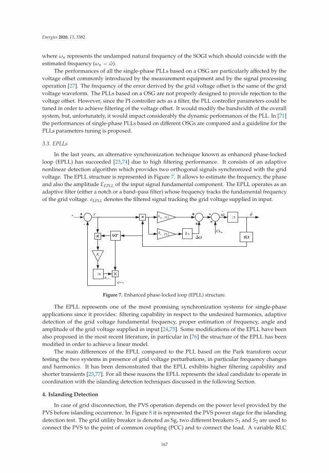
Energies 2020, 13, 3382

where ωn represents the undamped natural frequency of the SOGI which should coincide with theestimated frequency (ωn = ω).

The performances of all the single-phase PLLs based on a OSG are particularly affected by thevoltage offset commonly introduced by the measurement equipment and by the signal processingoperation [27]. The frequency of the error derived by the grid voltage offset is the same of the gridvoltage waveform. The PLLs based on a OSG are not properly designed to provide rejection to thevoltage offset. However, since the PI controller acts as a filter, the PLL controller parameters could betuned in order to achieve filtering of the voltage offset. It would modify the bandwidth of the overallsystem, but, unfortunately, it would impact considerably the dynamic performances of the PLL. In [71]the performances of single-phase PLLs based on different OSGs are compared and a guideline for thePLLs parameters tuning is proposed.

3.3. EPLLs

In the last years, an alternative synchronization technique known as enhanced phase-lockedloop (EPLL) has succeeded [23,74] due to high filtering performance. It consists of an adaptivenonlinear detection algorithm which provides two orthogonal signals synchronized with the gridvoltage. The EPLL structure is represented in Figure 7. It allows to estimate the frequency, the phaseand also the amplitude EEPLL of the input signal fundamental component. The EPLL operates as anadaptive filter (either a notch or a band–pass filter) whose frequency tracks the fundamental frequencyof the grid voltage. eEPLL denotes the filtered signal tracking the grid voltage supplied in input.

θε

K

p PLLk

i PLLk

ω

Figure 7. Enhanced phase-locked loop (EPLL) structure.

The EPLL represents one of the most promising synchronization systems for single-phaseapplications since it provides: filtering capability in respect to the undesired harmonics, adaptivedetection of the grid voltage fundamental frequency, proper estimation of frequency, angle andamplitude of the grid voltage supplied in input [24,75]. Some modifications of the EPLL have beenalso proposed in the most recent literature, in particular in [76] the structure of the EPLL has beenmodified in order to achieve a linear model.

The main differences of the EPLL compared to the PLL based on the Park transform occurtesting the two systems in presence of grid voltage perturbations, in particular frequency changesand harmonics. It has been demonstrated that the EPLL exhibits higher filtering capability andshorter transients [23,77]. For all these reasons the EPLL represents the ideal candidate to operate incoordination with the islanding detection techniques discussed in the following Section.

4. Islanding Detection

In case of grid disconnection, the PVS operation depends on the power level provided by thePVS before islanding occurrence. In Figure 8 it is represented the PVS power stage for the islandingdetection test. The grid utility breaker is denoted as Sg, two different breakers S1 and S2 are used toconnect the PVS to the point of common coupling (PCC) and to connect the load. A variable RLC

167

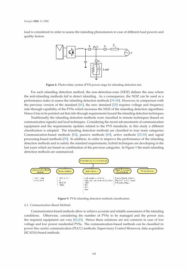
Energies 2020, 13, 3382

load is considered in order to assess the islanding phenomenon in case of different load powers andquality factors.

e

gZ

Figure 8. Photovoltaic system (PVS) power stage for islanding detection test.

For each islanding detection method, the non-detection-zone (NDZ) defines the area wherethe anti-islanding methods fail to detect islanding. As a consequence, the NDZ can be used as aperformance index to assess the islanding detection methods [78–80]. However, in comparison withthe previous version of the standard [81], the new standard [25] requires voltage and frequencyride-through capability of the PVSs which increases the NDZ of the islanding detection algorithms.Hence it has to be pointed out that ride-through requirements hazard the islanding detection techniques.

Traditionally the islanding detection methods were classified in remote techniques (based oncommunication signals) and local techniques. Considering the recent advancements of communicationequipment and the requirements updates related to the PVS standards, in this study a differentclassification is adopted. The islanding detection methods are classified in four main categories:Communication-based methods [82], passive methods [49], active methods [25,50] and signalprocessing-based methods [55]. In addition, in order to improve the performance of the islandingdetection methods and to satisfy the standard requirements, hybrid techniques are developing in thelast years which are based on combination of the previous categories. In Figure 9 the main islandingdetection methods are summarized.

Figure 9. PVSs islanding detection methods classification.

4.1. Communication-Based Methods

Communication-based methods allow to achieve accurate and reliable assessment of the islandingconditions. Otherwise, considering the number of PVSs to be managed and the power size,the required equipment can vary [82,83]. Hence these solutions are not common in case of lowvoltage and low power residential PVSs. The communication-based methods can be classified in:power line carrier communication (PLCC) methods, Supervisory Control Moreover, data acquisition(SCADA)-based methods.

168

Energies 2020, 13, 3382

4.1.1. PLCC-Based Methods

The PLCC-based methods allow a continuous test of the grid connection. A continuous carrier isadopted [84–87] and all the PVSs are equipped with a receiver. When the grid breaker Sg is opened asa consequence of grid disconnection, the receivers do not catch signals and the islanding conditionis detected. The PLCC-based techniques are particularly resilient to noise since the PVSs invertersswitching frequencies do not influence the PLCC signals.

4.1.2. SCADA-Based Methods

The SCADA-based methods assess the status of the breakers connecting the PVSs to thegrid [57,88,89]. Using the SCADA methods, the coordination between the PVS and the grid utilityoperations is significantly improved, and the islanding phenomenon can be detected avoiding a NDZarea. Cost and complexity of the equipment represent the main disadvantages.

4.2. Passive Methods

Compared to the communication-based methods, the passive islanding detection methods presentsimple implementation based on protection relays and synchronization systems [41,49]. The mostfamous passive methods are over/under voltage (OUV) and over-under frequency (OUF), phase jump(PJ), rate of change of frequency (ROCOF), voltage harmonic monitoring (VHM).

4.2.1. OUV and OUF Methods

All grid-connected PVS inverters are required to have OUV and OUF protections. The aim is toavoid power supply by the PVSs when the voltage amplitude and frequency values at the PCC aredifferent from set values [41,90].

Considering an RLC load whose resonant frequency is equal to the grid frequency, no reactivepower absorption is verified by the load. In case of grid disconnection, the power absorbed by the loadis equal to the active power provided by the PVS. Hence the RMS value of the voltage provided by thePVS at the PCC changes from EPVS = E before the disconnection to:

EPVS = δE (2)

where E is the rated RMS value of the grid voltage,

δ =

√PPVS

PL(3)

PPVS is the active power supplied by the PVS, PL is the rated load active power.In conclusion the voltage value at the PCC increases or decreases depending on the PVS power

generation. As a consequence, also the reactive power changes on the basis of the following relationship:

QPVS =

((1

LωPVS

)−CωPVS

)E2

PVS (4)

In (4) L and C are the inductive and capacitive components of the RLC load, ωPVS denotes thevoltage frequency at the PCC after the grid disconnection. Hence it results:

ωPVS =

−(

QPVSE2

PVSC

)+

√(QPVSE2

PVSC

)2+ 4

LC

2(5)

The voltage frequency and amplitude variations allow to detect islanding operation. Unfortunately,in case of power balance between the PVS generation and the load, no active and reactive power

169

Energies 2020, 13, 3382

variations are registered and consequently no voltage frequency and amplitude variations can bemeasured. Similarly, small active and reactive power variations imply small voltage variations interms of frequency and amplitude. For this reason, the OUV and OUF protection cannot detectislanding. OUV and OUF protections are considered insufficient anti-islanding techniques since theactive and reactive power variations due to the islanding phenomenon are commonly limited and, as aconsequence, there is high probability to fall into the NDZ.

4.2.2. Phase Jump Method

The aim of the phase jump (PJ) method is the detection of a “jump” between the PVS invertercurrent and voltage [78]. The PJ technique represents one of the first anti-islanding methods andit is based on the use of synchronization systems extracting information about the current and thevoltage phase. However, considering the present availability of fast PLLs and the development of highperformance current controllers, voltage and current synchronization could be achieved also duringislanding operation. Consequently, the detection of the islanding phenomenon based on this techniquecould fail.

4.2.3. Rate of Change of Frequency Method

The ROCOF islanding detection method measures the rate of change of frequency df/dt in a settime window. When the grid is disconnected, the power mismatch between generation and load causesfrequency variations. The PVS is tripped when df/dt exceeds the threshold value [91,92]. The thresholdsetting is the main issue of this method since it is necessary to distinguish islanding from load changes.Besides the ROCOF exhibits a wide NDZ combined with slow dynamics.

4.2.4. Voltage Harmonic Monitoring Method

The voltage harmonic monitoring (VHM) method is based on the voltage harmonic distortionestimation to detect the occurrence of the islanding phenomenon [49]. In grid-connected operation thevoltage at the PCC is set by the grid, but, in case of grid disconnection, the PVS inverter determines thevoltage at the PCC. Nevertheless, the voltage harmonic distortion varies with the grid impedance andit depends on the loads connected to the PCC. As a consequence, the accuracy of the method can behazarded if the islanding detection thresholds are not properly set. Better performance can be achievedmonitoring some selected harmonics variations rather than the overall voltage harmonic distortion.In this hypothesis the harmonics variations can be detected by means of PLLs tuned in order to trackthe selected harmonic components.

4.3. Active Methods

The active islanding detection methods are developed with the goal to achieve better performancethan the passive methods. The active methods introduce a perturbation in the PVS through theinjection of an active signal [50,93]. The active signal injection is designed considering starting fromideal operating conditions of the PVS. The main active methods can be classified in: Grid impedancevariation methods, active and reactive power injections methods, active frequency drift (AFD), Sandiafrequency shift (SFS), Sandia voltage shift (SVS), slip-mode frequency shift (SMS).

4.3.1. Grid Impedance Variation Methods

Islanding phenomenon assessment can be based on grid impedance variationsmonitoring [78,94,95]. A small harmonic current component is drained into the PVS. The gridimpedance is evaluated at the frequency of the injected harmonic component. Additional equipmentcan be employed to measure the grid impedance. Otherwise the grid impedance measurement can beembedded in the PVS inverter control system.

170

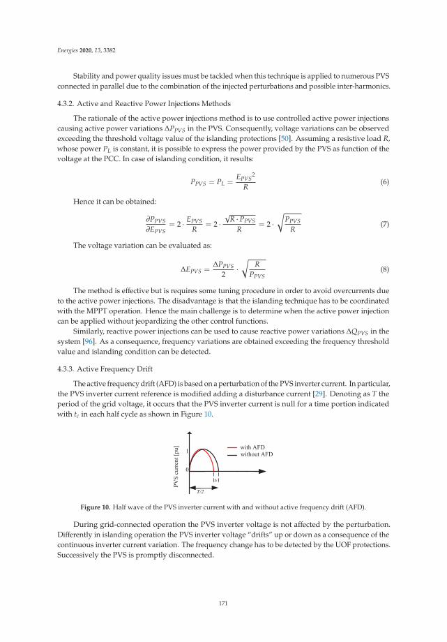
Energies 2020, 13, 3382

Stability and power quality issues must be tackled when this technique is applied to numerous PVSconnected in parallel due to the combination of the injected perturbations and possible inter-harmonics.

4.3.2. Active and Reactive Power Injections Methods

The rationale of the active power injections method is to use controlled active power injectionscausing active power variations ΔPPVS in the PVS. Consequently, voltage variations can be observedexceeding the threshold voltage value of the islanding protections [50]. Assuming a resistive load R,whose power PL is constant, it is possible to express the power provided by the PVS as function of thevoltage at the PCC. In case of islanding condition, it results:

PPVS = PL =EPVS

2

R(6)

Hence it can be obtained:

∂PPVS∂EPVS

= 2 · EPVSR

= 2 ·√

R · PPVS

R= 2 ·

√PPVS

R(7)

The voltage variation can be evaluated as:

ΔEPVS =ΔPPVS

2·√

RPPVS

(8)

The method is effective but is requires some tuning procedure in order to avoid overcurrents dueto the active power injections. The disadvantage is that the islanding technique has to be coordinatedwith the MPPT operation. Hence the main challenge is to determine when the active power injectioncan be applied without jeopardizing the other control functions.

Similarly, reactive power injections can be used to cause reactive power variations ΔQPVS in thesystem [96]. As a consequence, frequency variations are obtained exceeding the frequency thresholdvalue and islanding condition can be detected.

4.3.3. Active Frequency Drift

The active frequency drift (AFD) is based on a perturbation of the PVS inverter current. In particular,the PVS inverter current reference is modified adding a disturbance current [29]. Denoting as T theperiod of the grid voltage, it occurs that the PVS inverter current is null for a time portion indicatedwith tc in each half cycle as shown in Figure 10.

T/2

tctc

Figure 10. Half wave of the PVS inverter current with and without active frequency drift (AFD).

During grid-connected operation the PVS inverter voltage is not affected by the perturbation.Differently in islanding operation the PVS inverter voltage “drifts” up or down as a consequence of thecontinuous inverter current variation. The frequency change has to be detected by the UOF protections.Successively the PVS is promptly disconnected.

171

Energies 2020, 13, 3382

The AFD method is characterized by a chopping factor c which measures the amount ofthe perturbation:

c =2tc

T(9)

The method ensures correct islanding detection and simple implementation, but the maindisadvantage is the power quality detriment due to the current variation. Hence the method is notappropriate in case of numerous PVSs connected in parallel.

4.3.4. Sandia Frequency Shift

The Sandia frequency shift (SFS) methods derives from the AFD technique. SFS perturbs the PVSadding a dead-time to the PVS inverter reference current. Hence the inverter current exhibits a phase“shift” [29,97–99].

For this method, the chopping factor cS is defined as:

cS = cSo + kSFS( fPVS − f ) (10)

where kSFS is a proportional gain, cSo is the chopping factor in absence of frequency error, f is the gridfrequency and fPVS is the output frequency of the PVS inverter.

When the PVS is connected to the grid, the frequency error is null since the grid sets the frequencyat the PCC. On the contrary, during islanding operation, the frequency error is not negligible. As aconsequence, the PVS inverter current grows in order to overcome the phase shift, the choppingfrequency increases, and the frequency varies beyond the OUF threshold values. Hence islandingis detected.

The SFS NDZ is smaller than the AFD NDZ. The improved islanding detection performancesare achieved to the detriment of the power quality performances. In addition, in case of high PVSspenetration, unexpected transient disturbances can be registered.

4.3.5. Sandia Voltage Shift

The Sandia voltage shift (SVS) method operates with positive feedback of the PCC voltageamplitude [29,100]. During grid-connected operation of the PVS no significant variations are observed.In case of disconnection of the grid, voltage variations are monitored at the PCC. As a consequence,also the PVS inverter voltage varies and later the PVS is tripped since the voltage variations exceed theOUV protections threshold values. The NDZ of the SVS method is very small. However, the powerquality is worsened and also the efficiency is reduced since the power processed by the inverter varies.

4.3.6. Slip-Mode Frequency Shift

The slip-mode frequency shift (SMS) detects islanding phenomenon using positive feedback tolead the PVS towards instability in case of grid disconnection [80,101,102]. In case of grid disconnection,the PVS frequency changes naturally. The PVS PLL action can be modified in order to increase thefrequency rate of change rather than to annul it. The phase is forced to be a function of the voltagefrequency at the PCC. The PLL acts to increase the frequency until the PVS inverter voltage phasegrows faster than the phase of the RLC load (unstable region). The PVS is tripped when the invertervoltage frequency exceeds the threshold value. The method can fail when the load phase slope ishigher than the slope achieved by the SMS technique. In this case instability could not be recognized.

In Figure 11 there is shown how the action of the PVS PLL is modified on the basis of the SMSrationale. The PVS phase angle changes from θPVS to θSMS.

172

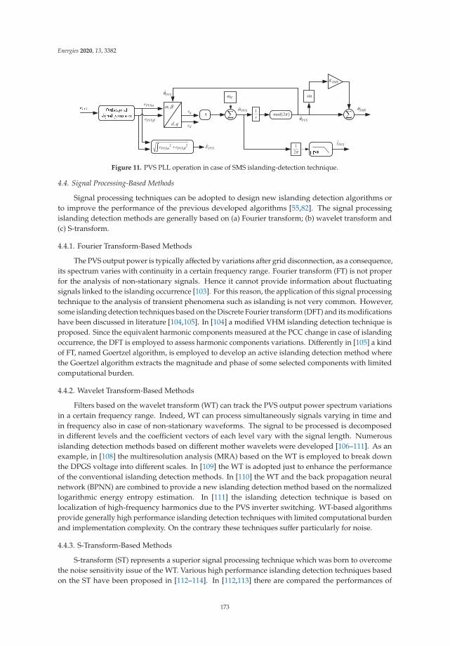
Energies 2020, 13, 3382

qe

PVSθ

PVSf

( )π

PVS PVSe eα β+

ICω

s

πPVSE

PVSωPVSe α

PVSe β

α β

d qde

PVSθ

SMSK

SMSθ

Figure 11. PVS PLL operation in case of SMS islanding-detection technique.

4.4. Signal Processing-Based Methods

Signal processing techniques can be adopted to design new islanding detection algorithms orto improve the performance of the previous developed algorithms [55,82]. The signal processingislanding detection methods are generally based on (a) Fourier transform; (b) wavelet transform and(c) S-transform.

4.4.1. Fourier Transform-Based Methods

The PVS output power is typically affected by variations after grid disconnection, as a consequence,its spectrum varies with continuity in a certain frequency range. Fourier transform (FT) is not properfor the analysis of non-stationary signals. Hence it cannot provide information about fluctuatingsignals linked to the islanding occurrence [103]. For this reason, the application of this signal processingtechnique to the analysis of transient phenomena such as islanding is not very common. However,some islanding detection techniques based on the Discrete Fourier transform (DFT) and its modificationshave been discussed in literature [104,105]. In [104] a modified VHM islanding detection technique isproposed. Since the equivalent harmonic components measured at the PCC change in case of islandingoccurrence, the DFT is employed to assess harmonic components variations. Differently in [105] a kindof FT, named Goertzel algorithm, is employed to develop an active islanding detection method wherethe Goertzel algorithm extracts the magnitude and phase of some selected components with limitedcomputational burden.

4.4.2. Wavelet Transform-Based Methods

Filters based on the wavelet transform (WT) can track the PVS output power spectrum variationsin a certain frequency range. Indeed, WT can process simultaneously signals varying in time andin frequency also in case of non-stationary waveforms. The signal to be processed is decomposedin different levels and the coefficient vectors of each level vary with the signal length. Numerousislanding detection methods based on different mother wavelets were developed [106–111]. As anexample, in [108] the multiresolution analysis (MRA) based on the WT is employed to break downthe DPGS voltage into different scales. In [109] the WT is adopted just to enhance the performanceof the conventional islanding detection methods. In [110] the WT and the back propagation neuralnetwork (BPNN) are combined to provide a new islanding detection method based on the normalizedlogarithmic energy entropy estimation. In [111] the islanding detection technique is based onlocalization of high-frequency harmonics due to the PVS inverter switching. WT-based algorithmsprovide generally high performance islanding detection techniques with limited computational burdenand implementation complexity. On the contrary these techniques suffer particularly for noise.

4.4.3. S-Transform-Based Methods

S-transform (ST) represents a superior signal processing technique which was born to overcomethe noise sensitivity issue of the WT. Various high performance islanding detection techniques basedon the ST have been proposed in [112–114]. In [112,113] there are compared the performances of

173

Energies 2020, 13, 3382

the ST and of the WT. Better results in terms of islanding detection and localization are obtainedusing the ST instead of the WT. Similar results are achieved in [114] where the islanding detectionmethod is based on the analysis of the negative sequence voltage. For this reason, the method cannotbe applied to single-phase PVS avoiding modifications. However, it is demonstrated that the useof the ST results particularly advantageous to detect islanding condition also in presence of noise.In conclusion, higher performances are ensured in the islanding detection since S-transform allows theextraction of the phase of each frequency component related to the time-varying signals involved inthe islanding phenomenon. Nevertheless, these techniques require more computational burden thanthe WT-based methods.

4.5. Hybrid Methods

In the present standard [25], it is established that any requirements for ride-through shall notbe falsely inhibited by any methods or design features utilized to meet the unintentional islandingdetection when an actual unintentional island condition does not exist. Conversely, the unintentionalislanding detection requirements shall not be inhibited by ride-through during valid unintentionalislanding conditions.

Passive methods operating alone cannot provide satisfying results considering their poor islandingdetection performance and the need to ensure ride-through capability by the PVS. Better results can beobtained using active methods, but the power quality is often affected.

Taking into account also the recent advancement in computing capability and communicationsystems, hybrid islanding detection techniques, based on combinations of the four categoriespreviously discussed, represent the most promising techniques [115–125]. Starting from combinationor modification of conventional methods, in [115] some islanding detection methods are proposedas integration of well-known passive methods. In [116] a modified active SVS method is presented,and the modulation index is used as injected signal to achieve the voltage magnitude shift and todetect the islanding phenomenon. In [117] a hybrid active method is developed combining a thresholdfilter (based on a binary tree classifier) with a harmonic amplification factor used as perturbationto detect islanding. In [118] a modified active islanding detection method is obtained varying theamplitude of the PVS current periodically. In this case islanding occurrence is detected through theAFD method when high current variations are registered. In [119] an active technique is obtainedcombining the AFD with the SMS. In [120] a new active islanding detection method is proposed andbased on the droop control theory. The droop control is modified considering a correlation functionbetween the frequency and the reactive power. This function is used to detect the islanding condition.Moving towards more innovative solutions, in [121] a new islanding detection technique is based onthe addition of a variable impedance and a hybrid automatic transfer switch. In [122] computationalgeometry has been applied to derive an islanding detection technique based on a classifier module.As in case of the active methods, the technique discussed in [123] uses harmonic current injection.The islanding condition is detected through cross correlation. In [124] an original islanding detectionscheme based on machine learning adoption is proposed. In [125] a communication-based islandingdetection method is presented based on a wireless sensors network. The performances are improvedadding a combination of selected loads in the system in order to avoid excessive voltage variations.

4.6. Performances Evaluation of the Islanding Detection Methods

The performances of the considered islanding detection categories are reviewed in Table 1.The main advantages and disadvantages related to the same categories are summarized inTable 2. The hybrid methods are combinations of the islanding detection techniques categorizedas communication-based methods, passive methods, active methods and signal processing-basedmethods. The performances of the hybrid methods depend on the original characteristics of thetechniques that they match, hence hybrid methods are not reported in Tables 1 and 2. The hybridmethods are designed to overcome the disadvantages of the islanding detection techniques previously

174

Energies 2020, 13, 3382

developed. As a consequence, hybrid methods are progressively updated, and they can be assessed astradeoff among advantages of the original methods and increased implementation complexity.

Table 1. Performances of the islanding detection methods.

Communication-Based Methods Passive Methods Active Methods Signal Processing-Based Methods

Accuracy high poor high highNDZ area absent wide limited absent or limitedDynamics fast generally fast medium slow fast

Impact on the grid no no medium or significant noPrice high limited limited high

Table 2. Advantages and disadvantages of the islanding detection methods.

Communication-BasedMethods

Passive Methods Active Methods Signal Processing-Based Methods

Advantage reliability simplicity accuracyrelative simplicity accuracy

Disadvantage expensive with regard to lowpower PVSs

erroneousdetection in case ofpower balancebetween generationand load

power quality detriment complexity

improperestimation due toride-throughrequirementscompliance

stability hazard in case ofnumerous PVSs connectedin parallel

5. Synchronization and Islanding Detection Coordination

ZCD methods and ZCD-based PLLs exhibit low dynamic performance and are not suitable forgrid voltage monitoring in case of abrupt changes of the grid voltage and power quality disturbances.Arctangent-based PLLs are not particularly widespread due to implementation issues. The PLLs basedon Park transform and SOGI OSG, known as SOGI PLLs and the EPLLs represent the most promisingsynchronization systems for single-phase PVSs due to high filtering capability, also in presence of gridvoltage harmonic distortion, accuracy and high dynamic performances also in case of grid voltageabrupt variations. SOGI PLLs and EPLLs are ideal candidates to be employed in the islanding detectionand in the reconnection of a PVS to the main grid after an islanding event.

5.1. Impact of the Synchronization Systems on the Islanding Detection Methods

Many islanding detection methods are based on information about the amplitude, the phaseand the frequency of the PVS voltage. These methods do not require additional synchronizationsystems to be included in the PVS control structure. The SOGI PLLs and the EPLLs represent the bestsynchronization systems for this kind of applications. Other islanding detection techniques requireadditional synchronization systems in order to monitor some selected harmonics and the PVS currentor can require some modification of the synchronization system generally used to track the PVS voltage.There are also some islanding detection techniques which are not based on synchronization systemsinformation. In Table 3 there are reported the main devices used by the different islanding detectionmethods discussed in Section 4. The islanding detection methods which employ PLLs or EPLLs arepointed out. Hybrid methods are not included in Table 3 since their characteristics depend on theoriginal methods that they combine.

Looking at Table 3, it can be observed that both communication-based techniques and signalprocessing-based techniques avoid the use of PLLs. Indeed, the communication-based islandingdetection techniques are based on communication interface equipment, in particular receivers.The signal processing-based techniques are based on harmonics measurement and localization relatedto time-varying electrical signals such as voltage, power, entropy, etc. The harmonics decomposition isachieved through the use of the FT, the WT or the ST.

175

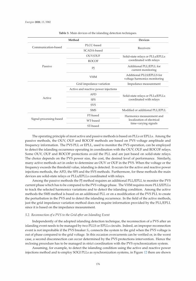
Energies 2020, 13, 3382

Table 3. Main devices of the islanding detection techniques.

Method Devices

Communication-basedPLCC-based

ReceiversSCADA-based

Passive

OUV/OUF Solid-state relays or PLLs/EPLLscoordinated with relaysROCOF

PJ Additional PLL/EPLL forcurrent monitoring

VHM Additional PLLS/EPLLS forvoltage harmonics monitoring

Active

Grid impedance variation Impedance measurement

Active and reactive power injections

Solid-state relays or PLLs/EPLLscoordinated with relays

AFD

SFS

SVS

SMS Modified or additional PLL/EPLL

Signal-processing-basedFT-based Harmonics measurement and

localization of electricaltime-varying signals

WT-based

ST-based

The operating principle of most active and passive methods is based on PLLs or EPLLs. Among thepassive methods, the OUV, OUF and ROCOF methods are based on PVS voltage amplitude andfrequency information. The PVS PLL or EPLL, used to monitor the PVS operation, can be employedto detect the islanding occurrence operating in coordination with the OUV, OUF and ROCOF relays.Some OUV, OUF and ROCOF protections avoid the PLL and are just based on solid-state relays.The choice depends on the PVS power size, the cost, the desired level of performance. Similarly,many active methods act in order to determine an OUV or OUF in the PVS. When the voltage or thefrequency exceeds the threshold value, islanding is detected. It occurs for the active and reactive powerinjections methods, the AFD, the SFS and the SVS methods. Furthermore, for these methods the maindevices are solid-state relays or PLLs/EPLLs coordinated with relays.

Among the passive methods the PJ method requires an additional PLL/EPLL to monitor the PVScurrent phase which has to be compared to the PVS voltage phase. The VHM requires more PLLS/EPLLsto track the selected harmonics variations and to detect the islanding condition. Among the activemethods the SMS method is based on an additional PLL or on a modification of the PVS PLL to createthe perturbation in the PVS and to detect the islanding occurrence. In the field of the active methods,just the grid impedance variation method does not require information provided by the PLL/EPLLsince it is based on the impedance measurement.

5.2. Reconnection of a PVS to the Grid after an Islanding Event

Independently of the adopted islanding detection technique, the reconnection of a PVS after anislanding event needs to be managed by two PLLS or EPLLs circuits. Indeed, an improper reconnectionevent is not improbable if the PVS breaker S1 connects the system to the grid when the PVS voltage isout of phase compared to the grid voltage. In this occasion overcurrents can be verified or, in the worstcase, a second disconnection can occur determined by the PVS protections intervention. Hence thereclosing procedure has to be managed in strict coordination with the PVS synchronization system.

Assuming, for example, to detect the islanding condition using the active and reactive powerinjections method and to employ SOGI PLLs as synchronization systems, in Figure 12 there are shown

176

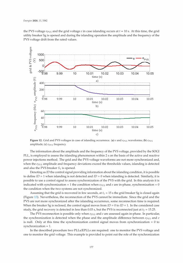
Energies 2020, 13, 3382

the PVS voltage ePVS and the grid voltage e in case islanding occurs at t = 10 s. At this time, the gridutility breaker Sg is opened and during the islanding operation the amplitude and the frequency of thePVS voltage drift from the rated values.

gri

d &

PV

S vo

ltage

s(V

)

time (s)a)

9.98 9.99 10 10.01 10.02 10.03 10.04 10.050

200

400

ePV

S am

plitu

de (V

)

time (s)b)

9.98 9.99 10 10.01 10.02 10.03 10.04 10.0520

40

60

ePV

S freq

uenc

y (H

z)

time (s)c)

Figure 12. Grid and PVS voltages in case of islanding occurrence. (a) e and ePVS waveforms; (b) ePVS

amplitude; (c) ePVS frequency.

The information about the amplitude and the frequency of the PVS voltage, provided by the SOGIPLL, is employed to assess the islanding phenomenon within 2 s on the basis of the active and reactivepower injections method. The grid and the PVS voltage waveforms are not more synchronized and,when the ePVS amplitude and frequency deviations exceed the thresholds values, islanding is detectedand also the PVS breaker S1 is opened.

Denoting as ID the control signal providing information about the islanding condition, it is possibleto define ID = 1 when islanding is not detected and ID = 0 when islanding is detected. Similarly, it ispossible to use a control signal to assess synchronization of the PVS with the grid. In this analysis it isindicated with synchronization = 1 the condition when ePVS and e are in-phase, synchronization = 0the condition when the two systems are not synchronized.

Assuming that the grid is recovered in few seconds, at t1 = 15 s the grid breaker Sg is closed again(Figure 13). Nevertheless, the reconnection of the PVS cannot be immediate. Since the grid and thePVS are not more synchronized after the islanding occurrence, some reconnection time is required.When the breaker Sg is reclosed, the control signal moves from ID = 0 to ID = 1. In the considered casestudy, the grid recovery is detected in less than 0.03 s, but the PVS is reconnected just at t2 = 15.25.

The PVS reconnection is possible only when ePVS and e are assessed again in-phase. In particular,the synchronization is detected when the phase and the amplitude difference between ePVS and eis null. Only at this time the synchronization control signal moves from synchronization = 0 tosynchronization = 1.

In the described procedure two PLLs/EPLLs are required: one to monitor the PVS voltage andone to monitor the grid voltage. This example is provided to point out the role of the synchronization

177

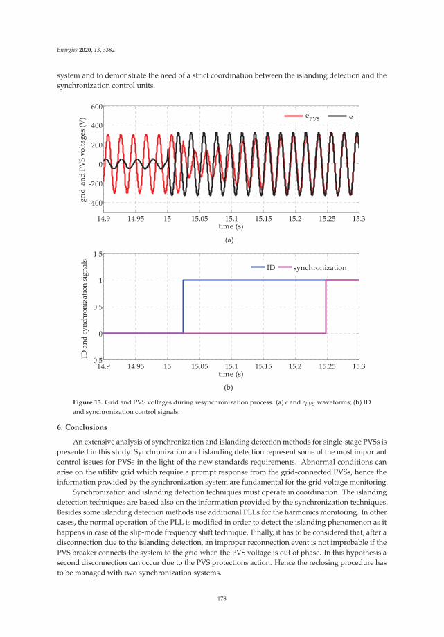
Energies 2020, 13, 3382

system and to demonstrate the need of a strict coordination between the islanding detection and thesynchronization control units.

14.9 14.95 15 15.05 15.1 15.15 15.2 15.25 15.3

-400

-200

0

200

400

600

grid

and

PV

S vo

ltage

s (V

)

time (s)

ePVS e

14.9 14.95 15 15.05 15.1 15.15 15.2 15.25 15.3-0.5

0

0.5

1

1.5

ID a

nd sy

nchr

oniz

atio

n si

gnal

s

time (s)

ID synchronization

(b)

(a)

Figure 13. Grid and PVS voltages during resynchronization process. (a) e and ePVS waveforms; (b) IDand synchronization control signals.

6. Conclusions

An extensive analysis of synchronization and islanding detection methods for single-stage PVSs ispresented in this study. Synchronization and islanding detection represent some of the most importantcontrol issues for PVSs in the light of the new standards requirements. Abnormal conditions canarise on the utility grid which require a prompt response from the grid-connected PVSs, hence theinformation provided by the synchronization system are fundamental for the grid voltage monitoring.

Synchronization and islanding detection techniques must operate in coordination. The islandingdetection techniques are based also on the information provided by the synchronization techniques.Besides some islanding detection methods use additional PLLs for the harmonics monitoring. In othercases, the normal operation of the PLL is modified in order to detect the islanding phenomenon as ithappens in case of the slip-mode frequency shift technique. Finally, it has to be considered that, after adisconnection due to the islanding detection, an improper reconnection event is not improbable if thePVS breaker connects the system to the grid when the PVS voltage is out of phase. In this hypothesis asecond disconnection can occur due to the PVS protections action. Hence the reclosing procedure hasto be managed with two synchronization systems.

178

Energies 2020, 13, 3382

For all these reasons synchronization and islanding detection issues were analyzed together.More than 120 publications were revised and discussed in order to provide a combined review.Both the synchronization and the islanding detection techniques were categorized. The choice of theislanding detection technique depends on numerous criteria. The EPLL and the SOGI PLL represent thepreferable synchronization systems to operate in coordination with the islanding detection techniques.

Funding: This research received no external funding.

Conflicts of Interest: The authors declare no conflict of interest.

References

1. IEA PVPS Annual Report 2019. Available online: https://iea-pvps.org/wp-content/uploads/2020/02/5319-iea-pvps-report-2019-08-lr.pdf (accessed on 26 March 2020).

2. Solar PV—Statistics & Facts, The Statistics Portal. Available online: https://www.statista.com/topics/993/solar-pv/ (accessed on 15 April 2020).

3. International Renewable Energy Agency IRENA. Renewable Capacity Statistics 2020. Available online: https://www.irena.org/publications/2020/Mar/Renewable-Capacity-Statistics-2020 (accessed on 26 March 2020).

4. Kausika, B.B.; Moraitis, P.; van Sark, W.G.J.H.M. Visualization of Operational Performance of Grid-ConnectedPV Systems in Selected European Countries. Energies 2018, 11, 1330. [CrossRef]

5. Ghosh, S.; Rahman, S. Global deployment of solar photovoltaics: Its opportunities and challenges.In Proceedings of the 2016 IEEE PES Innovative Smart Grid Technologies Conference Europe (ISGT-Europe),Ljubljana, Slovenia, 9–12 October 2016; pp. 1–6. [CrossRef]

6. Araujo, S.V.; Zacharias, P.; Mallwitz, R. Highly Efficient Single-Phase Transformerless Inverters forGrid-Connected Photovoltaic Systems. IEEE Trans. Ind. Electron. 2010, 57, 3118–3128. [CrossRef]

7. Olowu, T.O.; Sundararajan, A.; Moghaddami, M.; Sarwat, A.I. Future Challenges and Mitigation Methodsfor High Photovoltaic Penetration: A Survey. Energies 2018, 11, 1782. [CrossRef]

8. Integrating Renewable Electricity on the Grid—A Report by the APS Panel on Public Affairs, Washington,DC, USA. Available online: https://www.smartgrid.gov/document/integrating_renewable_electricity_grid_report_aps_panel_public_affairs (accessed on 20 November 2011).

9. Ropp, M.; Newmiller, J.; Whitaker, C.; Norris, B. Review of potential problems and utility concerns arisingfrom high penetration levels of photovoltaics in distribution systems. In Proceedings of the 33rd IEEEPhotovoltaic Specialists Conference PVSC ’08, San Diego, CA, USA, 11–16 May 2008; pp. 1–6. [CrossRef]

10. Appen, J.V.; Braun, M.; Stetz, T.; Diwold, K.; Geibel, D. Time in the Sun: The Challenge of High PV Penetrationin the German Electric Grid. IEEE Power Energy Mag. 2013, 11, 55–64. [CrossRef]

11. Molina-García, A.; Mastromauro, R.A.; García-Sánchez, T.; Pugliese, S.; Liserre, M.; Stasi, S. Reactive PowerFlow Control for PV Inverters Voltage Support in LV Distribution Networks. IEEE Trans. Smart Grid 2017, 8,447–456. [CrossRef]

12. Vasquez, J.C.; Mastromauro, R.A.; Guerrero, J.M.; Liserre, M. Voltage Support Provided by a Droop-ControlledMultifunctional Inverter. IEEE Trans. Ind. Electron. 2009, 56, 4510–4519. [CrossRef]

13. Mastromauro, R.A.; Liserre, M.; Kerekes, T.; Dell’Aquila, A. A Single-Phase Voltage-ControlledGrid-Connected Photovoltaic System with Power Quality Conditioner Functionality. IEEE Trans. Ind. Electron.2009, 56, 4436–4444. [CrossRef]

14. Koutroulis, E.; Blaabjerg, F. Design Optimization of Transformerless Grid-Connected PV Inverters IncludingReliability. IEEE Trans. Power Electron. 2013, 28, 325–335. [CrossRef]

15. Zhang, L.; Sun, K.; Feng, L.; Wu, H.; Xing, Y. A Family of Neutral Point Clamped Full-Bridge Topologies forTransformerless Photovoltaic Grid-Tied Inverters. IEEE Trans. Power Electron. 2013, 28, 730–739. [CrossRef]

16. Freddy, T.K.S.; Rahim, N.A.; Hew, W.; Che, H.S. Comparison and Analysis of Single-Phase TransformerlessGrid-Connected PV Inverters. IEEE Trans. Power Electron. 2014, 29, 5358–5369. [CrossRef]

17. Yang, Y.; Blaabjerg, F.; Wang, H. Low-Voltage Ride-Through of Single-Phase Transformerless PhotovoltaicInverters. IEEE Trans. Ind. Appl. 2014, 50, 1942–1952. [CrossRef]

18. Teodorescu, R.; Liserre, M.; Rodriguez, P. Grid Converters for Photovoltaic and Wind Power Systems; IEEE/Wiley:Chichester, UK, 2011.

179

Energies 2020, 13, 3382

19. Mastromauro, R.A.; Liserre, M.; Dell’Aquila, A. Control Issues in Single-Stage Photovoltaic Systems: MPPT,Current and Voltage Control. IEEE Trans. Ind. Inform. 2012, 8, 241–254. [CrossRef]

20. Johnson, B.B.; Dhople, S.V.; Hamadeh, A.O.; Krein, P.T. Synchronization of Parallel Single-Phase Inverterswith Virtual Oscillator Control. IEEE Trans. Power Electron. 2014, 29, 6124–6138. [CrossRef]

21. Hadjidemetriou, L.; Kyriakides, E.; Yang, Y.; Blaabjerg, F. A Synchronization Method for Single-PhaseGrid-Tied Inverters. IEEE Trans. Power Electron. 2016, 31, 2139–2149. [CrossRef]

22. Shitole, A.B.; Suryawanshi, H.M.; Talapur, G.G.; Sathyan, S.; Ballal, M.S.; Borghate, V.B.; Ramteke, M.R.;Chaudhari, M.A. Grid Interfaced Distributed Generation System with Modified Current Control Loop UsingAdaptive Synchronization Technique. IEEE Trans. Ind. Inform. 2017, 13, 2634–2644. [CrossRef]

23. Nagliero, A.; Mastromauro, R.A.; Liserre, M.; Dell’Aquila, A. Monitoring and Synchronization Techniquesfor Single-Phase PV Systems. In Proceedings of the 2010 International Symposium on Power Electronics,Electrical Drives, Automation and Motion SPEEDAM 2010, Pisa, Italy, 14–16 June 2010; pp. 1404–1409.[CrossRef]

24. Ghartemani, M.K.; Iravani, M.R. A nonlinear adaptative filter for online signal analysis in power systemsapplications. IEEE Trans. Power Deliv. 2002, 17, 617–622. [CrossRef]

25. IEEE Standard for Interconnection and Interoperability of Distributed Energy Resources with Associated ElectricPower Systems Interfaces; IEEE Std 1547-2003; IEEE: Piscataway, NJ, USA, 6 April 2018; pp. 1–138. [CrossRef]

26. Anani, N.; AlAli, O.A.-K.; Al-Qutayri, M.; AL-Araji, S. Synchronization of a renewable energy inverter withthe grid. J. Renew. Sustain. Energy 2012, 4. [CrossRef]

27. Lubura, S.; Soja, M.; Lale, S.; Ikic, M. Single-phase phase locked loop with dc offset and noise rejection forphotovoltaic inverters. IET Power Electron. 2014, 7, 2288–2299. [CrossRef]

28. Luna, A.; Rocabert, J.; Candela, J.I.; Hermoso, J.R.; Teodorescu, R.; Blaabjerg, F.; Rodríguez, P. Grid VoltageSynchronization for Distributed Generation Systems Under Grid Fault Conditions. IEEE Trans. Ind. Appl.2015, 51, 3414–3425. [CrossRef]

29. Bower, W.; Ropp, M. Evaluation of Islanding Detection Methods for Utility-Interactive Inverters in PhotovoltaicSystems. SANDIA REPORT SAND2002-3591. November 2002. Available online: https://pdfs.semanticscholar.org/2a29/ad6772ffef963d7dfdaece6a9db374e5e3b6.pdf (accessed on 29 March 2020).

30. Zhou, Y.; Li, H.; Liu, L. Integrated Autonomous Voltage Regulation and Islanding Detection for HighPenetration PV Applications. IEEE Trans. Power Electron. 2013, 28, 2826–2841. [CrossRef]

31. Yang, F.; Xia, N.; Han, Q. Event-Based Networked Islanding Detection for Distributed Solar PV GenerationSystems. IEEE Trans. Ind. Inform. 2017, 13, 322–329. [CrossRef]

32. Baghaee, H.R.; Mlakic, D.; Nikolovski, S.; Dragiccvic, T. Anti-Islanding Protection of PV-Based MicrogridsConsisting of PHEVs Using SVMs. IEEE Trans. Smart Grid 2020, 11, 483–500. [CrossRef]

33. Reddy, V.R.; Sreeraj, S.E. A Feedback-Based Passive Islanding Detection Technique for One-Cycle-ControlledSingle-Phase Inverter Used in Photovoltaic Systems. IEEE Trans. Ind. Electron. 2020, 67, 6541–6549. [CrossRef]

34. Hung, G.-K.; Chang, C.-C.; Chen, C.-L. Automatic phase-shift method for islanding detection ofgrid-connected photovoltaic inverters. IEEE Trans. Energy Convers. 2003, 18, 169–173. [CrossRef]

35. Serban, E.; Serban, H. A Control Strategy for a Distributed Power Generation Microgrid Applicationwith Voltage- and Current-Controlled Source Converter. IEEE Trans. Power Electron. 2010, 25, 2981–2992.[CrossRef]

36. IEEE Application Guide for IEEE Std 1547™, IEEE Standard for Interconnecting Distributed Resources with ElectricPower Systems; IEEE: Piscataway, NJ, USA, April 2009; pp. 1–217. [CrossRef]

37. IEEE Approved Draft Standard Conformance Test Procedures for Equipment Interconnecting Distributed EnergyResources with Electric Power Systems and Associated Interfaces; IEEE P1547.1/D9.9; IEEE: Piscataway, NJ, USA,January 2020; pp. 1–283.

38. IEEE Recommended Practice for Utility Interface of Photovoltaic (PV) Systems; IEEE Std 929-2000; IEEE: New York,NY, USA, 2000. [CrossRef]

39. IEC 61727-2004. Photovoltaic (PV) Systems—Characteristics of the Utility Interface; International ElectrotechnicalCommission: Geneva, Switzerland, 2004.

40. GB/T 19939-2005. Technical Requirements for Grid Connection of PV System; China National StandardizationAdministration Committee: Beijing, China, 2005.

41. CIGRE Working Group B5. The Impact of Renewable Energy Sources and Distributed Generation on SubstationProtection and Automation; CIGRE: Paris, France, 2010.

180

Energies 2020, 13, 3382

42. Gardner, F.M. Phaselock Techniques, 2nd ed.; Wiley-Interscience: Hoboken, NJ, USA, 1979; p. 304. ISBN -10:0471042943.

43. Jaalam, N.; Rahim, N.A.; Bakar, A.H.A.; Tan, C.; Haidar, A.M.A. A comprehensive review of synchronizationmethods for grid-connected converters of renewable energy source. Renew. Sustain. Energy Rev. 2016, 59,1471–1481. [CrossRef]

44. Guan-Chyun, H.; Hung, J.C. Phase-locked loop techniques. A Survey. IEEE Trans. Ind. Electron. 1996, 43,609–615. [CrossRef]

45. Golestan, S.; Guerrero, J.M.; Vasquez, J.C. Three-Phase PLLs: A Review of Recent Advances. IEEE Trans.Power Electron. 2017, 32, 1894–1907. [CrossRef]

46. Golestan, S.; Monfared, M.; Freijedo, F. Design-oriented study of advanced synchronous reference framephase-locked loops. IEEE Trans. Power Electron. 2013, 28, 765–778. [CrossRef]

47. Paiva, S.C.; Sanca, H.S.; Costa, F.B.; Souza, B.A. Reviewing of anti-islanding protection. In Proceedingsof the 11th IEEE/IAS International Conference on Industry Applications, Juiz de Fora, Brazil,7–10 December 2014; pp. 1–8. [CrossRef]

48. Li, C.; Cao, C.; Cao, Y.; Kuang, Y.; Zeng, L.; Fang, B. A review of islanding detection methods for microgrid.Renew. Sustain. Energy Rev. 2014, 35, 211–220. [CrossRef]

49. de Mango, F.; Liserre, M.; Dell’Aquila, A.; Pigazo, A. Overview of anti-islanding algorithms for PV systems.Part I: Passive methods. In Proceedings of the 12th International Power Electronics and Motion Conference,Portoroz, Slovenia, 30 August–1 September 2006; pp. 1878–1883. [CrossRef]

50. de Mango, F.; Liserre, M.; Dell’Aquila, A. Overview of anti-islanding algorithms for PV systems. Part II:Active methods. In Proceedings of the 12th International Power Electronics and Motion Conference, Portoroz,Slovenia, 30 August 30–1 September 2006; pp. 1884–1889. [CrossRef]

51. Abokhalil, A.G.; Awan, A.B.; Al-Qawasmi, A.R. Comparative Study of Passive and Active Islanding DetectionMethods for PV Grid-Connected Systems. Sustainability 2018, 10, 1798. [CrossRef]

52. Mahat, P.; Chen, Z.; Bak-Jensen, B. Review of islanding detection methods for distributed generation.In Proceedings of the Third International Conference on Electric Utility Deregulation and Restructuring andPower Technologies, Nanjing, China, 6–8 April 2008; pp. 2743–2748. [CrossRef]

53. Estébanez, E.J.; Moreno, V.M.; Pigazo, A.; Liserre, M.; Dell’Aquila, A. Performance Evaluation of ActiveIslanding-Detection Algorithms in Distributed-Generation Photovoltaic Systems: Two Inverters Case.IEEE Trans. Ind. Electron. 2011, 58, 1185–1193. [CrossRef]

54. Trujillo, C.L.; Velasco, D.; Figueres, E.; Garcerá, G. Analysis of active islanding detection methods forgrid-connected microinverters for renewable energy processing. Appl. Energy 2010, 87, 3591–3605. [CrossRef]

55. Raza, S.; Mokhlis, H.; Arof, H.; Laghari, J.A.; Wang, L. Application of signal processing techniques forislanding detection of distributed generation in distribution network: A review. Energy Convers. Manag.2015, 96, 613–624. [CrossRef]

56. Manikonda, S.K.G.; Gaonkar, D.N. Comprehensive review of IDMs in DG systems. IET Smart Grid 2019, 2,11–24. [CrossRef]

57. Khamis, A.; Shareef, H.; Bizkevelci, E.; Khatib, T. A review of islanding detection techniques for renewabledistributed generation systems. Renew. Sustain. Energy Rev. 2013, 28, 483–493. [CrossRef]

58. Singh, S.; Kewat, S.; Singh, B.; Panigrahi, B.K.; Kushwaha, M.K. Seamless Control of Solar PV Grid InterfacedSystem with Islanding Operation. IEEE Power Energy Technol. Syst. J. 2019, 6, 162–171. [CrossRef]

59. Lee, K.J.; Lee, J.P.; Shin, D.; Yoo, D.W.; Kim, H.J. A novel grid synchronization pll method based on adaptivelow-pass notch filter for grid-connected pcs. IEEE Trans. Ind. Electron. 2014, 61, 292–301. [CrossRef]

60. Wang, Y.F.; Li, Y.W. A Grid Fundamental and Harmonic Component Detection Method for Single-PhaseSystems. IEEE Trans. Power Electron. 2013, 28, 2204–2213. [CrossRef]

61. Karimi-Ghartemani, M. A Unifying Approach to Single-Phase Synchronous Reference Frame PLLs. IEEE Trans.Power Electron. 2013, 28, 4550–4556. [CrossRef]

62. Wall, R.W. Simple methods for detecting zero crossing. In Proceedings of the 29th Annual Conferenceof the IEEE Industrial Electronics Society IECON’03, Roanoke, VA, USA, 2–6 November 2003; Volume 3,pp. 2477–2481. [CrossRef]

63. Golestan, S.; Monfared, M.; Freijedo, F.D.; Guerrero, J.M. Dynamics Assessment of Advanced Single-PhasePLL Structures. IEEE Trans. Ind. Electron. 2013, 60, 2167–2177. [CrossRef]

181

Energies 2020, 13, 3382

64. Kandeepan, S.; Reisenfeld, S. Frequency tracking and acquisition with a four-quadrant arctan phase detectorbased digital phase locked loop. In Proceedings of the 2003 Joint Fourth International Conference onInformation, Communications and Signal Processing and the Fourth Pacific Rim Conference on Multimedia,Singapore, 15–18 December 2003; Volume 1, pp. 401–405. [CrossRef]

65. Konara, K.M.S.Y.; Kolhe, M.L.; Sankalpa, W.G.C.A. Grid synchronization of DC energy storage using VoltageSource Inverter with ZCD and PLL techniques. In Proceedings of the 2015 IEEE 10th International Conferenceon Industrial and Information Systems (ICIIS), Peradeniya, Sri Lanka, 18–20 December 2015; pp. 458–462.[CrossRef]

66. Weidenbrug, R.; Dawson, F.P.; Bonert, R. New synchronization method for thyristor power converters toweak AC-systems. IEEE Trans. Ind. Electron. 1993, 40, 505–511. [CrossRef]

67. Mur, F.; Cardenas, V.; Vaquero, J.; Martinez, S. Phase synchronization and measurement digital systemsof AC mains for power converters. In Proceedings of the 6th IEEE Power Electronics Congress CIEP 98,Morelia, Mexico, 12–15 October 1998; pp. 188–194. [CrossRef]

68. Choi, J.-W.; Kim, Y.-K.; Kim, H.-G. Digital PLL control for single-phase photovoltaic system. IEE Proc. EEElectr. Power Appl. 2006, 153, 40–46. [CrossRef]

69. Gonzalez-Espin, F.; Figueres, E.; Garcera, G. An Adaptive Synchronous-Reference-Frame Phase-Locked Loopfor Power Quality Improvement in a Polluted Utility Grid. IEEE Trans. Ind. Electron 2012, 59, 2718–2731.[CrossRef]

70. Yazdani, D.; Bakhshai, A.; Jain, P. Grid synchronization techniques for converter interfaced distributedgeneration systems. In Proceedings of the 2009 Energy Conversion Congress and Exposition, ECCE 2009,San Jose, CA, USA, 20–24 September 2009; pp. 2007–2014. [CrossRef]

71. Han, Y.; Luo, M.; Zhao, X.; Guerrero, J.M.; Xu, L. Comparative Performance Evaluation ofOrthogonal-Signal-Generators-Based Single-Phase PLL Algorithms—A Survey. IEEE Trans. Power Electron.2016, 31, 3932–3944. [CrossRef]

72. Yang, Y.; Blaabjerg, F.; Zou, Z. Benchmarking of Grid Fault Modes in Single-Phase Grid-ConnectedPhotovoltaic Systems. IEEE Trans. Ind. Appl. 2013, 49, 2167–2176. [CrossRef]

73. Rodriguez, P.; Teodorescu, R.; Candela, I.; Timbus, A.V.; Laabjerg, F.B. New positive-sequence voltagedetector for grid synchronization of power converters under faulty grid conditions. In Proceedings of the2006 37th IEEE Power Electronics Specialists Conference PESC’06, Jeju, Korea, 18–22 June 2006; pp. 1–7.[CrossRef]

74. Chittora, P.; Singh, A.; Singh, M. Adaptive EPLL for improving power quality in three-phase three-wiregrid-connected photovoltaic system. IET Renew. Power Gener. 2019, 13, 1595–1602. [CrossRef]

75. Karimi-Ghartemani, M. Enhanced Phase-Locked Loop Structures for Power and Energy Applications; Wiley-IEEEPress: Piscataway, NJ, USA, 21 March 2014. [CrossRef]

76. Karimi-Ghartemani, M. Linear and Pseudolinear Enhanced Phased-Locked Loop (EPLL) Structures.IEEE Trans. Ind. Electron. 2014, 61, 1464–1474. [CrossRef]

77. Sahoo, A.; Mahmud, K.; Ciobotaru, M.; Ravishankar, J. Adaptive Grid Synchronization Technique forSingle-phase Inverters in AC Microgrid. In Proceedings of the 2019 IEEE Energy Conversion Congress andExposition (ECCE), Baltimore, MD, USA, 29 September–3 October 2019; pp. 4441–4446. [CrossRef]

78. Task V Report IEA-PVPS T5-09:2002, Evaluation of Islanding Detection Methods for PhotovoltaicUtility-Interactive Power Systems. Available online: https://iea-pvps.org/wp-content/uploads/2020/01/rep5_09.pdf (accessed on 15 December 2002).

79. Ye, Z.; Kolwalkar, A.; Zhang, Y.; Du, P.; Walling, R. Evaluation of anti-islanding schemes based on nondetectionzone concept. IEEE Trans. Power Electron. 2004, 19, 1171–1176. [CrossRef]

80. Ropp, M.E.; Begovic, M.; Rohatgi, A.; Kern, G.A.; Bonn, R.H.; Gonzalez, S. Determining the relativeeffectiveness of islanding detection methods using phase criteria and nondetection zones. IEEE Trans.Energy Convers. 2000, 15, 290–296. [CrossRef]

81. IEEE Standard for Interconnecting Distributed Resources with Electric Power Systems; IEEE Std 1547-2003; IEEE:Piscataway, NJ, USA, 1–28 July 2003. [CrossRef]

82. Shrestha, A.; Kattel, R.; Dachhepatic, M.; Mali, B.; Thapa, R.; Singh, A.; Bista, D.; Adhikary, B.; Papadakis, A.;Maskey, R.K. Comparative Study of Different Approaches for Islanding Detection of Distributed GenerationSystems. Appl. Syst. Innov. 2019, 2. [CrossRef]

182

Energies 2020, 13, 3382

83. Samuelsson, O.; Strath, N. Islanding detection and connection requirements. In Proceedings of the 2007 IEEEPower Engineering Society General Meeting, Tampa, FL, USA, 24–28 June 2007; pp. 1–6. [CrossRef]

84. Ropp, M.; Larson, D.; Meendering, S.; MacMahon, D.; Ginn, J.; Stevens, J.; Bower, W.; Gonzalez, S.;Fennell, K.; Brusseau, L. Discussion of power line carrier communications-based anti-islanding schemeusing a commercial automatic meter reading system. In Proceedings of the 4th IEEE World Conference onPhotovoltaic Energy Conversion, Waikoloa, HI, USA, 7–12 May 2006; pp. 2351–2354. [CrossRef]

85. Benato, R.; Caldon, R. Distribution line carrier: Analysis procedure and applications to DG. IEEE Trans.Power Deliv. 2007, 22, 575–583. [CrossRef]

86. Xu, W.; Zhang, G.; Li, C.; Wang, W.; Wang, G.; Kliber, J. A power line signaling based technique foranti-islanding protection of distributed generators—Part i: Scheme and analysis. IEEE Trans. Power Deliv.2007, 22, 1758–1766. [CrossRef]

87. Wang, G.; Kliber, J.; Zhang, G.; Xu, W.; Howell, B.; Palladino, T. A power line signaling based technique foranti-islanding protection of distributed generators—Part ii: Field test results. IEEE Trans. Power Deliv. 2007,22, 1767–1772. [CrossRef]

88. Aphrodis, N.; Ntagwirumugara, E.; Vianney, B.J.M.; Mulolani, F. Design, Control and Validation of a PVSystem Based on Supervisory Control and Data Acquisition (SCADA) Viewer in Smartgrids. In Proceedingsof the 5th International Conference on Control, Automation and Robotics (ICCAR), Beijing, China,19–22 April 2019; pp. 23–28. [CrossRef]

89. Etxegarai, A.; Egua, P.; Zamora, I. Analysis of remote islanding detection methods for distributed resources.In Proceedings of the International Conference on Renewable Energies and Power Quality (ICREPQ’11),Las Palmas, Spain, 13–15 April 2011; pp. 1142–1147. Available online: http://www.icrepq.com/icrepq\T1\textquoteright11/580-etxegarai.pdf (accessed on 29 March 2020).

90. Vieira, W.X.J.C.; Freitas, W.; Morelato, A. Performance of frequency relays for distributed generationprotection. IEEE Trans. Power Deliv. 2006, 21, 1120–1127. [CrossRef]

91. Freitas, W.; Xu, W.; Affonso, C.M.; Huang, Z. Comparative analysis between ROCOF and vector surge relaysfor distributed generation applications. IEEE Trans. Power Deliv. 2005, 20, 1315–1324. [CrossRef]

92. Ten, C.F.; Crossley, P.A. Evaluation of Rocof Relay Performances on Networks with Distributed Generation.In Proceedings of the 2008 IET 9th International Conference on Developments in Power System Protection(DPSP 2008), Glasgow, Scotland, 17–20 March 2008; pp. 523–528. [CrossRef]

93. de la Fuente, D.V.; Rodriguez, C.L.T.; Narvaez, E.A. Review of Anti-Islanding Methods: Analysis by Figuresof Merit Tools for Controllers Reconfiguration in Microgrids. IEEE Lat. Am. Trans. 2015, 13, 679–686.[CrossRef]

94. Timbus, A.V.; Teodorescu, R.; Blaabjerg, F.; Borup, U. Online grid measurement and ENS detection for PVinverter running on highly inductive grid. IEEE Power Electron. Lett. 2004, 2, 77–82. [CrossRef]

95. Asiminoaei, L.; Teodorescu, R.; Blaabjerg, F.; Borup, U. A digital controlled PV-inverter with grid impedanceestimation for ENS detection. IEEE Trans. Power Electron. 2005, 20, 1480–1490. [CrossRef]

96. Jeraputra, P.N. Enjeti, Development of a robust anti-islanding algorithm for utility interconnection ofdistributed fuel cell powered generation. IEEE Trans. Power Electron. 2004, 19, 1163–1170. [CrossRef]

97. Du, P.; Ye, Z.; Aponte, E.E.; Nelson, J.K.; Fan, L. Positive-Feedback-Based Active Anti-Islanding Schemesfor Inverter-Based Distributed Generators: Basic Principle, Design Guideline and Performance Analysis.IEEE Trans. Power Electron. 2010, 25, 2941–2948. [CrossRef]

98. Zeineldin, H.H.; Conti, S. Sandia frequency shift parameter selection for multi-inverter systems to eliminatenon-detection zone. IET Renew. Power Gener. 2011, 5, 175–183. [CrossRef]

99. Reis, M.V.G.; Barros, T.A.S.; Moreira, A.B.; Nascimento, S.F.P.; Ruppert, F.E.; Villalva, M.G. Analysis ofthe Sandia Frequency Shift (SFS) islanding detection method with a single-phase photovoltaic distributedgeneration system. In Proceedings of the 2015 IEEE PES Innovative Smart Grid Technologies Latin AmericaISGT LATAM 2015, Montevideo, Uruguay, 5–7 October 2015; pp. 125–129. [CrossRef]

100. El-Moubarak, M.; Hassan, M.; Faza, A. Performance of three islanding detection methods for grid-tiedmulti-inverters. In Proceedings of the 2015 IEEE 15th International Conference on Environment and ElectricalEngineering (EEEIC), Rome, Italy, 10–13 June 2015; pp. 1999–2004. [CrossRef]

101. Mohammadpour, B.; Zareie, M.; Eren, S.; Pahlevani, M. Stability analysis of the slip mode frequencyshift islanding detection in single phase PV inverters. In Proceedings of the 2017 IEEE 26th InternationalSymposium on Industrial Electronics (ISIE), Edinburgh, UK, 19–21 June 2017; pp. 873–878. [CrossRef]

183

Energies 2020, 13, 3382

102. Mohammadpour, B.; Pahlevani, M.; Kaviri, S.M.; Jain, P. Advanced slip mode frequency shift islandingdetection method for single phase grid connected PV inverters. In Proceedings of the 2016 IEEE AppliedPower Electronics Conference and Exposition (APEC), Long Beach, CA, USA, 20–24 March 2016; pp. 378–385.[CrossRef]

103. Gu, Y.H.; Bollen, M.H.J. Time-Frequency and Time-Scale Domain Analysis of Voltage Disturbances. IEEE Trans.Power Deliv. 2000, 15, 1279–1284. [CrossRef]

104. Kim, I.-S. Islanding Detection Technique using Grid-Harmonic Parameters in the Photovoltaic System.Energy Procedia 2012, 14, 137–141. [CrossRef]

105. Kim, J.; Kim, J.; Ji, Y.; Jung, Y.; Won, C. An Islanding Detection Method for a Grid-Connected System Basedon the Goertzel Algorithm. IEEE Trans. Power Electron. 2011, 26, 1049–1055. [CrossRef]

106. Hanif, M.; Basu, M.; Gaughan, K. Development of EN50438 compliant wavelet-based islanding detectiontechnique for three-phase static distributed generation systems. IET Renew. Power Gener. 2012, 6, 289–301.[CrossRef]

107. Zhu, Y.; Yang, Q.; Wu, J.; Zheng, D.; Tian, Y. A novel islanding detection method of distributed generatorbased on wavelet transform. In Proceedings of the 2008 International Conference on Electrical Machines andSystems, Wuhan, China, 17–20 October 2008; pp. 2686–2688.

108. Ning, J.; Wang, C. Feature extraction for islanding detection using Wavelet Transform-based Multi-ResolutionAnalysis. In Proceedings of the 2012 IEEE Power and Energy Society General Meeting, San Diego, CA, USA,22–26 July 2012; pp. 1–6. [CrossRef]

109. Hsieh, C.-T.; Lin, J.-M.; Huang, S.-J. Enhancement of islanding-detection of distributed generation systemsvia wavelet transform-based approaches. Int. J. Electr. Power Energy Syst. 2008, 30, 575–580. [CrossRef]

110. Do, H.T.; Zhang, X.; Nguyen, N.V.; Li, S.S.; Chu, T.T. Passive-Islanding Detection Method Using the WaveletPacket Transform in Grid-Connected Photovoltaic Systems. IEEE Trans. Power Electron. 2016, 31, 6955–6967.[CrossRef]

111. Pigazo, A.; Liserre, M.; Mastromauro, R.A.; Moreno, V.M.; Dell’Aquila, A. Wavelet-Based Islanding Detectionin Grid-Connected PV Systems. IEEE Trans. Ind. Electron. 2009, 56, 4445–4455. [CrossRef]

112. Ray, P.; Mohanty, S.; Kishor, S.; Dubey, H. Coherency determination in grid connected distributed generationbased hybrid system under islanding scenarios. In Proceedings of the IEEE International Conference onPower and Energy (PECon2010), Kuala Lumpur, Malaysia, 29 November–1 December 2010; pp. 85–88.[CrossRef]

113. Ray, P.; Kishor, N.; Mohanty, S. S-Transform based islanding detection in grid connected distributed generationbased power system. In Proceedings of the 2010 IEEE International Energy Conference (ENERGYCON2010),Manama, Bahrain, 18–22 December 2010; pp. 612–617. [CrossRef]

114. Ray, P.; Mohanty, S.; Kishor, N. Disturbance detection in grid-connected distributed generation system usingwavelet and S-Transform. Electr. Power Syst. Res. 2011, 81, 805–819. [CrossRef]

115. Quoc-Tuan, T. New methods of islanding detection for photovoltaic inverters. In Proceedings of the 2016IEEE PES Innovative Smart Grid Technologies Conference Europe (ISGT-Europe), Ljubljana, Slovenia,9–12 October 2016; pp. 1–5. [CrossRef]

116. Liu, S.; Zhuang, S.; Xu, Q.; Xiao, J. Improved voltage shift islanding detection method for multi-invertergrid-connected photovoltaic systems. IET Gener. Transm. Distrib. 2016, 10, 3163–3169. [CrossRef]

117. Dhar, S.; Dash, P.K. Harmonic Profile Injection-Based Hybrid Active Islanding Detection Technique forPV-VSC-Based Microgrid System. IEEE Trans. Sustain. Energy 2016, 7, 1473–1481. [CrossRef]

118. Yu, B.; Matsui, M.; So, J.; Yu, G. A high power quality anti-islanding method using effective power variation.Sol. Energy 2008, 82, 368–378. [CrossRef]

119. Yu, B.; Matsui, M.; Jung, Y.; Yu, G. A combined active anti-islanding method for photovoltaic systems.Renew. Energy 2008, 33, 979–985. [CrossRef]

120. Muñoz-Cruzado-Alba, J.; Villegas-Núñez, J.; Vite-Frías, J.A.; Carrasco-Solís, J.M.; Galván-Díez, E.New Low-Distortion Q–f Droop Plus Correlation Anti-Islanding Detection Method for Power Converters inDistributed Generation Systems. IEEE Trans. Ind. Electron. 2015, 62, 5072–5081. [CrossRef]

121. Papadimitriou, C.N.; Kleftakis, V.A.; Hatziargyriou, N.D. A novel islanding detection method for microgridsbased on variable impedance insertion. Electr. Power Syst. Res. 2015, 121, 58–66. [CrossRef]

184

Energies 2020, 13, 3382

122. Vyas, S.; Kumar, R. Computational geometry-based methodology for identification of potential islandinginitiators in high solar PV penetration distribution feeders. IET Renew. Power Gener. 2018, 12, 456–462.[CrossRef]

123. Voglitsis, D.; Papanikolaou, N.P.; Kyritsis, A.C. Active Cross-Correlation Anti-Islanding Scheme for PVModule-Integrated Converters in the Prospect of High Penetration Levels and Weak Grid Conditions.IEEE Trans. Power Electron. 2019, 34, 2258–2274. [CrossRef]

124. Baghaee, H.R.; Mlakic, D.; Nikolovski, S.; Dragicevic, T. Support Vector Machine-based Islanding and GridFault Detection in Active Distribution Networks. IEEE J. Emerg. Sel. Top. Power Electron. 2019. [CrossRef]

125. Eshraghi, A.; Ghorbani, R. Islanding detection and over voltage mitigation using controllable loads.Sustain. Energy Grids Netw. 2016, 6, 125–135. [CrossRef]

© 2020 by the author. Licensee MDPI, Basel, Switzerland. This article is an open accessarticle distributed under the terms and conditions of the Creative Commons Attribution(CC BY) license (http://creativecommons.org/licenses/by/4.0/).

185

MDPISt. Alban-Anlage 66

4052 BaselSwitzerland

Tel. +41 61 683 77 34Fax +41 61 302 89 18

www.mdpi.com

Energies Editorial OfficeE-mail: energies@mdpi.com

www.mdpi.com/journal/energies

MDPI St. Alban-Anlage 66 4052 Basel Switzerland

Tel: +41 61 683 77 34 Fax: +41 61 302 89 18

www.mdpi.com ISBN 978-3-03936-849-5