1 23

Coral ReefsJournal of the International Society forReef Studies ISSN 0722-4028 Coral ReefsDOI 10.1007/s00338-013-1033-1

Ground-level spectroscopy analysesand classification of coral reefs using ahyperspectral camera

T. Caras & A. Karnieli

1 23

Your article is protected by copyright and

all rights are held exclusively by Springer-

Verlag Berlin Heidelberg. This e-offprint is

for personal use only and shall not be self-

archived in electronic repositories. If you

wish to self-archive your work, please use the

accepted author’s version for posting to your

own website or your institution’s repository.

You may further deposit the accepted author’s

version on a funder’s repository at a funder’s

request, provided it is not made publicly

available until 12 months after publication.

REPORT

Ground-level spectroscopy analyses and classification of coralreefs using a hyperspectral camera

T. Caras • A. Karnieli

Received: 16 May 2012 / Accepted: 15 March 2013

� Springer-Verlag Berlin Heidelberg 2013

Abstract With the general aim of classification and map-

ping of coral reefs, remote sensing has traditionally been

more difficult to implement in comparison with terrestrial

equivalents. Images used for the marine environment suffer

from environmental limitation (water absorption, scattering,

and glint); sensor-related limitations (spectral and spatial

resolution); and habitat limitation (substrate spectral simi-

larity). Presented here is an advanced approach for ground-

level surveying of a coral reef using a hyperspectral camera

(400–1,000 nm) that is able to address all of these limita-

tions. Used from the surface, the image includes a white

reference plate that offers a solution for correcting the water

column effect. The imaging system produces millimeter size

pixels and 80 relevant bands. The data collected have the

advantages of both a field point spectrometer (hyperspectral

resolution) and a digital camera (spatial resolution). Finally,

the availability of pure pixel imagery significantly improves

the potential for substrate recognition in comparison with

traditionally used remote sensing mixed pixels. In this study,

an image of a coral reef table in the Gulf of Aqaba, Red Sea,

was classified, demonstrating the benefits of this technology

for the first time. Preprocessing includes testing of two

normalization approaches, three spectral resolutions, and

two spectral ranges. Trained classification was performed

using support vector machine that was manually trained and

tested against a digital image that provided empirical veri-

fication. For the classification of 5 core classes, the best

results were achieved using a combination of a 450–660 nm

spectral range, 5 nm wide bands, and the employment of red-

band normalization. Overall classification accuracy was

improved from 86 % for the original image to 99 % for the

normalized image. Spectral resolution and spectral ranges

seemed to have a limited effect on the classification accu-

racy. The proposed methodology and the use of automatic

classification procedures can be successfully applied for reef

survey and monitoring and even upscaled for a large survey.

Keywords Spectroscopy � Classification � Remote

sensing � Hyperspectral � Glint � Monitoring � Survey

Introduction

Remotely sensed spectral data analysis has the potential to

become a cost-effective practice for reef investigation,

assessment, and monitoring (e.g., Mumby et al. 2004;

Knudby et al. 2007; Collin and Planes 2012). The most

desired application for remote sensing analysis of a coral

reef is usually a basic classification (or thematic mapping),

whereby the researcher wishes to quantify or map sub-

strates in the study area (Johansen et al. 2008; Kendall and

Miller 2008; Leiper et al. 2012). However, the integrity of

remotely sensed results is often questionable as three main

sources for errors obfuscate the image processing: (1)

Analysis of marine habitats is confounded by the optical

effect of the water and air columns above the substrate of

interest (e.g., Pope and Fry 1997; Holden and LeDrew

2000; Hedley et al. 2010); (2) spatial, spectral, and noise

limitations are imposed by the sensor itself (e.g., Yamano

and Tamura 2004; Kendall and Miller 2008); and (3)

similarities between the reflectance of the desired sub-

strates may cause errors in their identification (e.g., Hedley

Communicated by Geology Editor Prof. Bernhard Riegl

T. Caras (&) � A. Karnieli

The Remote Sensing Laboratory, Jacob Blaustein Institutes

for Desert Research, Ben-Gurion University of the Negev,

Sede-Boker Campus, 84990 Beersheba, Israel

e-mail: divething@yahoo.com

123

Coral Reefs

DOI 10.1007/s00338-013-1033-1

Author's personal copy

et al. 2004; Knudby et al. 2007). These three limitations are

detailed below.

Unlike terrestrial substrates, marine substrates are lim-

ited in their available spectral range to somewhere between

400 and 700 nm, dependent on water quality and clarity

(e.g., Smith and Baker 1981; Pope and Fry 1997; Zheng

et al. 2002). Predominantly, the effect of the water column

is that it scatters the shorter wave section of the spectrum

(up to about 450 nm) and absorbs most of the available

light above 600 nm (e.g., Lee et al. 1999; Wozniak et al.

2010). Understanding the effects of water and their cor-

rection is a formidable challenge and has been the subject

of numerous studies; these complexities and their potential

solutions are beyond the scope of this paper. Regardless,

within the spectral range available through water, spectral

features are concentrated between 550 and 700 nm (e.g.,

Hedley and Mumby 2002; Kutser et al. 2003; Hochberg

et al. 2006). Furthermore, it is important to note that even

with a good water correction procedure, the analysis is

confined to a maximum of 3–6 m water depth, beyond

which very little light above 600 nm leaves the water

(Kutser et al. 2003; Hedley et al. 2010).

Another environmental effect caused by the air–water

interface is the glint. This element is dependent on lighting

directionality in relation to the sensor position and there-

fore is often referred to as specular reflection (Kay et al.

2009). Glint can be produced by waves or wavelets that, in

a micro-scale, can change the water surface angle, thereby

producing a localized glint-like effect. In affected samples

(pixels or areas in the image), the reflection measured is

significantly higher than other (e.g., neighboring) samples.

The correction for glint is relatively simple and is based on

normalizing effected pixels to unaffected pixels using a

none-water-penetrating wavelength in the near-infrared

(NIR) spectral range (Hochberg et al. 2003a; Hedley et al.

2005; Kay et al. 2009).

Spatial resolution (i.e., pixel, the size of the land cov-

ered by each remotely sensed unit) and spectral resolution

(the number of spectral bands and their width) are usually

limited by the ability of the sensor to collect enough energy

(Mather and Koch 2004). Put together, even without the

effect of water absorbance, the total available radiance

(reflected light from the substrate) has to be balanced or

optimized between the unit area (pixel) and the number of

bands. To this end, with the available technology, it is

virtually impossible to achieve both high spectral resolu-

tion and high spatial resolution. Therefore, to date, anyone

who aims to study the reef using remote sensing has

essentially to choose between high spatial resolution (with

low spectral resolution) and high spectral resolution (cou-

pled with low spatial resolution). The choice in this

dilemma is fundamentally dependent on the scientific task

at hand.

A coral reef is a highly heterogeneous habitat in which

even the finest spatial resolution available (1–4 m) from

spaceborne systems is unlikely to contain a single substrate

(Andrefouet et al. 2002; Hochberg and Atkinson 2003;

Leiper et al. 2012). Not having a single substrate in a pixel

makes the classification infinitely more difficult as the

combination of substrates present may not necessarily be

linearly contributing to the pixel’s reflection (Joyce and

Phinn 2002; Hedley 2004). Studies attempting to address

this problem have used a combination of solutions such as

sub-pixel analysis (e.g., Hedley et al. 2012), or limiting

classification resolution to specific highly detectable sub-

strates, such as bleaching (Wooldridge and Done 2004;

Dekker et al. 2005; Dadhich et al. 2012). Many of the

solutions suggested above can be undertaken only with a

high spectral resolution that, in turn, limits the worker to a

coarser spatial resolution (from tens of meters upwards)

(Sterckx et al. 2005; Kutser et al. 2006; Hedley et al. 2012).

Reef substrates’ spectral separability is another subject

that has drawn considerable attention (e.g., Hochberg et al.

2003b; Lee et al. 2007; Leiper et al. 2012). Most examples

for spectral analysis rely on the benefits of hyperspectral

resolution and the ability to detect unique spectral features

of pure substrate measurements (e.g., Hochberg et al.

2003b; Karpouzli et al. 2004; Hamylton 2009). Examples

of coral reef pure substrate spectra are usually in situ

sampling using a hand-held spectrometer (Holden and

LeDrew 2002; Wettle et al. 2003). To date, only Hochberg

and Atkinson (2000) have used practically pure pixels for

their aerial remote sensing analysis despite pixel size of

0.5–0.9 m. This was possible because the substrate unit

and area coverage were very homogeneous and do not

represent a typical case study for habitats such as coral

reefs.

An alternative for coral reef remote sensing is in situ

digital photography. Taken underwater or above, it can

provide very high spatial resolution (unmatched compared

with remote sensing) but provides only three bands.

Although these are highly accurate pure pixel images, their

analysis is limited by the minimal spectral resolution.

Therefore, a typical data analysis of digital photography

requires lengthy manual post-processing and is manpower

intensive for large-scale coral reef monitoring (English

et al. 1997). That said, the potential for extracting high-

quality quantitative data, such as species identification or

accurate percent cover, could be good if the worker is well

trained and manpower is not limited.

Recent developments in sensor production provide

innovative remote sensing solutions tested in this study for

the first time. The use of a hyperspectral camera from the

surface offers an opportunity to deliver a potential solution

for all three sources of error discussed earlier: (1) Water

correction can be addressed by placing white reference

Coral Reefs

123

Author's personal copy

targets within the image (atmospheric correction is unnec-

essary) (Mather and Koch 2004); (2) the hyperspectral

camera is very similar to the AISA Eagle aerial sensor,

featured with the same spectral resolution and up to 80

bands within the relevant range. This spectral resolution far

exceeds the resolution recommended for coral reef deter-

mination (e.g., Lubin et al. 2001; Hochberg et al. 2003b;

Kutser et al. 2003). While this spectral resolution exists in

other aerial sensors such as AISA Eagle and CASI, the

special resolution is unmatched. Spatial resolution (pixel

size) is expected to be finer than that of the target substrate

units (e.g., coral colony), thus delivering a pure substrate

spectrum in each pixel (much like a digital image); and (3)

the combination of high spectral and high spatial (pure

pixels) resolution would allow superior recognition of

underwater substrates, leading to accurate quantitative

estimates of cover within the sampled area (the image). To

date, hyperspectral imaging data of this type have never

been used in the shallow marine environment. Therefore, it

resembles a combination of a field point spectrometer that

provides hyperspectral resolution and a digital camera that

produces high spatial resolution. Using the proposed tech-

nology may lead to the development of an image acquisition

and processing system that enables the analysis of the reef

features in a fast, accurate, and efficient way. An advanced

and improved design will support a semi-automatically run

system with minimal operator input over larger areas. All

these reasons together formed a strong rationale for testing

the capabilities of the proposed technology.

The aim of this study was to provide a preliminary

assessment of ground-level, above-water, remote sensing

of a coral reef. The objectives include acquiring a hyper-

spectral image, correction of environmental distortions,

and classification of the underwater substrates. In line with

the aim, the key objective is achieving the best (most

accurate) classification for the given image, using only

basic processing steps. Given the pioneering level of pro-

cessing protocol, objectives included testing a variety of

variables relevant to image preprocessing, including spec-

tral resolution and spectral ranges.

Methods

Study site

The coral-reef marine park (CRMP, 29�330N 34�570E) is

located at the northern end of the Gulf of Aqaba, 8 km

south of the city of Eilat, Israel. The study site is catego-

rized as fringing reef and is relatively small while the reef

table is approximately 25 m wide and 2 km long. The

choice of location is based on the availability of an over-

water dry structure and the relatively flat reef table.

Image acquisition

The hyperspectral image was obtained from the jetty

(bridge) over the reef (Fig. 1). Time to provide the best

results, the image was acquired during the late morning—

when the sun was at an angle that avoided glint effect.

Other conditions included low wind (approximately

5 knots), and the water was close to low tide, so the

average depth was 30 cm (ranging from 20 to 50 cm). The

camera/instrument used was a pushbroom line scanner

Spectral Camera HS by Specim Systems. It was fixed on a

boom, overhanging the reef as close as possible to the nadir

position. The camera’s 28� lens, opening at 2.5 m above

target, captured approximately 2 9 3 m of the reef table,

and the acquisition time was near 32 s. The camera pro-

vides 1,600 pixels per line (the image width); therefore,

divided by 2 m of image width, it gives, on average,

1.25 mm of reef substrate area per pixel. Lengthwise, the

camera is able to provide up to 2,500 lines although only

1,400 of those were captured to minimize image distortion

at the edges. Spectrally, 849 bands are captured in the

spectral range of 400–1,000 nm with a 0.67–0.74 nm band

width.

For demonstrating the technique, a subset of 500 9 500

pixels was selected from the entire image in order to

minimize pixel stretching due to camera angle (Fig. 2a, b).

The image included a plastic quadrate frame and two white

reference plates—one at the reef table depth (Fig. 2a) and

another at the water surface (not shown).

Image preprocessing and analysis

A digital number (DN) is a value assigned to a pixel in a

digital image that depicts the average radiance of the basic

Fig. 1 The construction of the hyperspectral camera on the bridge.

At this fully extended boom height, the camera can cover 3 9 6 m of

reef

Coral Reefs

123

Author's personal copy

picture element (pixel). The white reference needed for

water correction was an extracted spectrum of the under-

water white reference plate placed within the image at the

reef depth. Dividing the DN values by those of the white

reference converts all irradiance values into reflectance

values completing the image preparation (Lillesand and

Kiefer 2003; Mather and Koch 2004). Measuring that plate

underwater offers an opportunity to correct the effect of the

water medium on light passing through. This is based on

the assumption that—just like on land—those plates pro-

vide a baseline measurement representing all the light that

can be reflected from the target in those conditions. Since

the image analysis is undertaken in reflectance values and

the correction was based on an image-derived white ref-

erence, radiometric correction is an unneeded step and was

omitted from the image preparation sequence. Altogether,

three images were created to test the spectral resolution

parameter. The original image was spectrally resampled to

three spectral resolutions: 5 nm bands, 10 nm bands, and

20 nm bands, reducing the original number of bands

between 400 and 800 nm to 80, 40, and 20, respectively.

The final step of the pre-processing focused on

addressing the severe variability in spectral albedo,

including the glinting effects caused by surface ripples

(Fig. 2c). Those glinted pixels were different from their

surrounding pixels, both by their reflectance magnitude and

by their spectral features in the NIR spectral range (Fig. 3a).

Instead of filtering out high albedo pixels and imposing a

uniform correction approach on the darker pixels as well as

the light ones, a normalization procedure was employed.

This processing adopted the deglinting method described by

Hochberg et al. (2003a) and Hedley et al. (2005). This

correction is based on using the water opacity in the NIR

wavelengths (thus reflectance values are independent of

water absorption) as a baseline for normalization. In this

respect, it is similar to more familiar normalization tech-

niques based on the mean or mode of all bands. In the first

stage of this routine, each band is divided by a specific near-

a

b

c

Fig. 2 An example of a

hyperspectral image. a the

original full size image; b a clip

used for all analyses; and c a

close-up section showing

glinted (under the cross) and

non-glinted pixels

Coral Reefs

123

Author's personal copy

infrared (NIR) band (not specified). The second stage of this

method suggests normalizing all pixels to a certain mini-

mum value originally termed NIR min but referred to as

‘min’ from here on. The min value is derived from non-

glinted pixels selected manually by the operator. In this

step, the linear relationship, created earlier, is reversed by

simple multiplication using the new min value (instead of

the original NIR band used for division). The output is an

image where all pixels in the image have a uniform baseline

based on the min derived from a non-glinted pixel.

Theoretically, glint correction should come in earlier

stages of preprocessing, prior to reflection conversion, as

the glinted pixels contain reflection spectra that did not

enter the water column (reflected from the surface directly)

at all. However, in this case, because the ‘deglinting’

approach is used only as a normalization agent, the intro-

duced bias is ignored. The leading rationale in this choice

was that any bias is applied to all spectra and since it is

derived from the image itself, its effect is uniform across the

image. Moreover, since classification training is also based

on the same biased within-image spectra, the classification

itself is not affected by their radiometric incorrectness.

Additionally, the most affected part of the spectrum would

be in the NIR—an area of the spectrum not taking part in the

classification anyway. The normalization procedure tested

four bands based on the above method. In the first stage,

each spectrum was expressed as a proportion to one of the

following bands (red bands: 675, 680 and NIR bands: 760

and 775 nm). The two red bands were chosen since they

represented an area in the spectrum that is typical to a living

substrate (i.e., typical chlorophyll absorption peak at

675 nm) and also because their standard deviation was the

smallest in the image. The NIR section bands were chosen

based on low standard deviation alone following Hedley

et al. (2005). Next, the images were multiplied by 0.3, the

average reflection of bands 675 and 680 nm in well-lit

pixels (i.e., pixels that are not affected by glint or shade). A

similar process took place for the NIR-divided images that

were multiplied by 0.92. The resulting normalized images

were used for classification.

The general spectral range of water-leaving radiance

suggested in the literature is 400–700 nm. From this range,

two sets of spectral ranges were selected based on close

observation of the spectra in the image and the following

rationale. Due to a combination of high light scattering and

the lack of useful spectral features (e.g., Lubin et al. 2001),

the spectral range between 400 and 450 nm was omitted.

The spectral range between 650 and 700 nm is highly

affected by water absorption but does contain important

spectral features, like the chlorophyll absorption peak at

675 nm. Because omitting this range may affect the sepa-

rability of tested substrate, two spectral ranges were selec-

ted to represent the spectral range options 450–650 nm and

450–700 nm.

Image classification

Image classification was applied using support vector

machine (SVM), a standard supervised classification pro-

cedure in ENVI software. SVM is based on modeling the

training classes in hyperspace and minimizing each pixel’s

distance to its most similar target. The SVM enables one to

seek those distances in a nonlinear way (Cortes and Vapnik

1995) and is particularly effective with spectral data.

Image classification focused on five classes: massive

hard coral, branching hard coral, deeper turf rock, shallow

turf rock, and shade. For every identified class, 10 adjacent

pairs of areas of interest (AOI) were selected; each AOI

contained in excess of 250 pixels (therefore, each class

average was based on more than 2,000 pixels). Adjacent

AOIs were expected to contain pixels of the same class, so

one of every pair was allocated for classification training

while the second AOI was later used for verification

(Fig. 4). Altogether, classification was undertaken ten

a

b

Fig. 3 Glinted and non-glinted spectra of massive coral and their

normalization. After conversion to reflectance, the Y axis represents

the fraction of reflectance from the maximum, and their values should

range between 0 and 1 (i.e., white reference should reach one).

Spectra that are over the value of one suggest that they are

overexposed as result of glinting effect. a While spectra of branching

coral tend to be fairly consistent in their albedo, glinted spectra (blue)

are more varied and their spectral features not consistent beyond

700 nm. b Spectra of glinted massive hard coral before and after

normalization. Shown here are also non-glinted pixels before and

after normalization. Note that normalization affects albedo without

affecting the spectral features themselves

Coral Reefs

123

Author's personal copy

times: There were five images, including the original image,

two red-band-normalized images and two NIR-band-nor-

malized images; each of those was classified twice using the

two spectral ranges 450–650 nm and 450–700 nm. Confu-

sion matrices, calculated from the resulting classed images,

offered a quantitative assessment for the success of the

classification in each image. Two measurements for accu-

racy were calculated—total accuracy, representing the

number of correct classifications as a fraction of the total,

and the Kappa coefficient, representing accuracy that takes

into account classification occurring by chance.

Results

Deglinting

Deglinted pixels were only a small proportion of the entire

image (*3 %), and their effect ranged from saturated

pixels (i.e., after white reference correction, pixels con-

tained values larger than 1) to over-lit pixels (Fig. 3a). It

seems that due to the sensor’s pushbroom action, glint was,

in many cases, recorded in lines. The key for the normal-

ization success was assumed to be in choosing the right

band on which to base the correction and from which to

extract the ‘min’ values. Although spectrally biased, both

correction procedures produced an improved spectral

image where much of the within-substrate unit variability

(shade or glint) was reduced without losing useful spectral

features (Fig. 3b).

Classification

Overall, the most accurate classification was achieved

using the combination of 5 nm bands, a 450–660-nm range,

and red-band normalization (total accuracy was 0.99 and

Kappa coefficient was 0.99, Table 1). Of the five images

tested, the two images corrected with NIR bands (765 and

775 nm) and the two images corrected with the red bands

(675 and 680 nm) produced identical accuracies (not pre-

sented). Out of the two spectral ranges, the wide spectral

range (450–700 nm) gave better results than that of the

narrow spectral range (450–650 nm). The exclusion to the

above rule was the red-band corrections that were generally

improved using the narrower spectral range and narrower

bands. Both normalization treatments improved the clas-

sification in comparison with that of the original image

although red-band normalization consistently produced

more accurate results (e.g., 0.99 for red versus 0.9 for NIR-

corrected bands classified between 450 and 650 nm bands

and 5 nm band width). Overall accuracy scores for all the

tested images and the corresponding Kappa coefficient

scores were highly correlated (R2 = 0.99).

Throughout, despite the normalization, severely glinted

spectra and very dark spectra were more likely to be mis-

classified or unclassified. Normalization improved the

micro-scale—within colony—classification (Fig. 5) for

both high albedo (glint) and low albedo (shade) pixels. For

example, the spherical coral shade is classified as ‘shade’

(or unclassified) in the original image, while correctly

identified as ‘coral’ in the normalized images. In all cases,

class perimeter is better defined after normalization that

improves the identification of turf areas significantly

(Fig. 6).

Discussion

The results presented in this preliminary study suggest that

ground-level hyperspectral imagery can be used success-

fully to classify coral reef substrates. Furthermore, the

addition of normalization significantly increases classifi-

cation accuracy. Despite the fact that the red-band nor-

malization is radiometrically biased, it achieves better

accuracy than that of the NIR band because the classifi-

cation endmembers and the classified pixels are subjected

to the same treatment. This may have to be addressed if

classification were to rely on external data, such as a

spectral library or endmembers derived from another

image. Using a different form of normalization may

improve accuracy without imposing bias limitations and

also may allow cross referencing between images (Roger

et al. 2003). In contradiction to previous work where nor-

malization was not used (e.g., Lubin et al. 2001; Kutser

Fig. 4 Spectra used for classification. The solid lines represent the

average spectra used for classification while the dashed line is the

average spectra of the verification areas of interest. The classes

include branching hard coral, massive hard coral, turf rock, rock, and

shade. Note that while the albedo is not always identical, spectral

features are similar

Coral Reefs

123

Author's personal copy

et al. 2003), spectral resolution or spectral range limitations

did not seem to have played an important role in improving

accuracy. The SVM is a practical tool in extracting a

classification model when the data are noisy or when the

spectra are not well defined, such as marine substrates

(Cortes and Vapnik 1995; Kruse 2008). As a classification

approach, it is somewhat similar to the principal compo-

nent analysis (PCA) that was suggested by previous

workers as a good method of maximizing the benefit of

high spectral resolution data sources (e.g., Holden and

LeDrew 1998; Hochberg and Atkinson 2003; Hedley et al.

2012).

If we consider that the remote sensing of coral reefs

suffers from additional drawbacks in comparison with

terrestrial equivalents, using the hyperspectral camera over

the reef table seems to overcome these limitations well

(environmental, sensor, and habitat). The first, and in many

cases the hardest, to encounter is the environmental prob-

lem of water scattering and absorption. The use of an

in situ white reference plate used in this study was found to

a

b

c

d

e

f

Fig. 5 Deglinting and

classification results. a–c are the

images before normalization,

after NIR-band normalization,

and after red-band

normalization, respectively. The

marked areas of interest (AOI)

in the image represent the

training and verification AOIs

used for the classification

process. Color legend follows

previous colors (Fig. 3). c–e are

the classified images. c is the

non-deglinted image; d is the

classified deglinted image; and

e is the normalized. Accuracy in

classification is visually noticed

Table 1 Confusion matrix results of the most successful image classification tested (5 nm bands, 450–660 nm range, and red-band

normalization)

Confusion matrix Verification

Branching hard coral Massive hard coral Turf rock Deeper turf rock Shade

Classification

Branching hard coral 388 0 0 0 0

Massive hard coral 0 849 2 2 0

Turf rock 1 2 492 0 5

Deeper turf rock 7 0 0 258 0

Shade 0 0 12 0 802

The total accuracy was 0.99 and Kappa coefficient was 0.99

Coral Reefs

123

Author's personal copy

be useful in the reef table conditions especially in omitting

the need for water correction. In this respect, water quality

and water type (Jerlov 1951) are not considered, and water

correction is not necessary (Lee et al. 1999). The success of

this option is currently tested for deeper water and will be

applied in different conditions. Another environmental,

water-related drawback is the distortion caused by glint

(Kay et al. 2009). This element seemed to be overcome

successfully by using a simple correction procedure in two

variations.

The second limitation, imposed by the sensor itself, is

the camera’s most significant merit. Even the finest-scaled

remote sensing image pixel exceeds substrate unit sizes

(e.g., pixels size may be 1 m but average coral heads at the

study site may range to around 25 cm in diameter). The

hyperspectral camera provides millimeter-scale pixels, an

impressive spatial scale allowing all of the pixels in the

image to contain a single substrate. In fact, both resolution

elements (spectral and spatial) offered by the sensor used

here are well over the minimum needed to execute marine

substrate classification successfully (Hochberg et al.

2003b; Kutser et al. 2006; Knudby et al. 2010).

The final difficulty outlined earlier is the similarity

between the different reef living-substrate spectra as they

are all dominated by the same chlorophyll absorption fea-

tures. Hyperspectral imagery is probably the only means

for addressing the feature separation necessary for positive

identification of different marine substrates (Kutser and

Jupp 2006; Leiper et al. 2012). The spectral resolution of

the camera used for this study provides adequate spectral

resolution to successfully separate the common substrates

within the study site.

Bridging the technological capabilities between remote

sensing and in situ spectroscopy offers a good opportunity

for testing resolution limitations. Starting off at the fine

resolution offered by this sensor, reducing the spectral

resolution by resampling the same data set may facilitate

further investigation into the limits of the spectral resolu-

tion parameter.

The ability to provide pure pixels offers an opportunity

to run a simple classification on the selected scene, an

uncommon option for in situ analysis of marine substrates

(Hochberg and Atkinson 2003). Furthermore, results pre-

sented here suggest that sub-classification to branching

hard coral (e.g., Acropora spp.) and massive hard coral

(e.g., Platygyra spp.) was also possible, a novel applica-

bility not possible to date. To this end, even pixels of a few

centimeters (and tenfold upscale!) would provide a very

useful classification and quantification data set. The

potential for testing the effect of spatial up-scaling may

help in optimizing the remote sensing effort in future

research (Andrefouet et al. 2002; Purkis and Riegl 2005;

Dadhich et al. 2012). In contrast, the combination of micro-

scale pure pixels and high spectral resolution provides an

exciting opportunity to investigate and address within-class

variability, such as shading and the 3D complexity of

marine substrates. Understanding these effects can help

explain the spectral nonlinear mixing described by several

studies that attempted to perform these tasks (Hedley and

Mumby 2003; Goodman and Ustin 2007; Bioucas-Dias and

Plaza 2010). At this scale, models of classification can test

approaches in contextual classifications (Mumby et al.

1998; Vanderstraete et al. 2005), textual classifications

(Mumby and Edwards 2002; Riegl and Purkis 2005; Purkis

et al. 2006) or object recognition techniques (Gilbes et al.

2006; Phinn et al. 2011; Leon et al. 2012). Particularly

important is the sharper substrate unit edges obtained using

the red-band normalization. Being able to identify and

isolate different units in the scene is a major step-up in

object recognition processing (Gilbes et al. 2006).

With all this in mind, it is important to remember that

the pushbroom technology poses a problematic limita-

tion—the exposure time. Even if the current exposure time

can be reduced by decreasing spectral resolution, the

instrument currently used has to be fixed to a static base.

To date, there is no reflex camera alternative although the

technology is being developed (FluxData; SurfaceOptics-

Corporation; Habel et al. 2012).

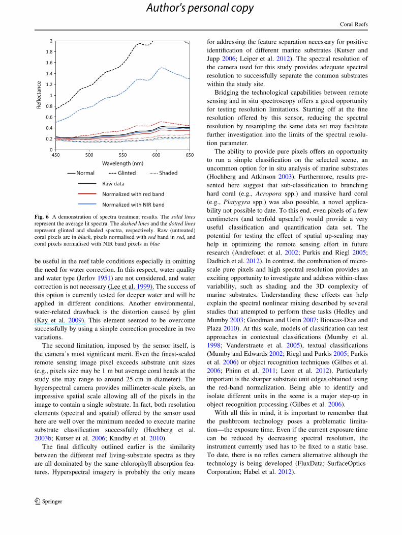
Fig. 6 A demonstration of spectra treatment results. The solid linesrepresent the average lit spectra. The dashed lines and the dotted linesrepresent glinted and shaded spectra, respectively. Raw (untreated)

coral pixels are in black, pixels normalised with red band in red, and

coral pixels normalised with NIR band pixels in blue

Coral Reefs

123

Author's personal copy

For monitoring and conservation, the potential appli-

cations demonstrated by this study include automated

quantitative image analysis and accurate substrate identi-

fication. In turn, this facilitates larger scale campaigns (i.e.,

multiple image analysis) with much less manpower

investment, compared to knowledge-based digital photog-

raphy analysis. The immediate applicability is currently

limited by the need for camera mounting (such as a tripod

or the jetty used for this study). This may be overcome

using a reflex-type camera as described earlier but could be

also overcome by using a higher mounting for the current

sensor. For example, raising the sensor to 6 meter above

the reef may cover an extended portion of the reef,

approximately 3 m 9 6 m (effectively spatial up-scaling).

In this case, the spatial resolution will be reduced but that

is unlikely to affect the image analysis. Even with all the

current limitations, for the study site described in this

study—using the two jetties to take 5 images at each side

would result in a set of 20 images. If, as suggested above,

every image covers 18 m2, this amounts to a sizable survey

effort.

The aim of this paper was to give a quick and sim-

plified account of the potentiality of a new technology for

marine spectroscopy at ground level. The three key limi-

tations relevant to remote sensing of coral reefs are suc-

cessfully overcome. The presented results show that the

combination of image specification 5 nm bands, a

450–660 nm range and the red-band normalization can

produce unprecedented classification accuracies of 99 %.

To this end, the camera’s specifications open a new ave-

nue of research in the spectroscopy, image analysis, and

remote sensing relevant to this environment. The advan-

tage of such resolution is limited in respect to computer

power and data handling. To overcome this problem,

currently the possibility of reducing spatial and spectral

resolution is being tested. Up-scaling experiments may

provide resolution limits for this type of remote sensing

analysis of coral reefs. Scaling up the area surveyed can

be done empirically by rising the sensor’s mounting point

and by creating mosaics of several images together.

Another area in need of improvement is the normalization

technique that currently is image specific. Further work

planned for this source of imagery focuses on testing

different normalization techniques. The results presented

here show how well the classification handles a relatively

simple scene with only five class definitions. In more

complex scenes, the number of classes may be doubled,

and class integrity may be reduced. Tests with more

complex classification techniques, such as PLS-DA and

object recognition, are planned and may yield better

results with more complex scenes. Additional avenues for

exploration include micro-scale (single colony) spectral

variation and spatial up-scaling of similar images.

References

Andrefouet S, Berkelmans R, Odriozola L, Done T, Oliver J, Muller-

Karger FE (2002) Choosing the appropriate spatial resolution for

monitoring coral bleaching events using remote sensing. Coral

Reefs 21:147–154

Bioucas-Dias J, Plaza A (2010) Hyperspectral unmixing: Geometri-

cal, statistical and sparse regression-based approaches. SPIE

Remote Sensing Europe, Image and Signal Processing for

Remote Sensing Conference

Collin A, Planes S (2012) Enhancing coral health detection using

spectral diversity indices from WorldView-2 Imagery and

Machine Learners. Remote Sens 4:3244–3264

Cortes C, Vapnik V (1995) Support-vector networks. Machine

Learning 20:273–297

Dadhich AP, Nadaoka K, Yamamoto T, Kayanne H (2012) Detecting

coral bleaching using high-resolution satellite data analysis and

2-dimensional thermal model simulation in the Ishigaki fringing

reef, Japan. Coral Reefs 31:425–439

Dekker AG, Wettle M, Brando VE (2005) Coral reef habitat mapping

using MERIS: can MERIS detect coral bleaching? MERIS

(A)ATSR Workshop 2005 Published on CDROM:25.21

English S, Wilkinson C, Baker V (1997) Survey manual for tropical marine

resources. Australian Institute of Marine Science, Townsville

FluxData I The FD-1665-MS 7 Channel Camera

Gilbes F, Armstrong RA, Goodman J, Velez M, Hunt S (2006)

Censsis seabed: diverse approaches for imaging shallow and

deep coral reefs. Proceedings of Ocean Optics XVIII

Goodman JA, Ustin SL (2007) Classification of benthic composition

in a coral reef environment using spectral unmixing. J Appl

Remote Sens 1:011501. doi:10.1117/1.2815907

Habel R, Kudenov M, Wimmer M (2012) Practical spectral photog-

raphy. Eurographics 2012

Hamylton S (2009) Determination of the separability of coastal

community assemblages of the Al Wajh Barrier Reef, Red Sea,

from hyperspectral data. European J Geosci 1:1–11

Hedley J (2004) Spectral unmixing of coral reef benthos under ideal

conditions. Ph.D. thesis, University of Exeter, pp 108–149

Hedley JD, Mumby PJ (2002) Biological and remote sensing

perspectives of pigmentation in coral reef organisms. Adv Mar

Biol 43:277–317

Hedley JD, Mumby PJ (2003) A remote sensing method for resolving

depth and subpixel composition of aquatic benthos. Limnol

Oceanogr 48:480–488

Hedley J, Mumby P, Joyce K, Phinn S (2004) Spectral unmixing of

coral reef benthos under ideal conditions. Coral Reefs 23:60–73

Hedley JD, Harborne AR, Mumby PJ (2005) Simple and robust

removal of sun glint for mapping shallow-water benthos. Int J

Remote Sens 26:2107–2112

Hedley J, Roelfsema C, Phinn SR (2010) Propogating uncertainty

through a shallow water mapping algorithm based on radiative

transfer model inversion. Ocean Optics XX

Hedley JD, Roelfsema CM, Phinn SR, Mumby PJ (2012) Environ-

mental and sensor limitations in optical remote sensing of coral

reefs: Implications for monitoring and sensor design. Remote

Sens 4:271–302

Hochberg EJ, Atkinson MJ (2000) Spectral discrimination of coral

reef benthic communities. Coral Reefs 19:164–171

Hochberg EJ, Atkinson MJ (2003) Capabilities of remote sensors to

classify coral, algae, and sand as pure and mixed spectra. Remote

Sens Environ 85:174–189

Hochberg EJ, Andrefouet S, Tyler MR (2003a) Sea surface correction

of high spatial resolution Ikonos images to improve bottom

mapping in near-shore environments. IEEE Transactions on

Geoscience and Remote Sensing 41:1724–1729

Coral Reefs

123

Author's personal copy

Hochberg EJ, Atkinson MJ, Andrefouet S (2003b) Spectral reflec-

tance of coral reef bottom-types worldwide and implications for

coral reef remote sensing. Remote Sens Environ 85:159–173

Hochberg EJ, Appril A, Atkinson MJ, Bidigare RR (2006) Bio-optical

modeling of photosynthetic pigments in corals. Coral Reefs

25:99–109

Holden H, LeDrew E (1998) Deconvolution of measured spectra

based on principal components analysis and derivative spectros-

copy. Geoscience and Remote Sensing Symposium Proceedings,

1998. IGARSS ‘98. 1998 IEEE International 2:760–762

Holden H, LeDrew E (2000) Optical water column properties of a coral

reef environment: towards correction of remotely sensed imagery.

Geoscience and Remote Sensing Symposium, 2000. Proceedings.

IGARSS 2000. IEEE 2000 International 6:2666–2668

Holden H, LeDrew E (2002) Hyperspectral linear mixing based on

in situ measurements in a coral reef environment. Geoscience

and Remote Sensing Symposium, 2002. IGARSS ‘02. 2002

IEEE International 1:249–251

Jerlov NG (1951) Optical studies of ocean water. Report of Swedish

Deep-Sea Expeditions 3:1–59

Johansen K, Roelfsema C, Phinn S (2008) High spatial resolution

remote sensing for environmental monitoring and management

preface. J Spatial Sci 53:43–47

Joyce KE, Phinn SR (2002) Bi-directional reflectance of corals. Int J

Remote Sens 23:389–394

Karpouzli E, Malthus T, Place C (2004) Hyperspectral discrimination

of coral reef benthic communities in the western Caribbean.

Coral Reefs 23:141–151

Kay S, Hedley JD, Lavender S (2009) Review: Sun glint correction of

high and low spatial resolution images of aquatic scenes: a

review of methods for visible and near-infrared wavelengths.

Remote Sens 1:697–730

Kendall MS, Miller T (2008) The influence of thematic and spatial

resolution on maps of a coral reef ecosystem. Mar Geodesy

31:75–102

Knudby A, LeDrew E, Newman C (2007) Progress in the use of

remote sensing for coral reef biodiversity studies. Prog Phys

Geogr 31:421–434

Knudby A, Newman C, Shaghude Y, Muhando C (2010) Simple and

effective monitoring of historic changes in nearshore environ-

ments using the free archive of Landsat imagery. Int J Appl

Earth Obs Geoinform 12:S116–S122

Kruse FA (2008) Expert system analysis of hyperspectral data. SPIE

Defense and Security, Algorithms and Technologies for Multi-

spectral, Hyperspectral, and Ultraspectral Imagery XIV, Con-

ference DS43 6966–25

Kutser T, Jupp DL (2006) On the possibility of mapping living corals

to the species level based on their optical signatures. Estuar

Coast Shelf Sci 69:607–614

Kutser T, Dekker AG, Skirving W (2003) Modeling spectral

discrimination of Great Barrier Reef benthic communities by

remote sensing instruments. Limnol Oceanogr 48:497–510

Kutser T, Miller I, Jupp DLB (2006) Mapping coral reef benthic

substrates using hyperspectral space-borne images and spectral

libraries. Estuar Coast Shelf Sci 70:449–460

Lee Z, Carder KL, Mobley CD, Steward RG, Patch JS (1999) Hyperspec-

tral remote sensing for shallow waters: 2. Deriving bottom depths and

water properties by optimization. Appl Opt 38:3831–3843

Lee Z, Carder K, Arnone R, He M (2007) Determination of primary

spectral bands for remote sensing of aquatic environments.

Sensors 7:3428–3441

Leiper I, Phinn S, Dekker AG (2012) Spectral reflectance of coral reef

benthos and substrate assemblages on Heron Reef, Australia. Int

J Remote Sens 33:3946–3965

Leon J, Phinn SR, Woodroffe CD, Hamylton S, Roelfsema C,

Saunders M (2012) Data fusion for mapping coral reef

geomorphic zones: possibilities and limitations Proceedings of

the 4th GEOBIA, Rio de Janeiro, pp 261–266

Lillesand TM, Kiefer RW (2003) Remote sensing and image

interpretation. John Wiley and Sons, New York

Lubin D, Li W, Dustan P, Mazel CH, Stamnes K (2001) Spectral

signatures of coral reefs: Features from space. Remote Sens

Environ 75:127–137

Mather PM, Koch M (2004) Computer processing of remotely-sensed

images: An introduction. John Wiley and Sons

Mumby PJ, Edwards AJ (2002) Mapping marine environments with

IKONOS imagery: enhanced spatial resolution can deliver

greater thematic accuracy. Remote Sens Environ 82:248–257

Mumby PJ, Green EP, Clark CD, Edwards AJ (1998) Benefits of

water column correction and contextual editing for mapping

coral reefs. Int J Remote Sens 19:203–210

Mumby PJ, Skirving W, Strong AE, Hardy JT, LeDrew EF, Hochberg

EJ, Stumpf RP, David LT (2004) Remote sensing of coral reefs

and their physical environment. Mar Pollut Bull 48:219–228

Phinn SR, Roelfsema CM, Mumby PJ (2011) Multi-scale, object-

based image analysis for mapping geomorphic and ecological

zones on coral reefs. Int J Remote Sens 33:3768–3797

Pope RM, Fry ES (1997) Absorption spectrum 380–700 nm of pure

water. II. Integrating cavity measurements. Appl Opt 36:8710–8723

Purkis SJ, Riegl B (2005) Spatial and temporal dynamics of Arabian

Gulf coral assemblages quantified from remote-sensing and

in situ monitoring data. Mar Ecol Prog Ser 287:99–113

Purkis SJ, Myint SW, Riegl B (2006) Enhanced detection of the coral

Acropora cervicornis from satellite imagery using a textural

operator. Remote Sens Environ 101:82–94

Riegl BM, Purkis SJ (2005) Detection of shallow subtidal corals from

IKONOS satellite and QTC View (50, 200 kHz) single-beam sonar

data (Arabian Gulf; Dubai, UAE). Remote Sens Environ 95:96–114

Roger JM, Chauchard F, Bellon Maurel V (2003) EPO - PLS external

parameter orthogonalisation of PLS application to temperature-

independent measurement of sugar con-tent of intact fruits.

Chemometrics and Intelligent Laboratory Systems 66:191–204

Smith RC, Baker KS (1981) Optical properties of the clearest natural

waters (200–800 nm). Appl Opt 20:177–184

Sterckx S, Debruyn W, Vanderstraete T, Goossens R, Van der Heijden P

(2005) Hyperspectral data for coral reef monitoring. A case study:

Fordate, Tanimbar, Indonesia. EARSeL eProceedings 4(1):18–25

SurfaceOpticsCorporation SOC700Hz/SOC760 Real-time Hyper-

spectral (HS) Imager

Vanderstraete T, Goossens R, K. GT (2005) Coral reef habitat

mapping in the Red Sea (Hurghada, Egypt) based on remote

sensing. EARSeL eProceedings 3(2):191–207

Wettle M, Ferrier G, Lawrence AJ, Anderson K (2003) Fourth

derivative analysis of Red Sea coral reflectance spectra. Int J

Remote Sens 24:3867–3872

Wooldridge S, Done T (2004) Learning to predict large-scale coral

bleaching from past events: A Bayesian approach using remotely

sensed data, in-situ data, and environmental proxies. Coral Reefs

23:96–108

Wozniak SB, Stramski D, Stramska M, Reynolds RA, Wright VM,

Miksic EY, Cichocka M, Cieplak AM (2010) Optical variability

of seawater in relation to particle concentration, composition,

and size distribution in the nearshore marine environment at

Imperial Beach. California. J Geophys Res 115:C08027

Yamano H, Tamura M (2004) Detection limits of coral reef bleaching

by satellite remote sensing: Simulation and data analysis.

Remote Sens Environ 90:86–103

Zheng X, Dickey T, Chang G (2002) Variability of the downwelling

diffuse attenuation coefficient with consideration of inelastic

scattering. Appl Opt 41:6477–6488

Coral Reefs

123

Author's personal copy