Hierarchical models for multi-project planning and scheduling

312 European Journal of Operational Research 64 (1993) 312-325 North-Holland

Hierarchical models for multi-project planning and scheduling

M. Grazia Speranza

Dipartimento di Metodi Quantitativi, Universit~ di Brescia, 25122 Brescia, Italy

Carlo Vercellis *

Dipartimento di Economia e Produzione, Politecnico di Milano, 20133 Milano, Italy

Abstract: We propose a model-based approach to nonpreemptive multi-project management problems, based on a hierarchical two-stage decomposition of the planning and scheduling process. Two performance criteria are considered: the net present value, which includes investment costs, operating costs, revenues, penalties for late completion; and the service level, expressed as the agreement between the completion times of the different projects and the customer needs. The resulting hierarchy of integer programming models is aimed at assisting the planners in understanding the interrelations among the allocation of resources, the timing of the activities, the cash flows. A class of branch-and-bound procedures is then proposed for the solution of these integer programming models.

Keywords: Multi-project planning; Hierarchical decomposition; Project scheduling

1. Introduction

The area of project management includes planning activities which range from the tactical level - in which milestones and due dates have to be determined, along with the allocation of limited resources, for a number of projects within the same organization - to the operational level - in which the scheduling of specific activities must be established in light of an appropriate trade-off between time, cost and resource usage. This paper deals with the planning and scheduling process in a multi-project environment, and gives particular emphasis to the methodologies for achieving a high degree of integration between tactical and operational stages of the decision process.

In the project management practice, planners are generally concerned with a number of different decision criteria, often contrasting among each other. The intrinsic multi-objective nature of the decision process involved in project management emerges with particular evidence in conjunction with the tactical planning phase, over medium to long term time horizon. Hence, this conflict of objectives appears particularly relevant in the early stages of analysis of the project plan, when establishing milestones for bidding proposals and allocating scarce resources among different projects. Indeed, even if the productivity performance is of major concern to most project managers, other factors, such as the service time to the customer and the reliability in meeting the promised delivery dates, should be explicitly taken into account.

* Partially supported by Research Project 'Construction Building' of the National Research Council. Correspondence to: Prof. C. VerceUis, Dipartimento di Economia e Produzione, Politecnico di Milano, Piazza Leonardo da Vinci 32, 20133 Milano, Italy.

0377-2217/93/$06.00 © 1993 - Elsevier Science Publishers B.V. All rights reserved

M. Grazia Speranza, C. Vercellis / Multi-project planning and scheduling 313

Furthermore, project managers are mostly interested in understanding how the controllable key decisions, such as timing, costs and resource usage for the different activities, do interact in terms of productivity, service and reliability. In general, every activity can be performed in one among several alternative modes, each one corresponding to a different combination of time duration, cost and absorbtion of resources. Thus, planners are requested to determine, for each activity, the most appropriate mode of accomplishment, in order to obtain an acceptable level of performance in terms of the multiple conflicting objectives. The decision process associated to the various planning activities, from the tactical to the operational phases, is made particularly complex also because of its dynamic nature, since the relevant objectives and the available information are usually modified as the decision process evolves. At least in principle, one could draw a mathematical model representing variables, objectives and constraints of the planning process. Yet, the multiobjective nature and the size of the resulting model, together with the dynamic nature of the objectives and the information, would make such a 'monolithic' modelling approach inadequate to deal with most practical applications.

In front of the complexity of the outlined decision process, the large majority of models proposed in the OR literature, as well as the available commercial software for project planning and scheduling, tend to disregard the multiobjective character of project planning. One exception is represented by Slowinski (1981), in which, however, the attention is confined to the case of preemptive scheduling problems. Other papers, such as Deckro and Hebert (1990), have developed multiple objective approaches for resource unconstrained project scheduling problems. On the other side, several papers have been devoted to nonpreemptive project scheduling problems with limited resources, addressing issues of model formulation (Balas, 1970), of computational complexity (Blazewicz et al., 1983), of exact (Christofides et al., 1987; Davis and Heidorn, 1971; Doersch and Patterson, 1977; Gorenstein, 1972; Patterson and Huber, 1974; Patterson, 1984; Talbot and Patterson, 1978) and approximate (Davis and Patterson, 1975; Norbis and MacGregor Smith, 1988; Patterson, 1976; Russel, 1986) solution algorithms. However, very limited attention has been paid to the analysis of the case in which activities can be performed in alternative modes, notable exceptions being represented by Talbot (1982) and Patterson et al. (1989). With respect to the planning time horizon, a few authors, such as those aimed at maximizing the net present value (Doersch and Patterson, 1977; Elmaghraby and Herroelen, 1988; Russell, 1970; Russell, 1986), seem to adhere, more or less explicitly, to the tactical level of analysis. Most of the others, generally aimed at the minimization of the completion time, seem to place their methodologies at the operational level. Specific attention to the problems arising in a multi-project environment is given in few papers, such as Kurtulus and Narula (1985). Moreover, a mathematical programming formulation is presented in Pritsker et al. (1969) and a categorization of priority rules in Kurtulus and Davis (1982), both implicitly referring to scheduling at the operational level. A 'macro' formulation, aimed at a tactical analysis and based upon continuity assumptions, is given in Valadares Tavares (1987). To our knowledge, no effort has been devoted to the development of a structured quantitative approach addressing the issue of integration between the tactical and operational stages of the planning process.

In order to overcome these limitations, in this paper w e propose a multiobjective model-based methodology for nonpreemptive multi-project management problems, which results in a hierarchical two-stage decomposition of the planning and scheduling process. Two performance criteria are considered: the net present value, which includes investment and operating costs, revenues and penalties for late completion; the service level, i.e. the agreement of the completion times of the different projects with the customer needs. The methodology we propose hierarchically decomposes the project planning decision process in two stages, to a large extent corresponding to the tactical and operational levels of analysis. Decisions at both levels do interact by means of an explicit coordination scheme: at the higher level, decisions are influenced by an approximate evaluation of the future effects on the lower level; on the other hand, when higher level decisions have been taken, they influence future decisions through the constraints incorporated into lower level models. Our approach seems to achieve a number of advantages. For example, a single objective can be attributed to each stage, hence leading to single objective optimization models. Moreover, the size of the resulting models is significantly reduced with respect to the model size within the monolithic approach. Furthermore, this decomposition scheme is likely to

314 M. Grazia Speranza, C. Vercellis / Multi-project planning and scheduling

reflect the temporal and organizational structure of the decision process within companies operating in the project business. More specifically, the first stage corresponds to determining due dates for the projects and allocating the limited resources among them, with the productivity objective dominating the other criteria. The second stage deals with determining the actual modes and timing of the activities within each project, with the service level as the main objective.

In our model resources are grouped into two categories, which reflect the possibility that a resource is constrained on a period by period basis, or on the whole lifetime of the set of projects. These resources are called renewable and nonrenewable respectively (Slowinski, 1981). Activities can be performed according to alternative modes, corresponding to different combinations of resources consumption, cost and time duration. Starting from an activity on nodes network representat ion of the multi-project, it will be assumed that a set of node-disjoint subnetworks can be identified by the planner, corresponding to individual projects. Referring to the hierarchical decomposition of the decision process, at the tactical stage of analysis an aggregated network is considered whose nodes correspond to entire projects, and therefore are regarded as macro-activities. These macro-activities, in turn, will be disaggregated in elementary activities during the subsequent stage, corresponding to the operational analysis.

While Section 2 is devoted to the general discussion and formulation of the multi-project planning problem, in Section 3 our decomposition approach will be introduced together with the models it is based upon. Finally, in Section 4 a class of branch-and-bound procedures is proposed for solving the integer programming models developed in the previous section.

2. The multiobjective resource constrained project planning and scheduling problem

We will consider a discrete-time model, in which the integer T denotes the total length of the time horizon, measured in a suitable time unit - in most cases ranging between one week and one month. We further assume that the current t ime is t = 0.

A project s consists of a given set ~ of activities, on which a partial order relation, denoted by -<, is defined. We say that i -< k, i.e. i precedes k, whenever activity i must be finished before starting activity k. The set 1/s includes two dummy activities, a s and z s, representing the start and the end of the project, respectively. It will be assumed that a s -< i and i -< zs, for every activity i. An activity-on-node representa- tion of a given project relies on the definition of an oriented acyclic graph G s = ( ~ , Ps) in which the set of vertices V s is identified with the set of activities of project s. An arc (i, k ) ~ Ps exists whenever i < k.

In order to be performed, each activity requires the usage of a given amount of specific resources, whose availability over time is generally limited for the whole set of projects. In particular, it is assumed that two sets ~ ' and ~ of renewable and nonrenewable resources are given. A limited amount W r of each resource r ~ is available in each time period, while the consumption of each resource r ~ ~ is limited over the whole life of the project by the quantity Qr. The usage cost of a unit of resource r ~ U J during a unit of time will be denoted by c~ v. In order to model situations in which the availability of a renewable resource involves a fixed cost, to each unused unit of a resource r ~5~' will be inputted a cost c~.

We will assume that each activity i can be carried out in several modes, each mode corresponding to different resource requirements and to a different processing time. Let M i be the set of modes of accomplishment for activity i. Thus, due to the previous assumptions relative to the cost of the resources, it follows that different modes of accomplishment correspond also to different costs for each activity. Specifically, if activity i is carried out in mode j, an amount Wijrt of resource r ~ ' is consumed at time t, where the time index is computed relative to the starting time of activity i. An amount qijr of resource r ~ X is consumed by activity i in mode j. It is assumed that the absorption of resource r ~ J over time is uniform, which means that if activity i is accomplished in mode j the consumption at each time period is given by qqr/d i j . The duration of activity i carried out according to mode j will be denoted by dij. A single mode is defined for each of the dummy activities, denoted as 1, which does not require any resource, and whose duration is given by das I = 0 for activity a s a n d dz, 1 = 0 for activity z s.

M. Grazia Speranza, C. VerceUis / Multi-project planning and scheduling 315

A feasibility interval [el, l i] is associated to each activity i, where ei and l~ represent the earliest and latest starting time of activity i, respectively. In case these quantities are not defined in the input data, an estimation can be easily obtained. Indeed, e~ can be given the length of the longest path from a s to i, taking as duration of each activity the one corresponding to the fastest mode. Analogously, l i can be assigned the length of the time hor izon T minus the length of the longest path from i to z s, again taking as duration of each activity the one which is associated to the fastest mode of accomplishment.

Each project is part of a program, constituted by a set S of projects, whose cardinality will be denoted by S. The projects are interrelated and influence each other in two ways: at a general level, they are in competit ion for the use of the limited resources ~ u X ; moreover, at least in specific cases, they can be related by a partial order relation < p. We say that project s~ precedes project s 2 whenever zs, -< p as2.

The program can be represented by an oriented acyclic graph G = (V, P). The set of vertices V = U s ~ s ~ u a U z includes two dummy vertices a and z which represent the start and end of the entire program. Again, these dummy activities have a single mode, denoted as 1, and time durations dal = 0 and dzl = 0. The set of arcs P = U s~sPs UPs is composed by the precedence arcs P~ for each project s ~ S, and by additional arcs Ps which are introduced for two different reasons. First, there are arcs expressing precedence relationships between projects. Such an arc (zs,, as2) ~ Ps exists whenever project s 1 precedes project s 2. Then, there are arcs connecting the beginning and the end of some projects to the dummy nodes a and z, respectively: an arc (a, a s) ~ Ps exists whenever project s is not preceded by any other project and analogously an arc ( % z) e Ps exists whenever project s does not precede any other project.

Analogously to the elementary activities, a feasibility interval [ % l s] is associated to each project s, where e~ and I s represent the earliest and latest starting time of the project respectively. Moreover, a due date h s can be associated to each project s: If a project s is not completed within h s, a penalty p~

i and is will be paid at time h s. The amount of the investment for project s will be denoted by c s independent from the modes of accomplishment of the activities of the project. It is assumed that such amount has to be paid at the beginning of the project. A revenue fs will give rise to a positive cash flow at the completion time of-the project.

The solution of the project planning and scheduling problem corresponds to determining the mode of accomplishment and the starting time for each activity. In order to formulate the constraints in linear form, it is convenient to introduce the following binary decision variables, for i ~ V, j ~ M~, t = e~ . . . . . l,,

10 if activity i starts at time t in mode j, xut = otherwise.

Multi-prolect scheduling

Single-project scheduling

Multi-project model

Figure. 1. The hierarchy of models

J sh,,ok,o0 J .,--~'"Y'" ....... . .............. ~ model


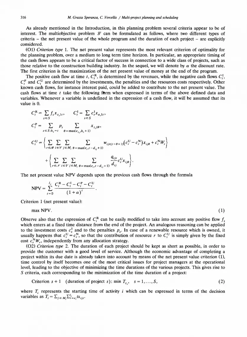
As already mentioned in the Introduction, in this planning problem several criteria appear to be of interest. The multiobjective problem ~ can be formulated as follows, where two different types of criteria - the net present value of the whole program and the duration of each project - are explicitly considered.

(O1) Criterion type 1. The net present value represents the most relevant criterion of optimality for the planning problem, over a medium to long term time horizon. In particular, an appropriate timing of the cash flows appears to be a critical factor of success in connection to a wide class of projects, such as those relative to the construction building industry. In the sequel, we will denote by a the discount rate. The first criterion is the maximization of the net present value of money at the end of the program.

The positive cash flow at time t, C R, is determined by the revenues, while the negative cash flows C], C f and C U are determined by the investments, the penalties and the resources costs respectively. Other known cash flows, for instance interest paid, could be added to contribute to the net present value. The cash flows at time t take the following f~rm when expressed in terms of the above defined data and variables. Whenever a variable is undefined in the expression of a cash flow, it will be assumed that its value is 0.

cR~- E fsXzslt, Clt = E I CsXaslt, s~S s~S

CP= E Ps E XZslO' s~S:h¢=t O=max(ez,,hs + l )

CY-~ ( ~ E E E Wijr(t-O+I)(Cy--cN)xijo+CNr Wr) r i~Vj~M i O=max(ei,t-dij+l)

q-( E E E E Q!Jrcyxijo I" r~" i~V j~M i O=max(ei,t-dij+ l ) dij J

The net present value NPV depends upon the previous cash flows through the formula

c I - c ,

NPV = /=0 ( l + a ) t

Criterion 1 (net present value):

max NPV. (1)

Observe also that the expression of Ct R can be easily modified to take into account any positive flow fs which enters at a fixed time distance from the end of the project. An analogous reasoning can be applied to the investment costs c~ and to the penalties Ps. In case of a renewable resource which is owned, it usually happens that cy = cy, so that the contribution of resource r to C U is simply given by the fixed cost cNwr, independently from any allocation strategy.

(02) Criterion type 2. The duration of each project should be kept as short as possible, in order to provide the customer with a good level of service. Although the economic advantage of completing a project within its due date is already taken into account by means of the net present value criterion (1), time control by itself becomes one of the most critical issues for project managers at the operational level, leading to the objective of minimizing the time durations of the various projects. This gives rise to S criteria, each corresponding to the minimization of the time duration of a project:

Criterion s + 1 (duration of project s) : rain Tzs, s = 1 . . . . . S, (2)

where T i represents the starting time of activity i which can be expressed in terms of the decision variables as T/= t, ~j E Mi~t ~eitX ijt"

M. Grazia Speranza, C. Vercellis / Multi-project planning and scheduling 3 1 7

A number simplify their as defined by

of constraints must be satisfied by a solution to the project planning problem. In order to formulation, we will introduce an additional variable D~ denoting the duration of activity i, (4). We have therefore the following set of constraints:

li

T i = E E txi j t , i ~ V , jE.M i t=e i

li

D i = ~ dij ~ x i j t , i ~ V , j ~ M i t =e i

Tk-T~>_D i, ( i , k ) eP ,

li

E E q i j r E X i j , < Q r , r~Jl/', iEV j E M i t--e i

min(li + dij- 1 ,t )

E E E Wi j r ( t_O+l)Xi jo~Wr, r E ~ , t = l , . . . , T , i ~ V j ~M i 0 = m a x ( e / , t - dij + 1)

(3)

(4)

(5)

(6)

(7)

E E X i j t = 1 , i ~ V , (8) j E M i t=e i

xij t~{O, 1 }, i ~ V , j ~ M i , t = e i . . . . . l i. (9)

Inequalities (5) express the precedence relationships between pairs of activities. Constraints (6) and (7) take into account the limitations on the availability of the nonrenewable and renewable resources, respectively. Finally, equalities (8) stipulate that each activity must be started exactly once, in a given time period and for a given mode of accomplishment.

As already mentioned in the Introduction, relevant difficulties arise as one tries to solve the above monolithic model of the project planning and scheduling problem. On the one hand, the different criteria described, relative to either a monetary unit or a time unit, do not appear easily amenable to single objective optimization models. On the other hand, even if admittedly one might succeed in identifying a single criterion optimization model, instances of the multi-project planning problem of realistic size would be computationally intractable, at least for the current state of development of exact methods. Furthermore, at the beginning of the decision process, the uncertainty about the data related to the detailed features of the single projects is high. This would make of questionable value the related decisions, which would probably require a later revision, as soon as new information concerning the activities is known. These difficulties in solving the multi-objective planning problem motivate the decomposition approach proposed in the next section as our solution methodology.

3. The hierarchical decomposition approach

The hierarchical decomposition of problem ~" developed in this section gives rise to three models, whose main interrelations are depicted in Figure 1. Here, the heavy arrow expresses a logical precedence relation within the decision process. The dotted arrows show how the different stages of the decision process correspond to the optimization models. Finally, the continuous arrows describe the information flows among the models.

At the higher level, corresponding to the tactical planning stage, a single objective optimization model is considered by restricting the attention to the aggregate multi-project network, in which each node represents a whole project. We will refer to a project represented by a single node of a network as a


macro-activity. This model, referred in what follows as the multi-project model, has the net present value as its objective function and is aimed at determining the timing of the projects and the distribution of the resources among the projects. Since the multi-project model regards an entire project as a single macro-activity, without decomposing it in its elementary activities, it requires an estimate of the time-cost-resources trade-off characterizing the aggregate behaviour of each macro-activity. Specifically, each macro-activity is described by a set of macro-modes of accomplishment, corresponding to different time durations and different levels of usage of the resources, therefore resulting in different costs. The number N~ of modes to perform a macro-activity s, that is an entire project composed by its elementary activities, is obviously given by the cardinality of the Cartesian product of the modes corresponding to the elementary activities, i.e.

Ns= I-I [Mi[. i ~ V s

Unfortunately, this number grows very large for realistic sized programs. In order to keep the aggregate network model of moderate size, one would like to take into account, for each macro-activity, only the most effective macro-modes of accomplishment. The shrinking model presented in the next subsection has precisely the objective of determining, from the total number of N s macro-modes, only a small subset of modes which identify the curve of most efficient time-cost trade-offs. It can be regarded as a way for anticipating to the multi-project model information about the consequences that planning decisions will determine on future scheduling performance.

Thus, the combination of the shrinking model and the multi-project model is used for generating a solution at the tactical planning stage. This solution determines the timing and the resource availability profile for each project. At this point, the activities of each project require to be scheduled, within the resource and budget limits derived from higher level decisions. In the resulting detailed project model the network structure of the project is resorted, with all the alternative modes of accomplishment for the elementary activities. The completion time of the project becomes the relevant objective. It is worth observing that the information about the project features, and therefore the data of the model, can be different from the information available at the running time of the shrinking model. The differences can cover both the network structure of the project and the features of the activities. Hence, the output of the detailed project model consists of the timing of the elementary activities and the resource distribution among them.

The shrinking model

The shrinking model is applied to each of the projects constituting the multi-project environment. As already mentioned, the aim of this model is to support the transformation of a project into a single macro-activity, to be incorporated into the multi-project model, by means of the identification of the efficient macro-modes of a project. In designing the shrinking model, one should try to balance two conflicting requirements: on one side, in order to make the decisions of the multi-project model consistent with the detailed project features, the model should transform each project into a single macro-activity with as many macro-modes as possible; on the other hand, to keep the size of the multi-project model moderate, the model should select as few macro-modes as possible. As a compro- mise, the shrinking model tries to identify the modes which belong to the maximum efficiency frontier between time duration and cost. This is done by solving a sequence of optimization models, which correspond to determining the minimum project duration for different selected values of budget monetary availability.

More specifically, we assume that a set K s of cost values can be identified, which represent a reasonable discretization of the possible budget limitations for project s. Since the actual timing of the projects will be decided by the multi-project model, it turns out that the cost relative to resource consumption is the only economic quantity which remains of interest within the shrinking model. Then, for each project s, the following problem has to be solved for each element k~ ~ K s, v = 1, 2,. . . I Ks I. It

M. Grazia Speranza, C. Vercellis /Multi-project planning and scheduling 319

will be referred as problem ~ ( s , v), to express the dependence from the project index s and from the index of the budget limitation k~.

(~¢(s, v)) min tz,

subject to

i~Vs j i

li t li

E E E Wijr(t--O+ l)CUXijo -[- E qijrCUr E X ijt r ~ ' t=e i O=t-d i j+ l r~.4 ~ t=e i

~ k ~ , (10)

( 3 ) - ( 9 ) w h e r e i ~ V s, ( i , k ) ~ P s r e p l a c e i ~ V , ( i , k ) ~ P .

Constraint (10) expresses the limitation on the budget of project s and takes the form of the constraints on the capacity of the nonrenewable resources.

The solution of problem ~ ( s , v), for a given level k~ of cost limitation, consists of a project duration and a corresponding resource requirement profile, i.e. in the specification of a macro-mode u of accomplishment for the macro-activity s. The profile of resource requirements of the macro-activity s in mode v is found from an optimal solution x* to problem 5~'(s, v) as follows. The resource requirement of the nonrenewable resource r ~ X is given by

li

qsvr = E E qijr E X~jt, i ~ j E M i t=e i

while the resource requirement of the renewable resource r ~q~ at time t is

min(li + d i j - 1,t)

E E E * = Wijr(t - 0 + 1)Xijo" i¢ V s j ~ M i O=max(ei,t-dij+ 1)

Obviously, the duration of the macro-activity s in mode v is given by dsv = min Tzs. The quantities ffs~,rt and dsv will be input data for the multi-project model. We will denote by M s the set of macro-modes determined by the shrinking model for the macro-activity s. Notice that the constraints on the resource availability, taking into account for project s the limitations Qr and W r which hold for the whole program, are only apparently loose. Indeed, the resources are indirectly limited through the bound k~ on the resource cost. A loose limitation in this budget constraint will determine a macro-mode of accomplishment for project s which is likely to be fast but also resource consuming; on the contrary, a tight budget value will correspond to a macro-mode which is slower but less resource consuming.

A heuristic approach has been adopted for the solution of problem ~¢(s, v), since it has to be solved Es e s I Ks I times. A fast heuristic solution can be obtained by limiting the size of the tree created by the branch-and-bound algorithm described in Section 4.

The multi-project model

In the multi-project model an oriented acyclic graph G s = ( V s, pS ) is considered which represents the precedence relations among the projects. The set of vertices V s consists of the set of projects to which two dummy projects a and z have been added, representing the start and the end of the program, respectively. The set of arcs pS is in a one-to-one correspondence with the set of arcs Ps defined in Section 2: an arc O1, s2) ~ pS is associated to the arc ( z w a s ) ~ Ps, while an arc (a, sl) ~ pS and an arc (s 2, z ) ~ pS correspond to the arc (a, as,) ~ Ps and the arc ~zs2, z ) ~ Ps, respectively.

We will assume that each macro-activity s can be carried out in [ Ms I -< Ns macro-modes, determined by the shrinking model, each one corresponding to a given processing time and resource requirement profile. Let us define the following binary decision variables:

_ (10 if project s starts at time t in macro-mode v, X st"t = otherwise.


We can therefore formulate the following optimization model, in which the net present value is taken as the objective function.

,z c , " - c : - c , - c t max NPV =

/=0 (1 +Or) t

subject to

ls

T~= E E t2svt, s ~ S , u~M s t=e s

Is

Os~-" E dsv E . ~ s v t , s ~ S , o~M s t=e s

(s,k) e s, ls

E E qsvr E X s v t < O r , r ~ ' r , s~S v~M s t=e s

minus +ds,,- 1 ,t)

E E E Wsvr(t_O+l).~svO<_~Wr, r~q~, t = l , . . . , T , s~S v~M s O=max(es,t-dsv + l )

Is

Y'~ ~ ' ~ 2 , ~ t = l , s ~ S , v~M s t=e s

x,ot ~ { 0 , 1 } , s ~ S , v ~ M s , t = e ~ . . . . . 1,.

The expressions for Ct R, C], Ct e and C U have been given in Section 2. A solution of problem .or corresponds to selecting a macro-mode and a starting time for each macro-activity s. In other words, problem at v schedules the projects over the time horizon taking the resource constraints into account and at the same time allocates the resources globally available among the different projects in such a way that the net present value is maximized.

Denoting by x* an optimal solution to problem .4¢', the amount of resource r ~ .4," required by project s is given by

1,

Osr = E qsvr E X:v,, v~M s t=e s

while the amount ffz~ of resource r ~o~' required by project s at time t is

min(l s +dsv- 1,t)

[~rSt = E E I~svr(t -- 0 + 1)x*~0. v~Ms O=max(es,t-dsv + 1)

Since the accuracy in solving problem a¢ ¢ is particularly relevant for the success of the whole decomposition approach, a branch-and-bound algorithm for its solution has been developed (see Section 4). The adoption of an exact method is also justified by the fact that the size of problem a¢" can be made tractable by restricting the number of macro-modes considered for each project.

The detailed project model

After the multi-project model has identified the resource requirement profile and the starting time for each project s, a detailed project model is needed to determine modes of accomplishment and starting


times for the single activities of each project. As already mentioned, at the operational level, the duration of the project is considered as the main objective, to express the level of service to the customer. Although the model formulation which follows adopts the same notation used for the shrinking model, we notice that it may happens that the network structure, as well as the value of the parameters, are different at the time the detailed model is solved. This corresponds to the already mentioned dynamic nature of the decision process associated to planning and scheduling.

The allocation of the resources ff'~ and Qr ~ to project s has been determined by means of the multi-project model. These quantities represent tight constraints to the resource consumption, period by period and on the whole project life, respectively. Obviously, ff'rt ~ 0 only for the time period t belonging to the time interval in which project s has been scheduled. For each project s the following problem .g(s) has to be solved.

( ~ ( s ) )

min Tz,

subject to

li

E E qijrEXijt<-~O s, r ~ . / Y , (11 ) i~V j ~ M i t=e i

min(li + dlj- 1,t)

E E E Wijr(t_O+l)Xijo<_~l'VrSt, r ~ , t = l . . . . . T, (12) i~Vs j ~ M i O=max(ei,t-dij+ l)

( 3 ) - ( 5 ) , ( 8 ) , ( 9 ) w h e r e i ~ V ~ , ( i , k ) ~ P s r e p l a c e i ~ V , ( i , k ) ~ P .

Observe that problem .~(s) differs from problem .a:(s, v) since the former does not include the constraint (10) on the budget limitation. Notice also that this constraint can be dropped because it is implied by the set of constraints (11)-(12), which limit the usage of renewable and nonrenewable resources, due to the optimal distribution of resources among the various projects derived from the multi-project model.

In Section 4 a branch-and-bound procedure for this problem is described which can, in case of large projects, be truncated and therefore produce heuristic solutions.

4. A branch-and-bound algorithm

In this section a class of branch-and-bound algorithms for solving the three integer programming models presented in Section 3 will be described. We first confine our attention to the case of model

_~(s). In the sequel, -~(s) will be denoted as -~, without referring to a specific project, and the corresponding network as G = (V, P). Notice also that model ~ '(s , v) can be regarded as a particular case of 2 , so that the same branch-and-bound algorithm applies to it. Then, we will discuss how the algorithm should be modified to be extended to the multi-project model Jr'.

To provide a description of the branch-and-bound scheme we need some preliminary definitions and properties. A schedule S = {(T 1, ml), (T 2, m 2) . . . . . (Tn, mn)} is represented by an assignment of a mode m i ~ M i and a starting time T~ to each activity i ~ V. A schedule S is said to be feasible if it satisfies the constraints relative to the precedence relations, to the time windows determined by earliest and latest start times, and to the availability of the resources. A feasible schedule S = {(T,, mi)} is said to be tight if there not exist an activity k, a mode rh k ~ M k and a starting time T k such that the schedule

= S - {(Tk,mk)} U {(7~k, rhg)} is feasible and for which the following condition is satisfied:

Tk + dg,~ k < Tk + dkmk"

Hence, a schedule is tight if there is no feasible way to reduce the completion time of an activity, all the


modes and the starting times of other activities remaining unchanged. It is clear from this definition that the following dominance property holds:

Proposition 4.1. f f there exists an optimal schedule for problem _~, then there exists an optimal tight schedule.

Due to Proposition 4.1, within the branch-and-bound procedure one is allowed to restrict the search for an optimal schedule to tight schedules only. In particular, let the generic node in the enumeration tree be denoted by the integer g. A partial schedule

S g = { ( T l , m l ) , ( T z , m 2 ) , . . . , ( T y , my)}, y < n ,

consists of an assignment of modes and starting times to a subset Ag c V of activities, with I Ag ] = y. The set Ag includes those activities which have been scheduled in Sg, while those in V - A g are still unscheduled. A partial schedule Sg is feasible if it satisfies the constraints of problem 2 , restricted to the activities in A e.

A node g in the branch-and-bound tree is characterized by a triple (Sg, ~'e, E(g)), where Sg is the partial schedule associated to node g. Here, ~'g represents the current time, which is defined for each node in the tree on the basis of the current time associated to its parent node, according to the rule described in the sequel. The current time ~'e has the main role of partitioning the activities in Ag in two subsets: F e, which contains those activities which are finished at time ~-g, and Pe = A g - F g containing those which are still in process. E(g) is an n-dimensional array of vectors, associated to the activities: the i-th vector has I Mi ] components, corresponding to the possible modes of accomplishment of activity i. The generic element ei/(g) represents the current earliest start time for activity i in mode j associated to node g. As for the current time ~g, also the earliest start times E(g) are defined for each node by updating the values associated to the parent node, according to the rule described below.

Given a node g, let Bg C_ V - A g be the set composed by all the activities i ~ V - A e for which the following two conditions hold:

• For every arc (k, i) ~ P the activity k has been scheduled and finished at time ~'g, i.e. if k E A e and

T k + dkmk < ~'g. • There exists at least one mode j ~ M i such that activity i can be started in mode j before time 7e,

i.e. eli(g) <_ Cg. Hence, B e is the set of all free activities which can be scheduled corresponding to node g. For each activity i E Be, let Mi(g)c_M i denote the set of modes j for which e i j (g )<. fg . Given any subset of activities I CBg U P e, define as dominating an assignment K = {(T~, m/), i ~ I} of starting times and modes of accomplishment to the activities i ~ I such that the schedule S o U K is feasible and the following relations hold:

Ti + dim, <- Ti + di,~ for each fn i ~ Mi( g ) and each i ~ I.

A maximal extension H of the partial schedule S e associated to node g is defined as a dominating assignment of starting times and modes of accomplishment to a maximal Subset H C_Bg U Pg of activities, which are either free or still in process at time ~'e" Thus, given a maximal extension H and denoted by H the set of associated activities, the addition of any activity k ~ B e k) Pg - H to the dominating assignment will determine a conflict in the usage of resources with the activities belonging to H. In general, there are several maximal extensions of the partial schedule Se, each one corresponding to an alternative way of resolving ihe conflicts in the usage of resources. Let ,,~g denote the set of all maximal extensions H associated to node g.

We are now ready to define the rule for branching from a given node g within the branch-and-bound procedure. The descendants of node g correspond to all_maximal extensions ~q ~ gfe of the partial schedule Sg. Let u be one such descendant, and denote by H u the corresponding maximal extension and by H u the corresponding set of activities. The set of scheduled activities is given by A u -- Fg U H u. The


partial schedule S, is obtained from Sg by scheduling all the activities belonging to H u according to their dominating assignments. The update of the earliest start times E ( g ) for each unfinished activity in V - F, is based on two different expressions, depending on the condition i ~ Bg U Pg - Hu, in which case we have

ei~(u ) = m a x { e i j ( g ) , min{Ti: S, U {(T/, j)} is feasible}},

or the alternative condition i ~ V - A e - B g holding, in which case we have

e l i (U) = max{ei~( g ) , ~'g}.

Finally, the current time ~. corresponds to the 'next ' event which takes place after the current time of the parent node. Formally, r u is defined as the smallest between the minimum of the finish times of activities still in process at t ime ~-g and the minimum of the earliest start times of the set of unscheduled activities whose precedence relations are fulfilled at time ~'g, which will be denoted by K. :

~-. = min(min{Ti + dimi, i ~ Pu}, m i n { e i ~ ( u ) , i ~ K . , j ~ Mi} } .

By definition of the maximal extensions H . it directly follows that the following proposition holds:

Proposition 4.2. The proposed branching rule determines a parti t ion o f the tight complet ion schedules obtainable f r o m Sg in mutual ly exclusive sets, corresponding to the descendants o f node g.

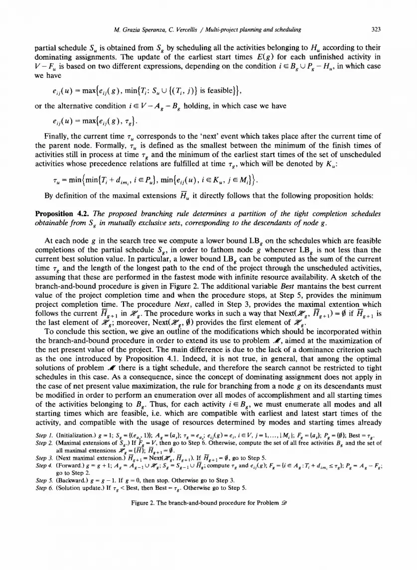
At each node g in the search tree we compute a lower bound LBg on the schedules which are feasible completions of the partial schedule Sg, in order to fa thom node g whenever LBg is not less than the current best solution value. In particular, a lower bound LBg can be computed as the sum of the current t ime rg and the length of the longest path to the end of the project through the unscheduled activities, assuming that these are performed in the fastest mode with infinite resource availability. A sketch of the branch-and-bound procedure is given in Figure 2. The additional variable Best mantains the best current value of the project completion time and when the procedure stops, at Step 5, provides the minimum project completion time. The procedure Nex t , called in Step 3, provides the maximal extention which follows the c u r r e n t /~g+l in ,~g. The procedure works in such a way that Next(,,TC'g, H g + l ) = ~ if /~g+l is the last e lement of ,,~g; moreover, Next(,,~g, ~) provides the first element of ,,~g.

To conclude this section, we give an outline of the modifications which should be incorporated within the branch-and-bound procedure in order to extend its use to problem ~ ' , aimed at the maximization of the net present value of the project. The main difference is due to the lack of a dominance criterion such as the one introduced by Proposition 4.1. Indeed, it is not true, in general, that among the optimal solutions of problem ~ there is a tight schedule, and therefore the search cannot be restricted to tight schedules in this case. As a consequence, since the concept of dominating assignment does not apply in the case of net present value maximization, the rule for branching from a node g on its descendants must be modified in order to perform an enumerat ion over all modes of accomplishment and all starting times of the activities belonging to Bg. Thus, for each activity i ~ Bg, we must enumerate all modes and all starting times which are feasible, i.e. which are compatible with earliest and latest start times of the activity, and compatible with the usage of resources determined by modes and starting times already

Step 1. (Initialization.) g = 1; sg = {(eas, 1)}; Ag = {as}; ~'g = e a ; eij(g) = e i, i E V, j = 1 ..... [ M i [; Fg = {as}; Pg ~ {~}; Best = zg. Step 2. (Maximal extensions of Sg,) IfFg --V, then go to Step 6. Otherwise, compute the set of all free activities Bg and the set of

all maximal extensions Xg --{H}; Hg+x = ~. Step 3. (Next maximal extension.) Hg+t = Next(,g,"g, Hg+l)- If_ Hg+l = ~, go to Step 5. Step 4. (Forward.) g = g + 1; A g = Ag_ I u ,~g; Sg = Sg_ 1U Hg; compute ~'g and eli(g); Fg = {i ~ A g : T i + dim ̀ <_ ~-g}; Pg = A g - Fg;

go to Step 2. Step 5. (Backward.) g = g - 1. If g = 0, then stop. Otherwise go to Step 3. Step 6. (Solution update.) If rg < Best, then Best = rg. Otherwise go to Step 5.

Figure 2. The branch-and-bound procedure for Problem


assigned to other activities. This enumeration process determines the descendants of node g, which are in general much larger in number than those obtained within the corresponding enumeration scheme for problem _~.

5. Computational considerations

It can be observed that other enumeration schemes for the solution of problem ~ have been proposed in the past, such as those in Talbot (1982) and Patterson et al. (1989). The latter, which can be regarded as an evolution of the former, is based on the idea of developing a systematic search through all possible permutations of the activities which are compatible with the precedence relationships, combined with the enumeration of all modes available for each activity. A drawback suffered by this enumeration procedure is redundancy, due to the possibility of generating more than once the same feasible schedule. Indeed, while a feasible schedule induces a unique permutation of the activities, obtained by lexicograph- ically ordering the activities according to their starting times, the converse is not true in general: two or more permutations and mode selections of the activities might correspond to the same feasible schedule, obtained by starting each activity at its earliest feasible time.

To avoid redundancy, hence reducing the number of nodes explicitly enumerated during the search, our branch-and-bound procedure is based on the idea of resolving conflicts, arising among activities for the use of critical resources, by means of appropriate delaying of some activities. Thus, these theoretical considerations indicate that there are advantages in our enumeration procedure with respect to the cited exact algorithm. Indeed, by exploiting the conflicts arising in the use of resources, the enumeration scheme proposed in Section 4 limits the tree search only to tight schedules, as suggested by Proposition 4.2. The algorithm proposed in Patterson et al. (1989), for instance, is likely to explicitly enumerate also schedules which are not tight, and, furthermore, it may generate the same schedule more than once, when such a schedule corresponds to multiple permutations of the activities.

In order to validate our hierarchical decomposition approach, as it is outlined in Section 3, and to establish the range of problem size which can be solved, the two versions of the branch-and-bound algorithm proposed in Section 4 have been implemented and tested on some problem instances whose data are drawn from a real world application to a company operating in the construction building industry. The computer program has been coded in C + + language on a PC IBM PS/2 70A21. In the tested problem instances the number of projects ranged from 5 to 10, while the number of activities per project ranged from 10 to 20, over a planning horizon of 24 months. Two or more modes per activity were generally available. The money was the only nonrenewable resource, while up to 6 renewable resources were consumed by the different activities. In general, each mode required the nonrenewable resource and 2 or 3 renewable resources. The computational experience showed that the running time of the whole hierarchical approach was heavily dependent on the number [ K s I of budget limitations in the solution of Problems ~¢(s, v). With the choice of I Ks I described below, running times were of the order of minutes.

In the implementation of the algorithm for solving the shrinking model, we found that in practice a good trade-off between computational effort and solution accuracy can be achieved by selecting the number I Ks [ of budget limitations in the range 3 to 5. To this aim, a simple iterative procedure has been adopted. First, Problem ~¢(s, v) is solved for a very large value of the budget limitation v. The solution determined in this way corresponds to a cost ~. The other macro-modes are derived by conducting a binary search in the interval (0, ~).

6. Conclusions

It has been argued that the multi-project planning and scheduling problem involves complex decision processes in a dynamic environment, related to multiple conflicting criteria, over short to medium time


horizons. These features make inadequate the support of a 'monolithic' single objective optimization model. The methodology proposed in this paper is based upon a hierarchy of integer programming optimization models, integrated by means of an explicit coordination scheme. In view of the design of a Decision Support System, the attention has been centered on the modeling aspects, to assist the decision makers in allocating scarce resources among projects; evaluating different cash flows in light of the net present value maximization; identifying the most appropriate modes of accomplishment of the various activities; and scheduling the elementary activities over the planning horizon. A class of branch-and-bound procedures has been proposed, to solve the models presented here.

Future developments of the proposed approach may lead to incorporate a third type of criteria, related to the project plan dependability, i.e. the reliability in actually meeting the scheduled dates. Further research will be devoted to the improvement of the branch-and-bound procedure by means of stronger lower bounds and to the design of heuristic procedures.

References

Balas, E. (1970), "Project scheduling with resource constraints", in: Applications of Mathematical Programming Techniques, Carnegie Mellon University, Pittsburgh.

Blazewicz, J., Lenstra, J.K., and Rinnooy Kan, A.H.G. (1983), "Scheduling subject to resource constraints: Classification and complexity", Discrete Applied Mathematics 5, 11-24.

Christofides, N., Alvarez-Valdez, R., and Tamarit, J.M. (1987), "Project scheduling with resource constraints: A branch and bound approach", European Journal of Operational Research 29, 262-273.

Davis, E.W., and Heidorn, G.E. (1971), "An algorithm for optimal project scheduling under multiple resource constraints", Management Science B 17, 803-816.

Davis, E.W., and Patterson, J.H. (1975), "A comparison of heuristic and optimal solutions in resource-constrained project scheduling", Management Science 21, 944-955.

Deckro, R.F., and Hebert, J.E., (1990), "A multiple objective programming framework for tradeoffs in project scheduling", Engineering Costs and Production Economics 18, 255-264.

Doersch, R.H., and Patterson, J.H. (1977), "Scheduling a project to maximize its present value: A zero-one programming approach", Management Science 23, 882-889.

Elmaghraby, S.E., and Herroelen, W.S. (1988), "The scheduling of activities to maximize the net present value of projects", Technical Report OR 222, North Carolina State University.

Gorestein, S. (1972), "An algorithm for project (job) sequencing with resource constraints", Operations Research 20, 835-850. Kurtulus, I., and Davis, E.W. (1982), "Multi-project scheduling: Categorization of heuristic rules performance", Management

Science 28, 161-172. Kurtulus, I.S., and Narula, S.C. (1985), "Multi-project scheduling: Analysis of project performs", IEEE Transactions 17, 58-66. Norbis, M.I., and MacGregor Smith, J. (1988), "A multiobjective, multi-level heuristic for dynamic resource constrained scheduling

problems, European Journal of Operational Research 33, 30-41. Patterson, J.H. (1976), "Project scheduling: The effects of problem structure on heuristic performance", Naval Research Logistics

Quarterly 23, 95-123. Patterson, J.H. (1984), "A comparison of exact approaches for solving the multiple constrained resource, project scheduling

problem", Management Science 30, 854-866. Patterson, J.H., and Huber, W.D. (1974), "A horizon-varying, zero-one approach to project scheduling", Management Science 20,

990-998. Patterson, J.H., Slowinski, R., Talbot, F.B., and Weglarz, J. (1989), "An algorithm for a general class of precedence and resource

constrained scheduling problems", in: Aduances in Project Scheduling, Elsevier Science Publishers, Amsterdam. Pritsker, L.J., Watters, A.A.B., and Wolfe, P.M. (1969), "Multiproject scheduling with limited resources: A zero-one programming

approach", Management Science 16, 93-108. Russell, A.H. (1970), "Cash flows in the networks", Management Science 16, 357-373. Russell, R.A. (1986), "A comparison of heuristics for scheduling projects with cash flows and resource restrictions", Management

Science 32, 1291-1300. Slowinski, R. (1981), "Multiobjective network scheduling with efficient use of renewable and nonrenewable resources", European

Journal of Operational Research 7, 265-273. Talbot, F.B. (1982), "Resource-constrained project scheduling with time-resource tradeoffs: The nonpreemtive case", Management

Science 28, 1197-1210. Talbot, F.B., and Patterson, J.H. (1978), "An efficient integer programming algorithm with network cuts for solving resource-con-

strained scheduling problems", Management Science 24, 1163-1174. Valadares Tavares, L. (1987), "Optimal resource profiles for program scheduling", European Journal of Operational Research 29,

83-90.

Documents

Hierarchical models for multi-project planning and scheduling