Embed Size (px)
Citation preview
i
Identifying indicators of financial crises
WJ du Toit
orcid.org/0000-0003-0427-4546
Dissertation submitted in fulfilment of the requirements for the degree Master of Commerce in Risk Management
at the North-West University
Supervisor: Prof WF Krugell
Co-Supervisor: Dr C Claassen
Graduation: May 2019
Student number: 23471336
ii
Abstract
Early warning models have gained prominence after the global financial crisis of 2008 struck
the world without remorse. The severity and the extent to which economies around the globe
was affected resulted in massive costs. The notion of early warning indicators being able to
identify areas of vulnerabilities with regard to oncoming financial crises justifies supplementary
research into early warning indicators. Based on a dataset proposed by Rohn et al., (2015),
this thesis discusses potential vulnerabilities that can lead to financial crises. The dataset
includes more than 70 vulnerability indicators for 34 OECD countries between 2005 and 2014.
However, monitoring an extensive list of potential vulnerabilities is not always possible.
Dynamic factor analysis was therefore applied to the dataset as a measure of data reduction
in order to identify a suitable set of early warning indicators that can be monitored to signal
oncoming financial crises.
Key words: financial crises; early warning indicators; dynamic factor analysis; co-movement

iii
Acknowledgements
“Reflect upon your present blessings, of which every man has plenty; not on your past
misfortunes, of which all men have some”
Charles Dickens
Words on paper cannot completely describe my gratitude towards the following people:
• My supervisors, Prof Waldo Krugell and Dr Carike Claassen for their guidance, inputs
and patience during the course of this study. I thank you.
• My wife, Madeli du Toit, for the endless sacrifices that you made during the course of
this study. Thank you for your support and love.
• My parents, Wilco and Mariza du Toit for teaching me to never give up. Thank you for
your unconditional love and support in this process. Thank you for giving me the
opportunity to pursue my dreams. I will always be grateful for what you have done for
me.
• My friend, Johnny Jansen van Rensburg, who went through this process with me.
Thank you for always being available and being a trusted confidant, I can always count
on. I am grateful for your support.
iv
Table of contents
CHAPTER 1: INTRODUCTION ............................................................................................. 1
1.1 Background ................................................................................................................. 1
1.2 Problem statement ...................................................................................................... 2
1.3 Objectives ............................................................................................................... 3
1.4 Research method ................................................................................................... 3
1.5 Outline .................................................................................................................... 3
CHAPTER 2: REVIEW OF THE LITERATURE ..................................................................... 4
2.1 Introduction .................................................................................................................. 4
2.2 Survey of the crisis literature ........................................................................................ 5
2.2.1 Monetary Policy .................................................................................................... 6
2.2.2 Deregulation .......................................................................................................... 7
2.2.3 Global imbalances ................................................................................................. 8
2.2.4 Asset price booms and busts ................................................................................ 8
2.2.5 Securitisation ........................................................................................................ 9
2.2.6 Fear (Human sentiment/irrational driver) ............................................................. 10
2.3 Types of crises .......................................................................................................... 11
2.3.1 Sudden stops and reversals (capital account or balance of payments crisis) ...... 11
2.3.2 Currency crisis .................................................................................................... 14
2.3.3 Banking crises ..................................................................................................... 15
2.3.4 Debt crises (domestic and sovereign) ................................................................. 17
2.3.5 Speculative bubbles and market failures ............................................................. 18
2.4 Indicators of financial crises ....................................................................................... 19
2.5 Other perspectives .................................................................................................... 28
2.6 Summary of conclusions ............................................................................................ 31
CHAPTER 3: EARLY WARNING INDICATORS ................................................................. 33
3.1 Introduction ........................................................................................................... 33
3.2 Financial sector imbalances....................................................................................... 35
3.2.1 Leverage and risk taking ..................................................................................... 36
3.2.2 Maturity and currency mismatches ...................................................................... 37
3.2.3 Interconnectedness and spill-overs ..................................................................... 37
3.3 Non-financial sector imbalances ................................................................................ 38
3.4 Asset market imbalances ........................................................................................... 40
3.5 Public sector imbalances ........................................................................................... 42
3.6 External sector imbalances ........................................................................................ 45
3.7 International spill-overs, contagion and global risks ................................................... 47
v
3.7.1 The main channels .............................................................................................. 47
3.7.2 Measuring vulnerabilities to international spill-overs, contagion and global risks . 50
3.8 Conclusion ............................................................................................................ 52
CHAPTER 4: EMPIRICAL ANALYSIS ................................................................................ 53
4.1 Introduction ................................................................................................................ 53
4.2 Dynamic factor analysis ............................................................................................. 53
4.2.1 The Model ........................................................................................................... 55
4.2.2 Data and Method................................................................................................. 57
4.3 Results from Hermansen and Rhon ........................................................................... 59
4.3.1 In-sample results ................................................................................................. 59
4.3.2 Out-of-sample results .......................................................................................... 60
4.4 Results from this study .............................................................................................. 61
4.4.1 Factor 1 ............................................................................................................... 62
4.4.2 Factor 2 ............................................................................................................... 73
4.5 Conclusion ............................................................................................................ 79
CHAPTER 5: CONCLUSION .............................................................................................. 80
5.1 Introduction ................................................................................................................ 80
5.2 Conclusion ................................................................................................................. 81
5.3 Recommendations for future research ....................................................................... 82
vi
List of figures
Figure 2.1: Tulip price index 18
Figure 2.2: Important early warning indicators 21
Figure 2.3: Global early warning indicators 21
Figure 2.4: Percentage of studies where leading indicators were found to be
statistically significant 27
Figure 3.1: Description of vulnerabilities 34
Figure 4.1: Factor 1 66
Figure 4.1.1: Factor 1 and household credit 68
Figure 4.1.2: Factor 1 and total private credit 69
Figure 4.1.3: Factor 1 and commercial real estate loans 70
Figure 4.1.4: Factor 1 and residential investment 71
Figure 4.1.5: Factor 1 and private bank credit 72
Figure 4.2: Factor 2 75
Figure 4.2.1: Factor 2 and household credit 76
Figure 4.2.2: Factor 2 and private bank credit 77
Figure 4.2.3: Factor 2 and total private credit 77
Figure 4.2.4: Factor 2 and external bank debt 78
vii
List of tables
Table 3.1.1 Indicators of financial sector imbalances 38
Table 3.1.2 Indicators of non-financial imbalances 40
Table 3.1.3 Indicators of asset market imbalances 42
Table 3.1.4 Indicators of public sector imbalances 44
Table 3.1.5 Indicators of external imbalances 47
Table 4.1 Variance shares of factor one 63
Table 4.2 Variance shares of factor two 74
1
CHAPTER 1: INTRODUCTION
1.1 Background
Financial crises, as odd as it may seem, always start with new hope. The ultimate effects of
financial crises are always dire, always driven by the self-interest of some party carried on the
back of the hope of the masses. Hope comes in many forms and shapes. Hope of a better
future, hope of financial stability, hope of wealth and even simply just hope of meeting basic
needs. When it comes to financial crises, history tends to repeat itself as it has shown us time
and time again. The most wide-ranging recent crises i.e. Turkish currency and debt crisis
(2018), Venezuelan crisis (2017) and global financial crisis (2008) to name a few, are all
excellent examples of history repeating itself. The context around the crises differs, but at the
core of the crisis, the same fundamentals are always present; markets, despite their collective
expertise, are destined to repeat history as irrational exuberance is followed by an equally
irrational despair (Anderson, 2018), resulting in inevitable periodic bouts of chaos.
The specific causes of every crisis differ and are more often than not widely debated. Modern
financial crises have several commonalities according to Anderson (2018) and often include
one or more of the following symptoms: excessive exuberance, poor regulatory oversight,
accounting irregularities, “herd” mentalities and deregulation of financial markets. However,
one truth is certain; the aftermath of a financial crises is always costly, regardless of what
caused the crisis.
The premise that policy-makers could be warned in advance of costly crisis events is giving
academics, private and public sector and economists alike a renewed eagerness to develop
successful early warning models. Early warning literature has been around for some time now
and can be traced back to the late 1970s when a number of currency crises put the focus on
leading indicators (Bilson & Frenkel, 1979) as well as theoretical models (Krugman, 1979)
offering explanations for such crises. However, it was only in the 1990s that a wide-ranging
methodological debate around early warning systems started (Alessi, Antunes, Babecky,
Baltussen, Behn, Bonfim, Bush, Detken, Frost, Guimaraes, Havranek, Joy, Kauko, Mateju,
Monteiro, Neudorfer, Peltonen, Rodrigues, Rusnak, Schudel, Sigmund, Stremmel, Smidkova,
van Tilburg, Vasicek, Zigraiova, 2014). This debate included literature from research on
banking crises, balance of payments problems (Kaminsky & Reinhart, 1996) as well as
currency crashes (Frankel & Rose, 1996).
Earlier models started off with the identification of single indicators where variable selection
was mostly based on the early signalling models such as that of Kaminsky, Lizondo & Reinhart
(1998). This quickly evolved into univariate signalling approaches which in effect, track and
2
record the historical time series data of a single indicator on historic crises and extract a
threshold value where crises are most likely to happen. The univariate approach is simple and
easy enough to apply and is therefore favoured by policy-makers. However, this approach
contains a degree of underlying risk as several factors may be close to their associated crisis
threshold values but because the threshold has not been reached, one might underestimate
the probability of a crisis (Borio & Lowe, 2002). More recent models have addressed this
problem by creating multi-variable early warning models by estimating the probability of a
future crisis event from a set of several potential early warning indicators (Frankel & Saravelos,
2012 and Rose & Spiegel, 2009). It is unlikely that financial crises will be totally avoided, but
with the help of ever-evolving early warning models, the associated costs and ultimate effects
of financial crises can potentially be mitigated.
The global financial crisis of 2008 is significant for various reasons, most notably, the speed
and severity with which it struck the global stage with (Rose & Spiegel, 2009). The global span
of the crisis has also been notable; as, basically, every industrialised country has been
affected in some way or another, be it on a small scale or severely. Developing and emerging
economies were also not left unscathed. The crisis led policymakers to implement various
costly policies to stimulate economies and mitigate the effects of the crisis. The actual cost of
the global financial crisis of 2008 is a hotly debated topic and is likely to remain so. Early
warning indicators are therefore an essential component that can help reduce the high losses
associated with crises (Drehmann & Juselius, 2013:3).
For multi-variable early warning models, there are many possible indicators of a potential
financial crisis, from simple rules of thumb like the deficit on the current account of the balance
of payments, through to the 70 indicators posed by Röhn, Sanchez, Hermansen & Rasmussen
(2015).
1.2 Problem statement
However, monitoring many indicators is costly. It may happen that different indicators present
different signals. Therefore, monitoring an appropriate set of early warning indicators is crucial
for reducing the risk of financial crises or at least mitigating their impact on the economy
(Babecky, Havranek, Mateju, Rusnak, Smidkova & Vasicek, 2011:112).
This dissertation sets out to identify indicators that should be monitored to signal oncoming
financial crises. In doing so, the aim is to re-examine the 70+ indicators identified by Röhn et
al. (2015) to identify parsimonious indicators of financial crises. The focus is on identifying
indicators of financial crises that experience similar movements during the build up to and
times of crisis. A dynamic factor model will be applied to the existing Röhn et al. (2015) dataset
3
to establish co-movement among the indicators. Indicators that co-vary will be pooled to create
a smaller number of factors that observers can monitor for oncoming crises.
1.3 Objectives
The main objective of this dissertation is to identify groups of indicators of financial crisis. As
such, it is a data reduction exercise that aims to determine co-movement between indicators
of crisis to group them as factors, or latent indicators, of crisis.
To achieve this objective, a number of secondary objectives need to be achieved:
• A review of the literature of the indicators of financial crises will place this dissertation
in the context of the models that predict co-movement of indicators, and earlier
empirical studies that find co-movement of indicators.
• An overview of the set of early warning indicators and a description of the data used
by Röhn et al. (2015) will clarify the inputs to the empirical analysis.
• A description of the dynamic factor analysis will show that the method is appropriate
for the question at hand and will inform the identification of the groups of indicators of
financial crisis.
• An explanation of the results of the empirical analysis will demonstrate the scientific
solutions to the research problem.
1.4 Research method
The methods employed in this study are a review of the literature as well as empirical analysis.
The empirical analysis will take the form of dynamic principle component analysis. The aim is
to use the existing Röhn et al. (2015) dataset with 70 possible early warning indicators of
financial crises and to apply this data reduction method to establish co-movement among the
indicators (see Appendix A for list of variables). Groups of indicators that co-vary are factors,
or so-called latent variables, that can then be monitored as indicators of crisis.
This application of the method draws on the so-called coupling/decoupling literature analysed
by among other Claassen (2016).
1.5 Outline
Chapter 1 has described the background, problem statement, objectives and method of this
study. Chapter 2 will present an overview of the literature on the indicators of financial crises.
In Chapter 3 the 70 indicators used by Röhn et al. (2015) and the dataset will be described.
4
Chapter 4 will explain the method of analysis and presents the results. Chapter 5 will present
a summary, conclusions and recommendations.
CHAPTER 2: REVIEW OF THE LITERATURE
2.1 Introduction
Regardless of their severity and origin, most financial crises are similar to past financial crises
in many dimensions. The recurrence of financial crises throughout history suggests that it is
unlikely that financial crises will be wholly prevented in the future (Allen, Babus & Carletti,
2009:14). The impact of financial crises can, however, be softened. The large costs associated
with financial crises gave rise to the concept of early warning systems, where early warning
indicators identify possible vulnerabilities in the economy most likely to be responsible for
causing a financial crisis. One of the main objectives of early warning systems is also to predict
the timing of crises (Kaminsky, et al., 1998:3). From a historical perspective, early warning
systems has had some measure of success at modelling the prevalence of crises across
banks, private firms and countries (Rose & Spiegel, 2009:1).
According to the Economist (2012) there have been several financial crises in various shapes
and forms throughout the 20th and 21st centuries. To give a brief overview of the most notable
of these crises: the Knickerbocker crisis of 1907 occurred when trust companies acted in the
likeness of banks, but these banks were inadequately regulated and when speculators tried
to offset falling share prices with borrowed funds, they worsened the situation; the Wall Street
crash of 1929 occurred due to the speculative boom that took place in the 1920s and ended
when the Federal Reserve hiked interest rates to restore markets to normal conditions; the Oil
Crisis of 1973 – 1974 took place due to the failure of the Bretton Woods system along with the
trade embargo enforced by Arab oil exporters on the Western world; the 1987 crisis called
Black Monday occurred due to significant drops in share prices and was amplified by
automated trading systems and portfolio-insurance schemes causing markets all over the
world to tumble; the 1997 Asian crisis where investors poured funds into emerging Asian
economies that led to artificially high asset prices reaching unsustainable levels causing an
inevitable crash of financial markets; the Dotcom crash of 2001 where shares in internet and
telecom firms increased rapidly on a large scale during the start of the web, and eventually
investors were not satisfied with the lack of profits of their investments in these companies,
which caused share prices of these firms to fall significantly and led to a crash in financial
markets. The most recent and familiar crisis, the sub-prime crisis of 2008 which eventually led
to a global financial crisis, was caused by elaborate mortgage related securities envisioned to
reduce risk but in effect, encouraged investors to stack up on investments in the American
5
housing market, the market eventually crashed (The Economist, 2012). The crises mentioned
above exercised a strong negative aftermath for economies, but the severity of the effects on
financial markets differed, and one truth comes forward: the majority of the financial crises had
devastating effects within the immediate economies and most of these crises caused “spill-
overs” to other economies, hindering economic growth, destroying plans for the future and
causing major setbacks throughout the world.
The history of financial crises indicates that the economic cost associated with crises is
extremely high and any plausible solution is worth researching. The idea that a crisis can be
predicted and therefore losses can be limited has led policy-makers and academics to take
an interest in indicators of financial crises.
The focus of this chapter is to review existing literature on financial crises in order to identify
possible indicators/measures of financial fragility. However, literature indicates that there is an
extensive range of possible vulnerability indicators. This chapter will review the literature on
the kinds of crises and the different indicators of crises. The analysis presented in the following
chapters will attempt to identify and group the most significant indicators by means of data
reduction through dynamic factor analysis.
2.2 Survey of the crisis literature
A financial crisis can be described as a disruption in financial markets taking the form of falling
asset prices and insolvency among debtors and intermediaries. Disturbances such as this
tend to spread through the financial system disrupting both the market’s capacity and ability
to allocate capital (Eichengreen & Portes, 1987:1). Financial crises are more often than not
linked to one or more of the following occurrences: severe disturbances in financial
intermediation and the supply of external financing to various role players in the economy;
considerable changes in the credit volume circulating in an economy along with substantial
changes in asset prices; balance sheet complications on a large scale (including complications
from firms, households, financial intermediaries along with sovereigns); large scale
government support in the form of financing and policy adaptations, more specifically liquidity
support and market recapitalisation (Claessens & Kose, 2013: 3).
Laeven and Valencia (2010:3) state that there are a number of resemblances when comparing
past and recent crises, both in the underlying causes of the crisis and policy responses to the
crisis. However, some noticeable differences in the economic as well as fiscal costs are linked
to more recent crises. The economic cost associated with recent crises is on average much
higher than the cost associated with past crises, in terms of both output losses and increasing
public debt. It was concluded that the median output loss is 25 percent of GDP in recent crises,
6
compared to the historical median of 20 percent of GDP. The median increase in public debt
(computed over a three-year period from the start of the crisis) is 24 percent of GDP for recent
crises, while the historical median is 16 percent. The increases in losses can partly be
attributed to the increase of interconnectedness and complexity of financial systems and the
fact that the recent crises all took place in high income countries (Laeven & Valencia, 2010:4)
Financial crises have been inescapable occurrences throughout history and Bordo,
Eichengreen, Klingebiel & Martinez-Peria (2001:53) found that the frequency of financial
crises in recent decades has been effectively double that of the Bretton Woods period of 1945
to 1971 and the Gold Standard Era of 1880 to 1933. The most recent global financial crisis of
2008 caught most people by surprise, and what was primarily seen as problems in the US
subprime mortgage market, rapidly escalated and spilled over to financial markets throughout
the world. The crisis was repressed at extremely high cost and changed the financial
landscape worldwide. The aftermath of the global financial crisis of 2008 has left policymakers,
researchers and academics with the need to explore both new and existing options to predict
and manage future financial crises. However, to explore these options, the economic drivers
leading to financial crises need to be identified first.
Claessens & Kose (2013:3) claim that crises are to some extent indicators of the interactions
and linkages between the financial sector and the real economy. These connections are often
a mixture of events driven by a variety of factors. Therefore, grasping the concept of financial
crisis requires an understanding of micro-financial linkages affecting an economy. Financial
crisis literature has identified drivers of crises; however, it remains a challenge to definitively
identify their deeper roots (Claessens & Kose, 2013:5). Numerous theories have been
developed in the past decades concerning the underlying causes of financial crises.
Fundamental factors such as macroeconomic imbalances and external or internal shocks are
often identified as culprits; however, the exact causes of financial crises still remain
questionable as financial crises appear to be occasionally driven by “irrational” drivers.
Irrational drivers refer to factors that are considered to be related to financial turmoil, such as
contagion and spill-overs in financial markets, credit crunches, sudden runs on banks and
limits to arbitrage during times of distress. Common drivers of financial crises will be discussed
in the following section.
2.2.1 Monetary policy
Literature has recognized several linkages that connect macroeconomic factors to financial
crises. Monetary policy, being one of these factors, is said to contribute to the build-up of
financial imbalances and Merrouche and Nier (2010:7) argue that for the 2008 global financial
crisis, these linkages are thought to have worked through policy rates that were kept too low
7
for an extended period. Relaxed monetary policy may have led to reduced cost of wholesale
funding for intermediaries, allowing these mediators to build up leverage (Adrian & Shin,
2008:2). This in turn caused banks and other financial institutions to take on higher levels of
risk. In the form of both credit and liquidity risks (Borio & Zhu, 2008:9) this led to an increased
supply as well as demand for credit, consequently inflating asset prices (Taylor, 2007:8).
2.2.2 Deregulation
Looking at the global financial crisis of 2008 in isolation, it could be argued that deregulation
played an important part in the build-up to the crisis specific to the US (Amadeo, 2016:1). The
repeal of Glass-Steagall Act1 by the Gramm-Leach-Bliley Act permitted banks to use deposits
to invest in derivates and gave banks the authority for bank holding companies to be used as
conduits for multi-office banking, subsequently penetrating new product markets (Bentley,
2015:36). Bankers stated that foreign firms posed a great threat as they could not compete at
the same level as these firms. As a result, most bankers only offered low risk securities to their
clients. The Commodity Futures Modernisation Act followed and allowed unregulated trading
of credit default swaps as well as other derivates, which was previously prohibited by state
laws in the US and was considered to be gambling (Amadeo, 2016:2). The main problem with
deregulation in the US seems to have been the repeal of the Glass-Steagall Act by the Gramm-
Leach-Bliley Act as its passing allowed what would normally have been commercial banks to
deal in the underwriting and trade of securities (Bentley, 2015:37). Consequently, banks took
on higher levels of credit risk as the interconnected relationship between banks, securities
exchanges and insurance firms strengthened. Large bank holding companies became major
role players in investment banking and the strategies of leading commercial banks started to
look like those of investment banks as they were associating themselves with securitisation,
which was the main cause for their failures in 2008 (McDonald, 2016). At the time banks were
growing larger while regulators were experiencing difficulties to effectively complete their
function. Banks experienced such high levels of growth that the idea of “too big to fail” took
over as these large banks came to realise that even in the event of financial distress, the
government would have to bail them out (Stiglitz, 2010 B:4). In contrast with this mindset,
banking regulations aim to promote competition between banks and forces them to utilize their
resources efficiently to retain their customers and remain in business (Bentley, 2015:31).
Supervision along with regulation of financial systems is a vital means to prevent financial
crises, by controlling moral hazard to a certain extent and discouraging excessive risk taking
on the part of financial institutions regulation is a key factor in maintaining a crisis free
1 The Glass-Steagall act was authorized in 1933 as a response to the banking crisis of the US during the
1920s and early 1930s. It imposed the separation of investment banking from commercial banking (McDonald, 2016).
8
environment (Merrouche & Nier, 2010:9). Deregulation, however, serves the self-interest of
financial institutions and the pursuit of self-interest can thus explains the drift toward
deregulation prior to the global financial crisis.
2.2.3 Global Imbalances
Global imbalances can be described as imbalances between savings and investments in the
world economy reflected in large and growing current account imbalances (Dunaway, 2009:3).
Current account imbalances are normally maintained at a sustainable level, however in some
cases countries with current account deficits start to feel increasing pressure in obtaining
financing when deficits reach unsustainable levels. Limited financing as a result of large
current account deficits applies pressure on economies which forces policymakers to adjust
domestic interest rates putting downward pressure on the real exchange rate. This in turn
hinders domestic economic activity. This is not only true for countries with deficits, as countries
with surpluses face similar pressures in the opposite direction, causing increased economic
activity leading to the appreciation of the real exchange rate. Literature on crises often does
not include discussions regarding economic policies that foster and facilitate global
imbalances. Dunaway (2009:13) takes this statement into account when looking back at the
2008 global financial crisis, and one can clearly see considerable and growing current account
imbalances within major economies. US deficits were increasing while emerging Asian
economies as well as oil exporting Middle Eastern countries were creating surpluses. Savings
and investment imbalances led to the existence of the “savings glut” in developing countries
where substantial amounts of capital flowed from developing countries to advanced
economies, the US being the primary recipient of these inflows of capital. The so-called
savings glut was followed by reduced interest rates around the world and simultaneously, a
growing demand rose from these emerging Asian economies along with some Middle Eastern
economies for official reserve assets. The great demand for such high quality, low risk assets,
contributed to financial excesses that culminated in the turmoil of financial markets.
2.2.4 Asset price booms and busts
Drastic hikes in asset prices and the crashes that follow them, have been around for centuries
(Laeven & Valencia, 2010:5). Asset prices occasionally diverge from what fundamentals would
suggest to be normal or fair and display patterns varying from predictions of standard models
operating in stable financial conditions. A bubble is an extreme form of such deviation and can
be described as the part of a complete upward asset price movement that cannot be explained
solely grounded on fundamentals (Garber, 2000:4). Patterns of extreme increases in asset
prices followed by crashes feature in numerous accounts of financial instability and go back
millenniums for both emerging market and advanced countries (Laeven & Valencia, 2010:5).
9
In an attempt to explain asset price bubbles, several models have been developed over time.
These models range from micro-economic distortions that cause mispricing, to considering
the impact of rational behaviour causing collective mispricing of assets, whereas other models
take irrationality of investors into account. Despite these attempts Laeven and Valencia
(2010:7) state that anomalies cannot easily be credited to specific, institution-related
distortions in asset prices.
2.2.5 Securitisation
Securitisation became an important role player in the 2008 global financial crisis as hedge
funds in the US sold mortgage backed securities2 such as collateralised debt obligations
(CDO) and other derivatives. Once an individual receives a mortgage from a bank, the bank
sells the mortgage to a hedge fund on the secondary market. Banks and Hedge funds then
bundled these mortgages with similar mortgages to create CDOs.
What made securitisation troublesome was “tranching”3. Tranching was initially implemented
to decrease the risk of upper tranches in order to achieve higher credit ratings (Bentley,
2015:13). Banks were allowed to tranche the mortgage pools and did so by dividing mortgage
pools into different tranches; the toxic waste tranche, the mezzanine tranche and the senior
tranche. A tranche bundle of securities is thus a collateralised debt obligation and most CDOs
consisted of seven or even eight tranches (Bentley, 2015:14). CDOs like these were then sold
to investors by hedge funds, which allowed banks to hand out new loans with the resources
received from selling these mortgages, however the bank still collected the payments on these
mortgages and sent them to the hedge funds who in turn sent these payments to investors
(Amadeo, 2016). All of the intermediaries took a pre-determined percentage of profit for their
part in the process, making this a popular investment and free of risk for the bank and hedge
fund. Investors took on all the risk of default as they had a way of mitigating the risk called
credit default swaps. These credit default swaps were sold by major insurance companies
making investors believe these securities were safe investments as they were “backed” by
mortgage bonds. Derivates backed by real estate and insurance were a profitable investment
and demand for these securities was high and growing. More and more mortgages were
needed to back the securities and to meet this high demand, banks as well as mortgage
brokers offered home loans to almost everyone. Banks eventually offered subprime
2 Mortgage backed securities are financial products where the price is based on the value of mortgages
being used for collateral security. 3 A common feature of CDO’s involves the division of the degree of credit risk pertaining to a pool of
securities into different risk classes. The interval between two different classes of risk is called a tranche. This tranche then absorbs the initial loss (high risk tranche) and is called the equity tranche. The remaining tranches are known as mezzanine or senior tranches (FINCAD, 2017)
10
mortgages to cover the high demand as the derivates were so profitable they did not need to
make much money from the loans (Amadeo, 2016).
Due to low interest rates imposed by the Federal Reserve Bank (Fed), many homeowners
who could not previously afford mortgages were approved for interest only loans.
Consequently, the percentage of subprime mortgages doubled from 10% to 20% from 2001
and 2006 and unintentionally created an asset bubble in the real estate sector around 2005
(Amadeo, 2016). The high demand for mortgages drove up the demand for housing which
construction contractors tried to meet. Because loans were cheap, speculators bought houses
as investments to sell as prices went up. The Fed adjusted interest rates and many individuals
could not repay their loans due to the higher interest rates, which in turn put pressure on
housing prices as more and more houses were being sold. The housing market bubble
resulted in a bust and contributed to the existence of the 2008 financial crisis.
2.2.6 Fear (Human sentiment/irrational driver)
Fear is aptly placed at the bottom of the list as it is not necessarily a driver or cause of a
financial crisis in itself, but rather a psychological catalyst amplifying crises. Fear is manifested
at the core of financial crises (Aldean & Brooks, 2010:1). Take a “bank run” as an example, in
the event where one bank defaults, fear is triggered among depositors of other banks despite
those banks being sound (Hoggarth, Reidhill & Sinclair, 2004:6). Similarly, fear can also be
“exported” on an international level. Historical accounts suggest that fear and greed are at the
roots of financial crises (Lo, 2011:622). Individuals, companies and financial institutions
behave in a self-serving manner, meaning that they want to protect their resources despite
taking on risk to enrich themselves. These groups will therefore always act conscientiously
when it comes to their resources, both conscientiously rational or irrational, depending on what
their perspective is.
As can be seen from the survey of financial crisis literature, there are numerous factors that
can attribute or lead to the existence of financial crises. As is the case with the majority of
crisis incidents, the root cause is intertwined and more often than not these root causes shift
blame to one another. Indicators of financial crises should thus not be considered in isolation,
but rather as a collective set of indicators as this would be a more meaningful measure
regarding early warning models. The ideal solution would be to find a universal set of indicators
that would be applicable in all crisis events to all countries, however considering the vast
degree of diversity between countries, it seems unlikely that one would be able to put forth a
set of indicators that provides consistent results for all countries. That being said, all financial
crises do have homogenous drivers to some extent. The aim is thus to put forth a credible set
of indicators to identify financial crisis crises at an early stage.
11
2.3 Types of crises
To better understand financial crises, it can be said that there are two types of crises; firstly,
crises classified by means of quantitative definitions and secondly, crises that are mostly
reliant on qualitative and judgemental analysis (Claessens & Kose, 2013:11). In addition to
this, crises classified by quantitative means can further be sub-classified into currency and
sudden stop crises, whereas financial crises reliant on qualitative and judgemental analysis
can be sub-classified into debt and banking crises.
2.3.1 Sudden stops and reversals (capital account or balance of payments crisis)
Sudden stops refer to events where the domestic economy loses access to international
capital markets as private foreign investors abruptly stop lending and investing to domestic
residents and companies. This results in panic due to the financial turmoil and leads to an
extreme shift of the supply of foreign funds to such an extent that the direction of capital flows
completely turns around (Jeasakul, 2005:5). Whereas a crisis originating from current account
deficits; in basic terms, a current account deficit implies that a country is spending more abroad
than it is receiving from abroad. According to the IMF the current account can be expressed
as the value of exported goods and services and the value of goods and services imported.
Thus, a deficit means a country is importing more goods and services than it is exporting. The
current account includes net income (in the likes of dividends and interests) along with
transfers (such as foreign aid), however these sections only make up a small percentage of
the of the total (Ghosh & Ramakrishnan, 2012). In the instance where a country runs a current
account deficit, it is effectively borrowing from the rest of the world.
Obstfeld (2012:2) stated that even in an ideal world free from economic frictions, both foreign
demand and supply conditions are constraints on the maximum welfare attainable by the
national economy. As a result, governments face incentives to manipulate such constraints to
benefit them. Basic neoclassical theory states that all entities will gain from free trade (which
includes balanced trade), however theory and reality are two very different things. In a world
filled with economic and political distortions, a government’s apparent short run advantage
may be heightened by policies focused on a trade surplus. Policies like these have adverse
consequences for trade partners as a surplus in one country indicates a deficit in the
corresponding trade partner. Government policies are also a key factor in current account
deficits and surpluses.
According to Milesi-Ferretti and Razin (1996:65) persistent current account imbalances are
often seen as a sign of weakness that implies the need for policy action. In contradiction to
this, economic theory suggests that intertemporal borrowing and lending are natural pathways
to achieve accelerated capital accumulation, the smoothing of consumption and a more
12
efficient investment allocation. Milesi-Ferretti and Razin (1996:65) conducted a study to
determine to what degree persistent current account imbalances can be taken as a sign of an
upcoming crisis. This particular study debated that traditional measures of sustainability, solely
based on the notion of intertemporal solvency, may not always be suitable, due to the fact that
they do not encompass the willingness of a country to meet its outstanding external
obligations. Nor the willingness of foreign investors to keep lending on current terms. To
compensate for these factors an alternative notion of sustainability that emphasizes the
willingness to pay and lend in addition to simple solvency was proposed. A list of indicators
based on theoretical considerations was compiled to shift the focus to the sustainability of
external imbalances. From this list, a few conclusions were made: A specific threshold on a
persistent current account deficit (such as the 5 percent of GDP for 5 years) is in itself not an
adequately informative indicator of sustainability. Rather than using a specific threshold, the
magnitude of current account imbalances should be taken into account along with exchange
rate policy and structural factors such as the degree of openness, the condition of the financial
system and the levels of investment and saving.
To add to literature regarding persisting current account imbalances, Edwards (2005:34) came
to the conclusion that in his sample period of 30 years the vast majority of countries have run
current account deficits. In this specific sample period, there had only been three regions
where the average current account balance has been a surplus, these regions being some
industrialised countries, the Middle East and Asia; however, all these surpluses have been
small. Literature indicates that large current account deficits have not persisted for extended
periods of time. A small number of countries have run prolonged deficits, however the degree
of persistence of large surpluses has been higher. Major reversals in current account deficits
have tended to be persistent throughout the sample period and are strongly associated to the
sudden stop of capital inflow. Regarding financial crises and reversals, a significant likelihood
of reversals leading to exchange rate crises exists. Additionally, evidence suggests that
countries that attempt to deal with reversals by significantly running down reserves, typically
do not succeed (Edwards, 2005:34).
Edwards (2005:12) analysed the working of current account movements throughout the global
economy in the past three decades and his main findings can be summarised as follows:
Firstly, large reversals in current account deficits tend to be linked to sudden stops of capital
inflow. Secondly the probability of countries experiencing reversals can be explained by a
smaller number of variables that include the current account to GDP ratio, the level of
international reserves, the external debt to GDP ratio, debt services and domestic credit
creation. Lastly current account reversals have been known to have negative effects on real
growth that goes beyond their direct effect on investments. This evidence indicates that the
13
negative effects of reversals on growth will depend on a country’s degree of openness, i.e.
more open countries will not be affected as much as countries with limited openness. In the
event where countries run large current account deficits for a prolonged period of time,
concerns arise as to whether these deficits are sustainable. Milesi-Ferretti and Razin (1996:1)
create some background regarding conventional wisdom on sustainable current account
deficits by stating that conventional wisdom should indicate disturbing signs if deficits persist
above 5 percent of GDP, especially when such a deficit is financed by making use of short-
term debt or foreign exchange reserves. It is therefore worth questioning whether something
such as the above-mentioned threshold on current account deficits should be taken seriously
and if so, which factors would be worth determining to evaluate if prolonged external
imbalances are likely to lead to external shocks. In regard to this question, history suggests
that several countries such as Australia, Ireland, Malaysia and Israel to name a few have been
able to run large current account imbalances for a number of years, however other countries
such as Mexico and Chile have not been able sustain their deficits and subsequently suffered
severe external crises. History thus suggests that there are more factors at work and grasp a
better understanding regarding persisting current account imbalances, these factors should
be identified and analysed. Another study even went as far as to claim that the prolonged
current account deficit of the US reflects a technological shift that has led to prosperity rather
than impose negative effects (Hervey & Merkel, 2001:12). This opens the door to possible
two-sided effects of prolonged current account deficits. The solvency of individual countries
can aid in explaining the differing results suggested by history and should therefore be
considered a key factor to be taken into account when assessing external imbalances. The
solvency of a country indicates its ability to generate a sufficient trade surplus to repay
outstanding debt.
Obstfeld (2012:3) claims that the circumstantial evidence of current account deficits being a
conduit of financial crises was preceded by historically large global imbalances in current
accounts, which includes large deficits that were run by a number of industrial economies
(including the U.S.) that consequently came to grief. What most debates miss regarding
current account imbalances is the remarkable progression and integration of international
financial markets during the past quarter century. Due to global imbalances financed by
multifaceted patterns of gross financial flows, flows that are usually much larger than the
current account gaps themselves, questions arise as to whether the commonly smaller net
current account balance still matters. However, a lesson of recent crises is that globalised
financial markets puts forward potential stability risks that people too often choose to ignore
at their own peril. Current account imbalances can signal preeminent macroeconomic as well
14
as financial tensions as was arguably the case of the mid-2000s. Historically big and ongoing
global imbalances deserve close attention from policymakers (Obstfeld, 2012:39).
Edwards (2005:1) put forward the argument that free capital mobility induces macro-economic
instability and adds to the existing problem of financial vulnerability in emerging economies.
Stiglitz (2010 A) reinforced this account in his critique of the Fed and the IMF by stating that
pressure was put on emerging economies to relax capital mobility controls during the 90s.
Stiglitz was of opinion that the easing of capital mobility control was at the centre of the majority
of currency crises in emerging markets during the last decade; Mexico 1994, East Asia 1997,
Russia 1998, Brazil 1999, Turkey 2001 as well as Argentina 2002. The IMF seems to have
changed their opinion and offer some level of support for controls of capital mobility as the
IMF managing director of 2003 (Horst Koehler) praised the policies of Prime Minister Mahatir
and his particular use of capital controls in the aftermath of the 1997 currency crisis (Edwards,
2004). Supporters of capital mobility controls claim that there are two obvious benefits of
restricting capital mobility: a) It reduces a country’s vulnerability to external shocks and
financial crises and b) it creates capacity for countries that have suffered a currency crisis to
lower interest rates, implement pro-growth policies, and it allows a country to rid themselves
of the effects of a crisis sooner than they would have done in any other case (Edwards, 2005:
1).
2.3.2 Currency crisis
Another crisis which can be described as a financial crisis is a currency crisis. A currency crisis
can be defined as a speculative attack on the foreign exchange value of a currency that results
in either a sharp depreciation of a currency or forces the government to defend their currency
by means of selling foreign exchange reserves or raising domestic interest rates (Glick &
Hutchinson, 2011:2). In most cases this causes the value of the currency to become unstable,
resulting in the currency losing its creditability as a reliable medium of exchange.
In the instance where an economy makes use of a fixed exchange rate, a currency crisis refers
to situations where the economy is under pressure to abandon the exchange rate peg used.
A successful attack on the currency will mean that the currency will depreciate, whereas an
unsuccessful attack may most likely leave the exchange rate unchanged, at a cost, the cost
consisting of all the foreign reserves spent or a higher domestic interest rate. Speculative
attacks on currencies often lead to a sharp depreciation in the exchange rate regardless of
strong policy responses to defend the value of a currency (Glick & Hutchinson, 2011:2).
According to Claessens and Kose (2013:12) there are three generations of models that are
normally used to explain currency crisis events that occurred throughout the past four
15
decades. The first-generation models were mainly driven by the collapse in the price of gold
as it was an important nominal anchor before the rise of floating exchange rates in the 1970’s.
These models were largely applied to currency devaluations in Latin America as well as other
developing markets. Described as “KFG” models they were inspired by seminal papers from
Krugman (1979) as well as Flood and Garber (1984). These models stipulate that sudden
speculative attacks on a fixed currency can be attributed to the rational behaviour on the side
of investors/speculators who correctly anticipate that a government has been consecutively
running excessive deficits with the use of central bank credit. Investors hold on to the currency
until they start expecting the peg is about to end. Investors then get rid of the currency, causing
central banks to rapidly lose their liquid assets or foreign currency on hand meant to support
the local currency. Consequently, the currency collapses.
The second-generation models shift its focus to multiple equilibria in the sense that doubts
concerning the extent to which a government is willing to maintain its exchange rate peg could
lead to multi-equilibria and currency crises. These models are also different in the sense that
self-fulfilling prophecies are a possibility. Basically, this means that the reason behind
investors’ mindsets to attack a currency is simply because investors anticipate other investors
attacking the currency. Policies prior to the attack in first-generation models can transcend
into a crisis, while changes in policies to answer in response to an attack can in itself lead to
it, as drastic measures often tend to trigger a crisis (Claessens and Kose, 2013).
The third-generation of currency crisis models opts to explain the rapid deterioration of balance
sheets linked to fluctuations in asset prices. This includes exchange rates and can often result
in currency crises. The Asian crisis of the late 1990s gave rise to these models, as
macroeconomic imbalances were rather small before the start of the crisis. Many Asian
countries were in a surplus position and in those who were not, current accounts seemed to
be manageable. However, vulnerabilities linked to financial and corporate sectors were
present. Third-generation models indicate how a balance sheet mismatch in these sectors
could result in a currency crisis (Claessens and Kose, 2013).
The above-mentioned types of crises are measured in quantitative measures whereas the
following types of crises are measure in a qualitative manner:
2.3.3 Banking crises
Banking crises are another type of financial crises. Systemic banking crises can be described
as disruptive events not only to financial systems but economies as a whole. Banking crises
are usually headed by prolonged periods of high credit growth, often accompanied with large
imbalances in the balance sheets of the private sector, more specifically factors such as
16
security mismatches and even exchange rate risk. Subsequently these factors tend to
translate into credit risk for the banking sector (Laeven & Valencia, 2010:3).
Banks are in the business of borrowing short and lending long. By doing so, they deliver a vital
service to the economy. Banks thus create credit that allows economies to grow and expand.
This so-called credit creation service is, however, based on an inherent fragility of the banking
system (Grauwe, 2008:2). In the case where depositors are absorbed by a collective
movement of doubt and distrust and decide to withdraw their deposits in a short period of time,
banks will be unable to satisfy such a high number of withdrawals as a large percentage of
their assets are not liquid. This will lead to a liquidity crisis which will result in possible spill-
over effects to other banks and can effectively bring an economy to its knees.
Due to the global integration of financial markets, banks are susceptible to a series of risks,
which mainly include credit risk, liquidity risk and interest rate risk. Credit risk is the risk of non-
performance of loans and other assets, liquidity risk is the risk of withdrawals exceeding the
available funds and interest rate risk is the risk of rising interest rates leading to reduced bond
values held by a bank, which will force the bank to pay more on its deposits than it receives
from loans (The World Bank, 2016). Systemic banking crises are disruptive proceedings not
exclusive to financial systems but also impacting the economy as a whole. Crises such as
these are not specific to recent history or even specific countries as the majority of countries
have not managed to avoid banking crises (Laeven & Valencia, 2010).
Deregulation of the banking system in the 1980s led to existence of bubbles and crashes in
financial markets of capitalist countries (Grauwe, 2008:2). Due to deregulation, banks, which
by their very nature are subject to liquidity risks, added major volumes of credit risk to their
balance sheets. In addition, investment banks that typically take on large amounts of credit
risk added the liquidity risks traditionally reserved to traditional banks to their balance sheets.
This led to huge credit exposure to both commercial and investment banks, creating credit
bubbles and eventually crashes in financial markets.
Laeven and Valencia (2010:2) presented a database regarding banking crises for the period
1970-2009. This database indicates that there are numerous commonalities between past and
recent crises, both in terms of primary causes and policy responses. One commonality is the
fact that all crises share a containment phase during which liquidity pressures are contained
through liquidity support and in some cases even guarantees on bank liabilities. Banking crises
are more often than not preceded by extended periods of rapid credit growth and are
repeatedly associated with large imbalances on the balance sheets of private sector entities.
These imbalances include maturity mismatches and exchange rate risk that ultimately creates
credit risk for the banking sector.
17
2.3.4 Debt crises (domestic and sovereign)
External debt crises, like all debt related subjects, involve the outright default on payment of
debt obligations incurred under foreign legal jurisdiction, repudiation or the restructuring of
debt into such a manner that the creditor is in a worse financial position than terms originally
stated (Reinhart & Rogoff, 2010:6).
Banking crises often either coincide with or precede sovereign debt crises as governments
tend to take on immense levels of debt from private banks, effectively undermining their own
solvency. Currency crises often also form part of banking crises as the latter precede currency
crashes when the failing value of the domestic currency follows the banking crisis which
undermines the solvency of both private and sovereign borrower who holds significant
amounts of foreign currency debts. A definitive chain thus exists from sovereign debt crises to
banking crises. Financial repression in conjunction with international capital controls allows
governments to pressure otherwise healthy banks to buy government debt in substantial
quantities. In the event where a government default does realise, these banks balance sheets
are directly impacted, causing the start of two different financial crises simultaneously. Even
in the instance where banks are not over-exposed to government interference/paper, the
“sovereign ceiling” in which corporate borrowers are rated equally to national governments
would translate into higher offshore borrowing costs and would most likely also affect the ease
of acquiring offshore monetary resources. This in turn would incur a sudden stop of resources
that will in theory relate to bank insolvencies (Reinhart & Rogoff, 2013:26)
Reinhart and Rogoff (2013:6) introduced the term multi-faced debt overhang when stating that
the overall debt problem facing advanced economies at the time was difficult to overstate as
several factors are at play; expanding social welfare dependence, an ageing society and
stagnant population growth are some of these challenges.
It is important to make the distinction between external and domestic debt as domestic debt
issued in the local currency usually offers a wider range of partial default options than foreign
currency-denominated external debt does. Financial repression can offer some extent of relief
concerning debt as governments stuff debt into local pension funds as well as insurance
companies and force them by means of regulation to accept lower rates of return than they
would have otherwise demanded. Domestic debt can also be reduced by inflation. A
combination between financial repression and inflation can be particularly effective in reducing
domestic-currency debt (Reinhart & Rogoff, 2013:6).
18
2.3.5 Speculative bubbles and market failures
Speculative bubbles can be defined as the trade of high volumes at prices that are at
considerable variance with intrinsic values of certain assets (Fetiniuc, Ivan & Gherbovet,
2014:1). Asset bubble bursts can lead to financial deprivation and liquidity crises which in turn
translates into financial crises on a national or even global scale.
Speculative bubbles are not new and there have been several incidences throughout history,
the first recorded nationwide instance being the Tulip mania of the Netherlands. The Tulip
mania was a period in Dutch history where contract prices for tulip bulbs stretched to
extraordinarily high levels and suddenly collapsed (Wang & Wen, 2009:2). At the height of the
crisis during February 1637, tulip bulb contracts sold for more than ten times the annual
income of a skilled craftsman. This amount exceeded the value of a fully furnished luxury
house in seventeenth-century Amsterdam (Wang & Wen, 2009:2).
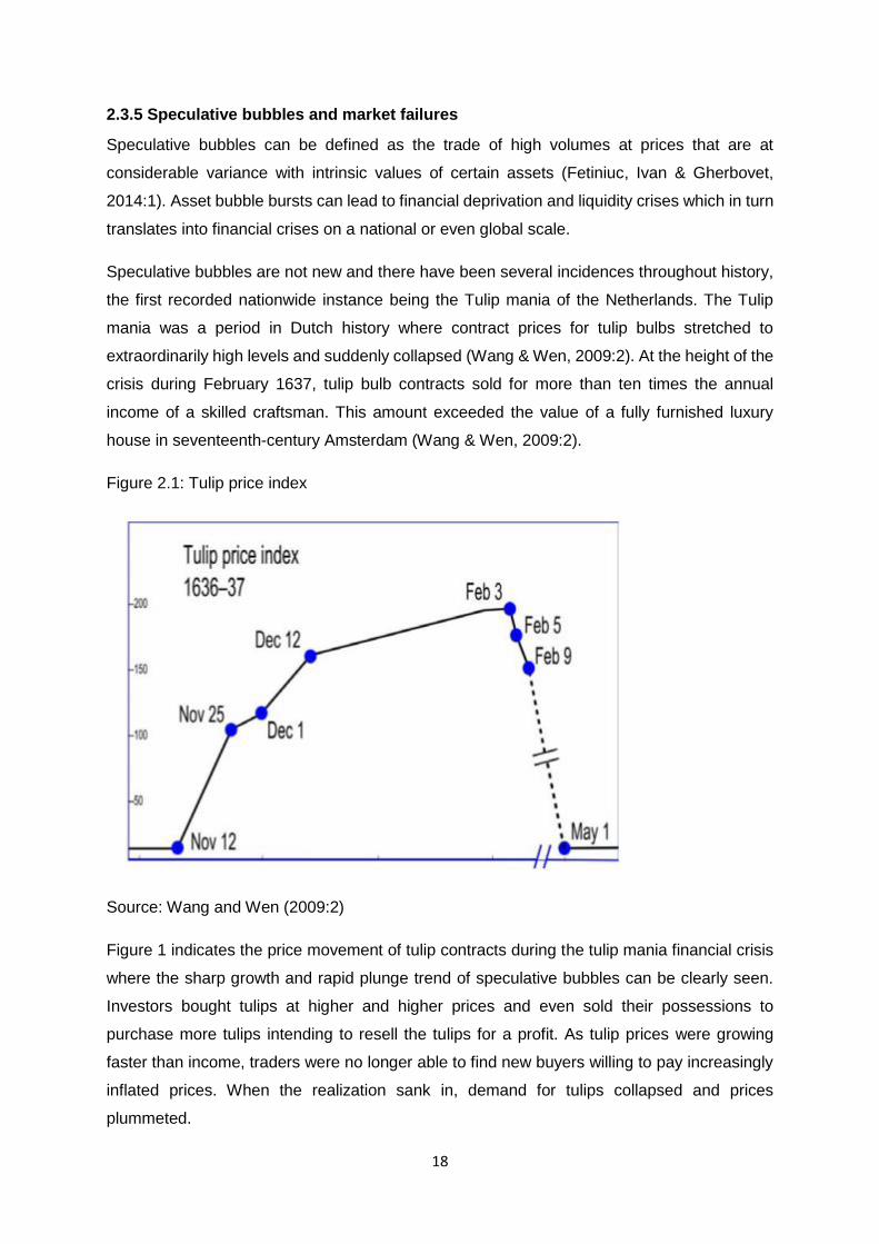
Figure 2.1: Tulip price index
Source: Wang and Wen (2009:2)
Figure 1 indicates the price movement of tulip contracts during the tulip mania financial crisis
where the sharp growth and rapid plunge trend of speculative bubbles can be clearly seen.
Investors bought tulips at higher and higher prices and even sold their possessions to
purchase more tulips intending to resell the tulips for a profit. As tulip prices were growing
faster than income, traders were no longer able to find new buyers willing to pay increasingly
inflated prices. When the realization sank in, demand for tulips collapsed and prices
plummeted.
19
The eventual crash after the asset bubble can destroy a large amount of wealth for both
consumers and institutions, which in turn leads to financial panic transitioning into a fully-
fledged financial crisis usually causing continuing economic disruption.
2.4 Indicators of financial crises
The prospect of being able to be warned of an oncoming financial crisis long before the crisis
actually happens, or even to avoid a financial crisis as a whole gives purpose to early warning
indicators. Indicators of financial crises, early warning indicators or vulnerability indicators
however you want to name them, are the focus of this study. These indicators serve as a
means to signal warning signs well before vulnerabilities have grown too large for
policymakers to control. As previously mentioned, the different types of financial crises often
go hand in hand, where the one crisis usually leads to the next. Several economists and writers
have quantifiably demonstrated that a number of indicators pose a relative degree of
correlation to the incidence of a financial crisis. Kaminsky et al. (1998:36) for one, set out to
do a detailed study regarding indicators of a crisis and concluded that most crises have
multiple indicators. From this study, a list of indicators said to be associated with financial
crises was produced and these include: M2 multiplier, ratio of domestic credit to nominal GDP,
real interest rate on deposits and the ratio of lending to deposit interest rates. Additional
indicators include the excess of real M1 balances, real commercial bank deposits as well as
the ratio of M2 or foreign exchange reserves. In this particular study, the indicators that
suggested the likelihood of a financial crisis in order of correlation are a) real interest rates, b)
real interest rate differential, c) terms of trade, d) reserves, e) outputs, f) exports as well as g)
stock prices.
Reinhart and Rogoff (2010:12) conducted a similar study with more modern views regarding
early warning indicators for both currency and banking crises and concluded that real
exchange rates, real housing prices, short term foreign direct investment, the current account
balance and real stock prices are the most effective indicators to signal an oncoming banking
crisis, whereas the worst indicators were found to be ratings, along with terms of trade. For
currency crises, the most effective indicators were identified to be real exchange rates,
banking crisis, current account balance, exports and international reserves (M2). Whereas the
least effective currency crisis indicators were found to be ratings, as well as domestic-foreign
interest differential.
Another early warning indicator model was created by Lestano, Jacobs & Kuper, (2003:1)
which distinguishes between three types of financial crises; currency crises, banking crises
and debt crises. Furthermore, this model extracts four groups of early warning indicators that
20
are likely to influence the probability of financial crises. The four groups are external indicators,
financial indicators, domestic indicators (real as well as public) and global indicators. A broad
set of potentially relevant indicators was extracted from existing crisis literature which was
then combined with the use of multi-factor analysis. The first two factors were identified as
current account variables and variables associated with the capital account as external early
warning indicators, whereas the third and fourth factors were financial variables and domestic
indicators respectively. Financial variables correlate with flows (such as values and rate of
growth) whereas the domestic indicators correlate with price. The global factor (fifth factor)
captures variations in the Fed’s interest rates and OECD output growth. More specifically, the
study identified the growth of money (both M1 and M2), bank deposits, GDP per capita, as
well as the flow and level of national savings are all indicators that correlate with all three
different types of financial crises listed in this study, whereas the ratio of M2 to foreign reserves
along with the growth of foreign reserves, the domestic real interest rate and inflation correlate
with banking crises and some instances of currency crises.
As early warning literature clearly depicts, it is crucial for the optimal timing of macroprudential
measures aimed at reducing the level of exposure inculcated by a financial crisis or at the very
least mitigating the impact of such a crisis on the economy. This can be accomplished by
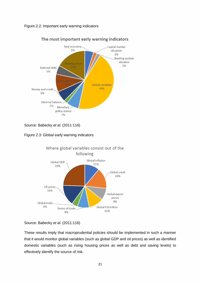
monitoring a suitable set of early warning indicators (Babecky et al., 2011:1). Babecky et al.
(2011:2) set out to identify early warning indicators that should be monitored with emphasis
on robust indicators that are not dependent on the choice of crisis prediction models.
Therefore, two mutually complementary crisis measures were combined; 1) The timing of the
crisis event and the intensity of the impact of the crisis on the economy. The two-model system
was created and applied to pre-crisis and crisis events for 40 advanced European Union and
OECD countries. The model identified rising house prices and external debt as the best
performing early warning indicators. The pie charts below indicate more specific results from
the two-factor model.
21
Figure 2.2: Important early warning indicators
Source: Babecky et al. (2011:116)
Figure 2.3: Global early warning indicators
Source: Babecky et al. (2011:116)
These results imply that macroprudential policies should be implemented in such a manner
that it would monitor global variables (such as global GDP and oil prices) as well as identified
domestic variables (such as rising housing prices as well as debt and saving levels) to
effectively identify the source of risk.
22
Vasicek et al. (2014:1) stated that researchers in academia, economists, as well as central
banks have developed several early warning systems with a single goal: to warn policymakers
and all relevant parties of potential oncoming financial crises. These early warning models are
based on different approaches and empirical models, so Vasicek et al. (2014) set out to
compare nine different models proposed by the Macroprudential Research Network (MaRs).
To ensure comparability, a single database of crises was created by MaRs to be used by all
the distinct models. The study found that multivariate models (in their many guises), have
great potential of identifying early warning indicators to signal oncoming crises over simple
signalling models.
Existing literature on early warning indicators does not offer a consensus on the process of
defining a crisis for the specific purpose of early warning models. It is thus most suitable to
make use of a multi-factor analysis model so that the choice of early warning indicators is as
robust as possible. Literature on early warning indicators of financial crises has thus far mainly
relied on one of two approaches, to be more specific; either the signalling approach or
categorical dependent variable regression (Vasicek et al., 2014:22). A great advantage of the
signalling approach is that the approach is user-friendly as an early warning signal is issued
when the relevant indicator breaches a pre-specified threshold with the help of historical data.
The main drawback of the signalling approach is that it mainly considers early warning
indicators in isolation whereas logit/probit regressions offer a multivariate framework where
the relative importance of several indicators in conjunction with one another can be assessed.
However, the logit/probit models offer an estimate of the contribution of each indicator to the
increase in the overall probability of a crisis, rather than a threshold value for each factor as is
the case with signalling models. The early warning threshold is then set in a second step with
referral to the estimated probability of a crisis realising. Another challenge regarding
logit/probit models is the fact that this type of framework is unable to process unbalanced
panels, as well as missing data, effectively. Despite these shortcomings Vasicek et al.
(2014:22) state that multivariate approaches, in their various forms, have significant potential
in generating meaningful crisis predictions as they offer considerable advantages regarding
prediction power over univariate signalling models. When opting to apply these results to
macro-prudential policy and taking the strengths and weaknesses of the various approaches
into account, multivariate models could be a superior approach in developing empirical macro-
prudential policy instruments.
The non-structural, MIMIC (Multiple-Indicator Multiple Cause) model from Rose and Spiegel
(2009:2) was applied to a cross-sectional dataset consisting of 107 countries. What makes
this model unique is the fact that the MIMIC specification clearly recognizes that the severity
of a financial crisis is an unceasing, rather than a distinct phenomenon, and of such a nature
23
that it can only be observed with error. This model also captures the severity of a financial
crisis as an unobserved variable, detected imperfectly in terms of information displayed by the
global financial crisis of 2008, where equity markets collapsed, exchange rates drastically
depreciated, declines in the perception of countries’ creditworthiness and recessionary
growth. The MIMIC model links early warning indicators of financial crises to the possible
causes of the crisis, allowing observers to attain estimates of the severity of each country’s
crisis experience along with estimates of the effect of probable drivers of the crisis. The broad
spectrum of possible vulnerability indicators examined by Rose and Spiegel (2009:28) covers
an extensive set of fundamentals including financial conditions, the regulatory framework and
the macroeconomic, institutional and geographic features of a country. Despite this evidence
indicated that nearly none of the suggested indicators seem to be statistically significant
factors of crisis severity in the sense that these indicators do not include the occurrence of the
crisis across countries. Despite being able to model the incidence of the crisis on a relatively
successful basis, the model has not been able to link the severity of the crisis across countries
to its causes. The potential flaw of the study was identified as possibly having poor measures
of the fundamental determinants of the crisis. Other possible explanations for the weakness
of results include a possibly problematic situation with the approach regarding modelling the
cross-country incidence of the crisis due to national characteristics. This is not suitable if the
fundamental causes of the specific crisis at hand are of international nature, for example
because the crisis spreads contagiously or if it is the aftermath of a common shock. Results
from the study imply that even though the crisis may have been transmitted through various
channels, its incidence seems unrelated to national fundamentals.
Global risk indicators consistently outperform domestic risk indicators with regard to
usefulness, emphasizing the importance of taking international development into account
when assessing a country’s vulnerabilities (Hermansen & Rhön, 2015:3). More specifically
measures of the global credit to GDP ratio, a global equity price gap and a global house price
gap perform exceptionally well both in sample as well as out of sample. This emphasises the
importance of taking international developments into account when analysing a country’s
vulnerabilities. Due to the increasing integration of the world’s financial markets, exposures
that escalate to a global level have the potential to transmit to countries around the world.
However, the successful performance of the global indicators is subject to a degree of caution
as the indicators do not differ across countries - they are particularly suited to identify
recessions that affect a large number of countries instantaneously, such as the global financial
crisis of 2008. The success of these indicators can therefore be partially attributed to the fact
that the global financial crisis encompasses a large share of all severe recessions in the
sample and reinforces the choice of the global financial crisis as a test of the out of sample

24
performance. The majority of the vulnerability indicators proposed by Hermansen and Rhön,
(2015) appear to be useful early warning indicators in the event of severe recessions when
policymakers are focused on avoiding severe recessions at all cost. The study shows that the
majority indicators issue the first warning signals on average more than 6 quarters in advance
of the onset of a severe recession, providing policymakers with a sufficient lead to react to
such abnormalities. The extent of signalling power does, however, vary across indicators and
the results are sensitive to the exact specification of policymakers’ preferences between
missing crises and false alarms.
Another study worth mentioning is that of Cesaroni (2013). This study used the economic crisis
classification with the hope to find a set of early warning indicators for each of the four crises
types that would allow for the potential prediction of the occurrence of a crisis event.
General structure of an early warning model as proposed by Cesaroni (2013:9)
t (index of crisis) = f (early warning indicators) t-i
where the crisis index = f (monetary policy stance, fiscal stance, interest rates, housing prices
etc.)
The study also provides an evaluation criterion for early warning indicators:
• The timing of the crisis with respect to the crisis index (these indicators are expected
to have leading properties).
• Frequency of which the specific early warning indicator makes an appearance.
• Timeliness of indicators.
• Reliability of indicators.
Cesaroni (2013:13) proceeded by creating main groups of indicators that consist of:
• Banking system condition/situation
• Capital market condition/situation
• Fiscal stance
• External balance
• Debt and savings
• Interest rates
25
• Money and credit supply
• Housing prices
• Real economy
• Global variables
As previously mentioned, the modern global economy is highly integrated and a disturbance
in one factor or variable will most likely lead to a disturbance in several other areas as well.
Due to this high degree of integration this study puts its main focus on measures for co-
movements.
A variable is said to be pro-cyclical or countercyclical depending on the correlation displayed
by the variable to economic activity, where a variable is pro-cyclical in the event where positive
significant correlation is displayed with economic activity and vice versa.
Cesaroni (2013:48) concluded by stating that indicators are in fact useful for predicting crises,
yet indicators do not provide the underlying reasons for financial crises. Crises tend to happen
with the convergence of multiple global as well as domestic factors, which usually overwhelms
the economy.
The following vulnerability indicators were identified as viable early warning indicators:
• Debt maturity profiles, interest rate sensitivity repayment schedules as well as currency
composition are indicators of global and domestic debt.
• External debt to exports and to GDP ratios are suitable indicators of tendencies in debt
and repayment capacity.
• Financial soundness indicators are important to assess the capital adequacy of
financial institutions within a country as well as the quality of assets, off-balance sheet
positions, profitability and liquidity as well as the quality and tempo of credit growth.
• Reserves adequacy indicators are viable early warning indicators, in particular the ratio
of reserves to short term debt is central to assessing the susceptibility of counties with
significant but uncertain access to capital markets.
• Corporate sector indicators are also useful with respect to foreign exchange and
interest rate exposure of domestic companies. These indicators allow for the
evaluation of the potential impact of exchange rate as well as interest rate movements
on the corporate sector’s balance sheets.

26
Drehmann and Juselius (2013:1) published a notable study on early warning indicators that
specifically focuses on banking crises with respect to policy costs and implications. Early
warning indicators are a central concept to the employment of time-varying macro-prudential
policies such as countercyclical capital buffers, that can be helpful by reducing the high losses
linked to banking crises. Deriving optimal empirical models for forecasting purposes requires
a comprehensive knowledge regarding the underlying decision problem or challenge. Yet such
detailed knowledge is at present not available in the context of macro-prudential policies as
there exists limited experience from which the expected costs and benefits could be derived.
However, one can still include the qualitative aspects of the policy-maker’s decision problem
into the estimation as well as evaluation measures for early warning indicators. The principal
approach for this study was to lay down such a method and to apply it to a wide range of early
warning indicators.
The most notable conclusions drawn from this study by Drehmann and Juselius (2013)
include: The valuations of early warning indicators specifically focused on banking crises,
should be based on the underlying decision problem of the policy maker as several features
of this problem have consequences for the choice of statistical evaluation procedures. For
example, vagueness around the costs and benefits of policy changes suggest that
assessments need to be robust over a wide range of the policymaker’s preferences. Early
warning indicator’s signals should be timely and the quality of these signals should not weaken
in the build-up to a crisis. These criteria were built into the statistical evaluation procedure for
early warning indicators used in the study.
The above-mentioned approach was applied to several early warning indicators and outcomes
and suggested that the credit-to-GDP gap, debt service ratios (DSR) and non-core liability
ratios all comply with the standard set by the statistical evaluation procedure. However, the
credit-to-GDP gap and debt service ratio consistently outperform the non-core liability ratio
and the credit-to-GDP gap dominates the longer time horizons and the debt service ratio the
shorter time horizons. The results obtained are robust in regard to changes in sample size and
crisis specification.
A unique feature of this assessment is that greater attention is paid to the progressive
dimension of early warning indicator signals. Results obtained from the study suggest that the
signalling power of the various early warning signals can fluctuate sharply over a period of
time. Therefore, greater consideration should be put into continuously well performing early
warning indicators within the policy-relevant forecasting period.
Additional significant early warning literature reinforcing the statement that early warning
indicators can indeed predict possible future crises was produced by Frankel and Saravelos
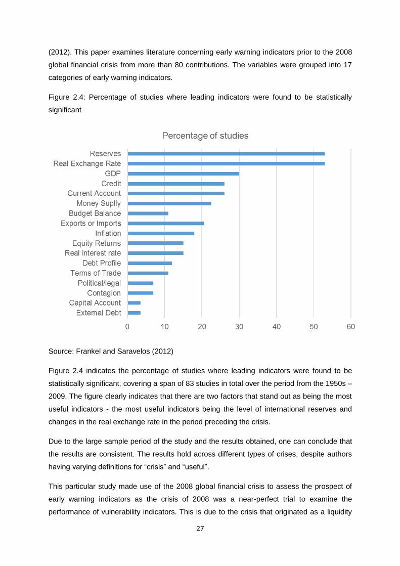
27
(2012). This paper examines literature concerning early warning indicators prior to the 2008
global financial crisis from more than 80 contributions. The variables were grouped into 17
categories of early warning indicators.
Figure 2.4: Percentage of studies where leading indicators were found to be statistically
significant
Source: Frankel and Saravelos (2012)
Figure 2.4 indicates the percentage of studies where leading indicators were found to be
statistically significant, covering a span of 83 studies in total over the period from the 1950s –
2009. The figure clearly indicates that there are two factors that stand out as being the most
useful indicators - the most useful indicators being the level of international reserves and
changes in the real exchange rate in the period preceding the crisis.
Due to the large sample period of the study and the results obtained, one can conclude that
the results are consistent. The results hold across different types of crises, despite authors
having varying definitions for “crisis” and “useful”.
This particular study made use of the 2008 global financial crisis to assess the prospect of
early warning indicators as the crisis of 2008 was a near-perfect trial to examine the
performance of vulnerability indicators. This is due to the crisis that originated as a liquidity
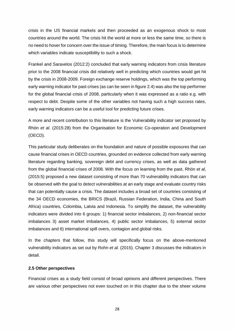
28
crisis in the US financial markets and then proceeded as an exogenous shock to most
countries around the world. The crisis hit the world at more or less the same time, so there is
no need to hover for concern over the issue of timing. Therefore, the main focus is to determine
which variables indicate susceptibility to such a shock.
Frankel and Saravelos (2012:2) concluded that early warning indicators from crisis literature
prior to the 2008 financial crisis did relatively well in predicting which countries would get hit
by the crisis in 2008-2009. Foreign exchange reserve holdings, which was the top performing
early warning indicator for past crises (as can be seen in figure 2.4) was also the top performer
for the global financial crisis of 2008, particularly when it was expressed as a ratio e.g. with
respect to debt. Despite some of the other variables not having such a high success rates,
early warning indicators can be a useful tool for predicting future crises.
A more and recent contribution to this literature is the Vulnerability indicator set proposed by
Rhön et al. (2015:28) from the Organisation for Economic Co-operation and Development
(OECD).
This particular study deliberates on the foundation and nature of possible exposures that can
cause financial crises in OECD countries, grounded on evidence collected from early warning
literature regarding banking, sovereign debt and currency crises, as well as data gathered
from the global financial crises of 2008. With the focus on learning from the past, Rhön et al,
(2015:5) proposed a new dataset consisting of more than 70 vulnerability indicators that can
be observed with the goal to detect vulnerabilities at an early stage and evaluate country risks
that can potentially cause a crisis. The dataset includes a broad set of countries consisting of
the 34 OECD economies, the BRICS (Brazil, Russian Federation, India, China and South
Africa) countries, Colombia, Latvia and Indonesia. To simplify the dataset, the vulnerability
indicators were divided into 6 groups: 1) financial sector imbalances, 2) non-financial sector
imbalances 3) asset market imbalances, 4) public sector imbalances, 5) external sector
imbalances and 6) international spill overs, contagion and global risks.
In the chapters that follow, this study will specifically focus on the above-mentioned
vulnerability indicators as set out by Rohn et al. (2015). Chapter 3 discusses the indicators in
detail.
2.5 Other perspectives
Financial crises as a study field consist of broad opinions and different perspectives. There
are various other perspectives not even touched on in this chapter due to the sheer volume
29
and extent of these studies, it is not possible to take all other opinions and perspectives into
account. A good example of these studies includes a 2013 article of Shin.
Shin (2013:3) set out to find a group of early warning indicators that would be able to identify
the vulnerabilities to financial turmoil that emerged from the outcome of the global financial
crisis of 2008. To achieve this goal Shin (2013:3) looked at historical literature and found that
there is extensive literature on early warning indicators for a crisis that is well defined by
Chamon and Crowe (2012:500). The existing literature at the time could be described as being
“eclectic” as well as “pragmatic”. Eclectic in the sense that the analysis enjoyed attention from
a range of inputs that includes external, financial, real, institutional as well as political factors
along with several measures of contagion. A problem with previous studies is such as one
conducted by Kaminsky et al. (1998:22) where a catalogue of 105 variables was recorded in
their overview of early warning literature at the time (1998). This was however, pragmatic in
the sense that researchers put their focus their attention on improving measures of goodness
of fit, rather than putting their focus on the underlying theoretical themes that could provide
possible links between different crisis episodes (Shin, 2013:4).
For example, it has been the conventional method to differentiate between emerging economy
crises and advanced economy crises by means of using different sets of variables for each
category. Emerging economy studies tend to focus mainly on capital flow reversals linked to
sudden stops, for which specific variables such as external borrowing denominated in foreign
currency is most important, while for advanced economy studies, variables such as housing
booms and household leverage take centre stage. The International Monetary Fund (IMF) also
distinguishes between advanced and emerging economies. The IMF created separate
vulnerability indicator sets for advanced and emerging economies. The Vulnerability Exercise
for Advanced Economies (VEA) and Vulnerability Exercise for Emerging Economies (VEE),
these two exercises can be combined to form a joint early warning exercise with the Financial
Stability Board (FSB) (Shin, 2013:4).
While the compartmentalisation of emerging and advanced economies aids in improving
measures regarding the goodness of fit, common linkages tends to be obscured (Milesi-
Ferretti & Razin (1998). These linkages tie together emerging and advanced economy crises.
For instance, the capital flow reversals in Spain and Ireland at the time of the European crisis
indicated, similar to that of a sudden stop, except that the outflow of private sector funds was
compensated for by the inflow of official funds. Although, since the Eurozone crisis took place
within a monetary union (common currency area), the traditional classification of emerging
market “currency crisis” where currency movements play an important role, do not necessarily
fit in the empirical exercise. Given the common linkages that bind together apparent differing
30
crises, it can be beneficial to take a step back from the practical imperatives of maximising
goodness of fit in exchange for considering the theoretical underpinnings of early warning
models (Shin, 2013:4). The study suggests that the pro-cyclicality of the financial system offers
an organising framework for the selection of indicators of vulnerability to crises, especially
those that are associated with banks and financial intermediaries more often.
More specifically, the study focuses on assessing three extensive sets of vulnerability
indicators as a means of early warning systems, and continues by determining their respective
likelihood of success. These three indicators along with their results are:
1) Indicators based on market prices, such as Credit Default Swap (CDS) spreads,
implied volatility and other price-based measures of default.
A notable fact implied by the study is how calm the CDS measure was before the global
financial crisis of 2008. There was barely any movement in the data series for the period 2004
– 2006 when vulnerability indicators were supposed to start signalling. Other price-based
measures such as Value-at-Risk (VaR), implied volatility and structural models of default
based on equity price all gave similar results.
The disappointment of price-based measures as early warning indicators can be attributed to
their implicit principle that the collaboration between market signals and the decisions led by
these signals are always related in the sense that they stabilize the virtuous circle, rather than
occasionally going awry and acting in concert in an amplifying malicious circle where market
signals and decisions guided by these signals reinforce an existing tendency in the direction
of pro-cyclicality.
2) Gap measures of the credit to GDP ratio.
Granting that credit booms are clear in hindsight, there are quite a lot of challenges to using
the deviation of the credit to GDP ratio from trend as an early warning indicator in real time.
One challenge is estimating the trend that serves as a measure for excessive growth. Ex-post
revisions to the credit-to-GDP ratio gap in real time are considerable for the US and as large
as the gap itself. However, the source of ex-post revisions is not the revision of the underlying
data, but rather from the revision of the estimated trend that is measured in real time Shin
(2013).
Another challenge is the fact that credit growth and GDP are affected and influenced by
different factors throughout the cycle and this causes the ratios to occasionally issue
misleading signals Shin (2013). For instance, bank lending may be influenced by pre-existing
31
contractual commitments, such as lines of credit, which contracts during periods of crisis.
Lending may initially proceed for some time after the onset of the crisis.
Despite these challenges, the credit-to-GDP ratio, under the Basel III framework takes a
principal role as the basis for the countercyclical capital buffer. This ratio has been found useful
as an indicator of the current stage of the financial cycle.
3) Banking sector liability aggregates, including monetary aggregates.
When credit is being extended faster than the available resources that are normally drawn on
by the bank (core liabilities), the bank will turn to other sources of funding to support the credit
expansion. The ratio of non-core to core liabilities therefore serves as a signal of the degree
of risk-taking that is undertaken by the bank and additionally the stage of the financial cycle.
Shin (2013:11) concluded that prices perform well as concurrent indicators of market
conditions, although they are not viable early warning indicators due to the fact that they have
no prediction value. Whereas total credit and liabilities suggest similar results, despite
performing better as early warning indicators, liabilities are more transparent and the
disintegration between core and non-core liabilities conveys significant information.
2.6 Summary of conclusions
One possible explanation for varying conclusions regarding early warning systems can be
ascribed to differences in the selected data periods, for example, most of the papers that
concluded negative results for early warning indicators predicting the global financial crisis of
2008, defined the crisis period as the year 2008. These studies lacked data on 2009 at the
time they were conducted. Frankel and Saravelos (2012:4) made use of an extended period
for consideration for an early crisis study, ranging through early 2009 as many facets of global
financial markets and the real economy had at the time not yet started to recover until the
second quarter of 2009. The results obtained therefore differ from some other studies possibly
due to varying periods under consideration. This statement was reinforced by Frankel and
Saravelos (2012:4) when their tests were rerun with the crisis period being 2008 such as that
of Rose and Spiegel (2009:1). The new results suggested similar outcomes to that of Rose
and Spiegel (2009:22); many indicators, such as reserves lose their significance.
Chamon and Crowe (2012:3) concluded that: 1) it is fairly clear which indicators tend to be
associated with crises, and 2) to predict the timing of crises is challenging. For example, not
many people would argue that an overvalued exchange rate peg is an important source of
vulnerability (however, determining the extent of the overvaluation can be problematic), also
than a large current account deficit that is financed through debt inflows is risky. The fact that
32
countries can be exposed to high levels of risk for extended periods without experiencing a
crisis makes the prediction of the timing of a crisis particularly difficult. The delay before the
onset of a crisis can possibly be ascribed to the time it takes for vulnerabilities to accumulate
to a “breaking point” when they become unsustainable (for example, to run a series of current
account deficits to such an extreme point that foreigners become unwilling to finance the
deficits). However, some aspects of timing may be driven by exogenous triggers, such as
foreign financed lending booms and foreign currency loans to households.
Therefore, predicting the timing of crises is most likely to remain an unsatisfactory exercise.
Alternatively, it seems to be more viable to use these types of early warning indicators to aid
in the identification of underlying vulnerabilities. It is important to distinguish between
underlying vulnerabilities and crisis risks due to underlying vulnerabilities being present but
not necessary for a crisis to occur. For example, underlying balance sheet vulnerabilities such
as extreme borrowing and currency or maturity mismatches can be present for extensive
periods without the occurrence of a crisis. Although, if this underlying vulnerability is combined
with an appropriate crisis trigger, such as interest rate hikes by major economies or an asset
reversal in financial markets, they can possibly lead to a crisis.
The focus of this study is to find parsimonious indicators of crisis through a data-reduction
exercise. The next chapter presents the indicators and dataset proposed by Rhön et al. (2015)
that will be used in the empirical analysis.
33
CHAPTER 3: EARLY WARNING INDICATORS
3.1 Introduction
Financial crises have several characteristics and cannot be attributed to a single event, but
rather to the collective state of an economy or the global economy. Within the global economy
there are wide-ranging factors at play, some of which can be useful as early warning indictors.
To enhance the effectiveness of such indicators, they should be considered as a
comprehensive collection of variables that result in certain outcomes rather than be regarded
in isolation (Rohn et al., 2015:5). As the economic environment changes, many of these
variables interact and, in some instances, even reinforce one another. Alternatively, the
collapse of one variable can prompt other variables to follow. Hence, if policymakers address
the shortcomings of one variable, they will most likely reduce the shortcomings of several
variables across a range of sectors within the economy. Similarly, if a single variable unwinds,
it can trigger the downfall of other variables as well.
Rohn et al. (2015) present the following diagram grouping different indicators of
vulnerabilities4.
4 Note that this thesis draws heavily from Rohn, et al, (2015) as this study is an extension of the aforementioned study making use of the same dataset applied to the global financial crisis of 2008 as well as the proposed imbalance categories (Dataset available at https://www.google.com/url?q=http://www.oecd.org/eco/growth/Vulnerability_Indicators-15-02-21017.xlsx&sa=U&ved=0ahUKEwjuu6aBzoHgAhUPuRoKHa3dBiIQFggKMAI&client=internal-uds-cse&cx=012432601748511391518:xzeadub0b0a&usg=AOvVaw0Z6Q0h68b-0bsRcYHt3wKM).
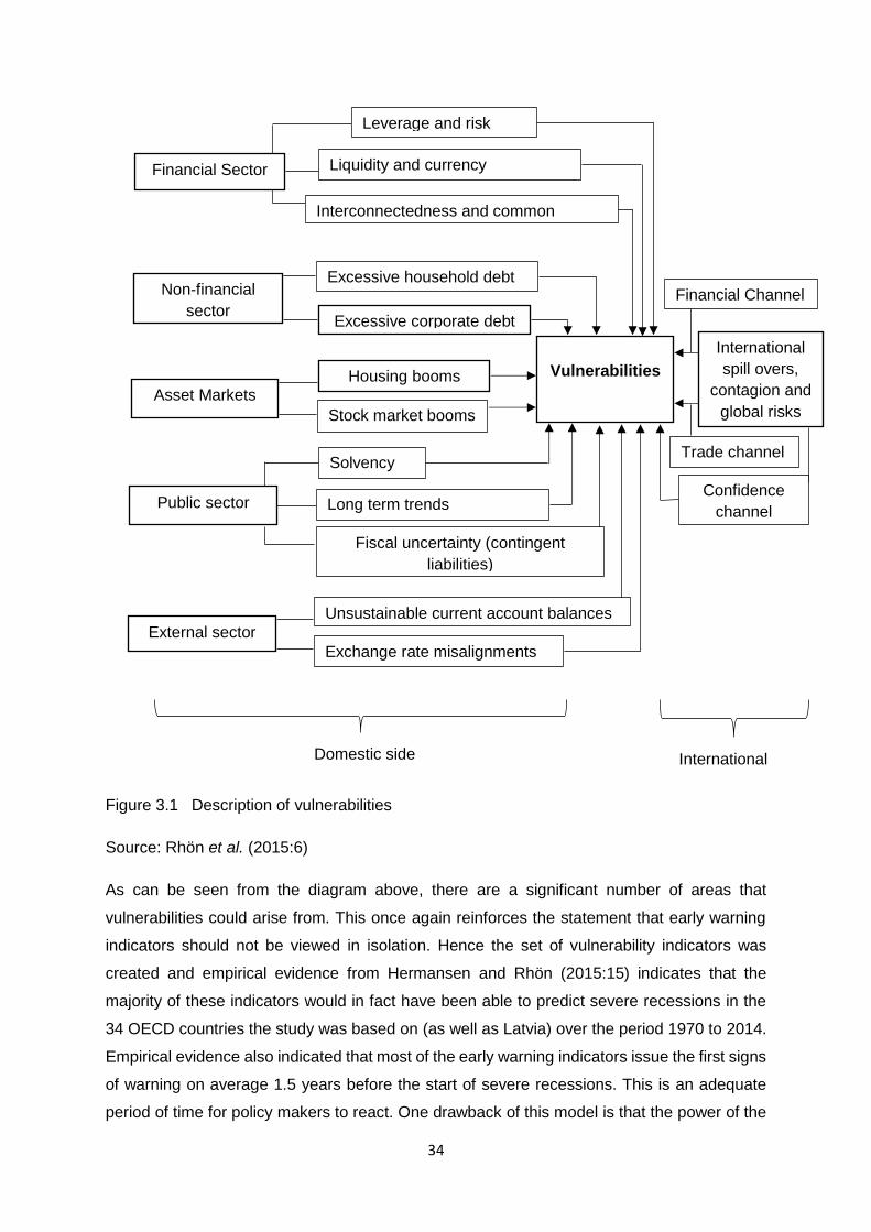
34
Figure 3.1 Description of vulnerabilities
Source: Rhön et al. (2015:6)
As can be seen from the diagram above, there are a significant number of areas that
vulnerabilities could arise from. This once again reinforces the statement that early warning
indicators should not be viewed in isolation. Hence the set of vulnerability indicators was
created and empirical evidence from Hermansen and Rhön (2015:15) indicates that the
majority of these indicators would in fact have been able to predict severe recessions in the
34 OECD countries the study was based on (as well as Latvia) over the period 1970 to 2014.
Empirical evidence also indicated that most of the early warning indicators issue the first signs
of warning on average 1.5 years before the start of severe recessions. This is an adequate
period of time for policy makers to react. One drawback of this model is that the power of the
Financial Sector
Non-financial
sector
Asset Markets
Public sector
External sector
International
spill overs,
contagion and
global risks
Vulnerabilities
Leverage and risk
taking
Liquidity and currency
mismatches
Interconnectedness and common
Excessive household debt
Excessive corporate debt
Housing booms
Stock market booms
Solvency
risk
Long term trends
((e.gtretrends(e.g.))ageing Fiscal uncertainty (contingent
liabilities)
Unsustainable current account balances
Exchange rate misalignments
Trade channel
Financial Channel
Confidence
channel
Domestic side International
35
signals differs from indicator to indicator and the results are sensitive to the precise
specification of policy maker’s preferences amongst false alarms and missing crises.
Indicators that tend to interact in a similar way were grouped together to simplify the sheer
number of possible explanatory early warning indicators. The discussion in this chapter makes
use of the categories proposed by Rohn et al. (2015:1). In chapter 4, all the indicators will be
used in a dynamic factor model in an attempt to identify parsimonious indicators of crises.
3.2 Financial sector imbalances
The failure of regulation in the financial sector along with the short-sightedness/greed of the
private sector could be attributed as some of the root causes of the global financial crisis of
2008 (Bank for International Settlements, 2012:1). The emphasis had shifted from securing a
sustainable financial sector which favours the people, to a self-centred short-term yield driven
system which does not serve the broader goals of sustainable macroeconomic policy.
In theory, the connection between financial markets and output volatility is vague (Rohn et al.,
2015:7). Well-established financial markets can fortify role-players in an economy against
idiosyncratic shocks through reductions in borrowing constraints allowing economic
stimulation by means of consumption and investment. Countries with advanced financial
markets could additionally reinforce monetary policy transmission to boost the effectiveness
of monetary policy in absorbing these idiosyncratic shocks. However, simultaneously, financial
markets could possibly intensify the output volatility caused by financial accelerator
mechanisms. Asymmetric information between borrowers and lenders indicates that lenders
pay attention to the financial capacity of borrowers, with the emphasis on the net worth of the
borrower. In the boom phase of an economy, the net worth of both consumers and investors
normally increases, which in turn lowers the agency costs, as the borrower’s collateral has
increased in value. This leads to an upsurge in the supply of credit, resulting in stimulation for
investment and consumption levels acting as the driving force of the boom cycle. As a result
of the higher levels of economic stimulation, asset prices will most likely keep on rising which
will see the borrowers’ financial position improving even more, further reducing borrowing
constraints. During economic crises, this process is reversed as the effects of a negative shock
turn into a “snowball”, the effects amplifying one another.
To summarize, the majority of empirical literature indicates that more established financial
markets tend to have reduced levels of consumption, output as well as investment rates during
times of low economic activity (i.e. times of crisis) (Duval, Elmeskov & Vogel, 2007:41).
However, these findings rest upon the conditions that economic crises do not arise in the
financial sector and that financial dealings continue in a functional way. The financial sector
36
is. however, more often than not the focal point of economic crises. The global economic crisis
of 2008 once again reinforced this statement.
A major challenge policymakers face in times of financial crises is the fact that monetary
policies are less effective during periods of impairment in the financial sector as households
and firms have to absorb shocks and do not necessarily have the capacity to do so effectively.
Financial accelerator mechanisms worsen this case as it creates a snowball effect through the
amplification and transmission of economic shocks throughout an economy. A shock to a fairly
small sub-market of the financial sector such as defaults in the sub-prime mortgage market
can result in a financial crisis through amplification (snowball effect). An amplifying effect such
as this is related to the build-up of several vulnerabilities within the financial sector. Rohn et
al. (2015:7) describe the most import vulnerabilities to be excessively large maturity
mismatches, interconnectedness and common exposure.
3.2.1 Leverage and risk taking
Excessive leverage and risk taking are frequent features to be observed in the financial sector
as role players within the financial sector are driven to maximise profits. This strong drive to
accumulate as much profit as possible often causes role players in the financial sector to
neglect building up sufficient buffer capital (acting as a risk cushion) during boom cycles in the
economy. High levels of leverage within a financial sector amplify the effects of a shock,
therefore indicators of leverage are useful as early warning indicators of banking crises
(Barrell, Davis, Karim & Liazde, 2010:10). Leverage indicators can be used in conjunction with
capital ratios as they account for the risk profile of assets. However, capital ratios were found
to be less effective in limiting banks credit risk (Blundell-Wignall, Atkinson & Roulet, 2014:19).
To use these indicators in isolation however, would most likely give an inaccurate view of
leverage and risk taking within the financial sector as data on capital ratios and leverage are
not widely available.
Rohn et al. (2015:8) made the observation that leverage increased significantly within the
shadow banking system during the build-up to the global financial crisis. Therefore, indicators
determining the magnitude of the shadow banking system would be useful. Periods of high
banking profitability are generally characterised by higher levels of risk taking, increasing the
probability of a banking crisis due to the nature of risks and higher levels of exposure (Behn,
Detken, Peltonen & Schudel, 2013). Excessive risk-taking by institutions considered to be
“too-big-to-fail” proved to be a significant vulnerability in the run-up to the global financial crisis.
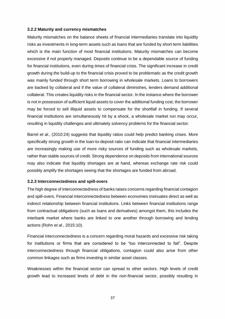
37
3.2.2 Maturity and currency mismatches
Maturity mismatches on the balance sheets of financial intermediaries translate into liquidity
risks as investments in long-term assets such as loans that are funded by short term liabilities
which is the main function of most financial institutions. Maturity mismatches can become
excessive if not properly managed. Deposits continue to be a dependable source of funding
for financial institutions, even during times of financial crisis. The significant increase in credit
growth during the build-up to the financial crisis proved to be problematic as the credit growth
was mainly funded through short term borrowing in wholesale markets. Loans to borrowers
are backed by collateral and if the value of collateral diminishes, lenders demand additional
collateral. This creates liquidity risks in the financial sector. In the instance where the borrower
is not in possession of sufficient liquid assets to cover the additional funding cost, the borrower
may be forced to sell illiquid assets to compensate for the shortfall in funding. If several
financial institutions are simultaneously hit by a shock, a wholesale market run may occur,
resulting in liquidity challenges and ultimately solvency problems for the financial sector.
Barrel et al., (2010:24) suggests that liquidity ratios could help predict banking crises. More
specifically strong growth in the loan-to-deposit ratio can indicate that financial intermediaries
are increasingly making use of more risky sources of funding such as wholesale markets,
rather than stable sources of credit. Strong dependence on deposits from international sources
may also indicate that liquidity shortages are at hand, whereas exchange rate risk could
possibly amplify the shortages seeing that the shortages are funded from abroad.
3.2.3 Interconnectedness and spill-overs
The high degree of interconnectedness of banks raises concerns regarding financial contagion
and spill-overs. Financial interconnectedness between economies insinuates direct as well as
indirect relationship between financial institutions. Links between financial institutions range
from contractual obligations (such as loans and derivatives) amongst them, this includes the
interbank market where banks are linked to one another through borrowing and lending
actions (Rohn et al., 2015:10).
Financial interconnectedness is a concern regarding moral hazards and excessive risk taking
for institutions or firms that are considered to be “too interconnected to fail”. Despite
interconnectedness through financial obligations, contagion could also arise from other
common linkages such as firms investing in similar asset classes.
Weaknesses within the financial sector can spread to other sectors. High levels of credit
growth lead to increased levels of debt in the non-financial sector, possibly resulting in
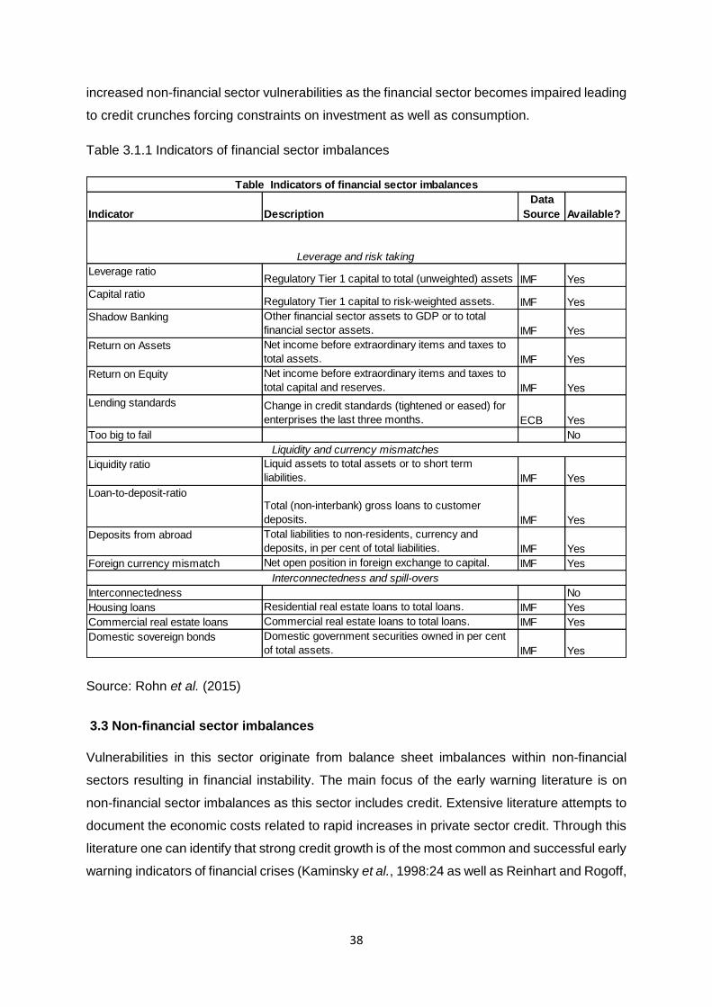
38
increased non-financial sector vulnerabilities as the financial sector becomes impaired leading
to credit crunches forcing constraints on investment as well as consumption.
Table 3.1.1 Indicators of financial sector imbalances
Source: Rohn et al. (2015)
3.3 Non-financial sector imbalances
Vulnerabilities in this sector originate from balance sheet imbalances within non-financial
sectors resulting in financial instability. The main focus of the early warning literature is on
non-financial sector imbalances as this sector includes credit. Extensive literature attempts to
document the economic costs related to rapid increases in private sector credit. Through this
literature one can identify that strong credit growth is of the most common and successful early
warning indicators of financial crises (Kaminsky et al., 1998:24 as well as Reinhart and Rogoff,
Indicator Description
Data
Source Available?
Leverage ratioRegulatory Tier 1 capital to total (unweighted) assets IMF Yes
Capital ratioRegulatory Tier 1 capital to risk-weighted assets. IMF Yes
Shadow Banking Other financial sector assets to GDP or to total
financial sector assets. IMF Yes
Return on Assets Net income before extraordinary items and taxes to
total assets. IMF Yes
Return on Equity Net income before extraordinary items and taxes to
total capital and reserves. IMF Yes
Lending standards Change in credit standards (tightened or eased) for
enterprises the last three months. ECB Yes
Too big to fail No
Liquidity ratio Liquid assets to total assets or to short term
liabilities. IMF Yes
Loan-to-deposit-ratioTotal (non-interbank) gross loans to customer
deposits. IMF Yes
Deposits from abroad Total liabilities to non-residents, currency and
deposits, in per cent of total liabilities. IMF Yes
Foreign currency mismatch Net open position in foreign exchange to capital. IMF Yes
Interconnectedness No
Housing loans Residential real estate loans to total loans. IMF Yes
Commercial real estate loans Commercial real estate loans to total loans. IMF Yes
Domestic sovereign bonds Domestic government securities owned in per cent
of total assets. IMF Yes
Table Indicators of financial sector imbalances
Leverage and risk taking
Liquidity and currency mismatches
Interconnectedness and spill-overs
39
2010:17). Credit intensive economic expansion is costlier in this sense as it tends to result in
deeper recessions and slower recoveries (Sutherland & Hoeller, 2012:29).
During the build-up of the global financial crisis of 2008 both private and household debt levels
increased considerably. This sharp increase in these levels can be attributed to financial
deregulation as well as financial innovation (Sutherland & Hoeller, 2012:23), more specifically
the emergence of mortgage market securitisation enabled huge sums of money to be
transferred to the mortgage market which included extended credit of lower income groups
(considered to be risky loans as the means of lower income groups to repay loans are
generally lower than those of medium or high-income groups).
High levels of private debt are often considered to be a useful vulnerability indicator as private
debt can influence macroeconomic stability (Rohn et al., 2015:12). High levels of private debt
can also intensify and, in some instances, even prolong economic downturns. On the other
hand, private debt can also reinforce macroeconomic stability as it facilitates consumption and
investment as the credit allows households and firms to utilise resources that would in the
absence of private debt not been possible. At excessive levels of private debt, this smoothing
ability can be hindered as consumers and firms have to service their debt despite the state of
the economy.
Non-financial sector vulnerabilities can in some instances also spread to the public and
external sectors. During times of economic crisis, governments are often forced to rescue or
“bail out” entities or stimulate areas worst affected by the crisis. This in turn affects
governments’ budgets through the deleveraging of other sectors, automatic responsive budget
reactions and counter-cyclical fiscal policy. Credit booms can also lead to the reorganisation
of resources from a tradable to non-tradable status, such as residential investment during a
housing boom. This outflow of resources may result in the weakening of the trade and current
account balance. Jorda, Schularick & Taylor, (2012:13) noted that the correlation between
significant increases in lending and current account imbalances have become more
noteworthy in recent decades.
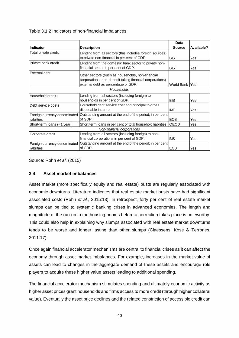
40
Table 3.1.2 Indicators of non-financial imbalances
Source: Rohn et al. (2015)
3.4 Asset market imbalances
Asset market (more specifically equity and real estate) busts are regularly associated with
economic downturns. Literature indicates that real estate market busts have had significant
associated costs (Rohn et al., 2015:13). In retrospect, forty per cent of real estate market
slumps can be tied to systemic banking crises in advanced economies. The length and
magnitude of the run-up to the housing booms before a correction takes place is noteworthy.
This could also help in explaining why slumps associated with real estate market downturns
tends to be worse and longer lasting than other slumps (Claessens, Kose & Terrones,
2011:17).
Once again financial accelerator mechanisms are central to financial crises as it can affect the
economy through asset market imbalances. For example, increases in the market value of
assets can lead to changes in the aggregate demand of these assets and encourage role
players to acquire these higher value assets leading to additional spending.
The financial accelerator mechanism stimulates spending and ultimately economic activity as
higher asset prices grant households and firms access to more credit (through higher collateral
value). Eventually the asset price declines and the related constriction of accessible credit can
Indicator Description
Data
Source Available?
Total private credit Lending from all sectors (this includes foreign sources)
to private non-financial in per cent of GDP. BIS Yes
Private bank credit Lending from the domestic bank sector to private non-
financial sector in per cent of GDP. BIS Yes
External debtOther sectors (such as households, non-financial
corporations, non-deposit taking financial corporations)
external debt as percentage of GDP. World Bank Yes
Household credit Lending from all sectors (including foreign) to
households in per cent of GDP. BIS Yes
Debt service costs Household debt service cost and principal to gross
disposable income IMF Yes
Foreign currency denominated
liabilities
Outstanding amount at the end of the period; in per cent
of GDP. ECB Yes
Short-term loans (<1 year) Short term loans in per cent of total household liabilities. OECD Yes
Corporate credit Lending from all sectors (including foreign) to non-
financial corporations in per cent of GDP. BIS Yes
Foreign currency denominated
liabilities
Outstanding amount at the end of the period; in per cent
of GDP. ECB Yes
Households
Non-financial corporations
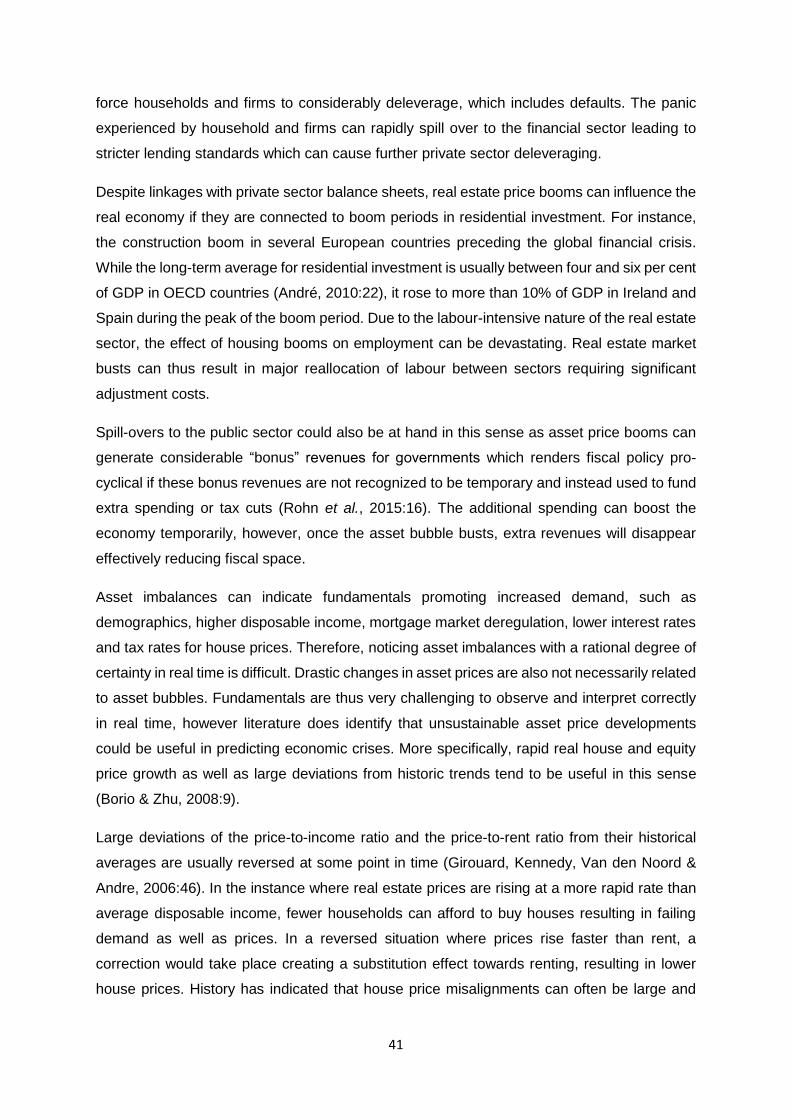
41
force households and firms to considerably deleverage, which includes defaults. The panic
experienced by household and firms can rapidly spill over to the financial sector leading to
stricter lending standards which can cause further private sector deleveraging.
Despite linkages with private sector balance sheets, real estate price booms can influence the
real economy if they are connected to boom periods in residential investment. For instance,
the construction boom in several European countries preceding the global financial crisis.
While the long-term average for residential investment is usually between four and six per cent
of GDP in OECD countries (André, 2010:22), it rose to more than 10% of GDP in Ireland and
Spain during the peak of the boom period. Due to the labour-intensive nature of the real estate
sector, the effect of housing booms on employment can be devastating. Real estate market
busts can thus result in major reallocation of labour between sectors requiring significant
adjustment costs.
Spill-overs to the public sector could also be at hand in this sense as asset price booms can
generate considerable “bonus” revenues for governments which renders fiscal policy pro-
cyclical if these bonus revenues are not recognized to be temporary and instead used to fund
extra spending or tax cuts (Rohn et al., 2015:16). The additional spending can boost the
economy temporarily, however, once the asset bubble busts, extra revenues will disappear
effectively reducing fiscal space.
Asset imbalances can indicate fundamentals promoting increased demand, such as
demographics, higher disposable income, mortgage market deregulation, lower interest rates
and tax rates for house prices. Therefore, noticing asset imbalances with a rational degree of
certainty in real time is difficult. Drastic changes in asset prices are also not necessarily related
to asset bubbles. Fundamentals are thus very challenging to observe and interpret correctly
in real time, however literature does identify that unsustainable asset price developments
could be useful in predicting economic crises. More specifically, rapid real house and equity
price growth as well as large deviations from historic trends tend to be useful in this sense
(Borio & Zhu, 2008:9).
Large deviations of the price-to-income ratio and the price-to-rent ratio from their historical
averages are usually reversed at some point in time (Girouard, Kennedy, Van den Noord &
Andre, 2006:46). In the instance where real estate prices are rising at a more rapid rate than
average disposable income, fewer households can afford to buy houses resulting in failing
demand as well as prices. In a reversed situation where prices rise faster than rent, a
correction would take place creating a substitution effect towards renting, resulting in lower
house prices. History has indicated that house price misalignments can often be large and
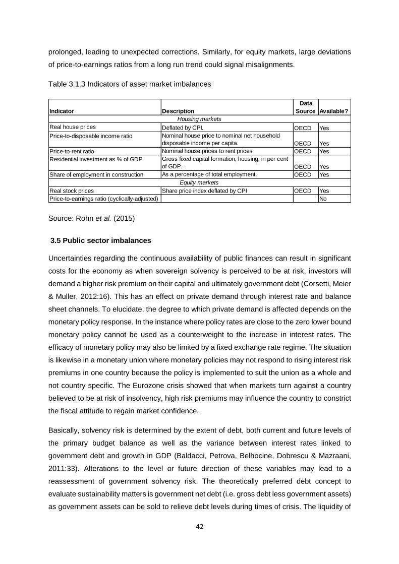
42
prolonged, leading to unexpected corrections. Similarly, for equity markets, large deviations
of price-to-earnings ratios from a long run trend could signal misalignments.
Table 3.1.3 Indicators of asset market imbalances
Source: Rohn et al. (2015)
3.5 Public sector imbalances
Uncertainties regarding the continuous availability of public finances can result in significant
costs for the economy as when sovereign solvency is perceived to be at risk, investors will
demand a higher risk premium on their capital and ultimately government debt (Corsetti, Meier
& Muller, 2012:16). This has an effect on private demand through interest rate and balance
sheet channels. To elucidate, the degree to which private demand is affected depends on the
monetary policy response. In the instance where policy rates are close to the zero lower bound
monetary policy cannot be used as a counterweight to the increase in interest rates. The
efficacy of monetary policy may also be limited by a fixed exchange rate regime. The situation
is likewise in a monetary union where monetary policies may not respond to rising interest risk
premiums in one country because the policy is implemented to suit the union as a whole and
not country specific. The Eurozone crisis showed that when markets turn against a country
believed to be at risk of insolvency, high risk premiums may influence the country to constrict
the fiscal attitude to regain market confidence.
Basically, solvency risk is determined by the extent of debt, both current and future levels of
the primary budget balance as well as the variance between interest rates linked to
government debt and growth in GDP (Baldacci, Petrova, Belhocine, Dobrescu & Mazraani,
2011:33). Alterations to the level or future direction of these variables may lead to a
reassessment of government solvency risk. The theoretically preferred debt concept to
evaluate sustainability matters is government net debt (i.e. gross debt less government assets)
as government assets can be sold to relieve debt levels during times of crisis. The liquidity of
Indicator Description
Data
Source Available?
Real house prices Deflated by CPI. OECD Yes
Price-to-disposable income ratio Nominal house price to nominal net household
disposable income per capita. OECD Yes
Price-to-rent ratio Nominal house prices to rent prices OECD Yes
Residential investment as % of GDP Gross fixed capital formation, housing, in per cent
of GDP. OECD Yes
Share of employment in construction As a percentage of total employment. OECD Yes
Real stock prices Share price index deflated by CPI OECD Yes
Price-to-earnings ratio (cyclically-adjusted) No
Housing markets
Equity markets
43
assets, however, may differ and some assets may not be eligible to sell as they kept for
specific purposes. Information regarding the liquidity of government assets are usually not
available. Additionally, methods of valuation and accounting variances across countries as
well as the lack of data regarding non-financial assets in many countries limits the
effectiveness of comparisons on government assets. Gross debt is thus often used to
determine sustainability and solvency risk.
In addition, early warning literature indicates that high levels of gross government debt to GDP
ratio is a strong indicator of currency, banking as well as sovereign debt crises (Babecky,
Havranek, Mateju, Rusnak, Smidkova & Vasicek, 2013:16) done on a sample of advanced
economies. Whereas Baldacci et al. (2011:34) claim that the difference between the
government interest rate and GDP growth is a robust predictor of fiscal stress events in
advanced economies.
Sovereign solvency risk can be identified by monitoring demographic and economic trends as
solvency does not only depend on the current fiscal position but also on some of the expected
future economic positions (Rohn et al., 2015:17), more specifically, future primary balances,
projections of long-term fiscal challenges that could have adverse effects on the current
solvency levels.
The composition of government debt could also have an impact on certain vulnerabilities. A
greater need to access the market in the short-term translates into higher risks regarding
adverse market reactions if solvency risk is high and the risk appetite does not allow for high
levels of risk taking (Rohn et al., 2015:17). High levels of short-term debt lead to a greater
exposure to roll-over and interest rate risks in the near future, even more so when market
conditions are unfavourable. The gross financing need (the sum of the total balance and the
stock of maturing public debt), the share of short-term debt compared to total debt as well as
the average maturity of outstanding government debt are all possible early warning indicators
for these risks. Baldacci et al. (2011:17) have found the gross financing need to be a profound
indicator of fiscal stress occurrences in advanced economies. Furthermore, countries with
high levels of public debt denominated in foreign currency (mostly emerging markets) are
exposed to exchange rate risk. Additionally, countries with high levels of public debt held by
non-residents are more vulnerable to turnarounds in foreign investor confidence as the
situation can be perceived as being more likely to address solvency challenges by “taxing
foreigners” through default rather than through corrective measures.
It is also possible for vulnerabilities to appear due to the uncertainty associated with the
outlook in public finances (Kopits, 2014:152). Contingent liabilities of the government are a
source of vulnerabilities that arise from uncertain outlooks in public finances. Such liabilities
44
can be both implicit or explicit, where the latter have a contractual basis and includes
government guarantees for depositors, exporters, farmers or investors in infrastructure (under
public-private partnership contracts), state-owned enterprises or subnational governments.
The opposite is true for implicit contingent liabilities, they are not based on a contractual basis
but are rather driven by expectations created by past practises or pressure from interest
groups. Implicit contingent liabilities normally include future liabilities of publicly funded
pensions to all employees or guarantees for private pensions, bailout support for important
industries that might experience distress, as well as costs related to natural disasters. Implicit
contingent liabilities that arise from within the financial sector can have devastating effects on
fiscal accounts (Rohn et al., 2015:18).
Public sector imbalances are particularly sensitive vulnerabilities as they can easily spill over
to other sectors of the economy (Rohn, et al., 2015:19). Government finances and the balance
sheet of the financial sector are intimately connected through (both implicit and explicit) public
guarantees and bank’s government bond holdings. Therefore, shocks to the public-sector
solvency risk may rapidly spill over to the financial sector. Movement in the government budget
balance will change total savings and ultimately the current account (Aizenman, Chinn & Ito,
2008:55). Literature put forth by Aizenman et al. (2008:55) suggests that a 1% of GDP change
of the fiscal balance can change the current account balance by around 0.5% of GDP.
Table 3.1.4 Indicators of public sector imbalances
Source: Rohn et al. (2015)
Indicator Description
Data
Source Available?
General government debt Gross government debt in per cent of GDP. OECD Yes
(r-g) Real 10-year sovereign bond yield potential GDP growth
rate differential. OECD Yes
Gross financing needs Public budget deficit plus short term debt by original
maturity plus long-term debt with payment due in one year
or less, in per cent of GDP.
OECD,
World Bank Yes
Short-term debt Short-term gross general government debt in per cent of
gross general government debt. World Bank Yes
Weighted average maturity of general
government debt No
Debt denominated in foreign currency In per cent of gross feneral government debt. World Bank Yes
Debt held by non-residents External gross general government debt in per cent of
gross general government debt. World Bank Yes
Short-term external government debt In per cent of gtoss general government debt. World Bank Yes
Government contingent liabilities
Guarantees and liabilities recorded off-balance sheet of
government; in per cent of GDP. Eurostat Yes
Basic fiscal solvency
Government debt composition
Fiscal risks or uncertainties

45
3.6 External sector imbalances
External imbalances are one of the main potential causes responsible for the global financial
crisis of 2008 (Chen, Curdia & Ferrero, 2012:59). The large-scale inflow of capital from
emerging Asian economies into the US government bond market lowered long-term interest
rates which caused investors to invest their resources into riskier assets in order to generate
higher rates of return. More specific to the eurozone area, countries with surplus current
accounts financed unsustainable consumption and housing booms in the short-term in high
current account deficit countries. Economic crisis literature indicates that countries with the
largest current account deficits during the build-up to the global financial crisis consequently
experienced the largest reduction in GDP (Lane & Milesi-Ferretti, 2014:6). Empirical evidence
from the global financial crisis of 2008 also suggests that greater current account deficits are
interrelated to higher potential output losses, pointing towards misallocation of resources in
the pre-crisis boom (Ollivaud & Turner, 2015:52). Surveys of early warning indicators
regarding financial crises, propose that current account deficits are among the most profound
vulnerability indicators (Frankel & Saravelos, 2012:227).
External imbalances (measured by the current account to GDP ratio), offer a summary of the
net lending or borrowing position of a single economy for a specific point in time. This
“summary” can then be used to compare the current position to that of the rest of the world.
External imbalances can originate from both “good” or “bad” reasons (Blanchard & Milesi-
Ferretti, 2009:23). This makes standardised valuations of external imbalances challenging.
External balances can be caused by utility-maximising behaviour without distortions to disrupt
this behaviour. To simplify, current account deficits are often observed in “catching-up”
economies. These economies usually provide a satisfactory level of political and macro-
economic stability as well as secure property rights, plentiful investment opportunities along
with high returns for foreign investors, whereas current account surpluses can indicate an
ageing society where accumulated savings for retirement are at hand. Nevertheless, external
imbalances can also be the result of policy-induced domestic market distortions. To give an
example, current account deficits can reflect underlying competitiveness challenges or may
originate from asset price booms. Persisting current account surpluses can indicate a lack of
domestic investment opportunities due to rigid product markets, export led growth strategies
or extreme precautionary saving, owing to inadequate public social safety nets.
External deficits jeopardise the sustainability of economic growth if it reaches a substantial
size, regardless of the underlying causes. The sustainability of current account deficits is
determined by the ability of a country to attract foreign capital and the ability to repay loans
(Rohn et al., 2015:20). High current account deficits are thus sustainable, depending on the
46
availability of willing lenders. There is another limiting factor; the larger the stock of net foreign
liabilities, the less sustainable a current account deficit is. This is true for trade deficits as well,
taking into account that a surplus trade balance is required to bring the net foreign debt to a
stable position. Countries with large current account deficits are more vulnerable to changes
in foreign investment sentiment. Should foreign investors change their sentiment regarding
repayment aspects, a foreign financing gap will emerge. This gap can be reduced/closed by
reduced domestic demand and increased exports. Countries that make use of a flexible
exchange rate system, are subject to exchange rate devaluations which can pose a serious
threat to financial stability if the domestic debtors hold significant amounts of foreign currency
denominated liabilities. Whereas a fixed exchange rate system often requires internal
devaluations such as price and wage growth below that of the trading partners, in order to
reach a sustainable current balance. This alteration may involve extended periods of high
unemployment rates as can be observed from peripheral countries in the Eurozone.
The structure of inflows that fund the external gap has an impact on the sustainability of a
country’s current account deficit as well as its financial vulnerability. To be more specific, short-
term loans and portfolio inflows are normally more susceptible to sudden reversals whereas,
long-term loans and foreign direct investment (FDI) inflows are considered to be more stable.
Furthermore, debt contracts entail regular repayments irrespective of the economic situation
the borrower finds himself in, whereas the equity and FDI inflows and equity are mainly state-
contingent liabilities. Furceri, Guichard & Rusticelli (2011:27) found that the effect of large
capital inflows on crises probability differs depending on the type of inflows characterising the
event. Particularly large debt-driven capital inflows considerably increase the odds of a
banking, currency as well as balance of payments crises. While inflows driven by equity
portfolio investment or FDI have an insignificant effect, literature by Ahrend and Goujard,
(2012:34) suggests that the share of debt (particularly bank debt) in total external liabilities,
short-term bank debt and currency mismatches between assets and liabilities is positively
related to the occurrence of systemic banking crises. This conclusion is in line with that of
Frankel and Saravelos (2012:19) who similarly found that external debt, particularly short-term
debt, is related to higher crisis frequencies.
Official foreign reserves serve as a buffer to sudden stops and capital flow reversals as it can
be drawn on during these events. According to Gourinchas and Obstfeld (2011:51) reserve
accumulation served two main purposes in emerging economies observed during the
aftermath of the global crisis; in the first place, it slowed down the appreciation of the domestic
currency during the pre-crisis boom period and secondly, it served as a self-insurance
mechanism throughout the crisis, preventing currency and banking panics. The so-called self-
insurance mechanism eliminated concerns regarding debt roll-over complications which
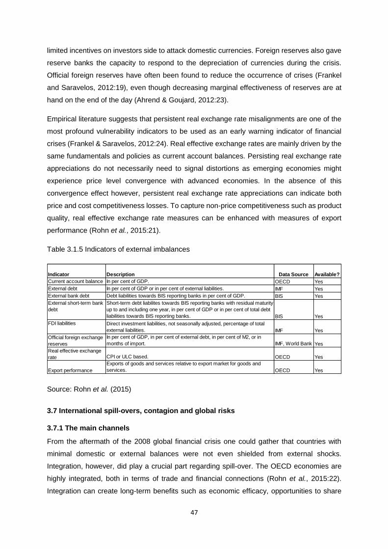
47
limited incentives on investors side to attack domestic currencies. Foreign reserves also gave
reserve banks the capacity to respond to the depreciation of currencies during the crisis.
Official foreign reserves have often been found to reduce the occurrence of crises (Frankel
and Saravelos, 2012:19), even though decreasing marginal effectiveness of reserves are at
hand on the end of the day (Ahrend & Goujard, 2012:23).
Empirical literature suggests that persistent real exchange rate misalignments are one of the
most profound vulnerability indicators to be used as an early warning indicator of financial
crises (Frankel & Saravelos, 2012:24). Real effective exchange rates are mainly driven by the
same fundamentals and policies as current account balances. Persisting real exchange rate
appreciations do not necessarily need to signal distortions as emerging economies might
experience price level convergence with advanced economies. In the absence of this
convergence effect however, persistent real exchange rate appreciations can indicate both
price and cost competitiveness losses. To capture non-price competitiveness such as product
quality, real effective exchange rate measures can be enhanced with measures of export
performance (Rohn et al., 2015:21).
Table 3.1.5 Indicators of external imbalances
Source: Rohn et al. (2015)
3.7 International spill-overs, contagion and global risks
3.7.1 The main channels
From the aftermath of the 2008 global financial crisis one could gather that countries with
minimal domestic or external balances were not even shielded from external shocks.
Integration, however, did play a crucial part regarding spill-over. The OECD economies are
highly integrated, both in terms of trade and financial connections (Rohn et al., 2015:22).
Integration can create long-term benefits such as economic efficacy, opportunities to share
Indicator Description Data Source Available?
Current account balance In per cent of GDP. OECD Yes
External debt In per cent of GDP or in per cent of external liabilities. IMF Yes
External bank debt Debt liabilities towards BIS reporting banks in per cent of GDP. BIS Yes
External short-term bank
debt
Short-term debt liabilites towards BIS reporting banks with residual maturity
up to and including one year, in per cent of GDP or in per cent of total debt
liabilities towards BIS reporting banks. BIS Yes
FDI liabilities Direct investment liabilities, not seasonally adjusted, percentage of total
external liabilities. IMF Yes
Official foreign exchange
reserves
In per cent of GDP, in per cent of external debt, in per cent of M2, or in
months of import. IMF, World Bank Yes
Real effective exchange
rate CPI or ULC based. OECD Yes
Export performance
Exports of goods and services relative to export market for goods and
services. OECD Yes
48
risk and puts countries in the favourable position to be less vulnerable against domestic
shocks. On the other hand, integration causes countries to be more vulnerable to external
shocks through spill-overs and contagion, particularly in times of global economic downturns.
Changes in the certain parts of the world can spill-over to domestic economies through three
main channels of contagion: the trade channel, the confidence channel and the financial
channel.
3.7.1.1 The trade channel
This particular area of contagion picks up changes in the cross-border goods and services as
a response to significant economic events in the rest of the world. For example, a negative
demand shock abroad will affect the export demand for a country, reducing both the quantity
and price of goods and services exported. Whereas import prices tend to increase due to
negative external supply shocks (such as an oil supply shock) leading to reduced profits for
firms and a reduction in the real disposable income of households. Spill-overs resulting from
this channel can also rely on a country’s degree of trade diversification as a country with more
trade partners and a greater range of traded products and services will mitigate trade losses
to a certain level. The more diversified a country’s trade portfolio is, the less vulnerable a
country will be to shocks regarding specific countries as well as specific goods and services
(Rohn et al., 2015:22).
The upsurge of global value chains (GVC) has had increasingly significant implications for
trade channels. More specifically, indirect trade effects are more likely to have a greater effect.
For instance, domestic economies might be more exposed to shocks in countries that are not
direct trading partners, but which operate on the same supply chains. A significant implication
regarding the upsurge of GVCs is that it may be a more suitable measure to identify
weaknesses to external shocks on the domestic GDP by measuring trade exposures by value
added rather than making use of traditional measure such as gross exports. Measuring value
added trade exposures is a feasible concept with the help of the OECD-WTO trade in value
added (TiVA) database (Rohn et al., 2015:22). Moreover, due to high levels of connectivity as
well as specialisation inside GVCs, a greater exposure to systemic risk for national economies
are at play. GVCs are thus known for their part in acting as a channel for contagion. Despite
their role in contagion, whether a shock in one link of the chain leads to a system-wide shock,
rests on the redundancy in the system (whether the loss of one supplier can be compensated
by other suppliers). Empirical evidence on this issue is scarce and not widely available. A final
assessment on whether GVCs ultimately increase or reduce vulnerabilities would therefore be
careless.
49
3.7.1.2 The financial channel
The financial channel captures movements of assets and liabilities on a cross-border basis.
Taking the importance of the banking sector contagion during the global financial crisis of 2008
into account, it is beneficial to differentiate between a banking channel (where spill-overs are
largely conveyed through bank balance sheets), and a non-banking channel. The banking
channel can then be further broken down into an asset and liability channel. Spill-overs via the
asset channel of banks’ balance sheets arise, for instance, if a domestic bank suffers losses
abroad. This causes a decrease in the domestic banks’ asset-to-capital ratio and may cause
the bank to decrease the size of its balance sheet by restricting lending in the local economy.
Whereas spill-overs on the liability side of the bank balance sheet may arise if a domestic
bank is dependent on funding from abroad. Specifically, via international inter-banking
wholesale markets as shocks that occur abroad may limit foreign funding. Pressure is then
put on the domestic bank to replace that “lost” funding. If there are no other sources of funding
the bank may be forced to sell assets or reduce domestic lending. In addition to these direct
connections, indirect contagion may also occur. For instance, banks may reduce lending to a
country as a result of losses suffered on loans to another country. This common creditor
contagion played a significant role in the global financial crisis (Ahrend & Goujard, 2012:19).
The non-banking channel functions via international equity and bond markets. A shock abroad
may cause domestic residents’ foreign held assets to decrease in value. By means of wealth
and financial accelerator mechanisms these losses can result in contracted domestic demand
on the side of firms and consumers. On the other hand, a shock abroad may motivate foreign
investors to limit their resources in the domestic market, causing a drop in the domestic bond
and asset markets, translating into reduced domestic demand through wealth and financial
accelerator mechanisms.
The uncertainty/confidence channel captures changes within the level of uncertainty in the
local economy as a result from shocks abroad. A negative shock may lead to a rise in the level
of uncertainty experienced by households and firms due to vagueness around how the
external shock might affect the domestic economy. Households will most likely reduce their
spending habits as a result of uncertainty, while firms may reassess their projections for
demand. Depending on the outcome of the assessment, firms may choose to suspend
investment for the time being. Elevated uncertainty may result in higher borrowing costs for
households and firms as investors seek greater returns for the higher levels of uncertainty
they have to undertake. Uncertainty and confidence shocks can also be conveyed via foreign
investors. The emergence of fiscal stress within a country may serve as warning signals to
other countries to reassess the exposure of other countries in the same area or countries with
50
similar risk profiles (Goldstein, 1998:135). Sudden swings in investor sentiment, be it foreign
or local investors, can occur when investors overestimate the economic interconnectedness
between a country experiencing fiscal stress and others. Extrapolation of new information on
countries experiencing fiscal stress to other countries can happen as well, this can also cause
possible swings in sentiment. Sudden swings in investor sentiment and the subsequent
reallocation of resources within portfolios can cause sudden reversals of capital flows and
therefore lead to the transmission of financial stress abroad. The uncertainty/confidence
channel is thought to be the main reason for the strong co-movement across countries during
crisis periods.
The underlying shock will determine the relative importance of the various spill-over channels.
For instance, financial shocks may mostly be conveyed through financial interconnectedness
whereas, demand shocks (such as consolidation) may most likely be conveyed through trade
channels (Rohn et al., 2015:23). However, these channels almost never function in isolation.
They interact and operate simultaneously. For instance, shocks spread by the uncertainty
channel may cause domestic exporters to revise their export strategy. A shock conveyed via
the financial channel may affect trade financing on a negative basis ultimately influencing
trade. Alternatively, trade openness can serve to lessen the influence of a sudden stop. In a
more open economy, the marginal propensity to import is larger. Therefore, a small drop in
GDP or a small currency devaluation is required to close an external funding gap (Cavallo &
Frankel, 2008:1449).
3.7.2 Measuring vulnerabilities to international spill-overs, contagion and global risks
Vulnerabilities regarding international spill-over and contagion can be captured in several
ways. For instance, indicators of trade openness or financial openness can be made use of.
These indicators will possibly measure vulnerabilities to global shocks or shocks arising in
major trade or financial centres (such as the US, Eurozone or China). Despite the
effectiveness of these measures in capturing global shocks, they are less effective in capturing
vulnerabilities to spill-overs and contagion from localised shocks as they do not take specific
exposure of countries into account (Rohn et al., 2015:23).
Measures of global imbalance offer an additional approach of capturing spill-over and
contagion risk. Global indicators are usually measured against a country’s GDP weighted
average of country specific imbalances. The reason behind the use of these indicators is that
imbalances, such as credit or asset price booms, can form a build-up pattern in several
countries at once. An unwinding effect in a single country can act as a spark to lead to the
unwinding of the imbalance in other counties. Moreover, if several countries unwind
51
imbalances (deleverage) simultaneously, countries that do not have imbalances are prone to
be affected through trade and financial channels (Chen et al., 2012).
More recent early warning literature has started to include global measures such as these
mentioned above with some degree of success (Rohn et al., 2015:23). For instance, indicators
of global liquidity (principally captured in terms of GDP-weighted credit averages) along with
domestic variables have been shown to be useful in predicting crises or costly asset booms
(Lo Duca & Peltonen, 2013:2192; Babecky et al., 2013:31, and also Behn et al., 2013:67).
Early warning literature also suggests that heightened global risk aversion is normally
accompanied by higher costs to the economy after crises (Babecky et al., 2013:30). Behn et
al. (2013:69) found that global equity price growth is positively correlated with future banking
crises. The fact that global and regional indicators enable one to capture risks of contagion
through the confidence channel along with the simplicity of use of the indicators is a huge
advantage. The main drawback of these indicators is the fact that they do not vary by country
and therefore do not give one the opportunity to assess country specific spill-over and
contagion risk. Global indicators also tend to distort the build-up of geographically bound
imbalances. For instance, global indicators, for the most part, missed the build-up of
imbalances in a number of Asian countries preceding the East Asian crisis (Rohn et al.,
2015:24). It is therefore recommended to make use of regional indicators to complement
global indicators when assessing vulnerabilities.
It is also possible to construct more relevant indicators of spill-over and contagion risk
grounded on cross-border bilateral data. Unlike the indicators mentioned above, these more
sophisticated indicators capture country specific spill-over or contagion risk. Bilateral trade
(such as OECD TiVA), portfolio investment (IMF CPIS data) or bank lending data (BIS
locational banking statistics) can be used in order to calculate a county’s principal geographic
exposures (Rohn et al., 2015:24). To make these measures even more effective, the bilateral
trade, portfolio investment or bank lending data can be used in conjunction with vulnerability
indicators to measure the exposure of a domestic economy to shocks from abroad or
vulnerabilities. Another approach suggested by Ahrend and Goujard (2012:33) is to generate
measures of banks’ balance sheet contagion by merging bilateral bank lending data with data
on country risk ratings.
Cross-country correlations amid consumer and business confidence indicators can serve as
a rough measure of spill-overs via the uncertainty channel. For example, a strong correlation
amongst consumer confidence indicators across countries in Europe with some differences
amid the core and peripheral countries was found arising in the midst of the global financial
52
crisis (Rohn et al., 2015:24). This could possibly be the consequence of synchronised
business cycles across the European continent, which serves as a confidence indicator proxy.
3.8 Conclusion
This chapter reinforces the statement that early warning indicators are a viable option to
explore regarding mitigating risks from oncoming crises as early warning indicators can indeed
be deployed to predict/forecast oncoming financial crises. There are several of these
indicators that appear to be useful in this regard. These indicators often tend to connect on
some underlying level and form a strong coherence between one another. Chapter 4 will
therefore focus on processing the vulnerability indicators as set out by Rohn et al. (2015)
through dynamic factor analysis to establish co-movement between these indicators.
53
CHAPTER 4: EMPIRICAL ANALYSIS
4.1 Introduction
Vulnerabilities to financial crisis can arise from a significant number of areas within an
economy. As previously mentioned, early warning indicators should not only be viewed in
isolation due to the high levels of interconnectedness and interaction between certain
vulnerabilities. On the other hand, the vast number of possible early warning indicators also
makes it difficult for decision-makers to effectively monitor all the variables. Therefore,
indicators that tend to interact similarly are typically grouped together (see chapter 3) to
simplify the sheer number of possible explanatory early warning indicators. Some indicators
also point to similar vulnerabilities within an economy, hence further motivating the use of
grouped measures. The literature does not explain how measures are grouped as Dynamic
factor analysis does not necessarily explain the type of relationship between variables. The
co-movement between the variables will however be identified in an attempt to group variables
with high levels of co-movement. The grouped variables will form one factor that comprises
out of several vulnerability indicators that can possibly be monitored to signal an oncoming
financial crisis. This process reduces the large number of possible indicators that need to be
monitored. This chapter will therefore explain how Dynamic factor analysis was used to identify
indicators that co-vary between countries and over time in an attempt to identify parsimonious
indicators of financial crises.
4.2 Dynamic factor analysis
Economists often have to work with diverging data structures as the number of years for which
there are trustworthy and appropriate data available is limited and can only be increased by
the passage of time. Fortunately, statistical agencies collected monthly/quarterly data during
the post-war period on an extensive range of financial, macroeconomic and sectoral variables.
Hence, economists have to process extensive data sets that contain several series,
sometimes hundreds and thousands of series. The number of observations can however be
relatively short for instance ten or 20 years of quarterly data. This is where dynamic factor
analysis (DFA - sometimes referred to as dynamic latent variables) comes in as it is a method
used to identify mutual patterns and relations within a set of time series data (Zuur, Fryer,
Jolliffe, Dekker & Beuekema, 2003:542).
Dynamic factor models were initially posited by Geweke (1977) as a time-series expansion of
factor models originally adapted for cross-sectional data, rather than time-series data (Stock
and Watson, 2010:2). Early literature by Sargent and Sims (1977) indicated that just two
dynamic factors could explain the variance of important U.S. quarterly macro-economic
54
variables, including output, employment, and prices to a certain level of accuracy. This vital
empirical result indicated that a few factors can describe a significant portion of the variance
of many macroeconomic series has been confirmed by several studies including Giannone,
Reichlin, and Sala (2004) as well as Stock and Watson (2010) to name some.
The success of DFMs led to an upsurge in the use of DFM by economists to estimate
“underlying” factors, as these factors often co-vary to a greater extent than perceived by
economists when building models. This practice brought forth more accurate measures of
underlying inflation. It has also been successfully applied to the real side of the economy and
been used in arbitrage pricing theory models of financial decision making (Ajevskis &
Davidsons, 2008:7).
The principal concept regarding a dynamic factor model is that a few latent dynamic factors
act as a driving force, resulting in co-movement of a high-dimensional vector of time-series
variables, which is also affected by a vector of mean-zero idiosyncratic disturbances. These
idiosyncratic disturbances emanate from measurement error and from distinct attributes that
are explicit to an individual series. The latent factors follow a time series course, which is
generally considered to be a vector autoregression (VAR) (Stock & Watson, 2010:3).
DFA will be used in this thesis to examine covariation between macroeconomic variables (in
this specific case, measures of vulnerabilities) across global economies. Usually within large
databases, each individual series contains two equilateral latent fundamentals (Claassen,
2016:27). On the one hand, the fundamental movement is driven by common influences.
These common influences are considered to be the underlying factors driving collective
movement in a database. While on the other hand, an idiosyncratic disturbance is also at work,
explicit to each series.
The fact that dynamic factor models can be functional in a wide range of applications makes
it an appealing model to use. Factor models have previously been applied to explore areas
such as finance and risk (Ross, 1977:24), consumer theory (Gorman, 1981:223); (Lewbel,
1991:714). It is also useful for short-term forecasting and monitoring of an economy (Clavel &
Minodier, 2009); (Altissimo, Cristadori, Forni, Lippi & Veronese, 2010:1031). However, more
specific to this study, the intention is to investigate the co-movement of variables within a
dataset. There are several examples of dynamic factor models being applied in similar
endeavours. Menden & Proano (2017:1) proposed the creation of financial cycle measures for
the US based on a large data set of macro-economic and financial variables in order to
estimate three synthetic financial cycle components that account for the majority of the
variation in the specific data set using a dynamic factor model. The main goal being to analyse
whether these financial cycle components have significant predictive power for economic
55
activity, inflation and short-term interest rates by means of Granger causality tests in a factor-
augmented VAR setup. DFA has also been used by Koopman, Lucas and Schwaab (2011:25)
to propose an innovative framework to investigate financial system risk by implementing a
dynamic factor framework constructed on state-space approaches to create coincident
measures. These measures serve as forward looking indicators for the probability of a
synchronised collapse of a significant number of financial intermediaries. Another study
developed a non-linear non-Gaussian dynamic factor model to estimate the breakdown of
systematic default risk conditions into a set of components that reacts in parallel with macro-
economic, financial and industry specific events Durbin and Koopman (2012:1). Jin and De
Simone (2012:33) joined the previously mentioned Geske model with a Generalized Dynamic
Factor Model and used the results by putting it into a dynamic t-copula as a technique for
obtaining banks’ interdependence. In doing so they developed a measure that produces an
early warning indicator regarding banks’ probability of default. Another study by Sheen, Truck,
Truong & Wang (2016:11) also made use of dynamic factor analysis in a model to identify
unobserved financial risk and ratings indicators for several regions by making use of observed
expected default frequencies. Vasilenko (2018:3) studied systemic risk and financial fragility
within the Chinese economy by means of a dynamic factor model approach. A dynamic factor
model was estimated in order to forecast systemic risk that displays noteworthy out-of-sample
forecasting power, accounting for the outcome of several macroeconomic factors on systemic
risk, including; economic growth slowdown, high levels of corporate debt, increase in shadow
banking as well as real estate market slowdown. The study proceeded to analyse the historical
working of financial fragility within the Chinese economy over the course of the previous ten
years. Results concluded that the level of financial fragility in the Chinese financial system
declined after the global financial crisis of 2008. The level of financial fragility has, however,
been systematically increasing since 2015.
For this study Dynamic factor analysis was selected over other models as DFA model
simultaneously considers a wide variety of macro-economic factors that could possibly result
in financial crises, whereas traditional models mostly consider single or occasionally multiple
factors. Dynamic Factor Analysis is an established technique to empirically analyse co-
movement (Claassen, 2016:28). DFA makes it possible to process the large data-series
without the risk of lost degrees of freedom, in so doing overcoming what is generally
acknowledged as the curse of dimensionality in data analysis.
4.2.1 The Model
As previously stated, the dynamic factor model is grounded on the concept that change in
time-series variables are driven by a smaller number of latent factors (𝑟). This can be called a
56
common component which is the driving force of co-movement among the variables (Zuur et
al. (2003). Co-movement or variance among the variables can in some instances also be
altered by specific features/events that are unique to individual data series. Variance caused
by such features/events are called idiosyncratic components (Altissimo et al. 2010).
Consequently, it is possible to embody a vector of time series ( 𝑌𝑡 = 𝑦1𝑡 , 𝑦2𝑡 , … 𝑦𝑁𝑡)’ as the sum
of a common component, (𝑋𝑡 = 𝑥1𝑡, 𝑥2𝑡 , … 𝑥𝑁𝑡 )’ and an idiosyncratic component, (𝐸𝑡 =
𝑒1𝑡, 𝑒2𝑡 , … 𝑒𝑁𝑡)’ (Claassen, 2016).
This results in:
𝑌𝑡 = 𝑋𝑡 + 𝑒𝑡
𝑌𝑡 =∧ 𝐹𝑡 + 𝑒𝑡 (1)
Where:
𝑋𝑡 =∧ 𝐹𝑡 exhibits the common component; the share of the series that is dependent on
common factors;
𝑒𝑡 exhibits the idiosyncratic component; the part of each series that is variable specific and
equilateral regarding the common component;
Moreover:
∧ symbolises the 𝑁 x 𝑟 matrix of factor loadings; comprising of the non-zero columns of ∧ and
with 𝑟 < 𝑁; where 𝑁 is the number of series within the dataset.
𝐹𝑡 symbolises the vector of 𝑟 common factors.
Since 𝑇, 𝑁 → ∞ the common components can be recognised by making use of principal
component analysis for the variance-covariance matrix of the perceivable data, 𝑐𝑜𝑣(𝑌𝑡). The
variance-covariance matrix is then summarised by using a dimension reduction matrix where
𝑁 x 1 vector of eigenvalues from the variance-covariance matrix where the first largest
eigenvalues and vectors have been calculated in such a way that:
𝑋𝑡 = 𝑉𝑉′𝑌𝑡 (2)
With:
𝑉′ representing the 𝑁 × 𝑟 matrix of eigenvectors which coincide with the largest 𝑟 eigenvalues
of the correlation matrix for 𝑌𝑡.
57
𝐹𝑡, the common factors, are estimated using principal component analysis and can be
embodied as follows (Stock & Watson, 2010):
𝐹𝑡 = 𝑉′𝑌𝑡 (3)
Where 𝑉 is an estimate of factor loadings equal to ∧. The idiosyncratic factors can thus be
defined as
𝑒𝑡 = 𝑋𝑡 − 𝑌𝑡 (4)
In a first attempt of this study, the number of static factors to be estimated was determined
using the approach proposed by Bai and Ng (2002)5. This approach focuses on establishing
the convergence rate for the factor estimate that enables a consistent estimation of the number
of static factors. Panel criteria are then introduced suggesting that the number of factors can
be consistently estimated through parameters presented by the criteria. The theory is
developed with the concept of large cross-sections (N) and large time dimensions (T). There
are no restrictions that constrain the relationship between the large cross-sections and large
time dimensions. Results from this approach indicate that the proposed criteria have sufficient
finite sample properties in many configurations of the panel data used in practice.
However, this approach was not successful as the Bai-Ng criteria do not converge and in this
specific case give no precise answer. An alternative approach proposed by Alessi, Barigozzi
& Capasso (2008) which is in effect a refinement of the criteria proposed by Bai and Ng,
drawing on the Hallin and Liska (2007)6 criteria for dynamic factors was used instead.
Basically, the penalty function is multiplied by a constant which brings the penalising power of
the function itself into tune/harmony. By evaluating the criterion for a series of values for this
constant factor, an estimation of the number of static factors can be reached. This process is
empirically more robust than it would normally be with a fixed constant. The consistency
properties’ premises of this method are precisely the same as the original Bai and Ng method,
the sole difference being the multiplicative constant.
4.2.2 Data and method
The data used in this dissertation is the same database used by Rohn et al. (2015) as the aim
was to re-examine the 70+ indicators identified by Röhn et al. (2015) to identify parsimonious
indicators of financial crises. The dataset contains OECD indicators of potential
5 For a more detailed explanation regarding the Bai-Ng approach to estimate the number of factors
see: Bai and Ng (2002). 6 Focused on developing an information criterion for determining the number of common shocks in the
general dynamic factor model rather than using the restricted model proposed by Bai and Ng. For a detailed explanation see Hallin and Liska (2007).
58
macroeconomic and financial vulnerabilities for 34 OECD countries, the BRICS countries
(Brazil, Russian Federation, India, China, and South Africa), Indonesia, Colombia, Costa Rica,
Latvia and Lithuania. The vulnerability indicator database was created from a number of data
sources as part of an Economics Department project on Economic Resilience. As mentioned
above, the choice of indicators is motivated in a related working paper, by Röhn et al. (2015),
wherein the source and nature of potential vulnerabilities that can lead to costly economic
crises, are also analysed. The dataset was compiled from a number of sources7 namely, the
OECD, IMF, ECB, BIS, World Bank, Eurostat as well as Benetrix, Lane & Shambaugh (2015).
The data observations in the dataset range from 1970 to 2015 depending on the indicator.
The frequency of the observed indicators also ranges from annual to monthly (including
quarterly) depending on the indicator observed. The number of countries for which data is
available for a certain indicator also ranges from nine to 44 depending on which indicator is
being observed. Due to the varying time-series and structure of the data within the dataset,
the main focus was put on the last ten years of the data (2005 to 2014) as data for this period
is more widely available which can be attributed to better record-keeping practices within the
private as well as public sector. The time slot of this period also enables an overview of the
build-up to the global financial crisis of 2008 right through to the actual crisis period as well as
the start of the recovery process after the crisis. This crisis period is also a near-perfect
experiment for testing the robustness of early warning indicators as the crisis started with a
shock that was exogenous as far as many countries of the world are concerned, namely a
liquidity crisis in US financial markets. The crisis hit everyone simultaneously, so it was not
necessary to worry about the issue of timing. Focus can be put on what economic variables
indicate vulnerability to such a shock.
The data was structured on a quarterly basis as this allowed more indicators to be included
into the analysis. After the rearrangement of the data, 54 of the original 73 indicators could be
used in the analysis. The sample size is 1468 (N) x 40 (T). The 54 indicators used amounted
to 1468 total variables with 40 quarters of data each, therefore resulting in 58720 data points.
To start off, the data was standardised in order make it easier to read results from regression
analysis and to ensure that all the variables contribute to a scale when added together. This
type of data can provide extremely important information about the relationship between the
response and predictor variables, while it can also produce excessive amounts of
multicollinearity. This could pose problematic as multicollinearity can hide statistically
significant terms and cause the coefficients to switch signs as well as making it more difficult
to specify the correct model. Standardizing the vulnerability indicator data is an effective way
7 See appendix for a detailed information regarding the source and frequency of specific vulnerability
indicators.
59
to account for and reduce multicollinearity. The next step was to identify the number of static
factors (r). As previously mentioned the number of static factors was estimated by making use
of the ABC criterion put forth by Alessi et al. (2008). The criteria indicated that two factors
should be estimated for the sample period identified. The estimated number of static factors
was then set as parameters to be estimated within the Bai-Ng criterion to analyse co-
movement through DFA and ultimately identify parsimonious indicators of financial crises.
4.3 Results from Hermansen and Rhon
To better explain the overall picture, the results from the creators of the database used will
first be explained. Hermansen and Rhon (2015) set out to provide empirical evidence
regarding the usefulness8 of the specific set of vulnerability indicators in predicting crises and
recessions. The study makes use of a signalling approach. The signalling approach takes
policy makers’ choice between avoiding crises and false alarms into consideration. Empirical
evidence gathered from the study indicates that the majority of vulnerability indicators would
have assisted in predicting crises and severe recessions in the 34 OECD economies as well
as Latvia between 1970 and 2014.
4.3.1 In-sample results
The study suggests that indicators of global risk outperform domestic indicators consistently
regarding their usefulness as early warning indicators. Global vulnerability indicators such as
an increasing (cumulative) global private bank credit-to-GDP ratio, a global equity price gap
as well as a global house price gap performs particularly well in predicting crisis periods. This
result is in line with findings from similar literature (e.g. Babecky et al., 2013; Behn et al., 2013;
Lo Duca & Peltonen, 2013). This emphasises the significance of taking international events
into consideration when assessing country specific vulnerabilities as economies become more
integrated, causing a higher risk of spill-overs to other economies. The successful results
regarding global indicators are however subject to a caveat. Global indicators do not vary
across countries and are therefore more likely to be picked up as they influence a number of
countries simultaneously. The good performance of global indicators of vulnerability is thus to
a certain extent explained by the share of severe recessions constituted by the global financial
crisis of 2008 within the sample. Global vulnerability indicators will therefore most likely be
less effective serving as early warning indicators for locally confined severe recessions.
8 A relative usefulness criterion was created to measure the performance of indicators in
forecasting severe recessions and financial crises. To see more detail regarding this criterion, see: Hermansen and Rhon, 2015. Economic Resilience: The Usefulness of Early Warning Indicators in OECD Countries. OECD Economics Department Working Papers. No. 1250: 1-30.
60
Useful domestic indicators of vulnerability include the house price-to-disposable-income ratio,
the house-price-to-rent ratio as well as the real house price gap. Borio and Drehmann (2009)
and Claessens et al. (2011) reinforce this outcome as unsustainable real estate booms tend
to be followed by costly economic declines. Hermansen and Rhon (2015:12) state that in
addition to the above domestic indicators, domestic credit related variables can also serve as
useful early warning indicators. More specifically, increases in domestic bank-credit-to-GDP
were found to be particularly useful. Early warning indicators of financial crisis literature
suggests that credit variables are amongst the most robust indicators (e.g. Kaminsky et al.
(1998), Reinhart and Rogoff (2008), Borio and Lowe (2002).
The Hermansen and Rhon (2015:12) study also suggests that official reserves (as a ratio of
M2) is useful in predicting economic recessions although other public sector imbalances
indicators fare poorly in predicting pre-severe recession periods.
4.3.2 Out-of-sample results
The out of sample results focus more on indicators that provide useful information regarding
the detection of the global financial crisis of 2008. The sample period was therefore split into
two samples, an estimation and evaluation sample. The starting date of the estimation for the
Hermansen and Rhon (2015:13) study depended on the data availability of the indicators and
the sample ends in 2004Q4 to exclude data from the global financial crisis. The starting date
of the evaluation sample was specified to be 2005Q1 and the end date was specified as
2012Q4.
Indicators were tested for their relative usefulness with different thresholds. Higher thresholds
indicated that the majority of the indicators were useful with several indicators performing even
better out-of-sample than in-sample. Once again global indicators fared particularly well,
reinforcing their success in the in-sample performance. The global equity price gap indicator
indicated the best results followed by indicators of global credit and global real house prices.
Domestic indicators also showed success with credit and asset market indicators performing
the best of the domestic indicators. Interestingly domestic credit gap indicators perform
particularly well and achieved greater success than out-of-sample than in-sample. This can
most probably be attributed to unsustainable domestic credit booms during the global financial
crisis. The real equity price gap championed the asset market imbalance indicators with good
performance, also performing better than in-sample. The residential investment-to-GDP ratio
also indicated better success out-of-sample. House price related indicators showed worse
performance than in-sample trials, although, the house-price-to-rent and house-price-to-
61
disposable income ratios gap perform better than the long-term trend. External imbalance
indicators perform poorly out-of-sample as well as fiscal imbalance indicators.
4.3.3 Summary
To conclude the results produced by Hermansen and Rhon (2015): results indicate that the
majority of early warning indicators would have aided in forecasting severe recessions in 34
OECD countries as well as Latvia between 1970 and 2014. It was found that most of the
indicators issue warning signals on average 1.5 years before the onset of a severe recession.
This allows policymakers to react with ample time, the signalling power differs between
indicators and the results are sensitive to the exact specification of policymakers’ preferences
regarding false alarms and missing crises. The study highlights the finding that global
vulnerability indicators consistently outperform domestic vulnerability indicators regarding their
usefulness. This once again emphasises the importance of taking international developments
into consideration when assessing a country’s vulnerabilities. On the domestic side, indicators
measuring asset market imbalances, more specifically, real house prices, real equity prices,
house price-to-income Ratio as well as price-to-rent ratio also perform reliably out-of-sample
as well as in-sample. Domestic credit associated indicators are successful in signalling
oncoming banking crises as well as forecasting the global financial crisis out of sample.
The results are robust and wide-ranging depending on the definition of severe recessions and
crises, varying forecasting periods as well as differing time and country samples. The early
warning indicators identified to be useful can be a valuable input for monitoring future risks.
The indicators should, however, be complemented with other successful monitoring tools
(including expert judgement).
4.4 Results from this study
The ultimate objective of early warning indicators is to forecast future crisis events. The results
from Hermansen and Rhön (2015) indicated that the majority of indicators from the set of
vulnerability indicators they identified was indeed useful in predicting oncoming crises. Results
from that study emphasise the effectiveness of some of the indicators, such as global
indicators. However, the indicators should not be viewed in isolation as the indicators often
tend to interact with one another. One indicator can reinforce other indicators, similarly
indicators can affect other indicators adversely and lead to one imbalance triggering the
unwinding of others ultimately leading to a downward spiral.
The aim of this study was therefore to re-examine the 70+ indicators identified by Röhn et al.
(2015) to identify parsimonious indicators of financial crises. Rather than considering single
62
indicators, the process through DFA and data reduction created a group of variables that make
out a single factor responsible for explaining the movement among the group of variables.
This makes monitoring a wide variety of indicators easier as a single factor consists of an
assortment of indicators.
As previously mentioned, a sample period (2005 to 2014, arranged quarterly) within the
original dataset compiled by Rohn et al. (2015) was identified as having been processed by
the DFA model. This was done to ensure that an adequate number of variables was available
to be analysed as earlier data in the dataset tend to be distorted in the sense of data
availability. The specific sample period also gives a sufficient overview of the build-up to the
global economic crisis of 2008 as well as the actual effects of the crisis and the remedial
process after the crisis.
The number of static factors was estimated to be two as per the ABC criteria (see Appendix B
for an overview of how the number of static factors was estimated). Dynamic factor analysis
groups the indicators into two factors. For each factor, the dynamic factor analysis model
creates a list of covarying variables. These variables were then sorted according to their
variance shares. For factor one variables with a variance share of less than 90 percent were
left out as the higher variance shares assures a higher level of co-movement between
variables. For factor two, the threshold was lowered to 75 percent as the DFM identified less
variables with high variance shares. Factor one was identified as private non-financial sector
imbalances including some asset market imbalances. Factor two was identified as private non-
financial sector imbalances (more focused on private bank credit and external debt whereas
factor one is more concerned with household and private credit as well as external sector
imbalances. This is in line with the results from Hermansen and Rhon (2015) as credit and
asset market indicators performed the best of the domestic indicators.
4.4.1 Factor 1
Below follows a table displaying the variance shares of each of the variables with a variance
share of more than 90 percent identified to form part of factor one. A high degree of co-
movement between the vulnerability indicators is present.

63
Table 4.1: Variance shares of factor 1, 2005Q1 – 2014Q4
Household credit_SWE 0.982276
Gross general government
debt_HUN 0.962302 Household credit_CZE 0.950933 Private bank credit_CZE 0.944200
Total private credit_FRA 0.981634 Total private credit_FIN 0.962039 Financial openness_GRC 0.950189 Total private credit_CAN 0.943757
Commercial real estate
loans_BRA 0.980687 External debt_GRC 0.961677 Corporate credit_FRA 0.949767
Short-term external bank
debt_BEL 0.943085
Private bank credit_FIN 0.979815 Corporate credit_CHE 0.959817 External debt_POL 0.949038 Household credit_POL 0.942469
Residential
investment_PRT 0.978384 FDI liabilities_BEL 0.958478 Tier 1 capital ratio_DEU 0.948326 Tier 1 capital ratio_GBR 0.940308
Household credit_BEL 0.978048
Gross general government
debt_usa 0.958252 Household credit_CAN 0.948157 Private bank credit_BRA 0.939803
Household credit_FRA 0.974288 Real house prices_BRA 0.956557 Total private credit_GRC 0.947277
Gross government debt
denominated in foreign
currency_LVA 0.938540
Total private credit_CZE 0.973310
External government
debt_usa 0.955669
Gross general government
debt_GBR 0.946018 Private bank credit_GRC 0.937523
Residential
investment_ESP 0.972382
Employment share in
construction_IRL 0.954213 Leverage ratio_LTU 0.945725 Total private credit_BEL 0.937436
Private bank credit_SWE 0.971888
Residential
investment_IRL 0.951532 Export performance_POL 0.945138
Gross general government
debt_LUX 0.936757
Household credit_LUX 0.968510 Total private credit_POL 0.951481
Short-term external bank
debt_GBR 0.944854 Capital ratio_LTU 0.936709
Household credit_FIN 0.964945
Short-term external bank
debt_BEL 0.951374
House prices-to-rent
ratio_PRT 0.944814
External government
debt_LUX 0.934378
External debt bias_BEL 0.964077 Tier 1 capital ratio_NOR 0.951054 Real stock prices_SVK 0.944750 Household credit_TUR 0.932922
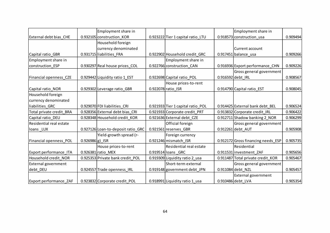
64
External debt bias_CHE 0.932105
Employment share in
construction_KOR 0.923222 Tier 1 capital ratio_LTU 0.918573
Employment share in
construction_usa 0.909494
Capital ratio_GBR 0.931715
Household foreign
currency denominated
liabilities_FRA 0.922902 Household credit_GRC 0.917451
Current account
balance_usa 0.909266
Employment share in
construction_ESP 0.930297 Real house prices_COL 0.922766
Employment share in
construction_CAN 0.916936 Export performance_CHN 0.909226
Financial openness_CZE 0.929442 Liquidity ratio 1_EST 0.922698 Capital ratio_POL 0.916592
Gross general government
debt_IRL 0.908567
Capital ratio_NOR 0.929302 Leverage ratio_GBR 0.922078
House prices-to-rent
ratio_ISR 0.914790 Capital ratio_EST 0.908045
Household foreign
currency denominated
liabilities_GRC 0.929070 FDI liabilities_CRI 0.921933 Tier 1 capital ratio_POL 0.914425 External bank debt_BEL 0.906524
Total private credit_BRA 0.928356 External debt bias_CRI 0.921933 Corporate credit_PRT 0.913832 Corporate credit_IRL 0.906422
Capital ratio_DEU 0.928348 Household credit_KOR 0.921636 External debt_CZE 0.912711 Shadow banking 2_NOR 0.906299
Residential real estate
loans _LUX 0.927126 Loan-to-deposit ratio_GRC 0.921561
Official foreign
reserves_GBR 0.912261
Gross general government
debt_AUT 0.905908
Financial openness_POL 0.926986
Yield-growth spread (r-
g)_ISR 0.921246
Foreign currency
mismatch_ISR 0.912172 Gross financing needs_ESP 0.905735
Export performance_ITA 0.926381
House prices-to-rent
ratio_MEX 0.919514
Residential real estate
loans _GRC 0.911531
Residential
investment_ZAF 0.905656
Household credit_NOR 0.925353 Private bank credit_POL 0.919309 Liquidity ratio 2_usa 0.911487 Total private credit_KOR 0.905467
External government
debt_DEU 0.924557 Trade openness_IRL 0.919148
Short-term external
government debt_JPN 0.911084
Gross general government
debt_NZL 0.905457
Export performance_ZAF 0.923832 Corporate credit_POL 0.918991 Liquidity ratio 1_usa 0.910486
External government
debt_LVA 0.905354
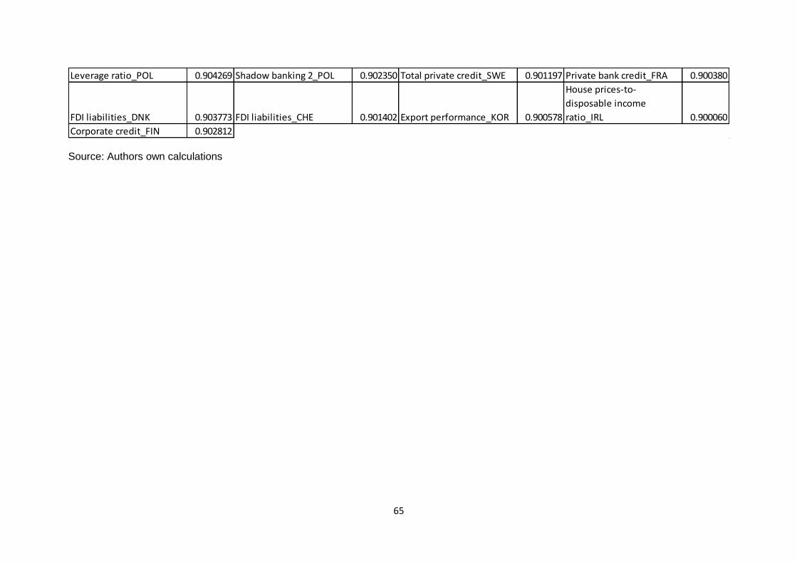
65
Source: Authors own calculations
Leverage ratio_POL 0.904269 Shadow banking 2_POL 0.902350 Total private credit_SWE 0.901197 Private bank credit_FRA 0.900380
FDI liabilities_DNK 0.903773 FDI liabilities_CHE 0.901402 Export performance_KOR 0.900578
House prices-to-
disposable income
ratio_IRL 0.900060
Corporate credit_FIN 0.902812
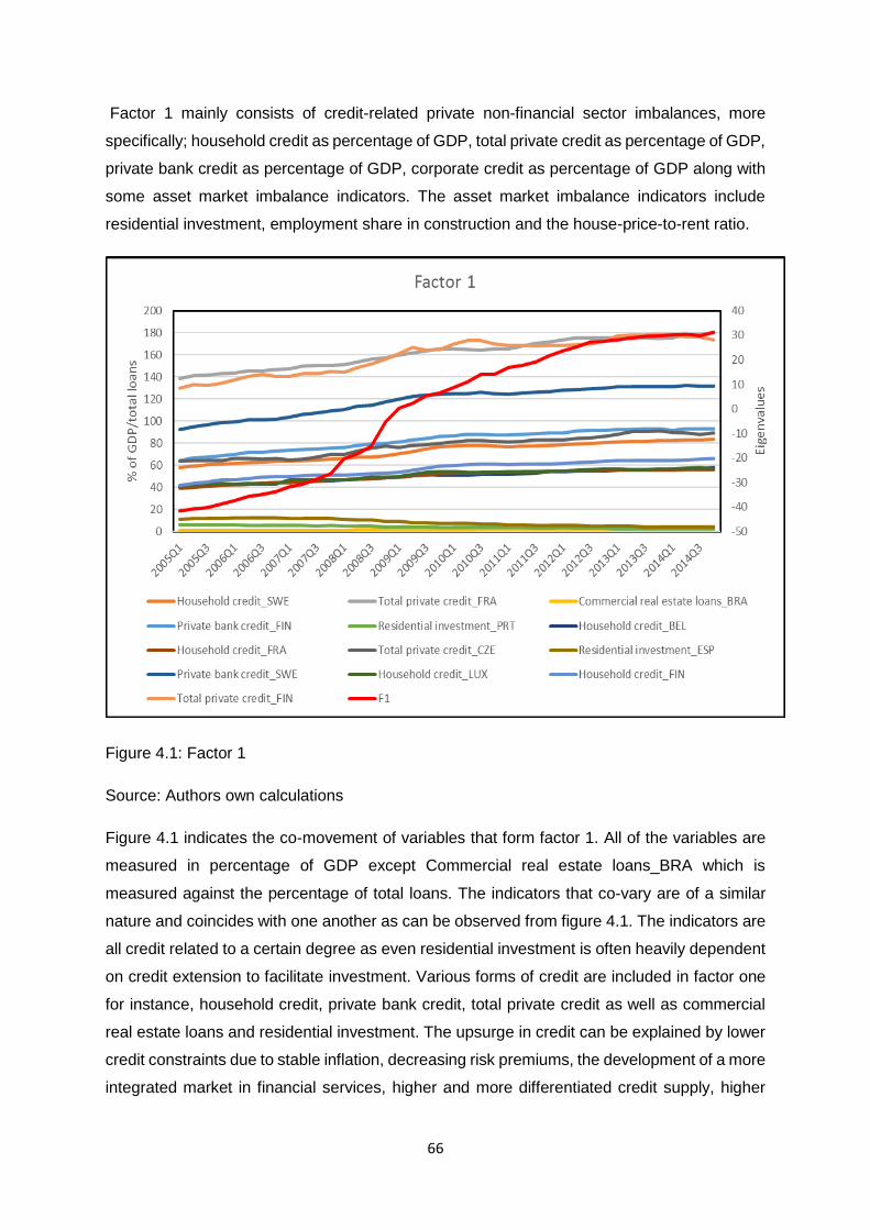
66
Factor 1 mainly consists of credit-related private non-financial sector imbalances, more
specifically; household credit as percentage of GDP, total private credit as percentage of GDP,
private bank credit as percentage of GDP, corporate credit as percentage of GDP along with
some asset market imbalance indicators. The asset market imbalance indicators include
residential investment, employment share in construction and the house-price-to-rent ratio.
Figure 4.1: Factor 1
Source: Authors own calculations
Figure 4.1 indicates the co-movement of variables that form factor 1. All of the variables are
measured in percentage of GDP except Commercial real estate loans_BRA which is
measured against the percentage of total loans. The indicators that co-vary are of a similar
nature and coincides with one another as can be observed from figure 4.1. The indicators are
all credit related to a certain degree as even residential investment is often heavily dependent
on credit extension to facilitate investment. Various forms of credit are included in factor one
for instance, household credit, private bank credit, total private credit as well as commercial
real estate loans and residential investment. The upsurge in credit can be explained by lower
credit constraints due to stable inflation, decreasing risk premiums, the development of a more
integrated market in financial services, higher and more differentiated credit supply, higher
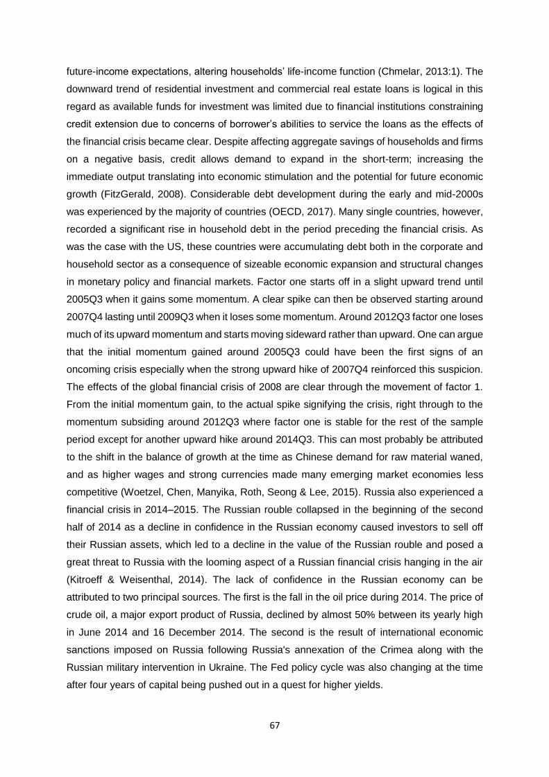
67
future-income expectations, altering households’ life-income function (Chmelar, 2013:1). The
downward trend of residential investment and commercial real estate loans is logical in this
regard as available funds for investment was limited due to financial institutions constraining
credit extension due to concerns of borrower’s abilities to service the loans as the effects of
the financial crisis became clear. Despite affecting aggregate savings of households and firms
on a negative basis, credit allows demand to expand in the short-term; increasing the
immediate output translating into economic stimulation and the potential for future economic
growth (FitzGerald, 2008). Considerable debt development during the early and mid-2000s
was experienced by the majority of countries (OECD, 2017). Many single countries, however,
recorded a significant rise in household debt in the period preceding the financial crisis. As
was the case with the US, these countries were accumulating debt both in the corporate and
household sector as a consequence of sizeable economic expansion and structural changes
in monetary policy and financial markets. Factor one starts off in a slight upward trend until
2005Q3 when it gains some momentum. A clear spike can then be observed starting around
2007Q4 lasting until 2009Q3 when it loses some momentum. Around 2012Q3 factor one loses
much of its upward momentum and starts moving sideward rather than upward. One can argue
that the initial momentum gained around 2005Q3 could have been the first signs of an
oncoming crisis especially when the strong upward hike of 2007Q4 reinforced this suspicion.
The effects of the global financial crisis of 2008 are clear through the movement of factor 1.
From the initial momentum gain, to the actual spike signifying the crisis, right through to the
momentum subsiding around 2012Q3 where factor one is stable for the rest of the sample
period except for another upward hike around 2014Q3. This can most probably be attributed
to the shift in the balance of growth at the time as Chinese demand for raw material waned,
and as higher wages and strong currencies made many emerging market economies less
competitive (Woetzel, Chen, Manyika, Roth, Seong & Lee, 2015). Russia also experienced a
financial crisis in 2014–2015. The Russian rouble collapsed in the beginning of the second
half of 2014 as a decline in confidence in the Russian economy caused investors to sell off
their Russian assets, which led to a decline in the value of the Russian rouble and posed a
great threat to Russia with the looming aspect of a Russian financial crisis hanging in the air
(Kitroeff & Weisenthal, 2014). The lack of confidence in the Russian economy can be
attributed to two principal sources. The first is the fall in the oil price during 2014. The price of
crude oil, a major export product of Russia, declined by almost 50% between its yearly high
in June 2014 and 16 December 2014. The second is the result of international economic
sanctions imposed on Russia following Russia's annexation of the Crimea along with the
Russian military intervention in Ukraine. The Fed policy cycle was also changing at the time
after four years of capital being pushed out in a quest for higher yields.
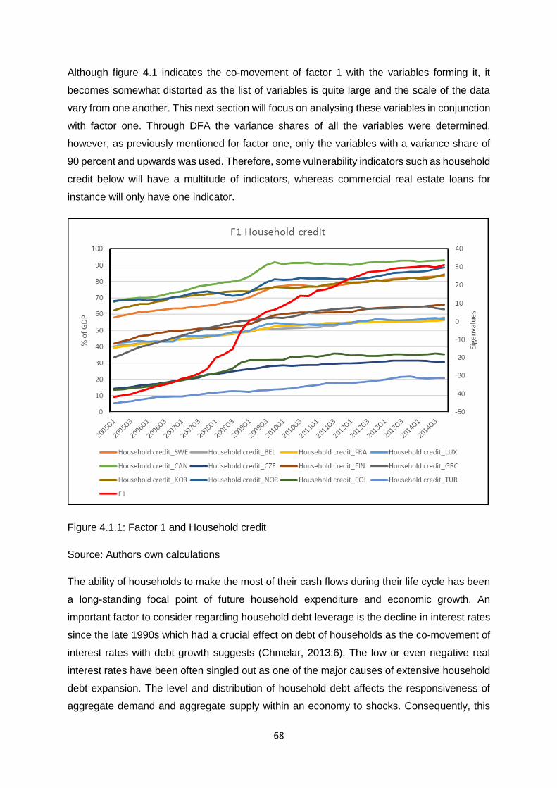
68
Although figure 4.1 indicates the co-movement of factor 1 with the variables forming it, it
becomes somewhat distorted as the list of variables is quite large and the scale of the data
vary from one another. This next section will focus on analysing these variables in conjunction
with factor one. Through DFA the variance shares of all the variables were determined,
however, as previously mentioned for factor one, only the variables with a variance share of
90 percent and upwards was used. Therefore, some vulnerability indicators such as household
credit below will have a multitude of indicators, whereas commercial real estate loans for
instance will only have one indicator.
Figure 4.1.1: Factor 1 and Household credit
Source: Authors own calculations
The ability of households to make the most of their cash flows during their life cycle has been
a long-standing focal point of future household expenditure and economic growth. An
important factor to consider regarding household debt leverage is the decline in interest rates
since the late 1990s which had a crucial effect on debt of households as the co-movement of
interest rates with debt growth suggests (Chmelar, 2013:6). The low or even negative real
interest rates have been often singled out as one of the major causes of extensive household
debt expansion. The level and distribution of household debt affects the responsiveness of
aggregate demand and aggregate supply within an economy to shocks. Consequently, this
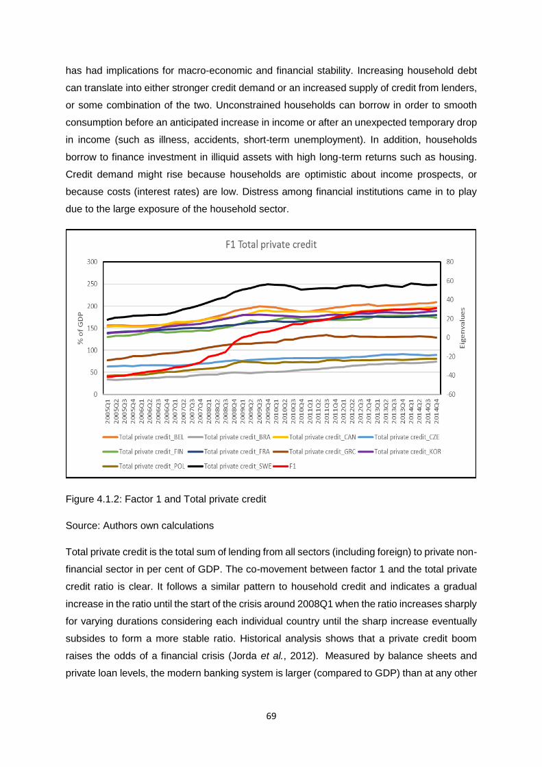
69
has had implications for macro-economic and financial stability. Increasing household debt
can translate into either stronger credit demand or an increased supply of credit from lenders,
or some combination of the two. Unconstrained households can borrow in order to smooth
consumption before an anticipated increase in income or after an unexpected temporary drop
in income (such as illness, accidents, short-term unemployment). In addition, households
borrow to finance investment in illiquid assets with high long-term returns such as housing.
Credit demand might rise because households are optimistic about income prospects, or
because costs (interest rates) are low. Distress among financial institutions came in to play
due to the large exposure of the household sector.
Figure 4.1.2: Factor 1 and Total private credit
Source: Authors own calculations
Total private credit is the total sum of lending from all sectors (including foreign) to private non-
financial sector in per cent of GDP. The co-movement between factor 1 and the total private
credit ratio is clear. It follows a similar pattern to household credit and indicates a gradual
increase in the ratio until the start of the crisis around 2008Q1 when the ratio increases sharply
for varying durations considering each individual country until the sharp increase eventually
subsides to form a more stable ratio. Historical analysis shows that a private credit boom
raises the odds of a financial crisis (Jorda et al., 2012). Measured by balance sheets and
private loan levels, the modern banking system is larger (compared to GDP) than at any other
70
point in history (Taylor, 2012:1). Taylor (2012:1) also stated that credit growth was a significant
predictor of financial crises.
Figure 4.1.3: Factor 1 and Commercial real estate loans
Source: Author’s own calculations
This ratio is regarded as the total commercial real estate loans to total loans. This vulnerability
addresses interconnectedness and common exposures. The high degree of
interconnectedness within modern institutions is a great risk regarding financial contagion and
spill-overs. The share of commercial real estate loans to total loans more than doubled during
the crisis period. This was most probably the result of the recession causing households to
default on their residential real estate loans as these loans are in effect liabilities to
households.
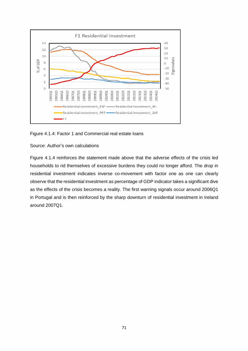
71
Figure 4.1.4: Factor 1 and Commercial real estate loans
Source: Author’s own calculations
Figure 4.1.4 reinforces the statement made above that the adverse effects of the crisis led
households to rid themselves of excessive burdens they could no longer afford. The drop in
residential investment indicates inverse co-movement with factor one as one can clearly
observe that the residential investment as percentage of GDP indicator takes a significant dive
as the effects of the crisis becomes a reality. The first warning signals occur around 2006Q1
in Portugal and is then reinforced by the sharp downturn of residential investment in Ireland
around 2007Q1.
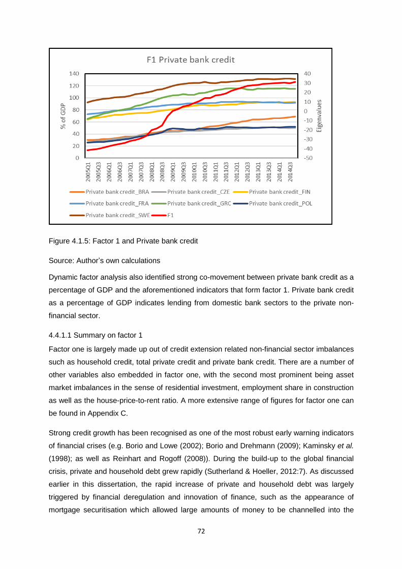
72
Figure 4.1.5: Factor 1 and Private bank credit
Source: Author’s own calculations
Dynamic factor analysis also identified strong co-movement between private bank credit as a
percentage of GDP and the aforementioned indicators that form factor 1. Private bank credit
as a percentage of GDP indicates lending from domestic bank sectors to the private non-
financial sector.
4.4.1.1 Summary on factor 1
Factor one is largely made up out of credit extension related non-financial sector imbalances
such as household credit, total private credit and private bank credit. There are a number of
other variables also embedded in factor one, with the second most prominent being asset
market imbalances in the sense of residential investment, employment share in construction
as well as the house-price-to-rent ratio. A more extensive range of figures for factor one can
be found in Appendix C.
Strong credit growth has been recognised as one of the most robust early warning indicators
of financial crises (e.g. Borio and Lowe (2002); Borio and Drehmann (2009); Kaminsky et al.
(1998); as well as Reinhart and Rogoff (2008)). During the build-up to the global financial
crisis, private and household debt grew rapidly (Sutherland & Hoeller, 2012:7). As discussed
earlier in this dissertation, the rapid increase of private and household debt was largely
triggered by financial deregulation and innovation of finance, such as the appearance of
mortgage securitisation which allowed large amounts of money to be channelled into the
73
mortgage market. It also helped facilitate the extension of mortgage credit to lower income
groups. Vulnerabilities on the balance sheets of non-financial firms and households can spill-
over to the financial sector as was the case with the global financial crisis. Rapid credit growth
tends to be accompanied by deregulation and a loosening of credit requirements to riskier
clients such as lower income groups. This was exactly the case in the global financial crisis
as it all started off with the defaults of borrowers in the subprime mortgage market of the US.
This resulted in liquidity shortages as well as solvency issues in the financial sector. Ultimately,
the financial sector amplified these vulnerabilities through the subsequent credit crunch forcing
the non-financial sector to unwind on a global scale (Rohn et al., 2015:13).
The strong presence of credit related vulnerabilities in factor 1 is therefore justified and
consistent with the findings of Hermansen and Rhon (2015:13) that credit and asset market
indicators prove to be particularly useful in predicting oncoming financial crises. Domestic
credit indicators emphasise the importance of unsustainable domestic credit booms within the
global financial crisis as early warning indicators.
4.4.2 Factor 2
The variance shares as per DFA for factor two will follow on the next page. Only variables with
a variance share of 75 percent and higher were taken into account. The variance share
threshold was lowered from 90 percent to 75 percent to make the pool of variables used to
determine factor two larger to ensure more accurate results.
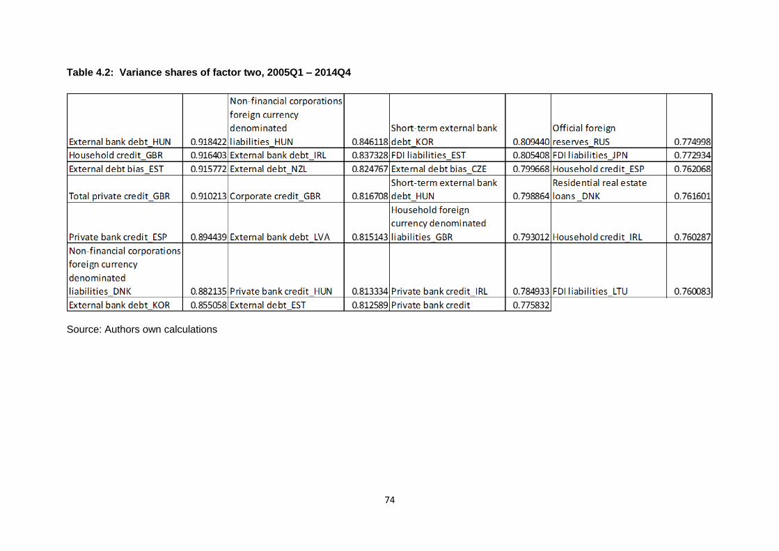
74
Table 4.2: Variance shares of factor two, 2005Q1 – 2014Q4
Source: Authors own calculations
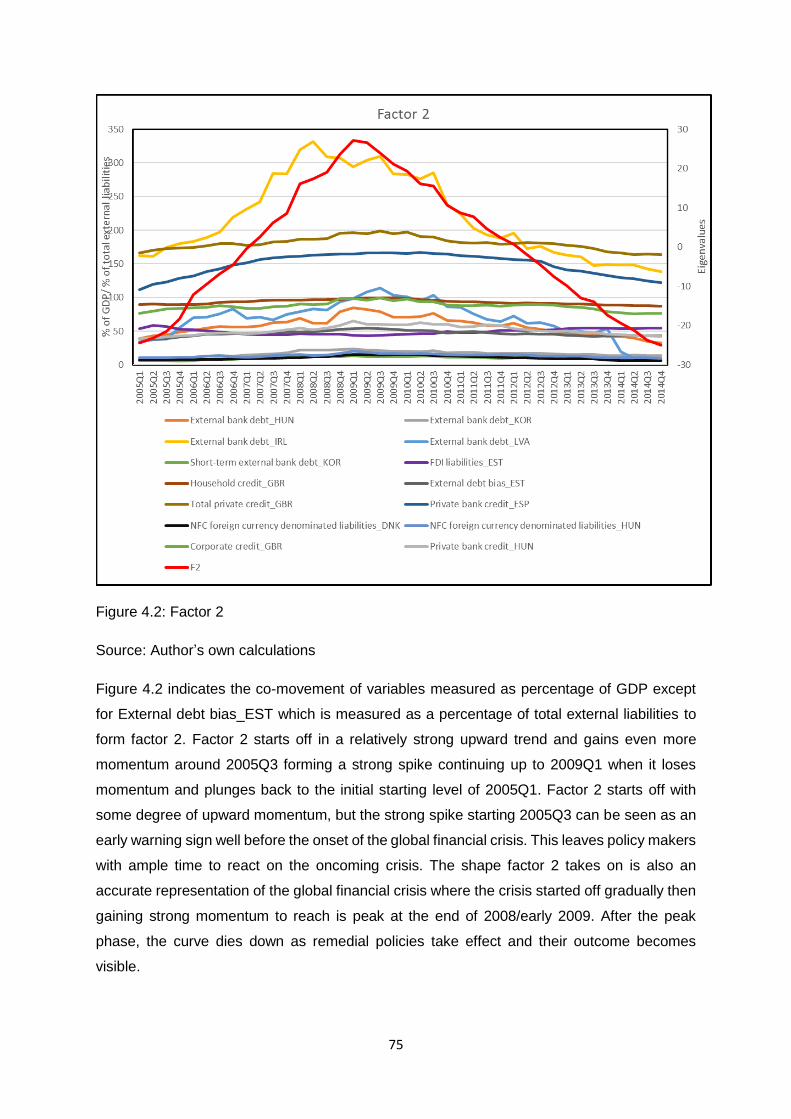
75
Figure 4.2: Factor 2
Source: Author’s own calculations
Figure 4.2 indicates the co-movement of variables measured as percentage of GDP except
for External debt bias_EST which is measured as a percentage of total external liabilities to
form factor 2. Factor 2 starts off in a relatively strong upward trend and gains even more
momentum around 2005Q3 forming a strong spike continuing up to 2009Q1 when it loses
momentum and plunges back to the initial starting level of 2005Q1. Factor 2 starts off with
some degree of upward momentum, but the strong spike starting 2005Q3 can be seen as an
early warning sign well before the onset of the global financial crisis. This leaves policy makers
with ample time to react on the oncoming crisis. The shape factor 2 takes on is also an
accurate representation of the global financial crisis where the crisis started off gradually then
gaining strong momentum to reach is peak at the end of 2008/early 2009. After the peak
phase, the curve dies down as remedial policies take effect and their outcome becomes
visible.
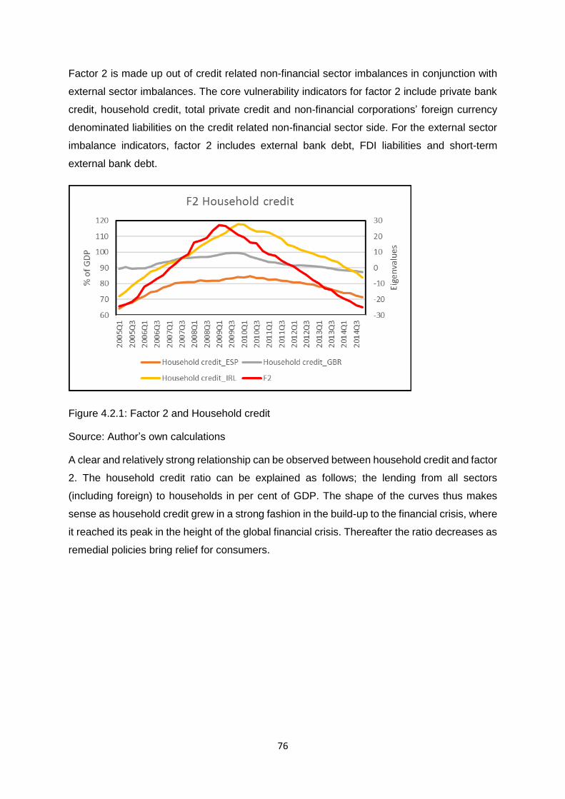
76
Factor 2 is made up out of credit related non-financial sector imbalances in conjunction with
external sector imbalances. The core vulnerability indicators for factor 2 include private bank
credit, household credit, total private credit and non-financial corporations’ foreign currency
denominated liabilities on the credit related non-financial sector side. For the external sector
imbalance indicators, factor 2 includes external bank debt, FDI liabilities and short-term
external bank debt.
Figure 4.2.1: Factor 2 and Household credit
Source: Author’s own calculations
A clear and relatively strong relationship can be observed between household credit and factor
2. The household credit ratio can be explained as follows; the lending from all sectors
(including foreign) to households in per cent of GDP. The shape of the curves thus makes
sense as household credit grew in a strong fashion in the build-up to the financial crisis, where
it reached its peak in the height of the global financial crisis. Thereafter the ratio decreases as
remedial policies bring relief for consumers.
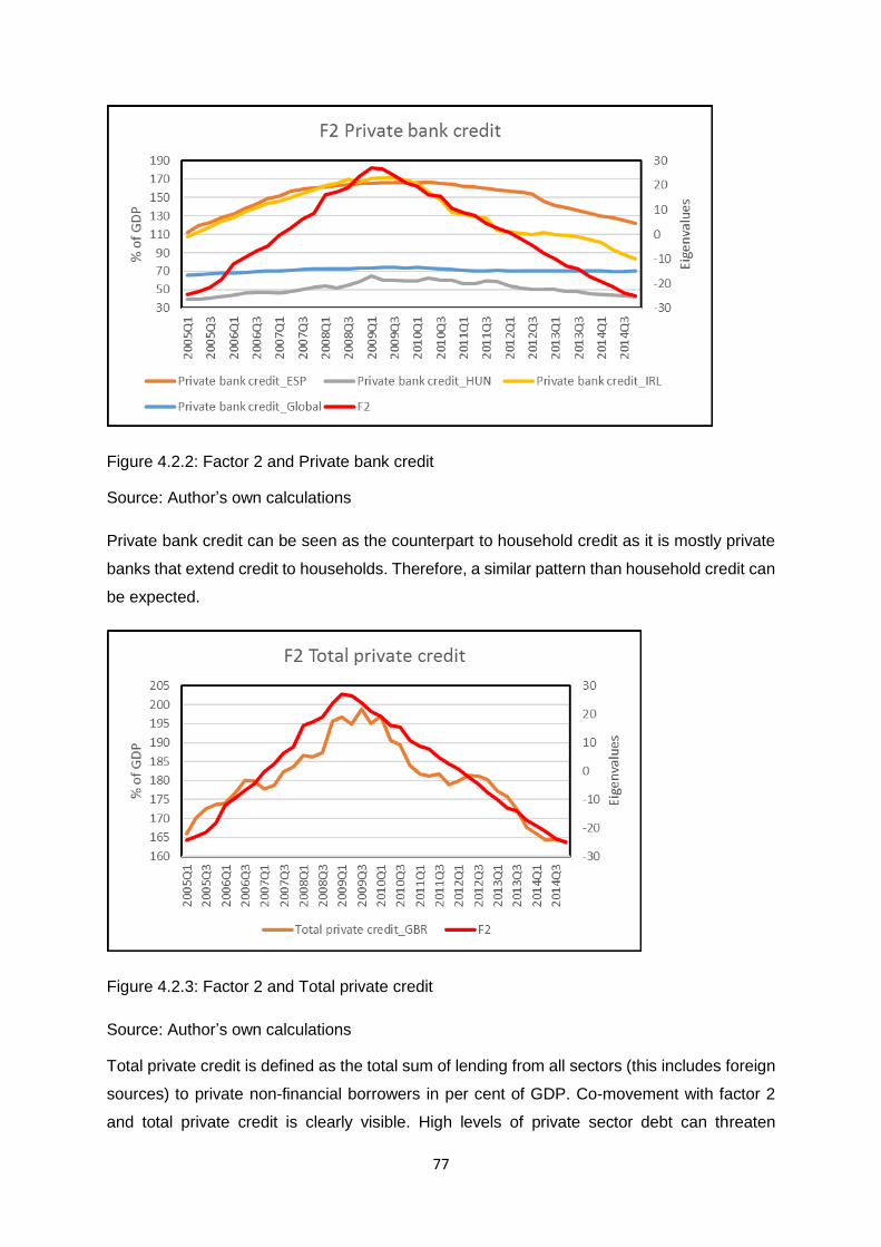
77
Figure 4.2.2: Factor 2 and Private bank credit
Source: Author’s own calculations
Private bank credit can be seen as the counterpart to household credit as it is mostly private
banks that extend credit to households. Therefore, a similar pattern than household credit can
be expected.
Figure 4.2.3: Factor 2 and Total private credit
Source: Author’s own calculations
Total private credit is defined as the total sum of lending from all sectors (this includes foreign
sources) to private non-financial borrowers in per cent of GDP. Co-movement with factor 2
and total private credit is clearly visible. High levels of private sector debt can threaten

78
sustainable economic growth. Within countries that are experiencing financial booms,
households and firms are in a vulnerable position as the risk of financial distress and
macroeconomic strains are ever present. Countries that were hit the hardest by the crisis, still
have high levels of private debt relative to output, making households and firms sensitive to
increases in interest rates. These countries could find themselves in a debt trap: seeking to
stimulate the economy through low interest rates, which encourages the taking-on of even
more debt, ultimately adding to the problem it is meant to solve.
Figure 4.2.4: Factor 2 and External bank debt
Source: Author’s own calculations
External bank debt is the total debt liabilities towards BIS reporting banks in per cent of GDP.
Both external bank debt and short-term external bank debt are indicators of integration through
international bank lending. International lending amplifies contagion shocks and increases the
risk of financial crises.
4.4.2.1 Summary of factor 2
Factor 2 is derived out of external sector imbalances in the likes of external bank debt, short-
term external bank debt, FDI liabilities as well as official foreign reserves. Factor 2 also
includes similar vulnerability indicators to that of factor 1 as some of the non-financial sector
imbalances were also identified to be useful early warning indicators. These vulnerability
indicators include; household credit, total private credit and private bank credit. A more
extensive range of figures for factor two can be found in Appendix C. The fact that these credit
related vulnerabilities feature in both factors, emphasises the usefulness of these indicators

79
to serve as early warning indicators. As previously mentioned these findings are in line with
results gathered from Hermansen and Rhon (2015) in the sense of being indicators that can
be monitored to serve as early warning indicators. The DFA model also indicates that external
sector imbalances can potentially serve as a useful early warning indicator. Bernanke (2009)
found that external imbalances feature prominently among the potential causes of both the
global financial crisis of 2008 as well as the sovereign debt crisis in the Eurozone (Chen, et
al., 2012).
4.5 Conclusion
By making use of Dynamic factor analysis, the core variables that can aid in forecasting future
financial crises were identified. The DFA model facilitated the process of data reduction and
grouped variables that co-vary with one another and can potentially serve as early warning
indicators to warn policymakers of oncoming crises. Both factor one and two include credit
related non-financial sector imbalance indicators as the main factors that tend to co-vary. More
specifically, these factors include household credit, private bank credit and total private credit.
However, the majority of the variables that were identified by the model as part of factors one
and two, were also found to be useful as early warning indicators by Hermansen and Rhon
(2015).
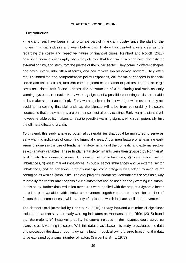
80
CHAPTER 5: CONCLUSION
5.1 Introduction
Financial crises have been an unfortunate part of financial industry since the start of the
modern financial industry and even before that. History has painted a very clear picture
regarding the costly and repetitive nature of financial crises. Reinhart and Rogoff (2010)
described financial crises aptly when they claimed that financial crises can have domestic or
external origins, and stem from the private or the public sector. They come in different shapes
and sizes, evolve into different forms, and can rapidly spread across borders. They often
require immediate and comprehensive policy responses, call for major changes in financial
sector and fiscal policies, and can compel global coordination of policies. Due to the large
costs associated with financial crises, the construction of a monitoring tool such as early
warning systems are crucial. Early warning signals of a possible oncoming crisis can enable
policy makers to act accordingly. Early warning signals in its own right will most probably not
avoid an oncoming financial crisis as the signals will arise from vulnerability indicators
suggesting that the symptoms are on the rise if not already existing. Early warning signals will
however enable policy makers to react to possible warning signals, which can potentially limit
the ultimate effects of a crisis.
To this end, this study analysed potential vulnerabilities that could be monitored to serve as
early warning indicators of oncoming financial crises. A common feature of all existing early
warning signals is the use of fundamental determinants of the domestic and external sectors
as explanatory variables. These fundamental determinants were then grouped by Rohn et al.
(2015) into five domestic areas: 1) financial sector imbalances, 2) non-financial sector
imbalances, 3) asset market imbalances, 4) public sector imbalances and 5) external sector
imbalances, and an additional international “spill-over” category was added to account for
contagion as well as global risks. The grouping of fundamental determinants serves as a way
to simplify the vast number of possible indicators that can be used as early warning indicators.
In this study, further data reduction measures were applied with the help of a dynamic factor
model to pool variables with similar co-movement together to create a smaller number of
factors that encompasses a wider variety of indicators which indicate similar co-movement.
The dataset used (compiled by Rohn et al., 2015) already included a number of significant
indicators that can serve as early warning indicators as Hermansen and Rhön (2015) found
that the majority of these vulnerability indicators included in their dataset could serve as
plausible early warning indicators. With this dataset as a base, this study re-evaluated the data
and processed the data through a dynamic factor model, allowing a large fraction of the data
to be explained by a small number of factors (Sargent & Sims, 1977).
81
5.2 Conclusion
The main aim of the study was to re-examine the 70+ indicators identified by Rohn et al. (2015)
to identify parsimonious indicators of financial crises. The dynamic factor model used identified
indicators that co-vary between countries and over time. The ABC criteria implemented to
determine the number of static factors suggested that two static factors be used. The two
factors specified was then identified as i) factor 1; private non-financial sector imbalances
which includes asset market imbalances and ii) factor 2; private non-financial sector
imbalances however, more focused on private bank credit and external debt whereas factor 1
is more concerned with household and private credit.
More specifically, factor 1 mainly comprises credit-related private non-financial sector
imbalances such as household credit as percentage of GDP, total private credit as percentage
of GDP, private bank credit as percentage of GDP, corporate credit as percentage of GDP.
Factor 1 is also strongly represented by asset market imbalance indicators. The asset market
imbalance indicators include residential investment, employment share in construction and
the house-price-to-rent ratio. These indicators are relevant in the build-up to periods of
financial crisis as they would usually experience drastic changes from pre-crisis periods to
times of actual financial crisis. These indicators were also pooled together because of their
similar co-movement during periods of shock.
Factor 2 consists of similar credit-related non-financial sector imbalances in combination with
external sector imbalances. The highest degree of co-movement between indicators for factor
2 includes private bank credit, household credit, total private credit and non-financial
corporation’s foreign currency denominated liabilities on the credit related non-financial sector
side. For the external sector imbalance indicators, factor 2 includes external bank debt, FDI
liabilities and short-term external bank debt. Once again, these vulnerability indicators are
most likely to experience similar radical co-movement during the build-up phase to financial
crises as well as times of actual financial crisis.
The majority of the indicators that were identified by the dynamic factor model as part of factors
one and two, was also found to be useful as early warning indicators by Hermansen and Rhon
(2015). However, the dynamic factor model simplified the monitoring process as the two
factors identified encompasses a large number of useful early warning indicators proposed by
Hermansen and Rhön (2015). Subsequently, these two factors could in theory be monitored
rather than a large set of variables acting as a drain on precious resources.
82
5.3 Recommendations for future research
The majority of vulnerability indicators within the proposed dataset is domestic indicators.
Whilst this is not necessarily bad, as country specific vulnerabilities can be addressed, the
high level of interconnectedness of the global economy calls for more emphasis to be put on
global vulnerabilities. Future research should include a wider variety of global vulnerability
indicators to account for interconnectedness and contagion. Global indicators in this study
were few and due to the nature of dynamic factor analysis, limited co-movement between the
identified factors and global indicators could be established.
The study indicated that the process of data reduction through dynamic factor analysis whilst
still achieving accurate results is plausible as the DFM pooled co-varying indicators together
as indicators of financial crises. Indicators of financial crises are therefore confirmed; however,
the actual usage of these indicators as early warning signals are still widely debated.
Additional research regarding the implementation of these indicators as early warning signals
should be investigated – more specifically, regarding the timing of crises.
83
References
Adrian, T. & Shin, H. S., 2008. Liquidity and financial contagion. Financial Stability Review,
11, pp. 1-9.
Ahrend, R. & Goujard, A., 2012. Drivers of Systemic Banking Crises: The Role of Bank-
Balance-Sheet Contagion and Financial Account Structure. Organisation for Economic Co-
operation and Development, 902, pp. 1-43.
Aizenman, J., Chinn, M. D. & Ito, H., 2008. Assessing the Emerging Global Financial
Architecture: Measuring the Trilemma's Configurations over Time. National Bureau of
Economic Research, 14533, pp. 1-73.
Ajevskis, V. & Davidsons, G., 2008. Dynamic Factor Models in Forecasting Latvia's Gross
Domestic Product. Bank of Latvia Working Papers.
Aldean, C. & Brooks, A., 2010. Recognizing a Financial Crisis. Economics of Crisis, pp. 1-9.
Allen, F., Babus, A. & Carletti, E., 2009. Financial Crises: Theory and Evidence. Annual
Review of Financial Economics, 1, pp. 97-116.
Alessi, L., Barigozzi, M. & Capasso, M. 2008. A Robust Criterion for Determining the
Number of Static Factors in Approximate Factor Models. European Central Bank Working
Paper Series, 903.
Altissimo, F., Cristadoro, R., Forni, M., Lippi, M. & Veronese, G. 2010. Tracking Economic
Growth in Real Time. The Review of Economics and Statistics, 92, pp. 1024-1034.
Amadeo, K., 2016. What caused the 2008 Global Financial Crisis?, s.l.: The Balance.
Anderson, S., 2018. International Financing Review. [Online]
Available at: http://www.ifre.com/a-history-of-the-past-40-years-in-financial-
crises/21102949.fullarticle
[Accessed 11 October 2018].
Andrè, C., 2010. A bird's eye view of OECD housing markets. Organisation for Economic
Co-operation and Development , 746, pp. 1-36.
Babecky, J. et al. 2011. Early Warning Indicators of Economic Crises: Evidence from a
Panel of 40 Developed Countries. Czech National Bank Research, C3, pp. 1-72.
Babecky, J. et al. 2013. Leading indicators of crisis incidence: Evidence from developed
countries. Journal of International Money and Finance, 35(C), pp. 1-19.
Bai, J. & Ng, S. 2002. Determining the Number of Factors in Approximate Factor Models.
Econometrica, 70, pp. 191-221.
Baldacci, E. et al. 2011. Assessing Fiscal Stress. International Monetary Fund, 100, pp. 1-
41.
Bank for International Settlements, 2012. Financial sector regulation for growth, equity and
stability. BIS Papers, 62, pp. 1-152.
84
Barrell, R., Davis, E. P., Karim, D. & Liadze , I., 2010. Calibrating Macroprudential Policy.
Bank for International Settlements, 165, pp. 1-22.
Behn, M., Detken, C., Peltonen, T. A. & Schudel, W., 2013. Setting Countercyclical Capital
Buffers Based on Early Warning Models. European Central Bank, 1725-2806, pp. 1-39.
Benetrix, A., Lane, P. R. & Shambaugh, J. C. 2015. International Currency Exposures,
Valuation Effects, and the Global Financial Crisis. National Bureau of Economic Research,
20820.
Bentley, K., 2015. The 2008 Financial Crisis: How Deregulation Led to the crisis. Lake
Forest Publications, pp. 1-80.
Bilson, J. F. O. & Frenkel, J. A., 1979. Dynamic Adjustment and the Demand for
International Reserves. National Bureau of Economic Research Working Paper Series,
0407.
Blanchard, O. & Milesi-Ferretti, G. M., 2009. Global Imbalances: In Midstream?. International
Monetary Fund, 29, pp. 1-31.
Blundell-Wignall, A., Atkinson , P. & Roulet, C., 2014. Bank business models and the Basel
system: Complexity and interconnectedness. Financial Market Trends, 2013/2, pp. 1-26.
Bordo, M., Eichengreen, B., Klingebiel, D. & Martinez-Peria, M. S., 2001. Is the crisis
problem growing more severe?. Wiley- Blackwell Centre for Economic Policy Research,
April, 16(32), pp. 53-82.
Borio, C. & Drehmann, M. 2009. Assessing the risk of banking crises - revisited. Bank for
International Settlements, 3, pp. 29-46.
Borio, C. & Lowe, P., 2002. Assessing the risk of banking crises. Bank for International
Settlements, 12, pp. 43-54.
Borio, C. & Zhu, H., 2008. Capital regulation, risk-taking and monetary policy: a missing link
in the transmission mechanism?. Bank for International Settlements, 268, pp. 1-46.
Cavallo, E. & Frankel, J., 2008. Does Openness to Trade Make Countries More Vulnerable
to Sudden Stops, or Less? Using Gravity to Establish Causality. Journal of International
Money and Finance, 27(8), pp. 1430-1452.
Cesaroni, T., 2013. Early warning indicators of economic crises. Bank of Italy.
Chamon, M. & Crowe, C., 2012. Predictive Indicators of Financial Crises. International
Monetary Fund.
Chen, H., Curdia, V. & Ferrero, A., 2012. The Macroeconomic Effects of Large-scale Asset
Purchase Programs. The Economic Journal, 49, pp. 50-79.
Chmelar, A. Household Debt and the European Crisis. Centre for European Policy Studies,
13.

85
Claassen, C., 2016. The state of decoupling before and during the great recession. [Online]
Available at: https://repository.nwu.ac.za/handle/10394/17993
[Accessed 14 May 2018].
Claessens, S., Kose, A. M. & Terrones, M. E., 2011. How Do Business and Financial Cycles
Interact?. International Monetary Fund Working Paper, 88, pp. 1-54.
Claessens, S. & Kose, A. M., 2013. Financial Crises: Explanations, Types, and Implications.
IMF Working Paper, January, 13(28), pp. 3-65.
Clavel, L. & Minodier, C., 2009. A monthly indicator of the French business climate.
Documents de Travail de la DESE.
Corsetti, G., Meier, A. & Muller, G. J., 2012. What Determines Government Spending
Multipliers?. International Monetary Fund, 150, pp. 1-45.
Drehmann, M. & Juselius, M., 2013. Evaluating early warning indicators of banking. Bank for
International Settlements, 421, pp. 1-35.
Dunaway, S., 2009. Global Imbalances and the Financial Crisis. Council on Foreign
Relations, 44, pp. 1-41.
Durbin, J. & Koopman, S. J. 2012. Time Series analysis by State Space Methods: Second
Edition. Oxford Statistical Science Series.
Duval, R., Elmeskov, J. & Vogel, L., 2007. Structural Policies and Economic Resilience to
Shocks. Organisation for Economic Co-operation and Development, 567, pp. 1-53.
Edwards, S., 2004. Managing the Capital Account. University of California.
Edwards, S., 2005. Capital Controls, Sudden Stops and current Account Reversals. National
Bureau of Economic Research, 11170, pp. 1-58.
Eichengreen, B. & Portes, R., 1987. The Anatomy of Financial Crises. National Bureau of
Economic Research, January, 2126, pp. 1-83.
Fetiniuc, V., Ivan, L. & Gherbovet, S., 2014. Speculative bubbles and financial crises.
Research Papers in Economics, pp. 1-10.
FINCAD, 2017. COLLATERALIZED DEBT OBLIGATIONS (CDOS), s.l.: FINCAD.
FitzGerald, 2008. Short-Term Capital Flows, The Real Economy And Income Distribution In
Developing Countries. Queen Elizabeth House Working Paper Series, 8.
Flood, R. P. & Garber, P. M., 1984. Collapsing exchange-rate regimes: Some linear
examples. Journal of International Economics, 17(1), pp. 1-13.
Frankel, J. A. & Rose, A. K., 1996. Currency crashes in emerging markets: an empirical
treatment. International Finance Discussion Papers, 534.
Frankel, J. & Saravelos, G., 2012. Can leading indicators assess country vulnerability?
Evidence from the 2008-09 global financial crisis. Journal of International Economics, 87, pp.
216-231.

86
Furceri, D., Guichard, S. & Rusticelli, E., 2011. Episodes of Large Capital Inflows and the
Likelihood of Banking and Currency Crises and Sudden Stops. Organisation for Economic
Co-operation and Development, 34(865), pp. 1-36.
Garber, P. M., 2000. Famous First Bubbles. The MIT Press, pp. 1-167.
Geweke, J. 1977. The Dynamic Factor Analysis of Economic Time Series Models.
Ghosh, A. & Ramakrishnan, U., 2012. Current Account Deficits: Is There a Problem, s.l.:
International Monetary Fund.
Giannone, D., Reichlin, L. & Sala, L., 2004. Monetary Policy in Real Time. National Bureau
of Economic Research, 19, pp. 161-224.
Girouard, N., Kennedy, M., Van den Noord, P. & Andre , C., 2006. Recent House Price
Developments. Organisation for Economic Co-operation and Development, 475, pp. 1-60.
Glick, R. & Hutchinson, M., 2011. Currency Crises. Federal Reserve Bank of San Fransisco,
September, 2011, pp. 1-31.
Goldstein, M., 1998. The Asian Financial Crisis: Causes, Cures, and Systematic
Implications. 1 ed. Washington DC: Institute of International Economics.
Gourinchas, P.-O. & Obstfeld, M., 2011. Stories of the Twentieth Century for the Twenty-
First. National Bureau of Economic Research, pp. 1-69.
Gorman, W. M., 1981. Some Engel Curves. Essays in the Theory and Measurements of
Consumer Behaviour, Cambridge University Press.
Grauwe, P. D., 2008. THe Banking Crisis: Causes, Consequences an Remedies. Centre for
European Policy Studies, November, 187, pp. 1-12.
Hallin, M. & Liska, R. 2012. Determining the Number of Factors in the General Dynamic
Factor Model. Journal of the American Statistical Association, 478.
Hermansen, M. & Rhön, O., 2015. Economic Resilience: The Usefulness of Early Warning
Indicators in OECD Countries. OECD Economics Department Working Papers, 150, pp. 1-
30.
Hervey , J. L. & Merkel, L. S., 2001. A record current account deficit: Causes and
implications. Federal Reserve Bank of Chicago, pp. 1-12.
Hoggarth, G., Reidhill, J. & Sinclair, P., 2004. On the resolution of banking crises: theory and
evidence. Bank of England, 229, pp. 1-29.
Jeasakul, P., 2005. Sudden Stops of International Capital Flows: Causes and
Consequences. [Online]
Available at: file:///C:/Users/NWU%20User/Downloads/studenttheses_245-OBJ.pdf
[Accessed 27 May 2017].
Jin, X. & De Simone, F. N. 2012. An Early-warning and Dynamic Forecasting Framework of
Default Probabilities for the Macroprudential Policy Indicators Arsenal. Central Bank of
Luxembourg Working Papers, 75.
87
Jorda, O., Schularick, M. & Taylor, A. M., 2012. When Credit Bites Back: Leverage,
Business Cycles, and Crises. Federal Reserve Bank of San Fransisco Working Paper
Series, 27, pp. 1-42.
Kaminsky, G., Lizondo, S. & Reinhart, C. M., 1998. Leading indicators of currency crises.
International Monetary Fund, 45, pp. 1-48.
Kaminsky, G. L. & Reinhart, C. M., 1996. The Twin Crises: The Causes of Banking and
Balance-of-Payments Problems. International Finance Discussion Papers, 544, pp. 1-28.
Kitroeff, N. & Weisenthal, J. 2014. Here's Why the Russian Ruble Is Collapsing. [Online]
Available at: https://www.bloomberg.com/news/articles/2014-12-16/no-caviar-is-not-getting-
cheaper-everything-you-need-to-know-about-the-russian-ruble-collapse
[Accessed 03 October 2018]
Koopman, S. J., Lucas, A. & Schwaab, B. 2011. Modelling frailty-correlated defaults using
many macroeconomic covariates. European Central Bank.
Kopits, G., 2014. Ireland's Fiscal Framework: Options for the Future. The Economic and
Social Review, 45(1), pp. 135-158.
Krugman, P., 1979. Increasing Returns, Monopolistic Competition and International Trade.
Journal of International Economics, 9, pp. 469-479.
Laeven, L. & Valencia, F., 2010. Resolution of Banking Crises: The Good, the Bad, and the
Ugly. International Monetary Fund, June.pp. 1-36.
Lane, P. R. & Milesi-Ferretti, G. M., 2014. Global Imbalances and External Adjustment after
the Crisis. International Monetary Fund, 151, pp. 1-44.
Lestano, N. V., Jacobs, J. & Kuper, G. H., 2003. Indicators of financial crises do work! An
early-warning system for six Asian countries. University of Groningen, pp. 1-39.
Lewbel, A. 1991. The Rank of Demand Systems: Theory and Nonparametric Estimation.
Econometrica, 59, pp. 711-730.
Lo Duca, M. & Peltonen, T. A., 2013. Assessing systemic risks and predicting systemic
events. Journal of Banking & Finance, 37, pp. 2183-2195.
Lo, A. W., 2011. Fear, Greed, and Financial Crises: A Cognitive Neurosciences Perspective.
Massachusetts Institute of Technology, pp. 622-662.
Menden, C. & Proano, C. 2017. Dissecting the financial cycle with dynamic factor models.
The Macroeconomic Policy Institute, 183.
McDonald, O., 2016. The Repeal of the Glass-Steagall Act: Myth and Reality, s.l.: Cato
Institute.
Merrouche, O. & Nier, E., 2010. What Caused the Global Financial Crisis? - Evidence on the
Drivers of Financial Imbalances 1999-2007. International Monetary Fund, 10(265), pp. 1-64.
Milesi-Ferretti, G. M. & Razin, A., 1998. Sustainability of Persistent Current Account Deficits.
National Bureau of Economic Research, 5467.
88
Obstfeld, M., 2012. Does the Current Account still matter?. National Bureau of Economic
Research, March, 17877, pp. 1-64.
Ollivaud, P. & Turner, D., 2015. The effect of the global financial crisis on OECD potential
output. Organisation for Economic Co-operation and Development, 2014, pp. 41-60.
Organisation for Economic Co-operation and Development, 2017. OECD Economic Outlook
2017. 2017:2.
Reinhart, C. M. & Rogoff, K. S., 2010. From Financial Crash To Debt Crisis. National Bureau
of Economic Research, 15795, pp. 1-48.
Reinhart, C. M. & Rogoff, K. S., 2013. Financial and Sovereign Debt Crisis: Some Lessons
Learned and those forgotten. International Monetary Fund, 13/266, pp. 1-21.
Rohn, O., Sanchez, A. C., Hermansen, M. & Rasmussen, M., 2015. Economic Resilience: A
New Set Of Vulnerability Indicators for OECD Countries. Organisation for Economic Co-
operation and Development, 1249, pp. 1-41.
Rose, A. K. & Spiegel, M. M., 2009. Cross-Country Causes and Consequences of the 2008
Crisis: International Linkages and American Exposure. National Bureau of Economic
Research Working Paper Series, 15(3), pp. 340-363.
Ross, S. A. 1977. The Determination of Financial Structure: The Incentive-Signalling
Approach. The Bell Journal of Economics, 8, pp. 23-40.
Sargent, T. J. & Sims, C. A., 1977. Business Cycle Modeling Without Pretending to Have
Too Much A Priori Economic Theory. Federal Reserve Bank of Minneapolis, 55, pp. 1-88.
Sheen, J., Truck, S., Truong, C. & Wang, B. Z. 2016. Early Warning Indicators of Systemic
Financial Risk in an International Setting. [Online]
Available at: http://www-econ2.kwansei.ac.jp/~efujii/Sheen.pdf
[Accessed 23 August 2018].
Shin, H. S., 2013. Procyclicality and the Search for Early Warning Indicators. International
Monetary Fund Working Paper Series, 13258, pp. 1-15.
Stiglitz, J. E., 2010 (A). Freefall. 1st ed. New York: W.W. Norton & Company.
Stiglitz, J. E., 2010 (B). Risk and Global Economic Architecture: Why Full Financial
Integration May Be Undesirable. National Bureau of Economic Research, 15718, pp. 1-12.
Stock, J. H. & Watson, M. W., 2010. Dynamic Factor Models. [Online]
Available at: https://www.princeton.edu/~mwatson/papers/dfm_oup_4.pdf
[Accessed 22 August 2018].
Sutherland, D. & Hoeller, P., 2012. Debt and Macroeconomic Stability: An Overview of the
Literature and some Empirics. Organisation for Economic Co-operation and Development
Working Paper, 1006, pp. 1-36.
Taylor, J. B., 2007. Housing and Monetary Policy. National Bureau of Economic Research,
13682, pp. 1-16.
89
Taylor, A. M., 2012. The Great Leveraging. Bank for International Settlements, 621.
The Economist, 2012. A brief history of financial crises, s.l.: s.n.
The Economist, 2012. Essay. [Online]
Available at: http://www.economist.com/news/essays-aspects-today-s-financial-crisis-
history.com
[Accessed 14 March 2016].
The World Bank, 2016. Banking Crisis, Washington, D.C.: World Bank.
Vasilenko, A. 2018. Systemic Risk and Financial Fragility in the Chinese Economy: A
Dynamic Factor Model Approach. Bank of Russia: Research and Forecasting Department.
Vasicek, B. et al. 2016. Comparing different early warning systems: Results from a horse
race competition among members of the Macro-prudential Research Network. European
Central Bank, pp. 1-27.
Wang, P. & Wen, Y., 2009. Speculative bubbles and financial crises. Federal Bank of St.
Louis, pp. 1-24.
Woetzel, J., Chen, Y., Manyika, J., Roth, E., Seong, J. & Lee, J., 2015. The China Effect on
Global Innovation. Mckinsey Global Institute.
Zuur, A. F., Fryer, R. J., Jolliffe, I. T., Dekker, R. & Beukema, J. J., 2003. Estimating
common trends in multivariate time series using dynamic factor analysis. Environmetrics, 14.
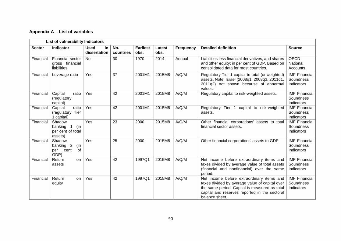
90
Appendix A – List of variables
List of vulnerability Indicators
Sector Indicator Used in dissertation
No. countries
Earliest obs.
Latest obs.
Frequency Detailed definition Source
Financial Financial sector gross financial liabilities
No 30 1970 2014 Annual Liabilities less financial derivatives, and shares and other equity; in per cent of GDP. Based on consolidated data for most countries.
OECD National Accounts
Financial Leverage ratio Yes 37 2001M1 2015M8 A/Q/M Regulatory Tier 1 capital to total (unweighted) assets. Note: Israel (2008q1, 2008q3, 2011q1, 2011q2) not shown because of abnormal values.
IMF Financial Soundness Indicators
Financial Capital ratio (regulatory capital)
Yes 42 2001M1 2015M8 A/Q/M Regulatory capital to risk-weighted assets. IMF Financial Soundness Indicators
Financial Capital ratio (regulatory Tier 1 capital)
Yes 42 2001M1 2015M8 A/Q/M Regulatory Tier 1 capital to risk-weighted assets.
IMF Financial Soundness Indicators
Financial Shadow banking 1 (in per cent of total assets)
Yes 23 2000 2015M8 A/Q/M Other financial corporations' assets to total financial sector assets.
IMF Financial Soundness Indicators
Financial Shadow banking 2 (in per cent of GDP)
Yes 25 2000 2015M8 A/Q/M Other financial corporations' assets to GDP. IMF Financial Soundness Indicators
Financial Return on assets
Yes 42 1997Q1 2015M8 A/Q/M Net income before extraordinary items and taxes divided by average value of total assets (financial and nonfinancial) over the same period.
IMF Financial Soundness Indicators
Financial Return on equity
Yes 42 1997Q1 2015M8 A/Q/M Net income before extraordinary items and taxes divided by average value of capital over the same period. Capital is measured as total capital and reserves reported in the sectoral balance sheet.
IMF Financial Soundness Indicators
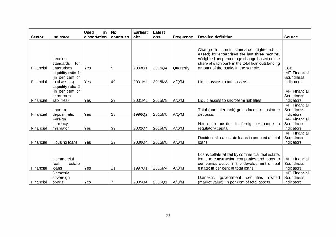
91
Sector Indicator Used in dissertation
No. countries
Earliest obs.
Latest obs. Frequency Detailed definition Source
Financial
Lending standards for enterprises Yes 9 2003Q1 2015Q4 Quarterly
Change in credit standards (tightened or eased) for enterprises the last three months. Weighted net percentage change based on the share of each bank in the total loan outstanding amount of the banks in the sample. ECB
Financial
Liquidity ratio 1 (in per cent of total assets) Yes 40 2001M1 2015M8 A/Q/M Liquid assets to total assets.
IMF Financial Soundness Indicators
Financial
Liquidity ratio 2 (in per cent of short-term liabilities) Yes 39 2001M1 2015M8 A/Q/M Liquid assets to short-term liabilities.
IMF Financial Soundness Indicators
Financial Loan-to-deposit ratio Yes 33 1996Q2 2015M8 A/Q/M
Total (non-interbank) gross loans to customer deposits.
IMF Financial Soundness Indicators
Financial
Foreign currency mismatch Yes 33 2002Q4 2015M8 A/Q/M
Net open position in foreign exchange to regulatory capital.
IMF Financial Soundness Indicators
Financial Housing loans Yes 32 2000Q4 2015M8 A/Q/M Residential real estate loans in per cent of total loans.
IMF Financial Soundness Indicators
Financial
Commercial real estate loans Yes 21 1997Q1 2015M4 A/Q/M
Loans collateralized by commercial real estate, loans to construction companies and loans to companies active in the development of real estate; in per cent of total loans.
IMF Financial Soundness Indicators
Financial
Domestic sovereign bonds Yes 7 2005Q4 2015Q1 A/Q/M
Domestic government securities owned (market value); in per cent of total assets.
IMF Financial Soundness Indicators
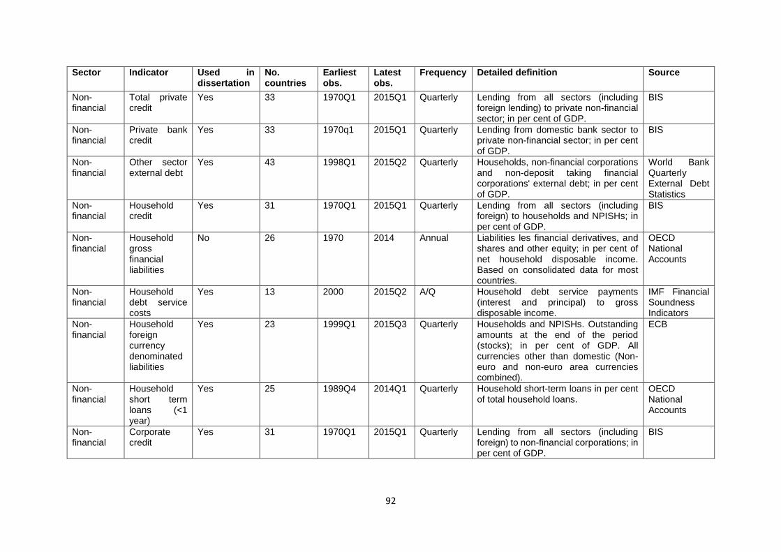
92
Sector Indicator Used in dissertation
No. countries
Earliest obs.
Latest obs.
Frequency Detailed definition Source
Non-financial
Total private credit
Yes 33 1970Q1 2015Q1 Quarterly Lending from all sectors (including foreign lending) to private non-financial sector; in per cent of GDP.
BIS
Non-financial
Private bank credit
Yes 33 1970q1 2015Q1 Quarterly Lending from domestic bank sector to private non-financial sector; in per cent of GDP.
BIS
Non-financial
Other sector external debt
Yes 43 1998Q1 2015Q2 Quarterly Households, non-financial corporations and non-deposit taking financial corporations' external debt; in per cent of GDP.
World Bank Quarterly External Debt Statistics
Non-financial
Household credit
Yes 31 1970Q1 2015Q1 Quarterly Lending from all sectors (including foreign) to households and NPISHs; in per cent of GDP.
BIS
Non-financial
Household gross financial liabilities
No 26 1970 2014 Annual Liabilities les financial derivatives, and shares and other equity; in per cent of net household disposable income. Based on consolidated data for most countries.
OECD National Accounts
Non-financial
Household debt service costs
Yes 13 2000 2015Q2 A/Q Household debt service payments (interest and principal) to gross disposable income.
IMF Financial Soundness Indicators
Non-financial
Household foreign currency denominated liabilities
Yes 23 1999Q1 2015Q3 Quarterly Households and NPISHs. Outstanding amounts at the end of the period (stocks); in per cent of GDP. All currencies other than domestic (Non-euro and non-euro area currencies combined).
ECB
Non-financial
Household short term loans (<1 year)
Yes 25 1989Q4 2014Q1 Quarterly Household short-term loans in per cent of total household loans.
OECD National Accounts
Non-financial
Corporate credit
Yes 31 1970Q1 2015Q1 Quarterly Lending from all sectors (including foreign) to non-financial corporations; in per cent of GDP.
BIS
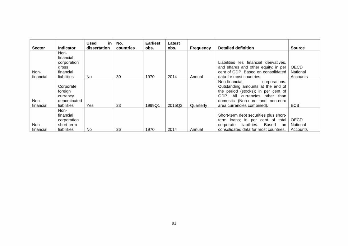
93
Sector Indicator Used in dissertation
No. countries
Earliest obs.
Latest obs. Frequency Detailed definition Source
Non-financial
Non-financial corporation gross financial liabilities No 30 1970 2014 Annual
Liabilities les financial derivatives, and shares and other equity; in per cent of GDP. Based on consolidated data for most countries.
OECD National Accounts
Non-financial
Corporate foreign currency denominated liabilities Yes 23 1999Q1 2015Q3 Quarterly
Non-financial corporations. Outstanding amounts at the end of the period (stocks); in per cent of GDP. All currencies other than domestic (Non-euro and non-euro area currencies combined). ECB
Non-financial
Non-financial corporation short-term liabilities No 26 1970 2014 Annual
Short-term debt securities plus short-term loans; in per cent of total corporate liabilities. Based on consolidated data for most countries.
OECD National Accounts
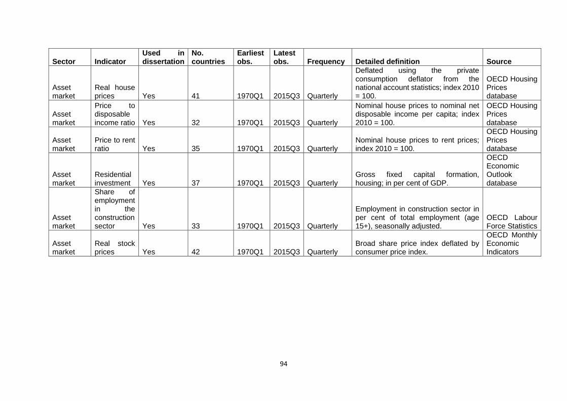
94
Sector Indicator Used in dissertation
No. countries
Earliest obs.
Latest obs. Frequency Detailed definition Source
Asset market
Real house prices Yes 41 1970Q1 2015Q3 Quarterly
Deflated using the private consumption deflator from the national account statistics; index 2010 = 100.
OECD Housing Prices database
Asset market
Price to disposable income ratio Yes 32 1970Q1 2015Q3 Quarterly
Nominal house prices to nominal net disposable income per capita; index 2010 = 100.
OECD Housing Prices database
Asset market
Price to rent ratio Yes 35 1970Q1 2015Q3 Quarterly
Nominal house prices to rent prices; index 2010 = 100.
OECD Housing Prices database
Asset market
Residential investment Yes 37 1970Q1 2015Q3 Quarterly
Gross fixed capital formation, housing; in per cent of GDP.
OECD Economic Outlook database
Asset market
Share of employment in the construction sector Yes 33 1970Q1 2015Q3 Quarterly
Employment in construction sector in per cent of total employment (age 15+), seasonally adjusted.
OECD Labour Force Statistics
Asset market
Real stock prices Yes 42 1970Q1 2015Q3 Quarterly
Broad share price index deflated by consumer price index.
OECD Monthly Economic Indicators
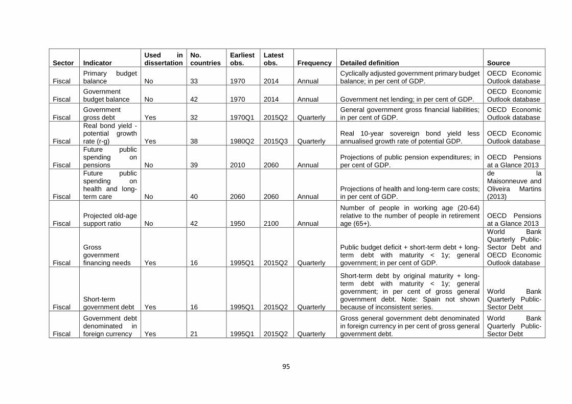
95
Sector Indicator Used in dissertation
No. countries
Earliest obs.
Latest obs. Frequency Detailed definition Source
Fiscal Primary budget balance No 33 1970 2014 Annual
Cyclically adjusted government primary budget balance; in per cent of GDP.
OECD Economic Outlook database
Fiscal Government budget balance No 42 1970 2014 Annual Government net lending; in per cent of GDP.
OECD Economic Outlook database
Fiscal Government gross debt Yes 32 1970Q1 2015Q2 Quarterly
General government gross financial liabilities; in per cent of GDP.
OECD Economic Outlook database
Fiscal
Real bond yield - potential growth rate (r-g) Yes 38 1980Q2 2015Q3 Quarterly
Real 10-year sovereign bond yield less annualised growth rate of potential GDP.
OECD Economic Outlook database
Fiscal
Future public spending on pensions No 39 2010 2060 Annual
Projections of public pension expenditures; in per cent of GDP.
OECD Pensions at a Glance 2013
Fiscal
Future public spending on health and long-term care No 40 2060 2060 Annual
Projections of health and long-term care costs; in per cent of GDP.
de la Maisonneuve and Oliveira Martins (2013)
Fiscal Projected old-age support ratio No 42 1950 2100 Annual
Number of people in working age (20-64) relative to the number of people in retirement age (65+).
OECD Pensions at a Glance 2013
Fiscal
Gross government financing needs Yes 16 1995Q1 2015Q2 Quarterly
Public budget deficit + short-term debt + long-term debt with maturity < 1y; general government; in per cent of GDP.
World Bank Quarterly Public-Sector Debt and OECD Economic Outlook database
Fiscal Short-term government debt Yes 16 1995Q1 2015Q2 Quarterly
Short-term debt by original maturity + long-term debt with maturity < 1y; general government; in per cent of gross general government debt. Note: Spain not shown because of inconsistent series.
World Bank Quarterly Public-Sector Debt
Fiscal
Government debt denominated in foreign currency Yes 21 1995Q1 2015Q2 Quarterly
Gross general government debt denominated in foreign currency in per cent of gross general government debt.
World Bank Quarterly Public-Sector Debt
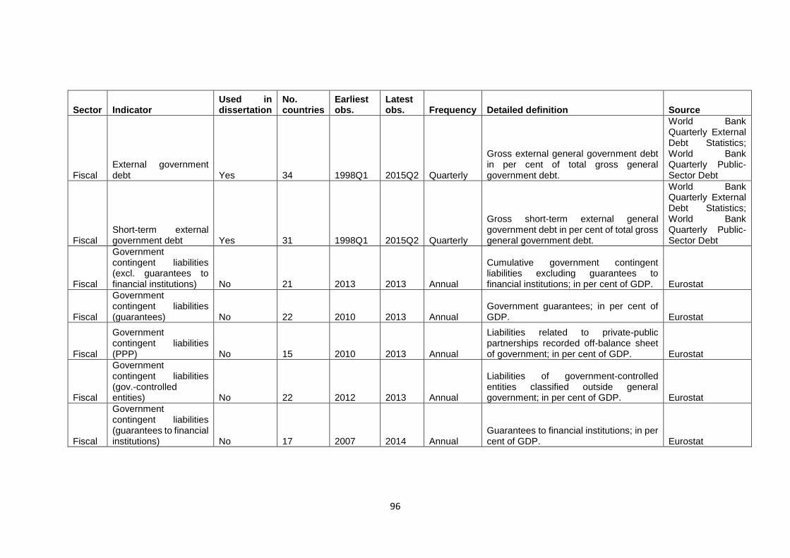
96
Sector Indicator Used in dissertation
No. countries
Earliest obs.
Latest obs. Frequency Detailed definition Source
Fiscal External government debt Yes 34 1998Q1 2015Q2 Quarterly
Gross external general government debt in per cent of total gross general government debt.
World Bank Quarterly External Debt Statistics; World Bank Quarterly Public-Sector Debt
Fiscal Short-term external government debt Yes 31 1998Q1 2015Q2 Quarterly
Gross short-term external general government debt in per cent of total gross general government debt.
World Bank Quarterly External Debt Statistics; World Bank Quarterly Public-Sector Debt
Fiscal
Government contingent liabilities (excl. guarantees to financial institutions) No 21 2013 2013 Annual
Cumulative government contingent liabilities excluding guarantees to financial institutions; in per cent of GDP. Eurostat
Fiscal
Government contingent liabilities (guarantees) No 22 2010 2013 Annual
Government guarantees; in per cent of GDP. Eurostat
Fiscal
Government contingent liabilities (PPP) No 15 2010 2013 Annual
Liabilities related to private-public partnerships recorded off-balance sheet of government; in per cent of GDP. Eurostat
Fiscal
Government contingent liabilities (gov.-controlled entities) No 22 2012 2013 Annual
Liabilities of government-controlled entities classified outside general government; in per cent of GDP. Eurostat
Fiscal
Government contingent liabilities (guarantees to financial institutions) No 17 2007 2014 Annual
Guarantees to financial institutions; in per cent of GDP. Eurostat
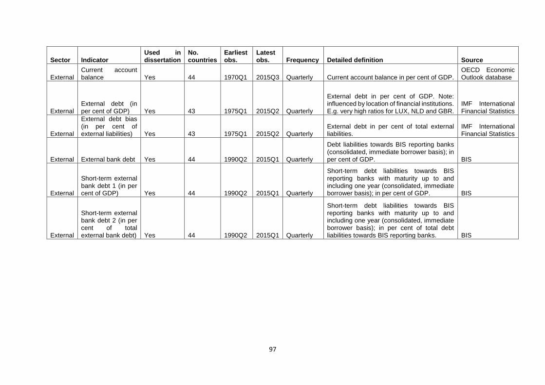
97
Sector Indicator Used in dissertation
No. countries
Earliest obs.
Latest obs. Frequency Detailed definition Source
External Current account balance Yes 44 1970Q1 2015Q3 Quarterly Current account balance in per cent of GDP.
OECD Economic Outlook database
External External debt (in per cent of GDP) Yes 43 1975Q1 2015Q2 Quarterly
External debt in per cent of GDP. Note: influenced by location of financial institutions. E.g. very high ratios for LUX, NLD and GBR.
IMF International Financial Statistics
External
External debt bias (in per cent of external liabilities) Yes 43 1975Q1 2015Q2 Quarterly
External debt in per cent of total external liabilities.
IMF International Financial Statistics
External External bank debt Yes 44 1990Q2 2015Q1 Quarterly
Debt liabilities towards BIS reporting banks (consolidated, immediate borrower basis); in per cent of GDP. BIS
External
Short-term external bank debt 1 (in per cent of GDP) Yes 44 1990Q2 2015Q1 Quarterly
Short-term debt liabilities towards BIS reporting banks with maturity up to and including one year (consolidated, immediate borrower basis); in per cent of GDP. BIS
External
Short-term external bank debt 2 (in per cent of total external bank debt) Yes 44 1990Q2 2015Q1 Quarterly
Short-term debt liabilities towards BIS reporting banks with maturity up to and including one year (consolidated, immediate borrower basis); in per cent of total debt liabilities towards BIS reporting banks. BIS
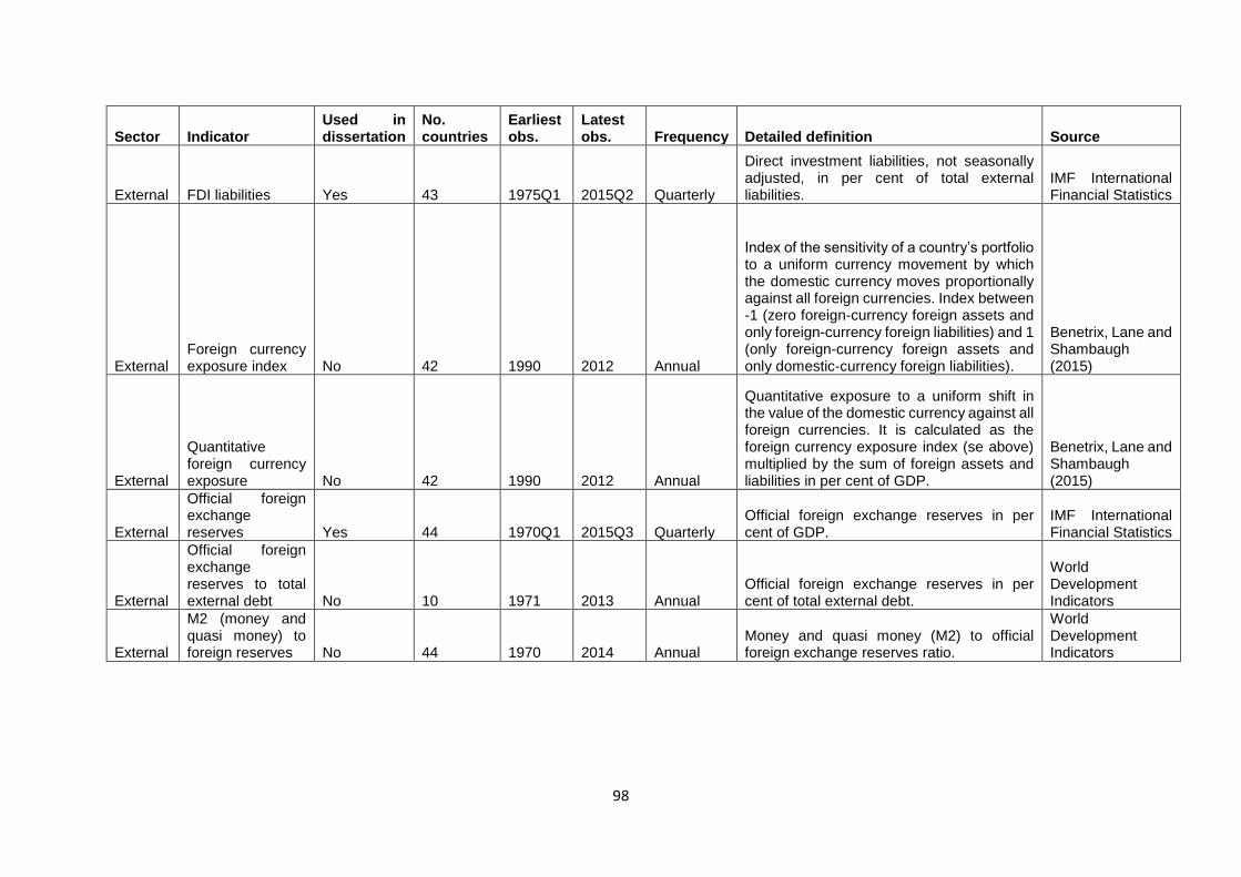
98
Sector Indicator Used in dissertation
No. countries
Earliest obs.
Latest obs. Frequency Detailed definition Source
External FDI liabilities Yes 43 1975Q1 2015Q2 Quarterly
Direct investment liabilities, not seasonally adjusted, in per cent of total external liabilities.
IMF International Financial Statistics
External Foreign currency exposure index No 42 1990 2012 Annual
Index of the sensitivity of a country’s portfolio to a uniform currency movement by which the domestic currency moves proportionally against all foreign currencies. Index between -1 (zero foreign-currency foreign assets and only foreign-currency foreign liabilities) and 1 (only foreign-currency foreign assets and only domestic-currency foreign liabilities).
Benetrix, Lane and Shambaugh (2015)
External
Quantitative foreign currency exposure No 42 1990 2012 Annual
Quantitative exposure to a uniform shift in the value of the domestic currency against all foreign currencies. It is calculated as the foreign currency exposure index (se above) multiplied by the sum of foreign assets and liabilities in per cent of GDP.
Benetrix, Lane and Shambaugh (2015)
External
Official foreign exchange reserves Yes 44 1970Q1 2015Q3 Quarterly
Official foreign exchange reserves in per cent of GDP.
IMF International Financial Statistics
External
Official foreign exchange reserves to total external debt No 10 1971 2013 Annual
Official foreign exchange reserves in per cent of total external debt.
World Development Indicators
External
M2 (money and quasi money) to foreign reserves No 44 1970 2014 Annual
Money and quasi money (M2) to official foreign exchange reserves ratio.
World Development Indicators
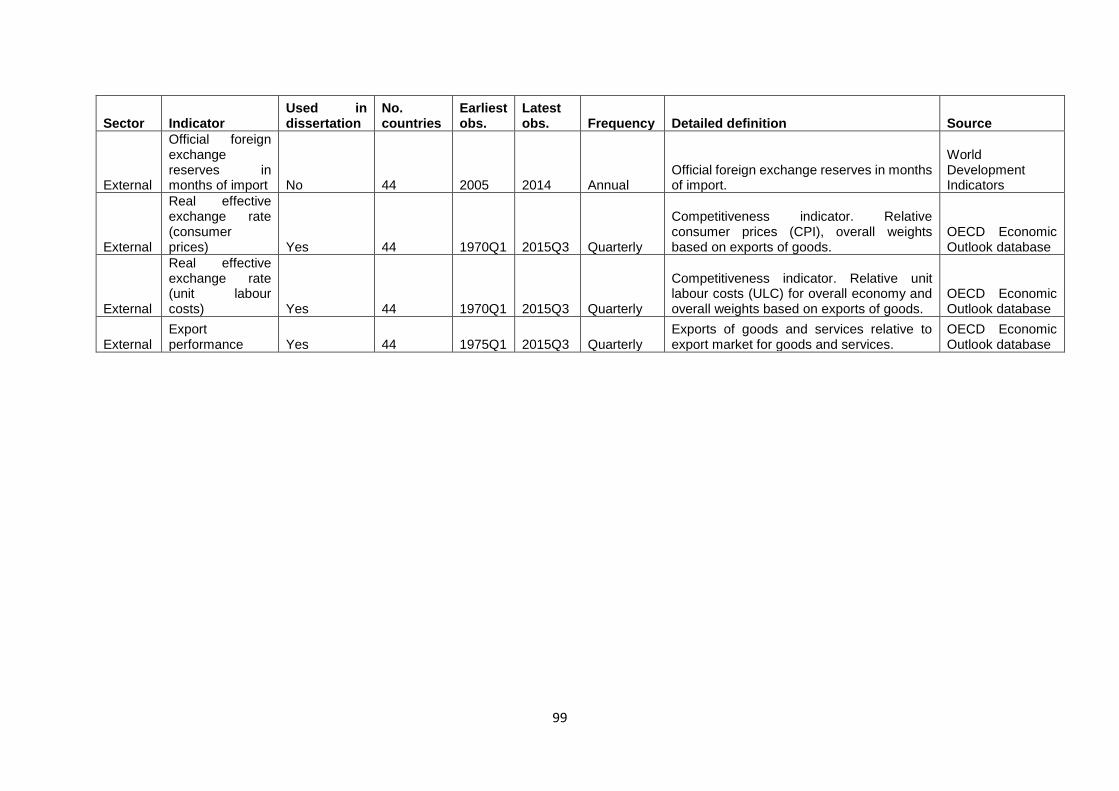
99
Sector Indicator Used in dissertation
No. countries
Earliest obs.
Latest obs. Frequency Detailed definition Source
External
Official foreign exchange reserves in months of import No 44 2005 2014 Annual
Official foreign exchange reserves in months of import.
World Development Indicators
External
Real effective exchange rate (consumer prices) Yes 44 1970Q1 2015Q3 Quarterly
Competitiveness indicator. Relative consumer prices (CPI), overall weights based on exports of goods.
OECD Economic Outlook database
External
Real effective exchange rate (unit labour costs) Yes 44 1970Q1 2015Q3 Quarterly
Competitiveness indicator. Relative unit labour costs (ULC) for overall economy and overall weights based on exports of goods.
OECD Economic Outlook database
External Export performance Yes 44 1975Q1 2015Q3 Quarterly
Exports of goods and services relative to export market for goods and services.
OECD Economic Outlook database
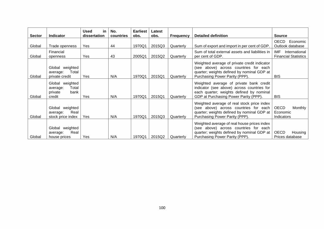
100
Sector Indicator Used in dissertation
No. countries
Earliest obs.
Latest obs. Frequency Detailed definition Source
Global Trade openness Yes 44 1970Q1 2015Q3 Quarterly Sum of export and import in per cent of GDP. OECD Economic Outlook database
Global Financial openness Yes 43 2005Q1 2015Q2 Quarterly
Sum of total external assets and liabilities in per cent of GDP.
IMF International Financial Statistics
Global
Global weighted average: Total private credit Yes N/A 1970Q1 2015Q1 Quarterly
Weighted average of private credit indicator (see above) across countries for each quarter; weights defined by nominal GDP at Purchasing Power Parity (PPP). BIS
Global
Global weighted average: Total private bank credit Yes N/A 1970Q1 2015Q1 Quarterly
Weighted average of private bank credit indicator (see above) across countries for each quarter; weights defined by nominal GDP at Purchasing Power Parity (PPP). BIS
Global
Global weighted average: Real stock price index Yes N/A 1970Q1 2015Q3 Quarterly
Weighted average of real stock price index (see above) across countries for each quarter; weights defined by nominal GDP at Purchasing Power Parity (PPP).
OECD Monthly Economic Indicators
Global
Global weighted average: Real house prices Yes N/A 1970Q1 2015Q2 Quarterly
Weighted average of real house prices index (see above) across countries for each quarter; weights defined by nominal GDP at Purchasing Power Parity (PPP).
OECD Housing Prices database
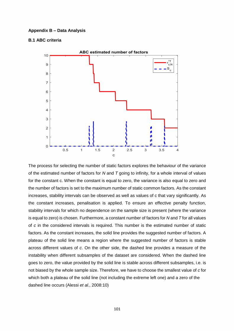
101
Appendix B – Data Analysis
B.1 ABC criteria
The process for selecting the number of static factors explores the behaviour of the variance
of the estimated number of factors for N and T going to infinity, for a whole interval of values
for the constant c. When the constant is equal to zero, the variance is also equal to zero and
the number of factors is set to the maximum number of static common factors. As the constant
increases, stability intervals can be observed as well as values of c that vary significantly. As
the constant increases, penalisation is applied. To ensure an effective penalty function,
stability intervals for which no dependence on the sample size is present (where the variance
is equal to zero) is chosen. Furthermore, a constant number of factors for N and T for all values
of c in the considered intervals is required. This number is the estimated number of static
factors. As the constant increases, the solid line provides the suggested number of factors. A
plateau of the solid line means a region where the suggested number of factors is stable
across different values of c. On the other side, the dashed line provides a measure of the
instability when different subsamples of the dataset are considered. When the dashed line
goes to zero, the value provided by the solid line is stable across different subsamples, i.e. is
not biased by the whole sample size. Therefore, we have to choose the smallest value of c for
which both a plateau of the solid line (not including the extreme left one) and a zero of the
dashed line occurs (Alessi et al., 2008:10)
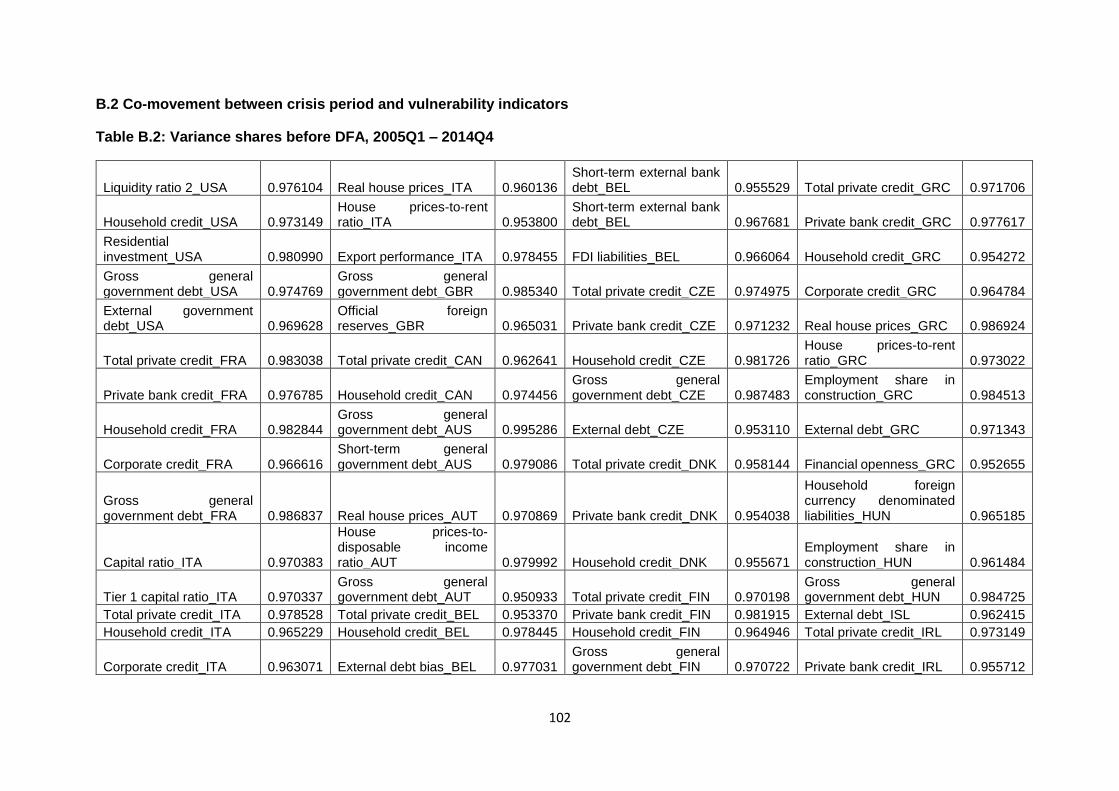
102
B.2 Co-movement between crisis period and vulnerability indicators
Table B.2: Variance shares before DFA, 2005Q1 – 2014Q4
Liquidity ratio 2_USA 0.976104 Real house prices_ITA 0.960136 Short-term external bank debt_BEL 0.955529 Total private credit_GRC 0.971706
Household credit_USA 0.973149 House prices-to-rent ratio_ITA 0.953800
Short-term external bank debt_BEL 0.967681 Private bank credit_GRC 0.977617
Residential investment_USA 0.980990 Export performance_ITA 0.978455 FDI liabilities_BEL 0.966064 Household credit_GRC 0.954272
Gross general government debt_USA 0.974769
Gross general government debt_GBR 0.985340 Total private credit_CZE 0.974975 Corporate credit_GRC 0.964784
External government debt_USA 0.969628
Official foreign reserves_GBR 0.965031 Private bank credit_CZE 0.971232 Real house prices_GRC 0.986924
Total private credit_FRA 0.983038 Total private credit_CAN 0.962641 Household credit_CZE 0.981726 House prices-to-rent ratio_GRC 0.973022
Private bank credit_FRA 0.976785 Household credit_CAN 0.974456 Gross general government debt_CZE 0.987483
Employment share in construction_GRC 0.984513
Household credit_FRA 0.982844 Gross general government debt_AUS 0.995286 External debt_CZE 0.953110 External debt_GRC 0.971343
Corporate credit_FRA 0.966616 Short-term general government debt_AUS 0.979086 Total private credit_DNK 0.958144 Financial openness_GRC 0.952655
Gross general government debt_FRA 0.986837 Real house prices_AUT 0.970869 Private bank credit_DNK 0.954038
Household foreign currency denominated liabilities_HUN 0.965185
Capital ratio_ITA 0.970383
House prices-to-disposable income ratio_AUT 0.979992 Household credit_DNK 0.955671
Employment share in construction_HUN 0.961484
Tier 1 capital ratio_ITA 0.970337 Gross general government debt_AUT 0.950933 Total private credit_FIN 0.970198
Gross general government debt_HUN 0.984725
Total private credit_ITA 0.978528 Total private credit_BEL 0.953370 Private bank credit_FIN 0.981915 External debt_ISL 0.962415
Household credit_ITA 0.965229 Household credit_BEL 0.978445 Household credit_FIN 0.964946 Total private credit_IRL 0.973149
Corporate credit_ITA 0.963071 External debt bias_BEL 0.977031 Gross general government debt_FIN 0.970722 Private bank credit_IRL 0.955712
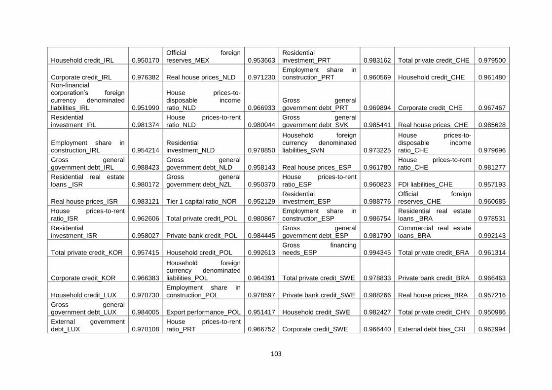
103
Household credit_IRL 0.950170 Official foreign reserves_MEX 0.953663
Residential investment_PRT 0.983162 Total private credit_CHE 0.979500
Corporate credit_IRL 0.976382 Real house prices_NLD 0.971230 Employment share in construction_PRT 0.960569 Household credit_CHE 0.961480
Non-financial corporation’s foreign currency denominated liabilities_IRL 0.951990
House prices-to-disposable income ratio_NLD 0.966933
Gross general government debt_PRT 0.969894 Corporate credit_CHE 0.967467
Residential investment_IRL 0.981374
House prices-to-rent ratio_NLD 0.980044
Gross general government debt_SVK 0.985441 Real house prices_CHE 0.985628
Employment share in construction_IRL 0.954214
Residential investment_NLD 0.978850
Household foreign currency denominated liabilities_SVN 0.973225
House prices-to-disposable income ratio_CHE 0.979696
Gross general government debt_IRL 0.988423
Gross general government debt_NLD 0.958143 Real house prices_ESP 0.961780
House prices-to-rent ratio_CHE 0.981277
Residential real estate loans _ISR 0.980172
Gross general government debt_NZL 0.950370
House prices-to-rent ratio_ESP 0.960823 FDI liabilities_CHE 0.957193
Real house prices_ISR 0.983121 Tier 1 capital ratio_NOR 0.952129 Residential investment_ESP 0.988776
Official foreign reserves_CHE 0.960685
House prices-to-rent ratio_ISR 0.962606 Total private credit_POL 0.980867
Employment share in construction_ESP 0.986754
Residential real estate loans _BRA 0.978531
Residential investment_ISR 0.958027 Private bank credit_POL 0.984445
Gross general government debt_ESP 0.981790
Commercial real estate loans_BRA 0.992143
Total private credit_KOR 0.957415 Household credit_POL 0.992613 Gross financing needs_ESP 0.994345 Total private credit_BRA 0.961314
Corporate credit_KOR 0.966383
Household foreign currency denominated liabilities_POL 0.964391 Total private credit_SWE 0.978833 Private bank credit_BRA 0.966463
Household credit_LUX 0.970730 Employment share in construction_POL 0.978597 Private bank credit_SWE 0.988266 Real house prices_BRA 0.957216
Gross general government debt_LUX 0.984005 Export performance_POL 0.951417 Household credit_SWE 0.982427 Total private credit_CHN 0.950986
External government debt_LUX 0.970108
House prices-to-rent ratio_PRT 0.966752 Corporate credit_SWE 0.966440 External debt bias_CRI 0.962994
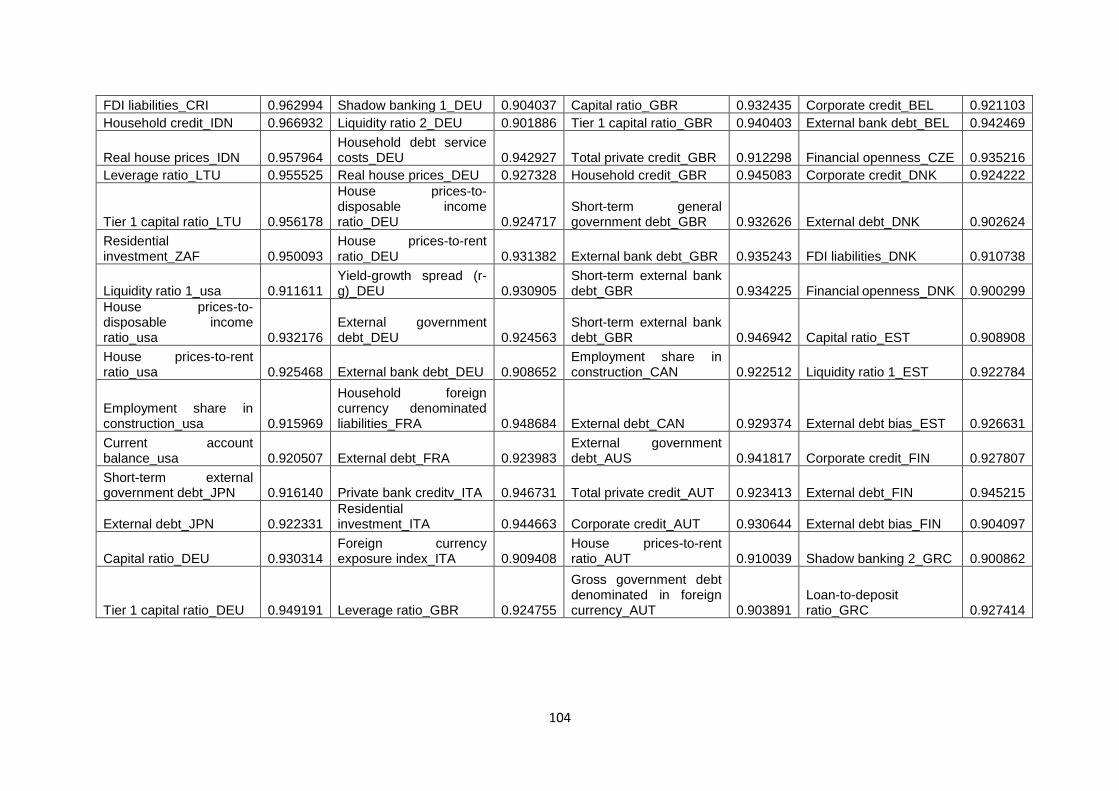
104
FDI liabilities_CRI 0.962994 Shadow banking 1_DEU 0.904037 Capital ratio_GBR 0.932435 Corporate credit_BEL 0.921103
Household credit_IDN 0.966932 Liquidity ratio 2_DEU 0.901886 Tier 1 capital ratio_GBR 0.940403 External bank debt_BEL 0.942469
Real house prices_IDN 0.957964 Household debt service costs_DEU 0.942927 Total private credit_GBR 0.912298 Financial openness_CZE 0.935216
Leverage ratio_LTU 0.955525 Real house prices_DEU 0.927328 Household credit_GBR 0.945083 Corporate credit_DNK 0.924222
Tier 1 capital ratio_LTU 0.956178
House prices-to-disposable income ratio_DEU 0.924717
Short-term general government debt_GBR 0.932626 External debt_DNK 0.902624
Residential investment_ZAF 0.950093
House prices-to-rent ratio_DEU 0.931382 External bank debt_GBR 0.935243 FDI liabilities_DNK 0.910738
Liquidity ratio 1_usa 0.911611 Yield-growth spread (r-g)_DEU 0.930905
Short-term external bank debt_GBR 0.934225 Financial openness_DNK 0.900299
House prices-to-disposable income ratio_usa 0.932176
External government debt_DEU 0.924563
Short-term external bank debt_GBR 0.946942 Capital ratio_EST 0.908908
House prices-to-rent ratio_usa 0.925468 External bank debt_DEU 0.908652
Employment share in construction_CAN 0.922512 Liquidity ratio 1_EST 0.922784
Employment share in construction_usa 0.915969
Household foreign currency denominated liabilities_FRA 0.948684 External debt_CAN 0.929374 External debt bias_EST 0.926631
Current account balance_usa 0.920507 External debt_FRA 0.923983
External government debt_AUS 0.941817 Corporate credit_FIN 0.927807
Short-term external government debt_JPN 0.916140 Private bank creditv_ITA 0.946731 Total private credit_AUT 0.923413 External debt_FIN 0.945215
External debt_JPN 0.922331 Residential investment_ITA 0.944663 Corporate credit_AUT 0.930644 External debt bias_FIN 0.904097
Capital ratio_DEU 0.930314 Foreign currency exposure index_ITA 0.909408
House prices-to-rent ratio_AUT 0.910039 Shadow banking 2_GRC 0.900862
Tier 1 capital ratio_DEU 0.949191 Leverage ratio_GBR 0.924755
Gross government debt denominated in foreign currency_AUT 0.903891
Loan-to-deposit ratio_GRC 0.927414
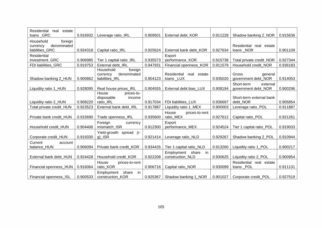
105
Residential real estate loans _GRC 0.916932 Leverage ratio_IRL 0.909501 External debt_KOR 0.911228 Shadow banking 2_NOR 0.915636
Household foreign currency denominated liabilities_GRC 0.934318 Capital ratio_IRL 0.925624 External bank debt_KOR 0.927634
Residential real estate loans _NOR 0.901109
Residential investment_GRC 0.906985 Tier 1 capital ratio_IRL 0.935573
Export performance_KOR 0.915738 Total private credit_NOR 0.927344
FDI liabilities_GRC 0.919753 External debt_IRL 0.947931 Financial openness_KOR 0.911579 Household credit_NOR 0.936183
Shadow banking 2_HUN 0.900862
Household foreign currency denominated liabilities_IRL 0.904123
Residential real estate loans _LUX 0.935020
Gross general government debt_NOR 0.914053
Liquidity ratio 1_HUN 0.928095 Real house prices_IRL 0.904555 External debt bias_LUX 0.908194 Short-term external government debt_NOR 0.900296
Liquidity ratio 2_HUN 0.908220
House prices-to-disposable income ratio_IRL 0.917034 FDI liabilities_LUX 0.936697
Short-term external bank debt_NOR 0.905854
Total private credit_HUN 0.923523 External bank debt_IRL 0.917887 Liquidity ratio 1_MEX 0.900003 Leverage ratio_POL 0.911887
Private bank credit_HUN 0.915690 Trade openness_IRL 0.935600 House prices-to-rent ratio_MEX 0.927612 Capital ratio_POL 0.921261
Household credit_HUN 0.904406 Foreign currency mismatch_ISR 0.912300
Export performance_MEX 0.924524 Tier 1 capital ratio_POL 0.919033
Corporate credit_HUN 0.919330 Yield-growth spread (r-g)_ISR 0.921414 Leverage ratio_NLD 0.929267 Shadow banking 2_POL 0.910944
Current account balance_HUN 0.906094 Private bank credit_KOR 0.934426 Tier 1 capital ratio_NLD 0.913260 Liquidity ratio 1_POL 0.900217
External bank debt_HUN 0.924428 Household credit_KOR 0.922208 Employment share in construction_NLD 0.930625 Liquidity ratio 2_POL 0.900954
Financial openness_HUN 0.916064 House prices-to-rent ratio_KOR 0.906716 Capital ratio_NOR 0.930099
Residential real estate loans _POL 0.911131
Financial openness_ISL 0.900533 Employment share in construction_KOR 0.925367 Shadow banking 1_NOR 0.901027 Corporate credit_POL 0.927519
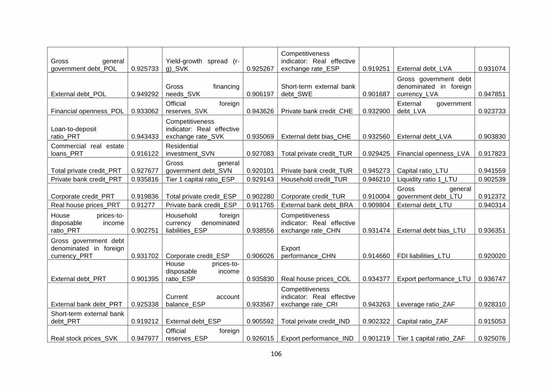
106
Gross general government debt_POL 0.925733
Yield-growth spread (r-g)_SVK 0.925267
Competitiveness indicator: Real effective exchange rate_ESP 0.919251 External debt_LVA 0.931074
External debt_POL 0.949292 Gross financing needs_SVK 0.906197
Short-term external bank debt_SWE 0.901687
Gross government debt denominated in foreign currency_LVA 0.947851
Financial openness_POL 0.933062 Official foreign reserves_SVK 0.943626 Private bank credit_CHE 0.932900
External government debt_LVA 0.923733
Loan-to-deposit ratio_PRT 0.943433
Competitiveness indicator: Real effective exchange rate_SVK 0.935069 External debt bias_CHE 0.932560 External debt_LVA 0.903830
Commercial real estate loans_PRT 0.916122
Residential investment_SVN 0.927083 Total private credit_TUR 0.929425 Financial openness_LVA 0.917823
Total private credit_PRT 0.927677 Gross general government debt_SVN 0.920101 Private bank credit_TUR 0.945273 Capital ratio_LTU 0.941559
Private bank credit_PRT 0.935816 Tier 1 capital ratio_ESP 0.929143 Household credit_TUR 0.946210 Liquidity ratio 1_LTU 0.902539
Corporate credit_PRT 0.919836 Total private credit_ESP 0.902280 Corporate credit_TUR 0.910004 Gross general government debt_LTU 0.912372
Real house prices_PRT 0.91277 Private bank credit_ESP 0.911765 External bank debt_BRA 0.909804 External debt_LTU 0.940314
House prices-to-disposable income ratio_PRT 0.902751
Household foreign currency denominated liabilities_ESP 0.938556
Competitiveness indicator: Real effective exchange rate_CHN 0.931474 External debt bias_LTU 0.936351
Gross government debt denominated in foreign currency_PRT 0.931702 Corporate credit_ESP 0.906026
Export performance_CHN 0.914660 FDI liabilities_LTU 0.920020
External debt_PRT 0.901395
House prices-to-disposable income ratio_ESP 0.935830 Real house prices_COL 0.934377 Export performance_LTU 0.936747
External bank debt_PRT 0.925338 Current account balance_ESP 0.933567
Competitiveness indicator: Real effective exchange rate_CRI 0.943263 Leverage ratio_ZAF 0.928310
Short-term external bank debt_PRT 0.919212 External debt_ESP 0.905592 Total private credit_IND 0.902322 Capital ratio_ZAF 0.915053
Real stock prices_SVK 0.947977 Official foreign reserves_ESP 0.926015 Export performance_IND 0.901219 Tier 1 capital ratio_ZAF 0.925076
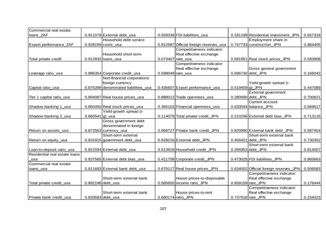
107
Commercial real estate
loans_ZAF 0.911079 External debt_usa 0.559336 FDI liabilities_usa 0.181199 Residential investment_JPN 0.657318
Export performance_ZAF 0.928199
Household debt service
costs_usa 0.812587 Official foreign reserves_usa 0.747733
Employment share in
construction_JPN 0.884405
Total private credit 0.912832
Household short-term
loans_usa 0.073407
Competitiveness indicator:
Real effective exchange
rate_usa 0.591951 Real stock prices_JPN 0.583908
Leverage ratio_usa 0.886354 Corporate credit_usa 0.598049
Competitiveness indicator:
Real effective exchange
rate_usa 0.696730
Gross general government
debt_JPN 0.166042
Capital ratio_usa 0.875398
Non-financial corporations
foreign currency
denominated liabilities_usa 0.435607 Export performance_usa 0.519409
Yield-growth spread (r-
g)_JPN 0.447089
Tier 1 capital ratio_usa 0.894087 Real house prices_usa 0.888013 Trade openness_usa 0.390690
External government
debt_JPN 0.700621
Shadow banking 1_usa 0.850450 Real stock prices_usa 0.365103 Financial openness_usa 0.633594
Current account
balance_JPN 0.669517
Shadow banking 2_usa 0.865541
Yield-growth spread (r-
g)_usa 0.114079 Total private credit_JPN 0.210296 External debt bias_JPN 0.713116
Return on assets_usa 0.872563
Gross government debt
denominated in foreign
currency_usa 0.668727 Private bank credit_JPN 0.820990 External bank debt_JPN 0.587454
Return on equity_usa 0.831915
Short-term external
government debt_usa 0.628216 External debt_JPN 0.456421
Short-term external bank
debt_JPN 0.730352
Loan-to-deposit ratio_usa 0.821594 External debt_usa 0.613916 Household credit_JPN 0.266953
Short-term external bank
debt_JPN 0.814007
Residential real estate loans
_usa 0.837565 External debt bias_usa 0.411708 Corporate credit_JPN 0.473025 FDI liabilities_JPN 0.865663
Commercial real estate
loans_usa 0.811683 External bank debt_usa 0.679117 Real house prices_JPN 0.634002 Official foreign reserves_JPN 0.506583
Total private credit_usa 0.892198
Short-term external bank
debt_usa 0.585655
House prices-to-disposable
income ratio_JPN 0.659159
Competitiveness indicator:
Real effective exchange
rate_JPN 0.176444
Private bank credit_usa 0.833583
Short-term external bank
debt_usa 0.680174
House prices-to-rent
ratio_JPN 0.737018
Competitiveness indicator:
Real effective exchange
rate_JPN 0.154023
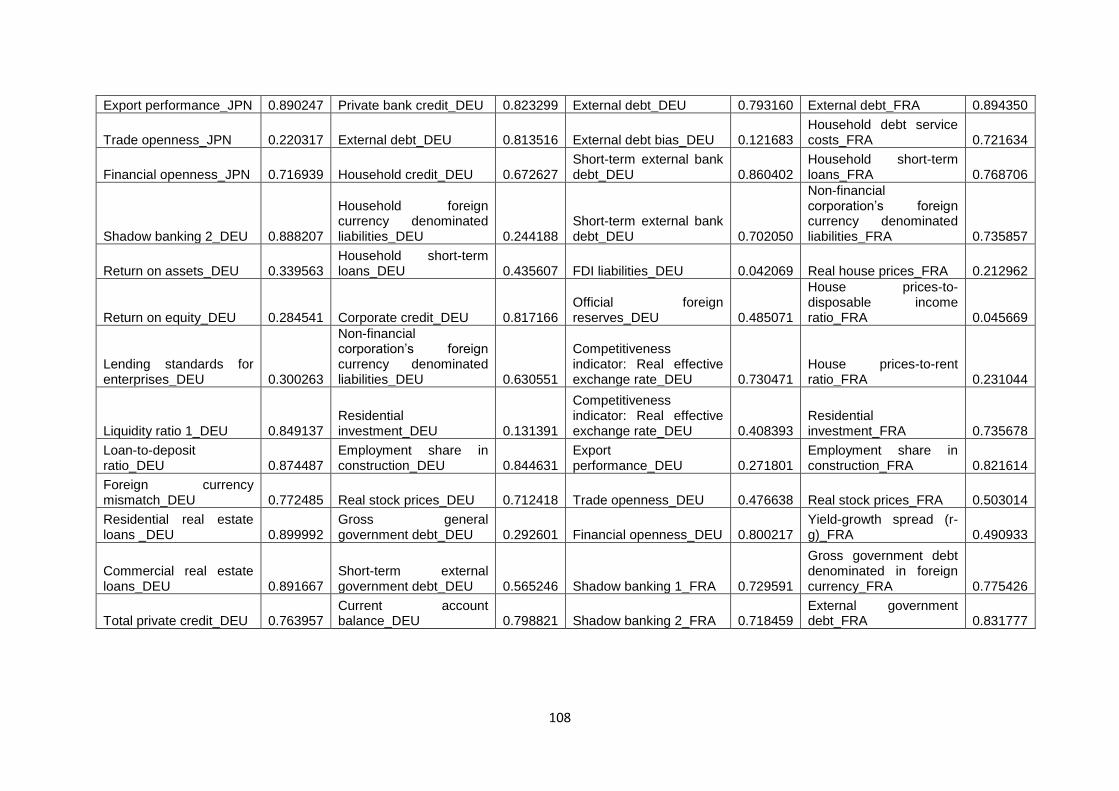
108
Export performance_JPN 0.890247 Private bank credit_DEU 0.823299 External debt_DEU 0.793160 External debt_FRA 0.894350
Trade openness_JPN 0.220317 External debt_DEU 0.813516 External debt bias_DEU 0.121683 Household debt service costs_FRA 0.721634
Financial openness_JPN 0.716939 Household credit_DEU 0.672627 Short-term external bank debt_DEU 0.860402
Household short-term loans_FRA 0.768706
Shadow banking 2_DEU 0.888207
Household foreign currency denominated liabilities_DEU 0.244188
Short-term external bank debt_DEU 0.702050
Non-financial corporation’s foreign currency denominated liabilities_FRA 0.735857
Return on assets_DEU 0.339563 Household short-term loans_DEU 0.435607 FDI liabilities_DEU 0.042069 Real house prices_FRA 0.212962
Return on equity_DEU 0.284541 Corporate credit_DEU 0.817166 Official foreign reserves_DEU 0.485071
House prices-to-disposable income ratio_FRA 0.045669
Lending standards for enterprises_DEU 0.300263
Non-financial corporation’s foreign currency denominated liabilities_DEU 0.630551
Competitiveness indicator: Real effective exchange rate_DEU 0.730471
House prices-to-rent ratio_FRA 0.231044
Liquidity ratio 1_DEU 0.849137 Residential investment_DEU 0.131391
Competitiveness indicator: Real effective exchange rate_DEU 0.408393
Residential investment_FRA 0.735678
Loan-to-deposit ratio_DEU 0.874487
Employment share in construction_DEU 0.844631
Export performance_DEU 0.271801
Employment share in construction_FRA 0.821614
Foreign currency mismatch_DEU 0.772485 Real stock prices_DEU 0.712418 Trade openness_DEU 0.476638 Real stock prices_FRA 0.503014
Residential real estate loans _DEU 0.899992
Gross general government debt_DEU 0.292601 Financial openness_DEU 0.800217
Yield-growth spread (r-g)_FRA 0.490933
Commercial real estate loans_DEU 0.891667
Short-term external government debt_DEU 0.565246 Shadow banking 1_FRA 0.729591
Gross government debt denominated in foreign currency_FRA 0.775426
Total private credit_DEU 0.763957 Current account balance_DEU 0.798821 Shadow banking 2_FRA 0.718459
External government debt_FRA 0.831777
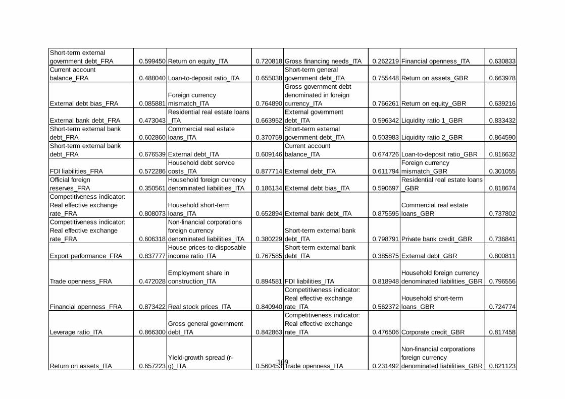
109
Short-term external
government debt_FRA 0.599450 Return on equity_ITA 0.720818 Gross financing needs_ITA 0.262219 Financial openness_ITA 0.630833
Current account
balance_FRA 0.488040 Loan-to-deposit ratio_ITA 0.655038
Short-term general
government debt_ITA 0.755448 Return on assets_GBR 0.663978
External debt bias_FRA 0.085881
Foreign currency
mismatch_ITA 0.764890
Gross government debt
denominated in foreign
currency_ITA 0.766261 Return on equity_GBR 0.639216
External bank debt_FRA 0.473043
Residential real estate loans
_ITA 0.663952
External government
debt_ITA 0.596342 Liquidity ratio 1_GBR 0.833432
Short-term external bank
debt_FRA 0.602860
Commercial real estate
loans_ITA 0.370759
Short-term external
government debt_ITA 0.503983 Liquidity ratio 2_GBR 0.864590
Short-term external bank
debt_FRA 0.676539 External debt_ITA 0.609146
Current account
balance_ITA 0.674726 Loan-to-deposit ratio_GBR 0.816632
FDI liabilities_FRA 0.572286
Household debt service
costs_ITA 0.877714 External debt_ITA 0.611794
Foreign currency
mismatch_GBR 0.301055
Official foreign
reserves_FRA 0.350561
Household foreign currency
denominated liabilities_ITA 0.186134 External debt bias_ITA 0.590697
Residential real estate loans
_GBR 0.818674
Competitiveness indicator:
Real effective exchange
rate_FRA 0.808073
Household short-term
loans_ITA 0.652894 External bank debt_ITA 0.875595
Commercial real estate
loans_GBR 0.737802
Competitiveness indicator:
Real effective exchange
rate_FRA 0.606318
Non-financial corporations
foreign currency
denominated liabilities_ITA 0.380229
Short-term external bank
debt_ITA 0.798791 Private bank credit_GBR 0.736841
Export performance_FRA 0.837777
House prices-to-disposable
income ratio_ITA 0.767585
Short-term external bank
debt_ITA 0.385875 External debt_GBR 0.800811
Trade openness_FRA 0.472028
Employment share in
construction_ITA 0.894581 FDI liabilities_ITA 0.818948
Household foreign currency
denominated liabilities_GBR 0.796556
Financial openness_FRA 0.873422 Real stock prices_ITA 0.840940
Competitiveness indicator:
Real effective exchange
rate_ITA 0.562372
Household short-term
loans_GBR 0.724774
Leverage ratio_ITA 0.866300
Gross general government
debt_ITA 0.842863
Competitiveness indicator:
Real effective exchange
rate_ITA 0.476506 Corporate credit_GBR 0.817458
Return on assets_ITA 0.657223
Yield-growth spread (r-
g)_ITA 0.560453 Trade openness_ITA 0.231492
Non-financial corporations
foreign currency
denominated liabilities_GBR 0.821123

110
Real house prices_GBR 0.338755
Competitiveness indicator: Real effective exchange rate_GBR 0.867181
Commercial real estate loans_CAN 0.522397
External bank debt_CAN 0.664585
House prices-to-disposable income ratio_GBR 0.427919
Export performance_GBR 0.599405
Private bank credit_CAN 0.887189
Short-term external bank debt_CAN 0.627721
House prices-to-rent ratio_GBR 0.189429 Trade openness_GBR 0.470086 External debt_CAN 0.679354
Short-term external bank debt_CAN 0.022389
Residential investment_GBR 0.890469
Financial openness_GBR 0.872390 Corporate credit_CAN 0.870465 FDI liabilities_CAN 0.779421
Employment share in construction_GBR 0.770450 Leverage ratio_CAN 0.006276
Real house prices_CAN 0.859310
Official foreign reserves_CAN 0.807108
Real stock prices_GBR 0.409317 Capital ratio_CAN 0.098718
House prices-to-disposable income ratio_CAN 0.770331
Competitiveness indicator: Real effective exchange rate_CAN 0.124327
Yield-growth spread (r-g)_GBR 0.701556 Tier 1 capital ratio_CAN 0.308253
House prices-to-rent ratio_CAN 0.837455
Competitiveness indicator: Real effective exchange rate_CAN 0.422530
Gross financing needs_GBR 0.742377
Shadow banking 1_CAN 0.405690
Residential investment_CAN 0.114593
Export performance_CAN 0.892698
External government debt_GBR 0.834225
Shadow banking 2_CAN 0.686692 Real stock prices_CAN 0.034809 Trade openness_CAN 0.749075
Short-term external government debt_GBR 0.791647 Return on assets_CAN 0.412967
Gross general government debt_CAN 0.892103
Financial openness_CAN 0.466717
Current account balance_GBR 0.294587 Return on equity_CAN 0.345500
Yield-growth spread (r-g)_CAN 0.214443 Leverage ratio_AUS 0.299916
External debt_GBR 0.891737 Liquidity ratio 1_CAN 0.436663 External government debt_CAN 0.887775 Capital ratio_AUS 0.510134
External debt bias_GBR 0.873578 Liquidity ratio 2_CAN 0.631080
Short-term external government debt_CAN 0.776151 Tier 1 capital ratio_AUS 0.672342
FDI liabilities_GBR 0.712620 Loan-to-deposit ratio_CAN 0.609058
Current account balance_CAN 0.856762
Shadow banking 1_AUS 0.229234
Competitiveness indicator: Real effective exchange rate_GBR 0.852332
Residential real estate loans _CAN 0.709667
External debt bias_CAN 0.653248
Shadow banking 2_AUS 0.166132
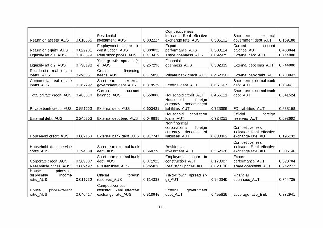
111
Return on assets_AUS 0.010865 Residential investment_AUS 0.802227
Competitiveness indicator: Real effective exchange rate_AUS 0.585102
Short-term external government debt_AUT 0.169188
Return on equity_AUS 0.022731 Employment share in construction_AUS 0.389032
Export performance_AUS 0.388114
Current account balance_AUT 0.433844
Liquidity ratio 1_AUS 0.766679 Real stock prices_AUS 0.413419 Trade openness_AUS 0.092975 External debt_AUT 0.744080
Liquidity ratio 2_AUS 0.790198 Yield-growth spread (r-g)_AUS 0.257296
Financial openness_AUS 0.502339 External debt bias_AUT 0.744080
Residential real estate loans _AUS 0.498851
Gross financing needs_AUS 0.715058 Private bank credit_AUT 0.452050 External bank debt_AUT 0.738942
Commercial real estate loans_AUS 0.362292
Short-term external government debt_AUS 0.379529 External debt_AUT 0.661667
Short-term external bank debt_AUT 0.789411
Total private credit_AUS 0.466310 Current account balance_AUS 0.553000 Household credit_AUT 0.466111
Short-term external bank debt_AUT 0.641524
Private bank credit_AUS 0.891653 External debt_AUS 0.603431
Household foreign currency denominated liabilities_AUT 0.723669 FDI liabilities_AUT 0.833198
External debt_AUS 0.245203 External debt bias_AUS 0.046898 Household short-term loans_AUT 0.724251
Official foreign reserves_AUT 0.692692
Household credit_AUS 0.807153 External bank debt_AUS 0.817747
Non-financial corporation’s foreign currency denominated liabilities_AUT 0.638462
Competitiveness indicator: Real effective exchange rate_AUT 0.196132
Household debt service costs_AUS 0.394834
Short-term external bank debt_AUS 0.660278
Residential investment_AUT 0.552528
Competitiveness indicator: Real effective exchange rate_AUT 0.005146
Corporate credit_AUS 0.369007 Short-term external bank debt_AUS 0.071922
Employment share in construction_AUT 0.173987
Export performance_AUT 0.828704
Real house prices_AUS 0.689497 FDI liabilities_AUS 0.265828 Real stock prices_AUT 0.623136 Trade openness_AUT 0.242272
House prices-to-disposable income ratio_AUS 0.011732
Official foreign reserves_AUS 0.614388
Yield-growth spread (r-g)_AUT 0.740949
Financial openness_AUT 0.744735
House prices-to-rent ratio_AUS 0.040417
Competitiveness indicator: Real effective exchange rate_AUS 0.518945
External government debt_AUT 0.455639 Leverage ratio_BEL 0.832941
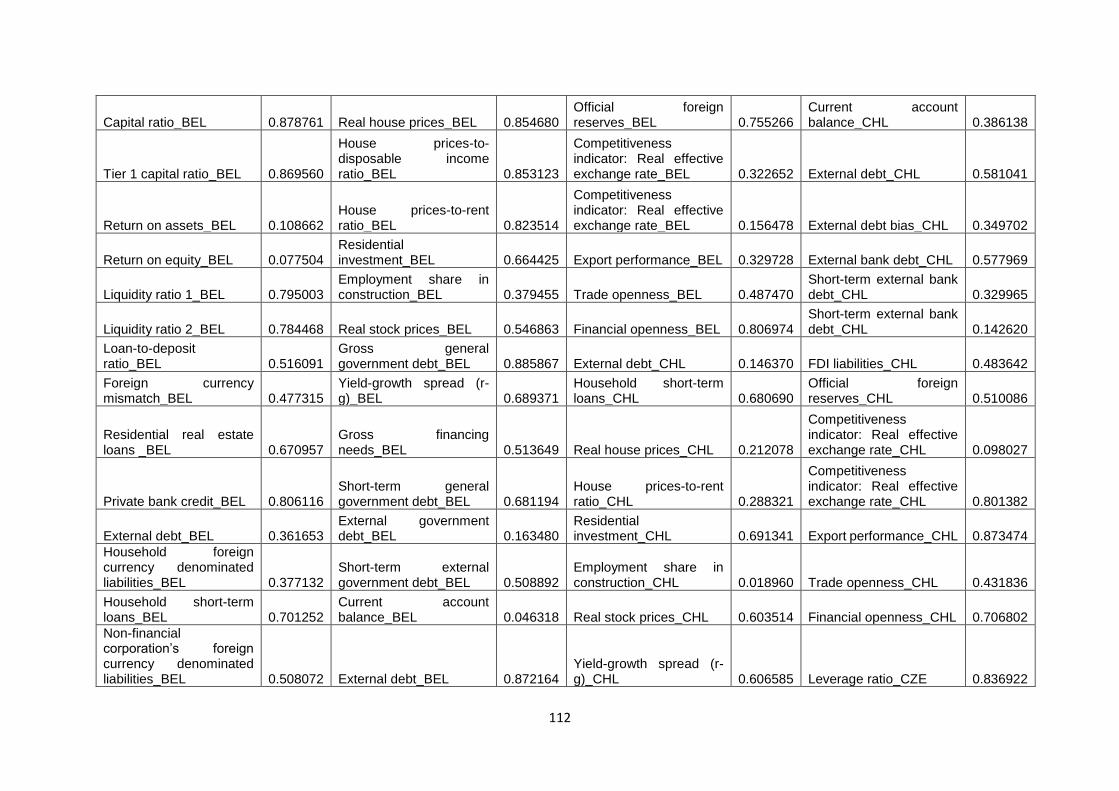
112
Capital ratio_BEL 0.878761 Real house prices_BEL 0.854680 Official foreign reserves_BEL 0.755266
Current account balance_CHL 0.386138
Tier 1 capital ratio_BEL 0.869560
House prices-to-disposable income ratio_BEL 0.853123
Competitiveness indicator: Real effective exchange rate_BEL 0.322652 External debt_CHL 0.581041
Return on assets_BEL 0.108662 House prices-to-rent ratio_BEL 0.823514
Competitiveness indicator: Real effective exchange rate_BEL 0.156478 External debt bias_CHL 0.349702
Return on equity_BEL 0.077504 Residential investment_BEL 0.664425 Export performance_BEL 0.329728 External bank debt_CHL 0.577969
Liquidity ratio 1_BEL 0.795003 Employment share in construction_BEL 0.379455 Trade openness_BEL 0.487470
Short-term external bank debt_CHL 0.329965
Liquidity ratio 2_BEL 0.784468 Real stock prices_BEL 0.546863 Financial openness_BEL 0.806974 Short-term external bank debt_CHL 0.142620
Loan-to-deposit ratio_BEL 0.516091
Gross general government debt_BEL 0.885867 External debt_CHL 0.146370 FDI liabilities_CHL 0.483642
Foreign currency mismatch_BEL 0.477315
Yield-growth spread (r-g)_BEL 0.689371
Household short-term loans_CHL 0.680690
Official foreign reserves_CHL 0.510086
Residential real estate loans _BEL 0.670957
Gross financing needs_BEL 0.513649 Real house prices_CHL 0.212078
Competitiveness indicator: Real effective exchange rate_CHL 0.098027
Private bank credit_BEL 0.806116 Short-term general government debt_BEL 0.681194
House prices-to-rent ratio_CHL 0.288321
Competitiveness indicator: Real effective exchange rate_CHL 0.801382
External debt_BEL 0.361653 External government debt_BEL 0.163480
Residential investment_CHL 0.691341 Export performance_CHL 0.873474
Household foreign currency denominated liabilities_BEL 0.377132
Short-term external government debt_BEL 0.508892
Employment share in construction_CHL 0.018960 Trade openness_CHL 0.431836
Household short-term loans_BEL 0.701252
Current account balance_BEL 0.046318 Real stock prices_CHL 0.603514 Financial openness_CHL 0.706802
Non-financial corporation’s foreign currency denominated liabilities_BEL 0.508072 External debt_BEL 0.872164
Yield-growth spread (r-g)_CHL 0.606585 Leverage ratio_CZE 0.836922
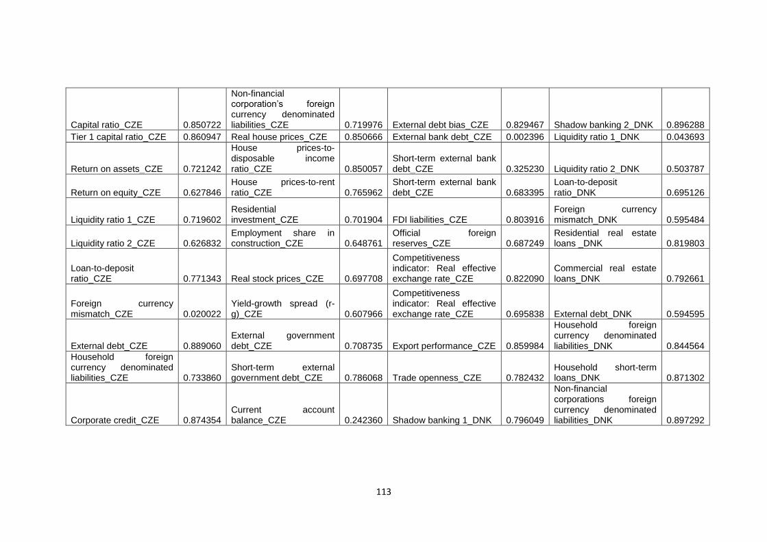
113
Capital ratio_CZE 0.850722
Non-financial corporation’s foreign currency denominated liabilities_CZE 0.719976 External debt bias_CZE 0.829467 Shadow banking 2_DNK 0.896288
Tier 1 capital ratio_CZE 0.860947 Real house prices_CZE 0.850666 External bank debt_CZE 0.002396 Liquidity ratio 1_DNK 0.043693
Return on assets_CZE 0.721242
House prices-to-disposable income ratio_CZE 0.850057
Short-term external bank debt_CZE 0.325230 Liquidity ratio 2_DNK 0.503787
Return on equity_CZE 0.627846 House prices-to-rent ratio_CZE 0.765962
Short-term external bank debt_CZE 0.683395
Loan-to-deposit ratio_DNK 0.695126
Liquidity ratio 1_CZE 0.719602 Residential investment_CZE 0.701904 FDI liabilities_CZE 0.803916
Foreign currency mismatch_DNK 0.595484
Liquidity ratio 2_CZE 0.626832 Employment share in construction_CZE 0.648761
Official foreign reserves_CZE 0.687249
Residential real estate loans _DNK 0.819803
Loan-to-deposit ratio_CZE 0.771343 Real stock prices_CZE 0.697708
Competitiveness indicator: Real effective exchange rate_CZE 0.822090
Commercial real estate loans_DNK 0.792661
Foreign currency mismatch_CZE 0.020022
Yield-growth spread (r-g)_CZE 0.607966
Competitiveness indicator: Real effective exchange rate_CZE 0.695838 External debt_DNK 0.594595
External debt_CZE 0.889060 External government debt_CZE 0.708735 Export performance_CZE 0.859984
Household foreign currency denominated liabilities_DNK 0.844564
Household foreign currency denominated liabilities_CZE 0.733860
Short-term external government debt_CZE 0.786068 Trade openness_CZE 0.782432
Household short-term loans_DNK 0.871302
Corporate credit_CZE 0.874354 Current account balance_CZE 0.242360 Shadow banking 1_DNK 0.796049
Non-financial corporations foreign currency denominated liabilities_DNK 0.897292
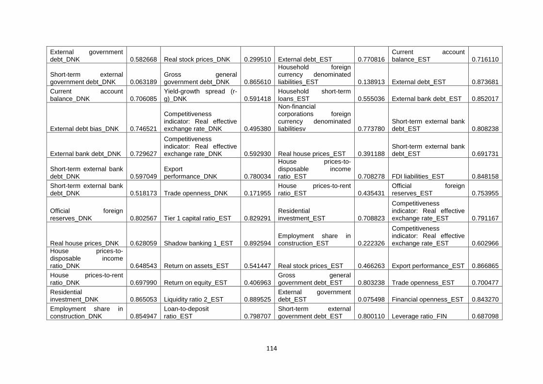
114
External government debt_DNK 0.582668 Real stock prices_DNK 0.299510 External debt_EST 0.770816
Current account balance_EST 0.716110
Short-term external government debt_DNK 0.063189
Gross general government debt_DNK 0.865610
Household foreign currency denominated liabilities_EST 0.138913 External debt_EST 0.873681
Current account balance_DNK 0.706085
Yield-growth spread (r-g)_DNK 0.591418
Household short-term loans_EST 0.555036 External bank debt_EST 0.852017
External debt bias_DNK 0.746521
Competitiveness indicator: Real effective exchange rate_DNK 0.495380
Non-financial corporations foreign currency denominated liabilitiesv 0.773780
Short-term external bank debt_EST 0.808238
External bank debt_DNK 0.729627
Competitiveness indicator: Real effective exchange rate_DNK 0.592930 Real house prices_EST 0.391188
Short-term external bank debt_EST 0.691731
Short-term external bank debt_DNK 0.597049
Export performance_DNK 0.780034
House prices-to-disposable income ratio_EST 0.708278 FDI liabilities_EST 0.848158
Short-term external bank debt_DNK 0.518173 Trade openness_DNK 0.171955
House prices-to-rent ratio_EST 0.435431
Official foreign reserves_EST 0.753955
Official foreign reserves_DNK 0.802567 Tier 1 capital ratio_EST 0.829291
Residential investment_EST 0.708823
Competitiveness indicator: Real effective exchange rate_EST 0.791167
Real house prices_DNK 0.628059 Shadow banking 1_EST 0.892594 Employment share in construction_EST 0.222326
Competitiveness indicator: Real effective exchange rate_EST 0.602966
House prices-to-disposable income ratio_DNK 0.648543 Return on assets_EST 0.541447 Real stock prices_EST 0.466263 Export performance_EST 0.866865
House prices-to-rent ratio_DNK 0.697990 Return on equity_EST 0.406963
Gross general government debt_EST 0.803238 Trade openness_EST 0.700477
Residential investment_DNK 0.865053 Liquidity ratio 2_EST 0.889525
External government debt_EST 0.075498 Financial openness_EST 0.843270
Employment share in construction_DNK 0.854947
Loan-to-deposit ratio_EST 0.798707
Short-term external government debt_EST 0.800110 Leverage ratio_FIN 0.687098
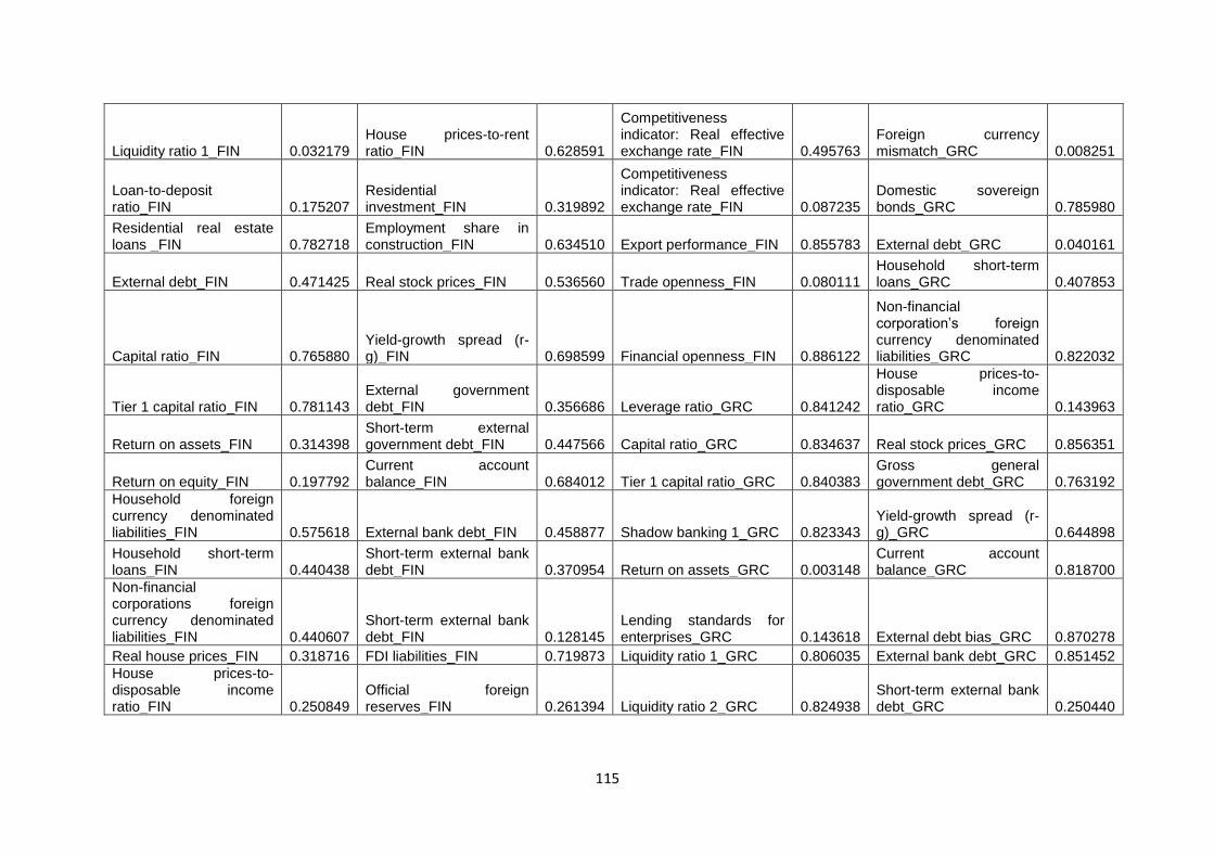
115
Liquidity ratio 1_FIN 0.032179 House prices-to-rent ratio_FIN 0.628591
Competitiveness indicator: Real effective exchange rate_FIN 0.495763
Foreign currency mismatch_GRC 0.008251
Loan-to-deposit ratio_FIN 0.175207
Residential investment_FIN 0.319892
Competitiveness indicator: Real effective exchange rate_FIN 0.087235
Domestic sovereign bonds_GRC 0.785980
Residential real estate loans _FIN 0.782718
Employment share in construction_FIN 0.634510 Export performance_FIN 0.855783 External debt_GRC 0.040161
External debt_FIN 0.471425 Real stock prices_FIN 0.536560 Trade openness_FIN 0.080111 Household short-term loans_GRC 0.407853
Capital ratio_FIN 0.765880 Yield-growth spread (r-g)_FIN 0.698599 Financial openness_FIN 0.886122
Non-financial corporation’s foreign currency denominated liabilities_GRC 0.822032
Tier 1 capital ratio_FIN 0.781143 External government debt_FIN 0.356686 Leverage ratio_GRC 0.841242
House prices-to-disposable income ratio_GRC 0.143963
Return on assets_FIN 0.314398 Short-term external government debt_FIN 0.447566 Capital ratio_GRC 0.834637 Real stock prices_GRC 0.856351
Return on equity_FIN 0.197792 Current account balance_FIN 0.684012 Tier 1 capital ratio_GRC 0.840383
Gross general government debt_GRC 0.763192
Household foreign currency denominated liabilities_FIN 0.575618 External bank debt_FIN 0.458877 Shadow banking 1_GRC 0.823343
Yield-growth spread (r-g)_GRC 0.644898
Household short-term loans_FIN 0.440438
Short-term external bank debt_FIN 0.370954 Return on assets_GRC 0.003148
Current account balance_GRC 0.818700
Non-financial corporations foreign currency denominated liabilities_FIN 0.440607
Short-term external bank debt_FIN 0.128145
Lending standards for enterprises_GRC 0.143618 External debt bias_GRC 0.870278
Real house prices_FIN 0.318716 FDI liabilities_FIN 0.719873 Liquidity ratio 1_GRC 0.806035 External bank debt_GRC 0.851452
House prices-to-disposable income ratio_FIN 0.250849
Official foreign reserves_FIN 0.261394 Liquidity ratio 2_GRC 0.824938
Short-term external bank debt_GRC 0.250440
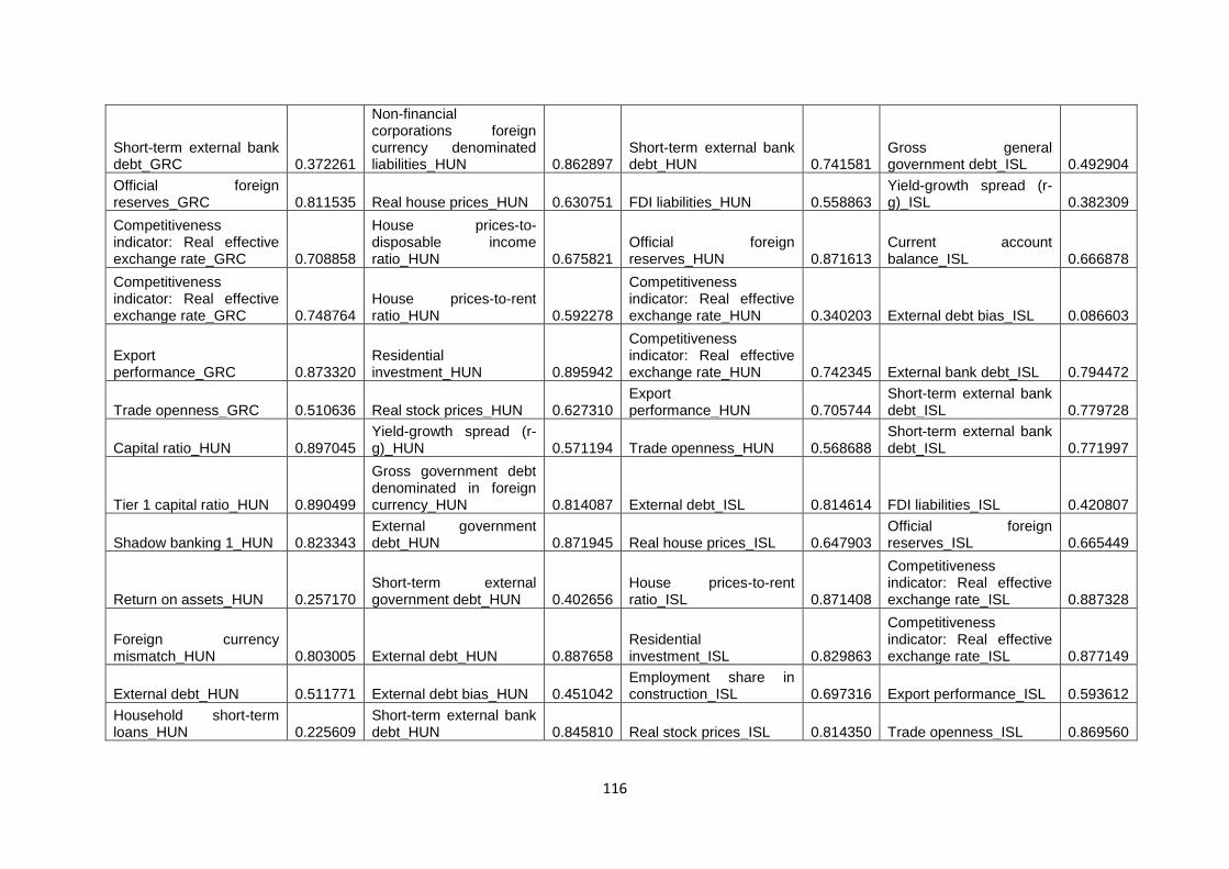
116
Short-term external bank debt_GRC 0.372261
Non-financial corporations foreign currency denominated liabilities_HUN 0.862897
Short-term external bank debt_HUN 0.741581
Gross general government debt_ISL 0.492904
Official foreign reserves_GRC 0.811535 Real house prices_HUN 0.630751 FDI liabilities_HUN 0.558863
Yield-growth spread (r-g)_ISL 0.382309
Competitiveness indicator: Real effective exchange rate_GRC 0.708858
House prices-to-disposable income ratio_HUN 0.675821
Official foreign reserves_HUN 0.871613
Current account balance_ISL 0.666878
Competitiveness indicator: Real effective exchange rate_GRC 0.748764
House prices-to-rent ratio_HUN 0.592278
Competitiveness indicator: Real effective exchange rate_HUN 0.340203 External debt bias_ISL 0.086603
Export performance_GRC 0.873320
Residential investment_HUN 0.895942
Competitiveness indicator: Real effective exchange rate_HUN 0.742345 External bank debt_ISL 0.794472
Trade openness_GRC 0.510636 Real stock prices_HUN 0.627310 Export performance_HUN 0.705744
Short-term external bank debt_ISL 0.779728
Capital ratio_HUN 0.897045 Yield-growth spread (r-g)_HUN 0.571194 Trade openness_HUN 0.568688
Short-term external bank debt_ISL 0.771997
Tier 1 capital ratio_HUN 0.890499
Gross government debt denominated in foreign currency_HUN 0.814087 External debt_ISL 0.814614 FDI liabilities_ISL 0.420807
Shadow banking 1_HUN 0.823343 External government debt_HUN 0.871945 Real house prices_ISL 0.647903
Official foreign reserves_ISL 0.665449
Return on assets_HUN 0.257170 Short-term external government debt_HUN 0.402656
House prices-to-rent ratio_ISL 0.871408
Competitiveness indicator: Real effective exchange rate_ISL 0.887328
Foreign currency mismatch_HUN 0.803005 External debt_HUN 0.887658
Residential investment_ISL 0.829863
Competitiveness indicator: Real effective exchange rate_ISL 0.877149
External debt_HUN 0.511771 External debt bias_HUN 0.451042 Employment share in construction_ISL 0.697316 Export performance_ISL 0.593612
Household short-term loans_HUN 0.225609
Short-term external bank debt_HUN 0.845810 Real stock prices_ISL 0.814350 Trade openness_ISL 0.869560
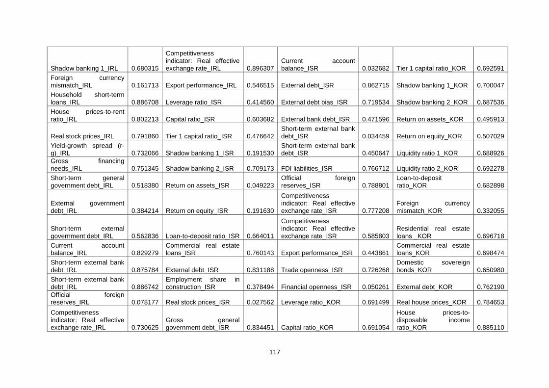
117
Shadow banking 1_IRL 0.680315
Competitiveness indicator: Real effective exchange rate_IRL 0.896307
Current account balance_ISR 0.032682 Tier 1 capital ratio_KOR 0.692591
Foreign currency mismatch_IRL 0.161713 Export performance_IRL 0.546515 External debt_ISR 0.862715 Shadow banking 1_KOR 0.700047
Household short-term loans_IRL 0.886708 Leverage ratio_ISR 0.414560 External debt bias_ISR 0.719534 Shadow banking 2_KOR 0.687536
House prices-to-rent ratio_IRL 0.802213 Capital ratio_ISR 0.603682 External bank debt_ISR 0.471596 Return on assets_KOR 0.495913
Real stock prices_IRL 0.791860 Tier 1 capital ratio_ISR 0.476642 Short-term external bank debt_ISR 0.034459 Return on equity_KOR 0.507029
Yield-growth spread (r-g)_IRL 0.732066 Shadow banking 1_ISR 0.191530
Short-term external bank debt_ISR 0.450647 Liquidity ratio 1_KOR 0.688926
Gross financing needs_IRL 0.751345 Shadow banking 2_ISR 0.709173 FDI liabilities_ISR 0.766712 Liquidity ratio 2_KOR 0.692278
Short-term general government debt_IRL 0.518380 Return on assets_ISR 0.049223
Official foreign reserves_ISR 0.788801
Loan-to-deposit ratio_KOR 0.682898
External government debt_IRL 0.384214 Return on equity_ISR 0.191630
Competitiveness indicator: Real effective exchange rate_ISR 0.777208
Foreign currency mismatch_KOR 0.332055
Short-term external government debt_IRL 0.562836 Loan-to-deposit ratio_ISR 0.664011
Competitiveness indicator: Real effective exchange rate_ISR 0.585803
Residential real estate loans _KOR 0.696718
Current account balance_IRL 0.829279
Commercial real estate loans_ISR 0.760143 Export performance_ISR 0.443861
Commercial real estate loans_KOR 0.698474
Short-term external bank debt_IRL 0.875784 External debt_ISR 0.831188 Trade openness_ISR 0.726268
Domestic sovereign bonds_KOR 0.650980
Short-term external bank debt_IRL 0.886742
Employment share in construction_ISR 0.378494 Financial openness_ISR 0.050261 External debt_KOR 0.762190
Official foreign reserves_IRL 0.078177 Real stock prices_ISR 0.027562 Leverage ratio_KOR 0.691499 Real house prices_KOR 0.784653
Competitiveness indicator: Real effective exchange rate_IRL 0.730625
Gross general government debt_ISR 0.834451 Capital ratio_KOR 0.691054
House prices-to-disposable income ratio_KOR 0.885110
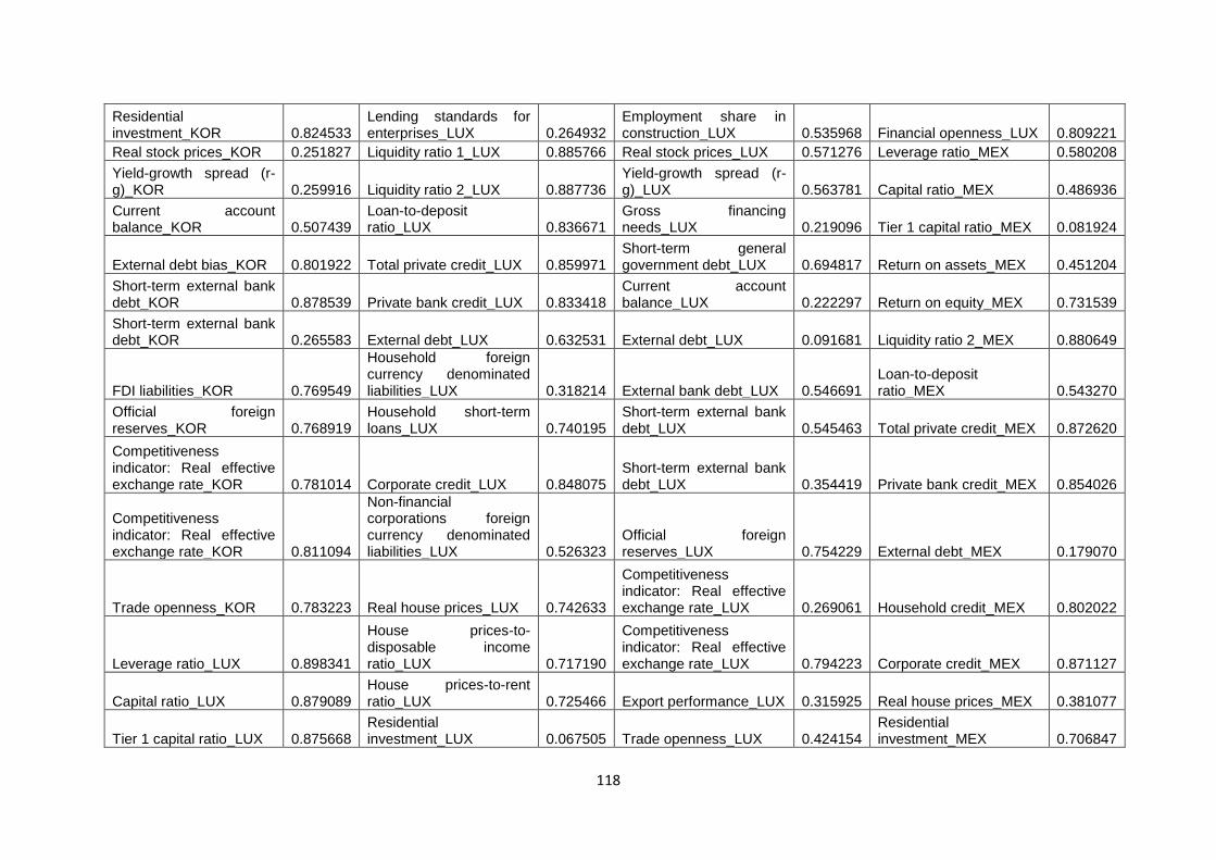
118
Residential investment_KOR 0.824533
Lending standards for enterprises_LUX 0.264932
Employment share in construction_LUX 0.535968 Financial openness_LUX 0.809221
Real stock prices_KOR 0.251827 Liquidity ratio 1_LUX 0.885766 Real stock prices_LUX 0.571276 Leverage ratio_MEX 0.580208
Yield-growth spread (r-g)_KOR 0.259916 Liquidity ratio 2_LUX 0.887736
Yield-growth spread (r-g)_LUX 0.563781 Capital ratio_MEX 0.486936
Current account balance_KOR 0.507439
Loan-to-deposit ratio_LUX 0.836671
Gross financing needs_LUX 0.219096 Tier 1 capital ratio_MEX 0.081924
External debt bias_KOR 0.801922 Total private credit_LUX 0.859971 Short-term general government debt_LUX 0.694817 Return on assets_MEX 0.451204
Short-term external bank debt_KOR 0.878539 Private bank credit_LUX 0.833418
Current account balance_LUX 0.222297 Return on equity_MEX 0.731539
Short-term external bank debt_KOR 0.265583 External debt_LUX 0.632531 External debt_LUX 0.091681 Liquidity ratio 2_MEX 0.880649
FDI liabilities_KOR 0.769549
Household foreign currency denominated liabilities_LUX 0.318214 External bank debt_LUX 0.546691
Loan-to-deposit ratio_MEX 0.543270
Official foreign reserves_KOR 0.768919
Household short-term loans_LUX 0.740195
Short-term external bank debt_LUX 0.545463 Total private credit_MEX 0.872620
Competitiveness indicator: Real effective exchange rate_KOR 0.781014 Corporate credit_LUX 0.848075
Short-term external bank debt_LUX 0.354419 Private bank credit_MEX 0.854026
Competitiveness indicator: Real effective exchange rate_KOR 0.811094
Non-financial corporations foreign currency denominated liabilities_LUX 0.526323
Official foreign reserves_LUX 0.754229 External debt_MEX 0.179070
Trade openness_KOR 0.783223 Real house prices_LUX 0.742633
Competitiveness indicator: Real effective exchange rate_LUX 0.269061 Household credit_MEX 0.802022
Leverage ratio_LUX 0.898341
House prices-to-disposable income ratio_LUX 0.717190
Competitiveness indicator: Real effective exchange rate_LUX 0.794223 Corporate credit_MEX 0.871127
Capital ratio_LUX 0.879089 House prices-to-rent ratio_LUX 0.725466 Export performance_LUX 0.315925 Real house prices_MEX 0.381077
Tier 1 capital ratio_LUX 0.875668 Residential investment_LUX 0.067505 Trade openness_LUX 0.424154
Residential investment_MEX 0.706847

119
Real stock prices_MEX 0.531998 Trade openness_MEX 0.825797 Corporate credit_NLD 0.085158 Official foreign reserves_NLD 0.861551
Yield-growth spread (r-g)_MEX 0.140952 Capital ratio_NLD 0.895766
Non-financial corporations gross financial liabilities_NLD 0.773375
Competitiveness indicator: Real effective exchange rate_NLD 0.440547
Gross financing needs_MEX 0.607203 Return on assets_NLD 0.357755 Real stock prices_NLD 0.511189
Competitiveness indicator: Real effective exchange rate_NLD 0.524875
Short-term general government debt_MEX 0.298982 Return on equity_NLD 0.267258
Yield-growth spread (r-g)_NLD 0.505549 Export performance_NLD 0.270817
Gross government debt denominated in foreign currency_MEX 0.119757 Liquidity ratio 1_NLD 0.889401
External government debt_NLD 0.508415 Trade openness_NLD 0.753656
External government debt_MEX 0.627354 Liquidity ratio 2_NLD 0.854233
Short-term external government debt_NLD 0.651019 Financial openness_NLD 0.864629
Short-term external government debt_MEX 0.897257
Residential real estate loans _NLD 0.879877
Current account balance_NLD 0.722635
Household short-term loans_NZL 0.502720
Current account balance_MEX 0.153506 Total private credit_NLD 0.663941 External debt_NLD 0.784677 Real house prices_NZL 0.200362
External bank debt_MEX 0.728527 Private bank credit_NLD 0.648477 External debt bias_NLD 0.829714
House prices-to-disposable income ratio_NZL 0.234537
Short-term external bank debt_MEX 0.738453 External debt_NLD 0.846678 External bank debt_NLD 0.507682
House prices-to-rent ratio_NZL 0.157515
Short-term external bank debt_MEX 0.499044 Household credit_NLD 0.841586
Short-term external bank debt_NLD 0.738659
Residential investment_NZL 0.736222
Competitiveness indicator: Real effective exchange rate_MEX 0.568656
Household foreign currency denominated liabilities_NLD 0.675534
Short-term external bank debt_NLD 0.833904
Employment share in construction_NZL 0.226733
Competitiveness indicator: Real effective exchange rate_MEX 0.452493
Household short-term loans_NLD 0.701100 FDI liabilities_NLD 0.879355 Real stock prices_NZL 0.793437
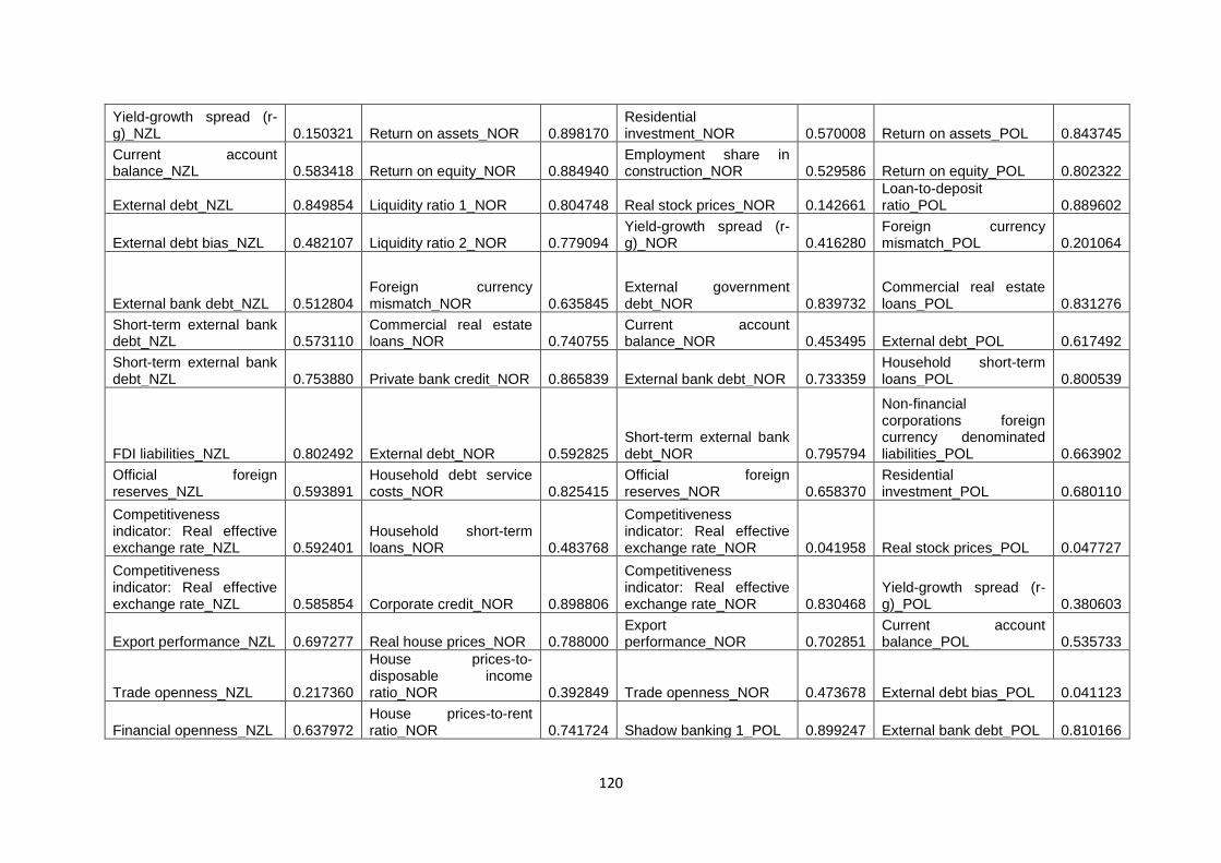
120
Yield-growth spread (r-g)_NZL 0.150321 Return on assets_NOR 0.898170
Residential investment_NOR 0.570008 Return on assets_POL 0.843745
Current account balance_NZL 0.583418 Return on equity_NOR 0.884940
Employment share in construction_NOR 0.529586 Return on equity_POL 0.802322
External debt_NZL 0.849854 Liquidity ratio 1_NOR 0.804748 Real stock prices_NOR 0.142661 Loan-to-deposit ratio_POL 0.889602
External debt bias_NZL 0.482107 Liquidity ratio 2_NOR 0.779094 Yield-growth spread (r-g)_NOR 0.416280
Foreign currency mismatch_POL 0.201064
External bank debt_NZL 0.512804 Foreign currency mismatch_NOR 0.635845
External government debt_NOR 0.839732
Commercial real estate loans_POL 0.831276
Short-term external bank debt_NZL 0.573110
Commercial real estate loans_NOR 0.740755
Current account balance_NOR 0.453495 External debt_POL 0.617492
Short-term external bank debt_NZL 0.753880 Private bank credit_NOR 0.865839 External bank debt_NOR 0.733359
Household short-term loans_POL 0.800539
FDI liabilities_NZL 0.802492 External debt_NOR 0.592825 Short-term external bank debt_NOR 0.795794
Non-financial corporations foreign currency denominated liabilities_POL 0.663902
Official foreign reserves_NZL 0.593891
Household debt service costs_NOR 0.825415
Official foreign reserves_NOR 0.658370
Residential investment_POL 0.680110
Competitiveness indicator: Real effective exchange rate_NZL 0.592401
Household short-term loans_NOR 0.483768
Competitiveness indicator: Real effective exchange rate_NOR 0.041958 Real stock prices_POL 0.047727
Competitiveness indicator: Real effective exchange rate_NZL 0.585854 Corporate credit_NOR 0.898806
Competitiveness indicator: Real effective exchange rate_NOR 0.830468
Yield-growth spread (r-g)_POL 0.380603
Export performance_NZL 0.697277 Real house prices_NOR 0.788000 Export performance_NOR 0.702851
Current account balance_POL 0.535733
Trade openness_NZL 0.217360
House prices-to-disposable income ratio_NOR 0.392849 Trade openness_NOR 0.473678 External debt bias_POL 0.041123
Financial openness_NZL 0.637972 House prices-to-rent ratio_NOR 0.741724 Shadow banking 1_POL 0.899247 External bank debt_POL 0.810166
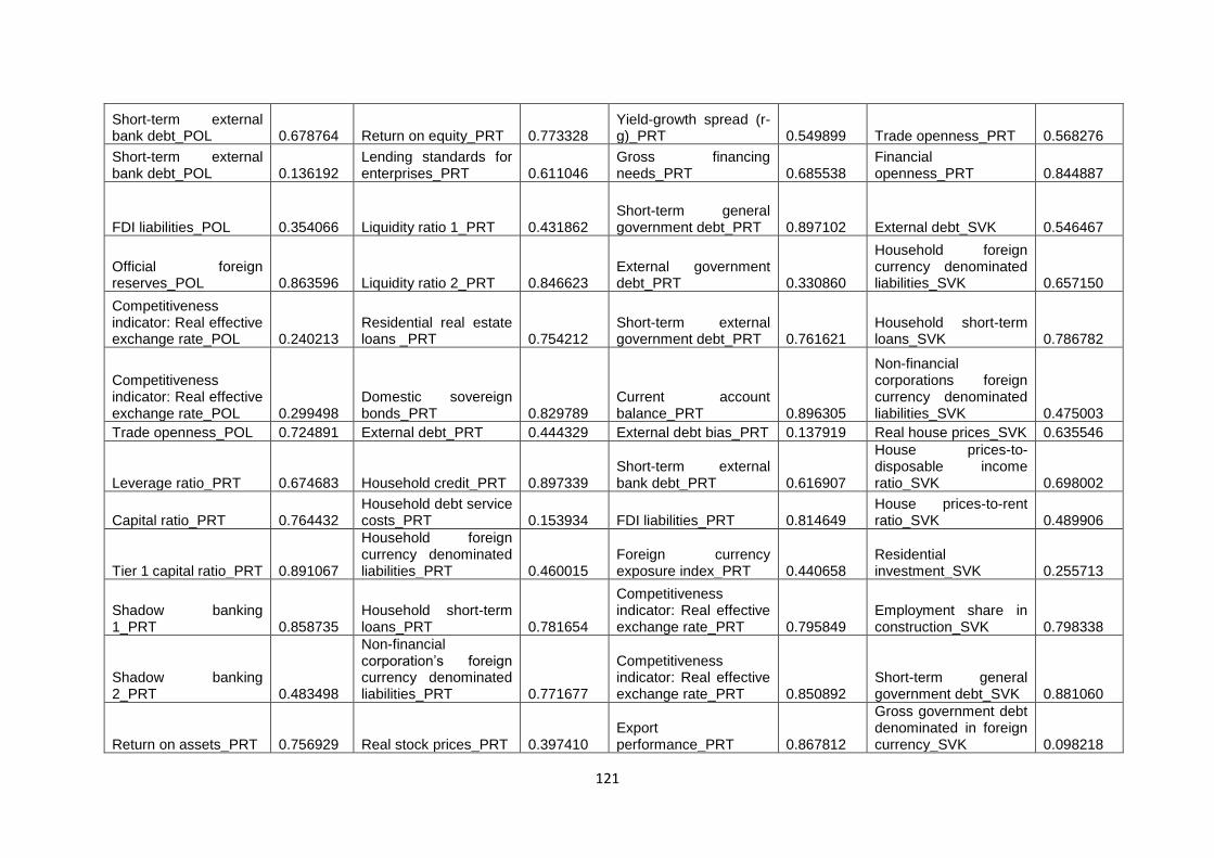
121
Short-term external bank debt_POL 0.678764 Return on equity_PRT 0.773328
Yield-growth spread (r-g)_PRT 0.549899 Trade openness_PRT 0.568276
Short-term external bank debt_POL 0.136192
Lending standards for enterprises_PRT 0.611046
Gross financing needs_PRT 0.685538
Financial openness_PRT 0.844887
FDI liabilities_POL 0.354066 Liquidity ratio 1_PRT 0.431862 Short-term general government debt_PRT 0.897102 External debt_SVK 0.546467
Official foreign reserves_POL 0.863596 Liquidity ratio 2_PRT 0.846623
External government debt_PRT 0.330860
Household foreign currency denominated liabilities_SVK 0.657150
Competitiveness indicator: Real effective exchange rate_POL 0.240213
Residential real estate loans _PRT 0.754212
Short-term external government debt_PRT 0.761621
Household short-term loans_SVK 0.786782
Competitiveness indicator: Real effective exchange rate_POL 0.299498
Domestic sovereign bonds_PRT 0.829789
Current account balance_PRT 0.896305
Non-financial corporations foreign currency denominated liabilities_SVK 0.475003
Trade openness_POL 0.724891 External debt_PRT 0.444329 External debt bias_PRT 0.137919 Real house prices_SVK 0.635546
Leverage ratio_PRT 0.674683 Household credit_PRT 0.897339 Short-term external bank debt_PRT 0.616907
House prices-to-disposable income ratio_SVK 0.698002
Capital ratio_PRT 0.764432 Household debt service costs_PRT 0.153934 FDI liabilities_PRT 0.814649
House prices-to-rent ratio_SVK 0.489906
Tier 1 capital ratio_PRT 0.891067
Household foreign currency denominated liabilities_PRT 0.460015
Foreign currency exposure index_PRT 0.440658
Residential investment_SVK 0.255713
Shadow banking 1_PRT 0.858735
Household short-term loans_PRT 0.781654
Competitiveness indicator: Real effective exchange rate_PRT 0.795849
Employment share in construction_SVK 0.798338
Shadow banking 2_PRT 0.483498
Non-financial corporation’s foreign currency denominated liabilities_PRT 0.771677
Competitiveness indicator: Real effective exchange rate_PRT 0.850892
Short-term general government debt_SVK 0.881060
Return on assets_PRT 0.756929 Real stock prices_PRT 0.397410 Export performance_PRT 0.867812
Gross government debt denominated in foreign currency_SVK 0.098218
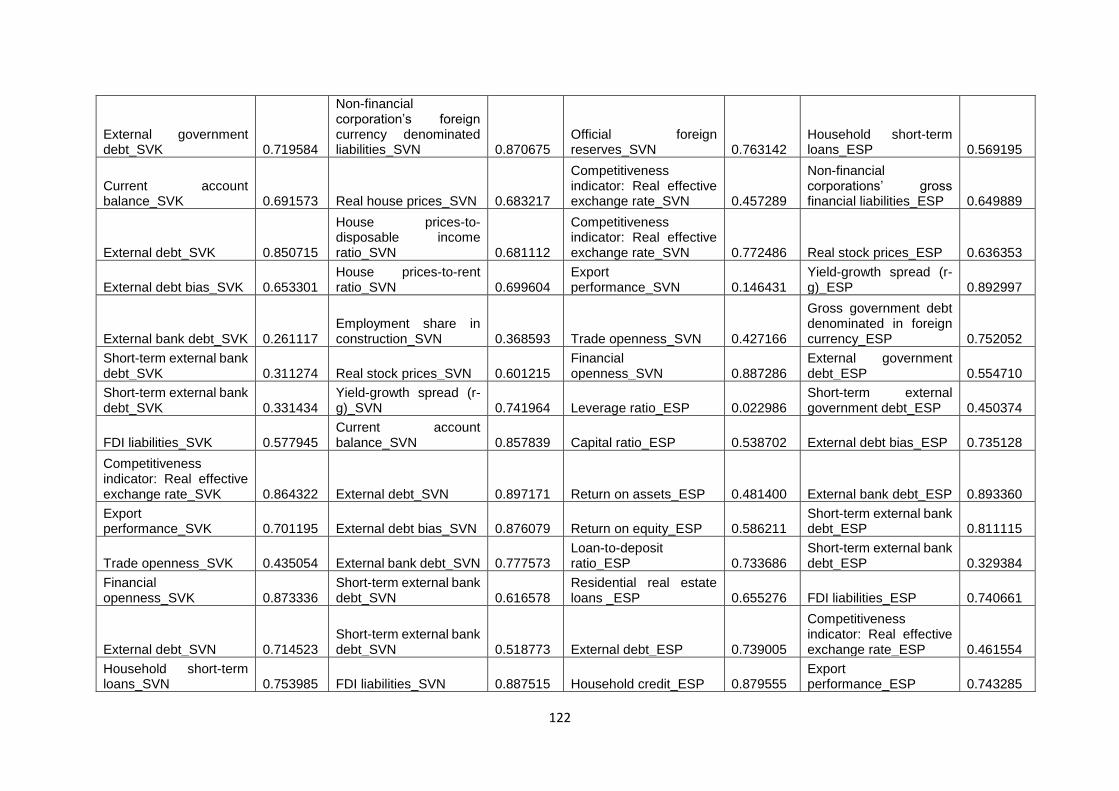
122
External government debt_SVK 0.719584
Non-financial corporation’s foreign currency denominated liabilities_SVN 0.870675
Official foreign reserves_SVN 0.763142
Household short-term loans_ESP 0.569195
Current account balance_SVK 0.691573 Real house prices_SVN 0.683217
Competitiveness indicator: Real effective exchange rate_SVN 0.457289
Non-financial corporations’ gross financial liabilities_ESP 0.649889
External debt_SVK 0.850715
House prices-to-disposable income ratio_SVN 0.681112
Competitiveness indicator: Real effective exchange rate_SVN 0.772486 Real stock prices_ESP 0.636353
External debt bias_SVK 0.653301 House prices-to-rent ratio_SVN 0.699604
Export performance_SVN 0.146431
Yield-growth spread (r-g)_ESP 0.892997
External bank debt_SVK 0.261117 Employment share in construction_SVN 0.368593 Trade openness_SVN 0.427166
Gross government debt denominated in foreign currency_ESP 0.752052
Short-term external bank debt_SVK 0.311274 Real stock prices_SVN 0.601215
Financial openness_SVN 0.887286
External government debt_ESP 0.554710
Short-term external bank debt_SVK 0.331434
Yield-growth spread (r-g)_SVN 0.741964 Leverage ratio_ESP 0.022986
Short-term external government debt_ESP 0.450374
FDI liabilities_SVK 0.577945 Current account balance_SVN 0.857839 Capital ratio_ESP 0.538702 External debt bias_ESP 0.735128
Competitiveness indicator: Real effective exchange rate_SVK 0.864322 External debt_SVN 0.897171 Return on assets_ESP 0.481400 External bank debt_ESP 0.893360
Export performance_SVK 0.701195 External debt bias_SVN 0.876079 Return on equity_ESP 0.586211
Short-term external bank debt_ESP 0.811115
Trade openness_SVK 0.435054 External bank debt_SVN 0.777573 Loan-to-deposit ratio_ESP 0.733686
Short-term external bank debt_ESP 0.329384
Financial openness_SVK 0.873336
Short-term external bank debt_SVN 0.616578
Residential real estate loans _ESP 0.655276 FDI liabilities_ESP 0.740661
External debt_SVN 0.714523 Short-term external bank debt_SVN 0.518773 External debt_ESP 0.739005
Competitiveness indicator: Real effective exchange rate_ESP 0.461554
Household short-term loans_SVN 0.753985 FDI liabilities_SVN 0.887515 Household credit_ESP 0.879555
Export performance_ESP 0.743285
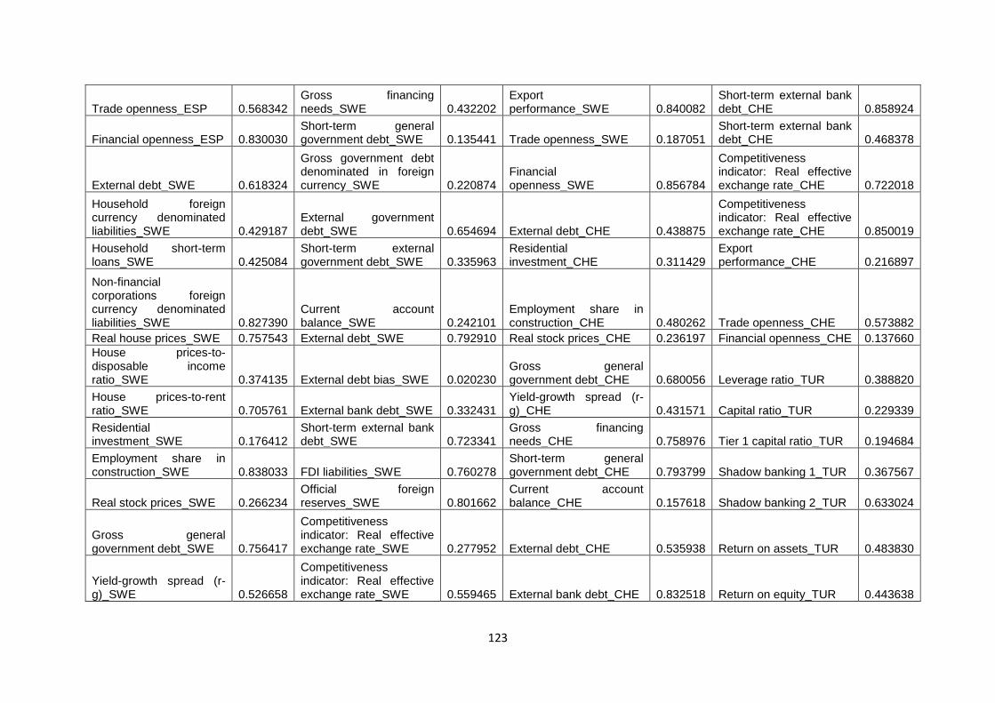
123
Trade openness_ESP 0.568342 Gross financing needs_SWE 0.432202
Export performance_SWE 0.840082
Short-term external bank debt_CHE 0.858924
Financial openness_ESP 0.830030 Short-term general government debt_SWE 0.135441 Trade openness_SWE 0.187051
Short-term external bank debt_CHE 0.468378
External debt_SWE 0.618324
Gross government debt denominated in foreign currency_SWE 0.220874
Financial openness_SWE 0.856784
Competitiveness indicator: Real effective exchange rate_CHE 0.722018
Household foreign currency denominated liabilities_SWE 0.429187
External government debt_SWE 0.654694 External debt_CHE 0.438875
Competitiveness indicator: Real effective exchange rate_CHE 0.850019
Household short-term loans_SWE 0.425084
Short-term external government debt_SWE 0.335963
Residential investment_CHE 0.311429
Export performance_CHE 0.216897
Non-financial corporations foreign currency denominated liabilities_SWE 0.827390
Current account balance_SWE 0.242101
Employment share in construction_CHE 0.480262 Trade openness_CHE 0.573882
Real house prices_SWE 0.757543 External debt_SWE 0.792910 Real stock prices_CHE 0.236197 Financial openness_CHE 0.137660
House prices-to-disposable income ratio_SWE 0.374135 External debt bias_SWE 0.020230
Gross general government debt_CHE 0.680056 Leverage ratio_TUR 0.388820
House prices-to-rent ratio_SWE 0.705761 External bank debt_SWE 0.332431
Yield-growth spread (r-g)_CHE 0.431571 Capital ratio_TUR 0.229339
Residential investment_SWE 0.176412
Short-term external bank debt_SWE 0.723341
Gross financing needs_CHE 0.758976 Tier 1 capital ratio_TUR 0.194684
Employment share in construction_SWE 0.838033 FDI liabilities_SWE 0.760278
Short-term general government debt_CHE 0.793799 Shadow banking 1_TUR 0.367567
Real stock prices_SWE 0.266234 Official foreign reserves_SWE 0.801662
Current account balance_CHE 0.157618 Shadow banking 2_TUR 0.633024
Gross general government debt_SWE 0.756417
Competitiveness indicator: Real effective exchange rate_SWE 0.277952 External debt_CHE 0.535938 Return on assets_TUR 0.483830
Yield-growth spread (r-g)_SWE 0.526658
Competitiveness indicator: Real effective exchange rate_SWE 0.559465 External bank debt_CHE 0.832518 Return on equity_TUR 0.443638

124
Liquidity ratio 1_TUR 0.745172 External bank debt_TUR 0.552316 Return on equity_BRA 0.836864
Competitiveness indicator: Real effective exchange rate_BRA 0.630339
Liquidity ratio 2_TUR 0.757650 Short-term external bank debt_TUR 0.759334 Liquidity ratio 1_BRA 0.732276
Competitiveness indicator: Real effective exchange rate_BRA 0.722508
Loan-to-deposit ratio_TUR 0.648415
Short-term external bank debt_TUR 0.581835 Liquidity ratio 2_BRA 0.642103 Export performance_BRA 0.824165
Foreign currency mismatch_TUR 0.267391 FDI liabilities_TUR 0.532371
Loan-to-deposit ratio_BRA 0.747454 Trade openness_BRA 0.353471
Residential real estate loans _TUR 0.511299
Official foreign reserves_TUR 0.520628
Foreign currency mismatch_BRA 0.219525 Financial openness_BRA 0.741006
Commercial real estate loans_TUR 0.449507
Competitiveness indicator: Real effective exchange rate_TUR 0.288881 External debt_BRA 0.612815 Private bank credit_CHN 0.843638
Domestic sovereign bonds_TUR 0.769394
Competitiveness indicator: Real effective exchange rate_TUR 0.237048
Household debt service costs_BRA 0.843011 Household credit_CHN 0.865401
External debt_TUR 0.566756 Export performance_TUR 0.606931 Real stock prices_BRA 0.511675 Corporate credit_CHN 0.623349
Household short-term loans_TUR 0.718839 Trade openness_TUR 0.657530
Current account balance_BRA 0.839189 Real stock prices_CHN 0.325573
Employment share in construction_TUR 0.559652 Financial openness_TUR 0.570165 External debt_BRA 0.708731
Current account balance_CHN 0.759347
Real stock prices_TUR 0.132831 Leverage ratio_BRA 0.424953 External debt bias_BRA 0.583196 External bank debt_CHN 0.774011
Yield-growth spread (r-g)_TUR 0.458231 Capital ratio_BRA 0.300272
Short-term external bank debt_BRA 0.857825
Short-term external bank debt_CHN 0.862186
Current account balance_TUR 0.175732 Tier 1 capital ratio_BRA 0.399276
Short-term external bank debt_BRA 0.194516
Short-term external bank debt_CHN 0.822125
External debt_TUR 0.547661 Shadow banking 2_BRA 0.709570 FDI liabilities_BRA 0.845698 Official foreign reserves_CHN 0.866303
External debt bias_TUR 0.398977 Return on assets_BRA 0.827740 Official foreign reserves_BRA 0.837726
Competitiveness indicator: Real effective exchange rate_CHN 0.870712
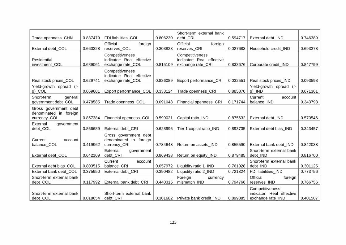
125
Trade openness_CHN 0.837479 FDI liabilities_COL 0.806230 Short-term external bank debt_CRI 0.594717 External debt_IND 0.746389
External debt_COL 0.660328 Official foreign reserves_COL 0.303828
Official foreign reserves_CRI 0.027683 Household credit_IND 0.693378
Residential investment_COL 0.689061
Competitiveness indicator: Real effective exchange rate_COL 0.815109
Competitiveness indicator: Real effective exchange rate_CRI 0.833676 Corporate credit_IND 0.847799
Real stock prices_COL 0.629741
Competitiveness indicator: Real effective exchange rate_COL 0.836089 Export performance_CRI 0.032551 Real stock prices_IND 0.093598
Yield-growth spread (r-g)_COL 0.069601 Export performance_COL 0.333124 Trade openness_CRI 0.885870
Yield-growth spread (r-g)_IND 0.671361
Short-term general government debt_COL 0.478585 Trade openness_COL 0.091048 Financial openness_CRI 0.171744
Current account balance_IND 0.343793
Gross government debt denominated in foreign currency_COL 0.857384 Financial openness_COL 0.599021 Capital ratio_IND 0.875632 External debt_IND 0.570546
External government debt_COL 0.866689 External debt_CRI 0.628996 Tier 1 capital ratio_IND 0.893735 External debt bias_IND 0.343457
Current account balance_COL 0.419962
Gross government debt denominated in foreign currency_CRI 0.784648 Return on assets_IND 0.855590 External bank debt_IND 0.842038
External debt_COL 0.642109 External government debt_CRI 0.869438 Return on equity_IND 0.879485
Short-term external bank debt_IND 0.816700
External debt bias_COL 0.803515 Current account balance_CRI 0.057972 Liquidity ratio 1_IND 0.761028
Short-term external bank debt_IND 0.301125
External bank debt_COL 0.375950 External debt_CRI 0.390482 Liquidity ratio 2_IND 0.721324 FDI liabilities_IND 0.773756
Short-term external bank debt_COL 0.117992 External bank debt_CRI 0.440315
Foreign currency mismatch_IND 0.794766
Official foreign reserves_IND 0.766756
Short-term external bank debt_COL 0.018654
Short-term external bank debt_CRI 0.301682 Private bank credit_IND 0.899885
Competitiveness indicator: Real effective exchange rate_IND 0.401507
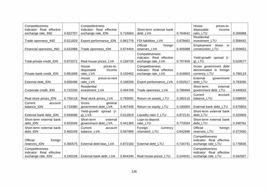
126
Competitiveness indicator: Real effective exchange rate_IND 0.822707
Competitiveness indicator: Real effective exchange rate_IDN 0.716664
Short-term external bank debt_LVA 0.764642
House prices-to-disposable income ratio_LTU 0.266988
Trade openness_IND 0.521829 Export performance_IDN 0.881776 FDI liabilities_LVA 0.878662 Residential investment_LTU 0.358442
Financial openness_IND 0.632988 Trade openness_IDN 0.674454 Official foreign reserves_LVA 0.405988
Employment share in construction_LTU 0.559652
Total private credit_IDN 0.872072 Real house prices_LVA 0.159726
Competitiveness indicator: Real effective exchange rate_LVA 0.797459
Yield-growth spread (r-g)_LTU 0.529577
Private bank credit_IDN 0.891699
House prices-to-disposable income ratio_LVA 0.150452
Competitiveness indicator: Real effective exchange rate_LVA 0.416963
Gross government debt denominated in foreign currency_LTU 0.798119
External debt_IDN 0.695498 House prices-to-rent ratio_LVA 0.168200 Export performance_LVA 0.552517
External government debt_LTU 0.793090
Corporate credit_IDN 0.722200 Residential investment_LVA 0.494709 Trade openness_LVA 0.789469
Short-term external government debt_LTU 0.440633
Real stock prices_IDN 0.759118 Real stock prices_LVA 0.793091 Return on assets_LTU 0.260110 Current account balance_LTU 0.598650
Current account balance_IDN 0.733380
Gross general government debt_LVA 0.407445 Return on equity_LTU 0.190000 External bank debt_LTU 0.670803
External bank debt_IDN 0.593096 Yield-growth spread (r-g)_LVA 0.612810 Liquidity ratio 2_LTU 0.872131
Short-term external bank debt_LTU 0.320609
Short-term external bank debt_IDN 0.503049
Short-term external government debt_LVA 0.441365
Loan-to-deposit ratio_LTU 0.770554
Short-term external bank debt_LTU 0.348781
Short-term external bank debt_IDN 0.465249
Current account balance_LVA 0.597969
Foreign currency mismatch_LTU 0.642696
Official foreign reserves_LTU 0.373450
Official foreign reserves_IDN 0.360575 External debt bias_LVA 0.872182 External debt_LTU 0.734741
Competitiveness indicator: Real effective exchange rate_LTU 0.778836
Competitiveness indicator: Real effective exchange rate_IDN 0.240109 External bank debt_LVA 0.844340 Real house prices_LTU 0.244031
Competitiveness indicator: Real effective exchange rate_LTU 0.542507
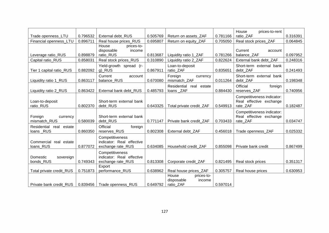
127
Trade openness_LTU 0.796532 External debt_RUS 0.505769 Return on assets_ZAF 0.781166 House prices-to-rent ratio_ZAF 0.316391
Financial openness_LTU 0.896711 Real house prices_RUS 0.695807 Return on equity_ZAF 0.705050 Real stock prices_ZAF 0.064845
Leverage ratio_RUS 0.898879
House prices-to-disposable income ratio_RUS 0.813687 Liquidity ratio 1_ZAF 0.781266
Current account balance_ZAF 0.097952
Capital ratio_RUS 0.858031 Real stock prices_RUS 0.310890 Liquidity ratio 2_ZAF 0.822624 External bank debt_ZAF 0.248316
Tier 1 capital ratio_RUS 0.882092 Yield-growth spread (r-g)_RUS 0.867911
Loan-to-deposit ratio_ZAF 0.835651
Short-term external bank debt_ZAF 0.241493
Liquidity ratio 1_RUS 0.863117 Current account balance_RUS 0.670080
Foreign currency mismatch_ZAF 0.011264
Short-term external bank debt_ZAF 0.198348
Liquidity ratio 2_RUS 0.863422 External bank debt_RUS 0.485793 Residential real estate loans _ZAF 0.884430
Official foreign reserves_ZAF 0.740956
Loan-to-deposit ratio_RUS 0.802370
Short-term external bank debt_RUS 0.643325 Total private credit_ZAF 0.549913
Competitiveness indicator: Real effective exchange rate_ZAF 0.182487
Foreign currency mismatch_RUS 0.580039
Short-term external bank debt_RUS 0.771147 Private bank credit_ZAF 0.703433
Competitiveness indicator: Real effective exchange rate_ZAF 0.034747
Residential real estate loans _RUS 0.860350
Official foreign reserves_RUS 0.802308 External debt_ZAF 0.456018 Trade openness_ZAF 0.025332
Commercial real estate loans_RUS 0.877072
Competitiveness indicator: Real effective exchange rate_RUS 0.634085 Household credit_ZAF 0.855098 Private bank credit 0.867499
Domestic sovereign bonds_RUS 0.749343
Competitiveness indicator: Real effective exchange rate_RUS 0.813308 Corporate credit_ZAF 0.821495 Real stock prices 0.351317
Total private credit_RUS 0.751873 Export performance_RUS 0.638962 Real house prices_ZAF 0.305757 Real house prices 0.630953
Private bank credit_RUS 0.839456 Trade openness_RUS 0.649792
House prices-to-disposable income ratio_ZAF 0.597014
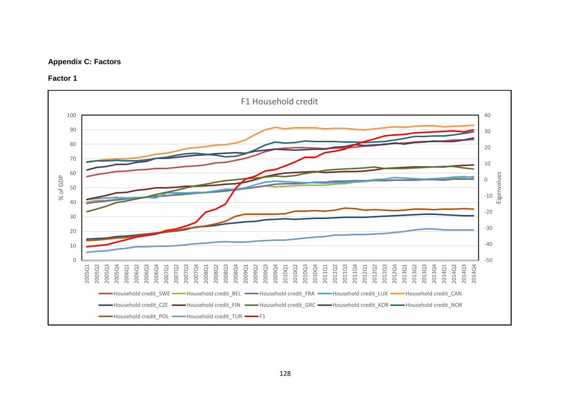
128
Appendix C: Factors
Factor 1
-50
-40
-30
-20
-10
0
10
20
30
40
0
10
20
30
40
50
60
70
80
90
100
20
05
Q1
20
05
Q2
20
05
Q3
20
05
Q4
20
06
Q1
20
06
Q2
20
06
Q3
20
06
Q4
20
07
Q1
20
07
Q2
20
07
Q3
20
07
Q4
20
08
Q1
20
08
Q2
20
08
Q3
20
08
Q4
20
09
Q1
20
09
Q2
20
09
Q3
20
09
Q4
20
10
Q1
20
10
Q2
20
10
Q3
20
10
Q4
20
11
Q1
20
11
Q2
20
11
Q3
20
11
Q4
20
12
Q1
20
12
Q2
20
12
Q3
20
12
Q4
20
13
Q1
20
13
Q2
20
13
Q3
20
13
Q4
20
14
Q1
20
14
Q2
20
14
Q3
20
14
Q4
Eige
nva
lues
% o
f G
DP
F1 Household credit
Household credit_SWE Household credit_BEL Household credit_FRA Household credit_LUX Household credit_CAN
Household credit_CZE Household credit_FIN Household credit_GRC Household credit_KOR Household credit_NOR
Household credit_POL Household credit_TUR F1
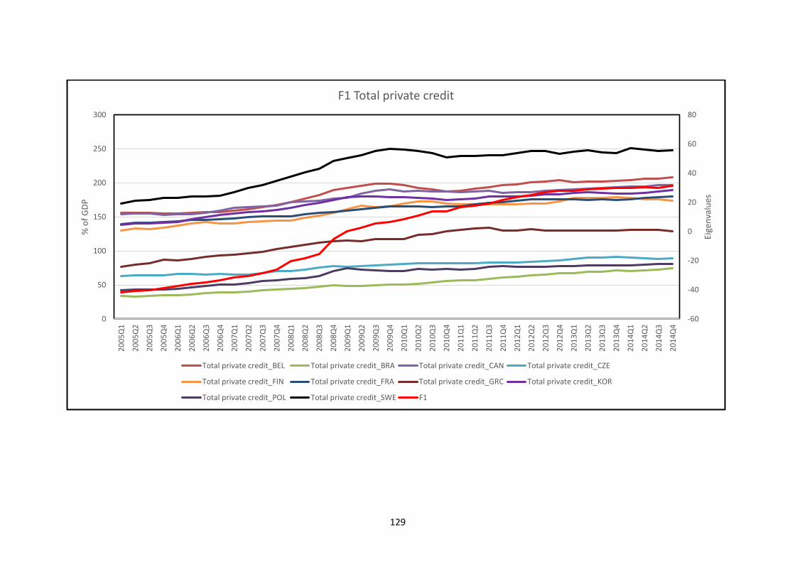
129
-60
-40
-20
0
20
40
60
80
0
50
100
150
200
250
3002
00
5Q
1
20
05
Q2
20
05
Q3
20
05
Q4
20
06
Q1
20
06
Q2
20
06
Q3
20
06
Q4
20
07
Q1
20
07
Q2
20
07
Q3
20
07
Q4
20
08
Q1
20
08
Q2
20
08
Q3
20
08
Q4
20
09
Q1
20
09
Q2
20
09
Q3
20
09
Q4
20
10
Q1
20
10
Q2
20
10
Q3
20
10
Q4
20
11
Q1
20
11
Q2
20
11
Q3
20
11
Q4
20
12
Q1
20
12
Q2
20
12
Q3
20
12
Q4
20
13
Q1
20
13
Q2
20
13
Q3
20
13
Q4
20
14
Q1
20
14
Q2
20
14
Q3
20
14
Q4
Eige
nva
lues
% o
f G
DP
F1 Total private credit
Total private credit_BEL Total private credit_BRA Total private credit_CAN Total private credit_CZE
Total private credit_FIN Total private credit_FRA Total private credit_GRC Total private credit_KOR
Total private credit_POL Total private credit_SWE F1
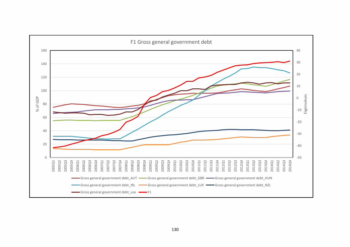
130
-50
-40
-30
-20
-10
0
10
20
30
40
0
20
40
60
80
100
120
140
1602
00
5Q
1
20
05
Q2
20
05
Q3
20
05
Q4
20
06
Q1
20
06
Q2
20
06
Q3
20
06
Q4
20
07
Q1
20
07
Q2
20
07
Q3
20
07
Q4
20
08
Q1
20
08
Q2
20
08
Q3
20
08
Q4
20
09
Q1
20
09
Q2
20
09
Q3
20
09
Q4
20
10
Q1
20
10
Q2
20
10
Q3
20
10
Q4
20
11
Q1
20
11
Q2
20
11
Q3
20
11
Q4
20
12
Q1
20
12
Q2
20
12
Q3
20
12
Q4
20
13
Q1
20
13
Q2
20
13
Q3
20
13
Q4
20
14
Q1
20
14
Q2
20
14
Q3
20
14
Q4
Eige
nva
lues
% o
f G
DP
F1 Gross general government debt
Gross general government debt_AUT Gross general government debt_GBR Gross general government debt_HUN
Gross general government debt_IRL Gross general government debt_LUX Gross general government debt_NZL
Gross general government debt_usa F1

131
-50
-40
-30
-20
-10
0
10
20
30
40
0
20
40
60
80
100
120
1402
00
5Q
1
20
05
Q2
20
05
Q3
20
05
Q4
20
06
Q1
20
06
Q2
20
06
Q3
20
06
Q4
20
07
Q1
20
07
Q2
20
07
Q3
20
07
Q4
20
08
Q1
20
08
Q2
20
08
Q3
20
08
Q4
20
09
Q1
20
09
Q2
20
09
Q3
20
09
Q4
20
10
Q1
20
10
Q2
20
10
Q3
20
10
Q4
20
11
Q1
20
11
Q2
20
11
Q3
20
11
Q4
20
12
Q1
20
12
Q2
20
12
Q3
20
12
Q4
20
13
Q1
20
13
Q2
20
13
Q3
20
13
Q4
20
14
Q1
20
14
Q2
20
14
Q3
20
14
Q4
Eige
nva
lues
% o
f G
DP
F1 Private bank credit
Private bank credit_BRA Private bank credit_CZE Private bank credit_FIN Private bank credit_FRA
Private bank credit_GRC Private bank credit_POL Private bank credit_SWE F1
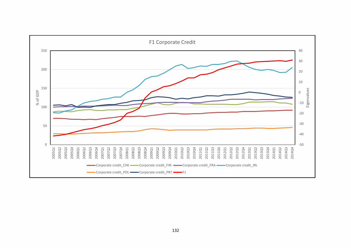
132
-50
-40
-30
-20
-10
0
10
20
30
40
0
50
100
150
200
2502
00
5Q
1
20
05
Q2
20
05
Q3
20
05
Q4
20
06
Q1
20
06
Q2
20
06
Q3
20
06
Q4
20
07
Q1
20
07
Q2
20
07
Q3
20
07
Q4
20
08
Q1
20
08
Q2
20
08
Q3
20
08
Q4
20
09
Q1
20
09
Q2
20
09
Q3
20
09
Q4
20
10
Q1
20
10
Q2
20
10
Q3
20
10
Q4
20
11
Q1
20
11
Q2
20
11
Q3
20
11
Q4
20
12
Q1
20
12
Q2
20
12
Q3
20
12
Q4
20
13
Q1
20
13
Q2
20
13
Q3
20
13
Q4
20
14
Q1
20
14
Q2
20
14
Q3
20
14
Q4
Eige
nva
lues
% o
f G
DP
F1 Corporate Credit
Corporate credit_CHE Corporate credit_FIN Corporate credit_FRA Corporate credit_IRL
Corporate credit_POL Corporate credit_PRT F1
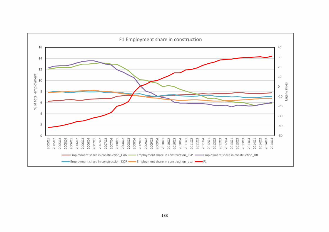
133
-50
-40
-30
-20
-10
0
10
20
30
40
0
2
4
6
8
10
12
14
162
00
5Q
1
20
05
Q2
20
05
Q3
20
05
Q4
20
06
Q1
20
06
Q2
20
06
Q3
20
06
Q4
20
07
Q1
20
07
Q2
20
07
Q3
20
07
Q4
20
08
Q1
20
08
Q2
20
08
Q3
20
08
Q4
20
09
Q1
20
09
Q2
20
09
Q3
20
09
Q4
20
10
Q1
20
10
Q2
20
10
Q3
20
10
Q4
20
11
Q1
20
11
Q2
20
11
Q3
20
11
Q4
20
12
Q1
20
12
Q2
20
12
Q3
20
12
Q4
20
13
Q1
20
13
Q2
20
13
Q3
20
13
Q4
20
14
Q1
20
14
Q2
20
14
Q3
20
14
Q4
Eige
nva
lues
% o
f to
tal e
mp
loym
ent
F1 Employment share in construction
Employment share in construction_CAN Employment share in construction_ESP Employment share in construction_IRL
Employment share in construction_KOR Employment share in construction_usa F1
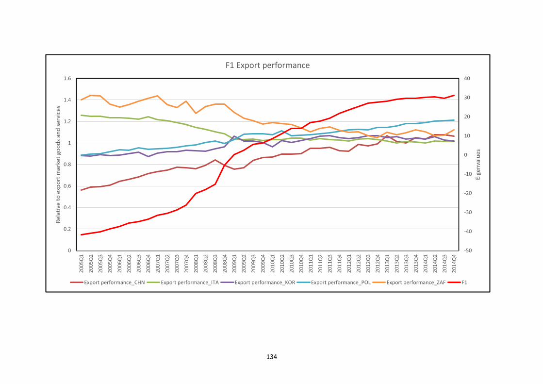
134
-50
-40
-30
-20
-10
0
10
20
30
40
0
0.2
0.4
0.6
0.8
1
1.2
1.4
1.62
00
5Q
1
20
05
Q2
20
05
Q3
20
05
Q4
20
06
Q1
20
06
Q2
20
06
Q3
20
06
Q4
20
07
Q1
20
07
Q2
20
07
Q3
20
07
Q4
20
08
Q1
20
08
Q2
20
08
Q3
20
08
Q4
20
09
Q1
20
09
Q2
20
09
Q3
20
09
Q4
20
10
Q1
20
10
Q2
20
10
Q3
20
10
Q4
20
11
Q1
20
11
Q2
20
11
Q3
20
11
Q4
20
12
Q1
20
12
Q2
20
12
Q3
20
12
Q4
20
13
Q1
20
13
Q2
20
13
Q3
20
13
Q4
20
14
Q1
20
14
Q2
20
14
Q3
20
14
Q4
Eige
nva
lues
Rel
ativ
e to
exp
ort
mar
ket
goo
ds
and
ser
vice
s
F1 Export performance
Export performance_CHN Export performance_ITA Export performance_KOR Export performance_POL Export performance_ZAF F1
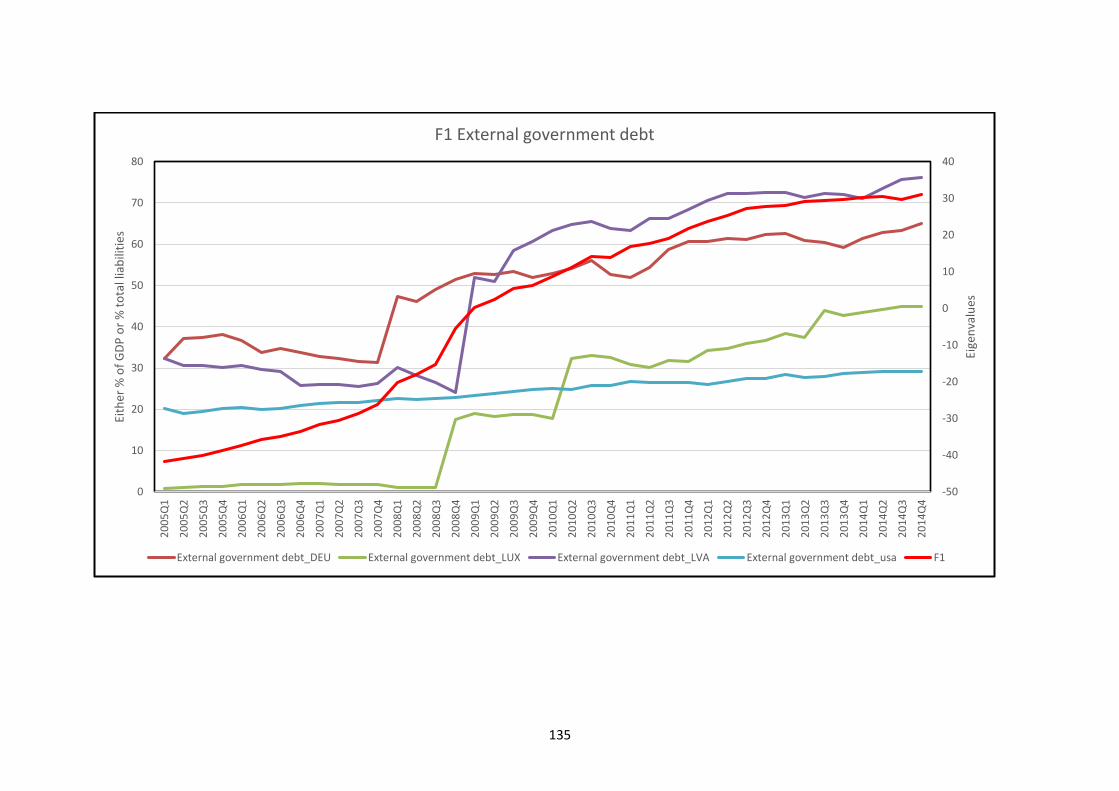
135
-50
-40
-30
-20
-10
0
10
20
30
40
0
10
20
30
40
50
60
70
802
00
5Q
1
20
05
Q2
20
05
Q3
20
05
Q4
20
06
Q1
20
06
Q2
20
06
Q3
20
06
Q4
20
07
Q1
20
07
Q2
20
07
Q3
20
07
Q4
20
08
Q1
20
08
Q2
20
08
Q3
20
08
Q4
20
09
Q1
20
09
Q2
20
09
Q3
20
09
Q4
20
10
Q1
20
10
Q2
20
10
Q3
20
10
Q4
20
11
Q1
20
11
Q2
20
11
Q3
20
11
Q4
20
12
Q1
20
12
Q2
20
12
Q3
20
12
Q4
20
13
Q1
20
13
Q2
20
13
Q3
20
13
Q4
20
14
Q1
20
14
Q2
20
14
Q3
20
14
Q4
Eige
nva
lues
Eith
er %
of
GD
P o
r %
to
tal l
iab
iliti
es
F1 External government debt
External government debt_DEU External government debt_LUX External government debt_LVA External government debt_usa F1
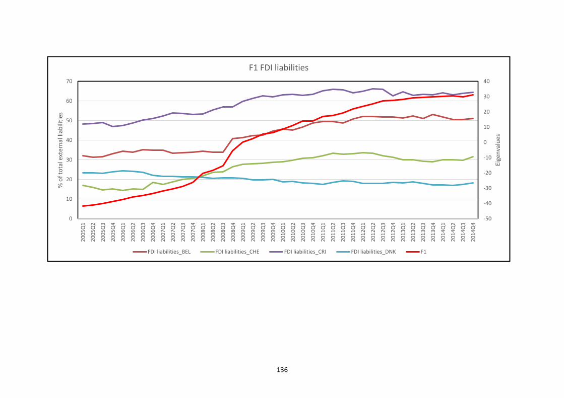
136
-50
-40
-30
-20
-10
0
10
20
30
40
0
10
20
30
40
50
60
702
00
5Q
1
20
05
Q2
20
05
Q3
20
05
Q4
20
06
Q1
20
06
Q2
20
06
Q3
20
06
Q4
20
07
Q1
20
07
Q2
20
07
Q3
20
07
Q4
20
08
Q1
20
08
Q2
20
08
Q3
20
08
Q4
20
09
Q1
20
09
Q2
20
09
Q3
20
09
Q4
20
10
Q1
20
10
Q2
20
10
Q3
20
10
Q4
20
11
Q1
20
11
Q2
20
11
Q3
20
11
Q4
20
12
Q1
20
12
Q2
20
12
Q3
20
12
Q4
20
13
Q1
20
13
Q2
20
13
Q3
20
13
Q4
20
14
Q1
20
14
Q2
20
14
Q3
20
14
Q4
Eige
nva
lues
% o
f to
tal e
xter
nal
liab
iliti
es
F1 FDI liabilities
FDI liabilities_BEL FDI liabilities_CHE FDI liabilities_CRI FDI liabilities_DNK F1
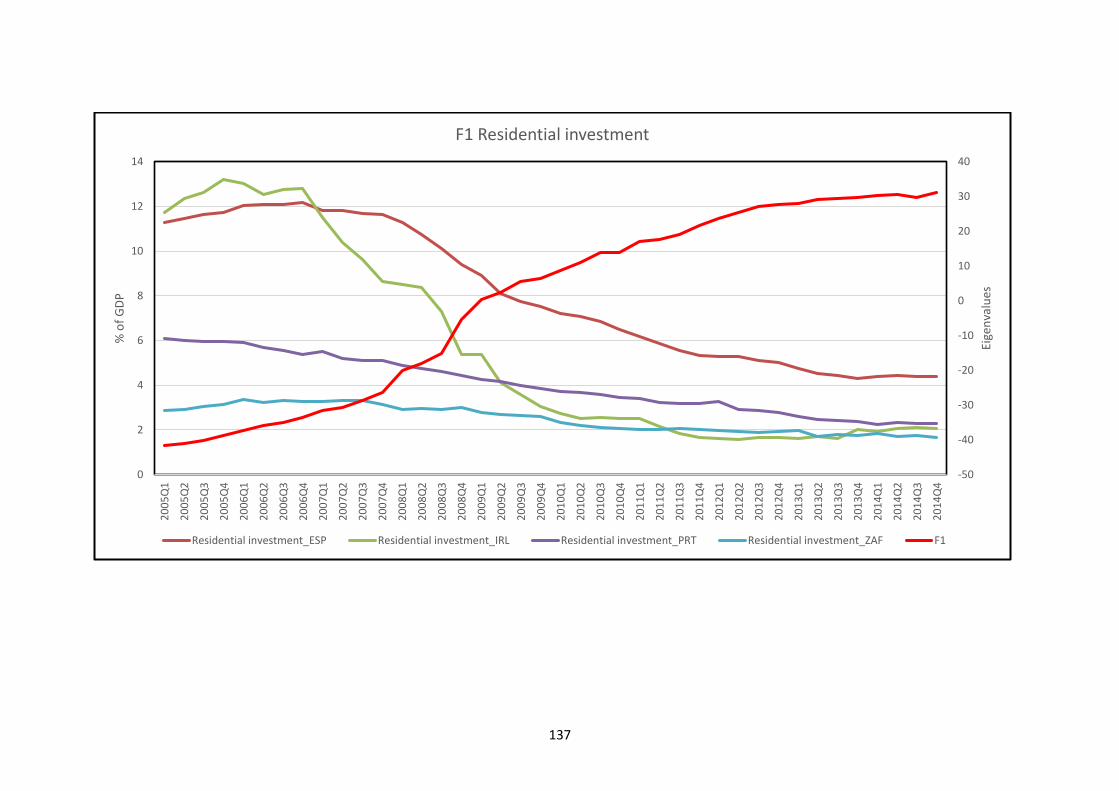
137
-50
-40
-30
-20
-10
0
10
20
30
40
0
2
4
6
8
10
12
142
00
5Q
1
20
05
Q2
20
05
Q3
20
05
Q4
20
06
Q1
20
06
Q2
20
06
Q3
20
06
Q4
20
07
Q1
20
07
Q2
20
07
Q3
20
07
Q4
20
08
Q1
20
08
Q2
20
08
Q3
20
08
Q4
20
09
Q1
20
09
Q2
20
09
Q3
20
09
Q4
20
10
Q1
20
10
Q2
20
10
Q3
20
10
Q4
20
11
Q1
20
11
Q2
20
11
Q3
20
11
Q4
20
12
Q1
20
12
Q2
20
12
Q3
20
12
Q4
20
13
Q1
20
13
Q2
20
13
Q3
20
13
Q4
20
14
Q1
20
14
Q2
20
14
Q3
20
14
Q4
Eige
nva
lues
% o
f G
DP
F1 Residential investment
Residential investment_ESP Residential investment_IRL Residential investment_PRT Residential investment_ZAF F1
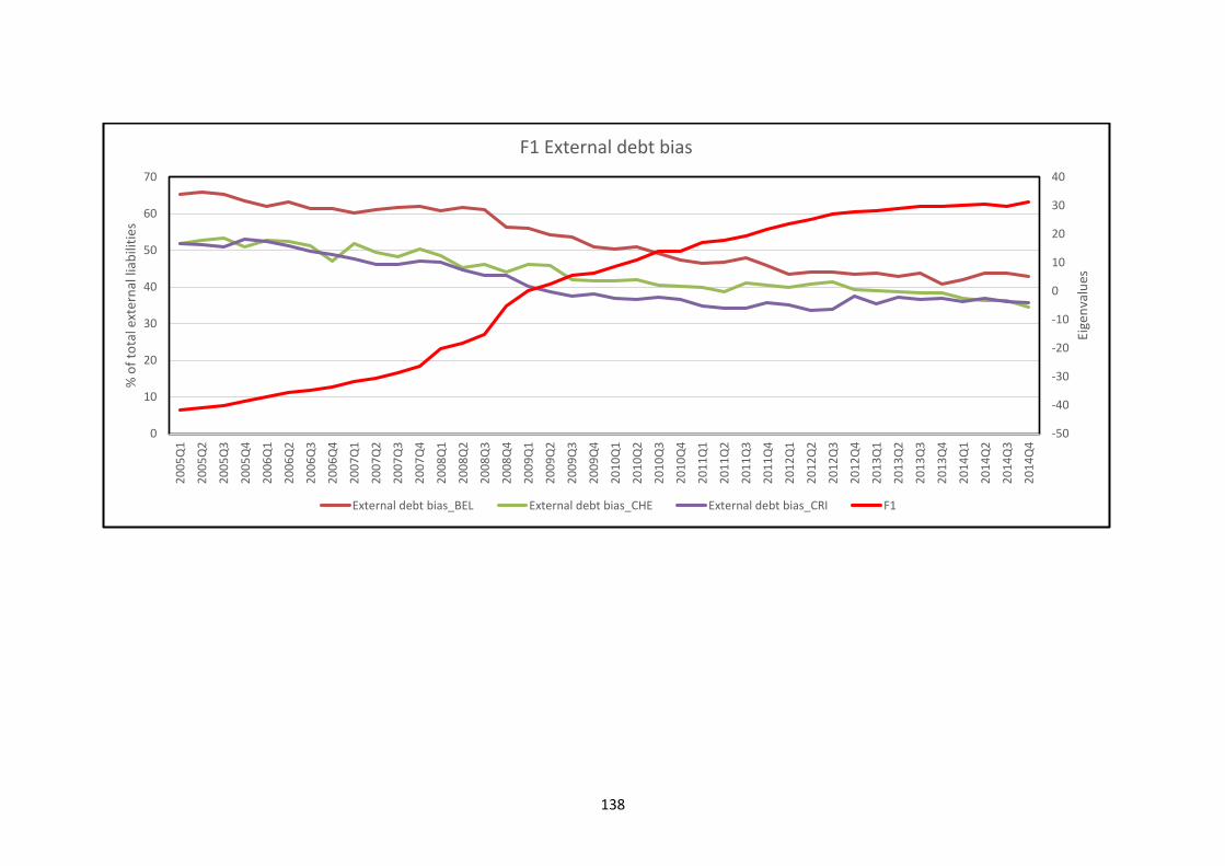
138
-50
-40
-30
-20
-10
0
10
20
30
40
0
10
20
30
40
50
60
702
00
5Q
1
20
05
Q2
20
05
Q3
20
05
Q4
20
06
Q1
20
06
Q2
20
06
Q3
20
06
Q4
20
07
Q1
20
07
Q2
20
07
Q3
20
07
Q4
20
08
Q1
20
08
Q2
20
08
Q3
20
08
Q4
20
09
Q1
20
09
Q2
20
09
Q3
20
09
Q4
20
10
Q1
20
10
Q2
20
10
Q3
20
10
Q4
20
11
Q1
20
11
Q2
20
11
Q3
20
11
Q4
20
12
Q1
20
12
Q2
20
12
Q3
20
12
Q4
20
13
Q1
20
13
Q2
20
13
Q3
20
13
Q4
20
14
Q1
20
14
Q2
20
14
Q3
20
14
Q4
Eige
nva
lues
% o
f to
tal e
xter
nal
liab
iliti
es
F1 External debt bias
External debt bias_BEL External debt bias_CHE External debt bias_CRI F1
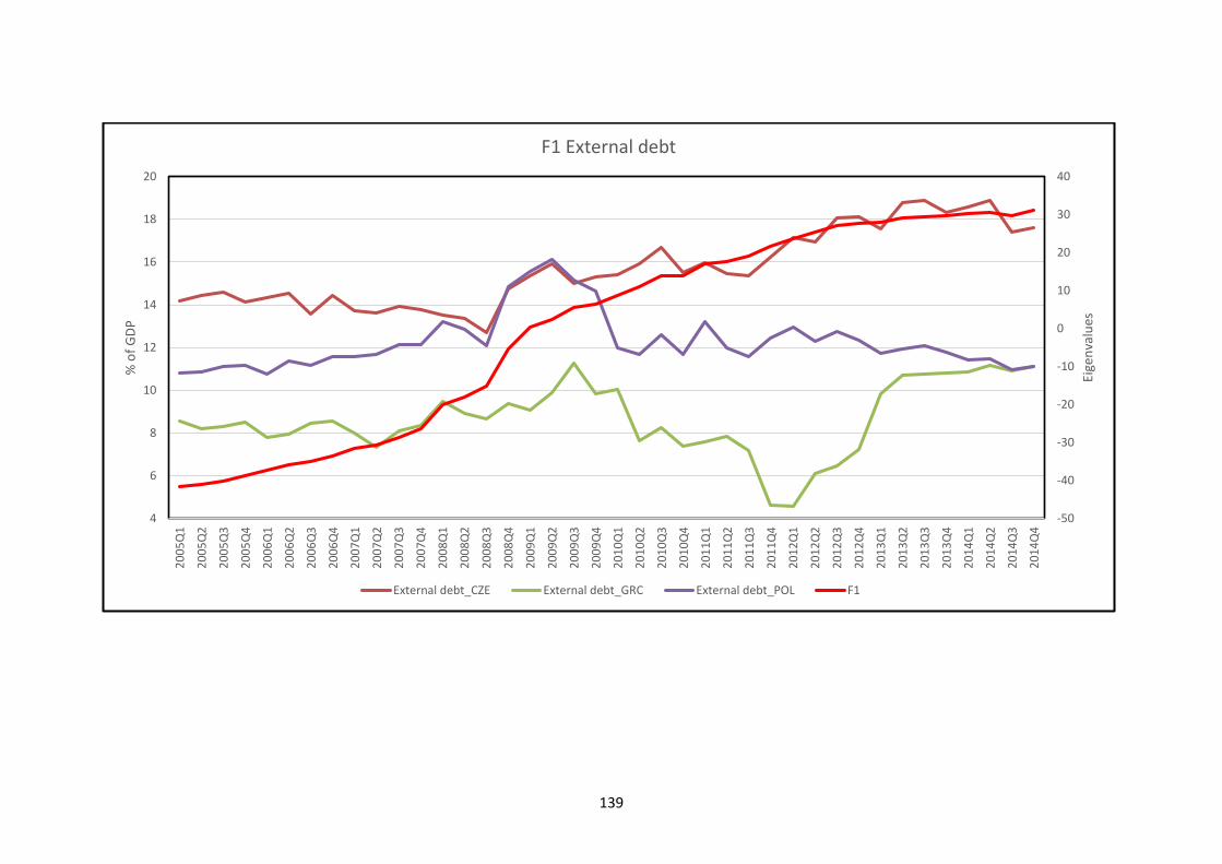
139
-50
-40
-30
-20
-10
0
10
20
30
40
4
6
8
10
12
14
16
18
202
00
5Q
1
20
05
Q2
20
05
Q3
20
05
Q4
20
06
Q1
20
06
Q2
20
06
Q3
20
06
Q4
20
07
Q1
20
07
Q2
20
07
Q3
20
07
Q4
20
08
Q1
20
08
Q2
20
08
Q3
20
08
Q4
20
09
Q1
20
09
Q2
20
09
Q3
20
09
Q4
20
10
Q1
20
10
Q2
20
10
Q3
20
10
Q4
20
11
Q1
20
11
Q2
20
11
Q3
20
11
Q4
20
12
Q1
20
12
Q2
20
12
Q3
20
12
Q4
20
13
Q1
20
13
Q2
20
13
Q3
20
13
Q4
20
14
Q1
20
14
Q2
20
14
Q3
20
14
Q4
Eige
nva
lues
% o
f G
DP
F1 External debt
External debt_CZE External debt_GRC External debt_POL F1
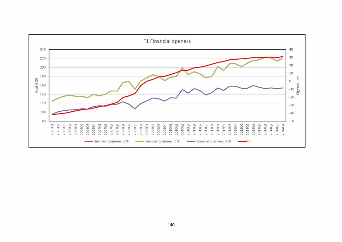
140
-50
-40
-30
-20
-10
0
10
20
30
40
80
100
120
140
160
180
200
220
2402
00
5Q
1
20
05
Q2
20
05
Q3
20
05
Q4
20
06
Q1
20
06
Q2
20
06
Q3
20
06
Q4
20
07
Q1
20
07
Q2
20
07
Q3
20
07
Q4
20
08
Q1
20
08
Q2
20
08
Q3
20
08
Q4
20
09
Q1
20
09
Q2
20
09
Q3
20
09
Q4
20
10
Q1
20
10
Q2
20
10
Q3
20
10
Q4
20
11
Q1
20
11
Q2
20
11
Q3
20
11
Q4
20
12
Q1
20
12
Q2
20
12
Q3
20
12
Q4
20
13
Q1
20
13
Q2
20
13
Q3
20
13
Q4
20
14
Q1
20
14
Q2
20
14
Q3
20
14
Q4
Eige
nva
lues
% o
f G
DP
F1 Financial openess
Financial openness_CZE Financial openness_CZE Financial openness_POL F1
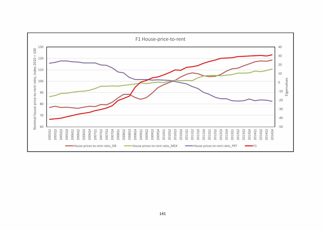
141
-50
-40
-30
-20
-10
0
10
20
30
40
60
70
80
90
100
110
120
1302
00
5Q
1
20
05
Q2
20
05
Q3
20
05
Q4
20
06
Q1
20
06
Q2
20
06
Q3
20
06
Q4
20
07
Q1
20
07
Q2
20
07
Q3
20
07
Q4
20
08
Q1
20
08
Q2
20
08
Q3
20
08
Q4
20
09
Q1
20
09
Q2
20
09
Q3
20
09
Q4
20
10
Q1
20
10
Q2
20
10
Q3
20
10
Q4
20
11
Q1
20
11
Q2
20
11
Q3
20
11
Q4
20
12
Q1
20
12
Q2
20
12
Q3
20
12
Q4
20
13
Q1
20
13
Q2
20
13
Q3
20
13
Q4
20
14
Q1
20
14
Q2
20
14
Q3
20
14
Q4
Eige
nva
lues
No
min
al h
ou
se p
rice
-to
-ren
t ra
tio
, in
dex
20
10
= 1
00
F1 House-price-to-rent
House prices-to-rent ratio_ISR House prices-to-rent ratio_MEX House prices-to-rent ratio_PRT F1
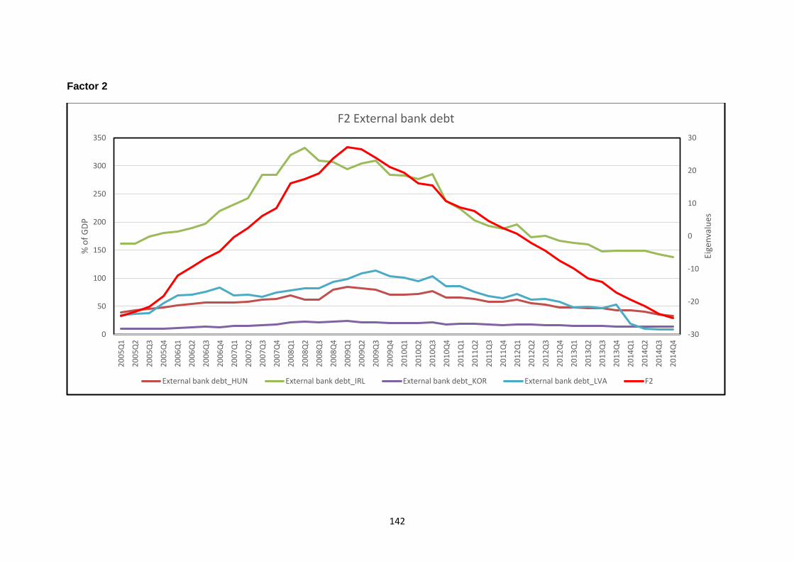
142
Factor 2
-30
-20
-10
0
10
20
30
0
50
100
150
200
250
300
350
20
05
Q1
20
05
Q2
20
05
Q3
20
05
Q4
20
06
Q1
20
06
Q2
20
06
Q3
20
06
Q4
20
07
Q1
20
07
Q2
20
07
Q3
20
07
Q4
20
08
Q1
20
08
Q2
20
08
Q3
20
08
Q4
20
09
Q1
20
09
Q2
20
09
Q3
20
09
Q4
20
10
Q1
20
10
Q2
20
10
Q3
20
10
Q4
20
11
Q1
20
11
Q2
20
11
Q3
20
11
Q4
20
12
Q1
20
12
Q2
20
12
Q3
20
12
Q4
20
13
Q1
20
13
Q2
20
13
Q3
20
13
Q4
20
14
Q1
20
14
Q2
20
14
Q3
20
14
Q4
Eige
nva
lues
% o
f G
DP
F2 External bank debt
External bank debt_HUN External bank debt_IRL External bank debt_KOR External bank debt_LVA F2
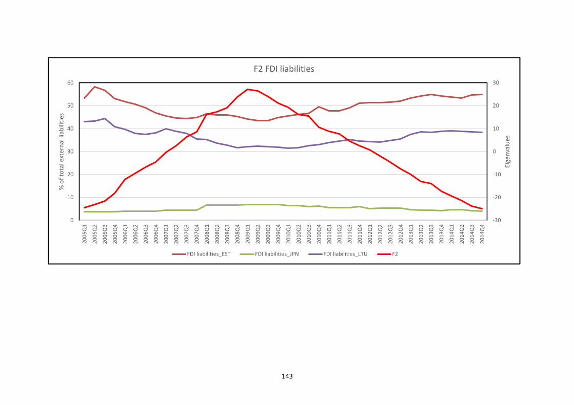
143
-30
-20
-10
0
10
20
30
0
10
20
30
40
50
602
00
5Q
1
20
05
Q2
20
05
Q3
20
05
Q4
20
06
Q1
20
06
Q2
20
06
Q3
20
06
Q4
20
07
Q1
20
07
Q2
20
07
Q3
20
07
Q4
20
08
Q1
20
08
Q2
20
08
Q3
20
08
Q4
20
09
Q1
20
09
Q2
20
09
Q3
20
09
Q4
20
10
Q1
20
10
Q2
20
10
Q3
20
10
Q4
20
11
Q1
20
11
Q2
20
11
Q3
20
11
Q4
20
12
Q1
20
12
Q2
20
12
Q3
20
12
Q4
20
13
Q1
20
13
Q2
20
13
Q3
20
13
Q4
20
14
Q1
20
14
Q2
20
14
Q3
20
14
Q4
Eige
nva
lues
% o
f to
tal e
xter
nal
liab
iliti
es
F2 FDI liabilities
FDI liabilities_EST FDI liabilities_JPN FDI liabilities_LTU F2
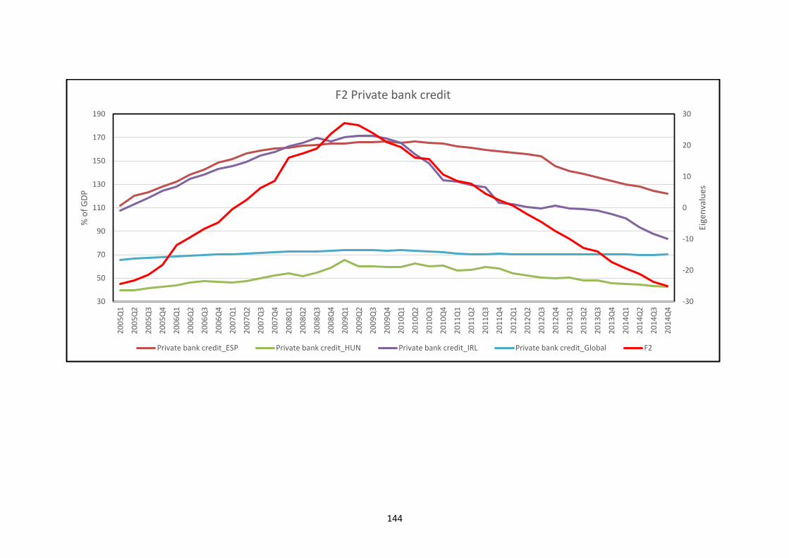
144
-30
-20
-10
0
10
20
30
30
50
70
90
110
130
150
170
1902
00
5Q
1
20
05
Q2
20
05
Q3
20
05
Q4
20
06
Q1
20
06
Q2
20
06
Q3
20
06
Q4
20
07
Q1
20
07
Q2
20
07
Q3
20
07
Q4
20
08
Q1
20
08
Q2
20
08
Q3
20
08
Q4
20
09
Q1
20
09
Q2
20
09
Q3
20
09
Q4
20
10
Q1
20
10
Q2
20
10
Q3
20
10
Q4
20
11
Q1
20
11
Q2
20
11
Q3
20
11
Q4
20
12
Q1
20
12
Q2
20
12
Q3
20
12
Q4
20
13
Q1
20
13
Q2
20
13
Q3
20
13
Q4
20
14
Q1
20
14
Q2
20
14
Q3
20
14
Q4
Eige
nva
lues
% o
f G
DP
F2 Private bank credit
Private bank credit_ESP Private bank credit_HUN Private bank credit_IRL Private bank credit_Global F2
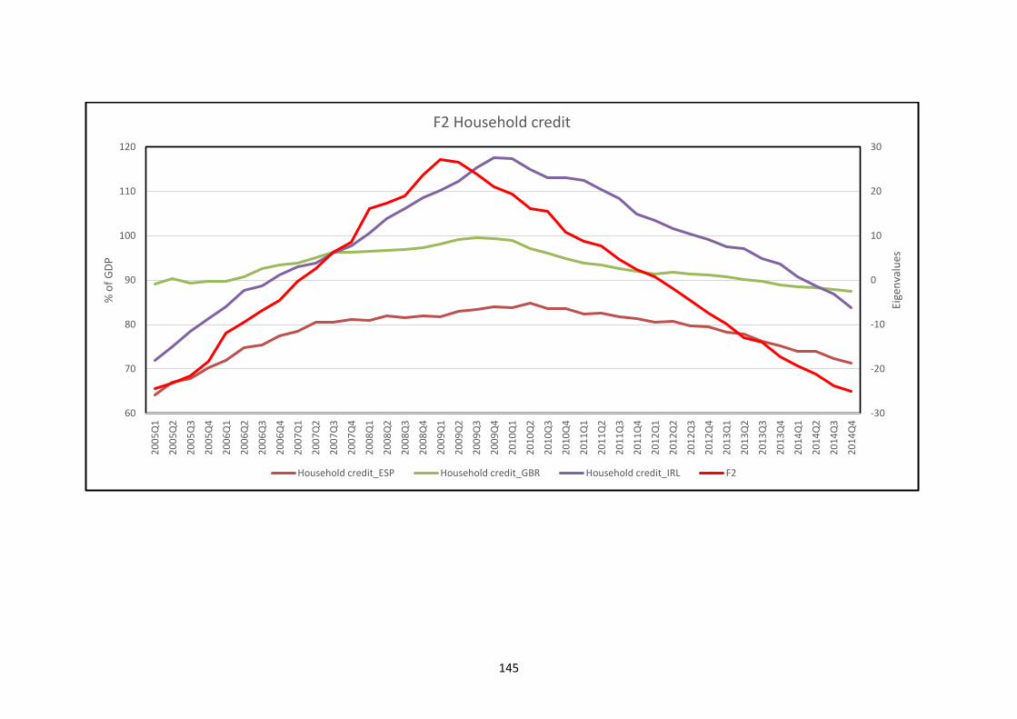
145
-30
-20
-10
0
10
20
30
60
70
80
90
100
110
1202
00
5Q
1
20
05
Q2
20
05
Q3
20
05
Q4
20
06
Q1
20
06
Q2
20
06
Q3
20
06
Q4
20
07
Q1
20
07
Q2
20
07
Q3
20
07
Q4
20
08
Q1
20
08
Q2
20
08
Q3
20
08
Q4
20
09
Q1
20
09
Q2
20
09
Q3
20
09
Q4
20
10
Q1
20
10
Q2
20
10
Q3
20
10
Q4
20
11
Q1
20
11
Q2
20
11
Q3
20
11
Q4
20
12
Q1
20
12
Q2
20
12
Q3
20
12
Q4
20
13
Q1
20
13
Q2
20
13
Q3
20
13
Q4
20
14
Q1
20
14
Q2
20
14
Q3
20
14
Q4
Eige
nva
lues
% o
f G
DP
F2 Household credit
Household credit_ESP Household credit_GBR Household credit_IRL F2
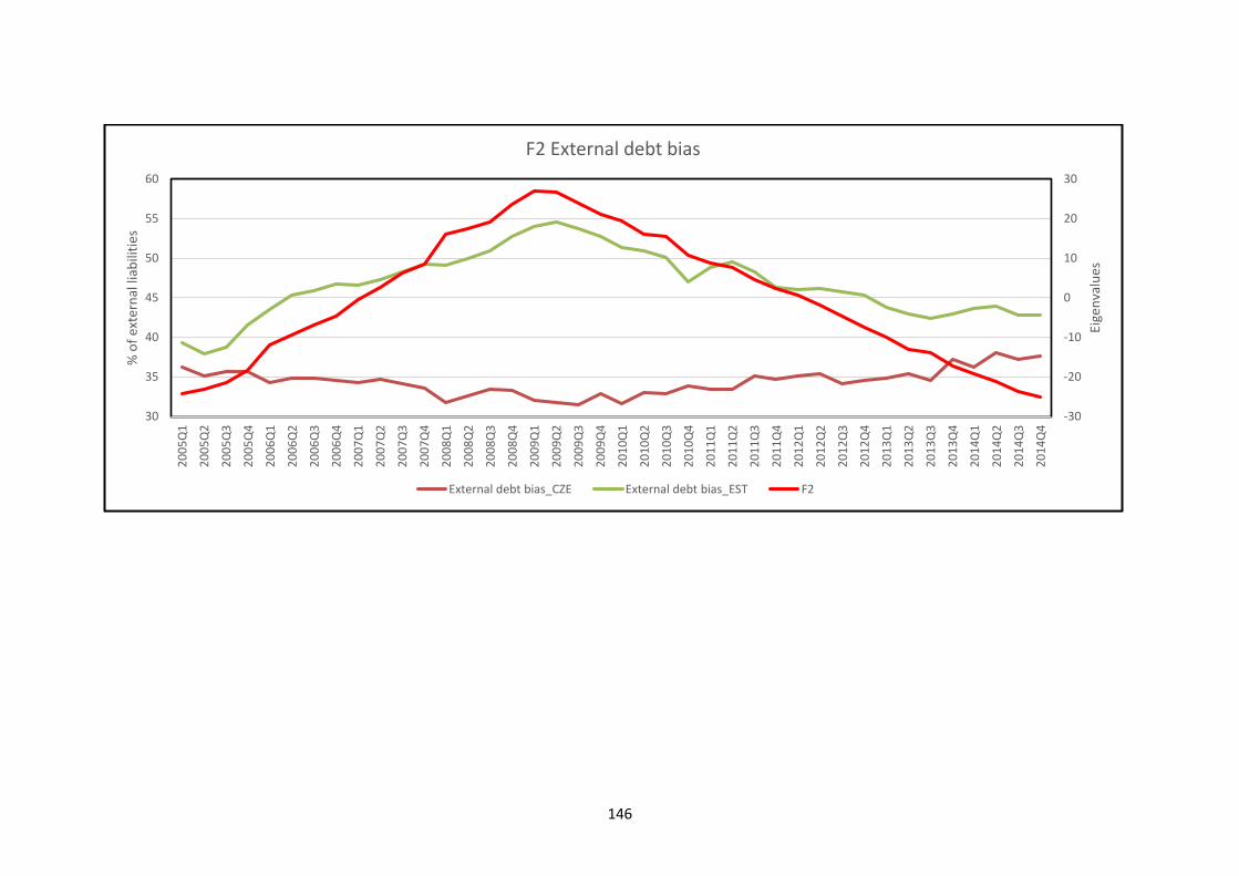
146
-30
-20
-10
0
10
20
30
30
35
40
45
50
55
602
00
5Q
1
20
05
Q2
20
05
Q3
20
05
Q4
20
06
Q1
20
06
Q2
20
06
Q3
20
06
Q4
20
07
Q1
20
07
Q2
20
07
Q3
20
07
Q4
20
08
Q1
20
08
Q2
20
08
Q3
20
08
Q4
20
09
Q1
20
09
Q2
20
09
Q3
20
09
Q4
20
10
Q1
20
10
Q2
20
10
Q3
20
10
Q4
20
11
Q1
20
11
Q2
20
11
Q3
20
11
Q4
20
12
Q1
20
12
Q2
20
12
Q3
20
12
Q4
20
13
Q1
20
13
Q2
20
13
Q3
20
13
Q4
20
14
Q1
20
14
Q2
20
14
Q3
20
14
Q4
Eige
nva
lues
% o
f ex
tern
al li
abili
ties
F2 External debt bias
External debt bias_CZE External debt bias_EST F2
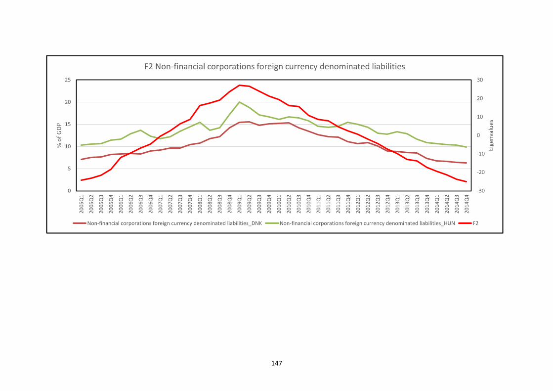
147
-30
-20
-10
0
10
20
30
0
5
10
15
20
252
00
5Q
1
20
05
Q2
20
05
Q3
20
05
Q4
20
06
Q1
20
06
Q2
20
06
Q3
20
06
Q4
20
07
Q1
20
07
Q2
20
07
Q3
20
07
Q4
20
08
Q1
20
08
Q2
20
08
Q3
20
08
Q4
20
09
Q1
20
09
Q2
20
09
Q3
20
09
Q4
20
10
Q1
20
10
Q2
20
10
Q3
20
10
Q4
20
11
Q1
20
11
Q2
20
11
Q3
20
11
Q4
20
12
Q1
20
12
Q2
20
12
Q3
20
12
Q4
20
13
Q1
20
13
Q2
20
13
Q3
20
13
Q4
20
14
Q1
20
14
Q2
20
14
Q3
20
14
Q4
Eige
nva
lues
% o
f G
DP
F2 Non-financial corporations foreign currency denominated liabilities
Non-financial corporations foreign currency denominated liabilities_DNK Non-financial corporations foreign currency denominated liabilities_HUN F2
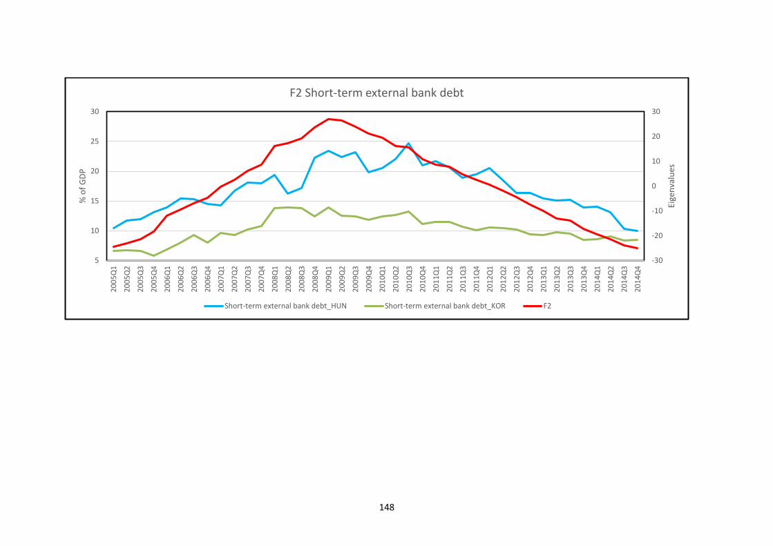
148
-30
-20
-10
0
10
20
30
5
10
15
20
25
302
00
5Q
1
20
05
Q2
20
05
Q3
20
05
Q4
20
06
Q1
20
06
Q2
20
06
Q3
20
06
Q4
20
07
Q1
20
07
Q2
20
07
Q3
20
07
Q4
20
08
Q1
20
08
Q2
20
08
Q3
20
08
Q4
20
09
Q1
20
09
Q2
20
09
Q3
20
09
Q4
20
10
Q1
20
10
Q2
20
10
Q3
20
10
Q4
20
11
Q1
20
11
Q2
20
11
Q3
20
11
Q4
20
12
Q1
20
12
Q2
20
12
Q3
20
12
Q4
20
13
Q1
20
13
Q2
20
13
Q3
20
13
Q4
20
14
Q1
20
14
Q2
20
14
Q3
20
14
Q4
Eige
nva
lues
% o
f G
DP
F2 Short-term external bank debt
Short-term external bank debt_HUN Short-term external bank debt_KOR F2
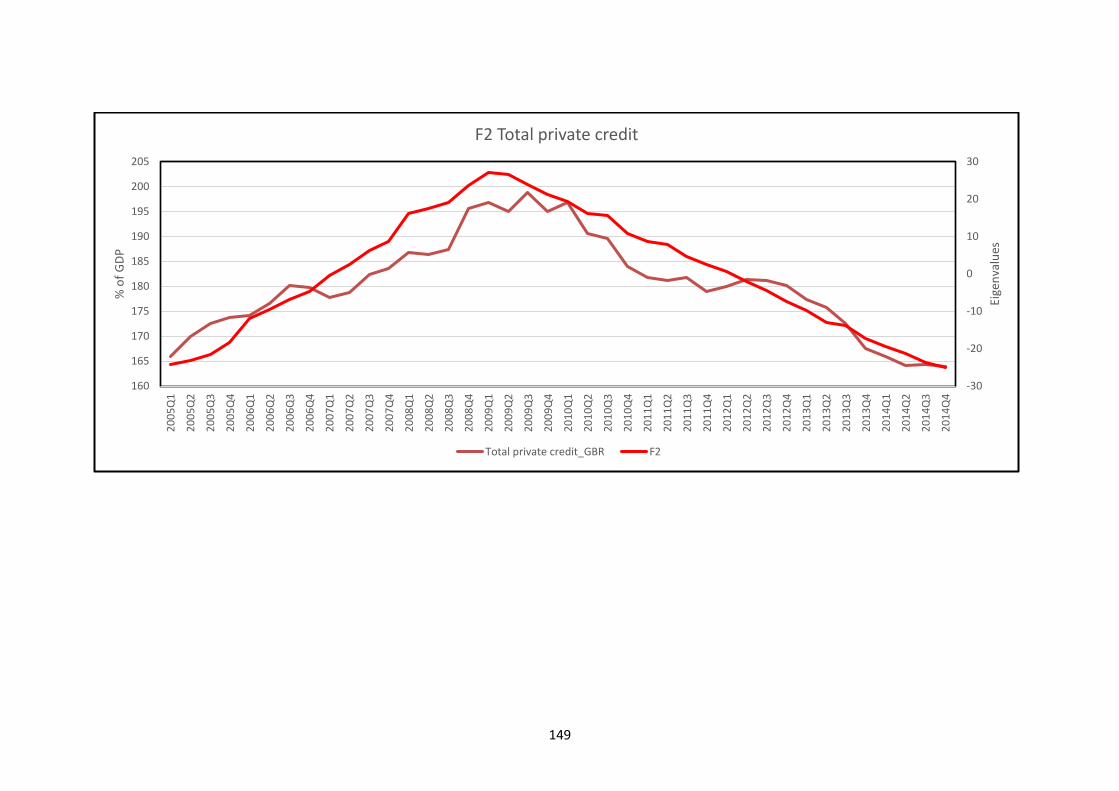
149
-30
-20
-10
0
10
20
30
160
165
170
175
180
185
190
195
200
2052
00
5Q
1
20
05
Q2
20
05
Q3
20
05
Q4
20
06
Q1
20
06
Q2
20
06
Q3
20
06
Q4
20
07
Q1
20
07
Q2
20
07
Q3
20
07
Q4
20
08
Q1
20
08
Q2
20
08
Q3
20
08
Q4
20
09
Q1
20
09
Q2
20
09
Q3
20
09
Q4
20
10
Q1
20
10
Q2
20
10
Q3
20
10
Q4
20
11
Q1
20
11
Q2
20
11
Q3
20
11
Q4
20
12
Q1
20
12
Q2
20
12
Q3
20
12
Q4
20
13
Q1
20
13
Q2
20
13
Q3
20
13
Q4
20
14
Q1
20
14
Q2
20
14
Q3
20
14
Q4
Eige
nva
lues
% o
f G
DP
F2 Total private credit
Total private credit_GBR F2


