Author version: Estuar. Coast. Shelf Sci., vol.88(2); 2010; 249-259

Impact of internal waves on sound propagation off Bhimilipatnam,

East coast of India

B.Sridevi, T.V. Ramana Murty, Y. Sadhuram, M.M.M. Rao, K. Maneesha, S. Sujith Kumar and P.L. Prasanna

National Institute of Oceanography, Regional center, 176, Lawsons bay colony Visakhapatnam-530 017, India Abstract: Internal waves (IWs) are identified off Bhimilipatnam, East Coast of India, from the time series

CTD (hourly interval) and thermistor chain data (2 minute interval) collected during 23 – 25 Feb, 2007.

The measurements were carried out at 94 m water depth on the continental shelf edge. These data

sets are used to describe the characteristics of IWs and their impact on acoustic fields. Garrett and

Munk (GM) model has been used to predict the characteristics of low frequency (LF) IWs with space

and time. Active IWs are seen in the layer 54 m – 94 m with a velocity of 0.548 km hr-1 and the

wavelengths of the order of 0.03 km to 21.8 km. The model could capture the IW features in the

thermocline region accurately than at the bottom. This could be due to the limitation of the model which

considers linearity. High frequency IWs observed at the bottom could be due to the advection of tidal

currents over the shallow irregular bottom in the presence of stratification. The study emphasizes linear

IWs rather than transient non-linear waves induced by tidal interaction with topography.

Acoustic simulation results for low frequency IW field reveal that the Intensity loss anomaly of

eigenrays was found to be 2.86 dB to 15.59 dB in the water column and maximum (38.48 dB) was

observed at the bottom due to the bottom interaction. Our results are well compared with those

reported earlier from simulation and acoustic field experiments in the Northern Indian Ocean.

Key words: Low frequency, Internal waves, Thermistor chain, GM model, acoustic simulation,

East Coast of India

1. Introduction:

Oceanic IWs are one of the most ubiquitous features on continental shelves (Fu and Holt,

1982). There are many hypothesized causes, including meteorological conditions (winds and pressure

changes), tides and flow over complex bottom topography, surface waves, submarine earthquakes,

landslides, and shear flow instabilities. They occur in the regions of strong vertical stratification, such as

the thermocline and produce unanticipated variability in measurements (La fond, 1962). Typical vertical

scales are around 10 m and the horizontal are from a few hundred meters to kilometers. Temporal

scales are of the order of hours, bounded by a minimum inertial frequency (a function of latitude) and a

maximum at the Brunt-Vaisala frequency (N2) (Robinson and Ding Lee, 1994). Physical oceanographers are interested to study the variability of ocean environment rather than

it’s mean. Oceanic changes relevant to underwater acoustics are classified into mean and fluctuating

components (De Santo 1979) with the following general model of the sound velocity equation )1(),(2)(1)(),( trCrCzoCtrC δδ ++=

r - three dimensional position; t – time; z - depth

having characteristics: 1) a mean vertical profile )(zCo that represents local climatology(C0 ~ 1500 m s-

1 ), 2) a meso-scale component( )(1 rCδ ) (fronts, eddies) -- deterministic with respect to the acoustic

time scale ( 210~/1−

oCCδ ), and 3) a statistical component ( ),(2 trCδ ) (i.e random with respect to

the acoustic time scale, 410~/2−

oCCδ ) that represents small scale fluctuations caused by Internal

Waves (IWs) (fine and micro structure). The IW of semi diurnal frequency - internal tides dominates the

low frequency (LF) band of IW, while IW of > 0.5 cph dominate the high frequency (HF) band of IW

(Murthy, 2002).

IWs are present in all levels of the water column, in deep ocean as well as in marginal coastal

areas. As the IWs oscillate underwater, they are potentially dangerous for submarines, off-shore

platforms and ships. Ocean engineers’ interest in IWs is due to their role in submarine detection and

the generation of anomalous drag on ships in fjords and some estuaries. In addition to simulation by

numerical modeling, field observation is one of the most important approaches to study the IW. Though

ordinary gravity waves are easily seen in day-to-day life, their measurements at Sea are complex.

These waves are identified from SAR images (Xiaofeng Li, et al. 1999), shipboard Radar (Dong-Jiing

Doong et.al, 2007), special instrumentation like Isothermal follower and thermistor chain etc. (Garrett

and Munk, 1979).

Till 1980, around the Indian coast, most of the IW studies (Murthy, 2002) are made utilizing the

time series bathythermograph data (La Fond and Rao, 1954, La Fond and La Fond, 1968, Ramam

et.al., 1979) from the stationary ships at fine resolutions for periods up to 3 weeks. After 1980’s, the

field measurements on IW were mostly made from moored buoys equipped with current meters or with

thermistor string (Murthy and Murthy, 1986, ; Shenoi and Antony, 1991; Murthy et.al., 1999, Kumar

et.al., 2001) and Satellite sensors (Nath and Rao, 1989; Fernandes et.al., 2000). The time series

measurements made from stationary ships and from buoys at different places in the seas around India

indicated prominent IW of tidal (0.08 cph) and high (1 – 10 cph) frequencies. The high frequency IWs

were found to exhibit diurnal variability with stronger activity during night-time compared to day-time

under the influence of local winds. The acoustic intensities can be expected to respond to this diurnal

variability. The above studies are confined to thermocline and no information is available at the bottom.

The generation of IWs due to the bottom topography and their impact on acoustic propagation

characteristics are presented in this study.

In this study predicted sound velocity realizations (with space and time) have been generated

by using the statistical universal spectrum GM model. The model incorporates more observational data

when compared with any other model and it has been widely accepted by the scientific community

(Appendix – A). Acoustic ray model simulation (Ramana Murty et.al., 2005) has been carried out in the

presence and absence of model generated IW field which is useful for naval operations.

2. Methodology: 2.1 Seafloor Topography off Bhimilipatnam: During the winter season (Dec – Feb), the study area experiences northeasterly winds with

magnitude of 3.0 to 6.0 m s-1.The tides in this region are semi diurnal. The mean spring tidal range is

1.43 m and the neap tidal range is 0.54 m at the nearest port (Visakhapatnam). SST varies from 25 –

260 C while at 50 m depth the temperature varies from 26 – 270 C which indicates inversion. This is a

common feature in this region and the details can be found in an earlier study (Pankajakshan et.al.,

2002). Salinity at surface varies from 27 – 32 psu, at 50 m it varies from 32 – 34 psu and about ≈ 35

psu at 100 m depth. The magnitude of currents varies from 20 - 40 cm s-1 and the direction varies from

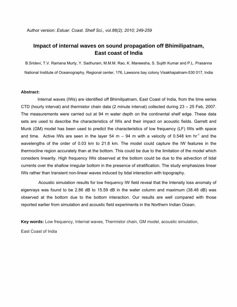
southwest to northeast from December to February (Varkey et.al., 1996). Knowledge of Seabed topography in the study area is also a prime requisite to understand

the pattern of the IWs in the water column. For this purpose, a representative profile of the high

resolution shallow seismic survey carried out earlier by National Institute of Oceanography, Regional

Center, Visakhapatnam is selected to study the nature of the seabed topography in the area comprising

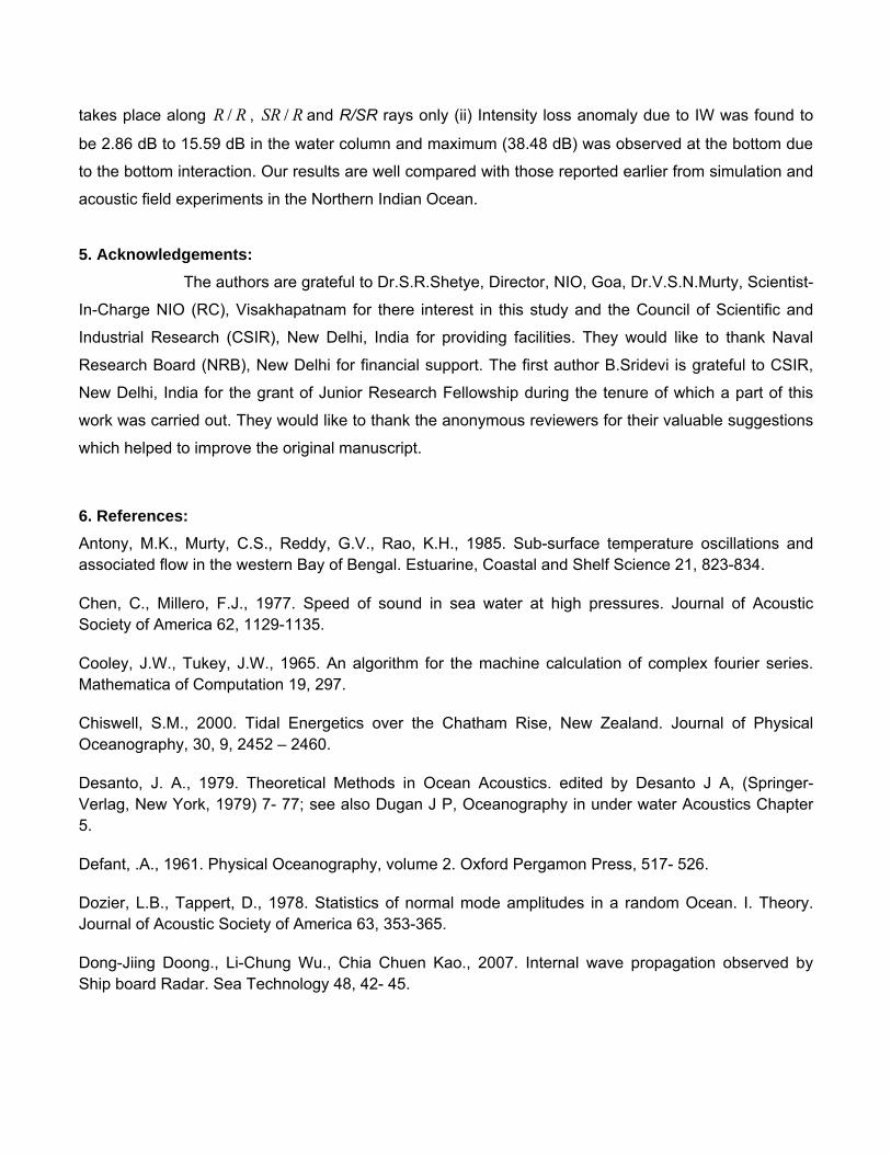
continental shelf and the upper slope regions off Bhimilipatnam (Fig.1). The figure 1a depicts the

location of the observational point and figure 1b shows the cross-sectional seabed topography along

AA’. This profile gives general nature of the seabed in terms of sediment quality and morphology. The

seismic record of this region, in general, reveals strong reflectors of the seafloor associated with

prominent morphological features such as reefs and pinnacles of varying relief’s in the outer shelf

regions. A well developed and prominent dome shaped reef feature with significant relief of 10 to 15 m

was noticed at the continental shelf edge (around 100 m depth) up to where the gradient of the shelf is

found to be moderate and it is abruptly turned to be very sharp and the seabed depth suddenly

increases to very higher depths of some hundreds of meters to some thousands of meters. This sharp

change in the bathymetry is due to the change in the bottom morphology from the continental shelf to

slope. The change in the bottom morphology off Bhimilipatnam from shelf to slope characteristics takes

place around the water depth of about 100 m. This part of the shelf is considered as paleo shore line

and got submerged due to Holocene transgression (Mohan Rao and Rao, 1994).

2.2 Field Program: Time series data (2 min interval) on temperature at five depths (5 m, 25 m, 50 m, 75 m and 94

m) have been collected using Thermistor chain during the period 23 – 25 Feb 2007. The sensors have

fast response (≈ 10 seconds) and the measuring range is 0 - 450C with an accuracy of ± 0.10 C. Time

series CTD data (hourly) had been obtained from SBE 19 plus Seacat profiler (Make: Seabird

Electronics, USA).

2.3 Modeling of Internal Waves

The IW parameters vary with space and time. The successful modeling of IW provides the

parameters at any interested site in the sea. Garrett and Munk (GM) (1975) succeeded in modeling

deep water IW and later it was modified for shallow water IW (Munk, 1981). The model requires time-

series temperature data field for frequency analysis and CTD data for Brunt-vaisala frequency, for

stratification parameter to provide initial and boundary conditions. For more details on IW modeling one

may refer to Krishna Kumar & Balasubramanian (2005) where in the frequency domain was used as

one of the inputs. In the present numerical simulation experiment, the wave number domain was used

for generation of IW field ( ),(2 trCδ ). IW eigen-frequencies and modes at a specified sequence of

horizontal wave numbers are computed by using “finite difference – Sturm sequence – bisection –

inverse iteration method”, with mean profile. From the model calculations, sequences of sound speed

realizations are obtained. Using the temporal and spatial distribution of sound velocity realizations, the

range-independent and range-dependent numerical ray tracing experiments are conducted to obtain

eigenrays and transmission losses etc., to study the impact of IW on sound propagation.

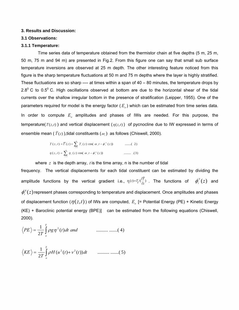
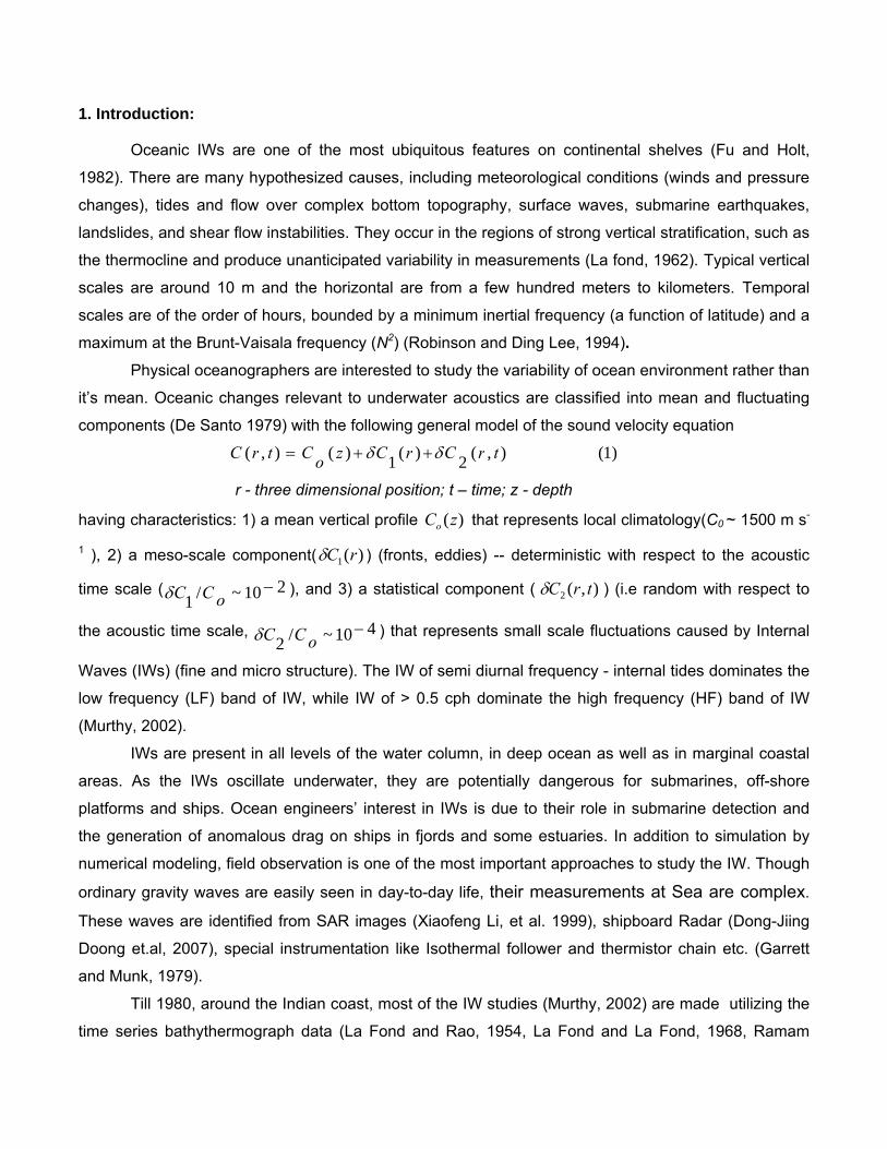
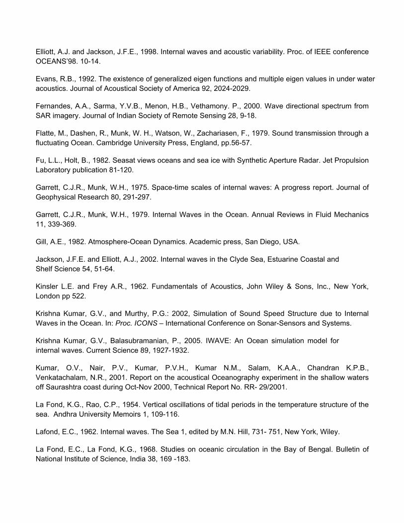
3. Results and Discussion: 3.1 Observations: 3.1.1 Temperature: Time series data of temperature obtained from the thermistor chain at five depths (5 m, 25 m,

50 m, 75 m and 94 m) are presented in Fig.2. From this figure one can say that small sub surface

temperature inversions are observed at 25 m depth. The other interesting feature noticed from this

figure is the sharp temperature fluctuations at 50 m and 75 m depths where the layer is highly stratified.

These fluctuations are so sharp ---- at times within a span of 40 – 80 minutes, the temperature drops by

2.80 C to 0.50 C. High oscillations observed at bottom are due to the horizontal shear of the tidal

currents over the shallow irregular bottom in the presence of stratification (Leipper, 1955). One of the

parameters required for model is the energy factor ( oE ) which can be estimated from time series data.

In order to compute oE amplitudes and phases of IWs are needed. For this purpose, the

temperature( ),( tzT ) and vertical displacement ( ),( tzη ) of pycnocline due to IW expressed in terms of

ensemble mean ( )(zT ),tidal constituents ( iω ) as follows (Chiswell, 2000).

)3.(.........))(cos()(),(

)2........())(cos()()(),(

1

1

ztztz

ztzTzTtzT

ii

n

ii

Tii

n

ii

ηφωηη

φω

−=

−+=

∑

∑

=

=

where z is the depth array, t is the time array, n is the number of tidal

frequency. The vertical displacements for each tidal constituent can be estimated by dividing the

amplitude functions by the vertical gradient i.e., )(/)(zT

iTzi ∂∂

=η . The functions of )(zTiφ and

)(ziηφ represent phases corresponding to temperature and displacement. Once amplitudes and phases

of displacement function ( ),( tzη ) of IWs are computed, oE [= Potential Energy (PE) + Kinetic Energy

(KE) + Baroclinic potential energy (BPE)] can be estimated from the following equations (Chiswell,

2000).

)5.......(..........))()((21

)4.......(..........)(21

22

2

∫

∫

+=

=

T

o

T

o

dttvtuHT

KE

anddttgT

PE

ρ

ηρ

)6.......(..........),()()(211 0

22

0

dtdztzzNzT

BPEH

T

∫∫−

= ηρ

where NHTvu ,,,,,, ρη are the displacement profile, zonal and meridonial components of currents ,

observational period, density , water depth and N2 respectively. Here < > indicates ensemble average.

Equations (4-6) have been performed by cubic spline method (Ralston and Wilf, 1967). Diurnal amplitudes are half of those of the semi diurnal in the water column. Maximum amplitudes of

3.4 m and 7.0 m were observed at 50 m depth (below mixed layer) for diurnal and semi diurnal tides

respectively. An increasing trend in the phase from bottom towards surface on diurnal scale suggested

that the displacement functions are bottom trapped. Similar results were reported over the Chatham

Rise, east of New Zealand by Chiswell (2000).

3.1.2 Sound Velocity: We choose to present sound velocity profiles (rather than temperature and salinity) because of

their direct utility in sonar range prediction models. Sound velocity is computed by Chen and Millero

(1977) and it’s distribution is presented in Fig. 3. From surface to 54 m depth, variation of sound

velocity is less and from 54 m to bottom strong velocity gradients are observed because of high

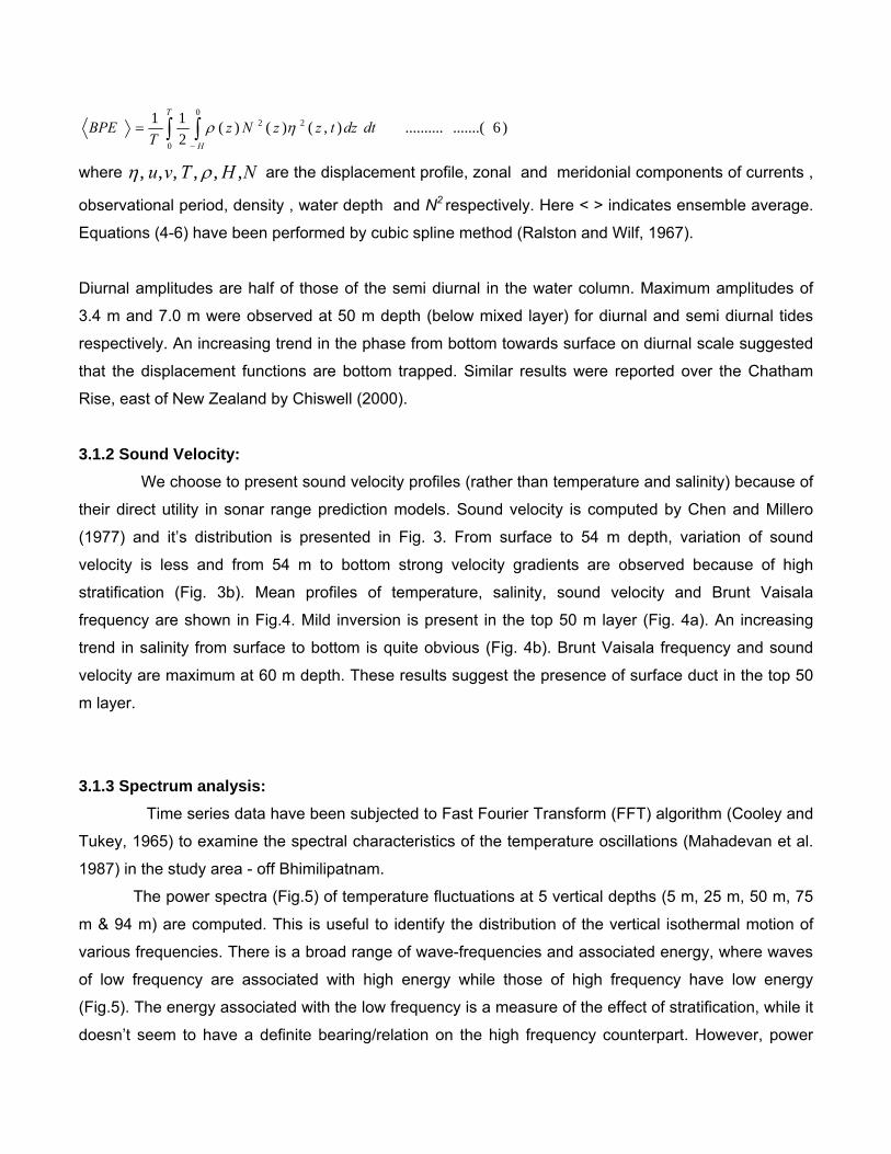
stratification (Fig. 3b). Mean profiles of temperature, salinity, sound velocity and Brunt Vaisala

frequency are shown in Fig.4. Mild inversion is present in the top 50 m layer (Fig. 4a). An increasing

trend in salinity from surface to bottom is quite obvious (Fig. 4b). Brunt Vaisala frequency and sound

velocity are maximum at 60 m depth. These results suggest the presence of surface duct in the top 50

m layer.

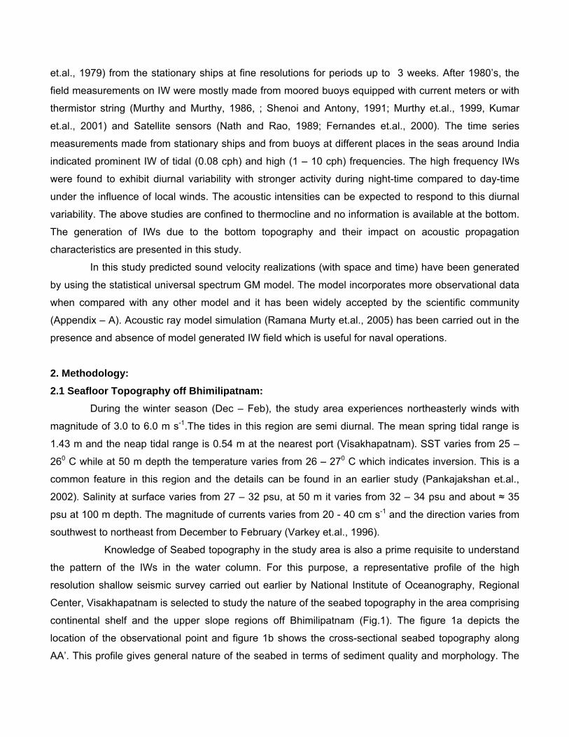
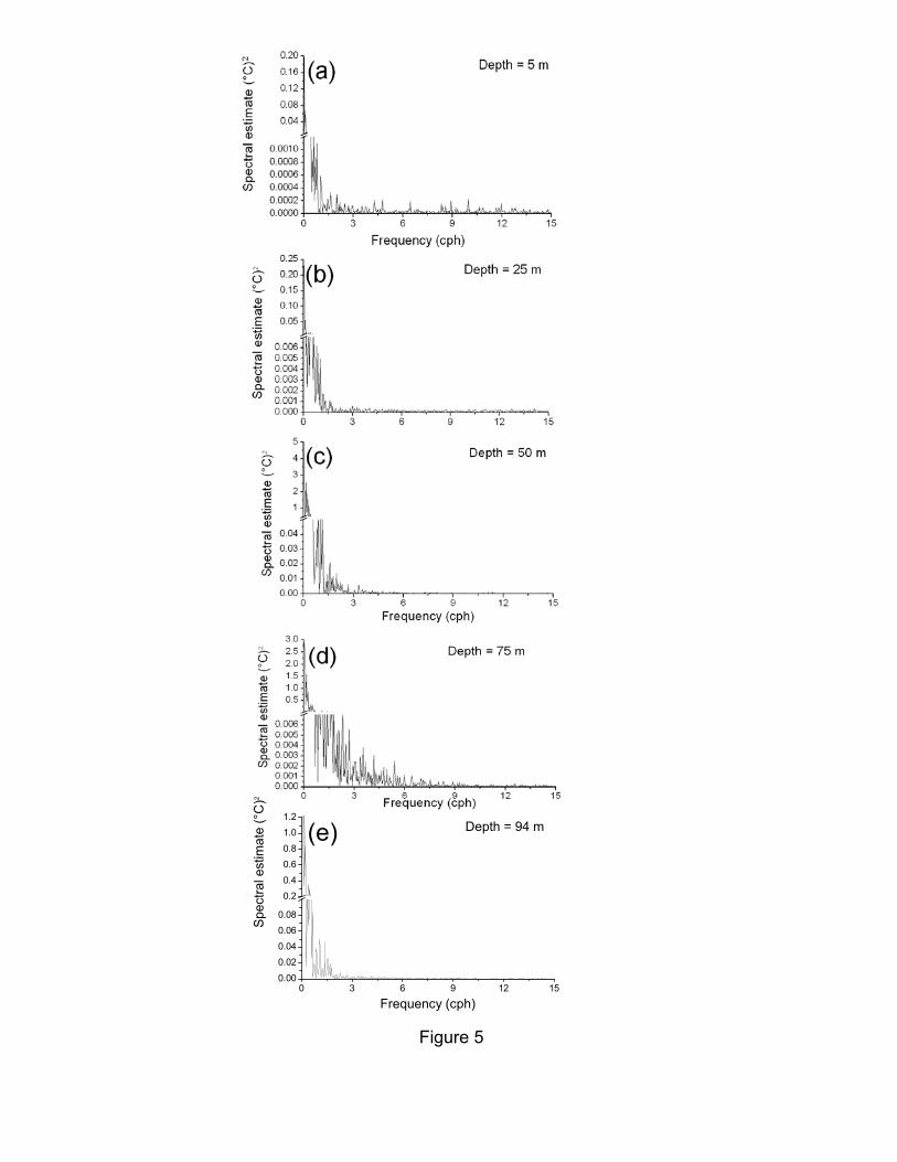
3.1.3 Spectrum analysis:

Time series data have been subjected to Fast Fourier Transform (FFT) algorithm (Cooley and

Tukey, 1965) to examine the spectral characteristics of the temperature oscillations (Mahadevan et al.

1987) in the study area - off Bhimilipatnam.

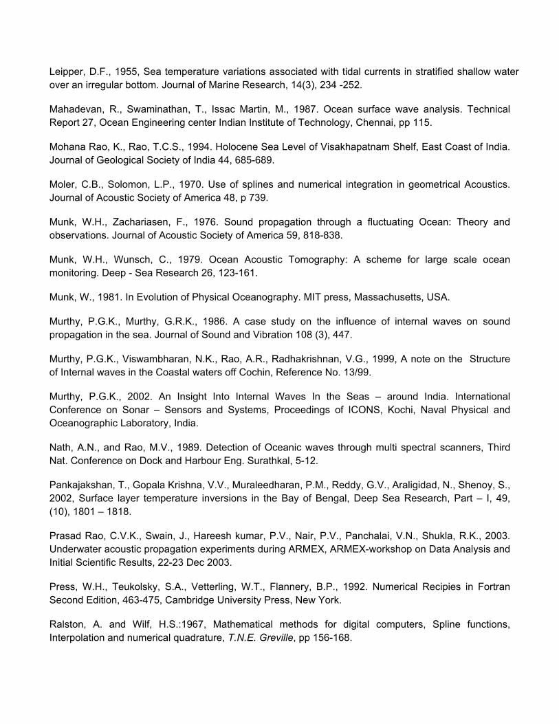
The power spectra (Fig.5) of temperature fluctuations at 5 vertical depths (5 m, 25 m, 50 m, 75

m & 94 m) are computed. This is useful to identify the distribution of the vertical isothermal motion of

various frequencies. There is a broad range of wave-frequencies and associated energy, where waves

of low frequency are associated with high energy while those of high frequency have low energy

(Fig.5). The energy associated with the low frequency is a measure of the effect of stratification, while it

doesn’t seem to have a definite bearing/relation on the high frequency counterpart. However, power

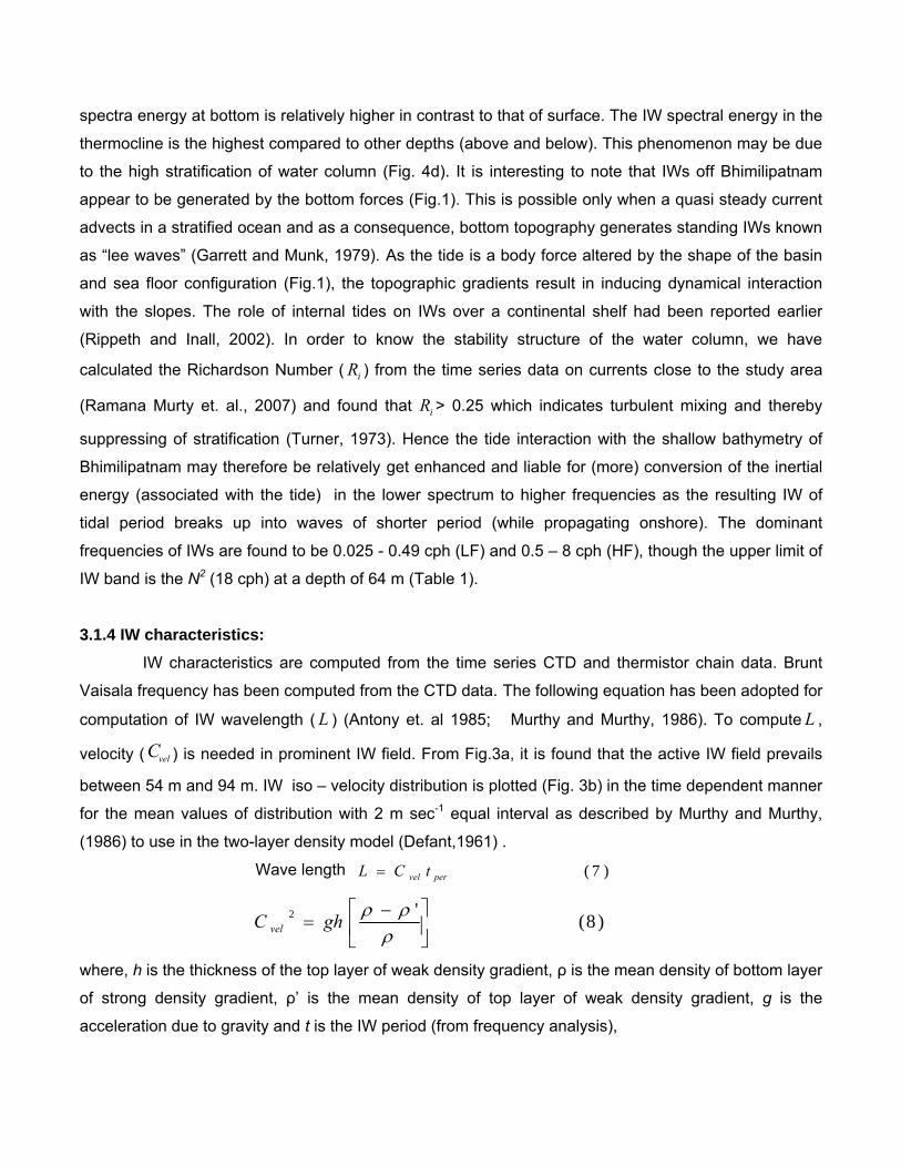
spectra energy at bottom is relatively higher in contrast to that of surface. The IW spectral energy in the

thermocline is the highest compared to other depths (above and below). This phenomenon may be due

to the high stratification of water column (Fig. 4d). It is interesting to note that IWs off Bhimilipatnam

appear to be generated by the bottom forces (Fig.1). This is possible only when a quasi steady current

advects in a stratified ocean and as a consequence, bottom topography generates standing IWs known

as “lee waves” (Garrett and Munk, 1979). As the tide is a body force altered by the shape of the basin

and sea floor configuration (Fig.1), the topographic gradients result in inducing dynamical interaction

with the slopes. The role of internal tides on IWs over a continental shelf had been reported earlier

(Rippeth and Inall, 2002). In order to know the stability structure of the water column, we have

calculated the Richardson Number ( iR ) from the time series data on currents close to the study area

(Ramana Murty et. al., 2007) and found that iR > 0.25 which indicates turbulent mixing and thereby

suppressing of stratification (Turner, 1973). Hence the tide interaction with the shallow bathymetry of

Bhimilipatnam may therefore be relatively get enhanced and liable for (more) conversion of the inertial

energy (associated with the tide) in the lower spectrum to higher frequencies as the resulting IW of

tidal period breaks up into waves of shorter period (while propagating onshore). The dominant

frequencies of IWs are found to be 0.025 - 0.49 cph (LF) and 0.5 – 8 cph (HF), though the upper limit of

IW band is the N2 (18 cph) at a depth of 64 m (Table 1).

3.1.4 IW characteristics: IW characteristics are computed from the time series CTD and thermistor chain data. Brunt

Vaisala frequency has been computed from the CTD data. The following equation has been adopted for

computation of IW wavelength ( L ) (Antony et. al 1985; Murthy and Murthy, 1986). To compute L ,

velocity ( velC ) is needed in prominent IW field. From Fig.3a, it is found that the active IW field prevails

between 54 m and 94 m. IW iso – velocity distribution is plotted (Fig. 3b) in the time dependent manner

for the mean values of distribution with 2 m sec-1 equal interval as described by Murthy and Murthy,

(1986) to use in the two-layer density model (Defant,1961) .

Wave length )7(pervel tCL =

)8('2⎥⎦

⎤⎢⎣

⎡ −=

ρρρghC vel

where, h is the thickness of the top layer of weak density gradient, ρ is the mean density of bottom layer

of strong density gradient, ρ’ is the mean density of top layer of weak density gradient, g is the

acceleration due to gravity and t is the IW period (from frequency analysis),

The computed values of pert , h, ρ, ρ’, velC , L and wave number (k=2 π/L ) are found to be 0.06

hrs - 40 hrs, 21 m, 1023.27 kg m-3, 1023.59 kg m-3, 0.548 km hr-1, 0.03 km - 21.8 km and 33.33 - 0.05

cycles km-1 for IWs respectively (Figs 2 & 3b) (Table 1). The calculated buoyancy force

( ρρρ Δ−=−−= ggFB )( ' ) is positive resulting an upward force (Stefanie and Wojcik 2006). In general,

the frequency of wave increases with strengthening of FB. In the present case it is increasing from the

starting to end of the observational period (Fig 3b). One can infer that band of high frequency IWs are

more active during night time which is supported by an earlier study (Murthy, 2002).

Another parameter required for the simulation of IW by the model, is wave number (k=2 π/L)

domain instead of frequency domain. The range of k in LF IW field is found to be 0.05 cycles km-1 to

0.91 cycles km-1. In the present paper, the simulation is confined to study the impact of lower frequency

IW field on sound propagation. Apart from the above parameters, total energy (6 oE ) is needed to

supplement input to the GM model. The estimated PE, KE, BPE and oE with the observed data

(Ramna Murty et.al., 2007) were found to be 0.489 J m-2, 0.278 J m-2, 0.175 J m-2 and 1.0 J m-2

respectively. The following section explains a procedure to generate displacements due to IW with the

statistics provided by Garrett – Munk power spectrum (Flatte.et al. 1979) and also conversion of

displacements into sound velocity realizations (Munk and Zachariasen, 1976).

3.2 Internal wave simulation:

To run the model, single profiles on temperature, salinity ,Brunt-Vaisala frequency and sound

velocity (Fig. 4) and an energy level, latitude, range and time scales, energy density factor ( oE ),

stratification scale ( B ) and bandwidth parameter ( *j ) are required (Fig. 4). Based on the input profiles

of N2 are generated on uniform mesh, with a depth increment zΔ = 2 m for the computation of IW

modes ( )(zW ) (Eq. 1A , Appendix A) and eigen-frequencies ( 2jγ ). These modes oscillate only in the

water column, where the IW frequency (ω) is smaller than the )(2 zN . Out side this region the solutions

are evanescent (i.e., exponentially decreasing). From our in-situ observations, it is evident that the

modes should oscillate between frequencies ωI = 0.025 cph to )(2 zN = 18 cph (i.e., maximum frequency

occurred in active IW field at a depth of 64 m), i.e in terms of wave number ( k ) given by 0.05 cycles

km-1 to 33.33 cycles km-1 (Table 1). The model has its own limitation i.e., the choice of maximum wave

number interval ( mink = 0.01 to maxk =0.5) containing the majority of energy in the IW spectrum

(Evans, 1992). The wave number sampling kΔ should span the spectrum of the IW field and is used to

approximate ( kΔ ), an integral over the spectrum (Eq. 4A , Appendix - A). Here, maxk = 0.5 cycles km-1

is used for the power spectrum. Accordingly we have performed the numerical experiment. A wave

number sampling increment of kΔ = 0.01 cycles km-1 is used with M = 46 samples between mink = 0.05

cycles km-1 to maxk = 0.5 cycles km-1 and the same is followed for negative wave numbers. The modal

band width parameter )43;32;21()( * ≥=≤= JforJforJforj ) which depends on the number of modes J

is chosen (Jackson and Elliott 2002). The maximum number of modes ( J ) depend on the depth of the

water column (H). Therefore, we choose J )25052501004;100253;2502( mHforandmHformHformHfor ≥<≤≤≤<<= , the maximum number of modes as

suggested by Elliott and Jackson (1998). The above mentioned scheme assumes that the first few

lower order modes account for 98% of the total energy in the shallow waters (Krishna Kumar &

Balasubramanian 2005). Accordingly we have selected *j =2 and j =3 for the present simulation. A

total of j = 3 internal wave modes ( )(zW ) and eigen-frequencies ( 2jγ ) are computed at each of the

wave numbers (M = 46). In the present analysis, modes of positive wave numbers are only considered.

The modes will explain the displacement of isopycnols due to IW. Once the internal eigen values ( 2jγ )

and modes ( )(zW ) are found, they can be used to generate realizations of displacements caused by

IWs. An energy density factor of oE = 1 with our observations is used to generate realizations of

displacements. Usually oE = 4 is adopted for deep waters (Flatte’, et al. 1979) Apart from the above

parameters, stratification scale ( B ) and extrapolated parameter ( oN ) are also needed for model and

can be computed from the formula Bzo eNzN /)( −= . A fixed value equal to the inertial frequency has

been considered for oN (Krishna Kumar & Balasubramanian 2005). Using N(z) from the observed data

B has been computed and value is found to be 0.091 km. Value of B is 1 km for deep tropical oceans

(Munk and Wunsch, 1979). Utilizing all the above parameters, sound velocity profiles (C) are obtained

by adding the fluctuations ( 2Cδ ) in the following equation (Munk and Zachariasen, 1976) to the

background profile ( 0C )

( ) ( ) )9(,,Re,,2 tzrdz

dctzrC p ζδ ⎟⎟

⎠

⎞⎜⎜⎝

⎛≅

where dzdcp / is the potential sound velocity gradient (m s-1) and ),,( tzrς the IW displacement

function (Eq. 4A , Appendix A). For acoustic simulation purpose, sound velocity profiles (C) are

generated for every 600 sec (10 minutes) between 0 and 21600 sec (6 hours) and for every 1 km

interval between 0 and 30 km. The spatial and temporal dependence of the sound velocity in the LF IW

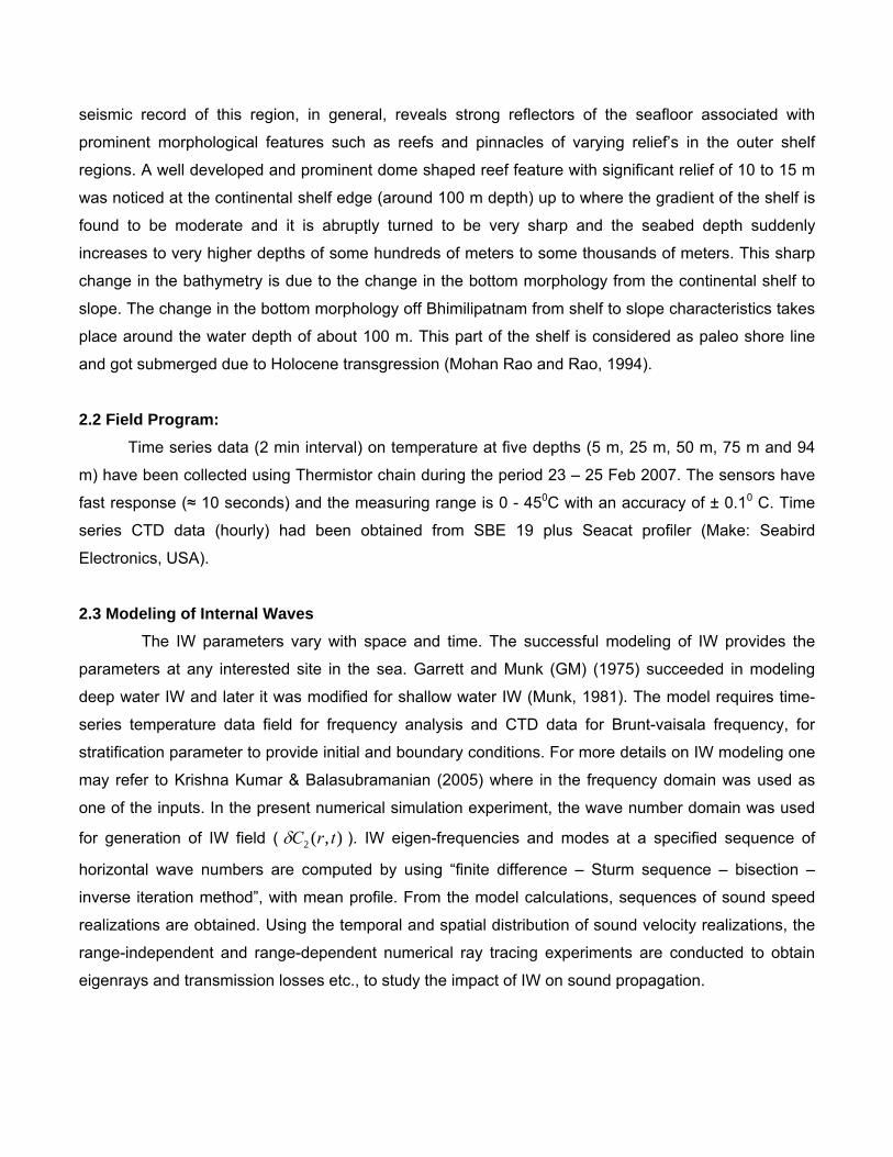
field in the contour form is shown in Fig. 6 (Flatte, et al. 1979). The range dependence of the sound

velocity profile is the most important consequence of the IWs, on the temporal and spatial scales

selected.

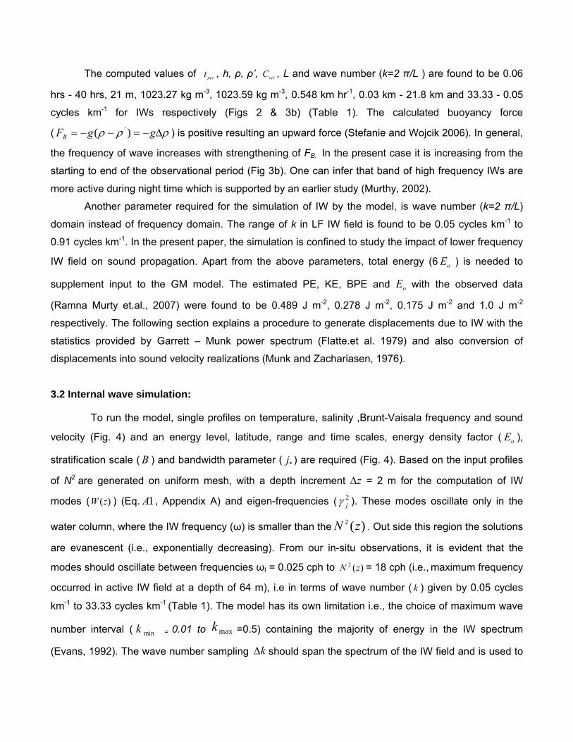
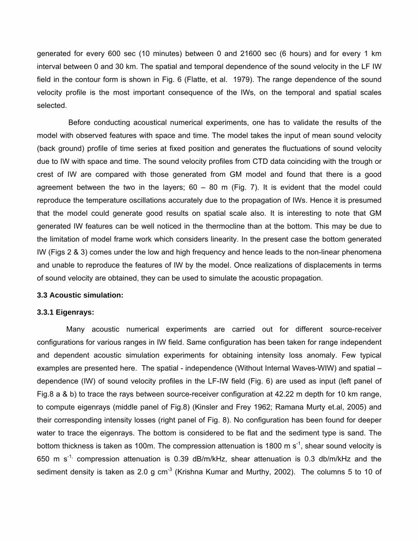
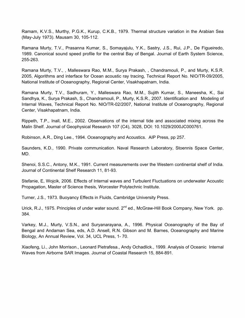
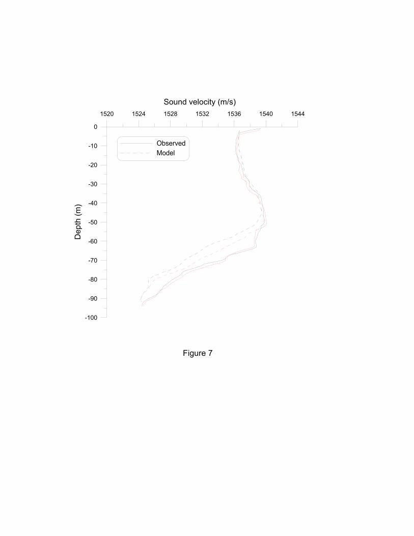
Before conducting acoustical numerical experiments, one has to validate the results of the

model with observed features with space and time. The model takes the input of mean sound velocity

(back ground) profile of time series at fixed position and generates the fluctuations of sound velocity

due to IW with space and time. The sound velocity profiles from CTD data coinciding with the trough or

crest of IW are compared with those generated from GM model and found that there is a good

agreement between the two in the layers; 60 – 80 m (Fig. 7). It is evident that the model could

reproduce the temperature oscillations accurately due to the propagation of IWs. Hence it is presumed

that the model could generate good results on spatial scale also. It is interesting to note that GM

generated IW features can be well noticed in the thermocline than at the bottom. This may be due to

the limitation of model frame work which considers linearity. In the present case the bottom generated

IW (Figs 2 & 3) comes under the low and high frequency and hence leads to the non-linear phenomena

and unable to reproduce the features of IW by the model. Once realizations of displacements in terms

of sound velocity are obtained, they can be used to simulate the acoustic propagation.

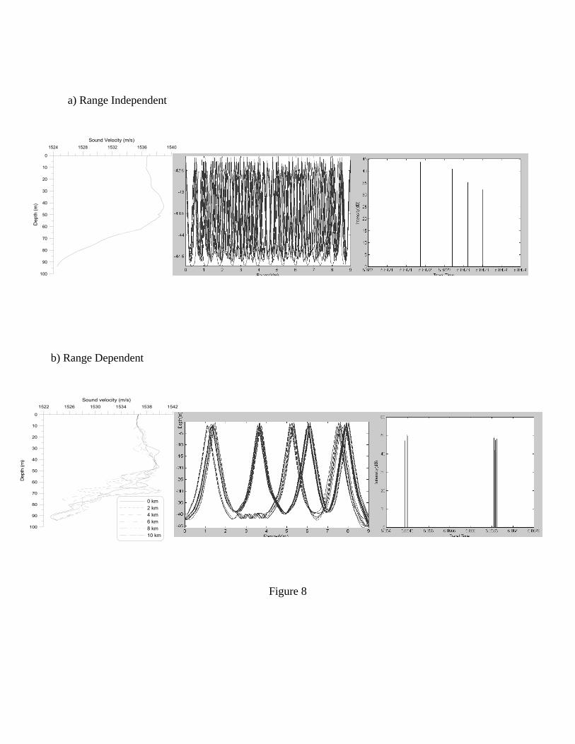
3.3 Acoustic simulation:

3.3.1 Eigenrays:

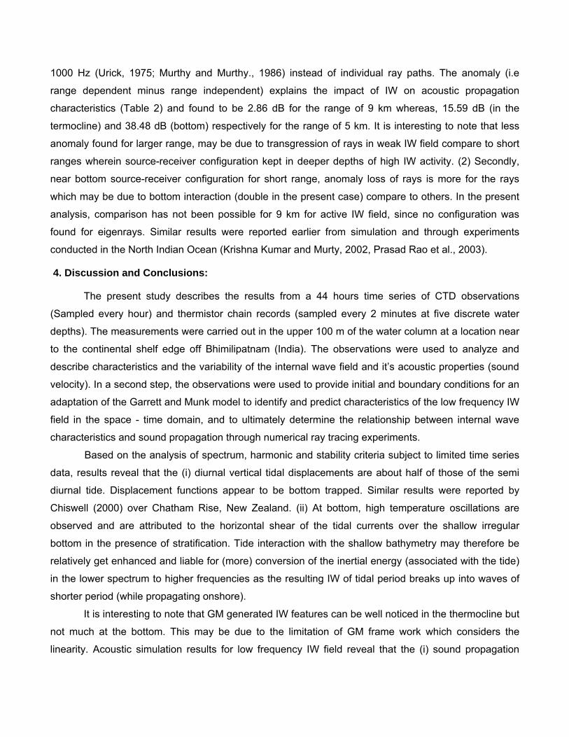
Many acoustic numerical experiments are carried out for different source-receiver

configurations for various ranges in IW field. Same configuration has been taken for range independent

and dependent acoustic simulation experiments for obtaining intensity loss anomaly. Few typical

examples are presented here. The spatial - independence (Without Internal Waves-WIW) and spatial –

dependence (IW) of sound velocity profiles in the LF-IW field (Fig. 6) are used as input (left panel of

Fig.8 a & b) to trace the rays between source-receiver configuration at 42.22 m depth for 10 km range,

to compute eigenrays (middle panel of Fig.8) (Kinsler and Frey 1962; Ramana Murty et.al, 2005) and

their corresponding intensity losses (right panel of Fig. 8). No configuration has been found for deeper

water to trace the eigenrays. The bottom is considered to be flat and the sediment type is sand. The

bottom thickness is taken as 100m. The compression attenuation is 1800 m s-1, shear sound velocity is

650 m s-1, compression attenuation is 0.39 dB/m/kHz, shear attenuation is 0.3 db/m/kHz and the

sediment density is taken as 2.0 g cm-3 (Krishna Kumar and Murthy, 2002). The columns 5 to 10 of

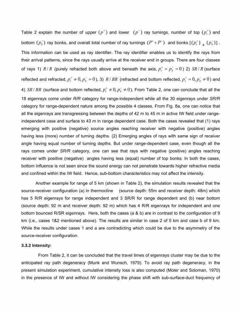
Table 2 explain the number of upper )( +p and lower )( −p ray turnings, number of top )( +tp and

bottom )( −bp ray bonks, and overall total number of ray turnings )( −++PP and bonks [ )( +

tp + )( −bp ] .

This information can be used as ray identifier. The ray identifier enables us to identify the rays from

their arrival patterns, since the rays usually arrive at the receiver end in groups. There are four classes

of rays 1) RR / (purely refracted both above and beneath the axis, 0== −+bt pp ) 2) RSR / (surface

reflected and refracted, 0,0 =≠ −+bt pp ), 3) BRR / (refracted and bottom reflected, 0,0 ≠= −+

bt pp ) and

4) BRSR / (surface and bottom reflected, 0,0 ≠≠ −+bt pp ). From Table 2, one can conclude that all the

18 eigenrays come under R/R category for range-independent while all the 30 eigenrays under SR/R

category for range-dependent nature among the possible 4 classes. From Fig. 8a, one can notice that

all the eigenrays are transgressing between the depths of 42 m to 45 m in active IW field under range-

independent case and surface to 43 m in range dependent case. Both the cases revealed that (1) rays

emerging with positive (negative) source angles reaching receiver with negative (positive) angles

having less (more) number of turning depths. (2) Emerging angles of rays with same sign of receiver

angle having equal number of turning depths. But under range-dependent case, even though all the

rays comes under SR/R category, one can see that rays with negative (positive) angles reaching

receiver with positive (negative) angles having less (equal) number of top bonks. In both the cases,

bottom influence is not seen since the sound energy can not penetrate towards higher refractive media

and confined within the IW field. Hence, sub-bottom characteristics may not affect the intensity.

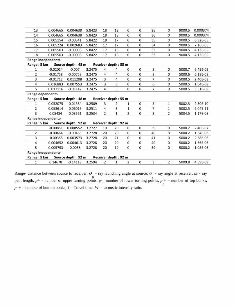
Another example for range of 5 km (shown in Table 2), the simulation results revealed that the

source-receiver configuration (a) in thermocline (source depth: 55m and receiver depth: 48m) which

has 5 R/R eigenrays for range independent and 3 SR/R for range dependent and (b) near bottom

(source depth: 92 m and receiver depth: 92 m) which has 4 R/R eigenrays for independent and one

bottom bounced R/SR eigenrays. Here, both the cases (a & b) are in contrast to the configuration of 9

km (i.e., cases 1&2 mentioned above). The results are similar in case 2 of 5 km and case b of 9 km.

While the results under cases 1 and a are contradicting which could be due to the asymmetry of the

source-receiver configuration.

3.3.2 Intensity:

From Table 2, it can be concluded that the travel times of eigenrays cluster may be due to the

anticipated ray path degeneracy (Munk and Wunsch, 1979). To avoid ray path degeneracy, in the

present simulation experiment, cumulative intensity loss is also computed (Moler and Soloman, 1970)

in the presence of IW and without IW considering the phase shift with sub-surface-duct frequency of

1000 Hz (Urick, 1975; Murthy and Murthy., 1986) instead of individual ray paths. The anomaly (i.e range dependent minus range independent) explains the impact of IW on acoustic propagation

characteristics (Table 2) and found to be 2.86 dB for the range of 9 km whereas, 15.59 dB (in the

termocline) and 38.48 dB (bottom) respectively for the range of 5 km. It is interesting to note that less

anomaly found for larger range, may be due to transgression of rays in weak IW field compare to short

ranges wherein source-receiver configuration kept in deeper depths of high IW activity. (2) Secondly,

near bottom source-receiver configuration for short range, anomaly loss of rays is more for the rays

which may be due to bottom interaction (double in the present case) compare to others. In the present

analysis, comparison has not been possible for 9 km for active IW field, since no configuration was

found for eigenrays. Similar results were reported earlier from simulation and through experiments

conducted in the North Indian Ocean (Krishna Kumar and Murty, 2002, Prasad Rao et al., 2003).

4. Discussion and Conclusions:

The present study describes the results from a 44 hours time series of CTD observations

(Sampled every hour) and thermistor chain records (sampled every 2 minutes at five discrete water

depths). The measurements were carried out in the upper 100 m of the water column at a location near

to the continental shelf edge off Bhimilipatnam (India). The observations were used to analyze and

describe characteristics and the variability of the internal wave field and it’s acoustic properties (sound

velocity). In a second step, the observations were used to provide initial and boundary conditions for an

adaptation of the Garrett and Munk model to identify and predict characteristics of the low frequency IW

field in the space - time domain, and to ultimately determine the relationship between internal wave

characteristics and sound propagation through numerical ray tracing experiments.

Based on the analysis of spectrum, harmonic and stability criteria subject to limited time series

data, results reveal that the (i) diurnal vertical tidal displacements are about half of those of the semi

diurnal tide. Displacement functions appear to be bottom trapped. Similar results were reported by

Chiswell (2000) over Chatham Rise, New Zealand. (ii) At bottom, high temperature oscillations are

observed and are attributed to the horizontal shear of the tidal currents over the shallow irregular

bottom in the presence of stratification. Tide interaction with the shallow bathymetry may therefore be

relatively get enhanced and liable for (more) conversion of the inertial energy (associated with the tide)

in the lower spectrum to higher frequencies as the resulting IW of tidal period breaks up into waves of

shorter period (while propagating onshore).

It is interesting to note that GM generated IW features can be well noticed in the thermocline but

not much at the bottom. This may be due to the limitation of GM frame work which considers the

linearity. Acoustic simulation results for low frequency IW field reveal that the (i) sound propagation

takes place along RR / , RSR / and R/SR rays only (ii) Intensity loss anomaly due to IW was found to

be 2.86 dB to 15.59 dB in the water column and maximum (38.48 dB) was observed at the bottom due

to the bottom interaction. Our results are well compared with those reported earlier from simulation and

acoustic field experiments in the Northern Indian Ocean.

5. Acknowledgements: The authors are grateful to Dr.S.R.Shetye, Director, NIO, Goa, Dr.V.S.N.Murty, Scientist-

In-Charge NIO (RC), Visakhapatnam for there interest in this study and the Council of Scientific and

Industrial Research (CSIR), New Delhi, India for providing facilities. They would like to thank Naval

Research Board (NRB), New Delhi for financial support. The first author B.Sridevi is grateful to CSIR,

New Delhi, India for the grant of Junior Research Fellowship during the tenure of which a part of this

work was carried out. They would like to thank the anonymous reviewers for their valuable suggestions

which helped to improve the original manuscript.

6. References: Antony, M.K., Murty, C.S., Reddy, G.V., Rao, K.H., 1985. Sub-surface temperature oscillations and associated flow in the western Bay of Bengal. Estuarine, Coastal and Shelf Science 21, 823-834.

Chen, C., Millero, F.J., 1977. Speed of sound in sea water at high pressures. Journal of Acoustic Society of America 62, 1129-1135.

Cooley, J.W., Tukey, J.W., 1965. An algorithm for the machine calculation of complex fourier series. Mathematica of Computation 19, 297.

Chiswell, S.M., 2000. Tidal Energetics over the Chatham Rise, New Zealand. Journal of Physical Oceanography, 30, 9, 2452 – 2460.

Desanto, J. A., 1979. Theoretical Methods in Ocean Acoustics. edited by Desanto J A, (Springer-Verlag, New York, 1979) 7- 77; see also Dugan J P, Oceanography in under water Acoustics Chapter 5.

Defant, .A., 1961. Physical Oceanography, volume 2. Oxford Pergamon Press, 517- 526.

Dozier, L.B., Tappert, D., 1978. Statistics of normal mode amplitudes in a random Ocean. I. Theory. Journal of Acoustic Society of America 63, 353-365.

Dong-Jiing Doong., Li-Chung Wu., Chia Chuen Kao., 2007. Internal wave propagation observed by Ship board Radar. Sea Technology 48, 42- 45.

Elliott, A.J. and Jackson, J.F.E., 1998. Internal waves and acoustic variability. Proc. of IEEE conference OCEANS’98. 10-14.

Evans, R.B., 1992. The existence of generalized eigen functions and multiple eigen values in under water acoustics. Journal of Acoustical Society of America 92, 2024-2029.

Fernandes, A.A., Sarma, Y.V.B., Menon, H.B., Vethamony. P., 2000. Wave directional spectrum from SAR imagery. Journal of Indian Society of Remote Sensing 28, 9-18.

Flatte, M., Dashen, R., Munk, W. H., Watson, W., Zachariasen, F., 1979. Sound transmission through a fluctuating Ocean. Cambridge University Press, England, pp.56-57.

Fu, L.L., Holt, B., 1982. Seasat views oceans and sea ice with Synthetic Aperture Radar. Jet Propulsion Laboratory publication 81-120.

Garrett, C.J.R., Munk, W.H., 1975. Space-time scales of internal waves: A progress report. Journal of Geophysical Research 80, 291-297.

Garrett, C.J.R., Munk, W.H., 1979. Internal Waves in the Ocean. Annual Reviews in Fluid Mechanics 11, 339-369.

Gill, A.E., 1982. Atmosphere-Ocean Dynamics. Academic press, San Diego, USA.

Jackson, J.F.E. and Elliott, A.J., 2002. Internal waves in the Clyde Sea, Estuarine Coastal and Shelf Science 54, 51-64.

Kinsler L.E. and Frey A.R., 1962. Fundamentals of Acoustics, John Wiley & Sons, Inc., New York, London pp 522.

Krishna Kumar, G.V., and Murthy, P.G.: 2002, Simulation of Sound Speed Structure due to Internal Waves in the Ocean. In: Proc. ICONS – International Conference on Sonar-Sensors and Systems.

Krishna Kumar, G.V., Balasubramanian, P., 2005. IWAVE: An Ocean simulation model for internal waves. Current Science 89, 1927-1932.

Kumar, O.V., Nair, P.V., Kumar, P.V.H., Kumar N.M., Salam, K.A.A., Chandran K.P.B., Venkatachalam, N.R., 2001. Report on the acoustical Oceanography experiment in the shallow waters off Saurashtra coast during Oct-Nov 2000, Technical Report No. RR- 29/2001.

La Fond, K.G., Rao, C.P., 1954. Vertical oscillations of tidal periods in the temperature structure of the sea. Andhra University Memoirs 1, 109-116.

Lafond, E.C., 1962. Internal waves. The Sea 1, edited by M.N. Hill, 731- 751, New York, Wiley.

La Fond, E.C., La Fond, K.G., 1968. Studies on oceanic circulation in the Bay of Bengal. Bulletin of National Institute of Science, India 38, 169 -183.

Leipper, D.F., 1955, Sea temperature variations associated with tidal currents in stratified shallow water over an irregular bottom. Journal of Marine Research, 14(3), 234 -252.

Mahadevan, R., Swaminathan, T., Issac Martin, M., 1987. Ocean surface wave analysis. Technical Report 27, Ocean Engineering center Indian Institute of Technology, Chennai, pp 115.

Mohana Rao, K., Rao, T.C.S., 1994. Holocene Sea Level of Visakhapatnam Shelf, East Coast of India. Journal of Geological Society of India 44, 685-689.

Moler, C.B., Solomon, L.P., 1970. Use of splines and numerical integration in geometrical Acoustics. Journal of Acoustic Society of America 48, p 739.

Munk, W.H., Zachariasen, F., 1976. Sound propagation through a fluctuating Ocean: Theory and observations. Journal of Acoustic Society of America 59, 818-838.

Munk, W.H., Wunsch, C., 1979. Ocean Acoustic Tomography: A scheme for large scale ocean monitoring. Deep - Sea Research 26, 123-161.

Munk, W., 1981. In Evolution of Physical Oceanography. MIT press, Massachusetts, USA.

Murthy, P.G.K., Murthy, G.R.K., 1986. A case study on the influence of internal waves on sound propagation in the sea. Journal of Sound and Vibration 108 (3), 447.

Murthy, P.G.K., Viswambharan, N.K., Rao, A.R., Radhakrishnan, V.G., 1999, A note on the Structure of Internal waves in the Coastal waters off Cochin, Reference No. 13/99.

Murthy, P.G.K., 2002. An Insight Into Internal Waves In the Seas – around India. International Conference on Sonar – Sensors and Systems, Proceedings of ICONS, Kochi, Naval Physical and Oceanographic Laboratory, India.

Nath, A.N., and Rao, M.V., 1989. Detection of Oceanic waves through multi spectral scanners, Third Nat. Conference on Dock and Harbour Eng. Surathkal, 5-12.

Pankajakshan, T., Gopala Krishna, V.V., Muraleedharan, P.M., Reddy, G.V., Araligidad, N., Shenoy, S., 2002, Surface layer temperature inversions in the Bay of Bengal, Deep Sea Research, Part – I, 49, (10), 1801 – 1818.

Prasad Rao, C.V.K., Swain, J., Hareesh kumar, P.V., Nair, P.V., Panchalai, V.N., Shukla, R.K., 2003. Underwater acoustic propagation experiments during ARMEX, ARMEX-workshop on Data Analysis and Initial Scientific Results, 22-23 Dec 2003.

Press, W.H., Teukolsky, S.A., Vetterling, W.T., Flannery, B.P., 1992. Numerical Recipies in Fortran Second Edition, 463-475, Cambridge University Press, New York.

Ralston, A. and Wilf, H.S.:1967, Mathematical methods for digital computers, Spline functions, Interpolation and numerical quadrature, T.N.E. Greville, pp 156-168.

Ramam, K.V.S., Murthy, P.G.K., Kurup, C.K.B., 1979. Thermal structure variation in the Arabian Sea (May-July 1973). Mausam 30, 105-112.

Ramana Murty, T.V., Prasanna Kumar, S., Somayajulu, Y.K., Sastry, J.S., Rui, J.P., De Figueiredo, 1989. Canonical sound speed profile for the central Bay of Bengal. Journal of Earth System Science, 255-263.

Ramana Murty, T.V., , Malleswara Rao, M.M., Surya Prakash, , Chandramouli, P., and Murty, K.S.R. 2005, Algorithms and interface for Ocean acoustic ray tracing, Technical Report No. NIO/TR-09/2005, National Institute of Oceanography, Regional Center, Visakhapatnam, India.

Ramana Murty, T.V., Sadhuram, Y., Malleswara Rao, M.M., Sujith Kumar, S., Maneesha, K., Sai Sandhya, K., Surya Prakash, S., Chandramouli, P., Murty, K.S.R., 2007. Identification and Modeling of Internal Waves, Technical Report No. NIO/TR-02/2007, National Institute of Oceanography, Regional Center, Visakhapatnam, India.

Rippeth, T.P., Inall, M.E., 2002. Observations of the internal tide and associated mixing across the Malin Shelf. Journal of Geophysical Research 107 (C4), 3028, DOI: 10.1029/2000JC000761.

Robinson, A.R., Ding Lee., 1994. Oceanography and Acoustics. AIP Press, pp 257.

Saunders, K.D., 1990. Private communication. Naval Research Laboratory, Stoennis Space Center, MD.

Shenoi, S.S.C., Antony, M.K., 1991. Current measurements over the Western continental shelf of India. Journal of Continental Shelf Research 11, 81-93.

Stefanie, E, Wojcik, 2006. Effects of Internal waves and Turbulent Fluctuations on underwater Acoustic Propagation, Master of Science thesis, Worcester Polytechnic Institute.

Turner, J.S., 1973. Buoyancy Effects in Fluids, Cambridge University Press.

Urick, R.J., 1975. Principles of under water sound. 2nd ed., McGraw-Hill Book Company, New York. pp. 384.

Varkey, M.J., Murty, V.S.N., and Suryanarayana, A., 1996. Physical Oceanography of the Bay of Bengal and Andaman Sea, eds, A.D. Ansell, R.N. Gibson and M. Barnes, Oceanography and Marine Biology, An Annual Review, Vol. 34, UCL Press, 1- 70.

Xiaofeng, Li., John Morrison., Leonard Pietrafesa., Andy Ochadlick., 1999. Analysis of Oceanic Internal Waves from Airborne SAR Images. Journal of Coastal Research 15, 884-891.

Appendix A Internal Wave Eigen value and Modes: Saunders (1990) had developed IW model with guiding principle that maximum simplicity should

prevail while producing results that are representative of the IW field based on the following

assumptions: (1) linearity, (2) no mean shear, (3) a Boussinesq fluid, (4) flat or slowly varying bottom,

and (5) horizontally homogeneous or slowly varying density field. The exact dispersion relation, for the

IWs in the density stratified rotated ocean, is the solution of the eigen values as given by Gill (1982).

The internal wave eigen values and modes are determined by water depth H in meters, the

buoyancy frequency profile )(2 zN and inertial frequency ωI in rad/s. Here2/1

)( ⎥⎦

⎤⎢⎣

⎡−=

dzdgzN ρ

ρ, where g is

the gravitational acceleration, and ρ the mean density of the medium. IW frequencies ω are limited to

the range between inertial frequency (ωI) at the lower end and maximum buoyancy frequency ( 2N ) at

the higher end. The internal wave modes )(zWi satisfy the eigen value problem

{ [ ] } )1(00)()()( 2222

2

2

AHzzWkzNdz

zWdjIj

j ≤≤=−−+ ωγ

where 0)()0( == HWW jj and k is a known spatial wave number in rad m-1. The quantities

Jjj ,1,2 =γ are the eigen values that are related to the eigen-frequencies by the equation

2222 / jIj k γωω += (Dozier and Tappert, 1978).

The eigen values of Eq. A1, are bounded below by 2k max [ ]22 )( IzN ω− , as can be established

using an extension of the argument given by Evans (1992). Each wave number k has its own set of

infinity depth-dependent vertical modes )(zW of the system. These modes oscillate only in the region of

the water column, where IW frequency ω is smaller than the buoyancy frequency ( )(2 zN ).Outside this

region the solutions are evanescent. Therefore, the vertical displacement of the linear IW field can be

expressed as a combination of plane waves as weighted double sum over mode number

Displacements: The complex internal wave displacements, with real and imaginary parts in meters, are taken

to have the form [ Dozier and Tappert, 1978].

[ ] )2()(exp),()(),,( 2

1

2 AdktkiikrzkWkAtzr j

J

jjj ωζ += ∑ ∫

=

∞

∞−

where the 2k dependence of the internal wave modes and eigen-frequencies are indicated explicitly.

The expansion coefficients )(kA j are identically distributed complex Gaussian random variables with

zero mean. Their variance is given by the Garrett-Munk power spectrum defined by Flatte’, et. al.

(1979) as

)3()(

34)( 222

2

2*

2202 A

kkkk

jjEkP

j

jj ++

=π

where ,)/( 0 jBNFk Ij π= B the stratification scale, (Ramana Murty et.al., 1989), N0 extroploated

Brunt-vaisala frequency and and E0 the energy density factor. The quantity FI is the inertial frequency

computed using FI = (1/12) sin (latitude) with units of cycles hour-1. Here the number of wave numbers

is doubled to account for both positive and negative wave numbers.

Computation of internal wave displacements requires a numerical approximation of integral in

Eq. (A2). This starts with a choice of a maximum wave number maxk to bound the interval that contains

the majority of the energy in the internal wave spectrum. For the Garrett-Munk power spectrum this is

around 0.5 cycles km-1 converted into rad m-1. The interval [0, maxk ] is divided into M parts of

size Mkk /max=Δ . The discrete horizontal wave numbers, used in the internal wave eigen-frequency

calculations, are taken to be kmkm Δ= , m =1, M. The integral in Eq. (A2) is approximated, using both

positive and negative values of m, by

)4(])(exp[),((

),,( 22,

1 1

2

AktkirikzkWGkkP

tzr mjmmjmj

J

j

M

m

mj Δ+Δ

≅∑ ∑=

±

±=

ωζ

where both the real and imaginary parts of Gj,m are Gaussian random variables with zero mean and unit

variance and r is the range, z is the depth and t is the time. Independent realizations of Gj,m are

generated by calling the subroutine “GASDEV” (Press. et.al., 1992) separately for the real and

imaginary parts and for each j and m (both positive and negative). Number of random realizations of

sound velocity created for the sequence of time and range according to requested number. If an odd

number is requested an extra realization is created to make the number of realizations even.

Sound speed Fluctuations: The displacement fields obtained from Eq. (A2) are converted into sound speed fluctuations

using the relation from Munk and Zachariasen (1976) [ ] )5(),,(Re)/(),,(2 Atzrdzdctzrc p ζδ ≅

where, dzdc p / is the potential sound speed gradient in (s-1). Here the potential sound speed gradient

is used to compute the sound speed realizations caused by the IWs.

List of Tables and Figures:- Tables:

Table 1: Derived characteristics of various components in the IW field

Table 2: a) Acoustic ray parameters (Range-independent)

b) Acoustic ray parameters (Range-dependent)

(source depth = 42 m, receiver depth = 42 m, Range = 10 km)

Figure Captions

Figure 1: a). Study area

b). Cross-sectional seabed topography along AA1 (shown in figure 1a)

Fgure 2: Time series data of temperature (2 min interval) collected from thermister chain at 5

depths (5 m, 25 m, 50 m, 75 m and 94 m) off Bhimilipatnam during 23 – 25 Feb

2007

Figure 3: a). Variation of sound velocity (m.s-1) off Bhimilipatnam

b). Sound velocity structure revealing internal waves. A, indicates sound velocity

structure after eliminating internal waves. Contour interval is 2 m s-1.

Figure 4: Mean profiles of a) Temperature (0C) b) Salinity (psu) c) Sound Velocity (ms-1) and

d) Brunt-Vaisala’s frequency (cph) off Bhimilipatnam during 23rd -25th Feb 2007

Figure 5: Energy spectra of temperature oscillations at (a) 5 m, (b) 25 m, (c) 50 m, (d) 75 m

and (e) 94 m depths off Bhimilipatnam during 23-25 Feb2007

Figure 6: Spatial (a) and temporal (b) dependence of sound velocity distribution in the

internal wave field off Bhimilipatnam

Figure 7: Comparison of Sound Velocity profiles between the observed and Model (GM) off

Bhimilipatnam (_____ observed; - - - - model)

Figure 8: Ray paths for a) Range-independent b) Range-dependent off Bhimilipatnam

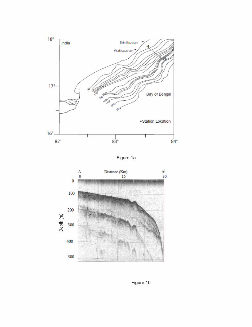
Figure 1a

Figure 1b

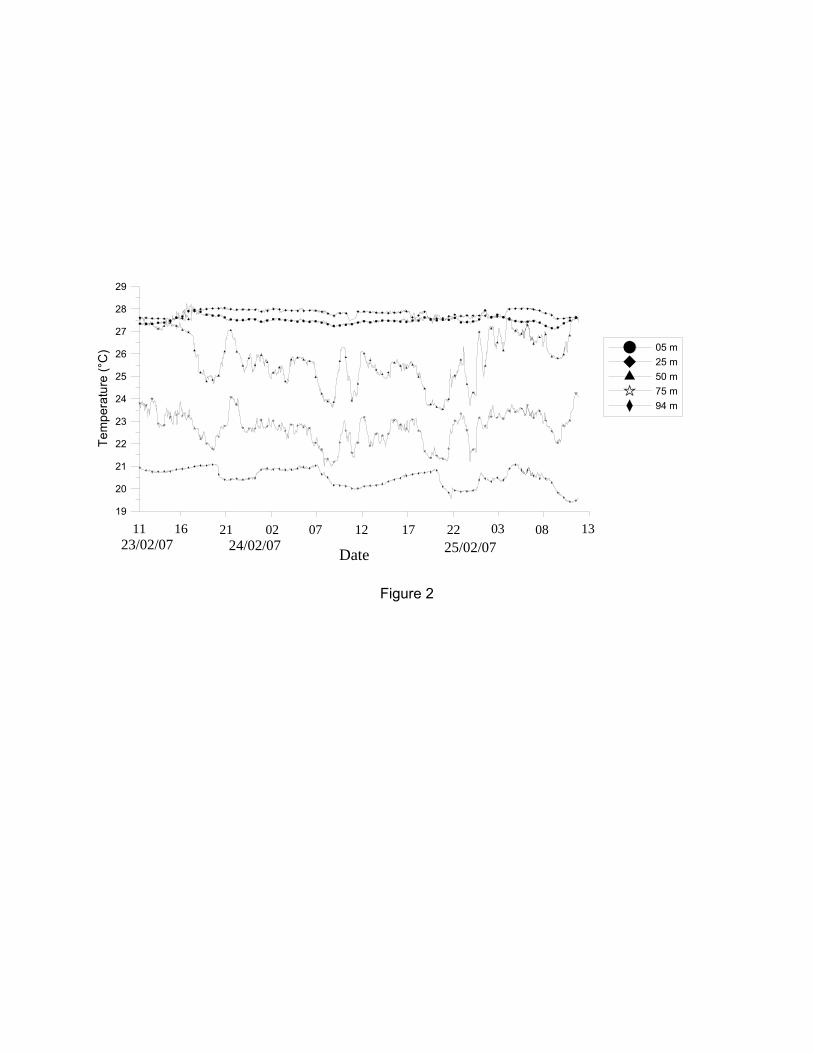
Figure 2

19

20

21

22

23

24

25

26

27

28

29

Tem

pera

ture

(°C

) 05 m25 m50 m75 m94 m

11 12 13 16 21 02 07 17 22 03 0823/02/07 25/02/07 24/02/07 Date

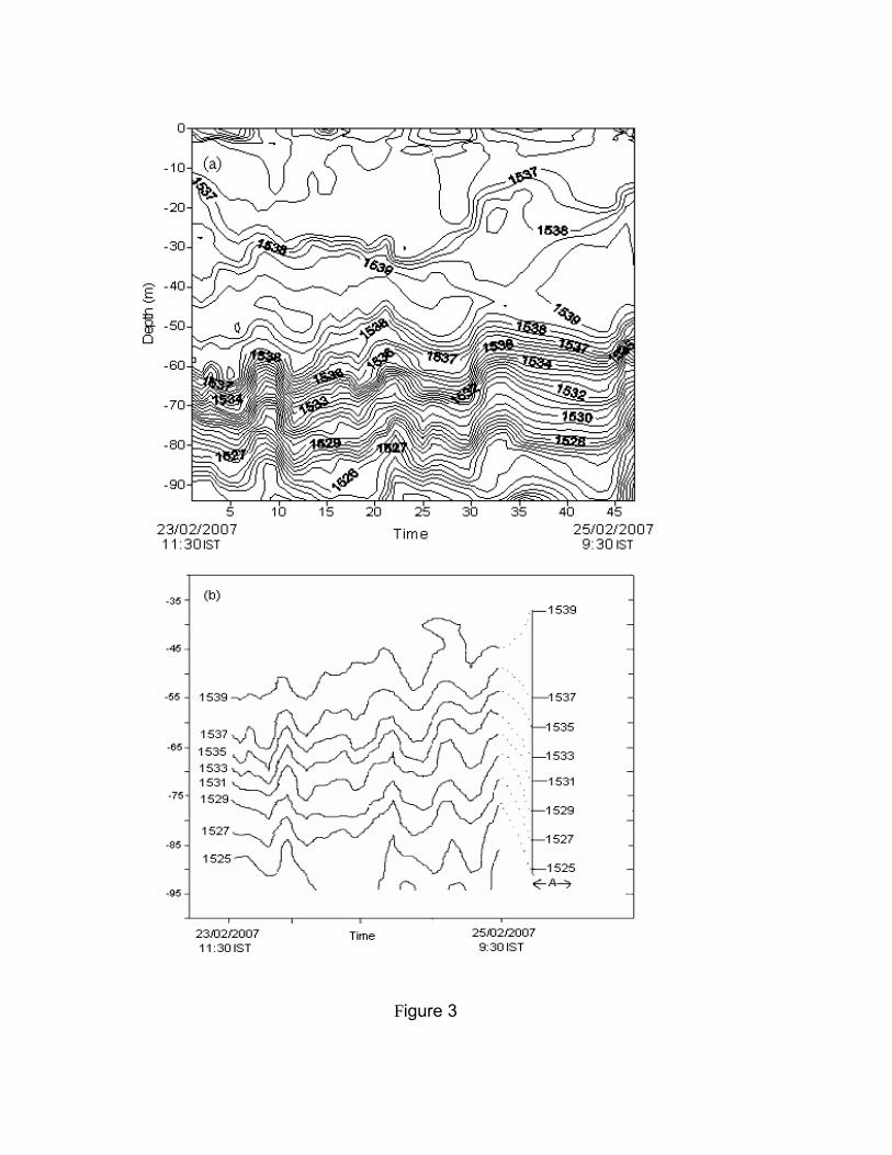
Figure 3

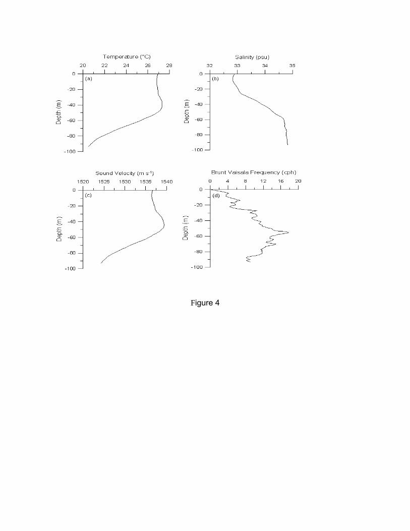
Figure 4

0 3 6 9 12 150.00

0.020.04

0.060.08

0.20.4

0.60.8

1.01.2

(e)

Spec

tral e

stim

ate

(°C

)2

Frequency (cph)

Depth = 94 m

Figure 5

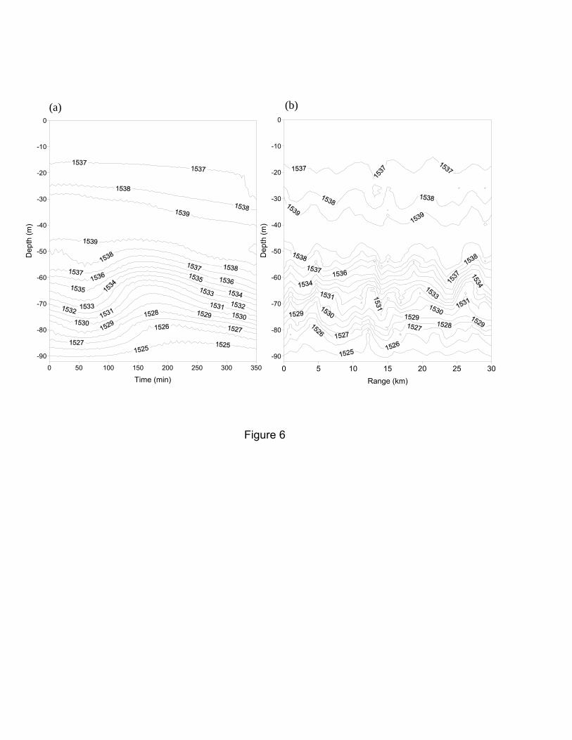
Figure 6

0 5 10 15 20 25 30Range (km)

-90

-80

-70

-60

-50

-40

-30

-20

-10

0

Dep

th (m

)

(b)

0 50 100 150 200 250 300 350

Time (min)

-90

-80

-70

-60

-50

-40

-30

-20

-10

0

Dep

th (m

)

(a)

1520 1524 1528 1532 1536 1540 1544

Sound velocity (m/s)

-100

-90

-80

-70

-60

-50

-40

-30

-20

-10

0

Dep

th (m

)

ObservedModel

Figure 7

a) Range Independent

b) Range Dependent

Figure 8

1524 1528 1532 1536 1540Sound Velocity (m/s)

100

90

80

70

60

50

40

30

20

10

0

Dep

th (m

)

1522 1526 1530 1534 1538 1542Sound velocity (m/s)

100

90

80

70

60

50

40

30

20

10

0

Dep

th (m

)

0 km2 km4 km6 km8 km10 km

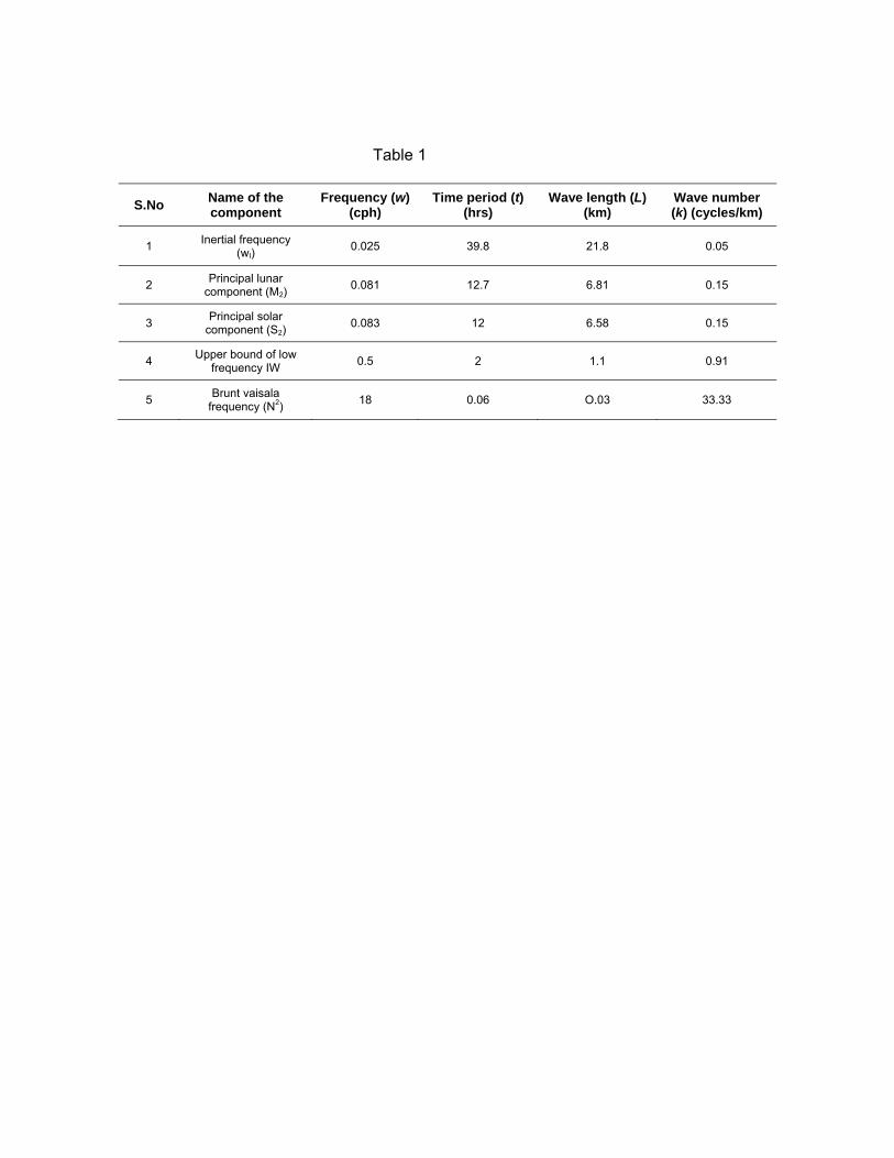
Table 1

S.No Name of the component

Frequency (w) (cph)

Time period (t) (hrs)

Wave length (L) (km)

Wave number (k) (cycles/km)

1 Inertial frequency (wI)

0.025 39.8 21.8 0.05

2 Principal lunar component (M2)

0.081 12.7 6.81 0.15

3 Principal solar component (S2)

0.083 12 6.58 0.15

4 Upper bound of low frequency IW 0.5 2 1.1 0.91

5 Brunt vaisala frequency (N2) 18 0.06 O.03 33.33

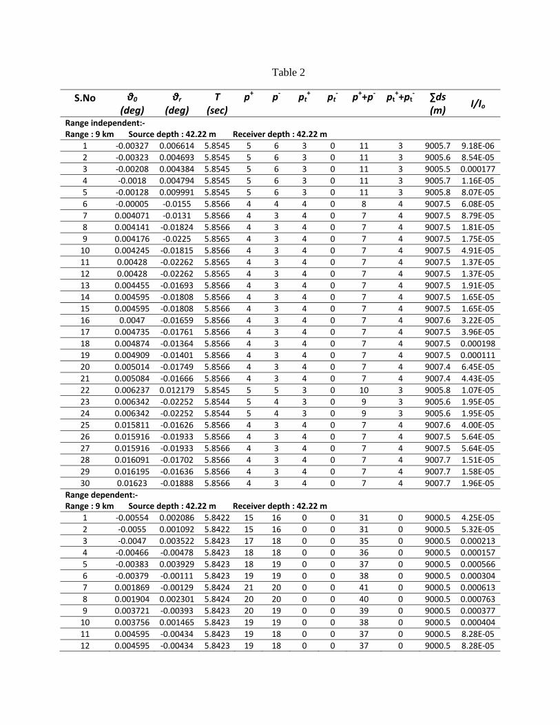
Table 2

S.No  θ0 (deg) 

θr  (deg) 

T (sec) 

p+  

p‐  

pt+  

pt‐  

p++p‐

 pt

++pt‐ 

 ∑ds (m) 

I/Io 

Range independent:‐ Range : 9 km       Source depth : 42.22 m        Receiver depth : 42.22 m 

1  ‐0.00327  0.006614  5.8545 5 6 3 0 11 3  9005.7 9.18E‐062  ‐0.00323  0.004693  5.8545 5 6 3 0 11 3  9005.6 8.54E‐053  ‐0.00208  0.004384  5.8545 5 6 3 0 11 3  9005.5 0.0001774  ‐0.0018  0.004794  5.8545 5 6 3 0 11 3  9005.7 1.16E‐055  ‐0.00128  0.009991  5.8545 5 6 3 0 11 3  9005.8 8.07E‐056  ‐0.00005  ‐0.0155  5.8566 4 4 4 0 8 4  9007.5 6.08E‐057  0.004071  ‐0.0131  5.8566 4 3 4 0 7 4  9007.5 8.79E‐058  0.004141  ‐0.01824  5.8566 4 3 4 0 7 4  9007.5 1.81E‐059  0.004176  ‐0.0225  5.8565 4 3 4 0 7 4  9007.5 1.75E‐0510  0.004245  ‐0.01815  5.8566 4 3 4 0 7 4  9007.5 4.91E‐0511  0.00428  ‐0.02262  5.8565 4 3 4 0 7 4  9007.5 1.37E‐0512  0.00428  ‐0.02262  5.8565 4 3 4 0 7 4  9007.5 1.37E‐0513  0.004455  ‐0.01693  5.8566 4 3 4 0 7 4  9007.5 1.91E‐0514  0.004595  ‐0.01808  5.8566 4 3 4 0 7 4  9007.5 1.65E‐0515  0.004595  ‐0.01808  5.8566 4 3 4 0 7 4  9007.5 1.65E‐0516  0.0047  ‐0.01659  5.8566 4 3 4 0 7 4  9007.6 3.22E‐0517  0.004735  ‐0.01761  5.8566 4 3 4 0 7 4  9007.5 3.96E‐0518  0.004874  ‐0.01364  5.8566 4 3 4 0 7 4  9007.5 0.00019819  0.004909  ‐0.01401  5.8566 4 3 4 0 7 4  9007.5 0.00011120  0.005014  ‐0.01749  5.8566 4 3 4 0 7 4  9007.4 6.45E‐0521  0.005084  ‐0.01666  5.8566 4 3 4 0 7 4  9007.4 4.43E‐0522  0.006237  0.012179  5.8545 5 5 3 0 10 3  9005.8 1.07E‐0523  0.006342  ‐0.02252  5.8544 5 4 3 0 9 3  9005.6 1.95E‐0524  0.006342  ‐0.02252  5.8544 5 4 3 0 9 3  9005.6 1.95E‐0525  0.015811  ‐0.01626  5.8566 4 3 4 0 7 4  9007.6 4.00E‐0526  0.015916  ‐0.01933  5.8566 4 3 4 0 7 4  9007.5 5.64E‐0527  0.015916  ‐0.01933  5.8566 4 3 4 0 7 4  9007.5 5.64E‐0528  0.016091  ‐0.01702  5.8566 4 3 4 0 7 4  9007.7 1.51E‐0529  0.016195  ‐0.01636  5.8566 4 3 4 0 7 4  9007.7 1.58E‐0530  0.01623  ‐0.01888  5.8566 4 3 4 0 7 4  9007.7 1.96E‐05

Range dependent:‐ Range : 9 km       Source depth : 42.22 m        Receiver depth : 42.22 m 

1  ‐0.00554  0.002086  5.8422 15 16 0 0 31 0  9000.5 4.25E‐052  ‐0.0055  0.001092  5.8422 15 16 0 0 31 0  9000.5 5.32E‐053  ‐0.0047  0.003522  5.8423 17 18 0 0 35 0  9000.5 0.0002134  ‐0.00466  ‐0.00478  5.8423 18 18 0 0 36 0  9000.5 0.0001575  ‐0.00383  0.003929  5.8423 18 19 0 0 37 0  9000.5 0.0005666  ‐0.00379  ‐0.00111  5.8423 19 19 0 0 38 0  9000.5 0.0003047  0.001869  ‐0.00129  5.8424 21 20 0 0 41 0  9000.5 0.0006138  0.001904  0.002301  5.8424 20 20 0 0 40 0  9000.5 0.0007639  0.003721  ‐0.00393  5.8423 20 19 0 0 39 0  9000.5 0.00037710  0.003756  0.001465  5.8423 19 19 0 0 38 0  9000.5 0.00040411  0.004595  ‐0.00434  5.8423 19 18 0 0 37 0  9000.5 8.28E‐0512  0.004595  ‐0.00434  5.8423 19 18 0 0 37 0  9000.5 8.28E‐05

13  0.004665  0.004638  5.8423 18 18 0 0 36 0  9000.5 0.00037414  0.004665  0.004638  5.8423 18 18 0 0 36 0  9000.5 0.00037415  0.005154  ‐0.00541  5.8422 18 17 0 0 35 0  9000.5 6.92E‐0516  0.005224  0.002683  5.8422 17 17 0 0 34 0  9000.5 7.16E‐0517  0.005503  ‐0.00098  5.8422 17 16 0 0 33 0  9000.5 4.13E‐0518  0.005503  ‐0.00098  5.8422 17 16 0 0 33 0  9000.5 4.13E‐05

Range independent:‐ Range : 5 km       Source depth : 48 m        Receiver depth : 55 m 

1  ‐0.02014  ‐0.007  3.2475 4 4 0 0 8 0  5000.7 6.49E‐092  ‐0.01758  ‐0.00758  3.2475 4 4 0 0 8 0  5000.6 6.18E‐083  ‐0.01712  0.011208  3.2475 3 4 0 0 7 0  5000.5 2.40E‐084  0.016883  0.007553  3.2475 3 3 0 0 6 0  5000.5 1.64E‐085  0.017116  ‐0.01142  3.2475 4 3 0 0 7 0  5000.5 3.51E‐08

Range dependent:‐ Range : 5 km       Source depth : 48 m        Receiver depth : 55 m 

1  0.052075  ‐0.01584  3.2509 3 2 1 0 5 1  5002.3 2.30E‐102  0.053614  ‐0.06016  3.2511 4 3 1 0 7 1  5002.5 9.04E‐113  0.05484  ‐0.03561  3.2534 2 1 2 0 3 2  5004.5 1.17E‐08

Range independent:‐ Range : 5 km       Source depth : 92 m        Receiver depth : 92 m 

1  ‐0.00851  0.008552  3.2727 19 20 0 0 39 0  5000.2 2.40E‐072  ‐0.00464  ‐0.00463  3.2728 20 20 0 0 40 0  5000.2 1.54E‐063  ‐0.00355  0.003573  3.2728 20 21 0 0 41 0  5000.2 2.68E‐064  0.004652  0.004613  3.2728 20 20 0 0 40 0  5000.2 1.66E‐065  0.005793  ‐0.0058  3.2728 20 19 0 0 39 0  5000.2 1.08E‐06

Range independent:‐ Range : 5 km       Source depth : 92 m        Receiver depth : 92 m 

1  0.14678  ‐0.14118  3.2594 2 1 2 0 3 2  5009.8 4.59E‐09

Range- distance between source to receiver, Ө0

- ray launching angle at source, Өr

- ray angle at receiver, ds - ray

path length, p+ - number of upper turning points, p-_ number of lower turning points, pt+ – number of top bonks,

p + – number of bottom bonks, T – Travel time, I/I – acoustic intensity ratio.