Institute for International Integration Studies

IIIS Discussion Paper

No.240/ January 2008

Impact of US Macroeconomic Surprises on Stock MarketReturns in Developed Economies

Brian LuceySchool of Business Studies, Trinity College Dublin

Ali NejadmalayeriDept. of Finance, William S. Spears School of Business,Oklahoma State University, USA

Manohar SinghAtkinson Graduate School of Management, WillametteUniversity, Salem, USA

IIIS Discussion Paper No. 240

Impact of US Macroeconomic Surprises on Stock Market Returns in Developed Economies

Brian Lucey Ali Nejadmalayeri Manohar Singh

Disclaimer Any opinions expressed here are those of the author(s) and not those of the IIIS. All works posted here are owned and copyrighted by the author(s). Papers may only be downloaded for personal use only.

Impact of US Macroeconomic Surprises on

Stock Market Returns in Developed Economies

Brian Luceya, Ali Nejadmalayerib, Manohar Singhc,

Abstract

Macroeconomic conditions are known to affect risks factors and thereby influence asset returns within a given economy. We explore this link in a global setting. Given the dominant role the U.S. economy plays in the global economic environment, U.S. Macro economic shocks are expected to affect asset returns in other countries. The impact should be more pronounced in the developed economies where the U.S. is a large trading and capital-flows partner. Our results shows that residual returns and conditional volatilities in major developed economies are significantly impacted by US macroeconomic surprises. We identify U.S. macro economic shocks that have spillover impact on global asset returns over and above those transmitted through equity market returns. While return levels are significantly influenced by productivity and retail sales surprises, return conditional volatilities are mainly influenced by inflation, personal income, industrial production, leading indicators, and gross domestic product surprises.

a School of Business Studies, Trinity College, The University of Dublin, Dublin, Ireland, Email: Brian.Lucey@tcd.ie. b Department of Finance, William S. Spears School of Business, Oklahoma State University, Tulsa, OK 74106, USA. Email: ali.nejadmalayeri@okstate.edu. c Atkinson Graduate School of Management, Willamette University, Salem, OR 97301, USA. Email: msingh@willemete.edu.

1

1. Introduction

As an old adage goes, “when the US gets a cold, the rest of the world gets pneumonia”, in

the globally open economy the US plays a critical role. While the impact of the U.S.

economic activity on other economies is well understood, the flow-through of these

activities onto capital markets is yet to be fully explained. Our goal is to take a step

forward in this direction by examining how the unexpected surprises in some major U.S.

macro economic indicators affect stock markets in the rest of developed world.

Conventional wisdom suggests (see for example, Fama and French, 1992 and

1995) that fundamental risk factors -- captured by macroeconomic variables --

significantly impact asset pricing. Supporting evidence (Flannery and Protopapadakis,

2002) indicates that within a given economy, unexpected macroeconomic surprises,

affect stock return levels and volatilities. While in a closed isolated economy the external

economic shocks should not matter, in an open economy external economic shocks are

expected to materially impact asset returns and their volatility. Moreover, the degree of

the impact would be positively related to the size of the shock generating economy. The

shocks transmitted by U.S. economy -- being the largest in world and dominant trading

partner of several of the developed open economies-- should be expected to have

significant impact on asset returns in these developed economies.

Until recently, the empirical evidence on the relevance of macroeconomic

indicators for asset pricing for the most part remained limited. Early research suggested

significance of inflation and monetary policy [see, e.g., Bodie (1976), Fama (1981),

Geske and Roll (1983), Pearce and Rolley (1983, 1985)]. One important issue in

2

identifying the various macroeconomics influences on asset returns is that of the

measurement of the macroeconomic state variables. Recently, Flannery and

Protopapadakis (2002) show that when measured by their surprises -- difference between

announced and expected values -- a number of macroeconomic variables seem to impact

both market-wide stock returns and conditional volatilities within a given economy.

Looking at the transmission of macroeconomic shocks onto cross-border asset

returns, Wongswan (2006) reports an economically significant relation between

developed-economy macroeconomic announcements and the volatility and trading

volume of developing-economy equity markets over intraday time horizons.

Our research straddles Flannery and Protopapadakis (2002) and Wongswan

(2006) research. While the former looks at the impact of macro shocks on the within-

economy financial markets the letter looks at the transmission of macro shock from a

developed economy to a developing financial market.

In this paper, using Flannery and Protopapadakis’ (2002) methodology, we

investigate how unexpected macroeconomics surprises in the U.S. affect the behavior of

daily equity market returns in major developed countries: Canada, France, Germany,

Hong Kong, Italy, Japan, Singapore, and United Kingdom. The motivation for studying

transmission of macro shocks from the U.S. to developed economies is twofold. First,

one may argue that the channels of transmission of shock between two developed

markets may be different than those between developed and developing markets. In

addition, the degree of absorption of shocks is expected to differ between developed and

developing markets given the differences in the depth and the breadth of these markets.

Our research, thus, looks at an intermediate case between the two extremes, namely

3

within economy shock transfer (Flannery etc al 2002) and shock transfer between

developed and developing markets (Wongswan 2006).

Our results indicate that even after controlling for seasonality, interest rates,

default risk, and exchange risk, US macroeconomic surprises significantly impact equity

market returns in developed economies. We report that while return levels are

significantly influenced by productivity and retail sales surprises, return conditional

volatilities are mainly influenced by inflation, personal income, industrial production,

leading indicators, and gross domestic product surprises.

2. Model Specification and Estimation

Following Flannery and Protopapadakis (2002), we model each of the Fama-

French factors with a GARCH (1,1) model, whereby the return and conditional volatility

of each factor is governed by:

[ ] tin

nttntintitti uFEFrEr ,

10

1,1, )()( +−+= �

=− β

(1)

tiJANt

iEYR

ktk

ik

tiTSt

iTBtFX

iFXtUS

iUSti

iitit

JANENDYRDW

TSPRDTBILLrrrrrE

ϕϕϕ

δδδδδ

+++

+++++=

�=

−−−−−−

4

1,

111,1,1,10,1 )(

(2)

i.i.d. and)1,0(~ where ti,,,, Nhu tititi εε≡ (3)

titii

ti

tiiiti u

hhh ,

21,1

1,

21,

102, Γ×

��

���

��

���

+Γ

+= −−

− θρ (4)

4

�

�

=

=−−

+

++++=Γ

10

1

4

111,

nnt

in

kPOSTPREkt

ikt

iTSt

iTBti

DF

POSTPREDWTSPRDTBILL

ζ

ηηηηη

(5)

Where,

ri,t = the ith country MSCI index return minus MSCI US index return on day t.

Et-1 (ri,t) = the (possibly time-varying) expected ith country’s excess return on day t.

Fnt = the announced nth macroeconomic indicator on day t.

Et(Fnt) = the consensus forecast of nth macroeconomic indicator on day t.

�in = the sensitivity of ith risk factor to nth macroeconomic shock.

ri0 = the zero-risk constant return for ith risk factor

hi,t = the conditional standard deviation of error term ui,t

To model the expected risk factor, we use following two sets of known determinants:

1. We include three variables that have been shown to influence daily movements of

stock returns and are correlated with Fama-French factors. Following the

convention of extant studies (e.g., Fama, 1990; Schwert, 1990; Flannery and

Protopapadakis, 2002), we include yield on a country’s one-year maturity

Government bond (TBILL), and the difference between the yields of a country’s

one-year and 10-year maturity Government bonds (TSPRD). We also include the

percentage change of exchange rate vis-à-vis US dollar, rFX, to capture the portion

of daily return attributable to exchange rate fluctuations. To insure that effects of

5

US macro announcement surprises are not mixed with a spill-over effect from US

market, we also control for lagged US MSCI index daily return, rUS.

2. Based on the findings in previous studies of calendar patterns in stock returns and

volatility (e.g., Cross, 1973; Gibbons and Hess, 1981; French and Roll, 1986;

Flannery and Protopapadakis, 1988; Flannery and Protopapadakis, 2002), we

include a series of calendar dummy for time of the year and time of week effects.

ENDYR is dummy variable indicating the last three days of December, JAN is the

dummy variable indicating days in the month of January, DWk are four dummy

variables indicating if the day of the week is Monday, Tuesday, Thursday, or

Friday.

To model the conditional volatility, we follow Flannery and Protopapadakis (2002). To

control for calendar effects, we use four dummy variables, DWk, indicating if the day of

the week is Monday, Tuesday, Thursday, or Friday. Additionally, we use two dummy

variables to indicate if the trading day is preceded by a holiday (POST) or followed by a

holiday (PRE). To separate the possible volatility effects of macroeconomic

announcements, we use ten dummy variables, DFnt, indicating if there has been an

announcement for the nth macroeconomic indicator on day t. As in Andersen and

Bollerslev (1997), Jones, Lamont, Lumsdaine (1998), and Flannery and Protopapadakis

(2002), we assume that aforementioned variables have multiplicative effect on

conditional variance. In contrast to Flannery and Protopapadakis (2002), we also assume

that both TBILL and TSPRD have multiplicative effects on conditional variance. This

enables us to allow the data to reveal the governing variance structure rather than

restricting the conditional variance sensitivities to Treasury and corporate yields.

6

3. Data

Estimating model (1) requires index levels, interest rates, foreign exchange rates,

macroeconomic announcements and their respective expectations. Additionally, we need

to control for seasonal and calendar effects using a series of dummy variables.

3.1 Index Levels and Other Control Variables

Our country indexes are from MSCI, measured in US dollar, reported for period of

August 3, 1999 to August 30, 2007. We use daily close-close returns of these indexes in

our model. For the foreign exchange rate, we use Federal Reserve Board of Governors

database. For the period of our analysis, Germany’s exchange rate is that of Euro. We use

daily percentage changes of the exchange rates as a determinant variable. Additionally,

we employ risk-free term structure of each country to construct two of our control

variables, namely, TBILL and TSPRD. All term structure variables are obtained from

central monetary authority of each respective country.

Holidays and weekdays have shown to affect stock returns. We use four dummy

variables for weekdays and two dummy variables to denote pre- and post-holidays.

These holidays are US holidays so that we can control for flow of information from US to

other markets.

3.2 Macroeconomic Announcements and their Expectations

US federal agencies regularly report different macro variables. The release date of

these announcements are usually known well in advance. Our goal, however, is to

measure the surprise associated with these announcements. To that end, we need

measures of expectations for the macro variables.

7

We gather macroeconomic expectations from two sources, MMS and Bloomberg.

On a weekly basis, MMS International (now a part of Standard and Poors) collected

money market economists’ current forecasts of different economic indicators. MMS

reported the median forecast as the measure of current expectation. Following previous

studies such as Flannery and Protopapadakis, 2002) and Wongswan (2006), we employ

MMS median forecast as a measure of current expectation. We use MMS data for a

series of eleven major macro variables for the period of August 1999 to April 2007. We

choose these eleven variables based on the previous evidence on their importance in the

US stock market.

The macro series, their mnemonic abbreviations, descriptions and sample

statistics are reported in Table 1. Most these announcements are made at the market open

in the US. This, of course, can cause subtle issues concerning synchronousness of

announcements and international daily returns. For instance, Frankfurt’s stock exchange

trading runs from 09:00 to 17:30 with closing auction from 17:30-17:35.1 This means

that for later four hours of the day, the German market could react to the US

announcement. However, what transpires afterwards would not be captured by the same

day returns in Germany but possibly by the price movements of the following day. To

address this issue, we align our international market returns with first, contemporaneous

and, second, last trading day announcements.

Following the tradition of the literature, we define surprise as a normalized

surprise: the difference between actual macro indicator and its median forecast divided by

its sample standard deviation. The intuition this measure is simple. The normalized

1 In November 2003, Late DAX was introduced running from 17:45 to 20:00 and in 2006 X-DAX was introduced running from 17:45-22:00 (in line with US trading hours).

8

surprise assumes that markets care about the percentage surprise compared to the

expected levels. Moreover, by normalizing actual surprise, we guarantee a unit variance

for all of our announcement surprise variables.

Most macro indicators are reported as growth rates. For other series like housing

starts and non-farm payroll, we use meaningful deflators to change these measures into

comparable variables. For housing starts, HOUSEST, we use total number of houses

(owned and rented) in United States as the deflator. The number houses is reported by

the US Census Bureau of the Department of Commerce on a quarterly basis. We use the

reported quarterly number of houses for the next three months. Alternatively, one can

use linear interpolated numbers of houses. In the trade-off between accuracy and time

variation, we side with caution and choose not to use interpolated numbers. We have

experimented with total number of houses owned as a deflator and results are

qualitatively robust. We use the US total population reported by the US Census Bureau

of the Department of Commerce on a monthly basis.

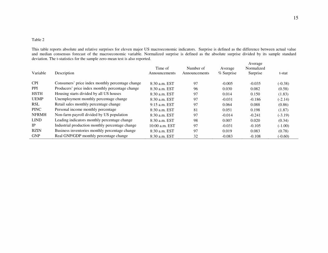
We first test for the unbiasedness of the forecasts. Table 2 reports the mean

forecast surprise and the corresponding zero-mean t-statistics. Except for housing starts

and non-farm payroll, for all other macro announcements we cannot reject the hypothesis

that mean announcement surprise is zero. Since our results in this respect resemble those

of Flannery and Protopapadakis (2002), we proceed with our analysis using the

aforementioned measures of announcement surprises.

9

4. Results

Table 4 reports the results of estimating model (1) using normalized surprise with

two different measures of international stock returns, the contemporaneous and the one-

day ahead returns.

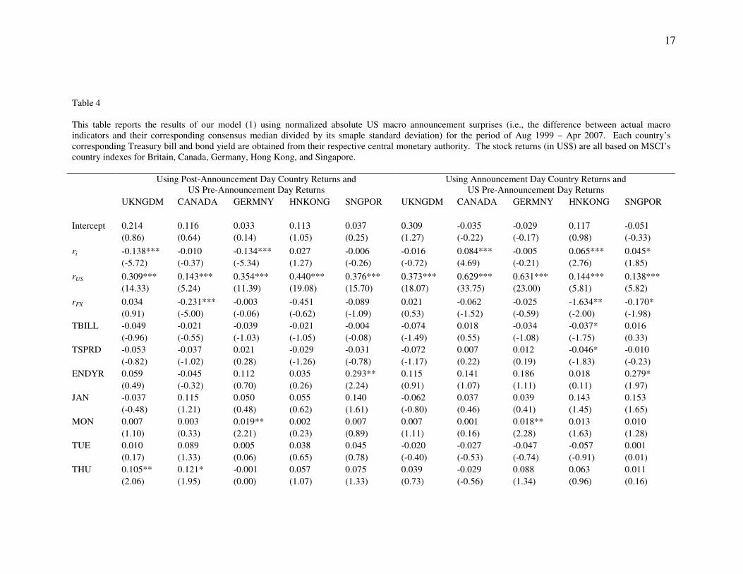
The results provide evidence supporting the basic premise of the paper that various

U.S. macro surprises affect both the returns and the conditional volatility of stock returns

in major developed economies. These effects vary across countries. Among all the macro

indicators, however, industrial production is the only one that affects stock returns in all

countries significantly positively post announcement. The coefficients on industrial

production surprise are of the order of magnitude of 0.40. Thus, for every percentage

positive surprise in the U.S. productivity, the developed economies’ stock markets

subsequently rise by almost 40 basis points. We find that the stock returns in Asian

countries are significantly affected by retail sales. Results also indicate that Canadian

stock market returns react negatively to the U.S. CPI positive surprises. Finally, we find

that Britain’s stock market returns are affected adversely by expected increases in U.S.

non-farm payroll.

The impact of U.S. macro surprises on developed economies’ stock return volatilities

are much more disperse and heterogeneous. There are no macro indicators that affect all

countries consistently. Positive productivity surprises lead to greater volatility in Britain,

Germany, and Singapore. Unexpected rises in the U.S. inflation, as measured by CPI and

PPI surprises, increases return volatilities in Canada, Germany, and Singapore. Positive

surprises in the U.S. personal income, leading indicators, gross domestic product, and

housing starts affect volatility of other developed markets negatively. However, these

10

effects vary across countries. While an unexpected rise in leading indicators decreases

stock volatilities in Canada, Germany and Hong Kong, a positive surprise in personal

income only decreases stock market volatility in Canada and Germany only. Unexpected

rises in the U.S. gross domestic products leads to lower volatility only in Canada and

Hong Kong.

Our results also indicate that U.S. market returns have significant positive impact on

both contemporaneous and one-day ahead country returns. The results provide evidence

supporting the premise that the flow of information from U.S. market affects returns in

other developed stock markets. Considering both the contemporaneous and one-day

ahead impacts, it appears that the U.S. stock market movements influence stock market

returns in Germany, Canada, Britain, Hong Kong and Singapore in a decreasing order of

magnitude respectively.

Table 4 also shows that when the U.S. market movements are controlled for, the

country contemporaneous and one-day ahead returns have little or no autocorrelation.

The estimated conditional volatility equations, however, indicate that all country return

volatilities have strong moving average properties.

5. Conclusion

We ask the question as to whether the U.S. macro economic surprises affect stock

returns in developed economies. We use a GARCH model of stock market returns and

their volatilities in five major markets—Britain, Canada, Germany, Hong Kong, and

Singapore—to investigate the impacts of announcement surprises of eleven U.S. macro

indicators. Our results show that indeed the U.S. macro announcement surprises affect

11

both the stock markets returns and their volatilities in these major developed economies.

While not the focus of our study, our results indicate that factors such as degree of cross

listing, magnitude of investors’ home bias, and various dimensions of economic and

capital market integration can perhaps explain why macro announcement surprises affect

various markets differently. We feel that future research can indeed shed light on the

reason behind these cross country differences.

12

Reference Andersen T.G. and T. Bollerslev (1997) “Intraday periodicity and volatility persistence in financial markets,” Journal of Empirical Finance, Vol. 4, No. 2, pp. 115-158(44) Bodie, Z. (1976) “Common stocks as a hedge against inflation,” The Journal of Finance Vol. 31, No. 2, pp. 459–470. Cross, F. (1973) “The behavior of stock prices on Fridays and Mondays,” Financial Analysts Journal, Vol. 29, No. 6, pp. 67-69. Dichev, I.D. (1998) “Is the risk of bankruptcy a systematic risk?” The Journal of Finance, Vol. 53, No. 3, pp. 1131-1147. Fama, E.F. (1981) “Stock returns, real activity, inflation and money,” American Economic Review, Vol. 71, No. 4, pp. 545–565. Fama, E.F., (1990) Stock returns, expected returns, and real activity, The Journal of Finance, Vol. 45, No. 4. (Sep., 1990), pp. 1089-1108. Fama, E. F. and K.R. French (1995), “Size and book-to-market factors in earnings and returns,” The Journal of Finance, Vol. 50, No. 1, pp. 131-155. Flannery, M.J. and A.A. Protopapadakis (1988) “From t-bills to common stocks: investigating the generality of intra-week return seasonality,” The Journal of Finance, Vol. 43, No. 2, pp. 431-450. Flannery, M.J. and A.A. Protopapadakis (2002) “Macroeconomic factors do influence aggregate stock returns,” The Review of Financial Studies, Vol. 15, No. 3, pp. 751-782. French, K. and R. Roll (1986) “Stock return variances: the arrival of information and the reaction of traders,” Journal of Financial Economics, Vol. 17, No. 1, pp. 5-26. Geske, R. and R. Roll (1983) “The fiscal and monetary linkage between stock returns and inflation,” The Journal of Finance, Vol. 38, No. 1, pp. 1-33. Gibbons, M.R. and P. Hess (1981) “Day of the week effects and asset returns,” The Journal of Business, Vol. 54, No. 4, pp. 579-596. Griffin, J.M and M.L. Lemmon (2002) “Book-to-market equity, distress risk, and stock returns,” The Journal of Finance, Vol. 57, No. 5, pp. 2317-2336 Jegadeesh, N. and S. Titman (1993) “Returns to buying winners and selling losers: implications for stock market efficiency,” The Journal of Finance, Vol. 48, No. 1, pp. 65-91.

13

Jones, C. M., O. Lamont, and R. L. Lumsdaine (1998) “Macroeconomic news and bond market volatility,” Journal of Financial Economics, Vol. 47, No. 3, 315-337. Pearce, D.K. and V.V. Roley (1983) “The reaction of stock prices to unanticipated changes in money: a note,” The Journal of Finance, Vol. 38, No. 4, pp. 1323-1333. Pearce, D.K. and V.V. Roley (1985) “Stock prices and economic news,” The Journal of Business, Vol. 58, No. 1, pp. 49-67. Schwert, G. W., (1990) “Stock returns and real activity: A century of evidence”, The Journal of Finance, Vol. 45, No. 4, pp. 1237-1257.

14

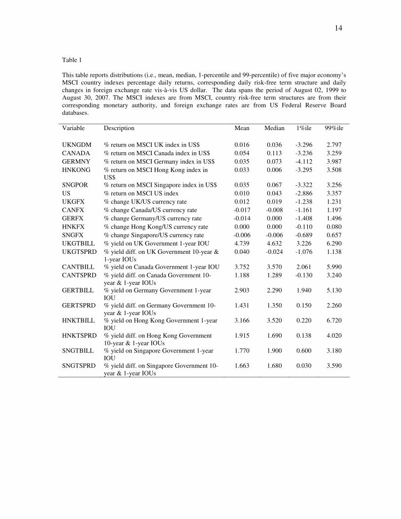
Table 1 This table reports distributions (i.e., mean, median, 1-percentile and 99-percentile) of five major economy’s MSCI country indexes percentage daily returns, corresponding daily risk-free term structure and daily changes in foreign exchange rate vis-à-vis US dollar. The data spans the period of August 02, 1999 to August 30, 2007. The MSCI indexes are from MSCI, country risk-free term structures are from their corresponding monetary authority, and foreign exchange rates are from US Federal Reserve Board databases. Variable Description Mean Median 1%ile 99%ile UKNGDM % return on MSCI UK index in US$ 0.016 0.036 -3.296 2.797 CANADA % return on MSCI Canada index in US$ 0.054 0.113 -3.236 3.259 GERMNY % return on MSCI Germany index in US$ 0.035 0.073 -4.112 3.987 HNKONG % return on MSCI Hong Kong index in

US$ 0.033 0.006 -3.295 3.508

SNGPOR % return on MSCI Singapore index in US$ 0.035 0.067 -3.322 3.256 US % return on MSCI US index 0.010 0.043 -2.886 3.357 UKGFX % change UK/US currency rate 0.012 0.019 -1.238 1.231 CANFX % change Canada/US currency rate -0.017 -0.008 -1.161 1.197 GERFX % change Germany/US currency rate -0.014 0.000 -1.408 1.496 HNKFX % change Hong Kong/US currency rate 0.000 0.000 -0.110 0.080 SNGFX % change Singapore/US currency rate -0.006 -0.006 -0.689 0.657 UKGTBILL % yield on UK Government 1-year IOU 4.739 4.632 3.226 6.290 UKGTSPRD % yield diff. on UK Government 10-year &

1-year IOUs 0.040 -0.024 -1.076 1.138

CANTBILL % yield on Canada Government 1-year IOU 3.752 3.570 2.061 5.990 CANTSPRD % yield diff. on Canada Government 10-

year & 1-year IOUs 1.188 1.289 -0.130 3.240

GERTBILL % yield on Germany Government 1-year IOU

2.903 2.290 1.940 5.130

GERTSPRD % yield diff. on Germany Government 10-year & 1-year IOUs

1.431 1.350 0.150 2.260

HNKTBILL % yield on Hong Kong Government 1-year IOU

3.166 3.520 0.220 6.720

HNKTSPRD % yield diff. on Hong Kong Government 10-year & 1-year IOUs

1.915 1.690 0.138 4.020

SNGTBILL % yield on Singapore Government 1-year IOU

1.770 1.900 0.600 3.180

SNGTSPRD % yield diff. on Singapore Government 10-year & 1-year IOUs

1.663 1.680 0.030 3.590

15

Table 2 This table reports absolute and relative surprises for eleven major US macroeconomic indicators. Surprise is defined as the difference between actual value and median consensus forecast of the macroeconomic variable. Normalized surprise is defined as the absolute surprise divided by its sample standard deviation. The t-statistics for the sample zero-mean test is also reported.

Variable Description Time of

Announcements Number of

Announcements Average

% Surprise

Average Normalized

Surprise t-stat CPI Consumers’ price index monthly percentage change 8:30 a.m. EST 97 -0.005 -0.035 (-0.38) PPI Producers’ price index monthly percentage change 8:30 a.m. EST 96 0.030 0.082 (0.58) HSTH Housing starts divided by all US houses 8:30 a.m. EST 97 0.014 0.150 (1.83) UEMP Unemployment monthly percentage change 8:30 a.m. EST 97 -0.031 -0.186 (-2.14) RSL Retail sales monthly percentage change 9:15 a.m. EST 97 0.064 0.088 (0.86) PINC Personal income monthly percentage 8:30 a.m. EST 81 0.051 0.198 (1.87) NFRMH Non-farm payroll divided by US population 8:30 a.m. EST 97 -0.014 -0.241 (-3.19) LIND Leading indicators monthly percentage change 8:30 a.m. EST 98 0.007 0.020 (0.34) IP Industrial production monthly percentage change 10:00 a.m. EST 97 -0.031 -0.105 (-1.00) BZIN Business inventories monthly percentage change 8:30 a.m. EST 97 0.019 0.083 (0.78) GNP Real GNP/GDP monthly percentage change 8:30 a.m. EST 32 -0.083 -0.108 (-0.60)

16

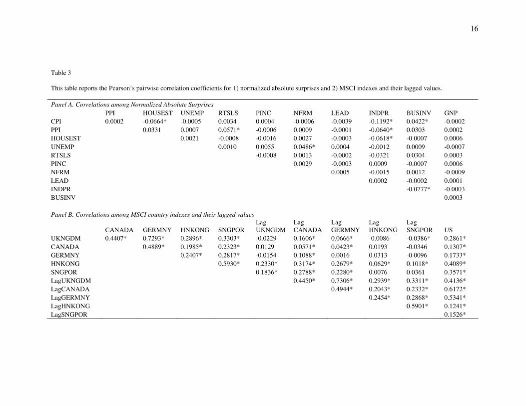
Table 3 This table reports the Pearson’s pairwise correlation coefficients for 1) normalized absolute surprises and 2) MSCI indexes and their lagged values. Panel A. Correlations among Normalized Absolute Surprises PPI HOUSEST UNEMP RTSLS PINC NFRM LEAD INDPR BUSINV GNP CPI 0.0002 -0.0664* -0.0005 0.0034 0.0004 -0.0006 -0.0039 -0.1192* 0.0422* -0.0002 PPI 0.0331 0.0007 0.0571* -0.0006 0.0009 -0.0001 -0.0640* 0.0303 0.0002 HOUSEST 0.0021 -0.0008 -0.0016 0.0027 -0.0003 -0.0618* -0.0007 0.0006 UNEMP 0.0010 0.0055 0.0486* 0.0004 -0.0012 0.0009 -0.0007 RTSLS -0.0008 0.0013 -0.0002 -0.0321 0.0304 0.0003 PINC 0.0029 -0.0003 0.0009 -0.0007 0.0006 NFRM 0.0005 -0.0015 0.0012 -0.0009 LEAD 0.0002 -0.0002 0.0001 INDPR -0.0777* -0.0003 BUSINV 0.0003 Panel B. Correlations among MSCI country indexes and their lagged values

CANADA GERMNY HNKONG SNGPOR Lag UKNGDM

Lag CANADA

Lag GERMNY

Lag HNKONG

Lag SNGPOR US

UKNGDM 0.4407* 0.7293* 0.2896* 0.3303* -0.0229 0.1606* 0.0666* -0.0086 -0.0386* 0.2861* CANADA 0.4889* 0.1985* 0.2323* 0.0129 0.0571* 0.0423* 0.0193 -0.0346 0.1307* GERMNY 0.2407* 0.2817* -0.0154 0.1088* 0.0016 0.0313 -0.0096 0.1733* HNKONG 0.5930* 0.2330* 0.3174* 0.2679* 0.0629* 0.1018* 0.4089* SNGPOR 0.1836* 0.2788* 0.2280* 0.0076 0.0361 0.3571* LagUKNGDM 0.4450* 0.7306* 0.2939* 0.3311* 0.4136* LagCANADA 0.4944* 0.2043* 0.2332* 0.6172* LagGERMNY 0.2454* 0.2868* 0.5341* LagHNKONG 0.5901* 0.1241* LagSNGPOR 0.1526*

17

Table 4 This table reports the results of our model (1) using normalized absolute US macro announcement surprises (i.e., the difference between actual macro indicators and their corresponding consensus median divided by its smaple standard deviation) for the period of Aug 1999 – Apr 2007. Each country’s corresponding Treasury bill and bond yield are obtained from their respective central monetary authority. The stock returns (in US$) are all based on MSCI’s country indexes for Britain, Canada, Germany, Hong Kong, and Singapore.

Using Post-Announcement Day Country Returns and

US Pre-Announcement Day Returns Using Announcement Day Country Returns and

US Pre-Announcement Day Returns UKNGDM CANADA GERMNY HNKONG SNGPOR UKNGDM CANADA GERMNY HNKONG SNGPOR Intercept 0.214 0.116 0.033 0.113 0.037 0.309 -0.035 -0.029 0.117 -0.051 (0.86) (0.64) (0.14) (1.05) (0.25) (1.27) (-0.22) (-0.17) (0.98) (-0.33) ri -0.138*** -0.010 -0.134*** 0.027 -0.006 -0.016 0.084*** -0.005 0.065*** 0.045* (-5.72) (-0.37) (-5.34) (1.27) (-0.26) (-0.72) (4.69) (-0.21) (2.76) (1.85) rUS 0.309*** 0.143*** 0.354*** 0.440*** 0.376*** 0.373*** 0.629*** 0.631*** 0.144*** 0.138*** (14.33) (5.24) (11.39) (19.08) (15.70) (18.07) (33.75) (23.00) (5.81) (5.82) rFX 0.034 -0.231*** -0.003 -0.451 -0.089 0.021 -0.062 -0.025 -1.634** -0.170* (0.91) (-5.00) (-0.06) (-0.62) (-1.09) (0.53) (-1.52) (-0.59) (-2.00) (-1.98) TBILL -0.049 -0.021 -0.039 -0.021 -0.004 -0.074 0.018 -0.034 -0.037* 0.016 (-0.96) (-0.55) (-1.03) (-1.05) (-0.08) (-1.49) (0.55) (-1.08) (-1.75) (0.33) TSPRD -0.053 -0.037 0.021 -0.029 -0.031 -0.072 0.007 0.012 -0.046* -0.010 (-0.82) (-1.02) (0.28) (-1.26) (-0.78) (-1.17) (0.22) (0.19) (-1.83) (-0.23) ENDYR 0.059 -0.045 0.112 0.035 0.293** 0.115 0.141 0.186 0.018 0.279* (0.49) (-0.32) (0.70) (0.26) (2.24) (0.91) (1.07) (1.11) (0.11) (1.97) JAN -0.037 0.115 0.050 0.055 0.140 -0.062 0.037 0.039 0.143 0.153 (-0.48) (1.21) (0.48) (0.62) (1.61) (-0.80) (0.46) (0.41) (1.45) (1.65) MON 0.007 0.003 0.019** 0.002 0.007 0.007 0.001 0.018** 0.013 0.010 (1.10) (0.33) (2.21) (0.23) (0.89) (1.11) (0.16) (2.28) (1.63) (1.28) TUE 0.010 0.089 0.005 0.038 0.045 -0.020 -0.027 -0.047 -0.057 0.001 (0.17) (1.33) (0.06) (0.65) (0.78) (-0.40) (-0.53) (-0.74) (-0.91) (0.01) THU 0.105** 0.121* -0.001 0.057 0.075 0.039 -0.029 0.088 0.063 0.011 (2.06) (1.95) (0.00) (1.07) (1.33) (0.73) (-0.56) (1.34) (0.96) (0.16)

18

FRI 0.022 0.136*** 0.034 0.070 0.049 0.154*** 0.124*** 0.090 0.072 0.101 (0.44) (2.38) (0.48) (1.18) (0.79) (3.06) (2.43) (1.42) (1.14) (1.62) CPI 0.130 0.081 0.133 0.005 0.073 -0.061 -0.027 -0.048 -0.100 -0.060 (1.54) (0.58) (0.98) (0.04) (0.61) (-0.57) (-0.26) (-0.38) (-0.87) (-0.50) PPI 0.025 0.055 0.039 -0.037 -0.046 0.038 -0.037 0.087 -0.087 -0.026 (0.37) (0.79) (0.42) (-0.52) (-0.62) (0.71) (-0.51) (1.23) (-1.32) (-0.39) HSTRT 0.024 0.110 0.057 -0.085 -0.126 0.004 0.041 0.050 -0.176 -0.149 (0.24) (0.94) (0.41) (-0.78) (-1.07) (0.03) (0.42) (0.37) (-1.57) (-1.14) UNEMP -0.075 0.051 -0.177 -0.162 -0.021 0.212* 0.045 0.135 -0.103 0.169 (-0.66) (0.50) (-1.08) (-1.27) (-0.14) (1.90) (0.51) (1.01) (-0.91) (1.41) RTLSLS -0.073 -0.111 0.063 0.034 0.205* -0.141 0.001 0.082 0.324*** 0.261** (-0.79) (-1.16) (0.53) (0.30) (1.94) (-1.49) (0.00) (0.70) (2.69) (2.04) PINC 0.025 0.007 -0.008 0.088 0.023 0.095 -0.043 0.067 0.199 0.146 (0.25) (0.06) (-0.07) (0.82) (0.18) (0.94) (-0.47) (0.53) (1.62) (1.18) NFRM -0.044 0.221** 0.194 -0.191 -0.033 -0.303*** -0.089 -0.104 0.078 0.087 (-0.39) (2.10) (1.22) (-1.38) (-0.21) (-2.85) (-0.77) (-0.77) (0.61) (0.69) LEAD -0.129 -0.257* -0.109 0.079 -0.212 -0.039 0.039 0.070 -0.186 0.247 (-1.03) (-1.69) (-0.56) (0.53) (-1.41) (-0.27) (0.24) (0.38) (-1.08) (1.31) INDPR 0.244*** 0.184* 0.162 0.172* 0.281*** -0.082 0.026 -0.118 -0.143 -0.141 (3.12) (1.74) (1.40) (1.79) (2.46) (-0.91) (0.28) (-1.08) (-1.42) (-1.46) BUSINV 0.007 0.094 0.125 -0.026 -0.119 0.030 0.031 -0.007 0.018 -0.030 (0.08) (0.98) (1.17) (-0.24) (-1.26) (0.34) (0.36) (-0.06) (0.16) (-0.27) GNP 0.066 0.070 -0.080 0.173 0.298* -0.036 -0.328** -0.167 -0.297 -0.149 (0.41) (0.48) (-0.41) (1.17) (1.77) (-0.27) (-2.34) (-0.87) (-1.63) (-0.89) h0 0.029* 0.036*** 0.032*** 0.021*** 0.039*** 0.209 0.125 0.066 -0.131 0.073 (1.67) (3.54) (3.70) (4.76) (3.82) (1.32) (0.79) (0.39) (-0.75) (0.43) �1 0.077 0.024*** 0.047*** 0.026*** 0.079*** -0.210 0.570*** -0.043 -0.181 -0.203 (1.66) (2.91) (3.31) (3.48) (4.33) (-1.24) (3.17) (-0.24) (-1.06) (-1.20) �1 0.795*** 0.833*** 0.847*** 0.884*** 0.855*** 0.029 -0.234 0.212 -0.115 0.385** (28.67) (27.87) (40.22) (53.77) (50.71) (0.18) (-1.41) (1.28) (-0.67) (2.32) TBILL 0.173 0.307*** 0.239*** 0.182*** 0.090 2.104* -1.730* 1.766** -0.707 -0.497 (1.49) (5.78) (4.46) (6.03) (1.52) (1.89) (-1.81) (2.21) (-0.94) (-0.75) TSPRD 0.255* 0.153*** 0.175* 0.278*** 0.152*** 0.156 -0.307* -0.018 0.067 0.079

19

(1.68) (2.78) (1.74) (6.17) (2.87) (0.97) (-1.87) (-0.10) (0.41) (0.47) MON -0.017* -0.022** -0.021** -0.020** -0.024*** 0.282* -0.205 0.326* 0.002 0.049 (-1.70) (-2.21) (-2.10) (-2.08) (-2.44) (1.71) (-1.24) (1.96) (0.01) (0.29) TUE 0.015 0.180** 0.158* -0.015 -0.019 -2.058* 1.897** -1.932*** 0.333 0.357 (0.16) (2.01) (1.71) (-0.16) (-0.20) (-1.85) (1.99) (-2.43) (0.45) (0.54) THU -0.023 -0.008 0.063 -0.281*** -0.095 -0.166 0.411*** -0.035 -0.087 0.179 (-0.25) (-0.09) (0.69) (-3.10) (-1.05) (-1.13) (2.71) (-0.24) (-0.58) (1.20) FRI 0.006 -0.043 0.087 0.105 0.248** 0.318* 0.319* 0.213 0.183 0.222 (0.05) (-0.41) (0.81) (0.99) (2.34) (1.83) (1.77) (1.21) (1.01) (1.30) PRE -0.981*** -1.104*** -0.575*** -0.739*** -0.812*** 0.068 -0.004 -0.040 0.054 0.225 (-4.82) (-5.45) (-2.87) (-3.68) (-4.06) (0.41) (-0.02) (-0.24) (0.33) (1.37) POST 0.299 0.175 0.072 0.289 -0.174 -0.043 -0.137 0.031 -0.186 -0.066 (1.55) (0.90) (0.37) (1.48) (-0.90) (-0.16) (-0.51) (0.12) (-0.71) (-0.25) CPI -0.165 0.335* 0.319* 0.318* 0.235 -0.032*** -0.021** -0.020** -0.020** -0.027*** (-0.96) (1.82) (1.80) (1.78) (1.24) (-3.19) (-2.14) (-2.02) (-2.04) (-2.73) PPI 0.386** -0.031 0.383** 0.146 0.149 -0.111 -0.062 -0.211** -0.267*** -0.362*** (2.34) (-0.19) (2.26) (0.87) (0.92) (-1.22) (-0.69) (-2.32) (-2.86) (-3.97) HSTRT -0.020 -0.182 0.089 0.029 0.065 0.082 -0.129 -0.010 -0.065 -0.213** (-0.12) (-1.08) (0.52) (0.17) (0.37) (0.90) (-1.44) (-0.11) (-0.73) (-2.33) UNEMP -0.469 0.358 -0.096 0.569 -1.093 -0.174 -0.241** -0.203* -0.175 -0.212** (-0.72) (0.44) (-0.15) (1.16) (-1.48) (-1.66) (-2.25) (-1.93) (-1.64) (-2.01) RTLSLS -0.039 -0.027 -0.230 -0.110 0.084 0.091 0.310 -0.094 -0.229 -0.422** (-0.24) (-0.15) (-1.39) (-0.64) (0.50) (0.47) (1.44) (-0.47) (-1.16) (-2.17) PINC -0.215 -0.261 -0.374** 0.143 0.237 0.087 -0.399** -0.029 0.092 -0.030 (-1.29) (-1.57) (-2.26) (0.86) (1.42) (0.44) (-2.06) (-0.15) (0.46) (-0.15) NFRM 0.222 -0.877 0.069 -0.633 1.234* 0.163* 0.211*** 0.218*** 0.245*** 0.112* (0.34) (-1.09) (0.11) (-1.30) (1.67) (1.80) (4.06) (4.50) (8.21) (1.86) LEAD -0.490*** -0.393*** -0.143 -0.032 -0.246 0.237* 0.077 0.177** 0.346*** 0.137*** (-3.29) (-2.60) (-0.91) (-0.21) (-1.65) (1.94) (1.33) (2.00) (8.11) (2.52) INDPR -0.036 0.134 0.071 0.096 0.502*** 0.027** 0.033*** 0.045*** 0.035*** 0.051*** (-0.20) (0.73) (0.39) (0.52) (2.74) (2.20) (2.81) (3.55) (4.33) (3.68) BUSINV -0.082 -0.112 -0.182 0.185 -0.259 0.067** 0.036*** 0.053*** 0.021*** 0.105*** (-0.50) (-0.64) (-1.08) (1.08) (-1.52) (2.20) (2.65) (3.22) (3.50) (4.02)

20

GNP 0.163 -0.605** -0.243 -0.382 -0.114 0.835*** 0.848*** 0.832*** 0.846*** 0.847*** (0.63) (-2.31) (-0.92) (-1.46) (-0.44) (40.28) (24.56) (34.06) (31.71) (47.41) Adj R2 0.086 0.014 0.019 0.145 0.114 0.156 0.374 0.270 0.012 0.007 F-statistic 14.20 2.06 2.87 25.63 19.44 27.92 90.07 55.71 1.78 1.11

Institute for International Integration StudiesThe Sutherland Centre, Trinity College Dublin, Dublin 2, Ireland