Impacts of urban sprawl on species richness of plants, butterflies, gastropods and birds: not only built-up area matters

1

Urban Ecosystems

DOI: 10.1007/s11252-015-0474-4

Impacts of urban sprawl on species richness of plants, butterflies, gastropods and birds:

not only built-up area matters

Elena D. Concepción1,*, Martin K. Obrist1, Marco Moretti1, Florian Altermatt2,3, Bruno Baur4,

Michael P. Nobis1

1WSL Swiss Federal Institute for Forest, Snow and Landscape Research, Zürcherstrasse 111,

CH-8903 Birmensdorf, Switzerland, [email protected], [email protected],

[email protected], [email protected]

2Eawag: Swiss Federal Institute of Aquatic Science and Technology, Überlandstrasse

133,CH-8600 Dübendorf, Switzerland, [email protected]

3Institute of Evolutionary Biology and Environmental Studies, University of Zurich

Winterthurerstrasse 190, CH-8057 Zürich, Switzerland.

4Section of Conservation Biology, Department of Environmental Sciences, University of

Basel, St. Johanns-Vorstadt 10, CH-4056 Basel, Switzerland, [email protected]

*Corresponding author:

Phone: +34 666 75 52 30. E-mail address: [email protected] (E.D. Concepción).

mailto:[email protected]







2

Abstract

Urban growth is a major factor of global environmental change and has important impacts on

biodiversity, such as changes in species composition and biotic homogenization. Most

previous studies have focused on effects of urban area as a general measure of urbanization,

and on few or single taxa. Here, we analyzed the impacts of the different components of urban

sprawl (i.e., scattered and widespread urban growth) on species richness of a variety of

taxonomic groups covering mosses, vascular plants, gastropods, butterflies, and birds at the

habitat and landscape scales. Besides urban area, we considered the average age,

imperviousness, and dispersion degree of urban area, along with human population density, to

disentangle the effects of the different components of urban sprawl on biodiversity. The study

was carried out in the Swiss Plateau that has undergone substantial urban sprawl in recent

decades.

Vascular plants and birds showed the strongest responses to urban sprawl, especially at the

landscape scale, with non-native and ruderal plants proliferating and common generalist birds

increasing at the expense of specialist birds as urban sprawl grew. Overall, urban area had the

greatest contribution on such impacts, but additional effects of urban dispersion (i.e., increase

of non-native plants) and human population density (i.e., increases of ruderal plants and

common generalist birds) were found. Our findings support the hypothesis that negative

impacts of urban sprawl on biodiversity can be reduced by compacting urban growth while

still avoiding the formation of very densely populated areas.

Key words:

Built-up area; biotic homogenization; imperviousness; human population density; time-lagged

effects; urban dispersion.

3

Introduction

Land-use change is a central component of global change and a major threat to biodiversity

(Sala et al. 2000). Urban growth is in turn an important driver of such land-use changes

(Grimm et al. 2008; Elmqvist et al. 2013). The growth of urban areas worldwide was

especially pronounced during the second half of the 20th century, but rapid urban expansion

still continues and is expected to persist in the next decades as the world’s population grows

and more people live in cities (Grimm et al. 2008; Mcdonald et al. 2008; Elmqvist et al.

2013).

Species richness has frequently been found to peak at moderate levels of urban development

(Rebele 1994; Blair 1999; Niemelä 1999; Crooks et al. 2004). However, not all organisms are

equally affected, and the impact of urban growth may noticeably vary depending on species

characteristics, such as dispersal ability, habitat specialization, or use of resources (Wood and

Pullin 2002; Devictor et al. 2007). The peak in species richness at moderate urbanization

levels usually results from an increase in common species adaptable to urban environments,

such as early successional plants (Deutschewitz et al. 2003) or generalist animals that take

advantage of high habitat heterogeneity and resource availability, as well as low competition

or predation rates in urban areas (Savard et al. 2000; Crooks et al. 2004; McKinney 2008). At

the same time, some species from the original communities that are sensitive to urban

conditions may still survive in the remaining natural or semi-natural habitats, adding to the

overall species richness (McKinney 2002, 2006, 2008).

Advanced stages of urbanization, however, usually cause a loss of native specialists in favor

of a few urban exploiters, such as ruderal and non-native plants, which tolerate high levels of

disturbance (Deutschewitz et al. 2003; Kühn and Klotz 2006; Nobis et al. 2009), or

synanthropic animals that depend on human-subsidized resources (Crooks et al. 2004;

Devictor et al. 2007). As a result, at high levels of urbanization species richness generally

4

decreases and urban biotas tend to become more and more similar – also called biotic

homogenization – dominated by a few common native species and some ubiquitous non-

native species (McKinney 2002, 2006; Clergeau et al. 2006; Lososová et al. 2012a, b; Le Viol

et al. 2012; Aronson et al. 2014; La Sorte et al. 2014).

The spatial scale at which effects of urbanization on biodiversity are analyzed has also been

found to be relevant, with impacts like biotic homogenization being more evident at larger

spatial scales, both in terms of the extent of the study area and in terms of grain size

(Deutschewitz et al. 2003; Kühn and Klotz 2006; La Sorte et al. 2014). However, studies have

traditionally focused on particular urban areas, and although some of them have compared

urban impacts in different cities across regions, countries, or even continents (see e.g. Pyšek

1993; Pyšek 1998; Aronson et al. 2014; La Sorte et al. 2014), large-scale analyses along broad

urbanization gradients are still scarce (Devictor et al. 2007; Lososová et al.2012a, b; Le Viol

et al. 2012).

Most previous studies analyzing urban impacts on biodiversity focused on responses of

organisms along urbanization gradients that typically consider increasing proportion of urban

area or other urban parameters, such as the degree of imperviousness (i.e., soil sealing) or

human population density (see McDonnell and Hahs 2008 for a review). However, most

studies lacked reliable measures of other components of the so-called urban sprawl (i.e.,

scattered and widespread urban growth; Jaeger et al. 2010). Specifically, the degree of urban

sprawl can be estimated with a combined measure of total urban area, intensity of urban land

use (e.g., population density), and degree of urban dispersion (Jaeger and Schwick 2014).

Besides built-up area (hereinafter referred to as ‘urban area’) and other characteristics of

urban environments, the spatial configuration of urban area, as well as natural or semi-natural

areas at the landscape level, may also affect biodiversity (Marzluff and Ewing 2001; Croci et

al. 2008; Sattler et al. 2010; Fontana et al. 2011; Latta et al. 2013). Furthermore, time lags

5

may occur before impacts of urban sprawl on biodiversity are apparent (Ramalho and Hobbs

2012). However, such delayed effects of urban development have rarely been explored (but

see Soga and Koike 2013).

Here, we present a comprehensive analysis of the effects of different components of urban

sprawl on species richness of various species groups in the Swiss Plateau, which represents

the largest biogeographic region of Switzerland (ca. 11,200 km2) and is affected by severe

past and current urban sprawl (Schwick et al. 2012). Overall, we aimed to contribute to a

better understanding of the impacts driven by the distinct urban sprawl components on species

richness and to generate guidelines for biodiversity monitoring and conservation under future

urban development. We addressed the following specific questions: (1) Which types of

organisms benefit and which suffer most under urban sprawl? (2) Which attributes or

components of urban sprawl have the strongest impacts on species richness? And lastly, (3) at

which spatial scales are effects of urban sprawl on biodiversity more evident?

We considered five taxonomic groups (i.e., birds, butterflies, terrestrial gastropods, vascular

plants, and mosses) that were covered in Swiss biodiversity monitoring programs at varying

spatial scales from 10 m2 (habitat level) to 1 km2 (landscape level). We evaluated effects of

urban sprawl on the species richness of each taxonomic group and of distinct ecological

groups defined according to species characteristics that were expected to be sensitive to urban

development (e.g., habitat and resource specialization, commonness, dispersal ability). We

investigated urban effects along with other environmental variables (climate, topography, and

land use) that are known to affect biodiversity. In addition, we used a wide set of urban

predictors to disentangle relationships between different components of urban sprawl and

species richness. Besides urban area, which was expected to strongly affect species richness,

we analyzed the impact of additional urban attributes of likely influence, such as the degree of

imperviousness, human population density, urban dispersion, and average age of urban area.

6

Methods

1) Study area, species richness, and ecological groups

Our study focused on the Swiss Plateau (Fig. 1), the central part of Switzerland between the

Alps and the Jura Mountains delimited according to the definition of Swiss biogeographic

regions (Gonseth et al. 2001). This region has a mean altitude of 540 m a.s.l. (range: 300–940

m a.s.l.), a mean annual temperature of 8.5 °C (6.5–9.5°C), and a mean annual precipitation of

1140 mm (730–2000 mm). In the Swiss Plateau, agricultural land use predominates (around

50% area), followed by forests (24%) and urban areas (15%). Total urban area has tripled

since the beginning of the 20th century, especially between 1960 and 1980 when an increase

of around 50% occurred, and is still expected to grow in the future, though at lower rates

(Schwick et al. 2012). We analyzed data on species richness of five taxonomic groups

(mosses, vascular plants, terrestrial gastropods, butterflies, and birds) regularly collected

using a systematic sampling design in the biodiversity monitoring programs of Switzerland

(BDM – Biodiversity Monitoring in Switzerland Coordination Office 2009) and of the Canton

of Aargau (LANAG; Kanton Aargau 1996). From the BDM program, we used species lists of

all available plots in the Swiss Plateau, that is, 109 plots at the landscape level (each 1 km2 in

area; including vascular plants, butterflies, and birds; BDM Z7 indicator) and 473 circular

plots at the habitat level (each 10 m2 in area; including mosses, vascular plants, and

gastropods; BDM Z9 indicator; Table 1, Fig. 1). From the LANAG program, we analyzed 436

plots at the habitat level located within the Swiss Plateau (10 m2 plots for vascular plants and

gastropods, 100 m radius-plots for birds, and 250 m transects for butterflies). From both

programs, we used data of surveys performed between 2007 and 2011 (see Table A.1 for

further details about sampling designs of the different biodiversity monitoring programs).

7

For each taxonomic group and monitoring program, we calculated overall species richness per

plot as well as species richness of a variety of ecological groups classified according to

species-specific characteristics that we expected to influence species’ responses to urban

sprawl. Species characteristics were morphological, physiological, or phenological features

(functional traits sensu Violle et al. 2007), such as dispersal ability, growth form, and resource

use (e.g., diet, habitat use and specialization). Species were additionally classified according

to their commonness or rarity (calculated as frequency of occurrence in the dataset), and in

the case of vascular plants as native and non-native species. We further classified non-native

vascular plant species according to time of introduction (archeophytes and neophytes, i.e.,

species introduced in Switzerland by humans before or after 1500 A.D.). Resource range and

habitat requirements were used to classify species as specialists or generalists (for a detailed

description of species characteristics and classification see Table A.2). To explicitly test for a

qualitative shift in species composition along the urbanization gradient, we calculated ratios

of generalist to specialist species, very common to rare species, and native to non-native plant

species. Threatened species according to Swiss Red Lists were also considered.

2) Urban sprawl data

To describe urban sprawl, we calculated a set of explanatory variables at the different plot

scales of the distinct biodiversity monitoring programs (see Table 1 for details). As urban

variables, we used urban area (defined as built-up area, i.e., houses, industries, roads, and

other infrastructures, but also gardens, parks, and other recreational areas), degree of

imperviousness (i.e., soil-sealing), average age of urban area (considered over a period of 125

years, i.e. 1885–2010), human population density (number of inhabitants per area), and the

spatial dispersion of urban areas. This last variable was quantified using the mean proximity

index of urban areas (MPI, with low MPI values meaning high urban dispersion) for larger

8

plot sizes, or the nearest distance to urban areas in the case of the small plots at the habitat

level. Overall, we investigated urban sprawl impacts along a broad urbanization gradient,

which covers a range from 0% up to 66% of urban area at the landscape scale (see Table 2 for

a detailed description of urban sprawl variables).

We also used other environmental predictors known to affect biodiversity, like climatic,

topographic, and additional land use variables (see e.g. Blair 1999; Wood and Pullin 2002;

Nobis et al. 2009; Lososová et al. 2012a), which were calculated at the same spatial scale as

species richness data to control for possible confounding effects (see Tables 1 and 2 for

details).

3) Data analyses

We followed a hierarchical approach to analyze the relationships between urban sprawl and

species richness. In a first step, we compared the overall importance of all urban versus all

non-urban predictors to explain the variability in species richness for the different taxonomic

and ecological groups. Second, for those groups for which urban predictors explained a

substantial amount of variability, independently from non-urban predictors, we looked at the

effects of individual urban predictors.

For the first step, we performed generalized linear models (GLMs) with species richness of

the different taxonomic and ecological groups as response and a Poisson error distribution for

count data. For the ratios of generalist to specialist species, very common to rare species, and

non-native to native plant species, we applied GLMs with a normal distribution of errors. We

used two sets of predictors: (1) all urban variables and (2) all environmental variables other

than urban ones (Tables 1 and 2). Pearson’s product-moment correlations between single

predictors were all below 0.8. To control for possible bias caused by collinearity, we

compared results of models both excluding and including human population density, the only

9

predictor that showed noticeable correlations with other urban predictors (|r| > 0.7; Dormann

et al. 2013). Linear and quadratic terms of urban predictors were included in models to

account for possible non-linear effects. For every response variable, we then calculated the

percentage of null deviance explained by full models (i.e., including the whole set of urban

and non-urban predictors; D2full), the percentage of null deviance (D2) explained by the two

sets of environmental predictors independently (D2I.Urban and D2

I.Non-urban), as well as their joint

contribution to deviance explanation (D2J).

In a second step, we examined the individual effects of urban predictors on species richness

for those taxonomic and ecological groups that were substantially affected by urban

predictors, independent from non-urban predictors (D2I.Urban ≥ 15%). We selected this

threshold because it coincided with significant effects (p ≤ 0.05) of single urban predictors

included in full models. We used multi-model inference based on model averaging in order to

calculate more robust estimates of the coefficients of urban predictors (Burnham and

Anderson 2002). For each response variable, we performed GLMs with all possible

combinations of predictors (including both urban and other environmental variables) and

ranked them according to the second-order Akaike’s information criterion (AICc), or its

quasi-likelihood counterpart (QAICc) in cases where over-dispersion occurred. We then

selected the most plausible models according to these criteria (delta AICc or QAICc ≤ 4) and

calculated averaged parameter estimates using Akaike’s weights. To assess the relative

contribution of each urban predictor to the overall effects of urban sprawl on species richness,

we calculated the relative variable importance (RVI), that is, the sum of Akaike weights that

measures the overall likelihood of the selected models in which the parameter of interest

appears. RVI values range from 0 (for predictors excluded in all selected models) to 1 (for

predictors included in all selected models; Burnham and Anderson 2002). Finally, we used

partial residual plots of best-fit models (AIC-based) to graphically illustrate and explore the

10

direction of significant relationships between distinct urban predictors and species richness.

Partial residuals plots of models represent relationships between response variables and an

explanatory variable of interest once the effects of all the other predictors have been

accounted for.

All statistical analyses were done in R 3.0.2 (R Core Team 2014), using the package MuMIn

(Bartón 2013) for model averaging. Urban and non-urban predictors were calculated using the

R package raster (Hijmans 2015), as well as ArcGIS and its extension Patch Analyst (ESRI

2011).

Results

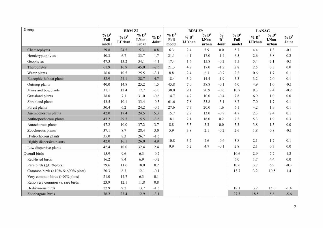
Urban predictors explained together and independently of other environmental predictors a

substantial proportion of the variability (D2I.Urban ≥ 15%) in species richness of distinct

ecological groups of vascular plants and birds. For these groups urban predictors were slightly

more relevant than the other environmental variables (23% D2I.Urban and 20% D2

I.Non-urban on

average; see Table 3 for details). These responses were found almost exclusively at the

landscape level (BDM Z7; with 16 responding groups out of 80), with only a few groups of

bird species being affected also at the habitat level (LANAG; 3 responding groups out of 82).

All these species groups showed significant responses to specific urban predictors (Table 3;

for additional details see Tables A.3 and A.4).

Urban area had on average the highest relative variable importance (RVI), followed by human

population density, degree of urban dispersion (i.e., mean proximity index of urban areas

[MPI] or nearest distance to urban areas), degree of imperviousness, and average age of urban

areas (Table 3, Fig. 2). Models excluding human population density as a predictor to control

for slight collinearity with other predictors (0.8 > |r| > 0.7) showed consistent results for the

11

remaining urban variables, and therefore we only present the models including the complete

set of predictors.

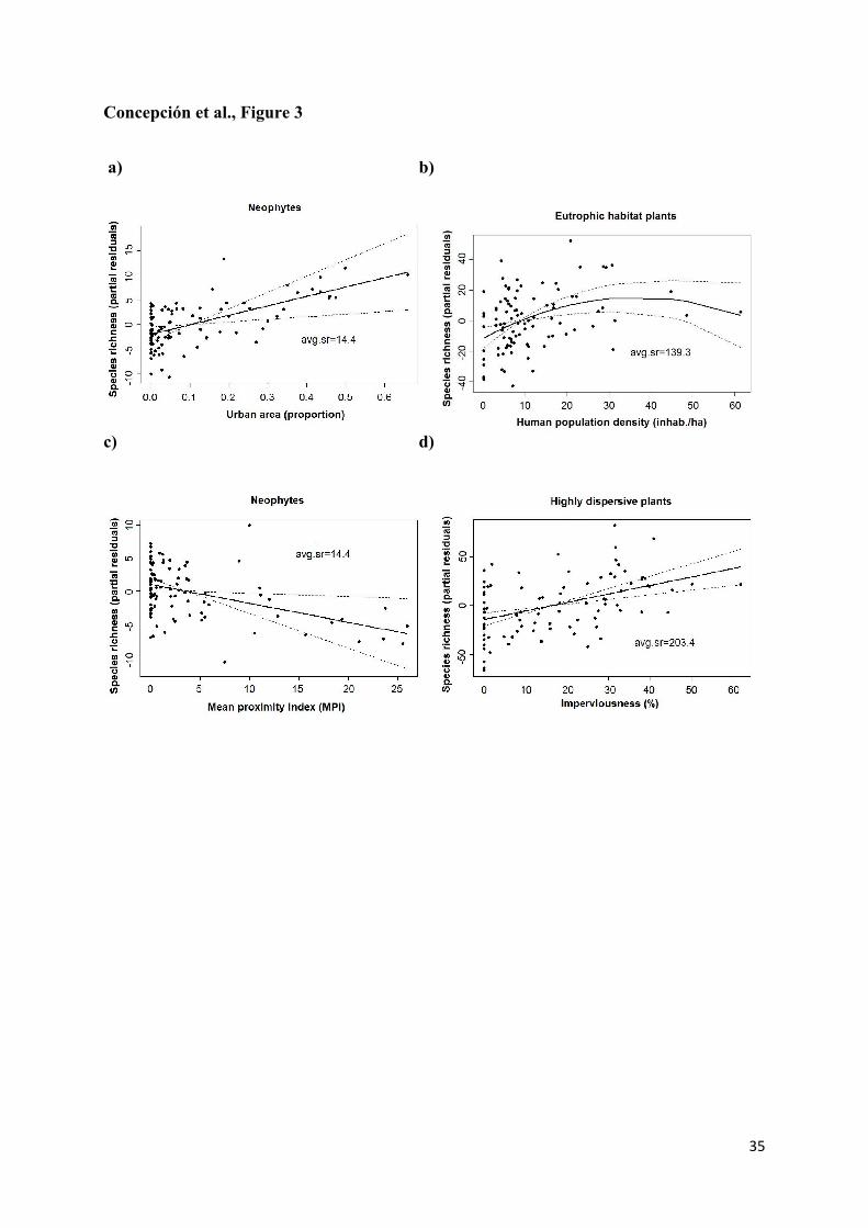
For vascular plants, partial regression plots showed along the gradient of increasing urban

area a considerable increase in species richness of non-natives, in particular neophytes (Table

3, Fig. 3a), specific growth forms (phanerophytes and chamaephytes), and human-dispersed

(anthropochorous) plants. In addition, species richness of plants inhabiting eutrophic habitats

(Fig. 3b), non-native, habitat specialist, and annual (therophytes) plants increased together

with human population density. The degree of urban dispersion had additional positive effects

on the ratio between non-native and native plant species and on the species richness of

neophytes, phanerophytes, and chamaephytes (i.e., negative effects of MPI; Table 3 and Fig.

3c). Last, the degree of imperviousness of urban areas mostly increased species richness of

highly dispersive and wind-dispersed (anemochorous) plants (Table 3 and Fig. 3d).

Among birds, species groups showing responses relevant to urban sprawl variables were

urban, zoophagous, ground breeding, and breeding generalist birds as well as the ratio of

breeding generalist to specialist birds. All these groups showed positive responses to urban

area and human population density, except ground breeding birds whose species richness

significantly decreased with the amount of urban area (see Fig. 4 for examples of the most

relevant effects of these variables on birds). When considered at the habitat level, species

richness of zoophagous and urban birds and the ratio of breeding generalist to specialist birds

significantly decreased as the nearest distance to urban areas increased, whereas the ratio of

breeding generalists to specialists increased with the average age of urban areas (Table 3).

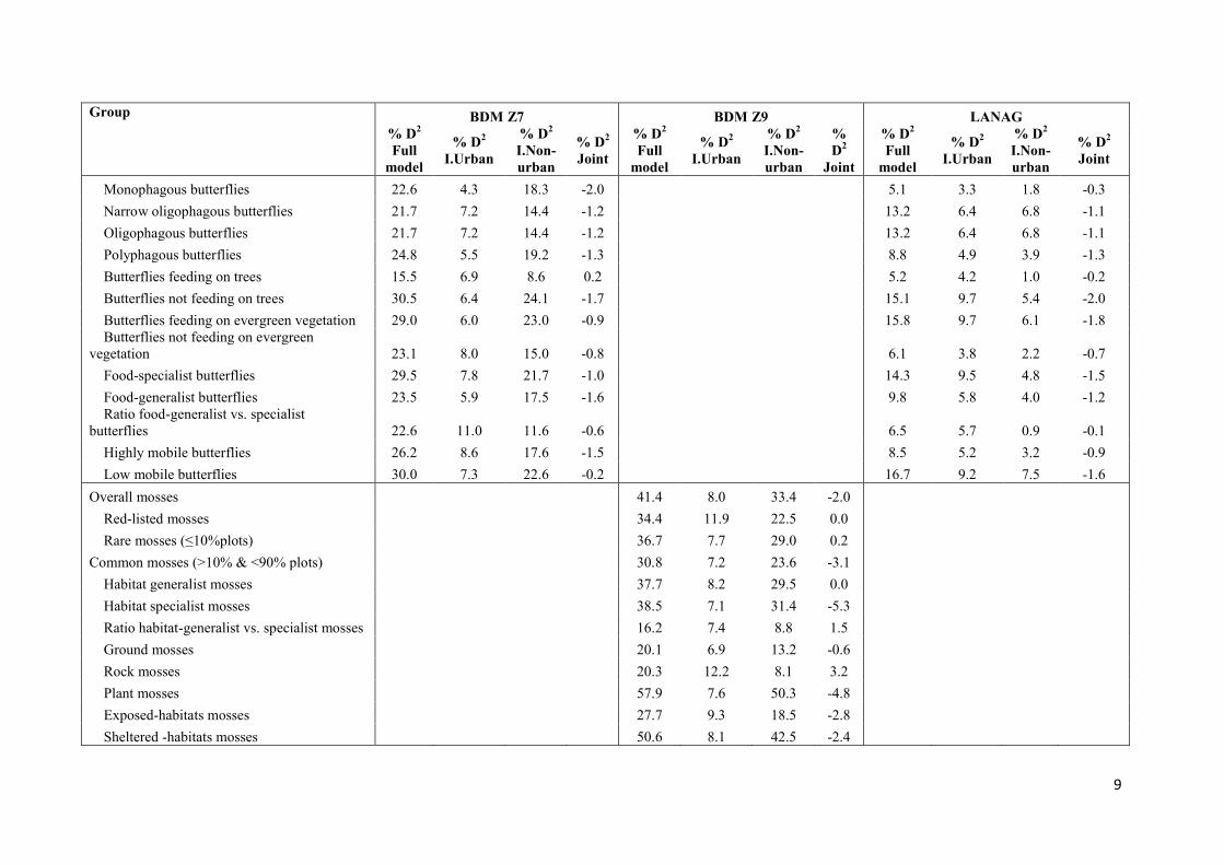
Species richness of all other ecological and taxonomic groups (i.e., mosses, gastropods and

butterflies), including endangered species of the different taxa, showed only weak (D2I.Urban <

15 %) or non-significant responses to urban sprawl variables, and were more strongly affected

12

by non-urban variables (7% D2I.Urban and 15% D2

I.Non-urban on average; see Tables A.3 and A.4

for details).

Discussion

Overall, our study showed important impacts of urban sprawl on species richness of distinct

taxonomic and ecological groups. As we hypothesized, these impacts considerably varied

depending on the species groups, urban sprawl components and spatial scales considered.

1) Taxonomic and ecological groups

Time of introduction, dispersal mode, growth form and habitat specialization were the species

characteristics that mainly affected the responses of plant species richness to urban sprawl.

Non-native species, especially neophytes, benefitted most from urban sprawl, which confirms

results of previous studies for our study area (Kühn and Klotz 2006; Nobis et al. 2009;

Lososová et al. 2012a).

Species richness of plants inhabiting eutrophic places, as well as annual, highly dispersive,

wind- and human dispersed plants, also benefitted from urban sprawl (see e.g. Knapp et al.

2009). These results are in line with previous findings revealing that native common

generalists still predominate in most urban areas (Lososová et al. 2012a, b; Schmidt et al.

2013; Aronson et al. 2014).

Habitat specialist plants also benefitted from intermediate levels of urbanization covered in

our study, probably because of the wide variety of habitats and more extreme environmental

conditions in urban areas (Rebele 1994; Niemelä 1999). According to our definition (Table

A.2), this group of plants consists of species with narrow ranges of habitat preferences, that is,

preferring habitat extremes with respect to temperature, continentality, light, or moisture, pH,

nutrients, humus, or aeration of soils. Valued species like native specialist or endangered

13

species are still known to inhabit less-disturbed urban sites (e.g. Kühn and Klotz 2006; Sattler

et al. 2010; Fontana et al. 2011; Lososová et al. 2012a; Schmidt et al. 2013). However, we did

not find significant responses of these valued species to urban sprawl, likely because they are

affected by factors related to local habitat characteristics that were not included in our set of

predictors. Likewise, specialist species from rare natural habitats are hardly covered in the

distinct biodiversity monitoring programs used in this study, given the broad extension they

cover and their regular sampling designs. In addition, whereas colonization by highly

dispersive species may more directly track environmental change caused by urban sprawl,

species that are negatively affected by urban sprawl may show less clear or direct responses

due to the delay in the manifestation of such effects in species richness (i.e., extinction debt;

Ramalho and Hobbs 2012; Soga and Koike 2013). Therefore, the positive response of habitat

specialists in our study was most probably driven by species occurring in disturbed eutrophic

or dry habitats, such as early successional plants, rather than specialist species from rare

natural habitats (Knapp et al. 2009). Most habitat specialist plants in our study actually were

common species inhabiting eutrophic places (around 70% of species occurrences), and both

groups of plants in fact showed similar responses to urban sprawl, being affected most by

population density (i.e., intensity of urban land use).

Habitat specialization, together with foraging and breeding traits, also had a large influence

on birds’ responses to urban sprawl. As expected, birds pre-defined as urban benefitted most,

confirming the classification developed by the Swiss Ornithological Institute

(http://www.vogelwarte.ch/). More interestingly, our results indicate a shift towards breeding

generalists, while species richness of ground breeding birds decreased as urban sprawl grew.

Breeding specialists, especially ground-nesting birds, tend to be highly sensitive to urban

development (McKinney 2002, 2006; Clergeau et al. 2006), whereas birds able to nest in

http://www.vogelwarte.ch/

14

buildings and on other artificial substrates such as cavity and cliff nesters (e.g., swifts, doves,

or falcons) benefit from urban areas (Blair 1996; Savard et al. 2000; Chace and Walsh 2006).

Species richness of zoophagous birds was also positively affected by urban sprawl, probably

driven by ground foragers and aerial insectivores that benefit from the high food availability

and the variety of open spaces at the still moderate levels of urbanization gathered in our

study (Beissinger 1982; Clergeau et al. 1998; McKinney 2002, 2006; Chace and Walsh 2006).

According to additional data from the Swiss Ornithological Institute, the groups of birds that

benefitted from urban sprawl hold larger population sizes in Switzerland than those that were

negatively affected. Breeding generalist species have on average ca. 122,000 (± 32,000 [SE])

breeding pairs, whereas breeding specialists and especially ground breeding specialists in our

study have on average only ca. 34,000 (± 7,000) breeding pairs. Birds pre-defined as urban

(ca. 90,000 ± 43,000 breeding pairs) or zoophagous (ca. 64,000 ± 12,000 pairs) also exceed

the mean population size of the overall set of bird species in our study (ca. 62,000 ± 12,000

pairs). Consequently, urban sprawl clearly favored more common generalist birds at the

expense of less-abundant specialist species and thus tended to homogenize bird communities

(see e.g. Savard et al. 2000; Devictor et al. 2007).

Surprisingly, all species groups of mosses, gastropods, and butterflies showed only marginal

responses to urban sprawl in our analyses. Lack of response of these groups is probably due to

either spatial or temporal constraints in our study that are discussed in depth in the last section

of the discussion, and therefore cannot directly be interpreted as a signal of insensitivity to

urbanization of these species groups.

2) Components of urban sprawl

15

As expected, urban area had the largest effects, but the other components of urban sprawl also

had a great influence. Besides urban area, relevant changes in species richness were also

driven by human population density and the degree of urban dispersion.

Human population density in urban areas can be related to the intensity of urban land use and

was positively related to groups of birds that are more tolerant of human disturbances. These

groups include common generalists with respect to both breeding and foraging requirements,

in contrast to more sensitive and specialist species (Blair 1996; Clergeau et al. 1998; Savard et

al. 2000; McKinney 2002, 2006). For plants, increased human population density mostly

favored species associated with eutrophic habitats. Likewise, degree of imperviousness,

which is related to the extent of modification of the previous habitats, favored highly

dispersive and wind-dispersed plant species. These species thus tend to occur in intensively

used (i.e., human-populated) or altered (i.e., impervious) urban sites and take advantage of

modified urban habitats that are maintained at early successional stages by recurrent urban

disturbances (Deutschewitz et al. 2003; Kühn and Klotz 2006; Nobis et al. 2009; Lososová et

al. 2012a, b).

The spatial configuration of urban areas also had relevant effects on species richness.

Increased urban dispersion (measured as mean proximity index [MPI] of urban area) mostly

favored the proliferation of non-native plant species, in particular neophytes. Neophytes tend

to proliferate in highly dispersed urban areas probably because these regions offer more

opportunities for species spread, with the consequent risk of dispersal into rural or semi-

natural areas.

With respect to the temporal component of urban sprawl, increased age of urban areas

augmented the ratio of breeding generalist to specialist birds at the habitat level. Despite

possible effects of building typology and structure related to the age of urban areas, this result

might indicate a time lag in the shift from breeding specialists to generalists related to urban

16

sprawl. Longer (i.e., more delayed) time-lagged effects of urbanization are usually expected

for organisms with lower turnover rates, such as birds or perennial plants, compared to short-

lived organisms like annual plants (Ramalho and Hobbs 2012; Soga and Koike 2013). Our

results partially support this postulate since birds behaved as expected, but we only found

marginally significant age-related effects for perennial plants.

3) Spatial scales and constraints

Most effects of urban sprawl on species richness were found at the landscape scale, and only a

few groups of birds significantly responded at the habitat scale, demonstrating that larger

spatial scales are more appropriate for monitoring impacts of urban sprawl on biodiversity.

This is probably due to the small size of plots at the habitat level, especially the 10 m2 plots,

where factors related to local habitat characteristics or land-use intensity and history might be

more important than our set of urban predictors, which describe a process occurring at the

landscape level. Species groups that showed strong responses at the landscape level, like

vascular plants, exhibited no clear responses at the habitat level at all. Hence, the lack of

responses of those taxonomic groups that were exclusively surveyed at the habitat level (i.e.,

mosses and gastropods) may be partly due to the unsuitability of this spatial scale to explore

impacts of urban sprawl. This is supported by the fact that birds that were surveyed at a larger

habitat scale (3.14 ha plots) in the Canton of Aargau (LANAG) responded similarly to those

sampled at the landscape scale (BDM Z7). Together with the typically large home ranges of

birds, this finding suggests that responses of birds at the habitat level also reflect what occurs

in the surrounding landscape (see e.g. Chace and Walsh 2006).

The absence of a significant impact of urban sprawl for some groups of organisms (mosses,

gastropods, butterflies, or endangered species), however, might also be due to strong declines

in species richness of these groups between 1950 to 1980 due to large-scale changes and

intensification of land uses in our study region (Lachat et al. 2010). Hence, past large-scale

17

declines of these taxonomic groups are likely to be masking potential urbanization signals in

the present. Specifically in the case of butterflies, we did not find clear responses to urban

variables at the landscape or at the habitat level. These results contradict previous studies that

have found this taxon to be highly sensitive to the loss of natural and semi-natural habitats

due to the expansion of urban areas and intensive agriculture (e.g. Blair 1999; Wood and

Pullin 2002; Stefanescu et al. 2004; Altermatt 2012; Casner et al. 2014). However,

contemporary levels of butterfly species richness in our study region are likely so low that no

further urbanization impacts are detectable. Mean species richness of butterflies per plot in

our dataset (22.4 species in landscape plots) was indeed lower than for those groups that

markedly responded to urban sprawl (i.e., plants and birds, with 248.4 and 40.2 species per

plot, respectively).

Meta-community dynamics of butterflies that move across dispersed patches of suitable

habitat in the landscape are probably influencing their responses to urban sprawl as well, so

that urban impacts may only be evident at even larger spatial scales than those considered in

our study (1 km2). Most studies showing urban impacts on butterfly diversity actually

measured urbanization levels in large areas around the sites where diversity data were

gathered (e.g., 5–10 km radius buffers; Stefanescu et al. 2004; Casner et al. 2014).

Lastly, due to the fact that our study did not cover a whole urban gradient, reaching only

maxima of 66% urban area at the landscape scale (see Table A.5 for details), impacts of urban

sprawl on species richness at the end of the urban gradient (i.e., completely urbanized areas)

were not explored and may have been unnoticed. Nevertheless, our approach allowed us to

investigate the impacts of urban sprawl in the transition from rural to urban landscapes, where

most relevant impacts on biodiversity are expected to occur (Miller and Hobbs 2002;

Mcdonald et al. 2008). The absence of response of some groups of organism, probably

because of either spatial (i.e., unsuitable scale of analysis) or temporal (i.e., remarkable

18

impacts happened in the past) constraints, also suggests that some impacts of urbanization

may have gone undetected. These facts compel us to be cautious in the interpretation of our

results, even more so if we consider possible time-lagged effects. A broader spatio-temporal

perspective might thus be required to find relevant impacts of urban sprawl for groups that

seemed to be unaffected in our analyses.

Conclusions

Urban sprawl was a strong predictor of species richness for distinct groups of plants and birds

in the Swiss Plateau. It mostly related to the proliferation of non-native, especially neophyte,

and ruderal plant species, as well as to the replacement of specialist birds with more common

and generalist species, and thus to the homogenization of species assemblages. Moreover, we

found that most impacts of urban sprawl were driven by the increase in urban area, but

interestingly other components of this process greatly contributed to these impacts as well. In

particular, the increases of ruderal plants and common generalist birds were highly related to

the intensity of urban land use, whereas the spread of non-native plants was strongly related to

urban dispersion. These results pointed out the negative impacts of urban spreading into

natural or semi-natural areas on biodiversity. In the context of the current discussion on urban

dispersion versus densification, the latter seems preferable (see also Soga et al. 2014). Hence,

new urban areas should be developed close to already urbanized areas rather than dispersed

into rural landscapes. However, such new developments should also provide enough high-

quality open spaces (i.e., parks, gardens and other green areas) that soften urban land use

intensity in order to support biodiversity and concurrently foster residents’ welfare (e.g.,

Miller and Hobbs 2002; Sattler et al. 2010; Fontana et al. 2011). Even though dense urban

development may reduce opportunities for people to live close to nature, it facilitates public

access (Sushinsky et al. 2013). Finally, if we consider present rates of land consumption by

19

urban development, both worldwide (Grimm et al. 2008; Mcdonald et al. 2008) and

particularly in our study region (Schwick et al. 2012), and the likely time lag in the

manifestation of some impacts of urban sprawl on biodiversity (Ramalho and Hobbs 2012),

the balance inclines towards an urban densification. Upper limits of urban densification have

however to be carefully investigated taking together into account biodiversity conservation

and human quality of life.

Acknowledgements

This work was supported by the Project ‘Biodiversitätskorrelate für Prozesse und Gradienten

der Raumentwicklung (BIKORA)‘of the WSL research program ‘Room for People and

Nature‘ (http://www.wsl.ch/raumanspruch). We gratefully acknowledge financial support

from the Federal Office for the Environment and the cantonal authorities of Aargau. We wish

to acknowledge M. Dawes for constructive comments. Suggestions made by two anonymous

referees were also very helpful. We are also grateful to all the specialists who participated in

the field surveys of the Swiss Biodiversity Monitoring Program (BDM) and LANAG.

References

Altermatt F (2012) Temperature-related shifts in butterfly phenology depend on the habitat.

Glob Chang Biol 18:2429–2438.

Aronson MFJ, La Sorte FA, Nilon CH, Katti M, Goddard MA, Lepczyk CA, Warren PS,

Williams NSG, Cilliers S, Clarkson B, Dobbs C, Dolan R, Hedblom M, Klotz S,

Kooijmans JL, Kühn I, MacGregor-Fors I, McDonnell M, Mörtberg U, Pysek P,

Siebert S, Sushinsky J, Werner P, Winter M (2014) A global analysis of the impacts of

20

urbanization on bird and plant diversity reveals key anthropogenic drivers A global

analysis of the impacts of urbanization on bird and plant diversity reveals key

anthropogenic drivers. Proc R Biol Sci 281:20133330.

Bartón K (2013) MuMIn: multi-model inference. R package version 1.9.13.

BDM - Biodiversity Monitoring in Switzerland Coordination Office (2009) The state of

biodiversity in Switzerland. Overview of the findings of Biodiversity Monitoring

Switzerland (BDM) as of May 2009. Abridged version. State of the Environment no.

0911. Federal Office for the Environment, Bern.

Beissinger SR (1982) Effects of urbanization on avian community organization. Condor

84:75–83.

Blair RB (1996) Land use and avian species diversity along an urban gradient. Ecol Appl

6:506–519.

Blair RB (1999) Birds and butterflies along an urban gradient: surrogate taxa for assessing

biodiversity? Ecol Appl 9:164–170.

Burnham KP, Anderson DR (2002) Model selection and multimodel inference: a practical

information-theoretic approach, 2nd edn. 488 p. Springer-Verlag, New York.

Casner KL, Forister ML, O’Brien JM, Thorne J, Waetjen D, Shapiro AM (2014) Contribution

of urban expansion and a changing climate to decline of a butterfly fauna. Conserv

Biol 28:773–782.

Chace JF, Walsh JJ (2006) Urban effects on native avifauna: a review. Landsc Urban Plann

74:46–69.

21

Clergeau P, Croci S, Jokimäki J, Kaisanlahti-Jokimäki M-L, Dinetti M (2006) Avifauna

homogenisation by urbanisation: Analysis at different European latitudes. Biol

Conserv 127:336–344.

Clergeau P, Savard JL, Mennechez G, Falardeau G (1998) Bird abundance and diversity

along an urban-rural gradient: a comparative study between two cities on different

continents. Condor 100:413–425.

Croci S, Butet A, Georges A, Aguejdad R, Clergeau P (2008) Small urban woodlands as

biodiversity conservation hot-spot: a multi-taxon approach. Landsc Ecol 23:1171–1186.

Crooks KR, Suarez A V, Bolger DT (2004) Avian assemblages along a gradient of

urbanization in a highly fragmented landscape. Biol Conserv 115:451–462.

Deutschewitz K, Lausch A, Kühn I, Klotz S (2003) Native and alien plant species richness in

relation to spatial heterogeneity on a regional scale in Germany. Glob Ecol Biogeogr

12:299–311.

Devictor V, Julliard R, Couvet D, Lee A, Jiguet F (2007) Functional homogenization effect of

urbanization on bird communities. Conserv Biol 21:741–751.

Dormann CF, Elith J, Bacher S, Buchmann C, Carl G, Carré G, García Marquéz JR, Gruber

B, Lafourcade B, Leitão PJ, Münkemüller T, McClean C, Osborne PE, Reineking B,

Schröder B, Skidmore AK, Zurell D, Lautenbach S (2013) Collinearity: a review of

methods to deal with it and a simulation study evaluating their performance.

Ecography 36:27–46.

22

Elmqvist T, Fragkias M, Goodness J, Güneralp B, Marcotullio PJ, Mcdonald RI, Parnell S,

Schewenius M, Sendstad M, Seto KC, Wilkinson C (2013) Urbanization, Biodiversity

and Ecosystem Services: Challenges and Opportunities. 755 p. Springer, New York.

ESRI (2011) ArcGIS Desktop: Release 10. Redlands, California: Environmental Systems

Research Institute.

Fontana S, Sattler T, Bontadina F, Moretti M (2011) How to manage the urban green to

improve bird diversity and community structure. Landsc Urban Plann 101:278–285.

Gonseth Y, Wohlgemuth T, Sansonnens B, Buttler A (2001) Die biogeographischen Regionen

der Schweiz. Erläuterungen und Einteilungsstandard. 48 p. Umwelt Materialien Nr.

137 Bundesamt für Umwelt, Wald und Landschaft, Bern.

Grimm NB, Faeth SH, Golubiewski NE, Redman CL, Wu J, Bai X, Briggs JM (2008) Global

change and the ecology of cities. Science 319:756–760.

Hijmans RJ (2015) raster: Geographic data analysis and modeling. R package version 2.3-24.

http://CRAN.R-project.org/package=raster.

Jaeger JAG, Bertiller R, Schwick C, Cavens D, Kienast F (2010) Urban permeation of

landscapes and sprawl per capita: New measures of urban sprawl. Ecol Indic 10:427–

441.

Jaeger JAG, Schwick C (2014) Improving the measurement of urban sprawl: Weighted Urban

Proliferation (WUP) and its application to Switzerland. Ecol Indic 38:294–308.

Kanton Aargau (1996) Das Projekt Langfristbeobachtung der Artenvielfalt in der

Normallandschaft des Kantons Aargau (LANAG). 3 p.

23

Knapp S, Kühn I, Bakker JP, Kleyer M, Klotz S, Ozinga W, Poschlod P, Thompson K,

Thuiller W, Römermann C (2009) How species traits and affinity to urban land use

control large-scale species frequency. Divers Distrib 15:533–546.

Kühn I, Klotz S (2006) Urbanization and homogenization – Comparing the floras of urban

and rural areas in Germany. Biol Conserv 127:292–300.

Lachat T, Pauli D, Gonseth Y, Klaus G, Scheidegger C, Vittoz P, Walter T (2010) Wandel der

Biodiversität in der Schweiz seit 1900: Ist die Talsohle erreicht? 435 p. Bristol-

Stiftung, Zürich.

La Sorte FA, Aronson MFJ, Williams NSG, Celesti-Grapow L, Cilliers S, Clarkson BD,

Dolan RW, Hipp A, Klotz S, Kühn I, Pyšek P, Siebert S, Winter M (2014) Beta diversity

of urban floras among European and non-European cities. Glob Ecol Biogeogr 23: 769–

779.

Latta SC, Musher LJ, Latta KN, Katzner TE (2013) Influence of human population size and

the built environment on avian assemblages in urban green spaces. Urban Ecosyst

16:463–479.

Le Viol I, Jiguet F, Brotons L, Herrando S, Lindström A, Pearce-Higgins JW, Reif J, Van

Turnhout C, Devictor V (2012) More and more generalists: two decades of changes in

the European avifauna. Biol Lett 8:780–782.

Lososová Z, Chytrý M, Tichý L, Danihelka J, Fajmon K, Hájek O, Kintrová K, Láníková D,

Otýpková Z, Řehořek V (2012a) Native and alien floras in urban habitats: a

comparison across 32 cities of central Europe. Glob Ecol Biogeogr 21:545–555.

24

Lososová Z, Chytrý M, Tichý L, Danihelka J, Fajmon K, Hájek O, Kintrová K, Kühn I,

Láníková D, Otýpková Z, Řehořek V (2012b) Biotic homogenization of Central

European urban floras depends on residence time of alien species and habitat types.

Biol Conserv 145:179–184.

Marzluff JM, Ewing K (2001) Restoration of fragmented landscapes for the conservation of

birds: A general framework and specific recommendations for urbanizing landscapes.

Restor Ecol 9:280–292.

Mcdonald RI, Kareiva P, Forman RTT (2008) The implications of current and future

urbanization for global protected areas and biodiversity conservation. Biol Conserv

141:1695–1703.

McDonnell MJ, Hahs AK (2008) The use of gradient analysis studies in advancing our

understanding of the ecology of urbanizing landscapes: current status and future

directions. Landsc Ecol 23:1143–1155.

McKinney ML (2002) Urbanization, biodiversity, and conservation. BioScience 52:883–890.

McKinney ML (2006) Urbanization as a major cause of biotic homogenization. Biol Conserv

127:247–260.

McKinney ML (2008) Effects of urbanization on species richness: A review of plants and

animals. Urban Ecosyst 11:161–176.

Miller JR, Hobbs RJ (2002) Conservation where people live and work. Conserv Biol 16:330–

337.

Niemelä J (1999) Ecology and urban planning. Biodivers Conserv 8:119–131.

25

Nobis MP, Jaeger JAG, Zimmermann NE (2009) Neophyte species richness at the landscape

scale under urban sprawl and climate warming. Divers Distrib 15:928–939.

Pyšek P (1993) Factors affecting the diversity of flora and vegetation in central European

settlements. Vegetatio 106:89–100.

Pyšek P (1998) Alien and native species in Central European urban floras: a quantitative

comparison. J Biogeogr 25:155–163.

R Core Team (2014). R: A language and environment for statistical computing. R Foundation

for Statistical Computing, Vienna, Austria. URL http://www.R-project.org/.

Ramalho CE, Hobbs RJ (2012) Time for a change: dynamic urban ecology. Trends Ecol Evol

27:179–188.

Rebele F (1994) Urban ecology and special features of urban ecosystem. Glob Ecol Biogeogr

Lett 4:173–187.

Sala OE, Chapin FS, Armesto JJ, Berlow E, Bloomfield J, Dirzo R, Huber-Sanwald E,

Huenneke LF, Jackson RB, Kinzig A, Leemans R, Lodge DM, Mooney HA,

Oesterheld M, Poff NL, Sykes MT, Walker BH, Walker M, Wall DH (2000) Global

Biodiversity Scenarios for the Year 2100. Science 287:1770–1774.

Sattler T, Duelli P, Obrist MK, Arlettaz R, Moretti M (2010) Response of arthropod species

richness and functional groups to urban habitat structure and management. Landscape

Ecol 25:941–954.

Savard J-PL, Clergeau P, Mennechez G (2000) Biodiversity concepts and urban ecosystems.

Landsc Urban Plann 48:131–142.

26

Schmidt KJ, Poppendieck H-H, Jensen K (2013) Effects of urban structure on plant species

richness in a large European city. Urban Ecosyst 17:427–444.

Schwick C, Jochen J, Bertiller R, Kienast F (2012) L’étalement urbain en Suisse - Impossible

à freiner? Analyse quantitative de 1935 à 2002 et conséquences pour l'aménagement

du territoire. Urban sprawl in Switzerland - Unstoppable? Quantitative analysis 1935

to 2002 and implications for regional planning. 216 p. Bristol-Stiftung, Zurich.

Soga M, Koike S (2013) Mapping the potential extinction debt of butterflies in a modern city:

implications for conservation priorities in urban landscapes. Anim Conserv 16:1–11.

Soga M, Yamaura Y, Koike S, Gaston KJ (2014) Land sharing vs. land sparing: does the

compact city reconcile urban development and biodiversity conservation? J Appl Ecol

51:1378–1386.

Stefanescu C, Herrando S, Páramo F (2004) Butterfly species richness in the north-west

Mediterranean Basin: the role of natural and human-induced factors. J Biogeogr

31:905–915.

Sushinsky JR, Rhodes JR, Possingham HP, Gill TK, Fuller RA (2013) How should we grow

cities to minimize their biodiversity impacts? Glob Chang Biol 19:401–410.

Violle C, Navas M-L, Vile D, Kazakou E, Fortunel C, Hummel I, Garnier E (2007) Let the

concept of trait be functional! Oikos 116:882–892.

Wood BC, Pullin AS (2002) Persistence of species in a fragmented urban landscape: the

importance of dispersal ability and habitat availability for grassland butterflies.

Biodivers Conserv 11:1451–1468.

27

Table 1. Details on species data from the different monitoring programs operating in the study areas at the habitat and landscape scales. The set of

urban and other environmental predictors (i.e., climate, topography and land use) tested for each taxonomic group and monitoring program is

provided. See also Table 2.

Spatial scale

Biodiversity monitoring program

Study area

Plot size

Taxonomic group

Urban predictors Other environmental predictors

Habitat BDM Z9 Swiss Plateau

10 m2 Mosses Urban area Age of urban area Imperviousness Human population density Nearest distance to urban areas (urban dispersion)

Mean annual temperature Mean annual precipitation Aspect Slope (surface roughness) Forest area

Vascular plants Gastropods LANAG Swiss

Plateau of the Canton of Aargau

10 m2 Vascular plants Gastropods

3.14 ha (100 m-radius buffers)

Birds

78.54 ha (250 m-transects around plot centers within 500 m-radius buffers)

Butterflies Urban area Age of urban area Imperviousness degree Human population density Mean proximity index (MPI) of urban area (urban dispersion)

Mean annual temperature Mean annual precipitation Aspect Standard deviation of altitude (surface roughness) Forest area

Landscape BDM Z7 Swiss Plateau

1 km2 Vascular plants Butterflies Birds

28

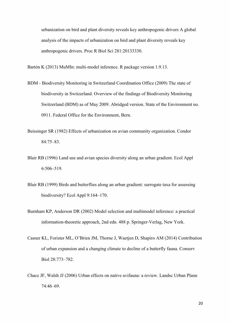
Table 2. Definitions and data sources of environmental predictors, including variables

describing urban sprawl and other environmental variables for the plots of the distinct

biodiversity monitoring programs at the habitat level (BDM Z9 and LANAG) and landscape

level (BDM Z7). See also Table 1.

Predictor Definition Data source Urban variables: Urban area Proportion of plot area occupied by

houses (including gardens), roads and other infrastructures, industries, parks and recreational areas, used for BDM Z7 plots and for butterflies in LANAG plots. Location in urban area, used for BDM Z9 plots and for LANAG plots (except butterflies)

Die Geographen schwick + spichtig

http://www.wsl.ch/info/fokus/zersiedelung

/ (2010, 15 m resolution)

Age of urban area Average age (weighted by area) of urban areas (in years) using 2011 as reference year, calculated from data on urban areas at different time points (1885, 1935, 1960, 1980, 2002, and 2010)



/ (time series: 1885–2010; 15 m

resolution)

Imperviousness of urban area

Degree of soil-sealing of urban area (%)

Pan-European Copernicus Land Monitoring Services http://www.copernicus.eu/ (2009, 20 m resolution)

Human population density in urban area

Number of human inhabitants (residents) per ha of urban area

Swiss Federal Statistical Office http://www.statistics.admin.ch/ (2011, 100 m resolution)

Mean proximity index (MPI) of urban area

Degree of dispersion of urban area (low MPI values = high dispersion), calculated as the ratio between the mean size of urban patches and the nearest neighbor distance to other urban patches (dimensionless). Used for BDM Z7 plots and for butterflies from LANAG plots



/ (2010, 15 m resolution)

Nearest distance to urban areas

Distance from plots to the nearest neighbor urban area (m). Used for BDM Z9 plots and for LANAG plots (except butterflies)

Non-urban variables:

Mean annual temperature Average value of monthly mean

temperatures (°C)

Swiss Federal Office of Meteorology and

Climatology

http://www.meteoswiss.ch/ (Data averaged

for the period 1961–1990, at 25 and100 m

resolution for the habitat and landscape

scales, respectively)

Annual precipitation Sum of monthly precipitation (mm)

Northness (aspect) Orientation or direction to which

slope faces, ranges from 1 (north-

Swiss Federal Office of Topography

http://www.copernicus.eu/

http://www.statistics.admin.ch/

29

facing slope) to -1 (south-facing

slope)

http://www.swisstopo.ch/

(Data at 25and100 m resolution for the

habitat and landscape scales, respectively) Surface roughness Standard deviation (SD) of altitude

(m a.s.l.), used for BDM Z7 plots

and for butterflies in LANAG plots.

Slope (surface inclination relative to

horizontal, 0–90°), used for BDM

Z9 plots and for LANAG plots

(except butterflies)

Forest area % plot area occupied by forest, used

for BDM Z7 plots and for butterflies

in LANAG plots.

Location in forest area, used for

BDM Z9 plots and for LANAG

plots (except butterflies)

Federal Statistical Office (FSO)

Land use statistics (2004/09, 100 m

resolution) http://www.bfs.admin.ch/

http://www.bfs.admin.ch/

30

Table 3. Results of the two steps of analysis. Step 1: Model performance D2full of the full models, i.e., percentage of null deviance explained by

urban and non-urban predictors, and the corresponding values D2I.Urban, i.e., the percentage of null deviance independently explained by urban

predictors based on hierarchical partitioning. All species groups with D2I.Urban ≥ 15% are shown. Step 2: Relative variable importance (RVI) of

single urban predictors from multi-model averaging. Values are provided for urban predictors included in best fitted models (delta AICc or QAICc

≤ 4) for each diversity variable. Arrows indicate the direction of effects (positive ↗ and negative ↘) based on partial regression plots of the best

fitted model (AIC-based) and coefficients estimates which are significantly different from zero (P<0.05; values in bold).

Step 1: Deviance partitioning Step 2: Multi-model averaging & partial regressions

Species group (Monitoring program)

D2full

(%) D2

I.Urban (%)

Urban area

Population density

Dispersion (MPI/ Nearest dist)

Imperviousness Average age

Vascular plants

Non-native plants (BDM Z7) 64.2 28.4 0.45 (↗) 0.97 (↗) 0.22 0.42 (↗) 0.03 Neophytes (BDM Z7) 61.8 41.9 1.00 (↗) 0.97 (↗) 1.00 (↘) 0.12 0.07

Ratio non-native vs. native plants (BDM Z7) 66.4 17.7 0.67 (↗) 0.69 (↗) 0.64 (↘) 0.07 - Habitat-specialist plants (BDM Z7) 43.8 15.7 - 0.67 (↗) 0.03 0.43 (↗) 0.02 Phanerophytes (BDM Z7) 42.6 19.3 0.98 (↗) 0.07 1.00 (↘) 0.13 (↗) 0.17

Chamaephytes (BDM Z7) 29.8 24.5 0.51 (↗) 0.01 0.83 (↘) 0.03 0.07 Therophytes (BDM Z7) 61.9 16.9 0.24 (↗) 0.49 (↗) - 0.41 (↗) 0.02 Eutrophic-habitat plants (BDM Z7) 52.9 24.1 - 0.97 (↗) 0.04 0.41 (↗) 0.05 (↘) Anemochorous plants (BDM Z7) 42.0 17.4 - - 0.07 1.00 (↗) 0.10 Anthropochorous plants (BDM Z7) 45.2 29.7 1.00 (↗) - 0.05 0.18 - Highly dispersive plants (BDM Z7) 42.0 16.1 0.05 0.11 (↗) 0.05 0.95 (↗) 0.12

Birds

Zoophagous birds (BDM Z7) 36.2 23.4 - 1.00 (↗) 0.03 - -

(LANAG) 27.3 18.5 0.96 (↗) 0.03 0.96 (↘) 0.07 0.03 Ground-breeding birds (BDM Z7) 28.6 15.0 0.92 (↘) 0.06 0.12 - 0.04 Urban birds (BDM Z7) 39.2 29.5 0.76 (↗) 0.29 (↗) 0.02 - 0.05

(LANAG) 37.9 31.7 1.00 (↗) 0.03 1.00 (↘) 0.05 0.04 Breeding-generalist birds (BDM Z7) 25.7 15.4 0.05 0.54 (↗) 0.02 0.04 0.05 Ratio breeding-generalist vs. specialist birds (BDM Z7) 31.0 24.2 1.00 (↗) 0.02 0.21 0.02 -

(LANAG) 41.7 28.9 0.02 1.00 (↗) 0.75 (↘) 0.14 1.00 (↗)

31

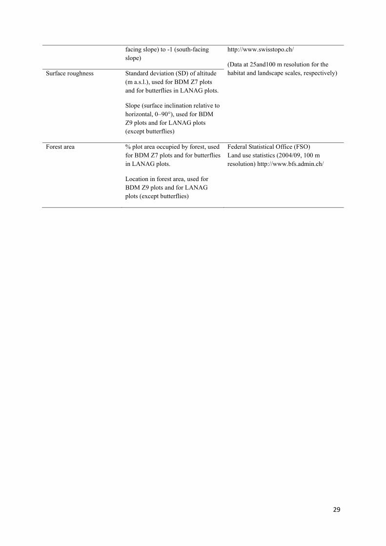
Figure 1. Delimitation of study area within Switzerland (thin boundary line), i.e. the Swiss

Plateau (thick solid boundary line; Gonseth et al. 2001), and the location of plots from the

different monitoring programs are shown: BDM Z7 indicator Species Diversity in Landscapes

(large dots; 109 plots of 1 km2); BDM Z9 indicator Species Diversity in Habitats (small dots;

473 circular plots of 10 m2); and LANAG program of the canton of Aargau (denser small

dots; 436 plots of different sizes at the habitat level in the Swiss Plateau). The location of the

main cities within the study area are indicated in grey.

Figure 2. Average (±SE) relative variable importance (RVI) of the different urban predictors

(i.e., urban area, population density, dispersion, imperviousness, and average age of urban

area) to explain the variation in species richness variables for all species groups that showed

relevant responses to urban sprawl (D2I.Urban ≥ 15%) independent from other environmental

predictors (see Table 3). Averaged-values are shown for all these groups (grey) and for the

subsets of groups for vascular plants (white) and birds (black).

Figure 3. Partial residual plots of significant responses of species richness to single

components of urban sprawl at the landscape scale for (a) neophytes and urban area (linear

term), (b) plants from eutrophic habitats and human population density of urban area (linear

and quadratic terms), (c) neophytes and urban disperson (MPI) (linear term), and (d) highly

dispersive plants and imperviousness (linear term). Partial residual plots represent the

estimated relationships between response variables and a predictor of interest (solid lines; ±1

SE, dotted lines) once the effects of other predictors have been accounted for. Mean values of

species richness per plot (avg.sr) are provided to contextualize the size of effects.

Figure 4. Partial residual plots of significant responses of birds to single components of urban

sprawl at the landscape scale for (a) species richness of ground breeding birds to urban area,

32

and (b) the ratio of breeding generalist to specialist bird species to urban area (linear terms).

Mean values of species richness/ratios per plot (avg.sr) are provided to contextualize the size

of effects. For further details on partial residual plots see Figure 3.

33

Concepción et al., Figure 1

34


35


a) b)

c) d)

36


a) b)

1

SUPPLEMENTARY MATERIAL

Table A.1. Details on biodiversity surveys for the set of studied taxa (mosses, vascular plants,

gastropods, butterflies and birds) from the different monitoring programs (BDM Z7, BDM Z9

and LANAG). For additional details, see http://www.biodiversitymonitoring.ch/ and

https://www.ag.ch/de/bvu/umwelt_natur_landschaft/naturschutz/biodiversitaet/erfolgskontroll

e___dauerbeobachtung/artenvielfalt___kessler_index/artenvielfalt___kessler_index_1.jsp

Program Description

BDM Z7 indicator Species Diversity in Landscapes monitors species diversity in representative

Swiss landscapes by using standardised survey methods of vascular plants (since 2001),

butterflies (since 2003) and breeding birds (since 2001) in sampling plots of 1 km2 area. BDM

Z7 represents species diversity held by mosaics of habitats within these survey areas. Species

diversity data are collected in 2500 m transects along paths and roads, within 2.5 m to each side

of the paths on the way forth and back, in 1 km2 plots for plants and butterflies, and in three

surveys during the breeding season along fixed routes within plots for birds. The national

sampling grid holds about 500 sampling plots regularly distributed all over Switzerland.

Approximately one-fifth of the plots is sampled each year, so a complete survey is

accomplished over five years.

Z9 indicator Species Diversity in Habitats monitors species diversity of mosses, vascular

plants and gastropods in circular sampling areas of 10 m2 (since 2001). BDM Z9 is used to

describe small-scale species diversity at the habitat level. The entire sampling grid (ca. 1600 10-

m2 sampling plots regularly distributed over Switzerland) is surveyed over five years.

LANAG Program of the canton of Aargau that has been monitoring species diversity at the habitat level

(similar to BDM Z9) since 1995 for breeding birds, since 1996 for vascular plants and

gastropods, and since 1998 for butterflies. Plants and gastropods are surveyed in 10 m2 circles,

birds in 100 m-radius circles, and butterflies in 250 m transects. The entire sampling grid

encompasses 517 sampling areas evenly distributed all over the canton. Like for the BDM

program, a complete survey is executed over five years.

2

Table A.2. Species characteristics of the different taxonomic groups used for the definition of

ecological groups on which effects of urban sprawl were analysed. Species characteristics

were extracted from information delivered by the Swiss Ornithological Institute

(http://www.vogelwarte.ch/) for birds, from expertise of the authors for butterflies (FA;

Altermatt 2010; Altermatt and Pearse 2011) and gastropods (BB; Kerney et al. 1983;

Bengtsson and Baur 1993; Falkner et al. 2001; B. Baur, unpubl. data), and from Landolt et al.

(2010) for vascular plants and mosses.

Species characteristics Ecological groups Birds Feeding Herbivorous

Zoophagous Breeding substrate Ground (including herb and shrub layer)

Holes (caves and tree hollows) Vertical structures, both natural (trees or rocks) and man-

made (buildings, bridges or towers) Habitat Greenland (grasslands and croplands)

Green structures (hedges and shrubland) Non-productive (rocks and bare soil) Urban areas (settlements and built-up areas) Vertical green structures (woodlands) Water (lakes, water courses, and wetlands)

Feeding specialisation: 1/number of items named as food

Feeding specialists (if ≥ median) Feeding generalists (if < median)

Breeding specialisation: 1/number of items named as breeding substrate

Breeding specialists (if ≥ median) Breeding generalists (if < median)

Habitat specialisation: 1/number of items named as habitat

Habitat specialists (if ≥ median) Habitat generalists (if < median)

Mobility: Wing load (weight/wing area; g/cm2)

Highly mobile(if ≥ median) Low mobile (if < median)

Threat status (Swiss Red List)

Red-listed species (included in some threat category, i.e., critically endangered, endangered, or vulnerable)

Commonness (Frequency of occurrence in plots from the different Swiss biodiversity monitoring programs)

Rare species (present in ≤10% of plots) Common species (present in >10% but <90% of plots) Very common species (present in ≥90% of plots)

Butterflies Larval feeding: Number of plant species on which larva feeds

Monophagous Narrow oligophagous Oligophagous Polyphagous

Type of food resources Feeding on trees and shrubs Feeding on evergreen plants

Degree of food specialisation: 1/(number of items named as larval food: plant species + type of food resources)

Feeding specialists (if ≥ median) Feeding generalists (if < median)

Mobility: Wing load proxy (body volume/wing


http://www.vogelwarte.ch/

3

area; cm) Threat status (Swiss Red List)

Red-listed species (included in some threat category, i.e., critically endangered, endangered, or vulnerable)



Gastropods Habitat Forest

Open land Ubiquitous

Habitat specialisation: Combined metric of habitat and humidity preferences and inundation tolerance (normalised).

Habitat specialists (if ≥ median) Habitat generalists (if < median)

Mobility: 1/shell size (corrected by shell shape)



Red-listed species (included in some threat category i.e., critically endangered, endangered, or vulnerable)



Vascular plants Growth forms Phanerophytes and nanophanerophytes (woody plants

with buds above the ground, i.e., trees and shrubs) Chamaephytes (perennial plants with buds on or very

close to the ground) Hemycryptophytes (plants with buds on or directly below

the ground) Geophytes (plants with buds below the ground, e.g., with

rhizomes, bulbs, or tubers) Therophytes (annual plants)

Habitat Forest Shrubland Grassland Eutrophic habitats (crops, hedges, and ruderal sites) Outcrop (sandy and rocky outcrops) Mires and bogs Water (water courses, lakes, and ponds)

Dispersal of diaspores Anemochorous (dispersed by wind) Anthropochorous (dispersed by men) Autochorous (self-dispersal) Hydrochorous (dispersed by water sources and run-off) Zoochorous (dispersed by animals)

Habitat specialisation: Combined metric of habitat and climatic preferences Temperature: from “alpine” (1) to

“very warm colline” (5). Continentality: from “oceanic” (1)

to “continental” (5). Light: from “deep shade” (1) to

“full light” (5). Moisture: from “very dry” (1) to

“flooded” (5). Reaction: from “extremely acid” (1)

to “alkaline, high pH” (5). Nutrients: from “very infertile” (1)

to “very fertile” (5).

Habitat specialists: Classified as specialist (i.e., preference for extreme values [1 or 5] or high or low values [2 or 4] with a small range of variation) for more than a half of criteria

Habitat generalists: Classified as generalist (i.e., preference for intermediate values [3] or high or low values [2 or 4] with a large range of variation) for at least a half of criteria.

4

Humus: from “little” (1) to “high” (5).

Soil aeration: from “bad” (1) to “good” (5)

Dispersal ability:

Dispersal modes (adapted from Vittoz and Engler 2007) Low dispersive plants:

o Authochorous (self-dispersal) o Ombrochorous (dispersed by rain drops) o Myrmerchorous (dispersed by ants) o Boleochorous (dispersed by wind gusts)

High dispersive plants: o Dyszoochorous (seeds cached by animals, afterwards

lost or forgotten) o Endozoochorous (seeds eaten and afterwards

deposited by animals) o Epizoochorous (seeds cling to fur, feathers or hooves

of animals) o Anthropochorous (dispersed by man) o Bythisochorous and nautochorous (dispersed by

water courses and surfaces), although the relevance of these dispersal modes is quite geographically limited.

o Meteorochorous (diaspores with special features that facilitate wind transportation).

Threat status (Swiss Red List) Red-listed species (included in some threat category, i.e., critically endangered, endangered or vulnerable)

Origin Native plant species Non-native plants species

o Archeophytes (introduced by man before 1500 A.D.) o Neophytes (introduced by man after 1500 A.D.)



Mosses Substrate Soil

Rocks Habitat Exposed microsites (disturbed places, rocks, gaps in

herbaceous vegetation , snow, open banks, etc.) Sheltered microsites (woodland, scrubs or herbaceous

vegetation, caves, holes, etc.) Habitat specialisation:

As for plants (see above), the classification was based on a combined metric of species preferences with respect to the following habitat and climatic parameters: temperature, continentality, light, moisture, reaction, nutrients, humus and soil aeration. Dispersal ability: Frequency of sporophyte production

Low dispersive mosses (extremely rare sporophyte production)

Highly dispersive mosses (frequent sporophyte production and in great quantities)


Red-listed species (included in some threat category, i.e., critically endangered, endangered or vulnerable)



Additional references of the appendix:

Altermatt F (2010) Tell me what you eat and I’ll tell you when you fly: diet can predict phenological changes in response to climate change. Ecol Lett 13:1475–1484.

5

Altermatt F, Pearse IS (2011) Similarity and specialization of the larval versus adult diet of European butterflies and moths. Am Nat 178:372–382.

Bengtsson J, Baur B (1993) Do pioneers have r-selected traits? Life-history patterns among colonizing terrestrial gastropods. Oecologia 94:17–22.

Falkner G, Obrdlik P, Castell E, Speight MCD (2001) Shelled Gastropoda of Western Europe. 267 p. Verlag, München.

Kerney MP, Cameron RAD, Jungbluth JH (1983) Die Landschnecken Nord- und Mitteleuropas. Paul Parey, Hamburg.

Landolt E, Bäumler B, Erhard A, et al (2010) Flora indicativa. Ecological Indicator Values and Biological Attributes of the Flora of Switzerland and the Alps. 376 p. Haupt, Bern.

Vittoz P, Engler R (2007) Seed dispersal distances: a typology based on dispersal modes and plant traits. Bot Helv 117:109–124.

6

Table A.3. Results of deviance partitioning between urban sprawl variables and non-urban predictors for the species richness of the distinct

taxonomic and ecological groups and monitoring programs at the landscape level (BDMZ7) and at the habitat level (BDM Z9 and LANAG).

Percentage of null deviance (%D2) explained by the full model subdivided into percentages independently explained by urban and non-urban

variables, as well as joint contribution to deviance explanation are provided. A grey highlight is used to stress models with urban variables

explaining a substantial portion of the deviance, independent from non-urban predictors (D2I.Urban ≥ 15 %).

Group BDM Z7 BDM Z9 LANAG

% D2

Full model

% D2

I.Urban

% D2 I.Non- urban

% D2 Joint

% D2

Full model

% D2

I.Urban

% D2 I.Non- urban

% D2

Joint

% D2

Full model

% D2

I.Urban

% D2 I.Non- urban

% D2 Joint

Overall plants 43.1 14.5 28.6 4.9 10.4 4.0 6.4 -0.7 3.7 2.1 1.7 0.1

Native plants 46.7 6.9 39.8 -1.5 12.7 4.4 8.3 0.3 3.5 3.1 0.4 0.0

Non-native plants 64.2 28.4 35.8 -0.8 28.7 5.8 22.9 -2.8 7.4 6.2 1.2 0.0

Neophytes 61.8 41.9 19.9 3.0 13.6 4.2 9.4 -1.9 5.5 3.4 2.1 0.0

Archeophytes 53.7 13.5 40.2 -2.1 30.8 4.8 25.9 -2.1 7.4 6.9 0.4 0.0

Ratio non-native vs. native plants 66.4 17.7 48.7 -4.4 36.4 3.9 32.4 0.4 9.7 5.7 4.1 0.2

Red-listed plants (Mittellands) 20.4 10.8 9.6 -0.4 25.7 12.8 12.9 -4.2

Rare plants (≤10%plots) 19.6 9.7 9.9 0.9 10.7 6.3 4.4 0.7 2.5 2.3 0.1 0.0

Common plants (>10% & <90% plots) 43.4 13.0 30.3 5.0 20.6 3.2 17.4 -1.2 5.8 2.0 3.8 0.0

Very common plants (≥90% plots) 34.5 14.0 20.6 0.0

Ratio very common vs. rare plants 21.6 11.8 9.8 1.1

Habitat-generalist plants 43.2 13.5 29.7 4.9 10.3 4.2 6.1 -0.5 4.1 2.7 1.4 0.1

Habitat-specialist plants 43.8 15.7 28.1 2.2 7.5 2.1 5.4 -0.8 3.0 1.0 2.0 -0.1

Ratio habitat-generalist vs. specialist plants 47.0 12.8 34.2 -2.9 11.0 3.8 7.1 -0.4 11.0 10.5 0.5 0.0

7

Group BDM Z7 BDM Z9 LANAG % D2

Full model

% D2

I.Urban

% D2 I.Non- urban

% D2 Joint

% D2

Full model

% D2

I.Urban

% D2 I.Non- urban

% D2

Joint

% D2

Full model

% D2

I.Urban

% D2 I.Non- urban

% D2 Joint

Chamaephytes 29.8 24.5 5.3 0.8 6.3 2.4 3.9 0.0 5.7 4.4 1.3 -0.1

Hemicryptophytes 40.3 6.7 33.7 1.7 21.1 4.1 17.0 -1.4 6.5 2.6 3.8 0.2

Geophytes 47.3 13.2 34.1 -4.1 17.4 1.6 15.8 -0.2 7.5 5.4 2.1 -0.1

Therophytes 61.9 16.9 45.0 -2.5 21.3 4.2 17.0 -1.2 2.8 2.5 0.3 0.0

Water plants 36.0 10.5 25.5 -3.1 8.8 2.4 6.3 -0.7 2.2 0.6 1.7 0.1

Eutrophic-habitat plants 52.9 24.1 28.7 4.7 18.4 3.9 14.4 -1.9 5.3 3.2 2.0 0.1

Outcrop plants 40.0 14.8 25.2 1.5 45.8 7.0 38.8 -0.1 6.0 4.9 1.0 -0.1

Mires and bog plants 31.1 13.4 17.7 -3.0 30.0 9.1 20.9 -0.6 10.7 8.3 2.4 -0.2

Grassland plants 38.0 7.1 31.0 -0.6 14.7 4.7 10.0 -0.4 7.8 6.9 1.0 0.0

Shrubland plants 43.5 10.1 33.4 -0.3 61.6 7.8 53.8 -3.1 8.7 7.0 1.7 0.1

Forest plants 30.4 6.2 24.2 -0.5 27.6 7.7 20.0 1.6 6.1 4.2 1.9 0.1

Anemochorous plants 42.0 17.4 24.5 5.3 15.7 2.7 13.0 -0.8 4.7 2.3 2.4 0.1

Anthropochorous plants 45.2 29.7 15.5 -3.6 18.1 2.1 16.0 0.2 7.2 5.3 1.9 0.3

Autochorous plants 47.2 10.0 37.2 3.7 8.8 5.5 3.3 0.0 5.3 3.8 1.5 0.0

Zoochorous plants 37.1 8.7 28.4 3.0 5.9 3.8 2.1 -0.2 2.6 1.8 0.8 -0.1

Hydrochorous plants 35.0 8.3 26.7 -1.5

Highly dispersive plants 42.0 16.1 26.0 4.9 10.8 3.2 7.6 -0.6 3.8 2.1 1.7 0.1

Low dispersive plants 42.4 10.0 32.4 2.4 9.9 5.2 4.7 -0.1 2.8 2.1 0.7 0.0

Overall birds 15.9 9.6 6.3 -0.2 10.6 2.9 7.7 1.2

Red-listed birds 16.2 9.4 6.9 -0.2 6.0 1.7 4.4 0.0

Rare birds (≤10%plots) 29.6 11.6 18.0 0.2 10.6 3.7 6.9 -0.3

Common birds (>10% & <90% plots) 20.3 8.3 12.1 -0.1 13.7 3.2 10.5 1.4

Very common birds (≥90% plots) 21.0 14.7 6.3 0.1

Ratio very common vs. rare birds 23.9 12.1 11.8 0.8

Herbivorous birds 22.9 9.2 13.7 -1.3 18.1 3.2 15.0 -1.4

Zoophagous birds 36.2 23.4 12.9 -3.1 27.3 18.5 8.8 -5.6

8


Full model

% D2

I.Urban

% D2 I.Non- urban

% D2 Joint

% D2

Full model

% D2

I.Urban

% D2 I.Non- urban

% D2

Joint

% D2

Full model

% D2

I.Urban

% D2 I.Non- urban

% D2 Joint

Ground-breeding birds 28.6 15.0 13.8 2.1 26.3 14.8 11.6 -5.5

Hole-breeding birds 25.7 7.0 18.7 -1.4 13.3 2.6 10.7 -0.6

Birds breeding in vertical structures 25.1 13.3 11.8 0.6 13.8 11.9 1.9 1.6

Green-land birds 38.6 8.8 29.9 -2.7 36.7 10.5 26.2 -6.8

Shrubland birds 20.2 8.6 11.6 -0.9 24.1 5.8 18.4 -0.6

Non-productive land birds 25.1 9.5 15.5 -2.3 27.9 12.8 15.1 -5.6

Urban birds 39.2 29.5 9.7 -5.0 37.9 31.7 6.2 -5.9

Tree birds 46.6 12.2 34.4 -4.4 40.1 9.7 30.4 -7.0

Water birds 41.7 8.2 33.5 -2.1 24.4 5.9 18.5 -3.0

Food-specialist birds 11.9 8.0 3.8 -0.3 9.2 5.0 4.1 2.0

Food-generalist birds 26.1 11.9 14.2 -0.8 14.9 3.1 11.8 -1.9

Ratio food-generalist vs. specialist birds 20.5 9.5 11.0 -1.7 13.6 9.1 4.5 -1.9

Breeding-specialist birds 15.3 11.0 4.3 -0.6 23.5 7.8 15.7 -4.7

Breeding-generalist birds 25.7 15.4 10.4 0.7 16.9 14.8 2.1 0.5

Ratio breeding-generalist vs. specialist birds 31.0 24.2 6.9 -0.7 41.7 28.9 12.8 -9.1

Habitat-specialist birds 36.8 13.4 23.3 0.6 20.0 3.7 16.3 -0.9

Habitat-generalist birds 16.3 4.8 11.6 0.1 5.9 4.4 1.5 0.5

Ratio habitat-generalist vs. specialist birds 58.6 12.6 46.0 -0.2 20.0 4.4 15.6 -1.9

Highly mobile birds 15.0 9.3 5.7 0.1 5.3 1.8 3.5 -0.2

Low mobile birds 16.1 9.4 6.7 -0.8 13.0 4.2 8.8 1.9

Overall butterflies 27.4 7.1 20.3 -1.4 14.3 9.2 5.1 -1.8

Red-listed butterflies 14.1 6.5 7.6 -1.0

Rare butterflies (≤10%plots) 26.1 4.5 21.6 0.1 11.0 4.0 6.9 -0.3

Common butterflies (>10% & <90% plots) 29.9 7.5 22.3 -1.3 14.8 9.3 5.5 -2.1

Very common butterflies (≥90% plots) 21.3 9.0 12.3 -1.2

Ratio very common vs. rare butterflies 11.5 5.4 6.2 0.6

9


Full model

% D2

I.Urban

% D2 I.Non- urban

% D2 Joint

% D2

Full model

% D2

I.Urban

% D2 I.Non- urban

% D2

Joint

% D2

Full model

% D2

I.Urban

% D2 I.Non- urban

% D2 Joint

Monophagous butterflies 22.6 4.3 18.3 -2.0 5.1 3.3 1.8 -0.3

Narrow oligophagous butterflies 21.7 7.2 14.4 -1.2 13.2 6.4 6.8 -1.1

Oligophagous butterflies 21.7 7.2 14.4 -1.2 13.2 6.4 6.8 -1.1

Polyphagous butterflies 24.8 5.5 19.2 -1.3 8.8 4.9 3.9 -1.3

Butterflies feeding on trees 15.5 6.9 8.6 0.2 5.2 4.2 1.0 -0.2

Butterflies not feeding on trees 30.5 6.4 24.1 -1.7 15.1 9.7 5.4 -2.0

Butterflies feeding on evergreen vegetation 29.0 6.0 23.0 -0.9 15.8 9.7 6.1 -1.8 Butterflies not feeding on evergreen

vegetation 23.1 8.0 15.0 -0.8 6.1 3.8 2.2 -0.7

Food-specialist butterflies 29.5 7.8 21.7 -1.0 14.3 9.5 4.8 -1.5

Food-generalist butterflies 23.5 5.9 17.5 -1.6 9.8 5.8 4.0 -1.2 Ratio food-generalist vs. specialist

butterflies 22.6 11.0 11.6 -0.6 6.5 5.7 0.9 -0.1

Highly mobile butterflies 26.2 8.6 17.6 -1.5 8.5 5.2 3.2 -0.9

Low mobile butterflies 30.0 7.3 22.6 -0.2 16.7 9.2 7.5 -1.6

Overall mosses 41.4 8.0 33.4 -2.0

Red-listed mosses 34.4 11.9 22.5 0.0

Rare mosses (≤10%plots) 36.7 7.7 29.0 0.2

Common mosses (>10% & <90% plots) 30.8 7.2 23.6 -3.1

Habitat generalist mosses 37.7 8.2 29.5 0.0

Habitat specialist mosses 38.5 7.1 31.4 -5.3

Ratio habitat-generalist vs. specialist mosses 16.2 7.4 8.8 1.5

Ground mosses 20.1 6.9 13.2 -0.6

Rock mosses 20.3 12.2 8.1 3.2

Plant mosses 57.9 7.6 50.3 -4.8

Exposed-habitats mosses 27.7 9.3 18.5 -2.8

Sheltered -habitats mosses 50.6 8.1 42.5 -2.4

10

Group BDM Z7 BDM Z9 LANAG

% D2

Full model

% D2

I.Urban

% D2 I.Non- urban

% D2 Joint

% D2

Full model

% D2

I.Urban

% D2 I.Non- urban

% D2

Joint

% D2

Full model

% D2

I.Urban

% D2 I.Non- urban

% D2 Joint

Highly dispersive mosses 33.7 8.7 25.0 -1.3

Low dispersive mosses 14.4 6.5 7.9 0.2

Gastropods 28.7 6.3 22.4 2.1 26.3 6.0 20.4 -0.2

Red-listed gastropods 17.5 4.2 13.2 0.4

Rare gastropods 29.0 4.3 24.7 2.1 26.1 6.5 19.6 0.8

Common gastropods 22.4 6.7 15.7 1.7 22.3 5.3 17.0 -0.4

Open land gastropods 58.1 6.5 51.7 -2.0 57.1 7.0 50.1 -4.6

Forest gastropods 11.8 5.8 6.0 -2.2 23.4 5.5 17.9 -2.8

Ubiquitous gastropods 25.9 9.3 16.6 2.7 18.9 7.9 11.1 0.6

Habitat specialist gastropods 26.6 5.4 21.2 2.1 25.8 4.3 21.4 -0.1

Habitat generalist gastropods 21.5 5.6 15.8 1.2 19.9 7.0 12.9 -0.3 Ratio habitat-generalist vs. specialist

gastropods 2.1 1.4 0.7 0.0 6.8 4.5 2.3 -0.4

Highly mobile gastropods 16.9 7.5 9.5 1.7 12.7 6.2 6.5 0.5

Low mobile gastropods 38.0 4.7 33.3 0.7 40.2 6.9 33.3 -2.6

11

Table A.4. Detailed results of multi-model averaging performed for diversity metrics of the different ecological groups of plants and birds at the

landscape (BDM Z7) and habitat (LANAG) levels for which urban sprawl variables explained a substantial portion of the deviance, independent

from non-urban predictors (D2I.Urban ≥ 15%). Percentage of null deviance (D2) explained by the full model, and percentage of D2 explained by all

urban sprawl predictors alone are provided. The two rows presented for every species group representaverage parameter estimates (β ± SE) of the

linear term (top row) and quadratic term (bottom row) of individual urban variables of best fitted models according to AICc or QAICc (delta ≤ 4).

Bold indicates significant effects. Significance levels: ***P<0.001, **P<0.01, *P<0.05, (*) P<0.10.

Group (Monitoring program)

D2

Full model (%)

D2 I.Urban variables (%)

Effects: β ± SE - Linear term - Quadratic term

Urban area Average age Imperviousness Dispersion Population density

Vascular plants

Non-native plants (BDM Z7) 64.2 28.4 37.56±15.12* -12.31±7.43 21.78±10.67* -17.68±13.57 42.42±14.4**

-14.22±8.01(*) 4.32±10.21 -17.27±7.11* -11.15±7.66 -21.35±8.32* Neophytes (BDM Z7) 61.8 41.9

33.38±10.21** -1.7±3.9 4.77±7.09 -15.41±6.81* 16.24±7.35*

-7.9±5.14 -6.67±5.76 -6.38±4.09 -6.93±4.47 -6.97±4.67 Ratio non-native vs. native plants (BDM Z7)

66.4 17.7 0.49±0.18** - 0.08±0.17 -0.36±0.15* 0.32±0.14*

-0.22±0.1* - -0.18±0.1(*) 0.09±0.1 -0.13±0.1 Habitat-specialist plants (BDM Z7)

43.8 15.7 - 15.96±8.68(*) 42.57±12.54*** 1.18±9.75 42.16±10.31***

- -3.81±10.55 -2.14±7.89 -13.07±7.79(*) -18.25±8.29* Phanerophytes (BDM Z7) 42.6 19.3

33.37±11.59** 11.27±5.73(*) 20.58±9.33* -1.56±9.34 14.51±12.75

9.52±7.89 -15.25±8.39(*) -1.38±6.5 -29.56±6.6*** -11.92±6.48(*) Chamaephytes (BDM Z7) 29.8 24.5

8.75±3.88* 3.14±2.42 3.32±3.15 4.94±4.38 2.42±3.29

-1.66±3.03 -1.26±3.39 -2.29±2.55 -7.55±2.84** -1.34±2.73 Therophytes (BDM Z7) 61.9 16.9

31.24±11.49** -12.84±7.78 32.42±11.41** - 35.16±9.8***

-16.22±7.95* -0.85±10 -12.35±7.52 - -11.36±7.88

12

Group (Monitoring program)

D2

Full model (%)

D2 I.Urban variables (%)

Effects: β ± SE - Linear term - Quadratic term

Built-up area Age of built-up areas

Imperviousness degree of built-up areas

MPI of / Nearest distance to built-up areas

Population density in built-up areas

Chamaephytes (BDM Z7) 29.8 24.5 8.75±3.88* 3.14±2.42 3.32±3.15 4.94±4.38 2.42±3.29

-1.66±3.03 -1.26±3.39 -2.29±2.55 -7.55±2.84** -1.34±2.73 Therophytes (BDM Z7) 61.9 16.9

31.24±11.49** -12.84±7.78 32.42±11.41** - 35.16±9.8***

-16.22±7.95* -0.85±10 -12.35±7.52 - -11.36±7.88 Eutrophic-habitat plants (BDM Z7)

52.9 24.1

- 0.33±13.05 56.47±24.18* 2.55±17.32 96.92±23.35***

- -34.75±16.77* -28.59±13.26* -27.46±13.85(*) -51.6±16.82**

Anemochorous plants (BDM Z7)

42.0 17.4

- -23.13±14.23 110.3±14.17*** 26.08±15.23(*) -

- -19.14±17.69 -5.91±12.36 -23.91±13.43(*) -

Anthropochorous plants (BDM Z7)

45.2 29.7 6.42±1.36*** - 2.52±1.64 -0.6±1.58 -

-1.44±1.15 - -0.88±1.11 -1.29±1.1 -

Highly dispersive plants (BDM Z7)

42.0 16.1

26.4±22.38 -36.09±18.2(*) 145.39±21.79*** 28.65±19.05 83.27±40.01*

20.58±18.24 -33.48±22.17 -12.91±16.05 30.41±16.79(*) -42.65±23.55(*)

Birds

Zoophagous birds (BDM Z7) 36.2 23.4

- - - -3.13±4.21 9.31±3.32**

- - - -1.52±3.2 -4.45±3.13

(LANAG) 27.3 18.5 10.65±3.07*** -2.91±4.17 5.39±5.27 -6.65±2.37** -1.95±3.57

-0.35±2.45 0.89±2.96 -2.6±2.69 1.94±2.05 -0.38±2.67

Ground-breeding birds (BDM Z7)

28.6 15.0 -7.23±3.09* -1.56±2.72 - -4.72±3.75 4.24±4.65

3.83±2.66 -2.06±3.75 - -0.61±2.74 -2.95±2.76

Urban birds(BDM Z7) 39.2 29.5 9.85±3.16** 2.34±2.36 - -3.65±4.23 8.63±3.81*

-3.32±2.69 0.81±3.29 - 0.27±2.82 -3.84±2.7

(LANAG) 37.9 31.7 18.38±2.85*** 2.42±3.8 4.2±4.27 -7.78±1.77*** -1.6±3.28

-2.34±2.22 0.75±2.75 0.56±2.64 2.6±1.56(*) -0.83±2.43

Breeding-generalist birds (BDM Z7)

25.7 15.4

6.48±4.42 4.72±4.25 6.84±4.55 -6.61±5.88 9.98±4.69*

-2.3±4.44 -5.18±4.31 -0.09±4.47 -0.8±4.51 -2.39±4.48

Ratio breeding-generalist vs. specialist birds (BDM Z7)

31.0 24.2 0.65±0.17*** - -0.03±0.2 -0.3±0.19 -0.08±0.22

-0.19±0.13 - -0.09±0.13 0.12±0.13 0.1±0.13

(LANAG) 41.7 28.9 -0.07±0.87 1.94±0.65** 0.85±0.73 -1.16±0.52* 1.71±0.55**

0.3±0.51 -1.42±0.48** -0.58±0.49 0.64±0.45 -0.66±0.48

13

Table A.5. Mean values and range of urban sprawl and other environmental variables, as well as species richness and ratios of the distinct

taxonomic and ecological groups analysed, in plots of the different monitoring programs (BDM Z7, BDM Z9, and LANAG) included in our study.

Variables BDM Z7 BDM Z9 LANAG

Mean Range Mean Range Mean Range

Urban sprawl variables:

Built-up area (%) 10.62 0 - 65.89 16.03 0.00 - 100 12.65 0 - 100

Age of built-up areas (years) 53.85 0 - 128.16 11.08 0.00 - 126 8.11 0 - 126

Degree of imperviousness of built-up areas (%) 16.35 0 - 61.74 6.01 0.00 - 98 5.32 0 - 100

MPI of / Near distance (m) to built-up areas 3.68 0 - 25.92 318.37 0.00 - 1738.30 355.90 0 - 1872.45

Population density in built-up areas (inhab./ha) 11.24 0 - 61.48 5.17 0.00 - 186 3.54 0 - 93

Other environmental variables:

Mean annual temperature (°C) 8.33 6.60 - 9.34 8.28 5.72 - 9.79 8.62 7.03 - 9.41

Mean annual precipitation (mm) 1162.9 920.8 - 1691.9 1153.2 838.3 - 1912 1112.2 887.4 - 1443.8

Northness -0.68 -1.00 - 0.86 0.06 -1.00 - 0.01 0.12 -1.00 - 0.01

SD Altitude (m.a.s.l.) / Slope (degree) 22.85 0.44 - 55.83 5.91 0 - 50 6.69 0 - 39

Forest area (%) 28.16 0 - 99 24.64 0 - 100 37.94 0 - 100

Species richness:

Overall plants 248.13 134 - 339 19.73 1 - 63 18.31 1 - 54

Native plants 147.93 49 - 230 11.03 0 - 39 10.95 0 - 40

Non-native plants 40.74 5 - 72 2.26 0 - 20 1.93 0 - 12

Neophytes 14.42 3 - 30 0.97 0 - 9 0.89 0 - 5

Archeophytes 24.34 0 - 44 1.19 0 - 11 0.97 0 - 9

Ratio non-native vs. native plants 0.29 0.03 - 0.78 0.29 0 - 4 0.27 0 - 4

Red-listed plants (Mittellands) 3.99 0 - 22 0.04 0 - 2 0.04 0 - 5

Rare plants (≤10%plots) 13.10 1 - 66 6.77 0 - 34 6.19 0 - 32

Common plants (>10% & <90% plots) 164.60 76 - 235 12.96 0 - 39 12.12 1 - 36

Very common plants (≥90% plots) 70.43 47 - 73

14



Ratio very common vs. rare plants 7.84 0.97 - 35.50

Habitat-generalist plants 199.97 101 - 268 16.54 0 - 53 15.42 0 - 45

Habitat-specialist plants 47.13 22 - 73 2.41 0 - 10 2.26 0 - 8

Ratio habitat-generalist vs. specialist plants 4.31 2.78 - 7.61 5.47 0 - 28.00 5.38 0 - 29.00

Phanerophytes 30.87 9 - 46 1.66 0 - 14 2.00 0 - 14

Chamaephytes 5.78 1 - 15 0.51 0 - 3 0.51 0 - 5

Hemicryptophytes 102.43 43 - 157 8.99 0 - 40 8.20 0 - 40

Geophytes 17.15 3 - 34 1.12 0 - 9 1.17 0 - 6

Therophytes 42.76 8 - 72 2.84 0 - 17 2.26 0 - 16

Water plants 26.23 9 - 56 1.35 0 - 11 1.30 0 - 8

Eutrophic-habitat plants 139.30 67 - 193 11.16 0 - 38 9.69 0 - 34

Outcrop plants 7.90 1 - 16 0.50 0 - 5 0.62 0 - 10

Mires and bog plants 2.14 0 - 7 0.09 0 - 2 0.10 0 - 1

Grassland plants 15.10 1 - 48 0.83 0 - 6 0.89 0 - 6

Shrubland plants 18.07 4 - 32 1.18 0 - 10 1.53 0 - 9

Forest plants 2.16 0 - 5 0.10 0 - 2 0.14 0 - 2

Anemochorous plants 124.40 63 - 183 8.83 0 - 31 7.93 0 - 31

Anthropochorous plants 2.57 0 - 7 0.15 0 - 1 0.14 0 - 1

Autochorous plants 20.70 12 - 30 1.56 0 - 9 1.56 0 - 7

Zoochorous plants 98.09 56 - 134 8.40 0 - 29 8.03 0 - 21

Hydrochorous plants 1.34 0 - 10

Highly dispersive plants 203.43 112 - 282 15.76 0 - 52 14.52 0 - 45

Low dispersive plants 43.65 21 - 64 3.19 0 - 14 3.16 0 - 11

Overall birds 40.29 17 - 55 19.76 2 - 38

Red-listed birds 0.91 0 - 5 0.43 0 - 4

Rare birds (≤10%plots) 1.66 0 - 9 1.18 0 - 8

Common birds (>10% & <90% plots) 23.28 5 - 34 17.66 1 - 36

Very common birds (≥90% plots) 15.35 9 - 16

15



Ratio very common vs. rare birds 8.77 1.50 - 16.00

Herbivorous birds 31.54 9 - 44 15.61 2 - 30

Zoophagous birds 8.75 4 - 16 4.14 0 - 9

Ground-breeding birds 6.62 2 - 15 2.66 0 - 7

Hole-breeding birds 10.49 2 - 18 6.02 0 - 13

Birds breeding in vertical structures 23.18 8 - 31 11.08 1 - 22

Green-land birds 5.76 1 - 12 1.82 0 - 11

Shrubland birds 1.87 0 - 4 0.86 0 - 3

Non-productive land birds 1.98 0 - 4 0.73 0 - 4

Urban birds 5.58 1 - 9 2.92 0 - 8

Tree birds 22.27 5 - 34 12.61 1 - 27

Water birds 2.84 0 - 11 0.83 0 - 7

Food-specialist birds 27.45 12 - 41 12.03 1 - 27

Food-generalist birds 12.85 5 - 17 7.73 1 - 14

Ratio food-generalist vs. specialist birds 0.46 0.26 - 0.72 0.62 0.07 - 1.50

Breeding-specialist birds 21.90 9 - 35 9.56 0 - 20

Breeding-generalist birds 18.39 8 - 23 10.20 0 - 18

Ratio breeding-generalist vs. specialist birds 0.82 0 - 1 1.10 0 - 9

Habitat-specialist birds 20.99 6 - 28 9.31 0 - 20

Habitat-generalist birds 19.30 10 - 31 10.45 1 - 20

Ratio habitat-generalist vs. specialist birds 0.92 0.57 - 2.56 1.11 0.43 - 5.00

Highly mobile birds 17.79 7 - 26 8.18 1 - 15

Low mobile birds 22.50 10 - 30 11.58 1 - 23

Overall butterflies 22.59 4 - 46 6.77 1 - 18

Red-listed butterflies 0.79 0 - 7

Rare butterflies (≤10%plots) 1.23 0 - 14 0.54 0 - 4

Common butterflies (>10% & <90% plots) 18.42 1 - 32 5.26 0 - 14

Very common butterflies (≥90% plots) 2.93 2 - 3

16



Ratio very common vs. rare butterflies 2.01 0.20 - 3.00

Monophagous butterflies 2.32 0 - 5 0.82 0 - 4

Narrow oligophagous butterflies 0.77 0 - 3 0.05 0 - 2

Oligophagous butterflies 0.77 0 - 3 0.05 0 - 2

Polyphagous butterflies 8.07 2 - 14 1.71 0 - 7

Butterflies feeding on trees 2.42 0 - 7 0.49 0 - 3

Butterflies not feeding on trees 18.02 3 - 36 4.94 0 - 15

Butterflies feeding on evergreen vegetation 14.18 3 - 29 3.80 0 - 12

Butterflies not feeding on evergreen vegetation 6.26 0 - 14 1.63 0 - 8

Food-specialist butterflies 13.82 1 - 32 4.16 0 - 13

Food-generalist butterflies 6.63 1 - 13 1.27 0 - 5

Ratio food-generalist vs. specialist butterflies 10.13 1 - 23 0.25 0 - 1.50

Highly mobile butterflies 10.32 2 - 20 2.34 0 - 9

Low mobile butterflies 0.46 0 - 1 3.09 0 - 10

Overall mosses 6.39 1 - 26

Red-listed mosses 0.82 0 - 8

Rare mosses (≤10%plots) 2.75 0 - 18

Common mosses (>10% & <90% plots) 3.64 0 - 10

Habitat generalist mosses 4.28 0 - 21

Habitat specialist mosses 0.67 0 - 5

Ratio habitat-generalist vs. specialist mosses 2.78 0 - 16

Ground mosses 2.97 0 - 14

Rock mosses 0.40 0 - 9

Plant mosses 1.59 0 - 12

Exposed-habitats mosses 0.69 0 - 6

Sheltered -habitats mosses 4.27 0 - 22

Highly dispersive mosses 1.68 0 - 10

Low dispersive mosses 0.90 0 - 6

17



Gastropods 6.87 0 - 34 6.87 0 - 33

Red-listed gastropods 0.13 0 - 4 0.04 0 - 2

Rare gastropods 1.56 0 - 19 1.42 0 - 17

Common gastropods 5.30 0 - 18 5.45 0 - 18

Open land gastropods 2.13 0 - 20 2.90 0 - 20

Forest gastropods 2.56 0 - 12 2.16 0 - 10

Ubiquitous gastropods 2.18 0 - 12 1.81 0 - 11

Habitat specialist gastropods 4.33 0 - 24 4.42 0 - 23

Habitat generalist gastropods 2.50 0 - 12 2.43 0 - 12

Ratio habitat-generalist vs. specialist gastropods 0.49 0 - 3 0.45 0 - 1.75

Highly mobile gastropods 4.09 0 - 21 3.65 0 - 18

Low mobile gastropods 2.77 0 - 19 3.22 0 - 19

Documents

Impacts of urban sprawl on species richness of plants, butterflies, gastropods and birds: not only built-up area matters