Implementation of an iterative scatter correction, the influence of attenuation map quality and

their effect on absolute quantitation in SPECT

This content has been downloaded from IOPscience. Please scroll down to see the full text.

Download details:

IP Address: 219.149.45.42

This content was downloaded on 04/10/2013 at 08:57

Please note that terms and conditions apply.

2007 Phys. Med. Biol. 52 1527

(http://iopscience.iop.org/0031-9155/52/5/020)

View the table of contents for this issue, or go to the journal homepage for more

Home Search Collections Journals About Contact us My IOPscience

IOP PUBLISHING PHYSICS IN MEDICINE AND BIOLOGY

Phys. Med. Biol. 52 (2007) 1527–1545 doi:10.1088/0031-9155/52/5/020

Implementation of an iterative scatter correction, theinfluence of attenuation map quality and their effecton absolute quantitation in SPECT

Eric Vandervoort1, Anna Celler2 and Ronald Harrop3

1 Department of Physics and Astronomy, University of British Columbia,6224 Agricultural Road, Vancouver, V6T 1Z1, Canada2 Department of Radiology, University of British Columbia, 828 West 10th Avenue,Vancouver, V5Z 1L8, Canada3 School of Computing Science Simon Fraser University, 8888 University Drive, Burnaby,V5A 1S6, Canada

E-mail: evander@physics.ubc.ca

Received 17 August 2006, in final form 14 December 2006Published 14 February 2007Online at stacks.iop.org/PMB/52/1527

AbstractWe investigated the accuracy of qSPECT, a quantitative SPECT reconstructionalgorithm we have developed which employs corrections for collimatorblurring, photon attenuation and scatter, and provides images in unitsof absolute radiotracer concentrations (kBq cm−3). Using simulated andexperimental phantom data with characteristics similar to clinical cardiacperfusion data, we studied the implementation of a scatter correction (SC)as part of an iterative reconstruction protocol. Additionally, with experimentalphantom studies we examined the influence of CT-based attenuation maps,relative to those obtained from conventional SPECT transmission scans,on SCs and quantitation. Our results indicate that the qSPECT estimatedscatter corrections did not change appreciably after the third iteration of thereconstruction. For the simulated data, qSPECT concentrations agreed withimages reconstructed using ideal, scatter-free, simulated data to within 6%.For the experimental data, we observed small systematic differences in thescatter fractions for data using different combinations of SCs and attenuationmaps. The SCs were found to be significantly influenced by errors in imagecoregistration. The reconstructed concentrations using CT-based correctionswere more quantitatively accurate than those using attenuation maps fromconventional SPECT transmission scans. However, segmenting the attenuationmaps from SPECT transmission scans could provide sufficient accuracy formost applications.

0031-9155/07/051527+19$30.00 © 2007 IOP Publishing Ltd Printed in the UK 1527

1528 E Vandervoort et al

1. Introduction

The accuracy of single photon emission computed tomography (SPECT) is limited primarilyby photon attenuation, scatter and resolution losses due to collimator blurring. Additionally,for structures smaller than the reconstructed voxel size and those with dimensions comparableto the full-width at half maximum characterizing the spatial resolution of the imaging system,the partial volume effect (PVE) can also lead to errors in the reconstructed images. Correctionsfor attenuation and/or collimator blurring are now becoming available on many commercialSPECT imaging systems and some of the model-based scatter correction techniques (Wellset al 1998, Beekman et al 2002, Frey et al 1996 and Bai et al 2000) are beginning to be fastand accurate enough to permit their use in clinics. In parallel, there has been a renewal ofinterest in absolute quantitation in SPECT, particularly in the field of targeted radiotherapy(e.g., Gonazalez et al (2001) and He et al (2005)) and in dopaminergic brain imaging (Soretet al 2003). Absolute quantification in cardiac SPECT has the potential to improve thesensitivity and specificity for the diagnosis of ischaemic heart disease and balanced triple-vessel disease. However, most of the previous work in quantitative cardiac imaging (e.g., Lianget al (1998) and Ye et al (1994)) employed the previous generation of energy-window-basedscatter corrections which can be very sensitive to non-uniformities in the detector response,electronic drift in the camera components and noise in the data (Logan and McFarland 1992,King et al 1992 and Ogawa et al 1991).

In this work we present a quantitative SPECT reconstruction algorithm (qSPECT) thatincludes patient-specific corrections for photon attenuation and scatter as well as compensationfor collimator blurring. Although no corrections are applied for the PVE, most of the structuresconsidered in this work are large enough, unless otherwise indicated, that PVE should notbe a significant image degrading effect. A single parameter, namely an experimentallydetermined camera sensitivity factor, is sufficient to convert count distributions in thesereconstructed images to absolute tracer concentrations. We have focused our investigationon the implementation of a scatter correction as part of an iterative reconstruction algorithmand on the evaluation of the influence of attenuation map quality on the resulting qSPECTimages. We evaluated the accuracy of both the absolute tracer concentrations for theqSPECT reconstructions and of the scatter correction itself using simulated and experimentalphantom studies performed with a commercial SPECT imaging system. In our previouswork (Vandervoort et al 2005), we introduced simplifications to an analytically-basedscatter correction for SPECT (Wells et al 1998) and implemented it as part of an iterativereconstruction algorithm. The objective of this earlier analysis was to compare relativequantitation (i.e., relative ratios of reconstructed voxel intensities), whereas the current workinvestigates the feasibility of recovering absolute radiotracer concentrations in the patient’sbody in absolute quantitative units (kBq cm−3).

Model-based scatter corrections require both a patient-specific attenuation map and anestimate of the distribution of activity in the body (activity map). The activity map, however,is exactly the unknown quantity we are trying to determine with the image reconstructionprocess. Therefore, the scatter estimate must be calculated using a reconstructed activity map.Using simulated data, we have investigated how the scatter correction could be incorporatedinto the reconstruction procedure and the influence this has on the quantitation of the results.In particular, for iterative image reconstruction it may be necessary to recompute the scattercorrection as the image (the estimate of the activity) is updated during the reconstructionprocess. It is not clear, however, how often the scatter estimate should be updated. InVandervoort et al (2005), our scatter correction was computed only once using a non-scatter corrected initial reconstructed image. It has been suggested (Beekman et al 2002),

Scatter corrections, attenuation map quality and absolute quantitation in SPECT 1529

however, that the scatter correction should be computed at each iteration, since high-frequencycomponents in the reconstructed image do not emerge until later iterations. Kadrmas et al(1998) found that scatter estimates updated in this way do not change significantly after the firstfew iterations, which may indicate that the distribution of scattered photons does not dependcritically on those high-frequency components. For all the data presented in this paper, wehave updated our scatter estimate at every iteration of the reconstruction process. Using thesimulation data, we directly compared the true component of scatter present in the SPECT datawith our scatter correction data at each iteration. For these data, we also compared the tracerconcentrations obtained from qSPECT scatter corrected reconstructions to the true activitydistribution.

Both accurate attenuation and model-based scatter corrections require a patient-specificattenuation map. The objective of our experimental phantom studies was to investigate howthe quality and accuracy of the attenuation map influences both the scatter correction and theabsolute quantitative accuracy of the reconstructed image. In SPECT, attenuation maps canbe obtained from a transmission scan in which an external source of radioactivity is used.However, such attenuation maps often contain artefacts related to insufficient intensity of thephoton beam and/or cross-talk effects (Celler et al 2003). Alternatively, attenuation maps canbe obtained using the high-resolution anatomical information available from other imagingmodalities such as x-ray CT. In this case, the linear attenuation coefficient necessary for SPECTcorrections must be surmised from the averaged linear attenuation coefficient for a spectrum ofx-ray energies (Hounsfield number). In practice the CT image is either rescaled or segmentinginto known anatomical regions and the appropriate attenuation coefficient for SPECT isassigned to each region. An additional step may also be required to spatially co-register theCT attenuation map with the SPECT image. Each of these steps may introduce inaccuraciesinto the attenuation and scatter corrections which cause artefacts in the reconstructed SPECTimage. Since combined SPECT and CT scanners are becoming more widely available, wecompared qSPECT reconstructions using a high-resolution CT attenuation map with thoseusing conventional transmission scans.

2. Methods

2.1. The qSPECT reconstruction algorithm

The qSPECT reconstruction software, developed by our research group at the VancouverGeneral Hospital, can be used to perform image reconstructions with different combinationsof corrections and reconstruction methods for SPECT data (Dixon et al 2004). In the presentwork, all data were reconstructed using the ordered-subsets expectation-maximization (OSEM)algorithm (8 iterations with 8 subsets over 64 projection views) and our most accurate set ofSPECT corrections. These corrections include attenuation correction (AC) calculated directlyfrom patient-specific attenuation maps and Klein Nishina-based scatter correction (SC) (Wellset al (1998) or Vandervoort et al (2005)) applied as an additive correction in the forwardprojection step of OSEM. We also perform fully 3D detector response compensation (DRC) inwhich the collimator response is modelled as a Gaussian blurring kernel with a depth dependentFWHM (Blinder et al 2001). The system matrix is pre-calculated and stored as a sparse array.For a 128 × 128 × 128 sized image and 128 × 128 × 64 sized sinogram, our presentimplementation of the qSPECT reconstruction requires about 1 Gb of RAM and 40 minof CPU time (excluding the time required for the scatter correction) using a 1.7 GHzprocessor. The reconstructed images, when divided by the experimentally determined camerasensitivity factor and by the known scan duration and volume of the image voxels, are then

1530 E Vandervoort et al

Activity Map (kBq cm−3)

0

50

Attenuation Map (cm−1)

0

0.05

0.1

0.15

0.2

0.25

0.3

(a) (b)

100

Figure 1. Transaxial slice through (a) the activity and (b) the attenuation distributions used in thesimulation studies.

expressed in units of absolute activity concentration (Ye et al 1994). The sensitivity factor isdetermined by recording the total number of counts detected for a point source with knownactivity.

Our SC was performed using two slightly different approaches. The first one was thefull analytic photon distribution (APD) method (Wells et al 1998). In this approach theexpected distribution of primary and scattered photons in SPECT projections are calculatedusing the attenuation map and an estimate of the activity distribution. The APD techniqueuses an accurate model of the photon interactions and the data acquisition process, but istoo computationally intensive to be used iteratively. Therefore, for the iterative qSPECTreconstructions we used a second scatter correction, namely the APD-interpolative (APDI)technique (Vandervoort et al 2005), a faster simplified version of the APD correction. InAPD, we compute the probabilities that the photons emitted from each voxel in the activitymap will undergo scatter interactions in the attenuating medium and be recorded in the arrayof detector bins. In the APDI method, these probabilities are computed for only a subsetof activity voxel positions and are estimated for the remaining voxels using interpolation.The total scatter contribution from each voxel, for both APD and APDI, is the product ofthe probability values and the activity present in that particular voxel. Both calculationsalso compute the contribution from primary photons. Before each scatter correction step,the scatter estimates are rescaled to match the total number of counts (sum of the APD orAPDI calculated primary and scattered photons) to the measured data. The APDI methodrequires much less computation time than APD and lends itself more easily to iterative updates(Vandervoort et al 2005). For example, in the experimental studies performed here, the fullAPD scatter correction required about 13.5 h of CPU time (1.7 GHz processor), while APDIrequired only about 2 h for the first iteration and 35 min for subsequent iterations.

2.2. Simulation study

The dynamic mathematical cardiac-torso phantom (MCAT) (Pretorius et al 1997) was used togenerate three-dimensional voxelized activity and attenuation distributions (shown in figure 1)to model a female patient with an inferior myocardial wall defect undergoing a typical SPECTcoronary perfusion scan. The MCAT program models the beating heart and was used toproduce an activity distribution averaged over a complete heart cycle. The myocardium,defect, liver, lungs and body contained 99mTc activity with concentrations of 148 kBq cm−3,0 kBq cm−3, 148 kBq cm−3, 18.5 kBq cm−3 and 37 kBq cm−3, respectively.

Scatter corrections, attenuation map quality and absolute quantitation in SPECT 1531

The simulated SPECT data used for our reconstructions were created by inputting theMCAT digital phantom into the APD calculation. We used APD for both data generationand scatter correction, instead of some independent simulation software, to avoid any smallinconsistencies related to differences in simulation models which might confound our results.This allowed us to evaluate the approximations introduced at each stage of the scatter correctionconsistently and independently, since any errors in the reconstructed image could only be theresult of that particular approximation. However, it is possible that errors in our scattercorrection model could remain undetected since the same approximations were made in datageneration and in the scatter corrections; these include assumptions and approximations usedto compute higher-order scatter (see Wells et al (1998)). Therefore, we also simulated fourreference projection views using conventional Monte-Carlo simulation software in order tovalidate the APD data. For these simulations we used GATE, the Geant4 Application forTomographic Emission (Jan et al 2004), a well-validated Monte-Carlo simulation tool fornuclear medicine applications.

Since the APD data are inherently noiseless, we could also investigate the influence noisehas on our reconstructions. For this analysis we reconstructed two datasets, one noise-freedataset and one in which Poisson noise was added to the APD data to simulate a noise levelsimilar to that of a standard clinical sestamibi scan acquired for 20 s at each projection view.By comparing the reconstructions that used noisy and noise-free data we were able to estimatehow different levels of statistical noise might influence the reconstruction process.

We compared our proposed qSPECT reconstruction method to three ‘ideal’reconstructions (that were only possible when using simulated data), one commonly usedholistic scatter correction (which does not explicitly estimate the distribution of scatteredphotons in the SPECT data), and one reconstruction which did not employ any scattercorrection whatsoever. All reconstructions discussed here used 8 iterations of OSEM with8 subsets over 64 projection views and included corrections for attenuation and collimatorblurring and differed only in the way in which the scatter correction was implemented. A totalof six different reconstructed datasets (described below) were analysed for both the noisy andnoise-free simulated data.

• In the first ‘ideal’ method, the ideal scatter rejection (ISR), we reconstruct an image usingonly the primary (scatter-free) photon data. In ISR images the accuracy of quantificationis only limited by noise in the data, approximations used in the AC and 3D-DRC and theill-conditioned nature of the SPECT reconstruction problem.

• In the second ‘ideal’ method (APD:True-Activity) the true scatter distribution is used in ascatter correction that is only applied in the forward projection step of OSEM. Anotherway to think of this reconstruction is that the true activity map is being used to compute thescatter correction. The scatter estimate (which is also the true scatter component for thissimulated data) remains constant at all iterations. A comparison of ISR and APD:True-Activity isolates the effects of using the mismatched forward and back projection systemmatrices.

• The third and final ‘ideal’ reconstruction (APDI:True-Activity) uses the more approximateAPDI method and the true activity map to generate the scatter estimate (also held constantat all iterations). We use this reconstruction to isolate the effects related to the APDIapproximations.

• We shall refer to our proposed qSPECT reconstruction method as APDI:Iterative todistinguish it from the ‘ideal’ reconstructions. This method does not use any informationabout the true activity map or true scatter distribution. The first scatter estimate iscomputed using the activity distribution reconstructed with only AC and DRC. Then

1532 E Vandervoort et al

the method iteratively updates the scatter distribution from the latest estimate of thereconstructed activity distribution. References to specific iterations of APDI:Iterative willappear as APDI:Iter. 1, APDI:Iter. 2, etc in the following text. The differences betweenimages obtained with the APDI:True-Activity and APDI:Iterative will demonstrate theeffects of using a reconstructed image rather than the true activity map to generate scattercorrections.

• The fifth method (BB) reconstructs images using attenuation maps that are scaled to so-called broad-beam attenuation coefficients, from 0.15 cm−1 to 0.12 cm−1 for 140 keVphotons in water (Jaszczak et al 1981), to partly compensate for photon scatter. Althoughthis simple and well-known method qualitatively improves the uniformity of reconstructedimages (Jaszczak et al 1981), it does not produce quantitatively accurate data (Jaszczaket al 1984). We use this reconstruction to evaluate image quality with accurate correctionsapplied only for attenuation and collimator blurring.

• The final method (No SC) reconstructs images without any form of scatter correction andwith no attenuation map rescaling.

2.3. Experimental procedure

Experimental data were acquired using a thorax phantom (Data Spectrum Corp.) consistingof an elliptical cylinder, with inserts for the lungs, spine and heart. The heart insert hasfillable chambers for the myocardium and left ventricle (LV) chamber. The 99mTc activityconcentrations were 122 kBq cm−3 in the myocardium and 25 kBq cm−3 in the body andLV. The spine and lung inserts contained no activity. The data were acquired on a SiemensE-cam camera with Profile transmission system (153Gd, 100 keV photon energy) using astandard cardiac acquisition protocol. Two types of profile attenuation maps were employedin this analysis. The first map (PRO-UNSEG) was a clinical Siemens attenuation map (FBPreconstruction, with values rescaled from 153Gd energy of 100 keV to 99mTc 140 keV usingthe ratio of linear attenuation coefficients for water at 100 keV and 140 keV). The secondmap (PRO-SEG) used a segmented version of the first map with all voxels above 50% of themaximum value assigned the attenuation coefficient for water (0.15 cm−1) while all otherswere set to zero. Both maps were smoothed using a Butterworth filter (of order 5, cutoff 0.3).

The CT attenuation map for the same phantom was obtained using the GE HawkeyeTM

CT scanner. The reconstructed CT image was co-registered with an initial reconstruction (ACand DRC only) of the SPECT emission data using Siemens’ SyngoTM software, then smoothedand rescaled to linear attenuation coefficients appropriate for the known composition of thephantom and the emission photon energy. Transaxial slices through all three of the attenuationmaps are shown in figure 2. This complex procedure allowed us to directly compare the effectsof using transmission, segmented transmission and CT attenuation maps to correct the sameset of emission data.

We also investigated the possible impact of spatial coregistration errors. For thisexperiment the CT attenuation map was shifted by 1.5 cm to the right and 0.5 cm in thedownward direction, so that it was no longer aligned with the emission data. A reconstructedemission image is displayed overlaid upon the two CT-based attenuation maps for the correctlyco-registered (CT) and misaligned (CT-MA) data in figure 3. Since the phantom has thickplastic walls and the activity is only present in a water solution inside the phantom, one wouldexpect that the activity image should display well inside the boundaries of the CT map as canbe seen in the left part of figure 3. This is not the case for the CT-MA image.

For the experimental data we generated a total of eight different reconstructed imagesusing different combinations of SCs and attenuation maps. Four of these reconstructions used

Scatter corrections, attenuation map quality and absolute quantitation in SPECT 1533

PRO−UNSEG

0.05

0.1

0.15

0.2

0.25

0.3

0.35

PRO−SEG

0.05

0.1

0.15

0.2

0.25

0.3

0.35

CT

0.05

0.1

0.15

0.2

0.25

0.3

0.35

Figure 2. Transaxial slice through the segmented and unsegmented Profile transmission dataattenuation maps (PRO-SEG and PRO-UNSEG) and the CT attenuation map.

CT CT−MA

Figure 3. Emission reconstruction overlaid upon the properly co-registered (CT) and themisaligned CT map (CT-MA). A threshold was applied on the emission image at 10% of itsmaximum value and is shown using a colour scale. The grey scale image of each CT map is shownin the background.

(This figure is in colour only in the electronic version)

different attenuation maps and the APDI iterative scatter correction. We will refer to thesereconstructions as APDI:CT, APDI:CT-MA, APDI:PRO-SEG and APDI:PRO-UNSEG. Forthese data the scatter correction was updated at each of the eight iterations of qSPECT. Theother four reconstructions, APD:CT, APD:CT-MA, APD:PRO-SEG and APD:PRO-UNSEGwere performed using the APD scatter estimation which was held constant at all iterations.The APD scatter correction was calculated using the final iteration of the corresponding,previously described APDI reconstruction for its activity map. We used this approach becauseAPD was considered to be too computationally intensive to be used iteratively. These data

1534 E Vandervoort et al

allowed us to quantify how the scatter corrections and image accuracy change when usingdifferent attenuation maps and SCs. We also used the APDI data to investigate how the scatterestimate changes during the iterative qSPECT reconstruction algorithm. Note that broad-beamvalues were not used for any of these reconstructions or corrections. To avoid confusion inthe following discussion, the name of each qSPECT reconstruction (activity map) will alwaysappear in italics, while references to a particular attenuation map will be written in normalfont.

2.4. Data analysis methods

The differences between scatter estimates obtained using various sets of parameters wereanalysed by comparing scatter fractions (SFs), that is, the sum of the counts due to scatterrelative to the total sum of the counts of the experimental data (which includes both primaryand scattered photon data). We also qualitatively compared profiles drawn through thescattered photon projection data. All the reconstructed images were also analysed by directlycomparing the reconstructed tracer concentrations with the known values in the digital orphysical phantom.

For the simulation data image concentration analysis, we first segmented the images intodifferent volumes of interest (VOIs), representing the different regions of each phantom. Theimages were separated into VOIs representing the heart, inferior defect, liver and body regionsof the phantom. The simulated organs in the MCAT phantom are modelled as continuousstructures and, due to the finite size of the image voxels and due to simulated heart motion,certain voxels close to the boundaries between different organs may consist of more than onetissue type. Therefore, for the heart and defect, we define two VOIs for the myocardium,heart (50%) and heart (80%) that includes all voxels, in which at least 50% and 80% of thevoxel volume (averaged over time) consist of heart tissue, respectively. For the ‘true’ MCATphantom, the 80% threshold excludes almost all of the voxels that are affected by the finitevoxel size and heart motion, while the 50% threshold provides a larger VOI and is more typicalof ones used in clinical studies. A defect VOI, representing a ‘cold spot’ (i.e., a small volumeof low activity in a higher-activity region), was defined as all voxels that consist of �50%defect tissue by volume. These thresholds include some boundary voxels making the ‘true’myocardium and defect concentrations differ from the static-heart values used as inputs tothe MCAT phantom (i.e., higher concentrations for the defect VOI and lower values for themyocardium in the ‘true’ MCAT phantom).

For the image concentration analysis of the experimental phantom data, the images weresegmented into heart, left ventricle (LV) chamber and body VOIs. For these data, we alsoconsidered two myocardium VOIs, heart (50%) and heart (80%). These were generated byapplying thresholds on the maximum reconstructed activity (i.e., �50% and �80% of themaximum activity level) in the APD:CT reconstructed image. The LV chamber and bodyVOIs consisted of a series of polygonal regions drawn manually on the APD:CT reconstructedimages.

3. Results

3.1. Simulations

The upper images in figure 4 show each of the four reference projection views (sum ofprimary and scattered photon contributions) for the Monte-Carlo (GATE) and the noiselessAPD data. The APD data have been rescaled to have the same total number of counts as

Scatter corrections, attenuation map quality and absolute quantitation in SPECT 1535

GATE Total: Angle=90o

0

10

20

30 GATE Total: Angle=180

0

10

20

30

40

GATE Total: Angle=−90o

0

10

20

30

40 GATE Total: Angle=0

0

10

20

30

40

APD Total: Angle=90

0

5

10

15

20 APD Total: Angle=180

0

10

20

30

APD Total: Angle=−90o

5

10

15

20

25APD Total: Angle=0o

10

20

30

0 10 20 30 40 50 60

50

100

150

200

250

300

350

400

450

Detector Bin

Cou

nts

Summed Profile: Angle=180o

0 10 20 30 40 50 60

50

100

150

200

250

300

350

400

450

Detector Bin

Cou

nts

Summed Profile: Angle=−90o

0 10 20 30 40 50 60

50

100

150

200

250

300

350

400

Detector Bin

Cou

nts

Summed Profile: Angle=0o

0 10 20 30 40 50 60

50

100

150

200

250

300

350

400

Detector Bin

Cou

nts

Summed Profile: Angle=90o

APD: TotalGATE: TotalAPD: ScatterGATE: Scatter

APD: TotalGATE: TotalAPD: ScatterGATE: Scatter

APD: TotalGATE: TotalAPD: ScatterGATE: Scatter

APD: TotalGATE: TotalAPD: ScatterGATE: Scatter

o o

o

o

Figure 4. Comparison of four simulated projections (sum of primary and scattered photons) forthe noiseless APD and GATE simulation data. The profiles shown in the lower portion of thefigure have been summed over all horizontal profiles shown between the two dashed lines in theprojections.

1536 E Vandervoort et al

0 20 40 600

10

20

30

40

50

60

Detector Bin

Sca

tter

Cou

nts

Horizontal Profile

APD: True ActivityAPDI: True ActivityAPDI: Iter. 1APDI: Iter. 3

−100 0 10023

24

25

26

27

28

29

Projection Angle (degrees)

Sca

tter

Fra

ctio

n (p

erce

nt)

APD: True ActivityAPDI: True ActivityAPDI: Iter. 1APDI: Iter. 3

(a) (b)

Figure 5. Horizontal profiles through the scatter projections for the simulated data are shown in(a). Figure (b) shows scatter fractions computed as a function of projection angle for these data.

Simulated Data

0

100

200

300

400

Figure 6. An example of a simulated projection (sum of primary and scattered photons)corresponding to the camera positioned above the simulated phantom (anterior view). The dashedline on the projection shows the position of the horizontal profiles shown in figure 5(a).

the GATE simulations. In the lower plots we also show summed horizontal profiles, for boththe total projection data and for just the Compton scattered photons. The data shown hereonly represent 2 s of simulated scan time but required about 12 days of CPU time (1.7 GHzprocessor) to compute. Therefore, the data have been summed across all profiles shownbetween the two dashed white lines to reduce noise in the simulated data. We also computedthe scatter fractions for the APD and GATE simulated projection views (data not shown) andfound that the values agree to within 2.0%. In this and all subsequent figures, the position ofthe camera for each projection angle is defined according the convention that the angle 90◦

refers to the camera to the phantom’s left-hand side, −90◦ refers to the camera to the right, 0◦

refers to the anterior position (above the phantom) and 180◦ the posterior.Figure 5(a) displays horizontal profiles through a scatter projection (for the camera

positioned above the simulated phantom) generated at the first and third iteration of theAPDI:Iterative reconstruction using the noisy APD simulated data. Also shown are the‘ideal’ scatter data for APD:True-Activity and APDI:True-Activity which use the true activitydistribution to generate their scatter estimates. Figure 5(b) shows the SF at each projectionangle for these data. The position of the profiles through the scatter projection is indicated bythe dashed line in figure 6 which shows the noisy simulated projection for this angular view.Using a calculated sensitivity factor of 3.15 cpm kBq−1, the known voxel volume (0.37 cm3)and scan duration (20 s per view), we computed the mean activity concentration for all of thereconstructed images obtained using the noisy and noise-free simulated data (summarized intable 1). The total volume of each VOI is also given in the table.

Scatter corrections, attenuation map quality and absolute quantitation in SPECT 1537

20 40 60 80 100 1200

5

10

15

20

25

30

35

40

Detector Bin

Sca

tter

Cou

nts

APD: CTAPD: PRO–SEGAPD: PRO–UNSEG

−50 0 50 100 15026

27

28

29

30

31

Projection Angle (degrees)

Sca

tter

Fra

ctio

ns (

perc

ent)

APD: CTAPD: PRO−SEGAPD: PRO−UNSEG

(a) (b)

Figure 7. Horizontal profiles through the APD:CT, APD:PRO-SEG and APD:PRO-UNSEG scatterprojection data (a). Figure (b) shows scatter fractions computed as a function of projection anglefor these data.

Experiment

0

50

100

Figure 8. An example of an experimental projection for the anterior angular view. The dashedline on the projection shows the position of all horizontal profiles shown for the experimental data.

Table 1. Comparison of reconstructed activity concentrations (kBq cm−3) with the truth forthe noisy simulation study. The corresponding values for the noiseless simulation are shown inbrackets below each value.

Activity concentration (kBq cm−3)

VOI APD: APDI: APDI: No(volume) Truth ISR True activity True activity Iterative BB SC

Heart (50%) 111 105 104 103 105 100 136(217 cm3) (106) (99) (103) (104) (99) (135)Heart (80%) 123 121 120 120 122 113 154(100 cm3) (122) (114) (118) (120) (111) (152)Defect 17 35 35 35 33 44 57(18 cm3) (33) (35) (35) (33) (44) (56)Liver 148 157 156 156 156 146 201(655 cm3) (157) (156) (156) (156) (147) (202)Body 37 40 40 40 40 42 53(6247 cm3) (40) (38) (40) (40) (42) (52)

3.2. Experimental data

Figures 7(a) and (b) display scatter projection profiles (anterior view) and SFs, respectively, forthe APD:CT, APD:PRO-SEG and APD:PRO-UNSEG reconstructions. The position of theseand all subsequent profiles is displayed in figure 8 which shows the experimental projection

1538 E Vandervoort et al

20 40 60 80 100 1200

5

10

15

20

25

30

35

40

Detector Bin

Sca

tter

Cou

nts

Vertical Profile

APDI: CTAPDI: PRO–SEGAPDI: PRO–UNSEG

−50 0 50 100 15024

25

26

27

28

29

30

Projection Angle (degrees)

Sca

tter

Fra

ctio

ns (

perc

ent)

APDI: CTAPDI: PRO–SEGAPDI: PRO–UNSEG

(b)(a)

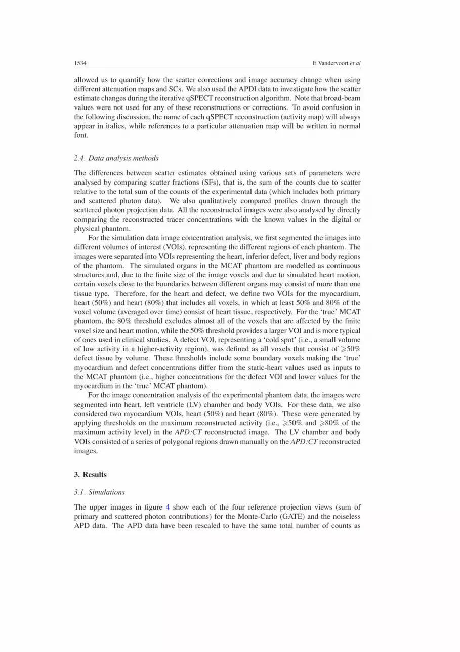
Figure 9. Horizontal profiles through the scatter projections computed at the eighth iteration of thereconstructions using the APDI:CT, APDI:PRO-SEG and APDI:PRO-UNSEG scatter corrections(a). Figure (b) shows scatter fractions computed as a function of projection angle for these data.

20 40 60 80 100 1200

5

10

15

20

25

30

35

Detector Bin

Sca

tter

Cou

nts

Vertical Profile

APD: CTAPDI: CT Iter. 1APDI: CT Iter. 3APDI: CT Iter. 8

−50 0 50 100 15024

25

26

27

28

29

30

Projection Angle (degrees)

Sca

tter

Fra

ctio

ns (

perc

ent)

APD: CTAPDI: CT Iter. 1APDI: CT Iter. 3APDI: CT Iter. 8

(a) (b)

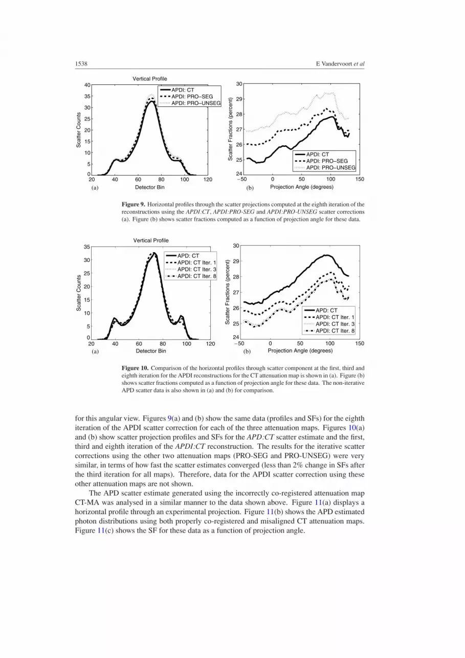
Figure 10. Comparison of the horizontal profiles through scatter component at the first, third andeighth iteration for the APDI reconstructions for the CT attenuation map is shown in (a). Figure (b)shows scatter fractions computed as a function of projection angle for these data. The non-iterativeAPD scatter data is also shown in (a) and (b) for comparison.

for this angular view. Figures 9(a) and (b) show the same data (profiles and SFs) for the eighthiteration of the APDI scatter correction for each of the three attenuation maps. Figures 10(a)and (b) show scatter projection profiles and SFs for the APD:CT scatter estimate and the first,third and eighth iteration of the APDI:CT reconstruction. The results for the iterative scattercorrections using the other two attenuation maps (PRO-SEG and PRO-UNSEG) were verysimilar, in terms of how fast the scatter estimates converged (less than 2% change in SFs afterthe third iteration for all maps). Therefore, data for the APDI scatter correction using theseother attenuation maps are not shown.

The APD scatter estimate generated using the incorrectly co-registered attenuation mapCT-MA was analysed in a similar manner to the data shown above. Figure 11(a) displays ahorizontal profile through an experimental projection. Figure 11(b) shows the APD estimatedphoton distributions using both properly co-registered and misaligned CT attenuation maps.Figure 11(c) shows the SF for these data as a function of projection angle.

Scatter corrections, attenuation map quality and absolute quantitation in SPECT 1539

20 40 60 80 100 1200

20

40

60

80

100

120

140

Detector Bin

Tot

al C

ount

sVertical Profile

ExperimentAPD: CTAPD: CT–MA

20 40 60 80 100 1200

5

10

15

20

25

30

35

Detector Bin

Sca

tter

Cou

nts

Vertical Profile

APD: CTAPD: CT–MA

−50 0 50 100 15023

24

25

26

27

28

29

30

Projection Angle (degrees)

Sca

tter

Fra

ctio

ns (

per

cent

)

APD: CTAPD: CT–MA

(a) (b)

(c)

Figure 11. Comparison of an experimental projection data profile and the CT and CT-MA estimatesof the sum of the scattered and unscattered photon data (a). A comparison of CT and CT-MAscatter profiles and scatter fractions are shown in (b) and (c), respectively.

Using an experimentally measured sensitivity factor of 5.59 ± 0.01 cpm kBq−1 and theknown voxel volume (0.11 cm3) and scan duration (20 s per view), the experimental datawere also converted into absolute reconstructed radiotracer concentrations. Tables 2 and 3summarize the average activity concentration over all voxels included in each VOI for thereconstruction methods which use the APD and APDI scatter corrections, respectively.

4. Discussion

4.1. Simulated data

The Monte-Carlo data generated using GATE agrees well with the APD data, both in termsof the appearance of the projections and the shape of the summed profiles shown in figure 4.The APD scatter fractions, for the views shown in this figure, were also found to be within2.0% of those computed for the GATE simulated data. These results are similar to the originalvalidation of Wells et al (1998), which found good agreement (e.g., normalized mean squareddifferences of less than two) between APD and two independent Monte-Carlo packages for

1540 E Vandervoort et al

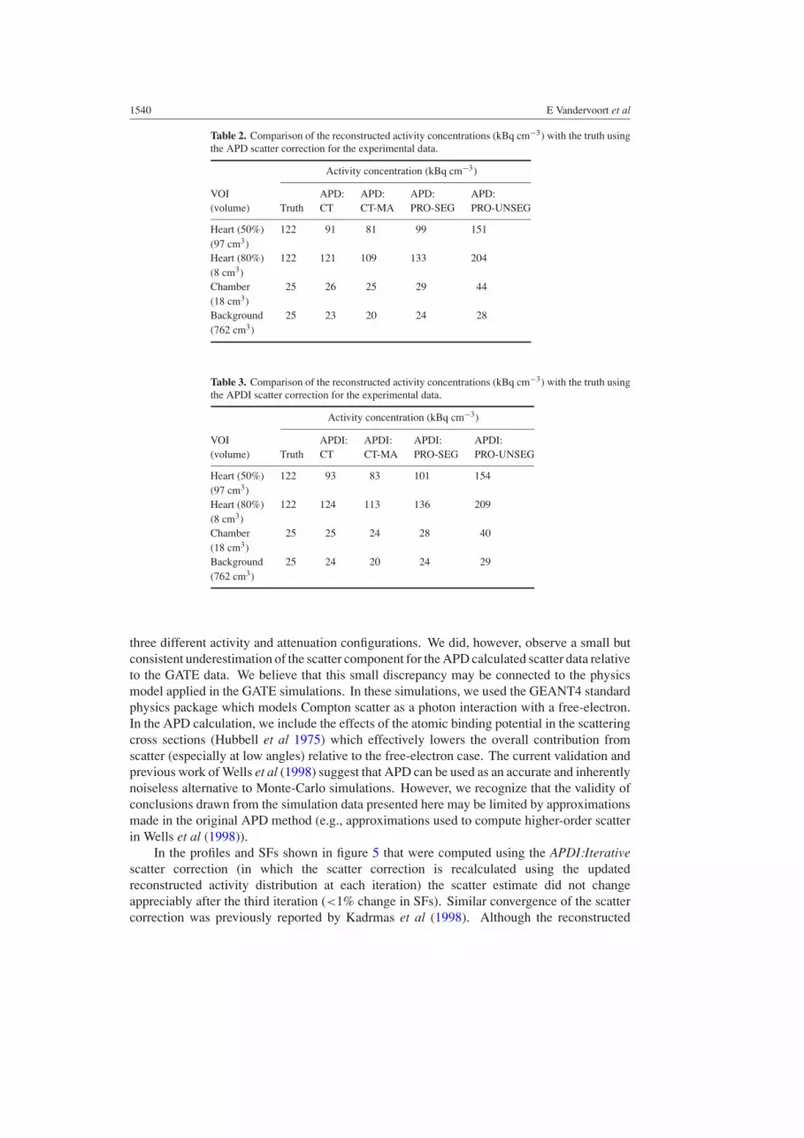
Table 2. Comparison of the reconstructed activity concentrations (kBq cm−3) with the truth usingthe APD scatter correction for the experimental data.

Activity concentration (kBq cm−3)

VOI APD: APD: APD: APD:(volume) Truth CT CT-MA PRO-SEG PRO-UNSEG

Heart (50%) 122 91 81 99 151(97 cm3)Heart (80%) 122 121 109 133 204(8 cm3)Chamber 25 26 25 29 44(18 cm3)Background 25 23 20 24 28(762 cm3)

Table 3. Comparison of the reconstructed activity concentrations (kBq cm−3) with the truth usingthe APDI scatter correction for the experimental data.

Activity concentration (kBq cm−3)

VOI APDI: APDI: APDI: APDI:(volume) Truth CT CT-MA PRO-SEG PRO-UNSEG

Heart (50%) 122 93 83 101 154(97 cm3)Heart (80%) 122 124 113 136 209(8 cm3)Chamber 25 25 24 28 40(18 cm3)Background 25 24 20 24 29(762 cm3)

three different activity and attenuation configurations. We did, however, observe a small butconsistent underestimation of the scatter component for the APD calculated scatter data relativeto the GATE data. We believe that this small discrepancy may be connected to the physicsmodel applied in the GATE simulations. In these simulations, we used the GEANT4 standardphysics package which models Compton scatter as a photon interaction with a free-electron.In the APD calculation, we include the effects of the atomic binding potential in the scatteringcross sections (Hubbell et al 1975) which effectively lowers the overall contribution fromscatter (especially at low angles) relative to the free-electron case. The current validation andprevious work of Wells et al (1998) suggest that APD can be used as an accurate and inherentlynoiseless alternative to Monte-Carlo simulations. However, we recognize that the validity ofconclusions drawn from the simulation data presented here may be limited by approximationsmade in the original APD method (e.g., approximations used to compute higher-order scatterin Wells et al (1998)).

In the profiles and SFs shown in figure 5 that were computed using the APDI:Iterativescatter correction (in which the scatter correction is recalculated using the updatedreconstructed activity distribution at each iteration) the scatter estimate did not changeappreciably after the third iteration (<1% change in SFs). Similar convergence of the scattercorrection was previously reported by Kadrmas et al (1998). Although the reconstructed

Scatter corrections, attenuation map quality and absolute quantitation in SPECT 1541

activity image used in the early iterations of OSEM usually has poor contrast, the scatterdistribution does not seem to depend strongly on the high-frequency components of the imagethat emerge in later iterations. Our results may indicate that it is only necessary to updatescatter during early iterations, and use a constant scatter estimate subsequently. We also foundvery little difference between the scatter estimates computed from reconstructions of the noisyand noise-free data. For example, the differences between the SFs for the APDI:Iterativereconstructions that used the noise-free (data not shown) and noisy data (shown in figure 5(b))differed by less than 0.2% at all iterations and for every projection view.

The scatter fraction (SF) and scattered photon profile data shown in figure 5 indicate thatthere is very little difference (<1% difference in SFs) between the APDI scatter correctionwith the true activity map (APDI:True-Activity) and those computed using later iterations(APDI:Iter. 2 and greater) of the qSPECT reconstructed activity map. However, the differencesbetween SFs computed using the more accurate APD and approximate APDI scatter correctionswere as high as 2.7% for certain projection angles even when the APDI correction used the trueactivity map. These differences are most noticeable in projection angles when the simulatedgamma camera was under the phantom (less than −90◦ or greater than +90◦) where the highlyattenuating spine and ribs influence the scatter distribution. These small discrepancies havebeen discussed previously in Vandervoort et al (2005) and are connected to approximationsmade in regards to the attenuation of scattered photons. These approximations combinedwith the coarse sampling of positions within the activity object (for which the probabilityof detecting scattered photons is calculated explicitly) can reduce the accuracy of the APDIcalculation under certain circumstances. For the simulation data, the APDI method used acoarse grid spacing of approximately 3 × 3 × 3 cm3. With this spacing, certain activity voxelpositions (e.g., those positions for which the spine or ribs lies directly between the activityvoxel and the detector array) may not be sampled in certain projection angles. This could leadto an underestimation of the attenuation of scattered photons (especially for low-angle scatter)and cause the intermittent ‘spikes’ or ‘dips’ in the SF values seen in figure 5(b). One possiblesolution for this problem would be to use finer sampling in highly non-uniform regions ofthe attenuation map to better sample the scatter probabilities in the APDI method. However,we do not expect that the differences between APD and APDI will have a significant effecton the reconstructions (which use the complete set of SPECT projections to create an image),since the differences between the SFs for the APD and APDI data (excluding APDI:Iter. 1)are less than 1% on average and do not exceed 3% for any projection view.

When the reconstructed activity concentrations in table 1 are compared to each other,there is very little difference between the concentrations using the ISR, APD or APDI scattercorrections. This seems to indicate that minor differences in how the scatter correction isimplemented (whether APD or APDI is used, only performing the scatter correction in theforward projection step, etc) influence only weakly the final activity concentrations. Whencomparing ISR to the reconstructions with APD or APDI scatter corrections, the maximumdifference between activity concentrations was 6% for the defect VOI and was less than 2%for all the other VOIs. For the BB and No SC reconstructions, however, the concentrations forthe defect VOI were 25% and 62% greater, respectively, than that of the ISR reconstruction.For the other VOIs (heart, liver and body), the concentrations for the BB reconstruction werewithin 5% to 7% of the ISR values while the No SC concentrations were between 27% and32% higher than those of the ISR reconstruction.

When the activity concentrations for the reconstructions that used the ISR, APD or APDIscatter corrections are compared with the ‘true’ measured values in table 1, these concentrationswere within 8% of the true values for all VOIs except the defect. The concentrations in thedefect VOI were about twice as large as the true value for the reconstructions with accurate

1542 E Vandervoort et al

SCs, and 2.6 and 3.4 times as large for the BB and No SC reconstructions, respectively. Asexpected, the No SC reconstruction provides the poorest agreement overall with the ‘true’concentrations, demonstrating the importance of performing some sort of scatter correctionfor cardiac SPECT. Large relative differences (≈7% and 8% ) were also observed for theAPDI:Iterative reconstructions for the low-threshold heart (50%) and liver VOI. Since similardifferences appeared in the ISR data in which no scatter was present in the data, they can notbe connected to the scatter correction and are related to other correction and reconstructionissues. In our opinion, the most likely explanation of these results is a combination of thepartial volume effect and imperfect resolution recovery. The diameter of the defect for thissimulation was about twice the FWHM of the spatial resolution of the simulated imagingsystem at the center of the field of view. For structures of this relative size, it is necessaryto correct the reconstructed images for the partial volume effect (PVE), using a method suchas that of Rousset et al (1998), in order to obtain more accurate quantification of radiotracerconcentrations. This type of VOI analysis could also benefit by repeating the entire processusing several different noise realizations of the simulated data. However, the analysis ofthe reconstruction using the noise-free data (where the largest differences in concentrationsbetween the noisy and noise-free data were about 5%) tentatively suggest that statistical noisedoes not play a large role in the results presented here.

4.2. Experimental data

The profiles and SFs shown in figure 7 and figure 9 demonstrate a systematic difference in theoverall magnitude of the scatter estimates corresponding to reconstructions that used differentattenuation maps. This was true regardless of whether APD or APDI scatter correctionswere used. The SF values presented in these two figures indicate that the overall sum of thecounts attributed to scatter was the lowest for the CT-based attenuation map. The SFs forthe segmented conventional SPECT attenuation map (PRO-SEG) were slightly higher (1%to 1.5% higher for certain projection angles) than the CT data SFs. The largest SFs werecalculated using the unsegmented SPECT attenuation map (PRO-UNSEG) with a maximumdifference between this and the CT data reaching about 2% for certain angles.

The comparison of the APD and the iterative APDI scatter correction data shown infigure 10 for the CT attenuation map displays similar behaviour to what was observed for theother two attenuation maps (data not shown). In general the scatter profiles and SFs appear toconverge (<1–2% change in SFs) by the second or third iteration. These results are consistentwith what was observed in the simulation studies and, once again, suggest that it may only benecessary to update the scatter correction in the early iterations of the reconstruction.

Systematic differences between the APD and APDI scatter corrections were obtainedusing the same attenuation map. These differences were similar in magnitude to the differencesbetween the SFs obtained using the same scatter correction with different attenuation maps.This may be seen, for example, in the APD and APDI scatter data for the CT attenuationmap in figure 10 and when comparing SFs for APD and APDI and all three attenuation mapsshown in figures 7 and 9. These differences were most pronounced for the CT attenuation mapwhere the ‘converged’ APDI scatter fraction data were on average about 2% lower than theAPD values. This was probably due to the larger errors in APDI approximations (discussedpreviously), since the higher-resolution CT map contained more variation in its attenuationvalues such as the phantom’s Teflon spine (see figure 2).

In general the properly co-registered CT and PRO-SEG reconstructed images displaythe best agreement with the measured ‘true’ concentrations. The reconstructed activityconcentrations summarized for the LV chamber and body VOIs in tables 2 and 3 are within

Scatter corrections, attenuation map quality and absolute quantitation in SPECT 1543

4% of the measured values for the CT attenuation map for both the APD and APDI scattercorrections. For the APDI:PRO-UNSEG and APD:PRO-UNSEG images there was a consistentoverestimation of concentrations due to the higher linear attenuation coefficients observed inthe attenuation map (see figure 2). This error in attenuation coefficients is probably due toinadequate corrections for cross-talk contamination in the transmission scans (Celler et al2003) and is more severe for objects deeper inside the attenuating medium (the heart andLV chamber VOIs). The improved activity concentration estimates obtained for the PRO-SEG data seem to indicate that these effects are largely overcome by simply segmenting theattenuation map.

In tables 2 and 3 large differences are evident between the true activity concentrationin the lower-threshold VOI, heart (50%), and the corresponding values for images obtainedusing all attenuation maps. As in the simulation study, this result is likely due to imperfectresolution recovery and the finite size of the reconstructed image voxel. The thickness ofthe myocardium insert is only about twice the size of the image voxels and is approximatelyequal to the spatial resolution of the imaging system at the centre of rotation. Therefore,a low threshold (50%) will inevitably include many voxels that only partially belong to themyocardium and hence decrease the average value of measured activity. The errors for thesimulation data were smaller because the ‘true’ concentrations for the heart and defect VOIs(that we compared to reconstructed values) included the effects of the finite voxel size andheart motion (see the discussion in section 2.2).

Errors in the scatter correction introduced by the misalignment of the CT attenuationmap (CT-MA) were considerably more significant than those observed using the other three(correctly aligned) attenuation maps. The differences in SFs between the CT and CT-MAdata were as high as 5% and the CT-MA scatter profiles were visibly skewed. The errorsin reconstructed activity concentration were comparable to those observed when using theunsegmented PRO-UNSEG data. Interestingly, in figure 11(a) the sum of primary andscatter distributions obtained using either of the CT maps appear to provide a good fit tothe experimental data. It is only when we consider the scatter distribution that the effects ofthe misalignment become more apparent (figure 11(b)).

5. Conclusions

We have presented a quantitative reconstruction algorithm, qSPECT, for the determination ofabsolute radiotracer concentrations in SPECT imaging. The qSPECT reconstruction employscorrections for collimator blurring, attenuation and scatter. Our investigation focused on theimplementation of an iterative scatter correction (SC) and on the influence of attenuationmap quality on quantitation. The accuracy of reconstructed tracer concentrations and scattercorrections were evaluated using simulated and experimental phantom studies.

Using simulated data we found that the qSPECT scatter correction did not changeappreciably (<1% change in the estimated scatter fractions) after the third iteration of theqSPECT reconstruction. These results indicate that SCs only need to be updated in the earlyiterations of the reconstruction process. Our conclusions are cautionary, however, since weare using a lower-resolution SC (i.e., in APDI only a subset of the activity voxels are sampled)which could lead to faster convergence than a higher resolution correction. For the simulationdata we found that radiotracer concentrations for qSPECT images were within 6% of the‘true’ values for all VOIs considered except for a ‘cold spot’ volume of interest (the defect).This error occurred even for simulated data in which no scatter was present (ISR), suggestingthat this effect is not related to the SC and is, rather, the result of imperfect corrections forcollimator blurring and the partial volume effect.

1544 E Vandervoort et al

For the experimental phantom data the iterative SC also remained relatively constant(<2–3% change in scatter fractions depending on the attenuation map and SC used) after thesecond or third iteration of the qSPECT reconstruction. We found systematic differences (ashigh as 2%) in the sum of the counts attributed to scatter when different attenuation maps andscatter corrections were used. Larger differences (as high as 5%) were observed in scatterfractions using a CT attenuation map that was intentionally misaligned (even by just a fewcentimetres). The quantitative accuracy of tracer concentrations were found to be better whenusing CT data than those that used conventional SPECT transmission scan (PRO-SEG andPRO-UNSEG). This conclusion is, however, based on the analysis of the phantom data whichhas more uniform attenuation and activity distributions than would occur in a typical patientstudy. Other issues (e.g., beam hardening and/or patient breathing and movement) mayreduce the accuracy of SPECT images using CT-based attenuation and scatter corrections.The general validity of the conclusions made here, regarding absolute quantitation in cardiacSPECT, could also be improved by repeating this type of analysis for many noise realizationsof the measured data and averaging the results.

References

Bai C, Zheng G and Gullberg G 2000 A slice-by-slice blurring model and kernel evaluation using the Klein-Nishinaformula for 3D scatter compensation in parallel and converging beam SPECT Phys. Med. Biol. 45 1275–307

Beekman F, de Jong H and Geloven S 2002 Efficient fully 3-D iterative SPECT reconstruction with Monte Carlo-basedscatter compensation IEEE Trans. Med. Imaging 21 867–77

Blinder S, Celler A, Wells R G, Thompson D and Harrop R 2001 Experimental verification of 3D detector responsecompensation using the OSEM reconstruction method IEEE Nucl. Sci. Symp. and Med. Imaging Conf. Rec.(San Diego, 2005) pp 2174–8

Celler A, Dixon K, Chang Z, Blinder S, Powe J and Harrop R 2005 Problems created in attenuation-corrected SPECTimages by artifacts in attenuation maps: a simulation study J. Nucl. Med. 46 335–43

Dixon K L, Vandervoort E J, Blinder S and Fung A 2004 The effect of SPECT reconstruction corrections on theabsolute and relative quantitative accuracy of myocardial perfusion studies IEEE Nucl. Sci. Symp. and Med.Imaging Conf. Rec. (Rome, 2004) pp 3643–7

Frey E and Tsui B 1996 A new method for modeling the spatially-variant, object-dependent scatter response functionin SPECT IEEE Nucl. Sci. Symp. and Med. Imaging Conf. Rec. (Anaheim, 1996) pp 1082–6

Gonzalez D E, Jaszczak R J, Bowsher J E, Akabani G and Greer K L 2001 High-resolution absolute SPECTquantitation for I-131 distributions used in the treatment of lymphoma: a phantom study IEEE Trans. Nucl. Sci.48 707–14

He B, Du Y, Song X, Segars W P and Frey E C 2005 A Monte Carlo and physical phantom evaluation of quantitativeIn-111 SPECT Phys. Med. Biol. 50 4169–85

Hubbell J H, Veigele W J, Briggs E A, Brown R T, Cromer D T and Howerton R J 1975 Atomic form factors,incoherent scattering functions, and photon scattering cross sections J. Phys. Chem. Ref. Data 4 471–538

Jan S et al 2004 GATE: a simulation toolkit for PET and SPECT Phys. Med. Biol. 49 4543–61Jaszczak R, Coleman R and Whitehead F 1981 Physical factors affecting quantitative measurements using camera-

based single photon emission computed tomography (SPECT) IEEE Trans. Nucl. Sci. 28 69–79Jaszczak R, Greer K, Floyd C, Harris C and Coleman R 1984 Improved SPECT quantification using compensation

for scattered photons J. Nucl. Med. 25 893–900Kadrmas D, Frey E, Karimi S and Tsui B 1998 Fast implementations of reconstruction-based scatter compensation

in fully 3D SPECT image reconstruction Phys. Med. Biol. 43 857–73King M A, Hademeos G and Glick S J 1992 A dual photopeak window method for scatter correction J. Nucl. Med.

33 606–12Liang Z, Ye J, Cheng J, Li J and Harrington D 1998 Quantitative cardiac SPECT in three dimensions: validation by

experimental phantom studies Phys. Med. Biol. 43 905–20Logan K W and McFarland W D 1992 Single photon scatter compensation by photopeak energy distribution analysis

IEEE Trans. Med. Imaging 11 161–4Ogawa K, Harata Y, Ichihara T, Kubo A and Hashimoto S 1991 A practical method for position-dependent Compton-

scatter correction in single photon emission CT IEEE Trans. Med. Imaging 10 408–12

Scatter corrections, attenuation map quality and absolute quantitation in SPECT 1545

Pretorius P, Xia W, King M, Tsui B, Pan T and Villegas B 1997 Evaluation of right and left ventricular volume andejection fraction using a mathematical cardiac torso phantom for gated pool SPECT J. Nucl. Med. 38 1528–34

Rousset O G, Ma Y and Evans A C 1998 Correction for partial volume effects in PET: principle and validationJ. Nucl. Med. 39 904–11

Soret M, Koulibaly P M, Darcourt J, Hapdey S and Buvat I 2003 Quantitative accuracy of dopaminergicneurotransmission imaging with 123I SPECT J. Nucl. Med. 44 1184–93

Vandervoort E J, Celler A, Wells R G, Blinder S, Dixon K L and Pang Y 2005 Implementation of an analyticallybased scatter correction in SPECT reconstructions IEEE Trans. Nucl. Sci. 52 645–53

Wells R G, Celler A and Harrop R 1998 Analytical calculation of photon distributions in SPECT projections IEEETrans. Nucl. Sci. 45 3202–14

Ye J, Liang Z and Harrington D P 1994 Quantitative reconstruction for myocardial perfusion SPECT: an efficientapproach by depth-dependent deconvolution and matrix rotation Phys. Med. Biol. 39 1263–79