Embed Size (px)
Citation preview
DOE/MC/28087 -- 5026 (DE96000S 5 5)
< J S T ~ Integrated Seismic Study of Naturally Fractured Tight Gas Reservoirs
Final Report September 1991 - January 1995
Gary Mavko Amos Nur
January 1995
Work Performed Under Contract No.: DE-AC2 1-9 1 MC28087
For U.S. Department of Energy Office of Fossil Energy Morgantown Energy Technology Center Morgantown, West Virginia
BY Stanford University Stanford, California
DISCLAIMER
This report was prepared as an account of work sponsored by an agency of the United States Government. Neither the United States Government nor any agency thereof, nor any of their employees, makes any warranty, express or implied, or assumes any legal liability or responsibility for the accuracy, completeness, or usefulness of any information, apparatus, product, or process disclosed, or represents that its use would not infringe privately owned rights. Reference herein to any specific commercial product, process, or service by trade name, trademark, manu- facturer, or otherwise does not necessarily constitute or imply its endorsement, recommendation, or favoring by the United States Government or any agency thereof. The views and opinions of authors expressed herein do not necessarily state or reflect those of the United States Government or any agency thereof.
This report has been reproduced directly from the best available COPY-
Available to DOE and DOE contractors from the Office of Scientific and Technical Information, 175 Oak Ridge Turnpike, Oak Ridge, TN 37831; prices available at (615) 576-8401.
Available to the public from the National Technical Information Service, U.S. Department of Commerce, 5285 Port Royal Road, Springfield, VA 22161; phone orders accepted at (703) 487-4650.
DOERvICI28087 -- 5026 (DE96000555)
Distribution Category UC-132
Integrated Seismic Study of Naturally Fractured Tight Gas Reservoirs
Final Report September 1991 - January 1995
Gary Mavko Amos Nur
Work Performed Under Contract No.: DE-AC2 1 -9 1 MC28087
For U.S. Department of Energy
Office of Fossil Energy Morgantown Energy Technology Center
P.O. Box 880 Morgantown, West Virginia 26507-0880
BY Stanford University
857 Serra Street, Room 260 Stanford, California 94305-22 1 5
ABSTRACT There is probably no single seismic attribute that will always tell us all that we need
to know about fracture zones. Therefore, our approach in this project has been to integrate the principles of Rock Physics into a quantitative processing and interpretation scheme that exploits, where possible, the broader spectrum of fracture zone signatures: (1) anomalous compressional and shear wave velocity; (2) Q and velocity dispersion; (3) increased velocity anisotropy; (4) amplitude vs. offset (AVO) response, and (5) variations in frequency content. As part of this we have attempted to refine some of the theoretical rock physics tools that should be applied in any field study to link the observed seismic signatures to the physical/geologic description of the fractured rock. Furthermore, while we have used standard shear wave techniques to process and analyze our field data, our ’
goal in this project has been to explore also non-shear wave methods. The project had 3 key elements: (1) Rock Physics studies of the anisotropic viscoelastic signatures of fractured rocks, (2) Acquisition and processing of seismic reflection field data, and (3) Interpretation of Seismic and well log data.
Throughout the field site, the fracture directions, inferred from the shear-wave rotation analysis on all four lines, trend consistently SW-NE - all generally within about 200 of each other. These trends were taken to be equal to the polarization direction of the fast shear wave after rotation. The fracture intensity was taken to be proportional to relative time difference between the fast and slow shear waves at each location. This travel time difference (inferred fracture intensity) is highly variable throughout the site - the corresponding shear-wave anisotropy in the Frontier-Nibrara zones ranges from near zero to as much as 7 percent. The regions of largest anisotropy along the four lines can be intepreted with two localized zones of relatively intense fracturing.
Several attributes of the P-wave data were found to be consistent with, and possibly indicators of fractures: Strong lateral variations in P-wave reflectivity, AVO response, and frequency content were observed. Although we did not attempt to model quantitatively their response, they could be indicators of gas and fractures. However, such scalar attributes along a single 2-D line - no matter how striking - cannot give information about the direction of fractures that is so critical for designing wells. It is possible that with more work, we could learn to combine these scalar attributes with independent fracture direction information (for example from regional trends, or measured stress directions) to quantitatively characterize fractures. We recommend further work in learning to quantify the various P-wave scalar attributes associated with fractures.
Perhaps most intriguing are the several indications of P-wave anisotropy that we observed. Azimuthal variations of AVO response and P-wave stacking velocity were observed at two locations where lines intersect. The azimuthal velocity variation is consistent with the directions of the fracture model.
Important conclusions are that P-wave fracture attributes look promising, but at the same time 2-D single component surveys are likely to be inadequate for fracture mapping. In our survey, only two line intersections allowed us to even look for azimuthal P-wave variations. We recommend looking for these variations in 3-D single component data. 3-D data will allow, in general, a more complete sampling of azimuths at many CDPs. Partly as a result of this work, new 3-D studies are underway to look for fracture- related azimuthal variations of P-wave stacking velocity and AVO.
ACKNOWLEDGMENTS
The authors gratefully acknowledge the Department of Energy Morgantown Energy Technology Center, and especially the DOE project manager, Royal Watts, for the major financial and technical support for this project. We also acknowledge Amoco Production Company (especially Pat Jackson, Craig Jarchow, Daniel Johnson, Clyde Kelley, Clyde McGee, and Mike Mueller) and ArcoNastar Resources (Rob Withers and Melinda Gale) for cofunding of the field operations and for many useful technical comments on the data acquisition design, processing, and interpretation. The Stanford team that contributed to this work also includes Dr. Jack Dvorkin, Wei Chen, Li Teng, Tapan Mukerji, Dr. Rob Walters, and Nikki Godfrey. Some of the Stanford Faculty and Students also received co-funding from the Stanford Rockphysics and Borehole geophysics (SRB) project, and Gas Research Institute.
TABLE OF CONTENTS
ABSTRACT ACKNOWLEDGMENTS EXECUTIVE SUMMARY INTRODUCTION BACKGROUND
Laboratory Studies Seismic Field Studies of Fracture Anisotropy The Problem of Upscaling from the Laboratory to the Field
Fluid Effects on Seismic Anisotropy A Method for Predicting Stress-induced Seismic Anisotropy
Regional Geologic Framework and Site Description Seismic Data Acquisition Shear Wave Data and Validation P-Wave Data Analysis
LABORATORY AND THEORETICAL ROCK PHYSICS
FIELD EXPERIMENT
CONCLUSIONS REFERENCES
page ii page iii
Page 1 Page 3 Page 5 page 5 Page 9 page 11 page 15 page 15 page 31 page 41 page 41 page 59 page 65 page 87 page 99
page 103
EXECUTIVE SUMMARY
There is probably no single seismic attribute that will always tell us all that we need to know about fracture zones. Therefore, our approach in this project has been to integrate the principles of Rock Physics into a quantitative processing and interpretation scheme that exploits, where possible, the broader spectrum of fracture zone signatures: (1) anomalous compressional and shear wave velocity; (2) Q and velocity dispersion; (3) increased velocity anisotropy; (4) amplitude vs. offset (AVO) response, and (5) variations in frequency content.
As part of this we have attempted to refine some of the theoretical rock physics tools that should be applied in any field study to link the observed seismic signatures to the physical/geologic description of the fractured rock. Furthermore, while we have used standard shear wave techniques to process and analyze our field data, our goal in this project has been to explore also non-shear wave methods. The project had 3 key elements:
Rock Physics studies of the anisotroDic viscoelastic signatures of fractured rocks.
We completed two major new contributions for relating the physical or geologic description of fractures to their seismic signatures. In the first study we discussed how the anisotropic viscoelastic signature of a fractured rock varies with the pore fluid type in the fracture, and furthermore how the anisotropic signature for a fluid-bearing rock can be much different at high frequencies than at low frequencies. Many previous studies have used Hudson's (1980) elegant formulation to describe fractured rocks without making the necessary corrections for these fluid and frequency effects.
In the second study we presented a simple procedure for using measured isotropic values of Vp and Vs versus hydrostatic loading to estimate the stress-induced velocity anisotropy under general nonhydrostatic loading. The method uses simple physical assumptions about crack closure to create the hydrostatic to nonhydrostatic stress transform. Yet, it is independent of any idealized crack geometry, and is not intrinsically limited to low crack concentrations. We represent the pore space with a generalized stress-dependent compliance, which can be determined from the hydrostatic measurements.
An area that needs additional work is to reconcile the various different theoretical formulations for fractured rock the elliptical inclusion model of Hudson (1980), the finely layered medium model of Schoenberg (1988), and the discrete fracture model of Pyrak-Nolte (1990). Each has its advantages and limitations; a unified description should result in a more flexible set of tools for modeling fractures.
Acquisition and processing of seismic reflection field data.
With the generous help and expertise of our partners at Amoco and Arcomastar Resources, we successfully acquired and processed nearly 50 km of 2-D, 9-component reflection data over a fractured site in the Powder River basin of Wyoming. The S-wave data were of moderately good quality, allowing us to develop a fracture model for the site by combining shear wave splitting rotation analysis with well control. The P-wave data were of very good quality, allowing us to see lateral variations in reflectivity, AVO response, and frequency content (attenuation) as well as some evidence for azimuthally dependent AVO and P-wave stacking velocities.
1
Intemretation of Seismic and well log: data
Throughout the site, the fracture directions, inferred from the shear-wave rotation analysis on all four lines, trend consistently SW-NE - all generally within about 200 of each other. These trends were taken to be equal to the polarization direction of the fast shear wave after rotation. The fracture intensity was taken to be proportional to relative time difference between the fast and slow shear waves at each location. This travel time difference (inferred fracture intensity) is highly variable throughout the site - the corresponding shear-wave anisotropy in the Frontier-Nibrara zones ranges fkom near zero to as much as 7 percent. The regions of largest anisotropy along the four lines can be intepreted with two localized zones of relatively intense fracturing.
The Red Mountain 1-H well was drilled near the intersection of line 2 and line 3 after the seismic study, using the derived fracture model. The well was reported hitting numerous fractures, consistent with the fracture model, and the test production on July 18, 1994 showed 1068 MCFGPD, 32BOPD and only 3 barrels of water per day. The initial result demonstrated once again the effectiveness of the four-component shear-wave method developed by Alford et. al. A number of older vertical wells confirm the fracture model. For example the Chinook Lois, Apache Githens, and Energetics Simms wells (Table 4) all lie within the fracture zones (gray in Figure 43) and all have shown reasonable production. A few others outside of the interpreted fracture zones performed much worse.
Several attributes of the P-wave data were found to be consistent with, and possibly indicators of fractures: Strong lateral variations in P-wave reflectivity, AVO response, and frequency content were observed. Although we did not attempt to model quantitatively their response, they could be indicators of gas and fractures. However, such scalar attributes along a single 2-D line - no matter how striking - cannot give information about the direction of fractures that is so critical for designing wells. It is possible that with more work, we could learn to combine these scalar attributes with independent fracture direction information (for example from regional trends, or measured stress directions) to quantitatively characterize fractures. We recommend further work in learning to quantify the various P-wave scalar attributes associated with fractures.
Perhaps most intriguing are the several indications of P-wave anisotropy that we observed. Azimuthal variations of AVO response and P-wave stacking velocity were observed at two locations where lines intersect. The azimuthal velocity variation is consistent with the directions of the fracture model.
Important conclusions are that P-wave fracture attributes look promising, but at the same time 2-D single component surveys are likely to be inadequate for fracture mapping. In our survey, only two line intersections allowed us to even-look for azimuthal P-wave variations. We recommend looking for these variations in 3-D single component data. 3-D data will allow, in general, a more complete sampling of azimuths at many CDPs. Partly as a result of this work, new 3-D studies are underway to look for fracture- related azimuthal variations of P-wave stacking velocity and AVO.
INTRODUCTION In situ permeability can be largely controlled by natural fracture systems. In tight
formations, which can include sandstones, shales, limestones, and coal, often the only practical means to extract hydrocarbons is by exploiting the increased drainage surface provided by natural fracture zones (Szpakiewicz et al., 1986; Lorenz et al., 1986). The practical difficulties that must be overcome before effectively using these fractures include: locating the position and orientation of fracture zones, determining the intensity of fracturing, and characterizing the spatial relationships of these fractures relative to reservoir heterogeneities which might enhance or inhibit the eventual gas flow.
Reflection seismic methods are, and will continue to be, the key geophysical tool for imaging these heterogeneities in the subsurface of the earth. Seismic methods provide a unique combination of penetration range and resolution that is not achievable by any other means. During the last 5 to 10 years, considerable emphasis has been placed on seismic velocity anisotropy as the key indicator of fractures. Multicomponent VSP and surface reflection seismic studies have shown striking evidence for anisotropy, primarily from shear wave splitting (Alford, 1986; Crampin et al., 1986; Mueller, 1992). Most seismic studies have focused only on these relatively expensive multicomponent (shear- wave) methods. Yet, we have not exploited fully the velocity, amplitude, and frequency information in the better-established and more cost effective single component (P-wave) data.
Another critical missing ingredient, which has limited the attractiveness of nearly all seismic studies to reservoir engineers, is the precise and quantitative connection at fieEd scales between seismic data and the fracture properties that control reservoir production. Laboratory studies have confmed the quantitative relation between seismic and fracture properties at the core scale. However, even the most comprehensive published field studies suggesting seismic evidence of fracturing have been validated only by anisotropy directions consistent with mapped fracture trends. Furthermore, until recently there has been no published theory that adequately predicts the velocity-fracture relations for dry and saturated anisotropic rocks over the range of frequencies and scales between in situ and laboratory conditions.
There is probably no single seismic attribute that will always tell us what we need to know about fracture zones. Therefore, our approach in this project has been to integrate the principles of Rock Physics into a quantitative processing and interpretation scheme that exploits, where possible, the broader spectrum of fracture zone signatures:
(1) anomalous compressional and shear wave velocity; (2) Q and velocity dispersion; (3) increased velocity anisotropy; (4) amplitude vs. offset (AVO) response, and (5) variations in frequency content,
As part of this we have attempted to refine some of the theoretical rock physics tools that should be applied in any field study to link the observed seismic signatures to the physical/geologic description of the fractured rock. Furthermore, while we have used standard shear wave techniques to process and analyze our field data, our goal in this project has been to explore also non-shear wave methods (i.e., single component, P-wave data), with several motivations in mind: (1) Four and nine-component data are very expensive to collect and process; (2) Most existing data (including all marine data) are
3
conventional compressional-wave data; (3) More and more 3D P-wave data of higher quality are becoming available, and a variety of their orientation-dependent attributes may be used to study the anisotropic properties of the Earth (Lewis, 1989).
The project had 3 key elements:
(1) Rock Physics studies of the anisotropic viscoelastic signatures of fractured rocks.
(2) Acquisition and processing of seismic reflection field data. (3) Integration and interpretation of seismic, well log, and laboratory data.
4
BACKGROUND: THE GEOPHYSICAL SIGNATURES OF FRACTURED ROCKS
LABORATORY STUDIES - THE HISTORICAL BASIS FOR GEOPHYSICAL FRACTURE DETECTION
The basis for virtually all modem seismic strategies for detecting fractures lies in laboratory studies, such as those performed by Nur and coworkers more than two decades ago (eg., Nur and Simmons, 1969; Nur, 1971). They discovered three key results that have been subsequently confirmed and refined by scores of other researchers (e.g., Toksoz et al., 1976; Lockner et al., 1977; Jones, 1983; Coyner, 1984; Coyner and Cheng, 1985; W i d e r , 1985,1986; Tariff, 1988; Zamora and Poirier, 1990):
Cracks and fractures always reduce the seismic P- and S-wave velocities in rocks, relative to the same rock without fractures. Gas in rocks can be distinguished by generally lower seismic P-wave velocities relative to fluid-saturated rocks, and this sensitivity is dramatically enhanced by the presence of cracks. Oriented fractures can result in marked, measurable P- and S-wave seismic anisotropy.
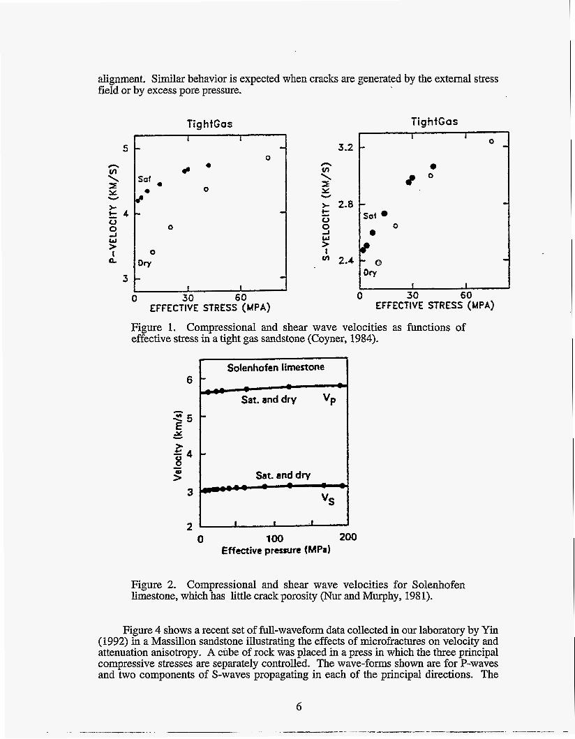
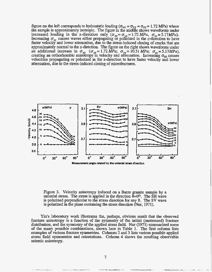
Typical behavior of P- and S-wave velocities in cracked crustal rocks is illustrated in Figure 1 for a tight gas sandstone. The dry and saturated data for both P and S waves show a large and rapid increase with confining pressure, which is usually attributed to crack and fracture porosity (Nur, 1971; Toksoz et al., 1976; Walsh, 1965). As confining pressure is increased, the most compliant pores (ie., cracks and fractures) are pressed closed, followed by the next less compliant, and so on. Contrast this behavior with velocities for Solenhofen limestone, shown in Figure 2. This rock is relatively free of cracks, and consequently there is very little change of velocity with confining pressure.
Fluid saturation has the greatest effect on the crack portion of the porosity in these examples (Figures 1 and 2) with the following key features:
Fluid saturation almost always increases compressional velocity, particularly at low effective pressure when cracks are present. Fluid saturation tends to decrease the dependence of compressional velocity on effective pressure. Fluid saturation has relatively little effect on shear velocity.
The implications of these are that cracks and fractures enhance our ability to seismically detect gas vs. water or oil saturation by (1) enhancing the net decrease in V p with gas, (2) by enhancing the drop in VpNs with gas, and if cracks are aligned, (3) by increasing the degree of velocity anisotropy.
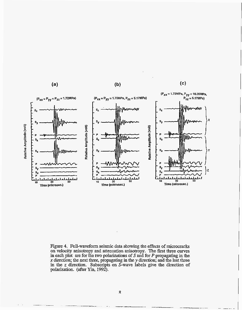
Figure 3 illustrates the effects of crack alignment on seismic anisotropy (Nur, 1971) - the central feature of seismic strategies for fracture detection. In this case the crack porosity is essentially isotropic at low stress. As uniaxial stress is applied, crack anisotropy is induced by preferentially closing cracks that are perpendicular or nearly perpendicular to the axis of compression. The velocities - compressional and two polarizations of shear - clearly vary with direction relative to the stress-induced crack
5
alignment. Similar behavior is expected when cracks are generated by the external stress field or by excess pore pressure.
TightGas
5 s
3
0 30 60 EFFECTIVE STRESS (MPA)
TightGas
3.2 h c E Y
+ 2.8 L I- 0 0 0 2 0 w > I
Saf -
v, 2.4 0 - - Dry
- I t
0 30 60 EFFECTIVE STRESS (MPA)
Figure 1. Compressional and shear wave velocities as functions of effective stress in a tight gas sandstone (Coyner, 1984).
Solenhofen iimestone
P 5 E s -
3
2 ' I 1 I 1
0 100 200 Effective pressure (MPa)
Figure 2. Compressional and shear wave velocities for Solenhofen limestone, which has little crack porosity (Nur and Murphy, 198 1).
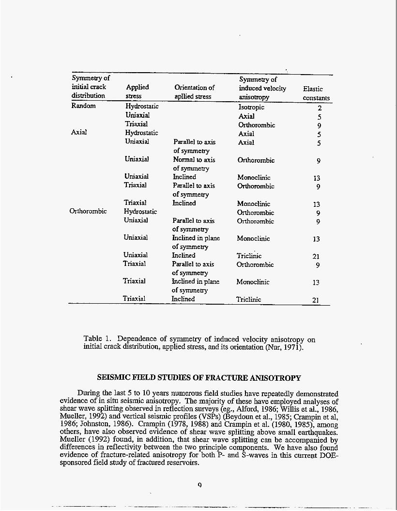
Figure 4 shows a recent set of full-waveform data collected in our laboratory by Yin (1992) in a Massillon sandstone illustrating the effects of microfractures on velocity and attenuation anisotropy. A cube of rock was placed in a press in which the three principal compressive stresses are separately controlled. The wave-forms shown are for P-waves and two components of S-waves propagating in each of the principal directions. The
6
= czz = 1.72 MPa) where figure on the left corresponds to hydrostatic loading (exx = the sample is approximately isotropic. The figure in the mid e shows waveforms under increased loading in the z-direction only (on = 0 = 1.72 MPa, oZ = 5.17MPa). Increasing o;, causes waves either propagating or p o g z e d in the z-direction to have faster velocity and lower attenuation, due to the stress-induced closing of cracks that are approximately normal to the z-direction. The figure on the right shows waveforms under an additional increase in our (oq= 1.72 MPa; B = 10.31 MPa; oZ=5.17MPa), creating an orthorhombic anisotropy in velocity and ai?ltenuation. Increasing czz causes velocities propagating or polarized in the z-direction to have faster velocity and lower attenuation, due to the stress-induced closing of microfractures.
e8
4.8
4.6 3 5.4.4 - >. u 0 .= 4.2
5 4.0
3.8
3.6
-
3.1 - sv o(MPa)
2.9 - /-=\20
1 I
0" 3oo .60° 9oo
2.7
3.1 - SH
2.7 10
1 I 4 I
o0 3oo 60" 90"
Measurement angle related to the uniaxial dross direction
Figure 3. Velocity anisotropy induced on a Barre granite sample by a uniaxial stress. The stress is applied in the direction 8=00. The SH wave is polarized perpendicular to the stress direction for any 8. The SV wave is polarized in the plane containing the stress direction (Nu, 1971).
Yin's laboratory work illustrates the, perhaps, obvious result that the observed fracture anisotropy is a function of the symmetry of the initial (unstressed) fracture distribution, and the symmetry of the applied stress field. Nur (1971) summarized some of the many possible combinations, shown here in Table 1. The first column lists examples of various fracture symmetries. Columns 2 and 3 lists various possible applied stress field symmetries and orientations. Column 4 shows the resulting observable seismic anisotropy.
7
pZz = 1.72MPa) (pXx = pW = 1.72MPa. Pu = 5.17MPa) r
Pxx = pyy = -
10 30 50 Time (microsec.)
SZ
- SY
-
'P
- sz
- sx - P - SY.
- sx P l . l . I . l . l . l . l . l . ~ . ~ ~ I 10 30 50
- Time (microsec.)
(Pxx = 1.72MPa. Pyy = 10.35MPa, P,, = 5.17MPa)
r
10 30 50 Time (microsec.)
Figure 4. Full-waveform seismic data showing the effects of microcracks on velocity anisotropy and attenuation anisotropy. The first three curves in each plot are for the two polarizations of S and for P propagating in the x direction; the next three, propagating in the y direction; and the last three in the z direction. Subscripts on S-wave labels give the direction of polarization. (after Yin, 1992).
Symmetry of Symmetry of initial crack Applied Orientation of induced velocity Elastic distribution smss apllied stress anisotropy cOnstantS Random
Axial
Orthorombic
Hydrostatic Uniaxial Triaxial Hydrostatic Uniaxial
Uniaxial
Uniaxial Triaxial
Triaxial Hydrostatic Uniaxial
Uniaxial
Uniaxial Triaxial
Triaxial
Triaxial
Parallel to axis of symmetry Normal to axis of symmetry Inclined Parallel to axis ofsymmetry Inclined
Parallel to axis
Inclined in plane
Inclined Parallel to axis
Inclined in plane of symmetry Inclined
of symmetry
of symmetry
ofsymmew
Isotropic Axial Orthorombic Axial Axial
Orthorombic
Monoclinic Orthorombic
Monoclinic Orthorombic Orthorombic
Monoclinic
Tricli&c Orthorombic
Monoclinic
9
13 9
13 9 9
13
21 9
13
Triclinic 21
Table 1. Dependence of symmetry of induced velocity anisotropy on initial crack distribution, applied stress, and its orientation (Nur, 1971).
SEISMIC FIELD STUDIES OF FRACTURE ANISOTROPY
During the last 5 to 10 years numerous field studies have repeatedly demonstrated evidence of in situ seismic anisotropy. The majority of these have employed analyses of shear wave splitting observed in reflection surveys (eg., Alford, 1986; Willis et al., 1986, Mueller, 1992) and vertical seismic profiles (VSPs) (Beydoun et al., 1985; Crampin et al, 1986; Johnston, 1986). Crampin (1978,1988) and Crampin et al. (1980, 1985), among others, have also observed evidence of shear wave splitting above small earthquakes. Mueller (1992) found, in addition, that shear wave splitting can be accompanied by differences in reflectivity between the two principle components. We have also found evidence of fracture-related anisotropy for both P- and S-waves in this current DOE- sponsored field study of fractured reservoirs.
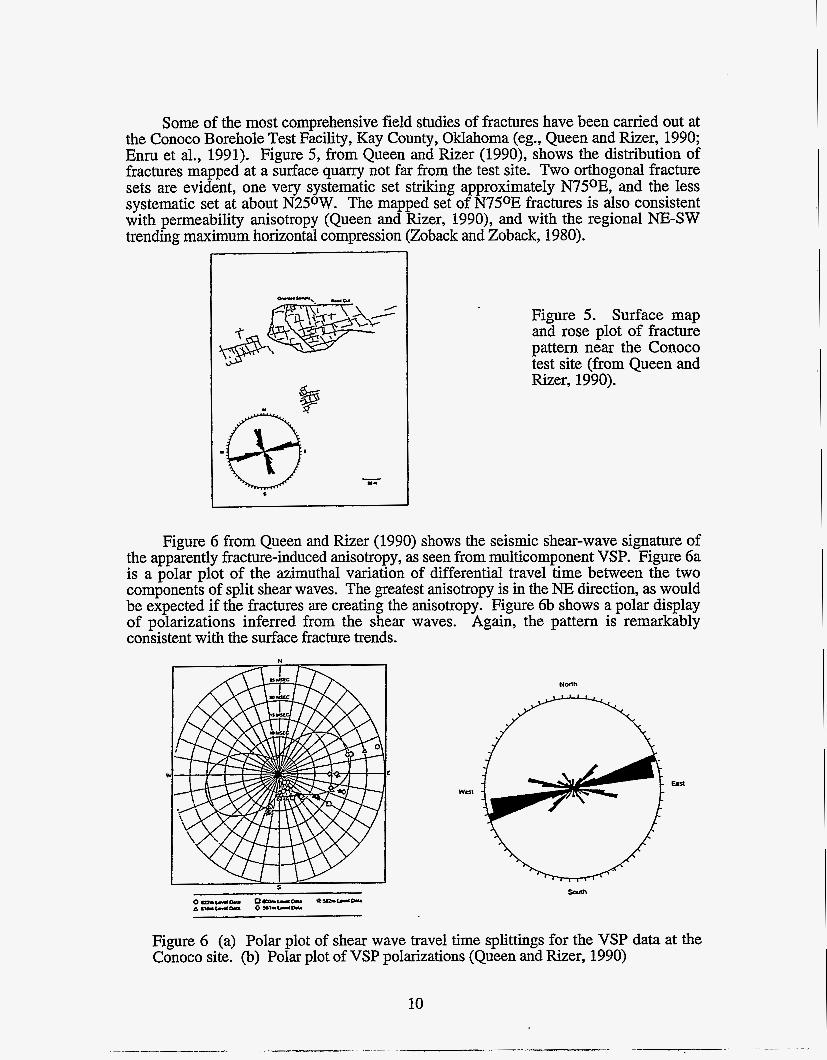
Some of the most comprehensive field studies of fractures have been carried out at the Conoco Borehole Test Facility, Kay County, Oklahoma (eg., Queen and Rizer, 1990; Enru et al., 1991). Figure 5, from Queen and Rizer (1990), shows the distribution of fractures mapped at a surface quarry not far from the test site. Two orthogonal fracture sets are evident, one very systematic set striking approximately N75OE, and the less systematic set at about N25OW. The mapped set of N750E fractures is also consistent with permeability anisotropy (Queen and Rizer, 1990), and with the regional NE-SW trending maximum horizontal compression (Zoback and Zoback, 1980).
Figure 5. Surface map and rose plot of fracture pattern near the Conoco test site (from Queen and Rizer, 1990).
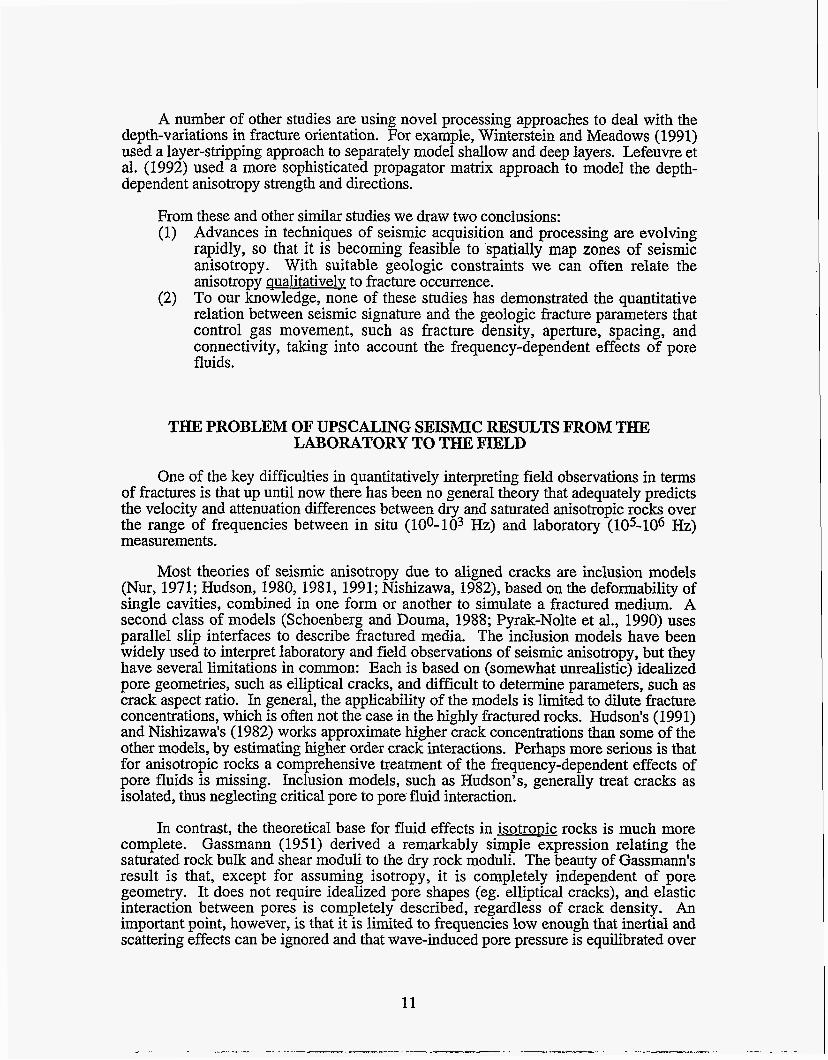
Figure 6 from Queen and Rizer (1990) shows the seismic shear-wave signature of the apparently fracture-induced anisotropy, as seen from multicomponent VSP. Figure 6a is a polar plot of the azimuthal variation of differential travel time between the two components of split shear waves. The greatest anisotropy is in the NE direction, as would be expected if the fractures are creating the anisotropy. Figure 6b shows a polar display of polarizations inferred from the shear waves. Again, the pattern is remarkably consistent with the surface fracture trends.
NMh
Figure 6 (a) Polar plot of shear wave travel time splittings for the VSP data at the Conoco site. (b) Polar plot of VSP polarizations (Queen and Rizer, 1990)
10
A number of other studies are using novel processing approaches to deal with the depth-variations in fracture orientation. For example, Winterstein and Meadows (1991) used a layer-stripping approach to separately model shallow and deep layers. Lefeuvre et al. (1992) used a more sophisticated propagator matrix approach to model the depth- dependent anisotropy strength and directions.
From these and other similar studies we draw two conclusions: (1) Advances in techniques of seismic acquisition and processing are evolving
rapidly, so that it is becoming feasible to 'spatially map zones of seismic anisotropy. With suitable geologic constraints we can often relate the anisotropy qualitatively to fracture occurrence.
(2) To our knowledge, none of these studies has demonstrated the quantitative relation between seismic signature and the geologic fracture parameters that control gas movement, such as fracture density, aperture, spacing, and connectivity, taking into account the frequency-dependent effects of pore fluids.
THE PROBLEM OF UPSCALING SEISMIC RESULTS FROM THE LABORATORY TO THE FIELD
One of the key difficulties in quantitatively interpreting field observations in terms of fractures is that up until now there has been no general theory that adequately predicts the velocity and attenuation differences between dry and saturated anisotropic rocks over the range of frequencies between in situ (100-103 Hz) and laboratory (105-106 Hz) measurements.
Most theories of seismic anisotropy due to aligned cracks are inclusion models (Nur, 1971; Hudson, 1980,1981,1991; Nishizawa, 1982), based on the deformability of single cavities, combined in one form or another to simulate a fractured medium. A second class of models (Schoenberg and Douma, 1988; Pyrak-Nolte et al., 1990) uses parallel slip interfaces to describe fractured media. The inclusion models have been widely used to interpret laboratory and field observations of seismic anisotropy, but they have several limitations in common: Each is based on (somewhat unrealistic) idealized pore geometries, such as elliptical cracks, and difficult to determine parameters, such as crack aspect ratio. In general, the applicability of the models is limited to dilute fracture concentrations, which is often not the case in the highly fractured rocks. Hudson's (1991) and Nishizawa's (1982) works approximate higher crack concentrations than some of the other models, by estimating higher order crack interactions. Perhaps more serious is that for anisotropic rocks a comprehensive treatment of the frequency-dependent effects of pore fluids is missing. Inclusion models, such as Hudson's, generally treat cracks as isolated, thus neglecting critical pore to pore' fluid interaction.
In contrast, the theoretical base for fluid effects in isotrotic rocks is much more complete. Gassmann (195 1) derived a remarkably simple expression relating the saturated rock bulk and shear moduli to the dry rock moduli. The beauty of Gassmann's result is that, except for assuming isotropy, it is completely independent of pore geometry. It does not require idealized pore shapes (eg. elliptical cracks), and elastic interaction between pores is completely described, regardless of crack density. An important point, however, is that it is limited to frequencies low enough that inertial and scattering effects can be ignored and that wave-induced pore pressure is equilibrated over
11
scales much larger than individual grains and pores. Brown and Korringa (1975) present a similar zero frequency analysis for anisotropic media.
Biot's (1956a, b) formulation relaxed some of the requifements of the low frequency theories, by including the dynamic coupling of fluid and solid stresses. This is sometimes called a large scale or "global" flow mechanism, because it describes the average solid- fluid motion on a scale much larger than an individual pore. The low frequency limit of Biot's formulation for bulk modulus is identical to Gassmann's, and a modest dispersion is predicted at higher frequencies.
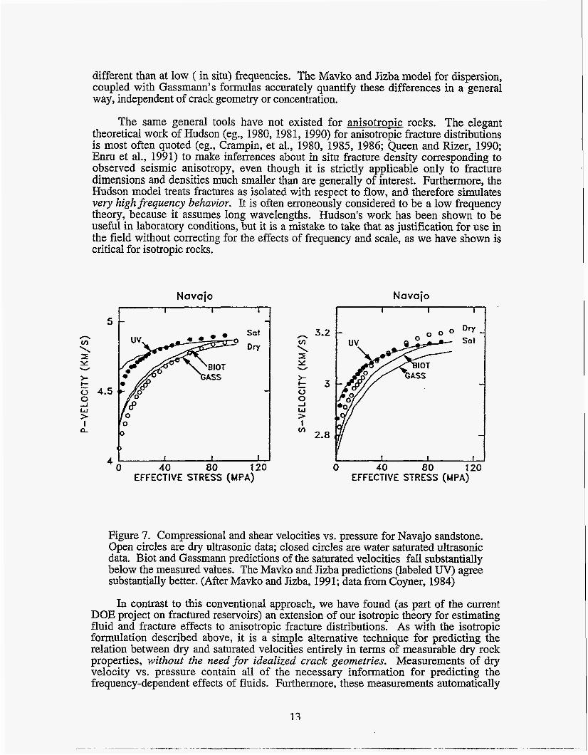
As illustrated in Figure 7 seismic velocities at ultrasonic frequencies are often much larger than those predicted by either the Gassmann or Biot formulations (Winkler, 1985, 1986). This is especially true for rocks with crack porosity. Experimental and modeling work (Mavko and Nur, 1975; 1979; O'Connell and Budiansky, 1974, 1977; Mavko and Jizba, 1991) suggest that the cause is related to the grain-scale microscopic flow field -- often referred to as "local flow" (Winkler, 1985) or "squirt flow" (Mavko and NU~, 1975). The squirt flow mechanism can be understood as follows: When a section of rock is excited by a passing wave, heterogeneities, such as variations in pore shape, saturation, and pore orientation are likely to produce pore pressure gradients and flow on the scale of individual pores. These unequilibrated pressure gradients at high frequencies make the rock stiffer than when the pore pressures are equilibrated at low frequencies. This frequency dependence accounts for substantial velocity dispersion and attenuation. Because the average of the local flow over many pores is zero, this mechanism is ignored in the original Biot (1956a,b) model. An important point is that for most crustal rocks, particularly rocks dominated by crack porosity, the fluid-related dispersive efsects are dominated by squirtflow, and the Biot mechanism can essentially be ignored.
We (Mavko and Jizba, 1991) have recently completed a formulation for quantifying the effects of squirt flow in isotropic rocks. It differs from previous estimates (Mavko and Nur, 1979; O'Connell and Budiansky, 1974,1977; Coyner and Cheng, 1984) in that no assumptions are made about specific crack geometries like ellipses, aspect ratios, etc. It is more like the results of Gassmann, and Brown and Korringa, in that the unrelaxed saturated moduli are estimated from Gry, KO, Kf, and@ with the additional information +(p) and I&Y(p). The latter two dry pressure dependent quantities carry information about the distribution of pore stiffness. The dispersive effects are most conveniently expressed in terms of the high frequency viscoelastic frame moduli:
1 - -- - Kdry
'Kdry K highP'
where Khighf and bighf are the high frequency frame moduli, Kfighp is the high pressure dry modulus, and +crack is the crack porosity. The results explain quite well the measured relation between dry and saturated velocities for a variety of rocks (Figure 7), both in terms of the magnitude of the saturated velocities and their pressure dependence.
The key point is that for isotrouic rocks, both P- and S-wave velocities are affected by fluid saturation, and their behavior at high (laboratory) frequencies may be quite
12
different than at low ( in situ) frequencies. The Mavko and Jizba model for dispersion, coupled with Gassmann’ s formulas accurately quantify these differences in a general way, independent of crack geometry or concentration.
The same general tools have not existed for anisotropic rocks. The elegant theoretical work of Hudson (eg., 1980, 1981, 1990) for anisotropic fracture distributions is most often quoted (eg., Crampin, et al., 1980, 1985, 1986; Queen and Rizer, 1990; Enru et al., 1991) to make inferrences about in situ fracture density corresponding to observed seismic anisotropy, even though it is strictly applicable only to fracture dimensions and densities much smaller than are generally of interest. Furthermore, the Hudson model treats fractures as isolated with respect to flow, and therefore simulates very highfrequency behavior. It is often erroneously considered to be a low frequency theory, because it assumes long wavelengths. Hudson’s work has been shown to be useful in laboratory conditions, but it is a mistake to take that as justification for use in the field without correcting for the effects of frequency and scale, as we have shown is critical for isotropic rocks.
>- I-
0
> I
p.
zs 4.5 J W
Navajo
5
5 40 80 120
EFFECTIVE STRESS (MPA) 4~
Navajo 1
n v) \ I Y
> t 0 0 J W >
I v)
W
3-2
3
2.8
0 40 80 120 EFFECTIVE STRESS (MPA)
Figure 7. Compressional and shear velocities vs. pressure for Navajo sandstone. Open circles are dry ultrasonic data; closed circles are water saturated ultrasonic data. Biot and Gassmann predictions of the saturated velocities fall substantially below the measured values. The Mavko and Jizba predictions (labeled UV) agree substantially better. (After Mavko and Jizba, 1991; data from Coyner, 1984)
In contrast to this conventional approach, we have found (as part of the current DOE project on fractured reservoirs) an extension of our isotropic theory for estimating fluid and fracture effects to anisotropic fracture distributions. As with the isotropic formulation described above, it is a simple alternative technique for predicting the relation between dry and saturated velocities entirely in terms of measurable dry rock properties, without the need for idealized crack geometries. Measurements of dry velocity vs. pressure contain all of the necessary information for predicting the frequency-dependent effects of fluids. Furthermore, these measurements automatically
contain all information about fracture interaction, so there is no limitation to low crack density. Hudson's approach, of course, would be one limiting case of this more general description.
In summary, it is very clear that corrections must be applied when comparing laboratory results with the field. Hudson's theory is a very high frequency theory, which has been shown to have some validity under certain laboratory conditions, but it cannot be applied directly to the field. We feel that our more generalized approach (1) will help to overcome the usual limitations of formulations to low fracture density and high frequency, and (2) it can be used, if desired, to apply a low frequency correction to Hudson's formulation, for more appropriate application to the field.
RESULTS I: LABORATORY AND THEORETICAL ROCK PHYSICS
PORE FLUID EFFECTS ON SEISMIC ANISOTROPY
Introduction
Most previous analysis techniques (eg., Hudson, 1980, 1981; Crampin, 1984; Thomsen, 1986) for cracked anisotropic rocks share one or more features which can limit their usefulness, particularly when comparing laboratory and field data: (1) They are based on idealized (and unrealistic) crack geometries, such as ellip- soidal cracks. (2) They are therefore intrinsically limited to low crack densities. (3) They often ignore the anisotropic mineral matrix. (4) Their treatment of frequency- dependent saturation effects is incomplete.
We present here a simple alternative technique for predicting the relation be- tween dry and saturated velocities in anisotropic rocks entirely in terms of measurable dry rock properties, without the need for idealized crack geometries. Measurements of dry velocity vs. pressure and porosity vs. pressure contain all of the necessary information for predicting the frequency-dependent effects of fluid saturation. Fur- thermore, these measurements automatically incorporate all pore interaction, so there is no limitation to low crack density.
We find that the velocities depend on five key interrelated variables:
0 Frequency
0 The distribution of compliant, crack-like porosity
0 The intrinsic or non-crack anisotropy
0 Fluid viscosity and compressibility
0 Effective pressure
The sensitivity of velocities to saturation is generally greater at high frequencies than at low frequences. The magnitude of the differences, from dry to saturated and from low frequency to high frequency, is determined by the compliant or crack-like porosity.
At low frequencies our results reduce to those of of Brown and Korringa (1975), which are an anisotropic extension of Gassmam’s (1951) relations. For high fre- quencies, we present a simple new method for predicting the amount of local flow or ”squirt” dispersion (Mavko and Nur, 1975; O’Connell and Budianski, 1977), which is an extension of our previous results for the isotropic case (Mavko and Jizba, 1991).
Using this formulation, we show that velocities and velocity anisotropy in satu- rated rocks can be quite different at low (in situ) frequencies than at high (laboratory)
15
frequencies. Consequently great care must be used when applying laboratory obser- vations to the field, or when using laboratory observations to validate a model.
Fluid Mechanisms
If a set of loads applied to a dry rock causes a decrease in pore volume, then saturating the rock with fluid will usually increase the rock’s stiffness under the same set of loads. Pore compression induces pore fluid pressure, which, in turn, resists the deformation. Gassmann (1951) quantified this for isotropic rocks with a simple expression relating the saturated rock bulk modulus to the dry rock bulk modulus:
where & , K d r y , K g s , and I{j are the bulk moduli of the mineral grains, the dry composite, the saturated composite, and the pore fluid, and q5 is the porosity. This result assumes isotropy, but is otherwise completely independent of pore geometry, and elastic interaction between pores is completely described. The result is limited to low frequencies so that inertial and scattering effects can be ignored and so that the pore pressure induced by the externally applied compression has time to equilibrate throughout the pore space.
Brown and Korringa (1975) extended Gassmann’s relation to anisotropic media:
where Sj.$ is the predicted saturated rock compliance, S$/) and S!kz are the com- pliances of the dry rock and mineral material, and ,f3f and po = Siapp are the com- pressibilities of the fluid and mineral material. This form again assumes that the frequencies are low, so that the induced pore pressures are everywhere equalized.
Biot’s (1956a) b) formulation relaxed some of the requirements of Gassmann’s low frequency theory, by including the dynamic coupling of fluid and solid stresses and the effects of contrasting inertial forces in the fluid and solid. The low frequency limit of Biot’s formulation for bulk modulus is identical to Gassmann’s, and a modest dispersion is predicted at higher frequencies. Biot (1962a) b) later extended this work to anisotropic media.
Measured seismic velocities in saturated rocks at ultrasonic frequencies (Winkler, 1985, 1986) are often much faster than predicted by either the Gassmann or Biot formulations. Both experiments (Murphy et al., 1984; Wang and Nur, 1988, 1990) and models (Mavko and Nur, 1979; O’Connell and Budiansky, 1974, 1977; Mavko and Jizba, 1991; Thomsen, 1991) suggest that the cause is related to the grain-scale microscopic flow field, refered to as ”local flow’’ or ”squirt” (Mavko and Nur, 1975). For most crustal rocks, particularly those with crack porosity, the Biot dispersion is small compared with squirt dispersion, and can often be ignored.
16
To understand the squirt mechanism, consider a saturated rock sample with the pore space vented to zero pore pressure. When an increment of stress is applied to the rock at very low frequencies, pore fluid can easily flow in and out of every pore; the rock behaves as though it is drained, and its moduli are essentially the same as dry rock moduli. At higher frequencies, viscous and inertial effects cause the thinnest pores to be isolated with respect to flow from the larger drained pores, and the external stress induces increments of pore pressure. Stiff portions of the pore space tend to have relatively low induced pore pressure; the compliant pores have relatively high induced pore pressure. The unequilibrated pore pressures make the rock stiffer than at low frequencies.
Our formulation considers the saturated compliant, crack-like fraction of the pore space to be part of the viscoelastic rock frame (Biot, 1962a,b), separate from the larger, stiffer fraction of the pore space where ”global” flow might occur. This is in contrast to the Biot-Gassmann-Brown-Korringa approach, which assumes that pore pressures are uniform throughout the pore space.
We proceed now to derive expressions for the unrelaxed frame compliances, which we label s i j k l (wet) , in terms of the dry or relaxed compliance, s i jk [ (dry) , at the same
pressure, and the dry compliance at very high confining pressure, s i j k , These relaxed and unrelaxed frame moduli can then be substituted into the Brown and Korringa or Biot formulations to predict the total dispersive behavior of the saturated rock.
Derivation of Unrelaxed Frame Moduli
We estimate the effect of the uneven pore pressure distribution on the unrelaxed
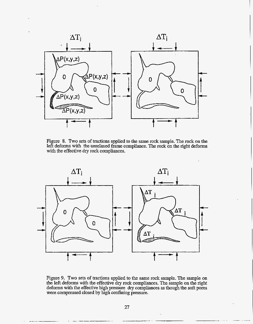
Jaeger and Cook, 1969). Consider the two sets of tractions applied to a rock with total volume V , as shown in Figure 8. The rock on the left is loaded by externally applied tractions Ti = Aaijnj, where .iz is the outward unit normal vector at each point on the surface, and Auij is an arbitrary constant stress tensor corresponding to the incremental loading of a passing wave. Internally applied normal tractions, AP(z, y, z) , (which are equal to the as yet unknown spatially variable incremental pore pressures induced by the wave) are applied to the unrelaxed compliant fraction of the pore space. Zero internal tractions are assumed on the drained fraction of the pore space. Therefore, it has the appearance of a partially saturated rock with fluid in the thin, compliant pores only, and it deforms with the unrelaxed frame compliance. The rock on the right has the same tractions T. applied to the external surfaces and zero tractions applied to the internal surfaces, so it deforms with the effective dry rock compliances, S/$’). Applying the reciprocity theorem, we can write:
frame compliance, s i j k l (wet) , using the Betti-Rayleigh reciprocity theorem (Walsh, 1965;
(3) ACijAOklSi$f)V - APnAvn = AOijAoklSijk. (wet) V n
The summations result from separating the integrals of work done on the pore walls into the sum of integrals over subsets of the pore space having approximately equal
17
induced pore pressure, AI',. Correspondingly, vn is the volume of that subset of pore space and Av, is the dry rock stress-induced change of pore volume.
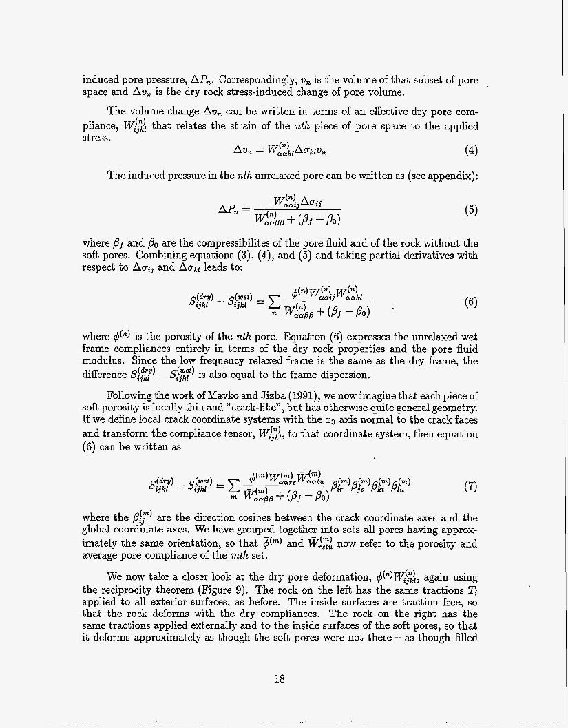
The volume change Avn can be written in terms of an effective dry pore com- pliance, W$\ that relates the strain of the nth piece of pore space to the applied stress.
Av, = W&\lAoklv, (4)
The induced pressure in the nth unrelaxed pore can be written as (see appendix):
W2)i Aa; j AP, = w&h? + ( P i - P o ) (5)
where pj and P o are the compressibilites of the pore fluid and of the rock without the soft pores. Combining equations (3), (4), and (5) and taking partial derivatives with respect to Aaij and Aakr leads to:
where is the porosity of the nth pore. Equation ( 6 ) expresses the unrelaxed wet frame compliances entirely in terms of the dry rock properties and the pore fluid modulus. Since the low frequency relaxed frame is the same as the dry frame, the difference Sj,$f) - Sj$' is also equal to the frame dispersion.
Following the work of Mavko and Jiaba (1991)) we now imagine that each piece of soft porosity is locally thin and "crack-like", but has otherwise quite general geometry. If we define local crack coordinate systems with the 23 axis normal to the crack faces and transform the compliance tensor, W$\, to that coordinate system, then equation (6) can be written as
where the /3i() are the direction cosines between the crack coordinate axes and the global coordinate axes. We have grouped together into sets all pores having approx- imately the same orientation, so that $m) and now refer to the porosity and average pore compliance of the mth set.
We now take a closer look at the dry pore deformation, $(n)W$), again using the reciprocity theorem (Figure 9). The rock on the left has the same tractions applied to all exterior surfaces, as before. The inside surfaces are traction free, so that the rock deforms with the dry compliances. The rock on the right has the same tractions applied externally and to the inside surfaces of the soft pores, so that it deforms approximately as though the soft pores were not there - as though filled
18
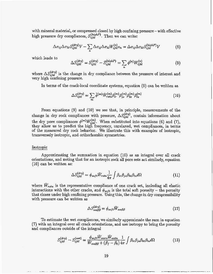
with mineral material, or compressed closed by high confining pressure - with effective high pressure dry compliances, S/:zhp'. Then we can write:
n
where ASj:L/) is the change in dry compliance between the pressure of interest and very high confining pressure.
In terms of the crack-local coordinate systems, equation (9) can be written as
From equations (9) and (10) we see that, in principle, measurements of the change in dry rock compliances with pressure, AS/:;:), contain information about the dry pore compliances q5(m)Wi;/. When substituted into equations (6) and (7), they allow us to predict the high frequency, unrelaxed, wet compliances, in terms of the measured dry rock behavior. We illustrate this with examples of isotropic, transversely isotropic, and orthorhombic symmetries.
Isotropic
Approximating the summation in equation (10) as an integral over all crack orientations, and noting that for an isotropic rock all pore sets act similarly, equation (10) can be written as:
where i%Tstu is the representative compliance of one crack set, including all elastic interactions with the other cracks, and is the total soft porosity - the porosity that closes under high confining pressure. Using this, the change in dry compressibility with pressure can be written as
To estimate the wet compliances, we similarly approximate the sum in equation (7) with an integral over all crack orientations, and use isotropy to bring the porosity and compliances outside of the integral
19
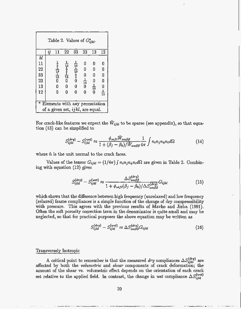
Table 2. Values of G&l. IJI kl 11 22 33 23 13 12
0 0
1 - 115 - - 5 15 0 0 0
0 0 0
0 0
1 15 -
1 15 - 0
0 0 0 0 0 1 15 -
I * Elements with any permutation of a given set, i.jkZ, are equal.
For crack-like features we expect the W i j k l to be sparse (see appendix), so that equa- tion (13) can be simplified to
where ti is the unit normal to the crack faces.
Values of the tensor Gijkl = (1/47r) ninjnknlda are given in Table 2. Combin- ing with equation (12) gives
which shows that the difference between high frequency (unrelaxed) and low frequency (relaxed) frame compliances is a simple function of the change of dry compressibility with pressure. This agrees with the previous results of Mavko and Jizba (1991). Often the soft porosity correction term in the denominator is quite small and may be neglected, so that for practical purposes the above equation may be written as
Transversely Isotropic
A critical point to remember is that the measured dry compliances AS$;;) are affected by both the volumetric and shear components of crack deformation; the amount of the shear vs. volumetric effect depends on the orientation of each crack set relative to the applied field. In contrast, the change in wet compliance ASijkl (wet)
20
is affected only by the decrease in volumetric compliance when pore fluid is added. The compressional effect can be seen in equation (3) as the crack-by-crack products of pressure increment times volume change, and also in equation ( 6 ) as the product of volumetric pore strains WaaijWaakl. To extract only the volumetric part of the dry compliances, it is necessary to carefully treat the crack orientations. For the isotropic case this was very simple, because we assume that all orientations exist. But for anisotropic rocks, we must take more care.
For example, the simplest (though not necessarily correct) model for transversely isotropic rocks assumes that all of the soft, crack-like porosity is parallel. We leave general the crack geometries, crack density, crack interaction, etc. With only this single crack set, equation (10) simplifies to
Equation (7) also simplifies for a single crack set and when combined with equation (17) gives
(dry) (dry)
(18) s$;;) - s$t) = Asaakl
(dry) ASaap, + (Pf - P O M s o f t
Here too, as in the isotropic case one can often neglect the small contribution from the second term in the denominator.
We now show how the measured dry compliances AS$/) can be uniquely decom- posed into its volumetric and shear components for any general transversely isotropic crack distribution. This includes not only a single crack set or a superposition of a single set over an isotropic distribution but also any other rotationally symmetric distribution of cracks. The extracted volumetric component is then used to calculate the unrelaxed high frequency saturated compliances. We assume sparseness of the crack compliance tensor miYj-1 (see appendix) and also assume the ratio of the normal to shear crack compliance to be unknown, but the same for the m different crack sets. The measured change in the dry compliances with pressure, equation (10 , can
H i j k l respectively as : be resolved into a sum of as yet unknown volumetric and shear components qekl 1 and
where
with
and
21
In the above expressions the tilde is used to denote the normalised change in dry compliances, and the p i j are the components of the Euler rotation matrix that relates the crack coordinates to the laboratory coordinate frame. Now making use of the orthonormality properties of the rotation matrix and transverse isotropic symmetry one can uniquely solve for the five independent components of GZir :
(28) Having thus extracted the volumetric part we can calculate the high frequency wet compliances from equation (7) as
where we have neglected the small contribution from the soft porosity correction term in the denominator. Note that if the AS$:) are isotropic, then Gg. reduces to the isotropic form in Table 2. If there is a single crack set, then equation (29) reduces to a simplified form of equation (18). (For a single crack set, equation (18) allows a completely general crack compliance tensor Wijkl, while equation (29) assumes a sparse Wijhl as described in the appendix.)
Orthorhombic
To model general pore distributions with orthorhombic symmetry, one would need to derive the equivalent forms of equations (19)-(28) for the 9 independent elements of G i j k l , which we have not done yet. We present here the specific case of orthorhombic symmetry associated with a finite number of crack sets - one, two, or three mutually perpendicular crack sets superimposed on a general orthorhombic background. Then equation (10) becomes
Assuming crack-like behavior of each set (sparse Wijkl) this becomes:
22
Similarly the unrelaxed wet moduli, equation (7), become:
Discussion
We have presented a technique for predicting the saturated velocities in anisotropic rocks in terms of measureable dry rock velocities. At low frequencies, representative of water saturated rocks measured in situ, the saturated elastic compliances citn be derived from the dry compliances and total porosity, using equation (2). At very high frequencies, as with untrasonic laboratory measurements, the saturated compliances depend on the distributions of crack orientations and compliances, and can be related to the change of dry rock compliance with pressure, plus a correction proportional to the difference between the compressibilites of the liquid and the mineral. As pointed out by Mavko and Jizba (1991) this has the simple interpretation that filling a com- pliant pore or crack with unrelaxed fluid resists compression, similar to filling it with mineral, or equivalently compressing it closed. The second order term compensates for the finite compressibility of the fluid.
The isotropic result, equations (15) and (16), is consistent with the results of Mavko and Jizba (1991). The tensor Gijkl (Table 2) represents the distribution of normal stresses resolved across the various crack orientations, for a given externally applied load aij. This form highlights the result found before that for an isotropic rock, the dispersion in bulk and shear are expected to be proportional.
The first transversely isotropic result, equation (18), is appropriate when all of the soft, crack-like, porosity is aligned normal to the 23 direction. This would be indicated by little or no change of the AS$;”$ and AS^^^^) dry compliances with stress. The second transversely isotropic result, equation (29), would be appropri- ate when the dry measurements indicate transversely isotropic behavior, but with stress-induced changes in more than the 3333 component. The general analysis of crack distributions, using equations (24)-(28 will indicate that a single set of cracks predominates when gi33 + 1 and q;,, G2i22, a q;122, q A 3 , @is 3 0.
The orthorhombic result, equation (32), is appropriate when the crack-like poros- ity lies in 1, 2, or 3 perpendicular sets. This would be recognized when the change in dry compliances AS$;”Z), AS{$;), AS$%) are much smaller than ASlll1 ( d r y ) , AS;%), AS%).
23
Finally, we emphasize that equations (15), (16), (18), (29), and (32) are for the unrelaxed wet compliances, which must be substituted into equation (2) for the completely saturated behavior.
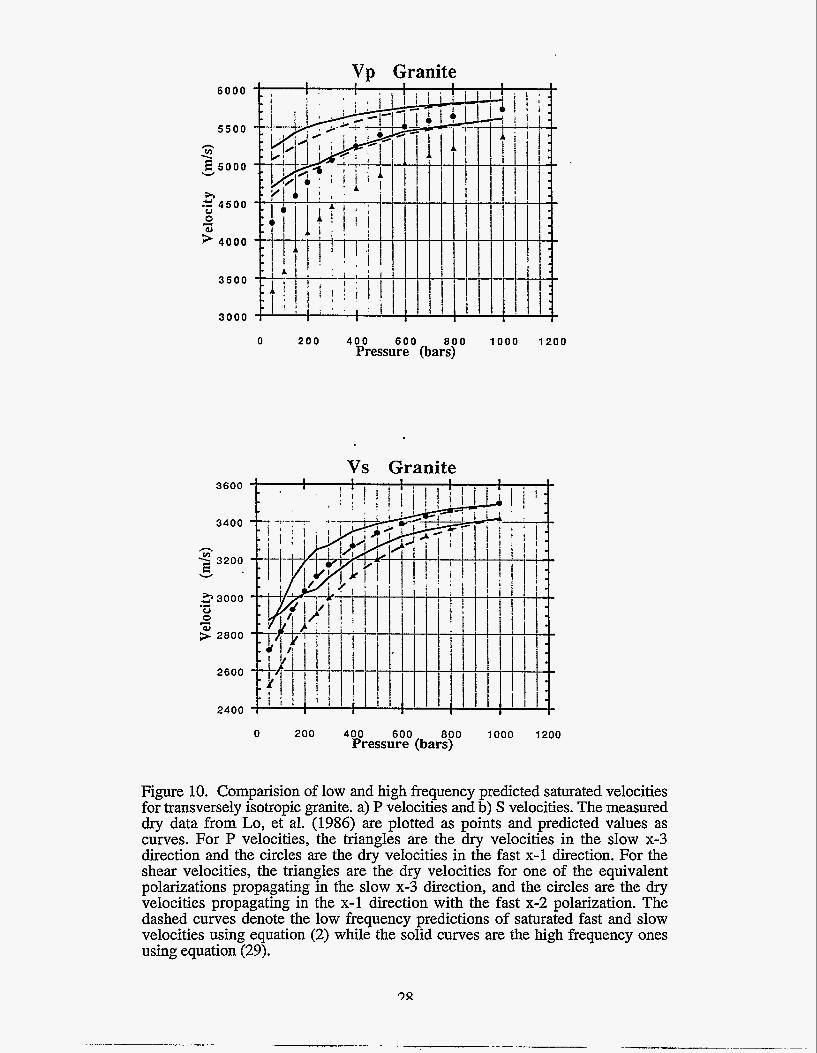
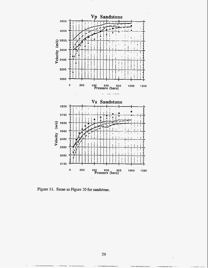
Figures (10) and (11) compare low and high frequency saturated P and S ve- locities for transversely isotropic granite and sandstone predicted using dry pressure- dependent data from Lo, et al. (1986). The measured dry data are plotted as points, and the predicted values are plotted as curves. For the compressional velocities, the triangles are the velocities in the slow 23 direction, and the circles are the velocities in the fast x1 direction. For the shear velocities, the triangles are the velocities for one of the equivalent polarizations propagating in the slow 23 direction, and the circles are the velocities propagating in the 21 direction with the fast 22 polarization. Note that the dry data show anisotropy, even at high pressure, when presumeably most of the cracks are closed. This intrinsic anisotropy accounts for much of the total anisotropy at the lower pressures. Therefore, interpretation of observed anisotropy entirely in terms of cracks can be misleading in rocks such as these.
The dashed curves show the low frequency prediction of saturated velocity, using equation (2), and the solid curves the high frequency prediction of saturated velocity, using equation (29). We found that for these rocks a single crack set, equation (18), was a poor representation of the crack-related anisotropy. The more complete analysis of the G$& indicated a distributed range of crack orientations, and ignoring the distribution often gave unrealistic results. As expected, the high frequency velocities are almost always faster than the corresponding low frequency values.
The low frequency theory predicts no change in the shear compliances AS2323 and AS1313 and hence a small drop in S velocities in the principal directions due to the density effect. For the low porosity granite (0.9%) the dry and low frequency saturated S velocities are barely distinguishable. The low frequency velocity in the sandstone (porosity 17%) is reduced about 5% upon saturation. Although not plotted, the low frequency shear compliances in the non-principal directions are predicted to stiffen with saturation. The high frequency theory predicts an increase in the saturated shear compliances relative to the low frequency saturated values and therefore an increase in the S velocities. For the low porosity granite the high frequency velocity is always higher than the dry or low frequency saturated values. For the higher porosity sandstone, the high frequency velocity is generally higher than the low frequency values, but still lower than the dry values due to the density effect. An interesting observation is the cross-over of the two high frequency saturated S velocity curves at low pressures for both rocks. This suggests that at high frequencies, the observed velocity anisotropy can be smaller or even in the opposite sense of the anisotropy observed in dry rocks or in saturated rocks at low frequencies. Therefore, finding relatively low velocity anisotropy in the laboratory (at high frequencies) does not preclude finding higher anisotropy in the field.
The compressional velocities for these rocks always increase from dry to satu- rated rocks and always increase from low frequency to high frequency. At some pres- sures the saturated velocities have equivalent or slightly smaller anisotropy compared with the dry rocks; but we also find that the high frequency saturated anisotropy can be larger than the dry anisotropy. Therefore, it is not correct to say that saturation always decreases anisotropy.
24

We summarize some key points illustrated by these examples:
1. Velocities and velocity anisotropy in dry rocks are generally expected to be different than in saturated rocks, although saturated shear velocities may be similar to dry shear velocities under certain conditions.
2. Velocities and velocity anisotropy are generally expected to be different at low frequencies typical of field measurements and high frequencies typical of labo- ratory measurements. Therefore, care must be taken when extrapolating from the laboratory to field situations. Our formulation gives a simple method for doing so in a geometry-independent way.
3. A rotationally symmetric distribution of cracks may often be a better model of crack induced transversely isotropic rocks than just a single set of aligned cracks.
4. Assigning all of the observed anisotropy to the presence of cracks may not always be correct as a significant fraction of the anisotropy could be due to the background matrix.
Finally, an often overlooked point is that inclusion models for velocity anisotropy, such as Hudson’s (1980, 1981), are usually high frequency theories, in terms of fluid effects. Hudson treats fluid-filled cavities as isolated with respect to fluid flow. As we have discussed, at high frequencies compliant cracks are isolated from the stiff portions of the pore space and from compliant cracks at other orientations; the resulting unequilibrated pore pressures make the rock stiffer. At low frequencies, pore fluid has sufficient time to flow and equilibrate the induced pore pressures throughout the pore space and hence cracks and pores are effectively connected with respect to fluid flow. Consequently Hudson’s work is best suited for describing ultrasonic laboratory measurements. Interpretations of low frequency field observations using Hudson’s formulation of saturated cracks is inappropriate. A better approach would be to use a dry rock model and to predict low frequency velocities using our equation (2).
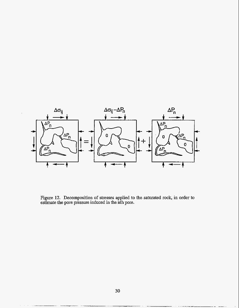
Appendix
Stress Induced Pore Pressure
We derive the stress induced pore pressure in the nth pore using linear super- position, as shown in Figure 12. The change in volume, Avn, can be written as the sum:
Equating this with the volume change of the fluid within the pore, Avn = APnPjvn, gives equation ( 5 ) .
Avn = vW$\(Acij - APnSij) + APnP0.n (33)
Sparse Crack Compliance Tensor
For crack like features we expect the intrinsic compliance tensor in the crack coordinate system, W i j h i , to be sparse. The largest components of the tensor are the normal compliance W3333 and the shear compliances m2323 and W1313. The other components are approximately zero. This is a general property of planar crack for- mulations and reflects an approximate decoupling of normal and shear deformation of the crack and decoupling of the in plane and out of plane compressive deformation. This allows us to write I;i".lapp M m3333 and mijaa M W33336i36j3.
26
t - t
I-
t I *
Figure 8. Two sets of tractions applied to the same rock sample. The rock on the left deforms with the unrelaxed frame compliance. The rock on the right deforms with the effective dry rock compliances.
t’-t I
c-
t *
Figure 9. Two sets of tractions applied to the same rock sample. The sample on the left deforms with the effective dry rock compliances. The sample on the right deforms with the effective high pressure dry compliances as though the soft pores were compressed closed by high confuling pressure.
27
VD Granite 6 0 0 0
5 5 0 0 n v) \
E 5 0 0 0 v
h -2 4 5 0 0 u 0 I
4 0 0 0
3 5 0 0
3 0 0 0
0 2 0 0 4 0 0 6 0 0 8 0 0 1 0 0 0 1 2 0 0 Pressure (bars)
Vs Granite 3600
3400
n
3200 E . v
2 3000 u 0
.I
I
2800
2600
2400
0 200 400 600 800 1000 1200 Pressure (bars)
Figure 10. Cornparision of low and high frequency predicted saturated velocities for transversely isotropic granite. a) P velocities and b) S velocities. The measured dry data from Lo, et al. (1986) are plotted as points and predicted values as curves. For P velocities, the triangles are the dry velocities in the slow x-3 direction and the circles are the dry velocities in the fast x-1 direction. For the shear velocities, the triangles are the dry velocities for one of the equivalent polarizations propagating in the slow x-3 direction, and the circles are the dry velocities propagating in the x-1 direction with the fast x-2 polarization. The dashed curves denote the low frequency predictions of saturated fast and slow velocities using equation (2) while the solid curves are the high frequency ones using equation (29).
VD Sandstone 4200
4000
3800. P E W
+, 3600 W 0
Y .-
3200
3000
0
2800
2700
n 2 2600 E W
2500 h
$ 2400 Y .I -
2300 $
2200
21 00
200 400 600 800 1000 Pressure (bars) 1200
Vs Sandstone
0 200 400 600 800 1000 Pressure (bars)
Figure 11. Same as Figure 10 for sandstone.
29
1200
AOij
Figure 12. Decomposition of stresses applied to the saturated rock, in order to estimate the pore pressure induced in the nth pore.
30
A SIMPLE TECHNIQUE FOR PREDICTING STRESS-INDUCED VELOCITY ANISOTROPY
Introduction
Seismic velocities in crustal rocks are almost always sensitive to stress. In the laboratory, for example, seismic P- and S-wave velocities almost always increase with increasing confining pressure (Nur and Simmons, 1969a). This is generally attributed to the closing of compliant, crack-like parts of the pore space, including microcracks and compliant grain boundaries. As confining pressure is increased, the most compliant pores are pressed closed, followed by the next most compliant, and so on. As more and more of the cracks are closed the mechanical stiffness increases, and the velocities increase (Walsh, 1965; Nur, 1971; Toksoz et al., 1976; Mavko and Nur, 1978).
Similar increases in velocity occur under non-hydrostatic stress, resulting in anisotropic velocities, as illustrated earlier in Figures 3 and 4.
This sensitivity suggests that, field measurements of velocity variations can be measures of in situ stress (eg., Nur, 1976; Crampin, 1978; Queen and Rizer, 1990), pore pressure changes (Nur and Simmons, 1969b; Nur, 1987), or stress concentrations (around boreholes, for example). The necessary link is to characterize the velocity-stress behavior of the rocks at each site.
Laboratory data, such as Yin's (1992), show the variation of seismic velocities as a function of each of the three principal stresses varied separately. In principle, they capture the essential anisotropic stress dependence of velocities, since a wide variety of stress fields can be constructed as a superposition of these principal stresses. However, velocities are generally not linear functions of stress, so that superimposing various applied stresses does not translate into a simple superposition of velocities. One approach for interpreting field data is simply to make laboratory measurements at all of the nonhydrostatic stress combinations that could be of interest at a given site. The problem is that this could require many tens or perhaps hundreds of measurements on each core sample. Another approach is to model the stress-induced anisotropy using angular distributions of idealized cracks with spectra of aspect ratios, which determine the stress dependence (Nur, 1971; Sayers, 1988). While these penny-shaped crack models (Eshelby, 1957; Hudson, 1981) have been relatively successful and provide a useful physical interpretation, they are limited to low crack concentrations, and may not represent well a broad range of crack geometries.
As an alternative, we present here a simple recipe for estimating stress-induced velocity anisotropy using only measured values of isotropic Vp and Vs versus hydrostatic pressure. The procedure applies to rocks that are approximately isotropic under hydrostatic stress and where the anisotropy is caused by crack closure under stress. [Sayers (1988) found evidence for some stress-induced opening of cracks also, which we ignore in this discussion.] Our method is conceptually similar to that used by Nur (1971) and Sayers (1988), who modeled cracks as idealized penny-shaped ellipsoids. However, our approach is relatively independent of any assumed crack geometry and therefore has no limitation to small crack densities. We estimate the generalized pore space compliance from the measurements of isotropic Vp and Vs. The physical assumption that the compliant part of the pore space is crack-like means that.the pressure dependence of the generalized compliances is governed primarily by normal tractions resolved across cracks and defects. This allows the measured pressure dependence to be mapped from
31
the hydrostatic stress state to any applied nonhydrostatic stress. Predicted P and S-wave velocities agree reasonably well with uniaxial stress data for Barre granite and Massillon sandstone.
Formulation
We will present the results in terms of the linearized elastic compliance tensor, sijkl( 6) , defined by
where 6 c k l and 6~~ are small stress and strain increments associated, for example, with seismic wave propagation. It is straightforward to compute the corresponding wave velocities as described, for example, by Auld (1990).
Following the work of Mukerji and Mavko (1994) we can write the elastic compliance of a rock as:
where sijkl(6) is the compliance at any given stress state 6, and s& is the reference compliance at some very large confining pressure when all of the compliant parts of the pore space are closed. Their difference, U i j k l ( 8 ) , is the extra compliance due to the presence of open cracks, and it is precisely this term that determines the measureable velocity-stress relation. The summation in equation (35) is over all of the open cracks, where the is the porosity of the qth crack and Wha is its crack compliance. Note that the product @@) W$ is a function of the stress state 6. If we define local crack coordinate systems with the 3-axis normal to the faces of each crack and transform the compliance tensor, W${ , to that coordinate system, then equation (35) can be written as:
where the are the direction cosines between each of the crack coordinate axes and the global coordinate axes. Note that repeated indices imply summation. In equation (36) we have grouped together into sets all cracks having approximately the same orientation, so that and IT,!$ now refer to the porosity and average pore compliance of the mth set. Since 9'"' IT,!$ always appears as a product, we find it convenient to absorb them into a single crack compliance
where 8 and @ are the Euler angles describing the orientation of the normal vector of the mth crack set. Finally, approximating the summation as an integral over all orientations, equation (36) can be written as
For the case of an isotropic rock under hydrostatic loading with effective pressure, p , the crack compliance W’, is independent of crack orientation, so that equation (38) can be written as
Now we make the important physical assumption that for thin cracks, the crack compliance tensor is sparse, so that only W‘3333, W’1313, and w’2323 are nonzero. (See Mukerji and Mavko, 1994.) Furthermore, we assume that the two unknown shear compliances are approximately equal, w’1313 = w’2323. Then, making use of the orthonormal properties of the PC , the unknown crack compliances can be determined from the measured effective compliances in the hydrostatic loading experiment using the relations:
Thus, we see that the pressure-dependent crack compliances, W’rstu, can be determined from the measured rock compliances versus hydrostatic pressure, AS$(p), which in turn are easily determined from P and S-wave velocities.
Our second important physical assumption is that for a thin crack under any stress field, it is primarily the normal component of stress, on, resolved on the faces of a crack that causes it to close and to have a stress-dependent compliance. For example, in the hydrostatic loading experiment described above, each crack feels the same normal stress, o n = p . Therefore, the stress-dependent compliances of a crack set, as derived in equations (40) and (41) are more precisely expressed as W’3333(0n) and $0,).
Now for general nonhydrostatic loading of the same rock, with stress tensor 3, the is normal stress acting on a crack with unit normal f i E (sin0 cos@, sin0 sin$, c 0 s 0 ) ~
given by
(42) AT- on=m cfi
where f i T is the transpose of f i . Combining equations (41) and (42) we can write:
where the sparse W’, are determined from the hydrostatic measurements using equations (40) and (41). Taking advantage of the sparseness of WtrStll and the implied summation, equation (43) can be written explicitly as:
+ 6jpiml + 6jlmimk - 4mimjmpl]sin€lded@
As an example, consider the case of uniaxial stress oo applied along the 3-axis to the initially isotropic rock. This causes the rock to take on tranversely isotropic symmetry, with five independent elastic constants. In this case the normal stress in any direction is on = cro cos2& Then the five independent components of ASijH in equation (44) become:
nn = 2 4 [l - 4$oocos28)] W ’ 3 3 3 3 ( ~ o ~ ~ ~ 2 e ) cos48 sine de
+ 2 7 ~ 1 ~ 4$o,cos28) W ‘ 3 3 3 3 ( ~ o ~ ~ ~ 2 e ) cos28 sine de 0
B u n i 2 z l d g [l - ~ $ o , c o s ~ ~ ) ] W’3333(oocos28) sin4@ sine de 1122 = 0
M u n i - 2 z 1 f l i - [l - ~ $ o , c o s ~ ~ ) ] W’,,,,(~,COS~~) sin2f3 cos28 sine de 1133-
34
(45)
Note that in equations (43), (44) and (45) the terms in the parentheses with yo and W3333(), are arguments to the yand W3333 pressure functions and not multiplicative factors.
Examples
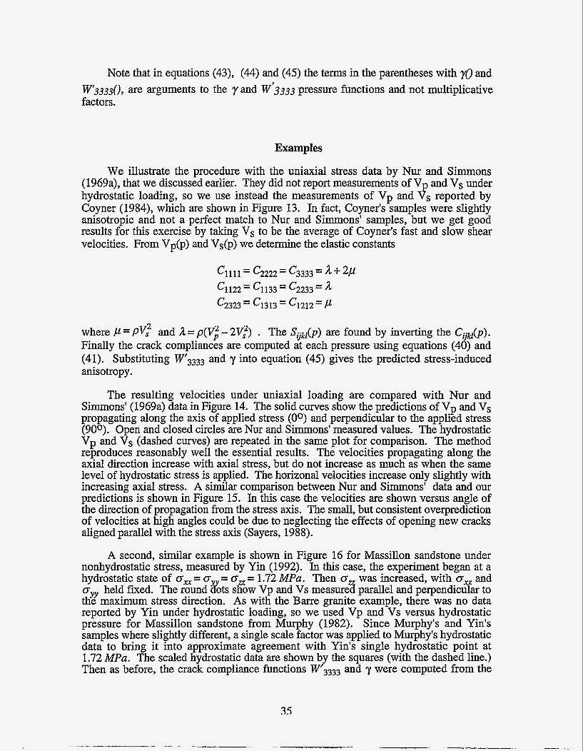
We illustrate the procedure with the uniaxial stress data by Nur and Simmons (1969a), that we discussed earlier. They did not report measurements of Vp and VS under hydrostatic loading, so we use instead the measurements of VP and VS reported by Coyner (1984), which are shown in Figure 13. In fact, Coyner's samples were slightly anisotropic and not a perfect match to Nur and Simmons' samples, but we get good results for this exercise by taking VS to be the average of Coyner's fast and slow shear velocities. From Vp(p) and Vs(p) we determine the elastic constants
2 where P = PV, and A = p(Vl- 2V:) . The SG&) are found by inverting the CGM(p). Finally the crack compliances are computed at each pressure using equations (40) and (41). Substituting W'3333 and y into equation (45) gives the predicted stress-induced anisotropy.
The resulting velocities under uniaxial loading are compared with Nur and Simmons' (1969a) data in Figure 14. The solid curves show the predictions of Vp and Vs propagating along the axis of applied stress (00) and perpendicular to the apphed stress (900). Open and closed circles are Nur and Simmons' measured values. The hydrostatic Vp and Vs (dashed curves) are repeated in the same plot for comparison. The method reproduces reasonably well the essential results. The velocities propagating along the axial direction increase with axial stress, but do not increase as much as when the same level of hydrostatic stress is applied. The horizonal velocities increase only slightly with increasing axial stress. A similar comparison between Nur and Simmons' data and our predictions is shown in Figure 15. In this case the velocities are shown versus angle of the direction of propagation from the stress axis. The small, but consistent overprediction of velocities at high angles could be due to neglecting the effects of opening new cracks aligned parallel with the stress axis (Sayers, 1988).
A second, similar example is shown in Figure 16 for Massillon sandstone under nonhydrostatic stress, measured by Yin (1992). In this case, the experiment began at a hydrostatic state of om = o = oz = 1.72 MPa. Then o was increased, with om and o,,,, held fned. The round &ts show Vp and Vs measures parallel and perpendicular to the maximum stress direction. As with the Barre granite example, there was no data reported by Yin under hydrostatic loading, so we used Vp and Vs versus hydrostatic pressure for Massillon sandstone from Murphy (1982). Since Murphy's and Yin's samples where slightly different, a single scale factor was applied to Murphy's hydrostatic data to bring it into approximate agreement with Yin's single hydrostatic point at 1.72 MPa. The scaled hydrostatic data are shown by the squares (with the dashed line.) Then as before, the crack compliance functions W'3333 and y were computed from the
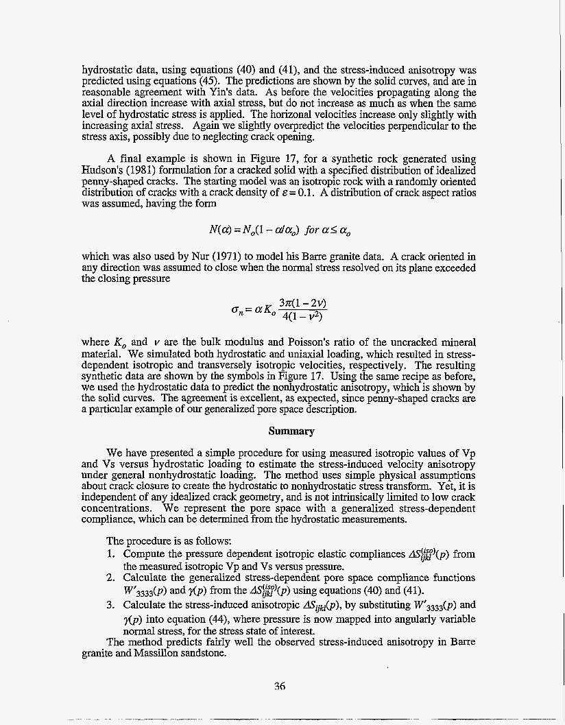
hydrostatic data, using equations (40) and (41), and the stress-induced anisotropy was predicted using equations (45). The predictions are shown by the solid curves, and are in reasonable agreement with Yin’s data. As before the velocities propagating along the axial direction increase with axial stress, but do not increase as much as when the same level of hydrostatic stress is applied. The horizonal velocities increase only slightly with increasing axial stress. Again we slightly overpredict the velocities perpendicular to the stress axis, possibly due to neglecting crack opening.
A final example is shown in Figure 17, for a synthetic rock generated using Hudson’s (1981) formulation for a cracked solid with a specified distribution of idealized penny-shaped cracks. The starting model was an isotropic rock with a randomly oriented distribution of cracks with a crack density of E = 0.1. A distribution of crack aspect ratios was assumed, having the form
N( a) = No( 1 - da,) for a I a,
which was also used by Nur (1971) to model his Barre granite data. A crack oriented in any direction was assumed to close when the normal stress resolved on its plane exceeded the closing pressure
3n(l- 2 ~ ) on= aK, 4( 1 - v2)
where KO and v are the bulk modulus and Poisson’s ratio of the uncracked mineral material. We simulated both hydrostatic and uniaxial loading, which resulted in stress- dependent isotropic and transversely isotropic velocities, respectively. The resulting synthetic data are shown by the symbols in Figure 17. Using the same recipe as before, we used the hydrostatic data to predict the nonhydrostatic anisotropy, which is shown by the solid curves. The agreement is excellent, as expected, since penny-shaped cracks are a particular example of our generalized pore space description.
Summary
We have presented a simple procedure for using measured isotropic values of Vp and Vs versus hydrostatic loading to estimate the stress-induced velocity anisotropy under general nonhydrostatic loading. The method uses simple physical assumptions about crack closure to create the hydrostatic to nonhydrostatic stress transform. Yet, it is independent of any idealized crack geometry, and is not intrinsically limited to low crack concentrations. We represent the pore space with a generalized stress-dependent compliance, which can be determined from the hydrostatic measurements.
The procedure is as follows: 1. Compute the pressure dependent isotropic elastic compliances AS@(p) from
the measured isotropic Vp and Vs versus pressure. 2. Calculate the generalized stress-dependent pore space compliance functions
W’3333(p) and f l p ) from the AS$J(p) using equations (40) and (41). 3. Calculate the stress-induced anisotropic ASijkl(p), by substituting W’3333(p) and
f lp ) into equation (44), where pressure is now mapped into angularly variable normal stress, for the stress state of interest.
The method predicts fairly well the observed stress-induced anisotropy in Barre granite and Massillon sandstone.
36
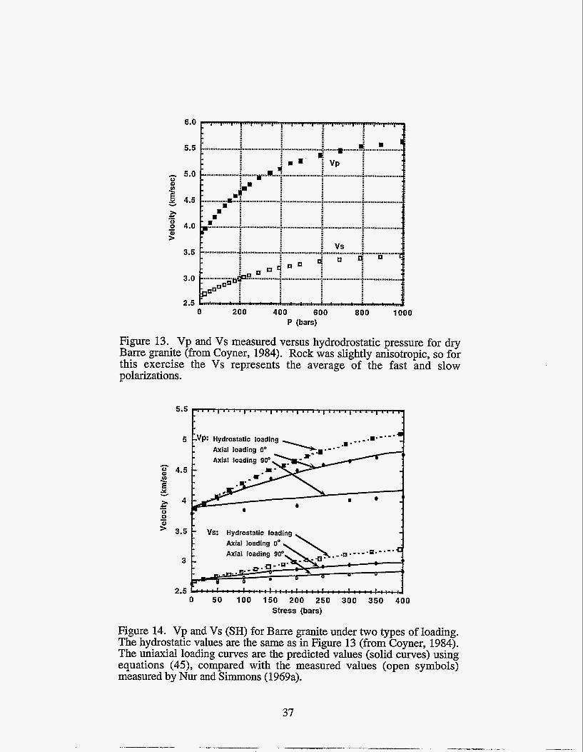
6.0
5.5
- 5.0
r E Y 4.5
- 8 4.0
u a
v
% L - s
3.5
3.0
2.5 0 200 400 600 800 1000
P (bars)
Figure 13. Vp and Vs measured versus hydrodrostatic pressure for dry Barre granite (from Coyner, 1984). Rock was slightly anisotropic, so for this exercise the Vs represents the average of the fast and slow polarizations.
5.5 a , , . I ., I ,, ,. , ,, , ,, , , I ,, , , ' , ,, , ,
t 1
3 -
0 5 0 100 150 200 250 300 350 400 Stress (bars)
Figure 14. Vp and Vs (SH) for Barre granite under two types of loading. The hydrostatic values are the same as in Figure 13 (from Coyner, 1984). The uniaxial loading curves are the predicted values (solid curves) using equations (45), compared with the measured values (open symbols) measured by Nur and Simmons (1969a).
37
h 0 al 2 E c
4.5
f
1
I- - r
%
u 0
04 - - 3.5
3
2.5 0 10 20 30 40 50 60 70 80 90
Angle (degrees)
Figure 15. Vp and Vs (SH) versus azimuth measured from the loading axis in uniaxial loading. The solid curves the the predicted values using equations (45); Dots are the data measured by Nur and Simmons (1969a).
38
.- - vp: Hydrostatic loading - Axial loading 0" 1
Axial loading 90". \ ...-. - 3 - -1
m - 0 W - fn
Y - -E 3- Y
2.5 - - - 0 0
$ Axial loading
- - - - VS: Hydrostatic loading -
2 - - - - - 1.5~"""'""''"''""'""
0 1 0 20 30 40 5 0 6 0 Stress (bars)
Figure 16. Vp and Vs for Massillon sandstone under two types of loading. The hydrostatic values are from Murphy (1982). The uniaxial loading curves are the predicted values (solid curves) using equations (45), compared with the measured values (open symbols) measured by Yin (1 992).
39
5 4.5 .-
3.5 4l 0 0 0 > -
vs: Hydrostatic loading . 1 Axial loading Oo
Axial loading 90'
3 0 50 100 150 200 250 300 350 400
Pressure (bars)
Figure 17. Vp and Vs for a synthetic rock generated using Hudson's model, under two types of loading. The uniaxial loading curves are the predicted values (solid curves) using equations (45), compared with the Hudson-values (circles).
RESULTS 11: FIELD EXPERIMENT
The study site is in a producing field operated by Amoco and Arc0 at the southern boundary of the Powder River basin in Wyoming. During the winter of 1992-1993 we (in cooperation with Amoco and ArcoNastar Resources) collected about 50 km of 9- component reflection seismic data and obtained existing log data from several wells in the vicinity. We describe here the geologic setting, along with the collection, processing, and interpretation of the seismic data.
REGIONAL GEOLOGIC FRAMEWORK AND SITE DESCRIPTION
Structural Features
The "Fort Fetterman" site is located at the southwestern margin of the Powder River basin, north of the town of Douglas, in Converse County, east-central Wyoming. The Powder River basin is one of many structural features formed during the Laramide Orogeny that occurred during latest Cretaceous to early Tertiary time in the western Cordillera (Dickinson et al., 1988). In the Rocky Mountain region, the typical structural style consists of a series of "basement-cored uplifts and intervening sediment-filled basins" (Dickinson et al., 1988) over a wide area. The study site is bounded to the south and west by the Casper Arch to the southeast by the Hartville Uplift (Figure 18). As discussed below, these structural features may have had a considerable influence on the formation of preferred fracture orientations.
Mitchell and Rogers (1993) note that the southern end of the Powder River basin has been significantly influenced by an extensional system of nearly vertical normal faults that affects Lower Cretaceous, Upper Cretaceous and Tertiary units. They proposed that these faults, which have throws of 30 ft or less, are basement derived, and controlled deposition of the Upper Cretaceous Frontier and Niobrara Formations. The fault systems appear to trend northwest-southeast in the south-central part of the basin, and northeast-southwest at the southern margin, parallel to the Hartville Uplift (Figure 19, Mitchell and Rogers, 1993). Slack (1981) also proposed a series of northeast- trending structural lineaments northeast of the study area, which extend northeastward to the Black Hills monocline. Mitchell and Rogers (1993) noted that a number of important producing fields in the southern Powder River basin have fracturing as an important reservoir component (Figure 20), and proposed that fracture potential is key to production from "conventional" sandstone reservoirs as well as shale reservoirs.
Ovemressure
Overpressuring is another potentially important parameter in defining the characteristics of reservoirs in the southern Powder River basin. The major source rocks in the southern Powder River basin are Lower Cretaceous shales (Skull Creek and Mowry) and the Upper Cretaceous Niobrara Formation, which is also a reservoir. Overpressuring is responsible for preservation of primary porosity at depth and maintenance of open fractures (Mitchell and Rogers, 1993). This fracture porosity is important at Silo Field, located more than 100 miles south of the study area, since the Niobrara in this field is a chalk rather than a shale. Mitchell and Rogers (1993) explain the abundance of hydrocarbon shows from "unconventional" reservoirs in the Upper Cretaceous Frontier equivalents (and the Niobrara) as being due to preserved primary porosity and the presence of open fractures.
41
420
38"
I
Figure 18: Laramide structural features in the central Rocky Mountain region, from Dickinson et al. (1988). Large dot at southwestern edge of Powder River basin in east-central Wyoming denotes approximate location of the study site.
42
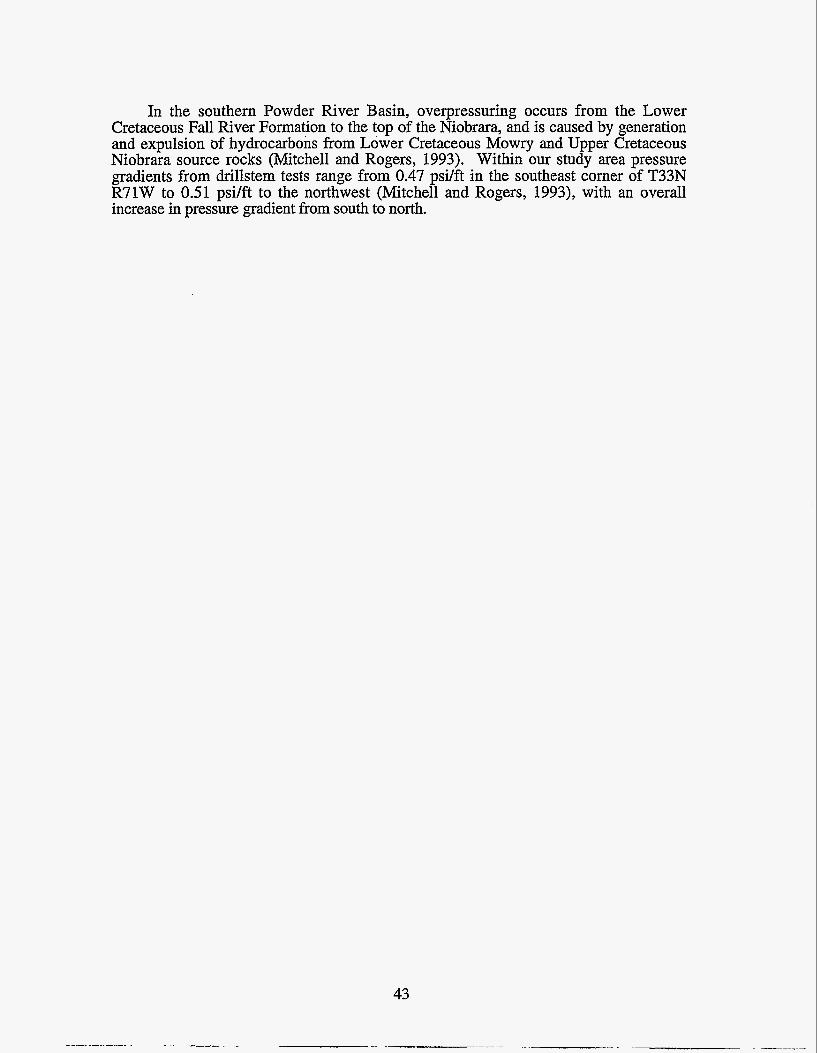
In the southern Powder River Basin, overpressuring occurs from the Lower Cretaceous Fall River Formation to the top of the Niobrara, and is caused by generation and expulsion of hydrocarbons from Lower Cretaceous Mowry and Upper Cretaceous Niobrara source rocks (Mitchell and Rogers, 1993). Within our study area pressure gradients from drillstem tests range from 0.47 psi/ft in the southeast corner of T33N R71W to 0.51 psi/ft to the northwest (Mitchell and Rogers, 1993), with an overall increase in pressure gradient from south to north.
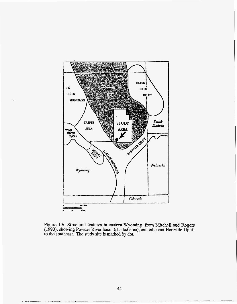
Figure 19: Structural features in eastern Wyoming, from Mitchell and Rogers (1993), showing Powder River basin (shaded area), and adjacent Hartville Uplift to the southeast. The study site is marked by dot.
44
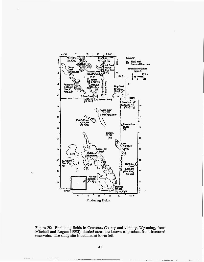
A R W , 71 70 69 R O W ,
41
40
- 39
4
Producing FicIds
40
39
38
57
36
35
34
35
T 9 - N
Figure 20: Producing fields in Converse County and vicinity, Wyoming, from Mitchell and Rogers (1993); shaded areas are known to produce from fractured reservoirs. The study site is outlined at lower left.
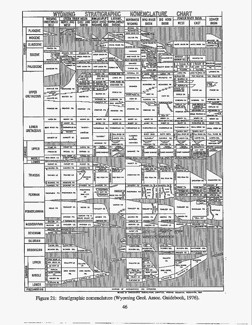
Figure 21: Stratigraphic nomenclature (Wyoming Geol. Assoc. Guidebook, 1976). 46
Regional Strati y-aphy and Depositional Environments
Figure 21 shows the stratigraphic nomenclature developed for various basins in Wyoming from the Precambrian to the Tertiary. This study is primarily concerned with upper Cretaceous sediments in the southwestern portion of the Powder River basin. Information for the formations listed below was taken from articles by Barlow and Haun (1966), Hando (1976), Merewether et al. (1976), Prescott (1975), and the Wyoming Geological Association Guidebook (1976).
'
S u m m q of Upper Cretaceous StratigraDhv in the Studv Area
Parkman Sandstone: offshore marine bar (shelf) sand, deposited in 100-200 ft water depths; composed of discrete sand lenses encased in siltstone and shale. Hydrocarbon productive in other areas of the Powder River basin.
Steele Shale: marine shale.
Sussex Sandstone: shelf sand, deposited in 100-200 ft water depths, influenced by longshore currents; composed of discrete, lenticular sand bodies encased in interbedded siltstone and shale. Hydrocarbon productive in other areas of the Powder River basin.
Niobraru Formation: unconformably overlies the Frontier; a series of fractured, marine chalks and limestones interbedded with calcareous shales and bentonites. Oil and gas reservoir that is its own source rock. Open fractures necessary for production due to low porosity and permeability.
First Frontier Sand: uppermost of three sands within the Frontier Formation; fractured, offshore marine bar sand containing interbedded shales in 3-4 transgressive-regressive cycles; grades upward regionally from marine shale to sandstone at the top. Reservoirs are thin, low permeability; pay section is coarse grained, reworked. Lower limit of 8% porosity is necessary for effective pay thickness.
Mowry Shale: dark grey to black, hard, siliceous shales interbedded with thin siltstone and sands, plus regionally extensive bentonite beds. Deposited in very stable depositional environment, greater than 500 ft water depths.
Frontier Formation
The Frontier and equivalent formations comprise the interval between the Mowry Shale and the Niobrara Formations in the lowermost part of the Upper Cretaceous in the Rocky Mountain region. The section includes sand bodies interbedded with marine shale, ranging up to 1,000 feet thick in central, west-central and northeast Wyoming (Barlow and Haun, 1966). The sands are interpreted as having been deposited by fluvio- deltaic processes along the margins of the Western Interior Seaway during early Late Cretaceous time. Rivers flowing eastward across the Cordillera during this time from a source area located west-northwest of the Yellowstone Park area created these areally extensive deltas (Barlow and Haun, 1966; Prescott, 1975).
The informal terms "first Frontier sandstone" and "second Frontier sandstone" denote the important producing sands, with the second Frontier accounting for most of the oil production from the giant Salt Creek field in Natrona County, Wyoming (Barlow
47
and Haun, 1966). Salt Creek field is located approximately 60 miles northwest of the study area. These sands were generally deposited in the subaqeous portion of the delta, and reflect a marine influence, rather than merely fluvial influx. Thus, they are part of the shore-zone system (Galloway and Hobday, 1983), whose components include beaches, barriers, lagoons and tidal flats.
At Spearhead Ranch field, located approximately 40 miles north-northwest of the study area in Converse County, the producing first Frontier reservoir is referred to as an "offshore marine bar" (Prescott, 1975). Detailed analysis of well logs from this field (Prescott, 1975) suggests three or four regressive-transgressive cycles within the first Frontier sandstone interval. In both the Spearhead Ranch and Salt Creek fields, the trapping mechanism is stratigraphic, and at Spearhead Ranch field, the interval dips uniformly to the southwest with no closure (Prescott, 1975).
In the southern Powder River basin, another stratigraphic classification divides the time-equivalent of the Frontier Formation into (oldest to youngest) the Belle Fourche Shale, Greenhorn Limestone, and the Carlile Formation (Mitchell and Rogers, 1993). The Carlile is then subdivided into the Turner Sandstone Member, consisting of well- sorted marine sands and silts, and the Sage Breaks Member, a marine, calcareous shale. This area includes the DOE site in southern Converse County, as well as parts of Campbell, Weston and Niobrara Counties. Mitchell and Rogers (1993) note that the Turner is a good potential target for horizontal drilling, since it is a fractured reservoir.
In the Kaycee-Tisdale Mountain area, the Frontier incorporates interstratified shale, siltstone, sandstone and bentonite, with the Wall Creek Sandstone Member at the top (Merewether et al., 1976). This area is located on the western flank of the Powder River Basin in Johnson County, northwest of Spearhead Ranch field. Merewether et al. (1976) suggest that most of the Frontier sands in this area were deposited in wave-dominated deltaic environments.
In southwest Wyoming, the Frontier in the Green River basin consists of both marine and nonmarine sandstones and shales, with increasing dominance of marine deposits to the east, toward the Western Interior Seaway (Dutton et al., 1992). Along the Moxa Arch, a north-trending uplift close to the eastern boundary of the Thrust Belt, the Frontier is composed of shoreline sands and fluvial channel-fill sands, and is encased by thick shales. The subdivisions into First Frontier sandstone, Second Frontier sandstone, etc. are applicable, and the Second Frontier (a fluvial-deltaic system) contains low permeability gas reservoirs from which the majority of the production in the western Green River Basin is derived (Dutton et al., 1992).
The Powell-Ross field is located in Converse County just northwest of the study site in T40N, R74W average porosity for this field is given as 15%. Typical porosities for Frontier reservoir sands in the Powell-Ross field range from a cutoff limit of 8% for effective pay thickness to a high of 22% (Hando, 1976). Completions from the Frontier produce both oil and gas, with the Powell II Unit No. 1 well completed for 624 BOPD and 2.2 MCFGPD (Hando, 1976). For the larger Spearhead Ranch field nearby, in T37- 40N, R74-75W, Prescott (1975) noted when porosities are less than 8%, the reservoir becomes uneconomic, due to insufficient permeability. Most development wells in this field average about 1,000 BOPD and 2-2.5 MMCFGPD (Prescott, 1975). The trapping mechanism at Spearhead Ranch is purely stratigraphic, and the first Frontier is an offshore marine bar. Hydrocarbon production from fractured reservoirs is not mentioned for these fields.
48
I
Frontier Formation: Fracture Patterns in Field Studies
Comparatively few published studies have attempted to relate fracture patterns in the field to those observed in cores. Dutton et al. (1992) conducted a detailed study of natural fractures in the Frontier Formation in the Moxa Arch and western Green River basin of southwestern Wyoming as part of the Gas Research Institute's Tight Gas Sands project. They examined data from both cores and outcrops; core data showed that, although extension fractures were closely spaced, they were often confiied to individual sand members and formed vertically discontinuous strands striking predominantly north and east, In outcrop, dominant strike directions near Kemmerer, Wyoming were bimodal, with a closely spaced (from 4" to 3') north-striking set and a younger, cross-cutting, more widely spaced set that strikes east-west.
Dutton et al. (1992) found no consistent relationship between the presence of a given fracture set and current structural position, and attributed subtle differences in original composition or diagenesis as important factors affecting the tendency of the rock to fracture. They found a compartmentalization of fracture arrays and drastically varying connectivity even within the same fracture set. In their study area, fracture origin is likely related to isostatic adjustment to loads imposed by proximity to thrust sheets. Dutton et al. (1992) concluded that the vertically confined, isolated fracture swarms in this area would present a more challenging exploration target than those in areas of uniformly spaced, orthogonal fracture sets.
Frontier Formation at the DOE Site
Within the study area, the First Frontier sand lies approximately 100 feet below the top of the Frontier Formation. The First Frontier sand contains fracture sets, as identified from fracture identification (dipmeter) logs. Figure 22 shows the gamma ray, sonic and density logs for the Apache #36-1 State well (see Figure 23 for location). At the well, located on the southeastern end of Line 2, this sand produces from a perforated interval from 11,695-11,785 ft. Initial production from a test on 3/17/81 was 70 BOPD and 1700 MCFGPD. Velocities in this interval, from the sonic log, are rather high, at 65 ps/ft, or 15,400 ft/sec; formation density is 2.5 gkm3 (Figure 22). The velocity decreases to 80 pdft, or 12,500 Wsec below this producing sand.
Another sonic log from the Davis Oil #1 well to the west of line 1 shows approximately the same high velocity character in the fiist Frontier sand. A core description from the Texaco #1 Sims well in section 15, T33N R71W, indicates that the first Frontier is a fine grained, Yight'' sandstone, with a trace of oil.
Niobrara Formation - Regional Stratimaphy and Fracture Patterns
The Upper Cretaceous Niobrara Formation directly overlies the Frontier interval. At Silo Field, located northeast of Cheyenne in far southeastern Wyoming, the Niobrara is a naturally fractured, oil-productive chalk (Lewis et al., 1991). Dips are gentle to the southwest, and the chalk is faulted where it drapes over a deeper Permian salt withdrawal, or salt dissolution structure. Fracture orientations parallel this paleostructure, and the average fracture strike is N50OW to N55OW (Lewis et al., 1991). This orientation was also confi ied by dipmeter logs and by 3-D rotation analysis of shear-wave seismic data. Anisotropy, as identified in the azimuthal rotation analysis, was determined to result from vertical fractures alone, rather than from the combined effects of vertical fractures and horizontal layering.
Sonnenberg and Weimer (1993) reported on oil production from the Niobrara in Silo field, and noted that the open fractures which provide the means of producing Erom this low permeability reservoir were created by a combination of folding, basement faulting, solution of older Permian evaporites, high fluid pressure, and the effects of the regional stress field. Porosities in the Niobrara chalk were found to be approximately 8%, and are proportional to maximum burial depth. Cumulative production from the fractured Niobrara (7600 ft to 8500 ft depths) is already greater than 1.3 million BO from 40 vertical wells, and adding in production from horizontal completions brought the total to over 2 million BO through June, 1992.
Log plotting software designed by X (Frank) Liu 1993
Figure 22: Plot of gamma ray, sonic and density logs from Apache #36-1 State well (see Figure 23 for location), with formation tops and fracture zones labeled. Producing interval within First Frontier sand is shaded.
50
______ ~~ -
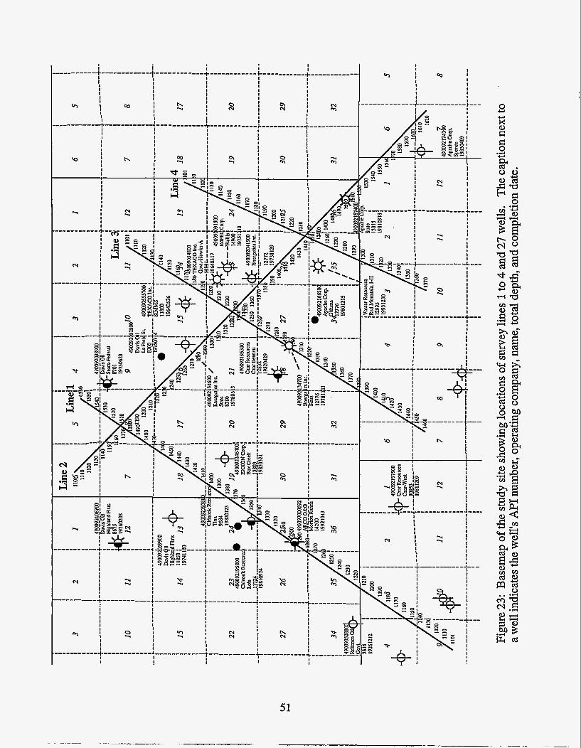
P
N -4
N
N -4
t\ N
51
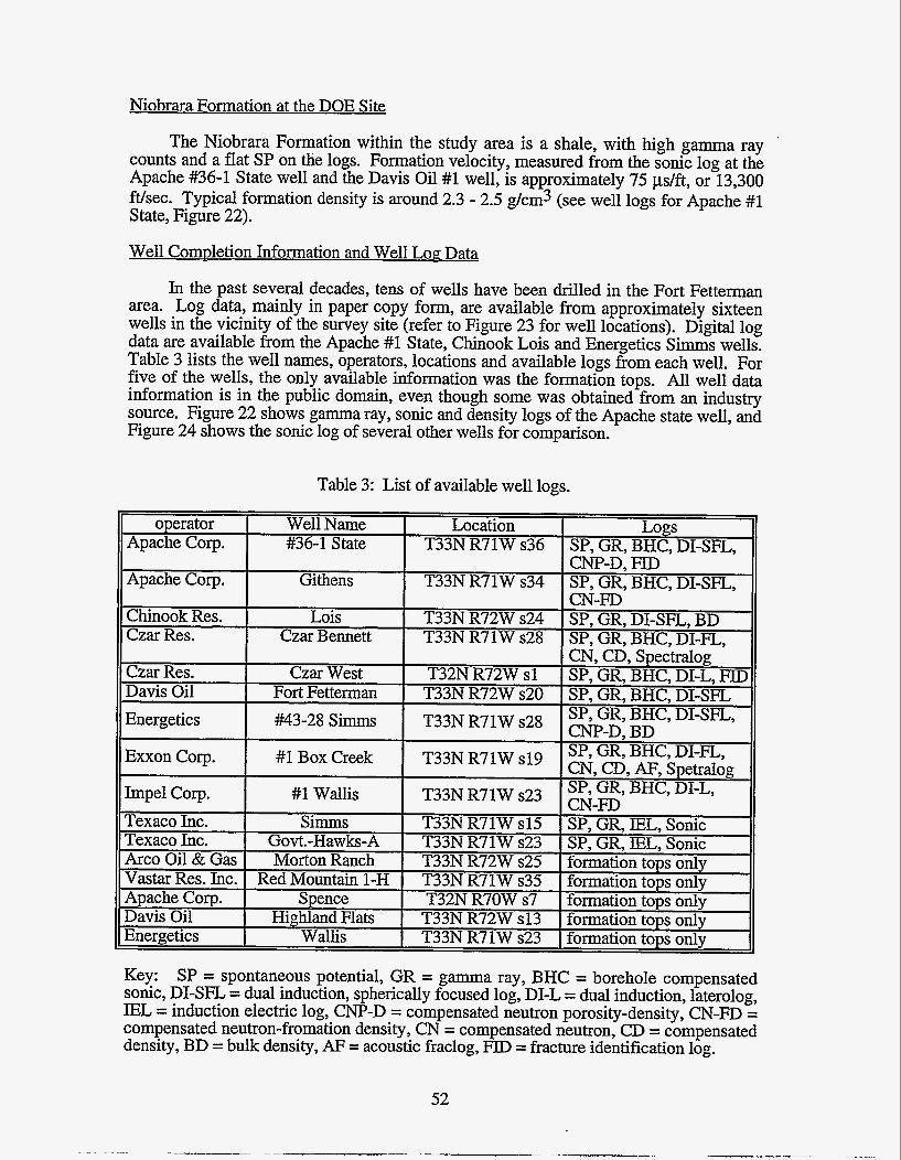
Niobrara Formation at the DOE Site
The Niobrara Formation within the study area is a shale, with high gamma ray counts and a flat SP on the logs. Formation velocity, measured from the sonic log at the Apache #36-1 State well and the Davis Oil #1 well, is approximately 75 ps/ft, or 13,300 ft/sec. Typical formation density is around 2.3 - 2.5 g/crn3 (see well logs for Apache #1 State, Figure 22).
Well Completion Information and Well Log: Data
In the past several decades, tens of wells have been drilled in the Fort Fetterman area. Log data, mainly in paper copy form, are available from approximately sixteen wells in the vicinity of the survey site (refer to Figure 23 for well locations). Digital log data are available from the Apache #1 State, Chinook Lois and Energetics Simms wells. Table 3 lists the well names, operators, locations and available logs from each well. For five of the wells, the only available information was the formation tops. All well data information is in the public domain, even though some was obtained from an industry source. Figure 22 shows gamma ray, sonic and density logs of the Apache state well, and Figure 24 shows the sonic log of several other wells for comparison.
Table 3: List of available well logs.
Key: SP = spontaneous potential, GR = gamma ray, BHC = borehole compensated sonic, DI-SFL = dual induction, spherically focused log, DI-L = dual induction, laterolog, E L = induction electric log, CNP-D = compensated neutron porosity-density, CN-FD = compensated neutron-fromation density, CN = compensated neutron, CD = compensated density, BD = bulk density, AF = acoustic fraclog, FID = fracture identification log.
52
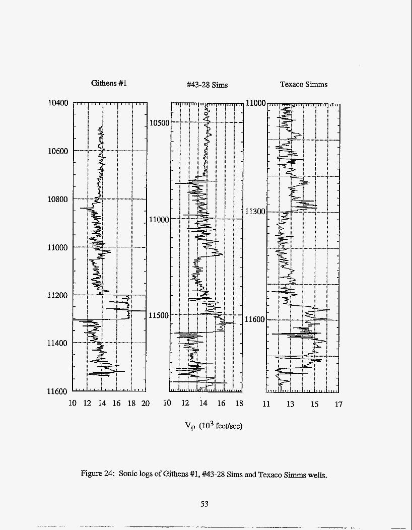
10400
10600
10800
11000
11200
11400
11600
m
........
....... -
.......
.......
- - - .......
J-L
Githens #1 #3-28 S i m ~ Texaco Simms i~ ............................
e : : . ..... .- ......... - ......... : :
t ! n 3- I - g ..........................
1(1/11(1111
TI
....
...
.... =
. . . . -
.......
- . . . . . . . . . - . . . . 1600 -..... ......... i ........ . . . . - : . . :- . . . . . - . . , . . . . . . . . . . . . - . . . . . . . . . . . .
- . . _. ....-...... - . . . . - . . . . . . . .
L 5 :
11 13
m
.....
..... b
- 2 .....
.....
.....
Y
E z c a - - - r - i
Lu
15
I 1 1 1 1 1 1 , , 7
.............._
-
............. -
..... - ......-
- .......... __.-
- ....... ).....-
- "i-- *..-
>: -
" i
- :
- . " i . . ............. -
-
u $ 1 I I * 1
17
Figure 24: Sonic logs of Githens #1, #3-28 Sims and Texaco Simms wells.
53
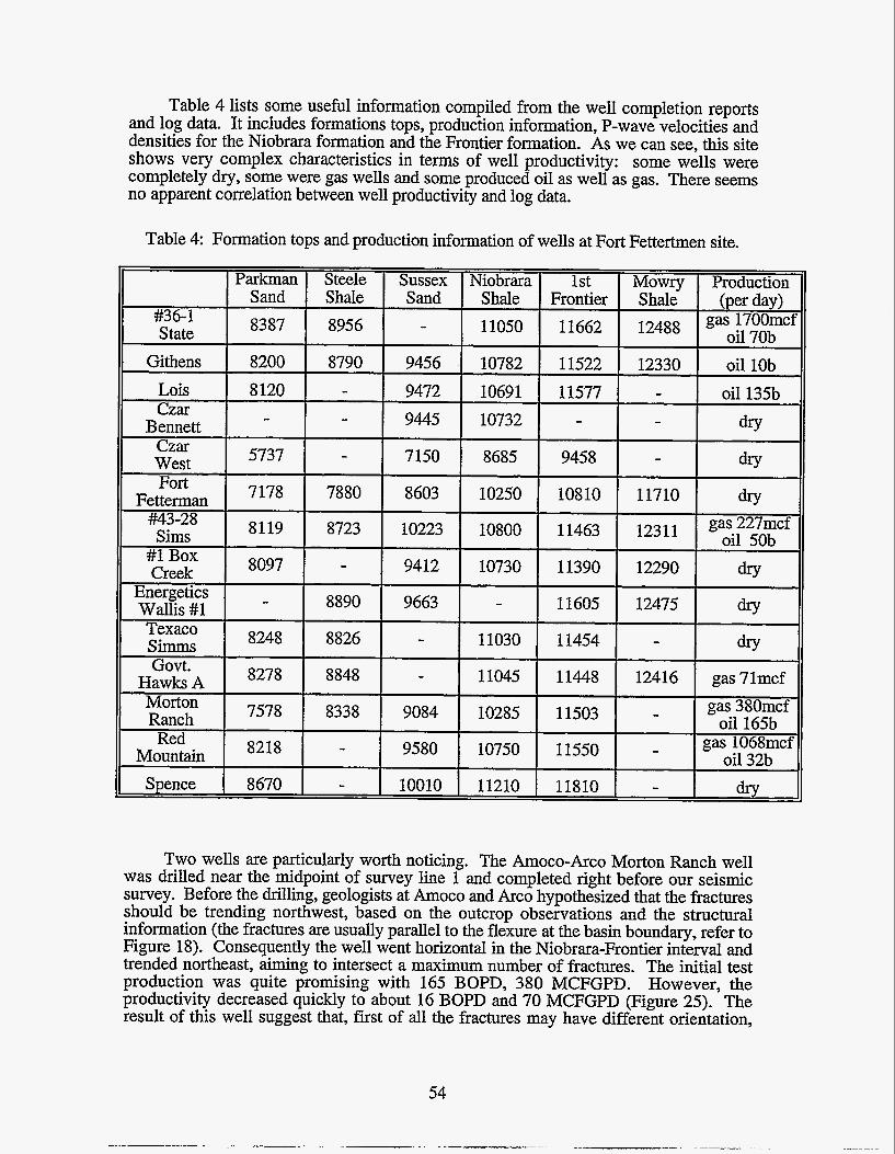
Table 4 lists some useful information compiled from the well completion reports and log data. It includes formations tops, production information, P-wave velocities and densities for the Niobrara formation and the Frontier formation. As we can see, this site shows very complex characteristics in terms of well productivity: some wells were completely dry, some were gas wells and some produced oil as well as gas. There seems no apparent correlation between well productivity and log data.
Table 4 Formation tops and production infomation of wells at Fort Fettertmen site.
Two wells are particularly worth noticing. The Amoco-Arc0 Morton Ranch well was drilled near the midpoint of survey line 1 and completed right before our seismic survey. Before the drilling, geologists at Amoco and Arc0 hypothesized that the fractures should be trending northwest, based on the outcrop observations and the structural information (the fractures are usually parallel to the flexure at the basin boundary, refer to Figure 18). Consequently the well went horizontal in the Niobrara-Frontier interval and trended northeast, aiming to intersect a maximum number of fractures. The initial test production was quite promising with 165 BOPD, 380 MCFGPD. However, the productivity decreased quickly to about 16 BOPD and 70 MCFGPD (Figure 25). The result of this well suggest that, first of all the fractures may have different orientation,
54
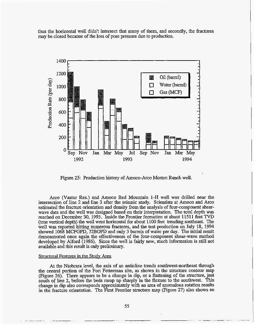
thus the horizontal well didn't intersect that many of them, and secondly, the fractures may be closed because of the loss of pore pressure due to production.
1400 1200 m n h cd
1000 8 pc W
22 800 2 ' 600
E 400
-5 7 a
200
0 Sep Nov Jan Mar May Jul Sep Nov Jan Mar May 1992 1993 1994
Figure 25: Production history of Amoco-Arc0 Morton Ranch well.
Arco (Vastar Res.) and Amoco Red Mountain 1-H well was drilled near the intersection of line 2 and line 3 after the seismic study. Scientists at Amoco and Arc0 estimated the fracture orientation and density from the analysis of four-component shear- wave data and the well was designed based on their interpretation. The total depth was reached on December 30, 1993. Inside the Frontier formation at about 1151 1 feet TVD (true vertical depth) the well went horizontal for about 1100 feet trending southeast. The well was reported bitting numerous fractures, and the test production on July 18, 1994 showed 1068 MCFGPD, 32BOPD and only 3 barrels of water per day. The initial result demonstrated once again the effectiveness of the four-component shear-wave method developed by Alford (1986). Since the well is fairly new, much information is still not available and this result is only preliminary.
Structural Features in the Studv Area
At the Niobrara level, the axis of an anticline trends southwest-northeast through the central portion of the Fort Fetterman site, as shown in the structure contour map (Figure 26). There appears to be a change in dip, or a flattening of the structure, just south of line 2, before the beds ramp up sharply in the flexure to the southwest. This change in dip also corresponds approximately with an area of anomalous rotation results in the fracture orientation. The First Frontier structure map (Figure 27) also shows an
55
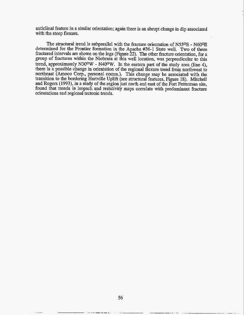
anticlinal feature in a similar orientation; again there is an abrupt change in dip associated with the steep flexure.
The structural trend is subparallel with the fracture orientation of N550E - N600E determined for the Frontier formation in the Apache #36-1 State well. Two of these fractured intervals are shown on the logs (Figure 22). The other fracture orientation, for a group of fractures within the Niobrara at this well location, was perpendicular to this trend, approximately N30°W - N4OoW. In the eastern part of the study area (line 4), there is a possible change in orientation of the regional flexure trend from northwest to northeast (Amoco Corp., personal comm.). This change may be associated with the transition to the bordering Hartville Uplift (see structural features, Figure 18). Mitchell and Rogers (1993), in a study of the region just north and east of the Fort Fetterman site, found that trends in isopach and resistivity maps correlate with predominant fracture orientations and regional tectonic trends.
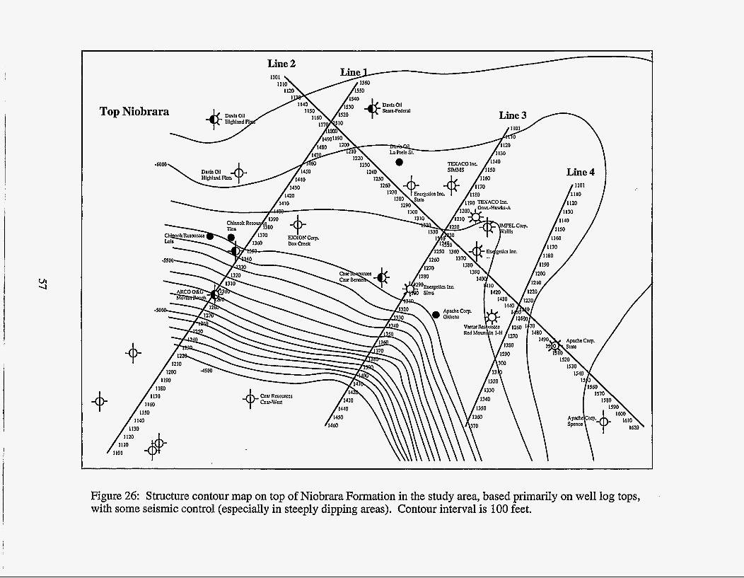
Figure 26: Structure contour map on top of Niobrara Formation in the study area, based primarily on well log tops, with some seismic control (especially in steeply dipping areas). Contour interval is 100 feet.
58
SEISMIC DATA ACQUISITION
The seismic data collection work was contracted to Amoco's Party 45, which is operated by Grant-Tensor. Four vertical component and four rotating base-plate horizontal component trucks were used as the seismic sources throughout the data collection.
Field Lavout and Geophones
The original plan was to shoot two two-dimensional seismic lines, lines 1 and 2, with funding from the DOE and Amoco. Line 1 strikes northeast and line 2 northwest (Figure 23). Their lengths are 13.8 km and 16.6 km respectively. Later, during the data acquisition stage, additional funding was obtained from ArcoNastar Resources to shoot two shorter lines, line 3 (10.8 km) and line 4 (8.1 km). These are both nearly parallel to line 2. This arrangement gives us far more extensive coverage of the survey area and the data reveal interesting lateral variations in terms of compressional wave amplitude, azimuth-dependent stacking velocity, shear wave splitting and P-SV/SH wave conversion.
The model of the geophones used in the seismic survey was SGR IV, manufactured by Geospace. The geophone spacing (group interval) was constant throughout the study at 30 meters. In each group there were six compressional-wave geophones polarized in the vertical direction. The geophones were evenly spaced at 5 meter intervals and centered on the group flag. Six horizontal (shear-wave) geophones were deployed in the same spatial pattern with their polarization parallel to the survey line, and six geophones had their polarization perpendicular to the survey line (Figure 28). A low-cut filter (3Hz) and 60Hz rejection were applied in the field. This geophone group allowed us to record all three component of the seismic signal from each shot. To simplify our discussion, we shall call the vertical component P, the in-line component S1 and the cross-line component S2.
There were 721 channels in every shot gather. Channel 1 was an auxiliary channel used for noise control purposes. Channels 2-241 recorded P-wave from the source. The in-line and cross-line components of the reflected shear-waves were recorded by channels 242-481 and 482-721, respectively. 60/180 split was used for most of the shots except for those at the end of the lines. This gave a maximum offset of 5400 meter (18000 feet) for most of the shot records, although sometimes the offset could be as large as 7200 meter (24000 feet). Note that the target depths of interest were at about 3300 meter (1 1000 feet).
Sources
We used three types of vibroseis sources. Conventional vertical (P-wave) vibrators generate nearly vertical particle motion by shaking the ground up and down, while shear- wave vibrators shake the ground horizontally. Two orthogonal polarizations are possible for the shear wave sources. We chose one to be in-line with the survey line (Sl) and the other perpendicular to it (S2). Because we use three types of sources and receivers, and all three components of every shot are recorded, we obtain nine different sets of data for each survey line. In the later discussion we shall call them by their source and receiver types, such as P-P, denoting signals recorded from P source to P receivers , and Sl-S2 from in-line shear source to cross-line shear receivers.
59
Four vibrator trucks aligned along the survey line are used simultaneously for each type of source. High quality signals were obtained by ground force phase locking on the
P-wave source
- Shear wave source
Figure 28: Geometry of the source and geophone arrays. The group interval is 30 m. For each component, six geophones are spaced evenly at 5 meter intervals and centered on the group flag. The moveup is 7.5 m for the vertical component trucks, and 3.75 m for the horizontal component trucks.
vibrators. Every "shot" consisted of several sweeps. The trucks uniformly moved forward along the line a small distance after each sweep. The number of sweeps was four for P-wave sources and eight for shear sources. Higher number of sweeps for shear sources was necessary because shear-waves usually attenuate faster than P-waves. To maintain the same source group length the move-up was 7.5 meters for P-wave sources and 3.75 meters for shear-wave sources. Diversity stack summing was performed in the field.
After analyzing the test shot gathers and taking into account the depth of our targets, the large offset of the geophone array and the data volume, it was decided that 4
60
msec sampling rate (125 Nyquist frequency) was appropriate for this project. Most of the P-wave signal energy was limited within 10 - 50Hz frequency band while no discernible shear-wave signal existed beyond 30Hz. The P-wave vibrators swept from 7 to 90 Hz and the shear-wave vibrators from 7 to 50 Hz. All sources swept for 10 seconds and the receivers listen for 18 seconds, which gave us 8 second data per channel after correlation. This was based on the face that the two-way travel time of the deepest target was about 2.5 seconds for P-wave and 4.5 seconds for shear wave.
Our design of the field layout followed the well-known stack array approach. Signals from a number of evenly spaced sources and receivers were stacked to form a single shot gather. This kind of stack array is commonly used to suppress the ground roll and other coherent noises (Anstey, 1986; Hildebrandt et al., 1986). Our design is illustrated in figure 28. The VP stations were centered between the flags, and the VP interval was 60 meters (shot every other group). The field parameters are summarized in Table 5.
Sometimes a vibrator truck would malfunction and a few shots were collected with only three vibrators. In such cases more sweeps were done to compensate for the loss of total source energy.
Table 5: Acquisition Parameters.
Group interval 30.0 meters Three-component sources, three-component receivers 6 geophones per group component, centered on the flag 240 channels per component, 180/60 split-spread shooting Four vertical (P-wave) vibrators, four rotating base-plate horizontal vibrators P-wave Shear-wave Frequency range, P-wave 7-90Hz, shear-wave 7-5OHz Sweep length 10 seconds Listen length 16 seconds Record length 6 second Field Filter
4 sweeps, 7.5 meter move-up 8 sweeps, 3.73 meter moveup
3 Hz low-cut, 60 Hz rejection
Dataset
The data acquisition work was done between October 26, 1992 and January 17, 1993. According to the observer's sheet, the ground was wet most of the time during the shooting of line 1 and line 2, and afterwards it was covered with snow while shooting lines 3 and 4.
The data were delivered in SEGY format on 21 8mm exabyte tapes. For each survey line the file number starts from 1 and increases in increment of one. There are
749, 832, 584 and 425 files for lines 1, 2, 3 and 4, respectively. The data volume is roughly 17 gigabytes.
The convention for numbering the sources is the same for all four lines. For a given line, the source point number starts with 101 as the last three digits. The P-wave sources are numbered in 1000 series, S1 (in-line shear) sources in 2000 series and S2 (cross-line shear) sources in 3000 series. The noise files are numbered in 5000 series. For example, the first P-wave, S1 and S2 sources are numbered 1101, 2101 and 3101, respectively, even though they are actually at the same location. The geophones are numbered in a similar fashion, with P-wave geophones in 1000 series, S1 geophones in 2000 series and S2 geophones in 3000 series, starting with 101 as the last three digits.
Name I Byte offset I byte length
A few header words are preloaded in the SEGY files. Their name, byte offset, length and format are listed in table 6. SHT-STAT, REC-STAT and CDP-SHAT represents shot, receiver and CDP station numbers.
format
REC-STAT
SHOT SGRSN GLCFNF DATE PERPOF SHOT10 OLDOFF STATIC LINNDX TYPE DCBIAS CDP-STAT SHT-STAT
187 L
9 191 193 195 199 203 207 21 1 213 215 271 183 185
4 2 2 4 4 4 4 2 2 2 4 2 2 n
INT INT INT INT INT INT INT INT INT INT
lBm INT INT INT
The ground survey was carried out in October, 1992, and the measurement of the absolute x-y coordinates and elevation for every station was compiled in four ASCIt files, one for each line. The data was delievered in IBM PC format.
SGR gain problem
After data acquisition of the four nine-component seismic lines, we plotted the stacking chart display of the line 2 S2-S2 trace amplitudes after spherical divergence correction (Figure 29). In Figure 29 each pixel represents the RMS (root mean square) amplitude of a trace within a time window, which was selected to contain a fixed set of events. The receiver and source station numbers were used as the horizontal and vertical coordinates in the plot. The checkered appearence suggested a gain problem of the recording instrument.
Our partner at Amoco also noticed the problem and investigated the causes. A program bug caused "most traces recorded on 4-channel SGRs (SGRNO > 400) to be 1/16 of the correct amplitude". The correction is made by simply multiplying amplitudes in each erroneously recorded trace by 16. A map of the affected traces is available for this purpose.
62
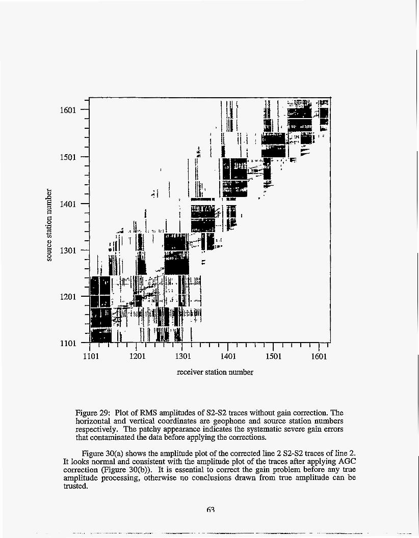
1501
1401
1301
1201
1101
1101 1201 1301 1401 1501 1601
receiver station number
Figure 29: Plot of FWS amplitudes of S2-S2 traces without gain correction. The horizontal and vertical coordinates are geophone and source station numbers respectively. The patchy appearance indicates the systematic severe gain errors that contaminated the data before applying the corrections.
Figure 30(a) shows the amplitude plot of the corrected line 2 S2-S2 traces of line 2. It looks normal and consistent with the amplitude plot of the traces after applying AGC correction (Figure 30(b)). It is essential to correct the gain problem before any true amplitude processing, otherwise no conclusions drawn from true amplitude can be trusted.
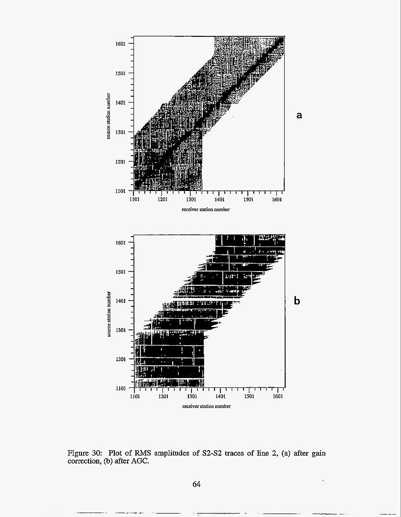
1601
1501
1401
1301
1201
1101
1601
1501
ki e C C 0
1401
2 - v1 0)
g 1301 s:
1201
1101
a
1201 1301 1401 lS0l 1601
receiver station number
b
li0l 1301 1401 li0l I601
receiver station number
Figure 30: Plot of R M S amplitudes of S2-S2 traces of line 2, (a) after gain correction, (b) after AGC.
64
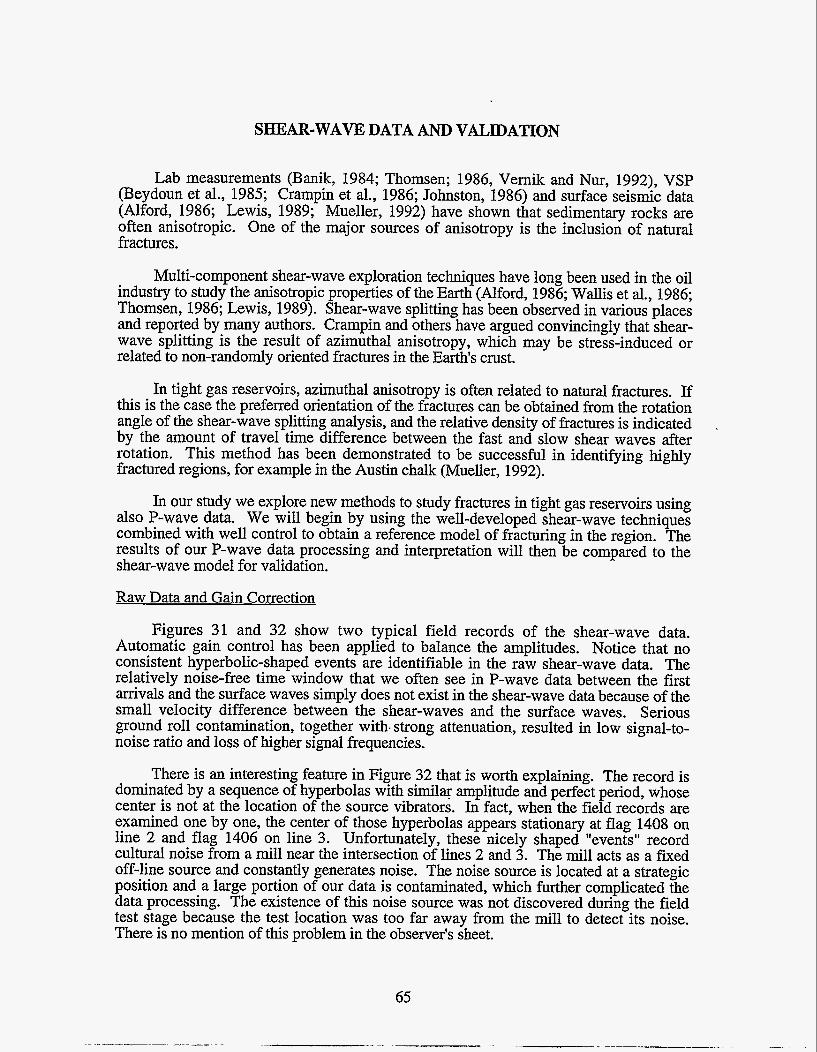
SHEAR-WAVE DATA AND VALIDATION
Lab measurements (Banik, 1984; Thomsen; 1986, Vernik and Nur, 1992), VSP (Beydoun et al., 1985; Crampin et al., 1986; Johnston, 1986) and surface seismic data (Alford, 1986; Lewis, 1989; Mueller, 1992) have shown that sedimentary rocks are often anisotropic. One of the major sources of anisotropy is the inclusion of natural fractures.
Multi-component shear-wave exploration techniques have long been used in the oil industry to study the anisotropic properties of the Earth (Alford, 1986; Wallis et al., 1986; Thomsen, 1986; Lewis, 1989). Shear-wave splitting has been observed in various places and reported by many authors. Crampin and others have argued convincingly that shear- wave splitting is the result of azimuthal anisotropy, which may be stress-induced or related to non-randomly oriented fractures in the Earth's crust.
In tight gas reservoirs, azimuthal anisotropy is often related to natural fractures. If this is the case the preferred orientation of the fractures can be obtained from the rotation angle of the shear-wave splitting analysis, and the relative density of fractures is indicated by the amount of travel time difference between the fast and slow shear waves after rotation. This method has been demonstrated to be successful in identifying highly fractured regions, for example in the Austin chalk (Mueller, 1992).
In our study we explore new methods to study fractures in tight gas reservoirs using also P-wave data. We will begin by using the well-developed shear-wave techniques combined with well control to obtain a reference model of fracturing in the region. The results of our P-wave data processing and interpretation will then be compared to the shear-wave model for validation.
Raw Data and Gain Correction
Figures 31 and 32 show two typical field records of the shear-wave data. Automatic gain control has been applied to balance the amplitudes. Notice that no consistent hyperbolic-shaped events are identifiable in the raw shear-wave data. The relatively noise-free time window that we often see in P-wave data between the first arrivals and the surface waves simply does not exist in the shear-wave data because of the small velocity difference between the shear-waves and the surface waves. Serious ground roll contamination, together with. strong attenuation, resulted in low signal-to- noise ratio and loss of higher signal frequencies.
There is an interesting feature in Figure 32 that is worth explaining. The record is dominated by a sequence of hyperbolas with similar amplitude and perfect period, whose center is not at the location of the source vibrators. In fact, when the field records are examined one by one, the center of those hyperbolas appears stationary at flag 1408 on line 2 and flag 1406 on line 3. Unfortunately, these nicely shaped "events" record cultural noise from a mill near the intersection of lines 2 and 3. The mill acts as a fixed off-line source and constantly generates noise. The noise source is located at a strategic position and a large portion of our data is contaminated, which further complicated the data processing. The existence of this noise source was not discovered during the field test stage because the test location was too far away from the mill to detect its noise. There is no mention of this problem in the observer's sheet.
65
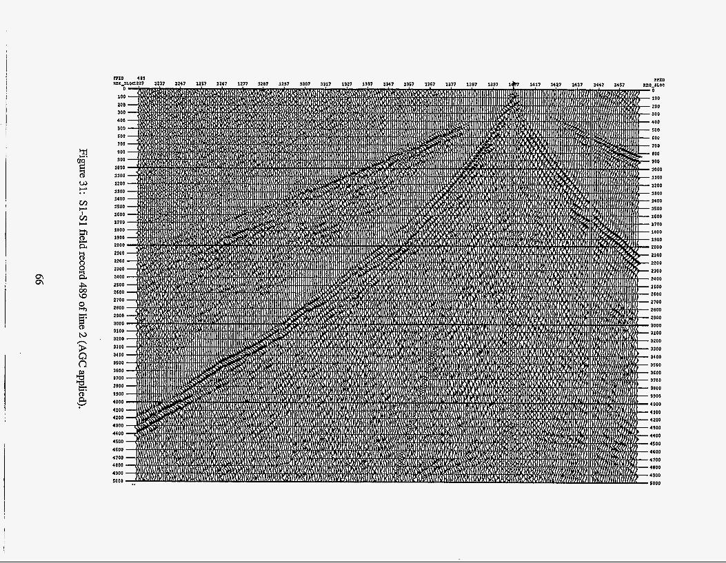
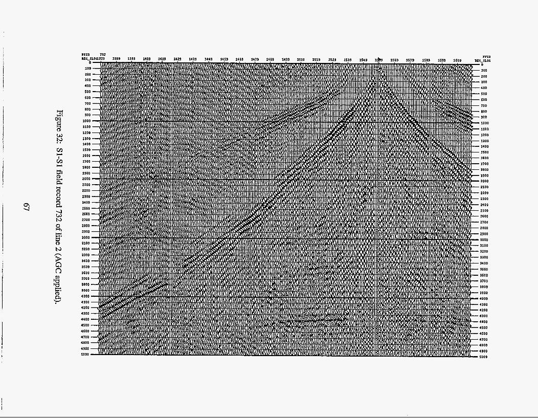
i? 8 w N ..
Eh a
??ID 732 IILC-SLOC1379 13?¶ 13?9 14?9 l4?9 W,29 14¶9 1449 1459 1469
0 100 200 300 400 500 600 700 800 900
1000 1100 1200 1300 1400 lS00 1600 1700 1800 1900 2000 2100 2200 2300 2400 2500 2600 2700 2800 2900 aooo 3100 3200 3300 a400 3500 3600 3700 3800 3900 4000 4100 4200 4800 4400 4500 4600 4700
1500 1600 1700 1800 1900 2000 2100 2200 2300 2400 2500 2600 2700 2800 2900 3000 3100 3200 3300 3400 3500 3600 3700 3800 3900 4000
t 4300 I- 4400 & 4500
4600 4700 4800 4900 5000
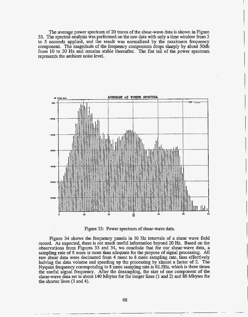
The average power spectrum of 20 traces of the shear-wave data is shown in Figure 33. The spectral analysis was performed on the raw data with only a time window from 2 to 5 seconds applied, and the result was normalized by the maximum frequency component. The magnitude of the frequency components drops sharply by about 30db from 10 to 20 Hz and remains stable thereafter. The flat tail of the power spectrum represents the ambient noise level.
61, f r a n u
0 20 30 )(z
...........................................................................................
AVERAGF, of POm SPECTRA ........................................ .................. .............................. : ................................ : ................................ : m. -
................................ ................................ ................................ ............................... .................... .i i i i
I 40
Figure 33: Power spectrum of shear-wave data.
Figure 34 shows the frequency panels in 10 Hz intervals of a shear wave field record. As expected, there is not much useful information beyond 20 Hz. Based on the observations from Figures 33 and 34, we conclude that for our shear-wave data, a sampling rate of 8 msec is more than adequate for the purpose of signal processing. All raw shear data were decimated from 4 msec to 8 msec sampling rate, thus effectively halving the data volume and speeding up the processing by almost a factor of 2. The Nyquist frequency corresponding to 8 msec sampling rate is 62.5Hz, which is three times the useful signal frequency. After the desampling, the size of one component of the shear-wave data set is about 140 Mbytes for the longer lines (1 and 2) and 80 Mbytes for the shorter lines (3 and 4).
68
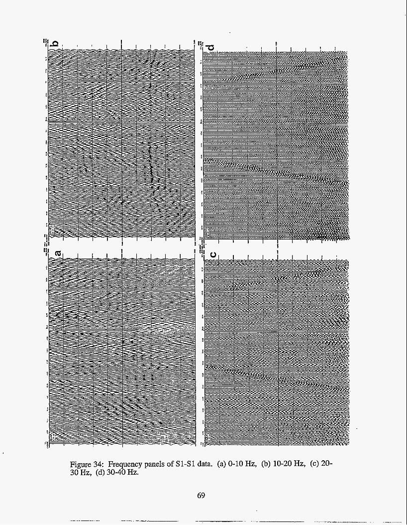
Figure 34: Frequency panels of S1-S1 data. (a) 0-10 Hz, (b) 10-20 Hz, (c) 20- 30 Hz, (d) 30-40 Hz.
69
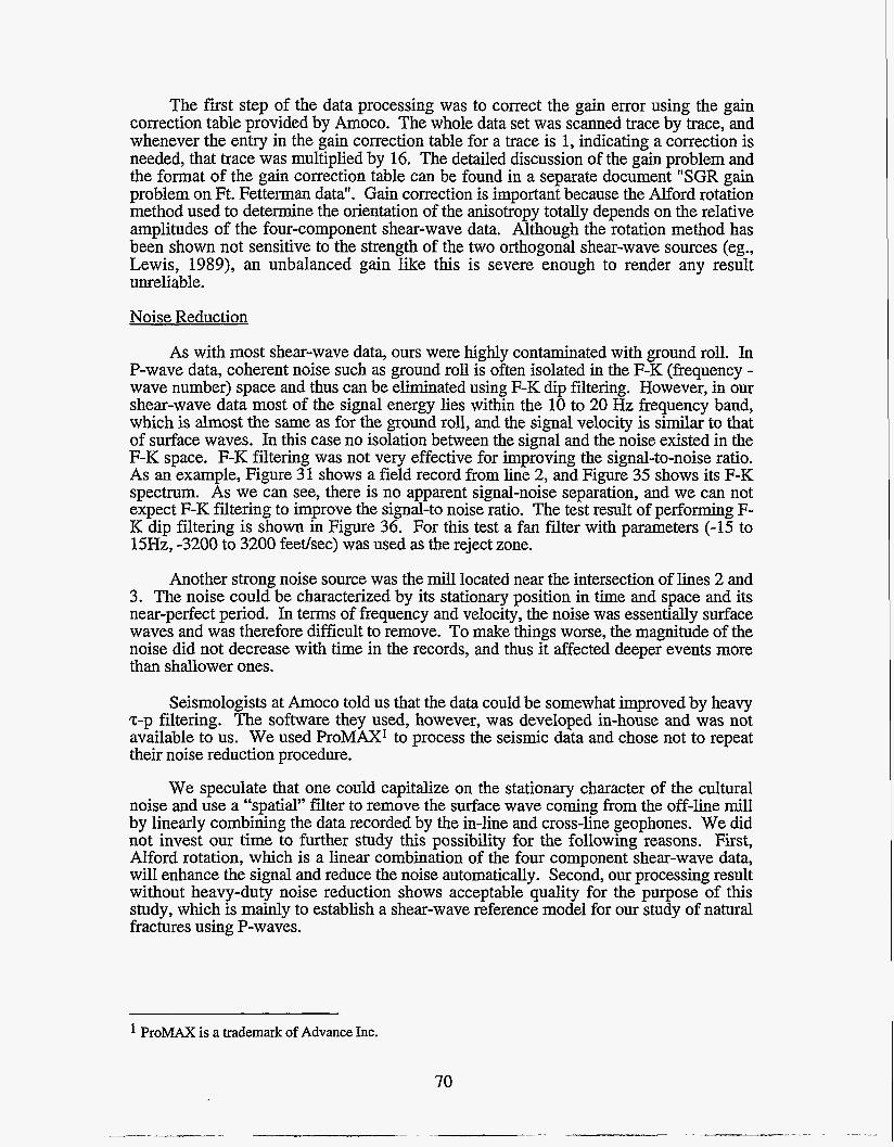
The first step of the data processing was to correct the gain error using the gain correction table provided by Amoco. The whole data set was scanned trace by trace, and whenever the entry in the gain correction table for a trace is 1, indicating a correction is needed, that trace was multiplied by 16. The detailed discussion of the gain problem and the format of the gain correction table can be found in a separate document “SGR gain problem on Ft. Fetterman data”. Gain correction is important because the Alford rotation method used to determine the orientation of the anisotropy totally depends on the relative amplitudes of the four-component shearAwave data. Although the rotation method has been shown not sensitive to the strength of the two orthogonal shear-wave sources (eg., Lewis, 1989), an unbalanced gain like this is severe enough to render any result unreliable.
Noise Reduction
As with most shear-wave data, ours were highly contaminated with ground roll. In P-wave data, coherent noise such as ground roll is often isolated in the F-K (frequency - wave number) space and thus can be eliminated using F-K dip filtering. However, in our shear-wave data most of the signal energy lies within the 10 to 20 Hz frequency band, which is almost the same as for the ground roll, and the signal velocity is similar to that of surface waves. In this case no isolation between the signal and the noise existed in the F-K space. F-K filtering was not very effective for improving the signal-to-noise ratio. As an example, Figure 3 1 shows a field record from line 2, and Figure 35 shows its F-K spectrum. As we can see, there is no apparent signal-noise separation, and we can not expect F-K filtering to improve the signal-to noise ratio. The test result of performing F- K dip filtering is shown in Figure 36. For this test a fan filter with parameters (-15 to 15Hz, -3200 to 3200 feethec) was used as the reject zone.
Another strong noise source was the mill located near the intersection of lines 2 and 3. The noise could be characterized by its stationary position in time and space and its near-perfect period. In terms of frequency and velocity, the noise was essentially surface waves and was therefore difficult to remove. To make things worse, the magnitude of the noise did not decrease with time in the records, and thus it affected deeper events more than shallower ones.
Seismologists at Amoco told us that the data could be somewhat improved by heavy T-p filtering. The software they used, however, was developed in-house and was not available to us. We used ProMAXl to process the seismic data and chose not to repeat their noise reduction procedure.
We speculate that one could capitalize on the stationary character of the cultural noise and use a “spatial” filter to remove the surface wave coming from the off-line mill by linearly combining the data recorded by the in-line and cross-line geophones. We did not invest our time to further study this possibility for the following reasons. First, Alford rotation, which is a linear combination of the four component shear-wave data, will enhance the signal and reduce the noise automatically. Second, our processing result without heavy-duty noise reduction shows acceptable quality for the purpose of this study, which is mainly to establish a shear-wave reference model for our study of natural fractures using P-waves.
P r o m is a trademark of Advance Inc.
70
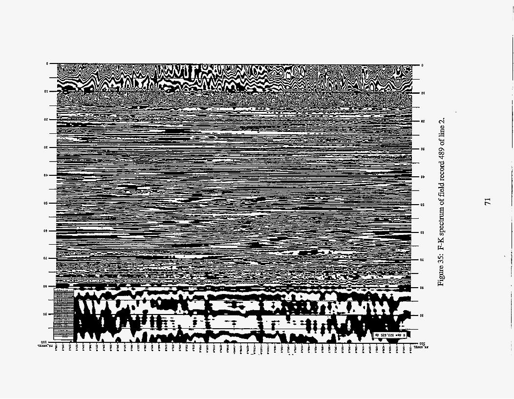
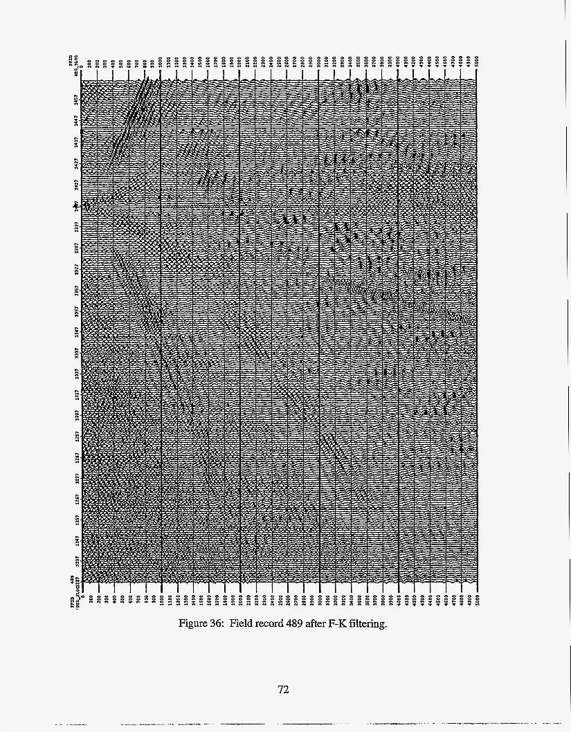
n r 5; L
I.
c . n
n . n n . 4 I.
n n
I. m rn n
I. I.
n m
I.
cm n
I. 0 n
I. x I.
n n
I.
rn n
:: n
n m n
I. m n
I.
N
I. I. N n
I. N
I. m n
I. x I.
N n
Figure 36: Field record 489 after F-K filtering.
72
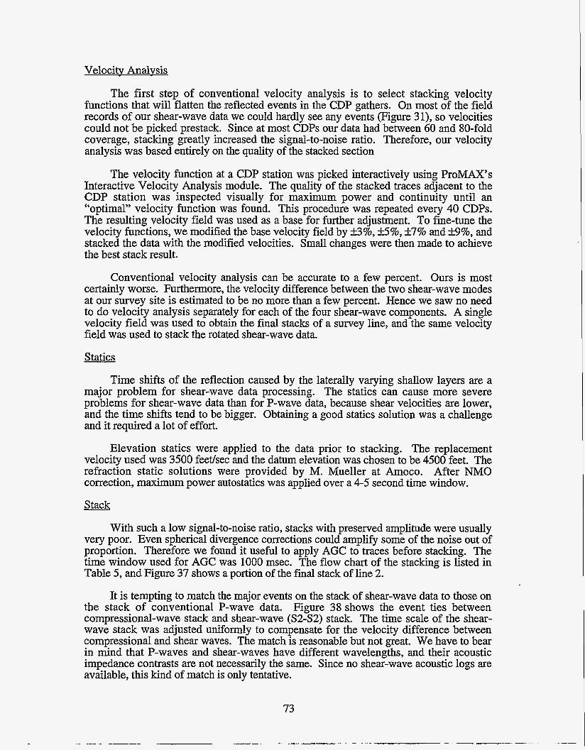
Velocitv Analysis
The first step of conventional velocity analysis is to select stacking velocity functions that will flatten the reflected events in the CDP gathers. On most of the field records of our shear-wave data we could hardly see any events (Figure 31), so velocities could not be picked prestack. Since at most CDPs our data had between 60 and 80-fold coverage, stacking greatly increased the signal-to-noise ratio. Therefore, our velocity analysis was based entirely on the quality of the stacked section
The velocity function at a CDP station was picked interactively using ProMAX’s Interactive Velocity Analysis module. The quality of the stacked traces adjacent to the CDP station was inspected visually for maximum power and continuity until an “optimal” velocity function was found. This procedure was repeated every 40 CDPs. The resulting velocity field was used as a base for further adjustment. To fine-tune the velocity functions, we modified the base velocity field by &3%, &5%, k7% and S%, and stacked the data with the modified velocities. Small changes were then made to achieve the best stack result.
Conventional velocity analysis can be accurate to a few percent. Ours is most certainly worse. Furthermore, the velocity difference between the two shear-wave modes at our survey site is estimated to be no more than a few percent. Hence we saw no need to do velocity analysis separately for each of the four shear-wave components. A single velocity field was used to obtain the final stacks of a survey line, and the same velocity field was used to stack the rotated shear-wave data.
Statics
Time shifts of the reflection caused by the laterally varying shallow layers are a major problem for shear-wave data processing. The statics can cause more severe problems for shear-wave data than for P-wave data, because shear velocities are lower, and the time shifts tend to be bigger. Obtaining a good statics solution was a challenge and it required a lot of effort.
Elevation statics were applied to the data prior to stacking. The replacement velocity used was 3500 feet/sec and the datum elevation was chosen to be 4500 feet. The refraction static solutions were provided by M. Mueller at Amoco. After NMO correction, maximum power autostatics was applied over a 4-5 second time window.
Stack
With such a low signal-to-noise ratio, stacks with preserved amplitude were usually very poor. Even spherical divergence corrections could amplify some of the noise out of proportion. Therefore we found it useful to apply AGC to traces before stacking. The time window used for AGC was 1000 msec. The flow chart of the stacking is listed in Table 5, and Figure 37 shows a portion of the final stack of line 2.
It is tempting to match the major events on the stack of shear-wave data to those on the stack of conventional P-wave data. Figure 38 shows the event ties between compressional-wave stack and shear-wave (S2-S2) stack. The time scale of the shear- wave stack was adjusted uniformly to compensate for the velocity difference between compressional and shear waves. The match is reasonable but not great. We have to bear in mind that P-waves and shear-waves have different wavelengths, and their acoustic impedance contrasts are not necessarily the same. Since no shear-wave acoustic logs are available, this kind of match is only tentative.
73
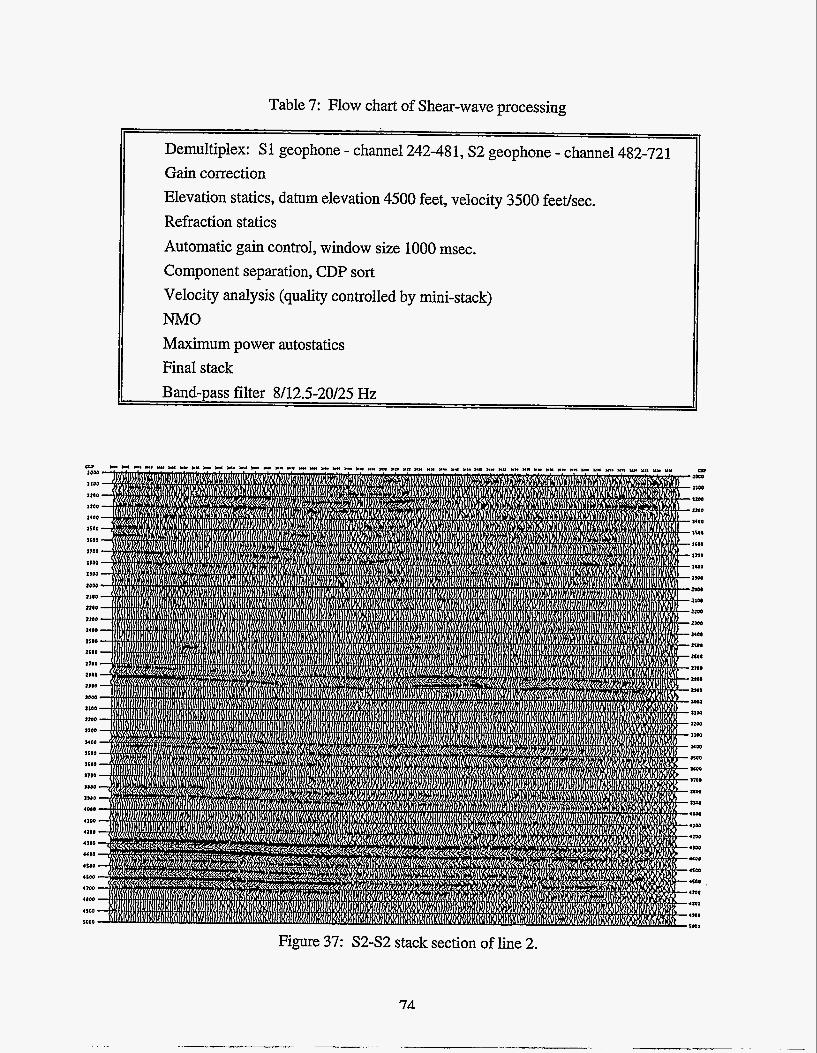
Table 7: Flow chart of Shear-wave processing
Demultiplex: S1 geophone - channel 242-481, S2 geophone - channel 482-721 Gain correction Elevation statics, datum elevation 4500 feet, velocity 3500 feet/sec. Refraction statics Automatic gain control, window size 1000 msec. Component separation, CDP sort Velocity analysis (quality controlled by mini-stack) NMO Maximum power autostatics Final stack Band-pass filter 8/12.5-20/25 Hz
Figure 37: S2-S2 stack section of line 2.
74
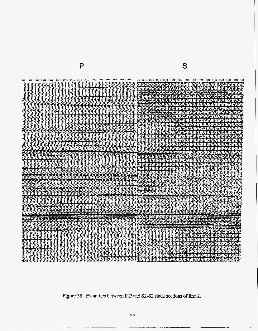
P S
Figure 38: Event ties between P-P and S2-S2 stack sections of line 2.
7 c
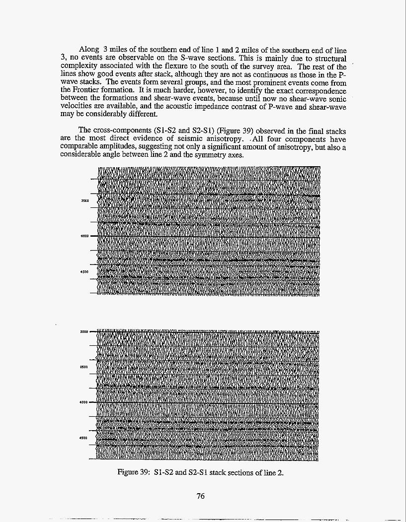
Along 3 miles of the southern end of line 1 and 2 miles of the southern end of line 3, no events are observable on the S-wave sections. This is mainly due to structural complexity associated with the flexure to the south of the survey area. The rest of the . lines show good events after stack, although they are not as continuous as those in the P- wave stacks. The events form several groups, and the most prominent events come from the Frontier formation. It is much harder, however, to identify the exact correspondence between the formations and shear-wave events, because until now no shear-wave sonic velocities are available, and the acoustic impedance contrast of P-wave and shear-wave may be considerably different.
The cross-components (Sl-S2 and SZ-Sl) (Figure 39) observed in the final stacks are the most direct evidence of seismic anisotropy. ,All four components have comparable amplitudes, suggesting not only a significant amount of anisotropy, but also a considerable angle between line 2 and the symmetry axes.
Figure 39: Sl-S2 and S2-S1 stack sections of line 2.
76
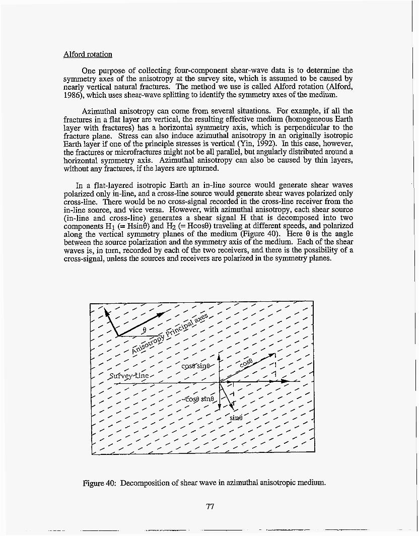
Alford rotation
One purpose of collecting four-component shear-wave data is to determine the symmetry axes of the anisotropy at the survey site, which is assumed to be caused by nearly vertical natural fractures. The method we use is called Alford rotation (Alford, 1986), which uses shear-wave splitting to identify the symmetry axes of the medium.
Azimuthal anisotropy can come from several situations. For example, if all the fractures in a flat layer are vertical, the resulting effective medium (homogeneous Earth layer with fractures) has a horizontal symmetry axis, which is perpendicular to the fracture plane. Stress can also induce azimuthal anisotropy in an originally isotropic Earth layer if one of the principle stresses is vertical (Yin, 1992). In this case, however, the fractures or microfractures might not be all parallel, but angularly distributed around a horizontal symmetry axis. Azimuthal anisotropy can also be caused by thin layers, without any fractures, if the layers are upturned.
In a flat-layered isotropic Earth an in-line source would generate shear waves polarized only in-line, and a cross-line source would generate shear waves polarized only cross-line. There would be no cross-signal recorded in the cross-line receiver from the in-line source, and vice versa. However, with azimuthal anisotropy, each shear source (in-line and cross-line) generates a shear signal H that is decomposed into two components Hi (= Hsin0) and H2 (= Hcos0) traveling at different speeds, and polarized along the vertical symmetry planes of the medium (Figure 40). Here 8 is the angle between the source polarization and the symmetry axis of the medium. Each of the shear waves is, in turn, recorded by each of the two receivers, and there is the possibility of a cross-signal, unless the sources and receivers are polarized in the symmetry planes.
Figure 40: Decomposition of shear wave in azimuthal anisotropic medium.
77
In principle, we can find the symmetry axes by linearly combining the four- component shear-wave data to minimize the cross-signal between perpendicularly polarized sources and receivers . If we “synthesize” a source from the real in-line and cross-line sources such that the new synthetic source has the polarization that is either parallel or perpendicular to the symmetry axis, and similarly rotate the geophones, there will be no cross-components recorded. One approach is to solve for 8 directly. However, due to the influence of the strong noise that usually companies shear-wave data, a direct inversion is often unstable. A more robust method is simply to search through a range of angles 8 until the cross-signal is minimized.
Under a rotation of angle 8, the resulting traces can be computed from the original data in terms of
u 1cos28 +u2,sin28 + u 12cos28 sin% - 0.5sin28(u 12+u21) 0.5sin%(u 1-u22)
U ~ ~ C O S ~ C I -u12sin28 - U ~ ~ C O S ~ ~ +ullsin28 - OSsin28(u 1-u22) 0 . 5 s i n 2 8 ( ~ ~ ~ + u ~ ~ )
where ull, u12, u21, u22 are the recorded four-component shear-wave traces and
= ( cos8 sin8 ) -sin8 cos8
is the rotation matrix. The appropriate rotation angle will cause the off-diagonal elements of matrix v to vanish. Of course in reality residual noise will always exist and we can not expect the cross-components of the rotated data to be perfectly zero. Only the coherent signals will disappear (or be minimized) after proper rotation.
Rotation Results
After Alford rotation, the processing procedures in Table 5 were reapplied and the data set restacked. The rotation was done fiist in 10 degree increments, and then in 5 degree increments near the proper rotation angle. Stacks with different rotation angles were visually inspected to choose the best angle. Figure 41 shows a portion of the stacked four-component data before and after the rotation. Notice that the two cross- components drop below the noise level after proper rotation. Where the events are strong, the rotation angle can be determined within a few degrees; where almost no events are discernible the rotation angle cannot be determined with much confidence.
A problem of multi-component shear-wave analysis is that the symmetry axes of the azimuthal anisotropy may not be the same for all depths. Near-surface layers are often anisotropic, and their anisotropy may be due to weathering or the current stress states that are not related to the fractures thousands of feet deep. Some researchers have suggested that a large part of the observed anisotropy comes from the shallow layers. For VSP data a layer stripping technique can be used to find out the real symmetry axis for each layer. For surface seismic data, the problem is much more difficult, because the geophones must be placed on the ground and the cumulative effects of all the layers are recorded.
78
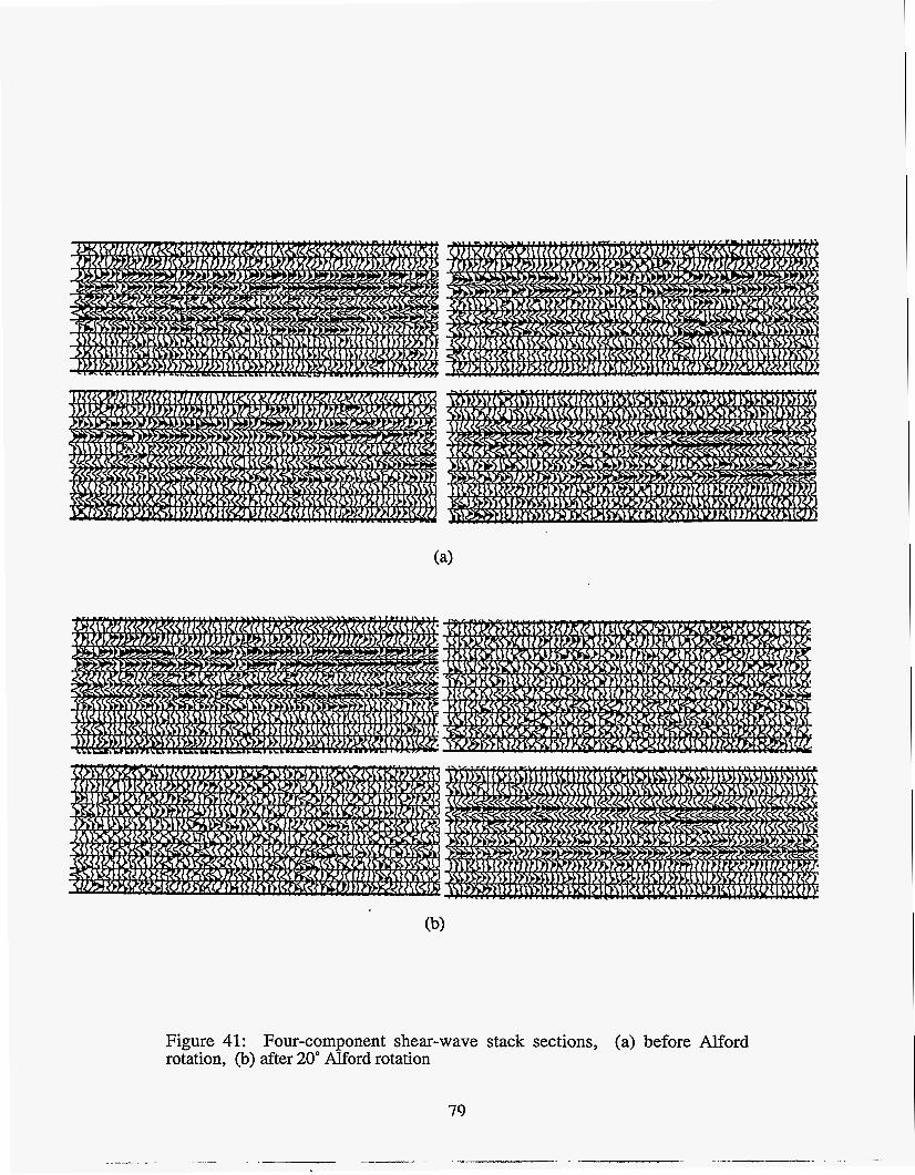
Figure 41: Four-component shear-wave stack sections, (a) before Alford rotation, (b) after 20" Alford rotation
79
-_I__ - -___~ _ _ -
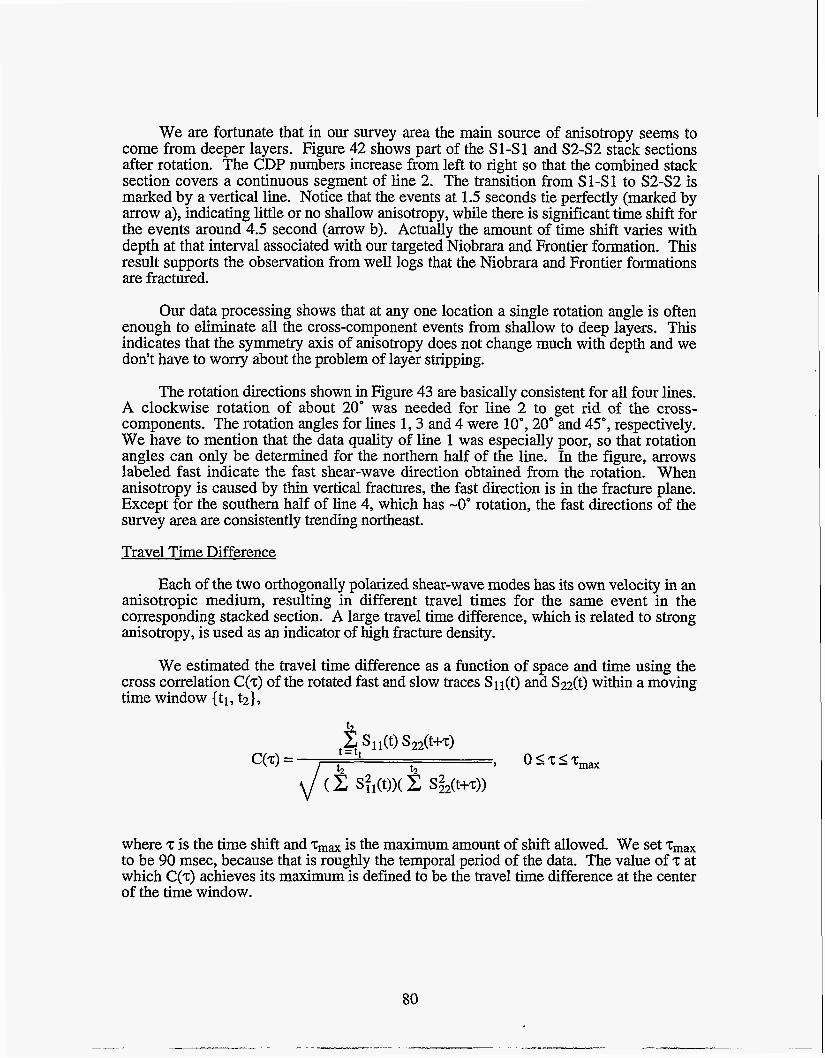
We are fortunate that in our survey area the main source of anisotropy seems to come from deeper layers. Figure 42 shows part of the S1-S1 and S2-S2 stack sections after rotation. The CDP numbers increase from left to right so that the combined stack section covers a continuous segment of line 2. The transition from S1-S1 to S2-S2 is marked by a vertical line. Notice that the events at 1.5 seconds tie perfectly (marked by arrow a), indicating little or no shallow anisotropy, while there is significant time shift for the events around 4.5 second (arrow b). Actually the amount of time shift varies with depth at that interval associated with our targeted Niobrara and Frontier formation. This result supports the observation from well logs that the Niobrara and Frontier formations are fractured.
Our data processing shows that at any one location a single rotation angle is often enough to eliminate all the cross-component events from shallow to deep layers. This indicates that the symmetry axis of anisotropy does not change much with depth and we don't have to worry about the problem of layer stripping.
The rotation directions shown in Figure 43 are basically consistent for all four lines. A clockwise rotation of about 20" was needed for line 2 to get rid of the cross- components. The rotation angles for lines 1,3 and 4 were lo", 20" and 45", respectively. We have to mention that the data quality of line 1 was especially poor, so that rotation angles can only be determined for the northern half of the line. In the figure, arrows labeled fast indicate the fast shear-wave direction obtained from the rotation. When anisotropy is caused by thin vertical fractures, the fast direction is in the fracture plane. Except for the southern half of line 4, which has -0" rotation, the fast directions of the survey area are consistently trending northeast.
Travel Time Difference
Each of the two orthogonally polarized shear-wave modes has its own velocity in an anisotropic medium, resulting in different travel times for the same event in the corresponding stacked section. A large travel time difference, which is related to strong anisotropy, is used as an indicator of high fracture density.
We estimated the travel time difference as a function of space and time using the cross correlation C(T) of the rotated fast and slow traces Sll(t) and S22(t) within a moving time window { tl, t2},
where 'I; is the time shift and T m a is the maximum amount of shift allowed. We set T m a to be 90 msec, because that is roughly the temporal period of the data. The value of z at which C(T) achieves its maximum is defined to be the travel time difference at the center of the time window.
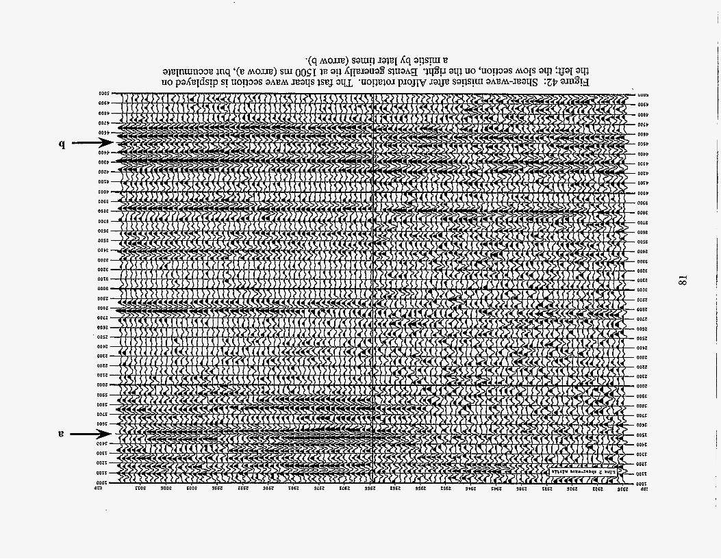
00 N
Davis Oil Hiphlvid Fhls
I
Figure 43: Interpretation of the four-component shear-wave processing. Arrows labeled "fast" and "slow" indicate shear polarization directions. Shading indicates interpreted fractured zones.
We use a sliding window to compute the time shift at each depth. The result for line 2 is shown in Figure 44. In spite of the fluctuations, we can see the regions where the time shifts are large, and that deeper layers have larger time shifts. The maximum value of the cross correlation indicates the similarity between the two rotated shear-wave components. They can be used to represent the reliability of the time shift results.
The amount of shear-wave splitting varies laterally along the lines, as might be expected. If we use a very large time window, the time shift can be viewed as the average of the whole trace. Figure 44 shows the result for a section on line 2 where signals are best. It changes smoothly between a few msec to 40 msec. Figure 45 shows the actual stack section. It is plotted using alternating fast and slow traces so that the amount of travel time difference can be easily seen at the boundaries. From Figure 45 we can estimate the amount of anisotropy in the Niobrara-Frontier formations. Around 4.2 seconds, for a sequence of events of about 300 msec, the travel time difference increases by 10-20 msec, thus the amount anisotropy is about 3-7%.
83
80 I I I 1 1 1 I I -
1401 f Line 4 1501 1601
Figure 44: Whole trace travel time difference between fast and slow shear wave stack sections of line 2.
84
U Y
fast slow fast slow
Figure 45: Alternating fast and slow shear-wave stacks showing the change of travel time difference along line 2.
,
Fracture Model for the Survey Area
Analysis of the shear-wave data, plus subsurface well control, allows us to construct a fracture model for our survey area (Figure 43). This model was largely developed by Melinda Gale of Vastar Resources and Mike Mueller of Amoco, and was reported at the 1994 Society of Exploration Geophysicists meeting in Los Angeles.
Throughout the site, the fracture directions, inferred from the shear-wave rotation analysis on all four lines, trend consistently SW-NE - all generally within about 200 of each other. These trends were taken to be equal to the polarization direction of the fast shear wave after rotation. These directions are labeled on the figure in a few locations with arrows.
The fracture intensity was taken to be proportional to relative time difference between the fast and slow shear waves at each location. This travel time difference (inferred fracture intensity) is highly variable throughout the site - the corresponding shear-wave anisotropy in the Frontier-Nibrara zones ranges from near zero to as much as 7 percent. The regions of largest anisotropy along the four lines can be intepreted with two localized zones of relatively intense fracturing (shown in gray in Figure 43).
Before beginning the survey, it was suggested that the fractures at depth would trend more along a NW-SE direction, parallel to the strike of the Casper Arch and the associated flexure along the SW edge of the survey (Figure 18). These were also interpreted from the second derivative of the known structure at depth. This trend is also seen in surface fractures mapped some km to the south of the survey area (Mueller, pers. comm.). The Amoco-Arc0 Morton Ranch well was drilled near the midpoint of survey line 1 and completed right before our seismic survey. Based on this pre-survey interpretation, the well went horizontal in the Niobrara-Frontier interval and trended northeast (almost parallel to line l), aiming to intersect a maximum number of fractures perpendicular to their trends. In fact, it was observed down-hole that it trended within about 20° of the fracture trend, consistent with the interpretation in Figure 43. The initial test production at Morton Ranch was quite promising with 165 BOPD, 380 MCFGPD. However, the productivity decreased quickly to about 16 BOPD and 70 MCFGPD (Figure 25). The result of this well suggest that, first of all the fractures may have different orientation, thus the horizontal well did not intersect many of them, and secondly, the fractures may be closed because of the loss of pore pressure due to production - consistent with poor fracture connectivity and low fracture density.
The Arc0 (Vastar Res.) and Amoco Red Mountain 1-H well was drilled near the intersection of line 2 and line 4 after the seismic study, using the interpretation essentially summarized in Figure 43. The total depth was reached on December 30,1993. Inside the Frontier formation at about 1151 1 feet TVD (true vertical depth) the well went horizontal for about 1100 feet trending southeast. The well was reported hitting numerous fractures, consistent with the fracture model, and the test production on July 18, 1994 showed 1068 MCFGPD, 32BOPD and only 3 barrels of water per day. The initial result demonstrated once again the effectiveness of the four-component shear-wave method developed by Alford (1986). Since the well is fairly new, much information is still not available and this result is only preliminary.
-
A number of older vertical wells tend to confirm the fracture model. For example the Chinook Lois, Apache Githens, and Energetics Simms wells (Table 4) all lie within the fracture zones (gray in Figure 43) and all have shown reasonable production. A few others outside of the interpreted fracture zones performed much worse.
86
P-WAVE DATA
P-wave data have traditionally been used to map underground structures. Travel time is usually the only information used to study reservoirs. However, since the early 1 9 8 0 ' ~ ~ people have been trying to use amplitude and amplitude versus offset (AVO) information as a hydrocarbon indicator (Ostrander, 1984,1985; Sengupta, 1987; Blangy, 1992), because AVO can be quite sensitive to Poisson's ratio. In recent years several papers have been published on the effects of anisotropy on AVO (Wright, 1987; Pelissier et al. 1991; Mallick and Frazer, 1991; Blangy, 1994). The results suggest the possibility of using P-wave data (azimuthal AVO, azimuthal stacking velocity) to study anisotropy.
Cost is the primary benefit of using P-wave data instead of tradition four- component shear-wave data. Collecting shear-wave data requires special sources and geophones, more time for ground work, and at least twice the amount of shooting time. The data volume can be six times that of P-wave data due to four components and longer travel time. Additional difficulties with shear waves come from low signal-to noise ratio, serious ground roll contamination, tougher statics problems, and more processing time. At the same time, 3D seismic methods are becoming more and more routine. The useful information such as amplitude, azimuthal variation of AVO and stacking velocity, and frequency has not been adequately exploited. In our data processing we emphasized these aspects and tried to relate them with anisotropy, and ultimately to natural fractures.
Velocitv Analvsis
For compressional wave data (P-P), the CDP location of a trace is the midpoint between the shot and receiver, which we number as the sum of the source station number and receiver station number. The f i s t station of a line is always numbered 1101, and the CDP numbers are 2202 to 3018 for line 1,2200 to 3243 for line 2,2202 to 2920 for line 3, and 2202 to 2742 for line 4. The average fold is about 70 and the distance between adjacent CDP stations is 15 m (50 feet).
After demultiplexing the traces and loading geometry information into trace headers, a gain correction was applied to each trace of the data set. The reason is that when the data were recorded in the field, some of the recording boxes malfunctioned and applied only one-sixteenth of the normal gain to the traces. (This was discovered by Amoco after the acquisition was finished.) This correction was essential for all detailed amplitude-sensitive processing, such as AVO analysis.
Elevation statics and refraction statics were applied afterwards. For elevation statics, the final datum elevation is 4500 feet and the replacement velocity is 6500 feet/sec. The refraction statics solution was provided by M. Mueller of Amoco. The values range from -130 to -220 msec.
In the fiist phase of data processing, we concentrated mainly on stacking velocity analysis. For this stage automatic gain control (AGC) with operator gate length 1000 msec was applied to balance the traces, which of course destroyed the true amplitude information at the same time. Velocity analysis was done in three passes. In the first pass, velocity functions were determined interactively about every 30 CDPs using ProMAXTM's interactive velocity analysis tool. The quality was controlled by both the semblance and the quality of the stacked section near the velocity functions. In the second pass we slightly changed the velocity function (B%, +6%) and re-examined the stack. A small adjustment was made to the velocity functions. Finally, the NMO corrected data were visually inspected every 10 CDP stations and the resulting velocity
87
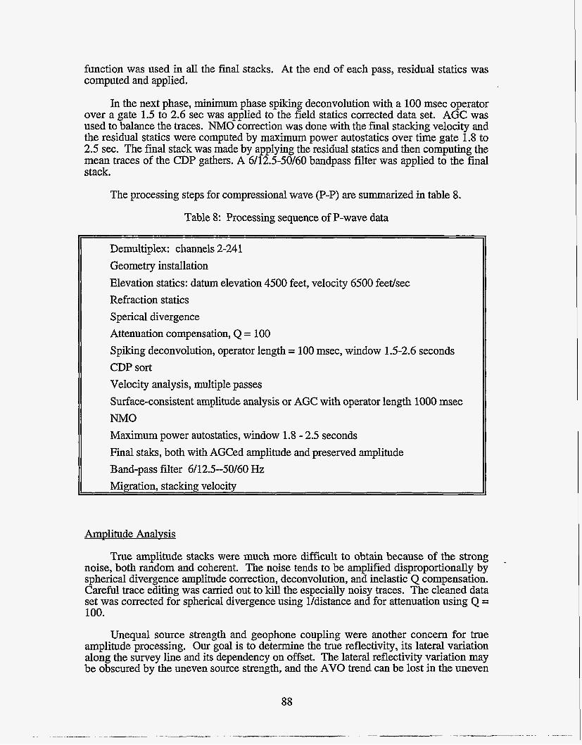
function was used in all the final stacks. At the end of each pass, residual statics was computed and applied.
In the next phase, minimum phase spiking deconvolution with a 100 msec operator over a gate 1.5 to 2.6 sec was applied to the field statics corrected data set. AGC was used to balance the traces. NMO correction was done with the final stacking velocity and the residual statics were computed by maximum power autostatics over time gate 1.8 to 2.5 sec. The final stack was made by applying the residual statics and then computing the mean traces of the CDP gathers. A 6/12.5-50/60 bandpass filter was applied to the final stack.
The processing steps for compressional wave (P-P) are summarized in table 8.
Table 8: Processing sequence of P-wave data
Demultiplex: channels 2-241 Geometry installation Elevation statics: datum elevation 4500 feet, velocity 6500 feet/sec Refraction statics Sperical divergence Attenuation compensation, Q = 100 Spiking deconvolution, operator length = 100 msec, window 1.5-2.6 seconds CDP sort Velocity analysis, multiple passes Surface-consistent amplitude analysis or AGC with operator length 1000 msec NMO Maximum power autostatics, window 1.8 - 2.5 seconds Final staks, both with AGCed amplitude and preserved amplitude Band-pass filter 6h2.5--50/60 Hz Migration, stacking velocity
Amplitude Analvsis
True amplitude stacks were much more difficult to obtain because of the strong noise, both random and coherent. The noise tends to be amplified disproportionally by spherical divergence amplitude correction, deconvolution, and inelastic Q compensation. Careful trace editing was carried out to kill the especially noisy traces. The cleaned data set was corrected for spherical divergence using Udistance and for attenuation using Q = 100.
Unequal source strength and geophone coupling were another concern for true amplitude processing. Our goal is to determine the true reflectivity, its lateral variation along the survey line and its dependency on offset. The lateral reflectivity variation may be obscured by the uneven source strength, and the AVO trend can be lost in the uneven
88
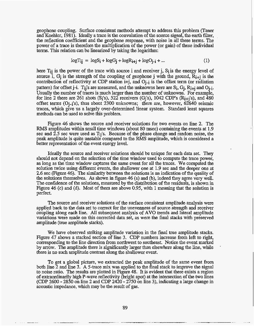
geophone coupling. Surface consistent methods attempt to address this problem (Taner and Koehler, 198 1). Ideally a trace is the convolution of the source signal, the earth filter, the reflection coefficient and the geophone response, with noise in all these terms. The power of a trace is therefore the multiplication of the power (or gain) of these individual terms. This relation can be linearized by taking the logarithm:
lOgTij = lo& + lOgGj + lOgRi+j + lOgOj-i + ... (1)
here T- is the power of the trace with source i and receiver j, Siis the energy level of source 1, Gj is the strength of the coupling of geophone j with the ground, Ri+j is the contribution of reflectivity at CDP station i+j, and Oj-i is the offset term (or radiation pattern) for offset j-i. Tij's are measured, and the unknowns here are Si, Gj, Ri+j and Oj-i. Usually the number of traces is much larger than the number of unknowns. For example, for line 2 there are 261 shots (Si's), 522 receivers (Gj's), 1042 CDP's (Ri+j's), and 480 offset terms (Oj-i'S), thus about 2300 unknowns; there are, however, 62640 seismic traces, which give us a largely over-determined linear system. Standard least squares methods can be used to solve this problem.
'3.
Figure 46 shows the source and receiver solutions for two events on line 2. The RMS amplitudes within small time windows (about 80 msec) containing the events at 1.9 sec and 2.5 sec were used as Tij's. Because of the phase change and random noise, the peak amplitude is quite unstable compared to the RMS amplitude, which is considered a better representation of the event energy level.
Ideally the source and receiver solutions should be unique for each data set. They should not depend on the selection of the time window used to compute the trace power, as long as the time window captures the same event for all the traces. We computed the solution twice using different events, the shallower one at 1.9 sec and the deeper one at 2.6 sec (Figure 46). The similarity between the solutions is an indication of the quality of the solutions themselves. As shown in figure 46 (a) and (b), indeed they agree very well. The confidence of the solutions, measured by the distribution of the residuals, is shown in Figure 46 (c) and (d). Most of them are above 0.95, with 1 meaning that the solution is perfect.
The source and receiver solutions of the surface consistent amplitude analysis were applied back to the data set to correct for the unevenness of source strength and receiver coupling along each line. All subsequent analysis of AVO trends and lateral amplitude variations were made on this corrected data set, as were the final stacks with preserved amplitude (true amplitude stacks).
We have observed striking amplitude variation in the final true amplitude stacks. Figure 47 shows a stacked section of line 3. CDP numbers increase from left to right, corresponding to the line direction from northwest to southeast. Notice the event marked by mow. The amplitude there is significantly larger than elsewhere along the line, while there is no such amplitude contrast along the shallower event.
.
To get a global picture, we extracted the peak amplitude of the same event from both line 2 and line 3. A 5-trace mix was applied to the final stack to improve the signal to noise ratio. The results are plotted in Figure 48. It is evident that there exists a region of extraordinarily high P-wave reflectivity (bright spot) at the intersection of the two lines (CDP 2600 - 2850 on line 2 and CDP 2420 - 2750 on line 3), indicating a large change in acoustic impedance, which may be the result of gas.
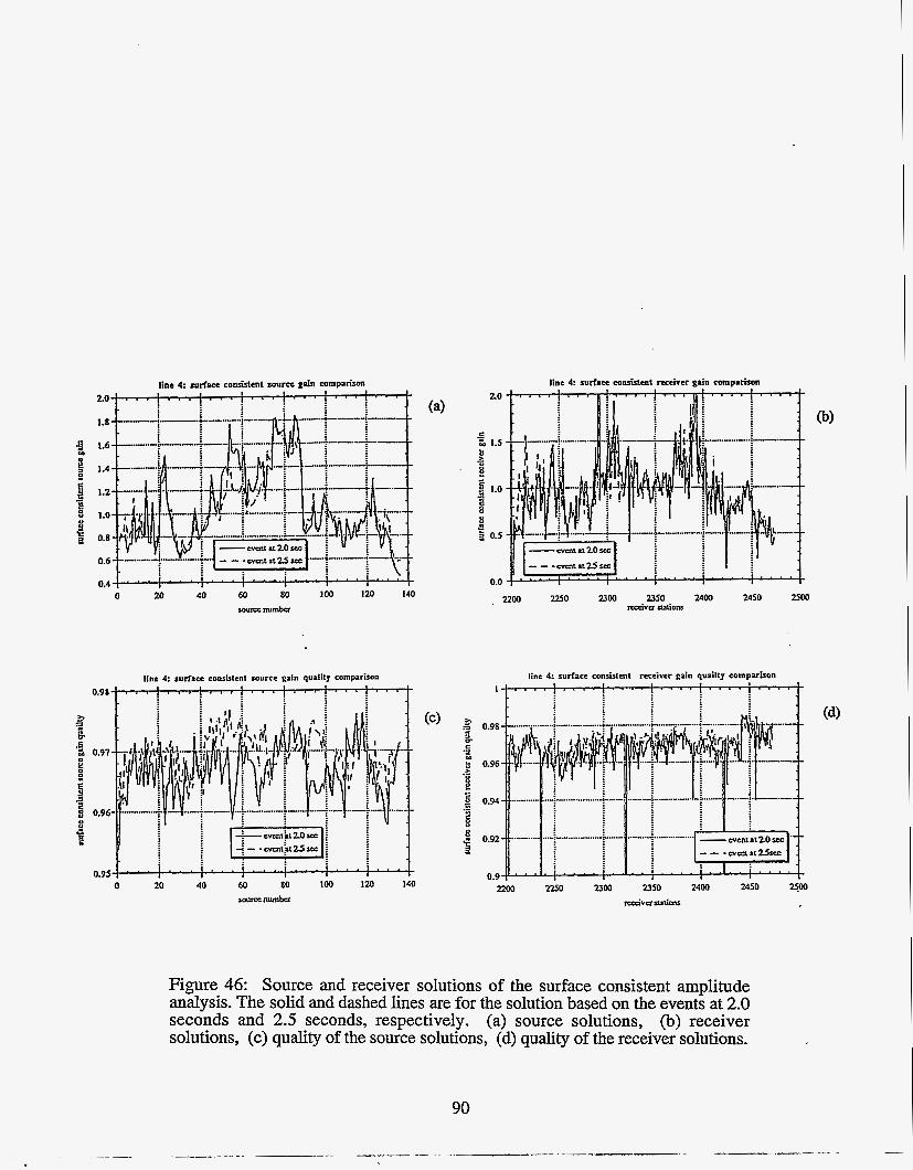
line 4: arfsce consislent source gain comparison
0 20 40 60 80 100 120 140 Sourscnumba
line 4: surface consistent d r a gain comparison
P I Y .;: B
line 4: surface conrklenl source gain quality comparison 0 . 9 8 ' . . . j I . . . . . . . . . . . . . . . . . . . . . . .
1 0
e - 0 1.5 b - E 5 1.0 3 8 8 d Q 0.5
0.0
2200 2250 2300 2350 2400 2450 2200 d V U aari0N
line 4: surface consistent receiver gain quaiity comparison
Po0 2250 2300 2350 2400 2450 + rcaivasutims
Figure 46: Source and receiver solutions of the surface consistent amplitude analysis. The solid and dashed lines are for the solution based on the events at 2.0 seconds and 2.5 seconds, respectively. (a) source solutions, (b) receiver solutions, (c) quality of the source solutions, (d) quality of the receiver solutions.
90
Figure 47: True amplitude stack of line 3. Notice the striking amplitude variation of the marked event.
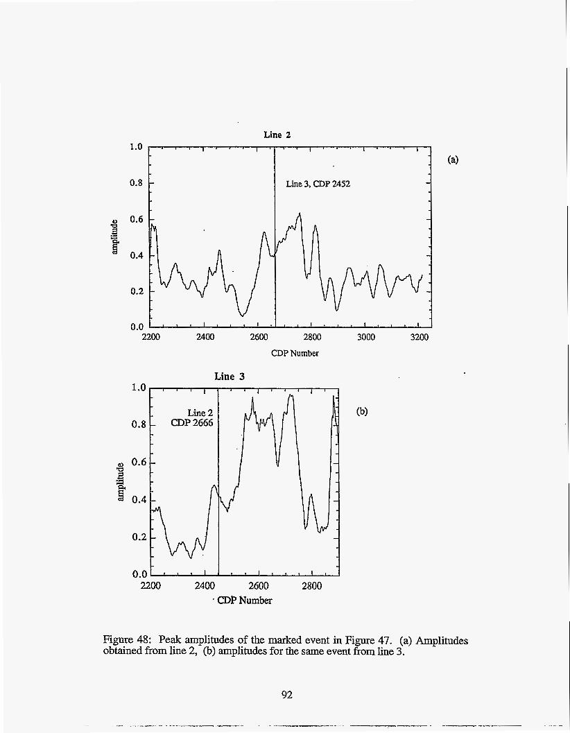
Line 2 1 .o i " ' l " ' l ' ' ' l ' ' ~ I
(a>
0.8 Line 3, CDP 2452 - -
p ) 0.6 - - 2 .d
0.2
0.0 2200 2400 2600 2800 3000 3200
CDP Number
Line 3 1 .o
0.8
0.6 -0 E!
2 0.4 ;7a
0.2
0.0 2200 2400 2600 2800
. CDP Number
Figure 48: Peak amplitudes of the marked event in Figure 47. obtained from line 2, (b) amplitudes for the same event from line 2
92
I Amplitucl=s
Stacking Chart Display of Amplitude
There are two technical problems with amplitude analysis that we have tried to solve efficiently: (1) it is difficult to visualize the lateral variation of reflectivity and AVO trend along a survey line, and (2) it is time-consuming to identify interesting areas for detailed study. Our solution is a stacking-chart display of the amplitudes (Figure 49). In Figure 49 the horizontal axis shows the geophone station numbers, and the vertical axis shows the source station numbers, just like a regular stacking chart. In this type of plot a horizontal line represents all of the traces in a single shot gather, and a vertical line represents a common receiver gather. The traces of a common offset gather are aligned on a 45" line from lower left to upper right. And finally, the CDP gathers are on the 45" lines from upper left to lower right.
We first ran a 5-trace mix on the shot gathers and then computed the RMS amplitudes of the traces. The time window on the trace where the amplitude is estimated is about 100 msec wide and is centered at 2.5 sec. In Figure 49, the RMS amplitude of a trace segment on line 2 is plotted at the location determined by the source and receiver numbers of that trace. Because there are fewer shots than geophone stations, linear interpolation was used to fill the blanks where no data were available.
Several patterns are evident. For example, the signals are much stronger on the northwest half of line 2 (stations 1101 to 1380). This appears to be CDP-consistent, which means it is probably due to subsurface effects. Notice, however, that the horizontal shot-consistent pattern near shot station number 1400 is an artifact of interpolation. There are no real data there.
There are a few distinct AVO trends shown in Figure 49. At CDP 2666, the reflection amplitude is very strong and relatively flat with offset. At CDP 2816, the signals are extraordinarily weak at all offsets. The corresponding CDP gather shows that there is almost no observable event. At CDP 2928, however, as offset increases, the reflector amplitude drops gradually, increases sharply and then drops again. At CDP 3004, the amplitude stays high until about 10000 feet. In addition, there also exist local high reflectivity zones (CDP 3004) and low reflectivity zones (CDP 3 120).
Center Freauencv of Post-stack Data
The effect of fractures on acoustic velocity and attenuation has been studied both theoretically and experimentally by many authors (Hudson, 1981,1991; Crampin, 1978, 1984; Mavko and Nur, 1979; Mukerji & Mavko, 1994 ). In general fractured rocks have higher attenuation because of the scattering effects of the cracks and the fluid-related dissipation between the crack surfaces. When waves pass through a highly fractured zone, high frequency components tend to have a greater loss than low frequency ones. The shape of the power spectrum of the seismic traces can be used as an attribute in our search for fractures by identifying high attenuation zones.
We compute the so-called "center frequency" or "center of gravity" of the power spectrum of the pre-stack P-wave data. It is an indication of relative changes in the high frequency components of the power spectrum. The algorithm is as follows. We first resample the final stack using 1 msec sample rate. Resampling is done solely for computational reasons. It allows us to use a time grid independent of the original sampling rate. Then we extract a small sequence of data at a certain depth with a tapered window. The power spectrum p(f) of the sequence is computed using a fast Fourier transform and finally the center frequency fc is calculated using
93
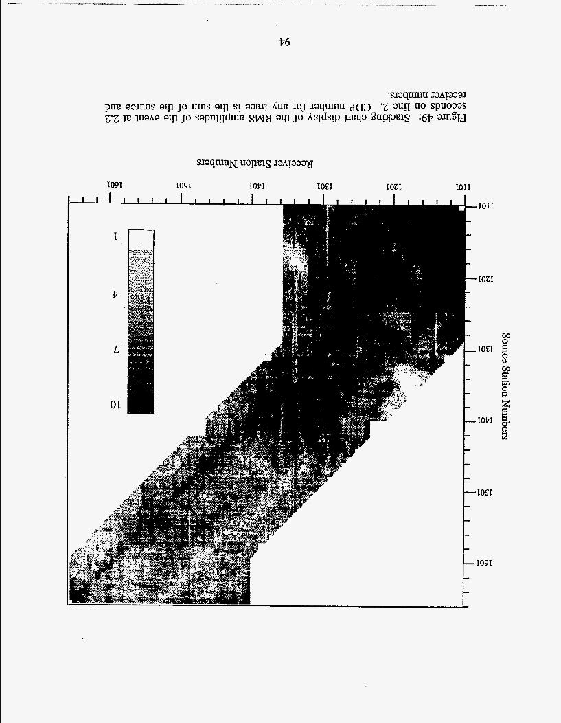
I76
1091
I -
1021 1011
1091
A
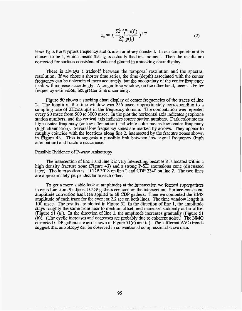
Here fN is the Nyquist frequency and a is an arbitrary constant. In our computation it is chosen to be 1, which means that fc is actually the first moment. Then the results are corrected for surface-consistent effects and plotted in a stacking-chart display.
There is always a tradeoff between the temporal resolution and the spectral resolution. If we chose a shorter time series, the time (depth) associated with the center frequency can be determined more accurately, but the uncertainty of the center frequency itself will increase accordingly. A longer time window, on the other hand, means a better frequency estimation, but greater time uncertainty.
Figure 50 shows a stacking chart display of center frequencies of the traces of line 2. The length of the time window was 256 msec, approximately corresponding to a sampling rate of 2Hdsample in the frequency domain. The computation was repeated every 20 msec from 500 to 3000 msec. In the plot the horizontal axis indicates geophone station numbers, and the vertical axis indicates source station numbers. Dark color means high center frequency (or low attenuation) and white color means low center frequency (high attenuation). Several low frequency zones are marked by arrows. They appear to roughly coincide with the locations along line 2, intersected by the fracture zones shown in Figure 43. This is suggests a possible link between low signal frequency (high attenuation) and fracture occurrence.
Possible Evidence of P-wave Anisotropy
The intersection of line 1 and line 2 is very interesting, because it is located within a high density fracture zone (Figure 43) and a strong P-SH anomalous zone (discussed later). The intersection is at CDP 3018 on line 1 and CDP 2340 on line 2. The two lines are approximately perpendicular to each other.
To get a more stable look at amplitudes at the intersection we formed supergathers in each line from 9 adjacent CDP gathers centered on the intersection. Surface-consistent amplitude correction has been applied to all CDP gathers. Then we computed the RMS amplitude of each trace for the event at 2.2 sec on both lines. The time window lena@h is 100 mec. The results are plotted in Figure 51 In the direction of line 1, the amplitude stays roughly the same from near to medium offset, and increases suddenly at far offset (Figure 51 (a)). In the direction of line 2, the amplitude increases gradually (Figure 51 (b)). (The cyclic increases and decreases are probably due to coherent noise.) The NMO corrected CDP gathers are also shown in Figure 51(c) and (d). The different AVO trends suggest that anisotropy can be observed in conventional compressional wave data.
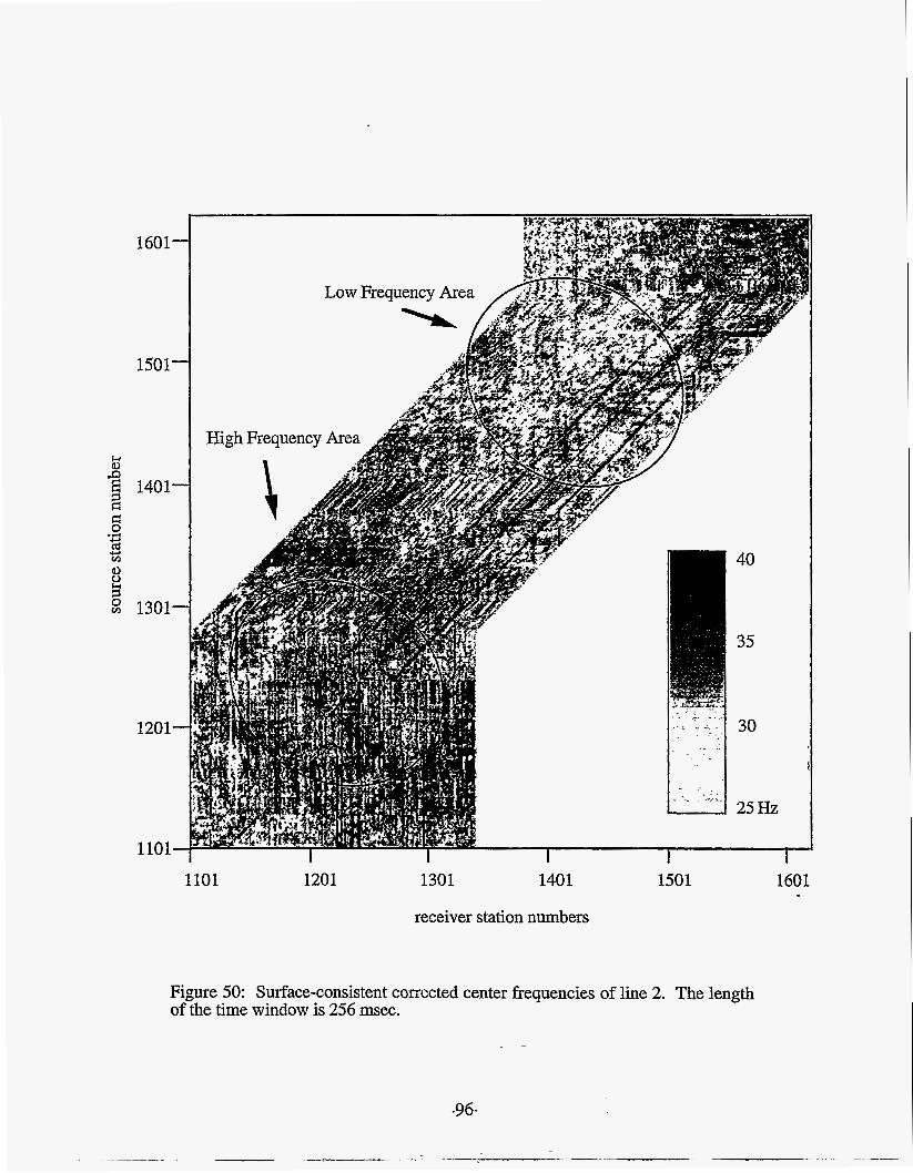
1601
1501
G E 1401 El E!
P
% 4-l
5 v)
d)
8 1301
1201
1101
1101 1201 1301 140 1 1501 1601
receiver station numbers
Figure 50: Surface-consistent coxccted center frequencies of line 2. The length of the time window is 256 msec.
-96-
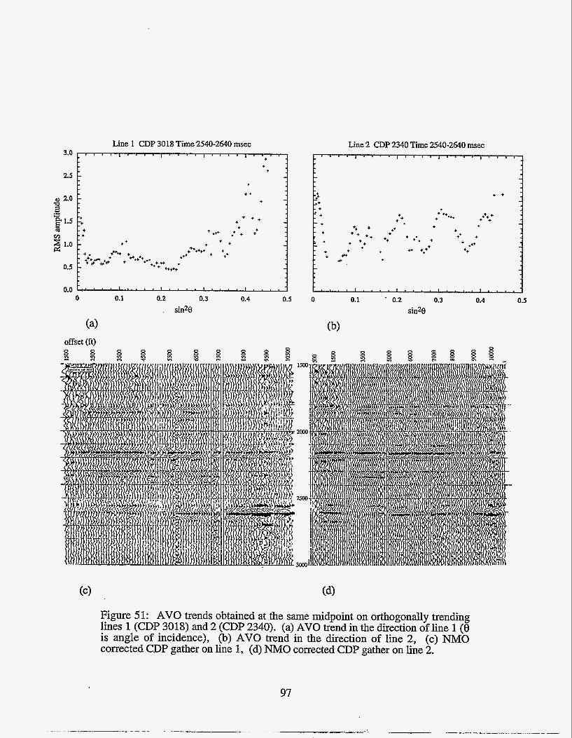
3.0
2.5
0 2.0 a 73 .d .I - g 1.5 m v1 3 1.0
0.5
Line 1 CDP 3018 Time 2540-2640 msec
0.0 : ' ' . * I ' . ' * I ' ' * " ' . ' ' 1 - " *
0 0.1 0.2 0.3 0.4 0.5 sin28
(a) offset (ftl
Line 2 CDP 2340 Time 2540-2640 msec
~ " ~ ' " ' " " ' ' " ' " ' " ' ' ~
0 0.1 . 0.2 0.3 0.4 0.5 sin28
(b)
* +
+ ++.+ +++ + + + + +
+* + + +' +
+ - *+* ++ + - * . +
c *++ ++
Figure 51: AVO trends obtained at the same midpoint on orthogonally trending lines 1 (CDP 3018) and 2 (CDP 2340). (a) AVO trend in the direction of line 1 (0 is angle of incidence), (b) AVO trend in the direction of line 2, (c) NMO corrected CDP gather on line 1, (d) NMO corrected CDP gather on line 2.
97
Figure 52 shows P-wave CDP gathers, recorded at the same midpoint but on the orthogonal trending lines 2 (CDP 2666) and 3 (CDP 2452). Both are moved out with the same stacking velocity, which is chosen to best flatten CDP 2666, but it leaves CDP 2452 overcorrected. This indicates a faster P-wave stacking velocity along line 3 than along line 2 at their point of intersection. The fractures are more nearly parallel with line 3 than line 2, consistent with this azimuthal variation in P-wave velocities.
0 0
? 0
2000
2100
2200
2300
2400
2500
2600
2700
0 0 0 2
Figure 52: CDP gathers at the same midpoint but on orthogonally trending lines 2 (CDP 2666) and 3 (CDP 2452). Both are moved out with the same stacking velocity. (a) CDP gather on line 2, (b) CDP gather on line 3, (c) tie of events on near offset stacks, (d) tie of events on far offset stacks.
CONCLUSIONS
There is probably no single seismic attribute that will always tell us all that we need to know about fracture zones. Therefore, our approach in this project has been to integrate the principles of Rock Physics into a quantitative processing and interpretation scheme that exploits, where possible, the broader spectrum of fracture zone signatures:
(1) anomalous compressional and shear wave velocity; (2) Q and velocity dispersion; (3) increased velocity anisotropy; (4) amplitude vs. offset (AVO) response, and (5) variations in frequency content,
As part of this we.have attempted to refine some of the theoretical rock physics tools that should be applied in any field study to link the observed seismic signatures to the physicaYgeologic description of the fractured rock. Furthermore, while we have used standard shear wave techniques to process and analyze our field data, our goal in this project has been to explore also non-shear wave methods. The project had 3 key elements:
Rock Phvsics studies of the anisotropic viscoelastic signatures of fractured rocks.
We completed two major new contributions for relating the physical or geologic description of fractures to their seismic signatures. In the first study we discussed how the anisotropic viscoelastic signature of a fractured rock varies with the pore fluid type in the fracture, and furthemore how the anisotropic signature for a fluid-bearing rock can be much different at high frequencies than at low frequencies. Many previous studies have used Hudson’s (1980) elegant formulation to describe fractured rocks without making the necessary corrections for these fluid and frequency effects.
In the second study we presented a simple procedure for using measured isotropic values of Vp and Vs versus hydrostatic loading to estimate the stress-induced velocity anisotropy under general nonhydrostatic loading. The method uses simple physical assumptions about crack closure to create the hydrostatic to nonhydrostatic stress transform. Yet, it is independent of any idealized crack geometry, and is not intrinsically limited to low crack concentrations. We represent the pore space with a generalized stress-dependent compliance, which can be determined from the hydrostatic measurements.
An area that needs additional work (which we plan to pursue) is to reconcile the various different theoretical formulations for fractured rock the elliptical inclusion model of Hudson (1980), the finely layered medium model of Schoenberg (1988), and the discrete fracture model of Pyrak-Nolte (1990). Each has its advantages and limitations; a unified description should result in a more flexible set of tools for modeling fractures.
.
Acquisition and processing; of seismic reflection field data.
With the generous help and expertise of our partners at Amoco and Arcomastar Resources, we successfully acquired and processed nearly 50 Ism of 2-D, 9-component reflection data over a fractured site in the Powder River basin of Wyoming. The S-wave data were of moderately good quality, allowing us to develop a fracture model for the site by combining shear wave splitting rotation analysis with well control. The P-wave data
99
were of very good quality, allowing us to see lateral variations in reflectivity, AVO response, and frequency content (attenuation) as well as some evidence for azimuthally dependent AVO and P-wave stacking velocities.
Interoretation of Seismic and well log data
Throughout the site, the fracture directions, inferred from the shear-wave rotation analysis on all four lines, trend consistently SW-NE - all generally within about 200 of each other. These trends were taken to be equal to the polarization direction of the fast shear wave after rotation. The fracture intensity was taken to be proportional to relative time difference between the fast and slow shear waves at each location. This travel time difference (inferred fracture intensity) is highly variable throughout the site - the corresponding shear-wave anisotropy in the Frontier-Nibrara zones ranges from near zero to as much as 7 percent. The regions of largest anisotropy along the four lines can be intepreted with two localized zones of relatively intense fracturing (shown in gray in Figure 43).
Before beginning the survey, it was suggested that the fractures at depth would trend more along a NW-SE direction, parallel to the strike of the Casper Arch and the associated flexure along the SW edge of the survey (Figure 18). These were also interpreted from the second derivative of the known structure at depth. This trend is also seen in surface fractures mapped some km to the south of the survey area (Mueller, pers. comm.). The Amoco-Arc0 Morton Ranch well was drilled near the midpoint of survey line 1 and completed right before our seismic survey. Based on this pre-survey interpretation, the well went horizontal in the Niobrara-Frontier interval and trended northeast (almost parallel to line 1), aiming to intersect a maximum number of fractures perpendicular to their trends. In fact, it was observed down-hole that it trended within about 200 of the fracture trend, consistent with the interpretation in Figure 43. The initial test production at Morton Ranch was quite promising with 165 BOPD, 380 MCFGPD. However, the productivity decreased quickly to about 16 BOPD and 70 MCFGPD (Figure 25). The result of this well suggest that, first of all that the horizontal well didn't intersect that many of them, and secondly, the fractures may be closed because of the loss of pore pressure due to production - consistent with poor fracture connectivity and low fracture density.
The Red Mountain 1-H well was drilled near the intersection of line 2 and line 4 after the seismic study, using the derived fracture model. The well was reported hitting numerous fractures, consistent with the fracture model, and the test production on July 18, 1994 showed 1068 MCFGPD, 32BOPD and only 3 barrels of water per day. The initial result demonstrated once again the effectiveness of the four-component shear-wave method developed by Alford. Since the well is fairly new, much information is still not available and this result is only preliminary. A number of older vertical wells confirm the fracture model. For example the Chinook Lois, Apache Githens, and Energetics Simms wells (Table 4) all lie within the fracture zones (gray in Figure 43) and all have shown reasonable production. A few others outside of the interpreted fracture zones performed much worse.
Several attributes of the P-wave data were found to be consistent with, and possibly indicators of fractures: Strong lateral variations in P-wave reflectivity, AVO response, and frequency content were observed along line 2. Although we did not attempt to model quantitatively their response, they could be indicators of gas and fractures. However, such scalar attributes along a single 2-D line - no matter how striking - cannot give information about the direction of fractures that is so critical for designing wells. It is \
100
possible that with more work, we could learn to combine these scalar attributes with independent fracture direction information (for example from regional trends, or measured stress directions) to quantitatively characterize fractures. We recommend further work in learning to quantify the various P-wave scalar attributes associated with fractures.
Perhaps most intriguing are the several indications of P-wave anisotropy that we observed. Azimuthal variations of AVO response and P-wave stacking velocity were observed at the intersections of lines 1-2 and 2-3. The azimuthal velocity variation is consistent with the directions of the fracture model.
An important conclusion is that 2-D single component surveys are likely to be inadequate for fracture mapping. In our survey, only two line intersections allowed us to even look for azimuthal P-wave variations. We recommend looking for these variations in 3-D single component data. 3-D data will allow, in general, a more complete sampling of azimuths at many CDPs. Partly as a result of this work, Arc0 is now beginning a 3-D study to look for fracture-related azimuthal variations of P-wave stacking velocity and we at Stanford are beginning a similar 3-D study to look for fracture-related azimuthal variations in AVO.
101

.
102
REFERENCES
Alford, R. M., 1986, Shear data in the presence of azimuthal anisotropy: Dilley, Texas, paper presented at the 56th Annual Meeting, SOC. of Explor. Geophys., Houston.
Anstey, N. A., Whatever happened to ground roll?: The leading edge, v. 5, no. 3, p. 40- 45.
Auld, B. A., 1990, Acoustic fields and waves in solids, v. I, It, Robert E. Krieger Publ. co.,
Banik, N. C., 1984, Velocity anisotropy of shales and depth estimation in the North Sea basin: Geophysics, v. 49, p. 1411-1419.
Barlow, J. A., and Haun, J. D., 1966, Regional stratigraphy of Frontier Formation and relation to Salt Creek field, Wyoming: AAPG Bulletin, v. 50, p. 2185-2196.
Beydoun, W. B., Cheng, C. H., and Toksoz, M. N., 1985, Detection of open fracture with vertical seismic profiling, J. Geophys. Res., v. 90, p. 4557-4566.
Biot, M. A., 1956a, Theory of propagation of elastic waves in a fluid saturated porous solid. I. Low-frequency range: J. Acoust. SOC. Amer., 28, 168-178.
Biot, M. A,, 1956b, Theory of propagation of elastic waves in a fluid-saturated porous solid. II. Higher-frequency range: J. Acoust. SOC. Amer., 28, 179-191.
Biot, M. A., 1962a, Generalized theory of acoustic propagation in porous dissipative media: J. Acoust. SOC. Amer., 34, 1254-1264.
Biot, M. A., 1962b, Mechanics of deformation and acoustic propagation in porous media: J. Appl. Physics, 33, 1482-1498.
Blangy, J. P., 1992, Integrated seismic lithologic interpretation: the petrophysical basis: Ph.D. dissertation, Stanford University.
Blangy, J. P., 1994, AVO in transversely isotropic media - an overview: Geophysics, v. 59, no. 5, p. 775-78 1.
Brown, R., and Korringa, J., 1975, On the dependence of the elastic properties of a porous rock on the compressibility of the pore fluid, Geophysics, 40,608-616.
Carmichael, R. S., 1981, Handbook of physical properties of rocks: C.R.C. press. Chang, C. H., Neidell, N. S., and Gardner, G. H. F., 1992, Effects of vertical fracturing
on surface seismic data: Abstracts, SEGEAEG summer workshop on AVO, p. 666. Coyner, K.B., 1984, Effects of stress, pore pressure, and pore fluids on bulk strain,
velocity, and permeability in rock, Ph.D. thesis, Massachusetts Institute of Technology.
Coyner, K. B., and Cheng, C. H., 1985, New laboratory measurements of seismic velocities in porous rocks: Geophysics, 50,309.
Crampin, S., 1978, Seismic wave propagation through a cracked solid: polarization as a possible dilatancy diagnostic, Geophys. J. R. Astron. SOC., 53,467-496.
Crampin, S., McGonigle, R. and Bamford, D., 1980, Estimating crack parameters from observations of P-wave anisotropy, Geophysics, v. 40, p. 345-360.
Crampin, S., 1984, Effective anisotropic elastic constants for wave propagation through cracked solids, Geophys. J. Roy. Astr. SOC., 76, 135-145.
Crampin, S., Evans, R., and Ucer, S. B., 1985, Analysis of records of local earthquakes: the Turkish dilatancy projects (TDP1 and TDP2), Geophys. J.R. Astron. SOC., 83,l- 16.
Crampin, S., Bush, I., Naville, C., and Tylor, D. B., 1986, Estimating the internal structure of reservoirs with shear-wave VSPs: The Leading Edge, v. 5, p. 35-39.
Crampin, S., 1988, Extensive-dilatancy anisotropy, new earthquake prediction tool (meeting report), Eos Trans. AGU, 69,729.
Daley, P. F, and Hron, F., 1977, Reflection and transmission coefficients for transversely isotropic media: Bull. Seis. SOC. Am., v. 67, p. 661-675.
103
Dickinson, W. R., mute, M. A., Hayes, M. J., Janecke, S. U., Lundin, E. R., McKittrick, M. A., and Olivares, M. D., 1988, Paleogeographic and paleotectonic setting of Laramide sedimentary basins in the central Rocky Mountain region: GSA Bulletin,
Dutton, S.P., Hamlin, H. S., and Laubach, S. E., 1992, Geologic controls on reservoir properties of low-permeability sandstone, Frontier Formation, Moxa Arch, southwest Wyoming: The University of Texas at Austin, Bureau of Economic Geology, topical report no. GRI-92/0127, prepared for the Gas Research Institute, 199 p.
Eshelby, J.D., 1957, The determination of the elastic field of an ellipsoidal inclusion, and related problems, Proc. R. SOC. (London), A241,376.
Galloway, W. E., and Hobday, D. K., 1983, Terrigenous clastic depositional systems: New York, Springer-Verlag, 423 p.
Gassmann F., 1951, Uber die elastizitat poroser medien: Vier. der Natur Gesellschaft,
Han. D., 1986, Effects of porosity and clay content on acoustic properties of sandstones and unconsolidated sediments: Ph.D. thesis, Stanford University.
Hando, R. E., 1976, Powell-Ross field, Converse County, Wyoming: Wyoming Geological Association Guidebook, 28th Annual Field Conference, pp. 139-145.
Hildebrandt, G. F., Morse, P. F., 1986, Suppression of coherent noise by the stack array: Geophysics, v. 51, no. 3, p. 873.
Hudson, J. A., 1980, Overall properties of a cracked solid, Math. Proc. Cambr. Phil. SOC.,
Hudson, J. A. ,198 1, Wave speeds and attenuation of elastic waves in material containing cracks, Geophys. J. Roy. Astr. SOC., 64,133-150.
Hudson, J. A., 1990, Overall elastic properties of isotropic materials with arbitrary distribution of circular cracks, Geophys. J. Int., v. 102, p. 465-469.
Hudson, J. A., 1991, Crack distributions which account for a given seismic anisotropy, Geophys. J. Int., 104,517-521.
Jaeger, J. C., and Cook, N. G. W., 1969, Fundamentals of rock mechanics: Chapman and Hall.
Johnston, D. H., 1986, VSP detection of fractured-induced velocityanisotropy, 56th Ann. Int. SEG Meeting, 1986, Houston, Expanded Abstracts, p. 464-466.
Jones, T.D., 1983, Wave propagation in porous rocks and models for crustal structure, Ph.D. Dissertation, Stanford University, Stanford, California.
Keller, J. D., 1989, Acoustic wave propagation in composite fluid saturated media: Geophysics, 54,1554-1563.
Kim, K. Y., Wrolstad, K. H., and Aminzadeh, F., 1993, Effects of transverse isotropy on P-wave AVO for gas sands, Geophysics, v. 58, p. 883-888.
Lewis, C., 1989, Three-dimensional Multicomponent Imaging of Reservoir Hetero- geneity, Silo Field, Wyoming, Ph.D. Dissertation, Colorado School of Mines.
Lewis, C., Davis, T. L., and Vuillermoz, C., 1991, Three-dimensional multicomponent imaging of reservoir heterogeneity, Silo field, Wyoming: Geophysics, v. 56, p.
Liu, E., Crampin, S, and Queen, J. H., 1991, Fracture detection using crosshole surveys and reverse vertical seismic profiles at the Conoco Borehole Test Facility, Oklahoma, Geophys. J. Int., v. 107, p. 449-463.
Lorenz, J. C:, Branagan, P., Warpinski, N. R., and Sattler, A. R., 1986, Fracture charactenstics and reservoir behavior of stress sensitive fracture systemsin flat-lying lenticular formations: Paper presented at Proceedings of Unconventional Gas Technical Symposium, SOC. of Pet. Eng., Louisville, Ky.
Lo, Tien-when, Coyner, K.B., and Toksoz, M.N., 1986, Experimental determination of elastic anisotropy of Berea sandstone, Chicopee shale and Chelmsford granite, Geophysics, 51,164-171.
V. 100, p. 1023-1039.
96, 1-23.
88,371-384.
2048-2056. ~
104
Lockner, D.A., Walsh, J.B., and Byerlee, J.D., 1977, Changes in velocity and attenuation during deformation of granite, J. Geophys. Res., 82,5374-5378.
Lucet, N.M.,. and Tarif, P.A., 1988, Shear wave birefringence and ultrasonic shear wave attenuation measurements, 58th SEG Extended Abstracts, paper S 10.2.
Lueschen, E., Nolte, B., and Fuchs, K., 1990, Shear wave evidence for an anisotropic lower crust beneath the Black Forest, Southwest Germany, Tectonophysics, 173,
Mallick, S. and Frazer, L. N., Reflectiodtransmission coefficients and azimuthal anisotropy in marine seismic studies: Geophys. J. Int., v. 105, p. 241-252.
Mavko, G. and Nur, A., 1975, Melt squirt in the asthenosphere, J. Geophys. Res., 80,
Mavko, G. and Nur, A., 1978, The effect of non-elliptical cracks on the compressibility
Mavko, G. and Nur, A., 1979, Wave attenuation in partially saturated rocks: Geophysics,
Mavko, G. and Jizba, D., 1991, Estimating grain-scale fluid effects on velocity dispersion in rocks, Geophysics, 56, 1940-1949.
Merewether, E. A., Cobban, W. A., and Spencer, C. W., 1976, The Upper Cretaceous Frontier Formation in the Kaycee-Tisdale Mountain area, Johnson County, Wyoming, Wyoming Geological Association Guidebook, 28th Annual Field Conference, p. 33-44.
Mitchell, G. C., and Rogers, M. H., 1993, Extensional tectonic influence on Lower and Upper Cretaceous stratigraphy and reservoirs, southern Powder River basin, Wyoming: The Mountain Geologist, v. 30, no. 2, p. 54-68.
Mueller, M., 1992, Using shear waves to predict lateral variability in vertical fracture intensitiy: The leading Edge, v. 11, no. 2, p. 29-35.
Mukerji, T. and Mavko, G., 1994, Pore fluid effects on seismic velocity in anisotropic rocks, in press, Geophysics..
Murphy, W., 1982, Effect of microstructure and pore fluid on the acoustic properties of granular sedimentary materials, Ph. D. dissertation, Stanford University.
Murphy, W.F., Winkler, K.W., and Kleinberg, 1984, Contact microphysics and viscous relaxation in sandstones, in Physics and Chemistry of Porous media, edited by D. L. Johnson and P.N. Sen, American Institute of Physics, New York.
Nishizawa,O., 1982, Seismic velocity anisotropy in a medium containing oriented cracks -- transversely isotropic case., J.Phys.Earth,30,33 1-347.
Nur, A. and Simmons, G., 1969a, Stress-induced velocity anisotropy in rock: An experimental study, J. Geophys. Res., 74 (27), 6667-6674.
Nur, A. and Simmons, G., 1969b, The effect of saturation on velocity in low porosity rocks, Earth and Planetary Science Letters, 7, 183-193.
Nur, A., 1971, Effects of stress on velocity anisotropy in rocks with cracks, J. Geophys., Res., 76,2022-2034.
Nur, A., 1976, Origin of velocity changes before earthquakes: the dilatancy diffusion hypothesis and its confirmation, Volcanoes and Tectonosphere, Hitoshi Aoki and Susumu Iizuka, eds. 173-186, Tokai University, Tokai University Press.
Nur, A., 1987, Seismic rock properties for reservoir description and monitoring, G. Nolet (ed) Seismic Tomography, 203-237.
Nur, A., 1989, Four-dimensional seismology and (true) direct detection of hydrocarbons: the petrophysical basis, Geophysics: the Leading Edge, September, 30-36.
O'Connell, R., and Budiansky B., 1974, Seismic velocities in dry and saturated cracked solids: J. Geophys. Res., 79,5412-5426.
O'Connell, R., and Budiansky B., 1977, Viscoelastic properties of fluid-saturated cracked solids: J. Geophys. Res., 82,5719-5736.
Ostrander, W. J.,. 1983, Plane-wave reflection coefficients for gas sands at non-normal angles of incidence: 52nd ann. int. SEG mtg., Dallas, Texas, p. 443
483-493.
1444-1448.
of rocks, J. Geophys. Res., 83,4459-4468.
44, 161-178.
.
105
Ostrander, W. J., 1984, Plane-wave reflection coefficients for gas sands at nonnormal angles of incidence: Geophysics, v. 49, p. 1637-1648.
Pelissier, M. A., Thomas-Betts, A. and Vestergaard, P. D., Azimuthal variations in scattering amplitudes induced by transverse isotropy: Geophysics, v. 56, p. 1584- 1595.
Prescott, M. W., 1975, Spearhead Ranch field, Converse County, Wyoming: Rocky Mountain Association of Geologists, A symposium on deep drilling frontiers in the central Rocky Mountains, p. 239-244.
Pullin, N.E., Matthews, L.W., and Hirsche, W.K., 1986, Techniques applied to obtain very high resolution 3-D seismic imaging at an Athabasca tar sands thermal pilot, 56th SEG Extended Abstracts, Houston, Texas.
Pyrak-Nolte, L., Myer, L.R., and Cook, N., 1990, Anisotropy in seismic velocities and amplitudes from multiple parallel fractures, J. Geophys. Res., 95, 11345-1 1358.
Queen, J., and Rizer, W., 1990, An integrated study of seismic anisotropy and the natural fracture system at the Conoco borehole test facility, Kay County, Oklahoma, J. Geophys. Res., 95,111255-1 11274.
Raleigh, C. B. and Evernden, J., 1982, Case for low deviatoric stress in the lithosphere, In: Mechanical behaviour of crustal rocks, N. L. Carter, M. Friedman, J. M. Logan and D. W. Steams, eds., Geophysical Monograph Series, AGU, Washington, D.C.,
Rutherford, S. R., and Williams, M. W., 1989, Amplitude-versusoffset variations in gas sands: Geophysics, v. 54, p. 680-688.
Sayers, C. M., 1988, Stress-induced ultrasonic wave velocity anisotropy in fractured rock, Ultrasonics, 26,3 11-3 17.
Schoenberg,M. and DoumaJ., 1988, Elastic wave propagation in media with parallel fractures and aligned cracks., Geophys.Prosp.,36,57 1-590.
Sengupta, M., 1987, Sensitivity analysis of amplitude versus offset (AVO) method: 57th ann. int. SEG mtg., New Orlean, LA, p. 621-623.
Slack, P. B., 198 1, Paleotectonics and hydrocarbon accumulation, Powder River basin, Wyoming: AAPG Bulletin, v. 65, p. 730-743.
Sonnenberg, S. A., and R. J. Weimer, 1993, Oil production from Niobrara Formation, Silo field, Wyoming: Fracturing associated with a possible wrench fault system: The Mountain Geologist, v. 30, no. 2, p. 39-53.
Spencer, J., and Nur, A., 1976, The effects of pressure, temperature and pore water on velocities in Westerly granite, J. Geophys. Res., 81,899-904.
Stoll, R. D., and Bryan, G. M., 1970, Wave attenuation in saturated sediments: J. Acoust. SOC. Am., 47, 1440-1447.
Szpakiewicz, M. J., McGee, K., and Sharma, B., 1986, Geologic problems related to characterization of clastic reservoirs for enhanced oil recovery: Proceedings of the SPE/DOE Fifth Symposium on Enhanced Oil Recovery, v. 2, p. 97-106, SOC. of Pet. Eng., Tulsa, Okla.
Taner, M. T. and Koehler, F., 1981, Surface consistent corrections: Geophysics, v. 46, no.
Tarif, P., 1986, Mesure de l'Attenuation des ondes compressionelles dans les roches: Application a la mesure de l'anisotropie d'attenuation, These de Doctorat de l'universite Paris 7.
Thomsen, L., 1986, Elastic anisotropy due to aligned cracks: Theoretical models, Trans. Am. Geoph. Union, 67,1207.
Thomsen, L., 1991, Elastic anisotropy due to aligned cracks in porous rocks, EAEG Mtg. Abstrs., 53,244.
Toksoz, M.N., C.H. Cheng, and A. Timur, 1976, Velocities of seismic waves in porous rocks, Geophysics, 41,4,621.
Vernik, L. and Nur, A., 1992, Ultrosonic velocity and anisotropy of hydrocarbon source- rocks: Geophysics, v.57, p. 727-735.
p 173-1 86.
1, p. 17-22.
106
Walls, J.D., 1983, Effects on pore pressure, confining pressure and partial saturation on permeability of sandstones, Ph.D. Dissertation, Stanford University.
Wallis, H., Rethford, G., and Bielanski, E., 1986, Azimuthal anisotropic media: 56th Ann. Int. SEG Mtg., Houston, Texas, Expanded Abstracts, p. 476-479.
Walsh, J. B., 1965, The effect of cracks on the compressibility of rock, J. Geophys. Res.,
Walsh, J., 1980, Static deformation of rock: Proc. ASME, 106, 1005-1019. Wang, Z., and Nur, A., 1988, Velocity dispersion and the "local flow" mechanism in
rocks, 58th Annual International Meeting, SOC. Explor. Geophys., Expanded Abstracts, 928-930.
Wang, Z., and Nur, A., 1990, Dispersion analysis of acoustic velocities in rocks, J.
Willis, H. A., Rethford, G. L. and Bielavski, E., 1986, Azimuthal anisotropy: occurrence and effect of shear wave data quality, paper presented at 56th Annual Meeting, SOC. of Explor. Geophys., Houston.
Winkler, K., 1985, Dispersion analysis of velocity and attenuation in Berea sandstone: J. Geophys. Res., 90,6793-6800.
Winkler, K., 1986, Estimates of velocity dispersion between seismic and ultrasonic frequencies: Geophysics, 51, 183-189.
Winterstein, D. F., and Meadows, M. A., 1991, Shear wave polarizations and subsurface stress directions at Lost Hills field, Geophysics, 56, 1331-1348.
Wright, J., The effects of transverse isotropy on reflection amplitude versus offset: Geophysics, v. 52, p. 564-567.
Wyoming Geological Association, 1976, Guidebook, 28th Annual Field Conference, Geology and energy resources of the Powder River: Casper, Wyoming, 328 p.
Yin, H., 1992, Acoustic Velocity and Attenuation of rocks: Isotropy Intrinsic Anisotropy, and Stress Induced Anisotropy, Ph.D. dissertation, Stanford University, Stanford, California.
Zamora, M., and Poirier, J. P., 1990, Experimental study of acoustic anisotropy and birefringence in dry and saturated Fontainebleau sandstone, Geophysics, 55, 1455- 1465.
70,381-389.
Acoust. SOC. Am., 87,2384-2395.
107


