Electronic copy available at: http://ssrn.com/abstract=1555951

IDB WORKING PAPER SERIES #IDB-WP-144

Integration, Resources Reallocation and Productivity:

The cases of Brazil and Chile

Juan Blyde Gonzalo Iberti Mauricio Mesquita Moreira

Inter-American Development Bank

Vice Presidency for Sectors and Knowledge

Integration and Trade Sector

November 2009

Electronic copy available at: http://ssrn.com/abstract=1555951

Integration, Resources Reallocation and Productivity:

The Cases of Brazil and Chile

Juan Blyde Gonzalo Iberti

Mauricio Mesquita Moreira

Inter-American Development Bank 2009

© Inter-American Development Bank, 2009 www.iadb.org Documents published in the IDB working paper series are of the highest academic and editorial quality. All have been peer reviewed by recognized experts in their field and professionally edited. The views and opinions presented in this working paper are entirely those of the author(s), and do not necessarily reflect those of the Inter-American Development Bank, its Board of Executive Directors or the countries they represent. This paper may be freely reproduced provided credit is given to the Inter-American Development Bank.

Integration, Resources Reallocation and Productivity:

The Cases of Brazil and Chile

Juan Blyde Gonzalo Iberti

Mauricio Mezquita

Abstract

Most microeconometric studies available for LAC have focused on measuring the direct impact of trade on plant productivity leaving aside other effects that arise through the market selection process. Additionally, most studies have focused on tariff barriers as the only obstacle to international trade and integration. In this paper we use data from Brazil and Chile to analyze how trade affects aggregate productivity through the process of resource reallocation and to explore not only the role of tariffs but also the role of transport costs. We find that trade costs affect the reallocative process by protecting inefficient producers, lowering their likelihood to exit, and also by limiting the expansion of efficient plants, lowering their likelihood to export. We also find that the reallocative impacts of trade come not only from tariff barriers but also from transport costs. JEL No. F13, F14 Key words: Tariff barriers, transport costs, productivity, resource reallocation

2

I. Introduction There is a rich literature that investigates the links between trade and productivity at the firm

level. Most studies available for LAC have focused on the impact of trade policies on plant

productivity (see for example, Lopez-Cordova and Mesquita, 2004; Fernandes, 2007, and IDB

2002). Yet, an increasing body of evidence indicates that an important share of aggregate

productivity growth, in both developed and developing countries, arises from the reallocation of

resources across plants of different productivity levels. Studies that analyze the impact of trade

on productivity through resource reallocation are rare in LAC. Pavcnik (2002), Tybout (1991)

and Tybout (1995) are some exceptions.

An additional shortcoming in most of the microeconometric studies of LAC has been the

excessive focus on tariff barriers. The attention on policy barriers reflects a more general trend

that has been going on for years in all aspects of LAC’s trade agenda. Trade policy has been all

too focused on removing tariffs and non-tariff barriers. There is little doubt that these barriers

were very high in the late 1980s and the emphasis on their removal was not only warranted but

also inexorable, given the prevailing political incentives and the constraints in terms of

administrative resources. However, after decades of trade liberalization, these obstacles have lost

relevance vis-à-vis other trade costs, for example, transport costs. A recent report by the IDB

indeed shows that for most LAC countries transport costs are today significantly higher than

tariffs -for both imports and exports- and that the effects of transport costs on export volumes or

export diversification are more important than the effects of tariffs (IDB, 2008). Therefore, it is

not possible to ignore anymore the role of transport costs as a barrier to trade, particularly when

one is interested in analyzing whether more trade could spur productivity. Doing so would

seriously miss an important part of the story, particularly when analyzing the LAC region.

This paper has two objectives. First, to fill the gap in the empirical literature by analyzing

the potential productivity gains arising from between firm resource reallocation driven by lower

trade costs. Second, to break away from the excessive focus on policy barriers by analyzing not

only tariffs but also the role of transport costs in the potential gains from resource reallocation.

The rest of the paper is divided as follows. Section II provides a brief summary of the

new trade models supporting the empirical analysis. A description of the datasets is also

provided in this section. Section III shows the econometric estimations and discusses the main

empirical findings. Section IV concludes.

3

II. Theoretical Background and Data Description

II.A. Theoretical Background

Our empirical strategy is guided by the heterogeneous-firm models derived by Melitz (2003) and

Bernard et al. (2003). In these models, when trade costs fall, industry productivity rises both

because low-productivity, non-exporting firms exit and because high-productivity firms expand

through exporting. More specifically, when trade costs fall, exporters experience greater profits

to which they respond by expanding their exports. Greater profits also induce more entry into the

market. Specifically, lower trade costs reduce the productivity threshold for exporting which

increases the number of firms that export to other markets. The new exporters are drawn from

the most productive non-exporters plants and from the new entrants. At the same time there is

exit from the market. In Melitz’s model, the increase in the labor demand led by the expansion of

the more productive firms through exporting and from the new entrants raises the real wage in

the industry and forces the least productive firms to exit. In Bernard et al.’s model the exit occurs

because lower trade costs mean that firms face more competition from foreign firms that on

average tend to be more productive than the domestic firms.

In summary, aggregate productivity gains occur with falling trade costs because the low

productivity plants exit, the most productive non-exporters begin to export, and the current

exporters, which are the high-productivity firms, expand their foreign sales. As argued by

Bernard et al., (2006), we can re-state these predictions as follows: i) a decrease in variable trade

costs raises the probability of firm exit; ii) a decrease in variable trade costs increases the

probability of becoming an exporter, and iii) a decrease in variable trade costs increases the

export sales of the existing exporters. Our exercises consist on investigating whether we observe

evidence of these effects in the data.

It should be noted that the predictions of the Melitz (2003) and Bernard et al. (2003)

models presume multilateral reductions in trade costs.1 This is precisely what we have in mind.

Our dataset covers the second half of the 1990s and also the first half of the 2000s (for Chile).

During this time, policy barriers decreased not only in Brazil and Chile but in many other parts

of the world. Therefore, even though we only employ tariff barriers from Brazil and Chile, policy

1 Melitz and Ottaviano (2008) show that a unilateral liberalization episode might not generate the same effects as in Melitz (2003) in the long run.

4

costs have also fallen in these countries’ destination markets mainly through trade agreements. A

similar situation has occurred with respect to transport costs. Even though LAC countries exhibit

in general larger transport costs relative to other regions, the evolution of these costs during the

period of consideration followed trends that were in general similar to many other countries (see

IDB, 2008).

II.B. Data Description

The manufacturing data for Chile come from the Encuesta Nacional Industrial Anual (ENIA).

This is an annual survey of manufacturing conducted by the Chilean statistics agency, the

Instituto Nacional de Estadísticas (INE). The data for Brazil come from the Pesquisa Industrial

Anual (PIA) conducted by the Brazilian statistical office, the Instituto Brasileiro de Geografia e

Estadística (IBGE). In both cases the surveys collect detailed information on plant

characteristics, such as manufacturing subsector, production, value added, exports, employment,

intermediate inputs, and investment. The available data covers the period 1995-2006 for the case

of Chile and 1996-2000 for the case of Brazil.

ENIA covers all plants with 10 or more employees encompassing an average of 5,400

plants per year. Sales, exports and value added from this survey were deflated to 1995 prices

with sectoral price indices obtained from INE. The capital stocks were constructed using the

perpetual inventory method for various types of capital including structures, vehicles and

machinery and equipment. Appropriate deflators from the Chilean Association of Builders and

the sectoral price indices were used to deflate the various components of capital. The initial

capital stock is constructed as the value of capital stock reported in books (deflated) minus the

reported depreciation that year. Subsequent years were calculated using the perpetual inventory

method with depreciation rates equal to 5% for structures, 15% for machinery and equipment

and 20% for vehicles (see Liu, 1993).

The PIA dataset originally comprises an average sample of 110,000 firms in 1996-2000.

While this dataset represents a larger and more representative sample than in previous years, its

major drawback is the lack of information on capital stock. The capital stock information was

then obtained crossing this survey with the 1995 PIA, a corporate income tax database from

Receita Federal and a balance sheet database from Fundacao Getulio Vargas. This led to a panel

of 11,900 firms which accounts for 83 percent of manufacturing industry value added and 62

5

percent of manufacturing employment over the period. Output and input variables were deflated

to 1995 prices using sectoral price indices while general price indices for the same year were

used to deflate non-sector specific variables such as investment. The capital stock series were

constructed using information on fixed assets for 1995 taken from the alternative databases

mentioned above and updating this information for subsequent years using the perpetual

inventory method (for more details, see Lopez-Córdova and Moreira, 2003)

A key issue in calculating total factor productivity with firm level data is the potential

correlation between unobservable productivity shocks and input levels. Profit-maximizing firms

respond to positive productivity shocks by expanding output, which in turn requires more inputs.

A widely used estimator that employs investment as a proxy for these unobservable shocks is

given by Olley and Pakes (1996). However, another estimator that uses intermediate inputs as

proxies of these shocks has been introduced more recently by Levinsohn and Petrin (2003).

These authors argue that intermediates may respond more smoothly to productivity shocks. We

use the Levinsohn and Petrin methodology to construct our measures of total factor productivity.

Unfortunately, neither the Olley and Pakes nor the Levinsohn and Petrin methodology deal with

a potentially different problem called the revenue bias (see Haltiwanger and Syverson, 2005;

Katayama, Lu and Tybout, 2006). This problem is related to the difficulty of measuring real

output at the firm level. In principle, any productivity index should measure the amount of output

a firm can produce with a given set of inputs. Unfortunately, a firm’s output is often not directly

observable because of lack of producer-level prices. Therefore, most empirical studies (including

the analysis on this study) use the firm’s revenues deflated by a common industry price index as

a proxy for output. However, if the firm produces differentiated products or has some pricing

power, the proxy for output might be incorrect and the productivity measure that is obtained

from estimating the production function could be biased. Therefore, for a robustness check, we

also employ an alternative measure of TFP calculated using a methodology proposed by

Levinsohn and Melitz (2002) which deals with the problem of unobserved productivity shocks as

well as the revenue bias. The idea behind this methodology is that sales depend on prices and, in

equilibrium, prices depend also on the demand side. Therefore, the method relies on recovering a

productivity measure after putting some structure on the demand side of the market.

6

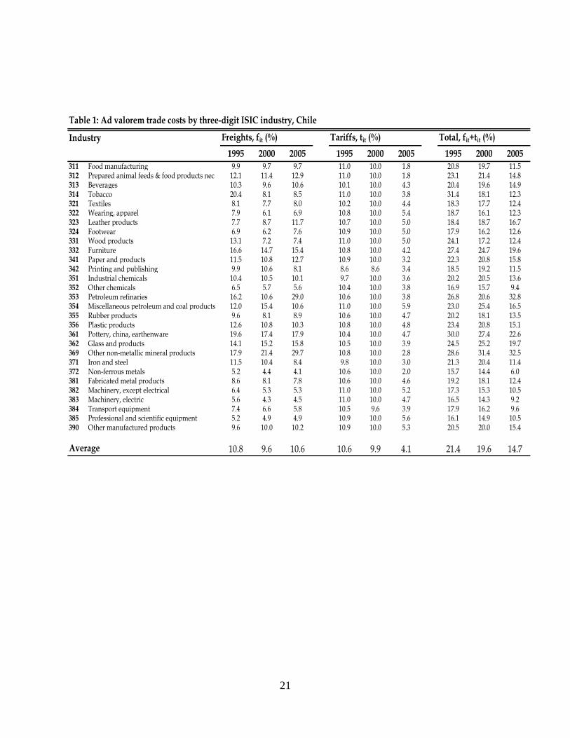
Our measure of trade costs includes both tariffs and freight rates. Ad valorem freight

rates are measured as the ratio of the value of freights and insurance over the values of imports

(fob). Similarly, the ad valorem tariff is the ratio of the import duty over the fob-value of the

imports. The data on tariff and freight costs come from the Foreign Trade Statistics System of

ALADI (Latin American Association of Foreign Trade) which is disaggregated at the 6-digit

Harmonized System level. In both cases, the rate for industry i is the weighted average rate

across all products in i, where the weights are the import values from all the countries. For the

case of Chile, information about the import duties is not available for the entire period of

analysis. Therefore, for this country we use applied tariff rates instead.2 Tables 1 and 2 report

selected years of trade costs for Chile and Brazil respectively.

For the case of Chile, average freight rates declined from 1995 to 2000, but increased

since then. For some industries, like petroleum refinery products (353), freight rates more than

double. This upward trend from 2000 onwards follows closely the overall increase in the

international price of oil and fuels for transportation. Despite this recent trend, 20 out of 29

industries experienced overall declines in freight rates between 1995 and 2005. In the case of

tariffs, all industries exhibited a fall in their applied tariff rates. While tariff rates remain

relatively stable between 1995 and 2000, the fall was more pronounced between 2000 and 2005.

On average, the applied ad valorem tariff declined by around 60% during the period of analysis.

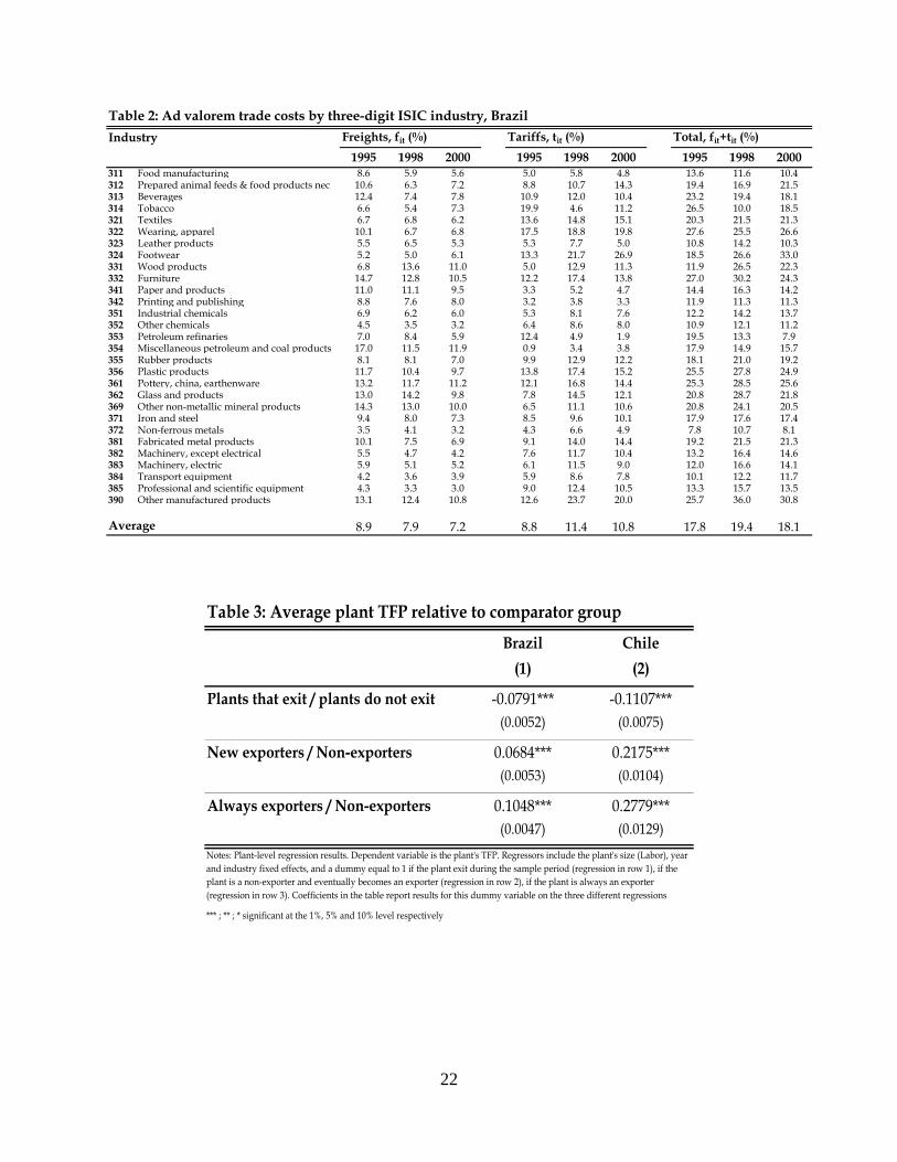
In the case of Brazil, the freight rates declined in 26 out of 29 industries between 1995

and 2000. The average freight rate fell by 19%. This is consistent with the trend observed in

Chile during this period. The average ad valorem tariff increased from 1995 to 1998, but

declined slightly afterwards. Relative to 1998, the protection rate fell in 21 industries.

One caveat with respect to our measures of trade costs should be noted. Ideally, we

would like to assess the effects of trade costs on productivity incorporating measures of trade

costs for both imports and exports. In fact, the theoretical models described above contemplate

symmetric reductions in trade costs, i.e., both outbound and inbound trade costs change in the

same way. Unfortunately, restrictions in our trade costs dataset do not allow us to construct

outbound trade costs that cover all the exports of these countries. However, to the extent that

inbound and outbound trade costs change in a similar way this should not be a significant

2 Applied tariff rates take into consideration preference schemes. The source of this data is Nicita and Olarreaga (2006)

7

problem. To check this, we combined the ALADI dataset with a dataset on US imports from the

US Census Bureau and constructed outbound trade costs for Brazil and Chile using the exports

of these countries to a handful of LAC countries –for which the data permits- and the US. We

found that the correlation of the changes in the inbound and the outbound trade costs across ISIC

3-digit industries was positive and significant at the 1% level for both countries. Nevertheless,

we should keep in mind that using inbound trade costs in our exercises is likely to reduce the

possibility of finding an export response. We will come back to this point later.

III. Empirical Analysis Before analyzing whether a fall in trade costs induces the reallocative effects predicted by

the new trade models, we can investigate whether firms that exit are less productive than firms

that do not exit, and whether exporters are more productive than the non-exporters. This is

shown in Table 3. Each row in the table reports results from a separate regression of the

following form:

ittjiitit XLTFP εααγβα +++++=)ln(

where the dependent variable is the TFP of plant; itL is the plant's labor force (a proxy for size);

jα and tα are industry and year fixed; and iX is a dummy variable equal to 1 in regression 1 if

the plant exit the market during the sample period and zero otherwise; a dummy variable equal to

1 in regression 2 if the plant becomes an exporter during the sample period and zero otherwise,

and a dummy variable equal to 1 in regression 3 if the plant is an exporter during the entire

sample period and zero otherwise. The coefficients in the table report the estimated γ̂ for the

three different regressions.

Consistent with evidence in other countries, the results in the first row indicate that after

controlling for differences in size and industry characteristics, plants that exit are indeed less

productive than plants that do not exit. In Brazil plants that exit are on average 8% less

productive than plants that do not exit while in Chile they are 11% less productive. The second

row shows that non-exporters that eventually become exporters are on average more productive

than the plants that never export. In Brazil these plants are 7% more productive while in Chile

they are 22% more productive. Finally, the third row shows that plants that export during the

8

entire period are also more productive than the plants that never export. These plants are, on

average, 11% more efficient in the case of Brazil and 28% in the case of Chile.3

While not directly testing the effects of trade on resource allocation, these results provide

some preliminary elements that are important for the trade-induced allocation effects to take

place, namely that the plants that normally exit are on average less productive than the plants that

do not exit and that the plants that export, or eventually become exporters, are usually more

productive than the plants that do not export. We now investigate the potential reallocative

effects of changing trade costs. The analysis follows closely Bernard et al. (2006) which consist

on examining the effect of changing trade costs on plant exit, export entry and export growth.

We start with plant exit.

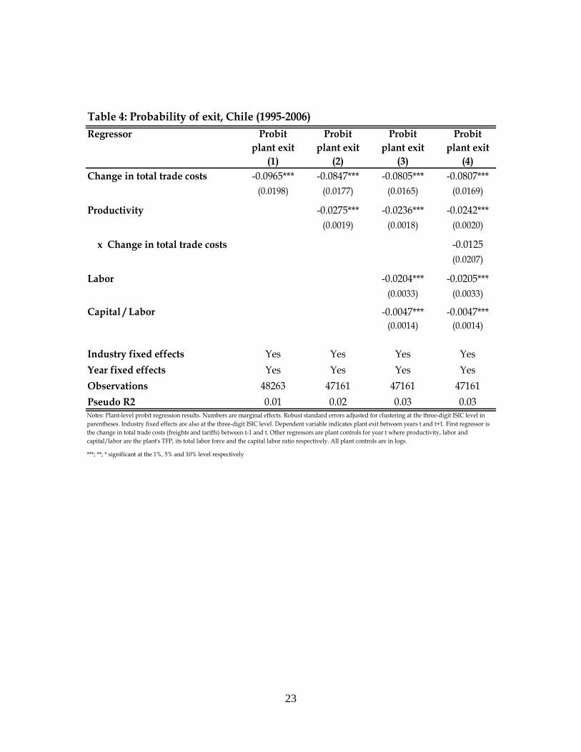
III.A. Plant exit To investigate whether plant exit is more likely as trade costs fall, we estimate a probit model of

the form:

)()Pr( 11 tjjitjtijt XCoste ααγβφ +++Δ= −+

where 1+jite takes the value of 1 if plant i in industry j exits between periods t and t+1; 1−Δ jtCost

is the change in trade costs in industry j between t-1 and t; ijtX is a vector of plant characteristics

and jα and tα are industry and time effects respectively. Results for Chile are presented in

Table 4. The first column focus only on trade costs4. The estimated coefficient has the right sign

and is significant at the 1% level. A reduction in trade costs increases the probability of plant

exit. The second column includes the plant’s productivity. As implied by theory and consistent

with results in Table 3, productivity is negatively and statistically significantly associated with

plant exit. This is also consistent with results in Tybout (1991), Liu (1993), Liu and Tybout

(1996), and Pavcnik (2002) that find that the probability of exiting is smaller for the more

efficient plants.

3 Similar evidence has been found by Alvarez and Lopez (2005) for the case of exporters in Chile. 4 Total trade costs include the sum of tariffs and freight costs.

9

In column 3, we include additional plant controls that may be related to the probability

of exit: the plant’s labor force (our proxy for size) and its capital intensity. Plants that are larger

and have higher capital labor ratios also exhibit lower probability of exit. Finally, in column (4)

we also include the interaction between the productivity of the plant and the change in trade

costs. This interaction seeks to explore whether the probability of exit when trade costs fall is

relatively lower for high-productivity plants. Therefore, the expected sign for this coefficient is

positive. The estimated coefficient is negative but is not statistically significant. We will come

back to this point later.

In regressions (2) to (4), even after we control for plant characteristics, the changes in

trade costs remain negatively and statistically significantly related to plant exit. The magnitudes

of the effect are considerable. A one standard deviation decline in total trade costs increases the

probability of exit by 0.7 percentage point.5 Since the probability of exit in the sample is about

11%, this implies an increase in the probability of exit of approximately 6%. The magnitude of

this effect is similar to the case of US in which a one standard deviation decline in total trade

costs increases the probability of exit by 1.3 percentage points or approximately 5% (see Bernard

et al., 2006).

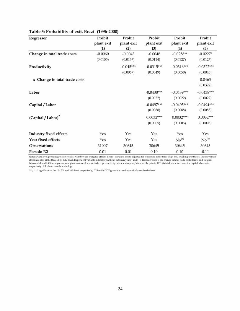
Table 5 presents the results for Brazil. The first three columns show similar regressions to

columns (1)-(3) in Table 4. The only minor difference is that we also include the squared of the

capital/labor ratio as an additional plant control. This is because capital affects the probability of

exit in a non-linear way on this sample. Specifically, plants with a larger capital/labor ratio have

a lower probability of exit -as expected- but this probability falls with capital intensity at a

decreasing rate. Most importantly, the results from the first three columns show that the effects

of trade costs, while negative, are not statistically significant. One shortcoming of the Brazilian

dataset is the relatively short period of time available for the analysis: 1996-2000. It is quite

possible, then, that the time effects are capturing the variability over time of the trade costs that

we want to exploit. Therefore, we follow Eslava, Haltiwanger, Kugler and Kugler (2009) and use

the country’s GDP growth instead of the time dummies. The growth of GDP is likely to capture

time-variant factors that could affect the probability of exit without absorbing all the variation in 5 Note that in nonlinear models, the magnitude of the effect of one independent variable is conditional to all the independent variables; therefore, we cannot simply multiply the change in the independent variable by its marginal effect. Rather, we need to evaluate the probability when the change in the trade costs is one standard deviation below its mean and the other independent variables are at their means and then calculate the difference between that probability and the one obtained when all the independent variables are at their means.

10

the trade costs variable. Results are reported in column (4). The coefficients for the plant controls

present almost the same values, while the coefficient for the change in trade costs is now

negative and statistically significant. Finally, we include the interaction term in column (5) but

the estimated coefficient is not statistically significant.

The magnitudes of the trade costs effects are considerable. According to the results, a one

standard deviation decline in total trade costs increases the probability of exit by 3%, a slightly

smaller percentage than in Chile. The probability of exit in Brazil’s sample is 7.5%.

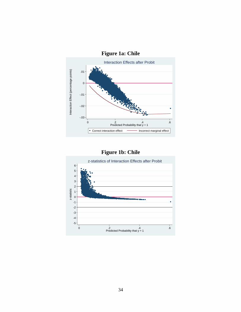
It is worth noting that although the coefficients for the interaction terms between plant

productivity and changes in trade costs in both probit models for Chile and Brazil do not seem to

be statistically significant, the interaction effects in nonlinear models cannot be evaluated simply

by looking at the sign, magnitude, or statistical significance of such coefficients (Ai and Norton,

2003). The marginal effects of interaction terms in nonlinear models require computing cross

derivatives that standard econometric packages do not perform. In addition, such marginal

effects could have different signs and different statistically significances for different

observations. Therefore, in order to explore whether the marginal effects of productivity on plant

exit increase with falling trade costs we use the Ai and Norton’s algorithm for computing

marginal effects of interaction terms in nonlinear models. The procedure calculates the

interaction effect, standard error, and z-statistic for each observation. Results are shown in

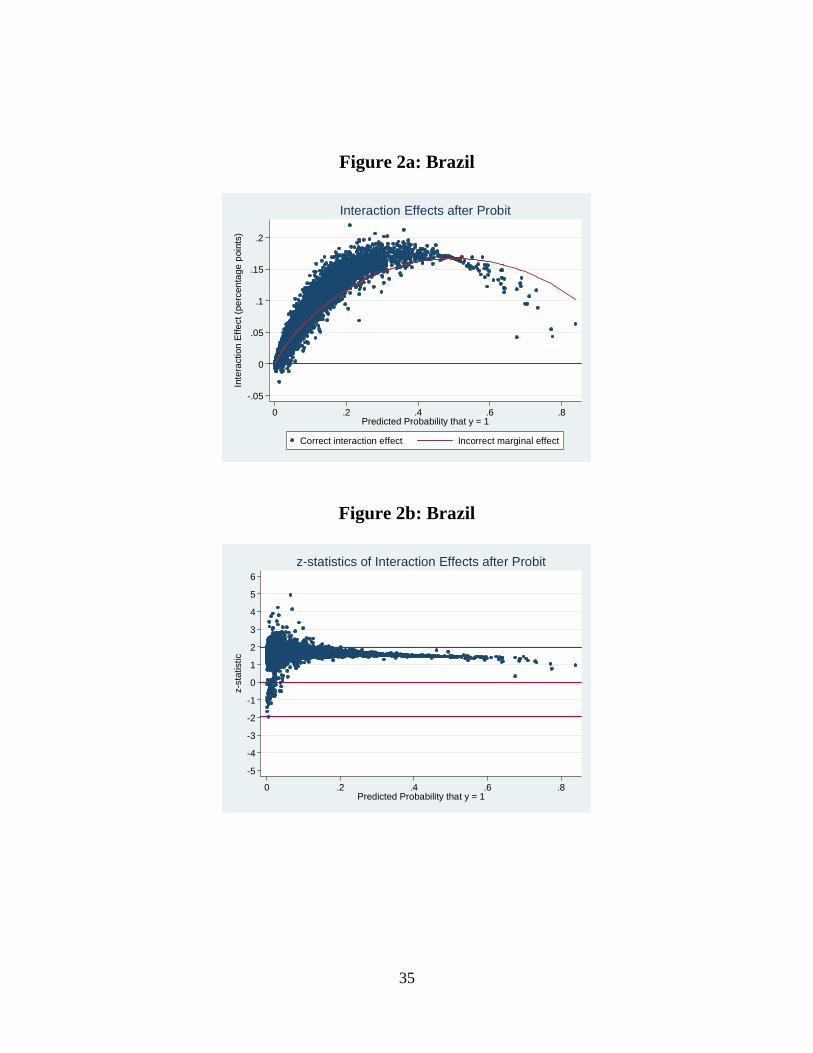
Figures 1a and 1b for the case of Chile and in Figures 2a and 2b for Brazil.

In the case of Chile, for example, the interaction term (Figure 1a) varies substantially

with positive values for some observations and negative values for others. In terms of the

significance, while the mean z-statistic for all the observations (0.18) is not statistically

significant, the interaction effects for a large group of observations with positive values are

indeed statistically significant (see Figure 1b). In the case of Brazil, most of the interaction terms

are positive (Figure 2a) and a fare amount of them are statistically significant (Figure 2b).

Indeed, the mean z-statistic for Brazil (1.74) is statistically significant at the 5% level. Note that

the finding that the statistically significant interaction terms are positive in value, for both Chile

and Brazil, is consistent with the theory: the marginal propensity that a plant will exit the market

driven by its low productivity increases with falling trade costs.

11

III.B. Export entry Now we investigate the reallocative process through the entry of new firms into

exporting. We estimate the impact of falling trade costs on the probability that a non-exporting

plant becomes an exporter using a probit model of the following form:

)()Pr( 11 tjijtjtijt XCosts ααγβφ +++Δ= −+

where 1+ijts takes the value of 1 if plant i in industry j is a non-exporter in period t and becomes

an exporter in period t+1; 1−Δ jtCost once again is the change in trade costs in industry j between

t-1 and t; ijtX is the vector of plant characteristics, and jα and tα are industry and time effects

respectively.

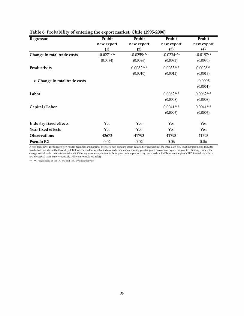
Results for Chile are reported in Table 6 with an increasing number of plant controls in

each column. In all the cases we find a negative and statistically significant relationship between

changes in trade costs and the probability of becoming an exporter. That is, the probability of

becoming an exporter is higher in industries with greater declines in trade costs. A one standard

deviation reduction in trade costs increases the probability of exporting by 0.19 percentage points

or in approximately 7%. The average probability of becoming an exporter in the sample is 2.9%.6

Using the Ai and Norton procedure to calculate the marginal effect of interaction terms in

nonlinear models, we find that the effect of the interaction between trade costs and productivity

is negative and significant for most of the observations. Indeed, the mean interaction effect for

all the observations is negative and significant at the 5% level (z-statistic is -1.96). The result is

consistent with the theory: falling trade costs increases the probability of becoming an exporter

relatively more in high productivity plants.

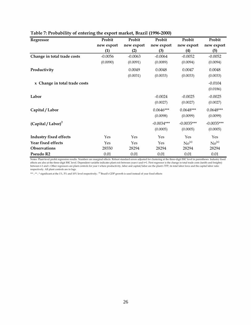
Results for Brazil are reported in Table 7. Although changes in trade costs are negatively

associated with the probability of exporting, as expected, the relationship is not statistically

significant at conventional levels in any of the regressions.7 We will see later, however, that this

lack of statistically significant results will change once we separate the effects of trade costs

between tariffs and freights rates. 6 The magnitude of this effect is higher than in the case of the US in which a one standard deviation decline in total trade costs increases the probability of exporting by 0.6% (Bernard et al., 2006). One potential contributing factor for this difference is that the reduction in trade costs was also larger in Chile than in the US. While total trade costs fell on average by 20% in the US, the reduction in Chile was about 31% during the sample period. 7 The interaction terms calculated for all the observations with the Ai and Norton procedure are also insignificant.

12

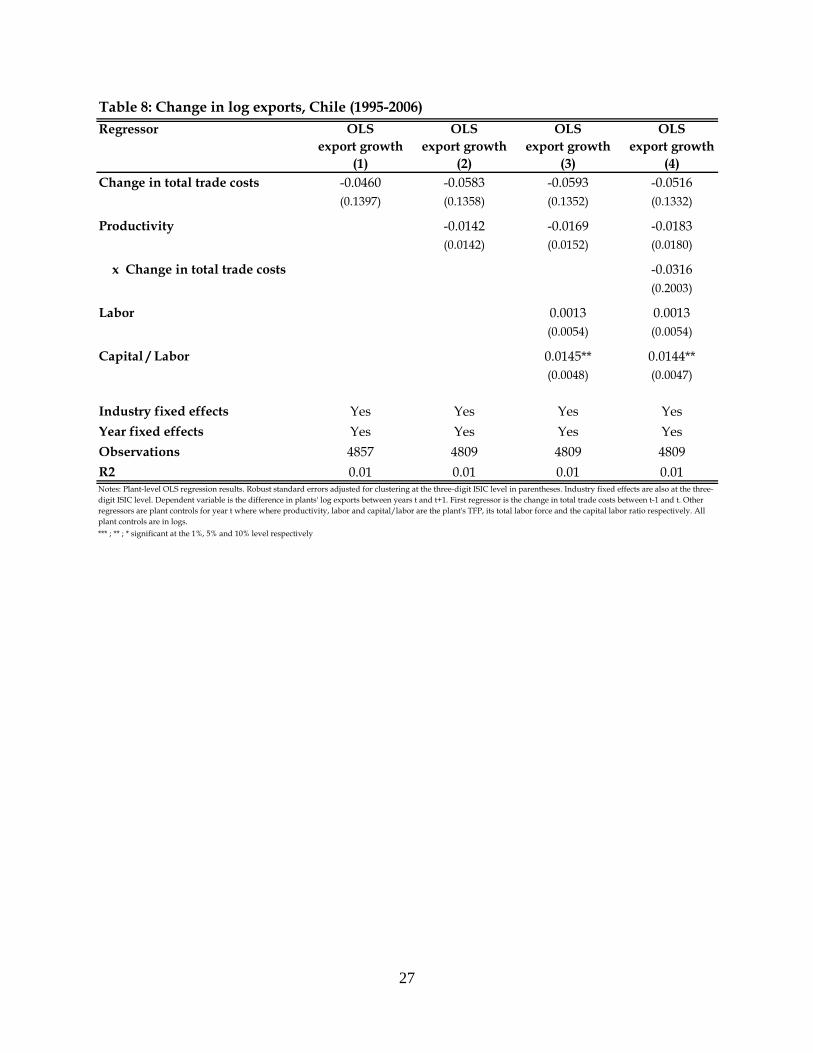
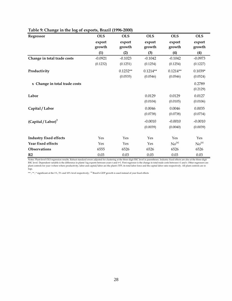
III.C. Export growth

Finally, we estimate whether a fall in trade costs leads to an export expansion of the firms

that are already exporting. To test this prediction we run the following regression:

tjijtjtijt XCostExp ααγβ +++Δ=Δ −+ 11

where 1+Δ itExp is the percentage change in exports between periods t and t+1 and the rest of the

variables are defined as before. Results for Chile and Brazil are shown in Tables 8 and 9

respectively. While the change in trade costs is negatively associated to export growth, as

expected, the coefficients are not statistically significant in any of the regressions.

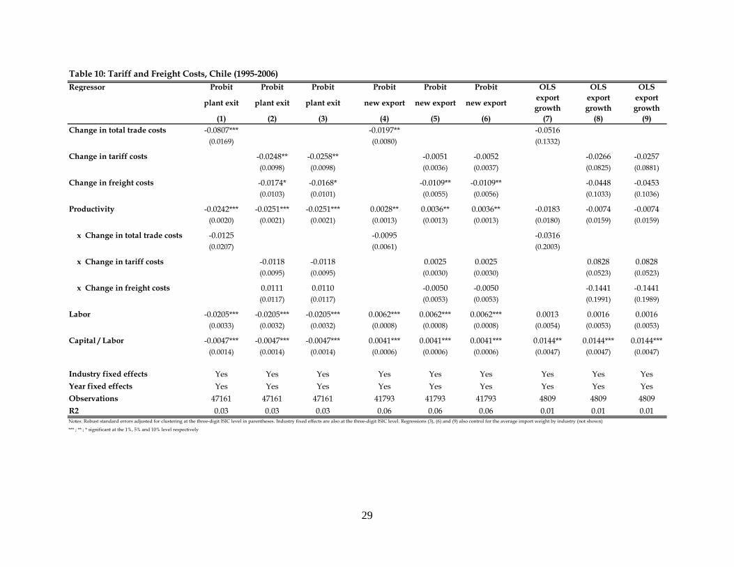
III.D. Tariffs and freight costs

So far, we have presented estimations with measures of total trade costs that add the

tariffs and the freight rates. However, we can include the tariffs and the freight rates separately to

investigate whether they have differential impacts on the reallocative process.

Table 10 presents the results for Chile. For comparison purposes, we added the original

estimation in which the total trade costs variable is used. Columns (1) - (3), for example, show

the probit model for plant exit. Column (1) presents the original estimation as shown in column

(4) of Table 4. The trade costs are introduced separately in column (2). The results indicate that

both types of costs, tariffs and freights, are important. The coefficient estimates for both the

change in tariffs and the change in freight rates are negative and statistically significant.8 In all

the specifications, any difference across industries is controlled by the industry fixed effects.

Nevertheless, in column (3) we also include the average import weight of the industry to

8 Our transport cost measure could be sensitive to exchange rate fluctuations, and therefore could be partly picking up macro conditions. If firms price their goods to market, but do not set their shipping costs, transport costs as a fraction of the value of imports may vary with the exchange rate. We estimate the correlations between the real exchange rate and the freight costs. While these correlations are both positive in Brazil and Chile they are not statistically significant.

13

explicitly control for industry differences in transport intensity. As shown in the table,

controlling for industry differences in weight do not change the results.

Columns (4) to (6) show the results for the probability of becoming an exporter. While

the coefficient for the tariff rate is negative it is not statistically significant. The coefficient for

the freight rate is significant at the 5% level. A one standard deviation decline in freights

increases the probability of exporting in approximately 5%. Once again, controlling for transport

intensity (column 6) does not change this finding.

Finally, columns (7) to (9) show the results for the growth of exports. The change in total

trade costs was not statistically significant in the original regression. Once we separate the

effects of tariff and freight costs, the coefficients are still not statistically significant at

conventional levels.

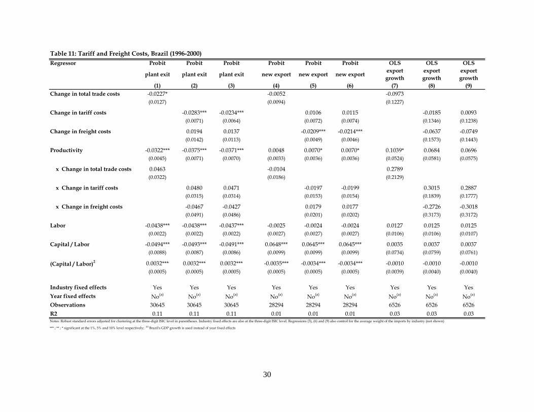
Table 11 presents the results for Brazil. We start again with the probability of exit which

is shown in columns (1) - (3). Similar to the case of Chile, the coefficient estimate for the change

in tariffs is negative and statistically significant. The coefficient for the change in freight costs

although positive is not significant at conventional levels.

Columns (4) to (6) in Table 11 report the results for the probability of becoming an

exporter. While the coefficient for the change in total trade costs was not statistically significant

in the original regression (column 4), once we separate the effects of the tariffs and the freight

costs, we find that the freight costs are negatively and significantly correlated with the

probability of exporting. A one standard deviation decline in the freight rates increases the

probability of becoming an exporter in approximately 3%.9 The result is similar in magnitude to

the case of Chile.

Finally, the last three columns in Table 11 show the results for the growth of exports. The

change in total trade costs was not statistically significant in the original regression (column 7).

Once we separate the effects of tariff and freight costs, although the coefficients have the right

sign, they are not statistically significant.

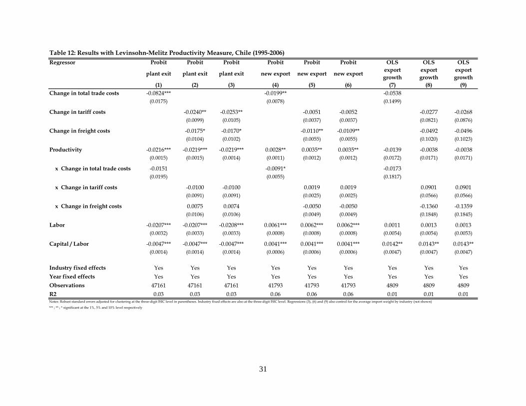
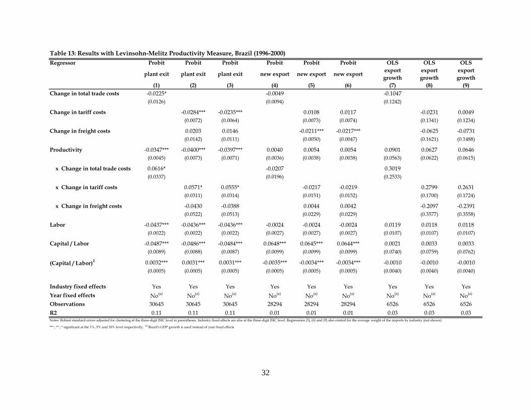
The results that we have presented so far are robust to other measures of TFP. This is

shown in Tables 12 and 13. In particular, we use in these tables a measure of TFP that corrects

for the revenue bias problem using the Levinsohn-Melitz (2002) methodology. In particular,

9 The average probability of becoming an exporter in the Brazilian sample is 9%.

14

Tables 12 and 13 show the same regressions as in Tables 10 and 11 but using the Levinsohn-

Melitz measure of TFP. All the qualitative results of the original regressions remain the same.

We mentioned before that using inbound trade costs may reduce the possibility of finding

an export response. Our lack of statistically significant results on the trade costs variables for the

growth of exports might be related to this shortcoming. To explore whether we find further

evidence on market selection effects, particularly for the export growth channel, we construct

two alternative proxies of outbound trade costs. First, as mentioned in the introduction, we

combine the ALADI dataset with a dataset on US imports from the US Census Bureau and

construct outbound trade costs for Brazil and Chile using the exports of these countries to a

handful of LAC countries, for which our data permits, and to the US. The drawback of this

measure, however, is that it covers only a limited fraction of the total manufacturing exports of

Brazil and Chile (53% for the case of Brazil and 30% for the case of Chile). Indeed, the

regressions with these trade costs (not shown) do not provide any additional support to the export

growth channel as the coefficients for the trade cost variables are once again not statistically

significant.

Our second proxy for outbound trade costs consists on differences between CIF and FOB

values. The advantage of this measure is that we can construct outbound trade costs that cover

100% of Brazil and Chile’s total manufacturing exports. There are two shortcomings with this

measure, however. First, we can only look at transport costs as import duties are not included in

the CIF value. Second, the difference between the CIF and the FOB values is normally a very

poor proxy for transport costs as the comparison relies on independent reports of the same trade

flow that have been shown to differ for reasons other than shipping costs (see Hummels and

Lugovskyy, 2006). Once again, the results with this proxy of transport costs show no significant

effects. Since these are all imperfect measures of outbound trade costs, we can still not rule out

the existence of a link between trade costs changes and export growth. Clearly, further research

with improved measures of outbound trade costs would be needed to assess this link more

properly.

15

III.E. Market selection effects of changes in trade costs We can use the estimates from the probit models to analyze, for example, by how much the

probability of exit and the probability of becoming an exporter would increase if trade costs in

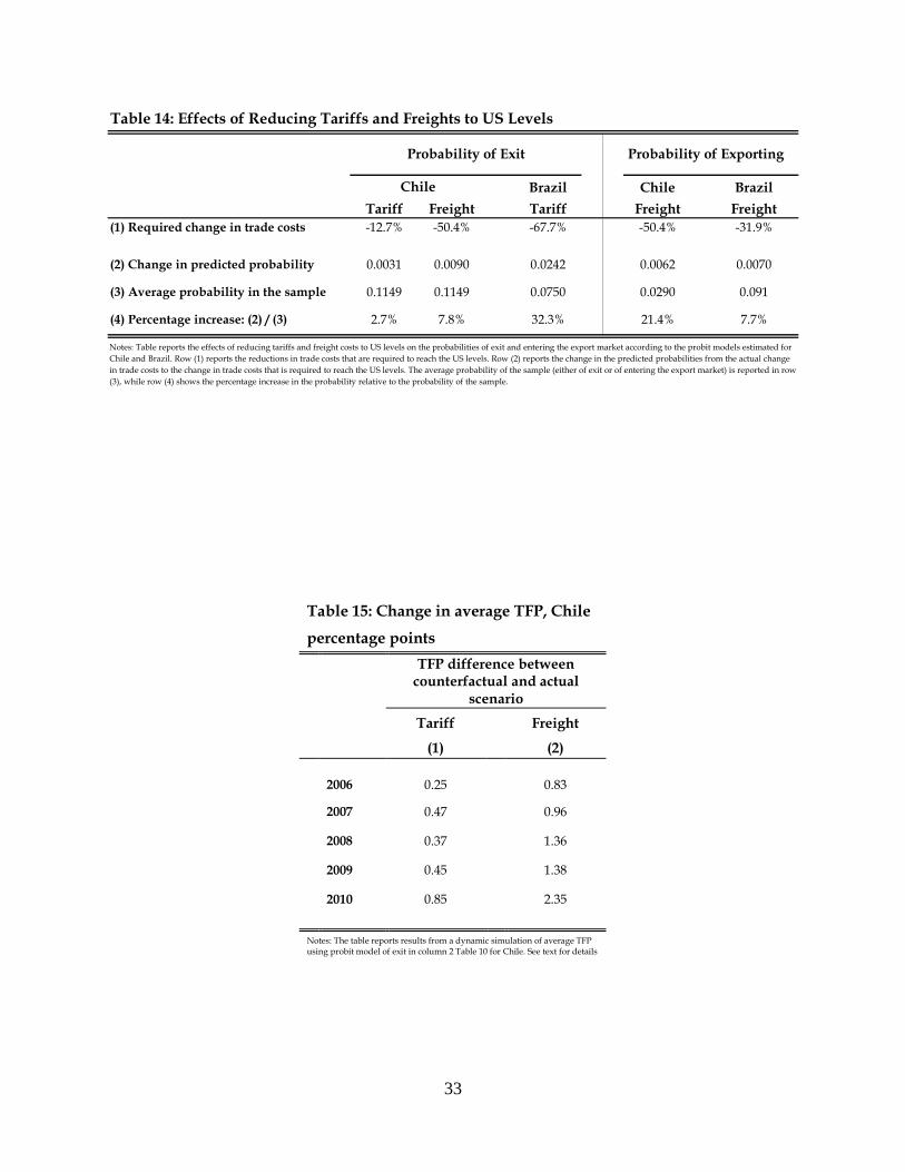
Brazil and in Chile fall to the levels observed in the US. In Table 14 we conduct a series of

exercises to answer this question. We use the results from the estimated probit models in

columns 2 and 5 from Table 10 for the case of Chile and from the same columns in Table 11 for

the case of Brazil.

The first row in Table 14 shows the percentage changes in trade costs that are necessary

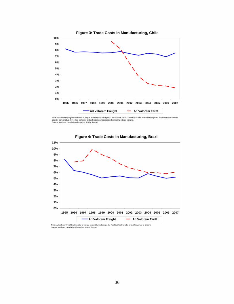
to reach the average trade costs in the US.10 Note that for the case of Chile, for example, the

average freight rate would need to fall by around 50% to reach the US level while the average

tariff rate would need to fall only by 13%. This is indicative of what we mentioned before that

transport costs are today much higher than tariff barriers in many countries in LAC and this is

particularly the case for Chile. This can also be seen in Figure 3 that shows the evolution of these

costs over time. For the case of Brazil, while tariff barriers have clearly felt since 1998 (see

Figure 4), they are still relatively high specially when compared to countries like Chile. Indeed,

in Brazil, the average tariff rate in manufacturing is currently at similar levels to the average

freight rate. Brazil has historically taken a more protectionist stand than Chile which explains

why tariff barriers have not fallen more dramatically. For Brazil, tariff and freight rates would

need to fall by 68% and 32% respectively to reach the US levels.

Row 2 in Table 14 reports the changes in the predicted probabilities for both countries

that are induced by the required falls in the trade costs.11 The average probability in the sample is

reported in row 3, while row 4 shows the percentage change in the predicted probability relative

to this probability in the sample.

The results are very intuitive. For the case of Chile, for example, the probability of exit

will increase relatively more when freight costs are reduced than when tariff rates are reduced

(7.8% versus 2.7%). This occurs even when the marginal effect of the tariff rate is higher than

the marginal effect of the freight cost (see Table 10) because the required reduction in freight

costs is much greater than the required reduction in the average tariff rate. For the case of Brazil, 10 We use 2005 as a benchmark for this exercise. 11 This is done by evaluating first the probit model when all the independent variables take their mean values and second when all the independent variables, except the change in trade costs, take their mean values while the change in trade costs takes the value necessary to reach the US levels. The difference between the predicted probabilities that arise under these two scenarios is the result reported in Table 12, row 2.

16

the increase in the probability of exit from a reduction in tariff rate is particularly large, 32.3%.

This large effect arises both, because the marginal effect of the tariff rate is large and because the

required fall in the average tariff rate is substantial too. The second panel to the right in Table 14

shows a similar exercise for the probability of entering the export market. For this case, only

freight costs turned out to be significant in the probit models for Brazil and Chile. Once again,

reducing trade costs to the levels observed in the US have considerable impacts in the

probabilities of becoming an exporter. The fall of 50.4% in the average freight rate in Chile

increases the probability of exporting in the country in about 21% while the fall of 32% in the

freight rate of Brazil increases the probability of exporting in almost 8%.

Finally, we would like to have an indication of how these changes in the intensity of the

market selection process translate into changes in productivity. In order to do this we perform a

dynamic simulation following a methodology similar to Eslava et al., (2009). The objective of

the simulation is to assess what would be the change in average TFP due to the increase in the

probabilities calculated in Table 14. We perform the simulation for the probability of exit and

illustrate it with the case of Chile.

The simulation is described as follows: first, we use the estimated probit model in column

2, Table 10, to obtain the fitted probabilities of exit for each plant. This allows us to rank plants

according to their probability of exit in 2005. We select the establishments that are predicted to

exit and survive according to this fitted probability. Under the actual scenario, the number of

establishments that exit is given by the actual predicted exit rate of the sample. Under the second

scenario, the number of plants that exit is higher and is given by the higher exit rate of the

“counterfactual” calculated in Table 14. Remember that these are the exit rates that would arise if

trade costs in Chile were to fall to the US levels. Since we want to simulate the impact of tariffs

and freights separately we have two counterfactuals, one for each trade cost. Once we obtain the

survivors for each counterfactual and actual scenario, we compute the average TFPs for each

sample and their differences. We also repeat the simulation over time in order to check for

cumulative effects. According to Eslava et al., the contribution to TFP from an increase in the

exit rate is likely to be cumulative since weeding out low productivity plants in a given year

implies that market selection in subsequent years will be based on an already improved and

select sample of plants. Note that throughout the simulation we keep plant TFP constant and

17

assume there are no new entrants. This allows us to isolate the role of exit from the role of other

factors focusing solely on how an increase in the exit rate impacts average TFP.

Table 15 reports the results. Columns 1 and 2 show the differences in the average TFP

between the counterfactual and the actual scenarios for the case of tariffs and for the case of

freights respectively. The exercise immediately shows that the effects induced by the reduction

in the freight rates are larger than the effects from the tariff rates. This was expected from Table

14 as the increase in the exit rate generated by the freight rate is higher than the increase

generated by the tariff rate. The results also show that the effects indeed accumulate over time as

argued by Eslava et al. (2009). For instance, the increase in the exit rate driven by the reduction

in the freight rate of 50% leads to an increase in average TFP of about 0.8 percentage points

during the first year but about 2.4 percentage points after 5 years. The results also show a gain of

an additional 0.9 percentage point in average productivity from the reduction in the tariff rate.

IV. Concluding Remarks This paper presents evidence that supports the notion that trade costs affect aggregate

productivity gains by limiting resource reallocation not only across sectors, but also between

firms within a sector. The evidence shows that trade costs affect the between-firm reallocative

process both, by protecting inefficient producers -lowering their likelihood to exit- and also by

limiting the expansion of efficient plants -lowering their likelihood to export.

The reallocative impacts that arise when trade barriers fall come not only from tariff

barriers but also from transport costs. According to the results, the potential reallocative impacts

can actually be larger in the case of transport costs than in the case of tariffs. This is particularly

the case for countries like Chile where the scope of reducing transport costs is much larger than

the scope of reducing tariffs. The result puts in perspective the need to address the issue of

transport costs in order to make further progress in reducing obstacles to trade and integration in

LAC.

18

References Ai, Chunrong, and Edward C. Norton (2003). “Interaction Terms in Logit and Probit Models”.

Economics Letters. Vol 80: 123-129.

Alvarez, Roberto, and Ricardo López. (2005). “Exporting and Performance: Evidence from

Chilean Plants”. Canadian Journal of Economics. Vol 38, No.4: 1385-1400.

Aw, B., S., Chung, and M. Roberts (2000). “Productivity and turnover in the export market:

micro-level evidence from the Republic of Korea and Taiwan (China), World Bank

Economic Review, 14, 65-90

Bartelsman, E., J. Haltiwanger, and S. Scarpetta (2004). "Microeconomic Evidence of Creative

Destruction in Industrial and Developing Countries," IZA Discussion Papers 1374,

Institute for the Study of Labor (IZA)

Bernard, A. B., Eaton, J., Jensen, J. B., Kortum, S. S. (2003). “Plants and productivity in

international trade” American Economic Review 93 (4), 1268-1290.

Bernard, A. B., and B. Jensen (1999). "Exceptional Exporter Performance: Cause, Effect, or

Both?" Journal of International Economics, 47(1), pp. 1-25

Bernard, A. B., and B. Jensen (2004). "Exporting and Productivity in the USA", Oxford Review

of Economic Policy, Vol. 20, No. 3

Bernard, A. B., B. Jensen, J. Bradford and P. Schott (2006). “Trade costs, firms and

productivity”. Journal of Monetary Economics 53, 917-937.

Clerides, S., S. Lach, and J. Tybout (1998). “Is Learning by Exporting Important? Micro-

dynamic Evidence from Colombia, Mexico and Morocco”, Quarterly Journal of

Economics, 113.

Eslava, M., J. Haltiwanger, A. Kugler, and M. Kugler (2009) “Trade Reforms and Market

Selection: Evidence from Manufacturing Plants in Colombia”, mimeo.

Fernandes, Ana. 2007. “Trade Policy, Trade Volumes and Plant Level Productivity in

Colombian Manufacturing Industries”. Journal of International Economics. Vol 71, No 1: 52-71

Foster, L., Haltiwanger, J., and C. Syverson (2005) “Reallocation, firm turnover, and efficiency:

selection on productivity or profitability?”, NBER working paper 11555.

Harrison, Ann (1994). “Productivity, Imperfect Competition and Trade Reform: Theory and

Evidence” Journal of International Economics, 36.

19

Hsieh, C. and P. Klenow (2007). "Misallocation and Manufacturing TFP in China and India,"

UC Berkeley mimeo.

Hummels, D. and V. Lugovskyy (2006). "Are Matched Partner Trade Statistics a Usable

Measure of Transportation Costs?," Review of International Economics, vol. 14(1), pages

69-86, 02

IDB 2008 “Unclogging the Arteries: The Impact of Transport Costs on Latin American and

Caribbean Trade” Special Report on Integration and Trade, Inter-American Development

Bank.

Katayama, H., Lu, S., and J. Tybout (2006) “Firm-level productivity studies: illusions and a

solution” mimeo.

Levinsohn, James and Marc Melitz (2002). “Productivity in a differentiated products market

equilibrium” mimeo.

Levinsohn, James and Petrin, Ariel (2003). “Estimating production functions using imputs to

control for unobservables” Review of Economics Studies 70, 317-341.

Liu, L. (1993) “Entry-Exit, Learning and Productivity Change: Evidence from Chile” Journal of

Development Economics, 42: 217-42

Liu, L. and J. Tybout (1996) “Productivity Growth in Colombia and Chile: Panel-Based

Evidence on the Role of Entry, Exit and Learning” in marke Roberts and James Tybout,

(eds), Industrial Evolution in Developing Countries, New York: Oxford University Press.

López-Córdova, Ernesto and Mauricio Mesquita Moreira (2003). “Regional Integration and

Productivity: The Experiences of Brazil and Mexico” Intal Working Paper 14. Inter-

American Development Bank.

Melitz, M.J. (2003) “The impact of trade on intra-industry reallocations and aggregate industry

productivity” Econometrica 71, 1695-1725

Melitz, M. and G. Ottaviano (2008) “Market Size, Trade, and Productivity," Review of Economic

Studies, vol. 75(1), pages 295-316, 01

Nicita, A. and M. Olarreaga (2006) “Trade, Production and Protection 1976-2004”, World Bank

document.

Pavcnik, N. (2002). “Trade Liberalization, Exit, and Productivity Improvements: Evidence from

Chilean Plants” Review of Economic Studies, 69

20

Restuccia, D. and R. Rogerson (2007). "Policy Distortions and Aggregate Productivity with

Heterogeneous Plants," NBER Working Paper 13018.

Tybout, J. (1991) “Linking Trade and Productivity: New Research Directions” World Bank

Economic Review 6: 189-212

21

1995 2000 2005 1995 2000 2005 1995 2000 2005311 Food manufacturing 9.9 9.7 9.7 11.0 10.0 1.8 20.8 19.7 11.5312 Prepared animal feeds & food products nec 12.1 11.4 12.9 11.0 10.0 1.8 23.1 21.4 14.8313 Beverages 10.3 9.6 10.6 10.1 10.0 4.3 20.4 19.6 14.9314 Tobacco 20.4 8.1 8.5 11.0 10.0 3.8 31.4 18.1 12.3321 Textiles 8.1 7.7 8.0 10.2 10.0 4.4 18.3 17.7 12.4322 Wearing, apparel 7.9 6.1 6.9 10.8 10.0 5.4 18.7 16.1 12.3323 Leather products 7.7 8.7 11.7 10.7 10.0 5.0 18.4 18.7 16.7324 Footwear 6.9 6.2 7.6 10.9 10.0 5.0 17.9 16.2 12.6331 Wood products 13.1 7.2 7.4 11.0 10.0 5.0 24.1 17.2 12.4332 Furniture 16.6 14.7 15.4 10.8 10.0 4.2 27.4 24.7 19.6341 Paper and products 11.5 10.8 12.7 10.9 10.0 3.2 22.3 20.8 15.8342 Printing and publishing 9.9 10.6 8.1 8.6 8.6 3.4 18.5 19.2 11.5351 Industrial chemicals 10.4 10.5 10.1 9.7 10.0 3.6 20.2 20.5 13.6352 Other chemicals 6.5 5.7 5.6 10.4 10.0 3.8 16.9 15.7 9.4353 Petroleum refinaries 16.2 10.6 29.0 10.6 10.0 3.8 26.8 20.6 32.8354 Miscellaneous petroleum and coal products 12.0 15.4 10.6 11.0 10.0 5.9 23.0 25.4 16.5355 Rubber products 9.6 8.1 8.9 10.6 10.0 4.7 20.2 18.1 13.5356 Plastic products 12.6 10.8 10.3 10.8 10.0 4.8 23.4 20.8 15.1361 Pottery, china, earthenware 19.6 17.4 17.9 10.4 10.0 4.7 30.0 27.4 22.6362 Glass and products 14.1 15.2 15.8 10.5 10.0 3.9 24.5 25.2 19.7369 Other non-metallic mineral products 17.9 21.4 29.7 10.8 10.0 2.8 28.6 31.4 32.5371 Iron and steel 11.5 10.4 8.4 9.8 10.0 3.0 21.3 20.4 11.4372 Non-ferrous metals 5.2 4.4 4.1 10.6 10.0 2.0 15.7 14.4 6.0381 Fabricated metal products 8.6 8.1 7.8 10.6 10.0 4.6 19.2 18.1 12.4382 Machinery, except electrical 6.4 5.3 5.3 11.0 10.0 5.2 17.3 15.3 10.5383 Machinery, electric 5.6 4.3 4.5 11.0 10.0 4.7 16.5 14.3 9.2384 Transport equipment 7.4 6.6 5.8 10.5 9.6 3.9 17.9 16.2 9.6385 Professional and scientific equipment 5.2 4.9 4.9 10.9 10.0 5.6 16.1 14.9 10.5390 Other manufactured products 9.6 10.0 10.2 10.9 10.0 5.3 20.5 20.0 15.4

10.8 9.6 10.6 10.6 9.9 4.1 21.4 19.6 14.7Average

Table 1: Ad valorem trade costs by three-digit ISIC industry, Chile

Industry Freights, fit (%) Tariffs, tit (%) Total, fit+tit (%)

22

1995 1998 2000 1995 1998 2000 1995 1998 2000311 Food manufacturing 8.6 5.9 5.6 5.0 5.8 4.8 13.6 11.6 10.4312 Prepared animal feeds & food products nec 10.6 6.3 7.2 8.8 10.7 14.3 19.4 16.9 21.5313 Beverages 12.4 7.4 7.8 10.9 12.0 10.4 23.2 19.4 18.1314 Tobacco 6.6 5.4 7.3 19.9 4.6 11.2 26.5 10.0 18.5321 Textiles 6.7 6.8 6.2 13.6 14.8 15.1 20.3 21.5 21.3322 Wearing, apparel 10.1 6.7 6.8 17.5 18.8 19.8 27.6 25.5 26.6323 Leather products 5.5 6.5 5.3 5.3 7.7 5.0 10.8 14.2 10.3324 Footwear 5.2 5.0 6.1 13.3 21.7 26.9 18.5 26.6 33.0331 Wood products 6.8 13.6 11.0 5.0 12.9 11.3 11.9 26.5 22.3332 Furniture 14.7 12.8 10.5 12.2 17.4 13.8 27.0 30.2 24.3341 Paper and products 11.0 11.1 9.5 3.3 5.2 4.7 14.4 16.3 14.2342 Printing and publishing 8.8 7.6 8.0 3.2 3.8 3.3 11.9 11.3 11.3351 Industrial chemicals 6.9 6.2 6.0 5.3 8.1 7.6 12.2 14.2 13.7352 Other chemicals 4.5 3.5 3.2 6.4 8.6 8.0 10.9 12.1 11.2353 Petroleum refinaries 7.0 8.4 5.9 12.4 4.9 1.9 19.5 13.3 7.9354 Miscellaneous petroleum and coal products 17.0 11.5 11.9 0.9 3.4 3.8 17.9 14.9 15.7355 Rubber products 8.1 8.1 7.0 9.9 12.9 12.2 18.1 21.0 19.2356 Plastic products 11.7 10.4 9.7 13.8 17.4 15.2 25.5 27.8 24.9361 Pottery, china, earthenware 13.2 11.7 11.2 12.1 16.8 14.4 25.3 28.5 25.6362 Glass and products 13.0 14.2 9.8 7.8 14.5 12.1 20.8 28.7 21.8369 Other non-metallic mineral products 14.3 13.0 10.0 6.5 11.1 10.6 20.8 24.1 20.5371 Iron and steel 9.4 8.0 7.3 8.5 9.6 10.1 17.9 17.6 17.4372 Non-ferrous metals 3.5 4.1 3.2 4.3 6.6 4.9 7.8 10.7 8.1381 Fabricated metal products 10.1 7.5 6.9 9.1 14.0 14.4 19.2 21.5 21.3382 Machinery, except electrical 5.5 4.7 4.2 7.6 11.7 10.4 13.2 16.4 14.6383 Machinery, electric 5.9 5.1 5.2 6.1 11.5 9.0 12.0 16.6 14.1384 Transport equipment 4.2 3.6 3.9 5.9 8.6 7.8 10.1 12.2 11.7385 Professional and scientific equipment 4.3 3.3 3.0 9.0 12.4 10.5 13.3 15.7 13.5390 Other manufactured products 13.1 12.4 10.8 12.6 23.7 20.0 25.7 36.0 30.8

8.9 7.9 7.2 8.8 11.4 10.8 17.8 19.4 18.1Average

Table 2: Ad valorem trade costs by three-digit ISIC industry, BrazilIndustry Freights, fit (%) Tariffs, tit (%) Total, fit+tit (%)

Brazil Chile(1) (2)

Plants that exit / plants do not exit -0.0791*** -0.1107***(0.0052) (0.0075)

New exporters / Non-exporters 0.0684*** 0.2175***(0.0053) (0.0104)

Always exporters / Non-exporters 0.1048*** 0.2779***(0.0047) (0.0129)

Table 3: Average plant TFP relative to comparator group

Notes: Plant-level regression results. Dependent variable is the plant's TFP. Regressors include the plant's size (Labor), year and industry fixed effects, and a dummy equal to 1 if the plant exit during the sample period (regression in row 1), if the plant is a non-exporter and eventually becomes an exporter (regression in row 2), if the plant is always an exporter (regression in row 3). Coefficients in the table report results for this dummy variable on the three different regressions

*** ; ** ; * significant at the 1%, 5% and 10% level respectively

23

Probit Probit Probit Probitplant exit plant exit plant exit plant exit

(1) (2) (3) (4)Change in total trade costs -0.0965*** -0.0847*** -0.0805*** -0.0807***

(0.0198) (0.0177) (0.0165) (0.0169)

Productivity -0.0275*** -0.0236*** -0.0242***(0.0019) (0.0018) (0.0020)

x Change in total trade costs -0.0125(0.0207)

Labor -0.0204*** -0.0205***(0.0033) (0.0033)

Capital / Labor -0.0047*** -0.0047***(0.0014) (0.0014)

Industry fixed effects Yes Yes Yes YesYear fixed effects Yes Yes Yes YesObservations 48263 47161 47161 47161Pseudo R2 0.01 0.02 0.03 0.03

***; **; * significant at the 1%, 5% and 10% level respectively

Table 4: Probability of exit, Chile (1995-2006)Regressor

Notes: Plant-level probit regression results. Numbers are marginal effects. Robust standard errors adjusted for clustering at the three-digit ISIC level in parentheses. Industry fixed effects are also at the three-digit ISIC level. Dependent variable indicates plant exit between years t and t+1. First regressor is the change in total trade costs (freights and tariffs) between t-1 and t. Other regressors are plant controls for year t where productivity, labor and capital/labor are the plant's TFP, its total labor force and the capital labor ratio respectively. All plant controls are in logs.

24

Probit Probit Probit Probit Probitplant exit plant exit plant exit plant exit plant exit

(1) (2) (3) (4) (5)Change in total trade costs -0.0060 -0.0043 -0.0048 -0.0258** -0.0227*

(0.0135) (0.0137) (0.0114) (0.0127) (0.0127)

Productivity -0.045*** -0.0315*** -0.0316*** -0.0322***(0.0067) (0.0049) (0.0050) (0.0045)

x Change in total trade costs 0.0463(0.0322)

Labor -0.0438*** -0.0439*** -0.0438***(0.0022) (0.0022) (0.0022)

Capital / Labor -0.0497*** -0.0495*** -0.0494***(0.0088) (0.0088) (0.0088)

(Capital / Labor)2 0.0032*** 0.0032*** 0.0032***(0.0005) (0.0005) (0.0005)

Industry fixed effects Yes Yes Yes Yes YesYear fixed effects Yes Yes Yes No(a) No(a)

Observations 31007 30645 30645 30645 30645Pseudo R2 0.01 0.01 0.10 0.10 0.11

RegressorTable 5: Probability of exit, Brazil (1996-2000)

Notes: Plant-level probit regression results. Numbers are marginal effects. Robust standard errors adjusted for clustering at the three-digit ISIC level in parentheses. Industry fixed effects are also at the three-digit ISIC level. Dependent variable indicates plant exit between years t and t+1. First regressor is the change in total trade costs (tariffs and freights) between t-1 and t. Other regressors are plant controls for year t where productivity, labor and capital/labor are the plant's TFP, its total labor force and the capital labor ratio respectively. All plant controls are in logs.

*** ; ** ; * significant at the 1%, 5% and 10% level respectively; (a) Brazil's GDP growth is used instead of year fixed effects

25

Probit Probit Probit Probitnew export new export new export new export

(1) (2) (3) (4)Change in total trade costs -0.0271*** -0.0259*** -0.0234*** -0.0197**

(0.0094) (0.0096) (0.0082) (0.0080)

Productivity 0.0052*** 0.0033*** 0.0028**(0.0010) (0.0012) (0.0013)

x Change in total trade costs -0.0095(0.0061)

Labor 0.0062*** 0.0062***(0.0008) (0.0008)

Capital / Labor 0.0041*** 0.0041***(0.0006) (0.0006)

Industry fixed effects Yes Yes Yes YesYear fixed effects Yes Yes Yes YesObservations 42673 41793 41793 41793Pseudo R2 0.02 0.02 0.06 0.06

*** ; ** ; * significant at the 1%, 5% and 10% level respectively

Table 6: Probability of entering the export market, Chile (1995-2006)Regressor

Notes: Plant-level probit regression results. Numbers are marginal effects. Robust standard errors adjusted for clustering at the three-digit ISIC level in parentheses. Industry fixed effects are also at the three-digit ISIC level. Dependent variable indicates whether a non-exporting plant in year t becomes an exporter in year t+1. First regressor is the change in total trade costs between t-1 and t. Other regressors are plant controls for year t where productivity, labor and capital/labor are the plant's TFP, its total labor force and the capital labor ratio respectively. All plant controls are in logs.

26

Probit Probit Probit Probit Probitnew export new export new export new export new export

(1) (2) (3) (4) (5)Change in total trade costs -0.0056 -0.0063 -0.0064 -0.0052 -0.0052

(0.0090) (0.0091) (0.0089) (0.0094) (0.0094)

Productivity 0.0049 0.0048 0.0047 0.0048(0.0031) (0.0033) (0.0033) (0.0033)

x Change in total trade costs -0.0104(0.0186)

Labor -0.0024 -0.0025 -0.0025(0.0027) (0.0027) (0.0027)

Capital / Labor 0.0646*** 0.0648*** 0.0648***(0.0098) (0.0099) (0.0099)

(Capital / Labor)2 -0.0034*** -0.0035*** -0.0035***(0.0005) (0.0005) (0.0005)

Industry fixed effects Yes Yes Yes Yes YesYear fixed effects Yes Yes Yes No(a) No(a)

Observations 28550 28294 28294 28294 28294Pseudo R2 0.01 0.01 0.01 0.01 0.01

RegressorTable 7: Probability of entering the export market, Brazil (1996-2000)

Notes: Plant-level probit regression results. Numbers are marginal effects. Robust standard errors adjusted for clustering at the three-digit ISIC level in parentheses. Industry fixed effects are also at the three-digit ISIC level. Dependent variable indicates plant exit between years t and t+1. First regressor is the change in total trade costs (tariffs and freights) between t-1 and t. Other regressors are plant controls for year t where productivity, labor and capital/labor are the plant's TFP, its total labor force and the capital labor ratio respectively. All plant controls are in logs.

*** ; ** ; * significant at the 1%, 5% and 10% level respectively; (a) Brazil's GDP growth is used instead of year fixed effects

27

OLS OLS OLS OLSexport growth export growth export growth export growth

(1) (2) (3) (4)Change in total trade costs -0.0460 -0.0583 -0.0593 -0.0516

(0.1397) (0.1358) (0.1352) (0.1332)

Productivity -0.0142 -0.0169 -0.0183(0.0142) (0.0152) (0.0180)

x Change in total trade costs -0.0316(0.2003)

Labor 0.0013 0.0013(0.0054) (0.0054)

Capital / Labor 0.0145** 0.0144**(0.0048) (0.0047)

Industry fixed effects Yes Yes Yes YesYear fixed effects Yes Yes Yes YesObservations 4857 4809 4809 4809R2 0.01 0.01 0.01 0.01

Table 8: Change in log exports, Chile (1995-2006)Regressor

*** ; ** ; * significant at the 1%, 5% and 10% level respectively

Notes: Plant-level OLS regression results. Robust standard errors adjusted for clustering at the three-digit ISIC level in parentheses. Industry fixed effects are also at the three-digit ISIC level. Dependent variable is the difference in plants' log exports between years t and t+1. First regressor is the change in total trade costs between t-1 and t. Other regressors are plant controls for year t where where productivity, labor and capital/labor are the plant's TFP, its total labor force and the capital labor ratio respectively. All plant controls are in logs.

28

OLS OLS OLS OLS OLSexport growth

export growth

export growth

export growth

export growth

(1) (2) (3) (4) (4)Change in total trade costs -0.0921 -0.1023 -0.1042 -0.1042 -0.0973

(0.1232) (0.1251) (0.1254) (0.1254) (0.1227)

Productivity 0.1232** 0.1214** 0.1214** 0.1039*(0.0535) (0.0546) (0.0546) (0.0524)

x Change in total trade costs 0.2789(0.2129)

Labor 0.0129 0.0129 0.0127(0.0104) (0.0105) (0.0106)

Capital / Labor 0.0046 0.0046 0.0035(0.0738) (0.0738) (0.0734)

(Capital / Labor)2 -0.0010 -0.0010 -0.0010(0.0039) (0.0040) (0.0039)

Industry fixed effects Yes Yes Yes Yes YesYear fixed effects Yes Yes Yes No(a) No(a)

Observations 6555 6526 6526 6526 6526R2 0.03 0.03 0.03 0.03 0.03

Table 9: Change in the log of exports, Brazil (1996-2000)Regressor

Notes: Plant-level OLS regression results. Robust standard errors adjusted for clustering at the three-digit ISIC level in parentheses. Industry fixed effects are also at the three-digit ISIC level. Dependent variable is the difference in plants' log exports between years t and t+1. First regressor is the change in total trade costs between t-1 and t. Other regressors are plant controls for year t where where productivity, labor and capital/labor are the plant's TFP, its total labor force and the capital labor ratio respectively. All plant controls are in logs.

*** ; ** ; * significant at the 1%, 5% and 10% level respectively; (a) Brazil's GDP growth is used instead of year fixed effects

29

Probit Probit Probit Probit Probit Probit OLS OLS OLS

plant exit plant exit plant exit new export new export new export export growth

export growth

export growth

(1) (2) (3) (4) (5) (6) (7) (8) (9)Change in total trade costs -0.0807*** -0.0197** -0.0516

(0.0169) (0.0080) (0.1332)

Change in tariff costs -0.0248** -0.0258** -0.0051 -0.0052 -0.0266 -0.0257(0.0098) (0.0098) (0.0036) (0.0037) (0.0825) (0.0881)

Change in freight costs -0.0174* -0.0168* -0.0109** -0.0109** -0.0448 -0.0453(0.0103) (0.0101) (0.0055) (0.0056) (0.1033) (0.1036)

Productivity -0.0242*** -0.0251*** -0.0251*** 0.0028** 0.0036** 0.0036** -0.0183 -0.0074 -0.0074(0.0020) (0.0021) (0.0021) (0.0013) (0.0013) (0.0013) (0.0180) (0.0159) (0.0159)

x Change in total trade costs -0.0125 -0.0095 -0.0316(0.0207) (0.0061) (0.2003)

x Change in tariff costs -0.0118 -0.0118 0.0025 0.0025 0.0828 0.0828(0.0095) (0.0095) (0.0030) (0.0030) (0.0523) (0.0523)

x Change in freight costs 0.0111 0.0110 -0.0050 -0.0050 -0.1441 -0.1441(0.0117) (0.0117) (0.0053) (0.0053) (0.1991) (0.1989)

Labor -0.0205*** -0.0205*** -0.0205*** 0.0062*** 0.0062*** 0.0062*** 0.0013 0.0016 0.0016(0.0033) (0.0032) (0.0032) (0.0008) (0.0008) (0.0008) (0.0054) (0.0053) (0.0053)

Capital / Labor -0.0047*** -0.0047*** -0.0047*** 0.0041*** 0.0041*** 0.0041*** 0.0144** 0.0144*** 0.0144***(0.0014) (0.0014) (0.0014) (0.0006) (0.0006) (0.0006) (0.0047) (0.0047) (0.0047)

Industry fixed effects Yes Yes Yes Yes Yes Yes Yes Yes YesYear fixed effects Yes Yes Yes Yes Yes Yes Yes Yes YesObservations 47161 47161 47161 41793 41793 41793 4809 4809 4809R2 0.03 0.03 0.03 0.06 0.06 0.06 0.01 0.01 0.01

Regressor

Notes: Robust standard errors adjusted for clustering at the three-digit ISIC level in parentheses. Industry fixed effects are also at the three-digit ISIC level. Regressions (3), (6) and (9) also control for the average import weight by industry (not shown)

*** ; ** ; * significant at the 1%, 5% and 10% level respectively

Table 10: Tariff and Freight Costs, Chile (1995-2006)

30

Probit Probit Probit Probit Probit Probit OLS OLS OLS

plant exit plant exit plant exit new export new export new export export growth

export growth

export growth

(1) (2) (3) (4) (5) (6) (7) (8) (9)Change in total trade costs -0.0227* -0.0052 -0.0973

(0.0127) (0.0094) (0.1227)

Change in tariff costs -0.0283*** -0.0234*** 0.0106 0.0115 -0.0185 0.0093(0.0071) (0.0064) (0.0072) (0.0074) (0.1346) (0.1238)

Change in freight costs 0.0194 0.0137 -0.0209*** -0.0214*** -0.0637 -0.0749(0.0142) (0.0113) (0.0049) (0.0046) (0.1573) (0.1443)

Productivity -0.0322*** -0.0375*** -0.0371*** 0.0048 0.0070* 0.0070* 0.1039* 0.0684 0.0696(0.0045) (0.0071) (0.0070) (0.0033) (0.0036) (0.0036) (0.0524) (0.0581) (0.0575)

x Change in total trade costs 0.0463 -0.0104 0.2789(0.0322) (0.0186) (0.2129)

x Change in tariff costs 0.0480 0.0471 -0.0197 -0.0199 0.3015 0.2887(0.0315) (0.0314) (0.0153) (0.0154) (0.1839) (0.1777)

x Change in freight costs -0.0467 -0.0427 0.0179 0.0177 -0.2726 -0.3018(0.0491) (0.0486) (0.0201) (0.0202) (0.3173) (0.3172)

Labor -0.0438*** -0.0438*** -0.0437*** -0.0025 -0.0024 -0.0024 0.0127 0.0125 0.0125(0.0022) (0.0022) (0.0022) (0.0027) (0.0027) (0.0027) (0.0106) (0.0106) (0.0107)

Capital / Labor -0.0494*** -0.0493*** -0.0491*** 0.0648*** 0.0645*** 0.0645*** 0.0035 0.0037 0.0037(0.0088) (0.0087) (0.0086) (0.0099) (0.0099) (0.0099) (0.0734) (0.0759) (0.0761)

(Capital / Labor)2 0.0032*** 0.0032*** 0.0032*** -0.0035*** -0.0034*** -0.0034*** -0.0010 -0.0010 -0.0010(0.0005) (0.0005) (0.0005) (0.0005) (0.0005) (0.0005) (0.0039) (0.0040) (0.0040)

Industry fixed effects Yes Yes Yes Yes Yes Yes Yes Yes YesYear fixed effects No(a) No(a) No(a) No(a) No(a) No(a) No(a) No(a) No(a)

Observations 30645 30645 30645 28294 28294 28294 6526 6526 6526R2 0.11 0.11 0.11 0.01 0.01 0.01 0.03 0.03 0.03

Regressor

Notes: Robust standard errors adjusted for clustering at the three-digit ISIC level in parentheses. Industry fixed effects are also at the three-digit ISIC level. Regressions (3), (6) and (9) also control for the average weight of the imports by industry (not shown)

*** ; ** ; * significant at the 1%, 5% and 10% level respectively; (a) Brazil's GDP growth is used instead of year fixed effects

Table 11: Tariff and Freight Costs, Brazil (1996-2000)

31

Probit Probit Probit Probit Probit Probit OLS OLS OLS

plant exit plant exit plant exit new export new export new export export growth

export growth

export growth

(1) (2) (3) (4) (5) (6) (7) (8) (9)Change in total trade costs -0.0824*** -0.0199** -0.0538

(0.0175) (0.0078) (0.1499)

Change in tariff costs -0.0240** -0.0253** -0.0051 -0.0052 -0.0277 -0.0268(0.0099) (0.0105) (0.0037) (0.0037) (0.0821) (0.0876)

Change in freight costs -0.0175* -0.0170* -0.0110** -0.0109** -0.0492 -0.0496(0.0104) (0.0102) (0.0055) (0.0055) (0.1020) (0.1023)

Productivity -0.0216*** -0.0219*** -0.0219*** 0.0028** 0.0035** 0.0035** -0.0139 -0.0038 -0.0038(0.0015) (0.0015) (0.0014) (0.0011) (0.0012) (0.0012) (0.0172) (0.0171) (0.0171)

x Change in total trade costs -0.0151 -0.0091* -0.0173(0.0195) (0.0055) (0.1817)

x Change in tariff costs -0.0100 -0.0100 0.0019 0.0019 0.0901 0.0901(0.0091) (0.0091) (0.0025) (0.0025) (0.0566) (0.0566)

x Change in freight costs 0.0075 0.0074 -0.0050 -0.0050 -0.1360 -0.1359(0.0106) (0.0106) (0.0049) (0.0049) (0.1848) (0.1845)

Labor -0.0207*** -0.0207*** -0.0208*** 0.0061*** 0.0062*** 0.0062*** 0.0011 0.0013 0.0013(0.0032) (0.0033) (0.0033) (0.0008) (0.0008) (0.0008) (0.0054) (0.0054) (0.0053)

Capital / Labor -0.0047*** -0.0047*** -0.0047*** 0.0041*** 0.0041*** 0.0041*** 0.0142** 0.0143** 0.0143**(0.0014) (0.0014) (0.0014) (0.0006) (0.0006) (0.0006) (0.0047) (0.0047) (0.0047)

Industry fixed effects Yes Yes Yes Yes Yes Yes Yes Yes YesYear fixed effects Yes Yes Yes Yes Yes Yes Yes Yes YesObservations 47161 47161 47161 41793 41793 41793 4809 4809 4809R2 0.03 0.03 0.03 0.06 0.06 0.06 0.01 0.01 0.01Notes: Robust standard errors adjusted for clustering at the three-digit ISIC level in parentheses. Industry fixed effects are also at the three-digit ISIC level. Regressions (3), (6) and (9) also control for the average import weight by industry (not shown)

*** ; ** ; * significant at the 1%, 5% and 10% level respectively

RegressorTable 12: Results with Levinsohn-Melitz Productivity Measure, Chile (1995-2006)

32

Probit Probit Probit Probit Probit Probit OLS OLS OLS

plant exit plant exit plant exit new export new export new export export growth

export growth

export growth

(1) (2) (3) (4) (5) (6) (7) (8) (9)Change in total trade costs -0.0225* -0.0049 -0.1047

(0.0126) (0.0094) (0.1242)

Change in tariff costs -0.0284*** -0.0235*** 0.0108 0.0117 -0.0231 0.0049(0.0072) (0.0064) (0.0073) (0.0074) (0.1341) (0.1234)

Change in freight costs 0.0203 0.0146 -0.0211*** -0.0217*** -0.0625 -0.0731(0.0142) (0.0111) (0.0050) (0.0047) (0.1621) (0.1488)

Productivity -0.0347*** -0.0400*** -0.0397*** 0.0040 0.0054 0.0054 0.0901 0.0627 0.0646(0.0045) (0.0073) (0.0071) (0.0036) (0.0038) (0.0038) (0.0563) (0.0622) (0.0615)

x Change in total trade costs 0.0616* -0.0207 0.3019(0.0337) (0.0196) (0.2533)

x Change in tariff costs 0.0571* 0.0555* -0.0217 -0.0219 0.2799 0.2631(0.0311) (0.0314) (0.0151) (0.0152) (0.1700) (0.1724)

x Change in freight costs -0.0430 -0.0388 0.0044 0.0042 -0.2097 -0.2391(0.0522) (0.0513) (0.0229) (0.0229) (0.3577) (0.3558)

Labor -0.0437*** -0.0436*** -0.0436*** -0.0024 -0.0024 -0.0024 0.0119 0.0118 0.0118(0.0022) (0.0022) (0.0022) (0.0027) (0.0027) (0.0027) (0.0107) (0.0107) (0.0107)

Capital / Labor -0.0487*** -0.0486*** -0.0484*** 0.0648*** 0.0645*** 0.0644*** 0.0021 0.0033 0.0033(0.0089) (0.0088) (0.0087) (0.0099) (0.0099) (0.0099) (0.0740) (0.0759) (0.0762)

(Capital / Labor)2 0.0032*** 0.0031*** 0.0031*** -0.0035*** -0.0034*** -0.0034*** -0.0010 -0.0010 -0.0010(0.0005) (0.0005) (0.0005) (0.0005) (0.0005) (0.0005) (0.0040) (0.0040) (0.0040)

Industry fixed effects Yes Yes Yes Yes Yes Yes Yes Yes YesYear fixed effects No(a) No(a) No(a) No(a) No(a) No(a) No(a) No(a) No(a)

Observations 30645 30645 30645 28294 28294 28294 6526 6526 6526R2 0.11 0.11 0.11 0.01 0.01 0.01 0.03 0.03 0.03Notes: Robust standard errors adjusted for clustering at the three-digit ISIC level in parentheses. Industry fixed effects are also at the three-digit ISIC level. Regressions (3), (6) and (9) also control for the average weight of the imports by industry (not shown)

*** ; ** ; * significant at the 1%, 5% and 10% level respectively; (a) Brazil's GDP growth is used instead of year fixed effects

Table 13: Results with Levinsohn-Melitz Productivity Measure, Brazil (1996-2000)Regressor

33

Brazil Chile BrazilTariff Freight Tariff Freight Freight

(1) Required change in trade costs -12.7% -50.4% -67.7% -50.4% -31.9%

(2) Change in predicted probability 0.0031 0.0090 0.0242 0.0062 0.0070

(3) Average probability in the sample 0.1149 0.1149 0.0750 0.0290 0.091

(4) Percentage increase: (2) / (3) 2.7% 7.8% 32.3% 21.4% 7.7%

Notes: Table reports the effects of reducing tariffs and freight costs to US levels on the probabilities of exit and entering the export market according to the probit models estimated for Chile and Brazil. Row (1) reports the reductions in trade costs that are required to reach the US levels. Row (2) reports the change in the predicted probabilities from the actual change in trade costs to the change in trade costs that is required to reach the US levels. The average probability of the sample (either of exit or of entering the export market) is reported in row (3), while row (4) shows the percentage increase in the probability relative to the probability of the sample.

Probability of Exit Probability of Exporting

Table 14: Effects of Reducing Tariffs and Freights to US Levels

Chile

Table 15: Change in average TFP, Chile percentage points

TFP difference between counterfactual and actual

scenario

Tariff Freight

(1) (2)

2006 0.25 0.83

2007 0.47 0.96

2008 0.37 1.36

2009 0.45 1.38

2010 0.85 2.35 Notes: The table reports results from a dynamic simulation of average TFP using probit model of exit in column 2 Table 10 for Chile. See text for details

34

Figure 1a: Chile

-.03

-.02

-.01

0

.01In

tera

ctio

n Ef

fect

(per

cent

age

poin

ts)

0 .2 .4 .6Predicted Probability that y = 1

Correct interaction effect Incorrect marginal effect

Interaction Effects after Probit

Figure 1b: Chile

-5

-4

-3

-2

-1

0

1

2

3

4

5

6

z-st

atis

tic

0 .2 .4 .6Predicted Probability that y = 1

z-statistics of Interaction Effects after Probit

35

Figure 2a: Brazil

-.05

0

.05

.1

.15

.2In

tera

ctio

n Ef

fect

(per

cent

age

poin

ts)

0 .2 .4 .6 .8Predicted Probability that y = 1

Correct interaction effect Incorrect marginal effect

Interaction Effects after Probit

Figure 2b: Brazil

-5

-4

-3

-2

-1

0

1

2

3

4

5

6

z-st

atis

tic

0 .2 .4 .6 .8Predicted Probability that y = 1

z-statistics of Interaction Effects after Probit

36

Figure 3: Trade Costs in Manufacturing, Chile

0%

1%

2%

3%

4%

5%

6%

7%

8%

9%

10%

1995 1996 1997 1998 1999 2000 2001 2002 2003 2004 2005 2006 2007

Ad Valorem Freight Ad Valorem Tariff

Note: Ad valorem freight is the ratio of freight expenditures to imports. Ad valorem tariff is the ratio of tariff revenue to imports. Both costs are derived directly from product-level data collected at the border and aggregated using imports as weights.Source: Author's calculations based on ALADI dataset

Figure 4: Trade Costs in Manufacturing, Brazil

0%

1%

2%

3%

4%

5%

6%

7%

8%

9%

10%

11%

1995 1996 1997 1998 1999 2000 2001 2002 2003 2004 2005 2006 2007

Ad Valorem Freight Ad Valorem Tariff

Note: Ad valorem freight is the ratio of freight expenditures to imports. Real tariff is the ratio of tariff revenue to importsSource: Author's calculations based on ALADI dataset