European Economic Review 16 (1981) 177-192. North-Holland Publishing Company

INTERPRETING ECONOMETRIC EVIDENCE

The Behaviour of Consumers’ Expenditure in the UK*

James E.H. DAVIDSON and David F. HENDRY

London School of Economics and Political Science, Anldwych WC2A 2AE, UK

The dynamic models of consumers’ e:cpenditure proposed by Davidson et al. (1978) and Hendry and von Ungern-Sternberg (1979) are re-appraiseld sn the light of Hall’s (1978) analysis of the empirical implications of the Life C;fcle/Permanent Income Hypothesis, in particular t.hat the l;eries for consumption should obey ‘a random walk apart from trend’. In an attempt to reconcile the conflicting findings, Monte Carlo experiments are used to demonstrate that if the Davidson et al. model were actually correct the: Hall model would appear to give a good description of the data and would probably not be rejected. All the models are re-estimated with new data for the UK, and these data do reject a modified ‘random-walk’ specification. In conclusion, we discuss the issue of income exogeneity, and comment on questions of model selection and interpretation.

1. Introduction

In Cwo recent papers [Davidson et al. (1978) denoted DHSY and Hendry and Ungern-Sternberg (1980) denoted HUS], an attempt was made to account for the empirical findings of tnost published ‘aggregate consumption function’ studies based on U.K. quarterly time-series data. Their approach involved specifying a number of criteria which any chosen empirical model should satisfy and sought to select a simple equation which was not only data-coherent and consistent in broad outline with the main tlhieories of consumers’ expenditure, but also explainerd m,hy previous studies obtained the results they reported and hald rot selected the ‘best’ equation. In both JDHSY and HUS, the gestalt of da: <A evidence strongly favoured error correction formu!ations for the dynamic respotlise of real consumers’ expenditure on non-durables (C) to real persohlal dispos;a@e ‘income (Y) - the laltter paper also included real personal sector liquid assets (1.) as an ‘integral’ corrj:ction. Moreover, although both papers, -were primarily concerned with methodological issues, their finally chosen equations seem to have continued to track the data with the anticipated accuracy despite further changes in

*Paper presen ted at the International Seminar in Macroeconomics, Oxford, June :23-::!4, 1980. We are indebted to Frank Srba for valuable assistance #and to Jobn Mueilbauer and participants at the Conference for helpful comments, This research was financed in part by the International Centre for Economics and Related Disciplines and the Social Science Research COL ?cil.

J.E.H. Dmihm and D.F. Hendry, lntqwering econometric evidence

nditure/income ratio and the data intercorrelations [see, e.g.,

nt approd was not investigated m either study, namely the on a permanent income/life cycle theory of consumers’

ure where agents hold rational expectations about future real income As an implication of that approach, Hall (1978) deduced that C, how a ‘random walk’, i.e.,

lows for a trend, and vt is ‘white noise’ independent of past g such an equation to quarterly (seasonally atijusted)

A, Hall found that (1) provided an adequate description of that such an equation seemed to have random residuals, and

appear signficantly if added. These findings were g the postulated thecry. Since the results in DHSY

encompassed an equation like (1) as a special case and were not incompatible with such a data process it seemed worth the validity of (1) for UK data.

ork is proposed for interpreting the econometric uation in DHSY and HUS survived a

passed most empirical models other than (1) : If C, h a completely autonomous error process [so (1)

;tes the true model] then it is inconceivable that any of the other survived predictive failure tests.

ently, we follow Hall in interpreting (1) as an implication of the data ut consider the situation in which a log-linear error

n mechanism (KM) defines the true model and income is strongly t different symbols are used, bearing the interpretation

Q ) are (C, Y ), respectively,

er-case letters denote logs of corresponding capitals, AjXl= nd O<;I,, yz c 1, with

ES a xrso-mechanism, (2) enables agents to maintain X =KQ I )glyJ in a world of stochastic variation around any path with constant growth rate A,q = g. Thus (2) is

e proportionality aspect of the permanent income

J.E.H. Davidson and D.F. Hendry, Interpreting econometric evidence 179

hypothesis, J

but otherwLse is based on ‘feedback’ rather than ?tnti.cipation assumptions. Eq. (3) is interpreted purely as a data description [see table 4c below] and issues of log versus linear, the endogeneity or ‘exogeneity’ of 4 etc. are discussed later. For the moment, it suffices to note that (2) is estimable by least squares under the assumptions stated and has an error variance of a:.

However, if an investigator only considered lagged regressors, then since (2) can be re-expressed as

where /I1 = yl, /I2 = (y2 - y1 ) and p3 - (f -pl), eliminating qr using (3 ) yields

4 =Itlqp-l+7r2x,_1 +w,p (6)

where x1 =(& +&;i), 172 =/& and w,= u,, +Y~z.+. The apparent equilibrium solution of (6) no longer yields proportionality between X and Q (unless I. = 1); also. ‘TIN typically will be small as PI and p2 usually have opposite signs (with 7tI ~0 possible); next, (&, p2) can be recovered onl!v b+ jointly modelling the x and 4 processes so that q, _ 1 is not weakly exogenous for the pi in (6) and finally even when (2) is structural, (6) is not for interventions which affect the data generation process of qt [see Engle et al. (1979)]. ConsequentBy, direct estimation (of the parameters of (6) is inefficient and could induce an incorrect decision to dele:te the ‘insignificant’ regressor ql_ 1,

leading to the selection of an equation like (1 ),

x,=0x,_,, +E,, (1’)

as the ‘appropriate’ model. Moreover, th[e deletion of q,_ 1 need not cause noticeable residual autocorrelation in (1’).

This analysis is most It:asily understoold by simulating the three models [(2), (6) and (1’)] when (2 j(4) defines the data generation process (analogous results obtain allowing for x to Gra.nger-cause q, but add little additional insight and so are not reported belo*w). The data generation process in the Monte Carlo ianalysis used ‘typical’ values for the parameters ‘based on DHSY, namely (PI, P2, f13) = (O-5., --0,4,0~9), E, := 0.95, o;f’ = I, at = 10 and T = 74 and replicated (2)-(4) 200 times, using NAIVE see Hendry and Srba (1980)]. The intercept was estimaltedl for every model, (q,} vms generated independently in each replication., and the first twenty initial data values were discarded. l ‘ A ’ denotes the “econometric’ estimate and ‘ - ’ the man p . simulation outcome. The following simulation statistics are reported : 9

‘Technically, there are difficult inference problems ior processes like (1) wherl r, IS ‘near’ the unit circle [see Phillips (1977) and Evans and Savin (198O)j and hence the inalclgue Monte Carlo considers only stiltionary processes; but pilot experiments suggested th;lt Grnilar results

obtained for R -z 1.02.

J.C.H. DaSdson and Df. Hendry, Interpreting econometric eoidence

= mean value of the coeficient 8 of the relevant regressor, mpling standard deviation of 8,

estimated standard error of 8, rtional rejection frequency of the null HO :S = 0,

= mean residual variance, zz roportional rejection frequency of the Lagrange multiplier test for

era! &th order residual autocorrelation.

tables, figures in parentheses denote minal significance levels.

) the results for eq. (2) are as might

Table 1

standard errlors; all tests are at

be anticipated ; see table Y ,.

Q 6 SD SE 1” Vl v4 CT2

0 O.:W 0.04 0.04 1.00 0.03 1.00 (0.01)

0.1101 0.12 0.04 0.04 0.92 (0.003)

t surpriskgly, the ECM adequately charaeterises the data and closely tion parameters; the two autocorrelation tests reject their nominal levels (but within two standard errors).

(fl, e3) from estimates of (2)+ (3) should yield standard errors of d (0.04,0.04 j [these figures are based on using var (I) = (1 - A2 )/7’, the

tic covariance matrix of (F and obtaining var (Zi) from the formula in rger et al. (1961)].

ext, the simuiation estimates of eq. (6) are presented in table 2.

Table 2

b 6 SD SE F 71 )/4 t?

a- 1 0.075 0.090 0.08 0.07 0.32 0.03 3.5 ~0.006) (0.01)

x,_ 1 0.83 0.10 0.09 1.00 (0.007 ’ _.- _-_____

standard errors are almost twice as large as in table 1 and HO : nl = 0

nly a third of the time, so the loss of efficiency is important. t32 estimates (0% -+ ;J:cT~) and, as earlier, ql, q, reject at about the 5 yO

if the investigator deleted ql__ 1 so that eq. (I’) was estimated, we ere b; = 8 is defined by plirn,, ao (c X,X,_ 1/x xf_ 1 );

- (I+ 36 j/T, the usual formula for the bias to O( T- ’ ).

J.E.H. Dauitlson and D.F. Hendr,r, Interpreting econometric epidmce 181

Regressor

X t- 1

-- __-----. --____ --_.-

6 F SD SE F 4, y/4 s2 --- -_-- -- -- pp.--._I__

0.98 0.93 0.05 0.04 1.00 0.10 O.o’P 3.6 (0.004 1 (0.02) (0.02 ]I

-_--- _-__-.___l_

Although 4 is highly autoregressive, and both qt, qt_ 1 are excluded, neither qn nor q4 detect residual autocorrelation more than a small percentage of the time, and ‘invalid’ tests (such as Durbin-Watson) should perform even worse. Given that a2 % close to that obtained for ‘eq. (6), it is easy to see HOW (1’)

might be selected when (2) is the true model and 4 exogenous., but (for whatever reason) only lagged regressors were considered.

The models used by DHSY and HIJS are certainly more complicated than (2) and the framework is not intended to imply that the eqiuivalent of 7il must be insignificant for UK data (in fact, y,_ 1 enters significantly Igelow). The analysis does show, however, that the same model [here (1)3 can be implied by ‘contradictory’ theories and hence while observing an ‘implication of a theory provides a check on its data consistency, it does not really offer ‘support’.

Before testing (l), it is clearly essential to re-establish the validity of the empirical equivalents of the analogue models and in the interval since DHSY and HUS selected their equations, new data (on a new, 19’75, price index basis) have accrued which allow a powerful, independent test of their formulations (see section 2). Following this, the implications for the Hall model are derived from HUS using the empirical equivalent of (3) and against this, (1) is tested. The evidence reads to rejection of (I), but seems consistent with HUS so section 4 briefly examines the issues of simu’ltaneity and data coherency. Finally, the interpretation of equations in terms of ‘forward’ versus ‘backward’ looking beh:I.viour is reconsidereld and suggests that there is less incompatibility between the various approaches than might appear at first sight.

2. A m-appraisal of DHSY and HUS

Eqs. (7) and (8) respectively report least squares re-estimates of t&se two models based on ‘the 1975 price index data;2 all series are quarterly, seasonally unadjusted and in constant prices over the period 1964(i) [T = l] to 1979(iv) CT=641 with C, Y; L as defined above and P and D denoting the retail price index and the dummy variable Ffor 1968(i)/(ii) and the introduction of Value Added Tax] used by ‘HUS. As earlier lower cast:: letters denote log, of corresponding capitals and dj depfvces a j-period difference.

2See! Economic 7?ends, Annual Supplement of January 1980 and the issue of May 10&O.

(7)

b b J.E.H. DarGfson and D.F. Mendry. Interpreting econt;metrk evidence

S, the DHSY model yields

~4L:,-0.48A4~t-0.27dr d,~,-O.ll(c-~)~-~~--O.l4d,y, (0.05 ) (0.07) (0.02) (0.05)

- 0.34 d 1 A&#, + 0.01 A&, 90.20) (0.003 )

T-6,44+296 R2 = 0.73, ci = 0.0088,

z,(20.33)=0.6, 2,(20)=25, ti z3(8)=9.3, z,(6)=5.7,

ere

T = a, 6 -I- nf denotes estimation from (a, b) and prediction over the next. n observations,

6 = residual standard deviation, t n, T-K )= F-test of parameter constancy due 80 Chow (1960) for a post-

sampie observations and K regressors, t&t) = asymptotically equivalent X2-test [see Hendry (1980)], z c0 = Box--Pierce autocorrelation statistic based on the residual

correlogrram, :,U 1 = Lagrange multiplier test for Ith order error autocorrelation (i.e.,

qI above).

Fig. 1 shows the graph of d,c, and the fit/predictions from (7) (note that ‘prediction’ means using known values for the regressors, with parameter

, 1 I I I

1 1970 1-r

1972 1974 1976 W6 1980

Fig. 1

J.E.H. Daoidson and D.F. Hendry, Interpreting econometric etiideme 183

estimates held fixed). The estimates in (7) are ciosely similar to those reported in DHSY, parameter constancy is maintained over the prediction period and no evidence is present of residual serial correlation. Also, extending the estimation sample to T=:6, 56 + 8j’ (so that only completely new observations are retained for the predictive failure tests) yields 6 = 0.0083, zr (8,45) = 0 P, z2 (8) = 8, z,(6) = 5.7. These empirical results corroborate those reported independently by Bean (1977) and Davies (1979) and provide further empirical support for the theoretical arguments developed in Deaton (1980).

Next,

d,&=O.O84~; (3-i)d,y;+--O.l5(c-y”),_,+O.O68(1-y”),_, (0.007 ) (0.06) ’ (0.018)

+O.Ol d,D,-0.15d,R,*_3-0.079-0.013Q,,-0.009Q,, (0.002) (0.09) (0.023) (0.005) (0.004)

-O.m7Q,,, (0.003) (8)

T=7,60$4f, 2 = 0.0078, b1 =0.31(0.16),

~(4,43)=0.3, q(4)=2, z,(5)=7.1., z,(7)=8.9.

where

Y” = log (Y -@L) and d is an 8-quarter moving average of the rate of change of the RPI,

R” = (R(l - TJ- d,p), where R is the local authority 3-month interest rate and Ty is the standard marginal rate of income tax,

Q.

L

= seasonal dummy variables, = estimated first-order autoregressive error coefficient,

z5 (k)= likelihood ratio test of the common factor restriction [see Sargan (1964, 1980)-J.

The specification in (8) differs slightly from HUS, but

AIR,*_3 is not significant3 (and has a ‘t’-value of about 0.6 if d 1 I,_ 1

is added, which in turn has a ‘t’ of 1.7 and reduces b1, supporting the HUS formulation) and the use of the single pk:riod value of (L-y”) (rather than a four-period moving average) improves both the fit and the predictions

‘R* was tried as a ‘control’ to partial out an) changes in real itlterest rates. in fact, A,!,- , retains a similar coeffkient to that reported by HUS if A, RI_3 is excluded (name!y 0.2). and this is used below In deriving eq. (10).

J.E.H. Daridsnn ard D.F. Yendry. Interpreting ecorlometric evidence

and removes the four period autocorrelation found by HIJS. Fig. 2 shows taph of (8) and fig. 3 provides the time-series of (c-y) and (c-v”) to

onstrate the e%cts of adjusting the income series for inflation induced

I r

1976 1972 1974 1976 1978 1990

Fig. 2

Consumption - Income ratio:.

Fig. 3

J.E.H. D~~ridson ~rnd D.F. ffendr_r, Inrerprefing econometric evidence 185

losses on liquid asset holdings. As with (7), the estimates are similar to those reported earlier (and seem robust to the noted changes in specification), and exhibit parameter constancy despite the draimatic changes which occurred in (c-y”) after 1976 (note that the adjusted expenditure/income ratio re:aches a peak in 1976 prior to falling sharply). Since z1 ( - ) and z2 ( * ) are Lagrange multiplier based tests, i t Is legitimate under the null to test other periods for parameter constancy after model fitting, and doing so for 1Of (using d 1 I, _ 1

as a regressor) yields z1 (10,37)= 1.1, z,(10)=31, &=0.0073. While parameter constancy is not rejected, z2 indicates that the estimates are not well determined over the shorter estimation period.

The long-run steady-state constant growth ‘equilibrium’ solutions from (7) and (8) have the form

where 4 =0, 0.45 in (7) and (8), respectively, and B( - ) depends negat.ively on the growth rate of Y(g) and inflation (@). Long-run proportionalit) as in (9) is a well-known attribute of both permanent income and life-cycle theorie:,, as is a negative dependence on g. The presence of (L/Y) can be rationalised in several ways when capital market imperfections and uncertainty prevail [see, e.g., Flemming (1973) and Pissarides (1978)]. Note that although the solution (9) takes the same form for (7) and (8) under the static equilibrium condition that (L/Y) is constant, margmalising with respect to all current and lagged values of L is an unnecessary restriction on the information set which would be counter productive if - he partial correlations bet ween included and excluded variables altered.

The empirical equivalent of (3$ is reported in table 4c below, and using this to eliminate current yt from (8) yields4

c,-0.31y,_ 1 +O.l7y,_, -O.l7y,__,-O.l4y,_, -O.O8y,_,

+O.8%,-4+0.21,_ ~-0.21,_~+O.O71,_~. (10)

Thus, on the hypothesis that (8) describes the data generation process, the data evidence suggests that lagged y and lagged I should influence c, given lagged c’s.

3. The Hall model

If C, is determined by permanent income (YIP)} and the latter is the discounted rational expectation of future income aocruals, since innovations to the informaiion set are white noise, Wall (1978) deduced that Ct would

41n fact, c,_ 1 ‘Granger-causes’ yr if added to table 4~ [see Granger (19691-j and irmrporabing this feature would further improve the ‘match’ with Izlter results.

EER --G

l86 J.E.H. Daridson und D.F. Hendry. Interpreting econometric ecidence

random walk’ wiih drift or trend as in (1). As noted above, the I evidence for the USA quoted by Hall is consistent with such an

ow, log-linear rather than linear models are used, but this change seems n~equential, and UK evidence favours the former. However, Hall’s data

ss~rn to have been seasonally adjusted and depending on the filter used for different series, the results could be distorted thereby [see Wallis (1974) DWSY]. Although it is unlikely that the substance of the arguments

changed radically by the use of adjusted versus raw series, the fit of requrres re-interpretation in tlxms of filtered data, and application to

usted data (as herein) involves substantially different lag lengths. 5th order autoregression for c, suggested the following

f ( f ) [see Prothero and “Wallis (1976)] :

.&<:, = 0.72 &c, _ 1 + O.Ol A4 D, + 0.006, (11) (3.25 j (O.wi) (0.006)

T=X,44+2OJ ci=o.o11t3, b1=0.19(0.32),

z,(20.33)= I.? zz(20)= 2c>,, z5(1)=o.s, z,(7)=7.0.

Fig. 4 provides the tImle-series graph, and at first sight the tracking

s / 1 TEST PERIOD

.

Fig. 4

inted out to us that an error on the relationship linking Cl to Yp would ge error on (1) (and hence bias the least squares estimates of

by, e.g., a Durbin-Watson test; see Muellbauer and Winter

performance appears satisfactory. However, the standard deviation of ,&c, is only 0.0195 and the & 2c3 interval from (11) is _tO.O220; specifically, on the six occasions when Aqc, changed by more than +0.022, the model’s prediction error/residual fell outside the + 28 interval four times, and of 29

sign changes in A, A4ct (i.e., when A4c, changed direction) (11) had the opposite sign (for A, A&) on 21 occasions. f Nevertheless, the residuals from (11) are not detectably autocorrelated, which entails that all othtir lagged values of c, are potentially legitimate instrumental variables.

It should be clear that neither (1) nor (11) is claimed to be the data generation process: both are derived models ancl there arc many objections to arguing that the true consumption equation is a random walk with an autonomous error process generated independently of 1: L, etc., not least the fact that random walks can drift anywhere and so produce C much in excess of Y. Rather, the stochastic implications obtained by Hall can be expressed suhx~iy ai: no other potential lagged variables Granger-cause the residuals in (1) [see Granger (1969), Engle et al. (1979)].

On methodological grounds, to adequately test (1) [or here, (11 jj against other models, all of the additional variables should be included at the outset. First testing c, on yt - j 0’2 1) alone, then on 1, -,i (j 2 1 ) alone etc. can seriously bias the outcome. Thus, table 4a reports the estimates for a model of the form

c, = i (!XjC(-j- f +piYy-j- 1 +yjl(--j- 1 t 6jRF j - 1 + ;-j&l ) j=O

+0,D,+0,D,_,+u,, (12)

where n is 5 for ya, 4 for c and 3 for Q, 1 and R* (in table 413, ‘ii is set to zero for all j).

Although such over-parameterised regressions must be treated with care, several lagged variables are individually significant rejecting the strong implications underlying (1). Indeed, the estimates in table 4b correspond reasonably to the solved ‘reduced form’ (10) which obtains on marginalising (8) with respect to current y, using the empirical data process reported in table 4c. Further, directly reparameterising table 4b yields

A&=0.12 A4y;_ 1 +0.54A,c,_ i + 0.40 A, I,- 1 +O.ol A,Q

(0.06) (0.12) (0.09 ‘I (0.003 )

+ 0.003 -0001Q,, + 0.002Q2, + O.OO;‘Q,,, (0.003) (0.004) (0.004) (O..W4l)

T=8,56+8J; R2 = 0.82, S = 0.0089,

(13)

2,(8,41)= 1.7, Q(8)= 16, 231(8)=9.4, z&3)=3.0_

.I 13 If. Dwidsnrt nnd D-F. Hendry. interpreting econometric erideme

I able 4a _c- r - _l__l_-_l _- w-e

0 1 2 3 4 5 6

-1 0.59 - 0.09 0.42 (0.22) (0.17) (0.16)

c. 8 P 0.20 0.03 -0.19 (0.09 ) (0.10) (0.10)

0.21 - 0.50 0.10 (0.19) (0.22) (0.23)

P 0 I 0.05 0.11 - 0.28 $.!9; (0.24) (0.27 )

P 0.10 - 0.06 - 0.01 - 0.04 (0.34) (0.02 : (O&2) (0.02)

0.02 -- - -

m_If )

4 = 7,5H + 6f. R2 = 0.994, ci = 0.0083

=r = 1.0. 22(6)= 12, ~(7) = 14.6, z*(6) = 8

0.71 -0.17 - (OJ.7) (0.24)

-0.13 - 0.25 0.01 (0.11) (0.11’ (0.10)

0.07 - - (0.14)

0.21 - - (6.19!

--0.01 - - (0.01)

Table 4b _. 1_-I-_. - -_-___ _--

B 0 1 2 3 4 5 6 --- -___

Q* : -1 0.52 - 0.07 0.40 0.71 -0.13 - (0.20) (0.16) (0.15) (0.16) (0.23) --

P . 97 j 0.21 0.013 -0.19 -0.14 - 0.22 - 0.02 (0.08) (0.09) (0.09 1 (0.10) (0.10) (0.09 )

- 0.32 -0.51 - 0.00 0.10 - .- -B (0.12) (0.19) (0.20) (0.12)

T=7,58+6J R2 = 0.993, 6 -= 0.00?9

qt6)= 19. z,(7)==9.7, z&6)=5

Table 4~ -___--._

/ 0 I 2 3 4 - 5 -~___-

C-j -1 0.58 0.34 -0.12 - 0.07 0.12 (0.18) (0.22) (0.24) (0.24) (0.20)

P ’ I i.4 - 0.05 -0.01 -0.01 0.001 -- (1.31 (0.02 ) (0.01) (O.O? ) (0.001)

= R2 = 0.97, C? = o.u20

=a = 1.0. z2(28)=%, z3(7)=5_0, z,(Gj==6

J.E.H. Davidson and D.F. Hendry, Interpreting eco4rometric evidence 189

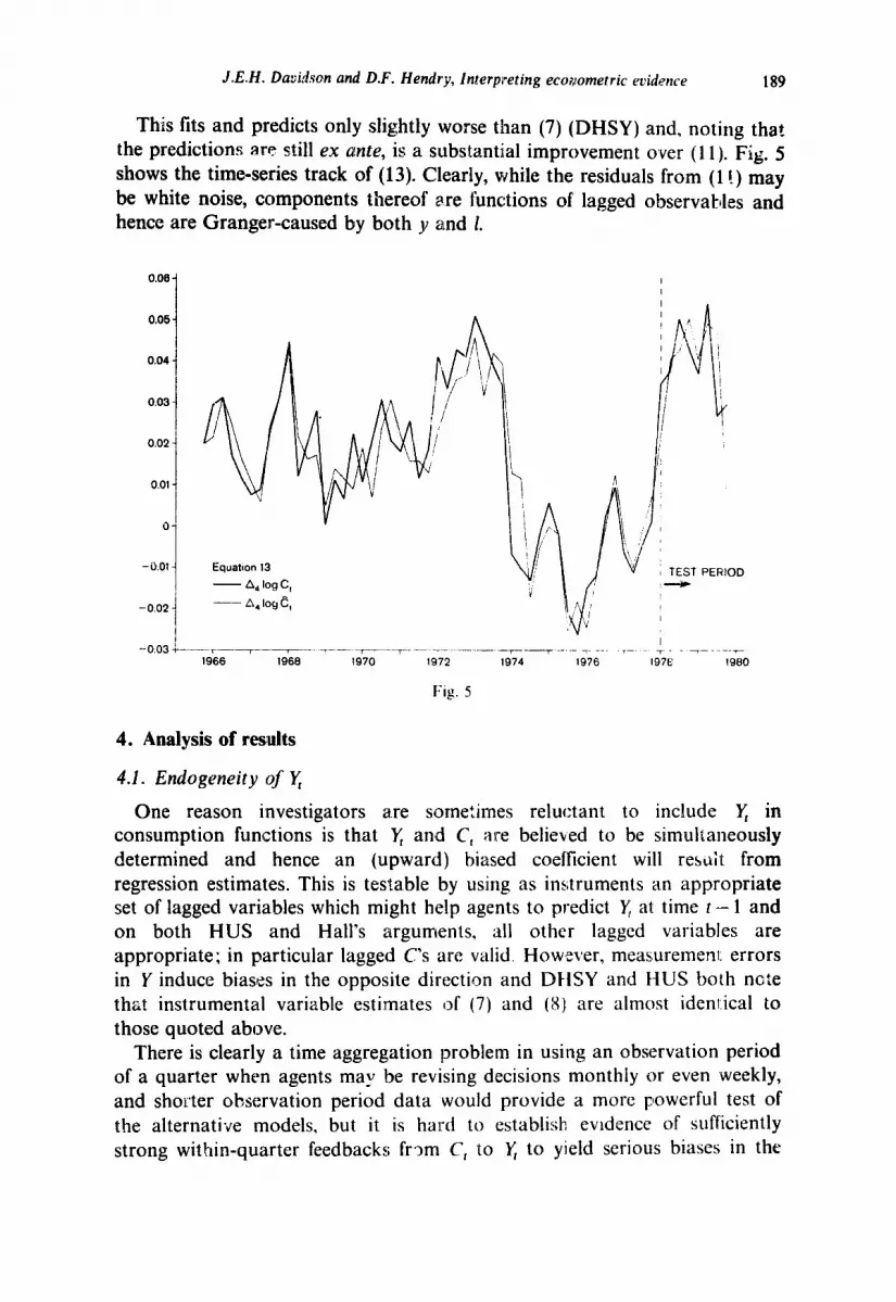
This fits and predicts only slightly worse than (7) (DHSY) and, noting that the predictions are still ex ante, is a substantial improvement over (11). Fig. 5 shows the time-series track of (13). Clearly, while the residuals from (1 !) may be white noise, components thereof are functions of lagged observahles and hence are Granger-caused by both ~7 and 1.

0.06

0.05

0.04

0.03

0.02

0.01

0

-0.01

-0.02

-0.03

Equation 13

- A, log C,

- A, log c,

) TEST PERIOD

-----l----7--- _- _- __~__ -..-- -_-_- l--r---- -- -7.- 19T7E 7-- -T-- 1966 1968 1970 1972 1974 1976 1980

Fig. 5

4. Analysis of results

4.1. Endogeneity of x

One reason investigators a.re sometimes reluctant to include x in consumption functions is that x and C, are believed to be simultaneously determined and hence an (upward) biased coefficient will restiit from regression estimates. This is testa.ble by using as instruments an appropriate set of lagged variables which might help agents to predict y al. time t -- 1 and on both HUS and Hall’s arguments, all other lagged variables are appropriate; in particular lagged C’s are valid. However, measurement errors in Y induce biases in the opposite direction and DHSY and HUS both ncte that instrumental variable estimates of’ (7) and (8) are almost idenl:ical &o those quoted above.

There is clearly a time aggregation problem in using an observation period of a quarter when agents may be revising d’ecisions monthly or even weekly, and shorter observation period data would provide a more powerful test of the alternative models, but it is hard to establish evrderrce of sufficiently strong within-quarter feedbacks from C, ‘to x to yield serious biases in the

J.E.h’. Dmidscn and D.F. Hendry, Interpreting econometric evidenlce

must be stressed that the fact that C, and x are elevant to the status of 5 as ‘endogenous’ or

to argue otherwise is to confuse the properties of the system with those of the data generation processes which

~f~~~~ outcomes: an identity is simply a constraint and per se cannot mter alia, Spanos (1979), Buiter (1980), and

are Sara,ent (E978)]. In any case, hazarding to predictive failure when correlations change jointly tests putative structurality, and weak neity [see Engle et al. (1979)]. Consequently, if some structural

on furrction existed, but (7) or (8) did not reasonably approximate was not weakly exogenous for its parameters (e.g., because of * then regression estimates should manifest predictive failure

r (7) which was initially selected from pre-1971 data]. Since ot occurred, the evidence does not support an assertion that

yl induces substantial simuhaneity bias in models of C,. The of (10) with the estimates in table 4b further supports such an

f-h empirical research treats a model as being data coherent if its fit iates onHy randomly from the observations. The converse, namely that

n-random residuals imply data incoherency, is certainly true; but although are many necessary conditions for model adequacy, there do not

ar to be any sufficient conditions in a scientific discipline. The terms om errors’ and ‘whi:e noise’ are often used loosely to refer to serially related time series, but strictly white noise disturbances should be

ned as innovations which are unpredictable relative to a given information Granger ( 1979)J. Typically, diagnostic tests for randomness in are simply tests for autocorrelation. However in checking for data

c~hcrency it is clear that a somewhat more general information set than the history of the series itself is appropriate. Serially uncorrelated series may rgely predictable from other lagged information, for example,

ependent when aisle from lagged data.

all the “j,r _ j are, yet all but yOvOt is predictable in Moreover, processes with a strong intertemporal

ent miay itill be serially uncorrelated, as for example,

(15)

J.E.H. Davidson and D.F. Hmdry, Interpreting econometric evidence 191

which contains,an infinite moving average but is ‘white noise’ if E$;, t~21 _ , ) =

- pE(c;,)/( 1 - p2). Hence, the criterion of uncorrelated residuals is a very weak test of model

adequacy - indefinite numbers of models which are ‘data coherent on this criteria will exist. It is found for example (see HUS) that deleting (y -x), _ 1

from (2) does not create detectable autocorrelation. We reiterate the stress which DHSY placed on the need to account for all other relevant empirical findings before according plausibility to an estimated model.

5. ‘Forward looking’ versus ‘backward looking’ behaviour

The original derivations of (7) and (8) placed stress on their servo- mechanism interpretations since minimal assumptions about the ‘rationality’ and/or ‘intelligence’ of agents were required : (7) ;sndjor (8) mimic ‘rational’ behaviour seeking to achieve a target like (9) in a steady-state world, without needing any “expectational’ hypot’heses. Nevertheless, $xdbuck c:ontrol rules frequently correspond to reformulations of state-variabte feedback solutions of forward looking optimal control problems [see e.g. Salmon and Young (1978) and Salmon (1979)]; indeed, the basic form of ECM first obtained by one of the authors, arose naturally in an optimal control context [see Hendry and Anderson (1977)]. Moreove r. Nickel1 (1980) has derived a range of circumstances in which ECM’s are the optimal responses of agents in a dynamic environment using optimal predictors of regressor variables. These arguments re-emphasise the non-uniqueness of interpretations of empirical findings as ‘support’ for postulated theories in non-experirnental disciplines: feedback and forward-looking belhaviour can ‘look-alike’ in many stales of nature if deliberately designed experimental perturbations of expectations are excluded. In fact, D, is a dumm.y precisely for such ‘experiments’ (albeit, ,inadvertently conducted) and demonstrates that agents arle fully capable of

’ anticipatory behtiviour - yet to date, we seem to lack general ways of modelling such events. Overall, the problem is not one of reconciling error correction or expectational interpretations, but of distinguishing their separate influences.

References

Bean, C.R., 19’17, Consumers’ expenditure equations, AP(77), 35 (H.M. Treasury. London). Buiter, W.H., 1980, Walras law and all that: Budget constraints and balance sheet constraints ir

period mod,els and continuous time models, Iinternational Economic Review 21. 1 - 16. Chow, G.C., 1960, Tests of equality between sets of coefkients in two linear regressions,

Econometrica 28, 591-605. Davidson, J.E.H., D.F. Hendry, F. Srba and S. Yeo, 19’78, Econometric modelling 4 the

aggregate t im+series relationship between consumers’ expenditure and income in the ‘JK,

Economic Journal 88, 661-692. Davies, G., 19179, The effects of government poiicy on ?he rise in unemploymem. Centr,e fo’

Labour Economics 95/16 (London School sf Economics. Lcndonf.

ussion paper 162 (University

metrica, forthcoming. arkets are imperfect: The

ed, Qxford Economic Papers 25, 16cP-172. eh, 1961, The covariance matrices of reduced form

a-3 of forecasts ftx a structural econometric model, Econometrica 29, 556-573. 1969, Investigating causal relations by econometric models and cross-spectral

nsmetrica 37. 424-438. 1979, Tfiting for causality - A personal viewpoint, Discussion paper 79-15

income hypothesis: Theory

Predictive failure and econometric modelling in macro-economics: The emand for money. in: P. Ormerod. cd., Economic modelling, Ch. 9

Anderson, 1977, Testing dynamic specification in small simultaneous ion to ;P model of building society behaviour in the United Kingdom, in:

Frontiers in quantitative economics, III (North-Holland, Amsterdam).

m: A.S. Deaton. ed., Essays in the theory and measurement of consumers’ (Cambridge Uni\rersity Press, Cambridge). .Y41. and D. Winter, 1980, Unemployment, employment and exports in British

ption, Quarterly Journal

ic time series (with discussion),

1979. Inference and prediction in so-called ‘incomplete’ dyr .fnic simultaneous systems, CQRE Discussion paper 7922 (Catholic University o .ouvain, Louvain-

r in the au / nce of an ‘optimal’

itative economic policy, in: S.

m: A study in econometric P.E. Hart. @. Mills and J.K. Whitaker, eds., Econometric analysis for planning (Butterworths. London). me tests of dynamic specifications for a single equd!ion, Econometrica 48,

onsumption, Journal of

atent variables and disequilibrium modeis, Unpublished paper (Birkbeck

asonal adjustment and relat,ons between variables, Journal of the