Bootstrap Test Statistics for Spatial Econometric Models

Kuan-Pin Lin*

Portland State University

Zhi-He Long† Wu Mei

South China University of Technology

Current Version: April 22, 2007

Abstract

We introduce and apply bootstrap method for testing spatial correlation in a linear

regression model. Given the consideration of a fixed spatial structure and

heteroscedasticity of unknown form in the data, spatial bootstrap is a hybrid of recursive

wild bootstrap method. Based on the Moran’s index I, two versions of LM-Error and LM-

Lag statistics, we demonstrate that the spatial bootstrap procedure can be used for model

identification (pre-test) and diagnostic checking (post-test) of a spatial econometric

model. With two empirical examples, the bootstrap method is proven to be an effective

alternative to the theoretical asymptotic approach for hypothesis testing when the

distribution assumption is violated.

Keyword: Spatial bootstrap, Moran’s index, LM-Error and LM-Lag test statistics, spatial

correlation.

JEL Classification: C12, C15, C21, R11

* Kuan-Pin Lin, Department of Economics, Portland State University, Portland, Oregon, USA, 97207. Tel:

001+503-725-3931. E-Mail: link@pdx.edu † Zhi-He Long, School of Business Administration, South China University of Technology, Guangzhou,

China, 510640. Tel: 86+20-8711-4048. E-Mail: l-zh720@163.com

1. Introduction

The rapid development of spatial econometrics began in about two decades ago

(Anselin [1988], See also Anselin and Bera [1997] for a survey). It studies the effects of

spatial structure and interaction in cross section and panel data. More recent applications

have extended to combine the time series dynamics in a spatial framework (see Baltagi,

[2003], Elhorst [2006], Kapoor, Keleijian, and Prucha [2006]). Fueled by the

breakthrough of GIS hardware and spatial statistical software, we foresee continuing

development of spatial econometric methods in years to come.

On the theoretical front, the asymptotic theory of the test statistics for spatial model

specification has been the investigation focus since Cliff and Ord (1972, 1973, see also

Sen [1976], King [1981], Anselin [1988], Anselin and Rey [1991], Anselin, Bera, Florax,

and Yoon [1996], Anselin and Florax [1995]). Only until recently, the general asymptotic

treatment of Moran-based test statistics has become available (Anselin and Keleijian

[1997], Keleijian and Prucha [2001], Pinkse [1999, 2004]). The theory confirms that

limited distributions exist for Moran-based statistics for testing spatial dependence under

a set of regularity conditions for the i.i.d. normal model error structure. For empirical

applications, however, it is rare that the theoretical requirements of the model will be

satisfied. Theory may serve the ideal condition for model construction, but its usefulness

in deriving the realistic interpretation is questionable, in particular with a small sample.

In this paper, we introduce a bootstrap method for diagnostic testing spatial correlation in

data and model specification. We believe that empirical evidence often in small sample

could be bootstrapped to emulate the theory in large sample.

In this paper, we apply bootstrap method for hypothesis testing spatial in a linear

regression model with spatial correlation and general heteroscedasticity. The particular

method we advocated is a hybrid version of residual-based recursive wild bootstrap (see

Wu [1986], Liu [1988], Davidson and Flachaire [2001], and Goncalves and Kilian [2004]

for a time series application). The bootstrap method for specification search begins from

a pre-test of a linear regression model under null hypothesis of spatial independence to

diagnostic checking or post-testing of the final model. The pre-test is typically performed

on a basic linear regression model in searching for a proper spatial model specification.

Given a certain spatial structure identified, the modified model is a non-linear regression

model that subject to diagnostic testing. The model is estimated with quasi-maximum

log-likelihood method with the concern that the model is potentially misspecified. We

bootstrap five Moran-based test statistics popular in the spatial econometric literature

within a consistent framework for both linear and nonlinear regression models. The test

statistics are not exact but they are asymptotic pivotal1, therefore asymptotic valid for the

application of bootstrap methods (see MacKinnon [2002] for a review on the asymptotic

theory of bootstrap). Theoretical investigation of the size and power of spatial bootstrap

method is beyond the scope of this paper, and will be an important topic for future

research.

In the next Section 2, we review several specifications of spatial econometric models

in a consistent framework of linear regression embedded with various spatial structures.

The resulting model is in general nonlinear in parameters, and estimated by nonlinear

maximum likelihood method. Section 3 summarizes the popular Moran-based statistics

for test spatial correlation in the model. These tests include the classical Moran’s I index,

the regular and robust version of two Lagrange multiplier based test statistics, one for a

spatial lag model and one for a spatial error model. Section 4 introduces the methodology

of bootstrap and develops the technique of spatial bootstrap for testing the spatially

dependent data in a context of the spatial econometric model. In Section 5, two examples

are used to illustrate the application of spatial bootstrap method. Finally, Section 6

concludes with hints on computing obstacle and challenge for future research.

2. Spatial Econometric Models

The basic idea of a spatial econometric model is to include spatial structure (spatial

heterogeneity and spatial correlation among cross-section units of observations) in a

classical linear regression model:

y X β ε= + (1)

Where y is the dependent variable, X is a set of exogenous variables, and ε is the error

term. As of spatial dependence, the model may be specified in two forms: a spatial lag

1 A test statistic is pivotal if its distribution does not depend on the unknown parameters under the null

hypothesis.

model specifying the spatial correlation in the dependent variable, and a spatial error

model allowing spatial autocorrelation in the nuisance error term. The former

incorporates the first order autoregression of the neighboring units (countries, regions, or

industries) as follows:

y Wy Xλ β ε= + + (2)

As in most of spatial econometric models (for example, Anselin [1988]), W is a row-

standardized, zero-diagonal, spatial weight matrix of size NxN, where N is the number of

units or observations. This is a very general description of the interconnected network

structure among all units. For simplicity, we assume W is a time independent, location-

based, binary-continuity, weight matrix, with entry’s value 1 for the adjacent neighbors

and 0 otherwise. Accordingly, Wy is the weighted average of neighboring observations of

y, and it is named the spatially lagged dependent variable. The coefficient λ is the

corresponding spatial lag coefficient. We note that X may include spatially lagged (or

weighted by W) exogenous variables.

On the other hand, a spatial error model relates the spatial dependence through the

model errors. Due to omitted or missing variables and other unobservable factors, spatial

interaction is modeled through the autocorrelated error structure. The error process can be

further divided into spatial autoregressive error process and spatial moving-average error

process. Let ε be the regression error and the random variable u is i.i.d. With the first-

order representation, we write the spatial error structure as: W uε ρ ε= + and u Wuε θ= −

for the autoregressive and moving-average process, respectively. Wε and Wu are the

spatial weighted or lagged error term, ρ and θ are the respective coefficients. Then the

spatial autocorrelation error model is written as:

1( )y X I W uβ ρ −= + − (3)

Similarly, the spatial moving average error model is:

( )y X I W uβ θ= + − (4)

In summary, the above mentioned variations of spatial regression model can be

combined into one representation:

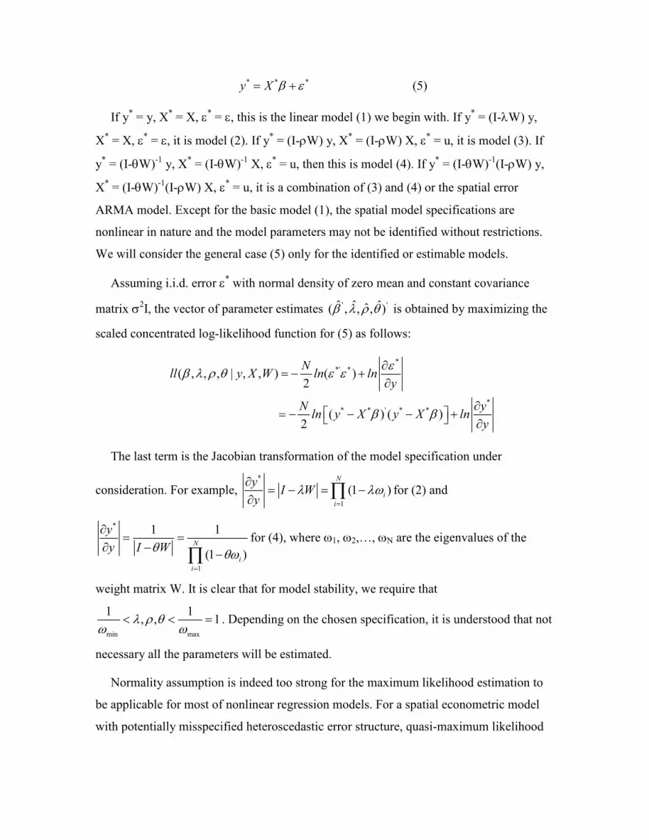
* * *y X β ε= + (5)

If y* = y, X

* = X, ε* = ε, this is the linear model (1) we begin with. If y

* = (I-λW) y,

X* = X, ε* = ε, it is model (2). If y

* = (I-ρW) y, X

* = (I-ρW) X, ε* = u, it is model (3). If

y* = (I-θW)

-1 y, X

* = (I-θW)

-1 X, ε* = u, then this is model (4). If y

* = (I-θW)

-1(I-ρW) y,

X* = (I-θW)

-1(I-ρW) X, ε* = u, it is a combination of (3) and (4) or the spatial error

ARMA model. Except for the basic model (1), the spatial model specifications are

nonlinear in nature and the model parameters may not be identified without restrictions.

We will consider the general case (5) only for the identified or estimable models.

Assuming i.i.d. error ε* with normal density of zero mean and constant covariance

matrix σ2I, the vector of parameter estimates ' 'ˆ ˆ ˆˆ( , , , )β λ ρ θ is obtained by maximizing the

scaled concentrated log-likelihood function for (5) as follows:

**' *

** * ' * *

( , , , | , , ) ( )2

( ) ( )2

Nll y X W ln ln

y

N yln y X y X ln

y

εβ λ ρ θ ε ε

β β

∂= − +

∂

∂ = − − − + ∂

The last term is the Jacobian transformation of the model specification under

consideration. For example, *

1

(1 )N

i

i

yI W

yλ λω

=

∂= − = −

∂ ∏ for (2) and

*

1

1 1

(1 )N

i

i

y

y I Wθ θω=

∂= =

∂ − −∏for (4), where ω1, ω2,…, ωN are the eigenvalues of the

weight matrix W. It is clear that for model stability, we require that

min max

1 1, , 1λ ρ θ

ω ω< < = . Depending on the chosen specification, it is understood that not

necessary all the parameters will be estimated.

Normality assumption is indeed too strong for the maximum likelihood estimation to

be applicable for most of nonlinear regression models. For a spatial econometric model

with potentially misspecified heteroscedastic error structure, quasi-maximum likelihood

(QML) method (White [1982]) is used so that the estimation is consistent and the

inference is robust2.

3. Moran-Based Test Statistics

No matter which model we will be based upon for the final analysis, the chosen model

must be correctly specified. Hypothesis testing is not only useful in selecting the best

model but also essential for diagnostic checking the estimated model. Usually we begin

with the basic linear regression model (1). Through pre-testing procedures, several model

specifications emerge. Diagnostic testing based on the estimated model in the general

form (5) is called for model validation. Diagnostic testing is different from the model pre-

testing in that the post-test statistics depend on the estimated parameters and the model

specification. The theoretical asymptotics for diagnostic checking is usually unknown,

the test statistics designed for pre-testing purpose do not have the same asymptotic

distribution when applied to diagnose the estimated model. In the case of spatial

econometric models, there are additional issues of endogenous regressors,

heteroscedasticity, and nonlinearity in the parameters.

The popular Moran-based tests available for spatial model diagnostics include the

original Moran’s I statistic, two versions of LM-Error and LM-Lag tests based on

Lagrange multiplier principle (see Anselin [1988], Florax, Folmer, and Rey [2003] for a

good review). Moran’s I test statistic was originally developed to study the spatial

correlation in random variables (Moran [1950]). Cliff and Ord [1973, 1981] applied this

statistic to test the regression residuals for spatial dependence. Under the assumption of

i.i.d. normal innovations, they derive the large sample distribution of the test statistic.

Based on the general model (5), * * *y X β ε= + , we write the Moran’s I statistic as

follows:

*' *

*' *

ˆ ˆ

ˆ ˆ

WI

ε εε ε

= (6)

Where *ε is the vector of regression residuals. Under the null hypothesis that the

model is correctly specified and there is no spatial dependence in the model errors,

2 The asymptotic theory of QML for spatially autoregressive model has been developed by Lee [2004].

Moran’s I test statistic is asymptotically normally distributed with the mean E(I) and

variance V(I) defined by:

* *' * 1 *'( )( ) , ( )

trace MWE I where M I X X X X

N K

−= = −−

' 2 22( ) [( ) ] [ ( )]

( ) ( )( )( 2)

trace MWMW trace MW trace MWV I E I

N K N K

+ += −

− − +

N is the number of sample observations, and K is the number of estimated parameters

in the model. The standardized Moran’s I is conveniently used in practice.

Moran’s I is useful to test the spatial dependence in the regression, but it does not

distinguish the two forms of spatial dependence in the model. Diagnostic tools for

identifying a spatial autocorrelation in the error term or a spatial lag in the dependent

variable are the LM-Error and LM-Lag tests. Define,

2*' *

2

ˆ ˆ

ˆ

W

LM ErrorT

ε εσ

− = (7)

2*' *

2

ˆ

ˆ

Wy

LM LagNJ

εσ

− = (8)

where

* ' *

2

* * 2 *' *

( ' )

1ˆ ˆ( ) ( )

ˆ

ˆ ˆ ˆˆ ˆ, /

T trace WW W W

J Wy M Wy TN

y X N

σβ σ ε ε

= +

= +

= =

Under the assumption that the model error is independently normally distributed, LM-

Error and LM-Lag test statistics are χ2(1) distributed asymptotically (Burridge [1980],

Anselin and Rey [1991]). There are robust versions of the LM tests, LM-Error* and LM-

Lag*, which are designed to test for spatial error autocorrelation in the presence of a

spatially lagged dependent variable and to test for endogenous spatial lag dependence in

the presence of spatial error autocorrelation, respectively. Asymptotically, they are χ2(1)

distributed as the classical versions (see Anselin, Bera, Florax, and Yoon [1996] for the

derivation and simulation results).

2*' * *' *

2 2

*

ˆ ˆ ˆ

ˆ ˆ

1

W T Wy

NJLM Error

TT

NJ

ε ε εσ σ

−

− = −

(9)

2*' * *' *

2 2

*

ˆ ˆ ˆ

ˆ ˆ

Wy W

LM LagNJ T

ε ε εσ σ

−

− =−

(10)

The primary use of the above Moran-based tests is to pre-test the spatial independence

in a linear regression model3. Anselin and Kelejian [1997] extend the test procedure to

cover the cases with endogenous regressors including the spatially lagged dependent

variable in the regression. Keleijian and Prucha [2001] consider the first-order spatially

lagged dependent variable and spatial autocorrelation error in the null, and derive the

asymptotic distribution for the Moran’s I test statistic. Their modification depends on the

instrumental variable estimation and allows for limited dependent variable. Pinkse [2004]

introduces a synthesis treatment of the Moran-flavored test statistics with nuisance

parameters as in the case of a spatial probit model. The consensus is that limited

distributions exist for Moran-based test statistics for spatial dependence under a set of

general conditions for the i.i.d. normal model error structure.

Based on the linear regression model (1), Moran-based test statistics are routinely

applied in the literature. Even if a regression model is corrected for spatial correlation, the

estimated model in the general form (5) is subject to further scrutiny for the remaining

spatial structure. Under the null hypothesis of no spatial dependence in a correctly

specified and consistently estimated model, we can apply Moran-based test procedure for

model validation. Consider the general model specification (5), the variables y* and X

*

are transformed in according to the spatial structure based on nonlinear maximum

likelihood estimates of the model parameters. For diagnostic testing purpose, however, it

is unlikely that the model error ε* is i.i.d. normal. For a chosen spatial structure, the

3 Several strategies for model identification and selection using LM test statistics are discussed in Florax,

Folmer, and Rey [2003].

model is nonlinear in the parameters and subject to misspecification. The point is that we

do not have a well-known distribution for the diagnostic test statistics. This leads us to

the empirical distribution approach such as bootstrapping. In the following, we introduce

bootstrap method for diagnostic testing the spatial dependence in the data and model.

4. Bootstrap Method

In statistics, the bootstrap method relies on resampling from the observed data to

approximate the probability distribution of the test statistics. Since its introduction by

Efron [1979], the bootstrap has become a popular method for inference about the

distribution of the parameters and related statistics. Without knowing the exact

distributional properties of a test statistic or quantity, bootstrap has proven to be a

practical method in many disciplines. See Efron and Tibshirani [1993], Davison and

Hinkley [1997] for an introduction of the theory and applications of bootstrap method.

4.1. Introduction to Bootstrap

The bootstrap is based on the idea that the sample is a good representation of the

underlying population distribution. It is a sort of Monte Carlo simulation in which we

resample from the available sample information for inference about a parameter estimator

or test statistic. Suppose τ is the test statistic of interest for a random variable x with the

probability distribution F(x;θ), where θ is the distribution parameter. We denote τ = τ(F).

Let ˆˆ ( ; )F F x θ= be the sample estimate of F(x;θ) and ˆˆ ( )Fτ τ= , where θ is the

maximum likelihood estimator of θ. Unless the asymptotic distribution of τ is known,

statistical inference is difficult to make. Even with the knowledge about the distribution

F(x;θ), the asymptotic distribution of the test statistic τ is complicated to derive and in

general unknown. The alternative distribution-free bootstrap method is to resample x with

replacement, denoted x*. Then we approximate the distribution F(x;θ) by * * ˆˆ ( ; )F F x θ= ,

from which we calculate the test statistic * *ˆˆ ( )Fτ τ= . After a large bootstrap sample of

*τ is collected, statistical inference is made based on its empirical distribution instead of

the asymptotic theory. By the law of large number, the empirical distribution of *τ

approximates the theoretical distribution of τ in large sample. That is, *τ converges to τ

in distribution. The consistency property of * * ˆˆ ( ; )F F x θ= which approximate

ˆˆ ( ; )F F x θ= is the foundation for bootstrap test to work well.

A standard bootstrap test proceeds as follows: First, based on the original N

observations of the sample data we estimate θ for F(x;θ) and compute test statistic τ.

Secondly, we resample from the N observations of the original data series with

replacement. Some observations may be selected more than once while some may not be

picked at all. The result of the resampling is a bootstrap sample of size N. Then the

bootstrap sample is used to estimate the model and to compute the test statistic exactly

the same way as we did with the original sample in the beginning. Continue this process

of replication until we collect sufficient number of bootstrap sample of the test statistic τ

so that its empirical distribution can be constructed and analyzed. For inference purpose,

a bootstrap P-value defined by the fraction of the bootstrap sample that the bootstrap *τ

greater than the estimated τ . Other tools such as confidence intervals may be

bootstrapped as well for inference.

The performance of a bootstrap procedure depends on the empirical distribution in

which the original data and model specification play the important role. Given the data

resampling with replacement, it is understood that the results can not be generalized

unless a large amount of replications is used. In addition, for bootstrap test, an

asymptotically pivotal test statistic works better than the non-pivotal one.

4.2. Spatial Bootstrap Method

Techniques for bootstrap dependent data are the forefront activities of recent

development (see Davison, Hinkley, and Young [2003], Horowitz [2003], MacKinnon

[2002]). In time series, block bootstrap and sieve bootstrap are the popular examples. For

spatial dependent data, earlier attempts were made since Cliff and Ord (1973) and Cressie

(1980) but went unrecognized possibly due to computing constraints at that time.

Recently there is no shortage of Monte Carlo methods in spatial econometric analysis, but

the bootstrap method based on the estimated model and data is unseen except in a

different context (See Lee and Lahiri, 2002, for example)4. It is crucial that spatial

structure must be preserved during data resampling. Because there is a fixed spatial

weight matrix W of the full sample size preventing bootstrap by blocks or subsampling, it

leaves only one option for us to bootstrap the regression residuals for a spatial

econometric model. Under the assumption of independently and identically distributed

residuals, for a fixed weight matrix W and a set of exogenous variables X we bootstrap

the dependent variable Y through nonparametric resampling procedure as we perform for

a classical linear regression model. Similar to the residual-based time series bootstrap, a

recursive or reverse process through matrix inversion has to be used to bootstrap the

dependent variable without destroying the spatial structure. The drawback of the residual-

based bootstrapping is that the residuals must be i.i.d. by design. If it is normally

distributed, then the parametric bootstrap is an alternative. We feel at the least the

problem of heteroscedasticity due to cross-section data in the spatial model must be

accounted for. Therefore, our bootstrap method for spatial econometric models is a

hybrid of recursive wild bootstrap to be described in details below.

Suppose we observed a sample (y,X) and a spatial weight matrix W. For simplicity,

we assume that the data matrix of exogenous variables X and the spatial weight matrix W

are fixed by design. We further assume that the model error is independently and

identically normally distributed, and the technique of quasi-maximum likelihood is used

to obtain the consistent parameter estimators and their robust standard errors. Based on

the estimated model (5), * * *ˆ ˆy X β ε= + , we discuss the bootstrap method for Moran’s I

statistic (6) *' *

*' *

ˆ ˆ

ˆ ˆ

WI

ε εε ε

= . For other models and other test statistics, the following

illustration is the same.

From *ε , we start to bootstrap a sample of residuals *εɶ . If the normality assumption of

the model error is acceptable, we could simply use the parametric bootstrap method. Let

*εɶ be a random draw from a normal distribution with zero mean and constant variance

2 *' *ˆ ˆˆ / Nσ ε ε= , and work around to get the bootstrap sample of y. Because * * *ˆy X β ε= + ɶɶ ,

4 Pinkse and Slade (1998) propose a simulation-based test in probit models, in the same

spirit of our bootstrap tests.

we apply a recursive or reverse process converting from *yɶ to yɶ . For example, if

* ˆˆ ( )y I W yλ= − as in the case of a spatial lag model (2), then 1 *ˆ( )y I W yλ −= −ɶ ɶ . Given

the fixed spatial weight matrix W, the bootstrap sample is ( , )y Xɶ . Using this bootstrap

sample, we repeat the estimation of model (5) and the computation of test statistic (6) to

obtain * * *ˆ ˆy X β ε= +ɶ ɶɶ and *' *

*' *

ˆ ˆ

ˆ ˆ

WI

ε ε

ε ε=ɶ ɶ

ɶ

ɶ ɶ

.

This idea of recursive bootstrap is similar to the time series autoregressive bootstrap,

except that the recursion is essentially a reverse or matrix inverse process involving a full

sample size spatial weight matrix W. The advantage is that it does not require pre-sample

initialization as the time series bootstrap, but the disadvantage is the high computing cost

of large matrix inversion. Although the spatial weight matrix W may be sparse in most

cases, its inverse in general is not. If the sample size is large, the repetitive computation

of matrix inversion may prevent the practcal application of spatial bootstrap. Indeed, if

the sample size is large we still depend on the asymptotic theory for inference.

Parametric bootstrap is convenient and powerful when the model assumption is correct.

Unfortunately, it is rare that the normality assumption of the model error will be satisfied.

A nonparametric bootstrap is called for this purpose. From the estimated model, the

bootstrap sample of the residuals *εɶ is a reampling of *ε with replacement. Based on the

general model (5), * * *ˆ ˆy X β ε= + , the regression model is nonlinear in parameters

estimated with quasi-maximum likelihood method. To be consistent with the constant

model variance, a re-scaled and re-centered residual is typically used in the bootstrap:

***

2 21

1, 1, 2,...,

1 1 1

Nji

i

ji j

Ne i N

N Nh h

εε

=

= − = − − −

∑ɶɶ

where h is leverage or the diagonal vector of the hat matrix X*(X

*’X

*)-1X

*’. Further

complication of a spatial econometric model using cross-section data is the presence of

general heteroscedacity of unknown form. The method of wild bootstrap was invented to

deal with this problem (Wu [1986]). That is, * *

i i ie e υ=ɶ with υi a random variable with

mean 0 and variance 1. Several choices of υi are available in the literature (see Liu [1988],

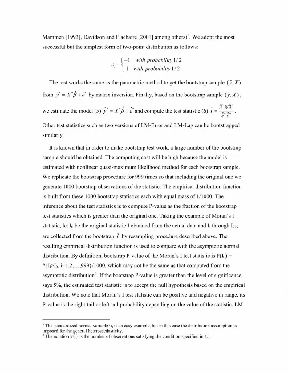
Mammen [1993], Davidson and Flachaire [2001] among others)5. We adopt the most

successful but the simplest form of two-point distribution as follows:

1 1/ 2

1 1/ 2i

with probability

with probabilityυ

−=

The rest works the same as the parametric method to get the bootstrap sample ( , )y Xɶ

from * * *ˆy X eβ= +ɶ ɶ by matrix inversion. Finally, based on the bootstrap sample ( , )y Xɶ ,

we estimate the model (5) * * *ˆˆ ˆy X eβ= +ɶɶ ɶ and compute the test statistic (6) *' *

*' *

ˆ ˆ

ˆ ˆ

e WeI

e e=ɶ ɶ

ɶ

ɶ ɶ

.

Other test statistics such as two versions of LM-Error and LM-Lag can be bootstrapped

similarly.

It is known that in order to make bootstrap test work, a large number of the bootstrap

sample should be obtained. The computing cost will be high because the model is

estimated with nonlinear quasi-maximum likelihood method for each bootstrap sample.

We replicate the bootstrap procedure for 999 times so that including the original one we

generate 1000 bootstrap observations of the statistic. The empirical distribution function

is built from these 1000 bootstrap statistics each with equal mass of 1/1000. The

inference about the test statistics is to compute P-value as the fraction of the bootstrap

test statistics which is greater than the original one. Taking the example of Moran’s I

statistic, let I0 be the original statistic I obtained from the actual data and Ii through I999

are collected from the bootstrap Iɶ by resampling procedure described above. The

resulting empirical distribution function is used to compare with the asymptotic normal

distribution. By definition, bootstrap P-value of the Moran’s I test statistic is P(I0) =

#{Ii>I0, i=1,2,…,999}/1000, which may not be the same as that computed from the

asymptotic distribution6. If the bootstrap P-value is greater than the level of significance,

says 5%, the estimated test statistic is to accept the null hypothesis based on the empirical

distribution. We note that Moran’s I test statistic can be positive and negative in range, its

P-value is the right-tail or left-tail probability depending on the value of the statistic. LM

5 The standardized normal variable υi is an easy example, but in this case the distribution assumption is

imposed for the general heteroscedasticity. 6 The notation #{.} is the number of observations satisfying the condition specified in {.}.

–based test statistics are all positive, therefore the corresponding P-values are right-tail

probability as defined earlier.

5. Empirical Examples

In this section, we use two examples to demonstrate the application of spatial

bootstrap procedure and provide empirical evidence of successfully bootstrap test

statistics for spatial econometric models7.

5.1. Example 1

By introducing the spatial econometric method to study urban crime incidents in

Columbus Ohio, Anselin [1988] suggests a model that urban crime rate as a function of

the family income and the real estates property value. Involving 49 neighborhoods in the

study, it is found that the number of crime incidents reported is negatively related to the

family income level and housing value in the neighborhood. The spatial dependence of

the neighborhoods is an additional important factor for urban crime incidents. The basic

regression model is:

(Crime Rate) = α + β (Family Income) + γ (Housing Value) + ε (Ε.1.1)

The estimated model is tested for spatial dependence in the regression residuals. Based

on the asymptotic distribution assumptions of the test statistics involved--Moran’s I,

regular and robust LM-Error, and LM-Lag, a spatially lagged dependent variable should

be included in the regression as follows:

(Crime Rate) = α + β (Family Income) + γ (Housing Value) + λ W (Crime Rate) + ε (Ε.1.2)

where W is the simple first-order contiguity spatial weight matrix (row-standardized)

for these 49 neighborhoods. In stead of relying on the asymptotic distribution

assumptions for the test statistics, we apply nonparametric spatial bootstrap method to

derive their empirical distributions and to compute P-values for the test statistics. First,

we duplicate the results of Anselin [1988] including quasi-maximum likelihood estimates

of the parameters, Moran’s I and LM test statistics. Then, in Table 1, we report our

7 All computations are performed using GPE2/GAUSS (see Lin [2001]) on a Pentium 4 2.4 Ghz Windows-

XP system.

findings of spatial bootstrap, particularly P-values and confidence intervals for the test

statistics.

From Table 1, by comparing the pre-test results, we find that both analytical and

simulated Moran’s I test statistic are close and at 5% level of significance the test

indicates the problem of spatial correlation. After the model has been corrected for spatial

correlation with the addition of the first spatially lagged dependent variable in the

regression equation (E.1.2), the post-test statistics confirm that there is no remaining

spatial correlation in the residuals. In addition to Moran’s I, two versions of bootstrap LM

tests validate the same conclusions from the asymptotic tests. In this case, we do not find

discrepancy in the test results even though the asymptotic distribution is no longer a valid

assumption for the estimated spatial lag model. The fact that both test results are similar

is probably due to the theoretical distribution and empirical distribution being close

enough for this particular data set and the estimated model.

[Insert Table 1]

5.2. Example 2

Using 28 provincial and city output data from 1978 to 2002, we study the regional

economic convergence in China (Lin, Long, and Wu [2004]). Our contribution was to

introduce the spatial econometric framework in an otherwise basic absolute convergence

model:

Growth = α + β (Initial Output) + ε (Ε.2.1)

Where (Initial Output) is measured by the provincial per capita GDP level in 1978,

and Growth is the GDP growth rate over 25 years of development. From the vast volume

of convergence literature, the estimated significant negative value of β indicates a

convergence process in the economic development. It is now clear that through various

stages of economic reform and policy change, the Chinese economy has developed with

increasing dependence and cooperation across regions. Regional growth has seen to be

influenced by the development of neighboring provinces and cities. In our previous study,

we investigate the spatial effect in the growth and convergence. For simplicity, a first-

order contiguity weight matrix W is used to specify the geographical connection of the

provinces and cities. In particular, the element of W is 1 for the neighboring provinces

and 0 otherwise. Furthermore, W is row-standardized and zero-diagonal.

Reading from the second column of Table 2, based on the basic model (E.2.1), there

are not much differences between the asymptotic and bootstrap test results. The

conclusion is in general consistent and suggests that the original model suffers the

ignorance of spatial correlation. Relying on the pre-test statistics for spatial correlation,

we have found that the spatial autoregressive error model is a plausible model

specification:

Growth = α + β (Initial Output) + ε ε = ρ W ε + u (E.2.2)

Based on the asymptotic theory, the post-test results for the estimated model do not

reveal further evidence of the spatial correlation. P-values for all the test statistics are

greater than 5% level of significance. Given the concern that we are working with a small

sample of 28 heterogeneous cross-section observations and the spatial model is estimated

by quasi-maximum likelihood method, the asymptotic distribution assumptions for the

various test statistics are questionable. Here we bootstrap test statistics based on the

estimated model (E.2.2) under the null hypothesis that there is no remaining spatial

correlation. Although the estimated model (E.2.2) was reported in the previous study, the

bootstrap post-test results shown in the third column of Table 2 indicate that the problem

of spatial correlation is still in existence. The previously reported spatial model may be

misspecified and subject to further scrutiny. The P-value of the bootstrap Moran’s I is too

small (P=0.01), contradictory to the P-value of the theoretical counterpart (P=0.489). The

alternative model specification is possibly a spatial lag model as follows:

Growth = α + β (Initial Output) + λ W (Growth) + ε (Ε.2.3)

The estimated model and diagnostic test results are presented in the column 4 of Table

2. At 5% level of significance, all tests including the asymptotic and bootstrap variants

are conclusive and consistent. Based on Maran’s I test, there is no remaining spatial

correlation in the residuals. Based on various LM test statistics, the estimated model

(E.2.3) is free of spatial dependence. One possible concern is the robust version of LM-

Error test, which has a marginal P-value at 0.046. The revised model for the regional

convergence in China is better specified as a spatial lag model or a combined spatial lag

and autoregressive error model. The later is not reported here due to space limitation.

With a small sample and potentially a misspecified model, bootstrap demonstrates its

power to distinguish a better candidate of the final model.

[Insert Table 2]

From these two examples, we learn that if the distribution assumption is known or

correct, both asymptotic and bootstrap methods will yield the same and consistent

conclusions. However, for diagnostic testing, it is rare that the estimated nonlinear model

by quasi-maximum likelihood will satisfy the asymptotic distribution assumption. For

post-test purpose, relying on the incorrect assumption of the distribution will in general

lead to wrong conclusion about the model. Therefore it is often contradictory to the

results based on bootstrap tests. The first example has a medium size of the sample, and

the empirical distribution is in line with the theory. The results are consistent. The second

example is more difficult to find a correct specification because we have only a small

sample and therefore uncertain about the distribution assumption. Bootstrap method

offers a better alternative instead of relying on the theoretical distribution. To make sure

that we have a large number of bootstrap samples to work with, spatial econometric

model can be tested and validated by the bootstrap methods.

6. Conclusion

This paper studies the bootstrap methods for diagnostic testing the spatial econometric

models. A residual based recursive wild bootstrap is suggested to handle potential model

misspecification due to nonlinearity in parameters and heteroscedasticity of unknown

form. The methodology of spatial bootstrap has shown to be useful in identifying a better

spatial structure than the classical approach which relies on the asymptotic distribution

assumption. For a small sample problem, the bootstrap method is of particular important

in diagnostic testing, provided a large number of bootstrap samples is used. Because of

expensive computing cost associated with the nonlinear quasi-maximum likelihood

estimation for each bootstrap spatial model, we are currently limited to examine only a

few cases of small to medium size problems. Although the empirical results are

promising, the formal asymptotic theory of spatial bootstrap is awaiting to be developed.

Theoretical and empirical investigation of the size and power of spatial bootstrap method

is an important topic for future research.

References

Anselin, L. (1988), Spatial Econometrics: Methods and Models. Kluwer, Dordrecht.

Anselin, L. and A. K. Bera (1997), “Spatial Dependence in Linear Regression Models

with an Introduction to Spatial Econometrics,” in Handbook of Applied Economic

Statistics, A. Ullah and D. Giles, eds., Marcel Dekker, New York.

Anselin, L. and A. K. Bera, R. J.G.M. Florax, and M. Yoon (1996), “Simple Diagnostic

Tests for Spatial Dependence,” Regional Sceience and Urban Economics, 26, 77-104.

Anselin, L. and R. Florax (1995), “Small Sample Properties of Tests for Spatial

Dependence in Regression Models: Some Further Results,” New Directions in Spatial

Econometrics. Spinger Verlag, New York, 21–74.

Anselin, L. and H. Kelejian (1997), “Testing for Spatial Autocorrelation in the Presence

of Endogenous Regressors,” International Regional Science Review, 20, 153–182.

Anselin, L. and S. Rey (1991), “Properties of Tests for Spatial Dependence in Linear

Regression Models,” Geographical Analysis, 23, 112-131.

Baltagi, B. H., S. H. Song, and W. Koh (2003), “Testing Panel Data Regression Models

with Spatial Error Correlation,” Journal of Econometrics, 117, 123-150.

Burridge, P. (1980), “On the Cliff-Ord test for Spatial Correlation,” Journal of the Royal

Statistical Society B, 42, 107-108.

Cliff, A. and J. Ord (1973), Spatial Autocorrelation, Pion, London.

Cliff, A. and J. Ord (1981), Spatial Processes, Models and Applications, Pion, London.

Cressie, N. A. C. (1980), Statistics for Spatial Data, Wiley, New York.

Davidson, R. and E. Flachaire (2001), “The Wild Bootstrap, Tamed at Last,” Working

Paper, Darp58, STICERD, London School of Economics.

Davison, A.C. and D.V. Hinkley (1997), Bootstrap Methods and Their Applications,

Cambridge, UK: Cambridge University Press.

Davison, A.C., D.V. Hinkley, and G. A. Young (2003), “Recent Developments in

Bootstrap Methodology,” Statistical Science, 18, 141-157.

Efron, B. (1979), “Bootstrap Methods: Another Look at the Jackknife,” Annals of

Statistics, 7, 1-26.

Efron, B. and R. J. Tibshirani (1993), An Introduction to the Bootstrap, Chapman and

Hall, New York.

Elhorst, J. P. (2003), “Specification and Estimation of Spatial Panel Data Models,”

International Regional Science Review, 26, 244-268.

Florax, R. J.G.M., H. Folmer, and S. Rey (2003), “Specification Searches in Spatial

Econometrics: The Relevance of Hendry’s Methodology,” Regional Science and Urban

Economics, 33, 557-579.

Goncalves, S. and L. Kilian (2004), “Bootstrapping Autoregressions with Conditional

Heteroscedasticity of Unknown Form,” Journal of Econometrics, 123, 89-120.

Horowitz, J. L. (2003), “The Bootstrap in Econometrics,” Statistical Science, 18, 211–

218.

Kapoor, M., H. Kelejian, and I.R. Prucha (2007), “Panel Data Models with Spatially

Correlated Error Components,” Journal of Econometrics (forthcoming).

Kelejian, H. and I.R. Prucha (2001)., “On the Asymptotic Distribution of Moran I Test

Statistic with Applications,” Journal Econometrics, 104, 219-257.

King, M. (1981), “A Small Sample Property of the Cliff-Ord Test for Spatial

Correlation,” Journal of the Royal Statistical Society B, 43, 263-264.

Lee, L. F. (2004), “Asymptotic Distributions of Quasi-Maximum Likelihood Estimators

for Spatial Autoregressive Models,” Econometrica, 72, 1899-1925.

Lee, Y. D. and S. N. Lahiri (2002), “Least Squares Variogram Fitting by Spatial

Subsampling,” Journal of the Royal Statistical Society B, 64, 837-854.

Lin, K.-P. (2001), Computational Econometrics: GAUSS Programming for

Econometricians and Financial Analysts, ETEXT Publishing, Los Angles.

Lin, K.-P., Z. Long, and M. Wu (2005), "A Spatial Econometric Analysis of Regional

Economic Convergence in China: 1978-2002," China Economic Quarterly (in Chinese),

Vol. 4, No. 2.

Liu, R. Y. (1988), “Bootstrap Procedure under Some Non-iid Models,” Annals of Statistics,

16, 1696-1708.

MacKinnon, J. G. (2002), “Bootstrap Inference in Econometrics,” Canadian Journal of

Economics, 35 615–645.

Mammen, E. (1993), “Bootstrap and Wild Bootstrap for High Dimensional Linear Models,”

Annals of Statistics, 21, 255-285.

Moran, P.A.P. (1950), “A Test for Spatial Independence of residuals,” Biometrika, 37, 178-

181.

Pinkse, J. (1999), “Asymptotics of the Moran Test and a Test for Spatial Correlation in

Probit Models,” UBC mimeo.

Pinkse, J. (2004), “Moran-Flavoured Tests with Nuisance Parameters: Examples,” in

Advances in Spatial Econometrics, L. Anselin, R. J.G.M. Florax, and S. Rey, eds., Springer-

Verlag, Berlin.

Sen, A. (1976), “Large Sample Size Distribution of Statistics Used in Testing for Spatial

Correlation,” Geographical Analysis, IX, 175-184.

White, H. (1982), “Maximum Likelihood Estimation of Misspecified Models,”

Econometrica, 50, 1-26.

Wu, C. F. J. (1986), “Jackknife, Bootstrap and Other Resampling Methods in Regression

Analysis,” Annals of Statistics, 14, 1261-1295.

Table 1. Crime Rate Regression (Anselin [1988])

Model

Estimate E.1.1 E.1.2

α 68.619

(4.1015)

45.079

(6.4049)

β -1.5973

(0.44664)

-1.0316

(0.42109)

γ -0.27393

(0.15753)

-0.26593

(0.17309)

λ 0.43102

(0.11067)

Log-likelihood -187.38 -182.39 Moran’s I

Computed 0.23564

(P-Value = 0.001569)

0.037981

(P-value = 0.21683)

Bootstrapped

[5% 95%]

[2.5% 97.5%]

(P-value = 0.006000)

[-0.17932 0.12782]

[-0.19715 0.16437]

(P-value = 0.182000)

[-0.12704 0.089921]

[-0.14245 0.10902] LM-Error

Computed 5.7230

(P-value = 0.016744)

0.14869

(P-value = 0.69979)

Bootstrapped

[5% 95%]

[2.5% 97.5%]

(P-value = 0.01000)

[0.0062075 3.6391]

[0.0018080 4.4472]

(P-value =0.56300)

[0.0010819 1.8888]

[0.00035909 2.3867] LM-Lag

Computed 9.3634

(P-value = 0.0022136)

0.013924

(P-value = 0.90607 )

Bootstrapped

[5% 95%]

[2.5% 97.5%]

(P-value = 0.00000)

[0.0026486 2.1393]

[0.00046042 2.7541]

(P-value = 0.85100)

[0.0015258 1.2972]

[0.00028477 1.7017]

LM-Error*

Computed 0.79502

(P-value = 0.77797)

0.21634

(P-value = 0.64184)

Bootstrapped

[5% 95%]

[2.5% 97.5%]

(P-value = 0.83200)

[0.0061038 6.4653]

[0.0016220 7.7925]

(P-value =0.68600)

[0.0042842 5.5576]

[0.0013590 7.5917]

LM-Lag*

Computed 3.7199

(P-value = 0.053768)

0.081577

(P-value = 0.77517 )

Bootstrapped

[5% 95%]

[2.5% 97.5%]

(P-value = 0.09500)

[0.0058830 4.8856]

[0.0020706 6.0520]

(P-value = 0.79900)

[0.0056133 5.2179]

[0.0010360 6.9529] Note: For parameter estimates, the numbers in parentheses are the estimated standard errors. All bootstrap simulation

of test statistics are based on 1000 bootstrap samples.

Table 2. Economic Convergence in China, 1978－－－－2002 (Lin, Long, and Wu [2004])

Model

Estimate E.2.1

E.2.2

E.2.3

α 2.4160

(0.33221)

3.0197

(0.59245)

1.9112

(0.31052 )

β -0.058628

(0.052548 )

-0.15943

(0.092431)

-0.10585

(0.061052)

ρ 0.43841

(0.16782)

λ 0.37813

(0.13202)

Log-likelihood -7.6072 -5.7684 -6.1010 Moran’s I

Computed 0.27442

(P-value= 0.0036847)

-0.045746

(P-value = 0.48903)

-0.018941

(P-value = 0.39898)

Bootstrapped

[5% 95%]

[2.5% 97.5%]

(P-value = 0.00600)

[-0.23818 0.16229]

[-0.27444 0.21030]

(P-value = 0.010000)

[-0.027654 0.049484]

[-0.038596 0.067128]

(P-value = 0.22000)

[-0.052542 0.055908]

[-0.073838 0.070236] LM-Error

Computed 4.1382

(P-value = 0.041927)

0.11500

(P-value = 0.73452)

0.019716

(P-value = 0.88833)

Bootstrapped

[5% 95%]

[2.5% 97.5%]

(P-value = 0.031000)

[0.0043722 3.5261]

[0.0013486 4.2463]

(P-value = 0.077000)

[1.4009E-05 0.14523]

[2.9718E-06 0.27488]

(P-value = 0.48100)

[0.00012237 0.28496]

[3.6335E-05 0.37424] LM-Lag

Computed 3.8297

(P-value = 0.050350)

0.31067

(P-value = 0.57727)

0.097340

(P-value = 0.75505)

Bootstrapped

[5% 95%]

[2.5% 97.5%]

(P-value =0.00100)

[0.0015043 1.7708]

[0.00043162 2.2681]

(P-value = 0.39800)

[0.00096615 1.6208]

[0.00027351 2.1724]

(P-value = 0.65000)

[0.0018191 1.7200]

[0.00048654 2.1677]

LM-Error*

Computed 1.9763

(P-value = 0.15978)

1.8394

(P-value = 0.17502)

2.3519

(P-value = 0.12513)

Bootstrapped

[5% 95%]

[2.5% 97.5%]

(P-value = 0.350000)

[0.014666 7.6498]

[0.0055873 9.3924]

(P-value = 0.052000)

[0.0018500 1.8715]

[0.00045045 2.6461]

(P-value = 0.04600)

[0.0020987 2.2837]

[0.00088087 2.9509]

LM-Lag*

Computed 1.6679

(P-value = 0.19654)

2.0351

(P-value = 0.15371)

2.4295

(P-value = 0.11907)

Bootstrapped

[5% 95%]

[2.5% 97.5%]

(P-value =0.3190)

[0.0050724 5.9553]

[0.0010728 7.1178]

(P-value = 0.12400)

[0.0027187 3.1525]

[0.00060973 4.2396]

(P-value = 0.115000)

[0.0042173 3.6673]

[0.0011298 4.6746] Note: For parameter estimates, the numbers in parentheses are the estimated standard errors. All bootstrap simulation

of test statistics are based on 1000 bootstrap samples.