arX

iv:n

lin/0

4080

06v3

[nl

in.A

O]

12 A

ug 2

004

Introduction to Random Boolean Networks

Carlos GershensonCentrum Leo Apostel, Vrije Universiteit Brussel. Krijgskundestraat 33 B-1160 Brussel, Belgium

cgershen@vub.ac.be http://homepages.vub.ac.be/˜cgershen

Abstract

The goal of this tutorial is to promote interest in the study ofrandom Boolean networks (RBNs). These can be very inter-esting models, since one does not have to assume any func-tionality or particular connectivity of the networks to studytheir generic properties. Like this, RBNs have been usedfor exploring the configurations where life could emerge.The fact that RBNs are a generalization of cellular automatamakes their research a very important topic.

The tutorial, intended for a broad audience, presents the stateof the art in RBNs, spanning over several lines of researchcarried out by different groups. We focus on research donewithin artificial life, as we cannot exhaust the abundant re-search done over the decades related to RBNs.

IntroductionRandom Boolean networks (RBNs) were originally devel-oped by Stuart Kauffman as a model of genetic regulatorynetworks (Kauffman, 1969; Kauffman, 1993). They are alsoknown asN−K models, or Kauffman networks. RBNs aregeneric, because one does not assume any particular func-tionality or connectivity of the nodes: these are generatedrandomly. This is a useful approach if the specific structureand/or function of a system are very complex and unknown.The generic properties found in the model can be then ap-plied to the particular system, in order to attempt to unveilits mechanisms.

Mathematical and computational modelling of geneticregulatory networks promises to uncover the fundamentalprinciples of living systems in an integrative and holisticmanner. It also paves the way toward the development ofsystematic approaches for effective therapeutic interventionin disease (Shmulevich et al., 2002). Single-gene studies arevery limited for such intertwined networks.

Even when there is a Boolean simplification, many sys-tems can be studied with near-binary states. This is becausethe behaviour of many systems is determined by thresholds,such as the ones determined by firing potentials of synapsesin neurons, or activation potentials of chemical reactionsinmetabolic networks.

Furthermore, random Boolean networks have been ap-plied and used as models in many different areas, suchas evolutionary theory, mathematics, sociology, neural net-works, robotics, and music generation.

In the next section, we will review the classic RBN model,its three characteristic phases (ordered, chaotic, and criti-cal, some explorations of the model, alternatives, and ex-tensions. Next we will review the effect of the updatingscheme in RBNs: syncrhonous-asyncrhonous, determiistic-non-deterministic. We mention briefly some applications ofRBNs, tools availabe for their study, and future lines of re-search.

Classical ModelKauffman proposed the original RBN model, supporting thehypothesis that living organisms could be constructed fromrandom elements, without the need of precisely programmedelements (Kauffman, 1969). Certain types of RBNs are veryrobust, and have many analogies to living organisms.

A RBN consists ofN nodes, which can take values of zeroor one (Boolean). The state (zero or one) of each node is de-termined byK connections coming from other (or the same)nodes. The connections are wired randomly, but remainfixed during the dynamics of the network, i.e. “quenched”.The way in which nodes affect each other is not only deter-mined by their connections, but by logic functions, whichare generated randomly, simply using lookup tables for eachnode, which take the states of the connecting nodes as in-puts, and the state of the node as output. These also remainfixed (quenched) during the dynamics of the network.

We can see that RBNs are a generalization of Boolean cel-lular automata (CA) (von Neumann, 1966; Wolfram, 1986;Wuensche and Lesser, 1992), where the state of each nodeis not affected necessarily by its neighbours, but potentiallyby any node in the network. RBNs withN = K are alsocalled random maps.

The updating of the nodes in classic RBNs issyn-chronous: the states of nodes at timet+1 depend on thestates of nodes at timet, so that all nodes “march in step”.We will see below that there can be drastic differences if we

change the updating scheme.Usually, an initial random state is chosen for the RBN,

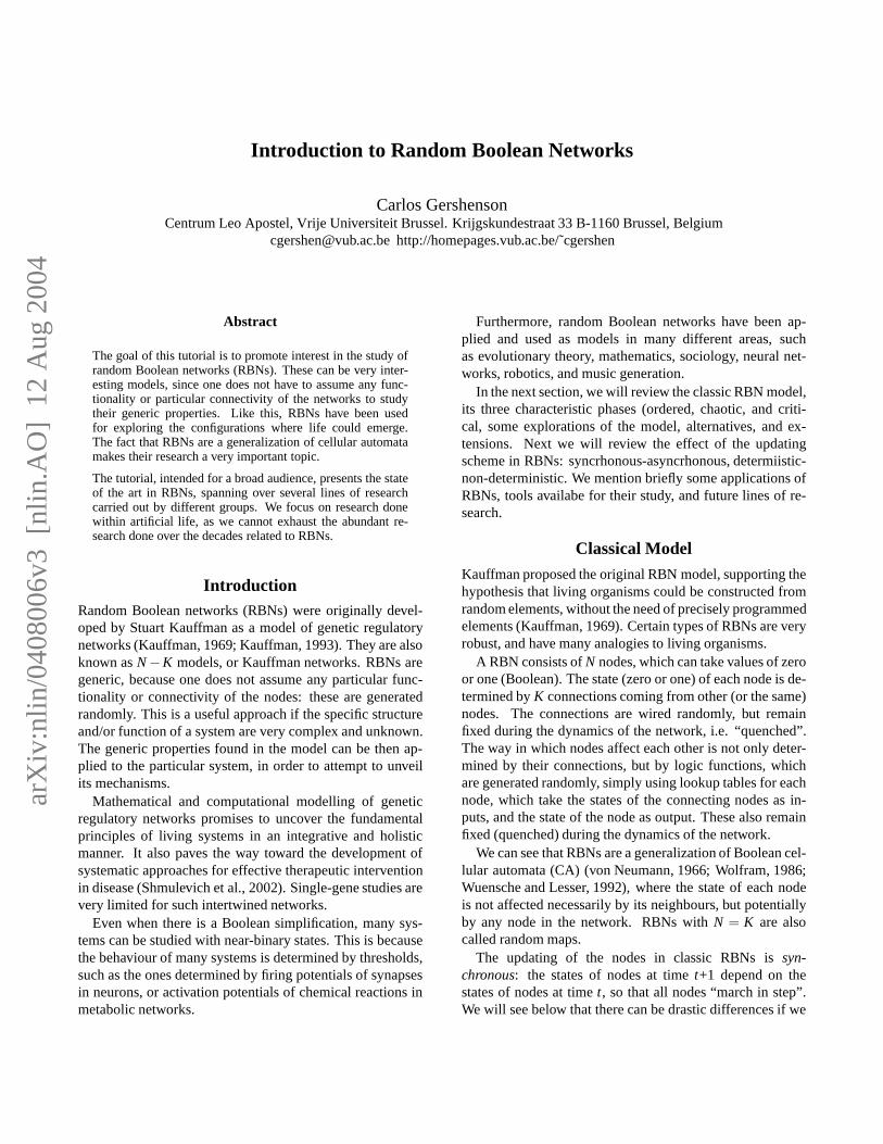
and the dynamics flow according to the updating functionsand scheme. Since the state space is finite (2N), eventually astate will be repeated. Since the dynamics are deterministic,this means that the network has reached anattractor. If theattractor consists of one state, it is called apoint attractor orsteady state, whereas if it consists of two or more states, itiscalled acycleattractor or state cycle. The set of states thatflow towards an attractor is called the attractorbasin. Anexample of a RBN withN = 3 andK = 3 is shown in Figure1.

If we try to imagine all possible networks, for each nodethere will be 22

Kpossible functions. And each node has

N!/(N−K)! possible ordered combinations forK differentlinks. Therefore all the possible networks for givenN andKwill be (Harvey and Bossomaier, 1997):

(

22KN!

(N−K)!

)N

(1)

Note that many of these will be equivalent, but neverthe-less we can see that the space of networks is immense. Thismakes things complicated for statistical studies. There isnot enough computational power to exhaust all possible net-works, so only “representative” properties can be studied.We should also mention that there is a very high variance inthe statistical studies of RBNs.

However, general properties can be extracted from thishuge universe of possible networks.

Order, Chaos, and the Edge

In RBNs, as well as in many dynamical systems, threephases can be distinguished:ordered, chaotic, andcritical.These phases can be identified with different methods, sincethey have several unique features.

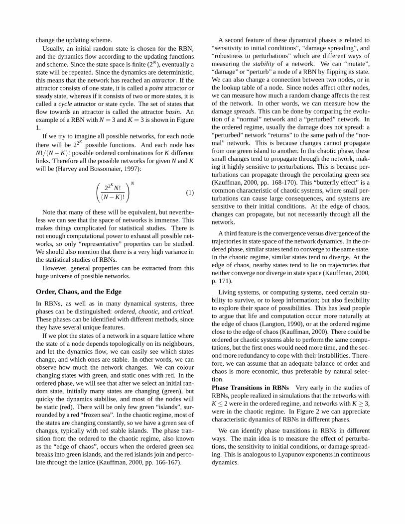
If we plot the states of a network in a square lattice wherethe state of a node depends topologically on its neighbours,and let the dynamics flow, we can easily see which stateschange, and which ones are stable. In other words, we canobserve how much the network changes. We can colourchanging states with green, and static ones with red. In theordered phase, we will see that after we select an initial ran-dom state, initially many states are changing (green), butquicky the dynamics stabilise, and most of the nodes willbe static (red). There will be only few green “islands”, sur-rounded by a red “frozen sea”. In the chaotic regime, most ofthe states are changing constantly, so we have a green sea ofchanges, typically with red stable islands. The phase tran-sition from the ordered to the chaotic regime, also knownas the “edge of chaos”, occurs when the ordered green seabreaks into green islands, and the red islands join and perco-late through the lattice (Kauffman, 2000, pp. 166-167).

A second feature of these dynamical phases is related to“sensitivity to initial conditions”, “damage spreading”,and“robustness to perturbations” which are different ways ofmeasuring thestability of a network. We can “mutate”,“damage” or “perturb” a node of a RBN by flipping its state.We can also change a connection between two nodes, or inthe lookup table of a node. Since nodes affect other nodes,we can measure how much a random change affects the restof the network. In other words, we can measure how thedamagespreads. This can be done by comparing the evolu-tion of a “normal” network and a “perturbed” network. Inthe ordered regime, usually the damage does not spread: a“perturbed” network “returns” to the same path of the “nor-mal” network. This is because changes cannot propagatefrom one green island to another. In the chaotic phase, thesesmall changes tend to propagate through the network, mak-ing it highly sensitive to perturbations. This is because per-turbations can propagate through the percolating green sea(Kauffman, 2000, pp. 168-170). This “butterfly effect” is acommon characteristic of chaotic systems, where small per-turbations can cause large consequences, and systems aresensitive to their initial conditions. At the edge of chaos,changes can propagate, but not necessarily through all thenetwork.

A third feature is the convergenceversus divergence of thetrajectories in state space of the network dynamics. In the or-dered phase, similar states tend to converge to the same state.In the chaotic regime, similar states tend to diverge. At theedge of chaos, nearby states tend to lie on trajectories thatneither converge nor diverge in state space (Kauffman, 2000,p. 171).

Living systems, or computing systems, need certain sta-bility to survive, or to keep information; but also flexibilityto explore their space of possibilities. This has lead peopleto argue that life and computation occur more naturally atthe edge of chaos (Langton, 1990), or at the ordered regimeclose to the edge of chaos (Kauffman, 2000). There could beordered or chaotic systems able to perform the same compu-tations, but the first ones would need more time, and the sec-ond more redundancy to cope with their instabilities. There-fore, we can assume that an adequate balance of order andchaos is more economic, thus preferable by natural selec-tion.Phase Transitions in RBNs Very early in the studies ofRBNs, people realized in simulations that the networks withK ≤ 2 were in the ordered regime, and networks withK ≥ 3,were in the chaotic regime. In Figure 2 we can appreciatecharacteristic dynamics of RBNs in different phases.

We can identify phase transitions in RBNs in differentways. The main idea is to measure the effect of perturba-tions, the sensitivity to initial conditions, or damage spread-ing. This is analogous to Lyapunov exponents in continuousdynamics.

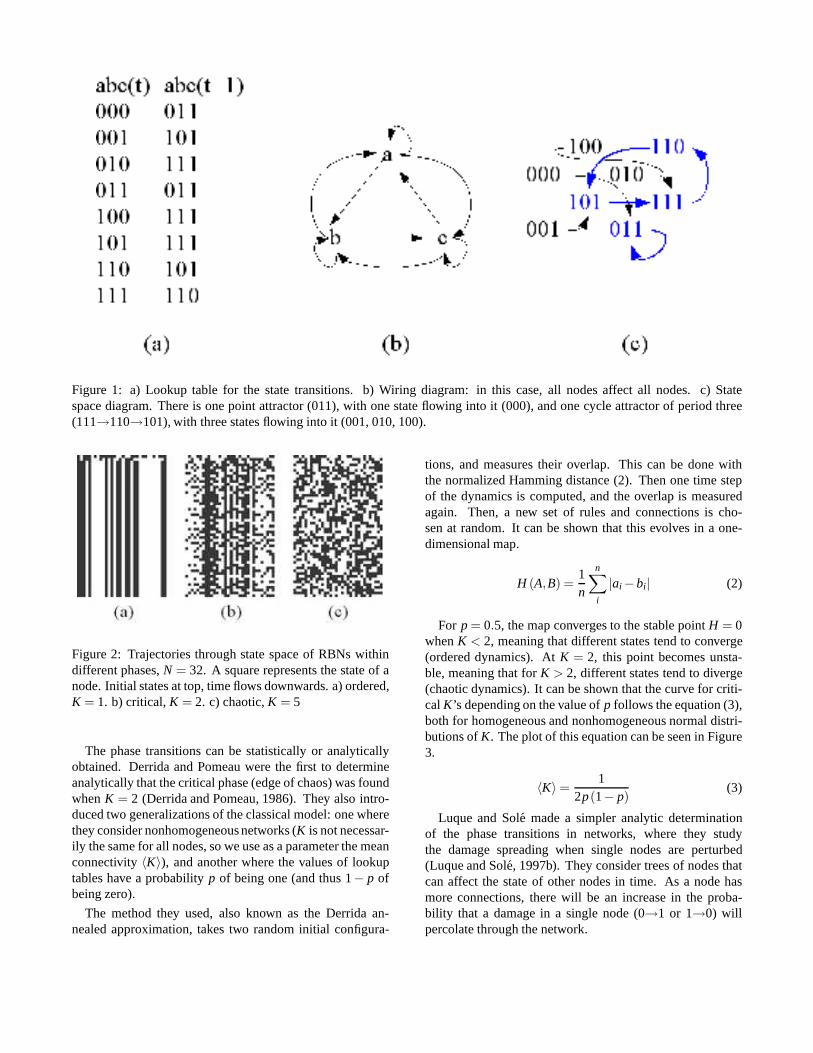
Figure 1: a) Lookup table for the state transitions. b) Wiring diagram: in this case, all nodes affect all nodes. c) Statespace diagram. There is one point attractor (011), with one state flowing into it (000), and one cycle attractor of period three(111→110→101), with three states flowing into it (001, 010, 100).

Figure 2: Trajectories through state space of RBNs withindifferent phases,N = 32. A square represents the state of anode. Initial states at top, time flows downwards. a) ordered,K = 1. b) critical,K = 2. c) chaotic,K = 5

The phase transitions can be statistically or analyticallyobtained. Derrida and Pomeau were the first to determineanalytically that the critical phase (edge of chaos) was foundwhenK = 2 (Derrida and Pomeau, 1986). They also intro-duced two generalizations of the classical model: one wherethey consider nonhomogeneous networks (K is not necessar-ily the same for all nodes, so we use as a parameter the meanconnectivity〈K〉), and another where the values of lookuptables have a probabilityp of being one (and thus 1− p ofbeing zero).

The method they used, also known as the Derrida an-nealed approximation, takes two random initial configura-

tions, and measures their overlap. This can be done withthe normalized Hamming distance (2). Then one time stepof the dynamics is computed, and the overlap is measuredagain. Then, a new set of rules and connections is cho-sen at random. It can be shown that this evolves in a one-dimensional map.

H (A,B) =1n

n∑

i

|ai −bi| (2)

For p = 0.5, the map converges to the stable pointH = 0whenK < 2, meaning that different states tend to converge(ordered dynamics). AtK = 2, this point becomes unsta-ble, meaning that forK > 2, different states tend to diverge(chaotic dynamics). It can be shown that the curve for criti-calK’s depending on the value ofp follows the equation (3),both for homogeneous and nonhomogeneous normal distri-butions ofK. The plot of this equation can be seen in Figure3.

〈K〉 =1

2p(1− p)(3)

Luque and Sole made a simpler analytic determinationof the phase transitions in networks, where they studythe damage spreading when single nodes are perturbed(Luque and Sole, 1997b). They consider trees of nodes thatcan affect the state of other nodes in time. As a node hasmore connections, there will be an increase in the proba-bility that a damage in a single node (0→1 or 1→0) willpercolate through the network.

0 20 40 60Kc

0

0.2

0.4

0.6

0.8

1

p Chaotic Phase

Figure 3: Phase diagram for the classical model, reprintedfrom (Aldana, 2003) with permission from Elsevier

Let us focus only in one nodei at time t, and a nodejof the severali can affect at timet + 1. There is a prob-ability p that j will be one, and a damage ini will mod-ify j towards one with probability 1− p. The complemen-tary case is the same. Now, forK nodes, we could expectthat at least one change will occur if〈K〉2p(1− p) ≥ 1,which leads to (3). This method can be also used for othertypes of networks. Luque and Sole later used the concept ofBoolean derivative to define Lyapunov exponents in RBNs(Luque and Sole, 2000):

λ = log[2p(1− p)K] (4)

where λ < 0 represents the ordered phase,λ > 0 thechaotic phase, andλ = 0 the critical phase.

Statistical studies confirm these analytical results. How-ever, it seems that,in practice, the size of the networkcan play a role in the phase transitions (Gershenson, 2004a;Gershenson, 2004b). We have seen that for large RBNs thephase transition (measured with the average of differencesofnormalized Hamming distances att → ∞ andt = 0, for min-imum initial distances of 1/N) is given forK shifted towardsone, and for very small networks forK shifted towards three.This is probably because for large networks, there is a higherprobability that asubnetworkwill be generating more noisethan “average”, thus propagating damage.

In practice, there are very high standard deviations inRBN studies, which are normal in this type of systems(Mitchell et al., 1993). We can clearly find (or design) or-dered networks forK ≫ 3 but on average, statistical studiesconfirm the analytical ones. Therefore, when we generate arandom network, there are high probabilities that it will bein a specific regime according toK andp.

Explorations of the Classical Model

There have been several explorations of differ-ent properties of RBNs, e.g. (Wuensche, 1997;Aldana-Gonzalez et al., 2003). One can measure, forexample, the number and length of attractors, the sizesand distributions of their basins, and how these dependon different parameters of RBNs, such asN, K, p, or thetopology.

The structure of the nodes is very important for the dy-namics of RBNs. Thedescendantsof a node are the nodesthat it affects, while theancestorsof a node are those thataffect it. To have cycle attractors, i.e. of period greaterthan one, there should be at least one node that will be itsown ancestor. A circuit of auto-activating nodes is called alinkage loop, and when there is no feedback,linkage treesare formed. Note that loops spread activation through trees,but not vice versa. Therelevantelements of a network arethose nodes that form linkage loops, and do not have con-stant functions, for these cause instabilities in the network,which might or not propagate. Note that as there are moreconnections in a network (higherK), the probability of hav-ing loops increases. Therefore, finding less stable dynamicsfor high values ofK is natural.

We should not confuse the node diagrams with the statespace diagrams. These show the dynamic trajectories ofstates of the network, while the first show the relations of thenetwork elements. Classic RBNs are dissipative systems: astate can have only onesuccessor, since the dynamics aredeterministic, but more than onepredecessoror pre-imagecan flow into a single state. Thein-degreeof a state is thenumber of predecessors it has. States without predecessorsare calledgarden-of-Edenstates. In this way, the dynamicsflow from garden-of-Eden states, converging towards attrac-tors. The time it takes to reach an attractor is calledtransienttime.

Attractor Lengths There have been analytic solutions ofRBNs forK = 1 (Flyvbjerg and Kjaer, 1988), and forK = N(Derrida and Flyvbjerg, 1987). The challenging problem offinding a general analytic solution is still open. Some sta-tistical studies have matched the analytic solutions for thespecial cases. People have observed the following, consid-ering p = 0.5 (Kauffman, 1993; Bastolla and Parisi, 1998;Aldana-Gonzalez et al., 2003):

For K = 1, the probability of having long attractors de-creases exponentially, and the average number of cyclesseems to be independent ofN (Bastolla and Parisi, 1998).The median lengths of state cycles are of order

√

N/2.For K ≥ N, the average length of attractors and the tran-

sient times required to reach them grow exponentially. Thisrestricts numerical investigations to small networks. Thetypical cycle length grows proportional to 2N/2.

For K = 2, at the critical phase, both the typical at-tractor lengths and the average number of attractors grow

algebraically withN. However, the precise dependenceof N is a matter of dispute. People long believed thatthe average number of attractors and their length wasproportional to

√N, (Kauffman, 1969; Kauffman, 1993;

Bastolla and Parisi, 1998). This result was very attractive,because the number of cell types and cell replication timesfor different organisms seem to scale also as the squareroot of genes for different species, although the precisenumber of genes of organisms keeps on changing. How-ever, Bilke and Sjunnesson did a full exploration of net-works, “decimating” irrelevant variables, and found thatthere is alinear dependence of number of attractors depend-ing on N (Bilke and Sjunnesson, 2002). This linear depen-dence has been confirmed in other complete statistical stud-ies (Gershenson, 2002; Gershenson et al., 2003). The differ-ence seems to lie on the bias caused byundersamplingthestate space.

Since there are 2N states, full statistical studies are possi-ble only for very small networks. For example, forN = 20there are more than a billion initial states. Therefore, thesestudies either concentrate on small networks, or take intoaccount only very few initial states. In the first case, someproperties of large networks will not be observed, whereas inthe second, some attractors would not be found, especiallyif their basins consist of very few states.

More research is needed in this direction. One argumentcould be that even when there would be potentially more at-tractors than the ones found by limited sampling, in practiceone would obtain the same result, since nature does not ex-haust all possible configurations (e.g. there could be morecell types for a given number of genes, butdevelopingintothem is impossible, i.e. their basins are very small). Also,ifwe could get the general analytical solution, it could be thatit would not match statistical studies, since a bias should beexpected in the statistical sampling, due to very high stan-dard deviations. However, for different purposes we mightbe more interested in the practical than the theoretical re-sults, or vice versa.

Convergence One can measure the convergence of stateswith different parameters. One of them is theG-density,which is the density of garden-of-Eden states. Another isthe in-degree frequency distribution, which can be plottedas a histogram (Wuensche, 1998). These measures revealfeatures at different phases.

At the ordered phase, there is a very highG-density, andhigh in-degree frequency. This leads to a high convergence,and very short transient times. The basins of attraction arevery compact, with many states flowing into few states.

At the critical phase, the in-degree distribution approx-imates a power-law, i.e. there are few states with highin-degree, and many states with low in-degree. There ismedium convergence.

At the chaotic phase, there are a relatively lowerG-

density, and a high frequency of low in-degrees. The basinsof attraction are very elongated, with few states flowing intoother states. This makes average transient times very long,and in some cases infinite in practice. Therefore, there is lowconvergence.

Other parameters that can be useful for measuringconvergence include Walker’s “internal homogene-ity” (Walker and Ashby, 1966), Langton’sλ param-eter (Langton, 1990), and Wuensche’s Z parameter(Wuensche, 1999). The latter one, together with the “input-entropy variance”, can be also used to automatically classifyrules of CA into ordered, complex (critical), and chaotic(Wuensche, 1999). This is useful, since “interesting”behaviour in CA tends to occur within complex rule space.

Multi-Valued NetworksThere have been some extensions to the Boolean idealizationof classical RBNs, namely where nodes can take more thantwo values.

Sole, Luque, and Kauffman, and more recently Luqueand Ballesteros have studied such multi-valued networks,and calculated their phase transitions (Sole et al., 2000;Luque and Ballesteros, 2004). For the special case whereonly two states are allowed, the results of Derrida are re-covered.

In nature, the components of certain systems exhibit a be-haviour that is better described with more than two states.Particular models should go beyond the boolean idealiza-tion. However, for theoretical purposes, we could combineseveral boolean nodes to act as a multi-valued one (codify-ing in base two its state).

TopologiesMany systems have been found to have a scale-free topol-ogy. It seems to be a persistent feature of complex networks(Barabasi, 2002): The Internet, molecular and genetic net-works, social networks, technology graphs, language net-works, food webs... they all share similar topological fea-tures: they have few elements with many links, and manyelements with few links. This distribution seems to haveseveral adaptive advantages, thought it is still not very wellunderstood.

However, most RBNs which have been studied have ho-mogeneous or normal topologies. Oosawa and Savageaustudied the effects of topology in the properties of RBNs(Oosawa and Savageau, 2002). Their results showed that thetopology can change drastically these properties. Networkswith the more uniform rank distributions exhibit more andlonger attractors and less entropy and mutual information(less correlation in their expression patterns), whereas moreskewed topologies exhibit less and shorter attractors andmore entropy and mutual information. A topology based onE. coli, which is scale-free, balances the parameters to avoidthe disadvantages of the extreme topologies.

1 1.5 2 2.5 3γ

0

0.2

0.4

0.6

0.8

1

p Chaotic PhaseOrdered

Phase

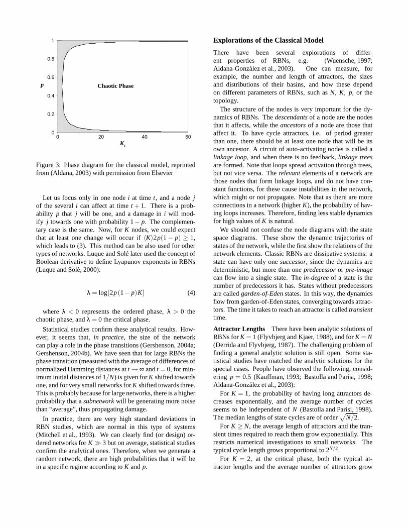
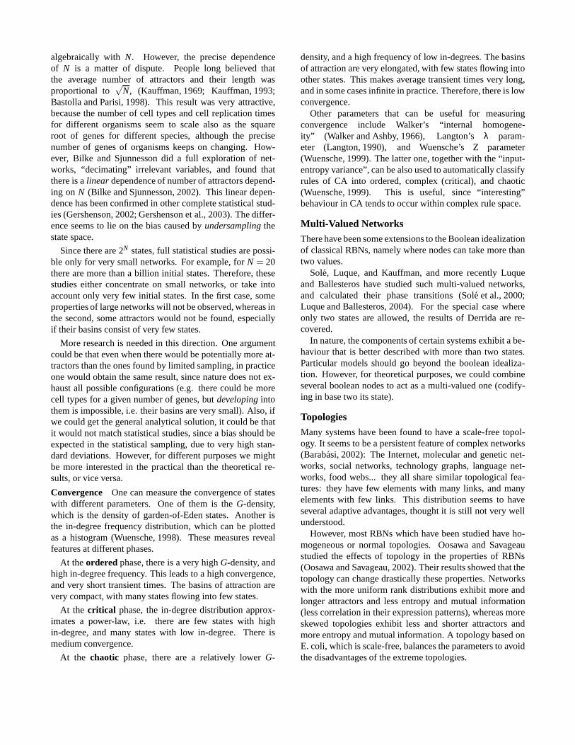
Figure 4: Phase diagram for the scale-free model, reprintedfrom (Aldana, 2003) with permission from Elsevier

Having this in mind, Aldana studied many properties ofRBNs with scale-free topology (Aldana, 2003). The connec-tivity of scale-free RBNs can be generated randomly usingthe probability distributionP(k) = [ζ(γ)kγ]−1, whereγ > 1andζ(γ) =

∑∞k=1k−γ is the Riemann Zeta function. In this

way, every node has at least one connection, but there arefew ones with many connections. The properties of the net-work are no longer determined by the average connectivity,but by the exponentγ.

Following Derrida’s method, Aldana found that the criti-cal value of the exponentγc where the phase transition fromorder to chaos occurs is determined by the transcendentalequation:

2p(1− p)ζ(γc−1)

ζ(γc)= 1 (5)

The values for which (5) is satisfied are plotted in Figure4. We can see thatγc ∈ [2,2.5] for any value ofp. Themaximum value ofγc ≈ 2.47875 is reached whenp = 0.5.

The network properties at each phase (e.g. number andlength of attractors, transient times) are analogous to theones obtained with homogeneous RBNs.

An important result is that evolvability has more space inscale-free networks, since these can adapt even in the or-dered regime, where changes in well-connected elements dopropagate through the network. However, experimental ev-idence shows that most biological networks are scale freewith exponent 2< γ < 2.5 (Aldana, 2003), i.e. “at the edgeof chaos”. The advantages of scale-free topologies are be-ginning to become evident, although they have been not em-braced by most researchers of RBNs.

RBN ControlRBNs usually do not consider external inputs. However, realsystems such as genetic networks can be influenced by ex-

ternal signals, such as molecular clocks related to sunlight.Methods of chaos control have been successfully

applied to chaotic RBNs (Luque and Sole, 1997a;Luque and Sole, 1998; Ballesteros and Luque, 2002).The main idea is to use a periodic function to drive a verychaotic network into a stable pattern. If a periodic functiondetermines the states of some nodes at some time, thesewill have a regularity that can spread through the rest of thenetwork, developing into a global periodic pattern. A highpercentage of nodes should be controlled to achieve this.However, once we control a small chaotic network, we canuse this to control a larger chaotic network, and this oneto control an even larger one, and so on. This shows thatit is possible to design chaotic networks controlled by fewexternal signals to force them into regular behaviour.

Different Updating SchemesKauffman has argued that the small average number of at-tractors found in RBNs compared with the number of possi-ble states can account for the number of cell types and cellreplication time in organisms compared with their numberof genes (Kauffman, 1969; Kauffman, 1993). In those days,about eighty thousand genes were thought to conform thehuman genome. Therefore, if the genome is seen as a RBNclose to the edge of chaos, the expected number of attractorswould be less than three hundred, matching the observednumber of cell types in humans. However, there are manydrawbacks to this calculation. The Boolean idealization hasbeen roughly accepted, since multi-valued networks haveshown similar results. Now that the human genome has beenmostly sequenced, it seems to consist of less than thirty fivethousand genes. The topology seems to be scale-free. Thereis certain amount of junk or structural DNA, without func-tionality. Many functions seem to be biassed (p 6= 0.5). Butthe heaviest argument has been the following:genes do notmarch in step. Genes do not change their states all at thesame moment, but some do it earlier than others. There wasno argument for the synchronicity in RBNs. In the next sec-tions we will review research made related to this criticism.

Asynchronous RBNsHarvey and Bossomaier introduced the criticism to the syn-chronicity of classic RBNs (Harvey and Bossomaier, 1997).It was well known that asynchronicity could change dras-tically the dynamics of a synchronous system, such as theprisoner’s dilemma (Huberman and Glance, 1993) or Con-way’s game of life (Bersini and Detours, 1994), and they dida similar thing for RBNs. Instead of updating the nodessynchronously, they defined asynchronous RBNs (ARBNs),where a node is picked up at random, and updated. Wehave to notice that ARBNs are not only asynchronous, butalso non-deterministic. This destroys the cycle attractors ofclassical RBNs (CRBNs), since it is very difficult that a se-quence of states will be repeated with a non-deterministic

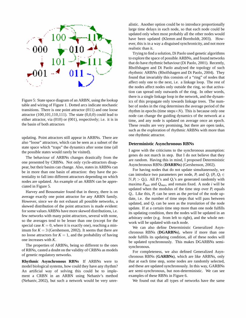
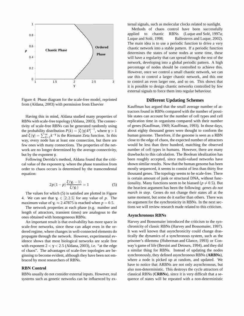
Figure 5: State space diagram of an ARBN, using the lookuptable and wiring of Figure 1. Dotted arcs indicate stochastictransitions. There is one point attractor (011) and one looseattractor (100,101,110,111). The state (0,0,0) could leadtoeither attractor, via (010) or (001), respectively; i.e. itis inthe basin of both attractors

updating. Point attractors still appear in ARBNs. There arealso “loose” attractors, which can be seen as a subset of thestate space which “traps” the dynamics after some time (allthe possible states would rarely be visited).

The behaviour of ARBNs changes drastically from theone presented by CRBNs. Not only cycle-attractors disap-pear, but their basins can change. Also, states in ARBNs canbe in more than one basin of attraction: they have the po-tentiality to fall into different attractors depending on whichnodes are updated. An example of an ARBN can be appre-ciated in Figure 5.

Harvey and Bossomaier found that in theory, there is onaverage exactly one point attractor for any ARBN family.However, since we do not exhaust all possible networks, askewed distribution of the point attractors is made evident:for some values ARBNs have more skewed distributions, i.e.few networks with many point attractors, several with none,so the averages tend to be lesser than one (except for thespecial caseK = 0, where it is exactly one), reaching a min-imum forK = 3 (Gershenson, 2002). It seems that there areno loose attractors forK = 1, and the probability of havingone increases withK.

The properties of ARBNs, being so different to the onesof RBNs, casted a doubt on the validity of CRBNs as modelsof genetic regulatory networks.

Rhythmic Asynchronous RBNs If ARBNs were tomodel biological systems, how could they have any rhythm?An artificial way of solving this could be to imple-ment a CRBN in an ARBN using Nehaniv’s method(Nehaniv, 2002), but such a network would be very unre-

alistic. Another option could be to introduce proportionallylarge time delays in each node, so that each node could beupdated only when most probably all the other nodes wouldhave been updated (Klemm and Bornholdt, 2003). How-ever, this is in a way a disguised synchronicity, and not morerealistic than it.

Trying to find a solution, Di Paolo used genetic algorithmsto explore the space of possible ARBNs, and found networksthat do have rhythmic behaviour (Di Paolo, 2001). Recently,Rholfshagen and Di Paolo analysed the topology of suchrhythmic ARBNs (Rholfshagen and Di Paolo, 2004). Theyfound that invariably this consists of a “ring” of nodes thataffect only one to the next, i.e. a linkage loop. The rest ofthe nodes affect nodes only outside the ring, so that activa-tion can spread only outwards of the ring. In other words,there is a single linkage loop in the network, and the dynam-ics of this propagate only towards linkage trees. The num-ber of nodes in the ring determines the average period of therhythm in epochs (time steps×N). This is because only onenode can change the guiding dynamics of the network at atime, and any node is updated on average once an epoch.These results are very promising, but there are open tasks,such as the exploration of rhythmic ARBNs with more thanone rhythmic attractor.

Deterministic Asynchronous RBNs

I agree with the criticisms to the synchronous assumption:genes do not march in step. But I do not believe that theyare random. Having this in mind, I proposed DeterministicAsynchronous RBNs (DARBNs) (Gershenson, 2002).

For having nodes that do not update simultaneously, wecan introduce two parameters per node,Pi andQi (Pi,Qi ∈N,Pi > Qi). All Pi ’s andQi ’s are generated randomly withmaximaPmax andQmax, and remain fixed. A nodei will beupdated when the modulus of the time step overPi equalsQi . Like this, Pi can be seen as theperiod of the node up-date, i.e. the number of time steps that will pass betweenupdated, andQi can be seen as thetranslationof the nodeupdate. If at a certain time step more than one node fulfillsits updating condition, then the nodes will be updated in anarbitrary order (e.g. from left to right), and the whole net-work will be updated with each node.

We can also define Deterministic Generalized Asyn-chronous RBNs (DGARBNs), where if more than onenode fulfills its updating condition, all of these nodes willbe updated synchronously. This makes DGARBNs semi-synchronous.

For completeness, we also defined Generalized Asyn-chronous RBNs (GARBNs), which are like ARBNs, onlythat at each time step, some nodes are randomly selected,and these are updated synchronously. In this way, GARBNsare semi-synchronous, but non-deterministic. We can seeexamples of these RBNs in Figure 6.

We found out that all types of networks have the same

Figure 6: State space diagrams of a DARBN, a DGARBN, and a GARBN, using the lookup table and wiring of Figure1. For the deterministic networks,P = {1,1,2} and Q = {0,0,0}. Numbers near arcs indicate the transitions which willoccur at time modulus two. There is one point attractor (011)and one cycle attractor, but different than the one of a CRBN(1001 → 1110 → 1111 → 1100), but the basins are different. For the GARBN, there is the same point attractor and looseattractor than for the ARBN, but there are more possible stochastic transitions, i.e. changes can potentially propagate faster

point attractors (Gershenson, 2002). This is because no mat-ter which node is updated, the state will not change. There-fore, the updating scheme does not affect point attractors.However, the attractor basins do change, and other types ofattractor. DARBNs and DGARBNs have properties muchcloser to the ones of CRBNs (Gershenson, 2002). Since theyare deterministic, cycle attractors are present. The numberof attractors, like in CRBNs, increases linearly withN, butmore slowly, meaning that there are even fewer attractors fora high possible number of states1. Also, the percentage ofstates in attractors is reduced exponentially, as with CRBNs,but even faster. These results imply that DGARBNs andDARBNs can perform even morecomplexity reductionthanCRBNs. We also concluded that the difference of CRBNsand ARBNs lies more in non-determinism than in asyn-chronicity.

Moreover, we proposed a method for mapping any deter-ministic asynchronous RBN into a CRBN. The main idea isto introduce new nodes, connected to every other previousnode, which codify in base two the maximum period of theDARBN. This is the least common multiple of allPi ’s.

Asynchronicity and Feedback We have to mention thatThomas developed much earlier an asynchronous modelof RBNs using delays, which could be both determinis-tic or stochastic, depending on the certainty of the delays(Thomas, 1973; Thomas, 1978; Thomas, 1991). However,these models were proposed and used mainly for the analysisof precise networks, their circuits, and feedback loops, andto my knowledge they have been not used for analytical orstatistical studies of ensembles (“families”) of networks. An

1ARBNs and GARBNs have also a linear increase in the aver-age number of attractors, when we consider loose attractorsin thestatistics (Gershenson, 2004b). These RBNs have less attractorsthan deterministic RBNs, but their sizes are much larger.

interesting finding of Thomas and coworkers was the follow-ing: a positive feedback loop (direct or indirect autocataly-sis) in a network implies the choice of two stable states, i.e.point attractors. This gives the property ofmultistationarity.On the other hand, a negative feedback loop implies peri-odic behaviour, i.e. point or cycle attractors. This can bedescribed ashomeostasis. The combinations of positive andnegative feedback loops give RBNs a plethora of possiblebehaviours, many of which are found in living systems.

Mixed-context RBNs

We can see the setsP andQ, consisting of allPi ’s andQi ’srespectively, as thecontextof a network. This is becauseexternal factors, such as temperature, can change the updat-ing periods of elements of a system. Like this, the sameDGARBN can have different behaviours in different con-texts, i.e. for differentP andQ.

Having this in mind, we can introduce non-determinism in contextual RBNs in a very specificway (Gershenson et al., 2003). For a given DGARBN,we can haveM “pure” contexts. Then, eachR time stepswe select randomly one of these contexts, and use it inthe network. Thus, we have defined Mixed-context RBNs(MxRBNs). An example is shown in Figure 7.

We should note that the non-determinism in MxRBNs isintroduced in a very controlled fashion. In GARBNs wehaveN “coin flips” per time step (selecting which nodeswill be updated). In ARBNs we have one coin flip per timestep (selecting which node will be updated). In MxRBNswe have one coin flip perR time steps (selecting which con-text will be used). The higher the value ofR and the lowernumber ofM contexts, the less stochasticity there will be.

MxRBNs have very similar number of attractors thanARBNs and GARBNs (considering loose attractors), andalso their number increases linearly and slowly withN.

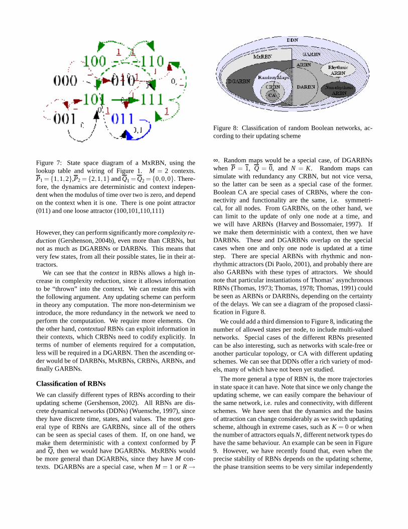
Figure 7: State space diagram of a MxRBN, using thelookup table and wiring of Figure 1.M = 2 contexts.P1 = {1,1,2},P2 = {2,1,1} andQ1 = Q2 = {0,0,0}. There-fore, the dynamics are deterministic and context indepen-dent when the modulus of time over two is zero, and dependon the context when it is one. There is one point attractor(011) and one loose attractor (100,101,110,111)

However, they can perform significantly morecomplexity re-duction(Gershenson, 2004b), even more than CRBNs, butnot as much as DGARBNs or DARBNs. This means thatvery few states, from all their possible states, lie in theirat-tractors.

We can see that thecontextin RBNs allows a high in-crease in complexity reduction, since it allows informationto be “thrown” into the context. We can restate this withthe following argument. Any updating scheme can performin theory any computation. The more non-determinism weintroduce, the more redundancy in the network we need toperform the computation. We require more elements. Onthe other hand,contextualRBNs can exploit information intheir contexts, which CRBNs need to codify explicitly. Interms of number of elements required for a computation,less will be required in a DGARBN. Then the ascending or-der would be of DARBNs, MxRBNs, CRBNs, ARBNs, andfinally GARBNs.

Classification of RBNs

We can classify different types of RBNs according to theirupdating scheme (Gershenson, 2002). All RBNs are dis-crete dynamical networks (DDNs) (Wuensche, 1997), sincethey have discrete time, states, and values. The most gen-eral type of RBNs are GARBNs, since all of the otherscan be seen as special cases of them. If, on one hand, wemake them deterministic with a context conformed byPandQ, then we would have DGARBNs. MxRBNs wouldbe more general than DGARBNs, since they haveM con-texts. DGARBNs are a special case, whenM = 1 or R→

Figure 8: Classification of random Boolean networks, ac-cording to their updating scheme

∞. Random maps would be a special case, of DGARBNswhen P = 1, Q = 0, and N = K. Random maps cansimulate with redundancy any CRBN, but not vice versa,so the latter can be seen as a special case of the former.Boolean CA are special cases of CRBNs, where the con-nectivity and functionality are the same, i.e. symmetri-cal, for all nodes. From GARBNs, on the other hand, wecan limit to the update of only one node at a time, andwe will have ARBNs (Harvey and Bossomaier, 1997). Ifwe make them deterministic with a context, then we haveDARBNs. These and DGARBNs overlap on the specialcases when one and only one node is updated at a timestep. There are special ARBNs with rhythmic and non-rhythmic attractors (Di Paolo, 2001), and probably there arealso GARBNs with these types of attractors. We shouldnote that particular instantiations of Thomas’ asynchronousRBNs (Thomas, 1973; Thomas, 1978; Thomas, 1991) couldbe seen as ARBNs or DARBNs, depending on the certaintyof the delays. We can see a diagram of the proposed classi-fication in Figure 8.

We could add a third dimension to Figure 8, indicating thenumber of allowed states per node, to include multi-valuednetworks. Special cases of the different RBNs presentedcan be also interesting, such as networks with scale-free oranother particular topology, or CA with different updatingschemes. We can see that DDNs offer a rich variety of mod-els, many of which have not been yet studied.

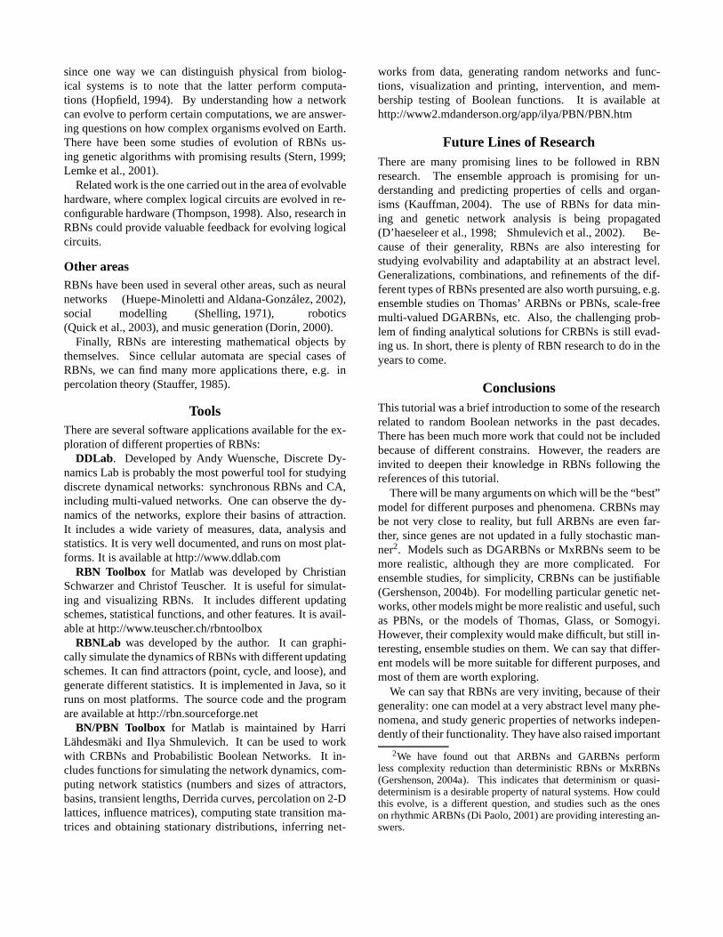
The more general a type of RBN is, the more trajectoriesin state space it can have. Note that since we only change theupdating scheme, we can easily compare the behaviour ofthe same network, i.e. rules and connectivity, with differentschemes. We have seen that the dynamics and the basinsof attraction can change considerably as we switch updatingscheme, although in extreme cases, such asK = 0 or whenthe number of attractors equalsN, different network types dohave the same behaviour. An example can be seen in Figure9. However, we have recently found that, even when theprecise stability of RBNs depends on the updating scheme,the phase transition seems to be very similar independently

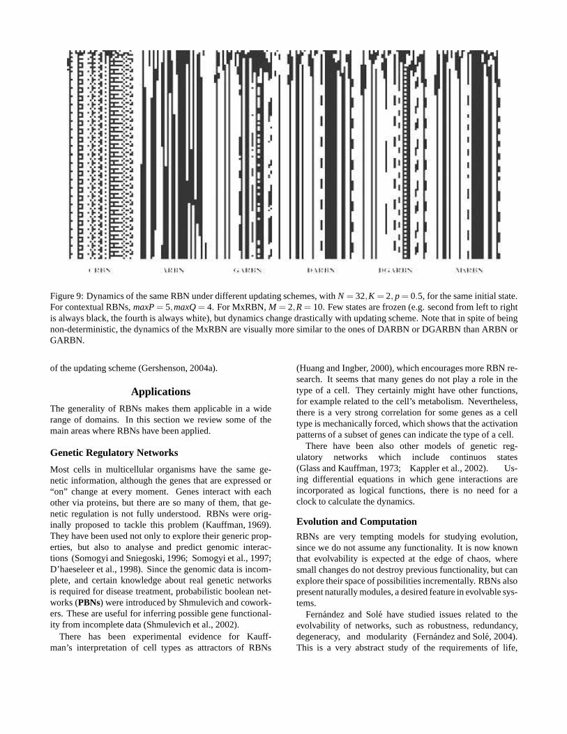
Figure 9: Dynamics of the same RBN under different updating schemes, withN = 32,K = 2, p = 0.5, for the same initial state.For contextual RBNs,maxP= 5,maxQ= 4. For MxRBN,M = 2,R= 10. Few states are frozen (e.g. second from left to rightis always black, the fourth is always white), but dynamics change drastically with updating scheme. Note that in spite ofbeingnon-deterministic, the dynamics of the MxRBN are visually more similar to the ones of DARBN or DGARBN than ARBN orGARBN.

of the updating scheme (Gershenson, 2004a).

Applications

The generality of RBNs makes them applicable in a widerange of domains. In this section we review some of themain areas where RBNs have been applied.

Genetic Regulatory Networks

Most cells in multicellular organisms have the same ge-netic information, although the genes that are expressed or“on” change at every moment. Genes interact with eachother via proteins, but there are so many of them, that ge-netic regulation is not fully understood. RBNs were orig-inally proposed to tackle this problem (Kauffman, 1969).They have been used not only to explore their generic prop-erties, but also to analyse and predict genomic interac-tions (Somogyi and Sniegoski, 1996; Somogyi et al., 1997;D’haeseleer et al., 1998). Since the genomic data is incom-plete, and certain knowledge about real genetic networksis required for disease treatment, probabilistic boolean net-works (PBNs) were introduced by Shmulevich and cowork-ers. These are useful for inferring possible gene functional-ity from incomplete data (Shmulevich et al., 2002).

There has been experimental evidence for Kauff-man’s interpretation of cell types as attractors of RBNs

(Huang and Ingber, 2000), which encourages more RBN re-search. It seems that many genes do not play a role in thetype of a cell. They certainly might have other functions,for example related to the cell’s metabolism. Nevertheless,there is a very strong correlation for some genes as a celltype is mechanically forced, which shows that the activationpatterns of a subset of genes can indicate the type of a cell.

There have been also other models of genetic reg-ulatory networks which include continuos states(Glass and Kauffman, 1973; Kappler et al., 2002). Us-ing differential equations in which gene interactions areincorporated as logical functions, there is no need for aclock to calculate the dynamics.

Evolution and Computation

RBNs are very tempting models for studying evolution,since we do not assume any functionality. It is now knownthat evolvability is expected at the edge of chaos, wheresmall changes do not destroy previous functionality, but canexplore their space of possibilities incrementally. RBNs alsopresent naturally modules, a desired feature in evolvable sys-tems.

Fernandez and Sole have studied issues related to theevolvability of networks, such as robustness, redundancy,degeneracy, and modularity (Fernandez and Sole, 2004).This is a very abstract study of the requirements of life,

since one way we can distinguish physical from biolog-ical systems is to note that the latter perform computa-tions (Hopfield, 1994). By understanding how a networkcan evolve to perform certain computations, we are answer-ing questions on how complex organisms evolved on Earth.There have been some studies of evolution of RBNs us-ing genetic algorithms with promising results (Stern, 1999;Lemke et al., 2001).

Related work is the one carried out in the area of evolvablehardware, where complex logical circuits are evolved in re-configurable hardware (Thompson, 1998). Also, research inRBNs could provide valuable feedback for evolving logicalcircuits.

Other areasRBNs have been used in several other areas, such as neuralnetworks (Huepe-Minoletti and Aldana-Gonzalez, 2002),social modelling (Shelling, 1971), robotics(Quick et al., 2003), and music generation (Dorin, 2000).

Finally, RBNs are interesting mathematical objects bythemselves. Since cellular automata are special cases ofRBNs, we can find many more applications there, e.g. inpercolation theory (Stauffer, 1985).

ToolsThere are several software applications available for the ex-ploration of different properties of RBNs:

DDLab. Developed by Andy Wuensche, Discrete Dy-namics Lab is probably the most powerful tool for studyingdiscrete dynamical networks: synchronous RBNs and CA,including multi-valued networks. One can observe the dy-namics of the networks, explore their basins of attraction.It includes a wide variety of measures, data, analysis andstatistics. It is very well documented, and runs on most plat-forms. It is available at http://www.ddlab.com

RBN Toolbox for Matlab was developed by ChristianSchwarzer and Christof Teuscher. It is useful for simulat-ing and visualizing RBNs. It includes different updatingschemes, statistical functions, and other features. It is avail-able at http://www.teuscher.ch/rbntoolbox

RBNLab was developed by the author. It can graphi-cally simulate the dynamics of RBNs with different updatingschemes. It can find attractors (point, cycle, and loose), andgenerate different statistics. It is implemented in Java, so itruns on most platforms. The source code and the programare available at http://rbn.sourceforge.net

BN/PBN Toolbox for Matlab is maintained by HarriLahdesmaki and Ilya Shmulevich. It can be used to workwith CRBNs and Probabilistic Boolean Networks. It in-cludes functions for simulating the network dynamics, com-puting network statistics (numbers and sizes of attractors,basins, transient lengths, Derrida curves, percolation on2-Dlattices, influence matrices), computing state transitionma-trices and obtaining stationary distributions, inferringnet-

works from data, generating random networks and func-tions, visualization and printing, intervention, and mem-bership testing of Boolean functions. It is available athttp://www2.mdanderson.org/app/ilya/PBN/PBN.htm

Future Lines of ResearchThere are many promising lines to be followed in RBNresearch. The ensemble approach is promising for un-derstanding and predicting properties of cells and organ-isms (Kauffman, 2004). The use of RBNs for data min-ing and genetic network analysis is being propagated(D’haeseleer et al., 1998; Shmulevich et al., 2002). Be-cause of their generality, RBNs are also interesting forstudying evolvability and adaptability at an abstract level.Generalizations, combinations, and refinements of the dif-ferent types of RBNs presented are also worth pursuing, e.g.ensemble studies on Thomas’ ARBNs or PBNs, scale-freemulti-valued DGARBNs, etc. Also, the challenging prob-lem of finding analytical solutions for CRBNs is still evad-ing us. In short, there is plenty of RBN research to do in theyears to come.

ConclusionsThis tutorial was a brief introduction to some of the researchrelated to random Boolean networks in the past decades.There has been much more work that could not be includedbecause of different constrains. However, the readers areinvited to deepen their knowledge in RBNs following thereferences of this tutorial.

There will be many arguments on which will be the “best”model for different purposes and phenomena. CRBNs maybe not very close to reality, but full ARBNs are even far-ther, since genes are not updated in a fully stochastic man-ner2. Models such as DGARBNs or MxRBNs seem to bemore realistic, although they are more complicated. Forensemble studies, for simplicity, CRBNs can be justifiable(Gershenson, 2004b). For modelling particular genetic net-works, other models might be more realistic and useful, suchas PBNs, or the models of Thomas, Glass, or Somogyi.However, their complexity would make difficult, but still in-teresting, ensemble studies on them. We can say that differ-ent models will be more suitable for different purposes, andmost of them are worth exploring.

We can say that RBNs are very inviting, because of theirgenerality: one can model at a very abstract level many phe-nomena, and study generic properties of networks indepen-dently of their functionality. They have also raised important

2We have found out that ARBNs and GARBNs performless complexity reduction than deterministic RBNs or MxRBNs(Gershenson, 2004a). This indicates that determinism or quasi-determinism is a desirable property of natural systems. Howcouldthis evolve, is a different question, and studies such as theoneson rhythmic ARBNs (Di Paolo, 2001) are providing interesting an-swers.

questions related to the differences between theory and prac-tice, since some analytical or statistical results do not matcheach other. This can be explained with skewed distributionsand very high standard deviations found in RBN statistics.However, this brings deeper philosophical questions: howmuch should we care about theory, and how much shouldwe care about practice? Which one will help us understandbetter the phenomena we try to study? It seems that a care-ful balanceof both is required. However, it is unknown howthis balance might be like.

AcknowledgementsThis work was enriched with discussions, suggestions, andassistance from Diederik Aerts, Maximino Aldana, JanBroekaert, Keith Campbell, Ezequiel Di Paolo, Inman Har-vey, Bernardo Huberman, Stuart Kauffman, Ilya Shmule-vich, and Andy Wuensche. I thank Marcelle Kaufman forintroducing me to the work of Rene Thomas. This work wassupported in part by the Consejo Nacional de Ciencia y Tec-nologia (CONACYT) of Mexico.

ReferencesAldana, M. (2003). Boolean dynamics of networks with

scale-free topology.

Aldana-Gonzalez, M., Coppersmith, S., and Kadanoff, L. P.(2003). Boolean dynamics with random couplings. InKaplan, E., Marsden, J. E., and Sreenivasan, K. R., ed-itors,Perspectives and Problems in Nonlinear Science.A Celebratory Volume in Honor of Lawrence Sirovich.Springer Applied Mathematical Sciences Series.

Ballesteros, F. J. and Luque, B. (2002). Random Booleannetworks response to external periodic signals.PhysicaA, 313:289 300.

Barabasi, A.-L. (2002).Linked: The New Science of Net-works. Perseus.

Bastolla, U. and Parisi, G. (1998). Relevant elements, mag-netization and dynamical properties in Kauffman net-works: A numerical study.Physica D, 115(3’4):203–218.

Bersini, H. and Detours, V. (1994). Asynchrony induces sta-bility in cellular automata based models. InProceed-ings of the IVth Conference on Artificial Life, pages382–387. MIT Press.

Bilke, S. and Sjunnesson, F. (2002). Stability of the Kauff-man model.Physical Review E, 65(016129).

Derrida, B. and Flyvbjerg, H. (1987). The random mapmodel: A disordered model with deterministic dynam-ics. J. Physique, 48:971978.

Derrida, B. and Pomeau, Y. (1986). Random networks of au-tomata: A simple annealed approximation.Europhys.Lett., 1(2):45–49.

D’haeseleer, P., Wen, X., Fuhrman, S., and Somogyi, R.(1998). Mining the gene expression matrix: Inferringgene relationships from large scale gene expressiondata. In Paton, R. C. and Holcombe, M., editors,In-formation Processing in Cells and Tissues, pages 203–212. Plenum Publishing.

Di Paolo, E. A. (2001). Rhythmic and non-rhythmic at-tractors in asynchronous random Boolean networks.Biosystems, 59(3):185–195.

Dorin, A. (2000). Boolean networks for the generation ofrhythmic structure. In Brown and Wilding, editors,Proceedings Australian Computer Music Conference2000, pages 38–45.

Fernandez, P. and Sole, R. (2004). The role of computa-tion in complex regulatory networks. In Koonin, E. V.,Wolf, Y. I., and Karev, G. P., editors,Power Laws,Scale-Free Networks and Genome Biology, number 03-10-055. Landes Bioscience.

Flyvbjerg, H. and Kjaer, N. (1988). Exact solution of theKauffman model with connectivity one.J. Phys. A,21(7):16951718.

Gershenson, C. (2002). Classification of random Booleannetworks. In Standish, R. K., Bedau, M. A., and Ab-bass, H. A., editors,Artificial Life VIII: Proceedingsof the Eight International Conference on Artificial Life,pages 1–8. MIT Press.

Gershenson, C. (2004a). Phase transitions in randomBoolean networks with different updating schemes.Submitted to Physica D.

Gershenson, C. (2004b). Updating schemes in randomBoolean networks: Do they really matter? InArtifi-cial Life IX. MIT Press.

Gershenson, C., Broekaert, J., and Aerts, D. (2003). Con-textual random Boolean networks. In Banzhaf, W.,Christaller, T., Dittrich, P., Kim, J. T., and Ziegler,J., editors,Advances in Artificial Life, 7th EuropeanConference, ECAL 2003 LNAI 2801, pages 615–624.Springer-Verlag.

Glass, L. and Kauffman, S. (1973). The logical analysisof continuous, nonlinear biochemical control networks.Journal of Theoretical Biology, 39:103–129.

Harvey, I. and Bossomaier, T. (1997). Time out of joint:Attractors in asynchronous random Boolean networks.In Husbands, P. and Harvey, I., editors,Proceedings

of the Fourth European Conference on Artificial Life(ECAL97), pages 67–75. MIT Press.

Hopfield, J. J. (1994). Physics, computation, and why biol-ogy looks so different.Journal of Theoretical Biology,171:53–60.

Huang, S. and Ingber, D. E. (2000). Shape-dependentcontrol of cell growth, differentiation, and apoptosis:Switching between attractors in cell regulatory net-works. Exp. Cell Res., 261:91–103.

Huberman, B. A. and Glance, N. S. (1993). Evolutionarygames and computer simulations.Proc. Natl. Acad. Sci.USA, 90:7716–7718.

Huepe-Minoletti, C. and Aldana-Gonzalez, M. (2002). Dy-namical phase transition in a neural network modelwith noise: An exact solution.Journal of StatisticalPhysics, 108(3/4):527–540.

Kappler, K., Edwards, R., and Glass, L. (2002). Dynam-ics in high dimensional model gene networks.SignalProcessing, 83:789–798.

Kauffman, S. A. (1969). Metabolic stability and epigenesisin randomly constructed genetic nets.Journal of Theo-retical Biology, 22:437–467.

Kauffman, S. A. (1993). The Origins of Order. OxfordUniversity Press.

Kauffman, S. A. (2000).Investigations. Oxford UniversityPress.

Kauffman, S. A. (2004). The ensemble approach to under-stand genetic regulatory networks.Physica A: Statisti-cal Mechanics and its Applications, In Press.

Klemm, K. and Bornholdt, S. (2003). Robust gene regula-tion: Deterministic dynamics from asynchronous net-works with delay. q-bio/0309013.

Langton, C. (1990). Computation at the edge of chaos:Phase transitions and emergent computation.PhysicaD, 42:12–37.

Lemke, N., Mombach, J. C. M., and Bodmann, B. E. J.(2001). A numerical investigation of adaptation inpopulations of random Boolean networks.Physica A,301(1-4):589–600.

Luque, B. and Ballesteros, F. J. (2004). Random walk net-works. Physica A: Statistical Mechanics and its Appli-cations, In Press.

Luque, B. and Sole, R. V. (1997a). Controlling chaos inKauffman networks.Europhys. Lett., 37(9):597–602.

Luque, B. and Sole, R. V. (1997b). Phase transitions in ran-dom networks: Simple analytic determination of criti-cal points.Physical Review E, 55(1):257–260.

Luque, B. and Sole, R. V. (1998). Stable core and chaoscontrol in random Boolean networks.J. Phys. A: Math.Gen., 31:1533–1537.

Luque, B. and Sole, R. V. (2000). Lyapunov exponents inrandom Boolean networks.Physica A, 284:33–45.

Mitchell, M., Crutchfield, J. P., and Hraber, P. T. (1993).Dynamics, computation, and the ”edge of chaos”: Are-examination. Technical Report 93-06-040, Santa FeInstitute.

Nehaniv, C. L. (2002). Evolution in asynchronous cellularautomata. In Standish, R. K., Bedau, M. A., and Ab-bass, H. A., editors,Artificial Life VIII: Proceedingsof the Eight International Conference on Artificial Life,pages 75–73. MIT Press.

Oosawa, C. and Savageau, M. A. (2002). Effects of alterna-tive connectivity on behavior of randomly constructedBoolean networks.Physica D, 170:143–161.

Quick, T., Nehaniv, C. L., Dautenhahn, K., and Roberts,G. (2003). Evolving embodied genetic regulatorynetwork-driven control systems. In Banzhaf, W.,Christaller, T., Dittrich, P., Kim, J. T., and Ziegler, J.,editors,Advances in Artificial Life: ECAL 2003, pages266–277. Springer.

Rholfshagen, P. and Di Paolo, E. A. (2004). The circulartopology of rhythm in random asynchronous booleannetworks.BioSystems, 73(2):141–152.

Shelling, T. C. (1971). Dynamic models of segregation.Journal of Mathematical Sociology, 1:143186.

Shmulevich, I., Dougherty, E., and Zhang, W. (2002). FromBoolean to probabilistic Boolean networks as modelsof genetic regulatory networks.Proceedings of theIEEE, 90(11):1778–1792.

Sole, R. V., Luque, B., and Kauffman, S. A. (2000). Phasetransitions in random networks with multiple states.Technical Report 00-02-011, Santa Fe Institute.

Somogyi, R., Fuhrman, S., Askenazi, M., and Wuensche,A. (1997). The gene expression matrix: Towardsthe extraction of genetic network architectures.Non-linear Analysis: Theory, Methods and Applications,30(3):1815–1824.

Somogyi, R. and Sniegoski, C. A. (1996). Modeling thecomplexity of genetic networks: Understanding multi-genic and pleiotropic regulation.Complexity, 1(6):45–63.

Stauffer, D. (1985). Introduction to Percolation Theory.Taylor and Francis, London.

Stern, M. D. (1999). Emergence of homeostasis and noiseimprinting in an evolution model.PNAS, 96:10746–10751.

Thomas, R. (1973). Boolean formalization of genetic con-trol circuits. J. Theor. Biol., 42:563–585.

Thomas, R. (1978). Logical analysis of systems comprisingfeedback loops.J. Theor. Biol., 73:631–656.

Thomas, R. (1991). Regulatory networks seen as asyn-chronous automata: A logical description.J. Theor.Biol., 153:1–23.

Thompson, A. (1998).Hardware Evolution: Automatic De-sign of Electronic Circuits in Reconfigurable Hardwareby Artificial Evolution. Distinguished dissertation se-ries. Springer-Verlag.

von Neumann, J. (1966).The Theory of Self-ReproducingAutomata. University of Illinois Press.

Walker, C. and Ashby, W. (1966). On the temporal charac-teristics of behavior in certain complex systems.Ky-bernetik, 3(2):100–108.

Wolfram, S. (1986).Theory and Application of Cellular Au-tomata. World Scientific.

Wuensche, A. (1997).Attractor Basins of Discrete Net-works. PhD thesis, University of Sussex.

Wuensche, A. (1998). Discrete dynamical networks andtheir attractor basins. In Standish, R., Henry, B., Watt,S., Marks, R., Stocker, R., Green, D., Keen, S., andBossomaier, T., editors,Complex Systems ’98, pages3–21, University of New South Wales, Sydney, Aus-tralia.

Wuensche, A. (1999). Classifying cellular automata auto-matically: Finding gliders, filtering, and relating space-time patterns, attractor basins, and the z parameter.Complexity, 4(3):47–66.

Wuensche, A. and Lesser, M. (1992).The Global Dynam-ics of Cellular Automata; An Atlas of Basin of At-traction Fields of One-Dimensional Cellular Automata.Santa Fe Institute Studies in the Sciences of Complex-ity. Addison-Wesley, Reading, MA.