Introduction to Transit (and Secondary Eclipse)

Spectroscopy

Heather Knutson Division of Geological and Planetary

Sciences, Caltech

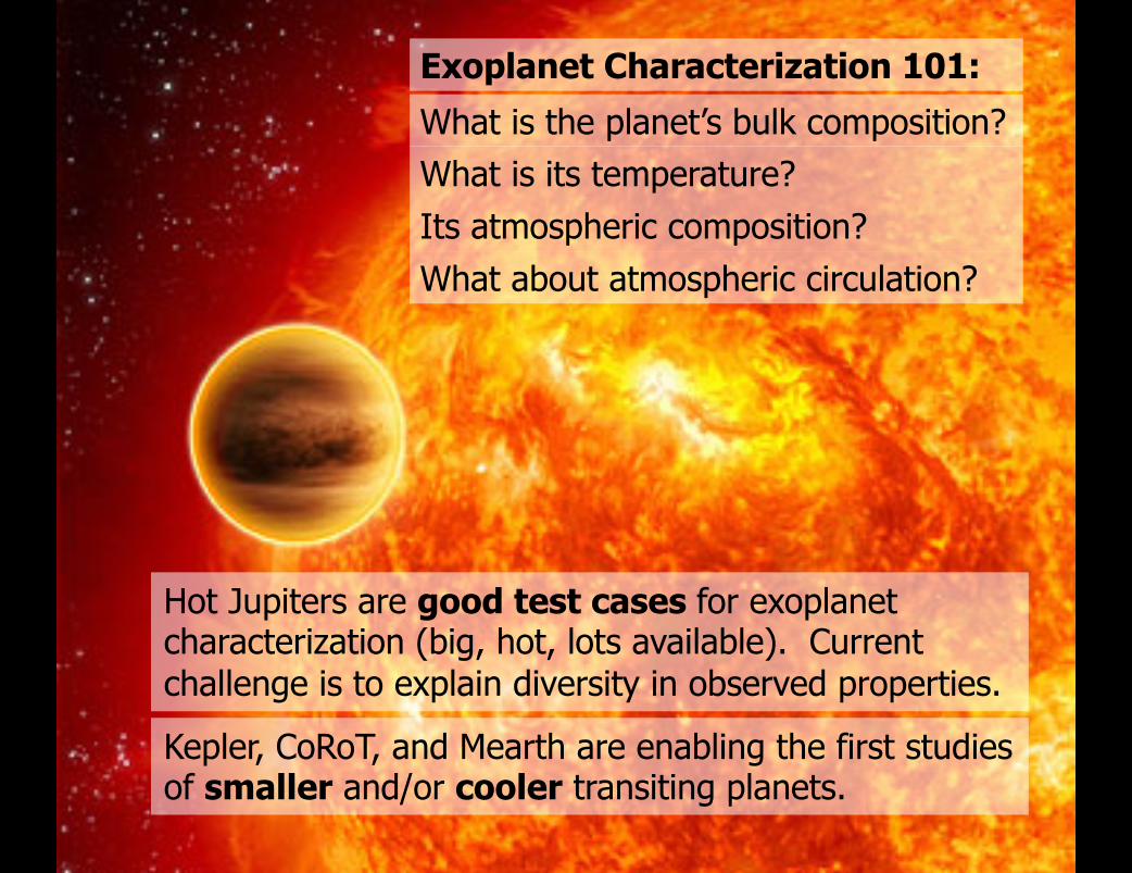
What is its temperature?

Its atmospheric composition?

What about atmospheric circulation?

Exoplanet Characterization 101:

What is the planet’s bulk composition?

Hot Jupiters are good test cases for exoplanet characterization (big, hot, lots available). Current challenge is to explain diversity in observed properties.

Kepler, CoRoT, and Mearth are enabling the first studies of smaller and/or cooler transiting planets.

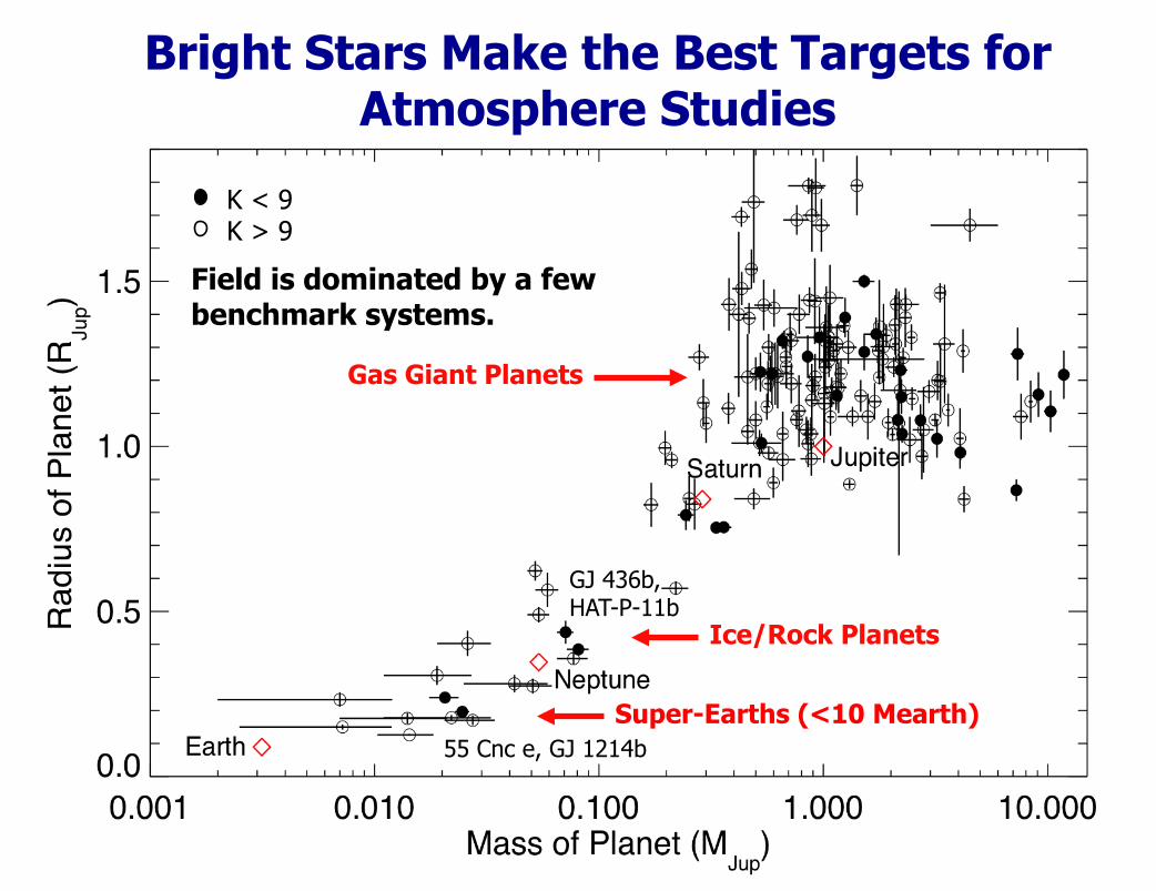
Bright Stars Make the Best Targets for Atmosphere Studies

Ice/Rock Planets

Gas Giant Planets

Super-Earths (<10 Mearth) 55 Cnc e, GJ 1214b

GJ 436b, HAT-P-11b

K < 9 K > 9

Field is dominated by a few benchmark systems.

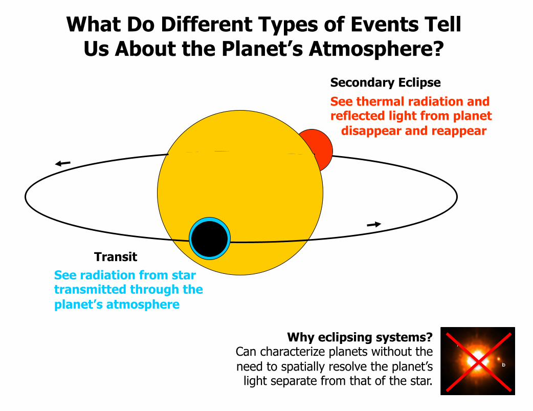
Transit

Secondary Eclipse

See thermal radiation and reflected light from planet disappear and reappear

See radiation from star transmitted through the planet’s atmosphere

What Do Different Types of Events Tell Us About the Planet’s Atmosphere?  

Why eclipsing systems? Can characterize planets without the need to spatially resolve the planet’s light separate from that of the star.

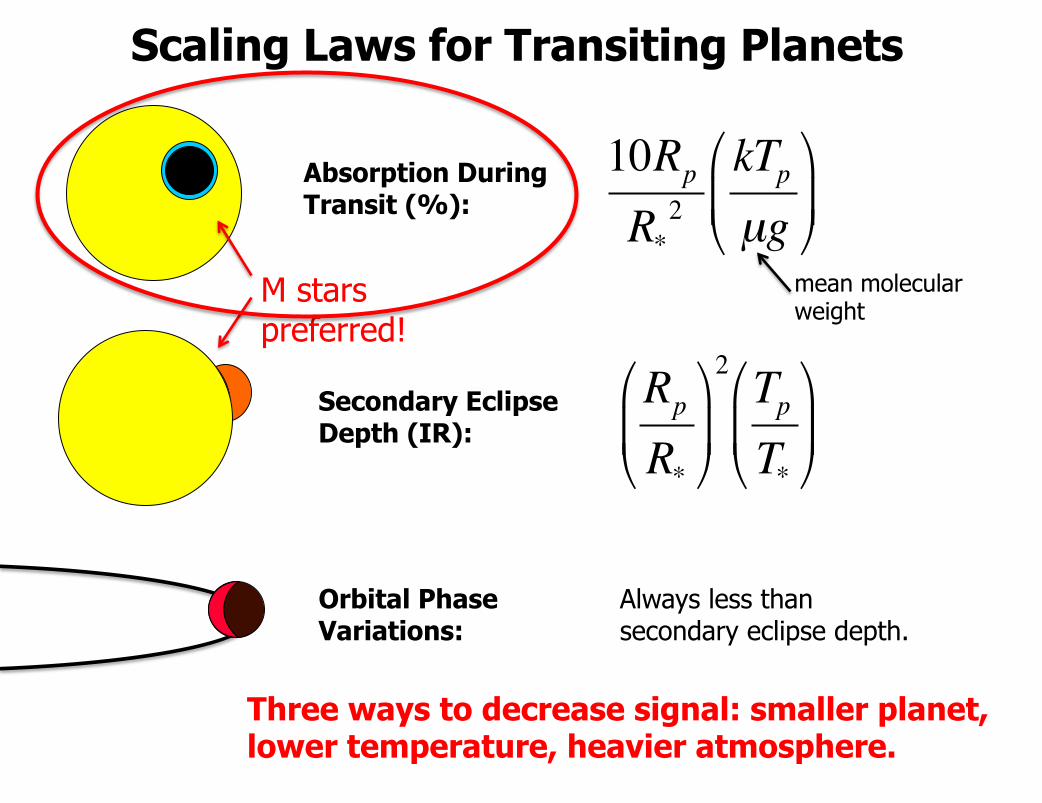
Absorption During Transit (%):

Secondary Eclipse Depth (IR):

Orbital Phase Variations:

Scaling Laws for Transiting Planets  

!

10Rp

R*2

kTpµg

"

# $

%

& '

!

Rp

R*

"

# $

%

& '

2 TpT*

"

# $

%

& '

Always less than secondary eclipse depth.

Three ways to decrease signal: smaller planet, lower temperature, heavier atmosphere.

M stars preferred!

mean molecular weight

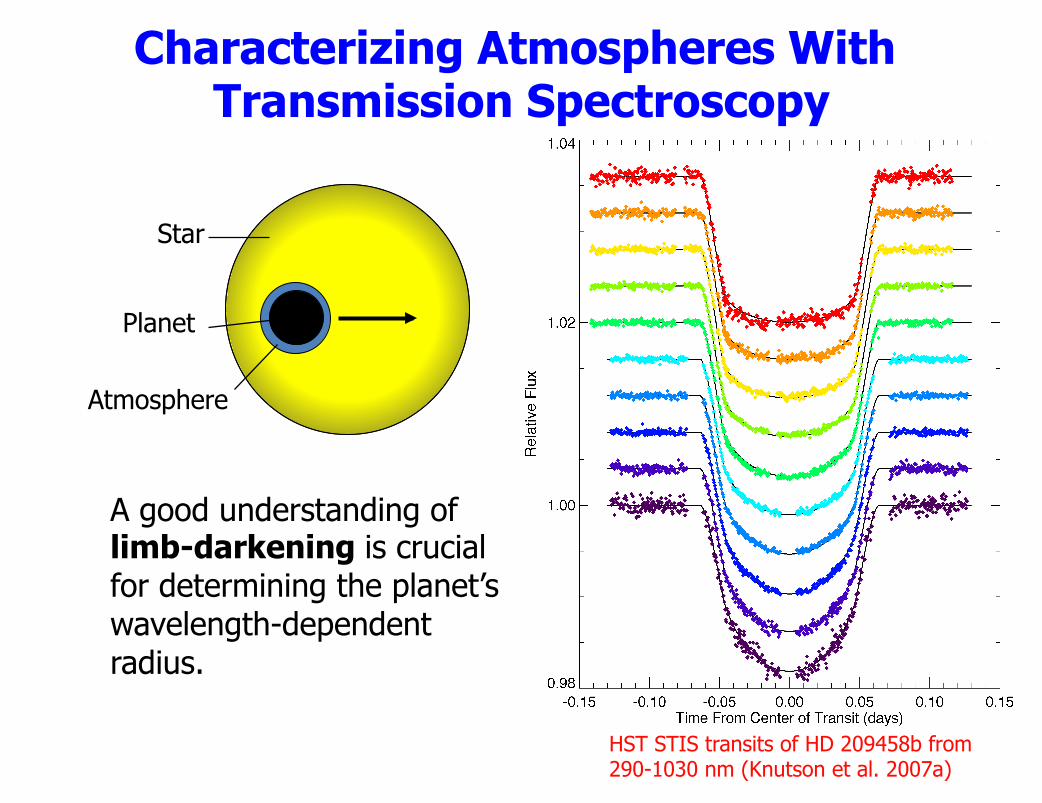
Characterizing Atmospheres With Transmission Spectroscopy

HST STIS transits of HD 209458b from 290-1030 nm (Knutson et al. 2007a)

Atmosphere

Star

Planet

A good understanding of limb-darkening is crucial for determining the planet’s wavelength-dependent radius.

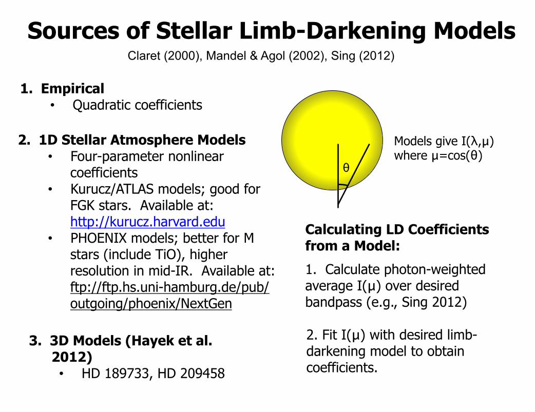
Sources of Stellar Limb-Darkening Models

1.  Empirical •  Quadratic coefficients

2.  1D Stellar Atmosphere Models •  Four-parameter nonlinear

coefficients •  Kurucz/ATLAS models; good for

FGK stars. Available at: http://kurucz.harvard.edu

•  PHOENIX models; better for M stars (include TiO), higher resolution in mid-IR. Available at: ftp://ftp.hs.uni-hamburg.de/pub/outgoing/phoenix/NextGen

Claret (2000), Mandel & Agol (2002), Sing (2012)

3.  3D Models (Hayek et al. 2012) •  HD 189733, HD 209458

θ

1. Calculate photon-weighted average I(μ) over desired bandpass (e.g., Sing 2012)

2. Fit I(μ) with desired limb-darkening model to obtain coefficients.

Models give I(λ,μ) where μ=cos(θ)

Calculating LD Coefficients from a Model:

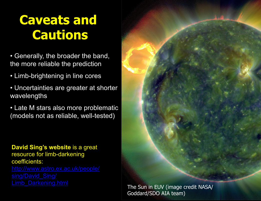
Caveats and Cautions

David Sing’s website is a great resource for limb-darkening coefficients: http://www.astro.ex.ac.uk/people/sing/David_Sing/Limb_Darkening.html

•  Generally, the broader the band, the more reliable the prediction

•  Limb-brightening in line cores

•  Uncertainties are greater at shorter wavelengths

•  Late M stars also more problematic (models not as reliable, well-tested)

The Sun in EUV (image credit NASA/Goddard/SDO AIA team)

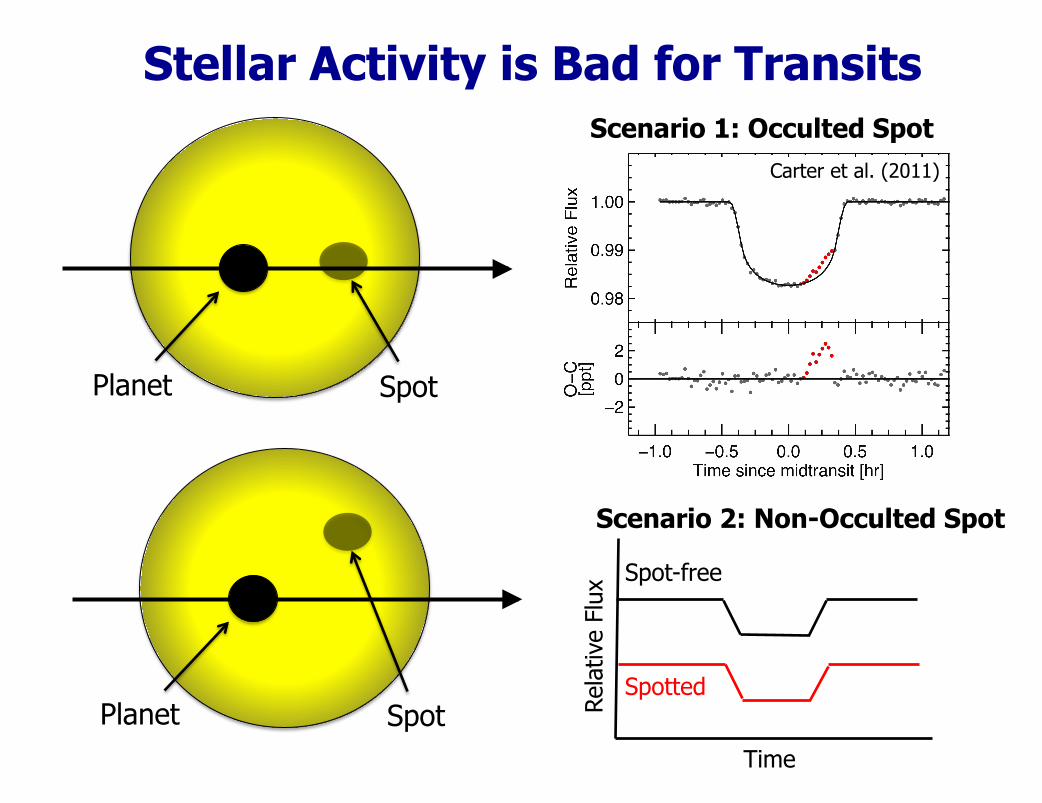
Stellar Activity is Bad for Transits

Planet Spot

Scenario 1: Occulted Spot

Carter et al. (2011)

Planet Spot

Scenario 2: Non-Occulted Spot

Time

Rela

tive

Flux

Spot-free

Spotted

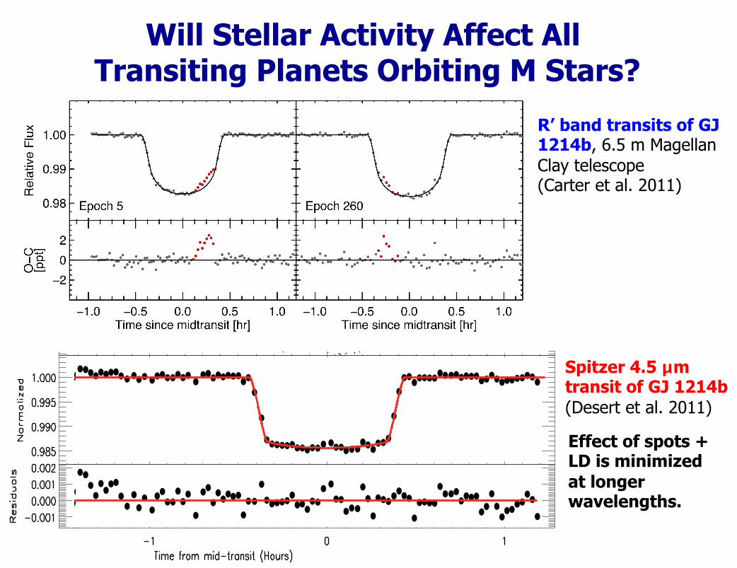
Will Stellar Activity Affect All Transiting Planets Orbiting M Stars?

R’ band transits of GJ 1214b, 6.5 m Magellan Clay telescope (Carter et al. 2011)

Spitzer 4.5 μm transit of GJ 1214b (Desert et al. 2011)

Effect of spots + LD is minimized at longer wavelengths.

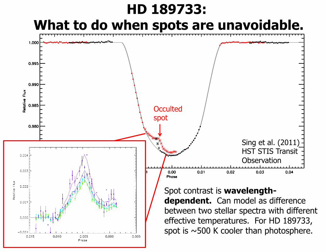
HD 189733: What to do when spots are unavoidable.

Sing et al. (2011) HST STIS Transit Observation

Spot contrast is wavelength-dependent. Can model as difference between two stellar spectra with different effective temperatures. For HD 189733, spot is ~500 K cooler than photosphere.

Occulted spot

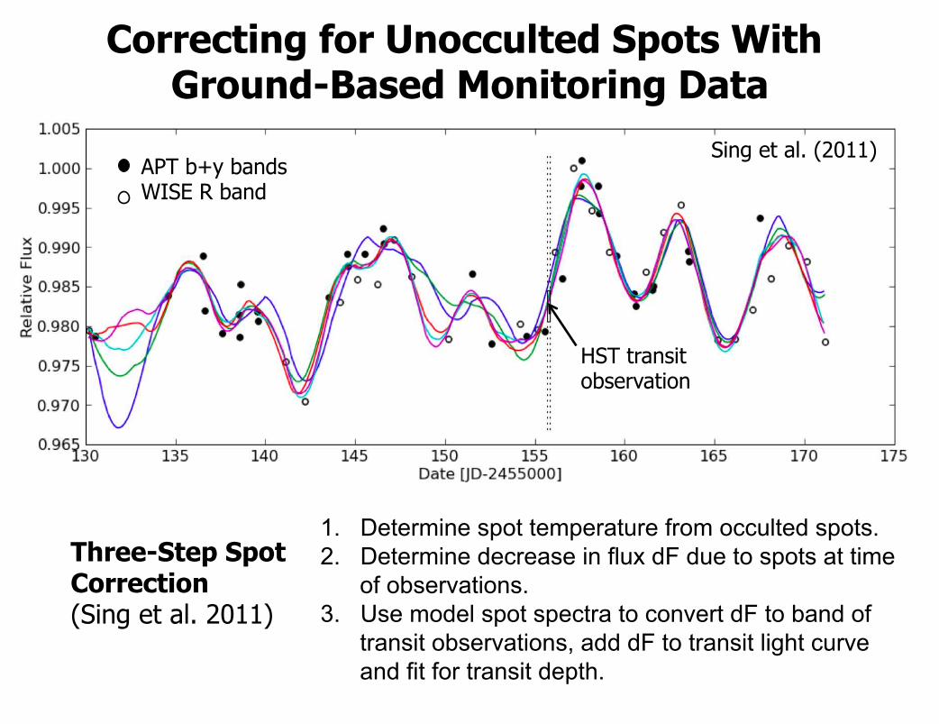
Correcting for Unocculted Spots With Ground-Based Monitoring Data

APT b+y bands WISE R band

Sing et al. (2011)

1.  Determine spot temperature from occulted spots. 2.  Determine decrease in flux dF due to spots at time

of observations. 3.  Use model spot spectra to convert dF to band of

transit observations, add dF to transit light curve and fit for transit depth.

Three-Step Spot Correction (Sing et al. 2011)

HST transit observation

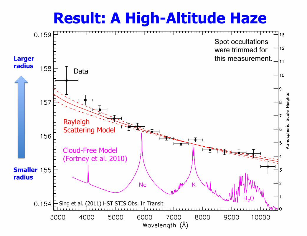
Result: A High-Altitude Haze

Sing et al. (2011) HST STIS Obs. In Transit

Rayleigh Scattering Model

Data

Larger radius

Smaller radius

Cloud-Free Model (Fortney et al. 2010)

Spot occultations were trimmed for this measurement.

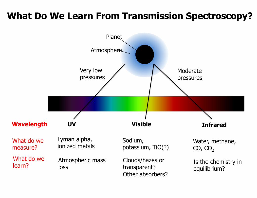
What Do We Learn From Transmission Spectroscopy?

UV Visible Infrared

Lyman alpha, ionized metals

Atmospheric mass loss

Wavelength

What do we measure?

What do we learn?

Very low pressures

Moderate pressures

Sodium, potassium, TiO(?)

Clouds/hazes or transparent? Other absorbers?

Water, methane, CO, CO2

Is the chemistry in equilibrium?

Atmosphere

Planet

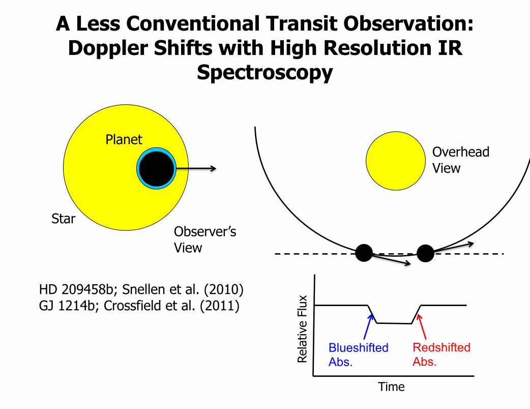
A Less Conventional Transit Observation: Doppler Shifts with High Resolution IR

Spectroscopy

HD 209458b; Snellen et al. (2010) GJ 1214b; Crossfield et al. (2011)

Planet

Star

Time

Rela

tive

Flux

Blueshifted Abs.

Redshifted Abs.

Overhead View

Observer’s View

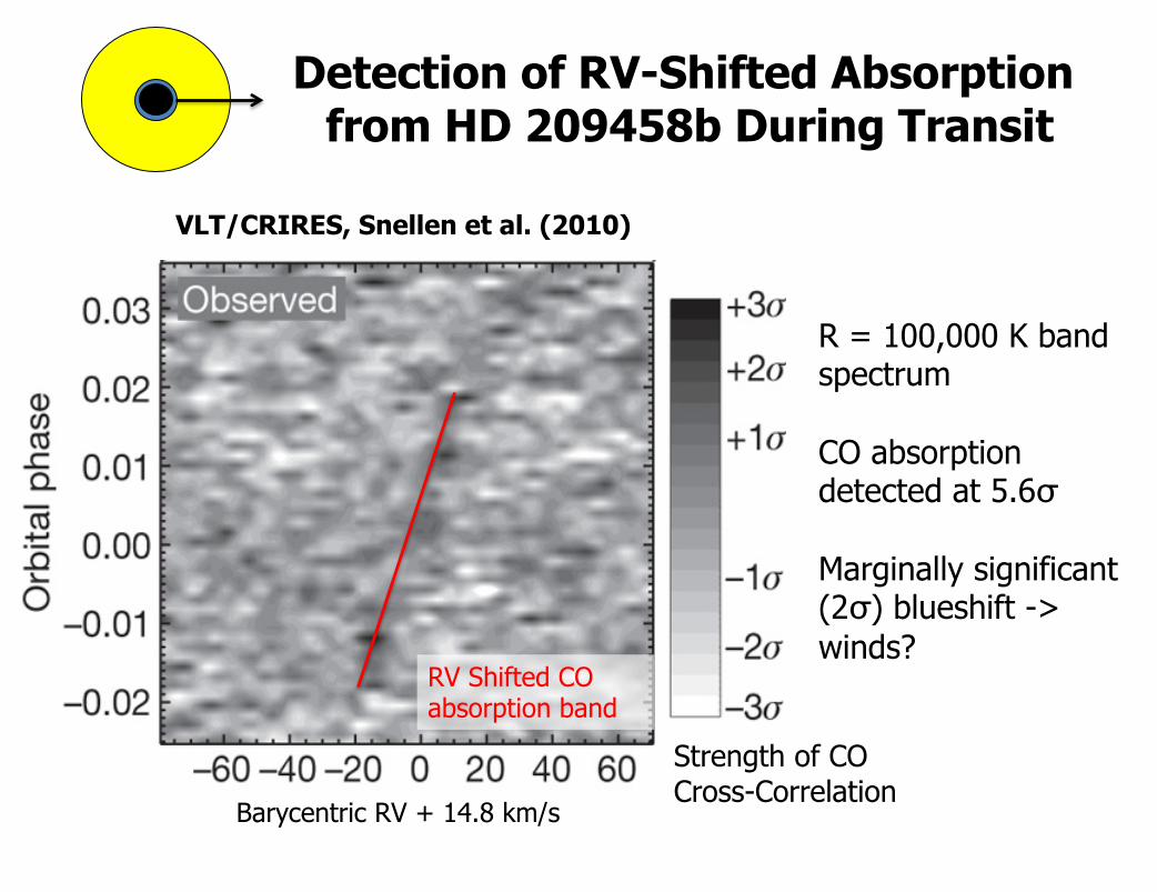
Detection of RV-Shifted Absorption from HD 209458b During Transit

Barycentric RV + 14.8 km/s

RV Shifted CO absorption band

R = 100,000 K band spectrum CO absorption detected at 5.6σ Marginally significant (2σ) blueshift -> winds?

Strength of CO Cross-Correlation

VLT/CRIRES, Snellen et al. (2010)

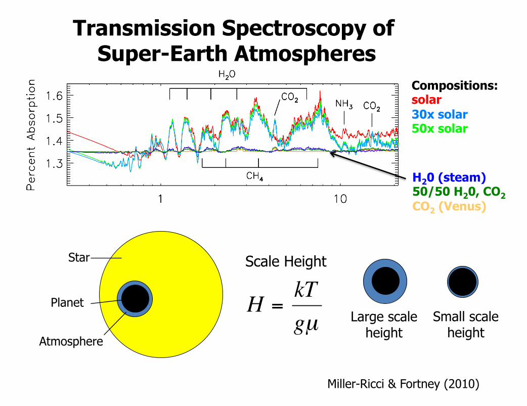
Transmission Spectroscopy of Super-Earth Atmospheres  

Compositions: solar 30x solar 50x solar

H20 (steam) 50/50 H20, CO2 CO2 (Venus)

Miller-Ricci & Fortney (2010)

Atmosphere

Star

Planet

Scale Height

!

H =kTgµ Large scale

height Small scale

height

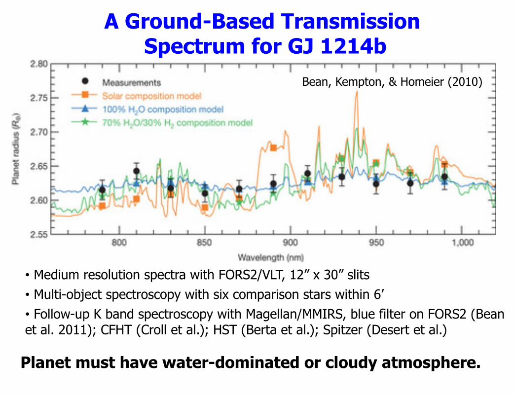
A Ground-Based Transmission Spectrum for GJ 1214b

Planet must have water-dominated or cloudy atmosphere.

Bean, Kempton, & Homeier (2010)

•  Medium resolution spectra with FORS2/VLT, 12” x 30” slits •  Multi-object spectroscopy with six comparison stars within 6’ •  Follow-up K band spectroscopy with Magellan/MMIRS, blue filter on FORS2 (Bean et al. 2011); CFHT (Croll et al.); HST (Berta et al.); Spitzer (Desert et al.)

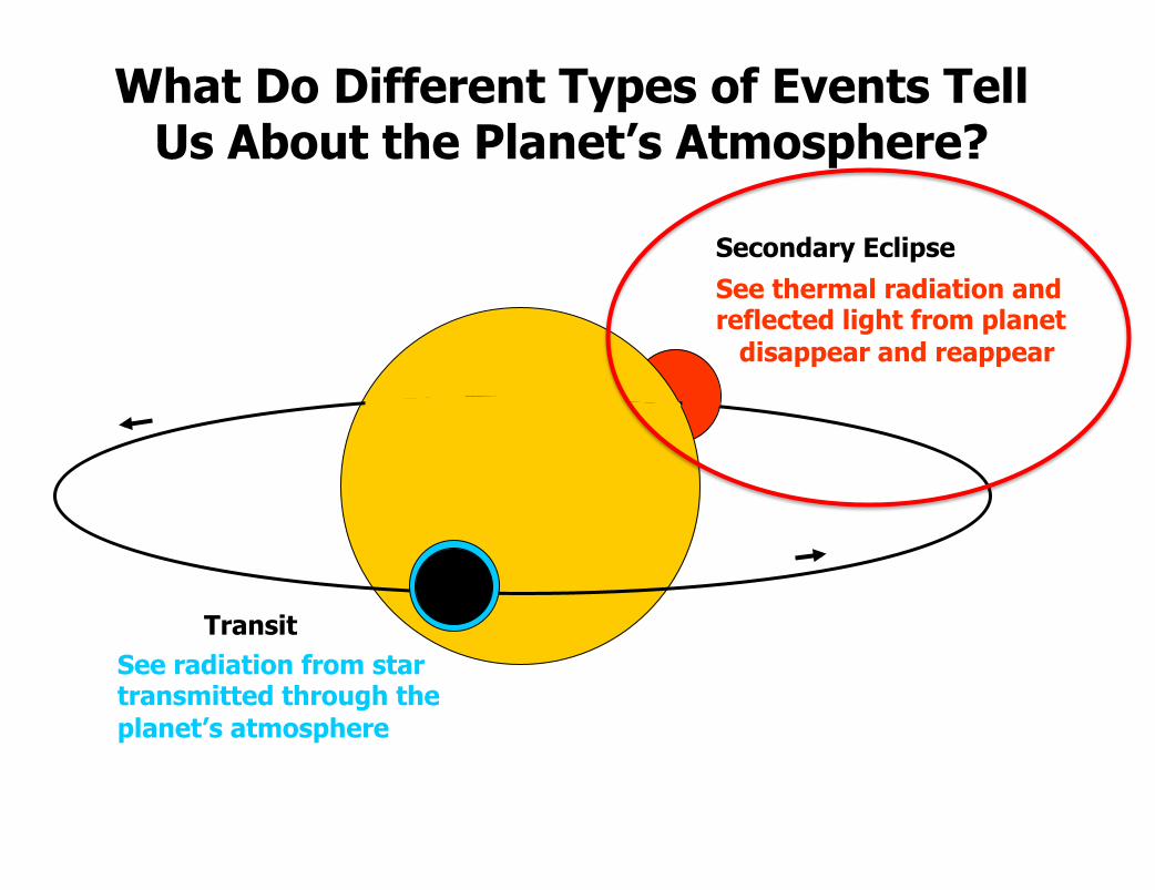
Transit

Secondary Eclipse

See thermal radiation and reflected light from planet disappear and reappear

See radiation from star transmitted through the planet’s atmosphere

What Do Different Types of Events Tell Us About the Planet’s Atmosphere?  

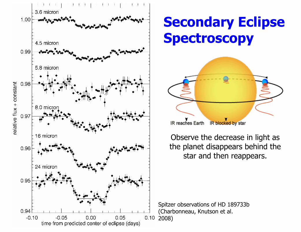
Spitzer observations of HD 189733b (Charbonneau, Knutson et al. 2008)

Observe the decrease in light as the planet disappears behind the

star and then reappears.

Secondary Eclipse Spectroscopy

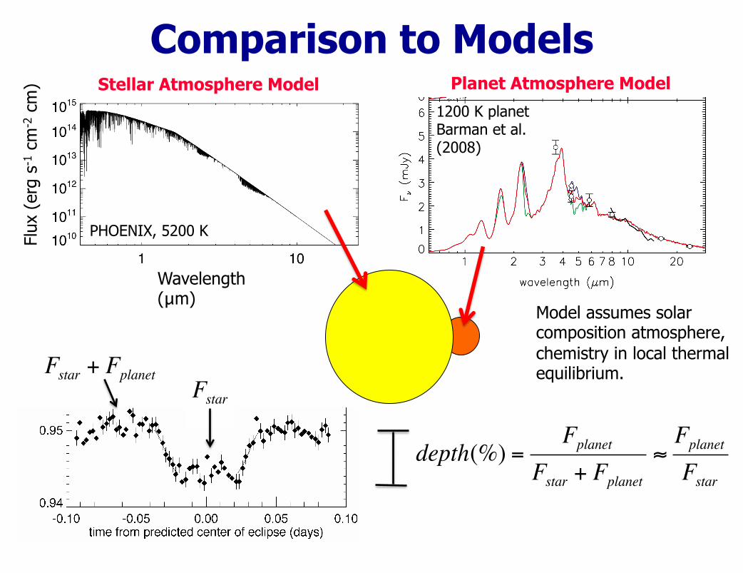
Comparison to Models

Wavelength (μm)

Flux

(er

g s-

1 cm

-2 c

m) Stellar Atmosphere Model

PHOENIX, 5200 K

1200 K planet Barman et al. (2008)

Planet Atmosphere Model

!

depth(%) =Fplanet

Fstar + Fplanet

"Fplanet

Fstar

Model assumes solar composition atmosphere, chemistry in local thermal equilibrium.

!

Fstar + Fplanet

!

Fstar

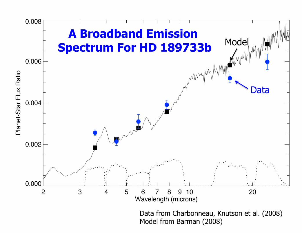
A Broadband Emission Spectrum For HD 189733b

Data from Charbonneau, Knutson et al. (2008) Model from Barman (2008)

Model

Data

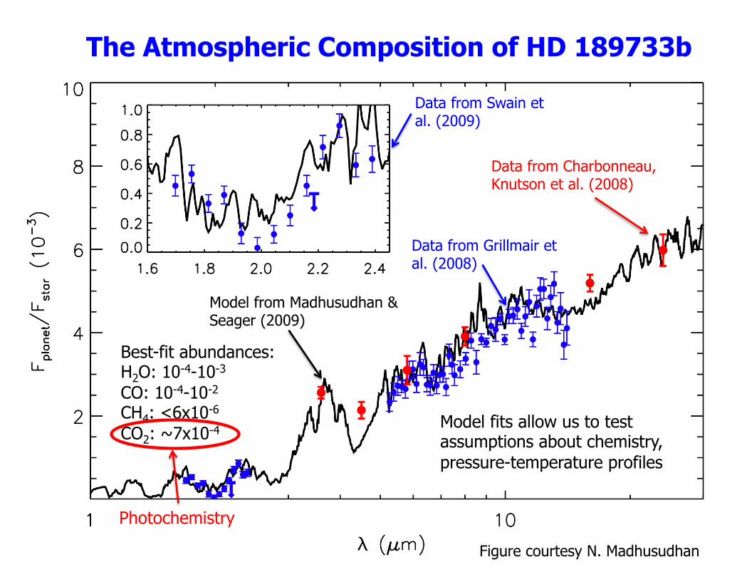
Best-fit abundances: H2O: 10-4-10-3

CO: 10-4-10-2

CH4: <6x10-6

CO2: ~7x10-4

Data from Charbonneau, Knutson et al. (2008)

Data from Grillmair et al. (2008)

Data from Swain et al. (2009)

The Atmospheric Composition of HD 189733b

Model from Madhusudhan & Seager (2009)

Model fits allow us to test assumptions about chemistry, pressure-temperature profiles

Photochemistry

Figure courtesy N. Madhusudhan

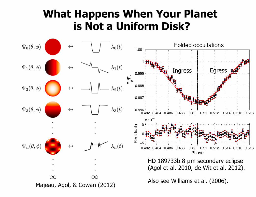
What Happens When Your Planet is Not a Uniform Disk?

Majeau, Agol, & Cowan (2012)

HD 189733b 8 μm secondary eclipse (Agol et al. 2010, de Wit et al. 2012).

Ingress Egress

Also see Williams et al. (2006).

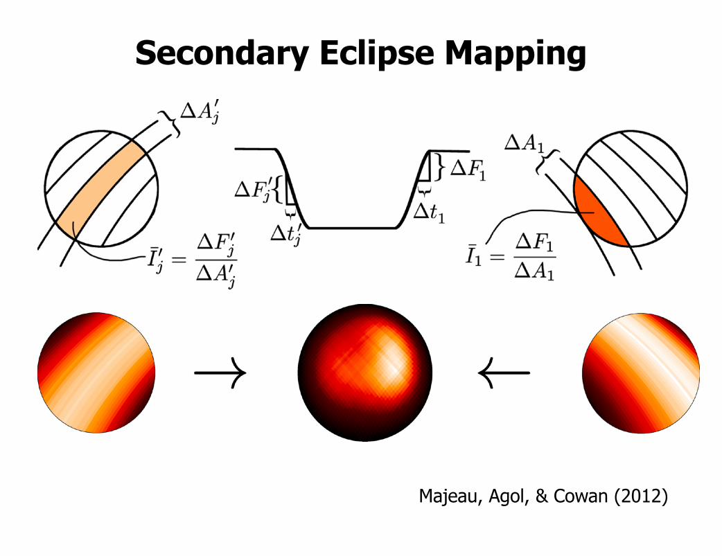
Secondary Eclipse Mapping

Majeau, Agol, & Cowan (2012)

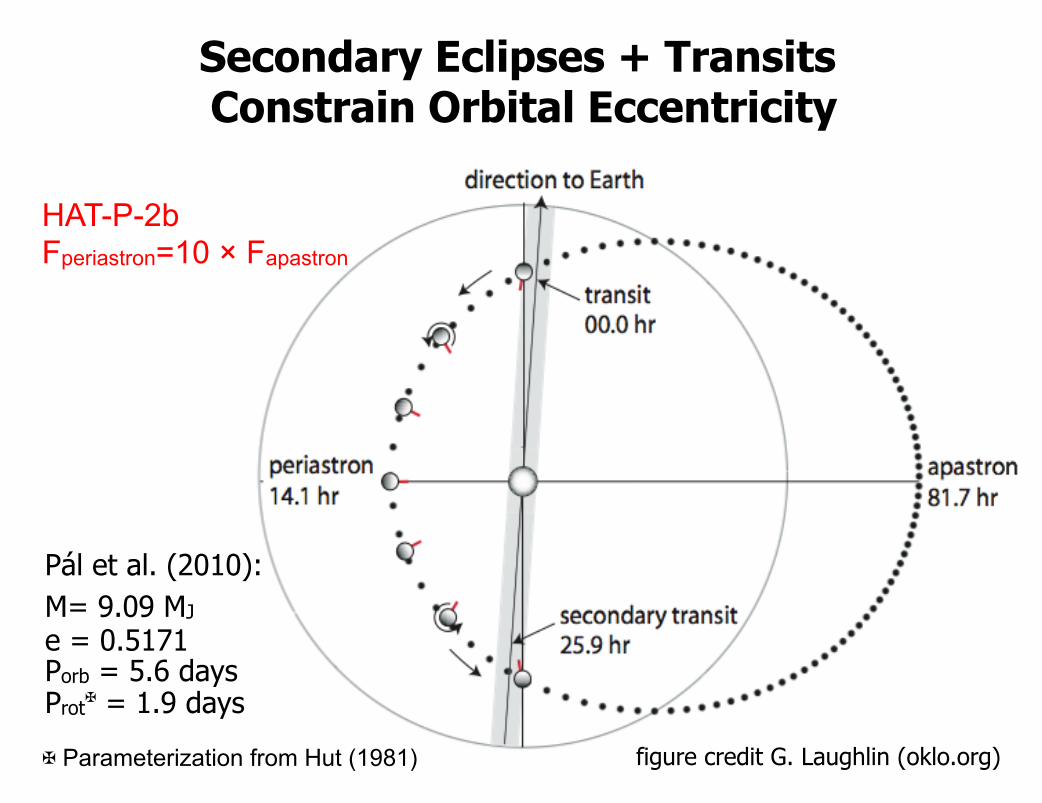
Pál et al. (2010): M= 9.09 MJ

e = 0.5171 Porb = 5.6 days Prot✠ = 1.9 days ✠ Parameterization from Hut (1981)

HAT-P-2b Fperiastron=10 × Fapastron

figure credit G. Laughlin (oklo.org)

Secondary Eclipses + Transits Constrain Orbital Eccentricity

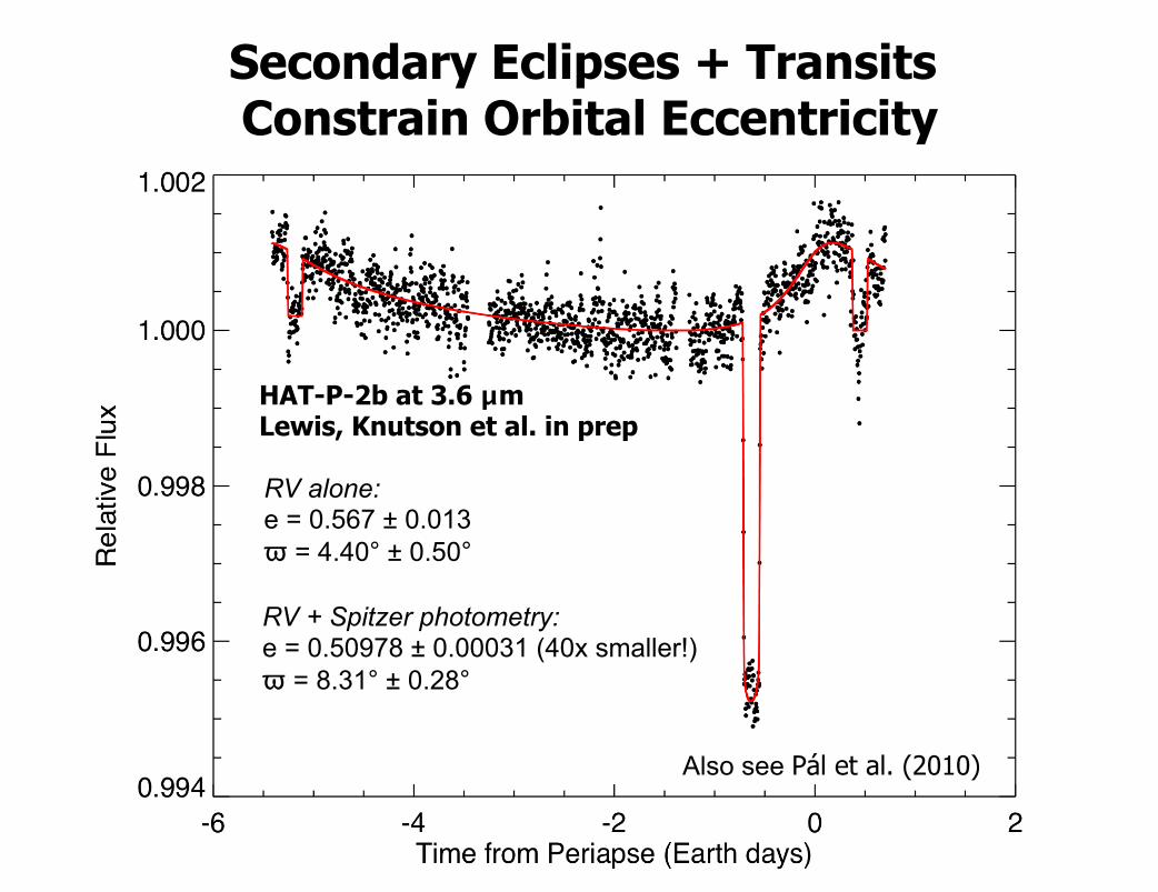
Secondary Eclipses + Transits Constrain Orbital Eccentricity  

HAT-P-2b at 3.6 μm Lewis, Knutson et al. in prep

RV alone: e = 0.567 ± 0.013 ϖ = 4.40° ± 0.50°

Also see Pál et al. (2010)

RV + Spitzer photometry: e = 0.50978 ± 0.00031 (40x smaller!) ϖ = 8.31° ± 0.28°

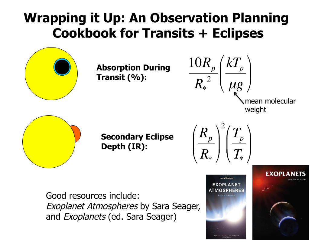
Wrapping it Up: An Observation Planning Cookbook for Transits + Eclipses

Absorption During Transit (%):

Secondary Eclipse Depth (IR): !

10Rp

R*2

kTpµg

"

# $

%

& '

!

Rp

R*

"

# $

%

& '

2 TpT*

"

# $

%

& '

Good resources include: Exoplanet Atmospheres by Sara Seager, and Exoplanets (ed. Sara Seager)

mean molecular weight

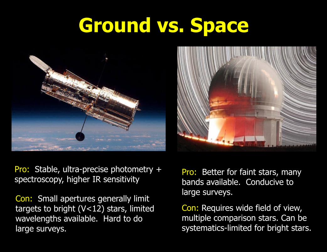
Ground vs. Space

Pro: Stable, ultra-precise photometry + spectroscopy, higher IR sensitivity

Con: Small apertures generally limit targets to bright (V<12) stars, limited wavelengths available. Hard to do large surveys.

Pro: Better for faint stars, many bands available. Conducive to large surveys.

Con: Requires wide field of view, multiple comparison stars. Can be systematics-limited for bright stars.

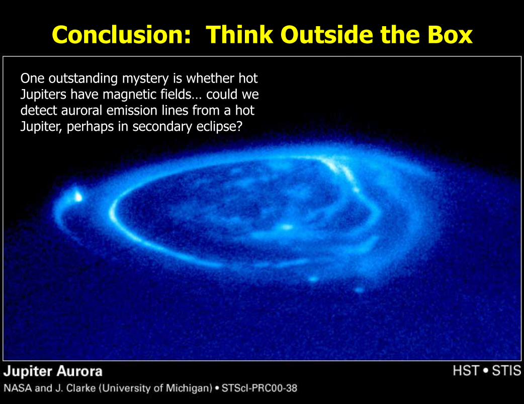
Conclusion: Think Outside the Box

One outstanding mystery is whether hot Jupiters have magnetic fields… could we detect auroral emission lines from a hot Jupiter, perhaps in secondary eclipse?