Invariant properties of cascaded six-pole networks - NAUN

Abstract— The invariant properties of input and output of two-port

circuits, established previously, are generalized for a multiport

network on the example of six-pole network.

The six-pole network is interpreted as two interconnected two-port

circuits because of final resistance of the general wire of these

circuits.

For the preset load conductivities, the projective coordinates of a

running regime point are introduced concerning of the characteristic

regime points, which set the projective coordinate systems on the

input and output of six-pole networks. The invariance or preservation

of the projective coordinate in these coordinate systems is shown.

The direct and reverse formulas of recalculation of currents and

non-uniform coordinates are obtained in the form of fractionally -

linear expressions of identical type.

The results allow separating or restoring two sensing signals via

input currents of the six-pole circuit or the three-wire line inputs

without determination of their transmission parameters.

Keywords— interference of loads, invariant properties, loading

characteristic, multi-port network, projective coordinates.

I. INTRODUCTION

N the electric circuits theory two-port networks are usually

considered, including their cascade connection with fixed

value of load conductivity [1]. But the special research of

influence of load changes reveals invariant properties of the

input and output regime parameters of such networks [2].

It is obvious, when there is the quantity expressed via

conductivities or currents, which keeps the value in all the sub

circuits or cross-section of circuit in the form of cascaded two-

port networks, then it is interesting for the theory and useful in

practice.

It is natural to discuss the question about detection of

invariant properties of multiport networks on an example of

the six-pole network which contains two output loads and two

input voltage sources. In this case, the interference of load

conductivities is observed. This six-pole network can be

interpreted as two interconnected two-port networks. In

practice, it can be the manifestation of final resistance of the

general wire of two circuits. The three-wire communication

line with use, for example, of physical "earth" as the third wire

can also be the example of such circuit.

A. Penin is with the Institute of Electronic Engineering and

Nanotechnologies “D. Ghitu”, Academy of Sciences of Moldova,

e-mail: [email protected]

II. PROJECTIVE COORDINATES OF A SIX-POLE NETWORK

OUTPUT

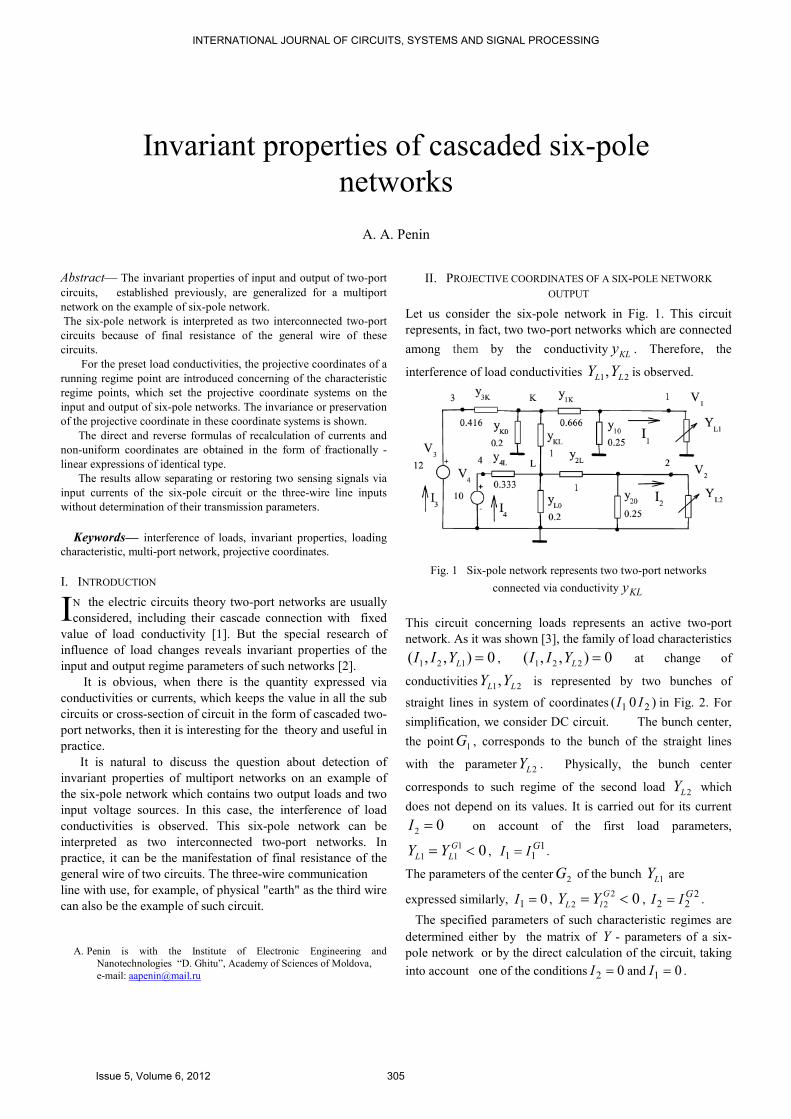
Let us consider the six-pole network in Fig. 1. This circuit

represents, in fact, two two-port networks which are connected

among them by the conductivityKLy . Therefore, the

interference of load conductivities 21, LL YY is observed.

Fig. 1 Six-pole network represents two two-port networks

connected via conductivity KLy

This circuit concerning loads represents an active two-port

network. As it was shown [3], the family of load characteristics

0),,( 121 =LYII , 0),,( 221 =LYII at change of

conductivities 21, LL YY is represented by two bunches of

straight lines in system of coordinates )0( 21 II in Fig. 2. For

simplification, we consider DC circuit. The bunch center,

the point1G , corresponds to the bunch of the straight lines

with the parameter2LY . Physically, the bunch center

corresponds to such regime of the second load 2LY which

does not depend on its values. It is carried out for its current

02 =I on account of the first load parameters,

01

11 <= G

LL YY , 1

11GII = .

The parameters of the center2G of the bunch

1LY are

expressed similarly, 01 =I , 02

22 <= G

lL YY ,2

22GII = .

The specified parameters of such characteristic regimes are

determined either by the matrix of Y - parameters of a six-

pole network or by the direct calculation of the circuit, taking

into account one of the conditions 02 =I and 01 =I .

Invariant properties of cascaded six-pole

networks

A. A. Penin

I

INTERNATIONAL JOURNAL OF CIRCUITS, SYSTEMS AND SIGNAL PROCESSING

Issue 5, Volume 6, 2012 305

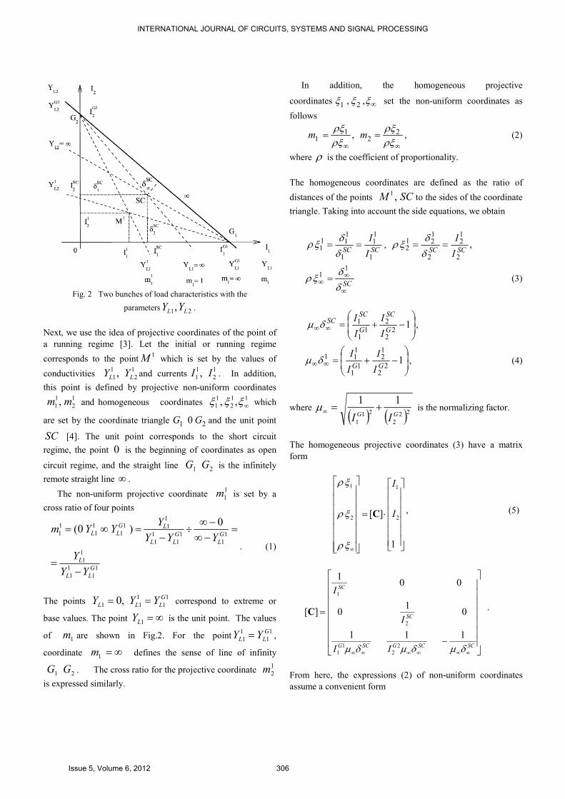
Fig. 2 Two bunches of load characteristics with the

parameters 21, LL YY .

Next, we use the idea of projective coordinates of the point of

a running regime [3]. Let the initial or running regime

corresponds to the point1M which is set by the values of

conductivities 1

2

1

1, LL YY and currents1

2

1

1 , II . In addition,

this point is defined by projective non-uniform coordinates 1

2

1

1 , mm and homogeneous coordinates 11

2

1

1 ,, ∞ξξξ which

are set by the coordinate triangle 21 0GG and the unit point

SC [4]. The unit point corresponds to the short circuit

regime, the point 0 is the beginning of coordinates as open

circuit regime, and the straight line 21 GG is the infinitely

remote straight line ∞ .

The non-uniform projective coordinate 1

1m is set by a

cross ratio of four points

1

1

1

1

1

1

1

1

1

1

1

1

1

11

1

1

1

1

1

0)0(

G

LL

L

G

L

G

LL

LG

LL

YY

Y

YYY

YYYm

−=

=−∞−∞

÷−

=∞=

. (1)

The points 1

1

1

11 ,0 G

LLL YYY == correspond to extreme or

base values. The point ∞=1LY is the unit point. The values

of 1m are shown in Fig.2. For the point1

1

1

1

G

LL YY = ,

coordinate ∞=1m defines the sense of line of infinity

21 GG . The cross ratio for the projective coordinate 1

2m

is expressed similarly.

In addition, the homogeneous projective

coordinates ∞ξξξ ,, 21 set the non-uniform coordinates as

follows

,11

∞=

ρξρξ

m∞

=ρξρξ2

2m , (2)

where ρ is the coefficient of proportionality.

The homogeneous coordinates are defined as the ratio of

distances of the points SCM ,1to the sides of the coordinate

triangle. Taking into account the side equations, we obtain

SCSC I

I

1

11

1

111

1 ==δ

δξρ , ,

2

12

2

121

2 SCSC I

I==

δ

δξρ

SC∞

∞∞ =

δ

δξρ

11

(3)

−+=∞∞ 1

22

2

11

1

G

SC

G

SCSC

I

I

I

Iδµ ,

−+=∞∞ 1

22

12

11

111

GG I

I

I

Iδµ , (4)

where

( ) ( )22

2

21

1

11

GG II+=∞µ is the normalizing factor.

The homogeneous projective coordinates (3) have a matrix

form

⋅=

∞1

][ 2

1

2

1

I

I

C

ξρ

ξρ

ξρ

, (5)

−

=

∞∞∞∞∞∞SCSCGSCG

SC

SC

II

I

I

δµδµδµ111

01

0

001

][

2

2

1

1

2

1

C.

From here, the expressions (2) of non-uniform coordinates

assume a convenient form



SCSCGSCG

SC

I

I

I

I

II

m

∞∞∞∞∞∞

−+=

δµδµδµ

1

1

22

2

11

1

1

11 ,

SCSCGSCG

SC

I

I

I

I

II

m

∞∞∞∞∞∞

−+=

δµδµδµ

1

1

22

2

11

1

2

22 . (6)

The inverse transformation

⋅=

∞

−

ξ

ξ

ξ

ρ

ρ

ρ

2

1

12

1

][

1

CI

I

, (7)

−

=

∞∞

−

SC

G

SC

G

SC

SC

SC

I

I

I

I

I

I

δµ2

2

2

1

1

1

2

1

1 00

00

][C ,

where the components of current vector define homogeneous

coordinates of a current.

From here, we find the current

==1

11 ρ

ρ II

SC

G

SC

G

SC

SC

mI

Im

I

I

mI

∞∞−⋅+⋅

⋅

δµ222

211

1

1

11 ,

SC

G

SC

G

SC

SC

mI

Im

I

I

mII

∞∞−⋅+⋅

⋅=

δµ222

211

1

1

222 . (8)

III. PROJECTIVE COORDINATES OF A SIX-POLE NETWORK INPUT

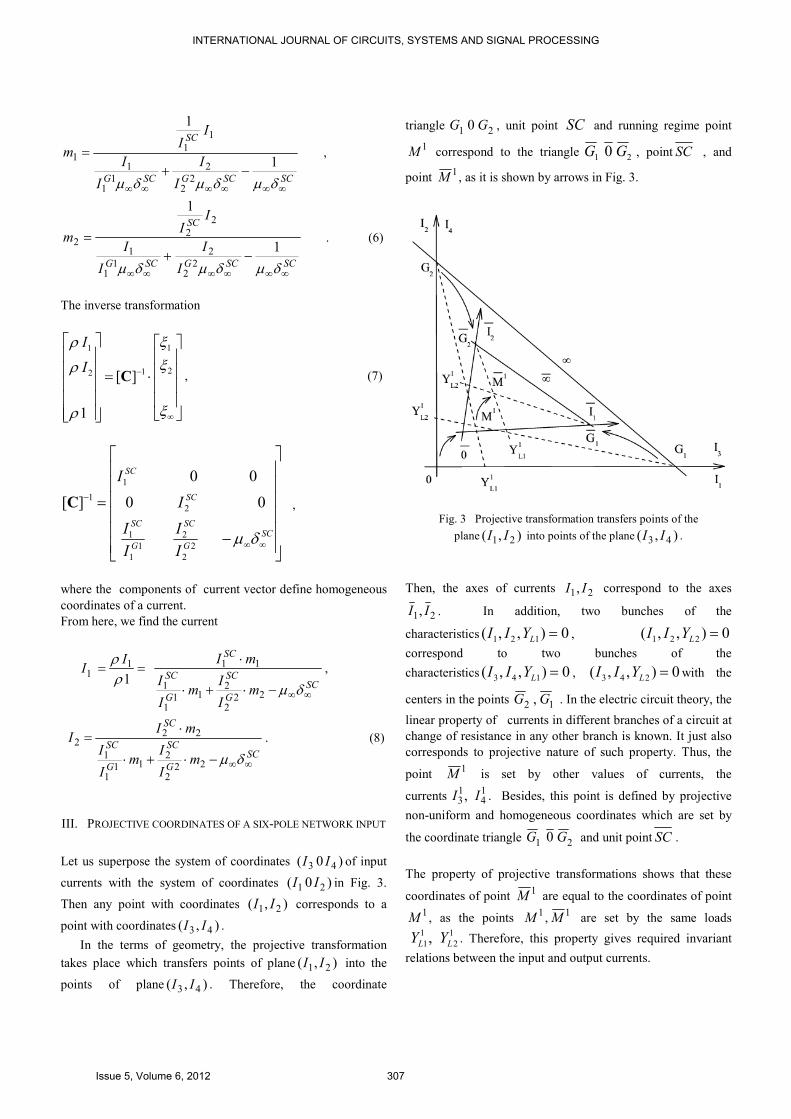
Let us superpose the system of coordinates )0( 43 II of input

currents with the system of coordinates )0( 21 II in Fig. 3.

Then any point with coordinates ),( 21 II corresponds to a

point with coordinates ),( 43 II .

In the terms of geometry, the projective transformation

takes place which transfers points of plane ),( 21 II into the

points of plane ),( 43 II . Therefore, the coordinate

triangle 21 0 GG , unit point SC and running regime point

1M correspond to the triangle21 0 GG , point SC , and

point 1M , as it is shown by arrows in Fig. 3.

Fig. 3 Projective transformation transfers points of the

plane ),( 21 II into points of the plane ),( 43 II .

Then, the axes of currents 21, II correspond to the axes

21, II . In addition, two bunches of the

characteristics 0),,( 121 =LYII , 0),,( 221 =LYII

correspond to two bunches of the

characteristics 0),,( 143 =LYII , 0),,( 243 =LYII with the

centers in the points 12 , GG . In the electric circuit theory, the

linear property of currents in different branches of a circuit at

change of resistance in any other branch is known. It just also

corresponds to projective nature of such property. Thus, the

point 1M is set by other values of currents, the

currents14

13 , II . Besides, this point is defined by projective

non-uniform and homogeneous coordinates which are set by

the coordinate triangle 21 0 GG and unit point SC .

The property of projective transformations shows that these

coordinates of point 1M are equal to the coordinates of point

1M , as the points 1M ,

1M are set by the same loads 1

2

1

1, LL YY . Therefore, this property gives required invariant

relations between the input and output currents.



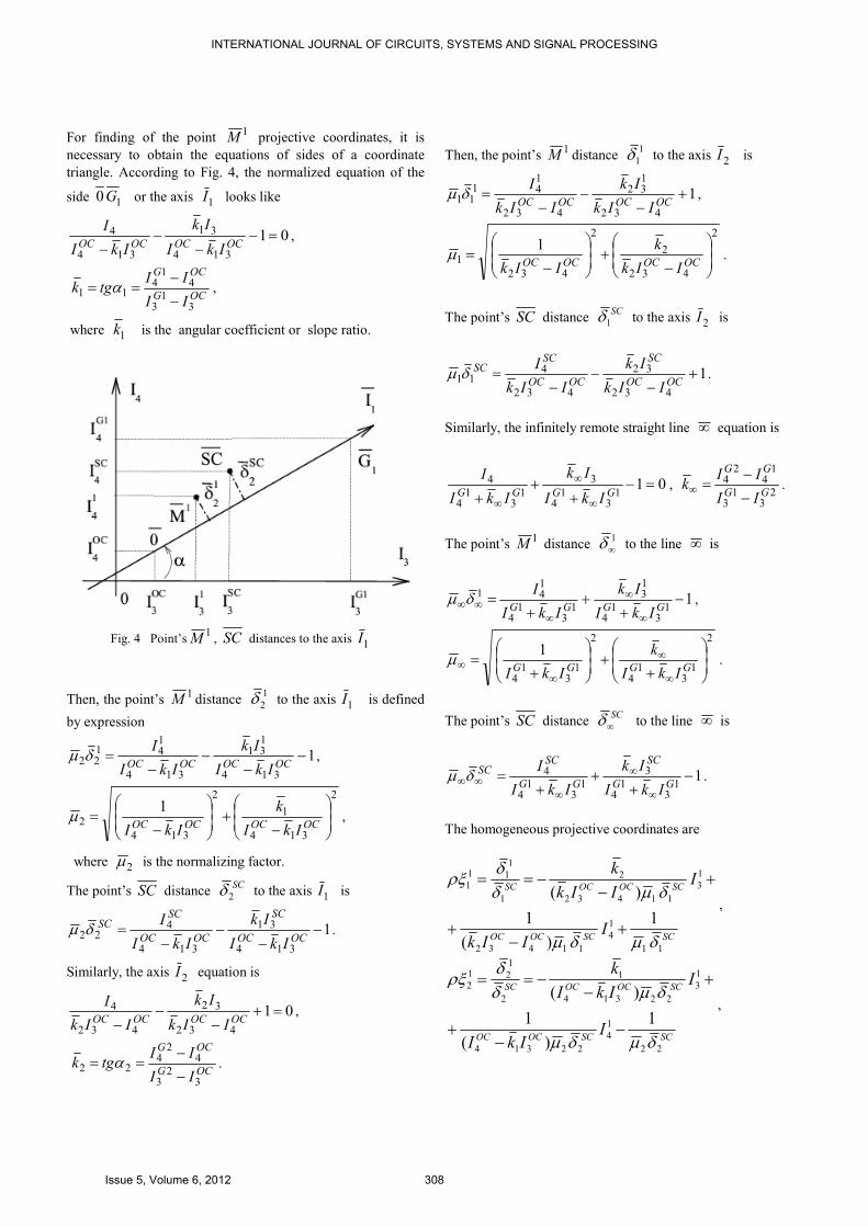
For finding of the point 1M projective coordinates, it is

necessary to obtain the equations of sides of a coordinate

triangle. According to Fig. 4, the normalized equation of the

side 10G or the axis 1I looks like

01

314

31

314

4 =−−

−− OCOCOCOC IkI

Ik

IkI

I,

OCG

OCG

II

IItgk

31

3

41

411

−

−== α ,

where 1k is the angular coefficient or slope ratio.

Fig. 4 Point’s1M , SC distances to the axis 1I

Then, the point’s 1M distance

1

2δ to the axis 1I is defined

by expression

1

314

131

314

141

22 −−

−−

=OCOCOCOC IkI

Ik

IkI

Iδµ ,

2

314

1

2

314

2

1

−+

−=

OCOCOCOC IkI

k

IkIµ ,

where 2µ is the normalizing factor.

The point’s SC distance SC

2δ to the axis 1I is

1

314

31

314

422 −

−−

−=

OCOC

SC

OCOC

SCSC

IkI

Ik

IkI

Iδµ .

Similarly, the axis 2I equation is

01

432

32

432

4 =+−

−− OCOCOCOC IIk

Ik

IIk

I,

OCG

OCG

II

IItgk

32

3

42

422

−

−== α .

Then, the point’s 1M distance

1


1

432

132

432

141

11 +−

−−

=OCOCOCOC IIk

Ik

IIk

Iδµ ,

2

432

2

2

432

1

1

−+

−=

OCOCOCOC IIk

k

IIkµ .



1

432

32

432

411 +

−−

−=

OCOC

SC

OCOC

SCSC

IIk

Ik

IIk

Iδµ .

Similarly, the infinitely remote straight line ∞ equation is

011

31

4

3

13

14

4 =−+

++ ∞

∞

∞GGGG IkI

Ik

IkI

I,

23

13

14

24

GG

GG

II

IIk

−

−=∞ .

The point’s 1M distance

1

∞δ to the line ∞ is

11

31

4

13

13

14

141 −

++

+=

∞

∞

∞∞∞ GGGG IkI

Ik

IkI

Iδµ ,

2

13

14

2

13

14

1

++

+=

∞

∞

∞∞ GGGG IkI

k

IkIµ .


∞δ to the line ∞ is

11

31

4

3

13

14

4 −+

++

=∞

∞

∞∞∞ GG

SC

GG

SCSC

IkI

Ik

IkI

Iδµ .

The homogeneous projective coordinates are

SCSCOCOC

SCOCOCSC

IIIk

IIIk

k

11

1

4

11432

1

3

11432

2

1

1

11

1

1

)(

1

)(

δµδµ

δµδδ

ρξ

+−

+

+−

−==

,

SCSCOCOC

SCOCOCSC

IIkI

IIkI

k

22

1

4

22314

1

3

22314

1

2

1

21

2

1

)(

1

)(

δµδµ

δµδδ

ρξ

−−

+

+−

−==

,



SCSCGG

SCGGSC

IIkI

IIkI

k

∞∞∞∞∞

∞∞∞

∞

∞

∞∞

−+

+

++

==

δµδµ

δµδδ

ρξ

1

)(

1

)(

1

41

3

1

4

1

31

3

1

4

11

.

and have a matrix form

⋅=

∞1

][ 4

3

2

1

I

I

C

ξρ

ξρ

ξρ

,

−

−−

−

=

∞∞∞SC

SC

SC

k

CC

k

CC

k

CC

δµ

δµ

δµ

1

1

1

][

3131

221

2121

112

1111

C , (9)

where the constituents of matrix are

SCOCOC IIk

kC

11432

211

)( δµ−= ,

SCOCOC IkI

kC

22314

121

)( δµ−= ,

SCGG IkI

kC

∞∞∞

∞

+=

δµ)( 13

14

31

From here, the non-uniform coordinates have the form similar

to (6)

SC

SC

Ik

CIC

Ik

CIC

m

∞∞∞

−+

++−=

δµ

δµ1

1

431

331

11

4

2

11311

1,

SC

SC

Ik

CIC

Ik

CIC

m

∞∞∞

−+

−+−=

δµ

δµ1

1

431

331

22

4

1

21321

2 (10)

The obtained expressions have a general appearance in

comparison to (6) because of nonorthogonal

coordinates 21 0 II . Thus, in practice, the characteristic values

of input and output currents (vertexes of coordinate triangles)

and the characteristic load values are precomputed or

preprogrammed by the calculation or testing the six-pole

network. Further, using the running values of input currents,

we find or, more precisely, restore the values of non-uniform

coordinates (10) and given load conductivities according to the

expressions )(),( 2211 mYmY HH which are reverse to

expression (1).

The formulated algorithm represents practical interest for

transfer of two sensing signals via an unstable six-pole

network or a three-wire line; it is by analogy to the signal

transmission via a two-port network [2].

Two cascaded six-pole networks. Let us consider the

cascaded six-pole networks in the Fig. 5.

Fig. 5 Cascaded six-pole networks.

Similarly, we superpose the system of coordinates )0( 65 II of

input currents of the first six-pole network with the matrix

63−Y of Y parameters with the systems of

coordinates )0( 43 II , )0( 21 II . Then, the projective

transformation, which transfers the plane ),( 21 II points to the

plane ),( 65 II points, takes place. Therefore, the coordinate

triangle 21 0 GG corresponds to the triangle 21

~0~~GG in

Fig.6.

Also, the unit point SC , the running regime point 1M

will correspond to the points CS~~

, 1~

M . Moreover, two

bunches of characteristics 0),,( 121 =LYII ,

0),,( 221 =LYII correspond to two bunches of characteristics

0),,( 165 =LYII , 0),,( 265 =LYII with the point centers

12

~,

~GG .



Fig. 6 Mapping of the coordinate triangles.

Too, the point 1~

M is defined by the projective non-

uniform and homogeneous coordinates which are set by the

coordinate triangle 21

~0~~GG and the unit point CS

~~. These

projective coordinates of the point 1~

M are equal to the

projective coordinates of the points 1M ,

1M according to

the property of projective transformations. Thus, the invariant

relationships between the input and output currents of

cascaded six-pole networks take place.

The projective coordinates of the point 1~

M are obtained

similarly to projective coordinates of the point 1M . For this

purpose, it is necessary to form the sides equations of the

triangle 21

~0~~GG .

IV. INVARIANCE OF REGIME CHANGES

Besides the invariance of projective coordinates, for example,

in the form of non-uniform coordinates (1), the invariance of

changes of these non-uniform coordinates on account of

changes of load conductivities takes place. Let the subsequent

regime corresponds to the point 2M with the parameters of

loads2

2

2

1, LL YY , currents22

21 , II , and non-uniform

coordinates22

21 , mm .

The subsequent currents according to (7), (8)

SC

G

SC

G

SC

SC

mI

Im

I

I

mII

∞∞−⋅+⋅

⋅=

δµ222

2

2211

1

1

2112

1 ,

SC

G

SC

G

SC

SC

mI

Im

I

I

mII

∞∞−⋅+⋅

⋅=

δµ222

2

2211

1

1

2222

2 . (11)

Further, we are using the results [3]. Let us present the

subsequent values of non-uniform coordinates via the initial

values 1

2

1

1 , mm and their changes212

211 , mm

1

1121

111

211

21

∞

⋅=⋅=ξ

ξmmmm ,

1

1221

212

212

22

∞

⋅=⋅=ξ

ξmmmm . (12)

Then, the expressions (11) are

11

2

21

22

2

21

1

21

11

1

1

1

1

21

112

1

∞∞∞−⋅⋅+⋅⋅

⋅⋅=

ξδµξξ

ξ

SC

G

SC

G

SC

SC

mI

Im

I

I

mII ,

11

2

21

22

2

21

1

21

11

1

1

1

2

21

222

2

∞∞∞−⋅⋅+⋅⋅

⋅⋅=

ξδµξξ

ξ

SC

G

SC

G

SC

SC

mI

Im

I

I

mII ,

or takes the matrix form

⋅⋅=

=

⋅

⋅=

∞

−

∞

−

1

12

11

211

1

12

11

212

211

122

21

][][

100

00

00

][

1

ξ

ξ

ξ

ξ

ξ

ξ

ρ

ρ

ρ

mC

m

m

CI

I

.

Taking into account (5), we obtain

⋅=

⋅⋅⋅=

−

1

][

1

][][][

1

12

11

2112

11

21122

21

I

I

MI

I

CmCI

I

ρ

ρ

ρ

, (13)

where the matrix of current changes is



−−

=

=

111

00

00

1

00

00

][

22

212

11

211

212

211

2132

2131

2122

2111

21

GG I

m

I

m

m

m

MM

M

M

M . (14)

The obtained relationship (13) allows carrying out the

recalculation of the load currents for the preset value of load

changes in the form of non-uniform coordinate changes.

These changes of non-uniform coordinates are also true for

input currents. Therefore, it is possible to obtain similar

relationships for recalculation of the input currents.

The reverse transformation to the (9) is

⋅=

∞

−

ξ

ξ

ξ

ρ

ρ

ρ

2

1

14

3

][

1

CI

I

, (15)

where

=

−−−

−−−

−−−

−

OCGG

OC

OC

G

G

G

G

IC

IC

IC

I

IC

I

IC

I

IC

CCC

3

1132

3

1121

3

111

3

41132

3

241

1213

141

11

113

112

111

1

111

][C ,

and the constituents of matrix are

SCG

GOC

OCOC

IIIkk

IIkC 11

131

3321

432111

))((δµ

−−

−=−

,

SCG

GOC

OCOC

IIIkk

IIkC 22

232

3321

431112

))((δµ

−−

−−=−

,

SCOC

GOC

GG

IIIkk

IIkC ∞∞

∞

∞−

−+

+= δµ31

331

14

131

13))((

.

From here, similarly to (11), we pass to the subsequent

currents

,111

3

113

222

3

112

211

3

111

113

22

112

21

1112

3

OCGG ICm

ICm

IC

CmCmCI

−−−

−−−

++

++=

OCGG

OC

OC

G

G

G

G

ICm

ICm

IC

I

ICm

I

ICm

I

IC

I

3

1

13

2

22

3

1

12

2

11

3

1

11

3

41

13

2

22

3

2

41

12

2

11

3

1

41

11

2

4 111 −−−

−−−

++

++= . (16)

The obtained expressions have a general appearance in

comparison to (11) because of nonorthogonal coordinates.

Convenience of reverse to each other the expressions (10),

(16) consists in their identical form. It is being reached on

account of change of variables; we replace the load

conductivities by the non-uniform projective coordinates, and

currents are already non-uniform coordinates.

Further, we use the changes of non-uniform coordinates

according to (12), and obtain the matrix expression

⋅⋅=

=

⋅

⋅=

∞

−

∞

−

1

12

11

211

1

12

11

212

211

124

23

][][

100

00

00

][

1

ξ

ξ

ξ

ξ

ξ

ξ

ρ

ρ

ρ

mC

C m

m

I

I

.

Using the transformation (9), we obtain

⋅=

⋅⋅⋅=

−

1

][

1

]][][

1

14

13

2114

13

21124

23

I

I

I

I

I

I

MC[mC

ρ

ρ

ρ

. (17)

If to carry out calculations, we receive the matrix ][21

M . The

matrix ][21

M of change of currents carries a general view in

comparison to (14).

Using the transformations (13), (17), we find the

subsequent currents

1111 1

222

2121

111

211

11

211

212

1

+⋅−

+⋅−

⋅==

II

mI

I

m

ImII

GG

ρρ

,

1

222

2 ρρI

I = , (18)



21

33

1

4

21

32

1

3

21

31

21

13

1

4

21

12

1

3

21

11

2

32

31 MIMIM

MIMIMII

+⋅+⋅+⋅+⋅

==ρρ

,

1

242

4 ρρI

I = . (19)

The calculation shows the equal values of the denominators of

the expressions (18), (19).

Example. The active network in Fig.1 is described by the

following system of the equations

]][[

4

3

2

1

44342414

34332313

24232212

14131211

4

3

2

1

UY=

−−−

−−−

−

−

=

U

U

U

U

YYYY

YYYY

YYYY

YYYY

I

I

I

I

,

[ ]

−−−

−−−

−

−

=

2803.0029.0159.00464.0

029.03247.0087.0147.0

159.0087.07727.01393.0

0464.0147.01393.06813.0

Y .

Hereinafter, the dimensions of values are not specified for

simplifying of record.

For the output of multiport we have the next results.

The parameters of the bunch centers 1G , 2G ,

1172.151

1 =GI , 7991.01

1 −=GLY ;

152

2 =GI , 9375.02

2 −=G

LY .

The short circuit currents, 636.2,229.2 21 == SCSC II .

The parameters of the initial regime, the point 1M

333.0,5.0 1

2

1

1 == LL YY , 8868.0,101.1 1

2

1

1 == II .

The non-uniform projective coordinates (1)

3848.07991.05.0

5.01

1

1

1

1

11

1 =+

=−

=G

LL

L

YY

Ym ,

2622.09375.0333.0

333.02

2

1

2

1

21

2 =+

=−

=G

LL

L

YY

Ym .

The homogeneous projective coordinates (3), (4)

4939.0229.2

101.1

1

1

11

1 ===SCI

Iξρ ,

3364.02

1

21

2 ==SCI

Iξρ , 2825.1

11 ==

∞

∞∞ SCδ

δξρ ,

where

868.0115

8868.0

1172.15

101.11 −=

−+=∞∞δµ ,

6768.0115

636.2

1172.15

229.2−=

−+=∞∞SCδµ .

Let us check up the values of the non-uniform projective

coordinates (2),

3851.02825.1

4939.011

1 ===∞ρξ

ρξm ,

2622.02825.1

3364.021

2 ===∞ρξ

ρξm .

Matrix [C] according to (5)

[ ]

⋅−

⋅−

=

6768.0

1

6768.015

1

6768.01172.15

1

06358.2

10

00229.2

1

C .

Let us check up the value of the non-uniform projective

coordinate (6)

286.1

494.0

6768.0

1

6768.015

8868.0

6768.01172.15

101.1

101.1229.2

1

11 =

+⋅

−⋅

−=m .

The inverse transformation matrix (7)

[ ]

=−

6768.01757.01474.0

06358.20

00229.21

C .

Then, the current (8)

101.17797.0

86.0

6768.02623.01757.03858.01474.0

3858.0229.211

==

=+⋅+⋅

⋅=I

.

For the input of multiport we have the next results.

The parameters of the bunch centers 1G , 2G

3886.61

3 =GI , 333.31

4 =GI , 52

3 =GI , 5

24 =GI .

The currents corresponding to the short circuit,

455.2,607.3 43 == SCSC II .



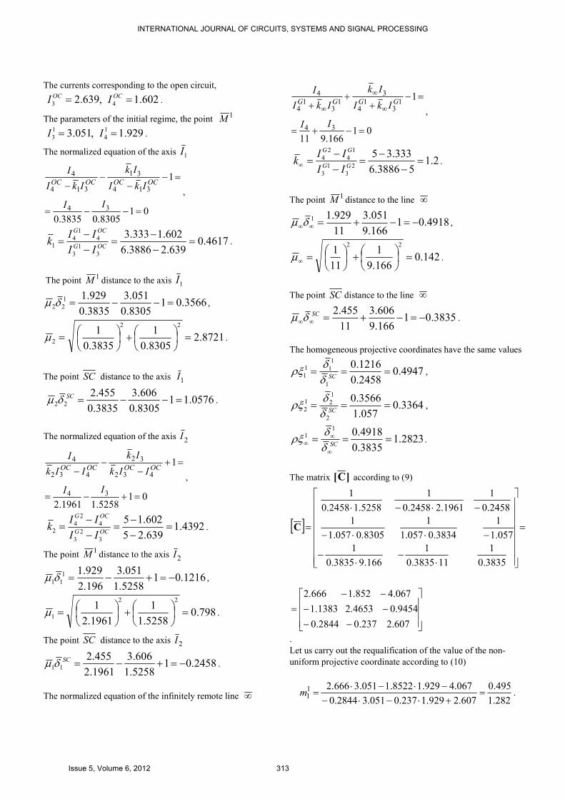
The currents corresponding to the open circuit,

602.1,639.2 43 == OCOC II .

The parameters of the initial regime, the point 1M

929.1,051.3 1

4

1

3 == II .

The normalized equation of the axis 1I

018305.03835.0

1

34

314

31

314

4

=−−=

=−−

−−

II

IkI

Ik

IkI

IOCOCOCOC

,

4617.0639.23886.6

602.1333.3

3

1

3

4

1

41 =

−−

=−−

=OCG

OCG

II

IIk .

The point 1M distance to the axis 1I

3566.018305.0

051.3

3835.0

929.11

22 =−−=δµ ,

8721.28305.0

1

3835.0

122

2 =

+

=µ .

The point SC distance to the axis 1I

0576.118305.0

606.3

3835.0

455.222 =−−=SCδµ .

The normalized equation of the axis 2I

015258.11961.2

1

34

432

32

432

4

=+−=

=+−

−−

II

IIk

Ik

IIk

IOCOCOCOC

,

4392.1639.25

602.15

3

2

3

4

2

42 =

−−

=−−

=OCG

OCG

II

IIk .

The point 1M distance to the axis 2I

1216.015258.1

051.3

196.2

929.11

11 −=+−=δµ ,

798.05258.1

1

1961.2

122

1 =

+

=µ .

The point SC distance to the axis 2I

2458.015258.1

606.3

1961.2

455.211 −=+−=SCδµ .

The normalized equation of the infinitely remote line ∞

01166.911

1

34

13

14

3

13

14

4

=−+=

=−+

++ ∞

∞

∞

II

IkI

Ik

IkI

IGGGG

,

2.153886.6

333.352

3

1

3

1

4

2

4 =−

−=

−−

=∞ GG

GG

II

IIk .

The point 1M distance to the line ∞

4918.01166.9

051.3

11

929.11 −=−+=∞∞δµ ,

142.0166.9

1

11

122

=

+

=∞µ .

The point SC distance to the line ∞

3835.01166.9

606.3

11

455.2−=−+=∞∞

SCδµ .

The homogeneous projective coordinates have the same values

4947.02458.0

1216.0

1

1

11

1 ===SCδ

δρξ ,

3364.0057.1

3566.0

2

1

21

2 ===SCδ

δρξ ,

2823.13835.0

4918.011 ===

∞

∞∞ SCδ

δρξ .

The matrix ]C[ according to (9)

[ ]

−−

−−

−−

=

=

⋅−

⋅−

−⋅⋅−

−⋅−⋅

=

607.2237.02844.0

9454.04653.21383.1

067.4852.1666.2

3835.0

1

113835.0

1

166.93835.0

1

057.1

1

3834.0057.1

1

8305.0057.1

1

2458.0

1

1961.22458.0

1

5258.12458.0

1

C

.

Let us carry out the requalification of the value of the non-

uniform projective coordinate according to (10)

282.1

495.0

607.2929.1237.0051.32844.0

067.4929.18522.1051.3666.211 =

+⋅−⋅−−⋅−⋅

=m .



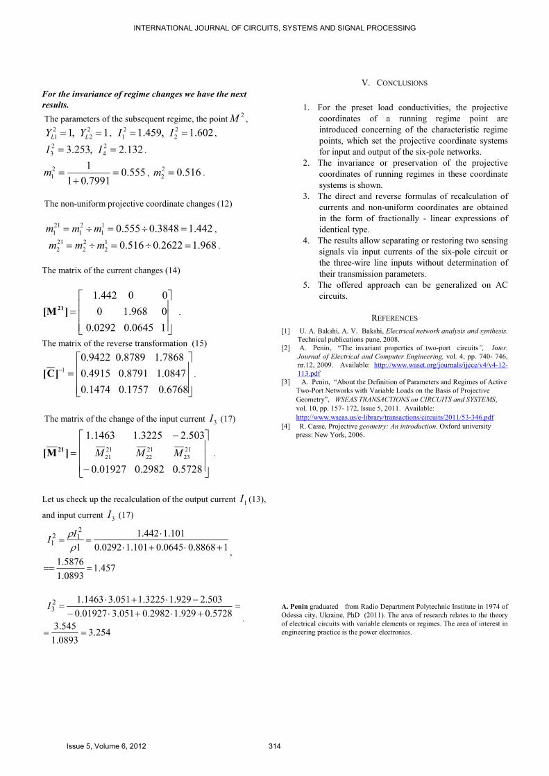
For the invariance of regime changes we have the next

results.

The parameters of the subsequent regime, the point2M ,

1,1 2

2

2

1 == LL YY , 602.1,459.1 2

2

2

1 == II ,

132.2,253.3 2

4

2

3 == II .

555.07991.01

12

1 =+

=m , 516.02

2 =m .

The non-uniform projective coordinate changes (12)

442.13848.0555.01

1

2

1

21

1 =÷=÷= mmm ,

968.12622.0516.01

2

2

2

21

2 =÷=÷= mmm .

The matrix of the current changes (14)

=

10645.00292.0

0968.10

00442.1

][M21.

The matrix of the reverse transformation (15)

=−

6768.01757.01474.0

0847.18791.04915.0

7868.18789.09422.01]C[ .

The matrix of the change of the input current 3I (17)

−

−

=

5728.02982.001927.0

503.23225.11463.1

21

23

21

22

21

21 MMM]M[ 21.

Let us check up the recalculation of the output current 1I (13),

and input current 3I (17)

457.10893.1

5876.1

18868.00645.0101.10292.0

101.1442.1

1

212

1

===

+⋅+⋅⋅

==ρ

ρII

,

254.30893.1

545.3

5728.0929.12982.0051.301927.0

503.2929.13225.1051.31463.123

==

=+⋅+⋅−

−⋅+⋅=I

.

V. CONCLUSIONS

1. For the preset load conductivities, the projective

coordinates of a running regime point are

introduced concerning of the characteristic regime

points, which set the projective coordinate systems

for input and output of the six-pole networks.

2. The invariance or preservation of the projective

coordinates of running regimes in these coordinate

systems is shown.

3. The direct and reverse formulas of recalculation of

currents and non-uniform coordinates are obtained

in the form of fractionally - linear expressions of

identical type.

4. The results allow separating or restoring two sensing

signals via input currents of the six-pole circuit or

the three-wire line inputs without determination of

their transmission parameters.

5. The offered approach can be generalized on AC

circuits.

REFERENCES

[1] U. A. Bakshi, A. V. Bakshi, Electrical network analysis and synthesis.

Technical publications pune, 2008.

[2] A. Penin, “The invariant properties of two-port circuits”, Inter.

Journal of Electrical and Computer Engineering, vol. 4, pp. 740- 746,

nr.12, 2009. Available: http://www.waset.org/journals/ijece/v4/v4-12-

113.pdf

[3] A. Penin, “About the Definition of Parameters and Regimes of Active

Two-Port Networks with Variable Loads on the Basis of Projective

Geometry”, WSEAS TRANSACTIONS on CIRCUITS and SYSTEMS,

vol. 10, pp. 157- 172, Issue 5, 2011. Available:

http://www.wseas.us/e-library/transactions/circuits/2011/53-346.pdf

[4] R. Casse, Projective geometry: An introduction. Oxford university

press: New York, 2006.

A. Penin graduated from Radio Department Polytechnic Institute in 1974 of

Odessa city, Ukraine, PhD (2011). The area of research relates to the theory

of electrical circuits with variable elements or regimes. The area of interest in

engineering practice is the power electronics.



Documents

Invariant properties of cascaded six-pole networks - NAUN