The Astrophysical Journal, 696:12–23, 2009 May 1 doi:10.1088/0004-637X/696/1/12C© 2009. The American Astronomical Society. All rights reserved. Printed in the U.S.A.

INVERTING COLOR–MAGNITUDE DIAGRAMS TO ACCESS PRECISE STAR CLUSTER PARAMETERS:A NEW WHITE DWARF AGE FOR THE HYADES

Steven DeGennaro1, Ted von Hippel

1,2, William H. Jefferys

1,3, Nathan Stein

1, David van Dyk

4,

and Elizabeth Jeffery1

1 Department of Astronomy, University of Texas at Austin, 1 University Station C1400, Austin, TX 78712-0259, USA; deg@astro.as.utexas.edu2 Visiting Scientist, Department of Physics, Florida International University, Miami, FL, USA

3 Department of Mathematics and Statistics, University of Vermont, Burlington, VT, USA4 Department of Statistics, University of California, Irvine, USA

Received 2008 June 5; accepted 2009 January 7; published 2009 April 13

ABSTRACT

We have extended our Bayesian modeling of stellar clusters—which uses main-sequence stellar evolutionmodels, a mapping between initial masses and white dwarf (WD) masses, WD cooling models, and WDatmospheres—to include binary stars, field stars, and two additional main-sequence stellar evolution models.As a critical test of our Bayesian modeling technique, we apply it to Hyades UBV photometry, with membershippriors based on proper motions and radial velocities, where available. Under the assumption of a particularset of WD cooling models and atmosphere models, we estimate the age of the Hyades based on coolingWDs to be 648 ± 45 Myr, consistent with the best prior analysis of the cluster main-sequence turnoff(MSTO) age by Perryman et al. Since the faintest WDs have most likely evaporated from the Hyades,prior work provided only a lower limit to the cluster’s WD age. Our result demonstrates the power ofthe bright WD technique for deriving ages and further demonstrates complete age consistency between WDcooling and MSTO ages for seven out of seven clusters analyzed to date, ranging from 150 Myr to 4 Gyr.

Key words: open clusters and associations: general – stars: evolution – white dwarfs

Online-only material: color figures

1. INTRODUCTION

Ages are fundamental in understanding astrophysical pro-cesses from the formation of planets to the formation of theUniverse. Yet, at present, we have precise ages for only theSolar System (4.566 ± 0.002 Gyr; Allegre et al. 1995) andthe Universe as a whole (13.7 ± 0.2 Gyr; Spergel et al. 2003,2007). For the ages of the Milky Way and its components, werely on two techniques that typically yield substantially less(� 20%) age precision, even with excellent data sets. Thesetwo techniques, based on the luminosity and/or color ofthe main-sequence turnoff (MSTO) and the luminosity ofwhite dwarfs (WDs), are based upon mature theories, thoughconsiderable technical difficulties remain in both theory andobservation.

Our goal is to improve the age precision of both the MSTOand WD techniques to ∼ 5%. Many investigators have collectedhigh-quality data sets, yet this 5% age precision is generallybeyond reach. Until the next generation of space-based trigono-metric parallaxes from satellites such as SIM and GAIA, weexpect no qualitative advances in precision of absolute photom-etry, stellar abundances, or cluster distances. In our judgment,the greatest gains we can currently make in age precision willcome from improved modeling techniques (see also Tosi et al.1991, 2007; Hernandez & Valls-Gabaud 2008). Any such mod-eling technique should both fully leverage the data we can collecttoday and provide a pathway to fully exploit the higher qualitydata we expect in the future.

We introduced our modeling technique in von Hippel et al.(2006, hereafter Paper I). Briefly, in paper I we developeda Bayesian technique that objectively incorporates our priorknowledge of stellar evolution, star cluster properties, and dataquality estimates to derive posterior probability distributions for

a cluster’s age, metallicity, distance, and line-of-sight absorp-tion. We simulated artificial data with a set of oft-used stellarevolution models and realistic photometric error, then recoveredthe posterior probability distributions of the cluster parametersas well as the masses for each star. We found that our techniqueyielded high precision for even modest numbers of cluster stars.For clusters with 50 to 400 members and one to a few dozenWDs, we found typical internal errors of σ ([Fe/H]) � 0.03 dex,σ ((m − MV)) � 0.02 mag, and σ (AV) � 0.01 mag. We derivedcluster WD ages with internal errors of typically only 0.04 dex(10%) for clusters with only three WDs and almost always �0.02 dex (� 5%) with ten WDs.

In Jeffery et al. (2007, hereafter Paper II), we demonstratedthe theoretical feasibility of determining cluster WD ages fromjust the bright WDs, when the coolest WDs are not observed.This technique, discussed below, exploits the slope and positionof the WD cooling sequence relative to the MS, extractingage information from the brightest cluster WDs, rather thanfrom the coolest WDs (as in the traditional method). Withthe assumption of a single-valued initial (MS) - final (WD)mass relation (IFMR), we achieved age precision of 10% withS/N � 30 when observations limit the WD sample to MV < 12.

In this paper, we extend our model ingredients and Bayesianapproach to include two additional models of main-sequencestellar evolution (Yi et al. 2001; Dotter et al. 2008), binary stars,and field stars. We then apply our updated model to the Hyadesstar cluster, for which more is known than perhaps any otherstar cluster. The Hyades is our benchmark for determining theprecision in the cluster parameters our model can recover, forshaking out subtleties with the current limits of stellar evolutiontheory, for understanding the complexities introduced by binaryand field stars, and for beginning the process of calibrating ourbright WD technique, placing it on an absolute age scale.

12

No. 1, 2009 PRECISION STAR CLUSTER AGES 13

2. STATISTICAL METHOD

The principles of Bayesian analysis that lie at the heart of ourstatistical method are more thoroughly discussed in Paper I andvan Dyk et al. (2009). Briefly, the goal of our technique is touse information from the data and from our prior knowledge toobtain posterior probability distributions on the parameters ofour model. Our prior knowledge is encoded in prior probabilitydistributions on the model parameters, which include clusterparameters such as age and metallicity and individual stellarparameters such as mass, cluster membership, and the massesof any unresolved binary companions. These parameters are theinputs to our cluster evolution model, which we use to derivepredicted photometric magnitudes. The likelihood function thencompares the predicted magnitudes with the observed data.

Bayes’ theorem relates the posterior distribution to theprior distribution and the likelihood function. If M =(M1,M2, . . . ,MN ) is a vector of masses of all stars in the clusterand Θ = (T , [Fe/H], AV, (m−MV)) is a vector of cluster param-eters, then we can treat the cluster evolution model as a functionG(M,Θ) that maps every reasonable choice of (M,Θ) to aresultant set of expected photometric magnitudes. To obtain thelikelihood, we assume that the errors in our measurements areindependently distributed and Gaussian with known variance.Suppose there are N stars in the cluster and we have observedthem through n different filters. Then the observed data forman n × N matrix X with typical element xij representing themagnitude in the ith filter of the jth star. By assumption, eachobserved magnitude is normally distributed,

xij ∼ N(μij , σ

2ij

), (1)

where μij and σ 2ij are the mean and variance of the modeled

photometry through filter i of star j. The means and variancesalso form n × N matrices, which we call μ and Σ. The fulllikelihood is then

L(μ,Σ|X) ∝ p(X|μ,Σ)

=N∏

j=1

⎛⎝ n∏

i=1

⎡⎣ 1√

2πσ 2ij

exp

(−(xij − μij )2

2σ 2ij

)⎤⎦

⎞⎠ . (2)

The variances Σ come from our knowledge of the precision ofour observations. The means μ are the predicted photometricmagnitudes that we obtain from the cluster evolution modelμ = G(M,Θ).

In a more generic notation, where y represents the observeddata (e.g., X) and θ represents the model parameters (e.g., Mand Θ), Bayes’ theorem states that the posterior density p(θ |y)on model parameters θ given data y is

p(θ |y) = p(y|θ )p(θ )

p(y), (3)

where p(y|θ ) is the likelihood, p(θ ) is the prior density onthe model parameters, θ , and p(y) = ∫

p(y|θ )p(θ )dθ is anormalizing constant.

From a Bayesian perspective, the posterior distribution is acomplete summary of what is known about the model param-eters. We can compute means and intervals of this distributionas parameter estimates and error bars. Because the distributionis complex and high dimensional, we use Monte Carlo integra-tion to compute these and other summaries. In particular, weuse Markov chain Monte Carlo (MCMC) to generate a sample

from the posterior distribution (Casella & George 1992; Chib& Greenberg 1995). MCMC constructs a Markov chain thatupon convergence delivers simulated values that are distributedaccording to the posterior distribution. The history of the chaincan be regarded as a correlated random sample from the pos-terior distribution. We can thus obtain quantities of interest,such as sample means and quantiles, without having to ana-lytically integrate the normalized posterior distribution. Thesesample quantities serve as numerical approximations of the cor-responding quantities of the posterior distribution.

We use the Metropolis–Hastings algorithm (Chib & Green-berg 1995) to construct our MCMC sampler. In particular, wesample one parameter at a time, conditioning on the currentvalues of all other parameters. For a given single parameter θ ,at iteration t, the sampled parameter is generated from a densityq(θ�|θ (t)), where θ� is a proposed new value that is acceptedwith probability, α equal to

α = min

[p(θ�|y)q(θ (t)|θ�)

p(θ (t)|y)q(θ�|θ (t)), 1

]

= min

[p(y|θ�)p(θ�)q(θ (t)|θ�)

p(y|θ (t))p(θ (t))q(θ�|θ (t)), 1

]. (4)

If the proposal is accepted, we set θ (t+1) = θ� and other-wise, set θ (t+1) = θ (t). Our sample is the parameter sequence(θ (n), θ (n+1), . . . , θ (N)), where N is the total number of itera-tions, and n − 1 is the number of iterations before the chainconverges, which are referred to as the burn-in.

Many of the cluster and stellar parameters are highly cor-related (e.g., an increase in the age of the cluster requires adecrease in the mass of a WD to keep its modeled photometrynear the observed photometry; a similar correlation exists be-tween MS masses and metallicity). Correlations such as thesedo not bias our results, but they tend to make the MCMC algo-rithm inefficient, as it wanders very slowly through parameterspace. Fortunately, these correlations are nearly linear and canbe removed using dynamic linear transformations computed vialinear regression during the burn-in.

To remove the WD age–mass correlation, for each star weintroduce a new parameter, Uj, and a new constant, βj , definedby

M(k)j = βj (T (k) − T ) + U

(k)j , (5)

where M(k)j , U

(k)j , and T (k) are the mass, decorrelated mass

parameter, and logarithm of the cluster age of the jth star atthe kth iteration, respectively, and T is the mean log clusterage. Then, rather than directly sampling mass, we sample onUj for each star. The MCMC algorithm computes the massat each iteration from Equation (5). The new parameter, Uj,is then decorrelated from distance modulus and metallicity in asimilar manner. Finally, the distance modulus and metallicity aredecorrelated from each other and then from reddening. Furthermathematical details can be found in Paper I and van Dyk et al.(2009).

The most significant additions to our methods since Paper Iare the ability to handle unresolved binaries and the abilityto handle field star contamination. We have also implementedadditional stellar evolution models.

2.1. New Stellar Evolution Models

In Paper I, we used exclusively the following model ingre-dients: main sequence and giant branch stellar evolution time

14 DEGENNARO ET AL. Vol. 696

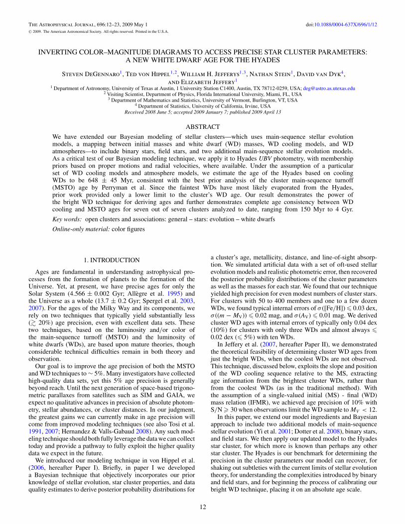
Figure 1. Comparison of isochrones for three different main-sequence model sets at the nominal age, distance, and metallicity of the Hyades. Solid (purple) lines =Girardi models, dotted (red) lines = Yale–Yonsei models, dashed (blue) lines = DSED models.

(A color version of this figure is available in the online journal.)

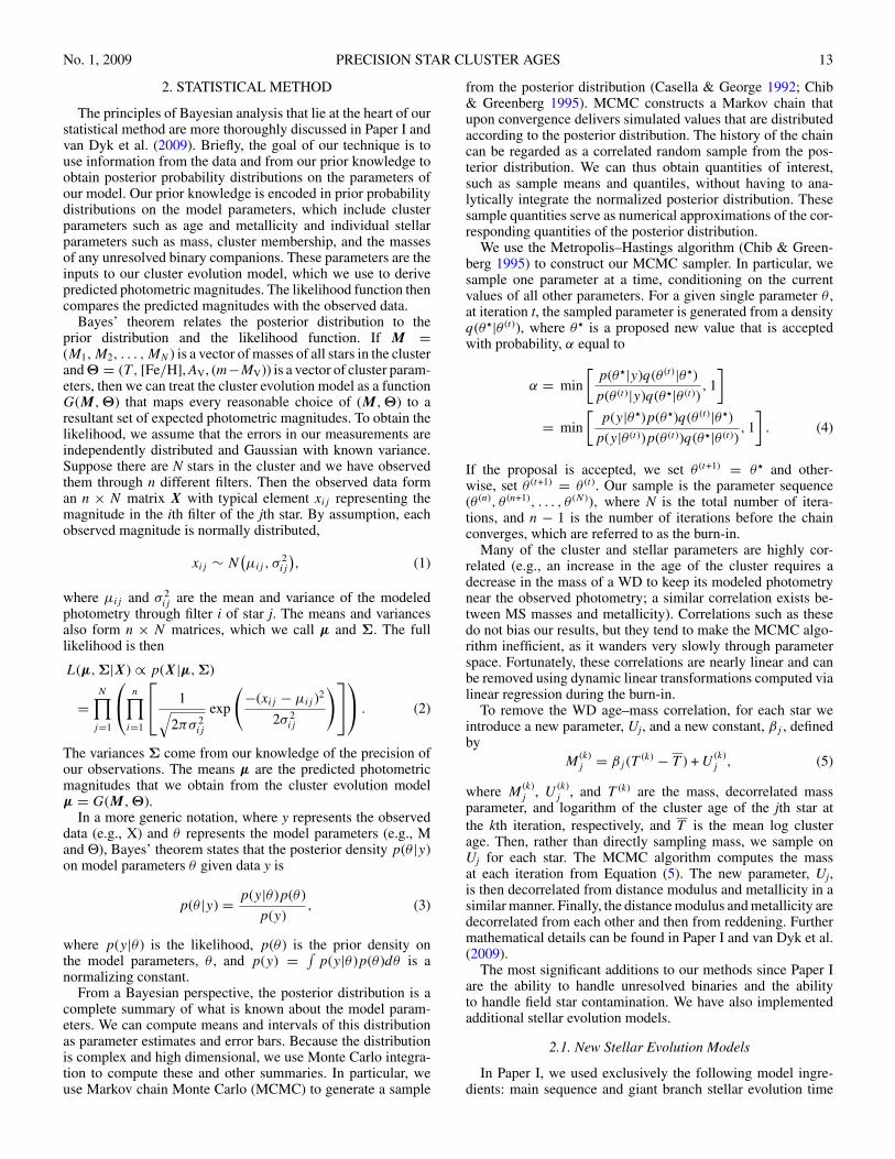
Figure 2. Close-up of the WD region of Figure 1. The crosses are the Hyades WDs, the other symbols show the positions of individual theoretical WDs of a givenmass along the WD tracks. The solid (purple) line = Girardi models, the dotted (red) line = Yale–Yonsei models, the dashed (blue) line = DSED models.

(A color version of this figure is available in the online journal.)

scales of Girardi et al. (2000), the initial–final mass relation ofWeidemann (2000), WD cooling time scales of Wood (1992),and WD atmosphere colors of Bergeron et al. (1995). We havesince incorporated two new sets of MS models—Yale–Yonsei(Yi et al. 2001), and a finer grid of models from the DartmouthStellar Evolution Database (DSED; Dotter et al. 2008) createdspecifically for this work in a range of ages and metallicitiesappropriate for the Hyades—as well as updated versions ofBergeron WD atmosphere models.5

Figure 1 shows the differences among the main-sequencemodels at the nominal age, metallicity, distance, and reddeningof the Hyades (see Section 3). There are some differences in theposition of the turnoff, as well as some important differences

5 http://www.astro.umontreal.ca/∼bergeron/CoolingModels/.

in the shapes of the main sequence. The WD tracks are nearlycoincident for all three sets of MS models. A closer look at theWD sequences (Figure 2) shows some differences, however.Here, individual WDs for different zero-age main-sequence(ZAMS) masses are plotted. Although the tracks are nearlycoincident, individual WDs of the same mass fall in differentplaces along the tracks. Near the top of the cooling sequence,where the progenitor lifetimes are a significant fraction of theWDs’ ages, small differences in the MS timescales have a largerimpact on the exact position of the WD along the sequence. Forthe more massive WDs, which have been cooling much longer,the MS lifetime is a smaller fraction of the WD’s total age, andby about 5 M�, the different MS models yield nearly identicalpositions. Note that these discrepancies in the upper part of

No. 1, 2009 PRECISION STAR CLUSTER AGES 15

the sequence will result in different mass determinations forindividual stars, but will not meaningfully alter the derived agefor the cluster (see Section 2.4).

Our goals in this work are to provide precise relative ages,and to use the well-studied Hyades cluster as a step toward cal-ibrating the absolute accuracy of our method. To this end, werestrict ourselves to single sets of WD cooling and atmospheremodels. In the case of the Hyades, where the WDs are stillrelatively warm, the physics of WD cooling is well-understood(Wood 1990; Fontaine et al. 2001). More astrophysically com-plicated phenomena such as crystallization, phase separation,and the onset of convective coupling do not occur until coolertemperatures than the Hyades WDs have had time to reach. Stillour results and error bars should be understood as being modeldependent.

We restrict our WD atmosphere models to hydrogen atmo-sphere (DA) WDs. The ratio of DAs to non-DAs for the fieldWDs (i.e., those not in open clusters) is between five and six toone, depending on temperature (Williams et al. 2006; DeGen-naro et al. 2008). In the so-called DB gap, 25000 K � Teff �45000 K, the ratio of DAs to non-DAs jumps to 12.5:1. Theexact corresponding ratios for open clusters are still a matter ofdebate, but they are almost certainly no smaller, and are likelyto be larger (Williams et al. 2006; Kalirai et al. 2008). More-over, the WDs included in our analysis of the Hyades are allspectroscopically confirmed DAs (Reid 1996).

2.2. Binaries

In our original model, each stellar system (i.e., each point ofphotometry in the CMD to be modeled) had a single mass. Thismass, together with the cluster parameters of age, metallicity,distance, and reddening, allowed our stellar evolution modelto derive a predicted photometry, which we compared to theobserved photometry to calculate the likelihood function. Thestellar evolution model has since been modified to accommodatepossible unresolved binary stars.

We now treat each stellar system as if it were a binary, andparameterize it in terms of the larger of the two masses, whichwe call the primary mass, Mj, and the ratio of the smaller massto the larger mass, qj, by definition confined to the interval [0, 1].These two parameters allow us to calculate the mass of a possibleunresolved secondary component. The two stars are evolvedindependently and their fluxes are added to determine theircombined photometry. The form of the likelihood probabilitydistribution function (Equation (2)) remains unchanged.

In the Bayesian framework, all fitted parameters require aprior. We choose to place priors on the physically meaningfulvariables of primary and secondary mass, rather than thesampled variables of decorrelated mass parameter and massratio. The prior on the primary mass, as in Paper I, is theMiller–Scalo IMF (Miller & Scalo 1979) normalized fromlog10(M/M�) = −1 to the maximum mass for WDs. The prioron the secondary mass is taken to be flat between 0 and theprimary mass.

The decorrelated mass parameter and the mass ratio aresampled on and accepted or rejected in series independently foreach stellar system. We use a uniform symmetrical step samplerfor the mass ratio, centered on the current value with a step sizedetermined dynamically by the code during the burn-in period.Proposals are reflected if necessary at the boundaries qj = 0and qj = 1. Note that a star without a secondary companionis equivalent to a mass ratio qj = 0, and can be adequatelymodeled by our cluster evolution model.

As with several other parameters in this multi-dimensionalproblem, the primary mass and mass ratio for a given MS star areoften correlated, meaning that a change in a star’s primary masscan be at least partially compensated for by a change in the massratio. Fortunately, this correlation is essentially linear over thesampled range of values, so again for reasons of computationalefficiency, we remove it using the same procedure outlined inSection 2.

In order to create secondary stars below the mass limitsof the main-sequence stellar evolution models, we extrapolatefrom the lowest two mass entries. In the future, we plan toincorporate improved models for low-mass stars. For all but thelowest MS primaries, a secondary companion below the masslimits (typically M < 0.4 M�) makes little or no differenceto the photometry of the system. Our extension exists only toprovide the evolution model with a means to traverse the distancebetween the smallest mass in the input models and 0. This servesadequately to differentiate between binaries and single stars, anddoes not affect the fundamental cluster parameters, which arethe target of this study.

Since low-mass MS companions do, however, have a mea-surable impact on the photometry of the much fainter WDs, wehave chosen to restrict the binary models to MS–MS binariesonly. While there may theoretically be some age informationin WD–WD or WD–MS binaries, in practice these types ofsystems, particularly when they are too close to be resolved,have often undergone a much more astrophysically complicatedevolutionary history due to mass exchange, etc. Modeling suchsystems would often, if not always, introduce a greater level ofuncertainty than whatever we might be able to gain by includingthem in the analysis.

Moreover, in the case of the Hyades, the WDs have all beenstudied spectroscopically (Reid 1996), ruling out any significantbinary companions for all but HZ9, which we have excludedfrom our analysis. More distant clusters could potentiallycontain unresolved white dwarf–M dwarf (WD+M) binaries.However, the vast majority of these stars reside in the broadspace between the MS and the WD region in the CMD. Atpresent, our code would reject such a star as a field star, so itwould have no effect on our results.

One aspect of MS–MS binary sampling that does affectthe cluster parameters is a degeneracy between secondarycompanions and cluster distance. A given point of photometryon the main sequence can equally well correspond to a singlestar or an equal mass binary somewhat farther away. Althoughthese two scenarios are indistinguishable from the data for asingle-star system, clusters have both a WD sequence and actualMS–MS binaries, which create a secondary MS above the true,single-star sequence. Still, in our analysis of simulated clusters,we observe a slight bias in the distance modulus, especiallywhen we include the redder bands of photometry (I through K),which are more sensitive to low-mass companions. Our analysisof the Hyades, which uses only U,B,V photometry, containsmany binary stars, and has a clearly defined WD sequence, isessentially unaffected by this bias.

For simplicity, from this point onward we use the word “star”to mean each individual point of photometry, regardless ofwhether that point is indeed a single star or an unresolved binary.

2.3. Field Stars

To deal with potential field star contamination in the CMD,we introduce an additional variable for each star, Zj, whichexclusively takes on a value of 0 or 1. If Zj = 1, then the

16 DEGENNARO ET AL. Vol. 696

star is considered to be a cluster member (for that iteration). Itis evolved as described above and contributes to the posteriorprobability distribution as outlined in Section 2. If Zj = 0,then the star is considered to be a field star, and its contributionto the posterior probability is calculated in a different mannerdescribed below.

The cluster star model relies on the ability to pool informationacross stars to leverage the data to determine cluster-wideparameters. In other words, we assume that all of the stars in thecluster share the same age, metallicity, distance, and reddening.These parameters, along with the individual stellar masses andmass ratios, allow us to calculate a predicted magnitude tocompare with the observed magnitude in the likelihood. Forthe field star model, we do not have enough information aboutan individual star to determine a predicted magnitude, so thelikelihood function for a star in the field star model must dependonly on its observed magnitude.

Currently this likelihood is taken to be uniform acrossthe entire observed CMD and normalized for each band ofphotometry between a minimum and maximum determinedfrom the photometry data. In principle, a probability map couldbe created from, say, an adjacent field or from some generalizedmap of field stars at a specific Galactic latitude, provided that (1)the map is properly normalized, and (2) the map is not createdfrom the data to be analyzed. We have plans to incorporate suchfeatures into our model in the future, but our testing has so farindicated that even our very rough approximation (i.e., uniformacross the CMD) is enough for our statistical model to arriveat reasonable answers for posterior distributions on each star’smembership status.

The cluster star model has two parameters for each star, onethat is related to the star’s primary mass and another that isequal to the ratio of secondary mass to primary mass. In thefield star model, on the other hand, these two parameters areinsufficient, in the absence of any other information about thatstar (e.g., age, metallicity, distance, absorption—none of whichwe know for a field star, nor are they of direct interest) to allowour model to predict where the star should lie in the CMD.Since the likelihood in the field star model is not dependenton the value of the two mass variables, their prior distributionsalone inform where they are allowed to wander when a staris classified as a field star for multiple consecutive iterations.If we were to leave these priors unchanged in the field starmodel, the variables would soon wander to regions where aproposed jump back to the cluster star model would be veryunlikely to be accepted, and the sampler might jump betweenmodels so rarely that the model space would not be adequatelysampled.

Fortunately, since these variables have no physical meaning inthe field star model, we can place whatever priors we choose onthem, including distributions that force them to remain in areasof high probability in the cluster star model. We accomplish thisby using a section of the burn-in period to calculate distributionsfor the decorrelated mass parameter and the mass ratio inthe cluster star model. We assume that these distributions canbe approximated by Gaussians, and we calculate a mean andvariance for each. This is essentially the final step in the burn-inperiod so that we can be confident that the cluster parametershave converged. For the actual priors, we use distributions withwider tails than Gaussian (specifically, student T distributionswith 6 degrees of freedom), so that if our means and variancesare somewhat off, the samplers will still be able to find theirway to areas of higher probability.

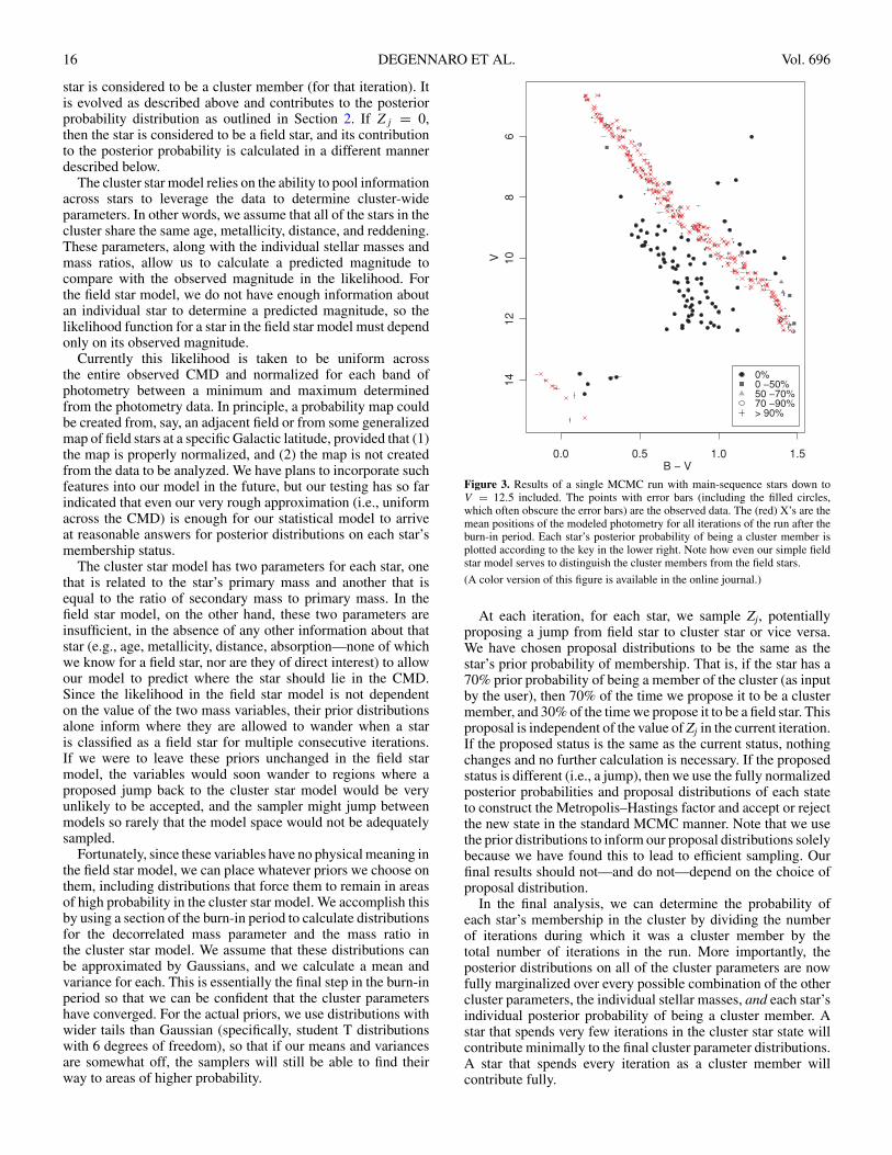
Figure 3. Results of a single MCMC run with main-sequence stars down toV = 12.5 included. The points with error bars (including the filled circles,which often obscure the error bars) are the observed data. The (red) X’s are themean positions of the modeled photometry for all iterations of the run after theburn-in period. Each star’s posterior probability of being a cluster member isplotted according to the key in the lower right. Note how even our simple fieldstar model serves to distinguish the cluster members from the field stars.

(A color version of this figure is available in the online journal.)

At each iteration, for each star, we sample Zj, potentiallyproposing a jump from field star to cluster star or vice versa.We have chosen proposal distributions to be the same as thestar’s prior probability of membership. That is, if the star has a70% prior probability of being a member of the cluster (as inputby the user), then 70% of the time we propose it to be a clustermember, and 30% of the time we propose it to be a field star. Thisproposal is independent of the value of Zj in the current iteration.If the proposed status is the same as the current status, nothingchanges and no further calculation is necessary. If the proposedstatus is different (i.e., a jump), then we use the fully normalizedposterior probabilities and proposal distributions of each stateto construct the Metropolis–Hastings factor and accept or rejectthe new state in the standard MCMC manner. Note that we usethe prior distributions to inform our proposal distributions solelybecause we have found this to lead to efficient sampling. Ourfinal results should not—and do not—depend on the choice ofproposal distribution.

In the final analysis, we can determine the probability ofeach star’s membership in the cluster by dividing the numberof iterations during which it was a cluster member by thetotal number of iterations in the run. More importantly, theposterior distributions on all of the cluster parameters are nowfully marginalized over every possible combination of the othercluster parameters, the individual stellar masses, and each star’sindividual posterior probability of being a cluster member. Astar that spends very few iterations in the cluster star state willcontribute minimally to the final cluster parameter distributions.A star that spends every iteration as a cluster member willcontribute fully.

No. 1, 2009 PRECISION STAR CLUSTER AGES 17

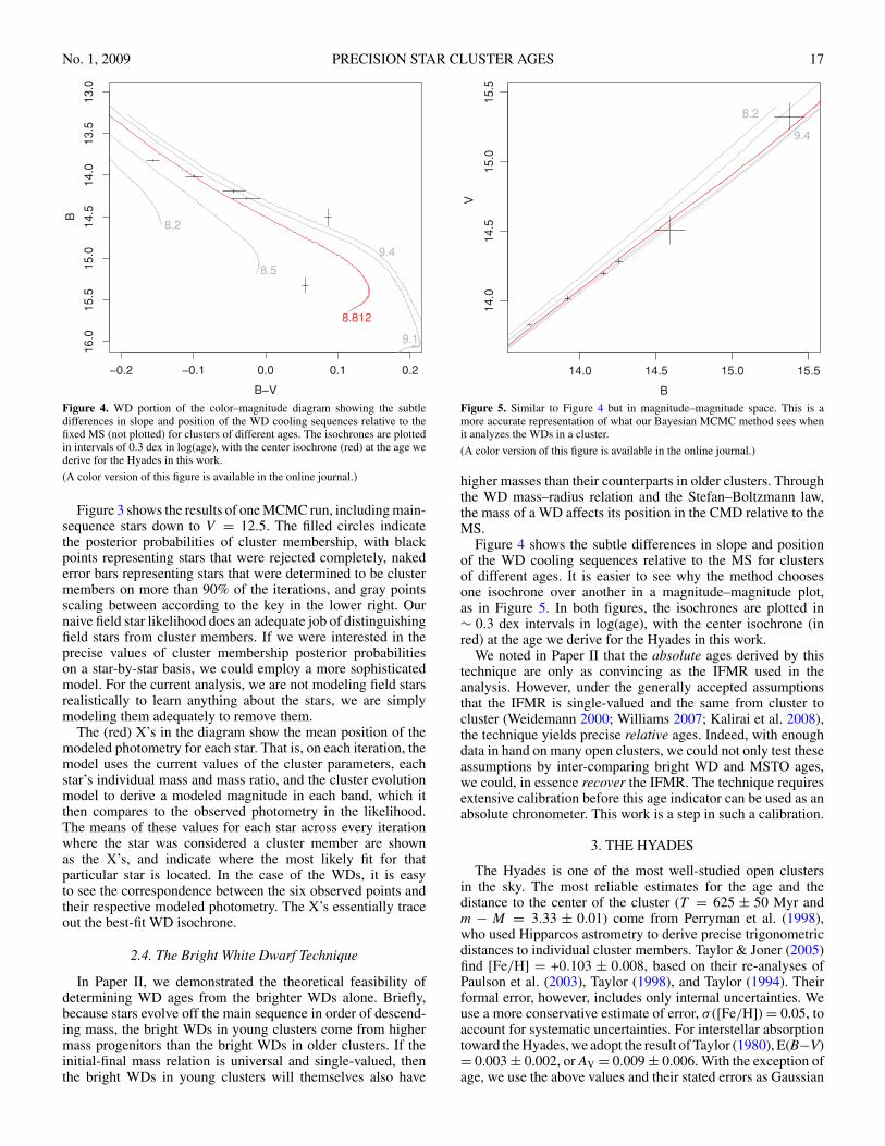
Figure 4. WD portion of the color–magnitude diagram showing the subtledifferences in slope and position of the WD cooling sequences relative to thefixed MS (not plotted) for clusters of different ages. The isochrones are plottedin intervals of 0.3 dex in log(age), with the center isochrone (red) at the age wederive for the Hyades in this work.

(A color version of this figure is available in the online journal.)

Figure 3 shows the results of one MCMC run, including main-sequence stars down to V = 12.5. The filled circles indicatethe posterior probabilities of cluster membership, with blackpoints representing stars that were rejected completely, nakederror bars representing stars that were determined to be clustermembers on more than 90% of the iterations, and gray pointsscaling between according to the key in the lower right. Ournaive field star likelihood does an adequate job of distinguishingfield stars from cluster members. If we were interested in theprecise values of cluster membership posterior probabilitieson a star-by-star basis, we could employ a more sophisticatedmodel. For the current analysis, we are not modeling field starsrealistically to learn anything about the stars, we are simplymodeling them adequately to remove them.

The (red) X’s in the diagram show the mean position of themodeled photometry for each star. That is, on each iteration, themodel uses the current values of the cluster parameters, eachstar’s individual mass and mass ratio, and the cluster evolutionmodel to derive a modeled magnitude in each band, which itthen compares to the observed photometry in the likelihood.The means of these values for each star across every iterationwhere the star was considered a cluster member are shownas the X’s, and indicate where the most likely fit for thatparticular star is located. In the case of the WDs, it is easyto see the correspondence between the six observed points andtheir respective modeled photometry. The X’s essentially traceout the best-fit WD isochrone.

2.4. The Bright White Dwarf Technique

In Paper II, we demonstrated the theoretical feasibility ofdetermining WD ages from the brighter WDs alone. Briefly,because stars evolve off the main sequence in order of descend-ing mass, the bright WDs in young clusters come from highermass progenitors than the bright WDs in older clusters. If theinitial-final mass relation is universal and single-valued, thenthe bright WDs in young clusters will themselves also have

Figure 5. Similar to Figure 4 but in magnitude–magnitude space. This is amore accurate representation of what our Bayesian MCMC method sees whenit analyzes the WDs in a cluster.

(A color version of this figure is available in the online journal.)

higher masses than their counterparts in older clusters. Throughthe WD mass–radius relation and the Stefan–Boltzmann law,the mass of a WD affects its position in the CMD relative to theMS.

Figure 4 shows the subtle differences in slope and positionof the WD cooling sequences relative to the MS for clustersof different ages. It is easier to see why the method choosesone isochrone over another in a magnitude–magnitude plot,as in Figure 5. In both figures, the isochrones are plotted in∼ 0.3 dex intervals in log(age), with the center isochrone (inred) at the age we derive for the Hyades in this work.

We noted in Paper II that the absolute ages derived by thistechnique are only as convincing as the IFMR used in theanalysis. However, under the generally accepted assumptionsthat the IFMR is single-valued and the same from cluster tocluster (Weidemann 2000; Williams 2007; Kalirai et al. 2008),the technique yields precise relative ages. Indeed, with enoughdata in hand on many open clusters, we could not only test theseassumptions by inter-comparing bright WD and MSTO ages,we could, in essence recover the IFMR. The technique requiresextensive calibration before this age indicator can be used as anabsolute chronometer. This work is a step in such a calibration.

3. THE HYADES

The Hyades is one of the most well-studied open clustersin the sky. The most reliable estimates for the age and thedistance to the center of the cluster (T = 625 ± 50 Myr andm − M = 3.33 ± 0.01) come from Perryman et al. (1998),who used Hipparcos astrometry to derive precise trigonometricdistances to individual cluster members. Taylor & Joner (2005)find [Fe/H] = +0.103 ± 0.008, based on their re-analyses ofPaulson et al. (2003), Taylor (1998), and Taylor (1994). Theirformal error, however, includes only internal uncertainties. Weuse a more conservative estimate of error, σ ([Fe/H]) = 0.05, toaccount for systematic uncertainties. For interstellar absorptiontoward the Hyades, we adopt the result of Taylor (1980), E(B−V)= 0.003 ± 0.002, or AV = 0.009 ± 0.006. With the exception ofage, we use the above values and their stated errors as Gaussian

18 DEGENNARO ET AL. Vol. 696

Table 1List of WDs in the Hyades, with Cross-References

GCPD identifier Reid (1996) EGGRa Reid (1992) McCook & Sion (1999)

HG7041 HZ4 26 · · · 0352+096vA292 VR7 36 192 0421+162vA490 VR16 37 265 0425+168vA722 HZ7 39 330 0431+1254003 HZ14 42 408 0438+108· · · LB227 29 81 0406+169vA673 HZ9 38 308 0429+176HG7126 LP 414−120 · · · 102 0410+188

Note. a Eggen & Greenstein (1965).

priors on the cluster parameters. The age prior is flat in log(age)between the limits of our models.

The data for the Hyades come from the General Catalogueof Photometric Data (GCPD; http://obswww.unige.ch/gcpd/gcpd.html; Mermilliod et al. 1997). For each Hyades star inthe database, they calculate weighted mean and dispersionsin the V band of photometry and the B − V and U − Bcolor indices. Their two-step process, outlined in Mermilliod& Mermilliod (1994, p. 1387), combines data from diversesources with the first step assigning weights based on the numberof independent measurements reported in the source, and thesecond step slightly shifting the weights to give lower weightingto discrepant measurements. We use the most recent reportedvalues in the database as of 2008 January, and use only thosestars for which U − B values are reported.

The errors they report are the dispersions between sources.For stars with three or more sources, we use the reporteddispersions to calculate the errors needed by our code. For starswith two or fewer sources, the reported dispersions can often beanomalously low or non-existent. Therefore, we adopt minimumdispersions using the estimates of the average error reported inMermilliod & Mermilliod (1994, p. 1387), namely: εV = 0.01,εB−V = 0.0075, εU−B = 0.011. Since our method needs errorsin each band of photometry, we take the error in the B band tobe the sum of the errors in V and B − V (i.e., the quadrature sumof the variances), and similarly the error in U to be the sum ofthe errors in B and U − B. We have eliminated four stars withanomalously high dispersions (σB > 0.1).

We match what stars we can with the stars in Perrymanet al. (1998), and determine a prior probability on each star’smembership in the cluster on the basis of their reported χ2

value (column (w) in their Table 2) and the number of degreesof freedom (3 for stars with radial velocity measurements, 2 forthose with proper motions only). Stars without reported valuesof membership probability are assigned a (somewhat arbitrary)0.5 prior probability.

Reid (1996) lists eight WDs as members of the Hyades.Table 1 shows these WDs, along with cross-identifications toother major works on Hyades WDs. Of these, vA673 is a knownWD–MS binary (Reid 1996), and LP 414−120 does not haveavailable U-band photometry. We eliminate both of these starsfrom our analysis. The remaining six WDs have individual massdeterminations (Weidemann 2000, and references therein). Twoof these, LB227 and HZ4, are used as photometric standards inLandolt & Uomoto (2007), and we use their photometry ratherthan the (less precise) photometry from GCPD.

The precision of the error bars on the photometry for thesetwo objects in particular highlights a problem one encounterswith very few open clusters: differential distance. The Hyades

is one of the only clusters for which differential distances posea serious problem. Perryman et al. (1998) quote a tidal radiusfor the Hyades of order 10 pc, with stars as far away as 20 pcfrom the center of mass. A star that is 20 pc nearer to us than theroughly 50 pc distance to the center of the cluster will appear∼ 1.2 mag too bright. A star 20 pc too distant will appear∼ 0.8 mag too faint. For the bright stars, which have individualparallaxes from Hipparcos, this differential distance can beaccounted for, though we do not do so in the present work.The WDs in any case are too faint to have Hipparcos parallaxes.

For the purposes of the present problem, we note that anuncertainty in the distance to an individual WD essentiallytranslates to an error in the apparent magnitude. For the twostars in question, we assume an unknown systematic error of0.1 mag in the V band, and use the errors in color as quoted inLandolt & Uomoto (2007). These errors are plotted as the rederror bars in Figure 2. We remind the reader as well that ourMCMC analysis does not directly analyze the color–magnitudeplot, but rather each band of photometry independently. Whatour Bayesian method sees looks more like Figure 5. Notice thatbecause the errors in U and B are the sums of the errors in the Vband and the appropriate color term(s), the 0.1 mag systematicadded to the V band translates to similar errors in the other twomagnitudes.

The starting masses and mass ratios for each star are chosenso as to minimize the time necessary during the initial wanderingperiod for each run. In theory, the posterior should not dependon the choice of initial values. In practice, this is usually thecase, provided that most of the starting values are within a fewtenths of a solar mass for the MS stars, and large enough for theWDs that the code does not try to put the star on the MS or giantbranch on the first iteration. If the latter happens, the star willusually be rejected as a field star. Consequently, we choose thestarting masses for any objects that lie significantly below andto the left of the main sequence to be > 3.0 M�.

Since we are interested in a comparison between ages derivedfrom traditional main-sequence turnoff fitting and our techniqueto determine WD ages, we remove the MS turnoff and giant starsfrom the data so that our code cannot derive any age informationfrom these stars. We cut off any stars with V < 4.5. There isstill some age information in the MS insofar as the lack of aturnoff fainter than V = 4.5 sets an upper limit on the age. Ourbright WD technique in part exploits this phenomenon.

A closer examination of Figure 1 reveals a long-standingproblem in stellar astronomy (for recent discussions see vonHippel et al. 2002; Grocholski & Sarajedini 2003). As we movedown the main sequence, the models and the data begin todiverge. There is a considerable difference among the modelswith regard to the shape of the MS. The Yale models fit bestoverall, particularly in the range of 7 < V < 10. All threesets of models considerably underestimate the V magnitude fora given B − V (or vice versa) at the bottom of the MS, withthe Girardi models dropping off first and most dramatically atV � 10.5, the Yale models following shortly thereafter, thoughnot as dramatically, and the DSED models showing reasonableagreement until dropping off precipitously at V � 12.5. TheDSED models also show considerable diversion from the datain the U−B versus B color–magnitude diagram, particularlyon the bright end. We expect, therefore, that the Yale models,showing the best overall agreement with the data, will yield themost accurate results for the cluster parameters.

The proper functioning of our code depends on the models’being accurate. We are currently exploring methods of dealing

No. 1, 2009 PRECISION STAR CLUSTER AGES 19

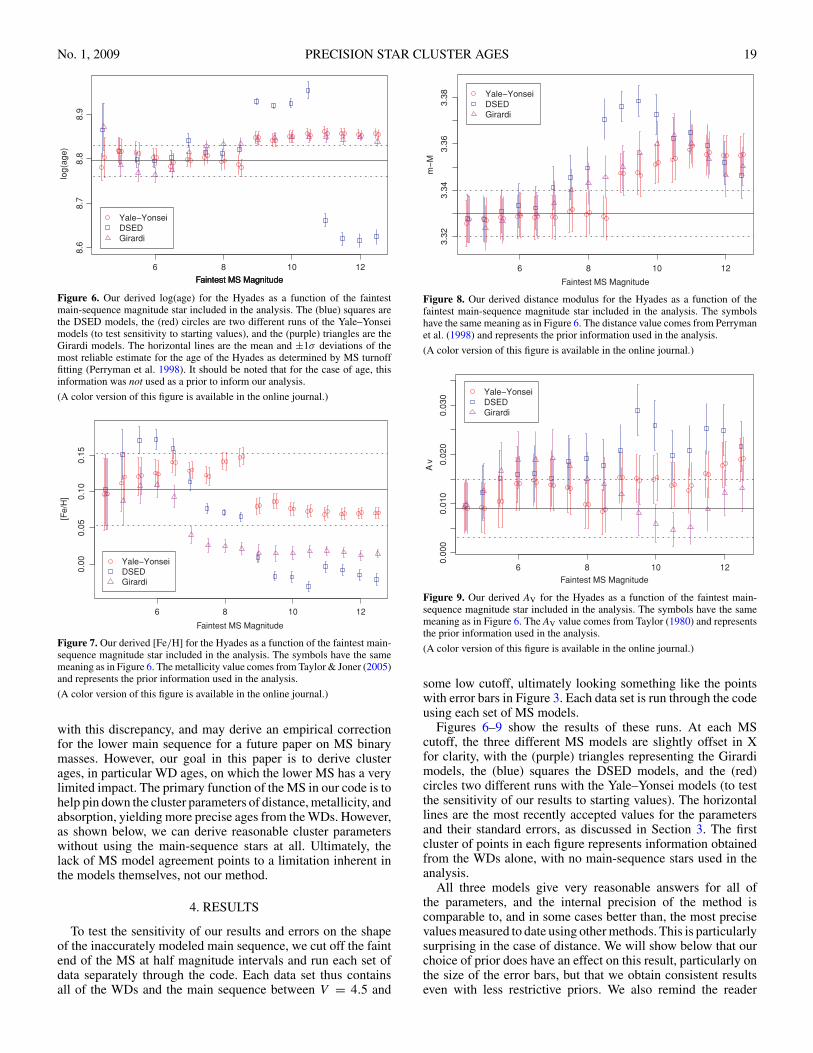
Figure 6. Our derived log(age) for the Hyades as a function of the faintestmain-sequence magnitude star included in the analysis. The (blue) squares arethe DSED models, the (red) circles are two different runs of the Yale–Yonseimodels (to test sensitivity to starting values), and the (purple) triangles are theGirardi models. The horizontal lines are the mean and ±1σ deviations of themost reliable estimate for the age of the Hyades as determined by MS turnofffitting (Perryman et al. 1998). It should be noted that for the case of age, thisinformation was not used as a prior to inform our analysis.

(A color version of this figure is available in the online journal.)

Figure 7. Our derived [Fe/H] for the Hyades as a function of the faintest main-sequence magnitude star included in the analysis. The symbols have the samemeaning as in Figure 6. The metallicity value comes from Taylor & Joner (2005)and represents the prior information used in the analysis.

(A color version of this figure is available in the online journal.)

with this discrepancy, and may derive an empirical correctionfor the lower main sequence for a future paper on MS binarymasses. However, our goal in this paper is to derive clusterages, in particular WD ages, on which the lower MS has a verylimited impact. The primary function of the MS in our code is tohelp pin down the cluster parameters of distance, metallicity, andabsorption, yielding more precise ages from the WDs. However,as shown below, we can derive reasonable cluster parameterswithout using the main-sequence stars at all. Ultimately, thelack of MS model agreement points to a limitation inherent inthe models themselves, not our method.

4. RESULTS

To test the sensitivity of our results and errors on the shapeof the inaccurately modeled main sequence, we cut off the faintend of the MS at half magnitude intervals and run each set ofdata separately through the code. Each data set thus containsall of the WDs and the main sequence between V = 4.5 and

Figure 8. Our derived distance modulus for the Hyades as a function of thefaintest main-sequence magnitude star included in the analysis. The symbolshave the same meaning as in Figure 6. The distance value comes from Perrymanet al. (1998) and represents the prior information used in the analysis.

(A color version of this figure is available in the online journal.)

Figure 9. Our derived AV for the Hyades as a function of the faintest main-sequence magnitude star included in the analysis. The symbols have the samemeaning as in Figure 6. The AV value comes from Taylor (1980) and representsthe prior information used in the analysis.

(A color version of this figure is available in the online journal.)

some low cutoff, ultimately looking something like the pointswith error bars in Figure 3. Each data set is run through the codeusing each set of MS models.

Figures 6–9 show the results of these runs. At each MScutoff, the three different MS models are slightly offset in Xfor clarity, with the (purple) triangles representing the Girardimodels, the (blue) squares the DSED models, and the (red)circles two different runs with the Yale–Yonsei models (to testthe sensitivity of our results to starting values). The horizontallines are the most recently accepted values for the parametersand their standard errors, as discussed in Section 3. The firstcluster of points in each figure represents information obtainedfrom the WDs alone, with no main-sequence stars used in theanalysis.

All three models give very reasonable answers for all ofthe parameters, and the internal precision of the method iscomparable to, and in some cases better than, the most precisevalues measured to date using other methods. This is particularlysurprising in the case of distance. We will show below that ourchoice of prior does have an effect on this result, particularly onthe size of the error bars, but that we obtain consistent resultseven with less restrictive priors. We also remind the reader

20 DEGENNARO ET AL. Vol. 696

6 8 10 12

8.7

08

.75

8.8

08

.85

Faintest MS Magnitude

log

(ag

e)

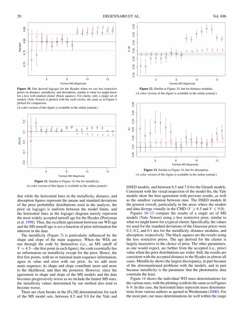
Figure 10. Our derived log(age) for the Hyades when we use less restrictivepriors on distance, metallicity, and absorption, similar to what we might knowfor a less well-studied cluster (black squares). For clarity, only a single set ofmodels (Yale–Yonsei) is plotted with the (red) circles, the same as in Figure 6plotted for comparison.

(A color version of this figure is available in the online journal.)

6 8 10 12

0.2

0.1

0.0

0.1

0.2

Faintest MS Magnitude

[Fe/H

]

Figure 11. Similar to Figure 10, but for metallicity.

(A color version of this figure is available in the online journal.)

that while the horizontal lines in the metallicity, distance, andabsorption figures represent the means and standard deviationsof the prior probability distributions used in the analysis, theprior on log(age) is uniform between the model limits, andthe horizontal lines in the log(age) diagram merely representthe most widely accepted turnoff age for the Hyades (Perrymanet al. 1998). Thus, the excellent agreement between our WD ageand the MS turnoff age is not a function of prior information butinherent in the data.

The metallicity (Figure 7) is particularly influenced by theshape and slope of the main sequence. When the WDs arerun through the code by themselves (i.e., an MS cutoff ofV = 4.5—the first point in each figure), the code essentially hasno information on metallicity except for the prior. Hence, thefirst few points, with no or minimal main sequence information,agree in value and error with our prior. As we add moremain sequence, its shape and slope contribute more and moreto the likelihood, and thus the posterior. However, since theagreement in shape and slope of the MS models and the databecomes progressively worse as we include the fainter MS stars,the metallicity values determined by our method also tend tobecome worse.

There are clear breaks in the [Fe/H] determinations for eachof the MS model sets, between 8.5 and 9.0 for the Yale and

6 8 10 12

3.2

03.2

53.3

03.3

53.4

03.4

53.5

0

Faintest MS Magnitude

mM

Figure 12. Similar to Figure 10, but for distance modulus.

(A color version of this figure is available in the online journal.)

6 8 10 12

0.0

00

.01

0.0

20

.03

0.0

40

.05

0.0

6

Faintest MS Magnitude

Av

Figure 13. Similar to Figure 10, but for absorption.

(A color version of this figure is available in the online journal.)

DSED models, and between 6.5 and 7.0 for the Girardi models.Consistent with the visual inspection of the model fits, the Yalemodels show the best agreement with previous results, as wellas the smallest variation between runs. The DSED models fitthe poorest overall, particularly in the areas where the modelsand data diverge visually in the CMD (V � 6.5 and V � 9.0).

Figures 10–13 compare the results of a single set of MSmodels (Yale–Yonsei) using a less restrictive prior, similar towhat we might know for a typical cluster. Specifically, the valueswe used for the standard deviations of the Guassian priors were0.3, 0.2, and 0.1 dex for the metallicity, distance modulus, andabsorption, respectively. The black squares are the results usingthe less restrictive priors. The age derived for the cluster islargely insensitive to the choice of prior. The other parameters,as one would expect, are farther from the accepted (i.e., prior)value when the prior distributions are wider. Still, the results areconsistent with the accepted distance to the Hyades in almost allcases. Metallicity shows the largest discrepancy, in part becauseof the aforementioned problems with the models, and in partbecause metallicity is the parameter that the photometric dataconstrain the least.

Figure 14 shows the individual WD mass determinations forthe various runs, with the plotting symbols the same as in Figures6–9. In this case, the horizontal lines represent mass determina-tions from various authors as quoted in Weidemann (2000). Forthe most part, our mass determinations lie well within the range

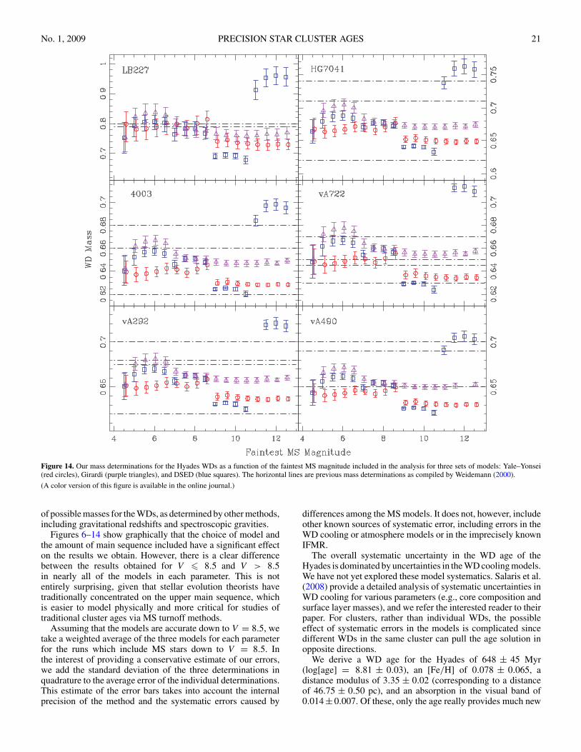
No. 1, 2009 PRECISION STAR CLUSTER AGES 21

Figure 14. Our mass determinations for the Hyades WDs as a function of the faintest MS magnitude included in the analysis for three sets of models: Yale–Yonsei(red circles), Girardi (purple triangles), and DSED (blue squares). The horizontal lines are previous mass determinations as compiled by Weidemann (2000).

(A color version of this figure is available in the online journal.)

of possible masses for the WDs, as determined by other methods,including gravitational redshifts and spectroscopic gravities.

Figures 6–14 show graphically that the choice of model andthe amount of main sequence included have a significant effecton the results we obtain. However, there is a clear differencebetween the results obtained for V � 8.5 and V > 8.5in nearly all of the models in each parameter. This is notentirely surprising, given that stellar evolution theorists havetraditionally concentrated on the upper main sequence, whichis easier to model physically and more critical for studies oftraditional cluster ages via MS turnoff methods.

Assuming that the models are accurate down to V = 8.5, wetake a weighted average of the three models for each parameterfor the runs which include MS stars down to V = 8.5. Inthe interest of providing a conservative estimate of our errors,we add the standard deviation of the three determinations inquadrature to the average error of the individual determinations.This estimate of the error bars takes into account the internalprecision of the method and the systematic errors caused by

differences among the MS models. It does not, however, includeother known sources of systematic error, including errors in theWD cooling or atmosphere models or in the imprecisely knownIFMR.

The overall systematic uncertainty in the WD age of theHyades is dominated by uncertainties in the WD cooling models.We have not yet explored these model systematics. Salaris et al.(2008) provide a detailed analysis of systematic uncertainties inWD cooling for various parameters (e.g., core composition andsurface layer masses), and we refer the interested reader to theirpaper. For clusters, rather than individual WDs, the possibleeffect of systematic errors in the models is complicated sincedifferent WDs in the same cluster can pull the age solution inopposite directions.

We derive a WD age for the Hyades of 648 ± 45 Myr(log[age] = 8.81 ± 0.03), an [Fe/H] of 0.078 ± 0.065, adistance modulus of 3.35 ± 0.02 (corresponding to a distanceof 46.75 ± 0.50 pc), and an absorption in the visual band of0.014 ± 0.007. Of these, only the age really provides much new

22 DEGENNARO ET AL. Vol. 696

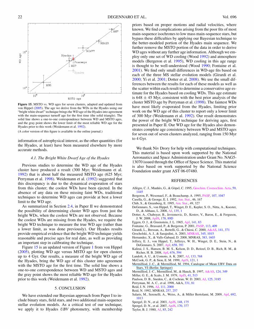
Figure 15. MSTO vs. WD ages for seven clusters, adapted and updated fromvon Hippel (2005). The age we derive from the WDs in the Hyades using our“bright white dwarf” technique brings the WD age of the Hyades into agreementwith the main-sequence turnoff age for the first time (the solid triangle). Thesolid line shows a one-to-one correspondence between WD and MSTO ages,and the gray point shows the lower limit of the most reliable WD age for theHyades prior to this work (Weidemann et al. 1992).

(A color version of this figure is available in the online journal.)

information of astrophysical interest, as the other quantities (forthe Hyades, at least) have been measured elsewhere by moreaccurate methods.

4.1. The Bright White Dwarf Age of the Hyades

Previous studies to determine the WD age of the Hyadescluster have produced a result (300 Myr; Weidemann et al.1992) that is about half the measured MSTO age (625 Myr;Perryman et al. 1998). Weidemann et al. (1992) suggested thatthis discrepancy is due to the dynamical evaporation of starsfrom this cluster; the coolest WDs have been ejected. In theabsence of any data on these missing faint WDs, traditionaltechniques to determine WD ages can provide at best a lowerlimit to the WD age.

As summarized in Section 2.4, in Paper II we demonstratedthe possibility of determining cluster WD ages from just thebright WDs, when the coolest WDs are not observed. Becausethe coolest WDs are missing from the Hyades, we require thebright WD technique to measure the true WD age (rather thana lower limit, as was done previously). Our Hyades resultsprovide empirical evidence that the bright WD technique yieldsreasonable and precise ages for real date, as well as providingan important step in calibrating the technique.

Figure 15 is an updated version of Figure 1 from von Hippel(2005), plotting WD age versus MSTO age for open clustersup to 4 Gyr. Our results, a measure of the bright WD age ofthe Hyades, bring the WD age of this cluster into agreementwith the MSTO age for the first time. The solid line shows aone-to-one correspondence between WD and MSTO ages andthe gray point shows the most reliable WD age for the Hyadesprior to this work (Weidemann et al. 1992).

5. CONCLUSION

We have extended our Bayesian approach from Paper I to in-clude binary stars, field stars, and two additional main-sequencestellar evolution models. As a critical test of our technique,we apply it to Hyades UBV photometry, with membership

priors based on proper motions and radial velocities, whereknown. We find complications arising from the poor fits of mostmain-sequence isochrones to low mass main-sequence stars, butbypass these difficulties by applying our Bayesian technique tothe better-modeled portion of the Hyades main sequence. Wefurther remove the MSTO portion of the data in order to deriveWD ages without any further age information. Although we em-ploy only one set of WD cooling (Wood 1992) and atmospheremodels (Bergeron et al. 1995), WD cooling in this age rangeis thought to be well-understood (Wood 1990; Fontaine et al.2001). We find only small differences in WD-age fits based oneach of the three MS stellar evolution models (Girardi et al.2000; Yi et al. 2001; Dotter et al. 2008). We use the small dif-ferences between the results for each of these models as well asthe scatter within each result to determine a conservative age es-timate for the Hyades based on cooling WDs. This age estimateis 648 ± 45 Myr, consistent with the best prior analysis of thecluster MSTO age by Perryman et al. (1998). The faintest WDshave most likely evaporated from the Hyades, limiting priorwork on the WD age of this cluster to report only a lower limitof 300 Myr (Weidemann et al. 1992). Our result demonstratesthe power of the bright WD technique for deriving ages, firstpresented in Paper II. Our WD age for the Hyades also demon-strates complete age consistency between WD and MSTO agesfor seven out of seven clusters analyzed, ranging from 150 Myrto 4 Gyr.

We thank Niv Drory for help with computational techniques.This material is based upon work supported by the NationalAeronautics and Space Administration under Grant No. NAG5-13070 issued through the Office of Space Science. This materialis also based on work supported by the National ScienceFoundation under grant AST 06-07480.

REFERENCES

Allegre, C. J., Manhes, G., & Gopel, C. 1995, Geochim. Cosmochim. Acta, 59,1445

Bergeron, P., Wesemael, F., & Beauchamp, A. 1995, PASP, 107, 1047Casella, G., & George, E. I. 1992, Am. Stat., 46, 167Chib, S., & Greenberg, E. 1995, Am. Stat., 49, 327DeGennaro, S., von Hippel, T., Winget, D. E., Kepler, S. O., Nitta, A., Koester,

D., & Althaus, L. 2008, AJ, 135, 1Dotter, A., Chaboyer, B., Jevremovic, D., Kostov, V., Baron, E., & Ferguson,

J. W. 2008, ApJS, 178, 89DEggen, O. J., & Greenstein, J. L. 1965, ApJ, 141, 83Fontaine, G., Brassard, P., & Bergeron, P. 2001, PASP, 113, 409Girardi, L., Bressan, A., Bertelli, G., & Chiosi, C. 2000, A&AS, 141, 371Grocholski, A. J., & Sarajedini, A. 2003, MNRAS, 345, 1015Hernandez, X., & Valls-Gabaud, D. 2008, MNRAS, 383, 1603Jeffery, E. J., von Hippel, T., Jefferys, W. H., Winget, D. E., Stein, N., &

DeGennaro, S. 2007, ApJ, 658, 391Kalirai, J. S., Hansen, B. M. S., Kelson, D. D., Reitzel, D. B., Rich, R. M., &

Richer, H. B. 2008, ApJ, 676, 594Landolt, A. U., & Uomoto, A. K. 2007, AJ, 133, 768McCook, G. P., & Sion, E. M. 1999, ApJS, 121, 1Mermilliod, J.-C., & Mermilliod, M. 1994, Catalogue of Mean UBV Data on

Stars, VI (Berlin: Springer)Mermilliod, J.-C., Mermilliod, M., & Hauck, B. 1997, A&AS, 124, 349Miller, G. E., & Scalo, J. M. 1979, ApJS, 41, 513Paulson, D. B., Sneden, C., & Cochran, W. D. 2003, AJ, 125, 3185Perryman, M. A. C., et al. 1998, A&A, 331, 81Reid, I. N. 1996, AJ, 111, 2000Reid, N. 1992, MNRAS, 257, 257Salaris, M., Serenelli, A., Weiss, A., & Miller Bertolami, M. 2009, ApJ, 692,

1013Spergel, D. N., et al. 2003, ApJS, 148, 175Spergel, D. N., et al. 2007, ApJS, 170, 377Taylor, B. J. 1980, AJ, 85, 242

No. 1, 2009 PRECISION STAR CLUSTER AGES 23

Taylor, B. J. 1994, PASP, 106, 600Taylor, B. J. 1998, PASP, 110, 708Taylor, B. J., & Joner, M. D. 2005, ApJS, 159, 100Tosi, M., Bragaglia, A., & Cignoni, M. 2007, MNRAS, 378, 730Tosi, M., Greggio, L., Marconi, G., & Focardi, P. 1991, AJ, 102, 951van Dyk, D. A., De Gennaro, S., Stein, N., Jefferys, W. H., & von Hippel, T.

2009, Ann. of Appl. Stat., in pressvon Hippel, T. 2005, ApJ, 622, 565von Hippel, T., Jefferys, W. H., Scott, J., Stein, N., Winget, D. E., DeGennaro,

S., Dam, A., & Jeffery, E. 2006, ApJ, 645, 1436von Hippel, T., Steinhauer, A., Sarajedini, A., & Deliyannis, C. P. 2002, AJ,

124, 1555

Weidemann, V. 2000, A&A, 363, 647Weidemann, V., Jordan, S., Iben, I. J., & Casertano, S. 1992, AJ, 104,

1876Williams, K. A. 2007, in ASP Conf. Ser. 372, 15th European Workshop on

White Dwarfs ed. R. Napiwotzki & M. R. Burleigh (San Francisco, CA:ASP), 85

Williams, K. A., Liebert, J., Bolte, M., & Hanson, R. B. 2006, ApJ, 643,L127

Wood, M. A. 1990, PhD thesis, Univ. of Texas, AustinWood, M. A. 1992, ApJ, 386, 539Yi, S., Demarque, P., Kim, Y.-C., Lee, Y.-W., Ree, C. H., Lejeune, T., & Barnes,

S. 2001, ApJS, 136, 417