Investigation and Disruption of Baker's Yeast / Chlorella

Investigation and Disruption of Baker’s

Yeast / Chlorella Vulgaris in High-Pressure

Homogenizer (HPH) to Improve Cost-

Effective Protein Yield

A thesis submitted for the degree of

Doctor of Philosophy

by

LEONARD EGHOSA NKEM EKPENI

[B.ENG. (HONS), M.SC., MIEI, AMIMECHE]

School of Mechanical and Manufacturing Engineering

Faculty of Engineering and Computing

Dublin City University

September 2015

Supervisors

Prof Abdul-Ghani Olabi

Dr Joseph Stokes

PhD 2015

I

Preface

This thesis describes original work which has not previously been submitted for a

degree in Dublin City University or at any other University. The investigations

were carried out in the School of Mechanical and Manufacturing Engineering,

Dublin City University, during the period October 2010 to December 2014, under

the supervision of Prof Abdul-Ghani Olabi and Dr Joseph Stokes. This work has

been disseminated through the following publications.

Journal Articles/Publication

Journal Articles:

1. Ekpeni, L. E. N., Benyounis, K. Y., Nkem-Ekpeni, Fehintola F., Stokes, J.,

Olabi, A.G., (2015). Underlying factors to consider in improving energy yield

from biomass source through yeast use on high-pressure homogenizer (HPH),

Energy, Volume 81, 2015, pp. 74-83, ISSN 0360-5442,

DOI:10.1016/j.energy.2014.11.038

2. Ekpeni, L. E. N., Nkem-Ekpeni, F. F., Benyounis, K. Y., Aboderheeba, A. K. M.,

Stokes, J., Olabi, A. G. (2014). Yeast: A Potential Biomass Substrate for the

Production of Cleaner Energy (Biogas). Energy Procedia, Volume 61, 2014, pp.

1718-1731 DOI:10.1016/j.egypro.2014.12.199

3. Ekpeni, L. E. N., Benyounis, K. Y., Nkem-Ekpeni, F. F., Stokes, J., Olabi, A. G.

(2014), Energy Diversity through Renewable Energy Source (RES) – A Case

Study of Biomass. Energy Procedia, Volume 61, 2014, pp. 1740-1747

DOI:10.1016/j.egypro.2014.12.202

4. Ekpeni, L. E. N and Olabi, A. G. (2013). A Change in the Transportation Needs

Today, a Better Future for Tomorrow: Climate Change Review. In Causes,

Impacts and Solutions to Global Warming. Part II (pp. 933-947). Springer New

York, DOI 10.1007/978-1-4614-7588-0_49 (Online ISBN 978-1-4614-7588-0)

5. Ekpeni, L. E. N and Olabi, A. G., (2012). Energy Sustainability – An Issue for

Today. Journal of Sustainable Development and Environmental Protection, 2 (2),

Apr – Jun. 2012. ierdafrica.org.

II

6. Ekpeni, L. E. N., Benyounis, K. Y., Stokes, J., and Olabi, A. G, Improved

disruption technique for biomass substrates using high-pressure homogenizer

(HPH) as an efficient means for protein production (Submitted to Applied Energy

Journal - Elsevier)

7. Ekpeni, L. E. N., Benyounis, K. Y., Stokes, J., and Olabi, A. G, Baker’s yeast

homogenization - An effective energy conversion process for higher protein

concentration yield (Submitted to Energy Conversion and Management Journal

- Elsevier)

International Conference Papers:

1. Ekpeni, L. E. N. and Olabi, A. G., Biogas Improvement Through Yeast Use in

High-Pressure Homogenizer, 3rd

International Symposium on Environmental

Management (SEM2011), Zagreb, Croatia, October 26 – 28, 2011.

2. Ekpeni, L. E. N., and Olabi, A. G., (2012). Energy Sustainability – An Issue for

Today. 2012 International Conference on Sustainable Development and

Environmental Protection. Bell University of Technology, Ota near Lagos,

Nigeria, March 20 – 22, 2012.

3. Ekpeni, L. E. N., Benyounis, K. Y., and Olabi, A. G., Gap Sizes Effects on

Homogenized Yeast and its Efficiency on Biogas Production. DCU 5th

International Conference on Sustainable Energy and Environmental Protection

(SEEP 2012), Dublin City University, Dublin, Ireland, June 5 – 8, 2012.

4. Ekpeni, L. E. N and Olabi, A. G. A Change in the Transportation Needs Today, a

Better Future for Tomorrow - Climate Change Review. Global Conference on

Global Warming (GCGW-12), Istanbul Technical University, Maslak, Istanbul,

Turkey, July 8 -12, 2012.

5. Ekpeni, L. E. N., Nkem-Ekpeni, F. F., and Olabi, A. G., Climate change effects

and its continuous environmental impacts on the developing nations, World

Climate 2013 World Conference on Climate Change and Humanity, Vienna,

Austria, May 25 – 26, 2013

6. Ekpeni, L. E. N., Benyounis, K. Y., Nkem-Ekpeni, F. F., Aidarous, H., and Olabi,

A. G., Viscosity of Yeast Suspension and the Effect of its Flow Rate in High

Pressure Homogenizer (HPH), CLIMA 2013 - 11th REHVA World Congress and

the 8th International Conference on Indoor Air Quality, Ventilation and Energy

III

Conservation in Buildings (IAQVEC), Prague, Czech Republic, June 16 – 19,

2013.

7. Ekpeni, L. E. N., Benyounis, K. Y., Stokes, J., and Olabi, A. G., Underlying

Factors to Consider in Improving Energy Yield from Biomass Source through

Yeast Use on High-Pressure Homogenizer (HPH), 6th

International Conference on

Sustainable Energy and Environmental Protection (SEEP) 2013, Maribor,

Slovenia, August 20 – 23, 2013.

8. Ekpeni, L. E. N., Bobadilla, M. C., González, E. P. V., and Lostado Lorza, R.,

Modification and Partial Elimination of Isocyanuric Acid from Swimming Pool

Water through Melamine Additives. The 8th Conference on Sustainable

Development of Energy, Water and Environment Systems (SDEWES),

Dubrovnik, Croatia, September 22 – 27, 2013

9. Ekpeni, L. E. N., Benyounis, K. Y., Nkem-Ekpeni, F. F., Stokes, J., Olabi, A. G,

Yeast: A Potential Biomass Substrate for the Production of Cleaner Energy

(Biogas). The 6th

International Conference on Applied Energy (ICAE2014),

Taipei, Taiwan, May 30th

– June 2nd

, 2014.


Energy Diversity through Renewable Energy Source (RES) – A Case Study of

Biomass. The 6th

International Conference on Applied Energy (ICAE2014),

Taipei, Taiwan, May 30th

– June 2nd

, 2014.


Improving and Optimizing Protein Concentration Yield from Homogenized

Baker’s Yeast at Different Ratios of Buffer Solution. 8th

International Conference

on Sustainable Energy and Environmental Protection (SEEP2015), University of

the West of Scotland, Paisley, Scotland, UK, August 11th

– 14th

, 2015.

Seminars and Posters:

1. Ekpeni, L. E. N., Olabi, A. G., Effects of Pressure Increase on Yeast Usage in

High-Pressure Homogenizer, Faculty Research Day, Dublin City University, May

12th

, 2011.

2. Ekpeni, L. E. N., Olabi, A. G., Biogas Improvement Through Yeast Use in High-

Pressure Homogenizer, Faculty Research Day, Dublin City University, September

12th

, 2012.

IV

3. Ekpeni, L. E. N., Martínez R. F., Bobadilla, M. C., Lostado Lorza, R., Olabi, A.

G., Stokes, J. Using R-Software to Statistically Determine the Effects of

Temperature, Pressure and Number of Cycles on Partially Diluted Yeast from

High-Pressure Homogenizer (HPH). The 8th Conference on Sustainable

Development of Energy, Water and Environment Systems (SDEWES),

Dubrovnik, Croatia, September 22 – 27, 2013

4. Ekpeni, L. E. N., Benyounis, K. Y., Stokes, J., Olabi, A. G. Effect of

Homogenized Baker’s Yeast Concentration on Protein in the Production of Biogas

Using High-Pressure Homogenizer (HPH). Sir Bernard Crossland Symposium,

National University of Ireland Galway, Galway, Ireland. April 28 - 29, 2014

Special Invitation to Attend Conference:

1. Ekpeni, L. E. N., Benyounis, K. Y., Stokes, J., Olabi, A. G. Protein Concentration

Yield from Treated and Untreated Samples of Homogenized Baker’s Yeast Using

High-Pressure Homogenizer (HPH). 28th

VH-Yeast Conference in Berlin,

Germany. April 13th

– 14th

, 2015.

V

Declaration

I hereby certify that this material, which I now submit for assessment on the

programme of study leading to the award of Doctor of Philosophy is entirely my

own work, that I have exercised reasonable care to ensure that the work is original,

and does not to the best of my knowledge breach any law of copyright, and has not

been taken from the work of others save and to the extent that such work has been

cited and acknowledged within the text of my work.

Signed: …………………....

(Leonard Eghosa Nkem Ekpeni)

ID No. 10100156

Date: 10th

September 2015

VI

Dedication

To my darling Wife (Fehintola), & my lovely Children; (Leonard Jnr., Lennox, Laura & Lynton):

For being part of my life and standing by me all through

these years of struggle and perseverance

To my great and precious Mother:

For nurturing and teaching me all the good deeds of the

world from childhood. I would have been nothing today

without her

And to the memory of my great and precious Mother-in-law:

For her kindness, prayers, and being a perfect mother-in-

law. May her gentle soul rest in perfect peace, Amen

VII

Acknowledgements

First and foremost, I would like to express my greatest thanks to my supervisors;

Professor Abdul-Ghani Olabi and Dr Joseph Stokes for their supervision and

guidance during the course of this work. Their supports, suggestions, comments

and hard work has been source of hope which has allowed me in completing this

thesis.

I would also like to thank the members of staff in the School of Mechanical and

Manufacturing Engineering at Dublin City University and all those that I have

been involved with during the course of this research, particularly the technical

staff; Mr Liam Domican, Mr Michael May, and Mr Keith Hickey for their

assistant and technical support they have all provided.

I would also like to thank the technical support provided by Ms. Allison Tipping,

Ms Teresa Cooney and Mr John Traynor of the School of Biotechnology, DCU.

Their invaluable help are so much appreciated as they were always available and

more than willing to offer me support in the course of the experimental work.

A special thanks go to Dr Khaled Benyounis for his support in the Design of

Experiment and Response Surface Methodology as well as to my friend; Ayad for

his constructive ideas and discussions we shared and Dr Robert Nooney for work

in particle size analysis. This helped me progress the work, and to my other

research colleagues I have not been able to list out here.

My sincere thanks go to my family; my mother, wife and children for their entire

support and putting up with my continuous absence from home during the course

of the research work. Especially to my loving wife who at the same time was

pursuing her academic degrees both far and away and to my dearest mother who

brought me into the world.

I also gratefully acknowledge and appreciate the financial support of Irish Higher

Education Grant and the support of Dublin Food Sales Limited in the supply of

Baker’s yeast throughout the period of this research. Without their support, I

would not have been able to fulfil my dreams today.

Finally and most importantly, I thank God almighty for the care, love and good

health, throughout the period of the research.

VIII

Abstract Leonard E. N. Ekpeni

BEng (Hons.), MSc, MIEI, AMIMechE

Investigation and Disruption of Baker’s Yeast / Chlorella Vulgaris in High-

Pressure Homogenizer (HPH) to Improve Cost-Effective Protein Yield

The presented work investigated two biomasses Baker’s yeast (Saccharomyces

cerevisiae) and microalgae (Chlorella vulgaris), through characterisation of their

cell disruptions in a high-pressure homogenizer (HPH).

As energy producing biomasses, emphasis has been placed on optimizing the

yeast/microalgae through determining the protein concentration yields and

associated cost to determine its economic feasibility. Through a One-Variable-At-

a-Time (OVAT) approach the dataset range was established for the parameters.

The results presented show yeast/microalgae homogenized at various pressures

(30 - 90 MPa), temperature (15 - 25 °C) as well as (30 - 50 °C), and the number of

cycles (passes) (1 - 5) against two responses; protein concentration yield and cost.

The high-pressure homogenizer (HPH), GYB40-10S (with a two stage

homogenizing valves pressure with a maximum pressure of 100 MPa) was used to

cause cell disruption. The homogenate in categorical ratio to buffer solution

(Solution C) of 10:90; 20:80 and 30:70 was centrifuged. Design Expert Software;

Design of Experiment (DOE) was used in establishing the design matrix and to

also analyse the experimental data. The relationships between the yeast/microalgae

homogenizing parameters (pressure, number of cycles, temperature, and ratio) and

the two responses (protein concentration and operating cost) were established.

Also, the optimization capabilities in Design-Expert software were used to

optimize the homogenizing process.

The mathematical models developed were tested for adequacy through the analysis

of variance (ANOVA) and other adequacy measures. In this investigation, the

optimal homogenizing conditions were identified at a pressure of 90MPa, 5 cycles,

a temperature of 20 oC and a buffer solution ratio of 30:70 which yielded a

maximum protein concentration of 1.7694 mg/mL, and a minimum total operating

cost of 0.28 Euro/hr for a 15 to 25 oC temperature range for Baker’s yeast

(Saccharomyces cerevisiae) as biomass.

IX

Table of Contents

Preface---------------------------------------------------------------------------------I

Declaration --------------------------------------------------------------------------V

Dedication---------------------------------------------------------------------------VI

Acknowledgements---------------------------------------------------------------VII

Abstract -------------------------------------------------------------------------VIII

Table of Contents------------------------------------------------------------------IX

List of Figures---------------------------------------------------------------------XV

List of Tables--------------------------------------------------------------------XXII

Nomenclature -------------------------------------------------------------------XXV

CHAPTER 1: INTRODUCTION

1.1. Introduction ------------------------------------------------------------------------------------------------ 1

1.1.1 Biochemical Conversion ----------------------------------------------------------------------- 4

1.1.2 Anaerobic Digestion ---------------------------------------------------------------------------- 5

1.1.3 Fermentation ------------------------------------------------------------------------------------- 5

1.1.4 Mechanical pre-treatment---------------------------------------------------------------------- 6

1.2. Research Approach --------------------------------------------------------------------------------------- 6

1.3 Statement of Investigation ------------------------------------------------------------------------------ 7

1.4 Thesis Outline --------------------------------------------------------------------------------------------- 9

1.5. Summary -------------------------------------------------------------------------------------------------- 10

CHAPTER 2: REVIEW OF LITERATURE

2.1 Introduction ---------------------------------------------------------------------------------------------------- 12

2.1.1 Background--------------------------------------------------------------------------------------- 12

2.2 Biomass Energy and Its Substrates ----------------------------------------------------------------------- 13

2.2.1 Microbes -------------------------------------------------------------------------------------------- 14

2.2.2 Yeast as a Biomass ------------------------------------------------------------------------------- 15

2.2.3 Classification of Yeasts-------------------------------------------------------------------------- 16

2.2.4 Yeast Cell wall and Plasma Membrane ------------------------------------------------------ 17

2.2.5 Baker’s Yeast (Saccharomyces Cerevisiae) Cell Wall ------------------------------------ 19

2.2.6 Micro Algae as a Biomass ---------------------------------------------------------------------- 20

2.2.7 Relationship between Protein Yield and Biogas -------------------------------------------- 23

X

2.2.8 Choices of Yeast and Microalgae substrates ------------------------------------------------ 25

2.2.9 Biogas properties/Composition and Uses ---------------------------------------------------- 26

2.2.10 Baker’s Yeast/ Micro Algae Compositions and Constituents -------------------------- 28

2.2.11 Release of Protein from Biological Host --------------------------------------------------- 29

2.2.12 Why Pre-Treat Biomass ----------------------------------------------------------------------- 30

2.3 Buffer Solution and Contents ------------------------------------------------------------------------------ 31

2.3.1 Properties of a Buffer ---------------------------------------------------------------------------- 32

2.4 Mechanical Pre-treatment Methods ----------------------------------------------------------------------- 32

2.4.1 Milling ---------------------------------------------------------------------------------------------- 33

2.4.2 Extrusion ------------------------------------------------------------------------------------------- 34

2.4.3 Ultrasonic ------------------------------------------------------------------------------------------ 35

2.4.4 Lysis-Centrifuge ---------------------------------------------------------------------------------- 36

2.4.5 Collision Plate ------------------------------------------------------------------------------------- 37

2.4.6 Hollander Beater ---------------------------------------------------------------------------------- 39

2.5 Other Mechanical Pre-treatment Method ---------------------------------------------------------------- 40

2.5.1 High-Pressure Homogenizer (HPH) ---------------------------------------------------------- 40

2.5.2 Different Types of High-Pressure Homogenizer ------------------------------------------- 41

2.5.3 GYB40-10S /GYB60-6S 2-Stage Homogenizing Valve HPH -------------------------- 44

2.5.4 Mechanism of the HPH Technique and Homogenization Process ---------------------- 46

2.5.4.1 Effects of Valve Head, Valve Seat and Impact Ring on Substrates --------------------- 47

2.5.4.2 The Effects of Homogenizing Valves Parts on GYB40-10S HPH ---------------------- 48

2.5.4.3 Valve Design and Homogenization Efficiency ---------------------------------------------- 49

2.6 Parameters Affecting High Pressure Homogenization ------------------------------------------------ 51

2.6.1 Temperature --------------------------------------------------------------------------------------- 51

2.6.2 High Pressure Gradient -------------------------------------------------------------------------- 52

2.6.3 Number of Cycles (Passes) --------------------------------------------------------------------- 54

2.6.4 Gap sizes ------------------------------------------------------------------------------------------- 55

2.6.5 pH ---------------------------------------------------------------------------------------------------- 56

2.6.6 Turbulence ----------------------------------------------------------------------------------------- 56

2.6.7 Cavitation ------------------------------------------------------------------------------------------ 57

2.6.8 Wall Impact and Impingement ----------------------------------------------------------------- 58

2.6.9 Shear Stress ---------------------------------------------------------------------------------------- 59

2.6.10 Separation ---------------------------------------------------------------------------------------- 60

2.7 Rheological Properties of Baker’s Yeast and Microalgae ------------------------------------------- 61

2.7.1 Viscosity -------------------------------------------------------------------------------------------- 62

2.7.2 Solubility ------------------------------------------------------------------------------------------- 63

XI

2.7.3 Density ---------------------------------------------------------------------------------------------- 63

2.7.4 Conductivity --------------------------------------------------------------------------------------- 64

2.8 Previous Research on Protein Yield from Homogenized Substrates – (Saccharomyces

cerevisiae/Chlorella vulgaris) ---------------------------------------------------------------------------------- 65

2.9 Summary -------------------------------------------------------------------------------------------------- 66

CHAPTER 3: EXPERIMENTAL AND ANALYTICAL PROCEDURES

3.1 Introduction ---------------------------------------------------------------------------------------------------- 68

3.2 Materials ------------------------------------------------------------------------------------------------------- 68

3.2.1 Baker’s Yeast (Saccharomyces cerevisiae) Substrate ------------------------------------- 69

3.2.1.1 Protein Extraction from Homogenized Baker’s Yeast ------------------------------------- 70

3.2.1.2 Baker’s Yeast form and Storage ---------------------------------------------------------------- 70

3.2.2 Microalgae (Chlorella vulgaris) Substrate -------------------------------------------------- 73

3.2.2.1 Previous Work on Chlorella Vulgaris --------------------------------------------------------- 73

3.2.2.2 Chlorella Vulgaris Sample and Storage ------------------------------------------------------ 74

3.2.3 Deionised Water ---------------------------------------------------------------------------------- 75

3.2.4 Buffer Solution Used in this Research-------------------------------------------------------- 76

3.2.5 Protein Reagent ----------------------------------------------------------------------------------- 76

3.3 Equipment ----------------------------------------------------------------------------------------------------- 77

3.4 Experimental Procedures ----------------------------------------------------------------------------------- 78

3.4.1 Experimental Procedure for Baker’s Yeast (Saccharomyces cerevisiae) -------------- 78

3.4.1.1 Homogenization ----------------------------------------------------------------------------------- 79

3.4.1.2 Centrifugation -------------------------------------------------------------------------------------- 80

3.4.1.3. Spectrophotometer ------------------------------------------------------------------------------- 81

3.4.2 Experimental Procedure for Microalgae (Chlorella vulgaris) --------------------------- 82

3.5 Protein curve preparation and spectrophotometer------------------------------------------------------ 82

3.6 Energy Cost Analysis ---------------------------------------------------------------------------------------- 83

3.7 Design of Experiment (DOE) ------------------------------------------------------------------------------ 83

3.7.1 Introduction ---------------------------------------------------------------------------------------- 83

3.7.2 Design of Experiment (DOE) Overview ----------------------------------------------------- 83

3.7.3 Response Surface Methodology (RSM) ------------------------------------------------------ 84

3.7.4 Box Behnken Design (BBD) ------------------------------------------------------------------- 86

3.7.5 Advantages of (BBD) over Central Composite Design (CCD) -------------------------- 87

3.7.6 Design Analysis ----------------------------------------------------------------------------------- 87

3.7.7 Response Surface Methodology (RSM) Required Steps ---------------------------------- 88

3.7.7.1 Determining the essential process input factors --------------------------------------------- 88

3.7.7.2 Finding the limits of each factor ---------------------------------------------------------------- 88

XII

3.7.7.3 The development of the design matrix -------------------------------------------------------- 89

3.7.7.4 Performing the experiment ---------------------------------------------------------------------- 90

3.7.7.5 Measuring the responses ------------------------------------------------------------------------- 90

3.7.7.6 Development of the mathematical model ----------------------------------------------------- 90

3.7.7.7 Estimation of the coefficient in the model ---------------------------------------------------- 90

3.7.7.8 Testing the adequacy of the developed models ---------------------------------------------- 90

3.7.7.9 Model reduction ----------------------------------------------------------------------------------- 92

3.7.7.10 Development of the final reduced model --------------------------------------------------- 92

3.7.7.11 Post analysis -------------------------------------------------------------------------------------- 92

3.7.8 Optimization --------------------------------------------------------------------------------------- 92

3.7.8.1 Optimization through Desirability Approach Function ------------------------------------ 92

3.7.8.2 Numerical and Graphical Optimization ------------------------------------------------------- 93

3.8 Summary -------------------------------------------------------------------------------------------------- 94

CHAPTER 4: RESULTS AND DISCUSSION

4.1 Introduction ---------------------------------------------------------------------------------------------------- 95

4.2 Baker’s Yeast Analysis -------------------------------------------------------------------------------------- 96

4.2.1 Baker’s Yeast Control Sample ----------------------------------------------------------------- 96

4.2.2 Comparison Analysis Based on Pressure, Number of Cycle and Ratios with Treated

Baker’s Yeast --------------------------------------------------------------------------------------------- 97

4.3 Microalgae Analysis --------------------------------------------------------------------------------------- 101

4.3.1 Microalgae Control Sample ------------------------------------------------------------------ 102

4.3.2 Comparison Analysis Based on Pressure, Number of Cycle and Ratios with Treated

Microalgae (Chlorella vulgaris) --------------------------------------------------------------------- 102

4.4 Structural Deformation of Baker’s Yeast and Analyses through Scanning Electron

Microscope (SEM) ---------------------------------------------------------------------------------------------- 107

4.4.1 SEM for Baker’s yeast homogenized between 15 – 25 °C temperature ranges ---- 107

4.4.2 SEM for Baker’s yeast homogenized between 30 – 50 °C temperature ranges ---- 114

4.5 Particle Size Analyses ------------------------------------------------------------------------------------- 120

4.5.1 Particle size analysis of Baker’s yeast using the Delsa Nano C – Dynamic Light

Scattering (DLS) Instrument------------------------------------------------------------------------- 120

4.5.2 Particle size analysis of Microalgae using Delsa Nano C ------------------------------ 123

4.6 Design of Experiment and Analyses of Results ------------------------------------------------------ 124

4.7 Baker’s yeast homogenized at a temperature of 15 - 25°C ----------------------------------------- 125

4.7.1 Development of mathematical model for Baker’s yeast cell wall disruption with

temperature range of 15 - 25°C --------------------------------------------------------------------- 128

4.8 Baker’s yeast homogenized at temperature 30 - 50°C ---------------------------------------------- 142

XIII

4.8.1 Development of mathematical models for Baker’s yeast with temperature range (30

- 50°C) --------------------------------------------------------------------------------------------------- 144

4.9 Microalgae homogenized at temperature 15 - 25°C ------------------------------------------------- 158

4.9.1 Development of mathematical models for Microalgae (Chlorella vulgaris) ------- 162

4.10 Optimization of homogenization process and parameters ---------------------------------------- 174

4.10.1 Baker’s yeast (Homogenized at temperature range 15 - 25°C) ---------------------- 175

4.10.1.1 Numerical Optimization (Over the 15 – 25 °C Temperature Range) ---------------- 175

4.10.1.2 Graphical Optimization (Over the 15 – 25 °C Temperature Range) ----------------- 179

4.10.2 Baker’s yeast (Homogenized at temperature range 30 - 50°C) ---------------------- 184



4.10.3 Microalgae (Homogenized at 15 - 25 °C temperature Range) ----------------------- 194



4.11 Summary --------------------------------------------------------------------------------------------------- 203

CHAPTER 5: CONCLUSION AND FUTURE WORK

5.1 Conclusion --------------------------------------------------------------------------------------------------- 204

5.2 Thesis Contribution ---------------------------------------------------------------------------------------- 206

5.3 Recommendation for Future Work --------------------------------------------------------------------- 206

REFERENCES ------------------------------------------------------------------------------------------- 198

APPENDICES --------------------------------------------------------------------------------------------- 198

Appendix A: ------------------------------------------------------------------------------------------------------ 228

Microalgae (Chlorella vulgaris) supply information ----------------------------------------------------- 228

Appendix B: ------------------------------------------------------------------------------------------------------ 233

Centrifuge user’s guide and operation ---------------------------------------------------------------------- 233

Appendix C: ------------------------------------------------------------------------------------------------------ 238

Water deionization information ------------------------------------------------------------------------------ 238

Appendix D: ------------------------------------------------------------------------------------------------------ 239

The Outline Sketch of GYB40-10S/ GYB60-6S 2-Stage Homogenizing Valves of HPH ------- 239

Appendix E: ------------------------------------------------------------------------------------------------------ 240

Laboratory Glassware ------------------------------------------------------------------------------------------ 240

Appendix F: ------------------------------------------------------------------------------------------------------ 243

Developed Protein Curve for Protein Analysis ------------------------------------------------------------ 243

Appendix G: ------------------------------------------------------------------------------------------------------ 244

Design of Experiment Equations ----------------------------------------------------------------------------- 244

XIV

G1: Equations for Design Analysis ---------------------------------------------------------------- 244

G2: Equation for Testing the Adequacy of the Developed Models -------------------------- 244

G3: Optimization through Desirability Approach Function ----------------------------------- 245

XV

LIST OF FIGURES

Figure 1 - 1: World Energy Demand - Long Term Sources [5] ............................... 2

Figure 1 - 2: World Rising Population as Predicted to 2050 [6] .............................. 2

Figure 1 - 3: Municipal solid waste (MSW) production, kg per person per day [7] 3

Figure 1 - 4: Pre-treatment of biomass by different methods removes

hemicelluloses and lignin from the polymer matrix [17] ......................................... 4

Figure 2 - 1: Global energy consumption and transitions, 1800-2010 [51] ........... 13

Figure 2 - 2: Scanning electronic microscope image of yeast cell wall [77] ......... 18

Figure 2 - 3: Schematic cross-section of yeast cell [78]........................................ 18

Figure 2 - 4: Saccharomyces cerevisiae cell wall showing the inner structure [80]

................................................................................................................................ 20

Figure 2 - 5: Biogas production process showing the different stages [54] ........... 24

Figure 2 - 6: Cross sectional view of the ball milling [121] .................................. 33

Figure 2 - 7: Extruded material obtained with: (a) 16 mm holes grate; (b) 8 mm

holes grate [123] ..................................................................................................... 34

Figure 2 - 8: Sound waves interaction with a liquid medium and the bubble growth

due to the expansion-compression cycles resulting in the localized “hot spots”

formation [129] ...................................................................................................... 36

Figure 2 - 9: Lysate-thickening centrifuge. Adapted from [130] ........................... 36

Figure 2 - 10: Schematic view of Collision Plate mechanical pre-treatment of

WAS [133] ............................................................................................................. 38

Figure 2 - 11: Microphotograph of WAS before (a) and after (b) pre-treatment at

30 bar (x400) using the collision plate. Adapted from [133] ................................. 38

Figure 2 - 12: Schematic view of Hollander Beater [135] ..................................... 39

Figure 2 - 13: Typical example of high-pressure homogenizer [143] .................... 41

Figure 2 - 14: Particle size trends for the different high pressure homogenizers

[144] ....................................................................................................................... 42

XVI

Figure 2 - 15: Homogenizing valve geometries (A) APV-Gaulin valve and (B)

Stansted valve as adapted from [146] .................................................................... 43

Figure 2 - 16: GYB40-10S 2-Stage Homogenizing Valves HPH [149] ................ 45

Figure 2 - 17: Homogenization valve parts ............................................................ 48

Figure 2 - 18: Schematic view of the flow channel during biomass homogenization

................................................................................................................................ 49

Figure 2 - 19: Schematic diagram showing input and output view of substrates

before and after disruption ..................................................................................... 49

Figure 2 - 20: Pressure homogenization valves [162] ............................................ 50

Figure 2 - 21: Temperature increases during high-pressure homogenization with

data representing individual experiments showing linear regression for all points

in plot [170] ............................................................................................................ 52

Figure 2 - 22: Pressure gradient of liquid passing through the homogenizer valve

[139] ....................................................................................................................... 53

Figure 2 - 23: Micrograph of Saccharomyces cerevisiae (10 x magnifications)

before and after HPH treatment at 150MPa with inlet temperature of 2°C. [176] 54

Figure 2 - 24: Results of numerical simulation for streamlines and pressure

contours in the valve region of a square-edged inlet valve seat (30 µm valve gaps,

7 MPa total pressure drop) [189] ............................................................................ 61

Figure 3 - 1: Sample of Baker’s yeast; (A) in Block form and (B) in homogenized

state ......................................................................................................................... 71

Figure 3 - 2: Chlorella vulgaris with strain number CCAP 211/11B [207] ........... 75

Figure 3 - 3: Schematic diagram for BBD of three factors [216] .......................... 86

Figure 4 - 1: Protein yields comparison from treated and untreated samples of

Baker’s yeast via pressure analysis ........................................................................ 98

Figure 4 - 2: Protein yields from treated and untreated samples of Baker’s yeast

with number of cycles as basis for consideration ................................................... 99

Figure 4 - 3: protein yields from treated and untreated samples with ratios 10:90,

20:80, and 30:70 for Baker’s yeast as centre for basis ......................................... 101

Figure 4 - 4: Comparison of protein yields from treated and untreated samples of

Microalgae at various pressures 30, 60 and 90 MPa ............................................ 103

XVII

Figure 4 - 5: Comparison of protein yields from treated and untreated samples of

Microalgae with the number of cycles as the basis for consideration .................. 105

Figure 4 - 6: Protein yields from treated and untreated samples of Microalgae at

varying ratios of 10:90, 20:80 and 30:70 ............................................................. 106

Figure 4 - 7: Untreated Baker’s yeast at no ratio and ratios at 10:90, 20:80 and

30:70 of solution ................................................................................................... 110

Figure 4 - 8: Homogenized Baker’s yeast at 1 Cycle with dilution ratio of 10:90,

20:80 and 30:70 of solution C .............................................................................. 111

Figure 4 - 9: Homogenized Baker’s yeast at 3 Cycles with dilution ratio of 10:90,

20:80 and 30:70 of solution C .............................................................................. 112

Figure 4 - 10: Homogenized Baker’s yeast at 5 Cycles with dilution ratio of 10:90,

20:80 and 30:70 of solution C .............................................................................. 113

Figure 4 - 11: Homogenized Baker’s yeast at 1 Cycle with dilution ratios of 10:90,

20:80 and 30:70 of solution C .............................................................................. 116

Figure 4 - 12: Homogenized Baker’s yeast at 3 Cycles with dilution ratios of

10:90, 20:80 and 30:70 of solution C ................................................................... 117


10:90, 20:80 and 30:70 of solution C ................................................................... 118

Figure 4 - 14: Combined graph showing Baker’s yeast number distribution as % of

concentration of particle dispersed versus diameter measured ............................ 121

Figure 4 - 15: The combined intensity frequencies versus diameter of Baker’s

yeast in suspension ............................................................................................... 122

Figure 4 - 16: Scatter diagrams of normal plot of residuals (a) and protein

concentration yields (b) ........................................................................................ 129

Figure 4 - 17: Perturbation plots (a), (b), and (c) showing the effect of process

parameters on protein concentration yield, with ratio as the categorical factor on

the response .......................................................................................................... 133

Figure 4 - 18: Interaction plot showing the effect of Pressure (A) and Ratio (D) on

protein concentration yield ................................................................................... 134

Figure 4 - 19: Scatter diagrams of normal plot of residuals (a) and cost (b)........ 136

Figure 4 - 20: Perturbation plot showing the effect of process parameters on cost

with ratios as the categorical factor on the response ............................................ 137

XVIII

Figure 4 - 21: Interaction plot showing the effect of Pressure (A) and number of

cycles (B) on cost ................................................................................................. 139

Figure 4 - 22: Interaction plot showing the effect of number of cycle (B) and

temperature (C) on cost ........................................................................................ 139

Figure 4 - 23: Contour plots (a) and (b) showing the effect of number of cycles,

temperature and pressure on the response – cost (this shows zone with highest

software-estimated cost) ....................................................................................... 140

Figure 4 - 24: Response surface plot of cost in Euro/h (with actual factors pressure

considered at 60 MPa and ratio of 10:90) ............................................................ 141

Figure 4 - 25: Scatter diagrams of normal plot of residuals (a) and cost (b) for 30 -

50 °C ..................................................................................................................... 146

Figure 4 - 26: Perturbation plots (a), (b), and (c) showing the effects of process

parameters on protein concentration yield with ratios as the categorical factor on

the response .......................................................................................................... 149

Figure 4 - 27: Contours plots (a), (b), and (c) showing the effect of the number of

cycles, temperature, and pressure on the response – protein concentration yield 150

Figure 4 - 28: Response surface plot of protein concentration yield in (mg/mL)

(with actual factors temperature considered at 40 °C and the ratio at 30:70) ...... 151

Figure 4 - 29: Scatter diagrams of normal plot of residuals (a) and cost (b) (30 - 50

Degree) range ....................................................................................................... 153

Figure 4 - 30: Perturbation plot showing the effect of process parameters on cost

with ratio as the categorical factor in the response .............................................. 155

Figure 4 - 31: Interaction plot showing the effect of Pressure (A) and number of

cycles (B) on cost ................................................................................................. 155

Figure 4 - 32: Contours plot showing the effect of number of cycles and

temperature on the response – cost (this shows zone with highest software-

estimated cost) ...................................................................................................... 156

Figure 4 - 33: Response surface plot of cost in Euro/h (with actual factors pressure

considered at 60 MPa and ratio at 20:80) ............................................................. 157

Figure 4 - 34: Scatter diagrams of normal plot of residuals (a) and of protein

concentration yields (b) ........................................................................................ 161

XIX


parameters on protein concentration yield with ratio as the categorical factor on

the response .......................................................................................................... 165

Figure 4 - 36: Interaction plot showing the effect of Pressure (A) and Ratio (D) on

protein concentration yield ................................................................................... 166

Figure 4 - 37: Interaction plot showing the effect of Temperature (C) and Number

of cycle (C) on protein concentration yield with categorical factor considered at

10:90 ..................................................................................................................... 167

Figure 4 - 38: Contours plots showing effect of the number of cycles and

temperature on the response – protein concentration yield (this shows zone with

highest software-estimated protein concentration yield)...................................... 168

Figure 4 - 39: Response surface plot of protein concentration (with actual......... 169

Figure 4 - 40: Scatter diagrams of normal plot of the residuals (a) and the cost (b)

(15 - 25 °C) range for Microalgae ........................................................................ 170

Figure 4 - 41: Contours plots showing the effect of number of cycles and


estimated cost) ...................................................................................................... 172

Figure 4 - 42: The perturbation plot showing the effect of process parameters on

cost with ratio as categorical factor ...................................................................... 173

Figure 4 - 43: The Response surface plot of cost in Euro/h (with actual factors

temperature considered at 20 °C and the categorical factor ratio at 10:90) ......... 174

Figure 4 - 44: Overlay plot showing the optimal region of higher protein yield

with associated cost for 10:90 ratios - (Quality) .................................................. 181

Figure 4 - 45: The optimal region of higher protein yield with associated cost for

20:80 ratios - (Quality) ......................................................................................... 181

Figure 4 - 46: The optimal region of higher protein yield with associated cost for

30:70 ratios - (Quality) ......................................................................................... 181

Figure 4 - 47: The optimal region of higher protein yield with associated Cost for

10:90 ratios ........................................................................................................... 183


20:80 ratios ........................................................................................................... 183


30:70 ratios ........................................................................................................... 183

XX

Figure 4 - 50: The optimal region of higher protein yield with associated Quality

for 10:90 ratios (Number of cycles vs. Pressure plot) .......................................... 187






for 30:70 ratios (at a temperature of 40.81°C) ..................................................... 188


10:90 ratios (Number of cycle vs. Pressure plot) ................................................. 189





Figure 4 - 57: shows the optimal region of higher protein yield with associated 190










for 10:90 ratios – (Restricted) .............................................................................. 200






10:90 ratios – (Restricted) .................................................................................... 202

XXI





XXII

List of Tables

Table 2 - 1: Microalgal species with high relevance for biotechnology applications

[87] ......................................................................................................................... 22

Table 2 - 2: Various algae production rates worldwide [87] .................................. 23

Table 2 - 3: Biogas composition (Actual (%) depends on substrate being

decomposed) [88] ................................................................................................... 27

Table 2 - 4: Components of lipid particles of yeast Saccharomyces cerevisiae

[107] ....................................................................................................................... 28

Table 2 - 5: General composition of different human food sources and of algae (%)

of dry matter [109] ................................................................................................. 29

Table 2 - 6: GYB40-10S / GYB 60-6S High Pressure Homogenizer technical

specification [149] .................................................................................................. 46

Table 3 - 1: Approximate chemical composition of yeast [200] ............................ 72

Table 3 - 2: Analysis of the dry matter of Baker’s yeast feed [107] ...................... 72

Table 3 - 3: Characterisation and Electrical Equipment......................................... 78

Table 3 - 4: ANOVA Table for full model [211]..................................................... 91

Table 4 - 1: Control Samples – Untreated Baker’s Yeast at Different Ratios........ 97

Table 4 - 2: Comparison analysis based on pressure for Baker’s yeast ................. 98

Table 4 - 3: Comparison of each analysis based on the number of cycles ............. 99

Table 4 - 4: Comparison analysis based on ratios 10:90, 20:80, and 30:70 with the

untreated Baker’s yeast ........................................................................................ 100

Table 4 - 5: Control samples – Untreated Microalgae at different ratios ............. 102

Table 4 - 6: Comparison analysis based on pressure for Microalgae ................... 103

Table 4 - 7: Comparison analysis of UV absorption and protein concentration at

various numbers of cycles and constant pressure and temperature ...................... 104

Table 4 - 8: Comparison analysis based on ratios 10:90, 20:80, and 30:70 with the

untreated Chlorella vulgaris ................................................................................. 106

XXIII

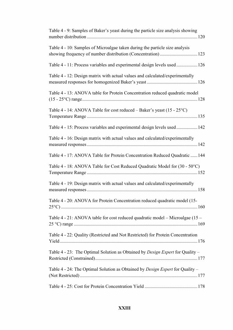
Table 4 - 9: Samples of Baker’s yeast during the particle size analysis showing

number distribution .............................................................................................. 120

Table 4 - 10: Samples of Microalgae taken during the particle size analysis

showing frequency of number distribution (Concentration) ................................ 123

Table 4 - 11: Process variables and experimental design levels used .................. 126

Table 4 - 12: Design matrix with actual values and calculated/experimentally

measured responses for homogenized Baker’s yeast ........................................... 126

Table 4 - 13: ANOVA table for Protein Concentration reduced quadratic model

(15 - 25°C) range .................................................................................................. 128

Table 4 - 14: ANOVA Table for cost reduced – Baker’s yeast (15 - 25°C)

Temperature Range .............................................................................................. 135

Table 4 - 15: Process variables and experimental design levels used .................. 142


measured responses .............................................................................................. 142

Table 4 - 17: ANOVA Table for Protein Concentration Reduced Quadratic ...... 144

Table 4 - 18: ANOVA Table for Cost Reduced Quadratic Model for (30 - 50°C)

Temperature Range .............................................................................................. 152


measured responses .............................................................................................. 158

Table 4 - 20: ANOVA for Protein Concentration reduced quadratic model (15-

25°C) .................................................................................................................... 160

Table 4 - 21: ANOVA table for cost reduced quadratic model – Microalgae (15 –

25 °C) range ......................................................................................................... 169

Table 4 - 22: Quality (Restricted and Not Restricted) for Protein Concentration

Yield ..................................................................................................................... 176

Table 4 - 23: The Optimal Solution as Obtained by Design Expert for Quality –

Restricted (Constrained) ....................................................................................... 177

Table 4 - 24: The Optimal Solution as Obtained by Design Expert for Quality –

(Not Restricted) .................................................................................................... 177

Table 4 - 25: Cost for Protein Concentration Yield ............................................. 178

XXIV

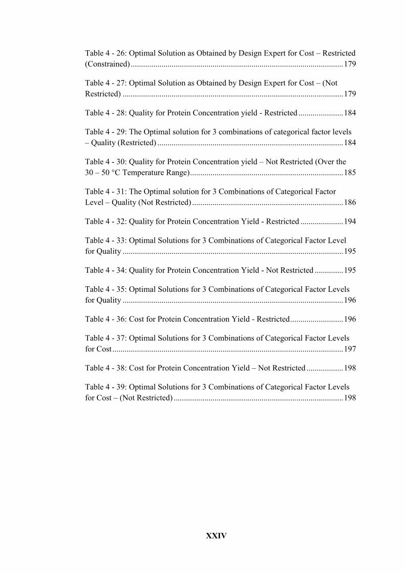
Table 4 - 26: Optimal Solution as Obtained by Design Expert for Cost – Restricted

(Constrained) ........................................................................................................ 179

Table 4 - 27: Optimal Solution as Obtained by Design Expert for Cost – (Not

Restricted) ............................................................................................................ 179

Table 4 - 28: Quality for Protein Concentration yield - Restricted ...................... 184

Table 4 - 29: The Optimal solution for 3 combinations of categorical factor levels

– Quality (Restricted) ........................................................................................... 184

Table 4 - 30: Quality for Protein Concentration yield – Not Restricted (Over the

30 – 50 °C Temperature Range) ........................................................................... 185

Table 4 - 31: The Optimal solution for 3 Combinations of Categorical Factor

Level – Quality (Not Restricted) .......................................................................... 186

Table 4 - 32: Quality for Protein Concentration Yield - Restricted ..................... 194

Table 4 - 33: Optimal Solutions for 3 Combinations of Categorical Factor Level

for Quality ............................................................................................................ 195

Table 4 - 34: Quality for Protein Concentration Yield - Not Restricted .............. 195

Table 4 - 35: Optimal Solutions for 3 Combinations of Categorical Factor Levels

for Quality ............................................................................................................ 196

Table 4 - 36: Cost for Protein Concentration Yield - Restricted .......................... 196


for Cost ................................................................................................................. 197

Table 4 - 38: Cost for Protein Concentration Yield – Not Restricted .................. 198


for Cost – (Not Restricted) ................................................................................... 198

XXV

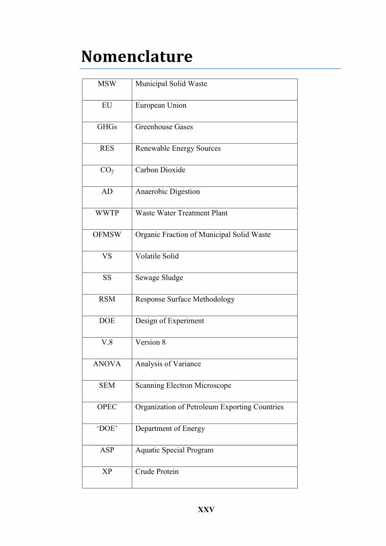
Nomenclature

MSW Municipal Solid Waste

EU European Union

GHGs Greenhouse Gases

RES Renewable Energy Sources

CO2 Carbon Dioxide

AD Anaerobic Digestion

WWTP Waste Water Treatment Plant

OFMSW Organic Fraction of Municipal Solid Waste

VS Volatile Solid

SS Sewage Sludge

RSM Response Surface Methodology

DOE Design of Experiment

V.8 Version 8

ANOVA Analysis of Variance

SEM Scanning Electron Microscope

OPEC Organization of Petroleum Exporting Countries

‘DOE’ Department of Energy

ASP Aquatic Special Program

XP Crude Protein

XXVI

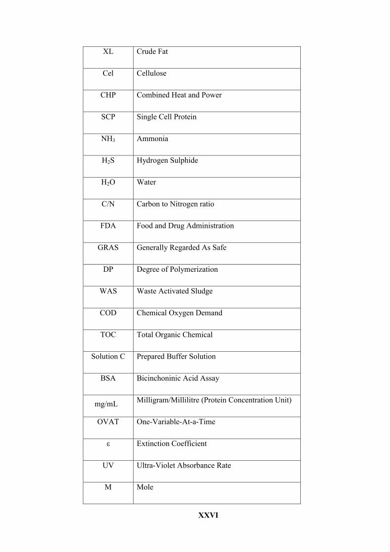
XL Crude Fat

Cel Cellulose

CHP Combined Heat and Power

SCP Single Cell Protein

NH3 Ammonia

H2S Hydrogen Sulphide

H2O Water

C/N Carbon to Nitrogen ratio

FDA Food and Drug Administration

GRAS Generally Regarded As Safe

DP Degree of Polymerization

WAS Waste Activated Sludge

COD Chemical Oxygen Demand

TOC Total Organic Chemical

Solution C Prepared Buffer Solution

BSA Bicinchoninic Acid Assay

mg/mL Milligram/Millilitre (Protein Concentration Unit)

OVAT One-Variable-At-a-Time

ε Extinction Coefficient

UV Ultra-Violet Absorbance Rate

M Mole

XXVII

BBD Box-Behnken Design

CCD Central Composite Design

Prob > F p-value

α Level of Significance

D Desirability Function

PDI Poly Dispersity Index

CFD Computational Fluid Dynamics

HHP High Hydrostatic Pressure

CW Cheese Whey

CCAP Culture Collection of Algae and Protozoa

μmol/m2s Culture Intensity

CH4, NaCl Methane, Sodium Chloride

μm, μl Microns in metre, Microns in litre

Kwh/m3 Kilowatt hour per cubic metre

Euro/h Euro per hour (Energy Cost for Protein Yield)

pH Concentration of Hydrogen ions

K2CO3 Potassium Carbonate

KH2PO4 Potassium Phosphate Monobasic

K2HPO4 Potassium Phosphate Monobasic Trihydrate

D Categorical Factor

ρ, v, d, x Density, Velocity jet, Distance, Impingement wall

1

Chapter 1 Introduction

1.1. Introduction

Energy is a vital input for social and economic development and affects all aspects

of modern life. Its demand is continually increasing at an exponential rate due to

the exponential growth of the world population [1, 2]. This means that the demand

for energy has been considered proportional to the growth of the population size

worldwide. Transportation, industrial activities, communication, health, and

education are some of the areas where energy cannot be substituted [3]. As the

world faces problems due to growing energy consumption and decline in the

supply of fossil fuels at this present time, this has inevitably led to the

development of energy from other sources. Sustainable energy has been perceived

as the ultimate solution to the current energy crisis being faced globally. Therefore

energy must be renewable, sustainable and economically viable to meet the needs

of the world’s growing population.

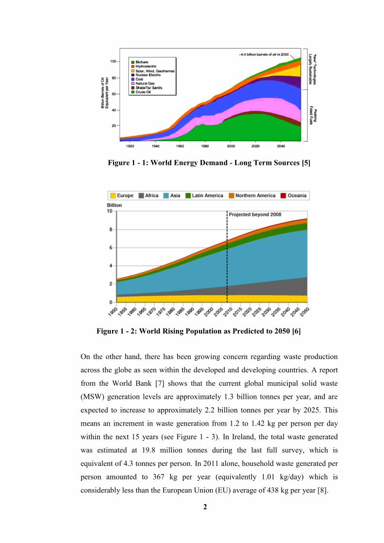
Currently, energy demand has been proposed to exceed the supply sources at an

exponential rate. By 2050, it is predicted to double or even triple, as the global

population rises and developing countries expand their economies [4]. Figure 1 - 1

shows the world energy demand on long term energy sources and Figure 1 - 2

shows the world’s rising population, predicted up to 2050. Based on these

available facts and figures, fossil fuels are not sustainable, and as such will not be

able to support the economic growth and energy security in the long term. The

volatility in the oil producing region and instability of the oil prices, along with

uncertainty in the supply, has resulted in some environmental factors that have

proven to be risky in the exploitation of fossil fuel.

2

Figure 1 - 1: World Energy Demand - Long Term Sources [5]

Figure 1 - 2: World Rising Population as Predicted to 2050 [6]

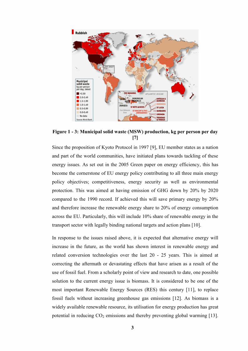
On the other hand, there has been growing concern regarding waste production

across the globe as seen within the developed and developing countries. A report

from the World Bank [7] shows that the current global municipal solid waste

(MSW) generation levels are approximately 1.3 billion tonnes per year, and are

expected to increase to approximately 2.2 billion tonnes per year by 2025. This

means an increment in waste generation from 1.2 to 1.42 kg per person per day

within the next 15 years (see Figure 1 - 3). In Ireland, the total waste generated

was estimated at 19.8 million tonnes during the last full survey, which is

equivalent of 4.3 tonnes per person. In 2011 alone, household waste generated per

person amounted to 367 kg per year (equivalently 1.01 kg/day) which is

considerably less than the European Union (EU) average of 438 kg per year [8].

3

Figure 1 - 3: Municipal solid waste (MSW) production, kg per person per day

[7]

Since the proposition of Kyoto Protocol in 1997 [9], EU member states as a nation

and part of the world communities, have initiated plans towards tackling of these

energy issues. As set out in the 2005 Green paper on energy efficiency, this has

become the cornerstone of EU energy policy contributing to all three main energy

policy objectives; competitiveness, energy security as well as environmental

protection. This was aimed at having emission of GHG down by 20% by 2020

compared to the 1990 record. If achieved this will save primary energy by 20%

and therefore increase the renewable energy share to 20% of energy consumption

across the EU. Particularly, this will include 10% share of renewable energy in the

transport sector with legally binding national targets and action plans [10].

In response to the issues raised above, it is expected that alternative energy will

increase in the future, as the world has shown interest in renewable energy and

related conversion technologies over the last 20 - 25 years. This is aimed at

correcting the aftermath or devastating effects that have arisen as a result of the

use of fossil fuel. From a scholarly point of view and research to date, one possible

solution to the current energy issue is biomass. It is considered to be one of the

most important Renewable Energy Sources (RES) this century [11], to replace

fossil fuels without increasing greenhouse gas emissions [12]. As biomass is a

widely available renewable resource, its utilisation for energy production has great

potential in reducing CO2 emissions and thereby preventing global warming [13].

4

In addition, using waste agricultural biomass does not compromise the production

of main food or non-food crops [14]. Biomass energy has been referred to as any

source of heat energy produced from non-fossil biological materials; this can come

from ocean and freshwater habitats as well as from land [15]. It is one of the

renewable energy sources capable of making a large contribution to the future

world’s energy supply. Although the role of bio-energy will depend on its

competitiveness with fossil fuels and on agricultural policies worldwide, it is

expected that the current bio-energy contribution of 40-55 1018

J per year will

increase considerably [16]. Different technologies are in place in the conversion of

biomass into energy using form. These are as detailed below.

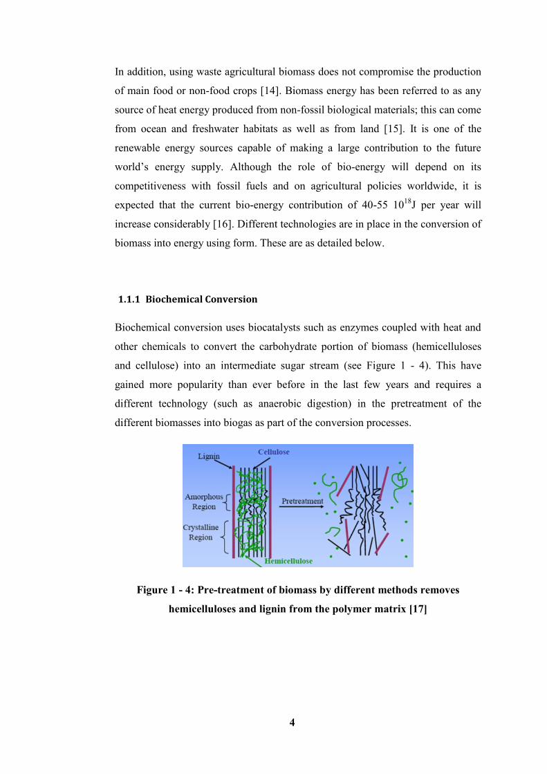
1.1.1 Biochemical Conversion

Biochemical conversion uses biocatalysts such as enzymes coupled with heat and

other chemicals to convert the carbohydrate portion of biomass (hemicelluloses

and cellulose) into an intermediate sugar stream (see Figure 1 - 4). This have

gained more popularity than ever before in the last few years and requires a

different technology (such as anaerobic digestion) in the pretreatment of the

different biomasses into biogas as part of the conversion processes.

Figure 1 - 4: Pre-treatment of biomass by different methods removes

hemicelluloses and lignin from the polymer matrix [17]

5

1.1.2 Anaerobic Digestion

Anaerobic digestion (AD) is the decomposition of biomass through bacterial

action in the absence of oxygen; it is essentially a fermentation process that

produces a mixed gas output of methane and carbon dioxide [18, 19]. Once broken

down, it reduces to simpler chemical components other than just methane and

carbon dioxide. The process is applicable to all biomass resources including wood

and wood wastes, agricultural crops and their waste by-products, municipal solid

waste (MSW), animal wastes, waste from food processing and aquatic plants and

algae [20]. Energy produced from the majority of biomass on average are rated at

64% for wood and wood wastes, MSW at 24%, agricultural waste at 5% and

landfill gases at 5% [21-23]. Agricultural biogas plants are considered most

suitable for digestion because they have lignocellulosic materials. But there are

more abundant raw materials from hardwood, softwood, grasses and agricultural

residues along with newsprint, office paper and municipal solid wastes [24]. These

are thought to consist of three types of polymers; lignin, cellulose and

hemicelluloses which are associated with each other [25], along with fractions of

other inner materials such as proteins and extractives

1.1.3 Fermentation

Another well-known biochemical process is fermentation. This is used

commercially on a large scale in various countries in the production of ethanol

from sugar crops and starch crops. This is ground down and the starch is converted

by enzymes to sugars with yeast converting the sugars to ethanol [26]. Mosier et

al. [17] have highlighted the four major units of operation in the processing of

lignocellulosics material as pretreatment, hydrolysis, fermentation, and product

separation. Hayes et al. [27], and Balat et al. [28] have indicated the complexity of

the substrate and the need for many different enzymes before these substrates can

be hydrolysed completely and effectively. The structure of lignocelluloses resists

degradation as result of cross linking between the polysaccharides (cellulose and

hemicelluloses) along with the lignin via ester and ether linkages. While Hendriks

and Zeeman [29], and Puri [30] viewed factors limiting hydrolysis as: degree of

polymerization, crystallinity, accessible surface area, and lignin distribution. Pre-

6

treatments are therefore considered as a prerequisite in the improvement of

cellulosic material degradation. This pre-treatment which could be physio-

chemical, biological, chemical or mechanical [31], is to enhance the overall yield

of methane.

1.1.4 Mechanical pre-treatment

This is the method employed in such pre-treatments as milling, irradiation, heat

treatment, liquid shear lysis-centrifuge, sonication, high-pressure homogenizer

(HPH), collision, maceration, and chipping. Ariunbaatar et al. [32] studied

maceration, sonication and HPH, and therefore reported these as the simplest

mechanical pre-treatments for organic solid waste (OSW) such as waste water

treatment plant (WWTP) sludge and lignocellulosic substrates. Size reduction of

lignocellulosic substrates therefore resulted in a 5 – 25% increase in hydrolysis

yield, depending on the mechanical methods used [29]. Whereas for WWTP

sludge and manure, the effects of pre-treatments significantly differ and applying

maceration pre-treatment enhances biogas production by 10–60% [33]. High

pressure homogenizer (HPH) increases the pressure up to several hundred bars,

and then homogenizes the substrates under strong depressurization [34]. These

pre-treatments methods are not common for the organic fraction of municipal solid

waste (OFMSW) but are to other substrates such as lignocellulosic materials,

manures and WWTP sludge. Engelhart et al. [35] studied the effect of HPH on the

AD of sewage sludge (SS), and achieved a 25% increased volatile solid (VS)

reduction. Overall, these pre-treatment methods are used to reduce crystallinity but

more importantly to give a reduction of particle size, to ease make material

handling, alongside increasing surface/volume ratio. This improvement was

achieved by an increase of soluble protein, lipid, and carbohydrate concentration.

1.2. Research Approach

In this research, a mechanical pre-treatment technique has been utilized,

employing a high-pressure homogenizer device in the treatment of biomass

substrates. This device also called a homogenizer machine, has the name “Cell

7

Disruption Machine” given to this method. Homogenizing lignocellulosic

materials result in decreased particle size and increased surface area. This will also

damage and change the structure of the component and then improve the high

recovery of protein yield. The homogenizing of the treated and untreated sets of

biomass materials with buffer solution were carried out and are presented within

this report.

Furthermore, so as to optimise the cell disruption process after homogenization,

statistical optimization work was carried out using Design of Experiment (DOE) -

Response Surface Methodology (RSM) techniques. In this part, Box Behnken

Design (BBD) was used to develop the experimental design (design matrix). After

this study was concluded, the optimum combinations of homogenization

parameters can be selected and used to achieve high levels of protein yield at a

minimal cost on energy usage.

1.3 Statement of Investigation

A high pressure homogenizer plays a dual role, it reduces the particle size and

increases the surface area. This is aimed at damaging and disrupting the cell walls

to improve the release of yeast/microalgae inner components [36-40]. The main

objectives of this study were:

- To introduce a mechanical pre-treatment technique through employing a

high-pressure homogenizer device Cell Disruption Machine to treat

cellulosic as well as lignocellulosic materials. The use of this equipment

has been achievable by considering and investigating the biomass

substrates through their pre-treatments in the determining of material

structures and the treatment effect on protein concentration yields which is

known to aid the production of biogas. This study also investigated the

behaviour and rheological properties of the substrates and the consequent

effect on the biomass parameters during homogenization. A cost

effectiveness energy analysis was also conducted so as to ascertain the

economic feasibility of the treatment technique.

- To predict and optimise the homogenizing process after treating yeast and

the micro algae using Response Surface Methodology (RSM) via the

8

Design Expert STATEASE Software to develop mathematical models that

relate the process input parameters to their output responses. Based on this

study, the three most important input parameters of the homogenization

process considered were the number of cycle (passes), temperature and

pressure. These were thoroughly investigated to determine their effects on

the homogenized substrates. The investigated output features are protein

concentration and cost for the energy consumption.

The following points further elucidate and summarise the second objective of this

study:

Applying Response Surface Methodology (RSM) to develop mathematical models

for the materials mentioned above through using Design Expert V.8 statistical

software to predict and optimise the following process responses;

Protein concentration

Energy cost

Present the developed models graphically to demonstrate the effect of each

homogenizing parameter selected on the responses as mentioned above.

Analysis of variance (ANOVA) was applied to have the adequacy of the

developed model tested, and also to have each term in the developed models

examined using statistical significance tools.

Determining the optimal combinations of input homogenizing factors, using the

developed models with numerical and graphical optimization, to achieve the

desired criterion for the responses listed above.

To investigate particle size effects of the biomass substrates particularly on the

effect of the process performance thus improving protein concentration yield.

The present study is not limited to the aforementioned processing parameters in

HPH. Previous work has demonstrated a correlation between homogenization of

biomass substrates and the processing parameter for higher protein yields. To

facilitate higher protein production yields and quality of target protein, the

production process should be optimised [41]. The work presented in this thesis

provides new insights into the investigation of biomasses in improvement of

protein production through their uses in high-pressure homogenizer (HPH).

9

1.4 Thesis Outline

The thesis has been laid out in a progressive manner that initially introduces the

reader to the problem at hand. This provides an introduction to the work as well as

the thesis statement of investigation and the thesis outline. Background knowledge

relating to the subject is then presented, followed by the detailed study of the cell

disruption machine (HPH), as well as the material and methods used in the work.

The results from the study are then elucidated followed by discussions, and finally

conclusions with recommendation for future work. The contents of each chapter

are highlighted below:

Chapter 2 – The aim of the chapter is to introduce the reader to the several

subjects the thesis encompasses. The chapter reviews the necessary background

and literature review on yeast (Saccharomyces Cerevisiae) and microalgae

(Chlorella Vulgaris), pre-treatment methods, high-pressure homogenizer and the

operating parameters. The reasons behind the choice of materials and processes

used in this research were considered also. This chapter also reveals previous work

carried out in this field, highlighting the short-comings that need improvements

and further study.

In addition, this chapter also details research on high-pressure homogenizer as the

main mechanical treatment (cell disruption machine) for this research with details

about how the device works, which in essence reflect the mechanism of the

technique.

Chapter 3 – The chapter aims at revealing the instrumentation and equipment

used, as well as the biomass substrates and their compositions which are detailed

in the experimental procedures in this study. This allows for experimental

repeatability by readers. This chapter also detailed the software package applicable

to the research; Design Expert V.8

Chapter 4 – This chapter presents the results and discussion from the experimental

findings. As the first step, it considered the one-variable-at-a-time approach

(OVAT) which determines the data range of the experiments conducted. Trial

experiments were conducted to showcase the workability of the experimentation

plans with data range for the parameters considered based on the trial experiments.

10

Particle size analysis was also considered in this chapter as size reduction means

in the liberation of the inner contents of substrates. The particle size measurements

were conducted using the Delsa Nano C equipment and Scanning Electron

Microscope (SEM) was also used in checking the deformation of substrates after

treatments.

Through the software, the chapter explains how the Design of Experiments (DOE)

and Response Surface Methodology (RSM) were implemented in this research for

optimization of the homogenized substrates. This involved the gradation and how

the experimental work has been sectioned in terms of result and analyses. Baker’s

yeast was used as the substrate, homogenized at temperature ranges 15 - 25 °C and

30 - 50 °C. While the microalgae experimental work was only considered at

temperature ranges 15 - 25 °C. The results therefore presented and discussed are

within the dataset of temperature indicated above. The chapter also contains the

optimization of experimental work using Design of Experiments (DOE) with

particular consideration of the responses, the protein concentration yield, and the

energy cost.

Chapter 5 – This chapter concludes by highlighting the most important findings

and recommendations for future research work.

1.5. Summary

This chapter has provided the general introductory note into the conducted

research topic with emphasis on the current energy trends coupled with the world

growing population, which is expected to double or even triple in the next 35

years. The areas of greater difficulties have been highlighted as the world faces

problems due to growing energy consumption and the decline in the supply of

fossil fuels at this present time. This coupled with climate change and energy

security poses a higher threat to the future energy need. However, renewable

energy has been foreseen as part solution to the current problem, and in line with

the current research biomass is ranked favourably for the provision of lasting

solution to the problem.

11

Based on this study, some biomass contributions have been highlighted in the

chapter, where energy saving opportunities is possible and as such will contribute

to enhancing future energy needs/trends. The chapter highlighted the steps

involved in complete disruption of biomass substrate in order to release protein

concentration keeping in mind cost effectiveness.

12

Chapter 2 Review of Literature

2.1 Introduction

This chapter introduces the reader to the literature review as it pertains to the

research topic. In this chapter the substrates, Baker’s yeast and microalgae will be

critically analysed and considered through protein yield when homogenized under

high pressure. The high-pressure homogenizer disruption equipment will also be

reviewed with emphasis on the mechanism, operation and its usefulness, in

comparison to other equipment for recovery intracellular product of

microorganisms.

2.1.1 Background

The view of energy in the 21st century has taken a dramatic change in terms of

energy demand and this has been accounted for due to population growth. This

growth in global energy demand is projected to rise sharply over the coming years

[42]. The continuous use of fossil fuels has been a leading cause of the current

global paradigm resulting in the emission of greenhouse gases, effects of global

warming as well as changes in the climate. Hall et al. [43] have related civilization

to technology. They indicated that technology has generally led to a greater use of

hydrocarbon fuels for most human activities. This then makes civilization

vulnerable to decreases in supply. Because our civilization has been heavily

dependent on the enormous flows of cheap hydrocarbons, many of our once-proud

ancient cultures have collapsed due to their inability to maintain energy resources

and societal complexity [44]. Accomplishing civilizations have largely advanced

through increased efficiencies and the extensive harnessing of the various forms of

energy as the result of human ingenuity [42]. Growing energy and environmental

concerns have become important issues amid concerns about high energy prices

and the occurrence of regional supply shortfalls [45-48]. An assessment of the

current state of oil security indicates that the risks of supply disruption have not

diminished [48]. Von Hippel et al. [49] reported the energy security concept as

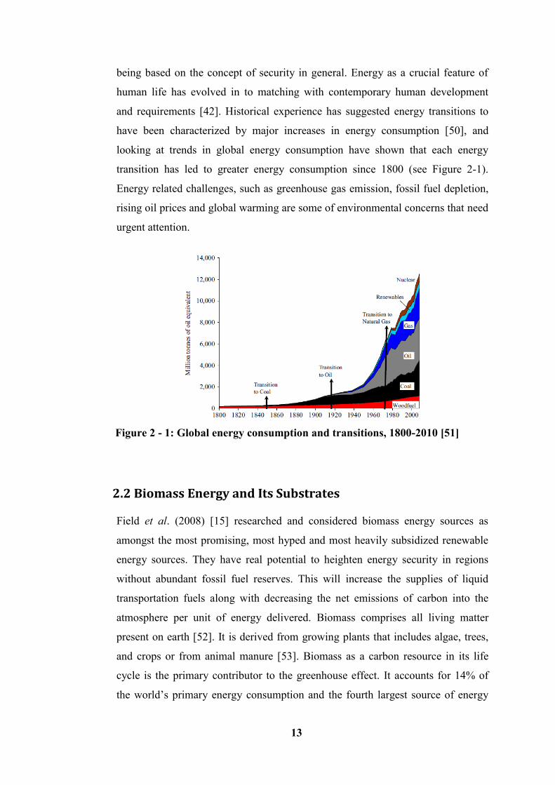
13

being based on the concept of security in general. Energy as a crucial feature of

human life has evolved in to matching with contemporary human development

and requirements [42]. Historical experience has suggested energy transitions to

have been characterized by major increases in energy consumption [50], and

looking at trends in global energy consumption have shown that each energy

transition has led to greater energy consumption since 1800 (see Figure 2-1).

Energy related challenges, such as greenhouse gas emission, fossil fuel depletion,

rising oil prices and global warming are some of environmental concerns that need

urgent attention.

Figure 2 - 1: Global energy consumption and transitions, 1800-2010 [51]

2.2 Biomass Energy and Its Substrates

Field et al. (2008) [15] researched and considered biomass energy sources as

amongst the most promising, most hyped and most heavily subsidized renewable

energy sources. They have real potential to heighten energy security in regions

without abundant fossil fuel reserves. This will increase the supplies of liquid

transportation fuels along with decreasing the net emissions of carbon into the

atmosphere per unit of energy delivered. Biomass comprises all living matter

present on earth [52]. It is derived from growing plants that includes algae, trees,

and crops or from animal manure [53]. Biomass as a carbon resource in its life

cycle is the primary contributor to the greenhouse effect. It accounts for 14% of

the world’s primary energy consumption and the fourth largest source of energy

14

after coal, petroleum, and natural gas. As an important energy resource globally, it

is used in meeting variety of energy needs and that includes electricity generation,

fuelling vehicles, and providing heat for industrial uses [53-55]. Özbay et al. [56]

and Demirbas, (2001) [57] have demonstrated biomass as the only renewable

energy source of carbon which can be converted into convenient solid, liquid and

gaseous fuels through different conversion processes. Based on their findings,

Sheth and Babu [58] showcased biomass as a unique renewable form of energy

with many ecological advantages. Through thermochemical conversion, they were

able to illustrate biomass as one of the promising routes amongst the renewable

energy options of future energy. Biomass with such substrates as wood, were

considered as predominant fuel in many non-OPEC (Organization of the

Petroleum Exporting Countries), tropical, developing countries and its use will

continue to be used for many years. Wood is used as a fuel in the domestic (for

cooking and water heating), commercial (water heating) and industrial (for water

heating and process heat) sector. Demirbas, (2000) [20] evaluated wood as it

competes well with fossil fuels due to its being renewable and with soft energies

like solar and wind, on account of its energy storage capability. Saxena et al. [52]

in their paper therefore evaluated biomass as being able to be converted into three

main types of products; electrical/heat energy, fuel for the transport sector, and

feedstock for chemical products.

Another area of great concern is the conversion technologies for utilizing biomass

and these can be separated into four basic categories: direct combustion,

thermochemical processes, biochemical processes, and agrochemical processes.

Biological processes are essentially microbial digestion and biochemical processes

convert biomass to ethanol and methane [59].

2.2.1 Microbes

Microbes are tiny single-cell organisms and are considered the oldest form of life

on earth. They form a most vital part of human existence as without them, no

human activities can take place. They can be divided into six main types such as;

archaea, bacteria, fungi, protista, viruses and microbial merger and are collectively

15

useful in all parts of human life in one form or another. The current surge in food

and fuel prices has sounded an alarm showing why providing a sustainable global

energy supply and minimizing climate change and are arguably two of the greatest

challenges facing 21st century society. Bacteria, yeasts, fungi and archaea as

unseen inhabitants of the microbial world have proven to be helpful in addressing

these challenges according to Wolin et al. [60]. To harness microbial activities in

the address of these challenges, much remains to be learned about the chemical

space these occupy. It is estimated that 1030

of these microbes exist on earth, vast

majority are still not known. Most microbes are beneficial, and their combined

activities positively affect numerous aspects of the biosphere inhabitants. Other

areas of great importance are the production of renewable energy which is now

serving a purpose in meeting the needs of our population worldwide.

2.2.2 Yeast as a Biomass

Baker’s yeast, whose scientific name is known as Saccharomyces cerevisiae has

been in use for a long time [61]. It is widely available in a number of forms,

including cake yeast known as wet, fresh or compressed yeast (see Figure 2-2),

active dry yeast, and instant or fast-rising yeast. It is a common name for the

strains of yeast commonly used as a leavening agent in baking bread and bakery

products where it converts the fermentable sugars present in the dough into carbon

dioxide and ethanol. Yeasts are single-cell organisms found to have extensive use

in the food and beverage industries [62-63]. Alais and Linden [64] and Reed and

Nagodawithana [65] have found yeast to be important as a raw material for the

food, pharmaceutical, and cosmetic industries, in addition to being an excellent

source of nutrients, mainly protein, vitamins of the B complex and essential

minerals. Inactivated yeast cells have also been used for animal feeding and as a

nutritional complement for humans [66-67].

Mostly widely used amongst microorganisms for ethanol fermentation is

Saccharomyces cerevisiae; this is due to its ability to hydrolyse cane sucrose into

fermentable sugars. This yeast has the ability to grow under anaerobic conditions,

and a certain amount of oxygen is necessary to synthesize essential fatty acids and

16

other compounds [68] contained in it to form energy. Yeast may be defined as

microorganisms in which the unicellular form is conspicuous, but belongs to

fungi. Most yeast cells are colourless and transparent, while some produces

carotenoid pigments like Rhodotorula. Beudeker et al. [69] elucidated and

considered Baker’s yeast (S. cerevisiae) as one of the most important

biotechnological products due to its several industrial applications. As a

commercial product, it has several formulations; hence it can be grouped into two

main types: compressed yeast (fresh yeast) in block forms along with the other

kinds; active dry yeast, and instant or fast-rising yeast. Apart from yeast uses in

the industry for energy production, its uses have been prominent as experimental

models since the very beginning of microbiology and biochemistry.

2.2.3 Classification of Yeasts

Phaff and Macmillan [70] classified yeasts into four groups;

1. Ascomycetous yeasts – capable of forming ascospores in asci.

2. Basidiomycetous yeast – those having a lifecycle similar to those of order

Ustilaginales or Basidiomycetes.

3. Ballistosporogenous yeasts – those that forcibly discharge spores by the

mechanism of excretion.

4. Asporogeneous yeasts (or Deuteromycetes or false yeasts) – these are

otherwise known as Fungi imperfecti members. They are incapable of

producing ascospores, ballistospores, or sporidia, since sexual lifecycle

does not occur or has not been observed so far.

Reed and Peppler [71] in their studies, named and classified yeasts into two

classes of fungi based on their spore-forming capabilities and industrial

importance. The true yeast and the false yeast which are known respectively to be

ascomycetes (or ascorporogeneous) and asexual deuteromycetes or

(asporogeneous) and based on this research, focus will only be on the species,

Saccharomyces cerevisiae also known as the Baker’s yeast. Species were named

on the basis of fermentation that they have always been associated with, like

Saccharomyces cerevisiae, Saccharomyces vinii or Saccharomyces sake. Since

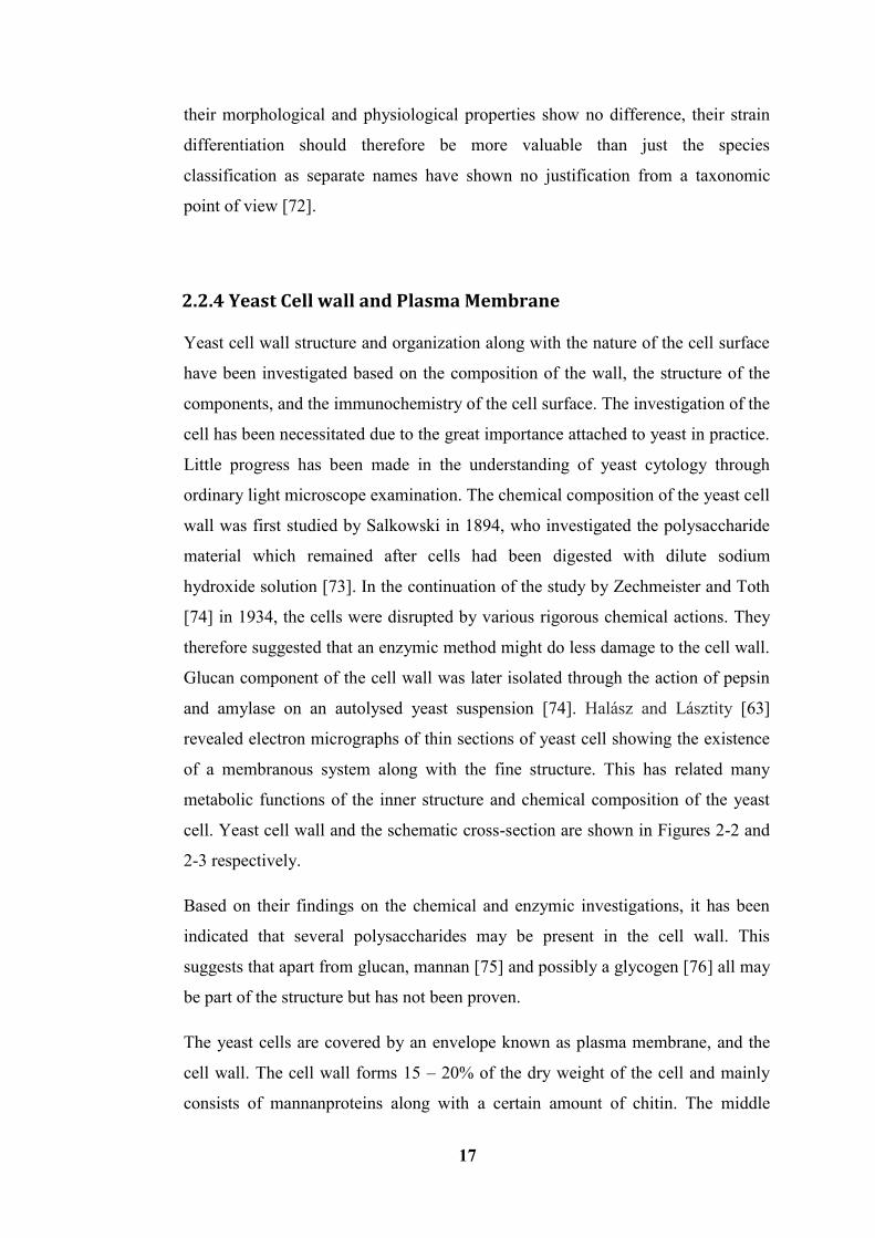
17

their morphological and physiological properties show no difference, their strain

differentiation should therefore be more valuable than just the species

classification as separate names have shown no justification from a taxonomic

point of view [72].

2.2.4 Yeast Cell wall and Plasma Membrane

Yeast cell wall structure and organization along with the nature of the cell surface

have been investigated based on the composition of the wall, the structure of the

components, and the immunochemistry of the cell surface. The investigation of the

cell has been necessitated due to the great importance attached to yeast in practice.

Little progress has been made in the understanding of yeast cytology through

ordinary light microscope examination. The chemical composition of the yeast cell

wall was first studied by Salkowski in 1894, who investigated the polysaccharide

material which remained after cells had been digested with dilute sodium

hydroxide solution [73]. In the continuation of the study by Zechmeister and Toth

[74] in 1934, the cells were disrupted by various rigorous chemical actions. They

therefore suggested that an enzymic method might do less damage to the cell wall.

Glucan component of the cell wall was later isolated through the action of pepsin

and amylase on an autolysed yeast suspension [74]. Halász and Lásztity [63]

revealed electron micrographs of thin sections of yeast cell showing the existence

of a membranous system along with the fine structure. This has related many

metabolic functions of the inner structure and chemical composition of the yeast

cell. Yeast cell wall and the schematic cross-section are shown in Figures 2-2 and

2-3 respectively.

Based on their findings on the chemical and enzymic investigations, it has been

indicated that several polysaccharides may be present in the cell wall. This

suggests that apart from glucan, mannan [75] and possibly a glycogen [76] all may

be part of the structure but has not been proven.

The yeast cells are covered by an envelope known as plasma membrane, and the

cell wall. The cell wall forms 15 – 20% of the dry weight of the cell and mainly

consists of mannanproteins along with a certain amount of chitin. The middle

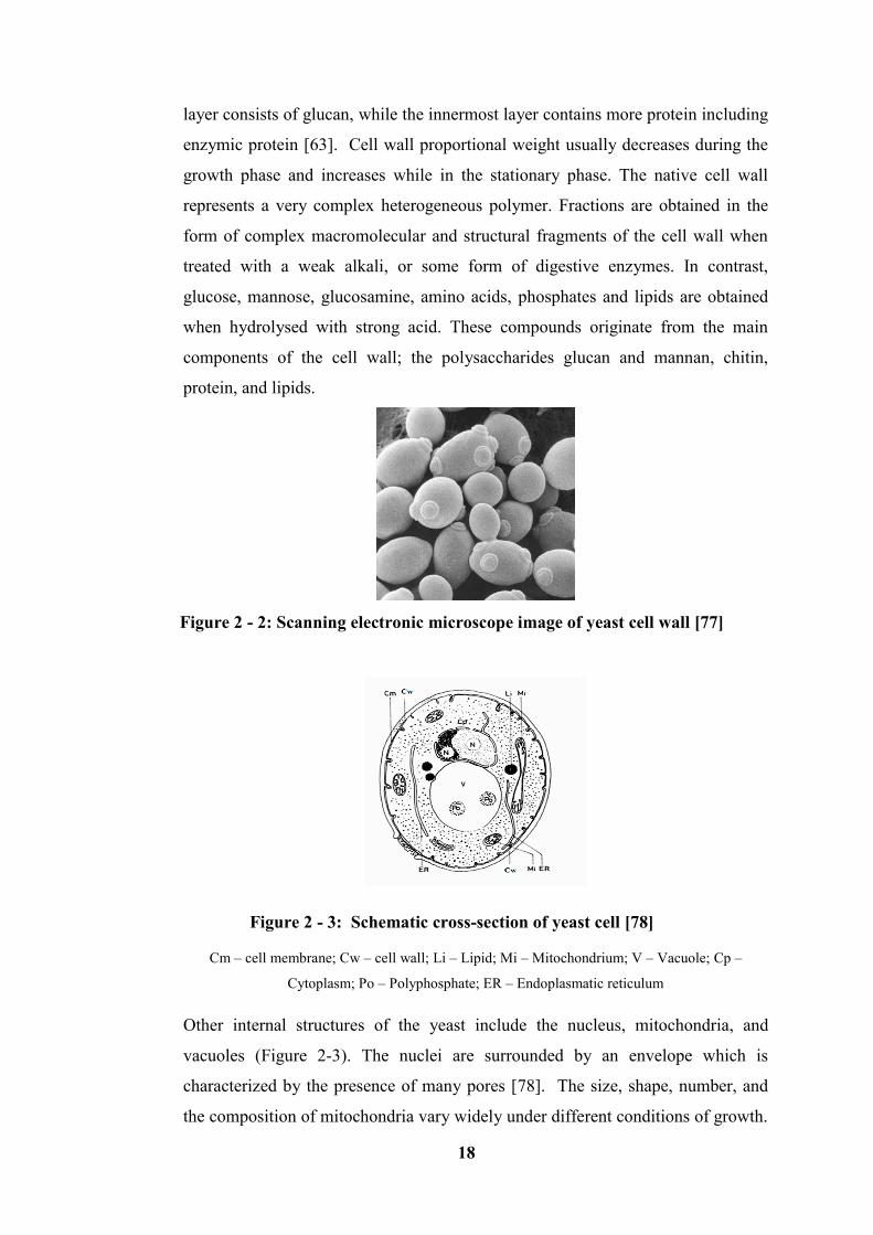
18

layer consists of glucan, while the innermost layer contains more protein including

enzymic protein [63]. Cell wall proportional weight usually decreases during the

growth phase and increases while in the stationary phase. The native cell wall

represents a very complex heterogeneous polymer. Fractions are obtained in the

form of complex macromolecular and structural fragments of the cell wall when

treated with a weak alkali, or some form of digestive enzymes. In contrast,

glucose, mannose, glucosamine, amino acids, phosphates and lipids are obtained

when hydrolysed with strong acid. These compounds originate from the main

components of the cell wall; the polysaccharides glucan and mannan, chitin,

protein, and lipids.

Figure 2 - 2: Scanning electronic microscope image of yeast cell wall [77]

Figure 2 - 3: Schematic cross-section of yeast cell [78]

Cm – cell membrane; Cw – cell wall; Li – Lipid; Mi – Mitochondrium; V – Vacuole; Cp –

Cytoplasm; Po – Polyphosphate; ER – Endoplasmatic reticulum

Other internal structures of the yeast include the nucleus, mitochondria, and

vacuoles (Figure 2-3). The nuclei are surrounded by an envelope which is

characterized by the presence of many pores [78]. The size, shape, number, and

the composition of mitochondria vary widely under different conditions of growth.

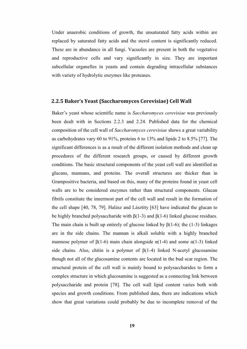
http://2.bp.blogspot.com/_207DNIaL-gc/TNrwiMk-7II/AAAAAAAAAUI/gzlgMa3etfU/s1600/YeastCellsforWine.jpg

19

Under anaerobic conditions of growth, the unsaturated fatty acids within are

replaced by saturated fatty acids and the sterol content is significantly reduced.

These are in abundance in all fungi. Vacuoles are present in both the vegetative

and reproductive cells and vary significantly in size. They are important

subcellular organelles in yeasts and contain degrading intracellular substances

with variety of hydrolytic enzymes like proteases.

2.2.5 Baker’s Yeast (Saccharomyces Cerevisiae) Cell Wall

Baker’s yeast whose scientific name is Saccharomyces cerevisiae was previously

been dealt with in Sections 2.2.3 and 2.24. Published data for the chemical

composition of the cell wall of Saccharomyces cerevisiae shows a great variability

as carbohydrates vary 60 to 91%, proteins 6 to 13% and lipids 2 to 8.5% [77]. The

significant differences is as a result of the different isolation methods and clean up

procedures of the different research groups, or caused by different growth

conditions. The basic structural components of the yeast cell wall are identified as

glucans, mannans, and proteins. The overall structures are thicker than in

Grampositive bacteria, and based on this, many of the proteins found in yeast cell

walls are to be considered enzymes rather than structural components. Glucan

fibrils constitute the innermost part of the cell wall and result in the formation of

the cell shape [40, 78, 79]. Halász and Lásztity [63] have indicated the glucan to

be highly branched polysaccharide with β(1-3) and β(1-6) linked glucose residues.

The main chain is built up entirely of glucose linked by β(1-6); the (1-3) linkages

are in the side chains. The mannan is alkali soluble with a highly branched

mannose polymer of β(1-6) main chain alongside α(1-4) and some α(1-3) linked

side chains. Also, chitin is a polymer of β(1-4) linked N-acetyl glucosamine

though not all of the glucosamine contents are located in the bud scar region. The

structural protein of the cell wall is mainly bound to polysaccharides to form a

complex structure in which glucosamine is suggested as a connecting link between

polysaccharide and protein [78]. The cell wall lipid content varies both with

species and growth conditions. From published data, there are indications which

show that great variations could probably be due to incomplete removal of the

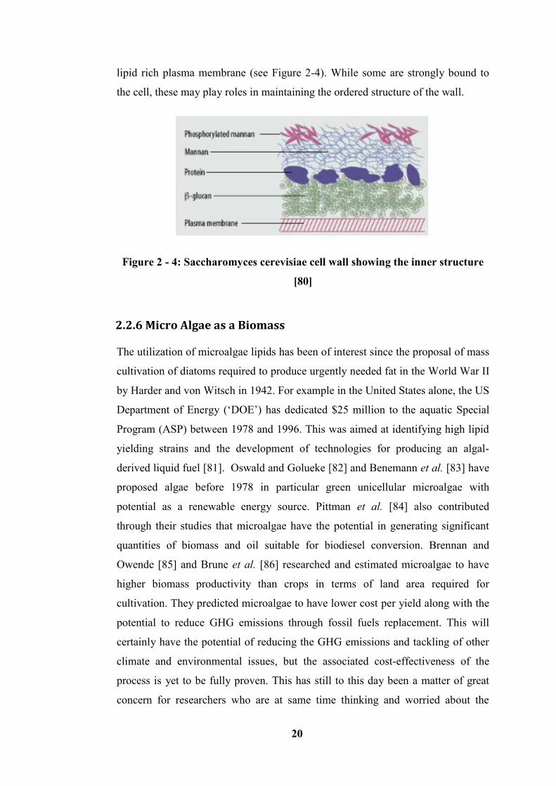
20

lipid rich plasma membrane (see Figure 2-4). While some are strongly bound to

the cell, these may play roles in maintaining the ordered structure of the wall.

Figure 2 - 4: Saccharomyces cerevisiae cell wall showing the inner structure

[80]

2.2.6 Micro Algae as a Biomass

The utilization of microalgae lipids has been of interest since the proposal of mass

cultivation of diatoms required to produce urgently needed fat in the World War II

by Harder and von Witsch in 1942. For example in the United States alone, the US

Department of Energy (‘DOE’) has dedicated $25 million to the aquatic Special

Program (ASP) between 1978 and 1996. This was aimed at identifying high lipid

yielding strains and the development of technologies for producing an algal-

derived liquid fuel [81]. Oswald and Golueke [82] and Benemann et al. [83] have

proposed algae before 1978 in particular green unicellular microalgae with

potential as a renewable energy source. Pittman et al. [84] also contributed

through their studies that microalgae have the potential in generating significant

quantities of biomass and oil suitable for biodiesel conversion. Brennan and

Owende [85] and Brune et al. [86] researched and estimated microalgae to have

higher biomass productivity than crops in terms of land area required for

cultivation. They predicted microalgae to have lower cost per yield along with the

potential to reduce GHG emissions through fossil fuels replacement. This will

certainly have the potential of reducing the GHG emissions and tackling of other

climate and environmental issues, but the associated cost-effectiveness of the

process is yet to be fully proven. This has still to this day been a matter of great

concern for researchers who are at same time thinking and worried about the

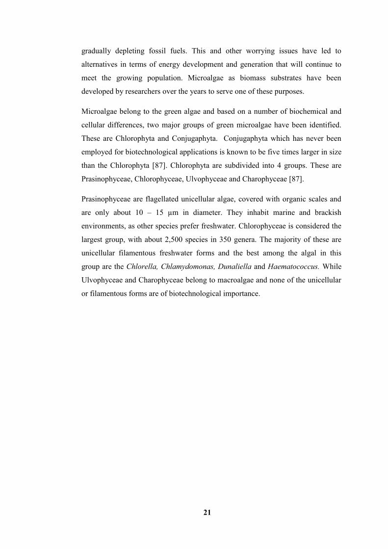
21

gradually depleting fossil fuels. This and other worrying issues have led to

alternatives in terms of energy development and generation that will continue to

meet the growing population. Microalgae as biomass substrates have been

developed by researchers over the years to serve one of these purposes.

Microalgae belong to the green algae and based on a number of biochemical and

cellular differences, two major groups of green microalgae have been identified.

These are Chlorophyta and Conjugaphyta. Conjugaphyta which has never been

employed for biotechnological applications is known to be five times larger in size

than the Chlorophyta [87]. Chlorophyta are subdivided into 4 groups. These are

Prasinophyceae, Chlorophyceae, Ulvophyceae and Charophyceae [87].

Prasinophyceae are flagellated unicellular algae, covered with organic scales and

are only about 10 – 15 µm in diameter. They inhabit marine and brackish

environments, as other species prefer freshwater. Chlorophyceae is considered the

largest group, with about 2,500 species in 350 genera. The majority of these are

unicellular filamentous freshwater forms and the best among the algal in this

group are the Chlorella, Chlamydomonas, Dunaliella and Haematococcus. While

Ulvophyceae and Charophyceae belong to macroalgae and none of the unicellular

or filamentous forms are of biotechnological importance.

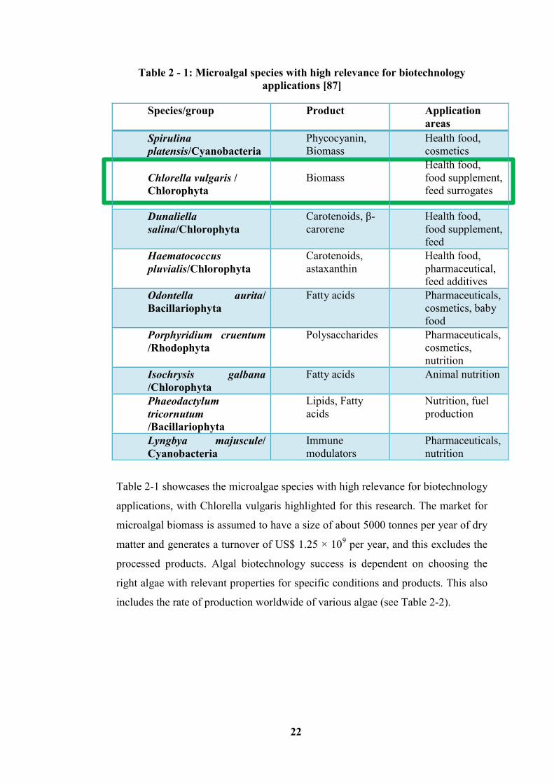
22

Table 2 - 1: Microalgal species with high relevance for biotechnology

applications [87]

Table 2-1 showcases the microalgae species with high relevance for biotechnology

applications, with Chlorella vulgaris highlighted for this research. The market for

microalgal biomass is assumed to have a size of about 5000 tonnes per year of dry

matter and generates a turnover of US$ 1.25 × 109 per year, and this excludes the

processed products. Algal biotechnology success is dependent on choosing the

right algae with relevant properties for specific conditions and products. This also

includes the rate of production worldwide of various algae (see Table 2-2).

Species/group Product Application

areas

Spirulina

platensis/Cyanobacteria

Phycocyanin,

Biomass

Health food,

cosmetics

Chlorella vulgaris /

Chlorophyta

Biomass

Health food,

food supplement,

feed surrogates

Dunaliella

salina/Chlorophyta

Carotenoids, β-

carorene

Health food,

food supplement,

feed

Haematococcus

pluvialis/Chlorophyta

Carotenoids,

astaxanthin

Health food,

pharmaceutical,

feed additives

Odontella aurita/

Bacillariophyta

Fatty acids Pharmaceuticals,

cosmetics, baby

food

Porphyridium cruentum

/Rhodophyta

Polysaccharides Pharmaceuticals,

cosmetics,

nutrition

Isochrysis galbana

/Chlorophyta

Fatty acids Animal nutrition

Phaeodactylum

tricornutum

/Bacillariophyta

Lipids, Fatty

acids

Nutrition, fuel

production

Lyngbya majuscule/

Cyanobacteria

Immune

modulators

Pharmaceuticals,

nutrition

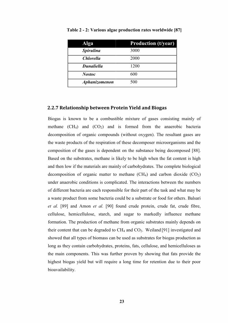
23

Table 2 - 2: Various algae production rates worldwide [87]

2.2.7 Relationship between Protein Yield and Biogas

Biogas is known to be a combustible mixture of gases consisting mainly of

methane (CH4) and (CO2) and is formed from the anaerobic bacteria

decomposition of organic compounds (without oxygen). The resultant gases are

the waste products of the respiration of these decomposer microorganisms and the

composition of the gases is dependent on the substance being decomposed [88].

Based on the substrates, methane is likely to be high when the fat content is high

and then low if the materials are mainly of carbohydrates. The complete biological

decomposition of organic matter to methane (CH4) and carbon dioxide (CO2)

under anaerobic conditions is complicated. The interactions between the numbers

of different bacteria are each responsible for their part of the task and what may be

a waste product from some bacteria could be a substrate or food for others. Balsari

et al. [89] and Amon et al. [90] found crude protein, crude fat, crude fibre,

cellulose, hemicellulose, starch, and sugar to markedly influence methane

formation. The production of methane from organic substrates mainly depends on

their content that can be degraded to CH4 and CO2. Weiland [91] investigated and

showed that all types of biomass can be used as substrates for biogas production as

long as they contain carbohydrates, proteins, fats, cellulose, and hemicelluloses as

the main components. This was further proven by showing that fats provide the

highest biogas yield but will require a long time for retention due to their poor

bioavailability.

Alga Production (t/year)

Spirulina 3000

Chlorella 2000

Dunaliella 1200

Nostoc 600

Aphanizomenon 500

24

Figure 2 - 5: Biogas production process showing the different stages [54]

Carbohydrates and proteins show much faster conversion rates but with lower gas

yields. Protein yield influences biogas production, as researched by [91-95], Oslaj

et al. [95] concluded that biogas production depended on the content of crude

protein. Sialve et al. [94] highlighted that the high proportion in proteins for

several species of microalgal composition was characterized by a low C/N

(carbon-Nitrogen ratio), especially if compared with terrestrial plants. Amon et al.

[92] researched on “Biogas production from maize and dairy cattle manure -

Influence of biomass composition on the methane yield”, and in their findings,

realized that the nutrients crude protein (XP), crude fat (XL), cellulose (Cel) and

hemi-cellulose (Hem), all proved to have significant influence on methane

production. They showed the contribution of each nutrient to the net total methane

yield. This therefore supported the previous work carried out by Amon et al. [96]

in their 2004 paper wherein crude fat (27.73) and crude protein (19.05) contributed

most to the net total methane energy value of maize silage. The biogas production

25

process is depicted in (Figure 2-5) showing the contribution of protein and other

constituents.

2.2.8 Choices of Yeast and Micro algae substrates

The use of Baker’s yeast (Saccharomyces Cerevisiae) and microalgae (Chlorella

Vulgaris) are fundamental to this research. Biomass has shown to have largest

potential which can only be considered as the best option in the meeting the

demand and insurance of future energy/fuel supply in a sustainable manner.

Chandra et al. [97] have clarified and suggested that the modernization of biomass

technologies have led to more efficient biomass production. They have further

stressed conversion as one possible direction for biomass resource efficient

utilization. The direct combustion of residues and wastes for electricity generation,

ethanol, biogas, and biodiesel as liquid fuels, and combined heat and power (CHP)

production from energy crops have all been considered as the main biomass

processes that will be expected to be utilized in the future. Biomass resources from

agriculture are considered and classified as either the food based portion, or the

non-food based portion. Chandra et al. [97] viewed oil and simple carbohydrates

of crops such as corn, sugarcane, beets as food based portion and complex

carbohydrates of crops such as the leaves, stalks, and cobs of corn stover, orchard

trimmings, rice husk, straw, along with perennial grasses, and animal waste as

non-food based.

Algae and yeast, amongst others, are microorganisms which utilize inexpensive

feedstocks and wastes as sources of carbon and energy for growth in the

production of biomass, protein concentrate, or amino acids. Due to protein

accounting for the quantitatively important part of the microbial cells, they are

therefore known as single cell protein (SCP) as natural protein concentrate [98].

Based on this nature of theirs, microbial biomass has been considered as an

alternative to conventional sources of food or feed. Saccharomyces Cerevisiae and

Chlorella Vulgaris choices as biomass substrates cannot be overemphasized.

On the other hand, microalgae species choices of Chlorella vulgaris is considered

commercially important because of its green nature and own its potential to serve

26

as a food and energy source as a result of their high photosynthetic efficiency.

This in theory can reach 8% and can be grown with autotropic and heterotrophic

modes [99]. Algal proteins are of high quality and comparable to conventional

vegetable proteins and Rasoul-Amini et al. [100] therefore concluded that due to

their high production costs and technical difficulties, its cultivation as protein is

still under evaluation. Kim et al. [101] were particularly concerned with yeast

small particle size, high protein content as SCP and their relatively low production

costs, resulting in their cells being substituted. For ease of cell wall disruption,

several methods such as; mechanical disruption, autolysis and enzymatic treatment

have been used in the improvement of the digestibility of SCP products [102].

2.2.9 Biogas properties/Composition and Uses

Biogas is composed of methane (CH4), carbon dioxide (CO2) and water (H2O) as

the main constituents. It is also constituted by a minority of other gases in which

some are considered toxic and thus be monitored due to their toxic nature. Such

gases are ammonia (NH3) and hydrogen sulphide (H2S). Biogas is a flammable gas

and the proportions of the biogas components depend directly on the substrates

being decomposed (see Table 2-3). It can be exploited in variety of ways and the

direct approach in the production of energy from biogas is through burning it in

chambers or boilers to produce both heat and electricity. Energy produced from

such means does not require any upgrade of biogas as long as emission limitations

are observed [103]. The composition of biogas varies and is dependent upon the

origin of the anaerobic digestion or conversion processes that are involved.

Landfill gas typically has methane concentrations around 50%. Advanced waste

treatment technologies can produce biogas with 55-75% CH4 [104].

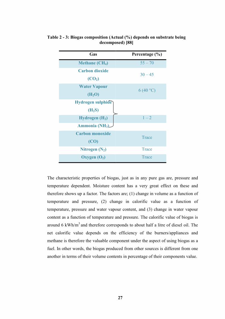
27

Table 2 - 3: Biogas composition (Actual (%) depends on substrate being

decomposed) [88]

The characteristic properties of biogas, just as in any pure gas are, pressure and

temperature dependent. Moisture content has a very great effect on these and

therefore shows up a factor. The factors are; (1) change in volume as a function of

temperature and pressure, (2) change in calorific value as a function of

temperature, pressure and water vapour content, and (3) change in water vapour

content as a function of temperature and pressure. The calorific value of biogas is

around 6 kWh/m3

and therefore corresponds to about half a litre of diesel oil. The

net calorific value depends on the efficiency of the burners/appliances and

methane is therefore the valuable component under the aspect of using biogas as a

fuel. In other words, the biogas produced from other sources is different from one

another in terms of their volume contents in percentage of their components value.

Gas Percentage (%)

Methane (CH4) 55 – 70

Carbon dioxide

(CO2) 30 – 45

Water Vapour

(H2O) 6 (40 °C)

Hydrogen sulphide

(H2S)

Hydrogen (H2) 1 – 2

Ammonia (NH3)

Carbon monoxide

(CO) Trace

Nitrogen (N2) Trace

Oxygen (O2) Trace

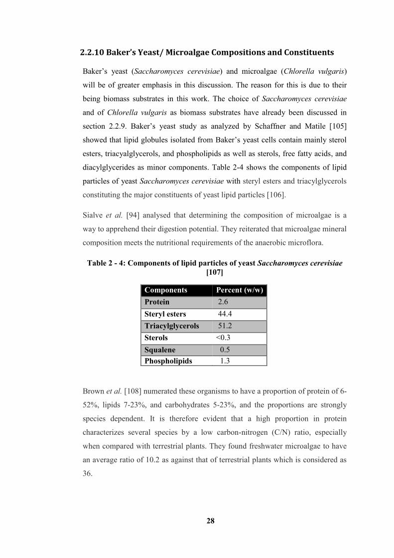
28

2.2.10 Baker’s Yeast/ Microalgae Compositions and Constituents

Baker’s yeast (Saccharomyces cerevisiae) and microalgae (Chlorella vulgaris)

will be of greater emphasis in this discussion. The reason for this is due to their

being biomass substrates in this work. The choice of Saccharomyces cerevisiae

and of Chlorella vulgaris as biomass substrates have already been discussed in

section 2.2.9. Baker’s yeast study as analyzed by Schaffner and Matile [105]

showed that lipid globules isolated from Baker’s yeast cells contain mainly sterol

esters, triacyalglycerols, and phospholipids as well as sterols, free fatty acids, and

diacylglycerides as minor components. Table 2-4 shows the components of lipid

particles of yeast Saccharomyces cerevisiae with steryl esters and triacylglycerols

constituting the major constituents of yeast lipid particles [106].

Sialve et al. [94] analysed that determining the composition of microalgae is a

way to apprehend their digestion potential. They reiterated that microalgae mineral

composition meets the nutritional requirements of the anaerobic microflora.

Table 2 - 4: Components of lipid particles of yeast Saccharomyces cerevisiae

[107]

Components Percent (w/w)

Protein 2.6

Steryl esters 44.4

Triacylglycerols 51.2

Sterols <0.3

Squalene 0.5

Phospholipids 1.3

Brown et al. [108] numerated these organisms to have a proportion of protein of 6-

52%, lipids 7-23%, and carbohydrates 5-23%, and the proportions are strongly

species dependent. It is therefore evident that a high proportion in protein

characterizes several species by a low carbon-nitrogen (C/N) ratio, especially

when compared with terrestrial plants. They found freshwater microalgae to have

an average ratio of 10.2 as against that of terrestrial plants which is considered as

36.

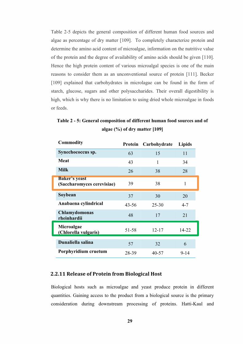
29

Table 2-5 depicts the general composition of different human food sources and

algae as percentage of dry matter [109]. To completely characterize protein and

determine the amino acid content of microalgae, information on the nutritive value

of the protein and the degree of availability of amino acids should be given [110].

Hence the high protein content of various microalgal species is one of the main

reasons to consider them as an unconventional source of protein [111]. Becker

[109] explained that carbohydrates in microlagae can be found in the form of

starch, glucose, sugars and other polysaccharides. Their overall digestibility is

high, which is why there is no limitation to using dried whole microalgae in foods

or feeds.

Table 2 - 5: General composition of different human food sources and of

algae (%) of dry matter [109]

Commodity Protein Carbohydrate Lipids

Synechococcus sp. 63 15 11

Meat 43 1 34

Milk 26 38 28

Baker’s yeast

(Saccharomyces cerevisiae) 39 38 1

Soybean 37 30 20

Anabaena cylindrical 43-56 25-30 4-7

Chlamydomonas

rheinhardii 48 17 21

Microalgae

(Chlorella vulgaris) 51-58 12-17 14-22

Dunaliella salina 57 32 6

Porphyridium cruetum 28-39 40-57 9-14

2.2.11 Release of Protein from Biological Host

Biological hosts such as microalgae and yeast produce protein in different

quantities. Gaining access to the product from a biological source is the primary

consideration during downstream processing of proteins. Hatti-Kaul and

30

Mattiasson [112] and Porro et al. [113] elucidated that microorganisms clearly

constitute the most common production systems for industrial enzymes and other

proteins. Production of protein at a higher level from engineered organisms

provides an alternative to protein extraction from natural sources. This has led to

yeast as microbial eukaryotic host systems combine the advantages of unicellular

organisms with the capability of a protein processing typical for eukaryotic

organisms for higher yield. Based on this fact, Saccharomyces cerevisae use by

the US Food and Drug Administration (FDA) as an organism is generally regarded

as safe (GRAS) [113]. This however is not an optimal host for large-scale

production of foreign protein due to the technical fermentation needs that require

highly sophisticated equipment. The similarities between yeast and microalgae

considered in this study make them a better biological host for protein production.

The choice of yeast is of paramount importance for the success of the whole

process [113].

Several protein products are still produced economically from animal and plant

materials despite the advantages of microorganisms being considered as a protein

source. This is because of the fact that high sufficient amounts are produced from

these sources.

2.2.12 Why Pre-Treat Biomass

Figure 1-4 in Chapter 1 depicted the pre-treatment of biomass by different

methods in the removal of hemicelluloses and lignin from the polymer matrix.

High-pressure homogenization is used extensively in improving the degradability

and the rate of cell wall breakage within the biomass material to improve and

increase the protein concentration yield. Biomass materials like lignocellulosic

plant residues contains up to 70% carbohydrates as cellulose and hemicelluloses.

These are prominent substrates for cheap ethanol production, and due to the

closeness of lignin in the plant cell wall, pre-treatment is necessary to make the

carbohydrates available for enzymatic hydrolysis and fermentation [114]. As in

the case of substrates considered for this research, the inner contents of protein are

coated with hard cell wall. These need to be completely homogenized over some

passes to liberate the protein inside. Most researchers in their conclusion show that

31

the barrier to the production and recovery of lignocellulosic material is the

lignocelluloses structure [31, 59]. Laureano-Perez et al. [115] pointed out that

several structural and compositional factors affect the enzymatic digestibility of

lignocellulosic materials and Hendriks and Zeeman [29] concluded that cellulose

crystallinity is just one of the factors that make hydrolysis of lignocelluloses

limited. As different feedstocks contain different amounts of lignin, Agbor et al.

[116] stressed the need for them to be removed via pre-treatment so as to enhance

biomass digestibility in both cases; homogenization and anaerobic digestion.

Based on the consistency that has been reported by several researchers, the main

factors for consideration in the pre-treatment of biomass are therefore highlighted

below [17];

To improve the rate of enzymatic hydrolysis,

To degrade so as to improve digestibility enhancement,

To aid in the intended product yields

To also alter the structural and compositional impediments to the

hydrolysis and homogenization processes

2.3 Buffer Solution and Contents

Buffer solution is an aqueous solution consisting of a mixture of weak acid and its

conjugate base or a weak base and its conjugate acid. Weak acids and bases do not

completely dissociate in water, and instead exist in solution as equilibrium of

dissociated and un-dissociated species. It has the property that the pH of the

solution changes very little when a small amount of strong acid or base is added to

it. All buffers have an optimal pH range over which they are able to moderate

changes in hydrogen ion concentration. This range is a factor of the dissociation

constant of the acid of the buffer (Ka). This is generally defined as the pKa (-logKa)

value plus or minus one pH unit [117].

32

Buffer solutions are used as a means of keeping pH at nearly constant value in a

wide variety of chemical applications. Buffer solutions in this study has become

necessitated as the pH values of biomass substrates will constantly need to be

monitored and maintained for higher protein yield during and after

homogenization of the substrates.

2.3.1 Properties of a Buffer

Buffer solutions are known to be solutions that resist changes to pH. It is

considered as one of the more important properties of an aqueous solution, which

is its concentration of hydronium ion. This ion has great effect on the solubility of

many inorganic and organic species, as well as on the nature of complex metallic

cations in the solutions and on the rates of many chemical reactions. Determining

pH value of a solution can be done in two ways; this is determined through the use

of a chemical called indicator. This is sensitive to pH. These substances have

colours that change over a relatively short pH range and can, when properly

chosen through its use determine the pH of a solution to an estimated value.

The other method for finding pH is a device called the pH meter. This device have

two electrodes, one of which is sensitive to [H3O+], are immersed in a solution.

The potential between the two electrodes is related to the pH. This is designed so

that the scale will directly furnish the pH of the solution and gives much more

precise measurement of pH than does a typical indicator [117]. Its use is required

when accuracy of pH value is needed and will be discussed further in chapter 3

under experimental and analytical procedures.

2.4 Mechanical Pre-treatment Methods

Other than mechanical pre-treatment which is also known as physical pre-

treatment, other known pre-treatment methods for the conversion of

lignocellulosic and biomass materials into biogas are the chemical and biological

pre-treatments. But for the purpose of this study, emphasis will be placed only on

the mechanical pre-treatment methods. This method is aimed at reducing the

particle size and crystallinity of the substrates, which in effect increases the

digestibility of the cellulose and hemicellulose in the biomass material. This

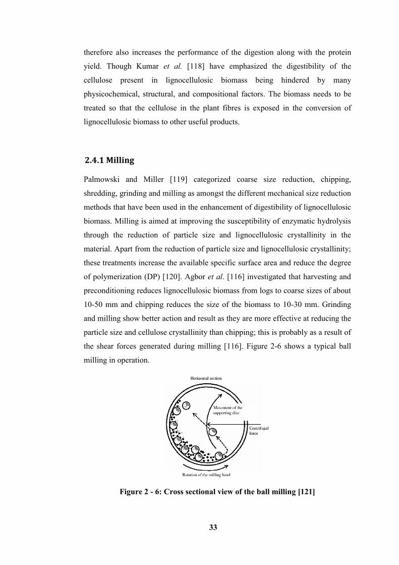
33

therefore also increases the performance of the digestion along with the protein

yield. Though Kumar et al. [118] have emphasized the digestibility of the

cellulose present in lignocellulosic biomass being hindered by many

physicochemical, structural, and compositional factors. The biomass needs to be

treated so that the cellulose in the plant fibres is exposed in the conversion of

lignocellulosic biomass to other useful products.

2.4.1 Milling

Palmowski and Miller [119] categorized coarse size reduction, chipping,

shredding, grinding and milling as amongst the different mechanical size reduction

methods that have been used in the enhancement of digestibility of lignocellulosic

biomass. Milling is aimed at improving the susceptibility of enzymatic hydrolysis

through the reduction of particle size and lignocellulosic crystallinity in the

material. Apart from the reduction of particle size and lignocellulosic crystallinity;

these treatments increase the available specific surface area and reduce the degree

of polymerization (DP) [120]. Agbor et al. [116] investigated that harvesting and

preconditioning reduces lignocellulosic biomass from logs to coarse sizes of about

10-50 mm and chipping reduces the size of the biomass to 10-30 mm. Grinding

and milling show better action and result as they are more effective at reducing the

particle size and cellulose crystallinity than chipping; this is probably as a result of

the shear forces generated during milling [116]. Figure 2-6 shows a typical ball

milling in operation.

Figure 2 - 6: Cross sectional view of the ball milling [121]

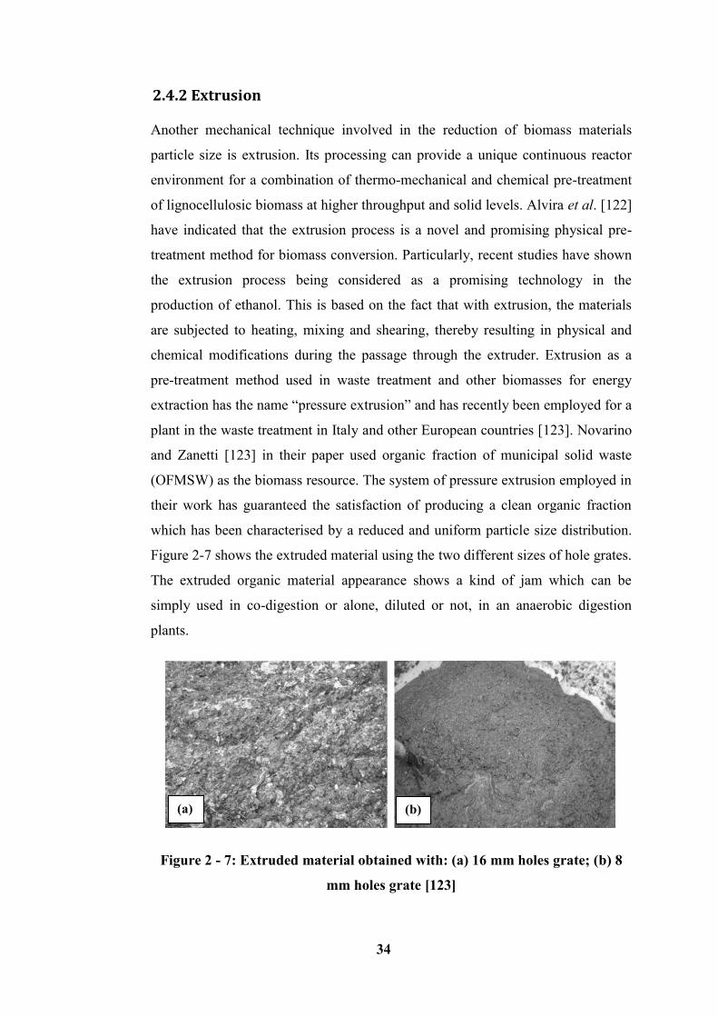
34

2.4.2 Extrusion

Another mechanical technique involved in the reduction of biomass materials

particle size is extrusion. Its processing can provide a unique continuous reactor

environment for a combination of thermo-mechanical and chemical pre-treatment

of lignocellulosic biomass at higher throughput and solid levels. Alvira et al. [122]

have indicated that the extrusion process is a novel and promising physical pre-

treatment method for biomass conversion. Particularly, recent studies have shown

the extrusion process being considered as a promising technology in the

production of ethanol. This is based on the fact that with extrusion, the materials

are subjected to heating, mixing and shearing, thereby resulting in physical and

chemical modifications during the passage through the extruder. Extrusion as a

pre-treatment method used in waste treatment and other biomasses for energy

extraction has the name “pressure extrusion” and has recently been employed for a

plant in the waste treatment in Italy and other European countries [123]. Novarino

and Zanetti [123] in their paper used organic fraction of municipal solid waste

(OFMSW) as the biomass resource. The system of pressure extrusion employed in

their work has guaranteed the satisfaction of producing a clean organic fraction

which has been characterised by a reduced and uniform particle size distribution.

Figure 2-7 shows the extruded material using the two different sizes of hole grates.

The extruded organic material appearance shows a kind of jam which can be

simply used in co-digestion or alone, diluted or not, in an anaerobic digestion

plants.

Figure 2 - 7: Extruded material obtained with: (a) 16 mm holes grate; (b) 8

mm holes grate [123]

(a) (b)

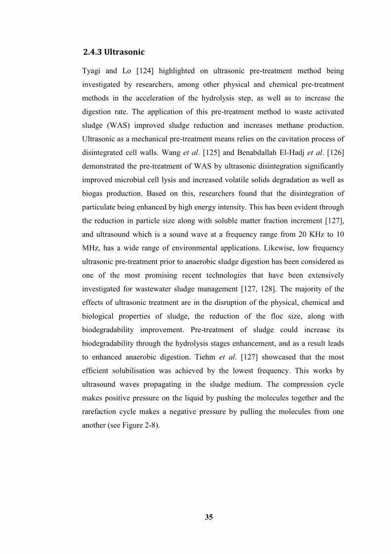
35

2.4.3 Ultrasonic

Tyagi and Lo [124] highlighted on ultrasonic pre-treatment method being

investigated by researchers, among other physical and chemical pre-treatment

methods in the acceleration of the hydrolysis step, as well as to increase the

digestion rate. The application of this pre-treatment method to waste activated

sludge (WAS) improved sludge reduction and increases methane production.

Ultrasonic as a mechanical pre-treatment means relies on the cavitation process of

disintegrated cell walls. Wang et al. [125] and Benabdallah El-Hadj et al. [126]

demonstrated the pre-treatment of WAS by ultrasonic disintegration significantly

improved microbial cell lysis and increased volatile solids degradation as well as

biogas production. Based on this, researchers found that the disintegration of

particulate being enhanced by high energy intensity. This has been evident through

the reduction in particle size along with soluble matter fraction increment [127],

and ultrasound which is a sound wave at a frequency range from 20 KHz to 10

MHz, has a wide range of environmental applications. Likewise, low frequency

ultrasonic pre-treatment prior to anaerobic sludge digestion has been considered as

one of the most promising recent technologies that have been extensively

investigated for wastewater sludge management [127, 128]. The majority of the

effects of ultrasonic treatment are in the disruption of the physical, chemical and

biological properties of sludge, the reduction of the floc size, along with

biodegradability improvement. Pre-treatment of sludge could increase its

biodegradability through the hydrolysis stages enhancement, and as a result leads

to enhanced anaerobic digestion. Tiehm et al. [127] showcased that the most

efficient solubilisation was achieved by the lowest frequency. This works by

ultrasound waves propagating in the sludge medium. The compression cycle

makes positive pressure on the liquid by pushing the molecules together and the

rarefaction cycle makes a negative pressure by pulling the molecules from one

another (see Figure 2-8).

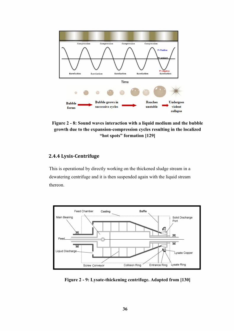
36

Figure 2 - 8: Sound waves interaction with a liquid medium and the bubble

growth due to the expansion-compression cycles resulting in the localized

“hot spots” formation [129]

2.4.4 Lysis-Centrifuge

This is operational by directly working on the thickened sludge stream in a

dewatering centrifuge and it is then suspended again with the liquid stream

thereon.

Figure 2 - 9: Lysate-thickening centrifuge. Adapted from [130]

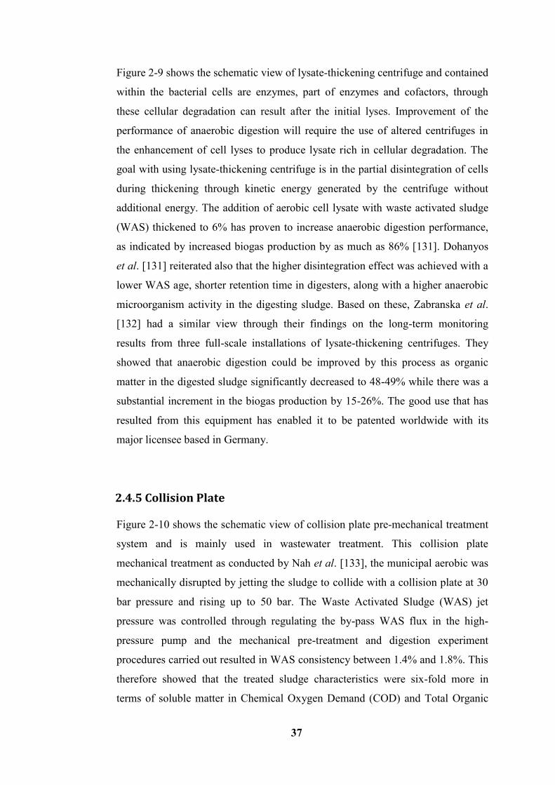
37

Figure 2-9 shows the schematic view of lysate-thickening centrifuge and contained

within the bacterial cells are enzymes, part of enzymes and cofactors, through

these cellular degradation can result after the initial lyses. Improvement of the

performance of anaerobic digestion will require the use of altered centrifuges in

the enhancement of cell lyses to produce lysate rich in cellular degradation. The

goal with using lysate-thickening centrifuge is in the partial disintegration of cells

during thickening through kinetic energy generated by the centrifuge without

additional energy. The addition of aerobic cell lysate with waste activated sludge

(WAS) thickened to 6% has proven to increase anaerobic digestion performance,

as indicated by increased biogas production by as much as 86% [131]. Dohanyos

et al. [131] reiterated also that the higher disintegration effect was achieved with a

lower WAS age, shorter retention time in digesters, along with a higher anaerobic

microorganism activity in the digesting sludge. Based on these, Zabranska et al.

[132] had a similar view through their findings on the long-term monitoring

results from three full-scale installations of lysate-thickening centrifuges. They

showed that anaerobic digestion could be improved by this process as organic

matter in the digested sludge significantly decreased to 48-49% while there was a

substantial increment in the biogas production by 15-26%. The good use that has

resulted from this equipment has enabled it to be patented worldwide with its

major licensee based in Germany.

2.4.5 Collision Plate

Figure 2-10 shows the schematic view of collision plate pre-mechanical treatment

system and is mainly used in wastewater treatment. This collision plate

mechanical treatment as conducted by Nah et al. [133], the municipal aerobic was

mechanically disrupted by jetting the sludge to collide with a collision plate at 30

bar pressure and rising up to 50 bar. The Waste Activated Sludge (WAS) jet

pressure was controlled through regulating the by-pass WAS flux in the high-

pressure pump and the mechanical pre-treatment and digestion experiment

procedures carried out resulted in WAS consistency between 1.4% and 1.8%. This

therefore showed that the treated sludge characteristics were six-fold more in

terms of soluble matter in Chemical Oxygen Demand (COD) and Total Organic

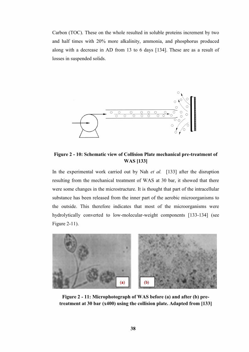
38

Carbon (TOC). These on the whole resulted in soluble proteins increment by two

and half times with 20% more alkalinity, ammonia, and phosphorus produced

along with a decrease in AD from 13 to 6 days [134]. These are as a result of

losses in suspended solids.

Figure 2 - 10: Schematic view of Collision Plate mechanical pre-treatment of

WAS [133]

In the experimental work carried out by Nah et al. [133] after the disruption

resulting from the mechanical treatment of WAS at 30 bar, it showed that there

were some changes in the microstructure. It is thought that part of the intracellular

substance has been released from the inner part of the aerobic microorganisms to

the outside. This therefore indicates that most of the microorganisms were

hydrolytically converted to low-molecular-weight components [133-134] (see

Figure 2-11).

Figure 2 - 11: Microphotograph of WAS before (a) and after (b) pre-

treatment at 30 bar (x400) using the collision plate. Adapted from [133]

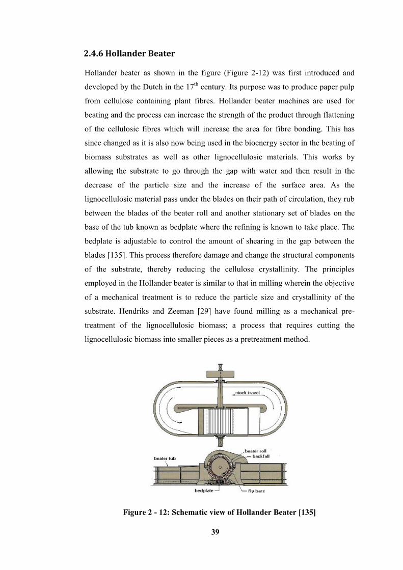
39

2.4.6 Hollander Beater

Hollander beater as shown in the figure (Figure 2-12) was first introduced and

developed by the Dutch in the 17th

century. Its purpose was to produce paper pulp

from cellulose containing plant fibres. Hollander beater machines are used for

beating and the process can increase the strength of the product through flattening

of the cellulosic fibres which will increase the area for fibre bonding. This has

since changed as it is also now being used in the bioenergy sector in the beating of

biomass substrates as well as other lignocellulosic materials. This works by

allowing the substrate to go through the gap with water and then result in the

decrease of the particle size and the increase of the surface area. As the

lignocellulosic material pass under the blades on their path of circulation, they rub

between the blades of the beater roll and another stationary set of blades on the

base of the tub known as bedplate where the refining is known to take place. The

bedplate is adjustable to control the amount of shearing in the gap between the

blades [135]. This process therefore damage and change the structural components

of the substrate, thereby reducing the cellulose crystallinity. The principles

employed in the Hollander beater is similar to that in milling wherein the objective

of a mechanical treatment is to reduce the particle size and crystallinity of the

substrate. Hendriks and Zeeman [29] have found milling as a mechanical pre-

treatment of the lignocellulosic biomass; a process that requires cutting the

lignocellulosic biomass into smaller pieces as a pretreatment method.

Figure 2 - 12: Schematic view of Hollander Beater [135]

40

2.5 Other Mechanical Pre-treatment Method

The previous section has discussed the most up to date mechanical pre-treatment

methods used in the treatment of substrates to enhance biomass-biogas conversion

including cell wall disruption of substrates. Based on these ideas of cell disruption

in biomass, a mechanical treatment employing a high-pressure homogenizer is

therefore introduced for the work in this research. This homogenizes and ruptures

the cell wall to liberate the intracellular products, including proteins which in turn

are designed to improve protein production after centrifugation where the

supernatant is separated from the solid. Homogenizing biomass materials result in

the decrease in particle size and increment in the surface area; these then results in

the damage and change in the component microstructure and which, as a result,

improves the yield in proteins.

2.5.1 High-Pressure Homogenizer (HPH)

Cell rupture is required in the recovering of biological products that are located

inside cells. This is required to be done either mechanically or non-mechanically

[136]. There are other methods, as well as those which are non-mechanical, which

could either be the physical way or the enzymatic way. In general, De Boer et al.

[137] emphasized mechanical methods being non-specific, but their efficiency is

considered higher with broader application in comparison to any of the other

methods. Ahmad-Raus et al. [138] have rated this as highly dependent on the

nature of the product of interest, the cell or tissue itself, like the extent of the cell’s

fragility. Cell disruption is otherwise considered as the isolation and preparation of

intercellular products which is important for use in research and in the industries

for manufacturing end products for consumers. In the industries, HPH application

is linked to the production of stable emulsions; hence it is widely used in such

areas [40, 137, 139, 140], and apart from it being able to emulsify it disrupts

particles into a disperse phase of suspension. It has also extensively proven to be

suitable for the inactivation of the microbial flora occurring in fruit juices and

milk-based beverages [141] especially contributing to the preservation of the

freshness and texture attributes, coupled with antioxidant capacity and the

polyphenols, vitamins, and flavonoids contents of the product [142]. HPH is

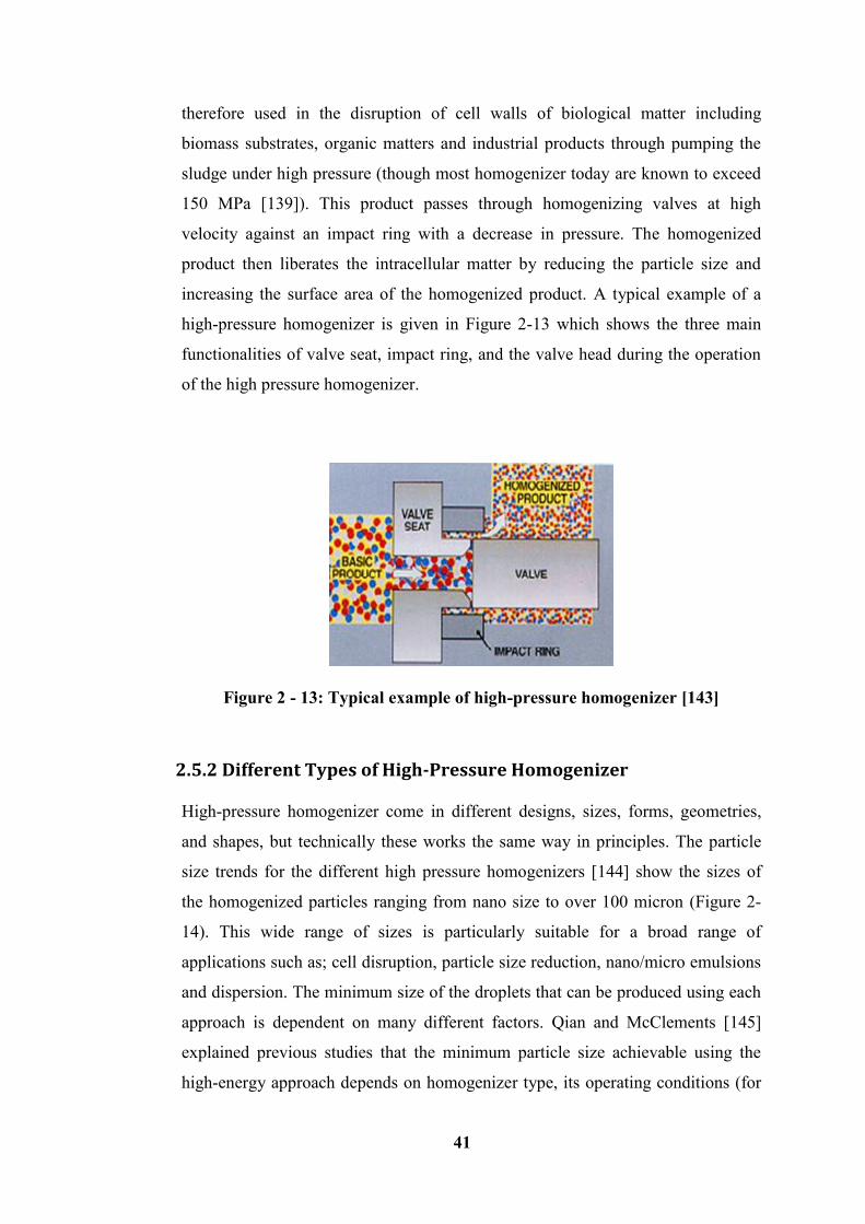
41

therefore used in the disruption of cell walls of biological matter including

biomass substrates, organic matters and industrial products through pumping the

sludge under high pressure (though most homogenizer today are known to exceed

150 MPa [139]). This product passes through homogenizing valves at high

velocity against an impact ring with a decrease in pressure. The homogenized

product then liberates the intracellular matter by reducing the particle size and

increasing the surface area of the homogenized product. A typical example of a

high-pressure homogenizer is given in Figure 2-13 which shows the three main

functionalities of valve seat, impact ring, and the valve head during the operation

of the high pressure homogenizer.

Figure 2 - 13: Typical example of high-pressure homogenizer [143]

2.5.2 Different Types of High-Pressure Homogenizer

High-pressure homogenizer come in different designs, sizes, forms, geometries,

and shapes, but technically these works the same way in principles. The particle

size trends for the different high pressure homogenizers [144] show the sizes of

the homogenized particles ranging from nano size to over 100 micron (Figure 2-

14). This wide range of sizes is particularly suitable for a broad range of

applications such as; cell disruption, particle size reduction, nano/micro emulsions

and dispersion. The minimum size of the droplets that can be produced using each

approach is dependent on many different factors. Qian and McClements [145]

explained previous studies that the minimum particle size achievable using the

high-energy approach depends on homogenizer type, its operating conditions (for

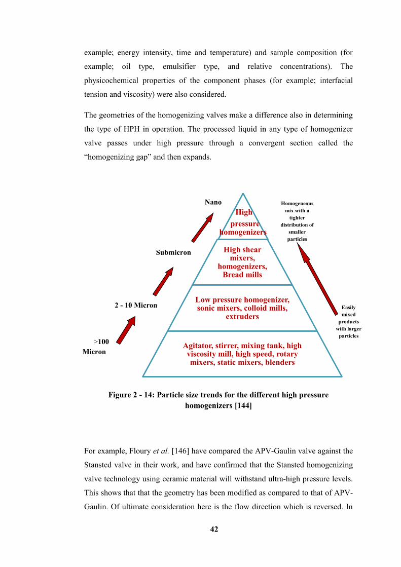
42

example; energy intensity, time and temperature) and sample composition (for

example; oil type, emulsifier type, and relative concentrations). The

physicochemical properties of the component phases (for example; interfacial

tension and viscosity) were also considered.

The geometries of the homogenizing valves make a difference also in determining

the type of HPH in operation. The processed liquid in any type of homogenizer

valve passes under high pressure through a convergent section called the

“homogenizing gap” and then expands.

Figure 2 - 14: Particle size trends for the different high pressure

homogenizers [144]

For example, Floury et al. [146] have compared the APV-Gaulin valve against the

Stansted valve in their work, and have confirmed that the Stansted homogenizing

valve technology using ceramic material will withstand ultra-high pressure levels.

This shows that that the geometry has been modified as compared to that of APV-

Gaulin. Of ultimate consideration here is the flow direction which is reversed. In

High

pressure homogenizers

High shear mixers,

homogenizers, Bread mills

Low pressure homogenizer, sonic mixers, colloid mills,

extruders

Agitator, stirrer, mixing tank, high viscosity mill, high speed, rotary mixers, static mixers, blenders

>100

Micron

2 - 10 Micron

Submicron

Easily

mixed

products

with larger

particles

Homogeneous

mix with a

tighter

distribution of

smaller

particles

Nano

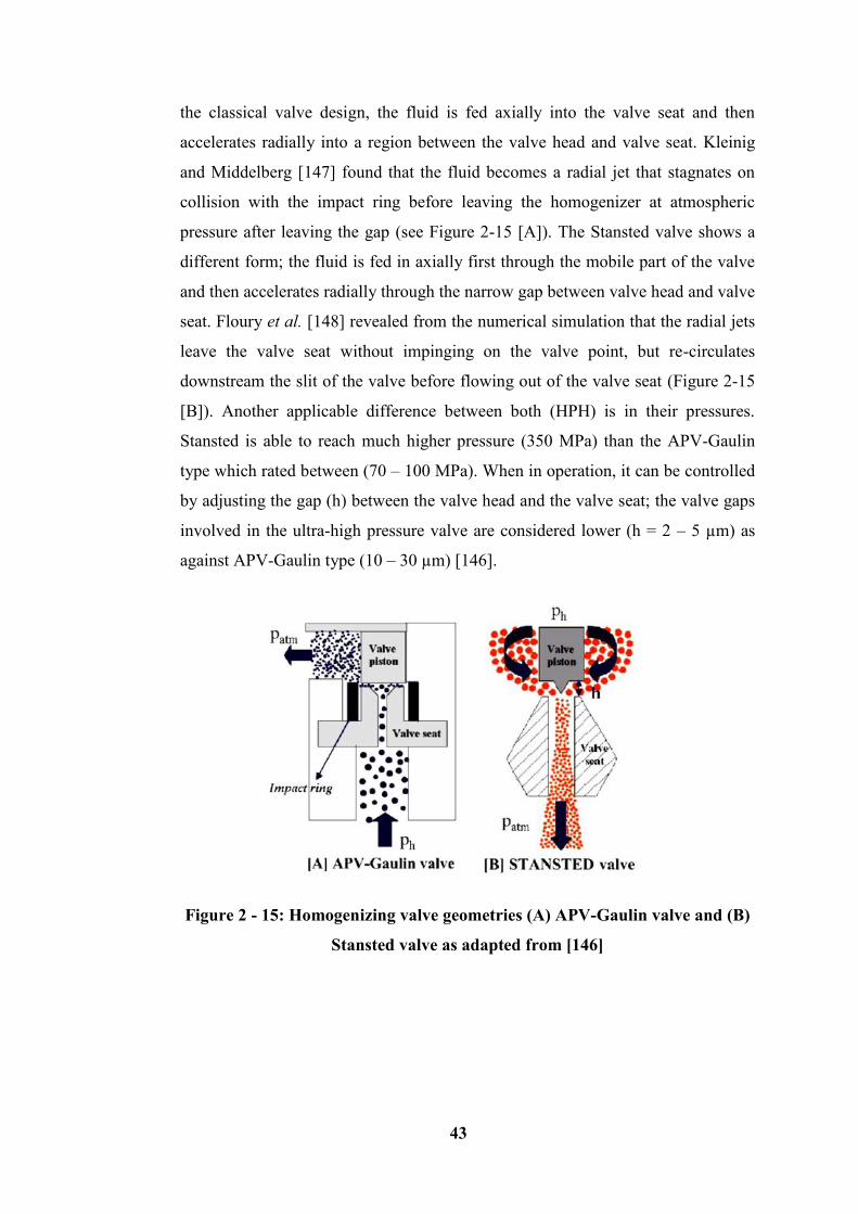
43

the classical valve design, the fluid is fed axially into the valve seat and then

accelerates radially into a region between the valve head and valve seat. Kleinig

and Middelberg [147] found that the fluid becomes a radial jet that stagnates on

collision with the impact ring before leaving the homogenizer at atmospheric

pressure after leaving the gap (see Figure 2-15 [A]). The Stansted valve shows a

different form; the fluid is fed in axially first through the mobile part of the valve

and then accelerates radially through the narrow gap between valve head and valve

seat. Floury et al. [148] revealed from the numerical simulation that the radial jets

leave the valve seat without impinging on the valve point, but re-circulates

downstream the slit of the valve before flowing out of the valve seat (Figure 2-15

[B]). Another applicable difference between both (HPH) is in their pressures.

Stansted is able to reach much higher pressure (350 MPa) than the APV-Gaulin

type which rated between (70 – 100 MPa). When in operation, it can be controlled

by adjusting the gap (h) between the valve head and the valve seat; the valve gaps

involved in the ultra-high pressure valve are considered lower (h = 2 – 5 µm) as

against APV-Gaulin type (10 – 30 µm) [146].

Figure 2 - 15: Homogenizing valve geometries (A) APV-Gaulin valve and (B)

Stansted valve as adapted from [146]

44

2.5.3 GYB40-10S /GYB60-6S 2-Stage Homogenizing Valve HPH

The GYB40-10S high pressure homogenizer has been employed in this research

for the mechanical treatment of biomass substrates. The GYB series high pressure

homogenizer is general-purpose equipment for the preparation of superfine liquid-

liquid emulsion or liquid-solid dispersion. It is widely used in the production and

research areas including food, beverage, pharmacy, chemical industries,

biotechnologies, and others not mentioned here. All parts with direct contact with

fluid media are made from materials of super abrasion durability and excellent

corrosion resistance, to avoid any adverse impact on the fluid to be handled.

The machine is made of a reciprocating plunger pump and a homogenizing valve,

with its homogenizing portion made up of a double stage homogenizing system

which includes a 1st stage homogenizing valve and a 2nd stage homogenizing

valve. The two stage homogenizing valve pressures are adjustable under the scope

of nominal pressure, and at the same time can also be used separately due to the

high-low of homogenizing pressure which directly relates to the speed of materials

through the homogenizing valve. The material particle size is considered to be less

than 2 µm. The GYB series HPH therefore makes the incompatibility in liquid-

liquid or liquid-solid materials to be compatible, superfine, and homogenous. The

stability in the liquid-liquid or solid-liquid under the multiple actions of

cavitations effect can result in high speed impact and shearing through the

adjustment of pressure homogenizing valve of the HPH [149]. Figure 2-16 with

the operating units depict the 2-stage homogenizing valve HPH with the serial

name as GYB40-10S /GYB60-6S, and this has been employed in this study based

on the technical specification as indicated in the Table 2-6. The high-pressure

homogenizer (HPH) has the same features as others, but its unique feature is in its

operation during homogenization in 2- stages with the different hand wheels for

raising pressure and stabilizing it at that point. This enables the homogenization

pressure to be read at any point during cell disruption.

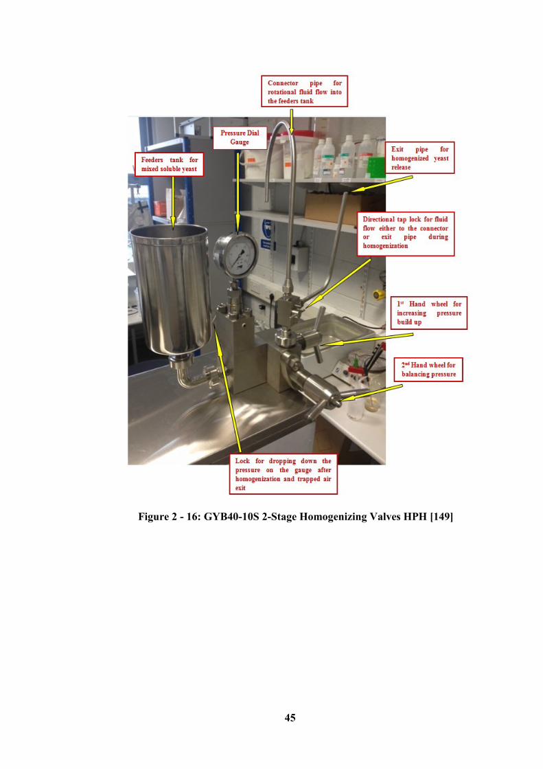
45

Figure 2 - 16: GYB40-10S 2-Stage Homogenizing Valves HPH [149]

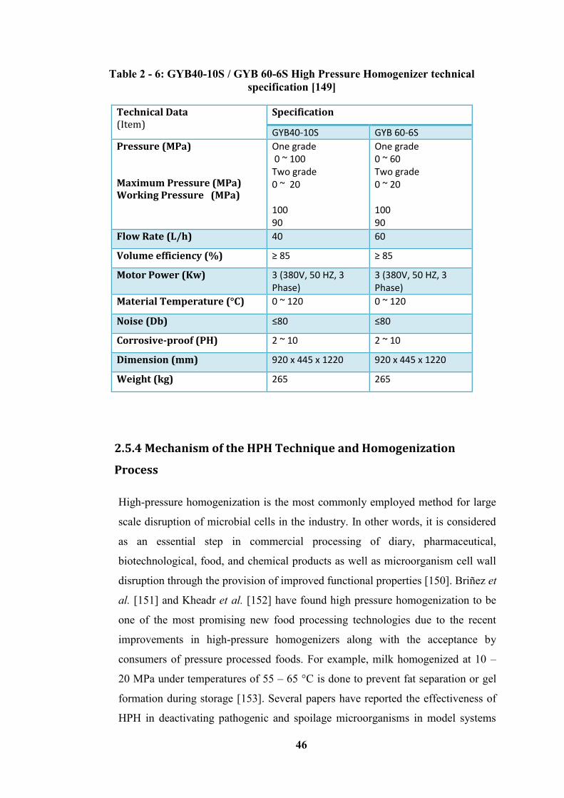
46

Table 2 - 6: GYB40-10S / GYB 60-6S High Pressure Homogenizer technical

specification [149]

Technical Data (Item)

Specification

GYB40-10S GYB 60-6S

Pressure (MPa) Maximum Pressure (MPa) Working Pressure (MPa)

One grade 0 ~ 100 Two grade 0 ~ 20 100 90

One grade 0 ~ 60 Two grade 0 ~ 20 100 90

Flow Rate (L/h) 40 60

Volume efficiency (%) ≥ 85 ≥ 85

Motor Power (Kw) 3 (380V, 50 HZ, 3 Phase)

3 (380V, 50 HZ, 3 Phase)

Material Temperature (°C) 0 ~ 120 0 ~ 120

Noise (Db) ≤80 ≤80

Corrosive-proof (PH) 2 ~ 10 2 ~ 10

Dimension (mm) 920 x 445 x 1220 920 x 445 x 1220

Weight (kg) 265 265

2.5.4 Mechanism of the HPH Technique and Homogenization

Process

High-pressure homogenization is the most commonly employed method for large

scale disruption of microbial cells in the industry. In other words, it is considered

as an essential step in commercial processing of diary, pharmaceutical,

biotechnological, food, and chemical products as well as microorganism cell wall

disruption through the provision of improved functional properties [150]. Briñez et

al. [151] and Kheadr et al. [152] have found high pressure homogenization to be

one of the most promising new food processing technologies due to the recent

improvements in high-pressure homogenizers along with the acceptance by

consumers of pressure processed foods. For example, milk homogenized at 10 –

20 MPa under temperatures of 55 – 65 °C is done to prevent fat separation or gel

formation during storage [153]. Several papers have reported the effectiveness of

HPH in deactivating pathogenic and spoilage microorganisms in model systems

47

and real foods and thus stimulating investigations on the application of HPH so as

to improve food safety and shelf-life [151, 154-156]. This method has been found

to be generally suitable for a variety of bacteria, yeast, and mycelia including

algae. The homogenization technique works by forcing cell suspensions through a

very narrow channel or orifice under pressure. Depending on the type of HPH, the

suspension may or may not impinge at high velocity on a hard-impact ring or

against another high velocity stream of cells coming from the opposite direction.

As the process requires the disruption of biomass substrates before

homogenization can take place, the cell wall of the microbial products are broken

down to release the proteins which are a great source and at the same time aid

biogas production.

2.5.4.1 Effects of Valve Head, Valve Seat and Impact Ring on Substrates

Homogenization considerations have shown high pressure homogenizers

consisting of a positive displacement pump and a homogenizing valve. And as

previously indicated, the pump is used to force the fluid into the homogenizing

valve where the work is done [157]. The three main components with useful value

and functionalities in the HPH are the valve head, valve seat, and impact ring.

These are within the internal structure of the designed HPH and are often regarded

as the powerhouse of the machine. In the homogenizing valve, the fluid is forced

under pressure through a small orifice between the valve head and valve seat (as

depicted in the Figures 2-15 [A] and [B]. The fluid leaves the gap in the form of a

radial jet that stagnates on an impact ring [157]. It therefore exits the homogenizer

finally at low velocity and atmospheric pressure. During operation, higher pressure

on the hand wheel compresses the valve seat against the valve head through the

impact ring. This, as a result reduces the gap size wherein the homogenized

suspension/emulsion flows through at a very low velocity. The disruption of the

cell wall leads to a large drop in pressure, and results in highly focussed turbulent

eddies along with strong shearing forces to occur. Effluent from the homogenizer

is normally chilled to minimise thermal damage to the product caused as a result

of the frictional heat which is generated due to the high fluid velocity that elevates

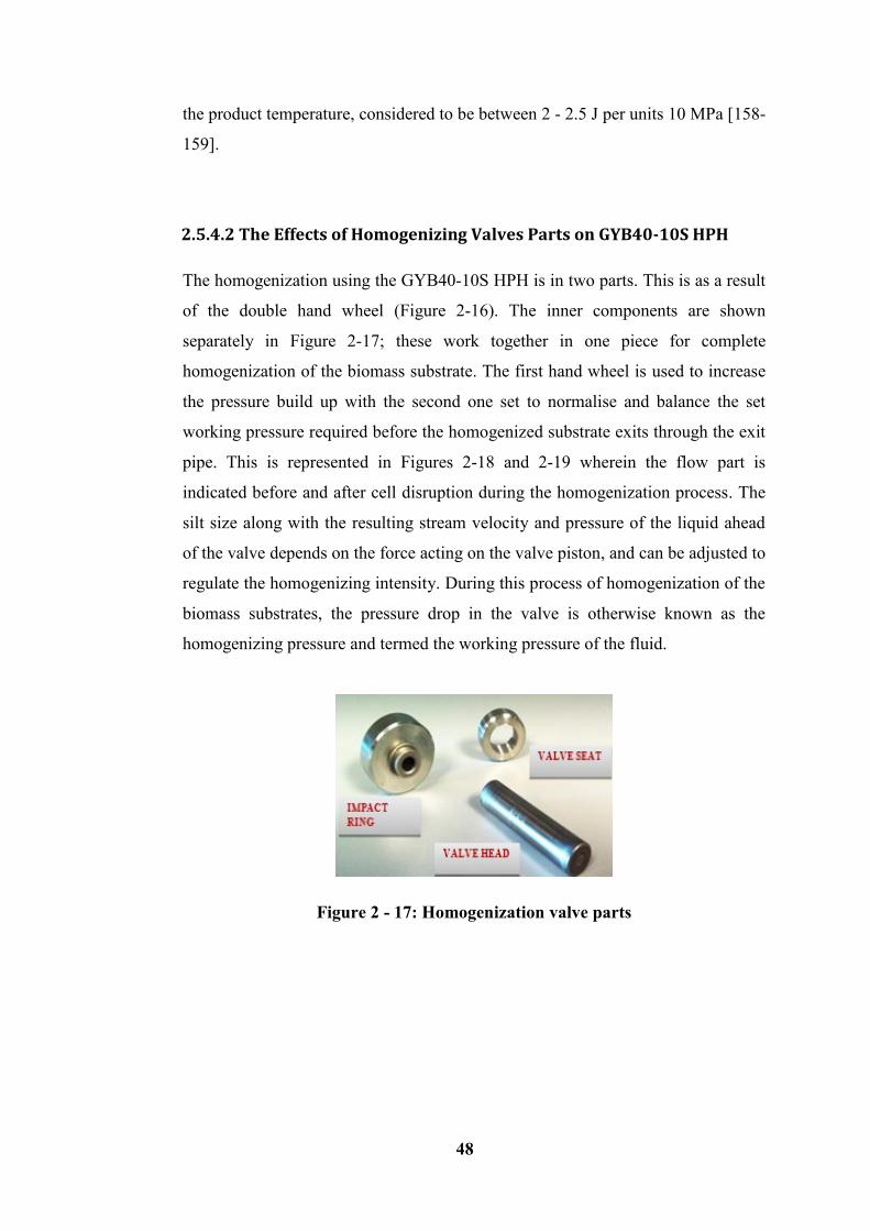
48

the product temperature, considered to be between 2 - 2.5 J per units 10 MPa [158-

159].

2.5.4.2 The Effects of Homogenizing Valves Parts on GYB40-10S HPH

The homogenization using the GYB40-10S HPH is in two parts. This is as a result

of the double hand wheel (Figure 2-16). The inner components are shown

separately in Figure 2-17; these work together in one piece for complete

homogenization of the biomass substrate. The first hand wheel is used to increase

the pressure build up with the second one set to normalise and balance the set

working pressure required before the homogenized substrate exits through the exit

pipe. This is represented in Figures 2-18 and 2-19 wherein the flow part is

indicated before and after cell disruption during the homogenization process. The

silt size along with the resulting stream velocity and pressure of the liquid ahead

of the valve depends on the force acting on the valve piston, and can be adjusted to

regulate the homogenizing intensity. During this process of homogenization of the

biomass substrates, the pressure drop in the valve is otherwise known as the

homogenizing pressure and termed the working pressure of the fluid.

Figure 2 - 17: Homogenization valve parts

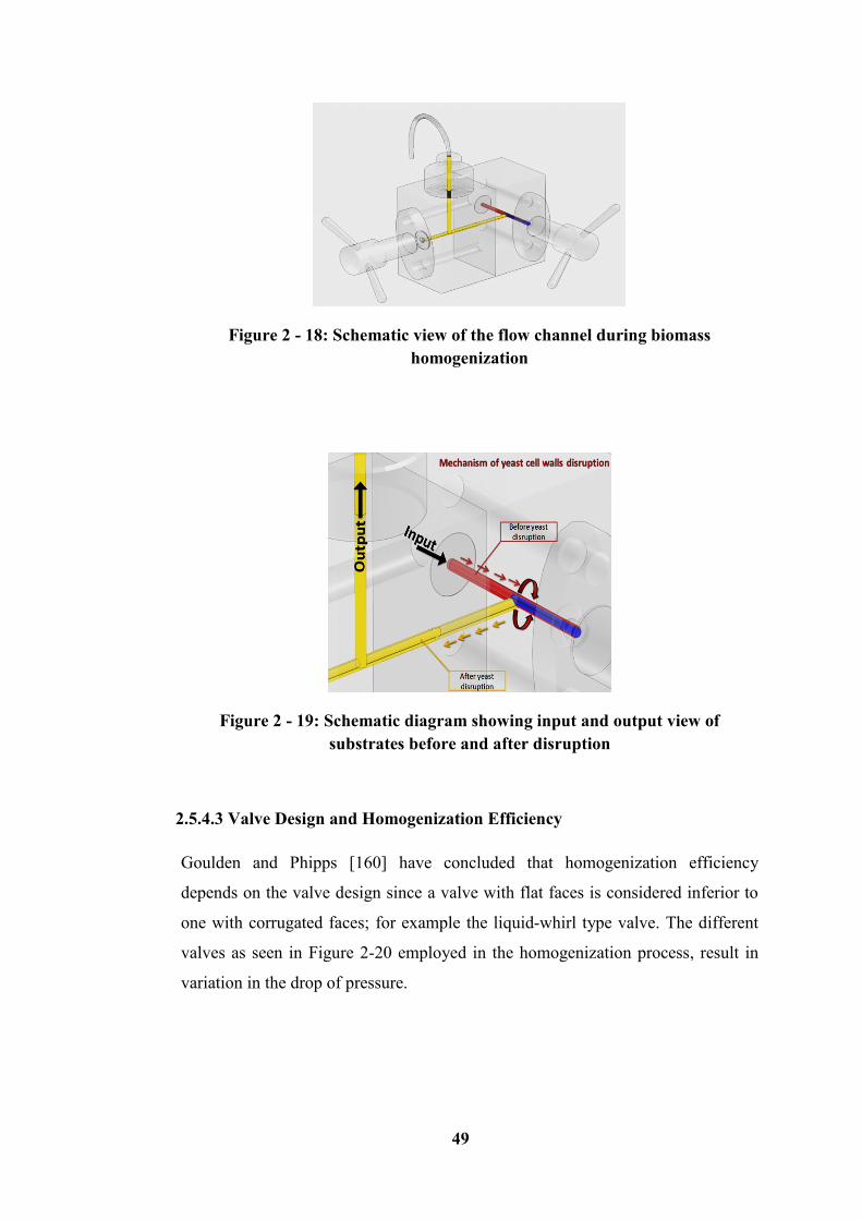
49

Figure 2 - 18: Schematic view of the flow channel during biomass

homogenization

Figure 2 - 19: Schematic diagram showing input and output view of

substrates before and after disruption

2.5.4.3 Valve Design and Homogenization Efficiency

Goulden and Phipps [160] have concluded that homogenization efficiency

depends on the valve design since a valve with flat faces is considered inferior to

one with corrugated faces; for example the liquid-whirl type valve. The different

valves as seen in Figure 2-20 employed in the homogenization process, result in

variation in the drop of pressure.

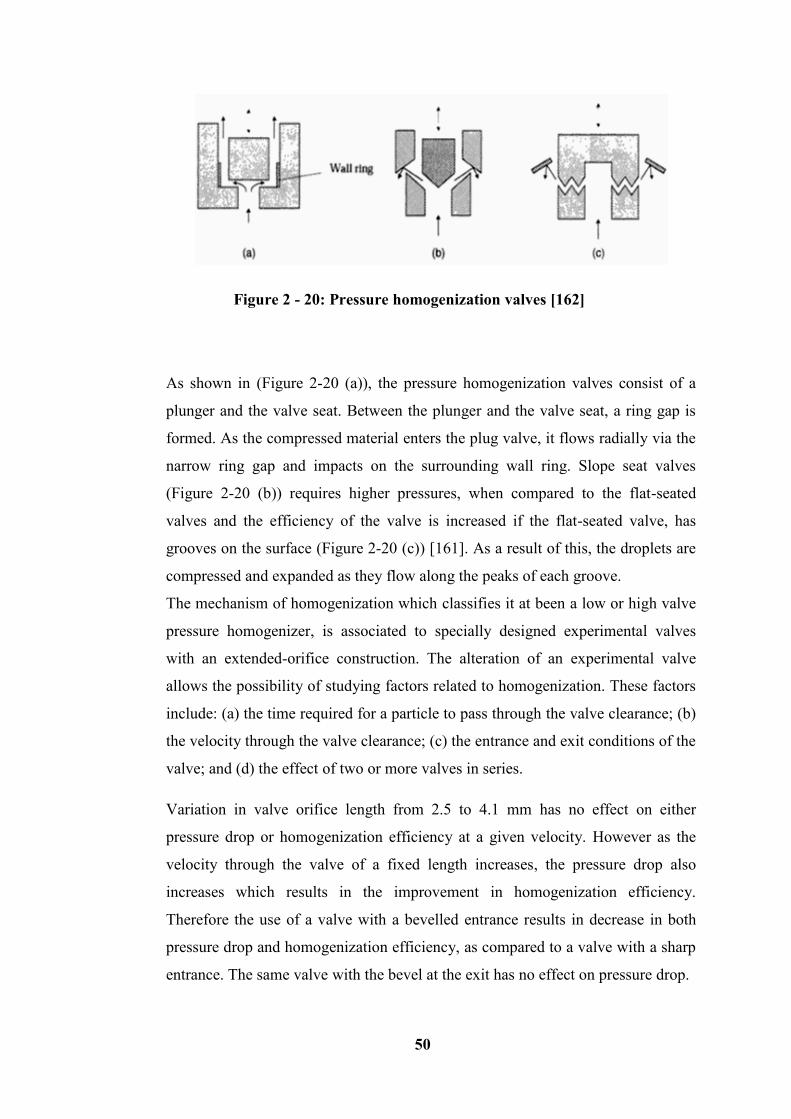
50

Figure 2 - 20: Pressure homogenization valves [162]

As shown in (Figure 2-20 (a)), the pressure homogenization valves consist of a

plunger and the valve seat. Between the plunger and the valve seat, a ring gap is

formed. As the compressed material enters the plug valve, it flows radially via the

narrow ring gap and impacts on the surrounding wall ring. Slope seat valves

(Figure 2-20 (b)) requires higher pressures, when compared to the flat-seated

valves and the efficiency of the valve is increased if the flat-seated valve, has

grooves on the surface (Figure 2-20 (c)) [161]. As a result of this, the droplets are

compressed and expanded as they flow along the peaks of each groove.

The mechanism of homogenization which classifies it at been a low or high valve

pressure homogenizer, is associated to specially designed experimental valves

with an extended-orifice construction. The alteration of an experimental valve

allows the possibility of studying factors related to homogenization. These factors

include: (a) the time required for a particle to pass through the valve clearance; (b)

the velocity through the valve clearance; (c) the entrance and exit conditions of the

valve; and (d) the effect of two or more valves in series.

Variation in valve orifice length from 2.5 to 4.1 mm has no effect on either

pressure drop or homogenization efficiency at a given velocity. However as the

velocity through the valve of a fixed length increases, the pressure drop also

increases which results in the improvement in homogenization efficiency.

Therefore the use of a valve with a bevelled entrance results in decrease in both

pressure drop and homogenization efficiency, as compared to a valve with a sharp

entrance. The same valve with the bevel at the exit has no effect on pressure drop.

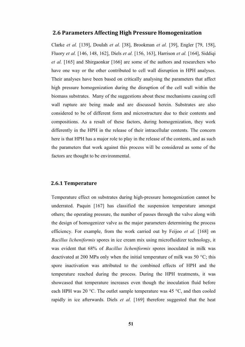
51

2.6 Parameters Affecting High Pressure Homogenization

Clarke et al. [139], Doulah et al. [38], Brookman et al. [39], Engler [79, 158],

Fluory et al. [146, 148, 162], Diels et al. [156, 163], Harrison et al. [164], Siddiqi

et al. [165] and Shirgaonkar [166] are some of the authors and researchers who

have one way or the other contributed to cell wall disruption in HPH analyses.

Their analyses have been based on critically analysing the parameters that affect

high pressure homogenization during the disruption of the cell wall within the

biomass substrates. Many of the suggestions about these mechanisms causing cell

wall rupture are being made and are discussed herein. Substrates are also

considered to be of different form and microstructure due to their contents and

compositions. As a result of these factors, during homogenization, they work

differently in the HPH in the release of their intracellular contents. The concern

here is that HPH has a major role to play in the release of the contents, and as such

the parameters that work against this process will be considered as some of the

factors are thought to be environmental.

2.6.1 Temperature

Temperature effect on substrates during high-pressure homogenization cannot be

underrated. Paquin [167] has classified the suspension temperature amongst

others; the operating pressure, the number of passes through the valve along with

the design of homogenizer valve as the major parameters determining the process

efficiency. For example, from the work carried out by Feijoo et al. [168] on

Bacillus licheniformis spores in ice cream mix using microfluidizer technology, it

was evident that 68% of Bacillus licheniformis spores inoculated in milk was

deactivated at 200 MPa only when the initial temperature of milk was 50 °C; this

spore inactivation was attributed to the combined effects of HPH and the

temperature reached during the process. During the HPH treatments, it was

showcased that temperature increases even though the inoculation fluid before

each HPH was 20 °C. The outlet sample temperature was 45 °C, and then cooled

rapidly in ice afterwards. Diels et al. [169] therefore suggested that the heat

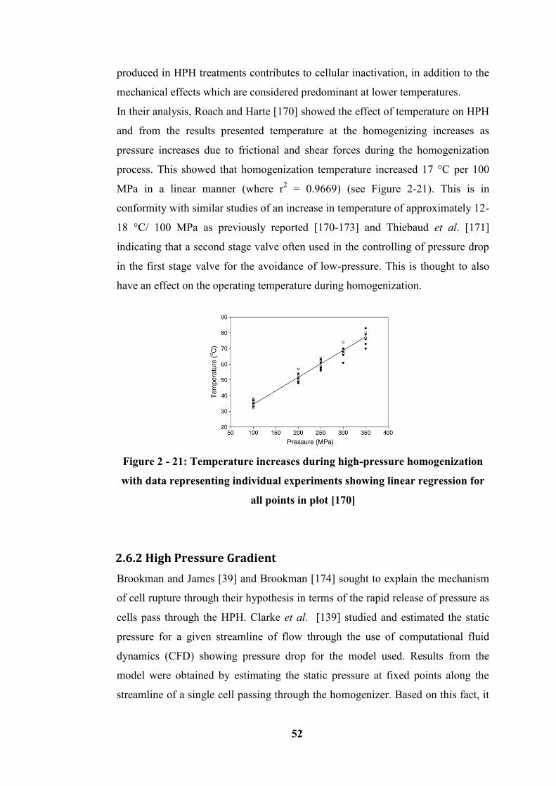
52

produced in HPH treatments contributes to cellular inactivation, in addition to the

mechanical effects which are considered predominant at lower temperatures.

In their analysis, Roach and Harte [170] showed the effect of temperature on HPH

and from the results presented temperature at the homogenizing increases as

pressure increases due to frictional and shear forces during the homogenization

process. This showed that homogenization temperature increased 17 °C per 100

MPa in a linear manner (where r2 = 0.9669) (see Figure 2-21). This is in

conformity with similar studies of an increase in temperature of approximately 12-

18 °C/ 100 MPa as previously reported [170-173] and Thiebaud et al. [171]

indicating that a second stage valve often used in the controlling of pressure drop

in the first stage valve for the avoidance of low-pressure. This is thought to also

have an effect on the operating temperature during homogenization.

Figure 2 - 21: Temperature increases during high-pressure homogenization

with data representing individual experiments showing linear regression for

all points in plot [170]

2.6.2 High Pressure Gradient

Brookman and James [39] and Brookman [174] sought to explain the mechanism

of cell rupture through their hypothesis in terms of the rapid release of pressure as

cells pass through the HPH. Clarke et al. [139] studied and estimated the static

pressure for a given streamline of flow through the use of computational fluid

dynamics (CFD) showing pressure drop for the model used. Results from the

model were obtained by estimating the static pressure at fixed points along the

streamline of a single cell passing through the homogenizer. Based on this fact, it

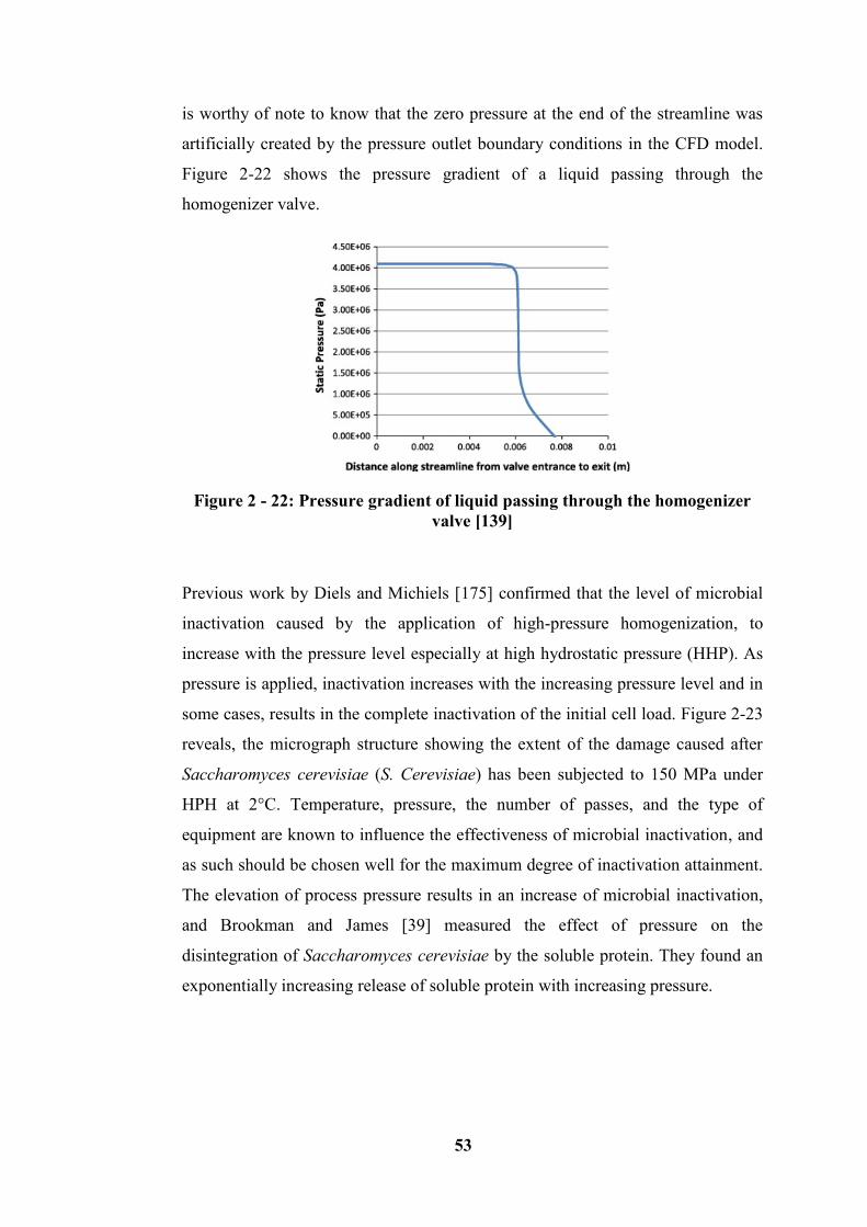
53

is worthy of note to know that the zero pressure at the end of the streamline was

artificially created by the pressure outlet boundary conditions in the CFD model.

Figure 2-22 shows the pressure gradient of a liquid passing through the

homogenizer valve.

Figure 2 - 22: Pressure gradient of liquid passing through the homogenizer

valve [139]

Previous work by Diels and Michiels [175] confirmed that the level of microbial

inactivation caused by the application of high-pressure homogenization, to

increase with the pressure level especially at high hydrostatic pressure (HHP). As

pressure is applied, inactivation increases with the increasing pressure level and in

some cases, results in the complete inactivation of the initial cell load. Figure 2-23

reveals, the micrograph structure showing the extent of the damage caused after

Saccharomyces cerevisiae (S. Cerevisiae) has been subjected to 150 MPa under

HPH at 2°C. Temperature, pressure, the number of passes, and the type of

equipment are known to influence the effectiveness of microbial inactivation, and

as such should be chosen well for the maximum degree of inactivation attainment.

The elevation of process pressure results in an increase of microbial inactivation,

and Brookman and James [39] measured the effect of pressure on the

disintegration of Saccharomyces cerevisiae by the soluble protein. They found an

exponentially increasing release of soluble protein with increasing pressure.

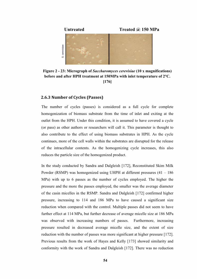
54

Figure 2 - 23: Micrograph of Saccharomyces cerevisiae (10 x magnifications)

before and after HPH treatment at 150MPa with inlet temperature of 2°C.

[176]

2.6.3 Number of Cycles (Passes)

The number of cycles (passes) is considered as a full cycle for complete

homogenization of biomass substrate from the time of inlet and exiting at the

outlet from the HPH. Under this condition, it is assumed to have covered a cycle

(or pass) as other authors or researchers will call it. This parameter is thought to

also contribute to the effect of using biomass substrates in HPH. As the cycle

continues, more of the cell walls within the substrates are disrupted for the release

of the intracellular contents. As the homogenizing cycle increases, this also

reduces the particle size of the homogenized product.

In the study conducted by Sandra and Dalgleish [172], Reconstituted Skim Milk

Powder (RSMP) was homogenized using UHPH at different pressures (41 – 186

MPa) with up to 6 passes as the number of cycles employed. The higher the

pressure and the more the passes employed, the smaller was the average diameter

of the casin micelles in the RSMP. Sandra and Dalgleish [172] confirmed higher

pressure, increasing to 114 and 186 MPa to have caused a significant size

reduction when compared with the control. Multiple passes did not seem to have

further effect at 114 MPa, but further decrease of average micelle size at 186 MPa

was observed with increasing numbers of passes. Furthermore, increasing

pressure resulted in decreased average micelle size, and the extent of size

reduction with the number of passes was more significant at higher pressure [172].

Previous results from the work of Hayes and Kelly [173] showed similarity and

conformity with the work of Sandra and Dalgleish [172]. There was no reduction

Untreated Treated @ 150 MPa

55

in micelle size up to a pressure of 150 MPa but there were some decreases at 200

MPa.

2.6.4 Gap sizes

Juliane Floury and co-researchers have contributed greatly to the field through

their various works and publications on gap sizes and its effect on HPH. They

have emphatically worked in this field to present a clearer view on the operation as

regards gap size effect on HPH. In the work of Floury et al. [148], measurements

of the thickness of about 20 microscopic views of wax threads give us a mean

value for the size of the narrow gap between valve and valve seat equal to 9.1 ±

0.71 µm at a homogenizing pressure of 10 MPa. As estimated by the equations of

Nakayama and Phipps, the results obtained were equal to 7.6 and 7.75 µm,

respectively, at the same operating pressure with water. Floury et al. [148]

suggested that the difference in value above may be a result of the increase of the

total pressure drop in the homogenizing valve when some wax grits that cross the

narrow gap size. Innings and Trägårdh [177] studied flow in HPH and considered

it very extreme with gaps of 10 – 100 µm and velocities of hundreds of m/s. This

practically makes it impossible to measure the velocity fields. Contrarily, HPH has

been found to be the most efficient means in the creation of sub-micron emulsions

in low-viscous fluids, and for the realization of this particle size emulsion the HPH

must be from a high-pressure piston pump with a narrow gap. Gap sizes are

assumed to be a great determinant in the formation of different particle sizes in

homogenized substrates. Innings and Trägårdh [177] explained that the pump

creates a pressure of 10-500 MPa with the emulsion accelerated to velocities of up

to hundreds of m/s in the gap. For the flow pattern and particle size distribution of

substrate, an established relationship has been developed between the valve gap

size and homogenizing pressure. The design of the gap size of the valve has been

considered as another important aspect as part of the evaluation for the

effectiveness on cell disruption in HPH [177]. Calligaris et al. [141] have

hypothesized that both the valve design and the flow conditions in the

homogenization valve gap allow different mechanical stresses to be suffered by

the product. In conclusion, the operative pressure during homogenization is not the

56

sole critical factor that controls the overall effect of the process as the equipment

engineering is inclusive to the efficient homogenization process.

2.6.5 pH

The pH value of the substrate in solution plays a role in the complete disruption of

cell walls during the homogenization process of Baker’s yeast and microalgae.

Prepared buffer liquid was set to 5.3 pH value before mixing the biomass

substrates in solution. Homogenized substrates were observed to have completely

changed in terms of the pH value, and this indicates that HPH has changed the

microstructure and content within the solution. Joscelyne and Trägårdh [178]

examined pH as another parameter that is product dependent. They observed that

membrane surface properties are pH dependent since membrane surfaces exhibit

an iso-electric point at a given pH where the surface has no net charge. Iordache

and Jelen [179] analysed heat treatment being the most measurable effect on whey

protein functionality while others consider moderate heat treatment (60-70°C) to

structurally unfold proteins, whereas at higher temperatures protein aggregation in

various degrees may occur. This is dependent on important factor as pH.

Floury et al. [162] studied the effect of homogenizing pressure from (20 to 300

MPa) on model emulsions stabilized by whey proteins and part of the findings was

that proteins are soluble on all ranges of pH and are also known as good

emulsifiers at pH < 7. It was also found that the micro-particles sizes obtained

from whey protein concentrate or isolate could be controlled by different

conditions of pH, heat treatment, microfluidizer pressure, and the number of

recirculations [167]. This therefore demonstrated that these micro-particles could

be incorporated into food products (0.5% w/w protein) and when

electronmicroscopy analysis was conducted [167].

2.6.6 Turbulence

In determining the true cause of cell wall breakage in a high pressure

homogenizer, Kelly and Muske [180] considered this to take place at low

57

operating pressure in liquids of low viscosity. They argued that the mechanism of

turbulence, pressure gradients and shear stresses could not be the cause of cell

breakage as their analyses predicted that no breakage should occur under these

conditions. According to Paquin [167], it is very difficult to rank cavitation, shear

and turbulence in order of importance due to their force-induced phenomena in

dynamic high pressure systems taking place simultaneously. Making some

assumptions about the violence of the turbulence Siddiqi et al. [165] calculated

that a tensile force of 540 μN could be generated along the cell wall of a 5 μm cell

in a liquid with density and viscosity similar to water, and it has been proposed

that to be sufficient to cause rupture in the cell wall breakage. On a similar note,

Doulah et al. [38] have hypothesized turbulence has the greatest influence on cell

wall disruption in HPH and in their prediction of the protein released, based on a

mathematical model, was successful. The results obtained showed similarity with

that from experimentation, and the turbulence produced as a result consists of

random effects in total with no dominating frequency of oscillation. Further to

this, Doulah et al. [38] stressed that where the energy of turbulence is high

enough, this can exceed the minimum energy needed to break the cell wall, and

through this disruption can occur. At that time Doulah et al. [38] have stated both

the turbulence characteristics in the HPH along with the physical properties of the

system, such as the cell wall breaking stress, to be unknown.

2.6.7 Cavitation

The cavitation effect on HPH has been analyzed and it is still under study. Gogate

et al. [181] elucidated that the underlying mechanism for this spectacular effect of

cavitation as the violent collapse of bubbles or cavities resulting in the generation

of extremely high temperatures and pressures locally. This has been classified into

four types; acoustic, hydrodynamic, optic and particle cavitation, depending on the

mode of generation. Emphasis here will be on the hydrodynamic cavitation

resulting from the disruption of Baker’s yeast and microalgae biomass substrates

in HPH. The collapse of cavities violently results in the formation of reactive

hydrogen atoms and hydroxyl radicals, which combine invariably to form of

hydrogen peroxide and to some extent, are considered responsible in the

58

promotion of oxidation reactions. Hydrodynamic cavitation can simply be

generated by the passage of liquid through a constriction such as an orifice plate

and when the liquid passes through the orifice, the kinetic energy or velocity of the

liquid increases at the expense of the pressure [181]. As a result of this boundary

layer separation occurs and substantial amount of energy will be lost in the form

of a permanent pressure drop. Engineers have generally looked with caution at

cavitation in hydraulic devices due to the problems of mechanical erosion.

Balasundaram and Harrison [182] classified this bubble collapsing phenomenon as

the conditions that are generated which would allow cell wall breakage to occur,

and therefore, it could be termed a mechanism for cell wall rupture. This collapse

can be studied more easily under the assumption that the bubble has become

detached from the surface irregularity and that it is now flowing freely in the

liquid before the external pressure is increased.

2.6.8 Wall Impact and Impingement

Wall impact and impingement are the two main causes of cell disruption in HPH

according to Keshavarz-Moore et al. [183]. Based on the understanding of these

words “impact” and “impingement”, they have been explained in the following

way, impact is the collision of two objects (for instance, a cell and the impact

ring), whereas impingement is a special case of impact in which one object (for

instance, the impact ring) is eroded gradually by large numbers of small impacts

caused by numerous discrete solid objects (cells or solid impurities) flowing in the

liquid at high velocity [183]. Engler and Robinson [184] suggested that shear,

turbulence, or stress caused by impingement of a high velocity jet on a stationary

surface may be responsible for disrupting cells when the flow pattern in a

homogenizing valve is being considered. They eventually came to the conclusion

that impingement of a high velocity jet of suspended cells on a stationary surface

is necessary for effective disruption of cell walls by HPH, having realized that

turbulence near the point of impact can enhance disruption. There have been

several mutually interacting mechanisms proposed in the recent past regarding the

cause of disruption, and these are still a matter of some debate, with different

authors having different views on the actual causes of cell wall rupture.

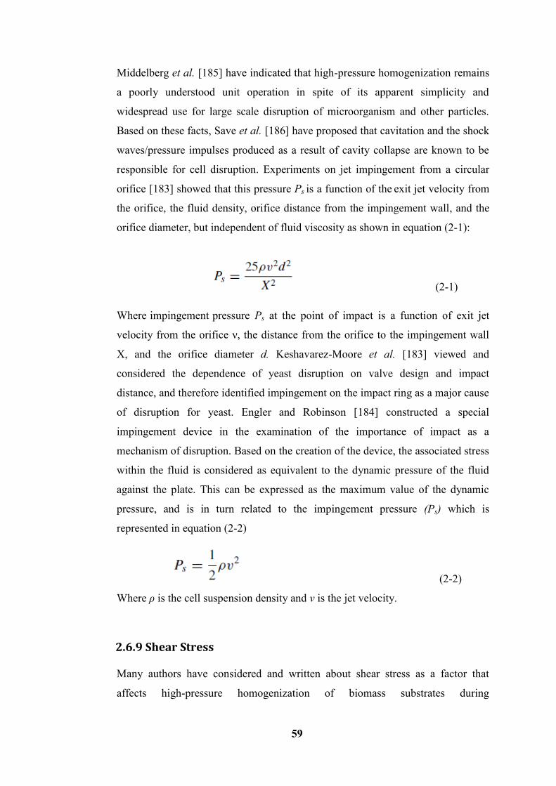
59

Middelberg et al. [185] have indicated that high-pressure homogenization remains

a poorly understood unit operation in spite of its apparent simplicity and

widespread use for large scale disruption of microorganism and other particles.

Based on these facts, Save et al. [186] have proposed that cavitation and the shock

waves/pressure impulses produced as a result of cavity collapse are known to be

responsible for cell disruption. Experiments on jet impingement from a circular

orifice [183] showed that this pressure Ps is a function of the exit jet velocity from

the orifice, the fluid density, orifice distance from the impingement wall, and the

orifice diameter, but independent of fluid viscosity as shown in equation (2-1):

(2-1)

Where impingement pressure Ps at the point of impact is a function of exit jet

velocity from the orifice ν, the distance from the orifice to the impingement wall

X, and the orifice diameter d. Keshavarez-Moore et al. [183] viewed and

considered the dependence of yeast disruption on valve design and impact

distance, and therefore identified impingement on the impact ring as a major cause

of disruption for yeast. Engler and Robinson [184] constructed a special

impingement device in the examination of the importance of impact as a

mechanism of disruption. Based on the creation of the device, the associated stress

within the fluid is considered as equivalent to the dynamic pressure of the fluid

against the plate. This can be expressed as the maximum value of the dynamic

pressure, and is in turn related to the impingement pressure (Ps) which is

represented in equation (2-2)

(2-2)

Where ρ is the cell suspension density and ν is the jet velocity.

2.6.9 Shear Stress

Many authors have considered and written about shear stress as a factor that

affects high-pressure homogenization of biomass substrates during

60

homogenization. Most authors have assumed this to have arisen on the surfaces of

cells in the operation of the homogenizer. Clarke et al. [139] highlighted that if

these stresses were large enough, they could cause the rupture of the cell wall.

There have been some controversies with this claim. These have denied the report

that shear stress results in the cause of microbial breakage in low density

suspension as that encountered with cells in water. Miller et al. [187] and Kelly

and Muske [180] have concluded that at low viscosity, channel shear stress is

unlikely to cause cell disruption. This was based on the gap size being in the range

of 1-11 μm, the viscosity between 1-5 mPa s and the pressure within (0.138-0.965

MPa). On the contrary, channel shear stress will be considered the main cause of

cell breakage only when viscosity is at higher value different from the data above.

Clarke et al. [139] also concluded that breakage of the cellular component in the

vicinity of the walls of the valve parts, either through shear or direct collision, as

well as tearing by vortex shedding on weak points, could also be characterized

under breakage by shear. Fluid shear stress has therefore been considered as the

most influential cause of cell breakage, and can be accepted that there will be a lag

of velocity in the gap region for the cells in comparison to the fluid. The

phenomenon surrounding shear stress is dependent on the relative velocity

between the solid as well as the surrounding liquid, and the same set of features is

said to occur irrespective of whether the liquid is accelerating or decelerating.

2.6.10 Separation

Phipps demonstrated that separation and cavitation were likely to occur in the

valve region at low pressures and were more susceptible to occur with square

edged seats than rounded seats [188]. Kleinig and Middelberg [189] have related

the pressure drop to separation. They have explained that pressure distributions

could be predicted with good accuracy downstream of entry conditions, but flow

near the inlet is considered to be dominated by separation and subsequent

reattachment, making analytical solutions for the total pressure drop impractical.

Some separation is predicted to occur in the square valve, but only at higher valve

gaps (see Figure 2-24). Kleinig and Middelberg [189] used computational fluid

dynamics in predicting valve region velocity and pressure fields, and based on the

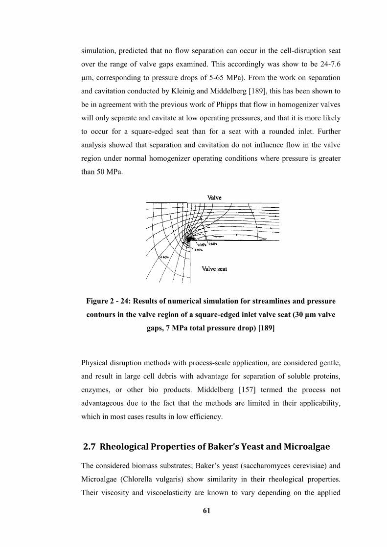
61

simulation, predicted that no flow separation can occur in the cell-disruption seat

over the range of valve gaps examined. This accordingly was show to be 24-7.6

µm, corresponding to pressure drops of 5-65 MPa). From the work on separation

and cavitation conducted by Kleinig and Middelberg [189], this has been shown to

be in agreement with the previous work of Phipps that flow in homogenizer valves

will only separate and cavitate at low operating pressures, and that it is more likely

to occur for a square-edged seat than for a seat with a rounded inlet. Further

analysis showed that separation and cavitation do not influence flow in the valve

region under normal homogenizer operating conditions where pressure is greater

than 50 MPa.

Figure 2 - 24: Results of numerical simulation for streamlines and pressure

contours in the valve region of a square-edged inlet valve seat (30 µm valve

gaps, 7 MPa total pressure drop) [189]

Physical disruption methods with process-scale application, are considered gentle,

and result in large cell debris with advantage for separation of soluble proteins,

enzymes, or other bio products. Middelberg [157] termed the process not

advantageous due to the fact that the methods are limited in their applicability,

which in most cases results in low efficiency.

2.7 Rheological Properties of Baker’s Yeast and Microalgae

The considered biomass substrates; Baker’s yeast (saccharomyces cerevisiae) and

Microalgae (Chlorella vulgaris) show similarity in their rheological properties.

Their viscosity and viscoelasticity are known to vary depending on the applied

62

external conditions, such as stress, strain, and temperature. Most commonly

known properties of rheology are: viscosity, solubility, density and conductivity.

2.7.1 Viscosity

Viscosity plays a major role in the microbial inactivation of biomass substrates, as

it is the measure of its resistance to gradual deformation by shear stress or tensile

stress. It is the collapsible force that is involved in the disruption during

homogenization. It is another form of bulk property with resistance to flow. Fluid

temperature, on the other hand, is inversely related to fluid viscosity and fluid

viscosity is known to affect bacterial inactivation by high-pressure

homogenization. Diels et al. [169] demonstrated that the temperature effect on

microbial inactivation could be explained by an indirect effect of fluid viscosity.

The viscosity of fluid has an effect on some of the proposed mechanisms of cell

disruption by high-pressure homogenization such as; turbulence [38], impact with

solid surface [183], and extensional stress [190]. Furthermore, Harrison et al.

[164], and Kleinig and Middelberg [189] explained the decrease in disruption with

increased cell concentration by the increased viscosity of the homogenate. For

example, E. coli based analysis as conducted by Diels et al. [163] demonstrated

that the viscosity of cell suspensions containing 105-10

8 cfu/ml was not notably

different, and neither was the efficiency of high-pressure homogenization

inactivation on these suspensions. Low viscosity of diluted cell suspensions, as

have been observed by Harrison et al. [164] and by Kleinig et al. [191] have used

this guiding principles in proposing the increased levels of high-pressure

homogenization inactivation upon E.coli cell suspension dilution. Therefore Diels

et al. [163] then substantiated their points through demonstrating that bacterial

inactivation by high-pressure homogenization was inversely related to the initial

fluid viscosity. This has then led to Stevenson and Chen [192] predicting that

viscosity influences the flow patterns in high-pressure homogenizing valves along

with having effects on cavitation and fluid turbulence. The CFD model developed

by Miller et al. [187] was eventually used in determining the effect of fluid

viscosity on various fluid dynamic parameters thought to contribute to cell

breakage in HPH.

63

2.7.2 Solubility

In comparison with clear distilled water most biomass substrates in solution are

said to exhibits some negative effects; for example, heat treatment during

homogenization decreases solubility. Temperature and homogenizing pressure are

considered as factors in this process that show, great effects on the substrates

during homogenization. As the pressure increases, so also the solubility of

substrates increases. For example, homogenization of heat denatured whey

proteins by a microfluidizer prior to spray drying causes an increment in the

solubility upon reconstitution and as proven by some authors, the treatment

employed could disintegrate the aggregate formed during heating. When compared

to a control, treated samples were shown to have restored gelling properties upon

heating. This was pH dependent. Floury et al. [193] showed 11S soy protein lost

its solubility at pressure above 150 MPa due to protein denaturation and

aggregation.

Similarly, Clarke et al. [139] have explained solubility on the basis of using

Henry’s law to support their claim, “The law states that the solubility of a gas is

proportional to the pressure in the liquid”. Solubility of the gas is said to decrease

as the external pressure in a liquid decreases also. This apparently shows the

release gas bubble noticeable in the liquid under reduced pressure, and the bubbles

grow smaller when the external pressure increases. The gas gets trapped inside the

bubble and eventually collapses as the bubble increases, but then slows down the

collapse. This explanation also shows interaction between cavitation and solubility

during homogenization.

2.7.3 Density

Density as a rheological property affects high-pressure homogenization (HPH) or

the substrate in some form or another. This is in the form of energy density has a

relationship with the machine parameters of pressure, rotational speed, and time,

and it is considered the minimum droplet size achievable during homogenization.

Energy density, or the volume specific energy input can simply be calculated from

the power consumption, and the volume flow rate and the mean droplet diameter

64

may often be empirically related to the energy density as long as other parameters

are kept constant. Similarly, emulsifier properties play a key role through the

relationship between energy density and the volume fraction. The achievable mean

droplet diameter as given depends strongly on the emulsifier. Clarke et al. [139]

have identified density as a factor that affects the high-pressure homogenizer, and

in their work the violent collapse of bubbles which explains the phenomenon of

cavitation, have been shown to be very small. The forces that cause the collapse

build up to such high values result in the density of the energy produced to be very

large. Further to the work of Clarke et al. [139], it was deemed appropriate in

modifying the computational fluid dynamics (CFD) to allow for special effects

that occur once the external pressure fell below atmospheric pressure. This was as

a result of the existence of large quantities of dissolved gases in cell suspensions

in most of the studies of cell rupture. In this situation, where the pressure remains

above atmospheric, the continuity equation can be simplified in predicting no

changes in the fluid density, and in this cased the fluid becomes incompressible.

When this is not the case, the pressure falls below atmospheric pressure and gas

bubbles will develop in large numbers in the fluids with quantities of microbial

cell suspensions. This will then result in a change in the average fluid density and

eventually the fluid becomes compressible.

2.7.4 Conductivity

Cavitation is the dynamic process of gas cavity growth and the collapse in a liquid

[175]. These cavities, in the presence of dissolved gases or vaporizable liquids, are

formed when the pressure in a certain fluid volume is less than the saturation

pressure of the gas or the vapour pressure of the liquid [175]. Conductivity is

interrelated to cavitation and has been found to influence the degree of cavitation

by affecting the heat dissipated from the collapsing bubble to the surrounding

solution. This is found to have resulted through thermal conductivity of the

dissolved gases. Exponential decrease in cavitation teds to increase the thermal

conductivity of the dissolved gases. In addition to conductivity, fluid viscosity is

considered to have also played an important role on the influence of cavitation. On

the other hand, Shirgaonkar et al. [166] expressed cavitation through using the

inception number. This is a dimensionless number generally used in the

65

characterization of the cavitation event, and can be represented with the equation

2-3 below:

(2-3)

These are presented in the following way;

P = Local static pressure

Pν = Vapour pressure of the fluid

ν = Local velocity

ρ = Fluid density

Knowing the predicted values of absolute pressure, as well as that of fluid velocity

at the gap exit from numerical simulations, enables other unknown data to be

worked out. There is the possibility of estimating the cavitation number in the

downstream region of the homogenizing valve where cavitation is supposed to

occur. Under ideal conditions cavitation occurs when σ ≤1.0 Shirgaonkar et al.

[166]. In reality, experiments have shown cavitation inception at values of σ > 1.0

[175].

2.8 Previous Research on Protein Yield from Homogenized

Substrates – (Saccharomyces cerevisiae/Chlorella vulgaris)

Saccharomyces cerevisiae and Chlorella vulgaris has become a household name

in research for renewable energy as biomass substrates. Their prominence as

biomasses is as a result of their continued usefulness in the energy world through

production of protein from their inner content. High-pressure homogenization as a

mechanical technique for cell wall disruption of these biomasses is considered

based on some of previous works done using the machine. In the work conducted

by Spiden et al. [194], it was highlighted that Saccharomyces cerevisiae was

chosen for their experimentation based on its representation as a model

microorganisms with a well understood structure and similar dimensions to

alternative industrial promising microorganisms such as oleaginous algae. High-

66

pressure homogenizer was selected as a technique for the disruption through

considering the process parameters, such as pressure and number of passes. These

were made to investigate cell counting, protein release, UV absorbance, turbidity,

mass loss analysis, viscosity and particle sizing.

In a similar development, Shynkaryk et al. [195] investigated Saccharomyces

cerevisiae in a combined electrically-assisted HPH technique for cell wall

disruption in aqueous suspensions. Efficiency of HPH technique was thought to

depend mainly on the homogenizing pressure and the number of passes but with

breakage critically dependent upon the pressure above the threshold for protein

yield. Yap et al. [196] evaluated microalgae cell for energy analysis through high-

pressure homogenization. Such microalgae species as Nannochloropsis was

considered and the analysis indicates that the energy load for HPH for algae

considered could be minimized. This is when operated at higher pressure and

fewer homogenization numbers of passes. Spiden et al. [197] compared

Saccharomyces cerevisiae against microalga such as; Chlorella sp., T. suecica and

Nannochloropsis sp. to evaluate their protein yield, cell count, UV absorbance and

turbidity through HPH. Their findings indicated that these biomass substrates were

all susceptible to rupture using the HPH with T. suecica considered has the most

susceptible to rupture by HPH followed by Saccharomyces cerevisiae and

Chlorella sp. while Nannochloropsis sp. showed more difficulty in terms of

disruption using HPH.

In general, authors and researchers above, all have similar view on cell wall

breakage of the biomasses considered in the release of protein concentration using

the high-pressure homogenizer of one form or the other.

2.9 Summary

The review of literature has been conducted extensively covering all parts of the

research work. Biomass as an energy source has been entirely covered with clear

indications of the reasons for Baker’s yeast and Chlorella vulgaris as choices of

substrates in this study. Investigations by different researchers and authors have

shown that protein content released are considered to be highly rated. Their

67

structures and inner contents are compatible when applicable buffer solutions are

applied to their treatment before and after homogenization.

The mechanical disruption process through the use of a high-pressure

homogenizer can result in higher protein yield as the disruption is rated to reduce

the substrate particle size as low as 2 microns. HPH was therefore considered as

the optimal choice for the disruption technique, and its use in the research

conducted is in conformity with previous views [139, 156, 164, 166]. Different

parameters are known to affect substrate during the homogenization process; these

have all been researched with an emphasis on pressure, temperature, and number

of cycles. Subsequent chapters will study these parameters to assess their effect on

the substrates used in this research.

68

Chapter 3 Experimental and Analytical

Procedures

3.1 Introduction

This chapter describes the materials, equipment and the methodologies used in this

research. The results of each of the experiments are presented in the chapters to

come with emphasis on the substrates and the dilution ratios of buffer against the

substrates highlighted. These are also based on the methodologies and applicable

equipment applied at the various steps taken in the course of the work. The

following sub-sections are separated and elucidated accordingly for clarity to the

reader.

Also, the software package selected for implementation of analysis in this

research; Design-Expert v.8 is discussed and generally overviewed in this Chapter.

This was to create clarity and readability for a better understanding of the work

presented with the applicable software. The software determined the ranges of

each process parameter, along with the experimental layout presented for each

biomass substrate. The section also will discuss the cost aspect in terms of energy

and cost analysis as applied to the research.

3.2 Materials

Two different biomass materials were used as the main substrate in this work;

yeast (Saccharomyces cerevisiae) and microalgae (Chlorella vulgaris). The

reasons for their selection have been fully explained in Chapter 2. Algae and yeast

amongst others are microorganisms which utilizes inexpensive feedstock and

waste as sources of carbon and energy for growth in the production of biomass,

protein concentrate and amino acids. Most notably the reason for selecting these as

biomass in this study is their superior nutritional quality, and potential to serve as

a food and energy source due to their high photosynthetic efficiency. These were

selected to be homogenized under the high-pressure using the High-pressure

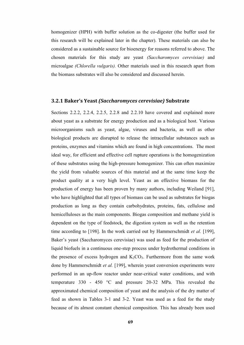
69

homogenizer (HPH) with buffer solution as the co-digester (the buffer used for

this research will be explained later in the chapter). These materials can also be

considered as a sustainable source for bioenergy for reasons referred to above. The

chosen materials for this study are yeast (Saccharomyces cerevisiae) and

microalgae (Chlorella vulgaris). Other materials used in this research apart from

the biomass substrates will also be considered and discussed herein.

3.2.1 Baker’s Yeast (Saccharomyces cerevisiae) Substrate

Sections 2.2.2, 2.2.4, 2.2.5, 2.2.8 and 2.2.10 have covered and explained more

about yeast as a substrate for energy production and as a biological host. Various

microorganisms such as yeast, algae, viruses and bacteria, as well as other

biological products are disrupted to release the intracellular substances such as

proteins, enzymes and vitamins which are found in high concentrations. The most

ideal way, for efficient and effective cell rupture operations is the homogenization

of these substrates using the high-pressure homogenizer. This can often maximize

the yield from valuable sources of this material and at the same time keep the

product quality at a very high level. Yeast as an effective biomass for the

production of energy has been proven by many authors, including Weiland [91],

who have highlighted that all types of biomass can be used as substrates for biogas

production as long as they contain carbohydrates, proteins, fats, cellulose and

hemicelluloses as the main components. Biogas composition and methane yield is

dependent on the type of feedstock, the digestion system as well as the retention

time according to [198]. In the work carried out by Hammerschmidt et al. [199],

Baker’s yeast (Saccharomyces cerevisiae) was used as feed for the production of

liquid biofuels in a continuous one-step process under hydrothermal conditions in

the presence of excess hydrogen and K2CO3. Furthermore from the same work

done by Hammerschmidt et al. [199], wherein yeast conversion experiments were

performed in an up-flow reactor under near-critical water conditions, and with

temperature 330 - 450 °C and pressure 20-32 MPa. This revealed the

approximated chemical composition of yeast and the analysis of the dry matter of

feed as shown in Tables 3-1 and 3-2. Yeast was used as a feed for the study

because of its almost constant chemical composition. This has already been used

70

for the production of proteins and amino acids in a closed batch reactor at

temperatures from 100 - 250 °C and pressures of 101.35 kPa - 3.97 MPa [200].

The choice of yeast choice in this research is not limited to just its homogenization

for the release of intracellular matter for energy conversion or for food products

manufacture, but also to the fact that its particle size can be reduced to as small as

0.02 μm for use in research.

3.2.1.1 Protein Extraction from Homogenized Baker’s Yeast

Fernandez et al. [201] have experimented through evaluating the rheological

behaviour and stability of oil-in-water emulsions prepared with aqueous

dispersions obtained from homogenized Baker’s yeast (Saccharomyces

cerevisiae), refined sunflower oil, and hydrocolloids that are widely used in low-

in-fat mayonnaises formulation. Preparation of yeast aqueous dispersions by high-

pressure homogenization was conducted by the rupturing of yeast whole cells in

an alkaline medium through HPH. The reduction of nucleic acid content (RNA)

was performed first by heat treating the sample at alkaline pH before the cell

rupture. Particle size distribution of the aqueous dispersion was determined by

laser diffraction using a Malvern Mastersizer 2000E analyser. From the results, it

was seen that higher yield in the formulation of yeast dressing with yeast aqueous

dispersion were obtained as compared to others such as water, refined sunflower

oil and hydrocolloids. This study also indicated, that the high pressure

homogenization (1500 bar, 3 passes) in alkaline medium ensured a good degree of

protein dispersibility (>50%) in aqueous dispersions. Yeasts possess advantages

over other microorganisms because of their larger size which makes it easier to

harvest. Other distinguishing factors that are advantageous to yeasts are; the lower

nucleic add content, high lysine content and ability to grow under acidic pH.

3.2.1.2 Baker’s Yeast form and Storage

Baker’s yeast (Saccharomyces cerevisiae) fresh and in block form during the

experimental research was provided by Dublin Food Sales, Ireland. This product

was refrigerated between 0 – 6 °C for freshness on the day of its collection so as to

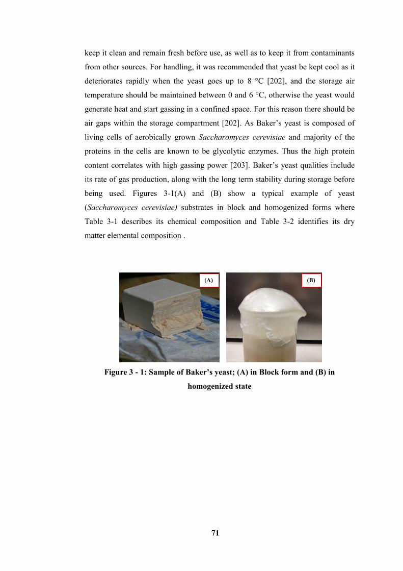
71

keep it clean and remain fresh before use, as well as to keep it from contaminants

from other sources. For handling, it was recommended that yeast be kept cool as it

deteriorates rapidly when the yeast goes up to 8 °C [202], and the storage air

temperature should be maintained between 0 and 6 °C, otherwise the yeast would

generate heat and start gassing in a confined space. For this reason there should be

air gaps within the storage compartment [202]. As Baker’s yeast is composed of

living cells of aerobically grown Saccharomyces cerevisiae and majority of the

proteins in the cells are known to be glycolytic enzymes. Thus the high protein

content correlates with high gassing power [203]. Baker’s yeast qualities include

its rate of gas production, along with the long term stability during storage before

being used. Figures 3-1(A) and (B) show a typical example of yeast

(Saccharomyces cerevisiae) substrates in block and homogenized forms where

Table 3-1 describes its chemical composition and Table 3-2 identifies its dry

matter elemental composition .

Figure 3 - 1: Sample of Baker’s yeast; (A) in Block form and (B) in

homogenized state

(A) (B)

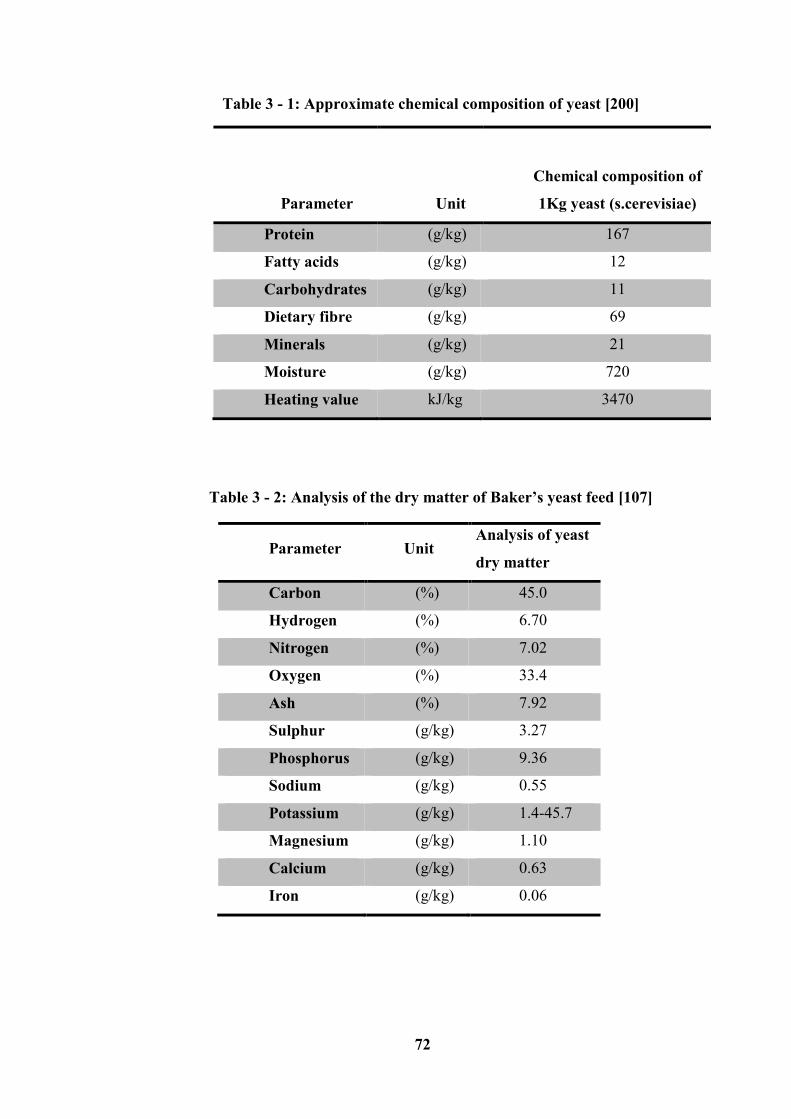
72

Table 3 - 1: Approximate chemical composition of yeast [200]

Parameter

Unit

Chemical composition of

1Kg yeast (s.cerevisiae)

Protein (g/kg) 167

Fatty acids (g/kg) 12

Carbohydrates (g/kg) 11

Dietary fibre (g/kg) 69

Minerals (g/kg) 21

Moisture (g/kg) 720

Heating value kJ/kg 3470

Table 3 - 2: Analysis of the dry matter of Baker’s yeast feed [107]

Parameter Unit Analysis of yeast

dry matter

Carbon (%) 45.0

Hydrogen (%) 6.70

Nitrogen (%) 7.02

Oxygen (%) 33.4

Ash (%) 7.92

Sulphur (g/kg) 3.27

Phosphorus (g/kg) 9.36

Sodium (g/kg) 0.55

Potassium (g/kg) 1.4-45.7

Magnesium (g/kg) 1.10

Calcium (g/kg) 0.63

Iron (g/kg) 0.06

73

3.2.2 Microalgae (Chlorella vulgaris) Substrate

Chlorella vulgaris has been discussed extensively in Section 2.2.6 and its

suitability as a biomass substrate is beyond question due to the fact that proteins

and lipids content within their cell is high enough to yield biogas as compared to

other biomass materials [85]. Their use has gone lately from human consumption

to the production of energy [85]. They can grow autotrophically and

heterotrophically with a wide range of tolerance to different temperatures, salinity,

pH and nutrient availabilities. Chlorella vulgaris along with Chlorella

Protothecoides are two widely available microalgae strains in the commercial

applications for food and nutritional purposes. Heredia-Arroyo et al. [204] have

indicated that they can show great potential as future industrial bioenergy

producers due to their robustness, high growth rate, and high oil content. They can

be cultured under the same conditions; autotrophic and heterotrophic.

Accordingly, Heredia-Arroyo et al. [204] revealed in their results that Chlorella

vulgaris could grow on autotrophic, mixotrophic and heterotrophic modes; and the

mixotrophic cultivation especially could produce more cell biomass than the

autotrophic or heterotrophic cultures, individually or combined [204].

3.2.2.1 Previous Work on Chlorella Vulgaris

The work carried out by Abreu et al. [205] in determining the growth parameters

and biochemical compositions of the green microalga Chlorella vulgaris

cultivated under different mixotrophic conditions showed similar results. It was

highlighted that using the main dairy industry by-product could be considered as a

feasible alternative in reducing the costs of microalgal biomass production. This is

based on the fact that the addition of expensive carbohydrates to the culture

medium would not be necessary. From the findings, the results indicate that the

highest specific growth rates were 0.43 and 0.47 g/day when the substrates were

cultivated under mixotrophic conditions using cheese whey (CW) powder

solution, along with mixtures of glucose and galactose as organic carbon sources,

respectively. This result is in agreement with the result from Heredia-Arroyo et al.

experimental work carried out using Chlorella vulgaris as a substrate, [204] which

74

also indicated that the values obtained were almost 3.5 times higher than those

produced under the photoautotrophic mode of nutrition. This again also agreed

with the findings from Kong et al. [206] which reported that mixotrophic

Chlorella vulgaris growth in glucose yielded higher biomass contents and

productivity than cells grown under photoautotrophic conditions. This yield, and

the biomass accumulation of Chlorella vulgaris during the cultivation, has been

promoted through the role played by the organic substrate. It therefore has come to

be realized that microalgae grew faster which thus provides high productivities of

biomass, lipids, starch, and proteins: hence, the particular reason for Chlorella

vulgaris choice as a biomass substrate in this research.

3.2.2.2 Chlorella Vulgaris Sample and Storage

Table 2-5 of Section 2.2.10 in Chapter 2 shows the general composition of

different human food sources and algae (% of dry matter). It shows Chlorella

vulgaris to be higher in terms of the protein content. This reflects the reason for

one of its consideration as a biomass substrate amongst others in this research.

A sample of the substrate is shown in Figure 3-2. This was supplied by a Culture

Collection of Algae and Protozoa (CCAP) of the Scottish Marine Institute, United

Kingdom. This determination of the strain, was through the identification of

CCAP 211/11B from the original author Beijerinck 1890, where freshwater in

Delft, Holland was used [207].

The culture conditions as demanded by the CCAP required the temperature to be

15 °C ± 2 °C, and for faster growth, it should be grown at 20 – 25 °C in cool white

fluorescent tubes about 10 cm from the culture, with an intensity of 30-40

μmol/m2s, and 12 hours light and 12 hours of darkness (for faster growth, use

continuous light). Refer to Appendix A for further information on the strain data.

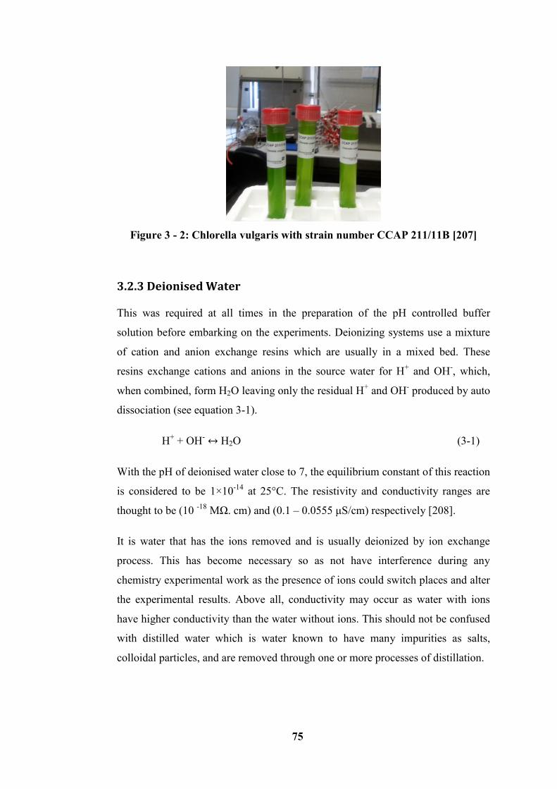
75

Figure 3 - 2: Chlorella vulgaris with strain number CCAP 211/11B [207]

3.2.3 Deionised Water

This was required at all times in the preparation of the pH controlled buffer

solution before embarking on the experiments. Deionizing systems use a mixture

of cation and anion exchange resins which are usually in a mixed bed. These

resins exchange cations and anions in the source water for H+ and OH

-, which,

when combined, form H2O leaving only the residual H+ and OH

- produced by auto

dissociation (see equation 3-1).

H+ + OH

- ↔ H2O (3-1)

With the pH of deionised water close to 7, the equilibrium constant of this reaction

is considered to be 1×10-14

at 25°C. The resistivity and conductivity ranges are

thought to be (10 -18

MΩ. cm) and (0.1 – 0.0555 μS/cm) respectively [208].

It is water that has the ions removed and is usually deionized by ion exchange

process. This has become necessary so as not have interference during any

chemistry experimental work as the presence of ions could switch places and alter

the experimental results. Above all, conductivity may occur as water with ions

have higher conductivity than the water without ions. This should not be confused

with distilled water which is water known to have many impurities as salts,

colloidal particles, and are removed through one or more processes of distillation.

76

3.2.4 Buffer Solution Used in this Research

The buffer solution for controlled pH was prepared using the chemical compounds

supplied from Sigma-Aldrich. The solutions denoted as A, B and C will be

explained therein.

Solution A

(0.1M KH2PO4 + 0.15M NaCl) (3-2)

This is equivalent of 1litre

13.6g of KH2PO4 weighed into beaker and dissolved using the deionised water,

also; 8.8g of NaCl weighed into a beaker and dissolved using the deionised water;

both are mixed together and filled to the 1 litre mark. This was repeated thrice for

3 litres of solution to be obtained.

Solution B

(0.1M K2HPO4 + 0.15M NaCl) (3-3)

4.6g of K2HPO4 was weighed into a beaker and dissolved using the deionised

water, also; 1.8g of NaCl weighed into a beaker and dissolved using the deionised

water. Again both were mixed together and filled to the 200 ml mark in a flat-

bottom volumetric flask.

Solution C

Put pH probe in solution A and gradually add Solution B into Solution A.

Continue stirring while the 3000 ml beaker is sitting on the magnetic stirrer until

the pH scale of attained 5.3 is obtained. The solution so obtained is known as

solution C.

3.2.5 Protein Reagent

This is a reagent for detecting protein in a solution. The key objective of this work

is to determine the protein concentration in the homogenized biomass substrates

using the reagent. Protein reagent is a blue solution through which a Bovine

77

Serum Albumin (BSA) standard curve is produced. A high-quality, calibrated

BSA solution (2 mg/mL) is serially diluted to create the protein assay standard

curves. This is required in the measurement of protein concentration by means of a

spectrophotometer. The procedure involved firstly preparing dilutions using 0.1 M

phosphate buffer, pH 7.0, of each protein to 0.5, 5, 2, 4, and 5 mg/mL, then a

series of dilutions were prepared starting at 100 mg/ based on the product, T1949

Total Protein Reagent [209]. These bovine serum albumin (BSA) solutions are

considered as protein concentration reference standards for use in bicinchoninic

acid assay (BCA), Bradford and other protein assay protocols. It is a universally

accepted reference protein for total protein quantitation with the albumin standard

precisely formulated at 2 mg/mL in an ultrapure 0.9% sodium chloride solution

[210].

3.3 Equipment

The main machine used in this research was the GYB40-10S /GYB60-6S 2-Stage

homogenizing valve HPH and has been described extensively in Chapter 2. Other

pieces of equipment used in this research work are as listed in Table 3-3 which

includes characterisation and electrical equipment. Others not listed can be

referred to in Appendix E

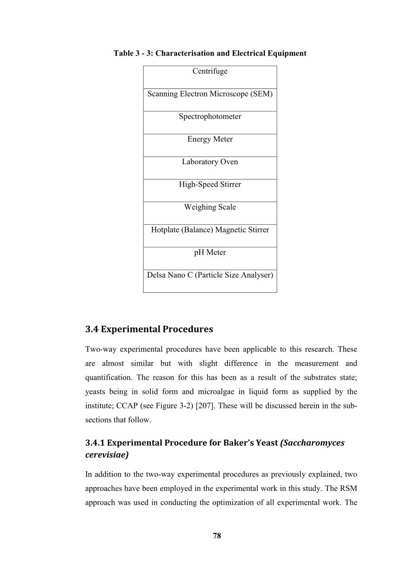
78

Table 3 - 3: Characterisation and Electrical Equipment

Centrifuge

Scanning Electron Microscope (SEM)

Spectrophotometer

Energy Meter

Laboratory Oven

High-Speed Stirrer

Weighing Scale

Hotplate (Balance) Magnetic Stirrer

pH Meter

Delsa Nano C (Particle Size Analyser)

3.4 Experimental Procedures

Two-way experimental procedures have been applicable to this research. These

are almost similar but with slight difference in the measurement and

quantification. The reason for this has been as a result of the substrates state;

yeasts being in solid form and microalgae in liquid form as supplied by the

institute; CCAP (see Figure 3-2) [207]. These will be discussed herein in the sub-

sections that follow.

3.4.1 Experimental Procedure for Baker’s Yeast (Saccharomyces

cerevisiae)

In addition to the two-way experimental procedures as previously explained, two

approaches have been employed in the experimental work in this study. The RSM

approach was used in conducting the optimization of all experimental work. The

79

experimental procedure based on the RSM technique will unfold in the next

Chapter.

The One-Variable-At-a-Time (OVAT) approach was also employed for the

experiments; this was aimed at investigating the effect of the higher pressure

homogenizer device (GYB40-10S 2-stage homogenizing valves HPH) as a cell

disruption machine on protein yield from the biomass materials considered which

have been homogenized using the buffer solution, and to determine range of

dataset for the parameters considered in the study.

3.4.1.1 Homogenization

For the experimental work on the use of the HPH, start by cleaning machine by

running clean water through it and while the machine is on for about half an hour,

it clears and cleans up the debris and particle that would probably cause error in

the process. While the cleaning up is in place, break down the solid Baker’s yeast

and weigh out 950 g into the beaker. Measure 725 ml of Phosphate buffer

(solution C) and then pour into the broken yeast. Mix using the electric laboratory

mixer. For further cleaning, pass 2 litres of deionised water through the

homogenizer and when the deionised water is almost completely empty in the

HPH that is when the poured deionised water is almost at the inlet conical section,

pass through the sample of yeast suspension (approx. 1625 ml) almost

immediately down the feeder’s tank of the HPH.

By turning the first and second hand wheel to increase pressure build up and

balancing of pressure respectively, the desired pressure is attained (see Figure 2-16

of Section 2.5.3 in Chapter 2). As the connected pipe for yeast collection at the

homogenizer outlet becomes cloudy during the substrate homogenization, this

flows through to the exit, then start collecting the suspension in a graduated

cylinder. It is important at this point to ensure that the temperature remain

constant. After collecting one litre of the cloudy suspension (yeast suspension

mixed with deionised water). This was thrown away as it would have mixed with

deionised water used for the cleaning of HPH at the start of the experiment. For

each new homogenized sample, pressure was recorded for data purposes. For

80

cycle more than 1, the collected homogenized yeast at the HPH exit was poured in

again into the feeder’s tank. Temperature was checked regularly with a

thermometer to achieve the desired temperature before pre-treating in the HPH.

The homogenized yeast collected, was considered as homogenized undiluted yeast

while the untreated yeast is regarded as the mixed soluble yeast that never passed

through high pressure homogenizer (HPH); i.e. unhomogenized. The homogenized

undiluted yeast was then separated into 4 tubes measuring 10 ml, 20 ml, 30 ml and

100 ml each. Phosphate buffer (solution C) with pH 5.3 in the ratio of 90 ml, 80

ml and 70 ml was added to the 10, 20 and 30 ml tubes respectively, to achieve 100

ml of sample, thus yielding ratios of 10:90, 20:80, 30:70 and 100% or 0.100.

3.4.1.2 Centrifugation

Each of the samples was emptied into the centrifuge tubes, and then centrifuged at

13,000 rpm over an hour as detailed in the operation manual. In order to separate

the supernatant from the pellets, the appropriate procedures were followed. The

supernatant was filtered using the syringe and syringe filter. 200 µl of the filtered

sample and 900 µl (×2) of the Buffer (solution C) was taken into a test tube, that

is; 2000 µl in total. Also, 2000 µl of homogenized undiluted yeast was taken. This

process was repeated 6 times.

500 µl of each of the replicate tubes were taken into a cuvette and then diluted

with 2000 µl of total protein reagent. The results for each of the six replicate

cuvettes for each sample in the dataset were averaged to form a single reading for

that sample, using the spectrophotometer and the results so achieved are read of on

the protein curve. The spectrophotometer was set at the wavelength of 550 nm.

This was left to stay for 30 minutes before determining the protein concentration.

81

3.4.1.3. Spectrophotometer

Technically, what the spectrophotometer is measuring is not how much light is

absorbed, but how much is transmitted. The percentage transmitted can be easily

converted to absorbance by using this formula (see equation 3-4);

(3-4)

There are two ways of determining protein concentration; the first way is through

the use of the Beers-Lambert law.

From the equation, the absorbance equals the concentration of the molecule of

interest (c), times the length of the path the light takes through the cuvette (b;

always 1 cm for our spectrophotometers), times the extinction coefficient (ε) as

shown in (equation 3-5);

Abs=εbc (3-5)

The extinction coefficient is the part that is specific for each compound and must

be determined experimentally. It can be determined from the standard curve

through solving for ε, because the absorbance and concentration are known, and it

can also measure the width of the cuvette. Once ε is known it can then be used for

other solutions of the same molecule.

The other way is by determining the concentration from the standard curve (a

graph of absorbance against concentration for standard solutions whose

concentrations are known). This is then compared with the absorbance of an

unknown solution of the same molecule to that curve. Using the linear graph

equation (equation of a straight line) equation 3-6;

y = mx + C (3-6)

Where, m = slope or gradient, and C = Intercept at Y-axis

82

Therefore, the protein concentration at the X-axis can then be solved since the

absorbance value on the Y-axis is known from the standard (protein) curve. Based

on the prepared standard protein curve (see Appendix F), the protein concentration

yield was determined through UV absorbance rate of the solution reading from the

Spectrophotometer as the light passes across the liquid (liquid diluted with the

total protein reagent). Section 3.5 below explains in detail protein curve

preparation and spectrophotometer.

3.4.2 Experimental Procedure for Microalgae (Chlorella vulgaris)

The experimental procedure for microalgae was basically similar to the procedure

described above for Baker’s yeast; the difference is the measurement and

quantification of the substrate against the phosphate buffer (solution C) pH 5.3.

10 ml of Chlorella vulgaris is mixed into 1000 ml of buffer solution C (phosphate

buffer) at any time before pre-treating in the homogenization stage. The

microalgae were not cultured and were pre-treated the same way supplied (by the

Institute; CCAP). After the pre-treatment using the HPH, the other steps taken

were same for the Baker’s yeast. For further reference on the strain supplied, refer

to Appendix A of this thesis.

3.5 Protein curve preparation and spectrophotometer

A standard protein curve preparation is needed for determination of the protein

concentration. One absolute way for determining the concentration of any given

protein in a solution having an unknown protein concentration is to compare the

unknown solution with a set of protein solutions of known concentrations. This

works by having the curve calibrated and in the process enable to determine the

exact protein concentration measure in a solution under investigation. Therefore

the absorbance associated with a set of protein solutions of known concentrations

is otherwise known as the protein standard curve. Before setting up the assay, the

protein to be used as a standard is decided upon and the range which it is likely to

be sensitive is determined. As sensitivity varies from one reagent batch to another,

immunoglobulin G (IgG) is frequently used as a standard in Bradford assay in the

83

same way as BSA (bovine serum albumin). With the BSA solutions, 0.1 M

phosphate buffer, pH 7.0 of each protein to 0.5, 1, 2, 4 and 5 mg/ml were prepared

to dilutions. Starting at 100 mg/ml and prepared serial dilutions were made using

Total Protein Reagent and with the UV procedure a Standard Curve for BSA was

prepared omitting 0.25 mg/ml dilution. The absorbance of the resulting solution is

measured using the spectrophotometer (Figure 3-10) and the measured absorbance

of the protein versus the known concentration of BSA is plotted. The resulting

graph will then be the protein standard curve for determining the unknown protein

concentration (see Appendix F).

3.6 Energy Cost Analysis

The cost analysis of the high-pressure homogenizer (HPH) was necessary in the

experimental set up, to determine how much energy was consumed in the

disruption of the biomasses, (Baker’s yeast and Chlorella vulgaris in the liberation

of the inner contents (protein) through their cell wall breakage). In doing this, an

energy meter by Efergy was employed, which measures electrical energy

consumption on any appliance. The tabulated and recorded cost for both

biomasses were then translated and entered into the design expert along with the

homogenization parameter to efficiently analyse the cost effectiveness of the

process.

3.7 Design of Experiment (DOE)

3.7.1 Introduction

The Section discusses the general view on design of experiment (DOE) in relation

to the considered design; Box Behnken design (BBD), analysis of the design as

well as the desirability approach function.

3.7.2 Design of Experiment (DOE) Overview

This technique enables designers in determining simultaneously the individual and

interactive effects of many factors that could affect the output results in any

design. This was developed by Sir Ronald Fisher in the early 1920s at Rothamsted

Agricultural Field Research Station in Harpenden London and in his experiment;

84

he used DOE that could differentiate the effect of fertilizer and the effect of other

factors. This has been used since in wide range of disciplines. It can be used in

finding answers in situations such as; “What is the relationship between factors

and responses?”, “What are the best combinations of factors value so as to

maximize or minimise multi responses?”, “What is the main contributing factor to

a system?” and so on.

Taguchi and 2-level factorial design methods are the commonest designs amongst

the many design of DOE. These are characterized by the lowest number of runs

when studying a process with multiple factors and multiple responses. However,

based on this fact, the quadratic effect of each factor cannot be determined using a

2-level factorial design, while also the interactions between the factors affecting

the process cannot be determined through the use of the Taguchi method. This is

as a result of the alias structures and this determines which factors are confounded

with each other [211]. For these two reasons, the Taguchi and 2-level factorial

designs are mainly used as screening designs in the identification of the main

effects within a system. Realistically, Response Surface Methodology (RSM) on t

one hand is able to fully determine all the factor’s effects and their interactions.

RSM is therefore considered as the chosen experimental methodology in this

research through specifically using the Box-Behnken Design (BBD) in the

implementation. RSM as a statistical technique is specially designed in optimizing

the system’s output, where the maximal and minimal goals are considered.

Equation 3.5 shows the function identifying the response surface and consists of

three capital-sigma summations. The operative and study regions are coincident in

this particular design and signified each factor being investigated over its whole

range. This is considered the competitive advantage for BBD over the central

composite design (CCD), which is another example of the RSM approach [212]

3.7.3 Response Surface Methodology (RSM)

Box and Wilson [213] introduced the response surface methodology (RSM)

concept in the 1950s having considered it as the best known type of DOE design.

It has been adopted for the experiments of this research and will be elucidated in

85

the chapters to come. This also follows the Box-Behnken Design (BBD) whose

variables are shown respectively in the appropriate chapters. RSM is a collection

of statistical and mathematical techniques that can be used in the improvement,

development, and in the optimizing processes, products, and systems. The goal is

to find the model of the proposed system, by performing data fitting and

regression analysis and the methodology is applied to the measured yields using

the statistical software, Design-Expert v 8.0. Based on this, RSM also specifies the

relationships among one or more of the measured responses and the essential

controllable input factors [214]. Therefore all variables being measurable, and be

repeated with negligible error, the response surface can be expressed by function

y, where k is considered the number of independent variables:

y = f(x1, x2, …xk) (3-7)

RSM is a mathematical and statistical technique set useful for modelling,

interpreting and predicting the outputs of interest to several input variables χ (from

level i to j) with the aim of optimizing a single or multiple responses ys [211, 213].

To optimize the responses ys, it is necessary to find an appropriate approximation

for the true functional relationship between the independent variables and the

response surface. A second order polynomial (Equation 3-8) is usually used in

RSM [211, 215], where the values of the model coefficients b0, bi, bij and bii can

be estimated using regression analysis.

2y iiiijiijiio bbbb (3-8)

The first summation term represents the main factor effects, the second term

reflects the quadratic effects, and the third stands for the two-factor interaction. As

stated above, the independent variables in this research will be described in

chapters to come. The second order polynomial model, given by equation 3-8 was

applied on one or two responses given as cost (Euro/hour) and protein yields

(mg/mL). The same statistical software was used in the generation of the analysis

of variance (ANOVA) and the response plots.

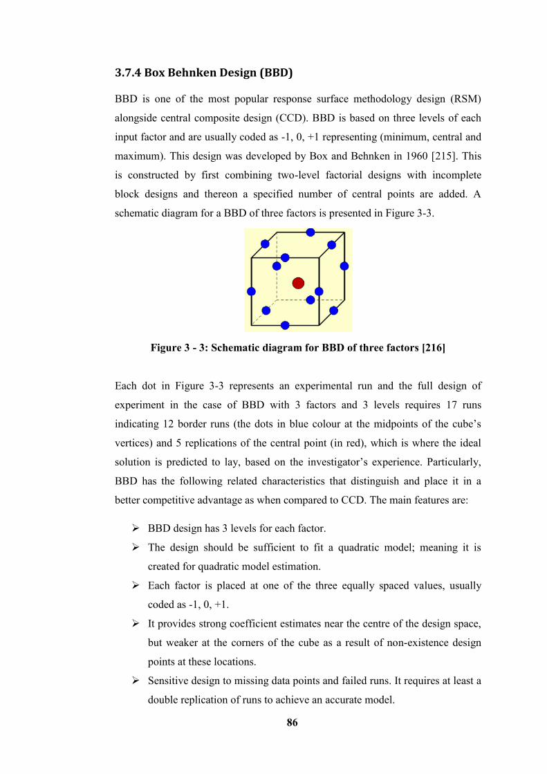
86

3.7.4 Box Behnken Design (BBD)

BBD is one of the most popular response surface methodology design (RSM)

alongside central composite design (CCD). BBD is based on three levels of each

input factor and are usually coded as -1, 0, +1 representing (minimum, central and

maximum). This design was developed by Box and Behnken in 1960 [215]. This

is constructed by first combining two-level factorial designs with incomplete

block designs and thereon a specified number of central points are added. A

schematic diagram for a BBD of three factors is presented in Figure 3-3.

Figure 3 - 3: Schematic diagram for BBD of three factors [216]

Each dot in Figure 3-3 represents an experimental run and the full design of

experiment in the case of BBD with 3 factors and 3 levels requires 17 runs

indicating 12 border runs (the dots in blue colour at the midpoints of the cube’s

vertices) and 5 replications of the central point (in red), which is where the ideal

solution is predicted to lay, based on the investigator’s experience. Particularly,

BBD has the following related characteristics that distinguish and place it in a

better competitive advantage as when compared to CCD. The main features are:

BBD design has 3 levels for each factor.

The design should be sufficient to fit a quadratic model; meaning it is

created for quadratic model estimation.

Each factor is placed at one of the three equally spaced values, usually

coded as -1, 0, +1.

It provides strong coefficient estimates near the centre of the design space,

but weaker at the corners of the cube as a result of non-existence design

points at these locations.

Sensitive design to missing data points and failed runs. It requires at least a

double replication of runs to achieve an accurate model.

87

Has user-defined specific and equidistant positioning of design points. The

estimation variance should more or less depend only on the distance from

the centre (this achievable exactly for the designs with 4 and 7 factors), and

should not vary too much inside the smallest cube containing the

experimental points.

3.7.5 Advantages of (BBD) over Central Composite Design (CCD)

BBD have some advantages over the Central Composite Design (CCD). These

will be elucidated below:

BBD requires that factors be varied over 3 levels as this makes

experimentation less costly if actual prototypes are being constructed in the

experimentation.

They are all spherical designs that can rotate with some provision of

orthogonal blocking.

Separation of runs into blocks for the Box-Behnken design allows blocks

to be used in such a way that the estimation of the regression parameters

for the factor effects is not affected by the blocks.

Another advantage of these designs is that there are no runs where all

factors are either at the +1 or -1 levels.

The main advantage of BBD is in addressing the issue of where the

experimental boundaries should be, and in particular avoidance of

treatment combinations that are extreme.

BBD offers the advantage of requiring fewer numbers of runs, but this

disappears when a factor of 4 or more is used.

3.7.6 Design Analysis

Determining the squares of the model requires the use of some mathematical

equations. These mathematical equations (3-9 – 3-16) are detailed completely in

Appendix G1.

88

3.7.7 Response Surface Methodology (RSM) Required Steps

The Response Surface Methodology approach is considered as a set of sequential

steps, studied with the purpose of optimizing the final protein yield and cost

effectiveness, which are regarded as the outcomes of the system under

investigation. The following steps were performed so as to develop a mathematical

model for the proposed protein production system:

1. Determining the essential process input factors.

2. Determining the limits for each factor considered.

3. The development of a design matrix.

4. Performing the experiment.

5. Measuring the responses.

6. Development of the mathematical model

7. Estimation of the coefficient in the model.

8. Testing the adequacy of the developed models.

9. Model reduction.

10. Development of the final reduced model.

11. Post analysis.

3.7.7.1 Determining the essential process input factors

The essential input factors that affect the output of the system can be identified

through conducted research and a literature review as applicable to this study or by

conducting a preliminary study. From the study, it emerged that particle size

reduction was an important variable on responses such as protein concentration

yield, and possibly production cost in euro/hour. The number of cycles (passes)

and temperature were considered as factors.

3.7.7.2 Finding the limits of each factor

In other to determine the limit of each factor, trial homogenization of biomass

substrate materials were performed, for ranges of pressure, temperature, and

number of cycles.

89

As different HPH’s have different working pressures, it was critical not to operate

above the working pressure specified by the manufacturer. For the current HPH;

GYB40-10S high pressure homogenizer, it had a maximum working pressure not

exceeding 90 MPa and as a result the range 30-90 MPa was considered after

several trials and from a literature study. The number of cycles, were set at 1-5,

and temperature ranges were set as 15 – 25 °C for the first set of experiments, and

30 – 50 °C for the second set of experiments. Design-Expert v.8 software was used

to code the data, develop the design matrix, and analyse the case; the limits for

each were coded via the following relationship;

X1 = 2(2𝑋−(𝑋𝑚𝑎𝑥+𝑋𝑚𝑖𝑛)

(𝑋𝑚𝑎𝑥−𝑋𝑚𝑖𝑛) (3-17)

Where;

X1 is the required coded value,

X is any value of the factor which wanted to be coded, and

Xmax, Xmin are the upper and lower limits of the factor being coded respectively

[208].

3.7.7.3 The development of the design matrix

The design matrix reported shows the response’s mean values for both biomasses;

Saccharomyces cerevisiae and Chlorella vulgaris, along with the different ratios

(10:90, 20:80 and 30:70) considered. For yeast (Saccharomyces cerevisiae) two

temperature ranges were applied (15-25°C) and (30-50°C) and for Microalgae

(Chlorella vulgaris) only one temperature range of (30-50°C) was applied.

Substrate to buffer ratios of (10:90, 20:80 and 30:70) were applicable to all

conducted experimental work and for the three factors, the total number of runs is

17. These experimental runs are enough to estimate the coefficients in Equation 3-

8.

90

3.7.7.4 Performing the experiment

The cell disruption and homogenization experiments were accomplished

accordingly in relation to the design matrix and in a random order so as to avoid

any systematic error occurrence in the experimental work.

3.7.7.5 Measuring the responses

All responses, mentioned previously in chapter one, were measured and recorded

for responses in all experiments and then used in the development of the model.

3.7.7.6 Development of the mathematical model

The functional relationship, as an example for three factors representing any

response of interest can be expressed as y = f (A, B, C) and Equation 3-8 can be

transformed into:

Y = b0 + b1A +b2B + b3C + B11A2 + b22B

2 + b33C

2 + b12AB

+b13AC + b23BC +b33C2 + b12AB + b13AC + b23BC (3-18)

3.7.7.7 Estimation of the coefficient in the model

Regression analysis was applied in order to estimate the values of the coefficients

in Equation 3-18.

3.7.7.8 Testing the adequacy of the developed models

The analysis of variance (ANOVA) was used to test the adequacy of the models

developed. The statistical significance of the models developed and of each term

was examined using the sequential F-test, lack-of-fit test, and other adequacy

measures (i.e. R2, Adj- R

2, Pred. R

2 and Adequate Precision) using the same

software to obtain the best fit. The Prob >F (is sometimes called the p-value) of

the model and of each term in the model can be computed by means of ANOVA.

If the Prob >F of the model and of each term in the model does not exceed the

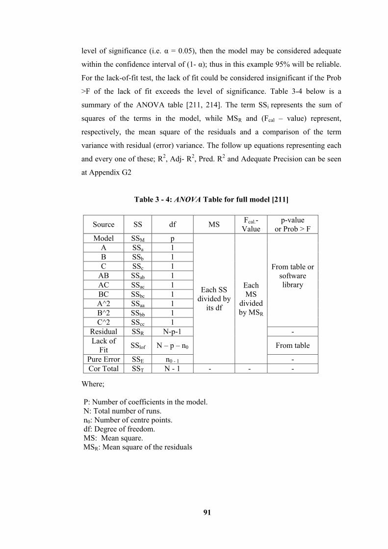
91

level of significance (i.e. α = 0.05), then the model may be considered adequate

within the confidence interval of (1- α); thus in this example 95% will be reliable.

For the lack-of-fit test, the lack of fit could be considered insignificant if the Prob

>F of the lack of fit exceeds the level of significance. Table 3-4 below is a

summary of the ANOVA table [211, 214]. The term SSi represents the sum of

squares of the terms in the model, while MSR and (Fcal – value) represent,

respectively, the mean square of the residuals and a comparison of the term

variance with residual (error) variance. The follow up equations representing each

and every one of these; R2, Adj- R

2, Pred. R

2 and Adequate Precision can be seen

at Appendix G2

Table 3 - 4: ANOVA Table for full model [211]

Where;

P: Number of coefficients in the model.

N: Total number of runs.

n0: Number of centre points.

df: Degree of freedom.

MS: Mean square.

MSR: Mean square of the residuals

Source SS df MS Fcal.-

Value

p-value

or Prob > F

Model SSM p

Each SS

divided by

its df

Each

MS

divided

by MSR

From table or

software

library

A SSa 1

B SSb 1

C SSc 1

AB SSab 1

AC SSac 1

BC SSbc 1

A^2 SSaa 1

B^2 SSbb 1

C^2 SScc 1

Residual SSR N-p-1 -

Lack of

Fit SSlof N – p – n0 From table

Pure Error SSE n0 - 1 -

Cor Total SST N - 1 - - -

92

3.7.7.9 Model reduction

The complete mathematical model as shown in Equation 3-18 would normally

contain some terms that are not significant and as such, are eliminated , i.e. terms

with p-value being greater than α. This elimination can be done manually or

automatically by choosing one of the selection procedure provided by the

software.

3.7.7.10 Development of the final reduced model

The final reduced model is determined by applying the above steps, and can be

built upon at this stage, by the software. The significant terms are only contained

in the final reduced model at this stage, but a further reduced quadratic ANOVA

Table can be produced if the need be.

3.7.7.11 Post analysis

Once the final model has been obtained, the factors and factors-interaction effects

will be interpreted via contours and perturbation plots provided by the software.

These plots can also be presented in the form of 3D graphs where they represent

the factors that contribute in the response.

Finally, by using the developed model, it is easy to optimise cell disruption and

homogenization conditions in the biomass substrates to improve the process and

lead to the desired protein concentration yield, as well as economic feasibility

(cost) of the conducted research.

3.7.8 Optimization

3.7.8.1 Optimization through Desirability Approach Function

The desirability approach is a method that allows for the optimization of a model

through constraining the allowed variability of certain factors. This is

recommended due to its advantages such as simplicity, availability in Design

Expert, and thus provides flexibility in weighting and giving user-defined

importance for input variables and responses. Solving such multiple response

93

optimization problems using this technique consists of using an approach that

combines multiple responses into a dimensionless measure performance known as

the overall desirability function (D). The desirability approach consists of

transforming each estimated response, Yi, into a unit-less bounded by 0 < di < 1,

where a higher di value indicates that Yi is more desirable. If di = 0, Yi is totally

undesirable, or vice versa when di = 1 [217].

In this study, the individual desirability for each response di is calculated using

equations 3-24 – 3-27 (see Appendix G3). The shape of the desirability function

can be changed by the weighted field wti. Weights are used to give emphases

which are added to the upper/lower bounds or to emphasize the target value.

Weights could be ranged between 0.1 and 10; weights greater than one gives more

emphasis to the goal (D), while weights less than one give less emphasis. In the

desirability objective function (D), each response can be assigned an important (r),

relative to the other responses. Importance varies from the least important of 1(+),

to the most important, a value of 5 (+++++). If the varying degrees of importance

are assigned to the different responses, the overall objective function is shown

below in equation 3-28 (see Appendix G3), where n denotes the number of

responses in the system and Ti is the target value of the ith

response [212].

3.7.8.2 Numerical and Graphical Optimization

Optimizing using the Design-Expert software identifies a combination of factor

levels that is simultaneously satisfying certain requirements which are usually

referred to as the “optimization criteria” at every one of the responses and input

variables, i.e. multiple-response optimization. Carrying optimization using the

graphical and numerical methods is by choosing the desired targets for each factor

and response. The numerical optimization features in the software so as to

maximize the objective function and provides the associated solution points in the

variable domain. This process that involves optimization combines the goals and

maximizes the overall desirability function (D)

The software defines regions where requirements simultaneously meet the

proposed criteria in the graphical optimization. This is done through

94

superimposing or overlaying critical response contours on a contour plot. The best

compromise can then be performed through visual search and when it involves

cases of many responses, it is best recommended to perform the numerical test

first; otherwise it will not be possible to cover the feasible region. The graphical

optimization displays the area of feasible response values in the factor space.

Regions that do not fit the optimization criteria are shaded [212]. Chapter 4

provides examples of numerical optimization with the desirability function (D)

selected.

3.8 Summary

The chapter have covered the materials and experimental procedures as applicable

to the research. Most importantly, the equipment characterisations have also been

highlighted. These were used in the different processes of the experimental work.

A protein curve was prepared to determine the protein content in the substrate

after homogenization through the use of a spectrophotometer. As the substrates

considered in the research were two, two different experimental procedures have

been presented with measurement and quantification showcased for both

substrates. Design of Experiment software has been highly studied and was

required to predict and optimise the homogenizing process after treating the yeast

and the micro algae via Response Surface Methodology (RSM) so as to develop

mathematical models that relate the process input parameters to their output

responses. The next chapter will study the three most important input parameters

of homogenization process; the number of cycle (passes), temperature, and

pressure. These will be thoroughly investigated to determine their effects on the

homogenized substrates along with the output features; protein concentration

yield, and cost for the energy consumption.

95

Chapter 4 Results and Discussion

4.1 Introduction

This Results and Discussion chapter has been divided into three categories. This

starts off by determining the set range by one-variable-at-a-time (OVAT) approach

for the operational parameter; (15 - 25°C) for temperature, (30 - 90 MPa) for

pressure and number of cycles as (1 - 5). These were determined through

experimentation with the substrates used in this study, Baker’s yeast

(Saccharomyces cerevisiae) and Microalgae (Chlorella vulgaris), to determine the

effect of temperature on yeast. Another range of temperature (30 – 50°C) was also

considered for Baker’s yeast (Saccharomyces cerevisiae) to compare these results.

As the results showed no appreciable difference between the two sets of

experiments conducted, the temperature range of 30 – 50 °C was not applied to

Microalgae (Chlorella vulgaris).

Particle size analysis was performed on the substrates using Delsa Nano C; a

software package for determining the distribution of particle sizes on substrates in

suspension, with sample size ranging between 0.6 nm to 7 μm. Scanning Electron

Microscope (SEM) analysis was also conducted on yeast biomass.

Characterisation analyses were conducted using the both processes to determine

the effect of HPH on the biomass substrates after homogenization.

For clarity and readability, the presented work in this section has been divided into

two parts: Baker’s yeast (Saccharomyces cerevisiae) and Microalgae (Chlorella

vulgaris), with the former further split into Baker’s yeast homogenized at

temperature range (15-25 °C) and Baker’s yeast homogenized at temperature

range of 30 to 50 °C, while the latter (Microalgae) is split into Microalgae

homogenized at a temperature range of 15 to 25 °C. The results obtained were

achieved through the application of Response Surface Methodology (RSM) in

developing mathematical models for the substrates above via the Design Expert

V.8. These were required in predicting the process. In further analysis the

substrates were also investigated considering the analysis of variance (ANOVA),

96

analysis for each response; their validation along with the effects of process

parameter of the substrates on each response. These are all discussed and

showcased in the Section.

Finally, numerical and graphical optimization was applied to the responses to

determine the energy cost and feasibility of the process.

4.2 Baker’s Yeast Analysis

In determining the protein concentration yields from treated and untreated Baker’s

yeast and to also determine the set range of the parameters for further

experimental work, different level experiments were conducted.

4.2.1 Baker’s Yeast Control Sample

Control samples were prepared, to compare them with the treated samples. This

was required in determining the set range of the parameters; pressure, temperature

and number of cycles (passes), applicable to this research before the

commencement of the experiments using the HPH. The control samples are those

samples that never passed through the homogenizer, i.e. are unhomogenized, but

have been treated with solution C (Refer to Chapter 3). The control samples did

not undergo any pressure and number of cycles, since they never passed through

HPH. It was however possible to determine the temperature, which was close to

that of the room temperature and could be quantified into ratios since it was

treated with solution C. The UV absorbance rate as shown in Table 4-1 is the

amount of protein content that has been absorbed under UV light in the

Spectrophotometer after being treated with the total protein reagent. For further

details, see Appendix F for the conversion process to protein concentration

(mg/mL).

Again as seen in the results presented in Table 4-1, it is seen that the untreated

Baker’s yeast can be considered as the control sample. The samples were

separated into ratios in solution with solution C at the rate of 10:90, 20:80 and

97

30:70. The results obtained indicate that protein concentration increased with the

increased ratio of dilution of Baker’s yeast against the solution (Solution C).

Untreated Baker’s yeast, at 10% to solution C at 90%, yielded 0.002 mg/mL,

While 20% to 80% of solution C and 30% to 70% of solution C resulted in 0.005

mg/mL and 0.008 mg/mL respectively.

Table 4 - 1: Control Samples – Untreated Baker’s Yeast at Different Ratios

Ratios UV Absorbance Rate Protein Conc. (mg/mL)

10:90

0.0901 0.002

20:80

0.0903 0.005

30:70

0.0905 0.008

4.2.2 Comparison Analysis Based on Pressure, Number of Cycle

and Ratios with Treated Baker’s Yeast

Tables 4-2 to 4-4 along with the graphs presented in Figures 4-1 to 4-3 represent

the comparison analyses based pressure, number of cycles, and ratio with the

control experiment sample at the different ratios depicted in Table 4-1. This

showcases the effect of the parameters on the yielded protein concentration. From

the conducted experiment, Table 4-2 shows the result obtained when the analysis

is based on pressure. Protein yields increased as the pressure applied during the

homogenization increased. With the dilution ratio, the number of cycles and

temperature constant, the protein yield rises with the pressure applied. This

supported the view of Brookman and James [39] that exponentially increasing

release of soluble protein being found with increasing pressure.

Figure 4-1 has also shows this graphically in the variation of the proteins yields in

the treated samples compared with the untreated Baker’s yeast. The treated

samples homogenized at 30, 60 and 90 MPa, against the untreated sample show

results of protein yields as; 0.020, 0.190 and 0.860 mg/mL respectively.

Protein yield was found to be minimal in the untreated sample as low as 0.002

mg/mL and only 0.020 mg/mL for the sample homogenized at 30 MPa pressure.

This therefore shows an increase of 11 times the original.

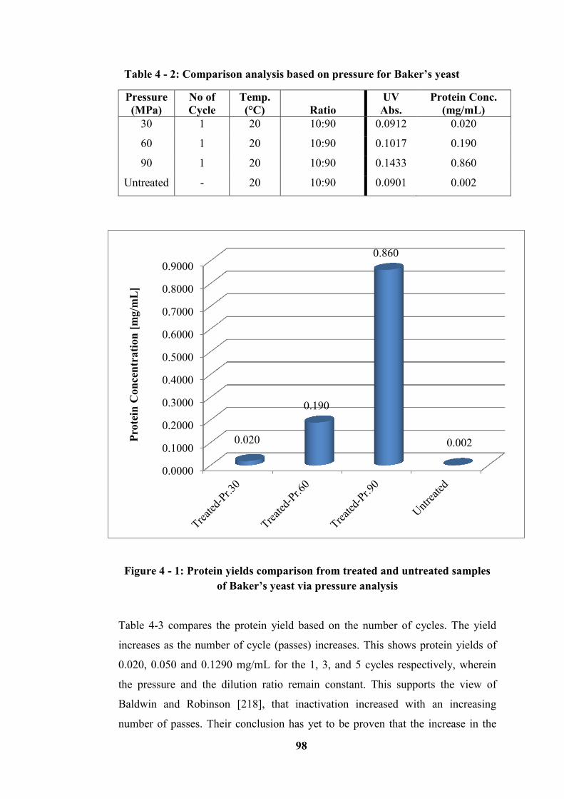
98

Table 4 - 2: Comparison analysis based on pressure for Baker’s yeast

Pressure

(MPa)

No of

Cycle

Temp.

(°C) Ratio

UV

Abs.

Protein Conc.

(mg/mL)

30 1 20 10:90 0.0912 0.020

60 1 20 10:90 0.1017 0.190

90 1 20 10:90 0.1433 0.860

Untreated - 20 10:90 0.0901 0.002

Figure 4 - 1: Protein yields comparison from treated and untreated samples

of Baker’s yeast via pressure analysis

Table 4-3 compares the protein yield based on the number of cycles. The yield

increases as the number of cycle (passes) increases. This shows protein yields of

0.020, 0.050 and 0.1290 mg/mL for the 1, 3, and 5 cycles respectively, wherein

the pressure and the dilution ratio remain constant. This supports the view of

Baldwin and Robinson [218], that inactivation increased with an increasing

number of passes. Their conclusion has yet to be proven that the increase in the

0.0000

0.1000

0.2000

0.3000

0.4000

0.5000

0.6000

0.7000

0.8000

0.9000

0.020

0.190

0.860

0.002 Pro

tein

Con

cen

trati

on

[m

g/m

L]

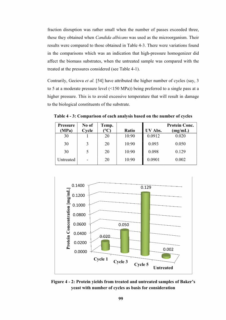
99

fraction disruption was rather small when the number of passes exceeded three,

these they obtained when Candida albicans was used as the microorganism. Their

results were compared to those obtained in Table 4-3. There were variations found

in the comparisons which was an indication that high-pressure homogenizer did

affect the biomass substrates, when the untreated sample was compared with the

treated at the pressures considered (see Table 4-1).

Contrarily, Geciova et al. [54] have attributed the higher number of cycles (say, 3

to 5 at a moderate pressure level (<150 MPa)) being preferred to a single pass at a

higher pressure. This is to avoid excessive temperature that will result in damage

to the biological constituents of the substrate.

Table 4 - 3: Comparison of each analysis based on the number of cycles

Pressure

(MPa)

No of

Cycle

Temp.

(°C) Ratio UV Abs.

Protein Conc.

(mg/mL)

30 1 20 10:90 0.0912 0.020

30 3 20 10:90 0.093 0.050

30 5 20 10:90 0.098 0.129

Untreated - 20 10:90 0.0901 0.002

Figure 4 - 2: Protein yields from treated and untreated samples of Baker’s

yeast with number of cycles as basis for consideration

0.0000

0.0200

0.0400

0.0600

0.0800

0.1000

0.1200

0.1400

Cycle 1Cycle 3

Cycle 5Untreated

0.020

0.050

0.129

0.002 Pro

tein

Con

cen

trati

on

[m

g/m

L]

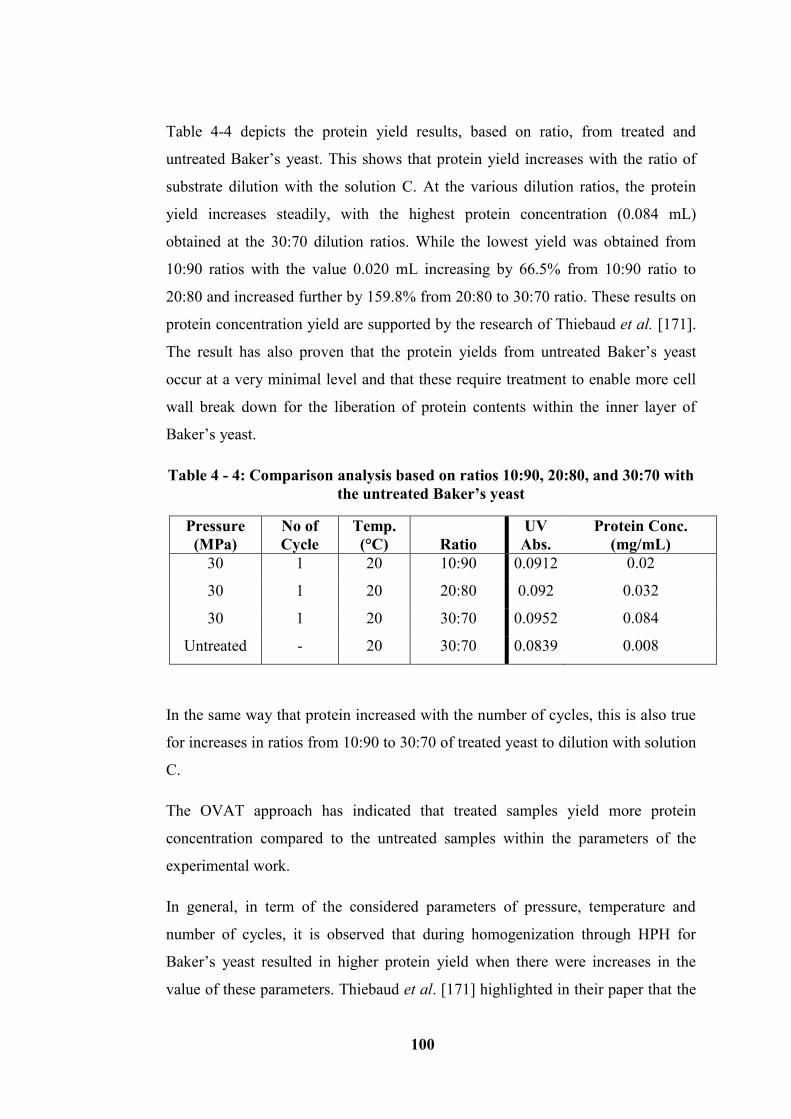
100

Table 4-4 depicts the protein yield results, based on ratio, from treated and

untreated Baker’s yeast. This shows that protein yield increases with the ratio of

substrate dilution with the solution C. At the various dilution ratios, the protein

yield increases steadily, with the highest protein concentration (0.084 mL)

obtained at the 30:70 dilution ratios. While the lowest yield was obtained from

10:90 ratios with the value 0.020 mL increasing by 66.5% from 10:90 ratio to

20:80 and increased further by 159.8% from 20:80 to 30:70 ratio. These results on

protein concentration yield are supported by the research of Thiebaud et al. [171].

The result has also proven that the protein yields from untreated Baker’s yeast

occur at a very minimal level and that these require treatment to enable more cell

wall break down for the liberation of protein contents within the inner layer of

Baker’s yeast.

Table 4 - 4: Comparison analysis based on ratios 10:90, 20:80, and 30:70 with

the untreated Baker’s yeast

Pressure

(MPa)

No of

Cycle

Temp.

(°C) Ratio

UV

Abs.

Protein Conc.

(mg/mL)

30 1 20 10:90 0.0912 0.02

30 1 20 20:80 0.092 0.032

30 1 20 30:70 0.0952 0.084

Untreated - 20 30:70 0.0839 0.008

In the same way that protein increased with the number of cycles, this is also true

for increases in ratios from 10:90 to 30:70 of treated yeast to dilution with solution

C.

The OVAT approach has indicated that treated samples yield more protein

concentration compared to the untreated samples within the parameters of the

experimental work.

In general, in term of the considered parameters of pressure, temperature and

number of cycles, it is observed that during homogenization through HPH for

Baker’s yeast resulted in higher protein yield when there were increases in the

value of these parameters. Thiebaud et al. [171] highlighted in their paper that the

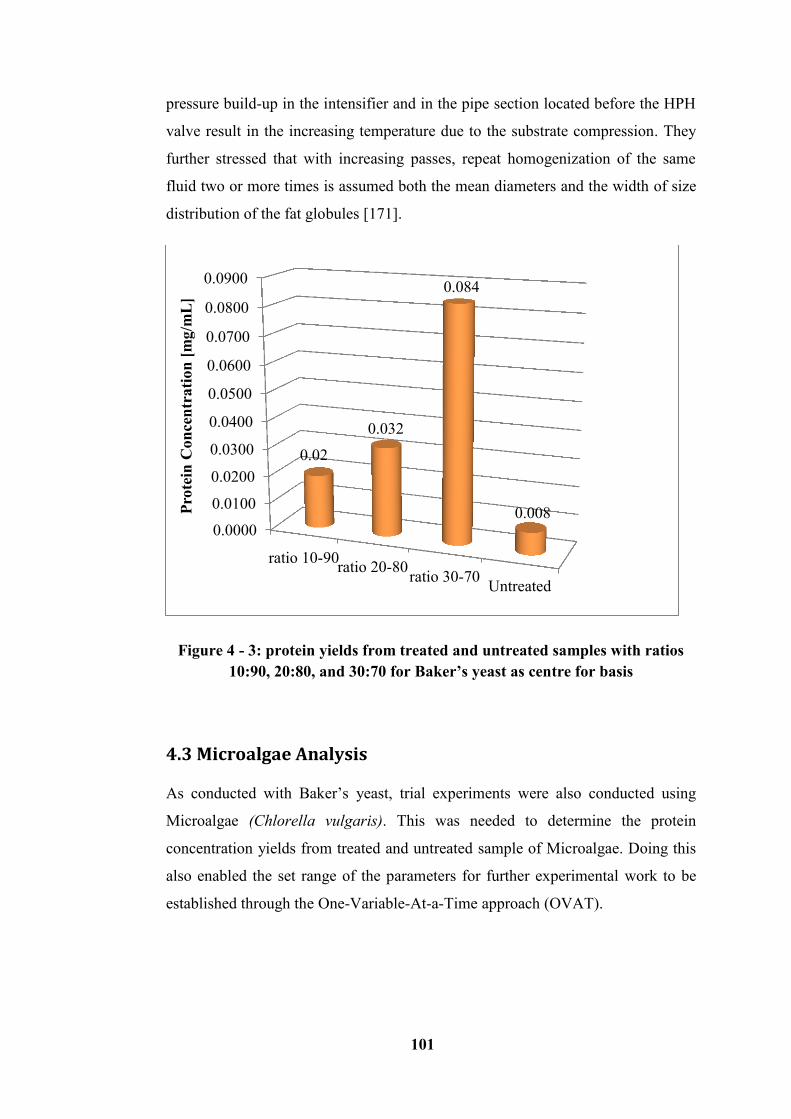
101

pressure build-up in the intensifier and in the pipe section located before the HPH

valve result in the increasing temperature due to the substrate compression. They

further stressed that with increasing passes, repeat homogenization of the same

fluid two or more times is assumed both the mean diameters and the width of size

distribution of the fat globules [171].

Figure 4 - 3: protein yields from treated and untreated samples with ratios

10:90, 20:80, and 30:70 for Baker’s yeast as centre for basis

4.3 Microalgae Analysis

As conducted with Baker’s yeast, trial experiments were also conducted using

Microalgae (Chlorella vulgaris). This was needed to determine the protein

concentration yields from treated and untreated sample of Microalgae. Doing this

also enabled the set range of the parameters for further experimental work to be

established through the One-Variable-At-a-Time approach (OVAT).

0.0000

0.0100

0.0200

0.0300

0.0400

0.0500

0.0600

0.0700

0.0800

0.0900

ratio 10-90ratio 20-80

ratio 30-70Untreated

0.02

0.032

0.084

0.008 Pro

tein

Con

cen

trati

on

[m

g/m

L]

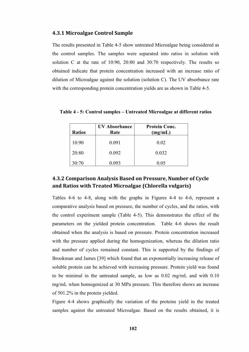
102

4.3.1 Microalgae Control Sample

The results presented in Table 4-5 show untreated Microalgae being considered as

the control samples. The samples were separated into ratios in solution with

solution C at the rate of 10:90, 20:80 and 30:70 respectively. The results so

obtained indicate that protein concentration increased with an increase ratio of

dilution of Microalgae against the solution (solution C). The UV absorbance rate

with the corresponding protein concentration yields are as shown in Table 4-5.

Table 4 - 5: Control samples – Untreated Microalgae at different ratios

4.3.2 Comparison Analysis Based on Pressure, Number of Cycle

and Ratios with Treated Microalgae (Chlorella vulgaris)

Tables 4-6 to 4-8, along with the graphs in Figures 4-4 to 4-6, represent a

comparative analysis based on pressure, the number of cycles, and the ratios, with

the control experiment sample (Table 4-5). This demonstrates the effect of the

parameters on the yielded protein concentration. Table 4-6 shows the result

obtained when the analysis is based on pressure. Protein concentration increased

with the pressure applied during the homogenization, whereas the dilution ratio

and number of cycles remained constant. This is supported by the findings of

Brookman and James [39] which found that an exponentially increasing release of

soluble protein can be achieved with increasing pressure. Protein yield was found

to be minimal in the untreated sample, as low as 0.02 mg/mL and with 0.10

mg/mL when homogenized at 30 MPa pressure. This therefore shows an increase

of 501.2% in the protein yielded.

Figure 4-4 shows graphically the variation of the proteins yield in the treated

samples against the untreated Microalgae. Based on the results obtained, it is

Ratios

UV Absorbance

Rate

Protein Conc.

(mg/mL)

10:90 0.091 0.02

20:80 0.092 0.032

30:70 0.093 0.05

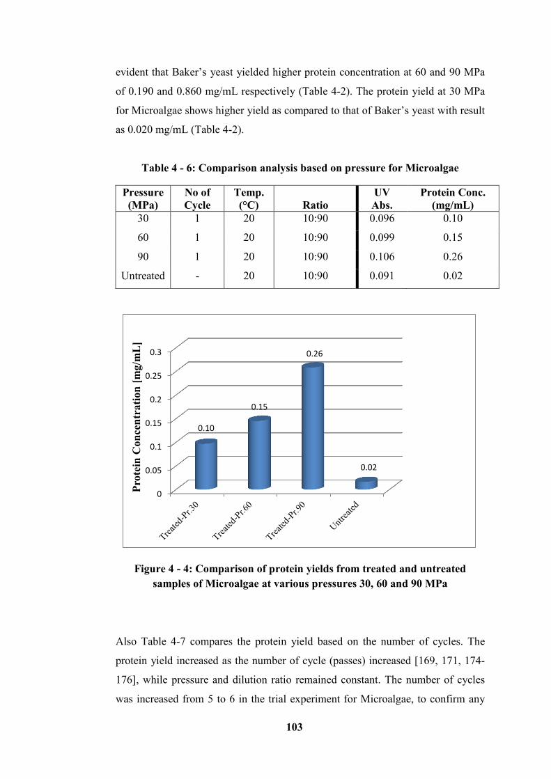
103

evident that Baker’s yeast yielded higher protein concentration at 60 and 90 MPa

of 0.190 and 0.860 mg/mL respectively (Table 4-2). The protein yield at 30 MPa

for Microalgae shows higher yield as compared to that of Baker’s yeast with result

as 0.020 mg/mL (Table 4-2).

Table 4 - 6: Comparison analysis based on pressure for Microalgae

Pressure

(MPa)

No of

Cycle

Temp.

(°C) Ratio

UV

Abs.

Protein Conc.

(mg/mL)

30 1 20 10:90 0.096 0.10

60 1 20 10:90 0.099 0.15

90 1 20 10:90 0.106 0.26

Untreated - 20 10:90 0.091 0.02

Figure 4 - 4: Comparison of protein yields from treated and untreated

samples of Microalgae at various pressures 30, 60 and 90 MPa

Also Table 4-7 compares the protein yield based on the number of cycles. The

protein yield increased as the number of cycle (passes) increased [169, 171, 174-

176], while pressure and dilution ratio remained constant. The number of cycles

was increased from 5 to 6 in the trial experiment for Microalgae, to confirm any

0

0.05

0.1

0.15

0.2

0.25

0.3

0.10

0.15

0.26

0.02

Pro

tein

Con

cen

trati

on

[m

g/m

L]

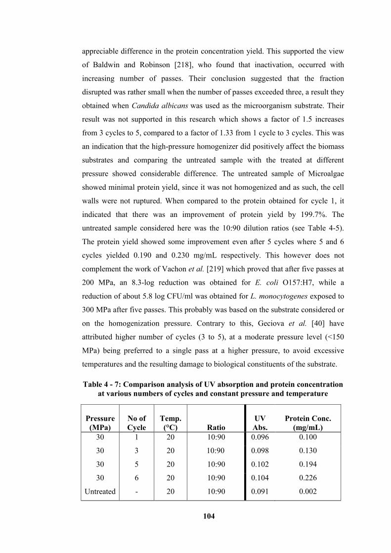
104

appreciable difference in the protein concentration yield. This supported the view

of Baldwin and Robinson [218], who found that inactivation, occurred with

increasing number of passes. Their conclusion suggested that the fraction

disrupted was rather small when the number of passes exceeded three, a result they

obtained when Candida albicans was used as the microorganism substrate. Their

result was not supported in this research which shows a factor of 1.5 increases

from 3 cycles to 5, compared to a factor of 1.33 from 1 cycle to 3 cycles. This was

an indication that the high-pressure homogenizer did positively affect the biomass

substrates and comparing the untreated sample with the treated at different

pressure showed considerable difference. The untreated sample of Microalgae

showed minimal protein yield, since it was not homogenized and as such, the cell

walls were not ruptured. When compared to the protein obtained for cycle 1, it

indicated that there was an improvement of protein yield by 199.7%. The

untreated sample considered here was the 10:90 dilution ratios (see Table 4-5).

The protein yield showed some improvement even after 5 cycles where 5 and 6

cycles yielded 0.190 and 0.230 mg/mL respectively. This however does not

complement the work of Vachon et al. [219] which proved that after five passes at

200 MPa, an 8.3-log reduction was obtained for E. coli O157:H7, while a

reduction of about 5.8 log CFU/ml was obtained for L. monocytogenes exposed to

300 MPa after five passes. This probably was based on the substrate considered or

on the homogenization pressure. Contrary to this, Geciova et al. [40] have

attributed higher number of cycles (3 to 5), at a moderate pressure level (<150

MPa) being preferred to a single pass at a higher pressure, to avoid excessive

temperatures and the resulting damage to biological constituents of the substrate.

Table 4 - 7: Comparison analysis of UV absorption and protein concentration

at various numbers of cycles and constant pressure and temperature

Pressure

(MPa)

No of

Cycle

Temp.

(°C) Ratio

UV

Abs.

Protein Conc.

(mg/mL)

30 1 20 10:90 0.096 0.100

30 3 20 10:90 0.098 0.130

30 5 20 10:90 0.102 0.194

30 6 20 10:90 0.104 0.226

Untreated - 20 10:90 0.091 0.002

105

Figure 4 - 5: Comparison of protein yields from treated and untreated

samples of Microalgae with the number of cycles as the basis for

consideration

Tables 4-8 gives the analyses of the protein concentration yield from treated and

untreated Microalgae at various ratios of 10:90, 20:80 and 30:70. This shows that

the protein concentration yield increased with ratio of substrate dilution with the

solution C. At the various dilution ratios, the protein yielded increases steadily

with the highest protein concentration rate obtained at the 30:70 dilution ratios to

the value of 0.10 mL. While lowest yield was obtained from 10:90 ratio increasing

by 16.63% from 10:90 ratio to 20:80 and increased again by 14.26% from 20:80 to

30:70 ratio. The results presented in terms of protein concentration yield supports

the findings of Thiebaud et al. [171], where protein concentration yield increased

with the increase of dilution ratio. The result has also proven that there are protein

yields, although minimal from untreated Microalgae. This shows that required

treatment enables more cell wall breakdown for the liberation of protein contents

within the inner layer of the substrates.

0.0000

0.0500

0.1000

0.1500

0.2000

0.2500

0.100

0.130

0.194

0.226

0.002

Pro

tein

Con

cen

trati

on

[m

g/m

L]

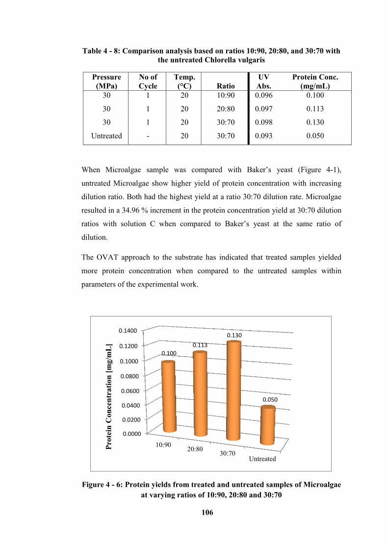
106

Table 4 - 8: Comparison analysis based on ratios 10:90, 20:80, and 30:70 with

the untreated Chlorella vulgaris

Pressure

(MPa)

No of

Cycle

Temp.

(°C) Ratio

UV

Abs.

Protein Conc.

(mg/mL)

30 1 20 10:90 0.096 0.100

30 1 20 20:80 0.097 0.113

30 1 20 30:70 0.098 0.130

Untreated - 20 30:70 0.093 0.050

When Microalgae sample was compared with Baker’s yeast (Figure 4-1),

untreated Microalgae show higher yield of protein concentration with increasing

dilution ratio. Both had the highest yield at a ratio 30:70 dilution rate. Microalgae

resulted in a 34.96 % increment in the protein concentration yield at 30:70 dilution

ratios with solution C when compared to Baker’s yeast at the same ratio of

dilution.

The OVAT approach to the substrate has indicated that treated samples yielded

more protein concentration when compared to the untreated samples within

parameters of the experimental work.

Figure 4 - 6: Protein yields from treated and untreated samples of Microalgae

at varying ratios of 10:90, 20:80 and 30:70

0.0000

0.0200

0.0400

0.0600

0.0800

0.1000

0.1200

0.1400

10:90 20:80

30:70Untreated

0.100

0.113

0.130

0.050

Pro

tein

Con

cen

trati

on

[m

g/m

L]

107

4.4 Structural Deformation of Baker’s Yeast and Analyses

through Scanning Electron Microscope (SEM)

This Section analyses and discusses structural deformation as effected by HPH

during yeast homogenization. This analysis was carried out using the Scanning

Electron Microscope (SEM). The SEM has been discussed previously in Chapter

3, and its use, enabled particle size analysis to be conducted on biomass substrates

such as Baker’s yeast. Studies carried out showed that SEM is not suitable for

liquid biomass substrates, and for this purpose it was unable to be used in

analysing Microalgae (Chlorella vulgaris) since it was delivered in liquid form.

Further attempt to dry it in the oven for possible analysis, left no traces of it to be

examined. Delsa Nano C was therefore considered as an alternative as use in

determining the particle size distribution of Microalgae (Chlorella vulgaris).

Analyses based on SEM have been sectioned into 2 parts; the 15 – 25 °C

temperature range, and the 30 – 50 °C temperature range. Untreated Baker’s yeast

with the treated (Homogenized) Baker’s yeast at different ratios; 10:90, 20:80, and

30:70 images were compared through accessing their deformation under SEM.

The operating parameters pressure, temperature, and the number of cycles for

homogenizing each samples were also considered. All SEM images provided

herein are at the same magnification of 100 microns

4.4.1 SEM for Baker’s yeast homogenized between 15 – 25 °C

temperature ranges

Untreated Baker’s yeast and the dilutions at the different ratios:

Figure 4-7 depicts SEM images that have not been treated through the HPH, and

in particular image (a) in the Figure is not in any ratio which means that it has not

been diluted with solution C in any form. Images b, c and d show the Baker’s

yeast structure untreated with the three ratios of dilution with solution C, 10:90,

20:80, and 30:70. From the image shown in Figure 4-7 (a), no deformations in the

images observed under the SEM, similarly ratios 10:90, 20:80, and 30:70 also

showed no structural damage because the samples had not passed through the

HPH. Figure 4-7 (a-d) compares them with other images in this research which

were treated and passed through the HPH. The magnification applied to the

108

images was the same throughout the study and because these are untreated,

pressure, temperature and the number of cycles has not been considered.

Treated (homogenized) Baker’s yeast at 30 MPa and at 25°C, along with the

dilutions at the different ratios:

Figure 4-8 depict images (e, f and g) corresponding to Baker’s yeast homogenized

at dilution ratios with solution C of 10:90, 20:80 and 30:70, respectively. These

have been homogenized at the first considered level of the cycle (1 Cycle) at a

temperature of 25 °C and at 30 MPa pressure. With the homogenized pressure at

30 MPa and cycle number at 1, the structural deformation on the images showed

some damage visible to the eye. The shaft-like state in image (e), spore-like state

in (f), and coated-like state in (g) are all due to the dilution and quantification rate

before dryness at 105°C. The original slurry state of the homogenized yeast at 1

cycle, 30 MPa and at 25 °C show some difference between before and after

homogenization. This is clearly seen when compared to the untreated samples in

Figure 4-7 (a, b, c, and d).

Treated (homogenized) Baker’s yeast at 30 MPa and at 20°C, along with the


Figure 4-9 depict images (h, i, and j) and these indicate the next level of cycle (3

Cycles), with the 3 different rates of dilution also shown to determine the extent of

structural deformation of the substrates after treatment. The Baker’s yeast has been

homogenized at a temperature of 20 °C and 30 MPa pressure. Homogenizing at 3

cycles is seen to create some distortion and deformation on the SEM images being

considered. Liu et al. [220] revealed that efficient breakage of the cell wall is as a

result of a strength-providing component which is necessary in the effective

removal of intracellular compounds. SEM use in the research has been

necessitated so as to observe any alteration undergone by the yeast cells after the

disruption process in every cycle. Disruption at every cycle during

homogenization is said to break open and releases the inner contents within the

cell walls. Another method of observing the alteration within the yeast cells after

109

disruption is the Transmission electron microscopy (TEM), but this has not been

considered in this research due to non-availability.

Treated (homogenized) Baker’s yeast at 30 MPa and 25°C, along with the


Figures 4-10 depict images (k, l, and m) and it is the third level of the cycle where

the substrates have been homogenized over 5 cycles in the treatment under the

high-pressure homogenizer. The pressure and temperature considered are same as

above; 30 MPa and 25 °C respectively. Running the homogenizer over 5 cycles on

the substrates elongates and stretches out the inner components that have not been

broken in the previous cycles. This as a result make the end product to be greatly

slurried, and the generated heat through cavitation then allows the homogenized

soluble Baker’s yeast to be very viscous due to the high pressure that have been

applied during the homogenization.

From a comparison of the images in Figures 4-8 to 4-10, with those in Figure 4-7,

it is clear and evident that there are changes in the microstructure and inner

content of Baker’s yeast after the homogenization processes. Physical changes

were observed during the homogenization process in the form of size of cell

debris, viscosity and the surface area of the homogenized yeast. These physical

changes are as a result of homogenizing at the considered parameters such as,

higher pressure, temperature, and the number of cycles. Baker’s yeast cell wall

disruption by mechanical means liberates the inner contents which are known to

contain protein. Accordingly, during the disruption process, the loss of cell wall

mannoproteins in the yeast will alter the wall porosity, and this is said to facilitate

the release of intracellular macromolecules with no effect on the wall integrity.

The release of these intracellular molecules is determined by the functionality of

the plasma membrane and the porosity of the yeast cell wall.

As a result of this, Shirgaonkar et al. [166] have highlighted alot of controversy

existing in the literature as regards the exact cause of the cell disruption in the

high-pressure homogenization (HPH). As discussed previously in Chapters 2,

many authors have therefore postulated their different views on this issue; Save et

al. [186] have proposed that cavitation and the shockwaves/pressure impulses

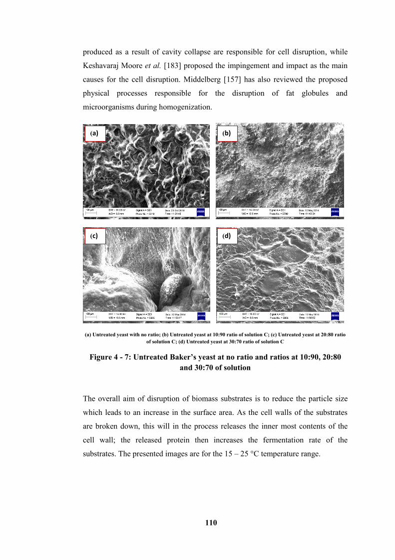
110

produced as a result of cavity collapse are responsible for cell disruption, while

Keshavaraj Moore et al. [183] proposed the impingement and impact as the main

causes for the cell disruption. Middelberg [157] has also reviewed the proposed

physical processes responsible for the disruption of fat globules and

microorganisms during homogenization.

(a) Untreated yeast with no ratio; (b) Untreated yeast at 10:90 ratio of solution C; (c) Untreated yeast at 20:80 ratio

of solution C; (d) Untreated yeast at 30:70 ratio of solution C

Figure 4 - 7: Untreated Baker’s yeast at no ratio and ratios at 10:90, 20:80

and 30:70 of solution

The overall aim of disruption of biomass substrates is to reduce the particle size

which leads to an increase in the surface area. As the cell walls of the substrates

are broken down, this will in the process releases the inner most contents of the

cell wall; the released protein then increases the fermentation rate of the

substrates. The presented images are for the 15 – 25 °C temperature range.

(a) (b)

(c) (d)

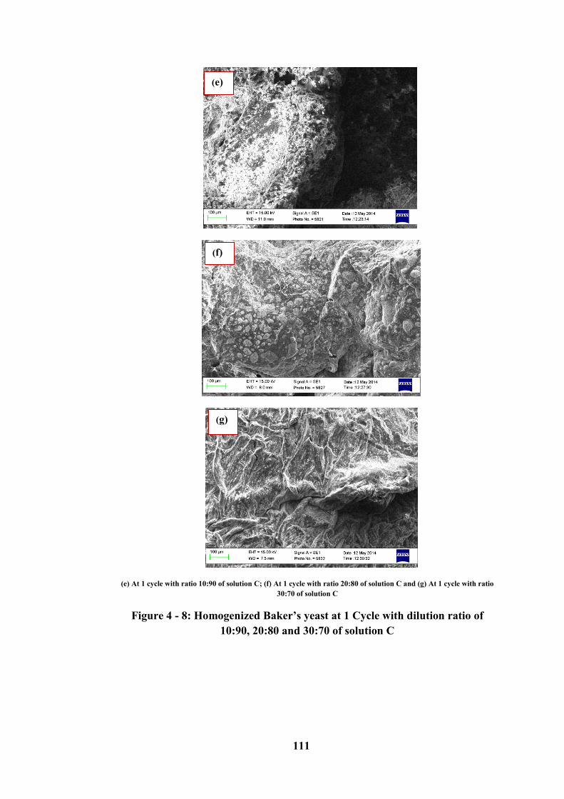
111

(e) At 1 cycle with ratio 10:90 of solution C; (f) At 1 cycle with ratio 20:80 of solution C and (g) At 1 cycle with ratio

30:70 of solution C

Figure 4 - 8: Homogenized Baker’s yeast at 1 Cycle with dilution ratio of

10:90, 20:80 and 30:70 of solution C

(e)

(f)

(g)

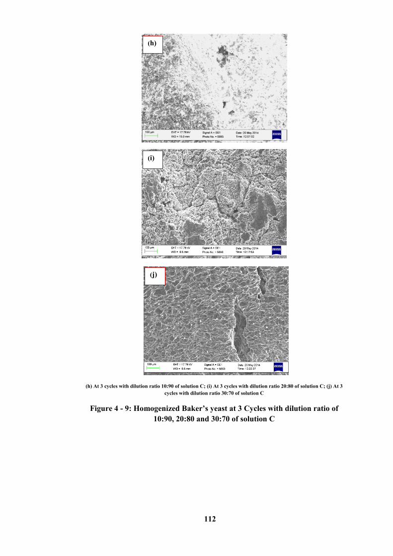
112

(h) At 3 cycles with dilution ratio 10:90 of solution C; (i) At 3 cycles with dilution ratio 20:80 of solution C; (j) At 3

cycles with dilution ratio 30:70 of solution C

Figure 4 - 9: Homogenized Baker’s yeast at 3 Cycles with dilution ratio of

10:90, 20:80 and 30:70 of solution C

(h)

(i)

(j)

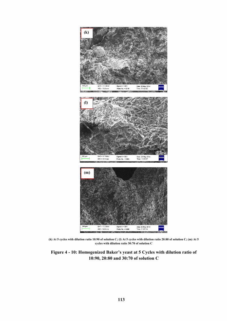
113

(k) At 5 cycles with dilution ratio 10:90 of solution C; (l) At 5 cycles with dilution ratio 20:80 of solution C; (m) At 5


Figure 4 - 10: Homogenized Baker’s yeast at 5 Cycles with dilution ratio of

10:90, 20:80 and 30:70 of solution C

(k)

(l)

(m)

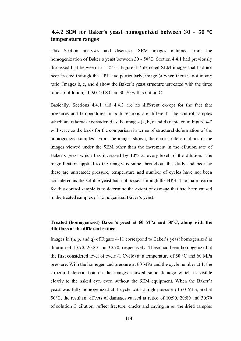
114

4.4.2 SEM for Baker’s yeast homogenized between 30 – 50 °C

temperature ranges

This Section analyses and discusses SEM images obtained from the

homogenization of Baker’s yeast between 30 - 50°C. Section 4.4.1 had previously

discussed that between 15 - 25°C. Figure 4-7 depicted SEM images that had not

been treated through the HPH and particularly, image (a when there is not in any

ratio. Images b, c, and d show the Baker’s yeast structure untreated with the three

ratios of dilution; 10:90, 20:80 and 30:70 with solution C.

Basically, Sections 4.4.1 and 4.4.2 are no different except for the fact that

pressures and temperatures in both sections are different. The control samples

which are otherwise considered as the images (a, b, c and d) depicted in Figure 4-7

will serve as the basis for the comparison in terms of structural deformation of the

homogenized samples. From the images shown, there are no deformations in the

images viewed under the SEM other than the increment in the dilution rate of

Baker’s yeast which has increased by 10% at every level of the dilution. The

magnification applied to the images is same throughout the study and because

these are untreated; pressure, temperature and number of cycles have not been

considered as the soluble yeast had not passed through the HPH. The main reason

for this control sample is to determine the extent of damage that had been caused

in the treated samples of homogenized Baker’s yeast.

Treated (homogenized) Baker’s yeast at 60 MPa and 50°C, along with the


Images in (n, p, and q) of Figure 4-11 correspond to Baker’s yeast homogenized at

dilution of 10:90, 20:80 and 30:70, respectively. These had been homogenized at

the first considered level of cycle (1 Cycle) at a temperature of 50 °C and 60 MPa

pressure. With the homogenized pressure at 60 MPa and the cycle number at 1, the

structural deformation on the images showed some damage which is visible

clearly to the naked eye, even without the SEM equipment. When the Baker’s

yeast was fully homogenized at 1 cycle with a high pressure of 60 MPa, and at

50°C, the resultant effects of damages caused at ratios of 10:90, 20:80 and 30:70

of solution C dilution, reflect fracture, cracks and caving in on the dried samples

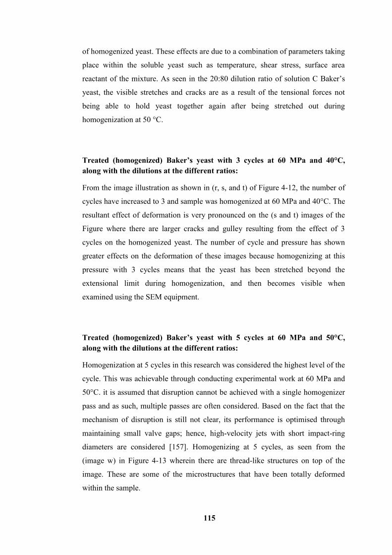
115

of homogenized yeast. These effects are due to a combination of parameters taking

place within the soluble yeast such as temperature, shear stress, surface area

reactant of the mixture. As seen in the 20:80 dilution ratio of solution C Baker’s

yeast, the visible stretches and cracks are as a result of the tensional forces not

being able to hold yeast together again after being stretched out during

homogenization at 50 °C.

Treated (homogenized) Baker’s yeast with 3 cycles at 60 MPa and 40°C,

along with the dilutions at the different ratios:

From the image illustration as shown in (r, s, and t) of Figure 4-12, the number of

cycles have increased to 3 and sample was homogenized at 60 MPa and 40°C. The

resultant effect of deformation is very pronounced on the (s and t) images of the

Figure where there are larger cracks and gulley resulting from the effect of 3

cycles on the homogenized yeast. The number of cycle and pressure has shown

greater effects on the deformation of these images because homogenizing at this

pressure with 3 cycles means that the yeast has been stretched beyond the

extensional limit during homogenization, and then becomes visible when

examined using the SEM equipment.

Treated (homogenized) Baker’s yeast with 5 cycles at 60 MPa and 50°C,

along with the dilutions at the different ratios:

Homogenization at 5 cycles in this research was considered the highest level of the

cycle. This was achievable through conducting experimental work at 60 MPa and

50°C. it is assumed that disruption cannot be achieved with a single homogenizer

pass and as such, multiple passes are often considered. Based on the fact that the

mechanism of disruption is still not clear, its performance is optimised through

maintaining small valve gaps; hence, high-velocity jets with short impact-ring

diameters are considered [157]. Homogenizing at 5 cycles, as seen from the

(image w) in Figure 4-13 wherein there are thread-like structures on top of the

image. These are some of the microstructures that have been totally deformed

within the sample.

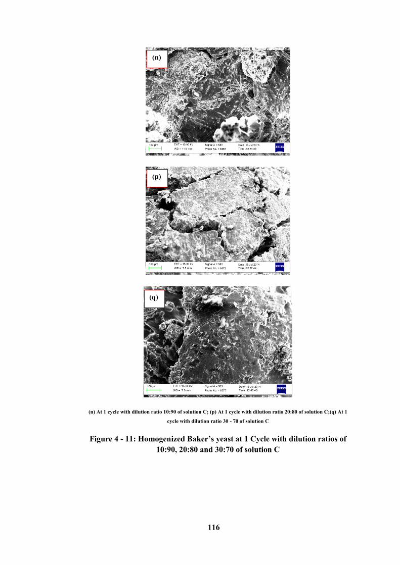
116

(n) At 1 cycle with dilution ratio 10:90 of solution C; (p) At 1 cycle with dilution ratio 20:80 of solution C;(q) At 1

cycle with dilution ratio 30 - 70 of solution C

Figure 4 - 11: Homogenized Baker’s yeast at 1 Cycle with dilution ratios of

10:90, 20:80 and 30:70 of solution C

(n)

(p)

(q)

117

(r) At 3 cycles with dilution ratio 10:90 of solution C; (s) At 3 cycles with dilution ratio 20:80 of solution C; (t) At 3



10:90, 20:80 and 30:70 of solution C

(r)

(s)

(t)

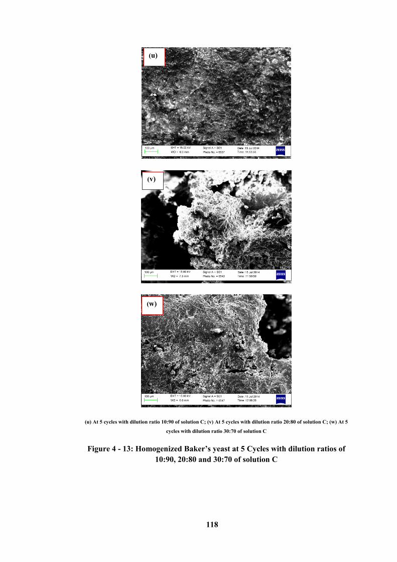
118

(u) At 5 cycles with dilution ratio 10:90 of solution C; (v) At 5 cycles with dilution ratio 20:80 of solution C; (w) At 5



10:90, 20:80 and 30:70 of solution C

(u)

(v)

(w)

119

On a general note, the different forms of deformation in the homogenized Baker’s

yeast have revealed some facts. It is evident that homogenization did in fact affect

changes in the microstructure of the Baker’s yeast substrates based on the SEM

analyses. The images shown in this study have invariably caused reductions of

particle sizes and resulted in the increment of the surface area (Figure 4-8 to 4-13)

when compared with image that have not undergone any treatment and at no ratio

of dilution as seen at Figure 4-7(a). The deformations, as shown, have great

disparity in the samples for temperature ranges (30 - 50°C) to those of (15 - 25°C).

There are several factors to consider in relation to these effects. Increased pressure

from 30 MPa to 60 MPa applied during the homogenization is one to consider.

This means that at this pressure, the gap size within the HPH would have reduced

as compared to the size during 30 MPa pressure. This will result in the

homogenized yeast being forced through the small opening gap size of about 1 –

11 μm according to Kelly and Muske [180].

Another factor to consider is the temperature effect which was increased from 20

and 25 °C to 40 and 50 °C, respectively. High temperature changed the viscosity

of the substrate but it was not proven to be the exact cause of changes in the inner

structure of the substrates. Based on this study, it is very apparent that high

temperature has effected changes in the deformation of the microstructure (see

Figures 4-11 to 4-13).

The biomass slurry state enabled its passage through HPH exit; this results in the

breaking down of yeast cell wall contents due to the effect of increasing the cycle

from 1 to 5. The deformation results further due to the increased cycle with the

gap size also constricted for the homogenized yeast to flow out at the exit. Based

on the need of this equipment (SEM) in this study, its usefulness cannot be

underestimated due to its requirement in analysing the microstructural features of

solid bodies’ surfaces as in the yeast cells.

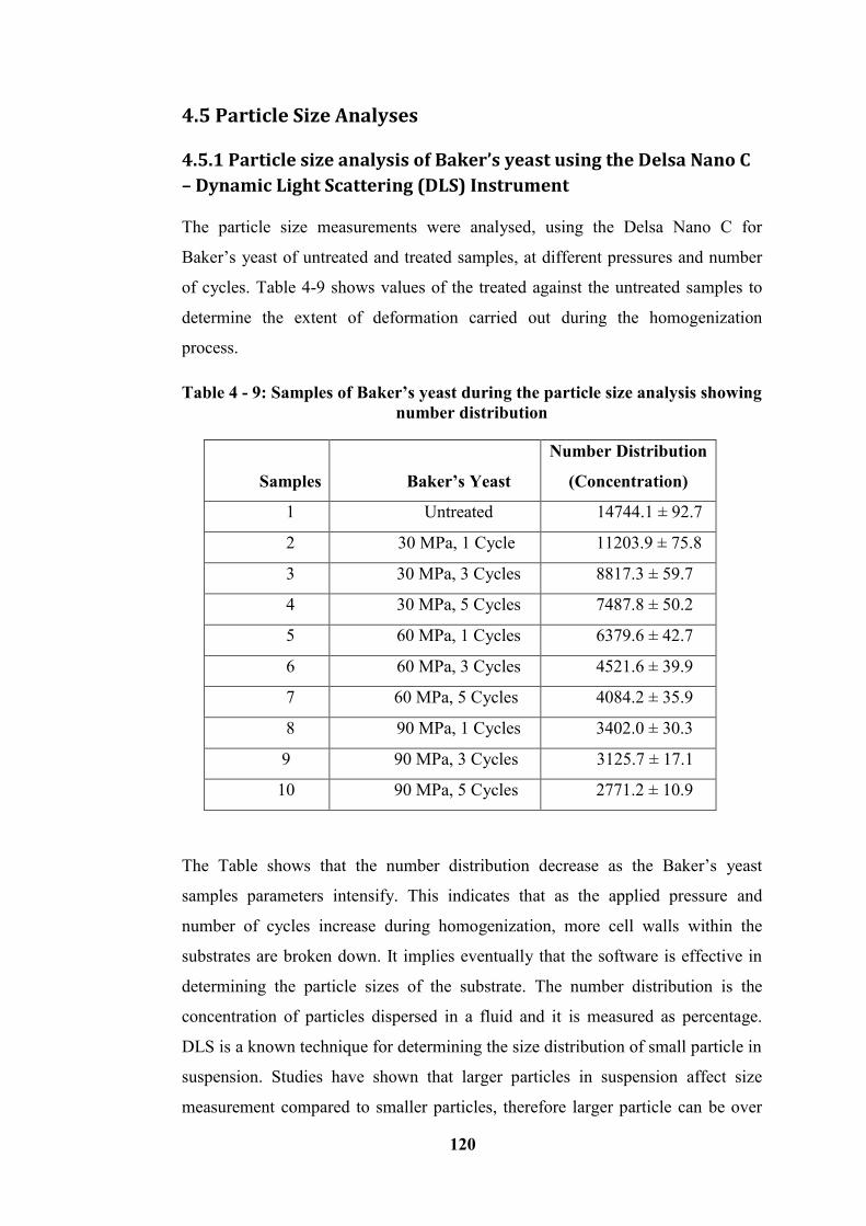
120

4.5 Particle Size Analyses

4.5.1 Particle size analysis of Baker’s yeast using the Delsa Nano C

– Dynamic Light Scattering (DLS) Instrument

The particle size measurements were analysed, using the Delsa Nano C for

Baker’s yeast of untreated and treated samples, at different pressures and number

of cycles. Table 4-9 shows values of the treated against the untreated samples to

determine the extent of deformation carried out during the homogenization

process.

Table 4 - 9: Samples of Baker’s yeast during the particle size analysis showing

number distribution

Samples

Baker’s Yeast

Number Distribution

(Concentration)

1 Untreated 14744.1 ± 92.7

2 30 MPa, 1 Cycle 11203.9 ± 75.8

3 30 MPa, 3 Cycles 8817.3 ± 59.7

4 30 MPa, 5 Cycles 7487.8 ± 50.2

5 60 MPa, 1 Cycles 6379.6 ± 42.7

6 60 MPa, 3 Cycles 4521.6 ± 39.9

7 60 MPa, 5 Cycles 4084.2 ± 35.9

8 90 MPa, 1 Cycles 3402.0 ± 30.3

9 90 MPa, 3 Cycles 3125.7 ± 17.1

10 90 MPa, 5 Cycles 2771.2 ± 10.9

The Table shows that the number distribution decrease as the Baker’s yeast

samples parameters intensify. This indicates that as the applied pressure and

number of cycles increase during homogenization, more cell walls within the

substrates are broken down. It implies eventually that the software is effective in

determining the particle sizes of the substrate. The number distribution is the

concentration of particles dispersed in a fluid and it is measured as percentage.

DLS is a known technique for determining the size distribution of small particle in

suspension. Studies have shown that larger particles in suspension affect size

measurement compared to smaller particles, therefore larger particle can be over

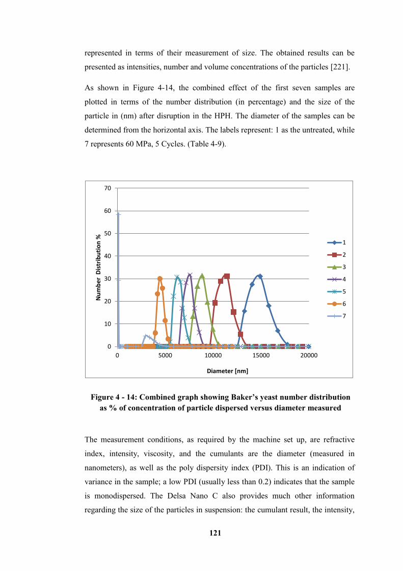
121

represented in terms of their measurement of size. The obtained results can be

presented as intensities, number and volume concentrations of the particles [221].

As shown in Figure 4-14, the combined effect of the first seven samples are

plotted in terms of the number distribution (in percentage) and the size of the

particle in (nm) after disruption in the HPH. The diameter of the samples can be

determined from the horizontal axis. The labels represent: 1 as the untreated, while

7 represents 60 MPa, 5 Cycles. (Table 4-9).

Figure 4 - 14: Combined graph showing Baker’s yeast number distribution

as % of concentration of particle dispersed versus diameter measured

The measurement conditions, as required by the machine set up, are refractive

index, intensity, viscosity, and the cumulants are the diameter (measured in

nanometers), as well as the poly dispersity index (PDI). This is an indication of

variance in the sample; a low PDI (usually less than 0.2) indicates that the sample

is monodispersed. The Delsa Nano C also provides much other information

regarding the size of the particles in suspension: the cumulant result, the intensity,

0

10

20

30

40

50

60

70

0 5000 10000 15000 20000

Nu

mb

er

Dis

trib

uti

on

%

Diameter [nm]

1

2

3

4

5

6

7

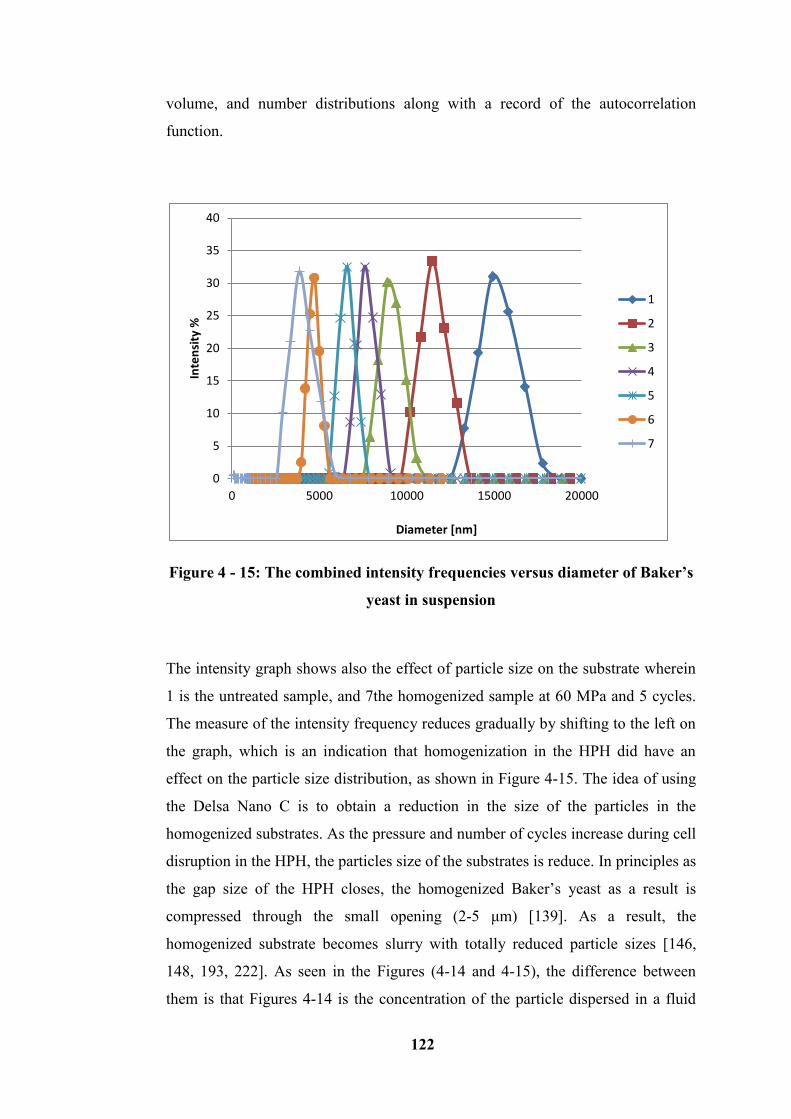
122

volume, and number distributions along with a record of the autocorrelation

function.

Figure 4 - 15: The combined intensity frequencies versus diameter of Baker’s

yeast in suspension

The intensity graph shows also the effect of particle size on the substrate wherein

1 is the untreated sample, and 7the homogenized sample at 60 MPa and 5 cycles.

The measure of the intensity frequency reduces gradually by shifting to the left on

the graph, which is an indication that homogenization in the HPH did have an

effect on the particle size distribution, as shown in Figure 4-15. The idea of using

the Delsa Nano C is to obtain a reduction in the size of the particles in the

homogenized substrates. As the pressure and number of cycles increase during cell

disruption in the HPH, the particles size of the substrates is reduce. In principles as

the gap size of the HPH closes, the homogenized Baker’s yeast as a result is

compressed through the small opening (2-5 μm) [139]. As a result, the

homogenized substrate becomes slurry with totally reduced particle sizes [146,

148, 193, 222]. As seen in the Figures (4-14 and 4-15), the difference between

them is that Figures 4-14 is the concentration of the particle dispersed in a fluid

0

5

10

15

20

25

30

35

40

0 5000 10000 15000 20000

Inte

nsi

ty %

Diameter [nm]

1

2

3

4

5

6

7

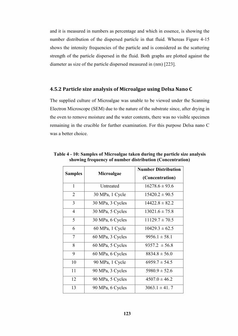
123

and it is measured in numbers as percentage and which in essence, is showing the

number distribution of the dispersed particle in that fluid. Whereas Figure 4-15

shows the intensity frequencies of the particle and is considered as the scattering

strength of the particle dispersed in the fluid. Both graphs are plotted against the

diameter as size of the particle dispersed measured in (nm) [223].

4.5.2 Particle size analysis of Microalgae using Delsa Nano C

The supplied culture of Microalgae was unable to be viewed under the Scanning

Electron Microscope (SEM) due to the nature of the substrate since, after drying in

the oven to remove moisture and the water contents, there was no visible specimen

remaining in the crucible for further examination. For this purpose Delsa nano C

was a better choice.

Table 4 - 10: Samples of Microalgae taken during the particle size analysis

showing frequency of number distribution (Concentration)

Samples Microalgae Number Distribution

(Concentration)

1 Untreated 16278.6 ± 93.6

2 30 MPa, 1 Cycle 15420.2 ± 90.5

3 30 MPa, 3 Cycles 14422.8 ± 82.2

4 30 MPa, 5 Cycles 13021.6 ± 75.8

5 30 MPa, 6 Cycles 11129.7 ± 70.5

6 60 MPa, 1 Cycle 10429.3 ± 62.5

7 60 MPa, 3 Cycles 9956.1 ± 58.1

8 60 MPa, 5 Cycles 9357.2 ± 56.8

9 60 MPa, 6 Cycles 8834.8 ± 56.0

10 90 MPa, 1 Cycle 6959.7 ± 54.5

11 90 MPa, 3 Cycles 5980.9 ± 52.6

12 90 MPa, 5 Cycles 4507.0 ± 46.2

13 90 MPa, 6 Cycles 3063.1 ± 41. 7

124

The Delsa nano C was used in the particle size analysis of Baker’s yeast and as

such, it was applied to Microalgae for same purpose. As in the case of Baker’s

yeast, Microalgae in solution as a substrate required particle sizing through

dynamic light scattering (DLS). Determining the particle sizing was performed

after high-pressure homogenization of the substrates at different pressures, number

of cycles, and temperature being the main parameters in this study.

Table 4-10 shows values of the treated against the untreated to determine the

extent of deformation during the homogenization process, to determine particle

sizing.

The substrates were homogenized at varying pressure and number of cycles. Each

sample was taken using the glass cuvette to analyse it in the particle size analyser

(Delsa Nano C). The aim of this work was to determine and to compare the treated

samples with the untreated (sample 1), which is considered as the control sample

in the conducted work. There were standard deviation error bars for each result

recorded; these are indications that the sample contained some level of impurities

which invariably will lead to some errors in value in the samples (from untreated

sample to sample 13). Results obtained for tests from untreated to sample 13 are

indication, and the presence of different particle sizes within the conducted

experiments. Unlike Baker’s yeast, there was more consistency in the generated

result as compared to the results for the Microalgae.

4.6 Design of Experiment and Analyses of Results

These onward sections will analyse experimental results based on three categories

of set of experiments and data acquisition. These are; Baker’s yeast homogenized

at temperature 15 - 25°C, Baker’s yeast homogenized at temperature 30 - 50°C, as

well as Microalgae homogenized at 15 - 25°C, with the dilution of substrate with

solution C considered as most important analytically in this study.

125

4.7 Baker’s yeast homogenized at a temperature of 15 – 25 °C

The experiment was designed based on a three level Box Behnken design (BBD)

which includes one full replication for this substrate. Trial samples of Baker’s

yeast were performed by varying one of the process variables in determining the

working range of each variable. With the maximum pressure of the high-pressure

homogenizer considered as 100 MPa from the manufacturer, it was recommended

never to go beyond 90 MPa as the operating working pressure. Also with a

pressure lower than 30 MPa considered as infinitesimal, and with whose

application in the HPH, never showed appreciable effect. Hence the working

pressure was set between 30 and 90 MPa. These were the criteria for choosing the

working ranges. Temperature ranges were chosen as the homogenization process

needed to be within ± 5 °C of room temperature since room temperature is around

20 °C [224]. The number of cycles used was chosen for an improved

homogenization process. Table 4-11 shows homogenizer input variables along

with the design levels used for this substrate and, the experiment was carried out

according to the design matrix shown in Table 4-12 in a random order to avoid

any systematic error using the HPH alongside with the two measured responses.

Ratios as a variable factor were used categorically and as identified by the design

expert software. This was required to determine the effect of the dilution

concentration of yeast and the solution C on other parameters. For this substrate,

two responses were identified; protein concentration and cost. The energy monitor

connected to the HPH was required to calculate and work out this cost. Other costs

were negligible as the same trends will be applicable to the overall cost at the end.

Mathematical models were developed successfully to predict the responses as

explained above. The procedures described earlier in Chapter 3 were followed to

determine and record these responses. Particularly, the averages of at least six

measurements for protein concentration are presented. The full experimental

measured data of protein concentration can be seen in Table 4-12. These were

obtained from the measured UV absorbance results using the spectrophotometer to

get the protein concentration from the homogenized yeast. The protein curve for

working out the protein concentration and the applied calculation is provided in

Appendix F.

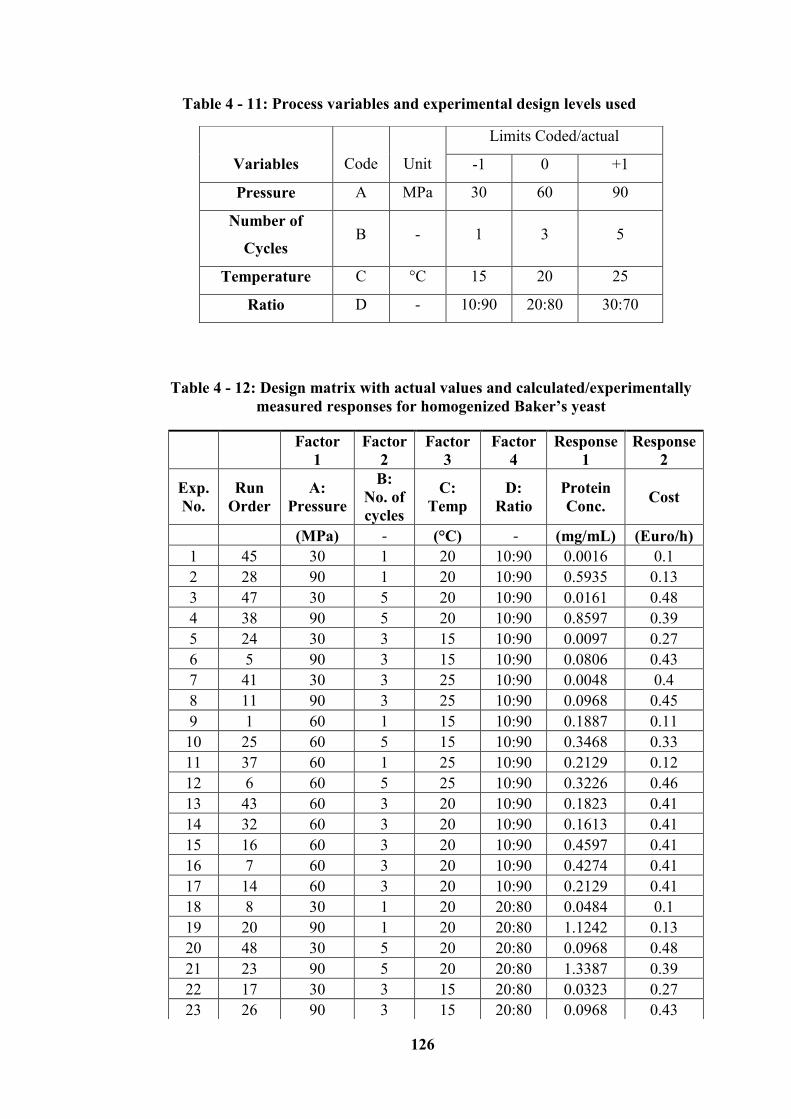
126

Table 4 - 11: Process variables and experimental design levels used


measured responses for homogenized Baker’s yeast

Variables

Code

Unit

Limits Coded/actual

-1 0 +1

Pressure A MPa 30 60 90

Number of

Cycles B - 1 3 5

Temperature C °C 15 20 25

Ratio D - 10:90 20:80 30:70

Factor

1

Factor

2

Factor

3

Factor

4

Response

1

Response

2

Exp.

No.

Run

Order

A:

Pressure

B:

No. of

cycles

C:

Temp

D:

Ratio

Protein

Conc. Cost

(MPa) - (°C) - (mg/mL) (Euro/h)

1 45 30 1 20 10:90 0.0016 0.1

2 28 90 1 20 10:90 0.5935 0.13

3 47 30 5 20 10:90 0.0161 0.48

4 38 90 5 20 10:90 0.8597 0.39

5 24 30 3 15 10:90 0.0097 0.27

6 5 90 3 15 10:90 0.0806 0.43

7 41 30 3 25 10:90 0.0048 0.4

8 11 90 3 25 10:90 0.0968 0.45

9 1 60 1 15 10:90 0.1887 0.11

10 25 60 5 15 10:90 0.3468 0.33

11 37 60 1 25 10:90 0.2129 0.12

12 6 60 5 25 10:90 0.3226 0.46

13 43 60 3 20 10:90 0.1823 0.41

14 32 60 3 20 10:90 0.1613 0.41

15 16 60 3 20 10:90 0.4597 0.41

16 7 60 3 20 10:90 0.4274 0.41

17 14 60 3 20 10:90 0.2129 0.41

18 8 30 1 20 20:80 0.0484 0.1

19 20 90 1 20 20:80 1.1242 0.13

20 48 30 5 20 20:80 0.0968 0.48

21 23 90 5 20 20:80 1.3387 0.39

22 17 30 3 15 20:80 0.0323 0.27

23 26 90 3 15 20:80 0.0968 0.43

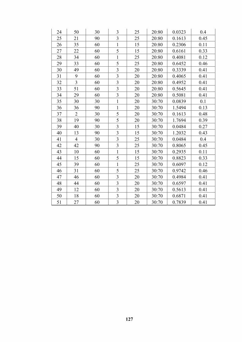
127

24 50 30 3 25 20:80 0.0323 0.4

25 21 90 3 25 20:80 0.1613 0.45

26 35 60 1 15 20:80 0.2306 0.11

27 22 60 5 15 20:80 0.6161 0.33

28 34 60 1 25 20:80 0.4081 0.12

29 33 60 5 25 20:80 0.6452 0.46

30 49 60 3 20 20:80 0.3339 0.41

31 9 60 3 20 20:80 0.4065 0.41

32 3 60 3 20 20:80 0.4952 0.41

33 51 60 3 20 20:80 0.5645 0.41

34 29 60 3 20 20:80 0.5081 0.41

35 30 30 1 20 30:70 0.0839 0.1

36 36 90 1 20 30:70 1.5494 0.13

37 2 30 5 20 30:70 0.1613 0.48

38 19 90 5 20 30:70 1.7694 0.39

39 40 30 3 15 30:70 0.0484 0.27

40 13 90 3 15 30:70 1.2032 0.43

41 4 30 3 25 30:70 0.0484 0.4

42 42 90 3 25 30:70 0.8065 0.45

43 10 60 1 15 30:70 0.2935 0.11

44 15 60 5 15 30:70 0.8823 0.33

45 39 60 1 25 30:70 0.6097 0.12

46 31 60 5 25 30:70 0.9742 0.46

47 46 60 3 20 30:70 0.4984 0.41

48 44 60 3 20 30:70 0.6597 0.41

49 12 60 3 20 30:70 0.5613 0.41

50 18 60 3 20 30:70 0.6871 0.41

51 27 60 3 20 30:70 0.7839 0.41

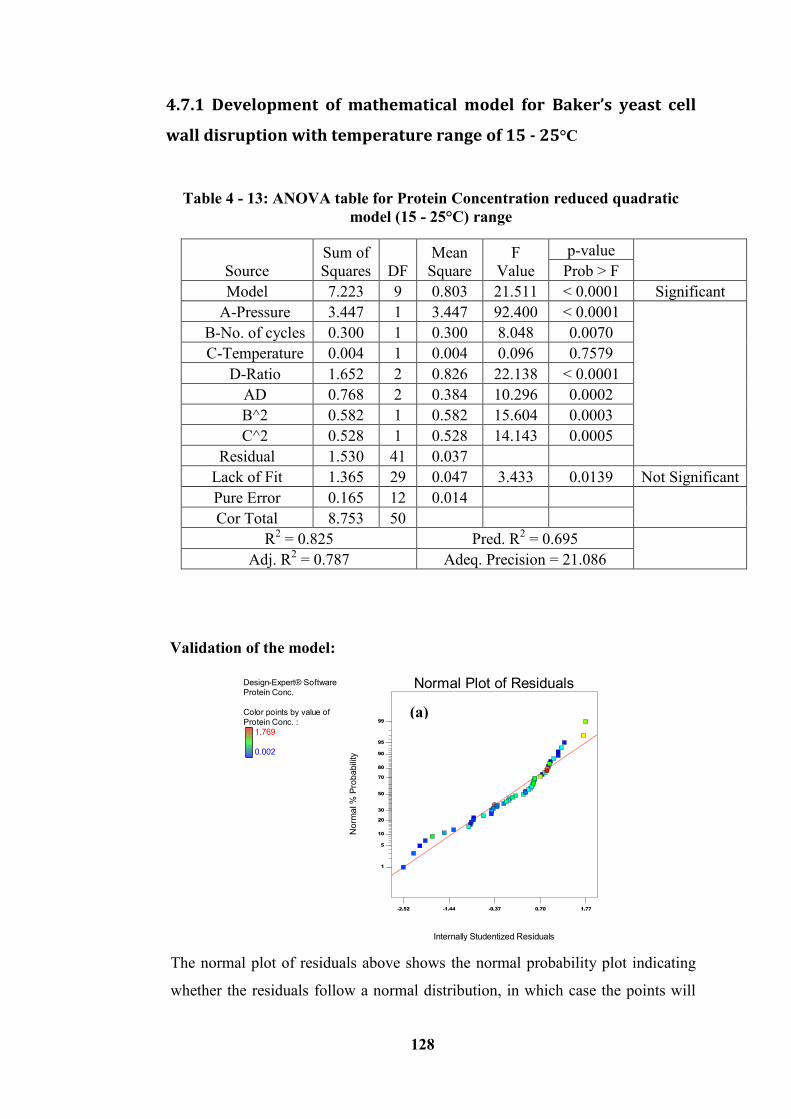
128

4.7.1 Development of mathematical model for Baker’s yeast cell

wall disruption with temperature range of 15 - 25°C

Table 4 - 13: ANOVA table for Protein Concentration reduced quadratic

model (15 - 25°C) range

Source

Sum of

Squares

DF

Mean

Square

F

Value

p-value

Prob > F

Model 7.223 9 0.803 21.511 < 0.0001 Significant

A-Pressure 3.447 1 3.447 92.400 < 0.0001

B-No. of cycles 0.300 1 0.300 8.048 0.0070

C-Temperature 0.004 1 0.004 0.096 0.7579

D-Ratio 1.652 2 0.826 22.138 < 0.0001

AD 0.768 2 0.384 10.296 0.0002

B^2 0.582 1 0.582 15.604 0.0003

C^2 0.528 1 0.528 14.143 0.0005

Residual 1.530 41 0.037

Lack of Fit 1.365 29 0.047 3.433 0.0139 Not Significant

Pure Error 0.165 12 0.014

Cor Total 8.753 50

R2 = 0.825 Pred. R

2 = 0.695

Adj. R2 = 0.787 Adeq. Precision = 21.086

Validation of the model:

The normal plot of residuals above shows the normal probability plot indicating

whether the residuals follow a normal distribution, in which case the points will

Design-Expert® Software

Protein Conc.

Color points by value of

Protein Conc. :

1.769

0.002

Internally Studentized Residuals

No

rma

l %

Pro

ba

bili

ty

Normal Plot of Residuals

-2.52 -1.44 -0.37 0.70 1.77

1

5

10

20

30

50

70

80

90

95

99

(a)

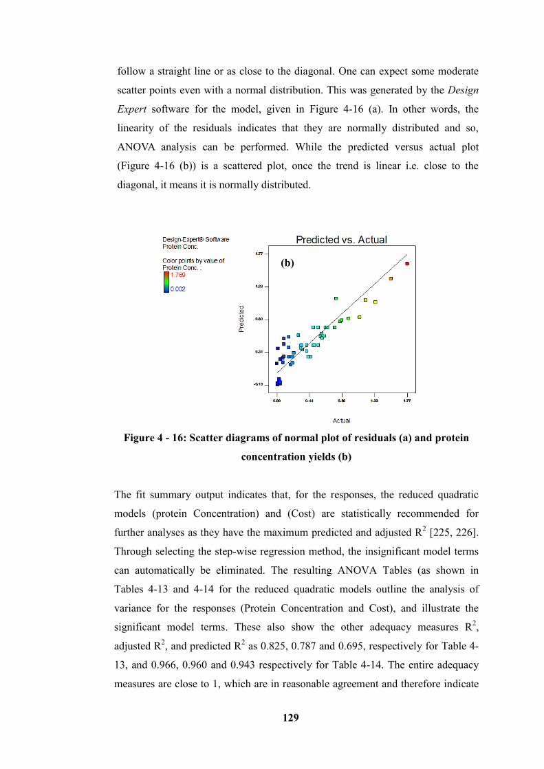
129

follow a straight line or as close to the diagonal. One can expect some moderate

scatter points even with a normal distribution. This was generated by the Design

Expert software for the model, given in Figure 4-16 (a). In other words, the

linearity of the residuals indicates that they are normally distributed and so,

ANOVA analysis can be performed. While the predicted versus actual plot

(Figure 4-16 (b)) is a scattered plot, once the trend is linear i.e. close to the

diagonal, it means it is normally distributed.

Figure 4 - 16: Scatter diagrams of normal plot of residuals (a) and protein

concentration yields (b)

The fit summary output indicates that, for the responses, the reduced quadratic

models (protein Concentration) and (Cost) are statistically recommended for

further analyses as they have the maximum predicted and adjusted R2 [225, 226].

Through selecting the step-wise regression method, the insignificant model terms

can automatically be eliminated. The resulting ANOVA Tables (as shown in

Tables 4-13 and 4-14 for the reduced quadratic models outline the analysis of

variance for the responses (Protein Concentration and Cost), and illustrate the

significant model terms. These also show the other adequacy measures R2,

adjusted R2, and predicted R

2 as 0.825, 0.787 and 0.695, respectively for Table 4-

13, and 0.966, 0.960 and 0.943 respectively for Table 4-14. The entire adequacy

measures are close to 1, which are in reasonable agreement and therefore indicate

(b)

130

adequate models because the statistical analysis as considered by the Design

Expert, it indicates that any value equal to or greater than 0.5 is considered as

close to 1 when determining the adequacy measures R2, adjusted R

2, and predicted

R2. The adequate precision being equal to 21.086 for protein concentration yield

and 35.186 for cost indicates an adequate model, as the adequacy value was >> 4

and an indication of good model discrimination [225, 226]. The adequate precision

compares the range of the predicted value at the design points to the average

prediction error.

Figure 4-16 (a and b) and 4-19 (a and b) are the replica plots of the predicted

against the actual response, and the residual of the normal plot of protein

concentration response and that of predicted versus actual response, and the

residual of the normal plot of cost response respectively. The analysis of variance

indicates that the number of cycles, pressure as well as temperature, and their

interactions are the most significant factors affecting the protein concentration

yields. The predicted vs. Actual plots are shown in Figure 4-16b and Figure 4-19b.

This figure indicates that the developed models are adequate because the residuals

are minimal, since these tend to be close to the diagonal line. The normal plot of

residuals in Figure 4-16a and 4-19a indicates that the assumptions of normal

distribution of the data are respected; therefore the ANOVA can be applied to

study the dataset.

An adequate model means that the reduced model has successfully passed all the

required statistical tests and can be used to predict the responses, or to optimize

the process, and so on. The final mathematical models linked to the responses with

regard to the coded factors and actual factors as determined by the software are

respectively in Equations (4-1) to (4-4) and (4-5) to (4-6) with equations 4-2 to 4-4

in the dilution ratio form; 10:90, 20:80 and 30:70, and Equation 4-6 representing

that for cost respectively.

Based on the ANOVA Table 4-13, the point prediction technique and an

appropriate model was based on the fact that, Adjusted R2 minus Predicted R

2

must be < 0.2 and in this case, it was 0.092.

As R2

equalled 0.825, it implied that 82.5% of the variability in the data has been

explained by the model and a F-Value model of 21.51 implied that the model was

significant since it is only 0.01% chance that the F-Value model was disrupted by

scatter/ noise.

131

Based on the final equation in terms of coded factors and those in terms of the

actual factors for ratios, 10:90, 20:80, and 30:70, protein concentration yield can

be worked out using the associated equation for any set of the ratios to determine

this yield. In the final equation in terms of coded factors, as given below, the

square brackets indicated, represents the ratios of categorical factor in coded

terms. This can be used to predict the protein concentration yield when

homogenized under HPH. For example in the ratios considered in this research;

10:90, 20:80, and 30:70, their representation in coded factors were [1, 0], [-1, -1]

and [0, 1] respectively and when solved into the equation of the coded factors

gives the result as shown in the final equation in terms of coded factors (see

Equation 4-1).

Final Equation in Terms of Coded Factors:

Protein Concentration = 0.44489468 + 0.379003898 * A + 0.111854839 * B

+ 0.012232258 * C - 0.204003099 * D [1] - 0.029809551 * D[2]

- 0.179205511*AD[1] - 0.065092608 * AD [2] + 0.214389389

* B^2 - 0.204106579 * C^2 (4-1)

Final Equation in Terms of Actual Factors:

Ratio 10:90;

Protein Concentration = -3.158745622 + 0.006659946 * Pressure - 0.265656664

* No. of cycles + 0.329016978 * Temperature +0.053597347

* No. of cycles^2 - 0.008164263 * Temperature^2

(4-2)

Ratio 20:80;


* No. of cycles + 0.329016978 * Temperature + 0.053597347


(4-3)

132

Ratio 30:70;


* No. of cycles + 0.329016978* Temperature + 0.053597347


(4-4)

Effect of process parameters on the responses - Protein Concentration

The perturbation plot for the protein concentration yield from the 15 – 25 °C

temperature range is illustrated in Figure 4-17 as (a), (b), and (c). The perturbation

plot helped in comparing the effect of all the factors at a particular point in the

design space. The lines represent the behaviours of each factor while holding the

others constant at the centre point. This type of display can be used to determine

the factors that most affect the response. From the illustrations, pressure and the

number of cycles affect the protein concentration yield. This was in agreement

with these authors and researchers [162-164, 171, 194, 197, 227-229] wherein

pressure showed a very significant effect in the production of protein. As

highlighted, an increase in pressure, A; resulted in high protein concentration

yield; while the number of cycle, B showed minimal rise in the effect to the yield

of protein, and the temperature factor was shown not to have an effect on the

yield.

Considering the categorical factor of ratio designated as D in this study, protein

concentration yield has been seen to give the highest yield at the ratio 30:70 when

compared to other ratios of 10:90 and 20:80. Invariably, this shows that as the

ratio increased, the yield in protein concentration also increased at the same rate as

the pressure rises seen at Figure 4-17(c).

From the three scenarios (Figure 4-17), it is evident that pressure (A) and number

of cycle (B) both have a strong effect on the protein concentration yield as both

have an upward trend from minimum to maximum factor. This is different from

that of the temperature (C) which showed a downward trend in its behaviour. The

behaviour of the three parameters are pronounced in the 30:70 ratio of the

perturbation plot where protein concentration yield was considered the highest

yield compared to other two ratios (10:90 and 20:80).

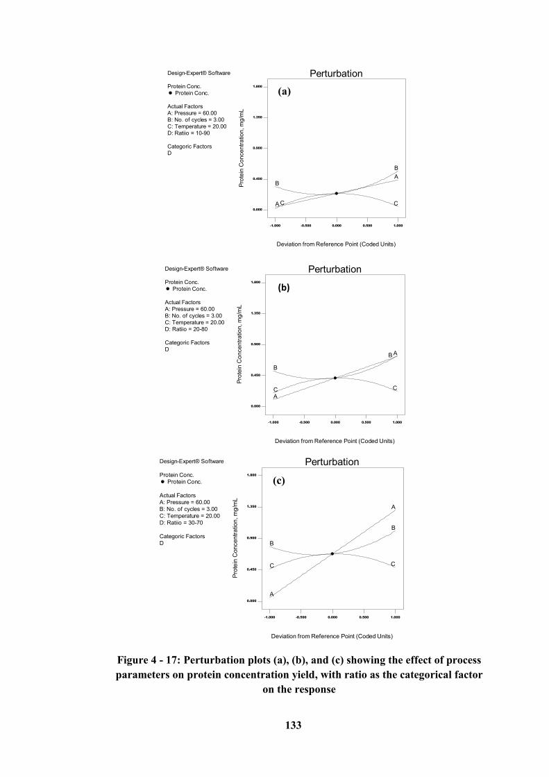
133


parameters on protein concentration yield, with ratio as the categorical factor

on the response


Protein Conc.

Protein Conc.

Actual Factors

A: Pressure = 60.00

B: No. of cycles = 3.00

C: Temperature = 20.00

D: Ratiio = 10-90

Categoric Factors

D

Perturbation

Deviation from Reference Point (Coded Units)P

rote

in C

on

ce

ntr

atio

n, m

g/m

L

-1.000 -0.500 0.000 0.500 1.000

0.000

0.450

0.900

1.350

1.800

A

AB

B

C C


Protein Conc.

Protein Conc.

Actual Factors

A: Pressure = 60.00



D: Ratiio = 20-80

Categoric Factors

D

Perturbation

Deviation from Reference Point (Coded Units)

Pro

tein

Co

nce

ntr

atio

n, m

g/m

L

-1.000 -0.500 0.000 0.500 1.000

0.000

0.450

0.900

1.350

1.800

A

A

B

B

C C


Protein Conc.

Protein Conc.

Actual Factors

A: Pressure = 60.00



D: Ratiio = 30-70

Categoric Factors

D

Perturbation


Pro

tein

Co

nce

ntr

atio

n, m

g/m

L

-1.000 -0.500 0.000 0.500 1.000

0.000

0.450

0.900

1.350

1.800

A

A

B

B

C C

(a)

(b)

(c)

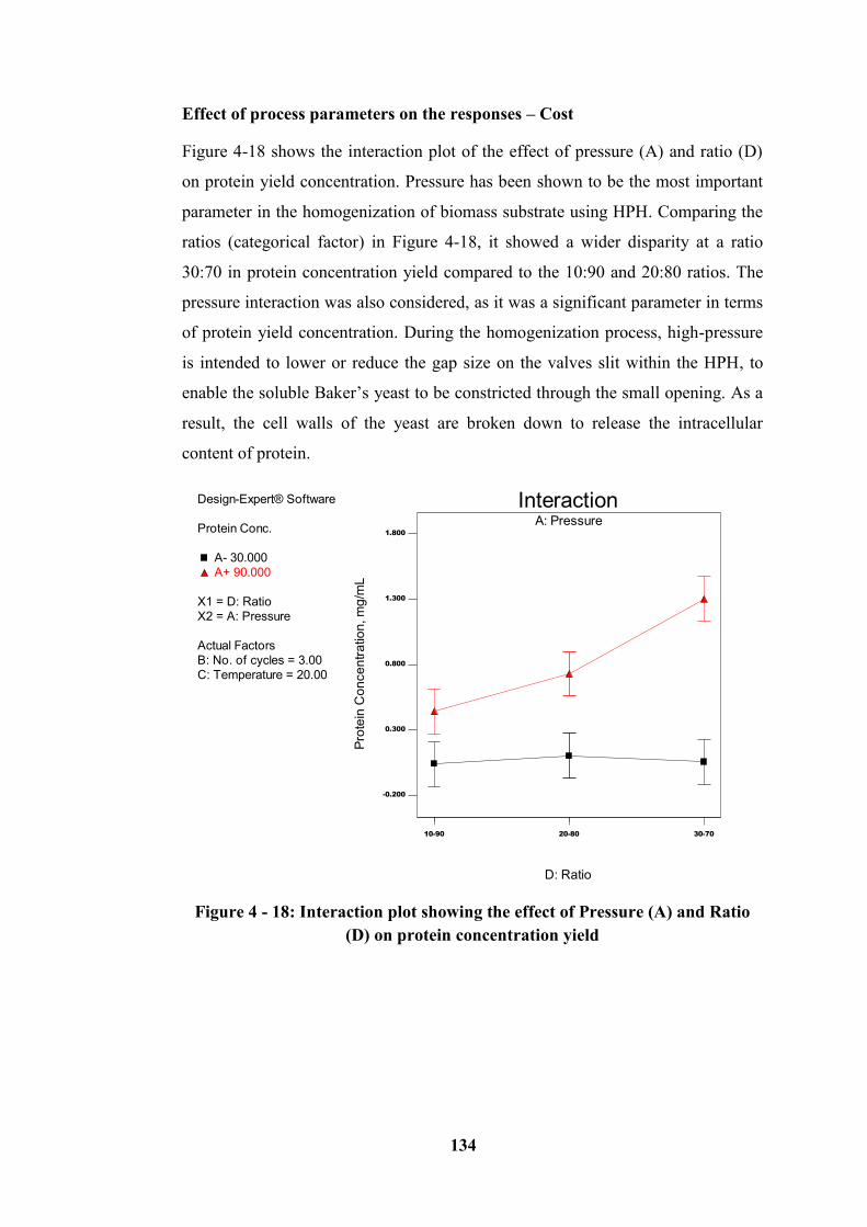
134

Effect of process parameters on the responses – Cost

Figure 4-18 shows the interaction plot of the effect of pressure (A) and ratio (D)

on protein yield concentration. Pressure has been shown to be the most important

parameter in the homogenization of biomass substrate using HPH. Comparing the

ratios (categorical factor) in Figure 4-18, it showed a wider disparity at a ratio

30:70 in protein concentration yield compared to the 10:90 and 20:80 ratios. The

pressure interaction was also considered, as it was a significant parameter in terms

of protein yield concentration. During the homogenization process, high-pressure

is intended to lower or reduce the gap size on the valves slit within the HPH, to

enable the soluble Baker’s yeast to be constricted through the small opening. As a

result, the cell walls of the yeast are broken down to release the intracellular

content of protein.

Figure 4 - 18: Interaction plot showing the effect of Pressure (A) and Ratio

(D) on protein concentration yield


Protein Conc.

A- 30.000

A+ 90.000

X1 = D: Ratio

X2 = A: Pressure

Actual Factors



A: Pressure

10-90 20-80 30-70

Interaction

D: Ratio

Pro

tein

Co

nce

ntr

atio

n, m

g/m

L

-0.200

0.300

0.800

1.300

1.800

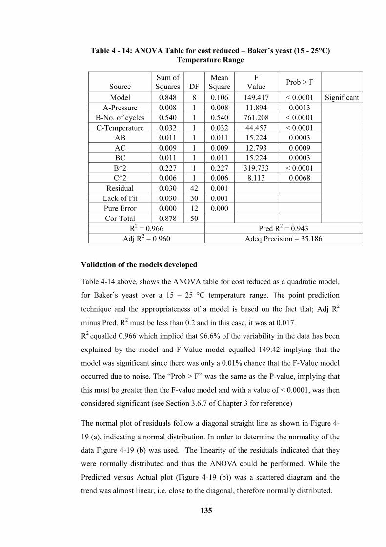
135

Table 4 - 14: ANOVA Table for cost reduced – Baker’s yeast (15 - 25°C)

Temperature Range

Source

Sum of

Squares

DF

Mean

Square

F

Value Prob > F


A-Pressure 0.008 1 0.008 11.894 0.0013

B-No. of cycles 0.540 1 0.540 761.208 < 0.0001

C-Temperature 0.032 1 0.032 44.457 < 0.0001

AB 0.011 1 0.011 15.224 0.0003

AC 0.009 1 0.009 12.793 0.0009

BC 0.011 1 0.011 15.224 0.0003

B^2 0.227 1 0.227 319.733 < 0.0001

C^2 0.006 1 0.006 8.113 0.0068

Residual 0.030 42 0.001

Lack of Fit 0.030 30 0.001

Pure Error 0.000 12 0.000

Cor Total 0.878 50

R2 = 0.966 Pred R

2 = 0.943

Adj R2 = 0.960 Adeq Precision = 35.186

Validation of the models developed

Table 4-14 above, shows the ANOVA table for cost reduced as a quadratic model,

for Baker’s yeast over a 15 – 25 °C temperature range. The point prediction

technique and the appropriateness of a model is based on the fact that; Adj R2

minus Pred. R2 must be less than 0.2 and in this case, it was at 0.017.

R2

equalled 0.966 which implied that 96.6% of the variability in the data has been

explained by the model and F-Value model equalled 149.42 implying that the

model was significant since there was only a 0.01% chance that the F-Value model

occurred due to noise. The “Prob > F” was the same as the P-value, implying that

this must be greater than the F-value model and with a value of < 0.0001, was then

considered significant (see Section 3.6.7 of Chapter 3 for reference)

The normal plot of residuals follow a diagonal straight line as shown in Figure 4-

19 (a), indicating a normal distribution. In order to determine the normality of the

data Figure 4-19 (b) was used. The linearity of the residuals indicated that they

were normally distributed and thus the ANOVA could be performed. While the

Predicted versus Actual plot (Figure 4-19 (b)) was a scattered diagram and the

trend was almost linear, i.e. close to the diagonal, therefore normally distributed.

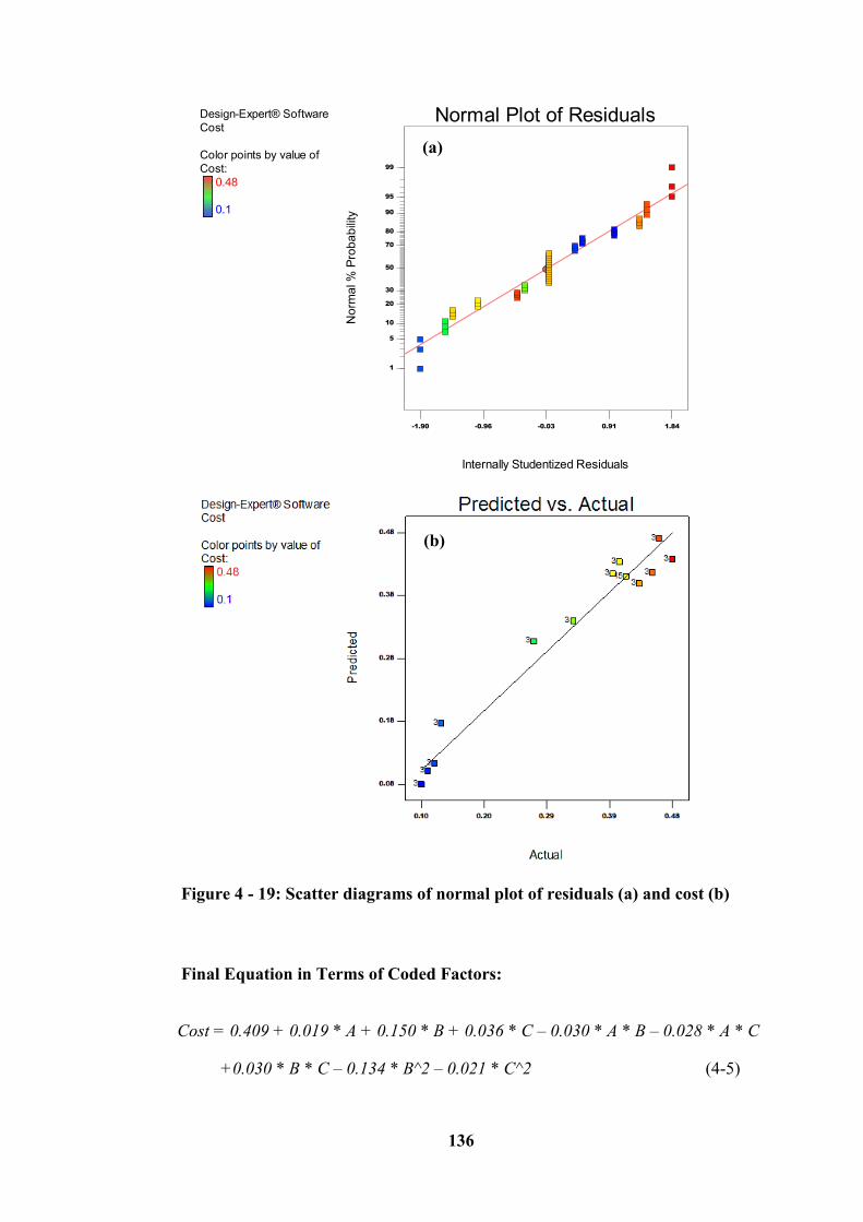
136

Figure 4 - 19: Scatter diagrams of normal plot of residuals (a) and cost (b)


Cost = 0.409 + 0.019 * A + 0.150 * B + 0.036 * C – 0.030 * A * B – 0.028 * A * C

+0.030 * B * C – 0.134 * B^2 – 0.021 * C^2 (4-5)


Cost


Cost:

0.48

0.1


No

rma

l %

Pro

ba

bili

ty


-1.90 -0.96 -0.03 0.91 1.84

1

5

10

20

30

50

70

80

90

95

99

(b)

(a)

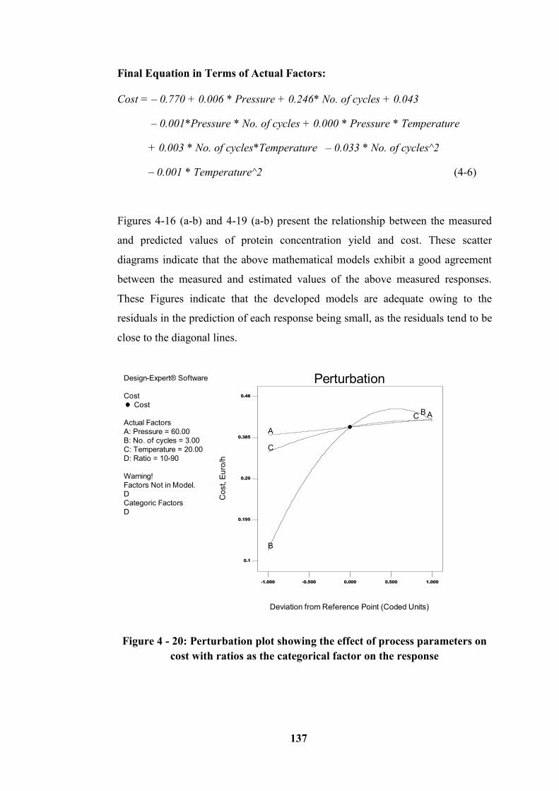
137


Cost = – 0.770 + 0.006 * Pressure + 0.246* No. of cycles + 0.043

– 0.001*Pressure * No. of cycles + 0.000 * Pressure * Temperature

+ 0.003 * No. of cycles*Temperature – 0.033 * No. of cycles^2

– 0.001 * Temperature^2 (4-6)

Figures 4-16 (a-b) and 4-19 (a-b) present the relationship between the measured

and predicted values of protein concentration yield and cost. These scatter

diagrams indicate that the above mathematical models exhibit a good agreement

between the measured and estimated values of the above measured responses.

These Figures indicate that the developed models are adequate owing to the

residuals in the prediction of each response being small, as the residuals tend to be

close to the diagonal lines.

Figure 4 - 20: Perturbation plot showing the effect of process parameters on

cost with ratios as the categorical factor on the response


Cost

Cost

Actual Factors

A: Pressure = 60.00



D: Ratio = 10-90

Warning!

Factors Not in Model.

D

Categoric Factors

D

Perturbation


Co

st, E

uro

/h

-1.000 -0.500 0.000 0.500 1.000

0.1

0.195

0.29

0.385

0.48

A

A

B

B

C

C

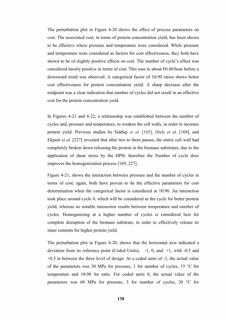
138

The perturbation plot in Figure 4-20 shows the effect of process parameters on

cost. The associated cost, in terms of protein concentration yield, has been shown

to be effective where pressure and temperature were considered. While pressure

and temperature were considered as factors for cost effectiveness, they both have

shown to be of slightly positive effects on cost. The number of cycle’s effect was

considered mostly positive in terms of cost. This rose to about €0.40/hour before a

downward trend was observed. A categorical factor of 10:90 ratios shows better

cost effectiveness for protein concentration yield. A sharp decrease after the

midpoint was a clear indication that number of cycles did not result in an effective

cost for the protein concentration yield.

In Figures 4-21 and 4-22, a relationship was established between the number of

cycles and, pressure and temperature, to weaken the cell walls, in order to increase

protein yield. Previous studies by Siddiqi et al. [165], Diels et al. [169], and

Ekpeni et al. [227] revealed that after two to three passes, the entire cell wall had

completely broken down releasing the protein in the biomass substrates, due to the

application of shear stress by the HPH, therefore the Number of cycle does

improves the homogenization process [169, 227].

Figure 4-21, shows the interaction between pressure and the number of cycles in

terms of cost; again, both have proven to be the effective parameters for cost

determination when the categorical factor is considered at 10:90. An interaction

took place around cycle 4, which will be considered as the cycle for better protein

yield, whereas no notable interaction results between temperature and number of

cycles. Homogenizing at a higher number of cycles is considered best for

complete disruption of the biomass substrate, in order to effectively release its

inner contents for higher protein yield.

The perturbation plot in Figure 4-20, shows that the horizontal axis indicated a

deviation from its reference point (Coded Units); -1, 0, and +1, with -0.5 and

+0.5 in between the three level of design. At a coded units of -1, the actual value

of the parameters was 30 MPa for pressure, 1 for number of cycles, 15 °C for

temperature and 10:90 for ratio. For coded units 0, the actual value of the

parameters was 60 MPa for pressure, 3 for number of cycles, 20 °C for

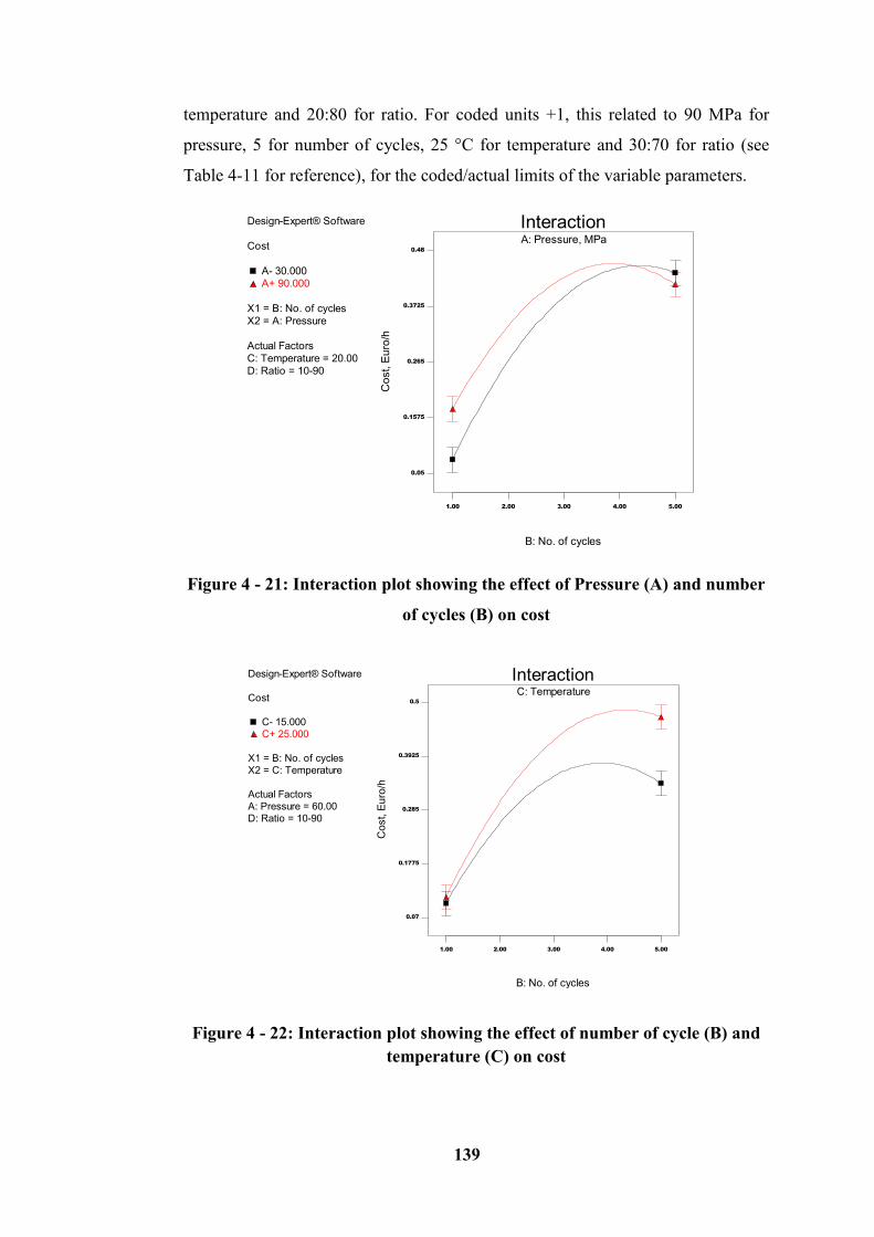
139

temperature and 20:80 for ratio. For coded units +1, this related to 90 MPa for

pressure, 5 for number of cycles, 25 °C for temperature and 30:70 for ratio (see

Table 4-11 for reference), for the coded/actual limits of the variable parameters.

Figure 4 - 21: Interaction plot showing the effect of Pressure (A) and number

of cycles (B) on cost

Figure 4 - 22: Interaction plot showing the effect of number of cycle (B) and

temperature (C) on cost


Cost

A- 30.000

A+ 90.000

X1 = B: No. of cycles

X2 = A: Pressure

Actual Factors


D: Ratio = 10-90

A: Pressure, MPa

1.00 2.00 3.00 4.00 5.00

Interaction

B: No. of cycles

Co

st, E

uro

/h

0.05

0.1575

0.265

0.3725

0.48


Cost

C- 15.000

C+ 25.000


X2 = C: Temperature

Actual Factors

A: Pressure = 60.00

D: Ratio = 10-90

C: Temperature

1.00 2.00 3.00 4.00 5.00

Interaction

B: No. of cycles

Co

st, E

uro

/h

0.07

0.1775

0.285

0.3925

0.5

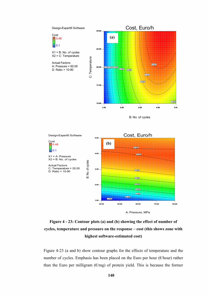
140

Figure 4 - 23: Contour plots (a) and (b) showing the effect of number of

cycles, temperature and pressure on the response – cost (this shows zone with

highest software-estimated cost)

Figure 4-23 (a and b) show contour graphs for the effects of temperature and the

number of cycles. Emphasis has been placed on the Euro per hour (€/hour) rather

than the Euro per milligram (€/mg) of protein yield. This is because the former


Cost

0.48

0.1


X2 = C: Temperature

Actual Factors

A: Pressure = 60.00

D: Ratio = 10-90

1.00 2.00 3.00 4.00 5.00

15.00

17.50

20.00

22.50

25.00

Cost, Euro/h

B: No. of cycles

C: T

em

pe

ratu

re

0.150 0.200 0.2500.300

0.350

0.350

0.400

0.450

0.423


Cost

0.48

0.1

X1 = A: Pressure


Actual Factors


D: Ratio = 10-90

30.00 45.00 60.00 75.00 90.00

1.00

2.00

3.00

4.00

5.00

Cost, Euro/h

A: Pressure, MPa

B: N

o. o

f cyc

les

0.100

0.150

0.200

0.250

0.300

0.350

0.400

0.450

0.450

(a)

(b)

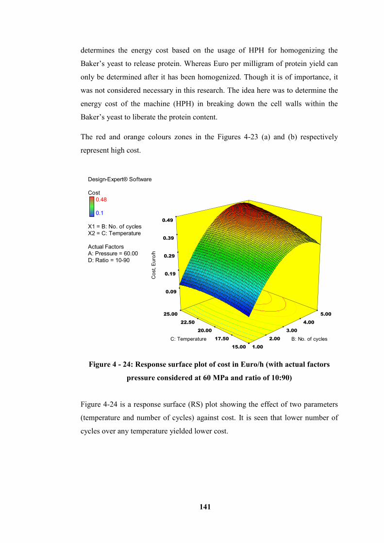
141

determines the energy cost based on the usage of HPH for homogenizing the

Baker’s yeast to release protein. Whereas Euro per milligram of protein yield can

only be determined after it has been homogenized. Though it is of importance, it

was not considered necessary in this research. The idea here was to determine the

energy cost of the machine (HPH) in breaking down the cell walls within the

Baker’s yeast to liberate the protein content.

The red and orange colours zones in the Figures 4-23 (a) and (b) respectively

represent high cost.

Figure 4 - 24: Response surface plot of cost in Euro/h (with actual factors

pressure considered at 60 MPa and ratio of 10:90)

Figure 4-24 is a response surface (RS) plot showing the effect of two parameters

(temperature and number of cycles) against cost. It is seen that lower number of

cycles over any temperature yielded lower cost.


Cost

0.48

0.1


X2 = C: Temperature

Actual Factors

A: Pressure = 60.00

D: Ratio = 10-90

1.00

2.00

3.00

4.00

5.00

15.00

17.50

20.00

22.50

25.00

0.09

0.19

0.29

0.39

0.49

C

ost, E

uro

/h

B: No. of cycles C: Temperature

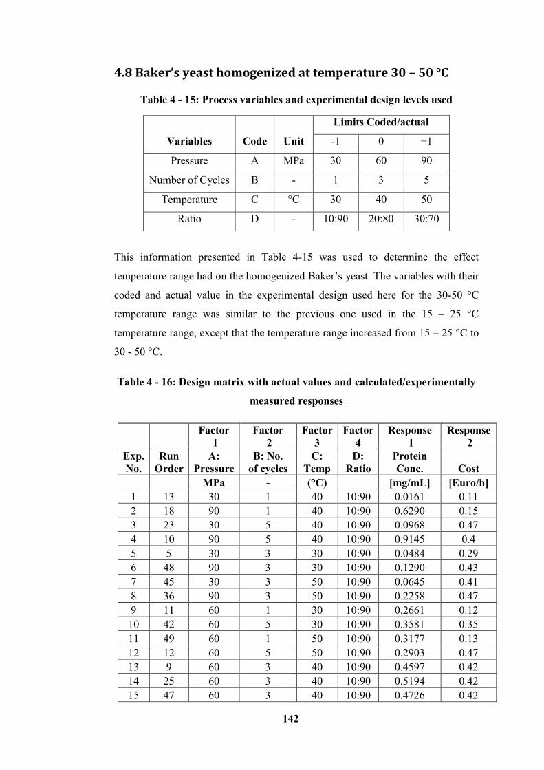
142

4.8 Baker’s yeast homogenized at temperature 30 – 50 °C

Table 4 - 15: Process variables and experimental design levels used

This information presented in Table 4-15 was used to determine the effect

temperature range had on the homogenized Baker’s yeast. The variables with their

coded and actual value in the experimental design used here for the 30-50 °C

temperature range was similar to the previous one used in the 15 – 25 °C

temperature range, except that the temperature range increased from 15 – 25 °C to

30 - 50 °C.


measured responses

Factor

1

Factor

2

Factor

3

Factor

4

Response

1

Response

2

Exp.

No.

Run

Order

A:

Pressure

B: No.

of cycles

C:

Temp

D:

Ratio

Protein

Conc. Cost

MPa - (°C) [mg/mL] [Euro/h]

1 13 30 1 40 10:90 0.0161 0.11

2 18 90 1 40 10:90 0.6290 0.15

3 23 30 5 40 10:90 0.0968 0.47

4 10 90 5 40 10:90 0.9145 0.4

5 5 30 3 30 10:90 0.0484 0.29

6 48 90 3 30 10:90 0.1290 0.43

7 45 30 3 50 10:90 0.0645 0.41

8 36 90 3 50 10:90 0.2258 0.47

9 11 60 1 30 10:90 0.2661 0.12

10 42 60 5 30 10:90 0.3581 0.35

11 49 60 1 50 10:90 0.3177 0.13

12 12 60 5 50 10:90 0.2903 0.47

13 9 60 3 40 10:90 0.4597 0.42

14 25 60 3 40 10:90 0.5194 0.42

15 47 60 3 40 10:90 0.4726 0.42

Variables

Code

Unit

Limits Coded/actual

-1 0 +1

Pressure A MPa 30 60 90

Number of Cycles B - 1 3 5

Temperature C °C 30 40 50

Ratio D - 10:90 20:80 30:70

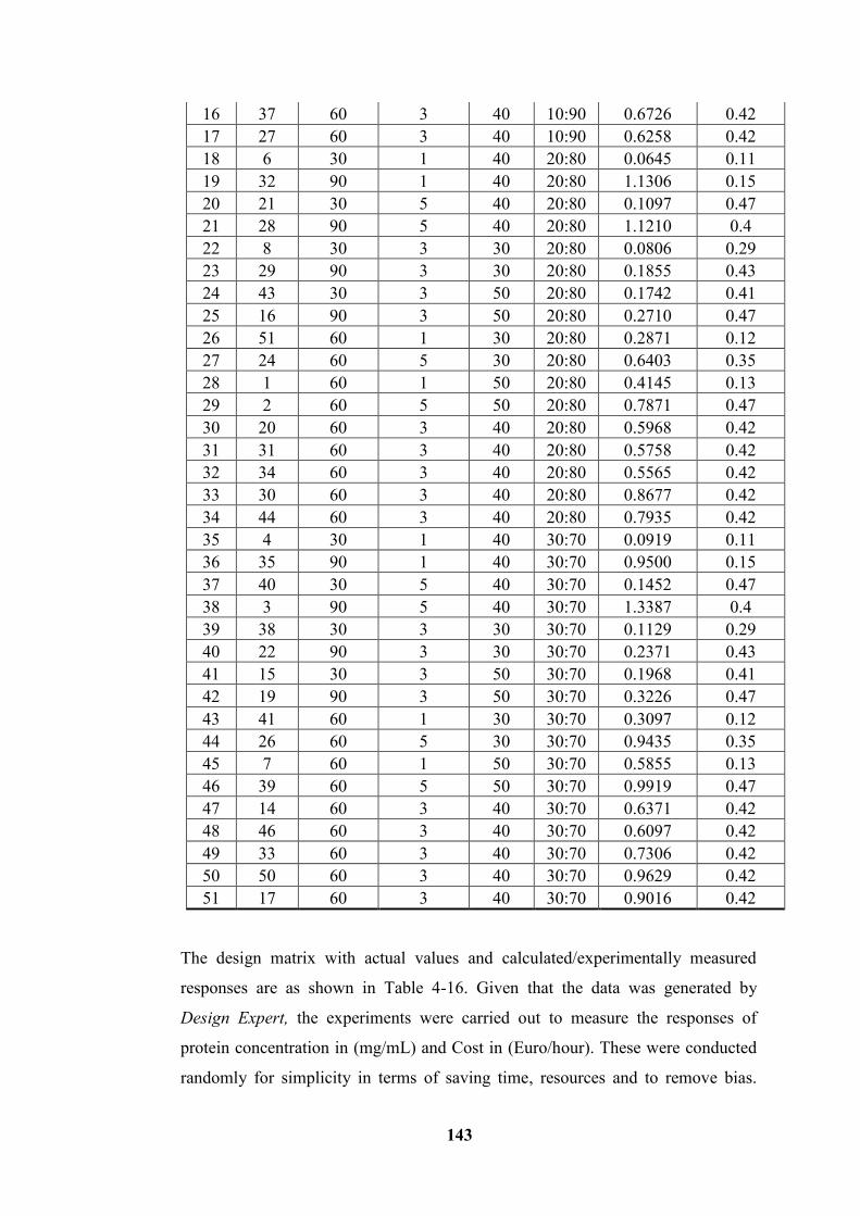
143

16 37 60 3 40 10:90 0.6726 0.42

17 27 60 3 40 10:90 0.6258 0.42

18 6 30 1 40 20:80 0.0645 0.11

19 32 90 1 40 20:80 1.1306 0.15

20 21 30 5 40 20:80 0.1097 0.47

21 28 90 5 40 20:80 1.1210 0.4

22 8 30 3 30 20:80 0.0806 0.29

23 29 90 3 30 20:80 0.1855 0.43

24 43 30 3 50 20:80 0.1742 0.41

25 16 90 3 50 20:80 0.2710 0.47

26 51 60 1 30 20:80 0.2871 0.12

27 24 60 5 30 20:80 0.6403 0.35

28 1 60 1 50 20:80 0.4145 0.13

29 2 60 5 50 20:80 0.7871 0.47

30 20 60 3 40 20:80 0.5968 0.42

31 31 60 3 40 20:80 0.5758 0.42

32 34 60 3 40 20:80 0.5565 0.42

33 30 60 3 40 20:80 0.8677 0.42

34 44 60 3 40 20:80 0.7935 0.42

35 4 30 1 40 30:70 0.0919 0.11

36 35 90 1 40 30:70 0.9500 0.15

37 40 30 5 40 30:70 0.1452 0.47

38 3 90 5 40 30:70 1.3387 0.4

39 38 30 3 30 30:70 0.1129 0.29

40 22 90 3 30 30:70 0.2371 0.43

41 15 30 3 50 30:70 0.1968 0.41

42 19 90 3 50 30:70 0.3226 0.47

43 41 60 1 30 30:70 0.3097 0.12

44 26 60 5 30 30:70 0.9435 0.35

45 7 60 1 50 30:70 0.5855 0.13

46 39 60 5 50 30:70 0.9919 0.47

47 14 60 3 40 30:70 0.6371 0.42

48 46 60 3 40 30:70 0.6097 0.42

49 33 60 3 40 30:70 0.7306 0.42

50 50 60 3 40 30:70 0.9629 0.42

51 17 60 3 40 30:70 0.9016 0.42

The design matrix with actual values and calculated/experimentally measured

responses are as shown in Table 4-16. Given that the data was generated by

Design Expert, the experiments were carried out to measure the responses of

protein concentration in (mg/mL) and Cost in (Euro/hour). These were conducted

randomly for simplicity in terms of saving time, resources and to remove bias.

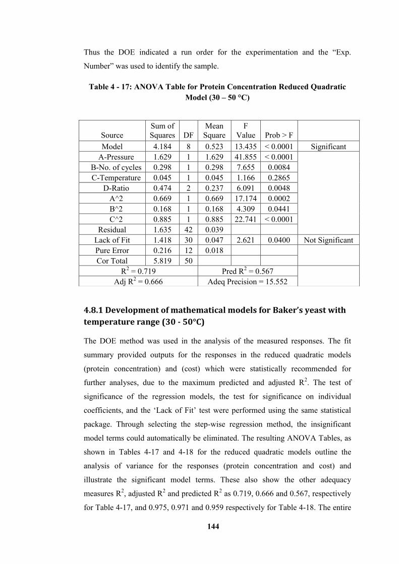
144

Thus the DOE indicated a run order for the experimentation and the “Exp.

Number” was used to identify the sample.

Table 4 - 17: ANOVA Table for Protein Concentration Reduced Quadratic

Model (30 – 50 °C)

4.8.1 Development of mathematical models for Baker’s yeast with

temperature range (30 - 50°C)

The DOE method was used in the analysis of the measured responses. The fit

summary provided outputs for the responses in the reduced quadratic models

(protein concentration) and (cost) which were statistically recommended for

further analyses, due to the maximum predicted and adjusted R2. The test of

significance of the regression models, the test for significance on individual

coefficients, and the ‘Lack of Fit’ test were performed using the same statistical

package. Through selecting the step-wise regression method, the insignificant

model terms could automatically be eliminated. The resulting ANOVA Tables, as

shown in Tables 4-17 and 4-18 for the reduced quadratic models outline the

analysis of variance for the responses (protein concentration and cost) and

illustrate the significant model terms. These also show the other adequacy

measures R2, adjusted R

2 and predicted R

2 as 0.719, 0.666 and 0.567, respectively

for Table 4-17, and 0.975, 0.971 and 0.959 respectively for Table 4-18. The entire

Source

Sum of

Squares

DF

Mean

Square

F

Value

Prob > F


A-Pressure 1.629 1 1.629 41.855 < 0.0001

B-No. of cycles 0.298 1 0.298 7.655 0.0084

C-Temperature 0.045 1 0.045 1.166 0.2865

D-Ratio 0.474 2 0.237 6.091 0.0048

A^2 0.669 1 0.669 17.174 0.0002

B^2 0.168 1 0.168 4.309 0.0441

C^2 0.885 1 0.885 22.741 < 0.0001

Residual 1.635 42 0.039


Pure Error 0.216 12 0.018

Cor Total 5.819 50

R2 = 0.719 Pred R

2 = 0.567


145

adequacy measurement are close to 1, which are in reasonable agreement because

the statistical analysis as recognised by the Design Expert, indicates that any value

equal to or greater than 0.5 is considered as close to 1 when determining the

adequacy measures R2, adjusted R

2, and predicted R

2. The adequate precision

being equal to 15.552 for protein concentration yield, and 41.65 for cost,

indicating an adequate model [225, 226], see Tables 4-17 and 4-18. The adequate

precision compared the range of the predicted values at the design points to the

average prediction error.

These values are >> 4; therefore an adequate model is implied [225]. Figures 4-25

(a and b) and 4-29 (a and b) were a replica plot of the Predicted versus the Actual

response, the residual of the normal plot of protein concentration response, as well

as the residual of the normal plot of cost response were found to be normally

distributed. The analysis of variance indicated that the number of cycles, pressure

as well as temperature and their interactions were the most significant factors

affecting the protein concentration yield. The predicted versus the actual plots are

shown in Figures 4-25(b) and 4-29(b) for protein yield and cost respectively,

indicating adequate models. The normal plot of residuals in Figure 4-25(a) and 4-

29(a) indicate that the assumptions of normal data distribution were respected;

therefore the ANOVA could be applied to the study.

The final mathematical models linked to the responses with regards to the coded

factors and actual factors as determined by the software, are given respectively in

Equations (4-7) to (4-10) and (4-11) to (4-12) with Equations (4-8) to (4-10),

including the dilution ratios; 10:90, 20:80 and 30:70 and Equation (4-12)

representing that of cost.

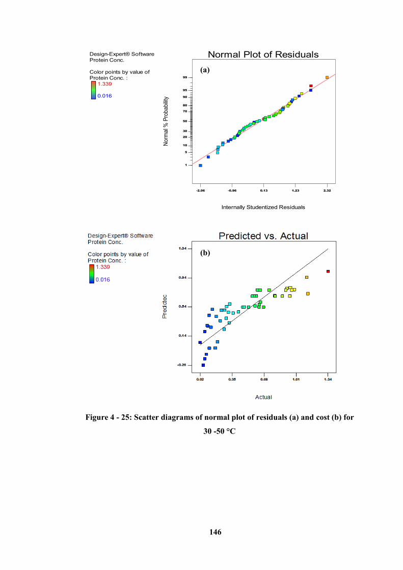
146

Figure 4 - 25: Scatter diagrams of normal plot of residuals (a) and cost (b) for

30 -50 °C


Protein Conc.


Protein Conc. :

1.339

0.016


No

rma

l % P

rob

ab

ility


-2.06 -0.96 0.13 1.23 2.32

1

5

10

20

30

50

70

80

90

95

99

(b)

(a)

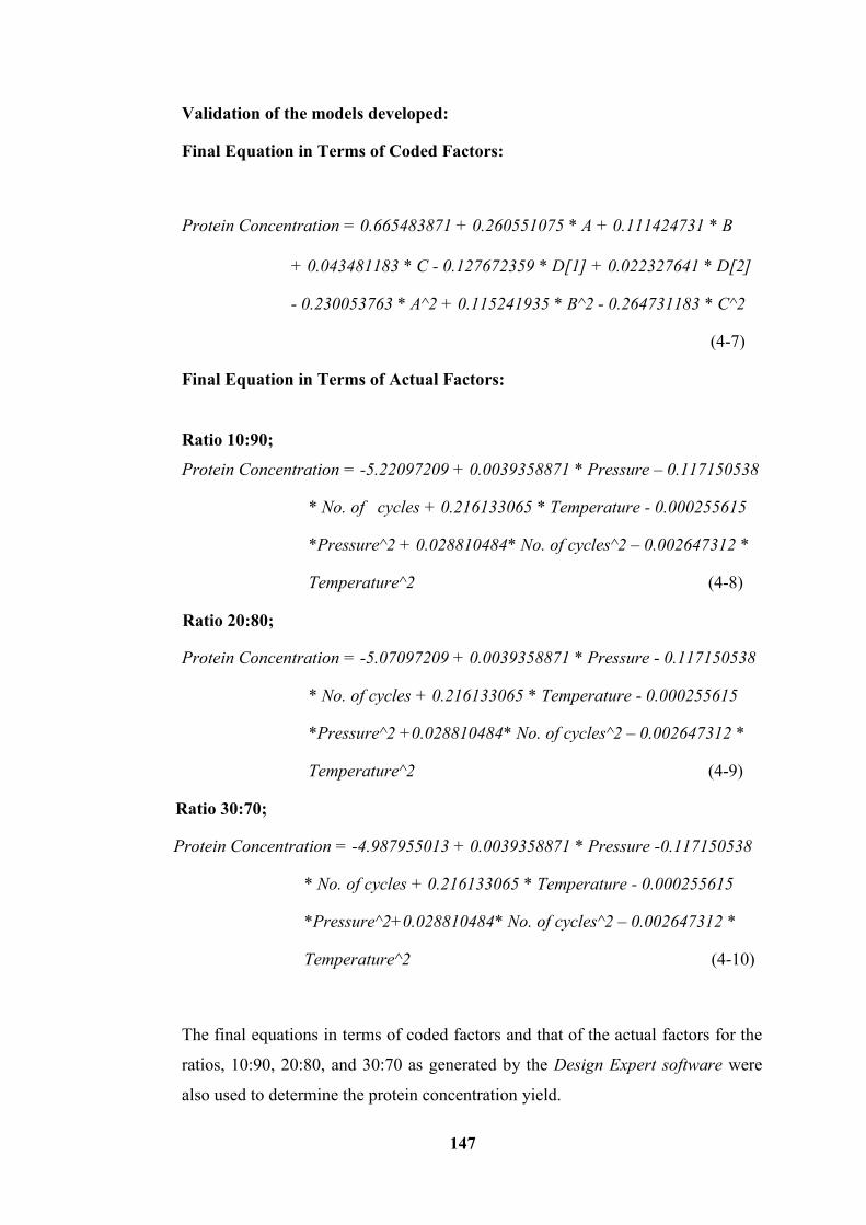
147

Validation of the models developed:


Protein Concentration = 0.665483871 + 0.260551075 * A + 0.111424731 * B

+ 0.043481183 * C - 0.127672359 * D[1] + 0.022327641 * D[2]

- 0.230053763 * A^2 + 0.115241935 * B^2 - 0.264731183 * C^2

(4-7)


Ratio 10:90;

Protein Concentration = -5.22097209 + 0.0039358871 * Pressure – 0.117150538

* No. of cycles + 0.216133065 * Temperature - 0.000255615

*Pressure^2 + 0.028810484* No. of cycles^2 – 0.002647312 *

Temperature^2 (4-8)

Ratio 20:80;



*Pressure^2 +0.028810484* No. of cycles^2 – 0.002647312 *

Temperature^2 (4-9)

Ratio 30:70;

Protein Concentration = -4.987955013 + 0.0039358871 * Pressure -0.117150538


*Pressure^2+0.028810484* No. of cycles^2 – 0.002647312 *

Temperature^2 (4-10)

The final equations in terms of coded factors and that of the actual factors for the

ratios, 10:90, 20:80, and 30:70 as generated by the Design Expert software were

also used to determine the protein concentration yield.

148


The perturbation plot for the protein concentration yield from the 30 - 50 degrees

temperature range is illustrated in Figure 4-26 as (a), (b), and (c). The perturbation

plot helped to compare the effect of all the factors at a particular point in the

design space. This has previously been discussed under the 15 - 25 °C temperature

ranges. Perturbation plots under this section have indeed shown great differences

as compared to that under the 15 - 25 °C temperature range. Temperature is shown

to be major contributing factor in protein concentration yield. Counter to the

results in the previous section, due to the temperature of the biomass substrate

before being homogenized. The pressure and temperature were effects on the yield

of protein concentration. The plot demonstrated that increasing both parameters

improved protein concentration yield up to the centre value and then started to

drop as both tended to increase above the centre limit. One of the reasons for this,

was because the substrate has been treated under heat to raise the temperature,

passing it through the HPH over number of cycles, say 3, would have entirely

broken down the cell wall of the yeast substrate.

Categorical factors of ratios in this study, was to determine the highest yield of

protein at any ratios. This has no implied order which means the settings of a

categorical factor were discrete and had no intrinsic order [230]. Protein

concentration yield is highest at the categorical factor of 30:70 ratios when

compared to the other ratios of 10:90 and 20:80. Invariably, it therefore means that

as the ratio increases, the yield in protein concentration also increases at the same

rate as the pressure rises. However, in this case here, only the number of cycles

has taken the incremental rate in the protein concentration yield. This can be seen

in Figure 4-26 (c). Both pressure and temperature effects had an opposite effect to

the number of cycles in terms of protein yield of as indicated in Figures 4-26 (a, b,

and c).

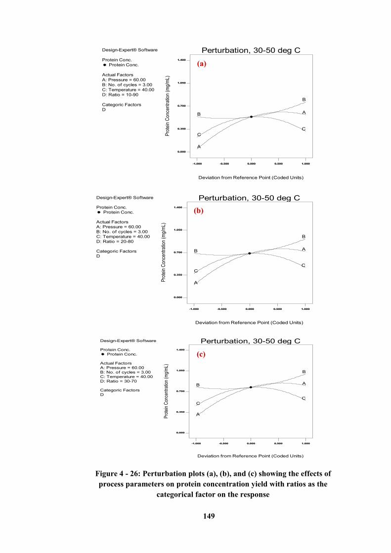
149

Figure 4 - 26: Perturbation plots (a), (b), and (c) showing the effects of

process parameters on protein concentration yield with ratios as the

categorical factor on the response


Protein Conc.

Protein Conc.

Actual Factors

A: Pressure = 60.00



D: Ratio = 10-90

Categoric Factors

D

Perturbation, 30-50 deg C


Pro

tein

Co

nce

ntr

atio

n (

mg

/mL

)-1.000 -0.500 0.000 0.500 1.000

0.000

0.350

0.700

1.050

1.400

A

AB

B

C

C


Protein Conc.

Protein Conc.

Actual Factors

A: Pressure = 60.00



D: Ratio = 20-80

Categoric Factors

D



Pro

tein

Con

cent

ratio

n (m

g/m

L)

-1.000 -0.500 0.000 0.500 1.000

0.000

0.350

0.700

1.050

1.400

A

AB

B

C

C


Protein Conc.

Protein Conc.

Actual Factors

A: Pressure = 60.00



D: Ratio = 30-70

Categoric Factors

D



Pro

tein

Con

cent

ratio

n (m

g/m

L)

-1.000 -0.500 0.000 0.500 1.000

0.000

0.350

0.700

1.050

1.400

A

AB

B

C

C

(a)

(b)

(c)

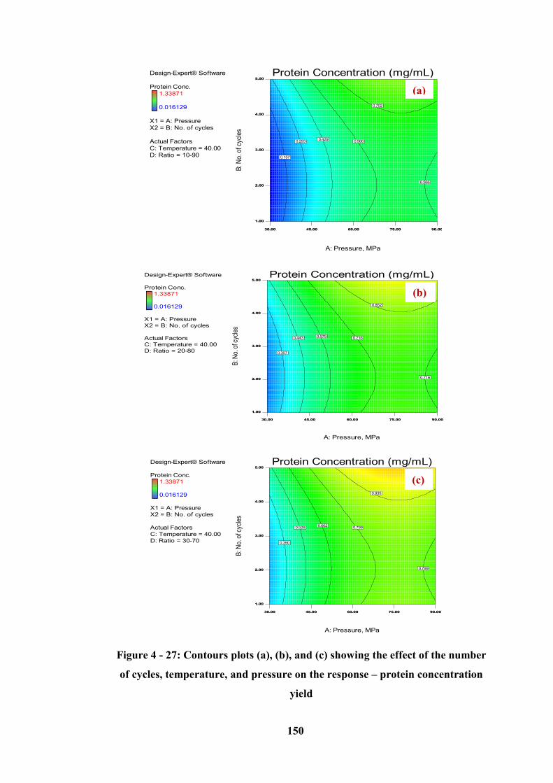
150

Figure 4 - 27: Contours plots (a), (b), and (c) showing the effect of the number

of cycles, temperature, and pressure on the response – protein concentration

yield


Protein Conc.

1.33871

0.016129

X1 = A: Pressure


Actual Factors


D: Ratio = 10-90

30.00 45.00 60.00 75.00 90.00

1.00

2.00

3.00

4.00

5.00

Protein Concentration (mg/mL)

A: Pressure, MPa

B: N

o. o

f cyc

les

0.157

0.2930.429

0.566

0.566

0.702


Protein Conc.

1.33871

0.016129

X1 = A: Pressure


Actual Factors


D: Ratio = 20-80

30.00 45.00 60.00 75.00 90.00

1.00

2.00

3.00

4.00

5.00


A: Pressure, MPa

B: N

o. o

f cyc

les

0.307

0.4430.579

0.716

0.716

0.852


Protein Conc.

1.33871

0.016129

X1 = A: Pressure


Actual Factors


D: Ratio = 30-70

30.00 45.00 60.00 75.00 90.00

1.00

2.00

3.00

4.00

5.00


A: Pressure, MPa

B: N

o. o

f cyc

les

0.390

0.5260.662

0.799

0.799

0.935

(b)

(c)

(a)

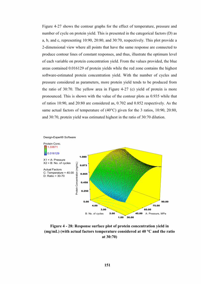
151

Figure 4-27 shows the contour graphs for the effect of temperature, pressure and

number of cycle on protein yield. This is presented in the categorical factors (D) as

a, b, and c, representing 10:90, 20:80, and 30:70, respectively. This plot provide a

2-dimensional view where all points that have the same response are connected to

produce contour lines of constant responses, and thus, illustrate the optimum level

of each variable on protein concentration yield. From the values provided, the blue

areas contained 0.016129 of protein yields while the red zone contains the highest

software-estimated protein concentration yield. With the number of cycles and

pressure considered as parameters, more protein yield tends to be produced from

the ratio of 30:70. The yellow area in Figure 4-27 (c) yield of protein is more

pronounced. This is shown with the value of the contour plots as 0.935 while that

of ratios 10:90, and 20:80 are considered as, 0.702 and 0.852 respectively. As the

same actual factors of temperature of (40°C) given for the 3 ratios, 10:90, 20:80,

and 30:70, protein yield was estimated highest in the ratio of 30:70 dilution.

Figure 4 - 28: Response surface plot of protein concentration yield in

(mg/mL) (with actual factors temperature considered at 40 °C and the ratio

at 30:70)


Protein Conc.

1.33871

0.016129

X1 = A: Pressure


Actual Factors


D: Ratio = 30-70

30.00

45.00

60.00

75.00

90.00

1.00

2.00

3.00

4.00

5.00

0.250

0.458

0.665

0.873

1.080

P

rote

in C

on

ce

ntr

atio

n (

mg

/mL

)

A: Pressure, MPa B: No. of cycles

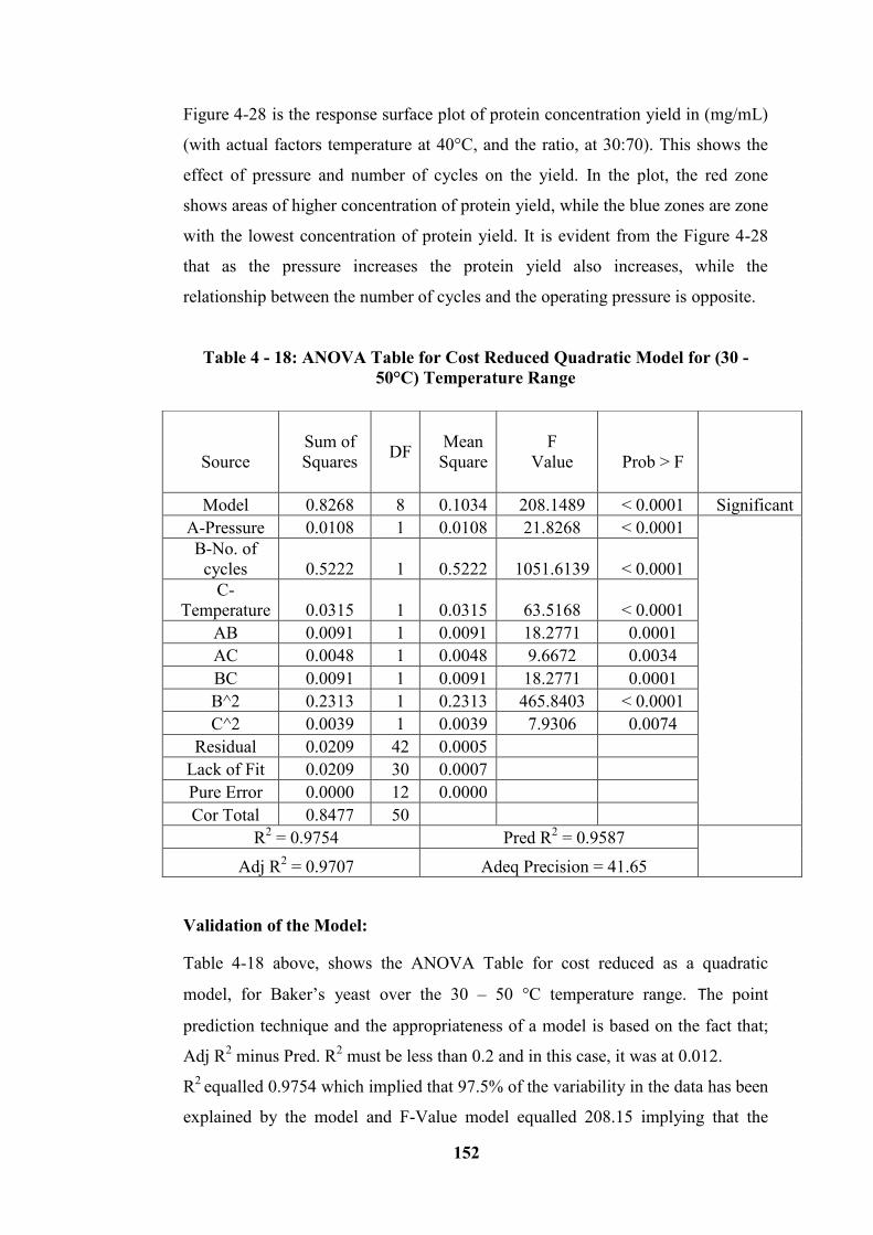
152

Figure 4-28 is the response surface plot of protein concentration yield in (mg/mL)

(with actual factors temperature at 40°C, and the ratio, at 30:70). This shows the

effect of pressure and number of cycles on the yield. In the plot, the red zone

shows areas of higher concentration of protein yield, while the blue zones are zone

with the lowest concentration of protein yield. It is evident from the Figure 4-28

that as the pressure increases the protein yield also increases, while the

relationship between the number of cycles and the operating pressure is opposite.

Table 4 - 18: ANOVA Table for Cost Reduced Quadratic Model for (30 -

50°C) Temperature Range

Validation of the Model:

Table 4-18 above, shows the ANOVA Table for cost reduced as a quadratic

model, for Baker’s yeast over the 30 – 50 °C temperature range. The point

prediction technique and the appropriateness of a model is based on the fact that;

Adj R2 minus Pred. R

2 must be less than 0.2 and in this case, it was at 0.012.

R2

equalled 0.9754 which implied that 97.5% of the variability in the data has been

explained by the model and F-Value model equalled 208.15 implying that the

Source

Sum of

Squares DF

Mean

Square

F

Value

Prob > F


A-Pressure 0.0108 1 0.0108 21.8268 < 0.0001

B-No. of

cycles 0.5222 1 0.5222 1051.6139 < 0.0001

C-

Temperature 0.0315 1 0.0315 63.5168 < 0.0001

AB 0.0091 1 0.0091 18.2771 0.0001

AC 0.0048 1 0.0048 9.6672 0.0034

BC 0.0091 1 0.0091 18.2771 0.0001

B^2 0.2313 1 0.2313 465.8403 < 0.0001

C^2 0.0039 1 0.0039 7.9306 0.0074

Residual 0.0209 42 0.0005

Lack of Fit 0.0209 30 0.0007

Pure Error 0.0000 12 0.0000

Cor Total 0.8477 50

R2 = 0.9754 Pred R

2 = 0.9587


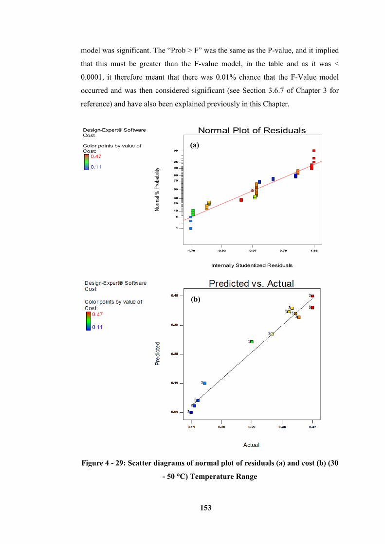
153

model was significant. The “Prob > F” was the same as the P-value, and it implied

that this must be greater than the F-value model, in the table and as it was <

0.0001, it therefore meant that there was 0.01% chance that the F-Value model

occurred and was then considered significant (see Section 3.6.7 of Chapter 3 for

reference) and have also been explained previously in this Chapter.

Figure 4 - 29: Scatter diagrams of normal plot of residuals (a) and cost (b) (30

- 50 °C) Temperature Range


Cost


Cost:

0.47

0.11


Nor

mal

% P

roba

bilit

y


-1.79 -0.93 -0.07 0.79 1.66

1

5

10

20

30

50

70

80

90

95

99

(a)

(b)

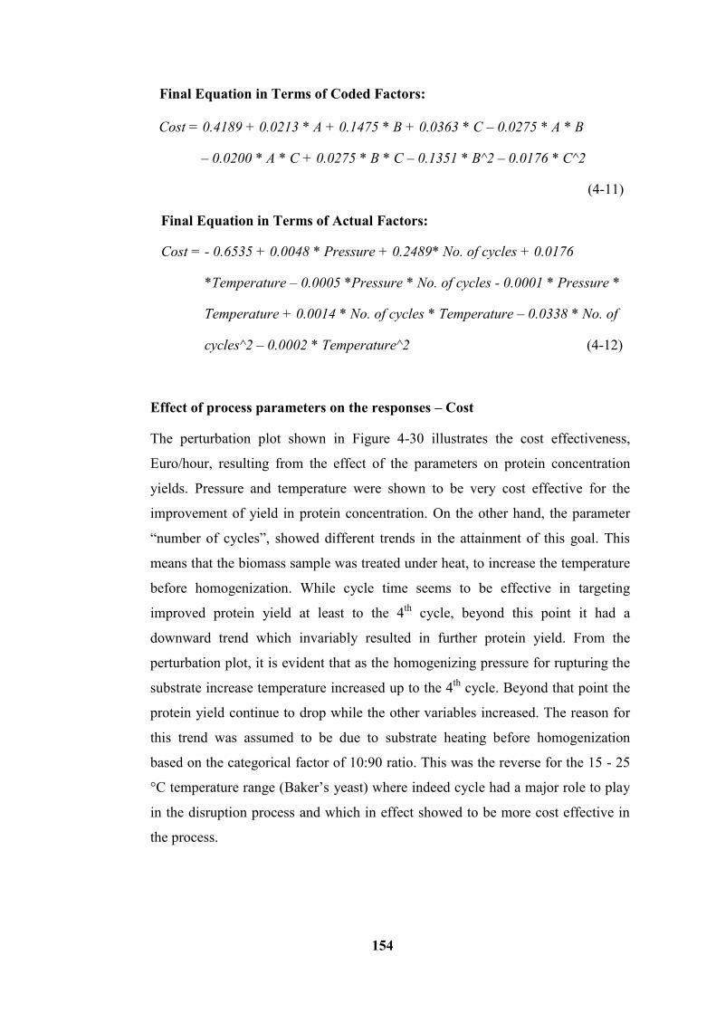
154


Cost = 0.4189 + 0.0213 * A + 0.1475 * B + 0.0363 * C – 0.0275 * A * B

– 0.0200 * A * C + 0.0275 * B * C – 0.1351 * B^2 – 0.0176 * C^2

(4-11)


Cost = - 0.6535 + 0.0048 * Pressure + 0.2489* No. of cycles + 0.0176

*Temperature – 0.0005 *Pressure * No. of cycles - 0.0001 * Pressure *

Temperature + 0.0014 * No. of cycles * Temperature – 0.0338 * No. of

cycles^2 – 0.0002 * Temperature^2 (4-12)

Effect of process parameters on the responses – Cost

The perturbation plot shown in Figure 4-30 illustrates the cost effectiveness,

Euro/hour, resulting from the effect of the parameters on protein concentration

yields. Pressure and temperature were shown to be very cost effective for the

improvement of yield in protein concentration. On the other hand, the parameter

“number of cycles”, showed different trends in the attainment of this goal. This

means that the biomass sample was treated under heat, to increase the temperature

before homogenization. While cycle time seems to be effective in targeting

improved protein yield at least to the 4th

cycle, beyond this point it had a

downward trend which invariably resulted in further protein yield. From the

perturbation plot, it is evident that as the homogenizing pressure for rupturing the

substrate increase temperature increased up to the 4th

cycle. Beyond that point the

protein yield continue to drop while the other variables increased. The reason for

this trend was assumed to be due to substrate heating before homogenization

based on the categorical factor of 10:90 ratio. This was the reverse for the 15 - 25

°C temperature range (Baker’s yeast) where indeed cycle had a major role to play

in the disruption process and which in effect showed to be more cost effective in

the process.

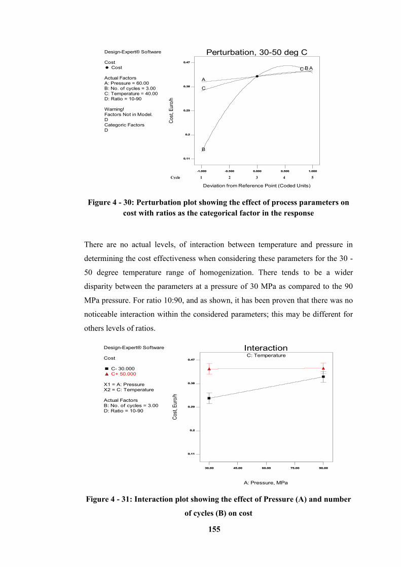
155

Figure 4 - 30: Perturbation plot showing the effect of process parameters on

cost with ratios as the categorical factor in the response

There are no actual levels, of interaction between temperature and pressure in

determining the cost effectiveness when considering these parameters for the 30 -

50 degree temperature range of homogenization. There tends to be a wider

disparity between the parameters at a pressure of 30 MPa as compared to the 90

MPa pressure. For ratio 10:90, and as shown, it has been proven that there was no

noticeable interaction within the considered parameters; this may be different for

others levels of ratios.

Figure 4 - 31: Interaction plot showing the effect of Pressure (A) and number

of cycles (B) on cost


Cost

Cost

Actual Factors

A: Pressure = 60.00



D: Ratio = 10-90

Warning!


D

Categoric Factors

D



Co

st, E

uro

/h-1.000 -0.500 0.000 0.500 1.000

0.11

0.2

0.29

0.38

0.47

A

A

B

B

C

C


Cost

C- 30.000

C+ 50.000

X1 = A: Pressure

X2 = C: Temperature

Actual Factors


D: Ratio = 10-90

C: Temperature

30.00 45.00 60.00 75.00 90.00

Interaction

A: Pressure, MPa

Cos

t, E

uro/

h

0.11

0.2

0.29

0.38

0.47

Cycle 1 2 3 4 5

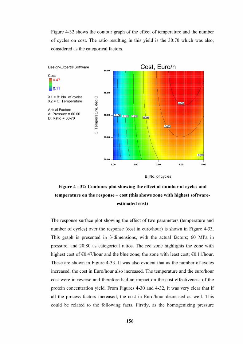
156

Figure 4-32 shows the contour graph of the effect of temperature and the number

of cycles on cost. The ratio resulting in this yield is the 30:70 which was also,

considered as the categorical factors.

Figure 4 - 32: Contours plot showing the effect of number of cycles and


estimated cost)

The response surface plot showing the effect of two parameters (temperature and

number of cycles) over the response (cost in euro/hour) is shown in Figure 4-33.

This graph is presented in 3-dimensions, with the actual factors; 60 MPa in

pressure, and 20:80 as categorical ratios. The red zone highlights the zone with

highest cost of €0.47/hour and the blue zone; the zone with least cost; €0.11/hour.

These are shown in Figure 4-33. It was also evident that as the number of cycles

increased, the cost in Euro/hour also increased. The temperature and the euro/hour

cost were in reverse and therefore had an impact on the cost effectiveness of the

protein concentration yield. From Figures 4-30 and 4-32, it was very clear that if

all the process factors increased, the cost in Euro/hour decreased as well. This

could be related to the following facts. Firstly, as the homogenizing pressure


Cost

0.47

0.11


X2 = C: Temperature

Actual Factors

A: Pressure = 60.00

D: Ratio = 30-70

1.00 2.00 3.00 4.00 5.00

30.00

35.00

40.00

45.00

50.00

Cost, Euro/h

B: No. of cycles

C: T

em

pe

ratu

re, d

eg

C

0.1740.238 0.302

0.366

0.366

0.430

0.470

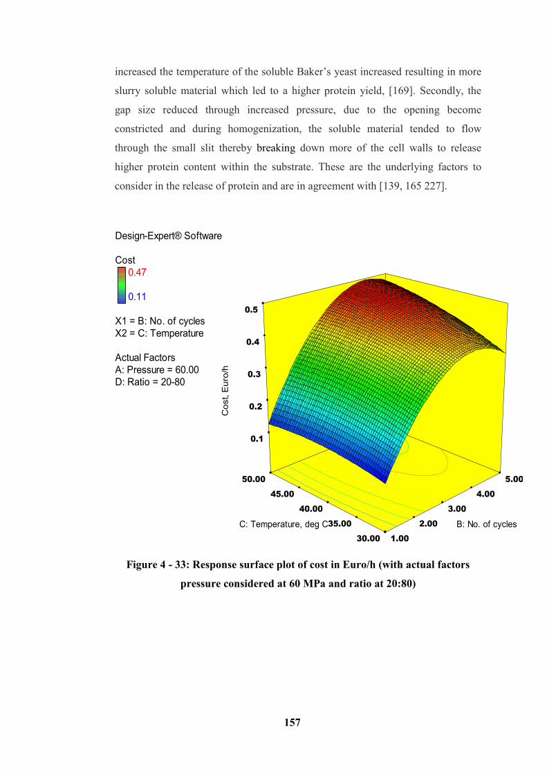
157

increased the temperature of the soluble Baker’s yeast increased resulting in more

slurry soluble material which led to a higher protein yield, [169]. Secondly, the

gap size reduced through increased pressure, due to the opening become

constricted and during homogenization, the soluble material tended to flow

through the small slit thereby breaking down more of the cell walls to release

higher protein content within the substrate. These are the underlying factors to

consider in the release of protein and are in agreement with [139, 165 227].

Figure 4 - 33: Response surface plot of cost in Euro/h (with actual factors

pressure considered at 60 MPa and ratio at 20:80)


Cost

0.47

0.11


X2 = C: Temperature

Actual Factors

A: Pressure = 60.00

D: Ratio = 20-80

1.00

2.00

3.00

4.00

5.00

30.00

35.00

40.00

45.00

50.00

0.1

0.2

0.3

0.4

0.5

C

ost, E

uro

/h

B: No. of cycles C: Temperature, deg C

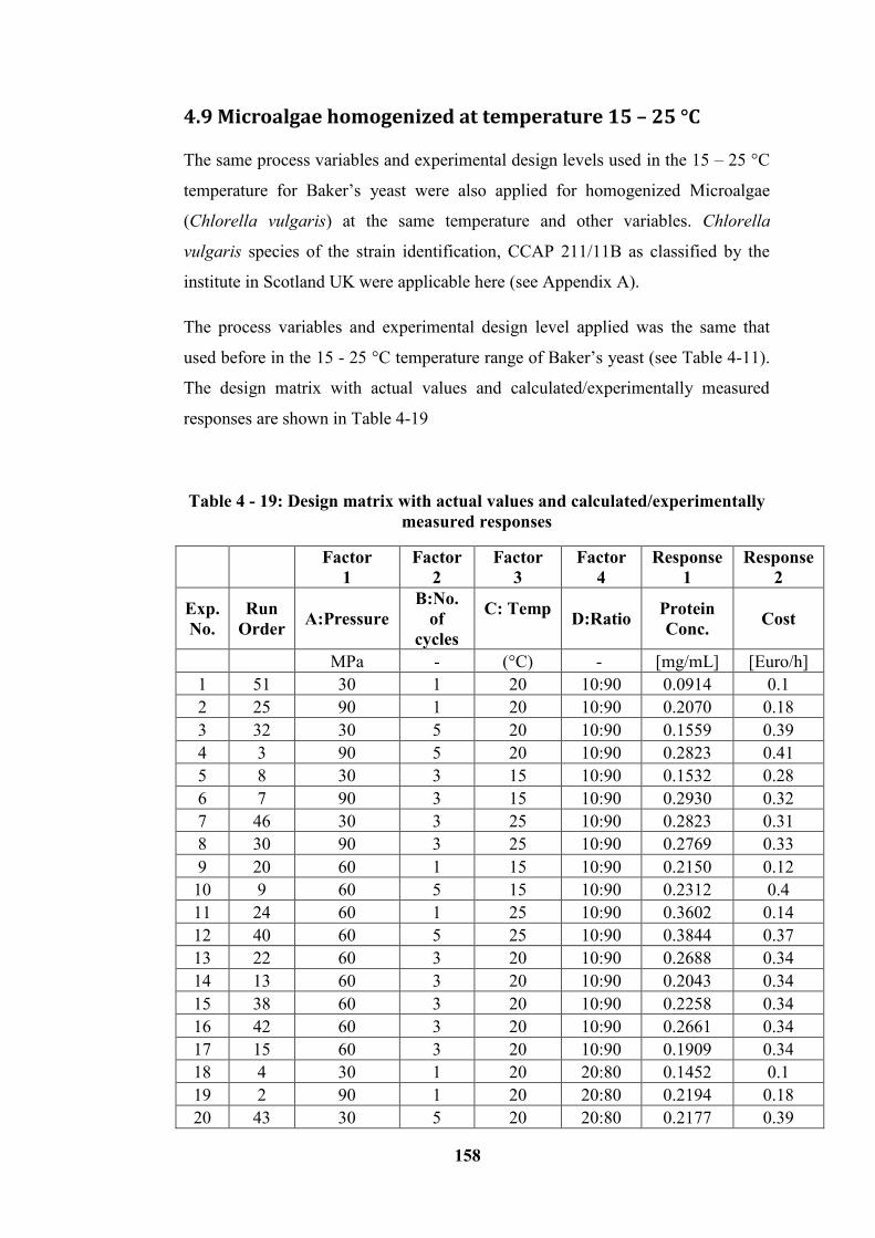
158

4.9 Microalgae homogenized at temperature 15 – 25 °C

The same process variables and experimental design levels used in the 15 – 25 °C

temperature for Baker’s yeast were also applied for homogenized Microalgae

(Chlorella vulgaris) at the same temperature and other variables. Chlorella

vulgaris species of the strain identification, CCAP 211/11B as classified by the

institute in Scotland UK were applicable here (see Appendix A).

The process variables and experimental design level applied was the same that

used before in the 15 - 25 °C temperature range of Baker’s yeast (see Table 4-11).

The design matrix with actual values and calculated/experimentally measured

responses are shown in Table 4-19


measured responses

Factor

1

Factor

2

Factor

3

Factor

4

Response

1

Response

2

Exp.

No.

Run

Order A:Pressure

B:No.

of

cycles

C: Temp

D:Ratio

Protein

Conc. Cost

MPa - (°C) - [mg/mL] [Euro/h]

1 51 30 1 20 10:90 0.0914 0.1

2 25 90 1 20 10:90 0.2070 0.18

3 32 30 5 20 10:90 0.1559 0.39

4 3 90 5 20 10:90 0.2823 0.41

5 8 30 3 15 10:90 0.1532 0.28

6 7 90 3 15 10:90 0.2930 0.32

7 46 30 3 25 10:90 0.2823 0.31

8 30 90 3 25 10:90 0.2769 0.33

9 20 60 1 15 10:90 0.2150 0.12

10 9 60 5 15 10:90 0.2312 0.4

11 24 60 1 25 10:90 0.3602 0.14

12 40 60 5 25 10:90 0.3844 0.37

13 22 60 3 20 10:90 0.2688 0.34

14 13 60 3 20 10:90 0.2043 0.34

15 38 60 3 20 10:90 0.2258 0.34

16 42 60 3 20 10:90 0.2661 0.34

17 15 60 3 20 10:90 0.1909 0.34

18 4 30 1 20 20:80 0.1452 0.1

19 2 90 1 20 20:80 0.2194 0.18

20 43 30 5 20 20:80 0.2177 0.39

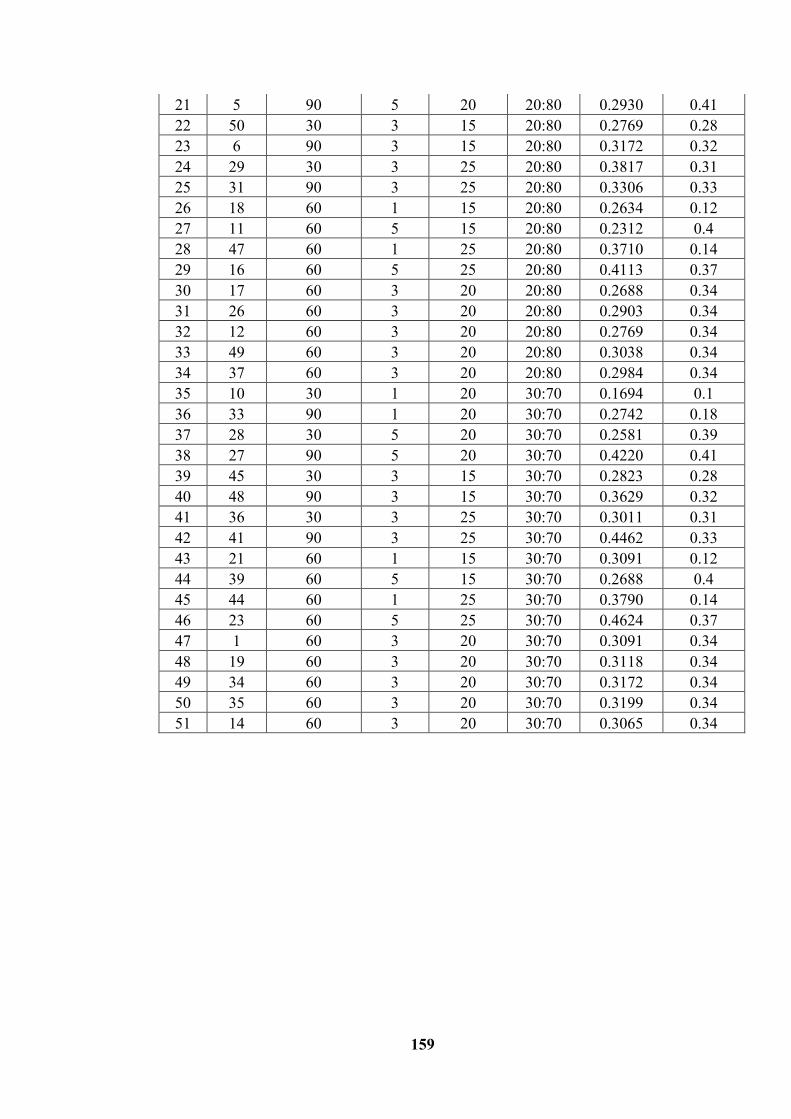
159

21 5 90 5 20 20:80 0.2930 0.41

22 50 30 3 15 20:80 0.2769 0.28

23 6 90 3 15 20:80 0.3172 0.32

24 29 30 3 25 20:80 0.3817 0.31

25 31 90 3 25 20:80 0.3306 0.33

26 18 60 1 15 20:80 0.2634 0.12

27 11 60 5 15 20:80 0.2312 0.4

28 47 60 1 25 20:80 0.3710 0.14

29 16 60 5 25 20:80 0.4113 0.37

30 17 60 3 20 20:80 0.2688 0.34

31 26 60 3 20 20:80 0.2903 0.34

32 12 60 3 20 20:80 0.2769 0.34

33 49 60 3 20 20:80 0.3038 0.34

34 37 60 3 20 20:80 0.2984 0.34

35 10 30 1 20 30:70 0.1694 0.1

36 33 90 1 20 30:70 0.2742 0.18

37 28 30 5 20 30:70 0.2581 0.39

38 27 90 5 20 30:70 0.4220 0.41

39 45 30 3 15 30:70 0.2823 0.28

40 48 90 3 15 30:70 0.3629 0.32

41 36 30 3 25 30:70 0.3011 0.31

42 41 90 3 25 30:70 0.4462 0.33

43 21 60 1 15 30:70 0.3091 0.12

44 39 60 5 15 30:70 0.2688 0.4

45 44 60 1 25 30:70 0.3790 0.14

46 23 60 5 25 30:70 0.4624 0.37

47 1 60 3 20 30:70 0.3091 0.34

48 19 60 3 20 30:70 0.3118 0.34

49 34 60 3 20 30:70 0.3172 0.34

50 35 60 3 20 30:70 0.3199 0.34

51 14 60 3 20 30:70 0.3065 0.34

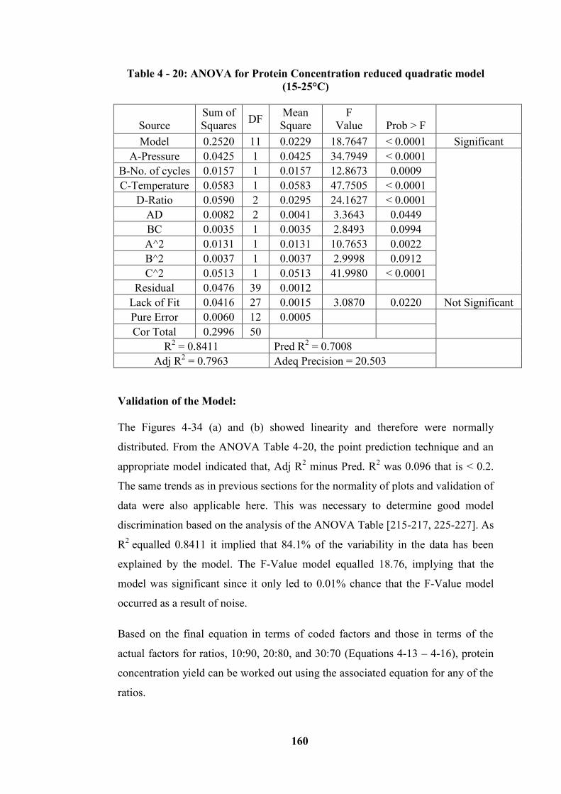
160

Table 4 - 20: ANOVA for Protein Concentration reduced quadratic model

(15-25°C)

Source

Sum of

Squares DF

Mean

Square

F

Value

Prob > F


A-Pressure 0.0425 1 0.0425 34.7949 < 0.0001

B-No. of cycles 0.0157 1 0.0157 12.8673 0.0009

C-Temperature 0.0583 1 0.0583 47.7505 < 0.0001

D-Ratio 0.0590 2 0.0295 24.1627 < 0.0001

AD 0.0082 2 0.0041 3.3643 0.0449

BC 0.0035 1 0.0035 2.8493 0.0994

A^2 0.0131 1 0.0131 10.7653 0.0022

B^2 0.0037 1 0.0037 2.9998 0.0912

C^2 0.0513 1 0.0513 41.9980 < 0.0001

Residual 0.0476 39 0.0012


Pure Error 0.0060 12 0.0005

Cor Total 0.2996 50

R2 = 0.8411 Pred R

2 = 0.7008


Validation of the Model:

The Figures 4-34 (a) and (b) showed linearity and therefore were normally

distributed. From the ANOVA Table 4-20, the point prediction technique and an

appropriate model indicated that, Adj R2 minus Pred. R

2 was 0.096 that is < 0.2.

The same trends as in previous sections for the normality of plots and validation of

data were also applicable here. This was necessary to determine good model

discrimination based on the analysis of the ANOVA Table [215-217, 225-227]. As

R2

equalled 0.8411 it implied that 84.1% of the variability in the data has been

explained by the model. The F-Value model equalled 18.76, implying that the

model was significant since it only led to 0.01% chance that the F-Value model

occurred as a result of noise.

Based on the final equation in terms of coded factors and those in terms of the

actual factors for ratios, 10:90, 20:80, and 30:70 (Equations 4-13 – 4-16), protein

concentration yield can be worked out using the associated equation for any of the

ratios.

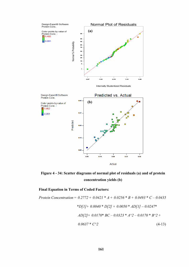
161

Figure 4 - 34: Scatter diagrams of normal plot of residuals (a) and of protein

concentration yields (b)


Protein Concentration = 0.2772 + 0.0421 * A + 0.0256 * B + 0.0493 * C – 0.0435

*D[1]+ 0.0040 * D[2] + 0.0050 * AD[1] – 0.0247*

AD[2]+ 0.0170* BC – 0.0323 * A^2 – 0.0170 * B^2 +

0.0637 * C^2 (4-13)


Protein Conc.


Protein Conc. :

0.462

0.091


No

rma

l % P

rob

ab

ility


-2.87 -1.53 -0.19 1.14 2.48

1

5

10

20

30

50

70

80

90

95

99

(b)

(a)

162


Ratio 10:90;

Protein Concentration = 0.8583 + 0.0059 * Pressure + 0.0043 * No. of cycles –

0.0972* Temperature + 0.0017 * No. of cycles*Temperature +

0.0000*Pressure^2 – 0.0043* No. of cycle^2 + 0.0025

*Temperature (4-14)

Ratio 20:80;




*Temperature (4-15)

Ratio 30:70;




*Temperature (4-16)

4.9.1 Development of mathematical models for Microalgae

(Chlorella vulgaris)

The same software was used to analyse the measured response. The test for

significance of the regression models, tests for significance on each model

coefficient, and lack of fit test were carried out. The step-wise regression method;

which eliminates the insignificant model terms automatically, was applied. Two

ANOVA Tables for the reduced quadratics models have been obtained (see Table

4-20 and 4-21). These Tables summarised the analysis of each response and

showed the significant model terms, and others, such as; Adequacy measure R2,

Adjusted R2 and Predicted R

2. From the Tables, the adequacy models are close to

163

1. The developed quadratic mathematical models, in terms of coded factors and

actual values, are represented in Equations 4-13 to 4-16 for protein concentration

yield (mg/mL) and 4-17 to 4-18 for cost in (Euro/hour). Wherein, these equations,

(Equations 4-13 and 4-17) represent the coded form.


The perturbation plot for the protein concentration yield from the 15 - 25 °C

temperature range for Microalgae (Chlorella vulgaris) is illustrated in Figure 4-35

as (a), (b), and (c). These aided in comparing the effect of all the factors at a

particular point in the design space. Perturbation plots under this Section showed

great difference as compared to that of the previous two; that of 15 - 25 °C and

that of 30 – 50 °C temperature ranges for Baker’s yeast. Temperature was shown

to be effective in protein concentration yield in the three plots. The reason for this

change has been attributed to the temperature effect of the biomass substrate

before homogenization. The substrate state would have changed completely and

the internal contents affected, due to heat effect before the treatment under HPH.

The substrate temperature was raised to within the room temperature before the

homogenization was conducted, (15, 20, and 25°C) that is, before the substrate

was passed through the high-pressure homogenizer. This process, affected the

change in behaviour of the substrate. Other parameters and their effects were also

of importance up till the midpoint, and then subsequently resulted in the behaviour

pattern by the shifting downward of the parameters A, and B, i.e. Pressure and

Number of cycles. Temperature influenced the higher yield of protein in 4-35 (a,

b, and c), considered highest in the ratio of 30:70 perturbation plots, the cell walls

would have been broken down completely to release the protein contents

internally [163, 169].

As the highest protein concentration yield has resulted from the homogenization

process, as seen in the plot (c), that was; at the ratio 30:70 with the yield of 0.3

mg/mL of protein concentration, and when compared to the previous two; 15 - 25

°C and 30 - 50 °C temperature ranges of Baker’s yeast, the results were 0.65 and

0.7 mg/mL respectively (see Figures 4-17 (c) and 4-26 (c)). This meant that as the

164

ratio increased, the yield in protein concentration also increased at the same rate as

pressure rose.

From the analysis, ratio played a very important role in the conversion of input

into responses (protein concentration yields and cost). A higher dilution ratio

resulted in higher protein concentration yield.

165


parameters on protein concentration yield with ratio as the categorical factor

on the response


Protein Conc.

Protein Conc.

Actual Factors

A: Pressure = 60.00



D: Ratio = 10-90

Categoric Factors

D

Perturbation


Pro

tein

Con

cent

ratio

n, (m

g/m

L)

-1.000 -0.500 0.000 0.500 1.000

0.090

0.185

0.280

0.375

0.470

A

A

B

BC

C


Protein Conc.

Protein Conc.

Actual Factors

A: Pressure = 60.00



D: Ratio = 20-80

Categoric Factors

D

Perturbation


Pro

tein

Co

nce

ntr

atio

n, (m

g/m

L)

-1.000 -0.500 0.000 0.500 1.000

0.090

0.185

0.280

0.375

0.470

A

A

B

BC

C


Protein Conc.

Protein Conc.

Actual Factors

A: Pressure = 60.00



D: Ratio = 30-70

Categoric Factors

D

Perturbation


Pro

tein

Co

nce

ntr

atio

n, (m

g/m

L)

-1.000 -0.500 0.000 0.500 1.000

0.090

0.185

0.280

0.375

0.470

A

A

B

BC

C(c)

(b)

(a)

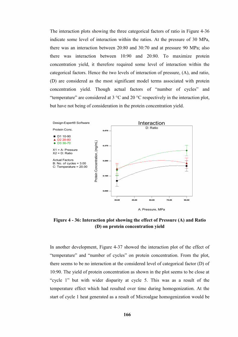
166

The interaction plots showing the three categorical factors of ratio in Figure 4-36

indicate some level of interaction within the ratios. At the pressure of 30 MPa,

there was an interaction between 20:80 and 30:70 and at pressure 90 MPa; also

there was interaction between 10:90 and 20:80. To maximize protein

concentration yield, it therefore required some level of interaction within the

categorical factors. Hence the two levels of interaction of pressure, (A), and ratio,

(D) are considered as the most significant model terms associated with protein

concentration yield. Though actual factors of “number of cycles” and

“temperature” are considered at 3 °C and 20 °C respectively in the interaction plot,

but have not being of consideration in the protein concentration yield.

Figure 4 - 36: Interaction plot showing the effect of Pressure (A) and Ratio

(D) on protein concentration yield

In another development, Figure 4-37 showed the interaction plot of the effect of

“temperature” and “number of cycles” on protein concentration. From the plot,

there seems to be no interaction at the considered level of categorical factor (D) of

10:90. The yield of protein concentration as shown in the plot seems to be close at

“cycle 1” but with wider disparity at cycle 5. This was as a result of the

temperature effect which had resulted over time during homogenization. At the

start of cycle 1 heat generated as a result of Microalgae homogenization would be


Protein Conc.

D1 10-90

D2 20-80

D3 30-70

X1 = A: Pressure

X2 = D: Ratio

Actual Factors



D: Ratio

30.00 45.00 60.00 75.00 90.00

Interaction

A: Pressure, MPa

Pro

tein

Co

nce

ntr

atio

n, (

mg

/mL

)

0.090

0.185

0.280

0.375

0.470

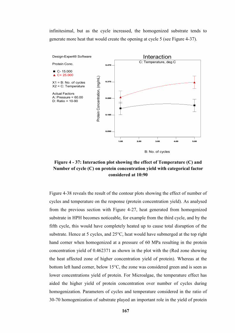
167

infinitesimal, but as the cycle increased, the homogenized substrate tends to

generate more heat that would create the opening at cycle 5 (see Figure 4-37).

Figure 4 - 37: Interaction plot showing the effect of Temperature (C) and

Number of cycle (C) on protein concentration yield with categorical factor

considered at 10:90

Figure 4-38 reveals the result of the contour plots showing the effect of number of

cycles and temperature on the response (protein concentration yield). As analysed

from the previous section with Figure 4-27, heat generated from homogenized

substrate in HPH becomes noticeable, for example from the third cycle, and by the

fifth cycle, this would have completely heated up to cause total disruption of the

substrate. Hence at 5 cycles, and 25°C, heat would have submerged at the top right

hand corner when homogenized at a pressure of 60 MPa resulting in the protein

concentration yield of 0.462371 as shown in the plot with the (Red zone showing

the heat affected zone of higher concentration yield of protein). Whereas at the

bottom left hand corner, below 15°C, the zone was considered green and is seen as

lower concentrations yield of protein. For Microalgae, the temperature effect has

aided the higher yield of protein concentration over number of cycles during

homogenization. Parameters of cycles and temperature considered in the ratio of

30-70 homogenization of substrate played an important role in the yield of protein


Protein Conc.

C- 15.000

C+ 25.000


X2 = C: Temperature

Actual Factors

A: Pressure = 60.00

D: Ratio = 10-90

C: Temperature, deg C

1.00 2.00 3.00 4.00 5.00

Interaction

B: No. of cycles

Pro

tein

Co

nce

ntr

atio

n, (

mg

/mL

)

0.090

0.185

0.280

0.375

0.470

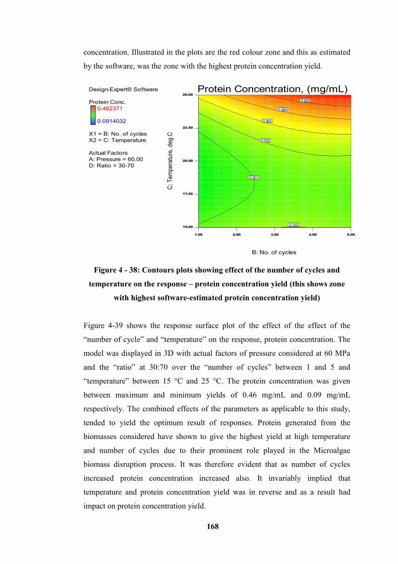
168

concentration. Illustrated in the plots are the red colour zone and this as estimated

by the software, was the zone with the highest protein concentration yield.

Figure 4 - 38: Contours plots showing effect of the number of cycles and

temperature on the response – protein concentration yield (this shows zone

with highest software-estimated protein concentration yield)

Figure 4-39 shows the response surface plot of the effect of the effect of the

“number of cycle” and “temperature” on the response, protein concentration. The

model was displayed in 3D with actual factors of pressure considered at 60 MPa

and the “ratio” at 30:70 over the “number of cycles” between 1 and 5 and

“temperature” between 15 °C and 25 °C. The protein concentration was given

between maximum and minimum yields of 0.46 mg/mL and 0.09 mg/mL

respectively. The combined effects of the parameters as applicable to this study,

tended to yield the optimum result of responses. Protein generated from the

biomasses considered have shown to give the highest yield at high temperature

and number of cycles due to their prominent role played in the Microalgae

biomass disruption process. It was therefore evident that as number of cycles

increased protein concentration increased also. It invariably implied that

temperature and protein concentration yield was in reverse and as a result had

impact on protein concentration yield.


Protein Conc.

0.462371

0.0914032


X2 = C: Temperature

Actual Factors

A: Pressure = 60.00

D: Ratio = 30-70

1.00 2.00 3.00 4.00 5.00

15.00

17.50

20.00

22.50

25.00

Protein Concentration, (mg/mL)

B: No. of cycles

C: T

em

pe

ratu

re, d

eg

C0.301

0.332

0.332

0.363

0.394

0.424

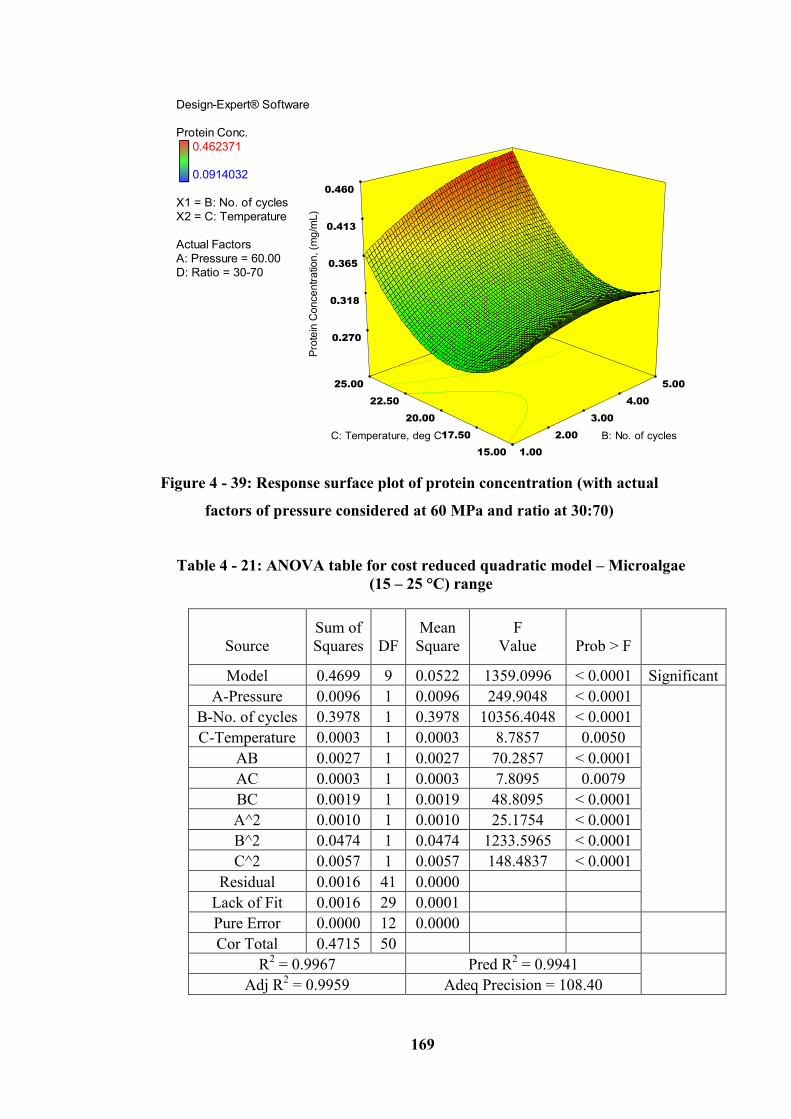
169

Figure 4 - 39: Response surface plot of protein concentration (with actual

factors of pressure considered at 60 MPa and ratio at 30:70)

Table 4 - 21: ANOVA table for cost reduced quadratic model – Microalgae

(15 – 25 °C) range

Source

Sum of

Squares

DF

Mean

Square

F

Value

Prob > F


A-Pressure 0.0096 1 0.0096 249.9048 < 0.0001

B-No. of cycles 0.3978 1 0.3978 10356.4048 < 0.0001

C-Temperature 0.0003 1 0.0003 8.7857 0.0050

AB 0.0027 1 0.0027 70.2857 < 0.0001

AC 0.0003 1 0.0003 7.8095 0.0079

BC 0.0019 1 0.0019 48.8095 < 0.0001

A^2 0.0010 1 0.0010 25.1754 < 0.0001

B^2 0.0474 1 0.0474 1233.5965 < 0.0001

C^2 0.0057 1 0.0057 148.4837 < 0.0001

Residual 0.0016 41 0.0000

Lack of Fit 0.0016 29 0.0001

Pure Error 0.0000 12 0.0000

Cor Total 0.4715 50

R2 = 0.9967 Pred R

2 = 0.9941



Protein Conc.

0.462371

0.0914032


X2 = C: Temperature

Actual Factors

A: Pressure = 60.00

D: Ratio = 30-70

1.00

2.00

3.00

4.00

5.00

15.00

17.50

20.00

22.50

25.00

0.270

0.318

0.365

0.413

0.460

P

rote

in C

on

ce

ntr

atio

n, (m

g/m

L)

B: No. of cycles C: Temperature, deg C

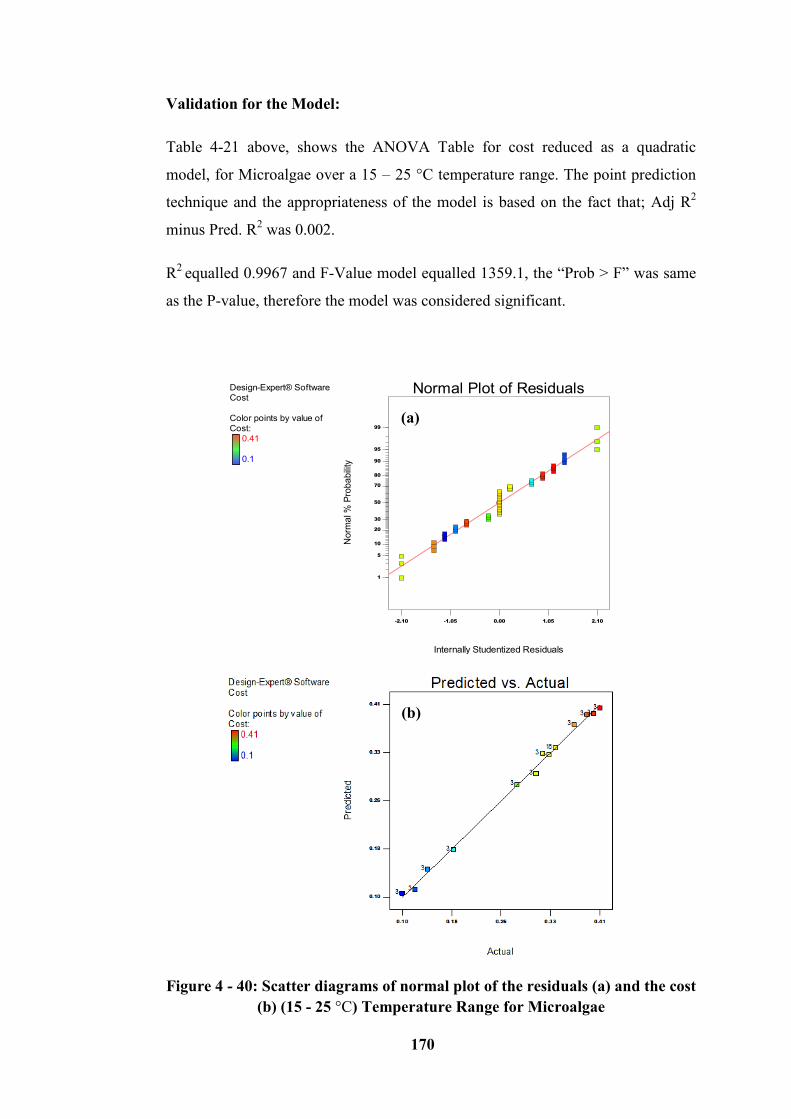
170

Validation for the Model:

Table 4-21 above, shows the ANOVA Table for cost reduced as a quadratic

model, for Microalgae over a 15 – 25 °C temperature range. The point prediction

technique and the appropriateness of the model is based on the fact that; Adj R2

minus Pred. R2 was 0.002.

R2

equalled 0.9967 and F-Value model equalled 1359.1, the “Prob > F” was same

as the P-value, therefore the model was considered significant.

Figure 4 - 40: Scatter diagrams of normal plot of the residuals (a) and the cost

(b) (15 - 25 °C) Temperature Range for Microalgae


Cost


Cost:

0.41

0.1


No

rma

l % P

rob

ab

ility


-2.10 -1.05 0.00 1.05 2.10

1

5

10

20

30

50

70

80

90

95

99

(a)

(b)

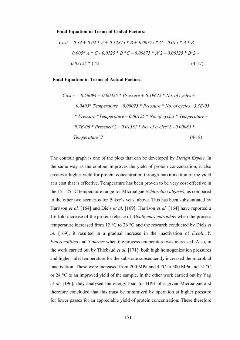
171


Cost = 0.34 + 0.02 * A + 0.12875 * B + 0.00375 * C – 0.015 * A * B –

0.005* A * C - 0.0125 * B *C – 0.00875 * A^2 – 0.06125 * B^2 –

0.02125 * C^2 (4-17)


Cost = – 0.58094 + 0.00325 * Pressure + 0.19625 * No. of cycles +

0.0405* Temperature – 0.00025 * Pressure * No. of cycles –3.3E-05

* Pressure *Temperature – 0.00125 * No. of cycles * Temperature –

9.7E-06 * Pressure^2 – 0.01531 * No. of cycles^2 - 0.00085 *

Temperature^2 (4-18)

The contour graph is one of the plots that can be developed by Design Expert. In

the same way as the contour improves the yield of protein concentration, it also

creates a higher yield for protein concentration through maximization of the yield

at a cost that is effective. Temperature has been proven to be very cost effective in

the 15 - 25 °C temperature range for Microalgae (Chlorella vulgaris), as compared

to the other two scenarios for Baker’s yeast above. This has been substantiated by

Harrison et al. [164] and Diels et al. [169]. Harrison et al. [164] have reported a

1.6 fold increase of the protein release of Alcaligenes eutrophus when the process

temperature increased from 12 °C to 26 °C and the research conducted by Diels et

al. [169], it resulted in a gradual increase in the inactivation of E.coli, Y.

Enterocolitica and S.aureus when the process temperature was increased. Also, in

the work carried out by Thiebaud et al. [171], both high homogenization pressures

and higher inlet temperature for the substrate subsequently increased the microbial

inactivation. These were increased from 200 MPa and 4 °C to 300 MPa and 14 °C

or 24 °C to an improved yield of the sample. In the other work carried out by Yap

et al. [196], they analysed the energy load for HPH of a given Microalgae and

therefore concluded that this must be minimized by operation at higher pressure

for fewer passes for an appreciable yield of protein concentration. These therefore

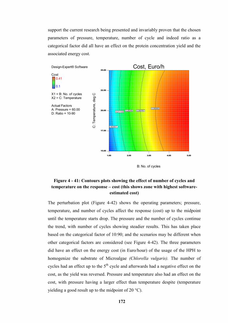
172

support the current research being presented and invariably proven that the chosen

parameters of pressure, temperature, number of cycle and indeed ratio as a

categorical factor did all have an effect on the protein concentration yield and the

associated energy cost.

Figure 4 - 41: Contours plots showing the effect of number of cycles and


estimated cost)

The perturbation plot (Figure 4-42) shows the operating parameters; pressure,

temperature, and number of cycles affect the response (cost) up to the midpoint

until the temperature starts drop. The pressure and the number of cycles continue

the trend, with number of cycles showing steadier results. This has taken place

based on the categorical factor of 10:90; and the scenarios may be different when

other categorical factors are considered (see Figure 4-42). The three parameters

did have an effect on the energy cost (in Euro/hour) of the usage of the HPH to

homogenize the substrate of Microalgae (Chlorella vulgaris). The number of

cycles had an effect up to the 5th

cycle and afterwards had a negative effect on the

cost, as the yield was reversed. Pressure and temperature also had an effect on the

cost, with pressure having a larger effect than temperature despite (temperature

yielding a good result up to the midpoint of 20 °C).


Cost

0.41

0.1


X2 = C: Temperature

Actual Factors

A: Pressure = 60.00

D: Ratio = 10-90

1.00 2.00 3.00 4.00 5.00

15.00

17.50

20.00

22.50

25.00

Cost, Euro/h

B: No. of cycles

C: T

em

pe

ratu

re, d

eg

C

0.161817

0.2111330.26045 0.309767

0.359083

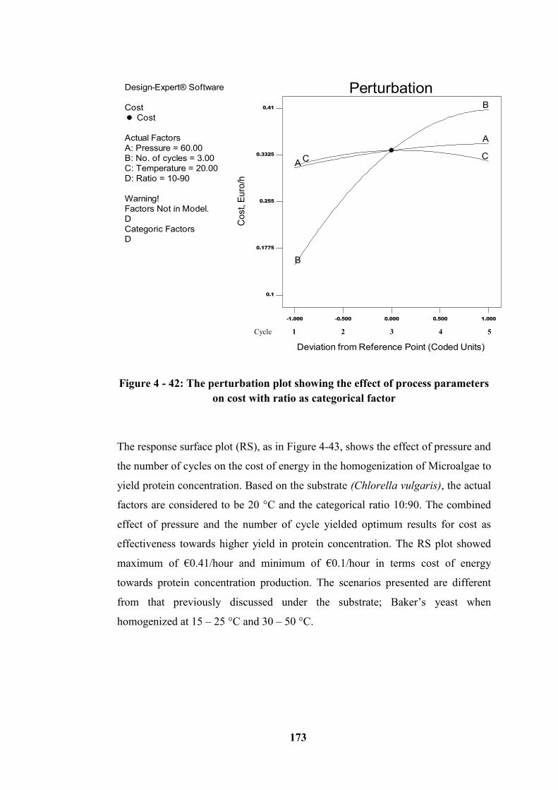
173

Figure 4 - 42: The perturbation plot showing the effect of process parameters

on cost with ratio as categorical factor

The response surface plot (RS), as in Figure 4-43, shows the effect of pressure and

the number of cycles on the cost of energy in the homogenization of Microalgae to

yield protein concentration. Based on the substrate (Chlorella vulgaris), the actual

factors are considered to be 20 °C and the categorical ratio 10:90. The combined

effect of pressure and the number of cycle yielded optimum results for cost as

effectiveness towards higher yield in protein concentration. The RS plot showed

maximum of €0.41/hour and minimum of €0.1/hour in terms cost of energy

towards protein concentration production. The scenarios presented are different

from that previously discussed under the substrate; Baker’s yeast when

homogenized at 15 – 25 °C and 30 – 50 °C.


Cost

Cost

Actual Factors

A: Pressure = 60.00



D: Ratio = 10-90

Warning!


D

Categoric Factors

D

Perturbation


Co

st, E

uro

/h

-1.000 -0.500 0.000 0.500 1.000

0.1

0.1775

0.255

0.3325

0.41

A

A

B

B

C C

Cycle 1 2 3 4 5

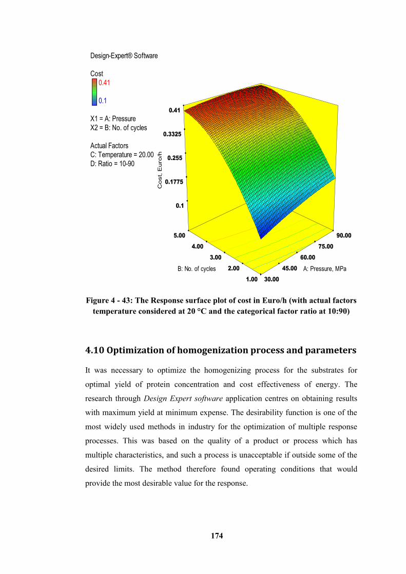
174

Figure 4 - 43: The Response surface plot of cost in Euro/h (with actual factors

temperature considered at 20 °C and the categorical factor ratio at 10:90)

4.10 Optimization of homogenization process and parameters

It was necessary to optimize the homogenizing process for the substrates for

optimal yield of protein concentration and cost effectiveness of energy. The

research through Design Expert software application centres on obtaining results

with maximum yield at minimum expense. The desirability function is one of the

most widely used methods in industry for the optimization of multiple response

processes. This was based on the quality of a product or process which has

multiple characteristics, and such a process is unacceptable if outside some of the

desired limits. The method therefore found operating conditions that would

provide the most desirable value for the response.


Cost

0.41

0.1

X1 = A: Pressure


Actual Factors


D: Ratio = 10-90

30.00

45.00

60.00

75.00

90.00

1.00

2.00

3.00

4.00

5.00

0.1

0.1775

0.255

0.3325

0.41

C

ost, E

uro

/h

A: Pressure, MPa B: No. of cycles

175

In this section, optimization will be considered in two ways; numerical and

graphical and in each of the cases; the 15 - 25 °C temperature range, 30 - 50 °C

temperature range both for Baker’s yeast homogenization and the 15 - 25 °C

temperature range for Microalgae homogenization, the optimization conditions

will be applied just as has been discussed in the previous chapters.

4.10.1 Baker’s yeast (Homogenized at temperature range 15 -

25°C)

4.10.1.1 Numerical Optimization (Over the 15 – 25 °C Temperature Range)

Four criteria have been implemented in the numerical optimization of this

substrate. The criteria were based on quality and cost where quality was referred to

as higher yield of protein concentration, and cost, as the most effective energy cost

in attaining the highest yield of protein concentration. Two criteria were

considered for quality (restricted and not restricted) while cost was also based on

two criteria (restricted and not restricted). The target was to minimise cost and

maximize protein concentration yield. The condition has been set out with one as

restricted (with constraints), and the other, without restriction.

Table 4-22 comparison of the quality (Protein concentration yield) in both

restricted and not restricted scenarios. The target was to maximize protein

concentration yield. For every factor and response, each goal was given a level of

importance rated between 1 and 5, where 1 was considered as the lowest rating

and 5 as the highest rating. As shown in Table 4-22, Protein concentration yield

was the target, therefore it was rated 5 and every other condition must be fulfilled

to achieve this goal by maximizing pressure, number of cycles, temperature, and

minimizing ratio at the minimum cost to achieve optimal protein concentration

yield, through numerical optimization.

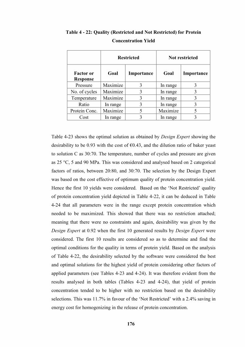
176

Table 4 - 22: Quality (Restricted and Not Restricted) for Protein

Concentration Yield

Restricted Not restricted

Factor or

Response

Goal Importance Goal Importance

Pressure Maximize 3 In range 3

No. of cycles Maximize 3 In range 3

Temperature Maximize 3 In range 3

Ratio In range 3 In range 3

Protein Conc. Maximize 5 Maximize 5

Cost In range 3 In range 3

Table 4-23 shows the optimal solution as obtained by Design Expert showing the

desirability to be 0.93 with the cost of €0.43, and the dilution ratio of baker yeast

to solution C as 30:70. The temperature, number of cycles and pressure are given

as 25 °C, 5 and 90 MPa. This was considered and analysed based on 2 categorical

factors of ratios, between 20:80, and 30:70. The selection by the Design Expert

was based on the cost effective of optimum quality of protein concentration yield.

Hence the first 10 yields were considered. Based on the ‘Not Restricted’ quality

of protein concentration yield depicted in Table 4-22, it can be deduced in Table

4-24 that all parameters were in the range except protein concentration which

needed to be maximized. This showed that there was no restriction attached;

meaning that there were no constraints and again, desirability was given by the

Design Expert at 0.92 when the first 10 generated results by Design Expert were

considered. The first 10 results are considered so as to determine and find the

optimal conditions for the quality in terms of protein yield. Based on the analysis

of Table 4-22, the desirability selected by the software were considered the best

and optimal solutions for the highest yield of protein considering other factors of

applied parameters (see Tables 4-23 and 4-24). It was therefore evident from the

results analysed in both tables (Tables 4-23 and 4-24), that yield of protein

concentration tended to be higher with no restriction based on the desirability

selections. This was 11.7% in favour of the ‘Not Restricted’ with a 2.4% saving in

energy cost for homogenizing in the release of protein concentration.

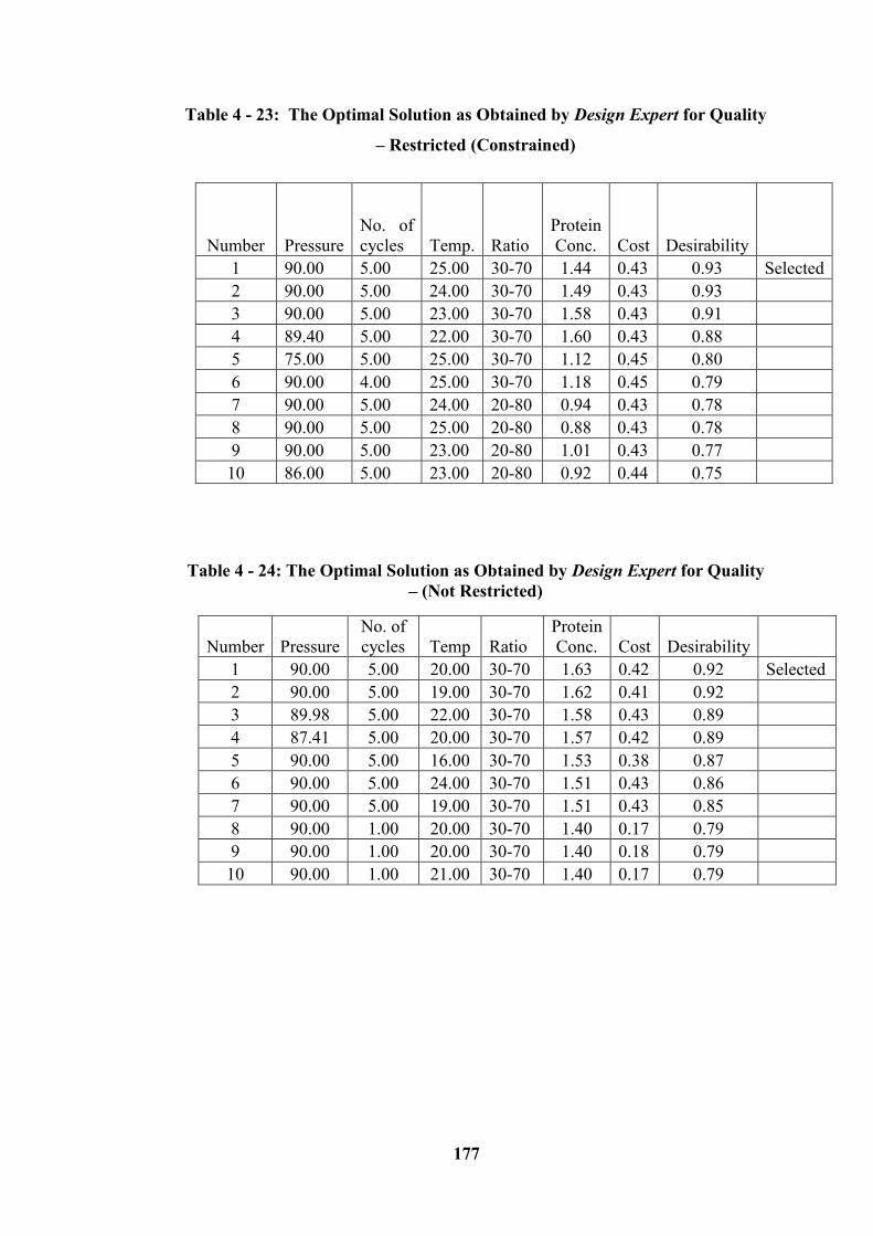
177

Table 4 - 23: The Optimal Solution as Obtained by Design Expert for Quality

– Restricted (Constrained)

Table 4 - 24: The Optimal Solution as Obtained by Design Expert for Quality

– (Not Restricted)

Number Pressure

No. of

cycles Temp Ratio

Protein

Conc. Cost Desirability

1 90.00 5.00 20.00 30-70 1.63 0.42 0.92 Selected

2 90.00 5.00 19.00 30-70 1.62 0.41 0.92

3 89.98 5.00 22.00 30-70 1.58 0.43 0.89

4 87.41 5.00 20.00 30-70 1.57 0.42 0.89

5 90.00 5.00 16.00 30-70 1.53 0.38 0.87

6 90.00 5.00 24.00 30-70 1.51 0.43 0.86

7 90.00 5.00 19.00 30-70 1.51 0.43 0.85

8 90.00 1.00 20.00 30-70 1.40 0.17 0.79

9 90.00 1.00 20.00 30-70 1.40 0.18 0.79

10 90.00 1.00 21.00 30-70 1.40 0.17 0.79

Number Pressure

No. of

cycles Temp. Ratio

Protein


1 90.00 5.00 25.00 30-70 1.44 0.43 0.93 Selected

2 90.00 5.00 24.00 30-70 1.49 0.43 0.93

3 90.00 5.00 23.00 30-70 1.58 0.43 0.91

4 89.40 5.00 22.00 30-70 1.60 0.43 0.88

5 75.00 5.00 25.00 30-70 1.12 0.45 0.80

6 90.00 4.00 25.00 30-70 1.18 0.45 0.79

7 90.00 5.00 24.00 20-80 0.94 0.43 0.78

8 90.00 5.00 25.00 20-80 0.88 0.43 0.78

9 90.00 5.00 23.00 20-80 1.01 0.43 0.77

10 86.00 5.00 23.00 20-80 0.92 0.44 0.75

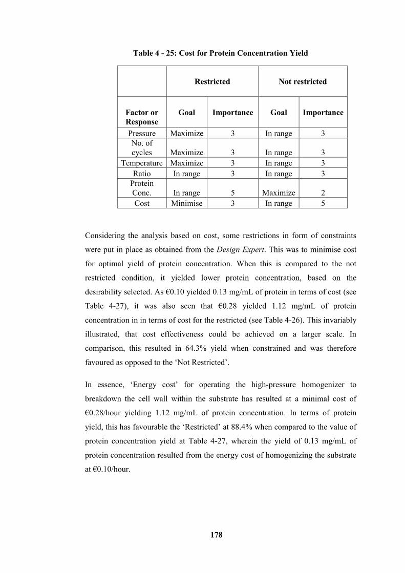
178

Table 4 - 25: Cost for Protein Concentration Yield

Restricted Not restricted

Factor or

Response

Goal Importance Goal Importance

Pressure Maximize 3 In range 3

No. of

cycles Maximize 3 In range 3

Temperature Maximize 3 In range 3

Ratio In range 3 In range 3

Protein

Conc. In range 5 Maximize 2

Cost Minimise 3 In range 5

Considering the analysis based on cost, some restrictions in form of constraints

were put in place as obtained from the Design Expert. This was to minimise cost

for optimal yield of protein concentration. When this is compared to the not

restricted condition, it yielded lower protein concentration, based on the

desirability selected. As €0.10 yielded 0.13 mg/mL of protein in terms of cost (see

Table 4-27), it was also seen that €0.28 yielded 1.12 mg/mL of protein

concentration in in terms of cost for the restricted (see Table 4-26). This invariably

illustrated, that cost effectiveness could be achieved on a larger scale. In

comparison, this resulted in 64.3% yield when constrained and was therefore

favoured as opposed to the ‘Not Restricted’.

In essence, ‘Energy cost’ for operating the high-pressure homogenizer to

breakdown the cell wall within the substrate has resulted at a minimal cost of

€0.28/hour yielding 1.12 mg/mL of protein concentration. In terms of protein

yield, this has favourable the ‘Restricted’ at 88.4% when compared to the value of

protein concentration yield at Table 4-27, wherein the yield of 0.13 mg/mL of

protein concentration resulted from the energy cost of homogenizing the substrate

at €0.10/hour.

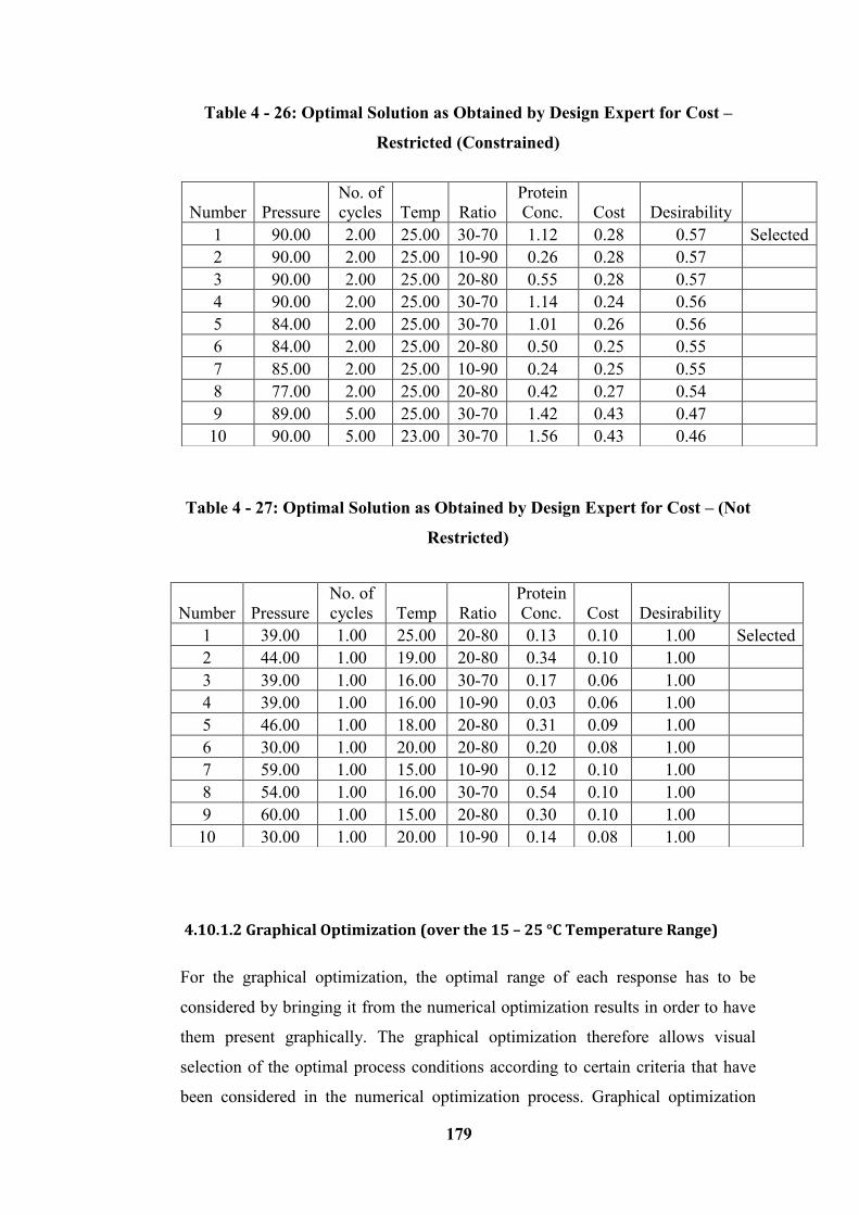
179

Table 4 - 26: Optimal Solution as Obtained by Design Expert for Cost –

Restricted (Constrained)

Table 4 - 27: Optimal Solution as Obtained by Design Expert for Cost – (Not

Restricted)

4.10.1.2 Graphical Optimization (over the 15 – 25 °C Temperature Range)

For the graphical optimization, the optimal range of each response has to be

considered by bringing it from the numerical optimization results in order to have

them present graphically. The graphical optimization therefore allows visual

selection of the optimal process conditions according to certain criteria that have

been considered in the numerical optimization process. Graphical optimization

Number Pressure

No. of

cycles Temp Ratio

Protein


1 90.00 2.00 25.00 30-70 1.12 0.28 0.57 Selected

2 90.00 2.00 25.00 10-90 0.26 0.28 0.57

3 90.00 2.00 25.00 20-80 0.55 0.28 0.57

4 90.00 2.00 25.00 30-70 1.14 0.24 0.56

5 84.00 2.00 25.00 30-70 1.01 0.26 0.56

6 84.00 2.00 25.00 20-80 0.50 0.25 0.55

7 85.00 2.00 25.00 10-90 0.24 0.25 0.55

8 77.00 2.00 25.00 20-80 0.42 0.27 0.54

9 89.00 5.00 25.00 30-70 1.42 0.43 0.47

10 90.00 5.00 23.00 30-70 1.56 0.43 0.46

Number Pressure

No. of

cycles Temp Ratio

Protein


1 39.00 1.00 25.00 20-80 0.13 0.10 1.00 Selected

2 44.00 1.00 19.00 20-80 0.34 0.10 1.00

3 39.00 1.00 16.00 30-70 0.17 0.06 1.00

4 39.00 1.00 16.00 10-90 0.03 0.06 1.00

5 46.00 1.00 18.00 20-80 0.31 0.09 1.00

6 30.00 1.00 20.00 20-80 0.20 0.08 1.00

7 59.00 1.00 15.00 10-90 0.12 0.10 1.00

8 54.00 1.00 16.00 30-70 0.54 0.10 1.00

9 60.00 1.00 15.00 20-80 0.30 0.10 1.00

10 30.00 1.00 20.00 10-90 0.14 0.08 1.00

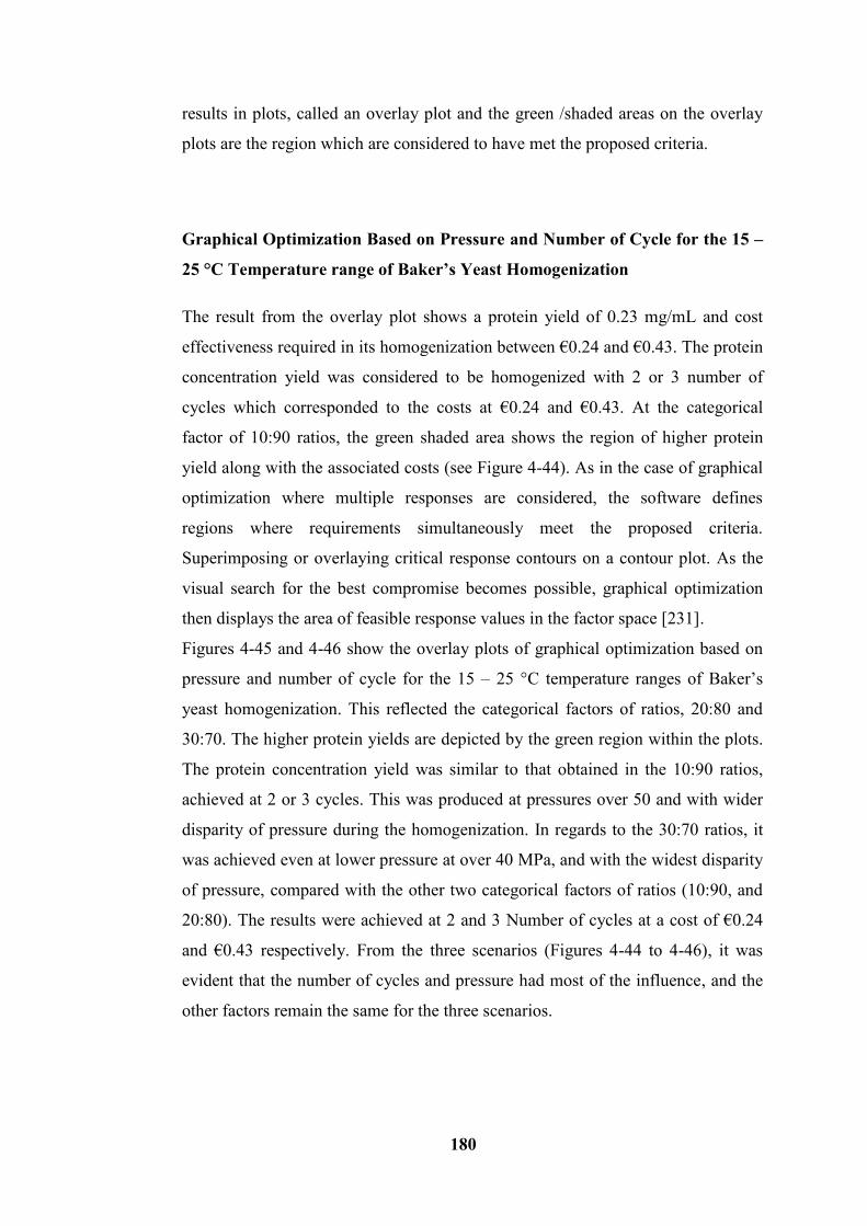
180

results in plots, called an overlay plot and the green /shaded areas on the overlay

plots are the region which are considered to have met the proposed criteria.

Graphical Optimization Based on Pressure and Number of Cycle for the 15 –

25 °C Temperature range of Baker’s Yeast Homogenization

The result from the overlay plot shows a protein yield of 0.23 mg/mL and cost

effectiveness required in its homogenization between €0.24 and €0.43. The protein

concentration yield was considered to be homogenized with 2 or 3 number of

cycles which corresponded to the costs at €0.24 and €0.43. At the categorical

factor of 10:90 ratios, the green shaded area shows the region of higher protein

yield along with the associated costs (see Figure 4-44). As in the case of graphical

optimization where multiple responses are considered, the software defines

regions where requirements simultaneously meet the proposed criteria.

Superimposing or overlaying critical response contours on a contour plot. As the

visual search for the best compromise becomes possible, graphical optimization

then displays the area of feasible response values in the factor space [231].

Figures 4-45 and 4-46 show the overlay plots of graphical optimization based on

pressure and number of cycle for the 15 – 25 °C temperature ranges of Baker’s

yeast homogenization. This reflected the categorical factors of ratios, 20:80 and

30:70. The higher protein yields are depicted by the green region within the plots.

The protein concentration yield was similar to that obtained in the 10:90 ratios,

achieved at 2 or 3 cycles. This was produced at pressures over 50 and with wider

disparity of pressure during the homogenization. In regards to the 30:70 ratios, it

was achieved even at lower pressure at over 40 MPa, and with the widest disparity

of pressure, compared with the other two categorical factors of ratios (10:90, and

20:80). The results were achieved at 2 and 3 Number of cycles at a cost of €0.24

and €0.43 respectively. From the three scenarios (Figures 4-44 to 4-46), it was

evident that the number of cycles and pressure had most of the influence, and the

other factors remain the same for the three scenarios.

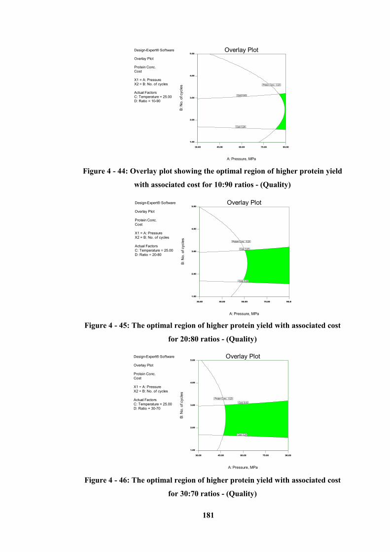
181

Figure 4 - 44: Overlay plot showing the optimal region of higher protein yield

with associated cost for 10:90 ratios - (Quality)

Figure 4 - 45: The optimal region of higher protein yield with associated cost

for 20:80 ratios - (Quality)

Figure 4 - 46: The optimal region of higher protein yield with associated cost

for 30:70 ratios - (Quality)


Overlay Plot

Protein Conc.

Cost

X1 = A: Pressure


Actual Factors


D: Ratio = 10-90

30.00 45.00 60.00 75.00 90.00

1.00

2.00

3.00

4.00

5.00

Overlay Plot

A: Pressure, MPa

B: N

o. o

f cycle

s Protein Conc. : 0.23

Cost: 0.24

Cost: 0.43


Overlay Plot

Protein Conc.

Cost

X1 = A: Pressure


Actual Factors


D: Ratio = 20-80

30.00 45.00 60.00 75.00 90.00

1.00

2.00

3.00

4.00

5.00

Overlay Plot

A: Pressure, MPa

B: N

o. o

f cycle

s

Protein Conc. : 0.23

Cost: 0.24

Cost: 0.43


Overlay Plot

Protein Conc.

Cost

X1 = A: Pressure


Actual Factors


D: Ratio = 30-70

30.00 45.00 60.00 75.00 90.00

1.00

2.00

3.00

4.00

5.00

Overlay Plot

A: Pressure, MPa

B: N

o. o

f cycle

s


Cost: 0.24

Cost: 0.43

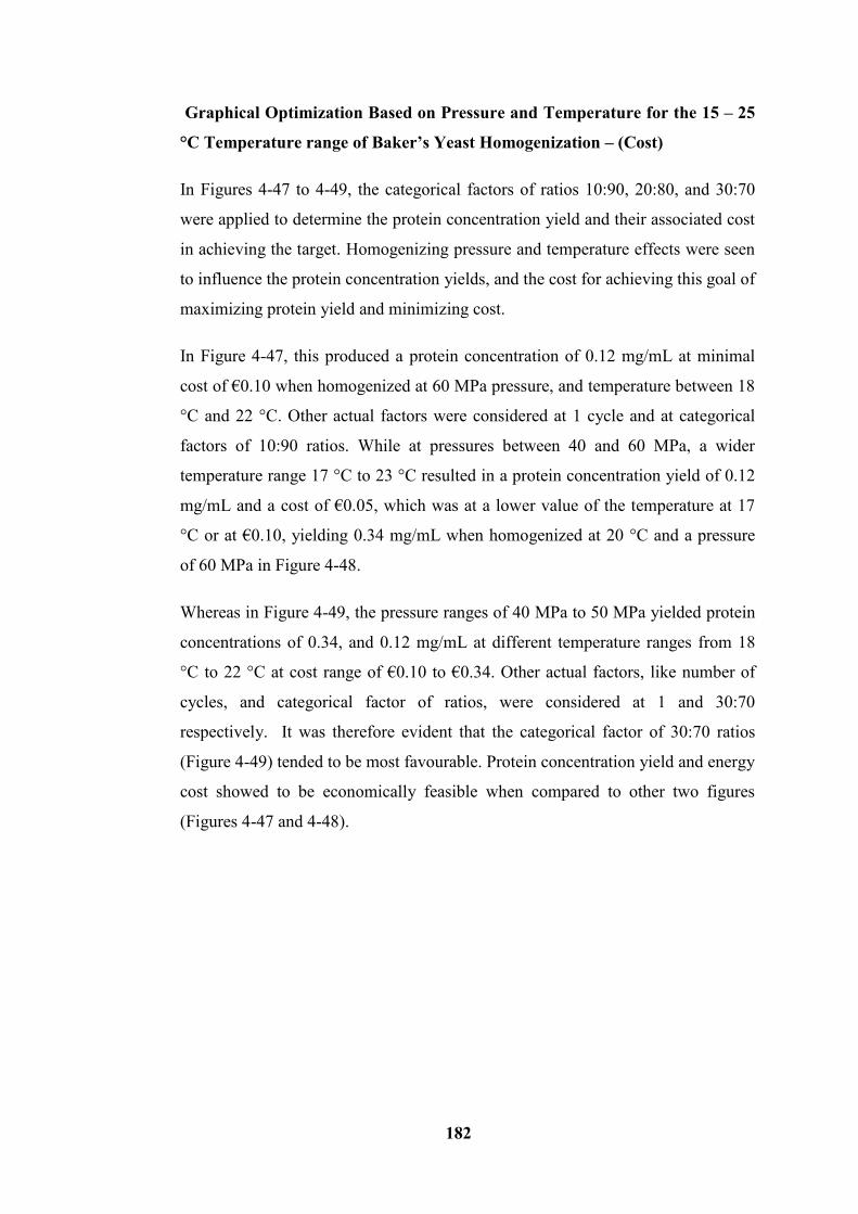
182

Graphical Optimization Based on Pressure and Temperature for the 15 – 25

°C Temperature range of Baker’s Yeast Homogenization – (Cost)

In Figures 4-47 to 4-49, the categorical factors of ratios 10:90, 20:80, and 30:70

were applied to determine the protein concentration yield and their associated cost

in achieving the target. Homogenizing pressure and temperature effects were seen

to influence the protein concentration yields, and the cost for achieving this goal of

maximizing protein yield and minimizing cost.

In Figure 4-47, this produced a protein concentration of 0.12 mg/mL at minimal

cost of €0.10 when homogenized at 60 MPa pressure, and temperature between 18

°C and 22 °C. Other actual factors were considered at 1 cycle and at categorical

factors of 10:90 ratios. While at pressures between 40 and 60 MPa, a wider

temperature range 17 °C to 23 °C resulted in a protein concentration yield of 0.12

mg/mL and a cost of €0.05, which was at a lower value of the temperature at 17

°C or at €0.10, yielding 0.34 mg/mL when homogenized at 20 °C and a pressure

of 60 MPa in Figure 4-48.

Whereas in Figure 4-49, the pressure ranges of 40 MPa to 50 MPa yielded protein

concentrations of 0.34, and 0.12 mg/mL at different temperature ranges from 18

°C to 22 °C at cost range of €0.10 to €0.34. Other actual factors, like number of

cycles, and categorical factor of ratios, were considered at 1 and 30:70

respectively. It was therefore evident that the categorical factor of 30:70 ratios

(Figure 4-49) tended to be most favourable. Protein concentration yield and energy

cost showed to be economically feasible when compared to other two figures

(Figures 4-47 and 4-48).

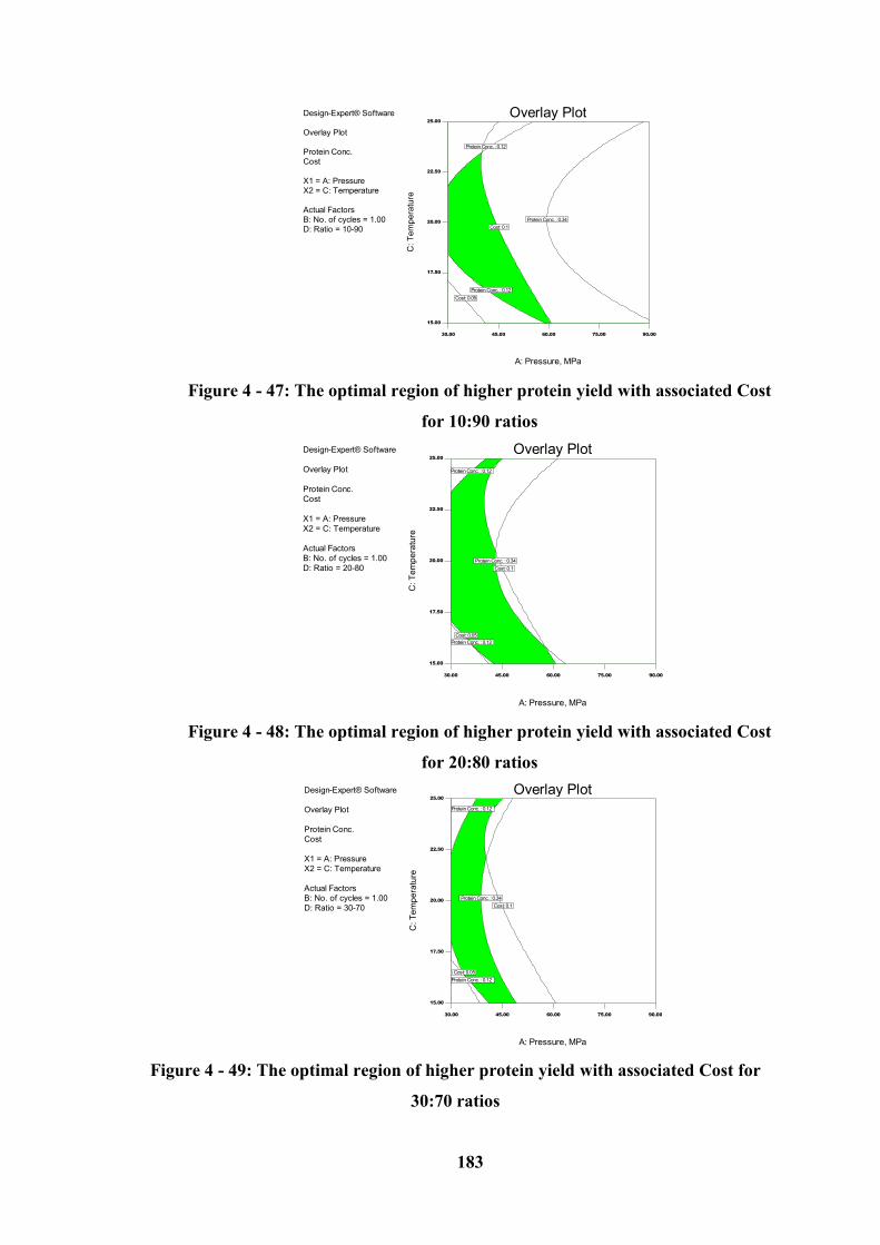
183

Figure 4 - 47: The optimal region of higher protein yield with associated Cost

for 10:90 ratios


for 20:80 ratios


30:70 ratios


Overlay Plot

Protein Conc.

Cost

X1 = A: Pressure

X2 = C: Temperature

Actual Factors


D: Ratio = 10-90

30.00 45.00 60.00 75.00 90.00

15.00

17.50

20.00

22.50

25.00

Overlay Plot

A: Pressure, MPa

C: T

em

pe

ratu

re




Cost: 0.05

Cost: 0.1


Overlay Plot

Protein Conc.

Cost

X1 = A: Pressure

X2 = C: Temperature

Actual Factors


D: Ratio = 20-80

30.00 45.00 60.00 75.00 90.00

15.00

17.50

20.00

22.50

25.00

Overlay Plot

A: Pressure, MPa

C: T

em

pe

ratu

re




Cost: 0.05

Cost: 0.1


Overlay Plot

Protein Conc.

Cost

X1 = A: Pressure

X2 = C: Temperature

Actual Factors


D: Ratio = 30-70

30.00 45.00 60.00 75.00 90.00

15.00

17.50

20.00

22.50

25.00

Overlay Plot

A: Pressure, MPa

C: T

em

pe

ratu

re




Cost: 0.05

Cost: 0.1

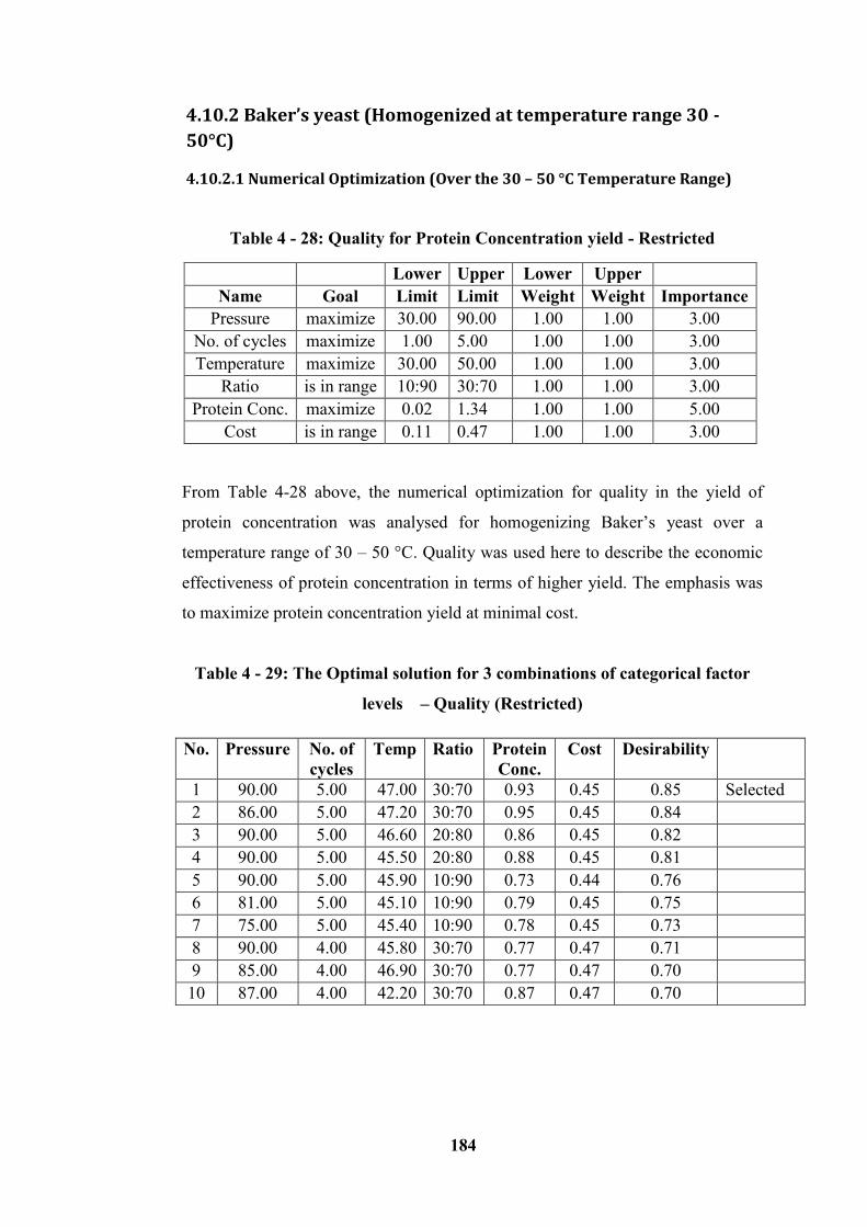
184

4.10.2 Baker’s yeast (Homogenized at temperature range 30 -

50°C)


Table 4 - 28: Quality for Protein Concentration yield - Restricted

Lower Upper Lower Upper

Name Goal Limit Limit Weight Weight Importance

Pressure maximize 30.00 90.00 1.00 1.00 3.00

No. of cycles maximize 1.00 5.00 1.00 1.00 3.00

Temperature maximize 30.00 50.00 1.00 1.00 3.00

Ratio is in range 10:90 30:70 1.00 1.00 3.00

Protein Conc. maximize 0.02 1.34 1.00 1.00 5.00

Cost is in range 0.11 0.47 1.00 1.00 3.00

From Table 4-28 above, the numerical optimization for quality in the yield of

protein concentration was analysed for homogenizing Baker’s yeast over a

temperature range of 30 – 50 °C. Quality was used here to describe the economic

effectiveness of protein concentration in terms of higher yield. The emphasis was

to maximize protein concentration yield at minimal cost.

Table 4 - 29: The Optimal solution for 3 combinations of categorical factor

levels – Quality (Restricted)

No. Pressure No. of

cycles

Temp Ratio Protein

Conc.

Cost Desirability

1 90.00 5.00 47.00 30:70 0.93 0.45 0.85 Selected

2 86.00 5.00 47.20 30:70 0.95 0.45 0.84

3 90.00 5.00 46.60 20:80 0.86 0.45 0.82

4 90.00 5.00 45.50 20:80 0.88 0.45 0.81

5 90.00 5.00 45.90 10:90 0.73 0.44 0.76

6 81.00 5.00 45.10 10:90 0.79 0.45 0.75

7 75.00 5.00 45.40 10:90 0.78 0.45 0.73

8 90.00 4.00 45.80 30:70 0.77 0.47 0.71

9 85.00 4.00 46.90 30:70 0.77 0.47 0.70

10 87.00 4.00 42.20 30:70 0.87 0.47 0.70

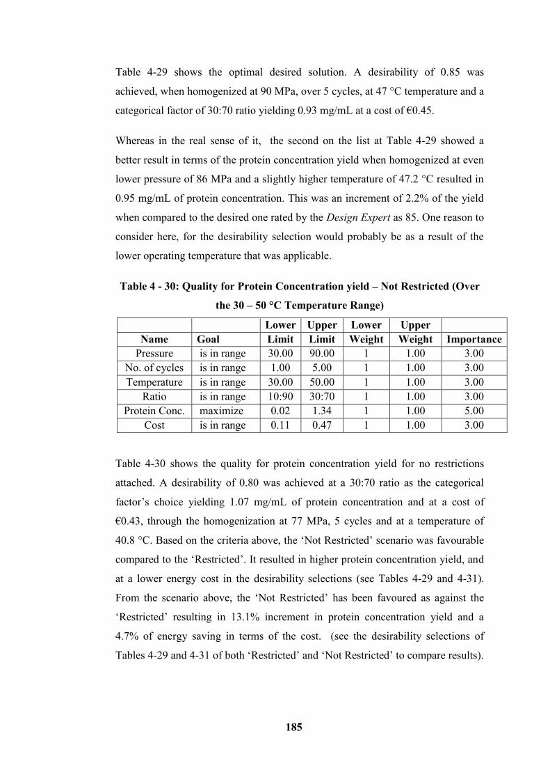
185

Table 4-29 shows the optimal desired solution. A desirability of 0.85 was

achieved, when homogenized at 90 MPa, over 5 cycles, at 47 °C temperature and a

categorical factor of 30:70 ratio yielding 0.93 mg/mL at a cost of €0.45.

Whereas in the real sense of it, the second on the list at Table 4-29 showed a

better result in terms of the protein concentration yield when homogenized at even

lower pressure of 86 MPa and a slightly higher temperature of 47.2 °C resulted in

0.95 mg/mL of protein concentration. This was an increment of 2.2% of the yield

when compared to the desired one rated by the Design Expert as 85. One reason to

consider here, for the desirability selection would probably be as a result of the

lower operating temperature that was applicable.

Table 4 - 30: Quality for Protein Concentration yield – Not Restricted (Over

the 30 – 50 °C Temperature Range)



Pressure is in range 30.00 90.00 1 1.00 3.00

No. of cycles is in range 1.00 5.00 1 1.00 3.00

Temperature is in range 30.00 50.00 1 1.00 3.00

Ratio is in range 10:90 30:70 1 1.00 3.00

Protein Conc. maximize 0.02 1.34 1 1.00 5.00

Cost is in range 0.11 0.47 1 1.00 3.00

Table 4-30 shows the quality for protein concentration yield for no restrictions

attached. A desirability of 0.80 was achieved at a 30:70 ratio as the categorical

factor’s choice yielding 1.07 mg/mL of protein concentration and at a cost of

€0.43, through the homogenization at 77 MPa, 5 cycles and at a temperature of

40.8 °C. Based on the criteria above, the ‘Not Restricted’ scenario was favourable

compared to the ‘Restricted’. It resulted in higher protein concentration yield, and

at a lower energy cost in the desirability selections (see Tables 4-29 and 4-31).

From the scenario above, the ‘Not Restricted’ has been favoured as against the

‘Restricted’ resulting in 13.1% increment in protein concentration yield and a

4.7% of energy saving in terms of the cost. (see the desirability selections of

Tables 4-29 and 4-31 of both ‘Restricted’ and ‘Not Restricted’ to compare results).

186

Table 4 - 31: The Optimal solution for 3 Combinations of Categorical Factor

Level – Quality (Not Restricted)

4.10.2.2 Graphical Optimization (Over the 30 – 50 °C Temperature Range)

The green shaded areas in the overlay Quality plots, Figures 4-50 to 4-53, are the

regions that met the best criteria. These depicted the categorical factors of 10:90,

20:80, and 30:70 ratios as seen in Figures 4-50 to 4-52 respectively while Figure

4-53 was another form of the Figure 4-52, over 30 to 50 °C temperature range.

Figure 4-50 tended to produce a higher yield protein of 0.72 mg/mL, however at

higher pressure and temperature, homogenized in 5 cycles, realistically it would

not be cost effective. The same trend was applicable to the categorical factors of

20:80 ratios; resulting in higher energy cost for the process (see Figure 4-51). At

the 30:70 categorical factor ratio, a protein concentration yield of 0.95 mg/mL was

achieved when homogenized at 5 cycles at an energy cost of €0.47 (Figure 4-52).

Also Figure 4-53 produced an optimal result at a reduced temperature of 40.81 °C

which was in contrast with the temperature applied in Figure 4-52 (46.96 °C). At 2

and 4 cycles a 0.76 mg/mL yield of protein concentration was achieved for €0.16

and €0.44 when homogenized at pressures of 58 and 9 MPa respectively. Figures

4-52 and 4-53 compared favourably when others (Figures 4-50 and 4-51) were

considered.

No. Pressure No. of

cycles Temp. Ratio

Protein


1 77.00 5.00 40.80 30:70 1.07 0.43 0.80 Selected

2 80.00 5.00 40.90 30:70 1.07 0.43 0.80

3 77.00 5.00 42.00 30:70 1.07 0.44 0.80

4 77.00 5.00 41.00 20:80 0.99 0.43 0.74

5 76.00 5.00 42.00 20:80 0.99 0.44 0.73

6 77.00 1.00 41.00 30:70 0.85 0.16 0.63

7 77.00 5.00 41.00 10:90 0.84 0.43 0.62

8 81.00 5.00 41.00 10:90 0.84 0.43 0.62

9 82.00 5.00 38.00 10:90 0.82 0.42 0.60

10 77.00 1.00 41.00 20:80 0.77 0.16 0.57

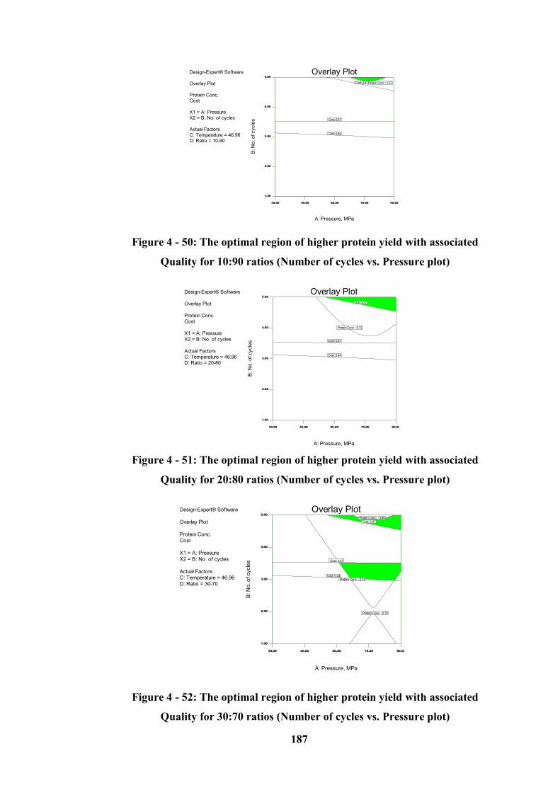
187

Figure 4 - 50: The optimal region of higher protein yield with associated

Quality for 10:90 ratios (Number of cycles vs. Pressure plot)






Overlay Plot

Protein Conc.

Cost

X1 = A: Pressure


Actual Factors


D: Ratio = 10-90

30.00 45.00 60.00 75.00 90.00

1.00

2.00

3.00

4.00

5.00

Overlay Plot

A: Pressure, MPa

B: N

o. o

f cycle

s


Cost: 0.44

Cost: 0.47

Cost: 0.47


Overlay Plot

Protein Conc.

Cost

X1 = A: Pressure


Actual Factors


D: Ratio = 20-80

30.00 45.00 60.00 75.00 90.00

1.00

2.00

3.00

4.00

5.00

Overlay Plot

A: Pressure, MPa

B: N

o. o

f cycle

s


Cost: 0.44

Cost: 0.47

Cost: 0.47


Overlay Plot

Protein Conc.

Cost

X1 = A: Pressure


Actual Factors


D: Ratio = 30-70

30.00 45.00 60.00 75.00 90.00

1.00

2.00

3.00

4.00

5.00

Overlay Plot

A: Pressure, MPa

B: N

o. o

f cycle

s




Cost: 0.44

Cost: 0.47

Cost: 0.47

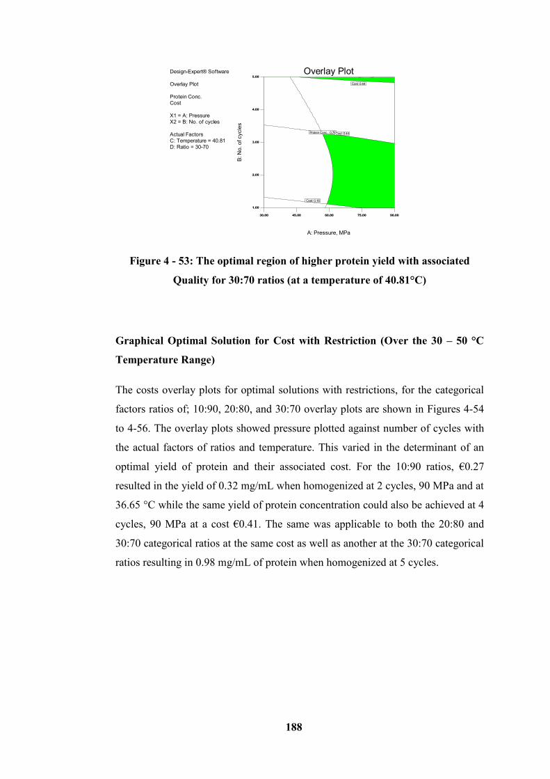
188


Quality for 30:70 ratios (at a temperature of 40.81°C)

Graphical Optimal Solution for Cost with Restriction (Over the 30 – 50 °C

Temperature Range)

The costs overlay plots for optimal solutions with restrictions, for the categorical

factors ratios of; 10:90, 20:80, and 30:70 overlay plots are shown in Figures 4-54

to 4-56. The overlay plots showed pressure plotted against number of cycles with

the actual factors of ratios and temperature. This varied in the determinant of an

optimal yield of protein and their associated cost. For the 10:90 ratios, €0.27

resulted in the yield of 0.32 mg/mL when homogenized at 2 cycles, 90 MPa and at

36.65 °C while the same yield of protein concentration could also be achieved at 4

cycles, 90 MPa at a cost €0.41. The same was applicable to both the 20:80 and

30:70 categorical ratios at the same cost as well as another at the 30:70 categorical

ratios resulting in 0.98 mg/mL of protein when homogenized at 5 cycles.


Overlay Plot

Protein Conc.

Cost

X1 = A: Pressure


Actual Factors


D: Ratio = 30-70

30.00 45.00 60.00 75.00 90.00

1.00

2.00

3.00

4.00

5.00

Overlay Plot

A: Pressure, MPaB

: N

o. o

f cycle

s


Cost: 0.16

Cost: 0.44

Cost: 0.44

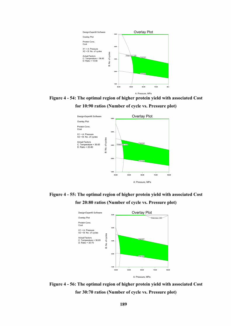
189


for 10:90 ratios (Number of cycle vs. Pressure plot)






Overlay Plot

Protein Conc.

Cost

X1 = A: Pressure


Actual Factors


D: Ratio = 20-80

30.00 45.00 60.00 75.00 90.00

1.00

2.00

3.00

4.00

5.00

Overlay Plot

A: Pressure, MPa

B: N

o. o

f cycle

s


Cost: 0.27

Cost: 0.41


Overlay Plot

Protein Conc.

Cost

X1 = A: Pressure


Actual Factors


D: Ratio = 30-70

30.00 45.00 60.00 75.00 90.00

1.00

2.00

3.00

4.00

5.00

Overlay Plot

A: Pressure, MPa

B: N

o. o

f cycle

s


Cost: 0.27

Cost: 0.41


Overlay Plot

Protein Conc.

Cost

X1 = A: Pressure


Actual Factors


D: Ratio = 10-90

30.00 45.00 60.00 75.00 90.00

1.00

2.00

3.00

4.00

5.00

Overlay Plot

A: Pressure, MPa

B: N

o. o

f cycle

s


Cost: 0.27

Cost: 0.41

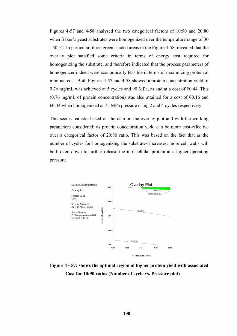
190

Figures 4-57 and 4-58 analysed the two categorical factors of 10:90 and 20:80

when Baker’s yeast substrates were homogenized over the temperature range of 30

- 50 °C. In particular, three green shaded areas in the Figure 4-58, revealed that the

overlay plot satisfied some criteria in terms of energy cost required for

homogenizing the substrate, and therefore indicated that the process parameters of

homogenizer indeed were economically feasible in terms of maximizing protein at

minimal cost. Both Figures 4-57 and 4-58 showed a protein concentration yield of

0.76 mg/mL was achieved at 5 cycles and 90 MPa, as and at a cost of €0.44. This

(0.76 mg/mL of protein concentration) was also attained for a cost of €0.16 and

€0.44 when homogenized at 75 MPa pressure using 2 and 4 cycles respectively.

This seems realistic based on the data on the overlay plot and with the working

parameters considered; as protein concentration yield can be more cost-effective

over a categorical factor of 20:80 ratio. This was based on the fact that as the

number of cycles for homogenizing the substrates increases, more cell walls will

be broken down to further release the intracellular protein at a higher operating

pressure.

Figure 4 - 57: shows the optimal region of higher protein yield with associated

Cost for 10:90 ratios (Number of cycle vs. Pressure plot)


Overlay Plot

Protein Conc.

Cost

X1 = A: Pressure


Actual Factors


D: Ratio = 10-90

30.00 45.00 60.00 75.00 90.00

1.00

2.00

3.00

4.00

5.00

Overlay Plot

A: Pressure, MPa

B: N

o. o

f cycle

s


Cost: 0.16

Cost: 0.44

Cost: 0.44

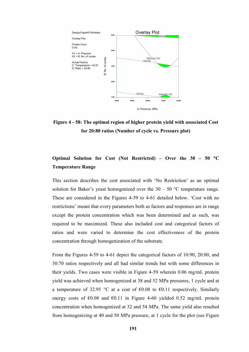
191



Optimal Solution for Cost (Not Restricted) – Over the 30 – 50 °C

Temperature Range

This section describes the cost associated with ‘No Restriction’ as an optimal

solution for Baker’s yeast homogenized over the 30 – 50 °C temperature range.

These are considered in the Figures 4-59 to 4-61 detailed below. ‘Cost with no

restrictions’ meant that every parameters both as factors and responses are in range

except the protein concentration which was been determined and as such, was

required to be maximized. These also included cost and categorical factors of

ratios and were varied to determine the cost effectiveness of the protein

concentration through homogenization of the substrate.

From the Figures 4-59 to 4-61 depict the categorical factors of 10:90, 20:80, and

30:70 ratios respectively and all had similar trends but with some differences in

their yields. Two cases were visible in Figure 4-59 wherein 0.06 mg/mL protein

yield was achieved when homogenized at 38 and 52 MPa pressures, 1 cycle and at

a temperature of 32.95 °C at a cost of €0.08 to €0.11 respectively. Similarly

energy costs of €0.08 and €0.11 in Figure 4-60 yielded 0.52 mg/mL protein

concentration when homogenized at 32 and 54 MPa. The same yield also resulted

from homogenizing at 40 and 50 MPa pressure, at 1 cycle for the plot (see Figure


Overlay Plot

Protein Conc.

Cost

X1 = A: Pressure


Actual Factors


D: Ratio = 20-80

30.00 45.00 60.00 75.00 90.00

1.00

2.00

3.00

4.00

5.00

Overlay Plot

A: Pressure, MPa

B: N

o. o

f cycle

s



Cost: 0.16

Cost: 0.44

Cost: 0.44

192

4-61), resulting in a similar cost. So despite the ratio, if one chose 1 cycle and an

average pressure of around 40 MPa, a maximum yield would be achieved but to

the greatest effect of using 20:80 or 30:70 ratios. That is, an increased dilution

ratio resulting in a higher protein concentration yield and this is in agreement with

work carried out by Diels & Michiels [175] and Save et al. [188].

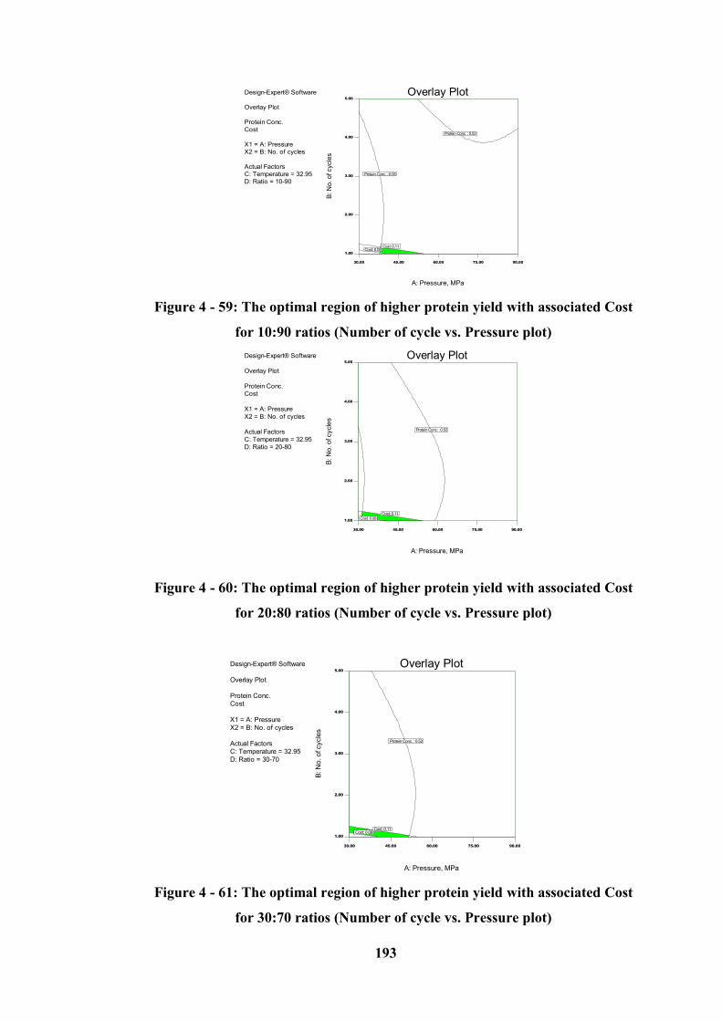
193








Overlay Plot

Protein Conc.

Cost

X1 = A: Pressure


Actual Factors


D: Ratio = 10-90

30.00 45.00 60.00 75.00 90.00

1.00

2.00

3.00

4.00

5.00

Overlay Plot

A: Pressure, MPa

B: N

o. o

f cycle

s



Cost: 0.08Cost: 0.11


Overlay Plot

Protein Conc.

Cost

X1 = A: Pressure


Actual Factors


D: Ratio = 20-80

30.00 45.00 60.00 75.00 90.00

1.00

2.00

3.00

4.00

5.00

Overlay Plot

A: Pressure, MPa

B: N

o. o

f cycle

s


Cost: 0.08

Cost: 0.11


Overlay Plot

Protein Conc.

Cost

X1 = A: Pressure


Actual Factors


D: Ratio = 30-70

30.00 45.00 60.00 75.00 90.00

1.00

2.00

3.00

4.00

5.00

Overlay Plot

A: Pressure, MPa

B: N

o. o

f cycle

s


Cost: 0.08Cost: 0.11

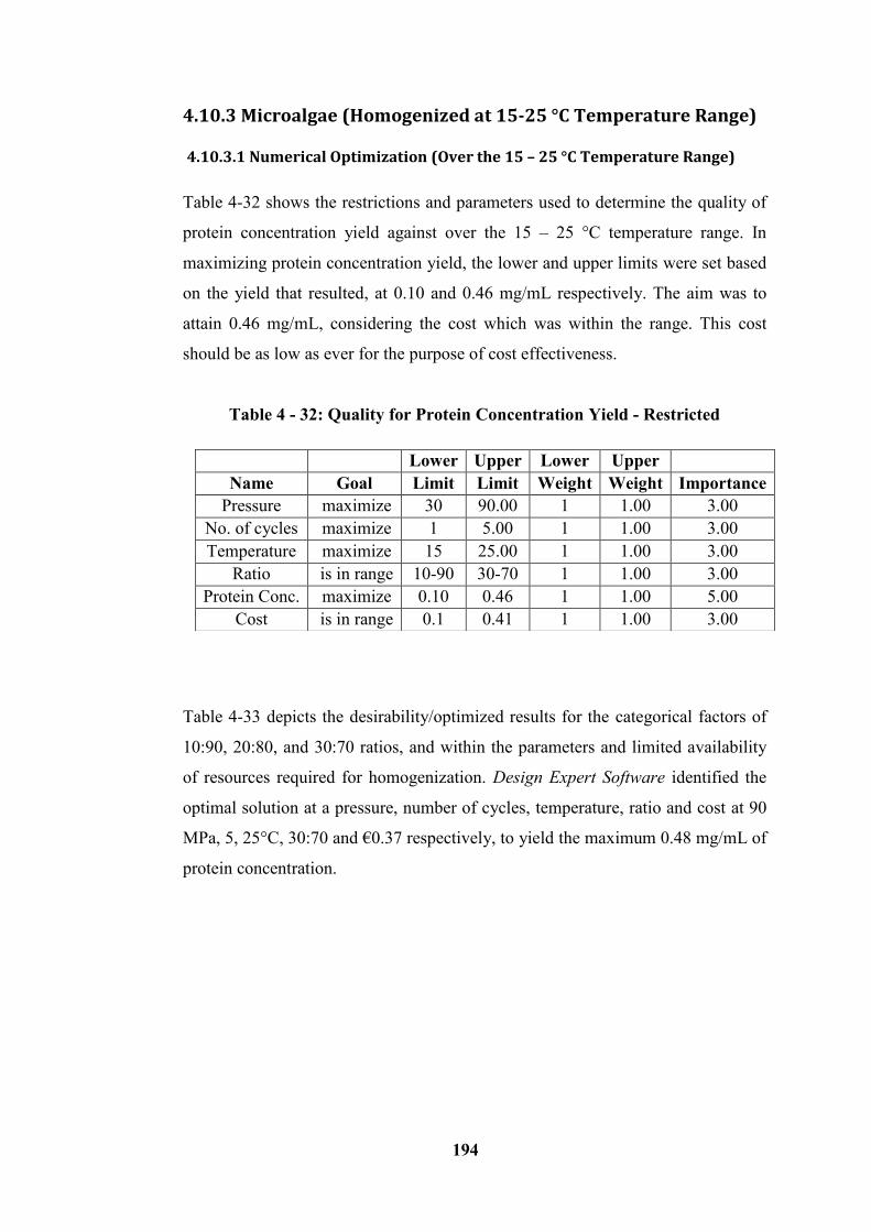
194

4.10.3 Microalgae (Homogenized at 15-25 °C Temperature Range)


Table 4-32 shows the restrictions and parameters used to determine the quality of

protein concentration yield against over the 15 – 25 °C temperature range. In

maximizing protein concentration yield, the lower and upper limits were set based

on the yield that resulted, at 0.10 and 0.46 mg/mL respectively. The aim was to

attain 0.46 mg/mL, considering the cost which was within the range. This cost

should be as low as ever for the purpose of cost effectiveness.

Table 4 - 32: Quality for Protein Concentration Yield - Restricted

Table 4-33 depicts the desirability/optimized results for the categorical factors of

10:90, 20:80, and 30:70 ratios, and within the parameters and limited availability

of resources required for homogenization. Design Expert Software identified the

optimal solution at a pressure, number of cycles, temperature, ratio and cost at 90

MPa, 5, 25°C, 30:70 and €0.37 respectively, to yield the maximum 0.48 mg/mL of

protein concentration.



Pressure maximize 30 90.00 1 1.00 3.00

No. of cycles maximize 1 5.00 1 1.00 3.00

Temperature maximize 15 25.00 1 1.00 3.00

Ratio is in range 10-90 30-70 1 1.00 3.00


Cost is in range 0.1 0.41 1 1.00 3.00

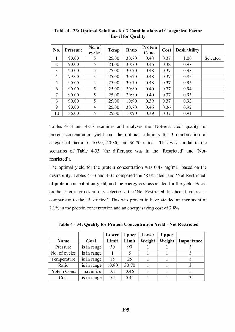
195

Table 4 - 33: Optimal Solutions for 3 Combinations of Categorical Factor

Level for Quality

Tables 4-34 and 4-35 examines and analyses the ‘Not-restricted’ quality for

protein concentration yield and the optimal solutions for 3 combination of

categorical factor of 10:90, 20:80, and 30:70 ratios. This was similar to the

scenarios of Table 4-33 (the difference was in the ‘Restricted’ and ‘Not-

restricted’).

The optimal yield for the protein concentration was 0.47 mg/mL, based on the

desirability. Tables 4-33 and 4-35 compared the ‘Restricted’ and ‘Not Restricted’

of protein concentration yield, and the energy cost associated for the yield. Based

on the criteria for desirability selections, the ‘Not Restricted’ has been favoured in

comparison to the ‘Restricted’. This was proven to have yielded an increment of

2.1% in the protein concentration and an energy saving cost of 2.8%

Table 4 - 34: Quality for Protein Concentration Yield - Not Restricted



Pressure is in range 30 90 1 1 3

No. of cycles is in range 1 5 1 1 3

Temperature is in range 15 25 1 1 3

Ratio is in range 10:90 30:70 1 1 3

Protein Conc. maximize 0.1 0.46 1 1 5

Cost is in range 0.1 0.41 1 1 3

No. Pressure No. of

cycles Temp Ratio

Protein


1 90.00 5 25.00 30:70 0.48 0.37 1.00 Selected

2 90.00 5 24.00 30:70 0.46 0.38 0.98

3 90.00 5 25.00 30:70 0.48 0.37 0.98

4 79.00 5 25.00 30:70 0.48 0.37 0.96

5 90.00 4 25.00 30:70 0.48 0.37 0.95

6 90.00 5 25.00 20:80 0.40 0.37 0.94

7 90.00 5 25.00 20:80 0.40 0.37 0.93

8 90.00 5 25.00 10:90 0.39 0.37 0.92

9 90.00 4 25.00 30:70 0.46 0.36 0.92

10 86.00 5 25.00 10:90 0.39 0.37 0.91

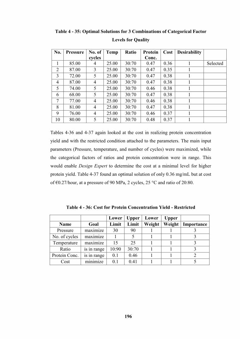
196


Levels for Quality

Tables 4-36 and 4-37 again looked at the cost in realizing protein concentration

yield and with the restricted condition attached to the parameters. The main input

parameters (Pressure, temperature, and number of cycles) were maximized, while

the categorical factors of ratios and protein concentration were in range. This

would enable Design Expert to determine the cost at a minimal level for higher

protein yield. Table 4-37 found an optimal solution of only 0.36 mg/mL but at cost

of €0.27/hour, at a pressure of 90 MPa, 2 cycles, 25 °C and ratio of 20:80.

Table 4 - 36: Cost for Protein Concentration Yield - Restricted



Pressure maximize 30 90 1 1 3

No. of cycles maximize 1 5 1 1 3

Temperature maximize 15 25 1 1 3

Ratio is in range 10:90 30:70 1 1 3

Protein Conc. is in range 0.1 0.46 1 1 2

Cost minimize 0.1 0.41 1 1 5

No. Pressure No. of

cycles

Temp Ratio Protein

Conc.

Cost Desirability

1 85.00 4 25.00 30:70 0.47 0.36 1 Selected

2 87.00 3 25.00 30:70 0.47 0.35 1

3 72.00 5 25.00 30:70 0.47 0.38 1

4 87.00 4 25.00 30:70 0.47 0.38 1

5 74.00 5 25.00 30:70 0.46 0.38 1

6 68.00 5 25.00 30:70 0.47 0.38 1

7 77.00 4 25.00 30:70 0.46 0.38 1

8 81.00 4 25.00 30:70 0.47 0.38 1

9 76.00 4 25.00 30:70 0.46 0.37 1

10 80.00 5 25.00 30:70 0.48 0.37 1

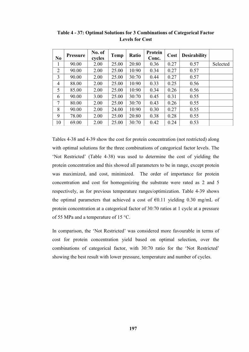
197


Levels for Cost

Tables 4-38 and 4-39 show the cost for protein concentration (not restricted) along

with optimal solutions for the three combinations of categorical factor levels. The

‘Not Restricted’ (Table 4-38) was used to determine the cost of yielding the

protein concentration and this showed all parameters to be in range, except protein

was maximized, and cost, minimized. The order of importance for protein

concentration and cost for homogenizing the substrate were rated as 2 and 5

respectively, as for previous temperature ranges/optimization. Table 4-39 shows

the optimal parameters that achieved a cost of €0.11 yielding 0.30 mg/mL of

protein concentration at a categorical factor of 30:70 ratios at 1 cycle at a pressure

of 55 MPa and a temperature of 15 °C.

In comparison, the ‘Not Restricted’ was considered more favourable in terms of

cost for protein concentration yield based on optimal selection, over the

combinations of categorical factor, with 30:70 ratio for the ‘Not Restricted’

showing the best result with lower pressure, temperature and number of cycles.

No Pressure

No. of

cycles Temp Ratio

Protein


1 90.00 2.00 25.00 20:80 0.36 0.27 0.57 Selected

2 90.00 2.00 25.00 10:90 0.34 0.27 0.57

3 90.00 2.00 25.00 30:70 0.44 0.27 0.57

4 88.00 2.00 25.00 10:90 0.33 0.25 0.56

5 85.00 2.00 25.00 10:90 0.34 0.26 0.56

6 90.00 3.00 25.00 30:70 0.45 0.31 0.55

7 80.00 2.00 25.00 30:70 0.43 0.26 0.55

8 90.00 2.00 24.00 10:90 0.30 0.27 0.55

9 78.00 2.00 25.00 20:80 0.38 0.28 0.55

10 69.00 2.00 25.00 30:70 0.42 0.24 0.53

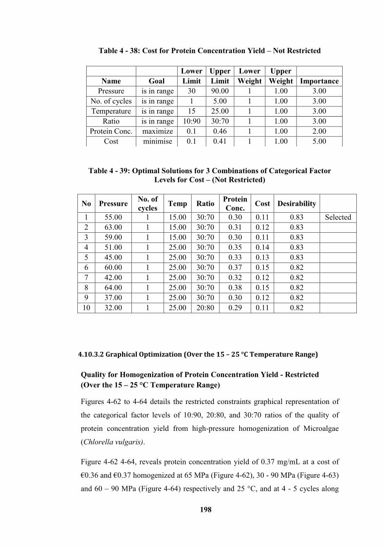
198

Table 4 - 38: Cost for Protein Concentration Yield – Not Restricted


Levels for Cost – (Not Restricted)

4.10.3.2 Graphical Optimization (Over the 15 – 25 °C Temperature Range)

Quality for Homogenization of Protein Concentration Yield - Restricted

(Over the 15 – 25 °C Temperature Range)

Figures 4-62 to 4-64 details the restricted constraints graphical representation of

the categorical factor levels of 10:90, 20:80, and 30:70 ratios of the quality of

protein concentration yield from high-pressure homogenization of Microalgae

(Chlorella vulgaris).

Figure 4-62 4-64, reveals protein concentration yield of 0.37 mg/mL at a cost of

€0.36 and €0.37 homogenized at 65 MPa (Figure 4-62), 30 - 90 MPa (Figure 4-63)

and 60 – 90 MPa (Figure 4-64) respectively and 25 °C, and at 4 - 5 cycles along



Pressure is in range 30 90.00 1 1.00 3.00

No. of cycles is in range 1 5.00 1 1.00 3.00

Temperature is in range 15 25.00 1 1.00 3.00

Ratio is in range 10:90 30:70 1 1.00 3.00


Cost minimise 0.1 0.41 1 1.00 5.00

No Pressure No. of

cycles Temp Ratio

Protein


1 55.00 1 15.00 30:70 0.30 0.11 0.83 Selected

2 63.00 1 15.00 30:70 0.31 0.12 0.83

3 59.00 1 15.00 30:70 0.30 0.11 0.83

4 51.00 1 25.00 30:70 0.35 0.14 0.83

5 45.00 1 25.00 30:70 0.33 0.13 0.83

6 60.00 1 25.00 30:70 0.37 0.15 0.82

7 42.00 1 25.00 30:70 0.32 0.12 0.82

8 64.00 1 25.00 30:70 0.38 0.15 0.82

9 37.00 1 25.00 30:70 0.30 0.12 0.82

10 32.00 1 25.00 20:80 0.29 0.11 0.82

199

with at a categorical factor of 10:90 ratios, 20:80 ratios, and 30:70 ratios

respectively.

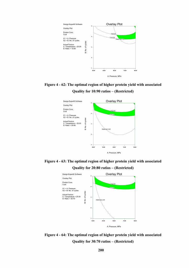
200


Quality for 10:90 ratios – (Restricted)






Overlay Plot

Protein Conc.

Cost

X1 = A: Pressure


Actual Factors


D: Ratio = 10-90

30.00 45.00 60.00 75.00 90.00

1

2

3

4

5

Overlay Plot

A: Pressure, MPa

B: N

o. o

f cycle

s


Cost: 0.36

Cost: 0.37


Overlay Plot

Protein Conc.

Cost

X1 = A: Pressure


Actual Factors


D: Ratio = 20-80

30.00 45.00 60.00 75.00 90.00

1

2

3

4

5

Overlay Plot

A: Pressure, MPa

B: N

o. o

f cycle

s


Cost: 0.36

Cost: 0.37


Overlay Plot

Protein Conc.

Cost

X1 = A: Pressure


Actual Factors


D: Ratio = 30-70

30.00 45.00 60.00 75.00 90.00

1

2

3

4

5

Overlay Plot

A: Pressure, MPa

B: N

o. o

f cycle

s


Cost: 0.36

Cost: 0.37

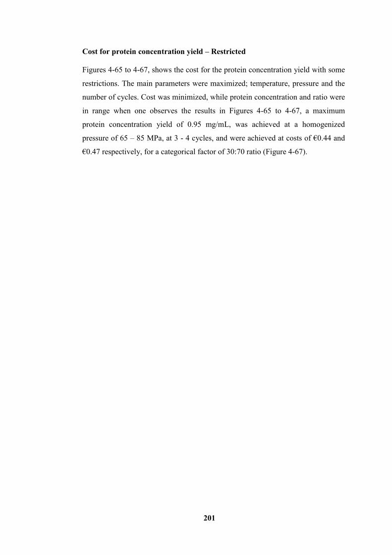
201

Cost for protein concentration yield – Restricted

Figures 4-65 to 4-67, shows the cost for the protein concentration yield with some

restrictions. The main parameters were maximized; temperature, pressure and the

number of cycles. Cost was minimized, while protein concentration and ratio were

in range when one observes the results in Figures 4-65 to 4-67, a maximum

protein concentration yield of 0.95 mg/mL, was achieved at a homogenized

pressure of 65 – 85 MPa, at 3 - 4 cycles, and were achieved at costs of €0.44 and

€0.47 respectively, for a categorical factor of 30:70 ratio (Figure 4-67).

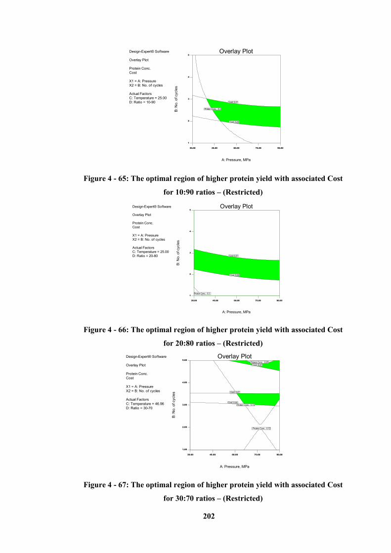
202


for 10:90 ratios – (Restricted)






Overlay Plot

Protein Conc.

Cost

X1 = A: Pressure


Actual Factors


D: Ratio = 10-90

30.00 45.00 60.00 75.00 90.00

1

2

3

4

5

Overlay Plot

A: Pressure, MPa

B: N

o. o

f cycle

s

Protein Conc. : 0.3

Cost: 0.24

Cost: 0.31


Overlay Plot

Protein Conc.

Cost

X1 = A: Pressure


Actual Factors


D: Ratio = 20-80

30.00 45.00 60.00 75.00 90.00

1

2

3

4

5

Overlay Plot

A: Pressure, MPa

B: N

o. o

f cycle

s

Protein Conc. : 0.3

Cost: 0.24

Cost: 0.31


Overlay Plot

Protein Conc.

Cost

X1 = A: Pressure


Actual Factors


D: Ratio = 30-70

30.00 45.00 60.00 75.00 90.00

1.00

2.00

3.00

4.00

5.00

Overlay Plot

A: Pressure, MPa

B: N

o. o

f cycle

s




Cost: 0.44

Cost: 0.47

Cost: 0.47

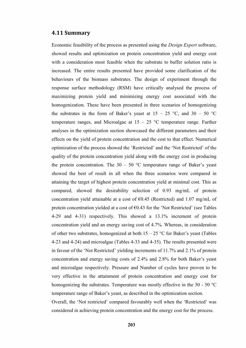
203

4.11 Summary

Economic feasibility of the process as presented using the Design Expert software,

showed results and optimization on protein concentration yield and energy cost

with a consideration most feasible when the substrate to buffer solution ratio is

increased. The entire results presented have provided some clarification of the

behaviours of the biomass substrates. The design of experiment through the

response surface methodology (RSM) have critically analysed the process of

maximizing protein yield and minimizing energy cost associated with the

homogenization. These have been presented in three scenarios of homogenizing

the substrates in the form of Baker’s yeast at 15 – 25 °C, and 30 – 50 °C

temperature ranges, and Microalgae at 15 – 25 °C temperature range. Further

analyses in the optimization section showcased the different parameters and their

effects on the yield of protein concentration and the cost to that effect. Numerical

optimization of the process showed the ‘Restricted’ and the ‘Not Restricted’ of the

quality of the protein concentration yield along with the energy cost in producing

the protein concentration. The 30 – 50 °C temperature range of Baker’s yeast

showed the best of result in all when the three scenarios were compared in

attaining the target of highest protein concentration yield at minimal cost. This as

compared, showed the desirability selection of 0.93 mg/mL of protein

concentration yield attainable at a cost of €0.45 (Restricted) and 1.07 mg/mL of

protein concentration yielded at a cost of €0.43 for the ‘Not Restricted’ (see Tables

4-29 and 4-31) respectively. This showed a 13.1% increment of protein

concentration yield and an energy saving cost of 4.7%. Whereas, in consideration

of other two substrates, homogenized at both 15 – 25 °C for Baker’s yeast (Tables

4-23 and 4-24) and microalgae (Tables 4-33 and 4-35). The results presented were

in favour of the ‘Not Restricted’ yielding increments of 11.7% and 2.1% of protein

concentration and energy saving costs of 2.4% and 2.8% for both Baker’s yeast

and microalgae respectively. Pressure and Number of cycles have proven to be

very effective in the attainment of protein concentration and energy cost for

homogenizing the substrates. Temperature was mostly effective in the 30 - 50 °C

temperature range of Baker’s yeast, as described in the optimization section.

Overall, the ‘Not restricted’ compared favourably well when the ‘Restricted’ was

considered in achieving protein concentration and the energy cost for the process.

204

Chapter 5 Conclusion and Future Work

5.1 Conclusion

In this study, Baker’s yeast (Saccharomyces cerevisiae) and Microalgae (Chlorella

vulgaris) have been thoroughly investigated as biomass substrates through their

use in a high-pressure homogenizer (HPH). A mechanical (cell disruption) pre-

treatment machine was utilized to shear the biomass in the liberation of the inner

contents, particularly protein, whose use has become prominent all over the world

as a feedstock for biogas production. Cell rupture enhanced the recovery of the

biological products, located inside cells; therefore, HPH is one method capable of

rupturing the cells, assuming the ideal optimized conditions are used to extract the

maximum protein concentrations. However the selection of ideal parameters has to

be weighed against cost, as to propose a biomass generation system. The cost of

production should be as low as possible to ensure an overall optimized system.

Thus this study investigated the production of stable emulsions from these

products, using HPH for each of these substrates, and assessed, the protein

concentration yield and its relative cost.

Based on the conducted research, the following conclusions were drawn from the

results obtained in the work and as such, should only be applicable to the

substrates considered:

A high-pressure homogenizer was found to enhance protein concentration

yield of both biomass substrates through the cell rupturing of the cell walls

to release the intracellular components of protein concentration within.

Adequate measurements showed that there was good model discrimination

for all statistical investigations conducted hence, model significance was

achievable.

For both One-Variable-At-a-Time and Design of Experiments (OVAT and

DOE) analysis, within the categorical factors of 10:90, 20:80, and 30:70

205

ratios, 30:70 ratios showed highest yields of protein concentration, and

thus, considered the best ratio for protein concentration output.

The influencing process parameters for high protein yield production (if

cost was not a factor) were the homogenizing pressure and the Number of

cycles. These tend to completely breakdown and disrupt the cell walls of

the substrates to release the entire protein content.

The optimal homogenizing conditions for Baker’s yeast were identified at

a pressure of 90MPa, 5 cycles, and a temperature of 20oC along with

categorical factors of 30:70 ratios yielding a maximum protein

concentration of 1.7694 mg/mL, and a minimum total operating cost of

€0.39/hour for a 15 to 25 oC temperature range of Baker’s yeast

(Saccharomyces cerevisiae) as biomass. This indicates that an increase in

dilution ratio of the substrate led to an increase in protein concentration

yield when homogenized.

Optimization analyses of the economic feasibility of the process through

the associated energy cost in maximizing protein concentration yield were

observed. This showed that optimizing the process, did improve the

maximization of the protein yield at minimal energy cost, (when

homogenized at 90 MPa, 2 cycles, 25 oC and at a categorical factor of

30:70 ratios. This yielded 1.12 mg/mL of protein concentration at a cost of

€0.28/hour). This therefore resulted in protein concentration yield

enhancement of 58% and an energy cost saving of 39.3%.

Results obtained from Chlorella vulgaris compared consistently well with

that from Saccharomyces cerevisiae – an indication that the applied

equipment and software were in good agreement on.

206

5.2 Thesis Contribution

The technique and method developed is applicable to a whole range of

applications. This work can act as a template that helps future researchers

in this related field.

In the conduct of experiments through OVAT and DOE, an approach of

specifying precise ranges proved beneficial. This technique can help future

researchers to build on the developed analysis.

Implementing DOE techniques to optimise the results found after HPH

treatment.

Identifying the most suitable variables as input parameters (Pressure,

Temperature, Number of Cycle and Ratio) along with protein

concentration (mg/mL) and cost (Euro/hr) as output (Responses) through

experimentation.

Identifying the best parameters for optimum yields of intracellular protein

release as an output (response).

Establish the ratios of dilution (substrate against solution C) during

experimental work which as a result, led to the categorical factors being

determined as; 10:90, 20:80 and 30:70 and which was required to identify

and optimize the highest yields from the results. This could be found more

accurately for higher protein concentration yield if the ratio was to be

increased.

Cost determinants as a function and guide towards optimum economic

yield of results of protein concentration.

5.3 Recommendation for Future Work

The following has been recommended as part of future work in addition to this

research;

207

Other biomass substrates like some species of microalga and energy

producing substrates should be considered to verify the use and results of

Saccharomyces cerevisiae/Chlorella vulgaris from HPH.

Other kinds of yeasts such as Brewer’s yeast and genetically engineered

types could be considered also to verify the results from the Baker’s yeast

(Saccharomyces cerevisiae).

Comparison of ultrasonic or autoclaves results to that of the current HPH

result, to determine any difference when set under the same conditions.

Alternative temperature ranges (50 o

C and over) and pressure ranges (90

MPa and over) to determine protein concentration yield and associated

energy cost so as to compare these with the current results.

For future particle size reduction, analysis could be performed by

increasing the range in number of cycles from 1-5 to different number of

cycles (e.g. 1 - 9). This will indicate if there are further deformations or

reduction in size of particles after the 5th

cycle of homogenization.

Particle size distribution using the “Delsa Nano C” (particle size analyser)

may be more accurately found if other techniques such as the Mastersizer

3000 were available.

Consideration of a different categorical factor of ratio, possibly 40:60 or

50:50 as against the current categorical factors of ratios used in this

research; 10:90, 20:80, and 30:70.

Other parameters such as Density, Viscosity and Cell turbidity could be

considered as well, to further determine the yield in protein concentration.

208

References

[1] Omer, A. M., (2008). Energy, environment and sustainable development.

Renewable and Sustainable Energy Reviews, 12, 2265-2300.

[2] Nzila, C., Dewulf, J., Spanjers, H., Kiriamiti, H and Van Langenhove, H.,

(2010). Biowaste energy potential in Kenya, Renewable Energy 35, 2698 –

2704.

[3] Oseni, M. O. (2011). An analysis of the power sector performance in Nigeria.

Renewable and Sustainable Energy Reviews 15(9), 4765-4774.

[4] Nelson, V. (2011). Introduction to renewable energy. CRC Press.

[5] Orr, L. (2006). Changing the world’s energy systems. Available at:

<http://www.energyandcapital.com/articles/trickle-down-enernomics/1488>

(Accessed August, 2015)

[6] United Nation (2013). World Rising Population to Reach 9.6 Billion. Available

at: <https://www.un.org/en/development/desa/news/population/un-report-

world-population-projected-to-reach-9-6-billion-by-2050.html> (Accessed

August, 2015)

[7] World Bank (2012) Available at:

<http://siteresources.worldbank.org/INTURBANDEVELOPMENT/Resources/3

36387-1334852610766/Chap3.pdf > (Accessed August, 2015)

[8] Environmental protection agency EPA (2010). Available at:

<http://www.epa.ie/pubs/reports/indicators/epa_factsheet_waste_v2.pdf>

(Accessed August 2015)

[9] Commission of the European Communities, (2005). Green Paper on Energy

Efficiency. Doing More with Less.com 265 final, Brussels.

[10] EC, (2009). Directive 2009/28/EC of 23 April 2009 on the promotion of the use

of energy from renewable sources. European Commission (EC), Brussels.

Available at: <http://eur-

lex.europa.eu/LexUriServ/LexUriServ.do?uri=OJ:L:2009:140:0016:0062:EN:P

DF> (Accessed August, 2015)

[11] Boerrigter H., Rauch R., (2006). Review of applications of gases from biomass

gasification, ECN Biomass, Coal & Environmental research, Petten,

Netherlands.

http://www.energyandcapital.com/articles/trickle-down-enernomics/1488

https://www.un.org/en/development/desa/news/population/un-report-world-population-projected-to-reach-9-6-billion-by-2050.html

https://www.un.org/en/development/desa/news/population/un-report-world-population-projected-to-reach-9-6-billion-by-2050.html

http://siteresources.worldbank.org/INTURBANDEVELOPMENT/Resources/336387-1334852610766/Chap3.pdf

http://siteresources.worldbank.org/INTURBANDEVELOPMENT/Resources/336387-1334852610766/Chap3.pdf

http://www.epa.ie/pubs/reports/indicators/epa_factsheet_waste_v2.pdf

http://eur-lex.europa.eu/LexUriServ/LexUriServ.do?uri=OJ:L:2009:140:0016:0062:EN:PDF



209

[12] Pueraria, F., Bosio, B., & Heyenb, G. (2014). Energy Efficiency Optimisation in

Different Plant Solutions for Methanol Production from Biomass Gasification.

Chemical Engineering, 37, 301-306 DOI: 10.3303/CET1437051

[13] United Nation Environmental Programme. (2012). Available at:

<http://www.unep.org/gpwm/FocalAreas/WasteAgriculturalBiomass/tabid/5645

6/Default.aspx > (Accessed August, 2015)

[14] Claassen, P. A. M., Van Lier, J. B., Contreras, A. L., Van Niel, E. W. J.,

Sijtsma, L., Stams, A. J. M., ... & Weusthuis, R. A. (1999). Utilisation of

biomass for the supply of energy carriers. Applied microbiology and

biotechnology, 52(6), 741-755.

[15] Field, C. B., Campbell, J. E., & Lobell, D. B. (2008). Biomass energy: the scale

of the potential resource. Trends in ecology & evolution, 23(2), 65-72.

[16] Faaij, A. (2006). Modern biomass conversion technologies. Mitigation and

adaptation strategies for global change, 11(2), 335-367.

[17] Mosier, N., Wyman, C., Dale, B., Elander, R., Lee, Y. Y., Holtzapple, M., &

Ladisch, M. (2005). Features of promising technologies for pretreatment of

lignocellulosic biomass. Bioresource technology, 96(6), 673-686.

[18] Divya, D., Gopinath, L. R., & Christy, P.M.(2015). A review on current aspects

and diverse prospects for enhancing biogas production in sustainable means.

Renewable and Sustainable Energy Reviews, 42, 690-699.

[19] Ward, A. J., Hobbs, P. J., Holliman, P. J., & Jones, D. L. (2008). Optimisation

of the anaerobic digestion of agricultural resources. Bioresource technology,

99(17), 7928-7940.

[20] Demirbas, A. (2000). Biomass resources for energy and chemical industry.

Energy Edu. Sci. Technol, 5(1), 21-45.

[21] Duku, M. H., Gu, S., & Hagan, E. B. (2011). A comprehensive review of

biomass resources and biofuels potential in Ghana. Renewable and Sustainable

Energy Reviews, 15(1), 404-415.

[22] Bioenergy, I. E. A. (2009). Bioenergy–a sustainable and reliable energy source.

International Energy Agency Bioenergy, Paris, France.

[23] Kaygusuz, K., & Keleş, S. (2012). Sustainable bioenergy policies in Turkey.

Journal of Engineering Research and Applied Science, 1(1), 34-43.

[24] Lee, J. (1997). Biological conversion of lignocellulosic biomass to ethanol.

Journal of biotechnology, 56(1), 1-24.

http://www.unep.org/gpwm/FocalAreas/WasteAgriculturalBiomass/tabid/56456/Default.aspx

http://www.unep.org/gpwm/FocalAreas/WasteAgriculturalBiomass/tabid/56456/Default.aspx

210

[25] Fengel, D., Wegener, G., (1984). Wood: Chemistry, Ultrastructure, Reactions.

De Gruyter, Berlin

[26] McKendry, P. (2002). Energy production from biomass (part 2): conversion

technologies. Bioresource technology, 83(1), 47-54.

[27] Hayes, D. J., Fitzpatrick, S., Hayes, M. H., & Ross, J. R. (2006). The Biofine

Process: Production of levulinic acid. furfural and formic acid from

lignocellulosic feedstocks. Biorefineries–Industrial Processes and Product, 1,

139-164.

[28] Balat, M., Balat, H., & Öz, C. (2008). Progress in bioethanol processing.

Progress in energy and combustion science, 34(5), 551-573.

[29] Hendriks, A. T. W. M., & Zeeman, G. (2009). Pretreatments to enhance the

digestibility of lignocellulosic biomass. Bioresource technology, 100(1), 10-18.

[30] Puri, V. P. (1984). Effect of crystallinity and degree of polymerization of

cellulose on enzymatic saccharification. Biotechnology and Bioengineering,

26(10), 1219-1222.

[31] Taherzadeh, M. J., & Karimi, K. (2008). Pretreatment of lignocellulosic wastes

to improve ethanol and biogas production: a review. International journal of

molecular sciences, 9(9), 1621-1651.

[32] Ariunbaatar, J., Panico, A., Esposito, G., Pirozzi, F., & Lens, P. N. (2014).

Pretreatment methods to enhance anaerobic digestion of organic solid waste.

Applied Energy, 123, 143-156.

[33] Carrère, H., Dumas, C., Battimelli, A., Batstone, D. J., Delgenès, J. P., Steyer, J.

P., & Ferrer, I. (2010). Pretreatment methods to improve sludge anaerobic

degradability: a review. Journal of hazardous materials, 183(1), 1-15.

[34] Mata-Alvarez J, Mace S, Llabres P. (2000)Anaerobic digestion of organic solid

wastes. An overview of research achievements and perspectives. Bioresour

Technol; 74:3–16

[35] Engelhart M, Kruger M, Kopp J, Dichtl N. (2000).Effects of disintegration on

anaerobic degradation of sewage excess sludge in down-flow stationary fixed

film digesters. Water Sci Technol 41:171–9.

[36] Chisti, Y., & Moo-Young, M. (1986). Disruption of microbial cells for

intracellular products. Enzyme and Microbial Technology, 8(4), 194-204.

211

[37] Follows, M., Hetherington, P. J., Dunnill, P., & Lilly, M. D. (1971). Release of

enzymes from bakers' yeast by disruption in an industrial homogenizer.

Biotechnology and bioengineering, 13(4), 549-560.

[38] Doulah, M. S., Hammond, T. H., & Brookman, J. S. G. (1975). A hydrodynamic

mechanism for the disintegration of Saccharomyces cerevisiae in an industrial

homogenizer. Biotechnology and Bioengineering, 17(6), 845-858.

[39] Brookman, G., & James, S. (1974). Mechanism of cell disintegration in a high

pressure homogenizer. Biotechnology and Bioengineering, 16(3), 371-383.

[40] Geciova, J., Bury, D., & Jelen, P. (2002). Methods for disruption of microbial

cells for potential use in the dairy industry—a review. International Dairy

Journal, 12(6), 541-553.

[41] Peternel, Š. (2013). Bacterial cell disruption: a crucial step in protein production.

New biotechnology, 30(2), 250-254.

[42] Asif, M., & Muneer, T. (2007). Energy supply, its demand and security issues

for developed and emerging economies. Renewable and Sustainable Energy

Reviews, 11(7), 1388-1413.

[43] Hall, C., Tharakan, P., Hallock, J., Cleveland, C., & Jefferson, M. (2003).

Hydrocarbons and the evolution of human culture. Nature, 426(6964), 318-322.

[44] Tainter, J. (1990). The collapse of complex societies. Cambridge University

Press.

[45] Wilkinson, P., Smith, K. R., Joffe, M., & Haines, A. (2007). A global

perspective on energy: health effects and injustices. The Lancet, 370(9591),

965-978.

[46] Yergin, D. (2006). Ensuring energy security. Foreign affairs, 69-82.

[47] Bang, G. (2010). Energy security and climate change concerns: Triggers for

energy policy change in the United States?. Energy Policy, 38(4), 1645-1653.

[48] Bielecki, J. (2002). Energy security: is the wolf at the door?. The quarterly

review of economics and finance, 42(2), 235-250.

[49] Von Hippel, D., Suzuki, T., Williams, J. H., Savage, T., & Hayes, P. (2011).

Energy security and sustainability in Northeast Asia. Energy Policy, 39(11),

6719-6730.

[50] Grubler, A., & Cleveland, C. J. (2008). Energy transitions. Encyclopedia of

Earth.

212

[51] Fouquet, R., (2009). A brief history of energy. In: Evans, J., Hunt, L.C. (Eds.),

International Handbook of the Economics of Energy. Edward Elgar Publica-

tions, Cheltenham, UK, and Northampton, MA, USA.

[52] Saxena, R. C., Adhikari, D. K., & Goyal, H. B. (2009). Biomass-based energy

fuel through biochemical routes: A review. Renewable and Sustainable Energy

Reviews, 13(1), 167-178.

[53] Bridgwater, A. V., Meier, D., & Radlein, D. (1999). An overview of fast

pyrolysis of biomass. Organic Geochemistry, 30(12), 1479-1493.

[54] Bridgwater, A. V. (1999). Principles and practice of biomass fast pyrolysis

processes for liquids. Journal of analytical and applied pyrolysis, 51(1), 3-22.

[55] Balat, M. (2005). Use of biomass sources for energy in Turkey and a view to

biomass potential. Biomass and Bioenergy, 29(1), 32-41.

[56] Özbay, N., Pütün, A. E., Uzun, B. B., & Pütün, E. (2001). Biocrude from

biomass: pyrolysis of cottonseed cake. Renewable Energy, 24(3), 615-625.

[57] Demirbaş, A. (2001). Biomass resource facilities and biomass conversion

processing for fuels and chemicals. Energy conversion and Management,

42(11), 1357-1378.

[58] Sheth, P. N., & Babu, B. V. (2009). Experimental studies on producer gas

generation from wood waste in a downdraft biomass gasifier. Bioresource

Technology, 100(12), 3127-3133.

[59] Balat, M. (2006). Biomass energy and biochemical conversion processing for

fuels and chemicals. Energy Sources, Part A, 28(6), 517-525.

[60] Wolin, M. J., Miller, T. L., & Stewart, C. S. (1997). Microbe-microbe

interactions. In The rumen microbial ecosystem (pp. 467-491). Springer

Netherlands.

[61] Cauvain, S. P., & Young, L. S. (2007). Technology of breadmaking. Springer.

[62] Dziezak, J. D. (1987). Yeasts and yeast derivatives: definitions, characteristics,

and processing. Food technology (USA).

[63] Halász, A., & Lásztity, R. (1990). Use of yeast biomass in food production.

CRC Press.

[64] Alais, C., & Linden, G. (1991). Food biochemistry. Ellis Horwood Ltd.

[65] Reed, G., & Nagodawithana, T. W. (1991). Yeast technology. 2nd

ed. New York:

Van Nostrand Reinhold; pp. 416.

213

[66] Russell, I., Jones, R., & Stewart, G. G. (1987). Yeast--the primary industrial

microorganism. Biological research on industrial yeasts/editors, Graham G.

Stewart, Russell I, Klein RD and Hiebsch RR, CRC Press, Boca Raton, FL, pp

2-20

[67] Evangelista J. (1989). Tecnologia de Alimentos, 2nd edn, Livraria Atheneu

Editora, Rio de Janeiro

[68] Fukuda, H., Kondo, A., & Tamalampudi, S. (2009). Bioenergy: Sustainable

fuels from biomass by yeast and fungal whole-cell biocatalysts. Biochemical

Engineering Journal, 44(1), 2-12.

[69] Beudeker, R. F., Van Dam, H. W., Van der Plaat, J. B., & Vellenga, K. (1990).

Developments in baker’s yeast production. Yeast biotechnology and

biocatalysis, 103-146.

[70] Phaff, H. J., & Macmillan, J. D. (1978). Yeasts: Description of various genera

and species of special interest. CRC Handbook of Microbiology, 295.

[71] Reed, G., & Peppler, H. J. (1973). Yeast technology.

[72] Clackmannanshire, S. (1979). S. Burrows. Microbial biomass, 4, 31.

[73] Northcote, D. H., & Horne, R. W. (1952). The chemical composition and

structure of the yeast cell wall. Biochemical Journal, 51(2), 232.

[74] Zechmeister, L., & Tóth, G. (1936). Einwirkung von flüssigem Ammoniak auf

Octaacetyl‐cellobiose. Justus Liebigs Annalen der Chemie, 525(1), 14-24.

[75] Haworth, W. N., & Hirst, E. L. (1937). F. A. Isherwood. J. Chem. Soc, 784.

[76] Ling, A R., Nanji, R. D. & Panton, F. J. (1925). J. Inst. Brew. 31, 316.

[77] Yeast cell wall structure. Available online at:

<http://bilingualbiology10.blogspot.ie/2010/11/kingdom-fungi.html> (Accessed

August, 2015)

[78] Lancashing, W. E. (1986). Modern genetics and brewing technology. B rew2 er,

72, 345.

[79] Engler, C. R. (1985). Disruption of microbial cells in comprehensive

biotechnology. In M. Moo-Young, & C.L. Cooney (Eds.), Vol. 2 (pp. 305–324).

UK: Pergamon.

[80] Yeast internal structure. Available online at:

<http://www.allaboutfeed.net/Special-focus/Yeast-Special/Application-of-yeast-

cell-wall-in-swine/> (Accessed August, 2015)

http://bilingualbiology10.blogspot.ie/2010/11/kingdom-fungi.html

http://www.allaboutfeed.net/Special-focus/Yeast-Special/Application-of-yeast-cell-wall-in-swine/%3e%20(Accessed

http://www.allaboutfeed.net/Special-focus/Yeast-Special/Application-of-yeast-cell-wall-in-swine/%3e%20(Accessed

214

[81] Dunahay, T., Benemann, J., & Roessler, P. (1998). A look back at the US

Department of Energy's aquatic species program: biodiesel from algae (Vol.

328). Golden: National Renewable Energy Laboratory.

[82] Oswald, W. J., & Golueke, C. G. (1960). Biological transformation of solar

energy. Advances in applied microbiology, 2, 223-262.

[83] Benemann, J. R., Weissman, J. C., Koopman, B. L., & Oswald, W. J. (1977).

Energy production by microbial photosynthesis. Nature, 268 (5615), 19-23.

[84] Pittman, J. K., Dean, A. P., & Osundeko, O. (2011). The potential of sustainable

algal biofuel production using wastewater resources. Bioresource Technology,

102(1), 17-25.

[85] Brennan, L., & Owende, P. (2010). Biofuels from Microalgae—a review of

technologies for production, processing, and extractions of biofuels and co-

products. Renewable and sustainable energy reviews, 14(2), 557-577.

[86] Brune, D. E., Lundquist, T. J., & Benemann, J. R. (2009). Microalgal biomass

for greenhouse gas reductions: potential for replacement of fossil fuels and

animal feeds. Journal of Environmental Engineering, 135(11), 1136-1144.

[87] Pulz, O., Scheibenbogen, K., & Groß, W. (2008). Biotechnology with

cyanobacteria and Microalgae. Biotechnology Set, Second Edition, 105-136.

[88] Jørgensen, P. J. (2009). Biogas-Green Energy: Process, Design, Energy Supply,

Environment. Researcher for a Day.

[89] Balsari, P., Bonfanti, P., Bozza, E., & Sangiorgi, F. 14–20 August 1983.

Evaluation of the influence of animal feeding on the performances of a biogas

installation (mathematical model). In Third International Symposium on

Anaerobic Digestion. Boston, MA, USA, A (Vol. 20, p. 7).

[90] Amon, T., Kryvoruchko, V., Amon, B., Moitzi, G., Lyson, D., Hackl, E., ... &

Pötsch, E. (2003). Optimierung der Biogaserzeugung aus den Energiepflanzen

Mais und Kleegras. Endbericht Juli.

[91] Weiland, P. (2010). Biogas production: current state and perspectives. Applied

microbiology and biotechnology, 85(4), 849-860.

[92] Amon, T., Amon, B., Kryvoruchko, V., Zollitsch, W., Mayer, K., & Gruber, L.

(2007). Biogas production from maize and dairy cattle manure—influence of

biomass composition on the methane yield. Agriculture, Ecosystems &

Environment, 118(1), 173-182.

215

[93] Pöschl, M., Ward, S., & Owende, P. (2010). Evaluation of energy efficiency of

various biogas production and utilization pathways. Applied Energy, 87(11),

3305-3321.

[94] Sialve, B., Bernet, N., & Bernard, O. (2009). Anaerobic digestion of Microalgae

as a necessary step to make microalgal biodiesel sustainable. Biotechnology

advances, 27(4), 409-416.

[95] Oslaj, M., Mursec, B., & Vindis, P. (2010). Biogas production from maize

hybrids. Biomass and bioenergy, 34(11), 1538-1545.

[96] Amon, T., Kryvoruchko, V., Amon, B., Buga, S., Amin, A., Zollitsch, W.,

Mayer, K., Pötsch, E., 2004a. Biogaserträge aus landwirtschaftlichen Gärgütern.

In: BAL Gumpenstein, BMLFUW (Ed.) BAL-Bericht über das 10.

Alpenländische Expertenforum zum Thema Biogasproduktion— Alternative

Biomassenutzung und Energiegewinnung in der Landwirtschaft am 18–19 März

2004. ISBN 3-901980-72-5, pp. 21–26. <http://www.nas.boku.ac.at/4536.html>


[97] Chandra, R., Takeuchi, H., & Hasegawa, T. (2012). Methane production from

lignocellulosic agricultural crop wastes: A review in context to second

generation of biofuel production. Renewable and Sustainable Energy Reviews,

16(3), 1462-1476.

[98] Nasseri, A. T., Rasoul-Amini, S., Morowvat, M. H., & Ghasemi, Y. (2011).

Single cell protein: production and process. American Journal of food

technology, 6(2), 103-116.

[99] Heredia-Arroyo, T., Wei, W., & Hu, B. (2010). Oil accumulation via

heterotrophic/mixotrophic Chlorella protothecoides. Applied biochemistry and

biotechnology, 162(7), 1978-1995.

[100] Rasoul-Amini, S., Ghasemi, Y., Morowvat, M. H., & Mohagheghzadeh, A.

(2009). PCR amplification of 18S rRNA, single cell protein production and fatty

acid evaluation of some naturally isolated Microalgae. Food Chemistry, 116(1),

129-136.

[101] Kim, J. K., Tak, K. T., & Moon, J. H. (1998). A continuous fermentation of

Kluyveromyces fragilis for the production of a highly nutritious protein diet.

Aquacultural engineering, 18(1), 41-49.

http://www.nas.boku.ac.at/4536.html

216

[102] Coutteau, P., Lavens, P., & Sorgeloos, P. (1990). Baker's yeast as a potential

substitute for live algae in aquaculture diets: Artemia as a case study. Journal of

the World Aquaculture Society, 21(1), 1-9.

[103] Cizik (2014). Utilization and properties of biogas/ Renewable alternative.

<http://www.renewable-alternative.com/2014/03/utilization-and-properties-of-

biogas.html > (Accessed August, 2015).

[104] Biogas Basics (2014). Available at:

<https://energypedia.info/wiki/Biogas_Basics> (Accessed August, 2015)

[105] Schaffner, G., & Matile, P. (1981). Structure and composition of baker’s yeast

lipid globules. Biochemie Und Physiologie Der Pflanzen, 176(7), 659-666.

[106] Zweytick, D., Athenstaedt, K., & Daum, G. (2000). Intracellular lipid particles

of eukaryotic cells. Biochimica et Biophysica Acta (BBA)-Reviews on

Biomembranes, 1469(2), 101-120.

[107] Leber, R., Zinser, E., Paltauf, F., Daum, G., & Zellnig, G. (1994).

Characterization of lipid particles of the yeast, Saccharomyces cerevisiae. Yeast,

10(11), 1421-1428.

[108] Brown, M. R., Jeffrey, S. W., Volkman, J. K., & Dunstan, G. A. (1997).

Nutritional properties of Microalgae for mariculture. Aquaculture, 151(1), 315-

331.

[109] Becker, W. (2004). 18 Microalgae in Human and Animal Nutrition. Handbook

of microalgal culture: biotechnology and applied phycology, 312.

[110] Becker, E. W. (1988). Micro-algae for human and animal consumption.

[111] Soletto, D., Binaghi, L., Lodi, A., Carvalho, J. C. M., & Converti, A. (2005).

Batch and fed-batch cultivations of Spirulina platensis using ammonium

sulphate and urea as nitrogen sources. Aquaculture, 243(1), 217-224.

[112] Hatti-Kaul, R., & Mattiasson, B. (2003). Release of protein from biological host.

Isolation and purification of proteins. CRC Press, Boca Raton, 1-28.

[113] Porro, D., Sauer, M., Branduardi, P., & Mattanovich, D. (2005). Recombinant

protein production in yeasts. Molecular biotechnology, 31(3), 245-259.

[114] Klinke, H. B., Thomsen, A. B., & Ahring, B. K. (2004). Inhibition of ethanol-

producing yeast and bacteria by degradation products produced during pre-

treatment of biomass. Applied microbiology and biotechnology, 66(1), 10-26.

http://www.renewable-alternative.com/2014/03/utilization-and-properties-of-biogas.html

http://www.renewable-alternative.com/2014/03/utilization-and-properties-of-biogas.html

https://energypedia.info/wiki/Biogas_Basics

217

[115] Laureano-Perez, L., Teymouri, F., Alizadeh, H., & Dale, B. E. (2005).

Understanding factors that limit enzymatic hydrolysis of biomass. Applied

Biochemistry and Biotechnology, 124(1-3), 1081-1099.

[116] Agbor, V. B., Cicek, N., Sparling, R., Berlin, A., & Levin, D. B. (2011).

Biomass pretreatment: fundamentals toward application. Biotechnology

advances, 29(6), 675-685.

[117] Arduengo, P.M. (2010) Sloppy technicians and the progress of science.

Promega Connections http://promega.wordpress.com/2010/03/15/sloppy-

technicians (Accessed August, 2015)

[118] Kumar, P., Barrett, D. M., Delwiche, M. J., & Stroeve, P. (2009). Methods for

pretreatment of lignocellulosic biomass for efficient hydrolysis and biofuel

production. Industrial & Engineering Chemistry Research, 48(8), 3713-3729

[119] Palmowski, L., & Miller, J. (2000). Influence of the size reduction of organic

waste on their anaerobic digestion. Water science and technology, 41(3), 155-

162.

[120] Sun, Y., & Cheng, J. (2002). Hydrolysis of lignocellulosic materials for ethanol

production: a review. Bioresource technology, 83(1), 1-11.

[121] Ball milling. Available at: <http://www.understandingnano.com/nanomaterial-

synthesis-ball-milling.html> (Accessed August, 2015)

[122] Alvira, P., Tomás-Pejó, E., Ballesteros, M., & Negro, M. J. (2010). Pretreatment

technologies for an efficient bioethanol production process based on enzymatic

hydrolysis: a review. Bioresource technology, 101(13), 4851-4861.

[123] Novarino, D., & Zanetti, M. C. (2012). Anaerobic digestion of extruded

OFMSW. Bioresource technology, 104: 44-50.

[124] Tyagi, V. K., & Lo, S. L. (2011). Application of physico-chemical pretreatment

methods to enhance the sludge disintegration and subsequent anaerobic

digestion: an up to date review. Reviews in Environmental Science and

Bio/Technology, 10(3), 215-242.

[125] Wang, F., Wang, Y., & Ji, M. (2005). Mechanisms and kinetics models for

ultrasonic waste activated sludge disintegration. Journal of Hazardous

Materials, 123(1), 145-150.

[126] Benabdallah El-Hadj, T., Dosta, J., Marquez-Serrano, R., & Mata-Alvarez, J.

(2007). Effect of ultrasound pretreatment in mesophilic and thermophilic

http://promega.wordpress.com/2010/03/15/sloppy-technicians

http://promega.wordpress.com/2010/03/15/sloppy-technicians

http://www.understandingnano.com/nanomaterial-synthesis-ball-milling.html

http://www.understandingnano.com/nanomaterial-synthesis-ball-milling.html

218

anaerobic digestion with emphasis on naphthalene and pyrene removal. Water

research, 41(1), 87-94.

[127] Tiehm, A., Nickel, K., Zellhorn, M., & Neis, U. (2001). Ultrasonic waste

activated sludge disintegration for improving anaerobic stabilization. Water

Research, 35(8), 2003-2009.

[128] Xie, X., Mikkelsen, T. S., Gnirke, A., Lindblad-Toh, K., Kellis, M., & Lander,

E. S. (2007). Systematic discovery of regulatory motifs in conserved regions of

the human genome, including thousands of CTCF insulator sites. Proceedings of

the National Academy of Sciences, 104(17), 7145-7150.

[129] Nieves-Soto, M., Hernández-Calderón, O. M., Guerrero-Fajardo, C. A.,

Sánchez-Castillo, M. A., Viveros-García, T., & Contreras-Andrade, I. (2012).

Biodiesel Current Technology: Ultrasonic Process a Realistic Industrial

Application.

[130] Lysis-centrifuge. Available at: <http://www.stowa-

selectedtechnologies.nl/Sheets/Sheets/Baker.Process..Lysate.Thickening.Centrif

uge.html#centrifuge > (Accessed August, 2015)

[131] Dohányos, M., Zábranská, J., & Jenícek, P. (1997). Enhancement of sludge

anaerobic digestion by using of a special thickening centrifuge. Water Science

and Technology, 36(11), 145-153.

[132] Zabranska, J., Dohanyos, M., Jenicek, P., Kutil, J., & Cejka, J. (2006, May).

Mechanical and rapid thermal disintegration methods of enhancement of biogas

production—full-scale applications. In Proceedings of the IWA specialized

conference on sustainable sludge management: state-of-the-art, challenges and

perspectives, Moscow, Russia, May (pp. 29-31)

[133] Nah, I. W., Kang, Y. W., Hwang, K. Y., & Song, W. K. (2000). Mechanical

pretreatment of waste activated sludge for anaerobic digestion process. Water

research, 34(8), 2362-2368.

[134] Elliott, A., & Mahmood, T. (2007). Pretreatment technologies for advancing

anaerobic digestion of pulp and paper biotreatment residues. Water research,

41(19), 4273-4286.

[135] Hollander beater machine. Available online at: < www.thefiberwire.com >


[136] Barbir, F. (2009). Transition to renewable energy systems with hydrogen as an

energy carrier. Energy 34 308-12.

http://www.stowa-selectedtechnologies.nl/Sheets/Sheets/Baker.Process..Lysate.Thickening.Centrifuge.html#centrifuge



http://www.thefiberwire.com/

219

[137] De Boer, K., Moheimani, N. R., Borowitzka M.A. & Bahri. P.A. (2012).

Extraction and conversion pathways for Microalgae to biodiesel: a review

focused on energy consumption. J. Appl Phycol

[138] Ahmad-Raus, R., Mel, M., Mohd-Abdullah, S.N & Yusoff, K. (2010). Cell

rupture of recombinant Escherichia coli using high pressure homogenizer.

Journal of Applied Sciences 10 (21) 2717-20

[139] Clarke, A., Prescott, T., Khan, A & Olabi, A.G. (2010). Causes of breakage and

disruption in a homogeniser. Applied Energy, 87: 3680-90

[140] Hopkins, T.R. (1991). Physical and chemical cell disruption for the recovery of

intercellular proteins. Bioprocess. Technol. 12 57-83

[141] Calligaris, S., Foschia, M., Bartolomeoli, I., Maifreni, M & Manzocco, L.

(2012). Study on the applicability of high-pressure homogenization for the

production of banana juices. Food Science and Technology 45: 117-21

[142] Donsi, F., Annunziata, M. & Ferrari, G. (2013). Microbial inactivation by high

pressure homogenization: Effect of the disruption valve geometry. Journal of

Food Engineering 115: 362-70

[143] High-pressure homogenizer. Available at: <http://www.pharmainfo.net/pharma-

student-magazine/nanoemulsions-0 > (Accessed August, 2015)

[144] High pressure homogenizer types. Available at: <http://www.beei.com/High-

Pressure-Homogenizer-Products> (Accessed August, 2015)

[145] Qian, C., & McClements, D. J. (2011). Formation of nanoemulsions stabilized

by model food-grade emulsifiers using high-pressure homogenization: factors

affecting particle size. Food Hydrocolloids, 25(5), 1000-1008.

[146] Floury, J., Legrand, J., & Desrumaux, A. (2004). Analysis of a new type of high

pressure homogeniser. Part B. Study of droplet break-up and recoalescence

phenomena. Chemical Engineering Science, 59(6), 1285-1294.

[147] Kleinig, A. R., & Middelberg, A. P. (1997). Numerical and experimental study

of a homogenizer impinging jet. AIChE journal, 43(4), 1100-1107.

[148] Floury, J., Bellettre, J., Legrand, J., & Desrumaux, A. (2004). Analysis of a new

type of high pressure homogeniser. A study of the flow pattern. Chemical

Engineering Science, 59(4), 843-853.

[149] GYB40-10S/GYB60-6S High pressure homogenizers Users’ Instruction.

Available at: <www.donghuamachine.com> (Accessed August, 2015)

http://www.pharmainfo.net/pharma-student-magazine/nanoemulsions-0

http://www.pharmainfo.net/pharma-student-magazine/nanoemulsions-0

http://www.beei.com/High-Pressure-Homogenizer-Products

http://www.beei.com/High-Pressure-Homogenizer-Products

http://www.donghuamachine.com/

220

[150] Ciron, C. I. E., Gee, V. L., Kelly, A. L., & Auty, M. A. E. (2010). Comparison

of the effects of high-pressure microfluidization and conventional

homogenization of milk on particle size, water retention and texture of non-fat

and low-fat yoghurts. International Dairy Journal, 20(5), 314-320.

[151] Briñez, W.J., Roig-Sagues, A.X., Hernández-Herrero, M. M., & Guamis-Lopez,

B., (2006a). Inactivation of Listeria innocua inoculated into milk and orange

juice using ultrahigh-pressure homogenization. Journal of Food Protection 69,

86–92.

[152] Kheadr, E.E., Vachon, J.F., Paquin, P., Fliss, I., (2002). Effect of dynamic high

pressure onmicrobiological, rheological and microstructural quality of Cheddar

cheese. International Dairy Journal 12, 435–446.

[153] Sodini, I., Remeuf, F., Haddad, S., & Corrieu, G. (2004). The relative effect of

milk base, starter, and process on yogurt texture: a review. Critical reviews in

food science and nutrition, 44(2), 113-137.

[154] Lanciotti, R., Sinigaglia, M., Angelini, P., & Guerzoni, M.E., (1994). Effects of

homogenization pressure on the survival and growth of some food spoilage and

pathogenic microorganisms. Letters in Applied Microbiology 18, 319–322.

[155] Guerzoni, M.E., Vannini, L., Lanciotti, R., & Gardini, F., (2002). Optimisation

of the formulation and of the technological process of egg-based products for

the prevention of Salmonella enteritidis survival and growth. International

Journal of Food Microbiology 73, 367–374.

[156] Diels, A.M.J., Wuytack, E.Y., & Michiels, C.W., (2003). Modelling inactivation

of Staphylococcus aureus and Yersinia enterocolitica by high-pressure

homogenisation at different temperatures. International Journal of Food

Microbiology 87, 55–62.

[157] Middelberg, A.P.J. (1995). Process–scale disruption of microorganisms.

Biotechnol. Adv. 13:491–551.

[158] Engler, C.R. (1990). Cell disruption by homogenizer. In J.A. Asenjo (ed.),

Separation processes in biotechnology. Marcel Dekker, New York, 95–105.

[159] Popper, L., and Knorr, D. 1990. Applications of high-pressure homogenization

for food preservation. Food Technol. 44:84–89.

[160] Goulden, J. D. S., & Phipps, L. W. (1962). The effect of homogenization

pressure on the mean diameter of the fat globules in homogenized milk. In

International Congress of Food Science & Technology (Vol. 1, pp. 765-768).

221

[161] Kessler, H.G. (1981). Food engineering and dairy technology. Freising,

Germany: A. Kessler Verlag.

[162] Floury, J., Desrumaux, A., & Lardieres, J. (2000). Effect of high pressure

homogenization on droplet size distributions and rheological properties of

model oil-in-water emulsions. Innovative Food Science and Emerging

Technologies, 1, 127–134.

[163] Diels, A. M. J., Callewaert, L., Wuytack, E. Y., Masschalk, B., & Michiels, W.

(2005). Inactivation of Escherichia coli by high-pressure homogenisation is

influenced by fluid viscosity but no by water activity and product composition.

International Journal of Food Microbiology, 101, 281–291.

[164] Harrison, S.T.L., Chase, H.A., and Dennis, J.S. (1991). The disruption of

Alcaligenes eutrophus by high pressure homogenization:key factors involved in

the process. Bioseparation 2:155–166.

[165] Siddiqi, S.F., Titchener-Hooker, N.J., and Shamlou, P.A. (1997). High-pressure

disruption of yeast cells: The use of scale down operations for the prediction of

protein release and cell debris size distribution. Biotechnol. Bioeng. 55:642–

649.

[166] Shirgaonkar, I.Z.S., Lothe, R.R., and Pandit, A.B. (1998). Comments on the

mechanism of microbial cell disruption in high-pressure and high-speed devices.

Biotechnol. Prog. 14:657–660.

[167] Paquin, P. (1999). Technological properties of high-pressure homogenizers: The

effect of fat globules, milk proteins and polysaccharides. Int. Dairy J. 9:329–

335.

[168] Feijoo, S. C., Hayes, W. W., Watson, C. E., & Martin, J. H. (1997). Effects of

Microfluidizer Technology on Bacillus licheniformis Spores in Ice Cream Mix.

Journal of dairy science, 80(9), 2184-2187.

[169] Diels, A. M., Callewaert, L., Wuytack, E. Y., Masschalck, B., & Michiels, C. W.

(2004). Moderate Temperatures Affect Escherichia coli Inactivation by High‐

Pressure Homogenization Only through Fluid Viscosity. Biotechnology

progress, 20(5), 1512-1517.

[170] Roach, A., & Harte, F. (2008). Disruption and sedimentation of casein micelles

and casein micelle isolates under high-pressure homogenization. Innovative

Food Science & Emerging Technologies, 9(1), 1-8.

222

[171] Thiebaud, M., Dumay, E., Picart, L., Guiraud, J. P., & Cheftel, J. C. (2003).

High-pressure homogenisation of raw bovine milk. Effects on fat globule size

distribution and microbial inactivation. International Dairy Journal, 13(6), 427-

439.

[172] Sandra, S., & Dalgleish, D. G. (2005). Effects of ultra-high-pressure

homogenization and heating on structural properties of casein micelles in

reconstituted skim milk powder. International Dairy Journal, 15(11),

1095−1104.

[173] Hayes, M. G., & Kelly, A. L. (2003). High pressure homogenization of raw

whole milk (a) effects on fat globule size and other properties. Journal of Dairy

Research, 70(3), 297−305.

[174] Brookman, J. S. (1975). Further studies on the mechanism of cell disruption by

extreme pressure extrusion. Biotechnology and Bioengineering, 17(4), 465-479.

[175] Diels, A. M., & Michiels, C. W. (2006). High-pressure homogenization as a

non-thermal technique for the inactivation of microorganisms. Critical reviews

in microbiology, 32(4), 201-216.

[176] Donsì, F., Ferrari, G., Lenza, E., & Maresca, P. (2009). Main factors regulating

microbial inactivation by high-pressure homogenization: Operating parameters

and scale of operation. Chemical Engineering Science, 64(3), 520-532.

[177] Innings, F., & Trägårdh, C. (2007). Analysis of the flow field in a high-pressure

homogenizer. Experimental Thermal and Fluid Science, 32(2), 345-354.

[178] Joscelyne, S. M., & Trägårdh, G. (2000).Membrane emulsification—a literature

review. Journal of Membrane Science, 169(1), 107-117.

[179] Iordache, M., & Jelen, P. (2003). High pressure microfluidization treatment of

heat denatured whey proteins for improved functionality. Innovative Food

Science & Emerging Technologies, 4(4), 367-376.

[180] Kelly, W. J., & Muske, K. R. (2004). Optimal operation of high-pressure

homogenization for intracellular product recovery. Bioprocess and biosystems

engineering, 27(1), 25-37.

[181] Gogate, P. R., Shirgaonkar, I. Z., Sivakumar, M., Senthilkumar, P., Vichare, N.

P., & Pandit, A. B. (2001). Cavitation reactors: efficiency assessment using a

model reaction. AIChE Journal, 47(11), 2526-2538.

223

[182] Balasundaram B, and Harrison, S.T.L. (2006). Disruption of Brewers’ yeast by

hydrodynamic cavitation: process variables and their influence on selective

release. Biotech Bioeng; 94(2).

[183] Keshavarz–Moore, E., Hoare, M., and Dunnill, P.(1990). Disruption of baker’s

yeast in a high–pressure homogenizer: New evidence on mechanism. Enzyme

Microbial Technol. 12:764–770.

[184] Engler, C. R., & Robinson, C. W. (1981). Disruption of Candida utilis cells in

high pressure flow devices. Biotechnology and Bioengineering, 23(4), 765-780.

[185] Middelberg, A.P.J., O’Neill, B.K., and Bogle, I.D.L. 1991. A novel technique

for the measurement of disruption in high–pressure homogenization: Study on

E. coli containing recombinant inclusion bodies. Biotechnol. Bioeng. 38:363–

370.

[186] Save, S.S., Pandit, A.B., and J.B. Joshi. (1994). Microbial cell disruption—role

of cavitation. Chem. Eng. J. Biochem. Eng. J. 55:B67–B72.

[187] Miller, J., Rogowski, M., and Kelly, W. (2002). Using a CFD model to

understand the fluid dynamics promoting E. coli breakage in a high-pressure

homogenizer. Biotechnol. Prog. 18:1060–1067.

[188] Phipps, L. W. (1975). The fragmentation of oil drops in emulsions by a high-

pressure homogenizer. Journal of Physics D: Applied Physics, 8(4), 448.

[189] Kleinig, A. R., & Middelberg, A. P. (1996). The correlation of cell disruption

with homogenizer valve pressure gradient determined by computational fluid

dynamics. Chemical Engineering Science, 51(23), 5103-5110

[190] Shamlou, P.A., Siddiqi, S.F., and Titicherner–Hooker, N.J. (1995). A physical

model of high-pressure disruption of bakers’ yeast cells. Chem. Eng. Sci.

50:1383–1391.

[191] Kleinig, A.R., Mansell, C.J., Nguyen, Q.D., Badalyan, A., and Middelberg,

A.P.J. (1995). Influence of broth dilution of the disruption of Escherichia coli.

Biotechnol. Technol. 9:759–762.

[192] Stevenson, M.J., and Chen, X.D. (1997). Visualization of the flow patterns in a

high-pressure homogenizing valve using a CFD package. J. Food Eng. 33:151–

165.

[193] Floury, J., Desrumaux, A., & Legrand, J. (2002). Effect of Ultra‐high‐pressure

Homogenization on Structure and on Rheological Properties of Soy Protein‐

stabilized Emulsions. Journal of food science, 67(9), 3388-3395. [194]

224

[194] Spiden, E. M., Scales, P.J., Kentish, S.E., Martin, G.J.O., (2013). Critical

analysis of quantitative indicators of cell disruption applied to Saccharomyces

cerevisiae processed with an industrial high pressure homogenizer. Biochemical

Engineering Journal, 70, 120-126

[195] Shynkaryk, M.V., Lebovka, N.I., Lanoisellé, J.-L., Nonus, M., Bedel-Clotour,

C., Vorobiev, E. (2009). Electrically-assisted extraction of bio-products using

high pressure disruption of yeast cells (Saccharomyces cerevisiae). Journal of

Food Engineering, 92, 189-195

[196] Yap, B.H.J., Dumsday, G.J., Scales, P.J., Martin, G.J.O. (2015). Energy

evaluation of algal cell disruption by high pressure homogenisation. Bioresource

Technology Journal, 184, 280-285.

[197] Spiden, E. M., Yap, B.H.J., Hill, D.R.A., Kentish, S.E., Scales, P.J. (2013).

Quantitative evaluation of the ease of rupture of industrially promising

Microalgae by high pressure homogenisation. Bioresource Technology Journal.

140, 165-171

[198] Braun R (2007). Anaerobic digestion: a multi-faceted process forenergy,

environmental management and rural development. In: Ranalli P (ed)

Improvement of crop plants for industrial end uses. Springer, Dordrecht pp.

335–415.

[199] Hammerschmidt, A., Boukis, N., Galla, U., Dinjus, E., & Hitzmann, B. (2011).

Conversion of yeast by hydrothermal treatment under reducing conditions. Fuel,

90(11), 3424-3432.

[200] Lamoolphak, W., Goto, M., Sasaki, M., Suphantharika, M., Muangnapoh, C.,

Prommuag, C., & Shotipruk, A. (2006). Hydrothermal decomposition of yeast

cells for production of proteins and amino acids. Journal of hazardous

materials, 137(3), 1643-1648.

[201] Fernandez, V. E., Palazolo, G. G., Bosisio, N. A., Martínez, L. M., & Wagner, J.

R. (2012). Rheological properties and stability of low-in-fat dressings prepared

with high-pressure homogenized yeast. Journal of Food Engineering, 111(1),

57-65.

[202] Mauri Product Limited. (Supplier: Dublin Food Sales). Pinnacle yeast, Hull

HU7 0XW, England, UK. Available at: <www.abmauri.com >

[203] Enfors, S. O., Hedenberg, J., & Olsson, K. (1990). Simulation of the dynamics

in the baker's yeast process. Bioprocess engineering, 5(5), 191-198.

http://www.abmauri.com/

225

[204] Heredia-Arroyo, T., Wei, W., Ruan, R., & Hu, B. (2011). Mixotrophic

cultivation of Chlorella vulgaris and its potential application for the oil

accumulation from non-sugar materials. Biomass and Bioenergy, 35(5), 2245-

2253.

[205] Abreu, A. P., Fernandes, B., Vicente, A. A., Teixeira, J., & Dragone, G. (2012).

Mixotrophic cultivation of Chlorella vulgaris using industrial dairy waste as

organic carbon source. Bioresource technology, 118, 61-66.

[206] Kong, W., Song, H., Cao, Y., Yang, H., Hua, S., & Xia, C. (2013). The

characteristics of biomass production, lipid accumulation and chlorophyll

biosynthesis of Chlorella vulgaris under mixotrophic cultivation. African

Journal of Biotechnology, 10(55), 11620-11630.

[207] Chlorella vulgaris. Culture collection of Algae Protozoa (CCAP), Scottish

Marine Institute, Oban Argyll, PA37 1QA, Scotland, UK. <www.ccap.ac.uk >

[208] Characteristics of Deionised Water. Available at: <www.pro-

analitika.hu/characteristics_of_deionized_water.pdf >(Accessed August, 2015)

[209] Protein Reagent and information. Available at: < www.Sigma-Aldrich.com>


[210] Pierce protein biology products. Chemistry of protein assays. Available at:

<http://www.piercenet.com/method/chemistry-protein-assays > (Accessed

August, 2015)

[211] Montgomery, D. C. (1984), Design and Analysis of Experiments. (2nd

ed.), John

Wiley & Sons, New York.

[212] Design-Expert software 8.0 user’s guide. (2010) Technical manual. ed., Stat-

Ease Inc., Minneapolis, USA.

[213] Box, G. E. P., & Wilson, K. B. (1951). On the experimental attainment of

optimum conditions. Journal of the Royal Statistical Society. Series B

(Methodological), 13(1), 1-45.

[214] Khuri, A. I., & Cornell, J. A. (1996). Response surfaces: designs and analyses

(Vol. 152). CRC press.

[215] Box, G. E., & Behnken, D. W. (1960). Some new three level designs for the

study of quantitative variables. Technometrics, 2(4), 455-475.

[216] Box-Behnken designs, Engineering Statistics Handbook. Available at:

<http://www.itl.nist.gov/div898/handbook/pri/section3/pri3362.htm> (Accessed

August, 2015)

http://www.ccap.ac.uk/

http://www.pro-analitika.hu/characteristics_of_deionized_water.pdf

http://www.pro-analitika.hu/characteristics_of_deionized_water.pdf

http://www.sigma-aldrich.com/

http://www.piercenet.com/method/chemistry-protein-assays

http://www.itl.nist.gov/div898/handbook/pri/section3/pri3362.htm

226

[217] Montgomery, D. C., & Myers, R. H. (1995). Response surface methodology:

process and product optimization using designed experiments. Raymond H.

Meyers and Douglas C. Montgomery. A Wiley-Interscience Publication.

[218] Baldwin, C. V., & Robinson, C. W. (1994). Enhanced disruption of Candida

utilis using enzymatic pretreatment and high‐pressure homogenization.

Biotechnology and bioengineering, 43(1), 46-56.

[219] Vachon, J. F., Kheadr, E. Essier., Giasson, J., Paquin, P., & Fliss, I. (2002).

Inactivation of foodborne pathogens in milk using dynamic high pressure.

Journal of Food Protection, 65(2), 345-352.

[220] Liu, D., Zeng, X. A., Sun, D. W., & Han, Z. (2013). Disruption and protein

release by ultrasonication of yeast cells. Innovative Food Science & Emerging

Technologies, 18, 132-137.

[221] Delsa Nano C for Dynamic Light Scattering Measurement. Available online at:

<https://ssl.arcor-secure.de/iuta.de/files/sop_dynamic_light_scattering.pdf.>

(Accessed August, 2015).

[222] Floury, J., Desrumaux, A., Axelos, M. A., & Legrand, J. (2003). Effect of high

pressure homogenisation on methylcellulose as food emulsifier. Journal of Food

Engineering, 58(3), 227-238.

[223] Delsa nano submicron particle size and zeta potential user’s manual. Serial No:

PN A54412AC (May 2011). Available online at: < www.beckmancoulter.com>


[224] <www.seai.ie> (Accessed August, 2015).

[225] Benyounis, K.Y., Olabi, A. G., Hashmi, M. S. J., (2008). Multi-response

optimization of CO2 laser-welding process of austenitic stainless steel. Opt

Laser Technol; 40(1):76-87.

[226] Eltawahni, H. A., Olabi A. G., Benyounis, K. Y., (2010). Effect of process

parameters and optimization of CO2 laser cutting of ultra high-performance

polyethylene. Mater Des; 31(8):4029-38.

[227] Ekpeni, L. E. N., Benyounis, K. Y., Nkem-Ekpeni, Fehintola F., Stokes, J.,

Olabi, A.G., (2015). Underlying factors to consider in improving energy yield

from biomass source through yeast use on high-pressure homogenizer (HPH),

Energy, 81, 74-83. ISSN 0360-5442, DOI:10.1016/j.energy.2014.11.038

[228] Hetherington P. J., Follows, M., Dunhill, P., Lilly, M.D. (1971). Release of

protein from bakers’ yeast. Trans Inst Chem Eng; 49:142–148.

https://ssl.arcor-secure.de/iuta.de/files/sop_dynamic_light_scattering.pdf

http://www.beckmancoulter.com/

http://www.seai.ie/

227

[229] Lovitt, R.W., Jones, M., Collins, S.E., Coss, G.M., Yau, C.P., Attouch C.

(2000). Disruption of bakers’ yeast using a disrupter of simple and novel

geometry. Process Biochemistry. 36, 415–421.

[230] www.researchgate.net/publictopics.PublicPostFileLoader.html?id

(jmp_DOE_guide) (Accessed August, 2015)

[231] Design-Expert Software, Version 7, (2005). User‘s Guide, Technical Manual‖,

Stat-Ease Inc., Minneapolis, MN, USA.

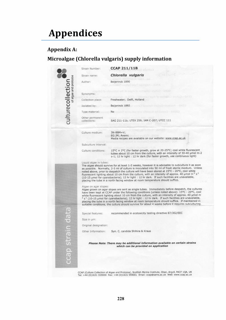
http://www.researchgate.net/publictopics.PublicPostFileLoader.html?id

228

Appendices

Appendix A:

Microalgae (Chlorella vulgaris) supply information

229

230

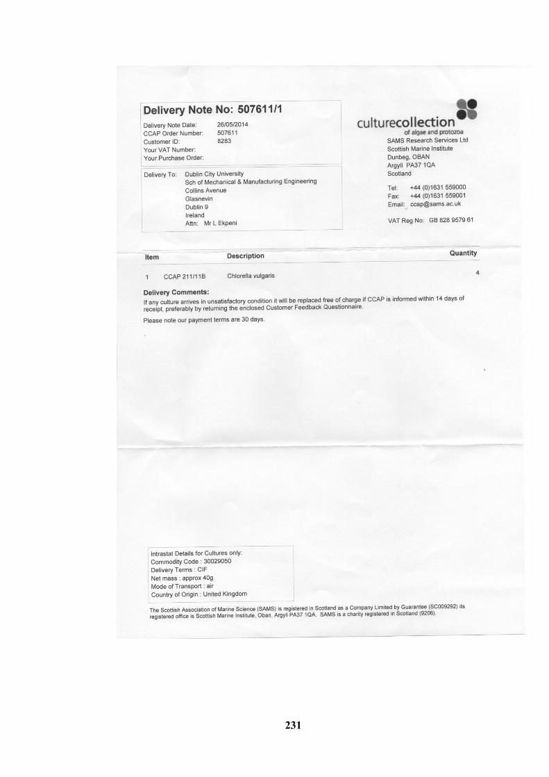
231

232

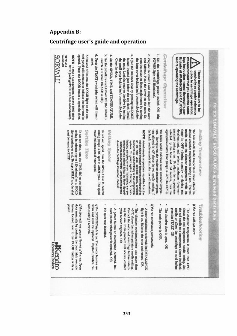
233

Appendix B:

Centrifuge user’s guide and operation

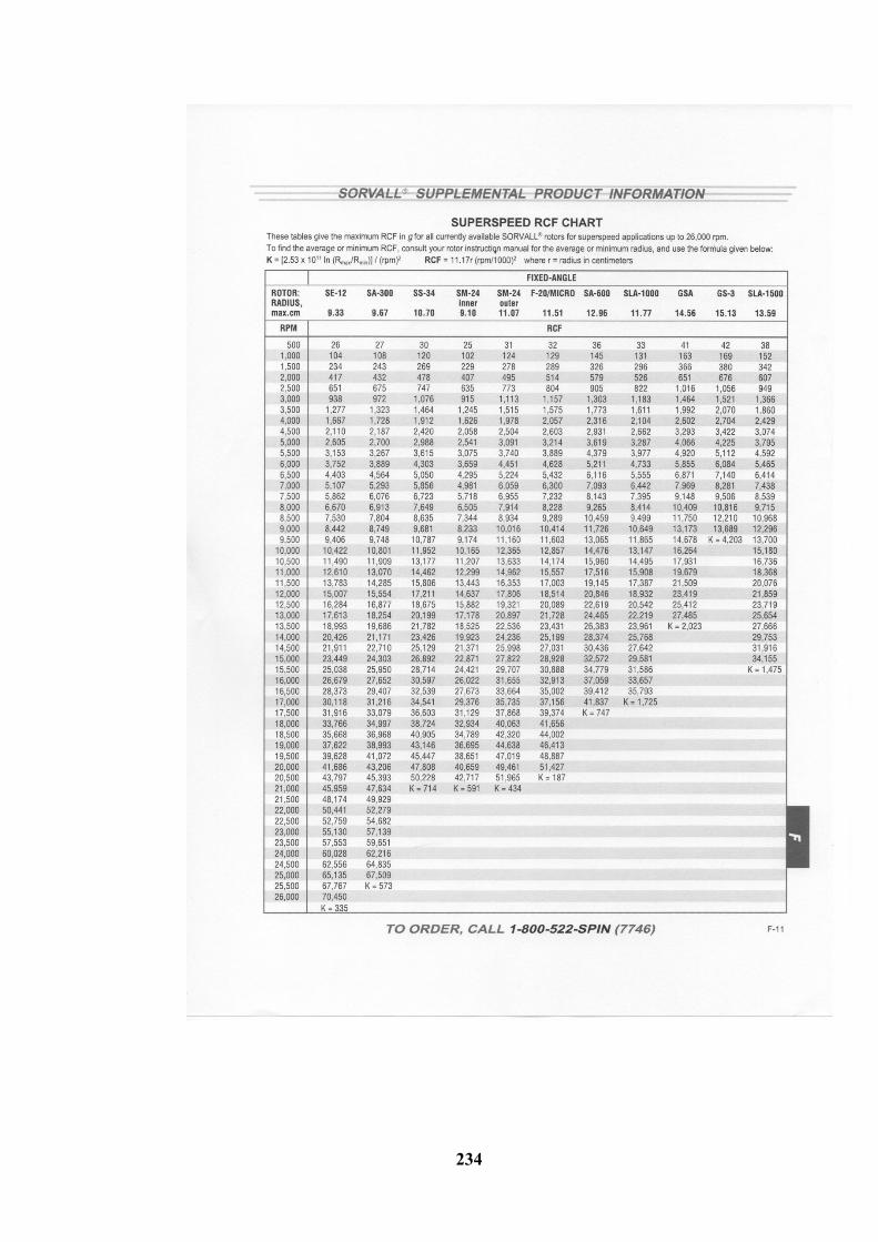
234

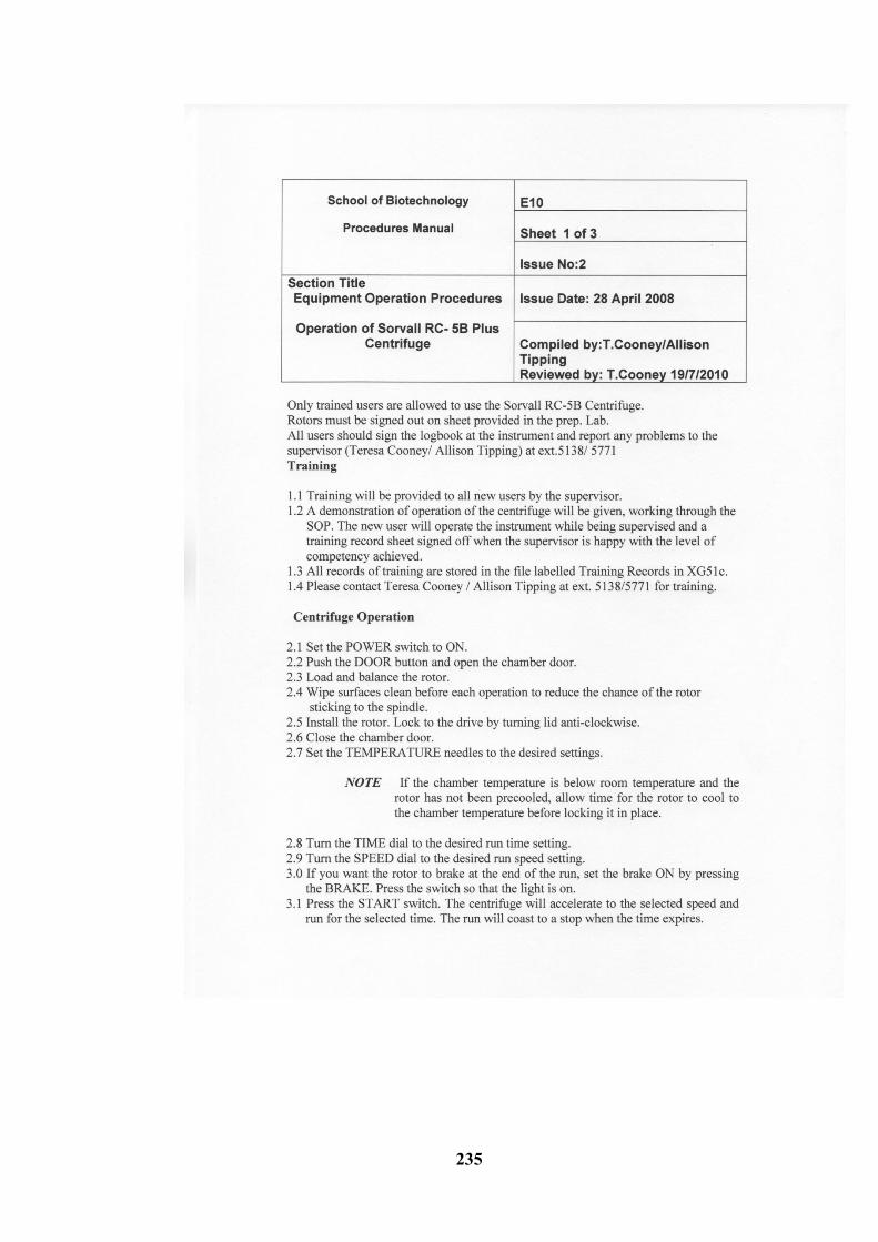
235

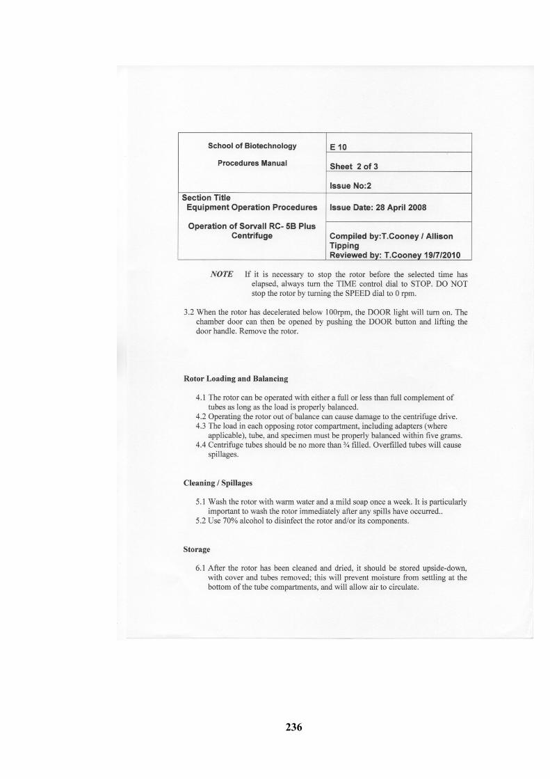
236

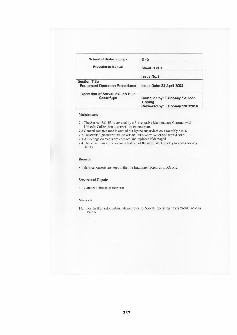
237

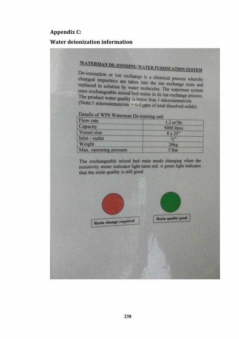
238

Appendix C:

Water deionization information

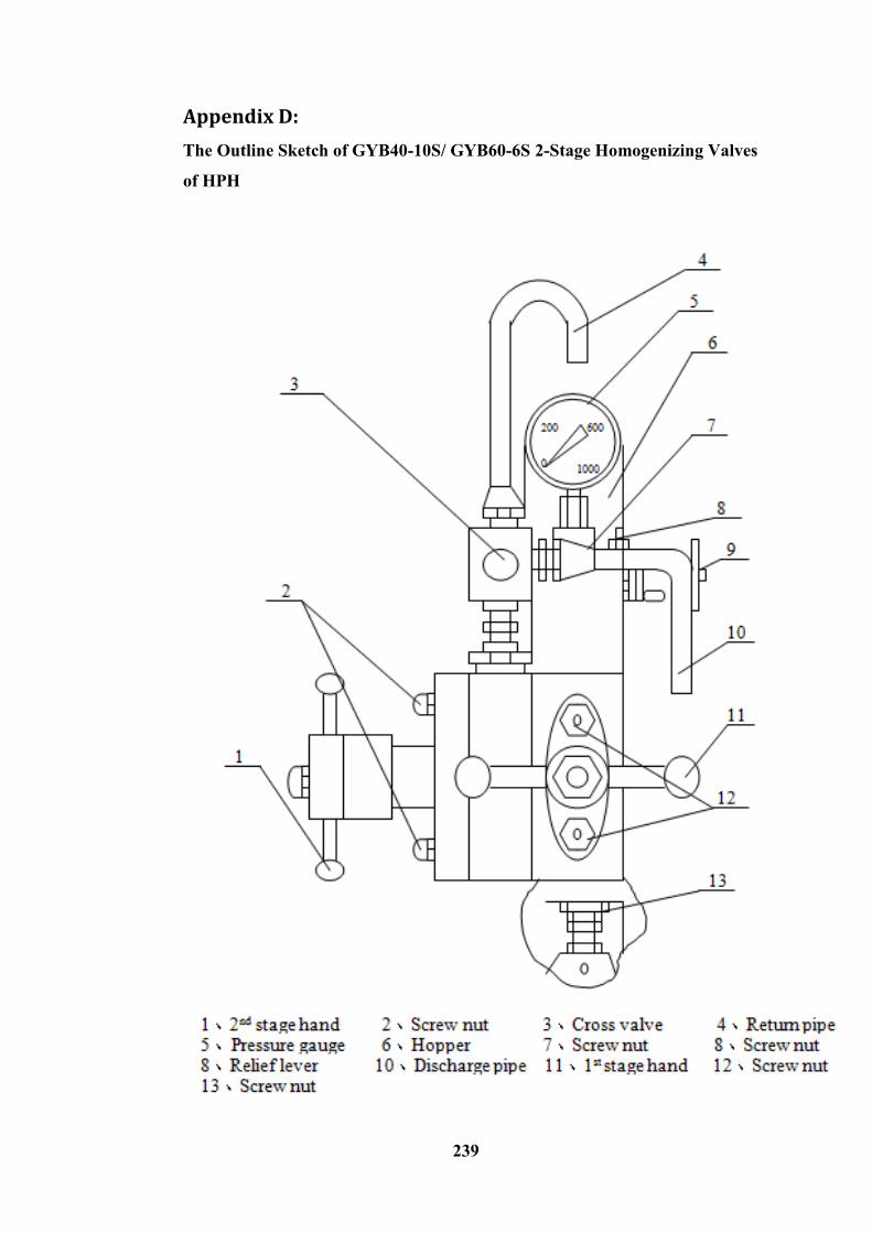
239

Appendix D:

The Outline Sketch of GYB40-10S/ GYB60-6S 2-Stage Homogenizing Valves

of HPH

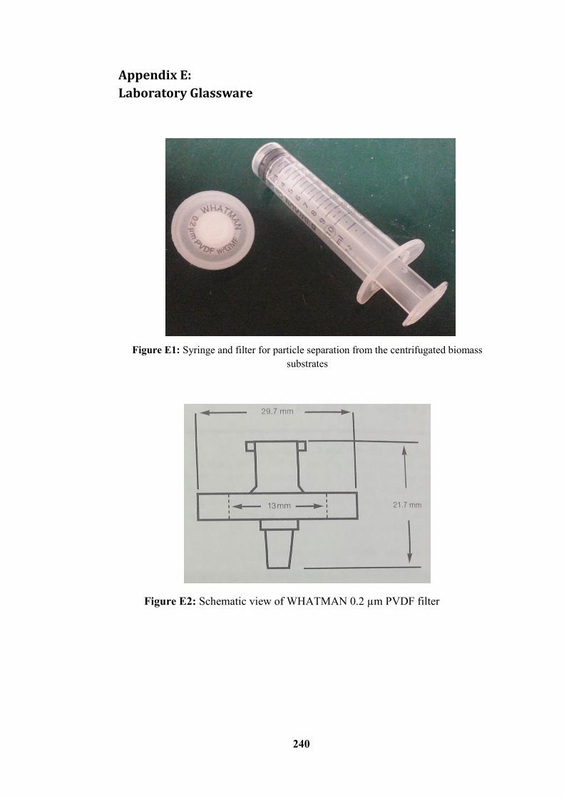
240

Appendix E:

Laboratory Glassware

Figure E1: Syringe and filter for particle separation from the centrifugated biomass

substrates

Figure E2: Schematic view of WHATMAN 0.2 µm PVDF filter

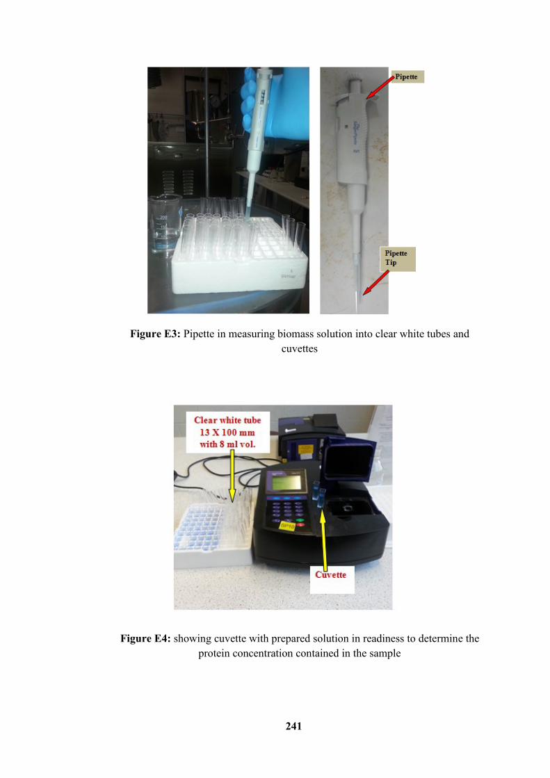
241

Figure E3: Pipette in measuring biomass solution into clear white tubes and

cuvettes

Figure E4: showing cuvette with prepared solution in readiness to determine the

protein concentration contained in the sample

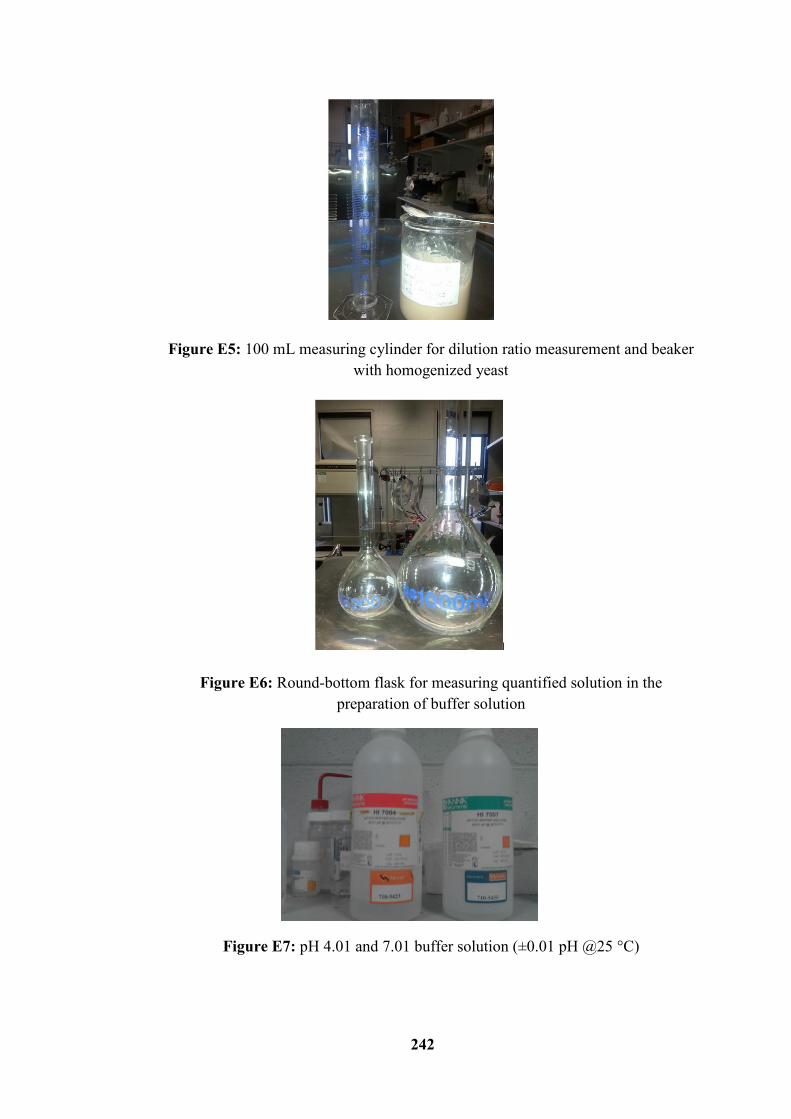
242

Figure E5: 100 mL measuring cylinder for dilution ratio measurement and beaker

with homogenized yeast

Figure E6: Round-bottom flask for measuring quantified solution in the

preparation of buffer solution

Figure E7: pH 4.01 and 7.01 buffer solution (±0.01 pH @25 °C)

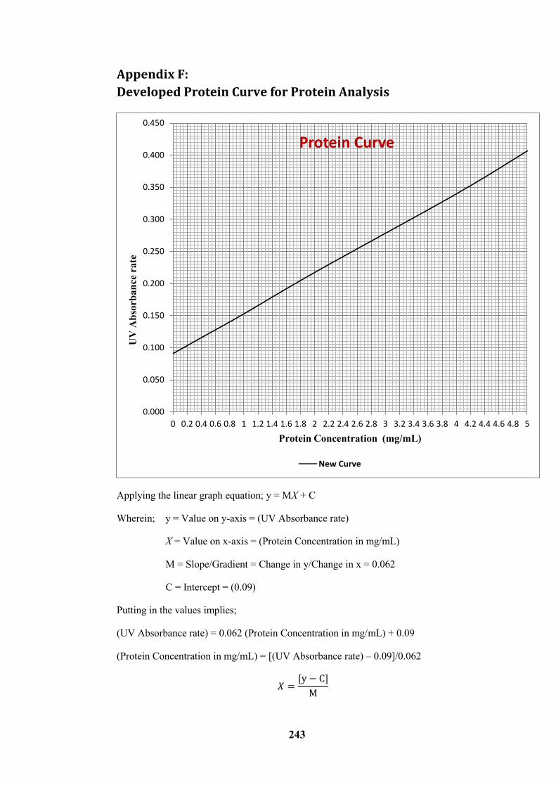
243

Appendix F:

Developed Protein Curve for Protein Analysis

Applying the linear graph equation; y = MX + C

Wherein; y = Value on y-axis = (UV Absorbance rate)

X = Value on x-axis = (Protein Concentration in mg/mL)

M = Slope/Gradient = Change in y/Change in x = 0.062

C = Intercept = (0.09)

Putting in the values implies;

(UV Absorbance rate) = 0.062 (Protein Concentration in mg/mL) + 0.09

(Protein Concentration in mg/mL) = [(UV Absorbance rate) – 0.09]/0.062

𝑋 =[y − C]

M

0.000

0.050

0.100

0.150

0.200

0.250

0.300

0.350

0.400

0.450

0 0.2 0.4 0.6 0.8 1 1.2 1.4 1.6 1.8 2 2.2 2.4 2.6 2.8 3 3.2 3.4 3.6 3.8 4 4.2 4.4 4.6 4.8 5

UV

Ab

sorb

an

ce r

ate


Protein Curve

New Curve

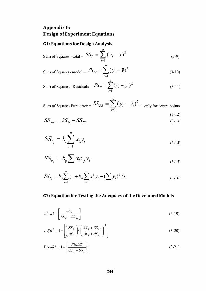
244

Appendix G:

Design of Experiment Equations

G1: Equations for Design Analysis

Sum of Squares –total = 2

1

)( yySSn

i

iT

(3-9)

Sum of Squares- model = 2

1

)ˆ( yySSn

i

iM

(3-10)

Sum of Squares –Residuals = 2

1

)ˆ( i

n

i

iR yySS

(3-11)

Sum of Squares-Pure error = ,)ˆ( 2

1

i

n

i

iPE yySSo

only for centre points

(3-12)

PERlof SSSSSS (3-13)

i

n

i

iib yxbSSi

1

(3-14)

ijiijb yxxbSSij

(3-15)

nyyxbybSS ii

n

i

iii

n

i

ibii/)( 2

1

2

1

0

(3-16)

G2: Equation for Testing the Adequacy of the Developed Models

MR

R

SSSS

SSR 12 (3-19)

1

2 1MR

MR

R

R

dfdf

SSSS

df

SSAdjR (3-20)

MR SSSS

PRESSedR 1Pr 2 (3-21)

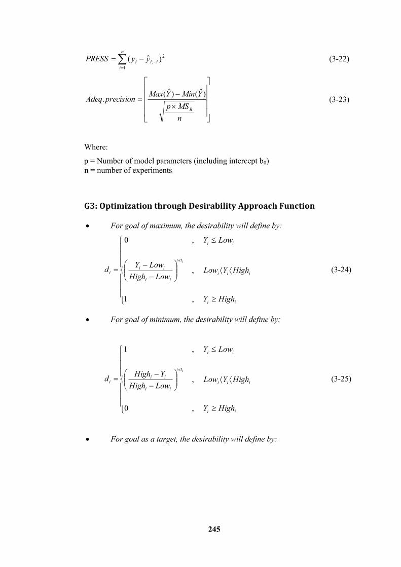
245

2

,

1

)ˆ( ii

n

i

i yyPRESS

(3-22)

n

MSp

YMinYMaxprecisionAdeq

R

)ˆ()ˆ(. (3-23)

Where:

p = Number of model parameters (including intercept b0)

n = number of experiments

G3: Optimization through Desirability Approach Function

For goal of maximum, the desirability will define by:

ii

iii

wt

ii

ii

ii

i

HighY

HighYLowLowHigh

LowY

LowY

d

i

,1

,

,0

(3-24)

For goal of minimum, the desirability will define by:

ii

iii

wt

ii

ii

ii

i

HighY

HighYLowLowHigh

YHigh

LowY

d

i

,0

,

,1

(3-25)

For goal as a target, the desirability will define by:

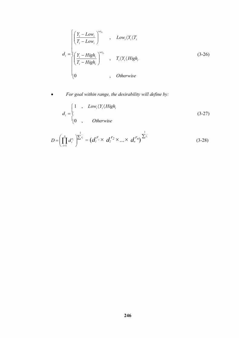
246

Otherwise

HighYTHighT

HighY

TYLowLowT

LowY

d

iii

wt

ii

ii

iii

wt

ii

ii

ii

i

,0

,

,

2

1

(3-26)

For goal within range, the desirability will define by:

Otherwise

HighYLow

d

iii

i

,0

,1

(3-27)

ii

rn

i

r

idD

1

1

= (d1

r1 × d2

r2 ×...× dn

rn) ir

1

(3-28)

Documents

Investigation and Disruption of Baker's Yeast / Chlorella