THESETHESEEn vue de l’obtention du

DOCTORAT DE L’UNIVERSITE DE TOULOUSEDelivre par : l’Institut National Polytechnique de Toulouse (INP Toulouse)

Presentee et soutenue le 11 decembre 2020 par :Quentin Male

Etude Numerique de l’Allumage par Prechambre dans lesMoteurs a Combustion Interne

Composition du jury:Christine Mounaım-Rousselle RapporteureRonan Vicquelin RapporteurNicolas Noiray ExaminateurThierry Poinsot Directeur de theseOlivier Vermorel Co-directeur de theseFrederic Ravet Invite

Ecole doctorale :Mecanique, Energetique, Genie civil & Procedes (MEGEP)

Specialite :Dynamique des fluides

Unite de recherche :Centre Europeen de Recherche et de Formation Avancee en Calcul Scientifique (CERFACS)

Directeurs de these :Thierry Poinsot et Olivier Vermorel

N U M E R I C A L I N V E S T I G AT I O N O F P R E - C H A M B E R I G N I T I O N I NI N T E R N A L C O M B U S T I O N E N G I N E S

quentin malé

A thesis submitted for the degree of Doctor of Philosophy

Dec. 2020

Quentin Malé: Numerical Investigation of Pre-Chamber Ignition in InternalCombustion Engines, A thesis submitted for the degree of Doctor ofPhilosophy, c© Dec. 2020

There is only one basic way of dealing with complexity:divide and conquer.

— Bjarne Stroustrup

Dedicated to my family.

A B S T R A C T

Homogeneous lean combustion is a great opportunity to reduce Inter-nal Combustion Engine (ICE) emissions (both greenhouse gases andpollutants) if combined with responsible use. Unfortunately, burninglean mixtures and meeting the demands of ICEs is complicated by lowreactions rates, extinction, instabilities and mild heat release. There istherefore a need for breakthrough technologies thwarting the adverseeffects of lean combustion to leverage lean-burn strategies in ICEs.The Pre-Chamber Ignition (PCI) concept has demonstrated its capabili-ties to induce very high burning rates enabling ultra-lean premixedmixtures to be burnt efficiently. This is achieved through the creationof multiple highly turbulent jets of hot burnt gases issuing into themain chamber of the engine. However, the optimization of the sizeof the pre-chamber orifices is something very complex that is not yetclearly understood. Small holes must be used in order to generateenough turbulence in the main chamber, but these small holes canalso inhibit the ignition of the main chamber because of too high jetcooling and/or speed.

Therein lies the challenge of this research work: how to design theholes connecting pre- and main chambers to maximize burning rateswithout exceeding the ignition limit? To answer this question, multi-ple numerical tools were used: kinetically detailed Direct NumericalSimulation (DNS), Large Eddy Simulation (LES) and zero-dimensionalmodelling. DNS was used to build precise knowledge on jet ignition.Especially, it helped to understand how the jet injection speed andtemperature govern ignition and revealed specific incipient flamestructures. It also allowed to build models to predict the outcome ofan ignition sequence. LES was used to study the whole PCI conceptin a real engine. It allowed to analyse the flow entering and leavingthe pre-chamber, to measure the cooling and quenching effects inthe connecting ducts, and to analyse the ignition and combustionprocesses for both normal and abnormal combustion cases. Finally, azero-dimensional model has been developed based on a multi-zoneapproach. It integrates key submodels to account for thermal effectsin the ducts and to predict the outcome of the jet ignition attempts inthe main chamber. Therefore, it provides a crucial tool to answer theresearch question by evaluating the result of multiple PCI designs interms of main chamber ignition at a low computational cost.

vii

R É S U M É

La combustion d’un mélange pauvre et homogène est une opportunitéde réduire les émissions des moteurs à combustion interne (à la fois entermes de gaz à effet de serre et de polluants) si elle est accompagnéed’une utilisation responsable. Mais brûler un mélange pauvre tout enassurant le fonctionnement normal d’un moteur est complexe car il enrésulte des faibles taux de réactions et des phénomènes d’extinctionou d’instabilités. Des solutions doivent alors être développées afinde contrecarrer les effets néfastes de la combustion pauvre et entirer profit. Le concept d’allumage par préchambre, qui génère demultiples jets turbulents composés de gaz brûlés à haute températureafin d’allumer la chambre principale, a démontré qu’il était capabled’induire une combustion rapide permettant de brûler efficacementdes prémélanges pauvres. Cependant, l’optimisation de la taille desorifices liants la préchambre à la chambre principale est délicate. Depetits trous doivent être utilisés afin de générer suffisamment deturbulence dans la chambre principale, mais ils peuvent égalementempêcher l’allumage en raison d’un refroidissement trop importantet/ou d’une vitesse de jet trop élevée.

D’où l’enjeu de ce travail : comment concevoir les trous de connexionde sorte à maximiser la vitesse de combustion sans dépasser la li-mite d’allumage ? Pour répondre à cette question, plusieurs outilsnumériques ont été utilisés, allant de simulations tridimensionnellesd’écoulements réactifs de type simulation directe (DNS) et simulationdes grandes échelles (LES) à de plus simples modèles réduits. La DNS

a été utilisée afin d’acquérir des connaissances précises sur l’allumagepar jet chaud. Elle a permis de comprendre l’influence de la vitessed’injection et de la température de jet sur l’allumage et a révélé desstructures de flamme spécifiques. Elle a également permis de bâtirdes modèles pour prédire la réussite ou l’échec d’un allumage parjet chaud. La LES a été utilisée pour étudier dans son ensemble leconcept d’allumage par préchambre dans un moteur. Elle a permisde caractériser l’écoulement au travers des conduits de connexion, demesurer les effets de refroidissement et d’extinction dans ces conduitset d’analyser les mécanismes d’allumage et de combustion qui ont lieupour des cas de combustion normale et anormale. Enfin, un modèlemoteur zérodimensionnel a été développé, intégrant des sous-modèlesessentiels afin de tenir compte des effets thermiques dans les conduitset de prédire l’allumage de la chambre principale. Il fournit un outilefficace afin de répondre aux besoins de dimensionnement en permet-tant l’évaluation du fonctionnement de plusieurs designs à un faiblecoût de calcul.

ix

P U B L I C AT I O N S

publications as leading author

Q Malé, G Staffelbach, O Vermorel, A Misdariis, F Ravet and T Poinsot."Large Eddy Simulation of Pre-Chamber Ignition in an Internal CombustionEngine." In: Flow, Turbulence and Combustion 103 (Apr. 2019), pp. 465–483.

Q Malé, O Vermorel, F Ravet and T Poinsot. "Direct Numerical Simulationsand Models for Hot Burnt Gases Jet Ignition." In: Combustion and Flame 223

(Jan. 2021), pp. 407-422.

Q Malé, O Vermorel, F Ravet and T Poinsot. "A Multi-Zone Model to PredictPre-Chamber Ignition in Internal Combustion Engines." Submitted to: AppliedThermal Engineering.

publication as co-author

A collaboration on the application of the Chemical Explosive Mode Analysis diagnos-tic tool to the study of a transition scenario from deflagration to detonation:T Jaravel, O Dounia, Q Malé and O Vermorel. "Deflagration to DetonationTransition in Fast Flames and Tracking with Chemical Explosive Mode Anal-ysis." In: Proceedings of the Combustion Institute (Oct. 2020).

xi

R E S E A R C H G R A N T S

PRACE (Partnership for Advanced Computing in Europe) 15 millioncore computing hours grant agreement no. 2019204881 (Oct. 2019 toSept. 2020).

Research visit to the Department of Mechanical Engineering of theUniversity of Melbourne co-funded by the Renault Group and theCERFACS (“Centre Européen de Recherche et de Formation Avancée enCalcul Scientifique”) (Dec. 2018 to Feb. 2019).

GENCI (“Grand Équipement National de Calcul Intensif”) “Grand Chal-lenge” early access 8 million core computing hours grant agreementno. gch0301 (Apr. 2018 to June 2018).

CIFRE (“Conventions Industrielles de Formation par la Recherche”)PhD research fellowship no. 2017/0295 attributed by ANRT (“Associa-tion Nationale de la Recherche et de la Technologie”) and the RenaultGroup (Oct. 2017 to Sept. 2020).

xiii

La pierre n’a point d’espoir d’être autre chose que pierre.Mais de collaborer, elle s’assemble et devient temple.

— Antoine de Saint-Exupéry

R E M E R C I E M E N T S

Cette thèse est le fruit d’un travail de recherche de près de trois ans.En préambule, je souhaite remercier ceux qui l’ont rendue possible.

Je tiens vivement à remercier Monsieur Thierry Poinsot, directeurde recherche à l’Institut de Mécanique des Fluides de Toulouse, ainsique Monsieur Olivier Vermorel, chercheur au Centre Européen deRecherche et de Formation Avancée en Calcul Scientifique, qui ontdirigé ces travaux de recherche. Je leur suis reconnaissant de m’avoirfait bénéficier de leur savoir et de leur rigueur intellectuelle. Qu’ilssoient assurés de ma profonde gratitude.

Je remercie Monsieur Frédéric Ravet, expert simulation dynamiquedes fluides au sein du Groupe Renault, pour avoir su maintenir unlien agréable entre le laboratoire et l’industrie et pour m’avoir laisséune grande liberté dans mes travaux. Sa confiance a été un élémentmoteur pour moi.

J’adresse tous mes remerciements à Madame Christine Mounaïm-Rousselle, Professeure à l’Université d’Orléans, ainsi qu’à MonsieurRonan Vicquelin, Professeur à l’Université Paris-Saclay, pour l’honneurqu’ils m’ont fait en acceptant d’être rapporteurs de cette thèse. Leursremarques et commentaires m’ont permis d’en améliorer la qualité.

J’exprime ma gratitude à Monsieur Nicolas Noiray, Professeur àl’École Polytechnique Fédérale de Zürich, pour le grand honneur qu’ilm’a fait en acceptant d’examiner cette thèse et d’en présider son jury.

Je tiens également à remercier le Centre Européen de Rechercheet de Formation Avancée en Calcul Scientifique pour l’accueil et lesconditions de travail privilégiées qui m’ont été offertes. Je remerciechaleureusement les permanents, les anciens et futurs docteurs, pourle partage et les échanges de savoir.

Je remercie enfin ceux qui me sont chers et que j’ai quelque peudélaissés au long de ce parcours. Je suis redevable à mes parents,Claudine Couget et Bernard Malé, pour leur soutien, leur patience etleur compréhension. Qu’ils trouvent, dans ces travaux, l’aboutissementde leurs efforts. Enfin, j’ai une pensée toute particulière pour mesgrands-parents, dont la bienveillance indéfectible illustre ce que l’êtrehumain peut avoir de meilleur.

xv

C O N T E N T S

i introduction

1 homogeneous lean combustion 3

1.1 Advantages of Burning Homogeneous Lean Mixtures . 3

1.2 Challenges of Burning Homogeneous Lean Mixtures . 4

2 technologies to leverage homogeneous lean com-bustion 5

2.1 Partially Stratified Charge . . . . . . . . . . . . . . . . . 5

2.2 High Energy Ignition Systems . . . . . . . . . . . . . . . 6

2.3 Homogeneous Charge Compression Ignition . . . . . . 6

2.4 Spark Controlled Compression Ignition . . . . . . . . . 7

2.5 Pre-chamber Ignition . . . . . . . . . . . . . . . . . . . . 7

3 how to design pre-chamber ignition systems 11

4 work plan 13

ii numerical simulation of reactive flows

5 governing equations for reactive flows 17

5.1 Balance Equations . . . . . . . . . . . . . . . . . . . . . . 17

5.2 Diffusion Velocities . . . . . . . . . . . . . . . . . . . . . 19

5.3 Transport Properties . . . . . . . . . . . . . . . . . . . . 20

5.4 Chemical Kinetics . . . . . . . . . . . . . . . . . . . . . . 20

6 large eddy simulation concept 23

6.1 Governing Equations . . . . . . . . . . . . . . . . . . . . 25

6.2 Unresolved Fluxes Modelling . . . . . . . . . . . . . . . 27

6.3 Combustion Modelling . . . . . . . . . . . . . . . . . . . 28

7 numerical methods 33

7.1 Moving Mesh . . . . . . . . . . . . . . . . . . . . . . . . 33

7.2 On the Fly Parallel Remeshing . . . . . . . . . . . . . . 33

iii detailed investigation of hot burnt gases jet ig-nition mechanisms using direct numerical simu-lation

8 hot burnt gases injection inside an atmosphere 37

8.1 Research Needs . . . . . . . . . . . . . . . . . . . . . . . 37

8.2 Configuration . . . . . . . . . . . . . . . . . . . . . . . . 40

8.3 Results . . . . . . . . . . . . . . . . . . . . . . . . . . . . 48

8.4 Conclusion . . . . . . . . . . . . . . . . . . . . . . . . . . 56

iv study of a pre-chamber ignition system in a real

engine using large eddy simulation

9 engine setup 59

9.1 Engine Features . . . . . . . . . . . . . . . . . . . . . . . 59

9.2 Large Eddy Simulation Framework . . . . . . . . . . . . 60

xvii

xviii contents

9.3 Mesh Characteristics . . . . . . . . . . . . . . . . . . . . 60

10 global behaviour , λ 1 .5 63

10.1 Research Needs . . . . . . . . . . . . . . . . . . . . . . . 63

10.2 Configuration . . . . . . . . . . . . . . . . . . . . . . . . 64

10.3 Results . . . . . . . . . . . . . . . . . . . . . . . . . . . . 67

10.4 Comparison With Spark Ignition . . . . . . . . . . . . . 77

10.5 Conclusion . . . . . . . . . . . . . . . . . . . . . . . . . . 79

11 ignition failure , λ 2 .0 81

11.1 Research Needs . . . . . . . . . . . . . . . . . . . . . . . 81

11.2 Configuration . . . . . . . . . . . . . . . . . . . . . . . . 81

11.3 Results . . . . . . . . . . . . . . . . . . . . . . . . . . . . 82

11.4 Conclusion . . . . . . . . . . . . . . . . . . . . . . . . . . 87

12 hydrogen addition, λ 2 .0 89

12.1 Research Needs . . . . . . . . . . . . . . . . . . . . . . . 89

12.2 Configuration . . . . . . . . . . . . . . . . . . . . . . . . 89

12.3 Results . . . . . . . . . . . . . . . . . . . . . . . . . . . . 90

12.4 Conclusion . . . . . . . . . . . . . . . . . . . . . . . . . . 95

13 late ignition, λ 1 .5 97

13.1 Research Needs . . . . . . . . . . . . . . . . . . . . . . . 97

13.2 Configuration . . . . . . . . . . . . . . . . . . . . . . . . 97

13.3 Results . . . . . . . . . . . . . . . . . . . . . . . . . . . . 97

13.4 Conclusion . . . . . . . . . . . . . . . . . . . . . . . . . . 101

v zero-dimensional pre-chamber ignition engine

model to assist technology design

14 pre-chamber engine modelling 105

14.1 Research Needs . . . . . . . . . . . . . . . . . . . . . . . 105

14.2 Modelling Approach . . . . . . . . . . . . . . . . . . . . 105

14.3 Thermodynamic State of the Zones . . . . . . . . . . . . 106

14.4 Wall Heat Losses . . . . . . . . . . . . . . . . . . . . . . 108

14.5 Submodel for the Connecting Ducts . . . . . . . . . . . 109

14.6 Submodel for Jet Ignition . . . . . . . . . . . . . . . . . 113

14.7 Turbulence . . . . . . . . . . . . . . . . . . . . . . . . . . 121

14.8 Flame Surface . . . . . . . . . . . . . . . . . . . . . . . . 121

14.9 Mass Transfer . . . . . . . . . . . . . . . . . . . . . . . . 122

14.10Resolution of the Ordinary Differential Equations . . . 123

15 application to pre-chamber ignition engine 125

15.1 Calibration of the Model Constants . . . . . . . . . . . . 125

15.2 Validation Using LES Data . . . . . . . . . . . . . . . . . 127

15.3 Conclusion . . . . . . . . . . . . . . . . . . . . . . . . . . 132

16 pre-chamber engine parametric studies 133

16.1 Variation of the Equivalence Ratio . . . . . . . . . . . . 133

16.2 Variation of the Diameter of the Ducts . . . . . . . . . . 134

16.3 Pre-Chamber Ignition Combustion Diagram . . . . . . 137

16.4 Conclusion . . . . . . . . . . . . . . . . . . . . . . . . . . 138

contents xix

vi conclusion

17 general conclusion 141

17.1 Research Approach . . . . . . . . . . . . . . . . . . . . . 141

17.2 Contributions . . . . . . . . . . . . . . . . . . . . . . . . 142

17.3 Limitations . . . . . . . . . . . . . . . . . . . . . . . . . . 143

17.4 Recommendations for Further Research . . . . . . . . . 145

bibliography 147

A C R O N Y M S

ALE Arbitrary Lagrangian Eulerian

ARC Analytically Reduced Chemistry

BSFC Brake Specific Fuel Consumption

BF Burnt Fraction

COR Convected Open Reactor

CEMA Chemical Explosive Mode Analysis

CAD Crank Angle Degree

CEM Chemical Explosive Mode

DNS Direct Numerical Simulation

DTFLES Dynamic Thickened Flame for Large Eddy Simulation

DRGEP Directed Relation Graph with Error Propagation

EOI End Of Injection

HCCI Homogeneous Charge Compression Ignition

HGE Hot Gases Ejection

HRR Heat Release Rate

IT Ignition Timing

ICE Internal Combustion Engine

IMEP Indicated Mean Effective Pressure

IVC Intake Valve Closing

IMEP Indicated Mean Effective Pressure

LES Large Eddy Simulation

LIF Laser-Induced Fluorescence

LOI Level Of Importance

MPI Message Passing Interface

ODE Ordinary Differential Equation

PDF Probability Density Function

xx

acronyms xxi

PSC Partially Stratified Charge

PDF Probability Density Function

PCI Pre-Chamber Ignition

PFI Port Fuel Injection

QSS Quasi Steady State

QSSA Quasi Steady State Approximation

RANS Reynolds Averaged Navier-Stokes

RHS Right Hand Side

RIF Representative Interactive Flamelet

RPM Revolutions Per Minute

SOI Start Of Injection

SI Spark Ignition

SCCI Spark Controlled Compression Ignition

TJI Turbulent Jet Ignition

TDC Top Dead Centre

TFLES Thickened Flame for Large Eddy Simulation

UFIP Unsteady Flamelet for Ignition Prediction

Part I

I N T R O D U C T I O N

In this first part, a brief introduction to homogeneous leancombustion is given, with its advantages and challenges toface. An overview of the main technologies used to extendthe lean limit is then given, with more details on the pre-chamber ignition concept which is studied throughout thiswork. Finally, the main research questions associated withthe design of pre-chamber ignition in internal combustionengines are described and the strategy to provide answersis established.

1H O M O G E N E O U S L E A N C O M B U S T I O N I N I N T E R N A LC O M B U S T I O N E N G I N E S

Transport almost entirely relies on Internal Combustion Engines (ICEs)burning petroleum-derived fuel. While the global demand for trans-port energy is large and is increasing, changing transport policy andimproving ICE is of major importance because of the climate and pollu-tion impact on earth. One way to improve ICEs is to use homogeneouslean combustion. Engines operating under these conditions can havevery low pollutant emissions and very high efficiency [1]. Detailsregarding these advantages and challenges appear in this chapter.

1.1 advantages of burning homogeneous lean mixtures

over stoichiometric ones

1.1.1 Advantages in Terms of Efficiency

Ideal thermal efficiency of ICEs, assuming an instantaneous isochoriccombustion at Top Dead Centre (TDC) (Otto cycle), reads

ηth = 1−1

vcrγ−1, (1.1)

where vcr is the volumetric compression ratio and γ is the ratio ofspecific heats of the inducted charge. Therefore, to maximize the ther-mal efficiency, the compression ratio and the specific heat ratio of theworking fluid should be maximized and lean combustion goes in thisdirection. First, γ of air is greater than γ of air/fuel mixture for typicalhydrocarbon fuels: the value of γ will be higher for lean mixturesthan for stoichiometric ones, leading to higher thermal efficiencies.Second, a higher compression ratio is attainable with leaner mixturesbefore auto-ignition occurs due to longer auto-ignition times thanstoichiometric mixtures.

In practice, other advantages of lean combustion appear. Lean com-bustion results in cooler burnt gases temperature than stoichiometriccombustion which reduces heat losses to the cylinder walls and there-fore increases engine efficiency. It also reduces pumping losses duringthe air intake throttling required to maintain specific air-fuel ratio(work is required to pump the mixture past a partially closed throttle).Lean combustion requires more air and therefore less throttling whichincreases part-load efficiency.

3

4 homogeneous lean combustion

1.1.2 Advantages in Terms of Pollutant Emissions

In addition to the increase in efficiency, homogeneous lean combustionis a good candidate to decrease pollutant emissions. Thermal nitrogenoxide formation is reduced because flame temperatures are typicallylow under lean combustion conditions. In addition, when leaningis accomplished, complete combustion generally results because ofthe air excess (i.e. an oxidizing environment), reducing hydrocarbonand carbon monoxide emissions. Burning a homogeneous lean mix-ture also limits pollutant formation by preventing combustion of richpockets as could be the case with a heterogeneous mixture. Therefore,homogeneous lean operation, within reason, can be an excellent strat-egy for reducing emissions and meeting emission standards withoutthe need for exhaust gas aftertreatment systems.

1.2 challenges of burning homogeneous lean mixtures

Burning homogeneous lean mixtures and meeting the demands ofpractical combustion systems is complicated by low reaction rates,extinction, instabilities and mild heat release associated to very leanmixtures. A major issue of lean combustion is that the flame consump-tion speed may be much lower than the stoichiometric one for highdilution rates while the combustion duration affects emissions andthermal efficiency. In an ideal engine, all the energy from combustionwould be instantly released at TDC. However, in a real engine, com-bustion of the fresh mixture takes time. The efficiency is then reducedcompared to the ideal cycle [2]. Since burning rates are highest closeto stoichiometry, using a lean mixture results in increased combustionduration. This then reduces the thermal efficiency, thereby tending tocounteract the advantages of lean combustion in terms of efficiency. Inaddition, operating an ICE with a lean mixture can cause misfires andpartial-burns that both deteriorate engine efficiency and increase un-burnt hydrocarbon emissions and combustion instabilities that preventproper operation [3, 4].

Therefore, to successfully implement a lean-burn strategy to min-imize exhaust emissions and maximize thermal efficiency, devicesshould be employed to enable the fastest possible combustion rate tobe achieved under all operating conditions. In practice, this meansproviding a reliable ignition and increasing the burning rate usingartifices.

2O V E RV I E W O F T E C H N O L O G I E S T O L E V E R A G EH O M O G E N E O U S L E A N C O M B U S T I O N

To address the challenges raised in Section 1.2, it is necessary todevelop new technologies since typical Spark Ignition (SI) in the mainchamber fails [3, 4]. Any technique which may provide stronger initialflame kernel and/or increase the burning rate should be beneficial.While stronger initial flame kernel can be reached using high energyignition systems, an increase in the burning rate is more difficult toachieve. Nevertheless, turbulence increases the burning rate throughflame wrinkling and so anything that enhances turbulence levelsduring the combustion event tends to be helpful. Other conceptsuse compression ignition to burn the premixed charge as a whole,eliminating the issues associated with low consumption speeds of thepropagating flame fronts.

2.1 partially stratified charge

In the Partially Stratified Charge (PSC) concept, a very small quantity The amount ofadditional fuel issmall enough for themixture to beconsideredhomogeneous.

of fuel is injected adjacent to the spark plug electrodes of a SI engine(Fig. 2.1) just before ignition, providing rapid and reliable ignition, andthe formation of a strong initial flame kernel. Reynolds and Evans [5]have shown that PSC significantly reduced ignition delay, as measuredfrom the spark to 5% heat release (Fig. 2.2). In addition, PSC reduces thecombustion duration (here evaluated using 5 to 95% heat release) andextend the lean limit. However, the improvement in the burning ratecompared to non-PSC is not sufficient to maintain efficiency (Fig. 2.2).It is an excellent example of the technology requirements: it must notonly provide rapid and reliable ignition, but also significantly increasethe subsequent burning rate.

Figure 2.1: Sketch of the PSC concept, from Ref. [5].

5

6 technologies to leverage homogeneous lean combustion

air-fuel equivalence ratio λ air-fuel equivalence ratio λ

Com

bust

ion

dura

tion

[CA

D]

BSFC

[g/k

Wh]

PSC Inj. Rate: 14 g/h

(1.1% of fuel at λ=1.6)

(0.6% of fuel at λ=1.6)

Figure 2.2: Left: combustion duration (spark to 5% and 5 to 95% heat release)versus air-fuel equivalence ratio for PSC with 14 g/h injection and non-PSC

case (perfectly homogeneous mixture). Right: Brake Specific Fuel Consump-tion (BSFC) versus air-fuel equivalence ratio for different PSC injection flowrates. From Ref. [5].

2.2 high energy ignition systems

A complete review on high energy ignition systems applied to ICEs canbe found in Ref. [6]. These systems include long duration sparks [7, 8],spark restrikes [9, 10], multiple spark plugs [11], corona spark plugs[12], plasma jet igniters [13], rail plugs [14], lasers [15] and microwaveconcepts [16]. All these systems aim at pushing the lean ignitionlimit. However, as for the PSC concept, slow flame travel still limit thelean operation because of low burning rates (e.g., [8]), implying thatsome method of increasing the flame speed is required to fully utilizethe benefits of increased ignition energy. Furthermore, these ignitionsystems are expensive and require large electrical energy (e.g., [13])which limits their wide marketing and commercial implementation,especially for automotive applications. Some sparked devices alsosuffer from erosion of the electrode metals because of the high energyelectrical discharge, limiting their operational lifetime (e.g., [17]).

2.3 homogeneous charge compression ignition

One way to overcome slow flame consumption issues of lean com-bustion is to not use flame fronts to consume the lean charge but tohave the charge volumetrically ignite throughout the cylinder: this isthe Homogeneous Charge Compression Ignition (HCCI) concept [18].Instead of using an ignition source, HCCI engines use high compres-sion ratios to ignite the air/fuel mixture. In addition to very rapidcombustion, HCCI engines typically run at higher compression ratiosthan SI engines, thus offering higher thermal efficiencies. However,HCCI engines have a limited load range that cannot support high load

2.4 spark controlled compression ignition 7

demands required by automotive applications. Almost instantaneousvolume combustion at high load can yield unacceptable pressure riserates and/or unacceptable peak cylinder pressure, causing excessivenoise and potentially damaging the engine. Besides, ignition dependson the thermochemical path of the mixture being compressed andtherefore on the temperature and pressure history of the gas mixture.This makes controlling the start of combustion a very difficult taskwhile stable and efficient engine operation requires that the combus-tion timing be tightly controlled to the proper set point. This is themain obstacle to the wide use of this technology in ICEs.

2.4 spark controlled compression ignition

Spark Controlled Compression Ignition (SCCI) brings a solution of thecombustion timing control issues of HCCI [19]. It uses spark to producea flame kernel that consumes a portion of the charge and increases thetemperature of the remaining charge by heat transfer and compressioneffects, causing it to auto-ignite earlier than it would have otherwise(Fig. 2.3). This provides temporal control over the combustion process,solving the lack of control of HCCI. However, volumetric auto-ignitionat high-load can still yield unacceptable pressure rise rates and/orunacceptable peak cylinder pressure. Production feasible engines thenneed to employ a combination of combustion strategies, such as stoi-chiometric SI combustion at high loads and leaner SCCI combustion atintermediate and low loads.

Figure 2.3: Sketch of the SCCI concept, from Mazda.

2.5 pre-chamber ignition

Pre-Chamber Ignition (PCI) consists in using a small semi-confined Some authors alsouse TJI for TurbulentJet Ignition to referto this technology.

volume (the pre-chamber) to create multiple hot turbulent jets andprovide multiple ignition sites for the homogeneous lean mixture inthe main chamber [20]. In addition to the multiple high energy ignition

8 technologies to leverage homogeneous lean combustion

sources, the turbulent jets increase the turbulence levels in the mainchamber, increasing the combustion speed and pushing back the airdilution limit of proper engine operation. Furthermore, the fast com-bustion induced by these systems not only directly increases engineefficiency but also allows to increase the knock limited compressionratio which further increases the engine efficiency.

In practice, air/fuel mixture flows from the main chamber to thepre-chamber during the compression stroke and is ignited inside thepre-chamber with a spark plug (Fig. 2.4). During the pre-chambercombustion, initially unburned mixture flows into the main chamber,but later the pre-chamber flame and/or jets with hot combustionproducts issue into the main chamber and ignite its lean mixture.The jets induce turbulence inside the main chamber and generatemultiple distributed ignition sites. This process is often dubbed asTurbulent Jet Ignition (TJI) and results in an overall increase of theburning rate. The pre-chamber can be filled only by the homogeneouspremixed mixture available in the main chamber, or also be filledusing an auxiliary fuel injection inside the pre-chamber. This allowsto decouple the equivalence ratio in the pre-chamber from the one inthe main chamber and so to burn richer mixtures in the pre-chamberwhich allows proper engine operation under ultra-lean conditions[21].

Figure 2.4: Sketch of the PCI concept, from Ref. [21].

Attard et al. [21, 22] have demonstrated the capability of the PCI

concept to drastically increase the air dilution limit above λ = 2.0whilemaintaining very high levels of engine efficiency thanks to the rapidmain chamber combustion induced by the multiple hot turbulentjets. More precisely, the lean limit have been pushed back by 44%

2.5 pre-chamber ignition 9

compared to the same engine platform with SI (not allowing operationbeyond a coefficient of variation of gross Indicated Mean EffectivePressure (IMEP) of 5). Ignition delays (measured by the differencebetween spark ignition and 10% mass fraction of burnt gases) havebeen reduced by up to 51%. Combustion duration (measured bythe difference between 10 and 90% mass fraction of burnt gases)have been reduced by up to 44%. This rapid combustion allows highlevels of air dilution while limiting losses from ideal engine cycleto real engine cycle. This results in an increase in indicated thermalefficiency by up to 19%. It confirms the capability of PCI to achievevery high efficiency levels. In addition, near zero engine out nitrogenoxide emissions have been observed. Baeta et al. [23] confirmed thesystem advantages, linked to a NOx, CO2 and CO emissions reduction.However, they found an increase in unburnt hydrocarbons linked toexcessive wall-wetting in the pre-chamber as they used liquid injectionfor pre-chamber additional fuelling.

0

2

4

6

8

10

12

0.6 0.8 1.0 1.2 1.4 1.6 1.8 2.0 2.2

Com

bust

ion

Stab

ility

[CoV

IMEP

g]

Spark IgnitionPre-chamber Jet Ignition

30

32

34

36

38

40

42

Indi

cate

d N

et T

herm

al E

ffici

ency

[%]

0

10

20

30

40

50

0.6 0.8 1.0 1.2 1.4 1.6 1.8 2.0 2.2

10-9

0% M

ass

Frac

tion

Burn

[CAD

]

0

10

20

30

40

0.6 0.8 1.0 1.2 1.4 1.6 1.8 2.0 2.2

0-10

% M

ass

Frac

tion

Burn

[CAD

]

0.6 0.8 1.0 1.2 1.4 1.6 1.8 2.0 2.2

+19%

5 CoV IMEPg

+44%

lean limit at 5 CoV IMEPgλ≈2.06

-51%

-44%

Figure 2.5: Combustion stability, thermal efficiency, ignition delay and com-bustion duration for both SI and PCI engines in the same contemporary PortFuel Injection (PFI) engine platform at 1500 Revolutions Per Minute (RPM),4.7 bar net IMEP. From Ref. [22].

3H O W T O D E S I G N P R E - C H A M B E R I G N I T I O NS Y S T E M S F O R AU T O M O T I V E A P P L I C AT I O N

Lean-burn PCI engines have demonstrated the capability to signifi-cantly extend the lean operation limit while maintaining reasonableburning rates, therefore improving the engine efficiency and decreas-ing pollutant emissions. However, the performance of a PCI engineis largely dependent on the pre-chamber design, which has to beoptimised for the particular main chamber and the foreseen operatingconditions. To date, the PCI concept has not yet been widely appliedin the automotive industry. The design is then based on empiricalapproaches rather than on theory or established rules, which motivatethe present work.

As shown experimentally by Sadanandan et al. [24] in a dividedchamber academic configuration, the size of the pre-chamber orificesis critical as it determines the injection speed and temperature of thejets. They emphasizes the role of the mixing rate and the jet temper-ature in the main chamber ignition process. One might think thatsmaller holes are always beneficial since they generate more vigorousjets causing faster combustion. Actually, when the size of the holesdecreases, pressure drop increases which does indeed generate higherinjection speeds, but this can inhibit ignition beyond a certain speeddue to excessive mixing rate in a finite rate chemistry environment.In addition, reducing the size of the holes increases the cooling ofthe gases as they pass through, resulting in lower temperature of thejets. Since chemical reactions are highly dependent on temperature,maximizing the burning rate of the main chamber by decreasing thesize of the holes must be done with special care in order to avoidmisfires.

The design of the connecting ducts is then an optimization problem.Too big, the main chamber ignition is ensured but little turbulence isgenerated and combustion is not fast enough to result in acceptableengine performances. Too small, the main chamber ignition fails dueto excessive mixing rates and/or too low temperature of the injectedgases. This is illustrated in Fig. 3.1 where an a priori combustiondiagram is proposed based on physical arguments. The burning raterb is proportional to the flame surface Af and the flame consumptionspeed Sc such that

rb ∝ AfSc. (3.1)

11

12 how to design pre-chamber ignition systems

Since Af and Sc are inversely proportional to the size of the holes dand the air-fuel equivalence ratio λ, respectively, it is possible to write

rb ∝ (dλ)−1 . (3.2)

An increase in λ at iso-d (horizontal lines in Fig. 3.1) results in alonger combustion duration. On the contrary, a decrease in d at iso-λ(vertical lines in Fig. 3.1) results in a shorter combustion duration (seeadditional graph on the upper right of Fig. 3.1). Therefore, maintaininga given combustion duration while increasing the air dilution meansdecreasing the size of the holes accordingly (iso-comb. duration linesin Fig. 3.1) until reaching the ignition limit, which increases with λ aschemistry weakens.

Of course, the pre-chamber orifices are not deformable. Once theengine has been designed, it is then only possible to move horizontallyin Fig. 3.1. If the holes have not been properly sized, the combustionduration limit or the ignition limit will be reached too quickly, thusnot allowing significant dilution levels to be achieved. If the limitin combustion duration is established by the engine designer, thisis not the case with the ignition limit which depends on multiplecomplex aerothermochemical phenomena and is not known a priori.Therein lies the major challenge of this research work: understandwhat dictates the ignition limit and succeed in predicting it withsimple tools to allow the optimization of PCI systems which require tobe operated close to the ignition limit to maximize burning rates andthus efficiency.

λ

Figure 3.1: A priori PCI combustion diagram. mc: main chamber.

4W O R K P L A N

Multiple numerical tools and strategies are combined in the presentwork to address the research question detailed in Ch. 3. Direct Nu-merical Simulation (DNS) is used to precisely study the ignition mech-anisms and the physical phenomena involved during the ignition ofa lean premixed mixture by a jet of hot burnt gases in an academicconfiguration. Particular attention is paid to the influence of the jetinjection speed and temperature on ignition. Actual behaviour in realengines may differ from idealized cases such the DNS configurationemployed. Large Eddy Simulation (LES) is therefore used to buildknowledge on PCI in a real ICE. This includes the study of normalengine operation, abnormal engine operation (misfires) and dual fueloperation (H2 addition). DNS and LES are of great help in understand-ing the physical phenomena involved in the use of PCI. However,the computational cost of these tools prevents them from being usedas a systematic approach to evaluate multiple designs. Thus, an en-gine model is developed using multi-zone approach combined withsubmodels to account for what burnt gases undergo when passingthrough the connecting ducts and, in particular, to predict the ignitionor not of the main chamber by the generated jets of hot burnt gases.This zero-dimensional engine model then makes it possible to carryout parametric studies of engine design at a low computational cost.

All these works are interconnected and feed each other (Fig. 4.1).The DNS data of jet ignition sequences (Ch. 8) are used to build modelsto predict the outcome of an ignition sequence (Section 14.6) whereone of them is integrated into the engine model described in Ch. 14.The LESs of Part iv are used to calibrate and evaluate the validitydomain of the zero-dimensional engine model (Ch. 15).

13

14 work plan

­

¡¢£¤¥¦

­ ­

­­ §

¨¤¨¦©

ª«¨ª¡¬¢

­ ­

Figure 4.1: Structure of the PhD work.

Part II

N U M E R I C A L S I M U L AT I O N O F R E A C T I V EF L O W S

Motion of viscous fluid substances can be mathematicallydescribed by a set of partial differential equations—theNavier-Stokes equations—which expresses conservation ofmomentum, mass and energy. These equations are usedto compute multi-dimensional reacting flows but requiresome additional terms to account for multi-species multi-reaction gas. This part concentrates on the presentationof these equations and their resolution. First, the balanceequations are introduced along with some simplificationsmade on transport and chemistry description. Then, thelarge eddy simulation concept is described. The balanceequations in this framework are detailed as well as themodels used for the unclosed quantities that arise. Finally,information regarding the numerical methods used to solvethe governing equations are given with some specificitieswith regard to the deformation of the fluid domain inpiston engines.

5G O V E R N I N G E Q UAT I O N S F O R R E A C T I V E F L O W S

In this work, the Navier-Stokes equations with some additional termsto account for multi-species multi-reactions gas are used to describemulti-dimensional reactive flows. The derivation of these equationsfrom mass, species, momentum and energy balances may be found inmany books (e.g., [25, 26]). From a mathematical point of view, theseequations are non-linear partial differential equations and, except insimple canonical cases, cannot be solved analytically. This chapterpresents these equations as well as the physical models used in themulti-species Navier-Stokes solver AVBP employed in this work.

5.1 balance equations

Combustion involves multiple species reacting through multiple chem-ical reactions. The variables required for the description of a compress-ible reactive flow are

U = (mx,my,mz, E, ρk)t , (5.1)

where m = (mx,my,mz)t is the momentum vector, E is the product

of the total non-chemical energy E by the density ρ which is the sumof the partial densities ρk (for k = 1 to N) of the N species present inthe mixture. The total non-chemical energy E is the sum of sensibleenergy es and kinetic energy ec.

E = es + ec =

N∑k=1

Ykes,k +1

2

3∑i=1

u2i , (5.2)

where ui is the ith component of the velocity vector, Yk is the massfraction of the kth species and the sensible energy of the kth specieses,k is defined as

es,k(T) =

∫TT0

Cv,k(Θ)dΘ, (5.3)

where T0 = 0 K is the reference temperature used and Cv,k is the massheat capacities at constant volume of the kth species.

To simplify the computation of the sensible energy from tempera-ture, the internal energy of each species is tabulated from data basesevery 100 K, in a range going from 0 to 5000 K. On each 100 K range,the heat capacity of any species is supposed constant. The energyat a given temperature is then obtained by linear interpolation. This

17

18 governing equations for reactive flows

interpolation also provides a fast method to recover temperature fromsensible energy data.

Assuming a mixture of ideal gases, the equation of state relatingtemperature T , pressure P and density ρ is

P = ρrT , (5.4)

where r is the specific gas constant defined as

r =

N∑k=1

Ykrk =

N∑k=1

YkR

Wk=

R

W, (5.5)

where R = 8.3143 J/K/mol is the universal ideal gas constant, Wk isthe molecular weight of the kth species and W is the mean molecularweight of the mixture given by

1

W=

N∑k=1

YkWk

. (5.6)

The computation of three-dimensional reactive flows requires solv-ing for the N+ 4 variables of Eq. 5.1. There is therefore a need forN+ 4 governing equations. These equations arise from species, mo-mentum and energy balances. They are now described using Einsteinsummation notation1.

species The species mass balance equations readThe sum of thespecies balance

equations gives themass conservation

equation.

∂ρYk∂t

+∂ρuiYk∂xi

= −∂Ji,k∂xi

+ ωk for k = 1,N , (5.7)

where ωk is the species chemical source term of the kth species andJi,k is the ith component of the diffusive flux of the kth species definedas

Ji,k = ρYkVk,i, (5.8)

where Vk,i is the ith component of the diffusion velocity vector Vk ofthe kth species that need to respect

N∑k=1

YkVk,i = 0 (5.9)

to ensure total mass conservation. The computation of the diffusionvelocity is discussed in Section 5.2.

1 Repeated indices are implicitly summed over.

5.2 diffusion velocities 19

momentum The momentum balance equations read

∂ρuj

∂t+∂ρuiuj

∂xi+∂Pδij

∂xi=∂τij

∂xifor j = 1, 3 , (5.10)

where δij is the Kronecker symbol2 and τij is the viscous tensordefined for a Newtonian fluid, neglecting the bulk viscosity [26] as

τij = −2

3µ∂uk∂xk

δij + µ

(∂ui∂xj

+∂uj

∂xi

), (5.11)

where µ is the dynamic viscosity (linked to the kinematic viscosityν = µ/ρ).

energy Multiple forms of energy equation can be written [27].Here, the total non-chemical energy (Eq. 5.2) is used to representenergy. The balance equation reads

∂ρE

∂t+∂ρuiE

∂xi+∂δijPui

∂xj= −

∂qi∂xi

+∂τijui

∂xj+ ωT + Q, (5.12)

where qi is the ith component of the energy flux defined as

qi = −λ∂T

∂xi+

N∑k=1

Ji,khs,k, (5.13)

where λ is the heat conduction coefficient of the mixture, ωT is theHeat Release Rate (HRR) due to combustion which reads

ωT = −

N∑k=1

∆h0f,kωk, (5.14)

where ∆h0f,k is the standard formation enthalpy of the kth speciesand Q is an external heat source term (due for example to an electricspark).

5.2 diffusion velocities

The exact computation of the diffusion velocities is very complexand expensive. The diffusion velocities are then computed usingHirschfelder and Curtiss approximation [28] which is the best first-order approximation to the exact formulation [29, 30]. Under thisapproximation, the diffusion velocities read

Vk = −Dk∇XkXk

+Vc for k = 1,N , (5.15)

where Dk is the diffusion coefficient of the kth species into the rest ofthe mixture andVc is a correction velocity to ensure mass conservation.

2 δij = 1 if i = j, 0 otherwise.

20 governing equations for reactive flows

Using Eq. 5.15 in Eqs 5.7 and summing all species equations, the massconservation equation must be recovered so that the proper expressionfor the correction velocity is

Vci =

N∑k=1

DkWkW

∂Xk∂xi

for j = 1, 3 . (5.16)

5.3 transport properties

Simple transport models are used. The dynamic viscosity µ of themixture is supposed independent of the species composition and onlydepends on the temperature through a standard power law

µ = µ0

(T

T0

)b, (5.17)

where the exponent b depends on the mixture and typically liesbetween 0.6 and 1.0. The species diffusion coefficients are evaluatedassuming a constant Schmidt number Sck for each species k such that

Dk =µ

ρSck, (5.18)

where the Schmidt numbers are dimensionless numbers that compareviscous and species diffusion rates. Similarly, the thermal conductivityλ is evaluated assuming a constant Prandtl number Pr such that

λ =µCp

Pr, (5.19)

where the Prandtl number compares the viscous and thermal diffusionrates.

5.4 chemical kinetics

5.4.1 General Formulation of the Chemical Reactions

Consider a chemical system of N species reacting through M reactionssuch that

N∑k=1

ν ′kjMk ⇐⇒N∑k=1

ν ′′kjMk for j = 1,M , (5.20)

where Mk is a symbol for the kth species, ν ′kj and ν ′′kj are the molarstoichiometric coefficients of the kth species in the jth reaction. Thespecies source terms ωk are the sum of the mass reaction rates ωk,j

produced by the M reactions

ωk =

M∑j=1

ωk,j =Wk

M∑j=1

νkjQj, (5.21)

5.4 chemical kinetics 21

where νkj = ν ′′kj − ν′kj and Qj is the progress rate of the jth reaction.

Mass conservation enforces

N∑k=1

ωk = 0. (5.22)

The progress rates of the jth reaction is given by

Qj = Kfj

N∏k=1

(ρYkWk

)ν ′kj−Krj

N∏k=1

(ρYkWk

)ν ′′kj, (5.23)

where Kfj and Krj are the forward and reverse rates of the jth reaction,respectively. The forward reaction rates are usually modelled usingthe empirical Arrhenius law

Kfj = Afj exp(−Eaj

RT

)for j = 1,M , (5.24)

where Afj and Eaj are the pre-exponential constant and the activationenergy of the jth reaction, respectively. At a molecular level, the Arrhe-nius law here describes the probability that an atom exchange occursdue to molecular collisions. The reverse reaction rates are usuallygiven by

Krj =Kfj

Keq,jfor j = 1,M , (5.25)

where Keq,j is the equilibrium constant of the jth reaction, defined as[26]

Keq,j =

(P0RT

)∑Nk=1 νkj

exp

(∆S0j

R−∆H0j

RT

), (5.26)

where P0 = 1 bar, ∆H0j and ∆S0j are the enthalpy and entropy changesoccurring when passing from reactants to products in the jth reaction,respectively.

5.4.2 Analytically Reduced Chemistry

Computing reactive flows requires chemical schemes that contain dataon all the species and reactions relevant to the combustion process.Using detailed mechanisms that contain a large number of species andreactions in three-dimensional reactive flows is not a viable optionbecause of the associated excessive computational cost. AnalyticallyReduced Chemistry (ARC) mechanisms widely discussed in Ref. [31]are therefore used in this work, resulting from a complex reductionprocess from a detailed mechanism to obtain an appropriate descrip-tion of the combustion processes retaining few species. Typically,

22 governing equations for reactive flows

retaining 10 to 30 species enable such mechanisms to be used forthree-dimensional reactive flows, keeping the computational cost atan affordable level [32–35].

The ARC mechanisms used throughout this work are specially con-structed using the yarc tool [36]. A set of canonical zero- or one-dimensional configurations is used to steer the reduction processtowards an accurate ARC mechanism. The configurations include one-dimensional premixed laminar flames and zero-dimensional auto-igniting homogeneous reactors. Starting from a detailed mechanism,the reduction process follows two steps. First, a skeletal reductionis performed. Unimportant species and reactions are removed fromthe detailed mechanism using the Directed Relation Graph with Er-ror Propagation (DRGEP) method [37]. Then, Quasi Steady State Ap-proximation (QSSA) is performed. Lu and Law [38] gave an accuratedefinition of a Quasi Steady State (QSS) species that are identifiedusing the Level Of Importance (LOI) criterion [39, 40]: “A QSS speciestypically features a fast destruction time scale, such that its small or mod-erate creation rate is quickly balanced by the self-depleting destruction rate,causing it to remain in low concentration after a transient period. The netproduction rate of the QSS species is therefore negligible compared with boththe creation and the destruction rates, resulting in an algebraic equation forits concentration.” QSSA does not only reduce stiffness from the chemi-cal mechanism but also replaces part of the differential equations forspecies concentrations by algebraic equations, whose cost of computa-tion is much lower.

The fundamental aspect of ARC is that expressions for all reactionsrates are readily obtained and rely directly upon the detailed chemistrymodel. It is expected that, by keeping the core physics of the problem,the operating range naturally broadens outside of specified targets thatsteer the reduction process. Species evolutions should naturally yieldrealistic levels, and the general behaviour of the kinetic system shouldbe trustworthy and realistic. Furthermore, these mechanisms naturallycontain intermediate species involved in the process of ignition by hotburnt gases [41–44] studied in this work.

6L A R G E E D D Y S I M U L AT I O N C O N C E P T

The direct numerical resolution of the set of balance equations de-scribed in Section 5.1 is still today limited to simple academic con-figurations, despite the increase in computational resources. Indeed,turbulent flows in real systems span a wide range of length scales in-cluding very small ones that require unreachable spatial and temporaldiscretization in complex geometries. The ratio between the integrallength scale lt and the dissipative Kolmogorov length scale lη can beroughly estimated by [45]

lt

lη= Re3/4, (6.1)

where Re is a characteristic flow Reynolds number. For standard au-tomotive ICEs, taking the mean piston speed as characteristic speed,the engine bore as characteristic length and the air viscosity at at-mospheric condition, Reynold number can be estimated at around This is a rough

estimate in order togive an order ofmagnitude.

4.6 · 104 at 3000 RPM. The ratio lt/lη giving the discretization requiredin each direction to compute all the turbulent scales of the flow, thenumber of grid points required Npt can be estimated as

Npt =(Re3/4

)3= Re9/4, (6.2)

leading to numerical grid containing around 31 billions points, whichis out of reach with current computational resources. Methods havetherefore been developed in order to be able to compute such configu-rations by modelling part of the problem.

Reynolds Averaged Navier-Stokes (RANS) methodology consists insolving for the mean values of all quantities. Solving these equationsprovides averaged quantities corresponding to averages over time forstationary mean flows or averages over different realizations (or cycles)for periodic flows like those found in piston engines (i.e. phase aver-aging). For a stabilized flame, the temperature predicted with RANS

at a given point is a constant corresponding to the mean temperatureat this point (Fig. 6.1). The balance equations for Reynolds or Favre(i.e. mass-weighted) averaged quantities are obtained by averagingthe instantaneous balance equations, exhibiting unclosed terms forwhich models should be used. These models represent the effect ofthe entire turbulence spectrum (Fig. 6.1). Because the largest scales ofthe turbulent motion strongly depend on the simulated configuration,the RANS closure models often lack universality. They should be usedwith care when exploring new designs.

23

24 large eddy simulation concept

Between modelling the effect of the whole turbulence spectrum(RANS) and computing all turbulent scales (DNS), LES consists in com-puting the turbulent large scales whereas modelling the effects of thesmaller ones (Fig. 6.1). This approach is expected to be much moreprecise than RANS as the turbulent large scales that drive the floware solved while there is a need for modelling only the effect of theturbulent small scales that have an isotropic and self-similar universalnature and whose role is mainly to dissipate kinetic energy [45, 46].Unlike RANS that provides time averaged quantities, LES variablesare filtered in space and therefore intrinsically capture unsteady flowfeatures. LES would capture the low-frequency variations of temper-ature in Fig. 6.2. It has experienced a fast development over the lasttwenty years and appears to be an excellent candidate to investigateunsteady phenomena in complex configurations where DNS is notcomputationally feasible, as for the ICE computations of this work(Part iv).

Figure 6.1: Turbulence en-ergy spectrum plotted as afunction of wave number.DNS, RANS and LES are sum-marized in terms of spatialfrequency range. kc is thecut-off wave number used inLES (log-log diagram, fromRef. [27]).

Figure 6.2: Time evolutions of local temperature computed with DNS, RANS

or LES in a turbulent flame brush (from Ref. [27]).

6.1 governing equations 25

6.1 governing equations

In the physical domain Ω, scale splitting is obtained by filtering thebalance equations (Section 5.1) using a filter G∆ such that

U(x, t) =∫Ω

U(y, t)G∆(x−y) d3y. (6.3)

Filtering the balance equations using the above definition introducesmany unclosed correlations between the fluctuations of any quantityand density that act as source terms [27] and are uneasy to handle. Toavoid this difficulty, mass-weighted filtering · (called Favre filtering)are usually preferred such that

U =ρU

ρ. (6.4)

Filtering the instantaneous balance equations of Section 5.1 leads tothe following equations:

- filtered species mass balance equations

∂ρYk∂t

+∂ρuiYk∂xi

=∂

∂xi

[−Ji,k − ρ(uiYk − uiYk)

]+ ωk for k = 1,N ; (6.5)

- filtered momentum balance equations

∂ρuj

∂t+∂ρuiuj

∂xi+∂Pδij

∂xi=

∂

∂xi

[τij − ρ(uiuj − uiuj)

]for j = 1, 3 ; (6.6)

- filtered energy balance equation

∂ρE

∂t+∂ρuiE

∂xi+∂δijPui

∂xj=

∂

∂xi

[−qi − ρ(uiE− uiE)

]+∂τijui

∂xj+ ωT + Qsp. (6.7)

In this set of equations, unresolved quantities arise and must be mod-elled: Reynods stresses (uiuj − uiuj), species fluxes (uiYk − uiYk),energy fluxes (uiE− uiE) and source terms ωk. Besides, to obtainthese equations, commutation between filtering and derivative wasassumed. This is true for a filter that does not depend on space ortime. The size of the filter being generally taken equal to the local cellsize, multiplied by a constant, the commutation assumption is validfor uniform and stationary meshes. Moving meshes, like those usedfor ICE computations, lead to temporal commutation errors. However,Moureau et al. [47] found that theses errors can be neglected in ICE

computations.

26 large eddy simulation concept

filtered viscous fluxes

- The filtered stress tensor

τij = 2µ

(Sij −

1

3δijSkk

)(6.8)

is approximated neglecting high order correlations between thedifferent variables of the expression as

τij ' 2µ(Sij −

1

3δijSkk

), (6.9)

with

Sij =1

2

(∂uj

∂xi+∂ui∂xj

)(6.10)

and

µ ' µ(T). (6.11)

- The filtered diffusive species flux

Ji,k = −ρ

(DkWkW

∂Xk∂xi

− YkVci

)(6.12)

is approximated neglecting high order correlations between thedifferent variables of the expression as

Ji,k ' −ρ

(DkWk

W

∂Xk∂xi

− YkVci

), (6.13)

with

Vci =

N∑k=1

DkWk

W

∂Xk∂xi

(6.14)

and

Dk 'µ

ρSck. (6.15)

- Similarly, the filtered heat flux

qi = −λ∂T

∂xi+

N∑k=1

Ji,khs,k (6.16)

is approximated as

qi ' −λ∂T

∂xi+

N∑k=1

Ji,khs,k, (6.17)

with

λ 'µCp(T)

Pr. (6.18)

6.2 unresolved fluxes modelling 27

6.2 unresolved fluxes modelling

Unclosed fluxes appearing in the filtered balance equations (Sec-tion 6.1) are called subgrid-scale fluxes. For the system to be solved,closures need to be supplied. Details on the forms and models usedin this work are given here:

- the Reynolds stress tensor τtij = −ρ(uiuj − uiuj) is expressed asa diffusion contribution by introducing a subgrid-scale viscosityµt following the turbulence viscosity assumption proposed byBoussinesq ([48–50]). Such an approach assumes that the effect ofthe subgrid-scale field on the resolved field is purely dissipative.This assumption is essentially valid within the cascade theoryintroduced by Kolmogorov [45]. The Reynolds stress tensor isdescribed using the viscous tensor τij expression retained forNewtonian fluids (Eq. 5.11) such that

τtij = 2µt

(Sij −

1

3δijSkk

). (6.19)

The question is now to evaluate the turbulent viscosity µt. A lotof turbulent viscosity models to estimate µt are available in theliterature such as the Smagorinsky model [51] that is efficientin homogeneous isotropic turbulent flows but is known to betoo dissipative and transitioning flows are not suited for itsuse [52]. Moreover, this formulation is known for not vanishingin near-wall regions and therefore cannot be used when wallsare treated as no-slip walls. In order to obtain correct scalinglaws in near-wall regions for wall bounded flows, the WALE

model was proposed by Ducros et al. [53]. However, this modelsuffers from incorrect subgrid-scale viscosity for solid rotationand axisymmetric expansion. To overcome this issue, Nicoudet al. [54] proposed the SIGMA model based on the singularvalues σ1 > σ2 > σ3 of the resolved velocity gradient tensor.The turbulent viscosity reads

µt = ρ(Cσ∆x)2σ3(σ1 − σ2)(σ2 − σ3)

σ21, (6.20)

where Cσ = 1.35 is a model constant and ∆x is the characteristicfilter width based on the mesh cell size. In addition, this modelbehaves correctly in the near-wall regions where the turbulentviscosity properly vanishes. It is therefore used throughout thiswork as the computed reactive flows feature large rotationalstructures, jet flames and wall interactions.

28 large eddy simulation concept

- the subgrid-scale species fluxes Jti,k = ρ(uiYk − uiYk) are de-scribed using a gradient assumption with a turbulent correctionvelocity introduced to ensure mass conservation such that

Jti,k = −ρ

(DtkWk

W

∂Xk∂xi

− YkVc,ti

), (6.21)

with

Vc,ti =

N∑k=1

DtkWk

W

∂Xk∂xi

(6.22)

and

Dtk =µt

ρSctk, (6.23)

where Sctk is the turbulent Schmidt number of the kth species,equal for all species Sctk = Sct = 0.6.

- the subgrid-scale energy fluxes qti = ρ(uiE − uiE) are repre-sented as a diffusive contribution with an associated turbulentheat conduction coefficient λt linked to the turbulent viscosityµt using a turbulent Prandtl number Prt = 0.6 such that

qti = −λt∂T

∂xi+

N∑k=1

Ji,khs,k, (6.24)

with

λt =µtCp

Prt. (6.25)

6.3 combustion modelling

The filtered chemical source terms ωk need to be modelled as afunction of the resolved fields. Premixed flame thickness at ICE rel-evant operating conditions is about 10 to 100µm which is generallysmaller than the LES mesh size. This arises a major problem as themost important contribution to the reaction rates probably occurs atthe subgrid-scale level suggesting that LES could be impossible forreactive flows [55]. To overcome this issue, several approaches havebeen proposed for premixed flames, e.g., simulation of an artificiallythickened flame [56–58], solving for a balance equation describing therate of change of the flame surface density [59, 60], use of a flamefront tracking technique (G-equation) [61, 62] and filtering with aGaussian filter larger than the mesh size [63]. Reviews proposed byVeynante and Vervisch [64], Pitsch [65] or the textbook of Poinsot andVeynante [27] give an overview of the combustion models that have

6.3 combustion modelling 29

been developed so far. In this work, the so-called thickened flamemodel is used to resolve the reactive zone of the flames computingthe reaction rates issuing from ARC mechanisms directly on the grid.Using this approach, various phenomena can be accounted for without It is precisely these

phenomena that arecritical duringpre-chamber ignitionsequences.

requiring ad-hoc submodels such as ignition, flame/wall interactions,heat losses, quenching, etc.

The main idea of the Thickened Flame for Large Eddy Simulation(TFLES) model which originates from the work of Butler and O’Rourke[56] is to artificially thicken the flame in order to be able to resolve thechemical reactions within the LES grid. Following simple theories oflaminar premixed flame [26, 66] assuming a global one-step chemistry,the premixed laminar flame speed S0L and flame thickness δ0L scale as

S0L ∝√DthA (6.26)

and

δ0L ∝√Dth/A, (6.27)

where Dth is the thermal diffusivity and A the pre-exponential con-stant of the global reaction. These scaling laws show that applying thetransformation D 7→ FD and ω 7→ 1/F ω to diffusivity and sourceterms in the LES equations, the flame thickness δL is multiplied by F

while the flame speed is maintained. F is then an adjustable parameterto obtain the desired grid points within the thickened flame front.

A limitation of the thickened flame model arises for turbulent flames:the wrinkling of the flame induced by turbulence increases the flamesurface leading to greater consumption of the fresh mixture. When theratio between the turbulent length scale and the flame thickness lt/δLis decreased, the flame becomes less sensitive to turbulence motions(Fig. 6.3). Thus, the flame surface deficit induced by the artificialthickening operation should be accounted for. This was investigatedusing DNS by Angelberger et al. [67], Colin et al. [68] and Charlette et al.[69] among others. They proposed an efficiency function E to properlyaccount for the unresolved wrinkling effects such that D 7→ FED andω 7→ E/F ω, which increases the flame speed by E without impactingthe flame thickness. E is simply the ratio between the wrinkling of thenon-thickened flame and the thickened one such that

E =Ξ(δ0l)

Ξ(Fδ0l

) , (6.28)

where the wrinkling factor Ξ, which is function of the flame thickness,is estimated assuming that there is no creation or destruction offlame surface at the subgrid-scale level (an equilibrium is reached).Numerous formulations have been proposed in the literature for Ξand interested readers are referred to Ref. [70]. In this work, the powerlaw model for the wrinkling factor of Charlette et al. [69] is used.

30 large eddy simulation concept

Figure 6.3: DNS of flame turbulence interactions. Reaction rate and vorticityfields are superimposed. a: reference flame; b: flame artificially thickenedby a factor F = 5. Because of the change in the length scale ratio lt/δL,turbulence/combustion interaction is changed and the thickened flame isless wrinkled by turbulence motions. From Ref. [27].

Applying TFLES factors to the LES equations throughout the wholecomputational domain increases diffusion in non-reacting fresh gasesand burnt gases, damping the fluctuations and altering the non-reacting flow. To avoid this issue, a dynamic thickening procedure isused to modify diffusivity and source terms only within the flamefronts. Dynamic Thickened Flame for Large Eddy Simulation (DTFLES)requires a flame sensor S to delineate the flame regions. The localthickening factor then reads

F = 1+ (Fmax − 1)S, (6.29)

where

Fmax = Nc∆x/δ0L (6.30)

is a local estimation of the thickening factor required to obtain thedesired number of grid points Nc within the flame front and where∆x is the local cell size.

In this work, the flame sensor S is based on the local value of HRR

ωT . As discussed by Misdariis [71], the flame sensor can be triggeredduring auto-ignition and inhibit the auto-ignition process by applyinga thickening factor F which increases diffusivity and decreases speciessource terms. Thus, the flame sensor should only be triggered whena propagating flame is established. For that, following the work ofMisdariis [71], a sensor with a threshold value based on the progressvariable is built such that

S =1

4

[1− tanh

(KS1

(Ω0 −KS2ωT

Ω0

))] [1− tanh

(KS3

(cthr − c

))],

(6.31)

where Ki are positive constants, Ω0 is the maximum HRR found ina corresponding premixed laminar flame, cthr the progress variable

6.3 combustion modelling 31

threshold value and c the progress variable based on CO and CO2

mass fraction

c =YCO + YCO2

(YCO + YCO2)eq , (6.32)

where eq superscript stands for equilibrium value. S is not triggeredwhen c < cthr which allows not to alter the auto-ignition processbefore completion and transition to a propagating flame. The valuesof the constants used in the ICE LESs are reported in Tab 6.1. Inputparameters for both flame sensor S and efficiency function E such asS0L, δ0L, Yeqk and Ω0 are tabulated before the LES computations andlocally estimated as a function of pressure, fresh gases temperature andequivalence ratio. Such an estimation is mandatory because pressure,temperature and equivalence ratio are changing over space and time,especially in ICEs.

KS1 KS2 KS3 cthr

5.0 5.0 250.0 0.8

Table 6.1: Values of the constants used forthe flame sensor in the ICE computations(Eq. 6.31).

Once S is computed throughout the whole computation domain,this scalar is filtered to give the flame sensor S. Filtering is employedfor two reasons:

1. it widens the sensor S in order to apply thickening in the pre-heatzone of a propagating flame where the HRR is not big enoughto trigger S while there are still chemical reactions such as fueldecomposition that must be resolved;

2. the thresholding of S causes the sensor to be cut in part of theflame front of propagating flames and the filtering makes itpossible to encompass the flame front again (Fig. 6.4).

32 large eddy simulation concept

Figure 6.4: Illustration of the thresholded and filtered flame sensor fromRef. [71].

7N U M E R I C A L M E T H O D S

Governing equations of DNS (Ch. 5) or LES (Ch. 6) are non-linear partialdifferential equations that cannot be solved analytically. Numericalmethods are then employed to solve these equations in discretizedspace called grid or mesh. The solver used throughout this work isan explicit cell-vertex massively-parallel code solving the governingequations on unstructured grids of any element type called AVBP1 [72,73]. To solve the convective part of the transport equations (relative toinviscid fluxes), a fully explicit two-step Taylor-Galerkin finite elementnumerical scheme is used [74] which offers third order accuracy inspace and time on irregular grids. Diffusion fluxes are treated witha standard second order centred scheme. Source terms are evaluatedat cells and then distributed to nodes. Multi-stage time marching isperformed with a global time step ensuring linear stability based onCourant–Friedrichs–Lewy and Fourier numbers. The global time stepis also limited by the time scale of the chemical source terms. Overthe last decade, AVBP has been optimized to have a good scalability onthousands of processors on various machine architectures.

7.1 moving mesh

In ICEs, moving walls (piston crown and valves) cause a deformationof the physical domain Ω and therefore of the body-fitted mesh.Moving mesh is handled using Arbitrary Lagrangian Eulerian (ALE)methods [75] where each node n of the mesh has its own displacementspeed Xn(t). The boundaries of the domain ∂Ω(t) match perfectlythe boundary nodes of the mesh. This approach allows to properlydescribe the boundary conditions using methods developed for fixedmeshes. The displacement and the deformation of the integrationvolumes must be taken into account by the numerical schemes. Thisis done by introducing a time dependency of the volumes and testfunctions during the derivation of the Taylor-Galerkin scheme [76].

7.2 on the fly parallel remeshing

Time variation of the size and aspect ratio of the cells have two conse-quences:

- the convergence order of the numerical schemes degenerateswhen the aspect ratio of the cells is greater than two [77];

1 https://www.cerfacs.fr/avbp7x/index.php

33

34 numerical methods

- the compression of the cells (decrease in cell size) during thepiston upward phase reduces the time step for explicit solver asAVBP.

Therefore, different meshes need to be used during the engine cycleto keep satisfying cell aspect ratios and sizes.

Mesh management was usually handled by interpolation techniqueson meshes generated before the computation (e.g., [78–83]). Thanks toparallel remeshing capacities recently implemented in AVBP, on the flyparallel remeshing and interpolation are used throughout this workto handle mesh management in ICE computations. Remeshing relieson the Mmg library [84] while load balancing and interpolation relyon the YALES2

2 library. Remeshing is triggered based on the maximumcell distortion in the domain. When it reaches a given threshold, theflow computation is stopped. The computational resources are thenused to remesh the domain conserving the characteristic cell sizesof the original mesh and to remap the solution onto the new cleanmesh (Fig. 7.1). The flow computation is then resumed after havingperformed dynamic load balancing.

Figure 7.1: Sketch of the moving mesh during the piston upward phase of anICE with the remeshing/interpolation/load balancing intermediate phases.From Ref. [77].

2 https://www.coria-cfd.fr/index.php/YALES2

Part III

D E TA I L E D I N V E S T I G AT I O N O F H O T B U R N TG A S E S J E T I G N I T I O N M E C H A N I S M S U S I N G

D I R E C T N U M E R I C A L S I M U L AT I O N

Direct numerical simulation is here used to study the phys-ical phenomena involved in the ignition of a premixedatmosphere by a jet of hot burnt gases and in particularthe effect of the jet injection speed and temperature on thepotential flame initiation and development. These simula-tions are also used later in Section 14.6 to build zero- andone-dimensional models to predict the outcome of a jetignition sequence (success or failure).

8H O T B U R N T G A S E S I N J E C T I O N I N S I D E AQ U I E S C E N T AT M O S P H E R E

8.1 research needs

In PCI systems, knowing the critical size for flame quenching in aduct [27] is not enough to establish the duct size limit that separatesmain chamber ignition success from ignition failure. It is not necessarythat an healthy flame escapes through a hole for ignition of an outerflammable mixture to be realized: the flame can quench in the holeand still push a jet of hot gases which are able to ignite the freshmixture depending on the temperature, composition and dynamics ofthe hot jet even if it has stopped reacting [24, 43, 85–87]. Therefore, thetrue ignition limits are set by the aerothermochemical processes takingplace in the outer atmosphere in which hot burnt gases penetrate.Designing a PCI system then requires a precise understanding ofthese aerothermochemical processes. In particular, the influence of theinjection speed and temperature on ignition must be well known toproperly design the injection holes since their sizes impact pressuredrop and heat losses.

Several studies have been carried out on pre-chamber/main cham-ber systems to investigate the effect of several parameters (ignitionlocation, hole size, fuel type, equivalence ratio, etc.) on the ignition ofa fresh mixture. Pioneering the field, Yamaguchi et al. [43] experimen-tally studied the effect of hole size, charge stratification and volumeratio of a divided chamber bomb filled with propane-air mixtures.They showed that the ignition pattern was greatly influenced by thehole size and the volume ratio and classified it into four categories,depending on the amount of flame kernel at the nozzle exit: chemicalchain ignition, composite ignition, flame kernel ignition and flamefront ignition. More recently, Sadanandan et al. [24] performed experi-mental investigations using hydrogen-air mixtures to gain informationabout the spatial and temporal evolution of the ignition process. Acombination of mixing reactor model/spectroscopic simulations wasused to link the observed OH Laser-Induced Fluorescence (LIF) signalswith certain states (extinction, ignition, and combustion). The influ-ence of the hot jet temperature and speed of mixing between the burntand fresh gases on the ignition process was highlighted: quenching ofthe flame inside the duct was observed by the absence of significantamount of OH radicals at the nozzle exit. Biswas et al. [87] used anexperimental setup to study the effects of pressure, temperature, equiv-alence ratio along with geometric factors on the ignition mechanisms

37

38 hot burnt gases injection inside an atmosphere

of hydrogen-air mixtures. They observed ignition even if the flamewas quenched passing through the connecting duct. A global Damköh-ler number was proposed to evaluate the ignition probability. It wasconstructed using a chemical time scale based on the fresh premixedmixture thermochemical properties and a flow time scale based on thevelocity fluctuations properties at the nozzle exit. Results showed thatthis number contains essential features as it successfully delineatedthe ignition modes and ignition limits. However, the potential heatlosses to the wall of the connecting duct which lower the ignitioncapacity of the hot jet are a missing key parameter. Mastorakos et al.[88] studied the pre-chamber combustion, jet injection and subsequentpremixed flame initiation for ethylene and methane-air mixtures usingan experimental test rig and LES. They described several jet ignitionphases, including the “outer flame ignition” phase that is of interestfor the present work. During this phase, the main ignition sites werespotted at the tip of the transient jet. High velocities and stretch ratesinhibit ignition at the sides of the jet. OH* and CH* emissions suggestquenching of the flame inside the duct, with subsequent reignition.Following this work, Allison et al. [42] used a similar setup to furtherinvestigate fundamental turbulent jet dynamics, with a particular em-phasis placed on the effect of fuel type, mixture composition, orificesize, and ignition location. Qin et al. [41] investigated full ignition andflame propagation processes in a methane-air mixture using DNS anddetailed chemical kinetics. The effects of the jet on the main chamberhave been categorized as chemical, thermal and potential enrichmenteffect due to mixture stratification. For their configuration which usesa rich mixture in the pre-chamber, the jet hot species OH, CH2O,and HO2 were found to play an important role in the ignition andpropagation of the main chamber flame. In a similar way, limitingthe DNSs to two dimensions, Benekos et al. [44] performed a paramet-ric study to investigate the combustion phenomenology and the jetignition process under different initial temperatures, main chambercompositions and wall boundary conditions. Several findings are rele-vant for the present work: the pre-chamber/main chamber interactionbegins as soon as combustion develops in the pre-chamber, whichgenerates a transient unburnt jet in the main chamber, which in turngenerates strong turbulence in the region close to the outlet of theconnecting duct. This first non-reactive jet has an important effect onthe subsequent interaction with the hot burnt gases jet later exiting thepre-chamber. Furthermore, they showed that the hot burnt gases jetexits the pre-chamber at a temperature that can be significantly lowerthan the adiabatic flame temperature of the corresponding mixturedue to wall heat losses. In the main chamber, the local flame structurediffered strongly from that of a one-dimensional premixed laminarflame.

8.1 research needs 39

A large part of the ignition processes does not depend on thedetails of the pre-chamber design and many authors using simulationsdecided to study only the jet of hot burnt gases into a premixedcharge. Ghorbani et al. [89] numerically investigated hot jet ignitionof a hydrogen-air coflow using a Probability Density Function (PDF)method to elucidate the mechanisms leading to ignition and explainthe processes governing the ignition delay time and location. It wasshown that mixing and chemical kinetics have a strong influence on theignition process and that a realistic model for ignition has to accountfor these processes. Validi et al. [90] carried out a DNS of a statisticallysteady jet of hot gases interacting with a coflow of a hydrogen-airmixture. It was found that turbulence wrinkles and alters the localflame structure which differs significantly from standard turbulentpremixed flames.

Sidey et al. [91] proposed an original approach, similar to theRepresentative Interactive Flamelet (RIF) method of Peters et al. [92–94], to study the ignition of a methane-air mixture by fully or par-tially burnt products: they used one-dimensional transient flameletsassuming that ignition occurs in thin layers between hot productsand fresh mixture. It was shown that high scalar dissipation ratesare able to freeze chemistry which is not fast enough to keep withmixing. When the degree of reaction completion in the hot productsstream is decreased, ignition is harder to achieve. Application of thepartially burnt hot stream flamelets to pre-chamber jet ignition cases isnevertheless disputable as the pre-chamber acts as a fully burnt gases,potentially cooled, reservoir.

Despite these contributions, the effects of the jet injection speed andtemperature on ignition have been rarely discussed independently:most recent parametric studies investigated the effect of variablesinfluencing multiple jet ignition key parameters at the same time.For example in pre-chamber/main chamber systems, decreasing thediameter of the connecting duct increases heat losses from the flowingmixture to the walls but also increases the jet injection speed becauseof higher overpressures in the pre-chamber. Decoupling and studyingindependently the effects of the jet injection speed and temperature isdifficult to achieve by using experiments. Another approach is to useDNS to directly control these key parameters. Therefore, the presentwork uses a three-dimensional, kinetically detailed, DNS parametricstudy to:

- gain knowledge on the physics of ignition by a jet of hot burntgases;

- investigate the effects of the jet injection speed and temperatureon flame initiation and development;

- build and test models to predict the outcome of an ignitionsequence (Section 14.6).

40 hot burnt gases injection inside an atmosphere

8.2 configuration

The configuration is a generic case where a ducted jet of hot burntgases enters a quiescent atmosphere filled with a premixed charge(Fig. 8.1). For the present study, the injected hot burnt gases have thesame equivalence ratio as the atmosphere. This corresponds to an ICE

where the pre-chamber generating burnt gases is previously filledwith the mixture of the main chamber by piston compression.

INLE

T

UPSTREAMCHAMBER DUCT DOWNSTREAM

CHAMBER

heat losses

computational domain

burntgases

burnt gases jet d

large atmosphere at constant pressure

fresh gases jet

quiescent premixed mixture

WA

LL

zone of interest

Figure 8.1: Left: hot burnt gases jet injection from an upstream chamber intoa downstream chamber through a duct. Right: corresponding DNS configu-ration. ξ is the mixture fraction of gases that stem from the hot burnt gasesjet.

Most existing jet ignition investigations in similar configurations[89, 95–97] have used at least one of the two simplifications that follow,which are relaxed here i) the injected jet composition corresponds tohot burnt gases at the initial time and ii) the injected gases are non-cooled: their temperature is the adiabatic flame temperature. Relaxingthese simplifications is important for two reasons:

- even if injecting burnt gases right from the start of the DNSs isconvenient for computation purposes, it does not correspond toreality and it affects results: combustion in an upstream partiallyenclosed volume first pushes out fresh gases before that burntgases reach the inlet of the duct and are pushed out in turn,entrained by the prior flow (Fig. 8.2). The structure of the jethead is then different from that of a sudden starting jet because ofthe entrainment effects and the turbulence potentially generatedby the fresh gases injection near the nozzle exit [44]. The DNSs

must therefore take into account the entire injection sequence sothat the jet develops as it would in real applications.

- burnt gases lose temperature to the walls when they flow throughthe injection hole. The temperature of the jet burnt gases Tinjis therefore smaller than the adiabatic flame temperature Tad.It will be shown that the difference between Tinj and Tad,Tdrop = Tad − Tinj is one of the key parameters controllingthe result of an ignition sequence. In piston engines using a pre-chamber for ignition, Tdrop can reach 200 K (Section 10.3.2.2).

8.2 configuration 41

Benekos et al. [44] found even larger Tdrop, up to 585 K in theirsimplified divided chamber setup.

burntgases

burntgases

freshgases

freshgases

2) Burnt gases injection:

1) Fresh gases injection: Figure 8.2: Typical in-jection sequence for ig-nition of fresh gasesby a jet of hot burntgases: 1) fresh gasesare pushed through theduct until 2) burntgases reach the orificeat a time t = ttr.

8.2.1 Numerical Setup

Balance equations described in Ch. 5 are solved by the explicit cell-vertex massively-parallel code AVBP using numerical methods brieflydescribed in Ch. 7. The DNSs are performed using 7200 MessagePassing Interface (MPI) tasks on the Irene12 BULL Sequana X1000 super-computer equipped with 1656 Intel Skylake 8168 bi-processors nodes(24 cores per proc.) at 2, 7 GHz.

8.2.2 Chemistry Description

Propane is used as fuel, air as oxidizer. Because of the importance ofchemistry in the process of ignition by hot products [41–43], using anaccurate description of chemistry containing intermediate species ismandatory. Mechanisms derived from ARC (Section 5.4.2) meet thisneed [34, 35]. Therefore, description of the chemical kinetics relies onan ARC mechanism specially constructed for this work using the YARC

tool [36]. A set of canonical zero- and one-dimensional configurationsis used to steer the reduction process towards an accurate ARC mech-anism. Here, the configurations include one-dimensional premixedlaminar flames and zero-dimensional auto-igniting homogeneous re-actors at the thermodynamic conditions of this work. Starting fromthe detailed San Diego mechanism [98–100], a skeletal reduction isperformed first: unimportant species and reactions are removed fromthe detailed mechanism using the DRGEP method [37]. The resultingskeletal mechanism is comprised of 35 species and 161 reactions. Then,

1 http://www-hpc.cea.fr/en/complexe/tgcc-JoliotCurie.htm

2 This work was granted access to the high performance computing resources of theTGCC under the PRACE grant agreement no. 2019204881.

42 hot burnt gases injection inside an atmosphere

14 species are identified as being QSS species by the LOI criterion [40].The resulting ARC mechanism3 retains 21 transported species and 14

QSS species.For the conditions of this work (pressure Pa = 1 atm, unburnt

temperature Tu = 298 K and equivalence ratio Φu = 0.8), the relativeerror on the laminar flame speed is equal to 3.4 %. The temporalevolution of the consumption speed of unsteady strained flameletsis predicted with less than 10 % relative error (Fig. 8.3). The relativeerrors on the auto-ignition times stay below 10 % (Fig. 8.4). To furtherevaluate the accuracy of the ARC mechanism applied to ignition byhot burnt gases, the behaviour of homogeneous mixtures of fresh andburnt gases are studied. Ignition times and the times to go from 10 to90 % temperature increment (Fig. 8.5) are fairly well reproduced.

Figure 8.3: Temporal evo-lution of the consumptionspeed Sc for strained flamesat 1 atm, unburnt temper-ature Tu and equivalenceratio Φu. Original, skeletaland ARC mechanisms.

Figure 8.4: Auto-ignitiontimes τAI of homogeneousunburnt mixtures at 1 atmand equivalence ratio Φu.Original, skeletal and ARC

mechanisms. Associated er-rors relative to the originalmechanism.

3 https://chemistry.cerfacs.fr/en/chemical-database/mechanisms-list/c3h8_

21_322_14_qm-arc-mechanism/

8.2 configuration 43

Figure 8.5: Ignition times τI (left) and times to go from 10 to 90 % temperatureincrement (right) for mixtures of unburnt and burnt gases at 1 atm, unburnttemperature Tu and equivalence ratio Φu. Burnt gases are product of freshgases equilibrium. Original, skeletal and ARC mechanisms. Associated errorsrelative to the original mechanism.

8.2.3 Computational Domain and Resolution

The computational domain consists of a constant pressure atmospherein which a 4 mm diameter cylindrical jet injects the burnt gases(Fig. 8.1). Walls are used on all boundaries and the domain is largeenough so that pressure remains almost constant during the simula-tions (the maximum rise in mean pressure is 0.2 Pa). The unstructuredtetrahedral meshes comprise a zone of interest with a characteristiccell size of 80 µm and, thanks to the unstructured capacities of thecode, much larger cell sizes are used elsewhere. To optimize the com-putational cost, the zone of interest is adjusted to the jet penetrationlength of the simulated cases. Depending on the jet injection speedand the simulation end time, different grid configurations M1 to M5

are used (Fig. 8.11) whose number of cells ncells is summarized inTable 8.1.

M1a M1b M2a M2b M2c M3 M4 M5

ncells · 10−6 217 272 358 435 786 449 696 769

Table 8.1: Number of cells in the different grid configurations.

For the conditions of this work (pressure Pa = 1 atm, unburnttemperature Tu = 298 K and equivalence ratio Φu = 0.8), the thermalflame thickness of the propane-air premixed laminar flame is 420

µm. To check that the flame is correctly resolved using 80 µm cellsizes, a one-dimensional premixed laminar flame was computed withthis resolution and compared with Cantera [101] results (Fig. 8.6).Temperature, species and HRR profiles are consistent with the Canteraflame.

44 hot burnt gases injection inside an atmosphere

Figure 8.6: One-dimensionalpremixed laminar flamecomputed using AVBP andCantera at 1 atm, unburnttemperature Tu and equiva-lence ratio Φu. Vertical thinlines indicate the AVBP gridpoints. Axial distance is rela-tive to the inflexion point ofthe temperature profile.

C3H8

OH

THRR

CO2

CO

AVBPCantera

80 µm

Furthermore, a grid independence study on the full three-dimensionalDNSs was used to verify that the 80 µm grid was sufficient to capturethe aerothermochemical processes during ignition.A grid refinementstep from a cell size of 80 µm to 50 µm was carried out to checkgrid independency for the case Uinj = 100 m/s, Tdrop = 0 K. It wasachieved by refining the zone of interest only, leading to 786 millioncells (grid M2c in Table 8.1). The maximum HRR in the domain, trackerof the evolution of local reactive regions, is almost unaffected by thegrid refinement (Fig. 8.7). More globally, the averaged HRR in thedomain shows a similar trend during ignition and is then slightlyimpacted by the cell size. This demonstrates that the ignition period isrelatively unaffected by the grid refinement starting with a cell size of80 µm.

Figure 8.7: Instantaneous andmoving average maximumHRR alongside volume meanHRR in the domain for Uinj =100 m/s, Tdrop = 0.0 K andtwo different grid cell sizes.

8.2.4 Initial Conditions

The atmosphere is initially at rest, filled with a perfectly premixedpropane-air lean mixture at an equivalence ratio Φu = 0.8, a tempera-ture Tu = 298 K and a pressure Pa = 1 atm. The lean equivalence ratiocorresponds to the target application: ICEs equipped with pre-chamber.

8.2 configuration 45

Atmospheric conditions were selected to make the three-dimensionalDNS parametric study computationally feasible. Although this doesnot cover the entire operating range of ICEs, main ignition mechanismsare not expected to differ from those at ICE relevant conditions.

8.2.5 Boundary Conditions

The walls of the computational domain are maintained at the initialtemperature Tu. A Navier-Stokes characteristic boundary condition[27, 102, 103] is used to handle the inlet injection and limit acousticreflections. No arbitrary turbulence is injected into the jet so thatpotential turbulent structures develop naturally in the atmosphere.To mimic the ignition sequence produced by the jet issuing from apre-chamber (Fig. 8.2), the DNS boundary condition at the jet inletuses two phases in time:

1) first, fresh gases are injected from the start of injection time tsito the transition time ttr;

2) then, burnt gases are injected until the end of injection time tei.

The injection timing is chosen so as to correspond to a typical injectiondue to combustion in a small partially enclosed volume (Ch. 10).Velocity and temperature profiles at the jet injection section are quasiflat profiles to correspond to a short injection tube from a pre-chamberwhere boundary layers do not have time to develop. The injectedburnt gases are equilibrium combustion products from a cold mixtureinitially at Φu, Tu and Pa which is burnt and then cooled by a fixedtemperature drop Tdrop before entering the DNS domain. The chemicalcomposition of the injected burnt and potentially cooled gases isalso changed to correspond to equilibrium values at temperatureTinj = Tad − Tdrop.

Mathematically, this results in several functions to describe thespatial and temporal evolution of the primitive variables at the inlet:

- the radial profile of the inlet axial velocity reads

U(r, t) = fU(t)U(r), (8.1)

where r is the duct radial distance from its axis, t is the simula-tion time, U(r) is the spatial velocity profile

U(r) = Uinj

[1−

(r

d/2

)N], (8.2)

where Uinj is the target injection speed, d is the duct diameter,N is the dampening function coefficient, and fU is the temporalvelocity function

fU(t) =1

2

[tanh

(t− tsiKU

)− tanh

(t− teiKU

)], (8.3)

46 hot burnt gases injection inside an atmosphere

where KU is a parameter which controls the transition width;

- the temperature profile reads

T(r, t) = fb(t)Tb(r) + (1− fb(t))Tu, (8.4)

where Tb(r) is the spatial burnt gases temperature profile

Tb(r) = Tu +(Tinj − Tu

) [1−

(r

d/2

)N], (8.5)

where Tinj is the target hot burnt gases temperature

Tinj = Tad − Tdrop, (8.6)

and fb(t) is the temporal burnt gases function

fb(t) =1

2

[tanh

(t− ttrKtr

)+ 1

], (8.7)

where Ktr is a parameter which controls the transition width;

- the species mass fraction profile reads

Yk(r, t) = fb(t)Yk,eq(r) + (1− fb(t))Yk,u, (8.8)

where the k subscript refers to the kth species, u subscript refersto the fresh gases and Yk,eq(r) are the species mass fraction atequilibrium at the temperature Tb(r).

Figure 8.8 shows the spatial and temporal profiles resulting from theparameters chosen for this work (Tab. 8.2). KU is chosen such that thetemporal velocity transition width defined as

eptfU =max(fU) − min(fU)∣∣∣max

(dfUdt

)∣∣∣ , (8.9)

is equal to 40 µs which allows relatively smooth transition from zerovelocity to jet injection. Ktr is adjusted to produce a spatial burnt gasestransition width defined as

epxfb =max(fb) − min(fb)∣∣∣max

(dfbdx

)∣∣∣ , (8.10)

equal to the laminar flame thermal thickness δ0L.

tsi [ms] ttr [ms] tei [ms] KU [-] Ktr [-] N [-]

0.05 0.35 1.05 2 · 10-5 δ0L/(2Uinj) 20

Table 8.2: Parameters used to describe the inlet injection.

8.2 configuration 47

duct axis

duct wall

freshgases

inj.

burntgases

inj.

Figure 8.8: Left: spatial inlet profile for axial velocity and temperature. Right:temporal inlet functions for injection speed (fU) and burnt gases (fb, steersboth temperature and mass fractions).

A change in the injection transition time ttr from 0.35 ms to 0.65ms was carried out to ensure that it has little impact on the results(Fig. 8.2). This change is done on the case Uinj = 100 m/s, Tdrop = 0

K. The maximum HRR in the domain remains unaffected by the freshgases injection duration (Fig. 8.9). The averaged HRR in the domainshows similar trend during ignition and then slightly deviates due tothe chaotic nature of the turbulent flow. Several end of injection timestei have been used (0.85, 1.05 and 1.25 ms) to ensure that the injectionof burnt gases is long enough so that the jet reaches a quasi-steadystate where the ignition outcome no longer depends on the durationof the burnt gases injection using tei = 1.05 ms in the parametricstudy. Figure 8.10 shows the chemical activity in the domain for thecase Uinj = 100 m/s, Tdrop = 0 K. The fact that the mean HRR

increases with tei shows that a longer burnt gases injection bringsmore ignition sites and therefore more reactive flame surface in thedomain. However, the main outcome of the jet ignition sequence is notaffected by the change in burnt gas injection duration. The maximumHRRs follow a similar trend and the atmosphere is ignited regardless ofthe end of injection time. Same conclusion is drawn for failed ignitioncase (Fig. 8.10) where ignition failure occurs regardless of the endof injection time: a very large number of ignition attempts has takenplace so that if the ignition has not succeeded, it will never succeed.The jet is therefore assumed to have reached a quasi-steady state fortei = 1.05 ms.

48 hot burnt gases injection inside an atmosphere

Figure 8.9: Instantaneous andmoving average maximumHRR alongside volume meanHRR in the domain for Uinj =100 m/s, Tdrop = 0.0 K andtwo different transition timesttr from fresh gases to hotburnt gases injection.

Uinj = 100 m/s Uinj = 250 m/s

Figure 8.10: Instantaneous maximum HRR alongside volume mean HRR inthe domain for Uinj = 100 and Uinj = 250 m/s, Tdrop = 0.0 K and threedifferent end of injection times tei.

8.3 results

8.3.1 Ignition Domain

Ignition sequences have been simulated for multiple combinations ofinlet injection speed Uinj and temperature drop Tdrop. Correspondingjet Reynolds numbers Rex defined as

Rex =Uinjd

νx, (8.11)

where ν is the kinematic viscosity of the injected gases and the x sub-script refers to the nature of the injected gases (burnt, b or unburnt,u), are displayed in Fig. 8.11 along with ignition results. Ignition se-quences are classified as successful if the initiated flame kernels aresufficiently strong to induce self-sustained flames after that burntgases injection stops and as failed otherwise. When the flow becomesturbulent, several realizations of an ignition sequence may differ. How-ever, the conditions encountered along the jet interface exhibit allpossible states for every simulation even when the realizations differslightly. The main outcome (ignition or no ignition) then does not

8.3 results 49

change: ignition may not occur at the same point but if it must oc-cur for this regime, it will. This was checked by repeating the samesimulation including various perturbations in spatial discretization(Section 8.2.3) or in injection timing (Section 8.2.5): the overall resultwas unaffected.

Ignition is governed by the competition between the rate of heatproduction due to chemical reactions of the fresh mixture diffusinginto the hot jet and the rate of heat losses due to thermal diffusion.When the jet velocity increases, the diffusion process responsible forthe transport of reactants toward the hot burnt gases becomes stronger.However, thermal diffusion also increases. It actually increases fasterthan molecular diffusion does, for fuels having a Lewis number greaterthan unity as for propane. Hence, chemistry may not be able to com-pensate for heat losses any more (black crosses in Fig. 8.11). Moreintuitively, a too large temperature drop Tdrop for the injected hotburnt gases weakens chemistry and leads to ignition failure. The Tdropmaximum value for ignition success decreases with increasing speeduntil ignition is no longer possible (here, Uinj above 200 m/s).

M1a M1a M1a M1b M1a

M2a M2b M2a

M3 M3 M3

M4 M4 M4

M5 M5

M5

M2a/c

M5 Mx: mesh configuration

13447503-724

268951006-1313

403421510-1794

537902013-2392

672372516-2737

806853019-3284

ReuRebrange

Figure 8.11: DNS results: ignition map of the studied cases in a Uinj − Tdropdiagram. The mesh configuration used for each case is specified above themarkers. Jet Reynolds numbers are given on the right.

DNS allows to analyse the local flame structure during the ignitionsequence: Fig. 8.12 displays the maximum HRR reached in the wholedomain versus time for multiple cases. This local maximum HRR

overshoots the maximum HRR found in a one-dimensional premixedlaminar flame max(HRR)1DL, showing that some additional mixingmay take place before combustion actually starts and/or that the flowalters the internal flame structure from its canonical laminar form.

Local HRR close to or higher than max(HRR)1DL do not necessaryimply that global ignition will eventually be reached (see cases [Uinj =200 m/s, Tdrop = 100 K], [Uinj = 250 m/s, Tdrop = 0 K] and [Uinj =300 m/s, Tdrop = 0 K]). Even if small local ignition spots are formed,the reactive flow structure may be disorganized by high turbulence

50 hot burnt gases injection inside an atmosphere

intensity and not be able to give rise to self-supported propagatingflames because of too many heat losses to the surrounding: these zonesmay be below the critical radius for flame kernel propagation.

0 K

100 K200 K

300 K

400 K

0 K

100 K

200 K

300 K

0 K 100 K

200 K

0 K

100 K

200 K

0 K

100 K

0 K

100 K

Uinj= 50 m/s Uinj= 100 m/s

Uinj= 200 m/s Uinj= 250 m/s Uinj= 300 m/s

Uinj= 150 m/s

max(HRR)1DL

max(HRR)1DL max(HRR)1DL

max(HRR)1DLmax(HRR)1DL

max(HRR)1DL

max

(HRR

) [W

/m3 ]

10-9

max

(HRR

) [W

/m3 ]

10-9

time [ms] time [ms] time [ms]

300 K

time [ms] time [ms]

200 K

Figure 8.12: Instantaneous and moving average maximum HRR in the domainfor various values of inlet injection speed Uinj and temperature drop Tdrop.

8.3.2 Analysis of Ignition Sequences

low injection speed For low injection speeds, no high-intensityturbulence structure is found (Fig. 8.13) and the flame elements are“flamelet-like”. The burnt gases jet develops in a mushroom shapeand detaches from the hole lips when injection stops. For Tdrop = 0,100, 200 and 300 K, the rolled-up toroidal structure at the jet headis a favourable place for flame kernel development, driven by largescale engulfment of fresh gases into the toroidal vortex core resultingin large scale mixing of fresh gases and hot burnt gases. At this lowspeed, it is necessary to increase the injected burnt gas cooling toTdrop = 400 K to obtain a failed ignition sequence. The failure is notdue to local flame kernels which ignite but are too small to grow: it isdue to the fact that chemical reactions are not excited by the cooled jetand ignition does not occur anywhere in the flow.

moderate injection speed For higher injection speeds, turbu-lent structures show up and strongly disrupt the jet structure and theflame development (Fig. 8.14) where no flamelet structure seems toappear. Moderate injection speed encompasses here Uinj = 100 to 200m/s. Only Uinj = 150.0 m/s results are shown but cases Uinj = 100.0and 200 m/s qualitatively show similar results. The initial jet headhas similarities with the low injection speed cases. Quickly, the highergenerated turbulence creates a disordered jet with intense mixingby small scale structures and the large scale vortex at the jet headis broken up. Ignition occurs within the inner volume of the intensemixing zone at the jet head in a broadened/distributed reaction mode

8.3 results 51

HRR [W/m3] 10-90 2 4

800 K 1300 K 1800 K

t = 1.0 ms t = 1.5 ms t = 2.0 ms

T drop

= 0

KT dr

op=

100

KT dr

op=

200

.0 K

T drop

= 3

00 K

T drop

= 4

00 K

success

success

success

success

failure

*

*

*

*

*

* rolled-up toroidal structure

Figure 8.13: Planar cut in the jet axis coloured by the HRR with three isolinesof temperature. Uinj = 50.0 m/s.

(also observed in Section 10). For Tdrop = 200 K, chemistry is notfast enough to compensate for heat losses due to intense mixing andignition fails. A parallel can be drawn with the findings of Shy etal. [104–106] that revealed turbulent-distributed flame kernels dur-ing the ignition process of a premixed charge by a spark dischargeunder intense turbulence regime. In this distributed ignition mode,significantly higher ignition energies must be provided to ensure thedevelopment of turbulent flame kernels because of increased heatlosses due to kernels disruption and turbulence.

high injection speed For Uinj > 200 m/s, ignition never hap-pens due to high levels of heat losses exerted by the intense turbulence(Fig. 8.15). Only small reactive kernels appear and they are quicklyextinguished by the flow so that global ignition of the atmosphere isnever reached.

52 hot burnt gases injection inside an atmosphere

HRR [W/m3] 10-90 2 4

800 K 1300 K 1800 K

t = 0.6 ms t = 0.8 ms t = 1.0 ms

T drop

= 0

KT dr

op=

100

KT dr

op=

200

.0 K

success

failure

success

Figure 8.14: Planar cut in the jet axis coloured by the HRR with three isolinesof temperature. Uinj = 150.0 m/s.

HRR [W/m3] 10-90 2 4

800 K 1300 K 1800 K

t = 0.7 ms t = 0.9 ms t = 1.1 ms

T drop

= 0

KT dr

op=

100

K

failure

failure

Figure 8.15: Planar cut in the jet axis coloured by the HRR with three isolinesof temperature. Uinj = 250.0 m/s.

8.3.3 Chemical Explosive Mode Analysis

Chemical Explosive Mode Analysis (CEMA) is a useful diagnostic tooldeveloped by Lu et al. [107] to identify flame and ignition structure inDNS of complex flows [108–114]. It is based on the eigenanalysis of theJacobian of the local chemical source terms in the governing equationsof a reacting flow

Dω(y)

Dt= Jω

Dy

Dt= Jω(ω+ s), (8.12)

where y is the vector of the local thermochemical dependent variablesincluding temperature and species mass fractions, ω is the vector ofthe chemical source terms, s is the vector of the diffusion source termsand Jω is the Jacobian matrix of the chemical source terms

Jω =∂ω

∂y. (8.13)

8.3 results 53

A Chemical Explosive Mode (CEM) exists if Jω has an unstable eigen-value characterized by a positive real part λe, related to the chemicalJacobian Jω by

λe = be · Jω ·ae, (8.14)

where ae and be are right and left eigenvectors associated with λe,respectively. A CEM indicates the propensity of a local mixture toignite in an lossless environment where sω. If multiple CEMs arepresent, λe refers to the largest eigenvalue by recognizing that ignitionis controlled by the fastest CEM.

Xu et al. [110] introduced a local combustion mode indicator α byprojecting Eq. 8.12 in the direction of the fastest CEM

Dφω

Dt= λeφω + λeφs +

Dbe

Dt·ω(y), (8.15)

where the projected chemical (φω) and diffusion (φs) source termsare defined as

φω ≡ be ·ω, (8.16)

φs ≡ be · s, (8.17)

and defining the local combustion mode indicator

α = φs/φω. (8.18)

This ratio compares the relative alignment of the contribution of thediffusion and chemical source terms with the fastest CEM and can beinterpreted as follows:

- if α > 1, diffusion dominates chemistry in the direction of thefastest CEM and promotes the ignition of the mixture;

- if α < −1, diffusion dominates chemistry in the opposite direc-tion of the fastest CEM and inhibits the ignition of the mixture;

- if |α| 6 1 chemistry dominates diffusion in the direction of thefastest CEM and promotes the ignition of the mixture.

CEMA requires the computation of the Jacobian of the local chemi-cal source terms Jω (Eq. 8.13). While the open-source software pyJac[115] offers optimized analytical generation of Jacobian matrices forclassical chemical mechanisms [116], it is not directly applicable toARC mechanisms where only transported species are included in thegoverning equation of the reacting flow (Eq. 8.12). To bypass thisobstacle, first order finite differences are used in this work to approxi-mate the Jacobian matrix of the local ARC mechanism chemical sourceterms. Eigenvalues and eigenvectors are computed using LAPACK

54 hot burnt gases injection inside an atmosphere

[117]. To validate the method, CEMA is applied to a one-dimensionalpremixed laminar flame using both pyJac and finite differences for theskeletal mechanism and only finite differences for the ARC mechanism(Fig. 8.16). The different approaches give very similar results, allow-ing finite differences to be used in this work. The freely propagatingpremixed flame is characterized by the lack of CEM in the unburntmixture. λe shows up in the preheat zone of the flame driven by backdiffusion of energy and radicals as shown by the projected diffusionsource terms φs which dominates the projected chemical source termsφω. λe continues to grow in the reaction zone where φω φs beforedisappearing, separating pre- and post-ignition zones [107].

Figure 8.16: Application of CEMA to a one-dimensional premixed laminar flame at 1atm, unburnt temperature Tu and equiv-alence ratio Φu. Multiple configurationsare shown: skeletal mechanism and ana-lytical generation of the Jacobian matrix(Skeletal, pyJac), skeletal mechanism andfinite difference approximation of the Ja-cobian matrix (Skeletal, finite diff.), ARC

mechanism and finite difference approxi-mation of the Jacobian matrix (ARC, finitediff.). Axial distance is relative to the in-flexion point of the temperature profile. 0.1 0.0 0.1 0.2

Position [mm]

400

600

800

1000

1200

1400

1600

1800Te

mpe

ratu

re [K

]

T

e

s

w

Skeletal, pyJacSkeletal, finite diff.ARC, finite diff.

0

1

2

3

4

5

6

e[s

1 ]10

4

1

0

1

[s1 ]

101

In premixed flames, the local combustion mode indicator α discrim-inates between the preheat zone where α > 1 and the reaction zonewhere |α| 6 1 (Fig. 8.17). Fig. 8.18 shows the local combustion mode in-dicator α for explosive mixture (i.e. λe > 0) for low, moderate and highinjection speed cases without any Tdrop. For low injection speed, thereaction zone is thin and not much distorted by the flow. The internalstructure of the flames is very similar to a one-dimensional premixedlaminar flame as shown by the one-dimensional plot through the inter-face between the fresh gases and the burnt gases. On the other hand, αdemonstrates the broadening of the reaction zone for higher injectionspeeds already depicted in Fig 8.14. |α| 6 1 zones become thickenedand/or distributed. For Uinj = 50 m/s, projected diffusion sourceterms mostly act in favour of the fastest CEM as in the preheat zoneof a premixed laminar flame where heat and combustion productsdiffuse back into the unburnt mixture leading to self-supported flames.For higher speeds, α < −1 zones appear where diffusion acts againstthe fastest CEM. In these zones, ignition is inhibited by the flow. ForUinj = 250 m/s (ignition failure), |α| 6 1 zones are quickly broken upand α < −1 zones dominates. More generally, as expected for ignitionby hot burnt gases, diffusion plays an important role in the ignitionprocess as shown by large |α| > 1 zones.

8.3 results 55

reactionzone

pre-heatzone

Figure 8.17: Example of CEMA ap-plied to a one-dimensional pre-mixed laminar flame at 1 atm, un-burnt temperature Tu and equiva-lence ratio Φu. Stared variables arenormalized by their maximum abso-lute value, Θ is the reduced temper-ature profile such that Θ(T = Tu) =

0 and Θ(T = Tad) = 1.

t = 1.0 ms t = 1.2 ms

Uin

j= 5

0 m

/sU

inj=

150

m/s

t = 0.6 ms t = 0.8 ms t = 1.0 msbroadened/distributedreaction zones

success

success

Uin

j= 2

50 m

/s

-1 +1[-] 800 K 1300 K 1800 K0.1max(HRR)1DL

t = 0.4 ms t = 0.6 ms t = 0.8 msfailure

line position [mm]

flamelet-likestructure

colored by α

plot over line

large α<-1 zones

Figure 8.18: Planar cut along the jet axis coloured by the local combustion mode indicator αwith three isolines of temperature and one isoline of HRR. Upper right plot reveals a CEMA

flame structure similar to a one-dimensional premixed laminar flame using a line cut throughthe three-dimensional flame. Stared variables are normalized by their maximum absolutevalue, Θ is the reduced temperature. Tdrop = 0 K.

56 hot burnt gases injection inside an atmosphere

8.4 conclusion

Multiple DNSs of hot burnt gases jet ignition sequence have been per-formed, varying the jet injection speed and temperature. Simulationsprove that jet injection speed and temperature (usually less than theadiabatic flame temperature because of cooling effects through theinjection hole) directly govern ignition. Increasing the heat energysupply by increasing the jet injection speed does not necessary favourignition: higher turbulence generation due to higher jet injection speedmay prevent ignition to be reached. This is a very important informa-tion for ICEs designers, seeking to increase turbulence to speed up themain charge consumption through flame wrinkling. This work hashighlighted a jet injection speed limit beyond which ignition wouldno longer be possible. This jet injection speed limit decreases whenthe temperature drop that the burnt gases undergo through the ductincreases. This highlights the importance of taking into account heatlosses in the small gaps from which jets issue, too often overlooked injet ignition studies.

The flame structure was found to be strongly impacted by thejet injection speed. Under low-intensity and large-scale turbulenceconditions, turbulence wrinkles the flames but is not able to penetratetheir preheat and reaction zones. For high-intensity and small-scaleturbulence, the entire structure of the reaction zone is substantiallydistorted by the penetration of small eddies. Thus, the reaction zoneis broadened and/or distributed. This broadened/distributed reactionzone regime—also observed in real engine applications (Ch. 10)—isdepicted through visual analysis of the HRR field and supported bythe CEMA diagnostic tool.

Part IV

S T U D Y O F A P R E - C H A M B E R I G N I T I O N S Y S T E MI N A R E A L E N G I N E U S I N G L A R G E E D D Y

S I M U L AT I O N

Large eddy simulation is a useful tool to study the be-haviour of pre-chamber ignition in real engines at internalcombustion engine relevant operating conditions wheredirect numerical simulation is not feasible. It allows toanalyse the flow entering and leaving the pre-chamber, tomeasure the cooling and quenching effects introduced bythe hot gas passages through the ducts connecting pre-and main chambers and to analyse the combustion in thepre-chamber and the potential ignition and combustionsequences in the main chamber. This part shows the studyof several combustion sequences including misfires andabnormal combustions.

9E N G I N E S E T U P

This chapter describes the engine equipped with a pre-chamber (1 cm3

volume) that is used for the LES studies presented throughout this part.It also presents some modelling aspects of the engine LESs as well asthe engine mesh characteristics.

9.1 engine features

Figure 9.1 shows a sketch of the simulated engine12. Table 9.1 lists thegeometric quantities. vcr is the volumetric compression ratio, Vpc andVmc are the volume of the pre- and main chamber, respectively, anddi is the ith duct diameter (the 4 ducts do not have the same diameter).The temperature of the engine walls is assumed to be at a constantvalue of 420 K (specified by the engine manufacturer). A premixedpropane-air mixture is used to fill the engine during the intake phase.

Additional fuellingsystem Pre-chamber

Spark plug

Ducts

Main chamber

123

4

Figure 9.1: Sketch of the engine used for the LES computations.

Bore [m] Stroke [m] vcr [−] VTDCmc /Vpc [−] d1,3 [m] d2,4 [m]

76 10−3 90 10−3 15.72 26.73 1.2 10−3 0.9 10−3

Table 9.1: Engine geometric properties.

1 The pre-chamber design has been released by the partners of the Efficient AdditivatedGasoline Lean Engine (EAGLE) project funded by the European Union’s Horizon2020 research and innovation programme under grant agreement no. 724084.

2 The engine baseline belongs to the Renault Group.

59

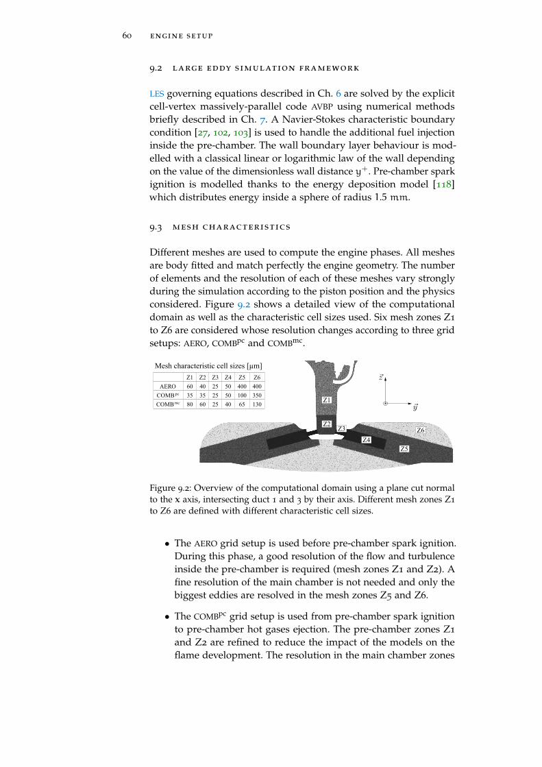
60 engine setup

9.2 large eddy simulation framework

LES governing equations described in Ch. 6 are solved by the explicitcell-vertex massively-parallel code AVBP using numerical methodsbriefly described in Ch. 7. A Navier-Stokes characteristic boundarycondition [27, 102, 103] is used to handle the additional fuel injectioninside the pre-chamber. The wall boundary layer behaviour is mod-elled with a classical linear or logarithmic law of the wall dependingon the value of the dimensionless wall distance y+. Pre-chamber sparkignition is modelled thanks to the energy deposition model [118]which distributes energy inside a sphere of radius 1.5 mm.

9.3 mesh characteristics

Different meshes are used to compute the engine phases. All meshesare body fitted and match perfectly the engine geometry. The numberof elements and the resolution of each of these meshes vary stronglyduring the simulation according to the piston position and the physicsconsidered. Figure 9.2 shows a detailed view of the computationaldomain as well as the characteristic cell sizes used. Six mesh zones Z1

to Z6 are considered whose resolution changes according to three gridsetups: AERO, COMBpc and COMBmc.

Z1

Z2Z3

Z4Z5

Z6

Z1 Z2 Z3 Z4 Z5 Z6AERO 60 40 25 50 400 400

COMB pc 35 35 25 50 100 350COMB mc 80 60 25 40 65 130

Mesh characteristic cell sizes [µm]

Figure 9.2: Overview of the computational domain using a plane cut normalto the x axis, intersecting duct 1 and 3 by their axis. Different mesh zones Z1

to Z6 are defined with different characteristic cell sizes.

• The AERO grid setup is used before pre-chamber spark ignition.During this phase, a good resolution of the flow and turbulenceinside the pre-chamber is required (mesh zones Z1 and Z2). Afine resolution of the main chamber is not needed and only thebiggest eddies are resolved in the mesh zones Z5 and Z6.

• The COMBpc grid setup is used from pre-chamber spark ignitionto pre-chamber hot gases ejection. The pre-chamber zones Z1

and Z2 are refined to reduce the impact of the models on theflame development. The resolution in the main chamber zones

9.3 mesh characteristics 61

Z4 to Z6 are also increased to allow an accurate description ofthe turbulent jets coming from the pre-chamber.

• The COMBmc grid setup is used during the ignition and thecombustion of the main chamber. The mesh resolution is reducedin the pre-chamber and increased in the main chamber, especiallyin the zones Z4 and Z5 where the mechanism of jet ignition isexpected to happen.

The mesh zone Z3 has a constant fine resolution to allow a precisedescription of the flow in the ducts throughout the simulation: 48 and36 points are used to discretize the diameter of the ducts no. 1 and 3

(1.2 mm) and the ducts no. 2 and 4 (0.9 mm), respectively. During thesimulations, the dimensionless wall-distance y+ reaches a maximumvalue of around 150 wall units in the ducts. This ensures that thelaw-of-the-wall remains in its domain of validity as needed for acorrect evaluation of pressure losses between pre- and main chambers.The meshes contain from 50 to 300 million cells depending on thepiston position and the grid setup. An example of the evolution of thenumber of grid cells during a computation is given in Section 10.2.3(Fig. 10.2). Automatic parallel remeshing techniques are used to ensurea limited cell distortion (Section 7.2).

10G L O B A L B E H AV I O U R , λ 1 . 5

10.1 research needs

Academic studies are essential to build knowledge on Pre-ChamberIgnition (PCI) but the question of extrapolation to full systems thenarises: how does PCI behave in a real engine? While Ch. 8 specificallystudies hot burnt gases jet ignition in an academic configuration, thischapter studies the global behaviour of an ICE equipped with a PCI

system detailed in Section 9.1. In a real ICE configuration:

- the geometry is changing with time due to the piston motionso that the spark Ignition Timing (IT) has a crucial effect onpre-chamber ignition and flame propagation;

- the aerodynamic flow created during the compression phaseaffects combustion in both chambers;

- the piston motion directly impacts the pressure difference be-tween the two chambers;

and only the study of a full engine can address these issues correctly.Most of the investigations on PCI systems applied to real engines

was carried out using experimental approaches (e.g., [21–23, 119–132]), often using a laboratory single cylinder engine. Although someexperimental setups give optical access to the combustion chamber,visualization is generally limited to the flame position only (e.g., [119–123]) and optical engines cannot be operated under high loads. Exper-imental engine tests generally only assess engine performances andemissions. They are then very useful to evaluate practical engine oper-ation using new designs or technologies such as PCI. However, they arenot adequate to gain precise knowledge on the aerothermochemicalprocesses taking place inside the combustion chambers.

Numerical simulation then provides a crucial tool to understand thephysical phenomena occurring inside the engines. RANS approachescannot be used here because they are too imprecise and do not captureunsteady phenomena. DNS is too expensive to be performed in a realengine. Then, only LES can be used to study the PCI behaviour in a realengine. LES is essential as a tool to understand and design complexsystems. Therefore, kinetically detailed LES is used now to study theoverall behaviour of the system, with particular attention to:

- the pre-chamber filling and mixture preparation;

- the pre-chamber combustion;

63

64 global behaviour , λ 1 .5

- the jets properties;

- the main chamber ignition and combustion mode.

10.2 configuration

LES is used to simulate the compression and combustion phases of asingle engine cycle at a single operating point. The initial solution forthe LES at Intake Valve Closing (IVC) is extracted from a prior RANS

simulation1. In practice, the primitive variables of the RANS solutionare interpolated on the LES grid and converted into conservative vari-ables. This allows to start the LES computation just after the enginescavenging from a phase-averaged flow and mixture composition. Theturbulent structures in the pre-chamber are very quickly generated bythe jets of fresh mixture from the main chamber during the compres-sion phase and by the additional fuel injection. In the main chamber,they are generated by the jets which emerge from the pre-chamberwhen combustion takes place in it. LES setup and mesh features canbe found in Section 9.2 and 9.3, respectively.

10.2.1 Operating Point

The engine operating point corresponds to a typical motorway engineoperation at 3000 revolutions per minute where consumption mustbe optimized. Propane is used as fuel for both intake lean premixedmixture and pre-chamber additional fuelling. Gaseous fuel injectioninside the pre-chamber starts immediately after IVC = −108.0 CrankAngle Degree (CAD) at the beginning of the compression phase andstops at End Of Injection (EOI) = −70.0 CAD so as to have a meanstoichiometric mixture inside the pre-chamber when igniting the pre-chamber at IT = −10.0 CAD. The mean pressure and temperatureinside the engine at IVC are equal to 2.6 bar and 373K, respectively.The air-fuel equivalence ratio λ of the intake premixed mixture is equalto 1.5 (fuel-air equivalence ratio Φ ' 0.667). This operating point islabelled #λ1.5 IT -10 throughout this manuscript.

10.2.2 Chemistry Description

As for the DNSs of Ch. 8, chemistry must rely on an accurate descrip-tion and contain intermediate species because of the importance ofchemistry in the process of ignition by hot products [41–43]. ARC mech-anisms (Section 5.4.2) are therefore still used for pre-chamber engineLES. The ARC mechanism is specially constructed using the YARC tool[36]. Reduction process of the propane chemistry starts from the San

1 This RANS simulation was realized by the Renault Group using the CONVERGE com-mercial software.

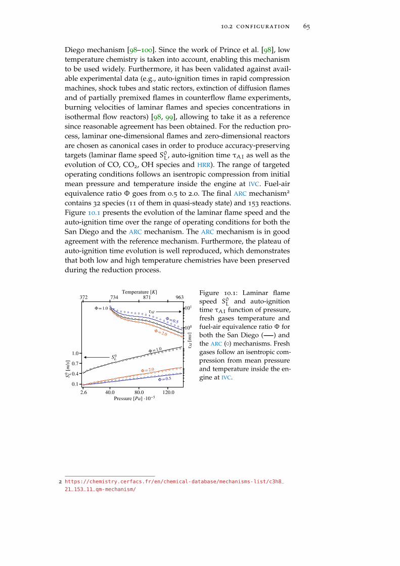
10.2 configuration 65

Diego mechanism [98–100]. Since the work of Prince et al. [98], lowtemperature chemistry is taken into account, enabling this mechanismto be used widely. Furthermore, it has been validated against avail-able experimental data (e.g., auto-ignition times in rapid compressionmachines, shock tubes and static rectors, extinction of diffusion flamesand of partially premixed flames in counterflow flame experiments,burning velocities of laminar flames and species concentrations inisothermal flow reactors) [98, 99], allowing to take it as a referencesince reasonable agreement has been obtained. For the reduction pro-cess, laminar one-dimensional flames and zero-dimensional reactorsare chosen as canonical cases in order to produce accuracy-preservingtargets (laminar flame speed S0L, auto-ignition time τAI as well as theevolution of CO, CO2, OH species and HRR). The range of targetedoperating conditions follows an isentropic compression from initialmean pressure and temperature inside the engine at IVC. Fuel-airequivalence ratio Φ goes from 0.5 to 2.0. The final ARC mechanism2

contains 32 species (11 of them in quasi-steady state) and 153 reactions.Figure 10.1 presents the evolution of the laminar flame speed and theauto-ignition time over the range of operating conditions for both theSan Diego and the ARC mechanism. The ARC mechanism is in goodagreement with the reference mechanism. Furthermore, the plateau ofauto-ignition time evolution is well reproduced, which demonstratesthat both low and high temperature chemistries have been preservedduring the reduction process.

Figure 10.1: Laminar flamespeed S0L and auto-ignitiontime τAI function of pressure,fresh gases temperature andfuel-air equivalence ratio Φ forboth the San Diego ( ) andthe ARC ( ) mechanisms. Freshgases follow an isentropic com-pression from mean pressureand temperature inside the en-gine at IVC.

2 https://chemistry.cerfacs.fr/en/chemical-database/mechanisms-list/c3h8_

21_153_11_qm-mechanism/

66 global behaviour , λ 1 .5

10.2.3 High Performance Computing

Throughout this part, the LESs are performed using 3600 to 7200 MPI

tasks on the Irene34 BULL Sequana X1000 supercomputer equippedwith 1656 Intel Skylake 8168 bi-processors nodes (24 cores per proc.)at 2, 7 GHz.

For the present LES (#λ1.5 IT -10) the evolution of the number ofcells in the meshes as a function of the simulation phase and pistonposition is given in Fig. 10.2. In order to optimize the computationalcost, the AERO (Section 9.3) computation is done using only 5 species:C3H8, O2, N2, CO2 and H2O, without solving chemical reactions. Thisis allowed by the condition of pressure and temperature which ex-clude auto-ignition events during this simulation phase: the chemicalcomposition is thus frozen. Thanks to this strategy combined witha relative low number of cells, the AERO computation accounts foronly 6% of the total computational cost despite its comparatively longphysical duration. The combustion phases COMBpc and COMBmc arethe major contributors to the total computational cost of 1.3 millioncore computing hours for this LES.

Figure 10.2 also shows the evolution of the reduced efficiency, de-fined as

redeff =ncores telapsed

nit ncell neq, (10.1)

where ncores is the number of cores used, telapsed the time elapsedduring the computation, nit the number of iterations, ncell the num-ber of cells and neq the number of transport equations solved. Thisindex measures the efficiency of the computation and should notchange with increasing ncell and neq. The maximum variation fromThese data were

collected duringearly access to the

supercomputer.

the average value is of the order of 10% during each of the three sim-ulation phases. The low deviation of redeff during these simulationphases shows the good behaviour of the numerical solver, as ncellchanges over time. The increase of redeff between AERO and COMB

computations is due to the computation of the chemical reactions andthe combustion model.

3 http://www-hpc.cea.fr/en/complexe/tgcc-JoliotCurie.htm

4 This work was granted access to the high performance computing resources of theTGCC under the GENCI “Grand Challenge” early access grant agreement no. gch0301.

10.3 results 67

SOI EOI IT

3600 cores

5 transported species21 transported

species7200 cores

/nos of cells

Figure 10.2: Number ofmesh cells and reducedefficiency during the LES

(#λ1.5 IT -10).

10.3 results

10.3.1 Pre-Chamber Filling Phase

This section describes the LES results from IVC (-108 CAD) to pre-chamber spark IT (-10 CAD). During this phase, the piston moves upand the pre-chamber is progressively filled by fresh gases coming fromthe main chamber at an air-fuel equivalence ratio λ = 1.5. In addition,from the Start Of Injection (SOI) (-108 CAD) to the EOI (-70 CAD), theadditional fuelling system (Fig. 9.1) adds pure fuel to achieve a nearstoichiometric mixture inside the pre-chamber at IT.

Figure 10.3 shows the evolution of mixture characteristics inside thepre-chamber during this filling phase. The mean air-fuel equivalenceratio of the pre-chamber λpc (based on the mass of oxidizer and fueltrapped inside the pre-chamber) significantly decreases during purefuel injection, then increases because of dilution by fresh gases comingfrom the main chamber to reach λpc ' 1 at IT (-10 CAD). Even ifthe target of a stoichiometric pre-chamber is reached on average, thestandard deviation of λ predicted by the LES inside the pre-chambershows high values which means high segregation of the mixture.Figure 10.4 illustrates this segregation: the rich mixture is located at thetop of the pre-chamber, pushed and confined by the flow of fresh gasescoming from the main chamber with limited mixing. At −10.5 CAD,just before spark IT, λ goes from 1.5 in the flow coming from the mainchamber to 0.4 in the interstices between the ground electrode andthe main chamber, where mixing is poor. Rich pockets may not burn,lead to slow combustion and produce pollutant emissions. To betterquantify the mixture composition at the location of spark ignition,the air-fuel equivalence ratio inside a sphere of radius 2 mm locatedat ignition center λi is plotted over time in Fig. 10.3. λi reaches anair-fuel equivalence ratio around 0.75 before ignition, which meansthat spark ignition takes place in a rich but flammable mixture.

68 global behaviour , λ 1 .5

Figure 10.3 also shows the evolution of the mass fraction of resid-uals gases trapped inside the pre-chamber YpcR that were not fullyscavenged during the exhaust and intake phases. At IVC (-108 CAD),residuals inside the pre-chamber are already diluted (YpcR ' 0.4) whichshows that the intake phase plays a role in the pre-chamber filling.During the compression phase, YpcR significantly decreases to reachYpcR ' 0.025 just before spark IT (-10 CAD): the mass of residuals is

negligible in comparison with the mass of fresh gases. Figure 10.5shows the field of residuals mass fraction YR inside the pre-chamberat −10.5 CAD, just before spark IT. Regions of high YR can inhibitcombustion and are located in the interstices around the spark plug,where the mixture is also very rich because of the poor mixing.

The analysis of the field of equivalence ratio and residuals insidethe pre-chamber leads to a common conclusion: for the present design,mixing could be significantly improved to produce a more homoge-neous charge inside the pre-chamber and dilute residuals. This maybe achieved by reducing interstices and creating a special flow pattern.

Figure 10.3: Air-fuel equivalenceratio inside the pre-chamber λpc

and inside a sphere of radius 2mm located at the spark ignitioncenter λi alongside the standarddeviation of the air-fuel equiva-lence ratio σλpc and the residualsmass fraction YpcR inside the pre-chamber (#λ1.5 IT -10). EOISOI IT

//

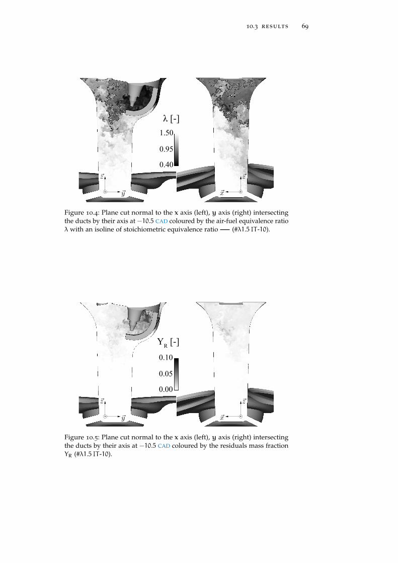
10.3 results 69

1.50

0.95

0.40

λ [-]

Figure 10.4: Plane cut normal to the x axis (left), y axis (right) intersectingthe ducts by their axis at −10.5 CAD coloured by the air-fuel equivalence ratioλ with an isoline of stoichiometric equivalence ratio (#λ1.5 IT -10).

0.10

0.05

0.00

YR [-]

Figure 10.5: Plane cut normal to the x axis (left), y axis (right) intersectingthe ducts by their axis at −10.5 CAD coloured by the residuals mass fractionYR (#λ1.5 IT -10).

70 global behaviour , λ 1 .5

10.3.2 Combustion Phase

This section describes the LES results obtained for the combustionphase from the pre-chamber spark ignition (-10 CAD) to the full con-sumption of the charge.

10.3.2.1 Global Behaviour

Figure 10.6 shows the pressure evolution inside the pre- and mainchambers, as well as the pressure ratio between the two chambers,the global Burnt Fraction (BF) and the CAx which represent the crankangle at which x% of the amount of fuel available have been burnt (i.e.BF = x%). Local BFs and CAx inside pre- and main chambers are shownin Fig. 10.7. BFs are calculated using the progress variable c (Eq. 6.32).After chemical run away time and kernel growth, 10% of the availablecharge inside the pre-chamber has been burnt at −1.7 CAD. Becauseof combustion inside a semi-confined small volume, the pressure inthe pre-chamber increases quickly: first, the flame consumption speedincreases with isentropic compression of fresh gases; second, freshgases are pushed out of the pre-chamber through the ducts. Thesetwo phenomena produce a fast increase of BFpc until approximativelyCA50

pc. Later, the pre-chamber combustion suffers from near-wallcombustion and heat losses inside the small volume as well as localrich mixture combustion due to mixture segregation which slowsdown the BFpc growth. The pressure ratio between the chambersreaches a maximum value of 1.61 which produces vigorous turbulentjets. 11 CAD after spark IT, the first hot gases cross the ducts and enterthe main chamber: Hot Gases Ejection (HGE) happens around 1 CAD.Turbulent jets of hot products successfully ignite the main chamberand 10% and 90% of the available charge inside the main chamber isburnt at 7.7 and 25.3 CAD, respectively. This demonstrates that leanmixtures can be burnt within a short time using such PCI system, asexpected for this device.

Figure 10.6: Pressure in-side pre- and main cham-bers, pre- over main cham-ber pressure ratio and globalBurnt Fraction (#λ1.5 IT -10).

IT

/

10.3 results 71

IT

Figure 10.7: Local BurntFraction inside pre- (BFpc)and main (BFmc) chambers(#λ1.5 IT -10).

10.3.2.2 Jets Properties

Figures 10.8 and 10.9 show ducts characteristic quantities integratedthrough a surface (illustrated in Fig. 10.8) normal to the ducts, locatedat the outlet (main chamber side). Figure 10.8 displays aerodynam-ics properties while Fig. 10.9 focuses on mixture composition. Anyvariable ξ surface mean reads

〈ξ〉 = 1

S

∫∫S

ξdS, (10.2)

where S is the surface of integration. The total enthalpy flow in Fig.10.8 is defined as

Ht =

∫∫S

ρhtu ·nSdS, (10.3)

where ρ is the density, ht is the total enthalpy per unit mass, u is theflow velocity, nS is the normal to the surface S. The Reynolds numbersRe of the ducts are calculated using duct diameter as length scale,surface mean value of density ρ, normal speed Un and temperatureT for viscosity calculation. Jet Reynolds numbers reach values upto 105 during fresh gases ejection and quickly fall during hot gasesejection due to the increase in viscosity. However, all jets remainturbulent. Although the pressure ratio between the chambers reacheshigh values up to 1.6 (Fig. 10.6), it does not reach the theoretical criticalchoked pressure ratio of 1.85 estimated with a constant heat capacityratio γ = 1.33 and no shock is observed: surface mean normal Machnumbers reach values up to 0.75 while normal speeds go over 600m/s.Turbulent Jet Ignition (TJI) starts when the first hot gases comingfrom the pre-chamber penetrate the main chamber (this instant isdenoted HGE) and ends when the pressure ratio between the twochambers becomes unity (mass flow becomes zero). TJI duration isabout 9 CAD (Fig. 10.8). The total enthalpy flow reaches values upto 23 kW for the two bigger ducts and 12 kW for the smaller ones.This is a huge flow of energy in comparison with a classical spark

72 global behaviour , λ 1 .5

plug. For example, a classical spark plug with a nominal electricalenergy of 100mJ and an overall duration of 400µs produces an overalltheoretical transfer of energy to the mixture of 0.25 kW, without takinginto account conductive and radiative losses. Figure 10.9 reveals thatthe composition of the hot gases produced by the pre-chamber toignite the main chamber varies considerably during the TJI process.An intermediates mass fraction YI can be introduced to analyse themixture composition such that

YI = 1− (YC3H8 + YO2 + YCO2 + YH2O + YN2) . (10.4)

The composition of the hot gases jets during TJI can be divided inthree parts (Fig. 10.9), whose exact limits are dependent on the ductconsidered:

1. Intermediate products of lean combustion (due to the pre-chamberflame) are exhausted through the ducts between approximatively1 and 4 CAD where 0.1 < 〈c〉 < 0.9. Even if there is a mean stoi-chiometric mixture inside the pre-chamber, the first hot productsto be exhausted, are produced by combustion of the lean gasesinitially present in the main chamber which flowed through theducts during the compression phase. It follows a simple rule:the last gases to be entered in the pre-chamber are the first to beejected and they control the initiation of the combustion in themain chamber.

2. Complete products of lean combustion are exhausted from ap-proximatively 4 to 7 CAD. The mass fraction of intermediatespecies is very small compared to the other phases.

3. Incomplete products of rich combustion previously trapped inthe upper part of the pre-chamber are then exhausted throughthe ducts except for duct 4. These incomplete combustion prod-ucts cause an increase in the intermediates mass fraction YI ofthe exhausted gases.

When the main chamber pressure becomes higher than the pre-chamber pressure at 10 CAD (Fig. 10.6), back-flow occurs: TJI endssince no hot jets enter the main chamber any more. The lean mainchamber mixture composed of flame kernels is convected back into thepre-chamber which contains hot products of incomplete combustion.The mixing of the lean main chamber mixture which includes O2

in excess with the hot incomplete rich combustion products createsvigorous reactions able to reverse the flow for a short while. However,the combustion in the main chamber is still going on and leads to flowreversal (around 14 CAD) until combustion weakens and mechanicalexpansion through piston movement makes pressure in the mainchamber always lower than in the pre-chamber.

10.3 results 73

Integration surfaces

Figure 10.8: Evolution of total enthalpy flow, surface mean normal speed, surface meantemperature, Reynolds number, surface mean normal Mach number and mass flow throughthe outlet of the ducts. Sketch of the integration surfaces used to compute the quantities(bottom right). #λ1.5 IT -10.

//

//

Figure 10.9: Surface mean species mass fraction, progress variable and fuel air equivalenceratio of the mixture flowing through the ducts (#λ1.5 IT -10).

74 global behaviour , λ 1 .5

Figure 10.10 shows differences of surface mean temperature ∆Tbetween two integration surfaces located at the inlet and at the outletof each duct during TJI. ∆T measures the cooling of the pre-chambergases during their flow through the cooled wall ducts. ∆T presents fluc-tuation at the beginning of TJI process because of the heterogeneitiesof the crossing mixture composed of both pockets of burn gases andfresh gases that flow intermittently through the ducts. Later, from 4 to8 CAD, the temperature drop through the ducts seems to be stabilizedaround 140K for the bigger ducts and 175K for the smaller ones. ∆Tgoes down as the mass flow tends to zero (∆T ∝ m−1) before backflow occurs and TJI ends.

Integration surfaces

Pre-chamber

Main chamber

Figure 10.10: Evolution of temperature difference between inlet and outlet ofthe ducts next to mass flow through the ducts (left). Sketch of the integrationsurfaces used to compute ∆T (right). #λ1.5 IT -10.

10.3.2.3 Main Chamber Ignition

Before Hot Gases Ejection (HGE), the fresh gases turbulent jets pro-duced by the pre-chamber act as a turbulence source for the mainchamber. Then, burnt gases reach the exhaust of the ducts and hotproducts turbulent jets act as both an ignition and a turbulence source.Once the main chamber has been ignited, jets sustain combustion untilpressure equilibrium between the two chambers. Figure 10.11 showsthe flame topology through a plane cut coloured by the HRR ωT forthree depicted sequences of the TJI process:

• Ignition by Hot Gases ejection (IHG): pre-chamber products enterthe main chamber. Close to the nozzle of the ducts, HRR is scarcedue to a combination of local stretch and temperature dropthrough wall heat losses and expansion between pre- and mainchambers. Because of the high turbulence intensity, mixing isfast, hot products are quickly diluted into the surrounding leanfresh mixture and the overall reaction rate is mainly limited bychemistry. Inner intense mixing regions are chemically activedownstream of the jets. No flamelet structure is observed.

10.3 results 75

• Combustion Sustained by Hot Gases ejection (CSHG): flames be-gin to organize as fronts while jets still sustain combustion byproviding more hot products and turbulence sources until thepressure difference between the two chambers becomes negligi-ble. Isolines of temperature become parallel suggesting that aflamelet regime is developing in most of the chamber.

• Combustion Unsustained by Hot Gases ejection (CUHG): wrin-kled flames sweep across the remaining space, consuming thefresh main chamber gases without significant effect of the weak-ened hot product jets. Flamelets are observed almost everywhere.

This ignition sequence corresponds well to the combustion patternsII experimentally established by Yamaguchi et al. [43] where a com-posite ignition due to a combined effect of chemical chain branchingreactions and flame kernels happens followed by wrinkled flames. Thebroadened/distributed reaction zone combustion mode depicted inthe moderate to high injection speed DNSs of Ch. 8 is also found hereduring the first instants of the engine TJI.

Figure 10.12 shows a qualitative estimation of the combustionregime which takes place inside the main chamber during combustionusing the diagram proposed by Peters [133]. lt is the integral lengthscale approximated close to TDC using an empirical relation suggestedby Lumley [134]

lt = hc/6, (10.5)

where hc is the clearance height. u ′t is the fluctuation speed at lengthscale lt estimated assuming a Kolmogorov cascade

u ′t = u′(lt/∆

)1/3, (10.6)

where u ′ is the fluctuation speed at the filter scale ∆ extracted fromthe LES using an operator derived by Colin et al. [58]. Each markercorresponds to a space-averaged value along the flame front (c =

0.3±0.05) inside the main chamber. This low value of progress variableis used to minimize the bias due to increased viscosity and densityacross the flame. As observed in Fig. 10.11, combustion seems tobegin in a thickened-wrinkled flame regime and tends to go towardswrinkled flamelets as u ′t decreases with time due to the diffusion ofthe turbulent kinetic energy previously generated by the jets.

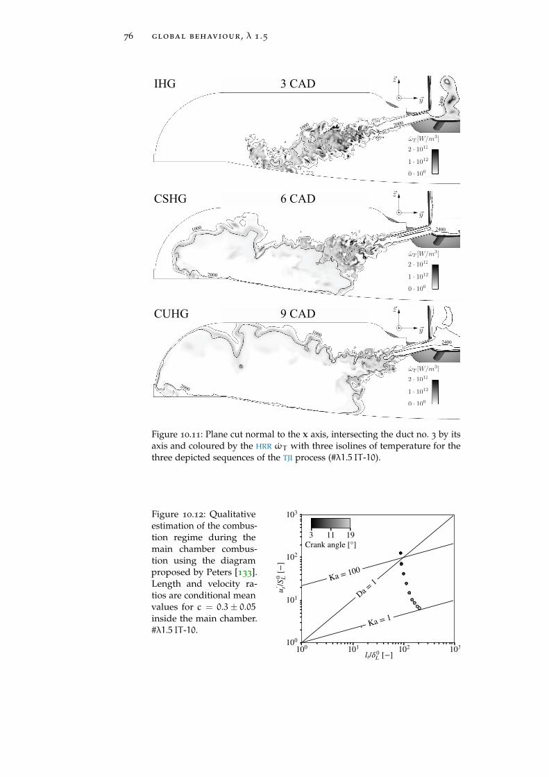
76 global behaviour , λ 1 .5

3 CAD

2400

2000

1000

IHG

6 CAD

2400

2000

1000

CSHG

9 CAD

2400

2000

1000

CUHG

Figure 10.11: Plane cut normal to the x axis, intersecting the duct no. 3 by itsaxis and coloured by the HRR ωT with three isolines of temperature for thethree depicted sequences of the TJI process (#λ1.5 IT -10).

Figure 10.12: Qualitativeestimation of the combus-tion regime during themain chamber combus-tion using the diagramproposed by Peters [133].Length and velocity ra-tios are conditional meanvalues for c = 0.3± 0.05inside the main chamber.#λ1.5 IT -10.

10.4 comparison with spark ignition 77

10.4 comparison with spark ignition

Simulation of an equivalent SI engine is used to assess the benefits ofPCI. The SI engine (Fig. 10.13) features the same geometric properties(Table 9.1) and is run under the same operating conditions as the PCI

engine. The equivalence ratio of the premixed mixture is adjusted totake into account the additional fuel injected into the pre-chamber ofthe PCI engine. The entire mesh is comprised of 130 µm cells to matchthe resolution of the Z6 main chamber zone of the PCI engine mesh(Fig. 9.2).

As expected, the LES results illustrate the major advantage of PCI thatvery quickly creates large flame surface in the main chamber whenthe jets come out (Fig. 10.14). This allows the main chamber charge tobe consumed very quickly, with a maximum burning rate more than3 times higher than that of the equivalent SI engine (Fig. 10.14). Thespark initiated flame kernel in the SI engine develops very slowly inthe combustion chamber while the jets of burnt gases cause very rapidconsumption in the main chamber of the PCI engine (Fig. 10.15).

Spark plug

Figure 10.13: Sketch of the equivalent SI engine.

Figure 10.14: Flame surface inside the main chamber Amcf and global BurntFraction BF for both spark ignition (SI) and pre-chamber ignition (PCI) enginesunder the same operating conditions (#λ1.5 IT -10).

78 global behaviour , λ 1 .5

SI PCI

Figure 10.15: Plane cut normal to the x axis intersecting the ducts no. 1 and 3 by their axis andcoloured by the normalized HRR with three isolines of temperature for both spark ignition (SI)and pre-chamber ignition (PCI) engines under the same operating conditions (#λ1.5 IT -10).

10.5 conclusion 79

10.5 conclusion

In this chapter, the behaviour of a PCI system used to ignite themain chamber of an engine has been studied using LES with complexchemistry and detailed geometry in a real engine. The LES allows toanalyse the flow entering and leaving the pre-chamber, to measurethe cooling and quenching effects introduced by the passage of hotgases through the ducts connecting pre- and main chambers and toanalyse the ignition and combustion sequences. For the case studiedhere, small amount of flame kernels are exhausted from the pre-chamber. Hot products penetrate the main chamber, disperse and mixwith the fresh reactants and lead to ignition. The combustion in themain chamber starts in a distributed reaction mode before reaching aflamelet propagation mode.

In addition, results have been compared with an equivalent SI enginerunning under the same operating conditions. The main chambercombustion duration is found to be significantly reduced by the earlycreation of a large flame surface by the pre-chamber jets using PCI.

11I G N I T I O N FA I L U R E , λ 2 . 0

11.1 research needs

Pre-chamber ignition technology only pushes the lean operation limitfurther: that limit still exists. Above a certain air dilution rate, ignitionof the main chamber may fail and this must be avoided for normal ICE

operation. This is a crucial issue for the engine efficiency. Typically, anengine running at λ = 1.5 may not be sufficiently efficient to justify theadditional production cost of pre-chamber technology but an enginerunning at λ = 2.0 certainly will. In this chapter, an ultra-lean (λ = 2.0)main chamber misfire observed during engine tests1 is studied usingLES to understand what are the causes of the ignition failure and givedesign indications that could push this limit further.

11.2 configuration

11.2.1 Operating Point

The operating point is the same as #λ1.5 IT -10 (Section 10.2.1) exceptthat the air-fuel equivalence ratio λ of the intake premixed mixture is2.0 (fuel-air equivalence ratio Φ = 0.5). It is then labelled #λ2.0 IT -10.The additional fuel injection is extended up to −51.2 CAD so as tomaintain a mean stoichiometric mixture inside the pre-chamber at IT2.

11.2.2 Chemistry Description

Since the ARC mechanism described in Section 10.2.2 predicts auto-ignition times which are a little too high compared to the referenceSan Diego mechanism for λ = 2.0 mixtures, a new ARC mechanism hasbeen specially derived. The chemical mechanism reduction follows asimilar process to that described in Section 10.2.2. Starting from the SanDiego mechanism, the final ARC mechanism3 contains 37 species (14of them in quasi-steady state) and 128 reactions. The evolution of thelaminar flame speed and the auto-ignition time (Fig. 11.1) predictedby the ARC mechanism over the range of operating conditions are in

1 Engine tests carried out as part of the Efficient Additivated Gasoline Lean Engine (EA-GLE) project funded by the European Union’s Horizon 2020 research and innovationprogramme under grant agreement no. 724084.

2 Injection is timed using the 0D engine model PEMIP described in Ch. 14.3 https://chemistry.cerfacs.fr/en/chemical-database/mechanisms-list/c3h8_

23_128_14_qm-arc-mechanism/

81

82 ignition failure , λ 2 .0

good agreement with the reference San Diego mechanism, even forultra lean mixtures.

Figure 11.1: Laminar flame speed S0L and auto-ignition time τAI functionof pressure P, fresh gases temperature Tu for laminar flames or initial freshgases temperature Ti for igniting reactors and fuel-air equivalence ratio Φ forthe reference (REF), the skeletal (SKEL) and the ARC mechanisms (ARC). Freshgases follow an isentropic compression from mean pressure and temperatureinside the engine at IVC.

11.3 results

11.3.1 Pre-Chamber Filling

Due to a larger quantity of pure fuel injected into the pre-chamber aswell as a leaner premixed mixture, the stratification of the mixture inthe pre-chamber is greater than it was for the λ = 1.5 case #λ1.5 IT -10(Fig. 11.2). However, the equivalence ratio close to the spark ignitionlocation is nearly the same: the spark ignition takes place under thesame mixture conditions.

Figure 11.2: Air-fuelequivalence ratio in-side a sphere of radius2 mm located at thespark ignition center λi

and standard deviationof the air-fuel equiva-lence ratio inside thepre-chamber σλpc forboth #λ1.5 IT -10 and#λ2.0 IT -10.

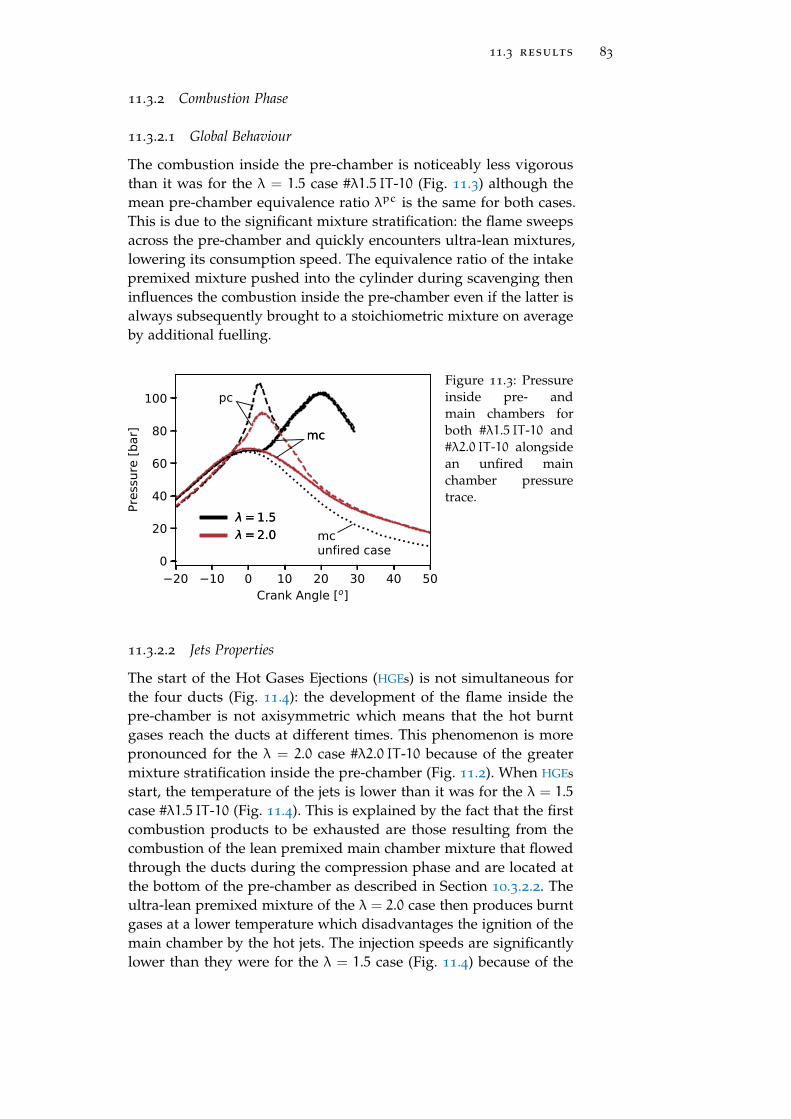
11.3 results 83

11.3.2 Combustion Phase

11.3.2.1 Global Behaviour

The combustion inside the pre-chamber is noticeably less vigorousthan it was for the λ = 1.5 case #λ1.5 IT -10 (Fig. 11.3) although themean pre-chamber equivalence ratio λpc is the same for both cases.This is due to the significant mixture stratification: the flame sweepsacross the pre-chamber and quickly encounters ultra-lean mixtures,lowering its consumption speed. The equivalence ratio of the intakepremixed mixture pushed into the cylinder during scavenging theninfluences the combustion inside the pre-chamber even if the latter isalways subsequently brought to a stoichiometric mixture on averageby additional fuelling.

mcunfired case

Figure 11.3: Pressureinside pre- andmain chambers forboth #λ1.5 IT -10 and#λ2.0 IT -10 alongsidean unfired mainchamber pressuretrace.

11.3.2.2 Jets Properties

The start of the Hot Gases Ejections (HGEs) is not simultaneous forthe four ducts (Fig. 11.4): the development of the flame inside thepre-chamber is not axisymmetric which means that the hot burntgases reach the ducts at different times. This phenomenon is morepronounced for the λ = 2.0 case #λ2.0 IT -10 because of the greatermixture stratification inside the pre-chamber (Fig. 11.2). When HGEs

start, the temperature of the jets is lower than it was for the λ = 1.5case #λ1.5 IT -10 (Fig. 11.4). This is explained by the fact that the firstcombustion products to be exhausted are those resulting from thecombustion of the lean premixed main chamber mixture that flowedthrough the ducts during the compression phase and are located atthe bottom of the pre-chamber as described in Section 10.3.2.2. Theultra-lean premixed mixture of the λ = 2.0 case then produces burntgases at a lower temperature which disadvantages the ignition of themain chamber by the hot jets. The injection speeds are significantlylower than they were for the λ = 1.5 case (Fig. 11.4) because of the

84 ignition failure , λ 2 .0

lower pressure difference between pre- and main chambers (Fig. 11.3).According to the findings of Ch. 8, this is not an issue for jet ignitionwhich, on the contrary, becomes more critical when the injection speedincreases and not when it decreases.

TJI ends herefor

Figure 11.4: Surface mean temperature < T > and normal speed < Un > atthe outlet of the ducts for both #λ1.5 IT -10 and #λ2.0 IT -10.

11.3.2.3 Main Chamber Ignition

Pressure traces suggest a discharge of the pre-chamber into the mainchamber without ignition and combustion of the main chamber charge.In the plane cutting the largest ducts (no. 1 and 3, Fig. 9.1), hot burntgases jets create well dispersed reactive regions but fail to give rise tohealthy propagating flame fronts that consume the charge as in theλ = 1.5 case (Fig. 11.5). For the smallest ducts (no. 2 and 4), hot andreactive regions are scarce and quickly dissipated in the fresh mixture(Fig. 11.6): the ignition failure is more obvious.

11.3 results 85

λ = 2.0 λ = 1.5

Figure 11.5: Plane cut normal to the x axis intersecting the ducts no. 1 and 3 by their axis andcoloured by the normalized HRR with three isolines of temperature for both #λ2.0 IT -10 and#λ1.5 IT -10.

86 ignition failure , λ 2 .0

λ = 2.0 λ = 1.5

Figure 11.6: Plane cut normal to the y axis intersecting the ducts no. 2 and 4 by their axis andcoloured by the normalized HRR with three isolines of temperature for both #λ2.0 IT -10 and#λ1.5 IT -10.

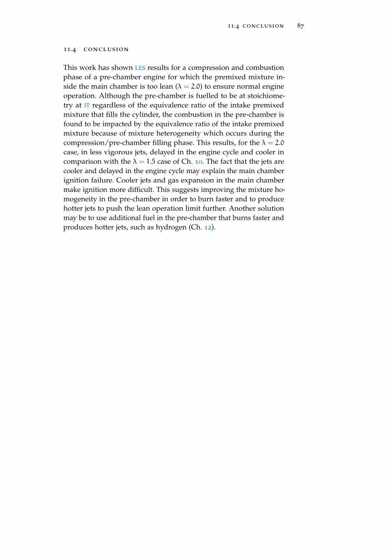
11.4 conclusion 87

11.4 conclusion

This work has shown LES results for a compression and combustionphase of a pre-chamber engine for which the premixed mixture in-side the main chamber is too lean (λ = 2.0) to ensure normal engineoperation. Although the pre-chamber is fuelled to be at stoichiome-try at IT regardless of the equivalence ratio of the intake premixedmixture that fills the cylinder, the combustion in the pre-chamber isfound to be impacted by the equivalence ratio of the intake premixedmixture because of mixture heterogeneity which occurs during thecompression/pre-chamber filling phase. This results, for the λ = 2.0case, in less vigorous jets, delayed in the engine cycle and cooler incomparison with the λ = 1.5 case of Ch. 10. The fact that the jets arecooler and delayed in the engine cycle may explain the main chamberignition failure. Cooler jets and gas expansion in the main chambermake ignition more difficult. This suggests improving the mixture ho-mogeneity in the pre-chamber in order to burn faster and to producehotter jets to push the lean operation limit further. Another solutionmay be to use additional fuel in the pre-chamber that burns faster andproduces hotter jets, such as hydrogen (Ch. 12).

12H Y D R O G E N A D D I T I O N , λ 2 . 0

12.1 research needs

Chapter 11 has shown that ultra lean λ = 2.0 main chamber premixedcharge fails to burn properly even when using PCI technology. Thisis a problem since these dilution levels must be reached in order tojustify the development of this technology in ICEs. Therefore, solutionsmust be sought. In this chapter, an additional fuelling of hydrogenin the pre-chamber is used to increase the pre-chamber combustionspeed and jets temperature in order to try to enable ultra lean maincharge combustion.

12.2 configuration

12.2.1 Operating Point

The operating point is the same as #λ2.0 IT -10 (Section 11.2.1) exceptthat hydrogen is used for additional pre-chamber fuelling. It is thenlabelled #λ2.0H2 IT -10. Due to the low hydrogen molecular weight,the injection diameter of the additional fuelling system (Fig. 9.1) is in-creased from 0.5 to 3 mm in order to allow sufficient pre-chamber fuelmass injection from IVC to −54.0 CAD to achieve a mean stoichiometricmixture inside the pre-chamber at IT1.

12.2.2 Chemistry Description

The ARC mechanism reported in Sec. 11.2.2 is used to properly describethe C3H8/H2-air chemistry. Figure 12.1 shows the laminar flame speedand the auto-ignition time for multiple hydrogen fuel addition to aλ = 2.0 C3H8-air mixture. This fuel addition is characterized by ahydrogen fuel mass ratio ξH2 defined as

ξH2 =YH2

YH2 + YC3H8. (12.1)

Results from the ARC mechanism are in good agreement with the ref-erence San Diego mechanism, showing that the H2 chemistry reactionpaths have been preserved during the reduction process.

1 Injection is timed using the 0D engine model described in Ch. 14.

89

90 hydrogen addition, λ 2 .0

Figure 12.1: Laminar flame speed S0L and auto-ignition time τAI functionof pressure P, fresh gases temperature Tu for laminar flames or initial freshgases temperature Ti for igniting reactors and hydrogen fuel mass ratioξH2 for the reference (REF), the skeletal (SKEL) and the ARC mechanisms(ARC). Fresh gases follow an isentropic compression from mean pressure andtemperature inside the engine at IVC. λC3H8 = 2.0, λ changes with ξH2 .

12.3 results

12.3.1 Pre-Chamber Filling

The mixture is still strongly stratified while a mean stoichiometricmixture is achieved at IT (Fig. 12.2). The higher hydrogen moleculardiffusivity does not improve mixing in the pre-chamber where hetero-geneities persist and pockets of rich gases are still trapped at the topof the pre-chamber (Fig. 12.3). The hydrogen fuel mass ratio inside thepre-chamber at IT is equal to 0.285.

Figure 12.2: Air-fuel equiv-alence ratio inside the pre-chamber λpc and inside asphere of radius 2 mm lo-cated at the spark ignitioncenter λi alongside the stan-dard deviation of the air-fuel equivalence ratio in-side the pre-chamber σλpc(#λ2.0H2 IT -10).

100 80 60 40 20Crank angle [°]

0.0

0.2

0.4

0.6

0.8

1.0

[] /

[

]

pci

pc

12.3 results 91

Figure 12.3: Plane cut normal to the x axis intersecting the ducts no. 1 and 3

by their axis at −10.5 CAD coloured by the air-fuel equivalence ratio λ withan isoline of stoichiometric equivalence ratio for both hydrogen (H2 inj.,#λ2.0H2 IT -10) and propane (C3H8 inj., #λ2.0 IT -10) additional fuelling.

12.3.2 Combustion Phase

12.3.2.1 Global Behaviour

Pre-chamber combustion is significantly boosted by the hydrogen ad-ditional fuelling leading to faster combustion and higher overpressurein the pre-chamber (Fig. 12.4). The pressure in the main chamberinitially seems to indicate a proper combustion initiation but thendrops suggesting a failed ignition.

mcunfired case

inj.inj.

Figure 12.4: Pressureinside pre- and main cham-bers for both hydrogen(H2 inj., #λ2.0H2 IT -10)and propane (C3H8 inj.,#λ2.0 IT -10) additionalfuelling alongside anunfired main chamberpressure trace.

92 hydrogen addition, λ 2 .0

12.3.2.2 Jets Properties

Faster pre-chamber combustion leads to earlier Hot Gases Ejections(HGEs) (Fig. 12.5). Hydrogen addition causes hotter jets due to thermo-chemical effects (i.e. higher adiabatic combustion temperature). Thejets injection speed is significantly higher as a result of the higherpre-chamber overpressure (Fig. 12.5). The heat released in the mainchamber quickly re-establishes a pressure balance between the pre-and main chambers (Fig. 12.4) which makes the injection shorter intime.

Figure 12.5: Surface mean temperature < T > and normal speed < Un >at the outlet of the ducts for both hydrogen (H2 inj., #λ2.0H2 IT -10) andpropane (C3H8 inj., #λ2.0 IT -10) additional fuelling.

12.3.2.3 Main Chamber Ignition

The hotter jets succeed in initiating flame fronts in the main chamber(Figs 12.6 and 12.7). While the pure propane case shows large welldispersed weakly reactive zones which do not transition to healthyflame fronts, the case with hydrogen additional fuelling quickly givesrise to established flame fronts in the main chamber as discussed inSection 10.3.2.3. This indicates (as expected from Fig. 12.4) that thehydrogen additional fuelling makes possible the ignition of the ultralean λ = 2.0 premixed mixture of the main chamber. However, oncethese flame fronts are established, the ultra lean flame consumptionrate is such that the main chamber charge is very slowly consumed.

12.3 results 93

H2 injection C3H8 injection

Figure 12.6: Plane cut normal to the x axis intersecting the ducts no. 1 and 3 by their axis andcoloured by the normalized HRR with three isolines of temperature for both hydrogen (H2 inj.,#λ2.0H2 IT -10) and propane (C3H8 inj., #λ2.0 IT -10) additional fuelling.

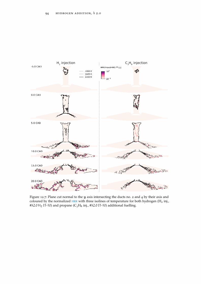
94 hydrogen addition, λ 2 .0

H2 injection C3H8 injection

Figure 12.7: Plane cut normal to the y axis intersecting the ducts no. 2 and 4 by their axis andcoloured by the normalized HRR with three isolines of temperature for both hydrogen (H2 inj.,#λ2.0H2 IT -10) and propane (C3H8 inj., #λ2.0 IT -10) additional fuelling.

12.4 conclusion 95

12.4 conclusion

Pre-chamber hydrogen additional fuelling has been used in an attemptto enable combustion of an ultra lean premixed λ = 2.0 propane-airmixture. Results show that it makes main chamber ignition and flamefronts initiation possible. However, the consumption speed of the ultralean flames is still too low to consume the main chamber charge fastenough, causing engine efficiency issues and possible partial burncycles. To overcome this, it is necessary to increase the flame surfacein the main chamber. This may be done, for example, by increasingthe jets speed (by decreasing the diameter of the connecting ducts)and/or by increasing the ignition sites (by increasing the number ofducts).

13L AT E I G N I T I O N , λ 1 . 5

13.1 research needs

In this chapter, LES is used to investigate another issue linked to pre-chamber engines: late ignition. Shortening the catalyst light-off timeis critical in order to reduce pollutant emissions during cold enginestarts. For that, engine manufacturers use delayed ignitions to burnlate in the engine cycle and increase the temperature of the exhaustgases. However, experimental results1 indicate an inability to delayignition with pre-chamber systems, without clear explanation. Thischapter presents an LES study of late ignition on a pre-chamber engineto understand the causes of ignition failures observed experimentally.

13.2 configuration

13.2.1 Operating Point

The operating point is the same as #λ1.5 IT -10 (Section 10.2.1) exceptthat the IT is shifted from −10 to +20 CAD to simulate a late ignitioncase. It is then labelled #λ1.5 IT+20.

13.2.2 Chemistry Description

The chemistry used is the same as that used for the LES of Ch. 10

described in section Section 10.2.2.

13.3 results

13.3.1 Pre-Chamber Filling

Now that ignition takes place after TDC, the flow in the pre-chamberchanges drastically: the pre-chamber mixture is sucked out during thepiston downward phase after having been supplied by the additionalfuel injection and by the main chamber premixed mixture duringthe piston upward phase. The mean pre-chamber equivalence ratiobecomes lean due to a longer filling by the main chamber lean mixturebut almost gets down to stoichiometry due to the mixture sucked outduring the piston downward phase (Fig. 13.1). The mixture has more

1 Engine tests carried out as part of the Efficient Additivated Gasoline Lean Engine (EA-GLE) project funded by the European Union’s Horizon 2020 research and innovationprogramme under grant agreement no. 724084.

97

98 late ignition, λ 1 .5

time to mix: it results in a lower equivalence ratio standard deviationand a near spark plug mixture closer to stoichiometry. The suction ofthe pre-chamber mixture during the piston downward phase makesthe additional fuel not to be stuck at the top of the pre-chamber andmakes it spread throughout the pre-chamber (Fig. 13.2). All thesephenomena lead to a more homogeneous mixture in the pre-chamber(σλpc = 0.19 for #λ1.5 IT+20 at IT versus σλpc = 0.35 for #λ1.5 IT -10 atIT), which should be beneficial for pre-chamber combustion.

Figure 13.1: Air-fuelequivalence ratio insidethe pre-chamber λpc

and inside a sphereof radius 2 mm lo-cated at the spark ig-nition center λi along-side the standard de-viation of the air-fuelequivalence ratio insidethe pre-chamber σλpc(#λ1.5 IT+20).

100 75 50 25 0Crank angle [°]

0.2

0.4

0.6

0.8

1.0

1.2

[] /

[

]

pc

i

pc

Figure 13.2: Plane cut normal to the x axis (left), y axis (right) intersectingthe ducts by their axis at +19.5 CAD coloured by the air-fuel equivalence ratioλ with an isoline of stoichiometric equivalence ratio (#λ1.5 IT+20).

13.3 results 99

13.3.2 Combustion Phase

The ignition failure—observed experimentally—is captured by theLES: a little overpressure is observed in the pre-chamber while themain chamber remains unaffected (Fig. 13.3). Combustion inside thepre-chamber stops before the entire charge is burned and no chemicalactivity appears inside the main chamber (Fig. 13.4). The flame kernelinitiated by the spark plug in the pre-chamber is sucked by the estab-lished flow from pre- to main chamber due to the piston downwardmovement (Fig. 13.5). This kernel is then trapped at the bottom ofthe pre-chamber while being cooled and discharged into the mainchamber without having time to consume the pre-chamber charge. Itis subsequently quenched by the cold walls, prematurely ending thecombustion in the engine.

0 10 20 30 40 50Crank Angle [o]

10

20

30

40

50

60

70

Pres

sure

[bar

]

mcpcmcpc

Figure 13.3: Pressure inside pre-and main chambers (#λ1.5 IT+20).

20 30 40 50Crank Angle [ ]

0.0

0.2

0.4

0.6

0.8

1.0

BF [-

]

0

2

4

6

mea

n(HR

R) [W

/m3 ]

10

9mcpcmcpc

Figure 13.4: Burnt Fraction and meanHRR inside pre- and main chambers(#λ1.5 IT+20).

100 late ignition, λ 1 .5

Figure 13.5: Plane cut normal to the x axis (left), y axis (right) intersecting theducts by their axis and coloured by the normalized HRR with three isolinesof temperature (#λ1.5 IT+20).

13.4 conclusion 101

13.4 conclusion

LES has been used to investigate misfires that occur when enginesequipped with pre-chambers are operated under late IT conditions.When ignition occurs before TDC, the developing flame is held insidethe pre-chamber under the effect of the inflow due to the main chambercompression during the piston upward phase. On the contrary, resultsshow that a late ignition after TDC causes the aspiration of the initiatedflame kernel by the outflow due to the main chamber expansionduring the piston downward phase. This flame kernel is maintainedat the bottom of the pre-chamber, cooled by the walls before beingsucked into the main chamber in the form of cold burnt gases withoutgiving rise to ignition.

Part V

Z E R O - D I M E N S I O N A L P R E - C H A M B E RI G N I T I O N E N G I N E M O D E L T O A S S I S T

T E C H N O L O G Y D E S I G N

DNS and LES are useful tools to gain knowledge on pre-chamber ignition technology. However, they cannot beused as industrial design tools to assess the performancesof numerous engine geometries and operating points be-cause of their relatively high computational cost. A zero-dimensional pre-chamber ignition engine model is thendeveloped to assess the influence of geometric or operatingpoint changes on engine operation at a low computationalcost. It incorporates a jet ignition submodel based on theDNS results of Part iii to track misfires. The engine modelis validated a posteriori on the LES results of Part iv. Thispart describes its construction and application.

14P R E - C H A M B E R E N G I N E M O D E L L I N G

This chapter presents a zero-dimensional model derived completelyduring this PhD. This tool uses a multi-zone approach, similar to theusual performance models used in industry. Its objective is to obtainthe speed, temperature and composition of the jets entering the mainchamber after having get through multiple ducts whose influence ismodelled. At this point, a model for Turbulent Jet Ignition (TJI) basedon the DNSs of Ch. 8 is used to predict whether main chamber ignitionoccurs. This engine model is dubbed PEMIP for Pre-chamber EngineModel with Ignition Prediction.

14.1 research needs

Efficient design processes that use optimization algorithms to get thebest combination of parameters to maximize a given quality functionrequire engine models using minimal computational resources sincethey may be called hundreds of thousands of times during the opti-mization process. Engine designers may also simply want to quicklystudy the effects of a design change.

Reduced models have been used for a very long time in all typesof engines, including PCI engines (e.g., [135–140]). However, as yetno model developed for PCI engines includes submodels to take intoaccount the thermal effects in the ducts connecting pre- and mainchambers, nor to predict the result of the main chamber jet ignitionattempts. They assume an automatic ignition of the main chamberand some of them even impose a combustion law like the well-knownWiebe law [141]. As a consequence, they totally miss an importantpart of the problem and cannot be used near the ignition limit.

This is why PEMIP, a zero-dimensional PCI engine model that in-cludes both duct thermal effects and jet ignition prediction, is nowderived.

14.2 modelling approach

The global model is decomposed into four open systems that canexchange mass with each other and heat with the outside. Thesesystems are called zones and are namely: the pre-chamber fresh gaseszone (pcf), the pre-chamber burnt gases zone (pcb), the main chamberfresh gases zone (mcf) and the main chamber burnt gases zone (mcb)(Fig. 14.1). Inside these gaseous zones, the temperature, the pressure

105

106 pre-chamber engine modelling

and the mixture are supposed to be homogeneous. The pressure P isuniform inside the pre-chamber (pc)

Ppc = Ppcf = Ppcb (14.1)

and inside the main chamber (mc)

Pmc = Pmcf = Pmcb. (14.2)

in out

­­­ ­­

Figure 14.1: Sketch of PEMIP zones and submodels.

14.3 evolution of the thermodynamic state of the zones

The state variables required for the description of each zone are

- P, the pressure of the zone;

- mk for k = 1 to N, the mass of the N species present in themixture;

- a state variable describing the energy of the system, here thetemperature T ;

- V , the volume of the zone.

There is therefore a need for N+ 3 equations per zone that steer theevolution of these state variables. These equations are then describedin this section. They arise from ideal gas law, species mass balance,energy balance and volume variation laws. The mass m inside eachzone simply reads

m =

N∑k

mk (14.3)

and the species mass fractions

Yk =mkm

for k = 1,N . (14.4)

14.3 thermodynamic state of the zones 107

14.3.1 Ideal Gas Law

The N species gaseous mixture that fills the four zones is supposed tobe ideal such that the equation of state reads PV = mRT/W or in itsderived form For clarity, the

specific zone suffixes(pcf, pcb, mcf andmcb) are omittedwhen the equation isvalid for the fourzones of PEMIP.

PdV

dt+V

dP

dt−

R

WTdm

dt−

R

WmdT

dt−RTm

N∑k

1

Wk

dYkdt

= 0, (14.5)

where R, t, W and Wk are the universal ideal gas constant, the time,the mean molecular weight and the molecular weight of the kth species,respectively.

14.3.2 Species Mass Balance

The zones can have multiple inlets and outlets. Gases exit the zones atthe outlets with the current state of the zones. The rate of change inthe mass of each species then reads

d (mk)

dt=

∑i

miYk,i −∑o

moYk, (14.6)

where Yk,i is the mass fraction of the kth species of the mixture enteringthe zone through the ith inlet, mi and mo are the mass flow enteringthe zone through the ith inlet and leaving the zone via the oth outlet,respectively. Summing Eq. 14.6 over all species, the expression of themass variation can be readily obtained

dm

dt=

∑i

mi −∑o

mo. (14.7)

14.3.3 Energy balance

The temperature T is used to describe the energy of the system. Writingthe first law of thermodynamics for an open system, the balanceequation for the total internal energy U reads

dU

dt= −P

dV

dt+ Qw +

∑i

mihi − h∑o

mo, (14.8)

where Qw is the rate of heat transfer through the walls, hi the enthalpyper unit mass of the mixture entering the zone through the ith inlet,and h the enthalpy per unit mass. For an ideal gas, the total internalenergy can be rewritten in terms of mass fractions and temperature

U = m

N∑k

Ykuk(T) (14.9)

108 pre-chamber engine modelling

or, in its derived form

dU

dt= u

dm

dt+mCv

dT

dt+m

N∑k

ukdYkdt

, (14.10)

where u is the total internal energy per unit mass, Cv the heat capacityat constant volume per unit mass, and uk the total internal energy perunit mass of the kth species. Substituting the corresponding derivativesand using h = u+PV/m yields a balance equation for the temperature

mCvdT

dt+ P

dV

dt= Qw +

∑i

mi

(hi −

N∑k

ukYk,i

)−PV

m

∑o

mo.

(14.11)

14.3.4 Volume Variation

The volume variation of the zones inside the constant volume pre-chamber follows

dVpcf

dt+dVpcb

dt= 0. (14.12)

In the main chamber, the volumes change such that

dVmcf

dt+dVmcb

dt=dVmc

dt, (14.13)

with

dVmc

dt=

14s cos(Ω)√

c2 − (12s sin(Ω))2+1

2

sΩ sin(Ω)πb2

4, (14.14)

where s, c, b, Ω and Ω are the engine stroke, connecting rod length,bore, crank angle and angular rotation speed, respectively.

14.4 wall heat losses

The rate of heat transfer through the walls of both chambers is com-puted as

Qw = Awhw(Tw − T), (14.15)

where Aw is the wall surface area, hw the wall heat transfer coefficient,and Tw the wall temperature supposed to be spatially uniform andconstant during the whole engine cycle. The heat transfer coefficientis estimated using a specific correlation for four-stroke engines [142]

hw =κ

LChw

(ρUpL

µ

)0.7

, (14.16)

14.5 submodel for the connecting ducts 109

where κ is the gas thermal conductivity, Chw a constant which dependson the engine geometry, ρ the gas density, µ the gas dynamic viscosity,L a characteristic length that equals the pre-chamber diameter dpc forthe pre-chamber zones and the engine bore b for the main chamberzones, and Up is the mean piston speed defined as

Up = sΩ

π. (14.17)

The wall surface of each zone is estimated using pre- (Apcw ) or mainchamber wall surface (Amcw ) weighted by the zone filling volumefraction, which compares the volume of the specific zone to the volumeof the chamber to which it belongs, such that

Apcfw = ApcwVpcf

Vpcf + Vpcb, (14.18)

Apcbw = ApcwVpcb

Vpcf + Vpcb, (14.19)

Amcfw = AmcwVmcf

Vmcf + Vmcb(14.20)

and

Amcbw = AmcwVmcb

Vmcf + Vmcb, (14.21)

with

Amcw = Apw+Ahw+πb

12s(1− cos(Ω)) + c−

√c2 −

(1

2sin(Ω)

)2 ,

(14.22)

where Apw and Ahw are the surface area of the piston and the head ofthe engine, respectively.

14.5 submodel for the connecting ducts

Due to a pressure difference between the divided chambers, a massflow from one of the two chambers (called the upstream chamber,up) to the other (called the downstream chamber, ds) occurs. Gases The flow can go both

ways: from pc to mcbut also vice versa.

first expand at the duct inlet (in) from Pup to Pin before flowing intothe constant cross section duct, exchanging heat through the walls(Fig. 14.2). The heat exchange can cause the temperature at the ductoutlet (out) Tout to be significantly different from the temperature atthe duct inlet (in) T in (Section 10.3.2.2 and Ref. [44]). This must betaken into account because the temperature of the burnt gases jets isone of the key parameters controlling the ignition of the main chamber(Section 8.3.1).

110 pre-chamber engine modelling

Figure 14.2: Sketch of a flowthrough a duct following anexpansion from an upstreamchamber to a downstreamchamber.

14.5.1 Inflow Properties

The inflow properties are estimated assuming an isentropic expansionat a constant heat capacity ratio γ equal to the heat capacity ratio of theupstream chamber γup. The critical pressure ratio between upstreamand downstream chambers from which the flow is choked is definedas

Pr,cr =

(γup + 1

2

) γup

γup−1

. (14.23)

Therefore, the pressure ratio between the upstream chamber and theinlet of a duct which acts as a throat reads

Pinr = min(Pup

Pds,Pr,cr

). (14.24)

The temperature at the inlet of a duct is estimated as

T in = TupPinr1−γup

γup (14.25)

and the mass flow of the jth duct as

md,j = CdjAd,jPup

√2γup

γup − 1

Wup

RTup

(Pinr

− 2γup − Pinr

−γup+1γup

),

(14.26)

where Ad,j is the cross section of the jth duct and Cdj the dischargecoefficient of the jth duct estimated using the correlation of Ashiminet al. [143]

Cdj =

[1.23+ 58

(md,jdd,j

Ad,jµin

)−1 ld,j

dd,j

]−1, (14.27)

where dd,j and ld,j are the diameter and length of the jth duct, re-spectively. The mixture composition is assumed not to change duringthe expansion from the upstream chamber to the inlet of a duct (i.e.Yupk = Yink ).

14.5 submodel for the connecting ducts 111

14.5.2 Outflow Properties

From the inlet to the outlet of the ducts, the gases exchange heatthrough the walls, which varies their temperature and potentially theirchemical composition. The quick hot gases discharge does not lastlong enough to significantly change the temperature of the walls Twwhich is supposed to be constant over the whole engine cycle.

14.5.2.1 Equations Describing the Evolution of the Flowing Mixture

Inside the ducts, the pressure is assumed to be homogeneous suchthat

Pin = Pout =Pup

Pinr. (14.28)

The residence time tres of a fluid element that goes through the jth

duct is estimated as

tres,j = ld,jρinAd,j

md,j, (14.29)

so that a Lagrangian approach is the most convenient one to determinethe flow state in the ducts. From t = 0 at the inlet to t = tres,j at theoutlet of the jth duct, the evolution of the bulk thermochemical vari-ables of the flowing mixture can be described by Ordinary DifferentialEquations (ODEs) taking into account potential chemical reactions:

- one equation for temperature

dT

dt=

1

ρCp

[4

ddh(Tw − T) −

N∑k

ωkhk

], (14.30)

where Cp is the heat capacity at constant pressure per unit mass,h the heat transfer coefficient, dd the duct diameter, ωk and hkare the chemical source term and the enthalpy per unit mass ofthe kth species, respectively;

- and one equation for each species mass fraction

dYkdt

=1

ρωk. (14.31)

14.5.2.2 Changes in Burnt Gases Composition

The evolution of the composition of the gases within the ducts mayimpact the subsequent potential ignition of the main chamber andmust be considered: the gases flowing in the ducts may reach outlettemperature chemical equilibrium, may be frozen at initial composi-tion, or may be in-between, depending on the ratio of chemical andflow times.

112 pre-chamber engine modelling

To assess the evolution of the composition of the burnt gases thatflow through a duct, Eqs 14.30 and 14.31 are integrated from t = 0 tot = tres,j thanks to a SciPy [144] wrapped ODE solver. Thermodynamicand kinetic parameters needed in each equation are computed usingCantera [101]. Data from LES of the real engine ignition sequence ofCh. 10 are used to assess whether the composition has time to change.It was chosen to extract the data in one of the smallest ducts (duct no.2) at the time when the residence time is the shortest during the burntgases injection period. In this way, if the mixture reaches equilibrium inthis situation (high temperature losses and short residence time) thenit would be possible to assume that the mixture reaches equilibriumin all cases. Initial thermodynamic properties are extracted from theLES, initial mixture composition is set to equilibrium. The convectiveheat transfer coefficient h is adjusted so that the final temperatureT(t = tres,2) equals the outlet temperature of the LES. Figure 14.3shows that under these conditions which are typical of a real engine,the residence time is too short for the mixture to reach equilibriumThe same chemical

mechanism was usedin both LES and

Cantera.

but long enough for the mixture to have time to react so that thecomposition changes. It is then impossible to assume equilibrium, norfrozen chemistry during the flow of burnt gases. The evolution ofchemistry must be resolved if a precise description of the compositionat the outlet of the duct is required.

Figure 14.3: Temperatureand species mass frac-tion evolution of burntgases loosing heat in agiven time alongside cor-responding equilibriumcomposition. Heat lossesand end time are set tomatch LES data of Ch. 10

at the shortest residencetime for the duct no. 2.

EquilibriumODEs integration

14.5.2.3 Strategy to Estimate the Outflow Mixture Properties

A slight variation in the burnt gases composition may have an effecton the ignition of the main chamber but has a negligible contributionto the thermodynamic properties of the zones. Thus, to reduce com-putational cost, an analytic expression for the temperature neglectingchemical reactions is used when the mixture does not react or when aslight variation in the burnt gases composition does not matter, i.e.:

- during fresh gases flow;

14.6 submodel for jet ignition 113

- during burnt gases flow, once the main chamber has been ig-nited.

Assuming that the mixture does not react and that thermodynamicproperties do not change from the inlet to the outlet of the jth duct,the outlet temperature can be analytically estimated as [145]

Toutj = Tw + (T in − Tw)exp

(−πdd,j ld,j h

inj

md,jCpin

). (14.32)

Eq. 14.32 is used during the whole engine cycle except during the burntgases jet ignition period, where Eqs 14.30 and 14.31 are integratedso as to know the exact composition of the jets of burnt gases. In allcases, the convective heat transfer coefficient is evaluated at the inletof the ducts and equals hinj , estimated using Sieder and Tate [146]

correlation multiplied by a correction factor 1+(dd,jld,j

)2/3to take into

account the effect of a non-developed temperature profile following asudden contraction in a short duct [147]

hinj =κin

dd,j0.027

(4md,j

µinπdd,j

)0.8(µinCpin

κin

)1/3(µin

µinw

)0.14

[1+

(dd,j

ld,j

)2/3]. (14.33)

14.6 submodel for jet ignition

Now that the temperature, speed and composition of the gases exitingthe holes are known, a model is needed to predict whether these gasesignite the main chamber. This ignition by the jets of hot burnt gasesmust be modelled in order to take into account potential misfires dueto too high injection speeds or too low temperatures (Section 8.3.1).Here, the DNSs of Ch. 8 are used to build and validate models for that.

Modelling the scenario of Fig. 8.1 requires assumptions on themechanisms controlling ignition. These mechanisms may change whenjet properties vary: for low injection speeds, chemistry evolves in ashorter time scale than mixing, making flamelet approaches probablyadequate; on the other hand, for larger injection speeds, mixing andchemical time scales may become comparable which suggests thatmodels not relying on any flame structure assumption may be moreappropriate. Therefore, two models are tested here (Fig. 14.4):

- The first one (called Unsteady Flamelet for Ignition Prediction(UFIP), Section 14.6.1) is a variation of the classical RIF proposedby N. Peters [92–94] and assumes that the ignition process takesplace (or not) in a thin, flamelet-like front.

114 pre-chamber engine modelling

- The second one (called Convected Open Reactor (COR), Sec-tion 14.6.2) adopts a Lagrangian vision to relax the flameletassumption: it views the ignition process as the evolution ofan open well-stirred reactor convected into the chamber, wherefresh gases and hot products mix at a certain rate and ignite ornot.

1 0

in

out

­

­

Figure 14.4: The two models developed from DNS to describe ignition by a jetof hot burnt gases.

In each of these models, the jets are assumed to act as an infi-nite source of ignition sites having the same aerothermochemicalproperties. As a consequence, a single ignition site can be used as arepresentation of the multiple ignition attempts. The DNSs of Ch. 8

have reached a quasi-steady state (Section 8.2.5) so that they generatedan infinity of ignition sites and are within the scope of the models.They will be then used as a reference to evaluate the models in thenext sections. Although they were realized at atmospheric conditions(fresh gases temperature Tu = 298K, pressure P = 1 atm), the mainignition mechanisms are not expected to differ from those at ICE rel-evant conditions. The fresh gases of the DNSs are lean and premixed(equivalence ratio Φu = 0.8): they are therefore within the scope ofPCI engines burning homogeneous lean mixtures.

14.6.1 Unsteady Flamelet for Ignition Prediction (UFIP) Model

As established by Peters [92], if chemistry is fast compared to trans-port processes, combustion takes place within asymptotically thinlayers embedded in the flow. Applying this concept to jet ignition, theboundary of the jet may be seen as a continuous interface strained andThis interface is

initiallynon-reacting but

later can ignite.

convected by the flow [91] (Fig. 14.4). Along this interface, the motionof any fluid line segment may be decomposed into translation, rotationand strain (given by the relative change in length of the line segment).In the reference frame of the fluid line segment, the only effect ofmotion that will be apparent is that of strain [148]. Translation androtation may change the mixture that the flame front encounters, but

14.6 submodel for jet ignition 115

only strain will alter the internal flame structure. These line segmentsembedded between the cold unburnt and the hot burnt gases arecalled flamelets (even before they start igniting), their inner structureis one-dimensional and time-dependent. They lose heat only to theunburnt gases side and can receive heat and chemically active radicalsfrom the burnt gases side. The concept of the UFIP model follows thisidea: one representative unsteady strained flamelet is supposed to cap-ture what is happening at the boundary of the jet in terms of ignition.In this work, the open-source software Ember [149] is used to computethis unsteady flamelet with high efficiency [150], assuming an infinitereservoir of burnt gases on the product side of the counterflow flame.

A flame in this configuration can never be completely extinguishedbecause there will always be a region of contact between reactantsand products where some heat release takes place: a threshold of HeatRelease Rate (HRR) is needed to distinguish between flamelets able toglobally ignite the fresh mixture or not. This threshold is arbitrarilyset to half of the max(HRR) found in a one-dimensional premixedlaminar flame at the same fresh gases conditions. As the temperaturedrop increases at the burnt gases side of the flamelets, chemistry isweakened and the time to reach this threshold increases (Fig. 14.5).For a fuel with Lewis number higher than unity, heat diffuses morequickly than mass, reducing the temperature in the reaction zonewhen strain increases and therefore the HRR decreases monotonicallywith the strain rate a [151].

Tdrop 0 K 100 K 200 K 300 K 400 K 500 K 600 K

max

(HRR

) [W

/m3 ]

10-9

max

(HRR

) [W

/m3 ]

10-9

time [ms] time [ms] time [ms]

max(HRR)1DL

max(HRR)1DL max(HRR)1DL

max(HRR)1DLmax(HRR)1DL

max(HRR)1DL

0.5 max(HRR)1DL

0.5 max(HRR)1DL 0.5 max(HRR)1DL

0.5 max(HRR)1DL0.5 max(HRR)1DL

0.5 max(HRR)1DL

‘‘failure’’ ‘‘failure’’ ‘‘failure’’

a = 10 s-1 a = 100 s-1 a = 500 s-1

a = 1500 s-1a = 1000 s-1a = 750 s-1

for Tdrop>400 K for Tdrop>200 K for Tdrop>100 K

Representative of Uinj = 50 m/s using KUFIP = 0.06

*

*

*

** *

+

++

++

* +

Figure 14.5: Temporal evolution of the maximum HRR in one-dimensionalstrained unsteady flamelets for multiple strain rates a and temperaturedrops Tdrop at 1 atm, Tu = 298K and Φu = 0.8. Dashed lines do not crossthe 0.5max(HRR)1DL horizontal line. It is assumed that the correspondingflamelets are too weak to lead to global ignition in jet ignition cases.

Hot burnt gases jet ignition exhibits different structural charac-teristics with increasing turbulence intensity starting from wrinkledflames to a more disorganized combustion pattern where small eddies

116 pre-chamber engine modelling

broke/broaden the reaction zone (Section 8.3.3). Results from UFIP

can only be compared to DNSs lying in the flamelet regime where thereaction zones are not distributed/broadened and the burnt gases arenot highly fragmented in space. This limit the range of application ofthe UFIP model to the Uinj = 50 m/s DNS cases only.

The UFIP model requires a relation between the stretch to imposeto the representative flamelet—which reduces to the strain in its zero-curvature planar configuration—and the aerodynamic features of thejet. In a three-dimensional flow field, at each point of an isosurface ofprogress variable c, the flame stretch is defined as

κ = −nn : ∇u+∇ ·u+ Sd(∇ ·n), (14.34)

where n is the flame normal pointing toward the fresh gases

n = −∇c|∇c|

, (14.35)

u is the flow velocity and Sd is the flame displacement speed

Sd =1

|∇c|Dc

Dt, (14.36)

where c is the progress variable computed using Eq. 6.32. Data fromthe DNSs can be post processed to evaluate the level of stretch that theinterface between burnt and fresh gases undergoes. However, thereare several obstacles: first, the flamelets at the interface of the jetare subject to a wide range of local stretches (Fig. 14.6). Second, thestrain rate of the interface changes in time as it is randomly disturbedby the flow. Constructing a single strain rate to apply to a flameletsupposed to represent what is happening at the whole interface of thejet becomes difficult: locally, a thin layer may undergo low strain ratesand lead to ignition even if globally, the average strain rate is high.Moreover, a flame may survive at higher unsteady strain rates than itwould at steady strain rates [152]. These difficulties prevent from usingthe unsteady and heterogeneous flow field of the DNSs to establish arelation between the UFIP strain to be applied and the jet characteristics.Here, to bypass this problem, a simpler approach is used: an equivalentstrain rate ae is defined as the steady strain applied to UFIP flameletswhich would be equivalent to what happens to the unsteady thinlayers featuring large strain variation. ae is supposed to scale as theinverse of a jet flow time scale defined as the ratio between the ductdiameter and the injection speed such that

ae = KUFIPUinj

d, (14.37)

where KUFIP is a scaling constant. The UFIP model is in good agreementwith the DNSs for KUFIP = 0.06 which results in ae = 750 s−1 forUinj = 50 m/s, close to the most probable stretch values encountered

14.6 submodel for jet ignition 117

in the DNSs for this injection speed (Fig. 14.6). For this strain rate,UFIP predicts an ignition failure for Tdrop > 300 K using the arbitrarythreshold 0.5max(HRR)1DL to distinguish between ignition successand failure (Fig. 14.5).

Tdrop= 0 K Tdrop= 100 K Tdrop= 200 K

Figure 14.6: Kernel density approximation and histogram of the stretchcomputed using 0.1 < c < 0.9 isosurfaces in the DNSs of Ch. 8. Annotatedstretches are most probable values. Uinj = 50 m/s.

14.6.2 Convected Open Reactor (COR) Model

The UFIP model is limited to flamelet-like thin reaction fronts, whichrestricts its range of application to low injection speeds. As an alterna-tive, a more general modelling approach (the COR model) is explorednow (Fig. 14.4). It consists in following an open reactor—small enoughto be homogeneous—full of burnt gases, convected into the chamber:these hot burnt gases then mix at a certain rate with the cold freshgases within this open reactor and chemistry inside the reactor can betracked using an ODE solver with complex chemistry. In this approach,the mixture fraction between the hot jet and the cold gases ξ in theopen reactor changes according to a mixing rate: it starts at ξ = 1 inthe injected burnt gases jet and goes to ξ = 0 as the reactor is con-vected inside the chamber and mixes with the fresh gases. The detailsof the convection movement are unimportant once the evolution of ξis specified.

The balance equations are those describing the evolution of an opensystem at constant pressure. The mass balance equation reads

dm

dt= min − mout, (14.38)

where m is the reactor mass, min is the mass flow entering the reactor(i.e. that comes from the flammable atmosphere) while mout is themass flow of gases leaving the reactor with the current state of thereactor. The rate of entrainment of the cold mixture into the system θ

is defined as

θ =minm

. (14.39)

The N species balance equations for the convected reactor read

dYkdt

= θ(Yink − Yk

)+rT

Pωk for k = 1,N , (14.40)

118 pre-chamber engine modelling

where Yink is the mass fraction of the kth species entering the reactor,and r the specific gas constant r = R/W.

The energy balance equation can be rearranged to describe theevolution of temperature

dT

dt=

1

Cp

[θ

N∑k=1

Yink(hink − hk

)−rT

P

N∑k=1

hkωk

], (14.41)

where Cp is the specific heat capacity at constant pressure, and hinkthe enthalpy per unit mass of the kth species entering the reactor.

The evolution of the mixture fraction ξ is described by a passivescalar balance equation similar to Eq. 14.40 without chemical sourceterm

dξ

dt= θ

(ξin − ξ

)= −ξθ, (14.42)

since ξin = 0 (the fresh gases entering the reactor have a zero mix-ture fraction). Thus, using chain’s rule, the system evolution can bedescribed as a function of ξ by a set of N+ 1 equations:

dYkdξ

=dYkdt

dt

dξ= −

1

ξ

(Yink − Yk

)−rT

θξPωk for k = 1,N (14.43)

and

dT

dξ=dT

dt

dt

dξ= −

1

ξCp

N∑k=1

Yink(hink − hk

)+

rT

ξθCpP

N∑k=1

hkωk .

(14.44)

This model was used to aid the interpretation of experimental resultsfor burnt gases jet ignition [24], namely the OH LIF signals. A similarconcept was also used to examine the evolution of a hot air kernelejected into a stratified coflow [153]. Here, the aim is to predict ignition.Balance equations 14.43 and 14.44 are integrated thanks to a SciPy[144] wrapped ODE solver. Thermodynamic and kinetic parametersneeded in each equation are computed using Cantera [101].

The weak part of the COR model is that all mixing aspects arehidden in the mixing rate θ (Eq. 14.39) which becomes the mostcritical parameter of the model. The mixing rate θ should be equal tozero in the fresh and in the burnt gases (i.e. θ(ξ = 1) = θ(ξ = 0) = 0)and should be non-zero in the mixing zones. Since mixing occursby removal of scalar variance and the scalar dissipation rate of ξ χξIn the DNSs, ξ is a

passive scalarinjected from the

inlet following theburnt gases function

fb (Eq. 8.7).

represents the rate at which the fluctuation of ξ are destroyed, it isassumed here that the mixing rate θ is linked to the rate at whichmixing occurs in the jet and therefore to χξ so that a linear relationbetween the mixing rate θ and the scalar dissipation rate of ξ is usedto close the model. To finalize the model for θ, the distribution of χξas a function of ξ in the DNSs (Fig. 14.7) can be used. χξ = f(ξ) seems

14.6 submodel for jet ignition 119

to follow a parabolic curve such that θ may be modelled using thefunction

θ = θ04ξ(1− ξ), (14.45)

where θ0 is the maximum mixing rate supposed to scale as the inverseof a jet flow time scale such that

θ0 = KCORUinj

d, (14.46)

where KCOR is a scaling constant.

Uinj= 50 m/s Uinj= 250 m/sUinj= 150 m/s

** *

*

DNS data

with

Figure 14.7: Scatter plot of the scalar dissipation rate of the jet mixturefraction χξ versus the corresponding value of jet mixture fraction ξ in theDNSs of Ch. 8 alongside the θ modelling function (Eq. 14.45) with KCOR = 0.3(—). Tdrop = 0 K, t = 0.4 ms.

Figure 14.8 shows an example of COR model results for Tdrop = 100

K using various values for the maximum mixing rate θ0. As expected,for large θ0, chemistry is not fast enough to balance the cooling effectof the entrainment of fresh gases. Temperature quickly falls to thefresh gases temperature: it is an ignition failure. For smaller θ0, therate of combustion heating exceeds the rate of entrainment coolingand temperature rises to the burnt gases temperature: it is an ignitionsuccess. The COR model captures the essence of the phenomena atplay here: ignition is controlled by the balance between the rate ofcombustion heating due to the combustion of the entrained fresh fueland the rate of mixing cooling due to the entrainment of fresh gases.

T [K

]

Tdrop = 100 K equilibrium

mixing

Figure 14.8: Evolution of the tempera-ture inside multiple COR model openreactors for different maximum mix-ing rates θ0 at 1 atm, Tu = 298K andΦu = 0.8. The trajectories start at ξ = 1

(in the hot burnt gases jet) and go toξ = 0 as the system fills with fresh gases.The mixing line corresponds to an in-finitely fast mixing case while the equi-librium line corresponds to an infinitelyfast chemistry case.

From this, it is possible to compute θcrit0 , the critical mixing ratewhich separates ignition success from ignition failure. Using KCOR =

120 pre-chamber engine modelling

0.3 in Eq. 14.46 the ignition limit established by the COR model is infairly good agreement with all DNS results (Fig. 14.9). This suggeststhat, despite its simplicity, the COR model (which accounts for complexchemistry effects) captures ignition limits reasonably.

Figure 14.9: Ignition map of thestudied cases (results of the DNSs ofCh. 8) together with the UFIP modelignition limit for KUFIP = 0.06 andthe COR model ignition limit forKCOR = 0.3. UFIP limit

COR limit

14.6.3 Conclusion

Two jet ignition models have been derived and calibrated using datafrom the DNSs of Ch. 8. Major drawbacks of the UFIP model are i) theneed of a representative steady strain rate and ii) the flamelet regimeassumption. The COR model adopts an opposite modeling strategyby assuming perfect mixing and no flamelet structure as the UFIP

model does. The ignition limits given by the COR model are in goodagreement with the DNSs of Ch. 8 showing that it is a good candidateto predict the ignition of a flammable atmosphere by jets of hot burntgases for which flamelet approaches (such as UFIP) are not adequate asmany regimes encountered during these ignition sequences, especiallyat large injection speeds, do not fall in the flamelet regime.

Therefore, the COR model will be used in PEMIP to predict theignition of the main chamber by the jets of hot burnt gases. For theapplication of this ignition model to the complete pre-chamber enginemodel PEMIP, the jets of hot burnt gases will be considered as asuccession of quasi-steady states, each generating an infinite numberof ignition attempts. Figure 14.10 shows guidelines for using the COR

model which is quite simple and can be coupled to the equations ofSection 14.5.

14.7 turbulence 121

Figure 14.10: Flowchart showing the practical use of the COR model.

14.7 turbulence

Turbulence kinetic energy in the pre- and main chambers is mod-elled using a simple phenomenological approach [138]. Turbulence issupposed to be only due to the inflowing duct jets such that in each The inflowing kinetic

energy is supposed tobe totally convertedinto turbulentkinetic energy.

chamber

dmK

dt=

∑j

md,jUoutj

2

2−mε, (14.47)

where K is the turbulence kinetic energy per unit mass, Uoutj is the jth

duct outlet velocity in the event that the ducted flow transfers into thechamber (pc or mc) and ε is the rate of dissipation of the turbulencekinetic energy defined as

ε =(2K/3)3/2

lt, (14.48)

with lt = dd, the mean duct diameter defined as

dd =

√√√√ 1

nd

∑j

dd,j2, (14.49)

where nd is the number of ducts.

14.8 flame surface

Combustion inside pre- and main chambers is modelled by a flamesurface Af that sweeps across the chambers consuming the fresh gases.

122 pre-chamber engine modelling

A simple closed balance equation for the flame surface density Σ maybe derived from heuristic arguments following Marble et al. [59] andDarabiha et al. [154], assuming that Σ is homogeneous

dΣ

dt= CA+,t

f

ε

KΣ−CA−

fS0L

Σ2

1− bf, (14.50)

where CA+,tf

and CA−f

are two model constants and ε/K represents theflame stretch generated by the turbulence. The first term in the RightHand Side (RHS) expresses the flame surface production due to thestretch rate acting on the flame surface, the second term expresses theflame annihilation, assumed to be proportional to the mean reactionand inversely proportional to the available reactants per unit of flamearea. S0L is the only chemical parameter appearing in the balanceequation. It is computed and tabulated using Cantera [101] beforebeing read according to the thermochemical conditions of the freshgases.

Integrating Eq. 14.50 over the pre-chamber volume, a balance equa-tion for the pre-chamber flame surface is obtained

dApcf

dt= Cpc

A+,tf

εpc

KpcApcf −Cpc

A−f

S0Lpc A

pcf2

1− bfpc, (14.51)

which describes the flame surface evolution after having been initiatedat spark IT as a sphere of radius 1.5mm.

In the main chamber, when burnt gases injection occurs and ignitionhas been realized, the production of flame surface by the jet injection ofburnt gases should be taken into account by an additional productionterm estimated as Cmc

A+,jetf

∑j πdd,jU

outj (Fig. 14.11). The main chamber

flame surface balance equation therefore reads

dAmcfdt

= CmcA+,tf

εmc

KmcAmcf −Cmc

A−fS0Lmc Amcf

2

1− bfmc+Cmc

A+,jetf

∑j

πdd,jUoutj .

(14.52)

Figure 14.11: Sketch offlame surface productionby a cylindrical jet ofburnt gases.

14.9 mass transfer

The zones can exchange mass with each other by different means: bycombustion (fresh gases zone to burnt gases zone) and by transfer

14.10 resolution of the ordinary differential equations 123

through the ducts. During combustion, the rate of mass transfer fromfresh gases to burnt gases in each chamber reads

mf→b = ρfS0LAf, (14.53)

where ρf is the density of the fresh gases that the flame is consuming.Before that hot burnt gases issue into the main chamber, the mixtureflowing from the main chamber to the pre-chamber is made up offresh gases. When combustion occurs in the pre-chamber, fresh gasesare first pushed out before that burnt gases reach the inlet of theducts and are pushed out in turn. This transition from fresh gasesto burnt gases ejection is controlled by BFpcthr, the pre-chamber BurntFraction (BF) threshold from which burnt gases are ejected through theducts. After that burnt gases ejection starts, if a backflow from mainto pre-chamber occurs due to the combustion in the main chamber, itis assumed that this flow is made up of burnt gases only.

14.10 resolution of the set of ordinary differential

equations

The set of ODEs comprises 2× (3+ 2× (2+N)) = 14+ 4×N equationswhereN is the number of species (Table 14.1). There are also 14+ 4×Nunknown variables (Table 14.2) so that the problem is closed. Themodel description has eight constants, namely:

- Cpchw and Cmchw, the wall heat transfer constants (Eq. 14.16);

- CpcA+,tf

and CmcA+,tf

, the flame surface production by flame stretch

constants (Eqs 14.51 and 14.52);

- CmcA

+,jetf

, the flame surface production by jet injection constant

(Eq. 14.52);

- CpcA−f

and CmcA−f

, the flame surface destruction constants (Eqs 14.51

and 14.52);

- BFpcthr, the pre-chamber Burnt Fraction threshold from whichburnt gases are ejected from the pre-chamber.

The set of ODEs can be written in a matrix form such as

Ad

dt(ψ(t)) = f (ψ(t)) , (14.54)

where A is the matrix that contains the coefficients in front of thederivatives of the ODEs and ψ is the vector of unknown variables. Byinverting the matrix A, all the time derivatives can be expressed as afunction of the instantaneous variables

d

dt(ψ(t)) = A−1f (ψ(t)) . (14.55)

124 pre-chamber engine modelling

Euler’s method is then used to approximate the solution over time,using linear approximation over a short time step dt

ψ(t+ dt) = ψ(t) +A−1ψ(t)dt. (14.56)

mc,pc

volume Eqs 14.12/14.13

turbulence kinetic energy Eq. 14.47

flame surface Eqs 14.51/14.52

f, b

ideal gas law Eq. 14.5

species mass balance Eq. 14.6

energy balance Eq. 14.11

Table 14.1: List of the 14+ 4×N ODEs.

mc,pcP, Af, K

f, b V , mk, T

Table 14.2: List of the 14+ 4×N variables.

15A P P L I C AT I O N T O P R E - C H A M B E R I G N I T I O NE N G I N E

The engine model PEMIP described in Ch. 14 is now applied to the PCI

engine introduced in Ch. 9 and used for the LESs of Part iv. First, themodel constants are calibrated using the LES of Ch. 10, then the resultsare compared to the LESs of Chs 11-13 and to an additional LES of anearly ignition case (not shown within Part iv).

15.1 calibration of the model constants

The operating point labelled #λ1.5 IT -10 and the LES data of Ch. 10

are used to calibrate the model constants detailed in Section 14.10.Unfired non reactive compression and expansion strokes are firstused to calibrate wall heat transfer constants before calibrating thecombustion model using fired strokes. Final model constants areshown in Table 15.1. More details on the calibration methodology aregiven in the following subsections.

CmcKwCpcKw

CmcA+,tf

Cpc

A+,tf

CmcA

+,jetf

CmcA−f

Cpc

A−f

BFpcthr

0.445 0.2 0.45 1.2 10.0 2.0 3.6 0.73

Table 15.1: Model constants calibrated to match the LES data of Ch. 10.

15.1.1 Non Reactive Case

The only unset model constants for non reactive (unfired) cases arethe two wall heat transfer constants CmcKw

and CpcKw , since the six otherconstants relate to the combustion model. These constants are cali-brated to match the pre- and main chamber mean temperature of anunfired LES at an intake premixed mixture air-fuel equivalence ratioλin = 1.5 (Fig. 15.1). Other zone state variables are in good agreement,the pre-chamber equivalence ratio differs during the piston down-ward phase because of mixture stratification (Section 10.3.1) that is notsolved by PEMIP: the mixture that escapes first is located at the bottomof the pre-chamber, this is the lean mixture that came from the mainchamber. Making it escape thus increases the fuel-air equivalence ratio.Duct quantities are in good agreement.

125

126 application to pre-chamber ignition engine

Figure 15.1: Temperature, pressure and fuel-air equivalence ratio inside pre-and main chambers (upper row) and duct mass flow, outlet speed and outlettemperature (bottom row) for both unfired PEMIP and LES (λin = 1.5).

15.1.2 Reactive Case

BFpcthr is directly set using the LES data, computing the Burnt Fraction(BF) inside the pre-chamber at the moment when the mean progressvariable at the outlet of the ducts exceeds 0.5 (2.35 CAD, BFpc= 0.73).The remaining constants of the flame surface models are calibrated tomatch the fired LES data (Fig. 15.2). First, pre-chamber flame surfaceconstants are tuned in order to match the flame surface of the LES. Forthe main chamber, the flame surface computed from the LES cannotbe targeted as part of the combustion takes place in a well dispersedcombustion regime where no flame front clearly consumes the charge(Section 10.3.2.3). Both pressure and combustion duration are targetedinstead. The jet ignition model predicts an instantaneous ignition forall ducted jets. Duct quantities can only be compared before that mainchamber combustion induces a backflow into the pre-chamber. Fromthis point, the backflow is supposed to be made up of burnt gases inPEMIP while the composition changes depending on the position ofthe flame in the actual engine (Section 10.3.2.2). Before this backflow,duct quantities are in good agreement. Outlet temperature is slightlyover estimated because of the pre-chamber mixture homogeneityassumption that does not hold in the actual engine: lean burnt mixtureis first pushed out of the pre-chamber (Section 10.3.1) that producescooler jets than stoichiometric burnt gases. In addition, the drop intemperature through the ducts is a little overestimated during the firstmoments of Turbulent Jet Ignition (TJI) (Fig. 15.3).

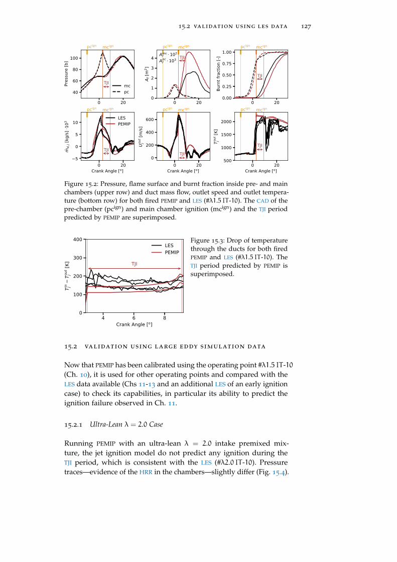
15.2 validation using les data 127

Figure 15.2: Pressure, flame surface and burnt fraction inside pre- and mainchambers (upper row) and duct mass flow, outlet speed and outlet tempera-ture (bottom row) for both fired PEMIP and LES (#λ1.5 IT -10). The CAD of thepre-chamber (pcign) and main chamber ignition (mcign) and the TJI periodpredicted by PEMIP are superimposed.

4 6 8Crank Angle [o]

0

100

200

300

400

Tin jTou

tj

[K] TJI

LESPEMIP

Figure 15.3: Drop of temperaturethrough the ducts for both firedPEMIP and LES (#λ1.5 IT -10). TheTJI period predicted by PEMIP issuperimposed.

15.2 validation using large eddy simulation data

Now that PEMIP has been calibrated using the operating point #λ1.5 IT -10(Ch. 10), it is used for other operating points and compared with theLES data available (Chs 11-13 and an additional LES of an early ignitioncase) to check its capabilities, in particular its ability to predict theignition failure observed in Ch. 11.

15.2.1 Ultra-Lean λ = 2.0 Case

Running PEMIP with an ultra-lean λ = 2.0 intake premixed mix-ture, the jet ignition model do not predict any ignition during theTJI period, which is consistent with the LES (#λ2.0 IT -10). Pressuretraces—evidence of the HRR in the chambers—slightly differ (Fig. 15.4).

128 application to pre-chamber ignition engine

In the pre-chamber, the overpressure observed with PEMIP is cer-tainly due to the mixture homogeneity assumption: in PEMIP, themixture is burnt close to stoichiometry whereas in the actual engine ithas been shown that pre-chamber combustion starts in a rich mixturetrapped at the top of the pre-chamber (Section 11.3.1). Rich mixturecombustion leads to lower burning rates and burnt temperatures andtherefore a lower overpressure in the partially enclosed pre-chamber.

In the main chamber, although the burnt gases jets do not give riseto healthy flame fronts (Section 11.3.2.3), there is still some reactiveregions during the TJI period that consumes some of the main chambercharge without giving rise to self-sustained flames. These complexphenomena are not taken into account in PEMIP which only gives ayes or no answer to the main chamber ignition. PEMIP main chamberBF then remains very low, only supplied by the burnt gases comingfrom the pre-chamber.

Figure 15.4: Pressure and burnt fraction inside pre- and main chambers forboth PEMIP and LES (#λ2.0 IT -10). The CAD of the pre-chamber ignition (pcign)and the TJI period predicted by PEMIP are superimposed.

15.2.2 Ultra-Lean λ = 2.0 Case With Hydrogen Addition

The case with hydrogen pre-chamber fuelling #λ2.0H2 IT -10 of Ch. 12

is now used in order to evaluate the capability of PEMIP to reproducethe key quantities giving rise to the ignition of the main chamber. InPEMIP, the propane pre-chamber injection is replaced by a hydrogeninjection and the premixed laminar flame speeds are tabulated as afunction of an additional variable: the hydrogen fuel mass ratio ξH2(Eq. 12.1) recalled here

ξH2 =YH2

YH2 + YC3H8.

Running PEMIP in this configuration, main chamber ignition occursduring the TJI period as for the LES (Fig. 15.5). Unlike #λ1.5 IT -10(Fig. 15.2) where main chamber ignition occurs at the same time forall the jets, here the jets issuing from the largest holes (d1,3) ignite the

15.2 validation using les data 129

main chamber before the jets issuing from the smallest holes (d2,4).This is consistent with what can be observed on LES results where at5 CAD the ignition of the main chamber by the jets of d1,3 occurred(Fig. 12.6) while it is necessary to wait until around 10 CAD to observemain chamber ignition from d2,4 jets (Fig. 12.7). This is due to acombined effect of temperature and mixing rate: when duct diameterdecreases, temperature loss and jet mixing rate increase (Fig. 15.6),which disadvantages jet ignition. Furthermore, the ignition followedby the slow main chamber charge consumption observed using LES iscorrectly retrieved by PEMIP.

The pre-chamber charge is consumed slightly faster in the LES. Thisis again due to the mixture homogeneity assumption of PEMIP whichmodels a homogeneous stoichiometric combustion in the pre-chamberwithout taking into account the equivalence ratio stratification. Here,the rich C3H8/H2-air mixture actually trapped at the top of the pre-chamber in the LES burns faster than a stoichiometric C3H8/H2-airmixture initially made up of the same C3H8-air mixture. This is il-lustrated in Fig. 15.7 where pure hydrogen has been added to aninitial C3H8-air mixture at λC3H8 = 2.0 for the condition of pressureand temperature of the pre-chamber at IT. At a fuel-air equivalenceratio equal to that inside a sphere of radius 2 mm located at the sparkignition center in the LES at IT Φi,ITLES = 1.58, the flame consumes thecharge faster than at stoichiometry as it is assumed in PEMIP.

Figure 15.5: Pressure and burnt fraction inside pre- and main chambers forboth PEMIP and LES (#λ2.0H2 IT -10). The CAD of the pre-chamber (pcign) andmain chamber ignition (mcign) and the TJI period predicted by PEMIP aresuperimposed. Jet ignitions from duct no. x are annotated dx.

130 application to pre-chamber ignition engine

Figure 15.6: Jet maximum mixing rate θ0 (Eq. 14.46) and duct outlet temper-ature for both PEMIP and LES (#λ2.0H2 IT -10). The CAD of the main chamberignition (mcign) and the TJI period predicted by PEMIP are superimposed. Jetignitions from duct no. x are annotated dx.

Figure 15.7: Premixed laminarflame speed S0L, adiabatic burntgases temperature Tad and globalfuel-air equivalence ratio Φ ofC3H8-air mixture at λC3H8 = 2.0with hydrogen addition. Φi,ITLES isthe fuel-air equivalence ratio in-side a sphere of radius 2 mm lo-cated at the spark ignition centerin the LES at IT.

i, ITLES

15.2.3 λ = 1.5 Late Ignition Case

The abnormal pre-chamber combustion observed in the late igni-tion case #λ1.5 IT+20 of Ch. 13 cannot be retrieved by PEMIP: only amulti-dimensional simulation of the reactive flow can capture the phe-nomena leading to the flame kernel suction and extinction observed.This is a limitation of zero-dimensional modelling. However, PEMIP

predicts a main chamber ignition failure like the LES. The flame suctionand extinction phenomena are not depicted but late pre-chamber igni-tion results in slower combustion due to a combined effect of slowerflame consumption speed and lower turbulence due to the stoppingof the jets of fresh gases from the main chamber that occurred duringthe piston upward phase. This causes a very slight overpressure andtherefore late weak jets of hot burnt gases which do not ignite themain chamber charge.

15.2 validation using les data 131

Figure 15.8: Pressure and burnt fraction inside pre- and main chambers forboth PEMIP and LES (#λ1.5 IT+20). The CAD of the pre-chamber ignition (pcign)and the TJI period predicted by PEMIP are superimposed.

15.2.4 λ = 1.5 Early Ignition Case

Since the late ignition case #λ1.5 IT+20 of Ch. 13 results in an abnormalcombustion that cannot be retrieved by PEMIP, another IT is usedhere to evaluate the behaviour of PEMIP following a change in IT.An IT of −30 CAD (#λ1.5 IT -30) is used in both PEMIP and anotherLES specially computed to assess the capability of PEMIP to modelthe effects of a change in IT. To keep a mean stoichiometric pre-chamber, the injection of additional propane stops at −84 CAD. Allother parameters are the same as those of #λ1.5 IT -10 (Ch. 10). Themain chamber ignition occurs in both the LES and PEMIP (Fig. 15.9).PEMIP predicts a pre-chamber combustion a little earlier but this donot affect the main chamber ignition outcome. This can still be due tothe mixture homogeneity hypothesis: the mixture has less time to mixwhen the pre-chamber is ignited earlier which may explain the latercombustion captured by the LES.

Figure 15.9: Pressure and burnt fraction inside pre- and main chambers forboth PEMIP and LES (#λ1.5 IT -30). The CAD of the pre-chamber (pcign) andmain chamber ignition (mcign) and the TJI period predicted by PEMIP aresuperimposed.

132 application to pre-chamber ignition engine

15.3 conclusion

The zero-dimensional multi-zone PCI engine model PEMIP described inCh. 14 has been calibrated using the LES of Ch. 10 as a reference thencompared to the LESs of Chs 11-13 and to an additional LES of an earlyignition case.

The ignition success for the λ = 1.5 case #λ1.5 IT -10 (Ch. 10) aswell as the failure observed for the ultra lean λ = 2.0 case #λ2.0 IT -10(Ch. 11) are retrieved by PEMIP. Moreover, the addition of hydro-gen to this ultra lean case—which gives rise to ignition in the LES

(#λ2.0H2 IT -10, Ch. 12)—also leverages ignition in PEMIP. This indi-cates that PEMIP retrieves the key quantities that predict whether themain chamber will ignite or not. This offers good prospects for findingthe main chamber lean limit of a pre-chamber engine for example, butalso to study the influence of other parameters on ignition. IT changeswere also evaluated: results are in good agreement with some limita-tions regarding late pre-chamber ignition which involves abnormalcombustion phenomena in the pre-chamber that PEMIP cannot capturedue to its intrinsic zero-dimensionality.

The COR jet ignition model embedded in PEMIP has shown its abilityto predict whether main chamber ignition occurs. It is a good exampleof a simple useful model based on DNS results. The DNSs have providedqualitative information on the physical mechanisms controlling theignition but also quantitative data to adjust the model (Section 14.6).Without these data, the COR jet ignition model and therefore PEMIP

would not have been possible to construct.

16P R E - C H A M B E R E N G I N E PA R A M E T R I C S T U D I E S

In this chapter, some examples of parametric studies using PEMIP aregiven in order to illustrate the capabilities of the PCI engine model toexplore new operating conditions and/or new designs.

16.1 variation of the intake premixed mixture equiva-lence ratio

Starting from the operating point #λ1.5 IT -10 (Ch. 10), equivalenceratio of the intake premixed mixture that fills the engine λin is var-ied from 1.5 to 2.0. Because this lean mixture fills the pre-chamberduring the compression phase (Section 10.3.1), the additional fuelinjection duration is adjusted to keep the same equivalence ratio inthe pre-chamber at IT. Since the zero-dimensional engine model doesnot have the capacity to take into account the mixture stratification inthe combustion chambers, the combustion in the pre-chamber is thenidentical whatever the equivalence ratio of the intake premixed mix-ture (Fig. 16.1). Only the combustion in the main chamber is impactedby this change in intake premixed mixture equivalence ratio.

Figure 16.1: Pressure in-side pre- and main cham-bers for multiple equiva-lence ratios of intake pre-mixed mixture λin. Mainchamber jet ignition oc-currences are indicated bygold coloured circles.

As expected, the increase in λin causes longer combustion durationsand lower pressures in the main chamber due to a combined effect oflower consumption speeds and lower heat release. Between λin = 1.86and λin = 1.87, a drastic change in the main chamber combustionprocess is observed suggesting main chamber ignition failures forλin > 1.87. This change corresponds to the moment when the ignitionby the d1,3 jets becomes delayed (Fig. 16.2). Ignition by the d2,4 jetsbecomes delayed earlier, for λin > 1.6, but this does not significantlyimpact the combustion in the main chamber as it is when both d1,3 and

133

134 pre-chamber engine parametric studies

d2,4 jet ignitions are delayed (λin > 1.87). Main chamber combustiondurations (given by CA10-90

mc, the crank angle difference betweenBFmc= 0.1 and BFmc= 0.9) indeed increase sharply for λin > 1.87, whilethey increase almost linearly in the range 1.5 6 λin 6 1.86 (Fig. 16.3).For λin > 1.87, the longer combustion duration combined with a laterignition results in very late end of combustion that deteriorates theengine efficiency. It is then reasonable to exclude intake premixedmixture with λin > 1.87 from engine operation for this type of pre-chamber setup.

Figure 16.2: Crank angle differ-ence between main chamber jetignition mcign and Hot GasesEjection HGE for multiple equiv-alence ratios of intake premixedmixture λin. This quantity mea-sures the ignition time of themain chamber.

comb. duration

1.861.86

Figure 16.3: Crank angle at which BFmc= 0.1 (CA10mc) and BFmc= 0.9 (CA90

mc),and crank angle difference between BFmc= 0.1 and BFmc= 0.9 for multipleequivalence ratios of intake premixed mixture λin.

16.2 variation of the diameter of the ducts

Still starting from the operating point of Ch. 10 (#λ1.5 IT -10), thediameter of the ducts is varied from 0.5 to 1.25 mm. Here, to simplifythe study, the four ducts have the same diameter dd. The change induct diameters implies a change in permeability which influences thefilling of the pre-chamber by the lean premixed mixture of the mainchamber. The additional fuel injection duration is then adjusted tokeep the same equivalence ratio in the pre-chamber at IT. However,the amount of fuel in the pre-chamber is not the same. The change inpermeability causes a variation in the mass of fresh mixture available

16.2 variation of the diameter of the ducts 135

in the pre-chamber. Thus, the quantity of fuel in the pre-chamberat stoichiometry is not the same depending on the diameter of theducts. This affects the amount of heat released during pre-chambercombustion.

Whatever the diameter of the ducts, no ignition delay is observed:the main chamber is either ignited as soon as the jets of hot burntgases emerge, or never ignited. The combustion duration in the mainchamber first decreases with the increase in the diameter of the ductsfor the smallest diameters (dd 6 0.6 mm), before combustion nolonger takes place for the 0.65 6 dd 6 0.7 mm diameters, then takesplace again for dd > 0.75 mm (Fig. 16.4). For dd > 0.75 mm, theevolution of the main chamber combustion duration which increaseswith the increase in the diameter of the ducts is what was expected:an increase in the diameter of the ducts results in less vigorous jets,less intense turbulence, and therefore slower combustion. The failedignition cases (0.65 6 dd 6 0.7 mm) prove that there is a limit indecreasing the diameter to enhance turbulent motions in the mainchamber: if the diameter of the ducts is too small, the mixing is toorapid and/or the duct wall heat losses are too high to allow ignitionby the jets of hot burnt gases. But the behaviour for dd 6 0.6 mm wasnot expected and is studied separately.

comb. duration

failed ignitionsfailed ignitions

Figure 16.4: Crank angle at which BFmc= 0.1 (CA10mc) and BFmc= 0.9 (CA90

mc),and crank angle difference between BFmc= 0.1 and BFmc= 0.9 for multipleduct diameters.

small diameters (dd 6 0 .65 mm) For these small diameters,the combustion in the pre-chamber is limited by the reduced filling offresh gases during the compression phase due to large pressure losses(Fig. 16.5). The low permeability is such that very little fresh chargeis in the pre-chamber at IT (Fig. 16.6). The fresh charge decreases somuch that the decrease in the diameter of the ducts causes a decreasein the overpressure in the pre-chamber during the combustion of itscharge (Fig. 16.5), and not an increase as one might think because ofcombustion in a more confined volume due to the reduction in thecross section of the ducts. The reduction in diameters then causes lessvigorous jets which causes slower combustion in the main chamber.

136 pre-chamber engine parametric studies

For dd = 0.65 mm (failed main chamber ignition), the pre-chamberis sufficiently filled with fresh gases to generate jets too vigorous toignite the main chamber.

Figure 16.5: Pressure in-side pre- and main cham-bers for multiple duct di-ameters dd 6 0.65 mm.Main chamber jet igni-tion occurrences are in-dicated by gold colouredsymbols.

Figure 16.6: Mass of fresh gasesinside the pre-chamber at IT formultiple duct diameters.

0.6 0.8 1.0 1.2Diameter of the ducts [mm]

10.0

12.5

15.0

17.5

20.0

22.5

25.0m

pcf [

kg]

106

large diameters (dd > 0 .7 mm) For these “large” diameters,the pre-chamber appears to be sufficiently permeable so as not to causestrong filling issues. From dd = 0.75 mm, ducts are large enough toensure main chamber ignition. The increase in the diameter of theducts has two effects on main chamber combustion: it creates lessvigorous jets and delays Hot Gases Ejections (HGEs) and therefore themain chamber ignition and combustion (Figs 16.4 and 16.7). Thesecombined effects act in favour of mild main chamber combustion asshown in Fig. 16.8. From this, an optimal range of duct diameters toinduce rapid main chamber combustion (optimizing engine efficiency)would be 0.75 6 dd 6 0.85 mm, close to the misfire limit.

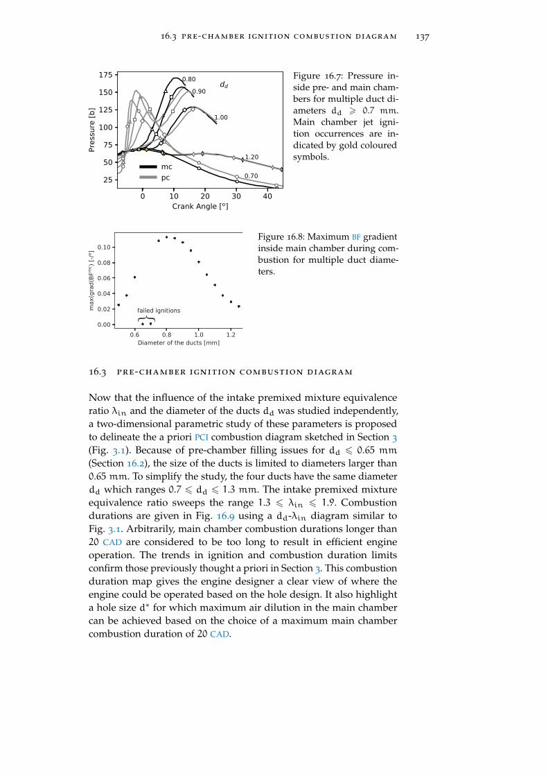
16.3 pre-chamber ignition combustion diagram 137

Figure 16.7: Pressure in-side pre- and main cham-bers for multiple duct di-ameters dd > 0.7 mm.Main chamber jet igni-tion occurrences are in-dicated by gold colouredsymbols.

failed ignitions

Figure 16.8: Maximum BF gradientinside main chamber during com-bustion for multiple duct diame-ters.

16.3 pre-chamber ignition combustion diagram

Now that the influence of the intake premixed mixture equivalenceratio λin and the diameter of the ducts dd was studied independently,a two-dimensional parametric study of these parameters is proposedto delineate the a priori PCI combustion diagram sketched in Section 3

(Fig. 3.1). Because of pre-chamber filling issues for dd 6 0.65 mm(Section 16.2), the size of the ducts is limited to diameters larger than0.65 mm. To simplify the study, the four ducts have the same diameterdd which ranges 0.7 6 dd 6 1.3 mm. The intake premixed mixtureequivalence ratio sweeps the range 1.3 6 λin 6 1.9. Combustiondurations are given in Fig. 16.9 using a dd-λin diagram similar toFig. 3.1. Arbitrarily, main chamber combustion durations longer than20 CAD are considered to be too long to result in efficient engineoperation. The trends in ignition and combustion duration limitsconfirm those previously thought a priori in Section 3. This combustionduration map gives the engine designer a clear view of where theengine could be operated based on the hole design. It also highlighta hole size d∗ for which maximum air dilution in the main chambercan be achieved based on the choice of a maximum main chambercombustion duration of 20 CAD.

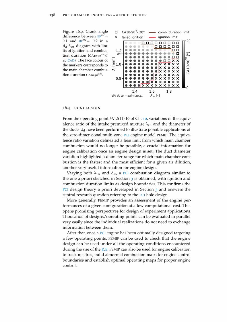
138 pre-chamber engine parametric studies

Figure 16.9: Crank angledifference between BFmc=

0.1 and BFmc= 0.9 in add-λin diagram with lim-its of ignition and combus-tion duration (CA10-90

mc620 CAD). The face colour ofthe markers corresponds tothe main chamber combus-tion duration CA10-90

mc.

comb. duration limitignition limit

d*

d*: to maximize

mc

mc

16.4 conclusion

From the operating point #λ1.5 IT -10 of Ch. 10, variations of the equiv-alence ratio of the intake premixed mixture λin and the diameter ofthe ducts dd have been performed to illustrate possible applications ofthe zero-dimensional multi-zone PCI engine model PEMIP. The equiva-lence ratio variation delineated a lean limit from which main chambercombustion would no longer be possible, a crucial information forengine calibration once an engine design is set. The duct diametervariation highlighted a diameter range for which main chamber com-bustion is the fastest and the most efficient for a given air dilution,another very useful information for engine design.

Varying both λin and dd, a PCI combustion diagram similar tothe one a priori sketched in Section 3 is obtained, with ignition andcombustion duration limits as design boundaries. This confirms thePCI design theory a priori developed in Section 3 and answers thecentral research question referring to the PCI hole design.

More generally, PEMIP provides an assessment of the engine per-formances of a given configuration at a low computational cost. Thisopens promising perspectives for design of experiment applications.Thousands of designs/operating points can be evaluated in parallelvery easily since the individual realizations do not need to exchangeinformation between them.

After that, once a PCI engine has been optimally designed targetinga few operating points, PEMIP can be used to check that the enginedesign can be used under all the operating conditions encounteredduring the use of the ICE. PEMIP can also be used for engine calibrationto track misfires, build abnormal combustion maps for engine controlboundaries and establish optimal operating maps for proper enginecontrol.

Part VI

C O N C L U S I O N

17G E N E R A L C O N C L U S I O N

This PhD thesis synthesizes a research work which focused on thenumerical study of Pre-Chamber Ignition (PCI) technology in ICEs.PCI has the potential to leverage homogeneous lean combustion bygenerating multiple highly turbulent jets of hot burnt gases issuinginto the main chamber of the engine and inducing fast burning ofthe main fuel-air lean mixture [20–22]. However, experiments alsoreveal that the design of the pre-chamber is critical: Sadanandan et al.[24] have shown that, in a divided chamber academic configuration,the size of the pre-chamber orifices determines the injection speedand temperature of the jets. During Turbulent Jet Ignition (TJI), twomechanisms compete:

1. mixing is necessary to create zones where the fresh gases of themain chamber and the hot gases of the jet are mixed so thatchemical reactions are accelerated;

2. this mixing also decreases temperature so that chemical reactionsare slowed down.

One might think that smaller holes are always beneficial since theygenerate more vigorous jets causing faster combustion. Actually, whenthe size of the holes decreases, the pressure drop increases which canindeed generate higher injection speeds, but can also inhibit ignitionbeyond a certain speed due to excessive mixing rate in a finite ratechemistry environment. In addition, reducing the size of the holesincreases the cooling of the gases as they pass through, resulting inlower jet temperature and chemical reaction rates.

There is therefore a real optimization problem which was at thecenter of this research work: how to optimize the size of the holes tomaximize the combustion speed without ever causing ignition failurewhich would be terrible for engine operation?

17.1 research approach

Multiple numerical tools and strategies were combined to provideanswers to the optimization problem while also providing insightsabout PCI in general.

- DNS (Part iii) was used to precisely study the TJI mechanisms of alean premixed mixture in an academic configuration dependingon the jet injection speed and temperature.

141

142 general conclusion

- LES (Part iv) was used to study the behaviour of the PCI conceptapplied to a real ICE, for both normal and abnormal engineoperation.

- A zero-dimensional model dubbed PEMIP for Pre-chamber En-gine Model with Ignition Prediction (Part v) has been derivedto assess the influence of geometric or operating point changeson engine operation at a low computational cost. It incorporateskey submodels to account for duct thermal effects and to predictthe TJI outcome (success or failure).

Each of these research tools has its advantages and limitations. Theyare interconnected and feed each other.

17.2 contributions

DNS made it possible to understand the influence of the burnt gasesjet injection speed and temperature on the ignition of a lean premixedmixture and on the structure of the incipient flames (Ch. 8). Resultshighlighted the importance of taking into account heat losses in thesmall gaps from which jets issue to correctly predict the potentialsubsequent ignition. They also highlighted the importance of mix-ing, which can cause the ignition to fail if it is too fast compared tochemistry. Except for low injection speeds, the flame structure wassubstantially distorted by the turbulence producing broadened and/ordistributed reaction zones also observed in real engine LESs. ChemicalExplosive Mode Analysis (CEMA) [107] was used to study the relativecontribution of diffusion and chemical source terms to the ChemicalExplosive Mode (CEM). CEMA clarified the disturbed flame structurefor moderate to high injection speeds and highlighted the role ofdiffusion in the ignition inhibition for the highest injection speeds.

LES allowed to study the PCI technology behaviour during the pre-chamber filling phase and the combustion phase for both normal andabnormal combustion cases1. During the pre-chamber filling phase,high levels of mixture stratification were revealed which impacts thecomposition of the jets of burnt gases later exiting the pre-chamberduring TJI. Lean mixture at the equivalence ratio of the main cham-ber is first ejected before that rich mixture trapped at the top of thepre-chamber is in turn. The burnt gases ejected from the pre-chamberare cooled by up to 200 K when passing through the connectingducts, which is not negligible and may prevent ignition accordingto the DNS results. For the succeeded ignition cases (Chs 10 and 12),the combustion in the main chamber started in a distributed reac-tion mode—similar to the DNS results for moderate to high injectionspeeds—before reaching a flamelet propagation mode. A case where

1 Results of the ignition sequences (success or failure) are in agreement with enginetests carried out within the Renault Group.

17.3 limitations 143

the premixed mixture inside the main chamber is too lean (λ = 2.0)to ensure normal engine operation was also studied (Ch. 11). Themixture stratification in the pre-chamber caused the jets to be too coldto be able to initiate combustion in the main chamber. This suggeststhat improving mixing in the pre-chamber is mandatory to extendthe lean operating limit. Hydrogen injection in the pre-chamber wasused as a way to extend the lean operating limit (Ch. 12). This madeit possible to initiate reactive flame fronts in the main chamber withmuch hotter jets, but the main charge consumption was still too slowto be acceptable. Finally, a post-TDC ignition was studied (Ch. 13).This gives rise to an abnormal combustion where the flame kernelis sucked towards the main chamber by the pressure difference gen-erated by the piston expansion, and quenched. More generally, LES

brought knowledge about the behaviour of the PCI technology andwhat causes its limits.

Models to predict the ignition of a premixed charge by a jet of hotburnt gases have been built based on DNS information (Section 14.6).The Convected Open Reactor (COR) model (Section 14.6.2), whichviews the ignition process as the evolution of an open well-stirredreactor mixing with the fresh gases at a certain rate, captures ignitionlimits reasonably. This proves that leading physical phenomena havebeen isolated and correctly integrated into the COR model whichaccounts for complex chemistry effects.

The COR model has been coupled to a model to take into accountthe thermal effects in the ducts connecting pre- and main chambers(Section 14.5) and integrated into a multi-zone zero-dimensional en-gine model called PEMIP (Ch. 14). To date, PEMIP is the only PCI enginezero-dimensional model to consider both duct thermal effects andjet ignition prediction. After calibration and validation, PEMIP makesit possible to carry out parametric studies of engine design at a lowcomputational cost. Varying the size of the holes, PEMIP allows toidentify the hole size limit below which main chamber ignition failsand highlights a range for which main chamber combustion is thefastest (Section 16.2). By doing so, PEMIP answers the central researchquestion referring to the PCI hole design.

17.3 limitations

Some simplifications have been made to allow this research work tobe carried out, which may limits its findings.

First, a gaseous fuel has been used so that liquid phase issues wereexcluded from this work. Using a liquid fuel in the pre-chamber cancause wall-wetting, forming fuel puddles, which impacts the air/fuelratio and increases unburnt hydrocarbon emissions [23].

The DNSs of Ch. 8 (used to bring fundamental knowledge on burntgases jet ignition and build models) were realized at atmospheric

144 general conclusion

conditions for reasons of computational cost. The competition betweenmixing and chemistry was found to govern the ignition process andthis has, a priori, no reason not to be the case under engine-likeconditions. However, this has not been formally demonstrated becauseof excessive computational cost. If computational resources ever allowDNS at engine relevant conditions, it might be worth checking this out.

Engine LES (Chs 10-13) was used for a single ignition sequence peroperating point studied. Cyclic variability was excluded from thisstudy. As a first approach, for a phenomenological study, this is not aissue. For engine design this is because even if “it ignites”, if too muchcyclic variability sets in then the engine will not operate properly.

During the LES sequences, the mean value of the ratio between theeffective viscosity and the dynamic viscosity (µ+ µt)/µ ranges from 3

to 15. According to Celik et al. [155], these values indicate fairly wellresolved LESs. In addition, the LES results of the ignition sequences andthe physical phenomena observed are in agreement with experiments.This allowed us to perform this work with some confidence in theresults of the LESs. However, it is worth mentioning that the influenceof a grid refinement on the LES results was not studied due to excessivecomputational cost: LES sequences were computed using heavy meshes(up to 300million cells) to limit the impact of the LES models, especiallyinside the connecting ducts and in the TJI zones (Section 9.3). Evenif the results are convincing, it would be interesting to carry out acomputation with a finer mesh in order to ensure trustworthy resultsif future computational resources allow it.

During the TJI period, the DTFLES combustion model is activatedonly in the zones that have transitioned to flame fronts (Section 6.3).Before that, the source terms of the multi-species chemistry are solvedon the grid without the action of any combustion model : unresolvedturbulence-chemistry interactions are neglected during this transitionphase, which could slightly bias part of the ignition process. Thiscould be the subject of an interesting study, which has been put asidefor now: the strategy was to use a fine mesh in the jet injection zonesto balance the loss of accuracy caused by not modelling this transitionphase.

The objective of PEMIP (Ch. 14) was to demonstrate the need tointegrate a model for jet ignition outcome coupled to a model forthermal effects inside the connecting ducts. As such, PEMIP is a suc-cess. However, the integrated turbulence and combustion models arevery simple and may not be accurate enough to perform quantitativeanalyses of engine performances.

Besides, PEMIP does not take into account mixture stratificationinside the zones of the divided chambers. Although the jet ignitionoutcome (success or failure) was in agreement with the LES results,this may impact the PEMIP results for PCI systems where high levels ofmixture stratification are found—as it is for the pre-chamber design

17.4 recommendations for further research 145

used throughout this work. The uncertainty on the PEMIP results dueto the homogeneity assumption was not studied because the pre-chambers will have to be built in the future so as not to produce thesehigh levels of stratification, which are a problem for system efficiencyand pollutant emissions.

17.4 recommendations for further research

From this work, many research directions can be drawn to go further.Cyclic variability would deserve to be studied for prospective engine

design: What characterizes these potential instabilities in PCI engines?Are they similar to the instabilities observed in SI engines? Are theyas much problematic? These are still unanswered questions.

Another interesting point which has not been explored is the influ-ence of radical species in the process of ignition by burnt gases. Thepre-chamber being systematically filled with a stoichiometric mixture,the burnt gases do not contain as many radical species as in the case ofa very rich mixture as is the case in the APIR pre-chamber concept [156,157] for example. Ignition was therefore reasonably assumed to bemainly influenced by temperature even though reactive intermediatescan still play a role (and are taken into account in the chemical kineticsused throughout this work, Section 5.4.2). The quantification of therole of reactive species in ignition would be an interesting topic forfundamental understanding of the ignition process.

Again referring to chemistry, Chemical Explosive Mode Analysis(CEMA) [107] was used to study the turbulence-chemistry interactionand the role of diffusion in the ignition outcome of burnt gases jetignition DNSs (Section 8.3.3) using ARC kinetics. The norm of thelargest eigenvalue and the norm of the projected source terms in aone-dimensional premixed laminar flame (Fig. 8.16) using the ARC

mechanism and the corresponding skeletal mechanism were checkedfor consistency. This was sufficient for this work as the direction ofthe Chemical Explosive Modes (CEMs) was not studied in detail. If amore in-depth study of chemistry would come to be carried out (tostudy the effect of intermediate species on ignition for example), itwould become necessary to study the difference in the direction ofthe CEMs between the ARC mechanism and the corresponding skeletalmechanism.

The zero-dimensional engine model PEMIP derived during this workshowed good agreement with the few operating points studied. How-ever, comparing PEMIP to engine tests—on intake premixed mixtureequivalence ratio sweeps for example—could enable to verify that thejet ignition limit is correctly retrieved.

If significant discrepancies in terms of combustion are noticed be-tween PEMIP and engine tests, the simple combustion and turbulence

146 general conclusion

models that have been integrated into PEMIP must be replaced by morecomplex models.

Besides, the full potential of PEMIP has not been exploited in thiswork. The objective of these computationally inexpensive zero-dimensionalmodels is to be able to be coupled with optimization algorithms whichrequire evaluating thousands of combinations of parameters veryquickly. A very interesting research work would be to develop anoptimization algorithm (with a quality function based on the combus-tion duration for example) with distribution of the computations overseveral thousand computation cores using a supercomputer. Once anoptimal design is established by this method, it would be interestingto confirm the optimization by LES and/or engine tests, and to under-stand why the optimisation algorithm steered the pre-chamber designin this direction.

Such optimization method could be applied to the optimizationof the size of the holes for the case of ultra lean combustion withthe addition of hydrogen inside the pre-chamber (Ch. 12). This caserequires smaller ducts to increase the main chamber burning rate:the addition of hydrogen requires a change in the design of the pre-chamber to be fully exploited. There are therefore many questionsaround the specificity of the design of a hydrogen fuelled pre-chamberwhich deserve to be studied to possibly achieve extreme air dilutionrates using this strategy. In addition to conventional PCI applications,the tools and knowledge built during this PhD thesis fully apply tofuture hydrogen PCI engines and can therefore contribute to theirdevelopment.

To be a man is to feel, when setting one’s stone,that one is contributing to the building of the world.

— Antoine de Saint-Exupéry

B I B L I O G R A P H Y

[1] D Dunn-Rankin and P Therkelsen. Lean Combustion. Technologyand Control. 2nd Edition. Academic Press, 2016.

[2] AS Campbell. Thermodynamic Analysis of Combustion Engines.John Wiley & Sons, 1979.

[3] AA Quader. “Lean Combustion and the Misfire Limit in SparkIgnition Engines.” In: Automobile Engineering Meeting. SAE In-ternational, Feb. 1974.

[4] AA Quader. “What Limits Lean Operation in Spark IgnitionEngines-Flame Initiation or Propagation?” In: Automobile Engi-neering Meeting. SAE International, Feb. 1976.

[5] CCOB Reynolds and RL Evans. “Improving emissions andperformance characteristics of lean burn natural gas enginesthrough partial stratification.” In: International Journal of EngineResearch 5.1 (Dec. 2005), pp. 105–114.

[6] JD Dale. “Application of high energy ignition systems to en-gines.” In: Progress in Energy and Combustion Science 23.5-6(1997), pp. 379–398.

[7] RW Johnston, JG Neuman, and PD Agarwal. “ProgrammableEnergy Ignition System For Engine Optimization.” In: WorldCongress & Exhibition. SAE International, Feb. 1975.

[8] WR Aiman. “Extended Spark Duration Improves Engine Oper-ation at High Exhaust Gas Recirculation Rates.” In: CombustionScience and Technology 15.3-4 (Oct. 2007), pp. 129–136.

[9] JA Harrington, RC Shishu, and JR Asik. “A Study of IgnitionSystem Effects on Power, Emissions, Lean Misfire Limit, andEGR Tolerance of a Single-Cylinder Engine-Multiple Sparkversus Conventional Single Spark Ignition.” In: World Congress& Exhibition. SAE International, Feb. 1974.

[10] JR Asik and B Bates. “The Ferroresonant Capacitor DischargeIgnition (FCDI) System: A Multiple Firing CD Ignition withSpark Discharge Sustaining Between Firings.” In: World Congress& Exhibition. SAE International, Feb. 1976.

[11] N Nakamura, T Baika, and Y Shibata. “Multipoint Spark Igni-tion for Lean Combustion.” In: Fall Fuels and Lubricants Meetingand Exhibition. SAE International, Oct. 1985.

[12] E Sher, J Ben-Ya’ish, A Pokryvailo, and Y Spector. “A CoronaSpark Plug System for Spark-Ignition Engines.” In: World Congress& Exhibition. SAE International, Feb. 1992.

147

148 bibliography

[13] JR Asik, P Piatkowski, MJ Foucher, and WG Rado. “Design ofa Plasma Jet Ignition System for Automotive Application.” In:World Congress & Exhibition. SAE International, Feb. 1977.

[14] MJ Hall, H Tajima, RD Matthews, MM Koeroghlian, WF Wel-don, and SP Nichols. “Initial Studies of a New Type of Ignitor:The Railplug.” In: International Fuels & Lubricants Meeting &Exposition. SAE International, Oct. 1991.

[15] JD Dale, PR Smy, and RM Clements. “Laser Ignited Inter-nal Combustion Engine - An Experimental Study.” In: WorldCongress & Exhibition. SAE International, Feb. 1978.

[16] FA Pertl and JE Smith. “Electromagnetic design of a novel mi-crowave internal combustion engine ignition source, the quarterwave coaxial cavity igniter.” In: Proceedings of the Institution ofMechanical Engineers, Part D: Journal of Automobile Engineering223.11 (Nov. 2009), pp. 1405–1417.

[17] PR Smy, RM Clements, JD Dale, D Simeoni, and DR Topham.“Efficiency and erosion characteristics of plasma jet igniters.” In:Journal of Physics D: Applied Physics 16.5 (Nov. 2000), pp. 783–791.

[18] TK Sharma, GAP Rao, and KM Murthy. “Homogeneous ChargeCompression Ignition (HCCI) Engines: A Review.” In: Archivesof Computational Methods in Engineering (May 2015), pp. 1–35.

[19] L Manofsky, J Vavra, DN Assanis, and A Babajimopoulos.“Bridging the Gap between HCCI and SI: Spark-Assisted Com-pression Ignition.” In: World Congress & Exhibition. SAE Inter-national, Apr. 2011.

[20] CEC Alvarez, GE Couto, VR Roso, AB Thiriet, and RM Valle.“A review of prechamber ignition systems as lean combustiontechnology for SI engines.” In: Applied Thermal Engineering 128

(Jan. 2018), pp. 107–120.

[21] WP Attard and P Parsons. “Flame Kernel Development for aSpark Initiated Pre-Chamber Combustion System Capable ofHigh Load, High Efficiency and Near Zero NOx Emissions.” In:SAE International Journal of Engines 3.2 (Oct. 2010), pp. 408–427.

[22] WP Attard and H Blaxill. “A Single Fuel Pre-Chamber JetIgnition Powertrain Achieving High Load, High Efficiency andNear Zero NOx Emissions.” In: SAE International Journal ofEngines 5.3 (Aug. 2011), pp. 734–746.

[23] JGC Baeta, FAR Filho, M Pontoppidan, RM Valle, and TRV daSilva. “Exploring the performance limits of a stratified torchignition engine using numerical simulation and detailed ex-perimental approaches.” In: Energy Conversion and Management126.15 (Oct. 2016), pp. 1093–1105.

bibliography 149

[24] R Sadanandan, D Markus, R Schießl, U Maas, J Olofsson, HSeyfried, M Richter, and M Aldén. “Detailed investigationof ignition by hot gas jets.” In: Proceedings of the CombustionInstitute 31.1 (Jan. 2007), pp. 719–726.

[25] FA Williams. Combustion Theory. Benjamin-Cummings Publish-ing Company, 1985.

[26] KK Kuo. Principles of Combustion. Wiley-Interscience, 2005.

[27] T Poinsot and D Veynante. Theoretical and Numerical Combustion.third. www.cerfacs.fr/elearning, Dec. 2011.

[28] JO Hirschfelder, CF Curtiss, and RB Bird. Molecular theory ofgases and liquids. Wiley, 1954.

[29] A Ern and V Giovangigli. Multicomponent transport algorithms.Springer, 1994.

[30] V Giovangigli. Multicomponent Flow Modeling. Birkhäuser, 1999.

[31] A Felden. “Development of Analytically Reduced Chemistries(ARC) and applications in Large Eddy Simulations (LES) ofturbulent combustion.” PhD thesis. Université de Toulouse,Aug. 2017.

[32] T Jaravel, E Riber, B Cuenot, and G Bulat. “Large Eddy Sim-ulation of an industrial gas turbine combustor using reducedchemistry with accurate pollutant prediction.” In: Proceedingsof the Combustion Institute 36.3 (Oct. 2016), pp. 3817–3825.

[33] B Rochette, F Collin-Bastiani, L Gicquel, O Vermorel, D Vey-nante, and T Poinsot. “Influence of chemical schemes, numeri-cal method and dynamic turbulent combustion modeling onLES of premixed turbulent flames.” In: Combustion and Flame191 (May 2018), pp. 417–430.

[34] A Felden, E Riber, and B Cuenot. “Impact of direct integrationof Analytically Reduced Chemistry in LES of a sooting swirlednon-premixed combustor.” In: Combustion and Flame 191 (May2018), pp. 270–286.

[35] A Felden, L Esclapez, E Riber, B Cuenot, and H Wang. “Includ-ing real fuel chemistry in LES of turbulent spray combustion.”In: Combustion and Flame 193 (July 2018), pp. 397–416.

[36] P Pepiot-Desjardins. “Automatic Strategies to Model Trans-portation Fuel Surrogates.” PhD thesis. Stanford University,May 2008.

[37] P Pepiot-Desjardins and H Pitsch. “An efficient error-propagation-based reduction method for large chemical kinetic mecha-nisms.” In: Combustion and Flame 154.1-2 (July 2008), pp. 67–81.

150 bibliography

[38] T Lu and CK Law. “Systematic Approach To Obtain AnalyticSolutions of Quasi Steady State Species in Reduced Mech-anisms.” In: The Journal of Physical Chemistry A 110.49 (Dec.2006), pp. 13202–13208.

[39] T Løvås, D Nilsson, and F Mauss. “Automatic reduction proce-dure for chemical mechanisms applied to premixed methane/airflames.” In: Proceedings of the Combustion Institute 28.2 (Jan.2000), pp. 1809–1815.

[40] T Løvås, P Amnéus, F Mauss, and E Mastorakos. “Comparisonof automatic reduction procedures for ignition chemistry.” In:Proceedings of the Combustion Institute 29.1 (Jan. 2002), pp. 1387–1393.

[41] Q Fei, A Shah, H Zhi-wei, P Li-na, P Tunestal, and B Xue-Song.“Detailed numerical simulation of transient mixing and com-bustion of premixed methane/air mixtures in a pre-chamber/main-chamber system relevant to internal combustion engines.” In:Combustion and Flame 188 (Feb. 2018), pp. 357–366.

[42] PM Allison, M de Oliveira, A Giusti, and E Mastorakos. “Pre-chamber ignition mechanism: Experiments and simulations onturbulent jet flame structure.” In: Fuel 230 (May 2018), pp. 274–281.

[43] S Yamaguchi, N Ohiwa, and T Hasegawa. “Ignition and burn-ing process in a divided chamber bomb.” In: Combustion andFlame 59 (Jan. 1985), pp. 177–187.

[44] S Benekos, CE Frouzakis, GK Giannakopoulos, M Bolla, YMWright, and K Boulouchos. “Prechamber ignition: An exploratory2-D DNS study of the effects of initial temperature and mainchamber composition.” In: Combustion and Flame 215 (May2020), pp. 10–27.

[45] AN Kolmogorov. “The local structure of turbulence in incom-pressible viscous fluid for very large Reynolds numbers.” In:Proceedings of the USSR Academy of Sciences 30 (1941), pp. 299–303.

[46] AN Kolmogorov. “Dissipation of energy in the locally isotropicturbulence.” In: Proceedings of the USSR Academy of Sciences 31

(1941), pp. 538–540.

[47] V Moureau, O Vasilyev, C Angelberger, and T Poinsot. “Com-mutation errors in Large-Eddy Simulation on moving grids:Application to piston engine flows.” In: Proceedings of the Sum-mer Program. Center for Turbulence Research, Stanford Univer-sity. 2004, pp. 157–168.

[48] JO Hinze. Turbulence. McGraw-Hill, 1959.

[49] H Tennekes and JL Lumley. A first course in turbulence. Cam-bridge: M.I.T. Press, 1972.

bibliography 151

[50] SB Pope. Turbulent flows. Cambridge University Press, 2000.

[51] J Smagorinsky. “General circulation experiments with the prim-itive equations: 1. The basic experiment.” In: Monthly WeatherReview 91 (1963), pp. 99–164.

[52] P Sagaut. Large eddy simulation for incompressible flows. Springer,2002.

[53] F Ducros, F Nicoud, and T Poinsot. “Wall-Adapting Local Eddy-Viscosity Models for Simulations in Complex Geometries.” In:6th Numerical Methods for Fluid Dynamics Conference. Institutefor Computational Fluid Dynamics, 1998, pp. 293–300.

[54] F Nicoud, H Baya Toda, O Cabrit, S Bose, and J Lee. “Usingsingular values to build a subgrid-scale model for large eddysimulations.” In: Physics of Fluids 23.8 (2011).

[55] SB Pope. “Computations of turbulent combustion: progressand challenges.” In: Symposium (International) on Combustion.The Combustion Institute. 1990, pp. 591–612.

[56] TD Butler and PJ O’Rourke. “A numerical method for twodimensional unsteady reacting flows.” In: Symposium (Interna-tional) on Combustion. The Combustion Institute. 1977, pp. 1503–1515.

[57] PJ O’Rourke and FV Bracco. “Two scaling transformationsfor the numerical computation of multidimensional unsteadylaminar flames.” In: Journal of Computational Physics 33.2 (Nov.1979), pp. 185–203.

[58] O Colin, F Ducros, D Veynante, and T Poinsot. “A thickenedflame model for large eddy simulations of turbulent premixedcombustion.” In: Physics of Fluids 12.7 (July 2000), pp. 1843–1863.

[59] FE Marble and JE Broadwell. The coherent flame model for tur-bulent chemical reactions. Tech. rep. TRW Defense and Space,1977.

[60] S Richard, O Colin, O Vermorel, A Benkenida, C Angelberger,and D Veynante. “Towards large eddy simulation of combus-tion in spark ignition engines.” In: Proceedings of the CombustionInstitute 31.2 (Jan. 2007), pp. 3059–3066.

[61] AR Kerstein, WT Ashurst, and FA Williams. “Field equationfor interface propagation in an unsteady homogeneous flowfield.” In: Physical Review A 37.7 (Apr. 1988), pp. 2728–2731.

[62] H Pitsch. “A consistent level set formulation for large-eddysimulation of premixed turbulent combustion.” In: Combustionand Flame 143.4 (Dec. 2005), pp. 587–598.

152 bibliography

[63] M Boger, D Veynante, H Boughanem, and A Trouvé. “Directnumerical simulation analysis of flame surface density conceptfor large eddy simulation of turbulent premixed combustion.”In: Symposium (International) on Combustion. The CombustionInstitute. 1998, pp. 917–925.

[64] D Veynante and L Vervisch. “Turbulent combustion modeling.”In: Progress in Energy and Combustion Science 28 (2002), pp. 193–266.

[65] H Pitsch. “Large Eddy Simulation of Turbulent Combustion.”In: Annual Review of Fluid Mechanics 38 (2006), pp. 453–482.

[66] FA Williams. Combustion Theory. Menlo Park, CA: BenjaminCummings, 1985.

[67] C Angelberger, D Veynante, F Egolfopoulos, and T Poinsot.“Large eddy simulations of combustion instabilities in pre-mixed flames.” In: Proceedings of the Summer Program. Centerfor Turbulence Research, Stanford University. 1998, pp. 61–82.

[68] O Colin, F Ducros, D Veynante, and T Poinsot. “A thickenedflame model for large eddy simulations of turbulent premixedcombustion.” In: Physics of Fluids 12.7 (2000), pp. 1843–1863.

[69] F Charlette, C Meneveau, and D Veynante. “A power-law flamewrinkling model for LES of premixed turbulent combustionPart I: non-dynamic formulation and initial tests.” In: Combus-tion and Flame 131.1-2 (Oct. 2002), pp. 159–180.

[70] PS Volpiani. “Modele de plissement dynamique pour la simula-tion aux grandes échelles de la combustion turbulente préeme-langée.” PhD Thesis. Université Paris-Saclay, 2017.

[71] A Misdariis. “Schémas cinétiques réduits et couplage ther-mique pour les simulation aux grandes échelles du cliquetisdans les moteurs à piston.” PhD thesis. Université de Toulouse,Jan. 2015.

[72] T Schonfeld and M Rudgyard. “Steady and Unsteady FlowSimulations Using the Hybrid Flow Solver AVBP.” In: AIAAJournal 37.11 (Nov. 1999), pp. 1378–1385.

[73] LYM Gicquel, N Gourdain, JF Boussuge, H Deniau, G Staffel-bach, P Wolf, and T Poinsot. “High performance parallel com-puting of flows in complex geometries.” In: Comptes RendusMecanique 339.2-3 (Feb. 2011), pp. 104–124.

[74] O Colin and M Rudgyard. “Development of High-Order Tay-lor–Galerkin Schemes for LES.” In: Journal of ComputationalPhysics 162.2 (Aug. 2000), pp. 338–371.

[75] CW Hirt, AA Amsden, and JL Cook. “An Arbitrary Lagrangian–EulerianComputing Method for All Flow Speeds.” In: Journal of Com-putational Physics 135 (Aug. 1997), pp. 203–216.

bibliography 153

[76] V Moureau, G Lartigue, Y Sommerer, C Angelberger, O Colin,and T Poinsot. “Numerical methods for unsteady compressiblemulti-component reacting flows on fixed and moving grids.”In: Journal of Computational Physics 202.2 (Jan. 2005), pp. 710–736.

[77] V Moureau. “Simulation aux grandes échelles de l’aérodynamiqueinterne des moteurs à piston.” PhD thesis. Ecole Centrale Paris,Dec. 2004.

[78] O Vermorel, S Richard, O Colin, C Angelberger, A Benkenida,and D Veynante. “Towards the understanding of cyclic vari-ability in a spark ignited engine using multi-cycle LES.” In:Combustion and Flame 156.8 (Aug. 2009), pp. 1525–1541.

[79] B Enaux, V Granet, O Vermorel, C Lacour, L Thobois, V Dugué,and T Poinsot. “Large Eddy Simulation of a Motored Single-Cylinder Piston Engine: Numerical Strategies and Validation.”In: Flow, Turbulence and Combustion 86.2 (Sept. 2010), pp. 153–177.

[80] B Enaux, V Granet, O Vermorel, C Lacour, C Pera, C Angel-berger, and T Poinsot. “LES study of cycle-to-cycle variationsin a spark ignition engine.” In: Proceedings of the CombustionInstitute 33.2 (2011), pp. 3115–3122.

[81] V Granet, O Vermorel, C Lacour, B Enaux, V Dugué, and TPoinsot. “Large-Eddy Simulation and experimental study ofcycle-to-cycle variations of stable and unstable operating pointsin a spark ignition engine.” In: Combustion and Flame 159.4 (Apr.2012), pp. 1562–1575.

[82] A Misdariis, A Robert, O Vermorel, S Richard, and T Poinsot.“Large-Eddy Simulation of Diesel Spray Combustion with Ex-haust Gas Recirculation.” In: Oil & Gas Science and Technology– Revue d’IFP Energies nouvelles 69.1 (Nov. 2013), pp. 155–165.

[83] A Misdariis, O Vermorel, and T Poinsot. “LES of knocking in en-gines using dual heat transfer and two-step reduced schemes.”In: Combustion and Flame 162.11 (Sept. 2015), pp. 4304–4312.

[84] C Dapogny, C Dobrzynski, and P Frey. “Three-dimensionaladaptive domain remeshing, implicit domain meshing, and ap-plications to free and moving boundary problems.” In: Journalof Computational Physics 262 (Apr. 2014), pp. 358–378.

[85] H Phillips. “On the transmission of an explosion through a gapsmaller than the quenching distance.” In: Combustion and Flame7 (Jan. 1963), pp. 129–135.

[86] HG Wolfhard and AE Bruszak. “The passage of explosionsthrough narrow cylindrical channels.” In: Combustion and Flame4 (1960), pp. 149–159.

154 bibliography

[87] S Biswas, S Tanvir, H Wang, and L Qiao. “On ignition mecha-nisms of premixed CH4/air and H2/air using a hot turbulentjet generated by pre-chamber combustion.” In: Applied ThermalEngineering 106 (Aug. 2016), pp. 925–937.

[88] E Mastorakos, P Allison, A Giusti, P De Oliveira, S Benekos, YWright, C Frouzakis, and K Boulouchos. “Fundamental Aspectsof Jet Ignition for Natural Gas Engines.” In: SAE InternationalJournal of Engines 10.5 (Sept. 2017), pp. 2429–2438.

[89] A Ghorbani, G Steinhilber, D Markus, and U Maas. “Ignition bytransient hot turbulent jets: An investigation of ignition mecha-nisms by means of a PDF/REDIM method.” In: Proceedings ofthe Combustion Institute 35.2 (Nov. 2014), pp. 2191–2198.

[90] A Validi and F Jaberi. “Numerical Study of Turbulent Jet Ig-nition in a Lean Premixed Configuration.” In: Flow, Turbulenceand Combustion 100.1 (July 2017), pp. 197–224.

[91] JAM Sidey and E Mastorakos. “Pre-Chamber Ignition Mecha-nism: Simulations of Transient Autoignition in a Mixing LayerBetween Reactants and Partially-Burnt Products.” In: Flow,Turbulence and Combustion 101.4 (Dec. 2018), pp. 1093–1102.

[92] N Peters. “Laminar flamelet concepts in turbulent combustion.”In: Symposium (International) on Combustion. The CombustionInstitute. Jan. 1988, pp. 1231–1250.

[93] C Felsch, M Gauding, C Hasse, S Vogel, and N Peters. “Anextended flamelet model for multiple injections in DI Dieselengines.” In: Proceedings of the Combustion Institute 32.2 (2009),pp. 2775–2783.

[94] C Hergart, H Barths, and N Peters. “Modeling the Combus-tion in a Small-Bore Diesel Engine Using a Method Based onRepresentative Interactive Flamelets.” In: International Fuels &Lubricants Meeting & Exposition. SAE International, Oct. 1999.

[95] ME Feyz, VR Hasti, JP Gore, A Chowdhury, and MR Nalim.“Scalar predictors of premixed gas ignition by a suddenly-starting hot jet.” In: International Journal of Hydrogen Energy 44

(42 Aug. 2019), pp. 23793–23806.

[96] S Fischer, D Markus, and U Maas. “Numerical investigation ofthe ignition of diethyl ether/air and propane/air mixtures byhot jets.” In: Journal of Loss Prevention in the Process Industries49 (Mar. 2017), pp. 832–838.

[97] I Iglesias, M Vera, AL Sánchez, and A Liñán. “Numerical analy-ses of deflagration initiation by a hot jet.” In: Combustion Theoryand Modelling 16.6 (Dec. 2012), pp. 994–1010.

[98] JC Prince and FA Williams. “Short chemical-kinetic mecha-nisms for low-temperature ignition of propane and ethane.” In:Combustion and Flame 159.7 (July 2012), pp. 2336–2344.

bibliography 155

[99] P Saxena and FA Williams. “Testing a small detailed chemical-kinetic mechanism for the combustion of hydrogen and car-bon monoxide.” In: Combustion and Flame 145.1-2 (Apr. 2006),pp. 316–323.

[100] MV Petrova and FA Williams. “A small detailed chemical-kinetic mechanism for hydrocarbon combustion.” In: Combus-tion and Flame 144.3 (Feb. 2006), pp. 526–544.

[101] DG Goodwin, RL Speth, HK Moffat, and BW Weber. Cantera:An Object-oriented Software Toolkit for Chemical Kinetics, Thermo-dynamics, and Transport Processes. Tech. rep. 2018.

[102] TJ Poinsot and SK Lele. “Boundary conditions for direct simu-lations of compressible viscous flows.” In: Journal of Computa-tional Physics 101.1 (July 1992), pp. 104–129.

[103] N Guezennec and T Poinsot. “Acoustically Nonreflecting andReflecting Boundary Conditions for Vortcity Injection in Com-pressible Solvers.” In: AIAA Journal 47.7 (July 2009), pp. 1709–1722.

[104] CC Huang, SS Shy, CC Liu, and YY Yan. “A transition onminimum ignition energy for lean turbulent methane combus-tion in flamelet and distributed regimes.” In: Proceedings of theCombustion Institute 31.1 (Jan. 2007), pp. 1401–1409.

[105] SS Shy, WT Shih, and CC Liu. “More on Minimum IgnitionEnergy Transition for Lean Premixed Turbulent Methane Com-bustion in Flamelet and Distributed Regimes.” In: CombustionScience and Technology 180.10-11 (Sept. 2008), pp. 1735–1747.

[106] SS Shy, CC Liu, and WT Shih. “Ignition transition in turbulentpremixed combustion.” In: Combustion and Flame 157.2 (Feb.2010), pp. 341–350.

[107] TF Lu, CS Yoo, JH Chen, and CK Law. “Three-dimensionaldirect numerical simulation of a turbulent lifted hydrogen jetflame in heated coflow: a chemical explosive mode analysis.”In: Journal of Fluid Mechanics 652 (May 2010), pp. 45–64.

[108] CS Yoo, T Lu, JH Chen, and CK Law. “Direct numerical simu-lations of ignition of a lean n-heptane/air mixture with temper-ature inhomogeneities at constant volume: Parametric study.”In: Combustion and Flame 158.9 (Sept. 2011), pp. 1727–1741.

[109] Z Luo, CS Yoo, ES Richardson, JH Chen, CK Law, and T Lu.“Chemical explosive mode analysis for a turbulent lifted ethy-lene jet flame in highly-heated coflow.” In: Combustion andFlame 159.1 (Jan. 2012), pp. 265–274.

[110] X Chao, P Ji-Woong, YC Sang, CJ H, and L Tianfeng. “Identifi-cation of premixed flame propagation modes using chemicalexplosive mode analysis.” In: Proceedings of the Combustion In-stitute 37.2 (July 2018), pp. 2407–2415.

156 bibliography

[111] K Aditya, A Gruber, C Xu, T Lu, A Krisman, MR Bothien, andJH Chen. “Direct numerical simulation of flame stabilizationassisted by autoignition in a reheat gas turbine combustor.”In: Proceedings of the Combustion Institute 37.2 (2019), pp. 2635–2642.

[112] O Schulz, E Piccoli, A Felden, G Staffelbach, and N Noiray.“Autoignition-cascade in the windward mixing layer of a pre-mixed jet in hot vitiated crossflow.” In: Combustion and Flame201 (Jan. 2019), pp. 215–233.

[113] O Schulz and N Noiray. “Combustion regimes in sequentialcombustors: Flame propagation and autoignition at elevatedtemperature and pressure.” In: Combustion and Flame 205 (July2019), pp. 253–268.

[114] R Shan, CS Yoo, JH Chen, and T Lu. “Computational diag-nostics for n-heptane flames with chemical explosive modeanalysis.” In: Combustion and Flame 159.10 (Oct. 2012), pp. 3119–3127.

[115] KE Niemeyer and NJ Curtis. pyJac v1.0.4. Tech. rep. 2017.

[116] KE Niemeyer, NJ Curtis, and CJ Sung. “pyJac: Analytical Ja-cobian generator for chemical kinetics.” In: Computer PhysicsCommunications 215 (June 2017), pp. 188–203.

[117] E Anderson et al. LAPACK Users’ Guide. Third. Philadelphia,PA: Society for Industrial and Applied Mathematics, 1999.

[118] G Lacaze, E Richardson, and T Poinsot. “Large eddy simulationof spark ignition in a turbulent methane jet.” In: Combustionand Flame 156.10 (Oct. 2009), pp. 1993–2009.

[119] WR Brandstetter and G Decker. “Fundamental studies on thevolkswagen stratified charge combustion process.” In: Combus-tion and Flame 25 (Aug. 1975), pp. 15–23.

[120] P Wolanski, Z Gut, W Niedziela, J Przastek, and S Siwiec.“Study of Combustion Dynamics in the Research Engine.”In: International Fuels & Lubricants Meeting & Exposition. SAEInternational, Oct. 1997.

[121] J Geiger, S Pischinger, R Böwing, HJ Koß, and J Thiemann.“Ignition Systems for Highly Diluted Mixtures in SI-Engines.”In: World Congress & Exhibition. SAE International, Mar. 1999.

[122] AA Boretti and HC Watson. “Enhanced combustion by jet igni-tion in a turbocharged cryogenic port fuel injected hydrogenengine.” In: International Journal of Hydrogen Energy 34.5 (Mar.2009), pp. 2511–2516.

bibliography 157

[123] WP Attard, E Toulson, A Huisjen, X Chen, G Zhu, and HSchock. “Spark Ignition and Pre-Chamber Turbulent Jet Igni-tion Combustion Visualization.” In: SAE Technical Paper (Apr.2012).

[124] A Roubaud and D Favrat. “Improving performances of a leanburn cogeneration biogas engine equipped with combustionprechambers.” In: Fuel 84.16 (Nov. 2005), pp. 2001–2007.

[125] A Jamrozik and W Tutak. “A study of performance and emis-sions of SI engine with a two-stage combustion system.” In:Chemical and Process Engineering 32.4 (Jan. 2012), pp. 172–19.

[126] EK Anderson, WP Attard, A Brown, P Litke, K Grinstead, andJ Hoke. “Experimental Study of a Pre-Chamber Jet Igniter in aTurbocharged Rotax 914 Aircraft Engine.” In: World Congress& Exhibition. SAE International, Apr. 2013.

[127] A Shah, P Tunestal, and B Johansson. “Effect of Relative Mix-ture Strength on Performance of Divided Chamber ‘AvalancheActivated Combustion’ Ignition Technique in a Heavy DutyNatural Gas Engine.” In: World Congress & Exhibition. SAE In-ternational, Apr. 2014.

[128] A Jamrozik. “Lean combustion by a pre-chamber charge strat-ification in a stationary spark ignited engine.” In: Journal ofMechanical Science and Technology 29.5 (May 2015), pp. 2269–2278.

[129] FAR Filho, JGC Baêta, AF Teixeira, RM Valle, and JLF de Souza.“E25 stratified torch ignition engine emissions and combus-tion analysis.” In: Energy Conversion and Management 121 (Aug.2016), pp. 251–271.

[130] RT Vedula, R Song, T Stuecken, GG Zhu, and H Schock. “Ther-mal efficiency of a dual-mode turbulent jet ignition engineunder lean and near-stoichiometric operation.” In: InternationalJournal of Engine Research 18.10 (Apr. 2017), pp. 1055–1066.

[131] J Benajes, R Novella, J Gomez-Soriano, PJ Martinez-Hernandiz,C Libert, and M Dabiri. “Evaluation of the passive pre-chamberignition concept for future high compression ratio turbochargedspark-ignition engines.” In: Applied Energy 248 (Aug. 2019),pp. 576–588.

[132] MHB Sandoval, CEC Alvarez, VR Roso, NDSA Santos, and RMValle. “The influence of volume variation in a homogeneousprechamber ignition system in combustion characteristics andexhaust emissions.” In: Journal of the Brazilian Society of Mechan-ical Sciences and Engineering 42 (Dec. 2019).

[133] N Peters. “The turbulent burning velocity for large-scale andsmall-scale turbulence.” In: Journal of Fluid Mechanics 384 (Apr.1999), pp. 107–132.

158 bibliography

[134] JL Lumley. Engines. Cambridge University Press, 1999.

[135] K Hiraoka, K Nomura, A Yuuki, Y Oda, and T Kameyama.“Phenomenological 0-Dimensional Combustion Model for Spark-Ignition Natural Gas Engine Equipped with Pre-Chamber.” In:World Congress & Exhibition. SAE International, Apr. 2016.

[136] IWSL Cruz, CEC Alvarez, AF Teixeira, and RM Valle. “Zero-dimensional mathematical model of the torch ignited engine.”In: Applied Thermal Engineering 103.C (June 2016), pp. 1237–1250.

[137] R Song, RT Vedula, G Zhu, and H Schock. “A control-orientedcombustion model for a turbulent jet ignition engine usingliquid fuel.” In: International Journal of Engine Research 19 (Sept.2017), pp. 813–826.

[138] K Bardis, G Xu, P Kyrtatos, YM Wright, and K Boulouchos. “AZero Dimensional Turbulence and Heat Transfer Phenomeno-logical Model for Pre-Chamber Gas Engines.” In: World Congress& Exhibition. SAE International, Apr. 2018.

[139] F Bozza, V De Bellis, D Tufano, E Malfi, C Müller, and KHabermann. “A Quasi-Dimensional Model of Pre-ChamberSpark-Ignition Engines.” In: World Congress & Exhibition. SAEInternational, Apr. 2019.

[140] K Bardis, P Kyrtatos, G Xu, C Barro, YM Wright, and K Boulou-chos. “Development and validation of a novel quasi-dimensionalcombustion model for un-scavenged prechamber gas engineswith numerical simulations and engine experiments.” In: Inter-national Journal of Engine Research 84.3 (Sept. 2020).

[141] II Wiebe. Progress in Engine Cycle Analysis: Combustion Rate andCycle Processes. Mashgiz, Ural-Siberia Branch, 1962.

[142] WJD Annand. “Heat Transfer in the Cylinders of ReciprocatingInternal Combustion Engines.” In: Proceedings of the Institutionof Mechanical Engineers 177.1 (Feb. 2006), pp. 973–996.

[143] VI Ashimin, ZI Geller, and SY A. “Discharge coefficients of areal fluid from cylindrical orifices.” In: Oil & Industry (1961).

[144] E Jones, T Oliphant, P Peterson, and others. SciPy: Open sourcescientific tools for Python. Tech. rep. 2001.

[145] FP Incropera. Fundamentals of Heat and Mass Transfer. Wiley,2006.

[146] EN Sieder and GE Tate. “Heat Transfer and Pressure Drop ofLiquids in Tubes.” In: Industrial & Engineering Chemistry 28.12

(Dec. 1936), pp. 1429–1435.

[147] WH McAdams. Heat Transmission. 1985.

bibliography 159

[148] Y Marzouk. Unsteady Strained Flames: Fundamentals and Numer-ical Modeling. MIT Department of Mechanical Engineering, Apr.2001.

[149] RL Speth. Ember: a quasi-one-dimensional, unsteady flame solver.Tech. rep. 2017.

[150] AE Long, RL Speth, and WH Green. “Ember: An open-source,transient solver for 1D reacting flow using large kinetic models,applied to strained extinction.” In: Combustion and Flame 195

(May 2018), pp. 105–116.

[151] C Petrov and A Ghoniem. “An unsteady strained flame modelfor turbulent combustion simulations.” In: 32nd Aerospace Sci-ences Meeting and Exhibit. American Institute of Aeronauticsand Astronautics, Feb. 2013, pp. 303–12.

[152] HN Najm, RW Schefer, RB Milne, CJ Mueller, KD Devine, andSN Kempka. Numerical and Experimental Investigation of VorticalFlow-Flame Interaction. Tech. rep. Mar. 1998.

[153] B Sforzo, J Kim, J Jagoda, and J Seitzman. “Ignition Probabilityin a Stratified Turbulent Flow With a Sunken Fire Igniter.”In: Journal of Engineering for Gas Turbines and Power 137.1 (Aug.2014), pp. 187–9.

[154] N Darabiha, V Giovangigli, A Trouvé, SM Candel, and E Es-posito. “Coherent Flame Description of Turbulent PremixedDucted Flames.” In: Turbulent Reactive Flows. Ed. by R Borghiand SNB Murthy. Springer US, 1989, pp. 591–637.

[155] IB Celik, ZN Cehreli, and I Yavuz. “Index of Resolution Qualityfor Large Eddy Simulations.” In: Journal of Fluids Engineering127.5 (2005), pp. 949–958.

[156] C Robinet, P Higelin, B Moreau, O Pajot, and J Andrzejew-ski. “A New Firing Concept for Internal Combustion Engines:“I’APIR”.” In: World Congress & Exhibition. SAE International,Mar. 1999.

[157] S Couet, P Higelin, and B Moreau. “APIR: A New Firing Con-cept for the Internal Combustion Engines - sensitivity to knockand in-cylinder aerodynamics.” In: International Spring Fuels &Lubricants Meeting. SAE International, May 2001.

D E C L A R AT I O N

I hereby declare that:

- no known competing financial interests or personal relationshipscould have appeared to influence the work reported in this thesis;

- this thesis represents my own work which has been done afterregistration for the degree of Doctor of Philosophy at “Universitéde Toulouse”, and has not been previously included in a thesisor dissertation submitted to this or any other institution for adegree, diploma or other qualifications.

Toulouse, Dec. 2020

Quentin Malé

colophon

This document was typeset using the typographical look-and-feelclassicthesis developed by André Miede and Ivo Pletikosic. Thestyle was inspired by Robert Bringhurst’s seminal book on typography“The Elements of Typographic Style”.

Final Version as of January 8, 2021 (V4.0).