Embed Size (px)
Citation preview

University of Kentucky University of Kentucky
UKnowledge UKnowledge
Theses and Dissertations--Civil Engineering Civil Engineering
2018
INVESTIGATION OF VOLATILE ORGANIC COMPOUNDS (VOCs) INVESTIGATION OF VOLATILE ORGANIC COMPOUNDS (VOCs)
DETECTED AT VAPOR INTRUSION SITES DETECTED AT VAPOR INTRUSION SITES
Mohammadyousef Roghani University of Kentucky, [email protected] Digital Object Identifier: https://doi.org/10.13023/etd.2018.430
Right click to open a feedback form in a new tab to let us know how this document benefits you. Right click to open a feedback form in a new tab to let us know how this document benefits you.
Recommended Citation Recommended Citation Roghani, Mohammadyousef, "INVESTIGATION OF VOLATILE ORGANIC COMPOUNDS (VOCs) DETECTED AT VAPOR INTRUSION SITES" (2018). Theses and Dissertations--Civil Engineering. 73. https://uknowledge.uky.edu/ce_etds/73
This Doctoral Dissertation is brought to you for free and open access by the Civil Engineering at UKnowledge. It has been accepted for inclusion in Theses and Dissertations--Civil Engineering by an authorized administrator of UKnowledge. For more information, please contact [email protected].

STUDENT AGREEMENT: STUDENT AGREEMENT:
I represent that my thesis or dissertation and abstract are my original work. Proper attribution
has been given to all outside sources. I understand that I am solely responsible for obtaining
any needed copyright permissions. I have obtained needed written permission statement(s)
from the owner(s) of each third-party copyrighted matter to be included in my work, allowing
electronic distribution (if such use is not permitted by the fair use doctrine) which will be
submitted to UKnowledge as Additional File.
I hereby grant to The University of Kentucky and its agents the irrevocable, non-exclusive, and
royalty-free license to archive and make accessible my work in whole or in part in all forms of
media, now or hereafter known. I agree that the document mentioned above may be made
available immediately for worldwide access unless an embargo applies.
I retain all other ownership rights to the copyright of my work. I also retain the right to use in
future works (such as articles or books) all or part of my work. I understand that I am free to
register the copyright to my work.
REVIEW, APPROVAL AND ACCEPTANCE REVIEW, APPROVAL AND ACCEPTANCE
The document mentioned above has been reviewed and accepted by the student’s advisor, on
behalf of the advisory committee, and by the Director of Graduate Studies (DGS), on behalf of
the program; we verify that this is the final, approved version of the student’s thesis including all
changes required by the advisory committee. The undersigned agree to abide by the statements
above.
Mohammadyousef Roghani, Student
Dr. Kelly G. Pennell, Major Professor
Dr. Tim Taylor, Director of Graduate Studies

INVESTIGATION OF VOLATILE ORGANIC COMPOUNDS (VOCs) DETECTED
AT VAPOR INTRUSION SITES
DISSERTATION
A dissertation submitted in partial fulfillment of the requirements for the degree of Doctor of Philosophy in the College of Engineering
at the University of Kentucky
By
Mohammadyousef Roghani
Lexington, Kentucky
Director: Dr. Kelly Pennell, Associate Professor of Civil Engineering
Lexington, Kentucky
Copyright © Mohammadyousef Roghani 2018

ABSTRACT OF DISSERTATION
INVESTIGATION OF VOLATILE ORGANIC COMPOUNDS (VOCs) DETECTED
AT VAPOR INTRUSION SITES
This dissertation investigates unexplained vapor intrusion field data sets that have
been observed at hazardous waste sites, including: 1) non-linear soil gas concentration
trends between the VOC source (i.e. contaminated groundwater plume) and the ground
surface; and, 2) alternative pathways that serve as entry points for vapors to infiltrate into
buildings and serve to increase VOC exposure risks as compared to the classic vapor
intrusion model, which primarily considered foundation cracks as the route for vapor
entry. The overall hypothesis of this research is that theoretical knowledge of fate and
transport processes can be systematically applied to vapor intrusion field data using a
multiple lines of evidence approach to improve the science-based understanding of how
and when vapor intrusion exposure risks will pose increased exposure risk; and, ultimately
this knowledge can be used to develop policies that reduce exposure risks. The first
objective of this research involved numerical modeling, field sampling and laboratory tests
to investigate which factors influence soil gas transport within the subsurface. Combining
results of all of these studies provide improved understanding of which factors influence
VOC fate and transport within the subsurface. Importantly, the results demonstrate a non-
linear trend between the VOC source concentration in the subsurface and the ground
surface concentration at the study site, which disagrees with many vapor intrusion
conceptual models. Ultimately, the source concentration may not be a good predictor of
shallow soil gas concentrations. Laboratory tests described the effect of soil characteristics
such as the soil water content on VOC vapor diffusion. The numerical model was able to
explain specific conditions that could not be described by the field and laboratory data
alone. A paper was published that summarizes the major outcomes from this objective
(Pennell et al, 2016). The second objective of this research investigated preferential
pathways for VOC vapor migration into buildings. Sewer systems can act as important
pathways for vapor intrusion. The research objective is to evaluate conditions that increase
the potential for inhalation exposure risks via vapor intrusion thorough sewer systems into
indoor spaces. A field study was conducted in California over a 4-year period to
investigate the spatial and temporal variability of alternative pathways (e.g. aging
infrastructure piping systems) within the context of vapor intrusion exposure risks. A paper

was published that summarizes the major outcomes from the field study (Roghani et al.
2018). The final research objective involved the development of a numerical model to
describe VOC fate and transport within a sewer system. The numerical model predicts
VOC mass transport. The model results were compared to the field data and provides
insight about the role preferential pathways play in increasing VOC exposure risks.
KEYWORDS: volatile organic compounds, vapor intrusion, hazardous sites, numerical
modeling, alternative pathway, sewer systems
Mohammadyousef Roghani
November 8, 2018

INVESTIGATION OF VOLATILE ORGANIC COMPOUNDS (VOCs) DETECTED
AT VAPOR INTRUSION SITES
By
Mohammadyousef Roghani
Kelly G. Pennell, PhD.
Director of Dissertation
Tim Taylor, PhD.
Director of Graduate Studies
November 8, 2018

iii
ACKNOWLEDGEMENTS
The completion of this work would not have been possible without the guidance and
support of many people. I would first like to express my deepest appreciation to my advisor
and Director of dissertation, Dr. Kelly Pennell, for her incredible support, encouragement,
insight and inspiration over the past few years. This research would not be possible if not
for her help and guidance.
I would like to thank the other members of my thesis committee—Dr. Lindell Ormsbee,
Dr. Yi-Tin Wang and Dr. Zach Hilt —for their support, guidance and time not only during
this research project, but throughout my education at the University of Kentucky.
I would like to thank the University of Kentucky and the Department of Civil
Engineering for the financial and educational support provided to me during my time as an
undergraduate and graduate student. I am grateful for the countless individuals at the
university and in the department who have lent a helping hand along the way.
I would like to acknowledge the USEPA Region 9, Entanglement Technologies and
Clearwater Group for their contributions to my research.
I would like to thank the other members of my research group, Evan Willett and Elham
Shirazi, for their support, insight, and help over the past few years.
Finally, I would like to thank my wife, my parents and my friends for their
unconditional love and support throughout my journey. Thank you for always inspiring me
to pursue my dreams.
Research reported herein was supported by a CAREER Award from the National
Science Foundation (Award #1452800) and the National Institute of Environmental Health

iv
Sciences of the National Institutes of Health (Award #P42ES007380). The content is solely
the responsibility of the author and does not necessarily represent the official views of the
National Science Foundation or the National Institutes of Health.

v
TABLE OF CONTENTS
Acknowledgements ...................................................................................................... iii
List of Tables …………………………………………………………………………x
List of Figures……………………………………………………………………….. xi
CHAPTER 1: Introduction ........................................................................................... 1
1.1. Background ................................................................................................... 1
1.2. Research objective ........................................................................................ 3
1.3. Dissertation organization .............................................................................. 4
CHAPTER 2: Theoretical Background: The Role of Geology and Moisture Content .7
2.1. Soil characteristics.............................................................................................. 7
2.2. Soil moisture .................................................................................................... 18
2.3. Capillary fringe ................................................................................................ 24
2.4. Vapor intrusion numerical models ................................................................... 28
CHAPTER 3: Soil Gas VOC Concentrations and Numerical Modeling .................... 33
3.1. Abstract ............................................................................................................ 33
3.2. Introduction ...................................................................................................... 34
3.3. Method and materials ....................................................................................... 35
3.3.1. Site description .......................................................................................... 35
3.3.2. Multiple lines of evidences approach ........................................................ 38
3.3.3. Field samplings .......................................................................................... 39
3.3.4. Chemical analysis ...................................................................................... 41
3.3.5. Computational modeling ........................................................................... 42
3.4. Results and discussion ...................................................................................... 44
3.4.1. Summary of field data and conceptual site model ..................................... 44
3.4.2. Multiple lines of evidence ......................................................................... 46
3.5. Conclusions ...................................................................................................... 59
CHAPTER 4: Column Studies.................................................................................... 61
CHAPTER 5: Sewer System as an Alternative Vapor Intrusion Pathway:
Background and Motivation ............................................................................................. 75
5.1. Occurrence of VOC in aquatic system ............................................................. 76

vi
5.2. Wastewater infrastructure condition ................................................................ 77
5.3. Sewer system designs ....................................................................................... 79
5.4. Conceptualizing the sewer gas pathway........................................................... 81
5.5. Historical review of sewer system acts as a vapor intrusion pathway ............. 85
5.6. Emerging the Problem ...................................................................................... 90
CHAPTER 6. Occurrence of VOCs in Sewer Systems .............................................. 91
6.1 Abstract: ............................................................................................................ 91
6.2. Introduction ...................................................................................................... 92
6.3. Methods and materials ..................................................................................... 96
6.3.1. Field sampling manholes and cleanouts .................................................... 96
6.3.2. Passive sampling........................................................................................ 99
6.3.3 Grab samples (TO-15) .............................................................................. 100
6.3.4. AROMA continuous gas monitor ............................................................ 101
6.3.5. Sewer liquid analysis ............................................................................... 102
6.3.6. Other site sampling .................................................................................. 102
6.4. Results and discussion .................................................................................... 102
6.5. Conclusions .................................................................................................... 125
CHAPTER 7: Developing A Numerical Model to Study Fate and Transport of VOCs
Inside the Sewer Systems................................................................................................ 129
7.1. Review of existing VOCs sewer gas modeling .............................................. 129
7.2. Fate and Transport of VOCs inside the sewer system: .................................. 134
7.2.1. Sorption ................................................................................................... 134
7.2.2. Biodegradation......................................................................................... 138
7.2.3. Liquid - gas mass transfer ........................................................................ 140
7.2.4. Vapors diffusion ...................................................................................... 143
7.2.5. Parameters affect sewer gas VOCs concentration ................................... 145
7.3. Sewer Gas Numerical Model ......................................................................... 155
7.3.1. Model development ................................................................................. 155
7.3.2. Model exercise ......................................................................................... 160
7.4. Conclusions .................................................................................................... 179
Chapter 8: Conclusion and Recommendations ......................................................... 181
8.1. Findings .......................................................................................................... 181
8.2. Limitation of the study ................................................................................... 183
vii
8.3. Research contributions ................................................................................... 184
8.4. Opportunities for future research ................................................................... 186
Appendices ................................................................................................................ 188
Appendix A ........................................................................................................... 188
Appendix B ........................................................................................................... 194
Appendix C ........................................................................................................... 198
References ................................................................................................................. 202
Vita ............................................................................................................................ 215

viii
LIST OF TABLES
Table 2.1. Average values of porosities for 12 SCS soil texture (USEPA, 2004) ...... 10
Table 2.2. Average values of conductivity for 12 SCS soil texture (USEPA, 2004) . 12
Table 2.3. Relationship between Deffective and Da (in the absence of water phases) .... 16
Table 2.4. Capillary fringe thickness .......................................................................... 28
Table 3.1. Sample Media and Collection Locations .................................................. 40
Table 3.2. Model Equations ....................................................................................... 44
Table 3.3. Maximum Chemical Concentrations Detected During Field Study ......... 45
Table 3.4. Summary of the Scenarios ......................................................................... 56
Table 4.1. Sieve analysis for ASTM D422 test .......................................................... 65
Table 4.2. Measured properties of the soil .................................................................. 67
Table 6.1. Sewer liquid results for TCE ................................................................... 118
Table 7.1. Effects of different parameters on VOC liquid-gas mass transfer ........... 132
Table 7.2. Sewer liquid calculation ........................................................................... 157
Table 7.3. Sewer headspace calculations .................................................................. 158
Table 7.4. Sewer model inputs .................................................................................. 161
Table 7.5. Results of the Scenario 1. ........................................................................ 162
Table 7.6. Results of the Scenario 2 ......................................................................... 163
Table 7.7. Results of scenario 3; effects of tributary flow ....................................... 165
Table 7.8. Effect of the drop structure height .......................................................... 166
Table 7.9. Effect of adsorption on TCE sewer gas and sewer liquid concentration 168
Table 7.10. Summaries of cases platted on figure 7.5 ............................................. 169
Table 7.11. Results of statistic comparison .............................................................. 172
Table 7.12. Comparing different factor on Toluene concentration ......................... 174
Table 7.13. Effect of sewer liquid depth fluctuation on TCE concentration ........... 176

ix
LIST OF FIGURES
Figure 2.1. Permeability and hydrologic conductivity for common geologic media.. 14
Figure 2.2. Soil horizon profile. (Source: USDA, 2018) ............................................ 20
Figure 2.3. Hydrologic horizons of soil profile. (Source: Dingman, 2002)................ 21
Figure 2.4. Soil moisture profile. (Source: Al-Hamdan and Cruise, 2010) ................ 22
Figure 2.5. USSCS classification chart showing centroid compositions. ................... 27
Figure 2.6. Conceptual J&E diagram of vapor intrusion ............................................ 29
Figure 3.1. Site Map Showing Sampling Location .................................................... 37
Figure 3.2. Preliminary Conceptual Models for the Site ............................................ 46
Figure 3.3. Comparison of Screening Level “Predicted” and Measured Indoor Air
Concentrations for Property A and Property C ................................................................. 49
Figure 3.4. Measured Groundwater (Vapor) Concentration and Attenuation Factors
(α) Line of Evidence 2: Soil Gas Concentrations. ........................................................... 50
Figure 3.5. Measured Soil Gas Concentrations as a Function of Sampling Depth ..... 52
Figure 3.6. PCE Concentration Gradient for Soil Gas Locations at Property B ......... 54
Figure 3.7. Modeled and Measured Soil Gas Concentrations For Three Cases. ........ 59
Figure 3.8. Conceptual Model Comparison. ............................................................... 59
Figure 4.1. Schematic the column study ..................................................................... 63
Figure 4.2. Designed column experiment set up......................................................... 64
Figure 4.3. Mechanical Sieve Shaker ......................................................................... 65
Figure 4.4. Constant Head Test for Measuring Soil Hydraulic Conductivity ............ 66
Figure 4.5. 2-D simulation of the column study ......................................................... 68
Figure 4.6. Measured sampling ports concentration profile for no soil scenario ....... 69
Figure 4.7. Comparing calculated vs measured data for no soil scenario ................... 69
Figure 4.8. Measured sampling ports concentration profile for dry soil scenario ...... 70
Figure 4.9. Comparing calculated vs measured data for dry soil scenario ................. 71
Figure 4.10. Measured sampling ports concentration profile for soil water content=
5% ..................................................................................................................................... 71
Figure 4.11. Comparing calculated vs measured data for soil water content= 5% ..... 71
Figure 4.12. Measured sampling ports concentration profile for soil water content=
10% ................................................................................................................................... 72
Figure 4.13. Comparing calculated vs measured data for soil water content= 10% ... 72
Figure 4.14. Measured sampling ports concentration profile for soil water content=
15% ................................................................................................................................... 73
Figure 4.15. Comparing calculated vs measured data for soil water content= 15% ... 73
Figure 4.16. Measured sampling ports concentration profile for soil water content=
21% ................................................................................................................................... 74
Figure 4.17. Comparing calculated vs measured data for soil water content= 21% ... 74
Figure 5.1. Separated and Combined Sewer System Design ...................................... 81
Figure 5.2. Different Pathways for Entry of VOCs into Sewer System Adjacent to
Industrial Facility .............................................................................................................. 83
Figure 5.3. VOC Vapors Pathways from Sewer System toward IA…………………85

x
Figure 6.1. Research study area and conceptual model. ............................................. 95
Figure 6.2. General Layout of Cleanout and Manhole Locations............................... 97
Figure 6.3. General sampling depths inside manholes. .............................................. 98
Figure 6.4. Sewer gas TCE concentrations measured in 2014 by TO-15 (grab). ..... 105
Figure 6.5. Sewer gas TCE concentrations measured in 2015. ................................ 108
Figure 6.6. Sewer Gas Concentrations Detected in Manholes and Cleanouts (2015).
......................................................................................................................................... 110
Figure 6.7 Sewer gas TCE concentrations measured by TO-17 and AROMA in 2016.
......................................................................................................................................... 117
Figure 6.8. MH-15 sewer gas TCE concentrations (g/m3) and sample depths, 2015 -
2017................................................................................................................................. 122
Figure 6.9. MH-17 sewer gas TCE concentrations (g/m3) and sample depths, 2014 -
2017................................................................................................................................. 124
Figure 6.10. MH-18 sewer gas TCE concentrations (g/m3) collected September 28,
2016................................................................................................................................. 125
Figure 7.1. Sewer flow direction on the Street B. ..................................................... 160
Figure 7.2. COMSOL buoyancy velocity calculation .............................................. 164
Figure 7.3. Effect of the drop structure height on TCE transfer from liquid phase to
the gas phase ................................................................................................................... 167
Figure 7.4. Effect of adsorption on sewer liquid and sewer gas TCE concentration of
different manholes (Ss = 500 (mg/L); Sd= 500 (mg/L)) .................................................. 168
Figure 7.5. TCE measured concentration VS calculated concentration .................. 171
Figure 7.6. Comparing sewer headspace velocity calculated by two models. .......... 178
Figure 7.7. Comparing sewer TCE concentrations calculated by two sewer headspace
velocity models ............................................................................................................... 179

1
CHAPTER 1: INTRODUCTION
1.1. Background
Considering the amount of time people spend inside buildings, indoor air is an
important health concern. One issue related to the indoor air contamination is vapor
intrusion. Vapor intrusion describes indoor air contamination that occurs due to volatile
organic compound (VOC) vapors migrating from subsurface sources into the overlying
buildings. Almost 25% of all hazardous waste sites in the United States (US) are estimated
to have the potential for vapor intrusion exposure risks (Colbert and Palazzo, 2008). Vapor
intrusion has been a health concern for decades and recently evaluation of the vapor
intrusion pathways is required for almost every hazardous waste site and it is a one of the
top priorities at the US Environmental Protection Agency (USEPA) Superfund Sites
nationwide (Manzanilla, 2014; Little and Pennell, 2017).
Vapor intrusion has been reported and investigated by several studies in last three
decades, e.g. (Nazaroff, 1988; Little et al., 1992; Hodgson et al, 1992; Ramu et al., 1992;
Hers et al, 2001; Hers et al, 2003; Karpinska et al. 2004; Eklund and Simon, 2007; Folkes
et al., 2009; McAlary and Johnson, 2009; Johnston and Gibson, 2011; Yao et al., 2013a;
Beckley et al., 2014; Holton et al., 2015; Johnston and Gibson, 2014;Pennell et al, 2016).
VOC vapor transport depends on various factors such as the source characteristics,
subsurface conditions, building characteristics, and general site conditions. Several
numerical models have been developed to investigate VOC vapor intrusion and its
concentration inside the building (e.g. Johnson and Ettinger, 1991; Pennell et al, 2009). A
classic vapor intrusion numerical model includes simulation of VOC mass transfer through
soil by diffusion and advection and its entry into the buildings through foundation’s cracks.
2
While vapor intrusion numerical models have significantly improved our
understanding about this process and strengthened our ability to interpret field data, it is
not typically the metric by which models have been tested. Rather, models have attempted
to explain well-defined theory. However, several field studies have reported that measured
soil gas concentrations and indoor air concentrations of VOCs were not expected based on
classic conceptual models on which numerical models were developed by regulators and
researchers.
The USEPA released a database of various filed sampling results collected from
different vapor intrusion sites through the US. The dataset was included soil gas, indoor
air, subslab and crawlspace measurements in residential, commercial and multi-use
buildings. A broad range of variations (including temporal and spatial) in ratios of indoor
air VOC concentrations to subsurface source (normally groundwater) VOC concentrations
can be observed in this database that is one of the big challenges for VI modeling. Several
numerical models with different considerations have been applied to assess compatibility
of the model results with the measured filed data (Pennell, et al., 2009; Shen, et al., 2013a).
USEPA measured data from different vapor intrusion sites suggested a trend of inverse
correlation between the indoor air VOC concentration attenuation factor and the subsurface
VOC concentration. This observation was not expected based on the vapor intrusion
classical models. Yao et al. (2013b) investigated various parameters that could be
responsible for this unexpected result and concluded that sampling limitations, uncertainty
in source characteristics and the soil water content impacts can be reasons for the
discrepancy between the measured and calculated results.

3
Because of the complexities associated with interpreting the field data and
characterizing the vapor intrusion pathway, the USEPA recommends a “multiple lines of
evidence approach” when making decisions about how to assess vapor intrusion exposure
risks (USEPA, 2015a; Pennell et al, 2016).
1.2. Research objective
This dissertation investigates unexplained vapor intrusion field data sets that have been
observed at hazardous waste sites, including: 1) non-linear soil gas concentration trends
between the VOC source (i.e. contaminated groundwater plume) and the ground surface;
and, 2) alternative pathways that serve as entry points for vapors to infiltrate into the
buildings and serve to increase VOC exposure risks as compared to the classic vapor
intrusion model that primarily considered foundation cracks as the route for vapor entry.
The overall hypothesis of this research is that theoretical knowledge of fate and
transport processes can be systematically applied to vapor intrusion field data using a
multiple lines of evidence approach to improve the science-based understanding of how
and when vapor intrusion exposure risks will pose increased exposure risks—ultimately
this knowledge can be used to develop policies that reduce exposure risks.
Research Objective 1: Numerical modeling, field sampling and laboratory tests were used
to investigate which factors influence soil gas transport within the subsurface. Combining
results of all of these studies provided a better understanding of which factors influence
VOC fate and transport within the subsurface. Importantly, the results demonstrate a non-
linear trend between the VOC source concentration in the subsurface and the ground
surface concentration existed at the study site, which disagrees with many vapor intrusion
conceptual models. Ultimately, the source concentration may not be a good predictor of

4
shallow soil gas concentrations. Laboratory tests described the effect of soil characteristics
such as the soil water content on VOC vapor diffusion. The numerical model was able to
explain specific conditions that could not be described by the field and laboratory data
alone. A paper was published that summarizes the major outcomes from this objective
(Pennell et al, 2016). In addition, the results of soil column studies were evaluated to further
investigate the role of soil moisture on non-linear soil gas concentration trends in the
subsurface. Chapters 3 and 4 relate to this research objective.
Research Objective 2: Field sampling, and fate and transport knowledge was used to
investigate preferential pathways for VOC vapor migration into buildings. Sewer system
can act as an important pathway for vapor intrusion and it has not been well characterized.
A field study was conducted in California over a 4-year period to investigate the spatial
and temporal variability of alternative pathways (e.g. aging infrastructure piping systems)
within the context of vapor intrusion exposure risks. A paper was published that
summarizes the major outcomes from the field study (Roghani et al. 2018). Chapters 5 and
6 specifically relate to this research objective.
Research Objective 3: Numerical modeling and field data was used to describe VOCs fate
and transport within a sewer system. The numerical model was developed to predict VOC
mass transport and the results were compared to the field data. The model provides insight
about the role preferential pathways play in increasing VOC exposure risks and offers
solutions to reduce VOC exposure risks. Chapter 7 relates to this research objective.
1.3. Dissertation organization
Eight chapters contribute into the objective of this study. This contribution of each
chapter is explained in this section.

5
Chapter 1: This chapter provides information about VOCs vapor intrusion background,
research objective of this dissertation and contribution of each chapter.
Chapter 2: This chapter provides theoretical background and general information
regarding the soil characteristics, water content of the soil and possible impact of soil
properties on VOC vapor intrusion. At the end of this chapter two different vapor intrusion
numerical model are described: Johnson and Ettinger (J&E) model and three dimensional
finite element model.
Chapter 3: In this chapter results of a vapor intrusion field study is compared with results
of a developed numerical model. The groundwater, soil gas and indoor air VOC
concentration were measured as part of this study. Results of a multi-university vapor
intrusion field study were compared with the results of a 3D numerical model. The
numerical model was able to explain specific conditions that could not be described by the
collected data alone. This study highlights the importance of applying the multiple lines of
evidence as an appropriate approach for evaluating vapor intrusion exposure risks. This
research is published in a peer-reviewed journal as part of the scholarly objectives of this
dissertation.
Chapter 4: Additional laboratory experiments were conducted to investigate impact of soil
moisture on VOC vapor mass transfer. In this chapter results of the laboratory experiments
are discussed.
Chapter 5: In this chapter the potential of sewer systems as alternative pathways for VOC
vapor intrusion is evaluated. Some vapor intrusion filed studies that sewer was the primary
source for VOC are reviewed and a conceptual model has been developed that describe

6
occurrence of VOC inside the sewer system and possible ways that VOCs can use to
migrate from the sewer system into the buildings.
Chapter 6: Result of a field study that conducted by our research group is explained. This
research evaluated the contribution of sewer system for VOC vapors migration into the
buildings. We collaborated with Entanglement Technologies (NSF/NIH-SBIR) and EPA
in Mountain View, CA. Occurrence of VOC inside a sewer system adjacent to and
extending hundreds of feet away from a previously defined vapor intrusion area is
investigated and spatial and temporal variations of sewer gas TCE concentration is
assessed. Several sampling methods were applied and the applicability of each of this
method is discussed. This study suggested that groundwater contamination sources
infiltrating into the sewer system as well as sewer gas transport mechanisms can be the
source of sewer gas TCE variations.
Chapter 7: In this chapter we developed a numerical model to simulate VOC fate and
transport inside the aging infrastructure piping systems. The liquid gas mass transfer, vapor
diffusion, adsorption and biodegradation are four major mass transfer mechanisms
included in this model. Result of the numerical model is compared with field study data
(chapter 6) to improve the numerical model considerations and to gain insight about the
role that preferential pathways play in increasing VOC exposure risks.
Chapter 8: This chapter summarizes the main findings of this study and describe
limitations for this research and offers suggestions to improve vapor intrusion risk
assessment.

7
CHAPTER 2: THEORETICAL BACKGROUND: THE ROLE OF GEOLOGY AND
MOISTURE CONTENT
Soil properties have important effects on vapor intrusion. In this section different soil
characteristics and their impact on VOC fate and transport are described. In addition impact
of soil moisture and capillary fringe on VOC vapor diffusion is discussed and two different
numerical models that simulate VOC mass transfer within the subsurface are described.
2.1. Soil characteristics
This section provides background about different characteristics of the soil and their
potential impacts on VOC vapor intrusion. In addition, conceptual and the theoretical
framework for VOC transport through soil is summarized.
Soil and the pores between the soil grains divide the VOC subsurface source and the
overlaying building. Vapor intrusion regulatory guidelines suggest that soil properties have
significant impacts on VOC vapor migration (ITRC, 2007; USEPA, 2015a). For a
comprehensive vapor intrusion risk assessment, soil characteristics such as total porosity,
soil water content, soil permeability, effective diffusivity and the soil total organic
compound fraction need to be analyzed since all of these parameters play important role in
vapor transport and vapor intrusion exposure risks (USEPA, 2015a; Johnston and Gibson,
2013).
Several vapor intrusion studies have investigated effect of the soil properties in vapor
intrusion. The USEPA (2012) database includes the site specific information such as soil
type for each vapor intrusion site. Results of this database suggested the important role of
soil type and soil particle size on vapor intrusion attenuation factor form the subsurface

8
source. A greater attenuation from groundwater to indoor air is expected for area that finer-
grained soils are predominant (USEPA, 2012a; Johnston and Gibson, 2013). USEPA
(2015a) suggested that the soil particle size does not have a considerable impact on
groundwater to sub-slab attenuation, while affect sub-slab to indoor air attenuation factor
by an average of 0.4 order of magnitude. Yao et al. (2017a) investigated the impact of soil
type on VOCs attenuation. They compared results of the soil column experiments with a
3D numerical model in a steady state condition. The result suggests that soil particle size
in shallow area (area between the sub-slab and the building foundation) affect the rate of
soil gas entry into the building, while the soil gas VOC concentration profile in deeper area
of the soil (>6m) is independent of the soil particle size. This is consistent with the USEPA
(2012) database conclusion. The process of VOC vapor diffusion is limited in deep soils
and soil characteristics near the building’s foundation is more important. The numerical
analysis of USEPA’s vapor intrusion database suggested that for vapor intrusion risk
assessment, characteristics of the soil in shallow areas beneath the building's foundation
need to be precisely evaluated (USEPA, 2012; Johnston and Gibson, 2013; Yao, et al.,
2017).
Soil porosity
Porosity of a soil is the fraction of soil's pore space and defined as the volume of the
void space over the soil total volume. Equation below shows different porosity definitions.
Total porosity (θt) =Vv
Vs=
𝑉𝑎+ 𝑉𝑤
𝑉𝑠 (2.1)
Vs= total volume of the soil, (m3);
Vv = void volume (m3);

9
Va = volume of the air in the soil texture, (m3);
Vw = volume of the water in the soil texture, (m3).
The total porosity of the soil can be filled by water or air. Equations below show how
porosity can be calculated and volumetric soil gas content, volumetric water content and
degree of water content saturation can be calculated.
θt = 1 −ρs
Gs × w
(2.2)
s= dry soil density, (g/ m3);
w= water density, (g/ m3);
Gs= soil specific gravity, dimensionless.
θt = θg + θw (2.3)
θg = total volumetric pore space;
θg = volumetric soil gas space;
θw= volumetric water space.
Sr = Vw
Vv =
MwMs
×Gs
θt (2.4)
Sr = Degree of water saturation, (m3/m3);
Mw = mass of water in the soil sample, (g);
Ms = mass of the soil sample, (g).
Void ratio of the soil (e) can be determined by calculating the total porosity of the soil.
e = θt
1+θt (2.5)
Porosity of the soil is a function of grain size, packing and particle shape and can be
measured by the volumetric measurements of core samples (Dingman, 2002). Soil is not

10
necessary homogeneous, so results of one sample of soil is not necessary representative for
the whole soil. Theoretically, the maximum porosity for a cubic packed box made of
perfectly spherical grains of a uniform size is approximately 0.48, and is independent of
grain size. Soils typically have irregularly shaped particles have varied porosities. Fine
grained soils may exhibit higher porosities than coarse grained soils; however, fine grained
soils may not have interconnected pores, whereas coarse grain soils will have larger, and
more interconnected pores. Table below shows the average values of the total porosity
(=saturated water content) for 12 SCS soil textural classifications (USEPA, 2004).
Table 2.1. Average values of porosities for 12 SCS soil texture (USEPA, 2004)
Soil Texture (USDA) Total Porosity (θt)
Clay 0.459
Clay loam 0.442
Loam 0.399
Loamy sand 0.390
Silt 0.489
Silty loam 0.439
Silty clay 0.481
Silty clay loam 0.482
Sand 0.375
Sandy clay 0.385
Sandy clay loam 0.384
Sandy loam 0.387
Soil conductivity
Conductivity refers to the ease of a fluid (could be liquid or gas) to move through the
soil media. It is important to recognize that it describes characteristics that are specific to
both the fluid and the soil. One of the most common ways to determine the hydraulic
conductivity of a soil, water movement through the soil media is observed and reported as
saturated hydraulic conductivity (kh). There are two general types of tests typically have

11
been used for measuring the hydraulic conductivity of a soil. 1. The constant head method
and 2. The falling head method. Darcy’s law (Darcy, 1856) has been used for calculating
the hydraulic conductivity for both of two methods. The water flow rate across a unit
section of a soil based on Darcy's low is calculated by applying equation 2.6.
Q= - kh.A.(∂h
∂x) (2.6)
Q= water flow rate, (m3/s);
kh = hydraulic conductivity, (m/s);
(∂h
∂x) = hydraulic head gradient over the length of the flow in the x-direction, (m/m);
A= the cross section area through the direction of flow, (m2).
The hydraulic head is defined by equation 2.7.
h =p
ρ.g + z (2.7)
Which p is the differential pressure (Kg.m/s2), is the density (m3/kg), g is the gravity
acceleration (m2/s) and z is the height (m). In a vertical column the equation 2.6 can be
written as equation 2.8 which has been used for calculating the kh.
Q= - kh.A.(Ha−Hb)
L (2.8)
Schaap et al. (1998) measured the average value of saturated hydraulic conductivity for
different classified soil texture. There are also several empirical formula for estimating the
hydraulic conductivity of the soil. These models typically estimated the hydraulic
conductivity of the soil (kh) based on the distribution of soil particles size. Vukovic and
Soro (1992) summarized some of these empirical models and suggested a general formula.
kh = g
v. C. 𝑓(n). de
2 (2.9)
v= kinetic viscosity, (m2/s);

12
𝑓(𝑛)= porosity function;
C=strong coefficient;
de= effective grain diameter, m;
As it is mentioned, equation 2.9 is a general form of empirical formulas. As an example
Hazen (1892), suggested equation 2.10 for estimating the hydraulic conductivity of
uniformly graded sands that wildly has been used for different types of soils.
kh = g
v× (6 × 10−4) × [1 + 10(θt − 0.26)]d10
2 (2.10)
d10 represents the effective size in the particle distribution curve that corresponds to the
grain diameter that 10% of the sample are finer that this size. A sieve analysis is required
to determine the particle distribution curve and the d10 value.
Table 2.2 shows the average values of saturated hydraulic conductivity for the 12 CSC
soil texture classifications (USEPA, 2004).
Table 2.2. Average values of conductivity for 12 SCS soil texture (USEPA, 2004)
Soil Texture (USDA) Average saturated hydraulic
conductivity(cm/h)
Average saturated hydraulic
conductivity(m/s)
Sand 26.78 7.44E-05
Loamy sand 4.38 1.22E-05
Sandy Loam 1.6 4.444E-06
Sandy clay loam 0.55 1.53E-06
Sandy clay 0.47 1.316E-06
Loam 0.5 1.39E-06
Clay loam 0.34 9.44E-07
Silt loam 0.76 2.11E-06
Clay 0.61 1.69E-06
Silty clay loam 0.46 1.28E-06
Silt 1.82 5.06E-06
Silty clay 0.4 1.11E-06
13
Intrinsic permeability (K)
The intrinsic permeability of the soil describes the characteristics of the soil to allow
fluids to flow through it, independent of the fluid. Muskat (1937) found a relationship
between the soil hydraulic permeability (Kh) and the unit weight of the fluid. Intrinsic
permeability (K) is defined by equation 2.11.
K= kh.μ
ρ.g (2.11)
K= intrinsic permeability, (m2);
µ= viscosity (water), (kg/m.s).
K is a function of soil particle shape, particle diameter and packing. Komen (1927)
derived a formula for calculating the K value based on the porosity by applying the Naiver-
stokes equations. θt is the porosity, C is the constant value for Kozeny's equation (shown
as equation 2.12) that depends on the capillary shape (typically consider 0.5 for circular
capillary) and S is the channel specific surface (m2/m3).
K= C.(θt)3
S2 (2.12)
This equation has been improved to the Kozeny's equation shown below (Carmen 1937
and Carmen, 1956).
K = dm
2
180 × (
(θt)3
(1−θt)2) (2.13)
dm= characteristic particle diameter, (m).
The hydraulic permeability is a function of gravity but the intrinsic permeability (K) is
independent of the gravity. The flow can be calculated by having the intrinsic permeability,
cross section area, viscosity and pressure gradient as it is shown in equation 2.14. Figure

14
2.1 shows permeability and hydrologic conductivity for common geologic media (Freeze
and Cherry, 1979).
Q= −K.A
μ (
∂p
∂x) (2.14)
Figure 2.1. Permeability and hydrologic conductivity for common geologic media,
(Freeze and Cherry, 1979).
Relative Permeability
In a porous media when multi phases are present, the permeability of the media to each
phase is called the effective permeability. The effective permeability is a strong function
of soil's saturation degree. The relative permeability of each fluid (phase) is defined based
on dividing the effective permeability of that fluid over the soil intrinsic permeability. The
soil's degree of water saturation is an important factor for calculating this parameter for
every fluid.

15
Based on the above definition the relative air permeability of soil (krg) is result of the
air effective permeability divided by intrinsic permeability of the soil. The relative air
permeability of soil can be calculated by equation 2.15 (Parker et al., 1987).
krg= (1- Se) 0.5(1- Se
1/M*) 2M* (2.15)
krg= relative air permeability of the soil, (0 ≤ krg≤ 1);
M*= van Genuchten parameter;
Se= relative moisture content, (θw−θr
θt−θr);
The relative water permeability of soil (krw) also can be defined by dividing the
effective permeability of water over to the saturated permeability of soil. Atteia and
Hohener, (2010) developed equation below to calculate this parameter.
(2.16) 2 ]1 − (1 – (Se)1
M∗)M∗[ √Se= rwk
Se= relative moisture content= θw−θr
θt−θr
M∗= van Genuchten parameter;
θr = residual water content.
The soil vapor permeability (kv) is an important parameter for calculating the vapors
advection flow. This parameter typically should be measured during the filed study by
conducting pneumatic tests. kv also can be estimated by multiplying the air relative
permeability (krg) to the intrinsic permeability (USEPA, 2004).
Effective diffusivity
VOC vapors can use the void area of a soil to migrate from the contaminated source
into buildings; therefore the effective diffusion of VOCs through soil is function of the soil
porosity. The magnitude of chemicals diffusion coefficient in air is different from this

16
magnitude in water. For example, pure air phase diffusion coefficients of VOCs such as
TCE (trichloroethylene) and PCE in the air are in order of 10-6 (m2/s) and the diffusion
coefficients of these chemicals in water are in the order of 10-10 (m2/s). Therefore, it is
important to calculate the volume of soil that is filled with water (water content porosity)
and the soil partial volume that is filled with air (the void volume).
There have been several attempts for calculating the diffusion coefficient of chemicals
in a porous media such as soil (Deffective) to find a relation between this diffusion coefficient
and the air diffusion coefficient (Da) (e.g. Buckingham, 1904; Penman, 1940; Millington
and Quirk, 1961; Moldrup et al., 2000). Table 2.3 shows the relation have been suggested
between (Deffective) and Da by some of these studies.
Theoretically, parameters that can be effective on the chemical diffusion rate through
porous media include total porosity, the air-filled porosity and water filled porosity and the
tortuosity of drained porous matrix (Kristensen et al., 2010).
Table 2.3. Relationship between Deffective and Da (in the absence of water phases)
Deffective
Da= θg
2 Buckingham, 1904 (2.17)
Deffective
Da= 0.66 θg Penman, 1940 (2.18)
Deffective
Da= (
θg3.33
θt2 ) Millington and Quirk, 1961 (2.19)
Deffective
Da= θg
1.5θg
θt Moldrup et al., 2000 (2.20)
The equation 2.21 known as Millington and Quirk equation has been used widely for
calculating the effective diffusivity of VOCs in soil or other porous media based on the
diffusion coefficient of VOC in air and in water (Millington and Quirk, 1961). It is
commonly adapted to include water-filled pores in soil systems.

17
Deffective = Da (θg
3.33
θt2 ) + (
Dw
Hc) (
θw3.33
θt2 ) (2.21)
Deffective = effective diffusion coefficient of VOC in the soil, (m2/s);
Da = effective diffusion coefficient of VOC in the air, (m2/s);
Dw = effective diffusion coefficient of VOC in the water, (m2/s);
Hc= Henry's law constant for the chemical “i”, (m3 liquid/m3 gas);
Millington and Quirk equation is derived theoretically and originally developed for
coarse and structural material with the uniform size and some studies have reported that
this equation underestimates the gas diffusion rate for structureless natural soils (Petersen
et al., 1994; Bartelt-Hunt and Smith, 2002; Werner et al., 2004). The Moldrup equation is
another equation have been used to describe chemical vapors diffusion through porous
media (Moldrup et al., 2000). This equation was originally developed for the sieved and
repacked soil but have been suggested by some studies to give better estimation for the
effective diffusion coefficient for natural soils (Kristensen et al., 2010). In the vapor
intrusion area, Moldrup equation (equation 2.22) has been used to calculate the effective
diffusion coefficient of VOCs though capillary fringe, with water-filled porosity terms
added (Shen et al., 2013).
Deffective = Da (θg
2.5
θt) + (
Dw
Hc) (
θw2.5
θt) (2.22)
Dispersion may also have some impact on VOC vapors diffusion through the soil. The
mechanical dispersion in subsurface is induced by the groundwater flow as the source of
VOC vapors in the vertical direction. Atteia and Hohener (2010) suggested to add a term
for dispersion to the Millington–Quirk equation. Equation 2.23 shows the relation they
suggested. The last term of the equation 2.23 (εz. uGW.kr,w
Hc) counts for the dispersion
18
introduced by groundwater flow and can be used for calculating the effective diffusion
coefficient for the capillary fringe layer.
Deffective = Da (θg
3.33
θt2 ) + (
Dw
Hc) (
θw3.33
θt2 ) + εz. uGW.
krw
Hc (2.23)
εz = the longitudinal dispersivity, (m);
uGW = the groundwater velocity, (m/s);
krw= the relative water permeability to the saturated permeability of water= ( K(θ)
Ksat).
Shen et al. (2013) concluded that adding dispersion to the Millington–Quirk equations
slightly improved the model accuracy for the deep layer (capillary fringe layer).
The overall diffusion coefficient for a multilayer soil that is a heterogeneous system
and composed from different layers of soil with different properties can be calculated by
applying equation 2.24.
Dtotal,effective= LT
∑Li
Di,effective
ni=0
(2.24)
Dtotal,effective= the total effective diffusion coefficient, (m2/s);
Di,effective= the effective diffusion coefficient for the soil layer i, (m2/s);
LT= total distance between VOCs source and bottom of the building foundation, (m);
Li= thickness of the soil layer i, (m).
2.2. Soil moisture
The soil water content (soil moisture) can have a significant effect on VOC vapor
intrusion. A high level of soil moisture in the area between the land surface and
groundwater table can drastically reduce the rate of VOC vapor diffusion by reducing the
effective diffusion coefficient which is explained above. In the area with no ground covers

19
such as asphalt or concrete, a greater water content can be expected in soil around the
building compare to the soil beneath the building's foundation (Tillman and Weaver, 2007).
There are different factors that can significantly change the soil moisture profile in an
area such as rainfall or irrigation infiltration (Shen et al., 2012). The groundwater level
fluctuation also can have some effect on the soil moisture profile (USEPA, 2015a).
Several studies have mentioned the significant effect of soil moisture on vapor intrusion
(McAlary et al., 2009; Tillman and Weaver, 2007; Shen et al., 2012; Shen et al., 2013).
Hers et al. (2003) concluded that VOC diffusion flux significantly changes when a layer of
soil with elevated moisture added to the model. Among the different parameters that have
some level of impacts on VOC vapor intrusion, assessing the soil water content is one of
the most complicated one (Shen et al, 2013). Although the importance of the soil moisture
on vapor intrusion rate have been confirmed by several studies, there have been limited
numerical analysis, evaluating this effect. Calculating the soil moisture profile in the area
of study is one of the biggest challenges, while there are difficulties to access the soil in
deep area of the soil and there are several parameters affecting the soil moisture profile.
On the other hand the soil effective diffusion coefficient in different layers (if it is
heterogeneous) need to be calculated based on the soil moisture profile.
The soil horizon profile has been characterized by considering several layers above the
groundwater table. The soil horizon profile includes the surface horizon (A), the subsoil
(B) and the substratum (C). The organic horizon (O) is also sometimes considered for the
on the top of the surface horizon (A). The major horizons of this profile are shown in figure
2.2 (USDA). O horizon is the humid ground surface. A horizon is the top layer of soil that

20
is normally rich in organic matter. B horizon is the layer normally contains minerals and C
horizon is the weathered bedrock.
Figure 2.2. Soil horizon profile. (Source: USDA, 2018)
The soil moisture distribution above the groundwater table can be divided to three
different zones as it shown in Figure 2.3. These three layers include: 1 the surface soil
layer; 2 the vadose zone; and, 3 the tension-saturated zone (Shen et al, 2013). Figure 2.3
also shows the range of water content that is typically expected for each of these layers.
The water content in the surface soil layer (root zone) is typically expected to be greater
than permanent wilting point moisture (θpwp) and less than the saturated water content of
the soil (θs). Above the water table in a tension saturated zone due to the capillary fringe
the soil is saturated. From this saturated zone the water infiltrates into the intermediate
zone. The range of water content in the intermediate zone is typically between the field
capacity (θfc) and saturation moisture (during dry conditions). During the rainfall or right
after a rainfall event this range is different.

21
Figure 2.3. Hydrologic horizons of soil profile. (Source: Dingman, 2002)
The soil water content profile is a function of soil water pressure, soil type and soil total
porosity. Several experimental and field measurements have been assessed the soil water
content profile (e.g. Robinson et al., 2008; Vereecken et al., 2008; Al-Hamdan and Cruise,
2010).
Al-Hamdan and Cruise (2010), developed a soil water content profile with depth for
three different scenarios; including during a rainfall, short time after a rainfall and longtime
after a rainfall. This study used the principle of maximum entropy (POME) approach to
calculate the soil moisture in different time steps. Two different phases including static and
dynamic were defined. The static phase is used for the wet case and dry case. The wet case
is defined for during the rainfall event or just after the rainfall and the soil water content in
this case increases from the bottom to the ground surface. The dry case is defined for the
long time after rainfall event and soil water content increases from the ground surface

22
toward bottom for this case. The dynamic phase was only applied for the short time after
rainfall event. The soil water content for this case increases form the ground surface toward
the wetting front depth and decreases from that point toward the bottom. This profile is
shown in figure 2.4.
Figure 2.4. Soil moisture profile. (Source: Al-Hamdan and Cruise, 2010)
van Genuchten (1980) developed relations for describing the soil moisture distribution
and calculating its retention curve. The van Genuchten relations applied two key
parameters (α∗and M∗) for calculating the soil water content retention curve. The
parameter α∗ represents the capillary pressure head on soil above the groundwater table
and the parameter M∗defines the curvature of the retention curve. These parameters need
to be measured by a laboratory test on the sampling soil. Equations 2.25 shows how
parameters α∗and M∗ can be used for calculating the soil moisture.
θw−θr
θs−θr= [1 + (α∗ × Hcp)
1
(1−M∗) ]−M∗ (2.25)
𝜃𝑟= residual soil moisture content;
𝛼∗= van Genuchten parameter, (1/m);

23
M∗= van Genuchten parameter.
θs = saturated water content;
Hcp= water pressure head (the capillary pressure head), (m).
The water pressure head is an important parameter for calculating the soil moisture
profile and this pressure head is proportional to the water tension force (Atteia and
Hohener, 2010; Shen et al., 2013). At a steady state condition, when there is an equilibrium
between the groundwater and overlaying soil, the water head is constant. Therefore the
water pressure head (Hcp) is equal to the elevation above the datum (the capillary fringe
raise). More explanation about the capillary fringe and different approaches for calculating
the capillary fringe pressure head and the thickness of capillary fringe layer is explained
later. Equation 2.25 can be rewritten as equation 2.26. This equation shows that soil
moisture is a function of the depth.
θw = θr + (θs − θr) [1 + (α∗ × Hcp)1
(1−M∗) ]−M∗ (2.26)
The USEPA Johnson and Ettinger model considers a uniform soil content and a
uniform water content for each layer of the soil includes saturated zone and unsaturated
zone. It means in this approach the soil water content in the saturated zone is equal to the
saturation moisture and for each of the top layers, a constant amount of water content is
considered; while by using the van Genuchen relations water content in each layer change
by the depth. Shen et al. (2013) concluded that calculating the soil water content by
applying these two methods, result in different soil gas VOC concentration profiles. The
magnitude of this difference depends on the type of the soil. For example for sandy soil
results indicated orders of difference in VOC soil vapor concentration while for sandy loam
this difference is smaller (Shen et al,2013). They suggested that soil moisture have a

24
significant effect on vapor intrusion and the soil gas VOC concentration profile is sensitive
to the soil moisture distribution. Shen et al. (2013) also concluded that the result of the
vapor intrusion model that used the van Genuchten relations for calculating the soil
moisture, was compatible with the results of their experimental study and they suggested
the van Genuchten relations is an appropriate approach for describing the soil moisture
profile.
2.3. Capillary fringe
Capillary fringe is the layer of soil saturated with water, right above the groundwater
table. The water is pulled up into this layer’s pores due to the capillary forces. The capillary
fringe layer acts as a significant resistant to vapor diffusion due to the high water content;
therefore a large soil gas VOC concentration gradient is expected across this layer. The
water content of this layer varies between the dry and saturated condition but is always less
than the total porosity. The capillary fringe pressure head is proportional to the water
tension force and can be calculated using equation 2.27 (Shen et al., 2013). Since in a
steady state condition, pressure gradient in the gas phase is so small compare to the water
pressure gradient (pg « pw), the equation 2.27 can be simplified to the equation 2.28.
Hcp= Capillary pressure
ρw.g =
pg−pw
ρw.g (2.27)
Hcp=−pw
ρw.g = z (2.28)
pg= the gas phase pressure, (Pa);
pw= the water phase pressure, (Pa);
w = density of the water, (kg/m3);
z= the elevation above the datum, (m).

25
The saturated water content in capillary fringe changes due to the air entrapment during
the wetting and rewetting processes (USEPA, 2004). The value of saturated water content
is always less that the fully saturated water content. The fully saturated water content is
equal to the soil total porosity. The water content of capillary fringe zone can be calculated
by applying equation 2.26. The thickness of the capillary fringe layer based on van
Genuchten variables can be calculated using equation below. The thickness of the saturated
layer is normally less than the capillary rise but for small uniform pore size these two can
be considered equal.
Hc, inf = 1
α∗ (1
M∗)1−M∗ (2.29)
Hc,inf = the thickness of the capillary fringe, (m).
The raise of capillary fringe can calculated by other studies. Fetter (1994) suggested
the equation below for calculating the mean water raise.
Lcz = 2 α2.COS(λ)
ρw. g .R (2.30)
Lcz = Mean raise of the capillary fringe zone, (cm);
α2 = water surface tension, (g/s);
λ= water meniscus angle with the capillary tube;
w = density of the water, (g/cm3);
g= gravity acceleration, (cm/s2);
R= Mean radius of the interparticle pore, (cm);
The water surface tension in a typical temperature (20°C) is about 73 (g/s) and λ
assumed to be zero. The mean interparticle pore radius can be estimated by using equation
below which D is the mean practice diameter (cm).

26
R= 0.2.D (2.31)
Based on the above assumptions the equation 2.30 can be simplified to equation 2.32
(USEPA, 2004). By applying this equation (2.32), the mean raise of water in capillary zone
can be calculated by having the particle size.
Lcz = 0.15
R (2.32)
The United States Soil Conservation Service (USSCS) classified 12 types of soil based
on their compositions. Figure 2.5 shows centroid compositions of the classified soils based
on USSCC definition. The van Genuchen soil water parameters for these 12 soils types are
shown in table A2 of the appendix (USEPA, 2004)). Nielson and Rogers (1990) calculated
the mean particle dimeter size for each of USSCS soil texture classification shown in table
A.1 of the appendix. Based on the values calculated for each type of the classified soil,
thickness of the capillary fringe for each soil type calculated by two different methods
(USEPA Johnson and Ettinger model and van Genuchten model) and are shown in table
2.4. Comparing the results of this table shows that the calculated capillary fringe thickness
by USEPA Johnson and Ettinger model is different from the calculated capillary fringe
thickness by van Genuchten model. This difference in calculating the capillary fringe
thickness and its water content significantly impact the calculated soil gas VOC
concentration profile (Shen et al., 2013b). Commonly used equations for describing VOC
vapor diffusion rate through the capillary fringe are Millington and Quirk equation
(Equation 2.21) and Moldrup equation (Equation 2.22) that result in similar estimation for
VOC diffusion rate within this layer (Shen et al, 2013b). Vapor intrusion models normally
consider a uniform soil property and an average value for water content in each layer and

27
apply a total effective diffusion coefficient for subsurface soil. These assumptions
especially with considering the capillary fringe effects, are not reliable and results in wrong
estimation for soil vapor VOC concentration (Shen et al, 2013a).
Figure 2.5. USSCS classification chart showing centroid compositions (solid circles).
Vapor intrusion studies have suggested that the capillary fringe can cause three to four
order of magnitude attenuation for soil gas VOC concentration (McCarthy and Johnson,
1993; Atteia and Hohener, 2010; Yao et al, 2017a). Therefore, obtaining the best approach
to estimate capillary fringe thickness is critical for vapor intrusion model.

28
Table 2.4. Capillary fringe thickness
SCS soil name Capillary fringe thickness
using the van Genuchen
relationship (equation 2.29)
Capillary fringe thickness
used by USEPA, 2004
(equation 2.27)
Clay loam 1.5 0.47
Silty clay 1.8 1.92
Silty clay loam 2.41 1.34
Sandy clay 1.28 0.3
Loam 1.95 0.38
Sandy clay loam 1.35 0.26
Clay 2.4 0.82
Silt loam 3.44 0.68
Sandy loam 0.84 0.25
Silt 2.61 1.63
Loamy sand 0.47 0.19
Sand 0.32 0.17
2.4. Vapor intrusion numerical models
Johnson and Ettinger (J&E) model
Johnson and Ettinger (1991) developed a model (known as J&E model) that calculate
the screening levels for VOCs transfer from subsurface sources to indoor area by
incorporating both advection and diffusion mechanisms. J&E model is a one dimensional
numerical model for VOCs vapor intrusion. The building’s dimensions, groundwater
depth, soil characteristics, soil water content profile and the chemical property are the
inputs for J&E model. The J&E model assumes advection occurs within the building zone;

29
while diffusion is the dominant mass transfer mechanism for VOC in soil between the
groundwater and building zone. The soil is assumed to be homogeneous in any horizontal
plane, advection is assumed to only occur in gas phase and transformation processes such
as biodegradation is not considered this model.
Figure 2.6. Conceptual J&E diagram of vapor intrusion
The J&E model is formulated by combining numerical solutions of these two mass
transfer mechanisms. For the diffusion effective area, the total VOC mass transfer rate can
be estimated by applying equation 2.33.
E1= AB(Csource−Csoil).Dtotal,effective
LT (2.33)
E1= VOC mass transfer rate through soil, (g/s);
AB= the cross section area, (m);
Csource= VOC vapor concentration at source, (g/m3);
Csoil= soil VOC concentration in building foundation, (g/m3);
LT= the distance from contamination source, (m);

30
The steady-state VOC transport flow rate from the shallow soil toward the building
through cracks can be calculated by applying equation 2.34. This equation is obtained by
combining diffusion and advection mass transfer mechanisms.
E2= (Qsoil .Csoil) - Qsoil(Csoil−Cbuilding)
[1−exp(Qsoil.Lcrack
Dcrack.Acrack)]
(2.34)
E2= VOC entry rate through cracks into the building, (g/s);
Qsoil= soil gas flowrate into the building, (m3/s);
Dcrack= the effective vapor diffusion coefficient through the cracks, (m2/s);
Lcrack= the thickness of the building foundation, (m);
Acrack= the opening area of the crack, (m2);
Cbuilding= VOC indoor air concentration, (g/m3);
At a steady state condition, E1 and E2 should be equal. Csoil then can be calculated by
solving E1=E2. The calculated Csoil then needs to be inserted in equation 2.33 to redefine
E1. In a well-mixed condition for the building's indoor air that is a typical assumption for
vapor intrusion models, we will have equation 2.35. It is assumed that any VOC vapor
entering into a building is homogeneously and instantly distributed. The indoor air VOC
concentration (Cbuilding) and the building ventilation rate (Qbuilding) can be defined by
equation 2.35.
E1= Cbuilding . Qbuilding (2.35)
Johnson and Ettinger (1991), defined an attenuation factor (α) as it is shown in equation
2.36 and calculated α based on above assumptions. Equation 2.37 shows the calculated α
value for a building overlying an infinite subsurface source of VOC based on defining
value for soil characteristics, building and cracks dimensions and VOC properties.

31
α= Cbuilding
Csource (2.36)
α= [(
Dtotal,effective.AB
Qbuilding.LT).exp(
Qsoil.Lcrack
Dcrack.Acrack)]
[exp(Qsoil.Lcrack
Dcrack.Acrack)+(
Dtotal,effective.AB
Qbuilding.LT)+(
Dtotal,effective.AB
Qsoil.LT).(exp(
Qsoil.Lcrack
Dcrack.Acrack)−1)]
(2.37)
The cross section area (AB) includes area of the building foundation that is in contact
with underlying soil and the total wall area below the grade. Equation 2.38 is used to
calculate the building ventilation rate (Qbuilding (m3/s)) in J&E model based on building’s
dimensions and air exchange rate.
Qbuilding = (LB.WB.HB. ER) (2.38)
LB= length of the building, (m);
WB= width of the building, (m);
HB= height of the building, (m);
ER=the air exchange rate, (1/s);
The soil gas flow rate into the building (Qsoil) of equation 2.38 is calculated by using
equation 2.39 suggested by Nazaroff (1988). This equation is result of an analytical
solution for a cylinder.
Qsoil= 2.π.∆P.kv .Xcrack
μ.(ln2.Zcrack
rcrack)
(2.39)
ΔP= pressure difference between the soil surface and the building, (Kg/m.s2);
Kv= the soil vapor permeability, (m2);
Xcrack= floor-wall seam perimeter, (m);
µ= viscosity (air), (kg/m.s);
Zcrack= crack depth below dared, (m);

32
rcrack= equivalent crack radius, (m).
The equivalent crack radius (rcrack) is defined by J&E model and can be calculated by
equation 2.40.
rcrack= η × (AB
Xcrack) (2.40)
η= Acrack/AB, (0 ≤ η ≤ 1) (2.41)
Three- Dimensional Finite Element Model
Although 1- D J&E model has provided a useful screening tool for vapor intrusion risk
assessment that is also easy to use, it cannot capture effects of all parameters that impact
VOC migrations. Developing a 3D numerical model help vapor intrusion risk assessment
by providing a better tool that can evaluate various parameters and site-specific features.
There are several approaches for solving the 3-D numerical models, but the finite element
approaches normally provide more flexibility due to their capability to work with non-
structure gridding. This capability provides a huge advantageous for solving the models
with complex geometries (Pennell, et al., 2009).
The 3-D model simulations included in the next chapter of this research were conducted
applying a commercially available CFD package, Comsol Multiphysics® that uses a finite
element code. This modeling approach has already been previously developed and
described (Bozkurt et al., 2009; Pennell et al., 2009; Yao et al., 2011). More detail about
the 3D model, dimensions, assumptions and equations that have been used are described
in chapter 3.

33
CHAPTER 3: SOIL GAS VOC CONCENTRATIONS AND NUMERICAL
MODELING (Published Article)
This chapter includes an article that is published in the Science of the Total Environment
journal (Pennell et al, 2016). “Field data and numerical modeling: a multiple lines of
evidence approach for assessing vapor intrusion exposure risk.”
(doi.org/10.1016/j.scitotenv.2016.02.185)
This article investigates results of a multi-year research study that was a multi-university
collaboration with the input from regulatory agencies. Authorship included five faculty,
seven graduate students, and a post-doc—from three different universities. The study
included field work in a community in a Metro-Boston neighborhood, which began in 2009
and was conducted by others through 2012. Analysis of the field data was ongoing for any
years (through 2016) with various outcomes. The results of numerical models with
different assumptions are compared with filed data and the importance of subsurface
feature on VOC vapor intrusion is highlighted. The major outcomes related to this research
are highlighted in this chapter and Chapter 4.
3.1. Abstract
USEPA recommends a multiple lines of evidence approach to make informed decisions
at vapor intrusion sites because the vapor intrusion pathway is notoriously difficult to
characterize. Our study uses this approach by incorporating groundwater, soil gas, indoor
air field measurements and numerical models to evaluate vapor intrusion exposure risks in
a Metro-Boston neighborhood known to exhibit lower than anticipated indoor air
concentrations based on groundwater concentrations. We collected and evaluated five

34
rounds of field sampling data over the period of one year. Field data results show a steep
gradient in soil gas concentrations near the groundwater surface; however as the depth
decreases, soil gas concentration gradients also decrease. Together, the field data and the
numerical model results suggest that a subsurface feature is limiting vapor transport into
indoor air spaces at the study site and that groundwater concentrations are not appropriate
indicators of vapor intrusion exposure risks in this neighborhood. This research also reveals
the importance of including relevant physical models when evaluating vapor intrusion
exposure risks using the multiple lines of evidence approach.
3.2. Introduction
Vapor intrusion involves indoor air contamination resulting from chemical
volatilization in the subsurface beneath the building. Because of the complexities
associated with characterizing the vapor intrusion pathway, the United States of
Environmental Protection Agency (USEPA) recommends a “multiple lines of evidence
approach” when making decisions about how to assess vapor intrusion exposure risks
(USEPA, 2015a). The multiple lines of evidence approach uses field data, modeling and
other pertinent site information to assess vapor intrusion exposure risks. However,
approaches for integrating the various sources of data are not well established. To gain a
better understanding of the implications of various approaches, the authors conducted a
vapor intrusion investigation in a neighborhood with a well-characterized subsurface
contamination plume and compared field data results with numerical modeling results.
USEPA issued two different documents that provide technical guidance on how to
interpret and evaluate vapor intrusion data; one document is primarily related to field data,
(USEPA, 2012a) and the other report results of a 3-D model used to evaluate various

35
conceptual site models (USEPA, 2012b). However, the comparison of high-quality,
temporally-correlated field data with model predictions remains a critical need within the
vapor intrusion community (Turczynowicz and Robinson, 2007; Yao et al., 2013c).
Using a systematic comparison of the model predictions and field measurements, this
paper represents one of the first attempts to report the results of a multiple lines of evidence
approach using a 3-D vapor intrusion model and field data collected using regulatory-
relevant sampling techniques at a real-world vapor intrusion site. The data show that in
order for multiple lines of evidence to provide meaningful information about vapor
intrusion exposure risks, relevant physical models must be included and evaluated.
Results discussed herein provide scientific insight about the multiple lines of evidence
approach, and also are grounded in the realistic constraints that a “living” site poses. This
study intentionally does not investigate new or emerging characterization techniques;
rather its main purpose is to provide novel insights about comparisons between data
collected using common field sampling techniques and results of a well-established vapor
intrusion numerical models. Accordingly, the findings summarized herein are timely and
relevant to the broad vapor intrusion community including researchers, practitioners and
regulatory agency staff.
3.3. Method and materials
3.3.1. Site Description
The field study site is the neighborhood adjacent to a former chemical handling facility
where bulk tetrachloroethylene (PCE) (and other chlorinated solvents) was transported for
off-site use. Over the period of time that the site operated (1955-2002), the soil and
groundwater became contaminated. Groundwater contamination (chlorinated VOCs,

36
predominantly PCE with little to no evidence of degradation) migrated northeast (GEI,
2009). The neighborhood consists of residential and commercial properties, as well as an
elementary school. The site had been involved in regulatory action for several years, dating
back to the mid-2000s. As part of the ongoing regulatory activities mandated by the
Massachusetts Department of Environmental Protection (MassDEP), the vapor intrusion
pathway was evaluated. A number of vapor intrusion mitigation systems had been installed
at buildings throughout the neighborhood, including the school, and many residences. In
accordance with MassDEP regulation, ongoing monitoring was conducted to evaluate
other buildings that might require mitigation and whether current mitigation systems are
performing adequately (GEI, 2009). This study was conducted to gain additional insight
about the vapor intrusion pathway at the site and to investigate the use of a 3-D vapor
intrusion model to inform and interpret vapor intrusion data sets.
The field study site is schematically shown on Fig. 1. The study included three
properties A, B and C. The selection of properties was made based on proximity to the
source of contamination and the property owners’ (and property tenants’) willingness to
participate in the study. Each property owner allowed research personnel access to his or
her outdoor and indoor premises on a repeated basis from 2010 through 2012. Throughout
the field study, members of the research team discussed results and the associated vapor
intrusions risks with the property owners, and MassDEP.
Property A includes a three story multi-family home (basement depth approximately
5.5 feet bgs) with a paved patio (approximately 32 ft by 23 ft) and a grassy area (42 ft by
29 ft) northwest of the home. Property B includes an open space grassy field
(approximately 50 ft by 50 ft) with a three-story multifamily home is located in the
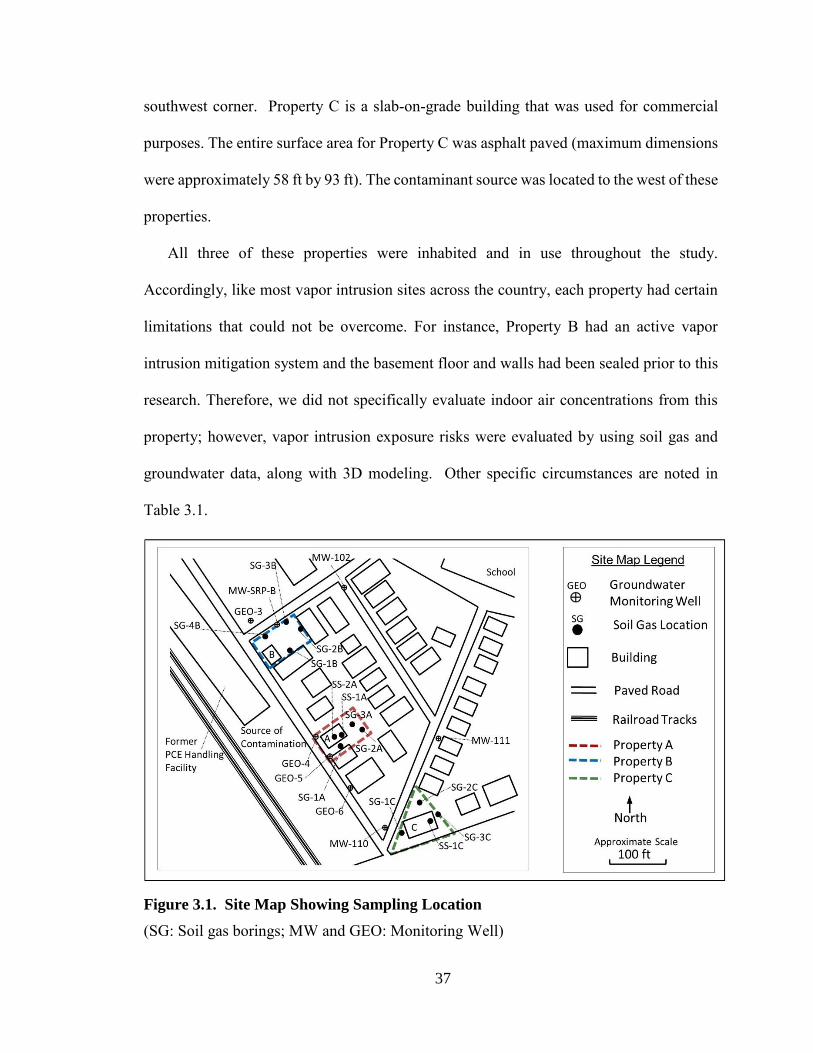
37
southwest corner. Property C is a slab-on-grade building that was used for commercial
purposes. The entire surface area for Property C was asphalt paved (maximum dimensions
were approximately 58 ft by 93 ft). The contaminant source was located to the west of these
properties.
All three of these properties were inhabited and in use throughout the study.
Accordingly, like most vapor intrusion sites across the country, each property had certain
limitations that could not be overcome. For instance, Property B had an active vapor
intrusion mitigation system and the basement floor and walls had been sealed prior to this
research. Therefore, we did not specifically evaluate indoor air concentrations from this
property; however, vapor intrusion exposure risks were evaluated by using soil gas and
groundwater data, along with 3D modeling. Other specific circumstances are noted in
Table 3.1.
Figure 3.1. Site Map Showing Sampling Location
(SG: Soil gas borings; MW and GEO: Monitoring Well)
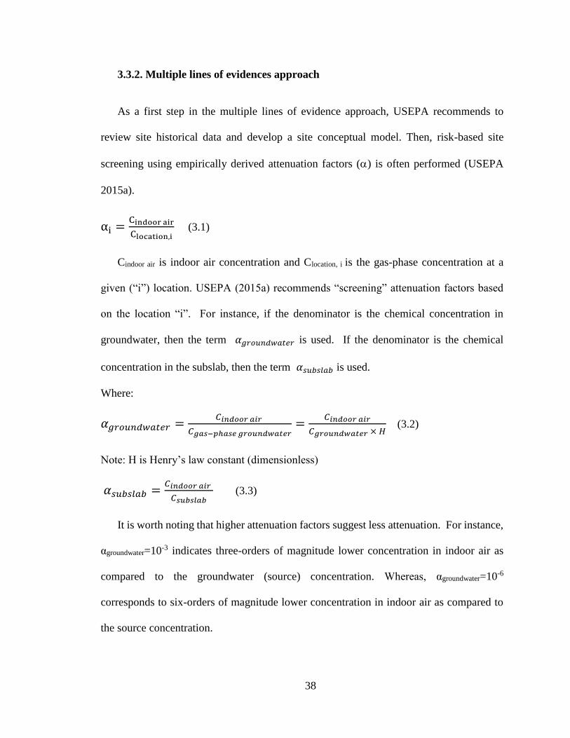
38
3.3.2. Multiple lines of evidences approach
As a first step in the multiple lines of evidence approach, USEPA recommends to
review site historical data and develop a site conceptual model. Then, risk-based site
screening using empirically derived attenuation factors () is often performed (USEPA
2015a).
αi =Cindoor air
Clocation,i (3.1)
Cindoor air is indoor air concentration and Clocation, i is the gas-phase concentration at a
given (“i”) location. USEPA (2015a) recommends “screening” attenuation factors based
on the location “i”. For instance, if the denominator is the chemical concentration in
groundwater, then the term 𝛼𝑔𝑟𝑜𝑢𝑛𝑑𝑤𝑎𝑡𝑒𝑟 is used. If the denominator is the chemical
concentration in the subslab, then the term 𝛼𝑠𝑢𝑏𝑠𝑙𝑎𝑏 is used.
Where:
𝛼𝑔𝑟𝑜𝑢𝑛𝑑𝑤𝑎𝑡𝑒𝑟 =𝐶𝑖𝑛𝑑𝑜𝑜𝑟 𝑎𝑖𝑟
𝐶𝑔𝑎𝑠−𝑝ℎ𝑎𝑠𝑒 𝑔𝑟𝑜𝑢𝑛𝑑𝑤𝑎𝑡𝑒𝑟=
𝐶𝑖𝑛𝑑𝑜𝑜𝑟 𝑎𝑖𝑟
𝐶𝑔𝑟𝑜𝑢𝑛𝑑𝑤𝑎𝑡𝑒𝑟 × 𝐻 (3.2)
Note: H is Henry’s law constant (dimensionless)
𝛼𝑠𝑢𝑏𝑠𝑙𝑎𝑏 =𝐶𝑖𝑛𝑑𝑜𝑜𝑟 𝑎𝑖𝑟
𝐶𝑠𝑢𝑏𝑠𝑙𝑎𝑏 (3.3)
It is worth noting that higher attenuation factors suggest less attenuation. For instance,
αgroundwater=10-3 indicates three-orders of magnitude lower concentration in indoor air as
compared to the groundwater (source) concentration. Whereas, αgroundwater=10-6
corresponds to six-orders of magnitude lower concentration in indoor air as compared to
the source concentration.

39
Comparison of predicted indoor air concentrations with risk-based guideline
concentrations provides rationale for measuring indoor air concentrations (USEPA 2015a).
For instance, if screening indicates the potential for vapor intrusion (e.g. an indoor air
concentration that is calculated to be greater than the regulatory indoor air target), then
indoor air samples are often collected; however, because consumer products contain many
of the same compounds as those that are a concern for vapor intrusion (USEPA, 2011),
indoor air samples often provide misleading information about the relative contribution of
vapors from the subsurface source. To overcome limitations of indoor air concentration
data, practitioners often install subslab (beneath the building foundation) and/or soil gas
vapor sampling points located outside of the building footprint.
As an initial step, we reviewed historic field data for the site and developed a site
conceptual model. Then, we collected indoor air and groundwater samples and compared
them to our vapor intrusion screening assessment (Line of Evidence 1). As subsequent
lines of evidence, we collected and evaluated soil gas data (Line of Evidence 2), and
evaluated the field data using computational models (Line of Evidence 3). Finally, we
created a revised site conceptual model based on the field data and numerical model results.
3.3.3. Field samplings
A total of fourteen (14) soil borings were advanced as part of this field study. Fig. 1
shows the sampling locations. Ten (10) borings (SG-1A, SG-2A, SG-3A, SG-1B, SG-2B,
SG-3B, SG-4B, SG-1C, SG-2C, and SG-3C) were completed as exterior soil gas sampling
points nested at multiple depths in the yards and parking areas of the three properties
included in the study (Properties A, B and C). One boring (MW-SRP-B) was completed as

40
a 1”-dia monitoring well (15 ft deep), located in the yard of Property B. Table 3.1
summarizes the sample locations included in the study.
Table 3.1. Sample Media and Collection Locations
Property Soil Gas Indoor Air Groundwater4 Location ft (bgs) Surface Cover
A SG-1A 3, 5, 7 Pavement Basement1
First Floor1
Outside
GEO-3
GEO-4
GEO-5
GEO-6
MW-102
MW-110
MW-111
MW-SRP-B
SG-2A 3, 5 Grass
SG-3A 3, 5 Pavement
SS-1A 1.75 Concrete
SS-2A 0.5 Concrete
B SG-1B 3, 5, 7 Grass Not included
in this study2 SG-2B 3, 5, 7 Grass
SG-3B 3, 5, 7 Grass
SG-4B 3, 5, 7 Pavement
C SG-1C 3, 5 Pavement First Floor3
Outside SG-2C 5, 7 Pavement
SG-3C 3, 5, 7 Pavement
SS-1C 5 Concrete
Notes: bgs: below ground surface
1 The indoor air on the first floor was only sampled during the first event due to access restrictions by the
property owner. Beginning with the second sampling event, only two basement indoor samples were
collected. 2 Soil gas and groundwater data were included in the analysis of Property B. However, since this property
had an active vapor intrusion mitigation system and the basement floor and walls had been sealed prior
to this research, indoor air data is not included herein. In addition, during sampling activities, sewer gas
was determined to be the source of elevated PCE concentrations detected in the indoor air for Property
B. Following the sewer connection being sealed, the PCE concentration detected in indoor air decreased
significantly. Pennell et al. (2013) discuss the sewer-to-indoor air pathway for Property B. 3 The building was a slab on grade construction, so there was no basement. 4 Groundwater samples were collected from each of these wells. All of the wells, except, MW-SRP-B
had been previously installed at the site as part of on-going regulatory action. MW-SRP-B was installed
as part of this study and was located within Property B’s boundary.
All soil gas sampling points were installed and sampled in accordance with
recommended procedures (NYDOH, 2006). Field personnel examined soil borings during
sample installation activities to gain insight about the site’s geology. When possible, a
Geoprobe was used to advance the soil borings, and soil cores were collected in 4-foot
acetate sleeves. Soil types were generalized based on field observations, coupled with sieve
analysis of select samples. Generally speaking, the soil geology was consistent with the

41
observations across the rest of the site, as previously reported by the environmental
consultant for the site (GEI, 2009). The soil geology was surprisingly consistent, including
two primary soil types: an upper unit (0-4 ft bgs) consisting of urban fill; and, a lower unit
consisting a dense, stiff, sandy clay loam (4-8 ft bgs).
3.3.4. Chemical analysis
Groundwater, air and soil gas samples were collected every 2-3 months over a period
of 12 months for a total of 5 sampling events. All samples (groundwater, indoor air and
soil gas) for a given property were collected within 48 hours for each of the 5 sampling
events. All samples (groundwater, air, and soil gas) were analyzed for selected VOCs based
on detections reported during historical site sampling activities: PCE; Trichloroethylene
(TCE); 1, 2, Dichloroethane (DCA); Trichloroethane (TCA); and Carbon tetrachloride
(CCl4).
Groundwater Sampling
Groundwater was collected from seven existing monitoring wells (GEO-3, GEO-4,
GEO-5, GEO-6, MW-102, MW-110, and MW-111) and one well installed as part of this
research (MW-SRP-B). Depth to groundwater was measured, and the groundwater level
was compared to well construction details to ensure that the well screen was not
submerged, as required for no-purge sampling. All groundwater samples were collected
with disposable bailers using the no-purge method (API, 2000). Although the no-purge
method is often limited to petroleum hydrocarbon sites, the nature of this field study posed
limits on hazardous waste generation (including purge water) and also the amount of time
to access each property. Therefore, the no-purge method was deemed the only possible

42
method for sampling. Samples were shipped on ice to Columbia Analytical Services and
analyzed for selected VOCs using EPA Method SW8260.
Air and Soil Gas Sampling
Air samples were collected inside and outside of each property for 24-hours using 6-L
certified summa canisters and shipped overnight to Columbia Analytical Services for TO-
15 analysis. Prior to sampling, research team members met with the residents to discuss
the sampling process and to survey and remove possible indoor sources of VOCs from the
home.
Soil gas samples were collected as grab samples over a period of 10 minutes using 1-
L certified summa canisters. Summa canisters (both 1L and 6L) were certified “clean” and
the flow controllers were certified by the laboratory prior to field sampling. All data
reported are from canisters with acceptable vacuums upon receipt at the laboratory.
Laboratory sample preparation and analysis was conducted by a National Environmental
Laboratory Accreditation Conference-certified laboratory (Columbia Analytical Services).
Analyses were compliant with USEPA Method TO-15 (Volatile Organic Compounds in
Air Analyzed by Gas Chromatography/Mass Spectrometry) and the laboratory’s standard
operating procedures that define requirements for calibration and acceptable results for QC
parameters. Detection limits are all below risk-based comparative values.
3.3.5. Computational modeling
In general, most vapor intrusion models are 1-D screening tools. The most widely
employed screening model is the Johnson and Ettinger, or J&E model (Johnson and
Ettlnger, 1991), which has been incorporated into a spreadsheet program by USEPA
43
(2004). The J&E model predicts attenuation factors based on user inputs; however it does
not incorporate information about soil gas concentrations and therefore is not useful in
interpreting the type of data typically collected during vapor intrusion investigations. 3-D
models provide information about the soil gas concentrations throughout the subsurface,
as well as the calculated attenuation factor, but are not widely available in practice settings
due to lack of practitioners and regulations who have access to and are trained using 3D
vapor intrusion models. In addition, there is a critical need for field data sets to be compared
to 3D model results. This research incorporated 3D model simulations to investigate soil
gas concentration profiles. For comparison purposes, results from USEPA’s version of
J&E model (groundwater contamination advanced model, GW-ADV-Feb04.xls (USEPA,
2004)) are also reported.
The 3-D model simulations included herein were conducted using a commercially
available software, Comsol Multiphysics®. The modeling approach has already been
extensively described (Bozkurt et al., 2009; Pennell et al., 2009; Yao et al., 2011). The
model incorporated a generic single building (10 m x 10 m) with a basement (1.67 m deep)
located in the center of an open field. A generic building geometry was used to allow
comparisons between the 1-D J&E model and the 3D model. The model was exercised
assuming a typical disturbance pressures (-5 Pa) at the perimeter crack (5mm wide) around
the entire floor of the basement. Groundwater (located at 11ft bgs and 13 ft bgs) was
assumed to be the vapor intrusion source. Various geological characteristics, including soil
type, depth and thickness of the soil layers and moisture content of the soil were
investigated and modeled. For this research, steady state model solutions are reported;

44
however, separate ongoing research is considering transient effects. Table 3.2 summarizes
the model equations.
Table 3.2. Model Equations
Equation 3.1:
Soil=gas continuity
−=
Kq
+=
P
Po
dPgz
Where:
q = gas velocity (L/t)
K = intrinsic permeability (L2)
= density of soil gas (M/L3)
= dynamic viscosity of soil gas (M/L/t)
g = gravitational acceleration (L/t2)
P = pressure of soil gas (M/L/t2)
z = elevation (L)
Note: Equation 1 is valid for gas flow in soils where slip flow is
negligible (sand and gravels). For fine-grained materials,
Darcy’s Law (Equation 1) may underestimate flow.
Equation 3.2:
Pressure drip across crack:
3
12
ck
ckgck
ckw
dQp
=
Note: Qck = QCER
Where :
pck = Pressure drop across crack (assumes parallel
plates)(M/L/t2)
wck = width of crack (L)
dck = length of crack through foundation depth (L)
QCER = soil-gas flow rate into the characteristic entrance region
(L3/t)
Qck = soil-gas flow rate through crack into building (L3/t)
Equation 3.3:
Chemical transport
JT ,i = q Ci − Deff,i
gasCi
10/3 10/3
0 2 2K
geff w wg
t H t
DD D
= +
Millington (1959)
Where:
JT = Bulk mass flux of “i” (M/L2/t)
C = Concentration of “i” in soil gas (M/L3)
D0eff = Effective diffusivity coefficient on “i” in soil-gas phase
(L2/t)
Dg = Molecular diffusivity coefficient on “i” in air (L2/t)
Dw = Molecular diffusivity coefficient on “i” in water (L2/t)
KH = Air-water partition (Henry’s) coefficient (unitless)
= porosity; t = total, g = gas-filled, w = water-filled (L3/L3)
Equation 3.4:
Indoor Air Concentration
ckbe
Tckindoor
QVA
JAC
+=
Ack = Area of the crack for vapor entry (L2)
Vb = Volume of enclosed indoor space (L3)
Aer = Air exchange rate in building (1/t)
3.4. Results and discussion
3.4.1. Summary of field data and conceptual site model
Table 3.3 summarizes the maximum chemical concentrations detected during this field
study for each sample medium. PCE and TCE were the constituents most often detected
across all media. Other constituents were detected but their concentrations fluctuated
during the various sampling events (data not shown). PCE was the only constituent that

45
was routinely detected at all of the properties included in the study. In addition, PCE was
detected at the highest concentration of all chemicals for all sample media. Analytical
results from historical sampling activities (GEI 2009) indicated that PCE was not
undergoing significant biodegradation and degradation byproducts were not typically
observed at the site.
Table 3.3. Maximum Chemical Concentrations Detected During Field Study
Sample Location 1,1,1 TCA 1,2 DCA PCE TCE Carbon
Tetrachloride
Vinyl
Chloride Media
GEO-3 17 <5 450 95 <5 <5
Groundwater
(g/L)
GEO-4 <100 <100 8100 100 <100 <100
GEO-5 110 <100 6100 190 <100 <100
GEO-6 <2 <2 25 7.2 <2 <2
MW-102 4.7 <2 74 6.5 <2 <2
MW-110 <2 <2 <2 <2 <2 <2
MW-111 <10 <10 880 12 <10 <10
MW-SRP-B 17 <2 300 84 <5 <5
Property A 17 <15 2300 0.38 <15 <15 Soil Gas
(g/m3) Property B 360 <5.5 3900 410 <5.5 <5.5
Property C <1.1 <1.1 2.8 <1.1 <0.40 <1.1
Property A 2.0 <0.42 300 7.7 <0.42 <0.42 Subslab
(g/m3) Property B NI NI NI NI NI NI
Property C <1.6 <1.6 28 2.3 0.86 <1.6
Property A 0.28 0.1 5.3 2.2 0.46 <0.04 Indoor Air
(g/m3) Property B * * * * * *
Property C 0.5 0.073 2.7 0.32 0.86 <0.047
95th Percentile Background
(EPA 2011)
3.4-28 <0.2 4.1-9.5 0.56-3.3 <1.1 <0.09 Indoor Air
(g/m3)
Residential
Threshold Values (MassDEP 2011)
3.0 0.09 1.4 0.8 0.54 0.27 Indoor Air
(g/m3)
IA Target (VISL) (EPA 2015b)
5200 0.11 11 0.48 0.47 0.17 Indoor Air
(g/m3)
Subslab Target (VISL)
(EPA 2015b)
170,000 3.6 360 16 16 5.6 Subslab
(g/m3)
Notes:
If a constituent was not detected during the study, the concentration is shown as less than the maximum
detection limit for the study (e.g. <5). Underlined data exceed typical background concentrations in indoor
air. Bolded data exceed threshold values set by MassDEP to be protective of human health. NI – Not
installed. IA – Indoor Air.
* Property B has an active vapor intrusion mitigation system and the basement had been sealed prior to this
research. Sewer gas was determined to be the source of elevated PCE concentrations detected in the indoor
air for Property B. Following the sewer connection being sealed, the PCE concentration detected in indoor
air decreased significantly. Pennell et al. (2013) discuss the sewer-to-indoor air pathway for Property B.
Two conceptual site models were established as relevant for the initial representations
of the vapor intrusion pathway at the site: 1) the classic conceptual model, a building
located in the middle of an open field; and 2) a building surrounded by impervious material.

46
Both of these conceptual models assumed groundwater was the source of chemical vapors
in the subsurface.
In the classic conceptual model, soil gas is trapped beneath the building footprint.
Outside the footprint, soil gas concentrations decrease as they approach the ground surface.
Similarly, for the situation where a building is surrounded by an impervious surface, soil
gas is trapped beneath the entire covered area. Outside the covered area, soil gas
concentrations decrease as they approach the ground surface. These conceptual
descriptions of vapor transport at the site guided the evaluation of each additional line of
evidence and were informed by conceptual models available in the literature (USEPA
2012b; Pennell et al 2009; Bozkurt et al 2009).
Figure 3.2. Preliminary Conceptual Models for the Site
Notes: Red color indicates high concentration. Blue color represents low concentration.
3.4.2. Multiple lines of evidence
As discussed earlier, we investigated three lines of evidence. First, we collected indoor
air samples and groundwater samples, and compared them to our vapor intrusion screening
assessment values (Line of Evidence 1). Then, as subsequent lines of evidence, we
47
collected and evaluated soil gas data (Line of Evidence 2), and finally we evaluated the
field data using computational models (Line of Evidence 3). As a final result, we developed
a revised conceptual site model.
Line of evidence 1.a: groundwater screening and indoor air concentration measurements
As the first line of evidence, evaluating attenuation factors provides information about
the propensity for vapor intrusion exposure risks at the site. For this line of evidence, we
considered data that were previously collected as part of regulatory activities at the site
(GEI 2009), as well as data specifically collected as part of this research. The results are
summarized below and show relatively good agreement in terms of historical site trends.
Line of evidence 1.b: evaluation of previously collected field data
Based on prior field data collected as part of regulatory activities for the three properties
included in this study (A, B and C), the attenuation factors ranged from approximately 10-
3 to 10-6. These attenuation factors were calculated using historical groundwater and indoor
air concentrations reported to MassDEP by the site consultant (GEI, 2009). The higher
attenuation factor (10-3) was detected in a Property B, which was later mitigated and the
basement floor was sealed. Several years after mitigation, Pennell et al. (2013) reported
evidence that a faulty sewer connection in Property B was a source for elevated PCE
concentrations in the indoor air on the first floor during the field study included in this
research. It is not known how long the sewer connection may have been influencing indoor
air concentrations in that property. For Property A and Property C, the attenuation factors
ranged from approximately 10-5 to 10-6, which are considerably lower and suggested vapor
intrusion may not be a concern at these buildings; however, using the 0.001 screening value
as the attenuation factor, “predicted” indoor air concentrations that are above MassDEP

48
health risk levels. Since there is considerable research showing that indoor air
concentrations vary temporally (e.g. Holton et al 2014), these data, by themselves, were
not adequate to suggest there was not a “potential” for vapor intrusion exposure risks.
Additional sampling was aimed at better understanding the potential for vapor intrusion
exposure risks at the site (Lines of Evidence 1 and 2).
Line of evidence 1.c: evaluation of data collected as part of “this” study
Groundwater and indoor air samples were collected from locations across the site. Fig.
3 shows a comparison between measured indoor air concentrations and predicted indoor
air concentrations using the USEPA screening attenuation factor of 0.001 (USEPA, 2015a)
and groundwater concentrations that were detected in nearby wells. Fig. 4 shows the site-
specific attenuation factors calculated based on indoor air concentrations detected at
Properties A and C. Indoor air concentrations presented on these figures were limited to
the lowest building level (the basement of Property A and the first-floor of Property C) and
groundwater concentration data collected from individual monitoring wells located near
the properties—Property A (GEO-4 and GEO-5) and Property C (MW-110, MW-111,
GEO-6). Property B was excluded from this line of evidence because indoor air
concentrations were known to be influenced by sewer gas entering the home (Pennell et al
2013). In should be noted that Property B is included in subsequent lines of evidence
because sewer gas entering the home did not influence the soil gas concentrations (Line of
Evidence 2) or modeling activities (Line of Evidence 3).
“Predicted” indoor air concentrations, calculated using the groundwater concentration
data collected from individual monitoring wells located near the properties—Property A
(GEO-4 and GEO-5) and Property C (MW-110, MW-111, GEO-6)—were above the

49
MassDEP residential threshold values and typical indoor air background concentrations
(MassDEP, 2011); however, nearly all of the measured indoor air concentrations detected
for Property A and C were below the background (i.e. “typical”) levels, which suggests
vapor intrusion exposure risks appeared low.
Note: Threshold values are based on the Massachusetts Department resiential value (2010)
Indoor air concentrations were measured for the lower level of the occupied building for each property.
GEO-3, GEO-4, GEO-5, GEO-6, MW-110, and MW-111 are groundwater monitoring
wells.
Figure 3.3. Comparison of Screening Level “Predicted” and Measured Indoor Air
Concentrations for Property A and Property C
As shown on Fig. 4, despite that each of the groundwater monitoring locations were
close to each of the respective properties (generally less than 100 feet) and were located in
the same groundwater aquifer (shallow), groundwater concentrations varied and resulted
in many orders of magnitude difference between the attenuation factors. This spatial
variation is a challenge for many vapor intrusion investigations and is consistent with the
analysis of other vapor intrusion field data (Yao et al., 2013d). The selection of appropriate
monitoring wells for preliminary evaluation of vapor intrusion exposure risks is important,
but not easily determined when designing a vapor intrusion investigation. Based on the

50
data shown on Figs. 4 and 5, Properties A and C appear to have limited potential for vapor
intrusion based on indoor air measurements, which is consistent with previous historical
field sampling results (Section 3.2.1.1); however based on the known likelihood for indoor
air concentrations to vary substantially with time (e.g. Holton et al 2014), additional
evaluation of other field is warranted to fully consider whether a potential for vapor
intrusion exposure risks is likely. To further evaluate the potential for exposure risks, soil
gas concentrations were evaluated.
Figure 3.4. Measured Groundwater (Vapor) Concentration and Attenuation
Factors (α) Line of Evidence 2: Soil Gas Concentrations.
Line of Evidence 2. Soil gas concentrations
Soil gas concentration data provide another indication of potential for vapor intrusion
exposure risks and are used as another line of evidence. Two different types of soil gas
data are often collected: subslab soil gas samples (collected from beneath the building
footprint); and, exterior soil gas samples (collected outside the building footprint).

51
Subslab Soil Gas Samples
Indoor air measurements at Property A suggest a low potential for vapor intrusion, but
subslab concentrations were above screening levels. The recommended subslab to indoor
air screening level attenuation factor (𝛼𝑠𝑢𝑏𝑠𝑙𝑎𝑏) is 0.03 (USEPA, 2015a). Therefore, the
screening level for subslab concentrations of PCE is 360 µg/m3, which assumes a target
indoor air concentration of approximately 11 µg/m3 (USEPA 2015b). All sub-slab
concentrations for Property A are below this level (ranging from 10-300 µg/m3). And, all
five rounds of indoor air sampling confirmed that indoor air concentrations of PCE were
at or below indoor air target concentrations. Subslab concentrations of PCE at Property C
were low, similar in magnitude to the measured indoor air concentrations (See Table 3.3),
and were inconsistent with the conceptual models shown in Fig 2. Exterior soil gas samples
(discussed below) provided additional information to develop a revised conceptual model
that could inform decisions at the site.
Exterior Soil Gas Samples
The exterior soil gas data trends provide information about vapor attenuation
throughout the subsurface (Fig. 5). The measured data show fluctuations over the course
of the study; however temporal variations were slight. During the January, April and June
sampling events, water-saturated conditions were observed in some of the shallow
sampling locations. However, these conditions did not appear to affect results for
subsequent events, which is likely related to the long time scales (i.e. many months)
required for water infiltration to affect vapor transport in shallow soils. Shen et al. (2012)
suggest the timescales for moisture content dynamics and the corresponding effects on
vapor transport are disparate.
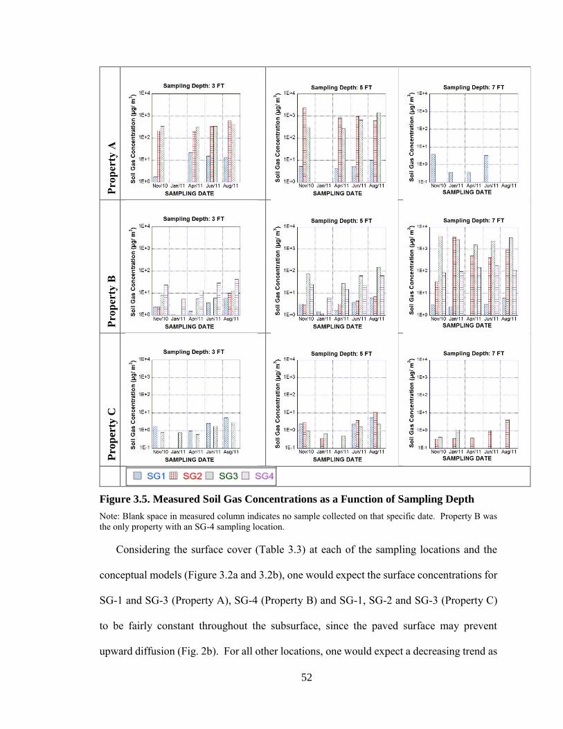
52
Pro
per
ty A
Pro
per
ty B
Pro
per
ty C
Figure 3.5. Measured Soil Gas Concentrations as a Function of Sampling Depth
Note: Blank space in measured column indicates no sample collected on that specific date. Property B was
the only property with an SG-4 sampling location.
Considering the surface cover (Table 3.3) at each of the sampling locations and the
conceptual models (Figure 3.2a and 3.2b), one would expect the surface concentrations for
SG-1 and SG-3 (Property A), SG-4 (Property B) and SG-1, SG-2 and SG-3 (Property C)
to be fairly constant throughout the subsurface, since the paved surface may prevent
upward diffusion (Fig. 2b). For all other locations, one would expect a decreasing trend as
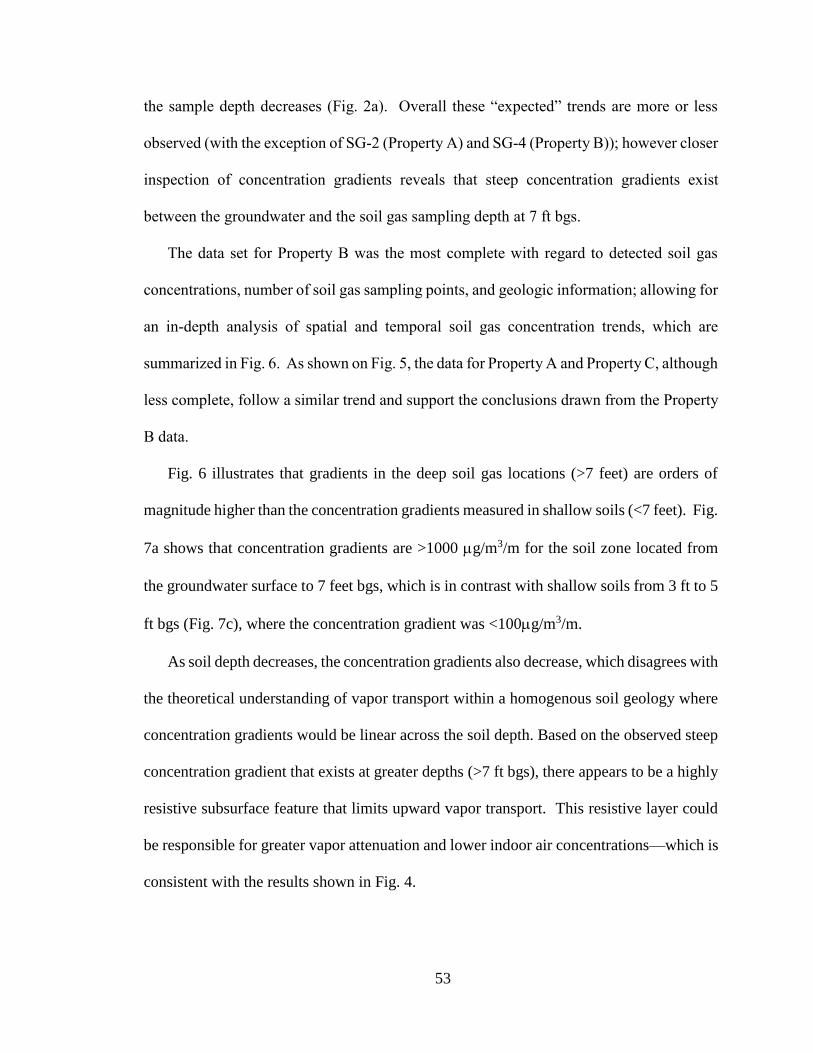
53
the sample depth decreases (Fig. 2a). Overall these “expected” trends are more or less
observed (with the exception of SG-2 (Property A) and SG-4 (Property B)); however closer
inspection of concentration gradients reveals that steep concentration gradients exist
between the groundwater and the soil gas sampling depth at 7 ft bgs.
The data set for Property B was the most complete with regard to detected soil gas
concentrations, number of soil gas sampling points, and geologic information; allowing for
an in-depth analysis of spatial and temporal soil gas concentration trends, which are
summarized in Fig. 6. As shown on Fig. 5, the data for Property A and Property C, although
less complete, follow a similar trend and support the conclusions drawn from the Property
B data.
Fig. 6 illustrates that gradients in the deep soil gas locations (>7 feet) are orders of
magnitude higher than the concentration gradients measured in shallow soils (<7 feet). Fig.
7a shows that concentration gradients are >1000 g/m3/m for the soil zone located from
the groundwater surface to 7 feet bgs, which is in contrast with shallow soils from 3 ft to 5
ft bgs (Fig. 7c), where the concentration gradient was <100g/m3/m.
As soil depth decreases, the concentration gradients also decrease, which disagrees with
the theoretical understanding of vapor transport within a homogenous soil geology where
concentration gradients would be linear across the soil depth. Based on the observed steep
concentration gradient that exists at greater depths (>7 ft bgs), there appears to be a highly
resistive subsurface feature that limits upward vapor transport. This resistive layer could
be responsible for greater vapor attenuation and lower indoor air concentrations—which is
consistent with the results shown in Fig. 4.

54
Inspection of the concentration gradients also reveals insight about spatial and temporal
variations. Small spatial variation in soil gas concentration gradients were observed at
depths >7 ft bgs, but slightly larger temporal variation (approximately 1-order of
magnitude) across seasons. For shallower soils, larger spatial variation (>5 orders of
magnitude) and smaller temporal variation (1.5 order of magnitude) are observed.
Concentration gradient= 𝛥𝑐
𝛥𝑥 =
𝐶 (𝑋2)−𝐶(𝑋1)
𝑋2−𝑋1
C(Xi)=Concentration at depth i
Xi = Depth i
Note: Horizontal line indicates the
average concentration gradient.
Figure 3.6. PCE Concentration Gradient for Soil Gas Locations at Property B

55
One possible explanation for increased attenuation in the subsurface is the capillary
fringe, which is the zone of soil located immediately adjacent to the top of the water table.
The effect of capillary fringe has been evaluated for vapor transport in laboratory settings
and resulted in orders of magnitude increase in vapor attenuation (McCarthy and Johnson,
1993). Within the capillary zone, capillary forces draw water up into the soil pores and
cause saturated soil conditions above the actual water table and reduces upward vapor
transport. Trapped air that exists within the capillary zone prevents the soil from becoming
fully saturated at the groundwater table surface; therefore, the effects of moisture content
on vapor transport through the capillary zone has been approximated previously by Waitz
et al. (1996) using moisture content estimates from water retention curve (e.g., van
Genuchten (1980)). Bekele et al. (2014) reported elevated VOC concentrations
(specifically TCE) in soil that was sandwiched between two high moisture zones. This
observation also supports the observations reported herein where soil moisture is thought
to have retarded VOC transport, trapping higher concentrations beneath highly resistive
soil layers. Modeling efforts by Shen et al. 2012, 2013a, 2013b, and Moradi et al. 2015
also emphasize the importance of soil moisture when evaluating vapor intrusion exposure
risks.
Line of evidence 3: interpret and evaluate field data using computational modeling
The purpose of the modeling exercises was to investigate possible site characteristics
that may provide a plausible explanation for the attenuation observed at the site. Modeling
focused on predicting soil gas concentration data because soil gas concentrations are less
prone to changes in building ventilation or chemical uses within the home. Further, indoor

56
air concentrations were low across the entire site and did not lend themselves to further
evaluation.
Model input values for the 3D model were based on field observations and relied on
values recommended by USEPA (2004). Table 3.4 (below) describes the three cases that
the models investigated. These cases were determined a priori and supported by site
specific characteristics and field data. During the field study, the depth to groundwater
varied in MW-B-SRP (located directly on Property B) from approximately 10 to 13 ft bgs;
therefore, Case 3 was exercised for groundwater depths that ranged between 11-13 ft bgs.
Case 1 and Case 2 were exercised for a groundwater depth of 11 ft bgs.
Table 3.4. Summary of the Scenarios
Case Description
3D
J&E model
1
Homogenous geology for the two predominant
soil types that were observed at the site (loamy
sand and sandy clay)
4.5E-05
to
1.6E-04
1.9 E-04
to
8.8 E-04
2
Two-layer geological system with the top layer as
a loamy sand and the bottom layer as a sandy clay. 3.3E-05
to
7 E-05
2.7 E-03
to
3.6 E-04
3
Three-layer geological system with the top layer
as a loamy sand, middle layer as a sandy clay, and
the bottom layer as a high moisture content
(>90%) layer (conceptualized as the capillary
fringe). Thickness of the capillary fringe varied
from 1 ft to 2.5 ft, which corresponds to the soil
types at the site.
1.6E-6
to
4.5E-6
4.00 E-06
to
1.00 E-05
The modeled attenuation factors are also shown in Table 3.4. It can be seen that adding
a resistive layer in Case 3 increases attenuation by as much as nearly two order of
magnitudes for both 3-D and J&E models. The attenuation factors demonstrate how site
features can dramatically influence the potential for vapor intrusion exposure risks;

57
however model simulations alone should not be used to make decisions at a site because
models are well known to be subject to uncertainty related to model structure and
environmental variability. Moradi et al (2015) highlights the effect of uncertainties on
vapor intrusion exposure risk predictions and their results suggest that model predictions
require the other lines of evidence to validate and inform about the likelihood of vapor
intrusion exposure risks.
Fig. 7 depicts the measured and modeled soil gas concentrations for Property B.
Spatially, a vertical concentration gradient was detected with the lowest concentrations
detected at 3 ft bgs, and the greatest concentrations detected at 7 ft bgs. However, this
gradient was not as steep as would be expected based on groundwater concentrations and
suggested that vapor attenuation was occurring deeper than the 7ft bgs sampling location.
The inclusion of the high resistivity zone (conceptualized as the capillary fringe (Case 3))
results in an order of magnitude decrease in predicted attenuation factors and, importantly,
improves model and field measurement agreement. Laterally, there was some variation in
results for each soil gas sampling location, but overall the variations were less than one-
order of magnitude.
Although the 3D model incorporated a capillary fringe layer, the highly resistive layer
does not necessarily need to be the capillary fringe. It could be a thin fine-grained soil
layer (i.e. clay and silt) located anywhere between groundwater and soil surface that can
act as a barrier preventing upward migration of soil gas. It also could be a biologically
reactive zone that prevents PCE from being transported upwards toward the surface prior
to being degraded. It may also be a lens of “clean” water that overlies the groundwater
surface; thereby reducing the source concentration that is estimated based on groundwater

58
concentrations detected in monitoring wells. At this site, the measured groundwater
concentrations did not provide a good indication of the vapor intrusion exposure risks (as
measured by indoor air and soil gas concentrations). Regardless of the exact nature of the
subsurface feature, the model established the location of the surface feature (which based
on field data was deeper than 7 ft) and confirmed that the field observations were not
consistent with the original conceptual models (Fig 2a/2b). Figure 3.8 is an updated
conceptual model.
Case
1
Case
2
Case
3

59
Note: Lines indicate lower and upper limits of model simulations.
Figure 3.7. Modeled and Measured Soil Gas Concentrations For Three Cases. (For case 2, 3 there are two lines which show a range for variation of steady state concentration for
different scenarios of each case)
Figure 3.8. Conceptual Model Comparison.
(Top-Classical, bottom-informed by this research).
L-S-Loamy sand, SC-Sandy clay
3.5. Conclusions
Characterizing vapor intrusion is difficult to accomplish because of sampling
limitations and because field data do not easily follow predicted trends; however by
systematically reviewing data and incorporating a numerical model to interpret field data
observations using a multiple lines of evidence approach, decisions can be made about how
to manage vapor intrusion exposure risks. Overwhelming evidence exists that a subsurface

60
feature is present over much of the study area that limits upward vapor-phase diffusion of
PCE. In addition, data suggest that the groundwater concentrations measured during this
research, as well as the groundwater concentrations collected historically at the site as part
of regulatory-driven activities, did not provide a good indication of vapor intrusion
exposure risks (as estimated using the multiple lines of evidence approach). When vapor
intrusion occurs in large communities where hundreds of homes are affected, our results
indicate that relying on groundwater concentrations for assessing vapor intrusion exposure
risks is not appropriate; and, deviations from classic conceptual vapor intrusion models
should be anticipated. Incorporating physical models as part of multiple lines of evidence
approach can inform conceptual models and improve risk management decisions.
While the collected data could not describe the exact nature of the subsurface “feature”
that was limiting transport, the model did provide evidence that the subsurface feature
would significantly alter the soil gas concentration profiles. Conceptually, the capillary
fringe may be one possible explanation. If capillary fringe is the sole explanation, then soil
gas concentrations at many vapor intrusion sites could be lower than expected based on the
“classic” conceptual model. However, the results of this research did not provide enough
information to support that claim. Rather, it suggests a need for additional research that
evaluates high-quality, temporally-correlated field data with model predictions to
investigate whether similar trends are present at other sites.

61
CHAPTER 4: COLUMN STUDIES
Following the publication of the Research in Chapter 3, additional questions about
VOC vapor transport still remained. Yao et al., (2017a) a co-author on the article described
in chapter 3, conducted a soil column studies to assess impact of soil texture on VOC vapor
intrusion. They studied three columns with three different mediums including sand, sand
soil and sandy loam soil. They measured TCE soil gas concentrations in different depths
of the columns to investigate TCE equilibrium concentration profile for each soil type and
compared the measured data with result of a numerical model. The soil water content
profile was also measured and data have been compared with the calculated water content
based on van Genuchten equation (1980). Results suggest an appropriate compatibility
between measured and calculated water content by van Genuchten equation. Millington
and Quirk (1961) equation also has been used to estimate the diffusion coefficient in
different depths of the soil based on the water content.
In a homogeneous soil with uniform water content, the diffusion coefficient is constant
with depth and therefore TCE steady state concentration profile in vertical direction is
expected to be linear. Results of the column study indicate that the water content curve for
the sand column was the most abrupt, that was expected by the van Genuchten parameter
and in case of the sandy loam soil, the water content curve and subsequently soil vapor
TCE concentration profile was the smoothest curve that is expected based on the smallest
value of van Genuchten parameter for sandy loam soil. Observing the good agreement
between the measured column study data and the concentrations calculated by the
numerical model support validity of the applying classical multiphase chemical transport
equations.

62
Soucy and Mumford, 2017 also conducted a series of column experiments to assess
impact of vertical movements of gas bubbles on VOC vapor intrusion. They measured the
bubble-facilitated VOC mass flux from contaminated source and compared this flux with
diffusion driven VOC vapor flux. Pentane was used in all experiments due to its high
volatility. Results of their column study suggested that dissolved gas and bubble transport
increase VOC vapor mass transfer with orders of magnitude compare to the diffusion
dominant VOC mass transfer inside the column. This study concluded that bubble-
facilitated VOC transport within the vadose zone can significantly increase VOC indoor
air concentration and therefore inhalation exposure risk. This mechanism is only active in
area that high concentrations of dissolved gases are accompanied with elevated
contamination of dissolved VOCs or volatile non-aqueous phase liquid (NAPL).
The laboratory experimental setup
Limited experimental testing was conducted to assess the accuracy of numerical models
for estimating effect of soil water content on the VOC mass transfer through soil, a
laboratory experimental set up was designed and conducted as part of this research. This
set up is consisted of a glass column with two sampling points and a supporting bed for
soil. The glass column that was used in this study was in the shape of cylinder with 60 cm
length and 4.8 cm diameter. Figure 4.1 shows the dimensions of the column study.

63
Figure 4.1. Schematic the column study
The designed soil column was assembled to the wood stand (Figure 4.2a). The quick
stop luer check valves shown in figure 4.2b were installed on the designed opening parts
of the glass column to allow us to take air samples from the column and a 10 ml gas tight
syringe was used for sampling (Shown in figure 4.2c). The quick luer consist of two parts:
the check valve and the luer adapter. The check valve remains close until it connects to the
luer adapters. We attached the luer adapters to the air tight syringe. Once the two parts of
the quick stop luer are engaged the check valve allows flow in both direction and we could
get air from the column.

64
a)
b)
c)
Figure 4.2. Designed column experiment set up
Before conducting any experiment on the soil column, the soil was needed to be
characterized. First the grain size of the soil should have been determined. The standard
method for dry preparation of the soil sample (ASTM D421) and the standard test for
particle size analysis of soils sample (ASTM D422) were performed. The ASTM D422 test
determines percentage of various grain sizes within the soil and provides the particle size
distribution curve. A Balance, set of sieves with different sizes, cleaning brush and a sieve
shaker are all we need for performing this test. The ASTM D422 test procedure and the
general format of table and grain size distribution are provided in the appendix. Sieves with
different numbers (#4, #10, #20, #40, #60, #140, and #200) were assembled in the sieve
stack and the sieve stack was placed in the mechanical shaker and after 10 minutes shaking
the mass retained in each sieve and the percentage of soil passing each sieve were

65
calculated. Figure below shows the mechanical shaker that sieve stack was placed in.
Results of this test are shown in table 4.1.
Figure 4.3. Mechanical Sieve Shaker
Table 4.1. Sieve analysis for ASTM D422 test
Sieve no. Diameter(mm) Mass retained % retained %passing
4 4.75 0 0% 100%
10 2.00 0 0% 100%
20 0.840 0.1 0.0193% 99.98%
40 0.425 26.4 5.098% 94.88%
60 0.250 480.76 92.83% 2.05%
100 0.150 10.33 1.99% 0.062%
200 0.075 0.2 0.386% 0.0234%
Pan 0.1 0.0193% 0.0041%
Total weight 517.89

66
The particle equivalent diameter then can be estimated by using the grain size
distribution curve provided in appendix (Bowels, 1992). The equivalent diameter for the
soil (D50) was calculated =0.35 (mm) using the distribution curve method. The density and
specific gravity of the soil simply were calculated. The soil total porosity, water content
porosity and air filled porosity were calculated using equations 2.1, 2.2 and 2.3. For
measuring the hydraulic conductivity of the soil the constant head test (standard method of
ASTM D 2434) was used. In this method we create a constant hydraulic gradient and
measure the average flow rate of water passing through the soil in a steady state condition.
Figure 4.4 illustrates the concept of this method and equation 4.1 shows how the hydraulic
conductivity can be calculated.
Figure 4.4. Constant Head Test for Measuring Soil Hydraulic Conductivity
kh = V.L
A.t.∆H (4.1)
kh= hydraulic conductivity of the soil, (cm/s);
V= Volume of the water, (cm3);

67
L= length of the soil sample, (cm);
T=time of the water discharge; (s);
A= across section area (=π
4D2), (cm2);
ΔH= hydraulic head difference across length L (= the vertical distance between the constant
funnel head level and the chamber overflow level), (cm);
By applying this method the hydraulic conductivity measured at 0.06234 (cm/s). The
intrinsic permeability then calculated by applying equation 2.11 and was =6.385e -11 that
is equal to 64.7 Darcy. Table 4.2 shows different characteristics of the dry soil that were
measured by applying above methods.
Table 4.2. Measured properties of the soil
Density of the soil 1.57 g/cm3
D30 0.28 mm
D50 0.35 mm
Specific gravity 2.65
Total Porosity 0.4142
Hydraulic conductivity 6.234e-4 m/s
Intrinsic permeability 6.385e-11 m2
Gas chromatography flame ionization detector (GC/FID) has been used for measuring
concentrations of tetrachloroethylene (PCE) in headspace. A calibration curve was
developed for PCE. The procedure of developing the calibration curve is provided in
appendix. 10 (µl) of pure PCE in liquid phase was injected to the bottom of the column.
Concentrations of PCE in headspace then were recorded for both sampling ports to assess
the mass transfer and the time of equilibrium in each scenario. 180 cm3 of the soil that were

68
analyzed earlier, with different water content is added to the soil column. The depth of the
soil was on 10 cm for all scenarios. The effective diffusion coefficient of PCE vapors
through the soil for each scenario was calculated by applying equation 3.3. A 2-D model
simulations is conducted by using a commercially available software, Comsol
Multiphysics® to calculate PCE mass transfer for this experiment. The numerical model
simulation is shown in figure 4.5. The soil properties were modified for each scenario. The
calculated PCE concertation by the numerical model for each sampling port is compared
with the measured PCE concentration.
For the first scenario, TCE concentrations in the soil column without soil were
measured and compared with the numerical model calculations to evaluate the model
accuracy. Figure 4.6 shows PCE concentration profile over time for two sampling ports
calculated by the numerical model and figure 4.7 compares this concentration profile with
the data measured during the column study for this scenario.
Figure 4.5. 2-D simulation of the column study

69
Figure 4.6. Measured sampling ports concentration profile for no soil scenario
Figure 4.7. Comparing calculated vs measured data for no soil scenario
For the second scenario a completely dry soil was added to the column. The height of
the soil (properties of the soil is provided in table 4.2) was 10 cm. 10 (µl) of pure PCE in
the liquid phase injected to the bottom of the column. The concentration of PCE in the gas
phase for both sampling ports were measured over the time. Figure 4.8 shows results of the
numerical model and figure 4.9 compares results of TCE concentration calculated for the

70
port 2 with the column measured concentrations. As figure 4.7 and figure 4.9 show there
is a good compatibility between results that the numerical model calculated for PCE
concentration in sampling ports and the measured concentrations.
For the scenario 3 soil with 5% of water content added to the column. The height of the
soil and the amount of PCE that added to the column was the same as other scenarios and
PCE concentrations were measured in both sampling ports over the time. For the next
scenarios the same procedure was followed with different soil water content. Different soil
water content including 10%, 14%, 21% were examined. Figure 4.10 to 4.17 show results
of PCE concentrations with different soil water content.
Figure 4.8. Measured sampling ports concentration profile for dry soil scenario

71
Figure 4.9. Comparing calculated vs measured data for dry soil scenario
Figure 4.10. Measured sampling ports concentration profile for soil water content=
5%
Figure 4.11. Comparing calculated vs measured data for soil water content= 5%

72
Figure 4.12. Measured sampling ports concentration profile for soil water content=
10%
Figure 4.13. Comparing calculated vs measured data for soil water content= 10%

73
Figure 4.14. Measured sampling ports concentration profile for soil water content=
15%
Figure 4.15. Comparing calculated vs measured data for soil water content= 15%
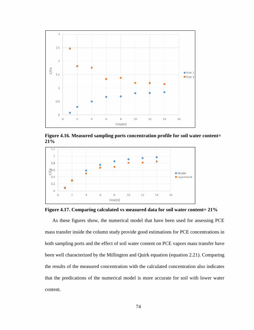
74
Figure 4.16. Measured sampling ports concentration profile for soil water content=
21%
Figure 4.17. Comparing calculated vs measured data for soil water content= 21%
As these figures show, the numerical model that have been used for assessing PCE
mass transfer inside the column study provide good estimations for PCE concentrations in
both sampling ports and the effect of soil water content on PCE vapors mass transfer have
been well characterized by the Millington and Quirk equation (equation 2.21). Comparing
the results of the measured concentration with the calculated concentration also indicates
that the predications of the numerical model is more accurate for soil with lower water
content.

75
CHAPTER 5: SEWER SYSTEM AS AN ALTERNATIVE VAPOR INTRUSION
PATHWAY: BACKGROUND AND MOTIVATION
For decades vapor intrusion has been studied based on the concept of VOC vapor
migration through subsurface soil and infiltration into the building through the
foundation’s cracks. Growing evidence has confirmed that VOC vapors can enter through
other pathways and infiltrate into the buildings. These vapor pathways that facilitate VOC
migration toward indoor air are named alternative pathways and VI field studies reported
aging infrastructure piping systems such as sewer systems as important pathways for VOC
vapor intrusion (USEPA, 2015). In this section we discuss sewer systems as an alternative
pathway for vapor intrusion.
Several field studies have reported detection of elevated concentrations of VOCs in
sewer gas and sewer liquid, providing evidence of sewer systems to act as pathways for
VOC migration to the indoor area (e.g. Riis et al., 2010; Pennell et al., 2013; Guo et al.,
2015; EPA, 2015a; Jacobs et al., 2015; McHugh et al., 2017; Roghani et al, 2017). US
Environmental Protection Agency’s (USEPA’s) noted that wastewater infrastructures
including drain lines and sewers systems are important exposure pathways in its most
recent vapor intrusion technical guidance (2015). There is lack of information regarding
the potential of sewer systems as pathways for VOC migration in VI studies. 1) There is
not enough information about the occurrence of VOCs inside the sewer system in both
liquid phase and gas phase and their temporal and spatial variations. 2) There is no standard
method for assessing sewer system as a potential pathway for VOC VI (e.g. sampling
location, time of sampling and sampling method). 3) There is no available numerical model
to explain VOC occurrence and variation within the sewer system.

76
5.1. Occurrence of VOC in aquatic system
Chlorinated solvents are organic compounds that have been used in different industrial,
commercial, and domestic processes for long time. Production of these chemicals began to
be decreased in the 1970s due to human health and environmental concerns. This chemicals
were used in large scales for various purposes including adhesives, paintings plastics,
drycleaners, fumigants and grease removal ‘s industries. Widespread and long-term usage
of chlorinated volatile organic compounds (VOC) in various industries and their potential
to persist and transfer within water systems make them enable to accumulate in the aquifers
and subsurface wastewater systems. Due to all of these reasons detection of VOC is not
limited to the specific area and they have been detected in most aquifers throughout the
country (USGS, 2006a; USGS, 2006b).
Chlorinated solvents have relatively high densities, relative to water, which enable
them to penetrate in the water table. They are soluble in water therefore move freely within
the water systems and generally have long half-lives in water compare to other organic
compounds which allow them to persist more in the water system (USGS, 2006a). These
properties give them a great potential to persist and to be transfer in water systems
including wastewater or groundwater.
United States Geological Survey (USGS) conducted a comprehensive national research
on VOCs occurrence in aquifers between 1985 and 2002. They collected more than 3500
water samples from different types of wells all over the U.S. Analysis of 2,401 domestic
wells and 1,096 public wells showed VOCs were detected in about 14 percent of the
domestic wells and 26 percent of the public wells. Different types of VOCs were detected
but typically at low concentrations. Chloroform, tetrachloroethylene (PCE) and

77
trichloroethylene (TCE) were among the most frequently detected VOCs in groundwater
and chloroform was the rank one VOC in groundwater (USGS, 2006 b).
Studying the fate and transport of VOC inside an aquifer system is not simple and there
are several of complexities involved. We need to have knowledge not only about present
and historical VOC sources in the area of study but also anthropogenic uses and chemicals
properties of the targeted VOC.
Chloroform is a byproduct of water and wastewater chlorination. The high occurrence
of chloroform inside the domestic and public walls is relevant to this process and is
expected while chlorination of the water has been a common method for water disinfection
for about a century all over the U.S.
While results indicate that over twenty percent of aquifers were contaminated with
VOCs, only 1 to 2 percent of samples were contained level of a VOC that is over its USEPA
maximum contaminant level (MCL) or health based screening level (HBSL). TCE and
PCE were detected more often higher than their MCLs compare to other chemicals (USGS,
2006a). Some level of VOC mixture occurrence also reported in this study that potentially
can be result of VOC degradation inside the water system. PCE-TCE is the most often
frequently detected VOC mixture and PCE-chloroform and TCE-chloroform are in rank of
second and third, respectively (USGS, 2006 b).
5.2. Wastewater infrastructure condition
The American Society of Civil Engineers (ASCE) defines infrastructure as the
foundation that connects communities with people and businesses to develop their life
quality (ASCE, 2013). Among the different types of infrastructure, water infrastructure has

78
the most essential role and collecting used, contaminated water and managing the sewage
is an important, expensive part of this infrastructure (ASCE, 2017). Wastewater
infrastructure in the United States (US) is in a state of disrepair. In the 2017 Report Card
for America’s Infrastructure, ASCE gave US wastewater infrastructure a grade of D+. This
grade indicates poor performance on the basis of capacity, condition, funding, future need,
operation, maintenance, public safety, resilience, and innovation. ASCE‘s report in 2017,
estimates capital investment requirements of $271 billion over the next two decades to
meet current and future water quality regulations. Meanwhile pipes represent the major
capital need with constituting three quarters of total costs (ASCE, 2017).
Currently, there are between 700,000 and 800,000 miles of public sewer mains
throughout the country, many of which were installed post-World War II and are
approaching the end of their design life. Fixing and renewal of the wastewater system needs
a huge funding and there is a capital funding gap for renewal program (ASCE, 2017). While
wastewater infrastructure is aging, and investments are not enough to keep up with their
maintenance needs, there is a need to establish a cost effective and efficient program to
protect health issue these aged wastewater infrastructures may expose.
These sewer systems were designed to transport residential, commercial, and industrial
liquid wastes to wastewater treatment plants without loss of wastes in transit. Several
decades after the installation of municipal sewer collection systems and the construction of
vented plumbing in buildings, many components of these legacy sewer systems experience
cracking, separation, and other damage. Several factors contribute to sewer degradation,
including earth subsidence, biological intrusion, pipe settling, and pipe material corrosion
or failure.

79
Within buildings, sewer plumbing systems were designed to properly vent sewer gases,
preventing their entry into inhabited indoor air spaces. Over time, however, vapor seals
that were designed to protect against sewer air intrusion into structures, may deteriorate.
(e.g., pipes crack, fittings loosen and P-traps dry out). When compromised sewer and
plumbing systems intersect VOC contaminated soil and groundwater plumes, water and
vapors containing VOCs can easily enter the sewer via infiltration and inflow (I&I) into
cracks in piping and manholes. In addition to I&I, water and vapor containing VOCs can
enter wastewater pipes through direct discharges to the sanitary sewer system.
Typical chemicals of human health concern related to sewer gas include hydrogen
sulfide (H2S), ammonia (NH3), methane (CH4), and to a lesser extent, carbon dioxide
(CO2). Human health risks due to exposure to these agents are focused on acute toxicity
and physical hazards (ATSDR, 2004). Human identification of sewer gas is determined by
an individual’s capacity to recognize the characteristic H2S odor. The estimated odor
threshold of H2S ranges from 0.004 to 0.03 mg/m3, while adverse health effects of H2S
occur at a much greater concentration in indoor environments (USEPA, 2003).
5.3. Sewer system designs
There are different types of collections for sewer systems. In a separate sewer
collection, sanitary sewer system and storm sewer system are separated and flow into
different pipes. Sanitary sewer is designed to collect and convey wastewaters originating
from sanitary fixtures inside the residential or commercial units such as sinks, toilets and
shower. The storm sewer system is designed to collect rainwater. Strom sewer pipes are
typically larger than sanitary sewer systems because they should be able to collect larger
amount of water during a heavy rainfall. Strom water from downspouts, groundwater sump

80
pumps, foundation drains or drain from driveways should be directed to the storm sewers
or above the ground drainage ditches based on the storm water discharge regulation. If
water that originates from other sources (any source except sanitary fixtures) infiltrate into
the sanitary sewer system, it is an improper sewer connection in a separate sewer collection
design. An improper connection can add large volume of water to the sanitary sewer system
and make a serious problem such as overloaded sanitary sewer which may cause basement
flooding. For example an eight-inch sanitary can convey sewer flow from 200 properties
but only 8 sump pumps connections or 6 homes with downspouts connected to the sanitary
sewer may lead to an overload.
In a combined sewer collection, which is a remnant of old infrastructure, residential
and industrial wastewaters and rainwater runoff being carried in a same pipe and all being
transported to the wastewater treatment plant. Because of its design, there is a high chance
of combined sewer overflow (CSO) in a heavy rainfall event or snowmelt. CSOs occurs
when total volume of the wastewater exceeds the combined sewer system capacity and it
can significantly contaminate surface water, lakes and rivers. There are potentially several
kind of contaminations such as industrial waste, toxic chemicals, debris and etc. which can
infiltrate into water bodies due to CSO. CSO is a priority concern for water quality of about
40 million people in approximately 860 municipalities all around the U.S with combined
sewer systems. USEPA provided a national framework to control CSO and limit and
manage combined sewer system (USEPA, 1994). Figure 5.1 illustrates these two different
sewer collection systems.
There have been some attempts to investigate combined sewer (McHugh, 2017;
Wallace and Friedrich, 2017) and some research studies on sanitary sewers (Pennell et al

81
2013; Willett 2018, and Roghani et al 2018 (this research)), but there has not been extensive
research considering the effect that storms have on combined sewer systems; however,
Wallace and Friedrich (2017) reports significant unexpected results from a combined sewer
that cannot easily be explained.
a. Separated sewer system b. Combined sewer system
Figure 5.1. Separated and Combined Sewer System Design
5.4. Conceptualizing the sewer gas pathway
VOCs may enter into the sewer systems through various routs. These pathways can
be divided in four major categories that are summarized below.
1. Direct discharge: Inflow of VOC-contaminated wastewater into the sewer
collection system could occur through discharge of contact water from VOC-using
industrial facilities. Dry cleaning separator water is an example of direct industrial
discharge and is a primary source of PCE, which is a commonly found VOC in sewers
(USEPA, 2006a).

82
2. Historical discharge of VOC-laden wastewater can result in accumulation of VOC-
contaminated sludge in the sewer line, which can then act as another potential VOC source
within the conduit.
3. Groundwater infiltration: When sewer lines are located below the groundwater
table, which is a scenario typical of regions with shallow groundwater, groundwater is able
to enter the sewer line through cracks or damaged joints in the sewer pipes. This
groundwater can then easily convey liquid and gas-phase VOCs throughout the sewer
system. VOC in groundwater can be result of the leaking of underground storage tank or
historical disposal.
Even in areas with a deeper groundwater table – meaning sewer lines do not intersect
groundwater – significant rise of the groundwater table is likely during periods of heavy
rainfall. Especially after a strong storm event, the rise of the groundwater table to the depth
of sewer lines allows contaminated groundwater to infiltrate the sewer system. VOCs
which enter the liquid waste stream of the sewer line by any of these mechanisms can then
partition to the gas-phase and enter the sewer headspace.
4. Gas-phase VOCs in the sewer lines do not originate only via stripping from sewer
liquid. VOC can also partition to the gas-phase from any subsurface source such as
contaminated soil or contaminated groundwater and the evaporated VOC can diffuse
through soil toward the ground surface. The contaminated soil gas vapors can infiltrate the
sewer line through any failures in the sewer system. If water is able to penetrate into the
sewer pipe, then there is no significant resistance for vapor infiltration into the sewer
system (Pennell et al., 2013). The magnitude of gas-phase VOC flow into the sewer system
depends on the depth of the groundwater and its distance from the sewer system,
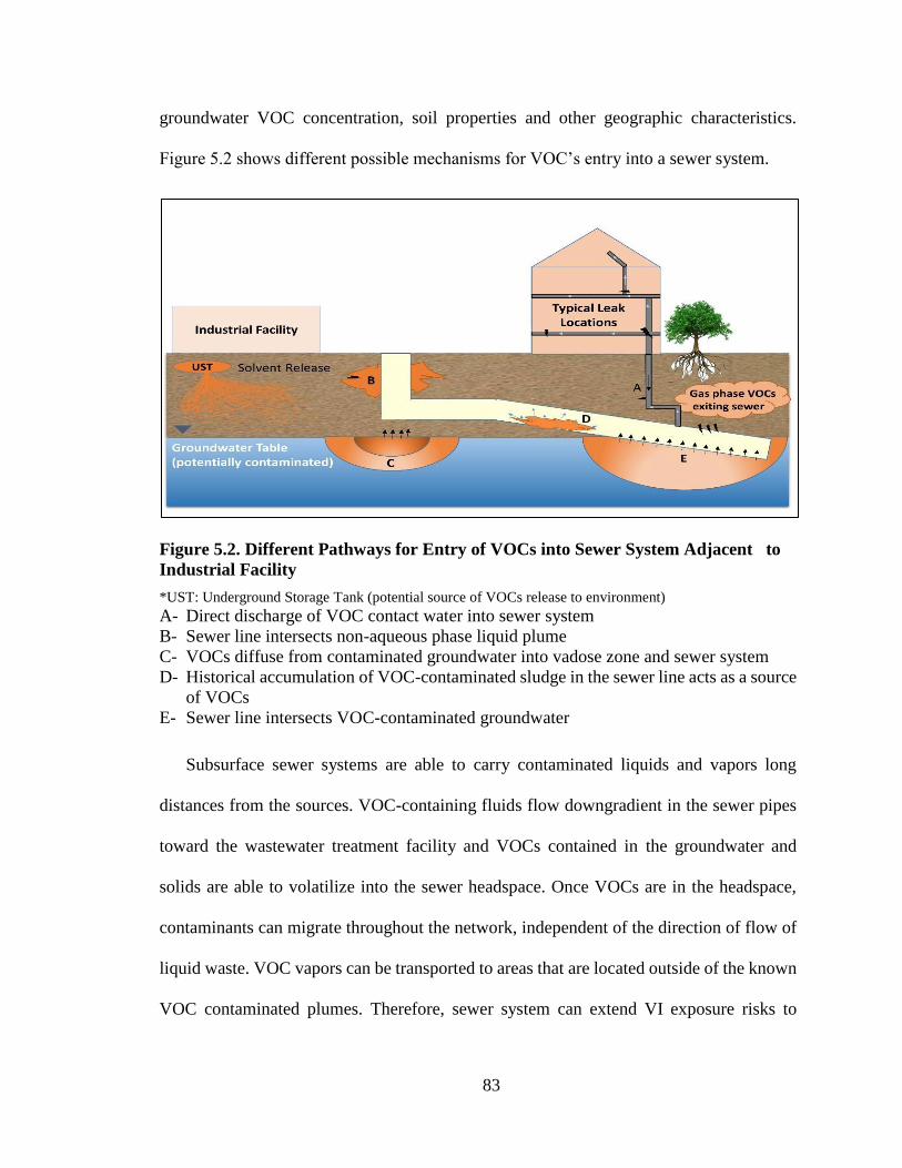
83
groundwater VOC concentration, soil properties and other geographic characteristics.
Figure 5.2 shows different possible mechanisms for VOC’s entry into a sewer system.
Figure 5.2. Different Pathways for Entry of VOCs into Sewer System Adjacent to
Industrial Facility
*UST: Underground Storage Tank (potential source of VOCs release to environment)
A- Direct discharge of VOC contact water into sewer system
B- Sewer line intersects non-aqueous phase liquid plume
C- VOCs diffuse from contaminated groundwater into vadose zone and sewer system
D- Historical accumulation of VOC-contaminated sludge in the sewer line acts as a source
of VOCs
E- Sewer line intersects VOC-contaminated groundwater
Subsurface sewer systems are able to carry contaminated liquids and vapors long
distances from the sources. VOC-containing fluids flow downgradient in the sewer pipes
toward the wastewater treatment facility and VOCs contained in the groundwater and
solids are able to volatilize into the sewer headspace. Once VOCs are in the headspace,
contaminants can migrate throughout the network, independent of the direction of flow of
liquid waste. VOC vapors can be transported to areas that are located outside of the known
VOC contaminated plumes. Therefore, sewer system can extend VI exposure risks to

84
communities which are far from a VOC contaminated source and always have been
considered “safe”.
A multitude of variables impact sewer air movement that will be discussed later. Gas-
phase VOCs are not exclusively gravity-driven and could exit the sewer system at any point
where the pipes or plumbing are not vapor tight. Sewer gas can be drawn into indoor air
through two different routes: 1. Flow through piping or conduits to the sub-foundation
region and subsequent migration to indoor air via foundation cracks and permeations. 2.
through direct connection of plumbing fixtures to indoor air. An intact vapor sealed plume
and foundation protect buildings from VI exposure.
Plumbing fixtures inside a building have an important role to protect indoor air form
VOC’s vapor intrusion when sewer system acts as a preferential pathway. Almost in all the
buildings with sewer system acts as the primarily route for VI, plumbing fixture inside the
building had failure. In a building with a perfectly installed and maintained plumbing
system, the sewer gas to indoor air pathway is not complete and sewer gas infiltration will
not occur. Nevertheless, development of any small failure in the plumbing or sewer system,
as mentioned above, could lead to VOC ingress into indoor air spaces. Generally, building
leak locations could include cracked waste stacks, dry p-traps, cracked vent stacks, loose
fittings, faulty wax ring seals, leaking joints, etc. (Jacobs et al., 2015). Figure 5.3
demonstrates sewer gas pathway into a building through the plumbing leakage.

85
Figure 5.3. VOC Vapors Pathways from Sewer System toward IA. (Source:
Reichman et al., 2017).
5.5. Historical review of sewer system acts as a vapor intrusion pathway
Several field studies have documented that piping conduits connected to buildings and
building foundations can served as alternative pathways for VOCs to enter indoor air
spaces at VI sites. Below is a summary of some key field studies.
Izzo et al., (1992) conducted a study in California’s Central Valley (US) and was one
of the first reports of a sewer system acting as a preferential pathway for VOC transport.
Several active dry cleaners were located on the area of study and PCE concentrations in
water wells were detected above hazardous levels. By measuring soil gas VOC levels using
glass tubes containing carbon adsorbents placed approximately 25-30 cm below ground
surface at various locations, they found elevated VOC concentrations proximal to sewer
lines. Nearly two decades later, Distler and Mazierski (2010) conducted a VI assessment
in Niagara Falls, New York (US), and found evidence of VOC migration through

86
subsurface utilities and sewer lines. Vroblesky et al. (2011) detected PCE and its
dechlorinating products in surface water and groundwater adjacent to a former dry-cleaning
facility at Parris Island, South Carolina. They concluded that a leaking sanitary sewer line
transports PCE from dry-cleaner into the groundwater. Contaminated groundwater then
migrated PCE into the storm sewer system through infiltration.
During a VI study in Skuldelev, Denmark, Riis et al. (2010) discovered higher than
expected VOC concentrations in indoor air at several houses adjacent to a former industrial
region and determined that the elevated indoor air concentrations were caused by sewer
gas intrusion. They conducted a tracer gas study to assess potential pathways for VOCs
and found elevated concentrations of PCE and its degradation byproducts,
trichloroethylene (TCE) and 1,2-dichloroethene, in the sewer line and plumbing fixtures.
The results clearly suggest that advective transport of contaminated soil gas and
groundwater into sewer pipes through fractures and shear failure offsets is the primary VI
pathway for the studied properties.
In a residential area in Boston, Massachusetts (US), Pennell et al. (2013) observed
higher PCE concentrations in indoor air on the first floor of a home than in the basement
indoor air of the same home. The property was adjacent to a former chemical handling
facility and this observation was coupled with the sewer-like odor reports by the
homeowner. Follow-up indoor air and sewer gas sampling demonstrated the sewer gas
from a faulty toilet connection was the primary source of PCE in indoor air. Similar
observations at other field sites were noted by McHugh et al (2011) and Gorder and
Dettenmaier (2011); however fewer details are available in the literature.

87
Guo et al. (2015) conducted a long-term VI continuous monitoring study at a property
near Hill Air Force Base (AFB) in Layton, Utah. This site overlies a groundwater plume
contaminated by 1,1-dichlorethylene (1,1-DCE), 1,1,1-trichloroethane (1,1,1-TCA), and
TCE. By applying the controlled-pressure-method testing (which includes whole house
pumping and indoor air sampling), soil gas sampling, and screening-level emission
calculations, the study concluded that subsurface pipe networks, including sewer mains
and land drains, may be significant alternative VI pathways. Importantly, this field study
included a preferential pathway that was an open pipe beneath the foundation. The open
pipe terminated under the building foundation and was connected to a sewer that contained
elevated levels of VOCs. The purpose of the pipe was presumed to be a foundation drain.
As part of the study, researchers installed a valve so that the land drain could be shut and
vapors could be prevented from being released (Guo et al., 2015).
McHugh et al. (2017) conducted a field study at the USEPA VI research duplex in
Indianapolis, Indiana. Results of VOC concentration measured by USEPA at this site were
not consistent with VI numerical model. The measured indoor air concentrations were
much higher than the calculated concentrations by multiplying the measured groundwater
concentrations to 0.001 attenuation factor. Also at this building during some sampling
events sub-slab soil gas PCE concentrations were recorded higher than soil-gas
concentrations in deeper area of the vadose zone. Elevated concentrations of chloroform
and PCE were also reported in a floor drain on the first floor of this duplex. Based on all
of these observations, a tracer study was conducted by McHugh et al. at this building. In
addition, vapors were collected from soil gas, sub slab, downstream and upstream
manholes, sewer lateral and some location inside the building. Sewer liquid and

88
groundwater VOC concentrations were also measured during the field sampling. The main
purpose of this study was to assess the role of combined sewer system in VOC vapor
intrusion in this property. Helium tracer study clearly verified vapor migration from the
sewer system into the building. Results also indicated the complexity of tracking the
leakage point. Leakage of VOCs was detected at the sewer lateral below the building’s
foundation. PCE concentrations above 100 (µg/m3) were detected in several manholes.
These manholes are located at the upstream of two former dry cleaning facilities. The sewer
system elevation in some manholes were shallower than groundwater average depth
suggesting groundwater/sewer infiltration potential. This study confirmed the significant
role of sewer system in migration of VOC from the subsurface source into the adjacent
building.
Wallace and Friedrich (2017) conducted a field study at a TCE contaminated site in
Indianapolis, IN. They incorporated sewer video inspections, sewer gas and sewer water
samplings, groundwater samplings, sub-slab and indoor air sampling data. While TCE was
not detected in groundwater in that area, elevated concentrations of TCE were reported in
sewer liquid and sewer gas. Sewer liquid TCE concentration were reported in the range of
180-220 (µg/L) and in the range of 14000-26000 (µg/m3) for sewer gas. The elevated
concentrations of TCE were also observed in sub-slab and indoor air. The sub-slabs TCE
concentrations were reported between 78-4000 (µg/m3) and indoor air TCE concentrations
in indoor air were reported in the range of 14-108 (µg/m3). The observed high
concentrations of TCE in sub-slab and indoor air combined with elevated TCE
concentrations inside the sewer system confirm the role of sewer system as a pathway for
TCE migration in this area.
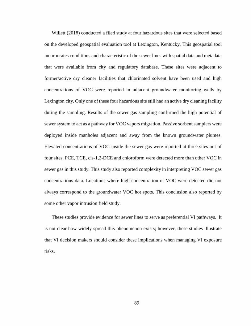
89
Willett (2018) conducted a filed study at four hazardous sites that were selected based
on the developed geospatial evaluation tool at Lexington, Kentucky. This geospatial tool
incorporates conditions and characteristic of the sewer lines with spatial data and metadata
that were available from city and regulatory database. These sites were adjacent to
former/active dry cleaner facilities that chlorinated solvent have been used and high
concentrations of VOC were reported in adjacent groundwater monitoring wells by
Lexington city. Only one of these four hazardous site still had an active dry cleaning facility
during the sampling. Results of the sewer gas sampling confirmed the high potential of
sewer system to act as a pathway for VOC vapors migration. Passive sorbent samplers were
deployed inside manholes adjacent and away from the known groundwater plumes.
Elevated concentrations of VOC inside the sewer gas were reported at three sites out of
four sites. PCE, TCE, cis-1,2-DCE and chloroform were detected more than other VOC in
sewer gas in this study. This study also reported complexity in interpreting VOC sewer gas
concentrations data. Locations where high concentration of VOC were detected did not
always correspond to the groundwater VOC hot spots. This conclusion also reported by
some other vapor intrusion field study.
These studies provide evidence for sewer lines to serve as preferential VI pathways. It
is not clear how widely spread this phenomenon exists; however, these studies illustrate
that VI decision makers should consider these implications when managing VI exposure
risks.

90
5.6. Emerging the Problem
As it is confirmed by several filed studies, deteriorated sewer systems are able to act as
unintended conveyance systems for subsurface contaminations. They also can be an
important source of VOC and affect indoor air quality through vapor intrusion.
There is no standard method for assessing the potential contribution of sewer pathways
in vapor intrusion sites. Also there is not enough information about the occurrence of VOC
contamination inside the sewer systems. In this study we tried to gain better understanding
regarding this issue. We conducted a field study and applied novel field techniques to
assess occurrence of VOC and their temporal and spatial variation inside a sewer system.
Different sampling methods have been used to characterize this pathway and the results are
compared in the manuscript. In the next chapter a numerical model also been used to
improve our insight regarding the field data.

91
CHAPTER 6. OCCURRENCE OF VOCS IN SEWER SYSTEMS
(Published article)
This chapter includes an article that is published in the Science of the Total
Environment journal (Roghani et al, 2018). The text included here is the pre-print.
“Occurrence of chlorinated volatile organic compounds (VOCs) in a sanitary sewer
system: Implications for assessing vapor intrusion alternative pathways.”
doi.org/10.1016/j.scitotenv.2017.10.205
6.1 Abstract:
Sewer systems have been recently recognized as potentially important exposure
pathways to consider during vapor intrusion assessments; however, this pathway has not
been well-characterized and there is need for additional information about the occurrence
of volatile organic compounds (VOCs) in sewer systems. This paper reports the results of
sewer gas sampling conducted in a sanitary sewer over the years of 2014-2017. Sewer gas
samples were collected and analyzed using several different techniques, including TO-15
(grab), TO-17 (passive), Radiello® (passive) and a novel continuous monitoring technique,
the Autonomous Rugged Optical Multigas Analyzer (AROMA). The applicability of each
of the different approaches used in this study is discussed in the context of investigating
sanitary sewers as a vapor intrusion alternative pathway. The data confirmed that
trichloroethylene (TCE) concentrations in sewer gas were detected adjacent to and
extending hundreds of feet away from a previously defined vapor intrusion area, where
TCE was a primary contaminant. TCE concentrations detected in sewer gas ranged from
non-detect to 1600 µg/m3. Temporal variability was observed in TCE concentrations over

92
timescales that ranged from minutes to months to years at discrete sampling locations.
Spatial variability in sewer gas concentrations was also observed throughout the study area.
Temporal and spatial variability may be caused by groundwater contamination sources in
the study area, as well as sewer gas transport mechanisms.
6.2. Introduction
Commonly, vapor intrusion (VI) has been conceptualized as the entry of volatile
organic compound (VOC) vapors into overlying buildings through cracks in foundations
and basements; however, alternative entry pathways, such as piping systems connected to
sewers, are being increasingly identified as important pathways for VI (e.g. Riis et al.,
2010; Pennell et al., 2013; Guo et al., 2015; EPA, 2015a; Jacobs et al., 2015; McHugh et
al., 2017). VOC transfer into sewer systems can be either intermittent or continuous. VOCs
present in soil vapors or groundwater can infiltrate sewer systems through cracks and other
openings. In addition, VOCs can be discharged directly to sewers from a variety of sources,
such as groundwater remediation system effluents and other legal (or even illegal)
discharge sources.
Once VOCs have entered sanitary sewer systems, there are many pathways by which
they can unintentionally enter back into the environment. VOCs in sewers can exit through
cracks in sewer pipes and contaminate subsurface soil and groundwater. VOCs can also be
transported through sanitary sewer systems and vapors can migrate through indoor
plumbing systems that are not properly maintained and sealed, as documented by Riis et
al. (2010), Pennell et al. (2013) and McHugh et al. (2017).
Theoretically, in buildings with perfectly installed and maintained plumbing systems,
the sewer gas to indoor air pathway would not be complete. Nevertheless, imperfections in
93
plumbing systems could lead to VOC entry into indoor air spaces. Ultimately, exposure
risks from this pathway would depend on many factors—importantly, building air
exchange rates and the rate of sewer gas entry into indoor air spaces. Understanding
inhalation exposure risks due to VOC vapors entering indoor air spaces through sanitary
and other plumbing systems at VI sites is a growing interest (EPA 2015a). Beyond the
United States, Denmark has identified sewer systems as important alternative VI exposure
pathways at > 20% of contaminated drycleaner sites in the Central Denmark Region
(Nielsen and Hvidberg, 2017).
VI alternative pathways are important to the national issue of aging infrastructure. In
2017, the American Society of Civil Engineers (ASCE) issued an infrastructure report card
for the United States (US), assigning a D+ grade for wastewater in part due to many of the
challenges aging sewer lines pose for modern cities (ASCE, 2017). Over 800,000 miles of
sewer mains exist in the US, with an additional 500,000 miles of sewer laterals (i.e. pipes
that connect buildings to the mains). The sanitary sewer pipe system investigated in this
research study serves a neighborhood in the South San Francisco Bay area and is an
example of the aging infrastructure issue. The sanitary sewer system is constructed of
vitrified clay pipe (VCP), which is known to crack and leak over time, and was installed in
the 1950s (with upgrades in the 1960s). The sewer system historically received
concentrated hazardous chemicals discharged as part of the semiconductor and electronics
manufacturing industry.
Extensive groundwater contamination exists near the study area, including a large TCE
groundwater plume (>5 g/L) (EPA, 1989; EPA, 2010). A portion (see pink shading) of
the 1.5-mile (north-south) chlorinated solvent groundwater plume is shown on Figure 6.1a.

94
In the mid-2000s, subsurface contamination was discovered outside the well-delineated
TCE groundwater plume; and, the historic release of TCE to the sewer system was
identified as by EPA as the source of TCE “hot spots” throughout the neighborhood to the
west (CPEO, 2013; CPEO, 2014; EPA 2015c; Bureau Veritas, 2013; Cornerstone Earth
Group, 2017). As shown on Figure 6.1a, the Environmental Protection Agency's (EPA) VI
study area was expanded beyond the extent of the TCE groundwater plume to include the
portion of the neighborhood where TCE “hot spots” had been identified (EPA, 2015c).
This research study included sampling in the residential area within the expanded VI study
area (see blue shading).
a) Sanitary sewer system and manhole locations.
Note: Pink shading shows EPA’s 2012 VI study area and blue shading shows expanded VI
study area (EPA, 2015c).
Not all manholes are shown, and sewer liquid flow directions are approximate.
Background image source: Google Maps
95
Street A (east of MH-6)
Street B
b) Groundwater table elevations relative to sewer pipes along Streets A and B.
Note: There is limited information to assess the groundwater elevations (relative to sewer
elevations) west of MH-6 along Street A; however, as the sewer along Street A extends to
the west and connects at MH-12, the sewer becomes deeper and approaches the
groundwater table.
Figure 6.1. Research study area and conceptual model.
Figure 6.1a and b provide a preliminary site conceptual model for TCE contaminated
groundwater infiltrating into the sewer system. Figure 6.1b shows, conceptually, a range
of historic groundwater fluctuations relative to the sewers along Street A and Street B.
While VOC vapors in soil gas can potentially enter the sewer through diffusive and/or
convective transport, groundwater entry is assumed to be a more significant source of
VOCs in the sewer system. Once groundwater enters the sewer system, VOC vapors can
be transported by convective and diffusive processes within the sewer system. Sewer gas
can leave through sewer ventilation processes, which act to dilute the VOC concentrations
in the sewer gas. As shown on Figure 6.1b, Street B has more potential for groundwater
infiltration than Street A based on groundwater and sewer main elevations; however, it is

96
important to note that the groundwater near MH-12, MH-13, MH-14, and MH-15 also
likely intersects the sewer system, which has important implications for this site.
Through the Freedom of Information Act (FOIA), EPA recently made sewer videos
publicly available. These videos indicate multiple cracks exist throughout the sewer system
and infiltration/exfiltration is possible into/from the sewer system (FOIA, 2017).
Importantly, cracks exist west of MH-21 within the TCE plume, as shown on Figure 6.1a.
These cracks allow contamination to leak into and out of the sewer system. Videos also
confirm groundwater infiltration east and west of MH-15 near an identified TCE
groundwater “hot spot.” Cracks were also observed in other locations throughout the sewer
system, but for simplification purposes are not explicitly shown on Figure 6.1a.
This research study developed the preliminary conceptual model shown in Figure 6.1a
and b to evaluate VOC concentrations in the sanitary sewer system that were collected
using different methods for sewer gas sampling (e.g. passive, grab and continuous). In
addition, this study specifically addresses the lack of information about how often
alternative VI pathways exist, and provides one of the few attempts to document the
occurrence and variability of VOCs in sanitary sewer gas. The data herein also provides
critical information about temporal and spatial variability of sewer gas concentrations. This
information is needed to ultimately inform about developing appropriate sampling
strategies, which are still emerging.
6.3. Methods and materials
6.3.1. Field sampling manholes and cleanouts
A total of nineteen (19) manholes and twenty (20) cleanouts were sampled as part of
this study. Cleanouts were located along sewer laterals and manholes were located in the

97
street along sewer mains (Figure 6.2). Passive, grab and continuous sampling methods were
utilized at both cleanouts and manholes. Manhole covers were left in place throughout all
sampling activities. The vent holes in the manhole covers (approximately 1 inch diameter)
served as access points for sampling and data collection.
Figure 6.2. General Layout of Cleanout and Manhole Locations.
In general, passive and grab samples were collected at shallow depths (point A) in the
manhole (Figure 6.3) for this research study (2014 -2017). In 2016 and 2017, additional
depths at MH-15, MH-17 and MH-18 were investigated (points B and C) and passive
samplers were nested, as shown. Most of the continuous monitoring data (AROMA
sensor) were collected at the deep location (point C). Exact depths and details are given
in the Results and Discussion section.

98
Figure 6.3. General sampling depths inside manholes.
Note: A: TO-15/TO-17 (2014, 2015, 2016 and 2017), B: Select TO-17 samples @ MH-
18 (2016) and Radiello® samples (2016 and 2017), C: AROMA data, except when noted
(2016 and 2017).
Several different sampling approaches were required for cleanouts due to variability in
size and pipe condition. Cleanout covers were inconsistent and, in some cases, non-
existent. For grab sampling, it was difficult to obtain an airtight seal for some of the
cleanouts. Therefore, in select cases the data may be subject to negative bias due to
atmospheric dilution. For passive sampling, most cleanout covers were replaced with
expandable well caps and passive sampler tubes were connected to the well caps with
approximately 6 in. of wire during the sampling event. The expandable well caps provided
an airtight seal on these cleanouts. In other cases, when expandable well caps could not be
tightly fitted to the cleanout pipe, openings in cleanout pipes were covered; however,
airtight seals on non-round pipes were not possible.

99
6.3.2. Passive sampling
Passive sewer gas sampling methods utilize adsorbent samplers to capture organic
compounds from air without forcing the flow rate of gas. Two types of passive samplers
were utilized in this study: stainless steel tubes packed with Carbopack X (TO-17) analyzed
by Beacon Environmental Services, Inc. (Beacon); and Radiello® samplers, analyzed by
EPA Region 9 Lab.
Carbopack X (TO-17)
Thermally-conditioned, stainless steel tubes packed with Carbopack X adsorbent
material, provided by Beacon, were suspended in the targeted manholes and cleanouts
using wire. Following sewer air exposure, these adsorbent tubes were sealed and returned
to Beacon's lab for analysis by Method TO-17. Thermal desorption-gas
chromatography/mass spectrometry (TD-GC/MS) instrumentation targeted a custom set of
chlorinated compounds. ISO 16017-2 procedure was used to convert the adsorbed mass on
each sampler to a gas concentration.
These passive samplers (TO-17) were deployed for different durations. During the
2015 sampling event, they were installed at all sampling locations for a period of seven
days. During the 2016 event, passive samplers were installed in MH-17 and MH-18 for 12
h and 24 h. Sample depths ranged from 1 to 3 ft below the manhole lid for most sampling
locations, except when explicitly noted in the text. Background samples of atmospheric air
were also collected during each event at various locations throughout the study area.
Analyzed results of the atmospheric air samples were below detection limits for all events.

100
Radiello® samplers
Radiello® 130 samplers, which contain stainless steel net cylinders packed with
activated charcoal, were deployed in MH-15 and MH-17 using wire during the 2016 and
2017 sampling events for several days. EPA Region 9 Laboratory in Richmond, California
conducted analyses of selected VOCs by GC/MS. Analyses were compliant with the
laboratory's standard operating procedures that define requirements for calibration and
acceptable results for QC parameters.
6.3.3 Grab samples (TO-15)
Sewer air grab samples were collected inside selected manholes and cleanouts for a
sampling time <5 min. Manhole samples were collected at a depth of approximately 3 ft
below the manhole lid. Sample depths from cleanouts varied depending on cleanout
geometry. Samples were collected using 1/4" o.d. Teflon tubing. Sample collection by
evacuated stainless steel canisters (1 L and 400 mL) was controlled by flow restrictors.
Before field sampling, canisters were certified “clean” and flow controllers were verified
by the laboratory.
Samples were analyzed by different labs for each of the distinct sampling events.
Samples from the January and July 2014 and the 2015 -2017 events were analyzed using
Method TO-15 by EPA Region 9 Laboratory in Richmond, California. Samples from the
February and March 2014 events were analyzed using Method TO-15 by Eurofins Air
Toxics, Folsom, California. Prior to sampling, all canisters were certified “clean” and flow
controllers were verified by the laboratory. All data from canisters are from canisters with
acceptable vacuums upon receipt at the laboratory. Analyses were compliant with each
101
laboratory's standard operating procedures that define requirements for calibration and
acceptable results for QC parameters.
6.3.4. AROMA continuous gas monitor
To assess temporal variability, sewer gas samples were collected at MH-17 and MH-
18 by AROMA. AROMA is a direct sampling vapor analyzer that determines analyte
concentrations through a combination of Cavity Ring-Down Spectroscopy and a surface
interaction-based chemical separation. Sewer vapor samples were automatically drawn into
the instrument using onboard mass flow control. Sampling protocol was based on recently
established sewer sampling methodology (McHugh et al., 2017). Sample inlet tubing
consisted of 12 ft of 3 mm Nylaflow® tubing extended with 10 ft of 1/8" PTFE tubing with
a total sample train volume of approximately 15 cm3. For each measurement, a purge
volume of 100 cm3 (at standard conditions for temperature and pressure (STP), defined as
0° C and 1 atm) was extracted prior to sampling. A sample volume of 200 cm3 (STP) was
drawn into the instrument over a 1-min sampling time for analysis. For all measurements
(excepting vertical profile measurements) the sample inlet was maintained at
approximately 1 ft above the floor of the manhole shaft. Sample analysis was performed
immediately after sampling and results were automatically logged. Analyses were
completed using Entanglement Technologies' standard operating procedures, and daily
calibration check values (CCVs) were recorded. Total sampling plus analysis time was
approximately 15 min. In the 200 cm3 (STP) sample configuration, the TCE limit of
detection of the AROMA instrument was 1.5 µg/m3.

102
6.3.5. Sewer liquid analysis
Sewer liquid was collected from MH-17 and MH-18 during the 2016 sampling event
(September 28, 2016). The depth to sewer liquid from ground surface was measured
immediately prior to sampling. All measurements were collected through the manhole
vents, so the manhole covers could be left in place during all sampling activities. The height
of the sewer liquid (above the bottom of sewer pipe) fluctuated between 0.65 ft (measured
at 8:44 am) and 0.38 ft (measured at 10:36 pm). Sewer liquid samples were collected with
disposable bailers through sewer vent holes. Samples were transferred to 40 mL Volatile
Organic Analysis (VOA) vials and delivered on ice to EPA Region 9 Laboratory,
Richmond, California for analysis of select VOCs (TCE, PCE, chloroform, cis-1,2-
dichloroethylene) using EPA Method 524.2. VOA vials were pre-conditioned to maintain
a pH below 2 (pursuant to EPA, 1995).
6.3.6. Other site sampling
A photoionization detector (PID) (MiniRAE 3000) was used as a portable VOC
monitor to screen locations with high total VOC concentrations. This PID has a detection
range between 0.1 and 15,000 ppm and detects VOCs within 3 s. A Trimble GeoExplorer®
3000 series was used to record GPS information of all sampled manholes and cleanouts.
6.4. Results and discussion
Sewer gas samples were collected from the sanitary sewer located to the west of a well-
defined TCE groundwater plume and the 2012 VI Study Area shown on Figure 6.1a. This
section summarizes the results from 2014 sampling efforts (TO-15) that show temporal
variation on a monthly (and biweekly) basis. Follow-up sampling in 2015 compared TO-
17 passive sampling with TO-15 grab sampling. These results, which are consistent with

103
the data from 2014, confirm spatial variability in sewer gas concentrations (particularly
TCE) throughout the sewer system, regardless of sampling method (grab vs. passive).
Continuous monitoring using the AROMA sensor, combined with passive sampling,
showed that temporal variation occurs even over the short-term (on the scale of hours).
Section below summarizes the sampling results from the entire study (2014 -2017) for MH-
15, MH-17 and MH-18. The results highlight temporal variability and considerations for
sampling depth.
2014 manhole sampling using TO-15 (grab) method
In 2014, sampling was conducted periodically from January through July. Figure 6.4a
and b show spatial variability in TCE sewer gas concentrations detected in manholes
located throughout the research study area along Street A and Street B, respectively. Sewer
flow direction along the area is also shown in Figure 6.4a and b.
As shown on Figure 6.4a, the highest TCE concentration in sewer gas along Street A
was detected in MH-13 during 2014 sampling. This manhole is located downstream of a
bend in the sewer system as Street A ends. Sewer liquid flows from MH-13 south into MH-
14, while sewer liquid from MH-16 flows to the north into MH-14. During the February
2014 event, the TCE concentration was higher in MH-14 than in MH-13 or MH-16. While
TCE sewer gas concentrations in MH-14 is a combination of streams from MH-13 and
MH-16, which would not explain the higher concentration detected at MH-14, turbulent
mixing at the “T” toward MH-15 may have also increased liquid-gas mass transfer in this
manhole and influenced the sewer gas TCE concentrations. The lowest concentration was
detected in MH-6, where the sewer was likely located above the groundwater table, as
discussed previously.

104
Figure 6.4b shows manholes located along Street B. Relatively high concentrations of
TCE (≥1000 g/m3) were detected in sewer gas at MH-1, MH-2, MH-17, MH-18 and MH-
19. Lower concentrations were observed in MH-3 and MH-4. These manholes are located
at the intersection of a sewer pipe with flow coming from the south, which may dilute
sewer liquid concentration (and therefore sewer gas concentrations) in this local area;
however, the intersection of sewer flow can also result in turbulence. Absent of other
factors, this turbulence could have locally increased sewer gas concentrations in this area.
Results from 2015 (Figure 6.5a and b) indicate the TCE concentration at MH-3 was higher
relative to the other manholes. It is likely that both dilution from incoming sewer streams
and liquid-gas mass transfer due to turbulence are complicating factors when interpreting
sewer gas concentration data.
The highest TCE concentration was detected in MH-17 (1600 g/m3) during the March
2014 event; however, four months later in July 2014, the TCE concentration had decreased
three orders of magnitude to 9 g/m3. The reason for this drastic decrease in TCE sewer
gas concentration at MH-17 is not known; however, as discussed below, additional
evaluation was conducted during 2016 and 2017 and temporal variation was observed
during those sampling events as well. The concentration detected during the March 2014
event (1600 g/m3) was the highest TCE sewer gas concentration detected at the site during
this entire study (2014 -2017).

105
a) Street A manholes plus MH-13, MH-14 and MH-16.
b) Street B manholes.
Figure 6.4. Sewer gas TCE concentrations measured in 2014 by TO-15 (grab).

106
Note: If no result is shown, sample was not collected at that location for that date. Arrows
indicate sewer liquid flow.
There are many possible explanations for the observed temporal and spatial variability
shown in Figure 6.4a and b. For instance, manholes were sampled during different times
of the day and sanitary sewers are well-known to have diurnal sewer usage patterns.
However, sampling times typically ranged from late morning until early afternoon (see
Table B.1 in appendix). Other possible explanations may include: fluctuations in the rates
of groundwater infiltration/exfiltration into/from the sewer in areas where the sewer system
was cracked or deteriorated; variability in sewer gas ventilation rates and direction of sewer
gas flow through manholes; variations in legal (or illegal) direct discharges to the sewer;
variations in total sewer liquid flow; etc.
2015 manhole sampling using TO-15 (grab) and TO-17 (passive, 1-week) methods
In 2015, additional sampling was conducted to investigate passive sampling by TO-17,
given the temporal and spatial variability of TCE sewer gas concentrations detected in
2014. For comparison purposes, samples were collected by both TO-17 (passive, 1 week)
and TO-15 (grab) methods. In addition to collecting sewer gas samples from manholes,
sewer gas samples were also collected from cleanouts. Manholes provide information
about the sewer gas concentrations in the sewer mains, while cleanouts provide information
about the sewer gas concentrations closer to the building plumbing connections (see Figure
6.2)—which may be useful when assessing potential exposure risks. Tracer studies capable
of determining the fraction of sewer gas that enters each home would be useful in
conjunction with cleanout sampling data (and indoor air sampling data) (e.g. Riis et al.,
2010); however, home access would be necessary and was not feasible during this study.

107
Figure 6.5a and b illustrate spatial variation of TCE concentrations detected in sewer
gas for the 2015 sampling event by TO-15 and TO-17 sampling methods, respectively. The
concentrations detected during this sampling event were an order of magnitude lower (in
general) than detected in 2014. The exact reasons for lower concentrations are not known;
however, these lower concentrations were confirmed by two different sampling/analytical
methods (TO-15 and TO-17) and, when combined with the rest of the data in this research
study, they highlight the temporal nature of VOC sewer gas concentrations.
Along Street B, a sewer gas TCE concentration gradient originating from the 2012 VI
Study Area (pink shaded region on Figure 6.5a and b) and dissipating to the west is present;
however, this trend is not necessarily expected to be always present—especially in
recognition of the 2014 data shown in Figure 6.4b. Along Street A, where tributaries
complicate the sewer flow, sewer gas concentration gradients do not emerge. Collectively,
Figure 6.5a and b illustrate that relatively wide variations in TCE concentrations in sewer
gas can exist laterally hundreds of feet from a well-established groundwater plume.
Several TCE “hot spots” are being investigated as part of ongoing regulatory activities
due to historical discharge of TCE to the sewer system and because the sewer system pipes
are suspected to have leaked. A TCE “hot spot” near MH-15 (see Figure 6.1a) has been
identified by others as part of ongoing site investigation activities in the area. Elevated TCE
soil gas concentrations near MH-12, MH-13, MH-14 and MH-15 have been detected, with
concentrations as high as 1.6 million g/m3 near MH-14 and MH-15 (Bureau Veritas,
2013; Cornerstone Earth Group, 2017) and TCE groundwater concentrations have been
detected up to 110,000 g/L (FOIA, 2017). The results of these site investigations confirm
TCE in groundwater, which is an important part of the site conceptual model, Figure 6.1a.

108
a) TO-15 (grab).
b) TO-17 (week-long passive).
Figure 6.5. Sewer gas TCE concentrations measured in 2015.
Note: Sewer lateral locations were approximated. The connection for CO-2 could not be
confirmed. Sewer flow directions were estimated. Not all manholes and cleanouts are
included.
Comparing the sampling methods, TO-15 grab samples (Figure 6.5a) did not detect as
high of TCE sewer gas concentrations as the TO-17 (week-long passive) samples (with the
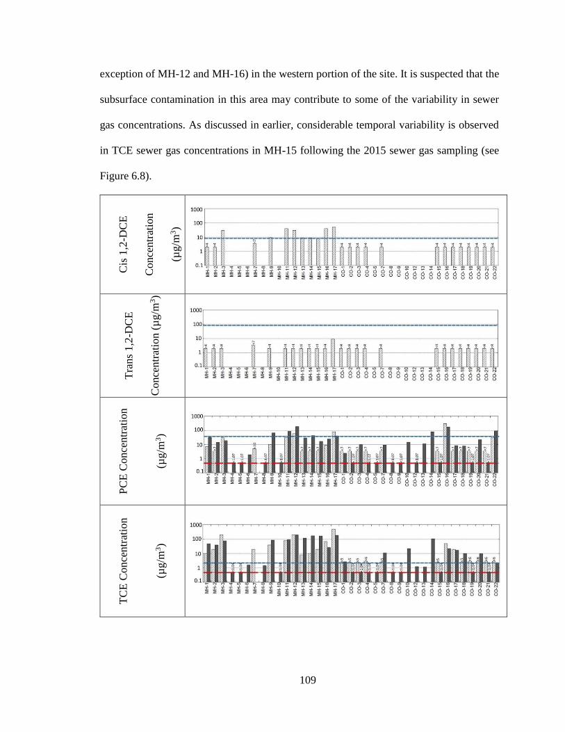
109
exception of MH-12 and MH-16) in the western portion of the site. It is suspected that the
subsurface contamination in this area may contribute to some of the variability in sewer
gas concentrations. As discussed in earlier, considerable temporal variability is observed
in TCE sewer gas concentrations in MH-15 following the 2015 sewer gas sampling (see
Figure 6.8).
Cis
1,2
-DC
E
Conce
ntr
atio
n
(µg/m
3)
Tra
ns
1,2
-DC
E
Conce
ntr
atio
n (
µg/m
3)
PC
E C
once
ntr
atio
n
(µg/m
3)
TC
E C
once
ntr
atio
n
(µg/m
3)

110
Figure 6.6. Sewer Gas Concentrations Detected in Manholes and Cleanouts (2015).
Note: Residential cancer and non-cancer inhalation exposure screening levels are based
on California’s indoor air screening level (EPA, 2016; DTSC, 2016). If a sample was not
collected, a blank is shown. For concentrations that did not exceed the laboratory level of
detection, the value is shown as one-half of the detection value and
“< Detection limit” is inserted above the sample.
Figure 6.6 compares the measured sewer gas concentrations of several additional
chemicals with California's cancer and non-cancer inhalation residential exposure
screening levels for each chemical. A summary of all chemicals analyzed and detected in
the sewer gas are provided in Tables B.2 and B.3 in appendix. PCE and TCE are the
chemicals that were most often detected at concentrations above California's indoor air
residential exposure screening levels. TCE was the VOC most frequently detected above
California's residential exposure air screening levels in the manholes and cleanouts in this
study area.
Although residential exposure air screening levels do not directly relate to sewer gas
concentrations, it is worth noting that TCE in sewer gas in many manholes and a few
cleanouts was detected at concentrations 1_2 orders of magnitude greater than the indoor
air screening levels. While building plumbing systems are designed to prevent sewer gas
entry, plumbing systems are well-known to fail and sewer gas odors are a common example
of these failures. However, the fraction of sewer gas that would enter a home as a result of
a faulty plumbing connection and cause elevated indoor concentrations of a given VOC is
not precisely known. Recent research by McHugh et al. (2017) showed that dilution of

111
sewer gas into indoor spaces varies from approximately 50 × to 500 × during their study at
the EPA VI Research Duplex.
Generally speaking, the concentrations detected in the manholes were greater than the
concentrations detected in the cleanouts. Caution should be exercised when drawing linear
relationships (i.e. attenuation factors) between manholes and cleanouts. Wastewater usage
is likely subject to many variables and may be responsible for variable sewer gas
concentrations. Additional research is needed to fully understand the variability of TCE
concentrations in sewer gas inside manholes and cleanouts.
For instance, the TO-17 passive sampling results (Figure 6.5b) shows that MH-9 had a
TCE concentration of 85 g/m3 and cleanouts, CO-12 and CO-13, on either side of MH-9
had concentrations of 1.26 and 1.14 g/m3, respectively. To the west of CO-13, CO-14 had
a concentration of 107 g/m3, which is two orders of magnitude higher than CO-13. The
nearest manhole to CO-14 is MH-11, which had a TCE concentration of 91.58 g/m3. The
TCE concentration detected at CO-14 was unexpectedly high based on nearby manholes
and other cleanouts. In addition, as shown on Figure 6.6, this cleanout contained the highest
TCE concentration of all the cleanouts sampled. Follow-up sampling was conducted in
2016 using a Radiello® sampler and the concentration had decreased to <9 g/m3.
Chloroform was occasionally detected in the sampling locations throughout the
research study area (see Tables B.2 and B.3 in appendix). This chemical is a byproduct of
chlorination and organics in wastewater, and therefore does not directly relate to the issue
of VI. However, it is interesting to note that the maximum concentration of chloroform
reported by TO-17 is 8.95 µg/m3, while the highest concentration reported by TO-15 is 300

112
µg/m3. Several locations reported TO-15 chloroform concentrations >100 µg/m3.
Considering that TO-15 samples were collected in the middle of the day during times of
potentially high water use, these results suggest that elevated concentrations of chloroform
in the sewer system may be associated with household appliances and laundry bleach,
which Shepherd et al. (1996) reported is an important source of chloroform in wastewater
systems.
Comparison of TO-15 and TO-17 methods for 2015
Figure 6.5a and b highlight that several manholes consistently contain “high” TCE
concentrations and “low” TCE concentrations (relative to other manholes) across the study
area, regardless of sampling/analysis approaches. For instance, the TCE concentrations
detected in MH-17 were among the highest detected by both TO-15 and TO-17. Similar
results were obtained at MH-3 and MH-12. In addition, there are several cleanout locations
such as CO-2 and CO-4 where undetected or “low” concentrations of TCE were reported
by TO-15 and TO-17, as compared to other sampling locations.
However, compatibility between results of TO-15 and TO-17 was not observed at all
sampling locations. For instance, comparing TO-15 and TO-17 data at MH-15 and MH-13
suggests inconsistency between the results. Coupled with the 2014 data (Figure 6.4a and
b), grab and passive sample results are not anticipated to necessarily correspond well due
to temporal variability. Sampling periods for grab and passive samplers were <5 min and
1 week, respectively. The challenge is to determine how to assess this pathway with regard
to potential variations and select the sampling method capable of providing the greatest
insight about this pathway. Given the low concentrations detected during the 2015 event,
as compared to concentrations detected during 2014, 2016 and 2017 (see Figures 6.8 and

113
6.9), it is assumed that a single 1-week passive sampling period is insufficient to
characterize sewer gas exposure risks. Multiple sampling events would likely be required,
but more research is need to determine how many sampling events are necessary.
There were several locations where PCE and/or TCE was reported below detection
limits by TO-15, but above the detection limits for TO-17. These data points are
particularly important because the TO-15 method did not identify the presence of TCE
and/or PCE in sewer gas, even though a longer sampling duration (TO-17) was able to
identify the presence of the chemical. Other locations, where PCE and/or TCE were not
detected by either method, suggest that both methods were equally able to corroborate the
absence of the compound in sewer gas. Generally speaking, considering the significant
temporal fluctuations observed in sewer gas concentrations (e.g. Figures 6.4a and b and
6.6), these data suggest that TO-15 and TO-17 should not be expected to detect the same
concentration at all locations at all times.
TO-15 grab samples may not detect sewer gas concentrations as frequently as TO-17
(longer duration) samples. TO-15 (grab sampling) and TO-17 (longer duration passive
sampling) report chemical concentrations over different ranges of time. Short-term
fluctuations in chemical concentrations are integrated over the longer TO-17 sample,
whereas peaks and valleys in concentrations may or may not be captured during a TO-15
grab sewer gas sample. In some locations, such as cleanouts, TO-15 grab samples may not
have resulted in detectable chemical concentrations because of difficulty creating an
adequate seal over the short sampling duration. In these cases, passive samplers that can
be sealed in place for several days may be advantageous.

114
There are some considerations for deploying passive samplers for several days. Air
velocity and humidity may affect the uptake rate of passive samplers and result in biased
concentrations. High humidity is an inescapable issue inside a sewer system. Hydrophobic
and nonporous samplers are advantageous for application in high humidity and high
velocity environments and were therefore used for TO-17 sampling during both 2015 and
2016 field studies (EPA, 2015d). The TO-17 samplers used in this research were packed
with Carbopack X, which has been shown to be compatible for high humidity applications
when the sampling tube is the same temperature as the air being sampled (Brown et al.,
2015), such as the sampling application used here where samplers were deployed in sewer
manholes and cleanouts for several days.
Passive sampling does not provide any information about temporal variation in VOC
concentrations. To gain better insight into time-based fluctuations, continuous monitoring
could be the best current option. Continuous monitoring (e.g. AROMA) was used in this
study to record fluctuations in sewer concentrations over short time periods. While
continuous monitoring provides benefits such as lower costs, quicker sampling rates, and
on-site measurement capabilities, the instrumentation (e.g. gas chromatography analyzers)
normally requires highly trained field personnel, frequent calibration, conditioning steps,
and maintenance for quality assurance (Holton, 2016).
Field sampling (2016) using TO-17 and AROMA sensor sampling methods
To assess short-term (e.g. hourly) temporal variations of sewer gas TCE concentrations,
MH-17 and MH-18 were investigated under fairly controlled conditions using passive (TO-
17) and continuous (AROMA) sampling techniques. These manholes are located along
Street B and are fairly close to the TCE groundwater plume. As shown on Figure 6.1, MH-

115
18 is located within the TCE groundwater plume (and 2012 VI Study Area), while MH-17
is located outside the plume area.
Sewer gas concentrations at MH-17 and MH-18 were measured by TO-17 for three
time intervals: day time, night time, and entire day. Day time and night time samples had
a residence time of approximately 12 h, while “entire day” samples had a residence time
of about 24 h. Using the passive sample results, a calculated time-weighted average was
determined. The entire-day average concentration and the measured entire-day
concentration agree relatively well (Figure 6.7a and b). For both manholes, day time and
night time samples were collected at 1.5 ft below ground surface (bgs), and entire day
samples were collected at 3 ft bgs. The AROMA sensor intake was suspended at 16 ft bgs
in MH-17 and MH-18, to collect and analyze a series of samples collected periodically
over several hours (Figure 6.7a and b). A discussion of sample depth and implications for
sewer gas concentration measurements is included in this section.
AROMA results suggest relatively high temporal variability of sewer gas TCE
concentrations in both manholes. Higher TCE concentrations were observed during noon
and afternoon sampling events compared to early morning. For MH-17, TCE
concentrations fluctuated between 138 µg/m3 and 684 µg/m3, with an average of 394
µg/m3. For MH-18, TCE concentrations fluctuated between 165 µg/m3 and 624 µg/m3,
with an average of 462 µg/m3. In addition, some significant variations occurred over short
timescales; for example, the TCE vapor concentration more than doubled in the 15 min
between AROMA samples at MH-17 during the noon sampling event. Overall, MH-17
(located outside of the 2012 VI Study Area) appeared to exhibit greater temporal variation
than MH-18 (located inside the 2012 VI Study Area). Sewer videos indicate cracks

116
upstream of both manholes (FOIA, 2017); however, it is not known whether infiltration
was occurring during the time of this field study.
For the TO-17 results, TCE concentrations were higher in the day time than night time
in both manholes. The night time TCE concentration was approximately 60% of the day
time concentration for both manholes. The entire day sample for MH-17 was
approximately 90% of the day time sample, whereas the entire day sample for MH-18 was
approximately 80% of the day time sample. The TCE concentrations detected by AROMA
and TO-17 highlight that even on a short-term (hourly to daily) basis, MH-17 and MH-18
exhibit variations in TCE sewer gas concentrations.

117
Figure 6.7 Sewer gas TCE concentrations measured by TO-17 and AROMA in 2016.
TCE concentrations in sewer liquid also exhibited temporal variations, as shown on
Figure 6.7a and b and summarized in Table 6.1. During the 2016 sampling event, sewer
liquid samples were collected periodically during the 24 h sampling period in MH-17 and
MH-18. For comparison purposes, 2014 sewer liquid data is shown in Table 6.1 for
manholes MH-20 and 21. Although MH-20 and MH-21 were not sampled as part of this
research study, they are located to the east of MH-17 and MH-18, within the 2012 VI Study

118
Area. Sewer videos indicate groundwater infiltration into the sewer may be occurring near
those locations (FOIA, 2017). The sewer liquid data for these manholes (in 2014) show
that fluctuations in concentrations varied based on sampling date and time (see Table 6.1).
As shown on Figure 6.1a, these manholes are important in terms of the conceptual model
for the site.
Table 6.1. Sewer liquid results for TCE
a Data below limit of quantification (LOQ) but above limit of detection (LOD) (City of
Palo Alto, 2014).
b Results for manhole are the 24-hour sampling average. Numbers in parentheses represent
the variation of TCE detected over the 24-hour period.
Manhole Sampling Date
Results
(µg/L)
MH-17
3/27/2014, 2 pm 1.80a
3/28/2014, 6 am 7.59
9/28-29/2016 1.64 (1.2 -2.1)b
MH-18 9/28/2016 1.62 (1.5 -1.8)b
MH-20
3/27/2014, 2 pm 29.43
3/28/2014, 6 am 77.56
MH-21
3/27/2014, 2 pm 16.47
3/28/2014, 6 am 36.22

119
Sewer headspace TCE concentrations were calculated assuming that liquid- and gas-
phase concentrations are in static equilibrium. At equilibrium, the gas-phase VOC
concentration, Cg, is given by the following equation:
Cg = Cl × Hc (6.1)
𝐶𝑙 is the sewer liquid VOC concentration, and 𝐻𝑐 is the dimensionless Henry’s Law
constant that varies with temperature. Wastewater temperatures normally range between
10 °C and 20 °C (WEF, 2007). Cg values reported on Figure 6.7b were determined using
Hc at 20 °C; however, it is worth noting that at 10 °C, Hc is approximately 60% of the Hc
value at 20 °C.
In addition to sewer liquid VOC concentrations, sewer gas VOC concentrations are
also a function of several other factors (Corsi and Birkett, 1995; Olson et al., 1998).
Groundwater VOC concentrations, groundwater depth, sewer liquid temperature, soil
properties, and slopes and elevations of sewer lines could influence liquid- and gas-phase
VOC concentrations within the sewer system. Turbulence induced by a drop structure
within a manhole can increase VOC stripping to the gas phase; however this alone does
not appear to provide an explanation for the variability observed in the TCE sewer gas
concentrations at the site. Sewer video logs can record this potential turbulence inside the
sewer line. Sewer headspace velocity can have an important effect on VOC concentrations
in the headspace and also on the VOC evaporation rates from sewer liquid to the gas phase.
Several parameters control sewer headspace velocity, including sewer liquid flow rate,
ambient air temperature and wind speed, and humidity and pressure gradient inside the
sewer system. These considerations are outside the scope of this current research study;

120
however, they are important in highlighting that sewer gas transport is a convective and
diffusive process. Ongoing and future research related to these topics would be useful in
better understanding which factors influence spatial and temporal variations of VOC
concentrations in sewer gas.
The data collected from the AROMA sensor show temporal variability through the day
time sampling period. No AROMA night time samples were collected. The passive
samplers show day time concentrations were higher than night time concentrations.
Together, these results indicate that the time of sample collection on any given day could
influence the TCE concentration detected. Sewer liquid concentrations also showed
fluctuations, which did not precisely map to the TCE concentration fluctuations measured
in the associated sewer gas.
Implications for sample depth and temporal evaluation of results from 2014 to 2017
Beginning in 2014, most of the sewer gas samples included in this research study were
collected at shallow depths (≤3 ft bgs). In general, it is useful for the sampling depth to be
consistent throughout the sampling study for comparison purposes. While higher sewer gas
concentrations are intuitively expected near the liquid-gas interface, it is of interest how
various sample depths compare. To investigate the effect of sample depth, the results of
sewer gas samples collected at different depths are summarized below. Figure 6.8, 6.9 and
6.10 compare sampling depths and sewer gas concentrations for MH-15, MH-17 and MH-
18, respectively. In addition, the data are combined with the data collected during all
sampling events from 2014 through 2017. The data are shown on log scales so that the
spread in the data can be shown across several orders of magnitude.
Manhole MH-15

121
Figure 6.8 illustrates that regardless of depth or sampling type, TCE concentrations
detected in MH-15 during 2016 sampling events were 1 -2 orders of magnitude higher than
detected in 2015 and 2017. MH-15 is located a considerable distance from the 2012 VI
Study Area known (Figure 6.1a). During the 2015 sampling, MH-15 (Figure 6.5b and 6.8)
showed elevated TCE sewer gas concentrations detected by TO-17. Ongoing subsurface
investigations in the vicinity of this manhole confirm elevated TCE groundwater
concentrations in its vicinity (Compliance and Closure, 2013; Stratus Environmental, 2010;
Bureau Veritas, 2013; Cornerstone Earth Group, 2017). Groundwater infiltration into the
sewer system can be intermittent and is a complicating factor when interpreting TCE sewer
gas concentrations in this manhole.
Over the duration of this study, the TCE concentration detected in sewer gas in MH-15
fluctuated considerably. In August 2015, the TCE concentration detected by TO-15 was 20
g/m3. And, during the same sampling event, TO-17 (1 week passive sample) detected the
TCE concentration at 166 g/m3. The maximum TCE concentration (1092 g/m3) was
detected in September 2016 by the AROMA sensor. Several other methods also confirmed
elevated TCE concentrations during this time period. Many months later the TCE
concentrations in MH-15 had decreased 1 -2 orders of magnitude.
The exact reason for the observed temporal variations in TCE sewer gas concentrations
is not known. Groundwater elevations relative to the bottom of the sewer elevation may
have resulted in intermittent groundwater infiltration into the sewer system. In addition,
the contribution of sewer ventilation as compared to mass transfer of TCE from sewer
liquid to the gas phase during specific sampling dates could have played a role in the

122
observed variability. Additional research is needed to gain an understanding of the factors
that are most important in temporal variability.
Figure 6.8. MH-15 sewer gas TCE concentrations (g/m3) and sample depths, 2015 -
2017.
Note: TCE residential cancer and non-cancer inhalation exposure screening levels are
based on California's indoor air screening level (EPA, 2016; DTSC, 2016). All non-detect
values shown on graph were plotted as half of the detection limit.
It is difficult to interpret the depth effect in the presence of the temporal changes in
sewer gas concentrations. The most useful information in evaluating depth implications in
this manhole is the passive sample results from September 2016, which showed that over
the 4-day duration of Radiello® sampling, there was little difference between the TCE
concentration detected in sewer gas at 5 ft and 10 ft. Overall, the results shown on Figure
6.8 suggest that temporal variability may have played a more important role than sample
depth in the observed TCE concentrations.
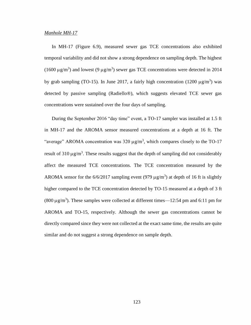
123
Manhole MH-17
In MH-17 (Figure 6.9), measured sewer gas TCE concentrations also exhibited
temporal variability and did not show a strong dependence on sampling depth. The highest
(1600 g/m3) and lowest (9 g/m3) sewer gas TCE concentrations were detected in 2014
by grab sampling (TO-15). In June 2017, a fairly high concentration (1200 g/m3) was
detected by passive sampling (Radiello®), which suggests elevated TCE sewer gas
concentrations were sustained over the four days of sampling.
During the September 2016 “day time” event, a TO-17 sampler was installed at 1.5 ft
in MH-17 and the AROMA sensor measured concentrations at a depth at 16 ft. The
“average” AROMA concentration was 320 g/m3, which compares closely to the TO-17
result of 310 g/m3. These results suggest that the depth of sampling did not considerably
affect the measured TCE concentrations. The TCE concentration measured by the
AROMA sensor for the 6/6/2017 sampling event (979 g/m3) at depth of 16 ft is slightly
higher compared to the TCE concentration detected by TO-15 measured at a depth of 3 ft
(800 g/m3). These samples were collected at different times—12:54 pm and 6:11 pm for
AROMA and TO-15, respectively. Although the sewer gas concentrations cannot be
directly compared since they were not collected at the exact same time, the results are quite
similar and do not suggest a strong dependence on sample depth.

124
Figure 6.9. MH-17 sewer gas TCE concentrations (g/m3) and sample depths, 2014 -
2017
Note: TCE residential cancer and non-cancer inhalation exposure screening levels are
based on California’s indoor air screening level (EPA, 2016; DTSC, 2016). All non-detect
values shown on graph were plotted as half of the detection limit.
Manhole MH-18
For MH-18 (Figure 6.10), depth appeared to play a limited role in the measured sewer
gas concentrations. In this manhole, two “night time” TO-17 samplers were deployed at
two different depths during the same sampling event (10.6 ft and 1.5 ft) and the results
showed that the deeper sample was 1.6 times higher than the shallow sample. Similarly,
the AROMA sensor consistently measured higher “average” day time concentrations (464
g/m3, placed at 16 ft) when compared to the TO-17 day time sampler (345 g/m3, placed
at 1.5 ft). Although depth appeared to play a limited role in this manhole, short-term
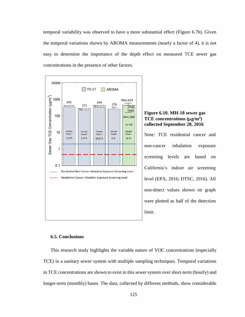
125
temporal variability was observed to have a more substantial effect (Figure 6.7b). Given
the temporal variations shown by AROMA measurements (nearly a factor of 4), it is not
easy to determine the importance of the depth effect on measured TCE sewer gas
concentrations in the presence of other factors.
Figure 6.10. MH-18 sewer gas
TCE concentrations (g/m3)
collected September 28, 2016
Note: TCE residential cancer and
non-cancer inhalation exposure
screening levels are based on
California’s indoor air screening
level (EPA, 2016; DTSC, 2016). All
non-detect values shown on graph
were plotted as half of the detection
limit.
6.5. Conclusions
This research study highlights the variable nature of VOC concentrations (especially
TCE) in a sanitary sewer system with multiple sampling techniques. Temporal variations
in TCE concentrations are shown to exist in this sewer system over short-term (hourly) and
longer-term (monthly) bases. The data, collected by different methods, show considerable

126
spatial variations also exist. It is plausible that the spatial and temporal variability of VOC
concentrations in sewer gas observed in this study may also exist in sanitary sewer systems
at (and near) other shallow VOC groundwater contaminated sites.
Sampling approaches to assess sewer gas concentrations need to account for the variability
which were observed in this research study. Single short-term approaches (i.e. TO-15 grab
sampling) may not be adequate for assessing long-term exposure risks associated with this
pathway. Passive sampling provides an approach for assessing time-averaged sewer gas
concentrations; however, there is difficulty in defining appropriate time over which to
deploy a passive sampler, as well as the number of sampling events, given the high level
of temporal variability reported in this study. Subsequent sampling events may be required
to capture longer-term temporal variations (see Figures 6.4a and b, 6.8 and 6.9). This
research demonstrates that incorporating passive samplers with continuous monitoring
devices can provide insight about temporal and spatial variations.
Sewer manholes and cleanouts are often easily accessible sampling locations for sewer
pathway investigations. While manholes provide information about the sewer system itself,
cleanouts can potentially provide information close to the point of exposure (e.g. inside
buildings). Even while additional information is emerging about VI alternative pathways,
multiple lines of evidence, such as VOC concentrations in and around the sewer system,
nearby groundwater level measurements to evaluate sewer level elevations relative to
groundwater table fluctuations, modeling, tracer studies to evaluate sewer gas transport,
and sewer videos, sewer as-built drawings etc. can be useful in conceptualizing field
observations and making decisions about how and when to mitigate exposure risks.

127
When considering the spatial and temporal variations in VOC concentrations detected
in the sewer system in this research study, there are several key observations that emerge.
Manholes near the 2012 VI Study Area (e.g. MH-17 and MH-18) are likely being (or
historically have been) impacted by groundwater infiltration from that general area and
sewer videos are useful in providing evidence of sewer cracks. However, in MH-15, which
is some distance from the 2012 VI Study Area, local groundwater infiltration/exfiltration
in the area of MH-15 is likely occurring. Sewer videos (FOIA, 2017) provide evidence that
infiltration could occur near MH-15 and historic subsurface sampling has indicated
elevated TCE concentrations in the vicinity of MH-15 (Compliance and Closure, 2013;
Stratus Environmental, 2010; FOIA 2017; Bureau Veritas, 2013; Cornerstone Earth Group,
2017). The temporal variation observed in this location is difficult to fully explain,
especially in light of the subsurface contamination in the area. Other nearby manholes—
MH-12, MH-13, and MH-14—also warrant additional evaluation; however, it is expected
that sewer gas concentrations in those manholes would also exhibit a fairly high level of
temporal variability.
Collectively, the data presented in this multi-year, multi-sampler research study
demonstrates that VI alternative pathways may require investigation along sewer lines that
are hundreds of feet away from well-defined groundwater contamination plumes. This is
especially true for aging sewer lines that may have received chemical wastes discharges as
part of historic operations. Interpreting sewer gas concentrations is complex due to spatial
and temporal variations. Other lines of evidence are critical to fully understanding the fate
and transport of VOCs in sewer systems and to assess the resulting inhalation exposure
risks that may exist in buildings that are connected to the sewer systems.

128
While research emerges with improved methods for characterizing VI alternative
pathways, exposure risks to sewer gas could be reduced by various mitigation techniques,
including proper plumbing maintenance, sewer venting, and controlling VOC entry into
sewers through sewer maintenance that addresses aging infrastructure issues. Perhaps one
of the most prudent and time-sensitive approaches to risk reduction might include
monitoring and ensuring proper operation of indoor plumbing fixtures, as well as investing
in upgrading aging infrastructure in areas where shallow groundwater with known VOC
contamination exists.

129
CHAPTER 7: DEVELOPING A NUMERICAL MODEL TO STUDY FATE AND
TRANSPORT OF VOCs INSIDE THE SEWER SYSTEMS
As it is mentioned in chapters 5 and 6, several field studies have reported the detection
of elevated concentrations of VOCs in sewer gas and sewer liquid, providing evidence of
sewer systems to act as pathways for VOC migration to the indoor area (e.g. Riis et al.,
2010; Pennell et al., 2013; Guo et al., 2015; USEPA, 2015a; Jacobs et al., 2015; McHugh
et al., 2017; Roghani et al, 2018). This pathway is just beginning to be considered as part
of VI modeling (e.g. Yao et al., 2017b); however the complexities have not been well
described. Currently, VI conceptual site models (CSM) consider the diffusion of VOC
vapors through soils and their infiltration into the indoor areas through the building
foundation's cracks as the primary mechanism for VI, and have just recently begun to
consider the sewer systems as an important alternative pathways.
Possessing a firm understanding about VOCs different mass transfer mechanisms
occurs in a sanitary sewer system in different phases, is vital for municipalities, industries,
and regulators to better analyze the field data collected from different locations and
structures in a sewer system. Development of a numerical model that can describe VOC
transport through the sewer system is useful for developing better screening tools and
assessing VOC exposure risks associated with potential inhalation of sewer gas due to entry
of sewer gas into indoor air spaces.
7.1. Review of existing VOCs sewer gas modeling
Several studies have assessed VOC mass transfer inside sewer systems and have
developed numerical models describe the process. Most of these models were developed

130
in the 1990s to assess VOC emissions from the sewer liquid in different sewer structures
and evaluated parameters that may affect VOC stripping from the liquid to the gas phases
(Corsi et al., 1992; Quigley and Corsi, 1995; Jones et al., 1996; Olson et al., 1997b; Corsi
and Birkett, 1995; Parker and Yu, 2001). The studies that are described below investigated
VOCs such as benzene, toluene, ethylbenzene, xylenes, tetrachlorothene, 1,1,1-
trichloroethane and etc.
Jones et al. (1996) compared accuracy of four different numerical models for predicting
VOC emissions from a municipal sewer system. They highlighted the substantial role of
headspace ventilation rate on VOC concentrations in sewer gas. Results suggests that vents
in sewer reaches between manholes and drop structures are the locations at which most
VOC emission occurs.
Corsi and Birkett (1995) assessed impacts of VOC physicochemical properties, sewer
liquid flow conditions and sewer gas flow rate on the stripping rate of VOCs from the liquid
phase to the gas phase. They concluded that VOC volatility, sewer channel slope, and head
space ventilation rate have a significant effect on VOC removal from the liquid phase.
Results of their study also highlights the impact of the sewer liquid depth in the pipe relative
to the pipe diameter on the VOC stripping rate. They concluded that as the ratio of liquid
depth to the sewer pipe diameter decreases, VOC mass transfer from liquid phase to the
gas phase increases. The reason is the slower sewer liquid flowrate, provides more time for
VOCs to transfer from the liquid phase to the gas phase. In addition, and perhaps more
importantly, lower sewer liquid depth in the pipe provides greater head-space volume,
which creates a greater driving force for VOCs mass transfer in the gas phase.

131
Parker and Yu (2001), developed a dynamic model to estimate VOC liquid-gas mass
transfer in different structures of a sewer network, including sewer reach, inverted siphon
and drop structure. They concluded that the presence of an inverted siphon in a sewer line
significantly reduces the sewer gas VOC concentration downstream of the siphon; while a
drop structure can significantly accelerate the mass transfer rate between the liquid phase
and gas phase. Sewer gas VOC concentrations are expected to be higher right at the drop
structure compared to the upstream and downstream concentrations. Results of their study
also indicates that the first drop structure in a sewer reach potentially has a greater impact
on VOCs stripping to the gas phase compare to the sequential drop structures. Bell et al.,
(1998) later estimated that a typical drop structure can strip more than 40% of VOC from
the liquid to gas phase.
Failure to include information about the sewer components in a numerical model can
lead to an inaccurate estimation of VOC concentrations in both liquid and gas phases.
Therefore, obtaining a detailed map of the sewer system and surrounding area prior to
model development is essential. By including this information we can develop a sewer
model that more accurately reflects the physical phenomena occur inside a sewer system.
Table 7.1 summarizes effects of different structure and variables on VOC liquid-gas mass
transfer concluded by different studies.

132
Table 7.1. Effects of different parameters on VOC liquid-gas mass transfer
Spatial Variables
Structure Effect Study
Drop structure
Significantly increase VOC stripping rate from
liquid phase to the gas phase. Headspace VOC
concentrations “at” drop structures are expected
to be elevated compared to upstream and
downstream concentrations. The first drop
structure in a sewer reach has greater impact on
VOC volatilization compare to sequential drop
structures.
Corsi et al.,
1992; Parker
and Yu, 2001.
Inverted siphon
Significantly decreases sewer gas VOC
concentrations in downstream direction.
Parker and
Yu, 2001.
P-trap
A wet P-trap acts like an inverted siphon. It
blocks the sewer gas (that is potentially
contaminated with VOC) entry into the building.
VOC vapors can infiltrate into indoor air through
leaked water trap. A damaged or dry P-trap allow
sewer gas to migrate into the indoor air.
Pennell et al.,
2013; Nielsen
and Hvidberg,
2017.

133
Ventilated manhole
A high headspace ventilation rate in a sewer
system decreases accumulation of VOCs in the
gas-phase. On the other hand, this creates a
greater driving force for VOC transfer from
liquid phase to the gas phase, thereby increasing
VOC mass transfer rate.
Corsi and
Birkett, 1995.
Temporal Variables
Variable Effect Study
Tributary discharge
Water or air that are contaminated by VOCs may
substantially increase both liquid- and gas-phase
VOC concentrations in the sewer. On the other
hand, relatively clean water or air may
significantly dilute VOC concentrations in the
sewer.
Jones et al.,
1996;
Roghani et al.,
2018.
Headspace ventilation
rate
Increasing ventilation rates increases liquid-gas
mass transfer of VOCs while simultaneously,
decreases gas-phase accumulation of VOCs.
Jones et al.,
1996; Olson et
al., 1997b;
Pescod and
Price, 1981.
Infiltration and Inflow
(I&I); Exfiltration and
The groundwater infiltration/exfiltration and
inflow/exflow can be expected for every sewer
system. A key factor in exfiltration/infiltration is
USEPA,
2000;

134
the hydraulic gradient between the groundwater
table elevation and the sewer liquid elevation.
Inflow from rainwater into the sewer system may
occur during and shortly after rainfall events. I&I
may significantly alter headspace and sewer
liquid VOC concentrations, depending on the
severity of VOC contamination of the
groundwater and soil in the area.
USEPA,
2014.
Sewer liquid depth
Sewer pipe diameter
VOC mass transfer to the gas-phase increases as
this ratio decreases.
Corsi and
Birkett, 1995.
7.2. Fate and Transport of VOCs inside the sewer system:
VOCs can enter into sanitary sewer systems through various routes, in both liquid phase
and gas phase. VOCs contaminated groundwater plumes, or contaminated soil can be
potential sources for VOCs vapors infiltrating into sewer systems. Sewer liquid and/or
sewer sludge also can act as VOC sources. Once, VOCs enter the sewer system, various
mechanisms govern the overall fate and transfer processes and control VOC transport
inside the sewer. Sorption, biodegradation, liquid/gas mass transfer and vapor diffusion are
four major fate and transport processes considered in this model.
7.2.1. Sorption
Organic compounds such as VOCs have relatively good potential to be adsorbed on the
surface of organic solids (Lin and Chou, 2006; Namkung and Rittmann, 1987), therefore
adsorption of VOCs on natural organic compounds in a sewer system is expected.

135
Biological volatile suspended solid (VSS) and dissolved organic carbons (DOC) can adsorb
VOCs inside a sewer system. The rate of VOCs adsorption and the concentration of VOCs
on the surface of adsorbent, depends on the properties of targeted VOC, concentration of
the VOC in the sewer liquid and concentration of the adsorbent in sewer liquid (e.g
suspended solids and dissolved organic carbons) (Lin and Chou, 2006). Partitioning of
VOCs in the aqueous phase between dissolved organic carbon and liquid phase can be
described as:
Cl C dissolved organic carbon
Koc = Cdissolved organic carbon
Cl =
CdSd
Cl (7.1)
Koc = dissolved organic carbon-water partitioning coefficient, (L water/Kg DOC);
C dissolved organic carbon= VOC concentration sorbed on DOC, (g VOC/ Kg doc);
Cd = concentration of VOC that bound on DOC, (g VOC/L water);
Sd = dissolved organic compound concertation in sewer liquid, (Kg doc/L water);
Cl = sewer liquid VOC concentration, (g VOC/L water).
In a sewer system containing active sludge, VOC adsorption on the surface of sludge
is a possible scenario. Biological cells adsorb VOCs and partition between a specific VOC
on aqueous phase and biological suspended solids can be described by:
Cl C suspended solids
Kp = Csuspended solid
Cl =
CsSs
Cl (7.2)
Kp= suspended solid-water partitioning coefficient (L water/Kg SS);
C suspended solid = VOC concentration sorbed on SS, (g VOC/ Kg SS);

136
Cs= concentration of VOC that bound on suspended solid, (g VOC/ L water);
Ss = suspended solid concertation in sewer liquid (Kg SS /L water).
Suspended solid-water petitioning coefficient (Kp), can be calculated by using the
organic carbon-water partitioning coefficient (Koc) (USEPA, 1993).
Kp= foc× Koc (7.3)
Koc = VOC concentration sorbed on organic carbon(
g
Kg)
VOC concentration in water (g
L)
foc =fraction of organic carbon in the solids, (g/g).
The Koc values for several VOCs are available in the table provided by USEPA
(USEPA, 1996). There are also few equations available for estimating Koc value for
different compounds. These equations typically use the octanol-water pertaining
coefficient value (Kow) of the compound to estimate Koc. Equation below is one of the
equation that has been suggested for VOCs (Weiner, 2012).The Koc value calculated by
this equation has the unit of liter per kilogram (L/kg).
Log Koc= 0.7919 Log Kow + 0.0784 (7.4)
Karickhoff et al., (1979) suggested equation 7.5 for estimating the Kp value for
hydrophobic pollutants. Namkung and Rittmann (1987), used this equation for VOC’s
adsorption in wastewater studies to calculate VOC emission rate at water treatment plants.
They consider C5H7O2N as the representative formula for biological cells in a wastewater
system and based on this assumption calculated the organic carbon fraction (foc) =0.531.
Equation 7.6 is calculated based on this estimation for foc and is used to calculate Kp.
Kp= (6.3×10⁻⁷).foc.Kow (7.5)

137
Kp= (3.345×10⁻⁷) Kow (7.6)
The rate of the VOC adsorption on dissolved organic carbon (R adsorption-DOC (g/s)) and
suspended solid (R adsorption-SS (g/s)) can be calculated by applying equations 7.7 and 7.8,
respectively.
R adsorption-DOC= Ql.Cl.Sd.Koc (7.7)
R adsorption-SS= Ql.Cl.Ss.Kp (7.8)
By assuming that VOCs inside a sewer system, only can be adsorbed on the suspended
solid and dissolved organic carbon, the total VOC adsorption rate can be calculated by
applying equation 7.9. It worth to note that non-dispersible materials such as wet wipes
that exist inside the sanitary sewer systems could be another potential adsorbent for VOCs.
They are not considered in this model due to the lack of information about their typical
concentrations inside the sewer system.
R adsorption= R adsorption-DOC + R adsorption-SS = Ql.Cl. (Sd.Koc + Ss.Kp) (7.9)
R adsorption = rate of VOC adsorption, (g/s);
Ql = the flow rate of the sewer liquid (m3/s)
Equation 7.9 can be written as:
R adsorption= Ql. Cl. Koc. (Sd + Ss. foc) (7.10)
By applying equation 7.10 rate of VOC adsorption inside the sewer system is
calculated. The calculated adsorption rate is based on the equilibrium sorption assumptions.
By applying the equilibrium calculations, we assumed there is an enough residential time
for VOCs adsorption to reach the equilibrium concentrations between two phases. This

138
assumption is reasonable at the relatively low concentration of VOC in a municipal sewer
system (Melcer et al., 1996).
Yaghmei and Rashidkhani (2005) concluded that adsorption didn’t have a considerable
effect on the VOC off-gas concentration. Namkung and Rittmann (1987) also reported that
adsorption is a negligible process for VOCs inside a sewer system. Dobbs et al. (1989)
estimated that 2.6% of chloroform and 2% of methyl chloride in a municipal sewer system
is removed by sorption; while 16% of the total TCE is removed by adsorption based on the
same study. They concluded that for VOCs with log10 Kow< 2.2 such as benzene and
chloroform, adsorption doesn’t have a considerable impact on VOC removal from the
liquid phase, while for VOCs with log10 Kow > 2.5 such as TCE and toluene, adsorption
could be an important process to be considered.
7.2.2. Biodegradation
Biodegradation is another mass transfer mechanism that may affect VOCs
concentration in the liquid phase and therefore change the rate of VOC's transfer to the gas
phase. The biological degradation rate can be estimated by using Monod kinetics model
(Monod, 1949).
R biodegradation = kmax Ss Cl Vl
Ks+ Cl (7.11)
R biodegradation = biological reaction rate, (g/s);
Ss= biological suspended solid concentration in the wastewater, (g VSS/m3);
Kmax = maximum specific substrate utilization, (g/s. g bio);
Ks = half saturation constant, (g/m3);
Cl = Sewer liquid VOC concentration (g/m3);

139
Vl =Sewer liquid phase volume (m3).
VOC's water solubility is limited and its concentration in wastewater and sewer liquid
is relatively low (Corsi and Card, 1991; Yaghmei and Rashidkhani, 2005), so Cl << Ks and
therefore equation 7.11 can be simplified as:
R biodegradation = Kl.Ss.Cl.V (7.12)
Kl = apparent first-order biological reaction constant (= kmas
Ks), (m3/g VSS.s).
Results of studies (Wilson et al., 1994; Namkung and Rittmann, 1987 and etc.) have
suggested that for VOCs that are less easily biodegradable in aerobic conditions such as
chloroform, PCE and TCE even in wastewater treatment plants with elevated
concentrations of activated biomass (Ss), biodegradation is not a significant removal
mechanism. However biodegradation can be an important removal mechanism for VOCs
such as toluene, methylene chloride, Xylene, ethylbenzene and benzene that are
biodegradable under aerobic conditions (Namkung and Rittmann, 1987; Wilson et al. 1994;
Weber and Jones, 1986).
Several important VOCs such as chloroform, PCE, TCE, 1,2 trans-DCE
(dichloroethylene), 1,1,1 trichloroethane, and 1,2 DCA (dichloroethane) are reported to
have negligible biodegradation rates in an aerobic system (e.g. sewer system) and the Kl
value for them in this model is considered to be zero (Kl −̃ 0). Other VOCs that are
considered to be a bigger group are degradable in an aerobic system and Kl > 0. Kl value
depends on the operation conditions. Having a good Kl value estimation is a big challenge
for calculating the rate of biodegradation. Namkung and Rittmann (1987), reported Kl
values for four different VOCs (benzene, chlorobenzene, ethylbenzene and toluene) in a
laboratory scale active sludge system which were ranged between 0.21 to 0.40 (m3/g Vss.

140
d)). In a sewer system with a lower air flow rate and less concentration of active sludge,
Kl value is expected to be smaller.
In the model, equation 7.12 is used to calculate the rate of VOC biodegradation in the
sewer system. Kl is considered to be zero for non-biodegradable VOCs and for
biodegradable VOCs different Kl values were assessed.
7.2.3. Liquid - gas mass transfer
Liquid-gas mass transfer has been reported as the dominant fate and transfer
mechanism for VOCs inside the sewer system in previous studies and the magnitude of
diffusion, adsorption/desorption and biodegradation were considered to be small compare
to this mechanism (Corsi and Birkett, 1995; Parker and Yu, 2001).
Interfacial VOCs mass transfer flowrate between liquid phase and gas phase can be
estimated by the two film theory' equation:
R liquid- gas= - KT× (Cli – (Cgi/Hc)) × A (7.13)
R liquid- gas= mass transfer rate of VOC between liquid and gas phase, (mg/s);
KT = overall mass-transfer coefficient for chemical “i”, (m/s);
Cl= concentration of the chemical “i” in the liquid phase, (mg/m3);
Cg = concentration of the chemical “i” in the gas phase, (mg/m3);
Hc= Henry's law constant for the chemical “i”, (m3 liquid/m3 gas);
A= interfacial contact area between wastewater and air, (m2).
The two film theory considers continuous mass transfer from both sides across the two
phase interface, till it reaches the equilibrium partitioning between two phases. The

141
equilibrium concentration is defined based on this partitioning. KT can be calculated by
equation below:
1
KT =
1
kl +
1
Kg × Hc (7.14)
Which kl is the liquid phase mass transfer coefficient (m/s) and kg is the gas phase mass
transfer coefficient (m/s). Parkhurst and Pomeroy (1972) developed a semi-empirical
model for oxygen mass transfer coefficient. They tested 12 operating municipal sewer
systems and by applying the mass balance equations, they calculated the mass transfer
coefficients for oxygen in different conditions. Based on the results they developed a
numerical model by using a non-linear regressions:
Klo = 2.6E-4 (1+0.17 Fr2).δ. (S.U) 3/8 (7.15)
Klo = the liquid mass transfer coefficient for oxygen, (m/s);
S= slope of the energy gradient, (m/m);
U= average velocity of wastewater, (m/s);
δ = temperature correction factor, dimensionless;
Fr= Froude number.
The Froude number is a dimensionless number. It is defined as the ratio between inertial
forces and gravitational forces and calculated by the equation below:
Fr = Ul
(g.d)0.5 (7.16)
Ul =the liquid (wastewater) velocity, (m/s);
g= gravitational constant, 9.81 (m/s2);
d= depth of the liquid (wastewater) flow, (m).
142
The empirical Manning’s equation that has been used for uniform flows in channels
since 1889, is used in the model to estimate correlation between the sewer liquid velocity
and the depth of the liquid inside the sewer system, shown in equation 7.17.
Ul = (k/n) × (A/P) 2/3×(S) 0.5 (7.17)
K = conversion factor, (1.49 for English units and 1.0 for SI units).
n = Manning’s roughness coefficient.
A =flow area of the pipe, culvert, or channel, (m2);
P =wetted perimeter (portion of the circumference that is in contact with water), (m);
S =downward (longitudinal) slope of the culvert, (m/m).
It has been shown that for chemicals with Hc>0.1, the liquid mass transfer coefficients
are proportional to the liquid molecular diffusion coefficients (Higbie, 1935 & Lewis and
Whitman, 1924)
Kl,1
Kl,2 =
D1
D2
n (7.18)
Which Di is the molecular diffusion coefficient for chemical "i" (m2/s) and "n" is the
power constant, theoretically varies between 0.5 and 1. In a well-mixed system “n” is
normally assumed to be 0.5. The sewer system due to its nature can be consider as a mixed
system and therefore "0.5" has been used as the value for "n" in the sewer systems (Parker
and Yu, 2001).The liquid mass transfer coefficient for any VOC in this model is estimated
by calculating the oxygen liquid mass transfer coefficient (equation 7.15) and applying
equation 7.18 for converting this value to the targeted VOC's liquid-gas mass transfer
coefficient.

143
Mackay and Yeun (1983) suggested a model to estimate organic compounds gas phase
mass transfer coefficient from the liquid surface.
Kg= 0.001+ (0.0462 ×U*× SCG - 0.67) (7.19)
U* = 10-2× (6.1+ 0.63×U10)0.5 ×U10 (7.20)
SCG= μa
Da ρa (7.21)
U* = air side friction velocity, (m/s);
U10 = wind speed 10m above water surface, m/s; (can be estimated by ~ Ug);
SCG=gas-phase Schmidt number;
µa = dynamic viscosity of air, (g/cm.s);
Da = molecular diffusion coefficient for a VOC in air, (cm2/s);
a = density of air, (g/cm3).
The overall mass transfer coefficient for the targeted chemicals can be calculated by
applying equations 7.14. For VOCs due to the nature of these chemicals in a typical
condition, the gas phase layer resistance to the mass transfer (represented by 1
kg.Hc ) is much
smaller than the liquid phase resistance to the mass transfer (represented by 1
kl ) and
therefore it can be assumed that the liquid phase controls the overall mass transfer rate.
Generally for VOCs or any chemical with Hc > 0.1 the total mass transfer coefficient (KT)
is almost equal to kl (Corsi et al., 1992). This simplification is used in the model to calculate
the overall mass transfer coefficient between liquid phase and gas phase.
7.2.4. Vapors diffusion
In a classical vapor intrusion model, VOC vapors migrate from the subsurface source
such as contaminated groundwater or contaminated soil toward indoor area through soil

144
layers. VOC vapors can infiltrate into the building through foundations cracks. Soil vapor
originates from the subsurface sources can also use sewer line’s cracks to infiltrate into the
sewer systems and contaminate the sewer gas. This diffusive flow can be calculate by using
equation below.
R diffusion, in= Deffective. Apipe. Fcracked. (dc
dx) groundwater-ground (7.22)
R diffusion, in = VOC mass flow through diffusion, (mg/s);
D effective = effective diffusive coefficient of VOC, (m2/s);
Apipe= area of the pipe, (m2);
Fcracked = average cracked ratio of the pipe, (m2/m2);
(dc
dx) groundwater-ground = VOC concentration gradient form groundwater to the ground surface,
((mg/m3)/m).
Accumulation of VOCs inside the sewer system through different mechanisms, creates
an elevated concentration of VOC inside the sewer system compare to the surrounding soil
gas and atmosphere. This contaminated sewer gas can act a new source of VOC. VOC
vapors can also leave the sewer system through cracks of the sewer pipe by diffusion due
to the VOC concentration gradient. This diffusive mass transfer leaving the sewer system
can be estimated by using equation below.
R diffusion, out= Deffective. Apipe. Fcracked. (dc
dx) sewer gas -ground surface (7.23)
Which (dc
dx) sewer gas -ground surface is the average gradient of the soil gas VOC concentration
from the sewer gas to the ground surface. It is worth to note, in this model the subsurface
soil assumed to be homogeneous and therefore the soil gas VOC concentration profile
assumed to be linear. In a time depended solution the concentration gradient is not
145
necessarily linear and the soil gas concentration slope could be different in different depths
of the soil.
7.2.5. Parameters affect sewer gas VOCs concentration
Sewer headspace ventilation
Natural headspace ventilation, cause by different factors inside the sewer systems, can
have a significant effect on the sewer gas VOCs concentration. Sewer gas velocity affect
both VOC's liquid-gas mass flux and VOCs sewer gas concentration. Liquid/gas drag force,
wind speed, buoyancy force, pressure differential and sewer liquid rise and fall affect sewer
gas velocity (Olson et al, 1997a).
The liquid-gas drag force is the momentum transfer mechanism from the sewer liquid
to the sewer headspace due to shear forces on the liquid-gas interface. Sewer liquid flow
rate and depth, sewer line slope and pipe's material are some parameters that affect the
shear stress force. Wind flow over the sewer system openings is another important factor
that can affect sewer headspace velocity. The sewer gas temperature gradient and water
content gradient creates a density gradient inside the sewer system. Sewer gas in deep areas
of a sewer system typically have smaller density compared to the ambient air and shallow
sewer gas (Pescod and Price 1981). The air in a deep area of the sewer system normally
have a higher temperature and higher water content (Lowe, 2016). The density of air
decreases with increase of temperature and/or increase of water content. Equation 7.24 is
obtained based on the ideal gas law. This equation shows dependency of the air density to
the temperature and water content. A density difference between the air inside the sewer
system and atmosphere air, creates the buoyancy driven air exchange. The buoyancy driven

146
air flow can be calculated by using equations below (Turner, 1993; Hunt and Linden,
1999).
= Pa
Ra .T +
Pw
Rw .T (7.24)
ΔP = g. ∫ ρ(z)H
0. ∂z (7.25)
Q buoyancy= CD. A. (2.ΔP/) 0.5 (7.26)
ΔP= pressure gradient due to the density gradient, (Kg/m.s2);
Q buoyancy= buoyancy flow rate, (m3/s);
CD= discharge coefficient for opening, dimensionless;
A= cross section area of the opening, (m2);
= density of the air, (kg/m3);
H= vertical distance of manhole, (m);
Pa = partial pressure of dry air, (Kg/m.s2);
Pw = partial pressure of water vapor, (Kg/m.s2);
Ra = specific gas constant for dry air, 287.05 (J/ (kg.K));
Rw = specific gas constant for water vapor, 461.495 (J/ (kg.K));
T= temperature, °K;
The air pressure profile is another factor that can have impact on the sewer gas
ventilation rate. Pescod and Price (1982) and WERF (2009) measured pressure differences
inside different manholes. They reported that the pressure differences inside the sewer
systems were in the range of (±) 0.02 bar. They concluded that the air pressure difference
inside a sewer system is typically too small to affect the sewer gas flow.

147
Olson et al. (1997b) concluded that individual effects of the all forces mentioned above
are not always strictly additive even when the forces are on the same direction. There are
several effective parameters involved on the sewer gas velocity profile. Corsi and Birkett
(1995) concluded that the magnitude of sewer gas velocity has more impact on VOCs
emission rate compare to the direction of the sewer gas velocity.
Several numerical models have already been developed to predict the behavior of the
sewer hydraulic system and they have been working with appropriate accuracy. Modeling
the sewer headspace behavior though has lots of complexities. Inside a real sewer system
with various effective forces and several openings to the atmosphere, defining the accurate
boundary conditions is a big challenge. Sewer gas velocity is the function of different
parameters and significant temporal and spatial variations are expected for most of these
parameters. Several studies have assessed sewer systems and applied different approaches
for estimating the sewer gas velocity in different conditions. Empirical (e.g. Pescod and
Price, 1982), computational fluid dynamic (e.g. Edwini-Bonsu and Steffler, 2004) and
thermodynamic-based (e.g. Olson et al., 1997a) approaches have been applied to model the
sewer headspace velocity but none of them had a good compatibility with the field results
(Lowe, 2016). Water environment research foundation's (WERF) study (2009) concluded
that models typically overestimate the sewer gas velocity. WERF also concluded that the
existing models work better in higher flow rates and are very inaccurate in lower sewer gas
flows (WERF, 2009).
The sewer liquid velocity is expected to be a strong indicator of sewer headspace
velocity. Water drag has been recognized as the dominant factor in calculating the sewer
gas velocity and studies have suggested that it is safe to assume that sewer gas follows the

148
same direction as the sewer liquid (WERF, 2009). The sewer headspace velocity is
expected to be less than wastewater velocity, same direction and in the rage of 4% to 38 %
of the sewer liquid velocity (WERF, 2009; Pescod and Price 1982). The empirical model
more closely calculated the headspace velocity. The most popular approach to estimate the
sewer gas velocity is an empirical model developed by Pescod and Price (1982) shown in
equation below.
Ug=0.397. (W. Ul /Pair) 0.7234 (7.27)
Ug= average headspace velocity, (m/s);
W = width of the water surface, (m);
Ul = sewer liquid velocity, (m/s)
Pair = headspace pipe perimeter, (m).
Equation 7.27 is used in this model to calculate the sewer gas velocity and therefore in
this study sewer gas velocity is always a strong function of the sewer liquid velocity. As a
result in this model any parameter that changes sewer liquid velocity, at the same time
changes the magnitude of the sewer headspace velocity.
Olson et al, (1998) assessed VOCs emission rate in a sewer pipe with three numerical
solutions defined by different air exchange rates. This study solved VOCs liquid- gas mass
transfer for three (3) scenarios: 1. Open system (very high air exchange rate and zero
accumulation in the gas phase therefore Cg=0) 2. Equilibrium condition (very small air
exchange rate so the sewer gas reaches the equilibrium with liquid phase and Cg= HC.Cl)
and 3. Concurrent ventilation solution that used mass transfer kinetics shown by equations
7.28 and 7.29. They concluded while in a low headspace ventilation rate, mass transfer is

149
limited by the equilibrium, at a high ventilation rate kinetic consideration, limits VOC's
mass transfer.
∂Cl
∂x= (
Kl .W
HcQl× Cg) − (
KlW
Ql× Cl) (7.28)
∂Cg
∂x= (
Kl .W
Ql× Cl) − (
KlW
HcQg× Cg) (7.29)
W= width of the air-water interface, (m).
Temperature
Solubility of VOCs in the liquid phase and VOCs partitioning between the liquid phase
and gas phase are functions of the temperature. Therefore, temperature have an important
role in VOC’s mass transfer and VOC concentration in both liquid and gas phases. The
effect of temperature on Henry’s constant (Hc) can be calculated by Van't Hoff's equation
(Sander, 2015):
d ln (Hc)
d(1
T)
= −(∆H)
R (7.30)
Which T is the liquid-gas interface temperature (° K), ΔH is the enthalpy change of
dissolution (J/mol) and R is the universal gas constant (8.314 J/mol.K). The value of
d ln (Hc)
d(1
T)
for different chemicals are calculated by several studies. This value is reported
4900(K) for TCE and 5100 (K) for PCE (Lincoff and Gossett, 1984) which both are
considerably higher that this value for chemical such as oxygen. d ln (Hc)
d(1
T)
value for oxygen
is reported 1500 (K) (Sander et al., 2001)). Elevated value of d ln (Hc)
d(1
T)
means partitioning
of these chemicals are highly sensitive to the temperature.

150
Sewer liquid temperature can be the best way to estimate the temperature of the liquid-
gas interface. Sewer liquid temperature typically changes in the range of 10°C to 20°C
(WEF, 2007). Temperature of the sewer liquid can significantly increase due to the
industrial discharges or suddenly decrease because of a storm water infiltration (WEF,
2007).
Temperature variations also affect the density and dynamic viscosity in both liquid
phase and gas phase. It also have some effects on the liquid-gas mass transfer coefficient.
Effect of temperature on the liquid-gas phase mass transfer coefficient is assessed by using
equation 7.31. This equation is originally developed for calculating the effect of
temperature on liquid-gas mass transfer for oxygen.
Klo (20) = Klo (T).θ (20-T) (7.31)
T= water temperature, °C;
θ = experimental temperature coefficient, dimensionless;
The value of 1.024 has been widely used for θ, determined by Elmore and West (1961).
Diffusion coefficients in both the liquid phase and the gas phase also change as a
function of temperature fluctuations. In the gas phase, the diffusion coefficient (Dgas) based
on Chapman–Enskog theory is proportional to T1.5. Fuller et al. (1966) assessed this
dependency and concluded Dgas ∝ T1.75. Marrero and Mason (1972) reported that for
majority of gases, the diffusion coefficient varies by temperature in the range of T1.5 to T2.
The diffusion coefficient in the liquid phase (D liquid) though can be estimated by
Stokes-Einstein equation shown below (Howe et al, 2012).
D liquid = k.T
6 π μ.r (7.32)

151
K= Boltzmann constant, dimensionless;
μ = dynamic viscosity, (g/m. s);
r= radius of the diffusing particle, (m).
Since viscosity is a strong function of the temperature, the liquid's diffusion coefficient
and temperature are not linearly dependent. An exponential Arrhenius relation can provide
a better estimation for diffusion coefficient and temperature relation.
D= D0. Exp (−EA
K.T) (7.33)
EA = activation energy of diffusion, (J/atom);
T= Temperature, (°K);
D0 = maximal diffusion coefficient at infinite temperature; (m2/s);
K= Boltzmann constant, dimensionless;
The diffusion coefficient in a porous media such as soil can be calculated using both
the VOC-water diffusion coefficient (Dw) and the VOC-air diffusion coefficient (Da) by
applying Millington quirk equation (1961):
D effective = Da ( θa
10/3
θt2 ) +
Dw
Hc (
θw10/3
θt2 ) (7.34)
θa = air porosity (volumetric soil gas content), (m3/m3)
θw = water porosity (volumetric water content), (m3/m3)
θt = total porosity of the soil (𝜃𝑡 = 𝜃𝑤 + 𝜃𝑎)
Equation 7.34 is used in this model to calculate soil's diffusion coefficient for the
targeted VOC based on soil characteristics such as soil total porosity and water content.
Sewer Structures

152
As is reported by several field studies and has been confirmed by numerical models
(e.g. Corsi et al., 1992; Parker and Yu, 2001), sewer structure can have a significant effect
on VOC mass transfer inside the sewer systems. In this section effect of some of this
structure on VOC mass transfer will be explained.
a. Drop structure
A drop structure in a sewer system is a small manmade structure for transporting the
sewer liquid from a higher elevation to a lower one. Normally when in a sewer system
design sewer line elevation changes significantly due to the geological characteristic a drop
structure will be considered. Some studies such as Corsi et al., (1992); Parker and Yu
(2001) have assessed VOCs emission from sewer liquid to the sewer gas within drop
structures. Results suggested that drop structure has a significant effect on VOCs mass
transfer inside a sewer system. Several mass transfer mechanisms get involved in a drop
structure including air bubble entrained in the tail water, agitated tail water surface, free
falling jet and splashing droplets (Tata et al., 2003). Result of a pilot study suggested about
40% increase in VOCs emission due to a drop structure while drop structure's height have
a considerable effect on this estimation (Bell et al, 1993).
Nakasone (1987) evaluated effect of the drop structure design on VOC stripping from
liquid to gas phase. He concluded that the drop height is the most important parameter in
VOC stripping to the gas phase while the tail water depth doesn’t have a significant impact
on the result. Nakasone (1987) proposed series of equations for calculating oxygen mass
transfer between liquid and gas phases in a drop structure. A general form of these
equations is shown in equation 7.35.

153
Ln (r0) = a. Hb. qc. Zd (7.35)
H= drop structure height, (m);
q= hydraulic weir loading, (m3/ m. h);
Z= tail water depth, (m);
a, b, c = empirical coefficients, dimensionless;
Rahme et al. (1997) used the equations below based on a non-regression analysis
performed on 48 different oxygen transfer experiments. Equations 7.36-7.39 suggested by
their study are used to calculated VOCs mass transfer between liquid and gas phases in a
drop structure.
Fraction Emitted: rv−1
rv+B.rv −B (7.36)
Ln (r0) = 1.081×H 0.784 × Ql -0.139 (7.37)
rv = r0 F.α.ѱ (7.38)
B = 𝑄𝐿
𝑄𝑔.𝐻𝑐 (7.39)
Ql = liquid flow rate (m3/min);
ro = the oxygen deficit ratio, dimensionless;
rv = VOC deficit ratio, dimensionless;
Ѱ = kl,VOC i
kl,o2 = (
DVOCi
DO2)
n
α = effect of contamination in the water on VOC diffusion in water;
F= correction coefficient.
Ѱ is the diffusion coefficient of VOC in water relative to the diffusion coefficient of
oxygen in the water and “n” is typically considered= 0.5 in a sewer system. The F value
depends on several parameters such as Hc and liquid-gas mass transfer coefficient. This

154
value is assumed to be 1 unless there is a significant stripping due to air entrainment. The
value is typically assumed to be 1 (Labocha et al., 1994).
b. Inverted Siphon
The present of a submerged inverted siphon inside a sewer system can completely block
the headspace flow and therefore an inverted siphon may have a significant impact on the
sewer gas VOC concentration in downstream and upstream. Parker and Yu (2001) reported
a substantial decrease of VOC sewer gas concentration immediately downstream of a
submerged inverted siphon.
c. Tributary
Tributary flows that join the sewer system, can have a significant impact on the sewer
liquid flowrate, depth and sewer liquid and sewer gas VOC concertation. The magnitude
of this influence depends on the tributary flowrate and its VOC concentration. Due to the
turbulent nature of sewer flows, it is assumed that tributary flows will be immediately
mixed with the sewer main flow in both liquid phase and gas phase. It is reported that
tributary flows that are free from VOC, considerably decrease sewer gas VOC concertation
at downstream (Parker and Yu, 2001). Equations below are used for both liquid and gas
phases to calculate the sewer gas and sewer liquid VOC concentration downstream of a
tributary.
Q downstream= Q upstream+ Q tributary (7.40)
Q downstream. C downstream = (Q upstream. C upstream) + (Q tributary. C tributary) (7.41)

155
7.3. Sewer Gas Numerical Model
7.3.1. Model development
General Description of the Model
The overall mass transfer equations for liquid phase and gas phase can be obtained by
considering all the above mass transfer mechanisms. For each phase we have equation 7.42.
R total = V. dc
dt = R in – R out + R liquid- gas + R diffusion + R adsorption + R biodegradation (7.42)
By considering all the effective mass transfer mechanisms in each phase, equation 7.43
and 7.44 are developed to calculate VOC concentrations in the liquid phase and gas phase
respectively. The sewer pipe between two manholes is considered as a continuous flow
stirred tank reactor (CFSTR) and equations 7.43 and 7.44 are solved simultaneously to
calculate VOC concentration for each phase.
𝑉𝑙.𝜕𝐶𝑙
𝜕𝑡 = ((Ql, in. Cl, in) + (Qtributary. Cl, tributary)) - ((Ql, in+ Qtributary) × Cl) - ((Kl. A) × (Cl −(
𝐶𝑔
𝐻𝑖)))
+ Kl.Ss.Cl.Vl + Ql.Cl.Koc. (Sd+ (Ss.foc)) (7.43)
𝑉𝑔.∂𝐶𝑔
∂t = ((Qg, in. Cg, in) + (Qtotal, in. Catm)) - ((Ql, in+ Qtotal, out) × Cl) + ((Kl. A) × (Cl −(
𝐶𝑔
𝐻𝑖))) -
(Deffective. Apipe. Fcracked. (𝑑𝑐
𝑑𝑥) sewer-ground) + (Deffective. Apipe. Fcracked. (
𝑑𝑐
𝑑𝑥) groundwater-ground) (7.44)
Qtotal, in = total air flow rate comes into the sewer system from atmosphere, (m3/s);
Qtotal, out =total air flow rate leaves the sewer system, (m3/s);
Catm = Atmosphere air VOC concertation, (mg/m3) (assumed to be zero in the model).
If there is a specific structure on the way of sewer line, equations 7.43 and 7.44 may be
modified. In case of a drop structure as an example, equations 7.36 through 7.39 were used
to calculate the effect of this structure on VOC concentrations in both liquid and gas phases.

156
If the manhole's caps are closed, it assumed there is no flow exchanges between atmosphere
and the sewer manhole. If manhole's cap have any opening (hole) it is assumed that there
is enough space for the air flow to exchange between the manhole and atmosphere. For the
open manhole cases, the total flow rate in each manhole is the sum of the buoyancy driven
flow rate and ventilation flow rate. Equations 7.24-7.26 were used to calculate the
buoyancy flow rate at each manhole. It is also assumed that if the airflow at the downstream
of a manhole is less that the upstream airflow rate, the difference between the two airflow
vents at the manhole and leave the sewer system. If the airflow rate at the downstream of
a manhole is greater that the upstream flow rate, the air flow equal to the difference of these
two flowrates drawn into the system (Lowe, 2016). Based on these consideration we used
equation 7.45 to calculate the total flow rate:
Q total= Q buoyancy+ Q ventilation (7.45)
Calculation of the sewer liquid information
The first step for the modeling of VOC mass transfer within a sewer system is to define
the hydraulic properties for the system. The sewer liquid depths, sewer liquid velocities
and the total liquid volume all over the sewer system need to be calculated based on the
given information. Depth of the sewer liquid (or flowrate of the sewer liquid) on the
upstream boundaries of the sewer system and any tributaries flows should be defined.
Based on the system's information such as pipes diameters, pipe's material and sewer
system slopes, sewer liquid velocity and the sewer depth all over the system will be
calculated by using equations below.

157
Table 7.2. Sewer liquid calculation
a) For sewer liquid depth < Sewer pipe radious
h= depth of the sewer liquid
Central angle (θ): 2.arccos(r−h
r) (7.46)
Flow area (Al): r2.(θ−sin(θ))
2 (7.47)
Wetted perimeter (Pw)= r× θ (7.48)
Hydraulic radius (Rh)= Al
Pw (7.49)
Ul= (1
𝑛). (Rh)
2/3. (S)0.5 (*Equation 7.17)
Liquid flow rate (Ql)= Ul * Al (7.50)
Total flow rate(Qt) = Ql+Qtributary (7.51)
Liquid Volume Vl= Al. L (7.52)
b) For sewer liquid depth > Sewer pipe radious
h=( 2.r) – (depth of the sewer liquid)
Central angle (θ): 2.arccos(r−h
r) same as (7.46)
Flow area (Al): Пr2 - ( r2.(θ−sin(θ))
2 ) (7.53)
Wetted perimeter (Pw)=2П - (r.θ ) (7.54)
Hydraulic radius (Rh)= Al
Pw same as (7.49)
Ul= (1
𝑛). (Rh)
2/3. (S)0.5 (*Equation 7.17)
Ql ,Qt and Vl are calualted by euqations 7.50, 7.51
and 7.52 respectively.
L = length of the each sewer pipe between two manhole(m).
r=sewer pipe radius (m);

158
By calculating the total sewer liquid flow in each section, the depth and velocity of the
sewer liquid inside the sewer line can be calculated using the equation above.
Calculation of the sewer Headspace velocity
After calculating the hydraulic propertis of the sewer system, the sewer headspace
velocity needs to be caluated for each sewer section. It is assumed that equation 7.27
dictates the relation between the sewer lqiuid velocity and sewer headpsace velocity all
over the sewer system. For using this equation, we need to calulate width of the water
surface and headpsace perimeter for each section. Equations below shows how these
parameters are calculated.
Table 7.3. Sewer headspace calculations
a) For sewer liquid depth < Sewer pipe radious
Ug= 0.397. (W. Ul /Pair) 0.7234 (7.27)
W(width of the water surface) = 2.r.sin (𝜃
2) (7.55)
Pair(headspace perimeter) = r. (2.П – θ) (7.56)
Headspace area (AH) = Пr2 - ( 𝑟2.(𝜃−sin(𝜃))
2 ) (7.57)
Sewer gas flow rate (Qg) = Ug. AH (7.58)
Vg= AH.L (7.59)
b) For sewer liquid depth > Sewer pipe radious
W (width of the water surface) = 2. r. sin (𝜃
2) same as (7.55)
Pair(headspace perimeter) = r.(θ) (7.60)
Headspace area (AH) = ( 𝑟2.(𝜃−sin(𝜃))
2 ) (7.61)
Qg and Vg are calculated by euqations 7.58 and 7.59 respectively.
θ (central angle) is calculated uisng euqation 7.46.
L = length of the sewer pipe between two manhole(m). r=sewer pipe radius (m);
159
Defining the boundry conditions
All sewer liquid and sewer gas streams that flow into the sewer system or flow out of
the system are need to be described. The rate of each flow, VOCs concentration, dissolved
organic carbon concentration and biological suspended sloids concentration of each flow
also need to be defined. For this study value of these parameters are assumed to be constant
until the system reaches a steady state condition, unless a fluctuated condition is assessed
by the model.
Solving the model equations
The entire sewer system is defined as a series of sewer connections. The sewer
connection is part of the sewer system that connects two adjacent sewer manholes. Each
sewer connection is considered as a CSRT reactor for the sewer model. Equations 7.43 and
7.44 are solved simultaneously to calculate VOC concentrations for the sewer liquid and
sewer gas flows. The sewer liquid flow and sewer gas flow that leaves one sewer
connection, enter the next sewer connection and therefore the outflow for one CSRT is the
inflow for the next one. Any other flow such as tributary that exist in this area is also
defined for the model. The Euler predictor-corrector method is used to solve VOC
concentrations for liquid phase and gas phase. After solving VOC concertation for both
phases and for all sewer connection, the time step goes one step forward and this process
continues to reach the steady state solution (or the defined final time). Equations 7.62-7.64
show the Euler predictor-corrector method that has been used to solve the ordinary
differential equations defined by the sewer model (equation 7.43 and 7.44):
y'= f(t, y), and y(t0) = y0 (7.62)
�̃�i+1= yi + h. ƒ (ti, yi) (7.63)

160
yi+1= yi + 1
2.h. (ƒ (ti, yi) + ƒ(ti+1,yi+1)) (7.64)
7.3.2. Model exercise
For assessing the validity of the sewer model, part of the sewer system in Street B of
the expanded VI study area (described in chapter 4.2) is chosen. There are different
potential sources for TCE in Street A of the study area and there is not enough information
available to conclude the major TCE source in this street (Roghani, et al, 2018), so Street
B has been chosen for the sewer model validity assessment. Figure 7.1 shows the study
area that the sewer model investigates and direction of the sewer liquid in this area.
Figure 7.1. Sewer flow direction on the Street B.
Sewer liquid flow rate, sewer liquid TCE concertation, sewer gas TCE concertation,
sewer line slopes and diameters are defined for the sewer model and equations 7.1 to 7.64
have been used to calculate VOC sewer liquid and sewer gas concentrations in different
manholes. Result of the numerical model with different scenarios are compared with TO-
17 sampling results. Table below shows the model inputs. All the model results are
calculated based on these inputs. The values are achieved by the city sewer as-built drawing
or measured data (or average measure data) during the field study.

161
Table 7.4. Sewer model inputs
Targeted Chemical: TCE
Temperature (T): 20°C (*)
Cl (TCE)at MH upstream (MH18): 1.62 (mg/L) (*)
Cg (TCE)at MH upstream (MH18): 287 (µg/L) (*)
Groundwater TCE concentration: 5(mg/L) (*)
Groundwater depth:4.04(m) (*)
MHs average depth: 5.70(m)
Pipe radius: defined for each reach (constant)
Sewer line slope : defined for each reach (constant)
MHs distance: defined for each reach (constant)
Sewer liquid depth at MH-18= 0.2 (m) (*)
Sewer liquid depth at other MHs= calculated (*)
Sewer liquid velocity = calculated (*)
Sewer headspace velocity= calculated (can change) (*)
Suspended solid and dissolved organic carbon concentration: defined (*)
Drop structure height: defined (can be assessed by model)
Mass transfer parameters are calculated based on the mentioned inputs, and changing
these inputs will change VOC mass transfer rate.
Note: (*) indicates variables that can change by time.
In this section different scenarios and their assumption are explained and results of the
different scenarios are compared with the measured TCE concentrations.
Scenario 1
For the first scenario, it is assumed that the liquid-gas mass transfer inside the sewer
system and VOC vapor diffusion are two main mass transfer mechanisms for VOCs inside
the sewer system. Adsorption and biodegradation are assumed to have no significant effects
on the results. The manhole's caps are considered closed with no hole and it is assumed
that the sewer system is completely closed to the atmosphere and no buoyancy or pressure

162
driven flows can be exchanged between the sewer system and atmosphere. Tributary flow
from MH-4 is considered to be negligible (Q tributary=0). Table 7.5 shows the calculated
TCE concentrations in the liquid phase and gas phase for different manholes with these
assumptions.
Table 7.5. Results of the Scenario 1.
Manhole Cl(mg/L) Cg(µg/m3)
MH-17 1.601 323.2
MH-3 1.582 347.0
MH-2 1.564 362.6
MH-1 1.546 376.9
As results indicate in a closed sewer system with no tributary, no adsorption and no
biodegradation, the sewer gas concentration constantly increases from MH-18 to MH-1.
The higher sewer gas TCE concentration in the direction of the sewer liquid flow is
expected for a closed system due to the accumulation of TCE in the gas phase.
Scenario 2; open sewer system vs closed sewer system
Scenario 2 is similar to the Scenario 1, with one major difference. In this scenario it is
assumed that manholes caps have some holes and so the air can be exchanged between the
atmosphere and the sewer system through the cap's open space. The buoyancy driven flow
and pressure driven flow are added together to calculate the total air flow exchange rate
between the sewer system and atmosphere (Qtotal). Three layers of air are defined with
different values for the temperature and water content and the average area velocity is
calculated. A 2-D model simulations is conducted by using a commercially available
software, Comsol Multiphysics® to calculate the average velocity of the buoyancy driven
flow. Figure 7.2a and 7.2b show these three layers and the air velocity profile. As table
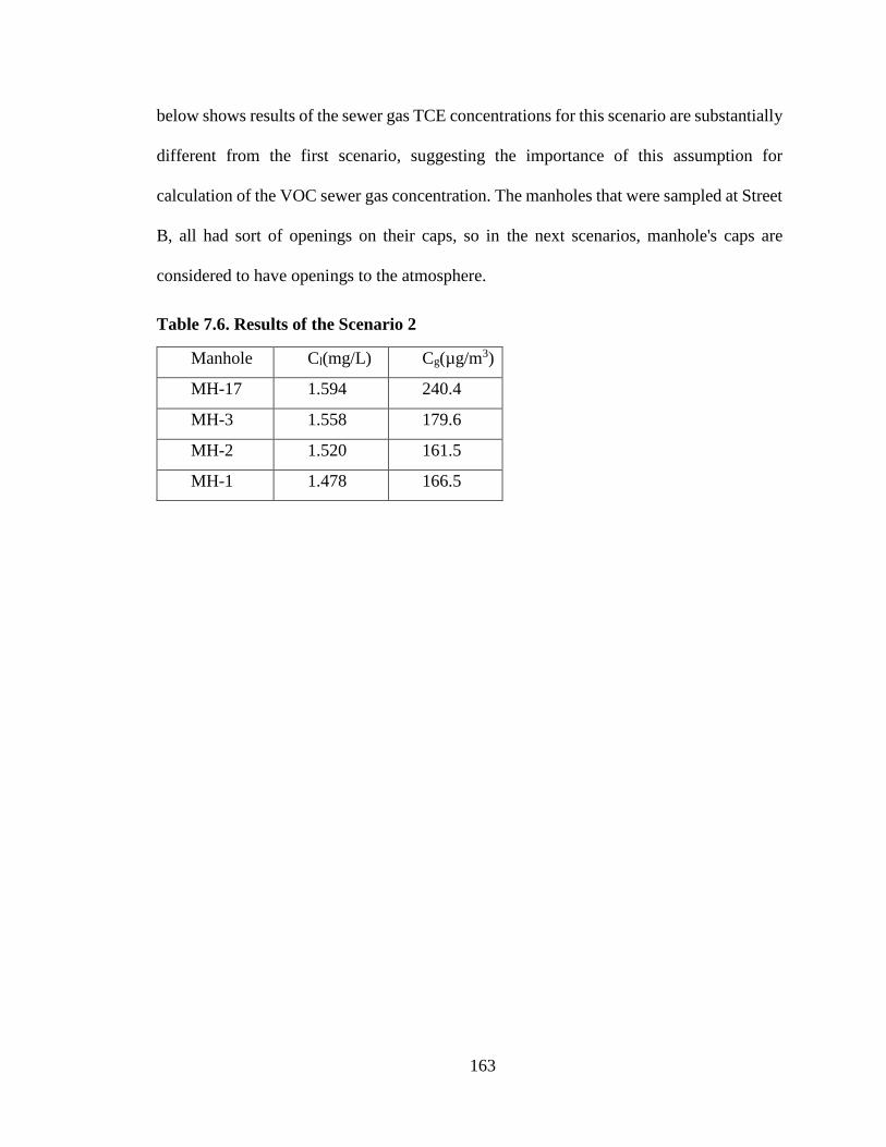
163
below shows results of the sewer gas TCE concentrations for this scenario are substantially
different from the first scenario, suggesting the importance of this assumption for
calculation of the VOC sewer gas concentration. The manholes that were sampled at Street
B, all had sort of openings on their caps, so in the next scenarios, manhole's caps are
considered to have openings to the atmosphere.
Table 7.6. Results of the Scenario 2
Manhole Cl(mg/L) Cg(µg/m3)
MH-17 1.594 240.4
MH-3 1.558 179.6
MH-2 1.520 161.5
MH-1 1.478 166.5

164
a) COMSOL manhole simulation
b) Velocity Profile calculated by COMSOL
Figure 7.2. COMSOL buoyancy velocity calculation
Scenario 3; tributary effect
For the Scenario 3 the sewer liquid and sewer gas that coming from MH-4 (tributary
flows) are added to the sewer model. This flow joins to the sewer main at MH-3. Different

165
depths for this flow is considered. Since all the measured TCE concentrations for this
manhole (MH-4) during different field sampling events were reported below the detection
limits (<1.04 µg/m3 for TO-17 method), it is assumed the sewer liquid and sewer gas that
join the sewer main from MH-4 are clean and TCE concentrations in both phases are equal
to zero. Sewer gas flow rate inside the sewer line is calculated by equation 7.27. Tables
7.7a - 7.7d show how the depth of the sewer liquid flow in MH-4, affect sewer liquid and
sewer gas concentrations all over the sewer system.
Table 7.7. Results of scenario 3; effects of tributary flow
a. Sewer liquid depth at MH-4= 0.01 m
Manhole Cl(mg/L) Cg(µg/m3)
MH-17 1.594 240.4
MH-3 1.528 133.6
MH-2 1.467 130.5
MH-1 1.404 149.4
b. Sewer liquid depth MH-4= 0.05 m
Manhole Cl(mg/L) Cg(µg/m3)
MH-17 1.594 240.4
MH-3 1.035 95.9
MH-2 1.007 92.5
MH-1 0.977 105.4
c. Sewer liquid depth at MH-4= 0.1 m
Manhole Cl(mg/L) Cg(µg/m3)
MH-17 1.59 240.4
MH-3 0.510 75.3
MH-2 0.504 64.9
MH-1 0.498 68.1
d. Sewer liquid depth at MH-4= 0.5 m
Manhole Cl(mg/L) Cg(µg/m3)
MH-17 1.594 240.4
MH-3 0.186 70.0
MH-2 0.186 52.8
MH-1 0.185 48.6
Result indicates sewer liquid and sewer gas concentration in MH-3 and downstream
of MH-3 are significantly affected by the tributary flow.

166
Scenario 4; Drop Structure effect
A drop structure is considered at the upstream of MH-3. Three different values are
considered for the drop structure height and results are shown in table below.
Table 7.8. Effect of the drop structure height
a. Drop structure height= 0.1m
Manhole Cl(mg/L) Cg(µg/m3)
MH-17 1.594 240.4
MH-3 0.471 95.3
MH-2 0.467 77.5
MH-1 0.462 77.1
b. Drop structure height= 0.25m
Manhole Cl(mg/L) Cg(µg/m3)
MH-17 1.594 240.4
MH-3 0.450 106.3
MH-2 0.447 84.4
MH-1 0.442 82.1
c. Drop structure height= 1 m
Manhole Cl(mg/L) Cg(µg/m3)
MH-17 1.594 240.4
MH-3 0.419 122.7
MH-2 0.417 94.7
MH-1 0.413 89.5
d. Drop structure height= 3 m
Manhole Cl(mg/L) Cg(µg/m3)
MH-17 1.594 240.4
MH-3 0.404 130.7
MH-2 0.402 99.8
MH-1 0.399 93.1
The sewer depth for MH-4 is considered to be =0.1 m. Figure 7.3 shows percentage of
TCE that transfers from the liquid phase to the gas phase. As it is shown in this figure the
drop structure transfer up to 21% of TCE from liquid phase to the gas phase. Figure 7.3
and table 7.8 also indicate substantial impact of the drop height on TCE mass transfer
between two phases and therefore TCE concentrations in both liquid and gas phases;
highlighting the necessity of having accurate information about the details of the sewer
line.

167
Figure 7.3. Effect of the drop structure height on TCE transfer from liquid phase
to the gas phase
Adsorption mechanisms
TCE adsorption inside the sewer system is added to the general mass transfer
mechanisms. Equation 7.10 has been used and different values for dissolved organic
compounds concentration (Sd) and suspended solid concentration (Ss) have been
considered. Sewer liquid depth at MH-4=0.1 m and drop structure height at MH-3=0.25 m.
Comparing results of the table 7.3b and table 7.4 suggests that adding adsorption to the
sewer model, decrease TCE concertation in both liquid and gas phases. This effect is
greater when Ss and Sd in the sewer liquid increases. Results also indicate that the impact
of adsorption on TCE sewer liquid concentration is greater than this impact on TCE sewer
gas concentration.

168
Table 7.9. Effect of adsorption on TCE sewer gas and sewer liquid concentration
a. Ss = 100 (mg/L); Sd= 100 (mg/L)
Manhole Cl(mg/L) Cg(µg/m3)
MH-17 1.557 239.3
MH-3 0.437 104.9
MH-2 0.423 82.8
MH-1 0.409 79.8
b. Ss = 250 (mg/L); Sd= 100 (mg/L)
Manhole Cl(mg/L) Cg(µg/m3)
MH-17 1.538 238.7
MH-3 0.430 104.2
MH-2 0.411 82.0
MH-1 0.393 78.6
c. Ss = 250 (mg/L); Sd= 200 (mg/L)
Manhole Cl(mg/L) Cg(µg/m3)
MH-17 1.515 238.0
MH-3 0.422 103.3
MH-2 0.397 81.1
MH-1 0.374 77.2
d. Ss = 500 (mg/L); Sd= 500 (mg/L)
Manhole Cl(mg/L) Cg(µg/m3)
MH-17 1.423 235.2
MH-3 0.389 99.7
MH-2 0.344 77.2
MH-1 0.304 71.9
Figure 7.4. Effect of adsorption on sewer liquid and sewer gas TCE concentration of
different manholes (Ss = 500 (mg/L); Sd= 500 (mg/L))

169
Figure 7.4 shows the impact of adding adsorption on TCE concentration in sewer liquid
and sewer gas (Sd=500 (mg/L) and Ss=500 (mg/L)) for different manholes .As figure 7.4
shows while by considering adsorption TCE concentration in liquid phase decrease 32% at
MH-1, TCE concertation in sewer gas only decreased 13% in sewer gas.
Biodegradation is not an important mass transfer mechanism for TCE in an aerobic
system such as a sanitary sewer (explained in section 7.2.2). Figure 7.5 compares the sewer
gas TCE concentration calculated for different cases with different assumptions with the
measured TCE concentrations at different manholes. Results of the one week passive
sampling at 2015 sampling event are used for comparison purpose since the average one
week TCE concentrations for all of these manholes were measure during that sampling
event.
Table 7.10. Summaries of cases platted on figure 7.5
a. Genral inputs of the model of all cases
Variables Comment
Targeted Chemical: TCE TCE was the major VOC
contamination at this site.
Temperature (T): 20°C (*) 20°C is used as the average
temperature for sewer liquid.
Cl (TCE)at MH upstream (MH18): 1.62 (mg/L) (*) Average TCE concentration in sewer
liquid for MH-18 measured at the site.
Cg (TCE)at MH upstream (MH18): 287 (µg/m3)) Average TCE concentration in sewer
gas for MH-18 measured at the site.
Groundwater TCE concentration: 5(mg/L) (*) The USEPA known plume at this site
is defined based on > 5(mg/L). The
study area is outside the known plume.
I used 5(mg/L) as the groundwater
TCE concentration in the study area.

170
Groundwater depth:4.04(m) (*) Averaged groundwater depth in the
study area, calculated based on
historical data.
MHs average depth: 5.70(m) Measured as part of field study.
Pipe radius: defined for each reach (constant) Obtained from sewer system as built
for this area.
Sewer line slope : defined for each reach (constant) Obtained from sewer system as built
for this area.
MHs distance: defined for each reach (constant) Calculated from sewer system as built
for this area.
Sewer liquid depth at MH-18= 0.2 (m) (*) Measured as part of field study
(average value).
Sewer liquid depth at other MHs= calculated (*) Calculated as part of sewer model
based on Sewer liquid depth at MH-18.
Sewer liquid velocity = calculated (*) Calculated as part of sewer model.
Sewer headspace velocity= calculated (*) Calculated as part of sewer model.
Suspended solid and dissolved organic carbon
concentration: defined (*)
Used different values (not measured).
Drop structure height: defined (can be assessed by
model)
Different values assessed by model.
Mass transfer parameters are calculated based on the mentioned inputs, and changing these
inputs will change VOC mass transfer rate. (*) indicates variables that can change by time.
b. Specific input of cases
Case 1 Close sewer system, no tributary from MH-4, no drop structure, no adsorption
Case 2 Open manhole , no tributary from MH-4, no drop structure, no adsorption
Case 3 Open manhole, depth at MH-4=0.1 m, no drop structure, no adsorption
Case 4 Open manhole, depth at MH-4=0.1 m, drop height=0.25 m, no adsorption
Case 5 Open manhole, depth at MH-4=0.1 m, drop height=0 m, adsorption (Ss = 250
(mg/L); Sd= 200 (mg/L))
Case 6 Open manhole, depth at MH-4=0.1 m, drop height=0.25 m, adsorption (Ss = 250
(mg/L); Sd= 200 (mg/L))

171
Figure 7.5. TCE measured concentration VS calculated concentration
For comparing results of the sewer gas model in different scenarios with the measured
TCE concentration, the one way ANOVA is used. P-values and standard error of estimate
are calculated for each case. The standard error of the estimate calculates the accuracy of
the models compared to the measured TCE concentrations. Equation 7.65 shows how this
value has been defined.
Standard error of the model estimate= √(∑(Ymodel−Ymeasured)2
df (7.65)
Ymodel = the value predicted by the model;

172
Ymeasured= the measured value (field data results);
df = degree of freedom.
Table 7.11. Results of statistic comparison
Case Standard error of the estimate P-value
Case 1 390.17 0.0003
Case 2 145.71 0.043
Case 3 44.58 0.671
Case 4 58.93 0.456
Case 5 41.58 0.703
Case 6 55.71 0.484
Result of the statistic comparison are shown in table 7.11. The P-values comparison
suggests TCE concentrations calculated by Case1 have significant differences with the
measured TCE concentrations, while TCE sewer gas concentrations calculated by case 3,
case 4, case 5 and case 6 are not significantly different from the measured TCE
concentrations. Comparing results of the standard error of estimation indicates Case 5
provides the best estimation of the measured TCE concentration. Results of Case 1 and
Case 2 do not match well with the field data; suggesting that considering the sewer line as
a closed system with no tributary are not appropriate assumptions for this model. Case 3
provides a better estimation compare to Case 4. Case 5 provides a better estimation
compare to Case 6; suggesting that scenarios with no drop structure are better matched
with the measured TCE concentrations and considering a drop structure in the sewer line
does not improve the model estimations for this area. Comparing accuracy of the Case 5
with Case 3 indicates that adding adsorption to the sewer model slightly improves the
model estimations but this effect is still not significant.

173
Biodegradation
As it is mentioned previously, biodegradation is not a significant mass transfer
mechanism for VOCs such as chloroform, PCE and TCE but it could be an important
mechanism to consider for VOCs such as toluene, methylene chloride, xylene and benzene
(Namkung and Rittmann, 1987; Wilson et al. 1994; Weber and Jones, 1986). In this section
the effect of biodegradation on toluene concentration in different scenarios is assessed. An
open sewer system with a 0.25 m drop structure at MH-3 and tributary flow with depth of
0.1 m from MH-4 to MH-3 is considered. Results of four different scenarios for toluene
sewer gas and sewer liquid concentrations are shown in table below. The boundary
conditions and model inputs are the same as mentioned in Table 7.4.
Both adoption and biodegradation affect toluene concentrations in both sewer liquid
and sewer gas. Kd is an important factor for calculating the biodegradation rate and as it
shown by Table 7.12 c and 7.12 d have a considerable impact on the results. Namkung and
Rittmann (1987) suggested a range of Kd values between 0.21(m3/g.d) and 0.4 (m3/g.d).
The rate of the biodegradation is a strong function of the system's condition. Depending on
the value chosen for Kd the effect of biodegradation on toluene concentration in sewer
liquid and sewer gas can be different.

174
Table 7.12. Comparing different factor on Toluene concentration
a. No adsorption/No biodegradation
Manhole Cl(mg/L) Cg(µg/m3)
MH-17 1.599 238.9
MH-3 0.456 103.6
MH-2 0.454 79.8
MH-1 0.451 75.8
b. Adsorption1 /No biodegradation
Manhole Cl(mg/L) Cg(µg/m3)
MH-17 1.541 236.4
MH-3 0.434 101.1
MH-2 0.419 77.0
MH-1 0.399 71.6
c. Adsorption/biodegradation
(Kd=0.1 (m3/g.d))
Manhole Cl(mg/L) Cg(µg/m3)
MH-17 1.416 231.2
MH-3 0.391 96.0
MH-2 0.361 71.8
MH-1 0.337 65.3
d. Adsorption/biodegradation
(Kd=0.4 (m3/g.d))
Manhole Cl(mg/L) Cg(µg/m3)
MH-17 1.139 219.6
MH-3 0.296 84.9
MH-2 0.247 60.9
MH-1 0.214 52.4
Note 1: For scenario b, c and d Ss= 250 (mg/L) and Sd= 200 (mg/L).
Temporal variations
Results of the vapor intrusion field studies indicate there is a significant temporal
variations for sewer gas VOC concentrations even for one sampling location (e.g. Roghani
et al., 2018). The sewer model inputs variation and their impact on the model result can be
assessed to evaluate the source of the temporal fluctuations. The sewer model inputs have
been summarized in table 7.4. Some of the model inputs such as temperature, groundwater
depth, groundwater VOC concentration, sewer liquid VOC concentration, sewer liquid
flowrate, sewer liquid depth inside the sewer system, sewer headspace velocity, sewer
liquid qualities such as suspended solid concentration and dissolved organic concentration
may change over time and their fluctuations potentially have different levels of impacts on
the rate of VOC mass transfer and on VOC concentrations inside the sewer system.

175
Variations of these parameters over time could be responsible for the observed temporal
variations of sewer gas VOC concentration. Some of the sewer model inputs such as the
sewer headspace velocity and sewer liquid depth have been reported to have substantial
impacts on the sewer gas VOC concentrations by previous studies. Considering the number
of parameters involved on the fate and transport of VOCs inside the sewer system the
substantial temporal variations can be expected.
Table 7.13 compares results of the sewer model for Case 5 (defined at Table 7.10) when
the depths of the sewer liquid flows that are coming to the defined system (from MH-18
and MH-4 (tributary flow)) proportionally change at the same time. The sewer liquid
depths coming from MH-18 and MH-4 both are multiplied to 0.5 for one scenario (result
shown on table 7.13 b) and multiplied to 1.5 for another scenario (results shown on table
7.13 c). As this table shows fluctuation in the sewer depths resulted in different ways for
different manholes. When the ratio of the sewer liquid depth to the pipe diameter decreases,
there is a greater headspace volume available for VOCs mass transfer and this increase the
rate of VOC mass transfer and remove more VOC from the liquid phase. It doesn’t
necessary result in more VOC concertation in the gas phase since the lower sewer liquid
depth provide more volume of gas. At the same time, by decreasing the depth of the sewer
liquid, the velocity of the sewer liquid also decreases and so it reduces the liquid gas mass
transfer rate. When sewer liquid velocity decreases, the headspace velocity also decrease,
therefore VOC accumulation rate in the sewer headspace increases. With lower VOC
concentration in the headspace a greater concentration gradient exist between liquid and
gas phases. Several parameters in this sewer model are the function of other parameters
and it is the biggest difference between results of this study with previously VOC mass

176
transfer studies (e.g. Corsi and Birkett, 1995; Parker and Yu, 2001). For example changing
the sewer system depths, changes the calculated sewer liquid velocity. At different sewer
liquid velocity we have different liquid-gas mass transfer rate and also different sewer
headspace velocity. This study suggests that investigating the impact of one parameter on
the result of VOC concentrations all over the sewer system without considering the possible
impact of this change on the other parameters, may result in misleading conclusions.
Table 7.13. Effect of sewer liquid depth fluctuation on TCE concentration
a. Case 5
Manhole Cl(mg/L) Cg(µg/m3)
MH-17 1.515 238.0
MH-3 0.476 74.1
MH-2 0.447 62.6
MH-1 0.419 63.9
b. Sewer liquid depths=0.5 * Case 0.5
Manhole Cl(mg/L) Cg(µg/m3)
MH-17 1.486 224.3
MH-3 0.471 65.0
MH-2 0.436 55.7
MH-1 0.402 54.2
c. Sewer liquid depths=1.5 * Case 5
Manhole Cl(mg/L) Cg(µg/m3)
MH-17 1.522 233.1
MH-3 0.468 90.0
MH-2 0.442 54.2
MH-1 0.416 59.8
Note: Doubling the sewer liquid depths
for both inflows (coming from MH-18 and
MH-4) to the system resulted in overflow
in sewer line between MH-3 and MH- 2,
suggested by the sewer model.
A Different approach for calculating sewer headspace velocity
There are several parameters that complicate the calculation of sewer headspace
velocity inside the sewer system. Sewer systems have thousands of openings to the
atmosphere through manholes. There is a unique air pressure profile through each manhole
and that makes it very complicated to develop a model to estimate sewer headspace

177
velocity through this system. Lows (2017) developed a numerical model to calculate the
sewer headspace velocity based on the USEPA storm water management model (SWMM)
hydraulic outputs. SWMM is a dynamic rainfall-runoff simulation model that provides
hydraulic inputs which are critical for calculating the air flow rate inside the sewer system.
Results of a field study conducted by Parker and Ryan (2001) in Ottawa-Carleton over
11km sanitary sewer system have been used to calibrate the model. SWMM model
computed the sewer liquid velocity and the sewer gas velocity were measured through the
field study. The best relation between the measured headspace velocity and the calculated
sewer liquid velocity (outputs of SWMM model) are described by a polynomial equation
shown by equation below.
Vg= 0.242 Vl – 0.032 (Vl) 2 (7.66)
Equation 7.66 was applied by the sewer model to calculate the sewer headspace
velocity. While sewer headspace velocities calculated by equation 7.27 are in the range of
15% - 30% of the sewer liquid velocities for the selected sewer system in Street A, the
sewer headspace velocities calculated by equation 7.66 are slightly different and in the
range of 13% - 23% of the sewer liquid velocities. Result of the sewer headspace velocity
for each manhole calculated by equation 7.66 is compared with the result of the sewer
headspace velocity calculated by equation 7.27 that are shown in figure below.

178
Figure 7.6. Comparing sewer headspace velocity calculated by two models.
Figure 7.7 compares results of the calculated sewer gas TCE concentrations calculated
by applying two different equations for estimating the sewer headspace velocity (Equation
7.27 and Equation 7.66). This figure shows that the different approaches for calculating
head space velocity equations (Prescod and Price 1982 (Equation 7.27) compared to Lowe
2017 (Equation 7.66)) for calculating the sewer headspace velocity does not have a
significant effect on TCE sewer gas concentration, as shown on Figure 7.7.

179
Figure 7.7. Comparing sewer TCE concentrations calculated by two sewer
headspace velocity models
7.4. Conclusions
There is increased evidence of the sewer systems to act as an alternative pathway for
vapor intrusion. Therefore, hazardous waste sites that are contaminated with VOCs may
need additional evaluation to determine if inhalation exposure due to sewer gas intrusion
is a concern. There is no standard method to investigate the potential contribution of sewer
pathways at hazardous sites. The occurrence of VOCs inside the sewer system and more
specifically sewer gas and temporal and spatial variations have not been well characterized.
In this chapter a numerical model was developed to assess the sewer gas VOC
concentration, the potential source of VOC and parameters that are responsible for sewer
gas temporal and spatial variations. Sewer gas VOC concentrations calculated by this
model are sensitive to the sewer specifics and several parameters; suggesting sewer gas

180
concentration in field settings are likely to exhibit high spatial and temporal variation. This
is confirmed by several vapor intrusion field studies. This model provides a tool to better
understand variations of VOCs inside the sewer system. Combining results of the field
study with numerical modeling allows us to improve our understanding regarding the
exposure risk associated with sewer gas inhalation and further to identify the primary
source of VOC in contaminated sites.

181
Chapter 8: CONCLUSION AND RECOMMENDATIONS
8.1. Findings
This research aimed to investigate unexpected observations during vapor intrusion field
studies at contaminated sites. The findings included: 1) non-linear soil gas concentration
trends between the VOC source and ground surface and 2) alternative pathways that serve
as entry points for VOC vapors to infiltrate into the buildings. These observations indicate
that VOC exposure risks as compared to the classic vapor intrusion models that primarily
consider groundwater sources and foundation cracks as the route for vapor entry are
inadequate.
The results of this research as described in Chapters 3 and 4 support that non-linear soil
gas VOC concentration trends between groundwater and atmosphere warrants careful
consideration and may not support groundwater concentrations being indicative of vapor
intrusion sources. As discussed in Chapters 5-7, when indoor air concentrations are
elevated, other sources of VOCs should be considered, such as sewer gas and other
conduits for VOC entry. By systematically reviewing data and incorporating numerical
modeling, this research applied a multiple lines of evidence approach to better understand
and interpret the field data.
For non-linear soil gas VOC concentration trends, the research suggested that a
subsurface feature present in the study area was limiting VOC vapor diffusion and may be
reducing upward VOC mass flux. The results of this study indicate that collected
groundwater data did not provide an appropriate metric for evaluating the inhalation
exposure risks and therefore relying on groundwater concentrations for investigating the
vapor intrusion exposure risk at the site is not adequate. Incorporating numerical models

182
with field samplings as part of multiple lines of evidence, can improve risk management
decisions at hazardous sites (Pennell et al. 2016).
When considering alternative pathways for vapor intrusion entry, the research
investigated the occurrence of VOCs in a sanitary sewer system adjacent to and extending
hundreds of feet away from a previously defined vapor intrusion area by conducting a field
study over the years of 2014-2017 (Roghani et al 2018). Different sampling techniques
were used for collecting data and a considerable spatial and temporal variations were
observed. Interpreting the sewer gas VOC concentrations is complex due to spatial and
temporal variations. Incorporating a numerical model with field data may improve one's
ability to evaluate the field data. A numerical sewer gas model is developed as part of this
research to improve our understanding about the results of the field study. The numerical
model simulates VOCs different mass transfer mechanisms within the sewer systems and
assesses the sewer gas VOC concentration for different scenarios to identify the best
assumptions. Sewer gas concentrations calculated by the model are sensitive to sewer
specifics and several parameters; suggesting sewer gas concentrations in field settings are
likely to exhibit high spatial and temporal variation. The result of the model for some
scenarios showed an appropriate compatibility with the field data. The developed model
provides a potential tool to better understand temporal and spatial variations of VOC inside
the sewer system and variables at play. It also allows an improved method for
understanding exposure risks associated with sewer gas intrusion.

183
8.2. Limitation of the study
Evaluating the inhalation exposure risk due to VOC vapor intrusion is complicated due
to several reasons. This research like most vapor intrusion studies was subject to the
following limitations:
1. Vapor intrusion characterization is difficult to accomplish because of the sampling
limitations. Like most vapor intrusion sites across the country, each property and area had
certain limitations that sometimes could not be overcome. For some data collections such
as indoor air sampling or manhole/clean-outs sampling, different access restrictions
existed. Prior to initiating such a study the field study team members should meet with the
residents to discuss the sampling process and to survey and remove possible indoor sources
of VOCs from the home. The access permission process is time consuming and is not
always successful so for the field study that we conducted in the South San Francisco Bay
area, we did not collect any indoor air samples. To access sewer manholes and laterals the
city permission is needed.
Some limitations for VOC samplings are site specific. For instance Property B of
Pennell et al (2016), had an active vapor intrusion mitigation system and the basement floor
and walls had been sealed prior to the research. The vapor intrusion exposure risks for this
building were evaluated by using soil gas and groundwater data, along with 3D modeling.
Other limitations for vapor intrusion field assessments include the amount of time the
sampling group have to access the property, the cost of sampling, the detection limits of
each method, and the accessibility of the sampling area. Assessing the real soil moisture
profile in the area is one of the biggest challenges, due to the difficulty to access soil in
deeper areas and because several parameters may change the soil moisture profile.
184
2. Temporal and spatial variations of the VOC concentrations are reported in several
vapor intrusion field studies. Most vapor intrusion field data do not easily follow the
predicted trends. One of the challenges for a vapor intrusion field study is to find a trend
and make sense of the data. This research suggests the essential need to apply a multiple
lines of evidence approach. Using this approach required collecting different data (e.g.
indoor air, soil gas in different depth, groundwater). Due to the high temporal variations
using a continuous monitoring devices can improve our understanding about the magnitude
of variations. These devices can be used for monitoring VOC concentrations and recording
the depth of groundwater with time. Applying these devices are usually expensive and
requires a trained operator.
3. The numerical models we developed calculate VOC concentration in a steady state
condition for each phase. We didn’t solve the numerical model for a transient situation.
The numerical model transient solution is more computationally expensive but could be
the focus of future research.
4. Investigating the temporal variations for VOC concentration in sewer gas or indoor
air is complicated. The developed model does not address the temporal variations impact
on the calculated concentrations. It may be possible by more sophisticated models.
8.3. Research contributions
This research aims to be useful for knowledge broker by improving the available
knowledge for assessing inhalation exposure risks associated with VOC vapor intrusion.
Knowledge brokers are middle-people (or organizations) that transfer knowledge, improve
the available knowledge and facilitate its sharing in more demanded and urgent direction.
This study investigated unexpected detections of VOCs at vapor intrusion sites. The

185
contributions of this research to the body of vapor intrusion risk assessment knowledge are
as follow:
1. Results of a field study with non-linear soil gas concentrations was investigated.
Through systematically reviewing historical and ongoing filed data and incorporating a
numerical model VOC vapor intrusion risk assessment at this site has been accomplished.
A site specific numerical model has been developed and different scenarios were examined
to predict VOC concentrations. This assessment highlighted the important potential of
subsurface features on VOC vapor intrusion. This study concludes that a numerical model
can address uncertainty in indoor air concentrations related to vapor intrusion and suggests
by applying a multiple lines of evidence approach, decisions can be made about how to
manage vapor intrusion exposure risks.
2. This research studied the unexpected detection of VOC in buildings due to
alternative pathways. Aging infrastructure and more specifically sanitary sewer systems
were investigated as part of this study. To date, the sewer gas to indoor air pathway at vapor
intrusion sites has not been well characterized and there are no standard procedures
available for assessing this pathway at vapor intrusion sites. As part of this research a multi-
year field study was conducted within a community in the California Bay Area to address
the lack of information about how often alternative vapor intrusion pathways exist, and
provides one of the few attempts to document the occurrence and variability of VOCs in
sanitary sewer gas. A preliminary conceptual model was developed and different sampling
methods were used to assess the temporal and spatial variability of VOCs within the sewer
system. This information is needed to ultimately inform about developing appropriate
sampling strategies, which are still emerging. This study concludes that a comprehensive

186
vapor intrusion risk assessment should include an investigation of any sewer lines that are
in close proximity to any nearby groundwater contamination plumes. The researchers
honed knowledge brokering skills by interacting with the city, federal regulatory agency
staff, consultants, and entrepreneurs.
3. Interpreting sewer gas concentrations is complex due to spatial and temporal
variations. Multiple lines of evidence are critical to fully understanding the fate and
transport of VOCs inside sewer systems and to assess the resulting inhalation exposure
risks that may exist in buildings that are connected to the sewer systems. Bases on this need
a numerical model is developed to investigate VOC concentrations within the sewer
system. This model provides a tool to better understand the temporal and spatial variations
of VOCs inside the sewer system and the associated relevant variables. It also allows an
improved method for understanding exposure risks associated with sewer gas intrusion.
The researchers communicated with the research community, federal regulatory staff and
community leaders about the research outcomes.
8.4. Opportunities for future research
Potential future research is needed in order to improve the available knowledge about
vapor intrusion and provide more insights about vapor intrusion risk assessment in VOC
contaminated sites. Such research includes the following:
1. Develop a transient model to assess soil gas and indoor air concentrations in response
to groundwater seasonal behavior may provide a better screening tool.
2. Improve the subsurface numerical model to consider the impact of water lenses,
groundwater fluctuations and atmospheric effects on soil gas transport and consider

187
possible mass transfer mechanisms in the subsurface such as biodegradation and
adsorption.
3. Conduct tracer studies to calculate headspace velocity inside the sewer system and
investigate sewer gas to indoor air attenuation factors for VOCs contaminated areas to
provide a better tool for decision makers about inhalation exposure risks.
4. Develop a transient numerical model for sewer gas that accounts for temporal
variations inside the sewer system and their potential impact on the results.
5. Develop a numerical model to calculate the sewer gas to indoor air attenuation factor
by considering different mass transfer mechanisms in the subsurface, sewer system, and
indoor air to account for the sewer system and the building’s characteristics.

188
APPENDICES
Appendix A
Soil Properties
Table A.2. Compositions, mean particle diameters and dry bulk density of the 12 SCS
soil textural classifications
Table A2. Compositions, mean particle diameters and dry bulk density of the 12 SCS soil
textural classifications
ASTM D422 test procedure (Sieve Analysis)
GC/FID Head Space Analysis Calibration (Direct Injection Method)
Table A1. Compositions, mean particle diameters and dry bulk density of the 12 SCS soil
textural classifications
SCS Texture
class clay% silt% sand%
Mean particle
diameter, cm
Dry bulk
density, g/cm
Sand 3.33 5.00 91.67 0.044 1.66
Loamy sand 6.25 11.25 82.50 0.040 1.62
Sandy loam 10.81 27.22 61.97 0.30 1.62
Sandy clay loam 26.73 12.56 60.71 0.029 1.63
Sandy clay 41.67 6.67 51.66 0.25 1.63
Loam 18.83 41.01 40.16 0.020 1.59
Clay loam 33.50 34.00 32.50 0.016 1.48
Silt loam 12.57 65.69 21.74 0.011 1.49
Clay 64.83 16.55 18.62 0.0092 1.43
Silty clay loam 33.50 56.50 10.00 0.0056 1.63
Silt 6.00 87.00 7.00 0.0046 1.35
Silty clay 46.67 46.67 6.66 0.0039 1.38

189
Table A2. Compositions, mean particle diameters and dry bulk density of the 12 SCS soil
textural classifications
SCS Texture class
Saturated
water
content
Residential
water
content
Van Genuchten parameters
α(1/cm) N M
Clay 0.459 0.098 0.01496 1.253 0.2019
Clay loam 0.422 0.079 0.01581 1.416 0.2938
Loam 0.399 0.061 0.01112 1.472 0.3207
Loamy sand 0.390 0.049 0.03475 1.746 0.4273
Silt 0.489 0.050 0.00658 1.679 0.4044
Silty loam 0.439 0.065 0.00506 1.663 0.3987
Silty clay 0.481 0.111 0.01622 1.321 0.2430
Silty clay loam 0.482 0.090 0.00839 1.521 0.3425
Sand 0.375 0.053 0.03524 3.177 0.6852
Sandy clay 0.385 0.117 0.03342 1.208 0.1722
Sandy clay loam 0.384 0.063 0.02109 1.330 0.2481
Sandy loam 0.387 0.039 0.02667 1.449 0.3099

190
ASTM D422 test procedure (Sieve Analysis):
1. Measure the weight of every sieve and the bottom pan.
2. Measure the weight of the given dry soil sample.
3. Clean the sieves and assemble them in the ascending order based on their numbers (#4
sieve at top and #200 sieve at bottom) and put the pan below #200 sieve.
4. Now pour the soil sample into the top sieve and place the cap over it.
5. Place the sieve stack in the mechanical shaker and shake for 10 minutes.
6. Remove the stack from the shaker, measure the weight of each sieve with its retained
soil. Don’t forget to measure the weight of the bottom pan with its retained fine soil.
Insert all this data in table below.
Sieve no. Diameter(mm) Mass retained % retained %passing
4
10
20
40
60
100
200
Pan
Total weight

191
Figure A1. The grain size distribution curve (Bowels, 1992).

192
GC/FID Head Space Analysis Calibration (Direct Injection Method)
1. Fill a 40 mL VOA with 30 mL of methanol and cap off. Inject 100 μL of PCE into the
methanol. Invert the VOA five times to mix and store upside down to prevent out-
gassing. This is solution A.
2. Fill another 40 mL VOA with 20 mL of deionized water and cap off. Inject 10 μL of
solution A. Invert this VOA five times to mix and store upside down to prevent out-
gassing.
3. Repeat step 2, using 20 μL, 50 μL, 100 μL, 200 μL and 200 μL of solution A.
4. Dilute solution A 10-fold by filling a 40 mL VOA with 1 mL of solution A and 9 mL
of methanol. This is solution B.
5. Repeat step 2, using 10 μL, 20 μL, and 50 μL of solution B.
6. Dilute solution B 10-fold (solution A 100-fold) by filling a 40 mL VOA with 1 mL of
solution B and 9 mL of methanol. This is solution C.
7. Repeat step 2, using 10 μL, 20 μL, 30 μL, and 50 μL of solution C.
8. Dilute solution C 10-fold (solution A 1,000-fold) by filling a 40 mL VOA with 1 mL
of solution C and 9 mL of methanol. This is solution D.
9. Repeat step 2, using 10 μL, 20 μL, 30 μL, and 50 μL of solution D.
10. Dilute solution D 10-fold (solution A 10,000-fold) by filling a 40 mL VOA with 1 mL
of solution D and 9 mL of methanol. This is solution F.
11. Repeat step 2, using 50 μL of solution F.
12. Allow all calibration solutions to equilibrate for at least 20 minutes.

193
13. When the samples are ready, insert a locked 10 mL locking syringe into the airspace
above the liquid in the VOA containing the lowest concentration of PCE (made in step
11), unlock the syringe, pull out 7 mL of air, and lock.
14. Screw the syringe into the GC injection port, depress the syringe to the 5 mL mark to
put air under pressure, unlock, and depress completely to push all air into the GC.
15. Immediately press Start to run the GC/FID method.
16. Repeat steps 13-15 for all remaining samples, injecting from lowest concentration of
PCE to highest concentration of PCE.

194
Appendix B
Occurrence of chlorinated volatile organic compounds (VOCs) in a sanitary
sewer system: Implications for assessing vapor intrusion alternative
pathways
Table B.3. TO-15 analytical results (sewer gas), 2014 − (µg/m3)
Table B.2. TO-17 analytical results (sewer gas), 2015 − (µg/m3)
Table B.3. TO-15 analytical results (sewer gas), 2015 − (µg/m3)
Chemical abbreviations:
TCE: Trichloroethylene; PCE: Tetrachloroethylene; CFC-113: 1,1,2-Trichloro-1,2,2-
trifluoroethane; DCE: Dichloroethene; DCA: Dichloroethane; TCA: Trichloroethane.

195
Table B.4 TO-15 analytical results (sewer gas), 2014 − (µg/m3)
Location Manhole invert
(ft bgs) Sample date Sample time TCE
MH-1 22.0 3/5/2014 11:26 1200
MH-2 19.8 3/5/2014 11:20 1000
MH-3 18.0 3/5/2014 11:15 64
7/18/2014 12:29 50
MH-4 13.1 3/5/2014 11:11 <5.4
7/18/2014 15:32 <5
MH-6 10.9 1/28/2014 16:51 <5
MH-9 11.4 3/5/2014 13:38 150
MH-11 10.7 2/13/2014 14:56 180
MH-12 11.2 2/13/2014 12:04 700c
MH-13 12.8 1/28/2014 17:25 1000c
2/13/2014 11:10 300c
MH-14 13.6 2/13/2014 10:55 800c
MH-16 9.1 2/13/2014 11:30 200
MH-17 17.0 3/5/2014 11:58 1600
7/18/2014 12:39 9a,d
MH-18 16.8 3/5/2014 11:05 1400
MH-19 16.8 3/5/2014 11:00 1300
Note 1: a Data below limit of quantification (LOQ) but above limit of detection (LOD). b Sample diluted at
laboratory to achieve concentrations in calibration range. c Sample re-analysis. d Estimated value.
bgs: below ground surface. NS—Not Sampled.
Note 2: Sampling depth for these events was 3 ft bgs. Sewer air grab samples were collected over a period
of < 5 min. For non-detected results, < detection limit is shown.
Note 3: All chemical abbreviations are provided on the first page of the Supplementary Material.

196
Table B.2 TO-17 analytical results (sewer gas), 2015 − (µg/m3)
Location
TO-17 Analytical Results (µg/m3)
TCE PCE Chloroform Toluene Ethylbenzene m- & p-
Xylene
o-
Xylene
MH-1 47b 32.22 <1.02 15.97 <2.23 2.25 <2.04
MH-2 39.30 14 <1.02 16.7 <2.23 2.62 <2.04
MH-3 78b 18.73 1.18a 38b <2.23 3.6 <2.04
MH-4 <1.04 <1.07 <1.02 7.91 <2.23 <2.04 <2.04
MH-5 <1.04 <1.07 <1.02 8.12 <2.23 <2.04 <2.04
MH-6 1.62a 1.91a <1.02 5.16 <2.23 <2.04 <2.04
MH-71 NS NS NS NS NS NS NS
MH-8 1.43a <1.07 <1.02 18.11 <2.23 <2.04 <2.04
MH-9 85b 65a 2.35 24.38 <2.23 2.69 <2.04
MH-10 <1.04 <1.07 <1.02 <1.88 <2.23 <2.04 <2.04
MH-11 91.58d 85.4d 2.69 30.84 <2.23 <2.04 <2.04
MH-12 201.77d 182.79d 1.22a 6.24 <2.23 <2.04 <2.04
MH-13 121d 29.33 <1.02 4.5 <2.23 <2.04 <2.04
MH-14 171.59d 42.61 1.57a 5.81 <2.23 <2.04 <2.04
MH-15 166.16d 17.06 1.08a <1.88 <2.23 <2.04 <2.04
MH-16 26.52 24.71 <1.02 6.33 <2.23 <2.04 <2.04
MH-17 187.43d 41.06 1.13a 15.84 <2.23 2.13 <2.04
CO-1 2.73 2.51 <1.02 <1.88 <2.23 <2.04 <2.04
CO-2 <1.04 <1.07 <1.02 <1.88 <2.23 <2.04 <2.04
CO-3 <1.04 9.88 <1.02 <1.88 <2.23 3.27 <2.04
CO-4 <1.04 <1.07 <1.02 <1.88 <2.23 <2.04 <2.04
CO-5 <1.04 <1.07 <1.02 <1.88 <2.23 <2.04 <2.04
CO-62 NS NS NS NS NS NS NS
CO-7 11.13 9.25 3.7 67b 2.64 7.2 2.56
CO-8 <1.04 <1.07 <1.02 <1.88 <2.23 <2.04 <2.04
CO-9 <1.04 <1.07 <1.02 <1.88 <2.23 <2.04 <2.04
CO-10 21.89 14.44 7.47 25.12 <2.23 3.94 <2.04
CO-112 NS NS NS NS NS NS NS
CO-12 1.26a <1.07 1.84a <1.88 <2.23 <2.04 <2.04
CO-13 1.14a 11.26 <1.02 <1.88 <2.23 3.93 <2.04
CO-14 107b 78b 6.51 11.22 <2.23 <2.04 <2.04
CO-15 <1.04 <1.07 <1.02 <1.88 <2.23 <2.04 <2.04
CO-16 21.69 173b 8.95 <1.88 <2.23 <2.04 <2.04
CO-17 17.02 8.27 <1.02 <1.88 <2.23 <2.04 <2.04
CO-18 10.26 7.94 1.55a <1.88 <2.23 <2.04 <2.04
CO-19 <1.04 <1.07 <1.02 <1.88 <2.23 <2.04 <2.04
CO-20 9.65 21.56 <1.02 2.09 <2.23 5.56 2.64
CO-21 <1.04 <1.07 <1.02 <1.88 <2.23 <2.04 <2.04
CO-22 2.27 92b <1.02 2.27 <2.23 8.39 4.34
Note 1: Benzene was not detected in all sampling locations.
Note 2: a Data below limit of quantification (LOQ) but above limit of detection (LOD). b Sample diluted at
laboratory to achieve concentrations in calibration range. c Sample re-analysis. d Estimated value because
concentration was above the calibration range. NS—Not Sampled. Sampling depth was 1 ft for all samples
in this event.
Note 3: 1 MH-7 sample was not analyzed because the sampling tube was absent from the manhole upon
retrieval. 2 CO-6 and CO-11 could not be accessed for sampling.
Note 4: All chemical abbreviations are provided on the first page of the Supplementary Material.

197
Table B.3 TO-15 analytical results (sewer gas), 2015 − (µg/m3)
Location TCE PCE Chloro-
form Toluene
1,1,1-
TCA
1,1-
DCE
trans-1,2-
DCE CFC-113 1,1-DCA
cis-1,2-
DCE
MH-1 10 7a,d 10 <4 <6 <4 <4 <8 <4b,d <4
MH-2 20 <7 50 5a,d <6 <4 <4 <8 <4b,d <4
MH-3 200 30 300c 60 <6 <4 <4 <8 <4b,d 30
MH-4 NS NS NS NS NS NS NS NS NS NS
MH-5 NS NS NS NS NS NS NS NS NS NS
MH-6 NS NS NS NS NS NS NS NS NS NS
MH-7 20c <10c 20a,c 6a,d,c <9c <7c <7c <10c <7b,d,c <7c
MH-8 NS NS NS NS NS NS NS NS NS NS
MH-9 40 10 100 6a,d <6 <4 <4 <8 <4 10
MH-10 NS NS NS NS NS NS NS NS NS NS
MH-11 80 30 80 <4 <6 <4 <4 <8 <4b,d 40
MH-12 200 60 30 <4 <6 <4 <4 <8 <4b,d 30
MH-13 8a,d <7 20 <4 <6 <4 <4 <8 <4b,d 9
MH-14 10 <7 20 <4 <5 <4 <4 <8 <4b,d 9
MH-15 20 <7 8a,d <4 <6 <4 <4 <8 <4b,d 9
MH-15 (2) 20 <7 6a,d <4 <5 <4 <4 <7 <4b,d 7a,d
MH-16 70 9a,d 100 10 <6 <4 <4 <8 <4b,d 40
MH-17 500c 80 300c 100c 9a,d 9 9 20 6a,b,d 50
CO-1 <5 <7 <5 <4 <6 <4 <4 <8 <4b,d <4
CO-2 <5 <7 <5 <4 <6 <4 <4 <8 <4b,d <4
CO-3 <5 <7 <5 <4 <5 <4 <4 <8 <4b,d <4
CO-4 <6 <7 <5 <4 <5 <4 <4 <8 <4b,d <4
CO-5 NS NS NS NS NS NS NS NS NS NS
CO-6 NS NS NS NS NS NS NS NS NS NS
CO-7 <5 <7 <5 <4 <6 <4 <4 <8 <4b,d <4
CO-8 NS NS NS NS NS NS NS NS NS NS
CO-9 NS NS NS NS NS NS NS NS NS NS
CO-10 NS NS NS NS NS NS NS NS NS NS
CO-11 NS NS NS NS NS NS NS NS NS NS
CO-12 NS NS NS NS NS NS NS NS NS NS
CO-13 NS NS NS NS NS NS NS NS NS NS
CO-14 NS NS NS NS NS NS NS NS NS NS
CO-15 <5 <7 <5 <4 <6 <4 <4 <8 <4b,d <4
CO-16 50 300c 200c <4 <6 <4 <4 <8 <4b,d <4
CO-17 20 <7 <5 <4 <6 <4 <4 <8 <4b,d <4
CO-18 <5 <7 <5 <4 <6 <4 <4 <8 <4b,d <4
CO-19 <6 <7 <5 <4 <6 <4 <4 <8 <4b,d <4
CO-20 <6 <7 <5 <4 <6 <4 <4 <8 <4b,d <4
CO-21 <6 <7 <5 <4 <6 <4 <4 <8 <4b,d <4
CO-22 <6 30 30 <4 <6 <4 <4 <8 <4b,d <4
Note 1: Vinyl Chloride, Benzene, Ethylbenzene, m- & p-Xylene, o-Xylene, and 1,2-Dichlorobenzene were
reported not detected in all sampling locations.
Note 2: a Data below limit of quantification (LOQ). b The initial calibration for this analyte did not meet
calibration criteria. c Sample re-analysis. d Estimated value. NS—Not Sampled. Sampling depth was 3 ft for
all samples in this event.
Note 3: All chemical abbreviations are provided on the first page of the Supplementary Material.
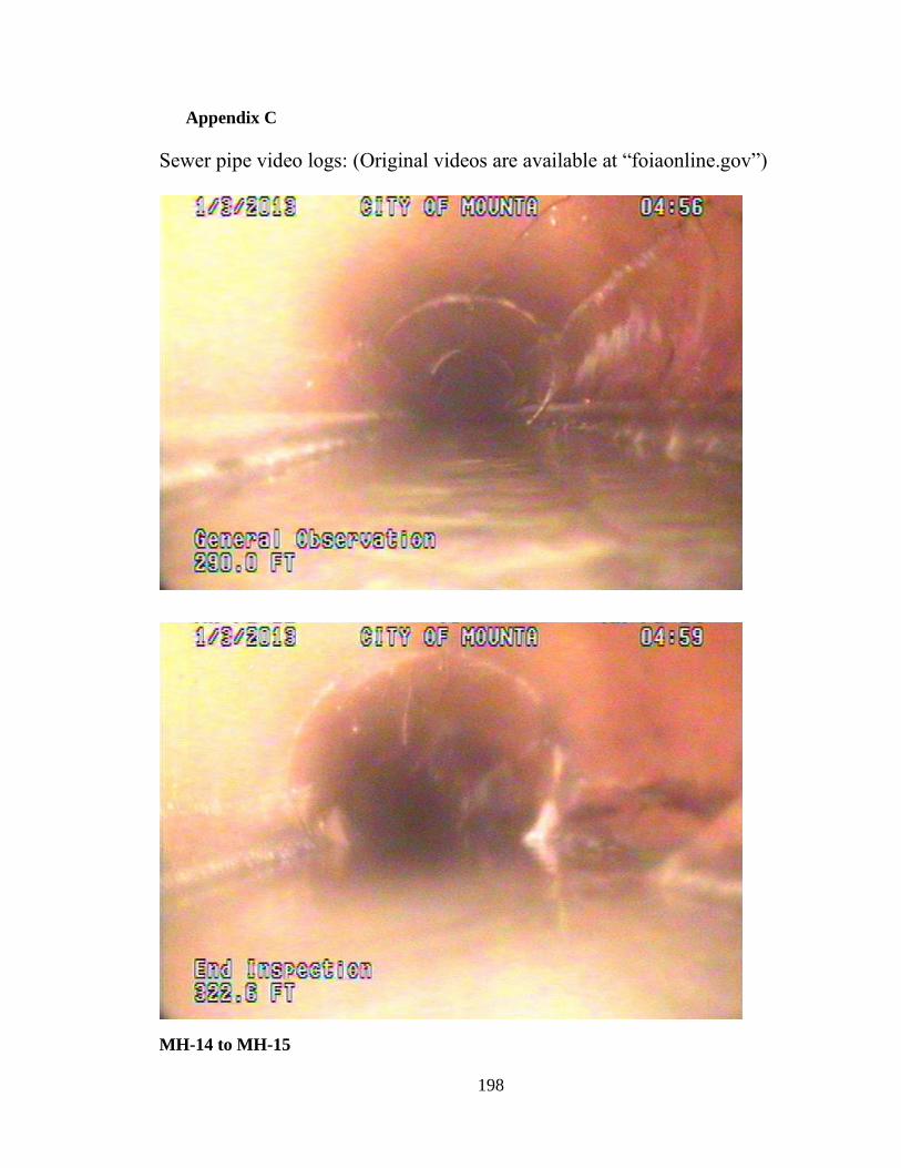
198
Appendix C
Sewer pipe video logs: (Original videos are available at “foiaonline.gov”)
MH-14 to MH-15

199
MH-14 to MH-15

200
MH-14 to MH-15
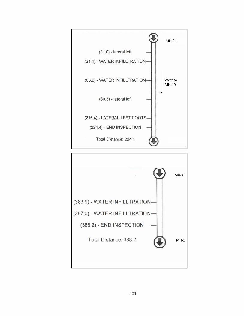
201

202
REFERENCES
Agency for Toxic Substances and Disease Registry (ATSDR), 2004. Health Consultation.
Mountain View sewer gas investigation, Scottsdale, Maricopa Country, Arizona.
Available at: (http://www.azdhs.gov/documents/preparedness/epidemiology-disease-
control/environmental-toxicology/mountain-view_consult.pdf).
Al-Hamdan, O.Z., Cruise, J.F., 2010. Soil moisture profile development from surface
observations by principle of maximum entropy. J. Hydrol. Eng. 15, 327–337.
API (American Petroleum Institute), 2000. No-Purge groundwater sampling: An Approach
for Long Term Monitoring, Bulletin 12.
ASCE (American Society of Civil Engineers), 2017. Infrastructure Report Card. A
Comprehensive Assessment of America's Infrastructure. Available at:
(https://www.infrastructurereportcard.org/wp-content/uploads/2016/10/2017-
Infrastructure-Report-Card.pdf).
Atteia, O., and Hohener, P., 2010. Semianalytical model predicting transfer of volatile
pollutants from groundwater to the soil surface. Environ. Sci. Technol. 44, 6228.
Bartelt-Hunt, S.L., Smith, J.A., 2002. Measurement of effective air diffusion coefficients
for trichloroethene in undisturbed soil cores. J. Contam. Hydrol. 56, 193–208.
Beckley, L., Gorder, K., Dettenmaier, E., Rivera-Duarte, I., McHugh, T.E., 2014. On-site
gas chromatography/mass spectrometry (GC/MS) analysis to streamline vapor intrusion
investigations. Environmental Forensics; 15:234–243.
Bekele D.N., Naidu R., Chadalavada S., 2014. Influence of spatial and temporal variability
of subsurface soil moisture and temperature on vapour intrusion. Atmospheric
Environment; 88:14-22.
Bell, J.P, Monteith, H.D, Parker, W.J., Corsi, R.L., Zytner, R., 1998. Modeling the
stripping and volatilization of VOC in wastewater collection and treatment systems. Project
91-TFT-1 Report. Water Environment Research Foundation. Alexandria Virginia.
Bell, J.P., Melcer, H., Monteith, H.D., Osinga, I. and Steel, P., 1993.Stripping of volatile
organic compounds at full-scale municipal wastewater treatment plants, Water Environ.
Res., 65(6), 708-716.
Bowels, J.E., 1992. Engineering Properties of Soils and Their Measurements, Fourth
Edition, McGraw-Hill Book Company, New York.
Bozkurt O., Pennell K.G., Suuberg E.M., 2009. Simulation of the vapor intrusion process
for nonhomogeneous soils using a three-dimensional numerical model. Ground Water
Monitoring & Remediation; 29:92-104.
Brown, J.L., Shimelis, O.I., Schultz, K.L., Vitkuske, D.S., Ye, M., Halpenny, M.R., 2015.
Use of unique retention properties of graphitized carbon toward passive sampling of 1, 3-
butadiene and other hazardous pollutants in air. Poster presented at Conference & Expo.
March 10, 2015; New Orleans, LA.

203
Brus, D., Skrabalová, L., Herrmann, E., Olenius, T., Travnickova, T., Makkonen, U.,
Merikanto, J., 2017. Temperature-Dependent Diffusion of H2SO4 in Air at
Atmospherically Relevant Conditions: Laboratory Measurements Using Laminar Flow
Technique. Atmosphere.10.3390.Available at: (http://www.mdpi.com/2073-
4433/8/7/132/pdf-vor).
Buckingham, E., 1904. Contributions to our knowledge of the aeration of soils. : USDA.
Bur. Soil Bul., 25. U.S. Gov. Print. Office, Washington, DC.
Bureau Veritas, 2013.Site Investigation Report. Moffett-Gateway Property, Former
Vector Control Yard 750 Moffett Boulevard and Northern Adjacent Caltrans 3-Scre
Parcel Mountain View, Santa Clara County, California. Available at:
(https://yosemite.epa.gov/r9/sfund/r9sfdocw.nsf/688299b284b16e92882574260073faef/8
ac40ed34e9df06888257c2400778071/$FILE/82019827.pdf/Investigation%20Rpt_Moffet
t%20Gateway%20F.pdf).
California Department of Toxic Substances Control (DTSC), 2016. Human Health Risk
Assessment (HHRA), NOTE NUMBER: 3, DTSC-modified Screening Levels (DTSC-
SLs).Available at: (https://www.dtsc.ca.gov/AssessingRisk/upload/HHRA_Note_3_-
2016-06.pdf).
Carmen, P.C. 1937. Fluid flow through a granular bed. Transactions of Institute of
Chemical Engineers, London, Vol.15, 150-157.
Carmen, P.C. 1956. Flow of Gases through Porous Media. Butterworths, London.
Center for Public Environmental Oversight (CPEO), 2013. Mountain View, California's
Mystery TCE Hotspots. Available at: (http://www.cpeo.org/pubs/MVHotspots.pdf).
Center for Public Environmental Oversight (CPEO), 2014. A Protective Approach to
Vapor Intrusion. Available at: (http://www.cpeo.org/pubs/MEWVIProtection.pdf).
City of Palo Alto, 2014. Regional water quality control plant lab letter dated April 28, 2014
to Kirsten Struve of Water Shed Protection from Samantha Bialorucki of City of Palo Alto,
Results of Analysis of Samples.
Colbert, K. L., Palazzo, J. E., 2008. Vapor Intrusion: Liability determination protects
profits and minimize risk. Real Estate Finance, 24:17-22.
Compliance and Closure, Inc., 2013. Letter to Ms. Elizabeth Wells from Gary R. Mulkey,
dated July 15, 2013, Re: Review of Existing VOC Field Data, CCI Project No. 12186-3).
Available at:
(https://geotracker.waterboards.ca.gov/regulators/deliverable_documents/2798978507/87
0%20Leong%20Drive%20Review%20of%20Existing%20VOC%20Field%20Data%20R
pt%20B.pdf).
Cornerstone Earth Group, 2017. Soil Management Plan and Air Monitoring Plan - 750
Moffett Blvd (Moffett Gateway), Mountain View, CA.
Availableat:(https://yosemite.epa.gov/r9/sfund/r9sfdocw.nsf/3dc283e6c5d6056f8825742
6007417a2/77150113b7fc80f98825813e007205c6/$FILE/49558409.pdf/486-
26%20Final%20Soil%20Management%20Plan%20Moffett%20Gateway%2006.12.17.pd
f).

204
Corsi, R.L., Birkett, S., 1995. A multi-parameter analysis of volatile organic compound
emissions from sewers. Water Environment Research, Volume 67, Number 5.
Corsi, R.L., Card, T.R., 1991. Estimation of VOC emissions using the BASTE model.
Environmental Progress, Vol. 10, No. 4.DOI:10.1002/ep.670100416.
Corsi, R.L., Chang, D.P.Y., Schroeder, E.D., 1992. A modeling approach for VOC
emissions from sewers. Water Environment Research, Volume 64. Pp.734-741(8).
https://doi.org/10.2175/WER.64.5.11.
Darcy, H., 1856. Les Fontaines publiques de la ville de Dijon, Paris.
Dingman, S.L., 2002. Physical hydrology. Second edition.
Distler M., Mazierski, P., 2010. Soil vapor migration through subsurface utilities,
Presented at Air & Waste Management Association, Vapor Intrusion Specialty Conference.
September 30.
Dobbs, R. A., Wang, L., and Govind, R., 1989. Sorption of toxic organic compounds on
wastewater solids: correlation with fundamental properties. Environ. Sci. Technol., 23 (9),
1092.
Edwini-Bonsu, S., Steffler, P.M., 2004. Air Flow in Sanitary Sewer Conduits due to
Wastewater Drag: A Computational Fluid Dynamics Approach. J. Environ. Eng. Sci. 3(5),
331–342.
Eklund, B.M., Simon, M.A., 2007. Concentration of Tetrachloroethylene in Indoor Air at
a Former Dry Cleaner Facility as a Function of Subsurface Contamination: A Case
Study. Journal of the Air and Waste Management Association. 57:753–760.
Elmore, H. L., and West, W. F., 1961. Effects of Water Temperature on Stream Reaeration.
J. Sanit. Eng. Div., 87, 59.
Eugene R. Weiner, 2012. Applications of Environmental Aquatic Chemistry: A Practical
Guide, Third Edition. Page 247-250.
Fetter, C. W., 1994. Applied Hydrogeology, 3rd Ed., Prentice-Hall, Inc. Englewood Cliffs,
New Jersey.
Folkes, D., Wertz, W., Kurtz, J., Kuehster, T., 2009. Observed Spatial and Temporal
Distributions of CVOCs at Colorado and New York Vapor Intrusion Sites.” Ground Water
Monitoring & Remediation 29 (1):70–80. doi:10.1111/gwmr.2009.29.issue-1.
Freedom of Information Act (FOIA), 2017. City of Mountain View Sewer Videos Released
by EPA, Region 9. EPA‐R9‐2017‐003246. Available at: (https://www.foia.gov).
Freeze A.R., Cherry, J.A., 1979. Groundwater. New Jersey: Prentice Hall.
Fuller, E.N., Schettler, P.D., Giddings, J.C., 1966. New method for prediction of binary
gas-phase diffusion coefficients.Ind.Eng.Chem.58, 18-27.
GEI (GEI Consultants), 2009. Immediate response action completion report and remedial
monitoring report no. 11. (RTN 3-23246).
Gorder KA, Dettenmaier E M., 2011. Portable GC/MS methods to evaluate sources of
CVOC contamination in indoor Air. Ground Water Monit Rem; 31(4):113–119.

205
Guo, Y., Holton, C., Luo, H., Dahlen, P., Gorder, K., Dettenmaier, E., Johnson, P., 2015.
Identification of alternative vapor intrusion pathways using controlled pressure testing, soil
gas monitoring, and screening model calculations. Environ. Sci. Technol. 49 (22),
13472e13482. (http://dx.doi.org/10.1021/acs.est.5b03564).
Hazen, A., 1892. Some Physical Properties of Sands and Gravels, with Special Reference
to their Use in Filtration. 24th Annual Report, Massachusetts State Board of Health,
Pub.Doc. No.34, 539-556.
Hers I., Zapf-Gilje R., Li L., Atwater J., 2001.The use of indoor air measurements to
evaluate intrusion of subsurface VOC vapors into buildings. Journal of the Air & Waste
Management Association. 51(9):1318–1331.
Hers, I., Zapf-Gilje, R., Johnson P.C., Li, L., 2003. Evaluation of the Johnson and Ettinger
model for prediction of indoor air quality. Ground Water Monit. Remed. 23,
119.doi:10.1111/j.1745-6592.2003.tb00678.
Hers, I., Zapf-Gilje, R., Johnson, P.C., Li, L., 2003. Evaluation of the Johnson and Ettinger
model for prediction of indoor air quality. Ground Water Monitoring and Remediation 23:
119–133.
Higbie, R., 1935.The Rate of Exposure of a Pure Gas into a Still Liquid during Short
Periods of Exposure. Trans. Amer. Inst, of Chem. Eng., 31, 365.
Hodgson A., Garbesi K., Sextro R., Daisey J.M., 1992. Soil-gas contamination and entry
of volatile organic compounds into a house near a landfill. Journal of the Air and Waste
Management Association. 42(3):277–283.
Holton, C., 2016. Increasing Availability of Continuous and Real-Time VOC Monitoring
Technologies for VI Assessment. Presented at EPA/AEHS Workshop. Association of
Environmental Health Sciences (AEHS), San Diego, CA. Available at:
(https://iavi.rti.org/attachments/WorkshopsAndConferences/13_Holton_Cont_RT_Monit
oring_AEHS_final.pdf).
Holton, C., Guo, Y., Luo, H., Dahlen, P., Gorder, K., Dettenmaier, E., Johnson, P.C., 2015.
Long-Term Evaluation of the Controlled Pressure Method for Assessment of the Vapor
Intrusion Pathway. Environmental science & technology. 49:2091–2098.
Holton, C.; Luo, H.; Dahlen, P; Gorder; K.; Johnson, P.C., 2013. Temporal variability in
indoor air concentrations under natural conditions in a house overlying a dilute chlorinated
solvent plume. Environmental Science and Technology, 47:13347-13354.
Howe, K.J., Hand, D.W., Crittenden, J.C., Trussell, R.R., Tchobanoglous, G., Principles
of water treatment. Wiley publication. 3rd edition .4, 118-122.
(https://nepis.epa.gov/Exe/ZyPDF.cgi/2000E6PB.PDF?Dockey=2000E6PB.PDF).

206
Hunt, G.R., Linden, P.F., 1999. The fluid mechanics of natural ventilation-displacement
ventilation by buoyancy-driven flows assisted by wind. Building and Environment.
34,707-720.
ITRC. 2007. Vapor intrusion pathway: A practical guideline. VI-1. Interstate Technol.
Regulatory Counc. Vapor Intrusion Team, Washington, DC.
Izzo VJ. Dry cleaners – a major source of PCE in ground water, California Regional Water
Quality Control Board, Central Valley Region. March 1992.
Jacobs, J.A., Jacobs, O.P., Pennell, K.G., 2015. One Alternate Exposure Pathway of VOC
Vapors from Contaminated Subsurface Environments into Indoor Air – Legacy Sewer-
Plumbing Systems; Groundwater Resources Association of California; Hydro visions p.
2024. Available at:
(http://nebula.wsimg.com/390f6305810d89bb2eff5bfaf022df59?AccessKeyId=5161BD9
21A995425678B&disposition=0&alloworigin=1).
Jacobs, J.A., Jacobs, O.P., Pennell, K.G., 2015. One Alternate Exposure Pathway of VOC
Vapors from Contaminated Subsurface Environments into Indoor Air – Legacy Sewer-
Plumbing Systems; Groundwater Resources Association of California; Hydro visions p.
20-24. Available at:
(http://nebula.wsimg.com/390f6305810d89bb2eff5bfaf022df59?AccessKeyId=5161BD9
21A995425678B&disposition=0&alloworigin=1).
Jensen, N.A., 1995. Empirical Modeling of Air-to-Water Oxygen Transfer in Gravity
Sewers. Water Environment Research, Vol. 67, No. 6. pp. 979-991. Available at:
(http://www.jstor.org/stable/25044652?origin=JSTOR-pdf).
Johnson, P.C., and Ettinger, R.A., 1991. Heuristic model for predicting the intrusion rate
of contaminant vapors into buildings. Environ. Sci. Technol. 25:1445–
1452.doi:10.1021/es00020a013.
Johnston, J.E., and Gibson, J.M., 2011. Probabilistic approach to estimating indoor air
concentrations of chlorinated volatile organic compounds from contaminated
groundwater: A case study in San Antonio, Texas. Environ. Sci. Technol. 45:1007–
1013.doi:10.1021/es102099h.
Johnston, J.E., and Gibson, J.M., 2013. Screening houses for vapor intrusion risks: A
multiple regression analysis approach. Environ. Sci. Technol. 47:5595–
5602.doi:10.1021/es4003795.
Johnston, J.E., Gibson, J.M., 2014. Spatiotemporal variability of tetrachloroethylene in
residential indoor air due to vapor intrusion: a longitudinal, community-based study.
Journal of Exposure Science and Environmental Epidemiology.24:564–571.
Johnston, J.E., Q. Sun, and J.M. Gibson. 2014. Updating exposure models of indoor air
pollution due to vapor intrusion: Bayesian calibration of the Johnson- Ettinger model.
Environ. Sci. Technol. 48:2130–2138.doi: 10.1021/es4048413.
Jones, D.L., Burklin, C.E., Seaman, J.C., Jones, J.W., Corsi, R.L., 1996. Models to
Estimate Volatile Organic Hazardous Air Pollutant Emissions from Municipal Sewer
Systems, Air & Waste Manage. Assoc. 46: 657-666.

207
Karickhoff, S. W., Brown, D.S., Scott, T.A., 1979. "Sorption of hydrophobic pollutants on
natural sediments." Water Res., (G. B.) 13, 241. (https://doi.org/10.1016/0043-
1354(79)90201-X).
Karpinska, M., Mnich, Z., Kapala, J., Antonowicz, K., 2004. Seasonal changeability of
indoor radon concentrations in one family house. Nukleonika 49, no. 1: 33–36.
Kozeny, J., 1927. Ueber kapillare Leitung des Wassers im Boden. Sitzungsber Akad.
Wiss., Wien, 136(2a), pp 271-306.
Kristensen, A.H., Thorbjørn, A., Jensen, M.P., Pedersen, M., Moldrup, P., 2010. Gas-
phase diffusivity and tortuosity of structured soils. J. Contam. Hydrol. 115,
26.doi:10.1016/j.jconhyd.2010.03.003.
Labocha, M., Zytner R.G., Corsi, R.L., 1994. Oxygen and VOC mass transfer at clarifier
weirs, 49th Perdue Industrial Waste Conference Proceedings, Lewis Publishers, Chelsea,
Michigan.
Lewis, W. K., Whitman, W. G., 1924. Principles of Gas Absorption. Ind. Eng. Chem., 16,
1215.
Lin, J.H., Chou, M.S., 2006a. Henry’s Law Constant Variations of Volatile Organic
Compounds in Wastewater and Activated Sludge, Aerosol and Air Quality Research, Vol.
6, No. 2, pp. 180-192.
Lin, J.H., Chou, M.S., 2006b. Partition of Volatile Organic Compounds in Activated
Sludge and Wastewater, Journal of the Air & Waste Management Association, 56:8, 1083-
1090. DOI: 10.1080/10473289.2006.10464538.
Lincoff, A. H., Gossett, J. M., 1984. The determination of Henry’s law constant for volatile
organics by equilibrium partitioning in closed systems, in: Gas transfer at water surfaces,
edited by: Brutsaert, W. and Jirka, G. H., D. Reidel Publishing Company, Dordrecht-
Holland, 17–25.
Little, J.C., Daisey, J.M., Nazaroff, W.W., 1992. Transport of subsurface contaminants into
buildings. Environmental Science & Technology 26(11): 2058 – 2066.
Little, P.C., Pennell, K.G., 2017. Measuring Vapor Intrusion: from Source Science Politics
to a Transdisciplinary Approach. Environmental Sociology. 3.2: 145-154.
Lowe, S., 2016. Sewer Ventilation: Factors Affecting Airflow and Modeling Approaches.
Journal of water Management Modeling. C395. DOI: 10.14796/JWMM.C395.
Mackay, D., Yeun, A., 1983. Mass Transfer Coefficient Correlations for Volatilization of
Organic Solutes from Water. Environ. Sci. Technol.17, 211.
Manzanilla, E., 2014. EPA Region 9 Response Level Action Levels and Recommendations
to Address Near-Term Inhalation Exposures to TCE in Air from Subsurface Vapor
Intrusion. Memorandum to Region 9 Superfund Division Staff and Managers. July 9, 2014.
Marczewski, A.W., Marczewska, A.D., Słota, A., 2013. Adsorption and desorption
kinetics of benzene derivatives on mesoporous carbons. Adsorption open access. Volume
19, Issue 2–4, pp 391–406.DOI 10.1007/s10450-012-9462-7.

208
Marrero, T.R., Mason, E.A., 1972. Gaseous diffusion coefficients. J. Phys. Chem. Ref.
Data. 1, 3-118. Doi:10.1063/1.3253094.
MassDEP (Massachusetts Department of Environmental Protection), 2011. Interim final
vapor intrusion guidance. WSC#11-435.
McAlary, T., Johnson, P.C., 2009. Editorial: GWMR Focus issue on vapor intrusion.
Ground Water Monitoring and Remediation. 29 (1):40-41.
McCarthy, K.A., Johnson, R.L., 1993. Transport of volatile organic compounds across the
capillary fringe. Water Resour. Res. 29:1675–1684. doi: 10.1029/93WR00098.
McHugh, T., Kuder, T., Fiorenza, S., Gorder, K., Dettenmaier, E., Philp, P., 2001.
Application of CSIA to distinguish between vapor intrusion and indoor sources of VOCs,
Environ Sci Technol; 45: 5952–5958.
McHugh, T., Beckley, L., Sullivan, T., Lutes, C., Truesdale, R., Uppencamp, R., Cosky,
B., Zimmerman, J., Schumacher, B., 2017. Evidence of a sewer vapor transport pathway
at the EPA vapor intrusion research duplex. Science of the Total Environment. 598:772-
779. (doi: 10.1016/j.scitotenv.2017.04.135).
Monod, J. 1949. The growth of bacterial cultures. A. Rev. Microbiol. 3, 371 394.
Melcer, H., Bell, J.P., Thompson, D.J., Yendt, C.M., Kemp, J., Steel, P., 1994. Modeling
volatile organic contaminants fate in wastewater treatment plants. J. Environ. ENG. 120(3):
588-609.
Millington R, Quirk J. Permeability of porous solids. Trans Faraday Soc 1961; 57:1200-7.
Millington, R. J., and J. P. Quirk, 1961. Transport in porous media [in soil science], Trans.
Int. Congr. Soil Sci., 7(1), 97–106.
Moldrup, P., Olesen, T., Gamst, J., Schjonning, P., Yamaguchi, T., Rolston, D.E.,
2000.Predicting the gas diffusion coefficient in repacked soil: water-induced linear
reduction model. Soil Sci. Soc. Am. J.64.1588-94.
Moradi, A., Tootkaboni, M., Pennell, K.G., 2015. A variance decomposition approach to
uncertainty quantification and sensitivity analysis of the J&E model. Journal of the Air &
Waste Management Association, 65(2): 154-164.
Muskat, M., 1937. The Flow of Homogeneous Fluids through Porous Media. McGraw-
Hill Book Company, New York.
Nakasone, H., 1987. Study of Aeration at Weirs and Cascades. J. Environ. Eng., 113, 64.
Namkung, E., Rittmann, B.E., 1987. Estimating Volatile Organic Compound Emissions
from Publicly Owned Treatment Works. Water Pollution Control Federation, Vol. 59, No.
7. pp. 670-678.
Nazaroff, W. W., 1988. Predicting the rate of 222Rn entry from soil into the basement of
a dwelling due to pressure-driven air flow. Radiation Protection Dosimetry, 24:199-202.
(https://doi.org/10.1093/oxfordjournals.rpd.a080269).

209
Nielsen K.B., Hvidberg B., 2017. Remediation techniques for mitigating vapor intrusion
from sewer systems to indoor air Remediation.27: 67–73.
(https://doi.org/10.1002/rem.21520).
Nielson, K. K., V. C. Rogers. 1990. Radon transport properties of soil classes for estimating
indoor radon entry. In: F. T. Cross (ed), Proceedings of the 29th Hanford Symposium of
Health and the Environment. Indoor Radon and Lung Cancer: Reality or Myth? Part 1.
Battelle Press, Richland, Washington.
NYDOH (New York State Department of Health), 2006. Final guidance for evaluating soil
vapor intrusion in the state of New York.
Olson, D.A., Rajagopalan, S.Z., Corsi, R.L., 1997a. Ventilation of Sewers: The Role of
Thermal Gradients, Adv. Environ. Res. 1(3), 312–322.
Olson, D., Rajagopalan, S.Z, Corsi R.L, 1997b. Ventilation of industrial process drains:
mechanisms and effects on VOC emissions. Journal of environmental engineering, 939.
Olson, D.A., Varma, S., Corsi, R.L., 1998. A new approach for estimating volatile organic
compound emissions from sewers: methodology and associated errors. Water Environment
Research, Volume 70.
Parker, W., Yu, J., 2001. Dynamic modeling to assess worker exposure to gas-phase
volatile organic compounds in collector sewers. Water Environment Research, Volume 73,
Number 4.
Parker, J. C., Lenhard, R.J., Kuppusamy, T., 1987. A parametric model for constitutive
properties governing multiphase flow in porous media. Water Resources Research,
23(4):618- 624.
Parkhurst, J.D., and Pomeroy, R.D., 1972. Oxygen Absorption in Streams. J. Sanit. Eng.,
Div. ASCE, v. 98, no. SA1, p. 101-124.
Penman, H.L., 1940. Gas and vapour movements in the soil I. The diffusion of vapours
through porous solids. J. Agric. Sci. 30, 437–462.
Pennell K.G., Bozkurt, O., Suuberg, E.M., 2009. Development and application of a three-
dimensional finite element vapor intrusion model. J. Air & Waste Manage. Assoc.
59(4):447–460.
Pennell, K.G., Scammell, M.K., McClean, M.D., Ames, J.,Weldon, B., Friguglietti, L.,
Suuberg, E.M., Shen, R., Indeglia, P.A., Heiger-Bernays, W.J., 2013. Sewer gas: an indoor
air source of PCE to consider during vapor intrusion investigations. Ground Water Monit.
Rem. 119–126. (http://dx.doi.org/10.1111/gwmr.12021).
Pennell, K.G., Scammell, M.K., McClean, M.D., Suuberg, E.M., Moradi, A., Roghani, M.,
Ames, J., Friguglietti, L., Indeglia, P.A., Shen, R., Yao, Y., Heiger-Bernays, W.J., 2016.
Field data and numerical modeling: A multiple lines of evidence approach for assessing
vapor intrusion exposure risks. Science of the Total Environment. 556: 291-301.
Pescod, M. B., Price, A. C., 1981. “Fundamentals of Sewer Ventilation as Applied to the
Tyneside Sewerage Scheme.” Water Pollution Control 90 (1): 17–33.

210
Pescod, M. B., Price, A. C., 1982. “Major Factors in Sewer Ventilation.” Journal of the
Water Pollution Control Federation 54 (4): 385–97.
Petersen, L.W., Rolston, D.E., Moldrup, P., Yamaguchi, T., 1994. Volatile organic vapor
diffusion and adsorption in soils. J. Environ. Qual. 23,799–805.
Predicting the gas diffusion coefficient in repacked soil: water induced linear reduction
model. Soil Sci. Soc. Am. J. 64, 1588–1594.
Quigley, C.J., Corsi, R.L., 1995. Emissions of VOCs from a Municipal Sewer, Journal of
the Air & Waste Management Association, 45:5,395-403.
(doi:10.1080/10473289.1995.10467371).
Rahme, Z. G., Zytner, R. G., Corsi, R. L., Madani-Isfahani, M., 1995. Predicting oxygen
uptake and VOC emissions at enclosed drop structures, J. Environ. Eng., 123(1): 47-53.
Ramu, M.C., Shaikh, A.N., Muraleedharan, T.S., Ramachandran, T.V., 1992.
Measurement of indoor radon levels in India using solid-state nuclear track detectors: Need
for standardization. Defence Science Journal 42, no. 4: 219–225.
Reichman, R., Roghani, M., Willett, E.J., Shirazi, E., Pennell, K.G., Air exchange rates
and alternative vapor entry pathways to inform vapor intrusion exposure risk
assessments. Rev Environ Health . 32(1-2):27-33. (https://doi.org/10.1515/reveh-2016-
0039).
Riis C.E., Christensen A.G., Hansen M.H. and Husum H., 2010.Vapor Intrusion through
sewer systems: migration pathways of chlorinated solvents from groundwater to indoor
air. Presented at the Seventh Battelle International Conference on Remediation of
Chlorinated and Recalcitrant Compounds, Monterey. Available at:
(http://indoorairproject.files.wordpress.com/2011/03/sgsattachment-1.pdf).
Robinson, D., Campbell, C., Hopmans, J., Hornbuckle, B., Jones, S., Knight, R., Ogden,
F., Selker, J., Wendroth, O., 2008. Soil moisture measurement for ecological and
hydrological watershed-scale observatories: A review. Vadose Zone J. 7, 358.
doi:10.2136/vzj2007.0143.
Roghani, M., Jacobs, O.P., Miller, M., Willett, E.J., Jacobs, J.A., Viteri, C.R., Shirazi, E.,
Pennell, K.G., 2018. Occurrence of chlorinated volatile organic compounds (VOCs) in a
sanitary sewer system: Implications for assessing vapor intrusion alternative pathways.
Science of the Total Environment. (doi: 10.1016/j.scitotenv.2017.10.205).
S.Yaghmaei, A. Rashidkhani., 2005. Estimating Volatile Organic Compound Emissions
vfrom Wastewater Circulating Aeration Tanks. Scientia Iraniaca. Vol. 12, NO. 3. PP300-
305.
Sander, S. P., Abbatt, J., Barker, J. R., Burkholder, J. B., Friedl, R. R., Golden, D. M.,
Huie, R. E., Kolb, C. E., Kurylo, M. J., Moortgat, G. K., Orkin, V. L., Wine, P. H.,
2011.Chemical Kinetics and Photochemical Data for Use in Atmospheric Studies,
Evaluation No. 17, JPL Publication 10-6, Jet Propulsion Laboratory, Pasadena, available
at:(http://jpldataeval.jpl.nasa.gov).
Schaap, M. G., F. J. Leij, and M. Th. van Genuchten. 1998. Neural network analysis for
hierachical prediction of soil water retention and saturated hydraulic conductivity. Soil sci.
soc. am. j., vol. 62.

211
Shen, R., Pennell, K.G., Suuberg, E.M., 2012. A numerical investigation of vapor
intrusion-The dynamic response of contaminant vapors to rainfall events,” Science of the
Total Environment; 437:110-120. (http://dx.doi.org/10.1016/j.scitotenv.2012.07.054)
Shen, R, Yao, Y, Pennell, KG, Suuberg, E.M., 2013a. Modeling quantification of the
influence of soil moisture on subslab vapor concentration. Environmental Science:
Processes and Impacts. 15(7): 1444-1451. (doi: 10.1039/c3em00225j)
Shen, R., Yao, Y., Pennell, K.G., Suuberg, E.M., 2013b. Influence of soil moisture on Soil
Gas Vapor Concentrations for Vapor Intrusion. Environmental Engineering Science.
30(10):628-637. (doi:10.1089/ees.2013.0133).
Shepherd. J.L., Corsi, R.L., Kemp, J., 1996. Chloroform in Indoor Air and Wastewater:
The Role of Residential Washing Machines. J. Air Waste Manage. Assoc. 46: 631-642.
Soucy, N.C., Mumford, K.G., 2017. Bubble-Facilitated VOC Transport from LNAPL
Smear Zones and Its Potential Effect on Vapor Intrusion. Environ. Sci. Technol. 2017, 51,
2795−2802. DOI:10.1021/acs.est.6b06061.
Stratus Environmental, Inc. 2010. Letter to Ms. Elizabeth Wells from Gowri S. Kowtha,
dated December 29, 2010, Re: Subsurface Environmental Site Assessment Report.
Available at:
(https://geotracker.waterboards.ca.gov/regulators/deliverable_documents/8155500113/85
0%20Leong%20Environmental%20Site%20Assessment%20Rpt.pdf).
Tillman, F.D., Weaver, J.W., 2007. Temporal moisture content variability beneath and
external to a building and the potential effects on vapor intrusion risk assessment. Sci Total
Environ; 379:1-15. (doi:10.1016/j.scitotenv.2007.02.003).
Turczynowicz L., Robinson N., 2007. Exposure assessment modeling for volatiles –
Towards an Australian Indoor Vapor Intrusion Model Journal of Toxicology and
Environmental Health, Part A; 70, 1619-1634.
Turner, L.W., 1993.ASHRAE Handbook Fundamentals. I-P Edition.
USDA (United States Department of Agriculture), 2018. A soil profile. Available at:
(https://www.nrcs.usda.gov/wps/portal/nrcs/detail/soils/edu/?cid=nrcs142p2_054308).
USEPA, 1989. Record of Decision for Fairchild, Intel and Raytheon Sites,
Middlefield/Ellis/Whisman (MEW) Study Area, Mountain View, California. Region 9,
San Francisco, CA. Available at:
(https://yosemite.epa.gov/r9/sfund/r9sfdocw.nsf/3dc283e6c5d6056f88257426007417a2/2
14a2ad20b145550882575f5006bb765/$FILE/Record%20of%20Decision,%20MEW%20
Study%20Area%20-%206-9-89.pdf).
USEPA, 1993. Office of Research and Development. Behavior and Determination of
Volatile Organic Compounds in Soil. A Literature Review. EPA/600/R-93/140. Available
at: (https://nepis.epa.gov/Exe/ZyPDF.cgi/30002W9Z.PDF?Dockey=30002W9Z.PDF).
USEPA, 1995. National exposure research laboratory office of research and development.
Method 524.2, Measurement of purgeable organic compounds in water by capillary column
gas chromatography/mass spectrometry, Revision 4.1. Available at:
(https://www.epa.gov/sites/production/files/2015-06/documents/epa-524.2.pdf).

212
USEPA, 1996, Office of solid waste and emergency response. Soil screening guidance:
Technical background document. Second edition. EPA/540/R95/128.
USEPA, 2000. Exfiltration in Sewer Systems. National risk management research
laboratory. EPA/600/R-01/034. Available at:
(https://nepis.epa.gov/Exe/ZyPDF.cgi/2000E6PB.PDF?Dockey=2000E6PB.PDF).
USEPA, 2004. User's Guide for Evaluating Subsurface Vapor Intrusion into Buildings.
Environmental Quality Management, Inc. Available at:
(https://www.dtsc.ca.gov/AssessingRisk/upload/VI_USEPA_Users-guide.pdf).
USEPA, 2010. Record of decision amendment for the vapor intrusion pathway.
Middlefield-Ellis-Whisman (MEW) superfund study area. Mountain View and Moffett
Field, California. Region 9 San Francisco, California. Available at:
(https://yosemite.epa.gov/r9/sfund/r9sfdocw.nsf/3dc283e6c5d6056f88257426007417a2/7
17b008a9431066288257782007790bc/$FILE/MEW%20VI%20ROD%20Amendment%2
0and%20RS%20-%20Aug%2016%202010.pdf).
USEPA, 2011. Background indoor air concentrations of volatile organic compounds in
North American residences (1990–2005): A compilation of statistics for assessing vapor
intrusion. United States Environmental Protection Agency.
USEPA, 2012a. EPA’s vapor intrusion database: Evaluation and characterization of
attenuation factors for chlorinated volatile organic compounds and residential buildings.
Office of Solid Waste and Emergency Response, USEPA, Washington, DC.
USEPA, 2012b. Conceptual model scenarios for the vapor intrusion pathway. United States
Environmental Protection Agency.
USEPA, 2014. Guide for Estimating Infiltration and Inflow. Available at:
(https://www3.epa.gov/region1/sso/pdfs/Guide4EstimatingInfiltrationInflow.pdf).
USEPA, 2015a. OSWER technical guide for assessing and mitigating the vapor intrusion
pathway from subsurface vapor sources to indoor air. Environmental Protection Agency,
Washington, DC, 2015a. Available at: (https://www.epa.gov/sites/production/files/2015-
09/documents/oswervapor-intrusion-technical-guide-final.pdf).
USEPA, 2015b. Vapor intrusion screening level (VISL) calculator version 3.4, United
States Environmental Protection Agency; 2015b.
USEPA, 2015c. EPA Update: TCE Hot Spot Areas Source Investigation Findings,
Middlefield-Ellis-Whisman (MEW) Superfund Study Area, Mountain View and Moffett
Field, CA Neighborhood Meeting. Available at:
(https://yosemite.epa.gov/r9/sfund/r9sfdocw.nsf/3dc283e6c5d6056f88257426007417a2/a
bf23a945d71295d88257f00007af0d7/$FILE/18687784.pdf/EPA%20TCE%20Source%20
Investigation%20-%20Neighborhood%20Mtg%20-%20Nov%201,%202015.pdf).
USEPA, 2015d. Passive Samplers for Investigations of Air Quality: Method Description,
Implementation, and Comparison to Alternative Sampling Methods. Available at:
(https://nepis.epa.gov/Adobe/PDF/P100MK4Z.pdf).
USEPA, 2016. Regional Screening Levels (RSLs) - Generic Tables. Available at:
(https://www.epa.gov/risk/regional-screening-levels-rsls-generic-tables-may-2016).

213
USGS (United States Geological Survey), 2006. Circular 1292, Chapter 5—Additional
Information for Selected VOCs, April 2006. Available at:
(http://water.usgs.gov/nawqa/vocs/national_assessment/report/chapter5.html).
van Genuchten, M.T., 1980. A closed-form equation for predicting the hydraulic
conductivity of unsaturated soils. Soil Science Society of America Journal. 44, 892-898.
Vereecken, H., Huisman, J., Bogena, H., Vanderborght, J., Vrugt, J., Hopmans, J., 2008.
On the value of soil moisture measurements in vadose zone hydrology: A review. Water
Resour. Res 44, W00D06. doi: 10.1029/2008WR006829.
Vroblesky, D.A., Petkewich, M.D., Lowery, M.A., Landmeyer, J.E., 2011. Sewers as a
Source and Sink of Chlorinated-Solvent Groundwater Contamination, Marine Corps
Recruit Depot, Parris Island, South Carolina. Ground Water Monitoring& Remediation
31, no. 4, fall 2011, pages 63–69. doi: 10.1111/j1745–6592.2011.01349.x.
Waitz M., Freijer J., Kreule P., Swartjes F., 1996. The VOLASOIL risk assessment model
based on CSOIL for soils contaminated with volatile compounds. National Institute of
Pulbic Health and the Environment, Bilthover. The Netherlands. Report No. 715810014.
Wallace, A., Friedrich, A., 2017. Vapor Intrusion Conceptual Site Model Development
for the Sewer Gas to Indoor Air Pathway. AEHS West Coast Conference, San Diego,
March 22.
Water Environment Federation (WEF), 2007. Characterization and Sampling of
Wastewater. Available at:
(www.wefnet.org/...Wastewater.../Chapter%2017%20Revised_6th%20Edition.pdf).
Water Environment Research Foundation (WERF), 2009. Collection System Ventilation
Research Report. Alexandria, VA: Water Environment Research Foundation. Report No.
04-CTS-1A.
Werner, D., Grathwohl, P., Hohener, P., 2004. Review of field methods for the
determination of the tortuosity and effective gas-phase diffusivity in the vadose zone.
Vadose Zone J. 3, 1240–1248. (doi:https://doi.org/10.2113/3.4.1240).
Wilson, S.C., Burnett, V., Waterhouse, K.S., Jones, K.C., 1994. Volatile Organic
Compounds in Digested United Kingdom Sewage Sledges. Environ. Sci. Technol., 28,
259-266.
Yao Y., Shen R., Pennell K.G., Suuberg E.M., 2011. Comparison of the Johnson-Ettinger
vapor intrusion screening model predictions with full three-dimensional model results.
Environmental Science and Technology; 45(6): 2227-2235.
Yao Y., Pennell K.G., Suuberg E.M., 2013a. A review of vapor intrusion models.
Environmental Science and Technology; 47 (6), pp 2457–2470.
Yao, Y., Shen, R., Pennell, K.G, Suuberg, E.M., 2013b. Examination of the Influence of
Environmental Factors in Contaminant Vapor Concentration Attenuation Factor with the
U.S. EPA’s Vapor Intrusion Database. Environmental Science and Technology 2013b;
47(2) 906-913.

214
Yao Y., Shen R., Pennell K.G., Suuberg E.M., 2013c. Examination of the U.S. EPA's vapor
intrusion database based on models. Environ. Sci. Technol. 47(3):1425–1433. [PubMed:
23293835].
Yao, Y., Shen, R., Pennell, K.G., Suuberg, E.M., 2013d. Estimation of contaminant subslab
concentration in vapor intrusion including lateral source-building separation. Vadose Zone
Journal.
Yao, Y., Wang, Y., Zhong, Z., Tang, M., Suuberg, E.M., 2017a. Investigating the Role of
Soil Texture in Vapor Intrusion from Groundwater Sources. J. Environ. Qual. 46:776–784.
doi:10.2134/jeq2017.01.0011.
Yao, Y., Mao, F., Ma, S., Yao, Y., Suuberg, E. M., Tang, X., 2017b. Three-dimensional
simulation of land drains as a preferential pathway for vapor intrusion into buildings. J.
Environ. Qual. 46:1424–1433. doi:10.2134/jeq2017.05.0211.

215
VITA
Mohammadyousef (Amir) Roghani
Place of Birth:
Amol, Mazandaran, Iran
Education:
Master of Science –Environmental Engineering 9/2009 – 8/2011
Sharif University of Technology (#1 Ranked Engineering University in Iran)
Thesis: Heavy metals removal from aqueous solution by polymer composites
Bachelor of Science – Chemical Engineering 9/2004 – 8/ 2009
Sharif University of Technology (#1 Ranked Engineering University in Iran)
Professional Experience:
University of Kentucky / Lexington, KY 1/2014 – Present
Graduate Research Assistant & Teaching Assistant
Researching fate and transport of hazardous chemicals in natural and engineered
environments.
Developing numerical model for fate and transport processes, including vapor intrusion.
Conducting laboratory analysis using GC/MS via EPA Method 8260.
Performing field studies using standard sampling methods (e.g.TO-15, TO-17 and
Radiello), and novel high frequency VOC sampling sensor technologies.
Ab Pardazan Bahar Co. / Tehran, Iran 6/2011 – 5/2013
Process Design Engineer
Designed industrial wastewater treatment plants, and provided installation, configuration
and laboratory guidelines. Supervised water treatment plant created and implemented
processes and trained employees.
Awards & Honors
− University of Kentucky Central Block fund, 2018.
− Karri Casner Environmental Sciences Fellowship Award, Spring 2017.
− SRP Trainee at University of Kentucky Superfund Research Center (UK-SRC)
translation core.
− Qualified for National Physics Olympiad, Iran, 2002.
Peer-reviewed Publications
Roghani, M., and Pennell, K.G., 2018. Developing a numerical model to study fate and
transport of VOCs inside the sewer systems. Environmental Science and Technology,
2018. In preparation.

216
Roghani, M., Jacobs, O.P., Miller, A., Willett, E.J., Jacobs, J.A., Viteri, C.R., Shirazi, E.,
& Pennell, K.G. (2018). Occurrence of chlorinated volatile organic compounds (VOCs) in
a sanitary sewer system: Implications for assessing vapor intrusion alternative pathways.
Science of the Total Environment 616–617:1149–1162.
Pennell, K.G., Scammell, M.K., McClean, M.D., Suuberg, E. M., Ames, J., Moradi
Gharehtapeh, A., Roghani, M., Indeglia, P.A., Friguglietti, L., Shen, R., Yao, Y., Heiger-
Bernays, W. (2016). Field Data and Numerical Modeling: A Multiple Lines of Evidence
Approach for Assessing Vapor Intrusion Exposure Risks. Science of the Total
Environment, 556: 291-301.
Reichman, R., Roghani, M., Willett, E.J., Shirazi, E., & Pennell, K.G. (2017). Air
Exchange Rates and Alternative Vapor Entry Pathways to Inform Vapor Intrusion
Exposure Risk Assessments. Reviews on Environmental Health, 32(1), pp. 27-34.
Roghani M., Nakhil, S.A.A., Aghajani, M., Rostami, M. H., Borghei, S.M. (2016).
Adsorption and Oxidation Study on Arsenite Removal from Aqueous Solutions by
Polyaniline/polyvinyl Alcohol Composite. Journal of Water Process Engineering 14 101–
107.
Certification
OSHA HAZWOPER in accordance with requirements of 29 CFR 1910.120(e).
Conference & Workshop Presentations
Roghani, M., Pennell, K.G. Sewer Systems and Volatile Organic Compounds: Indoor Air
Considerations for Buildings near Contaminated Groundwater Plumes. Oral
Presentation. Central and Eastern European Conference on Health and the
Environment (CEECHE): Environmental and health issues in fast changing
economies” Krakow, Poland. June 2018.
Roghani, M., Pennell, K.G. Vapor Transport through Sewer Systems: Mechanisms and
Variables. Poster Presentation. Battelle 2018: Remediation of Chlorinated and
Recalcitrant Compounds. Palm Springs, Ca. April 2018.
Roghani, M., Pennell, K.G. Fate and Transport of Volatile Organic Compounds (VOCs)
in a Sewer System: Numerical Model and Field Study. Poster Presentation. Kentucky
Water Resources Research Institute Annual Symposium (KWRRI). Lexington, KY.
March, 2018.
Roghani, M., Willett, E.J., Shirazi, E, Pennell, K.G. Mechanisms of Vapor Transport:
Expanding Exposure Risks in Communities. Oral Presentation. AEESP: Advancing
Healthy Communities through Environmental Engineering and Science, Ann Arbor,
MI. June 2017.
Willett, E.J., Roghani, M., and Pennell, K.G. A GIS-Based Approach for Assessing Sewer
Gas to Indoor Air Pathways near Hazardous Waste Sites. Oral Presentation. AEESP:
Advancing Healthy Communities through Environmental Engineering and Science,
Ann Arbor, MI. June 2017.
Pennell, K.G., Roghani*, M., Willett, E.J., Shirazi, E. Modeling and Measurement of
VOC Mass Transfer within Sewer Lines that Act as Preferential Pathways. Oral

217
Presentation. Battelle Fourth International Symposium on Bioremediation and
Sustainable Environmental Technologies, Miami, FL, May 2017.
Roghani, M., Willett, E.J., Shirazi, E, Pennell, K.G. Alternative Pathways for Subsurface
Groundwater Vapors to Enter Buildings: Modeling Approach. Poster Presentation.
Kentucky Water Resources Research Institute Annual Symposium (KWRRI),
Lexington, KY, March 2017.
Roghani, M., Willett, E.J., Shirazi, E., Pennell, K.G. “VOC Mass Transfer in Sewer
Systems and Vapor Intrusion”. Poster Presentation. NIEHS Superfund Research
Program (SRP) Annual Meetings, Durham, NC, December 5-8, 2016.
Roghani, M., Shirazi, E., Pennell, K.G. Lessons Learned: Vapor Intrusion Field
Measurements and Model Predictions. Presented in 26th Annual AEHS International
Conference on Soil, Water, Energy, & Air, San Diego, 21-24 March 2016, San Diego,
Ca.
Roghani, M., Shirazi, E., Willet, E., Pennell, K.G. “Investigation of VOC Transport in
Soil Vapors Due to Wind Effects Using Models and Measurement.” Poster
Presentation at the American Geophysical Union Fall Meeting, San Francisco, CA,
December 2014.
Roghani et al, Arsenic adsorption and oxidation in aqueous solutions by
Polyaniline/Polyvinyl Alcohol composites. Presented in Texas A&M University
System 11th Annual Pathways Student Research Symposium, November 8, 2013.


