JEOL JXA-8230User Manual

Dr. Julien M. Allaz

ETH Zürich – D-ERDW / Institute of Geochemistry and Petrology

***** Version 1.0 *****October 9th, 2019

Table of Contents

1) Presentation: JEOL JXA-8230 electron microprobe (EMP) ...........................1-11.1) Hardware ..............................................................................................................................1-1

1.1.1) Electron gun: W vs. LaB6 .............................................................................................................................1-11.1.2) Wavelength Dispersive Spectrometers (WDS) ..............................................................................................1-11.1.3) Energy Dispersive Spectrometers (EDS) ......................................................................................................1-21.1.4) SE and BSE detectors ....................................................................................................................................1-3

1.2) Software ................................................................................................................................1-31.2.1) Computers ......................................................................................................................................................1-31.2.2) JEOL computer: PC_SEM and PC_EPMA ...................................................................................................1-4

1.3) Overview of the PC_SEM interface ...................................................................................1-51.3.1) PC_SEM program menu .............................................................................................................................1-51.3.2) Menu & main options ....................................................................................................................................1-51.3.3) Image display .................................................................................................................................................1-81.3.4) Beam adjustment and imaging tool ...............................................................................................................1-81.3.5) Stage tools and guide .....................................................................................................................................1-91.3.6) Stage coordinate ............................................................................................................................................1-9

1.4) Overview of the PC_EPMA interface ................................................................................1-91.5) Probe for EPMA computer ............................................................................................... 1-11

1.5.1) Probe Software: Probe for EPMA, ProbeImage, CalcImage… .................................................................. 1-111.5.2) Software versions ........................................................................................................................................1-121.5.3) Software licenses & offline reprocessing ....................................................................................................1-13

2) Before your analysis day: sample preparation & coating ................................2-12.1) Requirements before your analysis session .......................................................................2-12.2) Sample preparation and coating ........................................................................................2-3

2.2.1) Sample preparation ........................................................................................................................................2-32.2.2) Conductive coating (carbon, rarely metal) ....................................................................................................2-3

2.2.2.1) Preparing samples for coating .................................................................................................................................. 2-4

3) Start your day: checks & sample loading ..........................................................3-13.1) General status of the microprobe .......................................................................................3-1

3.1.1) First look on the instrument ...........................................................................................................................3-13.1.2) Vacuum ..........................................................................................................................................................3-13.1.3) Electron gun: W or LaB6? ..............................................................................................................................3-2

3.1.3.1) W-filament: stand-by and filament saturation ........................................................................................................... 3-23.1.3.2) LaB6: always ON and at saturation! ......................................................................................................................... 3-2

3.2) Sample exchange ..................................................................................................................3-23.2.1) Mounting a new set of samples .....................................................................................................................3-23.2.2) Open the airlock (and unload a sample) ........................................................................................................3-23.2.3) Close the airlock (and load a new sample) ....................................................................................................3-6

3.3) Aligning the electron beam ..................................................................................................3-63.3.1) Acceleration voltage and beam current .........................................................................................................3-73.3.2) Filament saturation (W-filament only!).........................................................................................................3-73.3.3) Column Conditions ........................................................................................................................................3-83.3.4) Beam alignment: Tilt and Shift ......................................................................................................................3-93.3.5) Condenser lenses .........................................................................................................................................3-103.3.6) Final beam alignment ..................................................................................................................................3-10

3.3.6.1) Beam aperture alignment .........................................................................................................................................3-113.3.6.2) Beam alignment: Focus (objective lens) and Astigmatism .......................................................................................3-11

3.3.7) Beam stabilizer ............................................................................................................................................3-123.4) Navigate in your sample ....................................................................................................3-12

3.4.1) Using the stage control ................................................................................................................................3-123.4.2) Using the “Stage Map”, “Step Control”, or stage coordinates ....................................................................3-133.4.3) Using the optical image ...............................................................................................................................3-13

3.4.4) Using the electron image .............................................................................................................................3-133.4.5) Using a scanned image ................................................................................................................................3-133.4.6) Focus, focus, and focus! ..............................................................................................................................3-13

3.5) Start & end of your analytical session .............................................................................3-14

4) JEOL software “PC_SEM” and “PC_EPMA” .................................................4-14.1) Acquiring an SE, BSE, or TOPO image.............................................................................4-1

4.1.1) Generalities ....................................................................................................................................................4-14.1.2) Imaging multiple signals ...............................................................................................................................4-34.1.3) Image annotation ...........................................................................................................................................4-44.1.4) Reviewing acquired images ...........................................................................................................................4-4

4.2) Advanced image features in PC_SEM ...............................................................................4-54.2.1) Operation settings ..........................................................................................................................................4-5

4.2.1.1) “Image/Scan” tab ...................................................................................................................................................... 4-54.2.1.2) “Photo & Print Data” tab ......................................................................................................................................... 4-6

4.2.2) Comment about the “Freeze” mode ..............................................................................................................4-64.2.3) Step Control & Stage Maps ..........................................................................................................................4-64.2.4) Guide & Navigator ........................................................................................................................................4-7

4.3) PC_SEM: EDS acquisition ..................................................................................................4-84.3.1) EDS: “Spectrum” analysis .............................................................................................................................4-84.3.2) EDS: “Line” and “Multi-points Line” analysis .............................................................................................4-94.3.3) EDS: “Map” analysis ...................................................................................................................................4-124.3.4) Optimum EDS acquisition conditions .........................................................................................................4-12

4.4) PC_EPMA: Generalities ...................................................................................................4-154.4.1) Main panel ...................................................................................................................................................4-154.4.2) Main panel: Electron Optics Condition .......................................................................................................4-164.4.3) Main panel: Analysis Position Condition ....................................................................................................4-174.4.4) Side panels ...................................................................................................................................................4-17

Side panel 1 .............................................................................................................................................................................................. 4-18Side panel 2 .............................................................................................................................................................................................. 4-18

4.5) PC_EPMA: WDS scan acquisition ...................................................................................4-184.5.1) Setting up a WDS scan ................................................................................................................................4-204.5.2) Analytical conditions for WDS scan ...........................................................................................................4-204.5.3) Viewing and exporting data .........................................................................................................................4-21

4.6) PC_EPMA: Element mapping ..........................................................................................4-214.6.1) Setting up an element map (“Stage” mapping) ...........................................................................................4-214.6.2) Setting up an element map (“Beam” mapping) ...........................................................................................4-254.6.3) Analytical conditions for element mapping .................................................................................................4-264.6.4) Exporting map results ..................................................................................................................................4-284.6.5) Quantification of element map ....................................................................................................................4-28

4.7) PC_EPMA: Standard acquisitions & Quantitative analyses .........................................4-284.7.1) Standardization process ...............................................................................................................................4-304.7.2) Standard Management window (“Std Mng”) ..............................................................................................4-354.7.3) Copying existing standard ...........................................................................................................................4-354.7.4) Quantitative analysis ...................................................................................................................................4-364.7.5) Exporting quantitative analysis results ........................................................................................................4-39

4.8) PC_EPMA: Serial Analysis ...............................................................................................4-424.9) PC_EPMA: Data reprocessing, backup, & file system ...................................................4-42

4.9.1) Reprocessing quantitative analysis ..............................................................................................................4-434.9.2) Reprocessing element map ..........................................................................................................................4-43

4.10) Specimen Navigator .........................................................................................................4-464.11) Maintenance (at user level) .............................................................................................4-49

4.11.1) Restart and emergency shut down .............................................................................................................4-494.11.1.1) Computer restart .................................................................................................................................................... 4-504.11.1.2) Restarting the Operation Power ............................................................................................................................ 4-504.11.1.3) Complete shut-down (emergency or maintenance only!) .................................................................................... 4-51

4.11.2) Starting up the instrument ..........................................................................................................................4-514.11.3) Troubleshooting .........................................................................................................................................4-53

5) Quantitative analysis with “Probe for EPMA” .................................................5-1General comment on software buttons ....................................................................................................................................................... 5-1Comment on User Folders & Files ............................................................................................................................................................ 5-1

5.1) Starting Probe for EPMA ....................................................................................................5-25.2) Simple analytical run with two-point background ...........................................................5-2

5.2.1) Defining a “General Setup” for standard acquisition (two-pts bkg) ..............................................................5-35.2.1.1) Start a new setup ....................................................................................................................................................... 5-35.2.1.2) Elements/Cations properties ...................................................................................................................................... 5-35.2.1.3) Analytical Conditions ................................................................................................................................................ 5-55.2.1.4) PHA and Peak/Scan Options ..................................................................................................................................... 5-65.2.1.5) Count Times ............................................................................................................................................................... 5-65.2.1.6) Assigned standards .................................................................................................................................................... 5-85.2.1.7) Acquisition Options ................................................................................................................................................... 5-9

Miscellaneous Options ............................................................................................................................................................................. 5-105.2.1.8) Special Options ........................................................................................................................................................ 5-105.2.1.9) Peaking Options and Start Peaking ........................................................................................................................ 5-105.2.1.10) Stage, Locate, and Move ........................................................................................................................................5-115.2.1.11) Imaging ...................................................................................................................................................................5-115.2.1.12) Saving the setup ..................................................................................................................................................... 5-13

5.2.2) Manual standard acquisition ........................................................................................................................5-135.2.3) Automated standard acquisition ..................................................................................................................5-13

5.2.3.1) Defining the standard positions ............................................................................................................................... 5-135.2.3.2) Perform an automated peaking (and PHA scan)..................................................................................................... 5-145.2.3.3) Run an automated standard acquisition .................................................................................................................. 5-14

5.2.4) Review the standard acquisition ..................................................................................................................5-165.2.5) Preparing an analytical setup .......................................................................................................................5-175.2.6) Acquiring the analysis of an unknown in manual or automated mode ........................................................5-18

5.2.6.1) Manual unknown acquisition .................................................................................................................................. 5-185.2.6.2) Automated unknown acquisition .............................................................................................................................. 5-19

Define the samples positions .................................................................................................................................................................... 5-19Run the automation .................................................................................................................................................................................. 5-20

Chapters 5.3 to 5.5 are not written yet...

5.3) Advanced options ................................................................................................................5-225.3.1) Time Dependent Intensity (TDI) correction ..............................................................................................5-225.3.2) Peak interference correction ......................................................................................................................5-225.3.3) Combined EDS-WDS acquisition ..............................................................................................................5-225.3.4) Mean Atomic Number (MAN) background correction .............................................................................5-225.3.5) Multipoint background acquisition ............................................................................................................5-225.3.6) N-th point background acquisition ............................................................................................................5-225.3.7) Unknown count time factor ........................................................................................................................5-225.3.8) Alternate on-off acquisition .......................................................................................................................5-22

5.4) Acquiring a WDS scan (qualitative) ...................................................................................5-225.5) Treating your results ...........................................................................................................5-23

6) Element mapping with “Probe Image” .............................................................6-16.1) Preparing a map setup (Probe for EPMA) ........................................................................6-1

6.1.1) Element setting & standardization .................................................................................................................6-16.2) Acquiring maps (ProbeImage) ............................................................................................6-4

6.2.1) Spatial & analytical resolution, and mapping time .......................................................................................6-46.2.1.1) Pixel size, beam size, and analytical resolution ........................................................................................................ 6-46.2.1.2) Dwell time .................................................................................................................................................................. 6-46.2.1.3) Total counting time .................................................................................................................................................... 6-5

6.2.2) Preparing a map acquisition with Probe Image .............................................................................................6-56.2.3) Setting up the mapping area ..........................................................................................................................6-5

6.2.3.1) Beam scan map .......................................................................................................................................................... 6-56.2.3.2) Stage scan map – Center ........................................................................................................................................... 6-66.2.3.3) Stage scan map – Two-point ...................................................................................................................................... 6-6

6.2.4) Choice of elements (WDS Input) ..................................................................................................................6-66.2.5) Analog signal, and column conditions ...........................................................................................................6-86.2.6) Start the acquisition .......................................................................................................................................6-8

6.3) Example of mapping applications & settings ....................................................................6-96.3.1) Full thin section mapping ..............................................................................................................................6-9

Example of conditions: ............................................................................................................................................................................... 6-96.3.2) Quantitative mapping of simple phases .........................................................................................................6-9

Example of conditions: .............................................................................................................................................................................. 6-96.3.3) Quantitative mapping of beam sensitive phases ............................................................................................6-9

Example of conditions: ............................................................................................................................................................................ 6-106.3.4) Semi-quantitative mapping of monazite ...................................................................................................... 6-11

Example of conditions: ............................................................................................................................................................................ 6-116.3.5) Mapping of trace elements .......................................................................................................................... 6-11

7) Quantitative map treatment with CalcImage ...................................................7-17.1) Required files and data ........................................................................................................7-17.2) Processing element maps .....................................................................................................7-2

7.2.1) CalcImage: processing the raw intensity maps .............................................................................................7-27.2.1.1) Pre-processing of TDI files ........................................................................................................................................ 7-27.2.1.2) Quantification process of PRBIMG files ................................................................................................................... 7-2

7.2.2) Exporting quantified images ..........................................................................................................................7-67.2.2.1) Export to Surfer ......................................................................................................................................................... 7-67.2.2.2) Modification of plot colors and scaling (min/max) in Surfer .................................................................................... 7-77.2.2.3) Exporting the final results as JPG or PDF ................................................................................................................ 7-7

1-1

1) Presentation: JEOL JXA-8230 electron microprobe (EMP)The JEOL JXA-8230 electron microprobe (EMP) was acquired between 2018 and 2019 through a

combination of grants from ETH Zürich and the Institute of Geochemistry and Petrology (Profs. Olivier Bachmann & Max Schmidt). It was installed on April 4th, 2019 and was made available to researchers in early July 2019 after months of installation and testing from JEOL engineers Liviu Fanea and Thomas Köniz, and then by Julien Allaz and Eric Reusser. Additional JEOL support and training was provided by Juergen Boerder and Serguei Matveev.

The instrument provides in situ micro-analysis of solid materials (minerals, alloys, steels, ceramics, glasses, etc.), and is specifically designed to the quick, precise, and accurate quantitative analysis of major and minor elements from Na to U down to 10-100 ppm (part per million), and down to a few ppm under certain circumstances. The analysis of light elements from Be to F is also possible at the cost of a lower sensitivity than other element (low X-ray emission yield and other analytical difficulties), with detection limit in the range of 100s to 1000s ppm.

The present user manual depicts the essential protocols for basic users, with additional information on analysis preparation and some minimal troubleshooting. Refer to additional documentations provided by JEOL or Probe Software for details, or ask the manager or the assistant for help! The official JEOL manuals are in dark blue folders in the lab. Probe Software programs have very complete contextual help (press F1 in any window!), PDFs (found inside in the program folder “probewin.pdf”), and a web forum (http://probesoftware.com/smf/).

The theory behind the use of scanning electron microscope (SEM) and electron probe microanalyser (EPMA) is not covered here, only a few “hints” are given here and there. Students who need to use the EPMA on a regular basis without assistance are REQUIRED to follow the “Electron Microprobe Course” (once a year, around January-February), which covers the theory and practice.

1.1) Hardware

1.1.1) Electron gun: W vs. LaB6Two types of electron sources are available on the EMP at ETH Zürich: a tungsten filament (W) or

a lanthanum (or cerium) hexaborate crystal (LaB6/CeB6). The W filament is easier to handle, as it can be warmed up or cooled down quickly and is relatively cheap. However, they need to be replaced every ~1000 hours. The LaB6 crystal presents the advantage of a longer lifetime (5,000 to 20,000 hours expected), and a higher brightness, which translates into a greater stability and a better spatial resolution. Refer to the lab manager or to the note on the bottom-left side of the screen to determine if a W or LaB6 source is loaded.

WARNING: LaB6 crystal can be damaged if cooled down or warmed up too quickly. One crystal cost over CHF 1,000! Therefore (1) NEVER ever PUSH the HV OFF button when using LaB6, and (2) if

necessary, cool down / warm up the crystal SLOWLY! If you accidentally push the HV OFF button, press back ON again immediately, and contact the manager immediately!

1.1.2) Wavelength Dispersive Spectrometers (WDS)The JEOL-8230 has five wavelength-dispersive spectrometers (WDS). Spectrometer 1 is equipped

with four normal-size monochromators (J-type) for low-energy X-ray analysis (including light elements, Be to F), and spectrometer 2 is equipped with a J-type PET and a TAP crystal (large range, 60-250 mm). Spectrometer 3 is equipped with large-area monochromators, and spectrometer 4 and 5 are high-sensitivity (H-type) spectrometers. The latter three are ideal for minor and trace element analysis. The monochromators configuration mounted in each spectrometer is as follows:

• 1: TAP, PET-J, LDE1, LDE2 (P-10 counter)• 2: TAP, PET-J (P-10 counter)

1-2

• 3: PET-L, LIF-L (sealed Xe counter)• 4: PET-H, LIF-H (sealed Xe counter)• 5: TAP-H, PET-H (P-10 counter)Large-area (L-type) and high-sensitivity

spectrometers (H-type) on spectrometers 3 to 5 offer 2-3x higher count rate (compared to spectrometers 1 and 2) and should be preferred for minor and trace element analysis or for element(s) that can rapidly diffuse (e.g., F, Na). You should NEVER change (flip) the monochromator on a spectrometer during an analysis, as the reproducibility cannot be guaranteed.

1.1.3) Energy Dispersive Spectrometers (EDS)

The microprobe is equipped with a 30 mm2 silicon-drift EDS detector from JEOL, with a guaranteed resolution at Mn Ka of 129 eV (measured on our instrument in June 2019: 130 eV). This new detector reveals the major elements in a solid material in seconds and provides phase mapping in a few minutes. It can provide excellent combined EDS-WDS analysis with the major element analysed by EDS and the minor / trace by WDS. The detector can detect X-ray from beryllium (Be) and boron (B). However, only sample extremely rich in Be or B and analysed at low

Figure 1-1 Overview of the JEOL JXA-8230 at ETHZ.

Figure 1-2 Top-view of the JEOL JXA-8230, and connections to JEOL and Probe Software computer.

ROUTER 1

ROUTER 2

Probe Software(PS) computer

Eric’scomputer

Point Loggercomputer

Reprocessingcomputer

JEOLcomputer

JEOL JXA-8230ETH Zürich / D-ERDW

A90.1A90.2

Ionpump

Cam

era

EDS

Sample airlock

Door

#3

#5

#4

#2

SE

BSE

#1

TAP-HPET-H

PET-H LiF-HPET-L

LiF-L

TAP PET-J

TAP PET-JLDE1 LDE2

Beamaperture

JEOL JXA-8230

SP1TAP

PET-JLDE1LDE2

SP1TAP

PET-JLDE1LDE2

SP2TAP

PET-J

SP2TAP

PET-J

SP3PET-LLiF-L

SP3PET-LLiF-L

SP4PET-HLiF-H

SP4PET-HLiF-H

SP5TAP-HPET-H

SP5TAP-HPET-H

EDSEDS

Ionpump

Gun

Airlock

Cam

era

Col

umn

1-3

voltage might reveal a peak, as both the X-ray yield and the EDS collection efficiency of low-energy X-ray are very low, and they are easily absorbed by the analysed material. Carbon is the first element to be clearly identified and will be visible all the time when coating with carbon. Carbon-bearing samples can usually be identified by a higher C Ka intensity compared to its intensity measured on C-free material.

1.1.4) SE and BSE detectorsThe instrument is equipped with backscattered electron (BSE) and secondary electron (SE) detectors.

All together, these detectors offer three different imaging modes (two using the BSE detector):• SEI: SE detector, topography of the sample with minor effect from composition.• COMPO: Total signal from the BSE detector, function of the composition (brighter = denser).• TOPO: In this mode, two opposite quadrants of the BSE detector are subtracted from each other.

The resulting image reveal the topography of the sample with no compositional effect. The depth of field is better than the SEI (detector is above sample and not sideways), but the image resolution is not as good as the SEI (higher spatial resolution).

1.2) Software

1.2.1) ComputersThe JEOL JXA-8230 is fully-automated and operates with the JEOL software PC_SEM and PC_

EPMA software. In addition, the programs “Probe for EPMA” and “Probe Image” from Probe Software are installed on a second computer. These computers are never shut down, unless a maintenance is in progress. Logins and passwords will be communicated to you if needed. The following software are commonly used

Figure 1-3 Three different imaging modes: SE, BSE, and TOPO.

1-4

(short-cut on the desktop):• LEFT computer [JEOL] – Big screen:

* EPMA (JEOL): launch PC_SEM and PC_EPMA (imaging, quantitative analysis and mapping);* Specimen Navigator (load an image of your sample and move rapidely to an area of interest).* Mouse Without Borders (enable single computer & mouse for both PC)..

• RIGHT computer [PfE] – one (two in the future) medium-sized screen:* Probe for EPMA and related (for quantitative analysis);* Probe Image (for element mapping);* Mouse Without Borders;

In addition to the two computers, you will find on the desk two consoles, which control the electron beam, the scanning mode, the imaging, and the stage motion (X, Y and Z). These consoles are connected directly to the instrument. The large one on the right is the Main Console, and the smaller one on the left is the Stage Console. Most buttons on these consoles have their equivalent on the PC_SEM software.

WARNING: The computers should be used for microprobe work only. It is strictly forbidden to install programs or use it for private purpose. Use your personal computer or smart phone for this!

1.2.2) JEOL computer: PC_SEM and PC_EPMAPC_SEM and PC_EPMA both run simultaneously. If these programs are not opened, click on the

“EPMA” short-cut (in the taskbar, on the desktop, or in Windows menu). Usually, PC_SEM window is placed on the LEFT side, and PC_EPMA on the right side.

PC_SEM is the main JEOL interface used to generate, control, and alignment the electron beam, to control the stage, to acquire images and EDS analysis. You will commonly use it for…

• Sample exchange;• Acceleration voltage, beam current, and beam size controls;• Electron beam adjustments (tilt, shift, astigmatism, focus, wobble);• Electron image acquisitions;• Qualitative EDS analysis;• Use of beam stabilizer (rarely needed).

Figure 1-4 The electron microprobe laboratory, the two computers, and the main and stage consoles.

Microprobe

JEOL computer

Mainconsole

Stageconsole

PfEcomputer

Microprobe

JEOL computer

Mainconsole

Stageconsole

PfEcomputer

Don’t you think the PfE computer screen is “too small”? Yeah... me too.

1-5

These main points are covered in some detail later in this manual. PC_SEM offers additional feature used by the lab manager for maintenance purpose that are not extensively reviewed in this manual.

The PC_EPMA interface controls the acquisition of data by the Wavelength Dispersive Spectrometer (WDS). It offers data of good quality in simple samples (silicates, metals, no interference, few elements, etc.). The software allows to obtain qualitative WDS scan, element mapping, or quantitative analysis. Data can also be reprocessed after acquisition on a second computer in room A90.2.

PC_EPMA gives access to the “Optical Microscope” (OM) video signal (on the middle-right side) and shows the live status of the WDS spectrometer (position and current collected; top-right side).

A very useful feature in PC_EPMA is the ability to scan and identify all elements in a sample using the 5 WDS (= WDS scan). It also provides the ability to map areas defined by a rectangle or even an irregular polygon.

For complex analyses such as trace element, beam sensitive material, complex analysis, and other fancy analysis options, the “Probe for EPMA” software should be preferred. Talk to the lab manager if you don’t know which software you should use (JEOL vs. Probe Software)!

1.3) Overview of the PC_SEM interfaceThe following summarizes in a few figures each five main components of the PC_SEM window (beam

alignment, stage control, sample exchange, image and EDS acquisitions). Refer to the Chapters 3 to 5 for details (e.g., sample exchange, image or EDS acquisitions), or to the JEOL Operations manual.

1.3.1) PC_SEM program menu• File, Edit: See JEOL manual.• Function: Shift between different view mode: full screen, one, or multiple electron images.• Image Processing: See JEOL manual.• Tools:

* Measurement: activate tool to measure distances along X, Y, or diagonally.* Probe Current Detector: control of the PCD, IN (checked) or OUT.* Contrast/Brightness: open a window with values for B&C with sliders.

• Setups:* Operation Settings: Parameters for the software, including notably the step values for the Step

Control navigation tool, and the scanning rate controls for quick, fine, and photo modes.* User Manager: Don’t even think about it. Nothing for you here.

• Analysis:* Activate the EDS analysis mode (see Chapter 5).

• Maintenance:* GUN/VAC: Open the window showing the current status of the instrument vacuum and possible

error report. This window should be open any time a sample change is performed.* Self-diagnosis: Set of self-testing routine, see manual.* Maintenance: Not for regular user, see manual.* Energy Mode Schedule and Sleep Time: Do NOT use these features!

• Help: Not so helpful...

1.3.2) Menu & main optionsThe key controls of the electron beam and the scanning / spot mode are in the large buttons on the top

of the screen. They can be split in two major groups (see also Fig. 1-6):1) Control for the electron beam generation:

• Accel. Voltage: Choose the required acceleration voltage (15 keV for most application). Change the voltage by steps of 3-5 keV and wait a few seconds between each change as the emission and beam currents stabilize (check values on the top).

1-6

• Emission / Filament current: Current emitted by the filament (EMI, emission current, in µA) and current applied to the filament (FIL, in A).

• “EMI” (or “FIL”): Switch reading between emission current (EMI) and filament current (FIL).• Probe / Abs. current: Current flowing through the Faraday cup (PCD IN = Probe current) or through

the sample (PCD OUT = Absorbed current).• “PCD IN (OUT)”: Control for the Faraday cup (PCD = probe current detector):

* PCD “IN” = Faraday cup inserted, probe current is read* PCD “OUT” = Faraday cup removed, absorbed current is read.

2) Control for the beam scanning and image acquisition:• “Quick1 or 2”, “Fine1 or 2”: Buttons for quick and fine raster modes. The rastering speed setting for

each preset can be changed in menu “Setups > Operation Settings [Image/Scan]”. Default: Quick2 (scan rate 2 to 3), Fine1 (scan rate 8 to 10).

• “Freeze”: Press once to acquire an image and freeze it after a number of passes (defined in Operation Settings). When acquiring an image, the “Freeze” button will blink; when it is solid green, the image is frozen on the screen and can be saved by pressing “Photo”. Press twice to immediate freeze of the image (in the middle of the scan). When the freeze button is active, most scanning functions won’t work (change signal, magnification…). “Freeze” is activated when the beam is set in SPOT mode (black screen, green cursor, “Scan” is OFF), after an image acquisition (frozen image on screen), or after an EDS acquisition. To unfreeze the image and reactivate the scanning mode:

* After a single image acquisition, press the button “Freeze” OR the button “Prb Scn”;* After a multiple-signal acquisition (e.g., combined SE+BSE), press the menu button “Unfreeze

all” on the PC_SEM window to unfreeze all images. The “Freeze” button on the console will only unfreeze the currently selected image;

* After an EDS acquisition or a quantitative analysis, press first the button “Observation”, and the button “Prb Scn” if not already active.

• “Auto” (focus of electron beam): Do not use unless required (e.g., remote control). Activate auto-focus of the electron beam. It does not always work, and a good manual focusing do a better and quicker work. By default, only the electron auto-focus is performed; automatic astigmatism correction can also be performed (change option in “Setups > Operation Settings [Auto Function]”), but will take (much) longer…

12a 4

65

3b

2b

3a

1) Menus and main buttons controlling the electron beam: voltage, current, Faraday cup, beam scanning mode, etc. Most of these functions are also avail-able on the main console.

2a) Electron image display with legend.2b: buttons to activate the full screen view, the “normal” observation mode, the comparison mode (e.g., dual view SE and BSE), or the analysis mode for EDS acquisition.

3a) Beam adjustment and imaging tools:(a) Image File: list of acquired electron

images (SE, BSE, or TOPO).(b) Observation conditions: beam current

and size controls, scanning mode, beam focusing, and SEM Monitor.

(c) Extended Ajustment: gun bias, filament heat, beam stabilizer, etc.

(d) Alignment: beam alignment tools.3b: buttons equivalent to the tab selection in 3a.

4) Stage tools and guide:(a) Guide: some guideline to use PC_SEM.(b) Navigator: library of acquired images

used for navigation.(c) Step Control: fixed X, Y, and Z steps

defined as a value in mm or a frame %.(d) Stage Map: List of saved position for

navigation purpose and stage schematic.

5) Probe current and controls for EDS bias, window, and Time Constant.

6) Stage coordinates in mm (X, Y, Z).

Figure 1-5 Overview of the PC_SEM interface. See text for detail.

1-7

• “ACB” (Auto Contrast & Brightness): Automatic adjustment of brightness & contrast to reveal all features in the field of view without any under- or over-saturated object. May not work all the time. Use this button whenever the image is totally white, or dark, or with a strong contrast. For other cases, prefer the use of the manual adjustment wheels on the right side of the main console or change the value in menu “Tools > Contrast/Brightness”.

ALIGNMENTIMAGE SELECT

SCANNING MODE

MAGNIFICATION FOCUS

Probe Current

Display & Photo

IMAGE

NEVERpress

OFF!

Accelerationvoltage [keV]

Emissioncurrent [µA]

Toggle for reading ofemission (EMI) or

filament (FIL) current

Probe (PCD IN) orabsorbed (PCD OUT)

current [A]

Farady cupcontrol (IN/OUT)

PCD = probecurrent detector

Beam scanning mode(quick vs. slow rastering)

Beam autofocusAvoid using it!

Acquirea photo

Measurementtool (X, Y, Ø)

Indicators forSPOT vs.

SCANNINGmodes

Unfreeze ALLimages

Automaticcontrast &brightness

Beam shift(ON/OFF)

Show/hidecursor

LaB6 / W ALWAYSON!!!

ON: Image frozenOFF: Live mode (Scan = ON)

Freezingmode

View Inst Wobb Align Stig

Quickview

Fineview

PrbScan

Auto

RDCimage

AlignOFF

YX

ALIGNMENTIMAGE SELECT

SCANNING MODE

MAGNIFICATION FOCUS

Probe Current

Display & Photo

IMAGE

PCD

Coarse / Fine

Contrast

Brightness

Freeze ACB Photo

+- +-

+-

AVOID TOUCHINGafter beam alignment

Main Console

PC_SEM menu

Rastering & imaging

Electron beam emission

Figure 1-6 Top menus and commands in PC_SEM, and equivalents on the Main Console.

1-8

• “Photo”: Push this button to acquire an image. The probe will automatically start to scan in Fine mode (1 or 2, depending on the choice in “Operation Settings”) and ask to save the resulting image in a specific folder.

• “Shift”: When activated, it indicates that the beam is NOT centred, and currently deflected. When using Probe for EPMA, it should always be DE-activated (until bugs are fixed)!

• “Ruler”: Activate/deactivate the measurement tools (for X, Y, or diagonal).• “Cursor”: Show/hide the yellow cursor indicating the centre. This cursor can be moved when you

click-and-drag it! To make sure it is showing the centre position, de-activate and re-activate it.• “Spot”, “Scan”: Indicator for spot or scanning mode. When “Spot” is active, a green cursor appears

on the screen. When “Scan” is active (equivalent of “Prb Scan” on the console), the “Freeze” mode is automatically deactivated, and vice versa.

1.3.3) Image displayOn the top of the image display (top of [2a] in Fig. 1-5) is a series of click-and-drag buttons used to

change (a) the probe current, (b) the contrast and brightness, (c) the electron beam focus, (d) the magnification, and (e) the astigmatism correction. Their use is similar to most SEM (e.g., our own SEM JEOL-6390 in room A90.2): click and hold the left or the right mouse-button to perform respectively a fine or a coarse change. While still holding the mouse button, move it up or down to increase or decrease a value.

The RDC button reduces the scanning area. It is useful when performing a beam alignment, as the small image permits for a slow scanning rate at a fast refreshing rate.

On the bottom part of the image display is a banner containing the image information. Info displayed in this banner can be chosen in the menu “Setups > Operation Settings [Photo & Print Data]”. When the image is NOT frozen, click on the signal name (SEI, COMPO, or TOPO) to change the signal output, or press the button “View” on the Main Console to switch between SEI => COMPO => TOPO (=> SEI…).

1.3.4) Beam adjustment and imaging toolOn the bottom left side of PC_SEM ([3a, 3b] in Fig. 1-5), the first two tabs [Image File] and

[Observation Conditions] are the most important one for your all-day microprobe work. Other tabs are used for beam calibration purpose and for other “advanced-user” features or for maintenance (not covered here).

Image File: List all images in one folder, with the option to reload an image, to navigate back to the image position and/or to load the acquisition conditions (magnification, beam current, etc.).

Observation Conditions: Options to change the beam current and beam size, rotate the image (not recommended!), change the beam focus (don’t use on computer, use of the focus knob on the console!), turn ON/OFF the SE detector, show the histogram, change the image colour, brightness, contrast, or gamma. On the right side, the SEM Monitor shows a schematic of the microprobe, with indication of the current status.

Extended Adjustment: This tab controls notably the heat of the filament (i.e., current applied to the filament) and the gun bias. Depending on the filament used (W or LaB6) you may not need to access this tab:

• When using a W-filament, you will need to use this tab to perform an automatic filament saturation, and to turn back the filament heat to its standby value (usually 80) at the end of your session.

• When using a LaB6 cathode and as a simple user, you should NOT need to change anything in there. NEVER EVER modify the filament heat or apply an automatic filament saturation with a LaB6 cathode!

The bias of the electron gun (= the voltage applied between the filament/crystal and the Wehnelt cylinder to pull out the electrons from the filament) can also be modified in this tab and should only be changed by the lab manager.

WARNING: LaB6 crystal are very sensitive to abrupt changes in temperature! Do NOT change the saturation value or perform an auto-saturation when using LaB6. The optimum saturation value is set

when first installed, and only rarely changed by the manager.

1-9

Alignment: This tab is used when the beam needs to be adjusted, either by changing the parameters of the condenser lens (tilt & shift), or of the objective lens (astigmatism correction). Tilt and shift correction are also accessible using the button “Align” on the console. When using a W-filament, adjustments on the condenser lens (tilt & shift) is often necessary at the beginning of your day. When using a LaB6 crystal, tilt and shift varies very little, and a minimal adjustment is required most of the time. The astigmatism correction should be checked whenever the beam conditions are changed: saturation point, beam aperture setting, voltage, and large change in beam current.

1.3.5) Stage tools and guideThis left section contains four tabs: Guide, Navigator, Step Control, and Stage Map. Most of the time,

you will leave the tab “Stage Map” active, and sometime use the Step Control:• Guide: Information and tips about PC_SEM.• Navigator: Allow to store temporarily several images in order to ease the navigation. Refer to the

JEOL manual for more info.• Step Control: Navigate in your sample by a series of fixed step in millimetre or of a frame percentage.

You can change the displacement in menu “Setups > Operation Settings”. The motion by frame is convenient for particle search (e.g., with a motion of 80-90% of the frame per step).

• Stage Map: List of temporary user positions. Use the buttons on the right side of the stage map to add or delete points, and the buttons below to save points in a file or to upload a list of positions. P and Q points are reference point if the stage has some known position to calibrate and when the user upload a series of point (not used; prefer the “Specimen Navigator” program).

1.3.6) Stage coordinateList of current stage positions for X, Y, and Z. To manually enter a coordinate, click anywhere on the

X-Y-Z coordinate, modify the value in the stage coordinate window that opens, and click move.• The stage limits in millimetres are X [-45, +45], Y [-60, +40], and Z [+8.5, +16.0]. • There are two reference positions:

* The home position right in the middle (X = 0, Y = 0, Z = 11 mm);* The exchange position in the bottom-centre (X = 0, Y = -59.5, Z = 11 mm);

• The stage position value for X (or Y) increases from left to right (or from bottom to top). However, when navigating in your sample, it will appear as if the coordinates are reversed with X increasing to the left and Y increasing to the bottom. This is normal, as the coordinate are stage-referenced: when observing a feature situated on the top-right side of your sample, you need to move the stage to the bottom-left.

1.4) Overview of the PC_EPMA interfaceA quick overview is presented in Fig. 1-7. Basic operations for WDS scan, mapping, and quantitative

analysis using PC_EPMA are found in Chapter 4; for additional options not discussed in this manual, ask the manager or refer to the JEOL manual. The buttons on the top are used to select the WDS acquisition options and parameters.

• “Quick” contains several analytical setups (called recipes) that the user can call back and modify. There is also a list for the last few acquisitions that can be called back, very convenient if you need to restart a failed run, or if you want to duplicate a set of analysis in a different sample.

• The next 6 buttons are defining the mode of analysis to perform. Activating one of them will modify the content of the main panel (#3 in Fig. 1-7) to display the acquisition parameters:

* “Qual” for qualitative WDS scan;* “Line” for linear traverse (usually qualitative);* “Map” for element maps;* “Quant” for point analysis;* “Std” for standardization;

1-10

* “OffQnt” for reprocessing data offline.• Each panels of the acquisition parameters will most of the time include the following sub-panels:

* Top bar: Project path (data folder, usually on F:/ drive) and Project name, used to set where the data are saved.

* Title area: Comment field to input additional information about your analysis, buttons to start the analysis now (“Acquire”), later (“Add to Serial Analysis”), or to save as a “Recipe”. There is also a time estimate for your analysis (not accurate…).

* Electron optics condition: (green panel) Define the voltage and beam current (and alignment).* Quantitative Analysis Condition: (blue panel) Set of additional conditions of analysis, such

as the oxidation state for each element, options for peaking and background acquisition, etc. Only available in “Quant” or “Std” mode.

* Analysis Position Condition: (yellow panel) Define a set of points to be analysed.* Analysis Element Condition or Spectrum Scanning Condition: (orange-red panel) Define

the list of elements (or the range of spectrometer motion for WDS scan) to be acquired on each spectrometer along with detector parameters.

NOTE: Each section in this main panel has a “Detail” checkbox. Click it to see the extended view of the acquisition parameters.

• “Start” will start the acquisition. When an analysis is running, the buttons “Stop” and “Monitor” become available:

* “Stop” let you choose to stop the acquisition right away, or as soon as possible (ASAP);* “Monitor” shows the live results during an acquisition.

• The buttons “Data”, “Serial”, “Periodic”, “Search” and “PHA” correspond to the tab in the bottom section of the screen (#4 in Fig. 1-7).

• The button “Std Mng” will open a separate window with the list of standards available with referenced composition. Do NOT change anything in the Standard Management window! This window is exclusively used to move to a standard position.

• The last three buttons correspond to the tabs on the middle-right on the screen (#6 in Fig. 1-7) to display the Optical Microscope (OM) monitor, the spectrometer (SPC) control, or the probe tracking.

The following points are key functions you will use on a regular basis:• The OM tab (#6 in Fig. 1-7) on the middle-right section of the screen is the optical microscope. You

12 5

6

74

3

1) Menus and main buttons for selecting the type of analysis to be performed.

2) Name of current’s project name (subfolder) and path to main project folder.

3) Main screen part (content will change depending on the type of analysis).

4) Data, serial analysis, peak search and PHA scanning:

(a) EPMA Data: file explorer window to navigate in the results, and open them.

(b) Serial Analysis: List of tasks to be performed in automated mode.

(c) Periodic Table: element selection for peak search and for adding to analysis setup.

(d) Peak Search: Display of peak search.(e) PHA Scan: Perform & display PHA scan.

5) Spectrometer monitoring:(a) Spc Monitor: Current spectrometer positions

and count rate.(a) Ratemeter: Plot showing current counting

rate on each spectrometer.(a) Chart Recorder: For recording of beam

current and count rate over time.(a) X-ray Meas.: Quick counting on current

spectrometer position (time as input by user in seconds).

6) Optical microscope (OM), Spectrometer control (position+PHA), and Probe Tracking.

7) Current status of the instrument, with list of completed, running, or failed tasks.

Figure 1-7 Overview of PC_EPMA window.

1-11

will need it ALL THE TIME! Keep this window always visible. Click on the light bulb to turn ON or OFF the light. Click on the open square button (top-right of that screen) to detach this window and make it bigger. If the image is not visible even if the light is ON, detach the window and re-attach it back. It is also possible you are far away from the stage focus point.

• The Epma Data tab (#4 in Fig. 1-7) is like an explorer window to navigate and open your results files in the JEOL program. All data are saved in the folder “EpmaData Project”; in this folder, there is also a folder call “JEOL Spectra”, which contains example of WDS scan in (pure/simple) materials.

• The Peak search (#4 in Fig. 1-7) with PC_EPMA is a bit faster than with Probe for EPMA. To use it, select the tab “Periodic Table”, click on an element, click on search in the right section, and select the X-ray line and spectrometer (along with peak scan options), and run a quick peak search.

• The Spc Monitor (#5 in Fig. 1-7) window should always be visible, as it states the current position of each spectrometer and the count rate in cps (counts per second).

• The Chart Recorder (#5 in Fig. 1-7) records the count rate and the beam current over time (with measurement set at 0.2, 0.3, 0.5, 1, 2 or 3 seconds per step). Use it when checking for aligning the beam (tilt & shift correction) of for checking for change in count rate over time (beam stability test). Click on the open square button in the little Chart Recorder in PC_EPMA to detach the window and make it bigger.

• The X-ray Meas. (#5 in Fig. 1-7) can be used to quickly count for some specific element. Results are not recorded, just displayed on screen.

1.5) Probe for EPMA computer

1.5.1) Probe Software: Probe for EPMA, ProbeImage, CalcImage…Probe Software has three main programs that are described in this manual:• Probe for EPMA (PfE) for quantitative analysis;• Probe Image (PI) for X-ray element map acquisition;• CalcImage for quantification and processing of element map.Additional Probe Software programs not covered in this user manual are available, such as Standards

(standard database), Stage (stage and spectrometer control), CalcZAF (ZAF matrix calculations), etc. Refer to the manual and contextual help from Probe Software for additional information.

Probe for EPMA is the most versatile and advanced software available to the microprobe community.

Figure 1-8 Chart recorder in PC_EPMA

Click to expand window

Start/stop chart

Record chart in

a file

Refreshing rate for

recording

Select output(s)to display onchart: WDS

input (1 to 5) orProbe Current.

PC_EPMA - Chart Recorder ...define file here

1-12

It comes to a price: an apparent complexity with numerous options for acquisition and data treatment. Yet, after a few sessions, you will probably find it way more user-friendly. The program has four main windows:

• Log window: Text window with program menus, and three main buttons to open the other three main windows. All acquisition parameters, outputs, and results are displayed in the log window.

• Window “Acquire!”: Used to define the acquisition parameters, and to acquire one point at a time (standard, unknown, or WDS scan). It also displays the current status of the instrument: spectrometer and stage positions, timer and X-ray counts, analysis progress, etc.

• Window “Automate!”: Used to start a sequence of automated work using a list of digitized stage position (X, Y, Z) for standards, unknown, or WDS scan acquisition defined by the user. This is the most common way to analyse multiple points in large grains or domains, and when a stage reproducibility of 1 to 2 micron is acceptable. Currently, the software only allows to analyse in this order standards, unknown, and WDS scans (and standards again if necessary).

• Window “Analyse!”: Used for post-processing the data, and to analyse the raw data (cps/nA) to obtain weight-% or atomic proportion. The post-processing can easily be done offline (on the user Windows’ computer); multiple options can be changed after the acquisition, such as peak interferences, background, matrix correction and MAC table to use, etc.

Key features of the “Acquire!”, “Automate!”, and “Analyse!” windows are shown in Figure 1-9 to 1-11. Most essential features will be further described later in this manual. For others, refer to the Probe for EPMA contextual help: activate the window with a feature you want to learn about and press “F1”.

Probe for EPMA has no save button. Everything you do will be automatically saved, except when acquiring an image (SE, BSE). Only the raw data (counts) are saved, and data must be processed using the window “Analyse!” or exported in a DAT file format (text file with tab-separated data) to obtain results in element weight-percent, atomic proportion, k-ratio, etc.

Figure 1-9 Window Acquire! of Probe for EPMA

Current status of the probe: spectrometer & stage positions, X-ray counts, and timer for each

spectrometer. Beam current measurement is displayed during the analysis (faraday or absorbed).

Analysis progress: When analysis is running, a red rectangle (border) indicates the PCD is OUT, and a yellow bar on the left

indicates the progress, along with 5 columns showing the sequence of analysed element(s) on each spectrometer.

Info on current (or

last) analysis: name, type of acquisition, and number of acquired and “good”

data (i.e., not rejected).

Buttons to define the acquisition setup for your analysis. Each are discussed

step by step later in this guide.

Start an acquisition (single point, standard,

unknown or WDS scan).

Stage representation (Stage), stage & spectrometer control (Move), list of acquired

position (Locate), and Image acq. (BSE or SE).

1-13

Figure 1-10 Window Automate! of Probe for EPMA.

Select data to display.

Sample list: standards (St), unknowns (Un), or WDS scan

(Wa). Double-click to select and list the sample positions below.

Create a sample and digitize

(save) a series of positions.

Assign a setup for the analysis of the selected

sample(s).

Options to confirm

positions before

automation analysis begins.

Options to automate

peak search.

Confirm St/Un/Wa positions before each

acquisition.

Check ALL positions in

sample (unchecked = only 1st

point)

Autofocus for Z-stage position.

Options for std acquisition.

Start a mapping acquisition after point analyses.

START acquisition

Choose the type of setup to use for the automation; “Digitized Sample Setups” (assign a setup using the “Sample Setups” button) is recommended.

Highlight of analytical setup to be used on selected sample (black font) for the

automated work. (options in gray are inactive)

Digitized (X, Y, Z) positions for the selected sample (double-click on sample above to

reveal digitized positions). Double-click on a position to move to it. Right-click for

additional options: update position, focus flag, delete point, etc.

Import/export positions

Delete selected positions or samples (NO UNDO possible).

DO NOTCHECK

Options to automate

analysis of std, unknown, or WDS scan.

Currently displayed sample

1-14

Figure 1-11 Window Analyse! of Probe for EPMA.

Sample list: standard (St), unknown (Un), or WDS scan (Wa). Double-click on entry or click “Raw

Data” to list intensities; click “Analyze” to calculate wt-% or apfu.

Post-processing options. Some buttons are the same as the one in “Acquire!” window:

Standards Assignments, Specified Concentrations, Name/Description, Conditions, Elements/Cations,

Count Time, and Combined Conditions.

Select data to display.

Options for elemental / oxide calculation, element by difference or stoichiometry, mineral formula,

detection limit, sensitivity, homogeneity...

Sample disabling or enabling (*).

Check drift on std intensity.

Combine raw data or analyse of several samples with same analysis conditions.

Analytical conditions

on selected sample.

Results summary: average, standard deviation, error, relative standard deviation, min & max.

Results in cps/nA (= “Raw Data” / double-click) or in wt-% or atomic proportion (= ”Analyze”). Select &

make a right-click on a row to disable/enable data (*).

(*) Data (sample or analysis point) are never deleted, but flaged as “bad (B)” or “good (G)”.A * [star] is shown aside the sample name when it contains either no data or only “bad” data.

Nbr = unique serial number in run;G = GOOD data (enabled);B = BAD data (“ignored” / disabled).

1-15

1.5.2) Software versionsPrograms from JEOL are occasionally updated (once or twice a year at the best). Last update from

JEOL is from 2018 (updates PC_SEM 3.0.1.26 and PC_EPMA 1.16.0.2). Probe for EPMA is at version 12.7.5 (October 2019). This program is fast evolving, with an update every couple week (if not sooner) to correct minor bugs, and to regular release new or improved features. Most features presented in this manual should remain very similar, although some windows layout might slightly differ as new features are added...

1.5.3) Software licenses & offline reprocessingWe have two non-shareable licenses for the JEOL software. One for the instrument, one for a

reprocessing station. If you need to reprocess your data acquired with the JEOL software (PC_SEM or PC_EPMA), you must use the JEOL data reprocessing station situated in the SEM room (A90.2).

We have an unlimited license for installing Probe for EPMA. Reprocessing of data with this software can thus be done on any user’s computer, providing a Windows operating system is available. Instruction to download and install Probe for EPMA is available on request; ask the lab manager. One exception: if your setup includes a combined EDS-WDS analysis, reprocessing must be done on the JEOL reprocessing station.

ALWAYS contact the lab manager if you encounter any software or hardware issue! julien.allaz@erdw.ethz.ch – NW 84 – (044) 632 37 20

1-16

2-1

2) Before your analysis day: sample preparation & coating

Unexperienced and first-time users are REQUIRED to schedule a meeting with the lab manager to discuss the analytical needs.

2.1) Requirements before your analysis sessionYou must come prepared and on time to your analysis session. To help in this process, and before

reserving a day on the instrument, read carefully the following:• Prepare your sample (mounting, polishing, cleaning). For accurate quantitative analysis it is

mandatory to have a well-polished petrographic thin section or an epoxy round mount (1 inch Ø).• Document your sample, and get to know what information you will need to acquire:

* Locate the area(s) to analyze; the field of view at the microprobe is just 3-4 mm!* Locate the minerals or phases of interest. The use of a petrographic microscope (easy and

free to use) should be your first tool to identify minerals! * If you have unknown phases that is unrecognizable on the optical, you might need to book a

first session for mineral identification using the SEM and to determine the major and minor elements to analyze using the EDS.

* Take pictures of your sample at various scale (thin section scale and high magnification as needed)! Use a flatbed scanner and get a series of microphotographs. If needed, the programs Specimen Navigator on JEOL and PictureSnap on Probe for EPMA allows you to load an image, and to calibrate it to the microprobe stage coordinate to ease the navigation. It is also possible to scan your entire sample holder just before loading it on the microprobe, but this scan will be of relatively poor quality compared to microphotographs.

* Determine the list of elements that need to be analyzed (in each different phase), and estimate if each element is a major (> 5%), a minor (0.1 to 5%), or a trace element (< 0.1% or 1000 ppm).

* If the composition of the material is unknown: – Consider performing an EDS scan in the phase of interest to reveal all major and most

minor elements. This should be done on the SEM ahead of your microprobe session! – If necessary, WDS scan can reveal additional “trace” elements (down to 100-500 ppm).

• Set a plan for your analytical work and discuss it with the manager:* Think about the analytical setting to be used. You can use the website http://ethz.geoloweb.ch/

index.php?page=analysis_setting to guide you in this process. * Choose which X-ray line you will need to measure for each element:

– Prefer high energy lines (e.g., Ka over La; will depend on the acceleration voltage used);

– Prefer alpha lines over beta X-ray lines (or other) for maximum counting rate; – When there is a potential for (strong) peak interference (or background complications),

you may have to choose lower intensity X-ray lines (e.g., Kb, Lb, or Mb).* Determine the optimum acceleration voltage based on the highest critical ionization energy

of all X-ray lines to be analyzed (overvoltage >1.5x, ideally 2 to 3x), and on the desired spatial resolution (lower voltage = smaller analytical volume and larger beam size).

* Determine the optimum beam current and beam size depending on the material to be analyzed and the desired level of precision you want to reach. Some testing might be required. In general:

– 20 nA and focused (“0” µm) to 5 µm beam size for most application (major & minor elements in silicates, oxides, metal, etc.).

– Lower current (1-10 nA) and/or larger beam size (5-20 µm) for beam sensitive minerals such as glass, alkali-rich phase, hydrated or hydrous phase, carbonate, phosphate, etc.

– Adjust the beam size to the feature to be analyzed; beam size should be smaller than this feature.

– Use a higher current for trace element analysis (50 to 200 nA or more!). – The analytical volume should be restricted to the phase of interest. Run a Monte-

Carlo simulation with “Casino” to evaluate the analytical volume (e.g., http://www.gel.

2-2

usherbrooke.ca/casino). – Testing prior to the analysis might be required to evaluate the ideal conditions,

especially when dealing with beam sensitive materials, trace element analysis, or novel approach!

* Determine which monochromator you will need for each spectrometer. For most applications, you will use TAP, PET, or LiF (from low to high X-ray energy). For low energy X-ray lines (e.g., C, N, or O Ka), you will need an LDE1 or LDE2 (multilayer synthetic crystal, larger 2d). More than one monochromator might be available for a specific element (e.g., Ti Ka on LiF or PET), choice will depend on the desired spectrometer configuration, and on the choice of high spectral resolution or high count rate.

* Optimize your setting by minimizing the total analysis time: – Split the elements to analyze over all available spectrometers / monochromators. Do

NOT flip the monochromators during the analysis due to problem of reproducibility. – Adjust the counting time for peak & background to optimize the total analysis time, and

to ensure that all spectrometer finishes their acquisition at same time. If one spectrometer has a lot of spectrometer motion, you should count on some additional time as the spectrometer moves at ~2 millimeters per second.

– Use short counting time for major elements (10-20 sec). – Use longer counting time for minor and trace elements (30-60 sec and more). – Use the MAN background correction (Probe for EPMA only) for major to minor elements. – Take into consideration of the potential beam damage. Damage is proportional to the

beam current and size, and to the acquisition time! Sometimes you can only afford to analyze for 5 seconds! If you material is beam sensitive, consider using Probe for EPMA and the Time Dependent Intensity (TDI) correction or the Alternate Peak & Background acquisition.

– Balance the total counting time by considering what you really need between measuring multiple elements (>10) or obtaining precise analysis of trace or minor elements on a limited set of elements. For really high precision and low detection limit, a counting time of several minutes per element might be required, along with the use of multiple spectrometers to analyse a single element.

– etc.* Identify possible peak or background interferences.* Define the optimum background position. Whereas there is a list of acceptable background

position in silicates, you will have to evaluate this if you are analysing unconventional elements, especially when this element is present in minor or trace amount.

* Choose a series of adequate standards. A list of available standards is on the lab website (http://ethz.geoloweb.ch/index.php?page=std_list), and include a search feature. Each element constituting a material might requires a different standard. If you run “classical” silicate analysis, the permanent standard blocks have most likely all the elements / minerals you need. When multiple standards are available, choose the most appropriate one using the following criteria:

– High content of the element to be analyzed (most of the time >>10-20 wt-%). – Similar nature (e.g., metal for steel, silicates/oxide for silicate; carbonates for carbonate); – Similar density and mineral structure; – Similar composition; – Similar oxidation state; – A standard you are already using for another element (save time!); – Unless necessary, avoid using metal / pure element standard unless you are analyzing

metals. They often present an oxidation layer which should be removed before your analysis. Ask the manager if you absolutely need to use a metal, in order to re-polish and re-coat the necessary standard just before your analysis session. Do NOT polish and re-coat a standard yourself! Only the manager should do this...

– Watch out for “bad standards”! Such bad standards are usually marked with a red thumb down on the online standard listing). Work is in progress to evaluate all these

2-3

standards, some bad one might still be around! Report any suspicion you may have to the manager.

• Coat your sample: carbon coating only (see Chapter 2.2.2). Metal coating is also possible. However, all our standards are coated with 20 nm carbon coating, and therefore metal coating on your sample would not work (need the SAME coating material on standards and unknown). If you need assistance, contact the manager and drop your sample at least TWO DAYS before your analysis session.

2.2) Sample preparation and coating

2.2.1) Sample preparationElectron microprobe analysis of high quality requires careful sample preparation. Samples must be

solid, stable under vacuum, and mounted on either a petrographic thin section or a 1’’ (2.54 cm) epoxy mount. Sample of irregular size or oversized cannot be mounted. Ask the lab manager ahead of time to make sure your sample can be mounted.

It is your responsibility to obtain high-quality polished sample. Samples with poorly polished surface will result in bad analysis. Make sure to use low vapor pressure epoxy when mounting your sample (e.g., Buehler Epoxide, Epo-thin, Petropoxy 154, or Struers EpoFix).

Polishing pads for fine polishing from 9 µm down to 0.25 µm diamond suspension or Al-oxide is available on the E floor, lab E86.2, for quick repolishing or for removing the carbon coating (use the dedicated polishing pad with 1 µm Al-oxide for this latter). Use adequate liquid for polishing and for cleaning your sample: usually distilled water or ethanol, rarely other compounds for alcohol- or water-soluble materials. Do NOT use acetone, as it dissolves the epoxy!

2.2.2) Conductive coating (carbon, rarely metal)Most analyzed materials, especially geological samples, are non-conductive. It is therefore required

to coat the samples with a thin layer of conductive material, usually 20 nm carbon or 1-20 nm coating of another conductive metals. All our standards are coated with carbon, and therefore you should always use carbon to coat your samples. Only very special applications might require metal coating (or no coating at all for some conductive metal analysis) and should be always first discussed with the lab manager.

The IGP at ETHZ is equipped with one metal sputter (currently available: Au, Pt, Al) and two carbon evaporators; a small one for one to two samples in lab E86.2, and a larger one for mutliple samples and more accurate deposition in lab A90.1. All coaters are equipped with a quartz oscillator to control the thin film thickness during deposition. The following summarizes the key steps in the coating process for both carbon coaters. Ask for assistance if you are unsure how to proceed, or if you need to use the metal coater.

WARNING: The coating used on both standards and unknown must be rigorously the same, especially when using metal coating (effect is less important with C-coating). A thickness discrepancy can

lead to inaccuracy due to the stronger or weaker X-ray absorption effect.

IMPORTANT: Standards are very precious (and expensive). You should NEVER re-polish and re-coat any standard without approval & supervision from the manager!

Carbon coating is by far the most commonly used coating. It is a cheap, conductive, and has a low density and low X-ray absorption effect. It is producing chiefly one low energy X-ray line that will rarely interfere with your analysis. The deposited thin film is usually 20 nm thick and offers a low granularity.

Metal coating is used only for some restricted applications, notably analysis of trace element or very beam sensitive material. Metals usually have a higher conductivity, both thermally and electrically, compared to carbon coating, which helps to reduce beam damage effects. A thinner thin film around 1 to

2-4

10 nm is often sufficient. Metals have some disadvantages: (a) some metal can be one of the element to be analyzed (e.g., Al in most silicates), (b) heavy metals (Ag, Au, or Pt) will produce many X-ray lines, some of which can interfere with the X-ray line to be analyzed or with a background position, (c) metals have a higher X-ray absorption effect, which impacts the sensitivity of the analysis, (d) it will take more time to re-polish your sample to remove the coating.

Some metals like aluminum oxidized immediately when exposed to the atmosphere. To counteract this effect, a dual metal-carbon coating should be applied, with a 10-20 nm layer of Al, and a thin film of carbon (5-8 nm) on the top to prevent Al oxidation. Sadly, this technique is currently NOT available at IGP.

2.2.2.1) Preparing samples for coating

WARNING: Whenever you are touching a sample, you MUST wear gloves to prevent skin oil and other debris to get onto your sample. Grease and other liquids will prevent any coating to adhere properly.

1) Clean your sample in the ultrasonic bath (2-3 minutes) with ethanol or isopropanol to remove polishing residues. Final rinse with methanol or ethanol. Use a kimwipe to further clean the surface and remove the excess solvent.

2) If your sample is porous, you should dry it in an oven, on a hot plate, or under vacuum.3) Proceed with coating (coating information or manual is available near each coater - if you don’t

know how to use it, contact the manager or the assistant).

3-1

3) Start your day: checks & sample loading

3.1) General status of the microprobe

3.1.1) First look on the instrumentFirst, have a quick look at the two gas bottles (nitrogen and P-10 mixture) to ensure there is enough

pressure. Second, have a look at the main EMP control panel (behind a dark brown plastic door on the instrument) of the EMP instrument to ensure there is no error light on (orange). This would indicate a potentially serious hardware problem requiring the intervention of the lab manager or the assistant.

WARNING: The EMP control panel has also the main power buttons (main power, vacuum power, and instrument microcomputer [OPE PWR]) and buttons to control the venting of the electron gun or the

sample chamber. NEVER press any button unless the lab manager told you to do so!

3.1.2) VacuumHigh vacuum is required for the microprobe to work. When using a LaB6 electron gun, a vacuum of

better than low 10-4 Pa in the gun must be reached, as LaB6 (or CeB6) crystals are easily contaminated. This is achieved using the ion pump. It also help improving the life time of W-filament. It is important to check the vacuum, for instance at the beginning of your day, anytime when an abnormal shut-down or hardware error occurs, and at the beginning, during, and after a sample change.

To access the vacuum reading window: In the JEOL PC_SEM, open the “GUN/VAC” window under menu “Maintenance > GUN/VAC”. Ensure the vacuum reading in the chamber is in the low to mid 10-4 Pa, and ~1 order of magnitude better in the gun (mid to low 10-5 Pa). See Figure 3-1 for the optimum pressure range. If the vacuum is NOT reaching these values, contact the lab manager.

Figure 3-1 Normal status of the high-vacuum and of the electron beam (assuming a sample has been loaded).

ChamberWDS

Optimum Chamber:<5*10-4 PaGun (SIP):<5*10-5 Pa

Normal operation:- EVAC & HLDR ON;- VENT OFF (ON when open airlock)- EXCH POSN only ON when stage is in sample exchange position.

Pirani gauges

are in the light blue

range.

Voltage is set, current is on (~nA range). If there is no current, see Section 3.3.

PC_SEM - top-left menu

Menu “Maintenance > GUN/VAC” PC_SEM - “SEM Monitor”(under tab “Observation Condition”)

EPMA side panel

Electron beamFaraday cup

(PCD)

Sampleholder

Airlock

3-2

3.1.3) Electron gun: W or LaB6?Our instrument generates electron either using a W filament or a LaB6 crystal. A sign “W” or “LaB6”

on the bottom-left corner of the TV screen will tell you, which one is currently loaded. The procedure to turn ON the instrument is different depending on the type of electron gun used (see below and Chapter 3.3)!

WARNING: The electron gun (LaB6 or W) is ALWAYS ON! NEVER press the “HV OFF” button on the top-left part of the in PC_SEM window! If you accidentally pressed it, press immediately back the ON button. It might be OK with a W-filament but can be more

problematic with a LaB6 crystal (can break, pricey). Tell the manager if this happened!

3.1.3.1) W-filament: stand-by and filament saturationIf a W-filament is in use and if nobody was using the instrument before, it is likely the instrument will

be in stand-by mode and will not emit any electron (no current reading, low/no emission current). Follow the procedure to saturate the filament as described in Chapter 3.3 after your loading your sample (Chapter 3.2). At the end of the day, the filament heat value is usually set back to 80 (stand-by, no emission).

3.1.3.2) LaB6: always ON and at saturation!The procedure for LaB6 is easy – do nothing:• NEVER shut it down: HV always ON;• NEVER put it in stand-by mode: filament heat is at saturation, and should never be changed;• Report ANY abnormal or erroneous shut-down!The crystal is sensitive to changes in temperature and takes a long time to stabilize. Simply leave the

instrument ON at saturation level (value set by the manager - never change it!) and ensure the Faraday cup is inserted when you leave the lab. You only need to perform a beam alignment (tilt, shift, beam aperture, astigmatism, focus, and beam centring).

3.2) Sample exchangeThe sample holder (heavy base + holder itself) is often left inside the microprobe by the last user (light

“HLDR” is ON) and therefore you should first remove the sample. If the holder is not inside the sample chamber, look inside the desiccator. Once you have the sample holder and its base, you can prepare your new set of samples, and finally load the shuttle. See instructions below and Figure 3-2 for preparing the sample holder (Fig. 3-2), unloading (Fig. 3-3), and loading a sample (Fig. 3-4).

3.2.1) Mounting a new set of samplesSamples to be loaded in the microprobe should be either petrographic thin sections or one inch (2.54

cm) epoxy mounts (Fig. 3-2). Irregular or unconventional samples are hard to mount as no “universal” holder is currently available in our lab. If you suspect some problem with your sample (oversized thin section, unconventional samples, etc.), make sure to discuss with the manager BEFORE your analytical session. The samples have to be loaded using one of the three available sample holder:

1) Three thin sections holder (3TS);2) Two thin sections and two 1’’ round mounts holder (2TS+2R);3) Six 1’’ round mounts holder (6R).

WARNING: Whenever you manipulate a sample, a holder, or any part that is susceptible to go inside the microprobe, you MUST wear GLOVES (powder free) to minimize contamination!

3.2.2) Open the airlock (and unload a sample)1) On the “SEM Monitor” window in PC_SEM (bottom-right), push the button “Spec. Exchange” to

NEVER press!

3-3

move the stage in the sample exchange position (X=0, Y=59.5, Z=11; see Fig. 3-3, step 1). “EXCH POSN” on the side of the airlock and “Spec. Exchange” on PC_SEM turn green.

2) Open the vacuum monitoring window under menu “Maintenance > GUN/VAC”.3) If a sample holder is currently loaded in the probe (light “HLDR” aside the airlock is green), you

must first unload it and bring it inside the airlock:a) When the stage is in the “Spec. Exchange” position, lift the exchange rod in the horizontal

position up to its locked position (lock on the left-side of the airlock; it should “click”), and slide the black handle towards the microprobe, up to the backstop (Fig. 3-3, step 2).

b) Rotate the black handle 90-degree counter-clockwise; the white dot on the black handle rotates from the top to the left position. Pull back the black handle up to the end of the exchange rod, until it locks. The sample holder is now inside the airlock (Fig. 3-3, step 3).

c) Make sure the black handle is fully retracted.4) Push “Vent” on the side of the probe for 2 seconds (do NOT use the “Vent” button on the PC!). The

gate will close, and the airlock will be vented (Fig. 3-3, step 4).

1) Remove unused plate2) Prepare sample3) Mount on brass holder1) Remove unused plate2) Prepare sample3) Mount on brass holder

Step 1: Choose sample holder (for thin sections or round mounts).

Step 4: Mount sample holder on base. Pay attention to the holder orientation!

FRONTFRONT

RearRear

RearRear

BackstopBackstop

FRONTFRONT

FRONTFRONTRearRear

Slide in this waySlide in this way

“3T”: 2x thinsections

“2T+2R”: 2x thinsections + 2x round

“6R”: 6x 1-inchround mounts

screws

FRONTFRONT

REAR Inse

rt th

is w

ay in

EP

MA

Prepare sample mountStep 2: Get 1 flat and 2 heaxgonal screwdrivers (on table). Mount first your sample(s) on grey plate.

Recommended: Scan sample holder using scanner and “Sample Navigation” program.

Optional: Use “Point Logger” program in A90.2 to save analysis points prior to your session.

Step 3: Screw grey metallic plate on brass holder (unscrew unused plate if there is one...).

Push holder upto backstopPush holder upto backstop

Figure 3-2 (part 1 of 3) Mount sample on sample holder.

3-4

Figure 3-3 (part 2 of 3) Opening the airlock to remove a sample or load a new one (see next figure for loading).

EXCHANGE CHAMBER

STAGE

VENT EVAC

EXCHPOSN HLDR

Step 2: Lift exchange rod, insert black handle

Lift the handle...

...make sure it locks in place (lock is here)...

* Do NOT use handle to open!

Hold airlock HERE* to open!

* Do NOT use handle to open!Open airlock when

fully vented (~5 sec).

Rotate90°

Whitedot

Pull back handleto bring sample

in airlock

Rotate blackhandle to grab

holder in chamber

Step 1: Move stage to exchange position.

...and push blackhandle to load sample.

Step 3: Rotate black handle 90° CCW, and pull it back.

Step 4: Vent airlock. Step 5: Unlock & open airlock. Step 6: Remove sample / place new sample.

Press & hold “VENT”2 sec to vent airlock.

2 sec

Click!

Vacuum controlStep 0: Check instrument.

EXCHANGE CHAMBER

STAGE

VENT EVAC

EXCHPOSN HLDR

OPEN airlock (and UNLOAD a sample)

“EXCH POSN” = ON when the stage is in the

exchange position (X, Y, Z) @ (0, 59.5, 11).

“HLDR” = ON when a sample

holder is INSIDE the EPMA!

Watch out for EMF

post on the left when opening

airlock (not shown on picture)!

5) Unlock the airlock hatch (Fig. 3-3, step 5).6) Open the airlock door (Fig. 3-3, step 6). Watch out for the post of the EMF cage! 7) If a sample is present, and you need to unload it:

d) Remove the base plate with the sample holder (lift straight up) and place them both on the table.e) Close back the airlock to prevent dust in the airlock! f) Remove the unwanted samples from the holder (grey metal plate). Take back your samples or if

the samples are not yours, place them back in the desiccator (in their own box, if available). Do NOT leave the holder inside the airlock (or if you do, load it back inside the EMP, see next!).

8) If you need to load a new sample, see Chapter 3.2.3 and Figure 3-4.

3-5

Figure 3-4 (part 3 of 3) Closing the airlock and loading a new sample.

EXCHANGE CHAMBER

STAGE

VENT EVAC

EXCHANGE CHAMBER

VENT EVAC

EXCHPOSN HLDR

Step 1: Load sample holder, and inspect airlock seals.

Optimum vacuum:Chamber < 5*10-4 PaGun (SIP) ~2*10-5 Pa

SEM monitor shows the sample loaded in the instrument (white rectangle).

(Sputter Ion Pump)

Step 2: Close the airlock.

Close airlock andlock the hatch.

Step 3: Pump airlock.

Step 5: Insert handle to load sample, rotate it CW, and it pull back. Then fold down the rod.

Step 6: Check vacuum and select holder type.

In PC_SEM, choose a sample holder (there is not yet one for our holders, choose the closest one...).

Press and hold “EVAC”2 sec to pump airlock

2 sec

Insert black handleto load sample

Airlockgate

opens...

SEM

Mon

itor

(Obs

erva

tion

Con

ditio

n)

Mai

nten

ance

>G

UN

/VA

C

Whitedot

Rotate CW blackhandle to releaseholder in chamber

Rotate

Whitedot

Pull backblack handle

1) Pull tounlock...

Clean airlock seals to remove any dust

2) ...& fold down rod.

Wait until the pressure reaches< 5*10-4 Pa in the sample chamber

before running any analysis!

P

P

CLOSE airlock (and LOAD a sample)

Place holder carefully on

“T-end” of the exchange rod, watch out for electric wiring surrounding it!

Step 4: Check vacuum readings, wait for gate to open.

P decreasesin exchange

chamber

EXCHANGE CHAMBER

STAGE

VENT EVAC

EXCHPOSN HLDR

End of sample exchange

Status whensample loading

is finished

...P first increases in specimen chamber before decreasing.

3-6

3.2.3) Close the airlock (and load a new sample)1) Locate the sample holder (in the desiccator or in the EMP). If necessary, remove the holder from the

EMP and the samples mounted on it (see Chapter 3.2.2), and prepare your sample on the holder as described in Figure 3-2.

2) Scan the holder (grey metal plate only) with your sample using the flat-bed scanner on the right side of the table; this image can then be used to navigate in “Specimen Navigator” (JEOL) or “Picture Snap” (Probe for EPMA). Additional details about “Specimen Navigator” and “Picture Snap” are provided in Chapters 4.10 and 5.xxxx, respectively.

3) Mount your sample on the holder base (Fig. 3-2, step 3); see also Chapter 3.2.1.4) Mount the sample holder on the heavy metal block (Fig 3-2, step 4). Pay attention to the orientation!5) Load the sample holder and its heavy base on the plate inside the airlock. Make sure to carefully place

the hook on the T-shape end of the exchange rod (see Fig. 3-4, step 1). Inspect the O-ring and metal side of the door for potential leak, dry clean if necessary (with glove or kimwipe).

6) Close the airlock and lock the hatch of the airlock door (Fig. 3-4, step 2).7) Push and hold the button “Evac” on the side of the probe for 2 seconds (Fig. 3-4, step 3). The

scroll pump will start the rough pumping process (loud noise), and “Evac” will blink (until pumped at acceptable level). If you here a hissing noise, press “Vent” again, check for potential leak on the airlock seal, then press “Evac” again. Monitor the vacuum status (menu “Maintenance > GUN/VAC”; Fig. 3-4, step 4). The pressure in the Exchange Chamber (= airlock) should decrease steadily. When the pressure is close to the light blue level, the airlock gate will open. The Specimen Chamber pressure increases to low 10-2 (this is normal) and should rapidly come back to the 10-3 Pa range. It will likely take 15-30 min until the pressure reaches back the optimal low 10-4 Pa range; avoid any quantitative analysis during this time and check back the beam alignment when the pressure is back at the optimum range (low 10-4 Pa).

8) Insert the holder inside the probe by pushing straight the black handle of the exchange rod (Fig. 3-4, step 5). Do NOT touch the exchange rod itself! Push the handle all the way to the end. There should be little to no resistance when inserting the sample. If there is, stop right away and pull backward the exchange rod. You might simply NOT be in the exchange position. Call for assistance if needed!

9) When you reach the backstop, rotate the black handle 90° clockwise to release the holder inside the microprobe; the white dot on the black handle rotates from the left to the top position. Then, pull back the black handle towards you. When the exchange rod is inside the instrument, the probe might start “beeping” (due to a short circuit when the handle is connected to the holder, which is itself grounded inside the EMP); it will stop as soon as you remove the rod.

10) Unlock the exchange rod by pulling the black knob on the left side of the airlock, and fold down the exchange rod.

11) PC_SEM will automatically open a window asking to select the holder type loaded. None of the schematics for the holder we have are available. Simply choose the most similar one (e.g., 9-hole one). The holder type can be changed later by clicking on the schematic of the stage in SEM Monitor.

12) Check again the vacuum reading in the sample chamber. For optimal operation, it should be in the mid to low 10-4 Pa range in the chamber; it can take 10-30 min or longer if your sample is degassing (e.g., embedded in fresh epoxy or porous sample). A vacuum of low 10-4 is desirable for accurate quantitative data; low 10-3 to high 10-4 Pa range is acceptable for imaging or qualitative EDS analysis.

3.3) Aligning the electron beamOnce your samples are loaded, you must align the electron beam to ensure perfect imaging capability

and focusing of the electron beam. This is usually done once at the beginning of each day; if all goes right, day-to-day corrections are minimal. You should repeat the beam alignment, especially the beam focus and the astigmatism, as soon as the image resolution appears to degrade, or when you change significantly the beam current, e.g. from 10-20 to >100 nA, or if you change the acceleration voltage. The calibration is always done from the top of the column to the bottom, that is...

1) Filament saturation [for W only] or brief check on the emission pattern [“EMP”, for W or LaB6];2) Electron gun conditions: acceleration voltage and gun bias;3) Electron gun alignment: tilt and shift;

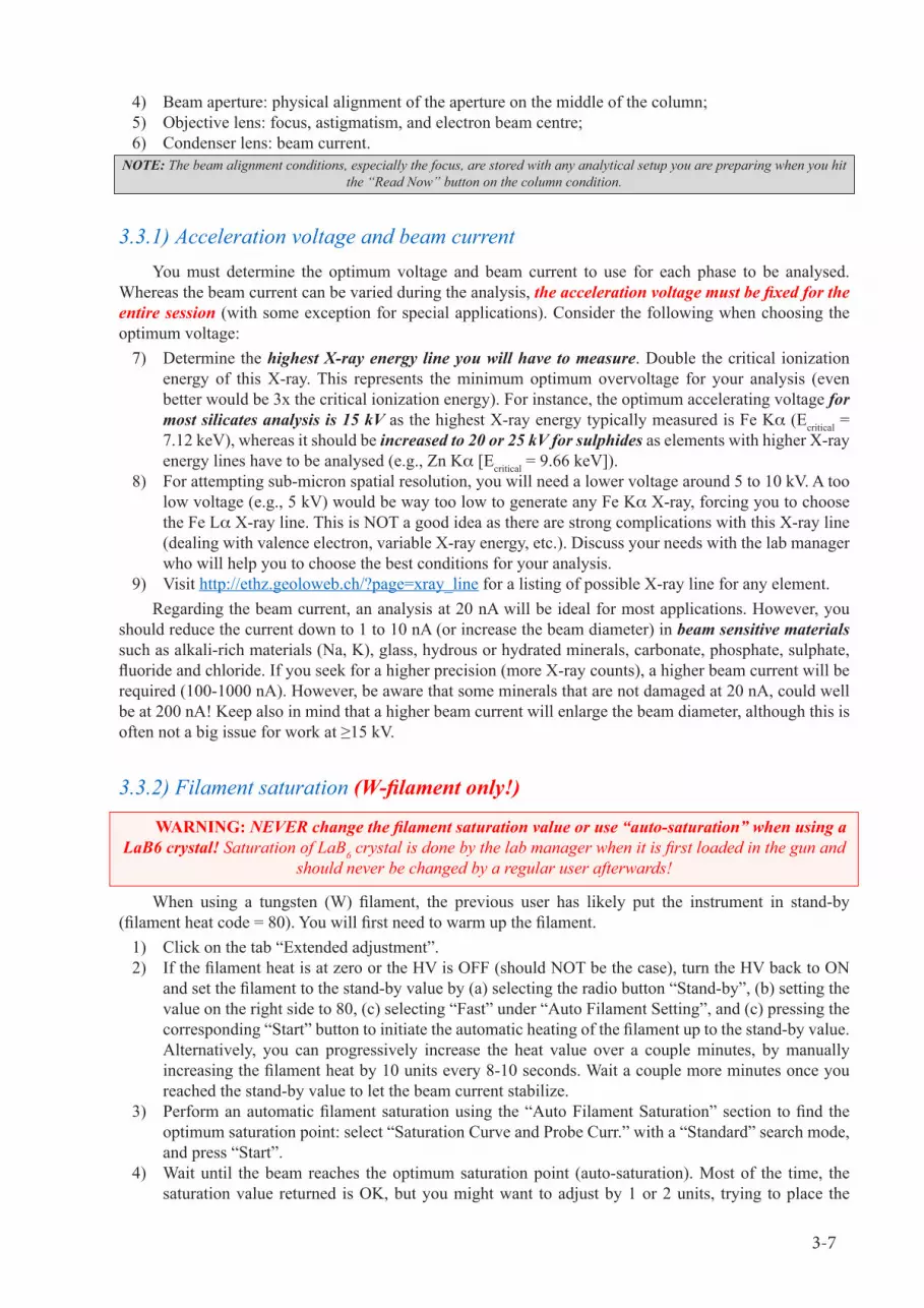
3-7

4) Beam aperture: physical alignment of the aperture on the middle of the column;5) Objective lens: focus, astigmatism, and electron beam centre;6) Condenser lens: beam current.

NOTE: The beam alignment conditions, especially the focus, are stored with any analytical setup you are preparing when you hit the “Read Now” button on the column condition.

3.3.1) Acceleration voltage and beam currentYou must determine the optimum voltage and beam current to use for each phase to be analysed.

Whereas the beam current can be varied during the analysis, the acceleration voltage must be fixed for the entire session (with some exception for special applications). Consider the following when choosing the optimum voltage:

7) Determine the highest X-ray energy line you will have to measure. Double the critical ionization energy of this X-ray. This represents the minimum optimum overvoltage for your analysis (even better would be 3x the critical ionization energy). For instance, the optimum accelerating voltage for most silicates analysis is 15 kV as the highest X-ray energy typically measured is Fe Ka (Ecritical = 7.12 keV), whereas it should be increased to 20 or 25 kV for sulphides as elements with higher X-ray energy lines have to be analysed (e.g., Zn Ka [Ecritical = 9.66 keV]).

8) For attempting sub-micron spatial resolution, you will need a lower voltage around 5 to 10 kV. A too low voltage (e.g., 5 kV) would be way too low to generate any Fe Ka X-ray, forcing you to choose the Fe La X-ray line. This is NOT a good idea as there are strong complications with this X-ray line (dealing with valence electron, variable X-ray energy, etc.). Discuss your needs with the lab manager who will help you to choose the best conditions for your analysis.

9) Visit http://ethz.geoloweb.ch/?page=xray_line for a listing of possible X-ray line for any element.Regarding the beam current, an analysis at 20 nA will be ideal for most applications. However, you

should reduce the current down to 1 to 10 nA (or increase the beam diameter) in beam sensitive materials such as alkali-rich materials (Na, K), glass, hydrous or hydrated minerals, carbonate, phosphate, sulphate, fluoride and chloride. If you seek for a higher precision (more X-ray counts), a higher beam current will be required (100-1000 nA). However, be aware that some minerals that are not damaged at 20 nA, could well be at 200 nA! Keep also in mind that a higher beam current will enlarge the beam diameter, although this is often not a big issue for work at ≥15 kV.

3.3.2) Filament saturation (W-filament only!)

WARNING: NEVER change the filament saturation value or use “auto-saturation” when using a LaB6 crystal! Saturation of LaB6 crystal is done by the lab manager when it is first loaded in the gun and

should never be changed by a regular user afterwards!

When using a tungsten (W) filament, the previous user has likely put the instrument in stand-by (filament heat code = 80). You will first need to warm up the filament.

1) Click on the tab “Extended adjustment”.2) If the filament heat is at zero or the HV is OFF (should NOT be the case), turn the HV back to ON

and set the filament to the stand-by value by (a) selecting the radio button “Stand-by”, (b) setting the value on the right side to 80, (c) selecting “Fast” under “Auto Filament Setting”, and (c) pressing the corresponding “Start” button to initiate the automatic heating of the filament up to the stand-by value. Alternatively, you can progressively increase the heat value over a couple minutes, by manually increasing the filament heat by 10 units every 8-10 seconds. Wait a couple more minutes once you reached the stand-by value to let the beam current stabilize.

3) Perform an automatic filament saturation using the “Auto Filament Saturation” section to find the optimum saturation point: select “Saturation Curve and Probe Curr.” with a “Standard” search mode, and press “Start”.

4) Wait until the beam reaches the optimum saturation point (auto-saturation). Most of the time, the saturation value returned is OK, but you might want to adjust by 1 or 2 units, trying to place the

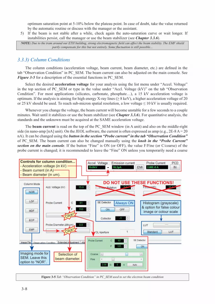
3-8

optimum saturation point at 5-10% below the plateau point. In case of doubt, take the value returned by the automatic routine or discuss with the manager or the assistant.

5) If the beam is not stable after a while, check again the auto-saturation curve or wait longer. If instabilities persist, call the manager or use the beam stabilizer (see Chapter 3.3.6).

NOTE: Due to the tram around our ETH building, strong electromagnetic field can affect the beam stability. The EMF shield partly compensate for this but not entirely. Some fluctuation is still possible...

3.3.3) Column ConditionsThe column conditions (acceleration voltage, beam current, beam diameter, etc.) are defined in the

tab “Observation Condition” in PC_SEM. The beam current can also be adjusted on the main console. See Figure 3-5 for a description of the essential functions in PC_SEM.

Select the desired acceleration voltage for your analysis using the list menu under “Accel. Voltage” in the top section of PC_SEM or type in the value under “Accl. Voltage (kV)” on the tab “Observation Condition”. For most applications (silicates, carbonate, phosphate…), a 15 kV acceleration voltage is optimum. If the analysis is aiming for high energy X-ray lines (≥ 8 keV), a higher acceleration voltage of 20 or 25 kV should be used. To reach sub-micron spatial resolution, a low voltage ≤ 10 kV is usually required.

Whenever you change the voltage, the beam current will become unstable for a few seconds to a couple minutes. Wait until it stabilizes or use the beam stabilizer (see Chapter 3.3.6). For quantitative analysis, the standards and the unknown must be acquired at the SAME acceleration voltage.

The beam current is read on the top of the PC_SEM window (in A unit) and also on the middle-right side (in nano-amp [nA] unit). On the JEOL software, the current is often expressed as amp (e.g., 2E-8 A = 20 nA). It can be changed using the button in the section “Probe current” in the tab “Observation Condition” of PC_SEM. The beam current can also be changed manually using the knob in the “Probe Current” section on the main console. If the button “Fine” is ON (or OFF), the value F/Fine (or C/coarse) of the probe current is changed; it is recommended to leave the “Fine” ON unless you temporarily need a coarse

Figure 3-5 Tab “Observation Condition” in PC_SEM used to set the electron beam condition

Click!

Click!

Imaging mode for SEM. Leave this option to “NOR”.

Selection of beam diameter.

Histogram (grayscale) & option for false colour image or colour scale

Controls for column condition...- Acceleration voltage (in kV)- Beam current (in A)- Beam diameter (in um).

Always ON

DO NOT USE THESE FUNCTIONS!

3-9

change to avoid abrupt and accidental change. For most common application and for navigation, a beam current of 10 to 20 nA is ideal. Avoid navigating on a sample at high current. For best image resolution, a smaller beam current (1-5 nA) can be used. The use of a higher beam current (50 to 300 nA) is recommended for minor and trace element analysis, for qualitative WDS scan, or for element mapping. When the tilt and shift of the condenser lens is aligned properly (see next section), a maximum probe current of >500 nA is usually achievable.

When navigating in the sample, you should always leave the beam size (probe diameter) to 0.0 (focused beam), in order to obtain the sharpest image possible. Keep the current low for navigation (1-20 nA). Navigating at high current (>50 nA) is not recommended, especially in beam sensitive materials (carbonate, clay, etc.), as it can damage the sample. Whenever you prepare an analysis, you will have the possibility to define a specific beam current and beam size for each series of analysis.

3.3.4) Beam alignment: Tilt and ShiftThe gun is equipped with a set of electromagnetic lenses used to align the emitted electron beam so

it does flow straight down and in the centre of the column below. This first set of lenses needs a regular adjustment, called the tilt and shift corrections, to correct for the position of the centre of emission (shift) and for the verticality of the electron beam (tilt). LaB6 (and often W, too) are very stable once a clean and high vacuum has been reached, and after a week at full power. However, a daily adjustment is still recommended. The tilt and the shift corrections must be performed iteratively, starting and ending with the tilt correction, and should aim at maximizing the beam current. WARNING: The refreshing rate of the beam current reading is slow and can take 1 to 2 seconds to update. Be patient!

1) Expend the “Chart Recorder” window (top-right of PC_EPMA) by clicking on the rectangle button:g) Select a fast refreshing rate (200 to 500 ms);h) Leave only activated the Probe current reading, and deactivate the WDx (bottom-left buttons);i) Start the chart recorder by pressing the “play” button;j) Click “stop” and “play” again to clean the chart as necessary;k) Leave this window visible, you will use it to maximize the beam current.

2) Set a low beam current (ca. 1 to 20 nA) for the tilt correction.3) Select the tab “Alignment” in PC_SEM and click on the button “Tilt” or press the button “Align” on

the main console (under the “Alignment” part).4) Turn alternatively the buttons X and Y under the Alignment part of the main console to modify the tilt

values and to reach a maximum probe current. You can also change manually the value in PC_SEM under “Setting Value”. Do NOT press the “reset (all)” button or you’ll have to start from scratch!

5) When the tilt is optimized, click “Shift”, or press again “Align” on the main console (toggle between “Tilt” and “Shift” correction).

6) Set a high beam current (> 100 nA) for the shift correction.7) Turn X & Y under the Alignment section until the maximum current is reached.8) Repeat the tilt and shift correction, until no significant change occurs when optimizing the tilt.9) When done, press the “Stigmator button” or “STIG” on the main console (= “Align OFF” button).

WARNING: Due to the presence of trams around our building, a small but significant beam current instability is expected, which renders the tilt and shift correction difficult... The EMF cancellation field

(cage surrounding the EMP) is partly compensating for this, but not optimally. We are working on improving this. In the meantime, do your best to find the highest emission point.

The JEOL program also has an automatic tilt and shift adjustment. This method is ideal when the filament is new, as we have no idea where the optimum is... However, this method is time consuming and a manual adjustment is often quicker. To perform an automated tilt & shift adjustment:

1) Select the “Extended Adjustment” tab;2) In the “Auto Gun Alignment” section, select either “from the present value” (for old filament) or from

the centre position (for new filament);

3-10

3) Select the range for the search: “Narrow” for a fine tuning, and “Wide” for a new filament or when the alignment is totally offset;

4) Optional: activate the Chart Recorder (probe current, with a 1 sec refreshing rate) to see the progress of the automatic alignment;

5) Press the “Start” button (the one on the right side, in the Auto Gun Alignment section!!!) and wait for the completion message.

3.3.5) Condenser lensesIn the column below the electron gun are the condenser lenses. They are controlling the amount of

current going through the beam aperture, and thus the beam current reaching your sample below. There is nothing to do at this point.

3.3.6) Final beam alignment

WARNING: Whenever you are adjusting the electron beam focusing point, you must first make sure that the stage is on focus (adjust manually and/or use the autofocus function, see Chapter 3.4.6)!

Once the electron emission at the gun has been aligned, the optimum electron beam focusing point on the sample (highest spatial resolution) must be found by adjusting the lower part of the column: the beam aperture, the astigmatism correction and the electron focus point. The SE signal is selected as it provides the best resolution possible. For these adjustments, it is required to locate a small feature (micron-sized dust, grain boundary, sub-micron inclusion…) that can be used to optimize the image, and that is not damageable (i.e., no epoxy, no area you will analyse later). Typically, this is done on the metal plate surrounding your sample. The located feature should be a micron-sized object or a set of linear features ideally intersecting at

Figure 3-6 Beam aperture on the JEOL JXA-8230.

X-axis

XY-axisY

Beam apertureselector (1 to 4)LEAVE ON 2!X-axis

XY-axisY

Beam apertureselector (1 to 4)LEAVE ON 2!

3-11

90° (e.g., surface micro-cracks or grain boundaries). Even if the metallic sample holder is “Swiss-clean”, I bet you’ll find plenty of micron-sized dust particles that will do the job...

3.3.6.1) Beam aperture alignmentThe microprobe is equipped with a beam aperture, which limits the amount of electron to flow further

down the column. Whereas SEM usually uses small apertures (10-100 µm) for a larger field of depth and better 3D-imaging, electron microprobe usually uses larger aperture (> 100 µm) to reach a higher maximum beam current over 100 nA. The beam aperture needs to be physically aligned compared to the emission point. Unless some maintenance has been performed recently, it rarely needs a strong adjustment! To optimize the beam aperture alignment (Fig. 3-6):

1) Move to the metal part of the sample holder or a non-damageable area in your sample (see Chapter 3.4 for options to move the stage; best as this point is to use “Stage Map”, Chapter 3.4.2).

2) Focus the stage (Z; see Chapter 3.4.6).3) If the button “Freeze” is green, click on it to activate the probe scan (live view; “Prb Scn” turns green).4) Choose first a low magnification (< 100x).5) Ensure that the probe current is set to a low current, e.g., 10-20 nA.6) Choose the SE electron signal by clicking on the name of the electron image in the caption of the

electron image window and selecting SEI.7) Remove the Faraday cup (button PCD “IN” => “OUT”).8) Adjust the brightness & contrast (buttons on the far right-side of the main console, or using the

corresponding button above the image in PC_SEM) and locate an area that shows some asperities and a good contrast (micron-sized particle or inclusion, intersecting grain boundaries, etc.).

9) Increase the magnification to > 1000x and optimize again the brightness & contrast if necessary.10) Press the “WOBB” button on the main console to activate the wobble mode (also found in the

“Alignment” tab in PC_SEM, button “OL Wobbler” on the top-right side). The SE image will appear to be defocussing (with maybe some twisting) back-and-forth. If you see some lateral motion, this is an indication that the aperture needs to be aligned:

a) Locate the beam aperture on the column (Fig. 3-6).b) Leave the beam aperture to position 2 (= large aperture for high beam current).c) With the wobble active, turn very slowly either the X or Y axis knob (Fig. 3-6), to minimize

the lateral motion of the feature / particle on screen.11) Close the Faraday cup (PCD OUT => IN).12) Press the WOBB button to deactivate the wobbling mode on the console or the equivalent button on

the “Alignment” tab in PC_SEM.

3.3.6.2) Beam alignment: Focus (objective lens) and AstigmatismThere are two other alignments that need to be done on a regular basis throughout your day, when

the imaging appears of poor quality despite the stage being perfectly on focus or when changing the beam conditions (current, voltage). First, the electron beam must be focused on the surface of your sample (electron focusing), and the beam must be corrected for astigmatism. You will likely have to alternate between the electron focusing adjustment and the astigmatism correction:

1) Move to a non-damageable area in your sample.2) Focus the Z-stage (Chapter 3.4.6).3) If the button “Freeze” is green, click on it to activate the probe scan (live view; “Prb Scn” turns green).4) Choose first a low magnification (40 - 200x).5) Remove the Faraday cup (button PCD “IN” => “OUT”).6) If the image does not appear sharp, turn the large “Focus” knob on the main console to obtain the

sharpest image as possible. 7) Progressively increase the magnification, and continue adjusting the focus when the image appears

blurry to you. Repeat until you reach a medium magnification (around 500x), and locate then a small particle (micron-sized), zoom on it, and perform a final focus adjustment at > 2000x magnification.

8) At this point, the beam is on focus, but astigmatism might be present:a) To check for potential astigmatism, rotate the focus knob back-and-forth (just half- to a full-

3-12

turn). If the particle you have located get blurry but should remain round, it is all good. If it is stretching along one of the diagonals or the other (depending if you increase or decrease the focus point), this indicate that astigmatism is present.

b) To correct the astigmatism, press “STIG” (= “Align OFF”) in the “Alignment” part of the main console and turn the knobs X & Y to adjust the astigmatism correction. Optimum is reached when you obtain the sharpest image and when defocussing doesn’t stretch the object in one diagonal or the other.

9) Alternate between the electron focusing and the astigmatism correction until you obtain the sharpest image. Sometime, the astigmatism correction is best adjusted when the beam is slightly defocused.

3.3.7) Beam stabilizerPrior to running any quantitative analysis, ensure the beam current is stable at least for the time of

your analysis; use the Chart Recorder to record the change of beam current over time. In case of strong beam instability, the JEOL JXA-8230 is equipped with a beam stabilizer. To manually activate the beam stabilizer in PC_EPMA:

1) Select the tab “Observation Condition” and adjust the beam current to the desired value.2) Select the tab “Extended Adjustment” in PC_SEM.3) Under the “Beam Stabilizer” section, select “Auto Repeat Mode”.4) Click on “Tilt BST/CL BST ON” to activate the two stabilizing option acting on the tilt and on the

condenser lens. If strong current variation occurs, it is possible the CL BST will not get activated (or will take for ever to get activated). In this case, try the “Tilt BST only” option. (*)

5) Wait until the two green lights above (Tilt BST and CL BST) turn ON.6) The beam should now be stable.

The beam stabilizer can be defined when setting up a series of quantitative analysis. However, when using Probe for EPMA, the beam stabilizer must first be set in the JEOL PC_SEM before starting an analysis (hopefully this will change in the future).

(*) As of August 2019, we still have some issue with the EMF cancellation device. As a result the “Tilt BST / CL BST” stabilizer option rarely works, and only the “Tilt BST” will. We are working on this issue.

3.4) Navigate in your sample

3.4.1) Using the stage controlThere are multiple ways for you to navigate in your sample. First of all is the stage panel. It allows you

to move the X and Y axes using the “+” and “–” buttons (move by step or continuous when click-and-hold) or the Z axis with the wheel (Z). You can also use the rolling ball to move the X and Y axis; just be careful it is very sensitive and hard to use for accurate positioning. The stage speed is controlled by (a) activating the “C” button for Coarse mode (or Fine mode when deactivated) or (b) changing the magnification (lower magnification = slower speed).

On the top-right of the stage panel are two essential buttons: “AF” for Z-stage autofocus and “JOG” for jogging the stage (= “Test” button on the old JEOL-8200). Before using the AF option, you should adjust the Z-stage position to be close to the optimum focusing point, as it will often fail if the stage is totally out of focus. The “JOG” function will move away from your current selection and come back to check for stage reproducibility. It is absolutely recommended to check for optimum Z-stage position and when you need to save a (X,Y)-stage position with high stage reproducibility (better than ± 2 µm in X and Y). When the stage is “jogged” it moves away from your point and come back to the stage position. If the position is the one you expect, you should expect a good reproducibility. If you observe a displacement, you should readjust the stage and jog again until you see a good reproducibility.

3-13

3.4.2) Using the “Stage Map”, “Step Control”, or stage coordinatesFor large motion such as between samples, it is convenient to use the “Stage Map” in PC_SEM (tab

on the top-right side). Make a RIGHT-click to move to a specific location in this “Stage Map”. The stage representation in this schematic view can be changed either after a sample change or by clicking on the holder photo under the section “SEM Monitor” of the tab “Observation Condition”.

When searching for particle, or for regular “scanning” over the sample, you can use the “Step Control” in PC_SEM (tab on the top-right side). You can then choose to move the stage by a pre-defined “Step” or by “Frame”. Prefer the use of the “Stage” displacement; AVOID using the “Beam” mode, which will actually move the beam away from the centre.

You can also click on any of the X, Y, or Z stage coordinates in PC_SEM (middle-right side). This will open a window where you can manually enter a coordinate and move the stage to this position.

3.4.3) Using the optical imageIn the OM Monitor window in PC_EPMA, make a right-click on a feature on the optical image,

and choose “Stage Move to Centre” in the contextual menu to centre this feature on the optical image. This navigation option is not very accurate. Do NOT refer to the optical image for centring the position to analyse! Inclusions, cracks, and other undesirable features can be invisible on the optical image! Always rely on the actual ELECTRON centre and what you see in electron image (BSE or SE, see next)!

3.4.4) Using the electron imageWhen observing a live electron image (SE, BSE, or TOPO), you can use the click-and-drag function

to navigate across the sample. This is probably the most convenient way to navigate in sample over small distances (~mm). You can also make a right-click on a feature of interest and choose “Stage Move to Centre” to move the stage over the feature of interest.

3.4.5) Using a scanned imageBoth JEOL and Probe for EPMA computers have a dedicated program that will reference ANY image

of your sample: “Specimen Navigator” on JEOL and “Picture Snap” in PfE. There basic principle remains the same: using an image, typically a scan of the sample holder, three reference points recognisable on both the image and on the microprobe (using SE or BSE imaging) are set. These points are then geo-referenced to the EMP stage coordinate. Once calibrated you can easily double-click to navigate to an area of interest.

3.4.6) Focus, focus, and focus!Pay special attention to the Z-stage (optical) focusing whenever

you set an analysis point or you acquire an image. Accuracy of electron microprobe analysis is very sensitive to the geometry (Bragg’s law of diffraction). Always make sure you are on optical focus with the stage:

• Always set manually the Z-stage focus to be close to the focus point (AF might fail if you are too far from the optimum).

• Use the Auto-Focus function “AF” on the stage control or on the OM Monitor of PC_EPMA to perform an auto-focussing.

• If the AF fail, perform a manual focusing using the stage control in “Fine” mode (button “C” [coarse] deactivated).

• Use the “Jog” button to ensure a good reproducibility.

3-14

The stage is on focus when you see two SHARP dark-grey diagonal lines on the OM monitor (picture above), in addition to the black horizontal- and vertical-micrometre lines.

The AF function should work 99% of the time if you are close to the focus point, i.e., you can see some blurry to sharp diagonal lines on the OM monitor. If you are totally out of focus (diagonal lines not visible, dark screen, or all blurry) or if your sample is perfectly flat with no contrast (e.g., no crack, grain boundary, or inclusion), the AF function can fail (limited search range). If you intend to rely on the auto-focus function during an automated work, you MUST still ensure a perfectly focused point is saved! If the AF function fail, it will return to the initial (saved) position.

Make the distinction between the Z-stage and the ELECTRON focusing. First, the stage is set on focus, and second the electron are focused on that plan. Both need to be focused for optimum results (spatial and quantitative). The electron beam alignment as described in the previous section is done at the stage Z-focus point for a specific beam condition, and you need to adjust the Z-position for every single point to be analysed. If this alignment has been done properly, you should only worry about the stage (Z) focusing, and only adjust the electron focusing when you change the column condition (beam current and/or acceleration voltage).

WARNING: Do NOT confuse the button “AF” (on stage control or in OM Monitor window) with the button labelled “Auto” (on the main control and on the PC_SEM top buttons). The button “Auto” will attempt a focusing of the electron beam, which is often less good than a manual adjustment (Chapter 4.1).

3.5) Start & end of your analytical sessionOnce your samples are loaded, that the beam has been aligned and set at the proper acceleration voltage

and current, and that the current is stable, you can start analysing or imaging your sample. Depending on the work to be done, refer to the following chapters:

• Chapter 4: Essential features of the JEOL software:* Imaging (SE, BSE, TOPO);* JEOL EDS system;* Qualitative WDS scanning;* Element mapping (WDS/EDS);* Standardization and quantitative analysis;* A few companion programs (e.g., “Specimen Navigator”);* etc.

• Chapter 5: Quantitative analysis with Probe for EPMA.• Chapter 6: X-ray element mapping with Probe Image.• Chapter 7: Treatment of quantitative element mapping with CalcImage.At the end of your session, make sure to remove your sample, and clean the lab space. If nobody is

working after you on the instrument, leave the sample holder and its base in the desiccator. Remove all your samples from the sample holder and take them back with you. The EMP lab is not a place to store your sample(s)! Leave the sample chamber and the airlock under vacuum, and leave the sample exchange bar down. If you had an overnight analysis and you are unable to remove your sample early the next day, please, advise the next user or come and get your samples ASAP. On the opposite, if you find samples inside the EMP when you start your analysis session, leave the samples in the desiccator.

Make sure to transfer all your results, including all the original files. For the JEOL files it is easier to transfer the data by first compressing the folder to transfer (ZIP file) and then copy the ZIP file to your device or send by email. For Probe for EPMA analyses, everything is saved in one MDB file (Microsoft Access file) plus your export files. We do NOT guarantee long-time storage or backup, so you are responsible for your own files! Use the reprocessing station in lab A90.2 to reprocess or transfer your data. Depending on your work to be done, you might have data…

• On the JEOL computer, your JEOL data (images & analyses) are in F:\EpmaData\Project\Your name• On the Probe for EPMA, files are in two locations:

* Probe for EPMA & CalcImage: C:\UserData\Your name* Probe Image: C:\UserImages\Your name

4-1

4) JEOL software “PC_SEM” and “PC_EPMA”The JEOL software can be used to acquire images, or WDS data (qualitative or quantitative). The

following is presented in this chapter:• PC_SEM:

* Image acquisition with PC_SEM;* EDS acquisition (qualitative);

• PC_EPMA:* WDS scan acquisition (qualitative);* Element mapping (simple setup);* Standard acquisitions and Quantitative analyses;* Data reprocessing and results exportation;* A few “Operation Settings” you are allowed to change;* User-level maintenance and fix to common issues.

• Specimen Navigator.Refer to Chapter 3 for information regarding the use of PC_SEM for sample exchange, beam

alignment, setting the beam conditions, and stage navigation. The present manual is only focussing on the functions a regular user will perform. For more information, discuss with the lab manager or refer to the JEOL manuals (see the blue folders in the probe lab).

4.1) Acquiring an SE, BSE, or TOPO image

4.1.1) GeneralitiesThe JEOL JXA-8230 offers three main electron imaging mode: Secondary Electron Image (SEI),

Backscattered Electron Image (BEI or COMPO), or Topographic Image (TOPO, subtract one side of the BSE detector from the other). You can also acquire the X-ray signal (XR1 to XR5 signals), but these are usually very low and (almost) useless at the fast scanning rate usually used for quick imaging.

The main controls for electron imaging are available through a series of button either on the main console or on the top of PC_SEM; their use is summarized in Figure 4-1. To acquire any electron image, the procedure is the same independent of the selected signal:

1) If not already done, select your own project folder for image acquisition in PC_SEM:a) Select the tab “Image Files”;b) Click on “Browse” to navigate to your folder;c) If needed, use Windows Explorer to create a new folder for your images within your project

folder in “F:\EpmaData\Projects\Last name First Name”. It is highly recommended to have a sub-folder for each of your “Project”.

2) Use an appropriate beam current and voltage; 10-20 nA at 15 keV recommended for basic imaging.3) Move to the area of interest.4) Adjust the stage Z-position to be on focus. An approximate focusing is okay for navigation purpose;

to obtain high-quality images, use the stage auto-focus (AF) function.5) Set the instrument into scanning mode:

a) If the FREEZE button is active, you must first deactivate it by pressing one of the button “Freeze” on the top menu of PC_SEM or on the main console. This will automatically activate the scanning mode (buttons “Scan” on PC_SEM and “Prb Scn” on the main console are activated). Note that activating the “Prb Scn” on the console or on the screen will have the same effect.

b) Set the magnification to a low value (< 100x).c) Choose the electron signal to display by either pressing the “View” button on the main console

(switch between the different imaging mode), or by clicking the signal name on the image display (choice between SEI, COMPO, TOPO, or XR [X-ray] signals).

6) Choose the scanning rate “Quick 2”, which is ideal for navigation. Fine 1 or 2 are used for photo.

4-2

7) Remove the Faraday cup by pressing the PCD “IN” button on PC_SEM or on the main console.8) Adjust the brightness and contrast to reveal the feature of interest using the buttons on the far-right

side of the main console. Press the “ACB” button if nothing is visible, or if it is too bright, or adjust manually the brightness and contrast using the button on the main console. You can also set the contrast and brightness values by clicking on menu “Tool > Brightness and Contrast” in PC_SEM.

9) Press the button “Photo” to start the image acquisition. The scanning mode is switched to Fine 1 or 2.10) At the end of the acquisition, a “save as” dialogue window will open. Ensure to check the box “Export”

so that the signal information, date and time, scale bar, etc. are visible at the bottom of the image.If the image appears blurry or not optimal, there could be multiple factors. As a reference, at 15 keV

and 10-20 nA, you should be able to identify sub-micron features. If this is not the case...• Check if the Z-stage is on focus.• Check if the beam alignment is OK, especially the electron focusing point (see Chapter 3.3 for beam

alignment procedure).• Check if the beam diameter is set to focused (Beam diameter = 0 µm).• Appreciate the magnification used! If the magnification scale is high (> 1,000x), some level of

Figure 4-1 Functions for generating an image on the PC_SEM menu and on the main console. See Chapter 3 for the use of the “Alignment” and “Probe Current” sections of the main console.

Beam shiftMust be OFF

Faraday cup

ALIGNMENTIMAGE SELECT

SCANNING MODE

MAGNIFICATION FOCUS

Probe Current

Display & Photo

IMAGE

Set voltage and current Faraday cupIN / OUT

PCD = probecurrent detector

Beam scanning mode(quick vs. slow rastering)

Beam autofocusAvoid using it!

Acquire aphoto (*)

Measurementtool (X, Y, Ø)

Spot or scanmode (see Freeze)

Auto contrast& brightness

Show/hidecursor

ON: Image frozenOFF: Live mode (Prb Scan ON)

Freezing mode(current or ALL)

View Inst Wobb Align Stig

Quickview

Fineview

PrbScan

Auto

RDCimage

AlignOFF

YX

ALIGNMENTIMAGE SELECT

SCANNING MODE

MAGNIFICATION FOCUS

Probe Current

Display & Photo

IMAGE

PCD

Coarse / Fine

Contrast

Brightness

Freeze ACB Photo

+- +-

+-

DO NOTTOUCH!

Main Console

PC_SEM menu

Rastering & imaging

Do not change anything here once the beam alignment has been done!

Avoid changing the current as a new beam alignment would then be required!

4-3

blurriness is normal as you approach the absolute spatial resolution on this instrument.Four additional features are only available in the PC_SEM top buttons:• “Shift 0” is the indicator of beam shift. In normal situation, it should always be deactivated. When

active, it indicates that the beam is deflected away from its centre. Press this button to place the beam back to its central position. The beam shift can be set in the PC_EPMA program for a specific analysis; it is however not recommended. It can also be set – often accidentally! – when scanning at over 20,000x magnification. At this magnification, any click-and-drag on the SE or BSE image will actually result in shifting the beam and NOT the actual stage position. All Probe Software programs are currently NOT compatible with the beam shift feature and therefore you should always ensure the beam is NOT shifted (“Shift 0” button NOT available) before starting an analysis with Probe for EPMA or Probe Image.

• “Ruler” is used to measure distance (horizontal, vertical, or diameter). Activate the ruler mode you need, and click-and-drag the green lines (or a corner) to move them and read the distance.

• “Cursor” is an indicator for the beam centre (yellow cross). It should be used to ensure the proper positioning of an analysis spot. It is possible to move the position of this cursor by clicking and dragging it. This movement will do nothing to the electron beam, it is only visual (on screen). If you accidentally moved it, and would like to see the real centre, simply de-activate and re-activate it.

• “Full Image” on the top-right of PC_SEM expands the image to the entire PC_SEM window.The default scanning rate for the pre-selections “Quick 1, 2” and “Fine 1, 2” along with the selection

of the scanning rate to acquire a photo can be modified in menu “Setup > Operation Settings [Image/Scan]” (see Chapter 4.2.1.1). The recommended speed settings are 1 and 4 for “Quick 1”and “Quick 2”, and 8 and 10 for “Fine 1” and “Fine 2” (corresponding to ca. 30 and 90 sec, respectively). You can also opt for a multiple-pass photo, although it is usually not needed and set by default to 1. In the Photo Button section, choose “Fine 1” or “Fine 2” and the image size you want (1024 x 768 recommended). It is usually pointless to increase the speed to a value >10, unless you are working at a very low current (1-2 nA or less).

All detectors are to some extent sensitive to light. When using a high contrast, it is possible that the brightness of the screen will change when you navigate, especially in BSE / COMPO mode, due to changes in the reflectivity of your sample surface. To avoid this issue, either set the contrast to a lower level, or switch off the light of the optical microscope (click on the light bulb in the OM Monitor).

4.1.2) Imaging multiple signalsIt is possible to see and take a simultaneous photo of up to four signals (Fig. 4-2). To do so, click on

the button “Comparison” on the right side of PC_SEM. The following new buttons appear on the middle-right side of PC_SEM:

• “Add”: overlap two signals in a composite Red-Green view. This mode is rarely used and might be useful for non-ideal samples with “rough” surface where an overlap of both SE and BSE signal can help identifying suitable analysis spot.

• “H-Dual” and “V-Dual”: acquire two images simultaneously. In the horizontal H-Dual mode, the image appears to be trimmed on the left and right side. However, when a “Photo” is acquired, both images will ultimately have the usual 4:3 ratio. This is not the case with the vertical V-Dual mode, where the resulting “Photo” images will effectively have a larger width-to-height ratio (this might be a bug from the software?!?).

• “Quad”: acquire simultaneously up to four signals, each with a 4:3 ratio.For each image provided in any of the aforementioned mode, you can change the signal source and

adjust the image brightness and contrast: 1) Click on one image to select it; a blue rim appears around it.2) Click on the “SEI” (or “COMPO”, or “TOPO”) in the caption of the electron image; a list of available

signal appears. Click the signal to display. If the list menu is not accessible, ensure the image is not frozen (click on “Freeze” or “Freeze all” if one or both of them are active).

3) Adjust the brightness & contrast using the buttons on the main console or atop the image.4) Repeat steps 1-3 for all other signal(s).

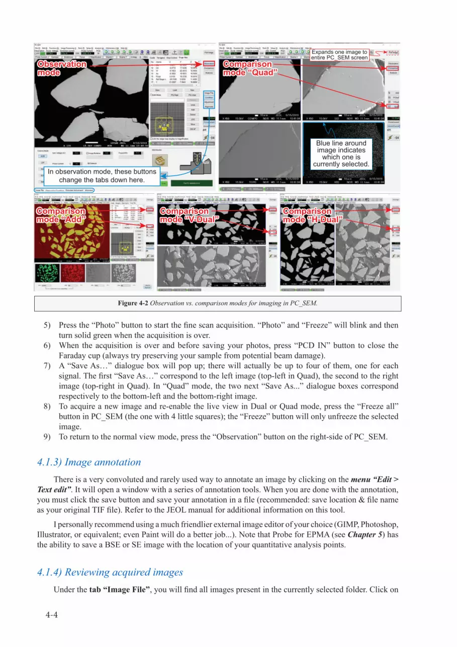
4-4

5) Press the “Photo” button to start the fine scan acquisition. “Photo” and “Freeze” will blink and then turn solid green when the acquisition is over.

6) When the acquisition is over and before saving your photos, press “PCD IN” button to close the Faraday cup (always try preserving your sample from potential beam damage).

7) A “Save As…” dialogue box will pop up; there will actually be up to four of them, one for each signal. The first “Save As…” correspond to the left image (top-left in Quad), the second to the right image (top-right in Quad). In “Quad” mode, the two next “Save As...” dialogue boxes correspond respectively to the bottom-left and the bottom-right image.

8) To acquire a new image and re-enable the live view in Dual or Quad mode, press the “Freeze all” button in PC_SEM (the one with 4 little squares); the “Freeze” button will only unfreeze the selected image.

9) To return to the normal view mode, press the “Observation” button on the right-side of PC_SEM.

4.1.3) Image annotationThere is a very convoluted and rarely used way to annotate an image by clicking on the menu “Edit >

Text edit”. It will open a window with a series of annotation tools. When you are done with the annotation, you must click the save button and save your annotation in a file (recommended: save location & file name as your original TIF file). Refer to the JEOL manual for additional information on this tool.

I personally recommend using a much friendlier external image editor of your choice (GIMP, Photoshop, Illustrator, or equivalent; even Paint will do a better job...). Note that Probe for EPMA (see Chapter 5) has the ability to save a BSE or SE image with the location of your quantitative analysis points.

4.1.4) Reviewing acquired imagesUnder the tab “Image File”, you will find all images present in the currently selected folder. Click on

Figure 4-2 Observation vs. comparison modes for imaging in PC_SEM.

Observationmode

Comparisonmode “H-Dual”

Comparisonmode “Add”

Comparisonmode “V-Dual”

Comparisonmode “Quad”

Observationmode

Comparisonmode “H-Dual”

Comparisonmode “Add”

Comparisonmode “V-Dual”

Comparisonmode “Quad”

In observation mode, these buttons change the tabs down here.

Blue line around image indicates

which one is currently selected.

Expands one image to entire PC_SEM screen

4-5

“Browse” to change folder. Using the images visible in the preview, you can...• Review / load back on screen the image by double-clicking on it and click on “Horizontal” when the

program asks you which orientation it should stretch the image.• Navigate back to the position of your image by making a right-click on the image and choosing the

option “Move this image point”. • Set back the instrument to the conditions of analysis of this image by choosing “Set Conditions”.In the folder containing your image, you will find two files, a TIF image and a text file. The text file

contains the acquisition conditions, such as beam conditions, magnification, stage coordinates, etc. Both files should have exactly the same name to be recognized as a valid image by the program PC_SEM.

4.2) Advanced image features in PC_SEM

4.2.1) Operation settingsThe “Operation settings” window regroups several tabs controlling the main software options; only

the two tabs you might modify are reviewed here: “Image/Scan” and “Photo & Print Data” (see Fig. 4-3). Whenever you change a setting, remember to press the “Set” button (green box in Fig 4-3). The “Save” and “Load” buttons allow to save or load a file containing some default settings. If you want to reset the status to the default, load the most recent file labelled “Default YYYY-MM-DD”.

WARNING: If you modified any option in Operation Settings (because you know what you are doing), you must re-set this option to its default value after your work! The next user will thank you!

You should NOT change anything in... “Auto function” (control for the auto-focus and ACB), “Preset” (choices for default voltage, magnification, and WD), “Signal name”, and “Mouse Control”.

4.2.1.1) “Image/Scan” tabThis tab controls the scanning rate of the different modes “Quick1”, “Quick2”, “Fine1”, “Fine2”, and

“Photo”, and the behaviour of the “Freeze” button. The “Scan/AVE.” section (top left) define the scanning rates. Default values are 1, 4, 8 and 10 for “Quick1”, “Quick2”, “Fine1”, and “Fine2”, respectively.

Choose the adequate photo option in the “Photo button” section (top-right; usually set to “Fine1” or “Fine2”). In most case, it is not necessary to use the integration mode. A rate of 8 (~30 s per image) is fine for general imaging, a rate of 10 (~80 s) will help reducing the noise. The image quality rarely improves

Figure 4-3 Operation Settings, tab “Image/Scan” for changing the default scanning rates (Quick, Fine, Photo).

Do not change anything here!

4-6

beyond 10, except maybe at low voltage (≤10 kV) or low current (<1-2 nA) conditions.

The behaviour of the “Freeze” button is modified in the “Integration” section (bottom-left). Avoid changing anything here. Currently, the integration mode is active: if the “Freeze” button is activated, it will integrate 128 images (in Quick) or 8 images (in Fine) before freezing the image completely. Note that if you want to freeze an image immediately, you can always click twice the “Freeze” button (1st = activate the freeze [button blinks]; 2nd = stop it [button solid-green]; click a 3rd time to unfreeze [button OFF]).

The “Auto-save” section of this tab contains the default setting for the behaviour of the “Save As…” dialogue. Do not change anything here.

4.2.1.2) “Photo & Print Data” tabThe tab “Photo & Print Data” (Fig 4.4) let you choose which information is being displayed in the

legend bar of the image, both on screen and on file. Note that this legend will only be visible on the TIF image if you checked the check box “Export” in the “Save as…” dialogue box. Bitte, do not alter the label (default: “ETHZ”) that marks where the picture was taken. Merci vilmal!

4.2.2) Comment about the “Freeze” modeThe “Freeze” mode is activated when the electron beam is in “spot” mode (i.e., not scanning), or

whenever an acquisition (image or WDS) is over (image frozen on screen). You must click on it to deactivate it, and thus “unfreeze” the image, switch back to scanning mode, and enable again the live view on the screen. If you want to just temporarily keep the current view on screen, without having to keep the beam on your sample (e.g., when working on beam sensitive materials), press twice on “Freeze” to immediately capture whatever is currently shown on the screen. You can then close back the Faraday cup (PCD OUT => IN), and the image will still be visible on the screen. If you press “Photo” when the “Freeze” is active (solid green) it will open a “Save As...” dialogue box.

4.2.3) Step Control & Stage Maps The Step Control tab is used to move the stage by a fixed distance in mm, or by a fixed percentage of a

frame. The step distance and frame percentage can be modified with menu “Edit > Operation Settings” and the tab “Stage/Beam Setting” (see Figs. 4-5 and 4-6).

Figure 4-4 Operation Settings, tab “Photo & Print Data” for selection of data to report on each saved image.

4-7

Saved position(right-click for options)

Step or framestage control

Counter &distance

Choose tomove thestage or

beam

Save/load set of position,“Edit mode”, and buttons

for fiducial point (PQ)

Choose tomove bystep or

by frame

Stage schematic, right-click to move

to a position

Buttons to add/delete positions, “jog”, move to a selected position and auto-focus for Z-stage

“Step Control” tab “Stage Map” tab

Figure 4-5 Highlights on the “Step Control” and “Stage Map” tabs in PC_SEM (right-side of screen).

Figure 4-6 Stage/Beam Setting in Operation Settings. The sections “Step size” or “Field factor” on the right side can be modified by the user. Avoid changing anything on the left side (Stage Link, Trackball, Rotation direction).

4.2.4) Guide & NavigatorNot covered here. “Guide” lists a few general tips, not so helpful... “Navigator” temporarily save a

snapshot of an area of interest so you can quickly return to this area later.

4-8

4.3) PC_SEM: EDS acquisitionThe EPMA is equipped with a 30 mm2 JEOL EDS system controlled through PC_SEM. This section

is a quick overview on the use of the EDS for qualitative work. Figure 4-7 highlights the key controllers of the EDS and shows how to activate the EDS detector. EDS is convenient for quick phase identification and is an excellent companion for combined EDS-WDS analysis or mapping, with major elements acquired by EDS. Refer to Chapters 4.6 & 4.7 for using the combined EDS-WDS quantitative analysis feature.

IMPORTANT: While in “Analysis” mode (see [3] in Fig. 4.7), the programs locks the imaging controls (PCD, scanning mode, etc.). To re-enable them, click on “Observation” and save your date as required.

4.3.1) EDS: “Spectrum” analysis“Spectrum” is the simplest and most useful mode you will used for quick mineral identification. It

offers the ability to either analyse whatever you are currently scanning, or to select points and areas in a frozen image to be analysed (equivalent to the so-called “Point & Shoot” on the SEM with the Thermo EDS system). The major steps are depicted in Figures 4-7 to 4-9:

1) Locate an area of interest and leave the Faraday cup out (PCD OUT). Activate the EDS detector:a) Activate the bias (“lightning” button);b) Open the EDS window (right-click on “DT” area and click “Open” or “Reduce”)c) Set the appropriate time constant (right-click on “DT” area and click on T1, T2, T3, or T4) so

that DT (= dead time percentage) is less than 40% (ideal = 20-30%).i) For “normal” operation at 15 keV and 20 nA, use the “Open” setting with T3 or T4.ii) For higher current applications or whenever DT is >40%, either choose the “Reduce”

window or set the time constant to T1 or T2.iii) See Figure 4-10 to help you choose an optimum window and time constant depending

on the count rate received or the probe current used.2) Select either a homogeneous area to analyse (= high magnification, usually > 2000x) or an area at an

intermediate to high magnification (usually > 500x).3) Click “Analysis” to enter the “Analysis” mode.4) Ensure “Spectrum” button is selected. Check the analysis condition (button “Condition”; see also Fig.

4-8) and adjust the counting time as required (see below for choosing the optimum counting time).a) If you press “Start”, an EDS acquisition of the currently scanned area will start.b) Alternatively, select “Point” or “Area” in the “Analysis position” section (* in Fig. 4-7) to

select multiple points over the image to be acquired: with “Point”, just click on the pixel to analyse and for “Area” click-&-drag. Then press “Start”. The analysis of each individual points & areas will start. Additional details on the use of the point & area analysis is in Figure 4-9.

c) During the acquisition, the remaining acquisition time will be displayed above the periodic table, and the button “Start” will change to “Stop”. Click “Stop” to abort immediately.

d) As soon as you start an EDS acquisition, the SE/BSE image are frozen and the main controls in PC_SEM or on the main console are locked. To gain back control, click on the button “Observation” (top-right of PC_SEM), and save your work if necessary (see below)!

5) Results of the EDS acquisition will be shown as a list; select an entry to display the results.6) Use the button “Save” to save the data in JEOL format. Results of EDS saved by JEOL will be

available in the “Image File” tab of PC_SEM with a blue label “Analysis” on the image.7) Use the button “Export” to save results either as an image (JPG) or as a text file (EMSA format).

The results are displayed on the bottom left of the screen with a periodic table on the right side (see Fig. 4-8 for details). After each EDS acquisition, the software will automatically label the peaks providing the button “Qual.” above the periodic table is active. Identified elements will be shown as grey area on the EDS spectrum (corresponding to the Region Of Interest [ROI]), and highlighted in pink in the periodic table. Elements in the periodic table that are light grey are “identifiable” elements, whereas elements in dark grey are “never identified” elements. You can toggle between different element status (identified, never identified, neutral) by clicking on an element. Additional element status are available by right-clicking on

4-9

Figure 4-7 Key steps for starting a simple EDS acquisition.

the element (“fixed” element in blue, “balance” element in yellow, “excluded from quantitative analysis” in yellow-green, selected element with black outline).

4.3.2) EDS: “Line” and “Multi-points Line” analysisIn “Line” mode (Fig. 4-11), it is possible to define a line over a grain and measure the possible variation

of composition along this line (e.g., plagioclase zoning, diffusion profile, etc.). Precision and sensitivity of

If scanning over heterogeneous domains, use the Analysis position tool (Point or Area) to select area(s) to be analysed (see also Fig. 4-9).

2) Move to area of interest: single homogeneous phase for single EDS analysis (averaged analysis) or scan over multiple phases at ≥ 1000x magnification for “Point & Shoot” (multiple points or areas analyses).

3) Click on “Analysis” on the top-right of PC_SEM when ready.

To acquire a single analysis or a “Point & Shoot”: For other options, see Figs. 4-9 and 4-11.

4) Select “Spectrum”, and check Acquisition Condition (Fig. 4-8). Select points or areas to analyse (*) (Fig. 4-9); if no point is selected, currently scanned image will be analysed. Press “Start”. Results will appear in “EDS result”, and elements will be automatically identified in “Periodic table” (colour-coded as identifiable (light grey), identified (pink), and excluded (dark grey);

5) Results are listed (and selectable) here. Use the “Export” or “Save” EDS data (6) to export in either EMSA or image format (JPG), or save as JEOL file. When done, turned off the detector bias, close the window (1), and click on “Observation” (3) to return to scanning mode.

Start the EDS detector and enter the “Analysis” mode

Scan set at high magnification in homogeneous domain (no inclusion, no zoning, etc.). EDS analyses results

are shown here:– 1 image (current scan)– 1 or more EDS scan(s)

1) Activate EDS detector: a) Turn ON bias by clicking

on “Lightning” button; b) Right-click on “DT: ...%”: * selecting “Open” or “Reduce”

to Open EDS window * Select Time Constant

“T1” (short) to “T4” (long).

Periodic table

EDS result

Right click! PCD IN: no signal (noise), DT 0% (blue)

Low current, DT 20-45%

(green; ideal)

Intermediate current,

DT 46-65% (not ideal)

High current, DT >65%

(red; MUST reduce it)

3

2

16

5

4

*

4-10

Single point Multi pointsMulti points

Leave defaultvalues here!

Leave defaultvalues here!

Leave defaultvalues here!

Default here!Default here!

Leave defaultvalues here!

Map setting Line settingLine setting

Erasespectrumscreen

Energy and counts at black cursor on spectrum(click on spectrum to select different energy).

Autoelement

ID

Quantanalysis

Don’t use...

Acquisitionconditions,see below

Selection of analysis type: - “Spectrum” (single

analysis or multiple points);- “Line” (1D variation);- “Map” (2D variation).

“Start” initiate the acquisition. If no specifc points are selected, the entire image area will be analyzed.

Notconsidered

here

Single point

Map setting

Chemical type (phase classification based on composition) and QBase (set of reference

EDS spectra for auto ID) not used...

Enter sample

name here or modify after in

sample list

Modification of the region of interest (grey area under identified element). Not used (will be considered automatically when running quant analysis

Open spectrum in a separate window

Reduce energy range

Increase energy range

Reduce intensity range

Increase intensity range

Automatic scale (intensity)

Automatic scale (energy)

Switch between different pre-defined energy ranges

Adjust process time:– T1 or T2 for high

count rate and low spectral resolution (e.g., mapping).

– T3 or T4 for high spectral resolution and low count rate.

Single point & point & shoot analysis: enter analysis time (preset value).

Map: define pixel size, number of frames (= sweep time), and dwell time.

Leave all other preset at their default value or consult the lab manager or the JEOL manuals for more info.

Acquisition Condition

Figure 4-8 Detail on the EDS results and periodic table. The buttons on the right are used to select the acquisition mode (spectrum, line, map) and to set the Acquisition Condition. The buttons in the middle are used to scale the EDS spectrum, and the buttons on the bottom are used to define a Region Of Interest

(ROI; not detailed here).

4-11

4

1

2

3a

3b

3c

3d

5a 5b

Click!

Points colour during analysis:Yellow = currently being acquiredPurple = point to be analysedGreen = last entry / currently selected point

1) Select “Spectrum”.

2) Click on either “Point” or “Area” to...

3) ...define an analysis point or area (3a to 3c). The points are listed in 3d.

4) Press “Start”. The points/areas will be sequentially analysed (spectrum in 5a), and elements will be automatically identified (5b).

5) Buttons to save and exporte data.

6

EDS: “Spectrum” (point & shoot mode)

Figure 4-9 Key steps for acquiring a series of EDS points and areas analyses defined on a scanning area. Whereas it is possible to obtain EDS spectrum over a large area (low magnification), best qualitative results are obtained when scanning over a smaller area at higher magnification (>500x), especially when dealing with fine grain or to enable 1:1 comparison of scans obtained in

the middle of the image versus scans obtained near the edges.

4-12

such a measurement is usually low and will only highlight significant changes in composition. This mode being rarely used, it is only briefly reviewed here. Refer to the JEOL manual for more information. Two modes are selectable in the “Analysis Position” section ([2] in Fig. 4-11):

• “Line”: define a horizontal line with a certain thickness and measure rapidly several EDS scans over this line. The thickness is set in “Lines” on the right side of “Analysis Position” (or directly expand the line on the screen using the middle green arrow). The results are displayed over the image;

• “Multi points line”: define a series of discrete points along a line and acquire (longer) EDS scans on each point.

The acquisition conditions are changed under “Condition”. For “Multi points line”, select the time constant and the time for each point. For “Line”, select the time constant, the image size, the “sweep time” (number of passes), and the dwell time for each pixel (usually set to 1 to 10 milliseconds).

4.3.3) EDS: “Map” analysisElement mapping with EDS can be performed by selecting the “Map” mode (Fig. 4-11). Mapping can

be used for quick (within minutes) phase mapping or to reveal large compositional variations. If you need only phase analysis or EDS mapping, prefer the use of the SEM! This mode is rarely used alone, and it is more common to acquire a combined EDS-WDS element map, with major elements mapped by EDS and key elements mapped by WDS (see Chapter 4.6).

EDS mapping is easily set up: choose an area to be mapped, click “Analysis”, and select the “Map” mode. The scanned area should be adjusted depending on the feature to be revealed; best qualitative results are obtained with a medium to high magnification (> 100-500x) to prevent defocussing effect on the edges; for better results increase even more the magnification (> 500-1000x). Set the Acquisition Condition by defining a mapping size (in pixels), the sweep time (number of passes), and a dwell time. EDS map are typically acquired with a fast scanning rate and multiple passes. Therefore, set the dwell time to 1 millisecond per pixel or less, and set the sweep time to a larger number (>10). Beam current is usually set high (> 50 nA) and focused; to prevent saturation of the detector, it is often required to use the “reduce” window, or to use a shorter time constant (T1 or T2) at the cost of a poorer spectral resolution. When ready, press “Start” and wait until completion or click “Stop” when the features to be revealed are visible.

Refer to the JEOL manual for more information on the EDS “Map” feature. Combined quantitative EDS-WDS analysis is set up and acquired using PC_EPMA and will be discussed in Chapter 4.7.

4.3.4) Optimum EDS acquisition conditionsYou will have to select the appropriate window (open or reduce) and time constant (T1 to T4; see Fig.

4-10) depending on the type of analysis to be performed and the beam current used. The choice of window

Counts per second (thousands) Probe current [nA]

Cou

nts

per s

econ

d (x

1000

)

Dea

d Ti

me

[%]

0 100 200 300 400 5000 0

0 50 100 150 200 250 300 350

200

100

50

150

250

20

40

60

T1

T2T3T4

OpenReduced

IDEAL: 20-30%

Window...

MgOFe2O3

MgOFe2O3

Win

dow Open

Reduce

max T1*

max T2*

max T3*

max T4*

* Max count rate at 30% Dead Time

Figure 4-10 Expected dead time percentage versus count rate, and count rate versus beam current in a low and a high density material. Prefer a long time constant (T4 or T3) for best spectral resolution (measurement from June 2019).

4-13

1

4

2

3

1

4

23

4b4a

EDS: “Multi-points line”

EDS: “Line”

Discrete points, longer counting time, useful to check for compositional variation.

Define a line with a user-defined width, rapid EDS scan, useful to check for homogeneity or for VERY large zoning / different phases.

EDS: “Map” (element mapping)Element mapping by EDS: consider rather the combined EDS-WDS mapping (or use the SEM)!

1) Select “Line” option.

2) Choose either “Line” or “Multi-points line”.

3) Set a line across the region of interest and set either the line width ot the number of points (multi-points).

4) Press “Start”. Results will be shown on the BSE/SE image (4a) for the automatically identified elements (4b). Results can be exported using button “Export” (5).

1

2

3

4b

4a

5

5

Figure 4-11 Key steps for acquiring Multi-point Line, Line, or Map using the EDS.

4-14

and time constant will impact the dead time percentage (DT% = percent of time when the detector is “blind” to any other incoming signal, as it is currently processing one). For optimal condition, DT% should be between 20 and 30% (10 to 45% is acceptable for qualitative check). Refer to Figure 4-10 for a summary of dead time percentage reached depending on the selected window and time constant. Remember that a shorter time constant (T1 or T2) will reduce the spectral resolution and increase the risk of peak overlap! As a thumb rule...

• Use a low current (10-20 nA) and long time-constant (T4 or T3) for point analysis, and especially for quantitative analysis in order to yield the best spectral resolution while keeping the dead time low.

• When using a high current (>50 nA), use the “reduce” window to reduce the count rate without losing the spectral resolution.

• Use a high current and short time constant (T1 or T2) for element mapping and quick line scan.

– Quick: access to recipes and recent analysis (double click to load analytical conditions);– Qual: WDS scan to check for background position & identify elements (Chapter 4.5);– Line: qualitative scan across a material (e.g., to check for possible change in composition);– Map: settings for element mapping (WDS only or combined EDS-WDS; Chapter 4.6);– Quant: settings for quantitative analysis (Chapter 4.7);– Std: settings for standard analysis (Chapter 4.7);– OffQnt: used for reprocessing data (Chapter 4.8);

MAIN panelSide

panel 2

Sidepanel 1

Bottom panel

MAIN panelSide

panel 2

Analysisstatus

Sidepanel 1

Bottom panel Analysisstatus

Project name & folder

Standard Management

– EpmaData: explore, open, and export (save) data;– Serial Analysis: create a list of task (automated acquisition);– Periodic table: periodic table for selecting an element or for performing a peak search;– Peak search: see the results of a peak search;– PHA Scan: acquire & see the results of a PHA scan (bias voltage or base line). B

otto

mpa

nel

MA

IN p

anel

Figure 4-12 Overview of PC_EPMA and highlight of the different panels.

4-15

4.4) PC_EPMA: GeneralitiesPC_EPMA is used to set qualitative WDS scan, element mapping, or for quantitative analysis. The

present manual will only summarize the essential features necessary for most users. The series of button on the top left are used to navigate between the different analysis mode (Fig. 4-12). The appearance of the MAIN panel (yellow in Fig. 4-12) will change depending on your selection. The bottom panel (blue in Fig. 4-12) is used to view and export data, to perform peak search and PHA scan, and to build a series of task (automated work). The essential functions of these different tabs are discussed in Chapters 4.5 to 4.9.NOTE: Click on the rectangle button available in tabs “EpmaData”, “Serial Analysis”, “Chart Recorder” or “OM Monitor”

to open the tab in a separate window. Click the same button to re-attach it.

4.4.1) Main panelThe main panel (Fig. 4-12) displays several sub-panels that are used to set up the analytical conditions.

There are up to four distinct sections:• Electron Optics Condition: acceleration voltage and beam current (see Fig. 4-13);• Analysis Position Condition: positions to be analysed (see Figs. 4-14 and 4-15);• Quantitative Analysis Condition (“Quant” only): analytical conditions related to matrix correction,

choice of metal or oxide, element valence, peak interference correction, etc;• Analysis Element Condition or Spectrum Scanning Condition (“Qual” only): elements to be

analysed by WDS or by EDS;• Quantitative Analysis Data (“OffQnt” only): list of analysis to be reprocessed for offline correction.The first two sub-panels (electron and position condition) are mostly identical in all analysis mode, and

are described in the following. Other sub-panels will be described throughout Chapters 4.5 to 4.9.

2

3b3a 1

5b

4

5a

Assuming the right conditions are set on the probe (voltage, current, beam alignment):1) Click on “Read Now”;2) Check if acceleration voltage is OK;3) Click on “Auto Probe Current” (3a), andadjust beam current value as necessary (3b);4) Ensure checkboxes are checked to automatically control acceleration voltage, beam current, and focus.5) Optional: check the box for using the beam stabilizer (5a) and activate the Tilt / CL beam stabilization (5b)6) Click “Detail” or “close” to return to main panel.

In PC_SEM, set acceleration voltage & beam current, and check the beam alignment (especially the beam focus).

0

Setting up electron beam condition

Click!

6

Leave as is (values updated

when clicking “Read Now”...)

Figure 4-13 Setting up the acceleration voltage and beam current in “Electron Optics Condition”.

4-16

4.4.2) Main panel: Electron Optics ConditionThe “Electron Optics Condition” sub-panel (Fig. 4-13) is used to set the acceleration voltage and beam

current conditions for the analysis, along with the beam alignment condition. It is the same window in all mode (Qual, Line, Map, Quant or Std). Unless the checkbox “Control of OL stigmator” and “Control of automatic anti-stigmator” are checked, the currently set astigmatism correction will be used. It is possible to activate the beam regulation (rarely used) by checking the box “Control of beam stabilizer” and setting the beam stabilizer option to “Tilt BST / CL BST” or “Tilt BST” only if the first option doesn’t work.

The easiest way to set the electron beam condition properly is to actually set the instrument at the desired voltage and beam current and to perform a beam alignment. Click then on “Read Now” to read the current instrument conditions (voltage, current, focus, etc.).

Set the probe to a stage position to be analysed, ensure that Z-focus and X-Y are accurate (button “Jog”).

0

62b2a

3

1

4

Assuming stage position is set on probe (0)...1) Enter a comment describing your analysis;2) Choose “Stage” option (2a) and click on “Read Position” (2b) to update the stage position below;3) For standard use the “Accumulation” feature as described in Chapter 4.7. This feature will average the result of many points in one. 4) Optional: Check the box “OM Auto Focus” to perform an auto-focus at this stage position.5) Set “Scan Mode” to either “Spot” (= focused beam) or “Circle” and set “Stage Circle” (= beam diameter, in µm).6) Click “Apply”; analysis position will be listed on top-right side (7).7) To modify an existing point, select it, apply the modifications, and click “Apply”. To update stage position click first “Read Position”, then “Apply”.

Click!

5

7

Display of stored positions on sample holder (see JEOL manual for details)

Probe tracking: only required for high

stage reproducibility (better than ±1-2 µm)

Click!

Setting up a single analysis point

See Fig. 4-16

Figure 4-14 Setting up a single stage position to be analysed in “Analysis Position Condition”.

4-17

4.4.3) Main panel: Analysis Position ConditionThe “Analysis Position Condition” sub-panel (Figs. 4-14 and 4-15) is used to save (X,Y,Z) stage

positions. Only the most basic options are presented here: single point (Fig. 4-14), multi-points along a line, and grid points (Fig. 4-15). In “Qual”, “Quant”, or “Std” analytical mode, you will most likely set single point(s) or points along a line or grid points. In “Line” analytical mode, you will be required to set two points (start & end points), or one point, a fixed distance and a number of points. Finally, for the “Map” analytical mode, you will have to define the area to be mapped by choosing one point (a corner or the middle of the map) and constrain the mapping size by fixing the number of pixel and the pixel size (see Chapter 4.6).

4.4.4) Side panelsThe side panel 1 and 2 shows the spectrometers status, with tools to measure X-rays, record counts and

beam current, access to the manual spectrometer controls and the optical microscope (OM), and the probe tracking. Important features for each option is shown in Figure 4-16.

IMPORTANT: For regular analysis, you should leave “Spc Monitor” in side panel 1 and “Spc Control” tab activated in side panel 2 visible all the time, and the “Om Monitor” window detached from side panel 2. Adjust the size of “Om Monitor” as required and ensure this window is always visible! Use the “Chart Recorder” window to monitor the beam current during beam alignment (see Chapter 3.3.4).

1

0

2

3

4

To set a traverse across a mineral (Line input) or a grid of points (Grid input), select the corresponding tab (0) and enter a comment describing your line/grid analysis (as in Fig. 4-15), then...1) Move stage to beginning of line or to corner of the grid, and click “Read” under “Start [mm]”;2) Move stage to end of line or to opposite corner of the grid, and click “Read” under “End[mm]”;3) Select “Step number” and enter the number of steps (= point along the line or [X,Y] matrix for a grid), or select “Step size” and enter the desired distance between each point;4) Define “Scan mode” to “Spot” (= focused beam) or to “Circle” (= defocused beam);5) When all is OK, click “Apply” (see Fig. 4-15) to generate a list of position to be analysed. RECOMMENDED: Check each points and update position if sitting over a crack, an inclusion, etc.NOTE: only the “2 points” option (top-left list menu) is shown here. The other option in this list is to set a single “Center”, “Start”, or “End” position, and to constrain the step size and the number of points to be acquired.

Setting up multiple points (line or grid)

Select “Line input” or “Grid input” in the bottom tabs

Figure 4-15 Setting up multiple stage positions along a line or as grid points in “Analysis Position Condition”.

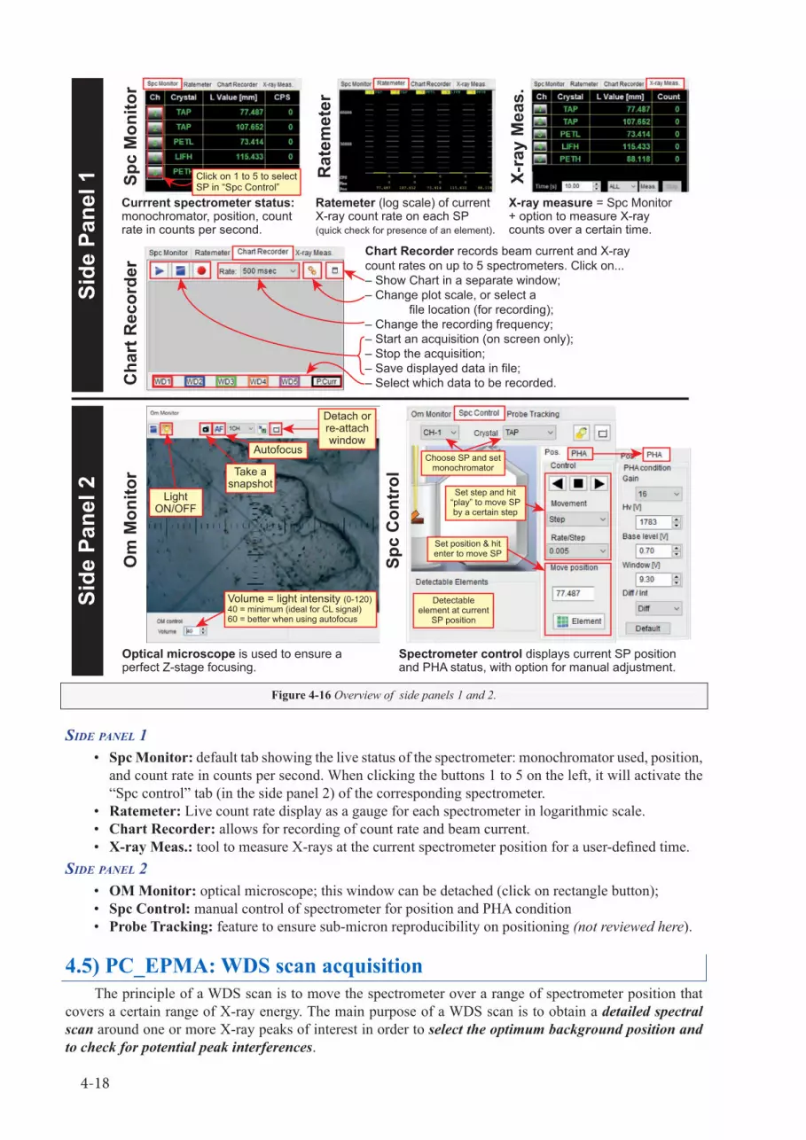
4-18

Side panel 1• Spc Monitor: default tab showing the live status of the spectrometer: monochromator used, position,

and count rate in counts per second. When clicking the buttons 1 to 5 on the left, it will activate the “Spc control” tab (in the side panel 2) of the corresponding spectrometer.

• Ratemeter: Live count rate display as a gauge for each spectrometer in logarithmic scale.• Chart Recorder: allows for recording of count rate and beam current.• X-ray Meas.: tool to measure X-rays at the current spectrometer position for a user-defined time.

Side panel 2• OM Monitor: optical microscope; this window can be detached (click on rectangle button);• Spc Control: manual control of spectrometer for position and PHA condition• Probe Tracking: feature to ensure sub-micron reproducibility on positioning (not reviewed here).

4.5) PC_EPMA: WDS scan acquisitionThe principle of a WDS scan is to move the spectrometer over a range of spectrometer position that

covers a certain range of X-ray energy. The main purpose of a WDS scan is to obtain a detailed spectral scan around one or more X-ray peaks of interest in order to select the optimum background position and to check for potential peak interferences.

Figure 4-16 Overview of side panels 1 and 2.

Click on 1 to 5 to select SP in “Spc Control”Sp

c M

onito

r

Rat

emet

er

Cha

rt R

ecor

der

X-ra

y M

eas.

Currrent spectrometer status: monochromator, position, count rate in counts per second.

Ratemeter (log scale) of current X-ray count rate on each SP (quick check for presence of an element).

Chart Recorder records beam current and X-ray count rates on up to 5 spectrometers. Click on...– Show Chart in a separate window;– Change plot scale, or select a file location (for recording);– Change the recording frequency; – Start an acquisition (on screen only);– Stop the acquisition;– Save displayed data in file;– Select which data to be recorded.

X-ray measure = Spc Monitor+ option to measure X-ray counts over a certain time.

Side

Pan

el 1

Side

Pan

el 2

Om

Mon

itor

Spc

Con

trol

Optical microscope is used to ensure a perfect Z-stage focusing.

Spectrometer control displays current SP position and PHA status, with option for manual adjustment.

Detectable element at current

SP position

Set position & hit enter to move SP

Set step and hit “play” to move SP by a certain step

Choose SP and set monochromator

LightON/OFF

Take asnapshot

Autofocus

Detach or re-attachwindow

Volume = light intensity (0-120) 40 = minimum (ideal for CL signal)60 = better when using autofocus

4-19

Figure 4-17 Setting up the analytical conditions for a Qualitative WDS scan (“Qual” analytical mode).

Setting up a WDS scan1

Click!

3

4

2

5

6

9b

7

8

9a

9c

10

11

13

Don’t forget to click “Apply” to validate your selection!

4-20

Whereas EDS analysis can immediately identify major and some minor elements over any energy range, it does not always identify minor and trace elements below 0.5 wt%. A slow WDS scan at high current (e.g., 1-2 sec per step, 100-200 nA) has the potential to reveal the presence of elements as low as 100-200 ppm or lower if the dwell time and current are increased.

4.5.1) Setting up a WDS scan1) Click on button “Qual” on the top bar of PC_EPMA (Fig. 4-17).2) Select a path and enter a project name.3) Set up the acceleration voltage and beam current (see Fig. 4-13 above); use a high beam current if the

analysed material permits it (50 to 200 nA).4) Define the stage position to be analysed (see Figs. 4-14 and 4-15 above). For long WDS scan (> 5-10

min) or for scan in beam sensitive material, use a defocused beam (option “Circle” set to 20-30 µm).5) Click “Detail” in the “Spectrum Scanning Condition” sub-panel to expand its view.6) Click “Add Spectrum” to generate an entry in the list on the left. One entry will represent one

continuous scan on one spectrometer. For a WDS scan on 5 spectrometers, you will therefore need 5 entries. More than (or less than) 5 entries are allowed (e.g., 10 entries representing two distinct spectrometer ranges on each spectrometer).

7) Click on a line to select and modify it.8) Select first the channel number (= spectrometer), then the monochromator (crystal) on this channel.9) Enter the spectrometer range to cover, the step size, and the time per step [9a]; see Chapter 4.5.2 for

examples of analytical conditions. You can define a scan covering a specific range of elements by clicking “Range by Element” [9b] and selecting the desired element(s) in the periodic table below. The scan range will be automatically adjusted to include the main X-ray line of all selected element(s). You can also manually move the start & end positions of the plot [9c].

10) Set up the PHA setting. Choose a PHA value that would be optimum for the average spectrometer values covered by the scan, or the optimum PHA value for the most important element in this scan. Set the PHA in “Integral” mode if you want to see 2nd and 3rd order X-ray lines.

11) Click “Apply” to validate your choice.12) Repeat steps 6 to 11 for each additional entry.13) When ready, click either “Acquire” to start the acquisition right away or click on “Add to Serial

Analysis” to add it to the list of tasks to be run in automated mode (see Chapter 4.8).

4.5.2) Analytical conditions for WDS scanThere is no absolute rule for a WDS scan; it will depend on what you want to do and the type of

material analysed (e.g., beam sensitive). Here are some examples:• Quick full scan: a scan for major and some minor elements can be done in 5-15 min at medium

current (20-50 nA) over a significant spectrometer range (60-85 to 210-250 mm) and with a relatively coarse spectrometer step (e.g., 100 µm) and a short counting time (100 to 200 ms). To gain time, you can cut on the spectrometer range covered (e.g., stop at ~210-220 mm).

• Long full scan: scan for major, minor and some trace elements will require both a higher current (100-200 nA) and a longer counting time (1000-2000 ms), and is typically done with a smaller step size (e.g., 50 µm). Such a scan will easily take an hour or more.

• Quick X-ray peak scan: scan over one or several peaks of interest, over a short spectrometer range (10-20 mm total), at medium to high current (50 to 200 nA) with a very small step size (e.g., 10 µm). Counting time will be either short (100-200 ms) if looking for a major element, or long (>1000 ms) for minor or trace element or to see small interfering peak(s).

• Scan in beam sensitive material: WDS scan in beam sensitive material can be tricky, as the mineral is degrading during the scan acquisition. To minimize this undesirable effect, the total scanning time should be minimized as much as possible, the beam current should be reduced, and the beam should be defocused to 20-30 µm (up to maximum 50 µm) if the medium homogeneity allows for it.

4-21

4.5.3) Viewing and exporting dataTo view the WDS scan results, click on the “EpmaData” tab in the bottom of PC_EPMA. Locate your

path and project folder, and find the result folder corresponding to the scan (“xxxx QLW” folder). Click on a file to view the data. A preview of the scans will appear in the bottom section. Double-click on the file to open the results of all WDS scan in this analysis in a separate window or double-click on the preview image on the bottom section to open a single scan within this file. In both cases, the sub-program “xqlw” will open with your WDS scan (Fig. 4-18).

The viewing window of WDS scan (“xqlw”) allows for multiple operations on the scan. Only a few important one are reviewed here. First and foremost, WDS scans can be exported either as tabulated data (CSV file) or as an image file (screenshot of the result):

• “File > Save Image... > [...]” to save a screenshot of results with or without the side text.• “File > Export...” to export results as CSV file: select the appropriate output folder (must be outside

your project folder, e.g. in an “Export” folder within your project folder!) and the data format (X-axis unit: millimeter, wavelength [Å or nm], or energy [keV]).

It is often useful to export both an image (with the peak identification) and a CSV file to reconstruct WDS scan and perform additional data treatment in a spreadsheet. Other useful operations are available by right-clicking on a specific WDS scan (also accessible under menu “Operate”). For details on each feature, refer to the JEOL manuals. The most common operations you will need include:

• “Full size”: show only the selected WDS scan. Right-click and unselect “Full size” to return to the overview of the multiple WDS scans.

• “Zoom...”: Changing the scale of the plot either by entering values in the X-Y min/max fields or by clicking and dragging over an area of the scan to zoom in.

• “Peak ID...”: peak identification. Click on a position to see a list of possible X-ray lines in this area. Include also other tool such as a length measurement, useful to determine a background position.

• “Calculate”: perform mathematical operation(s), including adding or subtracting spectra.NOTE: When using “xqlw”, the primary data are never deleted or overwritten: you don’t risk anything by just trying!

4.6) PC_EPMA: Element mappingElement mapping is sometime used in complement to quantitative analysis to reveal compositional

zoning in a mineral (e.g., in plagioclase, garnet, olivine, pyroxene) or a diffusion profile or reaction front in any material (e.g., glass, alloy, mineral). Element mapping can also highlight rare accessory phases that contains a unique element rarely high in “common” minerals (e.g., Zr in zircon, Ce/La in monazite or allanite, Y in xenotime, P in apatite and REE-phosphate). This later option has the ability to detect small grains (5-10 µm) even with a defocused beam at 20-30 µm and a very quick scan (30-50 ms per pixel).

4.6.1) Setting up an element map (“Stage” mapping)1) Click on button “Map” on the top bar of PC_EPMA (Fig. 4-19).2) Select a path and enter a project name.3) Set up the acceleration voltage and beam current (see Fig. 4-13 above); use a high beam current if the

analysed material permits it (50 to 200 nA).4) Define the area to be mapped (bottom part of Fig. 4-19). The following describes the procedure for a

“Stage” map. “Beam” mapping should only be used for very small maps (< 50 µm wide):a) Type in a comment for your element map.b) Choose “Stage” mapping (see Fig. 4-20 for “Beam” mapping). c) Choose “Point Reg.” to set the map using a single position. Choose which position to save

under “Point to set” (Centre or a corner [A, B, C or D]). Move the stage to this position and press “Register present stage position”. Click the “...” button to see the currently saved position. The option “Rectangle Reg.” allows you to calculate a mapping area based on a series of 2 or more reference points that should be included in the mapping area.

d) Define the map size by setting the pixel size and the size of one pixel (in µm). Uncheck the box

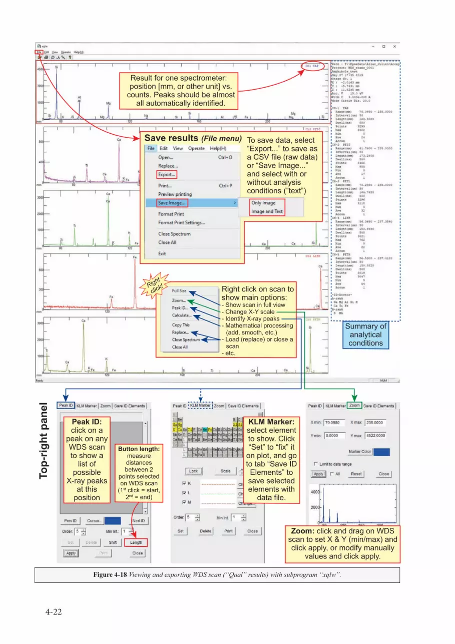
4-22

Save results (File menu) To save data, select “Export...” to save as a CSV file (raw data) or “Save Image...” and select with or without analysis conditions (”text”)

Right click on scan to show main options:- Show scan in full view- Change X-Y scale- Identify X-ray peaks- Mathematical processing

(add, smooth, etc.)- Load (replace) or close a

scan- etc.

Right

click!

Summary of analytical conditions

Result for one spectrometer: position [mm, or other unit] vs.

counts. Peaks should be almost all automatically identified.

Peak ID: click on a

peak on any WDS scan to show a

list of possible

X-ray peaks at this

position

Button length: measure distances between 2

points selected on WDS scan

(1st click = start, 2nd = end)

KLM Marker: select element to show. Click “Set” to “fix” it

on plot, and go to tab “Save ID Elements” to save selected elements with

data file.

Zoom: click and drag on WDS scan to set X & Y (min/max) and click apply, or modify manually

values and click apply.

Top-

right

pan

el

Figure 4-18 Viewing and exporting WDS scan (“Qual” results) with subprogram “xqlw”.

4-23

1

*

* For setting a beam map, see Fig. 4-20.

Software calculates mapping area to include all

user-defined positions in the list.

ab h

i

e

d

f

g

j

c

Click!

3

4

2

5

6

Click!

Fig. 4-21

Setting up an element map (1/3)

Stage mapping with one reference point

Option to set map to cover a set of points

Confirm center & corners of mapping area & adjust Z.h

Figure 4-19 Setting up the analytical conditions for a “Map” acquisition (“Stage” mapping).

4-24

“Fixed ratio” for rectangular area. Make sure that the pixel size for both X and Y are the same (to avoid distortion, as a pixel is always square...).

NOTE: The “Enhancing condition” offers more complex mapping possibility (e.g., mosaic beam mapping or 3D mapping on irregular samples). However, only the option “Normal Area” is reviewed here...

e) Check the yellow box to see the dimensions (in µm or mm) and time required for this map.f) Set the Stage Drive to “Uni-directional” (scan is done in one single direction). The “Bi-

directional” mode is only OK if your pixel size is larger than 5 µm, otherwise you take the risk of having a “zigzagging” map with a mismatch between two adjacent mapping line.

g) Set the Scan Mode to either “Spot” or “Circle”. Choose a focus beam if your step size is less than 1 µm, otherwise choose “Circle” and set the beam size to the size of your pixel.

h) Click “Confirm” to check the position of each corner. The stage will move to a corner of the area to be mapped. A separate window will open and allow you to adjust the Z-stage position for each corner: use the stage controller to adjust the Z-stage position, then click “Register Z axis and go to the next position”. Do the same for all corners. When done, click “Apply”.

i) Your mapping area should be listed on the right. When clicking on an entry from this list, the position parameters are loaded back on the left-side and can be modified. Remember to click again “Apply” to validate your modification.

j) To set an additional mapping area, select an empty entry in the list, and repeat steps (a) to (h).5) Define the list of elements to be mapped by WDS (and EDS, if applicable) as described in Figure

4-21. It is recommended to stick to 5 elements on WDS and set the major or less important elements to be mapped by EDS. If 2+ elements are set on a single spectrometer, multiple passes will be required; in this case, ensure to place the most important elements first.

a) Select “Peak” under “P/B”. Other options are to map on the peak position and one or two background positions (required for accurate quantitative mapping). Background acquisition is rarely done, as it will require additional passes and will take 2 (to 3) times longer.

b) Click on button “Periodic Table” to activate the tab below. To set an element on WDS (or EDS), click on “Optimization > WDS” (or “Optimization > EDS”), then click on an element. Add all required elements on WDS (and some major elements on EDS if desired).

a

b

h

e

d

f

c

Leave scan rotation at 0.0g

a) Enter a comment.b) Select “Beam”.c) Move stage and set magnification to area to

be mapped, click “Register present stage position”, and check magnification.

d) Define size (pixels), number of accumulation (passes) and dwell time.

e) Verify size (µm) and time for map.f) Check box “OM Auto Focus” if required.g) For long mapping, check “Apply probe

tracking”, enter a time interval, and conditions for image acquisition (default values are OK).

h) Click apply.

Setting up an element map (2/3) – Beam mapping

Figure 4-20 Setting up the position for “Beam” mapping.

4-25

c) Click and drag the elements to assign them to the proper spectrometer (channel) and select the appropriate monochromator (right-click on element).

d) Set the peak (and background) position and PHA setting. Perform a peak search and a PHA scan to determine these values. Alternatively, it is easier to first set the spectrometer to the right setting for instance by calling the condition of an element from the latest quantitative analysis, and then press “Rd” to read the spectrometer condition and apply them to this map setup.

6) When ready, click either “Acquire” to start the acquisition right away or click on “Add to Serial Analysis” to add it to the list of tasks to be run in automated mode (see Chapter 4.8).

4.6.2) Setting up an element map (“Beam” mapping)The procedure to set up a “Beam” mapping is very similar to the one described in Chapter 4.6.1 for

“Stage” mapping. It is ideal for any small maps at high magnification, with a maximum field of view of 50 µm. The map is done with a focused beam, with a pixel size below 1 µm. The only big difference resides in setting up the area to be mapped (see Fig. 4-20):

Setting up an element map (3/3)a

c e

d

b

b

1) Select “Peak” under “P/B” (bkg rarely acquired).2) Click on “Periodic Table” to open tab, choose

“Optimization” > “WDS” or “EDS”, select element(s).3) Assign elements on WDS (or EDS).4) Set element conditions. If setting peak & bkg maps,

bkg conditions will appear aside peak condition.5) If setting SE and/or BSE images (IMS), click on IMS

and fix the contrast & brigthness value for each signal without the light of the OM microscope!

From step #5 in Fig. 4-19

Figure 4-21 Setting up the element condition for a Map.

4-26

a) Type in a comment for your map.b) Select “Beam” mapping.c) Move the stage in position and set the magnification to cover the mapping area. Click on

“Register present stage position” to set the centre (X,Y,Z) point and the magnification.d) Define the size of the map (number of pixels in X and Y), the number of accumulation (passes;

usually left to 1), and the dwell time per pixel in milliseconds.e) Check the size in µm of the area to be mapped. To minimize the WDS defocussing effect, the

mapped area should be less than 50 µm.f) Click OM Auto Focus if required (e.g., automated work).g) Activate the probe tracking for long acquisitions (> 30 min) at high magnification (pixel size

below 1 µm). This feature will get an SE image every x seconds (= interval) at relatively low resolution (256 pixels default) and compare it with a reference image taken at the beginning of the acquisition. If the beam drifts (2nd image shows a translation), it will correct for it.

h) Click “Apply” to validate your mapping position.i) Repeat steps above for additional maps.j) Continue setting your map as described in Chapter 4.6.1.

4.6.3) Analytical conditions for element mappingElement mapping is done at high current, as the time spent on each pixel is usually short (< 1 second).

Depending on your needs, a map can be done in just a few minutes (quick qualitative map or small grain map) or over several hours (large area mapping or higher sensitivity required for minor or trace element). You can estimate the time required to map a grain by knowing the size of the object to map, the time per pixel (= dwell time), and the total number of pixel or the size (resolution) of your pixel (expressed as micrometre per pixel). Use the tool available at http://ethz.geoloweb.ch/?page=xraymap_calculator to estimate the acquisition time. Here are some guidelines to help you determining your optimum setup:

• Set the map to beam mode for grain smaller than 50 µm or to stage mode for larger one. For grain of intermediate size (e.g., 100-200 µm), consider multiple beam maps (mosaic mapping; results will have to be stitched manually).

• Define the pixel size based on the following criteria:* Small enough to easily permit the identification of the smallest feature to be revealed: if mapping

for features that are 5 µm in size, opt for a pixel size significantly smaller (e.g., 1 µm/px).* Time limit: increasing the pixel size will strongly reduce the total acquisition time, much more

than reducing the time.* Don’t use a pixel size less than 0.2-0.3 µm/px. The analytical volume and beam size are anyway

larger to this size in most cases. Getting smaller would be oversampling (blurry image).• Adjust the beam current (in parallel to the dwell time, see next) to (a) collect enough counts (check

on the mineral the expected count rate for each element to be mapped) and (b) avoid damaging the grain. If a defocused beam is used over beam sensitive material, the beam current can be increased. Avoid using a very high current while mapping for major elements by WDS, or you risk saturating the detector! Count rate should ideally remain below 20000 to 30000 cps! If you have both to map for minor / trace elements and for major, consider using the EDS to map for the major elements. Typical beam current ranges are...

* 100-300 nA for robust minerals, more when trace element mapping is required (> 1 µA);* 50-100 nA for beam sensitive material (e.g., plagioclase);* 20-50 nA for very sensitive material (e.g., carbonate), or less if extremely sensitive.

• The dwell time is chosen depending on the feature to be revealed:* Short (10-30 ms/px) for quick maps to highlight major and minor element zoning,* Long (80-100 ms/px) for a more detailed and smoother map, especially for minor element;* Very long (1000-2000 ms/px) for trace element mapping (very rarely done...).

• Total counting time for your map will depend on all the above parameters (map size and counting time. Small grains or quick maps are usually done within minutes, and higher quality maps or maps over large area will take several hours. Long run are normally set overnight or over-the-weekend.

4-27

4b

2

1

5

3

4a

RGB synthesis

Calculate

Analysis

Visual property

Layout

Rotate

Zoom

Savecolorlevel

Colorlevel

Key features of NMap (will open a panel on the top-right side):- Color level: change color scheme & min/max.- RGB synthesis: add three element maps and attribute one color to each (red, green, blue) to obtain a composite image.- Layout: change the display layout (number of maps, layout).

Color Level Map Layout

Menu “Process > Convert Conc.”

RGB synthesis

Summary of analytical conditions

Adjust min & max& click “Apply”

Change color scheme or switch to B&W, and

buttons to undo or reset the scale to default.

Result of RGB composite image

Define number of maps to show

Display options

(color and scale bars)

Click “All” to apply map layout to all. Avoid using interpolation

tool to keep the data “raw”.

Select three element maps

To convert maps into element or oxide wt-%, select menu “Process > Convert. Conc.”, then:1) Select an element map;2) Click “From Standard...”;3) Click “Search Stand-ard...” and look for most recent standardization;4) Click “OK”, A & B values will be updated;5) Click “Concentration” to convert counts in weight-%

Figure 4-22 Overview of “NMap” – a subroutine to visualize and export element maps – and its most important options.

4-28

4.6.4) Exporting map resultsTo view the element mapping results, click on the “EpmaData” tab in the bottom of PC_EPMA. Locate

your path and project folder and find the result folder corresponding to your map (“xxxx MAP” folder). Click on a file to select it; a preview of the acquired map(s) will appear in the bottom section. Double-click on the file to open the results of all element maps in this analysis in a separate window. Alternatively, double-click on the preview image on the bottom section to open a single map within this file. The sub-program “NMap” will open with one or more element maps (and SE/BSE images if included in mapping).

A few functionalities of the NMap sub-program are described below and summarized in Figure 4-22. It has several features to process and export your map as an image. Avoid processing too much your data; most of the time, you will just need to adjust the level, and maybe change the layout of the output window or colour-scale used.

If you have modified your data, click on menu “File > Save Results Map...” to save the modifications (JEOL file format). It should be possible to revert any change back to the raw data by “clearing” or “resetting” each modification. Clicking on menu “File > Save Image As...” to export element maps as an image (screenshot), and choose to save only the image or the image with the text (= analytical conditions). NOTE: If you need easy access to raw data (counts) for reprocessing in third party software, or if you want to perform accurate quantitative mapping, it is recommended to use the software Probe Image and treat the results with CalcImage and a series of

standardization obtained with Probe for EPMA. See Chapters 6 and 7 for more information about quantitative element mapping.

4.6.5) Quantification of element mapResults obtained with the JEOL system are usually considered as qualitative maps. They can be (semi-)

quantified in PC_EPMA or in NMap using standard data and “A & B” factors calculated from standard acquisitions. However, the accuracy of these results is questionable, especially if you don’t have a background map, and the routine converting the counts in weight-% doesn’t include a full matrix correction, only a simplified version of it. It is also possible to quantify using quantitative analysis results that were obtained within the mapping area (not tested; see JEOL manual for more info), and might be a little bit more accurate when considering the zoning in a single phase (e.g., plagioclase zoning, with two representative quantitative analysis that covers most of the compositional variation). Quantitative element mapping is better done using the “Probe Software” program suite (Probe Image, Probe for EPMA, and CalcImage; see Chapters 6 & 7). Maps can be quantified in NMap (as described below), and a similar routine is available using “OffQnt” in PC_EPMA (see Chapter 4.9.2). To quantify an element map in NMap:

• Open one or more map.• If you open multiple maps, select the one to process (red square surrounding the map).• Click menu “Process > Convert Conc.”.• In the tab opening on the right, select “From Standard...”.• Click “Search Standard...” in the new window and locate the standard to use for this element map.• Click “OK”. The A and B factors will be updated.• Select if you want an output as “Metal” or “Oxide” (and set the valence for the element).• Click “Concentration” to convert the map as element or oxide weight-%.

4.7) PC_EPMA: Standard acquisitions & Quantitative analysesSimple quantitative analyses are easy to set in JEOL with PC_EPMA. Basically, you first acquire all

required standards, and then you prepare your analytical setup for quantitative analysis. Like in the other analytical modes, you need to define (a) the electron beam condition, (b) the analysis condition, (c) the stage positions, and the (d) the element setups.

Before proceeding to any standardization, you MUST have a complete idea of your analytical protocol. If you don’t know your exact analytical conditions (major ones listed below), ask the manager or the assistant for help before your book an analytical session (SEE ALSO Chapter 2.1):

• Beam current and voltage: from 1 to 1000 nA and 10 to 25 keV, typically 10 to 20 nA and 15 keV.• Beam size: focused for robust minerals, defocused between 2 and 20-30 µm for sensitive materials.

4-29

• Choice of element and monochromator.• Repartition of the elements among the five WDS channels or on the EDS.• Choice of standard to use for each element.• Analysis time: short for major element, longer for minor, trace, or important elements.• etc.Analytical options in PC_EPMA from JEOL are relatively limited compared to the program “Probe

for EPMA” from Probe Software. Whereas PC_EPMA should be used for “simple” analyses without complications, Probe for EPMA software should be considered for complex analyses such as beam sensitive material, trace element[s] analysis, strong or numerous peak interferences, etc.

To ease the setting of standard and unknown analysis in common silicates, a list of default background positions and PHA conditions is available in the Appendix of this guide. Whereas background position should not change over time once you have found the optimum for your setting, PHA condition can change slightly on a daily basis. It is recommended to perform a PHA scan, at least the “High Voltage Bias” scan.

You should always analyse your standards and your unknown analyses within the same project. If a recent user has already standardized an element you need, you can consider copying the standardization folders into your own project folder (see Chapter 4.7.3).

1

3

2

6

7

4 5

1) Select “Std” mode.2) Select a path, enter a project name. All standard & quantitative analyses must be in this project.3) Set beam voltage and current.4) Select standard to acquire and define basic analysis condition (see top of Fig. 4-24).5) Set acquisition points using “Stage” mode only (accumulation mode; see bottom of Fig. 4-24).6) Set element(s) to be analysed (see Fig. 4-25).

Setting up a Standard acquisition

Fig. 4-24(top)

Fig. 4-24(bottom)

Fig. 4-25

Figure 4-23 Setting up the analytical conditions for a “Std” acquisition (Standard acquisition for quantitative analysis).

4-30

4.7.1) Standardization processThe standardization process is summarized in the next four figures, with an overview of the procedure

in Figure 4-23, the analysis condition and stage positions in Figure 4-24, the setting of element conditions in Figure 4-25, and the peak search and the PHA scan in Figure 4-26. To perform a standardization...

1) Click on the button “Std” on the top of PC_EPMA (Fig. 4-23).2) Select a “Path” for your analysis and enter a “Project Name”.3) Set up the acceleration voltage and beam current (see Fig. 4-13 above).

WARNING: Standards are acquired at 20 nA and 10 µm beam size. However, few standards will also require a lower beam current to limit the beam damage effect (e.g., carbonate or sulphate standards) or to lower the count rate on H- or L-type spectrometer (e.g., when approaching detector saturation such

as in metal standards or in pure oxide; try staying with a count rate below 20-30k counts per second).

4) Set up the analysis condition (top of Fig. 4-24):a) Click on “...” under “Standard” to open the Standard Management window:

– Click on the standard you need, usually under “Permanent Std”. – Click on “Move”; the stage will move on or near the standard. Adjust the stage position

to ensure you are on it (quick look on BSE at low magnification), ensure Z is on focus. – Click “OK” to validate your choice. The standard name should appear with a list of

elements present in the standard and a default name (no need to change it). – See Chapter 4.7.2 for additional information about the Standard Management window.

b) Set the “Peak Search of samples” to “None” (done manually, see [6d] below), the “Background measurement” to “Always”, and leave the “Asynchronous measurement” mode active (all spectrometers move independently from each other). To gain a little bit of time and in standard with an expected high peak-to-background ratio (e.g., metal, simple oxide), it is tolerable to measure the background only on the first point. In this case, select “Every” and set the value to 10, or any value higher than the number of points to acquire in your standard.

c) If you want to force acquiring all elements at a fixed time, check the box “Fixed times to all elements”. It will override any peak and background time entered in Element Analysis Condition (see [6] below).

5) Define the stage positions (bottom of Fig. 4-24):a) Click on “Stage” mode. No need to change the comment (based on standard name). Never

use “Beam” mode on standards! b) Ensure the stage is on a clean area of the standard and the Z-stage is on focus; use Auto Focus

button (AF) as necessary. Check the position using the “Jog” button on the stage controller (= “Test” button on the old JEOL-8200) to ensure a good stage reproducibility. Click then on “Read Position”.

c) For the standardization process, it is usually recommended to acquire at least 5-6 points. Rather than setting individual points (so 5-6 entries in the list), only a “single” point is defined with an accumulation of 5-6 multiple acquisitions that will be averaged at the end of the acquisition. Click on “...” under “Accumulation” to open the window “Analysis Multiplication setting”. Use this window to set additional measurement points:

– Ensure an empty line is selected (the first line is by default your first reference point); – Move the stage to another point in standard; – Click on “Add or Change” to add a new point; – Repeat to add a total of 5 to 6 different positions.

d) Set the “Scan Mode” to “Circle” and the “Probe Dia.” to at least 10 µm on all standards; this minimize both the risk of damaging the sample and of erroneous measurement due to micron- to submicron-scaled heterogeneities. For very beam sensitive materials (e.g., carbonate, apatite), a defocused beam as large as 20 µm can be used along with a lower current (10 nA, see [3] above); avoid larger beam size (spectrometer defocussing issue). Check the box “OM Auto Focus” to apply a Z-stage auto-focus before each point if necessary.

e) Click “Apply” to save the positions for standard acquisition. A single entry should be visible in the list on the right: it lists the standard name, (X,Y,Z) position for the first point, with an “A”

4-31

a

a

be

c

c

d

c

b

Standard Analysis Condition:a) Click “...” and select a standard, click “Move” to

move the stage and click “OK” to validate. Std name shows up with list of elements in std.

b) Select “None” under peak search, and “Always” under background measurement.

c) Check box “Fixed times...” to fix acquistion time (default: 20 s on peak, 10 s on each bkg).

Analysis Position Condition:a) Leave name in comment as is. Click “Stage”.b) Move stage on standard if not already on it,

and click “Read Position”.c) Set 5 to 6 points in accumulation mode by

clicking on “...” under Accumulation.d) Set beam in “Circle” mode (10 µm beam size),

click on “OM Auto Focus” if required.e) Click “Apply” to validate your entry.

Don’t use Probe Trackingfor standard acquisition!

Figure 4-24 Setting up the analysis condition in “Standard Analysis Condition” and the stage position for the acquisition in “Analysis Position Condition”.

4-32

aside the value for Z-stage position if an auto-focus is requested, the beam diameter, and further to the right the number of accumulation.

6) Set up the elements you need to analyse in the selected standard (Figs. 4-25). Make sure to only set elements that are present in LARGE quantity (e.g., do NOT set the analysis of Si in hematite):

a) Click on “Periodic Table” to show the corresponding tab in the bottom panel.b) Click on the tab “Element”; only the element present in the standard should become selectable. c) Select first “Optimization” and “WDS” or “EDS” [c1] and then click on the element you need

to standardize [c2]. If you need to standardize the same element on multiple spectrometers, click another time on this element. Ensure each element is set to the right spectrometer and crystal (monochromator) as you planned it [c3]; if not, click-and-drag the element to move it to another spectrometer, or right-click on the element to select another possible crystal.

d) Perform a “Peak Search” and a “PHA Scan” for all elements as described in Figure 4-26: – The easiest to start a peak search is to select an element, right-click on it, and choose

“Execute peak search” (Fig. 4-26 [a1]); it will use the default values for peak search. Peak search can be run simultaneously on multiple spectrometer.

– For more flexibility on the peak search acquisition, prefer the use of the “Search” option

Peak search & PHA scan: see Fig. 4-26.

Click!

a

c3

e

gf

Perform Peak Search & PHA scan (see Fig. 4-26).

“Periodic Table” (1a) with tab “Element” (1b) active only show elements present in standard, including

possible trace amounts (e.g., here Si in Fe2O3).Don’t standardize these trace elements!

d

d

b

c2c1

Figure 4-25 Setting up the element(s) condition in “Analysis Element Condition”.

4-33

f

i

h

g

Peak search result:– Click on Channel to check result.– Only if necessary, modify incorrect peak position value found by PC_EPMA by right-clicking on plot on desired value, and by selecting “Move spectrometer to position”.

Manual peak search:a2) Click on “Search” tab.b) Select element in Periodic Table.c) Select Channel &/ X-ray.d) Check search condition: crystal, search frequency (1 = fine, 2 = coarse+fine), etc.e) Click “Peak Search”.

Quick peak search:– Select element in“Analysis Element Condition”.– Right-click on element, and click on “Execute peak search”.

PHA scan, bias voltage:f) Click on “High Voltage”.g) Select channel.h) Set range to cover expected PHA value (see Appendix).i) Press button “Play” & wait...j) Click-&-drag blue line to adjust HV bias as necessary.

PHA scan, baseline:k) Click on “Base level”.l) Select channel.m) Click on “Play” (leave other values as default).n) Click-&-drag blue line for Base Level & Window if necessary

j

l k

Peak

sea

rch

resu

lt

PHA

scan

: Hig

h Vo

ltage

PHA

scan

: Bas

elin

e

a

b c

d e

Right

Click!To reposition spectro,

on peak only if necessary(i.e., not on peak)

Initiate peak search...

a1

a2

Right

click

Figure 4-26 Acquiring peak search and PHA scans (for “High Voltage” bias or “Base level”).

4-34

under the tab “Periodic Table” (Fig. 4-26 [a2]), then click on the element (Fig. 4-26 [b]), select the spectrometer and crystal to use (Fig. 4-26 [c]), define the default peak centre and the search type (frequency: 1 for fine peak search, 2 or more for a coarse scan followed by a fine scan), leave the option “Max” selected (Fig. 4-26 [d]), and click on “Peak Search” when ready (Fig. 4-26 [e]).

– Wait for peak search to complete; check and adjust, if necessary, the peak position under the tab “Peak Search” (should get active when a peak search request has been sent). To modify the returned peak centre, simply right-click on the position you think the peak centre is, and select “Move spectrometer to this position”; even if the blue line indicating the centroid found by the software does not move, the spectrometer will physically move to this position (you can see this in “Spc Monitor” on the side panel 1).

– Perform then a PHA scan by clicking on the “PHA Scan” tab, selecting first the High voltage tab (Fig. 4-26 [f]), and select the spectrometer (channel; [g]). Only one PHA scan on one spectrometer is possible on the JEOL software. Run first a bias scan to find the optimum bias voltage. Look at the reference value table in the Appendix to have a rough idea of the expected bias value so that you can reduce the range for the scan (“Start” and “End” values; [h]). Press the play button to start the scan [i]. When completed, adjust the bias value if necessary; it should be at the centroid of the peak. Once you have the proper bias voltage, click on tab “Base level” to run a baseline scan [j] on the same spectrometer [k] and using the proposed default parameters. Press the play button to start the scan [l]. Wait for completion and adjust the baseline level to cut on the electronic noise at low energy (usually between 0.5-1.0 V) and the window to include all the pulse and a good portion of the higher energy range. In case of doubt, leave the window relatively large.

e) Once the spectrometer is set to the right peak position and PHA setting, click on the button “Rd” to read the current spectrometer position and the current PHA setting.

f) Verify the values are properly updated, and that the PHA setting is set to differential mode

Figure 4-27 Standard Management window: used to drive the stage to a standard position or to select a standard for acquisition.

1

3b !!!

NEVERCHANGE

DATA HERE!2 3a

1) Click on “Std Mng.” to open Standard Sample Management window.2) Select standard folder, usually “Permanent STD” for most silicate analysis...3) Select standard from list (3a), and click “Move” (3b) to move stage to standard’s stored position.!!!) Avoid clicking on “Edit” (or other buttons) as it gives access to stored Standard Position

and reference composition. These should never be changed by any regular user!Positions for “Permanent STD” are regularly adjusted by manager. To update a position, drive stage on standard, and click “Read”. Standards position outside “Permanent STD” are often wrong as they are rarely loaded on same position...

Standard management window

NEVERCHANGE

DATA HERE!

4-35

(“Diff”; preferred mode) and not integral (“Int”). Change manually if necessary.g) Adjust the background position and the counting time on peak and background. If you are

using the “Fixed times...” option (see Fig. 4-24 [c] ), you don’t need to worry about the peak or background time.

h) Repeat points c) to g) for each element you have included in your analytical run.7) When ready, press either “Acquire” to start the acquisition right away, or press “Add to Serial

Analysis” to run the task later in automated mode (see Chapter 4.8).

4.7.2) Standard Management window (“Std Mng”)The Standard Management window contains the list of the standards with composition and reference

stage position. At the user level, the standard management window is only used to drive the stage to the stored standard position or to select a standard during a standard acquisition.

The standards are organised by mineral group (series A, B, C, etc.) with an extra group labelled “Permanent STD”, which you will mostly use. This latter contains all standards permanently mounted inside the electron microprobe. The database on the JEOL PC_EPMA software is incomplete compared to our collection of standards (see http://ethz.geoloweb.ch/?page=std_list). If you need a standard that is not listed in Standard Management, contact the manager or the assistant to define a new standard.

To move the stage on a standard position (Fig. 4-27), click on “Std Mng.” (1), select the appropriate folder [2], usually “Permanent STD”, and the standard you need [3a], then click “Move” [3b] to drive the stage. The standard position within the “Permanent STD” folder should be close, but sometime just a little bit aside. Always have a very quick look with SE or BSE image if you are (a) on the standard, and (b) not on an inclusion or crack, etc. Always make sure the Z-stage focus is perfect before performing any analysis (manual focus or stage auto-focus [AF])!

WARNING: The button “Edit” is used to set up the stage reference-position and the reference elemental composition for each standard, and the button “New” will create a new standard entry. A basic

user should NEVER use the “Edit” or “New” functions!

Reference position for each “Permanent STD” are set by the manager or the assistant only. Other standard positions (in folder A, B, C, etc.) can be updated by experienced users only. To do so, move

the stage on the standard and click “Read” in the “Standard sample edit” window (bottom-right on Fig. 4-27). Make sure you are on the right standard before reading the new position as there is no undo button!

4.7.3) Copying existing standard

WARNING: Never use the Windows file explorer to copy standardization folder into your project! PC_EPMA has a very strict file and folder name and structure affecting not only the file or folder names

but also several files metadata within some files!

If you are running quantitative analysis similar to what the previous user has done, you should take advantage of their standardization, as it usually holds for a few days if not a week or more when everything runs smoothly. Whereas it is technically possible to use a standard from another project folder, it is not a good practice. It is highly recommended to copy the standardization folder into your own project folder to make them available in your personal quantitative analysis folder. The process to copy standardization folders into your project folder is described below and in Figure 4-28:

a) Locate the standard analysis folder(s) you need to copy from another user’s project.b) Select all “xxxx STD” folders to copy on the right-side of the “EpmaData” sub-panel; hold

[Ctrl] and click to select multiple folders or hold [shift] to select a continuous series of folders. Right-click on one of the selected folders and select “Copy”, or use the [Ctrl]+[C] shortcut.

c) Create a project folder where you will copy the files if not existing already (for this step, you can use the Windows Explorer). Select the project folder where the STD folders need to be copied. Right-click on an empty space on the right-side of “EpmaData” sub-panel, and click

4-36

“Paste”, or use the [Ctrl]+[V] shortcut.d) Click “OK” to confirm the re-numbering of STD folders. Do NOT change the “Numbered

from” that is set to 1 if the project is blank or a higher number if other data already exist.e) A copy of the standard folders will appear in your project and should now be available in

“Quant” mode when setting up the element condition.

4.7.4) Quantitative analysisAfter the acquisition of all standards, you can prepare your analytical setup for quantitative analysis.

An overview of the process is shown in Figure 4-29 and is described in the following. Details on setting up the analysis and element conditions is in Figure 4-30.

1) Click on the button “Quant” on the top of PC_EPMA (Fig. 4-29).2) Select a “Path” for your analysis and enter a “Project Name”.3) Set up the acceleration voltage and beam current (see Fig. 4-13 above). Choose appropriate conditions

for your analysis: usually 20 nA, lower for beam sensitive material, and higher for precise minor &

a

c

d

e

b

To copy standard folder(s) [xxxx STD]:a) In “EpmaData” tab, locate project folder with

“xxxx STD” folders to import.b) Select STD to import; hold [Ctrl] for multiple

files selection. Right-click on one of selected STD => “Copy” (or [Ctrl+C]).

c) Click on your project folder, right-click in white space on right => “Paste” (or [Ctrl+V]).

d) Confirm renumbering with the suggested value (1 if no other STD are present in project folder, higher value otherwise).

e) Standards will appear in your project folder.

WARNINGS: Use only standards that are in your project. If you want to use an old standardization from a previous user, prefer to COPY all necessary STD folders using the tab “EpmaData” (this figure)! DO NOT use the Explorer from Windows to copy files!

Right

Click!

Right

Click!

Figure 4-28 Copying standard (STD) folders between projects using the tab “EpmaData”.

4-37

trace element analysis.4) Set up the analysis condition (top of Fig. 4-30):

a) Set the analysis type to “Oxide” for silicate and other oxides or “Metal” for elemental analysis (sulphide, metal/alloy, etc.). The recommended correction routine is “PRZ (Armstrong...)”.

b) Set Peak search to “None”, background to “Always”, and WDS to asynchronous mode.c) In “Oxide” mode, the valence of each cation can be set on the bottom-left side. Only the cations

entered under [5] below are shown (i.e., set up first the elements in [5], then return here...).NOTE: It is NOT recommended to use the “fixed time to all elements”. It is usually set independently for each element, as it

may vary (e.g., shorter time on spectrometer with a series of 3 elements compared to a spectrometer with only 1 or 2 elements). PC_EPMA offers also the possibility for an “Interference Correction”. This correction is not reviewed here. For cases with one

or more peak interferences, the use of Probe for EPMA is recommended as it has a more robust correction routine.

5) Define the stage positions as described in Chapter 4.4.3 above (Figs. 4-14 and 4-15):a) Click on “Stage” mode; never use “Beam” to setup quantitative points.b) Enter a comment for your analysis.c) Ensure the stage is on a clean area of the standard and the Z-stage is on focus; use Auto Focus

as necessary. Check position using the “Jog” button on the stage controller (= “Test” button on the old JEOL-8200) to test the stage reproducibility. Click then “Read Position”.

d) Set the “Scan Mode” to “Spot” for focused beam analysis or to “Circle” with a certain “Probe Dia.” for defocused beam (required for beam sensitive material such as hydrous phase,

1

3

4 5

2

6

7

1) Select “Quant” mode.2) Select a path, enter a project name. All standard & quantitative analyses must be in this project.3) Set beam voltage and current.4) Define basic analysis condition (no peak search, background always acquired).5) Set acquisition points using “Stage” mode only (see top of Fig. 4-30).6) Set element(s) to be analysed (see bottom of Fig. 4-30).

Setting up a Quantitative analysis

Figure 4-29 Setting up the analytical conditions for a “Quant” acquisition (Quantitative analysis).

4-38

a

(a) Select “Optimization” > “WDS” or “EDS”,and click on each element you need

a

b

Do NOT check this box! Time for each element set individually (see below).

b

c

ed

a

Quantitative Analysis Condition:a) Select “Oxide” or “Metal” (elemental analysis),

and set the Correction to “PRZ (Armstrong...)”.b) Select “None” under peak search, and “Always”

under background measurement.c) Set oxidation state if running “Oxide” analysis

(only elements set in “Analysis Element Cond.” shown here).

Analysis Element Condition:a) Click on “Periodic Table”, select “Optimisation”

choose “WDS” or “EDS”, and select elements to be analysed (see also Fig. 4-25).

b) Check if elements are on correct channel/crystal.c) Select appropriate standard and click “Read” to

read peak, bkg, and PHA values from standard (see Fig. 4-29)

d) Peak and PHA values taken from standard (don’t change it, must be the same as the std!).

e) Adjust bkg and counting time as necessary.

Figure 4-30 Setting up the analysis and element conditions in “Quantitative Analysis Cond.” & “Analysis Element Condition”.

4-39

carbonate, alkali-rich phase, etc.). Check the box “OM Auto Focus” to apply a Z-stage auto-focus before each point if necessary.

e) Click “Apply” to save the analysis position. Your point will be listed on the right. f) To add more point, make sure to have selected an empty line on the position list and repeat the

steps [a] to [e]. g) You can also set a series of point along a line or within a grid (tab “Line input” and “Grid

input”). These latter two options will generate automatically a (large) series of point. It is recommended to always check back each individual point set as a “Line” or a “Grid” to adjust points that would be out of Z-stage focus, or that would fall on a crack or inclusion, etc.

6) Set up the elements to analyse in your material (bottom of Fig. 4-30):a) Click on “Periodic Table” to show the corresponding tab in the bottom panel and click on the

tab “Element”. Select “Optimization” and “WDS” or “EDS” depending whether you want to analyse the element by WDS or by EDS. Click once on each element you need to analyse.

b) The “Optimization” should assign each element depending on your standard availability in your project. Ensure each element is set to the right spectrometer and crystal (monochromator) as you planned it. If not, click-and-drag the element to move it to another spectrometer or right-click on the element to select another possible crystal.

WARNING: NEVER flip the monochromator during an analysis (spectrometer reproducibility issue)!

c) Select an element, assign a standard, and read the standard parameters (see Fig. 4-31):i) The list should include all standards available for this element on this spectrometer within

your project folder. If no standard is listed, you might need to select the right project folder: click on “...”, locate your project folder, and select the folder on the middle panel, then click “OK” to validate your choice. Return to the standard list and select the standard you need. If the list of available standard is still empty, check if you are analysing the same X-ray line as defined in the standard and on the same monochromator.

ii) Click then the button “Read” button to open the “Read Standard Condition” window.iii) In this window, check the boxes “Peak”, “Back”, and “PHA Condition” to apply these

parameters to your element setup. Whereas the background position can be adjusted (see next), the PHA condition and the peak position MUST be the same between standard acquisition and quantitative analyses!

iv) Click “OK” to confirm.d) Verify the peak position and the PHA condition.e) Adjust the peak and background acquisition times, typically 20 s on peak and 10 s on each

background, and longer for minor / trace element. Adjust the total spectrometer time so that each spectrometer ends roughly at the same time. Adjust the background positions as required; use the default values for “classical” silicates/carbonates analyses in Appendix.

f) Repeat points (c) to (e) for each element to be analysed.7) When ready, press either “Acquire” to start the acquisition right away, or press “Add to Serial

Analysis” to start the task later (automation mode, see Chapter 4.8).If you have different phases to analyse that would require for instance a different beam current, set of

elements, or set of standards (e.g., silicate vs. oxide, beam sensitive glass vs. robust silicate, dense vs. light silicate), you should prepare a SECOND analytical setup. If you want to run one or more analysis setup in automated mode, you must use the “Serial Analysis” option and stack two or more analytical setups. See Chapter 4.8 for more information.

4.7.5) Exporting quantitative analysis resultsQuantitative analysis results can be exported in either text file format or CSV file for Excel. Exporting

the data must be done using the tab “EpmaData”. The process is summarized in Figure 4-32 and detailed in the following.

First, locate your project folder in the “EpmaData” explorer (left side of this tab). It should contain a series of folder “xxxx STD” (one for each standardization) and of folders “xxxx QNT”. Whereas STD folder

4-40

contains only one file for a single standard, a QNT folder can contain multiple files (one per analysis). A unique folder QNT is created each time you click on “Acquire” or each time a quantitative analysis is started with “Serial Analysis”.

You can only export one QNT folder at a time. Therefore, to ease the export, you should merge all the analyses points (= files) obtained with the same type analytical setup into one (large) QNT folder. DO NOT merge analyses of different type (e.g., different elements, standards, analytical conditions, etc.). To merge two QNT folders in one, click-and-drag your analyses files from one QNT folder to another in your project. After the merge, delete the remaining empty QNT folder. To export results (Fig. 4-32):

1) Select one QNT folder (1b) from your project folder (1a). If you have many (>100) analyses, it can take a few seconds before showing you all data files.

2) Click on button “Summary”.3) A separate window opens. Select first which “Parameter” to export. Most of the time, the option

“ALL” will output everything you need (and more). Key parameters are the Mass% result, Stage and

Locate project folder to use here!

iii

iii

iv

– Check standardization values including peak and bkg positions and PHA conditions (scroll down to see count rate statistics).– Check all three boxes to read peak & background positions and PHA setting.– Click “OK”.

Click on Standard list, and select standard. If no standard is available, click on “...” to navigate to your project.

– Use the “Data Selection” tool to navigate in your project.– Click on folder icon of standard in this project.– Click “OK” and return to selection of standard in list.

Scroll down for count statistics

Analysis ElementCondition (see Fig. 4-30)

Analysis ElementCondition (see Fig. 4-30)

Figure 4-31 Assigning a standard to an element and reading out the standard data (peak and background positions, PHA setting).

4-41

Standard Analysis data, and Current. Standard Deviation (S.D.%) and Detection Limit (D.L.) are sometime also useful, although we have some suspicion these results are underestimated...

4) Select which data from this QNT folder to export. By default, all are checked. Either (un)check individual analyses or use the buttons on the top to select them all (“Select All”), or none (“Clear All”), or a continuous series (“Some...”).

5) Select the option row or column. Column is preferred (one column = one element or oxide, one row = one analysis), with the option “Spreadsheet” for proper table formatting.

6) Click on “To Excel” to generate a temporary CSV file or “Type out” for text output. Save the CSV or text file right away inside a dedicated results folder within your user folder. Do NOT save a file or any other data within a PROJECT folder! It is recommended to create a folder “Export” at the root of your user path (for instance under “F:\EpmaData\LastName_FirstName\Export”).

1a

1b

2

3

4

4

56

1) Locate your project folder and a “xxxx QNT” folder to export.2) Click on “Summary”.

Single click on an analysis fileto show complete output

in frame below Frame can beexpanded...

Project name

Group ofquantitative

analysis

Project name

Sta

ndar

d an

alys

es

One file = one analysisDouble-click for details

in separate window

Group ofquantitative

analysis

Figure 4-32 Exporting quantitative analyses using

“Summary” in “EpmaData”.

4-42

4.8) PC_EPMA: Serial AnalysisThe window Serial Analysis is used to list a series of tasks to be run in automation. A task is added

to the list any time the button “Add to Serial Analysis” is clicked in any mode (Qual, Line, Map, Std, or Quant). Any type of analysis (Std, Quant, Map...) can be run in any sequence. For instance, you can first acquire some quantitative analyses, followed by standard analysis (to check for possible drift), and finally more quantitative analyses and other standards or an element map. An overview is given in Figure 4-33:

1) Use the button on the top to create a new list of tasks, save the sequence of tasks, or copy, paste, or delete a task;

2) Anytime the “Add to Serial Analysis” is clicked, a new entry (task) will be listed here. The automation will go in sequence from the top to the bottom of that list. You can activate or deactivate a task by clicking on the check mark on the left side (unchecked = will skip the task).

3) Select a task and use the arrow buttons on the right side to move it up or down in the list.4) The “Path” and “Project” associated to your task is depending on the “Path” and “Project” selected at

the time you set up your analysis. If your choice of Path and Project is wrong, you can overwrite this choice by clicking “Use this save path” and select a “Data path” and a “Project name”.

5) To modify an existing task, double-click on it. It will load back the complete analysis setup in the main panel of PC_EPMA. The button “Add to Serial Analysis” changes to “Update Serial Anal.”, and the yellow text “Serial Analysis” will remind you that you are updating an existing entry. Modify what you need, and validate your change by clicking on “Update Serial Anal.”.

6) Once all the tasks you want have been loaded in “Serial Analysis”, press the “Start” button. Note that Serial Analysis will NOT give you a time estimate for the completion of the task.

It is possible to save your sequence of analysis in a “Recipe”. To do this, click on the “Save” button with the “+” symbol (= “save as...”; see [1] in Fig. 4-33) and save your recipe under “User Recipe”. To call back this sequence, click on “Quick” on the top-left side of PC_EPMA and double-click on the recipe you have saved (under “User Recipe”). The series of tasks will be loaded back into “Serial Analysis”.

4.9) PC_EPMA: Data reprocessing, backup, & file systemThere is a dedicated computer in the SEM lab (A90.2) that you can use to reprocess your quantitative

analysis or to quantify element maps (convert counts into element or oxide weight-%). Software is not bug free, and always assumes the worse: before performing any offline reprocessing, always backup your analyses files (original JEOL files & export files)! Files generated by JEOL are numerous... It can make

Figure 4-33 Overview of “Serial Analysis” tab for automated work.

6

5

5

3

2

1

4

Click to detach & resize window

Double

click!

New Save as... Copy/Paste DeleteFunction (not reviewed here)

4-43

the copying of files very long. A simple solution is to create a ZIP file of your project and copy this ZIP file.

WARNING: Never attempt to use Windows Explorer to move a file to a different folder or to modify it, as it may render your entire analysis run unreadable for reprocessing! Refer to the JEOL manual or

ask the manager for details.

4.9.1) Reprocessing quantitative analysisReprocessing of quantitative analysis points is sometime required for instance to use different standards,

to add an element by difference, or to change the correction method. Key features are highlighted in Figure 4-34. First locate the files you need to reprocess, then:

1) Select “Batch processing” for processing multiple files.2) Select one or more analysis file(s) to process. Then, click-and-drag the file(s) in the box “Drag Quant.

data here.”. Repeat this operation for any other analysis file you need to treat. All selected files must have been acquired with the same analytical conditions! If you try loading a data with different acquisition parameters, it will simply fail and generate an error.

3) Select the material (“Oxide” or “Metal”) and the correction routine (usually PRZ / Armstrong).4) Click “Change standard sample...”. It opens a separate window that allows you to modify the standard

assigned to each element:a) Select an element.b) Use the list menu on the bottom-left to choose a standard.c) If the desired standard is not present in the list, or if no standard is listed beside “Cal-Std”, click

on “...” and navigate to the project containing the desired standards.d) Do NOT change any value on the bottom-right side of the window (data from standardization)!e) Click “Apply”; the selected standard should appear in the list in column “Name”.f) Once all standard have been selected, click “OK”.

5) Press “Start” for reprocessing the selected data. A new QNT folder will be created with the reprocessed data inside the Project / Path selected on the top of the main panel.

4.9.2) Reprocessing element mapMaps can also be quantified using standard. A first method using the sub-program NMap is presented

in Chapter 4.6.5. A similar quantification procedure is available in PC_EPMA. In both cases (NMap or PC_EPMA), the correction routine is not as accurate as the quantitative map routine from Probe Software (see Chapters 6 & 7), yet it will provide acceptable “semi-quantitative” data. The process is summarized in Figure 4-35 and detailed here:

1) Select “Quantitative Map”.2) Click-and-drag a map result file (one file = multiple element maps) in the box “Drop Map data here.”.3) Click on “Background” to apply a background correction. If you have a background map, you can

select it here (option “BG Map”). Otherwise, you can you a set of two standards of different average density to apply a background correction:

a) Select an element.b) Choose “From UNK” and click on “Get...”.c) Choose “Quant” and select two adequate standards by clicking on the buttons “Data...”. Ideally,

both standards should have different average atomic number (“Z”).d) Click “OK” to validate your choice, this will update the A and B factor that will be used to

perform a background correction.e) Repeat for each element.f) Click “OK” to confirm.

4) Optional: click “Mask” to limit the data to a range of element weight-% (e.g., only show pixel yielding between 20 and 33 wt-% Si to show only plagioclase.

5) Select the material (“Oxide” or “Metal”) and the correction routine (usually PRZ / Armstrong).6) Click “Change standard sample...” to open a separate window that allows you to modify the standard

4-44

Figure 4-34 Overview of “OffQnt” mode for offline correction of quantitative point analysis (QNT files / “Quant”).

Reprocessed datawill be saved here!Reprocessed datawill be saved here!

EpmaData

DO NOT CHANGEANYTHING HERE!!!DO NOT CHANGE

ANYTHING HERE!!!

2

21

4

a

b cd

ef

5

3

Select one or more files or QNT folderin this area (use Ctrl for multiple selection)

Click-and-drag data here

Selected analyses (file)or QNT folder

are shown here

Nothing to change in “Analysis Element Condition”...

See Fig. 4-35 for reprocessing maps

Select element, assign standard and click “Apply”. If no std or incorrect std is listed, use “...” to navigate to different project folder.

1) Select “Batch correction” in Off-line correction.

2) Click-and-drag quantitative analysis files (or click “Add samples...”).

3) Select “Metal” or “Oxide” and correction method.

4) Select standard for each element.5) Click on “Start”. A new QNT folder

will be created in the selected Path / Project (unless there is a bug, original files are never modified...).

4-45

Figure 4-35 Overview of “OffQnt” mode for offline quantification of element map results (MAP file / “Map”).

Reprocessed datawill be saved here!Reprocessed datawill be saved here!

1) Select “Quantitative Map” in Off-line correction.2) Click-and-drag one map file (containing multiple

element maps).3) Apply a background substraction (usually from

UNK, i.e., using two standard composition of different atomic number.

4) Apply a “Mask” if necessary, i.e., show only data for which one element is within a certain weight-% or atomic range.

5) Select standard for each element (see Fig. 4-36).6) Select “Metal” or “Oxide” and correction method.7) Click on “Start”. A new MAP folder will be created

in the selected Path / Project, and viewable with NMap (double-click on file) with pixel values expressed as element or oxide weight-%.

27 1

Click-and-drag map here

Quant map results (NMap)

346

5

4-46

assigned to each element (see Chapter 4.9.1 above for details).7) Press “Start” for reprocessing the selected map. A new MAP folder will be created with the reprocessed

data inside the Project / Path selected on the top of the main panel.

4.10) Specimen NavigatorSpecimen Navigator is a utility that allows to upload a sample image (e.g., scan of sample holder,

microphotograph) and to calibrate it to the stage coordinate. Figure 4-36 presents the basic functionalities to load an image or obtain a scan of the sample holder, and to navigate. The calibration procedure is described in Figure 4-37. Once the image is calibrated, it can be used to navigate quickly in an area of interest. If well calibrated, the accuracy on the positioning should be well below 1 millimetre.

1) Click on the scanner button to acquire a scan [1a] or on the folder to open an existing image file [1b].2) If you need to scan your sample...

a) Load your sample on the scanner.b) Turn ON the scanner.c) Press the scanner button in Specimen Navigator.d) Press “Vorschau” for a scan preview.e) Select the area to scan.f) Set the scanning parameters to the maximum resolution [1200 dpi] and adjust the other

parameters to enhance image quality.g) Click on “Scannen”.h) When the scan is over, save the resulting image file in the dedicated folder. File should be named

with the format “YYYY-MM-DD yourText”, for instance “2019-09-28 MySampleXYZ”.i) The image should now be loaded in Specimen Navigator.

3) Choose the holder type on the top-left corner. Currently four options are available: 6R for 6 round mounts, 2TS+2R for 2 thin sections and 2 round mounts, 3TS for 3 thin sections, and “Permanent Std” for the permanent standard block. In the future, each unique sample holder plate will be identified by a number (e.g., 6R_1, 6R_2). Each holder has a unique calibration file and a set of micro-marks that are used for calibration. It is therefore important to choose the right holder!

4) Hold [Ctrl] and use the mouse wheel to zoom in or out. 5) Proceed to the stage calibration (Fig. 4-37):

a) Define three reference points by clicking on the “Pin 1-3” button and then by clicking on three reference positions on the image (usually on the micro-marks). Use a high image magnification in Specimen Navigator to accurately place your reference points. Additional comments:

– Click on three points on the image that are preferably on three corners covering all your samples. By default the software suggests to define in the order a point on the top left [a1], the top-right [a2], and the bottom-left [a3]. However, during the calibration process, you must return in the same order to each point (see [c] below).

– Most sample holders have micro-marks on at least three corners. Use these micro-marks as reference points, or use any other feature that you can easily recognise both on your scan / image and on your sample in SE or BSE imaging mode.

– On each click, a thin red arrow will appear. If you want to correct the position, choose the selector tool (“white pointer” button), make a right-click, choose to delete the point, and start again.

b) Click on the button on the right of the holder selection to start the calibration process.c) The “Calibration” window opens:

– [c1] Check first that the correct holder is listed in the “Holder Name” field. Click “Next”. – [c2, c3] The next three steps will assign the (X,Y) stage reference position to each three

reference point [c3]. Move first to the first point defined as [a1]. If you are lucky and the previous users has properly calibrated this holder, you should be close to the micro-mark. See Figure 4-37 for an example of one type of micro-mark as seen in BSE and on the optical microscope. Have a quick look in BSE image at low magnification (40x) to locate the micro-mark. If you are far away, use the “Stage” tab in PC_SEM to navigate close to this reference point, and fine tune the location using the BSE image. No need to

4-47

Choice of holder6R = 6 round mounts2TS+2R = 2 round mounts, 2 thin sections3TS = 3 thin sections

Calibration(see Fig. 4-37)

Switch Sample <=> Std

Startscanner

Set calibrationpoints (Fig. 4-37)

Measurement& selector tools

Activate (X,Y) moveon double-click

Trackingmode

Openimage

Saveimage

Holder image in “Specimen Navigator” after scan of holder or after loading an image.

Hold [Ctrl] and use mouse wheel to zoom, use scrollbar to center to point of interest

Calibrate image to stage coordinate => see Fig. 4-37

After calibration, white square will indicate current stage position

Red arrow = reference point (see Fig. 4-37)

After calibration, activate “move on double-click” functionality and double-click on an area to move there.

– Click “Vorschau” for a preview– Select area (click-&-drag) to scan– Set scanning parameters (1200 dpi...)– Click “Scannen” to scan at high resolution– Save image with “YYYY-MM-DD ...” file name

1a

2a

1b

3

3

4

5

5

Click this button to switch view between sample holder and Permanent Standards.

7

6a6b

SampleHolder

PermanentStandards

7

Figure 4-36 Basic functions of “Sample Navigator”: scanning or loading an image and navigating.

4-48

ab

a1

a3

a2

a) Click on “Pin 1-3” button, and click on three reference points, usually in the order top-left [a1], top-right [a2], bottom-left [a3].

b) Ensure correct holder is selected and click on calibration button.

c1) Confirm holder selection, click “Next”.c2) Move stage on position of first reference point.c3) Click “Next” when in position & repeat for other two

reference points.c4) Set Z-value by moving in middle of sample and

adjusting Z-focus. Click “Finish”; holder is calibrated.

c1

c3

Same micro-mark view on Optical Microscope & on BSE

c2

c2

c4

Repeat for Point 2 & 3

Figure 4-37 Calibrating a sample image (microphotograph or scan) to the stage coordinate in “Sample Navigator”.

4-49

adjust the Z-stage here. Only the X and Y coordinate will be recorded. Click “Next” and set the remaining two reference points [a2] and [a3].

– [c4] On the last step an average Z-stage position must be set. Move the stage anywhere on one of your sample (e.g., in the middle one) and adjust roughly the Z-stage position to be close to focus. This will be used as a reference Z-stage position when using Specimen Navigator to move the stage. Click “Finish”; a dialog will confirm the calibration (click “OK”).

6) Once the calibration is done, click on the button “X-Y” (the one with a white square) to activate the displacement on double-click. Test your calibration by double-clicking on a couple easy-to-recognize features in your sample, and check with the BSE/SE image if the stage moved where it should. A white square on the sample image indicates the current stage position.

7) Click on the button with a green/brown rectangle to switch between the view of your sample (large rectangle) and the permanent standard (thinner rectangle).

4.11) Maintenance (at user level)

WARNING: Always discuss with the manager before proceeding to a maintenance or bug fix, and proceed very carefully! You may refer to the JEOL manual for detailed

information, HOWEVER keep in mind that...

(1) A LaB6 crystal MUST be cooled down and warmed up (saturated) SLOWLY (ca. 45-60 min total)

(2) IGNORE any suggestion from the JEOL manual about “daily shut-down and start-up”! Our instrument

remains ON all the time (HV ON, filament heat at saturation with LaB6 or in stand-by at heat of 80 for W).

This is the only way to guarantee stability and longevity of the electron gun!

4.11.1) Restart and emergency shut downThe instrument is usually NEVER shut down, and the filament heat is NEVER turned down when using

a LaB6 crystal or left in stand-by with a W filament at a heat value of 80. However, some situation will force you to shut down or restart the instrument. There are four levels of shut offs; you have to go in this order when shutting down the instrument, or in reverse order to restart again the instrument:

1) The computer programs (JEOL PC_SEM/PC_EPMA, Probe for EPMA, Thermo Pathfinder…);2) The Operation (OPE) Power I/O switch (microcomputer within the microprobe);3) The Vacuum Power I/O switch;4) The Main Power I/O switch.

The switches for steps 2 to 4 are found on the panel in front of the microprobe (behind a dark-brown plastic door).

WARNING: NEVER push any of the main I/O switch on the front panel or any other button on this panel without discussing first with the lab manager, unless this is an emergency and you know what to do...

You will rarely need to go further than the 1st or 2nd shut off to solve (minor) computer-related issues that is (a) restarting the computer programs (Chapter 4.11.1.1) or (b) the microprobe microcomputer (Chapter 4.11.1.2).

The complete shut-down and restart described in Chapter 4.11.1.3 is only required when performing maintenance or when there is an emergency or outage of some kind. A complete shut-down & restart should be performed by the lab manager only, or at least with his agreement and support! A complete shut-down

4-50

easily takes 1 to 2 hours, and depending how long the instrument was shut off, it will take up to a couple days to fully recover the vacuum and the beam stability, a bit faster if using a W filament (1/2 day?).

4.11.1.1) Computer restartIt is good to quite and restart the software or to reboot the computer once in a week or at least monthly;

this procedure won’t take too long (unless there is a Windows Update requested on restart, which can take hours...). This procedure should be used as a first attempt in resolving an apparent computer-related issue. Symptoms of communication issue can be extended “hanging time”, repetitive error messages, or worse, a program regularly crashing or become unresponsive. In most cases, this is linked to some computer bug in the communication between the JEOL computer and the PfE/Thermo computer or between the JEOL computer and the microprobe itself.

1) Close ALL programs, in this order:d) RIGHT computer (PfE):

– Probe for EPMA, Probe Image, and other programs from Probe Software. – Close any other programs (save your work before quitting!).

e) LEFT computer (JEOL): – Close Specimen Navigator. – Close all JEOL programs (PC_SEM / PC_EPMA: menu “File > Exit”). If the software

warns you that something is still connected and asks you if it is OK to disconnect, just ensure that all programs are closed on both computers and click “Yes”. If you cannot quit the software (e.g., PC_SEM crashes), use the “ResetEpma” (see next).

– Run the “ResetEpma” command script to kill all JEOL processes (short-cut on the desktop). Wait for the execution of the script.

– Close any other programs (save your work before quitting!). – Try again to restart PC_SEM and see if the problem is solved (some time just a software

restart do the trick...). If not, continue to the next step.2) In a last resort, force quitting the software causing problem using the Task Manager in Windows:

[Ctrl] + [Alt] + [Delete], select “Start Task Manager”, and end the hanging process(es).3) Shut-down the RIGHT computer (PfE).4) Shut-down the LEFT computer (JEOL).5) Restart the LEFT computer and log in (pwd EPMAUser).6) Change the “Display Setting” of the LEFT computer to “100% magnification” (right-click on desktop

and choose “Display Setting”), otherwise when you restart PC_SEM it will have an abnormal and buggy appearance.

7) Start the JEOL EPMA program, and log in (account EPMAUser, pwd EPMAUser).8) Change back the “Display Setting” to “125% magnification” for a more convenient view.9) Restart the RIGHT computer and log in (pwd minpet).10) Start the additional programs you need (e.g., Specimen Navigator, Probe for EPMA, Probe Image).

4.11.1.2) Restarting the Operation PowerWhen a simple computer reboot has not fixed your problem, it might indicate that the issue lays

between the microprobe microcomputer and the JEOL computer. A restart of the “Operation (OPE) Power” is then necessary. This will require to first shut-down the electron gun, which can be done in seconds with a W-filament, but much longer when a LaB6 is in-use:

1) Turn down the filament saturation (very slowly ~45 min if using a LaB6).2) While the filament cools down, exit all programs on the RIGHT computer (PfE; see Chapter 4.11.1.1).3) When the saturation reaches 0, the HV turns OFF.4) Exit the JEOL PC_SEM / PC_EPMA program (see Chapter 4.11.1.1).5) Double-click on the desktop short-cut “ResetEpma” to clean up all JEOL processes.6) Restart both computers.7) Open the panel in front of the probe and set OPE POWER to OFF.8) Wait at least 10 seconds and set back OPE POWER to ON.9) Wait 30 seconds. You will then here a “click” when the microcomputer of the instrument has fully

4-51

rebooted (the “click” is from the closing of the Faraday cup). 10) It is now safe to open again JEOL PC_SEM program. NOTE: If the PC_SEM program doesn’t respond when attempting to connect to the instrument, it is likely because you haven’t waited long enough for the microprobe microcomputer to reboot. Force quitting all JEOL software, wait a while, and try again.

11) Proceed to the filament saturation when the (ultra-)high vacuum is reached:* LaB6 crystal: Proceed very slowly (45-60 min) with the filament saturation, NEVER use the

automatic filament saturation. If the gun was shut off for a long period of time (1+ day), it is recommended to warm up the filament even more slowly by taking a long break (10-15 min) in the saturation process at one or two values before saturation (e.g., at ~90 and ~105). Carefully observe the emission pattern using the EMP signal: in bottom tab “Observation Condition” of PC_SEM, on the left-side “Column Mode”, choose “EMP” instead of “NOR”.

* W-filament: W-filament can be warmed up in just a couple minutes up to the stand-by value of 80 by manually increasing the filament head code by step of 10-20 units. Wait a few minutes when reaching 80. Then, proceed to an automatic filament saturation. Note that the W-filament does not absolutely require the ion pump to be ON, and it works fine at a pressure around 10-4 Pa. However, having the ion pump ON and a lower vacuum will enhance the filament lifetime.

* The beam might be unstable over the next hour; if necessary, use the beam stabilizer during the first hours of work (PC_SEM, tab “Extended Adjustment > Beam Stabilizer [option: Tilt or Tilt/CL]”).

* In any case, make sure to perform a careful and complete beam alignment over the next few days following the full restart!

4.11.1.3) Complete shut-down (emergency or maintenance only!)1) Abort any currently running analysis.2) Close all programs EXCEPT the JEOL PC_SEM and PC_EPMA programs, including any Probe

Software program that might be running on the LEFT computer. Force closing a program if it is not responding.

3) Turn down the filament saturation in PC_SEM (very slowly with LaB6 unless this is an emergency!).NOTE: In the worst case scenario that the JEOL EPMA programs (PC_SEM or PC_EPMA) is becoming unresponsive, force

quitting all JEOL programs (use the “EpmaReset” command script; short-cut on the desktop). Try then to restart PC_SEM / PC_EPMA. If you still don’t have any response from the JEOL program, quit again all programs, and proceed directly to step 5.

4) When the saturation reaches 0, the HV turns OFF.5) Exit all JEOL programs, run “ResetEpma” if necessary (it will kill all JEOL processes).6) Turn OFF both computers.7) Open the panel in front of the microprobe and…

f) Switch OPE POWER to OFF (control panel will switch OFF);g) Switch OFF the ion pump (SIP button OFF);h) Switch VACUUM PWR to OFF (all pumps will shut down);i) Switch MAIN PWR to OFF (no more power on the probe).

8) If you have to shut down the instrument for more than a day, close the gas bottles using the main valve on the top. Do NOT change the setting on the gas regulator part!

4.11.2) Starting up the instrumentStarting up the instrument takes a long time, especially if it was fully vented or OFF for several days.

Several steps are set on timer, notably the rough pumping (ca. 30 min), starting the turbo pump (15-30 min for reaching full speed and high vacuum), and the activation of the ion pump after reaching high vacuum in the chamber (another 30 min or so). Proceed to the following:

1) Ensure there is enough gas:* Nitrogen (N2), required for venting and for the pneumatic valves);* P-10 gas mixture (Ar + 10% CH4) for the gas flow proportional counter.

2) Ensure the water chiller is working (cube on the left corner behind the microprobe, screen illuminated in blue with water temperature (should be just below room temperature, 18-20°C).

3) Set MAIN PWR to ON.

4-52

4) Ensure there are no errors on the panel in front of the microprobe. Check also the Logger for possible issues that the previous users had. If there is any error, it must be fixed before restarting the microprobe! If you think the problem is solved, but the front panel still display an error, try to push the “Error Reset” button on the front panel using a pen. It will clear out any error(s) and check again everything. If an error light re-appears, this means the problem is not fixed. Contact the manager or the assistant ASAP and do NOT continue!

5) Make sure that the button “SIP” for the ion pump is NOT pressed (SIP must remain OFF, see next).6) Set the VACUUM PWR to ON. The pumping sequence should start automatically, starting with the

(loud) rotary pump, then after 20-30 min with the turbo pump. The whole sequence can take 1 hour or more! Leave SIP to OFF: high vacuum must be reached before turning ON the ion pump!

7) Wait at least 30-60 min, then only turn OPE PWR to ON!8) Open the JEOL PC_SEM program and open the vacuum reading window (menu “Maintenance >

GUN/VAC”). Wait until the “HV ready” light appears, which will indicate that a safe vacuum has been reached in the gun. A similar light “HV ready” is visible on the front panel.

9) Wait several hours (e.g., overnight) before turning the SIP (ion pump) to ON to allow for a fine pumping in the gun using the turbo pump.

10) When pressing the “SIP” button on the front panel, the “HV ready” light will turn OFF. Observe the reading of the gun pressure in the “GUN/VAC” window. It may show an unrealistic value first (in the 10-8 to 10-9 Pa range), and should rapidly show a normal pressure in the 10-4 Pa range. Wait 30 min (or more!) until the pressure is down in the high to middle 10-5 Pa range. If the pressure stays in the abnormal 10-8 Pa range after a couple minutes, switch OFF the SIP and call for assistance!

WARNING: When using a LaB6 crystal, you must reach at least the 10-5 Pa range in the gun before starting the crystal saturation process!

11) Proceed to the filament saturation when the (ultra-)high vacuum is reached:* LaB6 crystal: Proceed very slowly (45-60 min) with the filament saturation, NEVER use the

automatic filament saturation. If the gun was shut off for a long period of time (1+ day), it is recommended to warm up the filament even more slowly by taking a long break (10-15 min) in the saturation process at one or two values before saturation (e.g., at ~90 and ~105). Carefully observe the emission pattern using the EMP signal: in bottom tab “Observation Condition” of PC_SEM, on the left side “Column Mode”, choose “EMP” instead of “NOR”.

* W-filament: W-filament can be warmed up in just a couple minutes up to the stand-by value of 80 by manually increasing the filament head code by step of 10-20 units. Wait a few minutes when reaching 80. Then, proceed to an automatic filament saturation. Note that the W-filament does not absolutely require the ion pump to be ON, and it works fine at a pressure around 10-4 Pa. However, having the ion pump ON and a lower vacuum will enhance the filament lifetime.

12) It can take several hours and up to a full day for regaining full vacuum & beam stability; if necessary, use the beam stabilizer (tab “Extended Adjustment > Beam Stabilizer [option: Tilt or Tilt/CL]”).

13) You will certainly have to adjust the gun alignment (tilt, shift, focus…) a few times over the next day(s), as the filament warms up and the vacuum improves, especially with a LaB6.

14) When the vacuum is back to normal and the beam is stabilized, you can continue your work as usual.

4-53

4.11.3) Troubleshooting

The button PCD IN, or any other button on the main console, stops working, but the equivalent command on the screen works.

The microprobe microcomputer needs to be rebooted. If you can live with this handicap (i.e., only being able to use the screen button), continue your day. Otherwise, proceed to a restart of the instrument, which can take several hours when using a LaB6 crystal (see Chapter 4.11.1.2 on restarting the Operation [OPE] power).

When loading a sample, the required vacuum in the airlock cannot be reached, and the airlock ultimately time-out and vent again.

Option 1: There is a leak on the airlock door. Open the airlock, and carefully inspect the O-ring and the metal side for any scratch or dust. If necessary, remove the sample holder and use a dry kimwipe (or your clean glove) and the compressed air to clean it. Close and try again.Option 2: Sample is degassing too much. If the sample was freshly mounted in epoxy, if the sample is wet (it should NOT), or if your sample contains hydrated material that degas under vacuum, it might be releasing too much gas, preventing thus to reach the acceptable vacuum level to open the airlock gate. In this situation, you might want to leave your sample under vacuum (e.g., in the carbon coater or another vacuum jar with a rotary pump [better with also a high-vacuum pump]) at least overnight.Option 3: Other pumping problem, call for assistance...

One of the microprobe program (e.g., PC_SEM, PC_EPMA, Probe for EPMA) becomes unresponsive and Windows suggest to close this “not responding” program.

First, wait! The microprobe can be sometime sluggish in responding or the Windows computer is just getting temporarily slow after a command has been sent or while awaiting for a result or a respond from the instrument (e.g., when performing auto-focus, when setting the beam current or moving a spectrometer, when running complex calculation...). If the program is still not responsive after a minute or two, force closing it. If the program in question is PC_SEM or PC_EPMA, you must also close ALL OTHER programs, especially Specimen Navigator, and any Probe Software program on the RIGHT computer, then force quitting PC_SEM and PC_EPMA using the “ResetEpma” script if necessary. If the problem persist, call for assistance as you might have to restart the microprobe (see the shut down section above).

How can I see the emission pattern of a LaB6 to ensure my beam is well aligned?

Select the SE imaging mode. On the column mode, select EMP (stands for EMission Pattern) and adjust the brightness and contrast; use the ACB button if necessary. You should see a single spot, perfectly round and well centred. If the emission pattern is not centred or deformed, the beam must be re-aligned. A similar emission pattern can be observed also with a W-filament, although it will usually result in a broader and less well-defined spot.

4-54

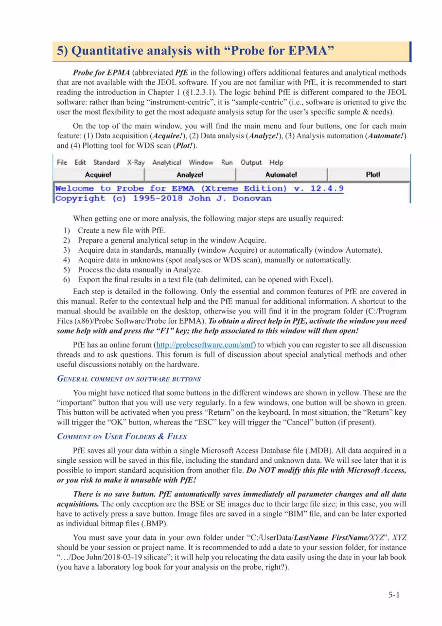
5-1

5) Quantitative analysis with “Probe for EPMA”Probe for EPMA (abbreviated PfE in the following) offers additional features and analytical methods

that are not available with the JEOL software. If you are not familiar with PfE, it is recommended to start reading the introduction in Chapter 1 (§1.2.3.1). The logic behind PfE is different compared to the JEOL software: rather than being “instrument-centric”, it is “sample-centric” (i.e., software is oriented to give the user the most flexibility to get the most adequate analysis setup for the user’s specific sample & needs).

On the top of the main window, you will find the main menu and four buttons, one for each main feature: (1) Data acquisition (Acquire!), (2) Data analysis (Analyze!), (3) Analysis automation (Automate!) and (4) Plotting tool for WDS scan (Plot!).

When getting one or more analysis, the following major steps are usually required:1) Create a new file with PfE.2) Prepare a general analytical setup in the window Acquire.3) Acquire data in standards, manually (window Acquire) or automatically (window Automate).4) Acquire data in unknowns (spot analyses or WDS scan), manually or automatically.5) Process the data manually in Analyze.6) Export the final results in a text file (tab delimited, can be opened with Excel).

Each step is detailed in the following. Only the essential and common features of PfE are covered in this manual. Refer to the contextual help and the PfE manual for additional information. A shortcut to the manual should be available on the desktop, otherwise you will find it in the program folder (C:/Program Files (x86)/Probe Software/Probe for EPMA). To obtain a direct help in PfE, activate the window you need some help with and press the “F1” key; the help associated to this window will then open!

PfE has an online forum (http://probesoftware.com/smf) to which you can register to see all discussion threads and to ask questions. This forum is full of discussion about special analytical methods and other useful discussions notably on the hardware.

General comment on Software buttonS

You might have noticed that some buttons in the different windows are shown in yellow. These are the “important” button that you will use very regularly. In a few windows, one button will be shown in green. This button will be activated when you press “Return” on the keyboard. In most situation, the “Return” key will trigger the “OK” button, whereas the “ESC” key will trigger the “Cancel” button (if present).

comment on uSer folderS & fileS

PfE saves all your data within a single Microsoft Access Database file (.MDB). All data acquired in a single session will be saved in this file, including the standard and unknown data. We will see later that it is possible to import standard acquisition from another file. Do NOT modify this file with Microsoft Access, or you risk to make it unusable with PfE!

There is no save button. PfE automatically saves immediately all parameter changes and all data acquisitions. The only exception are the BSE or SE images due to their large file size; in this case, you will have to actively press a save button. Image files are saved in a single “BIM” file, and can be later exported as individual bitmap files (.BMP).

You must save your data in your own folder under “C:/UserData/LastName FirstName/XYZ”. XYZ should be your session or project name. It is recommended to add a date to your session folder, for instance “…/Doe John/2018-03-19 silicate”; it will help you relocating the data easily using the date in your lab book (you have a laboratory log book for your analysis on the probe, right?).

5-2

5.1) Starting Probe for EPMA1) Ensure that the JEOL program is running (required for communication with the instrument).2) Ensure that the Pathfinder program (EDS) is running; it is required to get images and EDS data.3) Locate the shortcut “Probe for EPMA” on the desktop and double-click to open it.4) The program asks you if you want to connect to the instrument; answer “Yes” to the question and wait

for the connection to be established.5) (a) CREATE A NEW file: Click on menu “File > New”. In the “Save As…” window, navigate to your

User folder, and enter a name for your analysis file, and click “Save”. 6) (b) OPEN AN EXISTING file: Choose menu “File > Open” and select your existing MDB file. 7) Open the three main windows: Acquire, Analyze, and Automate. It is recommended to keep all three

windows open all the time on the first screen (Fig. 5-1). The third screen can be used for the EDS program. It is also recommended to keep the main log window on the second computer screen. The bottom part of the log window is listing the live status of the instrument, and it should be visible all the time!

5.2) Simple analytical run with two-point backgroundThe following describe a simple example of silicate analysis, and includes the 10 major elements in

silicate: Si, Al, Fe, Mn, Mg, Ca, Na, K, Ti, and Cr. For the example, virtual standard name (minerals) will be used. However, you should consult with the laboratory manager to decide which standard is the most appropriate for your analysis. As a thumb rule, and if multiple standards for one element are available, you should always choose the standard that is the closest in composition and/or density to the material to be analyzed.

The first step consists in declaring a general setup to be used for the standard acquisition. After the standard acquisition, this setup will be adjusted to fit your analytical need (e.g., different current and counting time).

Log window(on second screen)

Analyze! window

Automate! window

Acquire! windowStatus bar with Cancel / Pause button

Figure 5-1 Suggested arrangement of PfE windows

5-3

5.2.1) Defining a “General Setup” for standard acquisition (two-pts bkg)

5.2.1.1) Start a new setupTo declare a new sample setup, open the Acquire! window,

and click on “New Sample/Setup”. In the dialog window, select the radio button “Unknown” and enter a name for your run. We will call this first sample “General Setup” (Fig. 5-2). Click OK. You will then need to go through all major options of the Acquire! window as highlighted next.

5.2.1.2) Elements/Cations propertiesClick on Elements/Cations to declare all analyzed elements.

To enter one element, click an empty line and enter its acquisition parameters as described in the following and in Figure 5-3:

1) Enter the element name and the corresponding X-ray line (Ka for all elements in this first example). Change if necessary the oxidation state by entering the number of cation and oxygen and the charge. By default, the element will be written as “analyzed”; the other option is “specified”, in which case you will have to later enter a value in weight-%

Figure 5-2 Create a “New Sample/Setup”.

Figure 5-3 Definition of element / cation properties in “Elements/Cations” window.

List of elements

Sample setup currently selected

If available, you can select an element from the list of element setup.

Alternatively, you can also use the “Move” window (button in Acquire!) to setup an element on a spectrometer and then read the current spectrometer condition to add the element to the list.

1

2

3

4

5

Click!

5-4

or to add a constrain to fix this element (e.g., by stoichiometry for oxygen, or by a specific ratio to the number of oxygen atoms for carbon). You can also choose whether to acquire this element using the “WDS” or the “EDS”. For this first example, we will assume that all elements are analyzed by WDS. The combined EDS-WDS analysis will be discussed in the chapter “Advanced Options”.

2) Select the spectrometer and the crystal; the default peak position and background values will be automatically entered. Peak search will be performed later, and at this point you should leave the default values for the peak position. Change the background position to the desired value.

3) Enter the detector parameter: base line, window, gain, bias, and deadtime. If an empirical calibration for the PHA setting exists, click on the button “Calculate Empirical PHA”; numbers called through this empirical calibration will then appear in green. Check the box “Use Differential PHA Mode” for differential mode; if unchecked, the integral mode will be used. You will have the opportunity to perform a PHA scan later. Leave the deadtime value and the slit option to their default values.

4) To help with the selection of an appropriate background or to check for potential peak interference, you can click on the button “Hi…” or “Low Off-Peak Interferences” to display a list of potential interferences based on the list of elements given in the “acquired and specified elements” window.

5) Select the type of background. For this first example, we will consider only the “Off peak” option, using a “Linear” correction. Other options will be discussed in the chapter “Advanced Options”.

When all properties have been set for this element, click “OK” and repeat the process for all elements to be analyzed. You do not need to add oxygen (if analyzing oxide); this element will be added automatically and calculated by stoichiometry using the valence of each element during the processing of the results.

A summary of the setup will then be listed in the log window (Table 6-1). The first section of this output lists the peak backgrounds positions, both absolute and relative background positions, along with the dynamic offset (OFFSET). Next comes the parameters for the detector (PHA). The third paragraph lists the X-ray line analyzed and the spectrometer, the background type, and the count times. The last section lists the acceleration voltage used, the energy of the X-ray line analyzed, the absorption edge (= critical ionization energy), the overvoltage (Eo/Ec), and the assigned standard (0 if none selected).

Table 5-1 Example of setup listing after the definition of all analyzed element, as seen in the log window.

Un 1 General SetupTakeOff = 40.0 KiloVolt = 15.0 Beam Current = 20.0 Beam Size = 0(Magnification (analytical) = 4000), Beam Mode = Analog Spot(Magnification (default) = 600, Magnification (imaging) = 100)Aperture Number: 1Image Shift (X,Y): -2.00, 3.00

Formula Based on Sum of Cations = .000 Oxygen Calc. by StoichiometryNumber of Data Lines: 0 Number of ‘Good’ Data Lines: 0

On and Off Peak Positions:ELEM: Si ka Al ka Na ka Mg ka Ca ka Cr ka K ka Ti ka Fe ka Mn kaONPEAK 77.6741 90.9052 129.817 107.799 107.520 73.3229 119.775 88.0045 134.724 146.253OFFSET .000015 -.00002 -.00024 -.00049 -.00053 -.00002 .000427 .000015 -.00020 -.00014HIPEAK 81.1741 93.9052 133.817 113.299 111.020 75.8229 122.275 90.5045 137.724 149.253LOPEAK 70.6741 88.1052 123.817 102.299 104.520 70.3229 116.775 85.0045 131.724 143.253HI-OFF 3.50000 3.00000 4.00000 5.50000 3.50000 2.50000 2.50000 2.50000 3.00000 3.00000LO-OFF -7.0000 -2.8000 -6.0000 -5.5000 -3.0000 -3.0000 -3.0000 -3.0000 -3.0000 -3.0000

PHA Parameters:ELEM: Si ka Al ka Na ka Mg ka Ca ka Cr ka K ka Ti ka Fe ka Mn kaDEAD: 1.08 1.08 1.23 1.23 1.05 1.05 1.02 1.02 1.24 1.24BASE: .70 .70 .70 .70 .70 .70 .70 .70 .70 .70WINDOW 9.30 9.30 9.30 9.30 9.30 9.30 9.30 9.30 9.30 9.30MODE: DIFF DIFF DIFF DIFF DIFF DIFF DIFF DIFF DIFF DIFFGAIN: 8. 8. 8. 8. 64. 64. 64. 64. 32. 32.BIAS: 1640. 1640. 1650. 1650. 1650. 1650. 1650. 1650. 1650. 1650.

Last (Current) On and Off Peak Count Times: ELEM: Si ka Al ka Na ka Mg ka Ca ka Cr ka K ka Ti ka Fe ka Mn kaBGD: OFF OFF OFF OFF OFF OFF OFF OFF OFF OFFBGDS: LIN LIN LIN LIN LIN LIN LIN LIN LIN LINSPEC: 1 1 2 2 3 3 4 4 5 5CRYST: TAP TAP TAPL TAPL PETL PETL PETL PETL LIFL LIFLORDER: 1 2 1 2 1 2 1 2 1 2

5-5

ONTIM: 20.00 20.00 20.00 20.00 20.00 20.00 20.00 20.00 20.00 20.00HITIM: 10.00 10.00 10.00 10.00 10.00 10.00 10.00 10.00 10.00 10.00LOTIM: 10.00 10.00 10.00 10.00 10.00 10.00 10.00 10.00 10.00 10.00

Miscellaneous Sample Acquisition/Calculation Parameters: KILO: 15.00 15.00 15.00 15.00 15.00 15.00 15.00 15.00 15.00 15.00ENERGY 1.740 1.487 1.041 1.254 3.691 5.412 3.313 4.509 6.400 5.895EDGE: 1.839 1.560 1.073 1.305 4.039 5.990 3.608 4.967 7.112 6.539Eo/Ec: 8.16 9.62 13.98 11.49 3.71 2.50 4.16 3.02 2.11 2.29STDS: 301 337 301 322 322 319 334 344 302 342

5.2.1.3) Analytical ConditionsNext, you must define the beam voltage, current, and size to be used by clicking on the button “Analytical

Conditions” (Fig. 5-4). The “General Setup” we are defining first will be used for the analysis of standards, and we will set these conditions to 15 keV, 20 nA and 10 µm beam size. The use of a defocused beam is recommended on all standards in order to (a) minimize the risk of sample damage, and (b) sample a large volume to minimize possible small chemical variation at the micron-scale. This rule is valid for most silicate standards. If you are analyzing carbonate standards, it is recommended to lower the beam current down to 10 nA and to increase the beam size to 20 µm if possible. Leave the default value on all other fields.

Click “OK” to validate your choice. The selected analytical conditions will then be set on the instrument. Wait until the conditions are set (see the progress on the bottom of the log window). When OK, the message “Column: Ready” will appear.

Figure 5-4 Setting beam voltage, current, and size in “Analytical conditions”.

5-6

5.2.1.4) PHA and Peak/Scan OptionsThere is usually nothing to change under the PHA and the Peak/Scan options. However, each of these

options will show a summary of the PHA and the peak & background values for your current run, respectively.

The “PHA” button offers the ability to change the PHA values or to run a manual PHA scan (Fig. 5-5; see the chapter “Advanced options”). Rather than running a PHA scan manually, it is usually recommended to first perform a peak search and then a PHA scan in the same material (standard). This can be done during the peak search routine as described in the Chapter 6.2.1.9.

The “Peak/Scan Options” button shows a summary of the peak and background positions used, and also the parameters for a WDS scan (Fig. 5-6; see also “Acquiring a WDS scan” for more info on this window).

5.2.1.5) Count TimesClick on the button “Count Times” to set the peak and background count time for each element. To

change the count time of one element, click on the element (left image on Fig. 5-7), and then modify the peak and/or background counting time in the “Count Time Properties” window (right image on Fig. 5-7). You can also click-and-drag (multiple selection) to modify a series of contiguous elements.

For standards acquisition, a counting time of 20 seconds on the peak (On-Peak Time) and 10 seconds on each background (Hi and Lo Off Peak Time) is sufficient. We will use this count time for our first simple example. Always try to optimize the counting time, so that (a) all five spectrometer ends at the same moment, (b) the time is not too long to induce beam damage, and (c) use a short count time for major element and increase it for minor and trace elements.

The option “Nominal beam” should be set to 1.00. This is a scaling factor for the count results. When set to 1, the count results returned by the software will be shown as cps per 1 nA (normal situation). If you set this value to 30, the results will be expressed as cps per 30 nA. This nominal beam can be useful for

Set the conditions for the PHA distribution and Bias scan. Leave the Scan BaseL at 4.00 (= center of the pulse), and the scan window to 0.1. Adjust the range for the bias scan as required

(1600 to 1800 recommended).

Acquire a PHA distribution, set the counting time (default 0.2 sec) and the number of intervals (default 20).

Acquire a Bias scan, set the counting time (default 0.1 sec) and the number of intervals (default 80). Note that on JEOL

instrument it is not possible to run a gain scan.

Results of the PHA distribution or Bias scan will be displayed here; a larger window will appear when the scan is over.

Current setting

Summary of current PHA settings

Click!

Leave the default here...

Figure 5-5 PHA settings, with possibility to acquire a PHA distribution or a Bias scan.

5-7

Figure 5-7 “Count Times” window.

Summary of peak and background positions, or wavescan limits, or

peak scan limits, or peaking parameters.

Choose the parameters to be displayed using

the radio buttons.

Click!

Change parameters for peak and background position.

Choose the units to modify (mm position or angström)

and whether the position values are displayed as

absolute or relative.

Options for wavescan and peaking, see

“Advanced Options”.

Options for wavescan and peaking, see

“Advanced Options”.

Figure 5-6 Peak and scan options.

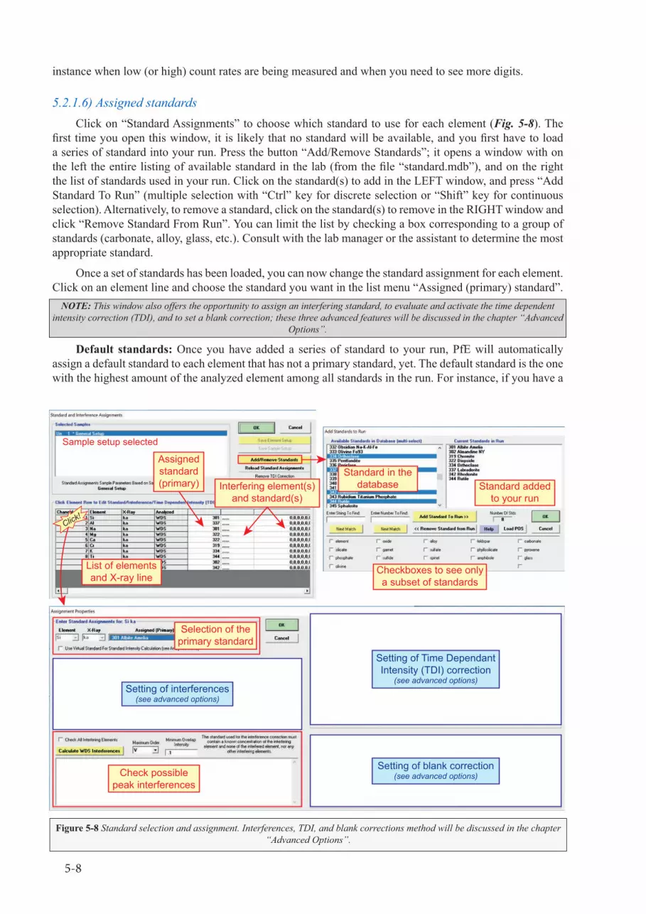
5-8

instance when low (or high) count rates are being measured and when you need to see more digits.

5.2.1.6) Assigned standardsClick on “Standard Assignments” to choose which standard to use for each element (Fig. 5-8). The

first time you open this window, it is likely that no standard will be available, and you first have to load a series of standard into your run. Press the button “Add/Remove Standards”; it opens a window with on the left the entire listing of available standard in the lab (from the file “standard.mdb”), and on the right the list of standards used in your run. Click on the standard(s) to add in the LEFT window, and press “Add Standard To Run” (multiple selection with “Ctrl” key for discrete selection or “Shift” key for continuous selection). Alternatively, to remove a standard, click on the standard(s) to remove in the RIGHT window and click “Remove Standard From Run”. You can limit the list by checking a box corresponding to a group of standards (carbonate, alloy, glass, etc.). Consult with the lab manager or the assistant to determine the most appropriate standard.

Once a set of standards has been loaded, you can now change the standard assignment for each element. Click on an element line and choose the standard you want in the list menu “Assigned (primary) standard”.

NOTE: This window also offers the opportunity to assign an interfering standard, to evaluate and activate the time dependent intensity correction (TDI), and to set a blank correction; these three advanced features will be discussed in the chapter “Advanced

Options”.

Default standards: Once you have added a series of standard to your run, PfE will automatically assign a default standard to each element that has not a primary standard, yet. The default standard is the one with the highest amount of the analyzed element among all standards in the run. For instance, if you have a

Figure 5-8 Standard selection and assignment. Interferences, TDI, and blank corrections method will be discussed in the chapter “Advanced Options”.

Sample setup selected

Assignedstandard(primary)

List of elementsand X-ray line

Selection of theprimary standard

Check possiblepeak interferences

Setting of interferences(see advanced options)

Setting of Time DependantIntensity (TDI) correction

(see advanced options)

Setting of blank correction(see advanced options)

Standard in thedatabase

Checkboxes to see onlya subset of standards

Standard addedto your run

Interfering element(s) and standard(s)

Click!

5-9

quartz and a series of feldspar standards and other silicates, PfE will automatically choose the quartz as the standard for Si. However, this might not be always the wisest choice, and you should carefully check which standard has been assigned to each element (e.g., use an albite standard for Si analysis in feldspar).

5.2.1.7) Acquisition OptionsThe “Acquisition Options” regroup several parameters related to the acquisition (Fig. 5-9). The top of

the window lists all elements, their acquisition order, the type of background used for the standard and for the unknown acquisition, the peaking option, and the option for the “n-th point background acquisition”. These

Leave this option to “asynchronous”

Parameters for EDS (discussed later)

Not applicable to the JEOL-8230

Click!

Do NOT use this, acquire images

manually...

Schematic view of the element acquisition

time & order.

Change manually the acquisition order when “User Defined Order Number” is enabled. If you changed the acquisition order, you must do so for each element on the same spectrometer.

Change the background type for the standard or the unknown acquisition. See “Advanced Options”.

Force running a peak search before each acquisition; NOT recommended.

When you activate the n-th point acquisition, the background is only acquired every interval of n-th point defined.

In Quick Standard Mode, the software acquires only a specific element if this standard is defined as “primary” or as “interference standard”). For instance, if you are analyzing Si, Al, Na & K, and orthoclase is defined as the primary standard for Si & K, the Quick Standard Mode will only acquire Si & K in orthoclase, and not Al or Na. The option “assigned or major elements” with a value of “10%”, then Al will also be acquired in the orthoclase standard as it is > 10 wt%, but not Na. It is usually recommended to leave this option as “Only Assigned Elements”.

Parameters for the n-th point background

acquisition. When activated, the background is

acquired only every n-th point, useful when analyzing homogeneous material. See

“Advanced Options”.

Activate the backlash on stage positions (std, unk, or wavescans) or spectrometers to force a backward motion of

the motors before returning in position. It

ensures a more accurate positioning of

the stage and spectrometer.

Force to change all background

acquisition to a two-point

background acquisition

(Off-Peak) or to the mean atomic

number background correction (MAN).

Choose the element acquisition order by

channel (default: elements analyzed in the sequence they are entered), ascending or descending angstroms value, or user defined (define the acquisition order by clicking on an

element in the table above and changing

the acquisition number. See text for details

Force to run the matrix correction

after each acquisition. It is

usually not activated, and the user will

have to manually press “Analyze” or to

export the results in order

to run the matrix correction at the

end of an analysis.

Figure 5-9 “Acquisition Options” window and default options checked.

5-10

options can be changed by clicking on an element. Some other options are briefly presented in Figure 5-9. Additional discussion on the background type, the n-th point background acquisition (MAN vs. multipoint), and the EDS acquisition (combined EDS-WDS analysis) will be discussed in “Advanced Options” chapter. Remember to hover on an option for a contextual help or press “F1” to obtain additional help on this window.

miScellaneouS optionS

Only the most important options are discussed below. If an option is not listed below, refer to the Probe for EPMA manual for information.

• Return to On Peaks After Acquisiton: Set back the spectrometer in position for the next point analysis at the end of the acquisition.

• Do Not Set Conditions During Acquisition: Force using the current column conditions (voltage, beam current and size, etc.). This option is NOT recommended (leave it unchecked).

• Blank Beam After Move and Acquisitions: Force to place back the Faraday cup before any move and at the end of each acquisition.

• Measure Absorbed Current On Sample: Take two measurements of the absorbed current at the beginning and just before the end of the analysis.

• Measure Beam On Sample Acquisitions: Take two measurements of the beam current before the beginning and at the end of the analysis.

• Use Decontamination/Incubation Delay: Force leaving the beam on a sample for X seconds before starting the acquisition. In most situation, this option is left unchecked; it is used for instance to let the carbon contamination build up on the sample before starting the acquisition.

• Use Only Digitized Standard Positions: Force using the standard position defined in the Automate window for the standard acquisition. If unchecked, the standard acquisition in automated mode will use the parameters defined on the left-side of the “Automate!” window (standard point to acquire, standard X increment, and re-standard Y increment).

The following will be discussed later in the chapter “Advance Options”:• Use Alternating On and Off Peak Acquire: Activate the alternate peak and background acquisition.• Load Standard Data From File Setup: Enable the option to load the standard acquisition data when

recalling a setup from a different MDB file.• Use Unknown Count Time For Interf. Std: Enable the acquisition of a peak interference factor on

a standard using the unknown counting time.

5.2.1.8) Special OptionsSpecial Options is used to activate the Time Dependent Intensity correction or the quick WDS scan.

This feature is not used in this simple example and will be discussed in the “Advanced Options”.

5.2.1.9) Peaking Options and Start PeakingPeak search can be done manually or in automated mode. The automation routine will be described in

the next section about the window “Automate!”. To perform a manual peaking (and PHA scan)…• Move first to an appropriate standard, for instance on wollastonite in order to perform a peak search

of Si Ka and Ca Ka.• Ensure the stage is on focus (Z position).• The analytical conditions defined under “Analytical Conditions” will be used to perform the peak

search. In this first example, you should have set it to 20 nA and 10 µm (double-check it!).• Click on the button “Peaking Options” (Fig. 5-10):

* Select one or more element to be peaked (hold down [Ctrl] key for selecting multiple elements), for instance Si on spectrometer 1 and Ca on spectrometer 3.

* Choose which type of ROM peaking to perform under the “ROM Peaking Type” section. It is recommended to use the “Gaussian” fitting for TAP and PET monochromators, and the “Maxima” for LiF monochromator. When using this feature in the automation mode (as we will see next), select the option “Dual Maxima/Gaussian”.

* Select additional options for the peak search under “Peak Center Options”, as desired. You

5-11

can for instance acquire automatically a PHA scan before or after the peak search, either baseline & window or bias scan. If you use the “Empirical PHA” value, a bias scan might not be necessary, but you may want to check the baseline & window. Additional option to consider is the box “Skip P/B Check […]”. If left UNchecked the software will run a quick count on the peak and background to ensure that the peak-to-background ratio is high enough. Providing the peak search is done in a material rich in the element(s) to be peaked, there is no need to perform such a check. Other options are self-explanatory (hover on the option for more info or press [F1]).

* When ready, click on “Start Peaking” to start the peak search. This button is available both in the “Peaking Options” window and in the “Acquire!” window.

Some additional functions for moving the spectrometers to a specific element are found on the bottom left part of the “Peaking Options” window. For instance, you can automatically select all elements from the 1st (or 2nd, 3rd…) spectrometer pass by selecting the appropriate “Spectrometer Order”, and then click the button “Move Selected Elements To On-Peak Positions” to force setting the selected elements on the corresponding spectrometer. Similarly, “Move To On Peak (start analysis) Positions” will set the first element to be acquired on each spectrometer. The “Plot Selected Peak Center” will show the last peak search for that element (if available).

5.2.1.10) Stage, Locate, and MoveThe button “Stage” is a small utility to navigate in a sample holder. Providing the image is properly

calibrated to the stage coordinate, you can double-click on an area to drive the stage to this coordinate. The “PictureSnap” feature described in a later chapter is often more practical to use than “Stage”, as it permits to upload and calibrate any picture such as a scan of a sample mount, a mosaic BSE image, or an element map.

The button “Locate” list all the standard and unknown positions that have been acquired in this file. It allows you to drive the stage back to one of this position. You can also export the positions.

The button “Move” is used to manually move the spectrometer or the stage (Fig. 5-11).

5.2.1.11) ImagingThe button “Imaging” will open a window to acquire a BSE or SE image (Fig. 5-12). Choose first the

signal to acquire (BSE or SE), then type in a name. By default, the name of the current sample setup is used (e.g., in our case “General Setup”. Choose then the speed for the mapping. On the JEOL-8230 system and due to limitation on the JEOL side, the minimum speed is 100 msec, meaning a 1024 px image will easily take 3 to 4 minutes acquisition time. If the Thermo interface is used to acquire an image a (much) faster scan is possible. ProbeSoftware is currently looking for a faster scanning solution through the JEOL interface. Choose then the image resolution (128, 256, 512 or 1024 pixel in X). The magnification and voltage are

Figure 5-10 Peaking Options.

5-12

Stage control: type in a XYZ coordinate

and press “Go Stage” to move the stage, or use the

cursor on the top-right to move by

increments.

Spectrometer control: type in a

spectrometer position and press “Go Spectros” to

move the spectrometer in

position. Open a periodic table and select a specific element.

Perform a peak search for this element at the current stage position.

Perform a PHA scan (will open the

“PHA” window).

Assigned element, Xtal, and position on that spectrometer

Figure 5-11 “Move” window: controlling the stage and spectrometer motors.

Choose signal (SE or BSE)

Enter name for image

Choose image resolution

Display scale bar

Function when clicking on the image: deflecting the beam or moving the stage

Display digitized positions (if points are set...)

Magnification and voltage are automatically read

Start image acquisition

Save image

Status bar

Choose scanning speed (currently minimum 100 msec on JEOL; faster with other system)

Options for setting up positions using the image (not discussed here)

Figure 5-12 “Imaging” window.

5-13

taken from the current status of the instrument. Press then “Start Image” to launch the image acquisition. The progress of the scan will be displayed in the status bar (bottom of the screen).

5.2.1.12) Saving the setupWhen the sample setup is completely defined, it should be made available as a “Sample Setup” using the

following procedure. After this, the setup can be easily recalled for a manual or for an automated acquisition.• Open the window “Analyze!”;• Select the radio button “Unknown” (top-left)• Select the sample “General Setup” (= the sample name defined under §6.2.1.1);• Click on the button “Add To Setups”.

5.2.2) Manual standard acquisition1) Open the window “Analyze!”;2) Click on “New Sample/Setup” (Fig. 5-13), and…

a) Select the radio button “Standard”.b) Select the standard to acquire in the list below. If the

standard you need is not listed, you must first add it to your run by pressing the button “Add/Remove Standards”.

c) Click on “Load Sample Setup” and select the setup defined under Chapter 5.2.1.12 (“General setup”).

d) Click OK.3) Move the stage to the standard: use the JEOL interface, unless

the standard position is already saved in the “Automate!” window – see §xxxxx for the use of the Automate! window.

4) Locate an appropriate position in the standard. Ensure the stage is on focus.

5) Perform a manual peak search if you have not done this before (see Chapter 5.2.1.9).

6) Click on “Start Standard or Unknown Acqusition” and wait until the completion of the analysis. Repeat the operation until you obtain a satisfactory statistics (usually 4-5 points minimum). A good standard measurement should yield a relative standard deviation around 0.3%, or at least 0.5% for the low count rates around 50 cps/nA.

5.2.3) Automated standard acquisitionThe automated standard acquisition is done through the window “Automate!”. This section reviews only

the essential functionalities commonly used for standard acquisition. Additional details will be discussed later.

5.2.3.1) Defining the standard positionsFor each standard, you must define at least one position within the “Automate!” window. The automation

routine will then use the digitized position(s) to acquire the standard. If you checked the box “Use Only Digitized Standard Positions” in the “Acquisition Options” window (see §6.2.1.7), you must define each individual point to acquire; if you want to acquire 5 points, you must define 5 points. However, if you have NOT checked this box, you only need to define 1 point and the automation routine will automatically acquire a certain number of points defined by the user in the automation routine. To define one or more positions…

• Open the “Automate!” window.• Select the radio button “Standards”.

Figure 5-13 New sample window, selection of a standard for a manual acquisition.

5-14

• Click on “Digitize”.• In the Digitize window, select the standard for which you want to define a stage position. If the

standard already exists in the list of positions, it will be listed in the bottom section of the “Automate!” window, otherwise a new entry will be created with an empty position list.

• To CREATE one or more position(s):* Drive the stage to the standard position to be analyzed.* Click on “Single” in the “Digitize” window to save the current position in the list of position.* There are other options to save points, such as a series of points along a line, or in a grid, or

random points. These options will be reviewed later.• To UPDATE an existing position (in “Automate!” window):

* Drive the stage to the standard position; you can double-click on the existing position to drive to this old position, and then adjust the stage accordingly.

* Select the position to be updated (normal click).* Right-click on the position and select “Update Selected Single Position”.

• To DELETE an existing position (in “Automate!” window):* Select the position to be deleted (normal click).* Right-click and select “Delete Selected Position”.

• See also Figure 5-14 for more information about the “Automate!” and the “Digitize” windows.

5.2.3.2) Perform an automated peaking (and PHA scan)You can perform automatically multiple peak searches and a PHA scans in a series of standard using

the “Automate!” window. Make sure you have at least one position for each standard required for the peak search. This functionality will only work if the last unknown defined in the window “Acquire!” is a setup without any acquired data (the peak position will be updated in this last unknown). This should be the case in our example here, as the “last unknown” is the “General setup” that has been defined in Chapter 6.2.1.

• Open the “Automate!” window.• Select all standards required for the peak search; use [shift]+click to select a continuous series of

standards, or use [ctrl]+click for individual (de-)selection.• On the right-side of the window:

* Check the box “Peak Spectrometers”.* Check the box “Peak on Assigned Standards”. This will force to only run the peak search on

the assigned standard, as defined in the “Assigned Standards” window (see Chapter 5.2.1.6).* Click the button “Peaking” and choose the appropriate options in the “Peaking” window (see

Chapter 5.2.1.9 and Fig. 5-10). Close the “Peaking” window.* Select the radio button “Use Last Unknown Sample” in the bottom right.* Click “Run Selected Samples”.

• The automation routine will then start the peak search in the selected standards. The peak position value will be automatically updated in the Sample “General Setup”.

5.2.3.3) Run an automated standard acquisitionYou can perform automatically a series of standard acquisition using the “Automate!” window. Before

continuing, you must ensure that (a) a setup containing all elements to be calibrated exists (see §6.2.1) and has been defined as a “Sample Setup” (see §6.2.1.12) or that the last unknown sample declare is matching the standard analysis to be performed (see §6.2.1), and (b) all standards to be analyzed have a valid stage position (on focus!) defined in the Position List in Automate! (see §6.2.3.1).

Refer then to Figure 5-14 to run a series of standard acquisition. After checking the appropriate options (acquire standard samples, entering # of points to acquire, etc.), click on “Run Selected Samples”. The program will give you a time estimate for this acquisition; confirm if OK. The analysis should start shortly after.Comment on the options to check for standard acquisition in the Automation List on the right:

• “Acquire Standard Samples” (required): acquire all currently selected standards.• “Use “Quick” Standards” (optional, recommended for two-point background analysis): force to

analyze an element in a standard only if that standard is defined as a primary standard for that element, or if this standard is used for a peak interference correction. For instance, the general

5-15

setup we have defined earlier contains 10 elements. However, when the standard “Wollastonite” is analyzed, only Si and Ca will be measured if wollastonite is defined as a primary standard for Si and Ca. If left unchecked, all elements will be analyzed in each standard.

WARNING: If you are opting for the “quick standards” option, you must use the option “Use Last Unknown Sample” under point #4; you cannot use the “Sample Setup” as described above. In our current

example, this is totally fine, as the “last unknown” is actually the sample setup that is being prepared in Chapter 6.2.1.

• “Use ROM Auto Focus” (optional): perform a Z-stage autofocus. Ensure to check the box “On Stds”. Select then the frequency of the autofocus. You can potentially do it on every point, although for the standard an autofocus on the first point (option “New Sample”) is usually sufficient.

• “Standard Points to Acquire” and “Standard X Increments (um)” (required): enter the number of points to acquire in a standard (5 to 6 points is usually sufficient) and a stage increment. For this

Figure 5-14 Defining standard positions in the Automation window.

3a

3b

4a

12

4b

1) Select the radio button “Standards”.2) Click on “Digitize”.3) In the Digitize window, select the standard for which

you want to define a stage position. If the standard already exists in the list of positions, it will be listed in the bottom section of the “Automate!” window, otherwise a new entry will be created with an empty position list.

4a) To enter a new position, drive the stage to the standard position, click on “Single” to save the current position in the list of position (other options such as Shotgun, Linear Traverse, etc. will be discussed later).

4b) To update an existing position, select the position to be updated (normal click), then right-click and select “Update Selected Single Position”.

5) To delete an existing position, select the position, then right-click and select “Delete Selected Position”.

List of stage positions will appear here. Right-click for additional

options (update or delete position, activate auto-focus, etc.)

List of standards will appear here...

5-16

latter, it is recommended to set an increment that is larger than the beam size (e.g., 15 µm if the beam size in 10 µm). The automation routine will drive to the first position stored for a standard, and then move by the X increment value for the next point, and repeat that for the number of points defined. Note that if you have checked the box “Use Only Digitized Standard Positions” in the “Acquisition Options”, only the positions that are actually digitized in a standard will be acquired.

• “Use Last Unknown Sample”: this option will force to use the last unknown defined in “Acquire!”. In the present situation, the “Last Unknown” should be the setup you have been defining in the section §6.2.1, and can therefore also be used.

• “Use Digitized Sample Setups”: this option will force to use the assigned Sample Setups to run the standard acquisition. The sample setup is selected using the “Sample Setups” button (#2 in Fig. 5-15).

5.2.4) Review the standard acquisitionAfter the completion of all standard acquisitions (either manual or automated), you should check for

possible outliers, and ensure a good counting statistic on each standard. A good statistic should be <0.5 to 0.3% relative standard deviation [%Rel SD] for standard with count rate above 2000 cps (100 cps/nA at 20 nA) and for a peak counting time of 20 s. To verify the standard acquisition data (Fig. 5-16):

• Open “Analyze!”.• Select the radio button “Standards” on the top-left of this window.• Double-click on a standard entry to see the data or press the button “Raw Data”. The raw data are

expressed as counts per second per nanoamp (cps/nA), unless you have set the “nominal beam” to a non-unitarian value (in which case, the data are expressed as cps / X nA, where X is the nominal beam value).

• Check the statistics on the analysis (%RSD should be <0.5%), and identify possible outliers.• To disable (“delete”) an outlier, select the outlier line (normal click on the line) or click-and-drag

over a series of outlier lines, and click “Disable Selected Line(s)”. Alternatively, you can also right-click on the line and choose the same option in the contextual menu. Note that the data are never deleted; instead they are marked as “bad” (the “G” aside the incremental number will be changed to

1

3

4

2

1) Select the radio button “Standards”, and select all standards to be acquired.

2) Click on “Sample Setups” and select select a setup that contains all elements to be analyzed (e.g. the “General Setup” created under §6.1.2).

3) Check the boxes as highlighted on this figure. See text for detail.

4) Ensure the option “Use Digitized Sample Setups” is selected, and click on “Run Selected Samples” to start the analysis.

Each standard has at least one

XYZ position

Select the Sample Setup containing all elements to be

analyzed and click “OK”.

Summary of analytical conditions in the selected setup.

Figure 5-15 Automation setting for acquiring standards data.

5-17

a “B”).• After disabling one or more outlier, double-click again on the standard to update the statistics value.

NOTE: If you have acquired all standards, you can also select a standard and press the button “Analyze” to see the results in weight-% instead of raw counts.

5.2.5) Preparing an analytical setupOnce all standards have been acquired, you should prepare a distinct sample setup with the appropriate

beam current and beam size, along with a specific set of elements to be analyzed. We will use the “General Setup” declared above (§6.2.1) and adjust the required parameters. As an example, we will define 3 setups:

1) Feldspar setup (1): 20 nA, 10 µm beam size, elements: Si Al Ca Na K Fe Mg.2) Feldspar setup (2): 20 nA, 5 µm beam size, elements: Si Al Ca Na K Fe Mg.3) Amphibole setup: 20 nA, 5 µm beam size, elements: Si Al Ca Na K Fe Mn Mg Ti Cr.

Here is how to proceed for each setup:• Open “Acquire!”.• Click on “New Sample/Setup” and choose the radio button “Unknown” on the top-left. Click on

“Load Sample Setup” and select the setup “General Setup” defined above (§6.2.1.12). Enter a name for the setup to be created under the field “New Sample/Setup Name” (e.g., “Setup Fsp 20nA 10um”). Click “OK”. This will load the setup with the list of elements, the corresponding peak and background positions, the right PHA setting, etc.

Double

click!

Click!

Right

click!

Select the standard to check in the window “Analyze!” and

double-click on it (or click Raw data) to obtain the statistics.

Identify the outliers (if any). For this example, let’s assume point

number 3 is an outlier. Select the point number 3. To disable this analysis, click on “Disable Selected Line(s)”.

This option is also available by right-clicking on the selected point.

Relativestandarddeviation

Average

OR

Figure 5-16 Checking standard data in the Analyze! window.

5-18

• At this point, you can go through each option in the Acquire! window to adjust your setup. For instance:

* Remove unnecessary elements: click on “Elements/Cations” (see §6.2.1.2), and click on the element you do not want (e.g., Mn, Ti, and Cr in feldspar). Click then on the button “Delete” in the window “Element/Cation Properties”. Click OK on all windows to validate your choice.

* Adjust the beam current and beam size in the window “Analytical Conditions” (see §6.2.1.3).

WARNING: Do NOT change the acceleration voltage (it MUST be the same as for the standard!).

* Adjust the counting time in the “Count Times” window (see §6.2.1.5).* Adjust other acquisition options using the “Acquisition Options” and “Special Options” if

necessary.• Once you have modified the required parameters, you must make this setup available as a true setup

(see Chapter 5.2.1.12). Go to the window “Analyze!”, select the setup you have just created (e.g., “Setup Fsp 20nA 10um”) and click “Add to Setups”.

• Repeat this operation for all setups you might need.

5.2.6) Acquiring the analysis of an unknown in manual or automated modeIt is often more convenient to set a bunch of (X,Y,Z) coordinates to be analyzed in automated mode.

However, for small grains or small inclusions in grain where a stage reproducibility of better than 2-3 µm is required, a manual acquisition is recommended.

In each situation (manual or automated acquisition), you will have to define a “Sample”. A sample in Probe for EPMA can contain one or more analyses. This sample will have one single “name”, and it will be the only text linked to your analysis (no additional comment possible for each individual analysis point within a sample). For best practice, include only one type of phase to be analyzed per sample. It is recommended to use a name that will include at least your sample number, the type of mineral analyzed, and some keywords to identify the area within the sample that has been analyzed (e.g., “SampleXYZ Fsp area1”). Here are a few examples of what you could do:

1) You would like a specific text for each individual analysis (e.g., “SampleXYZ Fsp area1 rim”). In this case, your sample will contain a single (X,Y,Z) position.

2) You analyze a single phase in a specific area and you want to set a traverse across that grain (e.g., “SampleXYZ Fsp area1 rim-to-rim”), or you want multiple analyses of the same phase in a specific area. In this case, you can use a more generic sample name and use your laboratory book and/or on a reference image to detail what you have done and where your analysis points are.

3) You don’t need to know exactly where you analyzed what, or a simple set of (X,Y,Z) coordinate will be sufficient. This is often the case for instance when you want to test the homogeneity of a certain phase. In this situation, you may want to create one sample per type of mineral to be analyzed (e.g., “SampleXYZ Feldspar”).

We will see later that there is a possibility to overlay the analysis points on a BSE image. However, this technique is not perfect, and the exact analyzed position might be off by a few microns. You should always document precisely in your laboratory book & reference image(s) what you have done!

5.2.6.1) Manual unknown acquisition• Open “Acquire!”.• Click on “New Sample/Setup”, click on “Load Sample Setup” and select the corresponding setup

that you have created in §6.2.5. Enter a name for your unknown sample (e.g., “Sample XYZ Fsp1 area1”), and click OK. The name you give to this sample is the only text that will be linked to your analysis. This “sample” can contain either one analysis (of a peculiar grain) or multiple analysis (of the same mineral grain, or all the mineral grains of that type in your sample).

• Move the stage to the point to be analyzed. Ensure the Z-stage is on focus.• Click on “Start Standard or Unknown Acquisition”.• The analysis will start immediately. Wait for completion.• Move then to the next point to analyze and press again “Start Standard or Unknown Acquisition”.

5-19

• Repeat as necessary.

Warning: As soon as you click again “New Sample/Setup”, it will generate a new entry in “Analyze”. You will NOT be able to add more analysis points to the former entry.

5.2.6.2) Automated unknown acquisitionThe automated analysis of unknown works almost the same as for the automated standard analysis

(see §6.2.3.1). The principle is to (a) declare a new “sample”, (b) set a series of (X,Y,Z) coordinates in this sample, (c) repeat for multiple samples, (d) assigned a sample setup for each set of “sample”, and (e) run the automation.

define the SampleS poSitionS

• Open “Automate!”.• Click on the radio button “Unknown” on the top-left corner.• Click on “Digitize”.• Enter a Name (and optionally a description) for the set of points to be analyzed.• Click “Add New Unknown To Position List”. This will create a new entry in the window “Automate!”.

This entry will first have a star * in front of the name, indicating that there are no (X,Y,Z) positions.• In the bottom part of the “Digitize” window, you will find several options to save the (X,Y,Z) stage

position(s) you need to analyze. The most commonly used one are:* “Singe Point(s)”: this option will save only the current stage position. Drive the stage to the

point to be analyzed and press this button. It will save the (X,Y,Z) stage position in the currently selected “Sample”.

* “Linear Traverse”: this option will set a series of points to be acquired between two points. Click on this button to open the window “Linear Traverse Parameters”, and drive the stage to the starting position of your linear traverse. Click then “Update Start” to save your starting position. Move the stage to the end of your traverse and click on “Update Stop”. The program will then calculate automatically the distance (in mm and in micrometer). In the bottom part of this window, you can choose to define a fixed number of points to be spread along this linear traverse, or a step size in micron (e.g., one analysis point every 20 µm). Once ready, press “OK”. A series of (X,Y,Z) positions will be automatically generated. It is recommended to check individually each point generated to ensure that (a) they are on the phase to be analyzed (and not for instance on an inclusion) and (b) the analysis point is not sitting on a crack, an asperity of the sample, or the very edge of a phase; see below how to drive the stage to a specific (X,Y,Z) position.

* “Digitize Image”: this option lets you define (X,Y,Z) position by clicking on a specific position in a BSE image. Whereas this option sounds attractive, it is not ideal if you are dealing with very fine material due to slight inaccuracy in the (X,Y,Z) positioning.

* “Shotgun”: randomly generate a number (“Number”) of points within a certain range (“Size” in micrometer) of the current stage position. Useful for homogeneity test.

* “Rectangular Grid”: set a series of points within a rectangular area. Like for the linear traverse, you will need to define the two edges of your rectangular area, and then define the grid size in X and Y. Points are generated automatically as soon as you click OK, and you should check each of them individually to ensure they are not on a crack, an asperity or on the edge of a grain.

* “Polygon Grid”: set a series of points within a polygon area. To define the area, you must drive the stage to one corner of the polygon, then press “Add Polygon Boundary Coordinate” to save this position, then move to the next corner and repeat the operation until you reach the last corner of your polygon. Set then the grid size and press “Calculate Number of Points In Polygon” to get an estimate of the points to be generated. Then press OK to generate the positions.

* “Digitize Cluster (of Random Points)”: Similar to the “Shotgun” option, but with the possibility to generate multiple cluster. Not reviewed further here.

• Once you have defined all the points in your “Sample”, enter a new name for your next “Sample” in the “Digitize” window and click again “Add New Unknown To Position List” to create a new entry.

5-20

Add your desired positions to be analyzed. Repeat as necessary.• If you want to add another point to an existing “Sample”, select the “Sample” in the “Automate!”

window and press again “Digitize” (even if the window is already opened). You should then see your “Sample” name in the name field. From this point, you can add points to this existing “Sample”.

• There are some cases where you should check individually the saved (X,Y,Z) positions (e.g., after generating a bunch of points in a linear traverse), and maybe either modify of delete an (X,Y,Z) entry:

• Double-click on a “Sample” in the Position List in “Automate!” to display all (X,Y,Z) entries.• To move to a specific (X,Y,Z) position, double-click on the (X,Y,Z) position. Alternatively, you can

select an (X,Y,Z) position and click the button “Go”.• To update or delete a specific (X,Y,Z) position, select the position and make a right-click. Then

choose “Update Selected Single Position” or “Delete Selected Positions”.run the automation

• Once you have all the sample positions defined, you will need to attribute a Sample Setup to each entry:

* In Automate, select all the “Sample” that will be analyzed with the same setup (e.g., all the “Sample” pertaining to the analysis of feldspar at 20 nA and 10 µm beam size). To select multiple entries, hold the <Ctrl> keyboard key. To select a continuous range, click on the first entry, hold <shift> and click on the last entry.

* Click on “Sample Setups”, and choose the setup corresponding to this set of samples.* Click “OK” and then “Yes” when the program asks to confirm your selection.* Repeat his operation for all samples to be analyzed.* To check if a setup has been properly attributed to a “Sample”, you can double click on the

sample entry and check the currently assigned setup just below the list of (X,Y,Z) position (dark gray area), on the top-right side (section “Sample Setup (row) Number = …”).

* IMPORTANT: make sure that each sample has a specific setup attributed to it!• Select then the automation actions (right-side of the Automate! window):

* Check “Acquire unknown”* To re-acquire the standards after your analysis, check “Acquire Standard Samples (again)”.* (optional) Check “Use ROM Auto Focus” if you want to perform an auto-focus during the

automation. You will have the choice between an auto-focus… – On the first point of each new sample – At every (X,Y,Z) position – At a specific interval of points – As specified in the flag on the digitized point (for this option to work, show a list of

position, make a right click on the (X,Y,Z) position where an auto-focus is desired, and select “Update Auto-Focus Flag”. If the auto-focus flag is set to “-1”, it will perform an auto-focus.

* (optional - ONLY with W-filament!) If this is your last run and no one is using the instrument right after you, check the box “Use Filament Standby Afterwards” to set the filament heat to the standby value (~80) after the acquisition.

* If you want to acquire only the unknowns: – Select all unknown positions to be acquired. – Ensure the radio button “Use Digitized Sample Setups” (bottom-right) is checked. – Click on “Run Selected Samples”. – The program will give you a time estimate of your analysis. Click “Yes” on the

confirmation window to run the analysis, or “No” if you still want to modify something (e.g., to add or remove positions to be analyzed).

* If you want to acquire the unknowns AND the standards before and/or after the analysis: – Check the radio button “All samples” on the top-left to see both the unknowns and the

standards positions. – Select all unknown and standards to be acquired. – Set the number of standard points to be acquired (5-6 recommended). – Set the X and Y increments for acquiring the standards (“Standard X increments (um)”

and “Re-Standard Y increment (um)”. The X increment is used to determine the motion

5-21

1

3

2b

2a

4

7

6

5b

5a

Select the samples (unknown and/or std) to be analyzed

Timeestimate

Auto-focusflag active

Right

click!

1) Click on “All samples” to display both the unknowns and the standards positions.2a,b) Assign a setup to each sample; the selected setup is visible in 1b when you double-click

on a sample. Right-click on a position to modify, delete, or activate the auto-focus flag. 3) Select all unknowns (and standards) to be acquired. Use <ctrl> for multiple selection.4) Choose the actions to perform (most commonly used are shown here).5a,b) Optional: Activate the filament standby mode after the analysis. Activate auto-focus during the acquisition.6) If standards are acquired, set the number of points to acquire and the X and Y increments.7) Ensure “Digitized Sample Setups” is selected and click “Run Selected Samples to start the

analysis. Check the time estimate; click ”Yes” if OK, or “No” to modify something.

Figure 5-17 Preparing an automated acquisition.

5-22

between a series of point to be acquired on each standard, and the Y increment is applied when the standards are acquired again (at the end of your unknown analyses).

– Ensure the radio button “Use Digitized Sample Setups” (bottom-right) is checked. – Click on “Run Selected Samples”. – The program will give you a time estimate of your analysis. Click “Yes” on the

confirmation window to run the analysis, or “No” if you still want to modify something (e.g., to add or remove positions to be analyzed).

A timer will appear on the top of the Automate! window (“Remaining Automation Time: 00:00:00”) once the analysis has been started. If you have checked the box “Use Filament Standby Afterwards”, a message will offer you the possibility to heat again the filament to the previous heat value. At the end of the automation, a message “Automation completed” will be visible.

5.3) Advanced optionsProbe for EPMA has many additional features. Some of the most important ones are summarized

below. Refer to §6.2 for details on the basics for standardizing or acquiring points.

5.3.1) Time Dependent Intensity (TDI) correction

5.3.2) Peak interference correction

5.3.3) Combined EDS-WDS acquisition

5.3.4) Mean Atomic Number (MAN) background correction

5.3.5) Multipoint background acquisition

5.3.6) N-th point background acquisition

5.3.7) Unknown count time factor

5.3.8) Alternate on-off acquisition

5.4) Acquiring a WDS scan (qualitative)

5-23

5.5) Treating your results

5-24

6-1

6) Element mapping with “Probe Image”Probe Image is normally recommended to acquire quantitative element maps. To obtain quantitative

images, you will need to acquire not only your maps, but also the standard. It is therefore recommended to first prepare a mapping setup with Probe for EPMA, acquire the standards with this setup, and then run the image acquisition.

Currently Probe Image can only offer WDS mapping. However, we hope that combined EDS-WDS mapping with Probe Image will be soon possible. In the meantime, qualitative combined EDS-WDS maps can be acquired with the Thermo EDS software “Pathfinder” and the 5-WDS input (see Chapter 5).

6.1) Preparing a map setup (Probe for EPMA)We assume here you know which elements you need to map. A first step is to prepare your mapping

setup in Probe for EPMA, and determine which elements is defined on which spectrometer. Once this setup is ready, it can be used to peak the element (find the exact X-ray position line) and to easily set up the element conditions in Probe Image.

If you intend to quantify your maps, you will have to acquire data with Probe for EPMA on standards for elements standardizations (count rates on standards), and for calibration of the MAN background curves. This standardization will be required when reprocessing the data with CalcImage (see Chapter 7).

IMPORTANT: For more information about the use of Probe for EPMA, refer to Chapter 5; only the essential steps are reminded in the following.

6.1.1) Element setting & standardization1) Open Probe for EPMA and create a new file.2) Open Acquire! and click “New Sample Setup”.3) Enter a generic name for your setup, not sample-related (e.g., “Map setup serpentinite”).4) Optional: choose to reload an existing setup from another MDB file by clicking on “File Setup” and

navigating to the MDB file that contains the mapping setup you need.5) Click OK in the New Sample Setup window.6) Click on “Elements/Cations”, enter the list of elements you need to map with the appropriate

parameters (see Fig. 7-1, step 1):a) The spectrometer and the monochromator;b) The peak position (use the default value first, peaking will be done next);c) The PHA setting (click the “Calculate Empirical PHA” button).d) The background(s), if applicable (required for quantitative analysis or for net counts):

i) It is recommended to use the MAN background correction by selecting the radio button “MAN” in the Background Type for each element in the Element/Cation Properties window. This technique is totally appropriate for major and minor elements down to 1000 ppm or better, which is probably far better than the sensitivity of your map data. See more about the MAN background technique in Chapter 5.

ii) For higher accuracy you might want to acquire either one or two background images. Keep in mind this will double (or triple) your total mapping time as a second (or third) pass will be required for each element. To use it, enter the right value for the low and/or high background. You will be able to select the low and/or high background map acquisition in Probe Image.

e) Other parameters can be left to their default value.7) Peak on the required element:

a) Move to a standard containing the element to peak. Ensure the Z-stage is focused.b) Click on “Peaking” (see Fig. 7-1, step 2):

iii) Select the element(s) to peak in the standard. For multiple element in the same standard click on a first element, hold Ctrl, and click on additional element(s) to peak.

6-2

iv) Select the peaking options. Recommended: dual Gaussian-maxima without PHA scan.v) Click on “Start Peaking”. Close the peaking window when done.

c) Repeat with the next standard / set of elements until you have peaked all elements.NOTE: if you have many elements to peak, you can also run the peaking in automated mode, in which case you will also need to

update the X-Y-Z position for the standards to be analyzed (see more about automated peaking in Chapter 6).

The following is only applicable, if you need quantitative analysis. Although this can be done after your maps, it is recommended to run it before running your maps, and run it a second time after if a problem occurs (e.g., spectrometer reproducibility issue). You will need at least 1 hour of calibration time for 5 elements.

1) Click on “Standard Assignments”:a) Click on “Add/Remove Standards” and add (or remove) the set of standards you may need

(or not), either for peaking purpose, for standardization, or for MAN background fitting (only required for quantification). Note that if you have recalled a setup from a previously existing file, the set of standards used in this past run will automatically be loaded in your new run.

b) Close the Add/Remove Standard window.c) Click on each element to assign the appropriate standard (and peak interference, if applicable).d) Click OK in “Standard Assignments”.e) Define the analytical conditions to be used for the standardization (NOT the mapping

conditions!), usually 20 nA and 10 µm is appropriate.2) Define the counting time for each element; 20 to 30 seconds is usually enough.3) If required, go through additional software options; you do not need to acquire EDS spectrum, at least

not until we have the combined EDS-WDS mapping implemented…4) Open Analyze! Window, and select the map setup you have created (see 3 above). Click “Add to

Setups”. The mapping setup is now available for automation work and for maps quantification.5) Acquire the required data in your standards:

a) You must have at least one standard for each element to be mapped. Ensure to choose a standard that has more of the highest element weight-% you aim to measure, and ideally a standard that is the closest in term of density and structure / composition.

b) If you aim to use the MAN background correction, you must collect data in at least 3-4 standards (strict minimum, 5-6 is already better…). In order to obtain an accurate fit, each of these standards for the MAN background should NOT contain the element to map and should NOT show any peak interference at the position of interest.

As an example, we will consider the acquisition of 10 elements in TWO passes: (1) Mg, Al, Ca, Cr, Fe and (2) Si, Na, Cl, Ti, Mn (all Ka lines). We will therefore need a set of two TAP monochromators for Mg, Si, Al and Na, two PETs for Ca, Cl, Cr and Ti, and one LiF for Fe and Mn; see Figure 7-1 for an example of this map setup in Probe for EPMA. Both passes use exactly the same crystal setup, and no crystal flip is required. A crystal flip between two map passes is technically possible, but NOT recommended (spectrometer reproducibility issue). If you only need 5 elements and you can put one element on each spectrometer, a single pass is naturally sufficient. Keep in mind that not all spectrometers can accept any elements! Most of the time, light elements (Si, Al, Na, Mg…) can only be put on spectrometer 1 and 2 as they require a TAP, whereas heavier elements (e.g., transition metals) can only be put on spectrometer 3 to 4 as they require an LiF.

6-3

Create a “New Sample Setup”.Enter the elements to be mapped.Recommended: choose MAN background for each element.

Element PEAKING:1) Move to a standard that contains the

element(s) to be peaked in large quantity.2) Find a clean spot and focus the stage.3) Select one or more elements to peak.4) Click “Start Peaking”.5) Repeat until all elements are peaked.

Analytical conditions for standardization (for quantitative element mapping): To quantify your element maps, you will need to acquire data in several standards. If this is the case, set up the analytical conditiond to 20 nA and 10 um, set the count time (20-30 sec), and assign a standard to each element. Refer to the chapter about Probe for EPMA for the standardization procedure.

Setting up spectrometer(s) to an element:1) Select up to 5 elements (one per spectro).2) Click “Move Selected Elements To On-Peak

Positions” to set each spectrometer.

Elementselection

Recommendedoptions

1

1

4

4

2,3

2,3

2

2

2

3

3

Figure 6-1 Preparing a setup for mapping in Probe for EPMA.

6-4

6.2) Acquiring maps (ProbeImage)

6.2.1) Spatial & analytical resolution, and mapping timeWhen preparing the acquisition of a map you will have to think about (a) the actual size of the area

to be mapped, (b) the desired spatial resolution, and (c) the desired analytical resolution (sensitivity). All these points will affect the total mapping time, and it is common to iteratively change these values due to time constraints.

6.2.1.1) Pixel size, beam size, and analytical resolutionThe level of spatial resolution on the final image is expressed as the size of one pixel in µm (= µm/px).

You will have to adjust this value depending on the size of the area to map and on the size of the feature to be revealed. Of course, ultimately time constraints might force you to review these values… For detailed map revealing all particles of interest, a minimum of 4 to 9 pixels should ideally cover the smallest particle to ensure at least one pixel is fully within the particle. In other words, the pixel resolution must be 1/2 to 1/3 of the size of the smallest grain or feature to be mapped. For instance, 3-µm wide exsolution lamellae in pyroxene would require a resolution of at least 1.5 to 1.0 µm/px. This rule is not absolute and can be broken in some cases when qualitative results are sufficient; see for instance the full thin section mapping technique in the applications below, which can reveal particles as small as 5 µm despite using a coarse resolution of over 20 µm/px.

The beam size is usually set to equal the pixel size. However, at a pixel size below 2 to 3 µm/px and under certain situations, the electron beam size or the emission volume might be larger than the pixel size. As a result, the map might appear blurrier than usual (oversampling). Pay attention to these rules:

• High current (>100 nA) are often required for mapping, and will increase the beam size;• Lower voltage increases the beam size;• The analytical volume is often larger than a sphere of 1 µm diameter…

* Lower density materials will allow electron to penetrate deeper;* Higher acceleration voltage will increase the analytical volume;* Lower energy X-ray (higher overvoltage) will have a larger excitation volume.

6.2.1.2) Dwell timeThe dwell time (= time spent on each pixel) is set based on the desired level of sensitivity, which is

different for each element to be mapped (different overvoltage and spectrometer efficiency). Depending on the spectrometer and X-ray line you are looking at, one element will have a higher count rate than another. You will have to decide the dwell time based on the most important element for you, and especially the ones with a low count rate. In the most common situation (15 keV, ≥50 nA) a dwell time of 20-30 msec is sufficient for mapping major elements, whereas a dwell time of >50 msec is recommended for minor elements. Trace element mapping is possible in theory, but not recommended as it is time consuming (10+ hours).

A more rigorous way to think about the dwell time is to estimate how many counts you can expect. You can for instance compare the X-ray count rate reached on a material (standard) of known concentration with the expected composition in your unknown (wt-% range) to estimate the number of counts you could receive in one pixel of your map using the (very short) mapping count time. This estimation is inaccurate, notably because it does not take into account of the different absorption effect in your sample vs. the standard. A first order evaluation of the achievable precision is obtained by calculating a 1-sigma standard deviation using Poisson statistics: (N)0.5/N (N = total number of counts). The program CalcZAF has a more robust routine to model the detection limit in a similar way (see menu “Run > Model Detection Limits”).

6-5

6.2.1.3) Total counting timeThe total time depends on the total number of pixels and the dwell time. The total number of pixels

is usually set at a value < 1 to 2 million pixels due to time constraints. Mapping time for major to minor elements can vary largely depending on the mapping area and the expected level of sensitivity:

• Small grain (50 µm) can be mapped in 5-30 min depending on the required sensitivity.• Qualitative work on major element over a few millimeters can be done in 1-2 hours.• mm-sized areas with µm-size spatial resolution will take 2-3 hours (or more for higher sensitivity).• Full thin section scan to reveal all accessory phases can usually be done in 4-6 hours at ≥25 µm/px.At the end, you will likely have to cut on the dwell time and/or on the size of the mapping area in

order to reach a reasonable mapping time. Use the mapping tool at http://cub.geoloweb.ch/?page=xraymap_calculator to estimate the total mapping time. There is a software delay on each line (variable), due to some software overhead time. Therefore, it is common to assume an extra 3 to 5 seconds per mapped line.

See also the example of applications in Section 7.3.

6.2.2) Preparing a map acquisition with Probe Image1) Open ProbeImage.2) Click on menu “Setup > Acquisitions…”.3) Delete all pre-existing maps in the top-right panel (“Acquisition samples”). Do NOT use the “Delete

All” button a bug in Probe Image will cause trouble setting your elements later. Rather, click-and-drag to select all but ONE entry, and click several times “Delete” until there is only one entry left.

4) Click on the sample name to enter the name of your first map. It is recommended to include the sample ID, an identification for the area to map, and (if applicable) the pass number (for mapping of >5 elements). Keep your sample name SHORT (e.g., “JMA01-b area3 #1”)!

5) Move the stage to the area of interest (center position) to visually estimate the area to be mapped.6) Ensure the stage is focused: manual focus first (if necessary), then auto-focusing with the “AF” button.7) Define visually (using the BSE / SE image) the area to be map.8) Follow then the instructions in Section 7.2.3 for setting a mapping area. Use a beam map setting

only for areas <50-100 µm wide (§7.2.3.1), otherwise use the stage map center or 2-pts (§7.2.3.2 or 7.2.3.3).

TIP: If you need to set additional maps, click the “Insert After” (or “…Before”) button. This button will automatically duplicate the last entry (below or above the selection). Therefore, if you intend to map several areas with the same element settings, it is good practice to do this AFTER having set the first map! Doing so, you will just need to adjust the stage coordinate and the column conditions (beam diameter or current).

6.2.3) Setting up the mapping area

6.2.3.1) Beam scan map1) Select the radio button “Beam”.2) Adjust the stage & magnification to have the BSE/SE image covering exactly the area to be mapped.3) Focus the Z-stage (manual focus if necessary, then AF).4) Click on the “Read X,Y,Z” button to update the stage coordinate.5) Click on the “Read” button aside the magnification to read the current magnification. This will define

the largest dimension of the map in µm (as shown below the magnification reading).6) Adjust the image size in pixels; you can map with any kind of pixel ratio for X and Y. The actual size

of one pixel is calculated by dividing the dimension of the map with the corresponding number of pixel. For instance, if a mapped area is 25 x 40 micron, and the map size is set to 50 x 80 pixels, then the pixel size will be 40 µm / 80 pixels = 0.5 µm/px. To double this resolution, the map is set at 100 x 160 pixels.

6-6

7) To avoid defocusing issues, ensure the map size is less than 50 µm to avoid strong defocusing issue on the edges.

6.2.3.2) Stage scan map – Center1) Select the radio button “Stage Ctr”.2) Adjust the stage and magnification to have the BSE/SE image covering the area to be mapped. Use

the “Rulers” button in the top of PC_SEM (diagonal measurement) to determine the size of the area to map.

3) Focus the Z-stage.4) Set the magnification to cover the area to be mapped.5) Click on the “Read X,Y,Z” button to update the stage coordinate.6) Click on the “Read” button aside the magnification to read the current magnification.7) Adjust the Image Size (pixels) and the Pixel size (in µm) to constrain the size of the area to be mapped.

6.2.3.3) Stage scan map – Two-point1) Select the radio button “Stage 2pts”.2) Move the stage to one of the corner of the area to be mapped.3) Focus the Z-stage.4) Click on “Read X,Y,Z” to update the X, Y and all four Z-values (one for each corner). Note that

clicking on “Read X,Y” will only update X and Y, NOT the Z-values; use this button for fine re-adjustment.

5) Move the stage to the opposite corner of the area to be mapped.6) Focus the Z-stage.7) Click on “Ready X2, Y2” to register the 2nd corner of your map.8) Click sequentially on the buttons Move UL, UR, LL, or LR to move to each corner (UL = upper left,

LR = lower right, etc.). For each, ensure the Z-stage is focused. Focus the Z-stage if necessary, and click on the “Read” button situated on the right of the Z(xx) reading.

6.2.4) Choice of elements (WDS Input)After selecting the area to be mapped, you must define the list of elements to be acquired. This is done

in the large panel below the acquisitions parameters window, under the tab “WDS Input”. Although you can enter data manually, it is best practice to use the setting you have created with Probe for EPMA (see Section 7.1.1 and Figure 7-1, step 3), which contains also the peaking of each element:

1) Open Probe for EPMA and the MDB file containing your mapping setup.2) Open Acquire! and ensure that the last entry (analysis) is corresponding to your map setup with all

the elements you need. If not, click on “New Sample Setup” and create a setup containing exactly the set of elements you are mapping. If you have a setup available (but it is not the last analysis), you can also recall this setup in the “New Sample” window.

3) In Acquire! window, click on “Peaking” (same button available also in Automate!).4) Select the set of 5 elements to be mapped. 5) Click on “Move Selected Elements To On Peak Position”.

It will take a few seconds to a minute to set the spectrometers in position and to set the PHA setting. When done, return to Probe Image, and click on the “Inst. All” button on the right to read the current instrument conditions, and then “Elm. ALL” to display the correct element name.

WARNING: To obtain accurate results, you MUST perform a peaking on a set of standards to find the exact X-ray line positions (see Section 7.1.1).

6-7

Stage coordinate (mapcenter) & magnification

Dwell time for background map

Map acquisition will be shown

here when being acquired

Beam map

List of maps to acquire

Selection beam / stage map Dwell time and map size

Stage map - Center

Stage map - Two Points

“Standard” Toolbar(~ File menu)

Menu FILE:- Open/Save image or acquisition file

- Convert image from JEOL or Cameca

- Import/export Surfer grid file

- Exit software

Menu ACQUIRE:- Start/Stop acquisition

Menu SETUP:- Prepare acquisition

Menu VIEW:- Line & shape drawing tools

- Open/close toolbar or panel

a

b

“Drawing”Tools

“Zoom”Toolbar

“Basic” & “Advanced”Toolbars: rotate,

crop, or flip images

“Navigation” Panel:Coordinates, and

pixel color (or intensity)

“Instrument” Panel:Status of instrument forstage, spectrometers &

Faraday cup“Event Log”Panel

“Histogram”Panel

Program status bar (will display remaining map lines to run)

Stage coordinate (twoopposite points = mapcorners) & pixel size

Stage coordinate (mapcenter) & pixel size

Figure 6-2 Setting up the mapping area (beam or stage map) with Probe Image.

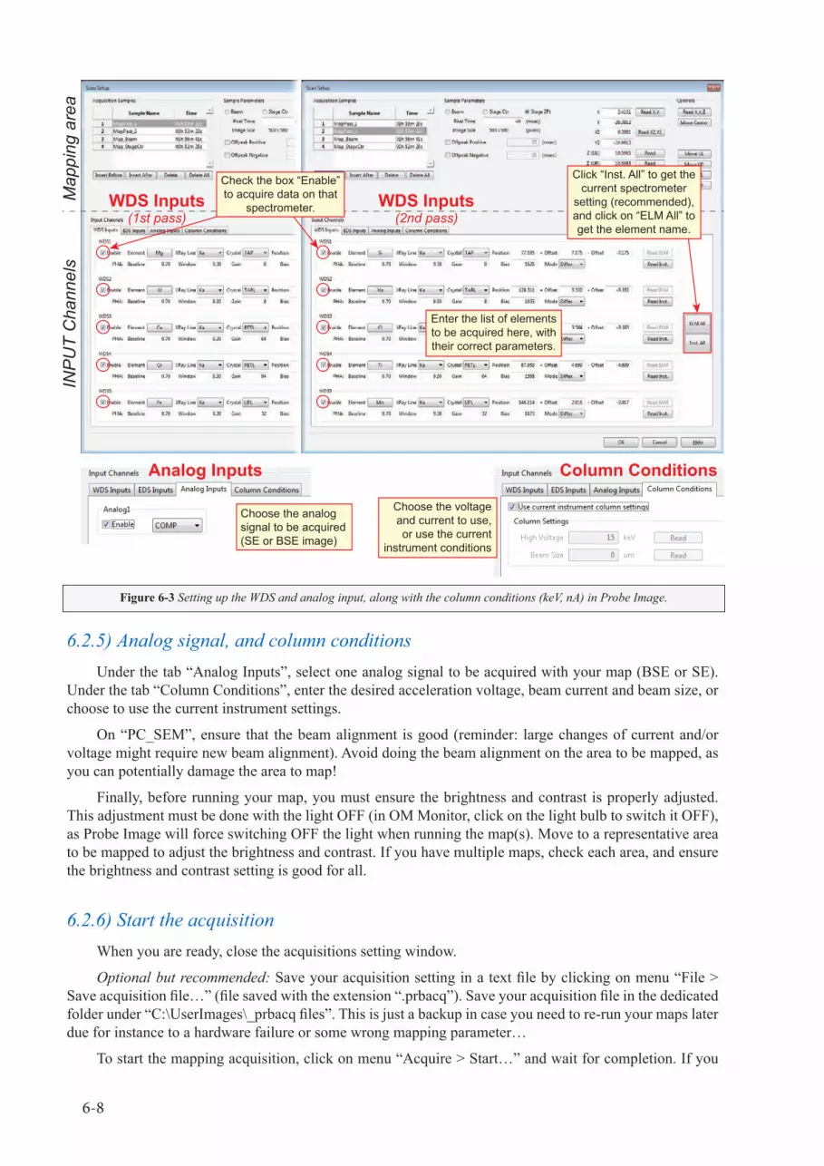
6-8

INP

UT

Cha

nnel

sM

appi

ng a

rea

Choose the analogsignal to be acquired(SE or BSE image)

Choose the voltageand current to use,or use the current

instrument conditions

Enter the list of elements to be acquired here, with their correct parameters.

Click “Inst. All” to get the current spectrometer

setting (recommended), and click on “ELM All” to get the element name.

Check the box “Enable” to acquire data on that

spectrometer.

Column ConditionsAnalog Inputs

WDS Inputs(2nd pass)

WDS Inputs(1st pass)

6.2.5) Analog signal, and column conditionsUnder the tab “Analog Inputs”, select one analog signal to be acquired with your map (BSE or SE).

Under the tab “Column Conditions”, enter the desired acceleration voltage, beam current and beam size, or choose to use the current instrument settings.

On “PC_SEM”, ensure that the beam alignment is good (reminder: large changes of current and/or voltage might require new beam alignment). Avoid doing the beam alignment on the area to be mapped, as you can potentially damage the area to map!

Finally, before running your map, you must ensure the brightness and contrast is properly adjusted. This adjustment must be done with the light OFF (in OM Monitor, click on the light bulb to switch it OFF), as Probe Image will force switching OFF the light when running the map(s). Move to a representative area to be mapped to adjust the brightness and contrast. If you have multiple maps, check each area, and ensure the brightness and contrast setting is good for all.

6.2.6) Start the acquisitionWhen you are ready, close the acquisitions setting window.

Optional but recommended: Save your acquisition setting in a text file by clicking on menu “File > Save acquisition file…” (file saved with the extension “.prbacq”). Save your acquisition file in the dedicated folder under “C:\UserImages\_prbacq files”. This is just a backup in case you need to re-run your maps later due for instance to a hardware failure or some wrong mapping parameter…

To start the mapping acquisition, click on menu “Acquire > Start…” and wait for completion. If you

Figure 6-3 Setting up the WDS and analog input, along with the column conditions (keV, nA) in Probe Image.

6-9

have made a mistake and want to stop the acquisition, click on menu “Acquire > Stop…”. If you stop an acquisition, be extremely patient: the map will need to finish a line (or two) before actually stopping and returning the command to the user.

6.3) Example of mapping applications & settings

6.3.1) Full thin section mappingFull thin section scan is a technique used to reveal the presence of a certain phase (usually an accessory

hard to find on the petrographic microscope) by mapping for a unique element present in large quantity only in this mineral or mineral group (e.g., Zr for zircon, Ce or La for REE phases, P for apatite and monazite, etc.). Despite the use of a large beam, even particles as small as 5 µm can be highlighted providing the targeted element is present in large quantity (>15-20%) with a decent count rate (at least 50-100 cps/nA).

example of conditionS:• Current: high to very high (200-350 nA);• Dwell time: short to medium (20-30 msec);• Pixel size: 20-35 µm;• Beam size: Equal to pixel size;• Mapping type: Two-point stage mapping;• Area: Up to 4 cm x 2.5 cm (ca. 1000 x 625 pixels).

NOTE: Only 5 elements can be set in a map, and therefore if your goal is to identify ALL particles in your sample and their (qualitative) composition, you should consider another technique such as the QEMSCAN.

6.3.2) Quantitative mapping of simple phasesWith the high count-rate of WDS, it is possible to map for major and minor elements in simple phases.

The map can be quantified providing all major elements composing the phase to map are analyzed (or specified or constrained). At 15 keV, you can expect to see details in the range of 1-2 µm spatial resolution, and high-quality maps will be at this spatial resolution or better. However, if you are mapping large grains (e.g., centimeter-sized garnet), you might first need a coarse map with >5 µm/px resolution, and then only return to one or more specific (smaller) areas of your grain to map with higher details if necessary. A quick and rough map can be acquired in 30-60 min; high-quality map of several millimeter-sized grains will easily take several hours. The current is usually set to a high value (> 50 nA), although you will have to consider potential beam damage (e.g., in carbonate, hydrated phases, alkali-rich phases, etc.).

example of conditionS: • Current: high (50-200 nA), lower in very beam sensitive phases (10-20 nA? to be tested…);• Dwell time: short to medium for rough map (20-30 msec), higher for high quality maps (40-60

msec);• Pixel size: depend on grain size: >5 µm for cm-sized area, ≤ 0.2 µm/px for sub-millimeter area;• Beam size: Equal to pixel size when pixel is ≥1 µm/px, or focused beam when pixel is < 1 µm;• Mapping type: Depends on the grain size …

* Two-point stage mapping for large grain not entirely visible at 40x;* Center stage mapping for grain < 3 mm (entirely visible at 40x);* Beam map for very small grains < 50-100 µm. Watch out for defocusing effects!

6.3.3) Quantitative mapping of beam sensitive phasesBeam sensitive materials is a very broad and vague term to describe any material or phase that is

susceptible to be damaged by the beam of electron. Damage is essentially caused by heat and the subsequent migration (diffusion) of element and the progressive breaking of bonds (reorganization of the crystal structure or amorphization). Any mineral is susceptible to beam damage, and key is to assess how much

6-10

energy a specific mineral can sustain before being damaged. The beam damage increases as a function of the time, the beam current. If you double the current, there will be twice more electron in the same activation volume (current dosage is doubled). However, the damage will decrease if a larger beam size is used, as it will spread the same amount of electron over a larger surface; doubling the beam diameter will divide the current dosage by 4.

It is possible to evaluate beam damage by measuring the change of count rate of a major elements over time. Such testing can be time consuming; yet, it can lead to higher accuracy in your data. The data are usually acquired over a certain period of time using the time dependent intensity correction, at a variable counting time, beam current, and beam size. The final results of these tests are usually represented in a plot of the X-ray intensity (in cps/nA) versus the current dosage. Key is to determine the current dosage limit at which beam damage occurs (as seen by a change in count rate). The current dosage is calculated by multiplying the counting time by the current and dividing it by the surface of the beam on the sample. When a focused beam is used, it is better to consider the projection of the analytical volume over the surface of the sample as being the actual “beam size”. In other situation, the surface of the beam is the surface assuming a round beam size (= π [½ * beam size]2).

Typical example of beam sensitive materials includes for instance alkali-rich phase, glass, carbonate, hydrous phases, sulfate, organic materials, etc. Depending on the exact composition of the phase, the degree of beam damage can vary. It is therefore important to perform testing in your own samples.

WARNING: Do NOT use the laboratory standards to perform testing, unless the lab manager has allowed you to do so! Standards are precious, and sometime rare (cannot be replaced) and expensive

($100-200 each).

For very beam sensitive phases, it is recommended to use a time dependent intensity correction (TDI). Such a correction can only be done successfully in small grains (50 µm), as beam scanning is recommended. To enable the TDI correction on a mapping acquisition, you simply have to duplicate several times the same mapping acquisition, and then apply the TDI correction during the reprocessing with CalcImage. Element maps of beam sensitive material that are TDI-corrected might be more accurate and might show a poorer precision, as we are now looking at an extrapolation. However, during the reprocessing, you can also opt to ignore the TDI acquisition, and add all images into one for higher precision.

When mapping very beam sensitive phases (carbonate, sulfate…), you might consider using metal coating. Metal coating will help diffusing both the heat and the electric charge faster than carbon coating. At CU, silver (Ag), aluminum (Al), and a little bit of gold (Au) are currently available. If you opt for metal coating, beware that you might have (a) issues of peak interferences from the coating material used, and (b) a stronger absorption effect compared to carbon coating. If you used metal coating and need to quantify your maps, it is recommended to coat the standards at the same time, which requires you contact the lab manager and discuss this idea first: repolishing and recoating the standards is not something we like to do often… However, you can potentially correct for different coating material used between the standards and the unknown by defining the coating material and thickness in standards and unknown in Probe for EPMA.

example of conditionS: • Current: low to very low (5-20 nA, to be tested);• Dwell time: short for very sensitive phases (5-10 msec), higher for high quality maps (20-30 msec);• Pixel size: >5 µm for cm-sized area, ≤ 0.2 µm/px for sub-millimeter area.

* Beam size: Defocus the beam as much as you can to minimize beam damage;• Mapping type:

* Small grains: acquire a series of 4-5 (or more) sequential maps of the same area in beam scanning mode, and apply the TDI correction when reprocessing the data with CalcImage.

* Large grains: two-point or Center stage mapping, one pass with the appropriate current & dwell time (no TDI). The TDI correction has not been tested on large area using a stage mapping mode.

6-11

6.3.4) Semi-quantitative mapping of monaziteFor accurate quantitative analysis, it is required to measure or constrain all the major elements. This

is a requirement for an accurate matrix correction. However, due to either time constrain and/or hardware limitations, it is not always possible to map for all major element. If the variation of the minor element is what interest you, it is possible to constrain the (approximate) composition by…

• Defining a fixed composition obtained from one or more quantitative analyses in this phase. This is often ideal for phases that shows a relative homogeneity for the major elements.

• Constrain by stoichiometry one or more elements, and specify others.With this technique, it is for instance possible to obtain semi-quantitative analysis in complex minerals,

such as monazite. Monazite is a REE-phosphate and commonly contains over 15 elements near or above 0.5 wt%. The mapping of monazite is notably required prior to dating monazite using the U-Th-Pbtotal dating technique. For dating, we commonly opt to map for the critical elements: Th, U, Y, Si and Ca. These are the major elements substituting for REE and P, and a change in composition in this element is often correlated with a different growth stage, and thus a potentially age difference. Unfortunately, these maps can usually not be quantified, as we are missing the major elements (essentially P and light REE). When reprocessing the maps, it is however possible to fix the composition of P and most REE (Ce, La, Nd, Sm, Pr and Gd). One of the REE (e.g., Ce) can be set to be calculated by difference. Even if the accuracy of the results can be questionable, this technique will allow to compare one-to-one different maps obtained in different samples. Three tests have been performed using different fixed composition (average monazite composition vs. Ce-rich vs. Gd-rich), and the observed variation is within the analytical error.

example of conditionS: • Current: high (50-200 nA), lower in very beam sensitive phases;• Dwell time: high for good quality maps (400-100 msec and more);• Pixel size: Depend on the grain size, but often small (0.2 to 0.5 µm) for 50-100 µm grains.• Mapping type: Beam map is preferable for quick mapping. If necessary, large grains can be mapped

in two or more small maps. Watch out for defocusing effects! Stage mapping (using the “Stage Center” option) is also possible but often lead to longer acquisition time.

6.3.5) Mapping of trace elementsTrace element analysis is usually not recommended, as it often takes many hours. However, if justified,

then you will have to consider using a very high current (1 µA or more!) and very long mapping time (8 to 24 hours), which then raise the question of potential beam damage… Some elements will perform better than others. For instance you will get very high count rate, and thus sensitivity when looking for Y La in garnet by using the TAP spectrometer; this X-ray line is near the lower spectrometer limit, and therefore has a very high count rate. Moreover, the overvoltage for Y La is usually high (Ecritical = 2.08 keV). However, other element such as the transition metals after Mn Ka at 15 keV will usually have a much lower sensitivity as (a) the overvoltage is often low (< 2x, Ecritical > ), and (b) the X-ray lines are on LiF at slightly higher position (> 100 mm). You can evaluate the detection limit you might be able to reach (along with the sensitivity). Refer for instance to the routine in CalcImage (menu “Run > Model Detection Limits”). Best for trace element is still a precise and accurate quantitative analysis (on a spot).

6-12

7-1

7) Quantitative map treatment with CalcImageElement maps obtained using Probe Image and the X-ray intensity from the WDS can be quantified

at certain conditions. At some point, it will be possible to include signal from EDS in the quantification process, however this is not yet possible. There are three requirements to enable the quantification process.

• First, you need all PRBIMG files created by ProbeImage in the mapped area at the end of a WDS mapping acquisition.

• Second, a Probe for EPMA file (MDB file) must exist and must contain the X-ray intensity measurements on standards for each mapped element.

• Third, the maps must be corrected for background intensity (Bremsstrahlung), either by acquiring another set of element maps at one (or two) background position(s) for each element, or by using the Mean Atomic Number (MAN) background correction (preferred solution).

For accurate map quantification, it is required to include ALL elements in the material to be mapped in order to achieve a total image around 100%. The microprobe has 5 WDS spectrometers, and therefore it is only possible to map 5 elements at a time. For mapping >5 element maps, multiple passes are required. For instance, mapping of feldspars requires at least Si, Al, Ca, Na, and K, which can be done in 1 pass. However, more complex minerals like amphibole might require 2 passes, e.g., to include Fe, Mg, and Mn. If you have to map for minor or trace element(s), you will likely have to use more than one spectrometer (in one pass), or to re-map the same element one or more times (in multiple passes) to improve the signal-to-noise ratio.

In some cases, there will be elements that you cannot measure, such as C and H. For ensuring quantitative accuracy on the measured elements, the content of these missing elements should be estimated as accurately as possible. You have the choice to calculate it by stoichiometry (e.g., oxygen), by constraining its ratio to another element (e.g., carbon in carbonate, with a 1:3 ratio of C:O), by difference, or by a fixed value (element or oxide wt-%). You sometime have to be “creative”. For instance, REE-minerals such as monazite are complex, with often over 20 elements, and not all major elements are mapped. For geological purposes, it is common to map for U, Th, Si, Y, and Ca in monazite, whereas the major elements (REE, P) are not mapped. It is however possible to specify the values for P and several REE, calculate one REE by difference, and set the oxygen by stoichiometry. Tests have been done, and the accuracy on the mapped element looks relatively accurate, although they remain semi-quantitative.

7.1) Required files and dataEach resulting element maps acquired with Probe Image are saved in two file formats: an image

output (TIF file), and a raw data file (binary, PRBIMG file). The TIF is helpful for quick observation but is limited by its low quality (0-255 grayscale values, 255 attributed to the maximum intensity). For higher quality images, it is necessary to treat the raw data using the PRBIMG files and the software CalcImage, as described in the following.

WARNING: Although the original PRBIMG files should never be altered throughout the process, you should always keep a backup copy of the original files.

For each set of maps to be treated, create a folder containing a copy of the MDB file (from Probe for EPMA). The MDB file is essential to the quantification process and must contain (a) the standardization data, (b) the background acquisition for MAN background correction (if applicable), and (c) a setup that describes the list of elements to be analyzed on which spectrometer. This setup must contain the list of elements you have mapped (in the proper passes order). The options you choose to attribute to this setup in “Element/Cations”, “Calculation Options”, “Standard Assignements” (including attribution of peak interferences), and “Specified Concentration” will be used in CalcImage. These options can be reviewed and modified during the quantification process. Other options such as the count time and beam current will be taken from the PRBIMG file.

WARNING: The numerous files processed with CalcImage will be saved within the folder containing the selected MDB file. It is highly recommended to have ONE specific folder for EACH analyzed area.

7-2

7.2) Processing element maps

7.2.1) CalcImage: processing the raw intensity mapsCalcImage will calculate the ZAF correction and correct for peak interferences (if applicable) and for

background at each individual pixel to properly quantify the element X-ray maps. The results are either corrected intensities (net intensity, k-ratio…), weight-% or atomic proportions. CalcImage uses the raw PRBIMG files (binary) which contains the raw count data. It will also need an MDB file from Probe for EPMA that contains both a setup corresponding to the elements mapped, and the required standardization for each element, along with a defined MAN background correction, if applicable.

For the following, we will assume you have…1) A set of PRBIMG files in a subfolder in the “User Images” folder, under your own user and session

subfolder. Ideally, each individual mapped area should be parsed in one folder.2) A folder under the “User Data” folder, under your own user/session subfolder, containing a copy of

the required MDB file. After the processing, this folder will contain all quantification results from CalcImage. Such a process can easily generate 20+ files, hence the requirement of a specific folder.

7.2.1.1) Pre-processing of TDI filesBeam sensitive materials can be problematic to map, as the use of a high beam current can affect the

mapping quality due to element diffusion and destruction of the material. To some extent, it is possible to correct for these effects using a series of maps acquired repeatedly (usually at least 4-5 times) over the same area. Any change in the count rate btween the different passes can be corrected, of course only on the first 5 elements acquired… This is usually done in beam mode to enable a fast scanning and to keep the total acquisition time low even after 5 repetitions (usually < 15-30 min).

If you have obtained TDI maps, you must first call a routine in CalcImage to properly treat the TDI files. It is hidden in the menu of the LOG window in CalcImage:

1) In the CalcImage window, choose menu “Window > Log Window”.2) In the Log window, choose menu “File > Convert Replicate PrbImg Files to TDI (rename and copy

to \TDI subfolder”.3) Select the FIRST set of maps acquired in the area, and click OK. If you have only one pass (i.e., most

of the time…), click CANCEL when the same explorer window opens again. If you really have two (or more passes), select the FIRST map of the second pass, then clcik CANCEL when all passes are loaded.

4) This routine will have created a subfolder “TDI” with a specific set of filename that will enable the TDI correction.

5) When you want to process your TDI maps, make sure to select the FIRST TDI map (element, not SE or COMPO image) in the TDI subfolder.

7.2.1.2) Quantification process of PRBIMG filesThis section includes two examples: (a) a maximum of 5 elements mapped (= one pass), and (b) 6 or

more elements (≥ 2 passes). Some indications are also given for special cases, such as the use of TDI maps. Examples of list of files and folders required for each example is given in Figure 7-1. To quantify a series of element maps…

1) Open CalcImage.2) Select menu “Project > Create (new) Project Wizard”, and follow the instructions:

a) Select the MDB file (working folder) containing the analysis setup and required standardization.b) Select the setup corresponding to the set of acquired maps. If the desired setup is not available

in CalcImage, ensure that (1) it is defined in the MDB file, and (2) it is included in the list of available setups (select the setup in the “Analyze!” window, and press “Add to Setups”).

c) Select one (any) PRBIMG file corresponding to an element map. If you have multiple passes (≥5 elements), select an element from the first pass. Do NOT choose a COMPO or SE image!

7-3

d) Click “OK”.e) The same window will pop up again…

i) If you have more than one mapping pass (i.e., ≥5 elements, Fig. 7-1b), select the next PRBIMG file corresponding to an element from the next mapping pass.

ii) If you have only one (or no more) mapping pass, click “Cancel”.3) The selected set of images will be loaded in CalcImage. For each element loaded, a GRD file will

be created in the MDB folder. This file contains the raw X-Y-Z data (stage coordinate and intensity).4) Click on menu “Project > Specify Quantitative Parameters!” (see Fig. 7-2) to select the data to be

calculated, and to adjust if necessary the analytical conditions.a) Verify the proper parameters in the bottom window are correct. If not, your PRBIMG files are

most likely corrupted and not usable.b) Review and adjust some analytical conditions.

5) “Calculation Options”: define if your analysis is “elemental” or “oxide” (oxygen by stoichiometry), number of atoms for the Formula Basis calculation, element by difference, or by stoichiometry to another element, etc.

6) Elements/Cations: used to set up the oxidation state (typically FeO vs Fe2O3) and to review spectrometer parameters (cannot be changed; from MDB file). You can also define a specified element:

User DataUser Images

1 pa

ss (5

ele

men

ts)

2 pa

sses

(10

elem

ents

)

C:\UserData\user\session\mapXYZC:\UserImages\user\session\mapXYZ

12 files (5 els + BSE)...6x TIF images

...6x PRBIMG binary

24 files (10 els + BSE)...12x TIF images

...12x PRBIMG binary10 elements definedin setup (MDB file)

5 elementsdefinedin setup

(MDB file)

a

b

Figure 7-1 Example of folder and file structures prior to the quantification of X-ray element maps. Image files are saved under “User Images”, whereas the MDB file and the future quantification results are under “User Data”. Examples include settings for

(a) a 5-element (one pass), and (b) a 10-element mapping (two passes).

7-4

(a) click on an empty row, (b) type the element name and leave empty (delete) the field “X-Ray Line”; this will automatically toggle the radio button to “specified” and disable all other parameters. Use then the “Specified Concentrations” option to enter a value (see below).

i) Standard Assignments: specify the standard to use for each element map, along with possible peak interference correction.

ii) Specified Concentrations: enter a fixed value, element or oxide weight-%, to each pixel on the map. To specify an element, it must first be defined as a “specified” element in Elements/Cations.

c) Select the data (checkbox) you want to include in your calculation:i) Output Net, Bkg, or k-ratio intensities: Usually not needed.ii) Output Quant Percents: Export results in elemental weight-% (always active).iii) Output Oxide Percents: Recommended. Export results in oxide weight-%.iv) Output Atomic Percents: Optional. Export results in atomic proportion (assuming a

total of 100 cations + oxygen).v) Output Formula Basis: Optional. Use the formula calculation number as defined under

“Calculation Options” to calculate an atomic proportion.vi) Output Detection Limit & Output Anal. Sensitivity: Optional. Calculate the detection

limit and analytical sensitivity on each pixel. If checked, “Do not blank value” will force showing all results of calculation even if beyond the recommended calculation range.

vii) Output Log Wt. Percent: Optional. May be useful when an element is expected to be a minor element in a mineral, and a major in another.

viii) Calculate “Totals” Image: Recommended. If all elements are analyzed, the total image should approach 100%, and can thus serve as quality control.

ix) Calculate Stoichiometric Oxygen Image: Recommended. Generate a map of oxygen calculated by stoichiometry.

x) Calculate Element by Difference: Optional. If you have set an element by difference.

Figure 7-2 “Specify Quantitative Parameters!” window. User must select the data to be calculated with the checkboxes on the right, and setup the analytical conditions (buttons). Recommended checkboxes are shown, but can vary on a case basis.

7-5

xi) SE/BSE: Recommended. If SE or BSE image is available, you can include it in the output.

d) If all analytical conditions are set up properly, click “OK” in the “Specify Quantitative Parameters!” window.

7) Select menu “Project > Output Sample Parameters” to ensure all parameters and required file are properly set up. The log window will appear (sometime hidden behind the main CalcImage window) and a summary of the quantification parameters will be given. If a problem occur, the log window will indicate it at the end in purple or red. Otherwise, some text in blue will state that all is good.

8) Select menu “Project > Calculate Quantitative Images!” to start the quantification process. Depending on the total pixel number, the complexity of the analysis, and the processing power of your computer, the process will take a few minutes to a couple hour. The process often runs a bit faster if the log window is closed and if the main CalcImage window is minimized.

Note that it is possible to open multiple instance of the software CalcImage. You can thus treat multiple maps at the same time, although at some point your computer capability will slow down the process. The list of input and output files is summarized in Figure 7-3.

Inpu

t file

sO

utpu

t (1)

Out

put (

2)Map1-pass1_00123_WDS*_Xy_SPC_.PRBIMGMap1-pass1_00123_WDS*_Xy_SPC_.PRBIMGMap1-pass1_00123_WDS*_Xy_SPC_.PRBIMG...Map1-pass2_00124_WDS*_Xy_SPC_.PRBIMG...

MapSetup.MDBFolder “...\UserImage\User\Session\” Folder “...\UserData\User\Session\”

Map1-pass1_00123_WDS*_Xy_SPC_####.GRDMap1-pass1_00123_.CIP

CalcImage: Calculate Quantitative Image process...

CalcImage => Surfer: Export Quantitative results...

NOTE: The quantitative calculation routine can generate many files. Each output option activated in the “Specify Quantitative Parameters!” window in CalcImage will generate as many files as the number of element maps. It might be good to re-organize your folder once the data processing is over and all maps have been exported to Surfer.

Map1-pass1_00123_WDS*_Xy_SPC_####_Image_Classify.DAT

Map1-pass1_00123_WDS*_Xy_SPC_####.BAS

Map1-pass1_00123_WDS*_Xy_SPC_####.SRF

Map1-pass1_00123_WDS*_Xy_SPC_####.JPG

...and some additional temporary files...

Filename

Incremental number,unique for each map / pass

WDS numberElement name

Monochromator

Quant = element weight-% resultsOxide = oxide weight-% resultsAtomic = atomic proportion (100)Kratio = k-ratio (= Iunk/Istd)

GRD file = file generated by CalcImage from the PRBIMG file, readable with Grapher.

DAT file = data file used in CalcImage for cluster analysis

NetInt = net intensity (cps/nA)BgdInt = background intensity (cps/nA)Formula_SumCations-#, AnalyticalSensitivity,

DetectionLimits, LogWeightPercent, etc...

CalcImage Project File: contains the list of file used in a project along with some saved options, can be re-call in CalcImage with menu “Project > Open (existing) project”

Text file, script for Surfer “Scripter” used to export data in Surfer.

Surfer file containing data and plots

JPG export of the plots from Surfer.

From Probe for EPMA, contains...- Standardization- MAN background correction- Setup for element map, including analytical conditions (*)

(*) The unknown used as a “map setup” in Probe for EPMA must be defined so by selecting the setup and clicking on the button “Add to Setups”.

Figure 7-3 List of input and output files from CalcImage.

7-6

7.2.2) Exporting quantified imagesEach image is saved in a GRD file format, which can be read with the program “Grapher”. The easiest

and best export option is with the program “Surfer”. Both “Grapher” and “Surfer” are programs from Golden Software (http://www.goldensoftware.com/).

7.2.2.1) Export to SurferOnce the calculation are done, there are multiple scripts available to automatically export the results in

Surfer. Surfer is a plotting tool that offers 3D option suitable for plotting X-Y-Z data such as an element map (stage coordinates + X-ray intensity). For the use of the program Surfer, refer to the corresponding software documentation or the Golden Software website.

At the menu “Project” of CalcImage, you will find several options to open (view) or export your data with Surfer. Each will open a submenu where you can choose which data to be exported (element or oxide weight-%, atomic proportion, detection limit, etc.). Of course, you can only export the data if they do exists (check the presence of the corresponding GRD file in your User Data folder).

• Output Image Statistics For: Create a text file with some statistical data on the map (min, max, average, standard deviation…).

• Convert Quantitative Images To: Subroutine to calculate endmembers for garnet, olivine and pyroxene, and to calculate age map in monazite with maps from U, Th and Pb.

• Open Images For Current Project: Open GRD files for all elements of an output (if existing).• Export the Project Grid Files For Presentation Ouput: Simple export of all maps in Surfer. By

default, 4 plots are included per page. You can change the number of plots per page in the menu Surfer Templates and Options.

• Export the Project Grid Files For “Slice” Cross Section Ouput: Export a line that you draw on your map. The result is a series of cross-section along your map, with an export of the element map, and a plot of the intensity (or weight-%) along that cross-section (one element per page). The routine also generate a DAT file (text file, tabulated values) with the X-Y-Z values for plotting in Excel.

• Export the Project Grid Files For “Polygon” Cross Section Ouput: Export for a polygon extracted from the mapped area. I have limited experience with this output option, but it should allow you to extract, for instance, a specific grain or a domain in a grain within the mapped area.

• Export the Project Grid Files For “Multiple Strip” Cross Section Ouput: Similar to the slice but for multiple lines / cross-sections.

In most case, you will simply use the “Export the Project Grid Files for Presentation Ouput” options, with 4 or 9 maps on each page. Once the results are exported, you can open the SRF file for further edition in Surfer.

The four export options will all generate a script file (BAS file) and will start the Scripter program of Surfer. This program will execute the script (after confirmation from your side), and export the data into Surfer. For the options “Slice”, “Polygon” and “Multiple Strip”, you will need to create a set of digitize point in Surfer that will be used for the export. Explanations are given in the script routine as a pop-up message with a button “Finished Digitizing”. The steps are summarized below:

1) Select the map.2) Right-click on the image, and select “Digitize” in the contextual menu.3) Left-click on the image to create an entry point. The digitized (X, Y) positon will be saved in the

Digitize window. Continue clicking to define a two-point (or multiple point line) or a polygon depending on the export option you have selected.

4) Once all points are selected, click in the menu “File > Save As…” in the Digitize window (that little window with the series of digitized (X, Y) coordinates.

5) Name the file “digitized.bln” (default name). Make sure to save it under the folder containing the required GRD files!

6) Click the “Finished Digitizing” button in the Scripter message window.

7-7

7.2.2.2) Modification of plot colors and scaling (min/max) in SurferSurfer works like Excel; even if you don’t see it there is a set of data linked to this file. Therefore, you

can change the limits for the Z-dimension (intensity or weight-%) without affecting the resolution. It is indeed recommended to adjust the values to enhance whatever feature your maps should show. To change the Z-dimension values and color scheme…

1) Click on the plot to modify.2) In the side bar “Property Manager” (bottom-left), select the tab “General”, and open the “General”

property section (click on the + sign).3) Click on the three dots […] aside the Colors to modify the color palette. In the Colormap window, you

can modify the limits of your plot by entering the desired values under “Minimum” or “Maximum” at the bottom of the window. You can also opt to use a logarithmic scaling.

4) Make sure the options “Interpolate pixels” is unchecked. This feature will tend to smoother your data and can potentially hide small but important feature in your map. It is recommended not to apply any filter to the data, unless this is for a good reason…

5) Click on the + of “Hill Shading” and make sure that the “Hill Shading” option is UNchecked. This effect is what makes a topographic map (for instance) interesting by adding a shading effect. However, this effect is absolutely awful on element maps…

There are many more options in Surfer, and I invite you to explore more. However, in most case, the simple modification presented above is the only key one you will need. If you are comparing multiple mapped area to show differences (either between samples or between area of a sample), it is advisable to use a same scale for each element on each mapped area (i.e., set the limits to 30-55% Si, 0-5% Mg, 10-27% Fe… on all mapped area).

7.2.2.3) Exporting the final results as JPG or PDF It is likely you would like to use the maps in either Illustrator or PowerPoint or Word for a figure in

a publication, a presentation, or a document. Surfer has multiple export options available under the menu “File > Export”. A classical JPG export always work, but for work with a vector image software (e.g., Adobe Illustrator), it is recommended to export the plot as “PDF (Vector)”. Surfer offers many more export options.

7-8