Embed Size (px)
Citation preview
TESIS DOCTORAL
Programa de Doctorado en Ciencias de la Tierra
JOINT ACTIVE AND PASSIVE SEISMIC
TOMOGRAPHY IN ACTIVE VOLCANOES:
THE CASE OF STUDY OF MT. ETNA, AND
FURTHER IMPLICATIONS IN ACTIVE
VOLCANIC REGIONS.
ALEJANDRO DÍAZ MORENO
UNIVERSIDAD DE GRANADA
AÑO 2016

Foto Portada: Volcán Stromboli, Italia. Foto de Alejandro Díaz Moreno.
Foto Capítulo 1: Volcán Mt. Etna, Italia. Foto de Alejandro Díaz Moreno.
Foto Capítulo 2: Volcán Mt. Etna, Italia. Foto de Alejandro Díaz Moreno.
Foto Capítulo 3: Volcán Stromboli, Italia. Foto de Alejandro Díaz Moreno.
Foto Capítulo 4: Volcán Decepción, Isla Decepción, Antártida. Foto de Alejandro Díaz
Moreno.
Foto Capítulo 5: Volcán Viluchiensky, Kamchatka, Rusia. Foto de Alejandro Díaz
Moreno.
Foto Capítulo 6: Volcán Vulcano, Italia. Foto de Alejandro Díaz Moreno.
Foto Capítulo 7: Isla de El Hierro, Canarias, España. Foto de Alejandro Díaz Moreno.
Foto Capítulo 8: Volcán Gorely, Kamchatka, Rusia. Foto de Alejandro Díaz Moreno.
Foto Capítulo 9: Volcán Mt. Etna, Italia. Foto de Alejandro Díaz Moreno.
Foto Anexo 1: Volcán Mutnovsky, Kamchatka, Rusia. Foto de Alejandro Díaz Moreno.
Foto Anexo 2: Volcán Vesubio, Italia. Foto de Alejandro Díaz Moreno.
Foto Anexo 3: Volcán Stromboli, Italia. Foto de Alejandro Díaz Moreno.
Foto Anexo 4: Volcán Mt. Etna, Italia. Foto de Alejandro Díaz Moreno.
Foto Anexo 5: Volcán Teide, Canarias, España. Foto de Alejandro Díaz Moreno.
Foto Anexo 6: Volcán Decepción, Isla Decepción, Antártida. Foto de Alejandro Díaz
Moreno.
TESIS DOCTORAL
Joint Active and Passive Seismic Tomography in
active volcanoes: The case of study of Mt. Etna,
and further implications in active volcanic regions.
REALIZADA POR:
Alejandro Díaz Moreno
Directores:
Dr. Jesús M. Ibáñez Godoy
Dra. Mª Araceli García Yeguas
Dr. Isaac Álvarez Ruiz
Departamento de Física Teórica y del Cosmos
Instituto Andaluz de Geofísica y Prevención de Desastres Sísmicos
Universidad de Granada

Joint Active and Passive Seismic Tomography in
active volcanoes: The case of study of Mt. Etna,
and further implications in active volcanic regions.
Alejandro Díaz Moreno
Palabras Clave: Tomografía Sísmica velocidad, sísmica activa, propagación ondas,


I
AGRADECIMIENTOS
Esta tesis de doctorado ha sido realizada gracias al apoyo de numerosas personas,
instituciones y proyectos a los que quiero formalmente agradecer en estas primeras palabras del
trabajo.
Entre los proyectos que han facilitado que esta tesis llegue a buen puerto se encuentran el
Subprograma de Ayudas FPI-MICINN BES-2012-051822 del Ministerio de Economía y
Competitividad que me ha financiado durante los 4 años en los que se ha desarrollado este
proyecto de investigación. Agradecer al proyecto EPHESTOS (CGL2011-29499-C02-01), al que
estaba ligado la mencionada beca FPI y que gracias a su financiación se pudieron llevar a cabo
muchas de las tareas requeridas durante el trabajo. Otros proyectos de investigación han
participado de manera fundamental en el desarrollo del presente trabajo, como son los proyectos
europeos MEDSUV.ISES (Seventh Framework Program for research, technological development
and demonstration under grant agreement No 308665) y EUROFLEET2 (Seventh Framework
Programme, Grant Agreement n° 312762), los proyectos españoles COCSABO (COC-DI-2011-
08), KNOWAVES TEC2015-68752-R (MINECO/FEDER) y CGL2015-67130-C2-2. Además,
agradecer enormemente al grupo de investigación de la Junta de Andalucía RNM-104 de Geofísica
y Sismología.
Son numerosas las instituciones que han colaborado a lo largo de estos 4 años tanto
españoles como extranjeras y que por tanto quiero agradecer y mencionar en estas páginas. Al
Departamento de Física Teórica y Del Cosmos y al Instituto Andaluz de Geofísica y Prevención de
Desastres Sísmicos (IAG) de la Universidad de Granada que me han acogido como becario
predoctoral de investigación y que me han facilitado los medios y la infraestructura donde
desarrollar mi trabajo de investigación. Al programa de doctorado de Ciencias de la Tierra bajo la
tutela del cuál presento este trabajo. Entre las instituciones de fuera de España a las que quiero
mostrar mi agradecimiento por su innegable e incalculable apoyo son al Departamento de Ciencias
de la Tierra y Océanos de la Universidad de Liverpool, del Reino Unido (Department of Earth and
Ocean Sciences, University of Liverpool), al Instituto de Geología del Petróleo y Geofísica de la
Academia de las Ciencias en Novosibirsk, Rusia (Institute of Petroleum Geology and Geophysics,
SB RAS, Novosibirsk), al Instituto Nacional de Geofisica y Vulcanologia de Italia y su sección en
Catania (INGV-OE) (Istituto Nazionale di Geofisica e Vulcanologia- Sezione di Catania-
Osservatorio Etneo), y a la Base Antártica Española (BAE) Gabriel de Castilla gestionada por el
Ejercito de Tierra Español.
II
Este trabajo de investigación no se habría podido llevar a cabo sin la realización de una
serie de estancias de investigación a las que debo agradecer. Mi primera estancia en la Universidad
de Liverpool (bajo la dirección del profesor S. De Angelis) me permitió sentar las bases de algunas
de las publicaciones que han permitido avalar esta tesis doctoral. La estancia de casi tres meses en
el Instituto de Geología del Petróleo y Geofísica de Novosibirsk tanto en Siberia como en
Kamchatka (bajo la dirección del profesor I. Koulakov) me permitió y aprender la metodología y
algoritmos necesarios para desarrollar el software de inversión tomográfica conjunta que
presentamos en este trabajo, así como participar en una campaña de campo para la instalación de
una red sísmica. Gracias a los programas de estancias breves del Ministerio de Economía y
Competitividad, asociadas al programa FPI realicé dos estancias de cuatro meses (EEBB-I-14-
07983; EEBB-I-15-09512) ambas en el INGV-OE (bajo la dirección del profesor D. Patanè) que
me permitieron: en la primera, participar activamente en la experimento de sísmica activa TOMO-
ETNA, y en la segunda, obtener e interpretar los resultados de inversión tomográfica, base de esta
tesis, obtenidos a partir de los datos de TOMO-ETNA. Como complemento a mi formación realicé
una estancia de dos meses en la BAE Gabriel de Castilla en la Isla de Decepción durante la cual
nos encargamos de la vigilancia activa de la actividad sismo-volcánica del volcán de Decepción.
En primer lugar a mis directores de tesis, Jesús M. Ibáñez Godoy, Mª Araceli García
Yeguas e Isaac Álvarez Ruiz por su entera disposición y su incalculable ayuda para llevar a buen
puerto este trabajo. Agradecer su ayuda en cada uno de los pasos de esta tesis, desde sus
comienzos hasta sus últimos retoques.
Agradecer también director del IAG, el catedrático José Morales Soto y al director del
Departamento de Física Teórica y del Cosmos, José Santiago Pérez, por acogerme en dichas
instituciones y poner a mi disposición el material y la infraestructura de apoyo necesaria.
Agradecer a Silvio de Angelis, profesor de la Universidad de Liverpool por acogerme y dirigirme
en mi estancia en Liverpool y formarme en la metodología de análisis del parámetro b utilizada en
esta tesis. Agradecer al profesor Ivan Koulakov, director del laboratorio Modelado Sísmico
Directo e Inverso del Instituto de Geología y Geofísica del Petróleo de Novosibirsk, por enseñarme
la metodología necesaria para el desarrollo del software de inversión tomográfica, fundamental
para el buen desarrollo de esta tesis. Agradecer también a Andrey Jakovlev por su ayuda en el
desarrollo de dicho software. Agradecer a Domenico Patanè, investigador del INGV-OE, por
acoger y dirigir mis estancias en Catania. Agradecer a Ornella Cocina, Luciano Zuccarello y
Graziella Barberi, investigadores del INGV-OE por dedicarme su tiempo durante mi estancia en
Catania y por su ayuda para resolver todos los problemas que fueron surgiendo. Agradecer a
Eugenio Privitera como director del INGV-OE, por acoger mi estancia en dicha institución. A
III
Giuseppe Puglisi como Investigador principal del proyecto MEDSUV.ISES. A Javier Almendros
por dirigir mi estancia en la BAE Gabriel de Castilla en Isla Decepción, de la cual aprendí no sólo
a analizar y vigilar la actividad sismo-volcánica en tiempo real, sino también a gestionar las
posibles crisis volcánicas. Agradecer a todo el personal investigador, técnico y de administración
del IAG: Teresa Teixidó, José Peña, Jaime Vílchez, Antonio Martos, Javier Moreno, José Manuel
López, Mercedes Feriche, Benito Martín, Paco Vidal, Carolina Aranda, Gerardo Alguacil, Alfonso
Ontiveros, Enrique Carmona, Inmaculada Serrano, Francisco Carrión, Flor de Lis Mancilla, Daniel
Stich, Federico Torcal, Rosa Martín, Janire Prudencio, Luciana Bonato, Rafael Abreu, Evelyn
Núñez, José Ángel López, Vanessa Jiménez, Guillermo Cortés y Antonio Molina. Son personas
con las que he compartido estos cuatro años y que en un modo u otro han aportado su granito de
arena (espero no olvidar a nadie).
Gracias al Departamento de Teoría de la Señal, Telemática y Comunicaciones con su
directora Mª Carmen, Benítez Ortúzar a la cabeza. Gracias a Isaac Álvarez, Luz García, Ángel de
la Torre, Manolo Titos…por todo su apoyo y paciencia al enseñarme un mundo desconocido hasta
el momento para mí, la programación. Agradeceros vuestra inestimable ayuda y trabajo en todo el
procesado de datos, sin vosotros hubiera sido imposible terminar todo a tiempo. Sin duda creo que
nuestra colaboración ha sido, es y será muy productiva y espero poder seguir colaborando con
vosotros mucho tiempo. Estoy seguro de que a partir de ahora sacaremos mucho más partido a
todo el trabajo de pre-procesado que tanto tiempo nos ha llevado.
Gracias a todos aquellos que participaron en el experimento TOMO-ETNA porque sin
ellos no hubiéramos podido llevar a cabo este ambicioso proyecto que tanto trabajo costó y que
ahora está empezando a dar los primeros de muchos frutos. Entre ellos al Geophysical Instrument
Pool Potsdam (GIPP)" del GFZ (Potsdam), por proporcionarnos las estaciones sísmicas. Además,
agradecer a las siguientes instituciones por su colaboración durante el experimento: Dipartimento
Regionale della Protezione Civile, Regione Siciliana; Dipartimento Azienda Regionale Foreste
Demaniali, Ufficio Provinciale de Catania; Ente Parco dell’Etna; Unidad de Tecnología Marina-
CSIC en Barcelona (Spain); Stato Maggiore Marina (Italian Navy General Staff), CINCNAV
(Command in Chief of the Fleet) y Marisicilia (Navy Command of Sicily); Guardia Costera de
Messina y Riposto; y por facilitar la obtención de los permisos de navegación para los Buques
Oceanográficos a las oficinas de Extranjería de España e Italia. También agradecer a todos los
propietarios de terrenos privados donde se instalaron estaciones por su ayuda y desinteresada
colaboración.
A nivel personal son muchas las personas a las que debo agradecer su apoyo y ayuda. A
mi director de tesis Jesús, le debo agradezco todo y más, no puedo poner por escrito todo y cuanto
IV
has hecho por mí en estos cuatro años que sin lugar a dudas están entre los mejores de mi vida. Me
has enseñado a ser mejor investigador y mejor persona, y gracias por tener tu despacho siempre
abierto aún a las 7:30 de la mañana para un becario con su libreta. Gracias por todas las
oportunidades que me has dado de viajar y conocer mundo, sin duda han dado sus frutos a nivel
investigador y a nivel personal me han ayudado a madurar como persona. Gracias por darme la
confianza para trabajar y tomar responsabilidades bajo tu tutela. Gracias por confiar siempre en
esta tesis y en encontrar siempre una salida a cualquier problema. Gracias por compartir tu
experiencia y sabiduría conmigo, sin duda eres un ejemplo a seguir (¡al menos ya puedo decir que
sé prepara diapositivas igual que tú!
Gracias a Araceli por su apoyo y consejos sobre todo al comienzo, cuando no sabía ni
usar Matlab ni Linux, gracias a tu comprensión y ayuda he llegado hasta aquí. Gracias por tu
paciencia con mi impaciencia cuando las cosas iban lentas al principio.
Gracias a Isaac por su extremada paciencia con un muggle de la programación. Me has
enseñado mucho, no sólo a programar, sino a pensar como programador, que no es fácil para un
geólogo… Gracias por no volverte loco con tanto filtro, tanto formato extraño… por esas decimas
antes o después….
Gracias a Ivan Koulakov porque sin su ayuda para desarrollar el programa de tomografía,
no podríamos haber terminado este trabajo…. Y porque bajo mi punto de vista no pudo haber
escogido nombre mejor para el programa… ¡ha sido todo un “parto”! Gracias también por la
oportunidad de trabajar con vosotros en Kamchatka y acogerme como a uno más. Aprovecho para
agradecer también a Andrey, Sergey, Arseny, Pasha, Evgeny y todos los componentes del grupo
de Novosbirsk por su ayuda durante mi estancia en Rusia.
A Luciano y Ornella por acogerme en Catania con tanto cariño. Por vuestra ayuda para
organizar TOMO-ETNA, vuestra paciencia con mi “itañol” por enseñarme vuestra cultura y
gastronomía (benditas granitas…). Además de apreciaros como investigadores os considero mis
amigos. ¡Habéis conseguido que sea obligatorio volver a Catania al menos una vez al año!
Gracias a Janire por toda su ayuda durante estos cuatro años, por compartir a Jesús, con
un nuevo becario recién llegado. Por tu ayuda e impresionante labor en TOMO-ETNA a pesar de
las dificultades. Por todos esos momentos buenos y no tan buenos, y por todas esas granitas.
¡Muchas Gracias!
Gracias a Pepe, Paco, Benito, Rafa, Merche… por todos los desayunos juntos en los que
arreglamos el mundo. Gracias a Edoardo del Pezzo y Francesca Bianco por sus ánimos y su apoyo,
y por confiar en que este trabajo iba a salir adelante.

V
Gracias a mis compañeros antárticos, Enrique, Vanessa, Lorenzo, Amós, Belén,
Mirenchu, Mariano, Javier, Luis y a todos los militares. Por toso los momentos que compartimos y
que espero que volvamos a compartir pronto.
A todos mis amigos/as, los que siempre han estado y a los recién llegados, con los que he
compartido todo o parte de estos cuatro maravillosos e inolvidables años, llenos de buenos y no
tan buenos momentos, por ser un gran apoyo cuando las cosas no salían y alegraros cuando sí.
¡Gracias por todo el apoyo moral!
Por último y no menos importante, a mi familia, en especial a mis padres y hermano, por
abrir la luz en este camino, por apoyarme y darme ánimos en todos y cada uno de los pasos que he
ido dando. Gracias por encontrar siempre las palabras de aliento que he necesitado en cada
momento. Gracias por lo que se ve y por lo que no se ve, gracias a cómo me habéis educado estoy
aquí ahora, así que esta tesis es tan mía como vuestra. Gracias por darme la oportunidad de estar
aquí terminando estas palabras de agradecimiento. Espero poder seguir viendo volcanes y
erupciones por todo el mundo para seguir contándooslo. A vosotros en especial os dedico esta tesis
(y perdón por escribirla en inglés jeje).


A mi padre, a mi madre y a mi hermano;


Índice
IX
ÍNDICE
Resumen Extendido (en español)….…………………………………………………….1
Resumen Extendido (en inglés)………………………………........................................9
Prólogo (en español).………..………...………………………………………………...17
1. Introducción. Motivación y Estado del Arte (en español)……...………………21
1.1. Volcanes………………………………………………………………………...23
1.1.1. Volcanes y Humanidad……………………………………………………23
1.1.2. Volcanes y Vigilancia……………………………………………………..25
1.2. Tomografía Sísmica…………………………………………………………….29
1.2.1. Tomografía sísmica pasiva………………………………………………..31
1.2.2. Tomografía sísmica activa………………………………………………...36
1.2.3. La Tomografía sísmica como herramienta.……………………………….41
1.2.4. Tomografía sísmica en Mt. Etna………………………………………….42
1.3. Experimento TOMO-ETNA……………………………………………………52
1.4. Localización de Precisión y Fracturación Hidráulica…………………………..53
1.5. Motivación y Objetivos………………………………………………………...53
2. Marco Geodinámico, Geofísico y Vulcanológico del volcán Mt. Etna, Islas Eolias
y Áreas Circundantes (en inglés)…………………………………............55
2.1. El volcán Mt. Etna ……………………………………………………………..60
2.2. Evolución Geológica……………………………………………………………62
2.3. Principales Rasgos Estructurales……………………………………………….66
2.4. Monitoreo Multidisciplinar en Mt. Etna….…………………………………….69
2.4.1. Monitoreo Vulcanológico………………………………………………...69
2.4.1.1. Geoquímica……………………………………………………..70
2.4.1.2. Petrología……………………………………………………….72
2.4.2. Monitoreo Geofísico en Mt. Etna………………………………………...73
2.4.2.1. Magnetismo…………………………………………………….73
2.4.2.2. Gravimetría…………………………………………………….79
2.4.2.3. Geodesia………………………………………………………..80
2.4.2.4. Sismología……………………………………………………...85
2.5. Modelo Geodinámico de Mt. Etna…...………………………………………...94
2.6. Archipiélago de las Islas Eolias………………………………………………..97
3. Experimento TOMO-ETNA. Campaña marina y terrestre de sísmica activa (en
inglés)……………….………………………………………………..………...…..101
3.1. La importancia de un experimento de tomografía sísmica activa en el volcán Mt.
Etna……………………………………………………………………………103
3.2. Instrumentación y Red Sísmica……………………………………………….110
Índice
X
3.2.1. Estaciones sísmicas de corto período…………………………………..111
3.2.2. Estaciones sísmicas de banda ancha……………………………………112
3.2.3. Sismómetros de Fondo Oceánico (OBSs)………………………………113
3.2.3.1. OBSs Españoles………………………………………………113
3.2.3.2. OBSs Italianos………………………………………………...115
3.2.4. Array Pozzo Pitarrone…………………………………………………..115
3.2.5. Red Sísmica Permanente………………………………………………..116
3.3. Fuentes Sísmicas………………………………………………………………118
3.3.1. Señales Air-gun …………………………………………………………118
3.3.2. Terremotos………………………………………………………………120
3.4. Operaciones en Tierra…………………………………………………………121
3.4.1. Búsqueda de emplazamientos…………………………………………..121
3.4.2. Despliegue……………………………………………………………….124
3.4.3. Mantenimiento…………………………………………………………..129
3.4.4. Recogida………………………………………………………………...129
3.5. Señales Sísmicas………………………………………………………………132
3.5.1. Base de Datos Sísmicos………………………………………………….132
3.6. Apuntes Finales………………………………………………………………..134
4. Avances en la estimación automática de llegadas de ondas sísmicas de tipo P (en
inglés)…………………………………………………………………….......137
4.1. Picking de Ondas Sísmicas (Enfoque Actual)……...…………………………139
4.2. Pre-procesado de Señales……………………………………………………...140
4.3. Algoritmo Multibanda Avanzado de Picking (AMPA)……………………….143
4.4. Calibración de AMPA………………………………………………………...146
4.5. Parámetros de Calidad………………………………………………………...146
4.6. Base de Datos de TOMO-ETNA ………………………………………….….148
4.7. Dataset y Apuntes Finales………………………………………………….….151
5. Software de Tomografía Activa y Pasiva Conjunta (PARTOS) (en inglés)..….155
5.1. Software de Tomografía. Estado del Arte…………………………………….157
5.2. Descripción del código………………………………………………………..163
5.2.1. Datos de Entrada………………………………………………………..164
5.2.2. Localización de Fuentes y Trazado del Rayo……………………………165
5.2.3. Construcción del Grid…………………………………………………...167
5.2.4. Cálculo e Inversión de la Matriz………………………………………..167
5.2.5. Combinación e Iteraciones de los Modelos de Velocidad……………168
5.2.6. Modelado Sintético……………………………………………………...169
5.3. Apuntes Finales………………………………………………………………..171
Índice
XI
6. Tomografía Sísmica en Velocidad de Ondas P Conjunta Activa Pasiva del
Volcán Mt. Etna, Islas Eolias y Áreas Circundantes (en inglés)………..……...173
6.1. Tomografía Sísmica Conjunta. Datos y Área de Estudio…………………….175
6.2. Modelo de Velocidad Inicial…………………………………………………..176
6.3. Inversión Sísmica Tomográfica Conjunta. Región 1…………………………177
6.3.1. Test Sintéticos…………………………………………………………...179
6.3.1.1. Checkerboards………………………………………………...179
6.3.1.2. Test de Anomalía Libre……………………………………….179
6.3.1.3. Jackknifing Test………………………………………………182
6.3.2. Densidad de Rayos……………………………………………………...182
6.3.3. Resultados de la Tomografía Conjunta. Región 1………………………182
6.4. Inversión Sísmica Tomográfica Conjunta. Región 2………………………….193
6.4.1. Test Sintéticos……………………………………………………………193
6.4.1.1. Checkerboards………………………………………………..194
6.4.1.2. Test de Anomalía Libre………………………………………194
6.4.1.3. Jackknifing Test………………………………………………194
6.4.2. Densidad de Rayos……………………………………………………..194
6.4.3. Resultados de la Tomografía Conjunta. Región 2……………………198
6.5. Inversión Sísmica Tomográfica Conjunta. Región 3………………………205
6.5.1. Test Sintéticos……………………………………………………………205
6.5.1.1. Checkerboards………………………………………………..205
6.5.1.2. Test de Anomalía Libre………………………………………205
6.5.1.3. Jackknifing Test………………………………………………205
6.5.2. Densidad de Rayos……………………………………………………..207
6.5.3. Resultados de la Tomografía Conjunta. Región 3………………………210
6.6. Apuntes Finales………………………………………………………………217
7. Un ejemplo de Aplicaciones Avanzadas: El Análisis de la Serie Sísmica Asociada
a la Actividad Volcánica en la Isla de El Hierro 2011-13, a la luz de Modelos
Estructurales de Alta Definición (en inglés)…………………………223
7.1. Aplicaciones Avanzadas de los Modelos de Velocidad………………………225
7.2. Caso de Estudio: Crisis Sismo-volcánica de El Hierro 2011-2013…………...226
7.2.1. Datos Sísmicos y Estimación del Parámetro b………………………….227
7.2.2. Localización Sísmica de Precisión………………………………………233
7.2.3. Curvas de Difusividad…………………………………………………...241
7.3. Discusión……………………………………………………………………...250
7.4. Aplicaciones preliminares en el volcán Mt. Etna……………………………256
8. Conclusiones (en inglés)….……………………………………………………..259
8.1. Conclusiones………………………………………………………………….261
Índice
XII
8.1.1. Bases de Datos………………………………………………………….261
8.1.2. Picking…………………………………………………………………..261
8.1.3. Código de Inversión Tomográfica………………………………………262
8.1.4. Imágenes Tomográficas…………………………………………………262
8.1.5. Aplicaciones Avanzadas………………………………………………....264
8.2. Trabajos Futuros………………………………………………………………264
8.2.1. En relación al volcán Mt. Etna…………………………………………..264
8.2.2. Aplicaciones Generales………………………………………………….265
9. Bibliografía (en inglés)…………………………………………………………..267
A. Anexo 1 (en inglés)………………………………………………………………321
A.1. Financiación y Proyectos de Investigación Asociados………………………323
A.2. Proyecto MED-SUV, núcleo del Experimento TOMO-ETNA ……………..323
A.3. EUROFLEETS2. Experimento TOMO-ETNA e Implicaciones Marinas……325
A.4. Otros Proyectos de Investigación y Negociaciones Paralelas………………...327
B. Anexo 2 (en inglés)………………………………………………………………331
B.1. Lista del Grupo de Trabajo de TOMO-ETNA ………………………………333
C. Anexo 3 (en inglés)………………………………………………………………337
C.1. Colaboraciones Internacionales………………………………………………339
D. Anexo 4 (en inglés)………………………………………………………………341
D.1. Gestión y Control de los Datos………………………………………………..343
E. Anexo 5 (en inglés)………………………………………………………………345
E.1. Guía de Usuario de PARTOS.………………………………………………...347
E.1.1. Estructura General en Directorios de PARTOS……………………...347
E.1.2. Directorio DATA……………………………………………………...348
E.1.3. Archivos de Entrada…………………………………………………...350
F. Anexo 6 (en inglés)………………………………………………………………361
F.1. Figuras Complementarias……………………………………………………..363
Contents
XIII
CONTENTS
Extended Abstract (in Spanish)………………………………………………….……...1
Extended Abstract (in English)……………………………………………....................9
Prologue (in Spanish)………………………………………………..…………….…...17
1. Introduction. Motivation and State of Art (in Spanish)……………………….21
1.1. Volcanoes……………………………………………………………………….23
1.1.1. Volcanoes and Humanity………………………………………………….23
1.1.2. Volcanoes and Surveillance……………………………………………….24
1.2. Seismic Tomography…………………………………………………………...29
1.2.1. Passive Seismic Tomography…………………………………………......31
1.2.2. Active Seismic Tomography………………………………………………36
1.2.3. Seismic Tomography as a tool….………………………………………...41
1.2.4. Seismic Tomographies on Mt. Etna volcano……………………………..42
1.3. TOMO-ETNA Experiment …………………………………………………….52
1.4. Precise Location and Hydraulic Fracturing…………………………………….53
1.5. Motivation and Objectives ……..………………………………………………53
2. Geophysical, Geodinamic and Volcanological framework of Mt. Etna volcano,
Eolian Islands and surrounding region (in English)……...…………………..55
2.1. Mt. Etna volcano………………………………………………………………..60
2.2. Geologic Evolution……………………………………………………………..62
2.3. Major structural features………………………………………………………..66
2.4. Multidisciplinary monitoring of Mt. Etna……………………………………..69
2.4.1. Volcanological Monitoring……………………………………………….69
2.4.1.1. Geochemistry…………………………………………………...70
2.4.1.2. Petrology………………………………………………………..72
2.4.2. Geophysical monitoring of Mt. Etna…………………………………….73
2.4.2.1. Magnetism……………………………………………………...73
2.4.2.2. Gravimetry……………………………………………………..79
2.4.2.3. Geodesy………………………………………………………...80
2.4.2.4. Seismology……………………………………………………..85
2.5. Godynamical Model of Mt. Etna…………...………………………………….94
2.6. Aeolian Island Archipelago……………………………………………………97
3. TOMO-ETNA experiment. Joint marine and on land seismic active survey (in
English)………………………………………………………………………….101
3.1. The importance of an active seismic tomography in Etna volcano………….103
3.2. Seismic instruments and networks…………………………………………..110
3.2.1. On-land portable short period seismic stations………………………111

Contents
XIV
3.2.2. On-land broadband portable seismic stations………………………….112
3.2.3. Ocean Bottom Seismometers (OBSs)…………………………………113
3.2.3.1. Spanish OBSs……………………………………………….113
3.2.3.2. Italian OBSs…………………………………………………115
3.2.4. Array Pozzo Pitarrone…………………………………………………115
3.2.5. Permanent network……………………………………………………116
3.3. Seismic Sources……………………………………………………………..118
3.3.1. Air-gun signals…………………………………………………………118
3.3.2. Earthquakes……………………………………………………………120
3.4. Land operations……………………………………………………………..121
3.4.1. Search of sites…………………………………………………………121
3.4.2. Deployment……………………………………………………………124
3.4.3. Maintenance……………………………………………………………129
3.4.4. Recovery……………………………………………………………….129
3.5. Seismic signals………………………………………………………………132
3.5.1. Seismic databases……………………………………………………….132
3.6. Final remarks………………………………………………………………..134
4. Advances on the automatic estimation of the P-wave onset time (in
English)…………………………………………………………………………..137
4.1. Seismic Waves Picking (An Approach)………………………………………139
4.2. Signal pre-processing………………………………………………………..140
4.3. Advanced Multiband Picking Algorithm (AMPA)…………………………143
4.4. Calibration of AMPA………………………………………………………...146
4.5. Quality Assessments…………………………………………………………146
4.6. TOMO-ETNA Database…………………………………………………….148
4.7. Final Dataset an Remarks.......………………………………………………151
5. Joint Passive Active Ray Tomographic Software (PARTOS) (in English)…155
5.1. Tomography Software State of the Art…………………………………….157
5.2. Description of the code……………………………………………………..163
5.2.1. Input Data………………………………………………………………164
5.2.2. Source locations and ray tracing………………………………………165
5.2.3. Grid Construction……………………………………………………..167
5.2.4. Matrix calculation and inversion………………………………………167
5.2.5. Combining the velocity models and iterating…………………………168
5.2.6. Synthetic modeling…………………………………………………….169
5.3. Final remarks…………………………………………………………………171
6. Joint active and passive P-wave seismic tomography of Mt. Etna volcano,
Aeolian Islands and related geodynamic region (in English)…..…………..173
Contents
XV
6.1. Joint Seismic Tomography: Database and Study Area.……………………….175
6.2. Initial Velocity Model.……………………………………………………….176
6.3. Joint Seismic Tomography Inversion. Region 1……………………………177
6.3.1. Synthetic Tests…………………………………………………………179
6.3.1.1. Checkerboards………………………………………………..179
6.3.1.2. Free Anomaly Tests………………………………………….179
6.3.1.3. Jackknifing Test………………………………………………182
6.3.2. Ray Density……………………………………………………………182
6.3.3. Joint Tomography Results. Region 1…………………………………182
6.4. Joint Seismic Tomography Inversion. Region 2……………………………193
6.4.1. Synthetic Tests …………………………………………………………193
6.4.1.1. Checkerboards……………………………………………….194
6.4.1.2. Free Anomaly Tests …………………………………………194
6.4.1.3. Jackknifing Test………………………………………………194
6.4.2. Ray Density…………………………………………………………….194
6.4.3. Joint Tomography Results. Region 2…………………………………198
6.5. Joint Seismic Tomography Inversion. Region 3…………………………..205
6.5.1. Synthetic Tests.………………………………………………………..205
6.5.1.1. Checkerboards………………….……………………………205
6.5.1.2. Free Anomaly Tests …………………………………………205
6.5.1.3. Jackknifing Test……………….……………………………..205
6.5.2. Ray Density……………………………………………………………207
6.5.3. Joint Tomography Results. Region 3…………………………………210
6.6. Final Remarks……………………………………………………………….217
7. An example of an Advanced Application: The analysis of The 2011–2013
seismic series associated to the volcanic activity of El Hierro Island on the light
of a 3D high definition structural model (in English)………………………..223
7.1. Advanced Applications of Velocity Models……………………………….225
7.2. Case of study: El Hierro seismo-volcanic crisis 2011-2013………………226
7.2.1. Seismic Data and b-value estimation………………………………….227
7.2.2. Precise Seismic Location ………………………………………………233
7.3. Diffusivity Curves………………………………………………………….241
7.4. Discussion…………………………………………………………………..250
7.5. Preliminary applications on Mt. Etna………………………………………256
8. Conclusions (in English)………………………………………………………259
8.1. Conclusive Remarks…………………………………………………………261
8.1.1. Databases………………………………………………………………261
8.1.2. Picking…………………………………………………………………261
Contents
XVI
8.1.3. Tomographic Inversion Code.…………………………………………262
8.1.4. Tomographic Images…………………………………………………..262
8.2. Advanced Applications…………………………………………………….264
8.3. Future Work…………………………………………………………………264
8.3.1. Regarding Mt. Etna Volcano…………………………………………...264
8.3.2. General Applications………………………………………………….265
9. Bibliography (in English)…………………..…………………………………...267
A. Appendix 1 (in English)……………………..…………………………………..321
A.1. Funding and associated research projects………………………………….323
A.2. MED-SUV Project the core project of the TOMO-ETNA experiment……323
A.3. EUROFLEETS2. TOMO-ETNA experiment and marine implications……325
A.4. Additional research projects and parallel negotiations…………………….327
B. Appendix 2 (in English)………………………….……………………………...331
B.1. List of the TOMO-ETNA working group…………………………………..333
C. Appendix 3 (in English)……………………..…………………………………..337
C.1. International collaborations in the TOMO-ETNA experiment ……………339
D. Appendix 4 (in English)………….……………...………………………………341
D.1. Data management and control of TOMO-ETNA data ………………………..343
E. Appendix 5 (in English)……….……………………...…………………………345
E.1. PARTOS User Guide…………………………………………………………347
E.1.1. General Folder Structure in PARTOS………………………………..347
E.1.2. DATA folder…………………………………………………………348
E.1.3. Input files…………………………………………………………….350
F. Appendix 6 (in English)……………...………………………………………….361
F.1. Complementary Figures…………………………………………………….363
Resumen Extendido
1
RESUMEN EXTENDIDO
Los objetivos de esta Tesis Doctoral se basan en dos pilares fundamentales: i)
obtención de un modelo de velocidad realista y tridimensional de la región que
comprende el volcán Mt. Etna, el archipiélago de las Islas Eolias y las áreas
circundantes, a partir de la inversión tomográfica conjunta de datos de sísmica activa y
pasiva; ii) Aplicaciones avanzadas de los modelos de velocidad para el estudio de los
mecanismos físicos que controlan la sismicidad en volcanes. Para la obtención del
modelo tomográfico conjunto se han utilizado los datos obtenidos mediante un complejo
experimento de sísmica activa y pasiva llamado TOMO-ETNA. Los datos han sido
posteriormente analizados y procesados utilizando novedosos algoritmos de procesado
de señales. Una vez analizados los datos sísmicos se procesan mediante un nuevo
software tomográfico desarrollado ad-hoc para esta Tesis Doctoral. Dicho código se
llama Passive Active Ray Tomography Software (PARTOS), y permite la inversión
conjunta y simultánea de datos de sísmica activa y pasiva. Por último, Se resalta un
estudio avanzado basado en el cálculo del parámetro b, en la localización precisa de
terremotos, y en el cálculo de curvas de difusividad para la serie sismo-volcánica de El
Hierro 2011-13, a partir de un modelo de velocidad tomográfico tridimensional que
permite interpretar de manera novedosa la distribución y evolución de la sismicidad
volcánica.
Capítulo 1. Introducción, Motivación y Estado del Arte
Los volcanes y los seres humanos están vinculados desde que se tiene registro.
Los innumerables beneficios que aportan los volcanes a la vida diaria nos hacen
acercarnos una y otra vez a ellos pese a los peligros que conlleva. Existen a lo largo de la
historia numerosas muestras del poder de los fenómenos volcánicos y cómo estos son
capaces de modelar el relieve, destruir poblaciones e incluso modificar el clima a nivel
global (Santorini, Vesubio, Toba, etc.).
Gracias a los avances científicos, en la actualidad, podemos predecir con bastante
eficacia la reactivación de un episodio volcánico. Disciplinas como la geoquímica, la
Resumen Extendido
2
geodesia, el magnetismo, la gravimetría o la sismología se encargan de la vigilancia
volcánica. Una de las claves de una vigilancia sólida es utilizar modelos lo más realista
posibles de la estructura interna del volcán en cuestión. Para ello, la tomografía sísmica se
presenta como una herramienta fundamental a la hora de obtener modelos estructurales
3D en velocidad o atenuación del interior de los volcanes, identificando heterogeneidades
y anomalías laterales.
Uno de los volcanes más activos del mundo y sin duda el más monitorizado es el
Etna, Sicila (Italia). Este volcán representa una oportunidad única para la aplicación de
las técnicas ya comentadas debido a su casi-continua actividad y a la cantidad de
poblaciones que se extienden en sus faldas. A raíz de esto, en 2014 se llevó a cabo un
ambicioso experimento llamado TOMOETNA, dentro del proyecto europeo
MEDSUV.ISES, que pretende el estudio del Etna y las regiones circundantes aunando las
bondades de la sísmica activa y la pasiva.
TOMOETNA generó una enorme cantidad de datos sísmicos de alta calidad que
han sido analizados utilizando algoritmos de tratamiento automático de señales que nos
han permitido realizar de manera fiable y rápida una selección de tiempos de viaje de
ondas P (picking) que son la base de la tomografía sísmica en velocidad.
Paralelamente hemos desarrollado un código tomográfico que nos permite
invertir simultáneamente datos de picking de terremotos (tomografía pasiva) y de fuentes
sísmicas activas (tomografía activa). Este programa se conoce como PARTOS (Passive
Active Ray Tomographic Software) y ha sido utilizado para obtener por primera vez en el
Etna una tomografía conjunta activa-pasiva. El resultado de esta inversión es un modelo
de velocidad de ondas P en 3D realista y que cubre toda la región del noreste de Sicilia,
incluyendo el volcán Etna y el archipiélago de las Islas Eolias.
No obstante, la tomografía sísmica no es únicamente un fin, sino que es la base
de un gran número de trabajos posteriores que requieren de un modelo realista y detallado
de la región. Es el caso de las localizaciones sísmicas de precisión que permiten estudiar
con detalle distintas zonas sismogenéticas y que, a su vez, permiten realizar estudios de
los patrones de la sismicidad, como son el parámetro b y el estudio de la difusividad de
Resumen Extendido
3
los enjambres sísmicos, o estudios de migración de estrés provocado por intrusiones
magmáticas (fracturación hidráulica).
Capítulo 2. Marco Geofísico, Geodinámico y Vulcanológico del volcán Mt.
Etna, Islas Eolias y Áreas Circundantes
El volcán Mt. Etna es considerado un volcán laboratorio debido a su casi continua
actividad, su fácil accesibilidad, y su cercanía de numerosas poblaciones. Por ello, existe
hoy en día una intensa vigilancia de la actividad del volcán que comprende un gran
número de disciplinas como son la volcanología, petrología, geoquímica, magnetismo,
geodesia, gravimetría o sismología.
Este despliegue científico tiene dos vertientes fundamentales: la vigilancia
volcánica en tiempo real y la investigación. La vigilancia permite alertar a la población y
a los servicios de protección civil ante cualquier reactivación volcánica. La investigación
utiliza la gran base de datos multidisciplinar que se genera día a día para avanzar en el
conocimiento de la estructura y la dinámica del Etna y exportarla a otros volcanes.
Hoy en día, aún existe controversia acerca de la estructura interna del Etna y el
origen del magma. En el capítulo 2 realizamos un repaso a las actuales teorías y
proponemos un modelo unificado.
Capítulo 3. Experimento TOMOETNA. Campaña marina y terrestre de
sísmica activa
En verano de 2014 se realizó un complejo experimento de sísmica activa en
Sicilia. El experimento llamado TOMO-ETNA, forma parte del proyecto europeo
MEDSUV, y pretende estudiar en detalle la compleja estructura interna del volcán Etna,
el archipiélago de las Islas Eolias, y la relación entre ambas regiones volcánicas. Para
ello, se realizaron más de 16.000 disparos de aire comprimido efectuados desde el BIO
Sarmiento de Gamboa de España, con el apoyo de la Marina Naval Italiana que puso a
disposición el Buque ‘Galatea’, y de una nave oceanográfica griega llamada ‘Aegeo’. El
experimento TOMO-ETNA, constó de dos ramas fundamentales: actividad en mar y en
tierra. La actividad marina se centró en: i) el despliegue de 27 sismómetros de fondo
oceánico (OBS); ii) llevar a cabo dos campañas de sísmica, una de refracción y otra de
reflexión; iii) realizar perfiles magnéticos; y iv) obtener imágenes del fondo marino
Resumen Extendido
4
mediante el uso de un robot (ROV), entre otras actividades. El equipo de tierra, en
cambio, se ocupó del despliegue y mantenimiento de una red sísmica temporal de cerca
de 100 estaciones de corto periodo y de banda ancha que, junto con la red sísmica
permanente ya instalada en Sicilia, formaron una red de 267 estaciones sísmicas que se
encargaron de registrar no sólo las explosiones realizadas a mar, sino toda la sismicidad
natural que pudiera ocurrir durante los 4 meses que duró instalada la red.
Dicho experimento, detallado en el capítulo 3, generó una gran base de datos con
más de tres millones de señales sísmicas incluyendo señales de sísmica activa y el
registro de más de 400 terremotos ocurridos en tal periodo. Dicha base de datos, que
contiene datos de sísmica activa y pasiva, fue la base para el desarrollo de la primera
tomografía sísmica en velocidad que integra simultáneamente fuentes activas y pasivas en
el Etna, la cual se presenta en esta Tesis Doctoral.
Capítulo 4. 4. Avances en la estimación automática de llegadas de ondas
sísmicas de tipo P
Para obtener dicha tomografía sísmica, en primer lugar se debieron obtener los
tiempos de llegada de la onda P. Detectar correctamente la llegada de las ondas sísmicas
generadas por terremotos o por fuentes artificiales, es un paso crítico para asegurar la
bondad y calidad de los futuros análisis que se realicen, desde una localización preliminar
del evento hasta estudios de atenuación o tomografías. En la mayoría de estos casos, la
detección de la llegada de las ondas P y S se realiza de forma manual, siendo un operador
experto quien se encarga de dicho procesado. El picking manual, por tanto tiene las
ventajas de que es supervisado por un operador experto y que se revisa cada señal de
manera independiente aplicando los filtros necesarios. Por tanto, en una base de datos
sísmica relativamente pequeña el uso del picking manual es altamente recomendable. Sin
embargo, el procesado manual tiene sus inconvenientes, y es que no todos los expertos
sismólogos coinciden siempre en el momento exacto de la llegada de la onda P al aplicar
distintos criterios (cruce por cero, superar un umbral de ruido, etc.). A esto, se le suma
posibles condicionantes externos como el cansancio, o fatiga tras varias horas realizando
el mismo proceso. Además, si se da el caso de que varios operadores trabajan con la
misma base de datos dicho cambio de criterio puede ser importante. Por estas razones
Resumen Extendido
5
desde hace décadas, la comunidad científica está centrando gran parte de sus esfuerzos en
desarrollar algoritmos de picking automático de ondas sísmicas ya sean ondas P o S.
Siguiendo este argumento, dichos nuevos algoritmos se basan en la necesidad de analizar
grandes bases de datos sísmicas en poco tiempo, siguiendo siempre un mismo criterio. En
el capítulo 4 de esta tesis, proponemos un detallado estado del arte en cuanto a los nuevos
avances en picking automático se refiere y describimos en profundidad uno de estos
algoritmos, que hemos utilizado para el análisis y la detección de las llegadas de las ondas
P de los datos generados por el experimento TOMO-ETNA.
Capítulo 5. Software de Tomografía Activa y Pasiva Conjunta (PARTOS)
Las tomografías sísmicas activas y pasivas se han realizado tradicionalmente por
separado. Sin embargo, no podemos desdeñar la potencialidad de una inversión conjunta
que nos permita sumar la información suministrada por ambas. En este sentido,
complementar la información en profundidad que ofrecen los terremotos con las ventajas
de conocer la hora origen y la localización de las fuentes sísmicas activas permite mejorar
considerablemente la información estructural del área en cuestión.
El proceso de inversión conjunta de datos activos y pasivos se ha realizado en
muy pocas ocasiones. Si bien es cierto, existen unos pocos ejemplos de interpretaciones
conjuntas de datos sísmicos activos y pasivos como los realizados en el complejo
Vesubio-Campi Flegrei con las imágenes de tomografía pasiva de la misma región; o el
en la región de Java Central (Indonesia). Estos trabajos permitieron demostrar la
potencialidad de esta metodología en su aplicación para distintas áreas volcánicas.
En el capítulo 5 de esta Tesis se describe un nuevo software desarrollado en
colaboración con el profesor Ivan Koulakov de la Universidad de Novosibirsk (Rusia),
que permite la inversión simultánea de datos de sísmica activa y pasiva. Dicho programa,
llamado Passive Active Ray TOmography Software (PARTOS), procesa por separado los
datos únicamente durante la fase de localización de las fuentes, ya que requieren un
procesado diverso. Una vez relocalizadas las fuentes sísmicas, se analizan conjuntamente
ambas bases de datos proporcionando una imagen tomográfica conjunta que combina las
ventajas de ambas técnicas.
Resumen Extendido
6
PARTOS se ha desarrollado utilizando como base dos códigos tomográficos bien
conocidos y ampliamente utilizados en todo el mundo que son LOTOS y ATOM-3D.
Capítulo 6. Tomografía Sísmica en Velocidad de Ondas P Conjunta Activa
Pasiva del Volcán Mt. Etna, Islas Eolias y Áreas Circundantes
En el capítulo 6 mostramos los principales resultados de la inversión tomográfica
conjunta de los datos obtenidos durante el Experimento TOMO-ETNA. Para ello, primero
discutimos la importancia de los modelos de velocidad de partida. A continuación, y antes
de mostrar las imágenes finales, mostramos los test sintéticos que nos permiten asegurar y
demostrar la calidad y fiabilidad de los resultados. Estos test incluyen checkerboards
verticales y horizontales, Jackknifing tests, e inversiones sintéticas utilizando modelos de
anomalía libre. Posteriormente mostramos los mapas de densidad de rayos que muestran
la cobertura de rayos del área invertida para, finalmente, mostrar e interpretar los
resultados tomográficos utilizando tanto cortes verticales como horizontales. Este
esquema lo seguimos para cada una de las tres regiones que distinguimos. Cada una de
las cuáles es invertida de manera independiente, incluyendo un modelo de velocidad
inicial ad-hoc. Estas regiones son: i) Área de Experimento TOMO-ETNA; ii)
Archipiélago de las Islas Eolias; y iii) Volcán Mt. Etna. En estas regiones destacamos e
interpretamos una serie de anomalías de velocidad de ondas P, en base a estudios
regionales y locales previos. Muchas de estas anomalías corresponden con estructuras ya
descritas por otros autores como son la el sistema de fallas conocido como “Aeolian-
Tindari-Letojanni Fault System” (ATLFS) que cruza el noreste de Sicilia con dirección
NW-SE, o el “High Velocity Body” (HVB) localizado ligeramente al sureste de los
cráteres principales del volcán Mt. Etna. Destacamos también la presencia de una serie de
anomalías no interpretadas en bibliografía y para las que proponemos una interpretación
preliminar a falta de estudiarlas más en detalle como parte de los trabajos futuros.
Resumen Extendido
7
Capítulo 7. Un ejemplo de Aplicaciones Avanzadas: El Análisis de la Serie
Sísmica Asociada a la Actividad Volcánica en la Isla de El Hierro 2011-13, a la luz
de Modelos Estructurales de Alta Definición
Como ya se ha comentado anteriormente, la tomografía sísmica no es el fin
último de un trabajo, sino que sirve de base fundamental para realizar otros muchos
estudios avanzados. En el capítulo 7 mostramos algunos de estos estudios posteriores a la
tomografía que permiten avanzar en el conocimiento ya no sólo de la estructura, sino de
la dinámica de los fenómenos volcánicos. La relocalización de precisión es un paso
inmediato a la obtención de un modelo de velocidad realístico y en 3D que permite
localizar con mucha mayor fidelidad los enjambres sísmicos y facilita la interpretación
geodinámica de los mismos. En este sentido, presentamos una localización sísmica de
precisión utilizando la serie sísmica registrada en la Isla de El Hierro (España) durante la
crisis sismo-volcánica ocurrida en 2011-13, aplicando algoritmos probabilísticos no
lineales (NonLinLoc) y algoritmos de relocalización relativa (HypoDD).
A su vez, una localización precisa permite realizar nuevos estudios en detalle para
entender la dinámica sísmica de la región, en especial en volcanes donde se acostumbra a
relacionar directamente la sismicidad con la migración del magma. Sin embargo, existen
otras posibilidades como la sismicidad causada por la migración de estrés relacionada a
su vez con intrusiones magmáticas en conductos cerrados. A este tipo de sismicidad se le
conoce como sismicidad inducida por fracturación hidráulica y en este capítulo
presentamos un estudio en detalle de la sismicidad asociada a la crisis volcánica ocurrida
en la isla de El Hierro (Canarias, España) en el período 2011-2013.
Capítulo 8. Conclusiones
Las principales conclusiones que podemos extraer de esta Tesis Doctoral son:
TOMO-ETNA es probablemente el experimento de sísmica active-pasiva conjunto
más complejo llevado a cabo en el mundo, especialmente si consideramos el número
de proyectos internacionales, países y personas involucradas.
AMPA es un nuevo algoritmo robusto, rápido, adaptable y fiable que nos permite
procesar los 3.000.000 de señales sísmicas en pocas horas, calculando al mismo
tiempo una serie de parámetros de calidad que nos permiten filtrarlas.

Resumen Extendido
8
El software de tomografía conjunta active pasiva (PARTOS) ha sido desarrollado
específicamente para analizar los datos del experimento TOMO-ETNA. Es
probablemente la primera vez que un código de tomografía conjunta tan robusto y
potente se pone abiertamente a disposición de la comunidad científica.
Presentamos imágenes tomográficas de alta resolución para tres regiones de gran
relevancia científica: i) Noreste de Sicilia, incluyendo Mar Jónico y Mar Tirreno
(Región 1); ii) Archipiélago de las Islas Eolias (Región 2); y iii) Volcán Mt. Etna
(Región 3).
La calidad, robustez, y estabilidad de los modelos de velocidad resueltos están
demostrados mediante numerosos test sintéticos.
Se presenta un completo caso de estudio en el que se utiliza un modelo de velocidad
como partida para realizar estudios avanzados que incluyen:
o Estimación del parámetro b.
o Localización sísmica de precision utilizando algorítmos de localización
probabilística no-linear y relativa.
o Cálculo de curvas de difusividad.
La fracturación hidráulica puede considerarse un importante mecanismo de control de
la migración sísmica y de stress en áreas volcánicas, especialmente cuando se
producen intrusiones magmáticas.
Extended Abstract
9
ABSTRACT
The objectives of this PhD Thesis are based on two main legs: i) Obtaining a
realistic, three-dimensional velocity model of the region comprising Mt. Etna volcano,
Aeolian Island Archipelago, and surrounding areas, by using joint active and passive
tomographic inversion; ii) Performing advanced applications of velocity models focused
on the study of the physical mechanisms controlling seismicity on volcanoes. For
obtaining the tomographic velocity model we used seismic data provided by a complex
active seismic experiment known as TOMO-ETNA. Data, including active and passive
seismic signals, has been further analysed using new signal processing algorithms. Once
analysed, seismic data is processed applying a new ad-hoc developed software for joint
active passive seismic tomography (PARTOS). Finally, we propose an advanced study
based on b value calculation, precise seismic locations, and diffusivity curves
calculations of the seismicity related to the El Hierro 2011-13 seimo-volcanic crisis. This
study requires as a priori information a realistic 3D velocity model, and allows us to
reinterpret the distribution and evolution of seismic swarms on volcanoes.
Chapter 1. Introduction. Motivation and State of Art
Volcanoes and humanity have been bonded since the beginning of times. The
uncountable benefits volcanoes provide, make us to stay near them even though their
associated risks. Volcanic phenomena are capable of modelling relief, destroy
populations and even modify global climate. There are many examples of these
consequences along history (e.g., Santorini, Vesusvius, Toba, etc).
Recent scientific advances predict with high accuracy rate a volcanic unrest.
Disciplines such as geochemistry, geodesy, magnetism, gravimetry or seismology, are in
focused on volcanic surveillance and monitoring. One of the keys of a robust and efficient
surveillance is the use of realistic structural models of the volcano. Thus, seismic
tomography appears as an essential tool for obtaining internal structural 3D models in
Extended Abstract
10
velocity or attenuation of the volcanoes interior, identifying lateral heterogeneities and
anomalies.
One of the most active volcanoes in the World, and certainly the most
monitorized, is Mt. Etna volcano in Sicily (Italiy). Due to the almost-persistent volcanic
activity, and the high population living nearby, it represents a unique opportunity for the
application of the mentioned geophysical techniques. In 2014 an ambitious active seismic
experiment named TOMOETNA took place. It was conceived under the framework of
MEDSUV.ISES European project and intended to study of Mt. Etna volcano and
surrounding areas merging active and passive seismic data.
TOMOETNA provided a huge high quality database that has been analysed using
automatic signal processing algorithms that has allowed us to detect trustfully, with low
time consuming, seismic P-waves first arrivals (picking). These first arrivals picking are
the base of seismic velocity tomography.
At the same time, we developed a new tomographic code that performs
simultaneous joint inversion of seismic travel times using both active and passive seismic
data. This Passive Active Ray Tomographic Software (PARTOS) has been implemented
in order to obtain for the first time in Mt. Etna and surrounding areas, a joint active
passive seismic tomography. Resulting from this inversion we obtained a 3D realistic P-
wave velocity model for Mt. Etna and surrounding areas, including Aeolian Island
Archipelago.
However, tomographic model are not the final result, but the initial step of several
advanced applications that require realistic 3D detailed velocity models. This is the case
of precise seismic locations that enlighten different seismogenetic zones and permit the
study of seismic patterns such as: i) b value analysis; ii) diffusivity curves calculations; or
iii) seismic stress migration analysis, caused by magmatic intrusions, among others
(hydraulic fracturing).
Chapter 2. Geophysical, Geodynamic and Volcanological framework of Mt.
Etna volcano, Aeolian Islands and surrounding areas
Mt. Etna volcano is considered a laboratory volcano due to its almost-persistent
volcanic activity, easy accessibility, and the highly populated surrounding areas. Indeed,
Extended Abstract
11
Mt. Etna volcano has the largest volcanic monitoring network in the World, comprising a
wide variety of disciplines including volcanology, petrology, geochemistry, geodesy,
magnetism, gravimetry or seismology, among others.
Such an intense monitoring is based on two different legs: surveillance and
research. Volcanic surveillance permits warning civil protection services and population
when a volcanic unrest begins. Volcanic research takes the huge multidisciplinary
database provided daily by the monitoring network to improve the current knowledge of
volcanic internal structure and dynamics at Mt. Etna and export it to other worldwide
volcanic regions.
Nowadays, the internal structure and magma origin and storage of Mt. Etna is still
controversial. Along Chapter 2 we discuss the main existent theories and merge them, and
proposing a unifying model.
Chapter 3. TOMOE-ETNA Experiment. Joint marine and on land seismic
active survey
During summer 2014 a complex active seismic survey took place in Sicily, Italy.
The experiment named TOMO-ETNA, was conceived in the framework of the European
Project MEDSUV.ISES and was aimed to study in detail the complex and controversial
internal structure of Mt. Etna volcano, AEOLIAN Island Archipelago and surrounding
areas. Therefore, more than 16,000 air-gun shots were fired as active seismic sources
from the Oceanographic Vessel “Sarmiento de Gamboa”, with the support of the Italian
Navy and the Oceanographic Vessel “Galatea” and the Greek Oceanographic Vessel
“Aegeo”. The survey was divided in two main legs: Marine and On land activities.
Marine survey was focused on: i) 27 Ocean Bottom Seismometers (OBS) deployment; ii)
Wide-Angle refraction Seismic (WAS) and Multi-Channel Seismic reflection (MCS)
surveys; iii) Carry out magnetic profiles and; iv) imaging and sampling of ocean bottom
using Remotely Operated Vehicle (ROV), among others. On land activities occupy on the
deployment and maintenance of a temporal seismic network of almost 100 short period
and broad-band seismic stations. This temporal network combined with the existent
permanent broad-band network operated by the Istituto Nazionale di Geofisica e
Vulcanologia Osservatorio Etneo (INGV-OE) provided a 267-station seismic network to
Extended Abstract
12
register the active sources generated by the air-guns. Additionally, this seismic network
recorded the natural seismicity of the region during a period of 4 months, in order to
complement the active sources with passive seismic data.
TOMO-ETNA experiment, described in Chapter 3, provided a huge database
with more than 3,000,000 seismic signals including active data and more than 400
earthquakes. This dataset was the base of the first joint active passive seismic velocity
tomography in Mt. Etna and surrounding areas that is presented in this PhD Thesis.
Chapter 4. Advances on the automatic estimation of the P-wave onset time
The first step of this promising seismic tomography was the travel time
calculation for the P-waves. Identifying correctly the seismic wave’s onset for both active
and passive signals, is a crucial matter to ensure the quality of the further analyses.
Usually, this estimation has been performed manually by an expertise human operator.
The operator analyses each trace individually or in small groups using a variety of filters
to detect the seismic wave onset as precisely as possible. Therefore, for small databases it
is highly recommended to use this procedure as the experience of the operator is essential.
Nonetheless, for larger datasets, manual picking may be inconvenient due to several
factors: i) Expertise own criteria (zero-crossing point, threshold, etc.); ii) Tiredness
becomes an important factor when analysing large amounts of data and it could end up in
biased P-wave onset readings; iii) different operators analysing the same dataset, may
lead to different results. In order to avoid these inconveniencies, since few decades ago,
the scientific community is focusing on developing trustful and robust algorithms that
could identify the seismic wave’s arrivals, both P- and S-waves, using always the same
criteria and with low time consuming. This chapter reviews the state of art of some of the
most important advances on this field, and describes in detail one of these algorithms.
The selected algorithm has been used to analyse and automatically identify the P-wave
seismic onsets of the TOMO-ETNA experiment database.
Chapter 5. Passive Active Ray Tomography Software (PARTOS)
Active and passive seismic tomographies have been carried out historically
independently. However, the potentiality of a joint inversion summing advantages of both
techniques must be taken into account. Combining information in depth provided by
Extended Abstract
13
natural seismicity with the a priori information regarding location and time origin of the
active seismic sources leads to a considerably improvement on the internal structure
information of the study area.
Merging active and passive seismic data has been carried out few times. Though,
there are some joint interpretations using both datasets performed at Vesusvius and
Campi Flegrei area; and in Central Java (Indonesia).
This chapter describes a new software developed in collaboration with the
University of Novosibirsk. This code, named Passive Active Ray TOmography Software
(PARTOS), permits simultaneous joint inversion of active and passive seismic data. The
algorithms implemented process independently the data only during the step of
preliminary source location, as each type of data requires different processing. Once the
relocation is performed, both dataset are merged and analysed as one during the rest of
the inversion.
PARTOS has been developed using two well-known and widely used
tomographic algorithms that are LOTOS and ATOM-3D.
Chapter 6. Joint active and passive P-waves seismic tomography of Mt.
Etna volcano, Aeolian Islands and related geodynamic region
In this chapter we show the main joint tomography results, obtained using the
TOMO-ETNA experiment dataset. Firstly, we discuss the importance of the starting
velocity models. Then, before showing the final images, we illustrate the synthetic tests
carried out. These synthetic analyses allowed us to confirm the quality and reliability of
the resulting images. Among them we present vertical and horizontal checkerboards,
jackknifing and free anomaly tests. Moreover, we plot the ray density maps denoting the
ray coverage of the inverted area. Finally, we show and interpret the joint inversion
tomographic images by using horizontal and vertical sections. This scheme is repeated
with each of three independent regions. Each of them is inverted independently, including
the use of an ad-hoc starting velocity model. These regions are: i) TOMO-ETNA
Experiment area; ii) Aeolian Islands Archipelago; and iii) Mt. Etna Volcano. We discuss
the interpretation of a series of P-wave velocity anomalies found in these regions, based
on previous regional and local studies. Many of these anomalies correspond to well-
Extended Abstract
14
known structures, widely discussed in previous works, such as the “Aeolian-Tindari-
Letojanni Fault System” (ATLFS) that crosses the northeastern Coast of Sicily with a
NW-SE direction, or the “High Velocity Body” (HVB) located slightly southeastern form
MT. Etna central craters. We highlight additional anomalies that have never been
enlightened or interpreted in previous studies. Indeed, we present a preliminary
interpretation of them, while further investigation must be done in future works.
Chapter 7. An example of an Advanced Application: The analysis of The
2011–2013 seismic series associated to the volcanic activity of El Hierro Island on
the light of a 3D high definition structural model
Seismic tomography is presented along the Thesis not just as an ending study, but
as the base for further advanced studies. This chapter is a review of some of these studies
that allow us to improve our knowledge of the internal structure of a volcano and the
related dynamics of the volcanic phenomena. Precise location of seismicity is a further
natural step after seismic tomography, as it permits to localize the events using a realistic
3D velocity model that takes into account lateral heterogeneities. Indeed, we present a
precise location of the seismicity occurred at El Hierro Island (Spain), during the 2011-13
seismo-volcanic crisis, by applying two different algorithms: i) Non-linear probabilistic
location algorithms (NonLinLoc) and; ii) relative location algorithms (HypoDD).
Additionally, the precise location permits to carry out further analyses to
enlighten the seismic dynamic of a region. Especially in volcanoes, seismicity is often
interpreted as magma migration, while other mechanisms may act. Magmatic intrusions
in close conduits may cause seismicity due to stress migration, known as hydraulic
fracturing induced seismicity. Along this chapter we propose a deep interpretation on the
seismicity recorded at El Hierro applying this advanced studies.
Chapter 8. Conclusions
The main conclusions of this PhD Thesis are:
TOMO-ETNA Experiment is probably the most complex active-passive seismic
survey carried out in the world. Especially when we consider the number of involved
people, countries, international projects, etc.

Extended Abstract
15
AMPA algorithm is a new fast, robust adaptable and reliable algorithm that allows us
the processing of all three million seismic signals in few hours, providing also a set of
quality assessment parameters.
Joint Active Passive Ray Tomography Software (PARTOS) has been developed ad-
hoc for the TOMO-ETNA experiment dataset. It is probably the first time that such
robust and powerful joint active passive tomography software has been developed
and openly shared within the scientific community.
High resolution tomographic images are presented for three different relevant
regions: i) North-eastern Sicily, comprising Ionian and Thyrrenian Seas (Region 1);
ii) Aeolian Islands Archipelago (Region 2); and iii) Mt. Etna Volcano (Region 3).
Stability, robustness and quality of the solutions are proved throughout a series of
synthetic tests.
We present a complete case of study using seismic velocity models as the base for
further advanced applications. This study comprise the use of several procedures:
o B-value estimation.
o Seismic precise location using relative and probabilistic non-linear
algorithms.
o Estimation of diffusivity curves.
Hydraulic fracturing can be considered as an important mechanism controlling stress
and seismic migration in volcanic areas, especially when magma intrusions occurred.

Prólogo
17
PRÓLOGO
La importancia del estudio y control volcánico se debe a la estrecha relación que
existe entre humanos y volcanes. En los últimos 20-30 años se ha avanzado muchísimo en
predicción de erupciones volcánicas, y, aunque no se pueda predecir erupciones al 100%,
sí se tiene una gran fiabilidad en lo que se conoce como “Alerta Temprana” (“Early
Warning”). Este procedimiento no es una predicción en sí, sino el resultado del análisis
de un conjunto de observables. Este análisis permite establecer un modelo de evolución
del estado del volcán y por tanto servir de aviso a las autoridades de que está teniendo
lugar una reactivación volcánica, ya sea a partir de indicadores sísmicos, geoquímicos, de
deformación, etc. Una alerta temprana efectiva permite poner en marcha mecanismos de
evacuación de poblaciones y mitigación de daños que pueden salvar muchas vidas. Para
que sea efectiva, la alerta se debe basar en un análisis en tiempo real de multitud de
parámetros geofísicos y geoquímicos.
Una de las claves de estos protocolos es el uso modelos lo más realistas posibles
de la estructura interna del volcán en cuestión. Para ello, la sismología y en especial la
tomografía sísmica se presentan como herramientas fundamentales a la hora de obtener
modelos 3D en velocidad o atenuación de las estructuras volcánicas, identificando
heterogeneidades y anomalías laterales. Estos modelos se suelen obtener a través del
análisis de terremotos o de fuentes sísmicas artificiales como generadores de señales
sísmicas, aunque recientemente también se están utilizando técnicas como el análisis del
ruido sísmico. Las fuentes artificiales se suelen usar generalmente en ambientes con
sismicidad no homogénea en tiempo y espacio. Además, disponemos a priori la
localización y tiempo origen de la señal sísmica, información que tendríamos que calcular
a posteriori en el caso de los terremotos. El uso de fuentes sísmicas artificiales está
limitado por varios factores entre los que se encuentra su alto coste económico y la
dificultad de utilizar la fuente sísmica más adecuada. Generalmente, se trata de evitar
fuentes invasivas que requieran modificar el terreno. Pese a estas limitaciones se
complementan a la perfección con la información obtenida a través de la sismicidad,
homogeneizando la resolución y distribución espacial de las fuentes sísmicas.
Prólogo
18
Con sus ventajas e inconvenientes, ambos métodos se han utilizado
tradicionalmente por separado, y raro es el caso en el que se realizan interpretaciones
conjuntas (ej. Campi Flegrei, Java, etc.). Sin embargo existe una gran potencialidad en
estudiar ambas metodologías conjuntamente ya que podemos aunar sus ventajas y
compensar sus debilidades. El caso ideal es el de un uso conjunto de ambas técnicas, ya
que nos permite realizar una “instantánea” de la estructura interna del volcán sin que esta
se vea afectada por la dinámica magmática. Este uno de los pilares fundamentales de esta
Tesis Doctoral.
El caso del volcán Etna, conocido mundialmente por su actividad y su intensa
monitorización, se presenta como una oportunidad única para aplicar una tomografía de
fuentes activas ya que junto a su alta sismicidad, nos permitirá realizar una “instantánea”
de su estructura interna. Bajo el marco del proyecto europeo MED-SUV, se consigue
llevar a cabo un ambicioso experimento de sísmica activa llamado TOMO-ETNA, en el
que cabe destacar la colaboración distintas instituciones internacionales y un gran número
de investigadores de todo el mundo. Esto ha dado lugar a un sólido consorcio de
investigación que ha permitido el éxito de dicho proyecto. El experimento TOMOETNA
tiene lugar en la región nororiental de Sicilia, con el objetivo de obtener un modelo de
velocidad que contemple las anomalías y heterogeneidades laterales que presenta una
región tan compleja en la que se encuadran: i) 2 grandes grupos volcánicos (el Etna y las
islas Eolias); ii) cadenas metamórifcas como la Maghrebí-Peloritana o iii) cuencas
sedimentarias como el Plateau Hybleo. TOMOETNA parte con la idea, no sólo de
realizar una tomografía activa, sino de complementarla con la información de sísmica
pasiva presente y aunar por primera vez en esta región sísmica activa y pasiva. El primer
resultado, es una enorme base de datos de más de tres millones de señales sísmicas de alta
calidad, que deben ser procesados posteriormente.
Gracias a la colaboración interdisciplinar que mantenemos con otros grupos de
investigación (Ej. Departamento de Teoría de la Señal, Telemática y Comunicaciones,
Universidad de Granada), hemos implementado un sistema automático de detección de
primeras llegadas de fases sísmicas (picking, de aquí en adelante) específico para nuestra
base de datos. Dicho picking automático nos permite detectar los tiempos de llegada de
Prólogo
19
las ondas P en muy poco tiempo, con una muy alta fiabilidad y un criterio común,
evitando las incertidumbres asociadas al picking manual.
La colaboración internacional que hemos establecido a partir de TOMOETNA, ha
permitido desarrollar un software de inversión tomográfica conjunta ad-hoc. Dicho
trabajo se ha llevado a cabo con la colaboración del Instituto de Geología y Geofísica del
Petróleo de Novosirbisk (Rusia). Dicho software se describe en esta Tesis Doctoral y se
utiliza para el análisis de los datos obtenidos en el experimento TOMOETNA, invirtiendo
conjuntamente los datos de fuentes sísmicas pasiva y activa.
El éxito del experimento TOMOETNA, el algoritmo automático de picking y el
programa de inversión tomográfica conjunta, no implica que llevar a cabo una tomografía
sísmica sea sencillo. Existen numerosos factores a tener en cuenta cuando se realiza un
estudio similar y que han determinado que hasta el momento no todos los volcanes
activos cuenten con un estudio detallado de su estructura interna. Entre estos
condicionantes se pueden encontrar la logística, los costes, o el personal humano que
debe participar. Por ello, el éxito de esta Tesis Doctoral se basa también en la gran
colaboración nacional e internacional, interdisciplinar y transversal entre distintas
instituciones, departamentos, universidades, etc.
Es importante remarcar que no consideramos la tomografía sísmica no como el
fin último de un trabajo, sino que sirve de base fundamental para realizar otros muchos
estudios avanzados. Por ello, presentamos un claro ejemplo de cómo la tomografía, sirve
de base para otros estudios avanzados que permiten avanzar en el conocimiento ya no
sólo de la estructura interna, sino de la dinámica de los fenómenos volcánicos.
Generalmente, los modelos interpretativos que estudian la evolución sísmica en volcanes
se basan en dónde se localizan los terremotos y cuáles son los mecanismos físicos que los
generan. En el caso de los volcanes, estos mecanismos pueden ser fundamentalmente por
movimiento del magma o por procesos de emplazamiento del mismo. Así, la localización
de precisión es una aplicación avanzada, que parte de la obtención de un modelo de
velocidad realista y en 3D, que permite localizar con mucha mayor precisión los
enjambres sísmicos y facilita la interpretación geodinámica de los mismos. En este
sentido, presentamos una localización de precisión utilizando algoritmos probabilísticos

Prólogo
20
no lineales y algoritmos de localización relativa que nos permiten avanzar en el
conocimiento de los mecanismos físicos responsables de la sismicidad.

1. INTRODUCCIÓN.
MOTIVACIÓN Y ESTADO
DEL ARTE

Capítulo 1 Introducción. Motivación y Estado del Arte
23
1.1. Volcanes
Los volcanes son posiblemente uno de los fenómenos naturales extremos más
fascinantes y sobrecogedores, transmitiendo admiración y miedo, a la vez que daños y
beneficios a la humanidad. Así, la relación hombre-volcán se encuentra en la propia
condición humana, con numerosas manifestaciones del papel jugado por los volcanes en
la historia (De Boer & Sanders, 2002). No sólo son un condicionante de la vida humana
sino que son una de las mejores vías para conocer cómo es el interior de la Tierra y cómo
se forman algunas rocas. Englobar a todos los volcanes dentro de una misma definición es
complicado debido a la gran variedad de lugares donde se pueden encontrar y las
diferentes tipologías (según su morfología, origen, frecuencia y tipo de actividad,
composición, etc.). Una de las descripciones que mejor engloba estas ideas es la de
Francis & Oppenheimer (2004), que los define como “La manifestación en la superficie
de un planeta o satélite de procesos térmicos internos a través de la emisión en superficie
de productos sólidos, líquidos o gaseosos”.
1.1.1. Volcanes y Humanidad
La humanidad se ha sentido siempre atraída y condicionada por los volcanes, no
sólo por su belleza y espectacularidad, sino por proporcionar una tierra fértil sobre la que
cultivar y asentar poblaciones. Además, son fuente fundamental de calor, facilitando el
acceso al agua caliente, a través de acuíferos, aguas hidrotermales, etc. Muchas de las
betas minerales de cobre, plomo cinc y diamantes, entre otros, se originaron a partir de
procesos volcánicos y por tanto se encuentran cerca de volcanes. Pese a ello, el hecho de
vivir junto a un volcán puede representar un gran número de amenazas para la población.
Dichas desventajas son consecuencia de los denominados peligros volcánicos que van
desde coladas y fuentes de lava, caída de cenizas, flujos piroclásticos, lahares, tsunamins,
etc. y que pueden afectar de manera local, regional e incluso global a la vida humana.
Estas consecuencias negativas en la población se deben fundamentalmente a la
falta de conocimiento y adaptación del ser humano de los fenómenos naturales asociados
a los volcanes. A continuación repasamos algunas de las erupciones volcánicas que más
repercusión han tenido sobre la población, desde escala local a global. Existen muchos, y
muy bien conocidos ejemplos de este tipo de consecuencias volcánicas a escala local (De
Capítulo 1 Introducción. Motivación y Estado del Arte
24
Boer & Sanders, 2002). Un ejemplo es la erupción del Vesubio que sepultó Pompeya y
Herculano en el año 79 d.C. matando a miles de personas, o la erupción del volcán
Nevado del Ruiz en 1985 que destruyó el pueblo de Armero causando la muerte de al
menos 28.000 personas a causa de los lahares. Un impacto a mayor escala lo tuvo por
ejemplo la erupción de Thera (Grecia) hace 3.500 años, que provocó la desaparición de la
isla de Thera debido al colapso de la caldera. Hoy en día conocemos dicha caldera de
6x11 km de diámetro como Santorini. Dicha erupción expulsó cerca de 60 km3 de
material volcánico y dio lugar a relatos bíblicos y a la desaparición de la cultura Minoica.
Más recientemente, el Eyjafjallajokull en 2010 provocó con sus nubes de cenizas el caos
en la actividad aérea en Europa durante varias semanas. Otro ejemplo es el de la erupción
del Krakatoa en 1883, que se escuchó a miles de kilómetros de distancia y que destruyó la
isla de Krakatoa provocando un tsunami que arrasó más de 160 pueblos de islas vecinas
matando a más de 40.000 personas. Sus efectos llegaron a inducir suicidios y pánicos en
Europa por el efecto “neblina u oscurecimiento” influyendo incluso en el arte (“El grito”,
de E. Munch).
Existen algunos ejemplos de erupción de una magnitud tal, que sus efectos se
hicieron notar en todo el globo. Son el caso del volcán Tambora (Indonesia) cuya
erupción y posterior colapso de la caldera en 1815 provocaron tal cantidad de cenizas que
cubrieron por completo la atmósfera terrestre dando lugar un descenso de las
temperaturas que acabó dando nombre al verano de 1816 como “el año sin verano”. Por
último existen los llamados “supervolcanes” (ej. Yellowstone, Toba), que se conocen en
base a los registros y la datación de antiguas erupciones. En el caso de Toba (Indonesia),
productos volcánicos (fundamentalmente cenizas) datados hace en torno a 75.000 años,
ocupan una extensión de miles de kilómetros. Esta mega-erupción se relaciona con una de
los más importantes descensos de la población mermándola a unos 10.000 individuos,
marcando un hito en la evolución humana. Además, en estos años la temperatura media
en la Tierra descendió varios grados. Por otro lado, Yellowstone (EE.UU) presenta
depósitos lávicos de un mismo periodo eruptivo que ocupan varios miles de km2. Dicho
periodo eruptivo tuvo lugar hace alrededor de 2,5 millones de años y fue de una magnitud
similar al de Toba.
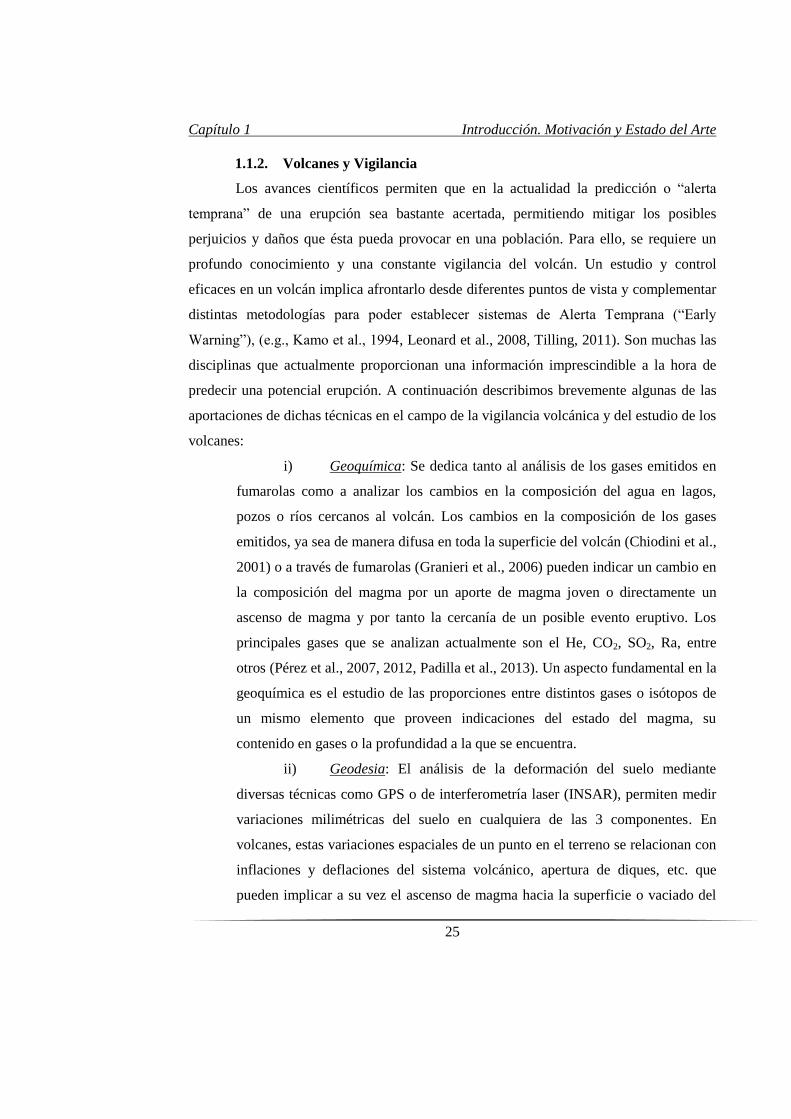
Capítulo 1 Introducción. Motivación y Estado del Arte
25
1.1.2. Volcanes y Vigilancia
Los avances científicos permiten que en la actualidad la predicción o “alerta
temprana” de una erupción sea bastante acertada, permitiendo mitigar los posibles
perjuicios y daños que ésta pueda provocar en una población. Para ello, se requiere un
profundo conocimiento y una constante vigilancia del volcán. Un estudio y control
eficaces en un volcán implica afrontarlo desde diferentes puntos de vista y complementar
distintas metodologías para poder establecer sistemas de Alerta Temprana (“Early
Warning”), (e.g., Kamo et al., 1994, Leonard et al., 2008, Tilling, 2011). Son muchas las
disciplinas que actualmente proporcionan una información imprescindible a la hora de
predecir una potencial erupción. A continuación describimos brevemente algunas de las
aportaciones de dichas técnicas en el campo de la vigilancia volcánica y del estudio de los
volcanes:
i) Geoquímica: Se dedica tanto al análisis de los gases emitidos en
fumarolas como a analizar los cambios en la composición del agua en lagos,
pozos o ríos cercanos al volcán. Los cambios en la composición de los gases
emitidos, ya sea de manera difusa en toda la superficie del volcán (Chiodini et al.,
2001) o a través de fumarolas (Granieri et al., 2006) pueden indicar un cambio en
la composición del magma por un aporte de magma joven o directamente un
ascenso de magma y por tanto la cercanía de un posible evento eruptivo. Los
principales gases que se analizan actualmente son el He, CO2, SO2, Ra, entre
otros (Pérez et al., 2007, 2012, Padilla et al., 2013). Un aspecto fundamental en la
geoquímica es el estudio de las proporciones entre distintos gases o isótopos de
un mismo elemento que proveen indicaciones del estado del magma, su
contenido en gases o la profundidad a la que se encuentra.
ii) Geodesia: El análisis de la deformación del suelo mediante
diversas técnicas como GPS o de interferometría laser (INSAR), permiten medir
variaciones milimétricas del suelo en cualquiera de las 3 componentes. En
volcanes, estas variaciones espaciales de un punto en el terreno se relacionan con
inflaciones y deflaciones del sistema volcánico, apertura de diques, etc. que
pueden implicar a su vez el ascenso de magma hacia la superficie o vaciado del
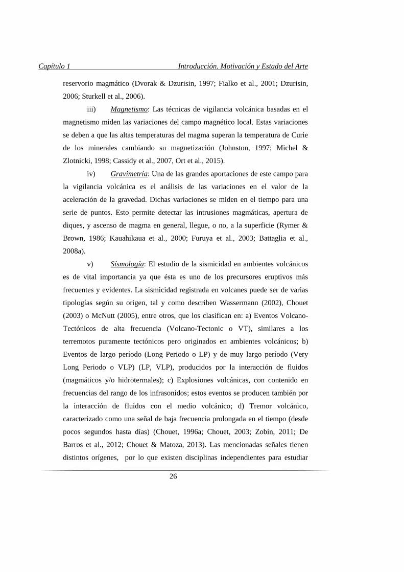
Capítulo 1 Introducción. Motivación y Estado del Arte
26
reservorio magmático (Dvorak & Dzurisin, 1997; Fialko et al., 2001; Dzurisin,
2006; Sturkell et al., 2006).
iii) Magnetismo: Las técnicas de vigilancia volcánica basadas en el
magnetismo miden las variaciones del campo magnético local. Estas variaciones
se deben a que las altas temperaturas del magma superan la temperatura de Curie
de los minerales cambiando su magnetización (Johnston, 1997; Michel &
Zlotnicki, 1998; Cassidy et al., 2007, Ort et al., 2015).
iv) Gravimetría: Una de las grandes aportaciones de este campo para
la vigilancia volcánica es el análisis de las variaciones en el valor de la
aceleración de la gravedad. Dichas variaciones se miden en el tiempo para una
serie de puntos. Esto permite detectar las intrusiones magmáticas, apertura de
diques, y ascenso de magma en general, llegue, o no, a la superficie (Rymer &
Brown, 1986; Kauahikaua et al., 2000; Furuya et al., 2003; Battaglia et al.,
2008a).
v) Sísmología: El estudio de la sismicidad en ambientes volcánicos
es de vital importancia ya que ésta es uno de los precursores eruptivos más
frecuentes y evidentes. La sismicidad registrada en volcanes puede ser de varias
tipologías según su origen, tal y como describen Wassermann (2002), Chouet
(2003) o McNutt (2005), entre otros, que los clasifican en: a) Eventos Volcano-
Tectónicos de alta frecuencia (Volcano-Tectonic o VT), similares a los
terremotos puramente tectónicos pero originados en ambientes volcánicos; b)
Eventos de largo período (Long Periodo o LP) y de muy largo período (Very
Long Periodo o VLP) (LP, VLP), producidos por la interacción de fluidos
(magmáticos y/o hidrotermales); c) Explosiones volcánicas, con contenido en
frecuencias del rango de los infrasonidos; estos eventos se producen también por
la interacción de fluidos con el medio volcánico; d) Tremor volcánico,
caracterizado como una señal de baja frecuencia prolongada en el tiempo (desde
pocos segundos hasta días) (Chouet, 1996a; Chouet, 2003; Zobin, 2011; De
Barros et al., 2012; Chouet & Matoza, 2013). Las mencionadas señales tienen
distintos orígenes, por lo que existen disciplinas independientes para estudiar
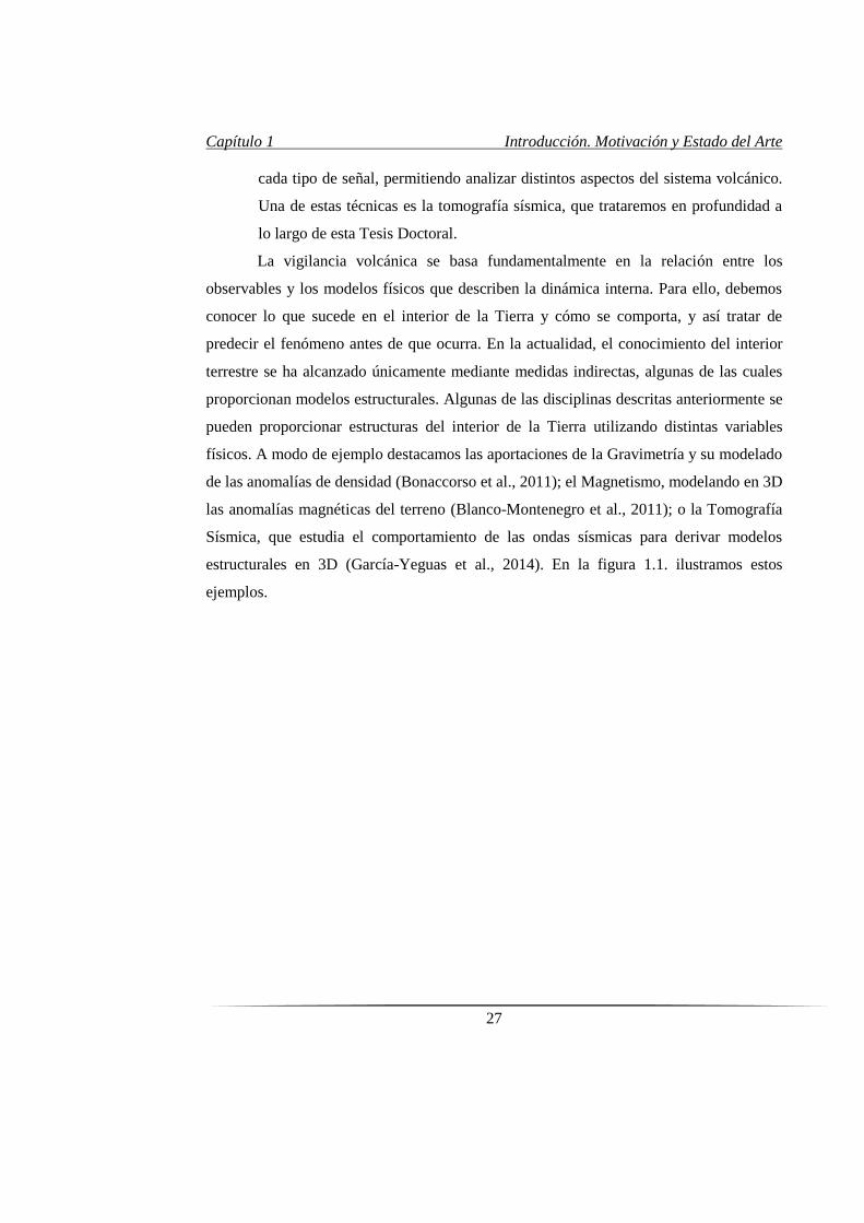
Capítulo 1 Introducción. Motivación y Estado del Arte
27
cada tipo de señal, permitiendo analizar distintos aspectos del sistema volcánico.
Una de estas técnicas es la tomografía sísmica, que trataremos en profundidad a
lo largo de esta Tesis Doctoral.
La vigilancia volcánica se basa fundamentalmente en la relación entre los
observables y los modelos físicos que describen la dinámica interna. Para ello, debemos
conocer lo que sucede en el interior de la Tierra y cómo se comporta, y así tratar de
predecir el fenómeno antes de que ocurra. En la actualidad, el conocimiento del interior
terrestre se ha alcanzado únicamente mediante medidas indirectas, algunas de las cuales
proporcionan modelos estructurales. Algunas de las disciplinas descritas anteriormente se
pueden proporcionar estructuras del interior de la Tierra utilizando distintas variables
físicos. A modo de ejemplo destacamos las aportaciones de la Gravimetría y su modelado
de las anomalías de densidad (Bonaccorso et al., 2011); el Magnetismo, modelando en 3D
las anomalías magnéticas del terreno (Blanco-Montenegro et al., 2011); o la Tomografía
Sísmica, que estudia el comportamiento de las ondas sísmicas para derivar modelos
estructurales en 3D (García-Yeguas et al., 2014). En la figura 1.1. ilustramos estos
ejemplos.
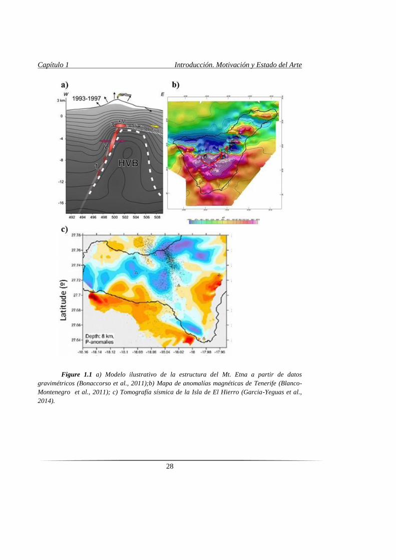
Capítulo 1 Introducción. Motivación y Estado del Arte
28
Figure 1.1 a) Modelo ilustrativo de la estructura del Mt. Etna a partir de datos
gravimétricos (Bonaccorso et al., 2011);b) Mapa de anomalías magnéticas de Tenerife (Blanco-
Montenegro et al., 2011); c) Tomografía sísmica de la Isla de El Hierro (Garcia-Yeguas et al.,
2014).
Capítulo 1 Introducción. Motivación y Estado del Arte
29
1.2. Técnica para inferir el interior de la Tierra usando ondas sísmicas:
Tomografía Sísmica
La tomografía sísmica se presenta en la actualidad como una de las herramientas
más potentes y robustas para el estudio de la estructura profunda de los volcanes (Lees,
2007). La tomografía, “imagen en capas” traducido literalmente, es un método para
obtener una imagen de regiones no accesibles de manera directa. Ha sido utilizada entre
otros como método para “ver” partes internas desde organismos vivos hasta el interior de
la Tierra, en el que se centra este trabajo (Lees, 2007). Las zonas de subducción, las
grandes fallas y los volcanes son algunas de las principales estructuras geológicas que se
pueden estudiar en detalle utilizando esta técnica. Sus comienzos en sismología a
mediados de los 70 (Aki et al., 1974) estuvieron más enfocados hacia estudios regionales
utilizando telesismos donde la resolución a pequeña escala era aún bastante limitada. Una
tomografía sísmica se realiza a partir de la inversión de los tiempos de viaje de las ondas
P y S que atraviesan dicha región y que se registran en una serie de estaciones sísmicas
instaladas en torno al mismo (Iyer, 1993). Estos tiempos de viaje se comparan con los
tiempos de viaje teóricos calculados con un modelo de velocidad inicial. Si el parámetro
estadístico que nos muestra su aproximación con los tiempos de viaje observados no se
considera adecuado se calcula un nuevo modelo de velocidad que se ajuste mejor a los
tiempos de viaje observados. Esto se conoce como el método inverso ya que a partir de
los resultados tratamos de inferir aquello que los produce. Centrándonos en su aplicación
en volcanes, no fue hasta mediados de los 80 cuando se tuvieron las herramientas y
algoritmos necesarios para su aplicación a escenarios más pequeños y complejos.
Probablemente, la primera tomografía de un volcán fue la realizada por Thurber (1984),
en la cual se determinó la estructura interna en velocidad del volcán Kilauea (Hawaii). El
principal resultado de esta tomografía fue la determinación de una anomalía de baja
velocidad y asísmica bajo el volcán que se interpretó como la cámara magmática del
Kilauea. Desde entonces, se han realizado numerosos trabajos en los que se ha estudiado
la estructura interna de un volcán “iluminando” desde estructuras profundas hasta detalles
en superficie. Detectar posibles zonas de acumulación de magma es uno de los
principales objetivos de estos estudios, no siempre fácil debido a la complejidad
Capítulo 1 Introducción. Motivación y Estado del Arte
30
estructural de los volcanes. Entre otras causas, depende enormemente del tipo de volcán,
la profundidad de dichas zonas de acumulación y el contenido en gases del magma entre
otros factores. Generalmente, las imágenes que más información aportan son las de
anomalías, respecto a un modelo teórico. Pueden ser de velocidad de las ondas P y/o de
las ondas S y /o del valor Vp/Vs, tanto positivas como negativas.
La tomografía sísmica, tal cómo se describe anteriormente, se desarrolló
basándose en el uso de los terremotos como fuente sísmica y se conoce como tomografía
sísmica pasiva. La gran ventaja del uso de terremotos como fuente sísmica se relaciona
con el amplio rango de profundidades a las que ocurren. De esta manera, se pueden
realizar estudios a distintas escalas, según el tipo de terremoto que utilicemos, ya sea
local, regional o telesismo. Sin embargo, el uso de terremotos como fuente sísmica no
siempre es posible, ya que sólo se podrán utilizar en regiones donde la sismicidad sea
elevada y tenga una distribución espacial homogénea. Precisamente, los volcanes se
suelen encontrar en regiones sísmicamente poco activas o con sismicidad irregular en el
tiempo y espacio, por lo que no siempre es posible aplicar la tomografía sísmica pasiva en
estas regiones.
Para solventar esta necesidad, entre otras, se comienzan a utilizar fuentes
artificiales como generadoras de ondas P. Dichas señales artificiales se pueden generar
con la ayuda de cañones de aire comprimido, explosiones, caída de grandes masas, etc.
(Koulakov & Shapiro 2015). Este método conocido como tomografía sísmica activa, tiene
varias desventajas como la energía de la fuente y por tanto en alcance en distancia, la
superficialidad de la región fuente y el consiguiente efecto de la atenuación, aparte de
potenciales elevados costes económicos y logísticos, como permisos, impactos
ambientales y gestión administrativa, por lo que organizar un experimento puede resultar
laborioso (Ver Anexos 1-4). Sin embargo, acumula un gran número de ventajas entre las
que se encuentra el conocer con absoluta precisión tanto la localización como la hora
origen en la que se generan dichas señales sísmicas. En contraposición a los terremotos,
de los cuáles la única información “a priori” que se tiene, son las llegadas de las ondas P
y S a las distintas estaciones. Es a partir de esas llegadas, cuando se localiza el terremoto
y se calcula su hora origen. Otra importante diferencia entra ambos tipos de fuente es el
Capítulo 1 Introducción. Motivación y Estado del Arte
31
área que cubren, en el caso de las fuentes artificiales se generan en su mayoría en la
superficie o a muy poca profundidad, por lo que el área que cubren los rayos hasta las
estaciones sísmicas es generalmente superficial, llegando hasta 5-10 km de profundidad
según el caso. Por lo que su uso, no resuelve estructuras demasiado profundas, pero en
cambio, si el número de fuentes es grande, se puede obtener una gran resolución de los
primeros kilómetros de la corteza. Por otro lado, los terremotos tienen un espectro mucho
más amplio pudiendo originarse hasta a cientos de kilómetros bajo la superficie terrestre,
permitiendo que la tomografía resuelva profundidades mayores con buena resolución.
Más adelante se retomará el interés en el uso de los datos activos.
En el Capítulo 5 de esta tesis se discute detalladamente la metodología seguida
para realizar una tomografía sísmica, tanto activa como pasiva y la combinación de
ambas. A continuación, y para ilustrar lo ya comentado y presentar el estado del arte
actual acerca de la tomografía sísmica en volcanes, ya sea activa o pasiva, en los
próximos párrafos se describen los más importantes y recientes trabajos realizados en este
campo, incluyendo distintos volcanes y distintas escalas, separándolos según hayan
utilizado sismicidad natural o fuentes artificiales.
1.2.1. Tomografías de velocidad usando sismicidad pasiva
El número de tomografías realizadas utilizando la sismicidad natural como fuente
sísmica es muy grande, y se ha desarrollado exponencialmente desde su comienzo en los
70. A continuación describimos algunas de las tomografías sísmicas pasivas más
relevantes realizadas en volcanes en los últimos 20 años (Figure 1.2). En previas Tesis
Doctorales realizadas por nuestro grupo de investigación se recogen otros interesantes
ejemplos (e.g., Martínez-Arévalo 2005; Zandomeneghi 2007; García-Yeguas 2010;
Prudencio 2014).
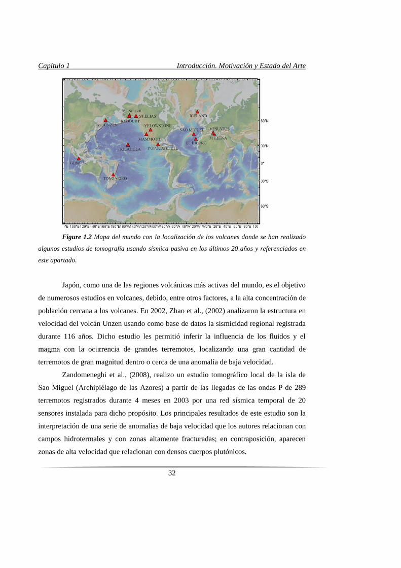
Capítulo 1 Introducción. Motivación y Estado del Arte
32
Figure 1.2 Mapa del mundo con la localización de los volcanes donde se han realizado
algunos estudios de tomografía usando sísmica pasiva en los últimos 20 años y referenciados en
este apartado.
Japón, como una de las regiones volcánicas más activas del mundo, es el objetivo
de numerosos estudios en volcanes, debido, entre otros factores, a la alta concentración de
población cercana a los volcanes. En 2002, Zhao et al., (2002) analizaron la estructura en
velocidad del volcán Unzen usando como base de datos la sismicidad regional registrada
durante 116 años. Dicho estudio les permitió inferir la influencia de los fluidos y el
magma con la ocurrencia de grandes terremotos, localizando una gran cantidad de
terremotos de gran magnitud dentro o cerca de una anomalía de baja velocidad.
Zandomeneghi et al., (2008), realizo un estudio tomográfico local de la isla de
Sao Miguel (Archipiélago de las Azores) a partir de las llegadas de las ondas P de 289
terremotos registrados durante 4 meses en 2003 por una red sísmica temporal de 20
sensores instalada para dicho propósito. Los principales resultados de este estudio son la
interpretación de una serie de anomalías de baja velocidad que los autores relacionan con
campos hidrotermales y con zonas altamente fracturadas; en contraposición, aparecen
zonas de alta velocidad que relacionan con densos cuerpos plutónicos.
Capítulo 1 Introducción. Motivación y Estado del Arte
33
En 2014 se estudiaron los volcanes de Kilauea y Mauna Loa en Hawaii
aprovechando la sismicidad registrada en la zona (Lin et al., 2014a, 2014b). Como en
casos anteriores, las anomalías negativas de velocidad se asociaron a la presencia de
volátiles y sedimentos altamente fracturados. En ambos volcanes se detectó la presencia
de las anomalías positivas de velocidad bajo las principales calderas. En este caso se
partió de una base de datos compuesta por cerca de 53.000 eventos registrados entre 1992
y 2009. Una de las ventajas de un estudio tomográfico como este, es la posibilidad de
utilizar el modelo 3-D más realista de velocidades para realizar posteriores
relocalizaciones de la sismicidad.
La península de Kamchatka (Rusia) es una de las zonas con mayor concentración
de volcanes activos del planeta y es el foco de numerosos estudios tomográficos para
conocer la estructura interna en velocidad de la corteza. Es una región cuya importancia
geológica es mayúscula pues se encuentra muy cerca de la zona de subducción del
Pacífico, por lo que no sólo hay una gran cantidad de volcanes sino que la sismicidad
registrada en la zona suele ser abundante y de gran magnitud. Se han presentado
tomografías regionales que incluyen gran parte de la península de Kamchatka, como el
complejo volcánico de Kluchevskoy (Koulakov et al., 2011, 2013a, 2016). En todos estos
casos, se ha considerado la sismicidad local y regional, es decir no sólo aquellos
terremotos VT ligados directamente a la dinámica volcánica sino también aquellos cuyo
origen se encuentra en la zona de subducción de la placa Pacífica, permitiendo alcanzar
resoluciones hasta profundidades en torno a 30 km bajo el nivel del mar (b.n.m.).
Otra zona de gran interés geológico y volcánologico es Alaska, conectada
también a la subducción de la placa Pacífica. En esta región podemos encontrar un
estudio de la estructura en velocidad del volcán Redoubt realizada por Kasatkina et al.,
(2014) en la que se invirtieron las llegadas de las ondas P y S para un total de 4.500
terremotos registrados durante 13 años. Durante el periodo considerado tuvo lugar al
menos una erupción por lo que se pudo comparar la estructura en velocidad antes y
después del evento eruptivo. Los resultados de este estudio mostraron la presencia de un
cuerpo de alta velocidad localizado bajo el volcán junto con anomalías para las ondas S
que antes de la erupción eran muy elevadas en comparación con los valores obtenidos
Capítulo 1 Introducción. Motivación y Estado del Arte
34
después. Otro volcán estudiado es el Mt. Spurr (Koulakov et al., 2013b), donde se
invirtieron 512 terremotos registrados durante 4 meses. En este caso la red sísmica
utilizada para registrarlos consistió en 26 sensores distribuidos en aproximadamente 900
km2. En total se utilizaron 5.960 llegadas de ondas P y 4.973 S. Zabelina et al., (2014)
realizó un nuevo estudio tomográfico en otro volcán de Alaska, el volcán Saint Elias,
donde se recogieron 8 años de sismicidad registrada en 22 estaciones. La base de datos,
con cerca de 8.000 terremotos se utilizó para invertir 150.000 ondas P y S y obtener la
estructura en velocidad de esta zona de colisión.
Recientemente, Dawson et al., (2016) realizaron un estudio tomográfico en el
volcán Mamooth Mountain en California (EE.UU). Los autores invirtieron las llegadas de
las ondas P, S y calcularon la relación Vp/Vs de un total de 2.604 terremotos. Para
registrarlos, se instaló una red sísmica temporal compuesta por 11 sensores de banda
ancha durante 2 años. Los resultados obtenidos muestran la presencia de un volumen bajo
el volcán con valores anómalamente bajos para las P y las S, que los autores interpretan
como un reservorio de CO2 posiblemente alimentado por un sistema magmático
subyacente.
La región de Java (Indonesia), ha sido ampliamente estudiada desde el punto de
vista tomográfico debido a su interés geológico y volcánico. Entre otros, Nugraha et al.,
(2013) estudiaron el complejo volcánico Guntur invirtiendo 4.686 P y 2343 S
correspondientes a 490 terremotos registrados en 20 estaciones. Los autores detectan
anomalías negativas de Vp, Vs y altos valores de Vp/Vs cuyo origen interpretan como un
reservorio magmático.
Uno de los volcanes más famosos del mundo, Yellowstone (EE.UU) fue el objeto
de un reciente estudio (Farrel et al., 2014). Los autores recabaron la sismicidad registrada
durante 26 años por la red sísmica local. En total, se invirtieron 48.622 llegadas de onda P
correspondientes a 4.520 terremotos de alta calidad. En este estudio se utilizan
únicamente las fases P de los terremotos y se invierte un área de 70.000 km2
aproximadamente, en la cual, los resultados muestran un gran cuerpo de baja velocidad
localizado en torno a 15 km de profundidad. Dicho volumen es interpretado por los
Capítulo 1 Introducción. Motivación y Estado del Arte
35
autores como la cámara magmática del sistema volcánico y en la que estiman entre un 5-
15% de material fundido.
No todos los estudios tomográficos encuentran o pretenden encontrar una cámara
magmática, sino que en muchos de ellos coincide la presencia de anomalías de alta
velocidad localizadas bajo el volcán como uno de los rasgos más característicos de los
edificios volcánicos. Estas anomalías generalmente se interpretan como acumulaciones de
rocas plutónicas posiblemente asociadas al enfriamiento de antiguos centros eruptivos
(Kasatkina et al., 2014; Lin et al., 2014a; García-Yeguas et al., 2012; Zandomeneghi et
al., 2008; entre otros muchos).
Realizar una tomografía sísmica en un volcán implica tener generalmente una
base de datos con suficientes terremotos para que sea fiable. De este breve resumen
verificamos que en la mayoría de volcanes, para cumplir este requisito deben pasar varios
meses incluso decenas de años. Esto implica, sobre todo en volcanes con actividad
eruptiva frecuente, que el resultado final no sea más que el promedio de la estructura
durante todo ese tiempo. De hecho, de ocurrir erupciones durante ese periodo estaríamos
minimizando su aportación al resultado final. De ahí, que surja la necesidad de realizar lo
que se conoce con “snapshots” o “instantáneas” que son tomografías en las que el
periodo en el que se han registrado los eventos es suficientemente corto como para
estimar que no se han producido cambios sustanciales en la estructura interna del volcán.
Esta técnica requiere un gran número de terremotos en un corto periodo de tiempo, cosa
que rara vez ocurre en volcanes. Sin embargo, cuando esto sucede se puede realizar este
tipo de estudios, incluso dando lugar a estudios evolución en el tiempo como la
tomografía 4-D. Uno de los casos más conocidos es la erupción de 2002-03 en el volcán
Mt. Etna. Dicha erupción estuvo acompañada por un intenso enjambre sísmico que
permitió a los investigadores dividir la base de datos en distintos intervalos temporales
para los cuáles invirtieron las llegadas de las ondas P, S y la razón Vp/Vs (Patanè et al.,
2006). Dicho estudio permitió individuar los posibles conductos magmáticos que
alimentaron dicha erupción gracias a los valores anómalos del valor Vp/Vs y su variación
temporal. En el siguiente apartado retomaremos los ejemplos de estudios de tomografía
usando sísmica activa.
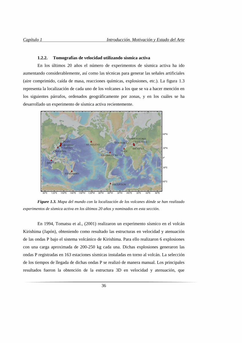
Capítulo 1 Introducción. Motivación y Estado del Arte
36
1.2.2. Tomografías de velocidad utilizando sísmica activa
En los últimos 20 años el número de experimentos de sísmica activa ha ido
aumentando considerablemente, así como las técnicas para generar las señales artificiales
(aire comprimido, caída de masa, reacciones químicas, explosiones, etc.). La figura 1.3
representa la localización de cada uno de los volcanes a los que se va a hacer mención en
los siguientes párrafos, ordenados geográficamente por zonas, y en los cuáles se ha
desarrollado un experimento de sísmica activa recientemente.
Figure 1.3. Mapa del mundo con la localización de los volcanes dónde se han realizado
experimentos de sísmica activa en los últimos 20 años y nominados en esta sección.
En 1994, Tomatsu et al., (2001) realizaron un experimento sísmico en el volcán
Kirishima (Japón), obteniendo como resultado las estructuras en velocidad y atenuación
de las ondas P bajo el sistema volcánico de Kirishima. Para ello realizaron 6 explosiones
con una carga aproximada de 200-250 kg cada una. Dichas explosiones generaron las
ondas P registradas en 163 estaciones sísmicas instaladas en torno al volcán. La selección
de los tiempos de llegada de dichas ondas P se realizó de manera manual. Los principales
resultados fueron la obtención de la estructura 3D en velocidad y atenuación, que
Capítulo 1 Introducción. Motivación y Estado del Arte
37
permitieron detectar una serie de estructuras superficiales bajo el volcán, a 1.5 km y 0.5
km bajo el nivel del mar (b.n.m.).
Durante ese mismo año, 1994, se realizó otro gran experimento sísmico, esta vez
en el volcán Vesubio (Italia). Dicho experimento tenía como objetivo reconstruir en
detalle la estructura superficial del volcán, pretendiendo incluso detectar el sistema de
alimentación del mismo (Zollo et al, 1996; Gasparini, 1998). Se realizaron 3 explosiones
bajo tierra, durante una primera fase, que fueron registradas por 84 sensores sísmicos
alineados siguiendo un perfil a lo largo del volcán. En una segunda fase tuvieron lugar 17
explosiones de entre 250 y 800 kg de explosivo colocadas a 50 m de profundidad. Tanto
las explosiones como las estaciones estaban distribuidas linealmente a lo largo de perfiles
de entre 25 y 40 km de largo. Para esta segunda fase del experimento se usaron un total
de 140 sismógrafos de 3 componentes. Los resultados de este experimento han permitido
mejorar considerablemente el conocimiento que se tenía acerca de la estructura interna
del Vesubio (e.g. Zollo et al., 1998; Di Stefano and Chiarabba, 2002; Zollo et al. 2002).
El volcán Bandai (Japón), fue el escenario de un nuevo experimento de sísmica
activa en 1997 (Yamakawi et al., 2004). De nuevo se utilizaron un total de 8 explosiones
como fuente sísmica, que se registraron en un total de 298 estaciones sísmicas instaladas
en un área de 25 x 20 km. Como resultado principal se obtuvo la tomografía sísmica en
velocidad de dicho volcán utilizando 2200 llegadas de onda P. Las estaciones utilizadas
eran de corto periodo (periodo natural de 0.5 s), 6 de las explosiones se realizaron con
200-250 kg de carga explosiva detonadas alrededor del volcán, y otras 2 (de 100 kg) se
detonaron en la parte central del volcán. En este caso, las primeras llegadas de las ondas P
se seleccionaron también de manera manual.
Durante 1997-98 se realizó en el volcán Merapi (Indonesia) un nuevo
experimento de sísmica activa (Zschau et al., 1998). Se instaló una red símica temporal de
75 sensores de corto periodo (periodo natural de 1 s) siguiendo 3 perfiles. En dos de los
perfiles de 3 km de longitud se colocaron 30 sismómetros de 3 componentes cada uno,
mientras que en el tercer perfil, de sólo 1.5 km de longitud se desplegaron los otros 15
sismómetros (Wegler et al., 1999; Wegler and Luerh, 2001). En este caso, las fuentes
sísmicas utilizadas fueron cañones de aire comprimido (de 2.5 l) instalados en tanques de
Capítulo 1 Introducción. Motivación y Estado del Arte
38
agua de 4.5 m de profundidad. Los disparos de aire comprimido se realizaron cada 2
minutos con una presión de 8 MPa. Cada estación desplegadas registró entre 20 y 120
disparos que permitieron analizar la estructura interna del volcán hasta una profundidad
de 300 m bajo los perfiles (Maercklin et al., 2000).
Otro experimento de sísmica activa tuvo lugar en el volcán Asama en Japón
durante el año 2006. La fuente sísmica utilizada fueron 5 cargas explosivas de 250-300 kg
(explosiones químicas) colocadas a 60 m de profundidad. Las ondas sísmicas provocadas
por estas explosiones fueron registradas por un total de 464 estaciones sísmicas (Mark L-
22D 2 Hz) (Aoki et al., 2009; Yamamoto and Sato, 2010). La geometría de despliegue se
compuso de dos perfiles (N-S y E-W) cruzando el volcán. En total se generaron más de
2000 fases P, cuyo tiempo de viaje fue seleccionado de forma manual para luego ser
utilizadas en la inversión tomográfica.
También en Japón, se realizó un experimento en el 2001 en el volcán Usu
(Onizawa et al., 2007). Se desplegaron 288 estaciones sísmicas (1-componente, 2Hz) con
una separación de 750 m entre ellas alrededor del volcán. Las fuentes sísmicas utilizadas
fueron 7 cargas explosivas de 200-250 kg. A partir de los datos de las llegadas de las
fases sísmicas P se realizó una tomografía sísmica que permitió obtener imágenes de la
estructura interna del volcán.
El experimento SERAPIS tuvo lugar en 2001 en el golfo de Nápoles y Pozzuoli
con el objetivo de estudiar en detalle el Vesubio y Campi Flegrei (Zollo et al., 2003). Para
generar las señales sísmicas se utilizaron 12 cañones de aire comprimido de 16 litros
montados en el buque oceanográfico NADIR (IFREMER). Se realizaron un total de 5000
disparos que se registraron en 62 estaciones sísmicas marinas (OBS) y 72 terrestres
(sensores de 3 componentes) instaladas todas en el golfo de Nápoles (OBSs), Campi
Flegrei, el Vesubio y las islas Ischia y Procida (Judenherc and Zollo, 2003; Vanorio et al.,
2005; De Siena et al., 2010; De Siena et al., 2011). Battaglia et al., (2008b) propuso
combinar los datos de sísmica activa recogidos en dicho experimento con los datos de
sismicidad natural.
Desde 1998 hasta 2003 se realizó en el volcán Iwate (Japón) un complejo
experimento de sísmica activa (Nishimura et al., 2000, 2005). Durante la primera parte
Capítulo 1 Introducción. Motivación y Estado del Arte
39
del experimento se detonaron 6 cargas, colocadas cerca unas de otras en un área de 30 x
10 m. Las ondas sísmicas provocadas se registraron en 8 estaciones. Durante este período
tuvo lugar incluso un terremoto de magnitud 6.1, dando mayor importancia al objetivo del
experimento que era estudiar posibles cambios temporales en la estructura en velocidad
de la corteza. Dicho terremoto ocurrió entre la primera y la segunda explosión. El resto de
explosiones se realizaron entre el año 2000 y 2003. Durante el año 2000 en la misma
región, Tanaka et al., (2002) realizaron un experimento con 9 explosiones de 200-250 kg
de carga e instalaron una red temporal de 330 estaciones de corto periodo de 1-
componente (2 Hz de periodo natural). El área de estudio ocupó aproximadamente 1600
km2 y los tiempos de viaje de las señales que se generaron fueron seleccionadas
manualmente para obtener 2676 llegadas de onda P utilizadas posteriormente para
realizar la tomografía sísmica en velocidad (Tanaka et al., 2002).
El volcán Isla Decepción en la Antártida fue el objetivo de un experimento de
sísmica activa (TOMODEC) en 2005 (Barclay et al., 2009; Ben-Zvi et al. 2009;
Zandomeneghi et al. 2009; García-Yeguas et al., 2011; Carmona et al., 2012; Prudencio
et al., 2013a; Prudencio et al., 2015a). En este experimento se utilizó un array de 6
cañones de aire comprimido de 57 litros instalado en el Buque Oceanográfico Hespérides.
Como red sísmica se instalaron 14 OBSs y 95 sensores en tierra. Se generaron más de
6600 disparos de aire comprimido obteniendo un registro final de 600.000 señales de alta
calidad. Dada la geometría de la isla (forma de herradura) se realizaron disparos incluso
dentro de la caldera siguiendo una malla de 0.5 km y disparando cada 120 m. En el
exterior de la isla se disparó cada 170-340 m, a lo largo de tres circunferencias a
distancias de 10, 15 y 20 km del centro de la isla. Además se realizaron 8 perfiles radiales
de 25 km de longitud. Para la tomografía sísmica en velocidad 2-D y 3-D realizada por
Ben-Zvi et al., (2009) y Zandomenghi et al., (2009) se utilizaron más de 70.000 fases
sísmicas de ondas P.
En 2007 en la isla de Tenerife se llevó a cabo un nuevo experimento (Ibáñez et
al., 2008; De Barros et al., 2012; García-Yeguas et al. 2012; Lodge et al., 2012;
Prudencio et al., 2013b; Prudencio et al., 2015b). En este caso se volvieron a utilizar los
cañones de aire comprimido montados en el Buque Oceanográfico Hespérides, siguiendo
Capítulo 1 Introducción. Motivación y Estado del Arte
40
una disposición por parejas. El array de cañones alcanzaba los 12 m de longitud y estaban
separados 2.5 m entre ellos. En tierra, se desplegaron tanto estaciones de banda ancha
como de corto periodo (siempre con sensores de 3 componentes). Una particularidad de
este experimento fue que durante el mismo, se trasladaron un 40% de las estaciones a
nuevas localizaciones con el objetivo de maximizar el área cubierta. Una vez trasladadas,
se realizó una segunda tanda de disparos siguiendo el mismo recorrido que en el primer
caso. En total se instalaron 137 estaciones que registraron más de 900.000 señales
producidas por los 6.850 disparos de aire comprimido realizados. Todas estas señales
fueron revisadas manualmente para seleccionar las llegadas de las ondas P.
El experimento SEA-CALIPSO se realizó en 2007 en la isla de Montserrat
(Caribe). Como en casos anteriores se optó por producir las señales sísmicas utilizando
cañones de aire comprimido montados sobre un Buque Oceanográfico (RRS James
Cook). Los cañones tenían una capacidad de 42.6 litros y dispararon 4.413 veces. Se
desplegó una red sísmica de 238 estaciones en tierra y 10 OBSs (Voight et al., 2014). Se
registraron cerca de 115.000 señales sísmicas de alta calidad que fueron utilizadas para
calcular el modelo de velocidad en 3-D bajo la isla de Monserrat Paulato et al., 2010;
Shalev et al., 2010).
El volcán Tongariro en Nueva Zelanda fue objeto de un experimento sísmico en
2012 en el que se utilizó como fuente sísmica el impacto de 11 masas liberadas desde un
helicóptero (Jolly et al., 2014). En este experimento se instalaron 4 estaciones sísmicas
que registraron las señales producidas por los impactos a distancias cercanas a los 10 km
con frecuencias de entre 3 y 12 Hz. Este experimento tenía como objetico comparar las
fuentes de sísmica activa con datos de sismicidad natural y poder discriminar la evolución
de actividad superficial compleja mediante nuevos métodos de correlación y localización
de fuentes.
En 2006 tuvo lugar en Stromboli un experimento utilizando nuevamente cañones
de aire comprimido. Para registrar las señales sísmicas se instalaron un total de 33
estaciones en tierra y 10 OBSs (Marsella et al., 2007; Castellano et al., 2008; Prudencio et
al., 2015c). El Buque Oceanográfico Urania llevó incorporado un array de 4 cañones de
aire comprimido que dispararon con una potencia máxima de 840 inches3. En total se
Capítulo 1 Introducción. Motivación y Estado del Arte
41
generaron más de 1.500 fuentes sísmicas siguiendo una serie de perfiles radiales y
circunferencias respecto al centro de la isla. Se disparó a intervalos de 2 minutos
separando las fuentes aproximadamente 250 m entre ellas.
Uno de los volcanes más famosos, Mt. St. Helens (EE.UU), fue objeto de estudio
mediante un complejo proyecto internacional involucrando fuentes pasivas, activas,
estudios de magnetotelúrica, análisis geológicos y geoquímicos, etc. (Kiser et al., 2013;
Levander et al., 2015). Una red sísmica de 70 estaciones de banda ancha registró la
sismicidad natural desde 2014 hasta principios de 2016. Un experimento de sísmica
activa iMUSH, se realizó a mediados de 2014 utilizando como fuentes sísmica
explosiones químicas de 454 y 908 kg, que fueron registradas por una densa red sísmica
temporal de 3.500 sensores de corto periodo. Dichos sensores se desplegaron formando
arrays que fueron desplazados durante el experimento para cubrir un área mayor. Uno de
los principales objetivos de este experimento, del cual no hay publicaciones disponibles
en el momento de escribir esta Tesis Doctoral, es la obtención de un modelo de velocidad
tomográfico que incluya eventos VT, sismicidad regional y las explosiones químicas
como fuentes sísmicas.
Por último, incluso el volcán Erebus en el continente Antártico ha sido estudiado
usando tomografía sísmica activa en 2008-09. Zandomeneghi et al., (2010,2013)
invirtieron los datos provistos por 12 explosiones químicas registradas por 91 estaciones
sísmicas desplegadas en 16 km2 en torno al volcán. La tomografía 3-D resultante permite
‘ver’ la estructura interna del volcán hasta una profundidad de 600m (Zandomeneghi et
al., 2013).
1.2.3. La Tomografía sísmica como herramienta
Una tomografía sísmica (pasiva o activa) no es el resultado último, sino que da
pie a numerosos y no menos importantes estudios acerca de las estructuras y la dinámica
volcánicas. Esto hace que deba considerarse como una herramienta fundamental para
muchos estudios avanzados. Así, la modelo 3D en velocidad resultante permite conocer
mejor a estructura interna del volcán, distinguiendo cuerpos de alta velocidad que se
relacionan generalmente con cuerpos fríos, densos y/o compactos, frente a cuerpos de
baja velocidad que se asocian a volúmenes más fracturados, de menor densidad y/o
Capítulo 1 Introducción. Motivación y Estado del Arte
42
presencia de fluidos. Este tipo de anomalías después se interpretan en base al
conocimiento geológico y geodinámico de la región.
Además, un modelo de velocidad 3D realista que tenga en cuenta las
heterogeneidades laterales es la base para realizar localizaciones de precisión (Díaz-
Moreno et al., 2015). Dicho estudio es de gran utilidad a la hora de interpreta la dinámica
sísmica de la región, permitiendo distinguir entre distintos mecanismos de generación de
terremotos como la migración del magma o el emplazamiento del mismo.
Otros trabajos a posteriori permiten mejorar las rutinas de alerta temprana
estableciendo mapas de peligrosidad y susceptibilidad en base a la interpretación de las
estructuras volcánicas inferidas a través de los modelos tomográficos. Estos mapas
ayudan a establecer protocolos de alerta que sirvan a la Protección Civil para mejorar los
planes de emergencia volcánica del área (Tilling et al., 2011).
1.2.4. Tomografía Sísmica en el Mt. Etna
El volcán Mt. Etna, en Sicilia (Italia), es, posiblemente el más activo de Europa y
por tanto representa un caso tipo de estudio. Conocido mundialmente, se considera un
volcán laboratorio debido a la gran vigilancia a la que está sometido, su accesibilidad y a
su casi continua actividad (Bonaccorso et al., 2004). Es el volcán activo más
monitorizado del mundo, incluyendo un gran número de disciplinas que van desde la
geoquímica, vulcanología y petrología hasta ramas geofísicas como geodesia, gravimetría
o sismología. Se caracteriza por una actividad frecuente de tipo generalmente
stromboliano con coladas lávicas y algunos episodios más explosivos. En los últimos 16
años el volcán ha sufrido un aumento considerable de la frecuencia de las manifestaciones
eruptivas. Algunos de los episodios más significativos durante este último siglo son las
erupciones de 2001, 2002-03, 2008 y 2015.
Además, el Mt. Etna representa un caso ideal desde el punto de vista del interés y
la repercusión social, ya que numerosos núcleos de población se encuentran en los
alrededores del edificio volcánico, lo que permite estudiar la ya comentada relación
volcán-hombre y la adaptación del ser humano a un ambiente volcánico activo. De hecho,
muchas de las erupciones pasadas han tenido ya graves repercusiones en las poblaciones
adyacentes por lo que es un caso tipo para poner en práctica estrategias de predicción,
Capítulo 1 Introducción. Motivación y Estado del Arte
43
prevención y mitigación del riesgo volcánico. Otra de las grandes ventajas que presenta el
estudio de un volcán como el Mt. Etna es la potencial exportación de los resultados a
otras regiones volcánicas ya sean más o menos activas.
Por estos motivos, se han realizado ya varias tomografías sísmicas en el Mt. Etna,
tratando de inferir la estructura interna del volcán, así como su sistema de alimentación.
La sismicidad asociada a la dinámica del volcán aun siendo alta no alcanza niveles
suficientes, salvo episodios concretos (Patanè et al., 2006) para realizar ‘snapshots’
tomográficos de un período corto de tiempo. Debido a esto, muchas de las tomografías
realizadas en el Mt. Etna utilizan bases de datos que abarcan varios años con el fin de
tener un número de eventos suficientemente significativo.
Desde que se instalara la primera red sísmica en Mt. Etna a mediados de los 70,
han sido varios los estudios enfocados a conocer la estructura interna del volcán. (Tabla
1.1). Uno de los primeros estudios se hizo en 1968, buscando conocer la estructura
interior de Sicilia, involucrando al Mt. Etna. Se realizaron una seria de perfiles de
refracción a lo largo de toda Sicilia. Uno de esos perfiles se localizó justo al norte del
volcán y permitió localizar una anomalía de baja velocidad entre 9 y 24 km bajo el mismo
y que se interpretó como efecto de la presencia de magma (Cassinis et al., 1969).
En 1977 se programó un experimento alrededor del Mt. Etna en el que se
instalaron un gran número de sensores sísmicos de 1- y 3-componentes (Colombi et al.,
1979). Los datos recogidos por dichos sensores sirvieron a Sharp et al., (1980) para,
usando una base de datos de llegada de las ondas P y S de eventos regionales y
telesismos, obtener la primera imagen tomográfica en velocidad del Mt. Etna. Esta
imagen caracterizó una gran anomalía de baja velocidad localizada bajo el volcán a unos
20 km de profundidad y que fue interpretada como una cámara magmática (Figura 1.4).
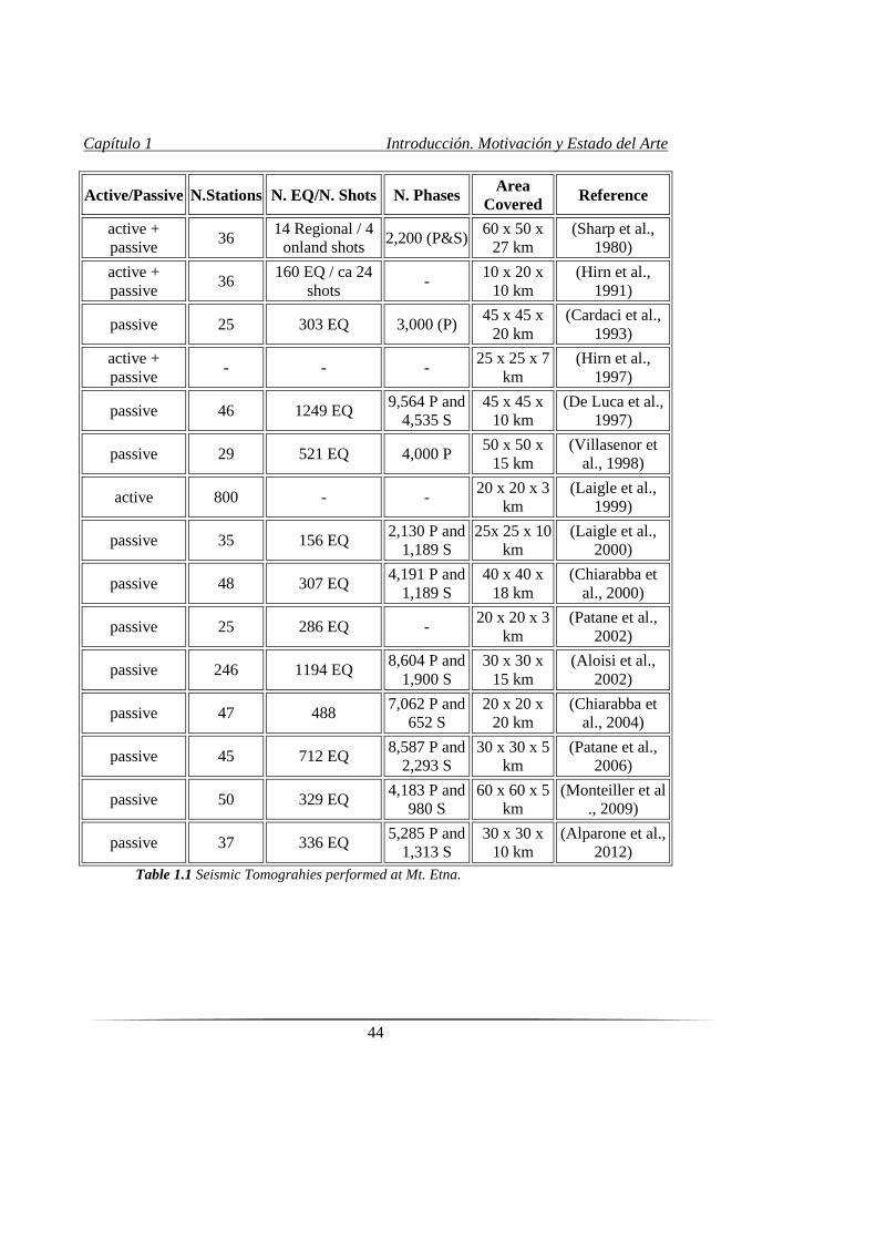
Capítulo 1 Introducción. Motivación y Estado del Arte
44
Active/Passive N.Stations N. EQ/N. Shots N. Phases Area
Covered Reference
active +
passive 36
14 Regional / 4
onland shots 2,200 (P&S)
60 x 50 x
27 km
(Sharp et al.,
1980)
active +
passive 36
160 EQ / ca 24
shots -
10 x 20 x
10 km
(Hirn et al.,
1991)
passive 25 303 EQ 3,000 (P) 45 x 45 x
20 km
(Cardaci et al.,
1993)
active +
passive - - -
25 x 25 x 7
km
(Hirn et al.,
1997)
passive 46 1249 EQ 9,564 P and
4,535 S
45 x 45 x
10 km
(De Luca et al.,
1997)
passive 29 521 EQ 4,000 P 50 x 50 x
15 km
(Villasenor et
al., 1998)
active 800 - - 20 x 20 x 3
km
(Laigle et al.,
1999)
passive 35 156 EQ 2,130 P and
1,189 S
25x 25 x 10
km
(Laigle et al.,
2000)
passive 48 307 EQ 4,191 P and
1,189 S
40 x 40 x
18 km
(Chiarabba et
al., 2000)
passive 25 286 EQ - 20 x 20 x 3
km
(Patane et al.,
2002)
passive 246 1194 EQ 8,604 P and
1,900 S
30 x 30 x
15 km
(Aloisi et al.,
2002)
passive 47 488 7,062 P and
652 S
20 x 20 x
20 km
(Chiarabba et
al., 2004)
passive 45 712 EQ 8,587 P and
2,293 S
30 x 30 x 5
km
(Patane et al.,
2006)
passive 50 329 EQ 4,183 P and
980 S
60 x 60 x 5
km
(Monteiller et al
., 2009)
passive 37 336 EQ 5,285 P and
1,313 S
30 x 30 x
10 km
(Alparone et al.,
2012)
Table 1.1 Seismic Tomograhies performed at Mt. Etna.
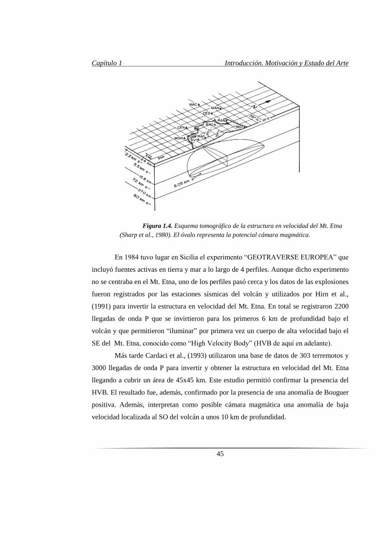
Capítulo 1 Introducción. Motivación y Estado del Arte
45
En 1984 tuvo lugar en Sicilia el experimento “GEOTRAVERSE EUROPEA” que
incluyó fuentes activas en tierra y mar a lo largo de 4 perfiles. Aunque dicho experimento
no se centraba en el Mt. Etna, uno de los perfiles pasó cerca y los datos de las explosiones
fueron registrados por las estaciones sísmicas del volcán y utilizados por Hirn et al.,
(1991) para invertir la estructura en velocidad del Mt. Etna. En total se registraron 2200
llegadas de onda P que se invirtieron para los primeros 6 km de profundidad bajo el
volcán y que permitieron “iluminar” por primera vez un cuerpo de alta velocidad bajo el
SE del Mt. Etna, conocido como “High Velocity Body” (HVB de aquí en adelante).
Más tarde Cardaci et al., (1993) utilizaron una base de datos de 303 terremotos y
3000 llegadas de onda P para invertir y obtener la estructura en velocidad del Mt. Etna
llegando a cubrir un área de 45x45 km. Este estudio permitió confirmar la presencia del
HVB. El resultado fue, además, confirmado por la presencia de una anomalía de Bouguer
positiva. Además, interpretan como posible cámara magmática una anomalía de baja
velocidad localizada al SO del volcán a unos 10 km de profundidad.
Figure Figura 1.4. Esquema tomográfico de la estructura en velocidad del Mt. Etna
(Sharp et al., 1980). El óvalo representa la potencial cámara magmática.
Capítulo 1 Introducción. Motivación y Estado del Arte
46
El primer experimento de sísmica activa realizado “ad-hoc” para determinar la
estructura del Mt. Etna fue el conocido como “ETNASEIS” en 1992. Éste consistió en
una serie de disparos con cañones de aire comprimido en el mar que serían registrados en
estaciones sísmicas instaladas alrededor del Mt. Etna. Se utilizaron 8 cañones
configurados para disparar en modo “burbuja única” con una potencia de 840 pulgadas
cúbicas a lo largo de 2 perfiles. En una segunda fase, una segunda nave realizó otros 3
perfiles disparando con 26 cañones y una potencia total de 3810 pulgadas cúbicas. Para
finalizar, los últimos 2 perfiles se realizaron con un barco equipado con un array de
cañones de aire comprimido de tipo industrial. Los datos obtenidos de este experimento
sirvieron a Hirn et al., (1997) para mejorar la tomografía previa de Hirn et al., (1991).
Debido a la alta atenuación de la estructura del volcán, los registros de las explosiones en
mar no se registraron lo suficientemente bien para poder obtener un modelo fiable de la
estructura en velocidad del volcán. El resultado es una mejora del modelo inicial de Hirn
et al., (1991) sobre una malla de 25x 25 km llegando a una profundidad de 15 km.
De Luca et al., (1997) proponen una tomografía pasiva del Mt. Etna, usando
sismicidad local, utilizando 1249 terremotos y 23000 llegadas de onda P y 10000 de onda
S. La inversión en velocidad de dicha base de datos permitió por primera vez sumar a las
evidencias ya existentes del HVB y de la anomalía positiva de Bouguer, la presencia de
una anomalía con valores de Vp/Vs bajos, manifestando la presencia de material
consolidado. Similares resultados fueron puestos en evidencia por Villaseñor et al.,
(1998) invirtiendo más de 4000 ondas P originadas por 512 terremotos registrados a lo
largo de 12 años utilizando una red sísmica de 29 estaciones.
Con el objetivo de describir y detallar el papel que juega el HVB en la dinámica
volcánica, se realizó un experimento sísmico en el que se realizaron 7 explosiones en
tierra alrededor del volcán. Las señales sísmicas generadas se recibieron en un array de
800 canales. Laigle et al., (1999) interpretan dicha anomalía como un cuerpo magmático
al que atribuyen emisiones de gases.
Durante el año 2000 se publicaron 3 estudios tomográficos relacionados con el
Mt. Etna, cada uno de ellos independiente y con sus propios datos. En primer lugar,
Laigle et al., (2000) obtuvieron una mejora de tomografías anteriores al utilizar
Capítulo 1 Introducción. Motivación y Estado del Arte
47
conjuntamente ondas P y S y poder calcular así la razón Vp/Vs. Dicho valor presenta
valores bastante heterogéneos en el área que corresponde al HVB. Los datos fueron
registrados por 35 estaciones sísmicas que conformaban la red sísmica del Mt. Etna en
aquel momento. Por otro lado, Chiarabba et al., (2000) invirtieron las primeras llegadas
de ondas P y S de un total de 300 eventos registrados entre 1994 y 1998 en 48 estaciones
sísmicas. Ambos estudios centran su interpretación en la descripción del HVB y su
importancia en la dinámica eruptiva (Figure 1.5). Por último, Nicolich et al., (2000)
realizó una serie de perfiles de reflexión en la costa del mar Ionio analizando los datos
obtenidos en el experimento ETNASEIS. Los principales resultados se asocian a un perfil
de reflexión que va con dirección NE-SO a lo largo de la costa oriental de Sicilia que
permiten detectar una serie de fallas principales que controlan la dinámica regional.
Un catálogo de 1194 terremotos registrados durante 13 años sirvió a Aloisi et al.,
(2002) para invertir los tiempos de llegada de 8600 ondas P y 1900 ondas S. Esta
inversión tomográfica pone de manifiesto nuevamente la presencia del HVB, que los
autores interpretan como un cuerpo magmático muy resistente formado por un conjunto
de cumulitas, diques, etc. No obstante, detectaron otra anomalía de velocidad, en este
caso negativa, al sur-oeste del HVB y que se interpreta como posibles conductos
magmáticos (Figure 1.6).
Durante los últimos 15 años la base de datos sísmica se ha incrementado
significativamente en parte debido a dos grandes erupciones laterales acompañadas de
una importante sismicidad superficial (< 5 km b.s.l). Este nuevo catálogo permitió a
Patanè et al., (2002) y Patanè et al., (2006) mejorar la resolución de las tomografías
precedentes en los primeros 7 kilómetros y detallando la parte más superficial del HVB.
Patanè et al., (2002) utilizó para la inversión ondas P y S de 286 terremotos de gran
calidad registrados durante la erupción lateral de 2001, “iluminando” la estructura en
velocidad del volcán hasta 3 km b.n.m.. Además, por primera vez hasta el momento, se
detecta una anomalía con valores bajos de Vp/Vs asociada a la zona de la fractura
principal de dicha erupción.
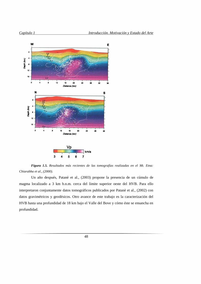
Capítulo 1 Introducción. Motivación y Estado del Arte
48
Figura 1.5. Resultados más recientes de las tomografías realizadas en el Mt. Etna:
Chiarabba et al., (2000).
Un año después, Patanè et al., (2003) propone la presencia de un cúmulo de
magma localizado a 3 km b.n.m. cerca del límite superior oeste del HVB. Para ello
interpretaron conjuntamente datos tomográficos publicados por Patanè et al., (2002) con
datos gravimétricos y geodésicos. Otro avance de este trabajo es la caracterización del
HVB hasta una profundidad de 18 km bajo el Valle del Bove y cómo éste se ensancha en
profundidad.
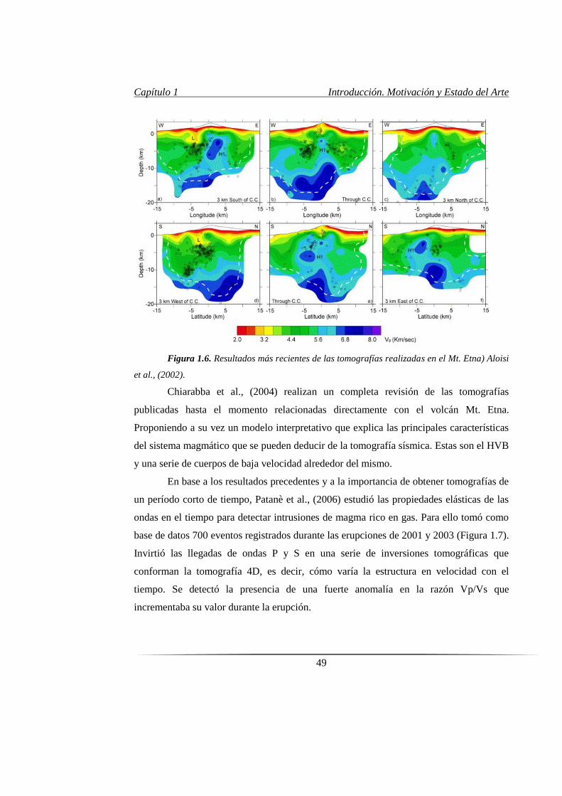
Capítulo 1 Introducción. Motivación y Estado del Arte
49
Figura 1.6. Resultados más recientes de las tomografías realizadas en el Mt. Etna) Aloisi
et al., (2002).
Chiarabba et al., (2004) realizan un completa revisión de las tomografías
publicadas hasta el momento relacionadas directamente con el volcán Mt. Etna.
Proponiendo a su vez un modelo interpretativo que explica las principales características
del sistema magmático que se pueden deducir de la tomografía sísmica. Estas son el HVB
y una serie de cuerpos de baja velocidad alrededor del mismo.
En base a los resultados precedentes y a la importancia de obtener tomografías de
un período corto de tiempo, Patanè et al., (2006) estudió las propiedades elásticas de las
ondas en el tiempo para detectar intrusiones de magma rico en gas. Para ello tomó como
base de datos 700 eventos registrados durante las erupciones de 2001 y 2003 (Figura 1.7).
Invirtió las llegadas de ondas P y S en una serie de inversiones tomográficas que
conforman la tomografía 4D, es decir, cómo varía la estructura en velocidad con el
tiempo. Se detectó la presencia de una fuerte anomalía en la razón Vp/Vs que
incrementaba su valor durante la erupción.
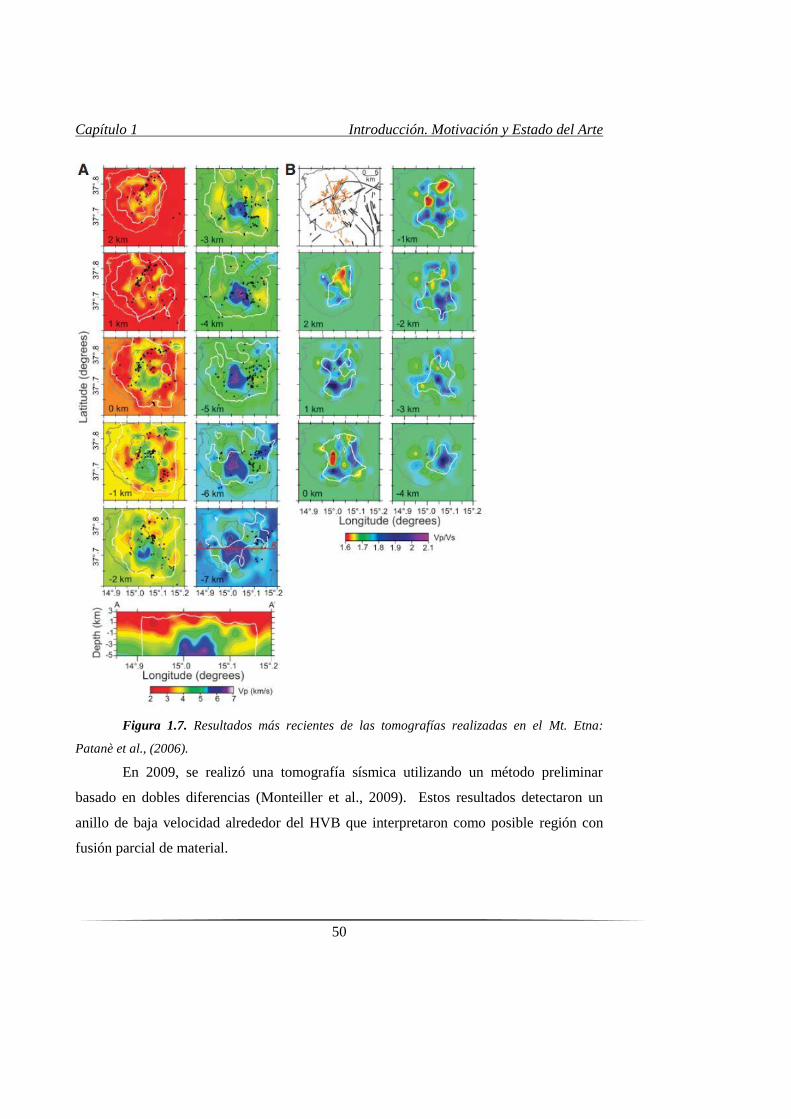
Capítulo 1 Introducción. Motivación y Estado del Arte
50
Figura 1.7. Resultados más recientes de las tomografías realizadas en el Mt. Etna:
Patanè et al., (2006).
En 2009, se realizó una tomografía sísmica utilizando un método preliminar
basado en dobles diferencias (Monteiller et al., 2009). Estos resultados detectaron un
anillo de baja velocidad alrededor del HVB que interpretaron como posible región con
fusión parcial de material.
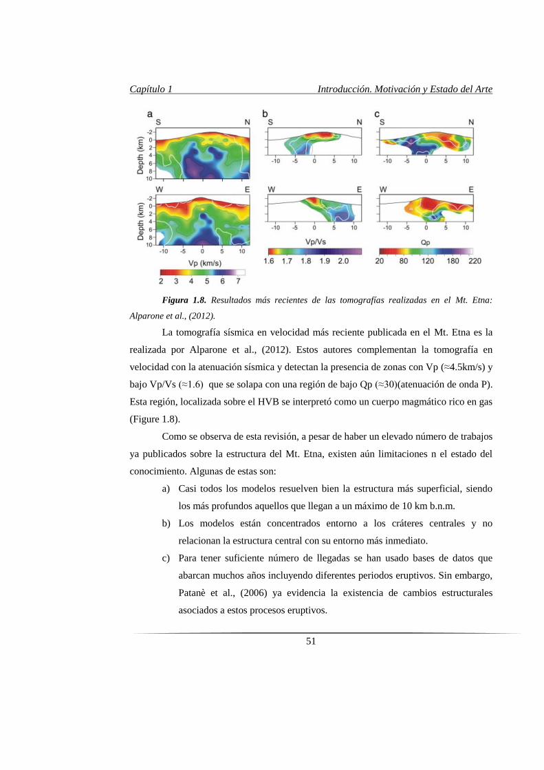
Capítulo 1 Introducción. Motivación y Estado del Arte
51
Figura 1.8. Resultados más recientes de las tomografías realizadas en el Mt. Etna:
Alparone et al., (2012).
La tomografía sísmica en velocidad más reciente publicada en el Mt. Etna es la
realizada por Alparone et al., (2012). Estos autores complementan la tomografía en
velocidad con la atenuación sísmica y detectan la presencia de zonas con Vp (≈4.5km/s) y
bajo Vp/Vs (≈1.6) que se solapa con una región de bajo Qp (≈30)(atenuación de onda P).
Esta región, localizada sobre el HVB se interpretó como un cuerpo magmático rico en gas
(Figure 1.8).
Como se observa de esta revisión, a pesar de haber un elevado número de trabajos
ya publicados sobre la estructura del Mt. Etna, existen aún limitaciones n el estado del
conocimiento. Algunas de estas son:
a) Casi todos los modelos resuelven bien la estructura más superficial, siendo
los más profundos aquellos que llegan a un máximo de 10 km b.n.m.
b) Los modelos están concentrados entorno a los cráteres centrales y no
relacionan la estructura central con su entorno más inmediato.
c) Para tener suficiente número de llegadas se han usado bases de datos que
abarcan muchos años incluyendo diferentes periodos eruptivos. Sin embargo,
Patanè et al., (2006) ya evidencia la existencia de cambios estructurales
asociados a estos procesos eruptivos.
Capítulo 1 Introducción. Motivación y Estado del Arte
52
Por tanto, cualquier mejora en los modelos estructurales pasa por solventar estas
limitaciones. Puesto que la mayoría de la sismicidad es fundamentalmente
superficial y no homogénea ni espacial ni temporalmente, resulta necesario
planificar un experimento que permita dar respuesta a estas cuestiones. Este es el
motivo por el que se ideó el experimento TOMO-ETNA.
1.3. Experimento TOMO-ETNA
La necesidad de mejorar el conocimiento que se tiene de la estructura interna de
los volcanes refuerza la importancia de los estudios tomográficos, dando un papel
relevante a una buena distribución de datos sísmicos de alta calidad y una red sísmica
densa. Estos aspectos no están siempre presentes en todos los volcanes, en donde los
experimentos de sísmica activa juegan un papel relevante. Nuestra experiencia parte con
el experimento TOMO-DEC en Isla Decepción (Archipiélago de las Shetland del Sur,
Antártida). Esta campaña se llevó a cabo en Enero de 2005 (e.g. Barclay et al., 2009;
Ben-Zvi et al., 2009; Zandomenghi et al., 2009; García-Yeguas et al., 2011). La calidad y
cantidad de datos obtenida, junto con el consorcio internacional que se empezó a crear,
nos permitieron afrontar un nuevo experimento sísmico, en este caso, en la isla de
Tenerife (Canarias, España). La campaña TOM-TEIDEVS tuvo lugar en Enero de 2007
(e.g. Ibáñez et al., 2008; De Barros et al., 2012; García-Yeguas et al., 2012). Este
experimento de sísmica activa estuvo centrado en el estudio de la estructura interna del
volcán Teide. Dicho volcán había tenido una reactivación sísmica en 2004 y por tanto
representó una oportunidad única para estudiar las causas de dicha reactivación y su
estructura interna. Ese mismo año se realizó otro experimento de características similares
en la isla de Stromboli (Castellano et al., 2008; Prudencio et al., 2015c).
Los resultados obtenidos en los distintos experimentos pusieron de manifiesto la
importancia de utilizar fuentes de sísmica activa para complementar la información
proporcionada por los terremotos, ya que en muchos de los casos ya mencionados la tasa
de sismicidad es bastante baja. Por ello, cuando se puso en marcha el proyecto europeo
MED-SUV, nació la posibilidad de realizar un ambicioso experimento de sísmica activa
centrado tanto en el Mt. Etna como en las regiones adyacentes y estructuralmente
relacionadas (Ver Capítulo 3). Bajo este marco, se desarrolló el experimento TOMO-
Capítulo 1 Introducción. Motivación y Estado del Arte
53
ETNA. El experimento se diseñó integrando actividades marinas y terrestres y realizando
estudios de Sísmica de Refracción (WAS), sísmica de reflexión multi-canal (MCS),
perfiles magnéticos e incluso inmersiones con un vehículo no tripulado (ROV). La
complejidad de este experimento, realizado entre Junio y Noviembre de 2014, se ve
reflejada en los proyectos que la financiaron (MED-SUV, EUROFLEETS2, COCSABO)
y la cantidad de instituciones que colaboraron para llevarlo a cabo (Ver Anexos 1-4).
Además, el experimento contó con la participación activa de varios buques: El Buque de
Investigación Oceanográfica (BIO) español “Sarmiento de Gamboa”; el Buque Hidro-
Oceanográfico italiano “Galatea”; y el BIO griego “AEGEAN”, junto al apoyo de dos
naves de la Marina Italiana. En total 26 instituciones académicas y de investigación de:
Italia, España, Alemania, Irlanda, EE.UU, Rusia, Francia, Grecia y México estuvieron
activamente involucradas en TOMO-ETNA (Para más información acerca del
experimento ver Capítulo 3 y Anexos 1-4).
1.4. Localización de Precisión y Fracturación Hidráulica
No obstante, los potenciales resultados derivados de este experimento, y de
cualquier tomografía sísmica, no se quedan solo en la estructura 3D en velocidad del
volcán. El siguiente paso natural es aprovechar este nuevo modelo 3D más realista para
realizar una relocalización de la sismicidad registrada en la región y así definir posibles
zonas sismogenéticas y su posible interpretación. En este sentido, hasta hace poco se
asociaban directamente los terremotos volcánicos a la presencia de magma (Waite, 2002;
Walter et al., 2007). Sin embargo, estudios recientes descritos en el capítulo 7 de esta
tesis demuestran que la sismicidad volcánica puede estar también ligada a procesos de
fracturación hidráulica y migración de esfuerzos (Díaz-Moreno et al., 2015). A la luz de
estos resultados, se podrán explicar e reinterpretar muchos enjambres sísmicos que hasta
la fecha se consideraban causados únicamente por la migración del magma.
1.5. Motivación y Objetivos
En esta tesis se presenta un estudio en detalle de la estructura interna en velocidad
del volcán Mt. Etna y las regiones circundantes, incluyendo otro complejo volcánico de
gran importancia como son las Islas Eolias. Los datos proceden del que probablemente
sea uno de los experimentos de sísmica activa en volcanes más complejo, costoso y
Capítulo 1 Introducción. Motivación y Estado del Arte
54
completo del mundo, el Experimento TOMO-ETNA. Dicho experimento nos permitió
obtener una gran base de datos de señales sísmicas de alta calidad que han sido
procesadas utilizando uno de los más novedosos y robustos algoritmos de análisis de
llegadas de ondas sísmicas basado en el análisis espectral de las señales (utilizando el
programa AMPA). El tiempo de llegada de las ondas P detectadas tanto de las fuentes
activas como de los terremotos, han sido invertidas conjuntamente en un nuevo software
desarrollado ad-hoc para la inversión tomográfica conjunta de datos de sísmica pasiva y
activa (utilizando el programa PARTOS). Por último, esta tesis muestra que la obtención
de la tomografía sísmica no es un resultado finalista, sino que proponemos una serie de
estudios posteriores de relocalización sísmica y análisis de curvas de difusividad que
permiten mejorar el conocimiento de la dinámica sísmica en regiones volcánica. Para
ello, se muestra un caso de estudio en la Isla de El Hierro, aprovechando la crisis sismo-
volcánica que tuvo lugar entre 2011 y 2013. Se ha elegido esta región debido a la alta
concentración de enjambres sísmicos en un corto periodo de tiempo. Así, realizar un
trabajo similar para el Mt. Etna, sería objeto de trabajos futuros debido a la cantidad de
enjambres sísmicos ocurridos en los últimos años y que deben ser analizados
independientemente y en profundidad. Aun así hemos llevado a cabo una primera
aproximación de dicho análisis utilizando datos correspondientes a un enjambre sísmico
de 2002-03. Una correcta interpretación de los resultados permitiría relacionar los
enjambres sísmicos con la migración de magma o con la migración de esfuerzos debido a
la inyección de fluidos.
En resumen, los objetivos de esta Tesis Doctoral se basan en dos pilares
fundamentales:
i) Obtención de un modelo de velocidad realista y tridimensional de la
región que comprende el volcán Mt. Etna, el archipiélago de las Islas
Eolias y las áreas circundantes, a partir de la inversión conjunta de
datos de sísmica activa y pasiva.
ii) ii) Aplicaciones avanzadas de los modelos de velocidad para el
estudio de los mecanismos físicos que controlan la sismicidad en
volcanes.
2. Geophysical, Geodinamic
and Volcanological
framework of Mt. Etna
volcano, Eolian Islands and
surrounding region

Chapter 2 Geophysical, Geodinamic and Volcanological Framework
57
The Mediterranean region is a complex puzzle located between the African and
European plates in which it is observable the presence of large-scale extensional basins
with evident convergent scenarios. In itself, the Mediterranean basin cannot be explained
as a uniform geodynamic framework (Figure 1). Thus several studies reveal that Central-
Western Mediterranean area is dominated by extensional basins placed in a back-arc
setting, ranging from Alboran Sea in the Western side to the complexity of the Thyrrenian
and Ionia Basins in the Center portion (e.g., Horvath and Berckhemer, 1982 and Rehault
et al., 1984, Monna et al., 2013). On the other hand, the Eastern Mediterranean area
(Aegean region) has been historically considered an ancient back-arc extensional basin
related to the northeast Hellenic arc subduction zone that at the present is not persistent
(Le Pichon, 1982, McClusky et al., 2000, Papanikolau et al., 2007). This geodynamic
complexity is also reflected in the variety of active volcanic scenarios, from the total
absence in the westernmost margin (Alboran Sea), through the very active Italian
volcanoes such as Mt. Etna, Stromboli or the volcanic complex Vesuvius-Campi Flegrei,
finishing in the Greek volcanic Islands such as Nisyros or Santorini (Figure 2.1). The
tectonic configuration of the area under study originates by the occurrence of major
tectonic processes which started after a stage of plate convergence, consuming a
subducting Mesozoic ocean from Gibraltar to Liguria, and were likely induced since the
Oligocene by the slab retreat (Figure 2.1). This new tectonic regime, through a
segmentation and reorganization of the convergent plate boundaries, has led to the
formation of highly arcuate orogenic belts encircling young back-arc oceanic basins, i.e.,
Liguro-Provençal, Algerian, Alboran, and Tyrrhenian basins (see Malinverno and Ryan,
1986; Jolivet and Faccenna, 2000; Faccenna et al., 2014).
Mt. Etna stands out astride different domains represented by the
Sicilian/Calabrian sectors of the collisional/subduction belt and the foreland which form
its basement. In particular, to the south, the Pelagian block and the Ionian Sea, separated
by a Mesozoic lithospheric boundary, the NNW–SSE-striking Hyblean–Maltese-
Escarpment fault system (e.g. Doglioni et al., 2001), represent the continental and oceanic
foreland of the underthrusting Nubia plate (the African plate west of the East African
Rift), respectively (Roure et al., 1990; Ben-Avraham and Grasso, 1991). The orogenic
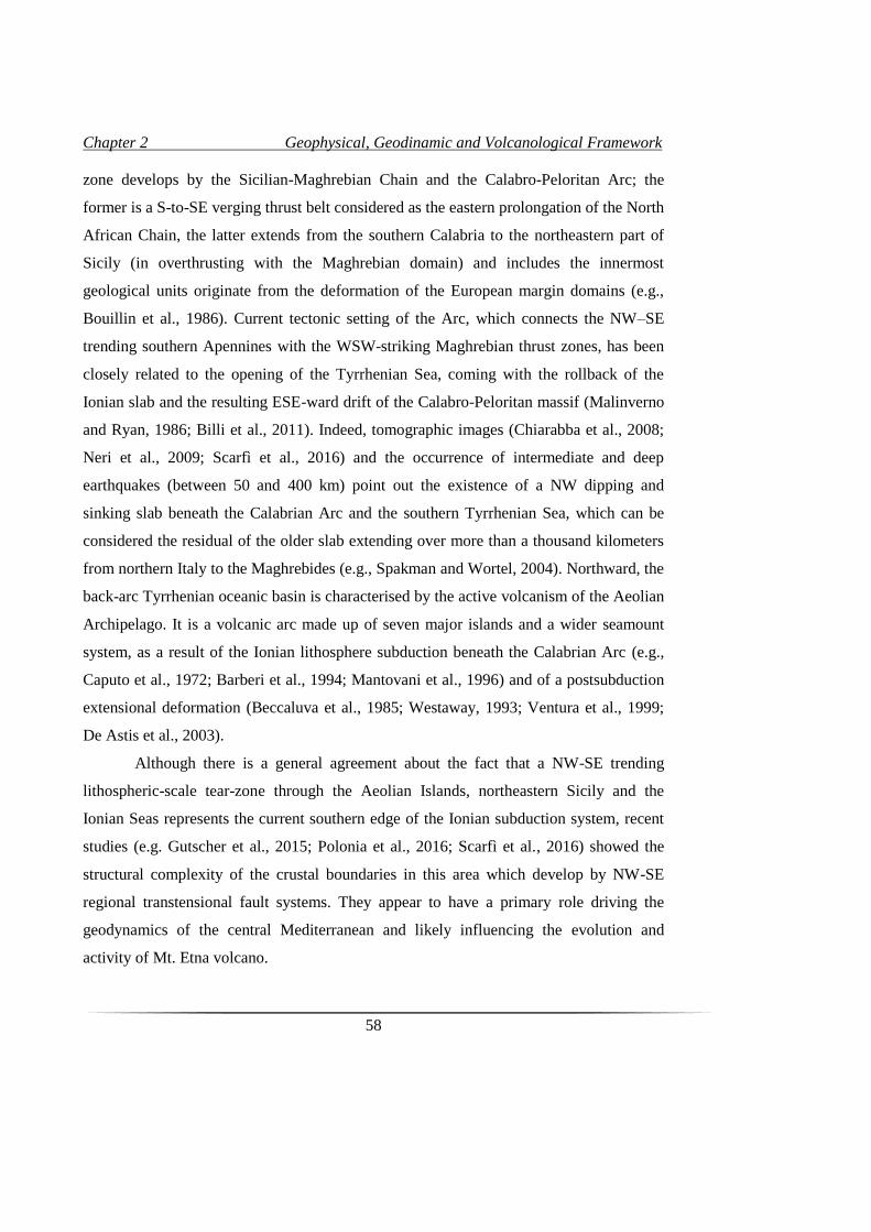
Chapter 2 Geophysical, Geodinamic and Volcanological Framework
58
zone develops by the Sicilian-Maghrebian Chain and the Calabro-Peloritan Arc; the
former is a S-to-SE verging thrust belt considered as the eastern prolongation of the North
African Chain, the latter extends from the southern Calabria to the northeastern part of
Sicily (in overthrusting with the Maghrebian domain) and includes the innermost
geological units originate from the deformation of the European margin domains (e.g.,
Bouillin et al., 1986). Current tectonic setting of the Arc, which connects the NW–SE
trending southern Apennines with the WSW-striking Maghrebian thrust zones, has been
closely related to the opening of the Tyrrhenian Sea, coming with the rollback of the
Ionian slab and the resulting ESE-ward drift of the Calabro-Peloritan massif (Malinverno
and Ryan, 1986; Billi et al., 2011). Indeed, tomographic images (Chiarabba et al., 2008;
Neri et al., 2009; Scarfì et al., 2016) and the occurrence of intermediate and deep
earthquakes (between 50 and 400 km) point out the existence of a NW dipping and
sinking slab beneath the Calabrian Arc and the southern Tyrrhenian Sea, which can be
considered the residual of the older slab extending over more than a thousand kilometers
from northern Italy to the Maghrebides (e.g., Spakman and Wortel, 2004). Northward, the
back-arc Tyrrhenian oceanic basin is characterised by the active volcanism of the Aeolian
Archipelago. It is a volcanic arc made up of seven major islands and a wider seamount
system, as a result of the Ionian lithosphere subduction beneath the Calabrian Arc (e.g.,
Caputo et al., 1972; Barberi et al., 1994; Mantovani et al., 1996) and of a postsubduction
extensional deformation (Beccaluva et al., 1985; Westaway, 1993; Ventura et al., 1999;
De Astis et al., 2003).
Although there is a general agreement about the fact that a NW-SE trending
lithospheric-scale tear-zone through the Aeolian Islands, northeastern Sicily and the
Ionian Seas represents the current southern edge of the Ionian subduction system, recent
studies (e.g. Gutscher et al., 2015; Polonia et al., 2016; Scarfì et al., 2016) showed the
structural complexity of the crustal boundaries in this area which develop by NW-SE
regional transtensional fault systems. They appear to have a primary role driving the
geodynamics of the central Mediterranean and likely influencing the evolution and
activity of Mt. Etna volcano.
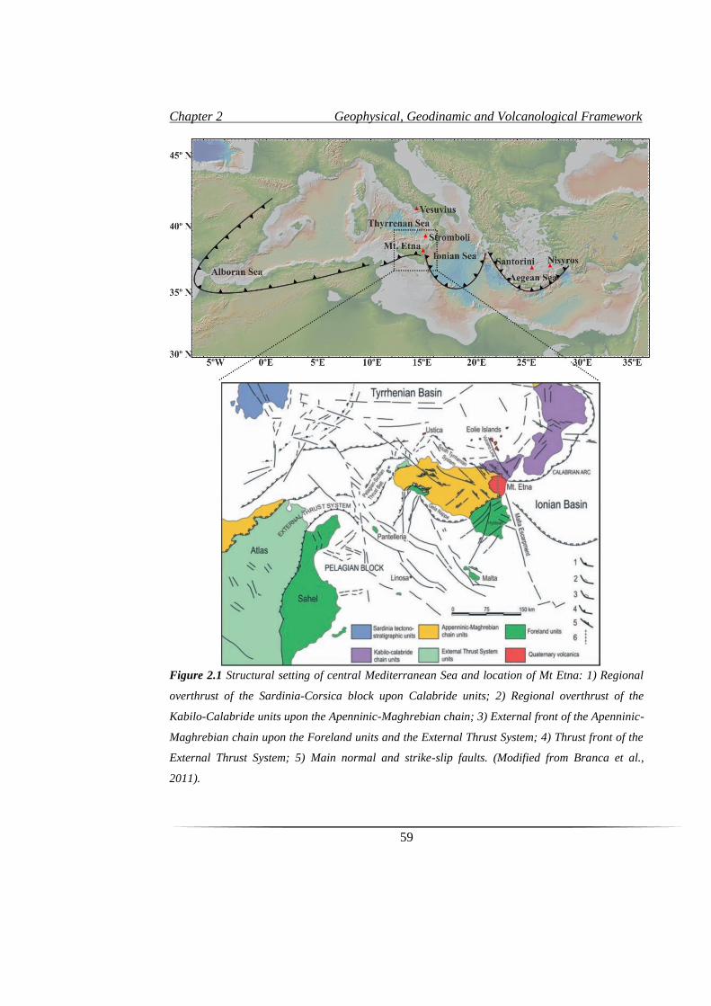
Chapter 2 Geophysical, Geodinamic and Volcanological Framework
59
Figure 2.1 Structural setting of central Mediterranean Sea and location of Mt Etna: 1) Regional
overthrust of the Sardinia-Corsica block upon Calabride units; 2) Regional overthrust of the
Kabilo-Calabride units upon the Apenninic-Maghrebian chain; 3) External front of the Apenninic-
Maghrebian chain upon the Foreland units and the External Thrust System; 4) Thrust front of the
External Thrust System; 5) Main normal and strike-slip faults. (Modified from Branca et al.,
2011).
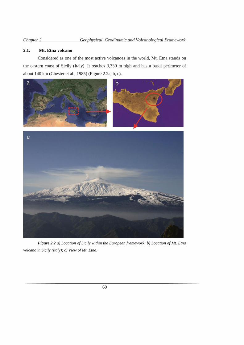
Chapter 2 Geophysical, Geodinamic and Volcanological Framework
60
2.1. Mt. Etna volcano
Considered as one of the most active volcanoes in the world, Mt. Etna stands on
the eastern coast of Sicily (Italy). It reaches 3,330 m high and has a basal perimeter of
about 140 km (Chester et al., 1985) (Figure 2.2a, b, c).
Figure 2.2 a) Location of Sicily within the European framework; b) Location of Mt. Etna
volcano in Sicily (Italy); c) View of Mt. Etna.
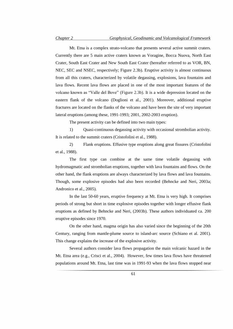
Chapter 2 Geophysical, Geodinamic and Volcanological Framework
61
Mt. Etna is a complex strato-volcano that presents several active summit craters.
Currently there are 5 main active craters known as Voragine, Bocca Nuova, North East
Crater, South East Crater and New South East Crater (hereafter referred to as VOR, BN,
NEC, SEC and NSEC, respectively; Figure 2.3b). Eruptive activity is almost continuous
from all this craters, characterized by volatile degassing, explosions, lava fountains and
lava flows. Recent lava flows are placed in one of the most important features of the
volcano known as “Valle del Bove” (Figure 2.3b). It is a wide depression located on the
eastern flank of the volcano (Doglioni et al., 2001). Moreover, additional eruptive
fractures are located on the flanks of the volcano and have been the site of very important
lateral eruptions (among these, 1991-1993; 2001, 2002-2003 eruption).
The present activity can be defined into two main types:
1) Quasi-continuous degassing activity with occasional strombolian activity.
It is related to the summit craters (Cristofolini et al., 1988).
2) Flank eruptions. Effusive type eruptions along great fissures (Cristofolini
et al., 1988).
The first type can combine at the same time volatile degassing with
hydromagmatic and strombolian eruptions, together with lava fountains and flows. On the
other hand, the flank eruptions are always characterized by lava flows and lava fountains.
Though, some explosive episodes had also been recorded (Behncke and Neri, 2003a;
Andronico et al., 2005).
In the last 50-60 years, eruptive frequency at Mt. Etna is very high. It comprises
periods of strong but short in time explosive episodes together with longer effusive flank
eruptions as defined by Behncke and Neri, (2003b). These authors individuated ca. 200
eruptive episodes since 1970.
On the other hand, magma origin has also varied since the beginning of the 20th
Century, ranging from mantle-plume source to island-arc source (Schiano et al. 2001).
This change explains the increase of the explosive activity.
Several authors consider lava flows propagation the main volcanic hazard in the
Mt. Etna area (e.g., Crisci et al., 2004). However, few times lava flows have threatened
populations around Mt. Etna, last time was in 1991-93 when the lava flows stopped near
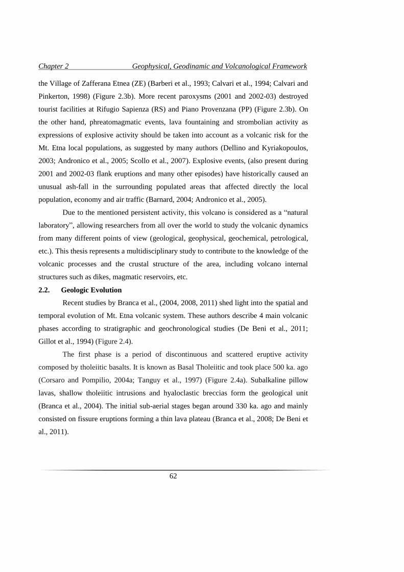
Chapter 2 Geophysical, Geodinamic and Volcanological Framework
62
the Village of Zafferana Etnea (ZE) (Barberi et al., 1993; Calvari et al., 1994; Calvari and
Pinkerton, 1998) (Figure 2.3b). More recent paroxysms (2001 and 2002-03) destroyed
tourist facilities at Rifugio Sapienza (RS) and Piano Provenzana (PP) (Figure 2.3b). On
the other hand, phreatomagmatic events, lava fountaining and strombolian activity as
expressions of explosive activity should be taken into account as a volcanic risk for the
Mt. Etna local populations, as suggested by many authors (Dellino and Kyriakopoulos,
2003; Andronico et al., 2005; Scollo et al., 2007). Explosive events, (also present during
2001 and 2002-03 flank eruptions and many other episodes) have historically caused an
unusual ash-fall in the surrounding populated areas that affected directly the local
population, economy and air traffic (Barnard, 2004; Andronico et al., 2005).
Due to the mentioned persistent activity, this volcano is considered as a “natural
laboratory”, allowing researchers from all over the world to study the volcanic dynamics
from many different points of view (geological, geophysical, geochemical, petrological,
etc.). This thesis represents a multidisciplinary study to contribute to the knowledge of the
volcanic processes and the crustal structure of the area, including volcano internal
structures such as dikes, magmatic reservoirs, etc.
2.2. Geologic Evolution
Recent studies by Branca et al., (2004, 2008, 2011) shed light into the spatial and
temporal evolution of Mt. Etna volcanic system. These authors describe 4 main volcanic
phases according to stratigraphic and geochronological studies (De Beni et al., 2011;
Gillot et al., 1994) (Figure 2.4).
The first phase is a period of discontinuous and scattered eruptive activity
composed by tholeiitic basalts. It is known as Basal Tholeiitic and took place 500 ka. ago
(Corsaro and Pompilio, 2004a; Tanguy et al., 1997) (Figure 2.4a). Subalkaline pillow
lavas, shallow tholeiitic intrusions and hyaloclastic breccias form the geological unit
(Branca et al., 2004). The initial sub-aerial stages began around 330 ka. ago and mainly
consisted on fissure eruptions forming a thin lava plateau (Branca et al., 2008; De Beni et
al., 2011).
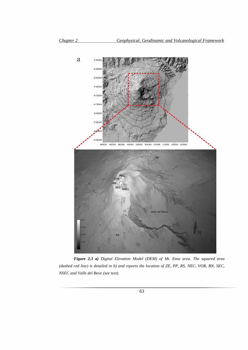
Chapter 2 Geophysical, Geodinamic and Volcanological Framework
63
Figure 2.3 a) Digital Elevation Model (DEM) of Mt. Etna area. The squared area
(dashed red line) is detailed in b) and reports the location of ZE, PP, RS, NEC, VOR, BN, SEC,
NSEC and Valle del Bove (see text).
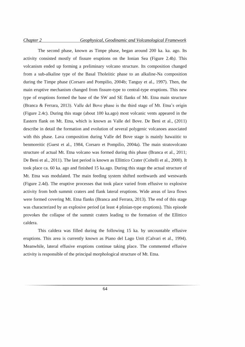
Chapter 2 Geophysical, Geodinamic and Volcanological Framework
64
The second phase, known as Timpe phase, began around 200 ka. ka. ago. Its
activity consisted mostly of fissure eruptions on the Ionian Sea (Figure 2.4b). This
volcanism ended up forming a preliminary volcano structure. Its composition changed
from a sub-alkaline type of the Basal Tholeiitic phase to an alkaline-Na composition
during the Timpe phase (Corsaro and Pompilio, 2004b; Tanguy et al., 1997). Then, the
main eruptive mechanism changed from fissure-type to central-type eruptions. This new
type of eruptions formed the base of the SW and SE flanks of Mt. Etna main structure
(Branca & Ferrara, 2013). Valle del Bove phase is the third stage of Mt. Etna’s origin
(Figure 2.4c). During this stage (about 100 ka.ago) most volcanic vents appeared in the
Eastern flank on Mt. Etna, which is known as Valle del Bove. De Beni et al., (2011)
describe in detail the formation and evolution of several polygenic volcanoes associated
with this phase. Lava composition during Valle del Bove stage is mainly hawaiitic to
benmoreitic (Guest et al., 1984, Corsaro et Pompilio, 2004a). The main stratovolcano
structure of actual Mt. Etna volcano was formed during this phase (Branca et al., 2011;
De Beni et al., 2011). The last period is known as Ellittico Crater (Coltelli et al., 2000). It
took place ca. 60 ka. ago and finished 15 ka.ago. During this stage the actual structure of
Mt. Etna was modulated. The main feeding system shifted northwards and westwards
(Figure 2.4d). The eruptive processes that took place varied from effusive to explosive
activity from both summit craters and flank lateral eruptions. Wide areas of lava flows
were formed covering Mt. Etna flanks (Branca and Ferrara, 2013). The end of this stage
was characterized by an explosive period (at least 4 plinian-type eruptions). This episode
provokes the collapse of the summit craters leading to the formation of the Ellittico
caldera.
This caldera was filled during the following 15 ka. by uncountable effusive
eruptions. This area is currently known as Piano del Lago Unit (Calvari et al., 1994).
Meanwhile, lateral effusive eruptions continue taking place. The commented effusive
activity is responsible of the principal morphological structure of Mt. Etna.
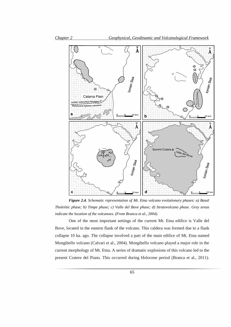
Chapter 2 Geophysical, Geodinamic and Volcanological Framework
65
Figure 2.4. Schematic representation of Mt. Etna volcano evolutionary phases: a) Basal
Tholeiitic phase; b) Timpe phase; c) Valle del Bove phase; d) Stratovolcano phase. Grey areas
indicate the location of the volcanoes. (From Branca et al., 2004).
One of the most important settings of the current Mt. Etna edifice is Valle del
Bove, located in the eastern flank of the volcano. This caldera was formed due to a flank
collapse 10 ka. ago. The collapse involved a part of the main edifice of Mt. Etna named
Mongibello volcano (Calvari et al., 2004). Mongibello volcano played a major role in the
current morphology of Mt. Etna. A series of dramatic explosions of this volcano led to the
present Cratere del Piano. This occurred during Holocene period (Branca et al., 2011).
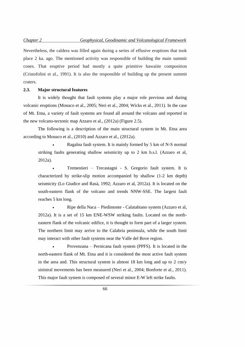
Chapter 2 Geophysical, Geodinamic and Volcanological Framework
66
Nevertheless, the caldera was filled again during a series of effusive eruptions that took
place 2 ka. ago. The mentioned activity was responsible of building the main summit
cones. That eruptive period had mostly a quite primitive hawaiite composition
(Cristofolini et al., 1991). It is also the responsible of building up the present summit
craters.
2.3. Major structural features
It is widely thought that fault systems play a major role previous and during
volcanic eruptions (Monaco et al., 2005; Neri et al., 2004; Wicks et al., 2011). In the case
of Mt. Etna, a variety of fault systems are found all around the volcano and reported in
the new volcano-tectonic map Azzaro et al., (2012a) (Figure 2.5).
The following is a description of the main structural system in Mt. Etna area
according to Monaco et al., (2010) and Azzaro et al., (2012a).
Ragalna fault system. It is mainly formed by 5 km of N-S normal
striking faults generating shallow seismicity up to 2 km b.s.l. (Azzaro et al,
2012a).
Tremestieri – Trecastagni - S. Gregorio fault system. It is
characterized by strike-slip motion accompanied by shallow (1-2 km depth)
seismicity (Lo Giudice and Rasà, 1992; Azzaro et al, 2012a). It is located on the
south-eastern flank of the volcano and trends NNW-SSE. The largest fault
reaches 5 km long.
Ripe della Naca – Piedimonte - Calatabiano system (Azzaro et al,
2012a). It is a set of 15 km ENE-WSW striking faults. Located on the north-
eastern flank of the volcanic edifice, it is thought to form part of a larger system.
The northern limit may arrive to the Calabria peninsula, while the south limit
may interact with other fault systems near the Valle del Bove region.
Provenzana – Pernicana fault system (PPFS). It is located in the
north-eastern flank of Mt. Etna and it is considered the most active fault system
in the area and. This structural system is almost 18 km long and up to 2 cm/y
sinistral movements has been measured (Neri et al., 2004; Bonforte et al., 2011).
This major fault system is composed of several minor E-W left strike faults.
Chapter 2 Geophysical, Geodinamic and Volcanological Framework
67
Figure 2.5 Volcano-tectonic map of Mt. Etna. Fault abbreviations: a, Ragalna system; b,
Tremestieri-Trecastagni-S. Gregorio system; c, Ripe della Naca-Piedimonte-Calatabiano system;
d, Pernicana system; AC, Acicatena; AP, Aciplatani; AT, Acitrezza; CA, Calcerana; FF,
Fiumefreddo; MC, Mt. Cicirello; PD, Piedimonte; PL, Punta Lucia; PN, Pizzi Deneri; PT,
Praiola-Torre Archirafi; SA, S. Alfio; SB, Serra S. Biagio; SG, S. Gregorio; SV, S. Venera; TD,
Tardaria. Inset map (a) illustrates the major regional tectonic structures (simplified from Lentini
et al., 2006; Argnani et al., 2009): AMT, front of the Appennine-Maghrebian thrust belt; ME,
Malta Escarpment; TF, supposed Taormina fault (From Azzaro et al., 2012a).
Chapter 2 Geophysical, Geodinamic and Volcanological Framework
68
Timpe fault system. It is composed of normal faults that dip
toward Ionian Sea. It is a 20 km-long belt located on the Eastern lower flank of
Mt. Etna. The fault trend changes from SSW.NNE on the northern part to a
NNW-SSE on the southern part (Monaco et al., 1995, 1997; Lanzafame et al.,
1996; Azzaro, 1999; Azzaro et al., 2012b). This belt is thought to play a major
role in the regional dynamics as it is the northern onshore expression of the Malta
Escarpment System.
NE Rift. It is a complex of subparallel fissures striking NE- SW
reaching 5 km long (Branca et al., 2003). It is located on the NN-E of the
volcanic edifice and it has been involved in many recent eruptive periods.
N-S fissure system. Placed on the southern flank of the volcano,
these fissures that are 2 km long, trend N-S down to Nicolosi village. Along these
fractures many monogenetic cones can be observed (Monaco et al., 2005).
The existence of instability phenomena and in particular eastward sliding
movements in the eastern flank of Mt. Etna is evidenced by a great variety of studies
(Gresta et al., 1990, 1997, Bonforte et al., 2009; Solaro et al., 2010, among others).
Actually, although the existence of these phenomena is overt, clear information about the
presence and location in depth of ‘dècollement’ surfaces is still lacking. This instable
region (Figure 2.6) is limited to the north by the E–W-trending Provenzana – Pernicana
Fault System ((b) in figure 2.5) with left-lateral to normal motion (Alparone et al 2013)
and, to the SW by the NS Ragalna Fault system with dextral to normal movement ((a) in
figure 2.5; Neri et al., 2007). Eastward this area is divided by several NW–SE trending
faults (Solaro et al., 2010). Moreover, eruptive activity and flank deformation appear
strictly related. On the one hand, magma intrusions may accelerate flank instability
(Bonforte and Puglisi, 2003; Neri et al., 2004; Puglisi and Bonforte, 2004), on the other
hand the extensional regime due to flank instability is able to facilitate shallow intrusion
in the volcano (Neri and Acocella, 2006).

Chapter 2 Geophysical, Geodinamic and Volcanological Framework
69
Figure 2.6 Main kinematic domains of Mt. Etna volcano. (From Bonforte et al., 2011).
2.4. Multidisciplinary monitoring of Mt. Etna volcano
Active volcanoes are very complex geological systems. Therefore, a
multidisciplinary approach is mandatory to improve the knowledge of volcano dynamics.
Mt. Etna is one of the highly monitored volcanoes in the world. This monitoring includes
multidisciplinary networks that range from geochemical to geodetic, gravimetric and
seismic among others.
2.4.1 Volcanological Monitoring
Volcanological monitoring at Mt. Etna is performed ‘24-7’ by researchers from
Osservatorio Etneo – Sezione di Catania dell’INGV (INGV-OE hereafter). Images from
remote thermal cameras and seismic signals are recovered in real-time to analyse the level
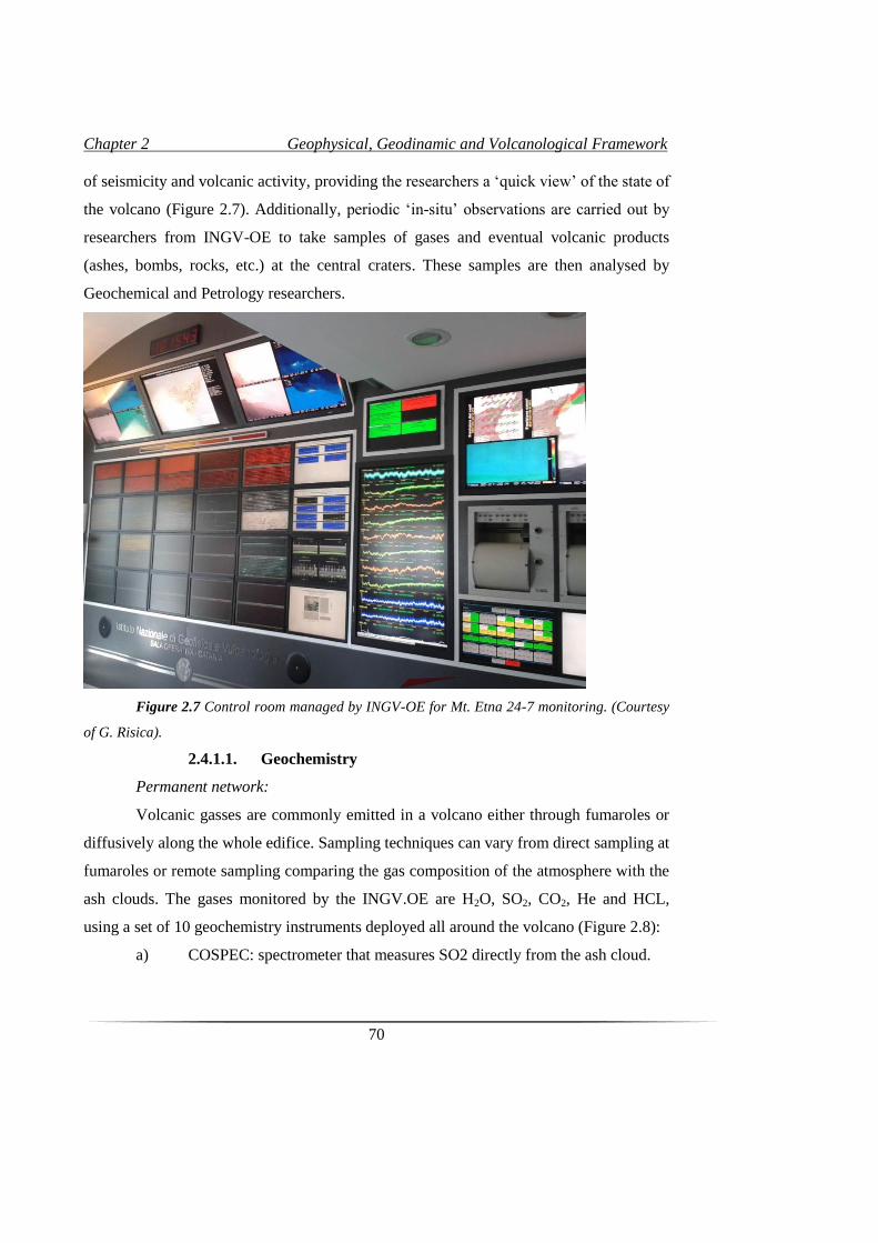
Chapter 2 Geophysical, Geodinamic and Volcanological Framework
70
of seismicity and volcanic activity, providing the researchers a ‘quick view’ of the state of
the volcano (Figure 2.7). Additionally, periodic ‘in-situ’ observations are carried out by
researchers from INGV-OE to take samples of gases and eventual volcanic products
(ashes, bombs, rocks, etc.) at the central craters. These samples are then analysed by
Geochemical and Petrology researchers.
Figure 2.7 Control room managed by INGV-OE for Mt. Etna 24-7 monitoring. (Courtesy
of G. Risica).
2.4.1.1. Geochemistry
Permanent network:
Volcanic gasses are commonly emitted in a volcano either through fumaroles or
diffusively along the whole edifice. Sampling techniques can vary from direct sampling at
fumaroles or remote sampling comparing the gas composition of the atmosphere with the
ash clouds. The gases monitored by the INGV.OE are H2O, SO2, CO2, He and HCL,
using a set of 10 geochemistry instruments deployed all around the volcano (Figure 2.8):
a) COSPEC: spectrometer that measures SO2 directly from the ash cloud.
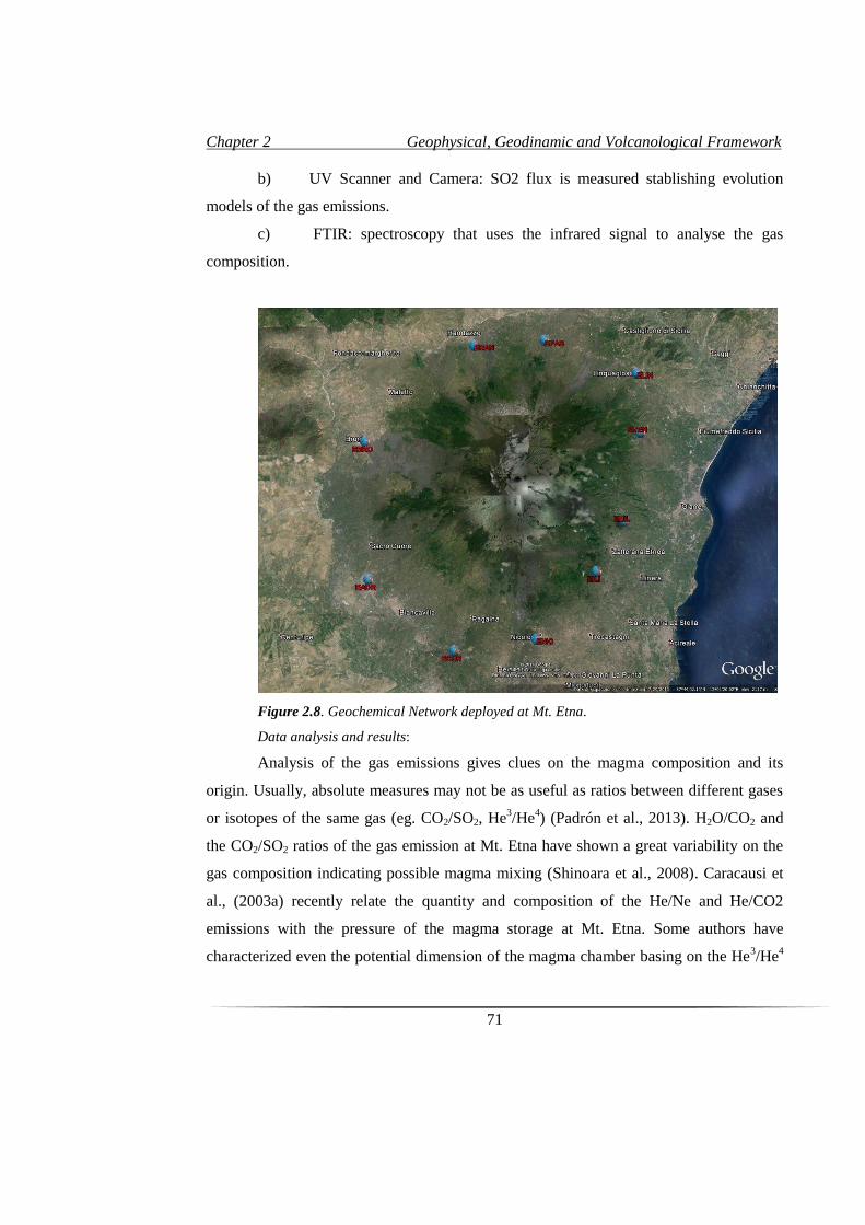
Chapter 2 Geophysical, Geodinamic and Volcanological Framework
71
b) UV Scanner and Camera: SO2 flux is measured stablishing evolution
models of the gas emissions.
c) FTIR: spectroscopy that uses the infrared signal to analyse the gas
composition.
Figure 2.8. Geochemical Network deployed at Mt. Etna.
Data analysis and results:
Analysis of the gas emissions gives clues on the magma composition and its
origin. Usually, absolute measures may not be as useful as ratios between different gases
or isotopes of the same gas (eg. CO2/SO2, He3/He
4) (Padrón et al., 2013). H2O/CO2 and
the CO2/SO2 ratios of the gas emission at Mt. Etna have shown a great variability on the
gas composition indicating possible magma mixing (Shinoara et al., 2008). Caracausi et
al., (2003a) recently relate the quantity and composition of the He/Ne and He/CO2
emissions with the pressure of the magma storage at Mt. Etna. Some authors have
characterized even the potential dimension of the magma chamber basing on the He3/He
4
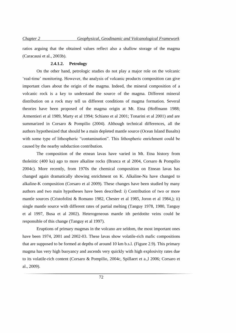
Chapter 2 Geophysical, Geodinamic and Volcanological Framework
72
ratios arguing that the obtained values reflect also a shallow storage of the magma
(Caracausi et al., 2003b).
2.4.1.2. Petrology
On the other hand, petrologic studies do not play a major role on the volcanic
‘real-time’ monitoring. However, the analysis of volcanic products composition can give
important clues about the origin of the magma. Indeed, the mineral composition of a
volcanic rock is a key to understand the source of the magma. Different mineral
distribution on a rock may tell us different conditions of magma formation. Several
theories have been proposed of the magma origin at Mt. Etna (Hoffmann 1988;
Armentieri et al 1989, Marty et al 1994; Schiano et al 2001; Tonarini et al 2001) and are
summarized in Corsaro & Pompilio (2004). Although technical differences, all the
authors hypothesized that should be a main depleted mantle source (Ocean Island Basalts)
with some type of lithospheric “contamination”. This lithospheric enrichment could be
caused by the nearby subduction contribution.
The composition of the etnean lavas have varied in Mt. Etna history from
tholeiitic (400 ka) ago to more alkaline rocks (Branca et al 2004, Corsaro & Pompilio
2004c). More recently, from 1970s the chemical composition on Etnean lavas has
changed again dramatically showing enrichment on K. Alkaline-Na have changed to
alkaline-K composition (Corsaro et al 2009). These changes have been studied by many
authors and two main hypotheses have been described: i) Contribution of two or more
mantle sources (Cristofolini & Romano 1982, Chester et al 1985, Joron et al 1984,); ii)
single mantle source with different rates of partial melting (Tanguy 1978, 1980, Tanguy
et al 1997, Busa et al 2002). Heterogeneous mantle ith peridotite veins could be
responsible of this change (Tanguy et al 1997).
Eruptions of primary magmas in the volcano are seldom, the most important ones
have been 1974, 2001 and 2002-03. These lavas show volatile-rich mafic compositions
that are supposed to be formed at depths of around 10 km b.s.l. (Figure 2.9). This primary
magma has very high buoyancy and ascends very quickly with high explosivity rates due
to its volatile-rich content (Corsaro & Pompilio, 2004c, Spillaert et a.,l 2006; Corsaro et
al., 2009).
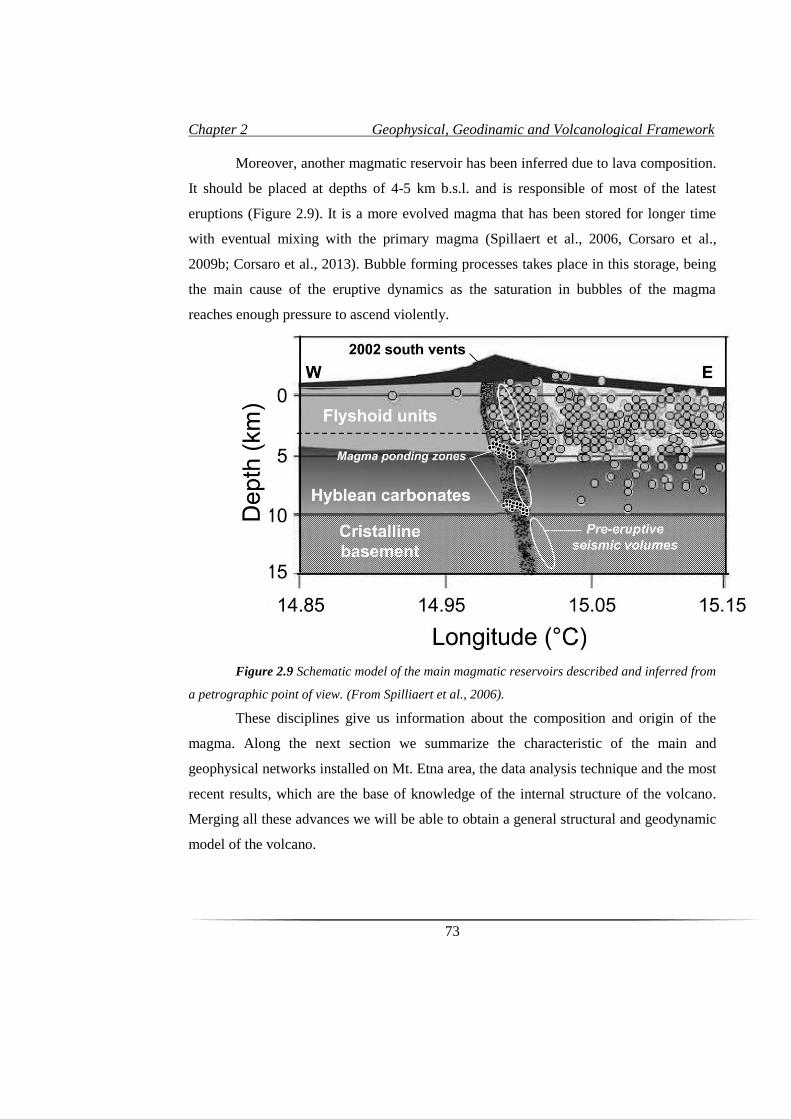
Chapter 2 Geophysical, Geodinamic and Volcanological Framework
73
Moreover, another magmatic reservoir has been inferred due to lava composition.
It should be placed at depths of 4-5 km b.s.l. and is responsible of most of the latest
eruptions (Figure 2.9). It is a more evolved magma that has been stored for longer time
with eventual mixing with the primary magma (Spillaert et al., 2006, Corsaro et al.,
2009b; Corsaro et al., 2013). Bubble forming processes takes place in this storage, being
the main cause of the eruptive dynamics as the saturation in bubbles of the magma
reaches enough pressure to ascend violently.
Figure 2.9 Schematic model of the main magmatic reservoirs described and inferred from
a petrographic point of view. (From Spilliaert et al., 2006).
These disciplines give us information about the composition and origin of the
magma. Along the next section we summarize the characteristic of the main and
geophysical networks installed on Mt. Etna area, the data analysis technique and the most
recent results, which are the base of knowledge of the internal structure of the volcano.
Merging all these advances we will be able to obtain a general structural and geodynamic
model of the volcano.
Chapter 2 Geophysical, Geodinamic and Volcanological Framework
74
2.4.2 Geophysical Monitoring
2.4.2.1. Magnetism
The signal registered in a magnetic station is the sum of three main magnetic
fields: i) the principal ii) the external and iii) the local field. The principal magnetic field
is that originated from the Earth core, while the external field is the one that arrives from
the sun. The magnetic local field, the most useful for volcanic monitoring, depends on the
local geology and structures. The main variations of this field on a volcano are caused by
termomagnetic, piezomagnetic, and electrokinetic anomalies. Termomagnetic anomalies
are caused by changes in the temperature of the rocks. Demagnetization appears as the
temperature of the rock is increased up to the Temperature of Curie (TC), when it loses its
magnetization. Therefore, it remains “invisible” for the magnetic sensors.
Remagnetization, on the other hand, occurs when the temperature decrease and the
minerals reach temperatures below the TC and getting magnetized. This type of anomaly
is very useful when a dyke intrusion takes place as the magnetic anomaly gets larger as it
coolest. However, the intrusion itself does not generate a termomagnetic anomaly but a
piezomagnetic one, caused by a sudden change in the stress field. Earthquakes, fractures
or dyke intrusion may lead to a magnetic anomaly of this type. Therefore, if an ongoing
eruption is accompanied by an earthquake swarm, the magnetic anomaly it could be
detected. Nonetheless, if the magma rise by an open conduit without fracturing the host
rock, no magnetic anomaly is registered until the magma coolest.
Magnetic permanent network:
The magnetic permanent network comprises 16 stations deployed following a N-
S profile along the summit craters (Figure 2.10):
1. Scalar (proton) magnetic sensors: measure the intensity of the magnetic
field. Usually used for the local campaigns.
2. Vectorial magnetic sensors: measure the intensity and the components of
the magnetic field.
3. Magnetotelluric sensors: only one, at the moment it does not work due to
technical issues.
4. Geoelectric sensors. Permit the study of the electrocinetic anomalies.
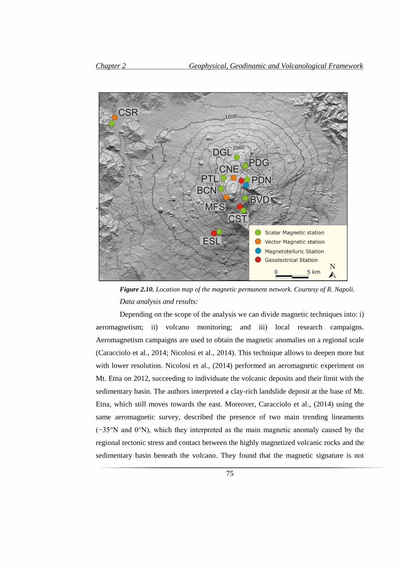
Chapter 2 Geophysical, Geodinamic and Volcanological Framework
75
Figure 2.10. Location map of the magnetic permanent network. Courtesy of R. Napoli.
Data analysis and results:
Depending on the scope of the analysis we can divide magnetic techniques into: i)
aeromagnetism; ii) volcano monitoring; and iii) local research campaigns.
Aeromagnetism campaigns are used to obtain the magnetic anomalies on a regional scale
(Caracciolo et al., 2014; Nicolosi et al., 2014). This technique allows to deepen more but
with lower resolution. Nicolosi et al., (2014) performed an aeromagnetic experiment on
Mt. Etna on 2012, succeeding to individuate the volcanic deposits and their limit with the
sedimentary basin. The authors interpreted a clay-rich landslide deposit at the base of Mt.
Etna, which still moves towards the east. Moreover, Caracciolo et al., (2014) using the
same aeromagnetic survey, described the presence of two main trending lineaments
(−35°N and 0°N), which they interpreted as the main magnetic anomaly caused by the
regional tectonic stress and contact between the highly magnetized volcanic rocks and the
sedimentary basin beneath the volcano. They found that the magnetic signature is not
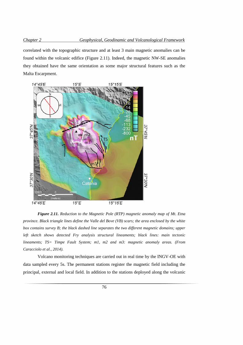
Chapter 2 Geophysical, Geodinamic and Volcanological Framework
76
correlated with the topographic structure and at least 3 main magnetic anomalies can be
found within the volcanic edifice (Figure 2.11). Indeed, the magnetic NW-SE anomalies
they obtained have the same orientation as some major structural features such as the
Malta Escarpment.
Figure 2.11. Reduction to the Magnetic Pole (RTP) magnetic anomaly map of Mt. Etna
province. Black triangle lines define the Valle del Bove (VB) scars; the area enclosed by the white
box contains survey B; the black dashed line separates the two different magnetic domains; upper
left sketch shows detected Fry analysis structural lineaments; black lines: main tectonic
lineaments; TS= Timpe Fault System; m1, m2 and m3: magnetic anomaly areas. (From
Caracciolo et al., 2014).
Volcano monitoring techniques are carried out in real time by the INGV-OE with
data sampled every 5s. The permanent stations register the magnetic field including the
principal, external and local field. In addition to the stations deployed along the volcanic
Chapter 2 Geophysical, Geodinamic and Volcanological Framework
77
edifice, one frame station has been installed 20 km away from the volcanic edifice. This
station is used to correct the principal and external magnetic fields from the recorded
signal in the rest of the stations. In the end, only the local magnetic field registered on the
permanent network is analysed. The permanent network installed on the volcano
registered some magnetic anomalies during the 2002-03 flank eruption. The anomalies
were first visible at PDN station and later registered by the PDG station. Del Negro et al.,
(2004) analysed these piezomagnetic anomalies and modelled the possible sources. As
the anomaly propagated towards the north-east, a series of NE-SW dike intrusions were
interpreted.
Magnetic modelling allowed Napoli et al., (2008) to “image” a magmatic
intrusion during the 2008 eruption. Piezomagnetic anomalies were registered at different
stations of the permanent network during the onset of this eruption. Seismic activity and
deformation rates helped to constrain the source that resulted in a NW-SE magmatic
intrusion located north-westward from the summit craters (Figure 2.12).
Local magnetic campaigns are usually carried by INGV-OE and involved small
shallow (up to 1 km depth) areas where high resolution is necessary (as shallow dike
structures activated during the eruptions (Del Negro et al., 2004). In this case, proton
magnetometers are used to register the local magnetic field. Several local experiments
have been performed in Mt. Etna volcanic edifice (Del Negro & Napoli, 2002; Del Negro
et al., 2002). Del Negro & Napoli, (2002) carried out a magnetic experiment that covered
the eastern flank of the volcano, including an offshore area. This study defines a wide
volcanoclastic deposit on the eastern flank (Chiancone deposit), interpreted as due to a
catastrophic event occurred in the past. Additionally, Del Negro et al., (2002) studied the
same region, and observed some highly magnetized materials interpreted as volcanic
lavas. These lavas are deposit following a NW-SE orientation, which results to be
coherent with Timpe fault system which is considered the onshore expression of the
Ibleo-Maltese Escarpment. Indeed, the authors interpret that the Malta Escarpment is the
responsible of a highly fractured crust area that has been used by the magma as a
preferential path. These volcanic bodies are located offshore and are related to the
Hyblean Plateau.
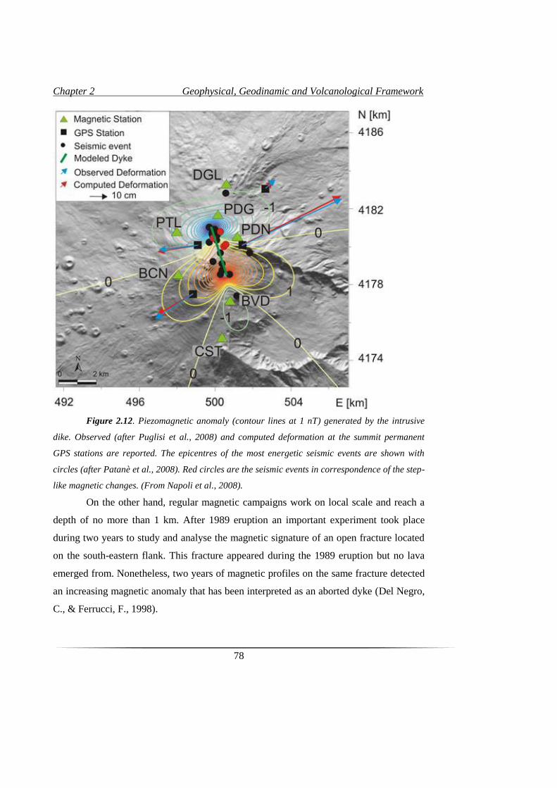
Chapter 2 Geophysical, Geodinamic and Volcanological Framework
78
Figure 2.12. Piezomagnetic anomaly (contour lines at 1 nT) generated by the intrusive
dike. Observed (after Puglisi et al., 2008) and computed deformation at the summit permanent
GPS stations are reported. The epicentres of the most energetic seismic events are shown with
circles (after Patanè et al., 2008). Red circles are the seismic events in correspondence of the step-
like magnetic changes. (From Napoli et al., 2008).
On the other hand, regular magnetic campaigns work on local scale and reach a
depth of no more than 1 km. After 1989 eruption an important experiment took place
during two years to study and analyse the magnetic signature of an open fracture located
on the south-eastern flank. This fracture appeared during the 1989 eruption but no lava
emerged from. Nonetheless, two years of magnetic profiles on the same fracture detected
an increasing magnetic anomaly that has been interpreted as an aborted dyke (Del Negro,
C., & Ferrucci, F., 1998).
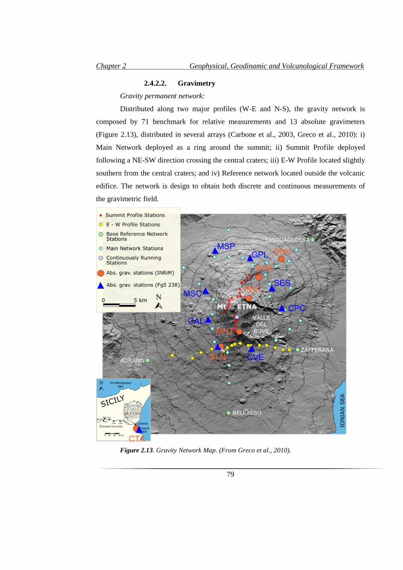
Chapter 2 Geophysical, Geodinamic and Volcanological Framework
79
2.4.2.2. Gravimetry
Gravity permanent network:
Distributed along two major profiles (W-E and N-S), the gravity network is
composed by 71 benchmark for relative measurements and 13 absolute gravimeters
(Figure 2.13), distributed in several arrays (Carbone et al., 2003, Greco et al., 2010): i)
Main Network deployed as a ring around the summit; ii) Summit Profile deployed
following a NE-SW direction crossing the central craters; iii) E-W Profile located slightly
southern from the central craters; and iv) Reference network located outside the volcanic
edifice. The network is design to obtain both discrete and continuous measurements of
the gravimetric field.
Figure 2.13. Gravity Network Map. (From Greco et al., 2010).
Chapter 2 Geophysical, Geodinamic and Volcanological Framework
80
-Data analysis and results:
The analysis of the microgravimetric data (±1mGal) is based on the anomalies of
the gravimetric values from a theoretical model. Nonetheless, several cases of
microgravity changes without any significant deformation have been detected. Many
authors have hypothesized the processes responsible of that behaviour (Carbone et al.,
2014; Currenti & Williams, 2014). A magma intrusion into void spaces could be one of
them (Johnson et al., 2010), but also significant changes on the density of magma bodies
could be responsible of the same effect (Battaglia et al., 2008a). Currenti & Williams,
(2014) propose and study the role of magma compressibility and source geometry effects
in the microgravity and deformation relationship. On the other hand, Carbone et al.,
(2014) suggest that microgravity changes without ground deformation could be related
with changes in the fracturing rate of the medium. This increase of fracturing may lead to
a new magma path.
Usually, both deformation and gravity data are analysed together, as they are in
many cases related. Bonaccorso et al., (2011) combined gravimetric and geodetic
measurements to analyse a seven-year period before the 2001 eruption. This analysis
enlightens a period of intense magmatic recharge characterized by a positive gravimetric
anomaly and an overall inflation of the volcanic edifice. An increase in the microgravity
values is related to a mass increase underneath the volcano, and is usually interpreted for
the case of Mt. Etna as a new magma intrusion or a recharge of the magmatic reservoir.
Moreover, gravity and seismology are also complementary techniques as postulated by
Carbone et al., (2009), who analysed together gravity and seismic data to model the long
term behaviour of the volcano.
2.4.2.3. Geodesy
Geodesy permanent network:
Geodetic Network aims to monitor the deformations on the volcano edifice as
well as some important structural systems (among these PPFS, Tremestieri – Trecastagni
- S. Gregorio fault system and Timpe fault system) whose activity is considered strictly
related to volcano dynamics. This network detects small changes on the surface of the
Chapter 2 Geophysical, Geodinamic and Volcanological Framework
81
edifice using: i) levelling; ii) clinometry; iii) global positioning system (GPS) and; iv)
interferometric synthetic aperture radar (InSAR) techniques (Puglisi et al., 2004).
The deformation network on Mt. Etna exists since the 1980s and during time, it
has gradually improved its coverage. From 1980 to 1988 it was composed of a series of
EDM stations that were distributed in three areas around the volcano. Since the early
1990s GPS sensors were installed improving dramatically the quantity and quality of the
data. Currently ca. 40 GPS stations, together with 13 biaxial electronic tiltmeters and 4
dilatometers are deployed all around the volcano (Figure 2.14). Additionally 80 GPS
benchmarks are available to perform local short-term experiments. GPS sensors measure
the spatial variations of the benchmark using satellites information sampling every 30 s.
Among other contributions, this daily sampling of the GPS data allows measuring the
average site velocity (Palano et al., 2010). The permanent tilt network at Mt. Etna is
installed in shallow boreholes (Bonaccorso et al., 1999). Precision of the tilt network is
around 0.2-0.5 μrad (for shallow sensors) and 0.05 μrad (for depth sensors), including
temperature and thermoelastic effects (Bonaccorso et al., 1999). For the tilt network the
sampling rate varies from 1 to 10 min. Data is recorded using static, quick-static or
kinematic measures. On the other side dilatometers are deployed in boreholes at 300 m
depth and measure the ground dilatation.
Currently, the stations are deployed following a series of frame network and
subnetworks that allow the study both the whole edifice and small structures (Puglisi et
al., 2004):
a- Frame network: a series of stations installed on the surrounding areas of
Mt. Etna that form part of a larger regional network. This network registers in static
mode.
b- Principal inner network: It is composed by around 18 station covering the
edifice from 600 to 2900 m above sea level (a.s.l.). It is connected both to the frame and
the gravimetric networks and it is mainly used to monitor the deformation of the whole
edifice.
c- East-West Kinematic Profile: ca. 15 stations located along an E-W profile
from 600 to 2000 m a.s.l.. Kinematic measures are performed with these sensors.
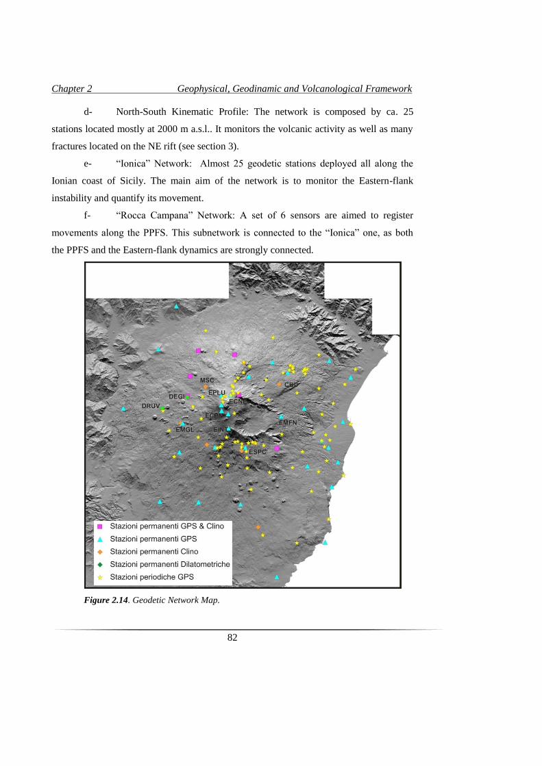
Chapter 2 Geophysical, Geodinamic and Volcanological Framework
82
d- North-South Kinematic Profile: The network is composed by ca. 25
stations located mostly at 2000 m a.s.l.. It monitors the volcanic activity as well as many
fractures located on the NE rift (see section 3).
e- “Ionica” Network: Almost 25 geodetic stations deployed all along the
Ionian coast of Sicily. The main aim of the network is to monitor the Eastern-flank
instability and quantify its movement.
f- “Rocca Campana” Network: A set of 6 sensors are aimed to register
movements along the PPFS. This subnetwork is connected to the “Ionica” one, as both
the PPFS and the Eastern-flank dynamics are strongly connected.
Figure 2.14. Geodetic Network Map.
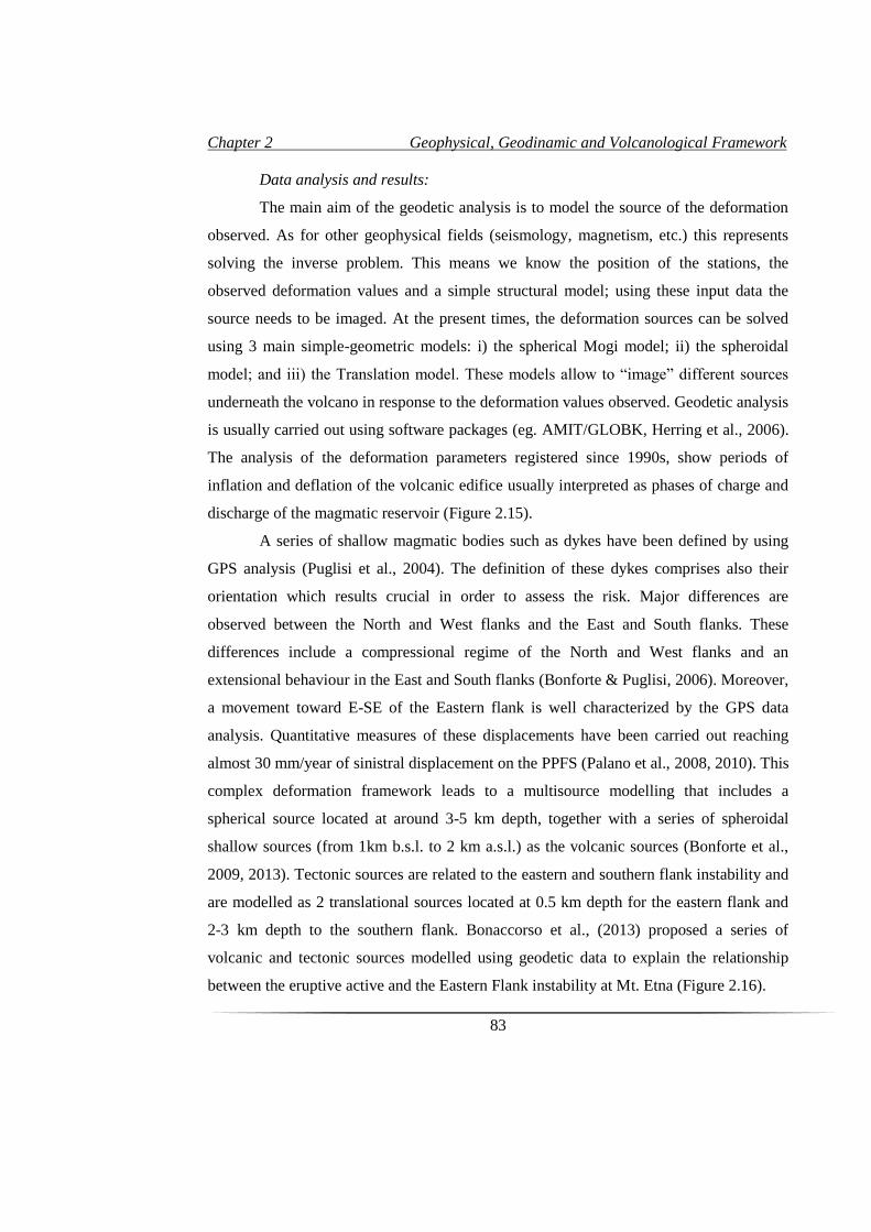
Chapter 2 Geophysical, Geodinamic and Volcanological Framework
83
Data analysis and results:
The main aim of the geodetic analysis is to model the source of the deformation
observed. As for other geophysical fields (seismology, magnetism, etc.) this represents
solving the inverse problem. This means we know the position of the stations, the
observed deformation values and a simple structural model; using these input data the
source needs to be imaged. At the present times, the deformation sources can be solved
using 3 main simple-geometric models: i) the spherical Mogi model; ii) the spheroidal
model; and iii) the Translation model. These models allow to “image” different sources
underneath the volcano in response to the deformation values observed. Geodetic analysis
is usually carried out using software packages (eg. AMIT/GLOBK, Herring et al., 2006).
The analysis of the deformation parameters registered since 1990s, show periods of
inflation and deflation of the volcanic edifice usually interpreted as phases of charge and
discharge of the magmatic reservoir (Figure 2.15).
A series of shallow magmatic bodies such as dykes have been defined by using
GPS analysis (Puglisi et al., 2004). The definition of these dykes comprises also their
orientation which results crucial in order to assess the risk. Major differences are
observed between the North and West flanks and the East and South flanks. These
differences include a compressional regime of the North and West flanks and an
extensional behaviour in the East and South flanks (Bonforte & Puglisi, 2006). Moreover,
a movement toward E-SE of the Eastern flank is well characterized by the GPS data
analysis. Quantitative measures of these displacements have been carried out reaching
almost 30 mm/year of sinistral displacement on the PPFS (Palano et al., 2008, 2010). This
complex deformation framework leads to a multisource modelling that includes a
spherical source located at around 3-5 km depth, together with a series of spheroidal
shallow sources (from 1km b.s.l. to 2 km a.s.l.) as the volcanic sources (Bonforte et al.,
2009, 2013). Tectonic sources are related to the eastern and southern flank instability and
are modelled as 2 translational sources located at 0.5 km depth for the eastern flank and
2-3 km depth to the southern flank. Bonaccorso et al., (2013) proposed a series of
volcanic and tectonic sources modelled using geodetic data to explain the relationship
between the eruptive active and the Eastern Flank instability at Mt. Etna (Figure 2.16).
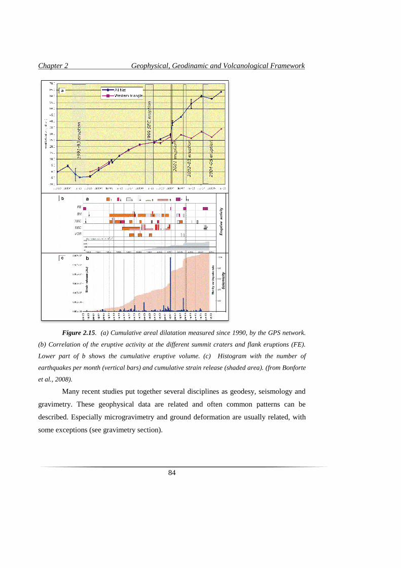
Chapter 2 Geophysical, Geodinamic and Volcanological Framework
84
Figure 2.15. (a) Cumulative areal dilatation measured since 1990, by the GPS network.
(b) Correlation of the eruptive activity at the different summit craters and flank eruptions (FE).
Lower part of b shows the cumulative eruptive volume. (c) Histogram with the number of
earthquakes per month (vertical bars) and cumulative strain release (shaded area). (from Bonforte
et al., 2008).
Many recent studies put together several disciplines as geodesy, seismology and
gravimetry. These geophysical data are related and often common patterns can be
described. Especially microgravimetry and ground deformation are usually related, with
some exceptions (see gravimetry section).
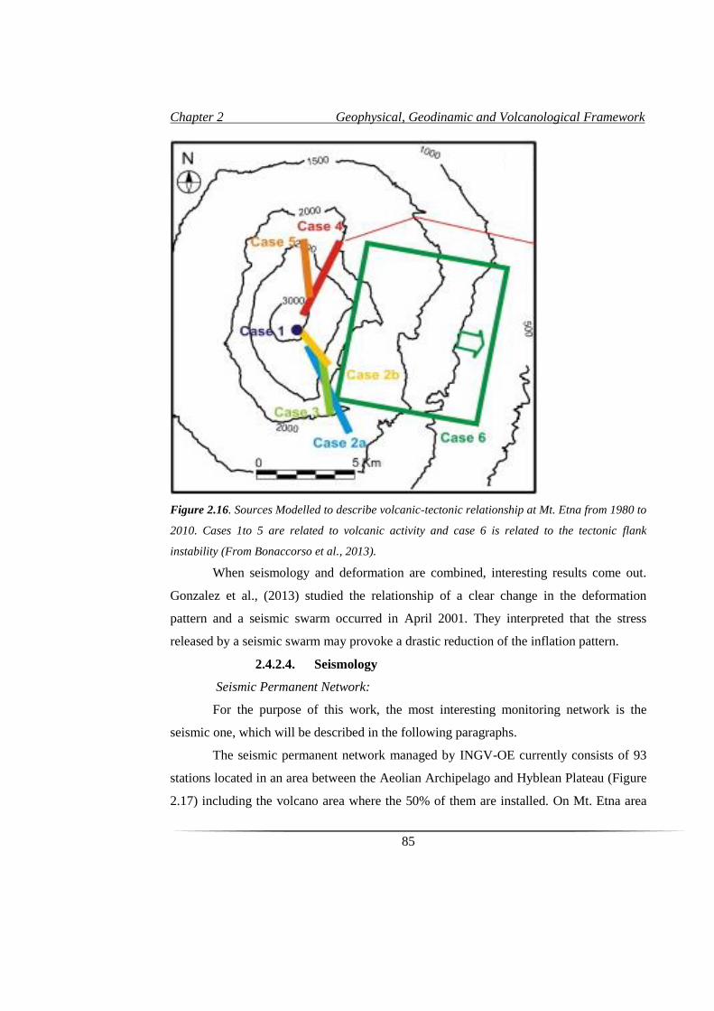
Chapter 2 Geophysical, Geodinamic and Volcanological Framework
85
Figure 2.16. Sources Modelled to describe volcanic-tectonic relationship at Mt. Etna from 1980 to
2010. Cases 1to 5 are related to volcanic activity and case 6 is related to the tectonic flank
instability (From Bonaccorso et al., 2013).
When seismology and deformation are combined, interesting results come out.
Gonzalez et al., (2013) studied the relationship of a clear change in the deformation
pattern and a seismic swarm occurred in April 2001. They interpreted that the stress
released by a seismic swarm may provoke a drastic reduction of the inflation pattern.
2.4.2.4. Seismology
Seismic Permanent Network:
For the purpose of this work, the most interesting monitoring network is the
seismic one, which will be described in the following paragraphs.
The seismic permanent network managed by INGV-OE currently consists of 93
stations located in an area between the Aeolian Archipelago and Hyblean Plateau (Figure
2.17) including the volcano area where the 50% of them are installed. On Mt. Etna area
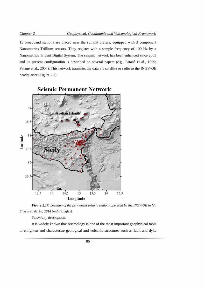
Chapter 2 Geophysical, Geodinamic and Volcanological Framework
86
13 broadband stations are placed near the summit craters, equipped with 3 component
Nanometrics Trillium sensors. They register with a sample frequency of 100 Hz by a
Nanometrics Trident Digital System. The seismic network has been enhanced since 2003
and its present configuration is described on several papers (e.g., Patanè et al., 1999;
Patanè et al., 2004). This network transmits the data via satellite or radio to the INGV-OE
headquarter (Figure 2.7).
Figure 2.17. Location of the permanent seismic stations operated by the INGV-OE in Mt.
Etna area during 2014 (red triangles).
Seismicity description:
It is widely known that seismology is one of the most important geophysical tools
to enlighten and characterize geological and volcanic structures such as fault and dyke
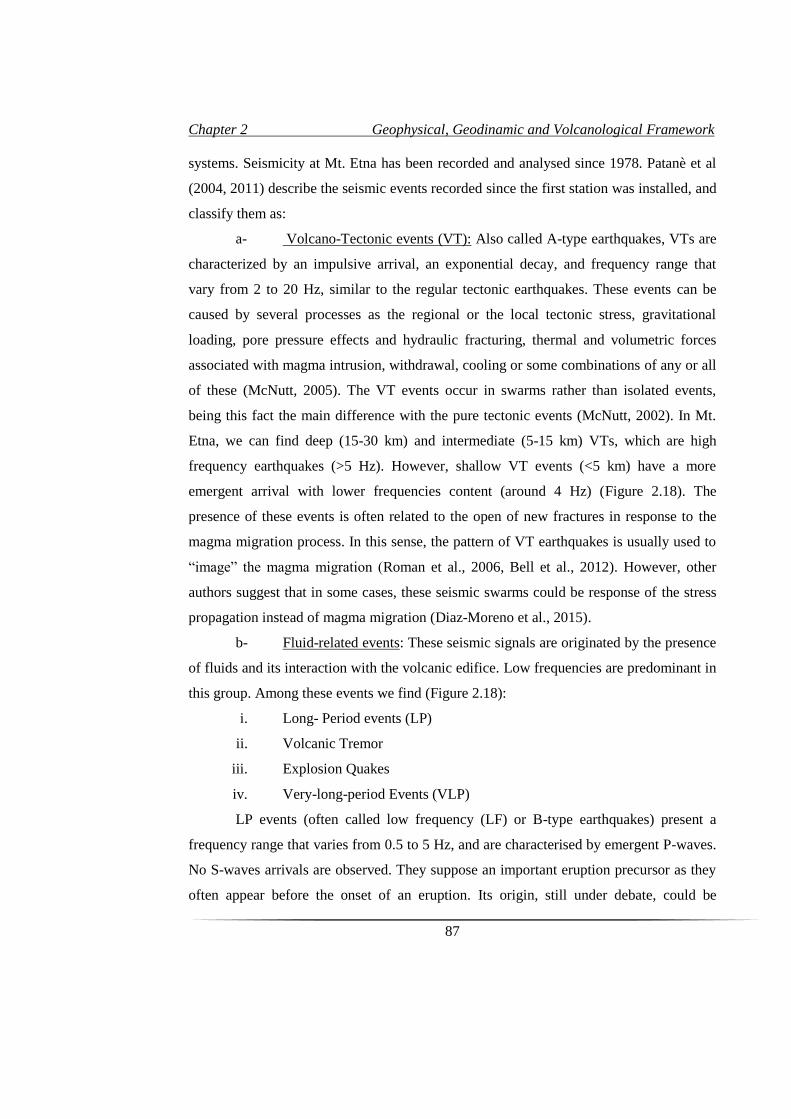
Chapter 2 Geophysical, Geodinamic and Volcanological Framework
87
systems. Seismicity at Mt. Etna has been recorded and analysed since 1978. Patanè et al
(2004, 2011) describe the seismic events recorded since the first station was installed, and
classify them as:
a- Volcano-Tectonic events (VT): Also called A-type earthquakes, VTs are
characterized by an impulsive arrival, an exponential decay, and frequency range that
vary from 2 to 20 Hz, similar to the regular tectonic earthquakes. These events can be
caused by several processes as the regional or the local tectonic stress, gravitational
loading, pore pressure effects and hydraulic fracturing, thermal and volumetric forces
associated with magma intrusion, withdrawal, cooling or some combinations of any or all
of these (McNutt, 2005). The VT events occur in swarms rather than isolated events,
being this fact the main difference with the pure tectonic events (McNutt, 2002). In Mt.
Etna, we can find deep (15-30 km) and intermediate (5-15 km) VTs, which are high
frequency earthquakes (>5 Hz). However, shallow VT events (<5 km) have a more
emergent arrival with lower frequencies content (around 4 Hz) (Figure 2.18). The
presence of these events is often related to the open of new fractures in response to the
magma migration process. In this sense, the pattern of VT earthquakes is usually used to
“image” the magma migration (Roman et al., 2006, Bell et al., 2012). However, other
authors suggest that in some cases, these seismic swarms could be response of the stress
propagation instead of magma migration (Diaz-Moreno et al., 2015).
b- Fluid-related events: These seismic signals are originated by the presence
of fluids and its interaction with the volcanic edifice. Low frequencies are predominant in
this group. Among these events we find (Figure 2.18):
i. Long- Period events (LP)
ii. Volcanic Tremor
iii. Explosion Quakes
iv. Very-long-period Events (VLP)
LP events (often called low frequency (LF) or B-type earthquakes) present a
frequency range that varies from 0.5 to 5 Hz, and are characterised by emergent P-waves.
No S-waves arrivals are observed. They suppose an important eruption precursor as they
often appear before the onset of an eruption. Its origin, still under debate, could be
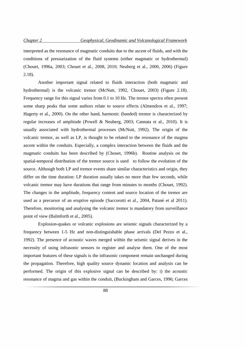
Chapter 2 Geophysical, Geodinamic and Volcanological Framework
88
interpreted as the resonance of magmatic conduits due to the ascent of fluids, and with the
conditions of pressurization of the fluid systems (either magmatic or hydrothermal)
(Chouet, 1996a, 2003; Chouet et al., 2008, 2010; Neuberg et al., 2000, 2006) (Figure
2.18).
Another important signal related to fluids interaction (both magmatic and
hydrothermal) is the volcanic tremor (McNutt, 1992, Chouet, 2003) (Figure 2.18).
Frequency range for this signal varies from 0.1 to 10 Hz. The tremor spectra often present
some sharp peaks that some authors relate to source effects (Almendros et al., 1997;
Hagerty et al., 2000). On the other hand, harmonic (banded) tremor is characterized by
regular increases of amplitude (Powell & Neuberg, 2003; Cannata et al., 2010). It is
usually associated with hydrothermal processes (McNutt, 1992). The origin of the
volcanic tremor, as well as LP, is thought to be related to the resonance of the magma
ascent within the conduits. Especially, a complex interaction between the fluids and the
magmatic conduits has been described by (Chouet, 1996b). Routine analysis on the
spatial-temporal distribution of the tremor source is used to follow the evolution of the
source. Although both LP and tremor events share similar characteristics and origin, they
differ on the time duration: LP duration usually takes no more than few seconds, while
volcanic tremor may have durations that range from minutes to months (Chouet, 1992).
The changes in the amplitude, frequency content and source location of the tremor are
used as a precursor of an eruptive episode (Saccorotti et al., 2004, Patanè et al 2011).
Therefore, monitoring and analysing the volcanic tremor is mandatory from surveillance
point of view (Balmforth et al., 2005).
Explosion-quakes or volcanic explosions are seismic signals characterized by a
frequency between 1-5 Hz and non-distinguishable phase arrivals (Del Pezzo et al.,
1992). The presence of acoustic waves merged within the seismic signal derives in the
necessity of using infrasonic sensors to register and analyse them. One of the most
important features of these signals is the infrasonic component remain unchanged during
the propagation. Therefore, high quality source dynamic location and analysis can be
performed. The origin of this explosive signal can be described by: i) the acoustic
resonance of magma and gas within the conduit, (Buckingham and Garces, 1996; Garces
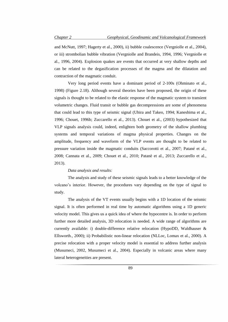
Chapter 2 Geophysical, Geodinamic and Volcanological Framework
89
and McNutt, 1997; Hagerty et al., 2000), ii) bubble coalescence (Vergniolle et al., 2004),
or iii) strombolian bubble vibration (Vergniolle and Brandeis, 1994, 1996; Vergniolle et
al., 1996, 2004). Explosion quakes are events that occurred at very shallow depths and
can be related to the degasification processes of the magma and the dilatation and
contraction of the magmatic conduit.
Very long period events have a dominant period of 2-100s (Ohminato et al.,
1998) (Figure 2.18). Although several theories have been proposed, the origin of these
signals is thought to be related to the elastic response of the magmatic system to transient
volumetric changes. Fluid transit or bubble gas decompressions are some of phenomena
that could lead to this type of seismic signal (Uhira and Takeo, 1994; Kaneshima et al.,
1996; Chouet, 1996b; Zuccarello et al., 2013). Chouet et al., (2003) hypothesized that
VLP signals analysis could, indeed, enlighten both geometry of the shallow plumbing
systems and temporal variations of magma physical properties. Changes on the
amplitude, frequency and waveform of the VLP events are thought to be related to
pressure variation inside the magmatic conduits (Saccorotti et al., 2007; Patané et al.,
2008; Cannata et al., 2009; Chouet et al., 2010; Patanè et al., 2013; Zuccarello et al.,
2013).
Data analysis and results:
The analysis and study of these seismic signals leads to a better knowledge of the
volcano’s interior. However, the procedures vary depending on the type of signal to
study.
The analysis of the VT events usually begins with a 1D location of the seismic
signal. It is often performed in real time by automatic algorithms using a 1D generic
velocity model. This gives us a quick idea of where the hypocentre is. In order to perform
further more detailed analysis, 3D relocation is needed. A wide range of algorithms are
currently available: i) double-difference relative relocation (HypoDD, Waldhauser &
Ellsworth., 2000); ii) Probabilistic non-linear relocation (NLLoc, Lomax et al., 2000). A
precise relocation with a proper velocity model is essential to address further analysis
(Musumeci, 2002, Musumeci et al., 2004). Especially in volcanic areas where many
lateral heterogeneities are present.
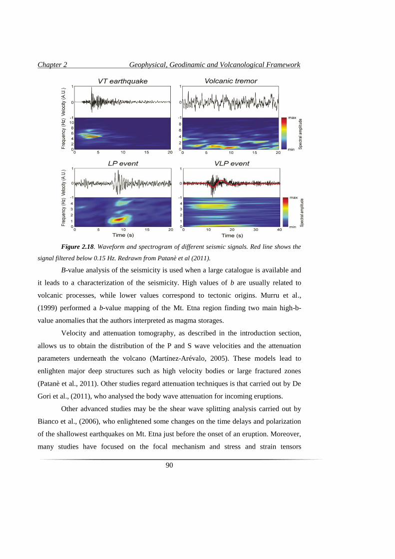
Chapter 2 Geophysical, Geodinamic and Volcanological Framework
90
Figure 2.18. Waveform and spectrogram of different seismic signals. Red line shows the
signal filtered below 0.15 Hz. Redrawn from Patanè et al (2011).
B-value analysis of the seismicity is used when a large catalogue is available and
it leads to a characterization of the seismicity. High values of b are usually related to
volcanic processes, while lower values correspond to tectonic origins. Murru et al.,
(1999) performed a b-value mapping of the Mt. Etna region finding two main high-b-
value anomalies that the authors interpreted as magma storages.
Velocity and attenuation tomography, as described in the introduction section,
allows us to obtain the distribution of the P and S wave velocities and the attenuation
parameters underneath the volcano (Martínez-Arévalo, 2005). These models lead to
enlighten major deep structures such as high velocity bodies or large fractured zones
(Patanè et al., 2011). Other studies regard attenuation techniques is that carried out by De
Gori et al., (2011), who analysed the body wave attenuation for incoming eruptions.
Other advanced studies may be the shear wave splitting analysis carried out by
Bianco et al., (2006), who enlightened some changes on the time delays and polarization
of the shallowest earthquakes on Mt. Etna just before the onset of an eruption. Moreover,
many studies have focused on the focal mechanism and stress and strain tensors
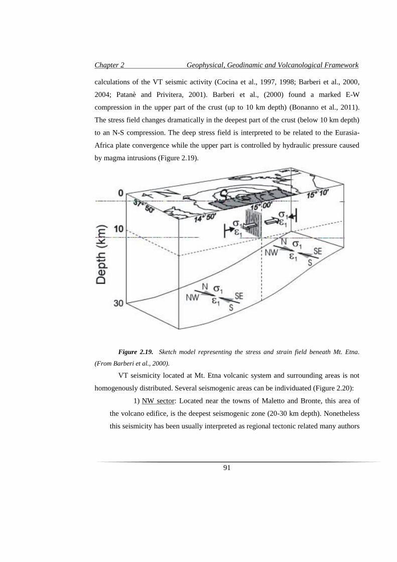
Chapter 2 Geophysical, Geodinamic and Volcanological Framework
91
calculations of the VT seismic activity (Cocina et al., 1997, 1998; Barberi et al., 2000,
2004; Patanè and Privitera, 2001). Barberi et al., (2000) found a marked E-W
compression in the upper part of the crust (up to 10 km depth) (Bonanno et al., 2011).
The stress field changes dramatically in the deepest part of the crust (below 10 km depth)
to an N-S compression. The deep stress field is interpreted to be related to the Eurasia-
Africa plate convergence while the upper part is controlled by hydraulic pressure caused
by magma intrusions (Figure 2.19).
Figure 2.19. Sketch model representing the stress and strain field beneath Mt. Etna.
(From Barberi et al., 2000).
VT seismicity located at Mt. Etna volcanic system and surrounding areas is not
homogenously distributed. Several seismogenic areas can be individuated (Figure 2.20):
1) NW sector: Located near the towns of Maletto and Bronte, this area of
the volcano edifice, is the deepest seismogenic zone (20-30 km depth). Nonetheless
this seismicity has been usually interpreted as regional tectonic related many authors
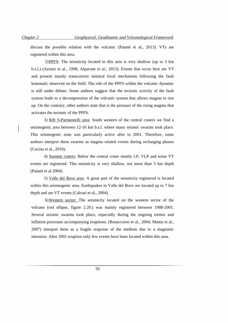
Chapter 2 Geophysical, Geodinamic and Volcanological Framework
92
discuss the possible relation with the volcanic (Patanè et al., 2013). VTs are
registered within this area.
2) PPFS: The seismicity located in this area is very shallow (up to 3 km
b.s.l.) (Azzaro et al., 1998; Alparone et al., 2013). Events that occur here are VT
and present mainly transcurrent sinistral focal mechanism following the fault
kinematic observed on the field. The role of the PPFS within the volcanic dynamic
is still under debate. Some authors suggest that the tectonic activity of the fault
system leads to a decompression of the volcanic system that allows magma to rise
up. On the contrary, other authors state that is the pressure of the rising magma that
activates the tectonic of the PPFS.
3) Rift S-Parmentelli area: South western of the central craters we find a
seismogenic area between 12-16 km b.s.l. where many seismic swarms took place.
This seismogenic zone was particularly active after to 2001. Therefore, some
authors interpret these swarms as magma related events during recharging phases
(Cocina et al., 2010).
4) Summit craters: Below the central crater mostly LP, VLP and some VT
events are registered. This seismicity is very shallow, not more than 5 km depth
(Patanè et al 2004).
5) Valle del Bove area: A great part of the seismicity registered is located
within this seismogenic area. Earthquakes in Valle del Bove are located up to 7 km
depth and are VT events (Calvari et al., 2004).
6) Western sector: The seismicity located on the western sector of the
volcano (red ellipse, figure 2.20.) was mainly registered between 1988-2001.
Several seismic swarms took place, especially during the ongoing tremor and
inflation processes accompanying eruptions. (Bonaccorso et al., 2004; Mattia et al.,
2007) interpret them as a fragile response of the medium due to a magmatic
intrusion. After 2001 eruption only few events have been located within this area.
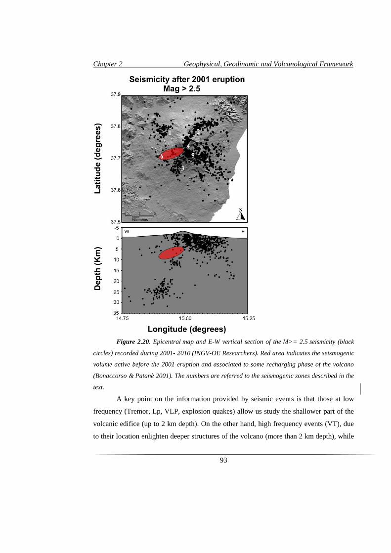
Chapter 2 Geophysical, Geodinamic and Volcanological Framework
93
Figure 2.20. Epicentral map and E-W vertical section of the M>= 2.5 seismicity (black
circles) recorded during 2001- 2010 (INGV-OE Researchers). Red area indicates the seismogenic
volume active before the 2001 eruption and associated to some recharging phase of the volcano
(Bonaccorso & Patanè 2001). The numbers are referred to the seismogenic zones described in the
text.
A key point on the information provided by seismic events is that those at low
frequency (Tremor, Lp, VLP, explosion quakes) allow us study the shallower part of the
volcanic edifice (up to 2 km depth). On the other hand, high frequency events (VT), due
to their location enlighten deeper structures of the volcano (more than 2 km depth), while
Chapter 2 Geophysical, Geodinamic and Volcanological Framework
94
their resolution on the shallower layers is poorer. The analysis of the low frequency
events (LPs, VLPs) is mainly focused on the location of the source and it dimension.
Accurate location is mandatory to develop moment tensor inversions that may shed light
into the source process. As no impulsive P-wave arrival is present, tremor location using
standard procedures is not possible. Therefore, tremor quantitative analysis is carried out
by applying new location methods based on the space distribution of the signal amplitude,
and using modern seismic arrays techniques (Battaglia and Aki, 2003; Di Grazia et al.,
2006; Di Lieto et al, 2006; Carbone et al., 2008). Many techniques are currently available
to assess the LP and VLP location and analysis (Zuccarello, 2015): i) semblance method
(Patanè et al., 2008), ii) seismic array techniques with frequency-slowness analysis
(Metaxian et al., 2002), iii) amplitude decay (Battaglia et al., 2003), iv) coupled inversion
for location and moment tensor (Kumagai et al., 2002), (v) travel time inversion with
improved pick readings achieved through stacking similar events (Saccorotti et al., 2007),
vi) absolute and cross-correlation location (De Barros et al., 2009). These methodologies
may lead to a better knowledge of the plumbing system (Falsaperla et al., 2002; Aiuppa et
al., 2010). Infrasonic events are also studied using advanced techniques that include
spectral analysis, clustering and classification methods, location with semblance method,
etc. (Cannata et al., 2011; Cannata et al., 2013a). Classify the different types of
infrasound events in different families is essential to distinguish different sources and it
can be carried out using SVM method (Langer et al., 2009). After characterising each
type of infrasonic events location methods are used to “image” the source (Cannata et al.,
2013b).
2.5. Geodynamical model of Mt. Etna
The analysis of more than 30 years of geophysical and volcanological data has
leaded to a better understanding of the internal (shallow and deep) structure of Mt. Etna.
There are many ways of getting to know the internal structure of a volcano as discussed
in the Introduction Chapter and along this Chapter. The next paragraphs try to summarize
and clarify a structural and dynamic model of Mt. Etna.
Seismology plays a major role in studying the internal deep structure of a volcano
and due to its relevance to this study we will focus on it. The study of seismic activity
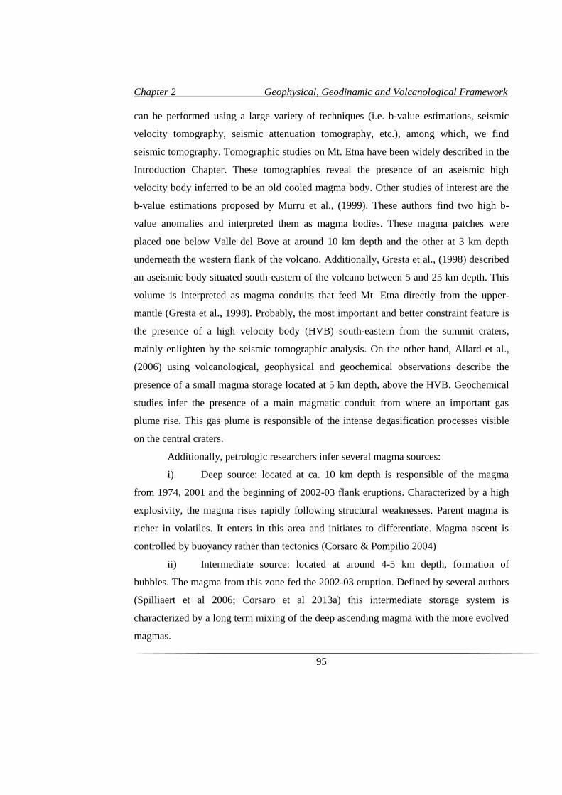
Chapter 2 Geophysical, Geodinamic and Volcanological Framework
95
can be performed using a large variety of techniques (i.e. b-value estimations, seismic
velocity tomography, seismic attenuation tomography, etc.), among which, we find
seismic tomography. Tomographic studies on Mt. Etna have been widely described in the
Introduction Chapter. These tomographies reveal the presence of an aseismic high
velocity body inferred to be an old cooled magma body. Other studies of interest are the
b-value estimations proposed by Murru et al., (1999). These authors find two high b-
value anomalies and interpreted them as magma bodies. These magma patches were
placed one below Valle del Bove at around 10 km depth and the other at 3 km depth
underneath the western flank of the volcano. Additionally, Gresta et al., (1998) described
an aseismic body situated south-eastern of the volcano between 5 and 25 km depth. This
volume is interpreted as magma conduits that feed Mt. Etna directly from the upper-
mantle (Gresta et al., 1998). Probably, the most important and better constraint feature is
the presence of a high velocity body (HVB) south-eastern from the summit craters,
mainly enlighten by the seismic tomographic analysis. On the other hand, Allard et al.,
(2006) using volcanological, geophysical and geochemical observations describe the
presence of a small magma storage located at 5 km depth, above the HVB. Geochemical
studies infer the presence of a main magmatic conduit from where an important gas
plume rise. This gas plume is responsible of the intense degasification processes visible
on the central craters.
Additionally, petrologic researchers infer several magma sources:
i) Deep source: located at ca. 10 km depth is responsible of the magma
from 1974, 2001 and the beginning of 2002-03 flank eruptions. Characterized by a high
explosivity, the magma rises rapidly following structural weaknesses. Parent magma is
richer in volatiles. It enters in this area and initiates to differentiate. Magma ascent is
controlled by buoyancy rather than tectonics (Corsaro & Pompilio 2004)
ii) Intermediate source: located at around 4-5 km depth, formation of
bubbles. The magma from this zone fed the 2002-03 eruption. Defined by several authors
(Spilliaert et al 2006; Corsaro et al 2013a) this intermediate storage system is
characterized by a long term mixing of the deep ascending magma with the more evolved
magmas.

Chapter 2 Geophysical, Geodinamic and Volcanological Framework
96
iii) Shallow source: described as a series of dykes and small stationary
reservoir, is located at depths < 5 km b.s.l depth (Corsaro et al 2013). Forming part of the
intermediate storage, very local short-term magmatic processes occur.
To explain the complex dynamic of Mt. Etna we find at least five models:
1. Tectonic plays a major role through three fault systems (ENE, NNW and
WNW) that intersect. This conjunction of faults produces a weakness zone that allows
magma to rise up (Ritmann, 1973; Cristofolini et al., 1979; Lo Giudice et al., 1982)
(Figure 2.21a).
2. Upwelling of the asthenosphere due to an extensive melting of a mantle
diaper. This model describes the emplacement of tholeiitic magma along the Moho
discontinuity. This magma evolves with time to an alkaline basaltic magma that feeds Mt.
Etna eruptions (Tanguy et al., 1997) (Figure 2.21b).
3. Great volume of magma originated in the asthenospheric part of the
subducted African plate (Gvirtzman and Nur, 1999) (Figure 2.21c). Doglioni et al.,
(2001) postulated a similar model in which a transtensional “window” appears between
the Sicilian and Ionian parts of the Apennines plate.
4. Magma ascent is highly conditioned by extensional stress features. These
structures are related to a series of normal crustal faults placed along the Ionian coast of
Sicily (Monaco et al., 1997, 2005) (Figure 2.21d).
5. The eastern flank to Mt. Etna plays a major role. Geodetic (i.e. GPS and
SAR) analyses have shown sliding movements of this flank towards the shore (Froger et
al., 2001; Lundgren et al., 2003). This area is confined to the north by the Pernicana fault
system and to the south by the NE rift and the Ragalna fault system. It includes the whole
Valle del Bove valley. Some authors postulate that this instability causes a decompression
of the volcano’s interior that allows magma to rise up (Branca et al, 2003; Neri et al.,
2004, Neri and Acocella, 2006). On the other hand, other authors infer that magma
uprising is the cause of this sliding motion and therefore the cause of the instability
(Bonforte and Puglisi, 2003; Neri et al., 2004; Puglisi and Bonforte, 2004; Neri et al.,
2009, (Figure 2.21e). However, the origin of this instability is still under discussion.
Some authors state that there is a shallow slip plane placed at 1 km a.s.l., which is in
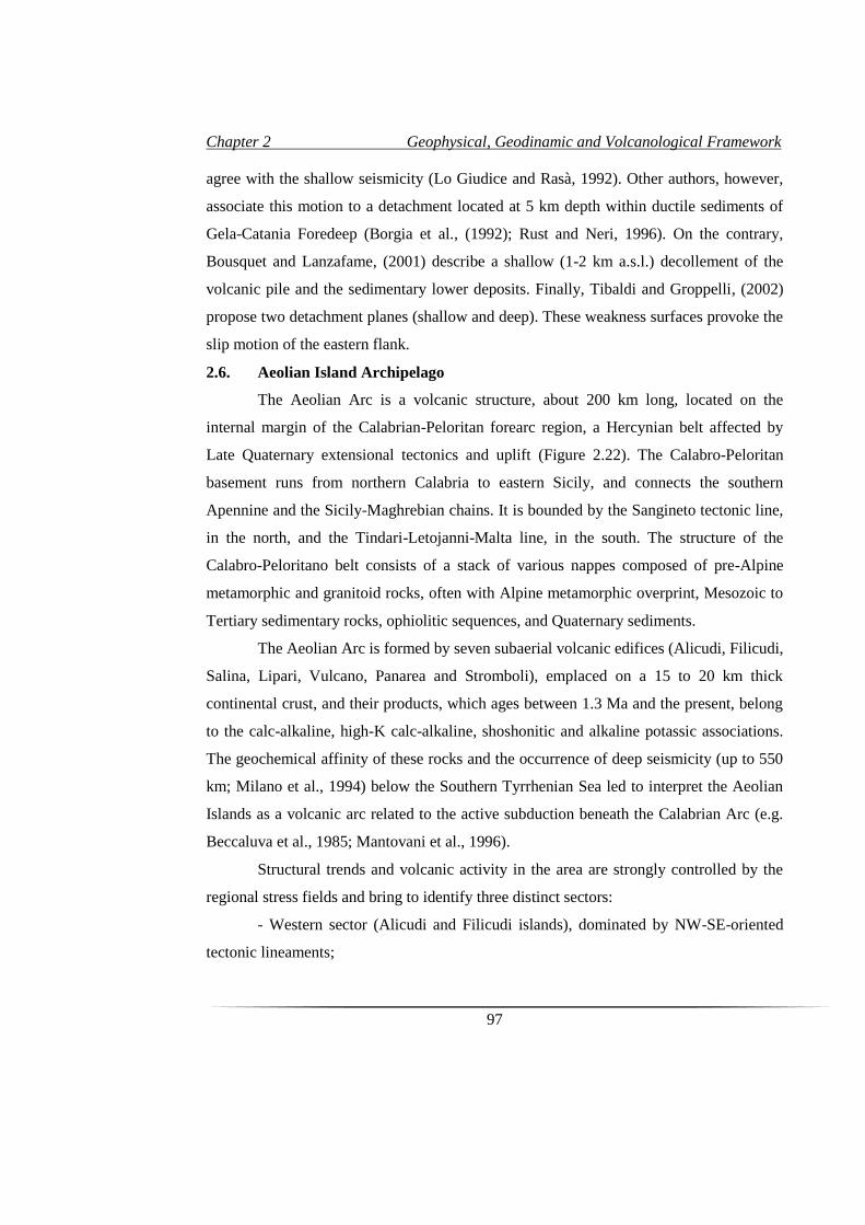
Chapter 2 Geophysical, Geodinamic and Volcanological Framework
97
agree with the shallow seismicity (Lo Giudice and Rasà, 1992). Other authors, however,
associate this motion to a detachment located at 5 km depth within ductile sediments of
Gela-Catania Foredeep (Borgia et al., (1992); Rust and Neri, 1996). On the contrary,
Bousquet and Lanzafame, (2001) describe a shallow (1-2 km a.s.l.) decollement of the
volcanic pile and the sedimentary lower deposits. Finally, Tibaldi and Groppelli, (2002)
propose two detachment planes (shallow and deep). These weakness surfaces provoke the
slip motion of the eastern flank.
2.6. Aeolian Island Archipelago
The Aeolian Arc is a volcanic structure, about 200 km long, located on the
internal margin of the Calabrian-Peloritan forearc region, a Hercynian belt affected by
Late Quaternary extensional tectonics and uplift (Figure 2.22). The Calabro-Peloritan
basement runs from northern Calabria to eastern Sicily, and connects the southern
Apennine and the Sicily-Maghrebian chains. It is bounded by the Sangineto tectonic line,
in the north, and the Tindari-Letojanni-Malta line, in the south. The structure of the
Calabro-Peloritano belt consists of a stack of various nappes composed of pre-Alpine
metamorphic and granitoid rocks, often with Alpine metamorphic overprint, Mesozoic to
Tertiary sedimentary rocks, ophiolitic sequences, and Quaternary sediments.
The Aeolian Arc is formed by seven subaerial volcanic edifices (Alicudi, Filicudi,
Salina, Lipari, Vulcano, Panarea and Stromboli), emplaced on a 15 to 20 km thick
continental crust, and their products, which ages between 1.3 Ma and the present, belong
to the calc-alkaline, high-K calc-alkaline, shoshonitic and alkaline potassic associations.
The geochemical affinity of these rocks and the occurrence of deep seismicity (up to 550
km; Milano et al., 1994) below the Southern Tyrrhenian Sea led to interpret the Aeolian
Islands as a volcanic arc related to the active subduction beneath the Calabrian Arc (e.g.
Beccaluva et al., 1985; Mantovani et al., 1996).
Structural trends and volcanic activity in the area are strongly controlled by the
regional stress fields and bring to identify three distinct sectors:
- Western sector (Alicudi and Filicudi islands), dominated by NW-SE-oriented
tectonic lineaments;
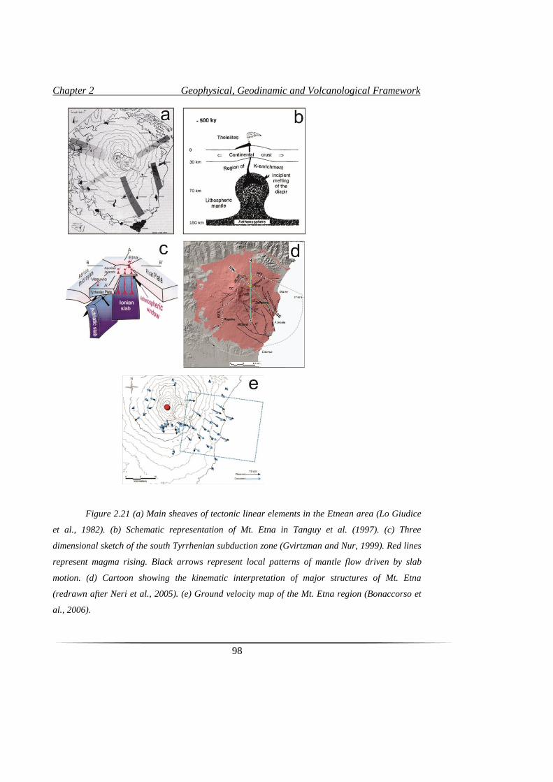
Chapter 2 Geophysical, Geodinamic and Volcanological Framework
98
Figure 2.21 (a) Main sheaves of tectonic linear elements in the Etnean area (Lo Giudice
et al., 1982). (b) Schematic representation of Mt. Etna in Tanguy et al. (1997). (c) Three
dimensional sketch of the south Tyrrhenian subduction zone (Gvirtzman and Nur, 1999). Red lines
represent magma rising. Black arrows represent local patterns of mantle flow driven by slab
motion. (d) Cartoon showing the kinematic interpretation of major structures of Mt. Etna
(redrawn after Neri et al., 2005). (e) Ground velocity map of the Mt. Etna region (Bonaccorso et
al., 2006).
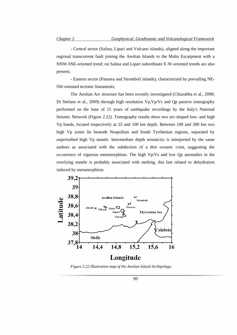
Chapter 2 Geophysical, Geodinamic and Volcanological Framework
99
- Central sector (Salina, Lipari and Vulcano islands), aligned along the important
regional transcurrent fault joining the Aeolian Islands to the Malta Escarpment with a
NNW-SSE-oriented trend; on Salina and Lipari subordinate E-W-oriented trends are also
present;
- Eastern sector (Panarea and Stromboli islands), characterized by prevailing NE-
SW-oriented tectonic lineaments;
The Aeolian Arc structure has been recently investigated (Chiarabba et al., 2008;
Di Stefano et al., 2009) through high resolution Vp,Vp/Vs and Qp passive tomography
performed on the base of 15 years of earthquake recordings by the Italy's National
Seismic Network (Figure 2.22). Tomography results show two arc-shaped low- and high
Vp bands, located respectively at 25 and 100 km depth. Between 100 and 300 km two
high Vp zones lie beneath Neapolitan and South Tyrrhenian regions, separated by
unperturbed high Vp mantle. Intermediate depth seismicity is interpreted by the same
authors as associated with the subduction of a thin oceanic crust, suggesting the
occurrence of vigorous metamorphism. The high Vp/Vs and low Qp anomalies in the
overlying mantle is probably associated with melting, this last related to dehydration
induced by metamorphism.
Figure 2.22 Illustration map of the Aeolian Island Archipelago.

3. TOMO-ETNA
experiment. Joint marine
and on land seismic active
survey

Chapter 3 TOMO-ETNA experiment
103
3.1. The importance of an active seismic tomography in Etna volcano
Mt. Etna is one of the most fascinating natural laboratories for studying the deep
structure of an active volcano using seismic tomography techniques. As described in
Chapter 2, Mt. Etna's eruptive dynamics are the result of a complex interaction between
magma in its plumbing system, the regional (deep crust) tectonic regime, and local
(shallow crust; volcanic edifice) structures, partially controlled by flank instability.
Magma ascent driving conditions (e.g., structural setting, tectonic forces) are not yet
completely understood. One of the main limitations in understanding the volcano's
eruptive dynamics is the insufficient knowledge of its intermediate and deep crust. As
indicated in Ibáñez et al. (2016a) in the last 25 years, several seismic and tomographic
experiments have been focused on the study of Mt. Etna’s structure using different
techniques and data sets. As most volcanoes, natural seismicity’s rate at Mt. Etna is not
very large, therefore, tomographic studies can only be performed with long time periods
of data.
The TOMO-ETNA experiment is an international and multi-institutional joint
effort focused on providing answers to some of the open questions associated to the
structure and dynamic of Mt. Etna (Ibáñez et al., 2016a, 2016b, Coltelli et al., 2016). This
experiment takes the advantage of the use of both active and passive seismic sources and
the combination of information of other seismic and geophysics measurements such as
marine seismic reflection (Coltelli et al., 2016; Firetto-Carlino et al., 2016), or magnetic
profiles (Cavallaro et al., 2016). Additional studies regarding TOMO-ETNA experiment
were focused on seismic array modelling (Zuccarello et al., 2016), seismic attenuation
(Zieger et al., 2016), and even monitoring the Cetacean activity during the marine
activities (Monaco et al., 2016).
A tomography image involves a great amount of seismic data (Lees, 2007)
recorded by a dense seismic network, a requisite often difficult to achieve in a reasonable
time interval due to an absence of seismicity or the lack of stable and dense seismic
networks (e.g Chouet, 1996, 2003; Chouet and Matoza, 2013; MacNutt, 2002, 2005;
Wassermann, 2002; Zobin, 2011). This problem can be solved by planning active seismic
experiments such as we will summarize in this section. Following Koulakov and Shapiro
Chapter 3 TOMO-ETNA experiment
104
(2015), it is possible to use different seismic sources divided into three categories:
human-made sources, earthquakes, and ambient seismic noise. Fully controlled artificial
sources are expected to provide the highest accuracy of tomographic images. At the same
time, their implementation on volcanoes is very sophisticated and expensive. Another
shortcoming of artificial sources is that they cannot be produced at depth. In regions with
well-distributed volcanic or local tectonic seismicity, earthquakes may give a distribution
of sources plausible for high-resolution seismic tomography. However, many volcanoes
do not generate sustained seismicity. Human-made seismic sources include explosions,
vibrators, air-gun shots, and weight (or mass) drops and are usually called active sources.
There are some onshore experiments which use chemical explosions of sufficiently large
magnitude to generate seismic signal propagating to the distances of dozens kilometers
and depths of a few kilometers. The problem of such explosions is that they are fairly
expensive and thus their number is strongly limited. Furthermore, chemical explosions
are not ecologically friendly and they are prohibited in most volcanic areas (Koulakov
and Shapiro, 2015). An alternative method of active-source onshore generation might be
using vibrators which are more ecologically safe compared to explosions. However, for
the purposes of volcano tomography, the vibrators should be sufficiently powerful and
heavy to enable the required propagation of seismic rays. In reality, the transportation of
powerful vibrators appears to be not possible in most volcanic areas; therefore, they are
not widely used in practice. In case a volcano is located close to the seashore, it is
possible to use underwater air-guns as sources of seismic signal. The advantage is that
air-gun shots are rather cheap and sufficiently powerful. They can be frequently generated
along the ship cruise that gives a huge data base with a clear technology of processing.
The main issue is that these sources are limited by the shore line and not suitable for most
volcanoes. The major advantage of the active sources is that their parameters are known.
The problem is that they are located close to the surface, and seismic signal propagate
along the nearly horizontal ray paths. Another difficulty, which is mostly observed for the
air-gun shots, is that they generate very weak S waves that cannot be picked and used for
tomography studies (Koulakov and Shaphiro, 2015).
Chapter 3 TOMO-ETNA experiment
105
In the last 20 years the number of dedicated experiments using active seismic
sources is increasing. In order to give a real dimension of the nature of the TOMO-ETNA
experiment, we summarize some of the most important experiment carried out in active
volcanoes around the word in Table 3.1. In figure 3.1 we plot the position of the
volcanoes described below. An important remark regarding the data analysis of the listed
experiments is that for all of them, first arrival picking has been performed manually.
This fact implies an enormous amount of work in order to produce quality P- and S-wave
travel times and will be discussed in detail along chapter 4.
Coming back to Mt. Etna volcano, Chiarabba et al., (2004) presented a complete
description of the previous active seismic experiments performed in this incredible
scenario. According to these authors, one of the first active seismic studies was done in
1968 to study the seismic refraction structure of Sicily and with only one profile to the
north near Mt. Etna (Cassinis et al., 1969). The first deep seismic sounding focused on
Mt. Etna’s structure was done in 1977 (Colombi et al., 1979). Further, in 1992 an active
seismic experiment was performed with the project ETNASEIS (Hirn et al., 1997;
Nicolich et al., 2000). This experiment consisted on offshore shots aiming to study the
structure of Mt. Etna together with additional profiles to study the Ionian marine basin.
Active seismic signals were generated by 8 air-guns with a power of 840 in3 of volume
shooting along 2 profiles. These shots were carried out with the oceanographic research
vessel N/O LE NADIR of IFREMER (France). Additional shots were carried out by N/O
OGS-EXPLORA vessel along 3 profiles. They shot with 26 guns of a total volume of
3,810 in3. Finally, 2 last profiles were performed using EXPLORA with an industrial-type
air-gun array. Hirn et al (1997) analyzed ETNASEIS data to improve their original
tomography (Hirn, 1991). Unfortunately, due to Etna’s heterogeneity structure together
with some instrumental issues, a convincing velocity model of the volcano edifice was
not obtained.

Chapter 3 TOMO-ETNA experiment
106
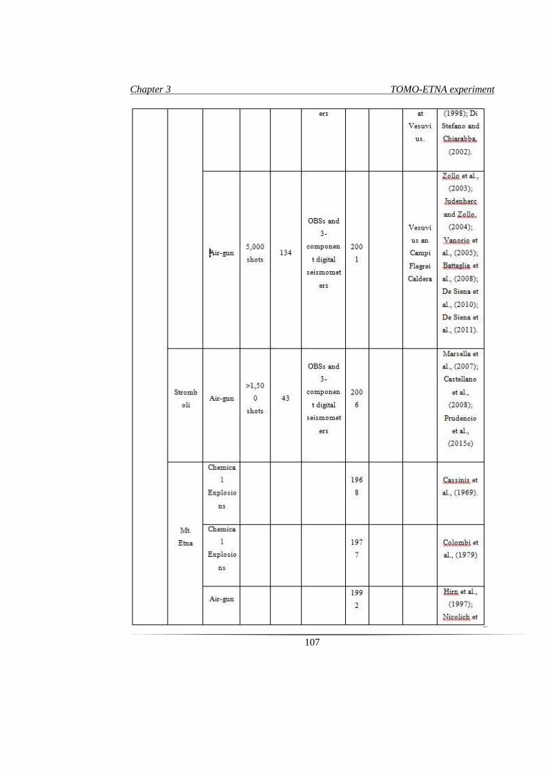
Chapter 3 TOMO-ETNA experiment
107
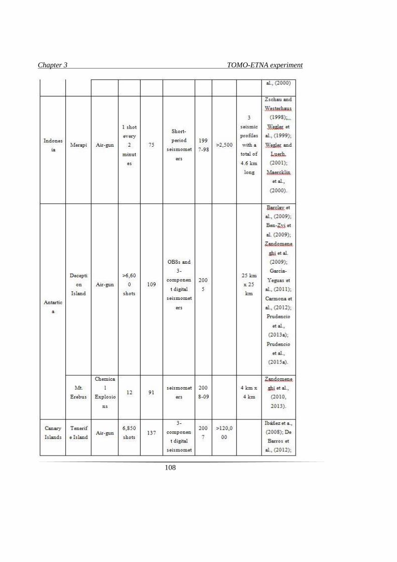
Chapter 3 TOMO-ETNA experiment
108
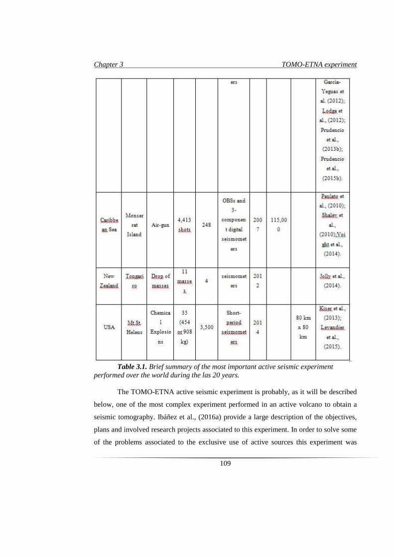
Chapter 3 TOMO-ETNA experiment
109
Table 3.1. Brief summary of the most important active seismic experiment
performed over the world during the las 20 years.
The TOMO-ETNA active seismic experiment is probably, as it will be described
below, one of the most complex experiment performed in an active volcano to obtain a
seismic tomography. Ibáñez et al., (2016a) provide a large description of the objectives,
plans and involved research projects associated to this experiment. In order to solve some
of the problems associated to the exclusive use of active sources this experiment was
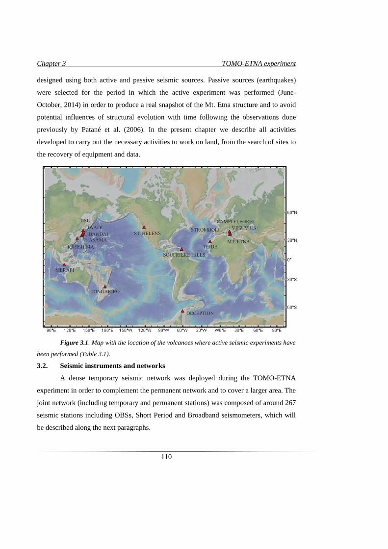
Chapter 3 TOMO-ETNA experiment
110
designed using both active and passive seismic sources. Passive sources (earthquakes)
were selected for the period in which the active experiment was performed (June-
October, 2014) in order to produce a real snapshot of the Mt. Etna structure and to avoid
potential influences of structural evolution with time following the observations done
previously by Patané et al. (2006). In the present chapter we describe all activities
developed to carry out the necessary activities to work on land, from the search of sites to
the recovery of equipment and data.
Figure 3.1. Map with the location of the volcanoes where active seismic experiments have
been performed (Table 3.1).
3.2. Seismic instruments and networks
A dense temporary seismic network was deployed during the TOMO-ETNA
experiment in order to complement the permanent network and to cover a larger area. The
joint network (including temporary and permanent stations) was composed of around 267
seismic stations including OBSs, Short Period and Broadband seismometers, which will
be described along the next paragraphs.
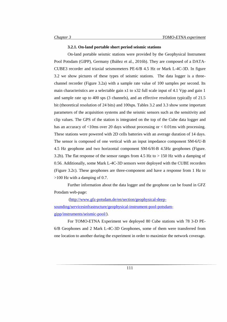
Chapter 3 TOMO-ETNA experiment
111
3.2.1. On-land portable short period seismic stations
On-land portable seismic stations were provided by the Geophysical Instrument
Pool Potsdam (GIPP), Germany (Ibáñez et al., 2016b). They are composed of a DATA-
CUBE3 recorder and triaxial seismometers PE-6/B 4.5 Hz or Mark L-4C-3D. In figure
3.2 we show pictures of these types of seismic stations. The data logger is a three-
channel recorder (Figure 3.2a) with a sample rate value of 100 samples per second. Its
main characteristics are a selectable gain x1 to x32 full scale input of 4.1 Vpp and gain 1
and sample rate up to 400 sps (3 channels), and an effective resolution typically of 21.5
bit (theoretical resolution of 24 bits) and 100sps. Tables 3.2 and 3.3 show some important
parameters of the acquisition systems and the seismic sensors such as the sensitivity and
clip values. The GPS of the station is integrated on the top of the Cube data logger and
has an accuracy of <10ms over 20 days without processing or < 0.01ms with processing.
These stations were powered with 2D cells batteries with an average duration of 14 days.
The sensor is composed of one vertical with an input impedance component SM-6/U-B
4.5 Hz geophone and two horizontal component SM-6/H-B 4.5Hz geophones (Figure.
3.2b). The flat response of the sensor ranges from 4.5 Hz to > 150 Hz with a damping of
0.56. Additionally, some Mark L-4C-3D sensors were deployed with the CUBE recorders
(Figure 3.2c). These geophones are three-component and have a response from 1 Hz to
>100 Hz with a damping of 0.7.
Further information about the data logger and the geophone can be found in GFZ
Potsdam web-page:
(http://www.gfz-potsdam.de/en/section/geophysical-deep-
sounding/servicesinfrastructure/geophysical-instrument-pool-potsdam-
gipp/instruments/seismic-pool/).
For TOMO-ETNA Experiment we deployed 80 Cube stations with 78 3-D PE-
6/B Geophones and 2 Mark L-4C-3D Geophones, some of them were transferred from
one location to another during the experiment in order to maximize the network coverage.
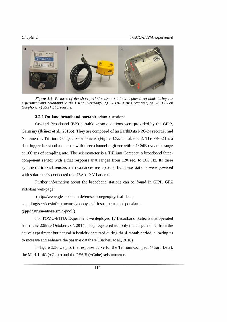
Chapter 3 TOMO-ETNA experiment
112
Figure 3.2. Pictures of the short-period seismic stations deployed on-land during the
experiment and belonging to the GIPP (Germany). a) DATA-CUBE3 recorder, b) 3-D PE-6/B
Geophone, c) Mark L4C sensors.
3.2.2 On-land broadband portable seismic stations
On-land Broadband (BB) portable seismic stations were provided by the GIPP,
Germany (Ibáñez et al., 2016b). They are composed of an EarthData PR6-24 recorder and
Nanometrics Trillium Compact seismometer (Figure 3.3a, b, Table 3.3). The PR6-24 is a
data logger for stand-alone use with three-channel digitizer with a 140dB dynamic range
at 100 sps of sampling rate. The seismometer is a Trillium Compact, a broadband three-
component sensor with a flat response that ranges from 120 sec. to 100 Hz. Its three
symmetric triaxial sensors are resonance-free up 200 Hz. These stations were powered
with solar panels connected to a 75Ah 12 V batteries.
Further information about the broadband stations can be found in GIPP, GFZ
Potsdam web-page:
(http://www.gfz-potsdam.de/en/section/geophysical-deep-
sounding/servicesinfrastructure/geophysical-instrument-pool-potsdam-
gipp/instruments/seismic-pool/)
For TOMO-ETNA Experiment we deployed 17 Broadband Stations that operated
from June 20th to October 28th, 2014. They registered not only the air-gun shots from the
active experiment but natural seismicity occurred during the 4-month period, allowing us
to increase and enhance the passive database (Barberi et al., 2016).
In figure 3.3c we plot the response curve for the Trillium Compact (+EarthData),
the Mark L-4C (+Cube) and the PE6/B (+Cube) seismometers.
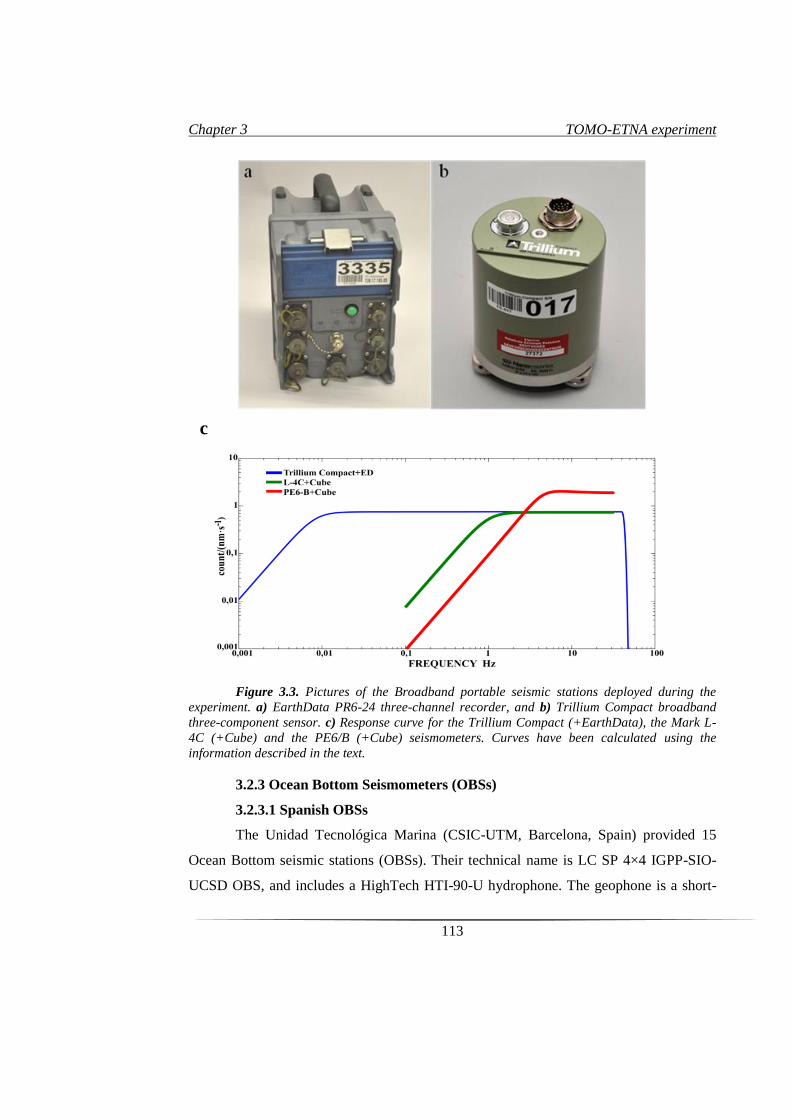
Chapter 3 TOMO-ETNA experiment
113
Figure 3.3. Pictures of the Broadband portable seismic stations deployed during the
experiment. a) EarthData PR6-24 three-channel recorder, and b) Trillium Compact broadband
three-component sensor. c) Response curve for the Trillium Compact (+EarthData), the Mark L-
4C (+Cube) and the PE6/B (+Cube) seismometers. Curves have been calculated using the
information described in the text.
3.2.3 Ocean Bottom Seismometers (OBSs)
3.2.3.1 Spanish OBSs
The Unidad Tecnológica Marina (CSIC-UTM, Barcelona, Spain) provided 15
Ocean Bottom seismic stations (OBSs). Their technical name is LC SP 4×4 IGPP-SIO-
UCSD OBS, and includes a HighTech HTI-90-U hydrophone. The geophone is a short-
c
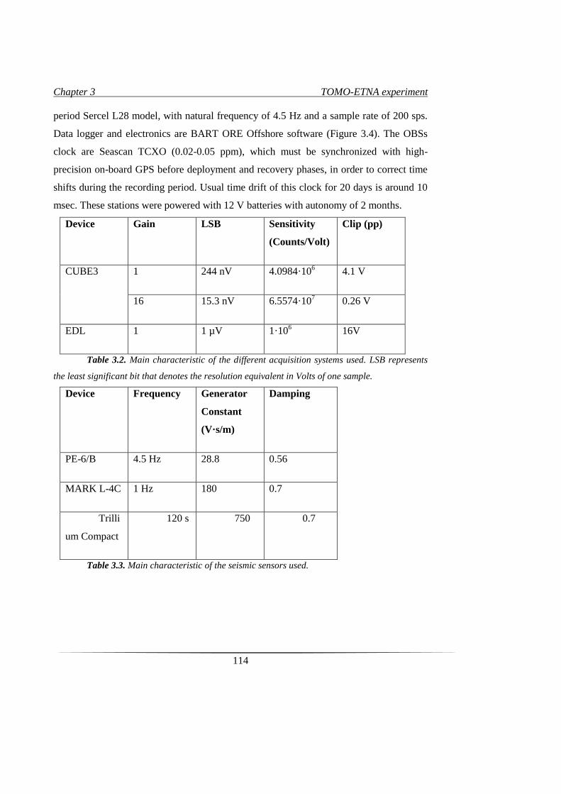
Chapter 3 TOMO-ETNA experiment
114
period Sercel L28 model, with natural frequency of 4.5 Hz and a sample rate of 200 sps.
Data logger and electronics are BART ORE Offshore software (Figure 3.4). The OBSs
clock are Seascan TCXO (0.02-0.05 ppm), which must be synchronized with high-
precision on-board GPS before deployment and recovery phases, in order to correct time
shifts during the recording period. Usual time drift of this clock for 20 days is around 10
msec. These stations were powered with 12 V batteries with autonomy of 2 months.
Device Gain LSB Sensitivity
(Counts/Volt)
Clip (pp)
CUBE3 1 244 nV 4.0984·106 4.1 V
16 15.3 nV 6.5574·107 0.26 V
EDL 1 1 µV 1·106 16V
Table 3.2. Main characteristic of the different acquisition systems used. LSB represents
the least significant bit that denotes the resolution equivalent in Volts of one sample.
Device Frequency Generator
Constant
(V·s/m)
Damping
PE-6/B 4.5 Hz 28.8 0.56
MARK L-4C 1 Hz 180 0.7
Trilli
um Compact
120 s 750 0.7
Table 3.3. Main characteristic of the seismic sensors used.
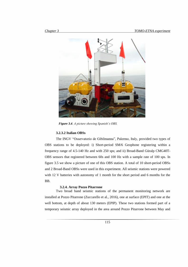
Chapter 3 TOMO-ETNA experiment
115
3.2.3.2 Italian OBSs
The INGV “Osservatorio de Gibilmanna”, Palermo, Italy, provided two types of
OBS stations to be deployed: i) Short-period SM/6 Geophone registering within a
frequency range of 4.5-140 Hz and with 250 sps; and ii) Broad-Band Güralp CMG40T-
OBS sensors that registered between 60s and 100 Hz with a sample rate of 100 sps. In
figure 3.5 we show a picture of one of this OBS station. A total of 10 short-period OBSs
and 2 Broad-Band OBSs were used in this experiment. All seismic stations were powered
with 12 V batteries with autonomy of 1 month for the short period and 6 months for the
BB.
3.2.4. Array Pozzo Pitarrone
Two broad band seismic stations of the permanent monitoring network are
installed at Pozzo Pitarrone (Zuccarello et al., 2016), one at surface (EPIT) and one at the
well bottom, at depth of about 130 meters (EPIP). These two stations formed part of a
temporary seismic array deployed in the area around Pozzo Pitarrone between May and
Figure 3.4. A picture showing Spanish’s OBS.
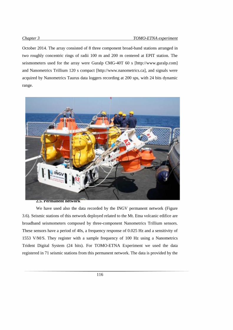
Chapter 3 TOMO-ETNA experiment
116
October 2014. The array consisted of 8 three component broad-band stations arranged in
two roughly concentric rings of radii 100 m and 200 m centered at EPIT station. The
seismometers used for the array were Guralp CMG-40T 60 s [http://www.guralp.com]
and Nanometrics Trillium 120 s compact [http://www.nanometrics.ca], and signals were
acquired by Nanometrics Taurus data loggers recording at 200 sps, with 24 bits dynamic
range.
Figure 3.5. A picture showing Italian’s OBS.
2.5. Permanent network
We have used also the data recorded by the INGV permanent network (Figure
3.6). Seismic stations of this network deployed related to the Mt. Etna volcanic edifice are
broadband seismometers composed by three-component Nanometrics Trillium sensors.
These sensors have a period of 40s, a frequency response of 0.025 Hz and a sensitivity of
1553 V/M/S. They register with a sample frequency of 100 Hz using a Nanometrics
Trident Digital System (24 bits). For TOMO-ETNA Experiment we used the data
registered in 71 seismic stations from this permanent network. The data is provided by the
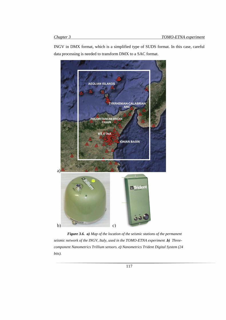
Chapter 3 TOMO-ETNA experiment
117
INGV in DMX format, which is a simplified type of SUDS format. In this case, careful
data processing is needed to transform DMX to a SAC format.
Figure 3.6. a) Map of the location of the seismic stations of the permanent
seismic network of the INGV, Italy, used in the TOMO-ETNA experiment .b) Three-
component Nanometrics Trillium sensors. c) Nanometrics Trident Digital System (24
bits).
a)
b) c)
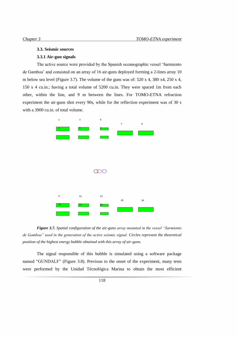
Chapter 3 TOMO-ETNA experiment
118
3.3. Seismic sources
3.3.1 Air-gun signals
The active source were provided by the Spanish oceanographic vessel ‘Sarmiento
de Gamboa’ and consisted on an array of 16 air-guns deployed forming a 2-lines array 10
m below sea level (Figure 3.7). The volume of the guns was of: 520 x 4, 380 x4, 250 x 4,
150 x 4 cu.in.; having a total volume of 5200 cu.in. They were spaced 1m from each
other, within the line, and 9 m between the lines. For TOMO-ETNA refraction
experiment the air-guns shot every 90s, while for the reflection experiment was of 30 s
with a 3900 cu.in. of total volume.
Figure 3.7. Spatial configuration of the air-guns array mounted in the vessel “Sarmiento
de Gamboa” used in the generation of the active seismic signal. Circles represent the theoretical
position of the highest energy bubble obtained with this array of air-guns.
The signal responsible of this bubble is simulated using a software package
named “GUNDALF” (Figure 3.8). Previous to the onset of the experiment, many tests
were performed by the Unidad Técnológica Marina to obtain the most efficient
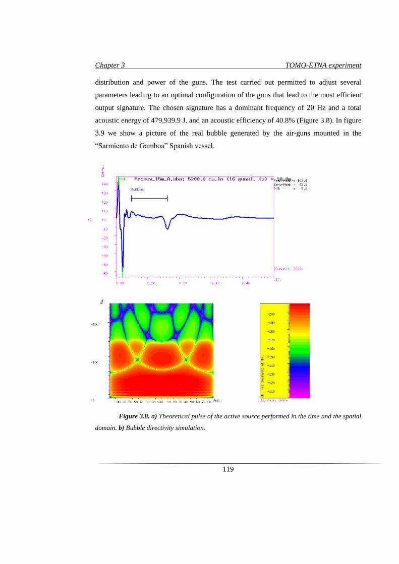
Chapter 3 TOMO-ETNA experiment
119
distribution and power of the guns. The test carried out permitted to adjust several
parameters leading to an optimal configuration of the guns that lead to the most efficient
output signature. The chosen signature has a dominant frequency of 20 Hz and a total
acoustic energy of 479,939.9 J. and an acoustic efficiency of 40.8% (Figure 3.8). In figure
3.9 we show a picture of the real bubble generated by the air-guns mounted in the
“Sarmiento de Gamboa” Spanish vessel.
Figure 3.8. a) Theoretical pulse of the active source performed in the time and the spatial
domain. b) Bubble directivity simulation.
a)
b)
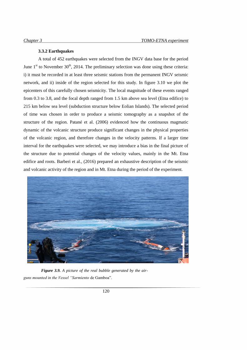
Chapter 3 TOMO-ETNA experiment
120
3.3.2 Earthquakes
A total of 452 earthquakes were selected from the INGV data base for the period
June 1st to November 30
th, 2014. The preliminary selection was done using these criteria:
i) it must be recorded in at least three seismic stations from the permanent INGV seismic
network, and ii) inside of the region selected for this study. In figure 3.10 we plot the
epicenters of this carefully chosen seismicity. The local magnitude of these events ranged
from 0.3 to 3.8, and the focal depth ranged from 1.5 km above sea level (Etna edifice) to
215 km below sea level (subduction structure below Eolian Islands). The selected period
of time was chosen in order to produce a seismic tomography as a snapshot of the
structure of the region. Patané et al. (2006) evidenced how the continuous magmatic
dynamic of the volcanic structure produce significant changes in the physical properties
of the volcanic region, and therefore changes in the velocity patterns. If a larger time
interval for the earthquakes were selected, we may introduce a bias in the final picture of
the structure due to potential changes of the velocity values, mainly in the Mt. Etna
edifice and roots. Barberi et al., (2016) prepared an exhaustive description of the seismic
and volcanic activity of the region and in Mt. Etna during the period of the experiment.
Figure 3.9. A picture of the real bubble generated by the air-
guns mounted in the Vessel “Sarmiento de Gamboa”.
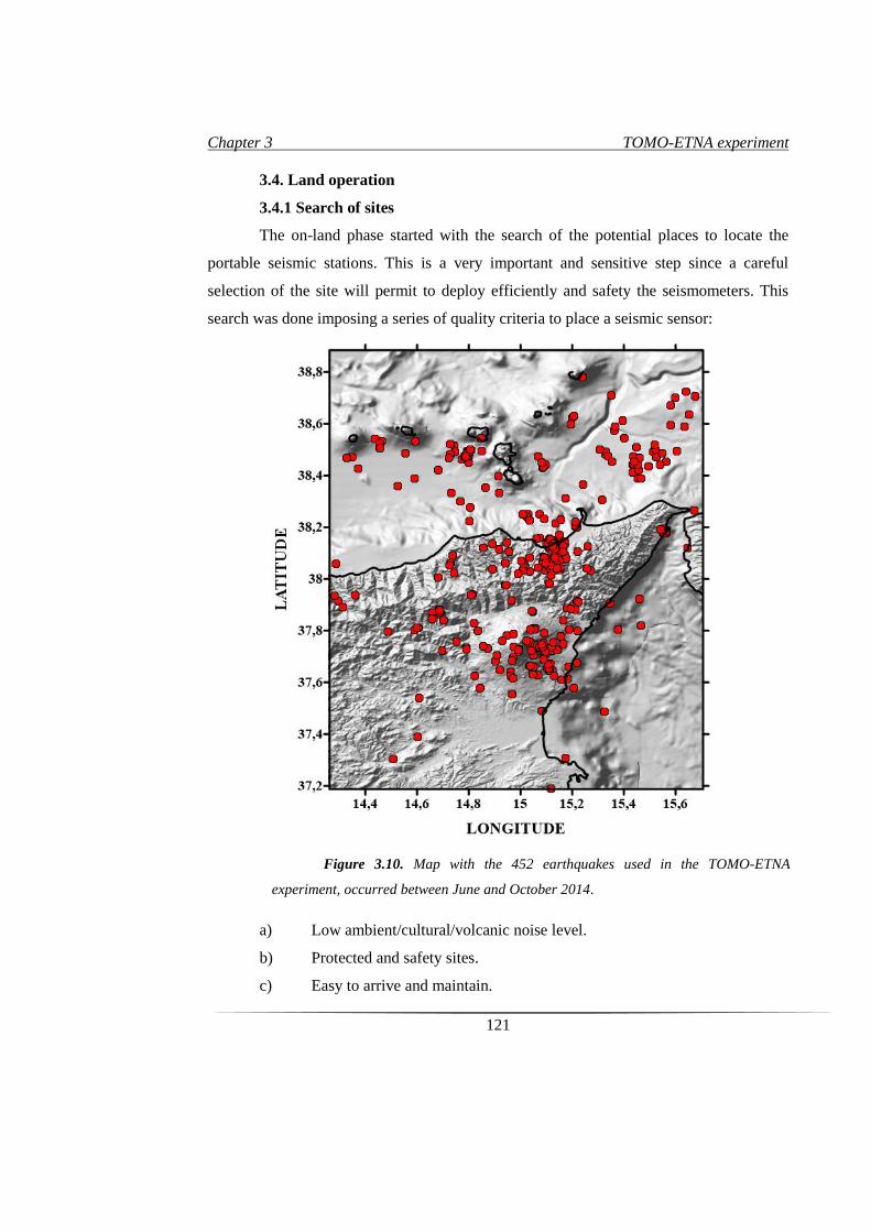
Chapter 3 TOMO-ETNA experiment
121
3.4. Land operation
3.4.1 Search of sites
The on-land phase started with the search of the potential places to locate the
portable seismic stations. This is a very important and sensitive step since a careful
selection of the site will permit to deploy efficiently and safety the seismometers. This
search was done imposing a series of quality criteria to place a seismic sensor:
a) Low ambient/cultural/volcanic noise level.
b) Protected and safety sites.
c) Easy to arrive and maintain.
Figure 3.10. Map with the 452 earthquakes used in the TOMO-ETNA
experiment, occurred between June and October 2014.
Chapter 3 TOMO-ETNA experiment
122
d) Consolidated host rock.
Initially, an area of 5,500 km2 was selected as the region to deploy the stations.
The size was estimated taking into account the main objective of the project: to produce a
seismic tomography of Mt. Etna volcano and surrounding areas in order to place this
volcano in a regional framework. This zone comprises the Eastern coast of Sicily and Mt.
Etna volcanic edifice (see Figure 1 of Ibáñez et al., 2016a). Although the area under
interest comprises part of Sicily Island, the Eolian Islands and part of the South of the
Italian Peninsula (Calabria), since in both Eolian Islands and Calabria the permanent
INGV seismic network has several stations, we centered our effort exclusively in Sicily
Island. The first step was to place on a map a set of 200 theoretical locations for the
portable seismic stations according to the above quality requirements. Once this
preliminary map was defined, from the beginning of April to end of May 2014 a team led
by A. Díaz-Moreno from the UGR and O. Cocina from INGV-Catania, with the support
of several researchers of the INGV-Catania, visited each of these locations, in some cases
more than once. Finally, 150 potential locations were selected covering almost
homogeneously the region under interest. The work of this team included to stablish
contact with the private owners or the public authorities responsible of the sites and ask
for permission to the temporal deployment of the seismic stations. Official documents
were provided by the INGV in order to have an additional support in this negotiation.
Preferentially the team selected public properties such as Cemeteries, Parks or Schools
(the planned shooting period was during a non-teaching season). If no public properties
were identified, then private areas with the possibility of restricted access were selected
such as golf resorts, rural hotels, farms, among others. In the Mt. Etna structure, the
special protected area due to the Natural Park declaration facilitates this search and
location of sites. This Natural Park characteristic was also used for several stations placed
in the Peloritani Mountains. In several times they had to convince both authorities and
private owners of the importance of the stations and the experiment. Many private owners
were concerned about possible health issues regarding the installation of the stations (the
most repeated question done for many owners was if the seismic stations had any level of
radioactivity or how noisy they could be). The search teams were always composed by at
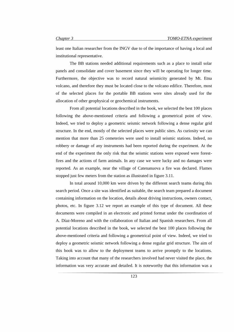
Chapter 3 TOMO-ETNA experiment
123
least one Italian researcher from the INGV due to of the importance of having a local and
institutional representative.
The BB stations needed additional requirements such as a place to install solar
panels and consolidate and cover basement since they will be operating for longer time.
Furthermore, the objective was to record natural seismicity generated by Mt. Etna
volcano, and therefore they must be located close to the volcano edifice. Therefore, most
of the selected places for the portable BB stations were sites already used for the
allocation of other geophysical or geochemical instruments.
From all potential locations described in the book, we selected the best 100 places
following the above-mentioned criteria and following a geometrical point of view.
Indeed, we tried to deploy a geometric seismic network following a dense regular grid
structure. In the end, mostly of the selected places were public sites. As curiosity we can
mention that more than 25 cemeteries were used to install seismic stations. Indeed, no
robbery or damage of any instruments had been reported during the experiment. At the
end of the experiment the only risk that the seismic stations were exposed were forest-
fires and the actions of farm animals. In any case we were lucky and no damages were
reported. As an example, near the village of Catenanuova a fire was declared. Flames
stopped just few meters from the station as illustrated in figure 3.11.
In total around 10,000 km were driven by the different search teams during this
search period. Once a site was identified as suitable, the search team prepared a document
containing information on the location, details about driving instructions, owners contact,
photos, etc. In figure 3.12 we report an example of this type of document. All these
documents were compiled in an electronic and printed format under the coordination of
A. Díaz-Moreno and with the collaboration of Italian and Spanish researchers. From all
potential locations described in the book, we selected the best 100 places following the
above-mentioned criteria and following a geometrical point of view. Indeed, we tried to
deploy a geometric seismic network following a dense regular grid structure. The aim of
this book was to allow to the deployment teams to arrive promptly to the locations.
Taking into account that many of the researchers involved had never visited the place, the
information was very accurate and detailed. It is noteworthy that this information was a
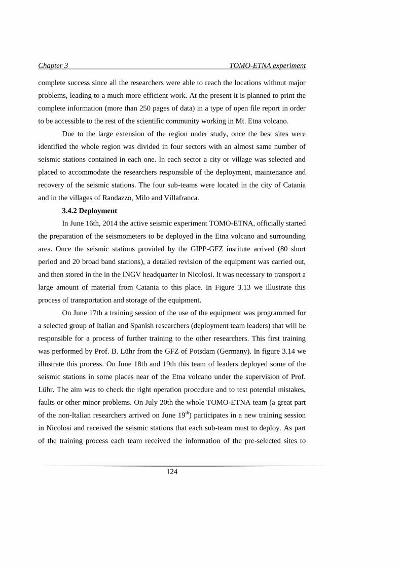
Chapter 3 TOMO-ETNA experiment
124
complete success since all the researchers were able to reach the locations without major
problems, leading to a much more efficient work. At the present it is planned to print the
complete information (more than 250 pages of data) in a type of open file report in order
to be accessible to the rest of the scientific community working in Mt. Etna volcano.
Due to the large extension of the region under study, once the best sites were
identified the whole region was divided in four sectors with an almost same number of
seismic stations contained in each one. In each sector a city or village was selected and
placed to accommodate the researchers responsible of the deployment, maintenance and
recovery of the seismic stations. The four sub-teams were located in the city of Catania
and in the villages of Randazzo, Milo and Villafranca.
3.4.2 Deployment
In June 16th, 2014 the active seismic experiment TOMO-ETNA, officially started
the preparation of the seismometers to be deployed in the Etna volcano and surrounding
area. Once the seismic stations provided by the GIPP-GFZ institute arrived (80 short
period and 20 broad band stations), a detailed revision of the equipment was carried out,
and then stored in the in the INGV headquarter in Nicolosi. It was necessary to transport a
large amount of material from Catania to this place. In Figure 3.13 we illustrate this
process of transportation and storage of the equipment.
On June 17th a training session of the use of the equipment was programmed for
a selected group of Italian and Spanish researchers (deployment team leaders) that will be
responsible for a process of further training to the other researchers. This first training
was performed by Prof. B. Lühr from the GFZ of Potsdam (Germany). In figure 3.14 we
illustrate this process. On June 18th and 19th this team of leaders deployed some of the
seismic stations in some places near of the Etna volcano under the supervision of Prof.
Lühr. The aim was to check the right operation procedure and to test potential mistakes,
faults or other minor problems. On July 20th the whole TOMO-ETNA team (a great part
of the non-Italian researchers arrived on June 19th) participates in a new training session
in Nicolosi and received the seismic stations that each sub-team must to deploy. As part
of the training process each team received the information of the pre-selected sites to
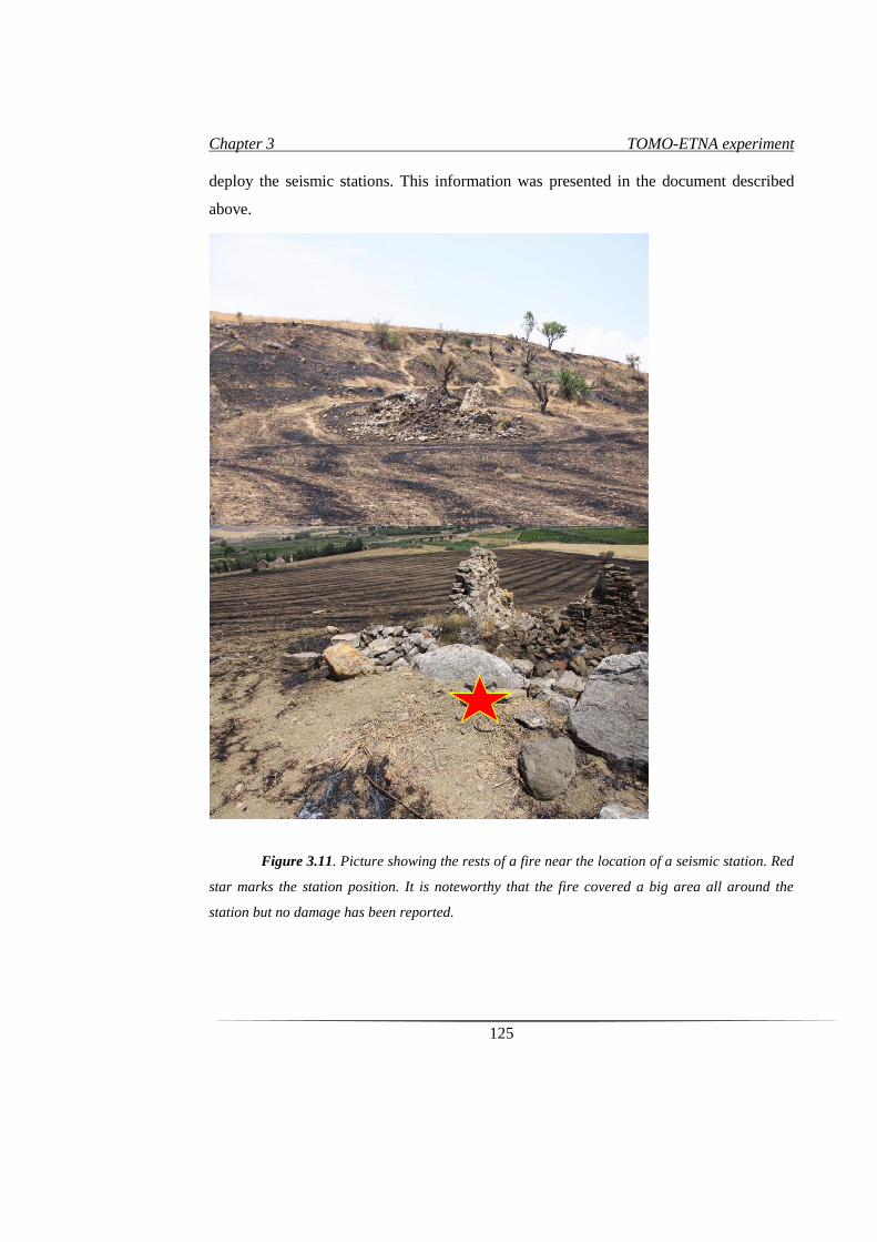
Chapter 3 TOMO-ETNA experiment
125
deploy the seismic stations. This information was presented in the document described
above.
Figure 3.11. Picture showing the rests of a fire near the location of a seismic station. Red
star marks the station position. It is noteworthy that the fire covered a big area all around the
station but no damage has been reported.
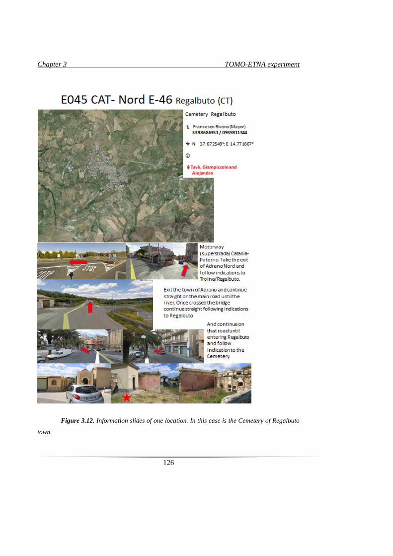
Chapter 3 TOMO-ETNA experiment
126
Figure 3.12. Information slides of one location. In this case is the Cemetery of Regalbuto
town.
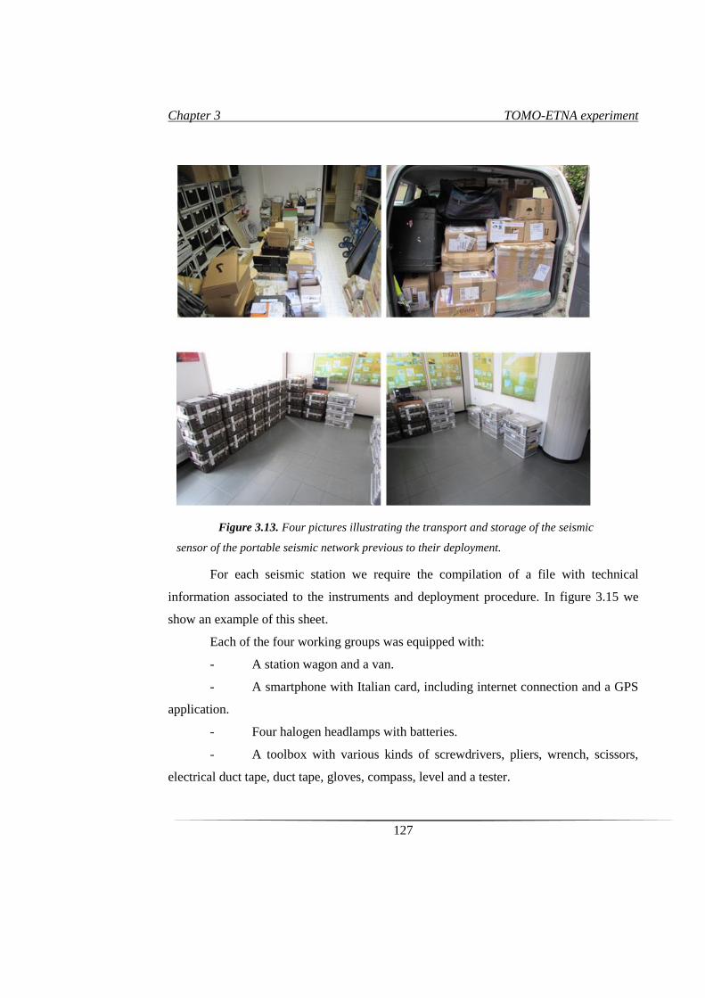
Chapter 3 TOMO-ETNA experiment
127
For each seismic station we require the compilation of a file with technical
information associated to the instruments and deployment procedure. In figure 3.15 we
show an example of this sheet.
Each of the four working groups was equipped with:
- A station wagon and a van.
- A smartphone with Italian card, including internet connection and a GPS
application.
- Four halogen headlamps with batteries.
- A toolbox with various kinds of screwdrivers, pliers, wrench, scissors,
electrical duct tape, duct tape, gloves, compass, level and a tester.
Figure 3.13. Four pictures illustrating the transport and storage of the seismic
sensor of the portable seismic network previous to their deployment.

Chapter 3 TOMO-ETNA experiment
128
- Two Picks, two shovel and two hoes.
- A fluorescent jacket for each person with identification of the project,
INGV and UGR.
- Two back-packs of 50 liters of capacity to transport sensors and batteries.
- Their correspondent number of data logger, seismometers and batteries,
including batteries of replacement for the data logger.
- A folder with the information of their respective stations (instruction of
use, replacement and maintenance), sites and routes to arrive to them.
- A clear identification sheet for the car and people in it, as they belonged
to the INGV-Catania, to the MED-SUV project and TOMO-ETNA experiment.
Additionally, we were supported by different INGV technicians from Catania,
Rome, Naples and Bologna. These technicians were in charge of the deployment of the
BB stations.
In June 23rd the deployment started. The working-plan for the deployment was
conceived in order to optimize the different assigned routes and to install the seismic
stations as fast and as safety as possible. In figure 3.16 we plot the stations location
distributed according the different working teams, moreover, we have marked, as an
example the different routes followed by the different teams in one day of work.
Additionally, in figure 3.17 we illustrate some moments of the installation process.
Summary of the number of seismic stations deployed:
a) Villafranca Group: 14 short period seismic stations.
b) Randazzo Group: 18 short period seismic stations.
c) Milo (Etna) Group: 12 short period seismic stations.
d) INGV-GPS technicians: 8 Broad Band seismic stations.
e) INGV-Seismiological technicians: 6 Broad Band seismic stations.
f) Catania Group: 4 Broad Band and 36 short period seismic stations.
In June 26th the 95% of the seismic station had been deployed in their different
sites according with the pre-establish selection. The final map with the sites of the whole
seismic network deployed for the TOMO-ETNA experiment, including the permanent
seismic network of the INGV is presented in figure 3.16.
Chapter 3 TOMO-ETNA experiment
129
3.4.3 Maintenance
After the phase of installation of the seismic stations, each group developed
activities of maintenance and control. These activities were focused mainly in the
controlling of the proper operation of the seismic stations and the change of the batteries.
The change of the batteries was done every 7 days to ensure a proper operation of the data
acquisition. To avoid potential vandalism on the seismic stations, every site was visited at
least once every 2 or 3 days.
As routine procedure, every day the operation coordinator, Dr. J. Prudencio,
contacted with each headquarter to indicate the activities of the day, potential changes,
recovery information and potential problems, including potential help of the other teams
to every site.
During the second stage of the shooting process, after July 10th, some of the short
period seismic stations were moved from their original planned sites to new one in order
to cover additional sites and improved the distribution of stations. In total 23 short period
stations were moved. In this case the initial planned 98 portable stations sites were
increased to 121 sites.
3.4.4 Recovery
On July 24th, 2014 the seismic active phase of the experiment TOMO-ETNA
finalized. At this date the whole portable short period seismic network was recovered.
The Broad Band seismic network remained operative until October, 28th 2014. At the
same time the Oceanographic Vessel “Sarmiento de Gamboa” arrived to the Catania
harbor after the recovery of 25 short period OBSs, leaving operative other 2 Broad Band
OBSs. They were recovered by the RV “Aegaeo” in November 25th, 2014. The recovery
process of all seismic stations was a success and all the deployed instruments were
recovered operating and with no damages. In total, more than 25.000 km were driven
during the experiment. In figure 3.16 we show the final position of the whole stations
used in the TOMO-ETNA experiment.
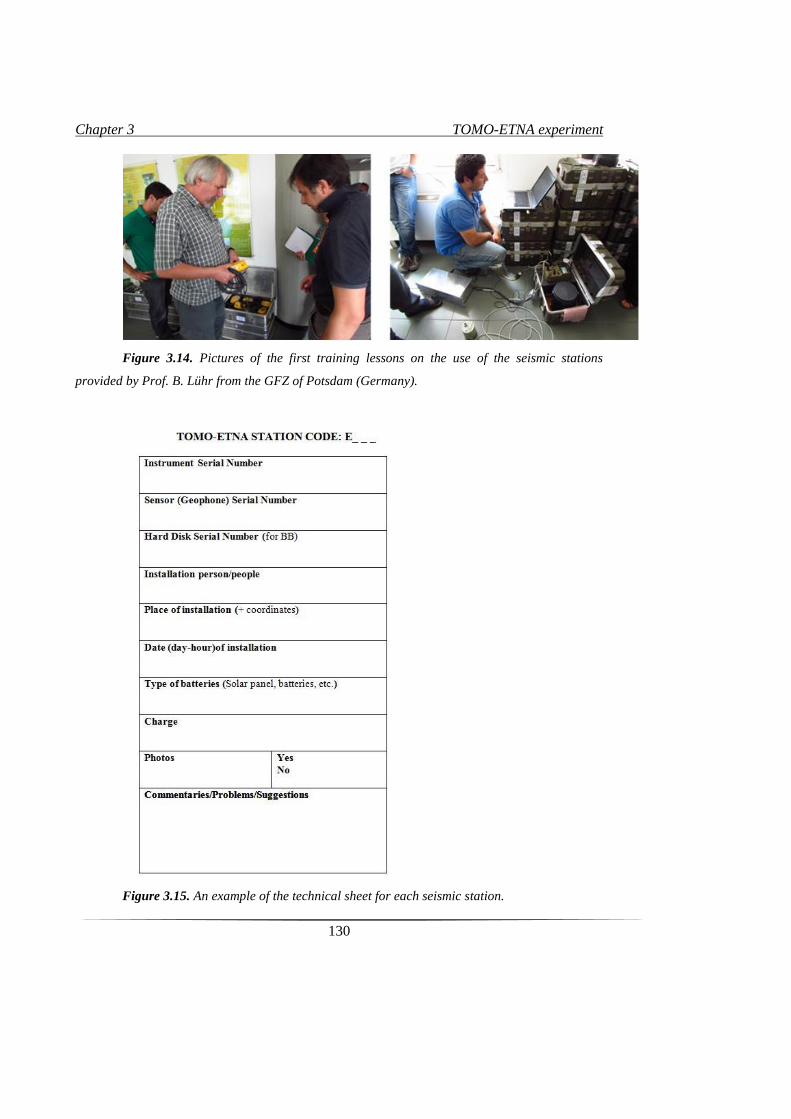
Chapter 3 TOMO-ETNA experiment
130
Figure 3.14. Pictures of the first training lessons on the use of the seismic stations
provided by Prof. B. Lühr from the GFZ of Potsdam (Germany).
Figure 3.15. An example of the technical sheet for each seismic station.
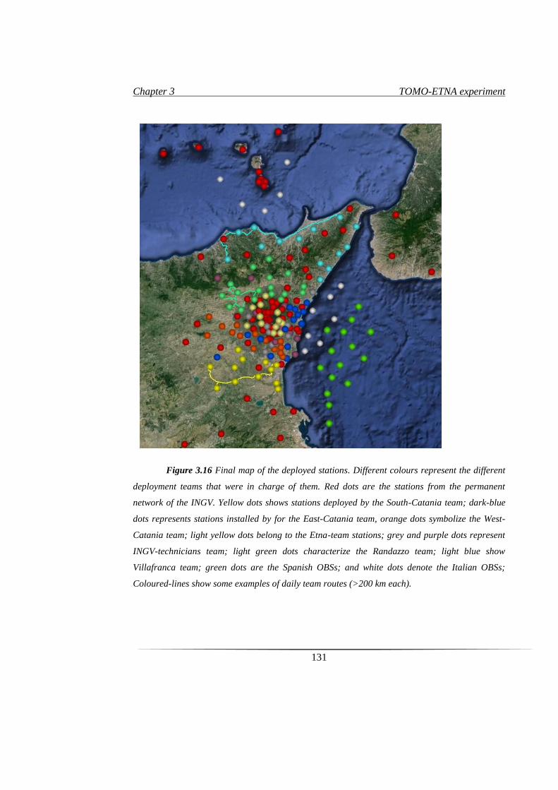
Chapter 3 TOMO-ETNA experiment
131
Figure 3.16 Final map of the deployed stations. Different colours represent the different
deployment teams that were in charge of them. Red dots are the stations from the permanent
network of the INGV. Yellow dots shows stations deployed by the South-Catania team; dark-blue
dots represents stations installed by for the East-Catania team, orange dots symbolize the West-
Catania team; light yellow dots belong to the Etna-team stations; grey and purple dots represent
INGV-technicians team; light green dots characterize the Randazzo team; light blue show
Villafranca team; green dots are the Spanish OBSs; and white dots denote the Italian OBSs;
Coloured-lines show some examples of daily team routes (>200 km each).
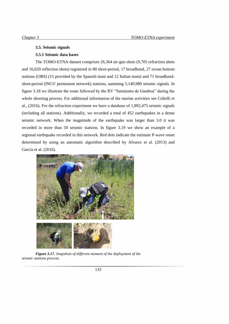
Chapter 3 TOMO-ETNA experiment
132
3.5. Seismic signals
3.5.1 Seismic data bases
The TOMO-ETNA dataset comprises 26,364 air-gun shots (9,705 refraction shots
and 16,659 reflection shots) registered in 80 short-period, 17 broadband, 27 ocean bottom
stations (OBS) (15 provided by the Spanish team and 12 Italian team) and 71 broadband-
short-period (INGV permanent network) stations, summing 5,140,980 seismic signals. In
figure 3.18 we illustrate the route followed by the RV “Sarmiento de Gamboa” during the
whole shooting process. For additional information of the marine activities see Coltelli et
al., (2016). For the refraction experiment we have a database of 1,892,475 seismic signals
(including all stations). Additionally, we recorded a total of 452 earthquakes in a dense
seismic network. When the magnitude of the earthquake was larger than 3.0 it was
recorded in more than 50 seismic stations. In figure 3.19 we show an example of a
regional earthquake recorded in this network. Red dots indicate the estimate P-wave onset
determined by using an automatic algorithm described by Alvarez et al. (2013) and
García et al. (2016).
Figure 3.17. Snapshots of different moment of the deployment of the
seismic stations process.
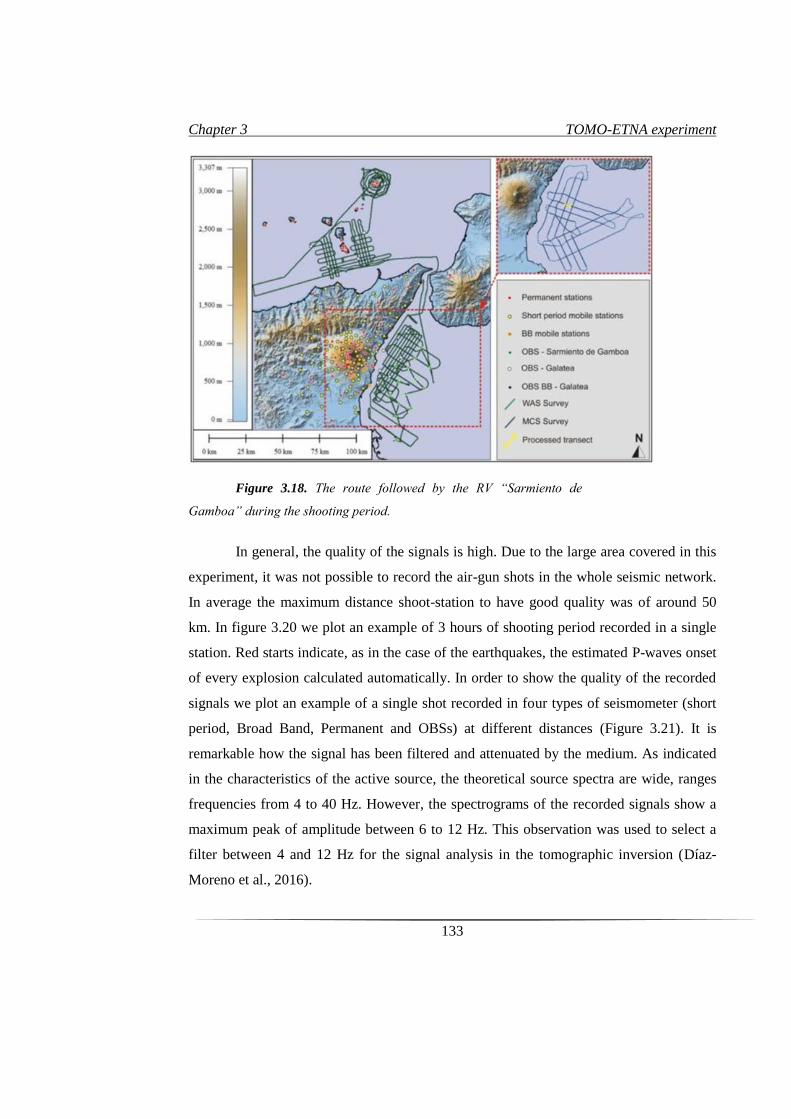
Chapter 3 TOMO-ETNA experiment
133
Figure 3.18. The route followed by the RV “Sarmiento de
Gamboa” during the shooting period.
In general, the quality of the signals is high. Due to the large area covered in this
experiment, it was not possible to record the air-gun shots in the whole seismic network.
In average the maximum distance shoot-station to have good quality was of around 50
km. In figure 3.20 we plot an example of 3 hours of shooting period recorded in a single
station. Red starts indicate, as in the case of the earthquakes, the estimated P-waves onset
of every explosion calculated automatically. In order to show the quality of the recorded
signals we plot an example of a single shot recorded in four types of seismometer (short
period, Broad Band, Permanent and OBSs) at different distances (Figure 3.21). It is
remarkable how the signal has been filtered and attenuated by the medium. As indicated
in the characteristics of the active source, the theoretical source spectra are wide, ranges
frequencies from 4 to 40 Hz. However, the spectrograms of the recorded signals show a
maximum peak of amplitude between 6 to 12 Hz. This observation was used to select a
filter between 4 and 12 Hz for the signal analysis in the tomographic inversion (Díaz-
Moreno et al., 2016).
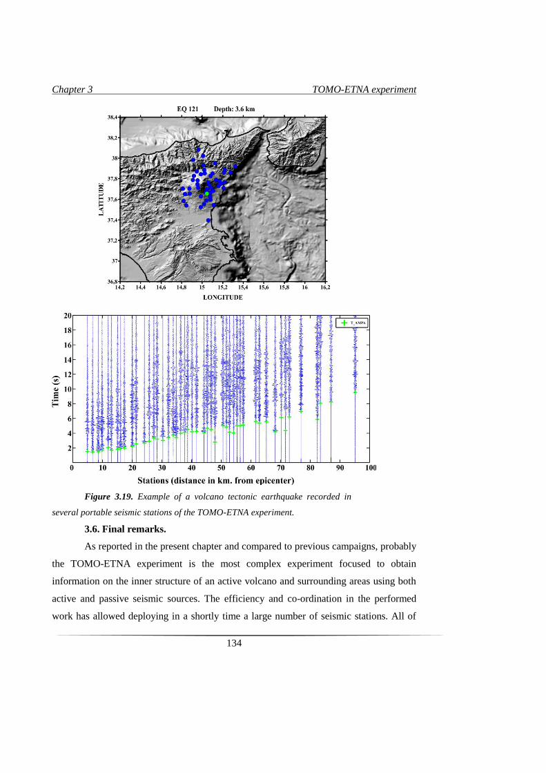
Chapter 3 TOMO-ETNA experiment
134
Figure 3.19. Example of a volcano tectonic earthquake recorded in
several portable seismic stations of the TOMO-ETNA experiment.
3.6. Final remarks.
As reported in the present chapter and compared to previous campaigns, probably
the TOMO-ETNA experiment is the most complex experiment focused to obtain
information on the inner structure of an active volcano and surrounding areas using both
active and passive seismic sources. The efficiency and co-ordination in the performed
work has allowed deploying in a shortly time a large number of seismic stations. All of
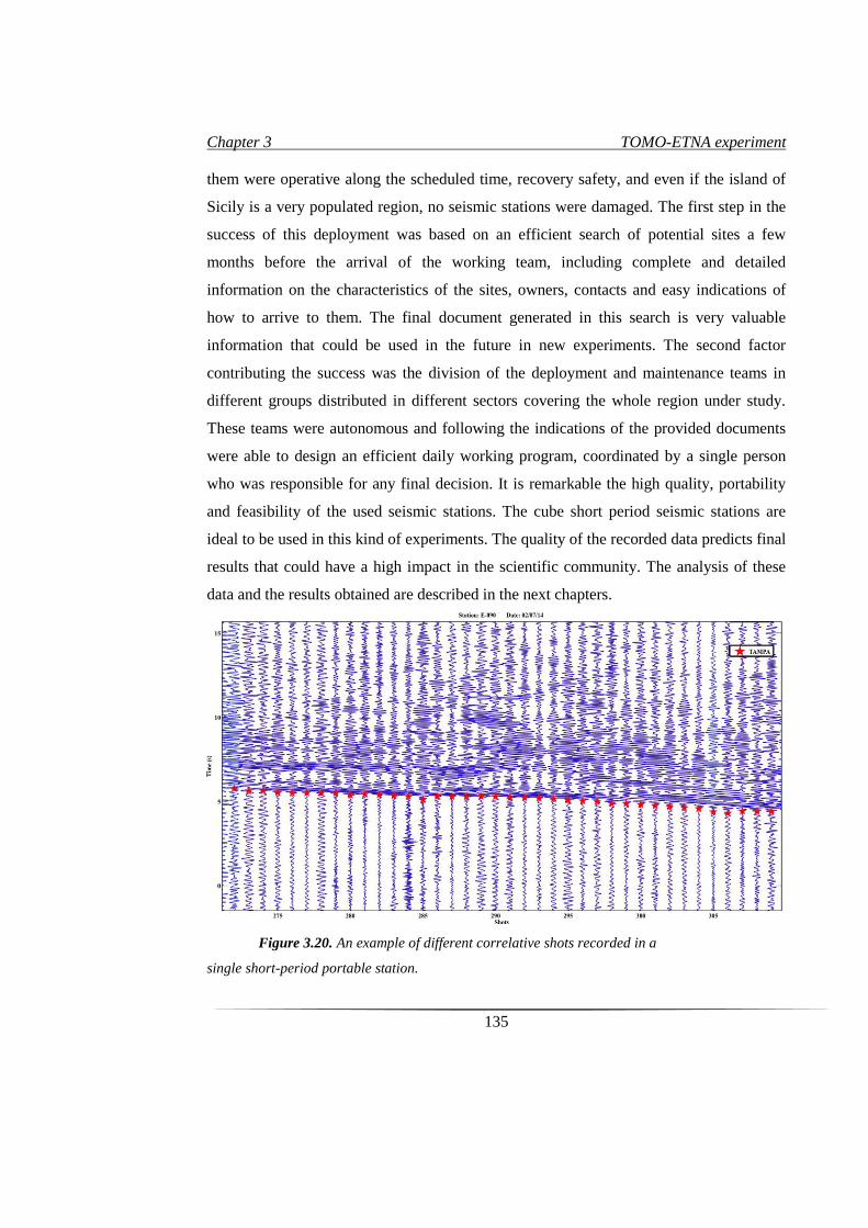
Chapter 3 TOMO-ETNA experiment
135
them were operative along the scheduled time, recovery safety, and even if the island of
Sicily is a very populated region, no seismic stations were damaged. The first step in the
success of this deployment was based on an efficient search of potential sites a few
months before the arrival of the working team, including complete and detailed
information on the characteristics of the sites, owners, contacts and easy indications of
how to arrive to them. The final document generated in this search is very valuable
information that could be used in the future in new experiments. The second factor
contributing the success was the division of the deployment and maintenance teams in
different groups distributed in different sectors covering the whole region under study.
These teams were autonomous and following the indications of the provided documents
were able to design an efficient daily working program, coordinated by a single person
who was responsible for any final decision. It is remarkable the high quality, portability
and feasibility of the used seismic stations. The cube short period seismic stations are
ideal to be used in this kind of experiments. The quality of the recorded data predicts final
results that could have a high impact in the scientific community. The analysis of these
data and the results obtained are described in the next chapters.
Figure 3.20. An example of different correlative shots recorded in a
single short-period portable station.
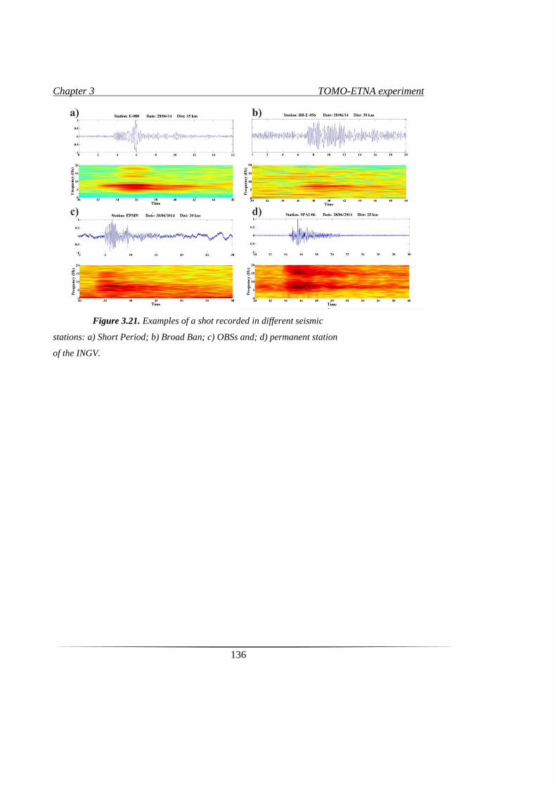
Chapter 3 TOMO-ETNA experiment
136
Figure 3.21. Examples of a shot recorded in different seismic
stations: a) Short Period; b) Broad Ban; c) OBSs and; d) permanent station
of the INGV.
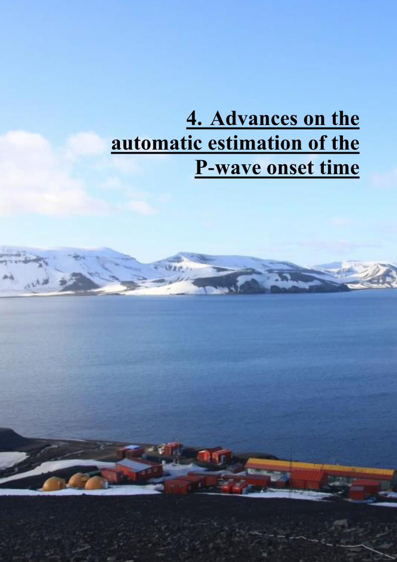
4. Advances on the
automatic estimation of the
P-wave onset time

Chapter 4 Advances on the automatic estimation of the P-wave onset time
139
4.1 Seismic Waves Picking (An Approach)
P- and S-wave arrival determination and travel time calculation are the first stage
and the base in most seismic studies. The picking of the seismic wave arrival can be
defined as the detection of the instant of time when the first energy of the fastest phase
arrives at a station. Such arrival is often identified by a change in energy, amplitude,
frequency contents or wave polarization higher than the background noise. This time
onset, when registered in several stations, is used to calculate the hypocentre and time
origin of the seismic source. Historically, these estimations have been determined
manually, which is optimal for few data, but requires a seismological expertise to carry it
out. However, when large datasets must be picked, the task becomes very time
consuming and human-made errors can occur, especially when the expertise changes.
Indeed, manual picking often lacks of objectivity, as each expertise may detect the onset
following slightly different criteria (i.e zero crossing, higher than a certain threshold,
etc.). During the last decades, providing an automatic picking algorithm has become a
key point in many seismic laboratories in order to assess large datasets and to diminish
potential human mistakes. Several methods have been proposed that fit well for certain
datasets but sometimes they are not exportable to other regions (Benítez et al., 2007,
Cortés et al., 2014). Along the following paragraphs we summarize some of the latest and
more relevant procedures proposed for automatic picking based on different parameters
analyses. We want to remark that this is not a detailed review of all the existing
techniques but a state of the art of the most important ones, regarding the frequency
domain analysis.
Many approaches for automatic picking have been proposed in time and
frequency domains like: the pioneer classical picker of Allen (1978) based on STA/LTA,
improved by Baer and Kradolfer (1987); approaches based on higher order statistics like
kurtosis or skewness (Saragiotis, 2002; Küperkock et al., 2010, Langet, 2014); picking
based on the waveforms predominant period (Hildyard et al., 2008); or wavelet analysis
(Zhang et al., 2003); and multiband frequency analysis (Álvarez et al., 2013) as examples
in the frequency domain. Autoregressive techniques based on the Akaike Information
Criterion (AIC) like Takanami and Kitagawa (1988), pattern recognition systems like
Chapter 4 Advances on the automatic estimation of the P-wave onset time
140
ANN (Gentili and Michelini, 2006) and polarization analysis have also been successfully
implemented (Reading et al., 2011; Ross et al., 2014; Kurzon et al., 2014).
Latest tendencies in automatic picking opt for combinations of several of the
referred techniques, selected according to specific needs and available data. Iterative,
tandem or parallel approaches like Nippress et al., (2010), Küperkoch et al., (2012),
Álvarez et al., (2013) or Ross et al., (2014), are jointly applied to combine
complementary strengthens.
The automatic procedure is needed because, besides the demand of capacity to
process the massive dataset produced, signals will have diverse signal to noise ratio
(SNR) due to the seismic noise generated in their path towards the seismometers and the
low density of the materials they have to travel across. Automatic real-time signal
processing and noise reduction permits outperforming human analysis in terms of
precision and consistency of the travel time estimations.
In this work, we have applied the P-phase picking procedure described by
Álvarez et al., (2013) and García et al., (2016). Along this chapter we will describe this
algorithm used to determine the P-wave arrivals for both active and passive data. The
dataset used is that recorded during the TOMO-ETNA experiment, and detailed in the
previous chapter. It includes more than 3 million raw seismic signals that must be
analysed. For such a large database, manual picking is discarded as it would need several
months to carry it out. Unifying the different signal formats recorded is the first stage and
it is detailed in the following paragraphs.
4.2. Signal pre-processing
The first step is to unify the data formats. Initially, all the seismic data is recorded
in a different format depending on the station (short-period, broadband, OBS, etc.). This
procedure is not as easy as it may seem, since it is a very sensitive procedure. In the
following paragraphs the different original formats and they conversion are detailed. Our
preferred format to work with is .mat (matlab) so that we can process the data in a less
time-consuming way.
We analysed separately both earthquake and shots data. For the shot database we
started with the CUBE stations. These stations save the data in binary daily files that
Chapter 4 Advances on the automatic estimation of the P-wave onset time
141
should be then converted to an appropriate format. The GFZ Potsdam institute provides
useful algorithms to convert Cube format to MiniSeed format. During the recorded
period, many of the 90 stations deployed lost the GPS signal sometimes, leading to more
than one daily file. The binary output format is transformed to a more accessible
MiniSeed format. We found out that the registered data had some gaps, meaning that for
certain periods of time the station did not register. The most probable cause of this is the
loss of GPS signal. Fortunately, MiniSeed files are written with an absolute scale of time,
thus, allowing us to identified and exclude these gaps. Another step we performed was to
convert MiniSeed to SAC in order to be able to choose the more suitable type file to work
with. On the other hand SAC files have the time information not in absolute values but in
a single time vector from 1 to the end of samples. Therefore, gaps could not be well
identified using this type of files. For this reason we decided to work directly with the
MiniSeed data. To reduce computation time we transform the data to .mat format taking
only the pieces of signal we needed. Indeed, we cut the signal 30s before that data and
60s after each shot. When we find a gap in the registration, the shots occurred in that
period are not taken into account for that station.
Once the Cube database is organized in the new format, we plotted all shots
registered in one station during one day using matlab tools. This way of representation
allows us view the movement of the vessel and to estimate the acoustic wave (1.5 km/s)
registered on the stations near the coast. Indeed, controlling the arrival time of the
acoustic wave is a simple and very effective procedure to check that the GPS data times
are correct, and that there is synchrony between the GPS data time of the airguns and the
stations (See chapter 6).
The data extracted from the broadband stations are in MiniSeed format; therefore,
not further conversion is needed, only to .mat files. In this case we followed the same
procedure as for the Cubes, we took the time data of each explosion to cut the MiniSeed
file 30s before it and 60s after it and save it in Matlab files. The only problem we address
in this step was that the coordinates of the broadband stations were daily calculated and
differ from one day to another in some decimals. In order to have a final station
coordinates we calculated the mean of all these daily GPS coordinates.
Chapter 4 Advances on the automatic estimation of the P-wave onset time
142
The INGV permanent stations provide data formatted in .DMX files, which result
to be a compressed type of .SUDS files. This type of file is organized in a completely
different way as the previously mentioned MiniSeed or SAC. They save registration of
1min for each station. In this case, the INGV research team provided the necessary tools
to convert them to a friendlier SAC format. In any case we may address the same
problems as with the Cube data; if any gaps are present we will not be able to detect them
with the SAC format. Nonetheless, we converted them to .mat files following the
previously discussed procedure and fortunately, we found no gaps for the registration of
these stations.
The Spanish OBS data is provided in RAW binary format. The tools for
conversion permit to obtain an output format known as PascalSegy. This data files were,
then, organized in the common .mat files for their analysis.
The Italian OBS data available at the time of this Thesis are only those recorded
by the Broadband OBSs. These data are saved in SAC files and therefore easy to handle.
Procedure was the same as for the rest of data, using .mal files as the final format.
Once the four different formats of raw data corresponding to the four types of
stations are converted into a unique readable format, missing data, registers with lack of
GPS signal, and extremely bad SNRs abrupt offset in amplitude, are detected and
discarded. Secondly, continuous registers are segmented into windows of analysis around
the expected arrival times based on the catalogue of shooting times for the active
database, and the earthquake catalogue for the passive data. Thirdly, band-pass filtering in
the band of interest is done. All the stations used in this experiment allow recording of the
three components as described in the previous chapter. Figure 4.1 shows signal associated
to the three components recorded by the CUBE station (E-108) on the 10th July 2014. The
movement of the vessel and the locations of the stations and Etna volcano are depicted
with a blue line, a red spot and a black spot, respectively. The upper panel shows the
seismogram registered 40 seconds after the air-gun shot number 70 (i.e. the zero time
corresponds to the time when the shot took place). The lower panel presents the
spectrograms associated to each component. The P-wave onset corresponds to a packet of
energy in the frequency range of [6-8] Hz. According to the Fermat’s principle and as can
Chapter 4 Advances on the automatic estimation of the P-wave onset time
143
be observed in this figure, the vertical component is the one providing the best
information of the wave arrival. Following this criterion, the signals registered in the
vertical component (Z) have been used in this work for estimating the wave arrival
associated to the shot.
Most of the signals registered in the different stations used in the experiment have
a low SNR (i.e. they are affected by strong background noise and /or non-stationary noise
processes). For example, the three components in figure 4.1a, present low SNR, with a
strong noisy artefact centred at about 18 Hz at around 20 seconds of time. Taking into
account the band of activity of the events we want to pick and in order to emphasizes only
P-wave arrivals, for both air-gun shots and earthquakes, all the Z-components have been
filtered using a band-pass linear phase filter in the band [4-12] Hz. The group delay was
compensated accordingly. This type of filter was opportunely chosen, based on the
previous simulations on which zero-phase filters demonstrated a worse behaviour in the
presence of an impulsive arrival. The left panel of figure 4.1b shows the recording of the
vertical component in the same site and date than figure 4.1a, for the first 80 shots. The
right panel shows the signals after filtering. The improvement in terms of SNR is
obvious. P-wave arrivals are difficult to identify in unfiltered signals while they are
clearly observed in the ones filtered.
4.3. Advanced Multiband Picking Algorithm (AMPA)
The automatic P-Phase picking algorithm used to calculate the travel times of the
TOMO-ETNA database, named AMPA, is fully detailed in (Álvarez et al., 2013). In such
work, the finest picking is obtained with AMPA working in tandem with the
autorregresive techniques applied by Takanami and Kitagawa (1988). Due to the
ineffective computational cost of this tandem approach, for the TOMO-ETNA database,
plain AMPA has been used. The picking algorithm is also available in an open-source
toolkit with a user-friendly windows environment and downloadable in Romero et al.,
(2016). AMPA, standing for Adaptive Multiband Picking Algorithm, is a picking strategy
focused on determining P arrival times for signals strongly affected by a low SNR or
processes involving non-stationary noises. In order to do so, AMPA performs two steps
with the signal to be picked:
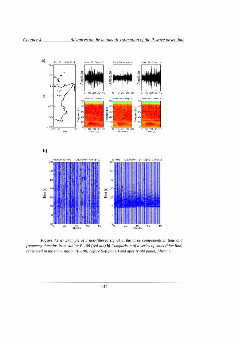
Chapter 4 Advances on the automatic estimation of the P-wave onset time
144
Figure 4.1 a) Example of a non-filtered signal in the three components in time and
frequency domains from station E-108 (red dot).b) Comparison of a series of shots (blue line)
registered in the same station (E-108) before (left panel) and after (right panel) filtering.
b)
a)
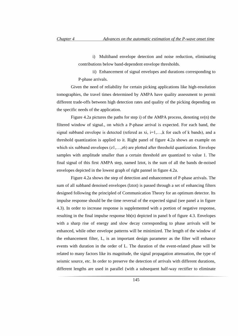
Chapter 4 Advances on the automatic estimation of the P-wave onset time
145
i) Multiband envelope detection and noise reduction, eliminating
contributions below band-dependent envelope thresholds.
ii) Enhancement of signal envelopes and durations corresponding to
P-phase arrivals.
Given the need of reliability for certain picking applications like high-resolution
tomographies, the travel times determined by AMPA have quality assessment to permit
different trade-offs between high detection rates and quality of the picking depending on
the specific needs of the application.
Figure 4.2a pictures the paths for step i) of the AMPA process, denoting sv(n) the
filtered window of signal., on which a P-phase arrival is expected. For each band, the
signal subband envelope is detected (refered as xi, i=1,…,k for each of k bands), and a
threshold quantization is applied to it. Right panel of figure 4.2a shows an example on
which six subband envelopes (z1,…,z6) are plotted after threshold quantization. Envelope
samples with amplitude smaller than a certain threshold are quantized to value 1. The
final signal of this first AMPA step, named lztot, is the sum of all the bands de-noised
envelopes depicted in the lowest graph of right pannel in figure 4.2a.
Figure 4.2a shows the step of detection and enhancement of P-phase arrivals. The
sum of all subband denoised envelopes (lztot) is passed through a set of enhancing filters
designed following the principled of Communication Theory for an optimum detector. Its
impulse response should be the time reversal of the expected signal (see panel a in figure
4.3). In order to increase response is supplemented with a portion of negative response,
resulting in the final impulse response hb(n) depicted in panel b of figure 4.3. Envelopes
with a sharp rise of energy and slow decay corresponding to phase arrivals will be
enhanced, while other envelope patterns will be minimized. The length of the window of
the enhancement filter, L, is an important design parameter as the filter will enhance
events with duration in the order of L. The duration of the event-related phase will be
related to many factors like its magnitude, the signal propagation attenuation, the type of
seismic source, etc. In order to preserve the detection of arrivals with different durations,
different lengths are used in parallel (with a subsequent half-way rectifier to eliminate
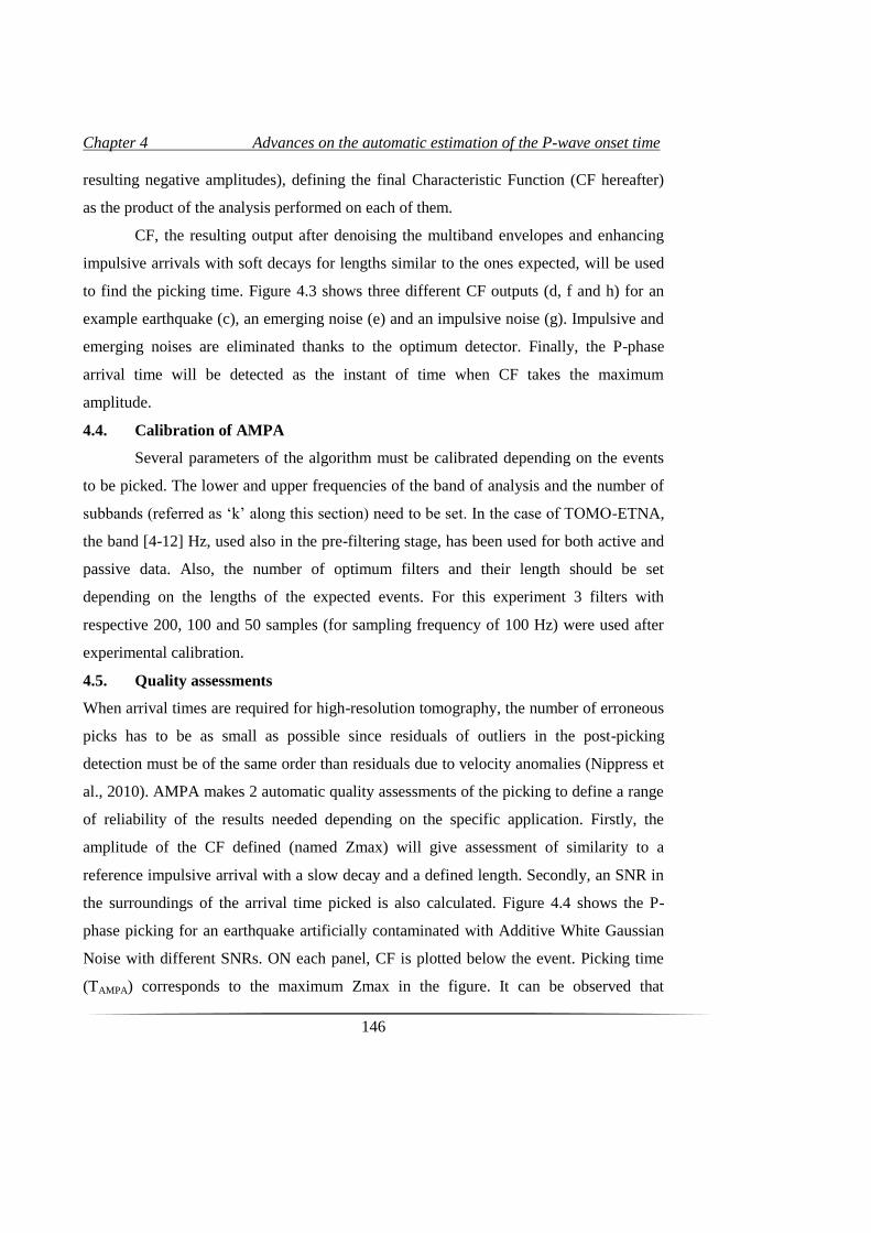
Chapter 4 Advances on the automatic estimation of the P-wave onset time
146
resulting negative amplitudes), defining the final Characteristic Function (CF hereafter)
as the product of the analysis performed on each of them.
CF, the resulting output after denoising the multiband envelopes and enhancing
impulsive arrivals with soft decays for lengths similar to the ones expected, will be used
to find the picking time. Figure 4.3 shows three different CF outputs (d, f and h) for an
example earthquake (c), an emerging noise (e) and an impulsive noise (g). Impulsive and
emerging noises are eliminated thanks to the optimum detector. Finally, the P-phase
arrival time will be detected as the instant of time when CF takes the maximum
amplitude.
4.4. Calibration of AMPA
Several parameters of the algorithm must be calibrated depending on the events
to be picked. The lower and upper frequencies of the band of analysis and the number of
subbands (referred as ‘k’ along this section) need to be set. In the case of TOMO-ETNA,
the band [4-12] Hz, used also in the pre-filtering stage, has been used for both active and
passive data. Also, the number of optimum filters and their length should be set
depending on the lengths of the expected events. For this experiment 3 filters with
respective 200, 100 and 50 samples (for sampling frequency of 100 Hz) were used after
experimental calibration.
4.5. Quality assessments
When arrival times are required for high-resolution tomography, the number of erroneous
picks has to be as small as possible since residuals of outliers in the post-picking
detection must be of the same order than residuals due to velocity anomalies (Nippress et
al., 2010). AMPA makes 2 automatic quality assessments of the picking to define a range
of reliability of the results needed depending on the specific application. Firstly, the
amplitude of the CF defined (named Zmax) will give assessment of similarity to a
reference impulsive arrival with a slow decay and a defined length. Secondly, an SNR in
the surroundings of the arrival time picked is also calculated. Figure 4.4 shows the P-
phase picking for an earthquake artificially contaminated with Additive White Gaussian
Noise with different SNRs. ON each panel, CF is plotted below the event. Picking time
(TAMPA) corresponds to the maximum Zmax in the figure. It can be observed that
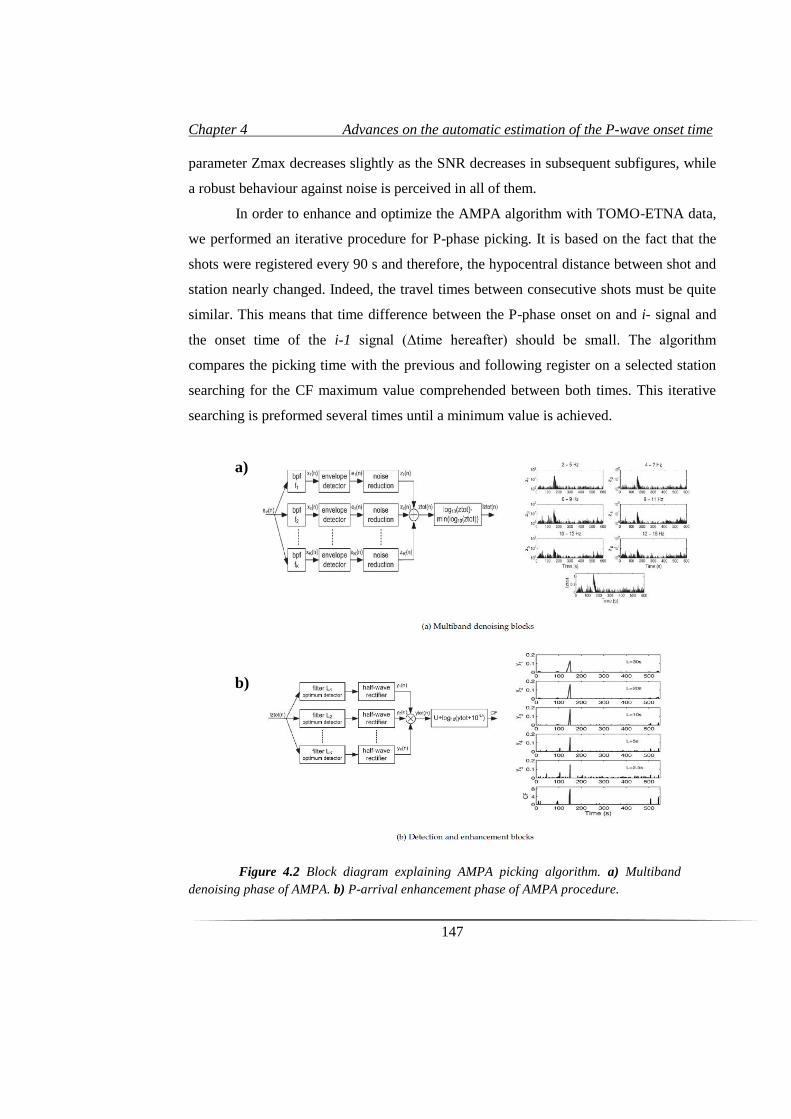
Chapter 4 Advances on the automatic estimation of the P-wave onset time
147
parameter Zmax decreases slightly as the SNR decreases in subsequent subfigures, while
a robust behaviour against noise is perceived in all of them.
In order to enhance and optimize the AMPA algorithm with TOMO-ETNA data,
we performed an iterative procedure for P-phase picking. It is based on the fact that the
shots were registered every 90 s and therefore, the hypocentral distance between shot and
station nearly changed. Indeed, the travel times between consecutive shots must be quite
similar. This means that time difference between the P-phase onset on and i- signal and
the onset time of the i-1 signal (Δtime hereafter) should be small. The algorithm
compares the picking time with the previous and following register on a selected station
searching for the CF maximum value comprehended between both times. This iterative
searching is preformed several times until a minimum value is achieved.
Figure 4.2 Block diagram explaining AMPA picking algorithm. a) Multiband
denoising phase of AMPA. b) P-arrival enhancement phase of AMPA procedure.
a)
b)
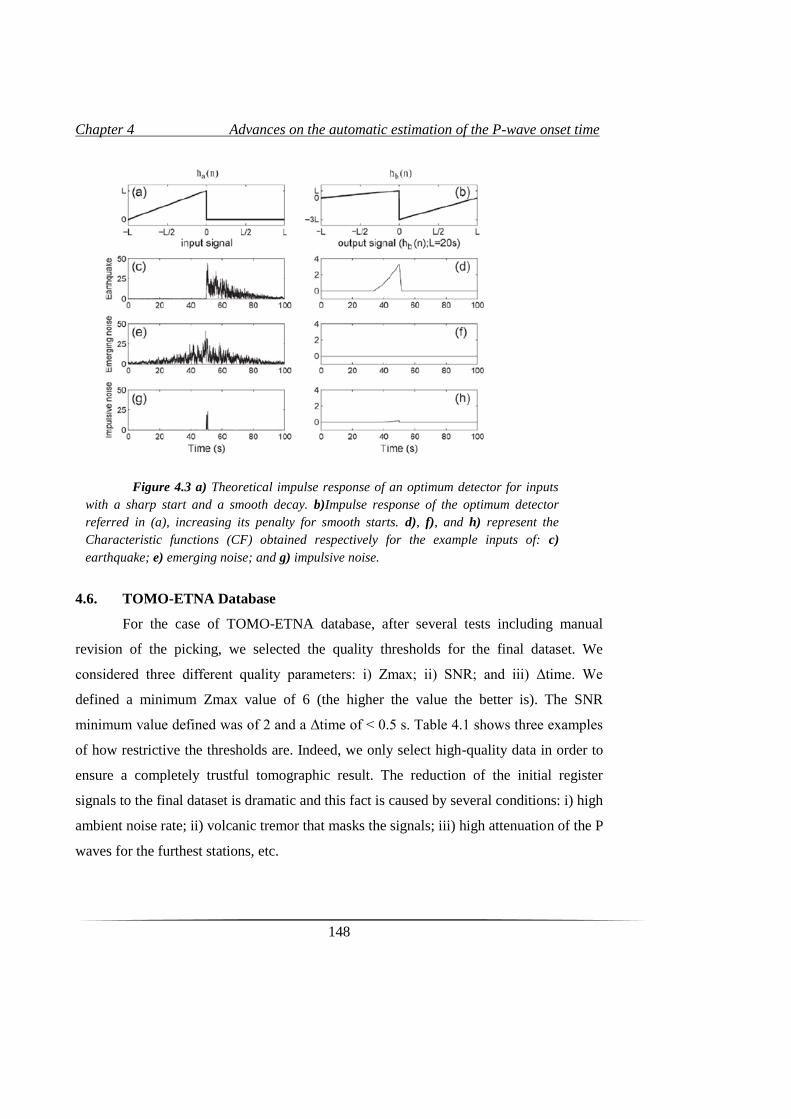
Chapter 4 Advances on the automatic estimation of the P-wave onset time
148
4.6. TOMO-ETNA Database
For the case of TOMO-ETNA database, after several tests including manual
revision of the picking, we selected the quality thresholds for the final dataset. We
considered three different quality parameters: i) Zmax; ii) SNR; and iii) Δtime. We
defined a minimum Zmax value of 6 (the higher the value the better is). The SNR
minimum value defined was of 2 and a Δtime of < 0.5 s. Table 4.1 shows three examples
of how restrictive the thresholds are. Indeed, we only select high-quality data in order to
ensure a completely trustful tomographic result. The reduction of the initial register
signals to the final dataset is dramatic and this fact is caused by several conditions: i) high
ambient noise rate; ii) volcanic tremor that masks the signals; iii) high attenuation of the P
waves for the furthest stations, etc.
Figure 4.3 a) Theoretical impulse response of an optimum detector for inputs
with a sharp start and a smooth decay. b)Impulse response of the optimum detector
referred in (a), increasing its penalty for smooth starts. d), f), and h) represent the
Characteristic functions (CF) obtained respectively for the example inputs of: c)
earthquake; e) emerging noise; and g) impulsive noise.
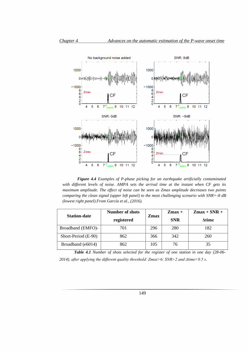
Chapter 4 Advances on the automatic estimation of the P-wave onset time
149
Station-date Number of shots
registered Zmax
Zmax +
SNR
Zmax + SNR +
Δtime
Broadband (EMFO)- 701 296 280 182
Short-Period (E-90) 862 366 342 260
Broadband (e6014) 862 105 76 35
Table 4.1 Number of shots selected for the register of one station in one day (28-06-
2014), after applying the different quality threshold: Zmax>6; SNR>2 and Δtime<0.5 s.
Figure 4.4 Examples of P-phase picking for an earthquake artificially contaminated
with different levels of noise. AMPA sets the arrival time at the instant when CF gets its
maximum amplitude. The effect of noise can be seen as Zmax amplitude decreases two points
comparing the clean signal (upper left panel) to the most challenging scenario with SNR=-8 dB
(lowest right panel).From García et al., (2016).
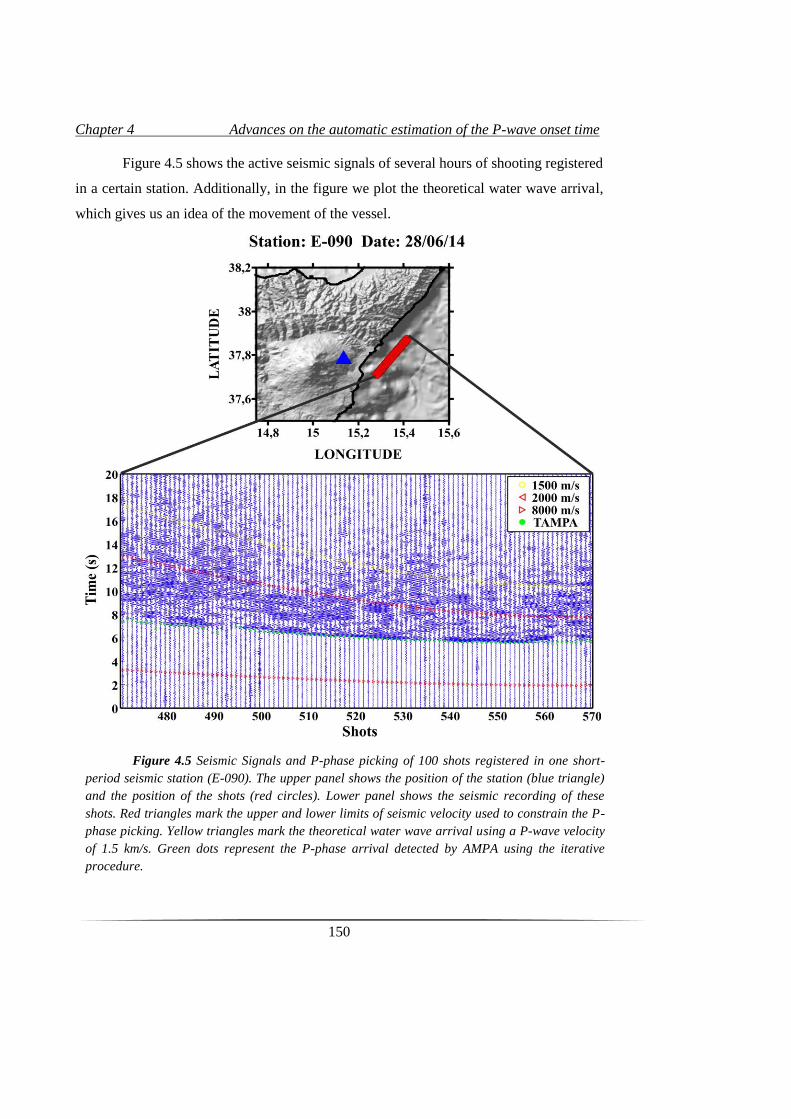
Chapter 4 Advances on the automatic estimation of the P-wave onset time
150
Figure 4.5 shows the active seismic signals of several hours of shooting registered
in a certain station. Additionally, in the figure we plot the theoretical water wave arrival,
which gives us an idea of the movement of the vessel.
Figure 4.5 Seismic Signals and P-phase picking of 100 shots registered in one short-
period seismic station (E-090). The upper panel shows the position of the station (blue triangle)
and the position of the shots (red circles). Lower panel shows the seismic recording of these
shots. Red triangles mark the upper and lower limits of seismic velocity used to constrain the P-
phase picking. Yellow triangles mark the theoretical water wave arrival using a P-wave velocity
of 1.5 km/s. Green dots represent the P-phase arrival detected by AMPA using the iterative
procedure.
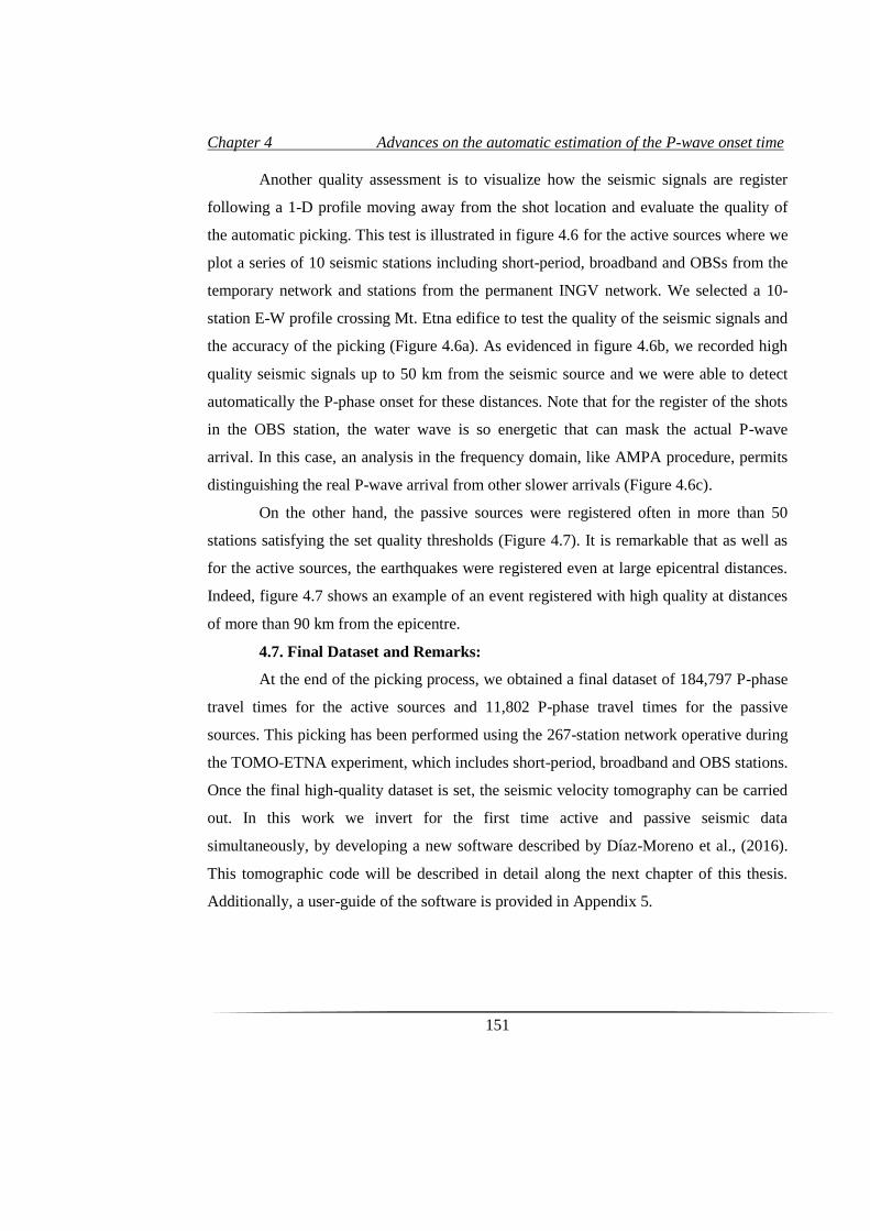
Chapter 4 Advances on the automatic estimation of the P-wave onset time
151
Another quality assessment is to visualize how the seismic signals are register
following a 1-D profile moving away from the shot location and evaluate the quality of
the automatic picking. This test is illustrated in figure 4.6 for the active sources where we
plot a series of 10 seismic stations including short-period, broadband and OBSs from the
temporary network and stations from the permanent INGV network. We selected a 10-
station E-W profile crossing Mt. Etna edifice to test the quality of the seismic signals and
the accuracy of the picking (Figure 4.6a). As evidenced in figure 4.6b, we recorded high
quality seismic signals up to 50 km from the seismic source and we were able to detect
automatically the P-phase onset for these distances. Note that for the register of the shots
in the OBS station, the water wave is so energetic that can mask the actual P-wave
arrival. In this case, an analysis in the frequency domain, like AMPA procedure, permits
distinguishing the real P-wave arrival from other slower arrivals (Figure 4.6c).
On the other hand, the passive sources were registered often in more than 50
stations satisfying the set quality thresholds (Figure 4.7). It is remarkable that as well as
for the active sources, the earthquakes were registered even at large epicentral distances.
Indeed, figure 4.7 shows an example of an event registered with high quality at distances
of more than 90 km from the epicentre.
4.7. Final Dataset and Remarks:
At the end of the picking process, we obtained a final dataset of 184,797 P-phase
travel times for the active sources and 11,802 P-phase travel times for the passive
sources. This picking has been performed using the 267-station network operative during
the TOMO-ETNA experiment, which includes short-period, broadband and OBS stations.
Once the final high-quality dataset is set, the seismic velocity tomography can be carried
out. In this work we invert for the first time active and passive seismic data
simultaneously, by developing a new software described by Díaz-Moreno et al., (2016).
This tomographic code will be described in detail along the next chapter of this thesis.
Additionally, a user-guide of the software is provided in Appendix 5.
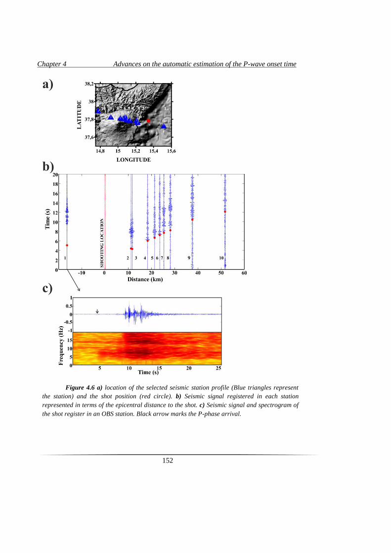
Chapter 4 Advances on the automatic estimation of the P-wave onset time
152
Figure 4.6 a) location of the selected seismic station profile (Blue triangles represent
the station) and the shot position (red circle). b) Seismic signal registered in each station
represented in terms of the epicentral distance to the shot. c) Seismic signal and spectrogram of
the shot register in an OBS station. Black arrow marks the P-phase arrival.
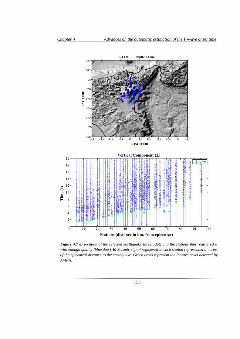
Chapter 4 Advances on the automatic estimation of the P-wave onset time
153
Figure 4.7 a) location of the selected earthquake (green dot) and the stations that registered it
with enough quality (blue dots). b) Seismic signal registered in each station represented in terms
of the epicentral distance to the earthquake. Green cross represent the P-wave onset detected by
AMPA.


5. Joint Passive Active Ray
Tomographic Software
(PARTOS)

Chapter 5 Joint Passive Active Ray Tomographic Software (PARTOS)
157
5.1. Tomographic Software State of the Art
The TOMO-ETNA experiment described in chapter 3 (Ibáñez et al., 2016a)
provided a large high-resolution seismic dataset, aiming to enlighten the complex internal
structure of Mt. Etna and surrounding areas. This database includes active and passive
data recorded during 2014 (Barberi et al., 2016; Ibáñez et al., 2016b). In this work we
take advantage of this large high-quality dataset to perform for the first time at Mt. Etna
volcano a simultaneous joint inversion of active and passive sources by applying a new
tomographic code developed ad-hoc (Díaz-Moreno et al., 2016). This software named
PARTOS (Passive Active Ray TOmography Software) will be described along this
chapter and a User Manual of it is provided in Appendix 5.
Seismic tomography methods appeared in the early 1970s and from their first
application these techniques have been widely used in different scales and environments.
Their theoretical and mathematical bases are well known by the scientific community, but
still new algorithms and approached are being developed. Implementation procedures on
a tomographic code may vary depending on the scope of the study (global, regional or
local) and the data available (Koulakov 2012, Koulakov and Shapiro 2015). At present,
several tomographic algorithms can be easily found among the international community.
Some of these codes were developed for a specific region and later adapted to other
regions. For example the code developed by Toomey et al., (1994) was initially applied in
the Pacific Rift and later adapted to other regions such as Deception Island in Antarctica
(Zandomeneghi et al., 2009). On the other hand, many codes have been developed to be
used in a wide range of areas. Some of the most relevant and well known codes are:
SIMULPS (Thurber 1983; Eberhart-Phillips 1993) applied in Vesuvius (Lomax et al.,
2001) and Mt. Etna (Patanè et al., 2006) among others; FAST (Zelt & Barton 1998)
applied in India by Rao et al., (2015); TOMODD (Zhang & Thurber 2003; applied for
example by Kato et al., (2010) in Wakayama, Japan; or Alparone et al., (2012) in Mt.
Etna, Italy); or LOTOS (Koulakov et al., 2009a). Each of these codes is different in some
procedures such as ray tracing, grid parameterization or matrix inversion among others.
When only passive seismic signals (earthquakes) are used, its application is mainly
limited to regions with high seismicity.
Chapter 5 Joint Passive Active Ray Tomographic Software (PARTOS)
158
LOTOS software (Koulakov, 2009a) has become one of the most widely used
codes for tomographic inversion of passive data. LOTOS code is a friendly widely used
tomographic code that permits study from small regions using local events to regional
inversions using teleseismic events (Jakovlev et al., 2013). The robustness of the
algorithms implemented and the capacity to handle different scales studies (regional or
local), together with its friendly use makes of this code one of the most popular and used
software among the scientific community. Robustness of the code has been highly proved
by the numerous of published works applying this software in a large variety of regions
(Table 1). These studies vary from active volcanic areas, dormant volcanoes and non-
volcanic areas, and demonstrate the versatility of the code. Passive seismic data comes
from local, regional and teleseismic earthquakes. These data are generated within a wide
range of depths and therefore give usually a better ray coverage in depth of the studied
region. However, number of earthquakes depends on the region. Earthquake location
coordinates and origin time are unknown and must be calculated by using the available
information: arrival of the seismic waves to the different seismic stations. Local and
regional seismicity usually produces clear P- and S-waves that are, then, inverted for
obtaining plausible velocity models and source parameters.
The limitation of lack of seismicity is partially solved with the use of active
sources. These seismic data comes from human-made seismic sources and there is a wide
range of methods: chemical reactions, drop of a mass, airgun shots, explosions, etc.
(Koulakov, 2012, Koulakov and Shapiro, 2015). At present, active source tomography
has been implemented in few codes such as FAST and ATOM-3D (Koulakov 2009b).The
main characteristic of these codes is that the take into account the water table when
computing the ray-tracing, which is a very sensible step when studying sea-related
environments such as volcanic islands.
ATOM-3D code follows the same structure as LOTOS, but for active datasets. In
this case, no relocation of the events is performed, as location and origin time of the
active source is a priori known, and it is taken as a fixed parameter. This algorithm has
been successfully tested in some active seismic studies such as Tenerife (García-Yeguas
et al. 2012) and Eastern Greece (Shahrukh et al. 2012). The main advantage of the use of
Chapter 5 Joint Passive Active Ray Tomographic Software (PARTOS)
159
active sources is that they permit to register seismic waves in whatever region.
Nonetheless, it is very expensive and therefore not always available (Koulakov & Shapiro
2015). Commonly, active sources give very detailed information of the shallower layers
of the crust. However, resolution in depth is poor due to the fact that they can only be
produced near the surface. The main characteristic of the active sources that make them
useful for seismic tomography is that we certainly know the exact time origin and
location of both source and receiver, and therefore we only have the ray tracing variable.
Clear P-wave arrival can be registered from active sources while S-wave arrivals are not
always available.
Recently, some efforts have been focused on the use of both seismic sources to
obtain a joint seismic tomographic image. For example, a few algorithms merge both
active and passive data (eg. Battaglia et al 2008b; Rawlinson & Urvoy 2006; Wagner et
al. 2007). The major complexity of these new joint procedures is that active and passive
seismic data have different characteristics such as its source location; therefore, it is
important to take into account these differences in order to better adapt the algorithms for
each case. The combination of these two types of sources permits to diminish their lack of
information and enhances their valuable information. Active sources can cover areas
where no natural seismicity is located. On the other hand, earthquakes may give
important information of the deep layers of the crust and of S-wave properties. By
merging active and passive data we obtain better ray coverage in both shallow and deep
layers, leading to a higher resolution of seismic tomography models.
Along this chapter, we describe PARTOS, a new tomographic code developed for
joint inversion of active and passive datasets. This code was born to solve the above
mentioned necessities.
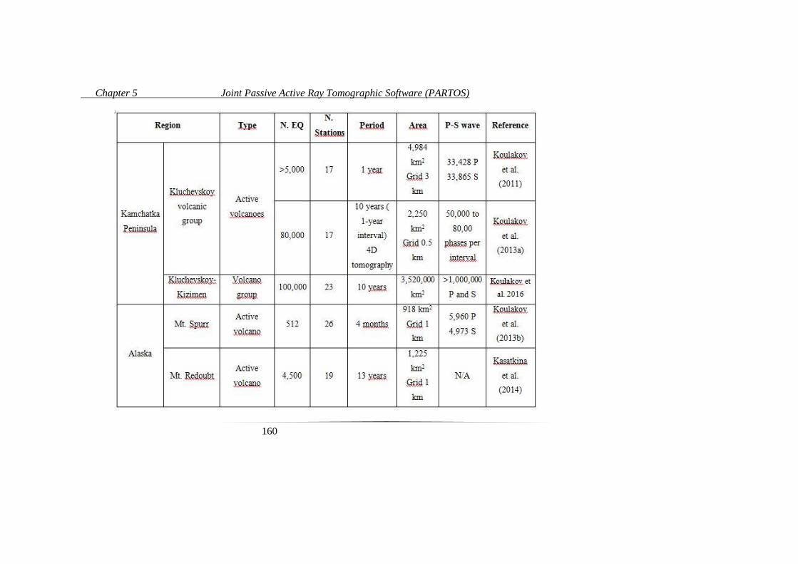
Chapter 5 Joint Passive Active Ray Tomographic Software (PARTOS)
160
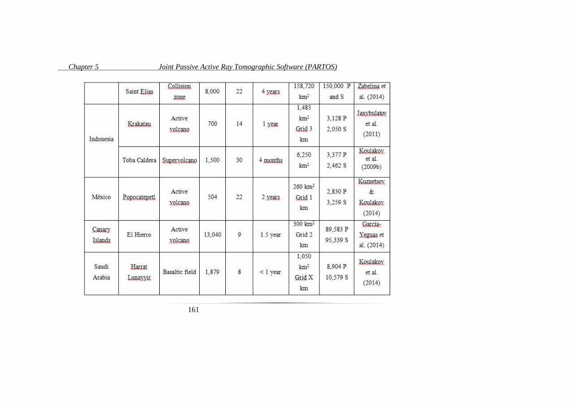
Chapter 5 Joint Passive Active Ray Tomographic Software (PARTOS)
161

Chapter 5 Joint Passive Active Ray Tomographic Software (PARTOS)
162
Table 1Recent most relevant tomographic studies performed using LOTOS code (Díaz-Moreno et al., 2016).
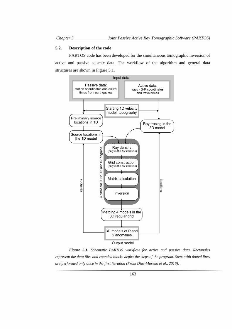
Chapter 5 Joint Passive Active Ray Tomographic Software (PARTOS)
163
5.2. Description of the code
PARTOS code has been developed for the simultaneous tomographic inversion of
active and passive seismic data. The workflow of the algorithm and general data
structures are shown in Figure 5.1.
Figure 5.1. Schematic PARTOS workflow for active and passive data. Rectangles
represent the data files and rounded blocks depict the steps of the program. Steps with dotted lines
are performed only once in the first iteration (From Díaz-Moreno et al., 2016).
Chapter 5 Joint Passive Active Ray Tomographic Software (PARTOS)
164
5.2.1 Input data:
The input data for the calculations include the data groups related to active and
passive seismic experiments, as well as the starting 1D velocity model and other
parameters for calculations. The passive source data include two files: one with
geographical coordinates of stations and another one with arrival times of P- and S waves
from earthquakes to the stations. The information on the source coordinates and origin
times is not strictly required. In case of its absence, the sources can be placed to the center
of the network or beneath the station with minimum arrival time. If the locations of
events are available a priori, they can be included to the initial data file that may facilitate
the calculations.
For the active source data, there is only one file. Each line in this file corresponds
to one ray containing geographical coordinates of the source and the receiver and travel
time of seismic wave. The first three lines should correspond to the gathers for which the
data were picked. In the cases of offshore surveys with the use of air-guns, the gathers are
usually the stations, whereas in the cases of using a few explosions and numerous
receivers, the gathers are the sources.
The initial data files may contain the two-dimensional map of topography (in case
of absence, the flat topography is predefined at zero depth). It is especially important in
cases of offshore experiments, when the travel time in the water layer between air-guns
and sea bottom should be taken into account.
The file with the 1D model of the P and S wave velocities should be defined. The
velocity values are set at some depth levels; between these levels, the velocity is linearly
interpolated. The values of the initial S-velocities are often determined from the P-
velocities based on constant Vp/Vs ratio.
In addition, a file with a set of different parameters used for calculations should
be defined. This file includes, among others, the grid spacing, parameters for ray tracing
and source locations, weights for the active and passive data, damping parameters for
inversion, and visualization settings. Defining these parameters is mostly based on several
trials of performing the inversions for real and synthetic datasets.
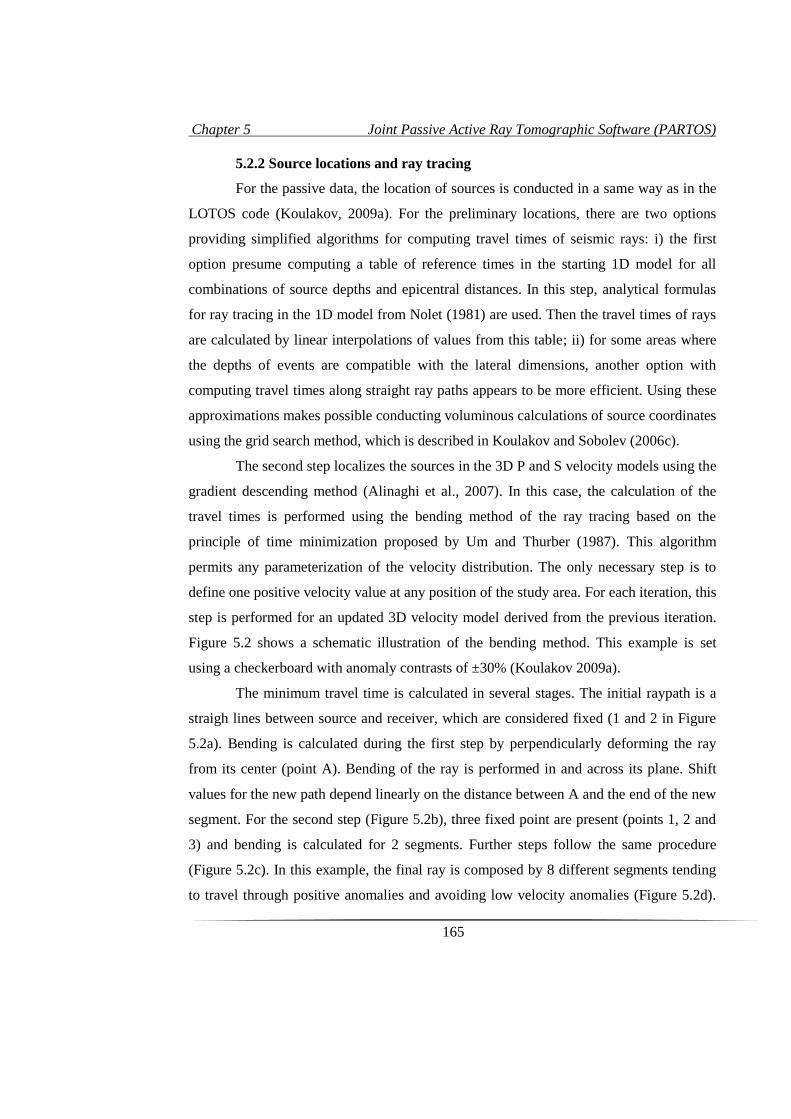
Chapter 5 Joint Passive Active Ray Tomographic Software (PARTOS)
165
5.2.2 Source locations and ray tracing
For the passive data, the location of sources is conducted in a same way as in the
LOTOS code (Koulakov, 2009a). For the preliminary locations, there are two options
providing simplified algorithms for computing travel times of seismic rays: i) the first
option presume computing a table of reference times in the starting 1D model for all
combinations of source depths and epicentral distances. In this step, analytical formulas
for ray tracing in the 1D model from Nolet (1981) are used. Then the travel times of rays
are calculated by linear interpolations of values from this table; ii) for some areas where
the depths of events are compatible with the lateral dimensions, another option with
computing travel times along straight ray paths appears to be more efficient. Using these
approximations makes possible conducting voluminous calculations of source coordinates
using the grid search method, which is described in Koulakov and Sobolev (2006c).
The second step localizes the sources in the 3D P and S velocity models using the
gradient descending method (Alinaghi et al., 2007). In this case, the calculation of the
travel times is performed using the bending method of the ray tracing based on the
principle of time minimization proposed by Um and Thurber (1987). This algorithm
permits any parameterization of the velocity distribution. The only necessary step is to
define one positive velocity value at any position of the study area. For each iteration, this
step is performed for an updated 3D velocity model derived from the previous iteration.
Figure 5.2 shows a schematic illustration of the bending method. This example is set
using a checkerboard with anomaly contrasts of ±30% (Koulakov 2009a).
The minimum travel time is calculated in several stages. The initial raypath is a
straigh lines between source and receiver, which are considered fixed (1 and 2 in Figure
5.2a). Bending is calculated during the first step by perpendicularly deforming the ray
from its center (point A). Bending of the ray is performed in and across its plane. Shift
values for the new path depend linearly on the distance between A and the end of the new
segment. For the second step (Figure 5.2b), three fixed point are present (points 1, 2 and
3) and bending is calculated for 2 segments. Further steps follow the same procedure
(Figure 5.2c). In this example, the final ray is composed by 8 different segments tending
to travel through positive anomalies and avoiding low velocity anomalies (Figure 5.2d).
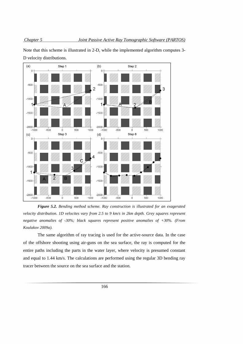
Chapter 5 Joint Passive Active Ray Tomographic Software (PARTOS)
166
Note that this scheme is illustrated in 2-D, while the implemented algorithm computes 3-
D velocity distributions.
Figure 5.2. Bending method scheme. Ray construction is illustrated for an exagerated
velocity distribution. 1D velocites vary from 2.5 to 9 km/s in 2km depth. Grey squares represent
negative anomalies of -30%; black squares represent positive anomalies of +30%. (From
Koulakov 2009a).
The same algorithm of ray tracing is used for the active-source data. In the case
of the offshore shooting using air-guns on the sea surface, the ray is computed for the
entire paths including the parts in the water layer, where velocity is presumed constant
and equal to 1.44 km/s. The calculations are performed using the regular 3D bending ray
tracer between the source on the sea surface and the station.
Chapter 5 Joint Passive Active Ray Tomographic Software (PARTOS)
167
5.2.3. Grid construction
To parameterize the 3D velocity distribution, we construct the mesh with nodes
distributed in the study volume according to the ray density. Between the nodes, the
velocity anomalies are continuously approximated using a linear interpolation. Because of
significant disproportion in the amount of passive and active data, the ray density is
computed using different weights for the P and S data. The nodes are placed only in areas
with sufficient ray coverage (typically, with the ray density of 0.1 of the average value).
In the map view, the nodes are installed regularly with a fixed grid spacing. In the vertical
direction, the grid spacing depends on the ray density; this is, the higher the ray density is
the finer the grid spacing can be. In well covered areas, the spacing is equal to the
minimum predefined value; and it becomes larger where the ray density is lower.
Usually, the grid spacing is set smaller than the expected resolution so that every
restored anomaly was based on several nodes. This helps to avoid the dependency of the
results on the grid configurations. To further reduce this effect, we perform the inversion
for several grids with different basic orientations (typically, four grids with orientations of
0, 22, 45 and 67 degrees). After computing results for all grids, they are averaged in one
3D model using a regular mesh. The grid is constructed only one time in the first
iteration. In the following iterations, the velocity anomalies are updated in the same
nodes.
5.2.4. Matrix calculation and inversion
To perform the tomography inversion, we compute one matrix which includes the
pairs of the active and passive data. The matrix elements responsible for the velocity
distributions are the first derivatives Aij representing time deviation along the j-th ray due
to the unit velocity variations in the i-th node (eq.1).
𝐴𝑖𝑗 = ∫ ∆𝑔𝑗(𝛾)𝑑𝑆/∆𝜎𝑗
𝛾 (1)
Where ∆𝑔𝑗 represents the slowness perturbation at the point of the ray caused by
slowness anomaly ∆𝜎𝑗, at the j-th node (Koulakov & Sobolev, 2006b). Their values are
computed by numerical integration along the ray paths derived after the steps of locations
(for the passive data) and ray tracing (for the active data). For the passive data, each row
Chapter 5 Joint Passive Active Ray Tomographic Software (PARTOS)
168
of the matrix contains also four elements responsible for source parameters (Px, Py, Pz
and 1) and one unit element responsible for the station correction (P or S). For the active
source data, there is only one additional element responsible for the gather correction
(usually, stations, for the air-gun surveys and sources, in cases of explosions on land).
The data vector contains the time residuals computed for the current velocity model.
The inversion is damped by using two additional matrix blocks. The first
block, which is responsible for amplitude damping, is a diagonal matrix containing only
one non-zero element in each row and zero data vectors. Increasing weight of this block
decreases the amplitude of the solution. The second damping block controls the flattening
of the solution. Each row of this block contains two nonzero elements with equal values,
but opposite signs, corresponding to all combinations of neighboring nodes in the
parameterization mesh. Increasing the weight of this block decreases velocity gradients in
the resulting models.
The inversion of the large sparse matrix is performed using the LSQR algorithm
(Page and Saunders, 1982; Nolet, 1981). The most important parameters controlling the
inversion with the values optimized for a specific case of the TOMO-ETNA experiment
are presented in Appendix 5. The values of these parameters are determined after several
trials with synthetic and observed data.
5.2.5. Combining the velocity models and iterating
The models computed for several differently oriented parameterization meshes
are averaged and combined in one model defined on a regular grid. This model is used in
the next iteration for performing the ray tracing (for active data) and source re-location
(for the passive data). Number of iterations is usually fixed at a predefined value as a
compromise between the calculation time and accuracy of the solution. To stablish the
number of iterations, we use a threshold parameter that represents the time residuals
(Koulakov, 2009a). This threshold is usually set at 0.5 and we consider the solution as
stable once it decreases slowly down the threshold (usually after 5-6 iterations). In this
case, tuning of the solution properties is conducted using the damping parameters. A
regular inversion running in a ‘core i7’ personal computer takes approximately 2 hours to
perform 5 iterations.
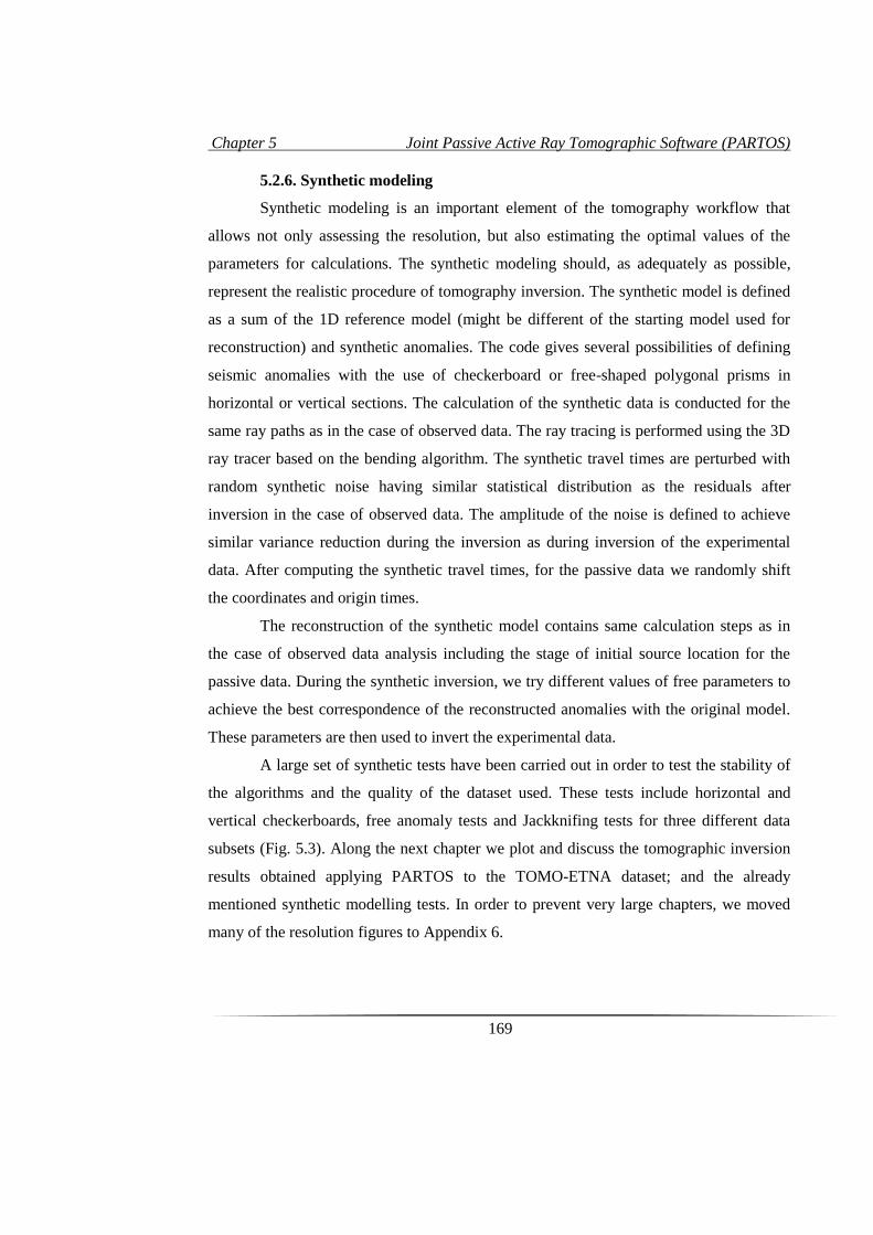
Chapter 5 Joint Passive Active Ray Tomographic Software (PARTOS)
169
5.2.6. Synthetic modeling
Synthetic modeling is an important element of the tomography workflow that
allows not only assessing the resolution, but also estimating the optimal values of the
parameters for calculations. The synthetic modeling should, as adequately as possible,
represent the realistic procedure of tomography inversion. The synthetic model is defined
as a sum of the 1D reference model (might be different of the starting model used for
reconstruction) and synthetic anomalies. The code gives several possibilities of defining
seismic anomalies with the use of checkerboard or free-shaped polygonal prisms in
horizontal or vertical sections. The calculation of the synthetic data is conducted for the
same ray paths as in the case of observed data. The ray tracing is performed using the 3D
ray tracer based on the bending algorithm. The synthetic travel times are perturbed with
random synthetic noise having similar statistical distribution as the residuals after
inversion in the case of observed data. The amplitude of the noise is defined to achieve
similar variance reduction during the inversion as during inversion of the experimental
data. After computing the synthetic travel times, for the passive data we randomly shift
the coordinates and origin times.
The reconstruction of the synthetic model contains same calculation steps as in
the case of observed data analysis including the stage of initial source location for the
passive data. During the synthetic inversion, we try different values of free parameters to
achieve the best correspondence of the reconstructed anomalies with the original model.
These parameters are then used to invert the experimental data.
A large set of synthetic tests have been carried out in order to test the stability of
the algorithms and the quality of the dataset used. These tests include horizontal and
vertical checkerboards, free anomaly tests and Jackknifing tests for three different data
subsets (Fig. 5.3). Along the next chapter we plot and discuss the tomographic inversion
results obtained applying PARTOS to the TOMO-ETNA dataset; and the already
mentioned synthetic modelling tests. In order to prevent very large chapters, we moved
many of the resolution figures to Appendix 6.
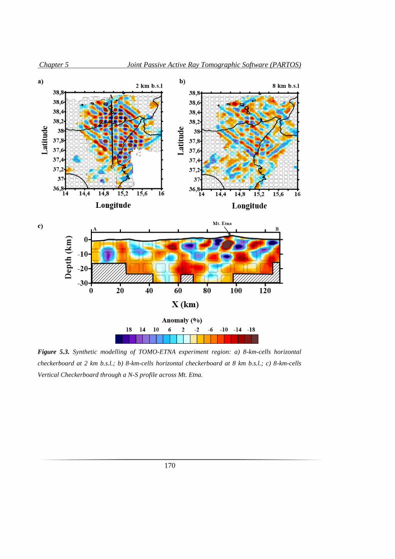
Chapter 5 Joint Passive Active Ray Tomographic Software (PARTOS)
170
Figure 5.3. Synthetic modelling of TOMO-ETNA experiment region: a) 8-km-cells horizontal
checkerboard at 2 km b.s.l.; b) 8-km-cells horizontal checkerboard at 8 km b.s.l.; c) 8-km-cells
Vertical Checkerboard through a N-S profile across Mt. Etna.

Chapter 5 Joint Passive Active Ray Tomographic Software (PARTOS)
171
5.3. Final remarks
As final remarks we can state that PARTOS is a friendly tomography code born
from the necessity of combining active and passive seismic data during a tomographic
inversion. The robustness of the algorithms used is widely proved as most of the
algorithms applied were adapted from previous versions of LOTOS and ATOM-3D
codes, which are widely used among the scientific community during the last decade.
New features have been implemented to enhance the robustness and completeness of the
calculations, making the software fast and adaptive to different kind of datasets.

6. Joint active and passive P-
wave seismic tomography of
Mt. Etna volcano, Aeolian
Islands and related
geodynamic region

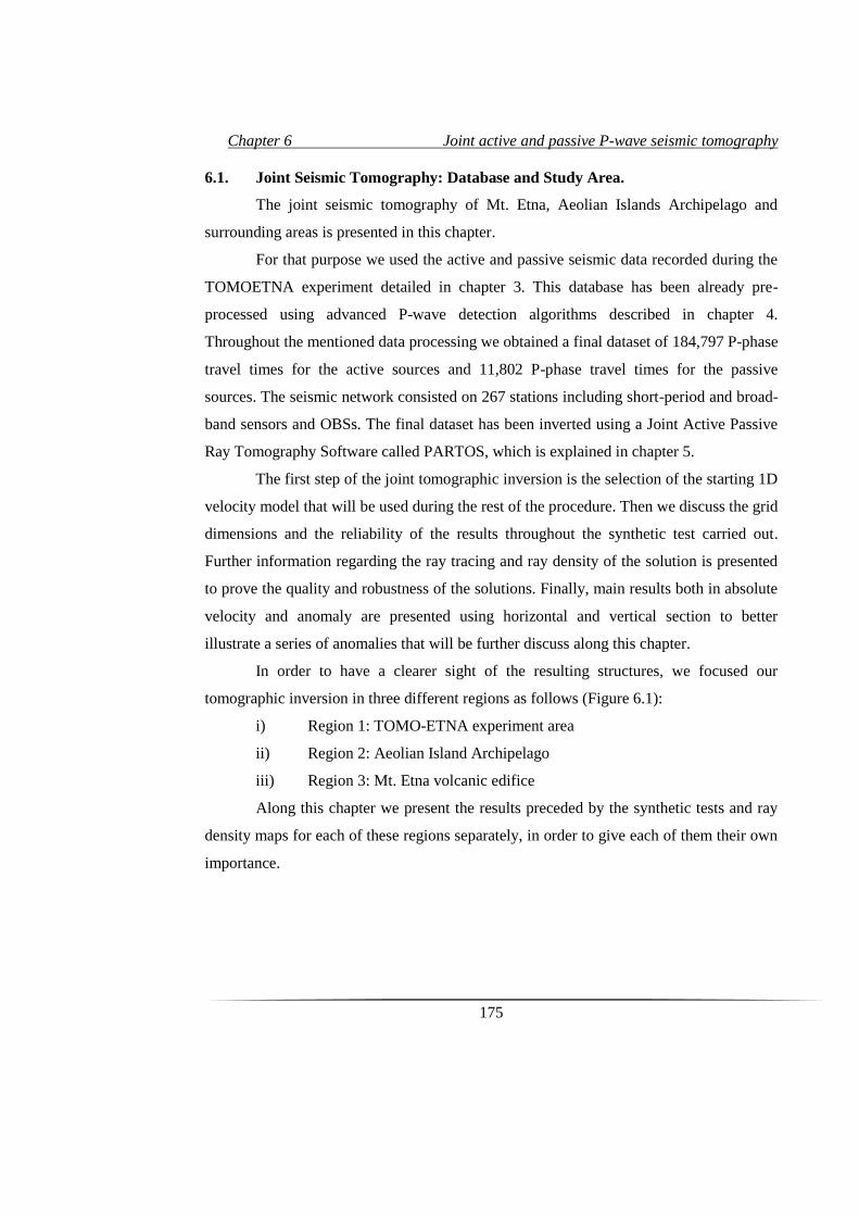
Chapter 6 Joint active and passive P-wave seismic tomography
175
6.1. Joint Seismic Tomography: Database and Study Area.
The joint seismic tomography of Mt. Etna, Aeolian Islands Archipelago and
surrounding areas is presented in this chapter.
For that purpose we used the active and passive seismic data recorded during the
TOMOETNA experiment detailed in chapter 3. This database has been already pre-
processed using advanced P-wave detection algorithms described in chapter 4.
Throughout the mentioned data processing we obtained a final dataset of 184,797 P-phase
travel times for the active sources and 11,802 P-phase travel times for the passive
sources. The seismic network consisted on 267 stations including short-period and broad-
band sensors and OBSs. The final dataset has been inverted using a Joint Active Passive
Ray Tomography Software called PARTOS, which is explained in chapter 5.
The first step of the joint tomographic inversion is the selection of the starting 1D
velocity model that will be used during the rest of the procedure. Then we discuss the grid
dimensions and the reliability of the results throughout the synthetic test carried out.
Further information regarding the ray tracing and ray density of the solution is presented
to prove the quality and robustness of the solutions. Finally, main results both in absolute
velocity and anomaly are presented using horizontal and vertical section to better
illustrate a series of anomalies that will be further discuss along this chapter.
In order to have a clearer sight of the resulting structures, we focused our
tomographic inversion in three different regions as follows (Figure 6.1):
i) Region 1: TOMO-ETNA experiment area
ii) Region 2: Aeolian Island Archipelago
iii) Region 3: Mt. Etna volcanic edifice
Along this chapter we present the results preceded by the synthetic tests and ray
density maps for each of these regions separately, in order to give each of them their own
importance.
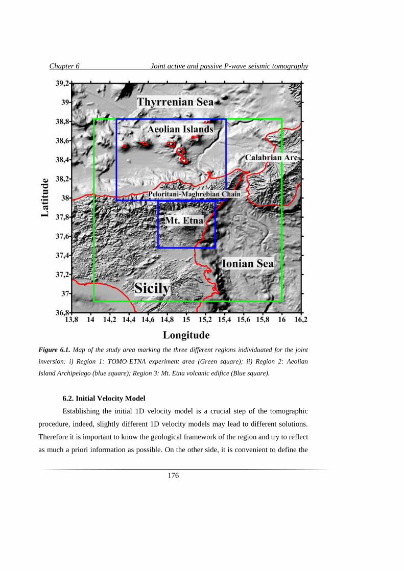
Chapter 6 Joint active and passive P-wave seismic tomography
176
Figure 6.1. Map of the study area marking the three different regions individuated for the joint
inversion: i) Region 1: TOMO-ETNA experiment area (Green square); ii) Region 2: Aeolian
Island Archipelago (blue square); Region 3: Mt. Etna volcanic edifice (Blue square).
6.2. Initial Velocity Model
Establishing the initial 1D velocity model is a crucial step of the tomographic
procedure, indeed, slightly different 1D velocity models may lead to different solutions.
Therefore it is important to know the geological framework of the region and try to reflect
as much a priori information as possible. On the other side, it is convenient to define the
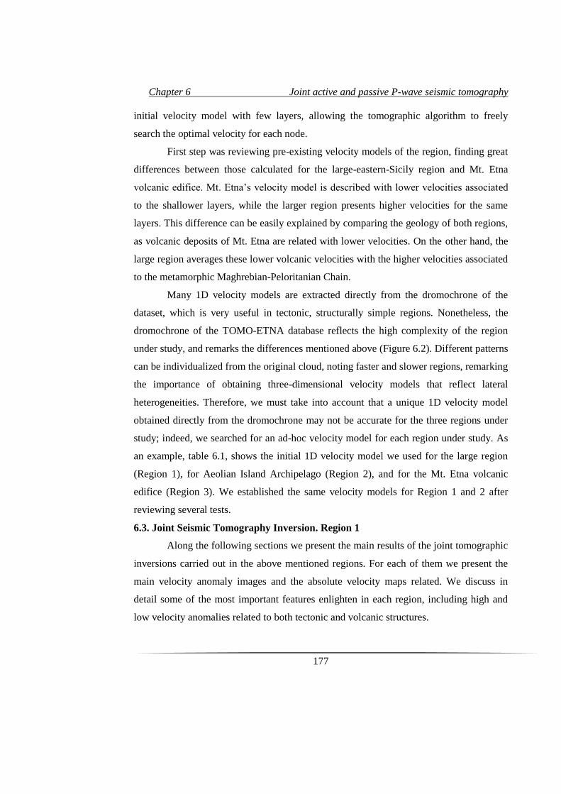
Chapter 6 Joint active and passive P-wave seismic tomography
177
initial velocity model with few layers, allowing the tomographic algorithm to freely
search the optimal velocity for each node.
First step was reviewing pre-existing velocity models of the region, finding great
differences between those calculated for the large-eastern-Sicily region and Mt. Etna
volcanic edifice. Mt. Etna’s velocity model is described with lower velocities associated
to the shallower layers, while the larger region presents higher velocities for the same
layers. This difference can be easily explained by comparing the geology of both regions,
as volcanic deposits of Mt. Etna are related with lower velocities. On the other hand, the
large region averages these lower volcanic velocities with the higher velocities associated
to the metamorphic Maghrebian-Peloritanian Chain.
Many 1D velocity models are extracted directly from the dromochrone of the
dataset, which is very useful in tectonic, structurally simple regions. Nonetheless, the
dromochrone of the TOMO-ETNA database reflects the high complexity of the region
under study, and remarks the differences mentioned above (Figure 6.2). Different patterns
can be individualized from the original cloud, noting faster and slower regions, remarking
the importance of obtaining three-dimensional velocity models that reflect lateral
heterogeneities. Therefore, we must take into account that a unique 1D velocity model
obtained directly from the dromochrone may not be accurate for the three regions under
study; indeed, we searched for an ad-hoc velocity model for each region under study. As
an example, table 6.1, shows the initial 1D velocity model we used for the large region
(Region 1), for Aeolian Island Archipelago (Region 2), and for the Mt. Etna volcanic
edifice (Region 3). We established the same velocity models for Region 1 and 2 after
reviewing several tests.
6.3. Joint Seismic Tomography Inversion. Region 1
Along the following sections we present the main results of the joint tomographic
inversions carried out in the above mentioned regions. For each of them we present the
main velocity anomaly images and the absolute velocity maps related. We discuss in
detail some of the most important features enlighten in each region, including high and
low velocity anomalies related to both tectonic and volcanic structures.
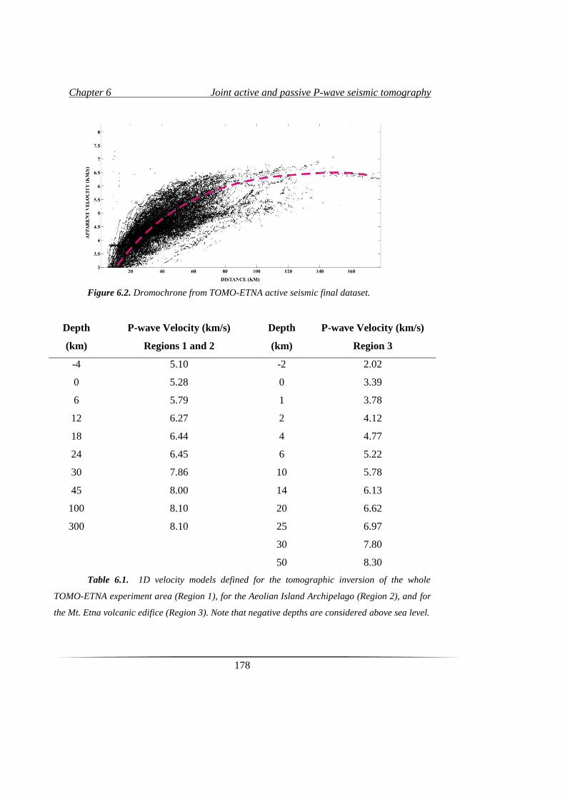
Chapter 6 Joint active and passive P-wave seismic tomography
178
Figure 6.2. Dromochrone from TOMO-ETNA active seismic final dataset.
Depth
(km)
P-wave Velocity (km/s)
Regions 1 and 2
Depth
(km)
P-wave Velocity (km/s)
Region 3
-4 5.10 -2 2.02
0 5.28 0 3.39
6 5.79 1 3.78
12 6.27 2 4.12
18 6.44 4 4.77
24 6.45 6 5.22
30 7.86 10 5.78
45 8.00 14 6.13
100 8.10 20 6.62
300 8.10 25 6.97
30 7.80
50 8.30
Table 6.1. 1D velocity models defined for the tomographic inversion of the whole
TOMO-ETNA experiment area (Region 1), for the Aeolian Island Archipelago (Region 2), and for
the Mt. Etna volcanic edifice (Region 3). Note that negative depths are considered above sea level.
Chapter 6 Joint active and passive P-wave seismic tomography
179
Region 1 is an area that covers 300x300 km comprising eastern Sicily, Mt. Etna
volcano, Ionian and Thyrrenian Seas and Aeolian Islands Archipelago (Figure 6.1).
Firstly, we present the results of some of the synthetic tests performed in order to
constrain grid dimensions and to estimate the reliable area based on our dataset. Then we
describe the ray density calculated and finally we show the tomographic images and
discuss the main anomalies observed.
6.3.1. Synthetic tests
For the tomographic inversion of this region we selected a grid with a step of 6
km in horizontal and 2 km in vertical, reaching to 30 km in depth. These final grid
dimensions were selected after several synthetic tests that vary from horizontal and
vertical checkerboards, jackknifing tests and free anomaly synthetic tests. In order to
make this chapter easy to read we only present few of the mentioned tests. For more
information, go to Appendix 6.
6.3.1.1. Checkerboards
In order to determine the optimal spatial resolution and the smearing effect we
carried out a series of checkerboard tests starting with a coarse area comprising the whole
TOMO-ETNA study region. Figure 6.3, shows the results of the horizontal and vertical
checkerboards inverted for this region. For the horizontal board we inverted a 300x300
km area, using different grid spacing ranging from 12 to 4 km. The horizontal
configuration that better resolves the compromise between anomaly size and solution
accuracy is a 6km-spacing anomalies. Checkerboard is computed by inverting a pattern of
±10% anomalies periodically placed with opposite polarity and separated 3 km from each
other. For this resolution, the model solves convincingly the anomaly pattern in a
horizontal region of around 180·120 km (Figure 6.3a, b) and up to 30 km in depth
beneath Mt. Etna (Figure 6c).
6.3.1.2. Free Anomaly test
Inverting a synthetic test using a predefined anomaly permits to determine
whether our resulting anomalies can be trusted or not. Following this premise, we have
designed 2 anomalies, one of them similar in size and shape to those expected with the
real inversions in order to check the capacity of the model to solve them. Positive and
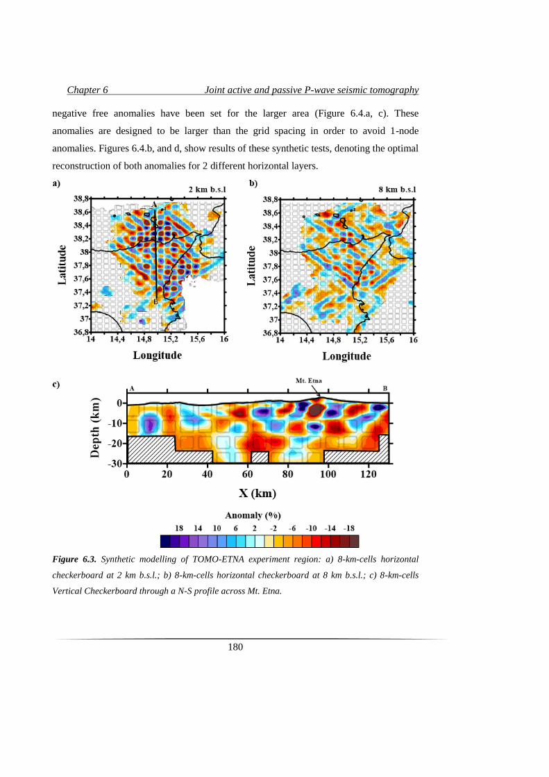
Chapter 6 Joint active and passive P-wave seismic tomography
180
negative free anomalies have been set for the larger area (Figure 6.4.a, c). These
anomalies are designed to be larger than the grid spacing in order to avoid 1-node
anomalies. Figures 6.4.b, and d, show results of these synthetic tests, denoting the optimal
reconstruction of both anomalies for 2 different horizontal layers.
Figure 6.3. Synthetic modelling of TOMO-ETNA experiment region: a) 8-km-cells horizontal
checkerboard at 2 km b.s.l.; b) 8-km-cells horizontal checkerboard at 8 km b.s.l.; c) 8-km-cells
Vertical Checkerboard through a N-S profile across Mt. Etna.
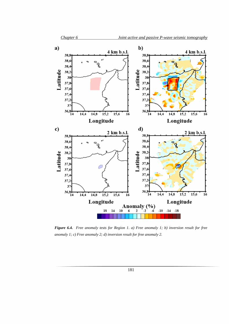
Chapter 6 Joint active and passive P-wave seismic tomography
181
Figure 6.4. Free anomaly tests for Region 1. a) Free anomaly 1; b) inversion result for free
anomaly 1; c) Free anomaly 2; d) inversion result for free anomaly 2.
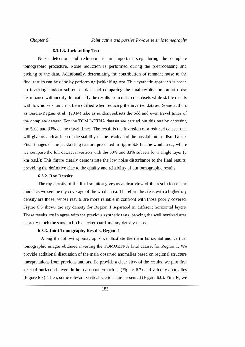
Chapter 6 Joint active and passive P-wave seismic tomography
182
6.3.1.3. Jackknifing Test
Noise detection and reduction is an important step during the complete
tomographic procedure. Noise reduction is performed during the preprocessing and
picking of the data. Additionally, determining the contribution of remnant noise to the
final results can be done by performing jackknifing test. This synthetic approach is based
on inverting random subsets of data and comparing the final results. Important noise
disturbance will modify dramatically the results from different subsets while stable results
with low noise should not be modified when reducing the inverted dataset. Some authors
as Garcia-Yeguas et al., (2014) take as random subsets the odd and even travel times of
the complete dataset. For the TOMO-ETNA dataset we carried out this test by choosing
the 50% and 33% of the travel times. The result is the inversion of a reduced dataset that
will give us a clear idea of the stability of the results and the possible noise disturbance.
Final images of the jackknifing test are presented in figure 6.5 for the whole area, where
we compare the full dataset inversion with the 50% and 33% subsets for a single layer (2
km b.s.l.); This figure clearly demonstrate the low noise disturbance to the final results,
providing the definitive clue to the quality and reliability of our tomographic results.
6.3.2. Ray Density
The ray density of the final solution gives us a clear view of the resolution of the
model as we see the ray coverage of the whole area. Therefore the areas with a higher ray
density are those, whose results are more reliable in confront with those poorly covered.
Figure 6.6 shows the ray density for Region 1 separated in different horizontal layers.
These results are in agree with the previous synthetic tests, proving the well resolved area
is pretty much the same in both checkerboard and ray-density maps.
6.3.3. Joint Tomography Results. Region 1
Along the following paragraphs we illustrate the main horizontal and vertical
tomographic images obtained inverting the TOMOETNA final dataset for Region 1. We
provide additional discussion of the main observed anomalies based on regional structure
interpretations from previous authors. To provide a clear view of the results, we plot first
a set of horizontal layers in both absolute velocities (Figure 6.7) and velocity anomalies
(Figure 6.8). Then, some relevant vertical sections are presented (Figure 6.9). Finally, we
Chapter 6 Joint active and passive P-wave seismic tomography
183
enlarge some of the most relevant horizontal layers (Figures 6.10, 6.11, 6.12 and 6.13),
and vertical sections (Figure 6.14) in order to better discuss the main structural anomalies.
Figure 6.5. Jackknifing test for Region 1: a) complete dataset inversion; b) 50% of the
dataset inverted; c) 33% of the dataset inverted.
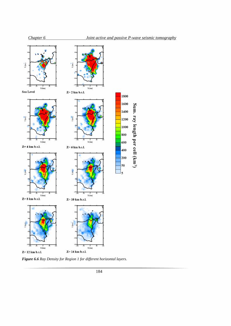
Chapter 6 Joint active and passive P-wave seismic tomography
184
Figure 6.6 Ray Density for Region 1 for different horizontal layers.
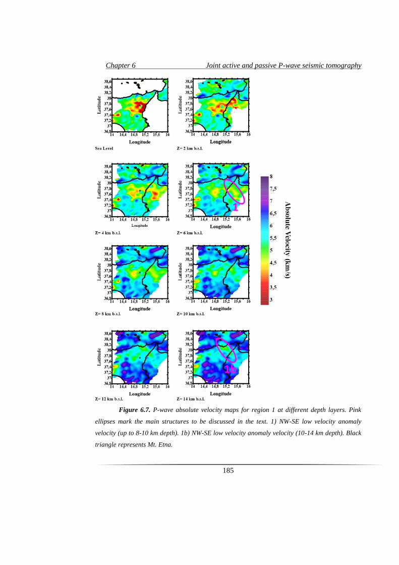
Chapter 6 Joint active and passive P-wave seismic tomography
185
Figure 6.7. P-wave absolute velocity maps for region 1 at different depth layers. Pink
ellipses mark the main structures to be discussed in the text. 1) NW-SE low velocity anomaly
velocity (up to 8-10 km depth). 1b) NW-SE low velocity anomaly velocity (10-14 km depth). Black
triangle represents Mt. Etna.
1
1b
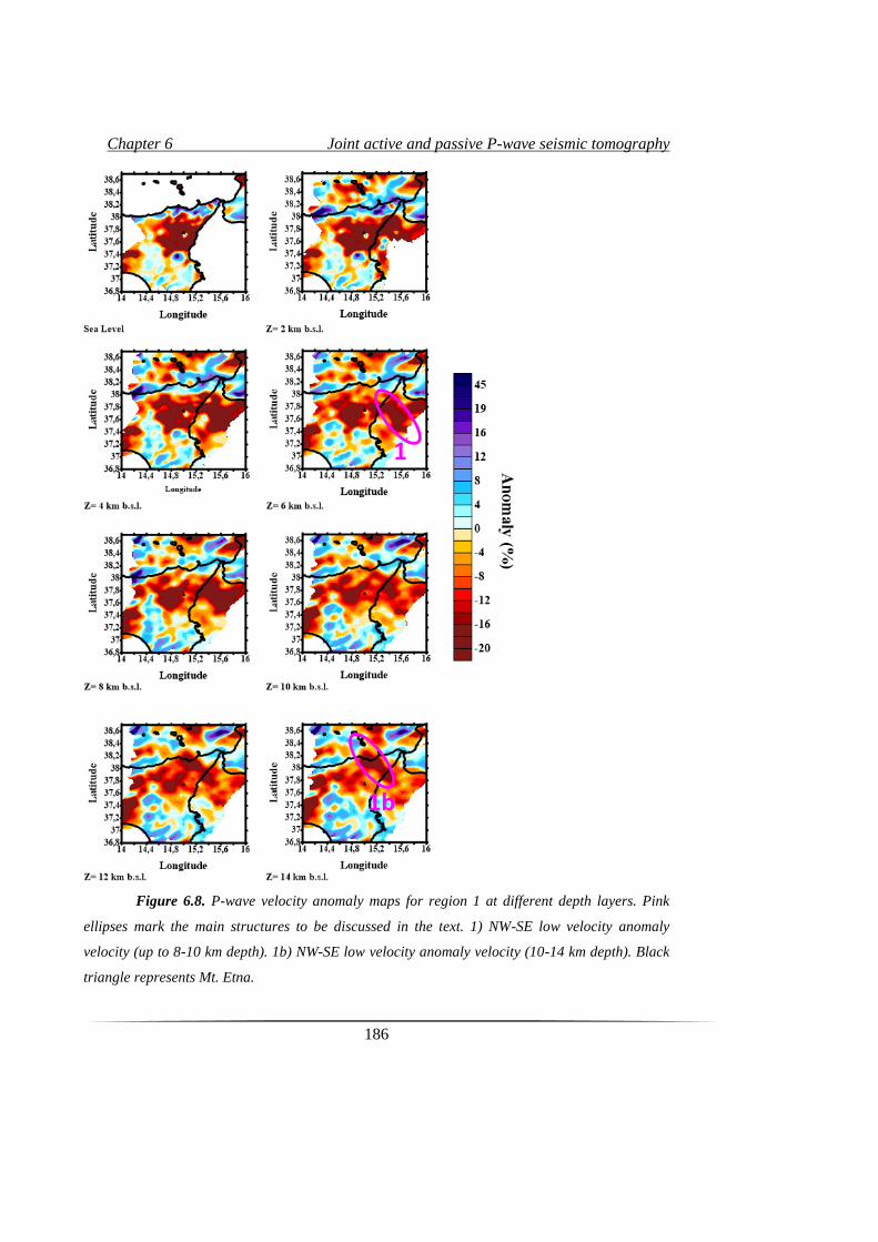
Chapter 6 Joint active and passive P-wave seismic tomography
186
Figure 6.8. P-wave velocity anomaly maps for region 1 at different depth layers. Pink
ellipses mark the main structures to be discussed in the text. 1) NW-SE low velocity anomaly
velocity (up to 8-10 km depth). 1b) NW-SE low velocity anomaly velocity (10-14 km depth). Black
triangle represents Mt. Etna.
1
1b
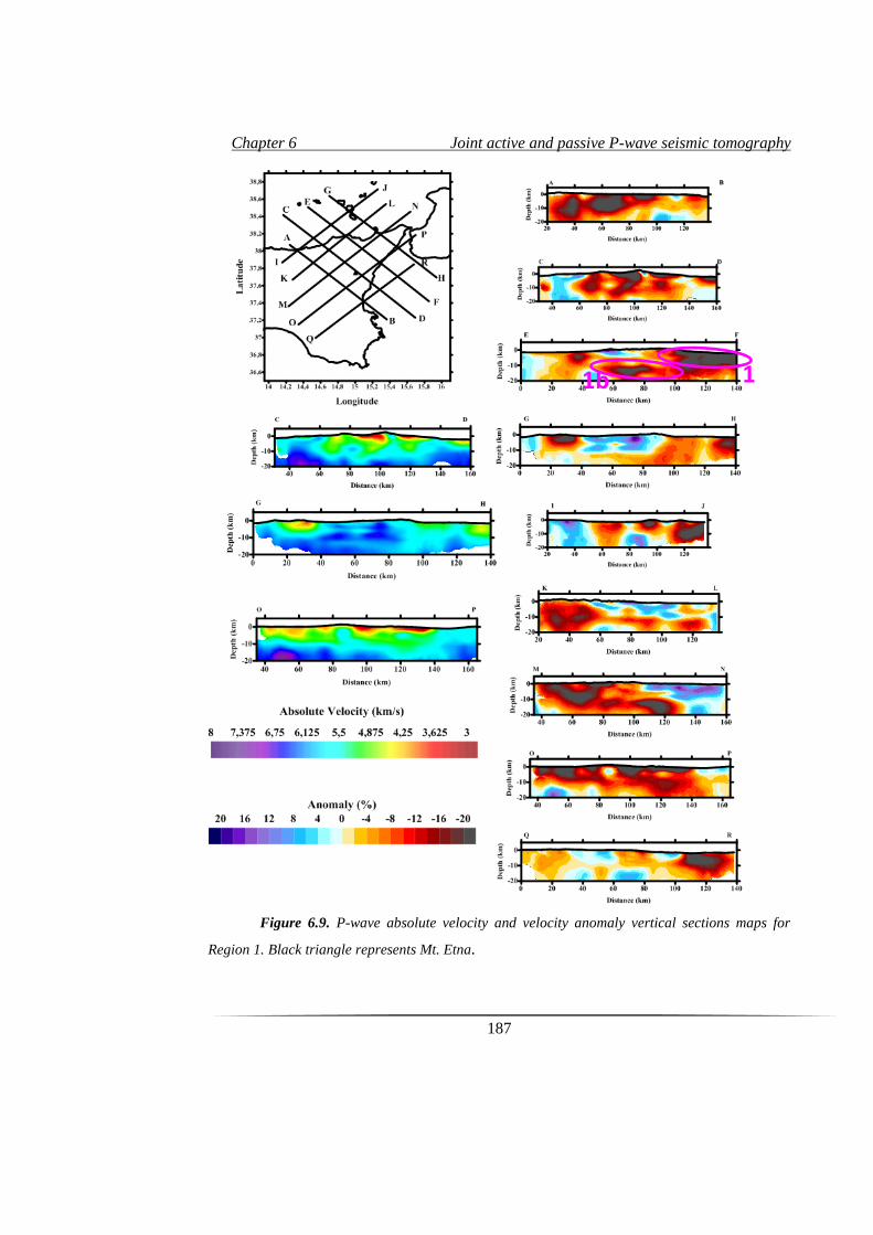
Chapter 6 Joint active and passive P-wave seismic tomography
187
Figure 6.9. P-wave absolute velocity and velocity anomaly vertical sections maps for
Region 1. Black triangle represents Mt. Etna.
1 1b
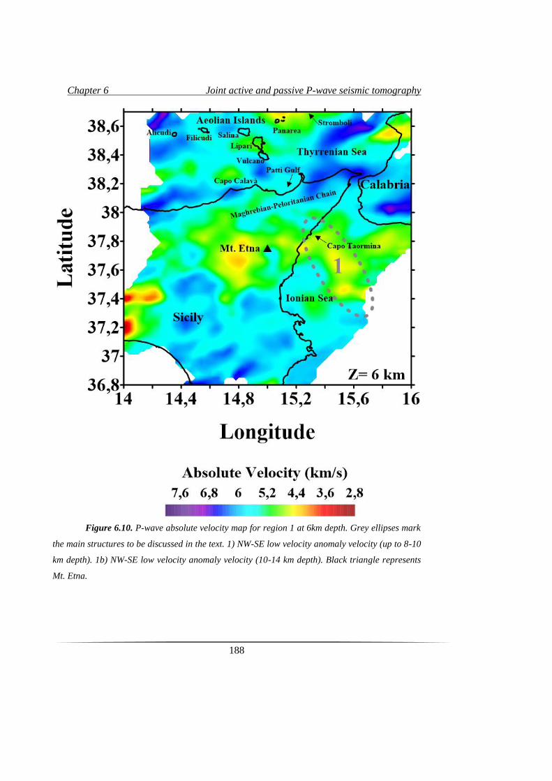
Chapter 6 Joint active and passive P-wave seismic tomography
188
Figure 6.10. P-wave absolute velocity map for region 1 at 6km depth. Grey ellipses mark
the main structures to be discussed in the text. 1) NW-SE low velocity anomaly velocity (up to 8-10
km depth). 1b) NW-SE low velocity anomaly velocity (10-14 km depth). Black triangle represents
Mt. Etna.
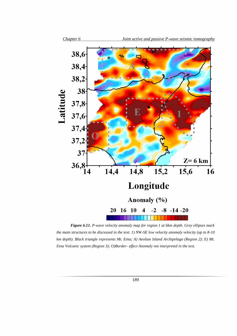
Chapter 6 Joint active and passive P-wave seismic tomography
189
Figure 6.11. P-wave velocity anomaly map for region 1 at 6km depth. Grey ellipses mark
the main structures to be discussed in the text. 1) NW-SE low velocity anomaly velocity (up to 8-10
km depth). Black triangle represents Mt. Etna; A) Aeolian Island Archipelago (Region 2); E) Mt.
Etna Volcanic system (Region 3); O)Border- effect Anomaly not interpreted in the text.
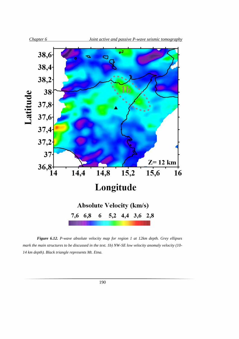
Chapter 6 Joint active and passive P-wave seismic tomography
190
Figure 6.12. P-wave absolute velocity map for region 1 at 12km depth. Grey ellipses
mark the main structures to be discussed in the text. 1b) NW-SE low velocity anomaly velocity (10-
14 km depth). Black triangle represents Mt. Etna.
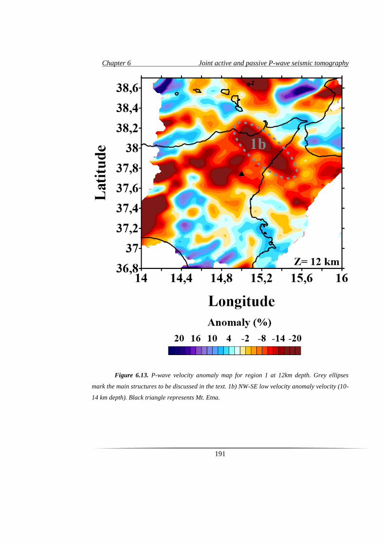
Chapter 6 Joint active and passive P-wave seismic tomography
191
Figure 6.13. P-wave velocity anomaly map for region 1 at 12km depth. Grey ellipses
mark the main structures to be discussed in the text. 1b) NW-SE low velocity anomaly velocity (10-
14 km depth). Black triangle represents Mt. Etna.
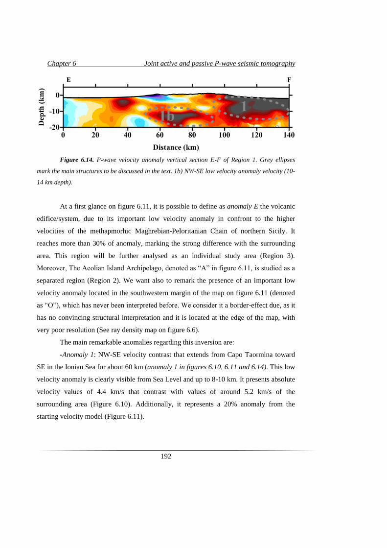
Chapter 6 Joint active and passive P-wave seismic tomography
192
Figure 6.14. P-wave velocity anomaly vertical section E-F of Region 1. Grey ellipses
mark the main structures to be discussed in the text. 1b) NW-SE low velocity anomaly velocity (10-
14 km depth).
At a first glance on figure 6.11, it is possible to define as anomaly E the volcanic
edifice/system, due to its important low velocity anomaly in confront to the higher
velocities of the methapmorhic Maghrebian-Peloritanian Chain of northern Sicily. It
reaches more than 30% of anomaly, marking the strong difference with the surrounding
area. This region will be further analysed as an individual study area (Region 3).
Moreover, The Aeolian Island Archipelago, denoted as “A” in figure 6.11, is studied as a
separated region (Region 2). We want also to remark the presence of an important low
velocity anomaly located in the southwestern margin of the map on figure 6.11 (denoted
as “O”), which has never been interpreted before. We consider it a border-effect due, as it
has no convincing structural interpretation and it is located at the edge of the map, with
very poor resolution (See ray density map on figure 6.6).
The main remarkable anomalies regarding this inversion are:
-Anomaly 1: NW-SE velocity contrast that extends from Capo Taormina toward
SE in the Ionian Sea for about 60 km (anomaly 1 in figures 6.10, 6.11 and 6.14). This low
velocity anomaly is clearly visible from Sea Level and up to 8-10 km. It presents absolute
velocity values of 4.4 km/s that contrast with values of around 5.2 km/s of the
surrounding area (Figure 6.10). Additionally, it represents a 20% anomaly from the
starting velocity model (Figure 6.11).
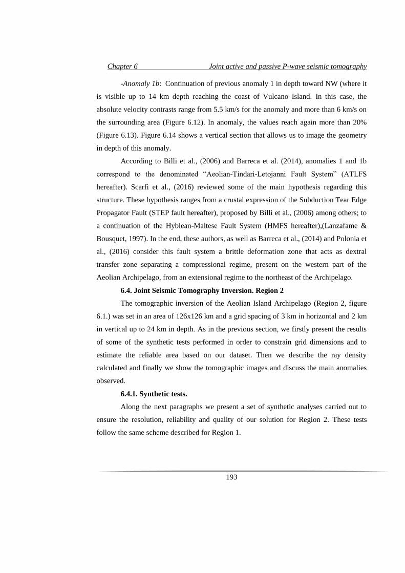
Chapter 6 Joint active and passive P-wave seismic tomography
193
-Anomaly 1b: Continuation of previous anomaly 1 in depth toward NW (where it
is visible up to 14 km depth reaching the coast of Vulcano Island. In this case, the
absolute velocity contrasts range from 5.5 km/s for the anomaly and more than 6 km/s on
the surrounding area (Figure 6.12). In anomaly, the values reach again more than 20%
(Figure 6.13). Figure 6.14 shows a vertical section that allows us to image the geometry
in depth of this anomaly.
According to Billi et al., (2006) and Barreca et al. (2014), anomalies 1 and 1b
correspond to the denominated “Aeolian-Tindari-Letojanni Fault System” (ATLFS
hereafter). Scarfì et al., (2016) reviewed some of the main hypothesis regarding this
structure. These hypothesis ranges from a crustal expression of the Subduction Tear Edge
Propagator Fault (STEP fault hereafter), proposed by Billi et al., (2006) among others; to
a continuation of the Hyblean-Maltese Fault System (HMFS hereafter),(Lanzafame &
Bousquet, 1997). In the end, these authors, as well as Barreca et al., (2014) and Polonia et
al., (2016) consider this fault system a brittle deformation zone that acts as dextral
transfer zone separating a compressional regime, present on the western part of the
Aeolian Archipelago, from an extensional regime to the northeast of the Archipelago.
6.4. Joint Seismic Tomography Inversion. Region 2
The tomographic inversion of the Aeolian Island Archipelago (Region 2, figure
6.1.) was set in an area of 126x126 km and a grid spacing of 3 km in horizontal and 2 km
in vertical up to 24 km in depth. As in the previous section, we firstly present the results
of some of the synthetic tests performed in order to constrain grid dimensions and to
estimate the reliable area based on our dataset. Then we describe the ray density
calculated and finally we show the tomographic images and discuss the main anomalies
observed.
6.4.1. Synthetic tests.
Along the next paragraphs we present a set of synthetic analyses carried out to
ensure the resolution, reliability and quality of our solution for Region 2. These tests
follow the same scheme described for Region 1.

Chapter 6 Joint active and passive P-wave seismic tomography
194
6.4.1.1. Checkerboards
Checkerboard test for region 2 have been carried out using different grid spacing
reaching to a final grid spacing of 3 km in horizontal and 2 km in vertical (Figure 6.15).
Nonetheless the results of these checkerboards are poor in confront with the previous
ones, the robustness of the final solutions is backed by the rest of the synthetic tests and
ray coverage. Figure 6.15., presents the results of the related checkerboard using 3 km
anomalies periodically sited with positive and negative values of 20% of anomaly.
6.4.1.2. Free Anomaly test
For the inversion of the Aeolian Islands the free anomalies designed are
represented in figure 6.16.a, c. Positive and negative anomalies are both convincingly
resolved as noted in figure 6.16.b,d. Designed anomalies have similar geometry as the
real ones, thus, the robustness and reliability of the results is confirmed.
6.4.1.3. Jackknifing Test
On the other hand, figure 6.17 shows the same Jackknifing test for Etnean (left
column) and Aeolian Islands (right column) regions. When compared with the complete
dataset inversion (see upper panels) no dramatic changes can be noticed and therefore the
stability of the resulting model is assessed.
6.4.2. Ray Density
Ray density of the inversion of Region 2 is shown in figure 6.18. The ray
distribution in this region allows us to confirm the quality of the results and the reliability
of the solutions as the study area is well covered by the rays, especially in the first 12 km.
Deeper than 12 km results are not 100% reliable since the number of rays crossing each
cell is too low.
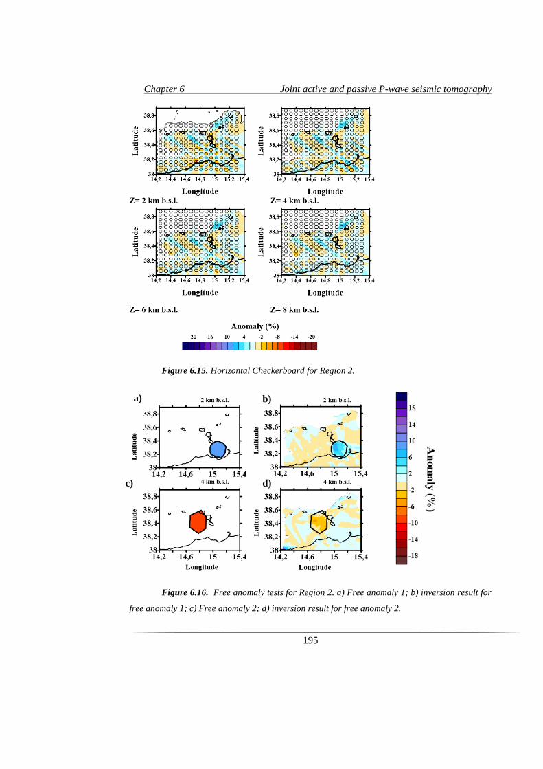
Chapter 6 Joint active and passive P-wave seismic tomography
195
Figure 6.15. Horizontal Checkerboard for Region 2.
Figure 6.16. Free anomaly tests for Region 2. a) Free anomaly 1; b) inversion result for
free anomaly 1; c) Free anomaly 2; d) inversion result for free anomaly 2.
a)
c)
b)
d)
Chapter 6 Joint active and passive P-wave seismic tomography
196
Figure 6.17. Jackknifing test for Region 2: a) complete dataset inversion; b) 50% of the
dataset inverted; c) 33% of the dataset inverted.
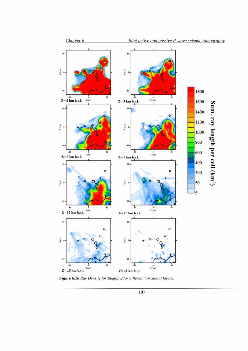
Chapter 6 Joint active and passive P-wave seismic tomography
197
Figure 6.18 Ray Density for Region 2 for different horizontal layers.
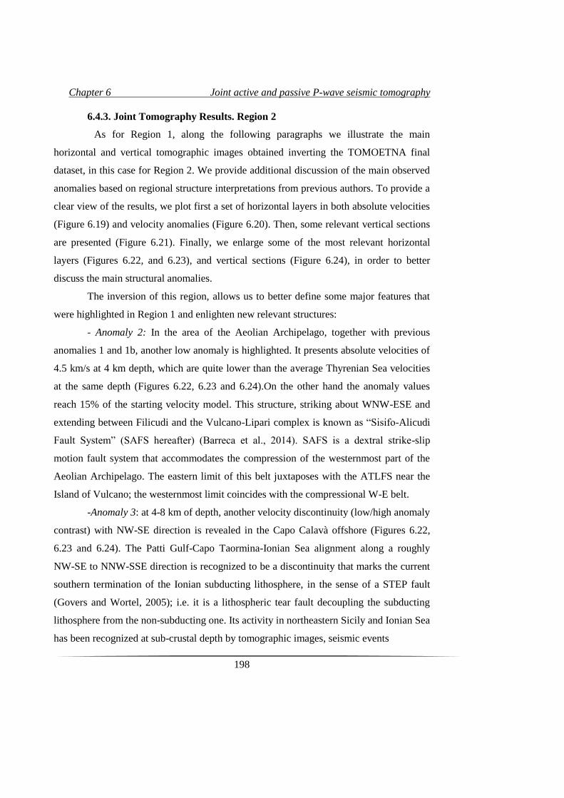
Chapter 6 Joint active and passive P-wave seismic tomography
198
6.4.3. Joint Tomography Results. Region 2
As for Region 1, along the following paragraphs we illustrate the main
horizontal and vertical tomographic images obtained inverting the TOMOETNA final
dataset, in this case for Region 2. We provide additional discussion of the main observed
anomalies based on regional structure interpretations from previous authors. To provide a
clear view of the results, we plot first a set of horizontal layers in both absolute velocities
(Figure 6.19) and velocity anomalies (Figure 6.20). Then, some relevant vertical sections
are presented (Figure 6.21). Finally, we enlarge some of the most relevant horizontal
layers (Figures 6.22, and 6.23), and vertical sections (Figure 6.24), in order to better
discuss the main structural anomalies.
The inversion of this region, allows us to better define some major features that
were highlighted in Region 1 and enlighten new relevant structures:
- Anomaly 2: In the area of the Aeolian Archipelago, together with previous
anomalies 1 and 1b, another low anomaly is highlighted. It presents absolute velocities of
4.5 km/s at 4 km depth, which are quite lower than the average Thyrenian Sea velocities
at the same depth (Figures 6.22, 6.23 and 6.24).On the other hand the anomaly values
reach 15% of the starting velocity model. This structure, striking about WNW-ESE and
extending between Filicudi and the Vulcano-Lipari complex is known as “Sisifo-Alicudi
Fault System” (SAFS hereafter) (Barreca et al., 2014). SAFS is a dextral strike-slip
motion fault system that accommodates the compression of the westernmost part of the
Aeolian Archipelago. The eastern limit of this belt juxtaposes with the ATLFS near the
Island of Vulcano; the westernmost limit coincides with the compressional W-E belt.
-Anomaly 3: at 4-8 km of depth, another velocity discontinuity (low/high anomaly
contrast) with NW-SE direction is revealed in the Capo Calavà offshore (Figures 6.22,
6.23 and 6.24). The Patti Gulf-Capo Taormina-Ionian Sea alignment along a roughly
NW-SE to NNW-SSE direction is recognized to be a discontinuity that marks the current
southern termination of the Ionian subducting lithosphere, in the sense of a STEP fault
(Govers and Wortel, 2005); i.e. it is a lithospheric tear fault decoupling the subducting
lithosphere from the non-subducting one. Its activity in northeastern Sicily and Ionian Sea
has been recognized at sub-crustal depth by tomographic images, seismic events
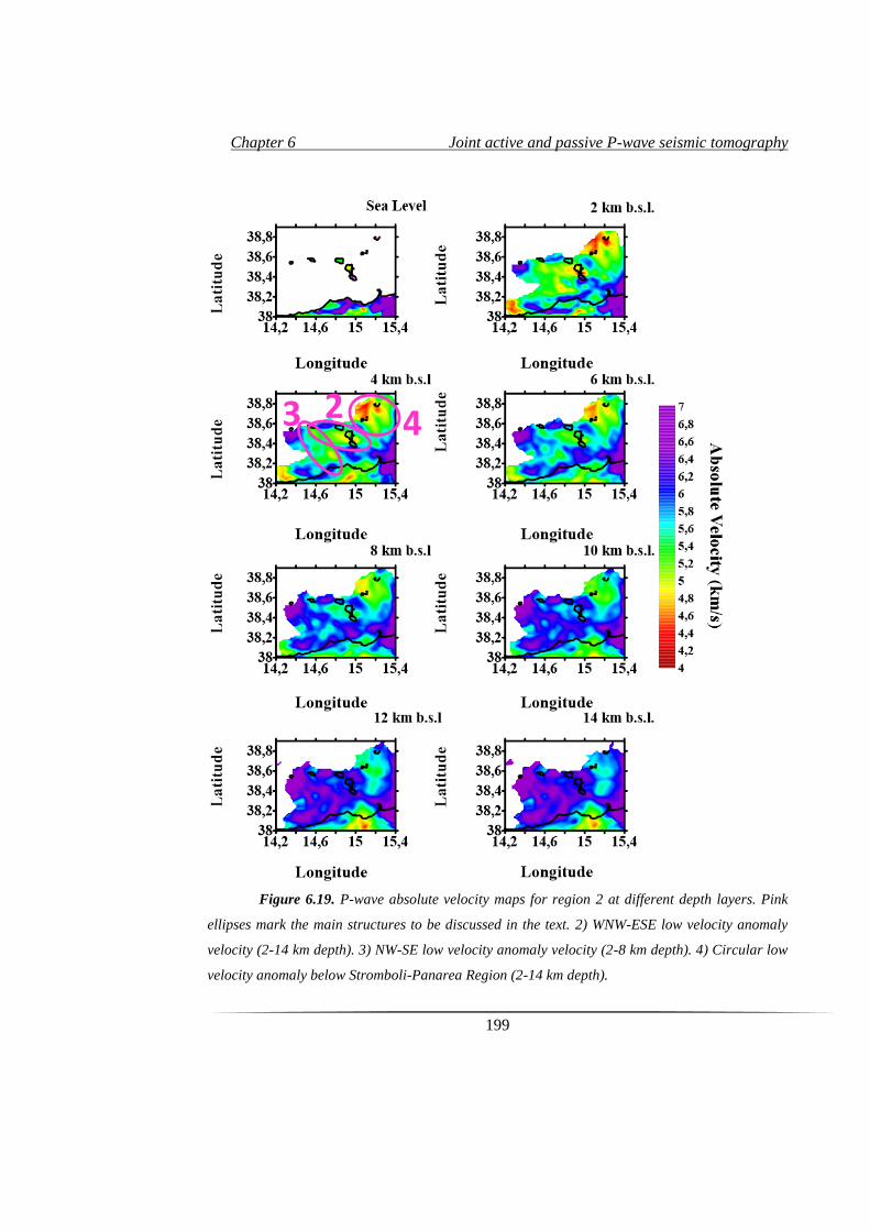
Chapter 6 Joint active and passive P-wave seismic tomography
199
Figure 6.19. P-wave absolute velocity maps for region 2 at different depth layers. Pink
ellipses mark the main structures to be discussed in the text. 2) WNW-ESE low velocity anomaly
velocity (2-14 km depth). 3) NW-SE low velocity anomaly velocity (2-8 km depth). 4) Circular low
velocity anomaly below Stromboli-Panarea Region (2-14 km depth).
4 3 2
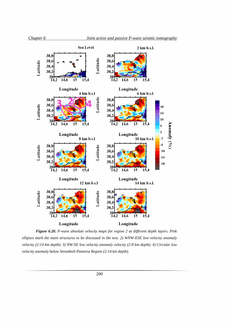
Chapter 6 Joint active and passive P-wave seismic tomography
200
Figure 6.20. P-wave absolute velocity maps for region 2 at different depth layers. Pink
ellipses mark the main structures to be discussed in the text. 2) WNW-ESE low velocity anomaly
velocity (2-14 km depth). 3) NW-SE low velocity anomaly velocity (2-8 km depth). 4) Circular low
velocity anomaly below Stromboli-Panarea Region (2-14 km depth).
4 3 2
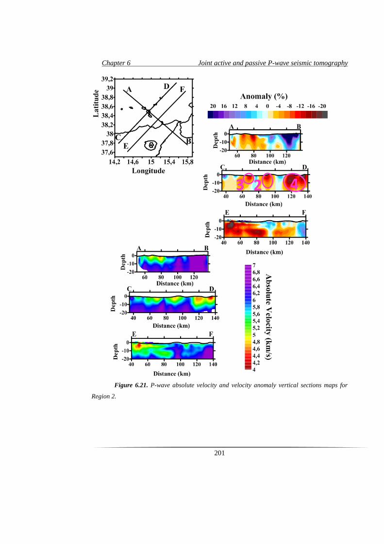
Chapter 6 Joint active and passive P-wave seismic tomography
201
Figure 6.21. P-wave absolute velocity and velocity anomaly vertical sections maps for
Region 2.
4 3 2

Chapter 6 Joint active and passive P-wave seismic tomography
202
Figure 6.22. P-wave absolute velocity map for region 2 at 4km depth. Grey ellipses mark
the main structures to be discussed in the text. 2) WNW-ESE low velocity anomaly velocity (2-14
km depth). 3) NW-SE low velocity anomaly velocity (2-8 km depth). 4) Circular low velocity
anomaly below Stromboli-Panarea Region (2-14 km depth).
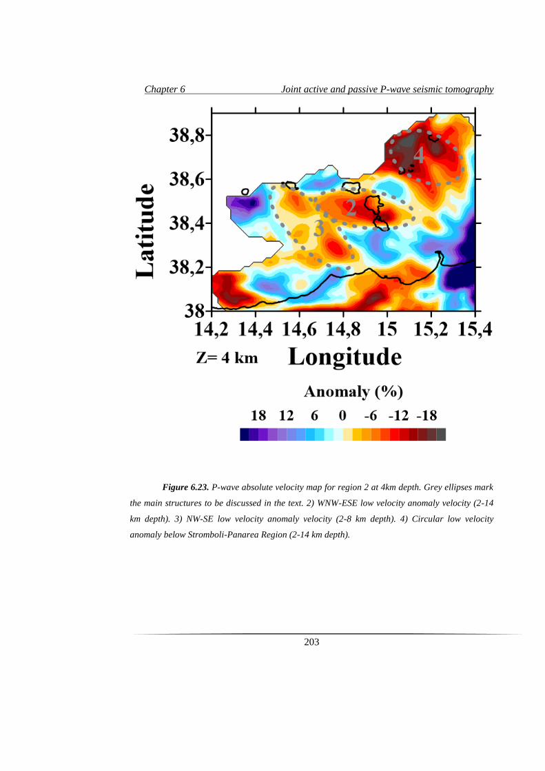
Chapter 6 Joint active and passive P-wave seismic tomography
203
Figure 6.23. P-wave absolute velocity map for region 2 at 4km depth. Grey ellipses mark
the main structures to be discussed in the text. 2) WNW-ESE low velocity anomaly velocity (2-14
km depth). 3) NW-SE low velocity anomaly velocity (2-8 km depth). 4) Circular low velocity
anomaly below Stromboli-Panarea Region (2-14 km depth).
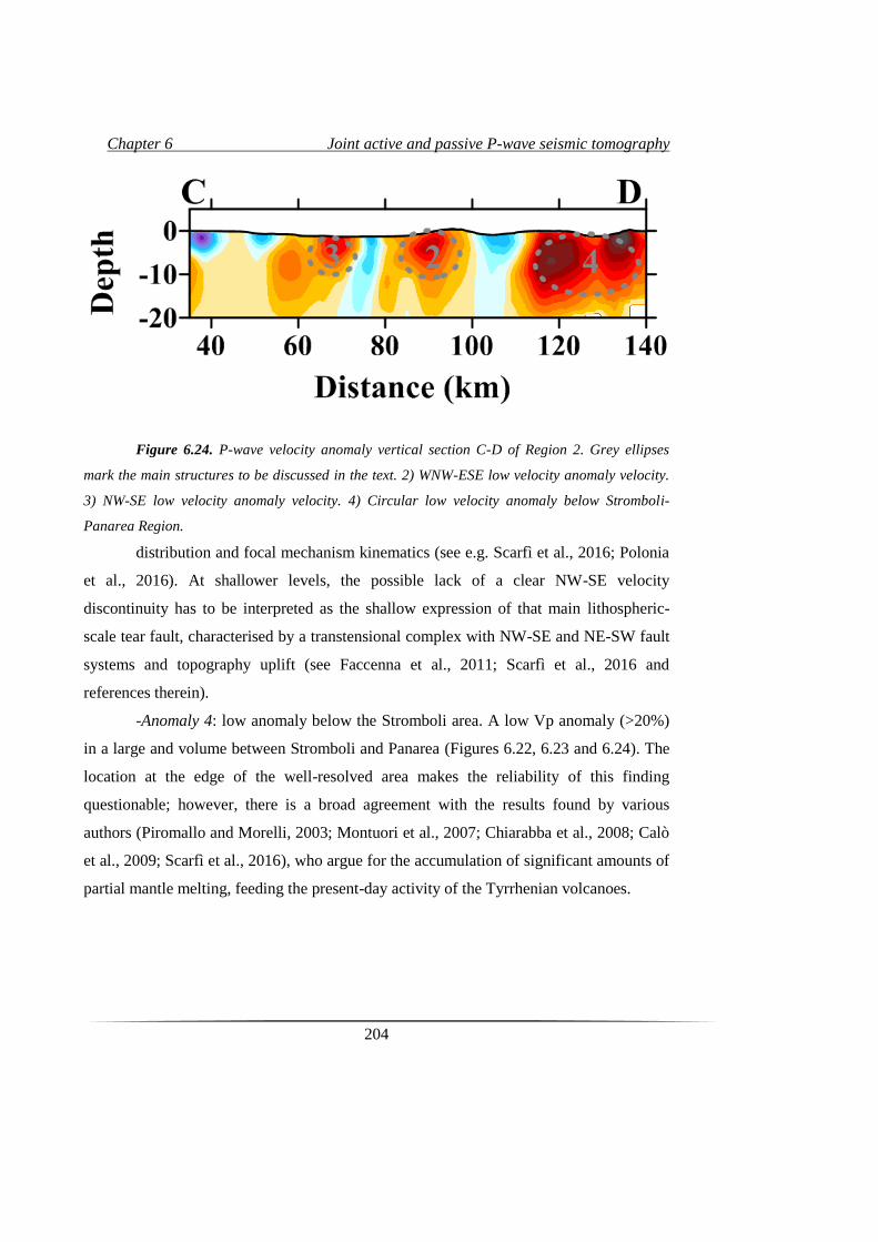
Chapter 6 Joint active and passive P-wave seismic tomography
204
Figure 6.24. P-wave velocity anomaly vertical section C-D of Region 2. Grey ellipses
mark the main structures to be discussed in the text. 2) WNW-ESE low velocity anomaly velocity.
3) NW-SE low velocity anomaly velocity. 4) Circular low velocity anomaly below Stromboli-
Panarea Region.
distribution and focal mechanism kinematics (see e.g. Scarfì et al., 2016; Polonia
et al., 2016). At shallower levels, the possible lack of a clear NW-SE velocity
discontinuity has to be interpreted as the shallow expression of that main lithospheric-
scale tear fault, characterised by a transtensional complex with NW-SE and NE-SW fault
systems and topography uplift (see Faccenna et al., 2011; Scarfì et al., 2016 and
references therein).
-Anomaly 4: low anomaly below the Stromboli area. A low Vp anomaly (>20%)
in a large and volume between Stromboli and Panarea (Figures 6.22, 6.23 and 6.24). The
location at the edge of the well-resolved area makes the reliability of this finding
questionable; however, there is a broad agreement with the results found by various
authors (Piromallo and Morelli, 2003; Montuori et al., 2007; Chiarabba et al., 2008; Calò
et al., 2009; Scarfì et al., 2016), who argue for the accumulation of significant amounts of
partial mantle melting, feeding the present-day activity of the Tyrrhenian volcanoes.
Chapter 6 Joint active and passive P-wave seismic tomography
205
6.5. Joint Seismic Tomography Inversion. Region 3
The area inverted for the Mt. Etna volcanic region extended 60x60 km in
horizontal and up to 24 km in depth (Region 3, figure 6.1). The grid spacing set was of 2
km in both horizontal and vertical directions.
6.5.1. Synthetic tests.
6.5.1.1. Checkerboards
The checkerboard related to this inversion is shown in figure 6.25. In this case the
anomaly pattern set was of ±20% anomaly with 2km size separated 5 km from each other.
Results show good horizontal resolution for a 60·60 km region (Figure 6.25.a, b) and
resolves anomalies of 2 km size up to 10-12 km depth beneath Mt. Etna (Figure 6.25.c).
6.5.1.2. Free Anomaly test
Similar procedure as for regions 1 and 2, we performed the free anomaly test for
Region 3. The configuration inverted for the region of Mt. Etna volcano is shown in
figure 6.26.a, and c. Again, the designed anomalies are sized taking into account the grid
spacing in order to try to reproduce realistic anomalies. Results of this test shown in
figure 6.26.b, and d, denote the high quality of the inversion. Moreover, this test supports
that similar anomalies in size and shape for real inversions can ben trustfully interpreted.
The free anomaly tests carried out for the three regions show in all of them very
promising reconstruction of the anomalies, proving that our obtained anomalies are
suitable to be solved by the inversion using the set parameters and model. Moreover, it
proves the robustness of the inversion code for modelling synthetic anomalies of
whatever geometry.
6.5.1.3. Jackknifing Test
On the other hand, figure 6.27 shows the Jackknifing test for Etnean region.
When compared with the complete dataset inversion (see upper panels) no dramatic
changes can be noticed and therefore the stability of the resulting model is assessed. The
Jackknifing test performed to all 3 regions confirms the very high quality of the data
selected for the inversion, as even using 33% of them the resultant images are quite
similar to the full dataset ones. Therefore we can ensure that our results are not biased by
noise effects from the data.
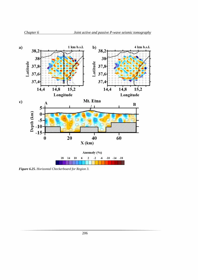
Chapter 6 Joint active and passive P-wave seismic tomography
206
Figure 6.25. Horizontal Checkerboard for Region 3.
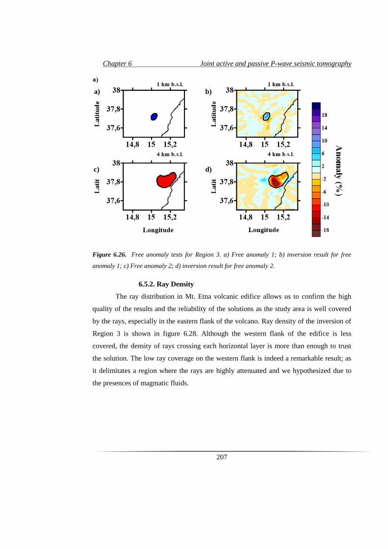
Chapter 6 Joint active and passive P-wave seismic tomography
207
Figure 6.26. Free anomaly tests for Region 3. a) Free anomaly 1; b) inversion result for free
anomaly 1; c) Free anomaly 2; d) inversion result for free anomaly 2.
6.5.2. Ray Density
The ray distribution in Mt. Etna volcanic edifice allows us to confirm the high
quality of the results and the reliability of the solutions as the study area is well covered
by the rays, especially in the eastern flank of the volcano. Ray density of the inversion of
Region 3 is shown in figure 6.28. Although the western flank of the edifice is less
covered, the density of rays crossing each horizontal layer is more than enough to trust
the solution. The low ray coverage on the western flank is indeed a remarkable result; as
it delimitates a region where the rays are highly attenuated and we hypothesized due to
the presences of magmatic fluids.
a)
c)
b)
d)
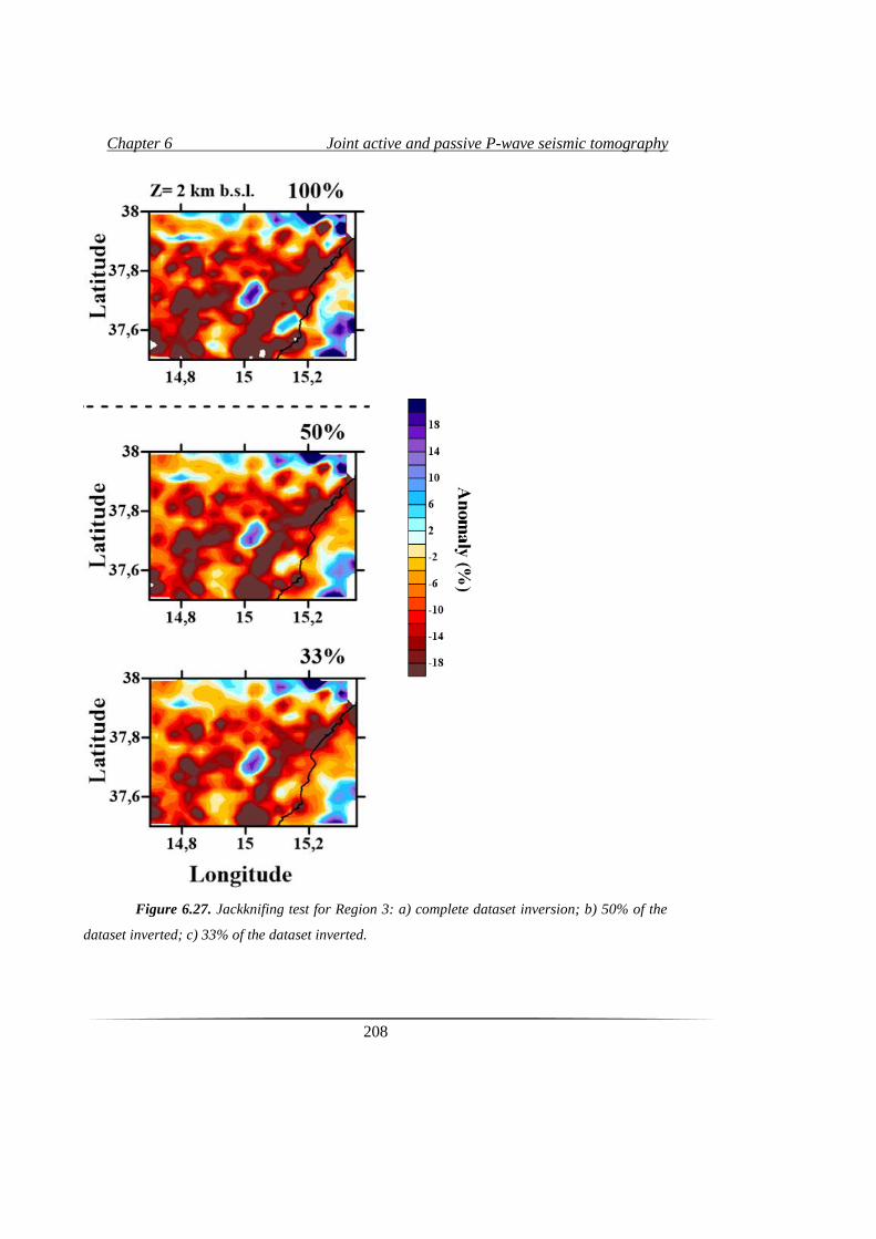
Chapter 6 Joint active and passive P-wave seismic tomography
208
Figure 6.27. Jackknifing test for Region 3: a) complete dataset inversion; b) 50% of the
dataset inverted; c) 33% of the dataset inverted.
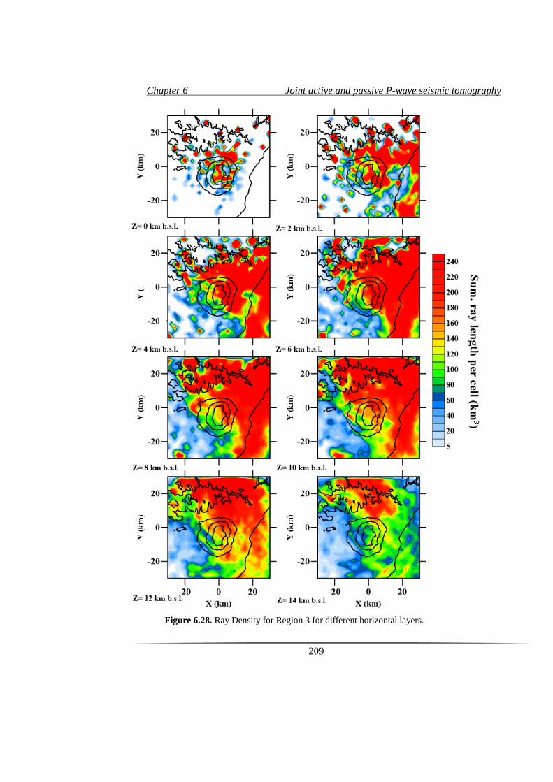
Chapter 6 Joint active and passive P-wave seismic tomography
209
Figure 6.28. Ray Density for Region 3 for different horizontal layers.
Chapter 6 Joint active and passive P-wave seismic tomography
210
6.5.3. Joint Tomography Results. Region 3
As for previous regions, along the following paragraphs we illustrate the main
horizontal and vertical tomographic images obtained inverting the TOMOETNA final
dataset, in this case for Region 3. We provide additional discussion of the main observed
anomalies based on regional structure interpretations from previous authors. To provide a
clear view of the results, we plot first a set of horizontal layers in both absolute velocities
(Figure 6.29) and velocity anomalies (Figure 6.30). Then, some relevant vertical sections
are presented (Figure 6.31. Finally, we enlarge some of the most relevant horizontal
layers (Figures 6.32, and 6.33), and vertical sections (Figure 6.34), in order to better
discuss the main structural anomalies.
From this tomographic inversion results, we highlight the presence of many high
and low velocity anomalies (Figures 6.32, 6.33 and 6.34). Some of them are connected in
depth (anomalies 5 and 6) (Figure 6.34) and some isolated (anomalies 7 and 8). These
four anomalies will be further described an interpreted in the following paragraphs:
-Anomaly 5: Located slightly southeastern underneath the central craters, this
high-velocity anomaly is widely known as High Velocity Body (see chapter 2). This
feature appears in all the previous tomographic analysis being located up to 18 km depth.
The dimensions of this volume may slightly differ from one author to another, averaging
ca 600 km3 (e.g., Chiarabba et al., 2004). Falsaperla et al., (2013) also presented different
tomographic cross sections, which better define the shape of the HVB up to 7 km b.s.l.,
and the results are clearly in agree with our observations. Moreover, this volume is
inferred to be composed of high strength mafic rocks such as cumulites or dykes (see
chapter 2). Its origin is interpreted as old magmatic deposits. Detailed studies of its
composition have been carried out by Corsaro et al., (2014). These authors analyzed the
composition of several xenoliths that may have the same origin of the HVB. Analyses
reveal an intrusive gabbroic rock composition of the volume, indeed, involving a slow
solidification process of a quite mafic magma.
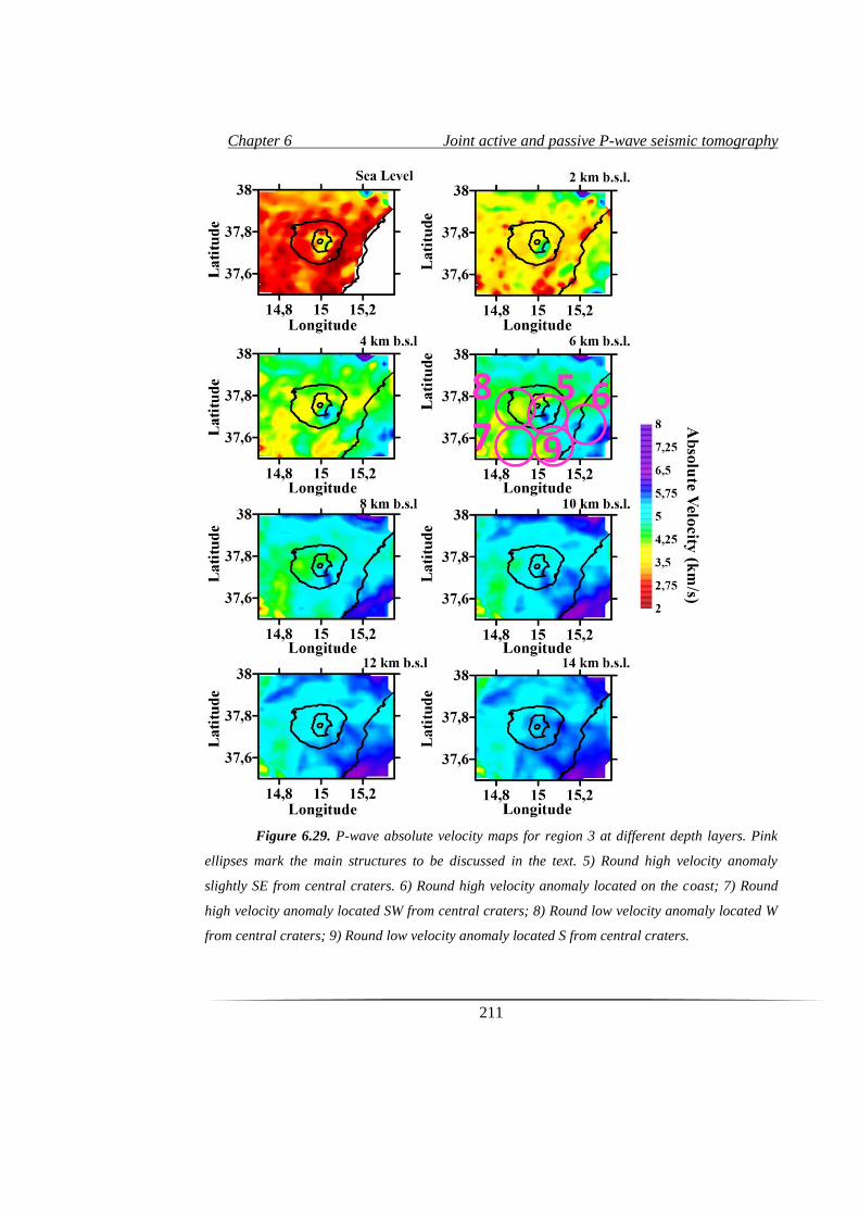
Chapter 6 Joint active and passive P-wave seismic tomography
211
Figure 6.29. P-wave absolute velocity maps for region 3 at different depth layers. Pink
ellipses mark the main structures to be discussed in the text. 5) Round high velocity anomaly
slightly SE from central craters. 6) Round high velocity anomaly located on the coast; 7) Round
high velocity anomaly located SW from central craters; 8) Round low velocity anomaly located W
from central craters; 9) Round low velocity anomaly located S from central craters.
5 6 7 8
9
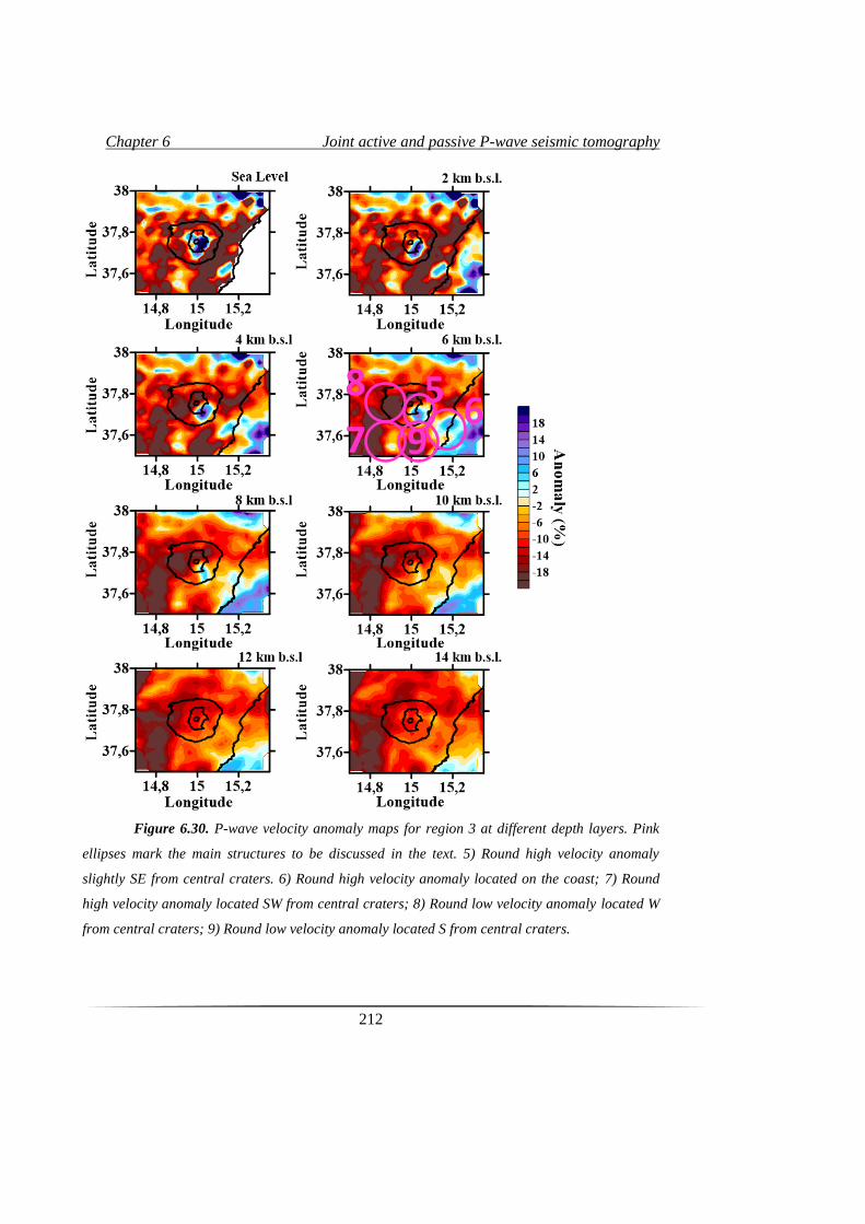
Chapter 6 Joint active and passive P-wave seismic tomography
212
Figure 6.30. P-wave velocity anomaly maps for region 3 at different depth layers. Pink
ellipses mark the main structures to be discussed in the text. 5) Round high velocity anomaly
slightly SE from central craters. 6) Round high velocity anomaly located on the coast; 7) Round
high velocity anomaly located SW from central craters; 8) Round low velocity anomaly located W
from central craters; 9) Round low velocity anomaly located S from central craters.
5 6
7
8
9
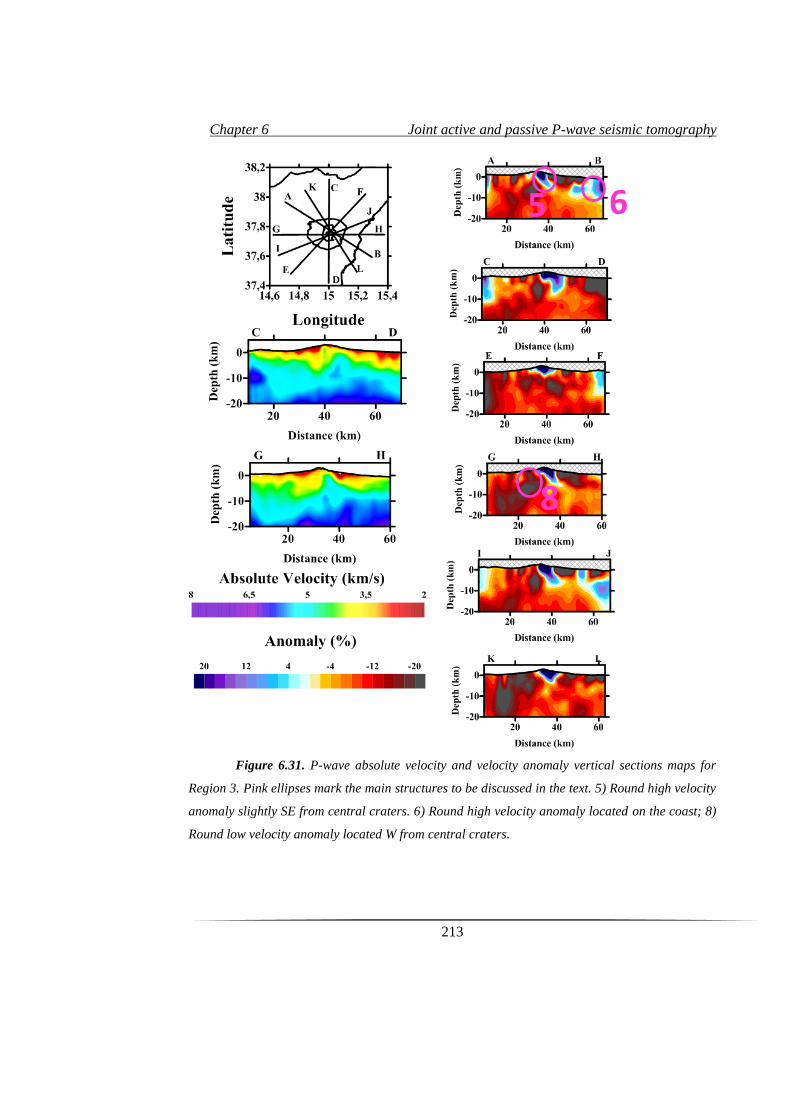
Chapter 6 Joint active and passive P-wave seismic tomography
213
Figure 6.31. P-wave absolute velocity and velocity anomaly vertical sections maps for
Region 3. Pink ellipses mark the main structures to be discussed in the text. 5) Round high velocity
anomaly slightly SE from central craters. 6) Round high velocity anomaly located on the coast; 8)
Round low velocity anomaly located W from central craters.
5 6
8
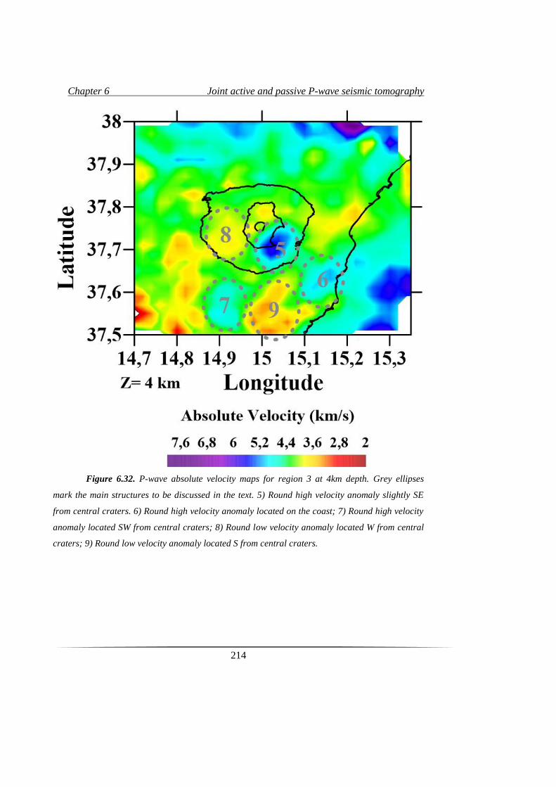
Chapter 6 Joint active and passive P-wave seismic tomography
214
Figure 6.32. P-wave absolute velocity maps for region 3 at 4km depth. Grey ellipses
mark the main structures to be discussed in the text. 5) Round high velocity anomaly slightly SE
from central craters. 6) Round high velocity anomaly located on the coast; 7) Round high velocity
anomaly located SW from central craters; 8) Round low velocity anomaly located W from central
craters; 9) Round low velocity anomaly located S from central craters.
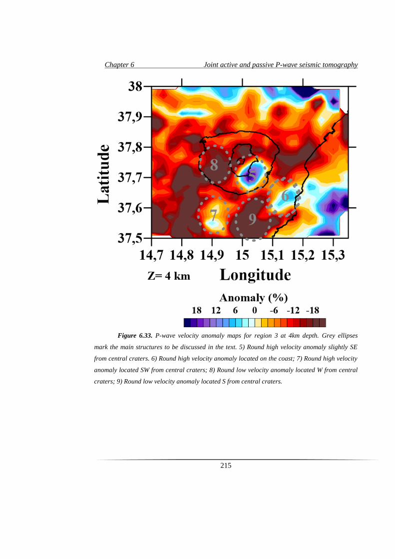
Chapter 6 Joint active and passive P-wave seismic tomography
215
Figure 6.33. P-wave velocity anomaly maps for region 3 at 4km depth. Grey ellipses
mark the main structures to be discussed in the text. 5) Round high velocity anomaly slightly SE
from central craters. 6) Round high velocity anomaly located on the coast; 7) Round high velocity
anomaly located SW from central craters; 8) Round low velocity anomaly located W from central
craters; 9) Round low velocity anomaly located S from central craters.
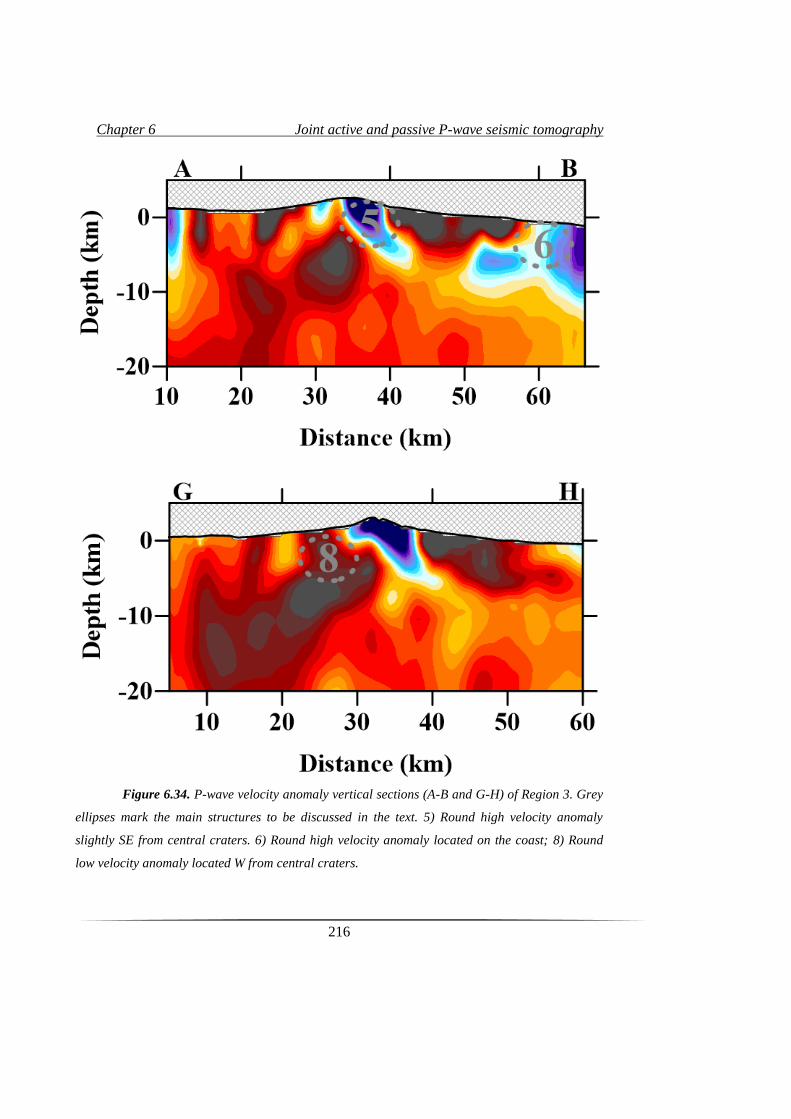
Chapter 6 Joint active and passive P-wave seismic tomography
216
Figure 6.34. P-wave velocity anomaly vertical sections (A-B and G-H) of Region 3. Grey
ellipses mark the main structures to be discussed in the text. 5) Round high velocity anomaly
slightly SE from central craters. 6) Round high velocity anomaly located on the coast; 8) Round
low velocity anomaly located W from central craters.
Chapter 6 Joint active and passive P-wave seismic tomography
217
-Anomaly 6: High Velocity anomaly located on the southeastern sector of Etna
area, close to the coast. This volume is clearly resolved between 4km and 14 km depth
where it seems to disappear or collide with a larger high velocity anomaly eastern
offshore. We are investigating on the relationships between this HV volume and the
presence of the Moho discontinuity upwelling, observed by Nicolich et al. (2000) in the
Ionian margin of Sicily up to 17 km b.s.l.. Moreover, we are also analyzing the probably
connection between the HVB (anomaly 5) and this volume (anomaly 6) at 4-8 km depth
approximately (see vertical sections A-B and I-J. Figures 6.31 and 6.34).
-Anomaly 7: High Velocity anomaly located southwestern of the volcanic edifice.
Due to the poor spatial resolution in this sector, as shown in the ray density distribution in
Figure 6.25, we do not furnish any interpretation of this anomaly. However, this high
velocity volume may be correlated up to 6 km b.s.l., with a high density anomaly,
revealed by preliminary gravimetric analyses (J. Fernández, personal communication). -
Anomaly 8: Low Velocity anomaly western from the central craters A low velocity
volume in this sector of the volcano have been highlighted by Aloisi et al. (2002), which
was associated with the presence of magmatic reservoir and correlated with the
anomalous b volume revealed by Murru et al., (1999).
-Anomaly 9: Low Velocity anomaly southern from Mt. Etna. This 20% negative
anomaly presents absolute velocity values of around 3.6 km/s at 4 km depth. This volume
has never been interpreted and therefore must be further investigated.
6.6 Final Remarks
It is important to note that the presented results correspond to a joint active
passive tomographic inversion of a very short in time dataset. Indeed, we consider our
results as a snapshot tomography that allows us to individuate volcanic structures without
averaging them through time. However, for a better enlightening of the regional tectonic
features, we propose further joint analyses including a larger passive dataset, as they
should not change dramatically in time.
Another important issue revealed from our work is the remarkable “shadow” area
western from Mt. Etna volcano where very poor resolution and ray coverage is found.
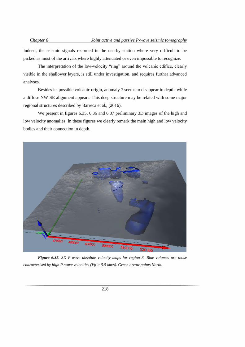
Chapter 6 Joint active and passive P-wave seismic tomography
218
Indeed, the seismic signals recorded in the nearby station where very difficult to be
picked as most of the arrivals where highly attenuated or even impossible to recognize.
The interpretation of the low-velocity “ring” around the volcanic edifice, clearly
visible in the shallower layers, is still under investigation, and requires further advanced
analyses.
Besides its possible volcanic origin, anomaly 7 seems to disappear in depth, while
a diffuse NW-SE alignment appears. This deep structure may be related with some major
regional structures described by Barreca et al., (2016).
We present in figures 6.35, 6.36 and 6.37 preliminary 3D images of the high and
low velocity anomalies. In these figures we clearly remark the main high and low velocity
bodies and their connection in depth.
Figure 6.35. 3D P-wave absolute velocity maps for region 3. Blue volumes are those
characterised by high P-wave velocities (Vp > 5.5 km/s). Green arrow points North.
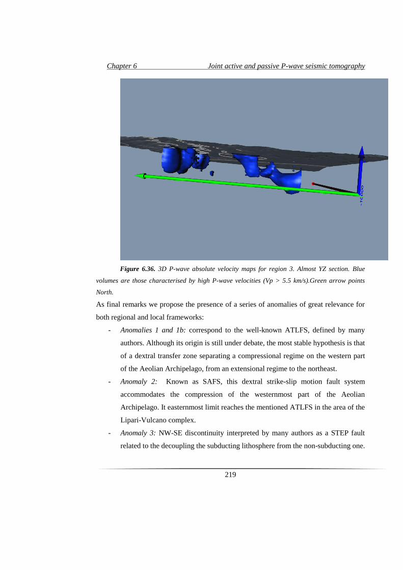
Chapter 6 Joint active and passive P-wave seismic tomography
219
Figure 6.36. 3D P-wave absolute velocity maps for region 3. Almost YZ section. Blue
volumes are those characterised by high P-wave velocities (Vp > 5.5 km/s).Green arrow points
North.
As final remarks we propose the presence of a series of anomalies of great relevance for
both regional and local frameworks:
- Anomalies 1 and 1b: correspond to the well-known ATLFS, defined by many
authors. Although its origin is still under debate, the most stable hypothesis is that
of a dextral transfer zone separating a compressional regime on the western part
of the Aeolian Archipelago, from an extensional regime to the northeast.
- Anomaly 2: Known as SAFS, this dextral strike-slip motion fault system
accommodates the compression of the westernmost part of the Aeolian
Archipelago. It easternmost limit reaches the mentioned ATLFS in the area of the
Lipari-Vulcano complex.
- Anomaly 3: NW-SE discontinuity interpreted by many authors as a STEP fault
related to the decoupling the subducting lithosphere from the non-subducting one.
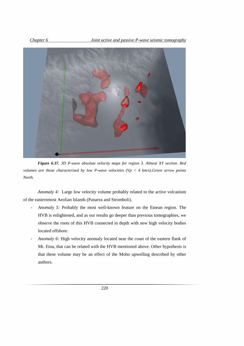
Chapter 6 Joint active and passive P-wave seismic tomography
220
Figure 6.37. 3D P-wave absolute velocity maps for region 3. Almost XY section. Red
volumes are those characterised by low P-wave velocities (Vp < 4 km/s).Green arrow points
North.
Anomaly 4: Large low velocity volume probably related to the active volcanism
of the easternmost Aeolian Islands (Panarea and Stromboli).
- Anomaly 5: Probably the most well-known feature on the Etnean region. The
HVB is enlightened, and as our results go deeper than previous tomographies, we
observe the roots of this HVB connected in depth with new high velocity bodies
located offshore.
- Anomaly 6: High velocity anomaly located near the coast of the eastern flank of
Mt. Etna, that can be related with the HVB mentioned above. Other hypothesis is
that these volume may be an effect of the Moho upwelling described by other
authors.

Chapter 6 Joint active and passive P-wave seismic tomography
221
There are some anomalies that never been interpreted and for which we present
some preliminary ideas that must be further investigated. It is the case of anomalies 7, 8
and 9.
Finally, we want to remark that these seismic tomographic models are not just
final results but also the key to carry out further advanced approaches as will be detailed
in chapter 7.

7. An example of an
Advanced Application: The
analysis of The 2011–2013
seismic series associated to
the volcanic activity of El
Hierro Island on the light of
a 3D high definition
structural model

Chapter 7 An example of an Advanced Application
225
7.1. Advanced Applications of Velocity Models
To carry out many seismic analyses, the use of a velocity model that describes the
different wave velocities at different depths becomes crucial. Thus, we could, for
example, follow the ray path of a certain type of wave from its source to the receiver.
Indeed, these velocities should be defined by considering both the regional geology and
local structures. However, knowing the deep structures is not always possible, therefore
seismic studies usually use simplified 1D velocity models to describe Earth Interior in
order to perform further analysis. Nevertheless, these 1D velocity models do not always
fit properly the studied region, especially in volcanic areas, which are known for their
vertical and lateral heterogeneities. In these cases, differences between a simplified 1D
velocity models and reality can be really large. To assess this problem, seismic velocity
tomography provides a realistic 3D velocity model of the studied area that can be used for
further analyses. These models, indeed, take into account vertical and lateral
heterogeneities as they give velocity values for each cell of the defined 3D grid.
A wide range of studies can be enhanced using a 3D velocity model as initial
input data: from routinely hypocentral location to more advanced seismic techniques.
The importance of obtaining realistic 3D velocity models throughout seismic
tomography has been deeply described along this thesis. In this chapter we present a case
of study with a complete set of seismic analyses for which we required a trustful
tomographic velocity model. This case of study is focused on the island of El Hierro
(Canary Islands, Spain) and the related seismo-volcanic crisis occurred on 2011.
Additionally, further analyses derived from realistic relocation are described. Especially
we present a new approach based on hydraulic fracturing and pore pressure diffusion
modelling to study volcanic seismicity in order to better understand its origin.
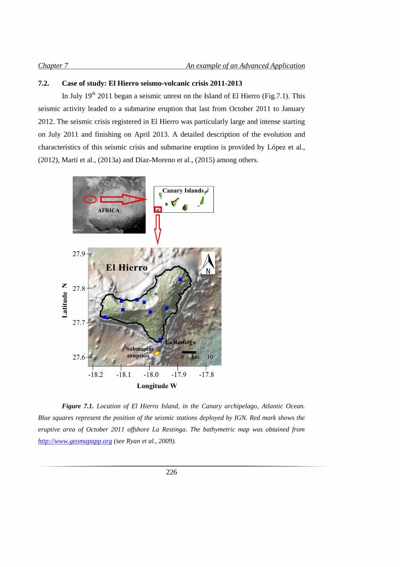
Chapter 7 An example of an Advanced Application
226
7.2. Case of study: El Hierro seismo-volcanic crisis 2011-2013
In July 19th 2011 began a seismic unrest on the Island of El Hierro (Fig.7.1). This
seismic activity leaded to a submarine eruption that last from October 2011 to January
2012. The seismic crisis registered in El Hierro was particularly large and intense starting
on July 2011 and finishing on April 2013. A detailed description of the evolution and
characteristics of this seismic crisis and submarine eruption is provided by López et al.,
(2012), Martí et al., (2013a) and Díaz-Moreno et al., (2015) among others.
Figure 7.1. Location of El Hierro Island, in the Canary archipelago, Atlantic Ocean.
Blue squares represent the position of the seismic stations deployed by IGN. Red mark shows the
eruptive area of October 2011 offshore La Restinga. The bathymetric map was obtained from
http://www.geomapapp.org (see Ryan et al., 2009).
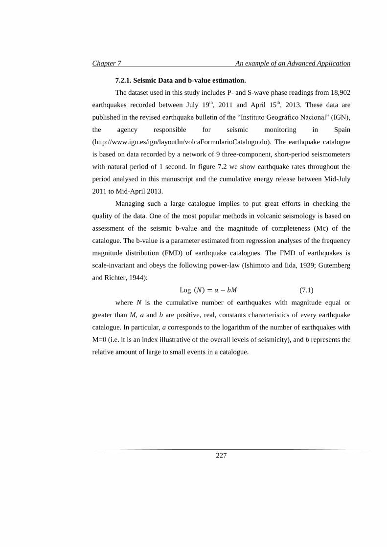
Chapter 7 An example of an Advanced Application
227
7.2.1. Seismic Data and b-value estimation.
The dataset used in this study includes P- and S-wave phase readings from 18,902
earthquakes recorded between July 19th, 2011 and April 15
th, 2013. These data are
published in the revised earthquake bulletin of the “Instituto Geográfico Nacional” (IGN),
the agency responsible for seismic monitoring in Spain
(http://www.ign.es/ign/layoutIn/volcaFormularioCatalogo.do). The earthquake catalogue
is based on data recorded by a network of 9 three-component, short-period seismometers
with natural period of 1 second. In figure 7.2 we show earthquake rates throughout the
period analysed in this manuscript and the cumulative energy release between Mid-July
2011 to Mid-April 2013.
Managing such a large catalogue implies to put great efforts in checking the
quality of the data. One of the most popular methods in volcanic seismology is based on
assessment of the seismic b-value and the magnitude of completeness (Mc) of the
catalogue. The b-value is a parameter estimated from regression analyses of the frequency
magnitude distribution (FMD) of earthquake catalogues. The FMD of earthquakes is
scale-invariant and obeys the following power-law (Ishimoto and Iida, 1939; Gutemberg
and Richter, 1944):
Log (𝑁) = 𝑎 − 𝑏𝑀 (7.1)
where N is the cumulative number of earthquakes with magnitude equal or
greater than M, a and b are positive, real, constants characteristics of every earthquake
catalogue. In particular, a corresponds to the logarithm of the number of earthquakes with
M=0 (i.e. it is an index illustrative of the overall levels of seismicity), and b represents the
relative amount of large to small events in a catalogue.
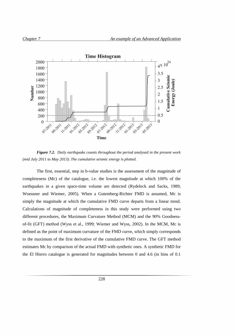
Chapter 7 An example of an Advanced Application
228
Figure 7.2. Daily earthquake counts throughout the period analysed in the present work
(mid July 2011 to May 2013). The cumulative seismic energy is plotted.
The first, essential, step in b-value studies is the assessment of the magnitude of
completeness (Mc) of the catalogue, i.e. the lowest magnitude at which 100% of the
earthquakes in a given space-time volume are detected (Rydeleck and Sacks, 1989;
Woessner and Wiemer, 2005). When a Gutemberg-Richter FMD is assumed, Mc is
simply the magnitude at which the cumulative FMD curve departs from a linear trend.
Calculations of magnitude of completeness in this study were performed using two
different procedures, the Maximum Curvature Method (MCM) and the 90% Goodness-
of-fit (GFT) method (Wyss et al., 1999; Wiemer and Wyss, 2002). In the MCM, Mc is
defined as the point of maximum curvature of the FMD curve, which simply corresponds
to the maximum of the first derivative of the cumulative FMD curve. The GFT method
estimates Mc by comparison of the actual FMD with synthetic ones. A synthetic FMD for
the El Hierro catalogue is generated for magnitudes between 0 and 4.6 (in bins of 0.1
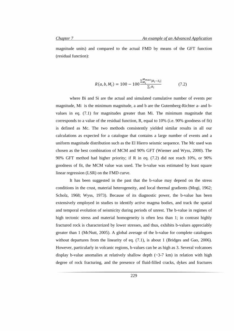
Chapter 7 An example of an Advanced Application
229
magnitude units) and compared to the actual FMD by means of the GFT function
(residual function):
𝑅(𝑎, 𝑏, 𝑀𝑖) = 100 − 100∑ |𝐵𝑖−𝑆𝑖|
𝑀𝑚𝑎𝑥𝑀𝑖
∑ 𝐵𝑖𝑖 (7.2)
where Bi and Si are the actual and simulated cumulative number of events per
magnitude, Mi is the minimum magnitude, a and b are the Gutemberg-Richter a- and b-
values in eq. (7.1) for magnitudes greater than Mi. The minimum magnitude that
corresponds to a value of the residual function, R, equal to 10% (i.e. 90% goodness of fit)
is defined as Mc. The two methods consistently yielded similar results in all our
calculations as expected for a catalogue that contains a large number of events and a
uniform magnitude distribution such as the El Hierro seismic sequence. The Mc used was
chosen as the best combination of MCM and 90% GFT (Wiemer and Wyss, 2000). The
90% GFT method had higher priority; if R in eq. (7.2) did not reach 10%, or 90%
goodness of fit, the MCM value was used. The b-value was estimated by least square
linear regression (LSR) on the FMD curve.
It has been suggested in the past that the b-value may depend on the stress
conditions in the crust, material heterogeneity, and local thermal gradients (Mogi, 1962;
Scholz, 1968; Wyss, 1973). Because of its diagnostic power, the b-value has been
extensively employed in studies to identify active magma bodies, and track the spatial
and temporal evolution of seismicity during periods of unrest. The b-value in regimes of
high tectonic stress and material homogeneity is often less than 1; in contrast highly
fractured rock is characterized by lower stresses, and thus, exhibits b-values appreciably
greater than 1 (McNutt, 2005). A global average of the b-value for complete catalogues
without departures from the linearity of eq. (7.1), is about 1 (Bridges and Gao, 2006).
However, particularly in volcanic regions, b-values can be as high as 3. Several volcanoes
display b-value anomalies at relatively shallow depth (~3-7 km) in relation with high
degree of rock fracturing, and the presence of fluid-filled cracks, dykes and fractures
Chapter 7 An example of an Advanced Application
230
(McNutt, 2005). Farrel et al. (2009), for instance, analysed the seismicity recorded in the
Yellowstone volcanic field between 1973 and 2008, a catalogue of about 30,000
earthquakes with magnitudes between -0.5 and 6. Spatial and temporal b-value mapping
identified areas of high b-value in relation to the migration of magmatic fluids, and
regions of low b-value attributed to high extensional stress regime. Jacobs and McNutt
(2010) used the b-value to investigate the sequence of earthquakes leading to the 2006
eruption of Augustine volcano; they found evidence of high b-value anomalies related to
changes in thermal gradients, pore pressure and stress, linked to the intrusion of a
magmatic dike before the onset of the eruption.
Possible temporal variations of b-value were also investigated by means of a
moving window technique (Wiemer and Wyss, 2000). This approach is known to be
affected by intervals with low levels of seismicity, thus, producing uneven temporal
sampling and smoothing of the b-value time series. The El Hierro catalogue, however, is
characterized by high enough earthquake rates to ensure that, given the right choice of
parameters, satisfactory results can be obtained. We tested multiple sets of input
parameters, including variable catalogue time spans, window lengths and overlap,
threshold magnitudes, and magnitude binning. The temporal variations in b-value were
estimated using 200-event moving windows, with 10% overlap.
Ibáñez et al., (2012) observed that the b-value during seismic swarms is a
powerful indicator of stress conditions. They reported changes in b-value from 2.25
during the early, pre-eruptive, period to 1.25 at the end of the eruptive phase. Their
interpretation was that earthquakes during the first phase of unrest occurred as the
consequence of stress transfer associated with magma migration from the upper mantle
into the curst. The larger magnitude earthquakes recorded at the end of the analysed
period were attributed to stress relaxation around the magma reservoir. In this section we
will reanalyse the whole seismic series starting with a detailed study of the temporal
variations of b-value.
In figure 7.3 we show temporal changes in b-value from which 6 seismic phases
can be clearly identified. Phases 1, 2 and 3 coincide with those previously identified by
Ibáñez et al. (2012) and correspond to the pre-eruptive and main submarine eruptive
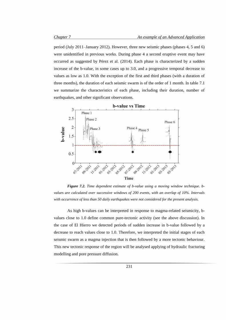
Chapter 7 An example of an Advanced Application
231
period (July 2011–January 2012). However, three new seismic phases (phases 4, 5 and 6)
were unidentified in previous works. During phase 4 a second eruptive event may have
occurred as suggested by Pérez et al. (2014). Each phase is characterized by a sudden
increase of the b-value, in some cases up to 3.0, and a progressive temporal decrease to
values as low as 1.0. With the exception of the first and third phases (with a duration of
three months), the duration of each seismic swarm is of the order of 1 month. In table 7.1
we summarize the characteristics of each phase, including their duration, number of
earthquakes, and other significant observations.
Figure 7.2. Time dependent estimate of b-value using a moving window technique. b-
values are calculated over successive windows of 200 events, with an overlap of 10%. Intervals
with occurrence of less than 50 daily earthquakes were not considered for the present analysis.
As high b-values can be interpreted in response to magma-related seismicity, b-
values close to 1.0 define common pure-tectonic activity (see the above discussion). In
the case of El Hierro we detected periods of sudden increase in b-value followed by a
decrease to reach values close to 1.0. Therefore, we interpreted the initial stages of each
seismic swarm as a magma injection that is then followed by a more tectonic behaviour.
This new tectonic response of the region will be analysed applying of hydraulic fracturing
modelling and pore pressure diffusion.
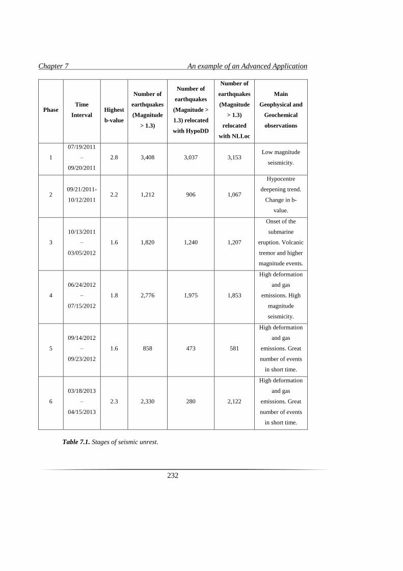
Chapter 7 An example of an Advanced Application
232
Phase Time
Interval
Highest
b-value
Number of
earthquakes
(Magnitude
> 1.3)
Number of
earthquakes
(Magnitude >
1.3) relocated
with HypoDD
Number of
earthquakes
(Magnitude
> 1.3)
relocated
with NLLoc
Main
Geophysical and
Geochemical
observations
1
07/19/2011
–
09/20/2011
2.8 3,408 3,037 3,153 Low magnitude
seismicity.
2 09/21/2011-
10/12/2011 2.2 1,212 906 1,067
Hypocentre
deepening trend.
Change in b-
value.
3
10/13/2011
–
03/05/2012
1.6 1,820 1,240 1,207
Onset of the
submarine
eruption. Volcanic
tremor and higher
magnitude events.
4
06/24/2012
–
07/15/2012
1.8 2,776 1,975 1,853
High deformation
and gas
emissions. High
magnitude
seismicity.
5
09/14/2012
–
09/23/2012
1.6 858 473 581
High deformation
and gas
emissions. Great
number of events
in short time.
6
03/18/2013
–
04/15/2013
2.3 2,330 280 2,122
High deformation
and gas
emissions. Great
number of events
in short time.
Table 7.1. Stages of seismic unrest.
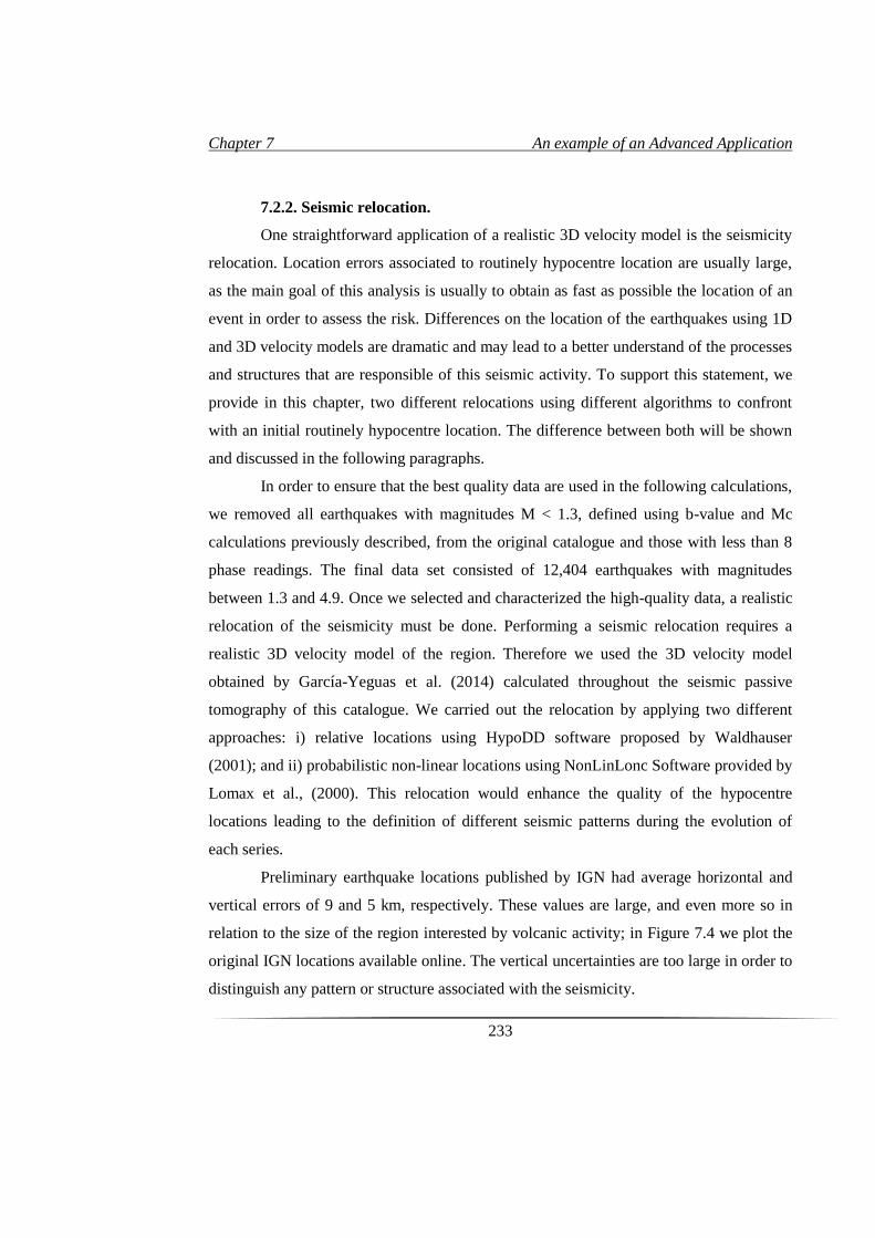
Chapter 7 An example of an Advanced Application
233
7.2.2. Seismic relocation.
One straightforward application of a realistic 3D velocity model is the seismicity
relocation. Location errors associated to routinely hypocentre location are usually large,
as the main goal of this analysis is usually to obtain as fast as possible the location of an
event in order to assess the risk. Differences on the location of the earthquakes using 1D
and 3D velocity models are dramatic and may lead to a better understand of the processes
and structures that are responsible of this seismic activity. To support this statement, we
provide in this chapter, two different relocations using different algorithms to confront
with an initial routinely hypocentre location. The difference between both will be shown
and discussed in the following paragraphs.
In order to ensure that the best quality data are used in the following calculations,
we removed all earthquakes with magnitudes M < 1.3, defined using b-value and Mc
calculations previously described, from the original catalogue and those with less than 8
phase readings. The final data set consisted of 12,404 earthquakes with magnitudes
between 1.3 and 4.9. Once we selected and characterized the high-quality data, a realistic
relocation of the seismicity must be done. Performing a seismic relocation requires a
realistic 3D velocity model of the region. Therefore we used the 3D velocity model
obtained by García-Yeguas et al. (2014) calculated throughout the seismic passive
tomography of this catalogue. We carried out the relocation by applying two different
approaches: i) relative locations using HypoDD software proposed by Waldhauser
(2001); and ii) probabilistic non-linear locations using NonLinLonc Software provided by
Lomax et al., (2000). This relocation would enhance the quality of the hypocentre
locations leading to the definition of different seismic patterns during the evolution of
each series.
Preliminary earthquake locations published by IGN had average horizontal and
vertical errors of 9 and 5 km, respectively. These values are large, and even more so in
relation to the size of the region interested by volcanic activity; in Figure 7.4 we plot the
original IGN locations available online. The vertical uncertainties are too large in order to
distinguish any pattern or structure associated with the seismicity.
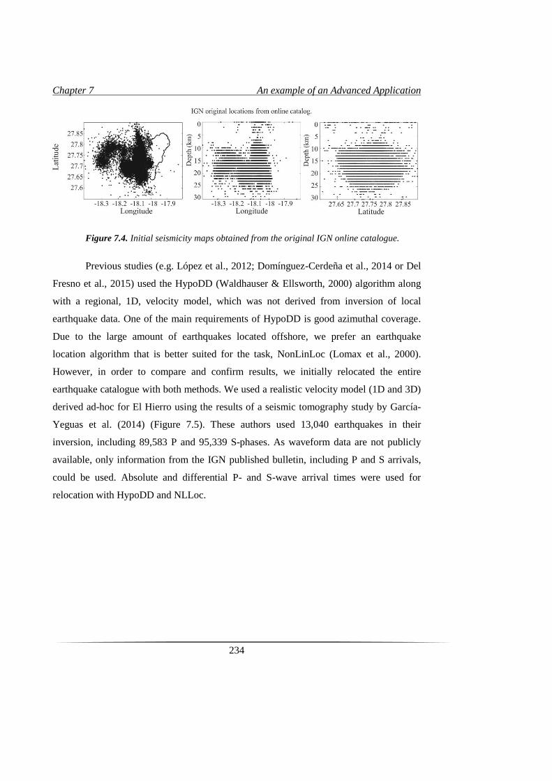
Chapter 7 An example of an Advanced Application
234
Figure 7.4. Initial seismicity maps obtained from the original IGN online catalogue.
Previous studies (e.g. López et al., 2012; Domínguez-Cerdeña et al., 2014 or Del
Fresno et al., 2015) used the HypoDD (Waldhauser & Ellsworth, 2000) algorithm along
with a regional, 1D, velocity model, which was not derived from inversion of local
earthquake data. One of the main requirements of HypoDD is good azimuthal coverage.
Due to the large amount of earthquakes located offshore, we prefer an earthquake
location algorithm that is better suited for the task, NonLinLoc (Lomax et al., 2000).
However, in order to compare and confirm results, we initially relocated the entire
earthquake catalogue with both methods. We used a realistic velocity model (1D and 3D)
derived ad-hoc for El Hierro using the results of a seismic tomography study by García-
Yeguas et al. (2014) (Figure 7.5). These authors used 13,040 earthquakes in their
inversion, including 89,583 P and 95,339 S-phases. As waveform data are not publicly
available, only information from the IGN published bulletin, including P and S arrivals,
could be used. Absolute and differential P- and S-wave arrival times were used for
relocation with HypoDD and NLLoc.
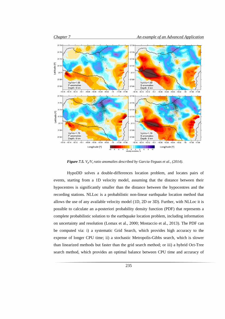
Chapter 7 An example of an Advanced Application
235
Figure 7.5. Vp/Vs ratio anomalies described by Garcia-Yeguas et al., (2014).
HypoDD solves a double-differences location problem, and locates pairs of
events, starting from a 1D velocity model, assuming that the distance between their
hypocentres is significantly smaller than the distance between the hypocentres and the
recording stations. NLLoc is a probabilistic non-linear earthquake location method that
allows the use of any available velocity model (1D, 2D or 3D). Further, with NLLoc it is
possible to calculate an a-posteriori probability density function (PDF) that represents a
complete probabilistic solution to the earthquake location problem, including information
on uncertainty and resolution (Lomax et al., 2000; Mostaccio et al., 2013). The PDF can
be computed via: i) a systematic Grid Search, which provides high accuracy to the
expense of longer CPU time; ii) a stochastic Metropolis-Gibbs search, which is slower
than linearized methods but faster than the grid search method; or iii) a hybrid Oct-Tree
search method, which provides an optimal balance between CPU time and accuracy of
Chapter 7 An example of an Advanced Application
236
the results (for additional information see Lomax & Curtis, 2001). We adopted the Oct-
Tree method. A probabilistic approach to earthquake location problems has been
demonstrated to be more reliable than linear inversion with limited seismic network
coverage (Presti et al., 2008), such as the case of El Hierro.
The results of relocations for each of the unrest phases are shown in figures 7.6a
and 7.6b. Figure 7.6a shows relative relocations obtained from the NLLoc algorithm and
Figure 7.6b illustrates the locations from HypoDD. Although in the previous section,
based on b-value patterns, we identified at least 6 seismic phases, the spatial distribution
of the VT earthquakes demonstrates that phases 1 and 2 are spatially indistinguishable.
Therefore, for the purpose of the present study we will consider them together. The two
algorithms produce comparable hypocentral distributions, an indication of the stability
and reliability of our results. The new earthquake location maps, compared with
previously published results (eg. López et al., 2012; Domínguez-Cerdeña et al., 2014 for
phases 1, 2 and 3), display less scatter, and the five temporal phases are also clearly
spatially separated. The lack of shallow (above 10 km depth) seismicity is noteworthy.
The NLLoc algorithm, combined with a 3D vP model and constant vP/vS ratio, yields
precise and reliable hypocentre locations. NLLoc also provides a reliable means to
identify poorly constrained hypocentre locations, and generally returns stable solutions
for most seismic events. Comparing the results from NLLoc and HypoDD, the former
exhibits more obvious clustering of seismicity and some linear features are also resolved.
Moreover, the root mean square (RMS) residuals and hypocentral errors obtained with
NLLoc are lower, less than 0.15 s and 0.5 km, respectively. The epicentres of events are
spread over a relatively broad area, mostly in the south-west direction. The focal depths
are constrained in the upper 25 km. Additional benefits of using 3D velocity models with
NLLoc include that the probabilistic earthquake location algorithm provides a complete
description of location uncertainties (Lomax et al., 2000). Conversely, hypocentral error
estimates by HypoDD are only relative, as the algorithm only inverts for relative
earthquake locations (e.g. Gambino et al., 2004).
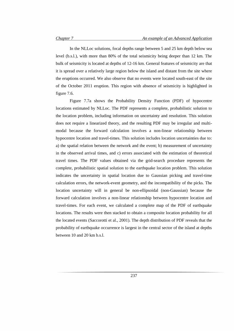
Chapter 7 An example of an Advanced Application
237
In the NLLoc solutions, focal depths range between 5 and 25 km depth below sea
level (b.s.l.), with more than 80% of the total seismicity being deeper than 12 km. The
bulk of seismicity is located at depths of 12-16 km. General features of seismicity are that
it is spread over a relatively large region below the island and distant from the site where
the eruptions occurred. We also observe that no events were located south-east of the site
of the October 2011 eruption. This region with absence of seismicity is highlighted in
figure 7.6.
Figure 7.7a shows the Probability Density Function (PDF) of hypocentre
locations estimated by NLLoc. The PDF represents a complete, probabilistic solution to
the location problem, including information on uncertainty and resolution. This solution
does not require a linearized theory, and the resulting PDF may be irregular and multi-
modal because the forward calculation involves a non-linear relationship between
hypocentre location and travel-times. This solution includes location uncertainties due to:
a) the spatial relation between the network and the event; b) measurement of uncertainty
in the observed arrival times, and c) errors associated with the estimation of theoretical
travel times. The PDF values obtained via the grid-search procedure represents the
complete, probabilistic spatial solution to the earthquake location problem. This solution
indicates the uncertainty in spatial location due to Gaussian picking and travel-time
calculation errors, the network-event geometry, and the incompatibility of the picks. The
location uncertainty will in general be non-ellipsoidal (non-Gaussian) because the
forward calculation involves a non-linear relationship between hypocentre location and
travel-times. For each event, we calculated a complete map of the PDF of earthquake
locations. The results were then stacked to obtain a composite location probability for all
the located events (Saccorotti et al., 2001). The depth distribution of PDF reveals that the
probability of earthquake occurrence is largest in the central sector of the island at depths
between 10 and 20 km b.s.l.
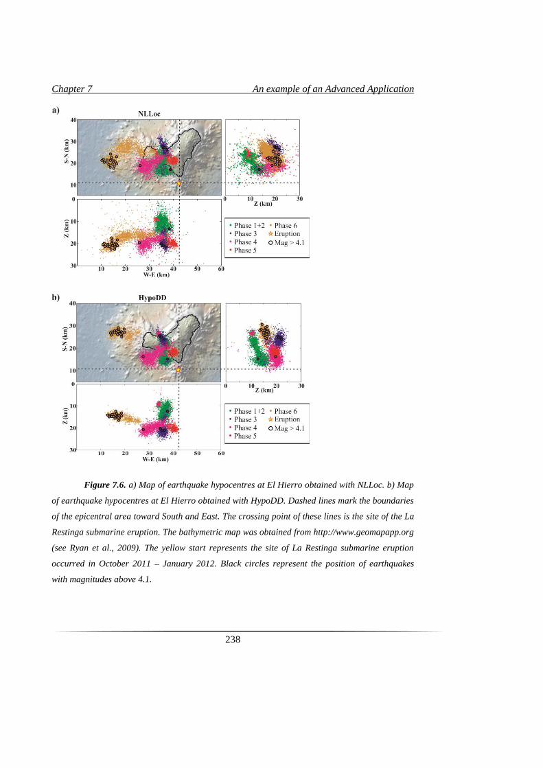
Chapter 7 An example of an Advanced Application
238
Figure 7.6. a) Map of earthquake hypocentres at El Hierro obtained with NLLoc. b) Map
of earthquake hypocentres at El Hierro obtained with HypoDD. Dashed lines mark the boundaries
of the epicentral area toward South and East. The crossing point of these lines is the site of the La
Restinga submarine eruption. The bathymetric map was obtained from http://www.geomapapp.org
(see Ryan et al., 2009). The yellow start represents the site of La Restinga submarine eruption
occurred in October 2011 – January 2012. Black circles represent the position of earthquakes
with magnitudes above 4.1.
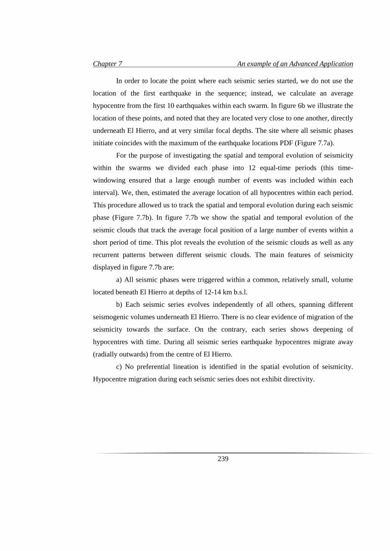
Chapter 7 An example of an Advanced Application
239
In order to locate the point where each seismic series started, we do not use the
location of the first earthquake in the sequence; instead, we calculate an average
hypocentre from the first 10 earthquakes within each swarm. In figure 6b we illustrate the
location of these points, and noted that they are located very close to one another, directly
underneath El Hierro, and at very similar focal depths. The site where all seismic phases
initiate coincides with the maximum of the earthquake locations PDF (Figure 7.7a).
For the purpose of investigating the spatial and temporal evolution of seismicity
within the swarms we divided each phase into 12 equal-time periods (this time-
windowing ensured that a large enough number of events was included within each
interval). We, then, estimated the average location of all hypocentres within each period.
This procedure allowed us to track the spatial and temporal evolution during each seismic
phase (Figure 7.7b). In figure 7.7b we show the spatial and temporal evolution of the
seismic clouds that track the average focal position of a large number of events within a
short period of time. This plot reveals the evolution of the seismic clouds as well as any
recurrent patterns between different seismic clouds. The main features of seismicity
displayed in figure 7.7b are:
a) All seismic phases were triggered within a common, relatively small, volume
located beneath El Hierro at depths of 12-14 km b.s.l.
b) Each seismic series evolves independently of all others, spanning different
seismogenic volumes underneath El Hierro. There is no clear evidence of migration of the
seismicity towards the surface. On the contrary, each series shows deepening of
hypocentres with time. During all seismic series earthquake hypocentres migrate away
(radially outwards) from the centre of El Hierro.
c) No preferential lineation is identified in the spatial evolution of seismicity.
Hypocentre migration during each seismic series does not exhibit directivity.
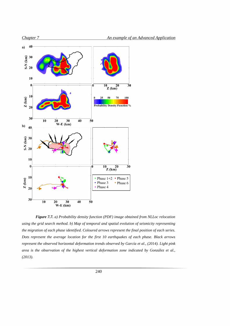
Chapter 7 An example of an Advanced Application
240
Figure 7.7. a) Probability density function (PDF) image obtained from NLLoc relocation
using the grid search method. b) Map of temporal and spatial evolution of seismicity representing
the migration of each phase identified. Coloured arrows represent the final position of each series.
Dots represent the average location for the first 10 earthquakes of each phase. Black arrows
represent the observed horizontal deformation trends observed by García et al., (2014). Light pink
area is the observation of the highest vertical deformation zone indicated by González et al.,
(2013).
Chapter 7 An example of an Advanced Application
241
It is remarkable that the horizontal projection of the onset region of every seismic
phase coincides with the area of highest deformation measured both using GPS and
satellite observations (González et al., 2013; and García et al. 2014) as also illustrated in
figure 7.7b. The light pink-coloured area represents the highest deformation values both
in elevation and in the horizontal direction, as inferred from interferometry and GPS
measurements published by Gonzalez et al. (2013) and Garcia et al. (2014). This
observation suggests, potentially, a unique magmatic plume located directly underneath
El Hierro. It should be noted that the relocated seismicity does not exhibit any obvious
spatial clustering around any potential pre-existing fracture systems, as observed in other
studies (e.g. Deichmann and Giardini, 2009). In order to detect the existence of specific
patterns in the spatial evolution the seismicity we study the differences in the relative
position of a given earthquake, n, and the successive one, n+1 (figure 7.8). The main
objective of this calculation is to understand whether there is any evidence of a
preferential direction in the fracture process. Analysing the position of a given event
relative to the next one, we investigate the existence of pre-existing fractures in the
medium controlling the temporal evolution of the rupture. Figure 7.8 shows all seismic
series sharing a similar characteristic: the lack of any preferential micro-fracture
direction. This result supports a model of stress and hydraulic fracture diffusion to
explain the mechanisms of seismogenic rupture in the El Hierro seismic series.
7.2.3. Diffusivity Curves
It is noteworthy that injection of fluids, such as magma or water, can initiate
seismic swarms (Pedersen et al., 2007). We infer that pore-pressure diffusion represents
an important triggering mechanism of these series. Pore-pressure diffusion as trigger
mechanism has been proposed in different studies: e.g. reservoir (large artificial lakes)
induced seismicity (Talwani, 2000), water table changes or stream discharge connected
with microseismicity (Lee and Wolf, 1998), earthquake swarms (Toda et al., 2002;
Parotidis et al, 2003), fluid injections (Shapiro et al., 2002; Rothert and Shapiro, 2003;
Parotidis et al, 2004; Deichmann and Giardini, 2009; Shapiro et al., 2010; Goertz-
Allmann et al., 2011), and aftershocks of strong earthquakes (Bosl and Nur, 2002;
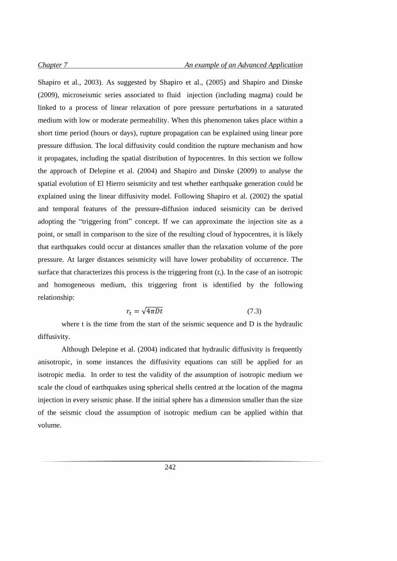
Chapter 7 An example of an Advanced Application
242
Shapiro et al., 2003). As suggested by Shapiro et al., (2005) and Shapiro and Dinske
(2009), microseismic series associated to fluid injection (including magma) could be
linked to a process of linear relaxation of pore pressure perturbations in a saturated
medium with low or moderate permeability. When this phenomenon takes place within a
short time period (hours or days), rupture propagation can be explained using linear pore
pressure diffusion. The local diffusivity could condition the rupture mechanism and how
it propagates, including the spatial distribution of hypocentres. In this section we follow
the approach of Delepine et al. (2004) and Shapiro and Dinske (2009) to analyse the
spatial evolution of El Hierro seismicity and test whether earthquake generation could be
explained using the linear diffusivity model. Following Shapiro et al. (2002) the spatial
and temporal features of the pressure-diffusion induced seismicity can be derived
adopting the “triggering front” concept. If we can approximate the injection site as a
point, or small in comparison to the size of the resulting cloud of hypocentres, it is likely
that earthquakes could occur at distances smaller than the relaxation volume of the pore
pressure. At larger distances seismicity will have lower probability of occurrence. The
surface that characterizes this process is the triggering front (rt). In the case of an isotropic
and homogeneous medium, this triggering front is identified by the following
relationship:
𝑟𝑡 = √4𝜋𝐷𝑡 (7.3)
where t is the time from the start of the seismic sequence and D is the hydraulic
diffusivity.
Although Delepine et al. (2004) indicated that hydraulic diffusivity is frequently
anisotropic, in some instances the diffusivity equations can still be applied for an
isotropic media. In order to test the validity of the assumption of isotropic medium we
scale the cloud of earthquakes using spherical shells centred at the location of the magma
injection in every seismic phase. If the initial sphere has a dimension smaller than the size
of the seismic cloud the assumption of isotropic medium can be applied within that
volume.
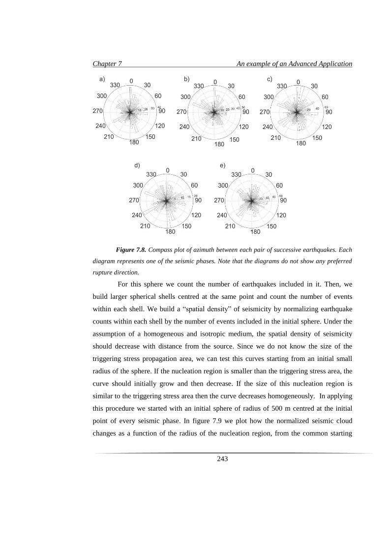
Chapter 7 An example of an Advanced Application
243
Figure 7.8. Compass plot of azimuth between each pair of successive earthquakes. Each
diagram represents one of the seismic phases. Note that the diagrams do not show any preferred
rupture direction.
For this sphere we count the number of earthquakes included in it. Then, we
build larger spherical shells centred at the same point and count the number of events
within each shell. We build a “spatial density” of seismicity by normalizing earthquake
counts within each shell by the number of events included in the initial sphere. Under the
assumption of a homogeneous and isotropic medium, the spatial density of seismicity
should decrease with distance from the source. Since we do not know the size of the
triggering stress propagation area, we can test this curves starting from an initial small
radius of the sphere. If the nucleation region is smaller than the triggering stress area, the
curve should initially grow and then decrease. If the size of this nucleation region is
similar to the triggering stress area then the curve decreases homogeneously. In applying
this procedure we started with an initial sphere of radius of 500 m centred at the initial
point of every seismic phase. In figure 7.9 we plot how the normalized seismic cloud
changes as a function of the radius of the nucleation region, from the common starting
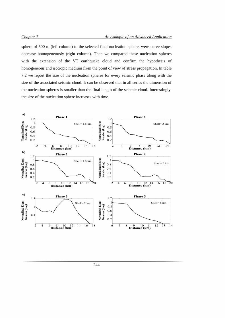
Chapter 7 An example of an Advanced Application
244
sphere of 500 m (left column) to the selected final nucleation sphere, were curve slopes
decrease homogeneously (right column). Then we compared these nucleation spheres
with the extension of the VT earthquake cloud and confirm the hypothesis of
homogeneous and isotropic medium from the point of view of stress propagation. In table
7.2 we report the size of the nucleation spheres for every seismic phase along with the
size of the associated seismic cloud. It can be observed that in all series the dimension of
the nucleation spheres is smaller than the final length of the seismic cloud. Interestingly,
the size of the nucleation sphere increases with time.
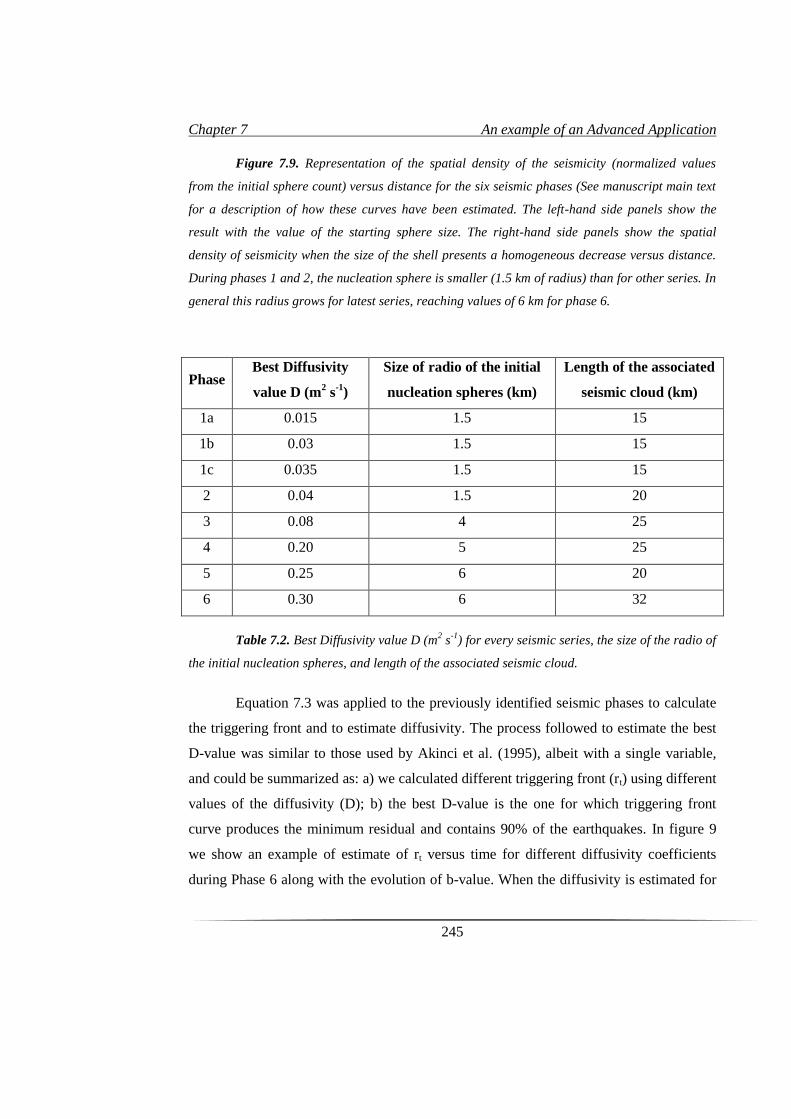
Chapter 7 An example of an Advanced Application
245
Figure 7.9. Representation of the spatial density of the seismicity (normalized values
from the initial sphere count) versus distance for the six seismic phases (See manuscript main text
for a description of how these curves have been estimated. The left-hand side panels show the
result with the value of the starting sphere size. The right-hand side panels show the spatial
density of seismicity when the size of the shell presents a homogeneous decrease versus distance.
During phases 1 and 2, the nucleation sphere is smaller (1.5 km of radius) than for other series. In
general this radius grows for latest series, reaching values of 6 km for phase 6.
Phase Best Diffusivity
value D (m2 s
-1)
Size of radio of the initial
nucleation spheres (km)
Length of the associated
seismic cloud (km)
1a 0.015 1.5 15
1b 0.03 1.5 15
1c 0.035 1.5 15
2 0.04 1.5 20
3 0.08 4 25
4 0.20 5 25
5 0.25 6 20
6 0.30 6 32
Table 7.2. Best Diffusivity value D (m2 s
-1) for every seismic series, the size of the radio of
the initial nucleation spheres, and length of the associated seismic cloud.
Equation 7.3 was applied to the previously identified seismic phases to calculate
the triggering front and to estimate diffusivity. The process followed to estimate the best
D-value was similar to those used by Akinci et al. (1995), albeit with a single variable,
and could be summarized as: a) we calculated different triggering front (rt) using different
values of the diffusivity (D); b) the best D-value is the one for which triggering front
curve produces the minimum residual and contains 90% of the earthquakes. In figure 9
we show an example of estimate of rt versus time for different diffusivity coefficients
during Phase 6 along with the evolution of b-value. When the diffusivity is estimated for
Chapter 7 An example of an Advanced Application
246
the whole interval (400 hours) the fit of the different D values is less robust and large
uncertainties are observed (Figure 7.10). The b-parameter (Figure 7.10a) increases to a
maximum value of 2.25 at about 130 hours after the onset of the swarm. Then, at about
250 hours later, it decreases smoothly to values close to 1.0. Based on these observations
we re-calculate the curve of r vs t for a shorter period (280 hours) during which the b-
value is stable with values of around 1.0. The new curve provides a better fit to the data,
and a diffusivity value of D= 0.3 m2 s
-1 is calculated. We performed similar fits to the rest
of the sequence for a selected period of time. We adopted the following criterion: the end-
time interval is the time at which the b-value, after reaching its maximum value,
decreases again close to 1.0.
In figures 7.11 and 7.12 we plot all the r vs t curves and the estimated best
diffusivity. It is interesting to observe that for phases 1, 2 and 3 this estimate was more
complex than for the rest of the series. This complexity is also reflected in the pattern of
the b-value (see figure 7.2). Since these phases are associated to the onset of volcanic
activity we could hypothesize the existence of more than three seismic phases. Phase 1
can be a combination of multiple magma injection processes. In figure 7.11 we plot 3
examples of rt vs t for phase 1 (named 1a, 1b and 1c). We also note a temporal evolution
of diffusivity, increasing with time. For the first seismic series, the best diffusivity value
is D= 0.015 m2 s
-1. For the rest of the series we obtained higher values ranging from D=
0.03 m2 s
-1 to D= 0.30 m
2 s
-1. In table 7.2 we summarize the best D values for each
seismic series.
The results suggest that the seismicity recorded at El Hierro is well described by a
model of linear diffusivity, and thus, it may be explained using theory of linear pore
pressure diffusion and hydraulic fracturing.
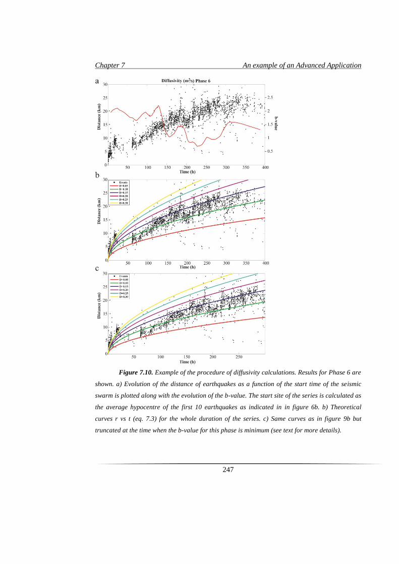
Chapter 7 An example of an Advanced Application
247
Figure 7.10. Example of the procedure of diffusivity calculations. Results for Phase 6 are
shown. a) Evolution of the distance of earthquakes as a function of the start time of the seismic
swarm is plotted along with the evolution of the b-value. The start site of the series is calculated as
the average hypocentre of the first 10 earthquakes as indicated in in figure 6b. b) Theoretical
curves r vs t (eq. 7.3) for the whole duration of the series. c) Same curves as in figure 9b but
truncated at the time when the b-value for this phase is minimum (see text for more details).
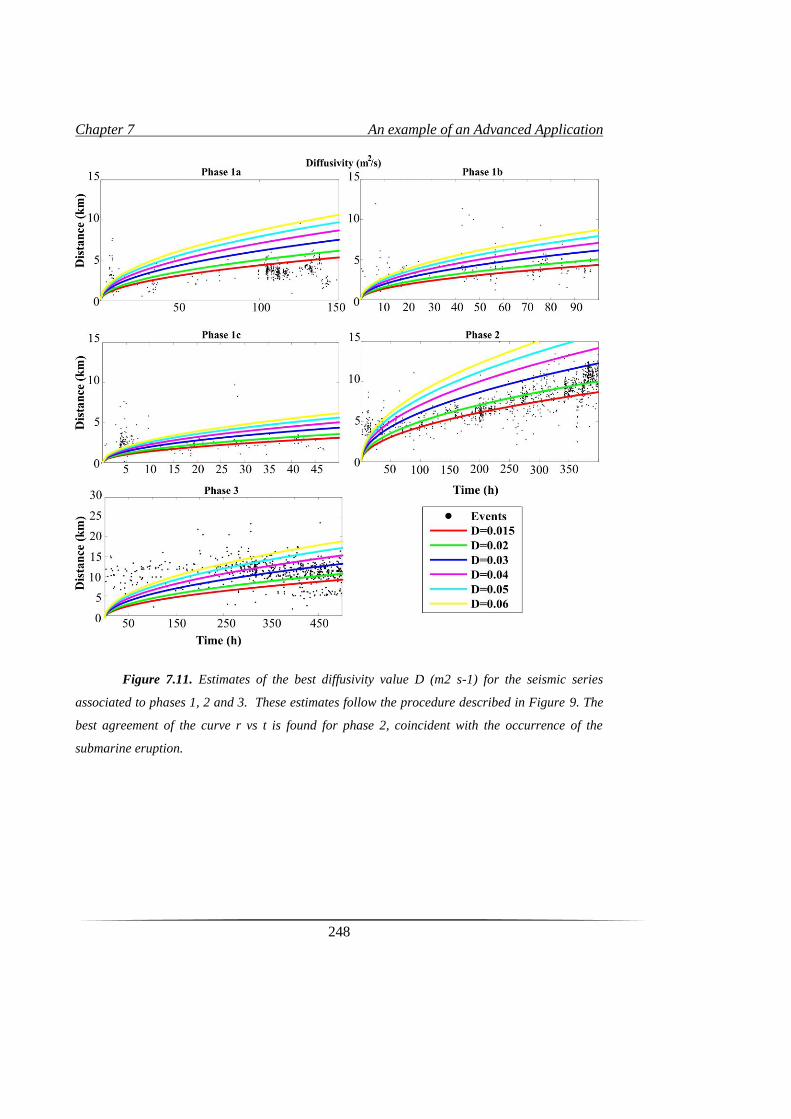
Chapter 7 An example of an Advanced Application
248
Figure 7.11. Estimates of the best diffusivity value D (m2 s-1) for the seismic series
associated to phases 1, 2 and 3. These estimates follow the procedure described in Figure 9. The
best agreement of the curve r vs t is found for phase 2, coincident with the occurrence of the
submarine eruption.
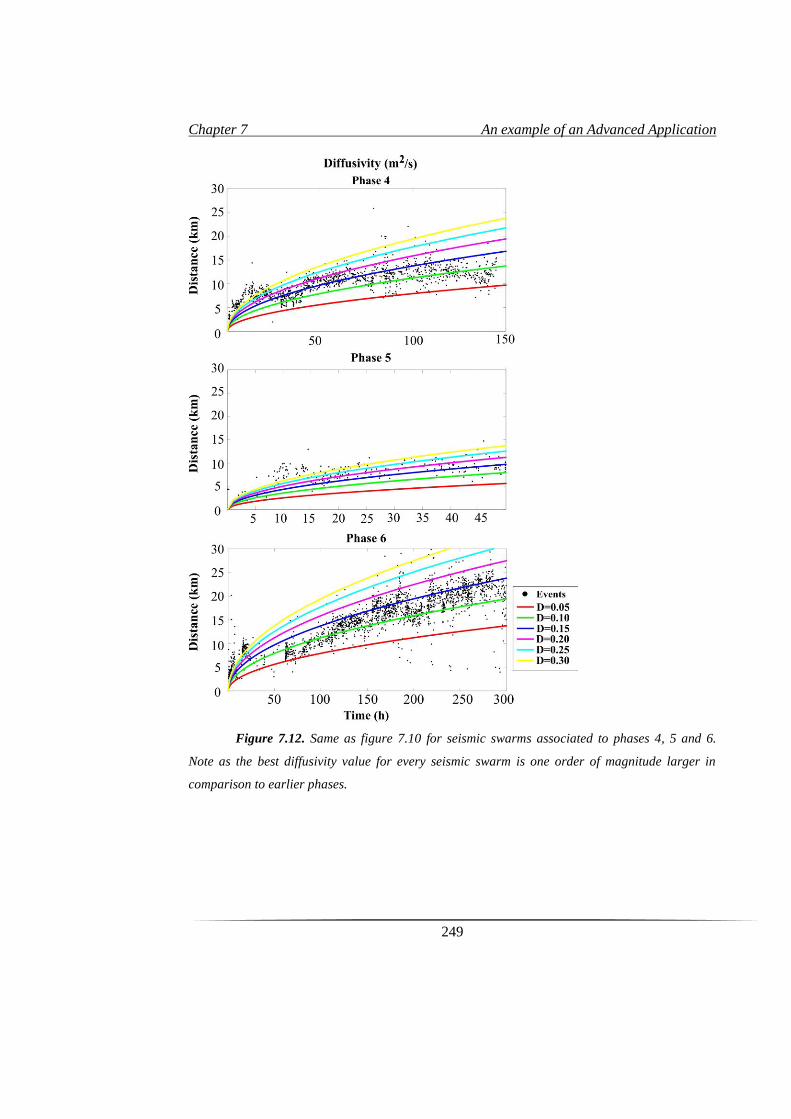
Chapter 7 An example of an Advanced Application
249
Figure 7.12. Same as figure 7.10 for seismic swarms associated to phases 4, 5 and 6.
Note as the best diffusivity value for every seismic swarm is one order of magnitude larger in
comparison to earlier phases.
Chapter 7 An example of an Advanced Application
250
7.3. Discussion
The present case of study is a reanalysis of the seismicity recorded during seismic
and volcanic activity on El Hierro Island (Canary Islands) between 2011 and 2013
(Ibáñez et al., 2012; Cerdeña-Domínguez et al. 2014; Díaz-Moreno et al., 2015). Here we
focused our efforts on analysing the mechanisms that control the occurrence of VT
earthquakes and on the applicability of models of pore-pressure diffusion and hydraulic
fracturing. Temporal changes in b-value show the occurrence of at least 6 main different
seismic swarms clearly associated to geochemical, geodetic and gravimetric observations
previously presented. Each of these seismic phases exhibits an increase in b-value up to
3.0 followed by a temporal decrease to values close to 1.0. This pattern, common to all
phases, suggests that the similar mechanisms were responsible for the seismic swarms:
the injection of multiple magmatic pulses from the Upper Mantle into the Oceanic Crust.
Earthquake relocation revealed an overall absence of seismicity at shallow depth
and around the site where eruptions took place. We also report lack any preferential
rupture direction based on the absence of clustering of seismicity along any preferential
direction, plane, or well-defined geological structure. As observed in figure 6, each
seismic phase migrates independently of the previous phase, with the only recurring
pattern being a tendency for hypocentres to deepen and expand radially outwards.
Analyses of the location of the onset of each seismic phase suggest that they all share a
common source region underneath the Island of El Hierro. Further, the hypocentral
distribution of seismicity reveals substantial lack of seismicity to the South and to East of
the eruption site in La Restinga Area. The eruption site is, indeed, located at the edge of
the seismogenic region. Montesinos et al. (2006), Gorbatikov et al. (2013) and García-
Yeguas et al. (2014) observed the presence of a high-velocity block centred underneath El
Hierro (up to 15km depth) whose boundaries are found around the eruption site. In the
same area, Blanco-Montenegro et al. (2008) observed before the 2011 eruption, a highly
magnetized vertical structure that had been interpreted as complex deep intrusive bodies.
Figure 6 in Gorbatikov et al., (2013) shows a nearly vertical high-velocity structure in the
vicinity of La Restinga submarine eruption site of October 2011. They identified this
structure surrounded by two main blocks of low shear-waves velocity and interpreted it as
Chapter 7 An example of an Advanced Application
251
the pre-existing feeding system that transported the magma aseismically from deep to the
surface. In the three-dimensional velocity model of García-Yeguas et al. (2014) a similar
vertical structure is identified with low body wave velocity. This vertical structure may
correspond to a structural barrier for stress propagation towards the South and East. Such
a block structure is a preferred model to explain the origin and evolution of the Canary
Islands archipelago (e.g. Anguita and Hernán, 2000).
A diffusivity model (eq. 7.3) fits well the observed spatial distribution of the
seismicity on El Hierro Island. The absence of any preferential rupture geometry or
direction further supports our proposed conceptual model. In our model, pore pressure
diffusion controls the generation of seismicity via hydraulic fracturing. When magma is
injected into the lower crust, across the mantle-crust boundary, hydrostatic pressure
conditions change in the region around the point of injection. Within this volume, which
is common to all seismic phases, pore pressure increases (e.g. Delepine et al. 2004; Zang
et al. 2014). As a result of this process, the effective normal stress across pre-existing
cracks and fractures decreases, thus triggering many small-magnitude earthquakes
(microseimicity), which spread out radially. The relatively high rates of smaller
magnitude earthquakes result in comparatively high b-values (e.g. Riedel et al., 2003).
The radial distribution of earthquake hypocentres generates a relatively homogeneous
seismic cloud around the magma injection point. After its initial injection across the
mantle-crust boundary, magma migrates either horizontally or upwards (see Martí et al.,
2013a) and the volumetric component of seismicity becomes less important (e.g. Kraft
and Deichmann, 2013; Zang et al., 2014). At this stage the effects of hydraulic fracturing,
local and regional stress conditions, and stress concentration due to magma migration
(pore-pressure diffusion),combine to control the spatial and temporal evolution of
seismicity (e.g. Albino and Sigmundsson, 2013). Conditions of increased shear stress lead
to larger magnitude earthquakes, an effect that is reflected in the overall decrease of the
observed b-values. Finally, at larger distances the influence of hydraulic fracturing may
become negligible, thus, preventing the generation of further seismicity. Similar seismic
patterns have been reported by other authors (e.g. Majer et al. 2007; Deichman and Ernst
2009; Goertz-Allmann et al., 2011; Zang et al. 2014) in geothermal regions. Our analyses,
Chapter 7 An example of an Advanced Application
252
along with similarities with previous case studies, suggest that the distribution and
evolution of earthquake hypocentres at El Hierro is not directly controlled by magma
migration. We suggest that seismicity results from the combined effects of stress transfer
pore pressure diffusion, hydraulic fracturing, and local and regional conditions, including
crustal heterogeneity.
It is interesting to note how the estimated radii of the earthquake nucleation
sphere, grow with time (see table 7.2). Combining such an increase with the observed
changes in the diffusivity values we could infer that the area affected by stress
propagation grew with times. This does not necessarily reflect an increase in the size of
the magmatic pulses; it may represent pervasive fracturing due to an increase in
background stress and deformation. During the initial stages of volcanic activity, magma
injection in the oceanic crust was mainly controlled by stresses linked to the gravitational
load of the island of El Hierro, and the overall tectonic regime in the region. As new
magma was injected into the lower crust, stress increased in the region as demonstrated
by deformation measured at the surface. Stress accumulation is reflected in the overall
increase of diffusivity values. During the last seismic swarm, in phase 6, seismicity had
the largest spatial extent and the largest earthquake magnitudes were recorded. The radius
of the nucleation shell and the diffusivity were also the largest. A similar case is
discussed in Murphy et al., (2013) and investigated by means of numerical modelling.
The authors indicate that under the assumption that fluid injection induces seismicity, the
triggering mechanism could be associated to two processes: i) increase in pore fluid
pressure, effectively reducing the normal stress within the affected volume, or ii) changes
in the Coulomb stress within the fault system. The extension of the seismogenic region
and the duration of the seismic swarms are linked to the permeability of the rocks in the
region. If low permeability is assumed, seismicity will be mostly located in the vicinity of
the injection, as for El Hierro during phases 1 and 2. When the permeability increases,
and Coulomb stress perturbations extend over a much larger area, pore diffusion will
affect regions outside of the injection plume generating more extensive and energetic
seismic swarms, as during phases 4, 5 and 6 (see energy evolution of figure 2 at El
Hierro.
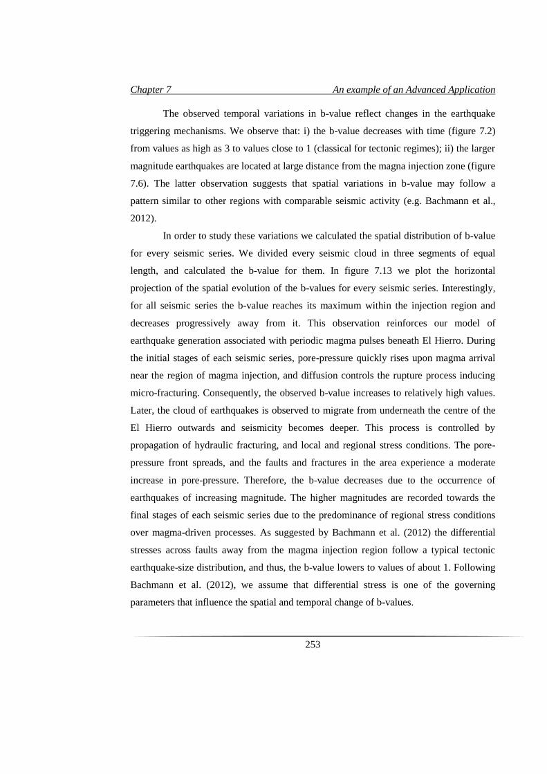
Chapter 7 An example of an Advanced Application
253
The observed temporal variations in b-value reflect changes in the earthquake
triggering mechanisms. We observe that: i) the b-value decreases with time (figure 7.2)
from values as high as 3 to values close to 1 (classical for tectonic regimes); ii) the larger
magnitude earthquakes are located at large distance from the magna injection zone (figure
7.6). The latter observation suggests that spatial variations in b-value may follow a
pattern similar to other regions with comparable seismic activity (e.g. Bachmann et al.,
2012).
In order to study these variations we calculated the spatial distribution of b-value
for every seismic series. We divided every seismic cloud in three segments of equal
length, and calculated the b-value for them. In figure 7.13 we plot the horizontal
projection of the spatial evolution of the b-values for every seismic series. Interestingly,
for all seismic series the b-value reaches its maximum within the injection region and
decreases progressively away from it. This observation reinforces our model of
earthquake generation associated with periodic magma pulses beneath El Hierro. During
the initial stages of each seismic series, pore-pressure quickly rises upon magma arrival
near the region of magma injection, and diffusion controls the rupture process inducing
micro-fracturing. Consequently, the observed b-value increases to relatively high values.
Later, the cloud of earthquakes is observed to migrate from underneath the centre of the
El Hierro outwards and seismicity becomes deeper. This process is controlled by
propagation of hydraulic fracturing, and local and regional stress conditions. The pore-
pressure front spreads, and the faults and fractures in the area experience a moderate
increase in pore-pressure. Therefore, the b-value decreases due to the occurrence of
earthquakes of increasing magnitude. The higher magnitudes are recorded towards the
final stages of each seismic series due to the predominance of regional stress conditions
over magma-driven processes. As suggested by Bachmann et al. (2012) the differential
stresses across faults away from the magma injection region follow a typical tectonic
earthquake-size distribution, and thus, the b-value lowers to values of about 1. Following
Bachmann et al. (2012), we assume that differential stress is one of the governing
parameters that influence the spatial and temporal change of b-values.
Chapter 7 An example of an Advanced Application
254
Figure 7.13. Spatial evolution of b-values for each seismic swarm (see the main
manuscript for details on spatial b-value calculations). Arrows portrait the spatial evolution of
each seismic cloud.
At El Hierro there was clear evidence of an eruption between October 2011 and
January 2012, and another potential eruptive episode in June 2012 (discussed by Pérez et
al., 2014, Blanco et al., 2015 and Pérez et al., 2015). It is well known that pre-eruptive
magma migration produces high b-values (e.g. Riedel et al., 2003). The occurrence of
eruptive activity at the surface confirms upward migration of magma. As the eruptions
did not occur directly above the inferred location of magma injection across the mantle-
crust boundary, several authors (e.g. Martí et al. 2013a; López et al., 2014 or Telesca et
al. 2015) inferred horizontal magma migration. Magma movement is expected to produce
changes in pore-pressure and should generate seismicity in the neighbouring regions;
therefore, we cannot neglect these processes in the generation of seismicity and in
explaining changes in b-value. However, the spatial evolution of phases 1 and 2,
associated to the main eruptive episode in October 2011, suggests that there are
discrepancies between horizontal migration of seismicity and the site of eruption.
Furthermore, vertical migration of the magma towards the surface is entirely aseismic.
Finally, we observe that all seismic series end with a tendency of earthquake hypocentres
Chapter 7 An example of an Advanced Application
255
to deepen, which is incompatible with mechanisms involving magma migration.
Therefore, we hypothesize that despite evidence of magma movement after its initial
injection, the influence of horizontal and vertical migration is secondary on earthquake
triggering. We suggest that the seismic clouds map the effects of pore-pressure
distribution and hydraulic fracturing rather than potential secondary magma migration.
The pattern of seismicity and the onset of every seismic series point to a model of
periodic injection of magma from the Upper Mantle into the lower crust. For example, the
evolution of b-values during phases 1 and 2 is complex. In these two periods, the b-value
does not decrease as uniformly as observed in the other series. Following our proposed
conceptual model, when the b-value is high pore-pressure diffusivity controls the rupture
process, and earthquake generation is associated to near-field effects of magma injection.
If the b-value exhibits increase-decrease cycles, it may be hypothesized that such pattern
reflects multiple injection episodes. Additional evidence of multiple pulses is observed
during phase 6 (figures 7.10 and 7.12). The pattern of seismicity recorded during the first
30 h of this series suggests a value of diffusivity much higher than expected. The b-value
(figure 7.3) for the same series exhibits an initial high value, associated with the initial 30
hours, before decreasing and, once again, increasing at about hour 50. It, then, steadily
decrease until the end of the series. This behaviour is compatible with multiple pulses of
magma injection.
Martí et al, (2013 b) proposed a model to explain seismic and volcanic activity
from June 2011 to January 2012. These authors combined petrological and geophysical
observations to provide insights into the mechanisms of seismicity. In their model,
seismicity during Phase 1 is generated by magma rising from the mantle into the Moho,
and thus, it tracks magma propagation, the size, and the shape of a potential magma
reservoir at about 15 km b.s.l. As the high velocity structure of El Hierro acts as a barrier
to upwards migration, magma migrated horizontally, producing additional seismicity.
Marti et al. (2013b) linked earthquake activity during this period to magma-driven
fracturing via shear fracturing. Finally, magma ascended towards the surface resulting in
an aseismic submarine eruption. The authors infer that the bulk of seismicity recorded
Chapter 7 An example of an Advanced Application
256
during Phase 3 could be associated to “gravitational and tectonic readjustments of the
plumbing system”. This model is compatible with our observations of phases 1 to 3.
The model discussed in this chapter is described in figure 7.14. We plot the
relocated seismicity together with the tomographic anomalies in order to image their
spatial relation. Additionally we mark the beginning of the different magma pulses we
have hypothesized in this discussion.
7.4. Preliminary applications on Mt. Etna
Mt. Etna, as described in Chapter 2, is a very active volcano, though, seismic
swarms in this region have never been as large and intense as the one occurred in the
seismic crisis of El Hierro Island. Nonetheless, we have a remarkable opportunity to
study this volcano following the same methodologies described in this work. We selected
a dataset of 300 events registered during the 2002-03 eruption already relocated using
previous 3D models. These are very shallow events and were triggered by the magmatic
ascent during the eruption. To analyse this new database we proceed following the same
methodology as for the case of El Hierro. We first calculated the b-value evolution with
time (figure 7.15) to identify the eruptive pattern. In this case we observe an increase in
the b-vale to reach values of 1.3 and then a decrease to values of 0.6. There are important
differences in terms of absolute values of b. However, the trend increase-decrease is the
same. Next step is the calculation of the diffusivity parameters for the seismic catalogue.
Preliminary results are shown in figure 7.16. It is noteworthy that the seismicity clearly
adjust to a curve of D= 0.3 m2s
-1, similar to that obtain for phase 6 for El Hierro
catalogue. Nonetheless it is important to note the difference in the number and magnitude
of events comparing Mt. Etna and El Hierro catalogues. Thus, further analyses will be
soon performed.
Along this chapter we demonstrated the utility of obtaining realistic 3D velocity
models throughout seismic tomography as a first step to perform advanced seismic
studies that allow us to enhance our present knowledge of volcanic dynamic and
structure.
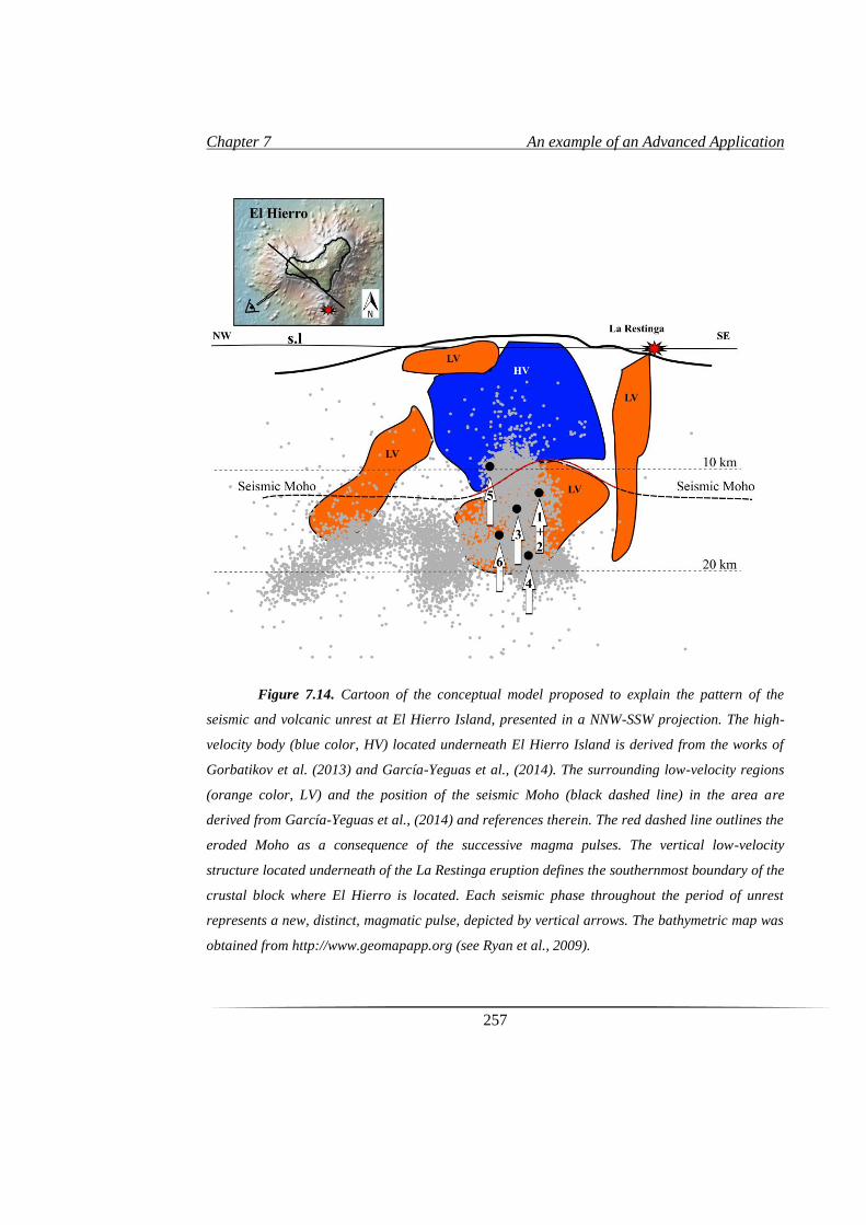
Chapter 7 An example of an Advanced Application
257
Figure 7.14. Cartoon of the conceptual model proposed to explain the pattern of the
seismic and volcanic unrest at El Hierro Island, presented in a NNW-SSW projection. The high-
velocity body (blue color, HV) located underneath El Hierro Island is derived from the works of
Gorbatikov et al. (2013) and García-Yeguas et al., (2014). The surrounding low-velocity regions
(orange color, LV) and the position of the seismic Moho (black dashed line) in the area are
derived from García-Yeguas et al., (2014) and references therein. The red dashed line outlines the
eroded Moho as a consequence of the successive magma pulses. The vertical low-velocity
structure located underneath of the La Restinga eruption defines the southernmost boundary of the
crustal block where El Hierro is located. Each seismic phase throughout the period of unrest
represents a new, distinct, magmatic pulse, depicted by vertical arrows. The bathymetric map was
obtained from http://www.geomapapp.org (see Ryan et al., 2009).

Chapter 7 An example of an Advanced Application
258
Figure 7.15. b-value time evolution of 2002-03 eruption at Mt. Etna calculated using the
same methodology describe in this chapter.
Figure 7.16. Diffusivity curves calculated for the 300 events registered in Mt. Etna.
8. Conclusions

Chapter 8 Conclusions
261
8.1. Conclusive Remarks
Along this chapter we present the main conclusions we extract from this
Doctoral Thesis. We divide them into different sections according to Databases, Picking,
Tomographic Inversion Code, Tomographic Images and Advanced Applications.
Additionally we provide a list of future works. Many of them are of immediate
application (some are already in preparation).
8.1.1. Databases
TOMO-ETNA Experiment is probably the most complex active-passive
seismic survey carried out in the world. Especially when we consider the
number of involved people, countries, international projects, etc.
The wide distribution of the seismic sources, both active and passive, allows
us to cover a very large region for an active experiment when compared to
previous active surveys in volcanoes.
Based on previous experiences on Deception Island, and Tenerife Island, we
state that the dataset obtained will provide results over at least the next 10
years, by applying new techniques, approaches, etc.
Regarding the TOMO-ETNA Experiment, we obtained more than three
million seismic signals, from which we selected more than 180,000 P-phase
travel times for the active sources and almost 12,000 P-phase travel times for
the passive sources. These final dataset represent a very high quality data
registered in seismic stations up to 50 km away from the active source.
The final dataset consists on: i) 184,797 P-phase travel times for the active
sources; ii) 11,802 P-phase travel times for the passive sources; iii) 267
stations.
8.1.2. Picking
The automatic P-wave detection algorithm developed ad-hoc for the TOMO-
ETNA dataset provides an accurate P-wave onset estimation using Multiband
Frequency Analysis (AMPA).
Chapter 8 Conclusions
262
AMPA algorithm is a new fast, robust adaptable and reliable algorithm that
allows us the processing of all three million seismic signals in less than 30
hours, providing also a set of quality assessment parameters.
Additional confrontation between manual and automatic picking has been
performed in order to estimate the possible discrepancies.
8.1.3. Tomographic Inversion Code
Joint Active Passive Ray Tomography Software (PARTOS) has been
developed ad-hoc for the TOMO-ETNA experiment dataset.
The robustness, reliability and quality of the algorithms involved are strongly
proved: i) it is based on two well-known tomographic codes developed for
active and passive seismic inversion respectively; ii) Many synthetic tests
have been carried out to validate the solutions.
It is probably the first time that such robust and powerful joint active passive
tomography software has been developed and openly shared within the
scientific community.
8.1.4. Tomographic Images
High resolution tomographic images are presented for three different relevant
regions: i) North-eastern Sicily, comprising Ionian and Thyrrenian Seas
(Region 1); ii) Aeolian Islands Archipelago (Region 2); and iii) Mt. Etna
Volcano (Region 3).
Stability, robustness and quality of the solutions are proved throughout a
series of synthetic tests.
The ray density maps show very high ray coverage within the areas of study,
reaching in some cases more than 1,800 rays per cell.
Region 1 main anomalies:
o Anomalies 1 and 1b: correspond to the well-known ATLFS, defined
by many authors. Although its origin is still under debate, the most
stable hypothesis is that of a dextral transfer zone separating a
compressional regime on the western part of the Aeolian
Archipelago, from an extensional regime to the northeast.
Chapter 8 Conclusions
263
o Anomaly E: Etnean volcanic region, characterised by low velocity
anomalies.
o Anomaly A: Aeolian Islands region, characterised by a series of low
velocity-high velocity anomaly distribution.
Region 2 main anomalies:
Anomaly 2: Known as SAFS, this dextral strike-slip motion fault system
accommodates the compression of the westernmost part of the Aeolian
Archipelago. It easternmost limit reaches the mentioned ATLFS in the area of
the Lipari-Vulcano complex.
Anomaly 3: NW-SE discontinuity interpreted by many authors as a STEP
fault related to the decoupling the subducting lithosphere from the non-
subducting one.
Anomaly 4: Large low velocity volume probably related to the active
volcanism of the easternmost Aeolian Islands (Panarea and Stromboli).
Region 3 main anomalies:
o Anomaly 5: Probably the most well-known feature on the Etnean
region. The HVB is enlightened, and as our results go deeper than
previous tomographies, we observe the roots of this HVB connected
in depth with new high velocity bodies located offshore.
o Anomaly 6: High velocity anomaly located near the coast of the
eastern flank of Mt. Etna, that can be related with the HVB
mentioned above. Other hypothesis is that these volume may be an
effect of the Moho upwelling described by other authors.
o Anomalies 7, 8 and 9: These are anomalies that have never been
interpreted and for which we present some preliminary ideas that
must be further investigated.

Chapter 8 Conclusions
264
8.1.5. Advanced Applications
We postulate 3D velocity models obtained throughout seismic tomography
not just as final results, but as an important tool for advanced studies.
We present a complete case of study using seismic velocity models as the
base for further advanced applications. This study comprise the use of several
procedures:
o B-value estimation
o Seismic precise location using relative and probabilistic non-linear
algorithms.
o Estimation of diffusivity curves
Results enlighten new mechanisms of seismic migration in active volcanic
regions.
We state that seismic migration in volcanic environments do not necessary be
directly related to magma migration.
Hydraulic fracturing can be considered as an important mechanism
controlling stress and seismic migration in volcanic areas, especially when
magma intrusions occurred.
8.2. Future Work
8.2.1 Regarding Mt. Etna Volcano
Joint Gravimetric and Seismic inversion. Combine both gravimetric and
seismic velocity models in order to determine elastic parameters distribution
(in preparation).
Advanced applications of the new seismic velocity model on Mt. Etna in the
light of Hydraulic Fracturing to better constrain the volcano-seismic swarms
(in preparation).
Seismic Attenuation tomography. It is a natural further step of the seismic
velocity tomography as evidenced by several studies (i.e. Deception Island,
Tenerife Island, Stromboli, etc.).
Application of new advanced algorithm on seismic waves arrival detection in
order to enhance the current high quality seismic database.

Chapter 8 Conclusions
265
New Joint Seismic Tomography of MT. Etna by including larger passive
database. The current tomography represents a snapshot, which permits to
enlighten volcanic structures that may change with time. However, structural
regional features should not change with time and therefore we could
improve our current knowledge of them by including more passive seismic
information to the current joint tomographic inversion.
8.2.2. General applications
Regarding the use of PARTOS, we pretend to carry out further joint
tomographies in Tenerife Island, and Montserrat Island as immediate studies.
Joint tomography of Deception Island is also on the focus for further studies.
Use hydraulic fracturing approach in other active volcanic regions. For that
purpose, we only need data from volcano-seismic swarms and a realistic 3D
velocity model.
Sharing Data, Results with the Scientific Community. We want to share with the
rest of the community our results, databases and methodologies in order to allow
other researchers to use them. This collaboration will also allow us to improve
the results and techniques and therefore improve our knowledge of different
volcanic regions. Sharing Data will be carried out throughout different ways:
o Nature Scientific Data Publications.
o KNOWAVES Spanish Research Project will provide necessary tools for
sharing results throughout online cloud systems.
o EPOS European Project will give us also the required tools to share
databases and results with the scientific community.

9. Bibliography

Chapter 9 Bibliography
269
Aiuppa, A., Cannata, A., Cannavò, F., Di Grazia, G., Ferrari, F., Giudice, G., ... & Patanè,
D. (2010). Patterns in the recent 2007–2008 activity of Mount Etna volcano
investigated by integrated geophysical and geochemical observations. Geochemistry,
Geophysics, Geosystems, 11(9).
Aki, K., Christoffersson, A., Husebye, E. S., & Powell, C. (1974). Three-dimensional
seismic velocity anomalies in the crust and upper-mantle under the USGS, California
seismic array. Eos Transactions. American Geophysical Union, 56, 1145.
Albino, F. & Sigmundsson, F. (2013) Stress transfer between magma bodies: Influence of
intrusions prior to 2010 eruptions at Eyjafjallajökull volcano, Iceland. Journal of
Geophysical Research: Solid Earth, 119, 2964-2975, doi:10.1002/2013JB010510.
Alinaghi, A., Koulakov, I., & Thybo, H. (2007). Seismic tomographic imaging of P-and
S-waves velocity perturbations in the upper mantle beneath Iran. Geophysical
Journal International, 169(3), 1089-1102.
Allard, P., Behncke, B., D’Amico, S., Neri, M., & Gambino, S. (2006). Mount Etna
1993–2005: Anatomy of an evolving eruptive cycle. Earth-Science Reviews, 78(1-2),
85–114. doi:10.1016/j.earscirev.2006.04.002.
Allen, R. V. (1978). Automatic earthquake recognition and timing from single traces.
Bulletin of the Seismological Society of America, 68(5), 1521-1532.
Aloisi, M., Cocina, O., Neri, G., Orecchio, B., & Privitera, E. (2002). Seismic
tomography of the crust underneath the Etna volcano, Sicily. Physics of the Earth
and Planetary Interiors, 134(3-4), 139–155. doi:10.1016/S0031-9201(02)00153-X.
Almendros, J., Alguacil, G., Del Pezzo, E., & Ortiz, R. (1997). Array tracking of the
volcanic tremor source at Deception Island, Antarctica. Geophysical Research
Letters, 24(23), 3069-3072.
Alparone, S., Barberi, G., Cocina, O., Giampiccolo, E., Musumeci, C., & Patanè, D.
(2012). Intrusive mechanism of the 2008-2009 Mt. Etna eruption: Constraints by
tomographic images and stress tensor analysis. Journal of Volcanology and
Geothermal Research, 229-230, 50–63. doi:10.1016/j.jvolgeores.2012.04.001.
Alparone, S., Cocina, O., Gambino, S., Mostaccio, A., Spampinato, S., Tuvè, T., &
Ursino, A. (2013). Seismological features of the Pernicana–Provenzana Fault System
Chapter 9 Bibliography
270
(Mt. Etna, Italy) and implications for the dynamics of northeastern flank of the
volcano. Journal of volcanology and geothermal research, 251, 16-26.
Alvarez, I., Garcia, L., Mota, S., Cortes, G., Benitez, C., & De la Torre, A. (2013). An
Automatic P-Phase Picking Algorithm Based on Adaptive Multiband Processing.
Geoscience and Remote Sensing Letters, IEEE, 10(6), 1488-1492.
Andronico, D., Branca, S., Calvari, S., Burton, M., Caltabiano, T., Corsaro, R. A., ... &
Murè, F. (2005). A multi-disciplinary study of the 2002–03 Etna eruption: insights
into a complex plumbing system. Bulletin of Volcanology, 67(4), 314-330.
Anguita, F., and Hernán, F. (2000). The Canary Islands origin: a unifying model. Journal
of Volcanology and Geothermal Research, 103(1), 1-26.
Aoki, Y., Takeo, M., Aoyama, H., Fujimatsu, J., Matsumoto, S., Miyamachi, H., ... &
Tanada, R. (2009). P-wave velocity structure beneath Asama Volcano, Japan,
inferred from active source seismic experiment. Journal of Volcanology and
Geothermal Research, 187(3), 272-277.
Argnani, A., Brancolini, G., Bonazzi, C., Rovere, M., Accaino, F., Zgur, F., & Lodolo, E.
(2009). The results of the Taormina 2006 seismic survey: possible implications for
active tectonics in the Messina Straits. Tectonophysics, 476(1), 159-169.
Armienti, P., Innocenti, F., Petrini, R., Pompilio, M., & Villari, L. (1989). Petrology and
Sr-Nd isotope geochemistry of recent lavas from Mt. Etna: bearing on the volcano
feeding system. Journal of Volcanology and Geothermal Research, 39(4), 315-327.
Auger, E., Gasparini, P., Virieux, J., & Zollo, A. (2001). Seismic evidence of an extended
magmatic sill under Mt. Vesuvius. Science, 294(5546), 1510-1512.
Azzaro, R., Branca, S., Giammanco, S., Gurrieri, S., Rasà, R., & Valenza, M. (1998).
New evidence for the form and extent of the Pernicana Fault System (Mt. Etna) from
structural and soil–gas surveying. Journal of volcanology and geothermal research,
84(1), 143-152.
Azzaro, R. (1999). Earthquake surface faulting at Mount Etna volcano (Sicily) and
implications for active tectonics. Journal of Geodynamics, 28(2), 193-213.
Azzaro, R., Branca, S., Gwinner, K., & Coltelli, M. (2012a). The volcano-tectonic map of
Etna volcano, 1:100.000 scale: an integrated approach based on a morphotectonic

Chapter 9 Bibliography
271
analysis from high-resolution DEM constrained by geologic, active faulting and
seismotectonic data. Italian Journal of Geosciences, 131(1), 153–170.
doi:10.3301/IJG.2011.29.
Azzaro, R., D’Amico, S., Peruzza, L., & Tuvè, T. (2012a). Earthquakes and faults at Mt.
Etna (southern Italy): problems and perspectives for a time-dependent probabilistic
seismic hazard assessment in a volcanic region. Bollettino di Geofisica Teorica ed
Applicata, 53(1), 75-88.
Bachmann, C. E., Wiemer, S., Goertz‐Allmann, B. P., & Woessner, J. (2012). Influence
of pore‐pressure on the event‐size distribution of induced earthquakes. Geophysical
Research Letters, 39(9). DOI: 10.1029/2012GL051480.
Baer, M., & Kradolfer, U. (1987). An automatic phase picker for local and teleseismic
events. Bulletin of the Seismological Society of America, 77(4), 1437-1445.
Balmforth, N. J., Craster, R. V., & Rust, A. C. (2005). Instability in flow through elastic
conduits and volcanic tremor. Journal of Fluid Mechanics, 527, 353-377.
Barberi, F., Carapezza, M. L., Valenza, M., & Villari, L. (1993). The control of lava flow
during the 1991–1992 eruption of Mt. Etna. Journal of volcanology and geothermal
research, 56(1), 1-34.
Barberi, F., A. Gandino, A. Gioncada, P. La Torre, A. Sbrana, and C. Zenucchini (1994),
The deep structure of the Eolian arc (Filicudi–Panarea–Vulcano sector) in light of
gravity, magnetic and volcanological data, J. Volcanol. Geotherm. Res., 61,189–206.
Barberi, G., Cocina, O., Neri, G., Privitera, E., & Spampinato, S. (2000). Volcanological
inferences from seismic-strain tensor computations at Mt. Etna Volcano, Sicily.
Bulletin of volcanology, 62(4-5), 318-330.
Barberi, G., Cocina, O., Maiolino, V., Musumeci, C., & Privitera, E. (2004). Insight into
Mt. Etna (Italy) kinematics during the 2002-2003 eruption as inferred from seismic
stress and strain tensors. Geophysical Research Letters, 31(21), 0–3.
doi:10.1029/2004GL020918.
Barberi,G., Giampiccolo, E., Musumeci, C., Scarfi, L., Bruno, V., Cocina, O., Díaz-
Moreno, A., Sicali, S., Tusa, G., Tuvè, T., Zuccarello, L., and Patanè, D., (2016).
Seismic and Volcanic activity during 2014 in the región involved by TOMO-ETNA
Chapter 9 Bibliography
272
seismic active experiment. . Special Volume: TOMOETNA. Eds. Morales J., and
Puglisi G.. Annals of Geophysics. doi:10.4401/ag-7082.
Barclay, A. H., Wilcock, W. S. D., & Ibáñez, J. M. (2009). Bathymetric constraints on the
tectonic and volcanic evolution of Deception Island Volcano, South Shetland
Islands. Antarctic Science, 21(02), 153-167.
Barnard, S. T. (2004). Results of a reconnaissance trip to Mt. Etna, Italy: the effects of the
2002 eruption of Etna on the province of Catania. Bulletin of the New Zealand
Society for Earthquake Engineering, 37(2), 47-61.
Barreca, G., Bruno, V., Cultrera, F., Mattia, M., Monaco, C., & Scarfì, L. (2014). New
insights in the geodynamics of the Lipari–Vulcano area (Aeolian Archipelago,
southern Italy) from geological, geodetic and seismological data. Journal of
Geodynamics, 82, 150-167.
Barreca, G., Scarfì, L., Cannavò, F., Koulakov, I., & Monaco, C. (2016). New structural
and seismological evidence and interpretation of a lithospheric scale shear zone at
the southern edge of the Ionian subduction system (central‐eastern Sicily, Italy).
Tectonics.
Battaglia, J., & Aki, K. (2003). Location of seismic events and eruptive fissures on the
Piton de la Fournaise volcano using seismic amplitudes. Journal of Geophysical
Research: Solid Earth, (1978–2012), 108(B8).
Battaglia, J., Got, J. L., & Okubo, P. (2003). Location of long‐period events below
Kilauea Volcano using seismic amplitudes and accurate relative relocation. Journal
of Geophysical Research: Solid Earth, (1978–2012), 108(B12).
Battaglia, M., Gottsmann, J., Carbone, D., & Fernández, J. (2008a). 4D volcano
gravimetry. Geophysics, 73(6), WA3-WA18.
Battaglia, J., Zollo, A., Virieux, J., & Dello Iacono, D. (2008b). Merging active and
passive data sets in traveltime tomography: the case study of Campi Flegrei caldera
(Southern Italy). Geophysical Prospecting, 56(4), 555-573.
Beccaluva, L., G. Gabbianelli, F. Lucchini, P.L. Rossi, and C. Savelli (1985), Petrology
and K/Ar ages of volcanic dredged from the Aeolian seamounts: implications for
Chapter 9 Bibliography
273
geodynamic evolution of the southern Tyrrhenian basin, Earth Planet. Sci. Lett., 74,
187–208.
Behncke, B., & Neri, M. (2003a). Cycles and trends in the recent eruptive behaviour of
Mount Etna (Italy). Canadian Journal of Earth Sciences, 40(10), 1405-1411.
Behncke, B., & Neri, M. (2003b). The July–August 2001 eruption of Mt. Etna (Sicily).
Bulletin of Volcanology, 65(7), 461-476.
Bell, A. F., and Kilburn, C. R. (2012). Precursors to dyke-fed eruptions at basaltic
volcanoes: insights from patterns of volcano-tectonic seismicity at Kilauea volcano,
Hawaii. Bulletin of volcanology, 74(2), 325-339.
Ben-Avraham, Z., and M. Grasso (1991). Crustal structure variations and transcurrent
faulting at the eastern and western margins of the eastern Mediterranean,
Tectonophysics, 75, 269–277.
Ben-Zvi, T., Wilcock, W. S., Barclay, A. H., Zandomeneghi, D., Ibáñez, J. M., &
Almendros, J. (2009). The P-wave velocity structure of Deception Island, Antarctica,
from two-dimensional seismic tomography. Journal of Volcanology and Geothermal
Research, 180(1), 67-80.
Benítez, M. C., Ramírez, J., Segura, J. C., Ibáñez, J. M., Almendros, J., García-Yeguas,
A., & Cortes, G. (2007). Continuous HMM-based seismic-event classification at
Deception Island, Antarctica. Geoscience and Remote Sensing, IEEE Transactions
on, 45(1), 138-146.
Bianco, F., Scarfı, L., Del Pezzo, E., & Patanè, D. (2006). Shear wave splitting changes
associated with the 2001 volcanic eruption on Mt Etna. Geophysical Journal
International, 167(2), 959–967. doi:10.1111/j.1365-246X.2006.03152.x.
Billi, A., Barberi, G., Faccenna, C., Neri, G., Pepe, F., & Sulli, A. (2006). Tectonics and
seismicity of the Tindari Fault System, southern Italy: crustal deformations at the
transition between ongoing contractional and extensional domains located above the
edge of a subducting slab. Tectonics, 25(2).
Billi, A., C. Faccenna, O. Bellier, L. Minelli, G. Neri, C. Piromallo, D. Presti, D. Scrocca,
and E. Serpelloni (2011). Recent tectonic reorganization of the Nubia-Eurasia
Chapter 9 Bibliography
274
convergent boundary heading for the closure of the western Mediterranean, Bull.
Soc. Géol. de France, 182, 279–303.
Blanco, M. J., Fraile-Nuez, E., Felpeto, A., Santana-Casiano, J. M., Abella, R.,
Fernández-Salas, L. M., ... & Vázquez, J. T. (2015). Comment on “Evidence from
acoustic imaging for submarine volcanic activity in 2012 off the west coast of El
Hierro (Canary Islands, Spain)” by Pérez NM, Somoza L, Hernández PA, González
de Vallejo L, León R, Sagiya T, Biain A, González FJ, Medialdea T, Barrancos J,
Ibáñez J, Sumino H, Nogami K and Romero C [Bull Volcanol (2014) 76: 882-896].
Bulletin of Volcanology, 77(7):62, 882-896. doi: 10.1007/s00445-015-0947-6.
Blanco-Montenegro, I., Nicolosi, I., Pignatelli, A., and Chiappini, M. (2008). Magnetic
imaging of the feeding system of oceanic volcanic islands: El Hierro (Canary
Islands). Geophysical Journal International, 173(1), 339–350. doi:10.1111/j.1365-
246X.2008.03723.x.
Blanco-Montenegro, I., Nicolosi, I., Pignatelli, A., García, A., & Chiappini, M. (2011).
New evidence about the structure and growth of ocean island volcanoes from
aeromagnetic data: The case of Tenerife, Canary Islands. Journal of Geophysical
Research: Solid Earth, 116(3), 1–17. doi:10.1029/2010JB007646.
Bonaccorso, A., Falzone, G., & Gambino, S. (1999). An investigation into shallow
borehole tiltmeters. Geophysical research letters, 26(11), 1637-1640.
Bonaccorso, A., & Patanè, D. (2001). Shear response to an intrusive episode at Mt. Etna
volcano (January 1998) inferred through seismic and tilt data. Tectonophysics,
334(2), 61-75.
Bonaccorso, A., Calvari, S., Coltelli, M., Del Negro, C., & Falsaperla, S. (Eds.). (2004).
Mt. Etna: Volcano Laboratory (Vol. 143). Washington, D. C.: American
Geophysical Union. doi:10.1029/GM143.
Bonaccorso, A., Bonforte, A., Guglielmino, F., Palano, M., & Puglisi, G. (2006).
Composite ground deformation pattern forerunning the 2004–2005 Mount Etna
eruption. Journal of Geophysical Research: Solid Earth, 111(B12).
Bonaccorso, A., Bonforte, A., Currenti, G., Del Negro, C., Di Stefano, A., & Greco, F.
(2011). Magma storage, eruptive activity and flank instability: inferences from
Chapter 9 Bibliography
275
ground deformation and gravity changes during the 1993–2000 recharging of Mt.
Etna volcano. Journal of Volcanology and Geothermal Research, 200(3), 245-254.
Bonaccorso, A., Currenti, G., & Del Negro, C. (2013). Interaction of volcano-tectonic
fault with magma storage, intrusion and flank instability: A thirty years study at Mt.
Etna volcano. Journal of Volcanology and Geothermal Research, 251, 127-136.
Bonanno, A., Palano, M., Privitera, E., Gresta, S., & Puglisi, G. (2011). Magma intrusion
mechanisms and redistribution of seismogenic stress at Mt. Etna volcano (1997-
1998). Terra Nova, 23(5), 339–348. doi:10.1111/j.1365-3121.2011.01019.x.
Bonforte, A., & Puglisi, G. (2003). Magma uprising and flank dynamics on Mount Etna
volcano, studied using GPS data (1994–1995). Journal of Geophysical Research:
Solid Earth, (1978–2012), 108(B3).
Bonforte, A., & Puglisi, G. (2006). Dynamics of the eastern flank of Mt. Etna volcano
(Italy) investigated by a dense GPS network. Journal of Volcanology and
Geothermal Research, 153(3), 357-369.
Bonforte, A., Bonaccorso, A., Guglielmino, F., Palano, M., & Puglisi, G. (2008). Feeding
system and magma storage beneath Mt. Etna as revealed by recent inflation/deflation
cycles. Journal of Geophysical Research: Solid Earth, 113(B5).
Bonforte, A., Gambino, S., & Neri, M. (2009). Intrusion of eccentric dikes: the case of
the 2001 eruption and its role in the dynamics of Mt. Etna volcano. Tectonophysics,
471(1), 78-86.
Bonforte, A., Guglielmino, F., Coltelli, M., Ferretti, A., & Puglisi, G. (2011). Structural
assessment of Mount Etna volcano from Permanent Scatterers analysis.
Geochemistry, Geophysics, Geosystems, 12(2).
Bonforte, A., Federico, C., Giammanco, S., Guglielmino, F., Liuzzo, M., & Neri, M.
(2013). Soil gases and SAR measurements reveal hidden faults on the sliding flank
of Mt. Etna (Italy). Journal of volcanology and geothermal research, 251, 27-40.
Borgia, A., Ferrari, L., & Pasquarè, G. (1992). Importance of gravitational spreading in
the tectonic and volcanic evolution of Mount Etna. Nature, 231-235.
Chapter 9 Bibliography
276
Bosl, W. J. (2002). Aftershocks and pore fluid diffusion following the 1992 Landers
earthquake. Journal of Geophysical Research, 107(B12), 2366.
doi:10.1029/2001JB000155.
Bouillin, J.P., M. Duran-Delga, and P. Olivier (1986). Betic-Rifian and Tyrrhenian arcs:
distinctive features, genesis and development stages, edited by F.C. Wezel, “The
origin of Arcs”, Elsevier: 281-304.
Bousquet, J. C., & Lanzafame, G. (2001). Nouvelle interpretation des fractures des
eruptions laterales de l'Etna; consequences pour son cadre tectonique. Bulletin de la
Société Géologique de France, 172(4), 455-467 (In French).
Bousquet, J. C., & Lanzafame, G. (2004). The tectonics and geodynamics of Mt. Etna:
synthesis and interpretation of geological and geophysical data. Mt. Etna: Volcano
Laboratory (Vol. 143). Bonaccorso, A., Calvari, S., Coltelli, M., Del Negro, C., &
Falsaperla, S. (Eds.). Washington, D. C.: American Geophysical Union.
Branca, S., Carbone, D., & Greco, F. (2003). Intrusive mechanism of the 2002 NE‐Rift
eruption at Mt. Etna (Italy) inferred through continuous microgravity data and
volcanological evidences. Geophysical Research Letters, 30(20).
Branca, S., Coltelli, M., & Groppelli, G. (2004). Geological evolution of Etna
volcano. Mt. Etna: Volcano Laboratory (Vol. 143). Bonaccorso, A., Calvari, S.,
Coltelli, M., Del Negro, C., & Falsaperla, S. (Eds.). Washington, D. C.: American
Geophysical Union, 49-63.
Branca, S., Coltelli, M., De Beni, E., & Wijbrans, J. (2008). Geological evolution of
Mount Etna volcano (Italy) from earliest products until the first central volcanism
(between 500 and 100 ka ago) inferred from geochronological and stratigraphic
data. International Journal of Earth Sciences, 97(1), 135-152.
Branca, S., Coltelli, M., Groppelli, G., & Lentini, F. (2011). Geological map of Etna
volcano, 1:50,000 scale. Italian Journal of Geosciences, 130(3), 265–291.
doi:10.3301/IJG.2011.15.
Branca, S., & Ferrara, V. (2013). The morphostructural setting of Mount Etna
sedimentary basement (Italy): Implications for the geometry and volume of the
volcano and its flank instability. Tectonophysics, 586, 46-64.
Chapter 9 Bibliography
277
Bridges, D. L., & Gao, S. S. (2006). Spatial variation of seismic b-values beneath
Makushin Volcano, Unalaska Island, Alaska. Earth and Planetary Science Letters,
245(1), 408-415.
Buckingham, M. J., & Garcés, M. A. (1996). Canonical model of volcano acoustics.
Journal of Geophysical Research: Solid Earth, (1978–2012), 101(B4), 8129-8151.
Busa, T., Clochiatti, R., & Cristofolini, R. (2002). The role of apatite fractionation and
REE distribution in alkaline rocks from Mt. Etna, Sicily. Mineralogy and Petrology,
74(1), 95-114.
Caló, M., Dorbath, C., Luzio, D., Rotolo, S. G., & D'anna, G. (2009). Local earthquake
tomography in the Southern Tyrrhenian region of Italy: Geophysical and petrological
inferences on the subducting lithosphere. In Subduction Zone Geodynamics (pp. 85-
99). Springer Berlin Heidelberg.
Calvari, S., & Pinkerton, H. (1998). Formation of lava tubes and extensive flow field
during the 1991–1993 eruption of Mount Etna. Journal of Geophysical Research:
Solid Earth (1978–2012), 103(B11), 27291-27301.
Calvari, S., Groppelli, G., & Pasquarè, G. (1994). Preliminary geological data on the
south-western wall of the Valle del Bove, Mt. Etna, Sicily. Acta Vulcanologica. , 5,
15-30.
Calvari, S., Tanner, L. H., Groppelli, G., & Norini, G. (2004). Valle del Bove, eastern
flank of Etna volcano: a comprehensive model for the opening of the depression and
implications for future hazards. Mt. Etna: Volcano Laboratory (Vol. 143).
Bonaccorso, A., Calvari, S., Coltelli, M., Del Negro, C., & Falsaperla, S. (Eds.).
Washington, D. C.: American Geophysical Union, 65-75.
Cannata, A., Hellweg, M., Di Grazia, G., Ford, S., Alparone, S., Gresta, S., … Patanè, D.
(2009). Long period and very long period events at Mt. Etna volcano:
Characteristics, variability and causality, and implications for their sources. Journal
of Volcanology and Geothermal Research, 187(3-4), 227–249.
doi:10.1016/j.jvolgeores.2009.09.007.
Chapter 9 Bibliography
278
Cannata, A., Di Grazia, G., Montalto, P., Ferrari, F., Nunnari, G., Patanè, D., & Privitera,
E. (2010). New insights into banded tremor from the 2008–2009 Mount Etna
eruption. Journal of Geophysical Research: Solid Earth, (1978–2012), 115(B12).
Cannata, A., Montalto, P., Aliotta, M., Cassisi, C., Pulvirenti, A., Privitera, E., & Patanè,
D. (2011). Clustering and classification of infrasonic events at Mount Etna using
pattern recognition techniques. Geophysical Journal International, 185(1), 253-264.
Cannata, A., Montalto, P., & Patanè, D. (2013a). Joint analysis of infrasound and seismic
signals by cross wavelet transform: detection of Mt. Etna explosive activity. Natural
Hazards and Earth System Sciences (NHESS).
Cannata, A., Di Grazia, G., Aliotta, M., Cassisi, C., Montalto, P., & Patanè, D. (2013b).
Monitoring seismo-volcanic and infrasonic signals at volcanoes: Mt. Etna case
study. Pure and Applied Geophysics, 170(11), 1751-1771.
Caputo, M., G.F. Panza, and D. Postpischl (1972), New evidences about the deep
structure of the Lipari arc, Tectonophysics, 15, 219–231.
Caracausi, A., Italiano, F., Paonita, A., Rizzo, A., & Nuccio, P. M. (2003a). Evidence of
deep magma degassing and ascent by geochemistry of peripheral gas emissions at
Mount Etna (Italy): assessment of the magmatic reservoir pressure. Journal of
Geophysical Research: Solid Earth, 108(B10).
Caracausi, A., Favara, R., Giammanco, S., Italiano, F., Paonita, A., Pecoraino, G., ... &
Nuccio, P. M. (2003b). Mount Etna: Geochemical signals of magma ascent and
unusually extensive plumbing system. Geophysical Research Letters, 30(2).
Caracciolo, F. A., Nicolosi, I., Carluccio, R., Chiappini, S., De Ritis, R., Giuntini, A., ...
& Chiappini, M. (2014). High resolution aeromagnetic anomaly map of Mount Etna
volcano, Southern Italy. Journal of volcanology and geothermal research, 277, 36-
40.
Carbone, D., Budetta, G., Greco, F., & Rymer, H. (2003). Combined discrete and
continuous gravity observations at Mount Etna. Journal of volcanology and
geothermal research, 123(1), 123-135.
Chapter 9 Bibliography
279
Carbone, D., Zuccarello, L., & Saccorotti, G. (2008). Geophysical indications of magma
uprising at Mt Etna during the December 2005 to January 2006 non‐eruptive period.
Geophysical Research Letters, 35(6).
Carbone, D., D’Amico, S., Musumeci, C., & Greco, F. (2009). Comparison between the
1994-2006 seismic and gravity data from Mt. Etna: New insight into the long-term
behavior of a complex volcano. Earth and Planetary Science Letters, 279(3-4), 282–
292. doi:10.1016/j.epsl.2009.01.007.
Carbone, D., Aloisi, M., Vinciguerra, S., & Puglisi, G. (2014). New insight into the
relationships between stress , strain and mass change at Mt . Etna during the period
between the 1993-94 and 2001 eruptions. Earth Science Reviews, 16, 11012.
doi:10.1016/j.earscirev.2014.07.004.
Cardaci, C., Coviello, M., Lombardo, G., Patanè, G., & Scarpa, R. (1993). Seismic
tomography of Etna volcano. Journal of volcanology and geothermal research,
56(4), 357-368.
Carmona, E., Almendros, J., Serrano, I., Stich, D., & Ibáñez, J. M. (2012). Results of
seismic monitoring surveys of Deception Island volcano, Antarctica, from 1999–
2011. Antarctic Science, 24(05), 485-499.
Cassidy, J., France, S. J., & Locke, C. A. (2007). Gravity and magnetic investigation of
maar volcanoes, Auckland volcanic field, New Zealand. Journal of volcanology and
geothermal research, 159(1), 153-163.
Cassinis, R., Finetti, I., Giese, P., Morelli, C., Steinmetz, L., & Vecchia, O. (1969). Deep
seismic refraction research on Sicily. Bollettino di Geofisica Teorica ed Applicata,
11(43/44), 140-160.
Castellano, M., Augusti, V., De Cesare, W., Favali, P., Frugoni, F., Montuori, C., ... &
Ulivieri, G. (2008). Seismic tomography experiment at Italy's Stromboli Volcano.
Eos, Transactions American Geophysical Union, 89(30), 269-270.
Catalano, R., Doglioni, C., & Merlini, S. (2001). On the mesozoic Ionian
basin.Geophysical Journal International, 144(1), 49-64.
Cavallaro, D., Cocchi, L., Coltelli, M., Muccini, F., Carmisciano, C., Firetto-Carlino, M.,
Ibáñez, J.M., Patanè, D., Filippone, M. and Buttaro, E., (2016). Acquisition
Chapter 9 Bibliography
280
procedures, processing methodologies and preliminary results of magnetic and ROV
data, collected during the oceanographic cruises of the Tomo-Etna experiment.
Special Volume: TOMOETNA. Eds. Morales J., and Puglisi G.. Annals of
Geophysics. doi:10.4401/ag-7084.
Chester, D. K. (1985). Mount Etna: the anatomy of a volcano. Stanford University Press.
Chiarabba, C., Amato, A., Boschi, E., & Barberi, F. (2000). Recent seismicity and
tomographic modeling of the Mount Etna plumbing system. Journal of Geophysical
Research: Solid Earth (1978–2012), 105(B5), 10923-10938.
Chiarabba, C., De Gori, P., & Patane, D. (2004). The Mt. Etna plumbing system: the
contribution of seismic tomography. Mt. Etna: Volcano Laboratory (Vol. 143).
Bonaccorso, A., Calvari, S., Coltelli, M., Del Negro, C., & Falsaperla, S. (Eds.).
Washington, D. C.: American Geophysical Union, 191-204.
Chiarabba, C., De Gori, P., & Speranza, F. (2008). The southern Tyrrhenian subduction
zone: deep geometry, magmatism and Plio-Pleistocene evolution. Earth and
Planetary Science Letters, 268(3), 408-423.
Chiodini, G., Frondini, F., Cardellini, C., Granieri, D., Marini, L., & Ventura, G. (2001).
CO2 degassing and energy release at Solfatara volcano, Campi Flegrei, Italy.
Journal of Geophysical Research: Solid Earth, 106(B8), 16213-16221.
Chouet, B. (1992). A seismic model for the source of long-period events and harmonic
tremor. Volcanic Seismology, (pp. 133-156). Springer Berlin Heidelberg.
Chouet, B. A. (1996a). New methods and future trends in seismological volcano
monitoring. Monitoring and mitigation of volcano hazards (pp. 23-97). Springer
Berlin Heidelberg.
Chouet, B. A. (1996b). Long-period volcano seismicity: its source and use in eruption
forecasting. Nature, 380(6572), 309-316, doi:10.1038/380309a0.
Chouet, B. (2003). Volcano seismology. Pure and Applied Geophysics, 160(3-4), 739-
788.
Chouet, B., Dawson, P., & Martini, M. (2008). Shallow-conduit dynamics at Stromboli
Volcano, Italy, imaged from waveform inversions. Geological Society, London,
Special Publications, 307(1), 57-84.
Chapter 9 Bibliography
281
Chouet, B. A., Dawson, P. B., James, M. R., & Lane, S. J. (2010). Seismic source
mechanism of degassing bursts at Kilauea Volcano, Hawaii: Results from waveform
inversion in the 10–50 s band. Journal of Geophysical Research: Solid Earth (1978–
2012), 115(B9).
Chouet, B. A., and Matoza, R. S. (2013). A multi-decadal view of seismic methods for
detecting precursors of magma movement and eruption. Journal of Volcanology and
Geothermal Research, 252, 108-175, doi: 10.1016/j.jvolgeores.2012.11.013.
Cocina, O., Neri, G., Privitera, E., & Spampinato, S. (1997). Stress tensor computations
in the Mount Etna area (southern Italy) and tectonic implications. Journal of
Geodynamics, 23(2), 109-127.
Cocina, O., Neri, G., Privitera, E., & Spampinato, S. (1998). Seismogenic stress field
beneath Mt. Etna (South Italy) and possible relationships with volcano-tectonic
features. Journal of volcanology and geothermal research, 83(3), 335-348.
Cocina, O., Barberi, G., Giampiccolo, E., Milluzzo, V., Musumeci, C., Sicali, S., &
Patanè, D. (2010). Seismic activity at Mt. Etna from July 2005 to January 2006:
evidence of a deep magmatic intrusion leading to the 2006 eruption. In EGU
General Assembly Conference Abstracts (Vol. 12, p. 9267).
Colombi, B., Guerra, I., Luongo, G., & Scarascia, S. (1979). Profilo sismico a rifrazione
Acireale-Termini Imerese. Contributi preliminari alla sorveglianza e rischio
vulcanico (Etna-Eolie), 155-170 (In Italian).
Coltelli, M., Carlo, P. Del, & Vezzoli, L. (2000). Stratigraphic constraints for explosive
activity in the past 100 ka at Etna Volcano, Italy. International Journal of Earth
Sciences, 89(3), 665-677.
Coltelli, M., Cavallaro, D., Firetto Carlino, M., Cocchi, L., Muccini, F., D’alessandro,
A., Claude, M.E, Monaco, C., Ibànez, J.M.,… and Rapisarda, S. (2016). The marine
activities performed within the TOMO-ETNA experiment. Special Volume:
TOMOETNA. Eds. Morales J., and Puglisi G.. Annals of Geophysics.
doi:10.4401/ag-7081.
Corsaro, R. A., & Pompilio, M. (2004a). Buoyancy‐controlled eruption of magmas at Mt
Etna. Terra Nova, 16(1), 16-22.
Chapter 9 Bibliography
282
Corsaro, R. A., & Pompilio, M. (2004b). Dynamics of magmas at Mount Etna. Mt. Etna:
Volcano Laboratory (Vol. 143). Bonaccorso, A., Calvari, S., Coltelli, M., Del Negro,
C., & Falsaperla, S. (Eds.). Washington, D. C.: American Geophysical Union, 91-
110.
Corsaro, R. A., & Pompilio, M. (2004c). Magma dynamics in the shallow plumbing
system of Mt. Etna as recorded by compositional variations in volcanics of recent
summit activity (1995–1999). Journal of volcanology and geothermal
research, 137(1), 55-71.
Corsaro, R. a., Métrich, N., Allard, P., Andronico, D., Miraglia, L., & Fourmentraux, C.
(2009). The 1974 flank eruption of mount etna: an archetype for deep dike-fed
eruptions at basaltic volcanoes and a milestone in etna’s recent history. Journal of
Geophysical Research: Solid Earth, 114(7). doi:10.1029/2008JB006013.
Corsaro, R. a., Di Renzo, V., Distefano, S., Miraglia, L., & Civetta, L. (2013).
Relationship between petrologic processes in the plumbing system of Mt. Etna and
the dynamics of the eastern flank from 1995 to 2005. Journal of Volcanology and
Geothermal Research, 251, 75–89. doi:10.1016/j.jvolgeores.2012.02.010.
Corsaro, R. A., Rotolo, S. G., Cocina, O., & Tumbarello, G. (2014). Cognate xenoliths in
Mt. Etna lavas: Witnesses of the high-velocity body beneath the volcano. Bulletin of
Volcanology, 76(1), 1–18. doi:10.1007/s00445-013-0772-8.
Cortés, G., García, L., Álvarez, I., Benítez, C., de la Torre, Á., & Ibáñez, J. (2014).
Parallel system architecture (PSA): An efficient approach for automatic recognition
of volcano-seismic events. Journal of Volcanology and Geothermal Research, 271,
1-10.
Crisci, G. M., Rongo, R., Di Gregorio, S., & Spataro, W. (2004). The simulation model
SCIARA: the 1991 and 2001 lava flows at Mount Etna. Journal of Volcanology and
Geothermal Research, 132(2), 253-267.
Cristofolini, R., & Romano, R. (1982). Petrologic features of the Etnean volcanic rocks.
Mem. Soc. Geol. Ital, 23, 99-115.
Chapter 9 Bibliography
283
Cristofolini, R., Lentini, F., Patanè, G., & Rasà, R. (1979). Intergrazione di dati geologici,
geofisici e petrologici per la stesura di un profilo crostale in corrispondenza
dell'Etna. Bollettino della Società Geologica Italiana, 98(2), 239-247 (In Italian).
Cristofolini, R., Gresta, S., Imposa, S., & Patanè, G. (1988). Feeding mechanism of
eruptive activity at Mt. Etna based on seismological and petrological data. Modeling
of Volcanic Processes (pp. 73-93).
CristofoIini R, Corsaro RA, Ferlito C (1991). Variazioni petrochimiche nella successione
etnea: un riesame in base a nuovi dati da campioni di superficie e da sondaggi. Acta
Vulc 1, 25-37.
Currenti, G., & Williams, C. A. (2014). Numerical modeling of deformation and stress
fields around a magma chamber: Constraints on failure conditions and rheology.
Physics of the Earth and Planetary Interiors, 226, 14-27.
Dawson, P. B., Iyer, H. M., Evans, J. R., & Achauer, U. (1987). Inversion of teleseismic
travel time residuals to investigate the three dimensional P velocity structure of the
crust and upper mantle, the Long Valley, California, region [abs]: International
Union of Geodesy and Geophysics, General Assembly. In Abstracts (Vol. 19, No. 1,
p. 55).
Dawson, P., Chouet, B., & Pitt, A. (2016). Tomographic image of a seismically active
volcano: Mammoth Mountain, California. Journal of Geophysical Research: Solid
Earth.
De Astis, G., G. Ventura, and G. Vilardo (2003), Geodynamic significance of the Aeolian
volcanism (Southern Tyrrhenian Sea, Italy) in light of structural, seismological and
geochemical data, Tectonics, 22 (4), 1040, http://dx.doi.org/10.1029/2003TC001506.
De Barros, L., Bean, C. J., Lokmer, I., Saccorotti, G., Zuccarello, L., O'Brien, G. S., ... &
Patane, D. (2009). Source geometry from exceptionally high resolution long period
event observations at Mt Etna during the 2008 eruption. Geophysical Research
Letters, 36(24).
De Barros, L., Martini, F., Bean, C. J., Garcia-Yeguas, A., & Ibáñez, J. (2012). Imaging
magma storage below Teide volcano (Tenerife) using scattered seismic wavefields.
Chapter 9 Bibliography
284
Geophysical Journal International, 191(2), 695–706. doi:10.1111/j.1365-
246X.2012.05637.x.
De Beni, E., Branca, S., Coltelli, M., Groppelli, G., & Wijbrans, J. R. (2011). 40Ar/39Ar
isotopic dating of Etna volcanic succession. Italian Journal of Geosciences, 130(3),
292-305.
De Boer, J. Z., & Sanders, D. T. (2002). Volcanoes in human history: the far-reaching
effects of major eruptions. Princeton University Press.
De Gori P., Chiarabba C., Giampiccolo E., Martinez-Arèvalo C. and Patanè D. (2011).
Body wave attenuation heralds incoming eruptions at Mt. Etna. Geology, 39, 503–
506, doi:10.1130/G31993.1.
De Luca, G. Filippi, L., Patani, G., Scarpa, R., & Vinciguerra, S. (1997). Three-
dimensional velocity structure and seismicity of Mt . Etna volcano , Italy. Journal of
Volcanology and Geothermal Research, 0273(1993).
De Siena, L., Del Pezzo, E., & Bianco, F. (2010). Seismic attenuation imaging of Campi
Flegrei: Evidence of gas reservoirs, hydrothermal basins, and feeding systems.
Journal of Geophysical Research: Solid Earth, (1978–2012), 115(B9).
De Siena, L., Del Pezzo, E., & Bianco, F. (2011). A scattering image of Campi Flegrei
from the autocorrelation functions of velocity tomograms. Geophysical Journal
International, 184(3), 1304-1310.
Deichmann, N., & Ernst, J. (2009). Earthquake focal mechanisms of the induced
seismicity in 2006 and 2007 below Basel (Switzerland). Swiss Journal of
Geosciences, 102(3), 457–466. doi:10.1007/s00015-009-1336-y.
Deichmann, N., & Giardini, D. (2009). Earthquakes Induced by the Stimulation of an
Enhanced Geothermal System below Basel (Switzerland). Seismological Research
Letters, 80(5), 784–798. doi:10.1785/gssrl.80.5.784.
Del Fresno, C., Dominguez Cerdena, I., Cesca, S., & Buforn, E. (2014). The 8 October
2011 Earthquake at El Hierro (Mw 4.0): Focal Mechanisms of the Mainshock and Its
Foreshocks. Bulletin of the Seismological Society of America, 105(1), 330–340.
doi:10.1785/0120140151.
Chapter 9 Bibliography
285
Del Negro, C., & Ferrucci, F. (1998). Magnetic history of a dyke on Mount Etna (Sicily).
Geophysical Journal International, 133(2), 451-458.
Del Negro, C., & Napoli, R. (2002). Ground and marine magnetic surveys of the lower
eastern flank of Etna volcano (Italy). Journal of volcanology and geothermal
research, 114(3), 357-372.
Del Negro, C., Napoli, R., & Sicali, A. (2002). Automated system for magnetic
monitoring of active volcanoes. Bulletin of volcanology, 64(2), 94-99.
Del Negro, C., Currenti, G., Napoli, R., & Vicari, A. (2004). Volcanomagnetic changes
accompanying the onset of the 2002–2003 eruption of Mt. Etna (Italy). Earth and
Planetary Science Letters, 229(1), 1-14.
Del Pezzo, E., Godano, C., Gorini, A., & Martini, M. (1992). Wave polarization and
location of the source of the explosion quakes at Stromboli Volcano. Volcanic
Seismology, (pp. 279-296). Springer Berlin Heidelberg.
Delépine, N., Cuenot, N., Rothert, E., Parotidis, M., Rentsch, S., & Shapiro, S. A. (2004).
Characterization of fluid transport properties of the Hot Dry Rock reservoir Soultz-
2000 using induced microseismicity. Journal of Geophysics and Engineering, 1(1),
77–83. doi:10.1088/1742-2132/1/1/010.
Dellino, P., & Kyriakopoulos, K. (2003). Phreatomagmatic ash from the ongoing eruption
of Etna reaching the Greek island of Cefalonia. Journal of volcanology and
geothermal research, 126(3), 341-345.
Di Grazia, G., Falsaperla, S., & Langer, H. (2006). Volcanic tremor location during the
2004 Mount Etna lava effusion. Geophysical research letters, 33(4).
Di Lieto, B., Saccorotti, G., Zuccarello, L., La Rocca, M., & Scarpa, R. (2007).
Continuous tracking of volcanic tremor at Mount Etna, Italy. Geophysical Journal
International, 169(2), 699-705.
Di Stefano, A., & Branca, S. (2002). Long‐term uplift rate of the Etna volcano basement
(southern Italy) based on biochronological data from Pleistocene sediments. Terra
Nova, 14(1), 61-68.
Chapter 9 Bibliography
286
Di Stefano, R., & Chiarabba, C. (2002). Active source tomography at Mt. Vesuvius:
constraints for the magmatic system. Journal of Geophysical Research: Solid Earth
(1978–2012), 107(B11), ESE-4.
Di Stefano, R., Kissling, E., Chiarabba, C., Amato, A., & Giardini, D. (2009). Shallow
subduction beneath Italy: Three‐dimensional images of the Adriatic‐European‐
Tyrrhenian lithosphere system based on high‐quality P wave arrival times. Journal
of Geophysical Research: Solid Earth, 114(B5).
Díaz‐Moreno, A., Ibáñez, J. M., De Angelis, S., García‐Yeguas, A., Prudencio, J.,
Morales, J., ... & García, L. (2015). Seismic hydraulic fracture migration originated
by successive deep magma pulses: The 2011–2013 seismic series associated to the
volcanic activity of El Hierro Island. Journal of Geophysical Research: Solid Earth,
120(11), 7749-7770.
Díaz-Moreno A., Koulakov I., García-Yeguas A., Cocina O, Barberi, G., Jakovlev A.,
Prudencio J., Zuccarello L., Álvarez I., García L., Benítez C., Scarfì, L., Patanè D.,
Ibáñez J.M., (2016). PARToS - Passive and Active Ray TOmography Software:
Description and preliminary analysis using TOMO-ETNA experiment’s dataset.
Special Volume: TOMOETNA. Eds. Morales J., and Puglisi G.. Annals of
Geophysics. doi:10.4401/ag-7088.
Dinc, A. N., Koulakov, I., Thorwart, M., Rabbel, W., Flueh, E. R., Arroyo, I., ... &
Alvarado, G. (2010). Local earthquake tomography of central Costa Rica: transition
from seamount to ridge subduction. Geophysical Journal International, 183(1), 286-
302.
Doglioni, C., Innocenti, F., & Mariotti, G. (2001). Why Mt Etna?. Terra Nova,13(1), 25-
31.
Domínguez-Cerdeña, I. D., Del Fresno, C., and Moreno, A. G. (2014). Seismicity patterns
prior to the 2011 El Hierro eruption. Bulletin of the Seismological Society of
America. 104 (1) doi: 10.1785/0120130200.
Dvorak, J. J., & Dzurisin, D. (1997). Volcano geodesy: The search for magma reservoirs
and the formation of eruptive vents. Reviews of Geophysics, 35(3), 343-384.
Chapter 9 Bibliography
287
Dzurisin, D. (2006). Volcano deformation: new geodetic monitoring techniques.
Springer-Verlag Berlin Heidelberg. 1st Edition. XXXVI, pp. 442. doi: 10.1007/978-
3-540-49302-0.
Eberhart-Phillips D.(1993). Local earthquake tomography: earthquake source regions.
H.M. Iyer, Irahara (Eds.), Seismic Tomography: Theory and Practice, Chapman and
Hall, New York, pp. 613–643.
Faccenna, C., Molin, P., Orecchio, B., Olivetti, V., Bellier, O., Funiciello, F., ... & Billi,
A. (2011). Topography of the Calabria subduction zone (southern Italy): Clues for
the origin of Mt. Etna. Tectonics, 30(1).
Faccenna, C., T.W. Becker, L. Auer, A. Billi, L. Boschi, J.P. Brun, F.A. Capitanio, F.
Funiciello, F. Horvàth, L. Jolivet, C. Piromallo, L. Royden, F. Rossetti, and E.
Serpelloni (2014). Mantle dynamics in the Mediterranean. Reviews of Geophysics,
52, 283–332, doi: 10.1002/2013RG000444.
Falsaperla, S., Privitera, E., Chouet, B., & Dawson, P. (2002). Analysis of long-period
events recorded at Mount Etna (Italy) in 1992, and their relationship to eruptive
activity. Journal of volcanology and geothermal research, 114(3), 419-440.
Falsaperla, S., Barberi, G., & Cocina, O. (2013). The failed eruption of Mt. Etna in
December 2005: Evidence from volcanic tremor analyses. Geochemistry,
Geophysics, Geosystems, 14(12), 4989–5005. doi:10.1002/2013GC004976.
Farrell, J., Husen, S., & Smith, R. B. (2009). Earthquake swarm and b-value
characterization of the Yellowstone volcano-tectonic system. Journal of Volcanology
and Geothermal Research, 188(1), 260-276.
Farrell, J., Smith, R. B., Husen, S., & Diehl, T. (2014). Tomography from 26 years of
seismicity revealing that the spatial extent of the Yellowstone crustal magma
reservoir extends well beyond the Yellowstone caldera. Geophysical Research
Letters, 41(9), 3068-3073.
Fialko, Y., Khazan, Y., & Simons, M. (2001). Deformation due to a pressurized
horizontal circular crack in an elastic half-space, with applications to volcano
geodesy. Geophysical Journal International, 146(1), 181-190.
Chapter 9 Bibliography
288
Firetto-Carlino, M., Zgur, F., Bruno, P.P., Coltelli, M., Sormani, L., Cavallaro, D.,
Ibáñez, J.M. and Patanè, D., (2016). Acquisition and preliminary analysis of multi-
channel seismic reflection data, acquired during the oceanographic cruises of the
Tomo-Etna experiment. Special Volume: TOMOETNA. Eds. Morales J., and Puglisi
G.. Annals of Geophysics. doi:10.4401/ag-7083.
Foulger, G. R., Julian, B. R., Pitt, A. M., Hill, D. P., Malin, P. E., & Shalev, E. (2003).
Three‐dimensional crustal structure of Long Valley caldera, California, and evidence
for the migration of CO2 under Mammoth Mountain. Journal of Geophysical
Research: Solid Earth, (1978–2012), 108(B3).
Francis, P. & Oppenheimer, C. (2004). Volcanoes. 2nd
Edt. Oxford University Press, New
York, Oxford, 521 p., ISBN 978-0199254699, ISBN 0199254699 (book),.
Froger, J. L., Merle, O., & Briole, P. (2001). Active spreading and regional extension at
Mount Etna imaged by SAR interferometry. Earth and Planetary Science Letters,
187(3), 245-258.
Furuya, M., Okubo, S., Sun, W., Tanaka, Y., Oikawa, J., Watanabe, H., & Maekawa, T.
(2003). Spatiotemporal gravity changes at Miyakejima Volcano, Japan: Caldera
collapse, explosive eruptions and magma movement. Journal of Geophysical
Research: Solid Earth (1978–2012), 108(B4).
Gambino, S., Mostaccio, A., Patanè, D., Scarfì, L., & Ursino, A. (2004). High‐precision
locations of the microseismicity preceding the 2002–2003 Mt. Etna eruption.
Geophysical research letters, 31, L18604. doi: 10.1029/2004GL020499.
Garcés, M. A., & McNutt, S. R. (1997). Theory of the airborne sound field generated in a
resonant magma conduit. Journal of volcanology and geothermal research, 78(3),
155-178.
Garcia, A., Fernandez-Ros, A., Berrocoso, M., Marrero, J. M., Prates, G., De la Cruz-
Reyna, S., & Ortiz, R. (2014). Magma displacements under insular volcanic fields,
applications to eruption forecasting: El Hierro, Canary Islands, 2011-2013.
Geophysical Journal International, 197(1), 322–334. doi:10.1093/gji/ggt505.
García, L., Álvarez, I., Benítez, C., Titos, M., Bueno, A., De la Torre, A., Alguacil, G.,
Díaz- Moreno, A., Prudencio, J., García-Yeguas, A., Ibáñez, J.M., Zuccarello, L.,
Chapter 9 Bibliography
289
and Cocina, O. (2016). Advances on the automatic estimation of the P-wave onset
time. Special Volume: TOMOETNA. Eds. Morales J., and Puglisi G.. Annals of
Geophysics. doi:10.4401/ag-7087.
García-Yeguas, A., Almendros, J., Abella, R., & Ibáñez, J. M. (2011). Quantitative
analysis of seismic wave propagation anomalies in azimuth and apparent slowness at
Deception Island volcano (Antarctica) using seismic arrays. Geophysical Journal
International, 184(2), 801-815.
García Yeguas, M. A. (2010). Estudio de heterogeneidades laterales de volcanes activos:
tomografía sísmica de alta resolución de la Isla de Tenerife, anomalías de
propagación de ondas sísmicas de la Isla Decepción y otros efectos. PhD Thesis at
the University of Granada.
García-Yeguas, A., Koulakov, I., Ibáñez, J. M., & Rietbrock, a. (2012). High resolution
3D P wave velocity structure beneath Tenerife Island (Canary Islands, Spain) based
on tomographic inversion of active-source data. Journal of Geophysical Research,
117(B9), B09309. doi:10.1029/2011JB008970.
García-Yeguas, A., Ibáñez, J.M., Koulakov, I., Jakovlev, A., Romero-Ruiz, M.C. and
Prudencio, J. (2014). Seismic tomography model reveals mantle magma sources of
recent volcanic activity at El Hierro Island (Canary Islands, Spain). Geophysical
Journal International, 199, 1739-1750. doi: 10.1093/gji/ggu339.
Gasparini, P. (1998). Looking inside mt. vesuvius. Eos, Transactions American
Geophysical Union, 79(19), 229–229. doi:10.1029/98EO00165.
Gentili, S., & Michelini, A. (2006). Automatic picking of P and S phases using a neural
tree. Journal of Seismology, 10(1), 39-63.
Gillot, P. Y., Kieffer, G., & Romano, R. (1994). The evolution of Mount Etna in the light
of potassium-argon dating. Acta Vulcanol, 5, 81-87.
Goertz-Allmann, B. P., Goertz, A., & Wiemer, S. (2011). Stress drop variations of
induced earthquakes at the Basel geothermal site. Geophysical Research Letters,
38(9). doi:10.1029/2011GL047498.
González, P. J., Samsonov, S. V., Pepe, S., Tiampo, K. F., Tizzani, P., Casu, F., ... &
Sansosti, E. (2013). Magma storage and migration associated with the 2011–2012 El
Chapter 9 Bibliography
290
Hierro eruption: Implications for crustal magmatic systems at oceanic island
volcanoes. Journal of Geophysical Research: Solid Earth, 118(8), 4361-4377.
Gorbatikov, A. V., Montesinos, F. G., Arnoso, J., Stepanova, M. Y., Benavent, M., &
Tsukanov, A. A. (2013). New Features in the Subsurface Structure Model of El
Hierro Island (Canaries) from Low-Frequency Microseismic Sounding: An Insight
into the 2011 Seismo-Volcanic Crisis. Surveys in Geophysics, 34(4), 463–489.
doi:10.1007/s10712-013-9240-4.
Granieri, D., Carapezza, M. L., Chiodini, G., Avino, R., Caliro, S., Ranaldi, M., ... &
Tarchini, L. (2006). Correlated increase in CO2 fumarolic content and diffuse
emission from La Fossa crater (Vulcano, Italy): Evidence of volcanic unrest or
increasing gas release from a stationary deep magma body?. Geophysical Research
Letters, 33(13).
Greco, F., Currenti, G., D'Agostino, G., Del Negro, C., Di Stefano, A., Germak, A., ... &
Sicali, A. (2010). Absolute and relative gravity measurements at etna volcano (italy).
IAG Symposium on Terrestrial Gravimetry: static and mobile measurements.
Gresta, S., Bella, D., Musumeci, C., & Carveni, P. (1997). Some efforts on active faulting
processes (earthquakes and aseismic creep) acting on the eastern flank of Mt. Etna
(Sicily). Acta Vulcanologica, 9, 101-108.
Gresta, S., Longo, V., & Viavattene, A. (1990). Geodynamic behaviour of eastern and
western sides of Mount Etna. Tectonophysics, 179(1), 81-92.
Gresta, S., Peruzza, L., Slejko, D., & Distefano, G. (1998). Inferences on the main
volcano-tectonic structures at Mt. Etna (Sicily) from a probabilistic seismological
approach. Journal of Seismology, 2(2), 105-116.
Guest, J. E., Chester, D. K., & Duncan, A. M. (1984). The Valle del Bove, Mount Etna:
its origin and relation to the stratigraphy and structure of the volcano. Journal of
volcanology and geothermal research, 21(1), 1-23.
Gutenberg, B., & Richter, C. F. (1944). Frequency of earthquakes in California. Bulletin
of the Seismological Society of America, 34(4), 185-188.
Gutscher M.A., S. Dominguez, B. Mercier De Lepinay, L. Pinheiro, F. Gallais, N.
Babonneau, A. Cattaneo, Y. Le Faou, G. Barreca, A. Micallef, and M. Rovere
Chapter 9 Bibliography
291
(2016), Tectonic expression of an active slab tear from high-resolution seismic and
bathymetric data offshore Sicily (Ionian Sea), Tectonics, 35, 39-54,
doi:10.1002/2015TC003898.
Gvirtzman, Z., & Nur, A. (1999). The formation of Mount Etna as the consequence of
slab rollback. Nature, 401(6755), 782–785. doi:10.1038/44555.
Hagerty, M. T., Schwartz, S. Y., Garces, M. A., & Protti, M. (2000). Analysis of seismic
and acoustic observations at Arenal Volcano, Costa Rica, 1995–1997. Journal of
Volcanology and Geothermal Research, 101(1), 27-65.
Havskov, J., & Alguacil, G. (Eds.). (2016). Instrumentation in earthquake seismology
(Vol. 22). 2nd
Edition. Springer International Publishing. XVI, pp. 413. doi:
10.1007/978-3-319-21314-9.
Herring, T. A., King, R. W., & McClusky, S. C. (2006). Introduction to
GAMIT/GLOBK, Release 10.3, Dep. of Earth Atmos. and Planet. Sci., Mass. Inst. of
Technol., Cambridge, Mass, 28.
Hildyard, M. W., Nippress, S. E., & Rietbrock, A. (2008). Event detection and phase
picking using a time-domain estimate of predominate period Tpd. Bulletin of the
Seismological Society of America, 98(6), 3025-3032.
Hirn, a, Nercessian, a, Sapin, M., Ferrucci, F., & Wittlinger, G. (1991). Seismic
Heterogeneity of Mt Etna - Structure and Activity. Geophysical Journal
International, 105(1), 139–153. doi:10.1111/j.1365-246X.1991.tb03450.x.
Hirn, A., Nicolich, R., Gallart, J., Laigle, M., Cernobori, L., & ETNASEIS Scientific
Group. (1997). Roots of Etna volcano in faults of great earthquakes. Earth and
Planetary Science Letters, 148(1-2), 171–191. doi:10.1016/S0012-821X(97)00023-
X.
Hofmann, A. W. (1988). Chemical differentiation of the Earth: the relationship between
mantle, continental crust, and oceanic crust. Earth and Planetary Science Letters,
90(3), 297-314.
Horvath, F., & Berckhemer, H. (1982). Mediterranean backarc basins. Alpine-
mediterranean geodynamics, 141-173.
Chapter 9 Bibliography
292
Ibáñez, J. M., Pezzo, E. Del, Almendros, J., La Rocca, M., Alguacil, G., Ortiz, R., &
García, A. (2000). Seismovolcanic signals at Deception Island volcano, Antarctica:
Wave field analysis and source modeling. Journal of Geophysical Research,
105(B6), 13905. doi:10.1029/2000JB900013.
Ibáñez, J., Almendros, J., Carmona, E., Martínez-Arévalo, C., & Abril, M. (2003). The
recent seismo-volcanic activity at Deception Island volcano. Deep Sea Research
Part II: Topical Studies in Oceanography, 50(10-11), 1611–1629.
doi:10.1016/S0967-0645(03)00082-1.
Ibáñez, J. M., Rietbock, A., & García‐Yeguas, A. (2008). Imaging an active volcano
edifice at Tenerife Island, Spain. Eos, Transactions American Geophysical Union,
89(32), 289-290.
Ibáñez, J. M., De Angelis, S., Díaz-Moreno, A., Hernández, P., Alguacil, G., Posadas, A.,
& Pérez, N. (2012). Insights into the 2011-2012 submarine eruption off the coast of
El Hierro (Canary Islands, Spain) from statistical analyses of earthquake activity.
Geophysical Journal International, 191(2), 659–670. doi:10.1111/j.1365-
246X.2012.05629.x.
Ibáñez, J.M, Prudencio, J., Díaz-Moreno, A., Patané, D. , Puglisi, G. , Luehr, B.G. ,
Carrión, F., Dañobeitia, J.J., Coltelli, M., Bianco, F., Del Pezzo, E., Dahm, T.,
Willmott ,V., and Mazauric, V. (2016a). The TOMO-ETNA experiment: an imaging
active campaign at Mt. Etna volcano. Context, main objectives, working-plans and
involved research projects. Special Volume: TOMOETNA. Eds. Morales J., and
Puglisi G. Annals of Geophysics. doi:10.4401/ag-7079.
Ibáñez, J.M., Díaz-Moreno, A., Prudencio, J.,…, Abramenkov, S.(2016b). TOMO-ETNA
experiment at Etna volcano: activities on land. Special Volume: TOMOETNA. Eds.
Morales J., and Puglisi G. Annals of Geophysics. doi:10.4401/ag-7080.
Ishimoto, M., & Iida, K. (1939). Observations of earthquakes registered with the
microseismograph constructed recently. Bulletin of Earthquake Research Institute,
17, 443-478.
Iyer, H. M. (1993). Seismic tomography: Theory and practice. Springer Science &
Business Media.
Chapter 9 Bibliography
293
Jacobs, K. M., & McNutt, S. R. (2006). Using seismic b-values to interpret seismicity
rates and physical processes during the preeruptive earthquake swarm at Augustine
Volcano 2005-2006. The 2006 Eruption of Augustine Volcano, Alaska. Power, J.A.,
Coombs, M.L., and Freymueller, J.T., editors. U.S. Geological Survey Professional
Paper 1769 59-83.
Jakovlev, A., Rümpker, G., Schmeling, H., Koulakov, I., Lindenfeld, M. and Wallner, H.,
2013. Seismic images of magmatic rifting beneath the western branch of the East
African rift. Geochemistry, Geophysics, Geosystems, 14(11), pp.4906-4920.
Jaxybulatov, K., Koulakov, I., Ibs-von Seht, M., Klinge, K., Reichert, C., Dahren, B., &
Troll, V. R. (2011). Evidence for high fluid/melt content beneath Krakatau volcano
(Indonesia) from local earthquake tomography. Journal of Volcanology and
Geothermal Research, 206(3), 96-105.
Johnson, D. J., Eggers, A. A., Bagnardi, M., Battaglia, M., Poland, M. P., & Miklius, A.
(2010). Shallow magma accumulation at Kīlauea Volcano, Hawai ‘i, revealed by
microgravity surveys. Geology, 38(12), 1139-1142.
Johnston, M. J. S. (1997). Review of electric and magnetic fields accompanying seismic
and volcanic activity. Surveys in Geophysics, 18(5), 441-476.
Jolivet, L., and C. Faccenna (2000). Mediterranean extension and the Africa-Eurasia
collision, Tectonics, 19(6), 1095–1106, doi:10.1029/2000TC900018.
Jolly, A. D., Lokmer, I., Kennedy, B., Keys, H. J. R., Proctor, J., Lyons, J. J., & Jolly, G.
E. (2014). Active seismic sources as a proxy for seismic surface processes: An
example from the 2012 Tongariro volcanic eruptions, New Zealand. Journal of
Volcanology and Geothermal Research, 286, 317-330.
Joron, J. L., & Treuil, M. (1984). Etude géochimique et pétrogenèse des laves de l'Etna,
Sicile, Italie. Bulletin Volcanologique, 47(4), 1125-1144.
Judenherc, S., & Zollo, A. (2004). The Bay of Naples (southern Italy): Constraints on the
volcanic structures inferred from a dense seismic survey. Journal of Geophysical
Research: Solid Earth, (1978–2012), 109(B10).
Kamo, K., Ishihara, K., & Tahira, M. (1994). Infrasonic and seismic detection of
explosive eruptions at Sakurajima Volcano, Japan, and the PEGASAS-VE early-
Chapter 9 Bibliography
294
warning system. In Volcanic Ash and Aviation Safety, Proceedings of the First Int
Symposium on Volcanic Ash and Aviation Safety (pp. 357-365).
Kaneshima, S., Kawakatsu, H., Matsubayashi, H., & Sudo, Y. (1996). Mechanism of
phreatic eruptions at Aso Volcano inferred from near-field broadband seismic
observations. Science, 273(5275), 642.
Kasatkina, E., Koulakov, I., West, M., & Izbekov, P. (2014). Seismic structure changes
beneath Redoubt Volcano during the 2009 eruption inferred from local earthquake
tomography. Journal of Geophysical Research: Solid Earth, 119(6), 4938–4954.
doi:10.1002/2013JB010935.
Kato, A., Sakai, S., Iidaka, T., Iwasaki, T., & Hirata, N. (2010). Non‐volcanic seismic
swarms triggered by circulating fluids and pressure fluctuations above a solidified
diorite intrusion. Geophysical Research Letters, 37(15).
Kauahikaua, J., Hildenbrand, T., & Webring, M. (2000). Deep magmatic structures of
Hawaiian volcanoes, imaged by three-dimensional gravity models. Geology, 28(10),
883-886.
Kilburn, C. R. (2003). Multiscale fracturing as a key to forecasting volcanic eruptions.
Journal of Volcanology and Geothermal Research, 125(3), 271-289.
Kiser, E., Levander, A., Harder, S., Abers, G., Creager, K., Vidale, J., ... & Malone, S.
(2013, April). iMUSH: The design of the Mount St. Helens high-resolution active
source seismic experiment. EGU General Assembly Conference Abstracts (Vol. 15,
p. 12325).
Koulakov, I. (2009a). LOTOS Code for Local Earthquake Tomographic Inversion:
Benchmarks for Testing Tomographic Algorithms. Bulletin of the Seismological
Society of America, 99(1), 194–214. doi:10.1785/0120080013.
Koulakov, I. (2009b). Code ATOM-3D for 3D tomographic inversion based on active
refraction seismic data. http://www.ivan-art.com/science/.
Koulakov, I. (2012). Multiscale Seismic Tomography Imaging of Volcanic Complexes.
INTECH Open Access Publisher.
Chapter 9 Bibliography
295
Koulakov, I. (2013). Studying deep sources of volcanism using multiscale seismic
tomography. Journal of Volcanology and Geothermal Research, 257, 205–226.
doi:10.1016/j.jvolgeores.2013.03.012.
Koulakov, I., Sobolev, S. V., & Asch, G. (2006). P - and S -velocity images of the
lithosphere-asthenosphere system in the Central Andes from local-source
tomographic inversion. Geophysical Journal International, 167(1), 106–126.
doi:10.1111/j.1365-246X.2006.02949.x.
Koulakov, I., Yudistira, T., & Luehr, B. G. (2009). P, S velocity and VP/VS ratio beneath
the Toba caldera complex (Northern Sumatra) from local earthquake tomography.
Geophysical Journal International, 177(3), 1121-1139.
Koulakov, I., Gordeev, E. I., Dobretsov, N. L., Vernikovsky, V. a., Senyukov, S., &
Jakovlev, A. (2011). Feeding volcanoes of the Kluchevskoy group from the results
of local earthquake tomography. Geophysical Research Letters, 38(9), n/a–n/a.
doi:10.1029/2011GL046957.
Koulakov, I., Gordeev, E. I., Dobretsov, N. L., Vernikovsky, V. a., Senyukov, S.,
Jakovlev, A., & Jaxybulatov, K. (2013a). Rapid changes in magma storage beneath
the Klyuchevskoy group of volcanoes inferred from time-dependent seismic
tomography. Journal of Volcanology and Geothermal Research.
doi:10.1016/j.jvolgeores.2012.10.014.
Koulakov, I., West, M., & Izbekov, P. (2013b). Fluid ascent during the 2004–2005 unrest
at Mt. Spurr inferred from seismic tomography. Geophysical Research Letters,
40(17), 4579-4582.
Koulakov, I., Jaxybulatov, K., Shapiro, N. M., Abkadyrov, I., Deev, E., Jakovlev, A., …
Chebrov, V. (2014). Asymmetric caldera-related structures in the area of the Avacha
group of volcanoes in Kamchatka as revealed by ambient noise tomography and
deep seismic sounding. Journal of Volcanology and Geothermal Research, 285, 36–
46. doi:10.1016/j.jvolgeores.2014.08.012.
Koulakov I., E. Kukarina, E.I. Gordeev, V.N. Chebrov and V.A. Vernikovsky (2016),
Magma sources in the mantle wedge beneath the Klyuchevskoy volcano group from
seismic tomography inversion, Russian Geology and Geophysics.
Chapter 9 Bibliography
296
Koulakov, I., Kaban, M. K., Tesauro, M., & Cloetingh, S. (2009). P - and S -velocity
anomalies in the upper mantle beneath Europe from tomographic inversion of ISC
data. Geophysical Journal International, 179(1), 345–366. doi:10.1111/j.1365-
246X.2009.04279.x.
Koulakov, I., & Sobolev, S. V. (2006a). A tomographic image of Indian lithosphere
break-off beneath the Pamir-Hindukush region. Geophysical Journal International,
164(2), 425–440. doi:10.1111/j.1365-246X.2005.02841.x.
Koulakov, I., & Sobolev, S. V. (2006b). Moho depth and three-dimensional P and S
structure of the crust and uppermost mantle in the Eastern Mediterranean and Middle
East derived from tomographic inversion of local ISC data. Geophysical Journal
International, 164(1), 218–235. doi:10.1111/j.1365-246X.2005.02791.x.
Koulakov I and Shapiro N (2015) Seismic Tomography of Volcanoes. In Beer M,
Kougioumtzoglou IA, Patelli E and Au S (Ed.) Encyclopedia of Earthquake
Engineering. Springer, Dordrecht, pp 3117-3134. DOI 10.1007/978-3-642-36197-
5_51-1.
Kraft, T. and Deichmann, N. (2013). High-precision relocation and focal mechanism of
the injection-induced seismicity at the Basel EGS. Geothermics, 52, 59-73.
Kumagai, H., Chouet, B. A., & Nakano, M. (2002). Waveform inversion of oscillatory
signatures in long‐period events beneath volcanoes. Journal of Geophysical
Research: Solid Earth, (1978–2012), 107(B11), ESE-7.
Küperkoch, L., Meier, T., Lee, J., Friederich, W., & EGELADOS Working Group.
(2010). Automated determination of P-phase arrival times at regional and local
distances using higher order statistics. Geophysical Journal International, 181(2),
1159-1170.
Küperkoch, L., Meier, T., & Diehl, T. (2012). Automated event and phase identification.
New manual of seismological observatory practice, 2, 1-52.
Kurzon, I., Vernon, F. L., Rosenberger, A., & Ben‐Zion, Y. (2014). Real‐time automatic
detectors of P and S waves using singular value decomposition. Bulletin of the
Seismological Society of America, 104(4), 1696-1708.
Chapter 9 Bibliography
297
Kuznetsov, P. Y., & Koulakov, I. Y. (2014). The three-dimensional structure beneath the
Popocatépetl volcano (Mexico) based on local earthquake seismic tomography.
Journal of Volcanology and Geothermal Research, 276, 10–21.
doi:10.1016/j.jvolgeores.2014.02.017.
Laigle, M., & Hirn, A. (1999). Explosion-seismic tomography of a magmatic body
beneath Etna: Volatile discharge and tectonic control of volcanism. Geophysical
Research Letters, 26(17), 2665. doi:10.1029/1998GL005300.
Laigle, M., Hirn, A., Sapin, M., Lépine, J. C., Diaz, J., Gallart, J., & Nicolich, R. (2000).
Mount Etna dense array local earthquake P and S tomography and implications for
volcanic plumbing. Journal of Geophysical Research: Solid Earth (1978–2012),
105(B9), 21633-21646.
Langer, H., Falsaperla, S., Masotti, M., Campanini, R., Spampinato, S., & Messina, A.
(2009). Synopsis of supervised and unsupervised pattern classification techniques
applied to volcanic tremor data at Mt Etna, Italy. Geophysical Journal International,
178(2), 1132-1144.
Langet, N., Maggi, A., Michelini, A., & Brenguier, F. (2014). Continuous Kurtosis‐Based
Migration for Seismic Event Detection and Location, with Application to Piton de la
Fournaise Volcano, La Réunion. Bulletin of the Seismological Society of America,
104(1), 229-246.
Lanzafame, G., Neri, M., & Rust, D. (1996). Active tectonics affecting the eastern flank
of Mount Etna: structural interactions at a regional and local scale. Etna: fifteen
years on, 1861740018, 25-33.
Lanzafame, G., & Bousquet, J. C. (1997). The Maltese escarpment and its extension from
Mt. Etna to Aeolian Islands (Sicily): importance and evolution of a lithosphere
discontinuity. Acta Vulcanologica, 9, 113-120.
Le Pichon, X., Lybéris, N., Angelier, J., & Renard, V. (1982). Strain distribution over the
East Mediterranean Ridge: a synthesis incorporating new sea-beam data.
Tectonophysics, 86(1), 243-274.
Chapter 9 Bibliography
298
Lee, M. K., & Wolf, L. W. (1998). Analysis of fluid pressure propagation in
heterogeneous rocks: Implications for hydrologically‐induced earthquakes.
Geophysical Research Letters, 25(13), 2329-2332.
Lees, J. M. (2007). Seismic tomography of magmatic systems. Journal of Volcanology
and Geothermal Research, 167(1-4), 37–56. doi:10.1016/j.jvolgeores.2007.06.008.
Lentini, F., Carbone, S., & Guarnieri, P. (2006). Collisional and postcollisional tectonics
of the Apenninic-Maghrebian orogen (southern Italy). Geological Society of America
Special Papers, 409, 57-81.
Leonard, G. S., Johnston, D. M., Paton, D., Christianson, A., Becker, J., & Keys, H.
(2008). Developing effective warning systems: Ongoing research at Ruapehu
volcano, New Zealand. Journal of Volcanology and Geothermal Research, 172(3),
/199-215.
Levander, A., Kiser, E., Palomeras, I., Zelt, C., Schmandt, B., Hansen, S., ... & Abers, G.
(2015, April). Preliminary Results from the iMUSH Active Source Seismic
Experiment. EGU General Assembly Conference Abstracts (Vol. 17, p. 7550).
Lin, G., Amelung, F., Lavallee, Y., & Okubo, P. G. (2014a). Seismic evidence for a
crustal magma reservoir beneath the upper east rift zone of Kilauea volcano, Hawaii.
Geology, 42(3), 187–190. doi:10.1130/G35001.1.
Lin, G., Shearer, P. M., Matoza, R. S., Okubo, P. G., & Amelung, F. (2014b). Three-
dimensional seismic velocity structure of Mauna Loa and Kilauea volcanoes in
Hawaii from local seismic tomography. Journal of Geophysical Research : Solid
Earth Three, 119, 4377–4392. doi:10.1002/2013JB010820.
Lo Giudice, E., Patanè, G., Rasà, R., & Romano, R. (1982). The structural framework of
Mount Etna. Memorie delle Società Geologica Italiana, 23, 125-158.
Lo Giudice, E., & Rasà, R. (1992). Very shallow earthquakes and brittle deformation in
active volcanic areas: The Etnean region as an example. Tectonophysics, 202(2),
257-268.
Lodge, A., Nippress, S. E. J., Rietbrock, A., García-Yeguas, A., & Ibáñez, J. M. (2012).
Evidence for magmatic underplating and partial melt beneath the Canary Islands
Chapter 9 Bibliography
299
derived using teleseismic receiver functions. Physics of the Earth and Planetary
Interiors, 212, 44-54.
Lomax, A., Virieux, J., Volant, P., and Berge-Thierry, C. (2000). Probabilistic earthquake
location in 3D and layered models. Advances in seismic event location, Springer
Netherlands, 101-134, doi: 10.1007/978-94-015-9536-0_5.
Lomax, A., and Curtis, A. (2001). Fast, probabilistic earthquake location in 3D models
using oct-tree importance sampling. Geophysical Research Abstracts, 3, 955.
Lomax, A., Zollo, A., Capuano, P., & Virieux, J. (2001). Precise, absolute earthquake
location under Somma–Vesuvius volcano using a new three-dimensional velocity
model. Geophysical Journal International, 146(2), 313-331.
López, C., Blanco, M. J., Abella, R., Brenes, B., Cabrera Rodríguez, V. M., Casas, B., …
and Villasante-Marcos, V. (2012). Monitoring the volcanic unrest of El Hierro
(Canary Islands) before the onset of the 2011-2012 submarine eruption. Geophysical
Research Letters, 39(13), n/a–n/a. doi:10.1029/2012GL051846.
López, C., Martí, J., Abella, R., & Tarraga, M. (2014). Applying fractal dimensions and
energy-budget analysis to characterize fracturing processes during magma migration
and eruption: 2011–2012 El Hierro (Canary Islands) submarine eruption. Surveys in
Geophysics, 35(4), 1023-1044.
Lu, Z., Wicks, C., Dzurisin, D., Thatcher, W., Freymueller, J. T., McNutt, S. R., & Mann,
D. (2000). Aseismic inflation of Westdahl volcano, Alaska, revealed by satellite
radar interferometry. Geophysical Research Letters, 27(11), 1567-1570.
Lu, Z., Wicks, C., Dzurisin, D., Power, J. A., Moran, S. C., & Thatcher, W. (2002).
Magmatic inflation at a dormant stratovolcano: 1996–1998 activity at Mount Peulik
volcano, Alaska, revealed by satellite radar interferometry. Journal of Geophysical
Research: Solid Earth, (1978–2012), 107(B7), ETG-4.
Lundgren, P., Berardino, P., Coltelli, M., Fornaro, G., Lanari, R., Puglisi, G., ... &
Tesauro, M. (2003). Coupled magma chamber inflation and sector collapse slip
observed with synthetic aperture radar interferometry on Mt. Etna volcano. Journal
of Geophysical Research: Solid Earth, (1978–2012), 108(B5).
Chapter 9 Bibliography
300
Maercklin, N., Riedel, C., Rabbel, W., Wegler, U., Lühr, B. G., & Zschau, J. (2000).
Structural investigation of Mt. Merapi by an active seismic experiment. Deutsche
Geophys, 13-16.
Majer, E. L., Baria, R., Stark, M., Oates, S., Bommer, J., Smith, B., & Asanuma, H.
(2007). Induced seismicity associated with enhanced geothermal systems.
Geothermics, 36(3), 185-222.
Malinverno, A., and W.B.F. Ryan (1986). Extension in the Tyrrhenian Sea and shortening
in the Apennines as result of arc migration driven by slab sinking in the lithosphere,
Tectonics, 5, 227–245.
Mantovani, E., D. Albarello, C. Tamburelli, and D. Babbucci (1996), Evolution of the
Tyrrhenian basin and surrounding regions as a result of the Africa–Euroasia
convergence, J. Geodyn., 21, 35–72.
Marsella, E., Favali, P., Castellano, M., Aiello, G., Bortoluzzi, G., Di Fiore, V., ... &
Rinke, N. R. (2007). The Stromboli geophysical experiment. Preliminary report on
wide angle refraction seismics and morphobathymetry of Stromboli island (Southern
Tyrrhenian sea, Italy) based on integrated offshore-onshore data acquisition (cruise
STRO-06 R/V Urania).
Martí, J., Pinel, V., López, C., Geyer, A., Abella, R., Tárraga, M., Blanco, M.J., Castro,
A. and Rodríguez, C. (2013a). Causes and mechanisms of the 2011–2012 El Hierro
(Canary Islands) submarine eruption. Journal of Geophysical Research: Solid Earth,
118(3), 823-839. DOI: 10.1002/jgrb.50087.
Martí, J., Castro, A., Rodriguez, C., Costa, F., Carrasquilla, S., Pedreira, R., and Bolos, X.
(2013b). Correlation of Magma Evolution and Geophysical Monitoring during the
2011-2012 El Hierro (Canary Islands) Submarine Eruption. Journal of Petrology,
0(0). doi:10.1093/petrology/egt014.
Martínez Arévalo, C. (2005). Estructura superficial de atenuación para ondas sísmicas
directas, P y S, en ambientes volcánicos: Aplicación al volcán Isla Decepción
(Antártida) y al volcán Etna (Italia). PhD Thesis at the University of Granada.
Martínez-Arévalo, C., Patanè, D., Rietbrock, A., & Ibánez, J. M. (2005). The intrusive
process leading to the Mt. Etna 2001 flank eruption: Constraints from 3-D
Chapter 9 Bibliography
301
attenuation tomography. Geophysical Research Letters, 32(21), 1–5.
doi:10.1029/2005GL023736.
Marty, B., Trull, T., Lussiez, P., Basile, I., & Tanguy, J. C. (1994). He, Ar, O, Sr and Nd
isotope constraints on the origin and evolution of Mount Etna magmatism. Earth and
Planetary Science Letters, 126(1), 23-39.
Mattia, M., Patane, D., Aloisi, M., & Amore, M. (2007). Faulting on the western flank of
Mt Etna and magma intrusions in the shallow crust. Terra Nova, 19(1), 89-94.
McClusky, S., Balassanian, S., Barka, A., Demir, C., Ergintav, S., Georgiev, I., ... &
Kastens, K. (2000). Global Positioning System constraints on plate kinematics and
dynamics in the eastern Mediterranean and Caucasus. Journal of Geophysical
Research: Solid Earth, 105(B3), 5695-5719.
McNutt, S. R. (1992). Volcanic tremor. Encyclopedia of earth system science, 4, 417-425.
McNutt, S. R. (2002). Volcano seismology and monitoring for eruptions. International
Geophysics Series, 81(A), 383-406.
McNutt, S. R. (2005). Volcanic Seismology. Annual Review of Earth and Planetary
Sciences, 33(1), 461–491. doi:10.1146/annurev.earth.33.092203.122459.
Métaxian, J. P., Lesage, P., & Valette, B. (2002). Locating sources of volcanic tremor and
emergent events by seismic triangulation: Application to Arenal volcano, Costa
Rica. Journal of Geophysical Research: Solid Earth, (1978–2012), 107(B10), ECV-
10.
Melián, G., Barrancos, J., Padilla, G., Dionis, S., Rodríguez, F., Nolasco, D., ... and
Peraza, M. D. (2012, April). Spatial and temporal variations of soil CO2 degassing
rate at El Hierro volcanic system and relation to the 2011 submarine eruption. EGU
General Assembly Conference Abstracts,14, 8903.
Michel, S., & Zlotnicki, J. (1998). Self‐potential and magnetic surveying of La Fournaise
volcano (Réunion Island): Correlations with faulting, fluid circulation, and eruption.
Journal of Geophysical Research: Solid Earth (1978–2012), 103(B8), 17845-17857.
Mogi, K. (1962). Magnitude frequency relation for elastic shocks accompanying fractures
of various materials and some related problems in earthquakes, Bull. Earthquake
Res. Inst. 40, 831- 853.
Chapter 9 Bibliography
302
Monaco, C., Petronio, L., & Romanelli, M. (1995). Tettonica estensionale nel settore
orientale del Monte Etna (Sicilia): dati morfotettonici e sismici. Studi Geol. Camerti,
2, 363-374 (In Italian).
Monaco, C., Tapponnier, P., Tortorici, L., & Gillot, P. Y. (1997). Late Quaternary slip
rates on the Acireale-Piedimonte normal faults and tectonic origin of Mt. Etna
(Sicily). Earth and Planetary Science Letters, 147(1), 125-139.
Monaco, C., Catalano, S., Cocina, O., De Guidi, G., Ferlito, C., Gresta, S., ... & Tortorici,
L. (2005). Tectonic control on the eruptive dynamics at Mt. Etna Volcano (Sicily)
during the 2001 and 2002–2003 eruptions. Journal of Volcanology and Geothermal
Research, 144(1), 211-233.
Monaco, C., De Guidi, G., & Ferlito, C. (2010). The morphotectonic map of Mt. Etna.
Italian journal of geosciences, 129(3), 408-428.
Monaco, C., Ibáñez, J.M., Carrión, F. and Tringali, L. M., (2016). Cetacean behavioural
responses to noise exposure generated by seismic surveys: how to mitigate better?.
Special Volume: TOMOETNA. Eds. Morales J., and Puglisi G. Annals of
Geophysics. doi:10.4401/ag-7089.
Monna, S., Cimini, G. B., Montuori, C., Matias, L., Geissler, W. H., & Favali, P. (2013).
New insights from seismic tomography on the complex geodynamic evolution of
two adjacent domains: Gulf of Cadiz and Alboran Sea. Journal of Geophysical
Research: Solid Earth, 118(4), 1587-1601.
Monteiller, V., Got, J.-L., Patanè, D., Barberi, G., Cocina, O., & Others. (2009). Double-
difference tomography at Mt Etna volcano: Preliminary results. The VOLUME
Project--VOLcanoes: Understanding Subsurface Mass moveMEnt, 9(October 2002),
7962.
Montesinos, F. G., Arnoso, J., Benavent, M., and Vieira, R. (2006). The crustal structure
of El Hierro (Canary Islands) from 3-D gravity inversion. Journal of Volcanology
and Geothermal Research, 150(1-3), 283–299.
doi:10.1016/j.jvolgeores.2005.07.018.
Chapter 9 Bibliography
303
Montuori, C., Cimini, G. B., & Favali, P. (2007). Teleseismic tomography of the southern
Tyrrhenian subduction zone: New results from seafloor and land recordings. Journal
of Geophysical Research: Solid Earth, 112(B3).
Mostaccio, A., Tuvè, T., Patanè, D., Barberi, G., and Zuccarello, L. (2013). Improving
Seismic Surveillance at Mt. Etna Volcano by Probabilistic Earthquake Location in a
3D Model. Bulletin of The Seismological Society Of America, 103, 4, 2447–2459,
doi: 10.1785/0120110202.
Murphy, S., O’Brien, G. S., McCloskey, J., Bean, C. J., and Nalbant, S. (2013).
Modelling fluid induced seismicity on a nearby active fault. Geophysical Journal
International, 194(3), 1613-1624.
Murru, M., Montuori, C., Wyss, M., & Privitera, E. (1999). The locations of magma
chambers at Mt. Etna, Italy, mapped by b‐ values. Geophysical research letters,
26(16), 2553-2556.
Musumeci, C. (2002). Magma system recharge of Mount St. Helens from precise relative
hypocenter location of microearthquakes. Journal of Geophysical Research,
107(B10), 2264. doi:10.1029/2001JB000629.
Musumeci, C., Cocina, O., De Gori, P., & Patanè, D. (2004). Seismological evidence of
stress induced by dike injection during the 2001 Mt. Etna eruption. Geophysical
Research Letters, 31(7), n/a–n/a. doi:10.1029/2003GL019367.
Napoli, R., Currenti, G., Del Negro, C., Greco, F., & Scandura, D. (2008).
Volcanomagnetic evidence of the magmatic intrusion on 13th May 2008 Etna
eruption. Geophysical Research Letters, 35(22).
Neri, M., & Acocella, V. (2006). The 2004–2005 Etna eruption: implications for flank
deformation and structural behaviour of the volcano. Journal of Volcanology and
Geothermal Research, 158(1), 195-206.
Neri, M., Acocella, V., & Behncke, B. (2004). The role of the Pernicana Fault System in
the spreading of Mt. Etna (Italy) during the 2002–2003 eruption. Bulletin of
Volcanology, 66(5), 417-430.
Chapter 9 Bibliography
304
Neri, M., Guglielmino, F., & Rust, D. (2007). Flank instability on Mount Etna: Radon,
radar interferometry, and geodetic data from the southwestern boundary of the
unstable sector. Journal of Geophysical Research: Solid Earth, (1978–2012),
112(B4).
Neri, G., B. Orecchio, C. Totaro, G. Falcone, and D. Presti (2009). Subduction beneath
southern Italy close the ending: results from seismic tomography, Seismol. Res.
Lett., 80, 63–70., 2002.
Neuberg, J., Luckett, R., Baptie, B., & Olsen, K. (2000). Models of tremor and low-
frequency earthquake swarms on Montserrat. Journal of Volcanology and
Geothermal Research, 101(1), 83-104.
Neuberg, J. W., Tuffen, H., Collier, L., Green, D., Powell, T., & Dingwell, D. (2006).
The trigger mechanism of low-frequency earthquakes on Montserrat. Journal of
Volcanology and Geothermal Research, 153(1), 37-50.
Nicolich, R., Laigle, M., Hirn, a., Cernobori, L., & Gallart, J. (2000). Crustal structure of
the ionian margin of Sicily: Etna volcano in the frame of regional evolution.
Tectonophysics, 329(1-4), 121–139. doi:10.1016/S0040-1951(00)00192-X.
Nicolosi, I., Caracciolo, F. A., Branca, S., Ventura, G., & Chiappini, M. (2014). Volcanic
conduit migration over a basement landslide at Mount Etna (Italy). Nature Scientific
Reports, 4.
Nippress, S. E. J., Rietbrock, A., & Heath, A. E. (2010). Optimized automatic pickers:
application to the ANCORP data set. Geophysical Journal International, 181(2), 911-
925.
Nishimura, T., N. Uchida, H. Sato, M. Ohtake, S. Tanaka, and H. Hamaguchi, (2000).
Temporal changes of the crustal structure associated with the M6.1 earthquake on
September 3, 1998, and the volcanic activity of Mount Iwate, Japan, Geophysical
Research Letters, 27, 269–272.
Nishimura, T., Tanaka, S., Yamawaki, T., Yamamoto, H., Sano, T., Sato, M., ... & Sato,
H. (2005). Temporal changes in seismic velocity of the crust around Iwate volcano,
Japan, as inferred from analyses of repeated active seismic experiment data from
1998 to 2003. Earth, planets and space, 57(6), 491-505.
Chapter 9 Bibliography
305
Nolet, G. (1981). Linearized inversion of (teleseismic) data. In The solution of the inverse
problem in geophysical interpretation (pp. 9-37). Springer US. 2,11, pp 9-37. DOI:
10.1007/978-1-4684-3962-5_2
Nugraha, A. D., Widiyantoro, S., Gunawan, A., & Suantika, G. (2013). Seismic Velocity
Structures beneath the Guntur Volcano Complex, West Java, Derived from
Simultaneous Tomographic Inversion and Hypocenter Relocation. Journal of
Mathematical and Fundamental Sciences, 45(1), 17-28.
Ohminato, T., Chouet, B. A., Dawson, P., & Kedar, S. (1998). Waveform inversion of
very long period impulsive signals associated with magmatic injection beneath
Kilauea Volcano, Hawaii. Journal of Geophysical Research: Solid Earth, (1978–
2012), 103(B10), 23839-23862.
Ort, M. H., Porreca, M., & Geissman, J. W. (2015). The use of palaeomagnetism and rock
magnetism to understand volcanic processes: introduction. Geological Society,
London, Special Publications, 396(1), 1–11. doi:10.1144/SP396.17.
Onizawa, S. Y., Oshima, H., Aoyama, H., Mori, H. Y., Maekawa, T., Suzuki, A., ... &
Okada, H. (2007). P-wave velocity structure of Usu volcano: Implication of
structural controls on magma movements and eruption locations. Journal of
volcanology and geothermal research, 160(1), 175-194.
Padilla, G. D., Hernández, P. A., Padrón, E., Barrancos, J., Pérez, N. M., Melián, G., …
and Hernández, I. (2013). Soil gas radon emissions and volcanic activity at El Hierro
(Canary Islands): The 2011-2012 submarine eruption. Geochemistry, Geophysics,
Geosystems, 14(2), 432-447. doi:10.1029/2012GC004375.
Padrón, E., Perez, N. M., Hernandez, P. A., Sumino, H., Melian, G. V., Barrancos, J., …
and Nagao, K. (2013). Diffusive helium emissions as a precursory sign of volcanic
unrest. Geology, 1–4. doi:10.1130/G34027.1.
Paige, C. C., & Saunders, M. a. (1982). LSQR: An Algorithm for Sparse Linear
Equations and Sparse Least Squares. ACM Transactions on Mathematical Software,
8(1), 43–71. doi:10.1145/355984.355989.
Chapter 9 Bibliography
306
Palano, M., Puglisi, G., & Gresta, S. (2008). Ground deformation patterns at Mt. Etna
from 1993 to 2000 from joint use of InSAR and GPS techniques. Journal of
Volcanology and Geothermal Research, 169(3), 99-120.
Palano, M., Rossi, M., Cannavò, F., Bruno, V., Aloisi, M., Pellegrino, D., ... & Mattia, M.
(2010). Etn@ ref: a geodetic reference frame for Mt. Etna GPS networks. Annals of
Geophysics.
Papanikolaou, D. J., & Royden, L. H. (2007). Disruption of the Hellenic arc: Late
Miocene extensional detachment faults and steep Pliocene‐Quaternary normal
faults—Or what happened at Corinth?. Tectonics, 26(5).
Parotidis, M. (2003). Pore-pressure diffusion: A possible triggering mechanism for the
earthquake swarms 2000 in Vogtland/NW-Bohemia, central Europe. Geophysical
Research Letters, 30(20), 2075. doi:10.1029/2003GL018110.
Parotidis, M. (2004). Back front of seismicity induced after termination of borehole fluid
injection. Geophysical Research Letters, 31(2), L02612.
doi:10.1029/2003GL018987.
Patanè, D., & Privitera, E. (2001). Seismicity related to 1989 and 1991–93 Mt. Etna
(Italy) eruptions: kinematic constraints by fault plane solution analysis. Journal of
volcanology and geothermal research, 109(1), 77-98.
Patanè, D., Ferrari, F., & Ferrucci, F. (1999). First application of ASDP software: a case
study at Mt. Etna volcano and in the Acri region (Southern Italy). Physics of the
earth and planetary interiors, 113(1), 75-88.
Patane, D., Chiarabba, C., Cocina, O., De Gori, P., Moretti, M., & Boschi, E. (2002).
Tomographic images and 3D earthquake locations of the seismic swarm preceding
the 2001 Mt. Etna eruption: evidence for a dyke intrusion. Geophysical Research
Letters, 29(10), 135-1.
Patanè, D., De Gori, P., Chiarabba, C., & Bonaccorso, A. (2003). Magma ascent and the
pressurization of Mount Etna's volcanic system. Science, 299(5615), 2061-2063.
Patanè, D., Cocina, O., Falsaperla, S., Privitera, E., & Spampinato, S. (2004). Mt. Etna
volcano: a seismological framework. Mt. Etna: Volcano Laboratory (Vol. 143).
Chapter 9 Bibliography
307
Bonaccorso, A., Calvari, S., Coltelli, M., Del Negro, C., & Falsaperla, S. (Eds.).
Washington, D. C.: American Geophysical Union, 147-165.
Patanè, D., Barberi, G., Cocina, O., De Gori, P., & Chiarabba, C. (2006). Time-resolved
seismic tomography detects magma intrusions at Mount Etna. Science (New York,
N.Y.), 313(5788), 821–3. doi:10.1126/science.1127724.
Patanè, D., Di Grazia, G., Cannata, A., Montalto, P., & Boschi, E. (2008). Shallow
magma pathway geometry at Mt. Etna volcano. Geochemistry, Geophysics,
Geosystems, 9(12).
Patanè, D., M.Aliotta, A. Cannata, C. Cassisi, M. Coltelli, G. Di Grazia, P. Montalto, and
L. Zuccarello (2011), Interplay between Tectonics and Mount Etna’s Volcanism:
Insights into the Geometry of the Plumbing System, in New Frontiers in Tectonic
Research-At the Midst of Plate Convergence, Edited by Uri Schattner, pp. 73-104,
ISBN 978-953-307-594-5.
Patanè, D., Aiuppa, A., Aloisi, M., Behncke, B., Cannata, A., Coltelli, M., ... & Salerno,
G. (2013). Insights into magma and fluid transfer at Mount Etna by a
multiparametric approach: a model of the events leading to the 2011 eruptive cycle.
Journal of Geophysical Research: Solid Earth, 118(7), 3519-3539.
Paulatto, M., Minshull, T. A., Baptie, B., Dean, S., Hammond, J. O. S., Henstock, T., ...
& Voight, B. (2010). Upper crustal structure of an active volcano from
refraction/reflection tomography, Montserrat, Lesser Antilles. Geophysical Journal
International, 180(2), 685-696.
Pedersen, R., Sigmundsson, F., & Einarsson, P. (2007). Controlling factors on earthquake
swarms associated with magmatic intrusions; Constraints from Iceland. Journal of
volcanology and geothermal research, 162(1), 73-80.
Pérez, N. M., Hernández, P. A., Padrón, E., Melián, G., Marrero, R., Padilla, G., ... &
Nolasco, D. (2007). Precursory subsurface 222Rn and 220Rn degassing signatures of
the 2004 seismic crisis at Tenerife, Canary Islands. Pure and Applied Geophysics,
164(12), 2431-2448.
Pérez, N. M., Padilla, G. D., Padrón, E., Hernández, P. A., Melián, G. V., Barrancos, J., ...
and Hernández, Í. (2012). Precursory diffuse CO2 and H2S emission signatures of
Chapter 9 Bibliography
308
the 2011–2012 El Hierro submarine eruption, Canary Islands. Geophysical Research
Letters, 39(16).
Pérez N. M., Somoza L., Hernández P. A., González de Vallejo L., León R., Sagita T.,
Biain A., González F. J., Medialdea T., Barrancos J., Ibáñez J., Sumino H., Nogami
K. and Romero C. (2014). Evidence from acoustic imaging for submarine volcanic
activity in 2012 off the west coast of El Hierro (Canary Islands, Spain). Bulletin of
Volcanology, 76:882. doi: 10.1007/s00445-014-0882-y.
Pérez, N. M., Somoza, L., Hernández, P. A., de Vallejo, L. G., León, R., Sagiya, T., ... &
Romero, C. (2015). Reply to comment from Blanco et al.(2015) on “Evidence from
acoustic imaging for submarine volcanic activity in 2012 off the west coast of El
Hierro (Canary Islands, Spain) by Pérez et al.[Bull. Volcanol.(2014), 76: 882–896].
Bulletin of Volcanology, 77(7):63, 1-8. doi: 10.1007/s00445-015-0948-5.
Piromallo, C., & Morelli, A. (2003). P wave tomography of the mantle under the Alpine‐
Mediterranean area. Journal of Geophysical Research: Solid Earth, 108(B2).
Polonia, A., L. Torelli, A. Artoni, M. Carlini, C. Faccenna, L. Ferranti, L. Gasperini, R.
Govers, D. Klaeschen, C. Monaco, G. Neri, N. Nijholt, B. Orecchio, R. Wortel
(2016). The Ionian and Alfeo-Etna fault zones: New segments of an evolving plate
boundary in the central Mediterranean Sea?, Tectonophysics, 675, 69–90,
doi:10.1016/j.tecto.2016.03.016.
Powell, T. W., & Neuberg, J. (2003). Time dependent features in tremor spectra. Journal
of Volcanology and Geothermal Research, 128(1), 177-185.
Presti, D., Orecchio, B., Falcone, G., and Neri, G. (2008). Linear versus non-linear
earthquake location and seismogenic fault detection in the southern Tyrrhenian Sea,
Italy. Geophysical Journal International, 172(2), 607–618. doi:10.1111/j.1365-
246X.2007.03642.x.
Prudencio Sóñora, J. (2014). From 2D to 3D attenuation tomography in volcanoes: the
study of Tenerife (Canary Islands) and Deception Island (Antarctica). PhD Thsis at
the University of Granada.
Prudencio, J., Ibáñez, J. M., García-Yeguas, A., Del Pezzo, E., & Posadas, A. M. (2013a).
Spatial distribution of intrinsic and scattering seismic attenuation in active volcanic
Chapter 9 Bibliography
309
islands–II: Deception Island images. Geophysical Journal International, 195(3),
1957-1969.
Prudencio, J., Del Pezzo, E., García-Yeguas, A., & Ibáñez, J. M. (2013b). Spatial
distribution of intrinsic and scattering seismic attenuation in active volcanic islands–
I: model and the case of Tenerife Island. Geophysical Journal International, ggt361.
Prudencio, J., De Siena, L., Ibáñez, J. M., Del Pezzo, E., García-Yeguas, A., & Díaz-
Moreno, A. (2015a). The 3D Attenuation Structure of Deception Island (Antarctica).
Surveys in Geophysics, 36(3), 371-390.
Prudencio, J., Ibáñez, J. M., Del Pezzo, E., Martí, J., García-Yeguas, A., & De Siena, L.
(2015b). 3D Attenuation Tomography of the Volcanic Island of Tenerife (Canary
Islands). Surveys in Geophysics, 36(5), 693-716.
Prudencio, J., Del Pezzo, E., Ibáñez, J. M., Giampiccolo, E., & Patané, D. (2015c). Two‐
dimensional seismic attenuation images of Stromboli Island using active data.
Geophysical Research Letters, 42(6), 1717-1724.
Puglisi, G., & Bonforte, A. (2004). Dynamics of Mount Etna Volcano inferred from static
and kinematic GPS measurements. Journal of Geophysical Research: Solid Earth,
(1978–2012), 109(B11).
Puglisi, G., Briole, P., & Bonforte, A. (2004). Twelve years of ground deformation
studies on Mt. Etna volcano based on GPS surveys Mt. Etna: Volcano Laboratory
(Vol. 143). Bonaccorso, A., Calvari, S., Coltelli, M., Del Negro, C., & Falsaperla, S.
(Eds.). Washington, D. C.: American Geophysical Union, 321-341.
Puglisi, G., Bonforte, A., Ferretti, A., Guglielmino, F., Palano, M., & Prati, C. (2008).
Dynamics of Mount Etna before, during, and after the July–August 2001 eruption
inferred from GPS and differential synthetic aperture radar interferometry data.
Journal of Geophysical Research: Solid Earth, (1978–2012), 113(B6).
Rawlinson, N., & Urvoy, M. (2006). Simultaneous inversion of active and passive source
datasets for 3‐D seismic structure with application to Tasmania. Geophysical
Research Letters, 33(24).
Chapter 9 Bibliography
310
Reading, A. M., Mao, W., & Gubbins, D. (2001). Polarization filtering for automatic
picking of seismic data and improved converted phase detection. Geophysical
Journal International, 147(1), 227-234.
Rehault, J. P., Boillot, G., & Mauffret, A. (1984). The western Mediterranean basin
geological evolution. Marine Geology, 55(3), 447-477.
Riedel, C., Petersen, T., Theilen, F., & Neben, S. (2003). High b-values in the leaky
segment of the Tjörnes Fracture Zone north of Iceland: are they evidence for shallow
magmatic heat sources?. Journal of volcanology and geothermal research, 128(1),
15-29.
Rittmann, A., & Sato, M. (1973). Structure and Evolution of Mount Etna [and
Discussion]. Philosophical Transactions of the Royal Society of London A:
Mathematical, Physical and Engineering Sciences, 274(1238), 5-16.
Roman, D. C., Cashman, K. V., Gardner, C. A., Wallace, P. J., & Donovan, J. J. (2006).
Storage and interaction of compositionally heterogeneous magmas from the 1986
eruption of Augustine Volcano, Alaska. Bulletin of Volcanology, 68(3), 240-254.
Ross, Z. E., & Ben-Zion, Y. (2014). Automatic picking of direct P, S seismic phases and
fault zone head waves. Geophysical Journal International, 199(1), 368-381.
Rothert, E., and Shapiro S. A. (2003), Microseismic monitoring of borehole fluid
injections: data modelling and inversion for hydraulic properties of rocks,
Geophysics, 68(2), 685– 689.
Roure, F., D.G. Howell, C. Muller, and I. Moretti (1990).Late Cenozoic subduction
complex of Sicily, Journ. Struct. Geol., 12, 259-266.
Rust, D., & Neri, M. (1996). The boundaries of large-scale collapse on the flanks of
Mount Etna, Sicily. Geological Society, London, Special Publications, 110(1), 193-
208.
Ryan, W.B.F., S.M. Carbotte, J.O. Coplan, S. O'Hara, A. Melkonian, R. Arko, R.A.
Weissel, V. Ferrini, A. Goodwillie, F. Nitsche, J. Bonczkowski, and R. Zemsky
(2009), Global Multi-Resolution Topography synthesis. Geochemistry, Geophysics,
Geosystems, 10, Q03014, doi:10.1029/2008GC002332.
Chapter 9 Bibliography
311
Rydelek, P. A., & Sacks, I. S. (1989). Testing the completeness of earthquake catalogues
and the hypothesis of self-similarity. Nature, 337(6204), 251-253.
Rymer, H., & Brown, G. C. (1986). Gravity fields and the interpretation of volcanic
structures: geological discrimination and temporal evolution. Journal of volcanology
and geothermal research, 27(3), 229-254.
Saccorotti, G., Bianco, F., Castellano, M., & Del Pezzo, E. (2001). The July–August 2000
seismic swarms at Campi Flegrei volcanic complex, Italy. Geophysical Research
Letters, 28, L13053, 2525-2528. doi: 10.1029/2001GL013053.
Saccorotti, G, Zuccarello, L., Del Pezzo, E., Ibáñez, J.M, and Gresta, S. (2004).
Quantitative analysis of the tremor wavefield at Etna volcano, Italy. Journ. Vol.
Geo. Res. , 136, 223-245.
Saccorotti, G., Lokmer, I., Bean, C. J., Di Grazia, G., & Patanè, D. (2007). Analysis of
sustained long-period activity at Etna Volcano, Italy. Journal of volcanology and
geothermal research, 160(3), 340-354.
Saragiotis, C. D., Hadjileontiadis, L. J., & Panas, S. M. (2002). PAI-S/K: a robust
automatic seismic P phase arrival identification scheme. Geoscience and Remote
Sensing, IEEE Transactions, 40(6), 1395-1404.
Scarfì L., Barberi G., Musumeci C., Patanè D. (2016). Seismotectonics of northeastern
Sicily and southern Calabria (Italy): New constraints on the tectonic structures
featuring in a crucial sector for the central Mediterranean geodynamics, Tectonics,
35, 812–832, doi:10.1002/2015TC004022.
Scollo, S., Del Carlo, P., & Coltelli, M. (2007). Tephra fallout of 2001 Etna flank
eruption: analysis of the deposit and plume dispersion. Journal of Volcanology and
Geothermal Research, 160(1), 147-164.
Schiano, P., Clocchiatti, R., Ottolini, L., & Busà, T. (2001). Transition of Mount Etna
lavas from a mantle-plume to an island-arc magmatic source. Nature, 412(6850),
900-904.
Scholz, C. H. (1968). The frequency-magnitude relation of microfracturing in rock and its
relation to earthquakes. Bulletin of the Seismological Society of America, 58(1), 399-
415.
Chapter 9 Bibliography
312
Shahrukh, M., Soupios, P., Papadopoulos, N., & Sarris, A. (2012). Geophysical
investigations at the Istron archaeological site, eastern Crete, Greece using seismic
refraction and electrical resistivity tomography. Journal of Geophysics and
Engineering, 9(6), 749.
Shalev, E., Kenedi, C. L., Malin, P., Voight, V., Miller, V., Hidayat, D., … Mattioli, G.
(2010). Three-dimensional seismic velocity tomography of Montserrat from the
SEA-CALIPSO offshore/onshore experiment. Geophysical Research Letters, 37(19).
doi:10.1029/2010GL042498.
Shapiro, S. A., & Dinske, C. (2009). Scaling of seismicity induced by nonlinear fluid-
rock interaction. Journal of Geophysical Research, 114(B9), B09307.
doi:10.1029/2008JB006145.
Shapiro, S. A., Rothert, E., Rath, V., & Rindschwentner, J. (2002). Characterization of
fluid transport properties of reservoirs using induced microseismicity. Geophysics,
67(1), 212-220.
Shapiro, S. A., Patzig, R., Rothert, E., & Rindschwentner, J. (2003). Triggering of
Seismicity by Pore-pressure Perturbations: Permeability-related Signatures of the
Phenomenon. Pure and Applied Geophysics, 160(5), 1051–1066.
doi:10.1007/PL00012560.
Shapiro, S. A., Rentsch, S., & Rothert, E. (2005). Characterization of hydraulic properties
of rocks using probability of fluid-induced microearthquakes. Geophysics, 70(2),
F27-F33.
Shapiro, S. A., Dinske, C., Langenbruch, C., & Wenzel, F. (2010). Seismogenic index
and magnitude probability of earthquakes induced during reservoir fluid
stimulations. The Leading Edge, 29(3), 304-309.
Sharp, A. D. L., Davis, P. M., & Gray, F. (1980). A low velocity zone beneath Mount
Etna and magma storage. Nature, 287, 587–591.
Shinohara, H., Aiuppa, A., Giudice, G., Gurrieri, S., & Liuzzo, M. (2008). Variation of
H2O/CO2 and CO2/SO2 ratios of volcanic gases discharged by continuous
degassing of Mount Etna volcano, Italy. Journal of Geophysical Research: Solid
Earth, 113(B9).
Chapter 9 Bibliography
313
Solaro, G., Acocella, V., Pepe, S., Ruch, J., Neri, M., & Sansosti, E. (2010). Anatomy of
an unstable volcano from InSAR: Multiple processes affecting flank instability at
Mt. Etna, 1994–2008. Journal of Geophysical Research: Solid Earth, (1978–2012),
115(B10).
Spakman, W., and R. Wortel (2004). A tomographic view on western Mediterranean
geodynamics, in The TRANSMED Atlas: The Mediterranean Region From Crust to
Mantle, pp. 31–52, Springer, Berlin.
Spilliaert, N., Allard, P., Métrich, N., & Sobolev, a. V. (2006). Melt inclusion record of
the conditions of ascent, degassing, and extrusion of volatile-rich alkali basalt during
the powerful 2002 flank eruption of Mount Etna (Italy). Journal of Geophysical
Research: Solid Earth, 111(4). doi:10.1029/2005JB003934.
Sturkell, E., Einarsson, P., Sigmundsson, F., Geirsson, H., Olafsson, H., Pedersen, R., ...
& Stefánsson, R. (2006). Volcano geodesy and magma dynamics in Iceland. Journal
of Volcanology and Geothermal Research, 150(1), 14-34.
Takanami, T., & Kitagawa, G. (1988). A new efficient procedure for the estimation of
onset times of seismic waves. Journal of Physics of the Earth, 36(6), 267-290.
Talwani, P. (2000). Seismogenic properties of the crust inferred from recent studies of
reservoir-induced seismicity—Application to Koyna. Current Science, 79(9), 1327-
1333.
Tanaka, S., Hamaguchi, H., Nishimura, T., Yamawaki, T., Ueki, S., Nakamichi, H., ... &
Aizawa, K. (2002). Three‐dimensional P‐wave velocity structure of Iwate volcano,
Japan from active seismic survey. Geophysical research letters, 29(10), 59-1.
Tanguy, J. C. (1978). Tholeiitic basalt magmatism of Mount Etna and its relations with
the alkaline series. Contributions to Mineralogy and Petrology, 66(1), 51-67.
Tanguy, J. C. (1980). L'Etna: étude petrologique et paléomagnétique: Implications
volcanologiques. These doc d’Etat, University of Paris, 618 pp.
Tanguy, J. C., Condomines, M., & Kieffer, G. (1997). Evolution of the Mount Etna
magma: constraints on the present feeding system and eruptive mechanism. Journal
of Volcanology and Geothermal research, 75(3), 221-250.
Chapter 9 Bibliography
314
Telesca, L., Lovallo, M., Molist, J. M., Moreno, C. L., & Meléndez, R. A. (2015).
Multifractal investigation of continuous seismic signal recorded at El Hierro volcano
(Canary Islands) during the 2011–2012 pre-and eruptive phases. Tectonophysics,
642, 71-77.
Thorwart, M., Dzierma, Y., Lieser, K., Buhs, H., & Rabbel, W. (2015). Shear-wave
velocity structure of the Chilean subduction zone (39–40° S) based on Rayleigh
wave dispersion: evidence of fluid release and melts in the mantle beneath the
Villarrica volcano. Geological Society, London, Special Publications, 410(1), 59-70.
Thurber C.H. (1983). Earthquake locations and three-dimensional crustal structure in the
Coyote Lake area, Central California. Journal of Geophysical Research. 88, pp.
8226–8236.
Thurber, C. H. (1984). Seismic detection of the summit magma complex of Kilauea
volcano, Hawaii. Science, 223(4632), 165-167.
Tibaldi, A., & Groppelli, G. (2002). Volcano-tectonic activity along structures of the
unstable NE flank of Mt. Etna (Italy) and their possible origin. Journal of
Volcanology and Geothermal Research, 115(3), 277-302.
Tilling, R. I. (2011). Volcanic hazards and early warning. In Extreme Environmental
Events (pp. 1135-1145). Springer New York. p. 1135-1145.
Toda, S., Stein, R. S., & Sagiya, T. (2002). Evidence from the AD 2000 Izu islands
earthquake swarm that stressing rate governs seismicity. Nature, 419(6902), 58-61.
Tomatsu, T., Kumagai, H., & Dawson, P. B. (2001). Tomographic inversion of P-wave
velocity and Q structures beneath the Kirishima volcanic complex, southern Japan,
based on finite difference calculations of complex traveltimes. Geophysical Journal
International, 146(3), 781-794.
Tonarini, S., Armienti, P., D’Orazio, M., & Innocenti, F. (2001). Subduction-like fluids in
the genesis of Mt. Etna magmas: evidence from boron isotopes and fluid mobile
elements. Earth and Planetary Science Letters, 192(4), 471-483.
Toomey, D. R., & Foulger, G. R. (1989). Tomographic inversion of local earthquake data
from the Hengill‐Grensdalur central volcano complex, Iceland. Journal of
Geophysical Research: Solid Earth, 94(B12), 17497-17510.
Chapter 9 Bibliography
315
Uhira, K., & Takeo, M. (1994). The source of explosive eruptions of Sakurajima volcano,
Japan. Journal of Geophysical Research: Solid Earth, (1978–2012), 99(B9), 17775-
17789.
Um, J., & Thurber, C. (1987). A fast algorithm for two point seismic ray tracing. Bulletin
of the Seismological Society of America, 77(June), 972–986.
Vanorio, T., Virieux, J., Capuano, P., & Russo, G. (2005). Three‐dimensional seismic
tomography from P wave and S wave microearthquake travel times and rock physics
characterization of the Campi Flegrei Caldera. Journal of Geophysical Research:
Solid Earth, (1978–2012), 110(B3).
Vargas, C. A., & Torres, R. (2015). Three-dimensional velocity structure of the Galeras
volcano (Colombia) from passive local earthquake tomography. Journal of
Volcanology and Geothermal Research, 301, 148-158.
Ventura, G., G. Vilardo, G. Milano, and N.A. Pino (1999), Relationship among crustal
structure, volcanism and strike-slip tectonics in the Lipari–Vulcano volcanic
complex (Aeolian Islands, Southern Tyrrhenian Sea, Italy), Phys. Earth Planet. Int.,
116, 31–52.
Vergniolle, S., & Brandeis, G. (1994). Origin of the sound generated by Strombolian
explosions. Geophysical Research Letters, 21(18), 1959-1962.
Vergniolle, S., & Brandeis, G. (1996). Strombolian explosions: 1. A large bubble
breaking at the surface of a lava column as a source of sound. Journal of
Geophysical Research: Solid Earth, (1978–2012), 101(B9), 20433-20447.
Vergniolle, S., Boichu, M., & Caplan-Auerbach, J. (2004). Acoustic measurements of the
1999 basaltic eruption of Shishaldin volcano, Alaska: 1. Origin of Strombolian
activity. Journal of Volcanology and Geothermal Research, 137(1), 109-134.
Villaseñor, A., Benz, H. M., Filippi, L., Luca, G. De, Scarpa, R., Patang, G., &
Vinciguerra, S. (1998). Three-dimensional of Mt. Etna, Italy P-wave velocity
structure. Geophysical Research Letters, 25(11), 1975–1978.
Voight, B., Sparks, R. S. J., Shalev, E., Minshull, T., Paulatto, M., Annen, C., ... &
Zamora, W. (2014). The SEA-CALIPSO volcano imaging experiment at Montserrat:
Chapter 9 Bibliography
316
plans, campaigns at sea and on land, scientific results, and lessons learned.
Geological Society, London, Memoirs, 39(1), 253-289.
Wagner, D., Koulakov, I., Rabbel, W., Luehr, B. G., Wittwer, A., Kopp, H., ... & Asch,
G. (2007). Joint inversion of active and passive seismic data in Central Java.
Geophysical Journal International, 170(2), 923-932.
Waite, G. P. (2002). Seismic evidence for fluid migration accompanying subsidence of
the Yellowstone caldera. Journal of Geophysical Research, 107(B9), 2177.
doi:10.1029/2001JB000586.
Waldhauser, F. (2001). hypoDD - A Program to Compute Double-Difference Hypocenter
Locations by. US Geological Survey. Open File Rep., 1–25.
Waldhauser, F., & Ellsworth, W. L. (2000). A double-difference earthquake location
algorithm: Method and application to the northern Hayward fault, California.
Bulletin of the Seismological Society of America, 90(6), 1353-1368.
Walter, T. R., Wang, R., Zimmer, M., Grosser, H., Lühr, B., & Ratdomopurbo, A. (2007).
Volcanic activity influenced by tectonic earthquakes: static and dynamic stress
triggering at Mt. Merapi. Geophysical Research Letters, 34(5).
Wassermann, J. (2002). Volcano seismology. IASPEI New Manual of Seismological
Observatory Practice, 1(13), 662-703.
Wegler, U., Lühr, B. G., & Ratdomopurbo, A. (1999). A repeatable seismic source for
tomography at volcanoes. Annals of Geophysics, 42(3).
Wegler, U., & Lühr, B.-G. (2001). Scattering behaviour at Merapi volcano (Java)
revealed from an active seismic experiment. Geophysical Journal International,
145(3), 579–592. doi:10.1046/j.1365-246x.2001.01390.x.
Westaway, R. (1993). Quaternary uplift of southern Italy. Journal of Geophysical
Research: Solid Earth, 98(B12), 21741-21772.
Wicks, C., de La Llera, J. C., Lara, L. E., & Lowenstern, J. (2011). The role of dyking
and fault control in the rapid onset of eruption at Chaitén volcano, Chile. Nature,
478(7369), 374-377.
Chapter 9 Bibliography
317
Wiemer, S., & Wyss, M. (2000). Minimum magnitude of completeness in earthquake
catalogs: examples from Alaska, the western United States, and Japan. Bulletin of the
Seismological Society of America, 90(4), 859-869.
Wiemer, S., & Wyss, M. (2003). Reply to “Comment onMinimum Magnitude of
Completeness in Earthquake Catalogs: Examples from Alaska, the Western United
States, and Japan,'by Stefan Wiemer and Max Wyss,” by Paul A. Rydelek and IS
Sacks. Bulletin of the Seismological Society of America, 93(4), 1868-1871.
Woessner, J., & Wiemer, S. (2005). Assessing the quality of earthquake catalogues:
Estimating the magnitude of completeness and its uncertainty. Bulletin of the
Seismological Society of America, 95(2), 684-698.
Wyss, M. (1973). Towards a physical understanding of the earthquake frequency
distribution. Geophysical Journal International, 31(4), 341-359.
Wyss M., Hasegawa A., Wiemer S., Umino N., 1999. Quantitative mapping of precursory
seismic quiescence before the 1989, M7.1 off-Sanriku earthquake, Japan, Ann.
Geofis., 42, 851–869.
Yamamoto, M., & Sato, H. (2010). Multiple scattering and mode conversion revealed by
an active seismic experiment at Asama volcano, Japan. Journal of Geophysical
Research: Solid Earth, (1978–2012), 115(B7).
Yamawaki, T., Tanaka, S., Ueki, S., Hamaguchi, H., Nakamichi, H., Nishimura, T., ... &
Yamaguchi, S. (2004). Three-dimensional P-wave velocity structure of Bandai
volcano in northeastern Japan inferred from active seismic survey. Journal of
volcanology and geothermal research, 138(3), 267-282.
Zabelina, I., Ruppert, N. A., & Freymueller, J. T. (2014). Velocity structure of the Saint
Elias, Alaska, Region from local earthquake tomography. Bulletin of the
Seismological Society of America, 104(5), 2597-2603.
Zandomeneghi, D. (2007). Passive and active seismic tomography of volcanic islands Sao
Miguel (Portugal) and Deception (Antarctica). PhD Thesis at University of Granada.
Zandomeneghi, D., Almendros, J., Ibáñez, J. M., & Saccorotti, G. (2008). Seismic
tomography of Central Sao Miguel, Azores. Physics of the Earth and Planetary
Interiors, 167(1), 8-18.
Chapter 9 Bibliography
318
Zandomeneghi, D., Barclay, A., Almendros, J., Ibañez Godoy, J. M., Wilcock, W. S., &
Ben‐Zvi, T. (2009). Crustal structure of Deception Island volcano from P wave
seismic tomography: Tectonic and volcanic implications. Journal of Geophysical
Research: Solid Earth, (1978–2012), 114(B6).
Zandomeneghi, D., Kyle, P., Miller, P., Passcal, I., Snelson, C., & Aster, R. (2010).
Seismic Tomography of Erebus Volcano, Antarctica. Eos, Transactions American
Geophysical Union, 91(6), 53-55.
Zandomeneghi, D., Aster, R., Kyle, P., Barclay, A., Chaput, J., & Knox, H. (2013).
Internal structure of Erebus volcano, Antarctica imaged by high‐resolution active‐
source seismic tomography and coda interferometry. Journal of Geophysical
Research: Solid Earth, 118(3), 1067-1078.
Zelt, C. A., & Barton, P. J. (1998). Three‐dimensional seismic refraction tomography: A
comparison of two methods applied to data from the Faeroe Basin. Journal of
Geophysical Research: Solid Earth (1978–2012), 103(B4), 7187-7210.
Zhang, H., & Thurber, C. H. (2003). Double-difference tomography: The method and its
application to the Hayward fault, California. Bulletin of the Seismological Society of
America, 93(5), 1875-1889.
Zhang, H., Thurber, C., & Rowe, C. (2003). Automatic P-wave arrival detection and
picking with multiscale wavelet analysis for single-component recordings. Bulletin
of the Seismological Society of America, 93(5), 1904-1912.
Zhao, D., & Hasegawa, A. (1993). P wave tomographic imaging of the crust and upper
mantle beneath the Japan Islands. Journal of Geophysical Research: Solid Earth,
98(B3), 4333-4353.
Zhao, D., Mishra, O. P., & Sanda, R. (2002). Influence of fluids and magma on
earthquakes: seismological evidence. Physics of the Earth and Planetary Interiors,
132(4), 249–267. doi:10.1016/S0031-9201(02)00082-1.
Zieger, T., Sens-Schönfelder, C., Ritter, J., Luehr, B.-G. and Dahm, T., (2016). P-wave
Scattering and the Distribution of Heterogeneity around Etna Volcano. Special
Volume: TOMOETNA. Eds. Morales J., and Puglisi G. Annals of Geophysics.
doi:10.4401/ag-7085.
Chapter 9 Bibliography
319
Zobin, V. M. (2011). Introduction to volcanic seismology. Elsevier.
Zollo, A. E. A., Gasparini, P., Virieux, J., & Le Meur, H. (1996). Seismic evidence for a
low-velocity zone in the upper crust beneath Mount Vesuvius. Science, 274(5287),
592.
Zollo, A., Gasparini, P., Virieux, J., Biella, G., Boschi, E., Capuano, P., ... & Iannaccone,
G. (1998). An image of Mt. Vesuvius obtained by 2D seismic tomography. Journal
of Volcanology and Geothermal Research, 82(1), 161-173.
Zollo, A., Marzocchi, W., Capuano, P., Lomax, A., & Iannaccone, G. (2002). Space and
time behavior of seismic activity at Mt. Vesuvius volcano, southern Italy. Bulletin of
the Seismological Society of America, 92(2), 625-640.
Zollo, A., Judenherc, S., Auger, E., D'Auria, L., Virieux, J., Capuano, P., ... &
Musacchio, G. (2003). Evidence for the buried rim of Campi Flegrei caldera from 3‐
d active seismic imaging. Geophysical Research Letters, 30(19).
Zschau, J., Sukhyar, R., Purbawinata, M.A., Luehr, B. &Westerhaus, M., 1998. Project
MERAPI—interdisciplinary research at a high-risk volcano, in Decade-Volcanoes
under Investigation, Vol. Sonderband III/1998 of DGG-Mitteilungen, pp. 3–8, eds
Zschau, J. &Westerhaus,M., Deutsche Geophysikalische Gesellschaft.
Zuccarello, L., Burton, M. R., Saccorotti, G., Bean, C. J., & Patanè, D. (2013). The
coupling between very long period seismic events, volcanic tremor, and degassing
rates at Mount Etna volcano. Journal of Geophysical Research: Solid Earth, 118(9),
4910-4921.
Zuccarello, L. (2015). Volcanic activity of Mt. Etna during the quiescent October 2005-
January 2006 period, inferred through very long period seismic events, volcanic
tremor, degassing rates and gravity. PhD Thesis at UCD School of Geological
Sciences, University College Dublin.
Zuccarello, L., Paratore, M., La Rocca, M., Ferrari, F., Messina, A., Branca, S.,
Contrafatto, D., Galluzzo, D., Rapisarda, S., García, L., (2016). Shallow velocity
model in the area of Pozzo Pitarrone, Mt. Etna, from single station, array methods
and borehole data. Special Volume: TOMOETNA. Eds. Morales J., and Puglisi G.
Annals of Geophysics. doi:10.4401/ag-7086.

A. Appendix 1

Anexo 1
323
A.1. Funding and associated research projects
The TOMO-ETNA experiment was evolved between 2011 and 2014, and mainly
integrates the European Union project “MEDiterranean SUpersite Volcanoes (MED-
SUV)” efforts with the resources of the EU project “EUROFLEETS2”. However other
funding agencies from Italy, Spain, and Germany supported this experiment. In addition,
the Italian Navy and the “Dipartimento di Protezione Civile della Regione Siciliana”
actively participated in the experiment. This such a long time interval includes several
negotiations with different research and civil agencies and the application of various
additional research project and parallel aids, including economic, equipment and human
additional support. Both main research projects (MED-SUV and EUROFLEETS2) will
be specifically described in next sections. The number of associated projects and other
negotiations is large, and a full description of then is reported in Appendix A3. Next we
will mention some of these negotiations processes and support obtained from them.
A.2. MED-SUV Project the core project of the TOMO-ETNA experiment
The TOMO-ETNA experiment was conceived, planned and carried out in the
framework of the EC-FP7 MEDiterranean Supersite Volcanoes (MED-SUV) project,
which overarching objective was to apply the Supersite rationale to the Italian active
volcanoes. The Supersite initiative born on 2007 at the conclusion of the 3rd
International Geohazards workshop of GEO held in November 2007 in Frascati, Italy,
with the aims “to stimulate an international and intergovernmental effort to monitor and
study selected reference sites by establishing open access to relevant datasets according to
Group Of Earth Observation (GEO) principles to foster the collaboration between all
various partners and end-users” (Frascati Declaration). Selected sites (Supersites) are
areas prone to earthquake, volcano or other hazards and for which significant Earth
Observation and ground-based data sets are available. Thus, although not explicitly
declared, Supersite initiative is intrinsically multiplatform being based on the use of data
provided by research infrastructures belonging to Space and Earth domains. On 2011 the
European Commission promoted the application of the Supersite approach in Europe
though a specific call; MED-SUV was one of the projects which positively responded to
this call, focused their activities on Mt. Etna and Campi Flegrei / Vesuvius volcanoes.
Anexo 1
324
Since 2013 these two areas have been appointed as Permanent Supersites from the
Scientific Advisory Committee (SAC) of GEO Geohazards Supersites and Natural
Laboratories (GSNL), also considering the existence of MED-SUV project. Indeed, more
than 3 million of people are exposed to potential volcanic hazards in a large region in the
Mediterranean Sea, where these two volcanic areas are located. The wide range of styles
and intensities of volcanic phenomena observed on these volcanoes, which can be
assumed as archetypes of ’closed’ and ‘open conduit’ volcano, together with the long-
term multidisciplinary data sets give an exceptional opportunity to improve the
understanding of a very wide spectrum of geohazards, as well as implementing a large
variety of innovative models for investigating the volcanic processes.
The improvement of the knowledge of the Supersites and the sharing of the
relevant data sets are two key principles of the Frascati Declaration, which are the base
for the enhancement of the hazard assessment and the risk reduction. MED-SUV adopted
these two principles in the work plan definition, by attempting to cope with the main gaps
in the knowledge in both areas and to improve the sharing of the data relevant to the two
Supersites (either provided by the ground-based monitoring institutions, Space Agencies
or collected during the project). The project proposes the development and
implementation of a state-of-the-art infrastructure for the volcanic risk management life-
cycle, from the observation to people preparedness. Thus, MED-SUV project offers the
opportunity to operate in natural laboratories by using cutting-edges technologies and
carrying out in-field and laboratories experiments.
Indisputably Mt. Etna and Campi Flegrei / Vesuvius are among the most well-
known volcanoes worldwide. However, one of the most relevant gaps in the knowledge
of Mt. Etna consisted in the relatively poor information concerning the deep structure of
this volcano. Indeed, this inadequacy in the knowledge of the crust limits the capability of
the models to investigate the dynamic of this volcano, despite through the last decades the
computational capacity improved dramatically and many sophisticated numerical
modelling approaches have been implemented.
Anexo 1
325
A.3. EUROFLEETS2. TOMO-ETNA experiment and marine implications
EUROFLEETS2 “New operational steps towards an alliance of European
research fleets” (01-03-2013 to 28-02-2017, Grant Agreement n° 312762) is a project
funded in the frame of the 7th Framework Programme of the European Commission. The
project is the extension and expansion of the first initiative, EUROFLEETS “Towards an
Alliance of European Research Fleets” (01-09-2009 to 31-08-2013, Grant Agreement n°
228344). Both projects were granted under the funding schemes of Research
Infrastructures and respectively a combination of Collaborative Project and Coordination
and Support Actions for Integrating Activities.
Research Vessels (RVs) and their embarked equipment are crucial infrastructures
necessary for marine sciences. They provide sea access to the whole community of
researchers, enable all kinds of observations, in-situ measurements, sampling and
mapping, and are necessary to maintain deep sea observatories. Over the years, the
missions assigned to RVs became more complex and technically sophisticated. This
encourages national marine institutions to increase their coordination and collaboration,
and to share their facilities in order to optimize the cost in operating their marine
infrastructures and to efficiently meet the scientific ever increasing demands.
By bringing together European research fleet owners and operators,
EUROFLEETS2 (http://www.eurofleets.eu) contributes to enhance operational
coordination between RVs and associated equipment. It has the aim of developing a new
pan-European distributed infrastructure with common strategic vision and coordinated
access to RVs and associated equipment, in order to facilitate the access to these rare
floating laboratories and maximize their contribution to the scientific knowledge
Through operational initiatives such as regional virtual fleets or the development
of common tools or methodologies, this project promotes more inter-operable and cost-
effective European research fleets for sustainable management of regional seas and
oceans. EUROFLEETS2 aims also to develop the impact of research infrastructures on
innovation by establishing links with industry and fostering the involvement of the
industrial sector on specific activities.
Anexo 1
326
EUROFLEETS2 involves multi-disciplinary expertise from thirty-one marine
institutes, universities, foundations and small and medium enterprises (SMEs) from
twenty member states of the European Union, four associated countries, and one
Overseas Country and Territory. The Project has ambitious objectives and the 31-member
consortium works together in three structured and complementary research activities:
i) the TransNational Access (TNA), as core activity of the project, to coordinate
access to European RVs and associated equipment for all European scientists and their
partners;
ii) the Joint Research Activity (JRA) for joint development of common
equipment or software;
iii) the Networking Activity (NA) with a range of actions for an enhanced
coordination of European research fleets including the polar components. This activity
includes also the opening of TNA calls and the evaluation of submitted proposals by a
European panel of experts. Specific tasks are undertaken as well for the training of young
marine scientists.
Within the innovative EUROFLEETS2 TNA activity, three different types of
calls were opened: i) three calls offering access to 22 European RVs operating in targeted
maritime regions (call 1 for polar and sub-polar regions, call 2 for North Atlantic and
Nord Sea, call 3 for Mediterranean Sea, Black Sea and Red Sea), ii) one “Embarked
Equipment” call aiming to deploy pieces of equipment from their non-usual RVs or
underwater vehicles, so contributing to higher inter-operability within European research
fleets, and iii) the so called “Super-Integration” call in which the MEDSUV.ISES
proposal was selected for funding.
With the “Super-Integration” call, EUROFLEETS2 wanted to further develop its
integrating actions by proposing a multi-platform experiment as an innovative way of
integrating European and international infrastructures. Such multi-platform experiments
are very rare as they require a high level of anticipation and coordination and the
objective was to allow the realization of a single multinational, large-scale scientific
project able to attract international scientific leaders and non-traditional end users on
board European RVs.
Anexo 1
327
To achieve this, an expression of interest was opened very early in the project to
allow potential candidates to check if their proposals were fitting with the “Super-
Integration philosophy”, and in that case, to check that EUROFLEETS2 could cover their
needs. A dedicated unique call for proposals was launched afterwards, but very early in
the project’s life, to seek a scientific project which needed to mobilize a combination of
EUROFLEETS2 TNA vessels, nationally funded RVs, together with other appropriate
scientific tools like research planes or shore infrastructures proposed with their own EC
or national funding. This call sought to identify a truly cross cutting proposal, able to
prove its scientific excellence and to mobilize private and public funding structures on top
of EUROFLEETS2 EC funding. High impact proposals with a significant cross cutting
theme could seek to develop a multi-annual programme focused on one European
location or develop a proposal which requires the deployment of several vessels and
platforms with their associated equipment to a number of locations with a common
theme.
The MEDSUV.ISES project was successfully selected for funding among a total
of four scientific proposals submitted within the “Super-Integration” call. The support
brought by EUROFLEETS2 to the TOMO-ETNA experiment of the MEDSUV project
represented a total of 25 days of ship-time in 2014 on board the Spanish RV “Sarmiento
de Gamboa” and the Greek RV “Aegaeo”.
A.4. Additional research projects and parallel negotiations
In this section we detail additional research projects that have supported the
TOMO-ETNA experiment and other parallel negotiations focused in the acquisition of
human and material resources.
a. Spanish COCSABO project. In order to use the Spanish Oceanographic vessel
“Sarmiento de Gamboa” the UGR team leaders by Jesús Ibáñez applied for a
project named MED-SUV (COC-DI-2011-08) in November of 2011. The proposal
was applied to “La Comisión de Coordinación y Seguimiento de las Actividades de
los Buques Oceanográficos (COCSABO)” belonging to “La Secretaría General de
Ciencia y Tecnología del Ministerio de Economía y Competitividad” of the
Spanish government. The proposal was approved in January 2014 and allowed to
Anexo 1
328
program 25 days of activities of the vessel “Sarmiento de Gamboa – CSIC” for the
summer of 2014. It is important to note that the negotiations of this applications
started before that the core project MED-SUV were approved and granted.
b. European project EUROFLEETS2. In order to complement the use of the Spanish
vessel “Sarmiento de Gamboa” and to include other additional oceanographic
vessels, the consortium INGV-Catania and UGR leaders by G. Puglisi, D. Patané
and J. Ibáñez applied for the project ”MED-SUV. Integration of on-shore and off-
shore passive and active Seismic Experiments in South Italy (MED-SUV.ISES)”
within the EUROFLEETS2 “Super-Integration” call opened in June of 2013 (a
more detailed description of EUROFLEETS2 is provided in the next section).
Successfully evaluated by a European panel of experts, the scientific proposal was
selected for funding in April 2014, permitting to complement the activities
programmed by the “Sarmiento de Gamboa” and to include new geophysical
activities using the Greek Research Vessel “Aegaeo” in November of 2014. Once
the use of the oceanographic vessels was secured by these two projects, the final
dates of the experiment were fixed definitively to start at the end of June of 2014.
c. German project TOMO-ETNA (Seismic TOMOgraphy of ETNA volcano and
Eolian Islands, Italy, using active and passive seismic data). In order to obtain and
homogeneous set of portable seismic stations, a proposal was submitted to the
German Geophysical Instrument Pool Potsdam (GIPP). This pool belongs to the
Helmholtz-Centre Potsdam - GFZ German Research Centre of Germany. In June
2013 the consortium comprising the GFZ-Postdam, INGV-Catania and the UGR
prepared a proposal for the use of instruments that was submitted in August 2013.
The leaders of this project were B. Luehr and T. Dahm from GFZ, G. Puglisi and
D. Patané from INGV-Catania and J.M. Ibáñez from UGR. In February 2014 we
obtained the final confirmation of the availability of 100 seismic stations, including
80 short period seismic stations and 20 BB, to be used in the period June-
November 2014.
d. Negotiation with Dipartimento Regionale della Protezione Civile, Regione
Siciliana for the use of their different resources in the TOMO-ETNA experiment.

Anexo 1
329
The INGV-Catania leader D. Patané prepared a preliminary agreement with the
Department that was signed. In this first document additional grants for the
expected onland chemical explosions were included. The working period of this
process was November 2013 to June 2014. Due to economical restrictions the final
support for the performing of chemical explosions on land was eliminated in July
2014, just when the experiment started, and these activities were cancelled in the
last minute.
e. Agreement with the INGV_Centro Nazionale Terremoti “Osservatorio di
Gibilmanna” to use Italian OBSs in the experiment. INGV-Catania leader D.
Patané requested to this institution the use of at least 12-14 OBSs. This agreement
was closed and they prepared the instrument to be deployed in the TOMO-ETNA
experiment, three of them remained deployed for around 6 months and were
recovered by the Greek vessel “Aegaeo”. The working period of this process was
November 2013 to June 2014.
f. Negotiation with the Unidad de Tecnología Marina-CSIC in Barcelona (Spain) to
use Spanish OBSs in the experiment. The UGR leader J. Ibáñez and INGV-Catania
leader D. Patané requested to this institution the use of at least 12-15 OBSs. This
agreement was confirmed and the CSIC team prepared the instruments that were
deployed in the TOMO-ETNA experiment. The working period of this process was
November 2013 to June 2014.
g. Negotiation with the Italian Navy (Italian Navy General Staff and Command in
Chief of the Fleet) for the use of a hydrographic vessel. In order to deploy the
Italian OBSs and to perform high definition bathymetry and magnetic profiles the
INGV-Catania leader D. Patané and M. Coltelli and INGV-Roma 2 (Porto Venere)
leader C. Carmisciano applied for an agreement between MED-SUV and the Italian
Navy. In this agreement allowed us to use, free of charges, the hydrographic vessel
“Galatea” for a period of 10 days starting on June 25, 2014.
h. Negotiation with the Italian Navy Command of Sicily in Augusta, for the use of a
logistic support ship and the use of a military dock during the experiment. The
INGV-Catania leader D. Patané and M. Coltelli, and UGR leader J.M. Ibáñez
Anexo 1
330
negotiated with this institution the use of a support ship that would have helped the
“Sarmiento de Gamboa” during the Seismic Reflection Experiment with the 3 km
long streamer. Additionally, in order to save cost, a negotiation to use the military
dock for ship berthing was opened. The working period of this process was
October 2013 to June 2014.
i. Bilateral negotiation between Spanish, Greek and Italian Foreign Offices to request
authorization of marine scientific work in the economic exclusive zones of Italy.
The UGR leader J.M. Ibáñez with the collaboration of D. Patane and M. Coltelli
from INGV-Catania prepared an official document and memorandum to obtain this
authorization. This negotiation implied the participation of the Spanish embassy in
Rome. The working period of this process was March 2014 to October 2014.
j. Negotiation with OGS, Trieste (Italy). M. Coltelli and D. Patané from INGV-Catania
established an agreement with the OGS institution in order to have access to
multichannel seismic instruments to be deployed from the “Aegaeo” vessel. These
instruments were: two GI guns in linear array and its air compressor arranged in
TEU-20 container, and a 96 channels, 300 m long digital streamer. This negotiation
started in September 2014, including a further negotiation with Italian Coast Guard
of Messina to obtain the local authorization to use air-gun without damage marine
mammals.

B. Appendix 2


Anexo 2
333
B.1. List of the TOMO-ETNA working group
Here it is the list of people who currently form the working group with a short
description of their contribution to the experiment.
UGR, Spain:
General coordinator of the experiment: Jesús M. Ibáñez.
Spanish marine coordinator: Francisco Carrión.
Onland activities Coordinator: Alejandro Díaz-Moreno; Janire Prudencio.
Onland seismic stations: Rafael Abreu; Gerardo Alguacil; Isaac Alvarez; Carolina
Aranda; Carmen Benitez; Luisa Buontempo; Mercedes Feriche; Luz García; Daniel
García; Cristina González; José Benito Martín; José Morales; Inmaculada Serrano;
Manuel Titos; Lucia Urbano.
Onboard marine activities: Judit González Santana; Nuria Gutiérrez Luna; Ana Isabel
Lozano Martínez; Diego Martín Jiménez; José Manuel Muñoz Hermosilla; Mayte
Pedrosa; Elsa María Alfonso Sánchez; Teresa Teixidó;
INGV-OE, Catania, Italy:
INGV General Coordinator: Domenico Patané.
Italian marine coordinator: Mauro Coltelli.
MED-SUV coordinator: Giuseppe Puglisi.
Onland activities coordinator: Ornella Cocina; Luciano Zuccarello.
Onland Seismic stations: Giampiero Aiesi; Raffaele Azzaro; Graziella Barberi; Massimo
Cantarero; Pasqualino Cappuccio; Danilo Contraffatto; Graziano La Rocca; Sergio Di
Prima; Susanna Falsaperla; Elisabetta Giampiccolo; Carla Musumeci; Daniele Pellegrino;
Mario Pulvirenti; Salvatore Rapisarda; Marco Sassano; Luciano Scarfì; Luciano Scuderi;
Antonino Sicali; Giuseppina Tusa; Tiziana Tuvè.
Onboard marine activities: Eloisa Claude; Marco Firetto Carlino; Salvatore Rapisarda.
INGV-OV, Napoli, Italy:
INGV-OV coordinator: Francesca Bianco;

Anexo 2
334
INGV-OV scientific coordinator: Edoardo Del Pezzo;
Onland seismic stations: Stefano Fiore; Danilo Galluzzo; Mario La Rocca; Mariantonietta
Longobardi; Luciano Nocerino; Solange Scognamiglio.
INGV-CNT, Roma, Italy:
Italian OBS coordinator: Giuseppe D'Anna;
Marine and onland activities: Pier Paolo Bruno; Fabio Criscuoli; Antonino D’Alessandro;
Roberto D’Anna; Pasquale De Gori; Gioacchino Fertitta; Lucian Giovani; Giuseppe
Passafiume; Marcello Silvestri; Stefano Speciale.
INGV-Roma2, Italy:
Project-Italian Navy coordinator: Cosmo Carmisciano;
Marine and onland activities: Carla Bottari; P. Bruno; Luca Cocchi; Filippo Muccini.
INGV-BO, Bologna, Italy:
Onland seismic stations: Simone Salimbeni.
OGS, Trieste, Italy:
Marine activities coordinator: Fabrizio Zgur.
Marine activities: Lorenzo Facchin; Giampaolo Visnovic; Lorenzo Sormani; Diego
Cotterle; Rita Blanos; Paolo Mansutti
GFZ, Potsdam, Germany:
Portable seismic stations coordinators: Birger-G. Luehr; Torsten Dahm
Univ. Catania, Italy:
Marine activities: Fabrizio Cultrera; Danilo Cavallaro; Clara Monaco.
Univ. La Coruña, Spain:
Onland seismic stations: Pedro Gea.

Anexo 2
335
Univ. Cádiz, Spain:
Onland seismic stations: Araceli García-Yeguas.
Univ. Jaén, Spain:
Onland seismic stations: Alfonso Ontiveros.
Univ. La Laguna, Spain:
Onland seismic stations: Enrique Coello; María Cordero; Cayetano Guillén; Carmen
Romero.
Univ. College of Dublin, Ireland:
Onland seismic stations: Hannah McCann.
Univ. Colima, Mexico:
Onland seismic stations: Mauricio Bretón.
Berckley Seismological Lab., USA:
Scientific coordinator: Margaret Hellweg.
Onland seismic stations: Sierra Boyd.
IPGG SB, Novrosibirsk, Russia:
Software coordinator: Ivan Koulaikov
Onland seismic stations: Sergey Abramenkov.

C. Appendix 3

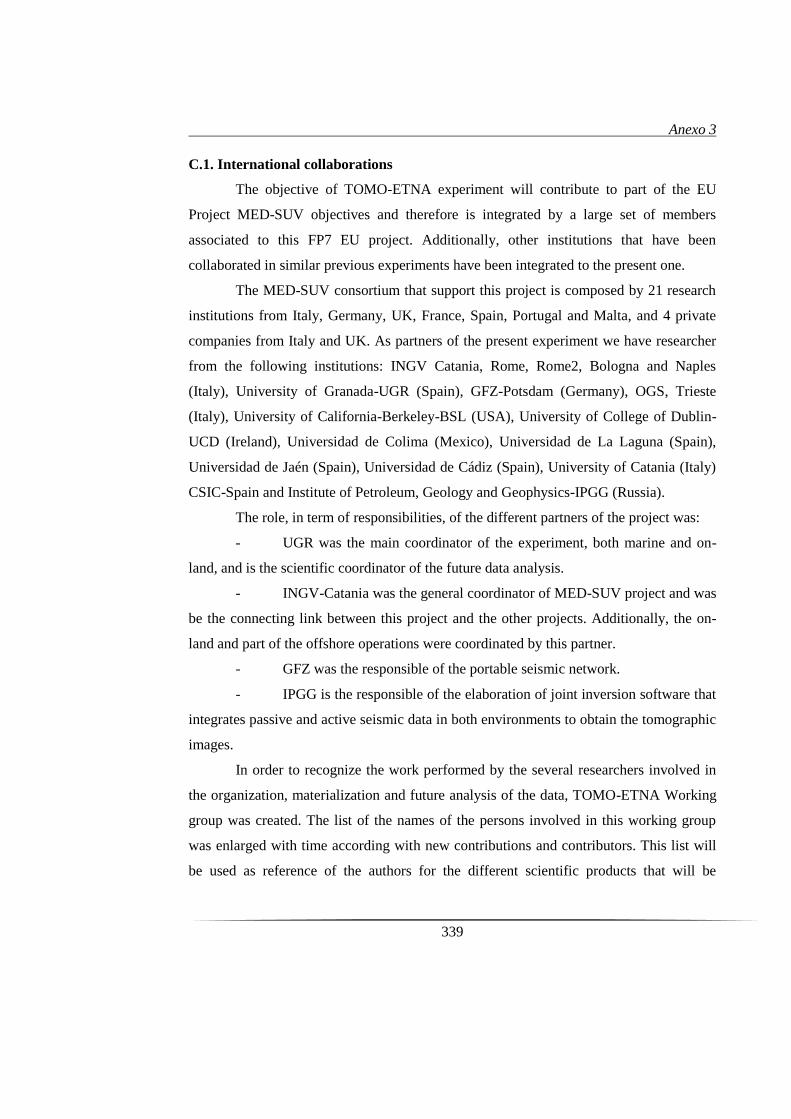
Anexo 3
339
C.1. International collaborations
The objective of TOMO-ETNA experiment will contribute to part of the EU
Project MED-SUV objectives and therefore is integrated by a large set of members
associated to this FP7 EU project. Additionally, other institutions that have been
collaborated in similar previous experiments have been integrated to the present one.
The MED-SUV consortium that support this project is composed by 21 research
institutions from Italy, Germany, UK, France, Spain, Portugal and Malta, and 4 private
companies from Italy and UK. As partners of the present experiment we have researcher
from the following institutions: INGV Catania, Rome, Rome2, Bologna and Naples
(Italy), University of Granada-UGR (Spain), GFZ-Potsdam (Germany), OGS, Trieste
(Italy), University of California-Berkeley-BSL (USA), University of College of Dublin-
UCD (Ireland), Universidad de Colima (Mexico), Universidad de La Laguna (Spain),
Universidad de Jaén (Spain), Universidad de Cádiz (Spain), University of Catania (Italy)
CSIC-Spain and Institute of Petroleum, Geology and Geophysics-IPGG (Russia).
The role, in term of responsibilities, of the different partners of the project was:
- UGR was the main coordinator of the experiment, both marine and on-
land, and is the scientific coordinator of the future data analysis.
- INGV-Catania was the general coordinator of MED-SUV project and was
be the connecting link between this project and the other projects. Additionally, the on-
land and part of the offshore operations were coordinated by this partner.
- GFZ was the responsible of the portable seismic network.
- IPGG is the responsible of the elaboration of joint inversion software that
integrates passive and active seismic data in both environments to obtain the tomographic
images.
In order to recognize the work performed by the several researchers involved in
the organization, materialization and future analysis of the data, TOMO-ETNA Working
group was created. The list of the names of the persons involved in this working group
was enlarged with time according with new contributions and contributors. This list will
be used as reference of the authors for the different scientific products that will be

Anexo 3
340
produced in the future such as presentation in international conferences. In Appendix B
we present the full list of this working group.
D. Appendix 4

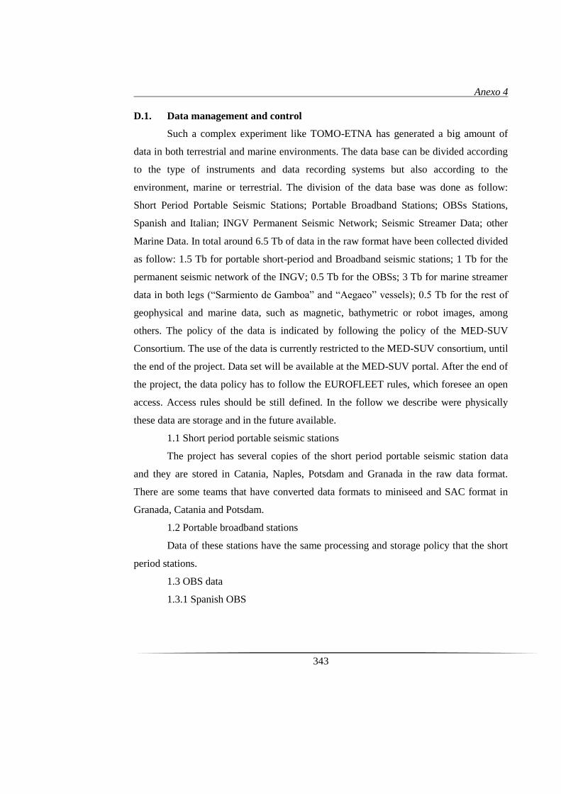
Anexo 4
343
D.1. Data management and control
Such a complex experiment like TOMO-ETNA has generated a big amount of
data in both terrestrial and marine environments. The data base can be divided according
to the type of instruments and data recording systems but also according to the
environment, marine or terrestrial. The division of the data base was done as follow:
Short Period Portable Seismic Stations; Portable Broadband Stations; OBSs Stations,
Spanish and Italian; INGV Permanent Seismic Network; Seismic Streamer Data; other
Marine Data. In total around 6.5 Tb of data in the raw format have been collected divided
as follow: 1.5 Tb for portable short-period and Broadband seismic stations; 1 Tb for the
permanent seismic network of the INGV; 0.5 Tb for the OBSs; 3 Tb for marine streamer
data in both legs (“Sarmiento de Gamboa” and “Aegaeo” vessels); 0.5 Tb for the rest of
geophysical and marine data, such as magnetic, bathymetric or robot images, among
others. The policy of the data is indicated by following the policy of the MED-SUV
Consortium. The use of the data is currently restricted to the MED-SUV consortium, until
the end of the project. Data set will be available at the MED-SUV portal. After the end of
the project, the data policy has to follow the EUROFLEET rules, which foresee an open
access. Access rules should be still defined. In the follow we describe were physically
these data are storage and in the future available.
1.1 Short period portable seismic stations
The project has several copies of the short period portable seismic station data
and they are stored in Catania, Naples, Potsdam and Granada in the raw data format.
There are some teams that have converted data formats to miniseed and SAC format in
Granada, Catania and Potsdam.
1.2 Portable broadband stations
Data of these stations have the same processing and storage policy that the short
period stations.
1.3 OBS data
1.3.1 Spanish OBS

Anexo 4
344
The original OBS data are in CSIC-UTM, Catania and Granada in the raw format.
UGR transformed them into SEGY format. These data are distributed to Catania, Naples,
and Potsdam.
1.3.2 Italian OBS
The original OBS data are stored in INGV-CNT in Gibilmana. Later the data will
be distributed to Catania, Naples Granada and Potsdam.
1.4 INGV permanent seismic network
A copy of the whole data from the period April-November 2014 is available in
Catania and Granada in dmx format. Naples can access to this copy via internal server.
Researchers from UGR converted this format to SAC.
1.5 Seismic streamer data
A copy of data associated to the “Sarmiento de Gamboa” vessel is available in
Catania and Granada (also in Barcelona as owner of the vessel). Data from “Aegaeo”
campaign is available in Catania and Trieste (as owner of the streamer).
1.6 Other marine data
This data base was obtained during the experiment by “Sarmiento de Gamboa”,
“Galatea” and “Aegaeo” vessels, and it is composed by: bathymetry data, magnetic data
and other measurements. This information is stored together with the MCS streamer data
and is available in Catania and Granada.
E. Appendix 5


Anexo 5
347
E.1. PARTOS User Guide
Along this section we present a user guide to start using PARTOS code.
The program runs is set to run in windows (not yet available to linux operative systems).
It is composed by a series of executable files (.exe), thus no installation procedure is
needed. The program main directory ‘./PARTOS/’ must be copied the in the computer.
The root directory structure is shown in figure A.1, and comprises a series of folders and
files. The mentioned executable files are saved in the ‘./PROG/’ directory.
E.1.1. General Folder Structure in PARTOS:
Figure A.1. Root directory structure of PARTOS software. Orange boxes represent
folders and white boxes represent files.
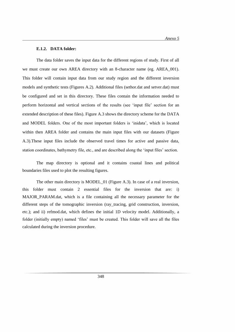
Anexo 5
348
E.1.2. DATA folder:
The data folder saves the input data for the different regions of study. First of all
we must create our own AREA directory with an 8-character name (eg. AREA_001).
This folder will contain input data from our study region and the different inversion
models and synthetic tests (Figures A.2). Additional files (sethor.dat and setver.dat) must
be configured and set in this directory. These files contain the information needed to
perform horizontal and vertical sections of the results (see ‘input file’ section for an
extended description of these files). Figure A.3 shows the directory scheme for the DATA
and MODEL folders. One of the most important folders is ‘inidata’, which is located
within then AREA folder and contains the main input files with our datasets (Figure
A.3).These input files include the observed travel times for active and passive data,
station coordinates, bathymetry file, etc., and are described along the ‘input files’ section.
The map directory is optional and it contains coastal lines and political
boundaries files used to plot the resulting figures.
The other main directory is MODEL_01 (Figure A.3). In case of a real inversion,
this folder must contain 2 essential files for the inversion that are: i)
MAJOR_PARAM.dat, which is a file containing all the necessary parameter for the
different steps of the tomographic inversion (ray_tracing, grid construction, inversion,
etc.); and ii) refmod.dat, which defines the initial 1D velocity model. Additionally, a
folder (initially empty) named ‘files’ must be created. This folder will save all the files
calculated during the inversion procedure.
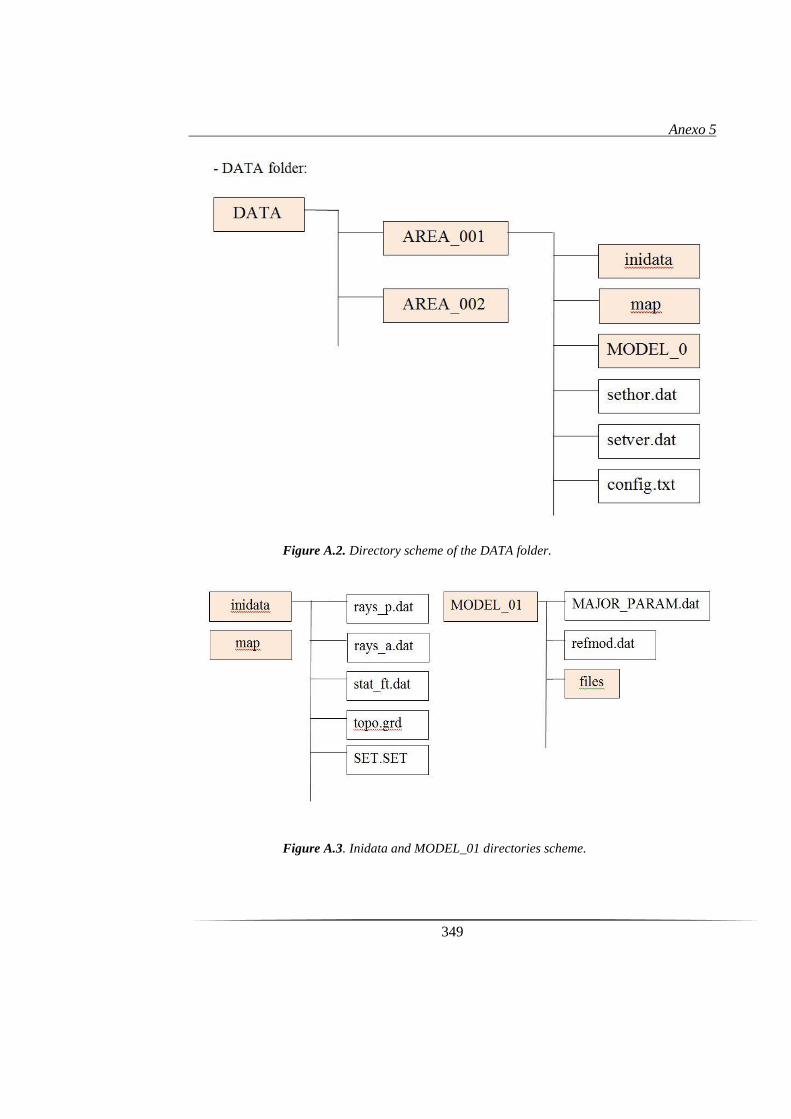
Anexo 5
349
Figure A.2. Directory scheme of the DATA folder.
Figure A.3. Inidata and MODEL_01 directories scheme.
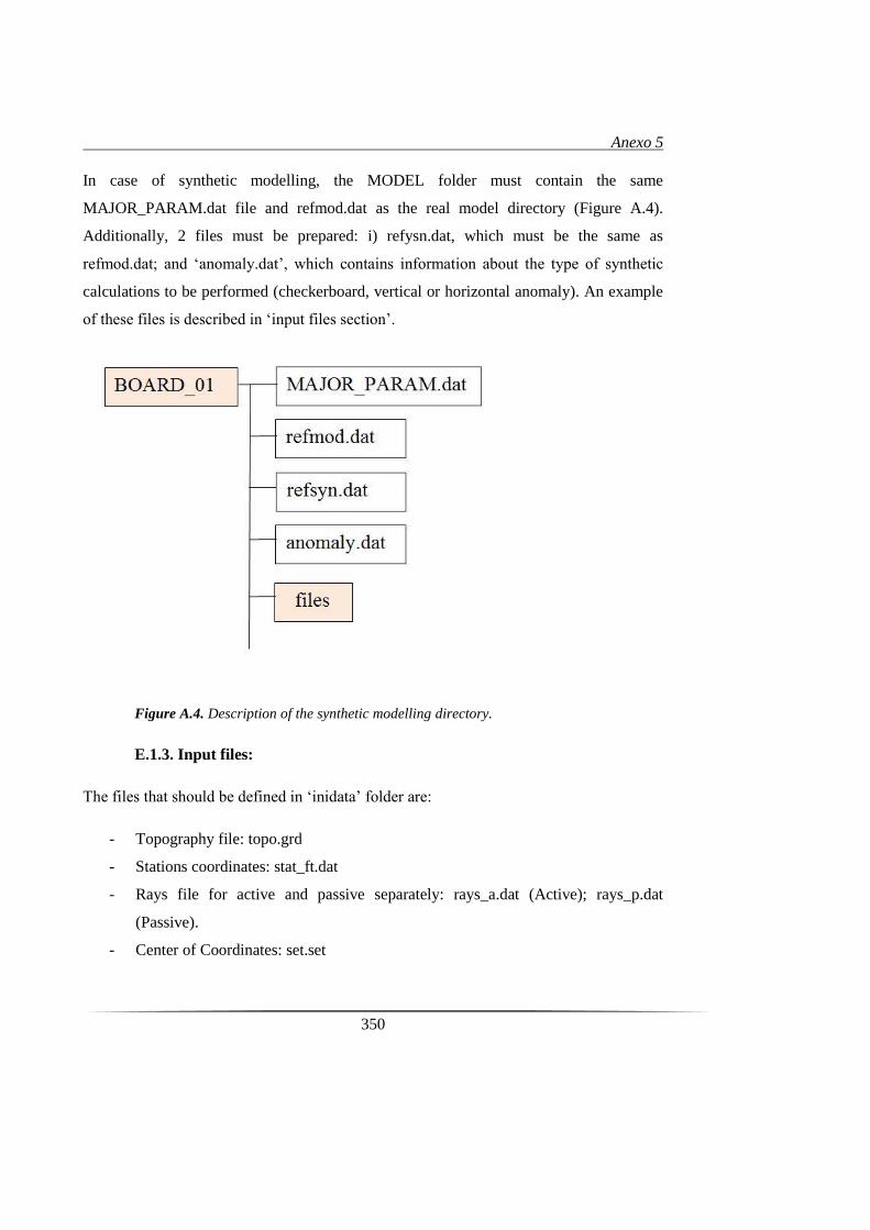
Anexo 5
350
In case of synthetic modelling, the MODEL folder must contain the same
MAJOR_PARAM.dat file and refmod.dat as the real model directory (Figure A.4).
Additionally, 2 files must be prepared: i) refysn.dat, which must be the same as
refmod.dat; and ‘anomaly.dat’, which contains information about the type of synthetic
calculations to be performed (checkerboard, vertical or horizontal anomaly). An example
of these files is described in ‘input files section’.
Figure A.4. Description of the synthetic modelling directory.
E.1.3. Input files:
The files that should be defined in ‘inidata’ folder are:
- Topography file: topo.grd
- Stations coordinates: stat_ft.dat
- Rays file for active and passive separately: rays_a.dat (Active); rays_p.dat
(Passive).
- Center of Coordinates: set.set

Anexo 5
351
All these files should be prepared in geographical coordinates and are saved in the inidata
folder. The format of each of these files is explained in the following paragraphs together
with some explanatory figures.
SET.SET: file with the geographical coordinates (Longitude and Latitude) of the center
of the studied region:
Stat_ft.dat: file with the stations coordinates.
1st column: longitude of the station
2nd
column: latitude of the station
3rd
column: altitude of the station (altitudes above sea level must be negative)
15.05900 37.39500 -0.00500
15.05200 37.42400 -0.00600
14.94300 37.45600 -0.02600
14.80000 37.43100 -0.04400
14.68700 37.39900 -0.31700
15.00 37.80 Fi0, Tet0, Center of conversion to XY

Anexo 5
352
Rays_a.dat: Rays file with the active data:
1st column: longitude of the station
2nd
column: latitude of the station
3rd
column: altitude of the station (altitudes above sea level must be negative)
4th column: longitude of the shot
5th column: latitude of the shot
6th column: depth of the shot
7th column: travel time
Rays_p.dat: Rays file with the passive data (same format as for LOTOS code):
1st column: longitude of the earthquake.
2nd
column: latitude of the earthquake.
3rd
column: depth of the earthquake.
4th column: number of phase readings.
Then one line for each phase readings with the following columns:
1st column: Phase identification (1 for P-phase or 2 for S-phase).
2nd
column: number of the station (line of the station coordinates in the stat_ft.dat file).
3rd
column: travel time.
15.05900 37.39500 -0.00500 15.30630 37.28030 0.01000 5.92000
15.05900 37.39500 -0.00500 15.30990 37.27830 0.01000 5.92000
15.05900 37.39500 -0.00500 15.32050 37.27230 0.01000 6.37000
15.05900 37.39500 -0.00500 15.32230 37.27130 0.01000 5.94000
15.05900 37.39500 -0.00500 15.33990 37.26150 0.01000 6.77000
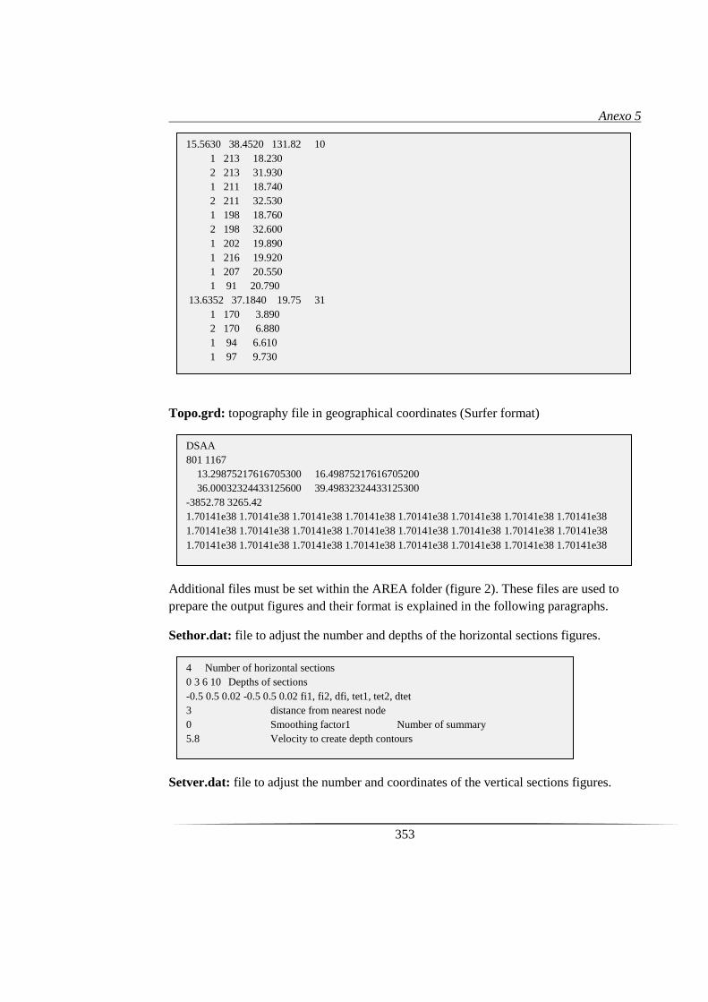
Anexo 5
353
Topo.grd: topography file in geographical coordinates (Surfer format)
Additional files must be set within the AREA folder (figure 2). These files are used to
prepare the output figures and their format is explained in the following paragraphs.
Sethor.dat: file to adjust the number and depths of the horizontal sections figures.
Setver.dat: file to adjust the number and coordinates of the vertical sections figures.
DSAA
801 1167
13.29875217616705300 16.49875217616705200
36.00032324433125600 39.49832324433125300
-3852.78 3265.42
1.70141e38 1.70141e38 1.70141e38 1.70141e38 1.70141e38 1.70141e38 1.70141e38 1.70141e38
1.70141e38 1.70141e38 1.70141e38 1.70141e38 1.70141e38 1.70141e38 1.70141e38 1.70141e38
1.70141e38 1.70141e38 1.70141e38 1.70141e38 1.70141e38 1.70141e38 1.70141e38 1.70141e38
4 Number of horizontal sections
0 3 6 10 Depths of sections
-0.5 0.5 0.02 -0.5 0.5 0.02 fi1, fi2, dfi, tet1, tet2, dtet
3 distance from nearest node
0 Smoothing factor1 Number of summary
5.8 Velocity to create depth contours
15.5630 38.4520 131.82 10
1 213 18.230
2 213 31.930
1 211 18.740
2 211 32.530
1 198 18.760
2 198 32.600
1 202 19.890
1 216 19.920
1 207 20.550
1 91 20.790
13.6352 37.1840 19.75 31
1 170 3.890
2 170 6.880
1 94 6.610
1 97 9.730
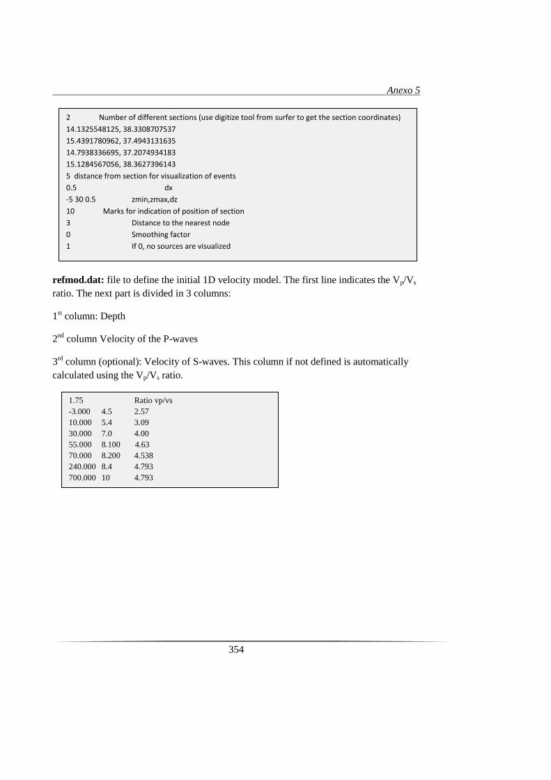
Anexo 5
354
refmod.dat: file to define the initial 1D velocity model. The first line indicates the Vp/Vs
ratio. The next part is divided in 3 columns:
1st column: Depth
2nd
column Velocity of the P-waves
3rd
column (optional): Velocity of S-waves. This column if not defined is automatically
calculated using the Vp/Vs ratio.
2 Number of different sections (use digitize tool from surfer to get the section coordinates)
14.1325548125, 38.3308707537
15.4391780962, 37.4943131635
14.7938336695, 37.2074934183
15.1284567056, 38.3627396143
5 distance from section for visualization of events
0.5 dx
-5 30 0.5 zmin,zmax,dz
10 Marks for indication of position of section
3 Distance to the nearest node
0 Smoothing factor
1 If 0, no sources are visualized
1.75 Ratio vp/vs
-3.000 4.5 2.57
10.000 5.4 3.09
30.000 7.0 4.00
55.000 8.100 4.63
70.000 8.200 4.538
240.000 8.4 4.793
700.000 10 4.793
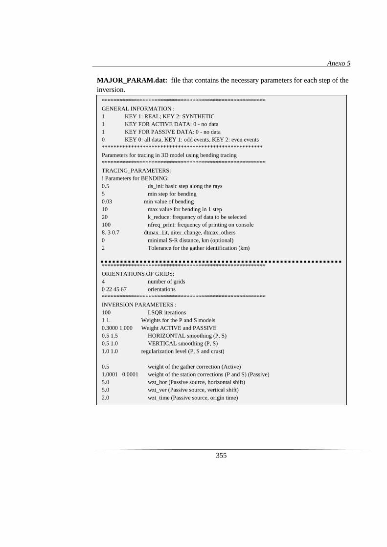
Anexo 5
355
MAJOR_PARAM.dat: file that contains the necessary parameters for each step of the
inversion.
********************************************************
GENERAL INFORMATION :
1 KEY 1: REAL; KEY 2: SYNTHETIC
1 KEY FOR ACTIVE DATA: 0 - no data
1 KEY FOR PASSIVE DATA: 0 - no data
0 KEY 0: all data, KEY 1: odd events, KEY 2: even events
*******************************************************
Parameters for tracing in 3D model using bending tracing
********************************************************
TRACING_PARAMETERS:
! Parameters for BENDING:
0.5 ds_ini: basic step along the rays
5 min step for bending
0.03 min value of bending
10 max value for bending in 1 step
20 k_reduce: frequency of data to be selected
100 nfreq_print: frequency of printing on console
8. 3 0.7 dtmax_1it, niter_change, dtmax_others
0 minimal S-R distance, km (optional)
2 Tolerance for the gather identification (km)
********************************************************
ORIENTATIONS OF GRIDS:
4 number of grids
0 22 45 67 orientations
********************************************************
INVERSION PARAMETERS :
100 LSQR iterations
1 1. Weights for the P and S models
0.3000 1.000 Weight ACTIVE and PASSIVE
0.5 1.5 HORIZONTAL smoothing (P, S)
0.5 1.0 VERTICAL smoothing (P, S)
1.0 1.0 regularization level (P, S and crust)
0.5 weight of the gather correction (Active)
1.0001 0.0001 weight of the station corrections (P and S) (Passive)
5.0 wzt_hor (Passive source, horizontal shift)
5.0 wzt_ver (Passive source, vertical shift)
2.0 wzt_time (Passive source, origin time)

Anexo 5
356
********************************************************
Parameters for location in 3D model using bending tracing
********************************************************
LOC_PARAMETERS:
! Parameters for BENDING:
1 ds_ini: basic step along the rays
10 min step for bending
0.05 min value of bending
10 max value for bending in 1 step
! Parameters for location
30 dist_limit=100 : within this distance the weight is equal
1 n_pwr_dist=1 : power for decreasing of W with distance
30 ncyc_av=10
0. res_loc1=0.2 : lower limit for location (for LT residuals, W=1)
1.5 res_loc2=1.5 : upper limit for location (for GT residuals, W=0)
2. w_P_S_diff=2 (+ causes better coherency of P and S)
10. stepmax
0.3 stepmin
10 Frequency for output printing
********************************************************
Parameters for 3D model with regular grid
********************************************************
3D_MODEL PARAMETERS:
-150. 150. 6 xx1, xx2, dxx,
-150. 150. 6 yy1, yy2, dyy,
-5. 30. 2 zz1, zz2, dzz
12 distance from nearest node
0 Smoothing factor1
********************************************************
Parameters for grid construction
********************************************************
GRID_PARAMETERS:
-150. 150. 6 grid for ray density calculation (X)
-150. 150. 6 grid for ray density calculation (Y)
-5. 30. 2. min and max levels for grid
0.05 100.0 !plotmin, plotmax= maximal ray density, relative to average
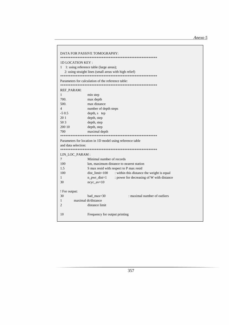
Anexo 5
357
DATA FOR PASSIVE TOMOGRAPHY:
********************************************************
1D LOCATION KEY :
1 1: using reference table (large areas);
2: using straight lines (small areas with high relief)
********************************************************
Parameters for calculation of the reference table:
********************************************************
REF_PARAM:
1 min step
700. max depth
500. max distance
4 number of depth steps
-5 0.5 depth, s tep
20 1 depth, step
50 3 depth, step
200 10 depth, step
700 maximal depth
********************************************************
Parameters for location in 1D model using reference table
and data selection:
********************************************************
LIN_LOC_PARAM :
7 Minimal number of records
100 km, maximum distance to nearest station
1.5 S max resid with respect to P max resid
100 dist_limit=100 : within this distance the weight is equal
1 n_pwr_dist=1 : power for decreasing of W with distance
30 ncyc_av=10
! For output:
30 bad_max=30 : maximal number of outliers
1 maximal dt/distance
2 distance limit
10 Frequency for output printing
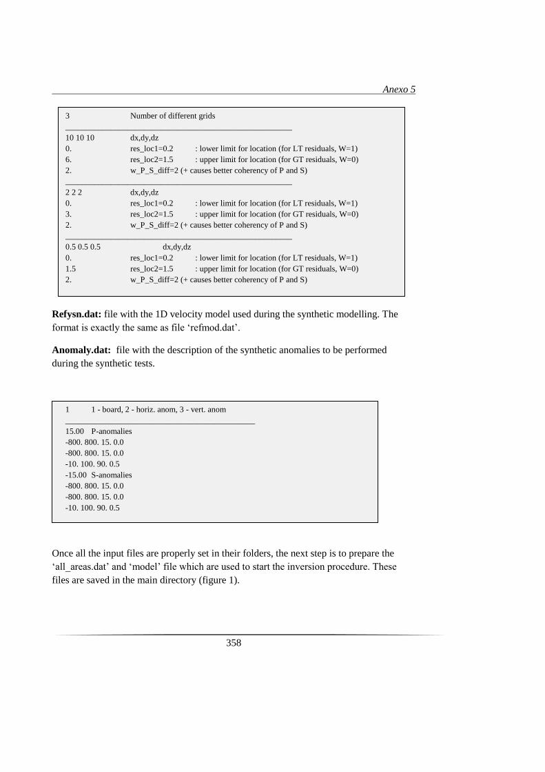
Anexo 5
358
Refysn.dat: file with the 1D velocity model used during the synthetic modelling. The
format is exactly the same as file ‘refmod.dat’.
Anomaly.dat: file with the description of the synthetic anomalies to be performed
during the synthetic tests.
Once all the input files are properly set in their folders, the next step is to prepare the
‘all_areas.dat’ and ‘model’ file which are used to start the inversion procedure. These
files are saved in the main directory (figure 1).
3 Number of different grids
_______________________________________________________
10 10 10 dx,dy,dz
0. res_loc1=0.2 : lower limit for location (for LT residuals, W=1)
6. res_loc2=1.5 : upper limit for location (for GT residuals, W=0)
2. w_P_S_diff=2 (+ causes better coherency of P and S)
_______________________________________________________
2 2 2 dx,dy,dz
0. res_loc1=0.2 : lower limit for location (for LT residuals, W=1)
3. res_loc2=1.5 : upper limit for location (for GT residuals, W=0)
2. w_P_S_diff=2 (+ causes better coherency of P and S)
_______________________________________________________
0.5 0.5 0.5 dx,dy,dz
0. res_loc1=0.2 : lower limit for location (for LT residuals, W=1)
1.5 res_loc2=1.5 : upper limit for location (for GT residuals, W=0)
2. w_P_S_diff=2 (+ causes better coherency of P and S)
1 1 - board, 2 - horiz. anom, 3 - vert. anom
______________________________________________
15.00 P-anomalies
-800. 800. 15. 0.0
-800. 800. 15. 0.0
-10. 100. 90. 0.5
-15.00 S-anomalies
-800. 800. 15. 0.0
-800. 800. 15. 0.0
-10. 100. 90. 0.5

Anexo 5
359
all_areas.dat: file specifying the name of the area, model and number of iterations to
invert.
Model.dat: file with the current name of area, model, iteration and grid number.
Finally, starting the inversion procedure needs only to launch the batch file
‘START.BAT’ located in the main directory (figure A.1).
1: name of the area
2: name of the model
3: number of iterations
*****************************************
ETNA_inv PASSIVE5 6
ETNA_inv
PASSIVE5
1
1

F. Appendix 6

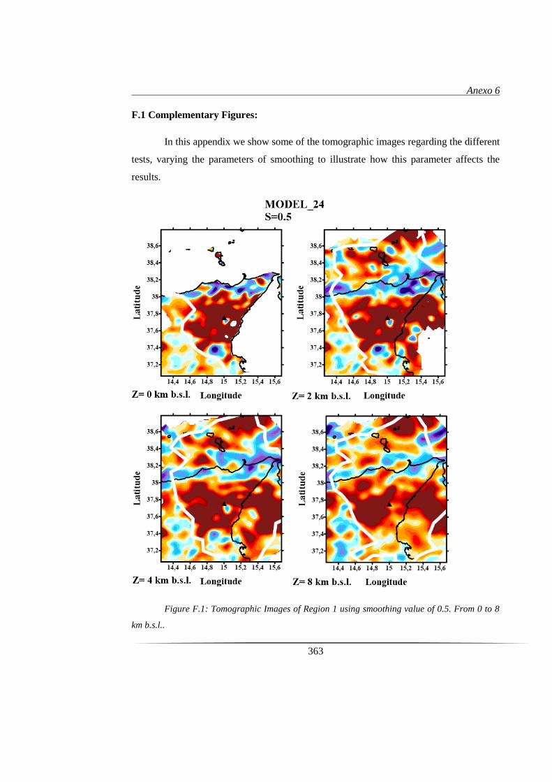
Anexo 6
363
F.1 Complementary Figures:
In this appendix we show some of the tomographic images regarding the different
tests, varying the parameters of smoothing to illustrate how this parameter affects the
results.
Figure F.1: Tomographic Images of Region 1 using smoothing value of 0.5. From 0 to 8
km b.s.l..
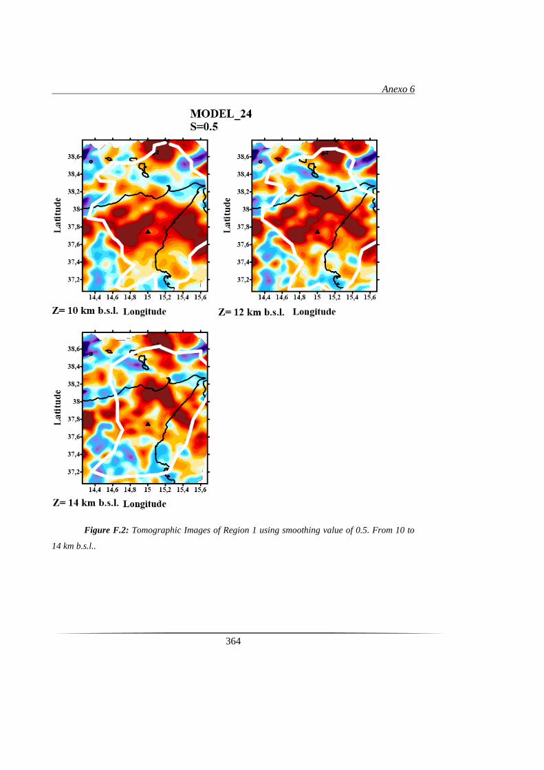
Anexo 6
364
Figure F.2: Tomographic Images of Region 1 using smoothing value of 0.5. From 10 to
14 km b.s.l..
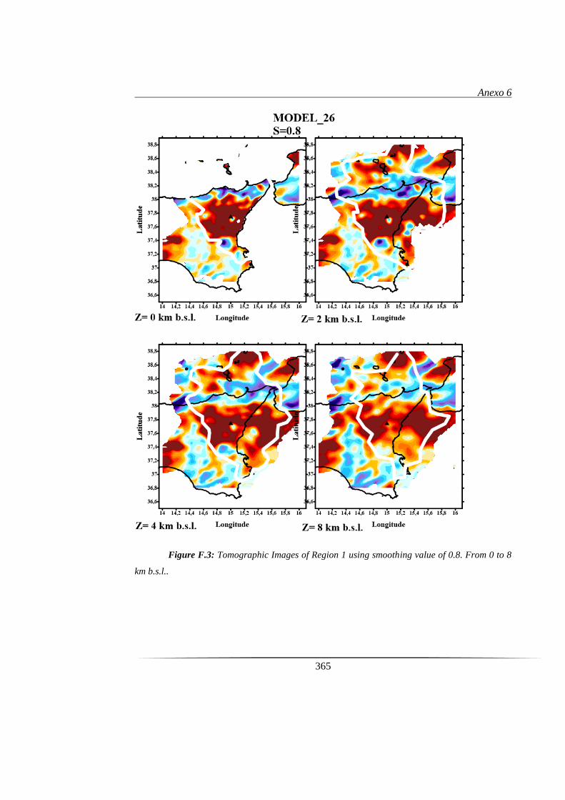
Anexo 6
365
Figure F.3: Tomographic Images of Region 1 using smoothing value of 0.8. From 0 to 8
km b.s.l..
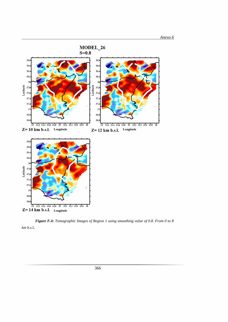
Anexo 6
366
Figure F.4: Tomographic Images of Region 1 using smoothing value of 0.8. From 0 to 8
km b.s.l..
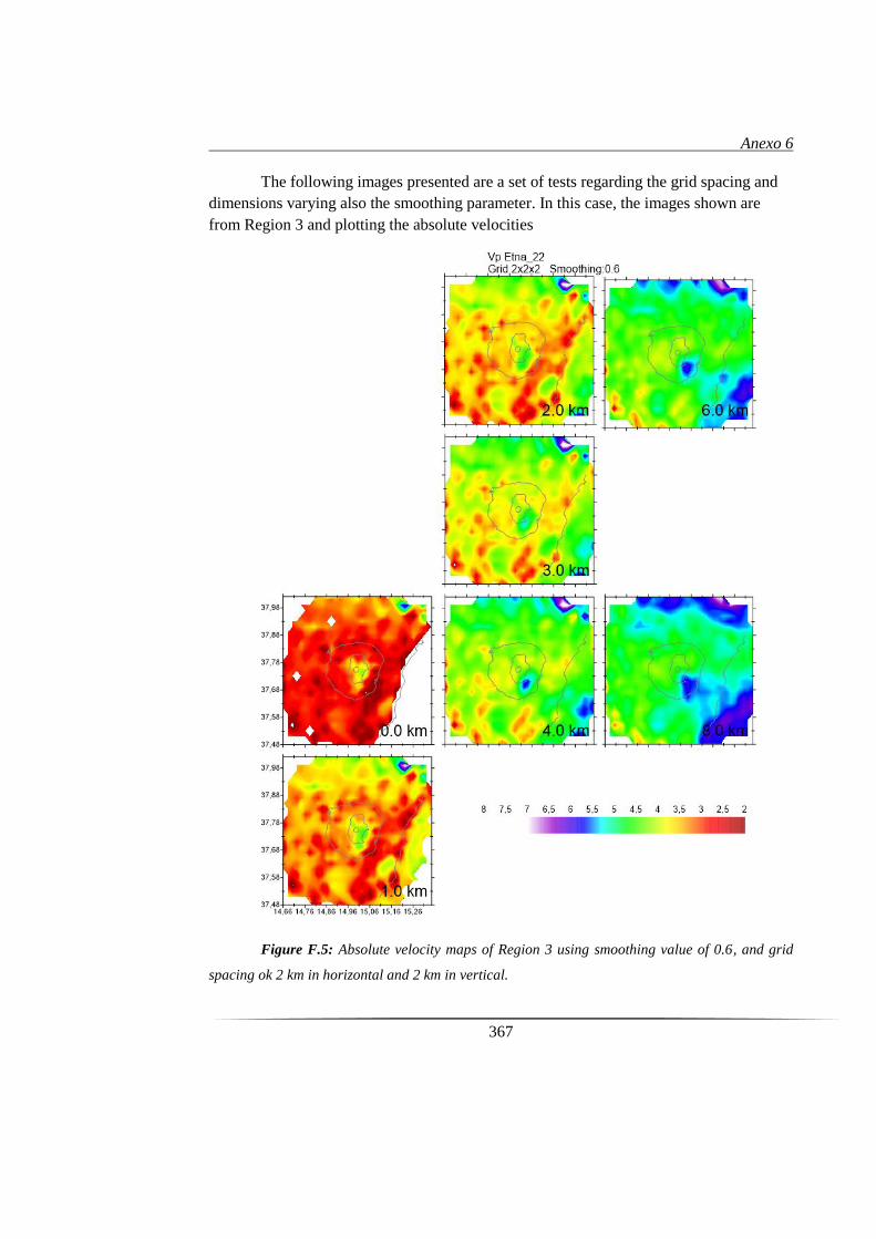
Anexo 6
367
The following images presented are a set of tests regarding the grid spacing and
dimensions varying also the smoothing parameter. In this case, the images shown are
from Region 3 and plotting the absolute velocities
Figure F.5: Absolute velocity maps of Region 3 using smoothing value of 0.6, and grid
spacing ok 2 km in horizontal and 2 km in vertical.
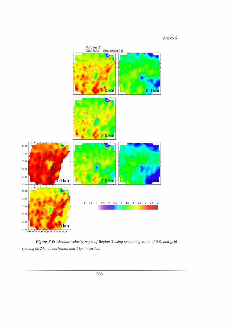
Anexo 6
368
Figure F.6: Absolute velocity maps of Region 3 using smoothing value of 0.6, and grid
spacing ok 2 km in horizontal and 1 km in vertical.
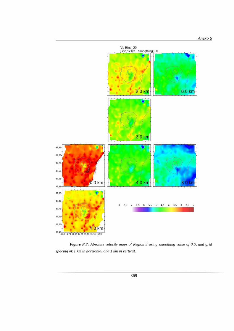
Anexo 6
369
Figure F.7: Absolute velocity maps of Region 3 using smoothing value of 0.6, and grid
spacing ok 1 km in horizontal and 1 km in vertical.

Anexo 6
370
Figure F.8: Absolute velocity maps of Region 3 using smoothing value of 1.5, and grid
spacing ok 2 km in horizontal and 2 km in vertical.
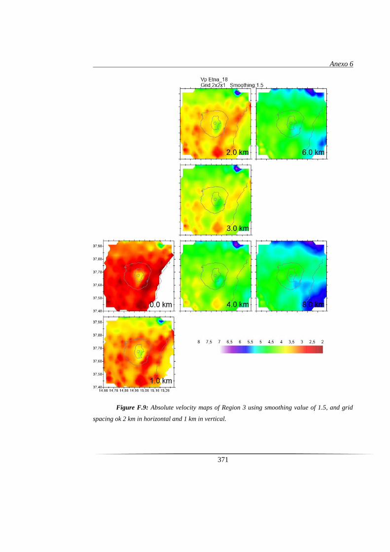
Anexo 6
371
Figure F.9: Absolute velocity maps of Region 3 using smoothing value of 1.5, and grid
spacing ok 2 km in horizontal and 1 km in vertical.
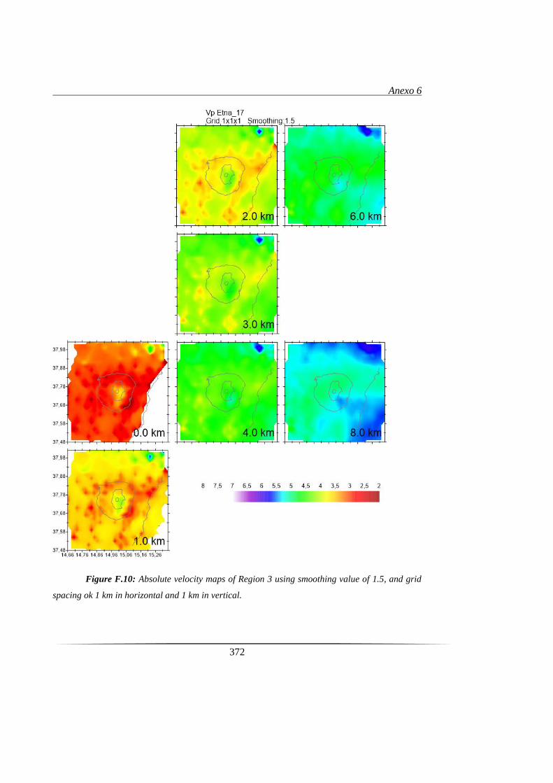
Anexo 6
372
Figure F.10: Absolute velocity maps of Region 3 using smoothing value of 1.5, and grid
spacing ok 1 km in horizontal and 1 km in vertical.
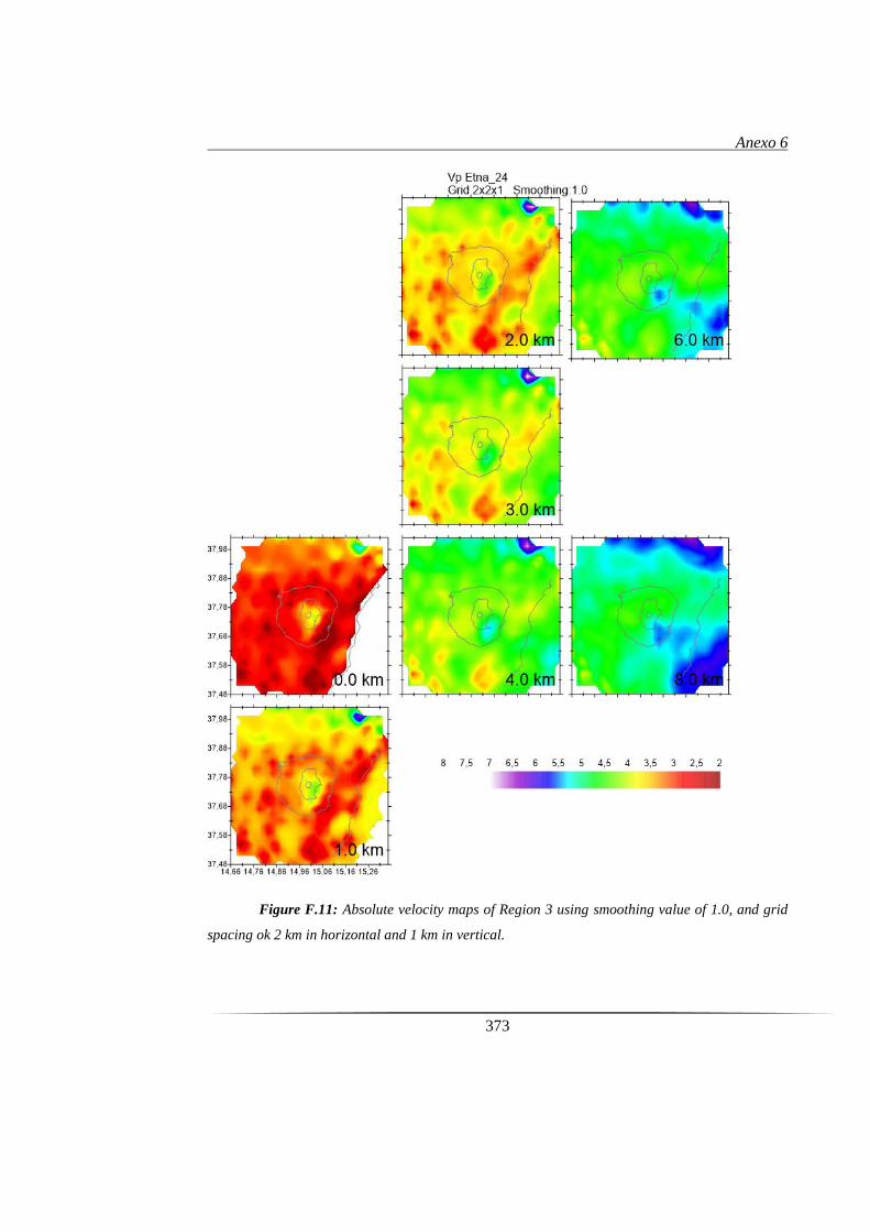
Anexo 6
373
Figure F.11: Absolute velocity maps of Region 3 using smoothing value of 1.0, and grid
spacing ok 2 km in horizontal and 1 km in vertical.
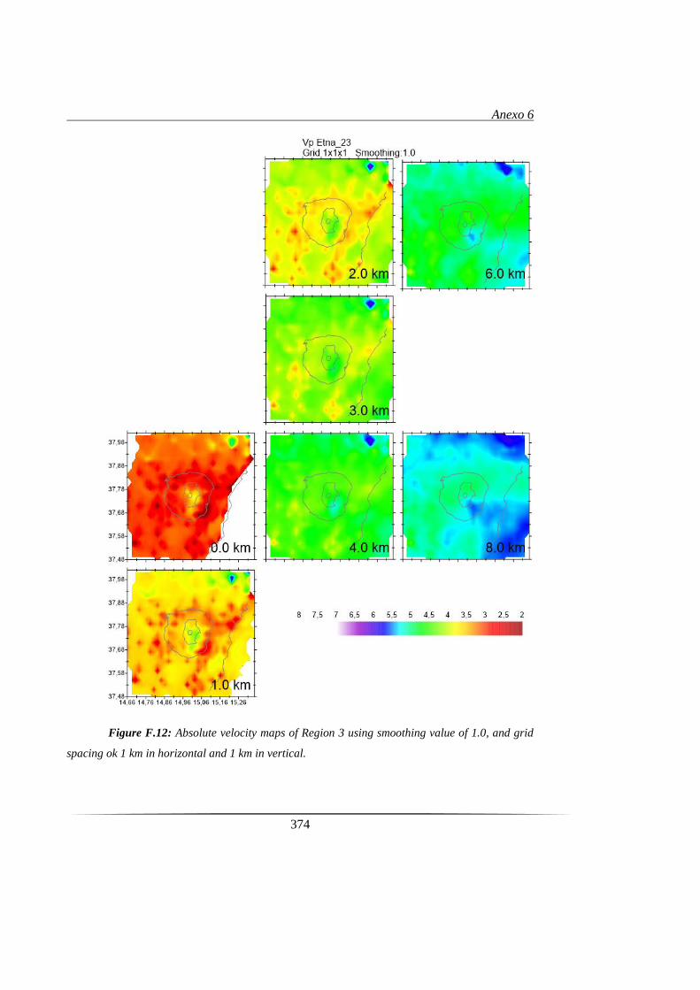
Anexo 6
374
Figure F.12: Absolute velocity maps of Region 3 using smoothing value of 1.0, and grid
spacing ok 1 km in horizontal and 1 km in vertical.
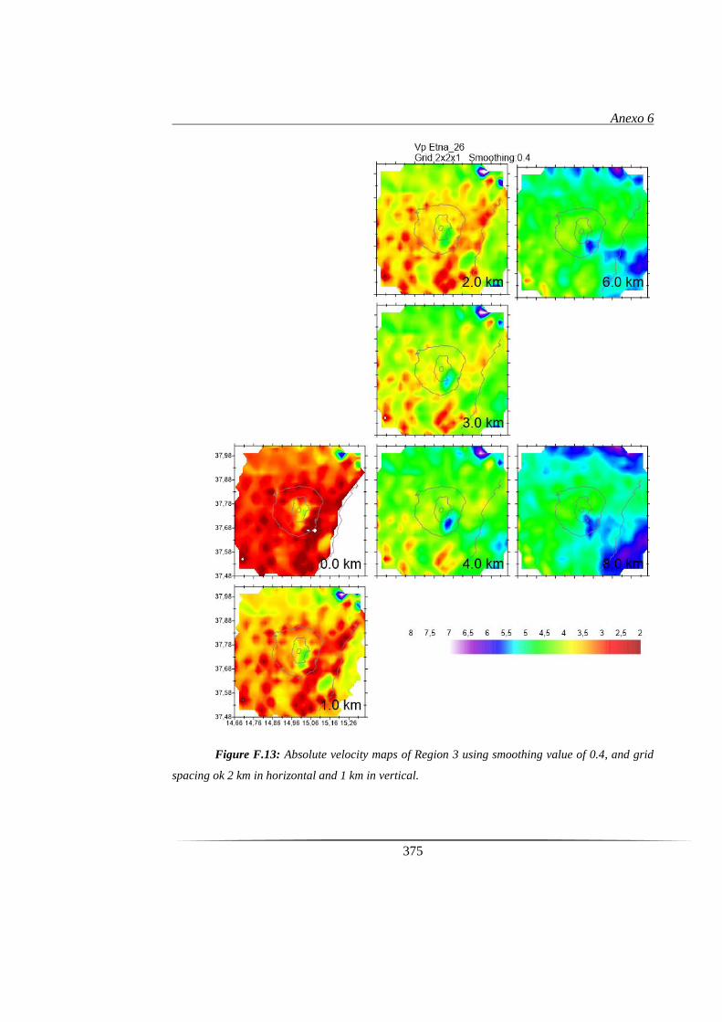
Anexo 6
375
Figure F.13: Absolute velocity maps of Region 3 using smoothing value of 0.4, and grid
spacing ok 2 km in horizontal and 1 km in vertical.
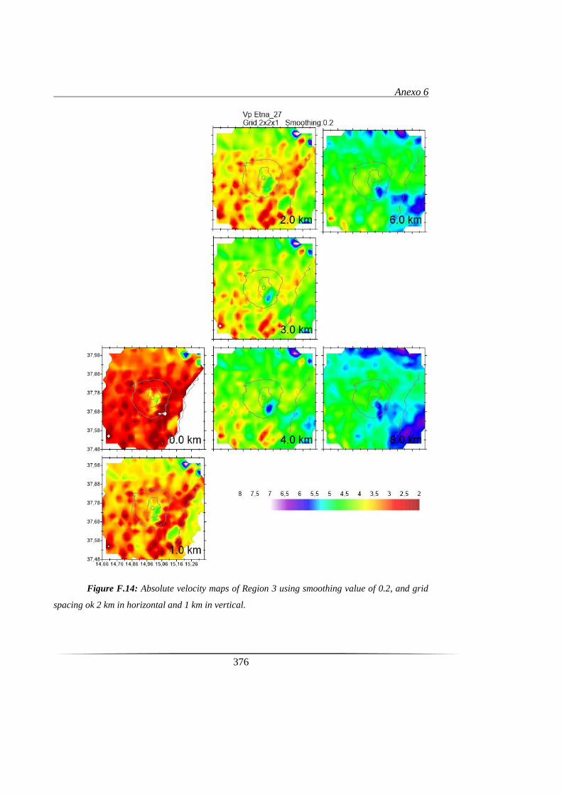
Anexo 6
376
Figure F.14: Absolute velocity maps of Region 3 using smoothing value of 0.2, and grid
spacing ok 2 km in horizontal and 1 km in vertical.


