Kalman Filtering with Nonlinear State Constraints

Kalman Filtering withNonlinear State Constraints

CHUN YANGSigtem Technology, Inc.

ERIK BLASCHAir Force Research Lab/RYAA

An analytic method was developed by D. Simon and T. L.

Chia to incorporate linear state equality constraints into

the Kalman filter. When the state constraint was nonlinear,

linearization was employed to obtain an approximately linear

constraint around the current state estimate. This linearized

constrained Kalman filter is subject to approximation errors and

may suffer from a lack of convergence. We present a method that

allows exact use of second-order nonlinear state constraints. It

is based on a computational algorithm that iteratively finds the

Lagrangian multiplier for the nonlinear constraints. Computer

simulation results are presented to illustrate the algorithm.

Manuscript received November 11, 2005; revised May 23 andDecember 29, 2006; released for publication December 10, 2008.

IEEE Log No. T-AES/45/1/932004.

Refereeing of this contribution was handled by Wolfgang Koch.

This research was supported in part under Contracts FA8650-04-M-1624 and FA8650-05-C-1808.

Authors’ addresses: C. Yang, Sigtem Technology, Inc., 1343 ParrottDr., San Mateo, CA 94402, E-mail: ([email protected]); E.Blasch, Air Force Research Lab/RYAA, 2241 Avionics Circle,WPAFB, OH 45433.

0018-9251/09/$25.00 c° 2009 IEEE

I. INTRODUCTION

Kalman filters are commonly used to estimatethe state of a dynamic system based on its stateprocess and measurement models. When a knownmodel or signal information about the state (calledstate constraints) cannot fit easily into the structureof a Kalman filter, it is often ignored or dealt withheuristically [11]. One example is the constraints onstate values that are derived a priori based on physicalconsiderations. Another example is ground targettracking. We know that a vehicle travels on a road yetthe radar track may indicate otherwise due to noiseand clutter in radar measurements. Without using thisadditional information about state constraints, theresulting estimates, even obtained with the Kalmanfilter, cannot be truly optimal simply because of theuse of an incomplete set of information.In a recent paper [11], a rigorous analytic method

was set forth to incorporate linear state equalityconstraints into the Kalman filtering process. Forthe above example of ground target tracking, whena vehicle travels off-road or on an unknown road, thestate estimation problem is unconstrained. However,when the vehicle is traveling on a known road, be itstraight or curved, the state estimation problem can becast as constrained using the road network informationavailable from, say, digital maps [12].To make use of state constraints, previous

attempts range from reducing the system modelparameterization to treating state constraints asperfect measurements. The constrained Kalmanfilter proposed in [11] consists of first obtainingan unconstrained Kalman filter solution and thenprojecting the unconstrained state estimate onto theconstrained surface.Instead of projecting the unconstrained solution to

the linear state constraints, an alternative approach,recently proposed in [5], consists of formulatinga projected system representation for linearlyconstrained systems and then applying the Kalmanfilter to the projected systems. The constrainedKalman filter by system projection was shown to yieldsmaller state estimation error covariance than that byunconstrained solution projection [5].Although the main results are restricted to linear

systems and linear state equality constraints, theauthors outlined steps to extend it to inequalityconstraints, nonlinear dynamics systems, andnonlinear state constraints. According to [11], theinequality constraints can be checked at each timestep of the filter. If the inequality constraints aresatisfied at a given time step, no action is taken sincethe inequality constrained problem is solved. If theinequality constraints are not satisfied at a giventime step, then the constrained solution is appliedto enforce the constraints. Furthermore, to applythe constrained Kalman filter to nonlinear systems

70 IEEE TRANSACTIONS ON AEROSPACE AND ELECTRONIC SYSTEMS VOL. 45, NO. 1 JANUARY 2009

and nonlinear state constraints, it is suggested in[11] to linearize both the system and constraintequations about the current state estimate. The formeris equivalent to the use of an extended Kalman filter(EKF).However, the projection of the unconstrained state

estimate onto a linearized state constraint is subject toconstraint approximation errors, which is a functionof the nonlinearity and more importantly the pointaround which the linearization takes place. This mayresult in convergence problems. It was suggested in[11] to take extra measures to guarantee convergencein the presence of nonlinear constraints.There are a host of constrained nonlinear

optimization techniques [7]. Primal methods searchthrough the feasible region determined by theconstraints. Penalty and barrier methods approximateconstrained optimization problems by unconstrainedproblems through modifying the objective function(e.g., add a term for higher price if a constraintis violated). Instead of the original constrainedproblem, dual methods attempt to solve an alternateproblem (the dual problem) whose unknowns are theLagrangian multipliers of the first problem. Cuttingplane algorithms work on a series of ever-improvingapproximating linear programs whose solutionsconverge to that of the original problem. Lagrangianrelaxation methods are widely used in discreteconstrained optimization problems.In addition to state constraints, work has been

done for constraints that are placed on the stateprocess and/or observation noise of a linear ornonlinear system. Such constraints are typicallyused to model bounded disturbances or randomvariables with truncated densities. Moving horizonestimation, which reformulates the estimationproblem as quadratic programming over a moving,fixed-size estimation window, becomes an importantapproach to constrained nonlinear estimation [9].Another approach to constrained linear estimationis to exploit the Lagrangian duality. Indeed, aconstrained linear estimation problem is shown to bea particular nonlinear optimal control problem [3].Constrained state estimation has also been studiedfrom a game-theoretical point of view (also called theminimax or H1 estimation) [10].In this paper, we present a method that allows for

the use of second-order nonlinear state constraintsexactly. The method is expected to provide betterapproximation to higher order nonlinearities.The new method is based on a computationalalgorithm that iteratively finds the Lagrangianmultiplier. For second-order constraints, it is atradeoff between reducing approximation errors tohigher order nonlinearities and keeping the problemcomputationally tractable.The paper is organized as follows. Section II

presents a brief summary of linearly constrained

state estimation and its problem when the first-orderlinearization is used to extend to nonlinear cases.Section III details the computational algorithm tosolve the second-order constrained least-squaredoptimization problem. In Section IV, computersimulation results are presented to illustrate thealgorithm. Finally, Section V provides concludingremarks and suggestions for future work.

II. LINEARLY CONSTRAINED STATE ESTIMATION

In this section, we first summarize the resultsfor linearly constrained state estimation [11] andthen point out the problem it may face whenthe linearization is used to extend it to nonlinearconstraints.Consider a linear time-invariant discrete-time

dynamic system together with its measurement as

xk+1 = Axk +Buk +wk (1a)

yk = Cxk + vk (1b)

where boldface indicates a vector quantity, thesubscript k is the time index, x is the state vector,u is a known input, y is the measurement, and wand v are state and measurement noise processes,respectively. It is implied that all vectors and matriceshave compatible dimensions, which are omitted forsimplicity.The goal is to find an estimate denoted by xk of

xk given the measurements up to time k denoted byYk = fy0, : : : ,ykg. Under the assumptions that the stateand measurement noises are uncorrelated zero-meanwhite Gaussian with w»Nf0,Qg and v»Nf0,Rgwhere Q and R are positive semi-definite covariancematrices, the Kalman filter provides an optimalestimator in the form of xk = Efxk j Ykg [2]. Startingfrom an initial estimate x0 = Efx0g and its estimationerror covariance matrix P0 = Ef(x0¡ x0)(x0¡ x0)Tgwhere the superscript T stands for matrix transpose,the Kalman filter equations specify the propagationof xk and Pk over time and the update of xk and Pk bymeasurement yk as

xk+1 = Axk +Buk (2a)

Pk+1 = APkAT+Q (2b)

xk+1 = xk+1 +Kk+1(yk+1¡Cxk+1) (2c)

Pk+1 = (I¡Kk+1C)Pk+1 (2d)

Kk+1 = Pk+1CT(CPk+1C

T+R)¡1 (2e)

where xk+1 and Pk+1 are the predicted state andprediction error covariance, respectively.Now in addition to the dynamic system of (1), we

are given the linear state constraint

Dxk = d (3)

YANG & BLASCH: KALMAN FILTERING WITH NONLINEAR STATE CONSTRAINTS 71

where D is a known constant matrix of full rank, d isa known vector, and the number of rows in D is thenumber of constraints, which is assumed to be lessthan the number of states. If D is a square matrix,the state is fully constrained and can thus be solvedby inverting (3). Although no time index is givento D and d in (3), it is implied that they can be timedependent, leading to piecewise linear constraints.The constrained Kalman filter according to [11] is

constructed by directly projecting the unconstrainedstate estimate xk onto the constrained surface S =fx :Dx= dg. It is formulated as the solution to theproblem

³x= argminx2S(x¡ x)TW(x¡ x) (4)

where W is a symmetric positive definite weightingmatrix.Derived using the Lagrangian multiplier technique

in Appendix A, the solution to the constrainedoptimization in (4) is given by

³x= x¡W¡1DT(DW¡1DT)¡1(Dx¡d): (5)

Several interesting statistical properties of theconstrained Kalman filter are presented in [11]. Thisincludes the fact that the constrained state estimateas given by (5) is an unbiased state estimate for thesystem in (1) subject to the constraint in (3) for aknown symmetric positive definite weighting matrixW. Furthermore when W = P¡1, the constrained stateestimate has a smaller error covariance than that ofthe unconstrained state estimate, and it is actuallythe smallest for all constrained Kalman filters of thistype. Similar results hold in terms of the trace of theestimation error covariance matrix when W = I.In practical applications, however, nonlinear

state constraints are likely to emerge. Consider thenonlinear state constraint of the form

g(x) = h: (6)

We can expand the nonlinear state constraintsabout a constrained state estimate ³x and for the ithrow of (6), we have

gi(x)¡hi = gi(³x) + g0i(³x)T(x¡ ³x)

+12!(x¡ ³x)Tg00i (³x)(x¡ ³x)+ ¢ ¢ ¢ ¡ hi

= 0 (7)

where the superscripts 0 and 00 denote the first andsecond partial derivatives.Keeping only the first-order terms as suggested in

[11], some rearrangement leads to

g0(³x)Tx¼ h¡ g(³x)+ g0(³x)T³x (8)

where g(x) = [: : :gi(x) : : :]T, h= [: : :hi : : :]

T, and g0(x) =[: : :g0i(x) : : :]. An approximate linear constraint istherefore formed by replacing D and d in (3) withg0(³x)T and h¡ g(³x) + g0(³x)T³x, respectively.

Fig. 1 illustrates this linearization process, whichidentifies possible errors associated with linearapproximation of a nonlinear state constraint. Asshown, the previous constrained state estimate³x¡ lies somewhere on the constrained surfacebut is away from the true state x. The projectionof the unconstrained state estimate x onto theapproximate linear state constraint produces thecurrent constrained state estimate ³x+, which ishowever subject to the constraint approximation error.Clearly, the further away is ³x¡ from x, the larger theapproximation-introduced error is. More critically,such an approximately linear constrained estimatemay not satisfy the original nonlinear constraintspecified in (6). It is therefore desired to reducethis approximation-introduced error by includinghigher order terms while keeping the problemcomputationally tractable. One possible approach ispresented in the next section.

III. NONLINEARLY CONSTRAINED STATEESTIMATION

In this section, we consider a second-orderstate constraint function, which can be viewedas a second-order approximation to an arbitrarynonlinearity, as

f(x) = [xT 1]·M m

mT m0

¸·x

1

¸= xTMx+mTx+ xTm+m0 = 0: (9)

As an example, a general equation of the seconddegree in two variables » and ´ is written as

f(»,´) = a»2 +2b»´+ c´2 +2d»+2e´+f

= [» ´ 1]

264a b d

b c e

d e f

375264 »´1

375= 0 (10)

which may represent a road segment in a digitalterrain map.Following the constrained Kalman filtering of [11],

we can formulate the projection of an unconstrainedstate estimation onto a nonlinear constraint surface asthe constrained least-square optimization problem

x= argminx(z¡Hx)T(z¡Hx) (11a)

subject to f(x) = 0: (11b)

If we let W =HTH and z=Hx, the formulationin (11) becomes the same as in (4). In a sense, (11)is a more general formulation because it can also beinterpreted as a nonlinear constrained measurementupdate or a projection in the predicted measurementdomain.


Fig. 1. Errors in linear approximation of nonlinear stateconstraints.

The solution to the constrained optimization (11)can be obtained again using the Lagrangian multipliertechnique, which is detailed in Appendix B, as

x=G¡1V(I+¸§T§)¡1e(¸) (12a)

q(¸) =Xi

e2i (¸)¾2i

(1+¸¾2i )2+2

Xi

ei(¸)tj1+¸¾2i

+m0 = 0

(12b)

where G is an upper right diagonal matrix resultingfrom the Cholesky factorization of W =HTH as

W(=HTH) =GTG: (12c)

V, an orthonormal matrix, and §, a diagonal matrixwith its diagonal elements denoted by ¾i, are obtainedfrom the singular value decomposition (SVD) of thematrix LG¡1 as

LG¡1 =U§VT (12d)

where U is the other orthonormal matrix of the SVDand L results from the factorization M = LTL, and

e(¸) = [: : :ei(¸) : : :]T = VT(GT)¡1(HTz¡¸m)

(12e)

t= [: : : ti : : :]T = VT(GT)¡1m: (12f)

As a nonlinear equation in ¸, it is difficult to finda closed-form solution in general for the nonlinearequation q(¸) = 0 in (12b). Numerical root-findingalgorithms may be used instead. For example, theNewton’s method is used below. Denote the derivativeof q(¸) with respect to ¸ as

_q(¸) = 2Xi

ei(¸)_ei(1+¸¾2i )¾

2i ¡ e2i (¸)¾4i

(1+¸¾2i )3

+2Xi

_eiti(1+¸¾2i )¡ ei(¸)ti¾2i

(1+¸¾2i )2

(13a)

where_e= [: : : _ei : : :]

T =¡VT(GT)¡1m: (13b)

Then the iterative solution for ¸ is given by

¸k+1 = ¸k ¡q(¸k)_q(¸k)

starting with ¸0 = 0: (14)

The iteration stops when j¸k+1¡¸kj< ¿ , a givensmall value, or the number of iterations reaches aprespecified number. Then bringing the convergedLagrangian multiplier ¸ back to (12a) provides theconstrained optimal solution.Now consider the special case where W =HTH,

z =Hx, and m= 0, that is, a quadratic constraint onthe state. Under these conditions, t= 0 and e is nolonger a function of ¸ so its derivative relative to ¸vanishes, _e= 0. The quadratic constrained solution isthen given by

³x= (W+¸M)¡1Wx (15a)

where the Lagrangian multiplier ¸ is obtainediteratively as in (14) with the corresponding q(¸) and_q(¸) given by

q(¸) =Xi

e2i ¾2i

(1+¸¾2i )2+m0 = 0 (15b)

_q(¸) =¡2Xi

e2i ¾4i

(1+¸¾2i )3: (15c)

The solution of (15) is also called the constrainedleast squares [8, pp. 765—766], which was previouslyapplied for the joint estimation and calibration [14].Similar techniques have been used for the designof filters for radar applications [1] and in robustminimum variance beamforming [6]. When M = 0,the constraint in (9) degenerates to a linear one.The constrained solution is still valid. However, theiterative solution for finding ¸ is no longer applicableand a closed-form solution is available as given in (5).As it can be seen from (12a) and (15a), the

constrained state solutions reduce to the unconstrainedone when ¸= 0. Given ¸ 6= 0, the state solution itselfinvolves rather simple matrix addition, inversion, andmultiplication wherein matrix factorization can beprecomputed. However, the Lagrangian multiplier callsfor a numerical iterative solution, which turns out tobe quite fast in convergence, to be further discussedlater with Fig. 8.When the nonlinear constraints are not exactly

second order, it is intuitive to believe that thesecond-order solution as presented in this paperwould outperform a first-order solution. The actualdesign of a second-order solution to higher ordernonlinearity would be similar in procedure to thatof a linear piecewise approximation to a nonlinearconstraint as shown in the simulation example ofSection IVB. This includes design optimization andtradeoff as to how many piecewise approximationsto use, where to apply, and how to switch betweenadjacent approximations. Although not addressed in


Fig. 2. Positioning vehicle along circular road segment.

this paper, it would be interesting to determine forwhat kind of nonlinearity, the performance gainedby a second-order solution warrants the addedcomputational complexity relative to a first-ordersolution. This and other issues are outlined in theconclusions for future work.

IV. SIMULATION RESULTS

In this section, two simulation examples arepresented in the context of ground vehicle tracking.One is the positioning of a stationary object and theother is the tracking of a moving target.

A. Positioning of Stationary Object

The first simulation is a simple example usedto demonstrate the effectiveness of the nonlinearconstrained method of this paper and to show itssuperior performance as compared with the linearizedconstrained method in [11] in a static manner.In this example, a ground vehicle is assumed to be

positioned somewhere along a circular road segmentas shown in Fig. 2 with the circle center chosen as theorigin of the x-y coordinates. Under this assumption,the road constraint is quadratic and can be written as

f(x,y) = x2 + y2¡ r2 = [x y]·1 0

0 1

¸·x

y

¸¡ r2 = 0:

(16)

Assume that the true position of the vehicle is atx= [rcosμ,r sinμ]T and an unbiased estimate denotedby x is obtained by a certain means such that

x»N (x,P) (17)

where P is the estimation error covariance matrix,which is assumed to take a diagonal form as P =diagf[¾2x ,¾2y ]g with ¾2x = ¾2y = ¾2. It is understandablethat additional errors will appear if the estimate x isbiased. Furthermore, if the error covariance matrix isnot diagonal, the correlation direction will also affectthe statistical property. Ruling out such variability in

conditions will make results analysis easier while notsacrificing the generality.To apply the linear constrained Kalman filter of

[11], the nonlinear constraint is linearized about aprevious constrained state denoted by ³x¡ and can bewritten as

[³x¡ ³y¡]·x

y

¸= r2: (18)

In terms of the matrix notations, we have D =[³x¡ ³y¡] and d = r2. Since the previous constrainedstate ³x¡ is also on the circular path, it can beparameterized as ³x¡ = [rcos(μ+¢μ),r sin(μ+¢μ)]T

where ¢μ is the angular offset and its distance to thetrue state is given by

k¢xk22 = k³x¡ ¡ xk22 = 2r2(1¡ cos¢μ) (19)

where k ¢ k2 stands for the 2-norm or length for thevector.With W = P¡1, the linearized constrained estimate

denoted by ³x+L can be calculated using (5). WithW = P¡1 (i.e., H = ¾¡1I2 and z=Hx), M = I2, whereIn stands for an identity matrix of dimension n, andm0 = r

2, the quadratic constrained estimate denoted by³x+NL is given by (15).In the first simulation, we set r = 100 m, μ = 45±,

and ¾ = 10 m and then draw samples of x fromthe distribution in (17) as the unconstrained stateestimates. We then calculate both the linearizedand nonlinear constrained state estimates ³x+L and³x+NL at two linearizing points, i.e., two previousconstrained state estimates ³x¡, with ¢μ = 0± and¡15±, respectively.Figs. 3 and 4 illustrate how the nonlinear

constrained method of this paper and the linearizedconstrained method of [11] actually projectunconstrained state estimates onto a nonlinearconstraint, which is a circular road segment in thisexample. In Fig. 3, for ¢μ = 0±, the linearizing point(small circle ±) coincides with the true state (diamond¦) (though the estimator is not aware of it). Thelinearized constraint is a line tangent to the circularpath at the point. There are 50 random samples drawnfrom the distribution of (17) as the unconstrainedstate estimates (dot ²), which are projected ontothe linearized constraint using (5) as the linearizedconstrained estimates (cross sign £) and using (15)as the quadratic constrained estimates (plus sign +).Clearly, all the quadratic constrained estimates fallonto the circle, thus satisfying the constraint whereasnot all linearized constrained estimates do so.In Fig. 4 for ¢μ =¡15±, the linearizing point

is away from the true state. At 100 m, an angularoffset is related to a separation error by a factor of1.74 m/deg. This corresponds to about 26 m for¢μ =¡15±. Although the linearized method using(5) effectively projects all the unconstrained stateestimates onto the linearized constraint, the linearized


Fig. 3. Projection of unconstrained estimates onto constraints (³x¡ = x).

Fig. 4. Projection of unconstrained estimates onto constraints (³x¡ 6= x).

constraint itself is tilted off, introducing larger errorsdue to the constraint approximation. In contrast, thequadratic constrained method, being independent ofthe prior knowledge about the state estimate, easilysatisfies the constraint.In the second simulation, we draw 5000

unconstrained state estimates for each linearizing point

¢μ, which varies from ¡20± to 20± in steps of 5±.At each linearizing point, we calculate the rms errorsbetween the true state and the linearized and nonlinearconstrained state estimates, respectively. Fig. 5 showsthe two rms values as a function of the linearizingpoint together with the unconstrained state estimationerror standard deviation ¾.


Fig. 5. RMS values of state estimates versus angular offset.

Fig. 6. Constraint satisfaction.

As expected, the rms values for the linearizedconstrained estimates (circle ±) grow large as theangular offset ¢μ increases. The rms values for thequadratic constrained estimates (dot ²) remain constantand are slightly smaller than the unconstrainedestimates, because the scattering along a constraintcurve is smaller than in a two-dimensional (2D)

plane. For the same reason, the rms values for thelinearized constrained estimates are smaller than thoseof the quadratic constrained estimates for j¢μj< 7±.However, the use of rms values for comparison isless meaningful in this case. As shown in Fig. 6, boththe unconstrained estimates (circle ±) and linearizedconstrained estimates (dot ²) do not always satisfy the


Fig. 7. Iterative quadratic constrained solution versus geometry solution.

nonlinear constraints whereas quadratic constrainedestimates (plus sign +) do all the time (i.e., theconstraint is satisfied if the distance to the origin is100 m).In a 2D setting, the circular path constraint of (18)

allows for a simple geometry solution to the problem.The desired on-circle point ³x is the intersectionbetween the circle and the line extending from theorigin to the off-circle point x. The geometry solutioncan be written as

³x= rcos·tan¡1

μy

x

¶¸(20a)

³y = r sin·tan¡1

μy

x

¶¸: (20b)

Since it is an exact solution for this particularsimulation example, we can use it to verify theiterative solution obtained by the quadratic constrainedmethod. Fig. 7 shows the quadratic constrainedestimates (cross £) obtained by the iterative algorithmof (15) and the exact geometry solutions (circle ±),which indeed match each other perfectly.Finally, we use Fig. 8 to show an example of the

Lagrangian multiplier as it is calculated iterativelyusing (15). The runs for five unconstrained stateestimates are plotted in the same figure and to makeit fit, the normalized absolute values of ¸ are taken.As shown, starting from zero, it typically takes 4iterations for the algorithm to converge in the examplepresented.In fact, for this simple example of a target

traveling along a circle used in the simulation, a

closed-form solution can be derived. Assume thatW = I2, M = I2, m= 0, and m0 =¡r2. The nonlinearconstraint can be equivalently written as

xTx= r2: (21)

The quadratic constrained estimate given in (15a)is repeated below for easy reference:

³x= (W+¸M)¡1Wx= (1+¸)¡1x (22)

where ¸ is the Lagrangian multiplier.Putting (22) back into (21) gives

³xT³x=μ

x1+¸

¶T x1+¸

= r2: (23)

The solution for ¸ is

¸=

pxTxr

¡1 = kxk2r¡1: (24)

Putting the solution for ¸ from (24) into (22) gives

³x= rxkxk2

: (25)

This indicates that for this particular case,the constraining results in normalization. This isconsistent with the geometric solution shown in theabove simulation.Using the 2nd-order nonlinear constraints

approach suggests a simple solution for somepractical applications. When a target is travelingalong a circular path (or approximately so), onecan first find the equivalent center of the circlearound which to establish a new coordinate system.


Fig. 8. Convergence in iterative Lagrangian multiplier.

Then express the unconstrained solution in thenew coordinate and normalize it as the constrainedsolution. Finally convert it back to the originalcoordinates. For noncircular but second-order paths,eigenvalue-based scaling may be effected followingcoordinate translation and rotation in order to applythis circular normalization. Reverse operations arethen used to transform back. For applications of highdimensionality, the scalar iterative solution of (14)may be more efficient.

B. Tracking of Moving Target

In this second simulation example, a groundvehicle is assumed to travel along a circular roadsegment as shown in Fig. 2. The turn center is chosenas the origin of the x-y coordinates and the turn radiusis again r = 100 m. The target maintains a constantturn rate of 5.7 deg/s with an equivalent linear speedof 10 m/s. The initial state is

xk=0 = [x _x y _y]T = [100 m,0 m/s,0 m,10 m/s]T:

(26)

The vehicle is tracked by a sensor with a samplinginterval of T = 1 s. The sensor provides positionmeasurements of the vehicle as

yk =·1 0 0 0

0 0 1 0

¸xk + vk (27)

where the measurement error v»N (0,R) is azero-mean Gaussian noise, independent in the x-axisand y-axis. The covariance matrix R = diag([¾2rx ¾

2ry])

uses the particular values of ¾rx = ¾ry = 7 m in thesimulation.The sensor uses the following discrete-time

second-order kinematic model for its tracker

xk+1 =

266641 T 0 0

0 1 0 0

0 0 1 T

0 0 0 1

37775xk +2666412T

2 0

T 0

0 12T

2

0 T

37775wk(28)

where the process noise w»N (0,Q) is also azero-mean Gaussian noise, independent of themeasurement noise v. The covariance matrix Q =diag([¾2x ¾

2y ]) uses the particular values of ¾x = ¾y =

0:32 m/s2 in the simulation.When represented in a Cartesian coordinate

system, a target traveling along a curved road iscertainly subject to acceleration in both the x-axis andy-axis. However, no effect is made in this simulationto optimize the tracker for maneuver but merely toselect Q and the initial conditions so as to focus onconstraining the estimates. The initial state is selectedto be the same as the true state, i.e., x0 = x0 and theinitial estimation error covariance is selected to be

P0 = diag([52 12 52 12]): (29)

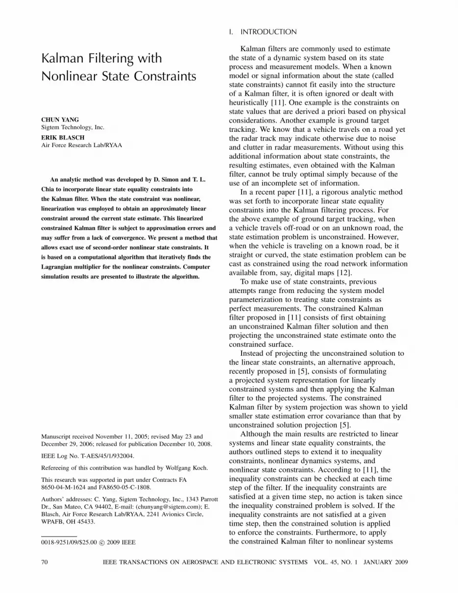
Fig. 9 shows sample trajectories of the linearconstrained Kalman filter. There are 5 curves and2 series of data points in the figure. The true stateis represented by a series of dots (²) at consecutive


Fig. 9. Sample trajectories for linear constrained Kalman filter.

sampling instants, which is plotted on the solidline being the road segment. The correspondingmeasurements are a series of circles (±).The estimates of the unconstrained Kalman filter

are shown as the connected triangles (¢) whereasthose of linearly constrained Kalman filters are shownas the connected crosses (£), stars (*), and pluses(+) for three linear approximations of the nonlinearconstraint of curved road, respectively.In the first approximation (the line with cross £

labeled “linear constraint 1”), a single linearizing pointat μ1 = 10

± is chosen to cover the entire curved road.The linearized state constraint at μ1 can be writtenas ·

cosμ1 0 sinμ1 0

0 cosμ1 0 sinμ1

¸x=

·r

0

¸: (30)

Although all estimates are faithfully projectedby the constrained filter onto this linear constraint,tangential to the curve at the linearizing point, it runsaway from the true trajectory and the resulting errorscontinue to grow. The apparent divergence is causedby the choice of linearization.In the second approximation (the line with star *

labeled “linear constraint 2”), two linearizing points atμ1 = 15

± and μ2 = 80± are chosen to cover the curved

road with two linear segments. The switching pointfrom one linear segment to the other in this case isat μ = 45±. As shown, the estimates are projectedonto one of the two linear segments. Except near thecorner where the two linear approximations intersect(which is far away from both linearizing points), the

linear constrained estimates typically outperform theunconstrained estimates (closer to the true state). Thisis better illustrated in Fig. 10 where the upper plot isfor the absolute position error in x while the lowerplot is for the absolute position error in y, both plottedas a function of time.Still with two linearizing points and the same

switching point at μ = 45±, the third approximation(the line with plus+ labeled “linear constraint 3”)adjusts linearizing points to μ1 = 20

± and μ2 = 70±.

A better overall performance is achieved as shown inFig. 10.It is clear from Fig. 9 that a nonlinear constraint

can be approximated with linear constraints in apiecewise fashion. By judicious selection of thenumber of linear segments and their placement (i.e.,the point around which to linearize), a reasonablygood performance can be expected. In the limit, anonlinear function is represented by a piecewisefunction composed of an infinite number of linearsegments. This naturally leads to the use of nonlinearconstraints.Fig. 11 shows sample trajectories of the nonlinear

constrained Kalman filter. There are 2 curves and 4series of data points in the figure. The true state isstill represented by a series of dots (²) at the samplinginstants, which is plotted on the solid line of roadsegment. The corresponding measurements are again aseries of circles (±). The unconstrained Kalman filteris shown as the connected crosses (£) whereas the


Fig. 10. Linear constrained position errors versus time.

Fig. 11. Sample trajectories for nonlinear constrained Kalman filter.

estimates of nonlinearly constrained Kalman filters areshown as a series of connected pluses (+) and stars(*) for two implementations, respectively.The first implementation (the series of pluses +)

only applies the nonlinear constraint to the positionestimate whereas the second implementation (theseries of stars *) applies constraints to both the

position and velocity estimates. In fact, we encountera hybrid (mixed) linear and nonlinear state constraintsituation. The constrained position estimate is givenby (15) for the quadratic case (equivalent to either(20) or (25) for a circular road). Since the velocitydirection is along the tangent of the road curve,the constrained velocity estimate is obtained by the


Fig. 12. Nonlinear constrained position errors versus time.

following projection

vconstrained = (vTunconstrained¹)¹ (31)

where v= [ _x _y]T is the estimated velocity vector and¹= [¡sinμ cosμ]T is the constrained unit directionvector associated with the constrained position atμ = tan¡1(y=x).For simplicity, the unconstrained estimation error

covariance is not modified in the present simulationafter the constrained estimate is obtained usingthe projection algorithms in (15) and (31). Theimplementation is therefore pessimistic (suboptimal)in the sense that it does not take into accountthe reduction in the estimation error covariancebrought in by constraining. One consequence of thissimplification is more volatile state estimates. Toquantify this effect, one approach is to project theunconstrained probability density function (i.e., anormal distribution with support on the whole statespace) onto the nonlinear constraint. Statistics canthen be calculated from the constrained probabilitydensity function with the constraint as its support.Again, the resulting error ellipse represented by thecovariance matrix is only an approximation to thesecond order.As shown in Fig. 11, both the nonlinear

constrained estimates fall onto the road as expected.Overall the position and velocity constrainedestimates are better (closer to the true state) than theposition-only constrained estimates. This is illustratedin Fig. 12 where the upper plot is for the absolute

position error in x while the lower plot is for theabsolute position error in y.Finally, Monte Carlo simulation is used to generate

the rms errors of state estimation. The results arebased on a total of 100 runs across 16 updates andsummarized in Table I. The performance improvementof the nonlinear constrained filter over the linearizedconstrained filter is demonstrated.

V. CONCLUSIONS

In this paper, we have presented a methodfor incorporating second-order nonlinear stateconstraints into a Kalman filter. It can be viewed asan extension of the Kalman filter with linear stateequality constraints of [11] to nonlinear cases [13].Simulation results demonstrated the performanceof this method as compared with linearized stateconstraints. Although the present solution considers ascalar constraint, it is possible to extend the solutionto cases where multiple nonlinear constraints areimposed. The simulation presented actually used acase of hybrid linear and nonlinear constraints.It is of interest to extend the iterative method

presented here for second-order nonlinear stateconstraints to other types of nonlinear constraintsof practical significance. When higher ordernonlinear constraints are addressed by this method,the constraint errors will be non-zero due toapproximation. The filter design will involve selectionof approximation regions, their placement, and amechanism for switching from one region to anotherin much the same way as what was done in the


TABLE IRMS Estimation Errors

RMS Estimation Error

Estimators Position (m) Velocity (m/s)

Unconstrained 8.3663 4.2640Best Linear Constrained 5.5386 2.5466Nonlinear Constrained 1.8056 0.4252

simulation for linear piecewise approximation of acircular path.Generally speaking, our future work will involve

the application of different nonlinear optimizationtechniques [7] briefly mentioned in the introductionto target tracking. More specifically in the contextof tracking ground targets on roads, there aredifferent ways to utilize the road map information.This includes using road constraints as pseudomeasurements, projecting unconstrained estimates ontolinear constraints [11] and onto nonlinear constraintsas suggested in this paper, and incorporating theconstraints into the estimation algorithm. The latterfurther includes incorporating linear constraints intothe process noise covariance matrix [4], projectinglinear systems onto linear constraints [5] and ontononlinear constraints (e.g., curvilinear representationof target motion on roads) among others [12]. It isour current interest to compare these methods viasimulation evaluation.Other directions of our future work will include

searching for more efficient root finding algorithms tosolve for the Lagrangian multiplier and investigationinto how to apply the present method to theconstrained H1 filter [10].

APPENDIX A

To solve the constrained optimization problem in(4), we form the Lagrangian

J(x,¸) = (x¡ x)TW(x¡ x) +2¸T(Dx¡d): (32)

The first-order conditions necessary for aminimum are given by

@J

@x= 0)W(x¡ x) +DT¸= 0 (33a)

@J

@¸= 0)Dx¡d= 0: (33b)

The solution for the optimal Lagrangian multiplier¸ can be found first as

¸= (DW¡1DT)¡1(Dx¡d): (34)

Bringing this solution back to (32) leads to theconstrained solution of the state in (5).Note that the above derivation does not depend on

the conditional Gaussian nature of the unconstrainedestimate x. It was shown in [11] that when W = I,

the solution in (5) is the same as what is obtained bythe mean square method, which attempts to minimizethe conditional mean square error subject to the stateconstraints, that is,

minxEfkx¡ xk22 j Yg such that Dx= d: (35)

Furthermore, when W = P¡1, i.e., the inverse ofthe unconstrained state estimation error covariance,the solution in (5) reduces to the result given by themaximum conditional probability method

maxxlnPrfx j Yg such that Dx= d: (36)

More results and proofs can be found in [11].

APPENDIX B

Construct the Lagrangian with the Lagrangianmultiplier ¸ as

J(x,¸) = (z¡Hx)T(z¡Hx)+¸f(x): (37)

Taking the partial derivatives of J(x,¸) withrespect to x and ¸, respectively, setting them to zeroleads to the necessary conditions

¡HTz+¸m+(HTH+¸M)x= 0 (38a)

xTMx+mTx+ xTm+m0 = 0: (38b)

Assume that the inverse matrix of HTH+¸Mexists. Then, x can be solved from (38a), giving theconstrained solution in terms of the unknown ¸ as

x= (HTH+¸M)¡1(HTz¡¸m) (39)

which reduces to the unconstrained least-squaressolution when ¸= 0.Assume that the matrix M admits the factorization

M = LTL and apply the Cholesky factorization toW =HTH as

W(=HTH) =GTG (40)

where G is an upper right diagonal matrix. We thenperform the SVD [8] of the matrix LG¡1 as

LG¡1 =U§VT (41)

where U and V are orthonormal matrices and § is adiagonal matrix with its diagonal elements denoted by¾i. For a square matrix, this becomes the eigenvaluedecomposition.Introduce two new vectors

e(¸) = [: : :ei(¸) : : :]T = VT(GT)¡1(HTz¡¸m)

(42a)

t= [: : : ti : : :]T = VT(GT)¡1m: (42b)

With these factorizations and new matrix andvector notations, the constrained solution in (39) can


be simplified into (12a), which is repeated below foreasy reference as

x=G¡1V(I+¸§T§)¡1e(¸): (43)

The first- and second-order terms of x in (38b) canbe expressed in ¸ as

xTMx= e(¸)T(I+¸§T§)¡T§T§(I+¸§T§)¡1e(¸)

=Xi

e2i (¸)¾2i

(1+¸¾2i )2

(44a)

mTx= tT(I+¸§T§)¡1e(¸) =Xi

ei(¸)ti1+¸¾2i

(44b)

xTm= e(¸)T(I+¸§T§)¡1t=Xi

ei(¸)ti1+¸¾2i

: (44c)

Putting these terms into the constrained equationin (38b) gives rise to the constraint equation, nowexpressed in terms of the unknown Lagrangianmultiplier ¸, as

q(¸) = (zTH¡¸mT)(HTH +¸M)¡2(HTz¡¸m)+mT(HTH+¸M)¡1(HTz¡¸m)+ (zTH¡¸mT)(HTH +¸M)¡1m+m0

= e(¸)T(I+¸ §T§)¡1§T§(I+¸§T§)¡1e(¸)

+ tT(I+¸§T§)¡1e(¸) + e(¸)T(I+¸§T§)¡1t+m0

=Xi

e2i (¸)¾2i

(1+¸¾2i )2+2Xi

ei(¸)tj1+¸¾2i

+m0 = 0 (45)

which is (12b) given in Section III.

ACKNOWLEDGMENTS

Thanks also go to Dr. Rob Williams, Dr. DevertWicker, and Dr. Jeff Layne of AFRL/SNAT fortheir valuable discussions and to Dr. Mike Bakichof AFRL/SNAA for his assistance. We appreciatethe reviewers and the editor for their comments andsuggestions.

REFERENCES

[1] Abromovich, Y. I., and Sverdlik, M. B.Synthesis of a filter response which maximizes the signalto noise ratio under additional quadratic constraints.Radio Engineering and Electronic Physics, 5 (Nov. 1970),1977—1984.

[2] Anderson, B., and Moore, J.Optimal Filtering.Englewood Cliffs, NJ: Prentice-Hall, 1979.

[3] Goodwin, G. C., De Dona, J. A., Seron, M. M., and Zhuo,X. W.Lagrangian duality between constrained estimation andcontrol.Automatica, 41 (June 2005), 935—944.

[4] Kirubarajan, T., Bar-Shalom, Y., Pattipati, K. R., andKadar, I.Ground target tracking with variable structure IMMestimator.IEEE Transactions on Aerospace and Electronic Systems,36 (Jan. 2000), 26—46.

[5] Ko, S., and Bitmead, R.State estimation for linear systems with state equalityconstraints.Automatica, 43, 8 (Aug. 2007), 1363—1368.

[6] Lorenz, R. G., and Boyd, S. P.Robust minimum variance beamforming.In J. Li and P. Stoica (Eds.), Robust AdaptiveBeamforming, Hoboken, NJ: Wiley-Interscience, 2006.

[7] Luenberger, D. G.Linear and Nonlinear Programming (2nd ed.).Reading, MA: Addison-Wesley, 1989.

[8] Moon, T. K., and Stirling, W. C.Mathematical Methods and Algorithms for SignalProcessing.Upper Saddle River, NJ: Prentice-Hall, 2000.

[9] Rao, C. V., Rawlings, J. B., and Mayne, D. Q.Constrained state estimation for nonlinear discrete-timesystems: Stability and moving horizon approximations.IEEE Transactions on Automatic Control, 48 (Feb. 2003),246—258.

[10] Simon, D.A game theory approach to constrained minimax stateestimation.IEEE Transactions on Signal Processing, 54 (February2006), 405—412.

[11] Simon, D., and Chia, T. L.Kalman filtering with state equality constraints.IEEE Transactions on Aerospace and Electronic Systems,38 (Jan. 2002), 128—136.

[12] Yang, C., Bakich, M., and Blasch, E.Nonlinear constrained tracking of targets on roads.In Proceedings of the 8th International Conference onInformation Fusion, Philadelphia, PA, July 2005, A8-3,1—8.

[13] Yang, C., and Blasch, E.Kalman filtering with nonlinear state constraints.In Proceedings of the 9th International Conference onInformation Fusion, Florence Italy, July 2006.

[14] Yang, C., and Lin, D. M.Constrained optimization for joint estimation of channelbiases and angles of arrival for small GPS antenna arrays.In Proceedings of the 60th Annual Meeting of the Instituteof Navigation, Dayton, OH, June 2004, 548—559.


Chun Yang received his Bachelor of Engineering from Northeastern University,Shenyang, China, in 1984. In 1986, he received his Diplome d’EtudesApprofondies from Institut National Polytechnique de Grenoble, Grenoble,France. In 1989, he received his title of Docteur en Science from Universite deParis XI, Orsay, France, in sciences physiques (LSS/CNRS-ESE).After two years of postdoctoral research at the University of Connecticut,

Storrs, he moved on with his industrial R&D career. Since 1994, he has beenwith Sigtem Technology, Inc. and has been working on adaptive array andbaseband signal processing for GNSS receivers and radar systems as well as onnonlinear state estimation with applications in target tracking, integrated inertialnavigation, and information fusion. He is also an Adjunct Professor of Electricaland Computer Engineering at Miami University.Dr. Yang is the coinventor of seven issued and pending U.S. patents.

Erik Blasch received his B.S. in mechanical engineering from the MassachusettsInstitute of Technology and Masters in mechanical, health science, and industrialengineering from Georgia Tech and attended the University of Wisconsin foran MD/PHD in mech. eng/neurosciences until being called to active duty in theUnited States Air Force. He completed an MBA, MSEE, M.S. Econ, M.S./Ph.D.Psychology (ABD), and a Ph.D. in EE from Wright State University.He is an information fusion evaluation tech lead for the Air Force Research

Laboratory–COMprehensive Performance Assessment of Sensor Exploitation(COMPASE) Center, adjunct EE and BME professor at Wright State University(WSU) and Air Force Institute of Technology (AFIT), and a reserve Maj withthe Air Force Office of Scientific Research. He was a founding member of theInternational Society of Information Fusion (ISIF) in 1998 and is the 2007 ISIFPresident.Dr. Blasch has many military and civilian career awards; but engineering

highlights include team member of the winning ’91 American Tour del Sol solarcar competition, ’94 AIAA mobile robotics contest, and the ’93 Aerial UnmannedVehicle competition where they were first in the world to automatically controla helicopter. Since that time, Dr. Blasch has focused on automatic targetrecognition, targeting tracking, and information fusion research compiling 200+scientific papers and book chapters. He is active in IEEE (AES and SMC) andSPIE including regional activities, conference boards, journal reviews, andscholarship committees; and participates in the Data Fusion Information Group(DFIG), the Program Committee for the DOD Automatic Target RecognitionWorking Group (ATRWG), and the SENSIAC National Symposium on Sensorand Data Fusion (NSSDF).


Documents

Kalman Filtering with Nonlinear State Constraints