Embed Size (px)
Citation preview
ADVERTIMENT. La consulta d’aquesta tesi queda condicionada a l’acceptació de les següents condicions d'ús: La difusió d’aquesta tesi per mitjà del servei TDX (www.tesisenxarxa.net) ha estat autoritzada pels titulars dels drets de propietat intel·lectual únicament per a usos privats emmarcats en activitats d’investigació i docència. No s’autoritza la seva reproducció amb finalitats de lucre ni la seva difusió i posada a disposició des d’un lloc aliè al servei TDX. No s’autoritza la presentació del seu contingut en una finestra o marc aliè a TDX (framing). Aquesta reserva de drets afecta tant al resum de presentació de la tesi com als seus continguts. En la utilització o cita de parts de la tesi és obligat indicar el nom de la persona autora. ADVERTENCIA. La consulta de esta tesis queda condicionada a la aceptación de las siguientes condiciones de uso: La difusión de esta tesis por medio del servicio TDR (www.tesisenred.net) ha sido autorizada por los titulares de los derechos de propiedad intelectual únicamente para usos privados enmarcados en actividades de investigación y docencia. No se autoriza su reproducción con finalidades de lucro ni su difusión y puesta a disposición desde un sitio ajeno al servicio TDR. No se autoriza la presentación de su contenido en una ventana o marco ajeno a TDR (framing). Esta reserva de derechos afecta tanto al resumen de presentación de la tesis como a sus contenidos. En la utilización o cita de partes de la tesis es obligado indicar el nombre de la persona autora. WARNING. On having consulted this thesis you’re accepting the following use conditions: Spreading this thesis by the TDX (www.tesisenxarxa.net) service has been authorized by the titular of the intellectual property rights only for private uses placed in investigation and teaching activities. Reproduction with lucrative aims is not authorized neither its spreading and availability from a site foreign to the TDX service. Introducing its content in a window or frame foreign to the TDX service is not authorized (framing). This rights affect to the presentation summary of the thesis as well as to its contents. In the using or citation of parts of the thesis it’s obliged to indicate the name of the author
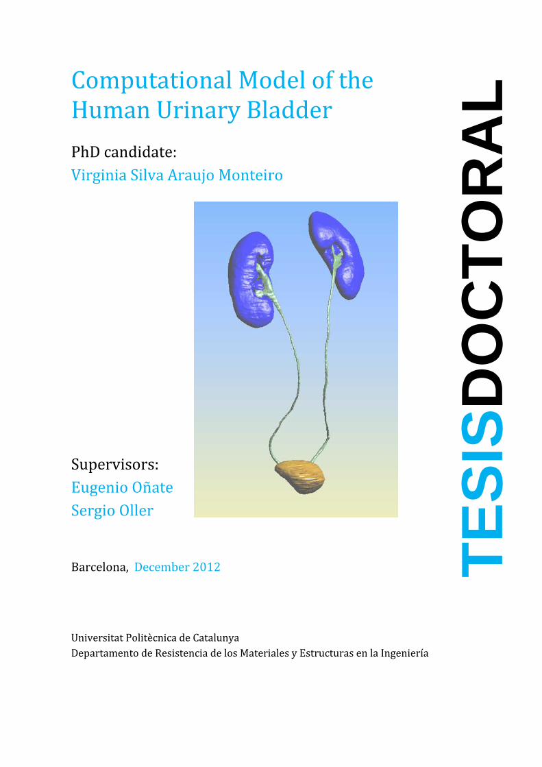
Computational Model of the
Human Urinary Bladder
PhD candidate:
Virginia Silva Araujo Monteiro
Supervisors:
Eugenio Oñate
Sergio Oller
Barcelona, December 20
Universitat Politècnica de Catalunya
Departamento de Resistencia de los Materiales
Computational Model of the
Human Urinary Bladder
Virginia Silva Araujo Monteiro
2012
Universitat Politècnica de Catalunya
Resistencia de los Materiales y Estructuras en la Ingeniy Estructuras en la Ingeniería
TE
SIS
DO
CT
OR
AL

ACTA DE CALIFICACIÓN DE LA TESIS DOCTORAL
Reunido el tribunal integrado por los abajo firmantes para juzgar la tesis doctoral:
Título de la tesis: ............................................................................................................
Autor de la tesis: ............................................................................................................
Acuerda otorgar la calificación de:
No apto
Aprobado
Notable
Sobresaliente
Sobresaliente Cum Laude
Barcelona, …………… de ….................…………….. de ..........….
El Presidente El Secretario
............................................. ............................................ (nombre y apellidos) (nombre y apellidos)
El vocal El vocal El vocal
............................................. ............................................ ..................................... (nombre y apellidos) (nombre y apellidos) (nombre y apellidos)


Dedico este trabajo a mis padres, Roberto y Ana Maria,
y a mis hermanos, Rodrigo, Joao Carlos y Rafael,
que han sido el fundamento de todo lo que
he podido realizar hasta hoy ,
a mi abuela Gioconda, por el ejemplo de fuerza,
y también a mi cariño, Jan Willem,
por todo el apoyo en la fase final de mi doctorado.

Agradecimientos i
Virginia Silva Araujo Monteiro
AGRADECIMIENTOS
En primer lugar quisiera agradecer a Prof. Eugenio Oñate, mi director de tesis, por haberme
dado esta oportunidad de, más que realizar un doctorado, vivir la investigación en un entorno
tan productivo. Le doy las gracias por haber creído en mi potencial y por haberme orientado en
la actividad investigadora. Asimismo, le estaré siempre agradecida por haber me apoyado en los
momentos que necesité y por la seguridad que me ha pasado a lo largo de eses 4 años de
desarrollo de la tesis.
Agradezco también a mi co-director de tesis, Prof. Sergio Oller, por compartir sus conocimientos
y experiencia en modelos constitutivos no-lineales para biomateriales, y también por orientarme
en la compilación de la tesis doctoral.
Agradecimiento especial a mi supervisor durante la estancia en KTH Suecia, Dr. Christian Gasser,
por engrandecer mi trabajo de investigación con sus conocimientos en modelos viscoelasticos y
biomecánica.
De los profesores que he tenido la alegría de conocer, agradezco a Prof. Marino y Prof. Carlos
Agelet Saracibar por las enseñanzas en mecánica de sólidos no-lineal. También quisiera
agradecer al Doctor Pooyan Dadvand por transferir su conocimiento de Kratos y programación
en C++, y a los doctores Riccardo Rossi y Pavel Ryzhakov, que me han inserido en el mundo de
iteración fluido estructura y enseñado a trabajar con fluido en Kratos.
Gracias a mis amigos y compañeros de despacho, Kazem Kamran, doctores Julio Martí y Roberto
López, y Jordi Carbonell, que tantas veces me ayudaran a aclarar mi entendimiento de
programación y compilación en Linux. Entre los amigos que hice en la UPC, Doctora Jussara
Limeira, doctores Albert de la Fuente y Sergio Henrique agradezco el apoyo en los estudios de
doctorado.
A mis compañeros del Centro Internacional de Métodos Numéricos (CIMNE) que muchas veces
fueran la inspiración que necesitaba para trasponer los obstáculos de la investigación. Entre
ellos, Eduardo Soudah por compartir las angustias y insights del trabajo de ingenieros en temas
biomédicos, Nelson Lafontaine por compartir interminables discusiones sobre implementación
de leyes constitutivas, y el equipo de GID, Enrique Escolano y Miguel Pasenau, por el apoyo.
Agradecimientos especiales al Hospital Clinic de Barcelona y a CIMA por el material fornecido
para validación del modelo numérico, y a Prof. Battista y Prof. Tonnar, por los datos
morfológicos fornecidos para construcción de la geometría.
Y, finalmente, agradezco el apoyo financiero de CIMNE y de la Generalitat de Catalunya, por la
beca pre-doctoral FI (ref. 2009-FI-B-0053) y por la Beca per a Estades a la Recerca fora de
Catalunya (ref. BE-DGR 2010), gestionadas por la AGAUR (Agència de Gestió d’Ajuts
Universitaris i de Recerca).

Resumen iii
Virginia Silva Araujo Monteiro
RESUMEN
La propuesta de una vejiga artificial es un obstáculo a trasponer. El cáncer de vejiga está entre los casos más frecuentes de enfermedades oncológicas en Estados Unidos y Europa. Ese cáncer es considerado un problema médico importante una vez que esa enfermedad presenta altas tasas de re-ocurrencia, muchas veces llevando a la remoción del órgano.
La solución más sofisticada para remplazar ese órgano es la vejiga ileal, que consiste en una neo-vejiga hecha de tejido intestinal del enfermo. Desafortunadamente, esa solución presenta no solo problemas mecánicos funcionales, descritos en la literatura como problemas de vaciado y fuga, peo también problemas de orden biológica (como ejemplo pérdida ósea, debido a la absorción por el intestino de substancias que necesitan ser eliminadas del organismo).
A través de la solicitación de la comunidad urológica del Hospital Clínico de Barcelona y con su experiencia en modelos numéricos para estructuras biomédicas, el Centro de Métodos Numéricos en Ingeniería (CIMNE) ha tenido la iniciativa de proporcionar actividad investigadora de la mecánica de la vejiga urinaria y de la simulación de interacción fluido-estructura para reproducir el llenado y vaciado de ese órgano con la orina.
La simulación de la vejiga humana por el Método de los Elementos Finitos (FEM) y un completo entendimiento de la mecánica de ese órgano y de su interacción con la orina dará la posibilidad de proponer mejora en la geometría y de analizar materiales para la solución artificial en caso de remplazamiento de la vejiga.
Para lograr ese objetivo, primeramente procedemos a una revisión bibliográfica de los modelos matemáticos del aparato urinario y un estudio comprehensivo de la fisiología y dinámica de la vejiga. Presentamos una revisión de las principales estructuras urológicas, riñón, uréter y uretra. Las estructuras anexas también son consideradas para entender las condiciones de contorno del problema estudiado.
Posteriormente, proponemos el modelo constitutivo para estudiar la vejiga urinaria humana. El comportamiento del musculo detrusor durante llenado y vaciado de la vejiga con orina, su habilidad de retención de orina a baja presión debe ser correctamente representada por medio de la implementación de un modelo constitutivo no-lineal. El modelo matemático necesita representar las variables mecánicas que gobiernan ese órgano, y también las propiedades de la orina. El comportamiento no-lineal de tejidos vivos es implementado y validado con ejemplos de la literatura. La propiedad quasi-incompressible de la orina y las ecuaciones Navier-Stokes son consideradas para análisis del fluido.
Para representar la geometría de la vejiga, implementamos un modelo computacional 3D a partir de imágenes de tomografía computadorizada de un cadáver adulto. Los datos son tratados para considerar las condiciones de contorno. Hemos construido dos modelos de malla: um mallado com tetrahedos de quatro nodos y outro mallado com elementos de membrana de tres nodos.
El esquema utilizado para calcular la interacción fluido-estructura debe ser adecuado para materiales de densidad muy parecidas. La análisis numérica de llenado y vaciado de la vejiga humana es validada con testes urodinámicos estandarizados.
La parte final de la tesis, presentamos una simulación de una neo-vejiga, siendo el primer paso para representar numéricamente materiales artificiales para remplazamiento de la vejiga.
iv Summary
Computational Model of the Human Urinay Bladder
SUMMARY
The proposal of an artificial bladder is still a challenge to overcome. Bladder cancer is among the most frequent cases of oncologic diseases in United States and Europe. It is considered a major medical problem once this disease has high rates of reoccurrence, often leading to the extirpation of this organ.
The most refined solution to replace this organ is the ileal bladder, which consists of a neobladder made of the patient’s intestinal tissue. Unfortunately this solution presents not only functional mechanical problems, described on the literature as voiding and leaking problems, but also biological ones (i.e. bone loss, given the absorption by the intestine of substances that should be eliminated from the organism).
Urged by the urological community of the Hospital Clinic de Barcelona and backgrounded by its experience in the numerical simulation of biomedical structures, the Center of Numerical Methods in Engineering (CIMNE) had the initiative to provide the research of the mechanics of the urinary bladder and the simulation of fluid structure interaction (FSI) to account for the filling and voiding of this organ with urine.
The Finite Element Method (FEM) simulation of the real bladder and the comprehensive understanding of the mechanics of this organ and its interaction with urine will give the possibility to propose geometrical improvements and study suitable materials for an artificial solution to address the cases on which the bladder needs to be removed.
To reach this goal, first we proceeded to the bibliographic review of mathematical models of the urinary apparatus and to a comprehensive study of the physiology and dynamics of the bladder. A review of the major urological structures, kidney, ureter and urethra, takes place. To consider boundary conditions other surrounding structures to the urinary system are also studied.
In the second part of the thesis, we propose the numerical model to study the human urinary bladder. The behavior of the detrusor muscle during filling and voiding of the bladder with urine and its ability to promote the storage of urine under low pressure need to be accurately represented, requiring the implementation of a non-linear constitutive model. The mathematical model needs to be capable to simulate the mechanical variables that govern this organ and the properties of the urine. The nonlinear behavior of living tissues is implemented and validated with examples from the literature. The quasi-incompressibility property of urine and the navier-stokes equations for the fluid are taken into account.
The geometry of the bladder needs to be taken into account, and the implementation of a 3D computational model obtained from the computerized tomography of a cadaver male adult is considered. The data has been treated to consider boundary conditions. Two models have been conceived: one meshed with four nodes tetrahedral and another meshed with shell elements.
FSI must work for the simulation of filling and voiding of the bladder. Due to the close densities of the materials the scheme used to solve fluid-structure needs to be carefully selected. The proposed numerical model and the filling and voiding analysis are finally validated with standardized urodynamic tests.
The final part of the thesis, the simulation of a neobladder is presented, being the first step to simulate numerically artificial materials for bladder replacement.
Index v
Virginia Silva Araujo Monteiro
INDEX
1. Introduction ........................................................................................................................................... 17
1.1. Introduction ..................................................................................................................................................................... 17
1.1.1. Interior of the bladder strucutres ......................................................................................................... 18
1.1.2. Bladder dynamics ......................................................................................................................................... 18
1.1.3. Urodynamics ................................................................................................................................................... 19
1.2. Motivation ......................................................................................................................................................................... 20
1.3. General Objectives ......................................................................................................................................................... 20
1.4. Objective details ............................................................................................................................................................. 20
1.5. Methodology .................................................................................................................................................................... 22
1.5.1. Bladder-material in short ......................................................................................................................... 22
1.5.2. The proposed constitutive model ......................................................................................................... 23
1.6. State of Art ........................................................................................................................................................................ 23
1.6.1. Proposed models for the bladder mechanics ................................................................................... 23
1.6.2. United States data on bladder cancer .................................................................................................. 25
1.6.3. Discussion ........................................................................................................................................................ 27
1.7. Structure of the thesis .................................................................................................................................................. 28
2. Anatomy of the Lower Urinary Tract and Urodynamics ...................................................... 29
2.1. Introduction ..................................................................................................................................................................... 29
2.2. Lower Urinary Tract Anatomy ................................................................................................................................. 29
2.2.1. Anterior abdominal wall ........................................................................................................................... 31
2.2.2. Soft Tissues of the Pelvis ........................................................................................................................... 32
2.2.3. Pelvic innervation......................................................................................................................................... 34
2.2.4. Pelvic Ureter ................................................................................................................................................... 35
2.2.5. Bladder Anatomic Relationships ........................................................................................................... 35
2.2.6. Prostate ............................................................................................................................................................. 41
2.2.7. Membranous Urethra ................................................................................................................................. 42
2.3. Urodynamics .................................................................................................................................................................... 44
2.3.1. Cystometry ...................................................................................................................................................... 45
2.3.2. Uroflow .............................................................................................................................................................. 54
2.3.3. Pressure-Flow Plots and Urethral Resistance Models ................................................................. 56
2.3.4. Videourodynamics ....................................................................................................................................... 57
2.3.5. Urethral Pressure Studies ......................................................................................................................... 58
2.4. Conclusions ....................................................................................................................................................................... 59
3. Proposal for the Numerical Simulation of the Human Urinary Bladder ......................... 61
3.1. Introduction ..................................................................................................................................................................... 61
3.1.1. Geometry .......................................................................................................................................................... 61
3.1.2. Constitutive Model ....................................................................................................................................... 61
vi Index
Computational Model of the Human Urinay Bladder
3.1.3. Structural analysis of the bladder ......................................................................................................... 63
3.1.4. Fluid flow analysis ...................................................................................................................................... 68
3.1.5. Validation ......................................................................................................................................................... 69
3.2. Geometry and Physiological data ........................................................................................................................... 69
3.2.1. Introduction .................................................................................................................................................... 69
3.2.2. MRI images ...................................................................................................................................................... 70
3.2.3. 3D Model .......................................................................................................................................................... 70
3.2.4. Aspects of the geometrical model ......................................................................................................... 71
3.2.5. Simplified geometry .................................................................................................................................... 72
3.3. Hyperelastic Model ....................................................................................................................................................... 73
3.3.1. Introduction .................................................................................................................................................... 73
3.3.2. The Neo-Hookean model ........................................................................................................................... 74
3.3.3. Validation of Hyperelastic constitutive model ................................................................................ 76
3.3.4. Retraction ........................................................................................................................................................ 82
3.3.5. Bladder inflation under pressure .......................................................................................................... 82
3.3.6. Results and analysis .................................................................................................................................... 85
3.3.7. Conclusions ..................................................................................................................................................... 88
3.4. Viscoelastic Model ......................................................................................................................................................... 88
3.4.1. Introduction .................................................................................................................................................... 88
3.4.2. The Generalized Maxwell model ............................................................................................................ 89
3.4.3. Preliminary test ............................................................................................................................................. 95
3.4.4. Bladder inflation under pressure .......................................................................................................... 97
3.5. Hyperelastic matrix reinforced with Viscoelastic fibers ........................................................................... 107
3.5.1. Introduction ................................................................................................................................................. 107
3.5.2. Computation of the fibers contribution term f
S ....................................................................... 107
3.5.3. Fiber orientation ........................................................................................................................................ 108
3.5.4. Bladder inflation under pressure ....................................................................................................... 109
3.5.5. Results and analysis ................................................................................................................................. 109
3.5.6. Conclusions .................................................................................................................................................. 111
3.6. Structural analysis of bladder constitutive models ..................................................................................... 111
3.6.1. Introduction ................................................................................................................................................. 111
3.6.2. Bladder as a 3D solid ................................................................................................................................ 111
3.6.3. Bladder modeled as a membrane ....................................................................................................... 112
3.6.4. Results and analysis ................................................................................................................................. 114
3.6.5. Conclusions .................................................................................................................................................. 119
3.7. Bladder-Urine interaction analysis ..................................................................................................................... 119
3.7.1. Introduction ................................................................................................................................................. 119
3.7.2. Bladder filling .............................................................................................................................................. 120
3.7.3. Bladder voiding .......................................................................................................................................... 131
3.7.4. Voiding of 75 ml of fluid ........................................................................................................................ 133
Index vii
Virginia Silva Araujo Monteiro
3.7.5. Conclusion .................................................................................................................................................... 136
4. Clinical Tests and Validation .......................................................................................................... 137
4.1. Introduction .................................................................................................................................................................. 137
4.2. Clinical tests................................................................................................................................................................... 137
4.2.1. Filling data .................................................................................................................................................... 139
4.2.2. Voiding data ................................................................................................................................................. 141
4.3. Bladder filling under cystometric conditions: 50ml/min infusion rate ............................................. 143
4.4. Bladder voiding ............................................................................................................................................................ 146
4.5. Numerical results vs Urodynamic tests ............................................................................................................ 146
4.6. Further studies ............................................................................................................................................................. 149
4.7. Conclusion ...................................................................................................................................................................... 151
5. Neobladder Numerical Analysis ................................................................................................... 153
5.1. Introduction .................................................................................................................................................................. 153
5.2. The orthotpic ileal neobladder ............................................................................................................................. 154
5.3. Geometry ........................................................................................................................................................................ 155
5.4. Numerical model ......................................................................................................................................................... 159
5.4.1. Material properties and physiology .................................................................................................. 160
5.4.2. Viscoelastic constitutive model ........................................................................................................... 162
5.5. Numerical analysis ..................................................................................................................................................... 163
5.5.1. Neobladder filling ...................................................................................................................................... 163
5.5.2. Neobladder voiding .................................................................................................................................. 165
5.6. Comparison with urodynamic tests .................................................................................................................... 167
5.7. Conclusion ...................................................................................................................................................................... 170
6. Conclusions and persperctives ..................................................................................................... 171
6.1. General conclusions ................................................................................................................................................... 171
6.2. Specific conclusions ................................................................................................................................................... 171
6.3. Perspectives for future work ................................................................................................................................. 172
6.4. Final considerations .................................................................................................................................................. 173
7. Conclusiones y perspectivas .......................................................................................................... 174
7.1. Conclusiones generales ............................................................................................................................................ 174
7.2. Conclusiones especificas .......................................................................................................................................... 174
7.3. Perspectivas .................................................................................................................................................................. 175
7.4. Consideraciones Finales .......................................................................................................................................... 176
References ..................................................................................................................................................... 177
ANNEX A – Finite element approach ................................................................................................... 185
ANNEX B – Geometry reconstruction ................................................................................................. 192
viii Index of tables
Computational Model of the Human Urinay Bladder
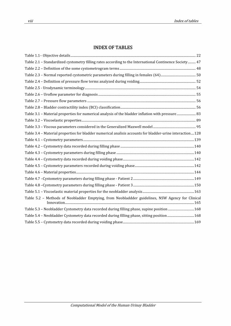
INDEX OF TABLES
Table 1.1– Objective details .............................................................................................................................................................. 22
Table 2.1 – Standardized cystometry filling rates according to the International Continence Society .......... 47
Table 2.2 – Definition of the some cystometrogram terms ................................................................................................ 48
Table 2.3 – Normal reported cystometric parameters during filling in females (64) ............................................ 50
Table 2.4 – Definition of pressure flow terms analyzed during voiding....................................................................... 52
Table 2.5 - Urodynamic terminology ............................................................................................................................................ 54
Table 2.6 – Uroflow parameter for diagnosis ........................................................................................................................... 55
Table 2.7 – Pressure flow parameters ......................................................................................................................................... 56
Table 2.8 – Bladder contractility index (BCI) classification ............................................................................................... 56
Table 3.1 – Material properties for numerical analysis of the bladder inflation with pressure ........................ 83
Table 3.2 – Viscoelastic properties ................................................................................................................................................ 89
Table 3.3 – Viscous parameters considered in the Generalized Maxwell model ...................................................... 95
Table 3.4 – Material properties for bladder numerical analisis accounts for bladder-urine interaction .... 128
Table 4.1 – Cystometry parameters ............................................................................................................................................ 139
Table 4.2 – Cystometry data recorded during filling phase ............................................................................................. 140
Table 4.3 – Cystometry parameters during filling phase .................................................................................................. 140
Table 4.4 – Cystometry data recorded during voiding phase .......................................................................................... 142
Table 4.5 – Cystometry parameters recorded during voiding phase ........................................................................... 142
Table 4.6 – Material properties ..................................................................................................................................................... 144
Table 4.7 –Cystometry parameters during filling phase - Patient 2 ............................................................................. 149
Table 4.8 –Cystometry parameters during filling phase - Patient 3 ............................................................................. 150
Table 5.1 – Viscoelastic material properties for the neobladder analysis ................................................................. 163
Table 5.2 – Methods of Neobladder Emptying, from Neobladdder guidelines, NSW Agency for Clinical
Innovation ................................................................................................................................................................... 165
Table 5.3 – Neobladder Cystometry data recorded during filling phase, supine position ................................. 168
Table 5.4 – Neobladder Cystometry data recorded during filling phase, sitting position .................................. 168
Table 5.5 – Cystometry data recorded during voiding phase .......................................................................................... 169
Index of Figures ix
Virginia Silva Araujo Monteiro
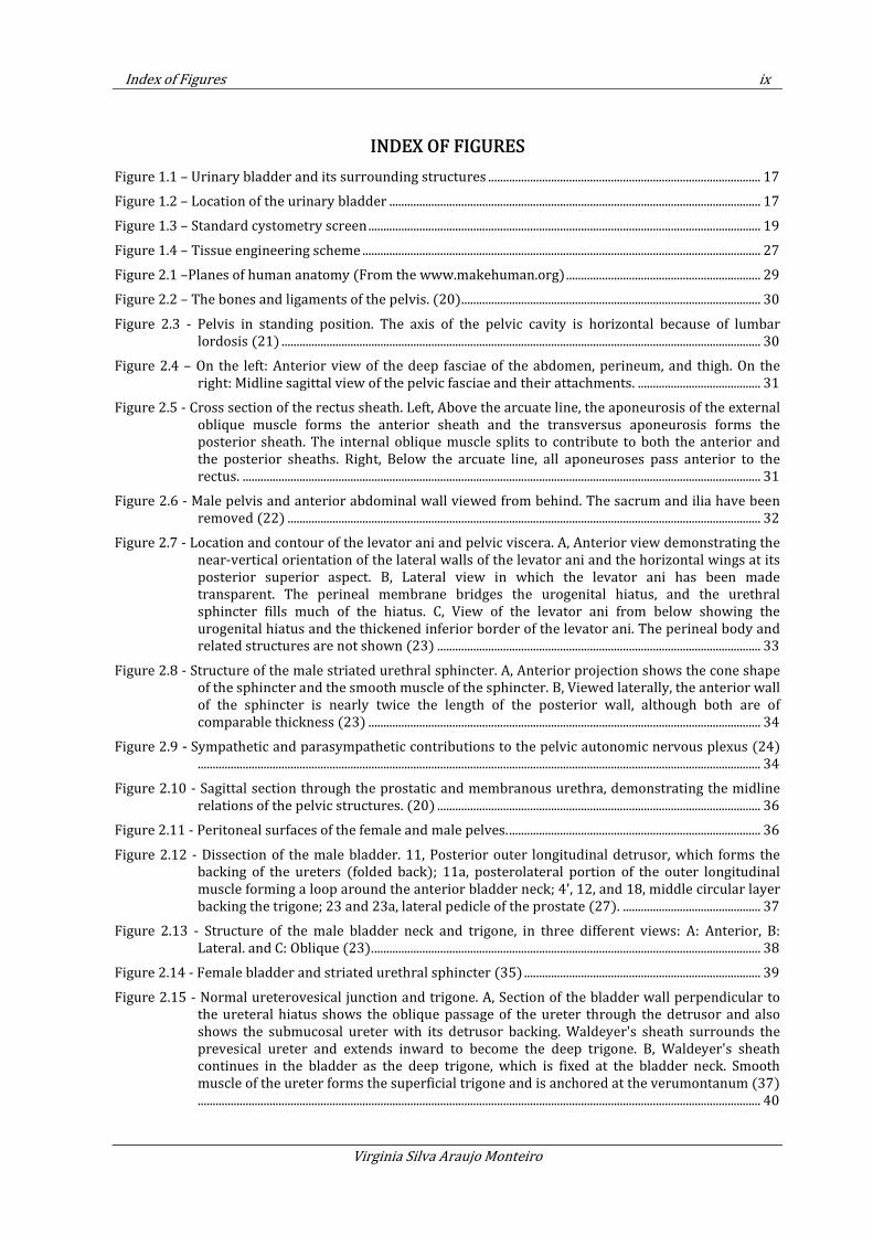
INDEX OF FIGURES
Figure 1.1 – Urinary bladder and its surrounding structures ........................................................................................... 17
Figure 1.2 – Location of the urinary bladder ............................................................................................................................ 17
Figure 1.3 – Standard cystometry screen ................................................................................................................................... 19
Figure 1.4 – Tissue engineering scheme ..................................................................................................................................... 27
Figure 2.1 –Planes of human anatomy (From the www.makehuman.org) ................................................................. 29
Figure 2.2 – The bones and ligaments of the pelvis. (20).................................................................................................... 30
Figure 2.3 - Pelvis in standing position. The axis of the pelvic cavity is horizontal because of lumbar
lordosis (21) ................................................................................................................................................................ 30
Figure 2.4 – On the left: Anterior view of the deep fasciae of the abdomen, perineum, and thigh. On the
right: Midline sagittal view of the pelvic fasciae and their attachments. ......................................... 31
Figure 2.5 - Cross section of the rectus sheath. Left, Above the arcuate line, the aponeurosis of the external
oblique muscle forms the anterior sheath and the transversus aponeurosis forms the
posterior sheath. The internal oblique muscle splits to contribute to both the anterior and
the posterior sheaths. Right, Below the arcuate line, all aponeuroses pass anterior to the
rectus. ............................................................................................................................................................................. 31
Figure 2.6 - Male pelvis and anterior abdominal wall viewed from behind. The sacrum and ilia have been
removed (22) .............................................................................................................................................................. 32
Figure 2.7 - Location and contour of the levator ani and pelvic viscera. A, Anterior view demonstrating the
near-vertical orientation of the lateral walls of the levator ani and the horizontal wings at its
posterior superior aspect. B, Lateral view in which the levator ani has been made
transparent. The perineal membrane bridges the urogenital hiatus, and the urethral
sphincter fills much of the hiatus. C, View of the levator ani from below showing the
urogenital hiatus and the thickened inferior border of the levator ani. The perineal body and
related structures are not shown (23) ............................................................................................................ 33
Figure 2.8 - Structure of the male striated urethral sphincter. A, Anterior projection shows the cone shape
of the sphincter and the smooth muscle of the sphincter. B, Viewed laterally, the anterior wall
of the sphincter is nearly twice the length of the posterior wall, although both are of
comparable thickness (23) ................................................................................................................................... 34
Figure 2.9 - Sympathetic and parasympathetic contributions to the pelvic autonomic nervous plexus (24)
............................................................................................................................................................................................ 34
Figure 2.10 - Sagittal section through the prostatic and membranous urethra, demonstrating the midline
relations of the pelvic structures. (20) ............................................................................................................ 36
Figure 2.11 - Peritoneal surfaces of the female and male pelves. .................................................................................... 36
Figure 2.12 - Dissection of the male bladder. 11, Posterior outer longitudinal detrusor, which forms the
backing of the ureters (folded back); 11a, posterolateral portion of the outer longitudinal
muscle forming a loop around the anterior bladder neck; 4', 12, and 18, middle circular layer
backing the trigone; 23 and 23a, lateral pedicle of the prostate (27). .............................................. 37
Figure 2.13 - Structure of the male bladder neck and trigone, in three different views: A: Anterior, B:
Lateral. and C: Oblique (23). ................................................................................................................................. 38
Figure 2.14 - Female bladder and striated urethral sphincter (35) ............................................................................... 39
Figure 2.15 - Normal ureterovesical junction and trigone. A, Section of the bladder wall perpendicular to
the ureteral hiatus shows the oblique passage of the ureter through the detrusor and also
shows the submucosal ureter with its detrusor backing. Waldeyer's sheath surrounds the
prevesical ureter and extends inward to become the deep trigone. B, Waldeyer's sheath
continues in the bladder as the deep trigone, which is fixed at the bladder neck. Smooth
muscle of the ureter forms the superficial trigone and is anchored at the verumontanum (37)
............................................................................................................................................................................................ 40
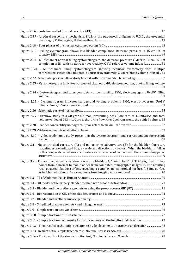
x Index of Figures
Computational Model of the Human Urinay Bladder
Figure 2.16 - Posterior wall of the male urethra (43) .......................................................................................................... 42
Figure 2.17 - Urethral suspensory mechanism. P.U.L. is the pubourethral ligament, U.G.D., the urogenital
diaphragm; V, the vagina; U, the urethra (48) .............................................................................................. 43
Figure 2.18 – Four phases of the normal cystometrogram (60) ...................................................................................... 48
Figure 2.19 - Filling cystemogram shows low bladder compliance. Detrusor pressure is 45 cmH2O at
capacity 155mL. ......................................................................................................................................................... 49
Figure 2.20 - Multichannel normal-filling cystometrogram. the detrusor pressure (Pdet) is 10 cm H2O at
completion of fill, with no detrusor overactivity. C Vol refers to volume infused. ....................... 51
Figure 2.21 - Multichannel filling cystometrogram showing detrusor overactivity with multiple
contractions. Patient had idiopathic detrusor overactivity. C Vol refers to volume infused. .. 51
Figure 2.22 - Schematic pressure-flow study labeled with recommended terminology ...................................... 52
Figure 2.23 – Cystometrogram indicates obstructed bladder. EMG, electromyogram; UroPV, filling volume.
........................................................................................................................................................................................... 53
Figure 2.24 – Cystometrogram indicates poor detrusor contractility. EMG, electromyogram; UroPV, filling
volume. ........................................................................................................................................................................... 53
Figure 2.25 – Cystometrogram indicates storage and voiding problems. EMG, electromyogram; UroPV,
filling volume; C Vol, volume infused. .............................................................................................................. 53
Figure 2.26 - Schematic curve of normal flow. ......................................................................................................................... 55
Figure 2.27 - Uroflow study in a 60-year-old man, presenting peak flow rate of 16 mL/sec. and total
volume voided of 263 mL. Qura is the urine flow rate; Qvol represents the voided volume . 55
Figure 2.28 - Bladder contractility nomogram. Qmax refers to maximum flow rate. ............................................ 57
Figure 2.29 –Videourodynamic evaluation scheme ............................................................................................................... 57
Figure 2.30 – Videourodynamic study presenting the cystometrogram and correspomdent fuoroscopic
image ............................................................................................................................................................................... 58
Figure 3.1 - Major principal curvature (A) and minor principal curvature (B) for the bladder. Curvature
magnitudes are indicated by gray scale and directions by vectors. When the bladder is full, as
in this case, wide variations in curvature exist because of contact with the surrounding pelvic
structures. ..................................................................................................................................................................... 69
Figure 3.2 - Three-dimensional reconstruction of the bladder. A, “Point cloud” of 3146 digitized surface
points from a normal human bladder from computed tomographic images. B, The resulting
reconstructed bladder surface, revealing a complex, nonspheroidal surface. C, Same surface
as in B but with the surface roughness from imaging noise removed. .............................................. 70
Figure 3.3 - CT of Abdomen Pelvis Human Anatomy ............................................................................................................ 70
Figure 3.4 – 3D model of the urinary bladder meshed with 4 nodes tetrahedras ................................................... 71
Figure 3.5 – Bladder and the urethers geometries using the pre-processor GID (87) .......................................... 71
Figure 3.6 – Representation in GID of the bladder, ureters and kidneys ..................................................................... 72
Figure 3.7 – Bladder and urethers surface geometry............................................................................................................ 72
Figure 3.8 – Simplified bladder geometry and triangular mesh ...................................................................................... 73
Figure 3.9 – Simple traction test, 2D scheme ............................................................................................................................ 76
Figure 3.10 – Simple traction test, 3D scheme ......................................................................................................................... 77
Figure 3.11 – Simple traction test, results for displacements on the longitudinal direction .............................. 77
Figure 3.12 – Final results of the simple traction test , displacements on transversal direction ...................... 78
Figure 3.13 –Results of the simple traction test, Nominal stress vs. Stretch ............................................................. 78
Figure 3.14 – Final results of the simple traction test, Nominal stress vs. Stretch .................................................. 79
Index of Figures xi
Virginia Silva Araujo Monteiro
Figure 3.15 – Final results of the simple traction test, with 9λ = .................................................................................. 79
Figure 3.16 - Inflated half-sphere is plotted in comparison with the original geometry (in green), showing
displacements in x direction. ................................................................................................................................ 81
Figure 3.17 - Inflated half-sphere is plotted in comparison with the original geometry (in green), showing
displacements in x, y and z directions .............................................................................................................. 81
Figure 3.18 – Cauchy stresses vs. Stretch λ ............................................................................................................................ 82
Figure 3.19 - Second-Piola stresses vs. Time ............................................................................................................................ 82
Figure 3.20 – Hydrostatic pressure computed with ULF, considering the initial volume of 50 ml .................. 83
Figure 3.21 – Post-process image of the 3D mesh with Membrane elements, comparing current and
reference configuration (in blue) ....................................................................................................................... 83
Figure 3.22 – View of bladder geometry inflated with internal pressure .................................................................... 84
Figure 3.23 – Applied internal pressure (Pa) vs. total bladder volume (ml) ............................................................. 84
Figure 3.24 – Hydrostatic pressure computed with PFEM, considering the initial volume of 440 ml ........... 85
Figure 3.25 –Aapplied internal pressure (Pa) vs. total bladder volume (ml), considering incremental
pressure (green) and hydrostatic pressure computed with ULF (red) ............................................ 85
Figure 3.26– Principal Cauchy stresses for bladder inflation up to 440ml, in four different locations .......... 86
Figure 3.27 – Principal Cauchy stresses vs bladder volume, in four different locations of the bladder ........ 87
Figure 3.28 – Principal Cauchy stresses vs time ...................................................................................................................... 87
Figure 3.29 – The generalized Maxwell model ......................................................................................................................... 89
Figure 3.30 –Scheme for the kinematics of the viscoelastic body ................................................................................... 90
Figure 3.31 – Simple traction test 2D scheme .......................................................................................................................... 96
Figure 3.32 – Simple traction test X and Y displacements .................................................................................................. 96
Figure 3.33 - Stress relaxation, Beta 0.15, Relaxation time 1000 ................................................................................... 97
Figure 3.34 – Plotted curve of applied internal pressure (Pa) vs. total bladder volume (ml) ........................... 98
Figure 3.35 – Plotted curve of applied internal pressure (Pa) vs. total bladder volume (ml), considering
incremental pressure (green) and hydrostatic pressure computed with ULF (red) .................. 99
Figure 3.36– Plotted principal Cauchy stresses for bladder inflation up to 440ml, in four different locations
............................................................................................................................................................................................ 99
Figure 3.37 – Principal Cauchy stresses vs bladder volume, in four different locations of the bladder ...... 100
Figure 3.38 – Plotted principal Cauchy stresses vs time ................................................................................................... 100
Figure 3.39 – Analysis of Cauchy stresses for the Hyperelastic, Viscoelastic (both with shear modulus
10KPa) and Cauchy obtained from the Laplace Equation ..................................................................... 101
Figure 3.40 – Principal Cauchy stresses vs time, viscoelastic model (shear modulus of 3,000 Pa) ............... 102
Figure 3.41 – Principal Cauchy stresses vs volume, viscoelastic model (shear modulus of 3 KPa) ............... 102
Figure 3.42 – Principal Cauchy stresses vs volume in four points of the bladder (the continuos line
represent Shear modulus of 5,000 Pa and the dashed line represent Shear modulus of 3,000
Pa), viscoelastic model .......................................................................................................................................... 103
Figure 3.43 – Principal Cauchy stresses for bladder inflation, in four different locations ................................. 104
Figure 3.44 – Principal cauchy stresses vs time (shear modulus 5 KPa), viscoelastic model........................... 104
Figure 3.45 – Principal Cauchy stresses vs volume (shear modulus of 5 KPa) ....................................................... 105
Figure 3.46 – Plotted principal cauchy stresses vs time (shear of 5 KPa) ................................................................. 106
Figure 3.47 –Principal Cauchy stresses vs volume (shear modulus of 5 KPa) ........................................................ 106
xii Index of Figures
Computational Model of the Human Urinay Bladder
Figure 3.48 - Principal Cauchy stresses vs. time (homogenized model, shear modulus of 5 KPa) ................ 110
Figure 3.49 - Plotted principal Cauchy stresses vs Volume (homogenized model, shear 5 KPa) ................... 110
Figure 3.50 – Results showing displacements in Y (a) and Z (b) directions after applying internal
pressure to the structure ..................................................................................................................................... 112
Figure 3.51 – Occurrence of localized problems during the inflation of the structure meshed with
tetrahedral elements .............................................................................................................................................. 112
Figure 3.52 – View of the bladder meshed with 3-node membrane elements ........................................................ 113
Figure 3.53 – Bladder inflated with pressure ......................................................................................................................... 113
Figure 3.54 – Inflated bladder vs. reference configuration (in blue) ........................................................................... 114
Figure 3.55 – Hydrostatic pressure computed with PFEM, considering the initial volume of 50 ml ............ 114
Figure 3.56 – Applied internal pressure (Pa) vs. total bladder volume (ml) ........................................................... 115
Figure 3.57 – Hydrostatic pressure computed with PFEM, considering the initial volume of 440 ml ......... 115
Figure 3.58 – Applied internal pressure (Pa) vs. total bladder volume (ml), considering incremental
pressure (green) and maximum hydrostatic pressure computed with ULF (red) .................... 116
Figure 3.59 – Plotted principal cauchy stresses for bladder inflation up to 440ml, in 4 different locations
......................................................................................................................................................................................... 117
Figure 3.60 – Principal Cauchy stresses vs bladder volume, in four different locations of the bladder ...... 118
Figure 3.61 – Principal cauchy stresses vs time .................................................................................................................... 118
Figure 3.62 – Pressure vs volume ................................................................................................................................................ 119
Figure 3.63 –Zero displacement imposed to the trigone area (in green) .................................................................. 120
Figure 3.64 –Restricted displacement imposed to the area in contact with pelvic musculature (in green)
......................................................................................................................................................................................... 120
Figure 3.65 – Deformation of the bladder, considering the trigone fixed .................................................................. 121
Figure 3.66 – Displacements vectors representing the deformation of the bladder and fluid ......................... 121
Figure 3.67 – Pre-process scheme of bladder and the supporting structure ........................................................... 122
Figure 3.68 –Nodes representing fluid (in blue) and structure (brown) .................................................................. 122
Figure 3.69 – Displacements vectors representing the initial condition for bladder filling .............................. 122
Figure 3.70 – Pre-process image of the geometry ................................................................................................................ 123
Figure 3.71 – Post-process image of the 3D mesh with membrane elements ......................................................... 123
Figure 3.72 – Post-process image of the pressure at the end of the filling ................................................................ 124
Figure 3.73 – Intravesical pressure (Pa) at t=0.025951 ................................................................................................... 125
Figure 3.75 – Image of pressure values at t=0.00005 ........................................................................................................ 125
Figure 3.76 – Pressure profile (upper figure) on the selected red points (lower figure) .................................. 126
Figure 3.77 – Final pressure distribution ................................................................................................................................. 126
Figure 3.78 – Total Lagrangian inlet boundary condition at imposed to line and surface (in green) .......... 127
Figure 3.79 – Fixed displacements boundary condition at imposed to surface (in green)................................ 128
Figure 3.80 – Displacement distribution and fluid nodes presented at different volumes: 56, 65, 75, 89, 100
and 113 ml respectively ....................................................................................................................................... 129
Figure 3.81 – Cauchy stresses distribution at 56, 65 and 113 ml respectively ....................................................... 130
Figure 3.82 – Pressure distribution at 56 and 65 ml respectively ................................................................................ 131
Figure 3.83 – Final shape of the hyperelastic model of bladder voiding with membrane elements ........... 132
Index of Figures xiii
Virginia Silva Araujo Monteiro
Figure 3.83 – Problems faced in fluid-strucuture interaction at a given time of the voiding process .......... 133
Figure 3.84 – Representation of fluid displacement vectors at a given time of the voiding process ............. 133
Figure 3.86 – Representation of bladder voiding pressure from time 0.01 sec (74 ml) to time 5.2 sec (56
ml) .................................................................................................................................................................................. 134
Figure 3.87 – Representation of displacements countours on bladder surface and fluid at time 0.01s
(70ml) and time 1.0 sec (63.8ml) ................................................................................................................... 135
Figure 3.88 – Representation of displacements countours on bladder surface and fluid at time 1.0 sec .. 135
Figure 4.1 – Overview picture of the cystometry of an adult patient with normal bladder activity, by
Hospital Clinic of Barcelona ................................................................................................................................ 137
Figure 4.2 – Cystometry analysis with the of an adult patient with normal bladder activity, by Hospital
Clinic of Barcelona................................................................................................................................................... 138
Figure 4.3 – Cystometry recorded during the filling phase .............................................................................................. 139
Figure 4.4 – Graphs static compliance (left) and Pressure vs. Volume (right)........................................................ 140
Figure 4.5 – Pressure vs. Volume, urodynamic data ............................................................................................................ 141
Figure 4.6 – Cystometry recorded during voiding phasis ................................................................................................. 141
Figure 4.7 – Cystometry recorded during voiding phase .................................................................................................. 143
Figure 4.8 –Nomograms> Abrams-Griffiths (left) and ICS (right), .............................................................................. 143
Figure 4.9 – Meshed geometry of the bladder filling ........................................................................................................... 143
Figure 4.10 – Pressure within the bladder for different volumes, 56ml and 65 ml respectively. ................... 144
Figure 4.11 – Results for the numerical analysis of bladder filling, Graph Volume vs. Time ............................ 145
Figure 4.12 – Results for the numerical analysis of bladder filling, Graph Pressure vs. Time .......................... 145
Figure 4.13 – Results for the numerical analysis of bladder filling, Graph Pressure vs. Volume .................... 146
Figure 4.14 – Results for the numerical analisis of bladder voiding, Graph Volume vs. Time .......................... 146
Figure 4.15 – Bladder displacements with different volumes, 55ml, 70ml, 100ml, 230ml and 300ml
respectively. ............................................................................................................................................................... 147
Figure 4.16 – Comparison of results for the Hyperelastic constitutive model considering structural and FSI
numerical analysis with the data obtained from cystometry, Graph Pressure vs. Volume .... 148
Figure 4.17 – Comparison of results for the Viscoelastic constitutive model the structural analysis with the
data obtained from cystometry, Graph Pressure vs. Volume .............................................................. 148
Figure 4.18 – Comparison of results for the FSI numerical analysis with the data obtained from
cystometry, Graph Volume vs. Time ............................................................................................................... 149
Figure 4.19 – Comparison of results for the numerical analysis with the data obtained from cystometry of
3 patients, Graph Pressure vs. Volume .......................................................................................................... 150
Figure 5.1 - Gastro-intesinal tract structures ......................................................................................................................... 153
Figure 5.2 - Small intestine structures: duodenum, jejunum and ileum ..................................................................... 154
Figure 5.3 - The small elongated reservoir (left), and the large spherical reservoir (right). .......................... 154
Figure 5.4 - Urinary apparathus with neobladder ................................................................................................................ 155
Figure 5.5 - MRI images of two orthotropic bladders, from patient A (on the left) and patient B (on the
right) ............................................................................................................................................................................. 156
Figure 5.6 – Volume of the neobladder geometry read by GID software compared with images of the organ
.......................................................................................................................................................................................... 157
Figure 5.7 – Initial mesh generated for the neobladder .................................................................................................... 158
xiv Index of Figures
Computational Model of the Human Urinay Bladder
Figure 5.8 – Surfaces generated in GID for the neobladder geometry compared with images of the organ
......................................................................................................................................................................................... 158
Figure 5.9 – Meshed geometry of the neobladder ................................................................................................................ 159
Figure 5.10 – Neobladder volume mesh (left) and boundary conditions in blue (right) ................................... 159
Figure 5.11 Schematic layers of the gastrointestinal tract ............................................................................................... 160
Figure 5.12 – Small intestine stress-strain curves (116) .................................................................................................. 161
Figure 5.13 – Relaxation parameters for small intestines (133) ................................................................................... 162
Figure 5.14 - Kock pouch, valves and outlet made from ileum ....................................................................................... 162
Figure 5.16 – Neobladder geometry filled with fluid .......................................................................................................... 163
Figure 5.15 – A: Neobladder total volume of 325 ml, B: neobladder total volume of 600 ml .......................... 164
Figure 5.16 – Inflation of the neobladder – Pressure (Pa) vs. Volume (mL) curve for the numerical analysis
......................................................................................................................................................................................... 165
Figure 5.18 - Deflation of the neobladder at three different stages with total volumes of A: 302 ml
(posterior and anterior view), B: 208 ml, and C: 34ml........................................................................... 166
Figure 5.19 – Voiding of the neobladder – Pressure (Pa) vs. Volume (mL) curve for the FSI analysis ........ 167
Figure 5.20 – Filling of the neobladder – Comparison curve with results from cystometry and numerical
analysis - Pressure (Pa) vs. Volume (mL) .................................................................................................... 169
Figure 5.19 – Voiding of the neobladder – Comparison curve with results from cystometry and fluid-
structure analysis .................................................................................................................................................... 170
Figure A.1 Updated Lagrangian description for FSI (ref Advances in the Particle Finite Lement Method
(PFEM) for Solving Coupled Problems in Engineering) ........................................................................ 187
Figure A.2 Sequence of steps to update a “cloud” of nodes representing a fluid-solid domain from time n with ( = ) to time n+2 ( = + 2∆) ................................................................................................. 188
Figure B.3 Geometry of the bladder meshed with approximately 1 million tetrahedral elements................ 193
Figure B.4 Inner and outer surfaces of the bladder geometry meshed with surface triangles ........................ 193
Figure B.5 Geometry of the bladder meshed with approximately 6,000 membrane elements ....................... 193
Figure B.6 DICOM series ................................................................................................................................................................... 194
Figure B.7 Volume of the neobladder geometry compared with MRI of the organ ............................................... 194
Figure B.8 Mesh, Surface geometry and MRI of the neobladder .................................................................................... 195
Symbols xv
Virginia Silva Araujo Monteiro
SYMBOLS
Empirical coefficient, viscoelasticity
Relaxation Parameter
Stretch computed projecting the Green Strain
Shear modulus
Density
p Pressure
Cauchy Stress
Viscoelastic Stress
Relaxation Time
Creep Time
∅ Volume fraction
Gravity
Bulk modulus
C Right Cauchy-Green deformation tensor
Young Modulus
E Green Strain Tensor
J Jacobian
Mass Matrix
Second Piola Kirchhoff Stress
Volume
Pves
Vesical pressure
detP Detrusor pressure
Pabd
Abbdominal pressure
Ψ Strain energy

Introduction
1. INTRODUCTION
1.1. Introduction
This thesis proposes a numerical approach to simulate the
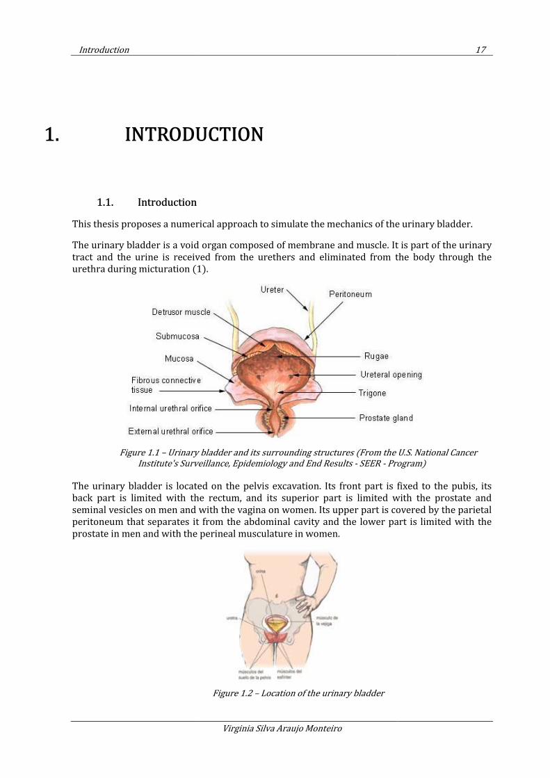
The urinary bladder is a void organ composed of membrane and muscle. It is part of the urinary
tract and the urine is received from
urethra during micturation (1)
Figure 1.1 – Urinary bladder and its
Institute's Surveillance, Epidemiology and End Results
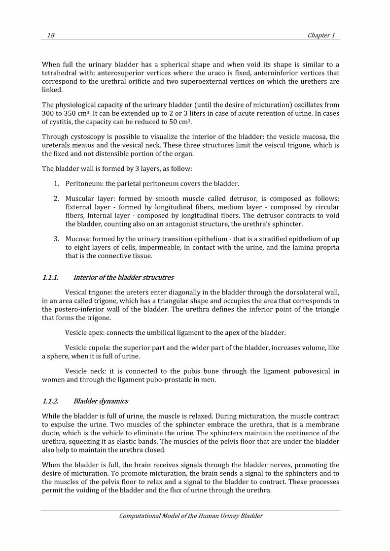
The urinary bladder is located on the pelvis excavation. Its front part is fixed to the pubis, its
back part is limited with the rectum, and its superior part is limited with the pro
seminal vesicles on men and with the vagina on women. Its upper part is covered by the parietal
peritoneum that separates it from the abdominal cavity and the lower part is limited with the
prostate in men and with the perineal musculature in wom
Virginia Silva Araujo Monteiro
NTRODUCTION
a numerical approach to simulate the mechanics of the
The urinary bladder is a void organ composed of membrane and muscle. It is part of the urinary
tract and the urine is received from the urethers and eliminated from the body through the
(1).
Urinary bladder and its surrounding structures (From the U.S. National Cancer
Institute's Surveillance, Epidemiology and End Results - SEER - Program)
The urinary bladder is located on the pelvis excavation. Its front part is fixed to the pubis, its
back part is limited with the rectum, and its superior part is limited with the pro
seminal vesicles on men and with the vagina on women. Its upper part is covered by the parietal
peritoneum that separates it from the abdominal cavity and the lower part is limited with the
prostate in men and with the perineal musculature in women.
Figure 1.2 – Location of the urinary bladder
17
mechanics of the urinary bladder.
The urinary bladder is a void organ composed of membrane and muscle. It is part of the urinary
the urethers and eliminated from the body through the
(From the U.S. National Cancer
Program)
The urinary bladder is located on the pelvis excavation. Its front part is fixed to the pubis, its
back part is limited with the rectum, and its superior part is limited with the prostate and
seminal vesicles on men and with the vagina on women. Its upper part is covered by the parietal
peritoneum that separates it from the abdominal cavity and the lower part is limited with the
18 Chapter 1
Computational Model of the Human Urinay Bladder
When full the urinary bladder has a spherical shape and when void its shape is similar to a tetrahedral with: anterosuperior vertices where the uraco is fixed, anteroinferior vertices that correspond to the urethral orificie and two superoexternal vertices on which the urethers are linked.
The physiological capacity of the urinary bladder (until the desire of micturation) oscillates from 300 to 350 cm3. It can be extended up to 2 or 3 liters in case of acute retention of urine. In cases of cystitis, the capacity can be reduced to 50 cm3.
Through cystoscopy is possible to visualize the interior of the bladder: the vesicle mucosa, the ureterals meatos and the vesical neck. These three structures limit the veiscal trigone, which is the fixed and not distensible portion of the organ.
The bladder wall is formed by 3 layers, as follow:
1. Peritoneum: the parietal peritoneum covers the bladder.
2. Muscular layer: formed by smooth muscle called detrusor, is composed as follows: External layer - formed by longitudinal fibers, medium layer - composed by circular fibers, Internal layer - composed by longitudinal fibers. The detrusor contracts to void the bladder, counting also on an antagonist structure, the urethra’s sphincter.
3. Mucosa: formed by the urinary transition epithelium - that is a stratified epithelium of up to eight layers of cells, impermeable, in contact with the urine, and the lamina propria that is the connective tissue.
1.1.1. Interior of the bladder strucutres
Vesical trigone: the ureters enter diagonally in the bladder through the dorsolateral wall, in an area called trigone, which has a triangular shape and occupies the area that corresponds to the postero-inferior wall of the bladder. The urethra defines the inferior point of the triangle that forms the trigone.
Vesicle apex: connects the umbilical ligament to the apex of the bladder.
Vesicle cupola: the superior part and the wider part of the bladder, increases volume, like a sphere, when it is full of urine.
Vesicle neck: it is connected to the pubis bone through the ligament pubovesical in women and through the ligament pubo-prostatic in men.
1.1.2. Bladder dynamics
While the bladder is full of urine, the muscle is relaxed. During micturation, the muscle contract to expulse the urine. Two muscles of the sphincter embrace the urethra, that is a membrane ducte, which is the vehicle to eliminate the urine. The sphincters maintain the continence of the urethra, squeezing it as elastic bands. The muscles of the pelvis floor that are under the bladder also help to maintain the urethra closed.
When the bladder is full, the brain receives signals through the bladder nerves, promoting the desire of micturation. To promote micturation, the brain sends a signal to the sphincters and to the muscles of the pelvis floor to relax and a signal to the bladder to contract. These processes permit the voiding of the bladder and the flux of urine through the urethra.
Introduction 19
Virginia Silva Araujo Monteiro
1.1.2.1. Components of the bladder control system
In order to provide a good control of the bladder, all the components must act together:
• The pelvis muscles must sustain the bladder and the urethra
• The sphincter muscles must be able to open and to close the urethra.
• The nerves must control the muscles of the bladder and the pelvis floor.
1.1.3. Urodynamics
The urethral muscle has its own tonus that maintains the urethra’s walls in contact during relief, denominating continence.
During the filling process, occurs the relaxation of bladder walls in a way that pressure is maintained almost constant (2). This process is guaranteed due to the following:
• The passive visco-elastic properties of the bladder
• The ability of the smooth muscle to maintain constant pressure during a long period of relaxation
Thus relaxation receptors communicate to the brain, promoting the desire of voiding. The urethra musculature contracts to increase the continence.
The process of voiding first occurs with the relaxation of the urethra musculature with posterior contraction of the detrusor muscle.
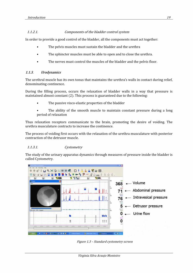
1.1.3.1. Cystometry
The study of the urinary apparatus dynamics through measures of pressure inside the bladder is called Cystometry.
Figure 1.3 – Standard cystometry screen
20 Chapter 1
Computational Model of the Human Urinay Bladder
This study comprises the voiding and gradual filling of the bladder, corresponding on average to a 50ml/min of filling rate.
1.2. Motivation
Today bladder cancer is among the most frequent cases of oncologic diseases in United States and Europe (3). This kind of cancer can be classified as superficial or invasive, depending if the cancer reaches or not the detrusor muscle. The detrusor muscle is responsible for the mechanics of filling and voiding of the bladder and storage of urine under low pressure.
The extirpation of the bladder is required in most of the cases of invasive cancer. This procedure is also called cystectomy and the bladder can be replaced by an ileal bladder, which consists of a bladder made of intestinal tissue. Unfortunately this solution presents not only functional mechanical problems (described on the literature as voiding and leaking problems) but also biological ones (i.e. bone loss, given the absorption by the intestine of substances that should be eliminated from the organism).
The Finite Element Method modeling of the bladder will allow to identify and measure the mechanical variables that govern this organ and to propose geometrical improvements and solutions to address the cases on which the bladder needs to be removed.
The numerical model requires the implementation of a non-linear constitutive model capable to accurately represent the mechanics of filling and voiding of the bladder, considering the low pressure storage of urine.
1.3. General Objectives
A tentative numerical model implemented using the Finite Element Method is proposed for the simulation of the urinary bladder. The objective is to simulate the main mechanic part of the bladder: the detrusor, a smooth muscle that is responsible for maintaining an almost constant pressure inside the bladder during the filling and the storage of the urine.
The challenge comprises also the representation of bladder dynamics of filling, storage and voiding considering the forces exerted by urine on the bladder wall. By modeling numerically the urine, it is possible to extract relevant fluid information, such as urine velocity, flow rate and flow pattern, that can explain urological conditions.
In order to represent numerically bladder mechanics and dynamics, four detailed objectives are defined and comprehend the basis of this thesis. These objectives are the implementation and validation of the constitutive model of the bladder; import and treatment of the geometrical model obtained by computerized tomography images; numerical simulation of bladder and urine considering fluid-structure interaction; and finally validation of the model with experimental data.
1.4. Objective details
Smooth muscles are known by its nonlinear behavior, and in the specific case of the detrusor the change in the stiffness is promoted not only by its mechanical properties but also by chemical
Introduction 21
Virginia Silva Araujo Monteiro
reactions. The detrusor is innervated by an autonomic nervous system that allows the muscle to be partly contracted, maintaining tonus for prolonged periods with low energy consumption.
Given the complexity of biological materials and its multi-scale hierarchy, some simplifications were made and the classical nonlinear continuum mechanics theory was applied. The proposed model is based in the representation of the detrusor tissue by two different structures: a hyperelastic matrix, representing the extracellular substance, and viscoelastic fibres, representing the passive fibres. For the sake of simplicity the chemical reactions were not taken into account in this model.
For the implementation, a stress-strain relationship is specified based on the evaluation of the strain energy function. The first part of the model consists on the implementation of a hyperelastic model, based on a quasi-incompressible neo-Hookean model, followed by its validation with results from the literature. Second the viscoelastic constitutive model has been implemented. The analysis is treated within a 3D framework in total Lagragian description and quasi-incompressible material. Benchmark experiments were done to validate it.
The interaction of the bladder wall with urine is modeled via the Particle Finite Element Method (PFEM) (4). The PFEM allows the reproduction of filling and voiding of the bladder with urine, accounting for the wall-fluid interaction effect. Examples of the bladder under different filling and voiding conditions are presented.
The points already exposed can be grouped in four main subjects and subdivided in specific items, as presented in Table 1.1.
Subject Objective details
Geometric model of
the bladder
treatment of geometric data obtained from computerized tomography;
simplification of the geometry to consider boundary conditions;
meshing geometric data using GID pre-post processor.
Implementation of
the constitutive
model of the
bladder
definition of the material parameters;
implementation and validation of hyperelastic neo-Hookean model;
implementation and validation of viscoelastic Generalized Maxwell model;
implementation of the homogenized model considering fibers,
structural analisis of the bladder considering the different constitutive models.
Numerical
Analysis with
Fluid-Strucuture
Interaction
consideration of different scenarios for the orientation of muscle fibers;
simulation of the filling of the bladder under different conditions: slow and fast filling rates;
simulation of voiding of the bladder under different conditions: considering abdominal
pressure and retraction of the musculature;
consideration of different boundary conditions;
evaluation and analysis of graphics: Cauchy stress vs Pressure, Tension vs Volume.
22 Chapter 1
Computational Model of the Human Urinay Bladder
Validation of the
Model
definition of representative urodynamic tests to represent the filling and voiding of the
bladder;
treatment of experimental data;
calibration of the numerical model to accurately represent the experimental data.
Table 1.1– Objective details
1.5. Methodology
The Finite Element Method (FEM) (5) modelling of the bladder allows the identification and measurement of the mechanical variables that govern this organ and to propose geometrical improvements and solutions to address the cases on which the bladder needs to be removed.
The numerical study requires the implementation of a non-linear constitutive model capable to accurately represent the mechanics of filling and voiding of the bladder, considering the low pressure storage of urine.
Smooth muscles are known by its nonlinear behavior, and in the specific case of the detrusor the change in the stiffness is promoted not only by its mechanical properties but also by chemical reactions. The detrusor is innervated by an autonomic nervous system that allows the muscle to be partly contracted, maintaining tonus for prolonged periods with low energy consumption.
Given the complexity of biological materials and its multi-scale hierarchy, some simplifications were made and the classical nonlinear continuum mechanics theory was applied. The proposed model is based on the three dimensional representation of the detrusor tissue by two different structures: a hyperelastic matrix, representing the extracellular substance, and viscoelastic fibres, representing the passive fibres (6). For the sake of simplicity, the chemical reactions are not taken into account in this model. The homogenization theory is considered to represent the integration of these two main structures.
To represent the mechanics of the bladder, the constitutive equations here presented are written in a total Lagragian approach, were the unknown displacements are described in the reference configuration.
In short, the model considers the implementation of a Hyperelastic-Viscoelastic constitutive law in a finite element code allowing for Fluid Structure Interaction (FSI) effect for the simulation of bladder wall and urine. The problem is solved iteractively by the Newton-Raphson method with a Bossak Scheme.
1.5.1. Bladder-material in short
The main mechanical part of the bladder consists on the detrusor, a smooth muscle that is responsible for maintaining an almost constant internal pressure during the filling and voiding of the bladder with urine. This phenomenon occurs because the detrusor accounts with its mechanical properties and also chemical reactions to change its stiffness.
Smooth muscles are innervated by an autonomic nervous system, that allows them to be partly contracted, maintaining tonus for prolonged periods with low energy consumption. In the case
Introduction 23
Virginia Silva Araujo Monteiro
of the bladder smooth muscle, stiffness is also increased due to a phenomenon called Latch Mechanism.
The detrusor can be represented as a sum of 3 main structures:
• Matrix: corresponds to extra-cellular substance, and have a hyperelastic behaviour
• Passive fibres: made of collagen, its mechanics can be represented through a viscoelastic model
• Active fibres: muscles cells responsible for increasing bladder stiffness when activated by electrical impulses, also called Latch Mechanism.
1.5.2. The proposed constitutive model
In order to have a numerical simulation of the bladder mechanics the FEM was chosen, and homogenization theory is putted in place to represent the integration of the three main structures described above.
To represent the mechanics the equations are written in a total Lagragian approach, were the unknown displacements are described in the reference conFiguretion.
The implementation of the code consists in 3 phases, as follows:
1. Hyperleastic Neo-Hookean model
2. Visco-elastic Generalized Maxwell model
3. Homogenized model: hyperelastic matrix with viscoelastic fibers
Simulations of filling and voiding of the bladder has been done in two different ways: first imposing constant pressure, and second through fluid-structure interaction.
Further in this chapter it is possible to find introductory information on general urology and a review of what has been done in modelling the bladder. The State of Art gives the background and essential knowledge to understand this thesis. The first theme is related to urology and in the second part of the chapter a review of computational models in urology is given, with emphasis on the simulation of the urinary bladder.
1.6. State of Art
The simulation of the urinary bladder is still a challenge to overcome. The first intend models considered hyperelastic constitutive models. The scientific community realized the necessity to implement more complex models to simulate this organ and accurately represent its ability to store urine under low pressure due to relaxation of its musculature. Viscoelastic models were introduced in the following years. More refined models with combined elasticity and viscoelasticity were considered. A homogenized model to represent the multi-scale hierarchy of elements in the smooth muscle tissue is proposed. The combination of hyperelasticity and viscoelasticity has been put in place in recent years (7; 8; 9; 10).
1.6.1. Proposed models for the bladder mechanics
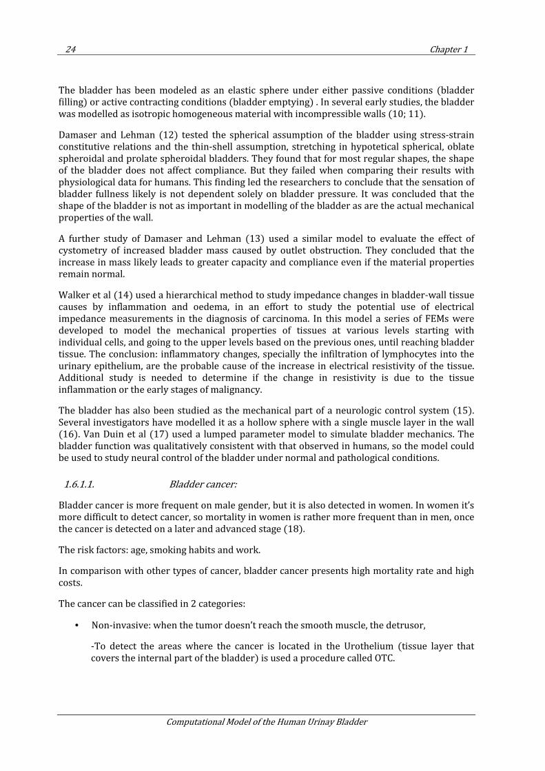
24 Chapter 1
Computational Model of the Human Urinay Bladder
The bladder has been modeled as an elastic sphere under either passive conditions (bladder filling) or active contracting conditions (bladder emptying) . In several early studies, the bladder was modelled as isotropic homogeneous material with incompressible walls (10; 11).
Damaser and Lehman (12) tested the spherical assumption of the bladder using stress-strain constitutive relations and the thin-shell assumption, stretching in hypotetical spherical, oblate spheroidal and prolate spheroidal bladders. They found that for most regular shapes, the shape of the bladder does not affect compliance. But they failed when comparing their results with physiological data for humans. This finding led the researchers to conclude that the sensation of bladder fullness likely is not dependent solely on bladder pressure. It was concluded that the shape of the bladder is not as important in modelling of the bladder as are the actual mechanical properties of the wall.
A further study of Damaser and Lehman (13) used a similar model to evaluate the effect of cystometry of increased bladder mass caused by outlet obstruction. They concluded that the increase in mass likely leads to greater capacity and compliance even if the material properties remain normal.
Walker et al (14) used a hierarchical method to study impedance changes in bladder-wall tissue causes by inflammation and oedema, in an effort to study the potential use of electrical impedance measurements in the diagnosis of carcinoma. In this model a series of FEMs were developed to model the mechanical properties of tissues at various levels starting with individual cells, and going to the upper levels based on the previous ones, until reaching bladder tissue. The conclusion: inflammatory changes, specially the infiltration of lymphocytes into the urinary epithelium, are the probable cause of the increase in electrical resistivity of the tissue. Additional study is needed to determine if the change in resistivity is due to the tissue inflammation or the early stages of malignancy.
The bladder has also been studied as the mechanical part of a neurologic control system (15). Several investigators have modelled it as a hollow sphere with a single muscle layer in the wall (16). Van Duin et al (17) used a lumped parameter model to simulate bladder mechanics. The bladder function was qualitatively consistent with that observed in humans, so the model could be used to study neural control of the bladder under normal and pathological conditions.
1.6.1.1. Bladder cancer:
Bladder cancer is more frequent on male gender, but it is also detected in women. In women it’s more difficult to detect cancer, so mortality in women is rather more frequent than in men, once the cancer is detected on a later and advanced stage (18).
The risk factors: age, smoking habits and work.
In comparison with other types of cancer, bladder cancer presents high mortality rate and high costs.
The cancer can be classified in 2 categories:
• Non-invasive: when the tumor doesn’t reach the smooth muscle, the detrusor,
-To detect the areas where the cancer is located in the Urothelium (tissue layer that covers the internal part of the bladder) is used a procedure called OTC.
Introduction 25
Virginia Silva Araujo Monteiro
-When the cancer is detected, the patient is submitted to TURB (surgery for the removal of the damaged parts). Flexible cystecopy is used to visualize the tumor (using White or blue light).
- The reoccurrence rate of this kind of tumor is the highest among all kinds of cancer (25-50%)
• Invasive: the tumor reaches the detrusor
-In most of the cases cystectomy is recommended (removal of the bladder)
-The bladder is replaced by an ileal bladder (a bladder made of intestine tissue)
1.6.2. United States data on bladder cancer
According to the Agency for Health Care Policy and Research of the US Public Health Service, annual expenditures are $2.2 billion for bladder cancer versus $1.4 billion for prostate cancer. Two thirds of the costs are spent with non-invasive cancer (3).
Bladder cancer results in the death of approximately 12,500 Americans each year. The vast majority of the 57,400 patients newly diagnosed with bladder cancer annually have noninvasive disease at the time of diagnosis, but they are prone to multiple recurrences. Although most of these patients are at low risk for cancer progression or death, monitoring is required to identify the need for further intervention. White persons are more likely to develop bladder cancer, but African Americans appear to have a worse prognosis.
Bladder cancer is the fourth most common cancer diagnosed in men. In contrast, it is the ninth most common cause of cancer in women. The number of men diagnosed with bladder cancer annually is 42,200, whereas the number of women diagnosed with bladder cancer annually is 15,200.
According to the US National Cancer Institute, bladder cancer affects approximately 500,000 people in America. Because most still have an intact bladder, the number of patients under surveillance approaches this figure.
1.6.2.1. Substitutes for the bladder
Ileal bladder (intestine):
Ileal tissue is a portion of the intestine of around 10 to 15 cm that connects small and large intestine. It can be used to make the ileal bladder, but this solution presents some functional problems:
- 33% leakage
- 22% voiding problems (21% related to mechanical problems and 1% related to a “non-relaxing pelvic floor”).
- Mucus and stones production
- Urinary infection
26 Chapter 1
Computational Model of the Human Urinay Bladder
In most of the cases, the ileal bladder is connected to a stoma (an orifice made in the skin) and connected to a plastic bag external to the body. When the ileal bladder is connected to the urethra, it is called orthotropic bladder. In this case, 22% of the women present incontinence. To avoid voiding a catheter (CIC) is used.
The patients also show discomfort and bone loss due to the fact that the intestine absorbs substances that should be eliminated from the body.
1.6.2.2. The artificial bladder
An artificial bladder must address the following (19):
- The bladder must maintain a maximum pressure of 40 to 70 cm H2O.
- Must maintain the capacity of 500 cm3
- The material to be considered must be sufficiently clean to avoid the culture of germs.
- Must distend in a progressive way
- Its duration must be 30 to 40 years
1.6.2.3. Tissue engineering
In April 2006, researchers declared the implementation of artificial bladders made through the culture of cells of the patients’ bladder. One advantage of this method is that the cells are originated from the patient, avoiding the risk of a negative answer from the immunologic system, and without any risk of rejection (20).
The process of cell culture is explained below (Figure 1.4).
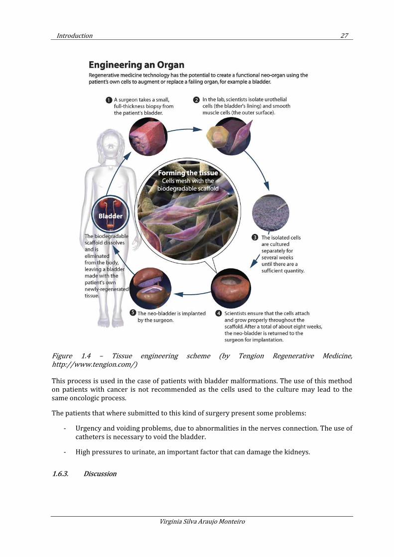
Introduction 27
Virginia Silva Araujo Monteiro
Figure 1.4 – Tissue engineering scheme (by Tengion Regenerative Medicine,
http://www.tengion.com/)
This process is used in the case of patients with bladder malformations. The use of this method on patients with cancer is not recommended as the cells used to the culture may lead to the same oncologic process.
The patients that where submitted to this kind of surgery present some problems:
- Urgency and voiding problems, due to abnormalities in the nerves connection. The use of catheters is necessary to void the bladder.
- High pressures to urinate, an important factor that can damage the kidneys.
1.6.3. Discussion
28 Chapter 1
Computational Model of the Human Urinay Bladder
The numerical simulation of the human bladder considering fluid structure interaction and a similar geometry for this organ is still an objective to overcome.
The difficulty to validate the model and to have in vivo experiments to accurately get the parameters for the constitutive model proposed for this organ is an obstacle to the correct simulation of the bladder.
1.7. Structure of the thesis
Introductory information on general urology is given In Chapter 2. The first part of this chapter is related to general urology, exposing the main structures of the Urinary Apparatus, explaining briefly each organ function and the form of interaction with each other. The second part comprises the is gives an overview on the anatomy of the lower urinary tract.
The main developments in this work are presented on Chapter 3. Both geometrical aspects and the constitutive model for the human bladder are detailed. This is probably the most dense and important topic of this thesis, and is derived from previous works of the scientific community and experience of CIMNE in computational models and bioengineering projects.
Having presented the mathematical model for the structural analyisis, Fluid-Structure Interaction is then introduced in Section 3.7. Considerations on the equations that govern the fluid are exposed.
Validation and Clinical data is exposed in Chapter 4. The data here presented was provided by Hospital Clinic of Barcelona.
Finally, we introduce in Chapter 5 the numerical simulation of a neobladder, the current alternative for bladder replacement.
Conclusions and perspectives for future work are presented in Chapter 6.
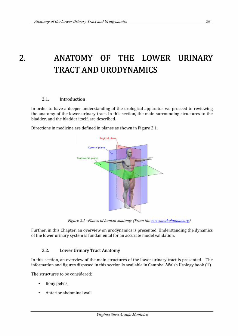
Anatomy of the Lower Urinary Tract and Urodynamics 29
Virginia Silva Araujo Monteiro
2. ANATOMY OF THE LOWER URINARY
TRACT AND URODYNAMICS
2.1. Introduction
In order to have a deeper understanding of the urological apparatus we proceed to reviewing the anatomy of the lower urinary tract. In this section, the main surrounding structures to the bladder, and the bladder itself, are described.
Directions in medicine are defined in planes as shown in Figure 2.1.
Figure 2.1 –Planes of human anatomy (From the www.makehuman.org)
Further, in this Chapter, an overview on urodynamics is presented. Understanding the dynamics of the lower urinary system is fundamental for an accurate model validation.
2.2. Lower Urinary Tract Anatomy
In this section, an overview of the main structures of the lower urinary tract is presented. The information and figures disposed in this section is available in Campbel-Walsh Urology book (1).
The structures to be considered:
• Bony pelvis,
• Anterior abdominal wall
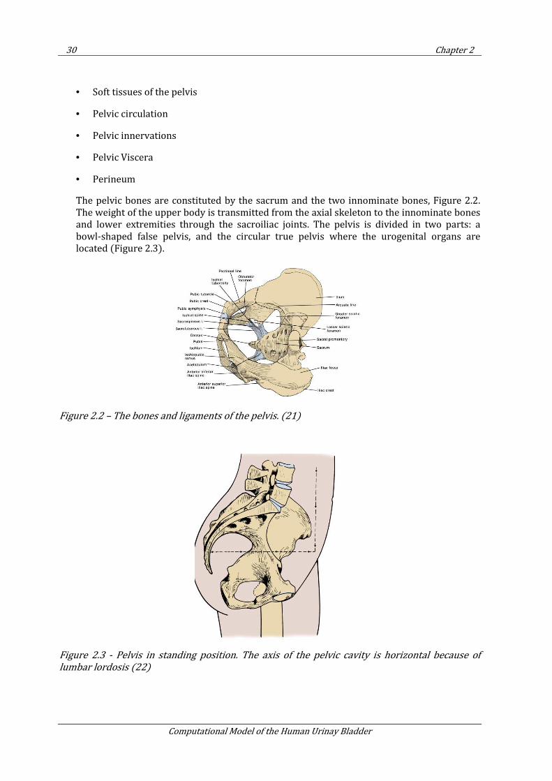
30 Chapter 2
Computational Model of the Human Urinay Bladder
• Soft tissues of the pelvis
• Pelvic circulation
• Pelvic innervations
• Pelvic Viscera
• Perineum
The pelvic bones are constituted by the sacrum and the two innominate bones, Figure 2.2. The weight of the upper body is transmitted from the axial skeleton to the innominate bones and lower extremities through the sacroiliac joints. The pelvis is divided in two parts: a bowl-shaped false pelvis, and the circular true pelvis where the urogenital organs are located (Figure 2.3).
Figure 2.2 – The bones and ligaments of the pelvis. (21)
Figure 2.3 - Pelvis in standing position. The axis of the pelvic cavity is horizontal because of
lumbar lordosis (22)
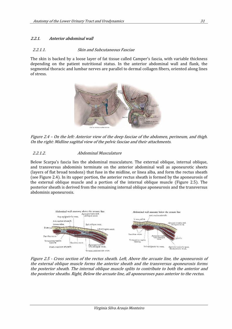
Anatomy of the Lower Urinary Tract and Urodynamics 31
Virginia Silva Araujo Monteiro
2.2.1. Anterior abdominal wall
2.2.1.1. Skin and Subcutaneous Fasciae
The skin is backed by a loose layer of fat tissue called Camper's fascia, with variable thickness depending on the patient nutritional status. In the anterior abdominal wall and flank, the segmental thoracic and lumbar nerves are parallel to dermal collagen fibers, oriented along lines of stress.
Figure 2.4 – On the left: Anterior view of the deep fasciae of the abdomen, perineum, and thigh.
On the right: Midline sagittal view of the pelvic fasciae and their attachments.
2.2.1.2. Abdominal Musculature
Below Scarpa's fascia lies the abdominal musculature. The external oblique, internal oblique, and transversus abdominis terminate on the anterior abdominal wall as aponeurotic sheets (layers of flat broad tendons) that fuse in the midline, or linea alba, and form the rectus sheath (see Figure 2.4). In its upper portion, the anterior rectus sheath is formed by the aponeurosis of the external oblique muscle and a portion of the internal oblique muscle (Figure 2.5). The posterior sheath is derived from the remaining internal oblique aponeurosis and the transversus abdominis aponeurosis.
Figure 2.5 - Cross section of the rectus sheath. Left, Above the arcuate line, the aponeurosis of
the external oblique muscle forms the anterior sheath and the transversus aponeurosis forms
the posterior sheath. The internal oblique muscle splits to contribute to both the anterior and
the posterior sheaths. Right, Below the arcuate line, all aponeuroses pass anterior to the rectus.
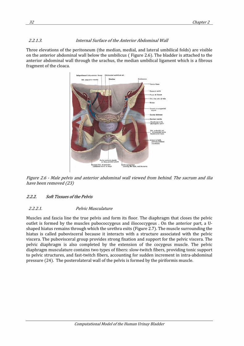
32 Chapter 2
Computational Model of the Human Urinay Bladder
2.2.1.3. Internal Surface of the Anterior Abdominal Wall
Three elevations of the peritoneum (the median, medial, and lateral umbilical folds) are visible on the anterior abdominal wall below the umbilicus ( Figure 2.6). The bladder is attached to the anterior abdominal wall through the urachus, the median umbilical ligament which is a fibrous fragment of the cloaca.
Figure 2.6 - Male pelvis and anterior abdominal wall viewed from behind. The sacrum and ilia
have been removed (23)
2.2.2. Soft Tissues of the Pelvis
2.2.2.1. Pelvic Musculature
Muscles and fascia line the true pelvis and form its floor. The diaphragm that closes the pelvic outlet is formed by the muscles pubococcygeus and iliococcygeus . On the anterior part, a U-shaped hiatus remains through which the urethra exits (Figure 2.7). The muscle surrounding the hiatus is called pubovisceral because it interacts with a structure associated with the pelvic viscera. The pubovisceral group provides strong fixation and support for the pelvic viscera. The pelvic diaphragm is also completed by the extension of the cocygeus muscle. The pelvic diaphragm musculature contains two types of fibers: slow-twitch fibers, providing tonic support to pelvic structures, and fast-twitch fibers, accounting for sudden increment in intra-abdominal pressure (24). The posterolateral wall of the pelvis is formed by the piriformis muscle.
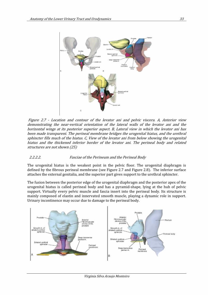
Anatomy of the Lower Urinary Tract and Urodynamics 33
Virginia Silva Araujo Monteiro
Figure 2.7 - Location and contour of the levator ani and pelvic viscera. A, Anterior view
demonstrating the near-vertical orientation of the lateral walls of the levator ani and the
horizontal wings at its posterior superior aspect. B, Lateral view in which the levator ani has
been made transparent. The perineal membrane bridges the urogenital hiatus, and the urethral
sphincter fills much of the hiatus. C, View of the levator ani from below showing the urogenital
hiatus and the thickened inferior border of the levator ani. The perineal body and related
structures are not shown (25)
2.2.2.2. Fasciae of the Perineum and the Perineal Body
The urogenital hiatus is the weakest point in the pelvic floor. The urogenital diaphragm is defined by the fibrous perineal membrane (see Figure 2.7 and Figure 2.8). The inferior surface attaches the external genitalia, and the superior part gives support to the urethral sphincter.
The fusion between the posterior edge of the urogenital diaphragm and the posterior apex of the urogenital hiatus is called perineal body and has a pyramid-shape, lying at the hub of pelvic support. Virtually every pelvic muscle and fascia insert into the perineal body. Its structure is mainly composed of elastin and innervated smooth muscle, playing a dynamic role in support. Urinary incontinence may occur due to damage to the perineal body.
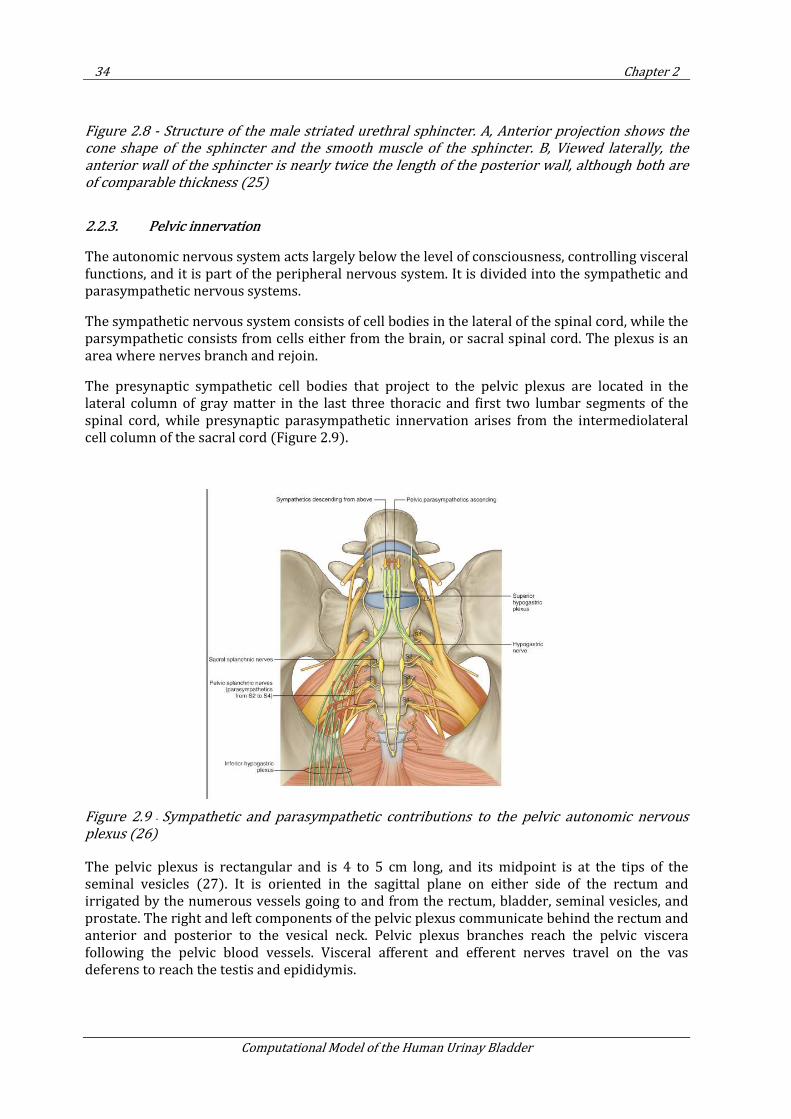
34 Chapter 2
Computational Model of the Human Urinay Bladder
Figure 2.8 - Structure of the male striated urethral sphincter. A, Anterior projection shows the
cone shape of the sphincter and the smooth muscle of the sphincter. B, Viewed laterally, the
anterior wall of the sphincter is nearly twice the length of the posterior wall, although both are
of comparable thickness (25)
2.2.3. Pelvic innervation
The autonomic nervous system acts largely below the level of consciousness, controlling visceral functions, and it is part of the peripheral nervous system. It is divided into the sympathetic and parasympathetic nervous systems.
The sympathetic nervous system consists of cell bodies in the lateral of the spinal cord, while the parsympathetic consists from cells either from the brain, or sacral spinal cord. The plexus is an area where nerves branch and rejoin.
The presynaptic sympathetic cell bodies that project to the pelvic plexus are located in the lateral column of gray matter in the last three thoracic and first two lumbar segments of the spinal cord, while presynaptic parasympathetic innervation arises from the intermediolateral cell column of the sacral cord (Figure 2.9).
Figure 2.9 - Sympathetic and parasympathetic contributions to the pelvic autonomic nervous
plexus (26)
The pelvic plexus is rectangular and is 4 to 5 cm long, and its midpoint is at the tips of the seminal vesicles (27). It is oriented in the sagittal plane on either side of the rectum and irrigated by the numerous vessels going to and from the rectum, bladder, seminal vesicles, and prostate. The right and left components of the pelvic plexus communicate behind the rectum and anterior and posterior to the vesical neck. Pelvic plexus branches reach the pelvic viscera following the pelvic blood vessels. Visceral afferent and efferent nerves travel on the vas deferens to reach the testis and epididymis.
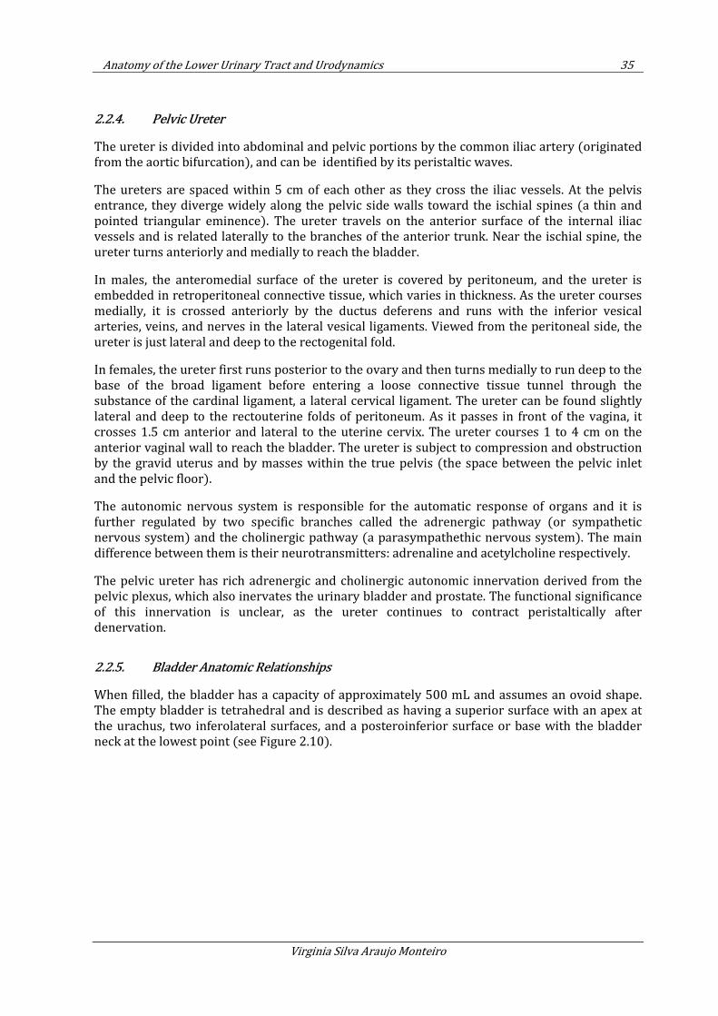
Anatomy of the Lower Urinary Tract and Urodynamics 35
Virginia Silva Araujo Monteiro
2.2.4. Pelvic Ureter
The ureter is divided into abdominal and pelvic portions by the common iliac artery (originated from the aortic bifurcation), and can be identified by its peristaltic waves.
The ureters are spaced within 5 cm of each other as they cross the iliac vessels. At the pelvis entrance, they diverge widely along the pelvic side walls toward the ischial spines (a thin and pointed triangular eminence). The ureter travels on the anterior surface of the internal iliac vessels and is related laterally to the branches of the anterior trunk. Near the ischial spine, the ureter turns anteriorly and medially to reach the bladder.
In males, the anteromedial surface of the ureter is covered by peritoneum, and the ureter is embedded in retroperitoneal connective tissue, which varies in thickness. As the ureter courses medially, it is crossed anteriorly by the ductus deferens and runs with the inferior vesical arteries, veins, and nerves in the lateral vesical ligaments. Viewed from the peritoneal side, the ureter is just lateral and deep to the rectogenital fold.
In females, the ureter first runs posterior to the ovary and then turns medially to run deep to the base of the broad ligament before entering a loose connective tissue tunnel through the substance of the cardinal ligament, a lateral cervical ligament. The ureter can be found slightly lateral and deep to the rectouterine folds of peritoneum. As it passes in front of the vagina, it crosses 1.5 cm anterior and lateral to the uterine cervix. The ureter courses 1 to 4 cm on the anterior vaginal wall to reach the bladder. The ureter is subject to compression and obstruction by the gravid uterus and by masses within the true pelvis (the space between the pelvic inlet and the pelvic floor).
The autonomic nervous system is responsible for the automatic response of organs and it is further regulated by two specific branches called the adrenergic pathway (or sympathetic nervous system) and the cholinergic pathway (a parasympathethic nervous system). The main difference between them is their neurotransmitters: adrenaline and acetylcholine respectively.
The pelvic ureter has rich adrenergic and cholinergic autonomic innervation derived from the pelvic plexus, which also inervates the urinary bladder and prostate. The functional significance of this innervation is unclear, as the ureter continues to contract peristaltically after denervation.
2.2.5. Bladder Anatomic Relationships
When filled, the bladder has a capacity of approximately 500 mL and assumes an ovoid shape. The empty bladder is tetrahedral and is described as having a superior surface with an apex at the urachus, two inferolateral surfaces, and a posteroinferior surface or base with the bladder neck at the lowest point (see Figure 2.10).
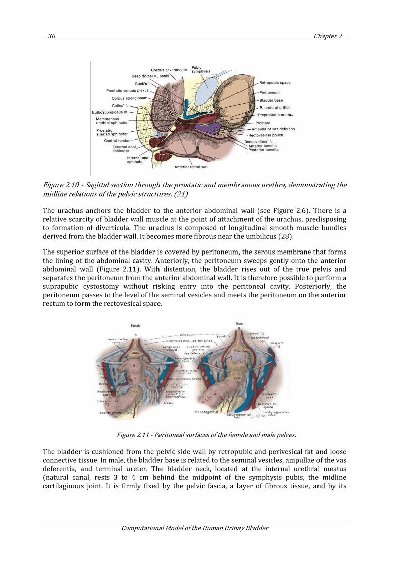
36 Chapter 2
Computational Model of the Human Urinay Bladder
Figure 2.10 - Sagittal section through the prostatic and membranous urethra, demonstrating the
midline relations of the pelvic structures. (21)
The urachus anchors the bladder to the anterior abdominal wall (see Figure 2.6). There is a relative scarcity of bladder wall muscle at the point of attachment of the urachus, predisposing to formation of diverticula. The urachus is composed of longitudinal smooth muscle bundles derived from the bladder wall. It becomes more fibrous near the umbilicus (28).
The superior surface of the bladder is covered by peritoneum, the serous membrane that forms the lining of the abdominal cavity. Anteriorly, the peritoneum sweeps gently onto the anterior abdominal wall (Figure 2.11). With distention, the bladder rises out of the true pelvis and separates the peritoneum from the anterior abdominal wall. It is therefore possible to perform a suprapubic cystostomy without risking entry into the peritoneal cavity. Posteriorly, the peritoneum passes to the level of the seminal vesicles and meets the peritoneum on the anterior rectum to form the rectovesical space.
Figure 2.11 - Peritoneal surfaces of the female and male pelves.
The bladder is cushioned from the pelvic side wall by retropubic and perivesical fat and loose connective tissue. In male, the bladder base is related to the seminal vesicles, ampullae of the vas deferentia, and terminal ureter. The bladder neck, located at the internal urethral meatus (natural canal, rests 3 to 4 cm behind the midpoint of the symphysis pubis, the midline cartilaginous joint. It is firmly fixed by the pelvic fascia, a layer of fibrous tissue, and by its
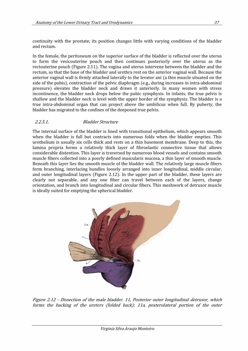
Anatomy of the Lower Urinary Tract and Urodynamics 37
Virginia Silva Araujo Monteiro
continuity with the prostate; its position changes little with varying conditions of the bladder and rectum.
In the female, the peritoneum on the superior surface of the bladder is reflected over the uterus to form the vesicouterine pouch and then continues posteriorly over the uterus as the rectouterine pouch (Figure 2.11). The vagina and uterus intervene between the bladder and the rectum, so that the base of the bladder and urethra rest on the anterior vaginal wall. Because the anterior vaginal wall is firmly attached laterally to the levator ani (a thin muscle situated on the side of the pubis), contraction of the pelvic diaphragm (e.g., during increases in intra-abdominal pressure) elevates the bladder neck and draws it anteriorly. In many women with stress incontinence, the bladder neck drops below the pubic symphysis. In infants, the true pelvis is shallow and the bladder neck is level with the upper border of the symphysis. The bladder is a true intra-abdominal organ that can project above the umbilicus when full. By puberty, the bladder has migrated to the confines of the deepened true pelvis.
2.2.5.1. Bladder Structure
The internal surface of the bladder is lined with transitional epithelium, which appears smooth when the bladder is full but contracts into numerous folds when the bladder empties. This urothelium is usually six cells thick and rests on a thin basement membrane. Deep to this, the lamina propria forms a relatively thick layer of fibroelastic connective tissue that allows considerable distention. This layer is traversed by numerous blood vessels and contains smooth muscle fibers collected into a poorly defined muscularis mucosa, a thin layer of smooth muscle. Beneath this layer lies the smooth muscle of the bladder wall. The relatively large muscle fibers form branching, interlacing bundles loosely arranged into inner longitudinal, middle circular, and outer longitudinal layers (Figure 2.12). In the upper part of the bladder, these layers are clearly not separable, and any one fiber can travel between each of the layers, change orientation, and branch into longitudinal and circular fibers. This meshwork of detrusor muscle is ideally suited for emptying the spherical bladder.
Figure 2.12 - Dissection of the male bladder. 11, Posterior outer longitudinal detrusor, which
forms the backing of the ureters (folded back); 11a, posterolateral portion of the outer
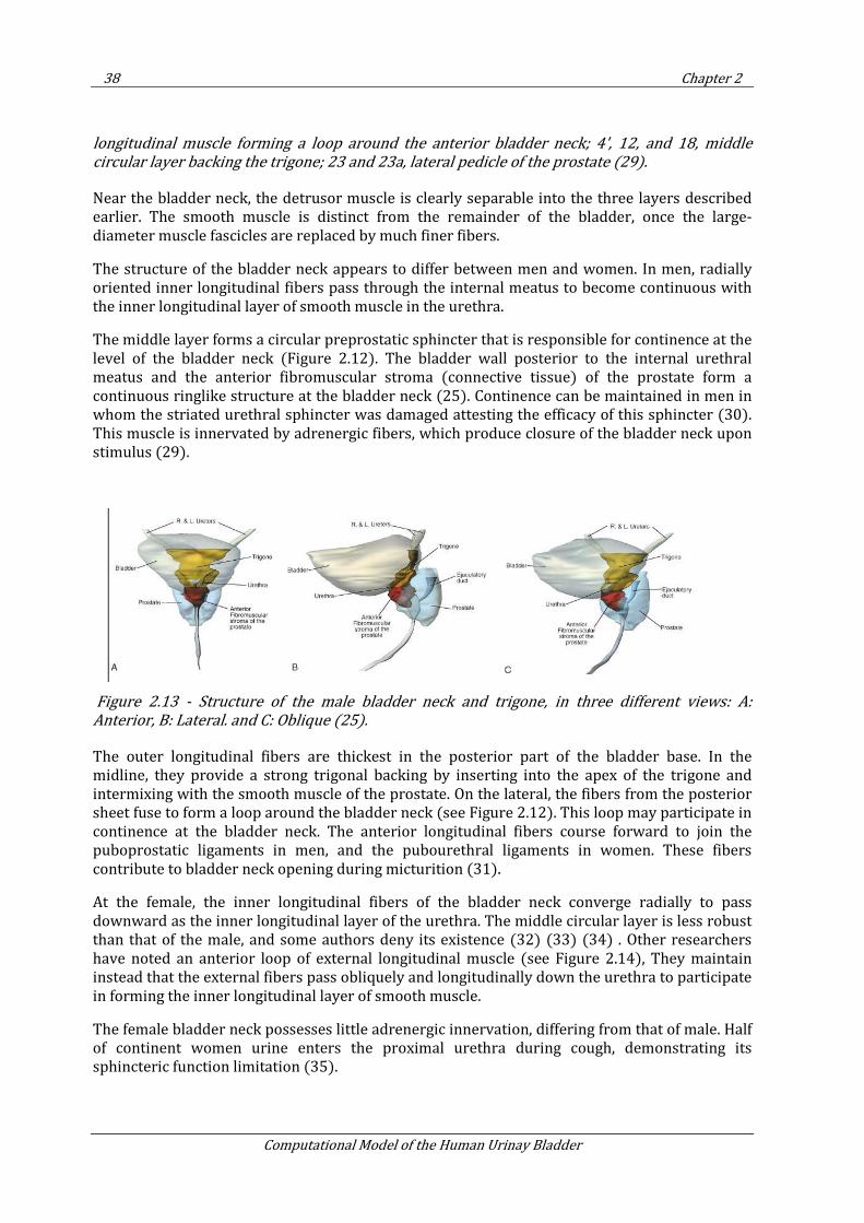
38 Chapter 2
Computational Model of the Human Urinay Bladder
longitudinal muscle forming a loop around the anterior bladder neck; 4', 12, and 18, middle
circular layer backing the trigone; 23 and 23a, lateral pedicle of the prostate (29).
Near the bladder neck, the detrusor muscle is clearly separable into the three layers described earlier. The smooth muscle is distinct from the remainder of the bladder, once the large-diameter muscle fascicles are replaced by much finer fibers.
The structure of the bladder neck appears to differ between men and women. In men, radially oriented inner longitudinal fibers pass through the internal meatus to become continuous with the inner longitudinal layer of smooth muscle in the urethra.
The middle layer forms a circular preprostatic sphincter that is responsible for continence at the level of the bladder neck (Figure 2.12). The bladder wall posterior to the internal urethral meatus and the anterior fibromuscular stroma (connective tissue) of the prostate form a continuous ringlike structure at the bladder neck (25). Continence can be maintained in men in whom the striated urethral sphincter was damaged attesting the efficacy of this sphincter (30). This muscle is innervated by adrenergic fibers, which produce closure of the bladder neck upon stimulus (29).
Figure 2.13 - Structure of the male bladder neck and trigone, in three different views: A:
Anterior, B: Lateral. and C: Oblique (25).
The outer longitudinal fibers are thickest in the posterior part of the bladder base. In the midline, they provide a strong trigonal backing by inserting into the apex of the trigone and intermixing with the smooth muscle of the prostate. On the lateral, the fibers from the posterior sheet fuse to form a loop around the bladder neck (see Figure 2.12). This loop may participate in continence at the bladder neck. The anterior longitudinal fibers course forward to join the puboprostatic ligaments in men, and the pubourethral ligaments in women. These fibers contribute to bladder neck opening during micturition (31).
At the female, the inner longitudinal fibers of the bladder neck converge radially to pass downward as the inner longitudinal layer of the urethra. The middle circular layer is less robust than that of the male, and some authors deny its existence (32) (33) (34) . Other researchers have noted an anterior loop of external longitudinal muscle (see Figure 2.14), They maintain instead that the external fibers pass obliquely and longitudinally down the urethra to participate in forming the inner longitudinal layer of smooth muscle.
The female bladder neck possesses little adrenergic innervation, differing from that of male. Half of continent women urine enters the proximal urethra during cough, demonstrating its sphincteric function limitation (35).
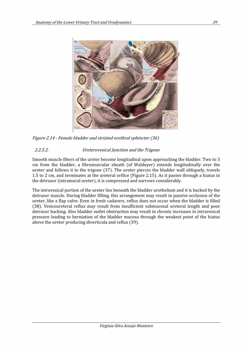
Anatomy of the Lower Urinary Tract and Urodynamics 39
Virginia Silva Araujo Monteiro
Figure 2.14 - Female bladder and striated urethral sphincter (36)
2.2.5.2. Ureterovesical Junction and the Trigone
Smooth muscle fibers of the ureter become longitudinal upon approaching the bladder. Two to 3 cm from the bladder, a fibromuscular sheath (of Waldeyer) extends longitudinally over the ureter and follows it to the trigone (37). The ureter pierces the bladder wall obliquely, travels 1.5 to 2 cm, and terminates at the ureteral orifice (Figure 2.15). As it passes through a hiatus in the detrusor (intramural ureter), it is compressed and narrows considerably.
The intravesical portion of the ureter lies beneath the bladder urothelium and it is backed by the detrusor muscle. During bladder filling, this arrangement may result in passive occlusion of the ureter, like a flap valve. Even in fresh cadavers, reflux does not occur when the bladder is filled (38). Vesicoureteral reflux may result from insufficient submucosal ureteral length and poor detrusor backing. Also bladder outlet obstruction may result in chronic increases in intravesical pressure leading to herniation of the bladder mucosa through the weakest point of the hiatus above the ureter producing diverticula and reflux (39).
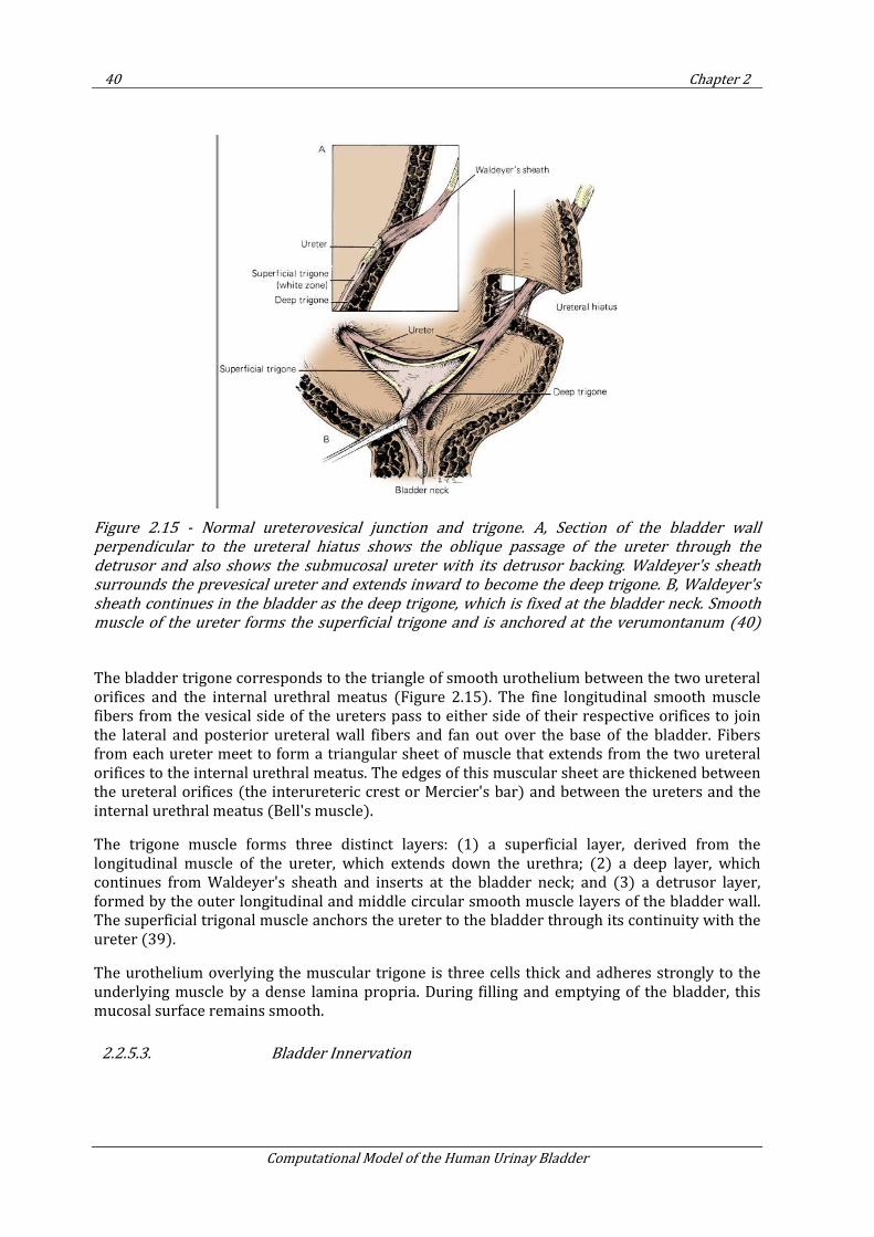
40 Chapter 2
Computational Model of the Human Urinay Bladder
Figure 2.15 - Normal ureterovesical junction and trigone. A, Section of the bladder wall
perpendicular to the ureteral hiatus shows the oblique passage of the ureter through the
detrusor and also shows the submucosal ureter with its detrusor backing. Waldeyer's sheath
surrounds the prevesical ureter and extends inward to become the deep trigone. B, Waldeyer's
sheath continues in the bladder as the deep trigone, which is fixed at the bladder neck. Smooth
muscle of the ureter forms the superficial trigone and is anchored at the verumontanum (40)
The bladder trigone corresponds to the triangle of smooth urothelium between the two ureteral orifices and the internal urethral meatus (Figure 2.15). The fine longitudinal smooth muscle fibers from the vesical side of the ureters pass to either side of their respective orifices to join the lateral and posterior ureteral wall fibers and fan out over the base of the bladder. Fibers from each ureter meet to form a triangular sheet of muscle that extends from the two ureteral orifices to the internal urethral meatus. The edges of this muscular sheet are thickened between the ureteral orifices (the interureteric crest or Mercier's bar) and between the ureters and the internal urethral meatus (Bell's muscle).
The trigone muscle forms three distinct layers: (1) a superficial layer, derived from the longitudinal muscle of the ureter, which extends down the urethra; (2) a deep layer, which continues from Waldeyer's sheath and inserts at the bladder neck; and (3) a detrusor layer, formed by the outer longitudinal and middle circular smooth muscle layers of the bladder wall. The superficial trigonal muscle anchors the ureter to the bladder through its continuity with the ureter (39).
The urothelium overlying the muscular trigone is three cells thick and adheres strongly to the underlying muscle by a dense lamina propria. During filling and emptying of the bladder, this mucosal surface remains smooth.
2.2.5.3. Bladder Innervation
Anatomy of the Lower Urinary Tract and Urodynamics 41
Virginia Silva Araujo Monteiro
The bladder is innervated by autonomic efferent fibers from the anterior portion of the pelvic plexus. Parasympathetic cholinergic nerve endings and postganglionic cell bodies supply the bladder wall.
The autonomic nervous system (or involuntary nervous system) activates the detrusor, and relaxation may occur due to sparse sympathetic innervation (41).
The male bladder neck receives sympathetic innervation and expresses α-adrenergic receptors. The female bladder neck has little adrenergic innervation. Nitric oxide synthase–containing neurons have been identified in the detrusor, particularly at the bladder neck, where they may facilitate relaxation during micturition.
The trigonal muscle is also innervated by adrenergic and nitric oxide synthase (an enzime)–containing neurons, and relaxes during micturition.
Bladder afferent innervation travels with sympathetic and parasympathetic nerves to reach the dorsal root ganglia (a mass of nerve cell bodies) located at thoracolumbar (reffering to the thoracic and lumbar parts of the spinal cord) and sacral (lower spine) levels.
2.2.6. Prostate
Traversed by the prostatic urethra, the average prostate measures 3 cm in length, 4 cm in width,
and 2 cm in depth, weighing 18 g. The prostate has an ovoid shape, but can be described through
its anterior, posterior, and lateral surfaces, with a narrowed apex inferiorly and a broad base
superiorly, contiguous with the bladder base. It is enclosed by a capsule composed of collagen,
elastin, and smooth muscle, an average thickness of 0.5 mm in its posteior and lateral parts. On
the anterior and anterolateral surfaces of the prostate, the capsule blends with the visceral
continuation of endopelvic fascia. The prostate is fixed to the pubic bone through the
puboprostatic ligaments.
The apex of the prostate is continuous with the striated urethral sphincter. Normal prostatic
glands can be found to extend into the striated muscle with no capsule. At the base of the
prostate, outer longitudinal fibers of the detrusor fuse and blend with the fibromuscular tissue
of the capsule. A preprostatic sphincter is formed with the middle circular and inner longitudinal
muscles extended down the prostatic urethra. No true capsule separates the prostate from the
bladder (42).
The prostate urethra is located closest to the anterior surface of the prostate. It is lined by transitional epithelium, which may extend into the prostatic ducts. The urothelium is surrounded by an inner longitudinal and an outer circular layer of smooth muscle. A urethral crest, a longitudinal fold on the posterior wall of the urethra, projects inward from the posterior midline, runs the length of the prostatic urethra, and disappears at the striated sphincter (Figure 2.16). To either side of this crest, a groove is formed (prostatic sinuses) into which all glandular elements drain (43).
The prostatic urethra is divided into proximal and distal segements functionally and anatomically discrete, at the urethra midpoint. In the proximal segment, the circular smooth muscle is thickened to form the involuntary internal urethral (preprostatic) sphincter. Small periurethral glands, extend between the fibers of the longitudinal smooth muscle to be enclosed by the preprostatic sphincter.
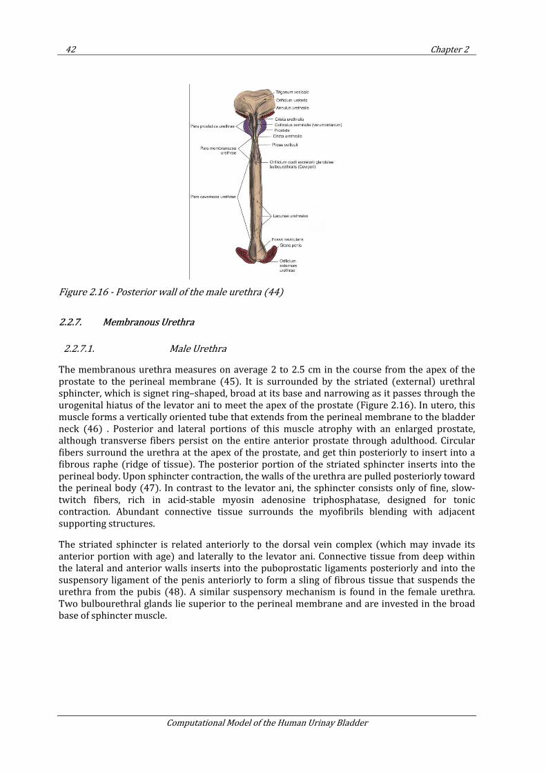
42 Chapter 2
Computational Model of the Human Urinay Bladder
Figure 2.16 - Posterior wall of the male urethra (44)
2.2.7. Membranous Urethra
2.2.7.1. Male Urethra
The membranous urethra measures on average 2 to 2.5 cm in the course from the apex of the prostate to the perineal membrane (45). It is surrounded by the striated (external) urethral sphincter, which is signet ring–shaped, broad at its base and narrowing as it passes through the urogenital hiatus of the levator ani to meet the apex of the prostate (Figure 2.16). In utero, this muscle forms a vertically oriented tube that extends from the perineal membrane to the bladder neck (46) . Posterior and lateral portions of this muscle atrophy with an enlarged prostate, although transverse fibers persist on the entire anterior prostate through adulthood. Circular fibers surround the urethra at the apex of the prostate, and get thin posteriorly to insert into a fibrous raphe (ridge of tissue). The posterior portion of the striated sphincter inserts into the perineal body. Upon sphincter contraction, the walls of the urethra are pulled posteriorly toward the perineal body (47). In contrast to the levator ani, the sphincter consists only of fine, slow-twitch fibers, rich in acid-stable myosin adenosine triphosphatase, designed for tonic contraction. Abundant connective tissue surrounds the myofibrils blending with adjacent supporting structures.
The striated sphincter is related anteriorly to the dorsal vein complex (which may invade its anterior portion with age) and laterally to the levator ani. Connective tissue from deep within the lateral and anterior walls inserts into the puboprostatic ligaments posteriorly and into the suspensory ligament of the penis anteriorly to form a sling of fibrous tissue that suspends the urethra from the pubis (48). A similar suspensory mechanism is found in the female urethra. Two bulbourethral glands lie superior to the perineal membrane and are invested in the broad base of sphincter muscle.
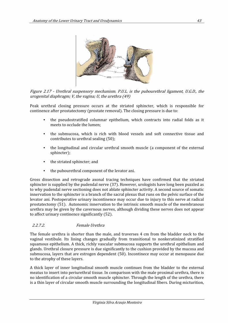
Anatomy of the Lower Urinary Tract and Urodynamics 43
Virginia Silva Araujo Monteiro
Figure 2.17 - Urethral suspensory mechanism. P.U.L. is the pubourethral ligament, U.G.D., the
urogenital diaphragm; V, the vagina; U, the urethra (49)
Peak urethral closing pressure occurs at the striated sphincter, which is responsible for continence after prostatectomy (prostate removal). The closing pressure is due to:
• the pseudostratified columnar epithelium, which contracts into radial folds as it meets to occlude the lumen;
• the submucosa, which is rich with blood vessels and soft connective tissue and contributes to urethral sealing (50);
• the longitudinal and circular urethral smooth muscle (a component of the external sphincter);
• the striated sphincter; and
• the pubourethral component of the levator ani.
Gross dissection and retrograde axonal tracing techniques have confirmed that the striated sphincter is supplied by the pudendal nerve (37). However, urologists have long been puzzled as to why pudendal nerve sectioning does not ablate sphincter activity. A second source of somatic innervation to the sphincter is a branch of the sacral plexus that runs on the pelvic surface of the levator ani. Postoperative urinary incontinence may occur due to injury to this nerve at radical prostatectomy (51). Autonomic innervation to the intrinsic smooth muscle of the membranous urethra may be given by the cavernous nerves, although dividing these nerves does not appear to affect urinary continence significantly (52).
2.2.7.2. Female Urethra
The female urethra is shorter than the male, and traverses 4 cm from the bladder neck to the vaginal vestibule. Its lining changes gradually from transitional to nonkeratinized stratified squamous epithelium. A thick, richly vascular submucosa supports the urethral epithelium and glands. Urethral closure pressure is due significantly to the cushion provided by the mucosa and submucosa, layers that are estrogen dependent (50). Incontinece may occur at menopause due to the atrophy of these layers.
A thick layer of inner longitudinal smooth muscle continues from the bladder to the external meatus to insert into periurethral tissue. In comparison with the male proximal urethra, there is no identification of a circular smooth muscle sphincter. Through the length of the urethra, there is a thin layer of circular smooth muscle surrounding the longitudinal fibers. During micturition,
44 Chapter 2
Computational Model of the Human Urinay Bladder
it occurs the coordinate contraction of the detrusor and longitudinal smooth muscle of the urethra to shorten and widen the urethra (32).
The striated urethral sphincter is present in the distal two thirds of the female urethra Figure 2.14 (53) and it is composed of slow-twitch fibers surrounded by collagen. Highest urethral pressure is found at the proximal part where it forms a complete ring around the urethra. The fibers continue on the lateral sides of the urethra to the anterior and lateral walls of the vagina. When contracted, urethra closes against the fixed anterior vaginal wall. The fibers completely surround the urethra and vagina forming a urethrovaginal sphincter, near the vestibule. Contraction of this muschle group, tightens the urogenital hiatus.
The urethra is suspended by the anterior and posterior urethral ligaments (reffered as suspensory ligament of the clitoris and the pubourethral ligaments respectively), forming a sling to suspend the urethra beneath the pubis. The pubourethral ligament is composed of an anterior portion (a suspensory ligament of the clitoris), a posterior portion (pubourethral ligament of endopelvic fascia), and an intermediate portion that bridges the other two (Figure 2.17) (54).
Similar to the male, dual somatic innervation, from the pudendal and pelvic somatic nerves, are found in the striated urethral sphincter (55). Parasympathetic cholinergic fibers are found throughout the smooth muscle, with presence of little sympathetic innervation. Somatic and autonomic nerves to the urethra travel on the lateral walls of the vagina near the urethra.
2.2.7.3. Female Pelvic Support
Prolapse of the urogenital organs through the hiatus is prevented by the pelvic muscles and fasciae. Support is provided by (22; 56; 57):
• the pubovisceral and perineal muscles, which form a sphincter around the urogenital hiatus;
• the levator plate, which acts as a horizontal shelf beneath the bladder, uterine cervix, posterior vagina, and rectum;
• and the cardinal and uterosacral ligaments, which anchor the pelvic viscera over the levator plate.
To compensate the effect of gravitational forces, pelvic muscles contract tonically. The levator ani contracts in response to stress, closing the urogenital hiatus and increasing the anteroposterior length of the levator plate. Increased intra-abdominal pressure forces the pelvic viscera downward against a fixed levator plate, closing the vagina like a flap valve.
The main structures responsible for pelvic support are pelvic and perineal muscles. During delivery, the urogenital sphincter may be destroyed due to damage to the perineal body, enlarging the urogenital hiatus, and eroding the levator plate. Aging and birth trauma partially denervate and weaken the levator ani (58). With loss of muscular support, intra-abdominal forces impinge directly on the pelvic fasciae causing it to tear or stretch.
2.3. Urodynamics
In order to accurately model and validate bladder activity under filling and voiding conditions, it is necessary to understand the dynamics of the lower urinary tract. In this section, we make an
Anatomy of the Lower Urinary Tract and Urodynamics 45
Virginia Silva Araujo Monteiro
overview of urodynamic tests currently performed in urinary investigation, introducing some important concepts of urodynamics.
Later in this thesis, we use urodynamic data to validate the numerical model proposed, as shown in Chapter 4.
The information and figures on urodynamic tests disposed in this chapter were obtained from Campbell Urology book (1).
2.3.1. Cystometry
Cystometry is an invasive urodynamic test used to investigate the filling component of bladder function, and its considered a valuable tool in diagnosis of patient’s dysfunction.
The procedure consists of measuring intravesical pressure during the filling and voiding of the bladder through the use of catheters. Fill medium and pressure measurement procedure are described further in this section.
Cystometric analysis generates a chart called Cystometrogram (CMG), where bladder volume and intravesical pressure are ploted.
2.3.1.1. The Procedure
There are several levels of complexity to undergo cystometry. In most cases, the study is performed by placement of a bladder recording catheter through the urethra.
The simplest test known is the eyeball or bedside urodynamics. It is performed with only a syringe, urethral catheter, and sterile water. The catheter is placed in the bladder and the syringe attached and held above the symphysis pubis. Fluid is infused by gravity, with the need to elevate the syringe to maintain filling as bladder pressure increases. Bladder capacity, sensation, and information about detrusor overactivity may be obtained.
By adding a transducer to the previous test, a Single-Channel recording of bladder pressures can be obtained. It allows measuring vesical pressure, but does not account for the pressure-related events from abdominal strain or patients' activity.
Single-channel cystometry is not capble to inform, for example, if a rise in bladder pressure is due to a bladder contraction or to increases in intra-abdominal pressure transmitted to the bladder. This occurs beacuse the measured intravesical pressure results in a summation of the pressure caused by bladder wall events (i.e. detrusor contraction) and the pressure caused by extravesical sources (i.e. abdominal straining). These factors can only be captured if abdominal pressure measurement is added, as recorded in the test “Multichannel Urodynamics”.
Multichannel urodynamics is a complete urodynamic study. Multichannel urodynamics use simultaneous recording of total bladder pressure (Pves) and abdominal pressure (Pabd). Detrusor pressure (Pdet) is the component of intravesical pressure (Pves) created by both active (bladder contractions) and passive (elasticity) forces from the bladder wall (59; 60). Changes in passive forces may be caused by a loss of bladder compliance, and changes in active forces may result from muscular or neurogenic events. The detrusor pressure (Pdet) can be computed by subtracting the Pabd from Pves (Pdet = Pves - Pabd). With this measurement, it is possible to identify abdominal pressure events (i.e. straining to void) and provide real data of detrusor activity.
46 Chapter 2
Computational Model of the Human Urinay Bladder
Multichannel cystometry allows the determination of the contributions of the individual components of Pves, Pdet, and Pabd. Because Pdet is the component of Pves that is created by the contractile forces within the bladder wall, it can not be obtained directly. It is critical to measure the Pabd, often recorded by a catheter placed in the rectum and Pves, recorded by a catheter placed in the bladder, through the urethra.
Prior to filling the bladder is recommendable to conduct a noninvasive Uroflow test, described in Section 2.3.2. The patient is then catheterized for a postvoid residual at the time of cystometry catheter placement.
2.3.1.2. Pressure Measurement
Before staring the infusion of the fluid and measure pressures within the bladder, it is necessary to measure the “zero pressure”. Zero pressure corresponds to the surrounding atmospheric pressure, and is measured with the transducer open or with the open end of a connected, fluid-filled tube positioned outside the bladder at the same level as the bladder (60).
The same reference level, the upper edge of the pubic symphysis, must be used for the pressure transducers for the bladder and rectal catheters. The rectal catheter should be zeroed to equal bladder pressure at the start of the study. Air bubbles in any of the transducers or tubing may cause pressure dampening or dissipation, and must be avoided.
The rectum is in close proximity to the bladder; therefore, the intra-abdominal pressure experienced by both is theoretically similar. A partially fluid-filled balloon catheter is used for rectal pressure monitoring. Generally the cathether is placed beyond the anal sphincter to try to avoid interference in pressure measurement caused by rectal contractions, that may be correlated with detrusor overactivity (61).
The patient should cough periodically during cystometry to ensure accurate pressure recording in all channels monitored, demonstrating a rise in rectal pressure (Pabd), a rise in vesical pressure (Pves), with no change in the subtracted detrusor pressure (Pdet).
If Pabd changes independent of Pves, the subtracted Pdet will also change, but this will be an artifact (poor pressure transmission, rectal contraction); true detrusor pressure cannot change in the absence of a change in Pves.
The measurement of Pdet is valuable in situations in which changes in Pabd would otherwise mask detrusor events (62). During provocative cystometry, coughing lead to increases in intra-abdominal pressure that would otherwise mask any detrusor pressure response, thereby causing an involuntary detrusor contraction to be missed. only by measuring Pdet, it is possible to diagnose stress-induced detrusor instability which corresponds to an involuntary bladder contraction triggered by a a rise in intra-abdominal (63).
2.3.1.3. Fill Medium and Fill rate
For the fill medium it can be uses either gas or liquid. Even if gas cystometry is quicker and more hygienic in case of incontinence, a physiologic liquid medium is preferable.
Gas is compressible and not physiologic, making it difficult to record volumes, and impossible to detect leakage. Therefore, it is difficult to presence incontinence or leaking point pressures. Here we list some of the gas limitations: bladder irritation due to dissolved CO2 forming of carbonic acid; changes in bladder pressure may be missed as CO2 is compressible; rapid fill rates may artificially change the normal bladder response; and impossibility to performe voiding studies.
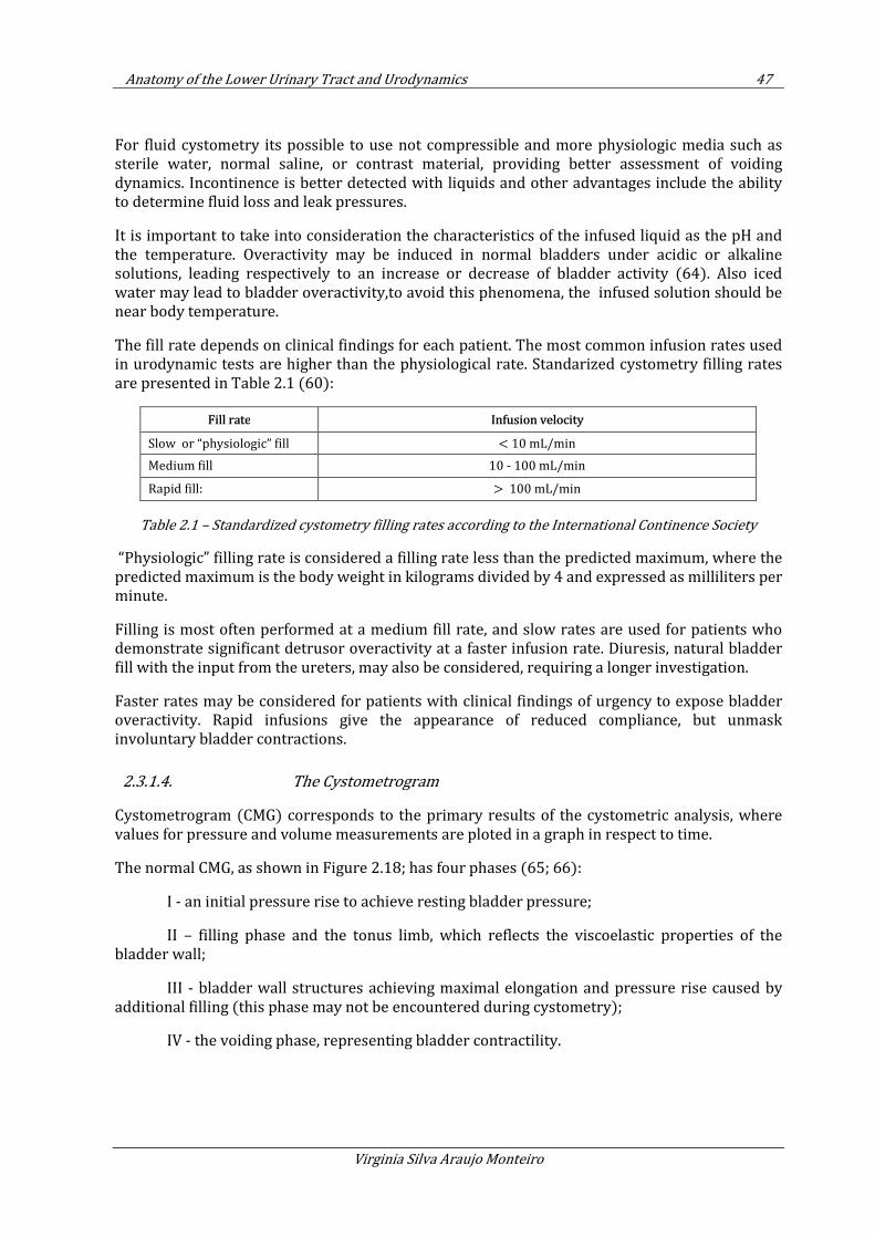
Anatomy of the Lower Urinary Tract and Urodynamics 47
Virginia Silva Araujo Monteiro
For fluid cystometry its possible to use not compressible and more physiologic media such as sterile water, normal saline, or contrast material, providing better assessment of voiding dynamics. Incontinence is better detected with liquids and other advantages include the ability to determine fluid loss and leak pressures.
It is important to take into consideration the characteristics of the infused liquid as the pH and the temperature. Overactivity may be induced in normal bladders under acidic or alkaline solutions, leading respectively to an increase or decrease of bladder activity (64). Also iced water may lead to bladder overactivity,to avoid this phenomena, the infused solution should be near body temperature.
The fill rate depends on clinical findings for each patient. The most common infusion rates used in urodynamic tests are higher than the physiological rate. Standarized cystometry filling rates are presented in Table 2.1 (60):
Fill rate Infusion velocity
Slow or “physiologic” fill < 10 mL/min
Medium fill 10 - 100 mL/min
Rapid fill: > 100 mL/min
Table 2.1 – Standardized cystometry filling rates according to the International Continence Society
“Physiologic” filling rate is considered a filling rate less than the predicted maximum, where the predicted maximum is the body weight in kilograms divided by 4 and expressed as milliliters per minute.
Filling is most often performed at a medium fill rate, and slow rates are used for patients who demonstrate significant detrusor overactivity at a faster infusion rate. Diuresis, natural bladder fill with the input from the ureters, may also be considered, requiring a longer investigation.
Faster rates may be considered for patients with clinical findings of urgency to expose bladder overactivity. Rapid infusions give the appearance of reduced compliance, but unmask involuntary bladder contractions.
2.3.1.4. The Cystometrogram
Cystometrogram (CMG) corresponds to the primary results of the cystometric analysis, where values for pressure and volume measurements are ploted in a graph in respect to time.
The normal CMG, as shown in Figure 2.18; has four phases (65; 66):
I - an initial pressure rise to achieve resting bladder pressure;
II – filling phase and the tonus limb, which reflects the viscoelastic properties of the bladder wall;
III - bladder wall structures achieving maximal elongation and pressure rise caused by additional filling (this phase may not be encountered during cystometry);
IV - the voiding phase, representing bladder contractility.
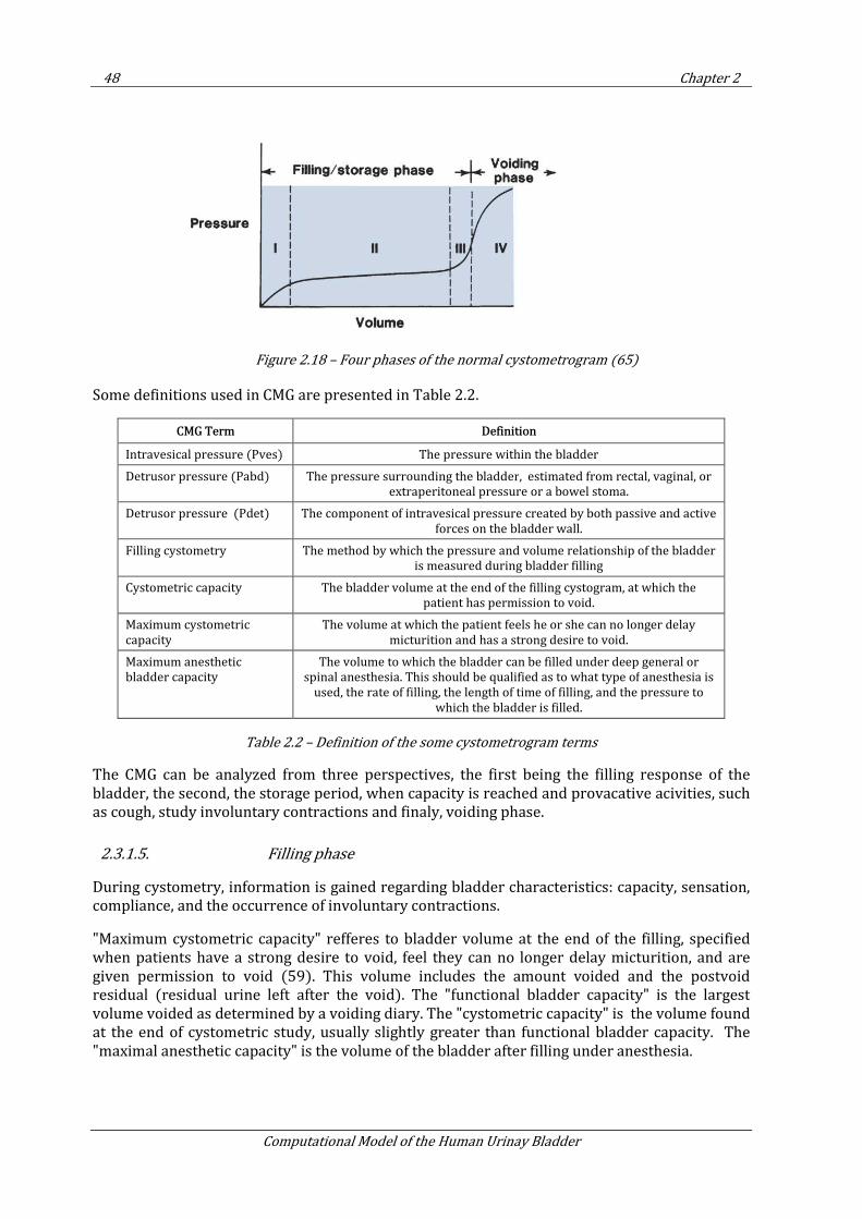
48 Chapter 2
Computational Model of the Human Urinay Bladder
Figure 2.18 – Four phases of the normal cystometrogram (65)
Some definitions used in CMG are presented in Table 2.2.
CMG Term Definition
Intravesical pressure (Pves) The pressure within the bladder
Detrusor pressure (Pabd) The pressure surrounding the bladder, estimated from rectal, vaginal, or
extraperitoneal pressure or a bowel stoma.
Detrusor pressure (Pdet) The component of intravesical pressure created by both passive and active
forces on the bladder wall.
Filling cystometry The method by which the pressure and volume relationship of the bladder
is measured during bladder filling
Cystometric capacity The bladder volume at the end of the filling cystogram, at which the
patient has permission to void.
Maximum cystometric
capacity
The volume at which the patient feels he or she can no longer delay
micturition and has a strong desire to void.
Maximum anesthetic
bladder capacity
The volume to which the bladder can be filled under deep general or
spinal anesthesia. This should be qualified as to what type of anesthesia is
used, the rate of filling, the length of time of filling, and the pressure to
which the bladder is filled.
Table 2.2 – Definition of the some cystometrogram terms
The CMG can be analyzed from three perspectives, the first being the filling response of the bladder, the second, the storage period, when capacity is reached and provacative acivities, such as cough, study involuntary contractions and finaly, voiding phase.
2.3.1.5. Filling phase
During cystometry, information is gained regarding bladder characteristics: capacity, sensation, compliance, and the occurrence of involuntary contractions.
"Maximum cystometric capacity" refferes to bladder volume at the end of the filling, specified when patients have a strong desire to void, feel they can no longer delay micturition, and are given permission to void (59). This volume includes the amount voided and the postvoid residual (residual urine left after the void). The "functional bladder capacity" is the largest volume voided as determined by a voiding diary. The "cystometric capacity" is the volume found at the end of cystometric study, usually slightly greater than functional bladder capacity. The "maximal anesthetic capacity" is the volume of the bladder after filling under anesthesia.
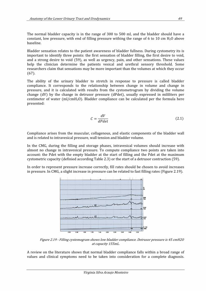
Anatomy of the Lower Urinary Tract and Urodynamics 49
Virginia Silva Araujo Monteiro
The normal bladder capacity is in the range of 300 to 500 ml, and the bladder should have a constant, low pressure, with end of filling pressure withing the range of 6 to 10 cm H2O above baseline.
Bladder sensation relates to the patient awareness of bladder fullness. During cystometry its is important to identify three points: the first sensation of bladder filling, the first desire to void, and a strong desire to void (59), as well as urgency, pain, and other sensations. These values help the clinician determine the patients vesical and urethral sensory threshold. Some researchers claim that sensations may be more important than the volumes at which they occur (67).
The ability of the urinary bladder to stretch in response to pressure is called bladder compliance. It corresponds to the relationship between change in volume and change in pressure, and it is calculated with results from the cystometrogram by dividing the volume change (dV) by the change in detrusor pressure (dPdet), usually expressed in mililiters per centimeter of water (ml/cmH2O). Bladder compliance can be calculated per the formula here presented:
=
(2.1)
Compliance arises from the muscular, collagenous, and elastic components of the bladder wall and is related to intravesical pressure, wall tension and bladder volume.
In the CMG, during the filling and storage phases, intravesical volumes should increase with almost no change in intravesical pressure. To compute compliance two points are taken into account: the Pdet with the empty bladder at the start of filling and the Pdet at the maximum cystometric capacity (definied according Table 2.3) or the start of a detrusor contraction (59).
In order to represent pressure increase correctly, fill rates should be chosen to avoid increases in pressure. In CMG, a slight increase in pressure can be related to fast filling rates (Figure 2.19).
Figure 2.19 - Filling cystemogram shows low bladder compliance. Detrusor pressure is 45 cmH2O
at capacity 155mL.
A review on the literature shows that normal bladder compliance falls within a broad range of values and clinical symptoms need to be taken into consideration for a complete diagnosis.
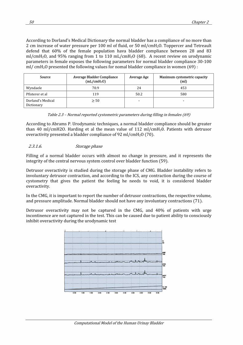
50 Chapter 2
Computational Model of the Human Urinay Bladder
According to Dorland's Medical Dictionary the normal bladder has a compliance of no more than 2 cm increase of water pressure per 100 ml of fluid, or 50 ml/cmH2O. Toppercer and Tetreault defend that 60% of the female population hava bladder compliance between 28 and 83 ml/cmH2O, and 95% ranging from 1 to 110 mL/cmH2O (68). A recent review on urodynamic parameters in female exposes the following parameters for normal bladder compliance 30-100 ml/ cmH2O presented the following values for nomal bladder compliance in women (69) :
Source Average Bladder Compliance (mL/cmH2O)
Average Age Maximum cystometric capacity (ml)
Wyndaele 70.9 24 453
Pfisterer et al 119 50.2 580
Dorland's Medical
Dictionary ≥ 50 - -
Table 2.3 – Normal reported cystometric parameters during filling in females (69)
According to Abrams P. Urodynamic techniques, a normal bladder compliance should be greater than 40 ml/cmH2O. Harding et al the mean value of 112 ml/cmH20. Patients with detrusor overactivity presented a bladder compliance of 92 ml/cmH2O (70).
2.3.1.6. Storage phase
Filling of a normal bladder occurs with almost no change in pressure, and it represents the integrity of the central nervous system control over bladder function (59).
Detrusor overactivity is studied during the storage phase of CMG. Bladder instability refers to involuntary detrusor contraction, and according to the ICS, any contraction during the course of cystometry that gives the patient the feeling he needs to void, it is considered bladder overactivity.
In the CMG, it is important to report the number of detrusor contractions, the respective volume, and pressure amplitude. Normal bladder should not have any involuntary contractions (71).
Detrusor overactivity may not be captured in the CMG, and 40% of patients with urge incontinence are not captured in the test. This can be caused due to patient ability to consciously inhibit overactivity during the urodynamic test
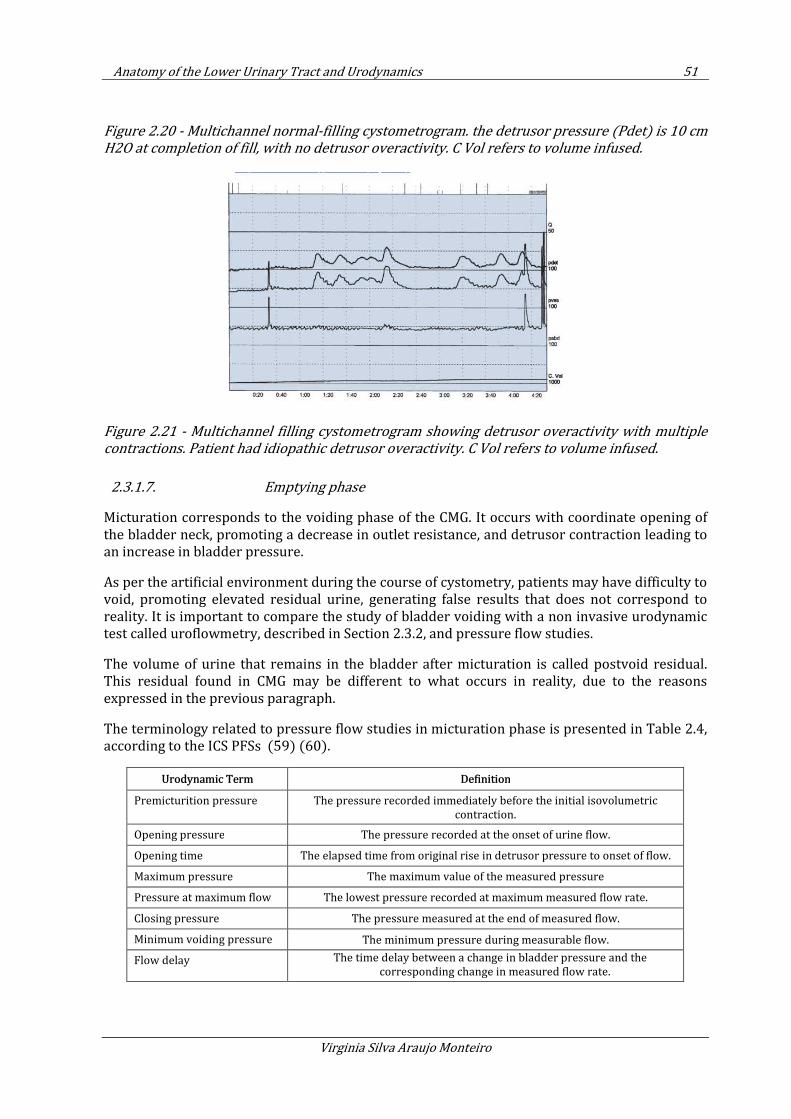
Anatomy of the Lower Urinary Tract and Urodynamics 51
Virginia Silva Araujo Monteiro
Figure 2.20 - Multichannel normal-filling cystometrogram. the detrusor pressure (Pdet) is 10 cm
H2O at completion of fill, with no detrusor overactivity. C Vol refers to volume infused.
Figure 2.21 - Multichannel filling cystometrogram showing detrusor overactivity with multiple
contractions. Patient had idiopathic detrusor overactivity. C Vol refers to volume infused.
2.3.1.7. Emptying phase
Micturation corresponds to the voiding phase of the CMG. It occurs with coordinate opening of the bladder neck, promoting a decrease in outlet resistance, and detrusor contraction leading to an increase in bladder pressure.
As per the artificial environment during the course of cystometry, patients may have difficulty to void, promoting elevated residual urine, generating false results that does not correspond to reality. It is important to compare the study of bladder voiding with a non invasive urodynamic test called uroflowmetry, described in Section 2.3.2, and pressure flow studies.
The volume of urine that remains in the bladder after micturation is called postvoid residual. This residual found in CMG may be different to what occurs in reality, due to the reasons expressed in the previous paragraph.
The terminology related to pressure flow studies in micturation phase is presented in Table 2.4, according to the ICS PFSs (59) (60).
Urodynamic Term Definition
Premicturition pressure The pressure recorded immediately before the initial isovolumetric
contraction.
Opening pressure The pressure recorded at the onset of urine flow.
Opening time The elapsed time from original rise in detrusor pressure to onset of flow.
Maximum pressure The maximum value of the measured pressure
Pressure at maximum flow The lowest pressure recorded at maximum measured flow rate.
Closing pressure The pressure measured at the end of measured flow.
Minimum voiding pressure The minimum pressure during measurable flow.
Flow delay The time delay between a change in bladder pressure and the
corresponding change in measured flow rate.
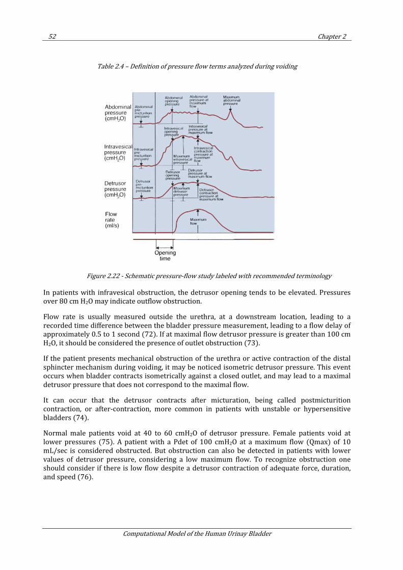
52 Chapter 2
Computational Model of the Human Urinay Bladder
Table 2.4 – Definition of pressure flow terms analyzed during voiding
Figure 2.22 - Schematic pressure-flow study labeled with recommended terminology
In patients with infravesical obstruction, the detrusor opening tends to be elevated. Pressures over 80 cm H2O may indicate outflow obstruction.
Flow rate is usually measured outside the urethra, at a downstream location, leading to a recorded time difference between the bladder pressure measurement, leading to a flow delay of approximately 0.5 to 1 second (72). If at maximal flow detrusor pressure is greater than 100 cm H2O, it should be considered the presence of outlet obstruction (73).
If the patient presents mechanical obstruction of the urethra or active contraction of the distal sphincter mechanism during voiding, it may be noticed isometric detrusor pressure. This event occurs when bladder contracts isometrically against a closed outlet, and may lead to a maximal detrusor pressure that does not correspond to the maximal flow.
It can occur that the detrusor contracts after micturation, being called postmicturition contraction, or after-contraction, more common in patients with unstable or hypersensitive bladders (74).
Normal male patients void at 40 to 60 cmH2O of detrusor pressure. Female patients void at lower pressures (75). A patient with a Pdet of 100 cmH2O at a maximum flow (Qmax) of 10 mL/sec is considered obstructed. But obstruction can also be detected in patients with lower values of detrusor pressure, considering a low maximum flow. To recognize obstruction one should consider if there is low flow despite a detrusor contraction of adequate force, duration, and speed (76).
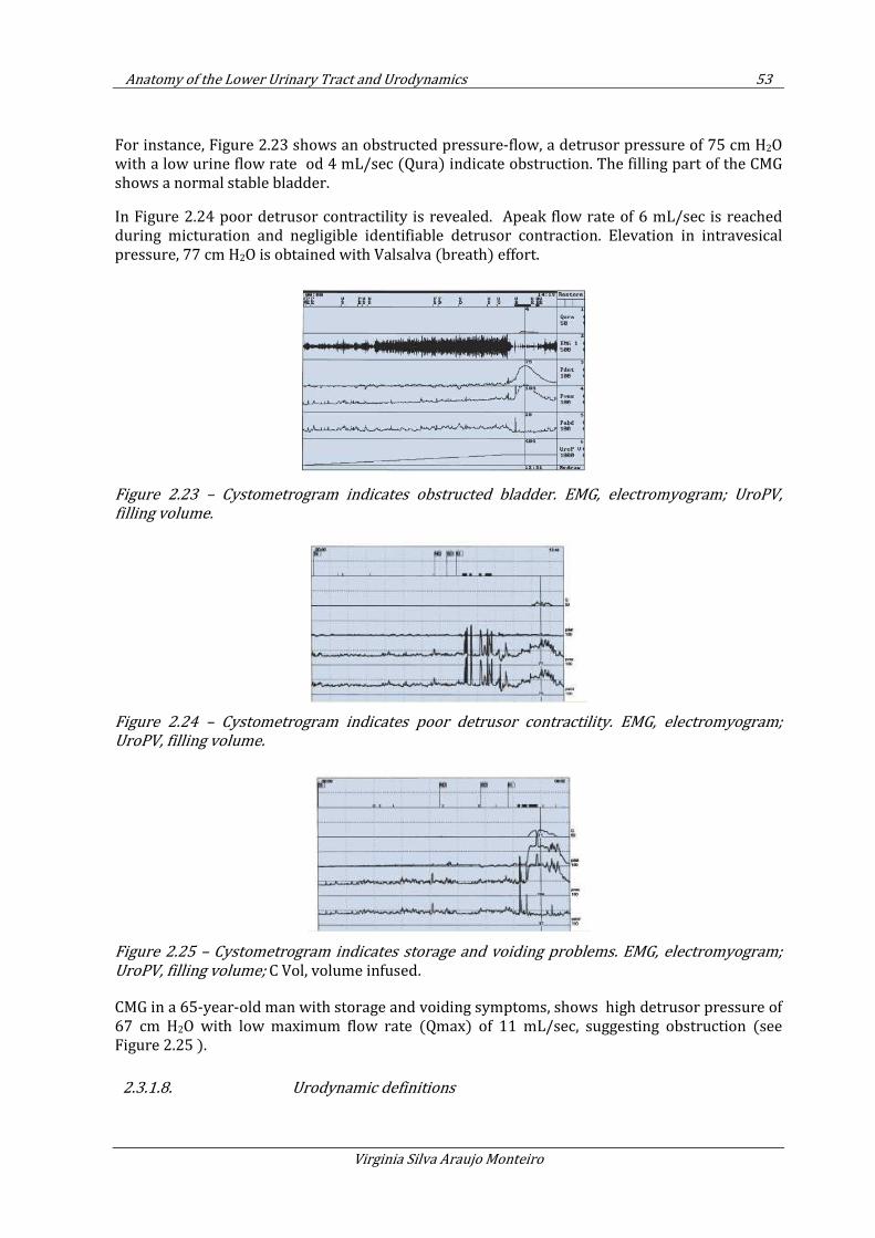
Anatomy of the Lower Urinary Tract and Urodynamics 53
Virginia Silva Araujo Monteiro
For instance, Figure 2.23 shows an obstructed pressure-flow, a detrusor pressure of 75 cm H2O with a low urine flow rate od 4 mL/sec (Qura) indicate obstruction. The filling part of the CMG shows a normal stable bladder.
In Figure 2.24 poor detrusor contractility is revealed. Apeak flow rate of 6 mL/sec is reached during micturation and negligible identifiable detrusor contraction. Elevation in intravesical pressure, 77 cm H2O is obtained with Valsalva (breath) effort.
Figure 2.23 – Cystometrogram indicates obstructed bladder. EMG, electromyogram; UroPV,
filling volume.
Figure 2.24 – Cystometrogram indicates poor detrusor contractility. EMG, electromyogram;
UroPV, filling volume.
Figure 2.25 – Cystometrogram indicates storage and voiding problems. EMG, electromyogram;
UroPV, filling volume; C Vol, volume infused.
CMG in a 65-year-old man with storage and voiding symptoms, shows high detrusor pressure of 67 cm H2O with low maximum flow rate (Qmax) of 11 mL/sec, suggesting obstruction (see Figure 2.25 ).
2.3.1.8. Urodynamic definitions
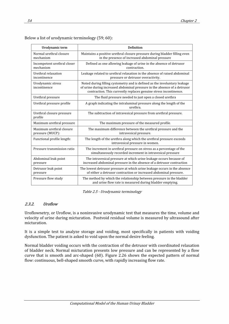
54 Chapter 2
Computational Model of the Human Urinay Bladder
Below a list of urodynamic terminology (59; 60):
Urodynamic term Definition
Normal urethral closure
mechanism
Maintains a positive urethral closure pressure during bladder filling even
in the presence of increased abdominal pressure
Incompetent urethral closer
mechanism
Defined as one allowing leakage of urine in the absence of detrusor
contraction.
Urethral relaxation
incontinence
Leakage related to urethral relaxation in the absence of raised abdominal
pressure or detrusor overactivity.
Urodynamic stress
incontinence
Noted during filling cystometry and is defined as the involuntary leakage
of urine during increased abdominal pressure in the absence of a detrusor
contraction. This currently replaces genuine stress incontinence.
Urethral pressure The fluid pressure needed to just open a closed urethra
Urethral pressure profile A graph indicating the intraluminal pressure along the length of the
urethra.
Urethral closure pressure
profile
The subtraction of intravesical pressure from urethral pressure.
Maximum urethral pressure The maximum pressure of the measured profile.
Maximum urethral closure
pressure (MUCP):
The maximum difference between the urethral pressure and the
intravesical pressure.
Functional profile length: The length of the urethra along which the urethral pressure exceeds
intravesical pressure in women.
Pressure transmission ratio The increment in urethral pressure on stress as a percentage of the
simultaneously recorded increment in intravesical pressure
Abdominal leak point
pressure
The intravesical pressure at which urine leakage occurs because of
increased abdominal pressure in the absence of a detrusor contraction
Detrusor leak point
pressure
The lowest detrusor pressure at which urine leakage occurs in the absence
of either a detrusor contraction or increased abdominal pressure.
Pressure flow study The method by which the relationship between pressure in the bladder
and urine flow rate is measured during bladder emptying.
Table 2.5 - Urodynamic terminology
2.3.2. Uroflow
Uroflownetry, or Uroflow, is a noninvasive urodynamic test that measures the time, volume and velocity of urine during micturation. Postvoid residual volume is measured by ultrasound after micturation.
It is a simple test to analyze storage and voiding, most specifically in patients with voiding dysfunction. The patient is asked to void upon the normal desire feeling.
Normal bladder voiding occurs with the contraction of the detrusor with coordinated relaxation of bladder neck. Normal micturation presents low pressure and can be represented by a flow curve that is smooth and arc-shaped (60). Figure 2.26 shows the expected pattern of normal flow: continuous, bell-shaped smooth curve, with rapidly increasing flow rate.
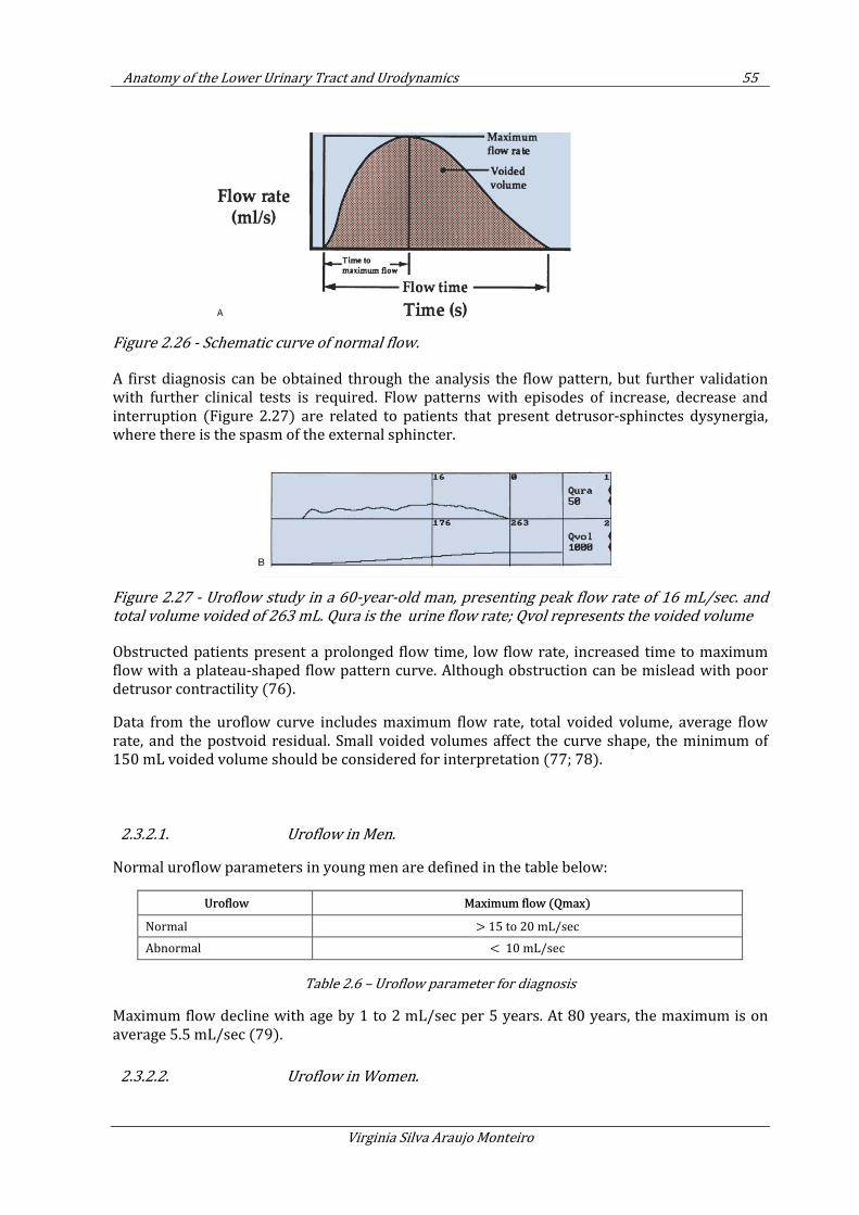
Anatomy of the Lower Urinary Tract and Urodynamics 55
Virginia Silva Araujo Monteiro
Figure 2.26 - Schematic curve of normal flow.
A first diagnosis can be obtained through the analysis the flow pattern, but further validation with further clinical tests is required. Flow patterns with episodes of increase, decrease and interruption (Figure 2.27) are related to patients that present detrusor-sphinctes dysynergia, where there is the spasm of the external sphincter.
Figure 2.27 - Uroflow study in a 60-year-old man, presenting peak flow rate of 16 mL/sec. and
total volume voided of 263 mL. Qura is the urine flow rate; Qvol represents the voided volume
Obstructed patients present a prolonged flow time, low flow rate, increased time to maximum flow with a plateau-shaped flow pattern curve. Although obstruction can be mislead with poor detrusor contractility (76).
Data from the uroflow curve includes maximum flow rate, total voided volume, average flow rate, and the postvoid residual. Small voided volumes affect the curve shape, the minimum of 150 mL voided volume should be considered for interpretation (77; 78).
2.3.2.1. Uroflow in Men.
Normal uroflow parameters in young men are defined in the table below:
Uroflow Maximum flow (Qmax)
Normal > 15 to 20 mL/sec
Abnormal < 10 mL/sec
Table 2.6 – Uroflow parameter for diagnosis
Maximum flow decline with age by 1 to 2 mL/sec per 5 years. At 80 years, the maximum is on average 5.5 mL/sec (79).
2.3.2.2. Uroflow in Women.
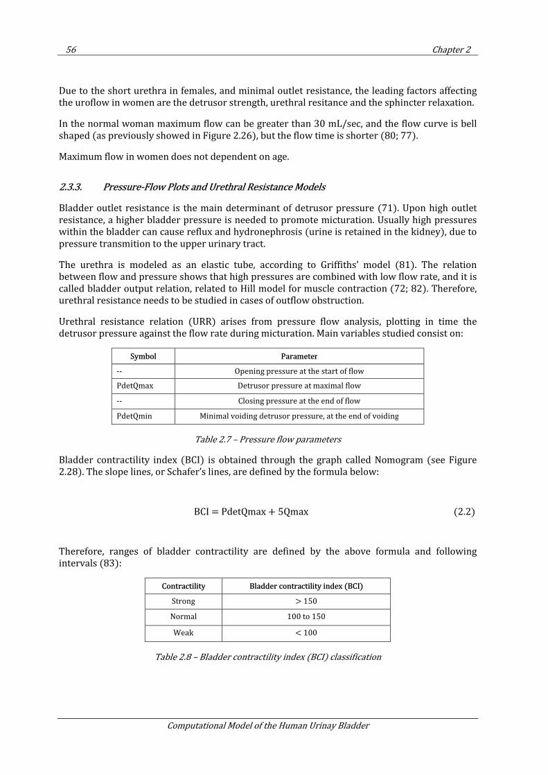
56 Chapter 2
Computational Model of the Human Urinay Bladder
Due to the short urethra in females, and minimal outlet resistance, the leading factors affecting the uroflow in women are the detrusor strength, urethral resitance and the sphincter relaxation.
In the normal woman maximum flow can be greater than 30 mL/sec, and the flow curve is bell shaped (as previously showed in Figure 2.26), but the flow time is shorter (80; 77).
Maximum flow in women does not dependent on age.
2.3.3. Pressure-Flow Plots and Urethral Resistance Models
Bladder outlet resistance is the main determinant of detrusor pressure (71). Upon high outlet resistance, a higher bladder pressure is needed to promote micturation. Usually high pressures within the bladder can cause reflux and hydronephrosis (urine is retained in the kidney), due to pressure transmition to the upper urinary tract.
The urethra is modeled as an elastic tube, according to Griffiths’ model (81). The relation between flow and pressure shows that high pressures are combined with low flow rate, and it is called bladder output relation, related to Hill model for muscle contraction (72; 82). Therefore, urethral resistance needs to be studied in cases of outflow obstruction.
Urethral resistance relation (URR) arises from pressure flow analysis, plotting in time the detrusor pressure against the flow rate during micturation. Main variables studied consist on:
Symbol Parameter
-- Opening pressure at the start of flow
PdetQmax Detrusor pressure at maximal flow
-- Closing pressure at the end of flow
PdetQmin Minimal voiding detrusor pressure, at the end of voiding
Table 2.7 – Pressure flow parameters
Bladder contractility index (BCI) is obtained through the graph called Nomogram (see Figure 2.28). The slope lines, or Schafer’s lines, are defined by the formula below:
BCI = PdetQmax + 5Qmax (2.2)
Therefore, ranges of bladder contractility are defined by the above formula and following intervals (83):
Contractility Bladder contractility index (BCI)
Strong > 150
Normal 100 to 150
Weak < 100
Table 2.8 – Bladder contractility index (BCI) classification
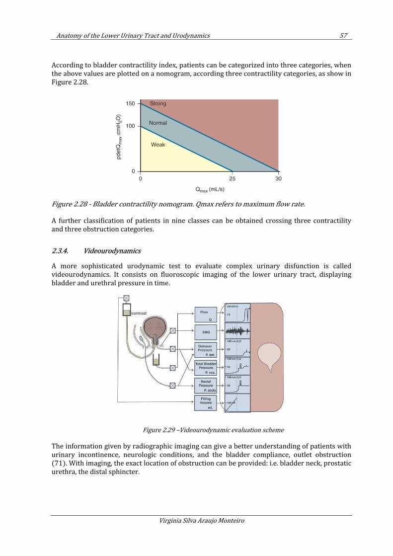
Anatomy of the Lower Urinary Tract and Urodynamics 57
Virginia Silva Araujo Monteiro
According to bladder contractility index, patients can be categorized into three categories, when the above values are plotted on a nomogram, according three contractility categories, as show in Figure 2.28.
Figure 2.28 - Bladder contractility nomogram. Qmax refers to maximum flow rate.
A further classification of patients in nine classes can be obtained crossing three contractility and three obstruction categories.
2.3.4. Videourodynamics
A more sophisticated urodynamic test to evaluate complex urinary disfunction is called videourodynamics. It consists on fluoroscopic imaging of the lower urinary tract, displaying bladder and urethral pressure in time.
Figure 2.29 –Videourodynamic evaluation scheme
The information given by radiographic imaging can give a better understanding of patients with urinary incontinence, neurologic conditions, and the bladder compliance, outlet obstruction (71). With imaging, the exact location of obstruction can be provided: i.e. bladder neck, prostatic urethra, the distal sphincter.
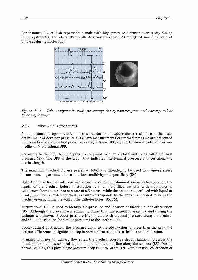
58 Chapter 2
Computational Model of the Human Urinay Bladder
For instance, Figure 2.30 represents a male with high pressure detrusor overactivity during filling cystometry and obstruction with detrusor pressure 123 cmH2O at max flow rate of 6mL/sec during micturation.
Figure 2.30 – Videourodynamic study presenting the cystometrogram and correspomdent
fuoroscopic image
2.3.5. Urethral Pressure Studies
An important concept in urodynamics is the fact that bladder outlet resistance is the main determinant of detrusor pressure (71). Two measurements of urethral pressure are presented in this section: static urethral pressure profile, or Static UPP, and micturitional urethral pressure profile, or Micturational UPP.
According to the ICS, the fluid pressure required to open a close urethra is called urethral pressure (59). The UPP is the graph that indicates intraluminal pressure changes along the urethra length.
The maximum urethral closure pressure (MUCP) is intended to be used to diagnose stress incontinence in patients, but presents low senditivity and specitficity (84).
Static UPP is performed with a patient at rest, recording intraluminal pressure changes along the length of the urethra, before micturation. A small fluid-filled catheter with side holes is withdrawn from the urethra at a rate of 0.5 cm/sec while the catheter is perfused with liquid at 2 mL/min. The recorded urethral pressure corresponds to the pressure needed to keep the urethra open by lifting the wall off the catheter holes (85; 86).
Micturational UPP is used to identify the presence and location of bladder outlet obstruction (85). Although the procedure is similar to Static UPP, the patient is asked to void during the catheter withdrawn. Bladder pressure is compared with urethral pressure along the urethra, and should be isobaric (or similar pressure) to the urethral one.
Upon urethral obstruction, the pressure distal to the obstruction is lower than the proximal pressure. Therefore, a significant drop in pressure corresponds to the obstruction location.
In males with normal urinary flow rates, the urethral pressure drops significantly across the membranous-bulbous urethral region and continues to decline along the urethra (85). During normal voiding, this physiologic pressure drop is 20 to 30 cm H2O with detrusor contraction of
Anatomy of the Lower Urinary Tract and Urodynamics 59
Virginia Silva Araujo Monteiro
50 to 55 cm H2O. In female, there is no significant pressure drop, with isobaric bladder and urethra pressures up to the distal 1 cm (87).
2.4. Conclusions
In this chapter we have presented an overview of the main structures of the urinary apparatus, especially concerning the structures relevant to the bladder function.
The next chapter introduces the methodology proposed to make a numerical analysis of the human bladder behavior during filling and voiding of this organ with urine.
Due to the complexity of the urinary tract and the surrounding structures, the numerical model presented in this thesis takes into account the approximated geometry of the male bladder and the ureters, and simplified boundary conditions to represent the surrounding structures. In this thesis some simplifications are made, and the urethra is not taken into the geometry considered. The proposed bladder geometry is presented in Section 3.2, as long as the ureters.
Results obtained from the bladder numerical analysis are validated in Chapter 4. Validation considers data provenient from the urodynamic tests described in the second part of this chapter, Urodynamics. More specifically, we used data from multichannel cystometry to validate bladder filling and voiding analysis.
The next chapter presents the methodology proposed to simulate numerically the behavior of the human bladder during filling and voiding of this organ with urine.

Proposal for the Numerical Simulation of the Human Urinary Bladder 61
Virginia Silva Araujo Monteiro
3. PROPOSAL FOR THE NUMERICAL
SIMULATION OF THE HUMAN URINARY
BLADDER
3.1. Introduction
In order to simulate the human urinary bladder, it is necessary to account for the different aspects of this organ, in special its fundamental mechanical properties, geometry and dynamics. In addition to important molecular and cellular parameters, tissue- and organ-level bladder properties are important to the function of the bladder during filling (88).
The mechanical properties include the stress-strain relationship, viscoelasticity and deformation of bladder tissue. The biomechanical components contributing to tissue mechanical responses have been studied in isolated detrusor tissue (89). However, an ongoing problem is to determine whether clinically observed alterations in detrusor function are due to changes in the contractile apparatus or in the surrounding extracellular matrix.
The geometry of the bladder is considered once the wall stress distribution of the whole organ is not homogenous. For example, changes in the cystometrogram in spinal cord injury could be a result of alterations in both bladder shape (90) and tissue properties.
The dynamics of the bladder can be accessed through an urodynamic test called cystometry. This test provides the pressure-volume relationship for this organ.
3.1.1. Geometry
To simulate the human bladder under filling and voiding conditions, we consider the geometry from a simplified high-resolution three-dimensional model of the human bladder of a 39 year old man, with no known urological diseases. The morphology came from the Visible Human Project (VH), and the input geometry from the work of Zbyněk Tonar et al (91). This geometry has been treated with the pre-post processor GID (92).
The geometry and mesh used on the following simulations are presented in Section 3.2. Annex B provides an overview on the concepts for geometry reconstruction.
3.1.2. Constitutive Model
The main mechanical part of the bladder consists on the detrusor, a smooth muscle that is responsible for maintaining an almost constant internal pressure during the filling and voiding of the bladder with urine. This phenomenon occurs because the detrusor accounts with its mechanical properties and chemical reactions to change its stiffness (1).
62 Chapter 3
Computational Model of the Human Urinay Bladder
The detrusor can be represented as a sum of three main structures:
• Matrix: corresponds to extra-cellular substance, and have a hyperelastic behaviour
• Passive fibres: made of collagen, its mechanics can be represented through a viscoelastic model
• Active fibres: muscles cells responsible for increasing bladder stiffness when activated by electrical impulses, also called Latch Mechanism.
One way to approach the complex structure of the bladder is to make use of the theory of mixtures, integrating the three main structures described above. The proportion of each of the
constituents of the bladder muscle is considered by using the volume fractions defined as mφ
(matrix), mφ (passive fibers) and
aφ (active fibers), and 1m f aφ φ φ+ + = . The Second Piola-
Kirchhoff stress tensor has the form (93):
( )p m m f f a a
ij ij ij ij ijS S p Sφ φ τ φ τ= + + +
)
(3.1)
The constitutive model proposed in this doctoral thesis is based on the implementation of a non-linear model to represent the main structures of bladder tissue described before: the hyperelastic matrix and passive fibers, but does not take into account volume fractions. Active fibers are not considered in the model for the sake of simplificity. Instead, a retraction formulation is implemented (Section 3.3.4).
This phenomenological model describes the macroscopic nature of the materials as a continua, and intends to represent the structure of bladder tissue. Its implementation consists on the following stages:
• Implementation of the hyperleastic constitutive model (Section 3.3),
• Expansion of the hyperelastic to a viscoelastic model (Section 3.4),
• Implementation of the composite model considering a hyperelastic matrix with viscous fibers (Section 3.5)
A stress-strain relationship is specified based on the evaluation of the strain energy function, in terms of classical non-linear continuum mechanics (94). The hyperelastic model is based in a neo-Hookean formulation, and the viscoelastic model on the generalized Maxwell scheme.
The bladder muscle, like many other soft biological tissues, is regarded as an incompressible material. In this work, we treat it as quasi-incompressible through the Ogden formulation (95). The general form of the Second Piola-Kirchhoff stress tensor takes the form of Eq 3.2, which splits the stress term into its volumetric part (volume-changing, or dilational),
vo lS , and its
isochoric part (volume-preserving, or distortional), iso
S (94).
vol iso
= +S S S (3.2)
Proposal for the Numerical Simulation of the Human Urinary Bladder 63
Virginia Silva Araujo Monteiro
The numerical analisis of the bladder mechanics is done with the FEM (see Annex A), the equations are written in a total Lagragian approach, were the unknown displacements are described in the reference conf iguration.
Material parameters are estimated from the literature and calibration of the model is done with clinical results, as presented on Chapter 4.
The numerical analisis of filling and voiding of the bladder is done considering two different approaches:
• Pure structural analisis, applying pressure to the structural element. A comparison between the constitutive models implemented is presented in Section 4.6.
• Fluid-structure interaction, with the Particle Finite Element Method (PFEM) to describe the fluid behavior (see Annex A).
The consitutivel model proposed in this thesis was implemented in a code developed in CIMNE for FEM and FSI analysis, Kratos Multiphysics. The code is written in C++, an object oriented programming language (96).
3.1.3. Structural analysis of the bladder
In this Section, we introduce the basis for the implementation of the numerical model.
3.1.3.1. FEM approach
The FEM is a powerful tool for structural analisis. It consists on a numerical method for solving problems of engineering and mathematical physics that normally requires the solution of ordinary or partial differential equations, which because of complicated geometries, loadings and material properties are not usually sustainable. Through the FEM, a system of simultaneous algebraic equations are solved, approximating the values of the unknowns at discrete number of points in the continuum. The numerical solution approximates to the analytical solution.
The problem here exposed involves the linearization of the constitutive equation in material description, as follows:
where D is the linear Gâteaux operator in respect to the incremental displacement field ∆u .
S u is the Second Piola Kirchoff tensor and C is the Lagrangian elasticity tensor
The Lagrangian (or material) elasticity tensor is evaluated as:
:D D = S u E uC (3.3)
2 ( )2 4
∂ ∂ ∂ Ψ= = =∂ ∂ ∂ ∂S S C
E C C CC (3.4)
64 Chapter 3
Computational Model of the Human Urinay Bladder
Where Ψ is the strain energy function.
The lagrangian elastiticy tensor C is a symmetric fourth-order tensor. The minor symmetries
i jkl jikl ijlk= =C C C come from the symmetries of the stress (S) and strain tensors (E ), it
independs of the existence of a strain-energy function and holds for all elastic materials. The
major symmetry i jkl kl ij=C C comes from the fact that the material possesses a smooth
portential Ψ is a function of E , a necessary and sufficient condition for the symmetry of the tangent stiffness matrix, and its often reffered to as the definition of hyperelasticity (94).
3.1.3.2. Total Lagrangian description
To represent the mechanics of the bladder, the constitutive equations here presented are written in a total Lagragian approach (94), were the unknown displacements in x, y and z directions are described in the material or reference configuration.
Some essential relations:
• The Jacobian of the deformation gradient: det( )ij
J F=
• The right Cauchy-Green deformation tensor: ij kj kjC F F= +
• The Green strain tensor: 1( )
2ij ij ijE C δ= −
• The stretch computed by projecting the Green strain: ( ) k
ij ij ijE u wε =
The total stress has the meaning of the Second Piola-Kirchhoff stress: ijS
3.1.3.3. Finite strain kinematics
As discussed before in Section 3.1.2, the bladder muscle is treated as quasi-incompressible material. Since it behaves quite differently in bulk and shear, we split the deformation locally into so called isochoric and volumetric part.
The deformation gradient F and the corresponding strain measure T=C F F , are decomposed
into:
1 1
3 3
1 2
3 3
( )
( )
J J
J J
= =
= =
F I F F
C I C C
(3.5)
Where F is the modified deformation gradient and C is the modified deformation right Cauchy-
Green tensor, with T=C F F , associated to the volume-preserving deformations.
Proposal for the Numerical Simulation of the Human Urinary Bladder 65
Virginia Silva Araujo Monteiro
Within the isothermal situation, the strain-energy function can be decoupled in volumetric and isochoric part (94), as follows:
( ) ( ) ( )vol iso
JΨ = Ψ + ΨC C (3.6)
And the second Piola-Kirchhoff stress:
vol iso= +S S S (3.7)
Where
The pressure p is defined as
3.1.3.4. Solvers
A common and simple numerical technique to solve the nonlinear equations in non linear solid mechanics using the FEM is to employ reliable incremental/iterative solution technique of Newton’s type. This efficient method features quadratic convergence rate near the solution point. To use this technique a consistent linearization of the variables involved in the non-linear problem, being replaced by a sequence of linear problems, which are solved at each iteration.
Linearization is based on the concept of directional derivatives (97; 98). The linearization of a nonlinear and smooth function F in the material description is presented below
Where ( )∆ • denotes de linearization operator, ∆u denotes de increment of the displacement
field u and ( )o • is the Landay order symbol denoting a small error that tends to zero faster
than 0∆ →u (see Eq. 3.11).
1( )
2 pvol
vol
JJ
−∂Ψ= =
∂S C
C (3.8)
( )vol
d Jp
dJ
Ψ= (3.9)
( ), ( ) ( , ) ( )F F F o∆ = + ∆ ∆ + ∆u u u u u u (3.10)
66 Chapter 3
Computational Model of the Human Urinay Bladder
To solve the system of equations that arrises from the structural problem, LUskyline is used.
A skyline matrix, or a variable band matrix, is a form of a sparse matrix storage format for a square, banded (and typically symmetric) matrix that reduces the storage requirement of a matrix more than banded storage. In banded storage, all entries within a fixed distance from the diagonal (called half-bandwidth) are stored. In column oriented skyline storage, only the entries from the first nonzero entry to the last nonzero entry in each column are stored. There is also row oriented skyline storage, and, for symmetric matrices, only one triangle is usually stored (99).
Skyline storage has become very popular in the finite element codes for structural mechanics, because the skyline is preserved by Cholesky decomposition (a method of solving systems of linear equations with a symmetric, positive-definite matrix; all fill-in falls within the skyline), and systems of equations from finite elements have a relatively small skyline. In addition, the effort of coding skyline Cholesky is about same as for Cholesky for banded matrices (available for banded matrices, e.g. in LAPACK; for a prototype skyline code).
Before storing a matrix in skyline format, the rows and columns are typically renumbered to reduce the size of the skyline (the number of nonzero entries stored) and to decrease the number of operations in the skyline Cholesky algorithm. The same heuristic renumbering algorithm that reduce the bandwidth are also used to reduce the skyline. The basic and one of the earliest algorithms to do that is RCM (Reverse Cuthill-McKee algorithm).
However, skyline storage is not as popular for very large systems (many millions of equations) because skyline Cholesky is not so easily adapted for massively parallel computing, and general sparse methods, which store only the nonzero entries of the matrix, become more efficient for very large problems due to much less fill-in.
To solve displacements in a given time step, the Newton-Raphson model is used.
The Bossak scheme, an implicit method, is used to solve in time, and Newton, to solve displacements in each time step. Bossak-Newmark algorithm is an extension of the well-known Newmark algorithm for the numerical integration of the equations of discretized structural dynamics problems (100). The extra parameter introduced here enables the method (when used on the test equation 2x w x= −&& ) to be simultaneously second order, unconditionally stable and with positive artificial damping.
The equation to be solved in the dynamic solver
+ + =Mx Cx Kx F&& & (3.12)
Where M , C and K are the mass, damping and stiffness matrix respectively and x , x& and x&&
are displacements, velocity and acceleration, respectively; and F is the external force vector.
0
( )lim 0
o
∆ →∆ =∆u
u
u
(3.11)
Proposal for the Numerical Simulation of the Human Urinary Bladder 67
Virginia Silva Araujo Monteiro
In the Bossak scheme:
2 2
1 1
1 1
1 1 1 1
1( ) ( ) ( )
2
(1 )
(1 )
n n n B n n
n n B n B n
B n B n n n n
x x tx t x t x
x x t x t x
Mx Mx Cx Kx F
β β
γ γ
γ α
+ +
+ +
+ + + +
= + ∆ + ∆ − + ∆
= + ∆ − + ∆
− + + + =
&& &&
&&& & && &
&& && &
(3.13)
In the given hyperelastic, viscoelastic and homogenized problems, no damping matrix is used, C 0= .
3.1.3.5. The structural element
The structural element used in the analysis is the triangular membrane element.
The membrane is a small thickness two dimensional solid, described in the 3 dimensional space. This element does not resist to bending, adjusting its shape when subjected to normal load, thus producing geometrical non-linearity (101).
Due to its low flexural stiffness, buckling phenomena it is taken into account. The element here presented a simple wrinkling model is used, featuring a consistent linearization. This procedure is suitable to the hyperelastic and viscoelastic isotropic cases.
In the case of bladder filling, the membrane is subjected to biaxial tension state, and its behaviour is purely elastic, and no wrinkling is considered.
The membrane here presented is written in total lagrangian formulation.
The formulation described in this Chapter was writen considering the tetrahedral element with
11 22 33 12 13 23( , , , , , )TE E E E E E=E , but we had convergence issues with the bladder geometry
meshed with tetrahedras, as shown in Section 3.6.2.
So we procceded to the condensation of the constitutive law to adequate to the membrane
element 11 22 12
( , , )Tmembrane
E E E=E , as follows
2 2
0
33 2
0
1
2z
h hE E
h
− = =
with 0
0
Ah h
A= (3.14)
The nodal stress vector for the membrane element; 11 22 12
( , , )Tmembrane
S S S=S .
The elasticity tensor presented below
68 Chapter 3
Computational Model of the Human Urinay Bladder
4 4 4 1
1 4 1 1
x x x x
x x z z
ε σ
ε σ
∗ =
A B
C D
M M with 3 3
0Z
S S= = (3.15)
The vector is condensed as shown
1
membrane membrane
− − ∗ = A BD C E S (3.16)
3.1.4. Fluid flow analysis
In this Section we expose the principles for the fluid flow simulation. Detailed fluid formulation is presented on Annex B. Simulations of filling and voiding of the bladder are presented in Section 3.7.
3.1.4.1. The fluid formulation
The formulation used for the fluid during the numerical simulation of bladder filling with urine is based on the Particle Finite Element Method (PFEM) (4; 102).
The PFEM adopts lagrangian framework for the fluid nodes, and the mesh nodes are treated as particles, and the variables of interest are stored in the nodes. The finite element mesh is created in every time step of the dynamic problem and the solution is then stored at the nodes. The mesh is rebuilt using Delauney triangulation.
The fluid used on the simulation of bladder filling with urine is a specific case of PFEM, written in an updated lagrangian formulation, also called Updated Lagrangian Fluid (ULF) (103). ULF formulation consists of modelling the incompressible fluid as the limiting case of the compressible formulation, in an implicit framework. The introduction of the heuristic constitutive pressure-displacement relation permits the definition of the monolithic FSI systems formulated in terms of displacements only.
The element used is in the formulation of the filling is a four-node the tetrahedra, with quasi-incompressible formulation. Bulk modulus need to be assumed high enough to simulate incompressibility.
3.1.4.2. Fluid-Structure Interaction (FSI)
The fluid-structure interaction is solved monolithically. In monolithic approach, the whole fluid-structure domain is discretized at once, and the total system is built and solved at every time step. This enables the solution of FSI problems involving large deformations, which is the case of the bladder simulation (104; 105; 103).
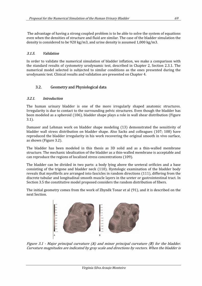
Proposal for the Numerical Simulation of the Human Urinary Bladder 69
Virginia Silva Araujo Monteiro
The advantage of having a strong coupled problem is to be able to solve the system of equations even when the densities of structure and fluid are similar. The case of the bladder simulation the density is considered to be 920 kg/m3, and urine density is assumed 1,000 kg/m3.
3.1.5. Validation
In order to validate the numerical simulation of bladder inflation, we make a comparison with the standard results of cystometry urodynamic test, described in Chapter 2, Section 2.3.1. The numerical model selected is subjected to similar conditions as the ones presented during the urodynamic test. Clinical results and validation are presented on Chapter 4.
3.2. Geometry and Physiological data
3.2.1. Introduction
The human urinary bladder is one of the more irregularly shaped anatomic structures. Irregularity is due to contact to the surrounding pelvic structures. Even though the bladder has been modeled as a spheroid (106), bladder shape plays a role in wall shear distribution (Figure 3.1).
Damaser and Lehman work on bladder shape modeling (13) demonstrated the sensitivity of bladder wall stress distribution on bladder shape. Also Sacks and colleagues (107; 108) have reproduced the bladder irregularity in his work recovering the original smooth in vivo surface, as shown (Figure 3.2).
The bladder has been modeled in this thesis as 3D solid and as a thin-walled membrane structure. The mechanic idealization of the bladder as a thin-walled membrane is acceptable and can reproduce the regions of localized stress concentrations (109).
The bladder can be divided in two parts: a body lying above the ureteral orificies and a base consisting of the trigone and bladder neck (110). Hystologic examination of the bladder body reveals that myofibrils are arranged into fascicles in random directions (111), differing from the discrete tubular and longitudinal smooth muscle layers in the ureter or gastrointestinal tract. In Section 3.5 the constitutive model proposed considers the random distribution of fibers.
The initial geometry comes from the work of Zbyněk Tonar et al (91), and it is described on the next Section.
Figure 3.1 - Major principal curvature (A) and minor principal curvature (B) for the bladder.
Curvature magnitudes are indicated by gray scale and directions by vectors. When the bladder is
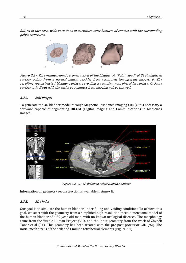
70 Chapter 3
Computational Model of the Human Urinay Bladder
full, as in this case, wide variations in curvature exist because of contact with the surrounding
pelvic structures.
Figure 3.2 - Three-dimensional reconstruction of the bladder. A, “Point cloud” of 3146 digitized
surface points from a normal human bladder from computed tomographic images. B, The
resulting reconstructed bladder surface, revealing a complex, nonspheroidal surface. C, Same
surface as in B but with the surface roughness from imaging noise removed.
3.2.2. MRI images
To generate the 3D bladder model through Magnetic Resonance Imaging (MRI), it is necessary a software capable of segmenting DICOM (Digital Imaging and Communications in Medicine) images.
Figure 3.3 - CT of Abdomen Pelvis Human Anatomy
Information on geometry reconstruction is available in Annex B.
3.2.3. 3D Model
Our goal is to simulate the human bladder under filling and voiding conditions To achieve this goal, we start with the geometry from a simplified high-resolution three-dimensional model of the human bladder of a 39 year old man, with no known urological diseases. The morphology came from the Visible Human Project (VH), and the input geometry from the work of Zbyněk Tonar et al (91). This geometry has been treated with the pre-post processor GID (92). The initial mesh size is of the order of 1 million tetrahedral elements (Figure 3.4).
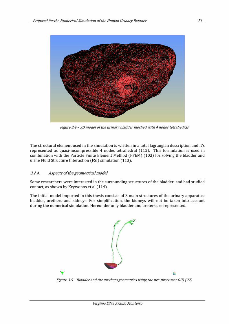
Proposal for the Numerical Simulation of the Human Urinary Bladder 71
Virginia Silva Araujo Monteiro
Figure 3.4 – 3D model of the urinary bladder meshed with 4 nodes tetrahedras
The structural element used in the simulation is written in a total lagrangian description and it’s represented as quasi-incompressible 4 nodes tetrahedral (112). This formulation is used in combination with the Particle Finite Element Method (PFEM) (103) for solving the bladder and urine Fluid Structure Interaction (FSI) simulation (113).
3.2.4. Aspects of the geometrical model
Some researchers were interested in the surrounding structures of the bladder, and had studied contact, as shown by Krywonos et al (114).
The initial model imported in this thesis consists of 3 main structures of the urinary apparatus: bladder, urethers and kidneys. For simplification, the kidneys will not be taken into account during the numerical simulation. Hereunder only bladder and ureters are represented.
Figure 3.5 – Bladder and the urethers geometries using the pre-processor GID (92)
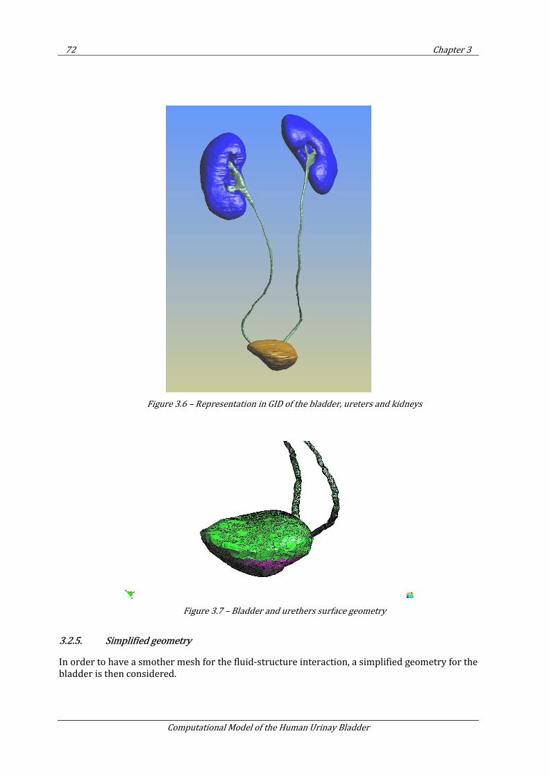
72 Chapter 3
Computational Model of the Human Urinay Bladder
Figure 3.6 – Representation in GID of the bladder, ureters and kidneys
Figure 3.7 – Bladder and urethers surface geometry
3.2.5. Simplified geometry
In order to have a smother mesh for the fluid-structure interaction, a simplified geometry for the bladder is then considered.
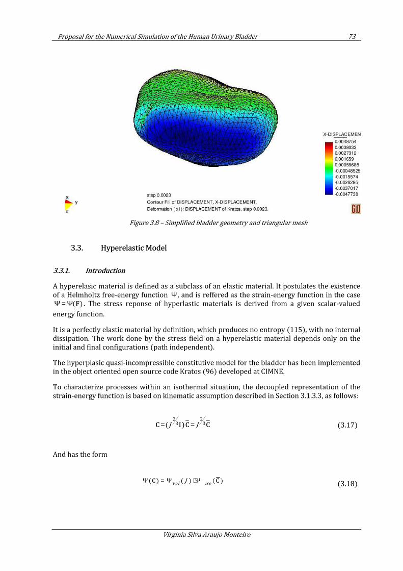
Proposal for the Numerical Simulation of the Human Urinary Bladder 73
Virginia Silva Araujo Monteiro
Figure 3.8 – Simplified bladder geometry and triangular mesh
3.3. Hyperelastic Model
3.3.1. Introduction
A hyperelasic material is defined as a subclass of an elastic material. It postulates the existence of a Helmholtz free-energy function Ψ , and is reffered as the strain-energy function in the case
( )Ψ = Ψ F . The stress reponse of hyperlastic materials is derived from a given scalar-valued
energy function.
It is a perfectly elastic material by definition, which produces no entropy (115), with no internal dissipation. The work done by the stress field on a hyperelastic material depends only on the initial and final configurations (path independent).
The hyperplasic quasi-incompressible constitutive model for the bladder has been implemented in the object oriented open source code Kratos (96) developed at CIMNE.
To characterize processes within an isothermal situation, the decoupled representation of the strain-energy function is based on kinematic assumption described in Section 3.1.3.3, as follows:
2 2
3 3(J J= =C I)C C
(3.17)
And has the form
( ) ( ) ( )vol iso
JΨ = Ψ + ΨC C
(3.18)
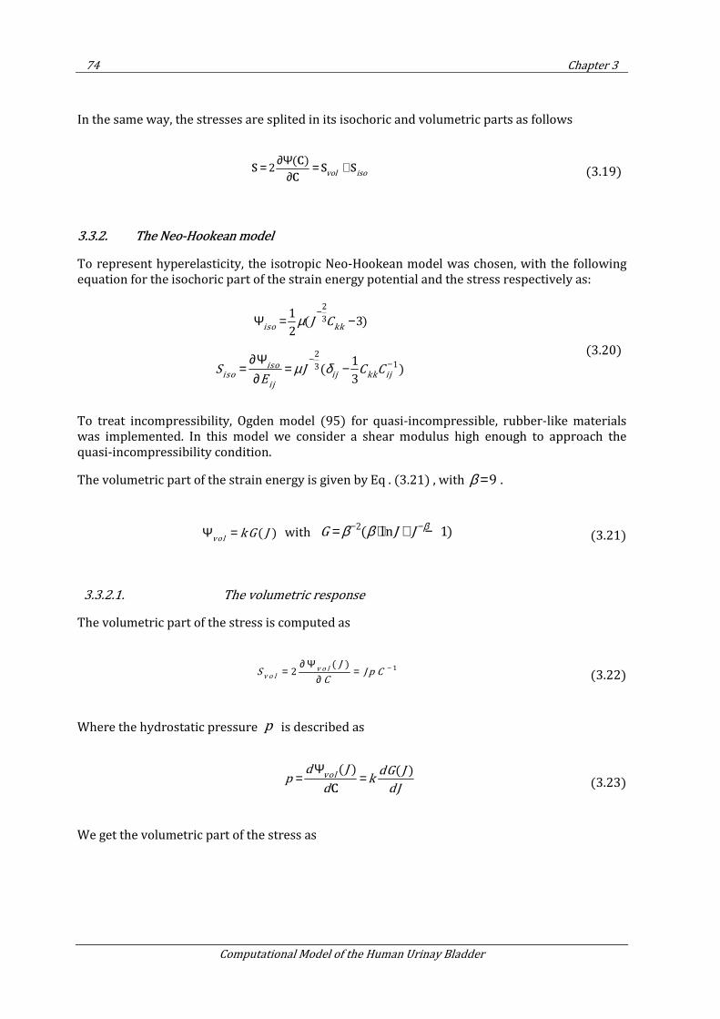
74 Chapter 3
Computational Model of the Human Urinay Bladder
In the same way, the stresses are splited in its isochoric and volumetric parts as follows
( )2
vol iso
∂Ψ= = +∂C
S S SC
(3.19)
3.3.2. The Neo-Hookean model
To represent hyperelasticity, the isotropic Neo-Hookean model was chosen, with the following equation for the isochoric part of the strain energy potential and the stress respectively as:
2
31
( 3)2iso kk
J Cµ−
Ψ = −
2
131
( )3
isoiso ij kk ij
ij
S J C CE
µ δ− −∂Ψ
= = −∂
(3.20)
To treat incompressibility, Ogden model (95) for quasi-incompressible, rubber-like materials was implemented. In this model we consider a shear modulus high enough to approach the quasi-incompressibility condition.
The volumetric part of the strain energy is given by Eq . (3.21) , with 9β = .
( )vol
kG JΨ = with
2( ln 1)G J Jββ β− −= ⋅ + − (3.21)
3.3.2.1. The volumetric response
The volumetric part of the stress is computed as
1( )
2 v o l
v o l
JS J p C
C
−∂ Ψ= =
∂ (3.22)
Where the hydrostatic pressure p is described as
( ) ( )
vold J dG J
p kd dJ
Ψ= =
C (3.23)
We get the volumetric part of the stress as
Proposal for the Numerical Simulation of the Human Urinary Bladder 75
Virginia Silva Araujo Monteiro
11 1(1 )
volS k C
Jββ
−= − (3.24)
3.3.2.2. The Lagrangian elasticity tensor
The tangent matrix, comes from the linearization process :D D = S u E uC . For the
hyperelastic case the lagrangian elasticity tensor that comes from Eq. 3.25 .
2
2 4∂ ∂ ∂ Ψ= = =∂ ∂ ∂ ∂S S
E C C CC (3.25)
The lagrangian elastiticy tensor C is a symmetric fourth-order tensor. The minor symmetries
i jkl jikl ijlk= =C C C come from the symmetries of the stress ( S ) and strain tensors (E ), it
independs of the existence of a strain-energy function and holds for all elastic materials. The
major symmetry i jkl kl ij=C C comes from the fact that the material possesses a smooth
portential Ψ is a function of E , a necessary and sufficient condition for the symmetry of the tangent stiffness matrix, and its often reffered to as the definition of hyperelasticity (94).
Considering all the symmetries described above, the fourth order tensor C of 81 components can be represented as a symmetric 6x6 matrix of 21 components.
For the isotropic hyperelastic case, Ψ can be described in terms of the of invariants (116; 115) as follow:
The elasticity tensor described in term of invariants (94):
Where 1I ,
2I and
3I are the invariants of Ψ as defined below:
1 2 3( ) , ( ) , ( )I I I Ψ = Ψ C C C (3.26)
1
1 3
1 2 3
2 2 2 ( 2I II I I
− ∂ ∂ ∂Ψ ∂ ∂Ψ ∂ ∂Ψ= = + + ∂ ∂ ∂ ∂ ∂ ∂ ∂
SI I-C) C
C C C CC
(3.27)
1( )I t r= C
( )2 2
2
1( ) ( )
2I tr tr
= − C C
2
3det( )I J= =C
(3.28)
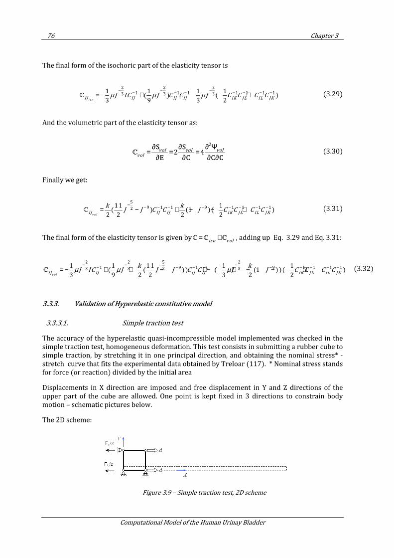
76 Chapter 3
Computational Model of the Human Urinay Bladder
The final form of the isochoric part of the elasticity tensor is
2 2 2
1 1 1 1 1 1 13 3 31 1 1 1
( ) ( )3 9 3 2iso
I J IJ IJ IJ IK JL IL JKJ IC J C C J C C C Cµ µ µ
− − −− − − − − − −= − + − − +C
(3.29)
And the volumetric part of the elasticity tensor as:
2
2 4vol vol vol
vol
∂ ∂ ∂ Ψ= = =
∂ ∂ ∂ ∂S S
E C C CC
(3.30)
Finally we get:
5
9 1 1 9 1 1 1 1211 1( ) (1 )( )
2 2 2 2volIJ IJ I J IK JL IL JK
k kJ J C C J C C C C
− − − − − − − − −= − + − − +C
(3.31)
The final form of the elasticity tensor is given byiso vol
= +C C C , adding up Eq. 3.29 and Eq. 3.31:
2 2 25
1 9 1 1 9 1 1 1 13 3 321 1 11 1 1
( ( )) ( (1 ))( )3 9 2 2 3 2 2vol
IJ IJ I J IJ IK JL IL JK
k kJ IC J J J C C J J C C C Cµ µ µ
− − −−− − − − − − − − −= − + + − + − + − − +C (3.32)
3.3.3. Validation of Hyperelastic constitutive model
3.3.3.1. Simple traction test
The accuracy of the hyperelastic quasi-incompressible model implemented was checked in the simple traction test, homogeneous deformation. This test consists in submitting a rubber cube to simple traction, by stretching it in one principal direction, and obtaining the nominal stress* - stretch curve that fits the experimental data obtained by Treloar (117). * Nominal stress stands for force (or reaction) divided by the initial area
Displacements in X direction are imposed and free displacement in Y and Z directions of the upper part of the cube are allowed. One point is kept fixed in 3 directions to constrain body motion – schematic pictures below.
The 2D scheme:
Figure 3.9 – Simple traction test, 2D scheme
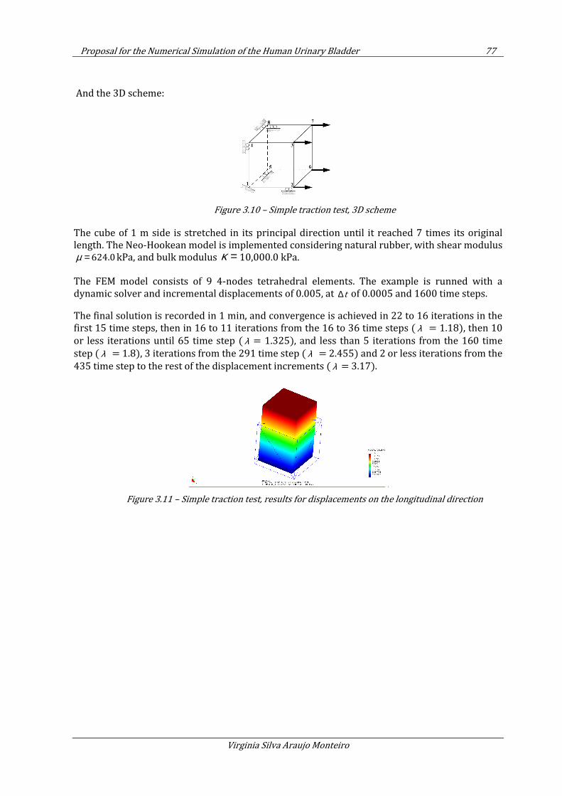
Proposal for the Numerical Simulation of the Human Urinary Bladder 77
Virginia Silva Araujo Monteiro
And the 3D scheme:
Figure 3.10 – Simple traction test, 3D scheme
The cube of 1 m side is stretched in its principal direction until it reached 7 times its original length. The Neo-Hookean model is implemented considering natural rubber, with shear modulus
624.0µ = kPa, and bulk modulus κ = 10,000.0 kPa.
The FEM model consists of 9 4-nodes tetrahedral elements. The example is runned with a dynamic solver and incremental displacements of 0.005, at t∆ of 0.0005 and 1600 time steps.
The final solution is recorded in 1 min, and convergence is achieved in 22 to 16 iterations in the first 15 time steps, then in 16 to 11 iterations from the 16 to 36 time steps ( λ = 1.18), then 10
or less iterations until 65 time step ( λ = 1.325), and less than 5 iterations from the 160 time
step ( λ = 1.8), 3 iterations from the 291 time step ( λ = 2.455) and 2 or less iterations from the
435 time step to the rest of the displacement increments ( λ = 3.17).
Figure 3.11 – Simple traction test, results for displacements on the longitudinal direction
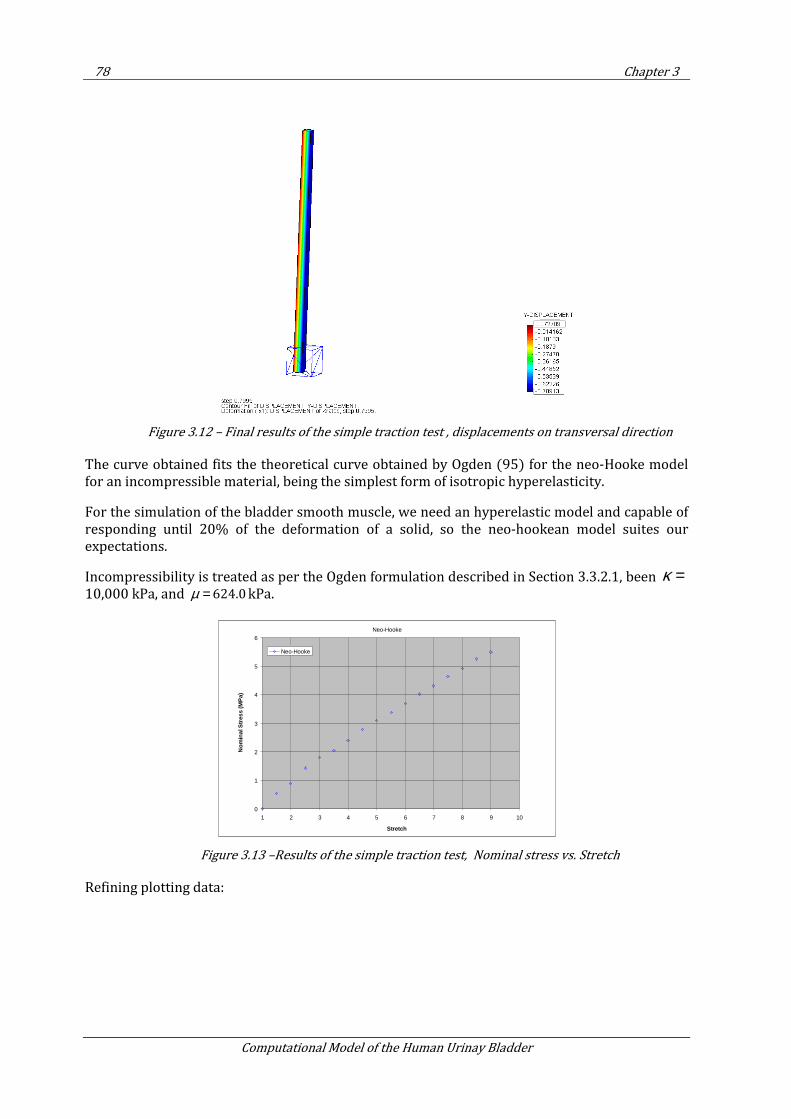
78 Chapter 3
Computational Model of the Human Urinay Bladder
Figure 3.12 – Final results of the simple traction test , displacements on transversal direction
The curve obtained fits the theoretical curve obtained by Ogden (95) for the neo-Hooke model for an incompressible material, being the simplest form of isotropic hyperelasticity.
For the simulation of the bladder smooth muscle, we need an hyperelastic model and capable of responding until 20% of the deformation of a solid, so the neo-hookean model suites our expectations.
Incompressibility is treated as per the Ogden formulation described in Section 3.3.2.1, been κ =10,000 kPa, and 624.0µ = kPa.
Figure 3.13 –Results of the simple traction test, Nominal stress vs. Stretch
Refining plotting data:
Neo-Hooke
0
1
2
3
4
5
6
1 2 3 4 5 6 7 8 9 10
Stretch
Nom
inal
Str
ess
(MP
a)
Neo-Hooke
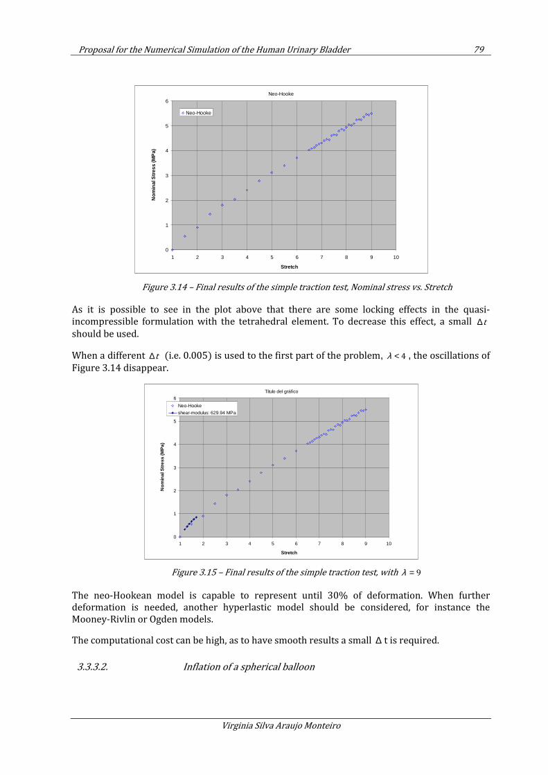
Proposal for the Numerical Simulation of the Human Urinary Bladder 79
Virginia Silva Araujo Monteiro
Figure 3.14 – Final results of the simple traction test, Nominal stress vs. Stretch
As it is possible to see in the plot above that there are some locking effects in the quasi-incompressible formulation with the tetrahedral element. To decrease this effect, a small t∆should be used.
When a different t∆ (i.e. 0.005) is used to the first part of the problem, 4λ < , the oscillations of
Figure 3.14 disappear.
Figure 3.15 – Final results of the simple traction test, with 9λ =
The neo-Hookean model is capable to represent until 30% of deformation. When further deformation is needed, another hyperlastic model should be considered, for instance the Mooney-Rivlin or Ogden models.
The computational cost can be high, as to have smooth results a small ∆ t is required.
3.3.3.2. Inflation of a spherical balloon
Neo-Hooke
0
1
2
3
4
5
6
1 2 3 4 5 6 7 8 9 10
Stretch
Nom
inal
Stre
ss (M
Pa)
Neo-Hooke
Título del gráfico
0
1
2
3
4
5
6
1 2 3 4 5 6 7 8 9 10
Stretch
Nom
inal
Stre
ss (M
Pa)
Neo-Hooke
shear-modulus: 629.94 MPa
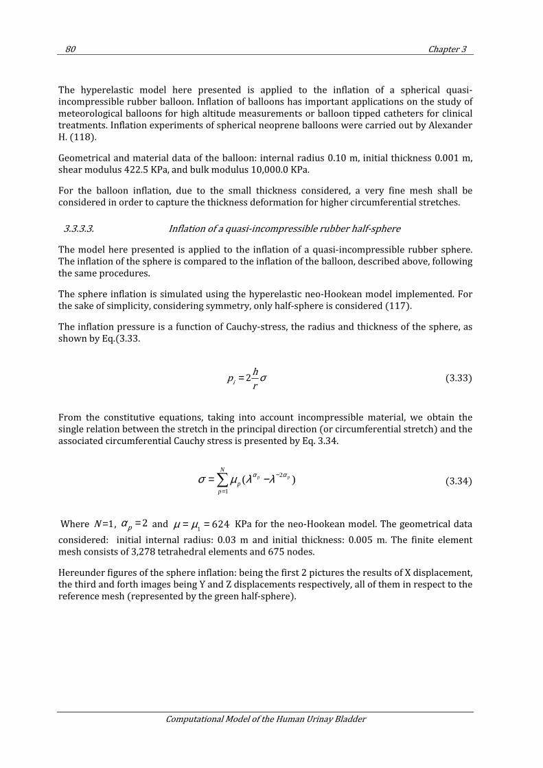
80 Chapter 3
Computational Model of the Human Urinay Bladder
The hyperelastic model here presented is applied to the inflation of a spherical quasi-incompressible rubber balloon. Inflation of balloons has important applications on the study of meteorological balloons for high altitude measurements or balloon tipped catheters for clinical treatments. Inflation experiments of spherical neoprene balloons were carried out by Alexander H. (118).
Geometrical and material data of the balloon: internal radius 0.10 m, initial thickness 0.001 m, shear modulus 422.5 KPa, and bulk modulus 10,000.0 KPa.
For the balloon inflation, due to the small thickness considered, a very fine mesh shall be considered in order to capture the thickness deformation for higher circumferential stretches.
3.3.3.3. Inflation of a quasi-incompressible rubber half-sphere
The model here presented is applied to the inflation of a quasi-incompressible rubber sphere. The inflation of the sphere is compared to the inflation of the balloon, described above, following the same procedures.
The sphere inflation is simulated using the hyperelastic neo-Hookean model implemented. For the sake of simplicity, considering symmetry, only half-sphere is considered (117).
The inflation pressure is a function of Cauchy-stress, the radius and thickness of the sphere, as shown by Eq.(3.33.
2i
hp
rσ= (3.33)
From the constitutive equations, taking into account incompressible material, we obtain the single relation between the stretch in the principal direction (or circumferential stretch) and the associated circumferential Cauchy stress is presented by Eq. 3.34.
(3.34)
Where 1N = , 2p
α = and 1
624µ µ= = KPa for the neo-Hookean model. The geometrical data
considered: initial internal radius: 0.03 m and initial thickness: 0.005 m. The finite element mesh consists of 3,278 tetrahedral elements and 675 nodes.
Hereunder figures of the sphere inflation: being the first 2 pictures the results of X displacement, the third and forth images being Y and Z displacements respectively, all of them in respect to the reference mesh (represented by the green half-sphere).
2
1
( )p p
N
pp
α ασ µ λ λ −
=
= −∑
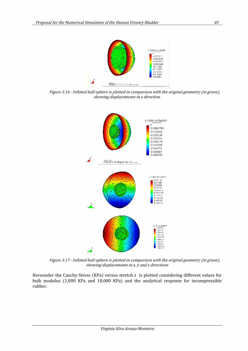
Proposal for the Numerical Simulation of the Human Urinary Bladder 81
Virginia Silva Araujo Monteiro
Figure 3.16 - Inflated half-sphere is plotted in comparison with the original geometry (in green),
showing displacements in x direction.
Figure 3.17 - Inflated half-sphere is plotted in comparison with the original geometry (in green),
showing displacements in x, y and z directions
Hereunder the Cauchy-Stress (KPa) versus stretch λ is plotted considering different values for
bulk modulus (1,000 KPa and 10,000 KPa) and the analytical response for incompressible rubber.
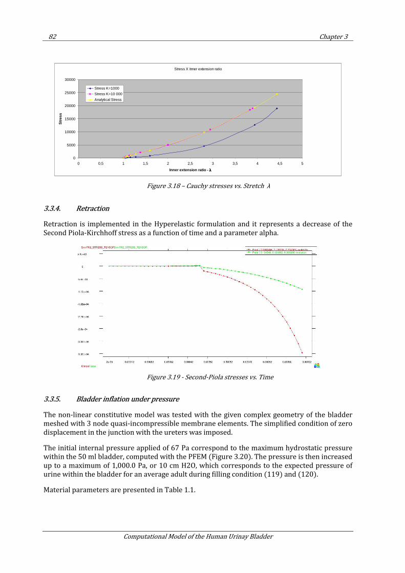
82 Chapter 3
Computational Model of the Human Urinay Bladder
Figure 3.18 – Cauchy stresses vs. Stretch λ
3.3.4. Retraction
Retraction is implemented in the Hyperelastic formulation and it represents a decrease of the Second Piola-Kirchhoff stress as a function of time and a parameter alpha.
Figure 3.19 - Second-Piola stresses vs. Time
3.3.5. Bladder inflation under pressure
The non-linear constitutive model was tested with the given complex geometry of the bladder meshed with 3 node quasi-incompressible membrane elements. The simplified condition of zero displacement in the junction with the ureters was imposed.
The initial internal pressure applied of 67 Pa correspond to the maximum hydrostatic pressure within the 50 ml bladder, computed with the PFEM (Figure 3.20). The pressure is then increased up to a maximum of 1,000.0 Pa, or 10 cm H2O, which corresponds to the expected pressure of urine within the bladder for an average adult during filling condition (119) and (120).
Material parameters are presented in Table 1.1.
Stress X Inner extension ratio
0
5000
10000
15000
20000
25000
30000
0 0,5 1 1,5 2 2,5 3 3,5 4 4,5 5
Inner extension ratio - λλλλ
Stre
ss
Stress K=1000
Stress K=10 000
Analytical Stress
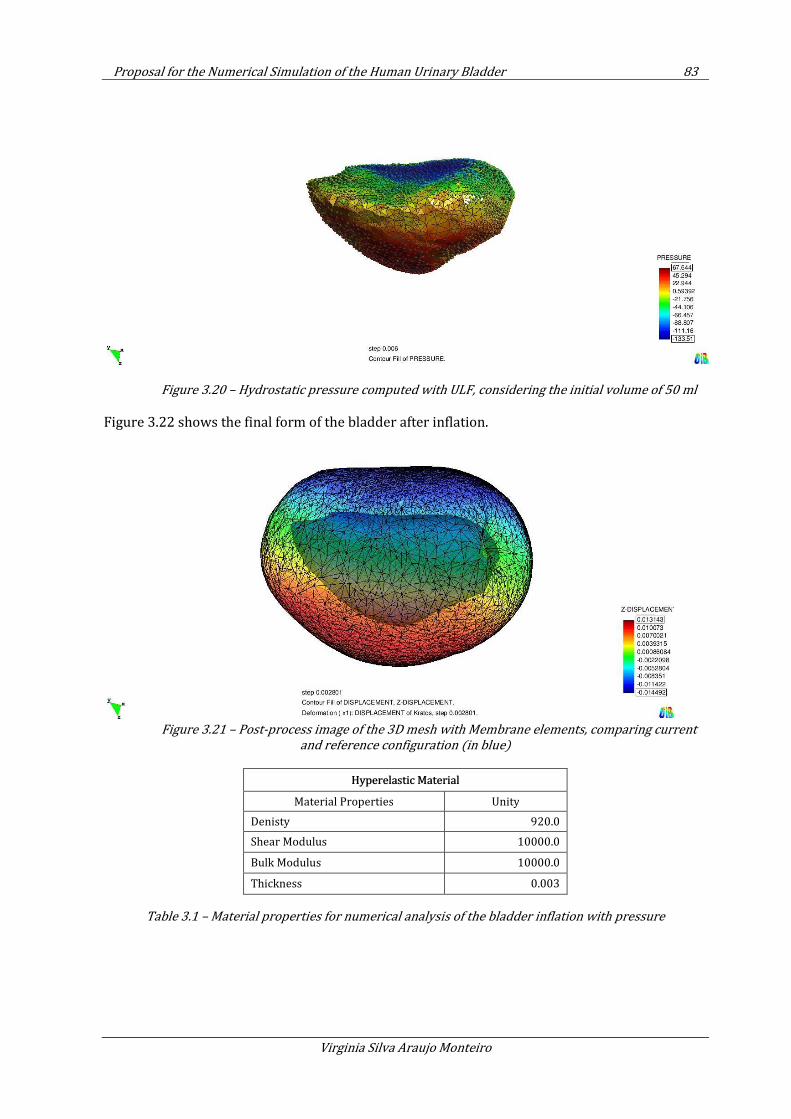
Proposal for the Numerical Simulation of the Human Urinary Bladder 83
Virginia Silva Araujo Monteiro
Figure 3.20 – Hydrostatic pressure computed with ULF, considering the initial volume of 50 ml
Figure 3.22 shows the final form of the bladder after inflation.
Figure 3.21 – Post-process image of the 3D mesh with Membrane elements, comparing current
and reference configuration (in blue)
Hyperelastic Material
Material Properties Unity
Denisty 920.0
Shear Modulus 10000.0
Bulk Modulus 10000.0
Thickness 0.003
Table 3.1 – Material properties for numerical analysis of the bladder inflation with pressure
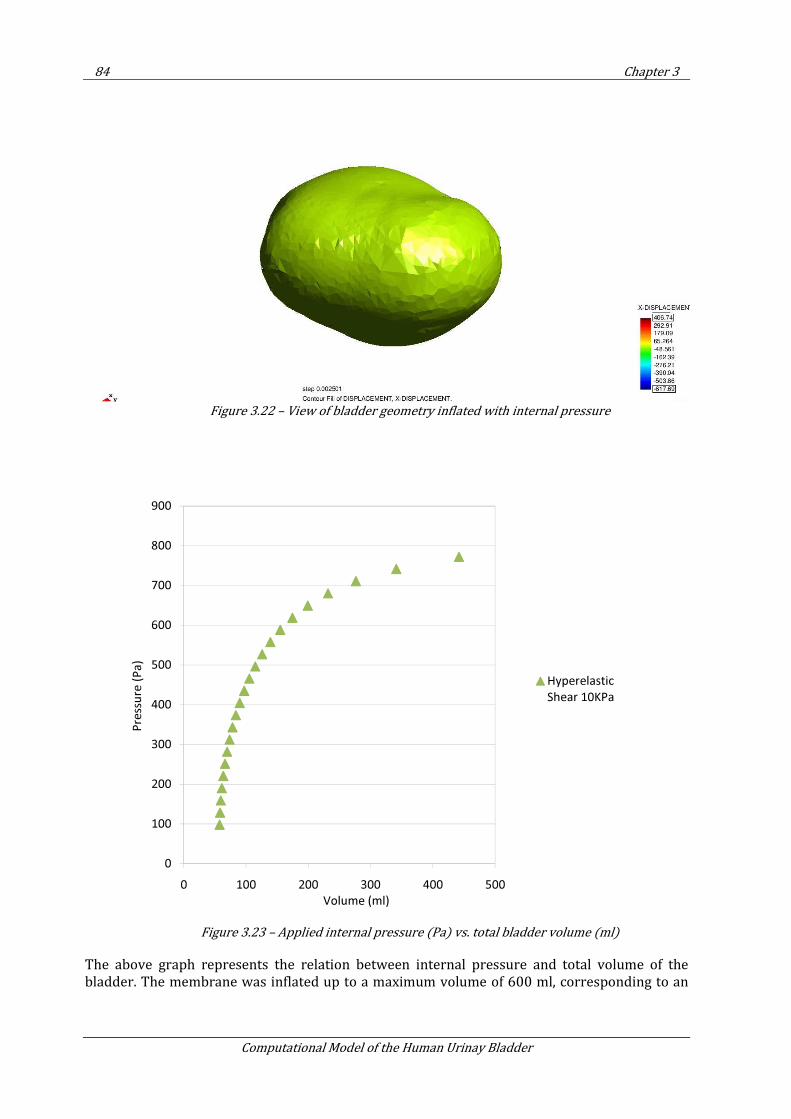
84 Chapter 3
Computational Model of the Human Urinay Bladder
Figure 3.22 – View of bladder geometry inflated with internal pressure
Figure 3.23 – Applied internal pressure (Pa) vs. total bladder volume (ml)
The above graph represents the relation between internal pressure and total volume of the bladder. The membrane was inflated up to a maximum volume of 600 ml, corresponding to an
0
100
200
300
400
500
600
700
800
900
0 100 200 300 400 500
Pre
ssu
re (
Pa
)
Volume (ml)
Hyperelastic
Shear 10KPa
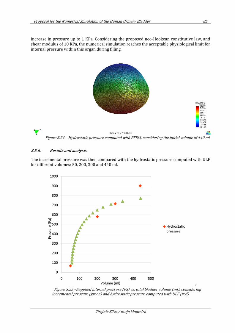
Proposal for the Numerical Simulation of the Human Urinary Bladder 85
Virginia Silva Araujo Monteiro
increase in pressure up to 1 KPa. Considering the proposed neo-Hookean constitutive law, and shear modulus of 10 KPa, the numerical simulation reaches the acceptable physiological limit for internal pressure within this organ during filling.
Figure 3.24 – Hydrostatic pressure computed with PFEM, considering the initial volume of 440 ml
3.3.6. Results and analysis
The incremental pressure was then compared with the hydrostatic pressure computed with ULF for different volumes: 50, 200, 300 and 440 ml.
c
Figure 3.25 –Aapplied internal pressure (Pa) vs. total bladder volume (ml), considering
incremental pressure (green) and hydrostatic pressure computed with ULF (red)
0
100
200
300
400
500
600
700
800
900
1000
0 100 200 300 400 500
Pre
ssu
re (
Pa
)
Volume (ml)
Hydrostatic
pressure
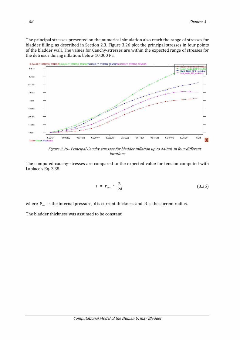
86 Chapter 3
Computational Model of the Human Urinay Bladder
The principal stresses presented on the numerical simulation also reach the range of stresses for bladder filling, as described in Section 2.3. Figure 3.26 plot the principal stresses in four points of the bladder wall. The values for Cauchy-stresses are within the expected range of stresses for the detrusor during inflation: below 10,000 Pa.
Figure 3.26– Principal Cauchy stresses for bladder inflation up to 440ml, in four different
locations
The computed cauchy-stresses are compared to the expected value for tension computed with Laplace's Eq. 3.35.
ves
R T P
2d= ∗ (3.35)
where vesP is the internal pressure, d is current thickness and R is the current radius.
The bladder thickness was assumed to be constant.
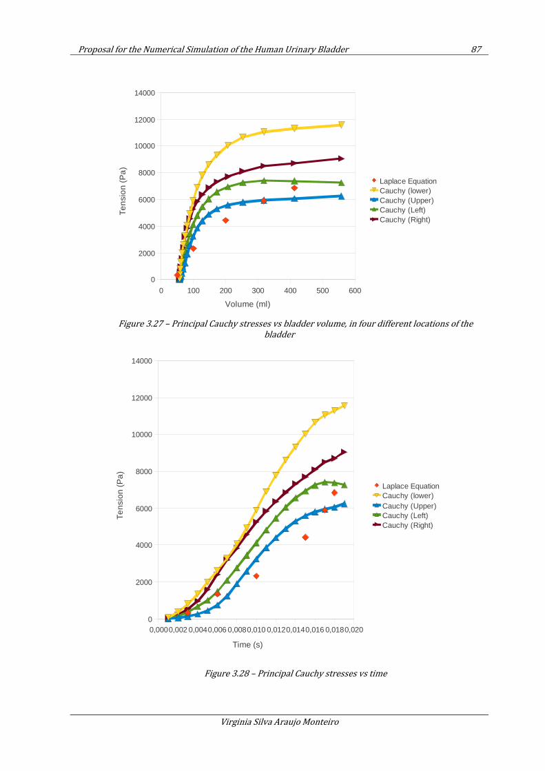
Proposal for the Numerical Simulation of the Human Urinary Bladder 87
Virginia Silva Araujo Monteiro
Figure 3.27 – Principal Cauchy stresses vs bladder volume, in four different locations of the
bladder
Figure 3.28 – Principal Cauchy stresses vs time
0 100 200 300 400 500 600
0
2000
4000
6000
8000
10000
12000
14000
Laplace EquationCauchy (lower)Cauchy (Upper)Cauchy (Left)Cauchy (Right)
Volume (ml)
Ten
sio
n (
Pa
)
0,0000,002 0,0040,006 0,0080,010 0,0120,0140,016 0,0180,0200
2000
4000
6000
8000
10000
12000
14000
Laplace EquationCauchy (lower)Cauchy (Upper)Cauchy (Left)Cauchy (Right)
Time (s)
Te
nsio
n (
Pa
)
88 Chapter 3
Computational Model of the Human Urinay Bladder
3.3.7. Conclusions
The hyperelastic Neo-Hookean constitutive model is able to represent the behaviour of the detrusor muscle under rapid filling conditions of the urinary bladder. The complex bladder behaviour is partially represented with the non-linear constitutive model here implemented.
When considering physiological rates of filling and storage of urine, the viscoelastic response of the muscle fibres shall be taken into account, to reproduce the relaxation of the detrusor muscle.
The viscoelastic model implemented in the thesis is described in the next section.
3.4. Viscoelastic Model
3.4.1. Introduction
The phenomenological model introduced in this section describes the macroscopic nature of bladder material as a continuum, and intends to represent the viscoelasticity effects of the collagen present in the bladder tissue. The formulation here introduced is an extension of the hyperelastic neo-Hookean constitutive model presented in Section 3.3.
The response of most materials inside the body depends on the temporal dependence and on history. In other words, depend if the load is applied fast or slow relative to a defined time scale. These materials are called viscoelastic.
The viscoelastic properties of the bladder were the subject of research among the biomechanical scientific community since for over 40 years (9). In vivo-experiments were done in dog and pig bladders to get the accurate parameters.
Perfectly viscous behavior is modeled by a dashpot, where the response depends on the speed (see Eq. 3.36). Damping is described by the constant c (or more comunily presented in
biomedical engineering community as "η").
The ideal dashpot can be represented by a piston moving in a cylinder that is filled with a viscous fluid. The displacement of the piston in the dashpot depends on its history. The parameter c describes the effects of viscosity for this macroscopic model and relates the force in the dashpot model to the speed of the piston in the viscous medium. It is related to the coefficient of viscosity.
Combining the ideal spring from Hooke law to the dashpot, we can obtain models for viscoelastic materials, and analyse the response of these materials to different stimuli that vary with time (121).
Viscoelasticity manifests in three interrelated forms: Creep, Stress relaxation and Hysteresis, summarized in Table 3.2
= = ()
(3.36)
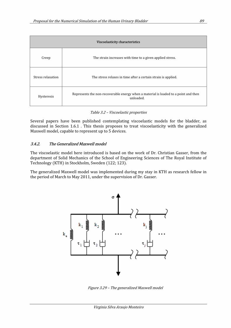
Proposal for the Numerical Simulation of the Human Urinary Bladder 89
Virginia Silva Araujo Monteiro
Viscoelasticity characteristics
Creep The strain increases with time to a given applied stress.
Stress relaxation The stress relaxes in time after a certain strain is applied.
Hysteresis Represents the non-recoverable energy when a material is loaded to a point and then
unloaded.
Table 3.2 – Viscoelastic properties
Several papers have been published contemplating viscoelastic models for the bladder, as discussed in Section 1.6.1 . This thesis proposes to treat viscoelasticity with the generalized Maxwell model, capable to represent up to 5 devices.
3.4.2. The Generalized Maxwell model
The viscoelastic model here introduced is based on the work of Dr. Christian Gasser, from the department of Solid Mechanics of the School of Engineering Sciences of The Royal Institute of Technology (KTH) in Stockholm, Sweden (122; 123).
The generalized Maxwell model was implemented during my stay in KTH as research fellow in the period of March to May 2011, under the supervision of Dr. Gasser.
Figure 3.29 – The generalized Maxwell model
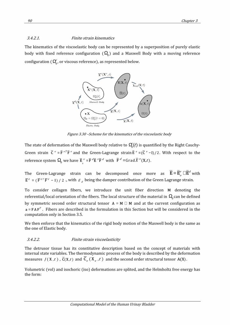
90 Chapter 3
Computational Model of the Human Urinay Bladder
3.4.2.1. Finite strain kinematics
The kinematics of the viscoelastic body can be represented by a superposition of purely elastic
body with fixed reference configuration (Ω0
) and a Maxwell Body with a moving reference
configuration ( Ω0
v
, or viscous reference), as represented below.
Figure 3.30 –Scheme for the kinematics of the viscoelastic body
The state of deformation of the Maxwell body relative to 0( )v
tΩ is quantified by the Right Cauchy-
Green strain v vT v=C F F and the Green-Lagrange strain ( )/2v v= −E C I . With respect to the
reference system Ω0
we have 0
v d v d=E F E F with Grad ( , )d vX t=F X .
The Green-Lagrange strain can be decomposed once more as v d
o= +E E E with
( ) / 2d d T d= −E F F I ., with d
E being the damper contribution of the Green Lagrange strain.
To consider collagen fibers, we introduce the unit fiber direction M denoting the
referential/local orientation of the fibers. The local structure of the material in Ω0
can be defined
by symmetric second order structural tensor = ⊗A M M and at the current configuration as T=a FAF . Fibers are described in the formulation in this Section but will be considered in the
computation only in Section 3.5.
We then enforce that the kinematics of the rigid body motion of the Maxwell body is the same as the one of Elastic body.
3.4.2.2. Finite strain viscoelasticity
The detrusor tissue has its constitutive description based on the concept of materials with internal state variables. The thermodynamic process of the body is described by the deformation
measures ( , )J tX , ( , )tC X and ( , )v v
tC X and the second order structural tensor )A(X .
Volumetric (vol) and isochoric (iso) deformations are splited, and the Helmholtz free energy has the form:
Proposal for the Numerical Simulation of the Human Urinary Bladder 91
Virginia Silva Araujo Monteiro
( ( ), ( ), ( ), ) ( ( )) ( ( ), ( ), )v v
vol isoJ t t t J t t t
∞Ψ = Ψ + ΨC C A C C Α (3.37)
For incompressible material, viscous effects only affect the isochoric part of the free energy and
its splited into: a thermodynamic equilibrium i s o
∞Ψ (pure hyperelastic deformation) and the
dissipative part i s o
ϒ (viscoelastic response). Consequently, Eq. 3.37 is writen as
( ( ), ( ), ( ), ) ( ( )) ( ( ), ) ( ( ), ( ), )v v
vol iso isoJ t t t J t t t t
∞ ∞Ψ = Ψ + Ψ + ϒC C A C Α C C Α (3.38)
Similarly, the Second Piola-Kirchhoff stress reads
0
( ( ), ( ), ( ), )2
( )
v
v
vol iso iso
J t t t
t
∞ ∞∂Ψ= = + +∂C C A
S S S SC
(3.39)
Where v o l
∞S corresponds to the volumetric part of the Second Piola-Kirchhoff stress
iso
∞S is
reffered to the hyperelastic response, and 0
v
isoS represents the overstress of the viscoelastic
solid and have time-dependent effects governed by the dissipative potential iso
ϒ .
The dissipative potential depends on the solid and viscous phases of the Maxwell body and, also,
on the evolution of its reference configuration0( )v
tΩ , as ( ( ), ( ), )v
isot tϒ C C A
The different components of the Second Piola-Kirchhoff stresses are computed as follows
0
( ( ))2
( )
( ( ), )2
( )
( ( ), ( ), )2
( )
vol
vol
vol
iso
v
v iso
iso
J t
t
t
t
t t
t
∞∞
∞∞
∂Ψ=
∂
∂Ψ=
∂
∂ϒ=
∂
SC
C AS
C
C C AS
C
(3.40)
The stress like variable Ξ reads
( ( ), ( ) , )2
( )
v
isot t
t
∂ϒ= −
∂C C Α
ΞC
(3.41)
92 Chapter 3
Computational Model of the Human Urinay Bladder
The model dissipation i n t
D has to be non-negative to satisfy the second law of thermodynamics
(the Clausius-Duhem inequality), i.e.
int 02 : : 0
v v
isoD = ϒ = = ≥Ξ C S C
& && (3.42)
3.4.2.3. The volumetric response
Compared to the hyperelastic constitutive model introduced in Section3.3, the volumetric part of the Second Piola-Kirchhoff stress does not change as neither the volumetric part of the strain energy tensor, as they both depend only in the hydrostatic pressure p for which in an quasi-
incompressible material is independent from the deformation. This allows to define the volumetric part of the Second Piola-Kirchhoff stress tensor as
1
volJp
∞ −=S C (3.43)
3.4.2.4. The Hyperelastic response
The hyperelastic response considered in the viscoelastic model is the one described in Section 3.3.
Recovering the formulation, the isochoric elastic part of the Second Piola-Kirchhoff stress is defined as
2
131
( )3
i s o
i s o i j k k i j
i j
S J C CE
µ δ−∞ −∂ Ψ
= = −∂
(3.44)
3.4.2.5. The Viscoelastic response
The Second Piola-Kirchhoff stress contribution 0
v
isoS defines the over-stress of the viscoelastic
solid an all time-dependent effects are governed by the dissipative potential ( ( ) , ( ) , )i s o
t tϒ C C A .
The energy i s o
ϒ depends on the solid and viscous phases of the Maxwell body and the evolution
of its reference configuration0( )v
tΩ .
According to the 1D kinematics of a Maxwell device at small strains (124), the generalized rate equation reads
0
0
v
v
τ+ =E
E E& & (3.45)
Proposal for the Numerical Simulation of the Human Urinary Bladder 93
Virginia Silva Araujo Monteiro
Where the relaxation time τ relates the elastic and viscous phase of the Maxwell body and
determines the time constant of the rate. τ is defined by the following relation:
0 0 0 0( ) ( )v v v v
iso isoτ=E EC (3.46)
where 0
v
i s o and ℂ
0
v
i s o are the viscous and elastic stiffness of the Maxwell Body.
With 0
v dE=E +E Eq. 3.45 can be re-writen as
1( )d d
τ= −E E E
& (3.47)
Eq. 3.47 is sufficient condition for isotropic materials. The finite strain viscoelasticity of the body is completely described by the rate equations 3.45 and 3.47 and the constitutive description of the Elastic and Maxwell Bodies.
Through linearization, the over-stress assumes the form:
0 0 0:
v v v
iso iso=S EC (3.48)
Where 0
v
isoC defines the isochoric stiffness with respect to
0Ω of the elastic phase of the
Maxwell Body.
Rephrasing Eq. 3.45 in a referential stress-space, we have
10
0 0: ( : )
v
v viso
iso iso iso isoτ∞ − ∞+ =
SS S& &C C (3.49)
Where iso
∞C is the stiffness of the Elastic Body.
For a class of materials, the elasticity of the Maxwell Body can be regarded as a fraction of the elasticity of the Elastic Body, as
0
v
iso isoβ ∞=C C (3.50)
With )0,β ∈ ∞ . The rate equation for the over-stress reads
94 Chapter 3
Computational Model of the Human Urinay Bladder
0
0
v
v viso
iso isoβ
τ+ =S
S S& & (3.51)
The closed solution of Eq. 3.51 leads to the convolution integral (125)
00
( )( ( ), ( ), ) exp ( ( ), )
T tv v
iso isoT
t Tt t t dTβ
τ= ∞
=
− −=
∫S C C A S C A& (3.52)
A contraction with E& gives the following expression for the dissipative potential
00
( )( ( ), ( ), ) 2 exp ( ( ), )
T tv
iso isoT
t Tt t t dTβ
τ= ∞
=
− −ϒ = Ψ
∫C C A C A& (3.53)
Through the relation2 : :v v
iso isoϒ = Ξ =C S C
& && , the constitutive expression for the stress like variable
reads
1
( : )v v
iso
−Ξ = S C C
& & (3.54)
3.4.2.6. Numerical integration of the evolution equation
To compute the viscoelastic stress, all state variables at time nt are supposed to be known, giving
the possibility to compute the viscoelastic over-stress at time1n
t + .
We have from Eq. 3.52:
1 1
2
0 1 0 1( )
n n n n
v v
iso n iso n iso isoξ βξ
+ +
∞ ∞+ += + −S S S S (3.55)
Where 1 1
exp /(2 )n n
tξ τ+ + = −∆ is a dimensionless parameter.
The viscoelastic stress is updated as
1 10 1n n
v
iso n iso nβξ
+ +
∞+= +S S H (3.56)
Where n
H stores the history variables and has the form
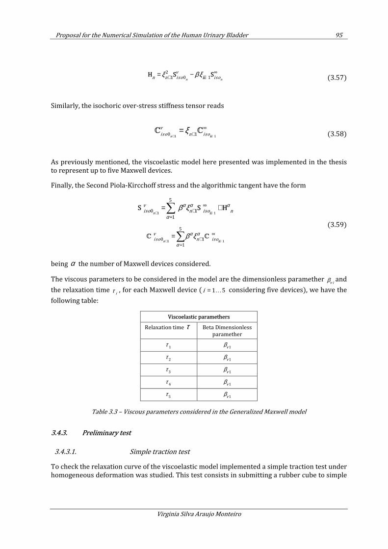
Proposal for the Numerical Simulation of the Human Urinary Bladder 95
Virginia Silva Araujo Monteiro
2
1 0 1n n
v
n n iso n isoξ βξ ∞
+ += −H S S (3.57)
Similarly, the isochoric over-stress stiffness tensor reads
1 10 1n n
v
iso n isoξ
+ +
∞+=C C (3.58)
As previously mentioned, the viscoelastic model here presented was implemented in the thesis to represent up to five Maxwell devices.
Finally, the Second Piola-Kircchoff stress and the algorithmic tangent have the form
1 1
5
0 1
1
n n
v
iso n iso n
α α α
αβ ξ
+ +
∞+
=
= +∑S S H
1 1
5
0 1
1
n n
v
iso n iso
α α
α
β ξ+ +
∞+
=
=∑C C
(3.59)
being α the number of Maxwell devices considered.
The viscous parameters to be considered in the model are the dimensionless paramether v i
β and
the relaxation time i
τ , for each Maxwell device ( 1 5i = K considering five devices), we have the
following table:
Viscoelastic paramethers
Relaxation time τ Beta Dimensionless
paramether
1τ
1vβ
2τ
1vβ
3τ
1vβ
4τ
1vβ
5τ
1vβ
Table 3.3 – Viscous parameters considered in the Generalized Maxwell model
3.4.3. Preliminary test
3.4.3.1. Simple traction test
To check the relaxation curve of the viscoelastic model implemented a simple traction test under homogeneous deformation was studied. This test consists in submitting a rubber cube to simple
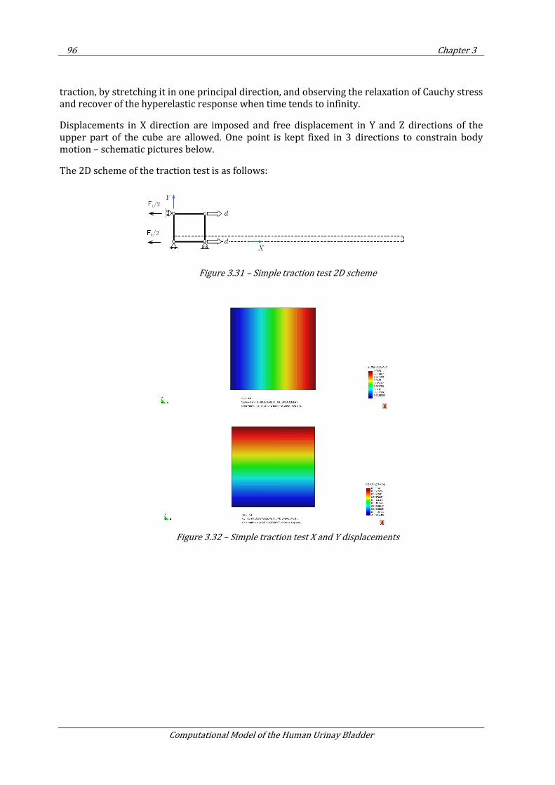
96 Chapter 3
Computational Model of the Human Urinay Bladder
traction, by stretching it in one principal direction, and observing the relaxation of Cauchy stress and recover of the hyperelastic response when time tends to infinity.
Displacements in X direction are imposed and free displacement in Y and Z directions of the upper part of the cube are allowed. One point is kept fixed in 3 directions to constrain body motion – schematic pictures below.
The 2D scheme of the traction test is as follows:
Figure 3.31 – Simple traction test 2D scheme
Figure 3.32 – Simple traction test X and Y displacements
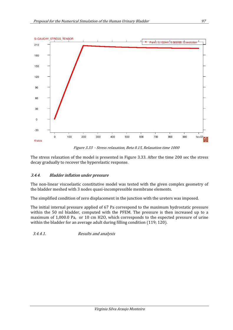
Proposal for the Numerical Simulation of the Human Urinary Bladder 97
Virginia Silva Araujo Monteiro
Figure 3.33 - Stress relaxation, Beta 0.15, Relaxation time 1000
The stress relaxation of the model is presented in Figure 3.33. After the time 200 sec the stress decay gradually to recover the hyperelastic response.
3.4.4. Bladder inflation under pressure
The non-linear viscoelastic constitutive model was tested with the given complex geometry of the bladder meshed with 3 nodes quasi-incompressible membrane elements.
The simplified condition of zero displacement in the junction with the ureters was imposed.
The initial internal pressure applied of 67 Pa correspond to the maximum hydrostatic pressure within the 50 ml bladder, computed with the PFEM. The pressure is then increased up to a maximum of 1,000.0 Pa, or 10 cm H2O, which corresponds to the expected pressure of urine within the bladder for an average adult during filling condition (119; 120).
3.4.4.1. Results and analysis
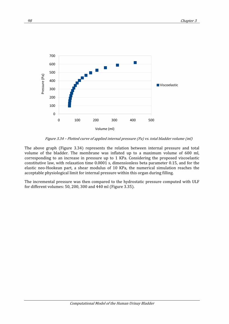
98 Chapter 3
Computational Model of the Human Urinay Bladder
Figure 3.34 – Plotted curve of applied internal pressure (Pa) vs. total bladder volume (ml)
The above graph (Figure 3.34) represents the relation between internal pressure and total volume of the bladder. The membrane was inflated up to a maximum volume of 600 ml, corresponding to an increase in pressure up to 1 KPa. Considering the proposed viscoelastic constitutive law, with relaxation time 0.0001 s, dimensionless beta parameter 0.15, and for the elastic neo-Hookean part, a shear modulus of 10 KPa, the numerical simulation reaches the acceptable physiological limit for internal pressure within this organ during filling.
The incremental pressure was then compared to the hydrostatic pressure computed with ULF for different volumes: 50, 200, 300 and 440 ml (Figure 3.35).
0
100
200
300
400
500
600
700
0 100 200 300 400 500
Pre
ssu
re (
Pa
)
Volume (ml)
Viscoelastic
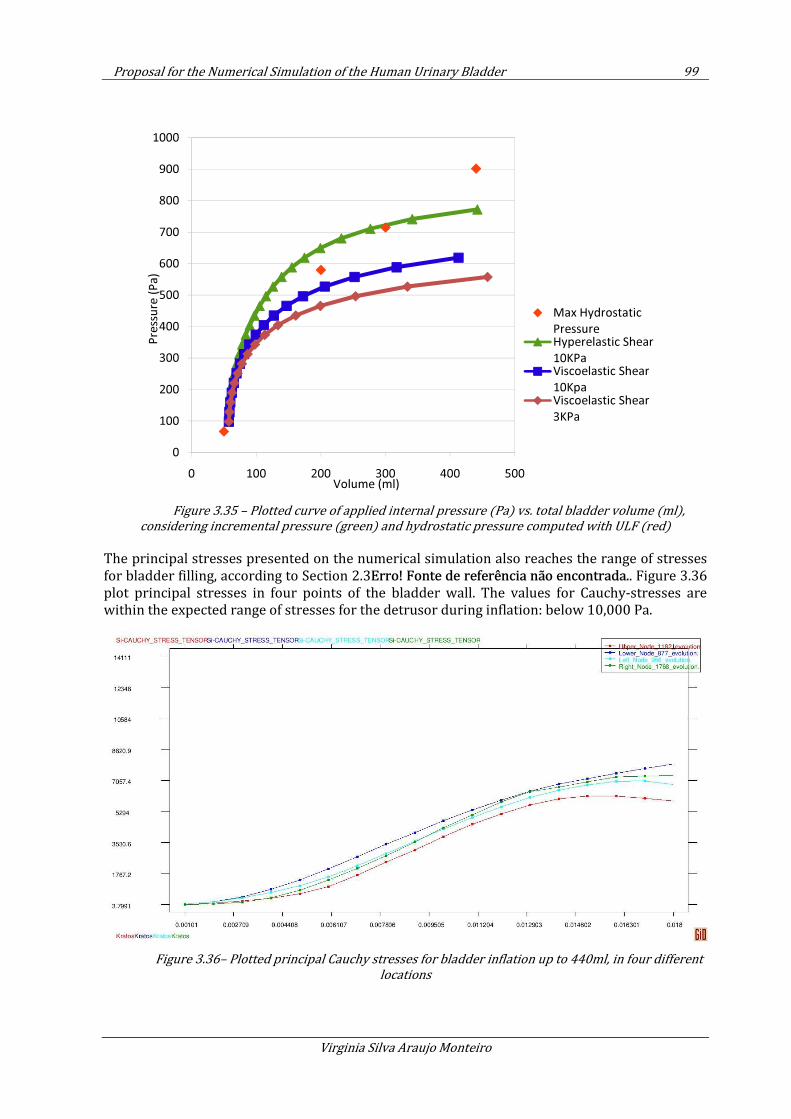
Proposal for the Numerical Simulation of the Human Urinary Bladder 99
Virginia Silva Araujo Monteiro
Figure 3.35 – Plotted curve of applied internal pressure (Pa) vs. total bladder volume (ml),
considering incremental pressure (green) and hydrostatic pressure computed with ULF (red)
The principal stresses presented on the numerical simulation also reaches the range of stresses for bladder filling, according to Section 2.3Erro! Fonte de referência não encontrada.. Figure 3.36 plot principal stresses in four points of the bladder wall. The values for Cauchy-stresses are within the expected range of stresses for the detrusor during inflation: below 10,000 Pa.
Figure 3.36– Plotted principal Cauchy stresses for bladder inflation up to 440ml, in four different
locations
0
100
200
300
400
500
600
700
800
900
1000
0 100 200 300 400 500
Pre
ssu
re (
Pa
)
Volume (ml)
Max Hydrostatic
PressureHyperelastic Shear
10KPaViscoelastic Shear
10KpaViscoelastic Shear
3KPa
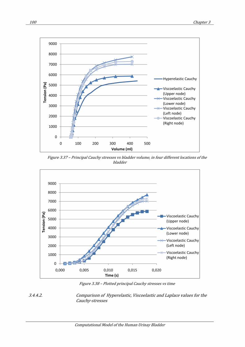
100 Chapter 3
Computational Model of the Human Urinay Bladder
Figure 3.37 – Principal Cauchy stresses vs bladder volume, in four different locations of the
bladder
Figure 3.38 – Plotted principal Cauchy stresses vs time
3.4.4.2. Comparison of Hyperelastic, Viscoelastic and Laplace values for the
Cauchy-stresses
0
1000
2000
3000
4000
5000
6000
7000
8000
9000
0 100 200 300 400 500
Te
nsi
on
(P
a)
Volume (ml)
Hyperelastic Cauchy
Viscoelastic Cauchy
(Upper node)
Viscoelastic Cauchy
(Lower node)
Viscoelastic Cauchy
(Left node)
Viscoelastic Cauchy
(Right node)
0
1000
2000
3000
4000
5000
6000
7000
8000
9000
0,000 0,005 0,010 0,015 0,020
Te
nsi
on
(P
a)
Time (s)
Viscoelastic Cauchy
(Upper node)
Viscoelastic Cauchy
(Lower node)
Viscoelastic Cauchy
(Left node)
Viscoelastic Cauchy
(Right node)
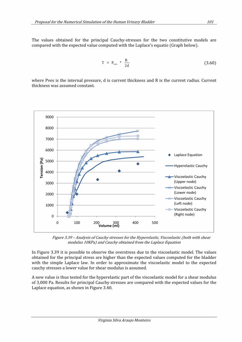
Proposal for the Numerical Simulation of the Human Urinary Bladder 101
Virginia Silva Araujo Monteiro
The values obtained for the principal Cauchy-stresses for the two constitutive models are compared with the expected value computed with the Laplace's equatio (Graph below).
ves
R T P
2d= ∗ (3.60)
where Pves is the internal pressure, d is current thickness and R is the current radius. Current thickness was assumed constant.
Figure 3.39 – Analysis of Cauchy stresses for the Hyperelastic, Viscoelastic (both with shear
modulus 10KPa) and Cauchy obtained from the Laplace Equation
In Figure 3.39 it is possible to observe the overstress due to the viscoelastic model. The values obtained for the principal stress are higher than the expected values computed for the bladder with the simple Laplace law. In order to approximate the viscoelastic model to the expected cauchy stresses a lower value for shear modulus is assumed.
A new value is thus tested for the hyperelastic part of the viscoelastic model for a shear modulus of 3,000 Pa. Results for principal Cauchy stresses are compared with the expected values for the Laplace equation, as shown in Figure 3.40.
0
1000
2000
3000
4000
5000
6000
7000
8000
9000
0 100 200 300 400 500
Te
nsi
on
(P
a)
Volume (ml)
Laplace Equation
Hyperelastic Cauchy
Viscoelastic Cauchy
(Upper node)
Viscoelastic Cauchy
(Lower node)
Viscoelastic Cauchy
(Left node)
Viscoelastic Cauchy
(Right node)
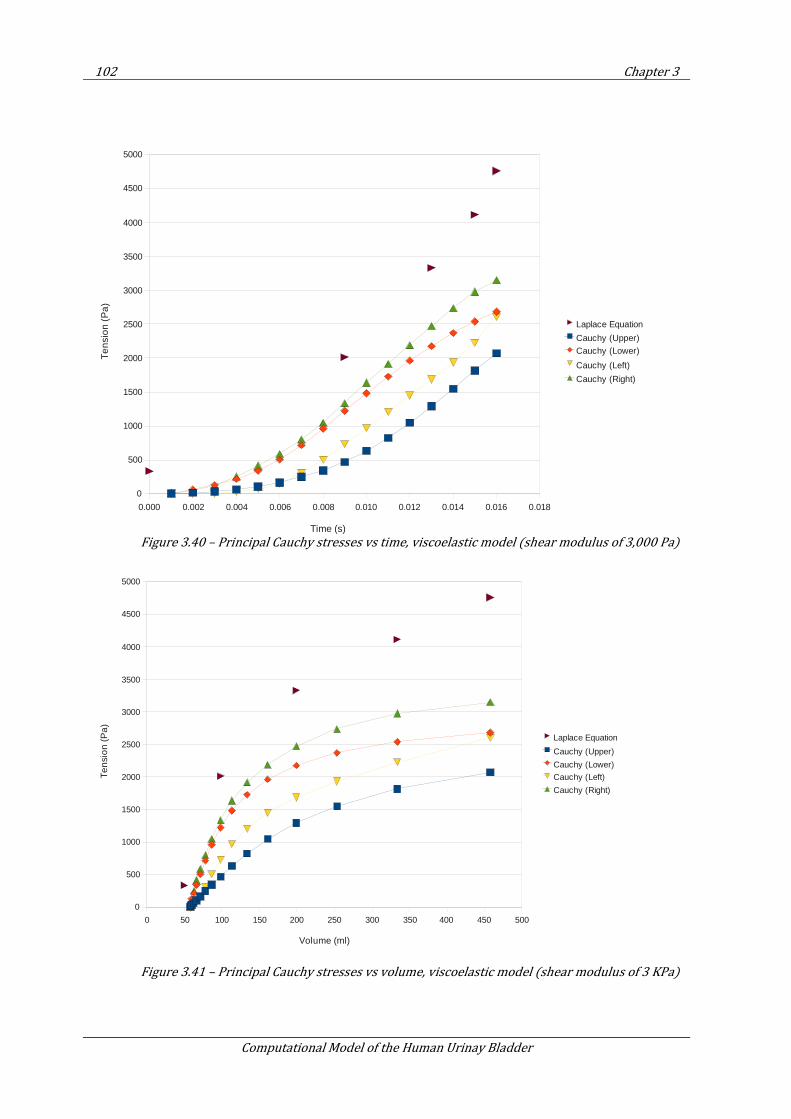
102 Chapter 3
Computational Model of the Human Urinay Bladder
Figure 3.40 – Principal Cauchy stresses vs time, viscoelastic model (shear modulus of 3,000 Pa)
Figure 3.41 – Principal Cauchy stresses vs volume, viscoelastic model (shear modulus of 3 KPa)
0.000 0.002 0.004 0.006 0.008 0.010 0.012 0.014 0.016 0.018
0
500
1000
1500
2000
2500
3000
3500
4000
4500
5000
Laplace Equation
Cauchy (Upper)Cauchy (Lower)
Cauchy (Left)
Cauchy (Right)
Time (s)
Te
nsi
on
(P
a)
0 50 100 150 200 250 300 350 400 450 500
0
500
1000
1500
2000
2500
3000
3500
4000
4500
5000
Laplace Equation
Cauchy (Upper)
Cauchy (Lower)
Cauchy (Left)
Cauchy (Right)
Volume (ml)
Te
nsi
on
(P
a)
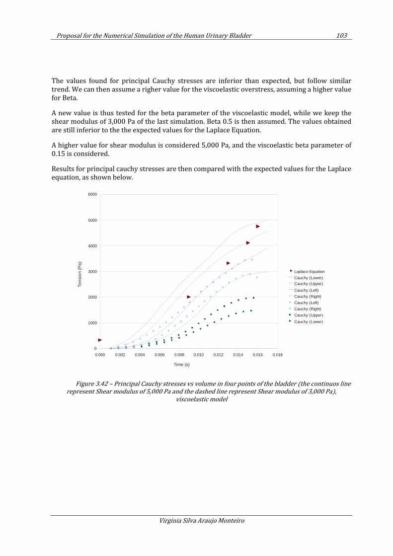
Proposal for the Numerical Simulation of the Human Urinary Bladder 103
Virginia Silva Araujo Monteiro
The values found for principal Cauchy stresses are inferior than expected, but follow similar trend. We can then assume a righer value for the viscoelastic overstress, assuming a higher value for Beta.
A new value is thus tested for the beta parameter of the viscoelastic model, while we keep the shear modulus of 3,000 Pa of the last simulation. Beta 0.5 is then assumed. The values obtained are still inferior to the the expected values for the Laplace Equation.
A higher value for shear modulus is considered 5,000 Pa, and the viscoelastic beta parameter of 0.15 is considered.
Results for principal cauchy stresses are then compared with the expected values for the Laplace equation, as shown below.
Figure 3.42 – Principal Cauchy stresses vs volume in four points of the bladder (the continuos line
represent Shear modulus of 5,000 Pa and the dashed line represent Shear modulus of 3,000 Pa),
viscoelastic model
0.000 0.002 0.004 0.006 0.008 0.010 0.012 0.014 0.016 0.018
0
1000
2000
3000
4000
5000
6000
Laplace Equation
Cauchy (Lower)
Cauchy (Upper)
Cauchy (Left)
Cauchy (Right)
Cauchy (Left)
Cauchy (Right)
Cauchy (Upper)
Cauchy (Lower)
Time (s)
Ten
sio
n (P
a)
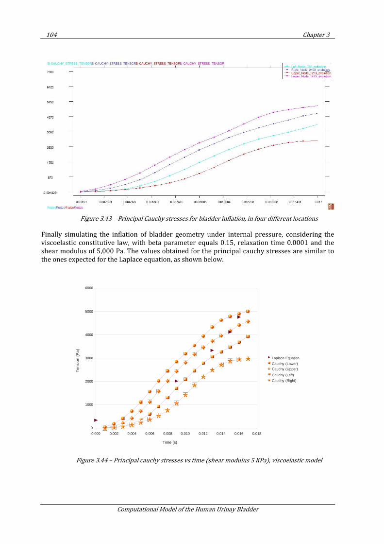
104 Chapter 3
Computational Model of the Human Urinay Bladder
Figure 3.43 – Principal Cauchy stresses for bladder inflation, in four different locations
Finally simulating the inflation of bladder geometry under internal pressure, considering the viscoelastic constitutive law, with beta parameter equals 0.15, relaxation time 0.0001 and the shear modulus of 5,000 Pa. The values obtained for the principal cauchy stresses are similar to the ones expected for the Laplace equation, as shown below.
Figure 3.44 – Principal cauchy stresses vs time (shear modulus 5 KPa), viscoelastic model
0.000 0.002 0.004 0.006 0.008 0.010 0.012 0.014 0.016 0.018
0
1000
2000
3000
4000
5000
6000
Laplace Equation
Cauchy (Lower)Cauchy (Upper)
Cauchy (Left)
Cauchy (Right)
Time (s)
Te
nsi
on
(P
a)
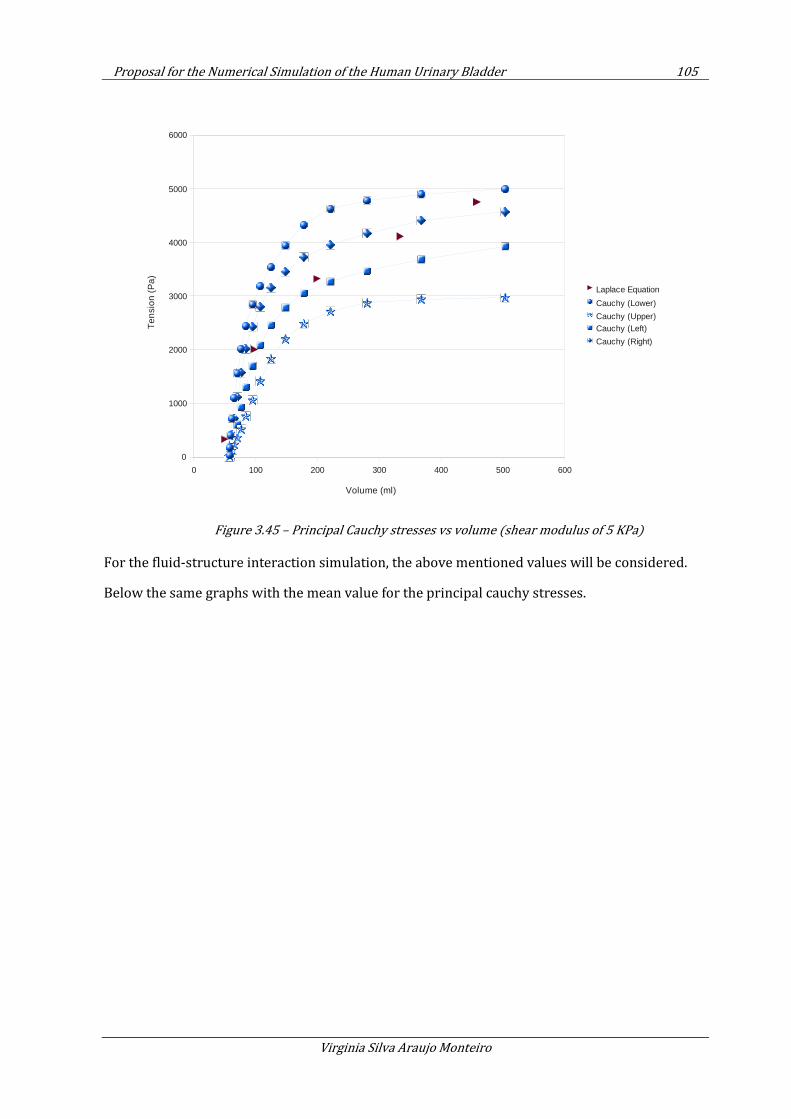
Proposal for the Numerical Simulation of the Human Urinary Bladder 105
Virginia Silva Araujo Monteiro
Figure 3.45 – Principal Cauchy stresses vs volume (shear modulus of 5 KPa)
For the fluid-structure interaction simulation, the above mentioned values will be considered.
Below the same graphs with the mean value for the principal cauchy stresses.
0 100 200 300 400 500 600
0
1000
2000
3000
4000
5000
6000
Laplace Equation
Cauchy (Lower)
Cauchy (Upper)Cauchy (Left)
Cauchy (Right)
Volume (ml)
Ten
sion
(P
a)
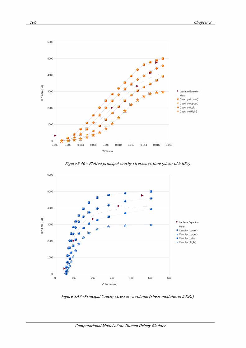
106 Chapter 3
Computational Model of the Human Urinay Bladder
Figure 3.46 – Plotted principal cauchy stresses vs time (shear of 5 KPa)
Figure 3.47 –Principal Cauchy stresses vs volume (shear modulus of 5 KPa)
0.000 0.002 0.004 0.006 0.008 0.010 0.012 0.014 0.016 0.018
0
1000
2000
3000
4000
5000
6000
Laplace Equation
Mean
Cauchy (Lower)
Cauchy (Upper)
Cauchy (Left)
Cauchy (Right)
Time (s)
Te
nsi
on
(P
a)
0 100 200 300 400 500 600
0
1000
2000
3000
4000
5000
6000
Laplace Equation
Mean
Cauchy (Lower)
Cauchy (Upper)
Cauchy (Left)
Cauchy (Right)
Volume (ml)
Te
nsi
on
(P
a)
Proposal for the Numerical Simulation of the Human Urinary Bladder 107
Virginia Silva Araujo Monteiro
3.5. Hyperelastic matrix reinforced with Viscoelastic fibers
3.5.1. Introduction
A third and more refined constitutive model is considered for the numerical simulation of the human bladder. It consists of a hyperelastic matrix reinforced with viscoelastic fibers. In a global perspective, random orientation of the fibers is considered. The model here presented intends to represent the phenomenological behavior of the micro-structure of the detrusor tissue, where the matrix consists of a neo-Hookean hyperelastic material and the collangen fibers are represented by two classes of perpendicular viscoelastic fibers at the element level. A similar model was proposed by Kondo et al in (9) where experiments were carried out to get the hyperelastic and viscoelastic parameters.
The neo-hookean model here considered was described in Section 3.3 and the viscoelastic model for the fiber is described in Section 3.4. The stress contribution of the fiber orientation is described in this chapter.
The phenomenological model considers the second Piola Kirchhoff of the model as a summation of these tensors:
vol iso fS S S
∞= + +S (3.61)
Where v o l
S and i so
S∞ are the volumetric and the hyperelastic contributions of the stress
respectively, computed as described in Section 3.3; f
S is the fiber contribution to the stress
tensor and is defined as:
v
f f fS S S
∞= + (3.62)
Where f
S∞ corresponds to the stress contribution of the elastic body of the Maxwell model and
v
fS corresponds to the viscous contribution of the the Maxwell model. The Generalized Maxwell
model is described in Section 3.4.
3.5.2. Computation of the fibers contribution term f
S
To consider collagen fibers, we introduce the unit fiber direction M denoting the
referential/local orientation of the fibers. The local structure of the material in Ω0
can be defined
by a symmetric second order structural tensor = ⊗A M M and at the current configuration as T=a FAF .
Once we introduce fibers, the material gets anisotropic. We thus introduce a fourth invariant 4I
to represent the fibers orientation, defined as
108 Chapter 3
Computational Model of the Human Urinay Bladder
4I = C : A (3.63)
The A tensor is:
0 0a a= ×A (3.64)
With 0a being the fiber direction.
The stored energy function reads
21
2 4
2
e xp ( 1) 12
kk I
k
Ψ = − − (3.65)
Where 1
k and 2
k are fiber parameters.
The first derivative of the stored energy function in respect to the fourth invariant is:
2
1 4 2 4
4
( 1)e x p ( 1)k I k II
∂ Ψ = − − ∂
(3.66)
Finally, the Second Piola-Kircchoff stress contribution of the fiber is
4 4
4
( )2 2
f
I I
I
∂Ψ ∂∂Ψ= =∂ ∂ ∂
SC C
2
13
4
12 ( : )
3fJ
I
− − ∂Ψ= − ∂ S A A C C
(3.67)
3.5.3. Fiber orientation
Two classes of fibers are considered, at the element level, being the first class of fibers perpendicular to the other.
Random fiber orientation
As discussed in Chapter 2, hystologic examination of the bladder body reveals that myofibrils are arranged into fascicles in random directions (111), differing from the discrete tubular and longitudinal smooth muscle layers in the ureter or gastrointestinal tract. The constitutive model here proposed considers the random distribution of fibers at the organ level.
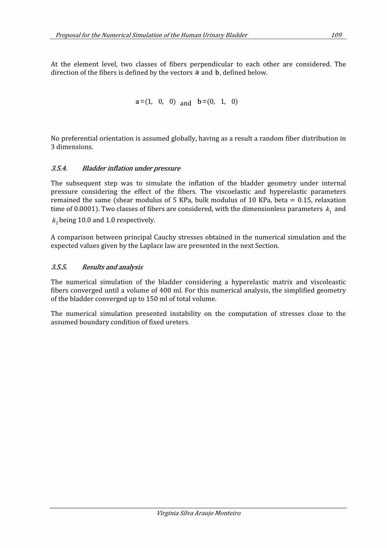
Proposal for the Numerical Simulation of the Human Urinary Bladder 109
Virginia Silva Araujo Monteiro
At the element level, two classes of fibers perpendicular to each other are considered. The direction of the fibers is defined by the vectors a and b , defined below.
(1, 0, 0)=a and (0, 1, 0)=b
No preferential orientation is assumed globally, having as a result a random fiber distribution in 3 dimensions.
3.5.4. Bladder inflation under pressure
The subsequent step was to simulate the inflation of the bladder geometry under internal pressure considering the effect of the fibers. The viscoelastic and hyperelastic parameters remained the same (shear modulus of 5 KPa, bulk modulus of 10 KPa, beta = 0.15, relaxation
time of 0.0001). Two classes of fibers are considered, with the dimensionless parameters 1
k and
2k being 10.0 and 1.0 respectively.
A comparison between principal Cauchy stresses obtained in the numerical simulation and the expected values given by the Laplace law are presented in the next Section.
3.5.5. Results and analysis
The numerical simulation of the bladder considering a hyperelastic matrix and viscoleastic fibers converged until a volume of 400 ml. For this numerical analysis, the simplified geometry of the bladder converged up to 150 ml of total volume.
The numerical simulation presented instability on the computation of stresses close to the assumed boundary condition of fixed ureters.
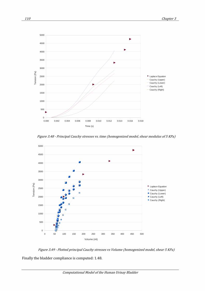
110 Chapter 3
Computational Model of the Human Urinay Bladder
Figure 3.48 - Principal Cauchy stresses vs. time (homogenized model, shear modulus of 5 KPa)
Figure 3.49 - Plotted principal Cauchy stresses vs Volume (homogenized model, shear 5 KPa)
Finally the bladder compliance is computed: 1.48.
0.000 0.002 0.004 0.006 0.008 0.010 0.012 0.014 0.016 0.018
0
500
1000
1500
2000
2500
3000
3500
4000
4500
5000
Laplace Equation
Cauchy (Upper)
Cauchy (Lower)
Cauchy (Left)
Cauchy (Right)
Time (s)
Te
nsi
on
(P
a)
0 50 100 150 200 250 300 350 400 450 500
0
500
1000
1500
2000
2500
3000
3500
4000
4500
5000
Laplace Equation
Cauchy (Upper)
Cauchy (Lower)
Cauchy (Left)
Cauchy (Right)
Volume (ml)
Te
nsi
on
(P
a)
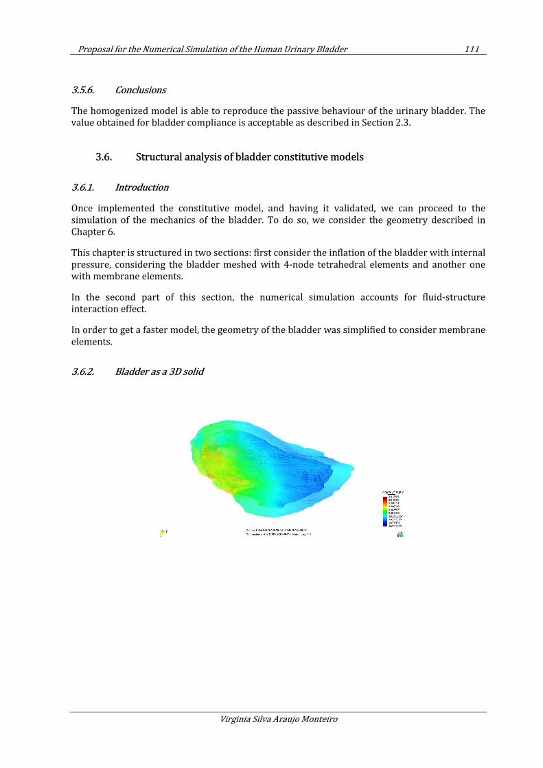
Proposal for the Numerical Simulation of the Human Urinary Bladder 111
Virginia Silva Araujo Monteiro
3.5.6. Conclusions
The homogenized model is able to reproduce the passive behaviour of the urinary bladder. The value obtained for bladder compliance is acceptable as described in Section 2.3.
3.6. Structural analysis of bladder constitutive models
3.6.1. Introduction
Once implemented the constitutive model, and having it validated, we can proceed to the simulation of the mechanics of the bladder. To do so, we consider the geometry described in Chapter 6.
This chapter is structured in two sections: first consider the inflation of the bladder with internal pressure, considering the bladder meshed with 4-node tetrahedral elements and another one with membrane elements.
In the second part of this section, the numerical simulation accounts for fluid-structure interaction effect.
In order to get a faster model, the geometry of the bladder was simplified to consider membrane elements.
3.6.2. Bladder as a 3D solid
112 Chapter 3
Computational Model of the Human Urinay Bladder
Figure 3.50 – Results showing displacements in Y (a) and Z (b) directions after applying internal
pressure to the structure
Figure 3.51 shows localized problems during the inflation of the bladder with pressure. These problems occur due to the different thickness of the structure and to the deformation of elements in certain areas. Stress concentration in these areas generate convergence problems.
Figure 3.51 – Occurrence of localized problems during the inflation of the structure meshed with
tetrahedral elements
3.6.3. Bladder modeled as a membrane
The geometry of the bladder modeled with 3-node triangular membrane elements is then inflated with internal pressure.
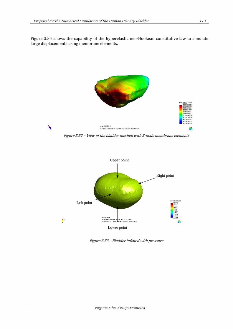
Proposal for the Numerical Simulation of the Human Urinary Bladder 113
Virginia Silva Araujo Monteiro
Figure 3.54 shows the capability of the hyperelastic neo-Hookean constitutive law to simulate large displacements using membrane elements.
Figure 3.52 – View of the bladder meshed with 3-node membrane elements
Figure 3.53 – Bladder inflated with pressure
Upper point
Right point
Left point
Lower point
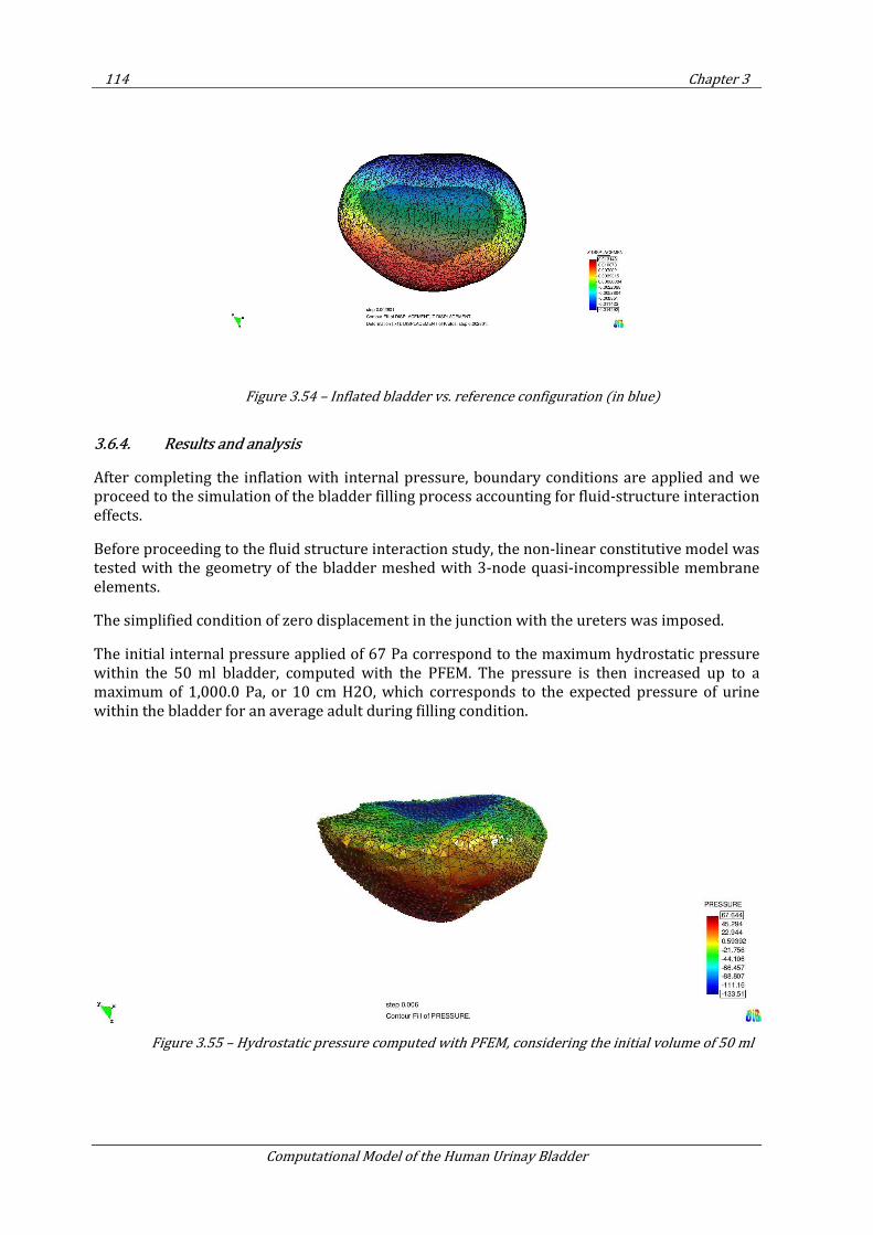
114 Chapter 3
Computational Model of the Human Urinay Bladder
Figure 3.54 – Inflated bladder vs. reference configuration (in blue)
3.6.4. Results and analysis
After completing the inflation with internal pressure, boundary conditions are applied and we proceed to the simulation of the bladder filling process accounting for fluid-structure interaction effects.
Before proceeding to the fluid structure interaction study, the non-linear constitutive model was tested with the geometry of the bladder meshed with 3-node quasi-incompressible membrane elements.
The simplified condition of zero displacement in the junction with the ureters was imposed.
The initial internal pressure applied of 67 Pa correspond to the maximum hydrostatic pressure within the 50 ml bladder, computed with the PFEM. The pressure is then increased up to a maximum of 1,000.0 Pa, or 10 cm H2O, which corresponds to the expected pressure of urine within the bladder for an average adult during filling condition.
Figure 3.55 – Hydrostatic pressure computed with PFEM, considering the initial volume of 50 ml
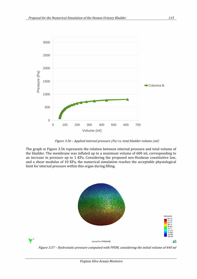
Proposal for the Numerical Simulation of the Human Urinary Bladder 115
Virginia Silva Araujo Monteiro
Figure 3.56 – Applied internal pressure (Pa) vs. total bladder volume (ml)
The graph in Figure 3.56 represents the relation between internal pressure and total volume of the bladder. The membrane was inflated up to a maximum volume of 600 ml, corresponding to an increase in pressure up to 1 KPa. Considering the proposed neo-Hookean constitutive law, and a shear modulus of 10 KPa, the numerical simulation reaches the acceptable physiological limit for internal pressure within this organ during filling.
Figure 3.57 – Hydrostatic pressure computed with PFEM, considering the initial volume of 440 ml
0 100 200 300 400 500 600 7000
500
1000
1500
2000
2500
3000
Columna B
Volume (ml)
Pre
ssu
re (
Pa)
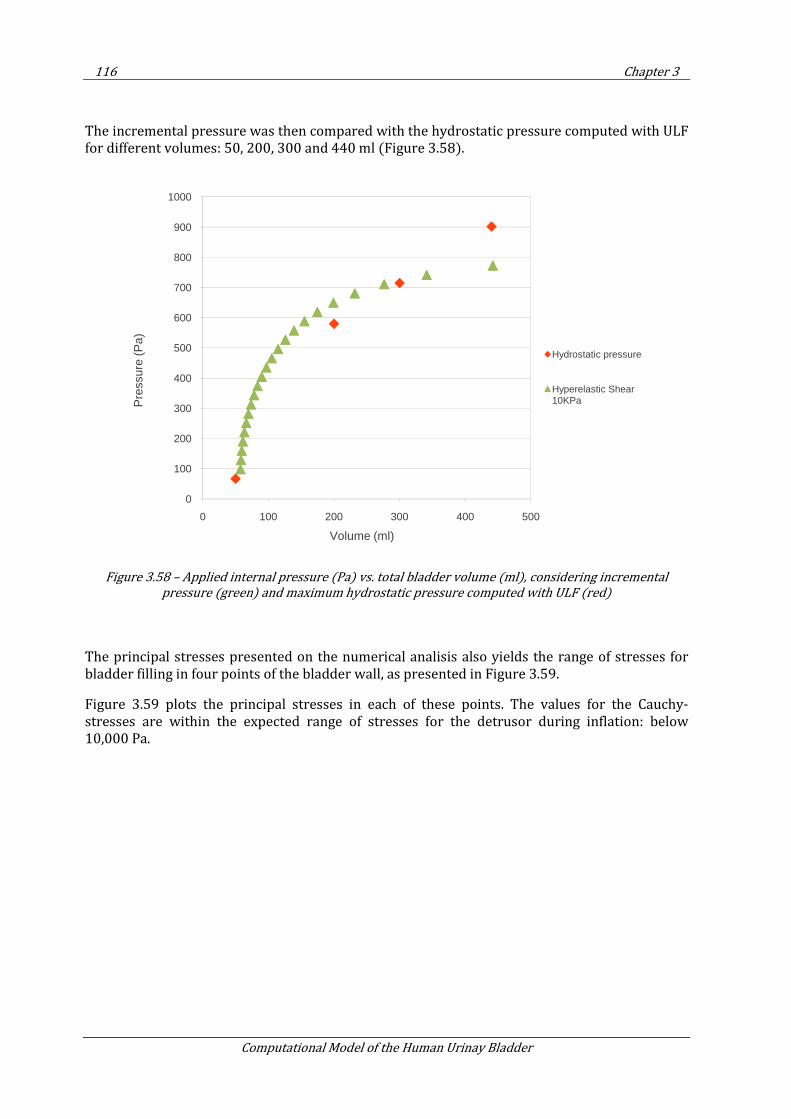
116 Chapter 3
Computational Model of the Human Urinay Bladder
The incremental pressure was then compared with the hydrostatic pressure computed with ULF for different volumes: 50, 200, 300 and 440 ml (Figure 3.58).
Figure 3.58 – Applied internal pressure (Pa) vs. total bladder volume (ml), considering incremental
pressure (green) and maximum hydrostatic pressure computed with ULF (red)
The principal stresses presented on the numerical analisis also yields the range of stresses for bladder filling in four points of the bladder wall, as presented in Figure 3.59.
Figure 3.59 plots the principal stresses in each of these points. The values for the Cauchy-stresses are within the expected range of stresses for the detrusor during inflation: below 10,000 Pa.
0
100
200
300
400
500
600
700
800
900
1000
0 100 200 300 400 500
Pre
ssur
e (P
a)
Volume (ml)
Hydrostatic pressure
Hyperelastic Shear 10KPa
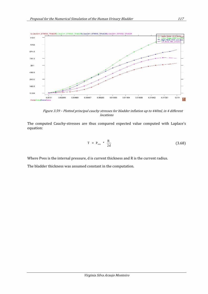
Proposal for the Numerical Simulation of the Human Urinary Bladder 117
Virginia Silva Araujo Monteiro
Figure 3.59 – Plotted principal cauchy stresses for bladder inflation up to 440ml, in 4 different
locations
The computed Cauchy-stresses are thus compared expected value computed with Laplace's equation:
ves
R T P
2d= ∗ (3.68)
Where Pves is the internal pressure, d is current thickness and R is the current radius.
The bladder thickness was assumed constant in the computation.
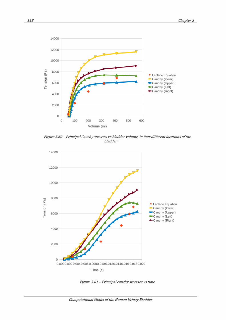
118 Chapter 3
Computational Model of the Human Urinay Bladder
Figure 3.60 – Principal Cauchy stresses vs bladder volume, in four different locations of the
bladder
Figure 3.61 – Principal cauchy stresses vs time
0 100 200 300 400 500 600
0
2000
4000
6000
8000
10000
12000
14000
Laplace EquationCauchy (lower)Cauchy (Upper)Cauchy (Left)Cauchy (Right)
Volume (ml)
Ten
sio
n (
Pa
)
0,0000,002 0,0040,006 0,0080,010 0,0120,0140,016 0,0180,0200
2000
4000
6000
8000
10000
12000
14000
Laplace EquationCauchy (lower)Cauchy (Upper)Cauchy (Left)Cauchy (Right)
Time (s)
Ten
sio
n (P
a)
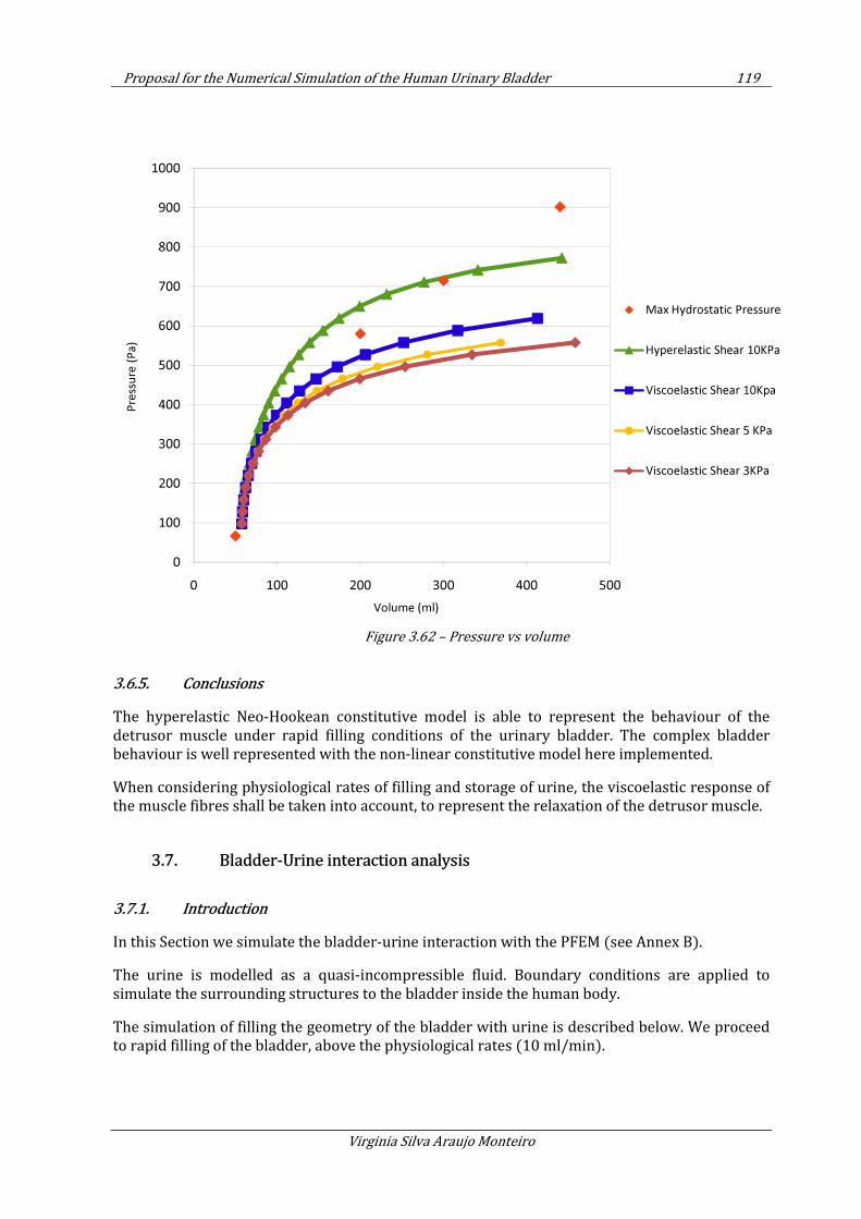
Proposal for the Numerical Simulation of the Human Urinary Bladder 119
Virginia Silva Araujo Monteiro
Figure 3.62 – Pressure vs volume
3.6.5. Conclusions
The hyperelastic Neo-Hookean constitutive model is able to represent the behaviour of the detrusor muscle under rapid filling conditions of the urinary bladder. The complex bladder behaviour is well represented with the non-linear constitutive model here implemented.
When considering physiological rates of filling and storage of urine, the viscoelastic response of the muscle fibres shall be taken into account, to represent the relaxation of the detrusor muscle.
3.7. Bladder-Urine interaction analysis
3.7.1. Introduction
In this Section we simulate the bladder-urine interaction with the PFEM (see Annex B).
The urine is modelled as a quasi-incompressible fluid. Boundary conditions are applied to simulate the surrounding structures to the bladder inside the human body.
The simulation of filling the geometry of the bladder with urine is described below. We proceed to rapid filling of the bladder, above the physiological rates (10 ml/min).
0
100
200
300
400
500
600
700
800
900
1000
0 100 200 300 400 500
Pre
ssu
re (
Pa
)
Volume (ml)
Max Hydrostatic Pressure
Hyperelastic Shear 10KPa
Viscoelastic Shear 10Kpa
Viscoelastic Shear 5 KPa
Viscoelastic Shear 3KPa
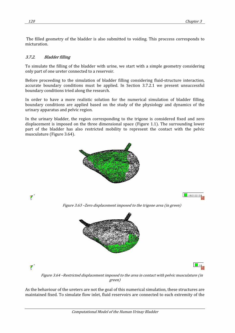
120 Chapter 3
Computational Model of the Human Urinay Bladder
The filled geometry of the bladder is also submitted to voiding. This proccess corresponds to micturation.
3.7.2. Bladder filling
To simulate the filling of the bladder with urine, we start with a simple geometry considering only part of one ureter connected to a reservoir.
Before proceeding to the simulation of bladder filling considering fluid-structure interaction, accurate boundary conditions must be applied. In Section 3.7.2.1 we present unsuccessful boundary conditions tried along the research.
In order to have a more realistic solution for the numerical simulation of bladder filling, boundary conditions are applied based on the study of the physiology and dynamics of the urinary apparatus and pelvic region.
In the urinary bladder, the region corresponding to the trigone is considered fixed and zero displacement is imposed on the three dimensional space (Figure 1.1). The surrounding lower part of the bladder has also restricted mobility to represent the contact with the pelvic musculature (Figure 3.64).
Figure 3.63 –Zero displacement imposed to the trigone area (in green)
Figure 3.64 –Restricted displacement imposed to the area in contact with pelvic musculature (in
green)
As the behaviour of the ureters are not the goal of this numerical simulation, these structures are maintained fixed. To simulate flow inlet, fluid reservoirs are connected to each extremity of the
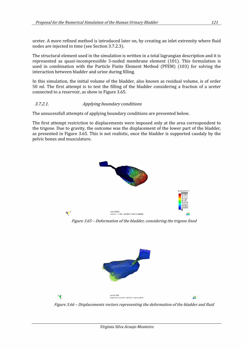
Proposal for the Numerical Simulation of the Human Urinary Bladder 121
Virginia Silva Araujo Monteiro
ureter. A more refined method is introduced later on, by creating an inlet extremity where fluid nodes are injected in time (see Section 3.7.2.3).
The structural element used in the simulation is written in a total lagrangian description and it is represented as quasi-incompressible 3-noded membrane element (101). This formulation is used in combination with the Particle Finite Element Method (PFEM) (103) for solving the interaction between bladder and urine during filling.
In this simulation, the initial volume of the bladder, also known as residual volume, is of order 50 ml. The first attempt is to test the filling of the bladder considering a fraction of a ureter connected to a reservoir, as show in Figure 3.65.
3.7.2.1. Applying boundary conditions
The unsucessfull attempts of applying boundary conditions are presented below.
The first attempt restriction to displacements were imposed only at the area correspondent to the trigone. Due to gravity, the outcome was the displacement of the lower part of the bladder, as presented in Figure 3.65. This is not realistic, once the bladder is supported caudaly by the pelvic bones and musculature.
Figure 3.65 – Deformation of the bladder, considering the trigone fixed
Figure 3.66 – Displacements vectors representing the deformation of the bladder and fluid
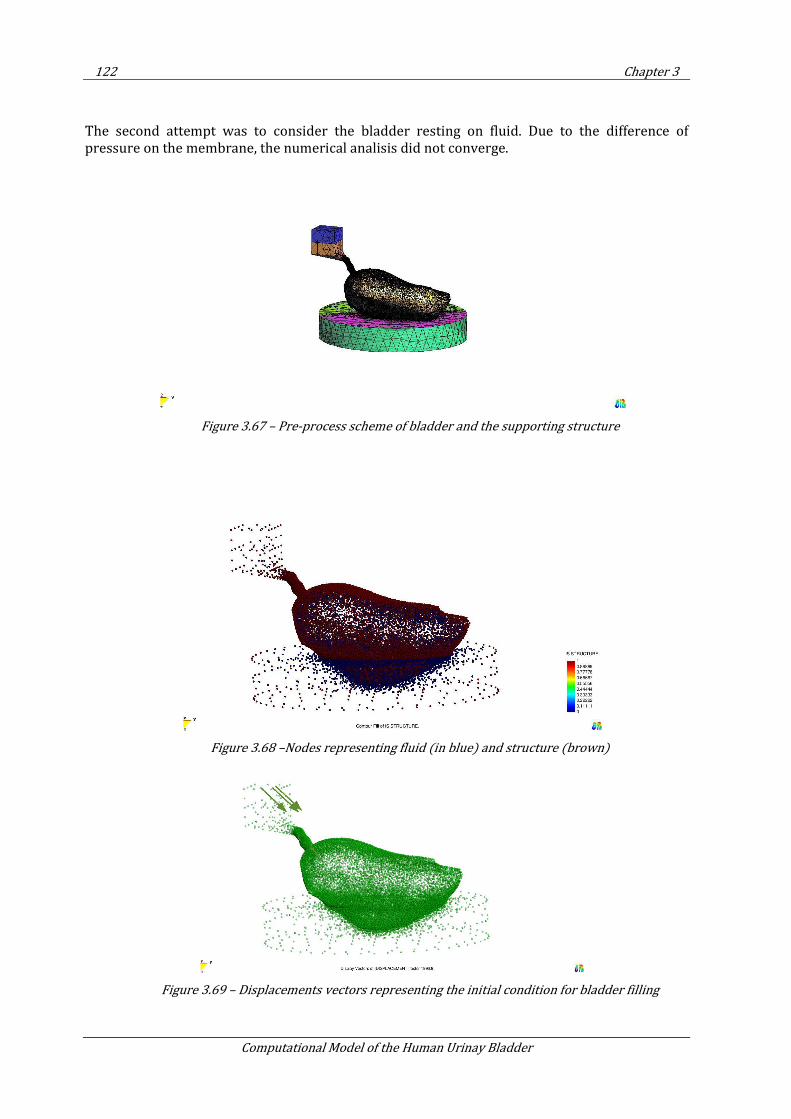
122 Chapter 3
Computational Model of the Human Urinay Bladder
The second attempt was to consider the bladder resting on fluid. Due to the difference of pressure on the membrane, the numerical analisis did not converge.
Figure 3.67 – Pre-process scheme of bladder and the supporting structure
Figure 3.68 –Nodes representing fluid (in blue) and structure (brown)
Figure 3.69 – Displacements vectors representing the initial condition for bladder filling
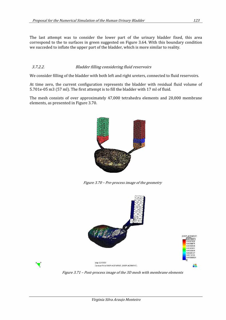
Proposal for the Numerical Simulation of the Human Urinary Bladder 123
Virginia Silva Araujo Monteiro
The last attempt was to consider the lower part of the urinary bladder fixed, this area correspond to the to surfaces in green suggested on Figure 3.64. With this boundary condition we succeded to inflate the upper part of the bladder, which is more similar to reality.
3.7.2.2. Bladder filling considering fluid reservoirs
We consider filling of the bladder with both left and right ureters, connected to fluid reservoirs.
At time zero, the current configuration represents the bladder with residual fluid volume of 5.701e-05 m3 (57 ml). The first attempt is to fill the bladder with 17 ml of fluid.
The mesh consists of over approximately 47,000 tetrahedra elements and 20,000 membrane elements, as presented in Figure 3.70.
Figure 3.70 – Pre-process image of the geometry
Figure 3.71 – Post-process image of the 3D mesh with membrane elements
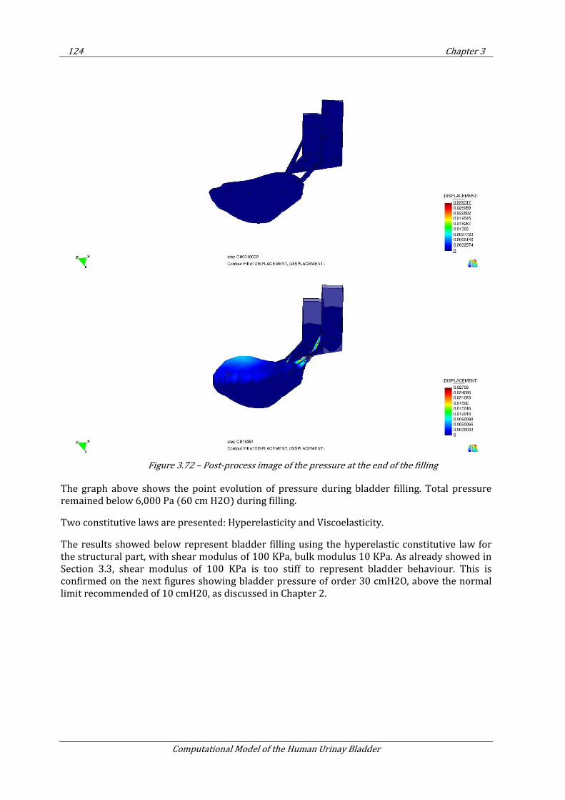
124 Chapter 3
Computational Model of the Human Urinay Bladder
Figure 3.72 – Post-process image of the pressure at the end of the filling
The graph above shows the point evolution of pressure during bladder filling. Total pressure remained below 6,000 Pa (60 cm H2O) during filling.
Two constitutive laws are presented: Hyperelasticity and Viscoelasticity.
The results showed below represent bladder filling using the hyperelastic constitutive law for the structural part, with shear modulus of 100 KPa, bulk modulus 10 KPa. As already showed in Section 3.3, shear modulus of 100 KPa is too stiff to represent bladder behaviour. This is confirmed on the next figures showing bladder pressure of order 30 cmH2O, above the normal limit recommended of 10 cmH20, as discussed in Chapter 2.
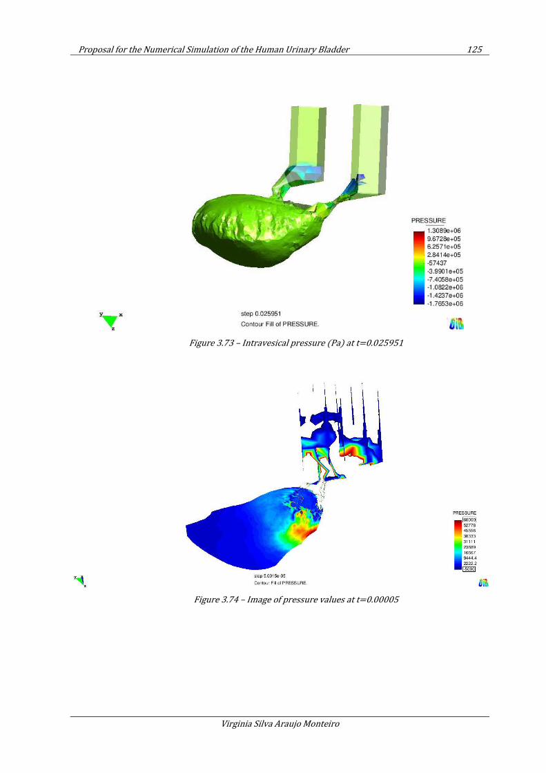
Proposal for the Numerical Simulation of the Human Urinary Bladder 125
Virginia Silva Araujo Monteiro
Figure 3.73 – Intravesical pressure (Pa) at t=0.025951
Figure 3.74 – Image of pressure values at t=0.00005
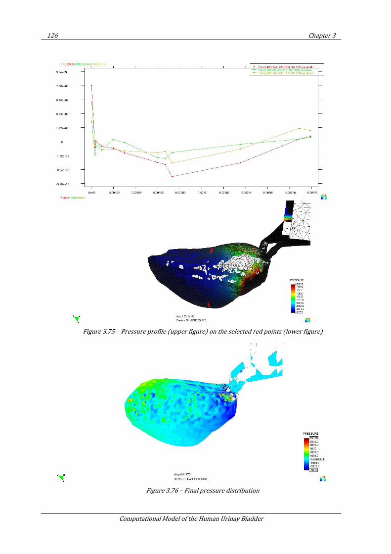
126 Chapter 3
Computational Model of the Human Urinay Bladder
Figure 3.75 – Pressure profile (upper figure) on the selected red points (lower figure)
Figure 3.76 – Final pressure distribution
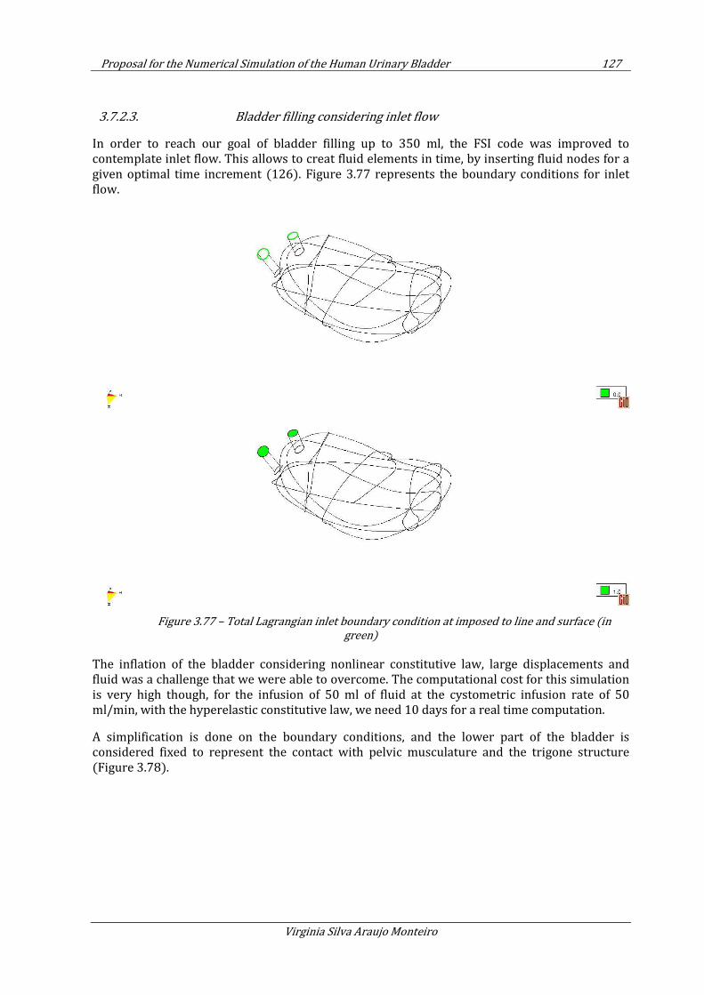
Proposal for the Numerical Simulation of the Human Urinary Bladder 127
Virginia Silva Araujo Monteiro
3.7.2.3. Bladder filling considering inlet flow
In order to reach our goal of bladder filling up to 350 ml, the FSI code was improved to contemplate inlet flow. This allows to creat fluid elements in time, by inserting fluid nodes for a given optimal time increment (126). Figure 3.77 represents the boundary conditions for inlet flow.
Figure 3.77 – Total Lagrangian inlet boundary condition at imposed to line and surface (in
green)
The inflation of the bladder considering nonlinear constitutive law, large displacements and fluid was a challenge that we were able to overcome. The computational cost for this simulation is very high though, for the infusion of 50 ml of fluid at the cystometric infusion rate of 50 ml/min, with the hyperelastic constitutive law, we need 10 days for a real time computation.
A simplification is done on the boundary conditions, and the lower part of the bladder is considered fixed to represent the contact with pelvic musculature and the trigone structure (Figure 3.78).
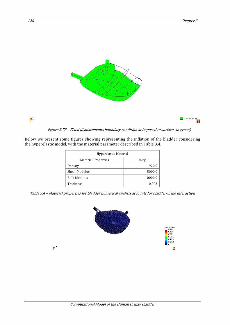
128 Chapter 3
Computational Model of the Human Urinay Bladder
Figure 3.78 – Fixed displacements boundary condition at imposed to surface (in green)
Below we present some figures showing representing the inflation of the bladder considering the hyperelastic model, with the material parameter described in Table 3.4.
Hyperelastic Material
Material Properties Unity
Denisty 920.0
Shear Modulus 5000.0
Bulk Modulus 10000.0
Thickness 0.003
Table 3.4 – Material properties for bladder numerical analisis accounts for bladder-urine interaction
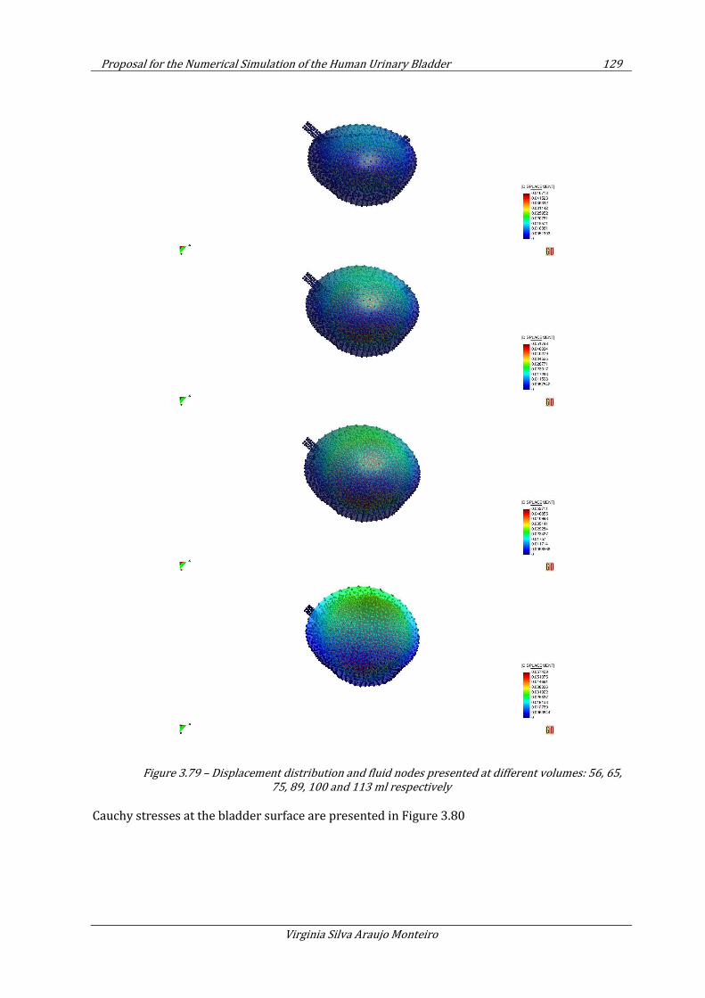
Proposal for the Numerical Simulation of the Human Urinary Bladder 129
Virginia Silva Araujo Monteiro
Figure 3.79 – Displacement distribution and fluid nodes presented at different volumes: 56, 65,
75, 89, 100 and 113 ml respectively
Cauchy stresses at the bladder surface are presented in Figure 3.80
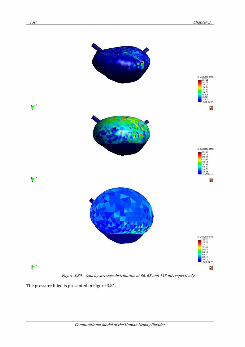
130 Chapter 3
Computational Model of the Human Urinay Bladder
Figure 3.80 – Cauchy stresses distribution at 56, 65 and 113 ml respectively
The pressure filled is presented in Figure 3.81.
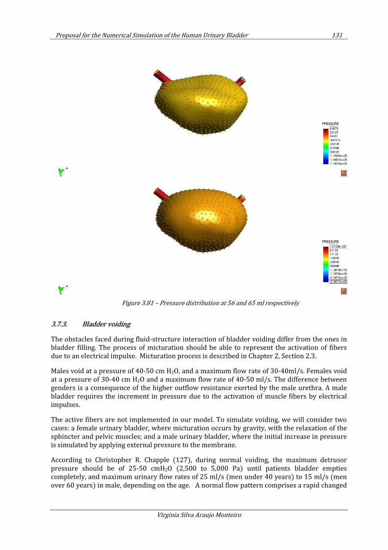
Proposal for the Numerical Simulation of the Human Urinary Bladder 131
Virginia Silva Araujo Monteiro
Figure 3.81 – Pressure distribution at 56 and 65 ml respectively
3.7.3. Bladder voiding
The obstacles faced during fluid-structure interaction of bladder voiding differ from the ones in bladder filling. The process of micturation should be able to represent the activation of fibers due to an electrical impulse. Micturation process is described in Chapter 2, Section 2.3.
Males void at a pressure of 40-50 cm H2O, and a maximum flow rate of 30-40ml/s. Females void at a pressure of 30-40 cm H2O and a maximum flow rate of 40-50 ml/s. The difference between genders is a consequence of the higher outflow resistance exerted by the male urethra. A male bladder requires the increment in pressure due to the activation of muscle fibers by electrical impulses.
The active fibers are not implemented in our model. To simulate voiding, we will consider two cases: a female urinary bladder, where micturation occurs by gravity, with the relaxation of the sphincter and pelvic muscles; and a male urinary bladder, where the initial increase in pressure is simulated by applying external pressure to the membrane.
According to Christopher R. Chapple (127), during normal voiding, the maximum detrusor pressure should be of 25-50 cmH2O (2,500 to 5,000 Pa) until patients bladder empties completely, and maximum urinary flow rates of 25 ml/s (men under 40 years) to 15 ml/s (men over 60 years) in male, depending on the age. A normal flow pattern comprises a rapid changed
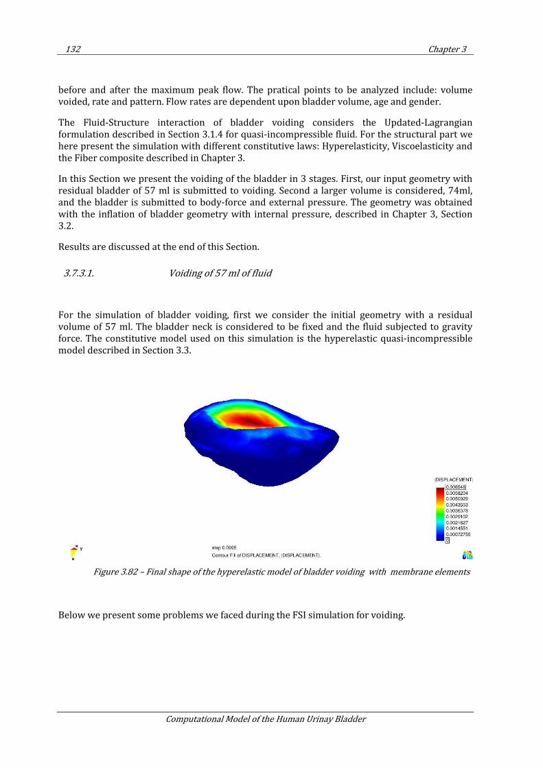
132 Chapter 3
Computational Model of the Human Urinay Bladder
before and after the maximum peak flow. The pratical points to be analyzed include: volume voided, rate and pattern. Flow rates are dependent upon bladder volume, age and gender.
The Fluid-Structure interaction of bladder voiding considers the Updated-Lagrangian formulation described in Section 3.1.4 for quasi-incompressible fluid. For the structural part we here present the simulation with different constitutive laws: Hyperelasticity, Viscoelasticity and the Fiber composite described in Chapter 3.
In this Section we present the voiding of the bladder in 3 stages. First, our input geometry with residual bladder of 57 ml is submitted to voiding. Second a larger volume is considered, 74ml, and the bladder is submitted to body-force and external pressure. The geometry was obtained with the inflation of bladder geometry with internal pressure, described in Chapter 3, Section 3.2.
Results are discussed at the end of this Section.
3.7.3.1. Voiding of 57 ml of fluid
For the simulation of bladder voiding, first we consider the initial geometry with a residual volume of 57 ml. The bladder neck is considered to be fixed and the fluid subjected to gravity force. The constitutive model used on this simulation is the hyperelastic quasi-incompressible model described in Section 3.3.
Figure 3.82 – Final shape of the hyperelastic model of bladder voiding with membrane elements
Below we present some problems we faced during the FSI simulation for voiding.
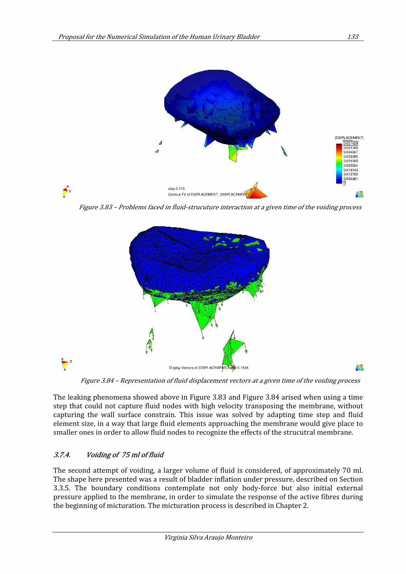
Proposal for the Numerical Simulation of the Human Urinary Bladder 133
Virginia Silva Araujo Monteiro
Figure 3.83 – Problems faced in fluid-strucuture interaction at a given time of the voiding process
Figure 3.84 – Representation of fluid displacement vectors at a given time of the voiding process
The leaking phenomena showed above in Figure 3.83 and Figure 3.84 arised when using a time step that could not capture fluid nodes with high velocity transposing the membrane, without capturing the wall surface constrain. This issue was solved by adapting time step and fluid element size, in a way that large fluid elements approaching the membrane would give place to smaller ones in order to allow fluid nodes to recognize the effects of the strucutral membrane.
3.7.4. Voiding of 75 ml of fluid
The second attempt of voiding, a larger volume of fluid is considered, of approximately 70 ml. The shape here presented was a result of bladder inflation under pressure, described on Section 3.3.5. The boundary conditions contemplate not only body-force but also initial external pressure applied to the membrane, in order to simulate the response of the active fibres during the beginning of micturation. The micturation process is described in Chapter 2.
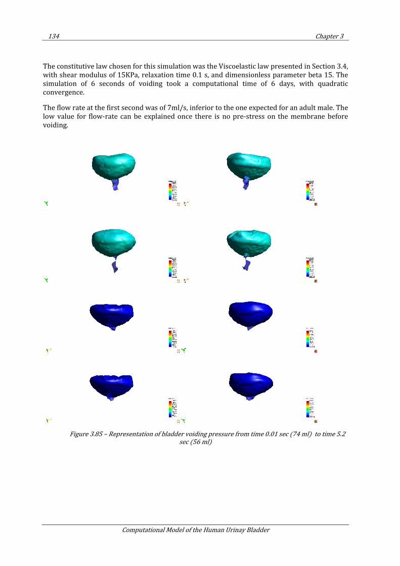
134 Chapter 3
Computational Model of the Human Urinay Bladder
The constitutive law chosen for this simulation was the Viscoelastic law presented in Section 3.4, with shear modulus of 15KPa, relaxation time 0.1 s, and dimensionless parameter beta 15. The simulation of 6 seconds of voiding took a computational time of 6 days, with quadratic convergence.
The flow rate at the first second was of 7ml/s, inferior to the one expected for an adult male. The low value for flow-rate can be explained once there is no pre-stress on the membrane before voiding.
Figure 3.85 – Representation of bladder voiding pressure from time 0.01 sec (74 ml) to time 5.2
sec (56 ml)
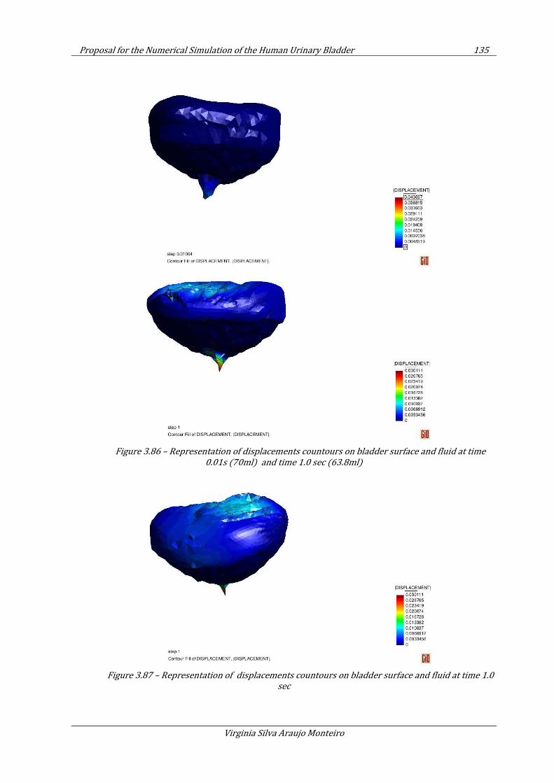
Proposal for the Numerical Simulation of the Human Urinary Bladder 135
Virginia Silva Araujo Monteiro
Figure 3.86 – Representation of displacements countours on bladder surface and fluid at time
0.01s (70ml) and time 1.0 sec (63.8ml)
Figure 3.87 – Representation of displacements countours on bladder surface and fluid at time 1.0
sec
136 Chapter 3
Computational Model of the Human Urinay Bladder
The bladder is then voided in 6 seconds, with a average flow rate of 8 ml/s, comparing to 13 ml/s, suggest by the literature (70).
3.7.5. Conclusion
The numerical simulation of bladder filling gives satisfactory results for rapid fluid filling rates. The PFEM is able to accurately simulate bladder filling and translate the urine pressure to the bladder wall.
We could also simulate the process of micturation, being able to study pressure profiles within the bladder.
The model here presented is a simplification of the complex urological apparatus, and does not properly address the behavior of ureters and urethra.
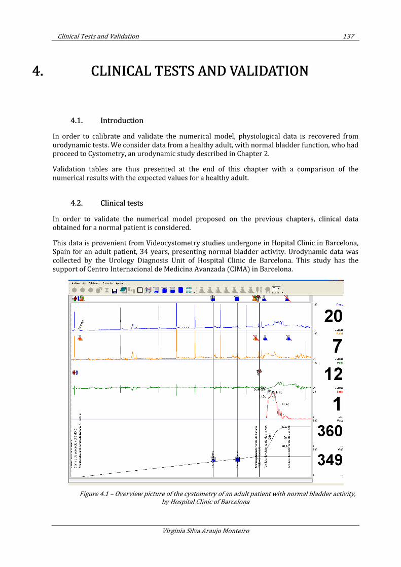
Clinical Tests and Validation 137
Virginia Silva Araujo Monteiro
4. CLINICAL TESTS AND VALIDATION
4.1. Introduction
In order to calibrate and validate the numerical model, physiological data is recovered from urodynamic tests. We consider data from a healthy adult, with normal bladder function, who had proceed to Cystometry, an urodynamic study described in Chapter 2.
Validation tables are thus presented at the end of this chapter with a comparison of the numerical results with the expected values for a healthy adult.
4.2. Clinical tests
In order to validate the numerical model proposed on the previous chapters, clinical data obtained for a normal patient is considered.
This data is provenient from Videocystometry studies undergone in Hopital Clinic in Barcelona, Spain for an adult patient, 34 years, presenting normal bladder activity. Urodynamic data was collected by the Urology Diagnosis Unit of Hospital Clinic de Barcelona. This study has the support of Centro Internacional de Medicina Avanzada (CIMA) in Barcelona.
Figure 4.1 – Overview picture of the cystometry of an adult patient with normal bladder activity,
by Hospital Clinic of Barcelona
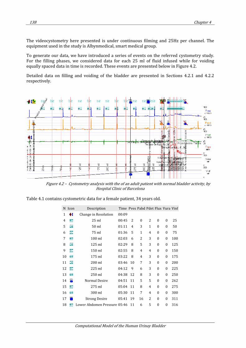
138 Chapter 4
Computational Model of the Human Urinay Bladder
The videocystometry here presented is under continuous filming and 25Hz per channel. The equipment used in the study is Albynmedical, smart medical group.
To generate our data, we have introduced a series of events on the referred cystometry study. For the filling phases, we considered data for each 25 ml of fluid infused while for voiding equally spaced data in time is recorded. These events are presented below in Figure 4.2.
Detailed data on filling and voiding of the bladder are presented in Sections 4.2.1 and 4.2.2 respectively.
Figure 4.2 – Cystometry analysis with the of an adult patient with normal bladder activity, by
Hospital Clinic of Barcelona
Table 4.1 contains cystometric data for a female patient, 34 years old.
N Icon Description Time Pves Pabd Pdet Flux Vura Vinf
1 Change in Resolution 00:09
4 25 ml 00:45 2 0 2 0 0 25
5 50 ml 01:11 4 3 1 0 0 50
6 75 ml 01:36 5 1 4 0 0 75
7 100 ml 02:03 6 2 3 0 0 100
8 125 ml 02:29 8 5 3 0 0 125
9 150 ml 02:55 8 4 4 0 0 150
10 175 ml 03:22 8 4 3 0 0 175
11 200 ml 03:46 10 7 3 0 0 200
12 225 ml 04:12 9 6 3 0 0 225
13 250 ml 04:38 12 8 3 0 0 250
14 Normal Desire 04:51 11 5 5 0 0 262
15 275 ml 05:04 11 8 4 0 0 275
16 300 ml 05:30 11 7 4 0 0 300
17 Strong Desire 05:41 19 16 2 0 0 311
18 Lower Abdomen Pressure 05:46 11 6 5 0 0 316
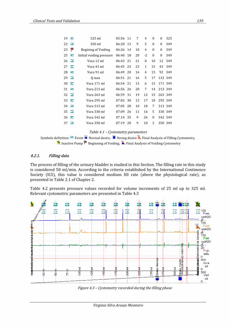
Clinical Tests and Validation 139
Virginia Silva Araujo Monteiro
19 325 ml 05:56 11 7 4 0 0 325
22 350 ml 06:20 13 9 5 0 0 349
23 Begining of Voiding 06:26 14 10 4 0 0 349
25 Initial voiding pressure 06:40 18 20 -2 0 0 349
26 Vura 12 ml 06:43 21 21 0 10 12 349
27 Vura 43 ml 06:45 23 23 1 15 43 349
28 Vura 91 ml 06:49 20 16 4 15 92 349
29 Q max 06:51 21 16 5 17 132 349
30 Vura 171 ml 06:54 21 15 6 15 171 349
31 Vura 213 ml 06:56 26 20 7 14 213 349
32 Vura 263 ml 06:59 31 19 12 15 263 349
33 Vura 295 ml 07:02 30 13 17 10 295 349
34 Vura 313 ml 07:05 28 10 18 7 313 349
35 Vura 330 ml 07:09 26 11 16 5 330 349
36 Vura 342 ml 07:14 35 9 26 0 342 349
37 Vura 350 ml 07:19 20 9 10 2 350 349
Table 4.1 – Cystometry parameters
Symbols definition: Event Normal desire, Strong desire Final Analysis of Filling Cystometry,
Inactive Pump Beginning of Voiding, Final Analysis of Voiding Cystometry
4.2.1. Filling data
The process of filling of the urinary bladder is studied in this Section. The filling rate in this study is considered 50 ml/min. According to the criteria established by the International Continence Society (ICS), this value is considered medium fill rate (above the physiological rate), as presented in Table 2.1 of Chapter 2.
Table 4.2 presents pressure values recorded for volume increments of 25 ml up to 325 ml. Relevant cystometric parameters are presented in Table 4.3
Figure 4.3 – Cystometry recorded during the filling phase
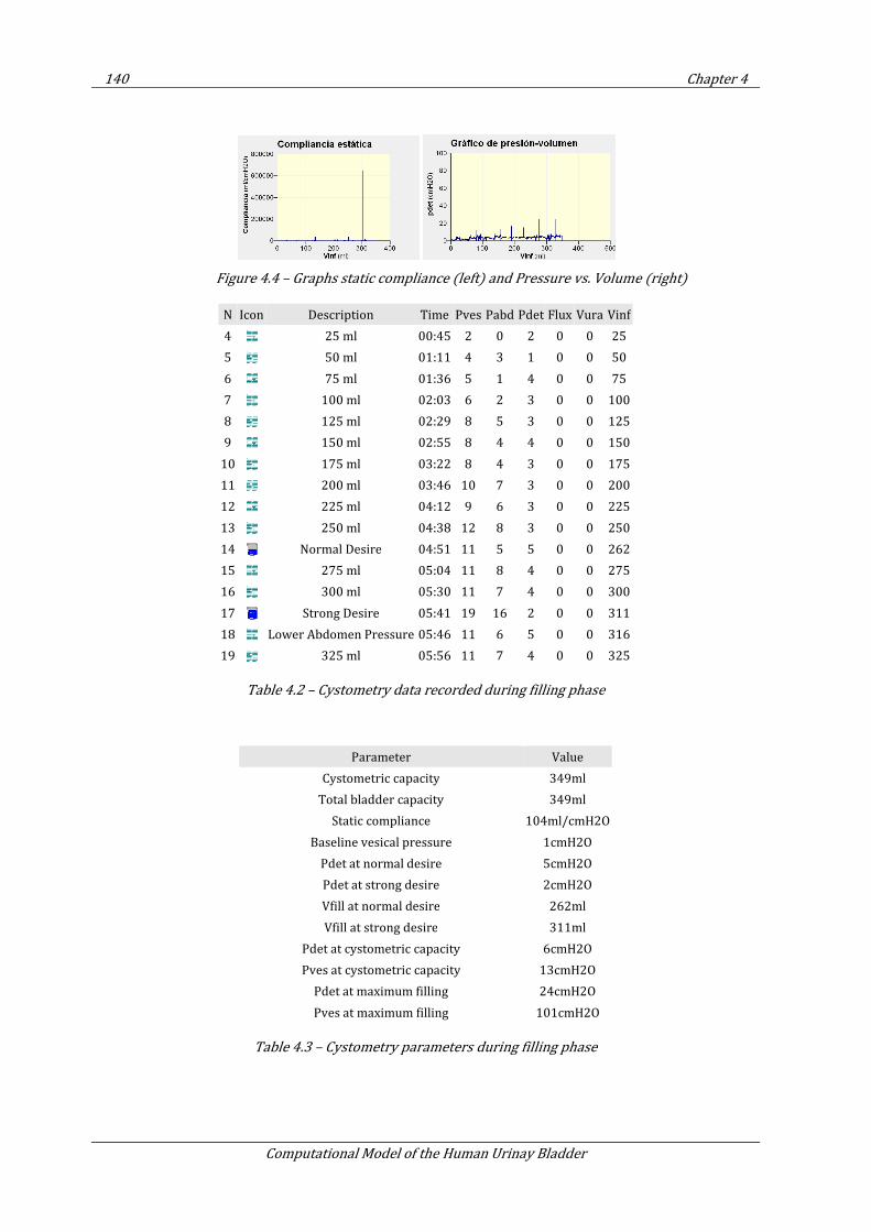
140 Chapter 4
Computational Model of the Human Urinay Bladder
Figure 4.4 – Graphs static compliance (left) and Pressure vs. Volume (right)
N Icon Description Time Pves Pabd Pdet Flux Vura Vinf
4 25 ml 00:45 2 0 2 0 0 25
5 50 ml 01:11 4 3 1 0 0 50
6 75 ml 01:36 5 1 4 0 0 75
7 100 ml 02:03 6 2 3 0 0 100
8 125 ml 02:29 8 5 3 0 0 125
9 150 ml 02:55 8 4 4 0 0 150
10 175 ml 03:22 8 4 3 0 0 175
11 200 ml 03:46 10 7 3 0 0 200
12 225 ml 04:12 9 6 3 0 0 225
13 250 ml 04:38 12 8 3 0 0 250
14 Normal Desire 04:51 11 5 5 0 0 262
15 275 ml 05:04 11 8 4 0 0 275
16 300 ml 05:30 11 7 4 0 0 300
17 Strong Desire 05:41 19 16 2 0 0 311
18 Lower Abdomen Pressure 05:46 11 6 5 0 0 316
19 325 ml 05:56 11 7 4 0 0 325
Table 4.2 – Cystometry data recorded during filling phase
Parameter Value
Cystometric capacity 349ml
Total bladder capacity 349ml
Static compliance 104ml/cmH2O
Baseline vesical pressure 1cmH2O
Pdet at normal desire 5cmH2O
Pdet at strong desire 2cmH2O
Vfill at normal desire 262ml
Vfill at strong desire 311ml
Pdet at cystometric capacity 6cmH2O
Pves at cystometric capacity 13cmH2O
Pdet at maximum filling 24cmH2O
Pves at maximum filling 101cmH2O
Table 4.3 – Cystometry parameters during filling phase
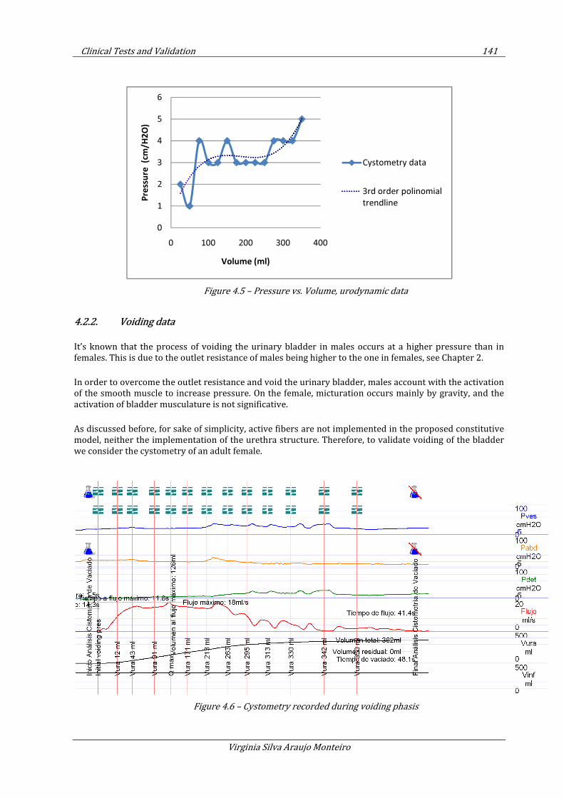
Clinical Tests and Validation 141
Virginia Silva Araujo Monteiro
Figure 4.5 – Pressure vs. Volume, urodynamic data
4.2.2. Voiding data
It’s known that the process of voiding the urinary bladder in males occurs at a higher pressure than in
females. This is due to the outlet resistance of males being higher to the one in females, see Chapter 2.
In order to overcome the outlet resistance and void the urinary bladder, males account with the activation
of the smooth muscle to increase pressure. On the female, micturation occurs mainly by gravity, and the
activation of bladder musculature is not significative.
As discussed before, for sake of simplicity, active fibers are not implemented in the proposed constitutive
model, neither the implementation of the urethra structure. Therefore, to validate voiding of the bladder
we consider the cystometry of an adult female.
Figure 4.6 – Cystometry recorded during voiding phasis
0
1
2
3
4
5
6
0 100 200 300 400
Pre
ssu
re (c
m/H
2O
)
Volume (ml)
Cystometry data
3rd order polinomial
trendline
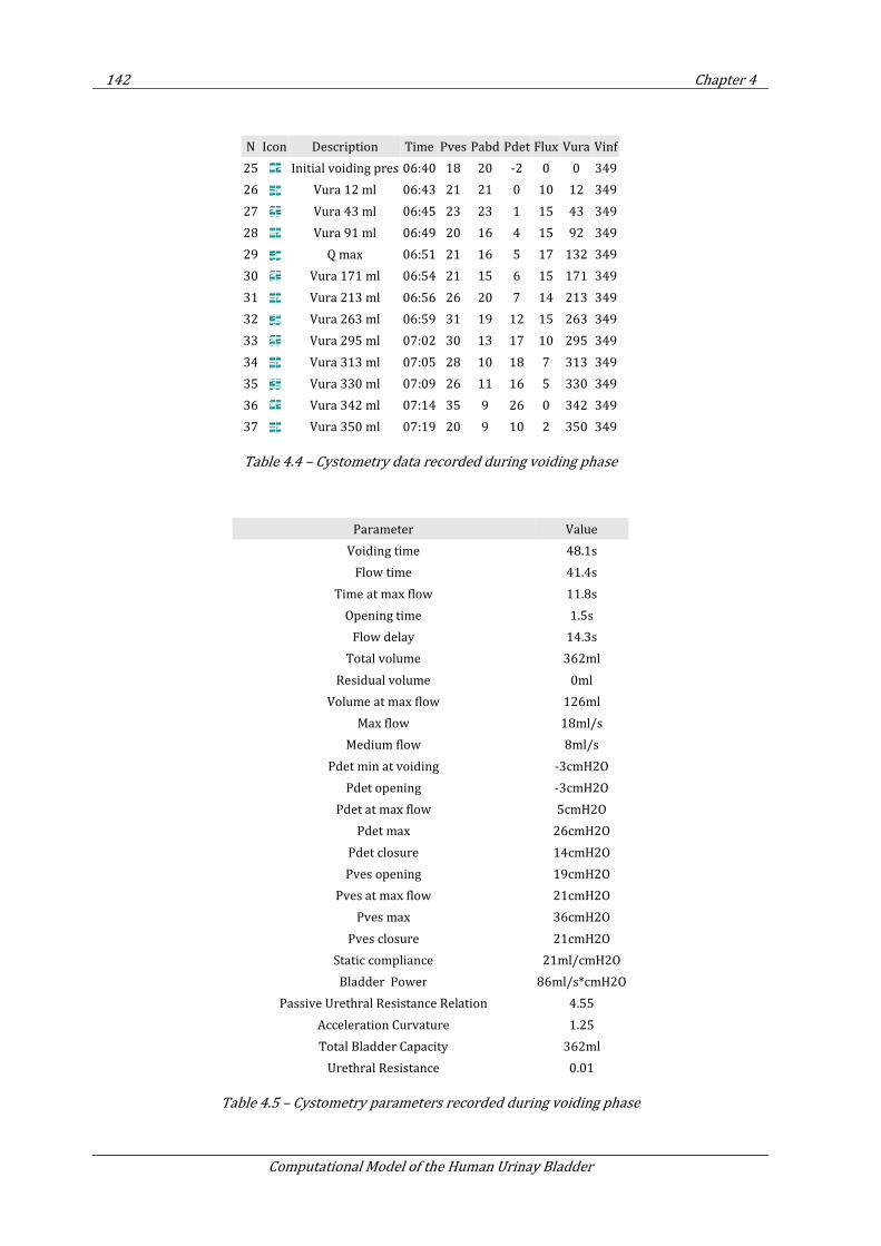
142 Chapter 4
Computational Model of the Human Urinay Bladder
N Icon Description Time Pves Pabd Pdet Flux Vura Vinf
25 Initial voiding pres 06:40 18 20 -2 0 0 349
26 Vura 12 ml 06:43 21 21 0 10 12 349
27 Vura 43 ml 06:45 23 23 1 15 43 349
28 Vura 91 ml 06:49 20 16 4 15 92 349
29 Q max 06:51 21 16 5 17 132 349
30 Vura 171 ml 06:54 21 15 6 15 171 349
31 Vura 213 ml 06:56 26 20 7 14 213 349
32 Vura 263 ml 06:59 31 19 12 15 263 349
33 Vura 295 ml 07:02 30 13 17 10 295 349
34 Vura 313 ml 07:05 28 10 18 7 313 349
35 Vura 330 ml 07:09 26 11 16 5 330 349
36 Vura 342 ml 07:14 35 9 26 0 342 349
37 Vura 350 ml 07:19 20 9 10 2 350 349
Table 4.4 – Cystometry data recorded during voiding phase
Parameter Value
Voiding time 48.1s
Flow time 41.4s
Time at max flow 11.8s
Opening time 1.5s
Flow delay 14.3s
Total volume 362ml
Residual volume 0ml
Volume at max flow 126ml
Max flow 18ml/s
Medium flow 8ml/s
Pdet min at voiding -3cmH2O
Pdet opening -3cmH2O
Pdet at max flow 5cmH2O
Pdet max 26cmH2O
Pdet closure 14cmH2O
Pves opening 19cmH2O
Pves at max flow 21cmH2O
Pves max 36cmH2O
Pves closure 21cmH2O
Static compliance 21ml/cmH2O
Bladder Power 86ml/s*cmH2O
Passive Urethral Resistance Relation 4.55
Acceleration Curvature 1.25
Total Bladder Capacity 362ml
Urethral Resistance 0.01
Table 4.5 – Cystometry parameters recorded during voiding phase
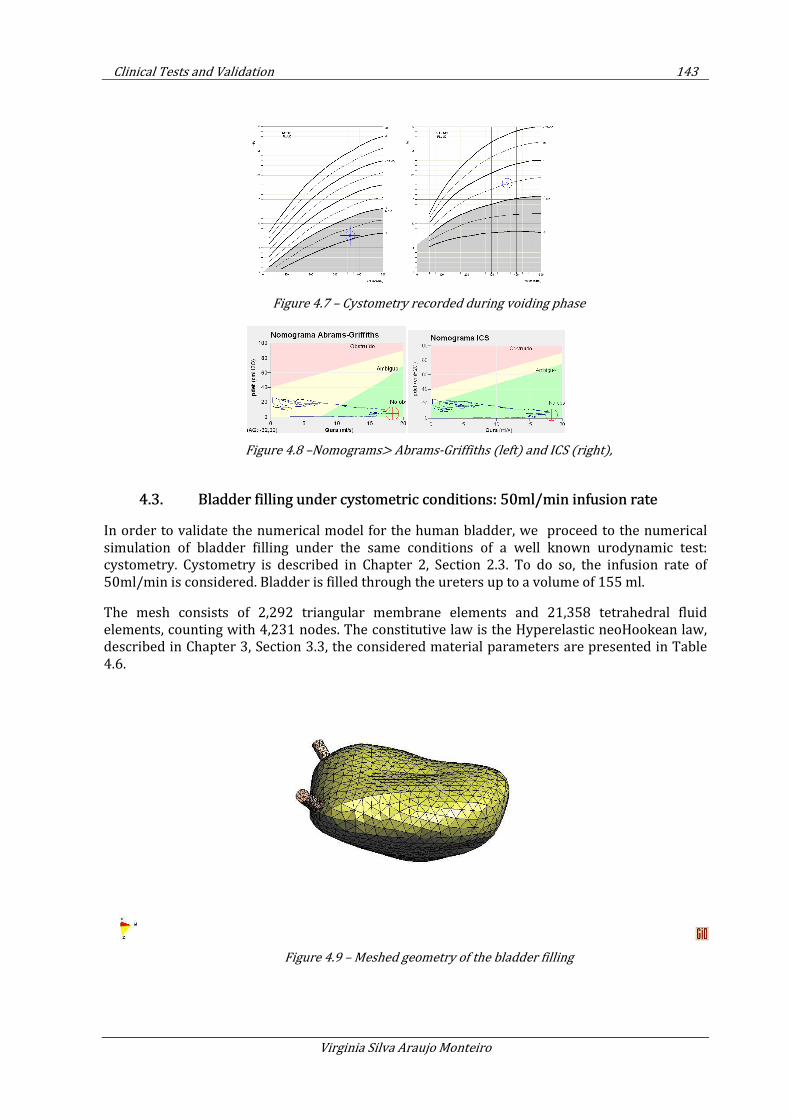
Clinical Tests and Validation 143
Virginia Silva Araujo Monteiro
Figure 4.7 – Cystometry recorded during voiding phase
Figure 4.8 –Nomograms> Abrams-Griffiths (left) and ICS (right),
4.3. Bladder filling under cystometric conditions: 50ml/min infusion rate
In order to validate the numerical model for the human bladder, we proceed to the numerical simulation of bladder filling under the same conditions of a well known urodynamic test: cystometry. Cystometry is described in Chapter 2, Section 2.3. To do so, the infusion rate of 50ml/min is considered. Bladder is filled through the ureters up to a volume of 155 ml.
The mesh consists of 2,292 triangular membrane elements and 21,358 tetrahedral fluid elements, counting with 4,231 nodes. The constitutive law is the Hyperelastic neoHookean law, described in Chapter 3, Section 3.3, the considered material parameters are presented in Table 4.6.
Figure 4.9 – Meshed geometry of the bladder filling
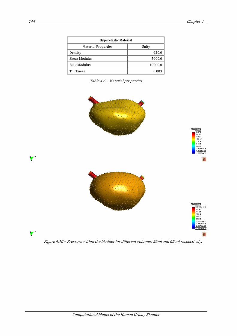
144 Chapter 4
Computational Model of the Human Urinay Bladder
Hyperelastic Material
Material Properties Unity
Density 920.0
Shear Modulus 5000.0
Bulk Modulus 10000.0
Thickness 0.003
Table 4.6 – Material properties
Figure 4.10 – Pressure within the bladder for different volumes, 56ml and 65 ml respectively.
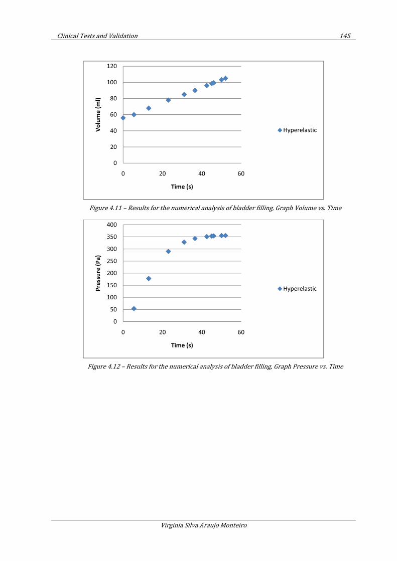
Clinical Tests and Validation 145
Virginia Silva Araujo Monteiro
Figure 4.11 – Results for the numerical analysis of bladder filling, Graph Volume vs. Time
Figure 4.12 – Results for the numerical analysis of bladder filling, Graph Pressure vs. Time
0
20
40
60
80
100
120
0 20 40 60
Vo
lum
e (
ml)
Time (s)
Hyperelastic
0
50
100
150
200
250
300
350
400
0 20 40 60
Pre
ssu
re (
Pa
)
Time (s)
Hyperelastic
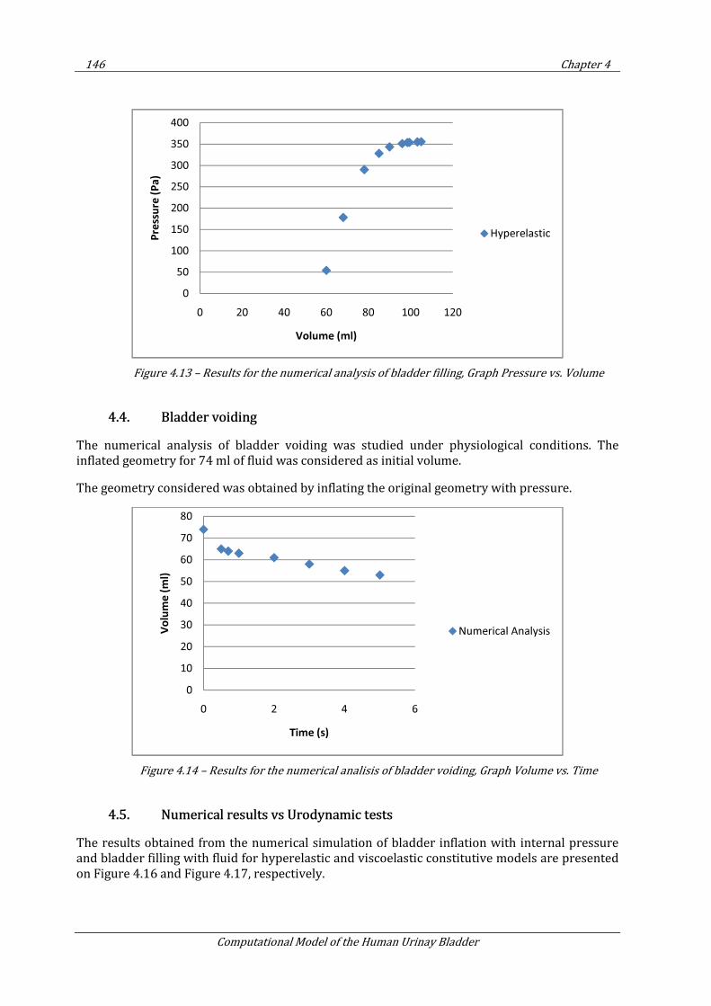
146 Chapter 4
Computational Model of the Human Urinay Bladder
Figure 4.13 – Results for the numerical analysis of bladder filling, Graph Pressure vs. Volume
4.4. Bladder voiding
The numerical analysis of bladder voiding was studied under physiological conditions. The inflated geometry for 74 ml of fluid was considered as initial volume.
The geometry considered was obtained by inflating the original geometry with pressure.
Figure 4.14 – Results for the numerical analisis of bladder voiding, Graph Volume vs. Time
4.5. Numerical results vs Urodynamic tests
The results obtained from the numerical simulation of bladder inflation with internal pressure and bladder filling with fluid for hyperelastic and viscoelastic constitutive models are presented on Figure 4.16 and Figure 4.17, respectively.
0
50
100
150
200
250
300
350
400
0 20 40 60 80 100 120
Pre
ssu
re (
Pa
)
Volume (ml)
Hyperelastic
0
10
20
30
40
50
60
70
80
0 2 4 6
Vo
lum
e (
ml)
Time (s)
Numerical Analysis
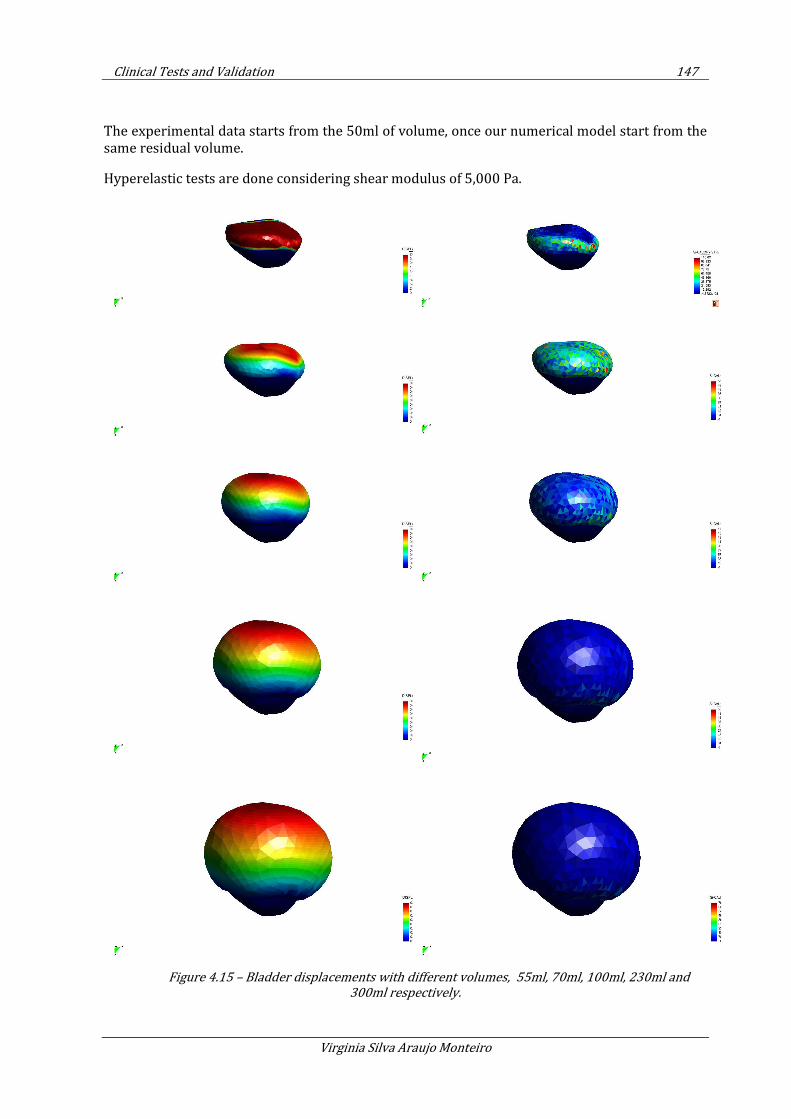
Clinical Tests and Validation 147
Virginia Silva Araujo Monteiro
The experimental data starts from the 50ml of volume, once our numerical model start from the same residual volume.
Hyperelastic tests are done considering shear modulus of 5,000 Pa.
Figure 4.15 – Bladder displacements with different volumes, 55ml, 70ml, 100ml, 230ml and
300ml respectively.
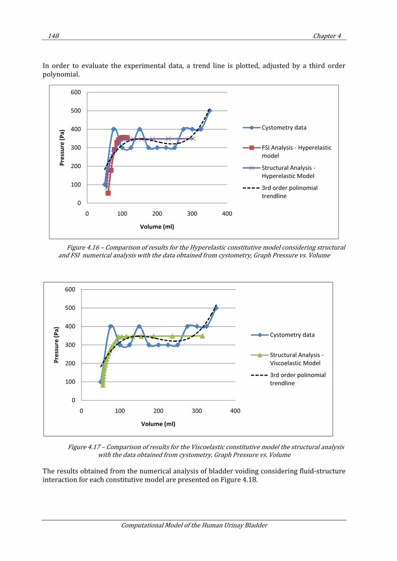
148 Chapter 4
Computational Model of the Human Urinay Bladder
In order to evaluate the experimental data, a trend line is plotted, adjusted by a third order polynomial.
Figure 4.16 – Comparison of results for the Hyperelastic constitutive model considering structural
and FSI numerical analysis with the data obtained from cystometry, Graph Pressure vs. Volume
Figure 4.17 – Comparison of results for the Viscoelastic constitutive model the structural analysis
with the data obtained from cystometry, Graph Pressure vs. Volume
The results obtained from the numerical analysis of bladder voiding considering fluid-structure interaction for each constitutive model are presented on Figure 4.18.
0
100
200
300
400
500
600
0 100 200 300 400
Pre
ssu
re (
Pa
)
Volume (ml)
Cystometry data
FSI Analysis - Hyperelastic
model
Structural Analysis -
Hyperelastic Model
3rd order polinomial
trendline
0
100
200
300
400
500
600
0 100 200 300 400
Pre
ssu
re (
Pa
)
Volume (ml)
Cystometry data
Structural Analysis -
Viscoelastic Model
3rd order polinomial
trendline
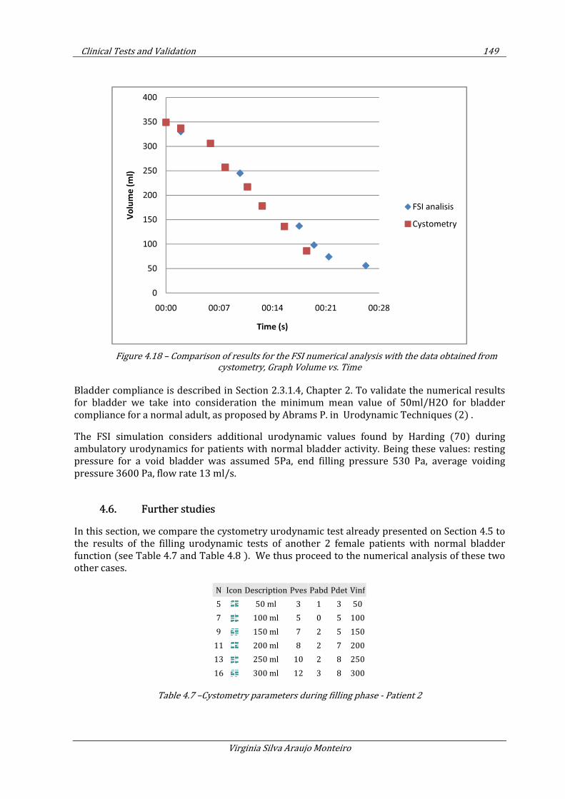
Clinical Tests and Validation 149
Virginia Silva Araujo Monteiro
Figure 4.18 – Comparison of results for the FSI numerical analysis with the data obtained from
cystometry, Graph Volume vs. Time
Bladder compliance is described in Section 2.3.1.4, Chapter 2. To validate the numerical results for bladder we take into consideration the minimum mean value of 50ml/H2O for bladder compliance for a normal adult, as proposed by Abrams P. in Urodynamic Techniques (2) .
The FSI simulation considers additional urodynamic values found by Harding (70) during ambulatory urodynamics for patients with normal bladder activity. Being these values: resting pressure for a void bladder was assumed 5Pa, end filling pressure 530 Pa, average voiding pressure 3600 Pa, flow rate 13 ml/s.
4.6. Further studies
In this section, we compare the cystometry urodynamic test already presented on Section 4.5 to the results of the filling urodynamic tests of another 2 female patients with normal bladder function (see Table 4.7 and Table 4.8 ). We thus proceed to the numerical analysis of these two other cases.
N Icon Description Pves Pabd Pdet Vinf
5 50 ml 3 1 3 50
7 100 ml 5 0 5 100
9 150 ml 7 2 5 150
11 200 ml 8 2 7 200
13 250 ml 10 2 8 250
16 300 ml 12 3 8 300
Table 4.7 –Cystometry parameters during filling phase - Patient 2
0
50
100
150
200
250
300
350
400
00:00 00:07 00:14 00:21 00:28
Vo
lum
e (
ml)
Time (s)
FSI analisis
Cystometry
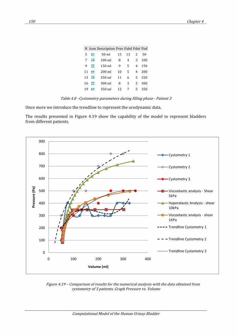
150 Chapter 4
Computational Model of the Human Urinay Bladder
N Icon Description Pves Pabd Pdet Vinf
5 50 ml 15 13 2 50
7 100 ml 8 4 3 100
9 150 ml 9 5 4 150
11 200 ml 10 5 4 200
13 250 ml 11 6 5 250
16 300 ml 8 3 5 300
19 350 ml 12 7 5 350
Table 4.8 –Cystometry parameters during filling phase - Patient 3
Once more we introduce the trendline to represent the urodynamic data.
The results presented in Figure 4.19 show the capability of the model to represent bladders from different patients.
Figure 4.19 – Comparison of results for the numerical analysis with the data obtained from
cystometry of 3 patients, Graph Pressure vs. Volume
0
100
200
300
400
500
600
700
800
900
0 100 200 300 400
Pre
ssu
re (
Pa
)
Volume (ml)
Cystometry 1
Cystometry 2
Cystometry 3
Viscoelastic analysis - Shear
5kPa
Hyperelastic Analysis - shear
10kPa
Viscoelastic analysis - shear
1KPa
Trendline Cystometry 1
Trendline Cystometry 2
Trendline Cystometry 3
Clinical Tests and Validation 151
Virginia Silva Araujo Monteiro
4.7. Conclusion
The results obtained in the numerical analysis of the urinary bladder are satisfactory to reproduce clinical data for bladder filling cystometry from 3 healthy patients of different ages.
Material parameters used in the numerical analysis range from 5 to 10 KPa for shear modulus value, within the range of elastic constant provided in the literature (128).
During the process of filling, the pressure registered in the organ is within the limit of 10 cm H2O suggested for the medical community, as presented in Chapter 2.
The constitutive models introduced in Chapter 3, are capable to reproduce the behavior of a healthy human urinary bladder up to the first desire of voiding, corresponding in this thesis to approximately 350 mL volume. Beyond this limit, it is necessary to take into account active fibers to reproduce the stiffening of the detrusor muscle.

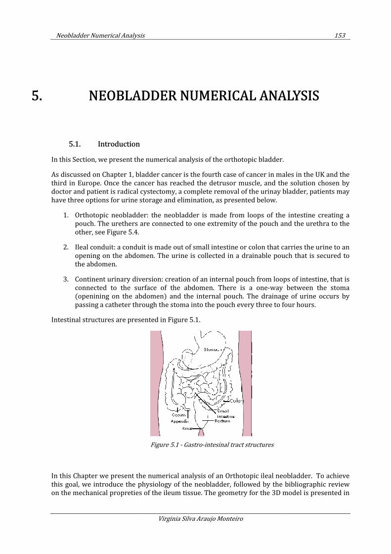
Neobladder Numerical Analysis
5. NEOBLADDER
5.1. Introduction
In this Section, we present the numerical analysis of the
As discussed on Chapter 1, bladder cancer is
third in Europe. Once the cancer has reached the detrusor muscle, and
doctor and patient is radical c
have three options for urine storage and elimination, as presented below.
1. Orthotopic neobladder:
pouch. The urethers are co
other, see Figure 5.4.
2. Ileal conduit: a conduit is made out of small intestine or colon that carries the
opening on the abdomen. The urine is collected in a drainable pouch that is secured to
the abdomen.
3. Continent urinary diversion: creation of a
connected to the surface of the abdomen. There is a
(openining on the abdomen) and the internal pouch. The drainage of urine occurs by
passing a catheter through the stoma into the pouch every three to four hours.
Intestinal structures are presented in
In this Chapter we present the numerical analysis of an Orthotopic
this goal, we introduce the physiology of the neobladder,
on the mechanical propreties of the ileum tissue. The
Neobladder Numerical Analysis
Virginia Silva Araujo Monteiro
BLADDER NUMERICAL ANALYSIS
the numerical analysis of the orthotopic bladder.
, bladder cancer is the fourth case of cancer in males in the UK and the
Once the cancer has reached the detrusor muscle, and the solution chosen by
cal cystectomy, a complete removal of the urinay bladder, patients may
have three options for urine storage and elimination, as presented below.
Orthotopic neobladder: the neobladder is made from loops of the intestine creating a
pouch. The urethers are connected to one extremity of the pouch and the urethra to the
Ileal conduit: a conduit is made out of small intestine or colon that carries the
opening on the abdomen. The urine is collected in a drainable pouch that is secured to
Continent urinary diversion: creation of an internal pouch from loops of intestine, that is
connected to the surface of the abdomen. There is a one-way between the stoma
(openining on the abdomen) and the internal pouch. The drainage of urine occurs by
passing a catheter through the stoma into the pouch every three to four hours.
tructures are presented in Figure 5.1.
Figure 5.1 - Gastro-intesinal tract structures
the numerical analysis of an Orthotopic ileal neobladder. To achieve
this goal, we introduce the physiology of the neobladder, followed by the
propreties of the ileum tissue. The geometry for the 3D model
153
NUMERICAL ANALYSIS
orthotopic bladder.
the fourth case of cancer in males in the UK and the
the solution chosen by
ystectomy, a complete removal of the urinay bladder, patients may
the neobladder is made from loops of the intestine creating a
nnected to one extremity of the pouch and the urethra to the
Ileal conduit: a conduit is made out of small intestine or colon that carries the urine to an
opening on the abdomen. The urine is collected in a drainable pouch that is secured to
internal pouch from loops of intestine, that is
way between the stoma
(openining on the abdomen) and the internal pouch. The drainage of urine occurs by
passing a catheter through the stoma into the pouch every three to four hours.
neobladder. To achieve
followed by the bibliographic review
the 3D model is presented in
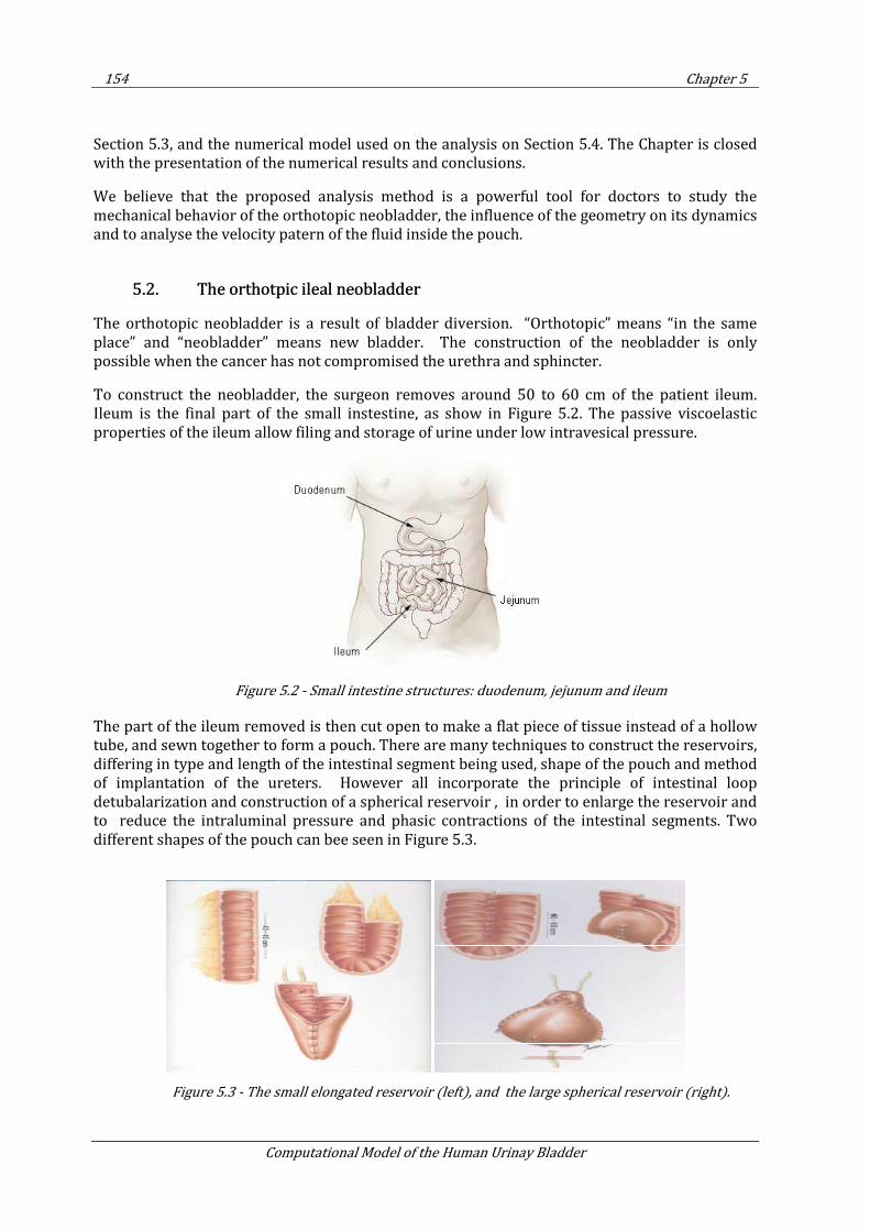
154 Chapter 5
Computational Model of the Human Urinay Bladder
Section 5.3, and the numerical model used on the analysis on Section 5.4. The Chapter is closed with the presentation of the numerical results and conclusions.
We believe that the proposed analysis method is a powerful tool for doctors to study the mechanical behavior of the orthotopic neobladder, the influence of the geometry on its dynamics and to analyse the velocity patern of the fluid inside the pouch.
5.2. The orthotpic ileal neobladder
The orthotopic neobladder is a result of bladder diversion. “Orthotopic” means “in the same place” and “neobladder” means new bladder. The construction of the neobladder is only possible when the cancer has not compromised the urethra and sphincter.
To construct the neobladder, the surgeon removes around 50 to 60 cm of the patient ileum. Ileum is the final part of the small instestine, as show in Figure 5.2. The passive viscoelastic properties of the ileum allow filing and storage of urine under low intravesical pressure.
Figure 5.2 - Small intestine structures: duodenum, jejunum and ileum
The part of the ileum removed is then cut open to make a flat piece of tissue instead of a hollow tube, and sewn together to form a pouch. There are many techniques to construct the reservoirs, differing in type and length of the intestinal segment being used, shape of the pouch and method of implantation of the ureters. However all incorporate the principle of intestinal loop detubalarization and construction of a spherical reservoir , in order to enlarge the reservoir and to reduce the intraluminal pressure and phasic contractions of the intestinal segments. Two different shapes of the pouch can bee seen in Figure 5.3.
Figure 5.3 - The small elongated reservoir (left), and the large spherical reservoir (right).
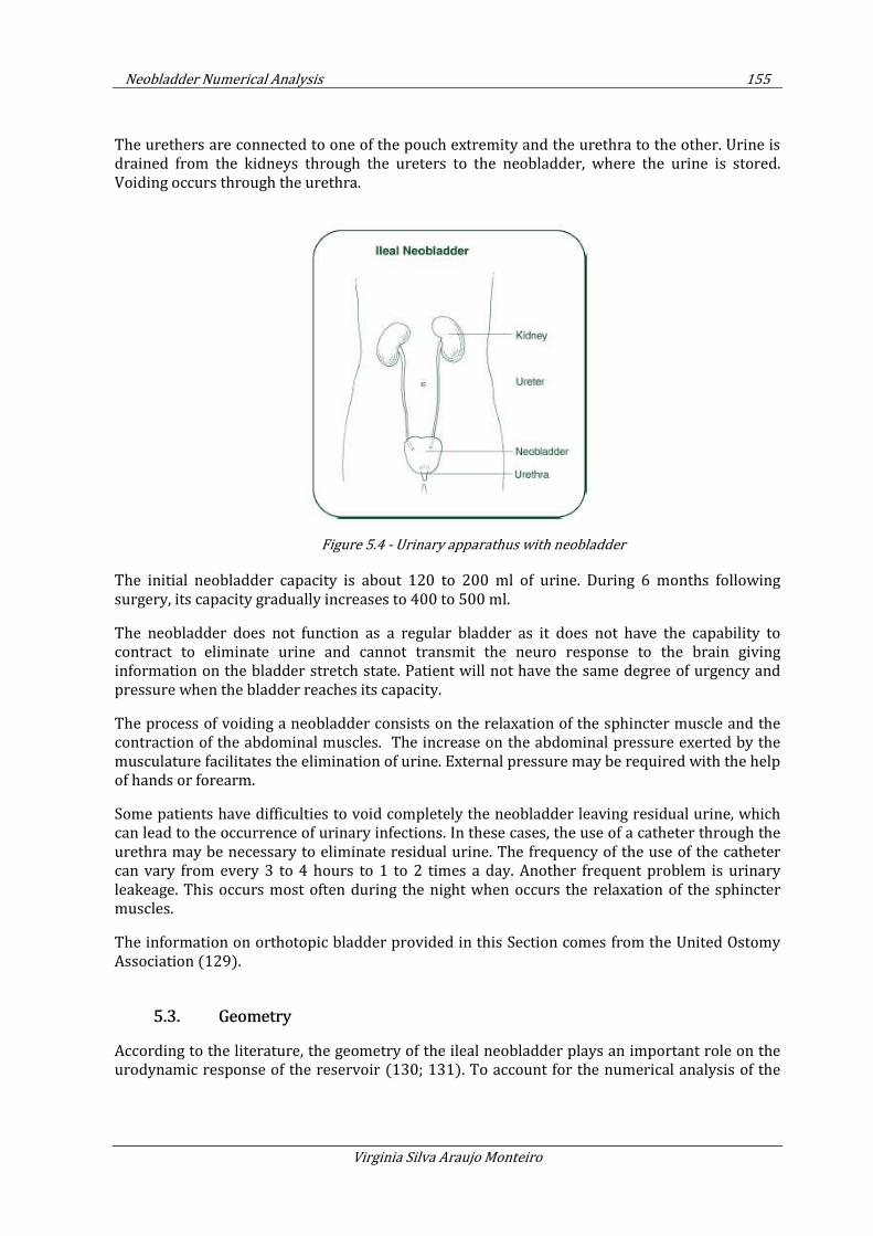
Neobladder Numerical Analysis 155
Virginia Silva Araujo Monteiro
The urethers are connected to one of the pouch extremity and the urethra to the other. Urine is drained from the kidneys through the ureters to the neobladder, where the urine is stored. Voiding occurs through the urethra.
Figure 5.4 - Urinary apparathus with neobladder
The initial neobladder capacity is about 120 to 200 ml of urine. During 6 months following surgery, its capacity gradually increases to 400 to 500 ml.
The neobladder does not function as a regular bladder as it does not have the capability to contract to eliminate urine and cannot transmit the neuro response to the brain giving information on the bladder stretch state. Patient will not have the same degree of urgency and pressure when the bladder reaches its capacity.
The process of voiding a neobladder consists on the relaxation of the sphincter muscle and the contraction of the abdominal muscles. The increase on the abdominal pressure exerted by the musculature facilitates the elimination of urine. External pressure may be required with the help of hands or forearm.
Some patients have difficulties to void completely the neobladder leaving residual urine, which can lead to the occurrence of urinary infections. In these cases, the use of a catheter through the urethra may be necessary to eliminate residual urine. The frequency of the use of the catheter can vary from every 3 to 4 hours to 1 to 2 times a day. Another frequent problem is urinary leakeage. This occurs most often during the night when occurs the relaxation of the sphincter muscles.
The information on orthotopic bladder provided in this Section comes from the United Ostomy Association (129).
5.3. Geometry
According to the literature, the geometry of the ileal neobladder plays an important role on the urodynamic response of the reservoir (130; 131). To account for the numerical analysis of the
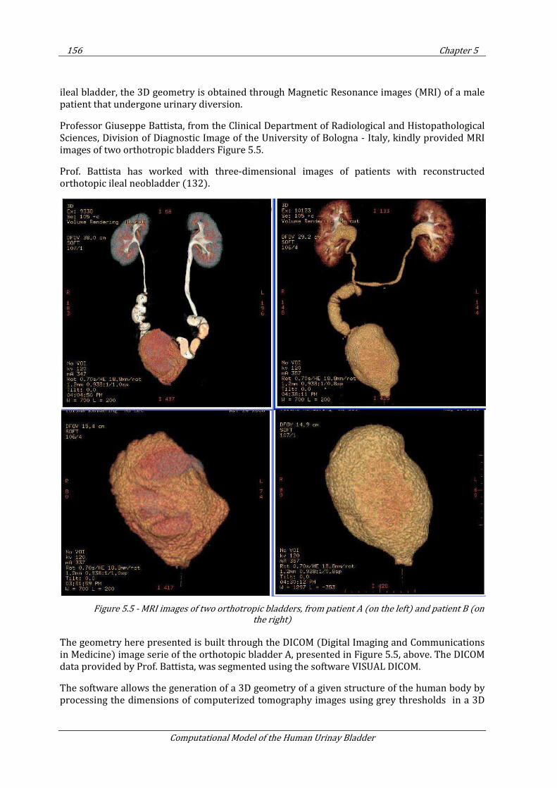
156 Chapter 5
Computational Model of the Human Urinay Bladder
ileal bladder, the 3D geometry is obtained through Magnetic Resonance images (MRI) of a male patient that undergone urinary diversion.
Professor Giuseppe Battista, from the Clinical Department of Radiological and Histopathological Sciences, Division of Diagnostic Image of the University of Bologna - Italy, kindly provided MRI images of two orthotropic bladders Figure 5.5.
Prof. Battista has worked with three-dimensional images of patients with reconstructed orthotopic ileal neobladder (132).
Figure 5.5 - MRI images of two orthotropic bladders, from patient A (on the left) and patient B (on
the right)
The geometry here presented is built through the DICOM (Digital Imaging and Communications in Medicine) image serie of the orthotopic bladder A, presented in Figure 5.5, above. The DICOM data provided by Prof. Battista, was segmented using the software VISUAL DICOM.
The software allows the generation of a 3D geometry of a given structure of the human body by processing the dimensions of computerized tomography images using grey thresholds in a 3D
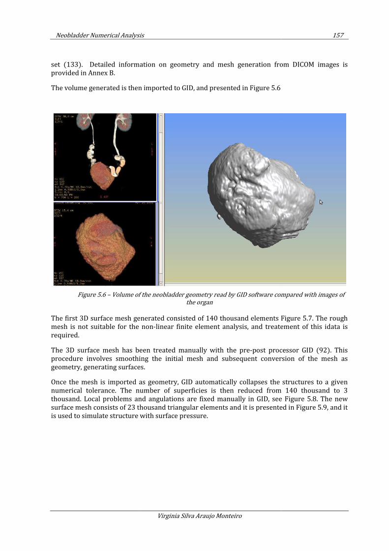
Neobladder Numerical Analysis
set (133). Detailed information on geometry
provided in Annex B.
The volume generated is then imported to GID, and presented in
Figure 5.6 – Volume of the neobladder geometry read by GID software compared with images of
The first 3D surface mesh generated
mesh is not suitable for the non
required.
The 3D surface mesh has been treated manually with the pre
procedure involves smoothing the initial mesh and subsequent conversion of the mesh as
geometry, generating surfaces.
Once the mesh is imported as geometry, GID automatically collapses the structures to a given
numerical tolerance. The number of superficies is then reduced from 140 thousand to
thousand. Local problems and angulations are fixed manually in GID, see
surface mesh consists of 23 thousand triangular elements and it is presented in
is used to simulate structure with surface pressure.
er Numerical Analysis
Virginia Silva Araujo Monteiro
Detailed information on geometry and mesh generation from DICOM images
is then imported to GID, and presented in Figure 5.6
Volume of the neobladder geometry read by GID software compared with images of
the organ
generated consisted of 140 thousand elements Figure
mesh is not suitable for the non-linear finite element analysis, and treate
The 3D surface mesh has been treated manually with the pre-post processor GID
procedure involves smoothing the initial mesh and subsequent conversion of the mesh as
geometry, generating surfaces.
Once the mesh is imported as geometry, GID automatically collapses the structures to a given
numerical tolerance. The number of superficies is then reduced from 140 thousand to
thousand. Local problems and angulations are fixed manually in GID, see
surface mesh consists of 23 thousand triangular elements and it is presented in
is used to simulate structure with surface pressure.
157
h generation from DICOM images is
Volume of the neobladder geometry read by GID software compared with images of
Figure 5.7. The rough
linear finite element analysis, and treatement of this idata is
post processor GID (92). This
procedure involves smoothing the initial mesh and subsequent conversion of the mesh as
Once the mesh is imported as geometry, GID automatically collapses the structures to a given
numerical tolerance. The number of superficies is then reduced from 140 thousand to 3
thousand. Local problems and angulations are fixed manually in GID, see Figure 5.8. The new
surface mesh consists of 23 thousand triangular elements and it is presented in Figure 5.9, and it
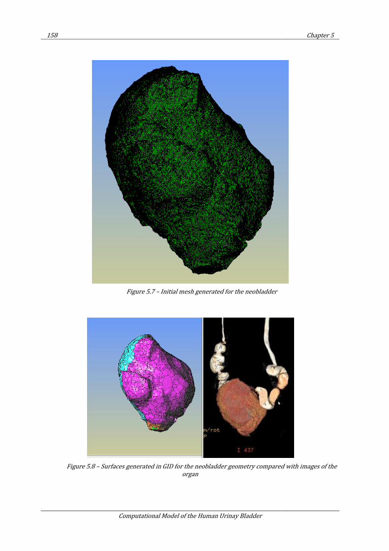
158
Computational Model of the Human Urinay Bladder
Figure
Figure 5.8 – Surfaces generated in GID for the neobladder geometry compared with images of the
Computational Model of the Human Urinay Bladder
Figure 5.7 – Initial mesh generated for the neobladder
Surfaces generated in GID for the neobladder geometry compared with images of the
organ
Chapter 5
Surfaces generated in GID for the neobladder geometry compared with images of the
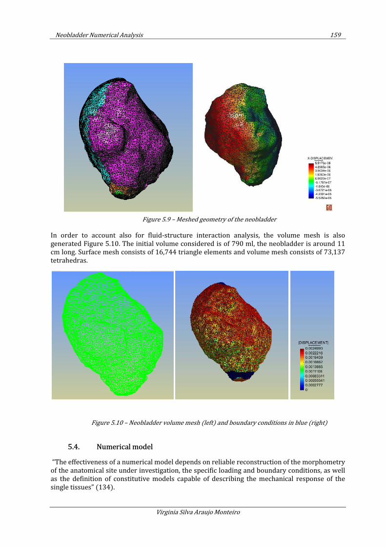
Neobladder Numerical Analysis 159
Virginia Silva Araujo Monteiro
Figure 5.9 – Meshed geometry of the neobladder
In order to account also for fluid-structure interaction analysis, the volume mesh is also generated Figure 5.10. The initial volume considered is of 790 ml, the neobladder is around 11 cm long. Surface mesh consists of 16,744 triangle elements and volume mesh consists of 73,137 tetrahedras.
Figure 5.10 – Neobladder volume mesh (left) and boundary conditions in blue (right)
5.4. Numerical model
“The effectiveness of a numerical model depends on reliable reconstruction of the morphometry of the anatomical site under investigation, the specific loading and boundary conditions, as well as the definition of constitutive models capable of describing the mechanical response of the single tissues” (134).
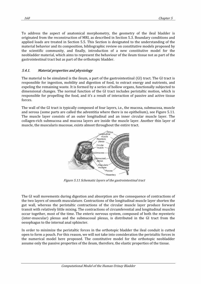
160 Chapter 5
Computational Model of the Human Urinay Bladder
To address the aspect of anatomical morphometry, the geometry of the ileal bladder is originated from the reconstruction of MRI, as described in Section 5.3. Boundary conditions and applied loads are treated in Section 5.5. This Section is designated to the understanding of the material behavior and its composition, bibliographic review on constitutive models proposed by the scientific community, and finally, introduction of a new constitutive model for the neobladder material, which aims to represent the behaviour of the ileum tissue not as part of the gastrointestinal tract but as part of the orthotopic bladder.
5.4.1. Material properties and physiology
The material to be simulated is the ileum, a part of the gastrointestinal (GI) tract. The GI tract is responsible for ingestion, mobility and digestion of food, to extract energy and nutrients, and expeling the remaining waste. It is formed by a series of hollow organs, functionally subjected to dimensional changes. The normal function of the GI tract includes peristaltic motion, which is responsible for propelling the food, and it’s a result of interaction of passive and active tissue forces.
The wall of the GI tract is typically composed of four layers, i.e., the mucosa, submucosa, muscle and serosa (some parts are called the adventitia where there is no epithelium), see Figure 5.11. The muscle layer consists of an outer longitudinal and an inner circular muscle layer. The collagen-rich submucosa and mucosa layers are inside the muscle layer. Another thin layer of muscle, the muscularis mucosae, exists almost throughout the entire tract.
Figure 5.11 Schematic layers of the gastrointestinal tract
The GI wall movements during digestion and absorption are the consequence of contractions of the two layers of smooth musculature. Contractions of the longitudinal muscle layer shorten the gut wall, whereas the peristaltic contractions of the circular muscle layer produce forward transit with relatively little mixing. The contractions of circumferential and longitudinal muscles occur together, most of the time. The enteric nervous system, composed of both the myenteric (inter-muscular) plexus and the submucosal plexus, is distributed in the GI tract from the oesophagus to the internal anal sphincter.
In order to minimize the peristaltic forces in the orthotopic bladder the ileal conduit is cutted open to form a pouch. For this reason, we will not take into consideration the peristaltic forces in the numerical model here proposed. The constitutive model for the orthotopic neobladder assume only the passive properties of the ileum, therefore, the elastic properties of the tissue.
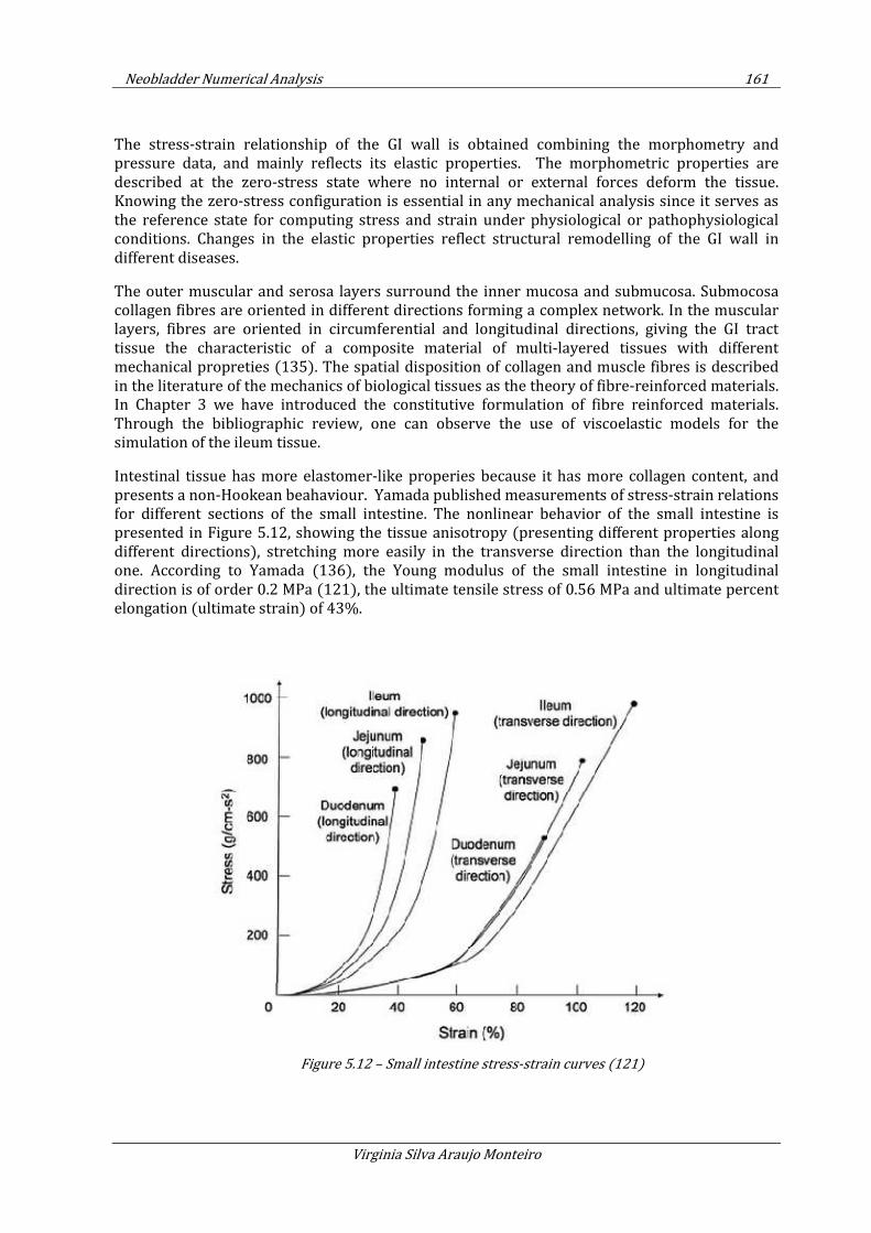
Neobladder Numerical Analysis 161
Virginia Silva Araujo Monteiro
The stress-strain relationship of the GI wall is obtained combining the morphometry and pressure data, and mainly reflects its elastic properties. The morphometric properties are described at the zero-stress state where no internal or external forces deform the tissue. Knowing the zero-stress configuration is essential in any mechanical analysis since it serves as the reference state for computing stress and strain under physiological or pathophysiological conditions. Changes in the elastic properties reflect structural remodelling of the GI wall in different diseases.
The outer muscular and serosa layers surround the inner mucosa and submucosa. Submocosa collagen fibres are oriented in different directions forming a complex network. In the muscular layers, fibres are oriented in circumferential and longitudinal directions, giving the GI tract tissue the characteristic of a composite material of multi-layered tissues with different mechanical propreties (135). The spatial disposition of collagen and muscle fibres is described in the literature of the mechanics of biological tissues as the theory of fibre-reinforced materials. In Chapter 3 we have introduced the constitutive formulation of fibre reinforced materials. Through the bibliographic review, one can observe the use of viscoelastic models for the simulation of the ileum tissue.
Intestinal tissue has more elastomer-like properies because it has more collagen content, and presents a non-Hookean beahaviour. Yamada published measurements of stress-strain relations for different sections of the small intestine. The nonlinear behavior of the small intestine is presented in Figure 5.12, showing the tissue anisotropy (presenting different properties along different directions), stretching more easily in the transverse direction than the longitudinal one. According to Yamada (136), the Young modulus of the small intestine in longitudinal direction is of order 0.2 MPa (121), the ultimate tensile stress of 0.56 MPa and ultimate percent elongation (ultimate strain) of 43%.
Figure 5.12 – Small intestine stress-strain curves (121)
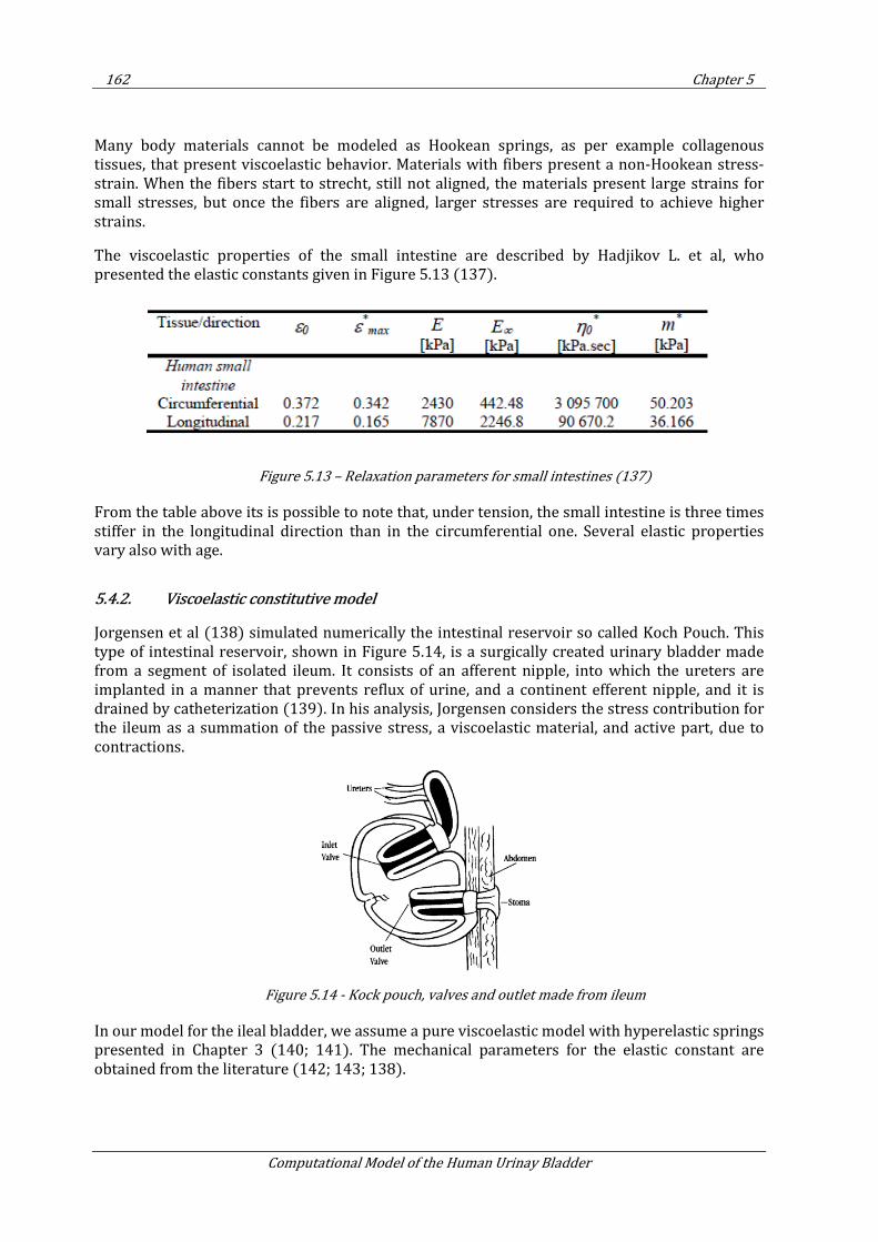
162 Chapter 5
Computational Model of the Human Urinay Bladder
Many body materials cannot be modeled as Hookean springs, as per example collagenous tissues, that present viscoelastic behavior. Materials with fibers present a non-Hookean stress-strain. When the fibers start to strecht, still not aligned, the materials present large strains for small stresses, but once the fibers are aligned, larger stresses are required to achieve higher strains.
The viscoelastic properties of the small intestine are described by Hadjikov L. et al, who presented the elastic constants given in Figure 5.13 (137).
Figure 5.13 – Relaxation parameters for small intestines (137)
From the table above its is possible to note that, under tension, the small intestine is three times stiffer in the longitudinal direction than in the circumferential one. Several elastic properties vary also with age.
5.4.2. Viscoelastic constitutive model
Jorgensen et al (138) simulated numerically the intestinal reservoir so called Koch Pouch. This type of intestinal reservoir, shown in Figure 5.14, is a surgically created urinary bladder made from a segment of isolated ileum. It consists of an afferent nipple, into which the ureters are implanted in a manner that prevents reflux of urine, and a continent efferent nipple, and it is drained by catheterization (139). In his analysis, Jorgensen considers the stress contribution for the ileum as a summation of the passive stress, a viscoelastic material, and active part, due to contractions.
Figure 5.14 - Kock pouch, valves and outlet made from ileum
In our model for the ileal bladder, we assume a pure viscoelastic model with hyperelastic springs presented in Chapter 3 (140; 141). The mechanical parameters for the elastic constant are obtained from the literature (142; 143; 138).
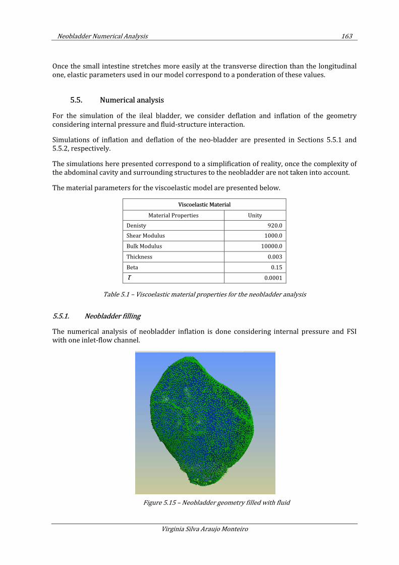
Neobladder Numerical Analysis 163
Virginia Silva Araujo Monteiro
Once the small intestine stretches more easily at the transverse direction than the longitudinal one, elastic parameters used in our model correspond to a ponderation of these values.
5.5. Numerical analysis
For the simulation of the ileal bladder, we consider deflation and inflation of the geometry considering internal pressure and fluid-structure interaction.
Simulations of inflation and deflation of the neo-bladder are presented in Sections 5.5.1 and 5.5.2, respectively.
The simulations here presented correspond to a simplification of reality, once the complexity of the abdominal cavity and surrounding structures to the neobladder are not taken into account.
The material parameters for the viscoelastic model are presented below.
Viscoelastic Material
Material Properties Unity
Denisty 920.0
Shear Modulus 1000.0
Bulk Modulus 10000.0
Thickness 0.003
Beta 0.15
τ 0.0001
Table 5.1 – Viscoelastic material properties for the neobladder analysis
5.5.1. Neobladder filling
The numerical analysis of neobladder inflation is done considering internal pressure and FSI with one inlet-flow channel.
Figure 5.15 – Neobladder geometry filled with fluid
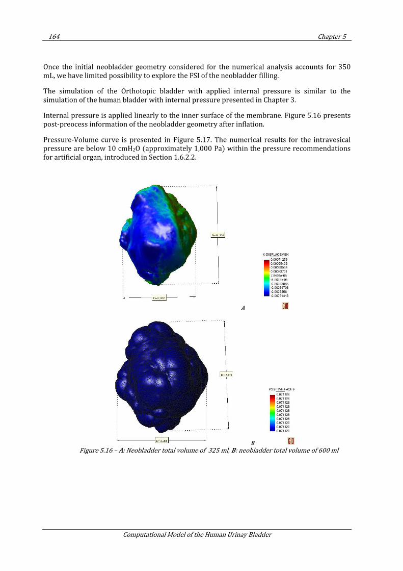
164 Chapter 5
Computational Model of the Human Urinay Bladder
Once the initial neobladder geometry considered for the numerical analysis accounts for 350 mL, we have limited possibility to explore the FSI of the neobladder filling.
The simulation of the Orthotopic bladder with applied internal pressure is similar to the simulation of the human bladder with internal pressure presented in Chapter 3.
Internal pressure is applied linearly to the inner surface of the membrane. Figure 5.16 presents post-preocess information of the neobladder geometry after inflation.
Pressure-Volume curve is presented in Figure 5.17. The numerical results for the intravesical pressure are below 10 cmH2O (approximately 1,000 Pa) within the pressure recommendations for artificial organ, introduced in Section 1.6.2.2.
A
B
Figure 5.16 – A: Neobladder total volume of 325 ml, B: neobladder total volume of 600 ml
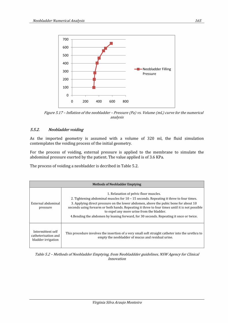
Neobladder Numerical Analysis 165
Virginia Silva Araujo Monteiro
Figure 5.17 – Inflation of the neobladder – Pressure (Pa) vs. Volume (mL) curve for the numerical
analysis
5.5.2. Neobladder voiding
As the imported geometry is assumed with a volume of 320 ml, the fluid simulation contemplates the voiding process of the initial geometry.
For the process of voiding, external pressure is applied to the membrane to simulate the abdominal pressure exerted by the patient. The value applied is of 3.6 KPa.
The process of voiding a neobladder is decribed in Table 5.2.
Methods of Neobladder Emptying
External abdominal
pressure
1. Relaxation of pelvic floor muscles.
2. Tightening abdominal muscles for 10 – 15 seconds. Repeating it three to four times.
3. Applying direct pressure on the lower abdomen, above the pubic bone for about 10
seconds using forearm or both hands. Repeating it three to four times until it is not possible
to expel any more urine from the bladder.
4.Bending the abdomen by leaning forward, for 30 seconds. Repeating it once or twice.
Intermittent self
catheterisation and
bladder irrigation
This procedure involves the insertion of a very small soft straight catheter into the urethra to
empty the neobladder of mucus and residual urine.
Table 5.2 – Methods of Neobladder Emptying, from Neobladdder guidelines, NSW Agency for Clinical
Innovation
0
100
200
300
400
500
600
700
0 200 400 600 800
Neobladder Filling
Pressure
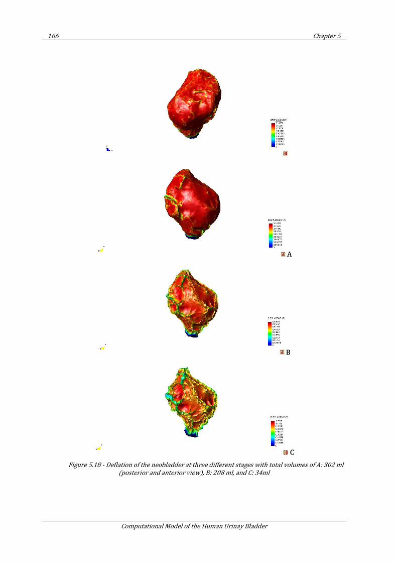
166 Chapter 5
Computational Model of the Human Urinay Bladder
A
B
C
Figure 5.18 - Deflation of the neobladder at three different stages with total volumes of A: 302 ml
(posterior and anterior view), B: 208 ml, and C: 34ml
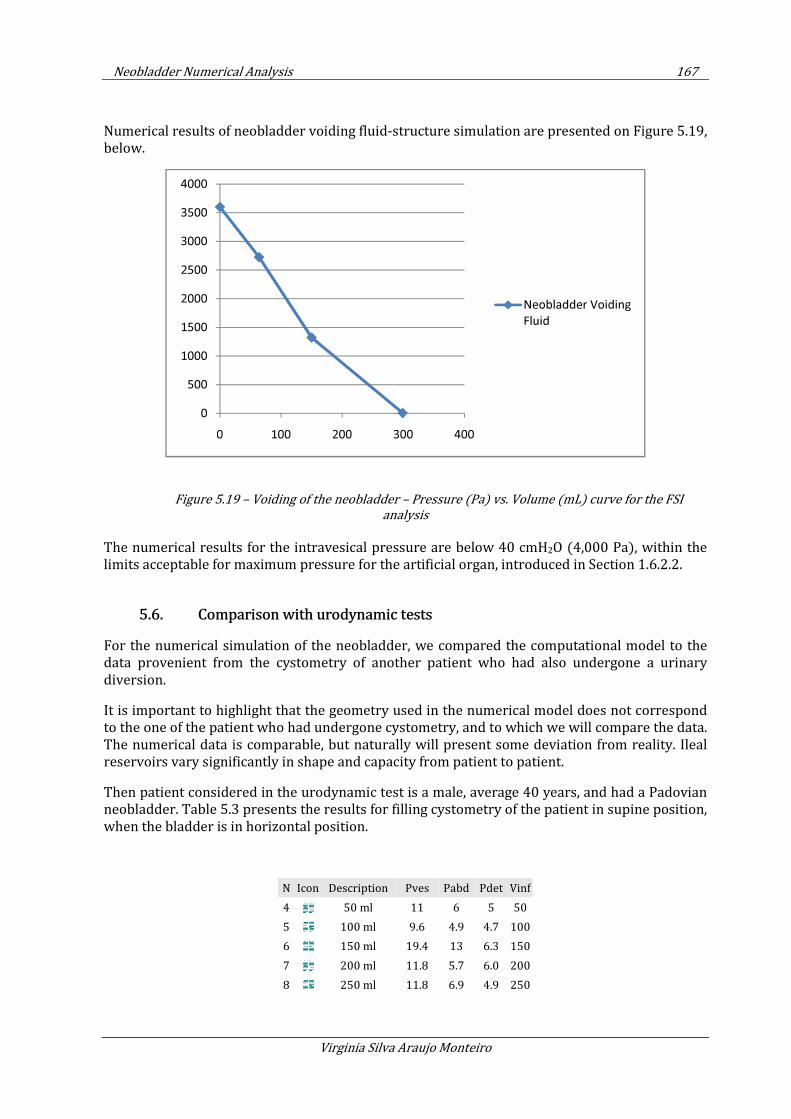
Neobladder Numerical Analysis 167
Virginia Silva Araujo Monteiro
Numerical results of neobladder voiding fluid-structure simulation are presented on Figure 5.19, below.
Figure 5.19 – Voiding of the neobladder – Pressure (Pa) vs. Volume (mL) curve for the FSI
analysis
The numerical results for the intravesical pressure are below 40 cmH2O (4,000 Pa), within the limits acceptable for maximum pressure for the artificial organ, introduced in Section 1.6.2.2.
5.6. Comparison with urodynamic tests
For the numerical simulation of the neobladder, we compared the computational model to the data provenient from the cystometry of another patient who had also undergone a urinary diversion.
It is important to highlight that the geometry used in the numerical model does not correspond to the one of the patient who had undergone cystometry, and to which we will compare the data. The numerical data is comparable, but naturally will present some deviation from reality. Ileal reservoirs vary significantly in shape and capacity from patient to patient.
Then patient considered in the urodynamic test is a male, average 40 years, and had a Padovian neobladder. Table 5.3 presents the results for filling cystometry of the patient in supine position, when the bladder is in horizontal position.
N Icon Description Pves Pabd Pdet Vinf
4 50 ml 11 6 5 50
5 100 ml 9.6 4.9 4.7 100
6 150 ml 19.4 13 6.3 150
7 200 ml 11.8 5.7 6.0 200
8 250 ml 11.8 6.9 4.9 250
0
500
1000
1500
2000
2500
3000
3500
4000
0 100 200 300 400
Neobladder Voiding
Fluid
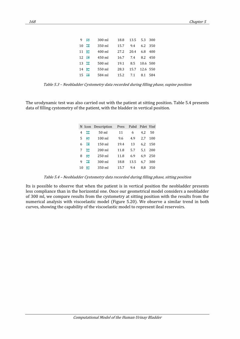
168 Chapter 5
Computational Model of the Human Urinay Bladder
9 300 ml 18.8 13.5 5.3 300
10 350 ml 15.7 9.4 6.2 350
11 400 ml 27.2 20.4 6.8 400
12 450 ml 16.7 7.4 8.2 450
13 500 ml 19.1 8.5 10.6 500
14 550 ml 28.3 15.7 12.6 550
15 584 ml 15.2 7.1 8.1 584
Table 5.3 – Neobladder Cystometry data recorded during filling phase, supine position
The urodynamic test was also carried out with the patient at sitting position. Table 5.4 presents data of filling cystometry of the patient, with the bladder in vertical position.
N Icon Description Pves Pabd Pdet Vinf
4 50 ml 11 6 4,2 50
5 100 ml 9.6 4.9 2,7 100
6 150 ml 19.4 13 6,2 150
7 200 ml 11.8 5.7 5,1 200
8 250 ml 11.8 6.9 6,9 250
9 300 ml 18.8 13.5 6,7 300
10 350 ml 15.7 9.4 8,8 350
Table 5.4 – Neobladder Cystometry data recorded during filling phase, sitting position
Its is possible to observe that when the patient is in vertical position the neobladder presents less compliance than in the horizontal one. Once our geometrical model considers a neobladder of 300 ml, we compare results from the cystometry at sitting position with the results from the numerical analysis with viscoelastic model (Figure 5.20). We observe a similar trend in both curves, showing the capability of the viscoelastic model to represent ileal reservoirs.
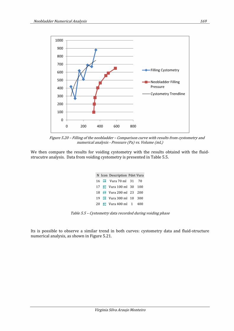
Neobladder Numerical Analysis 169
Virginia Silva Araujo Monteiro
Figure 5.20 – Filling of the neobladder – Comparison curve with results from cystometry and
numerical analysis - Pressure (Pa) vs. Volume (mL)
We then compare the results for voiding cystometry with the results obtaind with the fluid-strucutre analysis. Data from voiding cystometry is presented in Table 5.5.
N Icon Description Pdet Vura
16 Vura 70 ml 31 70
17 Vura 100 ml 30 100
18 Vura 200 ml 23 200
19 Vura 300 ml 10 300
20 Vura 400 ml 1 400
Table 5.5 – Cystometry data recorded during voiding phase
Its is possible to observe a similar trend in both curves: cystometry data and fluid-structure numerical analysis, as shown in Figure 5.21.
0
100
200
300
400
500
600
700
800
900
1000
0 200 400 600 800
Filling Cystometry
Neobladder Filling
Pressure
Cystometry Trendline
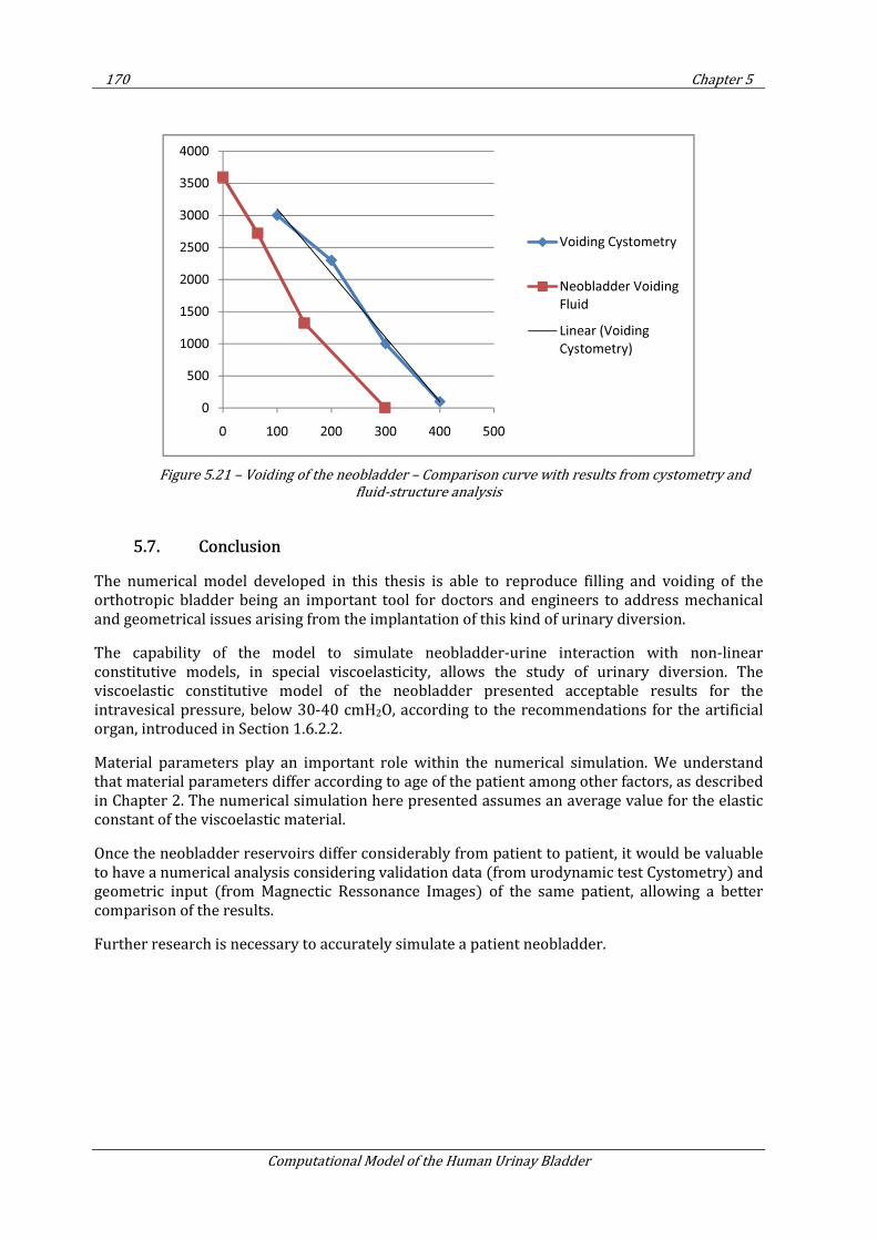
170 Chapter 5
Computational Model of the Human Urinay Bladder
Figure 5.21 – Voiding of the neobladder – Comparison curve with results from cystometry and
fluid-structure analysis
5.7. Conclusion
The numerical model developed in this thesis is able to reproduce filling and voiding of the orthotropic bladder being an important tool for doctors and engineers to address mechanical and geometrical issues arising from the implantation of this kind of urinary diversion.
The capability of the model to simulate neobladder-urine interaction with non-linear constitutive models, in special viscoelasticity, allows the study of urinary diversion. The viscoelastic constitutive model of the neobladder presented acceptable results for the intravesical pressure, below 30-40 cmH2O, according to the recommendations for the artificial organ, introduced in Section 1.6.2.2.
Material parameters play an important role within the numerical simulation. We understand that material parameters differ according to age of the patient among other factors, as described in Chapter 2. The numerical simulation here presented assumes an average value for the elastic constant of the viscoelastic material.
Once the neobladder reservoirs differ considerably from patient to patient, it would be valuable to have a numerical analysis considering validation data (from urodynamic test Cystometry) and geometric input (from Magnectic Ressonance Images) of the same patient, allowing a better comparison of the results.
Further research is necessary to accurately simulate a patient neobladder.
0
500
1000
1500
2000
2500
3000
3500
4000
0 100 200 300 400 500
Voiding Cystometry
Neobladder Voiding
Fluid
Linear (Voiding
Cystometry)
Conclusions and persperctives 171
Virginia Silva Araujo Monteiro
6. CONCLUSIONS AND PERSPERCTIVES
Based on the urge from the medical community to propose artificial solutions for the urinary bladder replacement, we have proposed in this thesis a numerical model for analysis of the urinary bladder based on the following:
• A geometry from the magnetic resonance images (MRI) of the organ;
• Non-linear constitutive models based on hyperelasticity and viscoelasticty to simulate the behavior of bladder tissue;
• Numerical analysis of the bladder considering bladder-urine interaction; and
• Validation of the numerical model with clinical tests.
After completion of these steps, we also proposed the application of the numerical method to the analysis of a neobladder, a first approach to simulate an artificial bladder.
6.1. General conclusions
The problem of simulating the human urinary bladder through the finite element method (FEM) is complex and requires an approach to combine non-linear geometry, non-linear constitutive model and fluid-structure interaction.
In this thesis, we used FEM to reproduce the behavior of the human urinary bladder and to study possible solutions for urinary diversion, including the study of the behavior of the neobladder.
The constitutive models proposed are capable to represent the behavior of the smooth muscle that constitutes the main mechanical part of the bladder. The problem solved contemplates the geometry of the bladder, part of the ureters, and simplified boundary conditions (BC). It is also possible to include more refined BCs, considering other urinary structures such as urethra, sphincter, prostate, and also surrounding organs (i.e. intestines), leading to larger number of elements to be computed, and consequent, more expensive computational cost.
The bladder-urine interaction to simulate bladder wall and urine is a powerful tool to understand the urodynamics of urinary reservoirs and to study pathologies related to the mechanics of the urinary apparatus. In this thesis we used the Particle Finite Element Method (PFEM) to compute fluid-structure interaction, giving satisfying results. The proposed computational urodynamic problem is solved monolithically.
Quadratic convergence of the non-linear structure was obtained in all cases.
6.2. Specific conclusions
The numerical model presented in this work is capable to represent the behavior of the bladder during filling conditions up to the first desire of voiding. The time step used in this problem is relatively small, depending on the quality and size of the mesh. Bladder filling at normal
172 Chapter 6
Computational Model of the Human Urinay Bladder
physiological rate has a high computational cost, with real time up to 30 days for running the infusion of 100ml fluid in the urinary bladder.
The model is able to simulate accurately the micturation process. As shown in Chapter 2, the response of the bladder voiding in male and female are different. Male urethra is longer and promotes more resistance to flow. For this reason, male bladder accounts with active fibers to increase bladder pressure and provide micturation. As the model presented in this thesis does not contemplate active fibers, the study of micturation is feasible to the analysis of female patients.
The numerical model proposed has been validated with clinical tests in Chapter 4. The data used is a preliminary approach to recover bladder response. A desirable validation should include geometry and cystometric data from the same patient. Due to the lack of data, the geometry of the urinary bladder considered in the numerical model and experiemental data used for validation are from different patients.
Comparison of the numerical results with urodynamic tests from three different patients at different ages showed the capability of the model to reproduce bladder mechanics during filling conditions for different material parameters. There was no correlation between age and material stiffening or relaxation.
In Chapter 5 satisfactory numerical results for the analysis of the neobladder were obtained. The pressure volume curve was compared with cystometry results from a patient with urinary diversion.
6.3. Perspectives for future work
The model here implemented accurately reproduces the experimental data up to a 300 ml of volume filling, corresponding to the first desire of voiding. We noticed that after this event an increase of pressure within the urinary bladder due to the activation of active fibers, inducing the progressive stiffing of the material. In order to represent the experimental data after this point, the numerical model can be improved to account for the effect of active fibers, simulating progressive stiffening of viscoelastic fibers.
Urethra resistance plays an important role on bladder continence, and affects the voiding phenomena. Further research on the urinary apparatus may address fluid-structure interaction simulations of other structures of the lower urinary tract, such as urethers and urethra.
A complete study of bladder function may include electrical response to maintain continence, and may include a geometrical model for the urethra to simulate outlet resistance.
The neobladder computational analysis presented in this thesis can be useful to study the mechanics of ileal reservoirs. Research on neobladder function may give important conclusions of reservoir shape for organ functionality. A partnership with a hospital urodynamic department, may promote the possibility to obtain MRI images of patients who undergone urinary diversion and who have performed post-operatory cystometry test, to have validation and calibration of the numerical results.
An adequate artificial bladder is still a challenge to overcome. The artificial bladder may contemplate voiding mechanism to eliminate urine, reducing residual volume which propitiates the bacteria growth leading to urinary infection. The proposal of an artificial bladder should take
173
Virginia Silva Araujo Monteiro
into consideration a biocompatible material with similar mechanical properties described in this thesis.
6.4. Final considerations
The work presented in this thesis is a contribution for the bio-engineering community to study the dynamic response of the human urinary bladder, introducing a tool to virtually experiment artificial solutions to replace this organ.
The methodology allows the numerical analysis of the lower urinary apparatus dynamics of bladder filling, storage and voiding, considering urine interaction with non-linear bio-material response and complex organ geometry.
The constitutive model can reproduce the visco-hyperelastic behavior of biomaterials, for organ structures designed with shell elements responding to fluid forces. Nevertheless, it is possible to expand the actual non-linear structure formulation to contemplate active response related to fiber contraction.
Numerical analysis is a powerful tool to reproduce the mechanics of bio-structures and their interaction with fluid. Once the virtual results meet the biological needs, one can proceed to experimental analysis for data validation.
Another application of the work presented in this thesis can be patient preventive diagnose. For example, in cases where obstruction is found in medical ultrasonography or MRI, the inclusion of different boundary conditions allows the numerical reproduction of urine flow in the lower urinary apparatus, predicting intravesical pressure rise that may affect kidneys function. A hospital partnership can be fruitful to analyze different bladder morphologies and material parameters.
174 Chapter 7
Computational Model of the Human Urinay Bladder
7. CONCLUSIONES Y PERSPECTIVAS
Motivados por la necesidad de la comunidad médica en proponer soluciones artificiales para remplazar la vejiga urinaria, hemos propuesto en esa tesis un modelo numérico para análisis de la vejiga urinaria humana, basada en:
• Una geometria de imagenes de resonancia magnetica (MRI) del organo;
• Modelos constitutivos no-lineales basados en hyperelasticidad y viscoelasticidad para simulación del comportamiento del tejido de la vejiga
• Análisis numérica de la vejiga considerando la interacción orina-vejiga; y
• Validación de el modelo numeric con testes clinicos.
Una vez completados eses pasos, hemos propuesto la aplicación de dicho modelo numérico a la análisis de una neo-vejiga, siendo una primera aproximación a la simulación de una vejiga artificial.
7.1. Conclusiones generales
El problema de simular el comportamiento de la vejiga urinaria humana con el método de los elementos finitos (FEM) es complejo y requiere una aproximación para combinar: una geometría no-lineal, un modelo constitutivo no-lineal y interacción fluido-estructura.
En esa tesis, hemos usado el FEM para reproducir el comportamiento de la vejiga urinaria y para estudiar posibles soluciones para derivación urinaria, incluyendo el estudio del comportamiento de una neo-vejiga.
Los modelos constitutivos propuestos son capaces de representar el comportamiento del musculo liso, que es la principal parte mecánica de la vejiga. El problema solucionado contempla la geometría de la vejiga, parte de los uréteres y condiciones de contorno (BC) sencillas. Es posible considerar BC más sofisticadas, considerando otras estructuras urinarias, como la uretra, sphincter, próstata, y órganos anexos (ejemplo: intestinos), llevando a un numero grande de elementos a calcular y, consecuentemente, alto coste computacional.
La interacción vejiga-orina para simulación de la pared de la vejiga y la orina es una herramienta útil para entendimiento de la urodinamica de reservatorios urinarios y para estudiar patologías relacionadas a la mecánica del aparato urinario. En esa tesis hemos usado el Particle Finite Element Method (PFEM) para calcular la interacción fluido-estructura, con obtención de resultados satisfactorios. El problema fue solucionado de forma monolitica.
Convergencia quadratica ha sido obtenida en todos los casos
7.2. Conclusiones especificas
Conclusiones y perspectivas 175
Virginia Silva Araujo Monteiro
El modelo numérico presentado en ese trabajo tiene la capacidad de representar el comportamiento de la vejiga durante las condiciones de llenado hasta el primer deseo de vaciado. El paso de tiempo utilizado en ese problema es relativamente pequeño, dependiendo de la cualidad e tamaño del mallado. El llenado de la vejiga a una razón fisiológica tiene un alto coste computacional, con el tiempo real de solución de hasta 30 días para simular una infusión de 100 ml de fluido en la vejiga.
El modelo tiene la capacidad de representar correctamente el proceso de micturacion. Como visto en el Capitulo 2, la respuesta del vaciado es diferente en el varón y la mujer. La uretra masculina es más larga, promoviendo más resistencia al flujo. Por esa razón, la vejiga masculina utiliza de sus fibras activas para aumentar la presión dentro la vejiga, permitiendo micturacion. El modelo presentado en esa tesis no contempla fibras activas, y el estudio de micturacion presentado es adecuado para el análisis de vaciado en mujeres.
El modelo numérico propuesto ha sido validado con testes clínicos presentados en el Capitulo 4. Los datos usados son una primera aproximación para recobrar la respuesta de la vejiga. Seria desiderable una validación que incluyese la geometría e los datos cistonometricos del mismo paciente. Debido a falta de datos, la geometría utilizada para la vejiga urinaria y los datos experimentales usados en la validación originanse de individuos diferentes.
La comparación de los resultados numéricos con testes urodinámicos de tres pacientes de diferente señoread han enseñado la capacidad de ese modelo de reproducir la mecánica de la vejiga durante las condiciones de llenado para distintos parámetros de los materiales. No hemos encontrado una correlación entre edad y rigidez del material de la vejiga.
En el Capitulo 5 hemos obtenidos resultados numéricos satisfactorios para la análisis de la neovejiga. La curva de volume-pression fue comparada com resultados de cistonometria de um paciente que sufrio derivación urinária.
7.3. Perspectivas
El modelo numérico presentado en ese trabajo tiene la capacidad de representar los datos experimentales hasta 300 ml de llenado, correspondiendo al primer deseo de vaciado. Hemos notado que después de ese evento ocurre un incremento en la presión dentro de la vejiga debido a la activación de las fibras activas, que inducen la rigidez progresiva del material. Para representar los datos experimentales después de ese evento, el modelo numérico puede ser mejorado para contemplar el efecto de las fibras activas, simulando la rigidez progresiva de las fibras viscoelásticas.
La resistencia de la uretra tiene una función importante en mantener la continencia urinaria, y afecta el fenómeno de vaciado. Investigación del aparato urinario puede tratar interacción fluido-estructura de otras partes de tracto urinario bajo, como los uréteres y la uretra.
Un estudio completo de la función de la vejiga puede incluir la respuesta erétrica para mantener continencia, considerando el modelo geométrico para la uretra para simular Resistencia uretral.
La analisis computacional de la neo-vejiga presentada en esas tesis puede ser útil para el estudio de la mecánica de reservatorio ileal. Investigación sobre la función de neovejigas pueden generar importantes conclusiones a cerda de la forma del reservatorio para la funcionalidad del órgano. En parceria com departamento urologico de hospitales pueden promover estudios
176 Chapter 7
Computational Model of the Human Urinay Bladder
especificos de um mismo paciente que tenga hecho cistectomia y performado estudios urodinamicos pos-operatorios y resonancia magnetica, para validacion y calibracion de los resultados numericos.
La propuesta de una vejiga artificial sigue un desafio a ser superado. La vejiga artificial debe contemplar un mecanismo de vaciado que permita la eliminación de orina, reduciendo el volumen residual, que propicia el crecimiento de bacterias que llevan a infeccion urinaria. La propuesta de una vejiga artificial debe considerar la biocompatibilidad del material y propiedades mecánicas similares a las descritas en esa tesis.
7.4. Consideraciones Finales
El trabajo presentado en esa tesis es una contribución para la comunidad de bioingeniería en su recto de estudiar la respuesta dinámica de la vejiga urinaria humana, introduciendo una herramienta para pruebas virtuales de soluciones artificial de remplazamiento de ese órgano.
La metodología posibilita el análisis numérico de la dinámica de llenado y vaciado del aparato urinario bajo considerando la interacción de la orina con un bio-material de respuesta no-lineal representado con por un órgano de compleja geometría.
El modelo constitutivo propuesto permite la reproducción del comportamiento visco-hiperelástico de biomateriales, para estructuras de órganos modeladas con elementos de membranas respondiendo a fuerzas de fluido. No obstante, es posible expandir la formulación no-lineal estructural para contemplar la respuesta activa de contracción de fibras.
El análisis numérico es una herramienta ponderosa para reproducir el comportamiento de bioestructuras y sus interacciones con fluido. Cuando resultados virtuales corresponden a las necesidades biológicas, es posible proceder al análisis experimental para validación de los datos.
Otra aplicación para el trabajo presentado en esa tesis puede ser el diagnostico preventiva de pacientes. Un ejemplo de diagnosis preventiva esta en el achado de obstrucción en imágenes medicas como ultrasonografia y MRI. La inclusión de adecuadas condiciones de contorno permiten la reproducción del flujo de orina en el aparato urinario bajo, permitiendo la predicción de incrementos en la presión intravesical que puede llevar a daños en la función de los riñones. La colaboración con hospitales puede ser productiva para analizar diferentes morfologías para la vejiga urinaria y distintos parámetros para el biomaterial.
References 177
Virginia Silva Araujo Monteiro
REFERENCES
1. Wein A., Kavoussi L., Novick A., Partin A., Peters C. Campbell-Walsh Urology. s.l. : Saunders, an Imprint of
Elsevier, 2007. 9.
2. Abrams P. Urodynamics Techniques. Urodynamics. London : Springer- Verlag, 2006. 3rd ed. 17-116.
3. US Public Health Service. Health Care Policy and Research of the US Public Health Service. website.
4. Onate E, Idelsohn S., Pin F. D., Aubry R. The particle finite element method, an overview. International
Journal of Computational Methods. 2004. Vol. 1, 2. 267-307.
5. Onate, E. Calculo de Estructuras por el Metodo de Elementos Finitos. s.l. : Centro Internacional de
Metodos Numericos en Ingenieria, 1995. 2. ISBN: 84-87867-00-6.
6. Oñate E., Bellomo F.J., Monteiro V., Oller S., Nallim L.G. Characterization of Mechanical Properties of
Biological Tissue - Application to the FEM analysis of the urinary bladder. s.l. : John Wiley and Sons.
7. Saito T., Oki F. The Strain-Energy Density Function of the Urinary Bladder. The Tohoku Journal of
Experimental Medicine. 1982. Vol. 137, (4). 401-08.
8. Venegas J., Woll J., Woolfson S., Cravalho E., Resnick N., Yalla S.,. Viscoelastic properties of the contracting
detrusor. I. Theoretical basis and II.Experimental approach. AJP Cell Physiology. 1991. Vol. 261, (2). 355-
63, 364-75.
9. Kondo A., Susset J., Lefaivre J. Viscoelastic properties of bladder, I. Mechanical model and its
mathematical analysis. Investigative Urology. 1972. Vol. 10, (2). 154-63.
10. Regnier C. H., Kolsky H., Richardson P. D., Ghoniem G. M. and Susset J. G. The elastic behavior of the
urinary bladder for large deformations. Journal of Biomechanics. 1983. Vol. 16, (11). 915-22..
11. Spirka T. A., Damaser M. S. Modeling Physiology of the Urinary Tract. Journal of Endurology. 2007. Vol.
21, 3.
12. Damaser M. S., Lehman S. L.,. The effect of Urinary Bladder Shape on its Mechanics During Filling. J.
Biomechanics. 1995. Vol. 28, 6. 725-732.
13. Damaser M. S., Lehman S. L. Two mathematical models predict the variation in capacity and compliance
of hypertropheid bladders. Adv Exp Med Biol. s.l. : PubMed - indexed for MEDLINE, 1995. 385. 255-6.
14. Walker D. C., Smallwood R. H., Keshtar a., Wilkinson A., Hamdy F.C. and Lee J.A. Modelling the electrical
properties of bladder tissue - quantifying impedance changes due to inflammation and oedema. Physiol
Meas. 2005. 26:251.
15. Hosein R. A., Griffiths D. Computer Simulation of the Neural. Control of Bladder and Urethra.
Neurourology and Urodynamics. 1990. 9:601-618.
16. Bastiaanssen E. H., van Leeuwen J. L., Vanderschoot J., Redert P. A. A Myocybernetic Model of the Lower
Urinary Tract. Journal of Theoretical Biology. 1996. Vol. 178, 2. 113-133.
17. Duin F. V., Rosier P. F. W. M., Rijkhoff N. J., Kerrebroek P. E., Debruyne F. M., Wijkstra H. A computer
model of the neural control of the lower urinary tract. Neurourol Urodyn. 1998. Vol. 17. (3):175-96.
18. Tanagho E., McAninch J. Smith’s General Urology. s.l. : McGraw-Hill Companies, 2008. 17. ISBN-10 /
ASIN: 0071457372.
178 References
Computational Model of the Human Urinay Bladder
19. Desgrandchampps F., Griffith D. P. The artificial bladder. European Urology. Paris, France : s.n., 1999.
Department of Urology, Saint;Louis Hospital,. 35:257-266.
20. Vogel V., Baneyx G. The tissue engineering puzzle: a molecular perspective, Annual review of
biomedical engineering. Annu. Rev. Biomed. Eng. 2003. Vol. 5. 441-463.
21. Hinman F. Jr. Atlas of Urosurgical Anatomy. Philadelphia : WB Saunders, 1993. pg 356.
22. Zacharin R. F. Pelvic floor anatomy and the surgery of pulsion enterocele. New York : Springer-Verlag,
1985.
23. Anderson J.E. Grant's Atlas of Anatomy. Baltimore, : Williams & Wilkins, 1978. 7th.
24. Gosling J. A., Dixon J. S., Critchley H. O., Thompson S. A. A comparative study of the human external
sphincter and periurethral levator ani muscles. Br J Urol. 1981. 53:35-41.
25. Brooks J. D., Chao W. M., Kerr J. Male pelvic anatomy reconstructed from the visible human data set. J
Urol. 1998. 159:868-872.
26. Drake R. L., Vogl W., Mitchell A. W. M. Gray's Anatomy for Students. Philadelphia : Elsevier, 2005.
27. Schlegel P. N., Walsh P. C. Neuroanatomical approach to radical cystoprostatectomy with preservation
of sexual function. Journal of Urology. 1987. 138: 1402-1406.
28. Begg R. C. The urachus: its anatomy, histology and development. J Anat. 1930. 64:170-183.
29. Uhlenhuth E. Problems in the anatomy of the pelvis. JB Lippincott. Philadelphia : s.n., 1953.
30. Waterhouse K., Abrahams J.I., Gruber H.,. The transpubic approach to the urinary tract. J Urol . 1973.
109:486-490.
31. DeLancey J. O. L. The pubovesical ligament: a separate structure from the urethral supports (“pubo-
urethral ligaments”). Neurourol Urodyn. 1989. 8:53-62.
32. Gosling J. A. The structure of the bladder and urethra in relation to function. Urol Clin North Am. 1979.
6:31-38..
33. Gosling J. The structure of the female lower urinary tract and pelvic floor. Urol Clin North Am. 1985.
12:207-214.
34. Williams P. L., Warwick R., Dyson M., Bannister L. H. Gray's anatomy. New York, : Churchill Livingstone,
1989. 37th.
35. Versi E., Cardozo L. D., Studd J. W. W. Internal urinary sphincter in maintenance of female continence.
BMJ. 1986. 292:166-173.
36. Brodel M. The Brödel Archives. Johns Hopkins School of Medicine. Baltimore : s.n.
37. Tanagho E. A. Anatomy of the lower urinary tract, Campbell's urology. Philadelphia : WB Saunders,
1992. 6th. 1992:40-69..
38. Thomson A. S., Dabhoiwala N. F., Verbeek F. J., Lamers W. H. The functional anatomy of the
ureterovesical junction. Br J Urol. 1994. 73:284-291.
39. Hutch J. A., Ayers R. D., Loquvam G. S. The bladder musculature with special reference to the
ureterovesical junction. J Urol. 1961. 85:531-539.
40. Tanagho E. A., Pugh R. C. The anatomy and function of the ureterovesical junction. Br J Urol. 1963.
35:151-165.
References 179
Virginia Silva Araujo Monteiro
41. Burnett A. L. Nitric oxide control of lower genitourinary tract functions: a review. Urology. 1995.
45:1071-1083.
42. Epstein J. I. The prostate and seminal vesicles. Sternberg S.S., Diagnostic surgical pathology. New York:
Raven : s.n., 1989. 1st. 1393-1432.
43. McNeal J. E. The prostate and prostatic urethra: a morphologic synthesis. J Urol. 1972. 107:1008-1016.
44. Anson B. J., McVay C. B. Surgical Anatomy. Philadelphia : WB Saunders, 1984. 6th. p 833.
45. Myers R. P. Male urethral sphincteric anatomy and radical prostatectomy. Urol Clin North Am. 1991.
18:211-227.
46. Oelrich T.M. The urethral sphincter in the male. Am J Anat. 1980. 158:229-246.
47. Strasser H., Frauscher F., Helweg G. Transurethral ultrasound: evaluation of anatomy and function of
the rhabdosphincter of the male urethra. J Urol . 1998. 159:100-105.
48. Steiner M. S. The puboprostatic ligament and the male urethral suspensory mechanism: an anatomic
study. Urology. 1994. 44:530-534.
49. Milley P. S., Nichols D. H. The relationship between the pubo-urethral ligaments and the urogenital
diaphragm in the human female. Anat Rec . 1971. 170:281-283.
50. Raz S., Caine M., Zeigler M. The vascular component in the production of intraurethral pressure. J Urol .
1972. 108:93-96.
51. Hollabaugh J. R. S., Dmochowski R. R., Steiner M. S. Neuroanatomy of the male rhabdosphincter.
Urology. 1997. 49:426-434.
52. Steiner M. S., Morton R. A., Walsh P. C. Impact of anatomical radical prostatectomy on urinary
continence. J Urol. 1991. 145:512-514.
53. Oelrich T. M. The striated urogenital sphincter muscle in the female. Anat Rec. 1983. 205:223-232.
54. Zacharin R. F. The suspensory mechanism of the female urethra. J Anat. London : s.n., 1963. 97:423-
427.
55. Borirakchanyavat S., Aboseif S. R., Carroll P. R. Continence mechanism of the isolated female urethra: an
anatomical study of the intrapelvic somatic nerves. J Urol. 1997. 158:822-826.
56. Mostwin J. L. Current concepts of female pelvic anatomy and physiology. Urol Clin North Am. 1991.
18:175-195.
57. DeLancey J. O. L. Anatomy and biomechanics of genital prolapse. Clin Obstet Gynecol. 1993. 36:897-
909.
58. Snooks S. J., Badenoch D. F., Tiptaft R. C., Swash M. Perineal nerve damage in genuine stress urinary
incontinence: an electrophysiological study. Br J Urol. 1985. 57:422-426.
59. Abrams P., Cardoza L., Fall M. The standardisation of terminology in lower urinary tract function.
Neurourol Urodyn, The standardisation sub-committee of the International Continence Society. 2002.
21:167-178.
60. Schafer W., Sterling A.M., Liao L. Good urodynamic practice. Neurourol Urodynam, the standardisation
sub-committee of the International Continence Society. 2002. 21:261-274.
61. Combs A. J., Nitti V. W. Significance of rectal contractions noted on multichannel urodynamics.
Neurourology & urodynamics, Journal Article. 1995. 14(1):73-80,.
180 References
Computational Model of the Human Urinay Bladder
62. Webster G. D., Lockhart J. L., Older R. A. The evaluation of bladder neck dysfunction. J Urol. 1980.
123(2):196-8.
63. Serels S. R., Rackley R. R., Appell R. A. Surgical treatment for stress urinary. J Urol. 2000. 163(3):884-7.
64. Sethia K. K., Smith J. C. The effect of pH and Lignocaine on detrusor instability. Br J Urol. 1987. 60: 516–
518.
65. Steers W. D., Barret D. M., Wein A. Voiding dysfunction: Diagnosis, classification and management. Adult
and Pediatric Urology - Grayhack JT, Howards SS, Duckett JW. St. Louis : Mosby–Year Book, 1996. 3rd.
66. Boone T. B. The Urologic Clinics of North America - Urodynamics I. s.l. : Saunders, 1996. Vol. 23:2. 243-
246.
67. Susset J. G., Galea G., Read L.,. Biofeedback therapy for female incontinence due to low urethral
resistance. J Urol. 1990. 143(6):1205-8.
68. Toppercer A., Tereault J.-P. Compliance of the bladder: an attempt to establish normal values.
Departments of Urology and Anesthesia, University of Sherbrooke. Quebec, Canada : s.n., 1979. Vol. XIV.
69. Mahfouz W., Afraa T.A., Campeau L., Corcos J. Normal urodynamic parameters in women, Part II—
invasive urodynamics. Int Urogynecol J. 2012. 23:269–277.
70. Harding C., Dorkin T. J., Thorpe A. C. Is Low Bladder Compliance Predictive of Detrusor Overactivity?
Neurourol Urodyn. 2009. 28(1):74-7.
71. McGuire E. J., Cespedes R. D., O’Connell H. E. Leakpoint pressures. Urol Clin North Am. 1996. 23:253-
262.
72. Griffiths D., Höfner K., Mastrigt R., Rollema H. J., Spångberg A., Gleason D. Standardization of terminology
of lower urinary tract function: Pressure-flow studies of voiding, urethral resistance, and urethral
obstruction. Neurourol Urodyn. 1997. 16:1–18.
73. Gerstenberg T. C., Anderson J. T., Klarskov P. High Flow Intravesical Obstruction, Symptomatology,
Urodynamics and the effects of Surgery. J Urol. 1982. 127:943-5.
74. Webster G. D., Koefoot R. B. Jr., Sihelnik S. Urodynamic abnormalities in neurologically normal children
with micturition dsyfunction. Journal of Urology. 1984. 132(1):74-77.
75. Brading A. F., Stephenson T. P. An assessment of the contribution of visco-elastic factors in the
aetiology of poor compliance in the human neurophathic bladder. British Journal of Urology. 1994. Vol. 74,
6. 744–748.
76. Chancellor M. B., Blaivas J. G., Kaplan S. A., Axelrod S. L. Bladder outlet obstruction versus impaired
detrusor contractility: The role of uroflow. J Urol. 1991. 145: 810-1.
77. Drach G. W., Layton T. N., Binard W. J.,. Male peak urinary flow rate: relationships to volume voided and
age. J Urol. 1979. 122:210–214.
78. Drach G. W., Steinbronn D. V. Clinical evaluation of patients with prostatic obstruction: correlation of
flow rates with voided, residual or total bladder volume. J Urol. 1986. 135:737–40.
79. Jørgensen J. B., Jensen K. E.,. Uroflowmetry. Urol Clin North Am. 1996. 23:237-242.
80. Bottaccini M. R., Gleason D. M. Urodynamic norms in women. I. Normals versus stress incontinents. The
Journal of Urology. 1980. 124.
81. Griffiths D. J. The mechanics of the urethra and of micturition. Br J Urol. 1973. 45:497–507.
References 181
Virginia Silva Araujo Monteiro
82. Schafer W. Principles and clinical application of advanced urodynamic analysis of voiding function.
Urol Clin North Am. 1990. 17:553-566.
83. Abrams P. Bladder outlet obstruction index, bladder contractility index and bladder voiding efficiency:
three simple indices to define bladder voiding function. BJU Int. 1999. 84:14-15.
84. Fitzpatrick C. C., Flood H., Punch M., Hilgers T. W., Elkins T. E., McGuire E. J.,. Bladder dysfunction after
repeat laparoscopic uterine nerve ablation (LUNA). International Urogynecology Journal and Pelvic Floor
Dysfunction. 1995. 6 (1): 31-33.
85. Yalla S. V., Sharma G. V., Barsamian E. M. Micturitional urethral pressure profile during voiding and the
implications. J Urol. 1980. 124:649-656.
86. Steele G. S., Sullivam M. P., Yalla S. V. Urethral pressure profilometry: vesicourethral pressure
measurements under resting and voiding conditions. In: Nitti VW. Philadelphia : WB Saunders, 1998.
Practical urodynamics. 108-130.
87. Sullivan M. P., Yalla S. V.,. Detrusor contractility and compliance characteristics in patients with bladder
outlet obstruction. J Urol. 1996. 155:1995–2000.
88. Damaser M. S., Brzezinski K., Longhurst P. A. Filling mechanics of obstructed and de-obstructed rat
urinary bladders. Neurourol. Urodynam. 1999. 18:659–671.
89. Wagg A., Fry C. H. Visco-elastic properties of isolated detrusor smooth muscle. Scand J Urol Nephrol
Suppl. 1999. 201:12–18.
90. Ogawa T, Yoshida T, Fujinaga T. Bladder deformity in traumatic spinal cord injury patients. Hinyokika
Kiyo. 1988 . 34(7):1173-8.
91. Tonar Z., Zátura F., Grill R. Surface Morphology of Kidney, Ureters and Urinary Bladder Models based
on data from the Visible Human Male. Biomedical Papers of the Medical Faculty of the University of
Palacky Olomuc Czech Republic. 2004. Vol. 148, (2). 249-51.
92. GID Pre-Post Processor. website: www.gidhome.com .
93. Cimrman R. Mathematical Modelling of Biological Tissues. PhD Thesis. s.l. : University of West
Bohemia, 2005.
94. Holzapfel, G. A. Nonlinear Solid Mechanics – A Continuum Approach for Engineering. s.l. : J. Wiley,
2000.
95. Ogden R. W. Non-linear Elastic Deformations. Courier Dover Publications. 1997. ISBN 0-486-69648-0.
96. Dadvand P., Rossi R., Oñate E. An object-oriented environment for developing finite element codes for
multidisciplinary applications. Archieves of Computational Methods in Engineering. 2010. Vol. 17, 3. 253-
297.
97. Hughes T. J., Pister K. S. Consistent linearization in mechanics of solids and structures. Comput. Struct.
1978. Vol. 8. 391–397.
98. Bonet J., Wood R. D.,. Nonlinear Continuum Mechanics for Finite Element Analysis. Cambridge :
Cambridge University Press, 1997.
99. Barrett R., Berry M., Chan T. F., Demmel J., Donato J., Dongarra J., Eijkhout V., Pozo R., Romine C., Van der Vorst H. Skyline Storage (SKS). Templates for the Solution of Linear Systems: Building Blocks for Iterative
Methods. 2.
100. Wood W. L., Bossak M., Zienkiewicz O. C. An alpha modification of Newmark's method. International
Journal for Numerical Methods in Engineering. Vol. 15, 10. 1562-1566.
182 References
Computational Model of the Human Urinay Bladder
101. Rossi R. Light weight structures: Structural Analysis and Coupling Issues. PhD thesis. s.l. : University
of Padova, 2005.
102. Onate E., Idelsohn S., Celigueta M.A., Rossi R.,. Advances in the particle finite element method for the
analysis of fluid-multibody interaction and bed erosion in free surface flows. Computer methods in
applied mechanics and engineering. 2008. Vol. 197. 1777-1800.
103. Rossi R., Ryzhakov P. B., Oñate E. A monolithic FE formulation for the analysis of membranes in fluids.
International Journal of Spatial Structures. 2009. Vol. 24, (4). 205-210.
104. Ryzhakov P. B., Oñate E., Rossi R., Idelsohn S. Lagrangian FE methods for coupled problems in fluid
mechanics. CIMNE Monograph. 2010. N M121, 199 pp, ISBN: 978-84-96736-97-9.
105. Ryzhakov P. B., Rossi R. , Idelsohn S. , Oñate E. A monolithic Lagrangian approach for fluid-structure
interaction problems. Journal of Computational Mechanics. 2010. Vols. 46-6. 883-899.
106. Griffiths D. J. Urodynamics: The Mechanics and Hydrodynamics of the Lower Urinary Tract. s.l. :
Taylor & Francis, 1980. 1.
107. Sacks M. S., Chuong C. J. In vivo 3-D reconstruction and geometric characterization of the right
ventricular free wall. Ann Biomed Eng. 1993. 21:263-275.
108. Sacks M. S., Vorp D. A. In vivo three-dimensional surface geometry of abdominal aortic aneurysms.
Ann Biomed Eng. 1999. 27:469-479.
109. Flügge W. Stresses in shells. New York : Springer, 1973. 2. 525.
110. Elbadawi A., Schenk E. S. Dual innervation of the mammalian urianry bladder. A histochemical study
of the distribution of cholinergic and adrenergic nerves. Am. J. Anat. 1966. 405-427.
111. Donker P. J., Droes J. T. P. M., Van Ulder B. M. Anatomy of the musculature and innervation of the
bladder and the urethra. In: Williams DI, Chilshon GD, Heinemann Medical Books. London : Scientific
Foundations of Urology, 1976. Vol. 2. 32–39.
112. Belytschko T., Liu W. K., Moran B.,. Nonlinear Finite Elements for Continua and Structures. s.l. : John
Wiley and Sons, 2000.
113. Idelsohn S., Del Pin F. y Rossi R., Oñate E. Fluid-Structure interaction problems with strong added
mass effect. International journal for numerical methods in engineering. 2009. Vol. 80, (10). 1261–94.
114. Krywonosa J., Fenwickbc J., Elkuta F., Jenkinsona I., Liud Y. H., Bruntb J. N. H., Scottb A., Malikb Z., Eswarb C. , Ren X. J. MRI image-based FE modelling of the pelvis system and bladder filling. Computer
Methods in Biomechanics and Biomedical Engineering. 2010. Vol. 13, 6. 669–676.
115. Truesdell C., Noll W.,. The nonlinear field theories of mechanics . by S. Antman. s.l. : Springer Verlag,
2004 . 3.
116. Gurtin M. E. An introduction to continuum mechanics. s.l. : Academic Press, 1981.
117. Treloar L. R. G. Stress-strain data for vulcanised rubber under various types of deformation.
Transactions of the Faraday Society. 1944. Vol. 40. 59-70.
118. Alexander H. Tensile Instability of Initially Spherical Balloons. International Journal of Engineering
Sciences. 1971. Vol. 9. 151-162.
119. Hinkel A., Pannek J. Transient ischemic attack after electromotive drug administration for chronic
noninfectious cystitis: report of two similar cases. Neurourol Urodyn. 2004. 23(2):180–2.
References 183
Virginia Silva Araujo Monteiro
120. Korkmaz I., Rogg B. A simple fluid-mechanical model for the prediction of the stress-strain relation of
the male urinary bladder. Journal of Biomechanics . Germany : s.n., 2007. 40. 663-668.
121. Herman I. Physics of the human body, Biological and medical physics, Biomedical engineering. s.l. :
Springer., 2007. P., 12..
122. Holzapfel G.A., Gasser T.C. A viscoelastic model for fiber-reinforced composites at finite strains:
Continuum basis, computational aspects and applications. Computer Methods in Applied Mechanics and
Engineering. 2001. Vol. 190, 34. 4379–4403.
123. Gasser T. C., Forsell C. The numerical implementation of invariant-based viscoelastic formulations at
finite strains. An anisotropic model for the passive myocardium. Computer Methods in Applied Mechanics
and Engineering. 2011. Vol. 200, 49:52. 3637–3645.
124. E., Malvern L. Introduction to the Mechanics of a Continuous Medium. Prentice Hall, Englewood Cliffs.
New Jersey : s.n., 1969.
125. Simo J. C. On a fully three-dimensional finite-strain viscoelastic damage model: formulation and
computational aspects. Compt. Methods Appl. Mech. Eng. 1987. 60. 153-173.
126. Ryzhakov P., Rossi R. , Oñate E. Fluid-structure Interaction Analisys of Thin Membranes with FEM.
Structural Membranes 2011, Conference proceedings. Barcelona, Spain, : s.n., 2011.
127. Chapple C. R., MacDiarmid S. A. Urodynamics Made Easy. s.l. : Churchill Livingstone, 2000. 2.
128. Saitoh M. Mechanical properties and functions of the urinary bladder. I. Stretch behavior of the
bladder in vivo. Nihon Hinyokika Gakkai Zasshi. 1991. 82(4):628-36.
129. United Ostomy Association, Inc. Orthotopic Neobladder - A surgical option for bladder diversion.
Website: www.uoa.org.
130. Nesrallah L. J., Srougi M., Dall'Oglio M. F. Orthotopic ileal Neobladder: the influence of reservoir
volume and configuration on urinary continence and emptying properties. BJU International. Division of
Urology. Federal University of Sao Paulo. 93: 375-378.
131. Gôgus C., Turkôlmez K., Fittôz S., Õzden E., Yagci C. 3-Dimensional computarized tomography in
follow-up patients with urinary diversion. International Urology and Nephrology. Ankara, Turkey : s.n.,
2005. Vols. 37:739-742. School of Medicine. International Urology an Ankara University..
132. Sassi C., Santilli L., Concetti S., Schiavina R., Amadori E., Severini E., Martorana G., Battista G. Three-
dimensional computed tomography of the orthotopic ileal neobladder reconstruction: normal and
abnormal findings. Urol Int. 2009. 82(3):301-5.
133. Soudah E., Oñate E., García J., Peres J. S., Mena A., Heidenreich E. , Rodrigues J. F., Doblare M. Fluid-
Structure Interaction Applied to Blood Flow Simulations. 2008. DOI:10.1007/978-1-4020-9086-8_15.
134. Liao D. H., Zhao J. B., Gregersen H. Gastrointestinal tract modelling in health and disease. World J.
Gastroenterol. 2009. 15(2):169-176.
135. Gregersen H., Kassab G. Biomechanics of the gastrointestinal tract. Neurogastroenterol Motil. 1996.
8(4):277-97.
136. Yamada, H. Strength of Biological Materials. New York : Krieger, 1973.
137. Hadjikov L., Stoytchev S., Alexandrova D., Egorov V., Baranov A., Schastlivtsev I., Turusov R. Non-linear
mechanical model of small human intestine at stress relaxation experiments. 10-th Jubilee Nat. Congress
on Theor. Appl. Mechanics. Varna, Bulgaria : s.n., 2005. Vol. 2. 124- 127.
184 References
Computational Model of the Human Urinay Bladder
138. Colding-Jorgensen M., Steven K. A model of the mechanics of smooth muscle reservoirs applied to the
intestinal bladder. Urodyn. 1993. 12(l):59-79.
139. Stein J. P., Skinner D. G. Surgical Atlas, The orthotopic T–pouch ileal neobladder. Los Angeles, CA, USA :
University of Southern California Keck School of Medicine, Norris Comprehensive Cancer Center.
140. Zhao J., Liao D., Yang J., Gregersen H. Viscoelastic behavior of small intestine in streptozotocin-induced
diabetic rats. Dig Dis Sci. 2003. 48:2271–2277.
141. Yang J., Zhao J. B., Zeng Y. J., Gregersen H. Biomechanical properties of ileum after systemic treatment
with epithelial growth factor. World J Gastroenterol. s.l. : PubMed, 2003. 9:2278–2283.
142. Hadjikov L., Kirilova M. , Stoytchev S., Pashkouleva D. Visco-elastic mechanical behaviour of human
abdominal fascia. Series on Biomechanics. Sofia, Bulgaria : s.n., 2007. Vol. 1, 1.
143. Herman, Irving P. Physics of the Human Body, Mechanical Properties of the Body. Biological and
Medical Physics, Biomedical Engineering. s.l. : Springer. 214-217.
144. Logan D. L. A first course in the Finite Element Method. International Student Edition. s.l. : Thomson.
4.
145. Simo J. C., Taylor R. L,. Quasi-incompressible Finite Elasticity in Principal Stretches. Continum Basis
and Numerical Algorithms, Comput Methods Appl Mech Eng. 1991. 85:273-310.
146. Idelsohn S. R., Oņate E., Calvo N., Del Pin F. The meshless finite element method. Int. J. Numer. Methods
Eng. 2003. Vol. 58, 6. 893-912.
147. Donea J., Huerta A.,. Finite element method for flow problems. s.l. : J.Wiley, 2003.
148. Zienkiewicz O. C., Taylor R. L., Nithiarasu P. The finite element method for fluid dynamics. s.l. :
Elsevier, 2006.
149. Edelsbrunner H., Mucke E. P. Three dimensional alpha shapes. ACM Trans. Graphics. 1999. Vol. 13.
43–72.
150. The Visible Human Project - US National Library of Medicine. website:
http://www.nlm.nih.gov/research/visible/visible_human.html.
151. Amira Software. website: http://www.amira.com/amira.html.
Annex 185
Virginia Silva Araujo Monteiro
ANNEX A – FINITE ELEMENT APPROACH
In order to virtually reproduce the dynamics and mechanics of the human urinary bladder, this thesis relies on the concepts of the Finite Element Method (FEM) and its developments for computational fluid dynamics (CFD) and fluid-structure interaction (FSI).
In short, the FEM allows finding the solution approximation of a system of Partial Differential Equations (PDE) by dividing the problem domain in a finite number of elements, and approximating values of the unknowns at discrete number of points in the continuum. As a special case of the Galerkin method, the solution approximates the PDE that govern the problem by means of weighted residuals (144; 5).
The structural part of the numerical model, the urinary bladder, is represented by the FEM, described through the classical non-linear solid mechanics. The fluid formulation, introduced in this work to simulate the urine, was developed in CIMNE using concepts of the Particle Finite Element Method (PFEM) (4; 102). The PFEM considers the representation of the Navier-Stokes equations on the deforming fluid domain based on a numerical method that uses a Finite Element mesh to discretize the physical domain integrates the differential governing equations for the fluid problem.
Developments of the concepts mentioned above, which are the basis of the numerical analysis presented in this thesis, are presented hereunder.
Structure Formulation
The biological soft tissue considered for the analysis of the urinary bladder is subjected to large deformations, and have a highly non-linear behavior, as shown in Chapter 3. The structural model accounts for the anisotropic behavior that arises from the fibers described in Section 3.4. Thus, the problem to be solved considers the formulation of finite strain non-linear elasticity in terms of invariants with uncoupled volumetric-deviatoric response.
The structural element used to model the urinary bladder wall is the membrane. Membrane formulation is described in (101), as a rotation-free element. The triangular shape adopted to mesh both the urinary bladder (in Chapters 3 and 4) and the neo-bladder (in Chapter 5) considers three degrees of freedom per node.
The constitutive model developed to describe the material mechanics is presented in Chapter 3. The stiffness matrix of the selected model is read in FEM and FSI as the stiffness matrix Ke.
In terms of classical non-linear solid mechanics, the deformation gradient F and the
corresponding strain measure T=C F F are defined.
The deformation gradient and C are decomposed into:
1 1
3 3
1 2
3 3
( )
( )
J J
J J
= =
= =
F I F F
C I C C
(A.1)
F
186 Annex
Computational Model of the Human Urinay Bladder
Where F is the modified deformation gradient and C is the modified deformation right
Cauchy-Green tensor, with T=C F F , associated to the volume-preserving deformations.
The total energy of the system, considering fibers formulation presented in Chapter 3, is given by
∏ = φ,,,dV
+ ∏() (A.2)
Where ∏ is the potential energy of the external loading, φ is the strain-energy function derived from Chapter 3, and in the case of fibers, and are fiber directions (145; 122).
For the structural analysis, the finite element formulation is based on the minimization of Eq. A.2.
In order to represent the standard finite element approximation, we approximate the unknown displacement vector as:
= N
(A.3)
where N is the isoparametric interpolation function, leading to the nonlinear system of equations.
The linear system of equations at the element level has the form:
∆ = − (A.4)
Where is the element stiffness matrix defined in Chapter 3.
Boundary conditions are imposed to the global system of equations, solving for ∆, allowing the computation of an approximation for the displacement field at iteration i+1.
= + ∆ (A.5)
The momentum equation for the structure reads:
+ = (A.6)
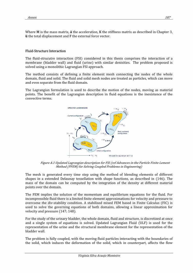
Annex 187
Virginia Silva Araujo Monteiro
Where M is the mass matrix, the acceleration, K the stiffness matrix as described in Chapter 3, the total displacement and F the external force vector.
Fluid-Structure Interaction
The fluid-strucutre interaction (FSI) considered in this thesis comprises the interaction of a membrane (bladder wall) and fluid (urine) with similar denisities. The problem proposed is solved using a monolithic Lagrangian FSI approach.
The method consists of defining a finite element mesh connecting the nodes of the whole domain, fluid and solid. The fluid and solid mesh nodes are treated as particles, which can move and even separate from the fluid domain.
The Lagrangian formulation is used to describe the motion of the nodes, moving as material points. The benefit of the Lagrangian description in fluid equations is the inexistence of the convective terms.
Figure A.1 Updated Lagrangian description for FSI (ref Advances in the Particle Finite Lement
Method (PFEM) for Solving Coupled Problems in Engineering)
The mesh is generated every time step using the method of blending elements of different shapes in a extended Delaunay tessellation with shape functions, as described in (146). The mass of the domain can be computed by the integration of the density at different material points over the domain.
The FEM implies the solution of the momentum and equilibrium equations for the fluid. For incompressible fluid there is a limited finite element approximations for velocity and pressure to overcome the div-stability condition. A stabilized mixed FEM based in Finite Calculus (FIC) is used to solve the governing equations of both domains, allowing a linear approximation for velocity and pressure (147; 148).
For the study of the urinary bladder, the whole domain, fluid and structure, is discretized at once and a single system of equations is solved. Updated Lagrangian Fluid (ULF) is used for the representation of the urine and the structural membrane element for the representation of the bladder wall.
The problem is fully coupled, with the moving fluid particles interacting with the boundaries of the solid, which induces the deformation of the solid, which in counterpart, affects the flow
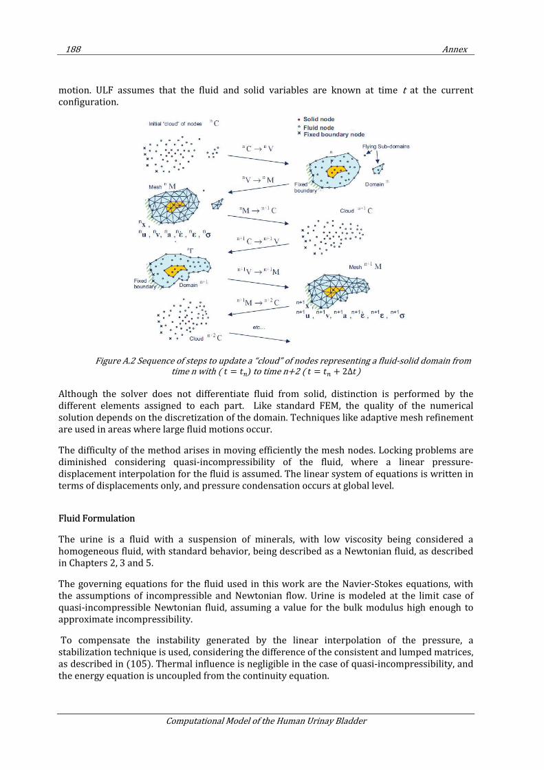
188 Annex
Computational Model of the Human Urinay Bladder
motion. ULF assumes that the fluid and solid variables are known at time t at the current configuration.
Figure A.2 Sequence of steps to update a “cloud” of nodes representing a fluid-solid domain from time n with ( =
) to time n+2 ( =
+ 2∆)
Although the solver does not differentiate fluid from solid, distinction is performed by the different elements assigned to each part. Like standard FEM, the quality of the numerical solution depends on the discretization of the domain. Techniques like adaptive mesh refinement are used in areas where large fluid motions occur.
The difficulty of the method arises in moving efficiently the mesh nodes. Locking problems are diminished considering quasi-incompressibility of the fluid, where a linear pressure-displacement interpolation for the fluid is assumed. The linear system of equations is written in terms of displacements only, and pressure condensation occurs at global level.
Fluid Formulation
The urine is a fluid with a suspension of minerals, with low viscosity being considered a homogeneous fluid, with standard behavior, being described as a Newtonian fluid, as described in Chapters 2, 3 and 5.
The governing equations for the fluid used in this work are the Navier-Stokes equations, with the assumptions of incompressible and Newtonian flow. Urine is modeled at the limit case of quasi-incompressible Newtonian fluid, assuming a value for the bulk modulus high enough to approximate incompressibility.
To compensate the instability generated by the linear interpolation of the pressure, a stabilization technique is used, considering the difference of the consistent and lumped matrices, as described in (105). Thermal influence is negligible in the case of quasi-incompressibility, and the energy equation is uncoupled from the continuity equation.
Annex 189
Virginia Silva Araujo Monteiro
The momentum and the continuity equations for the Newtonian fluid in Lagrangian formulation are defined in the compact form as follow:
∂∂ − ∇ ∙ ∇+ ∇ = (A.7)
∂∂ − ∇ ∙ = 0 (A.8)
in Ω for ( )0,t T∈ , where is the density, is the velocity vector, is the pressure, the
dynamic viscosity, ∇ the symmetric gradient operator, and the body force.
Neglecting ∇ ∙ ∇ , the momentum equation in terms of displacement reads:
∂∂ − ∆
∂ + ∇ = (A.9)
where ∆ is the Laplacian operator.
Rewriting the continuity equation in terms of the bulk modulus :
∂∂ = −∇ ∙
∂ (A.10)
In the weak form (with w and q as displancement and pressure test functions, respectively):
∂∂ ,+ ∆
∂ , + ∇, = ⟨,⟩ (A.11)
,∂∂ = − , ∇ ∙
∂ (A.12)
Considering M the mass matrix, Mp the pressure mass matrix, L the Laplacian operator, G the gradient operator and D the divergence operator, the semi-discrete equation have the form:
∂∂ −
∂ + = (A.13)
190 Annex
Computational Model of the Human Urinay Bladder
∂∂ = −"
∂ (A.14)
with and being the discrete counter part of the displacement and pressure, respectively.
Coupling with the Solid Formulation
The momentum equation for the structure reads:
+ = (A.15)
Where M is the mass matrix, the acceleration, K the stiffness matrix as described in Chapter 3, the total displacement and F the external force vector.
The residual and tangent stiffness for fluid and solid are assembled to the system to apply Newton method.
The monolithic FSI linearized system to be solved is:
#$ − % "&'( = ) (A.16)
Where $ is the FSI tangent stiffness and % " correponds to the global matrix defined for
the fluid.
The tangent stiffness $ should be read as the solid tangent stiffness $ or for the fluid, defined as:
$ = − (A.17)
The ) is the FSI dynamic residual, defined for solid and fluid, as follows:
) = − δx − δxδ #$ − %
"&'( (A.18)
Annex 191
Virginia Silva Araujo Monteiro
With the incremental displacement is δx = u − u .
The Code
The whole FSI problem was solved with Kratos Multiphisics. Kratos is a framework for building multi-disciplinary finite element programs, designed with an object oriented structure based on the finite element methodology.
PFEM was implemented in Kratos and follow the routine as described:
1. The starting point of the program is the cloud of points in the fluid and solid domains at time
2. Boundaries of fluid and solid domains are identified, defining the analysis domain nV . The method of boundary definition uses the concept of Alpha shape (149)
3. Discretization of the domain, with mesh generation n
M based on the extended Delaunay tessellation
4. The coupled Lagrangian equations of motion for the fluid and the solid are solved, computing for the updated configuration t t+ ∆ the state variables for the fluid (velocities, pressure, viscous stresses, etc) and the solid (displacements, stresses, strains, etc)
5. Update the mesh nodes 1n
C+ to the new configuration at time
6. Restart the loop at 1
To assemble the linear system of equations for the fluid and structure, both consider the same time integration scheme.
Results
Results are stored in vector form and read graphically in GID post processor (92).
) = − % + δxδ − δx − δx
δ (A.19)
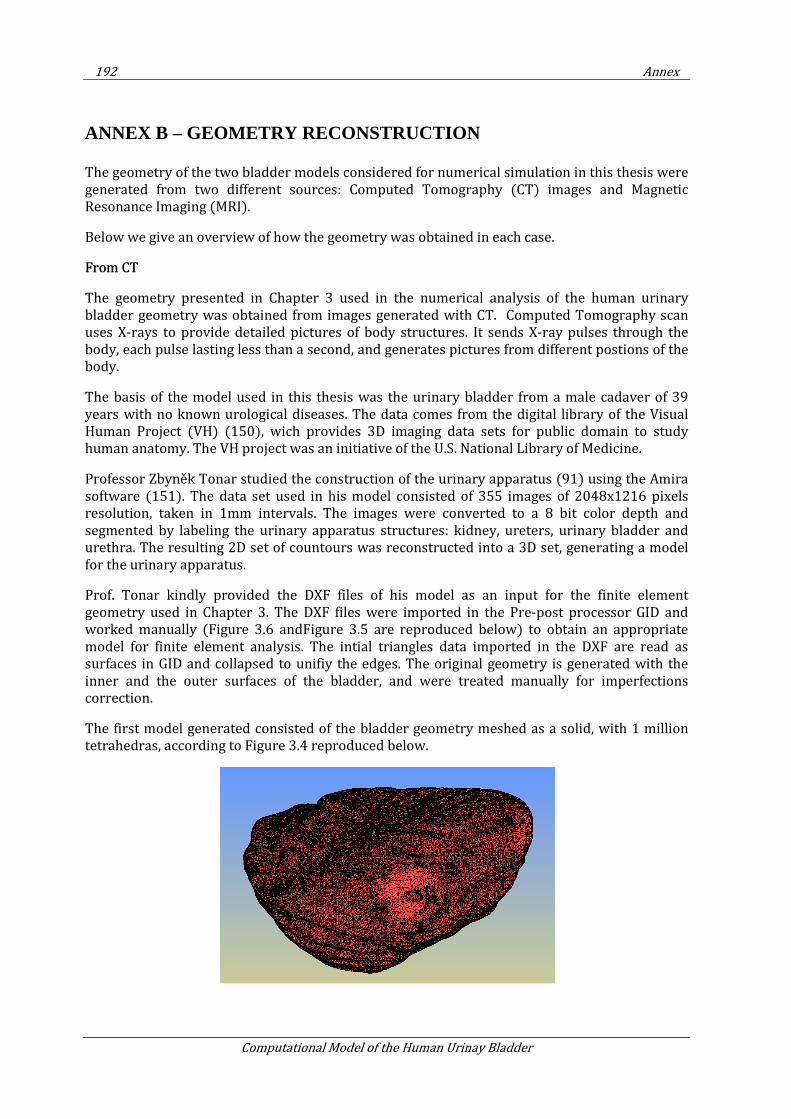
192 Annex
Computational Model of the Human Urinay Bladder
ANNEX B – GEOMETRY RECONSTRUCTION
The geometry of the two bladder models considered for numerical simulation in this thesis were generated from two different sources: Computed Tomography (CT) images and Magnetic Resonance Imaging (MRI).
Below we give an overview of how the geometry was obtained in each case.
From CT
The geometry presented in Chapter 3 used in the numerical analysis of the human urinary bladder geometry was obtained from images generated with CT. Computed Tomography scan uses X-rays to provide detailed pictures of body structures. It sends X-ray pulses through the body, each pulse lasting less than a second, and generates pictures from different postions of the body.
The basis of the model used in this thesis was the urinary bladder from a male cadaver of 39 years with no known urological diseases. The data comes from the digital library of the Visual Human Project (VH) (150), wich provides 3D imaging data sets for public domain to study human anatomy. The VH project was an initiative of the U.S. National Library of Medicine.
Professor Zbyněk Tonar studied the construction of the urinary apparatus (91) using the Amira software (151). The data set used in his model consisted of 355 images of 2048x1216 pixels resolution, taken in 1mm intervals. The images were converted to a 8 bit color depth and segmented by labeling the urinary apparatus structures: kidney, ureters, urinary bladder and urethra. The resulting 2D set of countours was reconstructed into a 3D set, generating a model for the urinary apparatus.
Prof. Tonar kindly provided the DXF files of his model as an input for the finite element geometry used in Chapter 3. The DXF files were imported in the Pre-post processor GID and worked manually (Figure 3.6 andFigure 3.5 are reproduced below) to obtain an appropriate model for finite element analysis. The intial triangles data imported in the DXF are read as surfaces in GID and collapsed to unifiy the edges. The original geometry is generated with the inner and the outer surfaces of the bladder, and were treated manually for imperfections correction.
The first model generated consisted of the bladder geometry meshed as a solid, with 1 million tetrahedras, according to Figure 3.4 reproduced below.
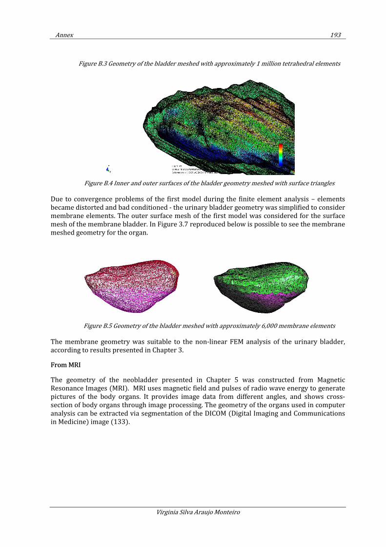
Annex 193
Virginia Silva Araujo Monteiro
Figure B.3 Geometry of the bladder meshed with approximately 1 million tetrahedral elements
Figure B.4 Inner and outer surfaces of the bladder geometry meshed with surface triangles
Due to convergence problems of the first model during the finite element analysis – elements became distorted and bad conditioned - the urinary bladder geometry was simplified to consider membrane elements. The outer surface mesh of the first model was considered for the surface mesh of the membrane bladder. In Figure 3.7 reproduced below is possible to see the membrane meshed geometry for the organ.
Figure B.5 Geometry of the bladder meshed with approximately 6,000 membrane elements
The membrane geometry was suitable to the non-linear FEM analysis of the urinary bladder, according to results presented in Chapter 3.
From MRI
The geometry of the neobladder presented in Chapter 5 was constructed from Magnetic Resonance Images (MRI). MRI uses magnetic field and pulses of radio wave energy to generate pictures of the body organs. It provides image data from different angles, and shows cross-section of body organs through image processing. The geometry of the organs used in computer analysis can be extracted via segmentation of the DICOM (Digital Imaging and Communications in Medicine) image (133).
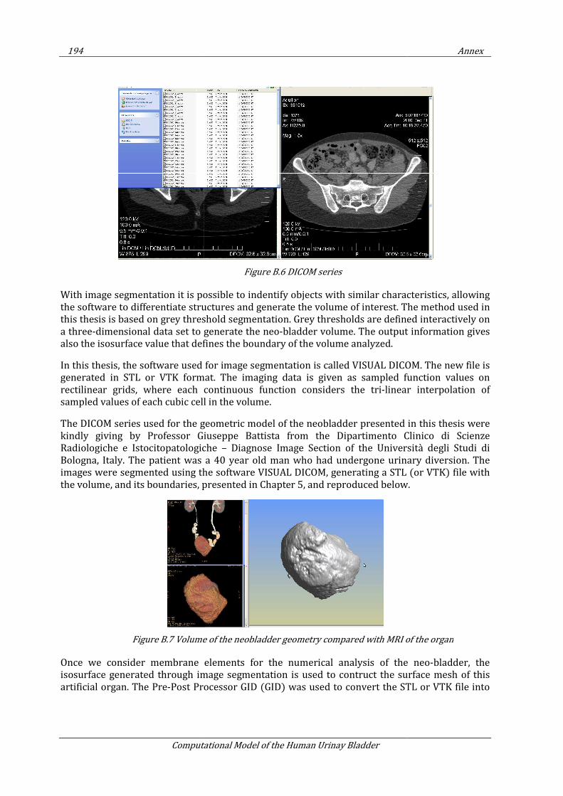
194
Computational Model of the Human Urinay Bladder
With image segmentation it is possible to indentify o
the software to differentiate structures and generate the volume of interest. The method used in
this thesis is based on grey threshold segmentation. Grey thresholds are defined interactively on
a three-dimensional data set to generate the neo
also the isosurface value that defines the boundary of the volume
In this thesis, the software used for image segmentation is called VISUAL DICOM. The new file is
generated in STL or VTK format.
rectilinear grids, where each continuous function considers the tri
sampled values of each cubic cell in the volume.
The DICOM series used for the geometric model of the neobladder presented in this thesis were
kindly giving by Professor Giuseppe Battista from the Dipartimento Clinico di Scienze
Radiologiche e Istocitopatologiche
Bologna, Italy. The patient was a 40 year old man who had undergone urinary diversion. The
images were segmented using the software VISUAL DICOM, generating
the volume, and its boundaries, presented in Chapter
Figure B.7 Volume of the neobladder geometry compared with MRI of the organ
Once we consider membrane ele
isosurface generated through image segmentation is used to contruct the surface mesh of this
artificial organ. The Pre-Post Processor GID (GID)
Computational Model of the Human Urinay Bladder
Figure B.6 DICOM series
With image segmentation it is possible to indentify objects with similar characteristics, allowing
the software to differentiate structures and generate the volume of interest. The method used in
this thesis is based on grey threshold segmentation. Grey thresholds are defined interactively on
onal data set to generate the neo-bladder volume. The output information gives
the isosurface value that defines the boundary of the volume analyzed.
In this thesis, the software used for image segmentation is called VISUAL DICOM. The new file is
rated in STL or VTK format. The imaging data is given as sampled function values on
ach continuous function considers the tri-linear interpolation of
sampled values of each cubic cell in the volume.
The DICOM series used for the geometric model of the neobladder presented in this thesis were
Professor Giuseppe Battista from the Dipartimento Clinico di Scienze
Radiologiche e Istocitopatologiche – Diagnose Image Section of the Universit
The patient was a 40 year old man who had undergone urinary diversion. The
images were segmented using the software VISUAL DICOM, generating a STL (or VTK)
the volume, and its boundaries, presented in Chapter 5, and reproduced below
Volume of the neobladder geometry compared with MRI of the organ
Once we consider membrane elements for the numerical analysis of the neo
isosurface generated through image segmentation is used to contruct the surface mesh of this
rocessor GID (GID) was used to convert the STL or VTK file into
Annex
bjects with similar characteristics, allowing
the software to differentiate structures and generate the volume of interest. The method used in
this thesis is based on grey threshold segmentation. Grey thresholds are defined interactively on
bladder volume. The output information gives
In this thesis, the software used for image segmentation is called VISUAL DICOM. The new file is
The imaging data is given as sampled function values on
linear interpolation of
The DICOM series used for the geometric model of the neobladder presented in this thesis were
Professor Giuseppe Battista from the Dipartimento Clinico di Scienze
Diagnose Image Section of the Università degli Studi di
The patient was a 40 year old man who had undergone urinary diversion. The
a STL (or VTK) file with
, and reproduced below.
Volume of the neobladder geometry compared with MRI of the organ
ments for the numerical analysis of the neo-bladder, the
isosurface generated through image segmentation is used to contruct the surface mesh of this
convert the STL or VTK file into
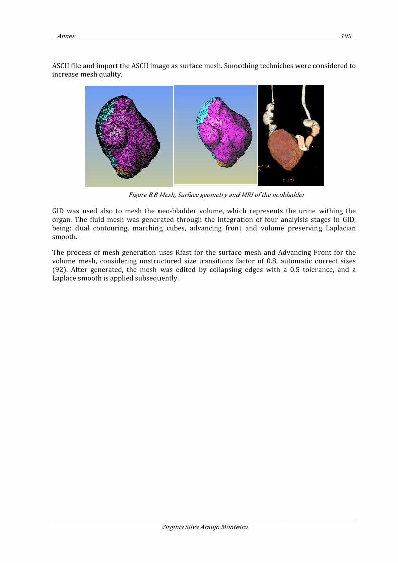
Annex
ASCII file and import the ASCII image
increase mesh quality.
Figure
GID was used also to mesh the neo
organ. The fluid mesh was generated through the integration of
being: dual contouring, marching cubes, advancing front and volume preserving Laplacian
smooth.
The process of mesh generat
volume mesh, considering unstructured size transitions factor of 0.8, automatic correct sizes
(92). After generated, the mesh
Laplace smooth is applied subsequently
Virginia Silva Araujo Monteiro
ASCII image as surface mesh. Smoothing techniches
Figure B.8 Mesh, Surface geometry and MRI of the neobladder
mesh the neo-bladder volume, which represents the urine withing the
generated through the integration of four analyisis stages in GID,
being: dual contouring, marching cubes, advancing front and volume preserving Laplacian
The process of mesh generation uses Rfast for the surface mesh and Advancing Front
, considering unstructured size transitions factor of 0.8, automatic correct sizes
After generated, the mesh was edited by collapsing edges with a
subsequently.
195
moothing techniches were considered to
Mesh, Surface geometry and MRI of the neobladder
which represents the urine withing the
four analyisis stages in GID,
being: dual contouring, marching cubes, advancing front and volume preserving Laplacian
and Advancing Front for the
, considering unstructured size transitions factor of 0.8, automatic correct sizes
by collapsing edges with a 0.5 tolerance, and a


