“main” — 2020/11/19 — 10:04 — page i — #1

Responsive Spectrum Management for WirelessLocal Area Networks: from Heuristic-basedPolicies to Model-Free Reinforcement Learning

Sergio Barrachina-Munoz

TESI DOCTORAL UPF / ANY 2020

Director de la tesiBoris BellaltaDepartament of Information and Communication Technologies

“main” — 2020/11/19 — 10:04 — page ii — #2

“main” — 2020/11/19 — 10:04 — page iii — #3

A l’Iris.

“main” — 2020/11/19 — 10:04 — page iv — #4

“main” — 2020/11/19 — 10:04 — page v — #5

AcknowledgmentsFirst and foremost, I would like to express my deepest gratitude to my advisor, Dr. BorisBellalta, for trusting me and letting me be part of his research group. His guidance throughoutthe PhD years has provided the best research environment to grow both as a researcher and aperson.

A special thanks goes to Dr. Francesc Wilhelmi, my preeminent colleague, for his invalu-able help and encouragement to overcome those moments of panic one shall encounter in thePhD path. A lot of what I have accomplished in this work is thanks to him. Let the Komondorsimulator be the vestige of our work together.

Because of the relaxed (and sometimes bottomless) chats and the inestimable help withintricate research issues, I am thankful to the rest of the members of the Wireless Networkinggroup: Kostis Dovelos, Alvaro Lopez, and Marc Carrascosa. Besides, I could never forgethow Albert Bel, Toni Adame, and Veronica Moreno embraced me when I started working as aresearch intern back in 2015. It has been a pleasure to take this journey with you all, guys.

Of course, the PhD would not have been the same without the undergraduate classes at Uni-versitat Pompeu Fabra. So, thanks to all the students I had the opportunity to teach something.One thing is sure: you have taught me so much.

I am also sincerely thankful to Prof. Edward Knightly and the members of the Rice Net-works Group for giving me such a warm welcoming when I joined the group as a visitor in 2018.Those were four fruitful months in Houston where I learned a lot from incredible researchers.It was an excellent opportunity to broaden my thesis scope towards hardware-related topics anddesign WACA, which has become one of the main assets of this thesis.

My friends outside the academic world were, are, and will always be a precious give. Al-bert, Edgar, Sergi, Jorge, Jacob, you are simply the best. Having you all around means a lot.Likewise, I want to express my deepest gratitude to my high school teacher Vıctor. He hasbeen a gentle and sage oracle throughout these years and made me understand that life, art, andscience are and should be all the same thing.

I wish to thank my parents, Enrique and Cati, and my brother Carlos, for raising me andmaking me always feel the family had my back. My academic career could not have beenpossible without their endless support.

Lastly, I would like to dedicate this thesis to Iris (and our dog Wilco) for always standingby my side. You are all one could ask for having a good life.

v

“main” — 2020/11/19 — 10:04 — page vi — #6

“main” — 2020/11/19 — 10:04 — page vii — #7

AbstractIn this thesis, we focus on the so-called spectrum management’s joint problem: efficient al-location of primary and secondary channels in channel bonding wireless local area networks(WLANs). From IEEE 802.11n to more recent standards like 802.11ax and 802.11be, bondingchannels together is permitted to increase transmissions’ bandwidth. While such an increasefavors the potential network capacity and the activation of higher transmission rates, it comesat the price of reduced power per Hertz and accentuated issues on contention and interferencewith neighboring nodes. So, if WLANs were per se complex deployments, they are becom-ing even more complicated due to the increasing node density and the new technical featuresrequired by novel highly bandwidth-demanding applications. This dissertation provides an in-depth study of channel allocation and channel bonding in WLANs and discusses the suitabilityof solutions ranging from heuristic-based to reinforcement learning (RL)-based.

To characterize channel bonding in saturated WLANs, we first propose an analytical modelbased on continuous-time Markov networks (CTMNs). This model relies on a novel, purpose-designed algorithm that generates CTMNs from spatially distributed scenarios, where nodesare not required to be within the carrier sense range of each other. We identify the key factorsaffecting the throughput and fairness of different channel bonding policies and expose criticalinterrelations among nodes in the spatial domain. By extending the analytical model to supportunsaturated regimes, we highlight the benefits of allocating channels as wide as possible alltogether with adaptive policies to cope with unfair situations.

Apart from the analytical model, this thesis relies on simulations to generalize channelbonding in dense scenarios while avoiding costly, sometimes unfeasible, experimental testbeds.Unfortunately, existing wireless network simulators tend to be too simplistic or too computa-tional demanding. That is why we develop the Komondor wireless network simulator, with theessential advantage over other well-known simulators lying in its high event processing rate.

We then deviate from analytical models and simulations and tackle real measurementsthrough the Wi-Fi All-Channel Analyzer (WACA), the first system specifically designed tosimultaneously measure the energy in all the 24 bondable Wi-Fi channels at the 5 GHz band.With WACA, we perform a first-of-its-kind spectrum measurement in areas including urbanhotspots, residential neighborhoods, universities, and even a football match in Futbol ClubBarcelona’s Camp Nou stadium. Our experimental findings reveal the underpinning factorscontrolling throughput gain, from which we highlight the inter-channel correlation.

As for solution proposals, we first cover heuristic-based approaches to find satisfactoryconfigurations quickly. In this regard, we propose dynamic-wise (DyWi), a lightweight, de-centralized, online primary channel selection algorithm for dynamic channel bonding. DyWiimproves the expected WLAN throughput by considering not only the occupancy of the targetprimary channel but also the activity in the secondary channels. Even when assuming signif-icant delays due to primary channel switching, simulations reveal important throughput anddelay improvements.

Finally, we identify machine learning (ML) approaches applicable to the spectrum manage-ment problem in WLANs and justify why model-free RL suits it the most. In particular, we putthe focus on the adequate performance of stateless variations of RL and anticipate multi-armedbandits as the right solution since i) we need fast adaptability to suit user experience in dy-namic Wi-Fi scenarios and ii) the number of multichannel configurations a network can adoptis limited; thus, agents can fully explore the action space in a reasonable time.

vii

“main” — 2020/11/19 — 10:04 — page viii — #8

Resum

En aquesta tesi ens centrem en el problema conjunt de la gestio de l’espectre: assignacio decanals primaris i secundaris a xarxes d’area local sense fils (WLAN) amb channel bonding. Desde l’estandard IEEE 802.11n fins a estandards mes recents com el 802.11ac, el 802.11ax i el802.11be, s’han anat proposant amplades de banda mes grans per permetre agrupar canals, aug-mentant aixı l’amplada de banda total per transmissio. Tot i que aquest augment en l’ampladade banda afavoreix la capacitat potencial de les xarxes, suportant aixı els requeriments de lesnoves aplicacions Wi-Fi, tambe redueix la potencia per Hertz i accentua els problemes de con-tencio i interferencia entre nodes veıns. En resum, si les xarxes WLANs ja eren complexes perse, s’estan tornant encara mes complexes a causa de l’augment de la densitat de nodes i de lesnoves prestacions incloses als darrers estandards.

Primer proposem un model analıtic basat en xarxes Markov en temps continu (CTMN)per caracteritzar channel bonding en WLANs saturades. Aquest model es basa en un noualgorisme que genera CTMNs a partir d’escenaris distribuıts espaialment, on no es necessarique els nodes estiguin dins del rang de contencio de la resta. Identifiquem els factors clausque afecten el rendiment i l’equitat de les diferents polıtiques de channel bonding i mostreml’existencia d’interrelacions crıtiques entre nodes en forma de reaccio en cadena. D’aixo se’ndespren que no hi ha una polıtica channel bonding optima unica per a cada escenari. En ampliarel model analıtic per donar suport a regims no saturats, destaquem els avantatges d’assignar elscanals tan amplis com sigui possible a les WLAN i implementar polıtiques d’acces adaptatiuper fer front a les situacions que poden apareixer tant en termes de rendiment com d’equitat.

A part dels models analıtics, aquesta tesi es basa en simulacions per generalitzar esce-naris evitant costosos bancs de proves experimentals, de vegades inviables. Malauradament,els simuladors de xarxes sense fils existents solen ser massa simplistes o molt costosos com-putacionalment. Es per aixo que desenvolupem el simulador de xarxes sense fils Komondor,concebut com una eina de codi obert accessible (llesta per utilitzar) per a la investigacio dexarxes sense fils. L’avantatge essencial de Komondor respecte d’altres simuladors sense filsconeguts rau en la seva elevada velocitat de processament d’esdeveniments.

A continuacio ens desviem de models analıtics i simulacions i abordem mesures reals atraves del Wi-Fi All-Channel Analyzer (WACA), el primer sistema que mesura simultaniamentl’energia de tots els 24 canals que permeten channel bonding a la banda Wi-Fi dels 5 GHz.Amb WACA, realitzem un estudi unic de localitzacions que inclouen nuclis urbans, barris res-idencials, universitats i fins i tot un partit a al Camp Nou, un estadi ple amb 98.000 aficionats i12.000 connexions Wi-Fi simultanies. Les dades experimentals revelen els factors fonamentalsque controlen el guany de rendiment, a partir dels quals ressaltem la correlacio entre canals.Tambe mostrem la importancia del conjunt de dades recopilades per trobar nous factors claus,que d’una altra manera no seria possible, ates que els models d’ocupacio de canals simplessubestimen els guanys potencials.

Pel que fa a solucions, primer discutim propostes basades en heurıstiques per trobar con-figuracions satisfactories rapidament. En aquest sentit, proposem dinamicament (DyWi), unalgorisme de seleccio de canal primari en lınia, descentralitzat i eficient per xarxes channelbonding. DyWi millora el rendiment esperat tenint en compte no nomes l’ocupacio del canalprimari objectiu, sino tambe l’activitat dels canals secundaris. Fins i tot quan suposem retardssignificatius a causa del canvi de canal primari, observem millores importants en termes derendiment i retard.

viii

“main” — 2020/11/19 — 10:04 — page ix — #9

Finalment, identifiquem els enfocaments d’aprenentatge automatic (o machine learning)aplicables al problema de la gestio de l’espectre a les WLAN i justifiquem per que l’aprenentatgedel tipus reinforcement learning (RL) es el mes adient. En particular, ens centrem en elrendiment adequat de les variacions d’RL sense estats i proposem multi-armed bandits comla solucio adequada, ja que i) necessitem una adaptabilitat rapida per millorar l’experienciad’usuari en escenaris Wi-Fi dinamics i ii) el nombre de configuracions multicanal que unaxarxa pot adoptar es limitat; per tant, els agents poden explorar completament l’espai d’accioen un temps raonable.

ix

“main” — 2020/11/19 — 10:04 — page x — #10

“main” — 2020/11/19 — 10:04 — page xi — #11

Contents

Abstract (English/Catala) vii

List of abbreviations xv

List of variables xvii

List of main publications xix

List of other publications xxi

1 INTRODUCTION 11.1 Spectrum management in uncoordinated Wi-Fi networks . . . . . . . . . . . . 21.2 Contributions . . . . . . . . . . . . . . . . . . . . . . . . . . . . . . . . . . . 41.3 Document structure . . . . . . . . . . . . . . . . . . . . . . . . . . . . . . . . 5

2 SPECTRUM MANAGEMENT IN IEEE 802.11 WLANS 72.1 Channel allocation . . . . . . . . . . . . . . . . . . . . . . . . . . . . . . . . 72.2 Channel bonding . . . . . . . . . . . . . . . . . . . . . . . . . . . . . . . . . 10

3 METHODOLOGY AND ENABLERS 153.1 Modeling spectrum management through continuous time Markov networks . . 15

3.1.1 CTMNs for channel bonding in spatially-distributed WLANs . . . . . . 153.1.2 Constructing the CTMN . . . . . . . . . . . . . . . . . . . . . . . . . 163.1.3 Extending CTMNs to unsaturated regimes . . . . . . . . . . . . . . . . 193.1.4 A Matlab framework for constructing WLAN CTMNs . . . . . . . . . 20

3.2 The Komondor wireless network simulator . . . . . . . . . . . . . . . . . . . . 213.2.1 The need of a new simulator . . . . . . . . . . . . . . . . . . . . . . . 213.2.2 Design principles . . . . . . . . . . . . . . . . . . . . . . . . . . . . . 22

3.3 Trace-driven evaluation of channel bonding . . . . . . . . . . . . . . . . . . . 233.3.1 Why a custom Wi-Fi spectrum analyzer? . . . . . . . . . . . . . . . . 243.3.2 The WACA platform . . . . . . . . . . . . . . . . . . . . . . . . . . . 243.3.3 On-field dataset . . . . . . . . . . . . . . . . . . . . . . . . . . . . . . 253.3.4 Trace-driven framework . . . . . . . . . . . . . . . . . . . . . . . . . 26

4 PERFORMANCE EVALUATION OF CHANNEL BONDING 294.1 Analytical characterization of channel bonding . . . . . . . . . . . . . . . . . 29

4.1.1 States and transitions depend on the policy . . . . . . . . . . . . . . . 29

xi

“main” — 2020/11/19 — 10:04 — page xii — #12

4.1.2 Being greedy is not always convenient . . . . . . . . . . . . . . . . . . 314.2 Assessment of high-density deployments . . . . . . . . . . . . . . . . . . . . . 32

4.2.1 Type of scenarios . . . . . . . . . . . . . . . . . . . . . . . . . . . . . 324.2.2 On the individual throughput and fairness . . . . . . . . . . . . . . . . 324.2.3 Traffic load and delay . . . . . . . . . . . . . . . . . . . . . . . . . . . 35

4.3 Trace-driven simulations from real-world measurements . . . . . . . . . . . . 384.3.1 A look into the world’s Wi-Fi spectrum . . . . . . . . . . . . . . . . . 384.3.2 Characterization of channel bonding in the real-world spectrum . . . . 39

5 HEURISTIC-BASED POLICIES 515.1 Heuristics to cope with complexity . . . . . . . . . . . . . . . . . . . . . . . . 515.2 Heuristic-based primary channel selection for dynamic channel bonding . . . . 52

5.2.1 Online selection of the primary channel . . . . . . . . . . . . . . . . . 525.2.2 Dynamic-wise primary channel selection . . . . . . . . . . . . . . . . 545.2.3 DyWi performance . . . . . . . . . . . . . . . . . . . . . . . . . . . . 55

6 MODEL-FREE REINFORCEMENT LEARNING 596.1 A change of paradigm towards reinforcement learning . . . . . . . . . . . . . . 59

6.1.1 What is reinforcement learning? . . . . . . . . . . . . . . . . . . . . . 606.1.2 Why RL and not other ML frameworks? . . . . . . . . . . . . . . . . . 61

6.2 Mapping the problem to RL . . . . . . . . . . . . . . . . . . . . . . . . . . . 626.2.1 System model . . . . . . . . . . . . . . . . . . . . . . . . . . . . . . . 626.2.2 Attributes and actions . . . . . . . . . . . . . . . . . . . . . . . . . . 636.2.3 Statuses, observations and states . . . . . . . . . . . . . . . . . . . . . 656.2.4 Problem definition . . . . . . . . . . . . . . . . . . . . . . . . . . . . 66

6.3 RL framework for the spectrum management problem . . . . . . . . . . . . . . 676.3.1 Learning architecture . . . . . . . . . . . . . . . . . . . . . . . . . . . 676.3.2 RL models . . . . . . . . . . . . . . . . . . . . . . . . . . . . . . . . 68

6.4 Multi-Armed Bandits . . . . . . . . . . . . . . . . . . . . . . . . . . . . . . . 716.4.1 The MAB problem . . . . . . . . . . . . . . . . . . . . . . . . . . . . 716.4.2 MAB taxonomies . . . . . . . . . . . . . . . . . . . . . . . . . . . . . 726.4.3 MAB exploration strategies . . . . . . . . . . . . . . . . . . . . . . . 74

6.5 Evaluation . . . . . . . . . . . . . . . . . . . . . . . . . . . . . . . . . . . . . 756.5.1 Self-contained dataset . . . . . . . . . . . . . . . . . . . . . . . . . . 756.5.2 Benchmarking RL algorithms . . . . . . . . . . . . . . . . . . . . . . 776.5.3 Generalization to high-density deployments . . . . . . . . . . . . . . . 82

7 CONCLUDING REMARKS 897.1 Summary . . . . . . . . . . . . . . . . . . . . . . . . . . . . . . . . . . . . . 897.2 Future work . . . . . . . . . . . . . . . . . . . . . . . . . . . . . . . . . . . . 89

Funding 91

Bibliography 93

Appendix 105

xii

“main” — 2020/11/19 — 10:04 — page xiii — #13

8 PUBLICATIONS 1098.1 Paper #1: Dynamic channel bonding in spatially distributed high-density WLANs1108.2 Paper #2: To overlap or not to overlap: enabling channel bonding in high-

density WLANs . . . . . . . . . . . . . . . . . . . . . . . . . . . . . . . . . . 1348.3 Paper #3: Komondor: A wireless network simulator for next-generation high-

density WLANs . . . . . . . . . . . . . . . . . . . . . . . . . . . . . . . . . . 1548.4 Paper #4: Online primary channel selection for dynamic channel bonding in

high-density WLANs . . . . . . . . . . . . . . . . . . . . . . . . . . . . . . . 1678.5 Paper #5: Wi-Fi all channel analyzer . . . . . . . . . . . . . . . . . . . . . . . 1758.6 Paper #6: Wi-Fi channel bonding: an all-channel system and experimental

study from urban hotspots to a sold-out stadium. . . . . . . . . . . . . . . . . . 188

xiii

“main” — 2020/11/19 — 10:04 — page xiv — #14

“main” — 2020/11/19 — 10:04 — page xv — #15

List of abbreviations

AM (or DCB): always-maxAP: access pointBSS: basic service setCA: channel allocationCB: channel bondingCCA: clear channel assessmentCDF: cumulative distribution functionCE: capture effectCSMA/CA: carrier sense multiple accesswith collision avoidanceCTMN: continuous time Markov networkCTS: clear to sendDCA: dynamic channel allocationDCB (or AM): dynamic channel bondingDCF: distributed coordination functionDIFS: DCF interframe spaceDFS: dynamic frequency selectionDRL: deep reinforcement learningDiWy: dynamic wiseDF: dynamic freeDR: dynamic randomFP: fixed primaryIEEE: Institute of Electrical andElectronics EngineersISM: industrial, scientific and medicalMAB: multi-armed banditMAC: medium access control

MCS: modulation and coding schemeML: machine learningNAV: network allocation vectorOBSS: overlapping basic service setOPS: online primary selectionPCF: point coordination functionPER: packet error ratePHY: physical (layer)PIFS: PCF interframe spacePU: probabilistic uniformRF: radio frequencyRL: reinforcement learningRSSI: received signal strength indicatorRTS: request to sendSC: single channelSCB: static channel bondingSIFS: short interframe spaceSNR: signal-to-noise ratioSINR: signal-to-noise-plus-interference ratioSDR: software defined radioTD: temporal differenceTPC: transmit power controlWACA: Wi-Fi all-channel analyzerWLAN: wireless local area networkWN: wireless networkWSN: wireless sensor network

xv

“main” — 2020/11/19 — 10:04 — page xvi — #16

“main” — 2020/11/19 — 10:04 — page xvii — #17

List of variables and terms

a: action (or arm) identifierA: action spaceb: maximum bandwidthB: bandwidth of a basic channelB: band of basic channelsBO: pending backoff timeBW: bandwidth usagec: basic channel identifierC: channel allocationC tx: transmission channelC: channelizationCE: capture effect thresholdd: packet delayd∗: minimum achievable delayD: channel bonding policyE: expected valueG: cumulative rewardh: hypothesis functionH: WLAN status (in RL)Iw: world of BSS w (in RL)J : Jain’s fairness indexQ: action valueK: number of actions (or arms)L: size of a data packet`: mean traffic loadL: quantized mean traffic loadm: maximum backoff stageM : matrix of transition ratesnC : number of basic channels in the systemnSTA: number of STAsoB: mean occupancy at band Bp: primary channel identifierP: probabilityq: backoff stager: instantaneous rewardR: reward function

s: feasible state (in CTMN) or state (in RL)S: feasible state space (in CTMN) or statespace (in RL)t: iteration identifier or timeT : number of iterationsTm: duration of a measurement (in WACA)Tper: duration of a period (or epoch)Tslot: duration of a slotU : UCB1 upper confidence boundw: BSS identifierW : number of BSS’sW ′: number of agent-empowered BSS’sα: learning rate~α: transition probabilitiesβ: set of configurable max. bandwidthsγ: discount factorΓ: throughputΓ: normalized Γ wrt single-channelδ: bounded delay ratioζ: throughput satisfactionη: throughput satisfaction ratioθ: reward probability distributionλ: packet transmission attempt rateµ: departure rate~ν: equilibrium distributionξ: inter-channel correlationπ: policy (in RL)ρ: long-term probability%: Pearson’s correlation coefficientσ: standard deviationψ: global state identifierΨ: global state spaceω: bandwidth deprivationΩ: context (in RL)

xvii

“main” — 2020/11/19 — 10:04 — page xviii — #18

“main” — 2020/11/19 — 10:04 — page xix — #19

List of main publications

The following publications constitute the backbone of this thesis. We refer to them in thedissertation as thesis papers #1 to #6.

1. S. Barrachina-Munoz, F. Wilhelmi, and B. Bellalta. Dynamic channel bonding in spa-tially distributed high-density WLANs. IEEE Transactions on Mobile Computing, 19(4):821–835, 2019.

2. S. Barrachina-Munoz, F. Wilhelmi, and B. Bellalta. To overlap or not to overlap: en-abling channel bonding in high-density WLANs. Computer Networks, 152:40–53, 2019.

3. S. Barrachina-Munoz, F. Wilhelmi, I. Selinis, and B. Bellalta. Komondor: A wirelessnetwork simulator for next-generation high-density WLANs. In 2019 Wireless Days(WD), pages 1–8. IEEE, 2019.

4. S. Barrachina-Munoz, F. Wilhelmi, and B. Bellalta. Online primary channel selectionfordynamic channel bonding in high-density WLANs. IEEE Wireless CommunicationsLetters, 9(2):258–262, 2019.

5. S. Barrachina-Munoz, B. Bellalta, and E. Knightly. Wi-Fi all channel analyzer. In The14th ACM Workshop on Wireless Network Testbeds, Experimental evaluation & CHar-acterization (WINTECH). ACM., 2020. Runner up, best paper award.

6. S. Barrachina-Munoz, B. Bellalta, and E. Knightly. Wi-Fi channel bonding: an all-channel system and experimental study from urban hotspots to a sold-out stadium. Sub-mitted to IEEE Transactions on Networking (under major revision), 2020.

xix

“main” — 2020/11/19 — 10:04 — page xx — #20

“main” — 2020/11/19 — 10:04 — page xxi — #21

List of other publications

While this dissertation does not directly include contributions from the following papers, theyhave significantly influenced the thesis’s development.

1. S. Barrachina-Munoz, B. Bellalta, T. Adame, and A. Bel. Multi-hop communication inthe uplink for LPWANs. Computer Networks, 123, 153-168, 2017.

2. S. Barrachina-Munoz and B. Bellalta. Learning optimal routing for the uplink in LP-WANs using similarity-enhanced e-greedy. In 2017 IEEE 28th Annual InternationalSymposium on Personal, Indoor, and Mobile Radio Communications (PIMRC), pages1–5. IEEE, 2017.

3. T. Adame, S. Barrachina-Munoz, B. Bellalta, and A. Bel. HARE: Supporting efficientuplink multi-hop communications in self-organizing LPWANs. Sensors, 18(1), 115,2019.

4. S. Barrachina-Munoz, T. Adame, A. Bel, and B. Bellalta. Towards energy efficient LP-WANs through learning-based multi-hop routing. In IEEE 5th World Forum on Internetof Things (WF-IoT) 2019, 2019.

5. F. Wilhelmi, S. Barrachina-Munoz, and B. Bellalta. On the Performance of the SpatialReuse Operation in IEEE 802.11 ax WLANs. In 2019 IEEE Conference on Standardsfor Communications and Networking (CSCN) (pp. 1-6). IEEE, 2019.

6. F. Wilhelmi, S. Barrachina-Munoz, B. Bellalta, C. Cano, A. Jonsson, G. Neu. Potentialand pitfalls of multi-armed bandits for decentralized spatial reuse in WLANs. Journal ofNetwork and Computer Applications, 127, 26-42, 2019.

7. F. Wilhelmi, B. Bellalta, C. Cano, A. Jonsson, and S. Barrachina-Munoz. Collaborativespatial reuse in wireless networks via selfish multi-armed bandits. Ad Hoc Networks, 88,129-141, 2019.

8. F. Wilhelmi, S. Barrachina-Munoz, B. Bellalta, C. Cano, A. Jonsson, and Ram, V. Aflexible machine-learning-aware architecture for future WLANs. IEEE CommunicationsMagazine, 58(3), 25-31, 2020.

xxi

“main” — 2020/11/19 — 10:04 — page xxii — #22

“main” — 2020/11/19 — 10:04 — page 1 — #23

Chapter 1

INTRODUCTION

Wireless local area networks (WLANs), with IEEE 802.11 as the most widely used standard,are a cost-efficient solution for wireless Internet access that can satisfy most of the current com-munication requirements in domestic, public, and business scenarios. Modern applications likeaugmented reality, virtual reality, or real-time 8K video are pushing next-generation WLANs tosupport ever-increasing performance demands along with 5G systems and beyond. Wi-Fi relieson basic service sets (BSS’s)1 composed of an access point (AP) and one or multiple stations(STAs). The AP provides access to the Internet to the STAs in downlink and uplink manner.This simple and flexible architecture has been a success since the first commercial deploymentsof Wi-Fi back in 1999.

Wi-Fi2 works primarily with the carrier sense multiple access with collision avoidance(CSMA/CA) method,3 where nodes attempt to avoid collisions by initiating transmissions onlyafter the channel is sensed idle during a random backoff time. This listen-before-talk schemeis critical to ensure fairness in the industrial, scientific, and medical (ISM) bands, license-free bands that everyone can use. So, before transmitting in a given channel, a Wi-Fi devicemust wait to sense that channel free during a time indicated by the backoff counter. Oncethe backoff expires, frame transmissions can be initiated. Since the introduction of channelbonding in the IEEE 802.11n [4] amendment, multichannel transmissions were also permit-ted to support larger bandwidths and reach higher capacities. Current and future amendmentslike 802.11ac/ax [5, 7] and 802.11be [6], respectively, extend channel bonding capabilities tosupport higher bandwidths and more channel combinations.

CSMA/CA is Wi-Fi’s cornerstone and has been performing extraordinarily well for singleand multichannel transmissions in previous years, when channels were vacated most of thetime, so one could typically transmit without significant delays nor losses due to interference.However, the random nature of CSMA/CA altogether with the scarce shared frequency spec-trum at the ISM bands and the emergence of new Wi-Fi features mandates adequate spectrummanagement to handle today’s and future’s Wi-Fi complexity.

Indeed, the number of hungry-bandwidth devices accessing the Internet through WLANAPs such as laptops, smart-phones, tablets, and wearables is increasing drastically at the same

1Some works in the literature use the term WLAN to refer to a BSS. However, it is more formal to separatesuch concepts as we do in this dissertation.

2The terms WLAN and Wi-Fi are often used interchangeably, as in this thesis. Nonetheless, a WLAN can bebuilt on various wireless technologies, including Wi-Fi (i.e., the IEEE 802.11 standards).

3New IEEE 802.11 amendments like 802.11ax introduce other medium access methods based on scheduling.However, CSMA/CA is still the most common access method due to its simplicity.

1

“main” — 2020/11/19 — 10:04 — page 2 — #24

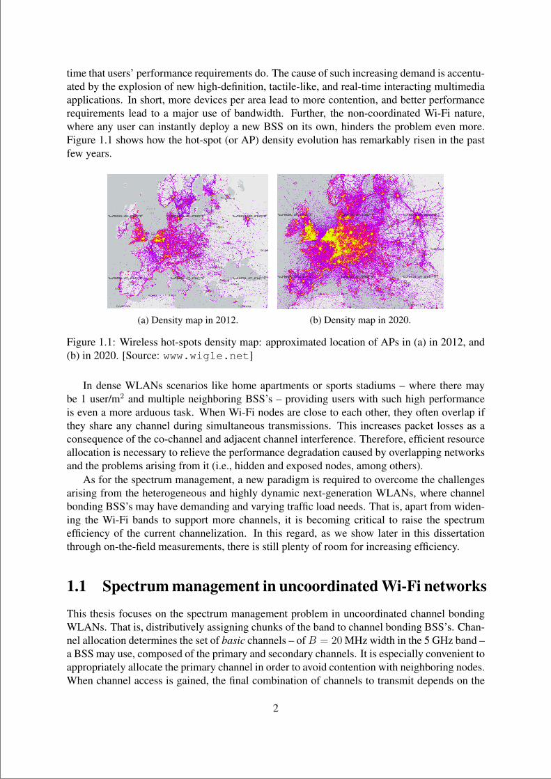
time that users’ performance requirements do. The cause of such increasing demand is accentu-ated by the explosion of new high-definition, tactile-like, and real-time interacting multimediaapplications. In short, more devices per area lead to more contention, and better performancerequirements lead to a major use of bandwidth. Further, the non-coordinated Wi-Fi nature,where any user can instantly deploy a new BSS on its own, hinders the problem even more.Figure 1.1 shows how the hot-spot (or AP) density evolution has remarkably risen in the pastfew years.

(a) Density map in 2012. (b) Density map in 2020.

Figure 1.1: Wireless hot-spots density map: approximated location of APs in (a) in 2012, and(b) in 2020. [Source: www.wigle.net]

In dense WLANs scenarios like home apartments or sports stadiums – where there maybe 1 user/m2 and multiple neighboring BSS’s – providing users with such high performanceis even a more arduous task. When Wi-Fi nodes are close to each other, they often overlap ifthey share any channel during simultaneous transmissions. This increases packet losses as aconsequence of the co-channel and adjacent channel interference. Therefore, efficient resourceallocation is necessary to relieve the performance degradation caused by overlapping networksand the problems arising from it (i.e., hidden and exposed nodes, among others).

As for the spectrum management, a new paradigm is required to overcome the challengesarising from the heterogeneous and highly dynamic next-generation WLANs, where channelbonding BSS’s may have demanding and varying traffic load needs. That is, apart from widen-ing the Wi-Fi bands to support more channels, it is becoming critical to raise the spectrumefficiency of the current channelization. In this regard, as we show later in this dissertationthrough on-the-field measurements, there is still plenty of room for increasing efficiency.

1.1 Spectrum management in uncoordinated Wi-Fi networks

This thesis focuses on the spectrum management problem in uncoordinated channel bondingWLANs. That is, distributively assigning chunks of the band to channel bonding BSS’s. Chan-nel allocation determines the set of basic channels – ofB = 20 MHz width in the 5 GHz band –a BSS may use, composed of the primary and secondary channels. It is especially convenient toappropriately allocate the primary channel in order to avoid contention with neighboring nodes.When channel access is gained, the final combination of channels to transmit depends on the

2

“main” — 2020/11/19 — 10:04 — page 3 — #25

channel allocation, the channel bonding policy, and the frequency spectrum status. In partic-ular, channel allocation is configuration-dependent, and channel bonding acts on a per-framebasis according to the sensed spectrum activity.

Channel bonding is a key mechanism for increasing Wi-Fi data rates as the maximum datarate increases in proportion to the total channel bandwidth. The Shannon-Hartley theorem for nchannels of bandwidth B establishes that the information-theoretic capacity of a link is defined(in bits per second) as

C = nB log2

(1 +

S/n

N

), (1.1)

where S/N is the signal-to-noise-ratio (SNR) that would be perceived at the receiver when thetransmitters use single-channel (n = 1). So, in regimes where the SNR is kept sufficientlyhigh, leading to a constant modulation and coding scheme (MCS) regardless of the bandwidth,the capacity grows linearly with the number of channels. However, the theoretical capacity issub-linear with the bandwidth (or the number of channels) as expressed by the term S/n

Nin the

logarithm of (1.1). The reason lies in the fact that for a given transmit power, the power perunit-Hertz halves when doubling the bandwidth, thus reducing the SNR and potential MCS asa consequence.

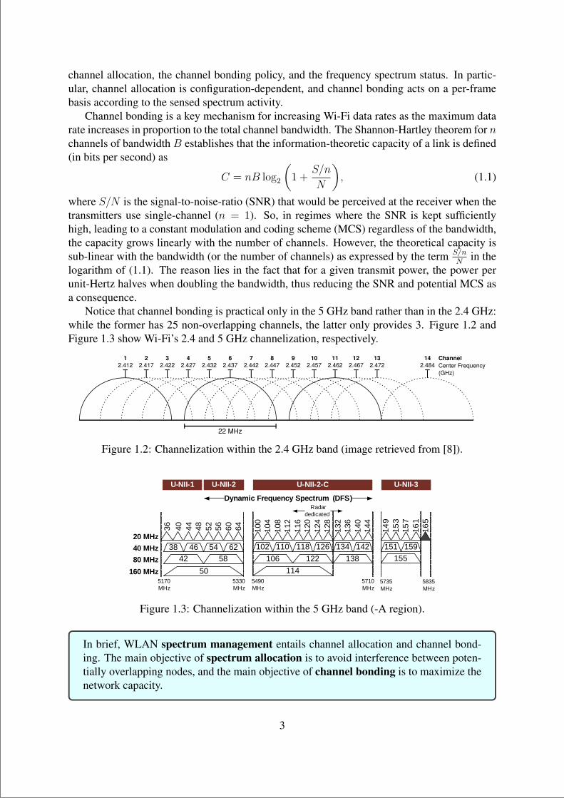
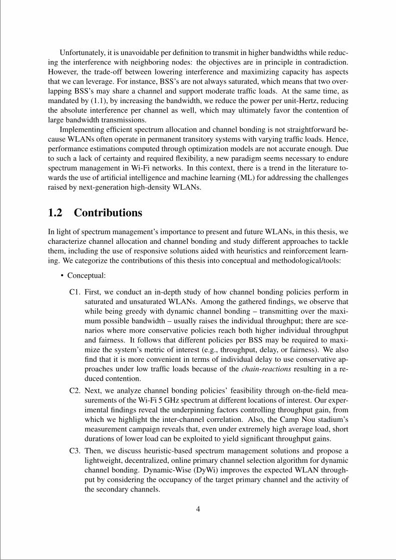
Notice that channel bonding is practical only in the 5 GHz band rather than in the 2.4 GHz:while the former has 25 non-overlapping channels, the latter only provides 3. Figure 1.2 andFigure 1.3 show Wi-Fi’s 2.4 and 5 GHz channelization, respectively.

12

2.467

1

2.412

22 MHz

Channel

Center Frequency

(GHz)

2

2.417

3

2.422

4

2.427

5

2.432

6

2.437

7

2.442

8

2.447

9

2.452

10

2.457

11

2.462

13

2.472

14

2.484

Figure 1.2: Channelization within the 2.4 GHz band (image retrieved from [8]).

36 40 44 48 52 56 60 64 100

104

108

112

116

120

124

128

132

136

140

144

149

153

157

161

165

38 46 6254 102 110 126118 134 142 151 159

42 58

50

106 122

114

138 15540 MHz

80 MHz

160 MHz

20 MHz

U-NII-1 U-NII-2 U-NII-2-C U-NII-3

Dynamic Frequency Spectrum (DFS)Radar

dedicated

5170MHz

5330MHz

5490MHz

5710MHz

5735MHz

5835MHz

Figure 1.3: Channelization within the 5 GHz band (-A region).

In brief, WLAN spectrum management entails channel allocation and channel bond-ing. The main objective of spectrum allocation is to avoid interference between poten-tially overlapping nodes, and the main objective of channel bonding is to maximize thenetwork capacity.

3

“main” — 2020/11/19 — 10:04 — page 4 — #26

Unfortunately, it is unavoidable per definition to transmit in higher bandwidths while reduc-ing the interference with neighboring nodes: the objectives are in principle in contradiction.However, the trade-off between lowering interference and maximizing capacity has aspectsthat we can leverage. For instance, BSS’s are not always saturated, which means that two over-lapping BSS’s may share a channel and support moderate traffic loads. At the same time, asmandated by (1.1), by increasing the bandwidth, we reduce the power per unit-Hertz, reducingthe absolute interference per channel as well, which may ultimately favor the contention oflarge bandwidth transmissions.

Implementing efficient spectrum allocation and channel bonding is not straightforward be-cause WLANs often operate in permanent transitory systems with varying traffic loads. Hence,performance estimations computed through optimization models are not accurate enough. Dueto such a lack of certainty and required flexibility, a new paradigm seems necessary to endurespectrum management in Wi-Fi networks. In this context, there is a trend in the literature to-wards the use of artificial intelligence and machine learning (ML) for addressing the challengesraised by next-generation high-density WLANs.

1.2 ContributionsIn light of spectrum management’s importance to present and future WLANs, in this thesis, wecharacterize channel allocation and channel bonding and study different approaches to tacklethem, including the use of responsive solutions aided with heuristics and reinforcement learn-ing. We categorize the contributions of this thesis into conceptual and methodological/tools:

• Conceptual:

C1. First, we conduct an in-depth study of how channel bonding policies perform insaturated and unsaturated WLANs. Among the gathered findings, we observe thatwhile being greedy with dynamic channel bonding – transmitting over the maxi-mum possible bandwidth – usually raises the individual throughput; there are sce-narios where more conservative policies reach both higher individual throughputand fairness. It follows that different policies per BSS may be required to maxi-mize the system’s metric of interest (e.g., throughput, delay, or fairness). We alsofind that it is more convenient in terms of individual delay to use conservative ap-proaches under low traffic loads because of the chain-reactions resulting in a re-duced contention.

C2. Next, we analyze channel bonding policies’ feasibility through on-the-field mea-surements of the Wi-Fi 5 GHz spectrum at different locations of interest. Our exper-imental findings reveal the underpinning factors controlling throughput gain, fromwhich we highlight the inter-channel correlation. Also, the Camp Nou stadium’smeasurement campaign reveals that, even under extremely high average load, shortdurations of lower load can be exploited to yield significant throughput gains.

C3. Then, we discuss heuristic-based spectrum management solutions and propose alightweight, decentralized, online primary channel selection algorithm for dynamicchannel bonding. Dynamic-Wise (DyWi) improves the expected WLAN through-put by considering the occupancy of the target primary channel and the activity ofthe secondary channels.

4

“main” — 2020/11/19 — 10:04 — page 5 — #27

C4. Lastly, we envision the need for machine learning to cope with the spectrum man-agement problem in high-density and dynamic settings. We justify the suitabilityof a stateless variation of reinforcement learning (RL) through multi-armed ban-dits (MABs) suits the task of adapting fast in uncoordinated deployments. Resultsfrom extensive experiments show the responsiveness of MABs in front of other RLapproaches.

• Methodological/tools:

M1. First, we design an analytical model based on continuous-time Markov networks(CTMNs) to capture the behavior of spatially-distributed WLANs implementingchannel bonding policies under saturated and unsaturated regimes. This is the firstCTMN model to capture partial overlaps in channel bonding WLANs. Part of con-tribution C1 is derived from analyses through this model.

M2. Second, we develop Komondor, a wireless network simulator for assessing thenovel IEEE 802.11 features in high-density WLAN deployments. Komondor pro-vides reliable simulations with much lower execution times than other well-knownsimulators such as ns-3. Findings on high-density deployments in contribution C1are gathered through Komondor. Besides, our wireless network simulator is alsoused for contributions C3 and C4.

M3. Finally, we design and build WACA, a novel spectrum analyzer covering all theWi-Fi’s 5 GHz band. We use it to gather a unique dataset covering multiple placesof interest, including a sold-out game in the Camp Nou stadium. The key noveltyof WACA is its ability to measure all the basic channels simultaneously. Through atrace-driven framework, we discover novel insights into channel bonding otherwisenot possible to get. These insights compose contribution C2.

To make our research results more accessible to the community, all the work made in thisthesis has been disclosed in open access. To that purpose, we have made publicly available allthe resources developed to undertake our research, including results, code, and datasets. Thetools used to enable open access are GitHub and Zenodo. We provide links to such sourcesthrough the chapters of this dissertation.

1.3 Document structureThis thesis is a compendium of articles resulting from the characterization and benchmarkingof channel bonding and channel allocation in Wi-Fi deployments. We refer to the thesis pub-lications attached at the end of this document (§8) as paper #1 to paper #6. Apart from thethe list of publications, a monograph is provided to introduce the research topic and emphasizethe main findings. This document is structured as follows. Chapter §2 introduces the problemof spectrum management in Wi-Fi networks. In Chapter §3, we depict the three main enablertools of this thesis. Next, in Chapter §4 we employ the presented enablers to assess spectrummanagement performance in a plethora of scenarios. The use of heuristics to cope with theproblem at issue is discussed in Chapter §5. Then, Chapter §6 treats the convenience of state-less reinforcement learning and benchmarks different solutions. Finally, Chapter §7 concludeswith the summary and future work.

5

“main” — 2020/11/19 — 10:04 — page 6 — #28

“main” — 2020/11/19 — 10:04 — page 7 — #29

Chapter 2

SPECTRUM MANAGEMENT IN IEEE802.11 WLANS

In this chapter, we briefly depict the Wi-Fi CSMA/CA operation and the features related tothe spectrum management in IEEE 802.11 WLANs. Spectrum management techniques can bemainly divided in spectrum allocation (or channel allocation) and channel bonding.

2.1 Channel allocationThe WLAN spectrum covers different frequency bands inside the ISM bands. The most sig-nificant are the 2.4 GHz (802.11b/g/n/ax) [4] and 5 GHz (802.11a/h/j/n/ac/ax) [5] bands, butthere are other bands like 3.65 GHz (802.11y) or 60 GHz (802.11ad/ay). Future amendmentslike the 802.11be [6] will also use the 6 GHz band. In the 2.4 GHz band, there are 14 channelsof 22 MHz, from which just 3 of them (channels 1, 6, and 11) do not overlap. Instead, in the 5GHz band, there are 25 non-overlapping basic channels of 20 MHz, from which 24 are bond-able, as shown in Figure 1.3. Nonetheless, different limitations exist depending on the country.For instance, in 2007, the Federal Communications Commission (FCC) began requiring thatdevices operating in the United States on basic channels 52 to 144 must employ dynamic fre-quency selection (DFS)1 and transmission power control capabilities to avoid interference withweather-radar and military applications [1].

As with any wireless communication technology, Wi-Fi nodes use electromagnetism tocommunicate through the channels mentioned above. What channels to use in a given transmis-sion depend on two factors: the channel allocation and the channel bonding policy. Channelallocation (CA), also known as spectrum allocation, channel assignment, or channel selection,refers to the process of allocating the potential transmission channels of a BSS or a group ofBSS’s. Such allocation contemplates (mandatorily) the primary channel and (optionally) one ormultiple secondary channels. Naturally, proper channel allocation planning should contributeto reducing interference while assigning sufficient bandwidth to each BSS.

Channel allocation (or spectrum allocation) refers to assigning the primary and sec-ondary channels to one or multiple BSS’s.

1DFS is the process by which the AP must detect the signature of existing government weather radar and otherpriority radio systems and vacate the channel accordingly during the time specified by the corresponding regulator.

7

“main” — 2020/11/19 — 10:04 — page 8 — #30

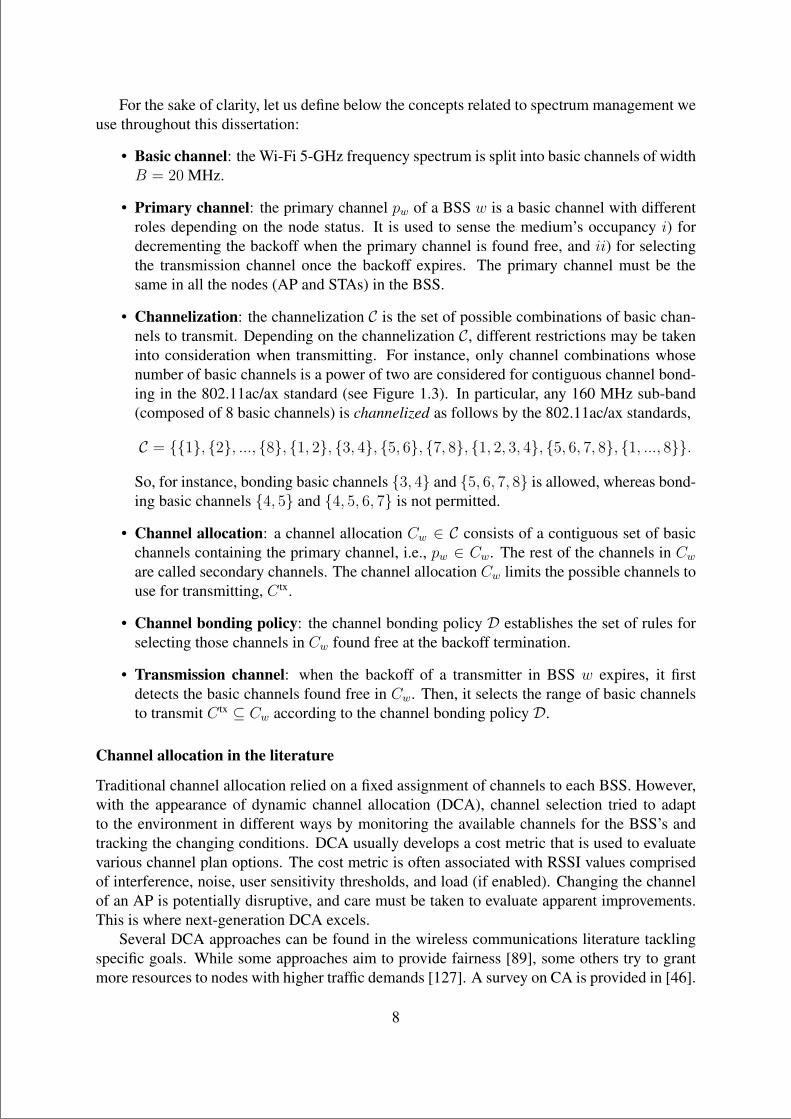
For the sake of clarity, let us define below the concepts related to spectrum management weuse throughout this dissertation:

• Basic channel: the Wi-Fi 5-GHz frequency spectrum is split into basic channels of widthB = 20 MHz.

• Primary channel: the primary channel pw of a BSS w is a basic channel with differentroles depending on the node status. It is used to sense the medium’s occupancy i) fordecrementing the backoff when the primary channel is found free, and ii) for selectingthe transmission channel once the backoff expires. The primary channel must be thesame in all the nodes (AP and STAs) in the BSS.

• Channelization: the channelization C is the set of possible combinations of basic chan-nels to transmit. Depending on the channelization C, different restrictions may be takeninto consideration when transmitting. For instance, only channel combinations whosenumber of basic channels is a power of two are considered for contiguous channel bond-ing in the 802.11ac/ax standard (see Figure 1.3). In particular, any 160 MHz sub-band(composed of 8 basic channels) is channelized as follows by the 802.11ac/ax standards,

C = 1, 2, ..., 8, 1, 2, 3, 4, 5, 6, 7, 8, 1, 2, 3, 4, 5, 6, 7, 8, 1, ..., 8.

So, for instance, bonding basic channels 3, 4 and 5, 6, 7, 8 is allowed, whereas bond-ing basic channels 4, 5 and 4, 5, 6, 7 is not permitted.

• Channel allocation: a channel allocation Cw ∈ C consists of a contiguous set of basicchannels containing the primary channel, i.e., pw ∈ Cw. The rest of the channels in Cware called secondary channels. The channel allocation Cw limits the possible channels touse for transmitting, C tx.

• Channel bonding policy: the channel bonding policy D establishes the set of rules forselecting those channels in Cw found free at the backoff termination.

• Transmission channel: when the backoff of a transmitter in BSS w expires, it firstdetects the basic channels found free in Cw. Then, it selects the range of basic channelsto transmit C tx ⊆ Cw according to the channel bonding policy D.

Channel allocation in the literature

Traditional channel allocation relied on a fixed assignment of channels to each BSS. However,with the appearance of dynamic channel allocation (DCA), channel selection tried to adaptto the environment in different ways by monitoring the available channels for the BSS’s andtracking the changing conditions. DCA usually develops a cost metric that is used to evaluatevarious channel plan options. The cost metric is often associated with RSSI values comprisedof interference, noise, user sensitivity thresholds, and load (if enabled). Changing the channelof an AP is potentially disruptive, and care must be taken to evaluate apparent improvements.This is where next-generation DCA excels.

Several DCA approaches can be found in the wireless communications literature tacklingspecific goals. While some approaches aim to provide fairness [89], some others try to grantmore resources to nodes with higher traffic demands [127]. A survey on CA is provided in [46].

8

“main” — 2020/11/19 — 10:04 — page 9 — #31

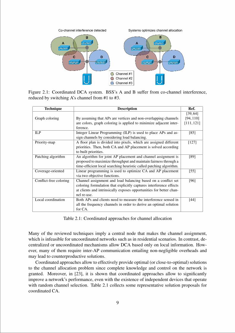
Figure 2.1: Coordinated DCA system. BSS’s A and B suffer from co-channel interference,reduced by switching A’s channel from #1 to #3.

Technique Description Ref.

Graph coloring By assuming that APs are vertices and non-overlapping channelsare colors, graph coloring is applied to minimize adjacent inter-ference.

[39, 64][94, 110]

[111, 121]

ILP Integer Linear Programming (ILP) is used to place APs and as-sign channels by considering load balancing.

[85]

Priority-map A floor plan is divided into pixels, which are assigned differentpriorities. Then, both CA and AP placement is solved accordingto built priorities.

[127]

Patching algorithm An algorithm for joint AP placement and channel assignment isproposed to maximize throughput and maintain fairness through atime-efficient local searching heuristic called patching algorithm.

[89]

Coverage-oriented Linear programming is used to optimize CA and AP placementvia two objective functions.

[55]

Conflict-free coloring Channel assignment and load balancing based on a conflict setcoloring formulation that explicitly captures interference effectsat clients and intrinsically exposes opportunities for better chan-nel re-use.

[96]

Local coordination Both APs and clients need to measure the interference sensed inall the frequency channels in order to derive an optimal solutionfor CA.

[44]

Table 2.1: Coordinated approaches for channel allocation

Many of the reviewed techniques imply a central node that makes the channel assignment,which is infeasible for uncoordinated networks such as in residential scenarios. In contrast, de-centralized or uncoordinated mechanisms allow DCA based only on local information. How-ever, many of them require inter-AP communication entailing non-negligible overheads andmay lead to counterproductive solutions.

Coordinated approaches allow to effectively provide optimal (or close-to-optimal) solutionsto the channel allocation problem since complete knowledge and control on the network isgranted. Moreover, in [23], it is shown that coordinated approaches allow to significantlyimprove a network’s performance, even with the existence of independent devices that operatewith random channel selection. Table 2.1 collects some representative solution proposals forcoordinated CA.

9

“main” — 2020/11/19 — 10:04 — page 10 — #32

Technique Description Ref.Least congested chan-nel search

APs listen to all the channels and select the one with the lowestsensed interference. Other parameters, such as traffic information,are also considered.

[9]

MinMax Based on the assumption that heavily loaded APs degrade the net-work performance, MinMax aims to minimize the maximum effec-tive channel utilization of those devices.

[86, 138][137]

Weighted coloring Uses the sensed interference and the number of overlapping devicesto minimize an objective function.

[95]

Pick-rand & pick-first Based on the sensed interference, a new channel is chosen randomlyor according to a ranking list (also based on the power sensed).

[12, 60][13]

Channel hopping With MAXchop, APs first obtain the hopping sequences of otherinterfering APs, and then compute the hopping sequence that max-imizes their throughput.

[97]

Table 2.2: Uncoordinated approaches for channel allocation

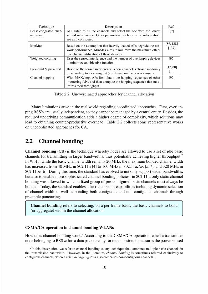
Many limitations arise in the real world regarding coordinated approaches. First, overlap-ping BSS’s are usually independent, so they cannot be managed by a central entity. Besides, therequired underlying communication adds a higher degree of complexity, which solutions maylead to obtaining counter-productive overhead. Table 2.2 collects some representative workson uncoordinated approaches for CA.

2.2 Channel bondingChannel bonding (CB) is the technique whereby nodes are allowed to use a set of idle basicchannels for transmitting in larger bandwidths, thus potentially achieving higher throughput.2

In Wi-Fi, while the basic channel width remains 20 MHz, the maximum bonded channel widthhas increased from 40 MHz in 802.11n [4] to 160 MHz in 802.11ac/ax [5, 7], and 320 MHz in802.11be [6]. During this time, the standard has evolved to not only support wider bandwidths,but also to enable more sophisticated channel bonding policies: in 802.11n, only static channelbonding was allowed in which a fixed group of pre-configured basic channels must always bebonded. Today, the standard enables a far richer set of capabilities including dynamic selectionof channel width as well as bonding both contiguous and non-contiguous channels throughpreamble puncturing.

Channel bonding refers to selecting, on a per-frame basis, the basic channels to bond(or aggregate) within the channel allocation.

CSMA/CA operation in channel bonding WLANs

How does channel bonding work? According to the CSMA/CA operation, when a transmitternode belonging to BSSw has a data packet ready for transmission, it measures the power sensed

2In this dissertation, we refer to channel bonding as any technique that combines multiple basic channels inthe transmission bandwidth. However, in the literature, channel bonding is sometimes referred exclusively tocontiguous channels, whereas channel aggregation also comprises non-contiguous channels.

10

“main” — 2020/11/19 — 10:04 — page 11 — #33

in primary channel pw. Once the primary channel has been detected free, i.e., the power sensedat pw is smaller than the clear channel assessment (CCA) threshold, the node starts the backoffprocedure by selecting a random initial value of BO ∈ [0,CW− 1] time slots of duration Tslot.The contention window is defined as CW = 2qCWmin, where q ∈ 0, 1, 2, ...,m is the backoffstage with maximum value m, and CWmin is the minimum contention window. When a frametransmission fails, q is increased by one unit, and reset to 0 when the frame is acknowledged.

After computing BO, the node starts decreasing the backoff counter while sensing the pri-mary channel. Whenever the power sensed at pw is higher than its CCA, the backoff is pausedand set to the nearest higher time slot until pw is detected free again, at which point the count-down is resumed. When the backoff counter reaches zero, the node selects the transmissionchannel C tx based on the set of basic channels found free and on the channel bonding policyD.

The selected transmission channel C tx is normally kept throughout the whole frame ex-changes between the transmitter and receiver involved in the transmission of a data frame,which may aggregate multiple data packets. Namely, a request to send (RTS) – used for notify-ing the selected transmission channel – a clear to send (CTS), and an acknowledgment (ACK)or block ACK frame are also transmitted in C tx. Any other node that receives an RTS in its pri-mary channel with enough power to be decoded will enter in network allocation vector (NAV)state, used for deferring channel access and avoiding packet collisions. Notice that with theintroduction of the adaptive RTS/CTS mechanism for dynamic bandwidth in the 802.11ac [5],the receiver can modify the original transmission channel of the RTS if it detects any secondarychannel in C tx busy. If so, the transmission bandwidth is reduced, and the receiver respondswith a CTS packet in a subset of C tx.

36(1)

40(2)

44(3)

48(4)

chan

nel

Backoff 1DIFS

PIFSt

SIFS Data SIFS

Noise & interference

Packet transmission

20 MHz

RTS CTSSIFS

ACK

(a) Single-channel.

backoff1DIFS

PIFSt

DIFS backoff2

PIFS

DIFS DIFS backoff336(1)

40(2)

44(3)

48(4)

chan

nel

Noise & interference

20 MHz

(b) Static channel bonding.

backoff1DIFS

PIFSt

Data SIFS

Data SIFS

DIFS backoff2RTS

SIFS

RTSSIFS

PIFS

RTS

RTS

SIFS

SIFS

CTS

CTS

CTS

40 MHz 8 0 MHz

SIFSRTS CTS

SIFSACK

ACKSIFS

RTS CTSSIFS

36(1)40(2)

44(3)

48(4)

chan

nel

(c) Dynamic channel bonding.

backoff1DIFS

PIFSt

Data SIFS

Data SIFS

DIFS backoff2RTS

SIFS

PIFS

CTS

40 MHz

SIFSRTS CTS

SIFSACK

ACKSIFS

RTS CTSSIFS

36(1)

40(2)

44(3)

48(4)

chan

nel

(d) Stochastic channel bonding.

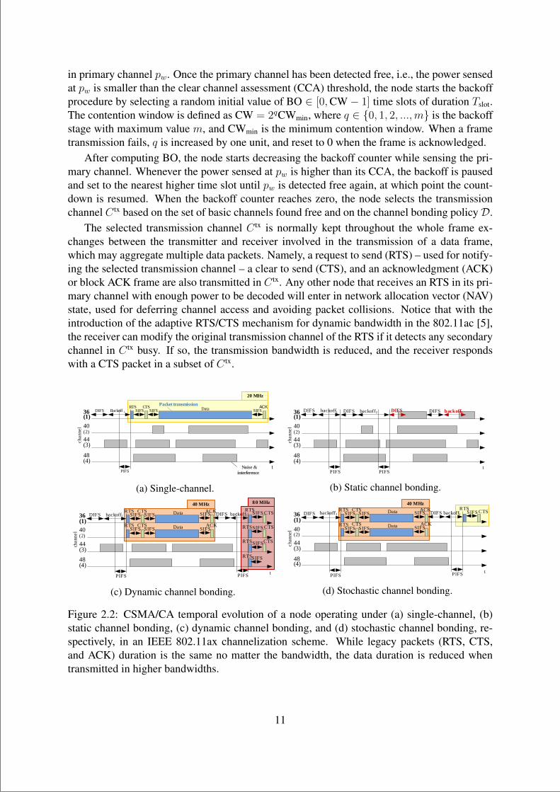
Figure 2.2: CSMA/CA temporal evolution of a node operating under (a) single-channel, (b)static channel bonding, (c) dynamic channel bonding, and (d) stochastic channel bonding, re-spectively, in an IEEE 802.11ax channelization scheme. While legacy packets (RTS, CTS,and ACK) duration is the same no matter the bandwidth, the data duration is reduced whentransmitted in higher bandwidths.

11

“main” — 2020/11/19 — 10:04 — page 12 — #34

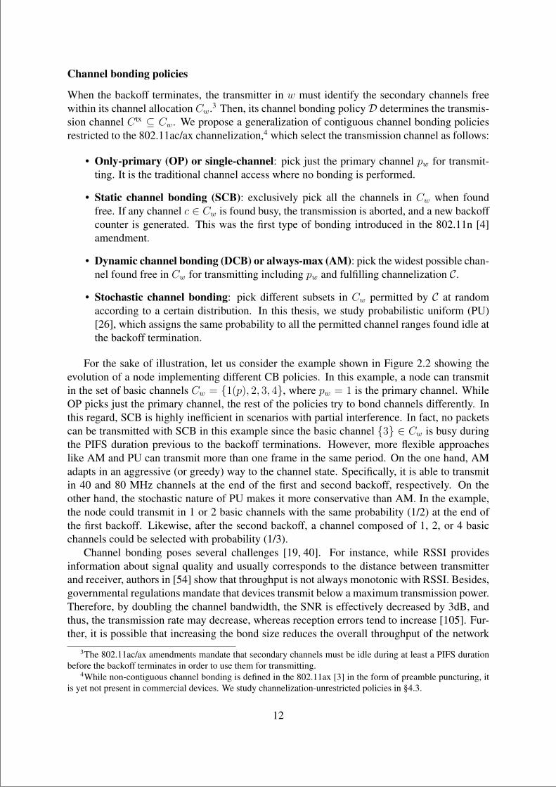
Channel bonding policies

When the backoff terminates, the transmitter in w must identify the secondary channels freewithin its channel allocation Cw.3 Then, its channel bonding policyD determines the transmis-sion channel C tx ⊆ Cw. We propose a generalization of contiguous channel bonding policiesrestricted to the 802.11ac/ax channelization,4 which select the transmission channel as follows:

• Only-primary (OP) or single-channel: pick just the primary channel pw for transmit-ting. It is the traditional channel access where no bonding is performed.

• Static channel bonding (SCB): exclusively pick all the channels in Cw when foundfree. If any channel c ∈ Cw is found busy, the transmission is aborted, and a new backoffcounter is generated. This was the first type of bonding introduced in the 802.11n [4]amendment.

• Dynamic channel bonding (DCB) or always-max (AM): pick the widest possible chan-nel found free in Cw for transmitting including pw and fulfilling channelization C.

• Stochastic channel bonding: pick different subsets in Cw permitted by C at randomaccording to a certain distribution. In this thesis, we study probabilistic uniform (PU)[26], which assigns the same probability to all the permitted channel ranges found idle atthe backoff termination.

For the sake of illustration, let us consider the example shown in Figure 2.2 showing theevolution of a node implementing different CB policies. In this example, a node can transmitin the set of basic channels Cw = 1(p), 2, 3, 4, where pw = 1 is the primary channel. WhileOP picks just the primary channel, the rest of the policies try to bond channels differently. Inthis regard, SCB is highly inefficient in scenarios with partial interference. In fact, no packetscan be transmitted with SCB in this example since the basic channel 3 ∈ Cw is busy duringthe PIFS duration previous to the backoff terminations. However, more flexible approacheslike AM and PU can transmit more than one frame in the same period. On the one hand, AMadapts in an aggressive (or greedy) way to the channel state. Specifically, it is able to transmitin 40 and 80 MHz channels at the end of the first and second backoff, respectively. On theother hand, the stochastic nature of PU makes it more conservative than AM. In the example,the node could transmit in 1 or 2 basic channels with the same probability (1/2) at the end ofthe first backoff. Likewise, after the second backoff, a channel composed of 1, 2, or 4 basicchannels could be selected with probability (1/3).

Channel bonding poses several challenges [19, 40]. For instance, while RSSI providesinformation about signal quality and usually corresponds to the distance between transmitterand receiver, authors in [54] show that throughput is not always monotonic with RSSI. Besides,governmental regulations mandate that devices transmit below a maximum transmission power.Therefore, by doubling the channel bandwidth, the SNR is effectively decreased by 3dB, andthus, the transmission rate may decrease, whereas reception errors tend to increase [105]. Fur-ther, it is possible that increasing the bond size reduces the overall throughput of the network

3The 802.11ac/ax amendments mandate that secondary channels must be idle during at least a PIFS durationbefore the backoff terminates in order to use them for transmitting.

4While non-contiguous channel bonding is defined in the 802.11ax [3] in the form of preamble puncturing, itis yet not present in commercial devices. We study channelization-unrestricted policies in §4.3.

12

“main” — 2020/11/19 — 10:04 — page 13 — #35

due to the fact that the bond may cause harmful co-channel and adjacent channel interference.As for energy efficiency, any increase in channel bandwidth implies that more power will berequired to transmit if the coverage range is kept. Besides, extra power is wasted when nodesexchange control messages for multichannel sensing and operation.

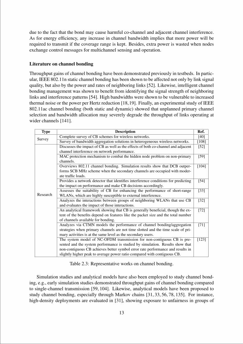
Literature on channel bonding

Throughput gains of channel bonding have been demonstrated previously in testbeds. In partic-ular, IEEE 802.11n static channel bonding has been shown to be affected not only by link signalquality, but also by the power and rates of neighboring links [52]. Likewise, intelligent channelbonding management was shown to benefit from identifying the signal strength of neighboringlinks and interference patterns [54]. High bandwidths were shown to be vulnerable to increasedthermal noise or the power per Hertz reduction [18,19]. Finally, an experimental study of IEEE802.11ac channel bonding (both static and dynamic) showed that unplanned primary channelselection and bandwidth allocation may severely degrade the throughput of links operating atwider channels [141].

Type Description Ref.

Survey Complete survey of CB schemes for wireless networks. [40]Survey of bandwidth aggregation solutions in heterogeneous wireless networks. [108]

Research

Discusses the impact of CB as well as the effects of both co-channel and adjacentchannel interference on network performance.

[52]

MAC protection mechanism to combat the hidden node problem on non-primarychannels.

[59]

Overviews 802.11 channel bonding. Simulation results show that DCB outper-forms SCB MHz scheme when the secondary channels are occupied with moder-ate traffic loads.

[104]

Provides a network detector that identifies interference conditions for predictingthe impact on performance and make CB decisions accordingly.

[54]

Assesses the suitability of CB for enhancing the performance of short-rangeWLANs, which are highly susceptible to external interference.

[33]

Analyzes the interactions between groups of neighboring WLANs that use CBand evaluates the impact of those interactions.

[32]

An analytical framework showing that CB is generally beneficial, though the ex-tent of the benefits depend on features like the packet size and the total numberof channels available for bonding.

[72]

Analyzes via CTMN models the performance of channel bonding/aggregationstrategies when primary channels are not time slotted and the time scale of pri-mary activities is at the same level as the secondary users.

[71]

The system model of NC-OFDM transmission for non-contiguous CB is pre-sented and the system performance is studied by simulation. Results show thatnon-contiguous CB achieves better symbol error rate performance and results inslightly higher peak to average power ratio compared with contiguous CB.

[123]

Table 2.3: Representative works on channel bonding.

Simulation studies and analytical models have also been employed to study channel bond-ing, e.g., early simulation studies demonstrated throughput gains of channel bonding comparedto single-channel transmission [59, 104]. Likewise, analytical models have been proposed tostudy channel bonding, especially through Markov chains [31, 33, 56, 78, 135]. For instance,high-density deployments are evaluated in [31], showing exposure to unfairness in groups of

13

“main” — 2020/11/19 — 10:04 — page 14 — #36

overlapping BSS’s. Analytical models for unsaturated traffic have been also proposed [78].Table 2.3 collects some relevant works on channel bonding.

The joint problem of spectrum management

The joint problem of spectrum management refers to dealing with channel allocation and chan-nel bonding at the same time. That is, selecting the primary and secondary channels to boostthe performance of channel bonding policies.

The joint problem of spectrum management refers to performing channel allocationin channel bonding WLANs to raise performance.

As discussed before, there are many valuable works in the literature dealing with channel al-location and channel bonding in wireless networks. However, only a few of them treat the jointproblem altogether in the context of WLANs. We cover heuristic-based and ML approachesfor the joint spectrum management problem in chapter §5 in chapter §6, respectively.

Chapter summaryThis chapter described channel allocation and channel bonding and reviewed relevant workson the matter. We have seen that channel allocation is for assigning the primary and secondarychannels, and channel bonding for selecting the transmission bandwidth on a per-frame basis.We also discussed the challenges posed by these techniques and proposed a generalization ofchannel bonding policies to be later studied. Next, we depict the enablers and tools we haveused for getting the main results of this dissertation.

14

“main” — 2020/11/19 — 10:04 — page 15 — #37

Chapter 3

METHODOLOGY AND ENABLERS

This chapter presents the methodology and the different enablers we used throughout the thesis,including the modeling of channel bonding WLANs through CTMNs, the Komondor wirelessnetwork simulator, and the WACA spectrum analyzer.

3.1 Modeling spectrum management through continuous timeMarkov networks

We introduce below our model for channel bonding WLANs based on CTMNs. The thesispapers of reference are #1 [26] and #2 [28].

3.1.1 CTMNs for channel bonding in spatially-distributed WLANs

A Markov chain or Markov network is a stochastic process that satisfies the Markov property,meaning a process that depends only on the present state to make predictions of future states,not on the sequence of events that preceded it. This Markov assumption allows for a significantreduction in the number of parameters when studying stochastic processes. Markov chains areused to compute the probabilities of events occurring by viewing them as states transitioninginto other states or transitioning into the same state as before. A continuous-time Markov chain(CTMC) or network (CTMN) is a Markov chain in which, for each state, the process willchange the state according to an exponential random variable and then move to a different stateas specified by the transition probabilities.

The analysis of CSMA/CA networks through CTMN models for saturated WLANs wasfirstly introduced in [38]. Such modelling approach was later applied to IEEE 802.11 networksin [30, 32, 33, 35, 56, 73, 78], among others. Experimental results in [88, 103] demonstrate thatCTMN models, while idealized, provide remarkably accurate throughput estimates for currentIEEE 802.11 systems. A comprehensible example-based tutorial of CTMN models applied todifferent wireless networking scenarios can be found in [34]. Nevertheless, to the best of ourknowledge, the works that model channel bonding through CTMNs study standard channelbonding policies or assume fully overlapping scenarios. Therefore, there is an essential lackof insights on more general Wi-Fi scenarios, where such conditions usually do not hold, andinterdependencies among nodes have a critical impact on their performance.

15

“main” — 2020/11/19 — 10:04 — page 16 — #38

In this section, we depict our extended version of the algorithm introduced in [56] for gen-erating the CTMNs corresponding to spatially distributed WLAN scenarios implementing anychannel bonding policy. The corresponding thesis paper is #1 [26]. Notice that the CTMNmodel considers additive interference, which results from the combination of different simul-taneous interfering transmissions. With this extension, as fully overlapping networks are nolonger required for constructing the corresponding CTMNs, we can make more factual obser-vations from spatially distributed deployments.

Implications of the use of CTMNs to model WLAN dynamics

It is worth pointing out some assumptions made by the CTMN model. First, only downlink traf-fic is assumed, and the interference produced in the uplink (i.e., CTS and ACK control packets)is not considered. Second, modeling WLAN scenarios with CTMNs requires the backoff andtransmission times to be exponentially distributed. It follows that, because of the negligiblepropagation delay, the probability of packet collisions between two or more nodes within thecarrier sense range of the others is zero. The reason is that two BSS’s will never end theirbackoff at the same time, and therefore they will never start a transmission at the same timeeither. Also, it is shown that the state probabilities are insensitive to the backoff and trans-mission time distributions [88, 114]. However, even though the authors in [56] prove that theinsensitivity property does not hold for channel bonding networks, the sensitivity to the backoffand transmission time distributions is minimal. Therefore, the analytical results obtained usingthe exponential assumption offer a good approximation for deterministic distributions of thebackoff, data rate, and packet length. Despite all those are unrealistic assumptions, the modelis particularly useful to depict inter-BSS interactions.

A crucial disadvantage of the CTMN model is its computational cost when characterizingcrowded deployments. Indeed, modeling dense scenarios becomes intractable since the numberof feasible states increases in a combinatorial manner with the number of BSS’s and basicchannels. However, the CTMN model is very useful to understand the new kind of inter-BSSinteractions resulting from channel bonding in spatially-distributed deployments. Besides, itallows us to validate the implementation of the spectrum management techniques developed inthe Komondor wireless simulator we present later in §3.2.

3.1.2 Constructing the CTMNA state in the CTMN is defined by the set of active BSS’s and the basic channels on which theyare transmitting. Essentially, we say that a BSS is active if it is transmitting in some channeland inactive otherwise. For simplicity, we consider that each BSS is composed by one APand one STA. Hence, we simply refer to the BSS activity as a single entity.1 We define twotypes of state spaces: the global state space (Ψ) and the feasible state space (S). A global stateψ ∈ Ψ is a state that accomplishes two conditions: i) the channels in which the active BSS’s aretransmitting comply with the channelization scheme C, and ii) all active BSS’s transmit insidetheir allocated channels. That is, Ψ only depends on the particular channelization scheme Cin use and on the channel allocation of the BSS’s in the system. In contrast, a feasible states ∈ S ⊆ Ψ exists only if each of the active BSS’s in such state started their transmissions by

1Notice that the model could also estimate the long-run mean performance of multiple STAs by generatingnew states indicating the receiver STA corresponding parameters like the SINR or data rate.

16

“main” — 2020/11/19 — 10:04 — page 17 — #39

accomplishing the CCA requirement (or contention) derived from the assigned channel bondingpolicy. Namely, given a global state space, S depends only on the spatial distribution and onthe channel bonding policies assigned to each BSS.

The first step for constructing the CTMN is to identify the global state space Ψ, which issimply composed of all the possible combinations given by the channelization under consider-ation and the channel allocations of the BSS’s. The feasible states in S are later identified byexploring the states in Ψ. The transitions among feasible states are represented by the transi-tion rate matrix M . Essentially, as long as there are discovered states in S that have not beenexplored yet, for any feasible state sk ∈ S not explored, and for each BSS w in the system,we determine if w is active or not. If w is active, we then set possible backward transitions toalready known and unknown states. To do so, it is required to fully explore Ψ by looking forstates where: i) other active BSS’s in the state remain transmitting in the same transmissionchannel, and ii) BSS w is not active.

On the other hand, if BSS w is inactive in state sk, we try to find forward transitions toother states by fully exploring Ψ looking for states where i) other active BSS’s in the stateremain transmitting in the same transmission channel, and ii) w is active in the new state asa result of applying its channel bonding policy Dw. It is important to remark that in order toapply such a policy, the set of idle basic channels in state sk must be identified according tothe power sensed in each of the basic channels allocated to w and on its CCA threshold. Eachtransition between two states s and s′ has a corresponding transition rate Ms,s′ . For forwardtransitions, the packet transmission attempt rate (or simply backoff rate) has an average durationλ = 1/(E[BO]Tslot), where E[BO] is the expected backoff duration in time slots, determinedby the minimum contention window, i.e., E[B] = (CWmin − 1)/2. Furthermore, for backwardtransitions, the departure rate (µ) depends on the duration of a successful transmission, i.e.,µ = 1/Tsuc,2 which in turn depends on both the data rate given by the selected MCS andtransmission channel width, and on the expected frame length. In this regard, the data rateand packet error rate of a BSS w depends on the state of the system, which collects suchinformation, i.e., µw(s).

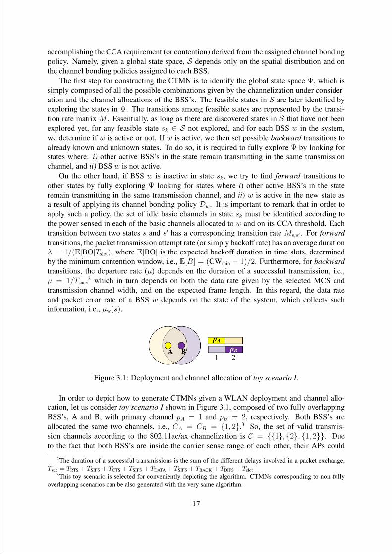
Figure 3.1: Deployment and channel allocation of toy scenario I.

In order to depict how to generate CTMNs given a WLAN deployment and channel allo-cation, let us consider toy scenario I shown in Figure 3.1, composed of two fully overlappingBSS’s, A and B, with primary channel pA = 1 and pB = 2, respectively. Both BSS’s areallocated the same two channels, i.e., CA = CB = 1, 2.3 So, the set of valid transmis-sion channels according to the 802.11ac/ax channelization is C = 1, 2, 1, 2. Dueto the fact that both BSS’s are inside the carrier sense range of each other, their APs could

2The duration of a successful transmissions is the sum of the different delays involved in a packet exchange,Tsuc = TRTS + TSIFS + TCTS + TSIFS + TDATA + TSIFS + TBACK + TDIFS + Tslot

3This toy scenario is selected for conveniently depicting the algorithm. CTMNs corresponding to non-fullyoverlapping scenarios can be also generated with the very same algorithm.

17

“main” — 2020/11/19 — 10:04 — page 18 — #40

∅s1

A21

s3

A11

s2

B22

s4

B21

s5

A11B

22

s6

A22B

22

ψ7

~αA,∅(s2)

λA,µA(

s2)

1, 5

~αA,∅(s3)λA, µA(s3)

2, 7~αB,∅(s4)λB, µB(s4)3, 9

~αB,∅ (s

5 )λB , µ

B (s5 )

4, 10

λB , µB(s5)6, 12

λA, µA

(s5)

8,11

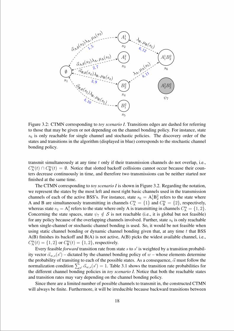
Figure 3.2: CTMN corresponding to toy scenario I. Transitions edges are dashed for referringto those that may be given or not depending on the channel bonding policy. For instance, states6 is only reachable for single channel and stochastic policies. The discovery order of thestates and transitions in the algorithm (displayed in blue) corresponds to the stochastic channelbonding policy.

transmit simultaneously at any time t only if their transmission channels do not overlap, i.e.,C tx

A (t) ∩ C txB (t) = ∅. Notice that slotted backoff collisions cannot occur because their coun-

ters decrease continuously in time, and therefore two transmissions can be neither started norfinished at the same time.

The CTMN corresponding to toy scenario I is shown in Figure 3.2. Regarding the notation,we represent the states by the most left and most right basic channels used in the transmissionchannels of each of the active BSS’s. For instance, state s6 = A1

1B22 refers to the state where

A and B are simultaneously transmitting in channels C txA = 1 and C tx

B = 2, respectively,whereas state s3 = A2

1 refers to the state where only A is transmitting in channels C txA = 1, 2.

Concerning the state spaces, state ψ7 /∈ S is not reachable (i.e., it is global but not feasible)for any policy because of the overlapping channels involved. Further, state s6 is only reachablewhen single-channel or stochastic channel bonding is used. So, it would be not feasible whenusing static channel bonding or dynamic channel bonding given that, at any time t that BSSA(B) finishes its backoff and B(A) is not active, A(B) picks the widest available channel, i.e.,C tx

A (t) = 1, 2 or C txB (t) = 1, 2, respectively.

Every feasible forward transition rate from state s to s′ is weighted by a transition probabil-ity vector ~αw,s(s′) – dictated by the channel bonding policy of w – whose elements determinethe probability of transiting to each of the possible states. As a consequence, ~α must follow thenormalization condition

∑s′ ~αw,s(s

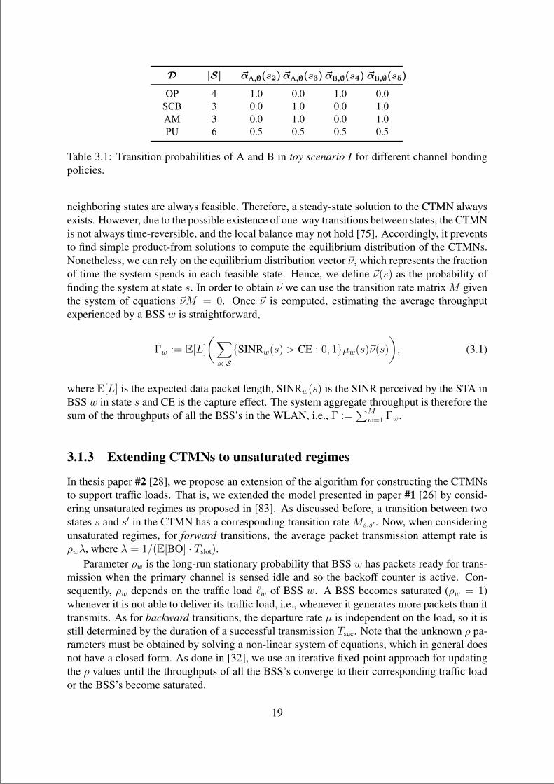
′) = 1. Table 3.1 shows the transition rate probabilities forthe different channel bonding policies in toy scenario I. Notice that both the reachable statesand transition rates may vary depending on the channel bonding policy.

Since there are a limited number of possible channels to transmit in, the constructed CTMNwill always be finite. Furthermore, it will be irreducible because backward transitions between

18

“main” — 2020/11/19 — 10:04 — page 19 — #41

D |S| ~αA,∅(s2) ~αA,∅(s3) ~αB,∅(s4) ~αB,∅(s5)

OP 4 1.0 0.0 1.0 0.0SCB 3 0.0 1.0 0.0 1.0AM 3 0.0 1.0 0.0 1.0PU 6 0.5 0.5 0.5 0.5

Table 3.1: Transition probabilities of A and B in toy scenario I for different channel bondingpolicies.

neighboring states are always feasible. Therefore, a steady-state solution to the CTMN alwaysexists. However, due to the possible existence of one-way transitions between states, the CTMNis not always time-reversible, and the local balance may not hold [75]. Accordingly, it preventsto find simple product-from solutions to compute the equilibrium distribution of the CTMNs.Nonetheless, we can rely on the equilibrium distribution vector ~ν, which represents the fractionof time the system spends in each feasible state. Hence, we define ~ν(s) as the probability offinding the system at state s. In order to obtain ~ν we can use the transition rate matrix M giventhe system of equations ~νM = 0. Once ~ν is computed, estimating the average throughputexperienced by a BSS w is straightforward,

Γw := E[L]

(∑

s∈SSINRw(s) > CE : 0, 1µw(s)~ν(s)

), (3.1)

where E[L] is the expected data packet length, SINRw(s) is the SINR perceived by the STA inBSS w in state s and CE is the capture effect. The system aggregate throughput is therefore thesum of the throughputs of all the BSS’s in the WLAN, i.e., Γ :=

∑Mw=1 Γw.

3.1.3 Extending CTMNs to unsaturated regimes

In thesis paper #2 [28], we propose an extension of the algorithm for constructing the CTMNsto support traffic loads. That is, we extended the model presented in paper #1 [26] by consid-ering unsaturated regimes as proposed in [83]. As discussed before, a transition between twostates s and s′ in the CTMN has a corresponding transition rate Ms,s′ . Now, when consideringunsaturated regimes, for forward transitions, the average packet transmission attempt rate isρwλ, where λ = 1/(E[BO] · Tslot).

Parameter ρw is the long-run stationary probability that BSS w has packets ready for trans-mission when the primary channel is sensed idle and so the backoff counter is active. Con-sequently, ρw depends on the traffic load `w of BSS w. A BSS becomes saturated (ρw = 1)whenever it is not able to deliver its traffic load, i.e., whenever it generates more packets than ittransmits. As for backward transitions, the departure rate µ is independent on the load, so it isstill determined by the duration of a successful transmission Tsuc. Note that the unknown ρ pa-rameters must be obtained by solving a non-linear system of equations, which in general doesnot have a closed-form. As done in [32], we use an iterative fixed-point approach for updatingthe ρ values until the throughputs of all the BSS’s converge to their corresponding traffic loador the BSS’s become saturated.

19

“main” — 2020/11/19 — 10:04 — page 20 — #42

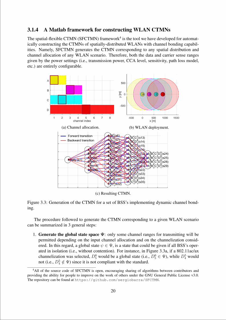
3.1.4 A Matlab framework for constructing WLAN CTMNsThe spatial-flexible CTMN (SFCTMN) framework4 is the tool we have developed for automat-ically constructing the CTMNs of spatially-distributed WLANs with channel bonding capabil-ities. Namely, SFCTMN generates the CTMN corresponding to any spatial distribution andchannel allocation of any WLAN scenario. Therefore, both the data and carrier sense rangesgiven by the power settings (i.e., transmission power, CCA level, sensitivity, path loss model,etc.) are entirely configurable.

(a) Channel allocation. (b) WLAN deployment.

(c) Resulting CTMN.

Figure 3.3: Generation of the CTMN for a set of BSS’s implementing dynamic channel bond-ing.

The procedure followed to generate the CTMN corresponding to a given WLAN scenariocan be summarized in 3 general steps:

1. Generate the global state space Ψ: only some channel ranges for transmitting will bepermitted depending on the input channel allocation and on the channelization consid-ered. In this regard, a global state ψ ∈ Ψ, is a state that could be given if all BSS’s oper-ated in isolation (i.e., without contention). For instance, in Figure 3.3a, if a 802.11ac/axchannelization was selected, D6

5 would be a global state (i.e., D65 ∈ Ψ), while D5

4 wouldnot (i.e., D5

4 /∈ Ψ) since it is not compliant with the standard.

4All of the source code of SFCTMN is open, encouraging sharing of algorithms between contributors andproviding the ability for people to improve on the work of others under the GNU General Public License v3.0.The repository can be found at https://github.com/sergiobarra/SFCTMN.

20

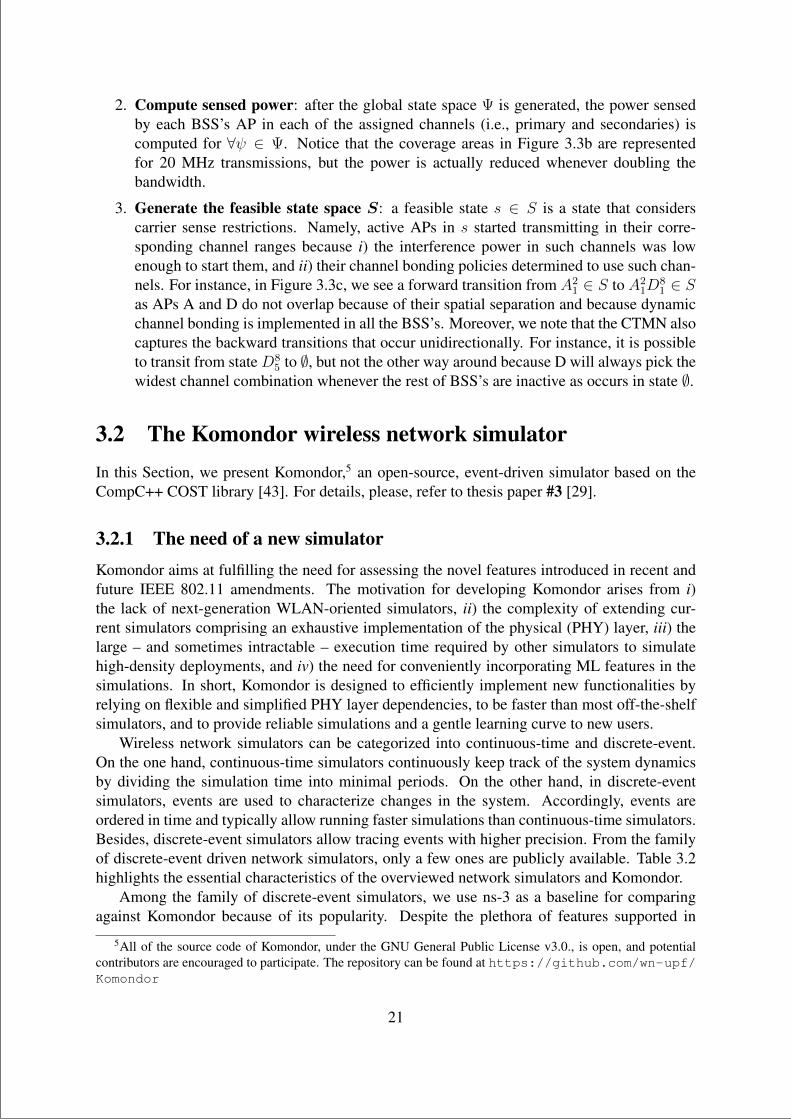
“main” — 2020/11/19 — 10:04 — page 21 — #43

2. Compute sensed power: after the global state space Ψ is generated, the power sensedby each BSS’s AP in each of the assigned channels (i.e., primary and secondaries) iscomputed for ∀ψ ∈ Ψ. Notice that the coverage areas in Figure 3.3b are representedfor 20 MHz transmissions, but the power is actually reduced whenever doubling thebandwidth.

3. Generate the feasible state space S: a feasible state s ∈ S is a state that considerscarrier sense restrictions. Namely, active APs in s started transmitting in their corre-sponding channel ranges because i) the interference power in such channels was lowenough to start them, and ii) their channel bonding policies determined to use such chan-nels. For instance, in Figure 3.3c, we see a forward transition from A2

1 ∈ S to A21D

81 ∈ S

as APs A and D do not overlap because of their spatial separation and because dynamicchannel bonding is implemented in all the BSS’s. Moreover, we note that the CTMN alsocaptures the backward transitions that occur unidirectionally. For instance, it is possibleto transit from state D8

5 to ∅, but not the other way around because D will always pick thewidest channel combination whenever the rest of BSS’s are inactive as occurs in state ∅.

3.2 The Komondor wireless network simulatorIn this Section, we present Komondor,5 an open-source, event-driven simulator based on theCompC++ COST library [43]. For details, please, refer to thesis paper #3 [29].

3.2.1 The need of a new simulatorKomondor aims at fulfilling the need for assessing the novel features introduced in recent andfuture IEEE 802.11 amendments. The motivation for developing Komondor arises from i)the lack of next-generation WLAN-oriented simulators, ii) the complexity of extending cur-rent simulators comprising an exhaustive implementation of the physical (PHY) layer, iii) thelarge – and sometimes intractable – execution time required by other simulators to simulatehigh-density deployments, and iv) the need for conveniently incorporating ML features in thesimulations. In short, Komondor is designed to efficiently implement new functionalities byrelying on flexible and simplified PHY layer dependencies, to be faster than most off-the-shelfsimulators, and to provide reliable simulations and a gentle learning curve to new users.

Wireless network simulators can be categorized into continuous-time and discrete-event.On the one hand, continuous-time simulators continuously keep track of the system dynamicsby dividing the simulation time into minimal periods. On the other hand, in discrete-eventsimulators, events are used to characterize changes in the system. Accordingly, events areordered in time and typically allow running faster simulations than continuous-time simulators.Besides, discrete-event simulators allow tracing events with higher precision. From the familyof discrete-event driven network simulators, only a few ones are publicly available. Table 3.2highlights the essential characteristics of the overviewed network simulators and Komondor.

Among the family of discrete-event simulators, we use ns-3 as a baseline for comparingagainst Komondor because of its popularity. Despite the plethora of features supported in

5All of the source code of Komondor, under the GNU General Public License v3.0., is open, and potentialcontributors are encouraged to participate. The repository can be found at https://github.com/wn-upf/Komondor

21

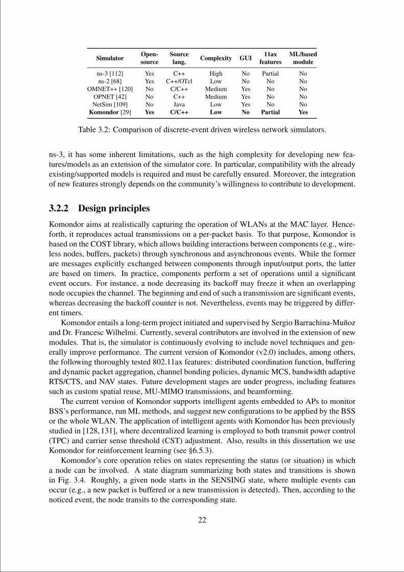
“main” — 2020/11/19 — 10:04 — page 22 — #44

Simulator Open-source

Sourcelang. Complexity GUI 11ax

featuresML/based

module

ns-3 [112] Yes C++ High No Partial Nons-2 [68] Yes C++/OTcl Low No No No

OMNET++ [120] No C/C++ Medium Yes No NoOPNET [42] No C++ Medium Yes No NoNetSim [109] No Java Low Yes No No

Komondor [29] Yes C/C++ Low No Partial Yes

Table 3.2: Comparison of discrete-event driven wireless network simulators.

ns-3, it has some inherent limitations, such as the high complexity for developing new fea-tures/models as an extension of the simulator core. In particular, compatibility with the alreadyexisting/supported models is required and must be carefully ensured. Moreover, the integrationof new features strongly depends on the community’s willingness to contribute to development.

3.2.2 Design principlesKomondor aims at realistically capturing the operation of WLANs at the MAC layer. Hence-forth, it reproduces actual transmissions on a per-packet basis. To that purpose, Komondor isbased on the COST library, which allows building interactions between components (e.g., wire-less nodes, buffers, packets) through synchronous and asynchronous events. While the formerare messages explicitly exchanged between components through input/output ports, the latterare based on timers. In practice, components perform a set of operations until a significantevent occurs. For instance, a node decreasing its backoff may freeze it when an overlappingnode occupies the channel. The beginning and end of such a transmission are significant events,whereas decreasing the backoff counter is not. Nevertheless, events may be triggered by differ-ent timers.

Komondor entails a long-term project initiated and supervised by Sergio Barrachina-Munozand Dr. Francesc Wilhelmi. Currently, several contributors are involved in the extension of newmodules. That is, the simulator is continuously evolving to include novel techniques and gen-erally improve performance. The current version of Komondor (v2.0) includes, among others,the following thoroughly tested 802.11ax features: distributed coordination function, bufferingand dynamic packet aggregation, channel bonding policies, dynamic MCS, bandwidth adaptiveRTS/CTS, and NAV states. Future development stages are under progress, including featuressuch as custom spatial reuse, MU-MIMO transmissions, and beamforming.

The current version of Komondor supports intelligent agents embedded to APs to monitorBSS’s performance, run ML methods, and suggest new configurations to be applied by the BSSor the whole WLAN. The application of intelligent agents with Komondor has been previouslystudied in [128, 131], where decentralized learning is employed to both transmit power control(TPC) and carrier sense threshold (CST) adjustment. Also, results in this dissertation we useKomondor for reinforcement learning (see §6.5.3).

Komondor’s core operation relies on states representing the status (or situation) in whicha node can be involved. A state diagram summarizing both states and transitions is shownin Fig. 3.4. Roughly, a given node starts in the SENSING state, where multiple events canoccur (e.g., a new packet is buffered or a new transmission is detected). Then, according to thenoticed event, the node transits to the corresponding state.

22

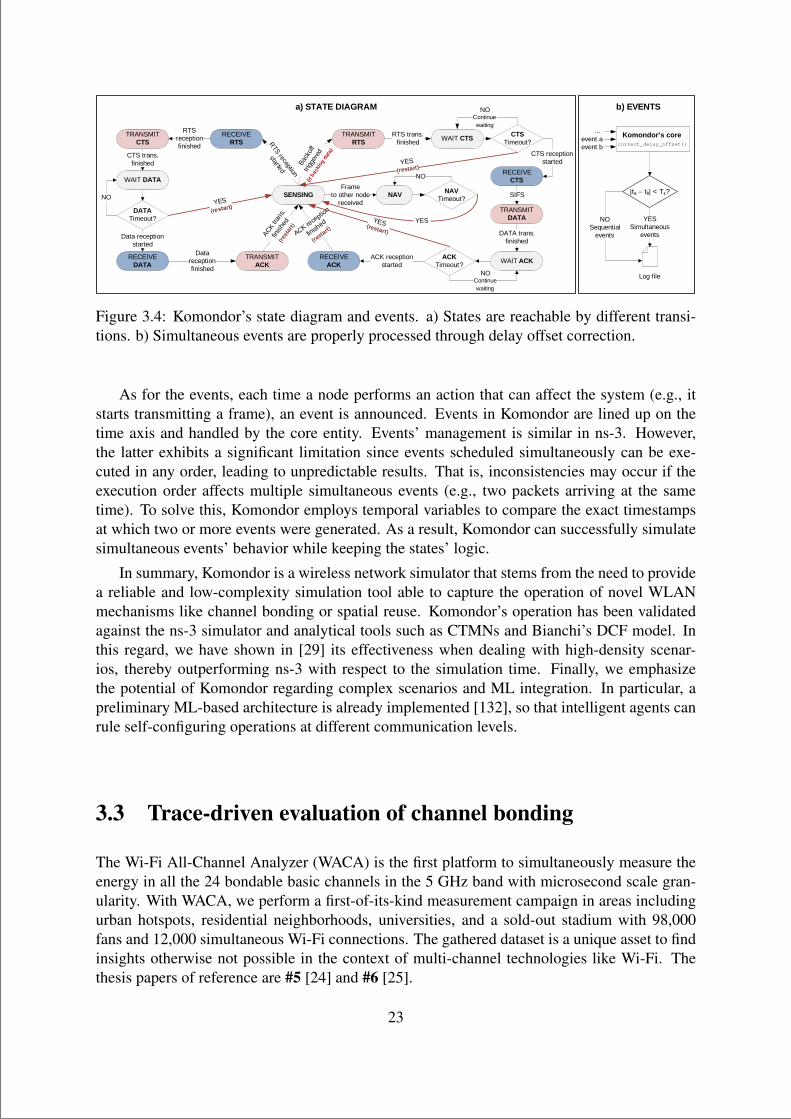
“main” — 2020/11/19 — 10:04 — page 23 — #45

|ta – tb| < Tε?SENSING

RECEIVERTS

TRANSMITRTS

Back

off

trigg

ered

(i f b

ackl

og d

ata)

TRANSMITCTS

ACK rece

ption

finish

ed

(restart)

WAIT CTSRTS trans.finished

CTSTimeout?

YES(restart)

NOContinuewaiting

a) STATE DIAGRAM

RECEIVECTS

CTS receptionstarted

TRANSMITDATA

SIFS

WAIT ACKACKTimeout?

RECEIVEACK

ACK receptionstarted

YES(restart)

NOContinuewaiting

DATA trans.finished

RTS reception

started

RTSreceptionfinished

WAIT DATA

CTS trans.finished

DATATimeout?

NOYES

(restart)

RECEIVEDATA

TRANSMITACK

Data receptionstarted

Data receptionfinished

ACK

trans

.fin

ishe

d(r

esta

r t)

NAVFrame

to other node received

NAVTimeout?

NO

YES

Komondor’s corecorrect_delay_offset()

b) EVENTS

YESSimultaneous

events

event aevent b

...

Log file

NOSequential

events

Figure 3.4: Komondor’s state diagram and events. a) States are reachable by different transi-tions. b) Simultaneous events are properly processed through delay offset correction.

As for the events, each time a node performs an action that can affect the system (e.g., itstarts transmitting a frame), an event is announced. Events in Komondor are lined up on thetime axis and handled by the core entity. Events’ management is similar in ns-3. However,the latter exhibits a significant limitation since events scheduled simultaneously can be exe-cuted in any order, leading to unpredictable results. That is, inconsistencies may occur if theexecution order affects multiple simultaneous events (e.g., two packets arriving at the sametime). To solve this, Komondor employs temporal variables to compare the exact timestampsat which two or more events were generated. As a result, Komondor can successfully simulatesimultaneous events’ behavior while keeping the states’ logic.

In summary, Komondor is a wireless network simulator that stems from the need to providea reliable and low-complexity simulation tool able to capture the operation of novel WLANmechanisms like channel bonding or spatial reuse. Komondor’s operation has been validatedagainst the ns-3 simulator and analytical tools such as CTMNs and Bianchi’s DCF model. Inthis regard, we have shown in [29] its effectiveness when dealing with high-density scenar-ios, thereby outperforming ns-3 with respect to the simulation time. Finally, we emphasizethe potential of Komondor regarding complex scenarios and ML integration. In particular, apreliminary ML-based architecture is already implemented [132], so that intelligent agents canrule self-configuring operations at different communication levels.

3.3 Trace-driven evaluation of channel bonding

The Wi-Fi All-Channel Analyzer (WACA) is the first platform to simultaneously measure theenergy in all the 24 bondable basic channels in the 5 GHz band with microsecond scale gran-ularity. With WACA, we perform a first-of-its-kind measurement campaign in areas includingurban hotspots, residential neighborhoods, universities, and a sold-out stadium with 98,000fans and 12,000 simultaneous Wi-Fi connections. The gathered dataset is a unique asset to findinsights otherwise not possible in the context of multi-channel technologies like Wi-Fi. Thethesis papers of reference are #5 [24] and #6 [25].

23

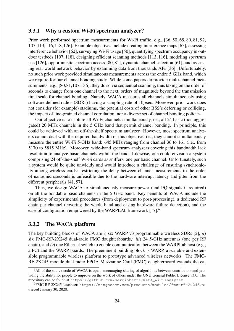
“main” — 2020/11/19 — 10:04 — page 24 — #46

3.3.1 Why a custom Wi-Fi spectrum analyzer?Prior work performed spectrum measurements for Wi-Fi traffic, e.g., [36, 50, 65, 80, 81, 92,107,113,116,118,126]. Example objectives include creating interference maps [65], assessinginterference behavior [62], surveying Wi-Fi usage [50], quantifying spectrum occupancy in out-door testbeds [107, 118], designing efficient scanning methods [113, 116], modeling spectrumuse [126], opportunistic spectrum access [80, 81], dynamic channel selection [61], and assess-ing real-world network behavior by examining data from thousands APs [36]. Unfortunately,no such prior work provided simultaneous measurements across the entire 5 GHz band, whichwe require for our channel bonding study. While some papers do provide multi-channel mea-surements, e.g., [80,81,107,136], they do so via sequential scanning, thus taking on the order ofseconds to change from one channel to the next, orders of magnitude beyond the transmissiontime scale for channel bonding. Namely, WACA measures all channels simultaneously usingsoftware defined radios (SDRs) having a sampling rate of 10µsec. Moreover, prior work doesnot consider (for example) stadiums, the potential costs of other BSS’s deferring or colliding,the impact of fine-grained channel correlation, nor a diverse set of channel bonding policies.

Our objective is to capture all Wi-Fi channels simultaneously, i.e., all 24 basic (non aggre-gated) 20 MHz channels in the 5 GHz band that permit channel bonding. In principle, thiscould be achieved with an off-the-shelf spectrum analyzer. However, most spectrum analyz-ers cannot deal with the required bandwidth of this objective, i.e., they cannot simultaneouslymeasure the entire Wi-Fi 5-GHz band: 645 MHz ranging from channel 36 to 161 (i.e., from5170 to 5815 MHz). Moreover, wide-band spectrum analyzers covering this bandwidth lackresolution to analyze basic channels within the band. Likewise, one could envision a systemcomprising 24 off-the-shelf Wi-Fi cards as sniffers, one per basic channel. Unfortunately, sucha system would be quite unwieldy and would introduce a challenge of ensuring synchronic-ity among wireless cards: restricting the delay between channel measurements to the orderof nano/microseconds is unfeasible due to the hardware interrupt latency and jitter from thedifferent peripherals [41, 57].

Thus, we design WACA to simultaneously measure power (and I/Q signals if required)on all the bondable basic channels in the 5 GHz band. Key benefits of WACA include thesimplicity of experimental procedures (from deployment to post-processing), a dedicated RFchain per channel (covering the whole band and easing hardware failure detection), and theease of configuration empowered by the WARPLAb framework [17].6

3.3.2 The WACA platformThe key building blocks of WACA are i) six WARP v3 programmable wireless SDRs [2], ii)six FMC-RF-2X245 dual-radio FMC daughterboards,7 iii) 24 5-GHz antennas (one per RFchain), and iv) one Ethernet switch to enable communication between the WARPLab host (e.g.,a PC) and the WARP boards. The preeminent building block is WARP, a scalable and exten-sible programmable wireless platform to prototype advanced wireless networks. The FMC-RF-2X245 module dual-radio FPGA Mezzanine Card (FMC) daughterboard extends the ca-

6All of the source code of WACA is open, encouraging sharing of algorithms between contributors and pro-viding the ability for people to improve on the work of others under the GNU General Public License v3.0. Therepository can be found at https://github.com/sergiobarra/WACA_WiFiAnalyzer.

7FMC-RF-2X245 datasheet: https://mangocomm.com/products/modules/fmc-rf-2x245, re-trieved January 30, 2020.

24

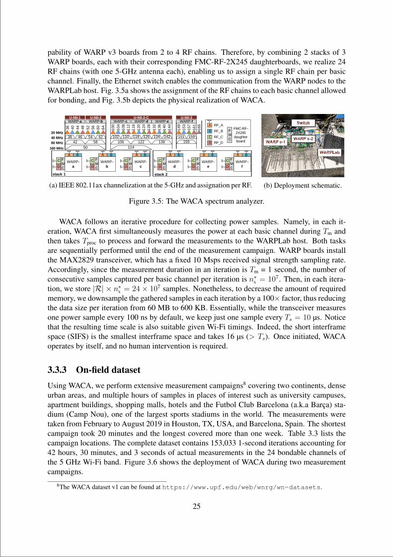
“main” — 2020/11/19 — 10:04 — page 25 — #47

pability of WARP v3 boards from 2 to 4 RF chains. Therefore, by combining 2 stacks of 3WARP boards, each with their corresponding FMC-RF-2X245 daughterboards, we realize 24RF chains (with one 5-GHz antenna each), enabling us to assign a single RF chain per basicchannel. Finally, the Ethernet switch enables the communication from the WARP nodes to theWARPLab host. Fig. 3.5a shows the assignment of the RF chains to each basic channel allowedfor bonding, and Fig. 3.5b depicts the physical realization of WACA.

WARP-a

A BFMCD

C WARP-b

A BFMCD

C WARP-c

A BFMCD

C WARP-d

A BFMCD

C WARP-e

A BFMCD

C WARP-f

A BFMCD

C

36 40 44 48 52 56 60 64 100

104

108

112

116

120

124

128

132

136

140

144 149

153

157

161

165

38 46 6254 102 110 126118 134 142 151 15942 58

50

WARP-a WARP-b WARP-c WARP-d WARP-e WARP-f

106 122114

138 155

A

B

C

D

RF_A

RF_B

RF_C

RF_D

FMC

FMC-RF-2X245

daughter board

40 MHz80 MHz

160 MHz

20 MHz

stack 1 stack 2

U-NII-1 U-NII-2 U-NII-2-C U-NII-3

(a) IEEE 802.11ax channelization at the 5-GHz and assignation per RF. (b) Deployment schematic.

Figure 3.5: The WACA spectrum analyzer.

WACA follows an iterative procedure for collecting power samples. Namely, in each it-eration, WACA first simultaneously measures the power at each basic channel during Tm andthen takes Tproc to process and forward the measurements to the WARPLab host. Both tasksare sequentially performed until the end of the measurement campaign. WARP boards installthe MAX2829 transceiver, which has a fixed 10 Msps received signal strength sampling rate.Accordingly, since the measurement duration in an iteration is Tm = 1 second, the number ofconsecutive samples captured per basic channel per iteration is n∗s = 107. Then, in each itera-tion, we store |R| × n∗s = 24× 107 samples. Nonetheless, to decrease the amount of requiredmemory, we downsample the gathered samples in each iteration by a 100× factor, thus reducingthe data size per iteration from 60 MB to 600 KB. Essentially, while the transceiver measuresone power sample every 100 ns by default, we keep just one sample every Ts = 10 µs. Noticethat the resulting time scale is also suitable given Wi-Fi timings. Indeed, the short interframespace (SIFS) is the smallest interframe space and takes 16 µs (> Ts). Once initiated, WACAoperates by itself, and no human intervention is required.

3.3.3 On-field datasetUsing WACA, we perform extensive measurement campaigns8 covering two continents, denseurban areas, and multiple hours of samples in places of interest such as university campuses,apartment buildings, shopping malls, hotels and the Futbol Club Barcelona (a.k.a Barca) sta-dium (Camp Nou), one of the largest sports stadiums in the world. The measurements weretaken from February to August 2019 in Houston, TX, USA, and Barcelona, Spain. The shortestcampaign took 20 minutes and the longest covered more than one week. Table 3.3 lists thecampaign locations. The complete dataset contains 153,033 1-second iterations accounting for42 hours, 30 minutes, and 3 seconds of actual measurements in the 24 bondable channels ofthe 5 GHz Wi-Fi band. Figure 3.6 shows the deployment of WACA during two measurementcampaigns.

8The WACA dataset v1 can be found at https://www.upf.edu/web/wnrg/wn-datasets.

25

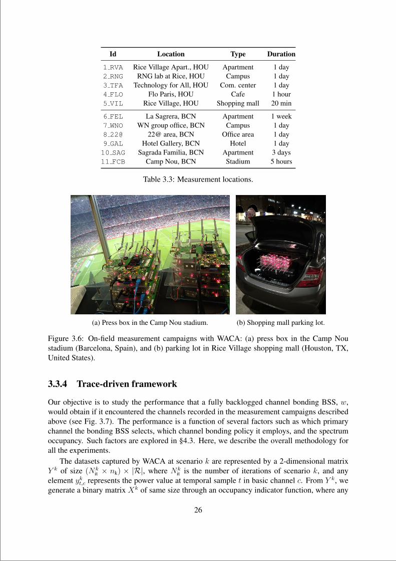
“main” — 2020/11/19 — 10:04 — page 26 — #48

Id Location Type Duration

1 RVA Rice Village Apart., HOU Apartment 1 day2 RNG RNG lab at Rice, HOU Campus 1 day3 TFA Technology for All, HOU Com. center 1 day4 FLO Flo Paris, HOU Cafe 1 hour5 VIL Rice Village, HOU Shopping mall 20 min

6 FEL La Sagrera, BCN Apartment 1 week7 WNO WN group office, BCN Campus 1 day8 22@ 22@ area, BCN Office area 1 day9 GAL Hotel Gallery, BCN Hotel 1 day10 SAG Sagrada Familia, BCN Apartment 3 days11 FCB Camp Nou, BCN Stadium 5 hours

Table 3.3: Measurement locations.

(a) Press box in the Camp Nou stadium. (b) Shopping mall parking lot.

Figure 3.6: On-field measurement campaigns with WACA: (a) press box in the Camp Noustadium (Barcelona, Spain), and (b) parking lot in Rice Village shopping mall (Houston, TX,United States).

3.3.4 Trace-driven framework

Our objective is to study the performance that a fully backlogged channel bonding BSS, w,would obtain if it encountered the channels recorded in the measurement campaigns describedabove (see Fig. 3.7). The performance is a function of several factors such as which primarychannel the bonding BSS selects, which channel bonding policy it employs, and the spectrumoccupancy. Such factors are explored in §4.3. Here, we describe the overall methodology forall the experiments.

The datasets captured by WACA at scenario k are represented by a 2-dimensional matrixY k of size (Nk

it × nk) × |R|, where Nkit is the number of iterations of scenario k, and any

element ykt,c represents the power value at temporal sample t in basic channel c. From Y k, wegenerate a binary matrix Xk of same size through an occupancy indicator function, where any

26

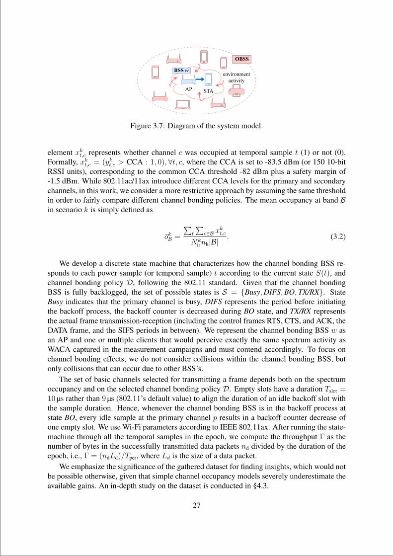
“main” — 2020/11/19 — 10:04 — page 27 — #49

STAAP

environmentactivity

BSSw

OBSS

Figure 3.7: Diagram of the system model.

element xkt,c represents whether channel c was occupied at temporal sample t (1) or not (0).Formally, xkt,c = (ykt,c > CCA : 1, 0),∀t, c, where the CCA is set to -83.5 dBm (or 150 10-bitRSSI units), corresponding to the common CCA threshold -82 dBm plus a safety margin of-1.5 dBm. While 802.11ac/11ax introduce different CCA levels for the primary and secondarychannels, in this work, we consider a more restrictive approach by assuming the same thresholdin order to fairly compare different channel bonding policies. The mean occupancy at band Bin scenario k is simply defined as

okB =

∑t

∑c∈B x

kt,c

Nkitnk|B|

. (3.2)

We develop a discrete state machine that characterizes how the channel bonding BSS re-sponds to each power sample (or temporal sample) t according to the current state S(t), andchannel bonding policy D, following the 802.11 standard. Given that the channel bondingBSS is fully backlogged, the set of possible states is S = Busy,DIFS,BO,TX/RX. StateBusy indicates that the primary channel is busy, DIFS represents the period before initiatingthe backoff process, the backoff counter is decreased during BO state, and TX/RX representsthe actual frame transmission-reception (including the control frames RTS, CTS, and ACK, theDATA frame, and the SIFS periods in between). We represent the channel bonding BSS w asan AP and one or multiple clients that would perceive exactly the same spectrum activity asWACA captured in the measurement campaigns and must contend accordingly. To focus onchannel bonding effects, we do not consider collisions within the channel bonding BSS, butonly collisions that can occur due to other BSS’s.

The set of basic channels selected for transmitting a frame depends both on the spectrumoccupancy and on the selected channel bonding policy D. Empty slots have a duration Tslot =10 µs rather than 9 µs (802.11’s default value) to align the duration of an idle backoff slot withthe sample duration. Hence, whenever the channel bonding BSS is in the backoff process atstate BO, every idle sample at the primary channel p results in a backoff counter decrease ofone empty slot. We use Wi-Fi parameters according to IEEE 802.11ax. After running the state-machine through all the temporal samples in the epoch, we compute the throughput Γ as thenumber of bytes in the successfully transmitted data packets nd divided by the duration of theepoch, i.e., Γ = (ndLd)/Tper, where Ld is the size of a data packet.

We emphasize the significance of the gathered dataset for finding insights, which would notbe possible otherwise, given that simple channel occupancy models severely underestimate theavailable gains. An in-depth study on the dataset is conducted in §4.3.

27

“main” — 2020/11/19 — 10:04 — page 28 — #50

Chapter summaryThis chapter depicted the three key enablers we used throughout this thesis: a CTMN modelfor spatially-distributed WLANs, a wireless network simulator for 802.11ax (and beyond), anda custom spectrum analyzer for simultaneously measuring the whole 5 GHz band. The nextchapter shows the main results and derived findings we got from using such enablers.

28

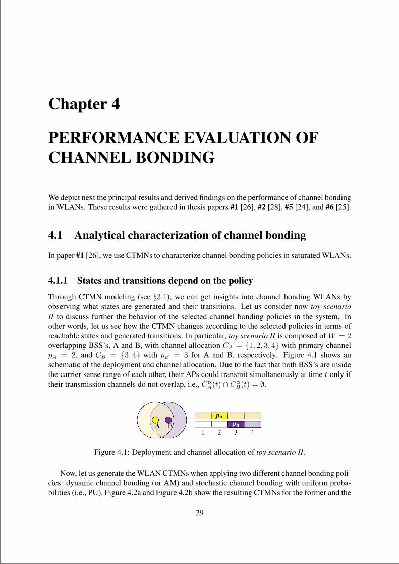
“main” — 2020/11/19 — 10:04 — page 29 — #51

Chapter 4

PERFORMANCE EVALUATION OFCHANNEL BONDING

We depict next the principal results and derived findings on the performance of channel bondingin WLANs. These results were gathered in thesis papers #1 [26], #2 [28], #5 [24], and #6 [25].

4.1 Analytical characterization of channel bondingIn paper #1 [26], we use CTMNs to characterize channel bonding policies in saturated WLANs.

4.1.1 States and transitions depend on the policy

Through CTMN modeling (see §3.1), we can get insights into channel bonding WLANs byobserving what states are generated and their transitions. Let us consider now toy scenarioII to discuss further the behavior of the selected channel bonding policies in the system. Inother words, let us see how the CTMN changes according to the selected policies in terms ofreachable states and generated transitions. In particular, toy scenario II is composed of W = 2overlapping BSS’s, A and B, with channel allocation CA = 1, 2, 3, 4 with primary channelpA = 2, and CB = 3, 4 with pB = 3 for A and B, respectively. Figure 4.1 shows anschematic of the deployment and channel allocation. Due to the fact that both BSS’s are insidethe carrier sense range of each other, their APs could transmit simultaneously at time t only iftheir transmission channels do not overlap, i.e., C tx

A(t) ∩ C txB(t) = ∅.

Figure 4.1: Deployment and channel allocation of toy scenario II.

Now, let us generate the WLAN CTMNs when applying two different channel bonding poli-cies: dynamic channel bonding (or AM) and stochastic channel bonding with uniform proba-bilities (i.e., PU). Figure 4.2a and Figure 4.2b show the resulting CTMNs for the former and the

29

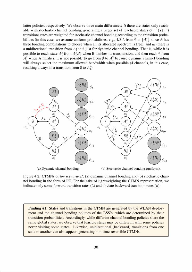
“main” — 2020/11/19 — 10:04 — page 30 — #52

latter policies, respectively. We observe three main differences: i) there are states only reach-able with stochastic channel bonding, generating a larger set of reachable states S = s, ii)transitions rates are weighted for stochastic channel bonding according to the transition proba-bilities (in this case, we assume uniform probabilities, e.g., 1/3 λ from ∅ to A4

1 since A hasthree bonding combinations to choose when all its allocated spectrum is free), and iii) there isa unidirectional transition from A2

1 to ∅ just for dynamic channel bonding. That is, while it ispossible to reach state A2

1 from A21B

43 when B finishes its transmission, and then reach ∅ from

A21 when A finishes, it is not possible to go from ∅ to A2

1 because dynamic channel bondingwill always select the maximum allowed bandwidth when possible (4 channels, in this case,resulting always in a transition from ∅ to A4

1).

∅s1

A41

s2

A21

s5

A22

ψ6

B33

ψ7

B43

s3

A21B

43 s4

A41B

33 ψ11

A41B

43 ψ12

A21B

33 ψ10

A22B

43 ψ9

A22B

33 ψ8

λA

λB

λA=

0

λA

λB

(a) Dynamic channel bonding.

∅s1

A41

s4

A21

s3

A22

s2

B33

s5

B43

s6

A21B

43 s10

A41B

33 ψ11

A41B

43 ψ12

A21B

33 s9

A22B

43 s8

A22B

33 s7

13λ A

13λA

13λA

12 λ

B

12 λ

B

12λB

12λA

(b) Stochastic channel bonding (uniform).

Figure 4.2: CTMNs of toy scenario II: (a) dynamic channel bonding and (b) stochastic chan-nel bonding in the form of PU. For the sake of lightweighting the CTMN representation, weindicate only some forward transition rates (λ) and obviate backward transition rates (µ).

Finding #1: States and transitions in the CTMN are generated by the WLAN deploy-ment and the channel bonding policies of the BSS’s, which are determined by theirtransition probabilities. Accordingly, while different channel bonding policies share thesame global states, we observe that feasible states may be different, with some policiesnever visiting some states. Likewise, unidirectional (backward) transitions from onestate to another can also appear, generating non-time-reversible CTMNs.

30

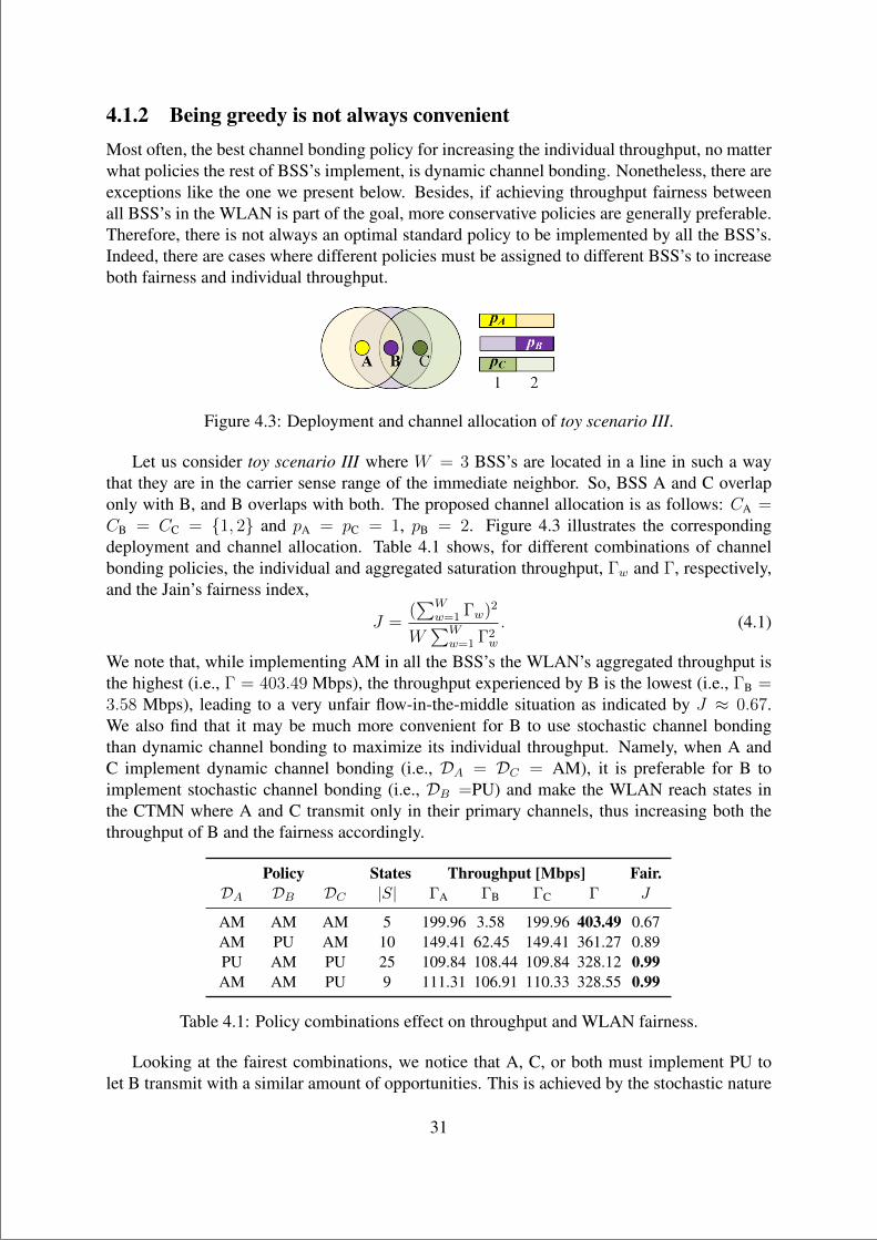
“main” — 2020/11/19 — 10:04 — page 31 — #53

4.1.2 Being greedy is not always convenientMost often, the best channel bonding policy for increasing the individual throughput, no matterwhat policies the rest of BSS’s implement, is dynamic channel bonding. Nonetheless, there areexceptions like the one we present below. Besides, if achieving throughput fairness betweenall BSS’s in the WLAN is part of the goal, more conservative policies are generally preferable.Therefore, there is not always an optimal standard policy to be implemented by all the BSS’s.Indeed, there are cases where different policies must be assigned to different BSS’s to increaseboth fairness and individual throughput.

Figure 4.3: Deployment and channel allocation of toy scenario III.

Let us consider toy scenario III where W = 3 BSS’s are located in a line in such a waythat they are in the carrier sense range of the immediate neighbor. So, BSS A and C overlaponly with B, and B overlaps with both. The proposed channel allocation is as follows: CA =CB = CC = 1, 2 and pA = pC = 1, pB = 2. Figure 4.3 illustrates the correspondingdeployment and channel allocation. Table 4.1 shows, for different combinations of channelbonding policies, the individual and aggregated saturation throughput, Γw and Γ, respectively,and the Jain’s fairness index,

J =(∑W

w=1 Γw)2

W∑W

w=1 Γ2w

. (4.1)

We note that, while implementing AM in all the BSS’s the WLAN’s aggregated throughput isthe highest (i.e., Γ = 403.49 Mbps), the throughput experienced by B is the lowest (i.e., ΓB =3.58 Mbps), leading to a very unfair flow-in-the-middle situation as indicated by J ≈ 0.67.We also find that it may be much more convenient for B to use stochastic channel bondingthan dynamic channel bonding to maximize its individual throughput. Namely, when A andC implement dynamic channel bonding (i.e., DA = DC = AM), it is preferable for B toimplement stochastic channel bonding (i.e., DB =PU) and make the WLAN reach states inthe CTMN where A and C transmit only in their primary channels, thus increasing both thethroughput of B and the fairness accordingly.

Policy States Throughput [Mbps] Fair.DA DB DC |S| ΓA ΓB ΓC Γ J

AM AM AM 5 199.96 3.58 199.96 403.49 0.67AM PU AM 10 149.41 62.45 149.41 361.27 0.89PU AM PU 25 109.84 108.44 109.84 328.12 0.99AM AM PU 9 111.31 106.91 110.33 328.55 0.99

Table 4.1: Policy combinations effect on throughput and WLAN fairness.

Looking at the fairest combinations, we notice that A, C, or both must implement PU tolet B transmit with a similar amount of opportunities. This is achieved by the stochastic nature

31

“main” — 2020/11/19 — 10:04 — page 32 — #54

of PU, which lets the CTMN explore more states. Accordingly, B experiences the highestthroughput, and the system achieves complete fairness (i.e., J ≈ 1). Nonetheless, the priceto pay is to decrease the throughput of A and C significantly. In essence, this toy scenariois a paradigmatic example showing that with less aggressive policies like PU (of probabilisticnature), not only more states in the CTMN can be potentially explored with respect to AM, butalso the probability of staying in states providing higher throughput (or fairness) may increase.Therefore, since it generally does not exist a global policy that satisfies all the BSS’s in thesystem, different policies should be adopted depending on the target performance metric.

Finding #2: Being greedy with dynamic channel bonding does not always maximizethe individual throughput. There are scenarios where more conservative policies likestochastic channel bonding are preferable since they tend to force the WLAN to reachmore favorable states in the CTMNs. Besides, we find that there is not a unique policyfor maximizing the performance metrics (e.g., aggregate throughput or fairness). Instead,the assignation of different policies to different BSS is sometimes required.

4.2 Assessment of high-density deploymentsApart from modeling WLANs through CTMNs, in the thesis papers #1 [26] and #2 [28], wesimulate high-density WLANs deployments under a variety of channel bonding policies, nodedensities, and traffic loads. We rely on the Komondor wireless network simulator [29] to sim-ulate thousands of scenarios in different deployments and configurations.

4.2.1 Type of scenariosThe type of high-density Wi-Fi deployments under evaluation consists of randomly spreadnodes in square maps of different areas. Random primary channel, spectrum allocation, and,sometimes, channel bonding policy, is assigned to the BSS’s in the WLAN. We deploy WBSS’s each with one AP and one or multiples STAs. We use typical IEEE 802.11ax parame-ters.1 In this section, we first assess full-buffer traffic loads and then a Poisson process whereBSS w generates a data packet every tw ∼ Exponential(1/`w), being `w the mean traffic load inpackets per second. We focus on studying a particular BSS in the WLAN, normally named A,as well as the whole WLAN. An example of the scenarios considered is shown in Figure 4.4.

4.2.2 On the individual throughput and fairnessIn thesis paper #1 [26], we study the throughput of saturated BSS’s under full-buffer traffic.

On the individual throughput

We aim to identify the optimal policy that a particular BSS should implement to increase its ownthroughput in a high-density, uncoordinated Wi-Fi deployment. We consider three rectangular

1We refer the reader to [26–28] for more details

32

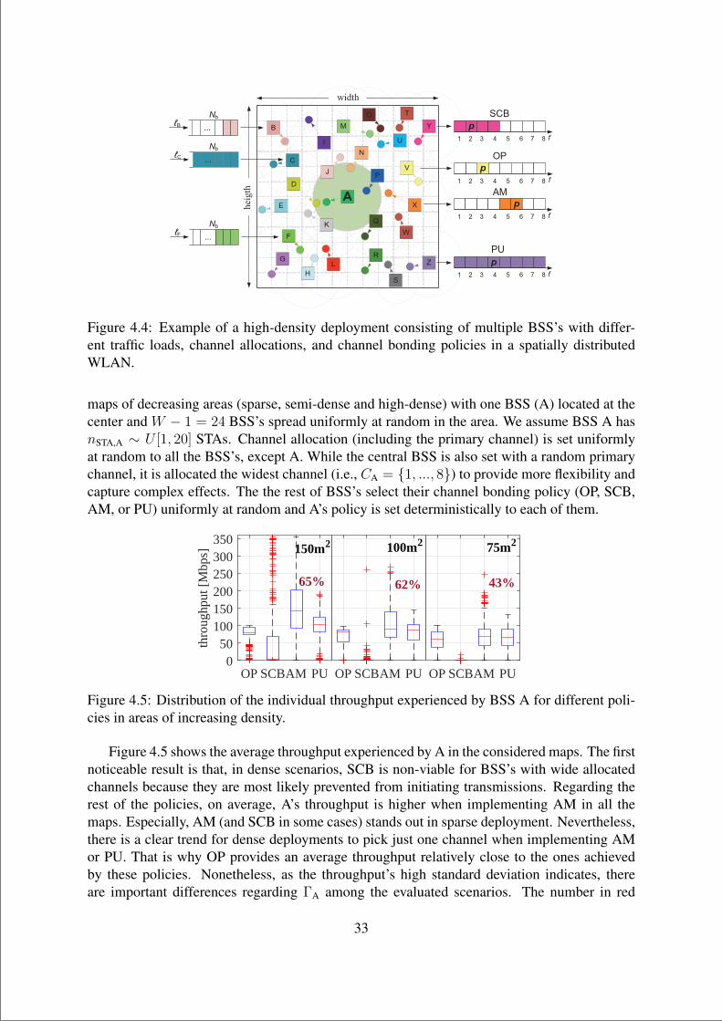
“main” — 2020/11/19 — 10:04 — page 33 — #55

Figure 4.4: Example of a high-density deployment consisting of multiple BSS’s with differ-ent traffic loads, channel allocations, and channel bonding policies in a spatially distributedWLAN.

maps of decreasing areas (sparse, semi-dense and high-dense) with one BSS (A) located at thecenter and W − 1 = 24 BSS’s spread uniformly at random in the area. We assume BSS A hasnSTA,A ∼ U [1, 20] STAs. Channel allocation (including the primary channel) is set uniformlyat random to all the BSS’s, except A. While the central BSS is also set with a random primarychannel, it is allocated the widest channel (i.e., CA = 1, ..., 8) to provide more flexibility andcapture complex effects. The the rest of BSS’s select their channel bonding policy (OP, SCB,AM, or PU) uniformly at random and A’s policy is set deterministically to each of them.

OP SCBAM PU OP SCBAM PU OP SCBAM PU0

50100150200250300350

thro

ughp

ut [

Mbp

s]

65% 62% 43%

100m2 75m2150m2

Figure 4.5: Distribution of the individual throughput experienced by BSS A for different poli-cies in areas of increasing density.

Figure 4.5 shows the average throughput experienced by A in the considered maps. The firstnoticeable result is that, in dense scenarios, SCB is non-viable for BSS’s with wide allocatedchannels because they are most likely prevented from initiating transmissions. Regarding therest of the policies, on average, A’s throughput is higher when implementing AM in all themaps. Especially, AM (and SCB in some cases) stands out in sparse deployment. Nevertheless,there is a clear trend for dense deployments to pick just one channel when implementing AMor PU. That is why OP provides an average throughput relatively close to the ones achievedby these policies. Nonetheless, as the throughput’s high standard deviation indicates, thereare important differences regarding ΓA among the evaluated scenarios. The number in red

33

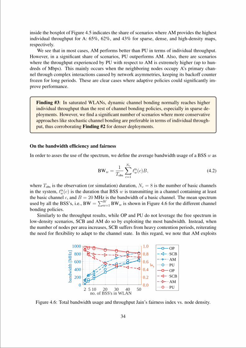
“main” — 2020/11/19 — 10:04 — page 34 — #56

inside the boxplot of Figure 4.5 indicates the share of scenarios where AM provides the highestindividual throughput for A: 65%, 62%, and 43% for sparse, dense, and high-density maps,respectively.

We see that in most cases, AM performs better than PU in terms of individual throughput.However, in a significant share of scenarios, PU outperforms AM. Also, there are scenarioswhere the throughput experienced by PU with respect to AM is extremely higher (up to hun-dreds of Mbps). This mainly occurs when the neighboring nodes occupy A’s primary chan-nel through complex interactions caused by network asymmetries, keeping its backoff counterfrozen for long periods. These are clear cases where adaptive policies could significantly im-prove performance.

Finding #3: In saturated WLANs, dynamic channel bonding normally reaches higherindividual throughput than the rest of channel bonding policies, especially in sparse de-ployments. However, we find a significant number of scenarios where more conservativeapproaches like stochastic channel bonding are preferable in terms of individual through-put, thus corroborating Finding #2 for denser deployments.

On the bandwidth efficiency and fairness

In order to asses the use of the spectrum, we define the average bandwidth usage of a BSS w as

BWw =1

Tobs

Nc∑

c=1

ttxw(c)B, (4.2)

where Tobs is the observation (or simulation) duration, Nc = 8 is the number of basic channelsin the system, ttxw(c) is the duration that BSS w is transmitting in a channel containing at leastthe basic channel c, and B = 20 MHz is the bandwidth of a basic channel. The mean spectrumused by all the BSS’s, i.e., BW =

∑Ww=1 BWw is shown in Figure 4.6 for the different channel

bonding policies.Similarly to the throughput results, while OP and PU do not leverage the free spectrum in

low-density scenarios, SCB and AM do so by exploiting the most bandwidth. Instead, whenthe number of nodes per area increases, SCB suffers from heavy contention periods, reiteratingthe need for flexibility to adapt to the channel state. In this regard, we note that AM exploits

2 5 10 20 30 40 50no. of BSS's in WLAN

0

200

400

600

800

1000

band

wid

th [M

Hz]

0.0

0.2

0.4

0.6

0.8

1.0 OPSCBAMPUOPSCBAMPU

Figure 4.6: Total bandwidth usage and throughput Jain’s fairness index vs. node density.

34

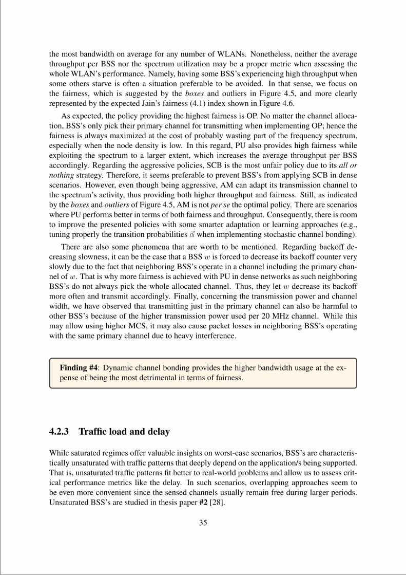
“main” — 2020/11/19 — 10:04 — page 35 — #57

the most bandwidth on average for any number of WLANs. Nonetheless, neither the averagethroughput per BSS nor the spectrum utilization may be a proper metric when assessing thewhole WLAN’s performance. Namely, having some BSS’s experiencing high throughput whensome others starve is often a situation preferable to be avoided. In that sense, we focus onthe fairness, which is suggested by the boxes and outliers in Figure 4.5, and more clearlyrepresented by the expected Jain’s fairness (4.1) index shown in Figure 4.6.

As expected, the policy providing the highest fairness is OP. No matter the channel alloca-tion, BSS’s only pick their primary channel for transmitting when implementing OP; hence thefairness is always maximized at the cost of probably wasting part of the frequency spectrum,especially when the node density is low. In this regard, PU also provides high fairness whileexploiting the spectrum to a larger extent, which increases the average throughput per BSSaccordingly. Regarding the aggressive policies, SCB is the most unfair policy due to its all ornothing strategy. Therefore, it seems preferable to prevent BSS’s from applying SCB in densescenarios. However, even though being aggressive, AM can adapt its transmission channel tothe spectrum’s activity, thus providing both higher throughput and fairness. Still, as indicatedby the boxes and outliers of Figure 4.5, AM is not per se the optimal policy. There are scenarioswhere PU performs better in terms of both fairness and throughput. Consequently, there is roomto improve the presented policies with some smarter adaptation or learning approaches (e.g.,tuning properly the transition probabilities ~α when implementing stochastic channel bonding).

There are also some phenomena that are worth to be mentioned. Regarding backoff de-creasing slowness, it can be the case that a BSS w is forced to decrease its backoff counter veryslowly due to the fact that neighboring BSS’s operate in a channel including the primary chan-nel of w. That is why more fairness is achieved with PU in dense networks as such neighboringBSS’s do not always pick the whole allocated channel. Thus, they let w decrease its backoffmore often and transmit accordingly. Finally, concerning the transmission power and channelwidth, we have observed that transmitting just in the primary channel can also be harmful toother BSS’s because of the higher transmission power used per 20 MHz channel. While thismay allow using higher MCS, it may also cause packet losses in neighboring BSS’s operatingwith the same primary channel due to heavy interference.

Finding #4: Dynamic channel bonding provides the higher bandwidth usage at the ex-pense of being the most detrimental in terms of fairness.

4.2.3 Traffic load and delay

While saturated regimes offer valuable insights on worst-case scenarios, BSS’s are characteris-tically unsaturated with traffic patterns that deeply depend on the application/s being supported.That is, unsaturated traffic patterns fit better to real-world problems and allow us to assess crit-ical performance metrics like the delay. In such scenarios, overlapping approaches seem tobe even more convenient since the sensed channels usually remain free during larger periods.Unsaturated BSS’s are studied in thesis paper #2 [28].

35

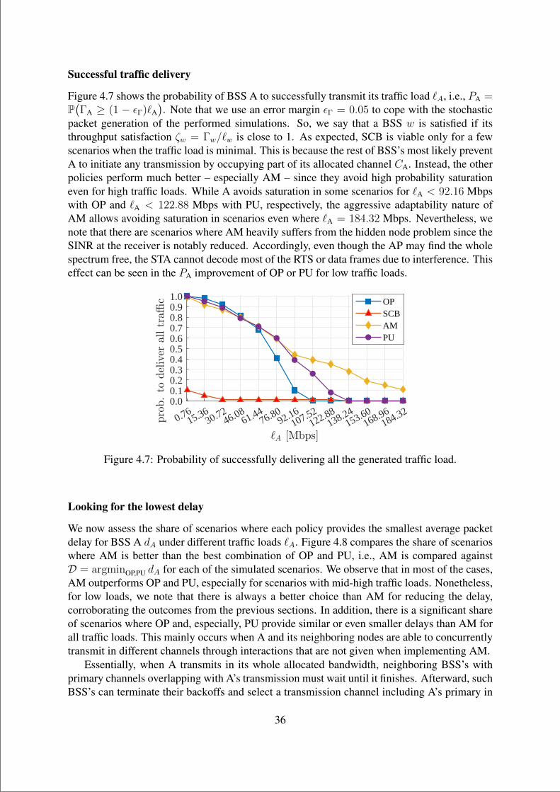
“main” — 2020/11/19 — 10:04 — page 36 — #58

Successful traffic delivery

Figure 4.7 shows the probability of BSS A to successfully transmit its traffic load `A, i.e., PA =P(ΓA ≥ (1 − εΓ)`A

). Note that we use an error margin εΓ = 0.05 to cope with the stochastic

packet generation of the performed simulations. So, we say that a BSS w is satisfied if itsthroughput satisfaction ζw = Γw/`w is close to 1. As expected, SCB is viable only for a fewscenarios when the traffic load is minimal. This is because the rest of BSS’s most likely preventA to initiate any transmission by occupying part of its allocated channel CA. Instead, the otherpolicies perform much better – especially AM – since they avoid high probability saturationeven for high traffic loads. While A avoids saturation in some scenarios for `A < 92.16 Mbpswith OP and `A < 122.88 Mbps with PU, respectively, the aggressive adaptability nature ofAM allows avoiding saturation in scenarios even where `A = 184.32 Mbps. Nevertheless, wenote that there are scenarios where AM heavily suffers from the hidden node problem since theSINR at the receiver is notably reduced. Accordingly, even though the AP may find the wholespectrum free, the STA cannot decode most of the RTS or data frames due to interference. Thiseffect can be seen in the PA improvement of OP or PU for low traffic loads.

0.7615.36

30.7246.08

61.4476.80

92.16107.52

122.88138.24

153.60168.96

184.320.00.10.20.30.40.50.60.70.80.91.0 OP

SCBAMPU

Figure 4.7: Probability of successfully delivering all the generated traffic load.

Looking for the lowest delay

We now assess the share of scenarios where each policy provides the smallest average packetdelay for BSS A dA under different traffic loads `A. Figure 4.8 compares the share of scenarioswhere AM is better than the best combination of OP and PU, i.e., AM is compared againstD = argminOP,PU dA for each of the simulated scenarios. We observe that in most of the cases,AM outperforms OP and PU, especially for scenarios with mid-high traffic loads. Nonetheless,for low loads, we note that there is always a better choice than AM for reducing the delay,corroborating the outcomes from the previous sections. In addition, there is a significant shareof scenarios where OP and, especially, PU provide similar or even smaller delays than AM forall traffic loads. This mainly occurs when A and its neighboring nodes are able to concurrentlytransmit in different channels through interactions that are not given when implementing AM.

Essentially, when A transmits in its whole allocated bandwidth, neighboring BSS’s withprimary channels overlapping with A’s transmission must wait until it finishes. Afterward, suchBSS’s can terminate their backoffs and select a transmission channel including A’s primary in

36

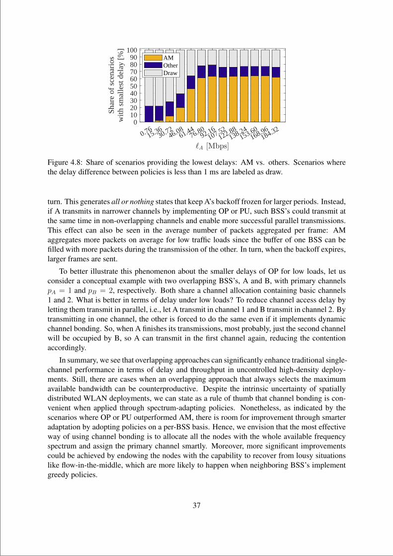
“main” — 2020/11/19 — 10:04 — page 37 — #59

0.7615.36

30.7246.08

61.4476.80

92.16107.52

122.88138.24

153.60168.96

184.320

102030405060708090

100

Shar

e of

sce

nari

osw

ith s

mal

lest

del

ay [

%]

AMOtherDraw

Figure 4.8: Share of scenarios providing the lowest delays: AM vs. others. Scenarios wherethe delay difference between policies is less than 1 ms are labeled as draw.

turn. This generates all or nothing states that keep A’s backoff frozen for larger periods. Instead,if A transmits in narrower channels by implementing OP or PU, such BSS’s could transmit atthe same time in non-overlapping channels and enable more successful parallel transmissions.This effect can also be seen in the average number of packets aggregated per frame: AMaggregates more packets on average for low traffic loads since the buffer of one BSS can befilled with more packets during the transmission of the other. In turn, when the backoff expires,larger frames are sent.

To better illustrate this phenomenon about the smaller delays of OP for low loads, let usconsider a conceptual example with two overlapping BSS’s, A and B, with primary channelspA = 1 and pB = 2, respectively. Both share a channel allocation containing basic channels1 and 2. What is better in terms of delay under low loads? To reduce channel access delay byletting them transmit in parallel, i.e., let A transmit in channel 1 and B transmit in channel 2. Bytransmitting in one channel, the other is forced to do the same even if it implements dynamicchannel bonding. So, when A finishes its transmissions, most probably, just the second channelwill be occupied by B, so A can transmit in the first channel again, reducing the contentionaccordingly.

In summary, we see that overlapping approaches can significantly enhance traditional single-channel performance in terms of delay and throughput in uncontrolled high-density deploy-ments. Still, there are cases when an overlapping approach that always selects the maximumavailable bandwidth can be counterproductive. Despite the intrinsic uncertainty of spatiallydistributed WLAN deployments, we can state as a rule of thumb that channel bonding is con-venient when applied through spectrum-adapting policies. Nonetheless, as indicated by thescenarios where OP or PU outperformed AM, there is room for improvement through smarteradaptation by adopting policies on a per-BSS basis. Hence, we envision that the most effectiveway of using channel bonding is to allocate all the nodes with the whole available frequencyspectrum and assign the primary channel smartly. Moreover, more significant improvementscould be achieved by endowing the nodes with the capability to recover from lousy situationslike flow-in-the-middle, which are more likely to happen when neighboring BSS’s implementgreedy policies.

37

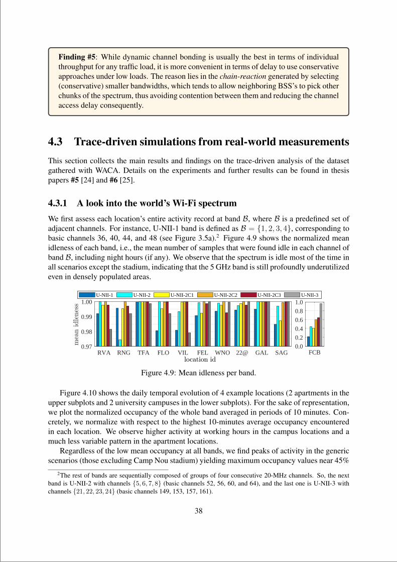
“main” — 2020/11/19 — 10:04 — page 38 — #60

Finding #5: While dynamic channel bonding is usually the best in terms of individualthroughput for any traffic load, it is more convenient in terms of delay to use conservativeapproaches under low loads. The reason lies in the chain-reaction generated by selecting(conservative) smaller bandwidths, which tends to allow neighboring BSS’s to pick otherchunks of the spectrum, thus avoiding contention between them and reducing the channelaccess delay consequently.

4.3 Trace-driven simulations from real-world measurementsThis section collects the main results and findings on the trace-driven analysis of the datasetgathered with WACA. Details on the experiments and further results can be found in thesispapers #5 [24] and #6 [25].

4.3.1 A look into the world’s Wi-Fi spectrumWe first assess each location’s entire activity record at band B, where B is a predefined set ofadjacent channels. For instance, U-NII-1 band is defined as B = 1, 2, 3, 4, corresponding tobasic channels 36, 40, 44, and 48 (see Figure 3.5a).2 Figure 4.9 shows the normalized meanidleness of each band, i.e., the mean number of samples that were found idle in each channel ofband B, including night hours (if any). We observe that the spectrum is idle most of the time inall scenarios except the stadium, indicating that the 5 GHz band is still profoundly underutilizedeven in densely populated areas.

RVA RNG TFA FLO VIL FEL WNO 22@ GAL SAG0.97

0.98

0.99

1.00

FCB0.0

0.2

0.4

0.6

0.8

1.0U-NII-1 U-NII-2 U-NII-2C1 U-NII-2C2 U-NII-2C3 U-NII-3

Figure 4.9: Mean idleness per band.

Figure 4.10 shows the daily temporal evolution of 4 example locations (2 apartments in theupper subplots and 2 university campuses in the lower subplots). For the sake of representation,we plot the normalized occupancy of the whole band averaged in periods of 10 minutes. Con-cretely, we normalize with respect to the highest 10-minutes average occupancy encounteredin each location. We observe higher activity at working hours in the campus locations and amuch less variable pattern in the apartment locations.

Regardless of the low mean occupancy at all bands, we find peaks of activity in the genericscenarios (those excluding Camp Nou stadium) yielding maximum occupancy values near 45%

2The rest of bands are sequentially composed of groups of four consecutive 20-MHz channels. So, the nextband is U-NII-2 with channels 5, 6, 7, 8 (basic channels 52, 56, 60, and 64), and the last one is U-NII-3 withchannels 21, 22, 23, 24 (basic channels 149, 153, 157, 161).

38

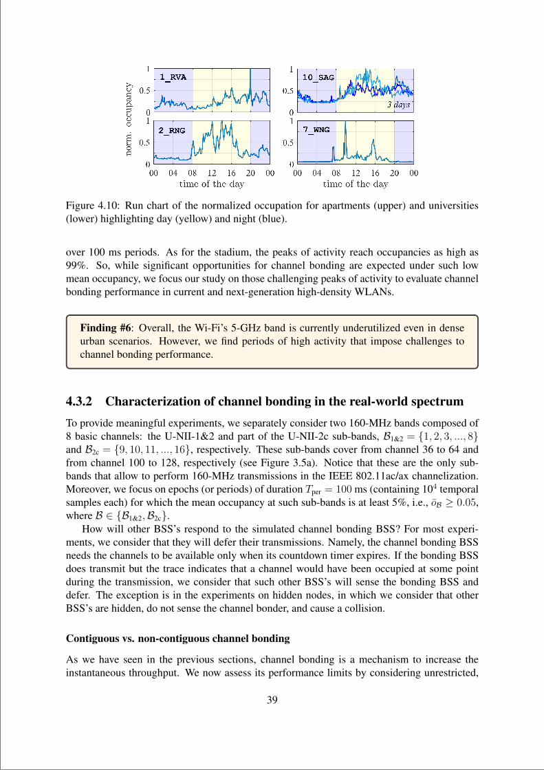
“main” — 2020/11/19 — 10:04 — page 39 — #61

Figure 4.10: Run chart of the normalized occupation for apartments (upper) and universities(lower) highlighting day (yellow) and night (blue).

over 100 ms periods. As for the stadium, the peaks of activity reach occupancies as high as99%. So, while significant opportunities for channel bonding are expected under such lowmean occupancy, we focus our study on those challenging peaks of activity to evaluate channelbonding performance in current and next-generation high-density WLANs.

Finding #6: Overall, the Wi-Fi’s 5-GHz band is currently underutilized even in denseurban scenarios. However, we find periods of high activity that impose challenges tochannel bonding performance.

4.3.2 Characterization of channel bonding in the real-world spectrumTo provide meaningful experiments, we separately consider two 160-MHz bands composed of8 basic channels: the U-NII-1&2 and part of the U-NII-2c sub-bands, B1&2 = 1, 2, 3, ..., 8and B2c = 9, 10, 11, ..., 16, respectively. These sub-bands cover from channel 36 to 64 andfrom channel 100 to 128, respectively (see Figure 3.5a). Notice that these are the only sub-bands that allow to perform 160-MHz transmissions in the IEEE 802.11ac/ax channelization.Moreover, we focus on epochs (or periods) of duration Tper = 100 ms (containing 104 temporalsamples each) for which the mean occupancy at such sub-bands is at least 5%, i.e., oB ≥ 0.05,where B ∈ B1&2,B2c.

How will other BSS’s respond to the simulated channel bonding BSS? For most experi-ments, we consider that they will defer their transmissions. Namely, the channel bonding BSSneeds the channels to be available only when its countdown timer expires. If the bonding BSSdoes transmit but the trace indicates that a channel would have been occupied at some pointduring the transmission, we consider that such other BSS’s will sense the bonding BSS anddefer. The exception is in the experiments on hidden nodes, in which we consider that otherBSS’s are hidden, do not sense the channel bonder, and cause a collision.

Contiguous vs. non-contiguous channel bonding

As we have seen in the previous sections, channel bonding is a mechanism to increase theinstantaneous throughput. We now assess its performance limits by considering unrestricted,

39

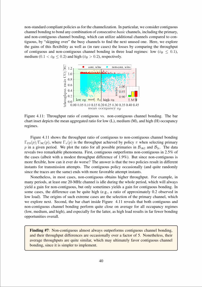
“main” — 2020/11/19 — 10:04 — page 40 — #62

non-standard compliant policies as for the channelization. In particular, we consider contiguouschannel bonding to bond any combination of consecutive basic channels, including the primary,and non-contiguous channel bonding, which can utilize additional channels compared to con-tiguous, by “skipping over” the busy channels to find the next unused one. Here, we explorethe gains of this flexibility as well as (in rare cases) the losses by comparing the throughputof contiguous and non-contiguous channel bonding in three load regimes: low (oB ≤ 0.1),medium (0.1 < oB ≤ 0.2) and high (oB > 0.2), respectively.

Figure 4.11: Throughput ratio of contiguous vs. non-contiguous channel bonding. The barchart inset depicts the mean aggregated ratio for low (L), medium (M), and high (H) occupancyregimes.

Figure 4.11 shows the throughput ratio of contiguous to non-contiguous channel bondingΓCO(p)/ΓNC(p), where Γπ(p) is the throughput achieved by policy π when selecting primaryp in a given period. We plot the ratio for all possible primaries in B1&2 and B2c. The datareveals two remarkable phenomena. First, contiguous outperforms non-contiguous in 2.5% ofthe cases (albeit with a modest throughput difference of 1.9%). But since non-contiguous ismore flexible, how can it ever do worse? The answer is that the two policies result in differentinstants for transmission attempts. The contiguous policy occasionally (and quite randomlysince the traces are the same) ends with more favorable attempt instants.

Nonetheless, in most cases, non-contiguous obtains higher throughput. For example, inmany periods, at least one 20-MHz channel is idle during the whole period, which will alwaysyield a gain for non-contiguous, but only sometimes yields a gain for contiguous bonding. Insome cases, the difference can be quite high (e.g., a ratio of approximately 0.2 observed inlow load). The origins of such extreme cases are the selection of the primary channel, whichwe explore next. Second, the bar chart inside Figure 4.11 reveals that both contiguous andnon-contiguous channel bonding perform quite close on average for all occupancy regimes(low, medium, and high), and especially for the latter, as high load results in far fewer bondingopportunities overall.

Finding #7: Non-contiguous almost always outperforms contiguous channel bonding,and their throughput differences are occasionally over a factor of 5. Nonetheless, theiraverage throughputs are quite similar, which may ultimately favor contiguous channelbonding, since it is simpler to implement.

40

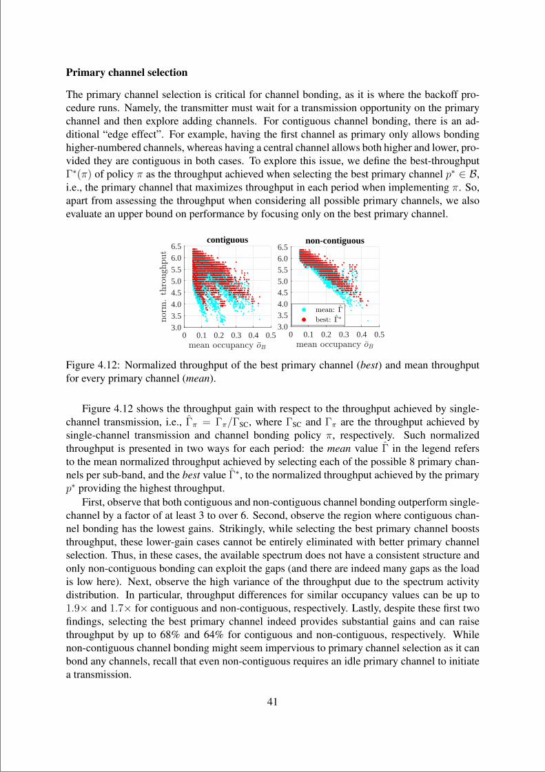
“main” — 2020/11/19 — 10:04 — page 41 — #63

Primary channel selection

The primary channel selection is critical for channel bonding, as it is where the backoff pro-cedure runs. Namely, the transmitter must wait for a transmission opportunity on the primarychannel and then explore adding channels. For contiguous channel bonding, there is an ad-ditional “edge effect”. For example, having the first channel as primary only allows bondinghigher-numbered channels, whereas having a central channel allows both higher and lower, pro-vided they are contiguous in both cases. To explore this issue, we define the best-throughputΓ∗(π) of policy π as the throughput achieved when selecting the best primary channel p∗ ∈ B,i.e., the primary channel that maximizes throughput in each period when implementing π. So,apart from assessing the throughput when considering all possible primary channels, we alsoevaluate an upper bound on performance by focusing only on the best primary channel.

0 0.1 0.2 0.3 0.4 0.53.0

3.5

4.0

4.5

5.0

5.5

6.0

6.5contiguous

0 0.1 0.2 0.3 0.4 0.53.03.54.04.55.05.56.06.5

non-contiguous

Figure 4.12: Normalized throughput of the best primary channel (best) and mean throughputfor every primary channel (mean).

Figure 4.12 shows the throughput gain with respect to the throughput achieved by single-channel transmission, i.e., Γπ = Γπ/ΓSC, where ΓSC and Γπ are the throughput achieved bysingle-channel transmission and channel bonding policy π, respectively. Such normalizedthroughput is presented in two ways for each period: the mean value Γ in the legend refersto the mean normalized throughput achieved by selecting each of the possible 8 primary chan-nels per sub-band, and the best value Γ∗, to the normalized throughput achieved by the primaryp∗ providing the highest throughput.

First, observe that both contiguous and non-contiguous channel bonding outperform single-channel by a factor of at least 3 to over 6. Second, observe the region where contiguous chan-nel bonding has the lowest gains. Strikingly, while selecting the best primary channel booststhroughput, these lower-gain cases cannot be entirely eliminated with better primary channelselection. Thus, in these cases, the available spectrum does not have a consistent structure andonly non-contiguous bonding can exploit the gaps (and there are indeed many gaps as the loadis low here). Next, observe the high variance of the throughput due to the spectrum activitydistribution. In particular, throughput differences for similar occupancy values can be up to1.9× and 1.7× for contiguous and non-contiguous, respectively. Lastly, despite these first twofindings, selecting the best primary channel indeed provides substantial gains and can raisethroughput by up to 68% and 64% for contiguous and non-contiguous, respectively. Whilenon-contiguous channel bonding might seem impervious to primary channel selection as it canbond any channels, recall that even non-contiguous requires an idle primary channel to initiatea transmission.

41

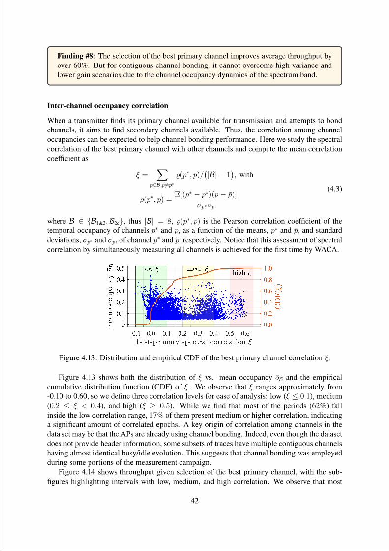
“main” — 2020/11/19 — 10:04 — page 42 — #64

Finding #8: The selection of the best primary channel improves average throughput byover 60%. But for contiguous channel bonding, it cannot overcome high variance andlower gain scenarios due to the channel occupancy dynamics of the spectrum band.

Inter-channel occupancy correlation

When a transmitter finds its primary channel available for transmission and attempts to bondchannels, it aims to find secondary channels available. Thus, the correlation among channeloccupancies can be expected to help channel bonding performance. Here we study the spectralcorrelation of the best primary channel with other channels and compute the mean correlationcoefficient as

ξ =∑

p∈B,p 6=p∗%(p∗, p)/

(|B| − 1

), with

%(p∗, p) =E[(p∗ − p∗)(p− p)]

σp∗σp

(4.3)

where B ∈ B1&2,B2c, thus |B| = 8, %(p∗, p) is the Pearson correlation coefficient of thetemporal occupancy of channels p∗ and p, as a function of the means, p∗ and p, and standarddeviations, σp∗ and σp, of channel p∗ and p, respectively. Notice that this assessment of spectralcorrelation by simultaneously measuring all channels is achieved for the first time by WACA.

Figure 4.13: Distribution and empirical CDF of the best primary channel correlation ξ.

Figure 4.13 shows both the distribution of ξ vs. mean occupancy oB and the empiricalcumulative distribution function (CDF) of ξ. We observe that ξ ranges approximately from-0.10 to 0.60, so we define three correlation levels for ease of analysis: low (ξ ≤ 0.1), medium(0.2 ≤ ξ < 0.4), and high (ξ ≥ 0.5). While we find that most of the periods (62%) fallinside the low correlation range, 17% of them present medium or higher correlation, indicatinga significant amount of correlated epochs. A key origin of correlation among channels in thedata set may be that the APs are already using channel bonding. Indeed, even though the datasetdoes not provide header information, some subsets of traces have multiple contiguous channelshaving almost identical busy/idle evolution. This suggests that channel bonding was employedduring some portions of the measurement campaign.

Figure 4.14 shows throughput given selection of the best primary channel, with the sub-figures highlighting intervals with low, medium, and high correlation. We observe that most

42

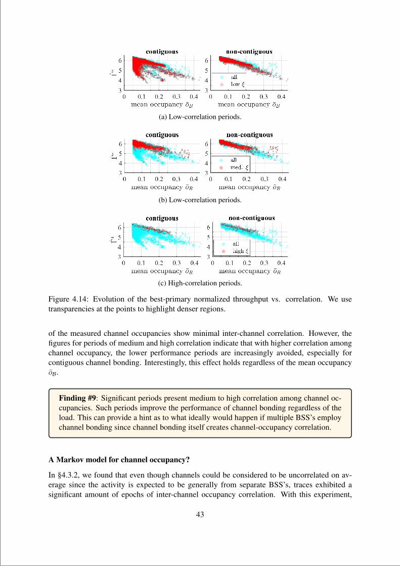
“main” — 2020/11/19 — 10:04 — page 43 — #65

(a) Low-correlation periods.

(b) Low-correlation periods.

(c) High-correlation periods.

Figure 4.14: Evolution of the best-primary normalized throughput vs. correlation. We usetransparencies at the points to highlight denser regions.

of the measured channel occupancies show minimal inter-channel correlation. However, thefigures for periods of medium and high correlation indicate that with higher correlation amongchannel occupancy, the lower performance periods are increasingly avoided, especially forcontiguous channel bonding. Interestingly, this effect holds regardless of the mean occupancyoB.

Finding #9: Significant periods present medium to high correlation among channel oc-cupancies. Such periods improve the performance of channel bonding regardless of theload. This can provide a hint as to what ideally would happen if multiple BSS’s employchannel bonding since channel bonding itself creates channel-occupancy correlation.

A Markov model for channel occupancy?

In §4.3.2, we found that even though channels could be considered to be uncorrelated on av-erage since the activity is expected to be generally from separate BSS’s, traces exhibited asignificant amount of epochs of inter-channel occupancy correlation. With this experiment,

43

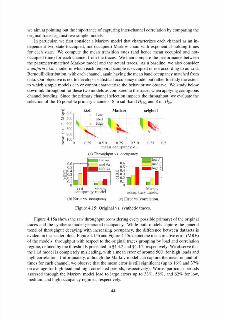
“main” — 2020/11/19 — 10:04 — page 44 — #66

we aim at pointing out the importance of capturing inter-channel correlation by comparing theoriginal traces against two simple models.

In particular, we first consider a Markov model that characterizes each channel as an in-dependent two-state (occupied, not occupied) Markov chain with exponential holding timesfor each state. We compute the mean transition rates (and hence mean occupied and not-occupied time) for each channel from the traces. We then compare the performance betweenthe parameter-matched Markov model and the actual traces. As a baseline, we also considera uniform i.i.d. model in which each temporal sample is occupied or not according to an i.i.d.Bernoulli distribution, with each channel, again having the mean band occupancy matched fromdata. Our objective is not to develop a statistical occupancy model but rather to study the extentto which simple models can or cannot characterize the behavior we observe. We study belowdownlink throughput for these two models as compared to the traces when applying contiguouschannel bonding. Since the primary channel selection impacts the throughput, we evaluate theselection of the 16 possible primary channels: 8 in sub-band B1&2 and 8 in B2c.

(a) Throughput vs. occupancy

i.i.d. Markov0

0.10.20.30.40.50.6

(b) Error vs. occupancy.

i.i.d. Markov0

0.10.20.30.40.50.6

(c) Error vs. correlation.

Figure 4.15: Original vs. synthetic traces.

Figure 4.15a shows the raw throughput (considering every possible primary) of the originaltraces and the synthetic model-generated occupancy. While both models capture the generaltrend of throughput decaying with increasing occupancy, the difference between datasets isevident in the scatter plots. Figure 4.15b and Figure 4.15c depict the mean relative error (MRE)of the models’ throughput with respect to the original traces grouping by load and correlationregime, defined by the thresholds presented in §4.3.2 and §4.3.2, respectively. We observe thatthe i.i.d model is completely misleading, with a mean error of around 50% for high loads andhigh correlation. Unfortunately, although the Markov model can capture the mean on and offtimes for each channel, we observe that the mean error is still significant (up to 16% and 37%on average for high load and high correlated periods, respectively). Worse, particular periodsassessed through the Markov model lead to large errors up to 33%, 58%, and 62% for low,medium, and high occupancy regimes, respectively.

44

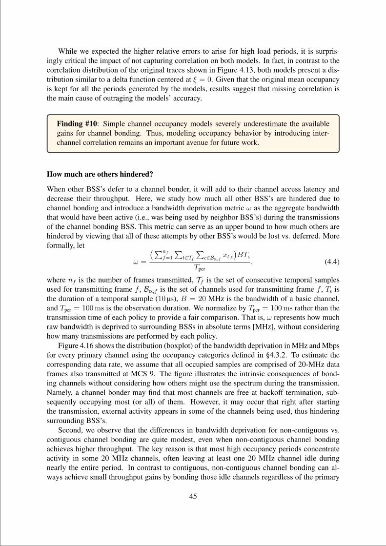
“main” — 2020/11/19 — 10:04 — page 45 — #67

While we expected the higher relative errors to arise for high load periods, it is surpris-ingly critical the impact of not capturing correlation on both models. In fact, in contrast to thecorrelation distribution of the original traces shown in Figure 4.13, both models present a dis-tribution similar to a delta function centered at ξ = 0. Given that the original mean occupancyis kept for all the periods generated by the models, results suggest that missing correlation isthe main cause of outraging the models’ accuracy.

Finding #10: Simple channel occupancy models severely underestimate the availablegains for channel bonding. Thus, modeling occupancy behavior by introducing inter-channel correlation remains an important avenue for future work.

How much are others hindered?

When other BSS’s defer to a channel bonder, it will add to their channel access latency anddecrease their throughput. Here, we study how much all other BSS’s are hindered due tochannel bonding and introduce a bandwidth deprivation metric ω as the aggregate bandwidththat would have been active (i.e., was being used by neighbor BSS’s) during the transmissionsof the channel bonding BSS. This metric can serve as an upper bound to how much others arehindered by viewing that all of these attempts by other BSS’s would be lost vs. deferred. Moreformally, let

ω =

(∑nf

f=1

∑t∈Tf

∑c∈Btx,f

xt,c)BTs

Tper, (4.4)

where nf is the number of frames transmitted, Tf is the set of consecutive temporal samplesused for transmitting frame f , Btx,f is the set of channels used for transmitting frame f , Ts isthe duration of a temporal sample (10 µs), B = 20 MHz is the bandwidth of a basic channel,and Tper = 100 ms is the observation duration. We normalize by Tper = 100 ms rather than thetransmission time of each policy to provide a fair comparison. That is, ω represents how muchraw bandwidth is deprived to surrounding BSSs in absolute terms [MHz], without consideringhow many transmissions are performed by each policy.

Figure 4.16 shows the distribution (boxplot) of the bandwidth deprivation in MHz and Mbpsfor every primary channel using the occupancy categories defined in §4.3.2. To estimate thecorresponding data rate, we assume that all occupied samples are comprised of 20-MHz dataframes also transmitted at MCS 9. The figure illustrates the intrinsic consequences of bond-ing channels without considering how others might use the spectrum during the transmission.Namely, a channel bonder may find that most channels are free at backoff termination, sub-sequently occupying most (or all) of them. However, it may occur that right after startingthe transmission, external activity appears in some of the channels being used, thus hinderingsurrounding BSS’s.

Second, we observe that the differences in bandwidth deprivation for non-contiguous vs.contiguous channel bonding are quite modest, even when non-contiguous channel bondingachieves higher throughput. The key reason is that most high occupancy periods concentrateactivity in some 20 MHz channels, often leaving at least one 20 MHz channel idle duringnearly the entire period. In contrast to contiguous, non-contiguous channel bonding can al-ways achieve small throughput gains by bonding those idle channels regardless of the primary

45

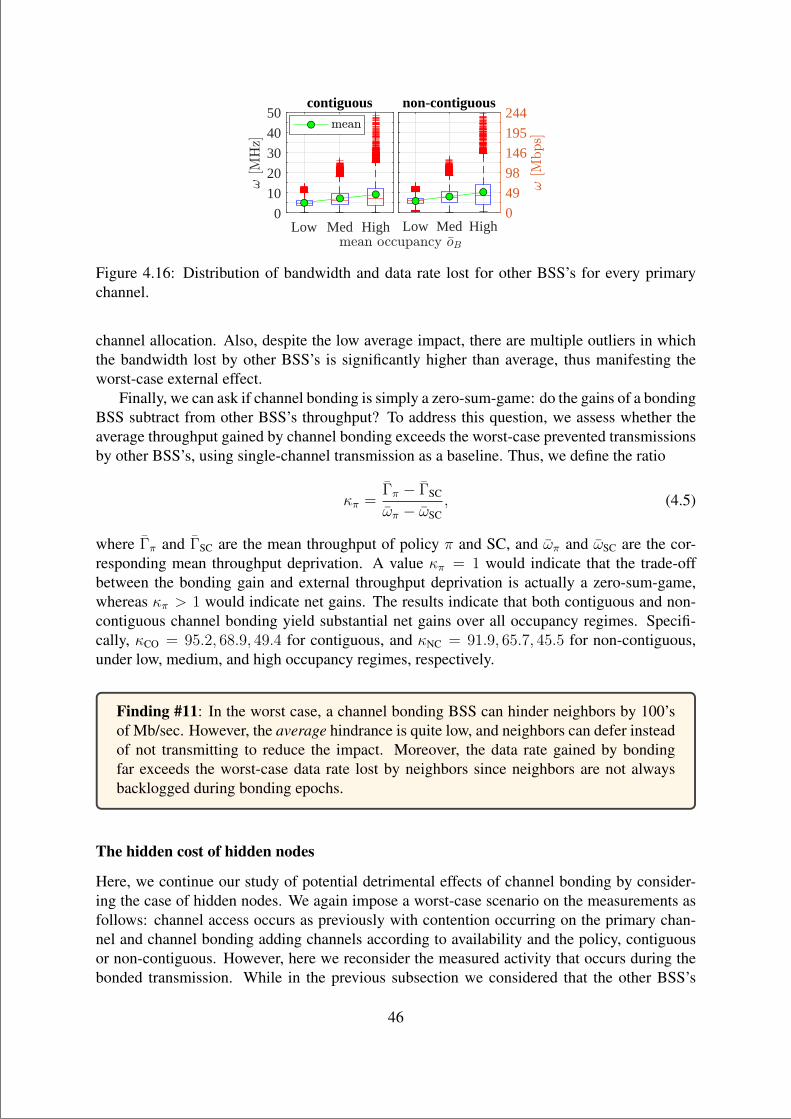
“main” — 2020/11/19 — 10:04 — page 46 — #68

Low Med High0

10

20

30

40

50contiguous

Low Med High0

49

98

146

195

244non-contiguous

Figure 4.16: Distribution of bandwidth and data rate lost for other BSS’s for every primarychannel.

channel allocation. Also, despite the low average impact, there are multiple outliers in whichthe bandwidth lost by other BSS’s is significantly higher than average, thus manifesting theworst-case external effect.

Finally, we can ask if channel bonding is simply a zero-sum-game: do the gains of a bondingBSS subtract from other BSS’s throughput? To address this question, we assess whether theaverage throughput gained by channel bonding exceeds the worst-case prevented transmissionsby other BSS’s, using single-channel transmission as a baseline. Thus, we define the ratio

κπ =Γπ − ΓSC

ωπ − ωSC, (4.5)

where Γπ and ΓSC are the mean throughput of policy π and SC, and ωπ and ωSC are the cor-responding mean throughput deprivation. A value κπ = 1 would indicate that the trade-offbetween the bonding gain and external throughput deprivation is actually a zero-sum-game,whereas κπ > 1 would indicate net gains. The results indicate that both contiguous and non-contiguous channel bonding yield substantial net gains over all occupancy regimes. Specifi-cally, κCO = 95.2, 68.9, 49.4 for contiguous, and κNC = 91.9, 65.7, 45.5 for non-contiguous,under low, medium, and high occupancy regimes, respectively.

Finding #11: In the worst case, a channel bonding BSS can hinder neighbors by 100’sof Mb/sec. However, the average hindrance is quite low, and neighbors can defer insteadof not transmitting to reduce the impact. Moreover, the data rate gained by bondingfar exceeds the worst-case data rate lost by neighbors since neighbors are not alwaysbacklogged during bonding epochs.

The hidden cost of hidden nodes

Here, we continue our study of potential detrimental effects of channel bonding by consider-ing the case of hidden nodes. We again impose a worst-case scenario on the measurements asfollows: channel access occurs as previously with contention occurring on the primary chan-nel and channel bonding adding channels according to availability and the policy, contiguousor non-contiguous. However, here we reconsider the measured activity that occurs during thebonded transmission. While in the previous subsection we considered that the other BSS’s

46

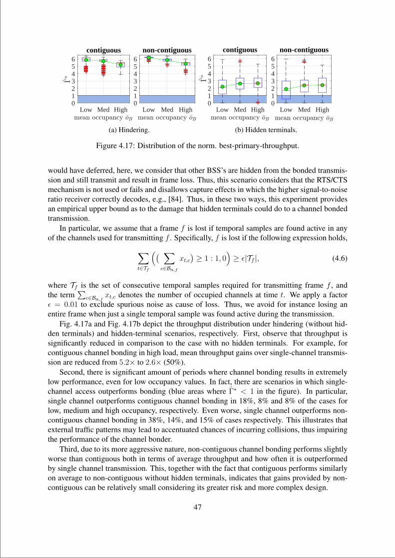
“main” — 2020/11/19 — 10:04 — page 47 — #69

Low Med High0123456

contiguous

Low Med High0123456

non-contiguous

(a) Hindering.

Low Med High0123456

contiguous

Low Med High0123456

non-contiguous

(b) Hidden terminals.

Figure 4.17: Distribution of the norm. best-primary-throughput.

would have deferred, here, we consider that other BSS’s are hidden from the bonded transmis-sion and still transmit and result in frame loss. Thus, this scenario considers that the RTS/CTSmechanism is not used or fails and disallows capture effects in which the higher signal-to-noiseratio receiver correctly decodes, e.g., [84]. Thus, in these two ways, this experiment providesan empirical upper bound as to the damage that hidden terminals could do to a channel bondedtransmission.

In particular, we assume that a frame f is lost if temporal samples are found active in anyof the channels used for transmitting f . Specifically, f is lost if the following expression holds,

∑

t∈Tf

(( ∑

c∈Btx,f

xt,c)≥ 1 : 1, 0

)≥ ε|Tf |, (4.6)

where Tf is the set of consecutive temporal samples required for transmitting frame f , andthe term

∑c∈Btx,f

xt,c denotes the number of occupied channels at time t. We apply a factorε = 0.01 to exclude spurious noise as cause of loss. Thus, we avoid for instance losing anentire frame when just a single temporal sample was found active during the transmission.

Fig. 4.17a and Fig. 4.17b depict the throughput distribution under hindering (without hid-den terminals) and hidden-terminal scenarios, respectively. First, observe that throughput issignificantly reduced in comparison to the case with no hidden terminals. For example, forcontiguous channel bonding in high load, mean throughput gains over single-channel transmis-sion are reduced from 5.2× to 2.6× (50%).

Second, there is significant amount of periods where channel bonding results in extremelylow performance, even for low occupancy values. In fact, there are scenarios in which single-channel access outperforms bonding (blue areas where Γ∗ < 1 in the figure). In particular,single channel outperforms contiguous channel bonding in 18%, 8% and 8% of the cases forlow, medium and high occupancy, respectively. Even worse, single channel outperforms non-contiguous channel bonding in 38%, 14%, and 15% of cases respectively. This illustrates thatexternal traffic patterns may lead to accentuated chances of incurring collisions, thus impairingthe performance of the channel bonder.

Third, due to its more aggressive nature, non-contiguous channel bonding performs slightlyworse than contiguous both in terms of average throughput and how often it is outperformedby single channel transmission. This, together with the fact that contiguous performs similarlyon average to non-contiguous without hidden terminals, indicates that gains provided by non-contiguous can be relatively small considering its greater risk and more complex design.

47

“main” — 2020/11/19 — 10:04 — page 48 — #70

Finally, also in contrast to Fig. 4.17a, Fig. 4.17b indicates that the decaying trend of meannormalized best-throughput with load when neighbors defer does not hold with hidden termi-nals. Indeed, we observe a slight increase of the normalized best-throughput as the occupancyincreases as fewer bonding opportunities also diminish the risk of collisions.

Finding #12: While channel bonding outperforms single-channel transmission in mostcases, it is vulnerable to hidden node interference, with non-contiguous channel bondingbeing impacted the most. To avoid the aforementioned worst-case throughput penalties,nodes can use RTS/CTS, implement capture (to better receive even while a hidden ter-minal transmission overlaps in time), or increase sensitivity, i.e., reduce the threshold forsensing channel activity to reduce the frequency of hidden terminal transmissions.

The Camp Nou: a sold out stadium

Finally, we assess if channel bonding can provide throughput gains in areas with persistentlyhigh load over all channels. Figure 4.18 shows normalized throughput under the best primarychannel selection when applying contiguous and non-contiguous channel bonding. Under loadsexceeding 90%, both policies have throughput close to single-channel transmission, indicatingminimal remaining margin for gain. Nonetheless, in transient epochs, where the load is low,both policies exploit throughput gains. For example, in the stadium during epochs of 20-30%load, the gain over single-channel throughput is 3.69× and 5.30× for contiguous and non-contiguous, respectively. In fact, we observe that non-contiguous significantly outperformscontiguous in a broad regime of “non-extreme” loads given the heterogeneous activity distribu-tion over channels. For example, at 40-50% average occupancy, contiguous channel bondinghas an average throughput gain of 2.38× whereas non-contiguous has 3.97×, a gain of 67%.

10 30 50 70 900123456

contiguous

10 30 50 70 900123456

non-contiguous

Figure 4.18: Gains for the bonding BSS assuming others defer.

Lastly, the story can turn quite negative if competing BSS’s do not defer to the channel bon-der, i.e., if other BSS’s are hidden. In such a worst-case, all bonded transmissions with subse-quent activity are considered lost. Figure 4.19 shows the results of this scenario for the stadiumtraces. As indicated by the blue shadowed areas, most of the periods achieve higher throughputwith single-channel transmission rather than channel bonding. Indeed, single-channel trans-mission outperforms both channel bonding policies in at least 80% of the epochs over all theoccupancy regimes.

48

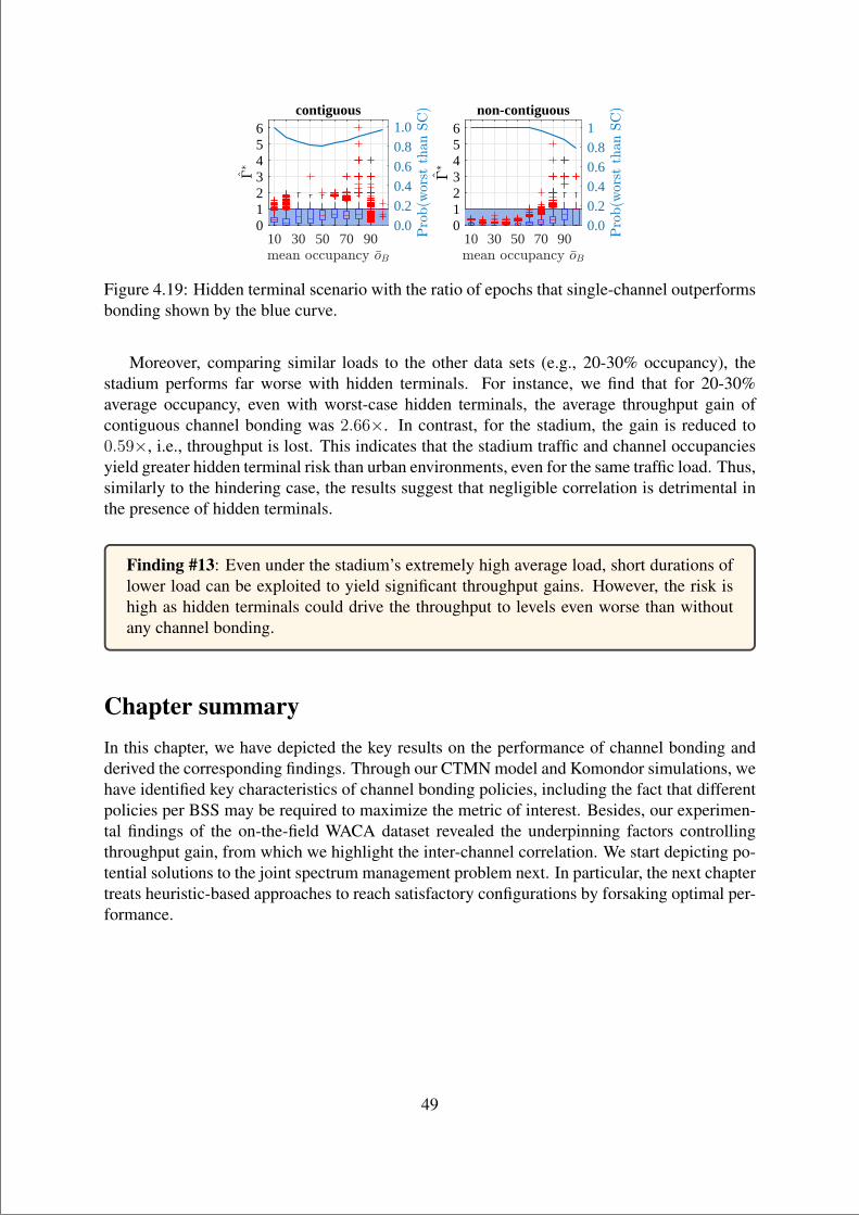
“main” — 2020/11/19 — 10:04 — page 49 — #71

10 30 50 70 900123456

0.00.20.40.60.81.0

contiguous

10 30 50 70 900123456

0.00.20.40.60.81

non-contiguous

Figure 4.19: Hidden terminal scenario with the ratio of epochs that single-channel outperformsbonding shown by the blue curve.

Moreover, comparing similar loads to the other data sets (e.g., 20-30% occupancy), thestadium performs far worse with hidden terminals. For instance, we find that for 20-30%average occupancy, even with worst-case hidden terminals, the average throughput gain ofcontiguous channel bonding was 2.66×. In contrast, for the stadium, the gain is reduced to0.59×, i.e., throughput is lost. This indicates that the stadium traffic and channel occupanciesyield greater hidden terminal risk than urban environments, even for the same traffic load. Thus,similarly to the hindering case, the results suggest that negligible correlation is detrimental inthe presence of hidden terminals.

Finding #13: Even under the stadium’s extremely high average load, short durations oflower load can be exploited to yield significant throughput gains. However, the risk ishigh as hidden terminals could drive the throughput to levels even worse than withoutany channel bonding.

Chapter summaryIn this chapter, we have depicted the key results on the performance of channel bonding andderived the corresponding findings. Through our CTMN model and Komondor simulations, wehave identified key characteristics of channel bonding policies, including the fact that differentpolicies per BSS may be required to maximize the metric of interest. Besides, our experimen-tal findings of the on-the-field WACA dataset revealed the underpinning factors controllingthroughput gain, from which we highlight the inter-channel correlation. We start depicting po-tential solutions to the joint spectrum management problem next. In particular, the next chaptertreats heuristic-based approaches to reach satisfactory configurations by forsaking optimal per-formance.

49

“main” — 2020/11/19 — 10:04 — page 50 — #72

“main” — 2020/11/19 — 10:04 — page 51 — #73

Chapter 5

HEURISTIC-BASED POLICIES

A heuristic – derived from the Greek word meaning “to discover” – is any problem-solvingmethod that employs a practical, flexible, shortcut that is not guaranteed to be optimal but isgood enough for reaching a short-term goal. Heuristics are then used to find quickly satisfactorysolutions in complex systems where finding an optimal solution is infeasible or impractical.

5.1 Heuristics to cope with complexity

As for the problem we deal with in this thesis, there are many valuable works in the literatureabout custom channel allocation and channel bonding solutions in wireless networks (e.g.,[104, 134, 139, 144]). Table 5.1 collects some of them. These solutions rely on certain types ofstatistics (e.g., channel occupancy, packet reception rate, or color conflicts) to operate. We callthese prefixed rule-based solutions as heuristic solutions in front of machine learning solutions,which we discuss in chapter §6.

While there are multiple works treating channel allocation and channel bonding separately,few of them assess the joint problem altogether in the context of WLANs. We highlight thefollowing ones. A distributed spectrum assignment for home WLANs relying on out-of-bandmeasurements is proposed in [63]. Continuous-time Markov networks are employed in [31]to study a centralized approach for maximizing network fairness. Besides, an algorithm forprimary channel selection based on the bonding direction likelihoods was recently presentedin [77]. However, such likelihoods are estimated by assuming a known number of users in eachchannel, which is usually not feasible in real deployments. It is worth noticing that the worksmentioned above consider fully-backlogged traffic, thus missing insights on more realistic pat-terns with different traffic needs. Conversely, an uncertain traffic channel allocation approachwas presented in [100]. Still, a centralized controller in the backend is required. Recently, weformulated DyWi (see §5.2), a decentralized, lightweight algorithm, adaptive in the sense thata new primary channel is only adopted when the BSS performance is under a given satisfactionthreshold [27]. We depict DyWi in the section below.

51

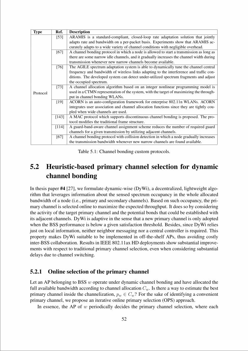
“main” — 2020/11/19 — 10:04 — page 52 — #74

Type Ref. Description

Protocol

[53] ARAMIS is a standard-compliant, closed-loop rate adaptation solution that jointlyadapts rate and bandwidth on a per-packet basis. Experiments show that ARAMIS ac-curately adapts to a wide variety of channel conditions with negligible overhead.

[67] A channel bonding protocol in which a node is allowed to start a transmission as long asthere are some narrow idle channels, and it gradually increases the channel width duringtransmission whenever new narrow channels become available.

[76] The AGILE spectrum adaptation system is able to dynamically tune the channel centralfrequency and bandwidth of wireless links adapting to the interference and traffic con-ditions. The developed system can detect under-utilized spectrum fragments and adjustthe occupied spectrum.

[73] A channel allocation algorithm based on an integer nonlinear programming model isused in a CTMN representation of the system, with the target of maximizing the through-put in channel bonding WLANs.

[19] ACORN is an auto-configuration framework for enterprise 802.11n WLANs. ACORNintegrates user association and channel allocation functions since they are tightly cou-pled when wide channels are used.

[143] A MAC protocol which supports discontinuous channel bonding is proposed. The pro-tocol modifies the traditional frame structure.

[114] A guard-band-aware channel assignment scheme reduces the number of required guardchannels for a given transmission by utilizing adjacent channels.

[67] A channel bonding protocol with collision detection in which a node gradually increasesthe transmission bandwidth whenever new narrow channels are found available.

Table 5.1: Channel bonding custom protocols.

5.2 Heuristic-based primary channel selection for dynamicchannel bonding

In thesis paper #4 [27], we formulate dynamic-wise (DyWi), a decentralized, lightweight algo-rithm that leverages information about the sensed spectrum occupancy in the whole allocatedbandwidth of a node (i.e., primary and secondary channels). Based on such occupancy, the pri-mary channel is selected online to maximize the expected throughput. It does so by consideringthe activity of the target primary channel and the potential bonds that could be established withits adjacent channels. DyWi is adaptive in the sense that a new primary channel is only adoptedwhen the BSS performance is below a given satisfaction threshold. Besides, since DyWi reliesjust on local information, neither neighbor messaging nor a central controller is required. Thisproperty makes DyWi suitable to be implemented in off-the-shelf APs, thus avoiding costlyinter-BSS collaboration. Results in IEEE 802.11ax HD deployments show substantial improve-ments with respect to traditional primary channel selection, even when considering substantialdelays due to channel switching.

5.2.1 Online selection of the primary channel

Let an AP belonging to BSS w operate under dynamic channel bonding and have allocated thefull available bandwidth according to channel allocation Cw. Is there a way to estimate the bestprimary channel inside the channelization, pw ∈ Cw? For the sake of identifying a convenientprimary channel, we propose an iterative online primary selection (OPS) approach.

In essence, the AP of w periodically decides the primary channel selection, where each

52

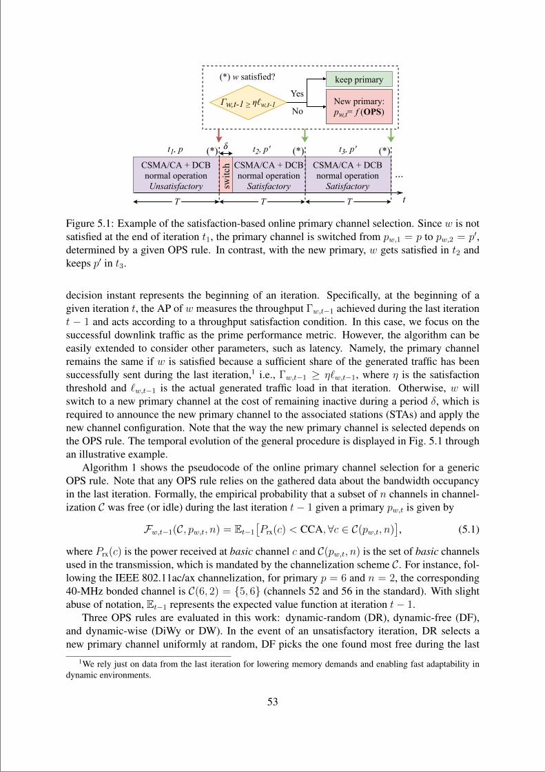
“main” — 2020/11/19 — 10:04 — page 53 — #75

CSMA/CA+DCBnormaloperationSatisfactory

CSMA/CA+DCBnormaloperationSatisfactory

CSMA/CA+DCBnormaloperationUnsatisfactory

Γw,t-1≥ηℓw,t-1

(*)wsatisfied?

T

t1,p

T

t2,p'

switch

T

t3,p'

t

keepprimary

No

Yes

...

(*) (*) (*)

Newprimary:pw,t=f(OPS)

Figure 5.1: Example of the satisfaction-based online primary channel selection. Since w is notsatisfied at the end of iteration t1, the primary channel is switched from pw,1 = p to pw,2 = p′,determined by a given OPS rule. In contrast, with the new primary, w gets satisfied in t2 andkeeps p′ in t3.

decision instant represents the beginning of an iteration. Specifically, at the beginning of agiven iteration t, the AP of w measures the throughput Γw,t−1 achieved during the last iterationt − 1 and acts according to a throughput satisfaction condition. In this case, we focus on thesuccessful downlink traffic as the prime performance metric. However, the algorithm can beeasily extended to consider other parameters, such as latency. Namely, the primary channelremains the same if w is satisfied because a sufficient share of the generated traffic has beensuccessfully sent during the last iteration,1 i.e., Γw,t−1 ≥ η`w,t−1, where η is the satisfactionthreshold and `w,t−1 is the actual generated traffic load in that iteration. Otherwise, w willswitch to a new primary channel at the cost of remaining inactive during a period δ, which isrequired to announce the new primary channel to the associated stations (STAs) and apply thenew channel configuration. Note that the way the new primary channel is selected depends onthe OPS rule. The temporal evolution of the general procedure is displayed in Fig. 5.1 throughan illustrative example.

Algorithm 1 shows the pseudocode of the online primary channel selection for a genericOPS rule. Note that any OPS rule relies on the gathered data about the bandwidth occupancyin the last iteration. Formally, the empirical probability that a subset of n channels in channel-ization C was free (or idle) during the last iteration t− 1 given a primary pw,t is given by

Fw,t−1(C, pw,t, n) = Et−1

[Prx(c) < CCA, ∀c ∈ C(pw,t, n)

], (5.1)

where Prx(c) is the power received at basic channel c and C(pw,t, n) is the set of basic channelsused in the transmission, which is mandated by the channelization scheme C. For instance, fol-lowing the IEEE 802.11ac/ax channelization, for primary p = 6 and n = 2, the corresponding40-MHz bonded channel is C(6, 2) = 5, 6 (channels 52 and 56 in the standard). With slightabuse of notation, Et−1 represents the expected value function at iteration t− 1.

Three OPS rules are evaluated in this work: dynamic-random (DR), dynamic-free (DF),and dynamic-wise (DiWy or DW). In the event of an unsatisfactory iteration, DR selects anew primary channel uniformly at random, DF picks the one found most free during the last

1We rely just on data from the last iteration for lowering memory demands and enabling fast adaptability indynamic environments.

53

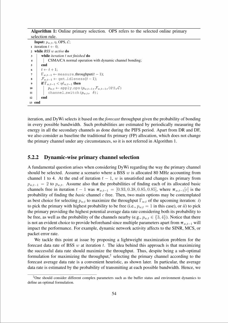
“main” — 2020/11/19 — 10:04 — page 54 — #76

Algorithm 1: Online primary selection. OPS refers to the selected online primaryselection rule.

Input: pw,t, η, OPS, C;1 iteration t← 0;2 while BSS w active do3 while iteration t not finished do4 CSMA/CA normal operation with dynamic channel bonding;5 end6 t← t+ 1;7 Γw,t−1 ← measure throughput(t− 1);8 Fw,t−1 ← get idleness(t− 1);9 if Γw,t−1 < η`w,t−1 then

10 pw,t ← apply ops(pw,t−1,Fw,t−1,OPS,C)11 channel switch(pw,t, δ);12 end13 end

iteration, and DyWi selects it based on the forecast throughput given the probability of bondingin every possible bandwidth. Such probabilities are estimated by periodically measuring theenergy in all the secondary channels as done during the PIFS period. Apart from DR and DF,we also consider as baseline the traditional fix primary (FP) allocation, which does not changethe primary channel under any circumstances, so it is not referred in Algorithm 1.

5.2.2 Dynamic-wise primary channel selection

A fundamental question arises when considering DyWi regarding the way the primary channelshould be selected. Assume a scenario where a BSS w is allocated 80 MHz accounting fromchannel 1 to 4. At the end of iteration t − 1, w is unsatisfied and changes its primary frompw,t−1 = 2 to pw,t. Assume also that the probabilities of finding each of its allocated basicchannels free in iteration t − 1 was πw,t−1 = [0.93, 0.38, 0.85, 0.85], where πw,t−1[c] is theprobability of finding the basic channel c free. Then, two main options may be contemplatedas best choice for selecting pw,t to maximize the throughput Γw,t of the upcoming iteration: i)to pick the primary with highest probability to be free (i.e., pw,t = 1 in this case), or ii) to pickthe primary providing the highest potential average data rate considering both its probability tobe free, as well as the probability of the channels nearby (e.g., pw,t ∈ 3, 4). Notice that thereis not an evident choice to provide beforehand since multiple parameters apart from πw,t−1 willimpact the performance. For example, dynamic network activity affects to the SINR, MCS, orpacket error rate.

We tackle this point at issue by proposing a lightweight maximization problem for theforecast data rate of BSS w at iteration t. The idea behind this approach is that maximizingthe successful data rate should maximize the throughput. Thus, despite being a sub-optimalformulation for maximizing the throughput,2 selecting the primary channel according to theforecast average data rate is a convenient heuristic, as shown later. In particular, the averagedata rate is estimated by the probability of transmitting at each possible bandwidth. Hence, we

2One should consider different complex parameters such as the buffer status and environment dynamics todefine an optimal formulation.

54

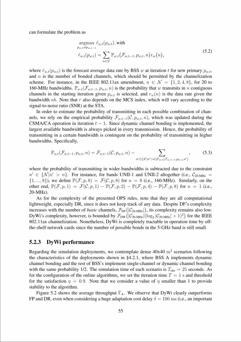
“main” — 2020/11/19 — 10:04 — page 55 — #77

can formulate the problem as

argmaxpw,t 6=pw,t−1

rw,t(pw,t),with

rw,t(pw,t) =∑

n∈NPw,t

(Fw,t−1, pw,t, n

)rw(n),

(5.2)

where rw,t(pw,t) is the forecast average data rate by BSS w at iteration t for new primary pw,t,and n is the number of bonded channels, which should be permitted by the channelizationscheme. For instance, in the IEEE 802.11ax amendment, n ∈ N = 1, 2, 4, 8, for 20 to160-MHz bandwidths. Pw,t(Fw,t−1, pw,t, n) is the probability that w transmits in n contiguouschannels in the starting iteration given pw,t is selected, and rw(n) is the data rate given thebandwidth nb. Note that r also depends on the MCS index, which will vary according to thesignal-to-noise ratio (SNR) at the STA.

In order to estimate the probability of transmitting in each possible combination of chan-nels, we rely on the empirical probability Fw,t−1(C, pw,t, n), which was updated during theCSMA/CA operation in iteration t − 1. Since dynamic channel bonding is implemented, thelargest available bandwidth is always picked in every transmission. Hence, the probability oftransmitting in a certain bandwidth is contingent on the probability of transmitting in higherbandwidths. Specifically,

Pw,t(Fw,t−1, pw,t, n) = Fw,t−1(C, pw,t, n)−∑

n′∈N|n′>nPw,t(Fw,t−1,pw,t,n′)

, (5.3)

where the probability of transmitting in wider bandwidths is subtracted due to the constraintn′ ∈ N |n′ > n. For instance, for bands UNII-1 and UNII-2 altogether (i.e., C20-MHz =1, ..., 8), we define P(F , p, 8) = F(C, p, 8) for n = 8 (i.e., 160-MHz). Similarly, on theother end, P(F , p, 1) = F(C, p, 1) − P(F , p, 2) − P(F , p, 4) − P(F , p, 8) for n = 1 (i.e.,20-MHz).

As for the complexity of the presented OPS rules, note that they are all computationallightweight, especially DR, since it does not keep track of any data. Despite DF’s complexityincreases with the number of basic channels, FDF

(|C20-MHz|

), its complexity remains also low.

DyWi’s complexity, however, is bounded by FDW(|C20-MHz|(log2 |C20-MHz| + 1)2

)for the IEEE

802.11ax channelization. Nonetheless, DyWi is completely tractable in operation time by off-the-shelf network cards since the number of possible bonds in the 5-GHz band is still small.

5.2.3 DyWi performanceRegarding the simulation deployments, we contemplate dense 40x40 m2 scenarios followingthe characteristics of the deployments shown in §4.2.1, where BSS A implements dynamicchannel bonding and the rest of BSS’s implement single-channel or dynamic channel bondingwith the same probability 1/2. The simulation time of each scenario is Tobs = 25 seconds. Asfor the configuration of the online algorithms, we set the iteration time T = 1 s and thresholdfor the satisfaction η = 0.9. Note that we consider a value of η smaller than 1 to providestability to the algorithm.

Figure 5.2 shows the average throughput ΓA. We observe that DyWi clearly outperformsFP and DR, even when considering a huge adaptation cost delay δ = 100 ms (i.e., an important

55

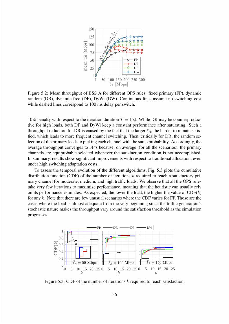
“main” — 2020/11/19 — 10:04 — page 56 — #78

Figure 5.2: Mean throughput of BSS A for different OPS rules: fixed primary (FP), dynamicrandom (DR), dynamic-free (DF), DyWi (DW). Continuous lines assume no switching costwhile dashed lines correspond to 100 ms delay per switch.

10% penalty with respect to the iteration duration T = 1 s). While DR may be counterproduc-tive for high loads, both DF and DyWi keep a constant performance after saturating. Such athroughput reduction for DR is caused by the fact that the larger ¯

A, the harder to remain satis-fied, which leads to more frequent channel switching. Then, critically for DR, the random se-lection of the primary leads to picking each channel with the same probability. Accordingly, theaverage throughput converges to FP’s because, on average (for all the scenarios), the primarychannels are equiprobable selected whenever the satisfaction condition is not accomplished.In summary, results show significant improvements with respect to traditional allocation, evenunder high switching adaptation costs.

To assess the temporal evolution of the different algorithms, Fig. 5.3 plots the cumulativedistribution function (CDF) of the number of iterations k required to reach a satisfactory pri-mary channel for moderate, medium, and high traffic loads. We observe that all the OPS rulestake very few iterations to maximize performance, meaning that the heuristic can usually relyon its performance estimates. As expected, the lower the load, the higher the value of CDF(k)for any k. Note that there are few unusual scenarios where the CDF varies for FP. Those are thecases where the load is almost adequate from the very beginning since the traffic generation’sstochastic nature makes the throughput vary around the satisfaction threshold as the simulationprogresses.

0 5 10 15 20 250

0.2

0.4

0.6

0.8

1

0 5 10 15 20 25 0 5 10 15 20 25

FP DR DF DW

Figure 5.3: CDF of the number of iterations k required to reach satisfaction.

56

“main” — 2020/11/19 — 10:04 — page 57 — #79

Finding #14: Harnessing heuristics from occupancy of secondary channels in chan-nel bonding BSS’s is a useful approach to select the primary that maximizes individualthroughput and reaches fast satisfaction under steady environments.

Notice that DyWi and the rest of OPS rules have been assessed under steady environments,where only one BSS was able to change its configuration. So, the used heuristics are reliable inthe sense that they are not outdated and can provide meaningful hints. For multi-agent setupswhere multiple BSS’s may change its configuration, such heuristics are no longer trustful. So,we leave as future work the design of a CSMA/CA-like mechanism where DyWi can be pausedunder the observation of performance inconsistencies and resume after a random period. Thisway, agents would generate a more stable environment at the cost of sacrificing short-termperformance maximization.

Chapter summaryThis chapter overviewed heuristic-based approaches related to the spectrum management prob-lem and presented the DyWi algorithm for online primary channel selection. Relying uponheuristics allows finding rapid good enough configurations by forsaking optimal performance.In the next chapter, we question whether machine learning can aid further in the problem.

57

“main” — 2020/11/19 — 10:04 — page 58 — #80

“main” — 2020/11/19 — 10:04 — page 59 — #81

Chapter 6

MODEL-FREE REINFORCEMENTLEARNING

This chapter discusses various model-free reinforcement learning approaches to tackle theproblem of channel allocation in distributed, dynamic channel bonding WLANs under varyingtraffic load demands. The focus is on the adaptability or learning speed of the multi-agent-empowered BSS’s to achieve adequate performance. We motivate why stateless RL and par-ticularly multi-armed bandits are the most suitable approach for the problem. In contrast tomost of the works on RL for spectrum management, we evaluate different MAB explorationtechniques by simulating realistic physical and MAC operation in two different settings: a self-contained toy scenario with known optimal configurations and generalized random scenariosto benchmark the MABs under different node densities and traffic load variations.

This chapter has no thesis paper of reference. At the time of depositing this dissertation,the contents in this chapter are original and have not been submitted for publication.

6.1 A change of paradigm towards reinforcement learningAs discussed in the chapter before, heuristics are low-complex solutions that work well insteady scenarios. However, in highly dynamic scenarios, its performance is severely under-mined since they rely on statistics only from recent observations that tend to be outdated whenapplied. So, heuristics are limited to the meaningfulness of the gathered observations, and suchmeaningfulness is hard to keep when the environment changes. Then, in uncoordinated, high-density deployments, where multiple BSS’s operating under different traffic regimes adapt theirspectrum configurations at their own, estimating and designing accurate hand-crafted spectrummanagement techniques is unfeasible.

Are there alternatives to tackle this dynamism and high complexity imposed by the jointproblem of spectrum allocation and channel bonding? Indeed, ML solutions have been widelystudied in wireless networks for a plethora of problems. In fact, we find a clear trend towardsML-aided solutions, which are expected to cope with the ever-increasing complexity of newapplications and services like Vehicle to Everything (V2X) communications, Machine TypeCommunications (mMTC), or Ultra-Reliable Low-Latency Communication (uRLLC). The ca-pability of ML for automatically learning (and adapting) to (un)seen situations can cope withheterogeneous scenarios, including different mobility, connectivity, and performance require-ments. That is, a change of paradigm towards solutions aided with artificial intelligence and ML

59

“main” — 2020/11/19 — 10:04 — page 60 — #82

is getting increasingly common in the context of present and future wireless networks [93,140].Different surveys on the matter have been published in the last years, from which we high-light [16, 37, 70, 79, 124, 142] and references therein.

As for the joint problem of channel allocation and channel bonding, multi-channel next-generation WLANs’ complex dynamics will make it necessary to rely on some sort of learningto overcome hand-crafted alternatives. That is, relying on prior hard-coded rules and protocolsseems not an option in the quest to support the ever-increasing demands of next-generationservices and applications in terms of very high throughputs and very low delays. Further,undertaking new protocol designs that could consider all the dynamism and generalize to acomplete set of scenarios is merely hopeless.

6.1.1 What is reinforcement learning?

RL refers to sequentially training ML models based on decisions taken towards maximizinga cumulative reward. RL relies on agents that ought to learn how to achieve a goal in anuncertain, potentially complex environment. The agent employs trial and error to come upwith a solution to the problem. To get the agent to do what the programmer (or administrator)wants, the agent gets either rewards (e.g., throughput) or penalties (e.g., delay) for the actionsit performs (e.g., switch to another primary channel). Its goal is to maximize the total reward(e.g., mean throughput during an observation time). Although the designer sets the rewardfunction and policy, i.e., the rules of the game (e.g., the more throughput, the better), he/shegives the model no hints or suggestions for how to solve the game. It is up to the strategy orexploration algorithm to figure out how to perform the task to maximize the reward, normallystarting from random trials and finishing with sophisticated tactics.

More formally, RL models an agent that tries to learn how to behave in an environment byperforming actions and observing the collected rewards. At a given iteration t, action a resultsin a reward observation drawn from a reward distribution rt(a) ∼ θa. In the context of WLANs,an agent could be installed into an AP that tries to maximize a certain BSS performance metricby testing different configuration settings and adapting to the collected reward observations.

Model-based vs. model-free

There are two main RL approaches: i) model-based approach to first estimate the systemmodel from observations and then apply dynamic programming or a computationally efficientheuristic policy such as myopic or Whittle index [90] policies, and ii) model-free approachto learn the policy directly through interactions with the system without estimating the systemmodel. The model-based approach is less favored for our problem since the user’s limitedobservation capability may result in a bad (and most times outdated) system model estimation.

In particular, since the system interactions in the spectrum management problem are com-plex and generated by multiple actors (nodes), we must undoubtedly rely on model-free ap-proaches. That is, when getting rid of strong assumptions like Markovian channels (e.g.,[48, 49, 99]), it would not make sense to have an agent trying to infer what is the model be-hind the interactions perceived at the varying power levels detected at each of the channels.Moreover, even in the case where such interference model was stationary (and let us also as-sume simple enough to be accurately captured through a model), in the very moment that theagent-empowered AP initiated a transmission, the contention and interference generated to sur-

60

“main” — 2020/11/19 — 10:04 — page 61 — #83

rounding nodes may completely change the learned model consequently. Thus, one can easilyderive that having a giant model considering all the possibilities, or a specific models per eachconfiguration, is not viable.

6.1.2 Why RL and not other ML frameworks?In plain words, RL seems to fit more naturally to the spectrum management problem than theother two principal ML alternatives: supervised learning (SL) and unsupervised learning (UL).We reason why below.

Supervised learning (SL) is the ML task of learning a function that maps an input x to anoutput y based on example input-output pairs (xi, yi). It infers a function from labeled trainingdata consisting of a set of training examples. An SL algorithm then analyzes the trainingdata and produces an inferred function, which can be used for mapping new examples (i.e.,generalizing). One way to use SL in our problem would be to try to learn the general andtrue WLAN behavior, function f(x) = y, through an estimate hθ(x) = y, where hθ(x) is thelearned function. Then, once the hypothesis hθ(x) is learned – i.e., the error is sufficiently lowwith respect to f(x) – one could try to infer the input (or configuration) x∗ that maximizes theperformance y∗, hoping that x∗ would also result in the actual y∗.

The main three drawbacks of SL for our problem are i) designing the model to fit, whichshould consist of a vast number of attributes (e.g., nodes’ locations, configuration parameters,performance metrics, etc.), ii) it needs a lot of data to learn accurate functions in complexsystems (e.g., multi-parameter non-linear models), so our agents would not have that amount oftime to do so,1 and iii) SL is thought to generalize to unknown scenarios, but this is not the focusof our problem because we want the agent to adapt to potentially infinite different worlds fromscratch. The only way to overcome such a task with SL would be to measure the performanceof numerous settings in a lot of scenarios (primarily offline), then try to infer some generalbehavior from the true and unknown function y = f(x), where input x is the representation ofthe action setting and the environment around the agent, and finally predicting the performancey = hθ(x

′) for unlabeled (unknown) input x′. The significant issues are that the input domain ofx is multi-dimensional (with even categorical dimensions) and tends to infinity. The function frepresenting WLANs’ behavior is so complex that learning an accurate estimate hθ for realisticdeployments is simply inconceivable.

Moreover, there is another issue when trying to replicate Wi-Fi through (deep) supervisedlearning: the problem of estimating a function is different from the problem of maximizingan unknown function. That is, even though we could get a good estimator hθ(x) of the truefunction, the optimal of such estimated function may be completely different than the trueoptimal of f . In other words, our oracle may work well for most of the inputs x but fail for theinput x∗ maximizing f(x). To showcase such an issue, let us introduce the example illustratedin Figure 6.1, where a unidimensional input x ∈ [0, 20] produces an output y. The true andunknown function f is plotted in blue. The pairs (x, y) that have been sampled to later feedthe ML model are highlighted in yellow. Finally, the learned function hθ is plotted in red.We observe that while both functions (h and f ) are really similar (leading to a small meanprediction error), we fail at inferring the argmax by just looking at hθ (around x∗ = 2, where

1We state that generating a dataset rich enough to generalize is unfeasible since data samples should have largemulti-dimensional attributes to be meaningful. So, for instance, simply by moving one STA one meter away, anew scenario (or data sample) would be generated.

61

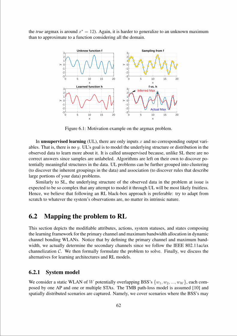
“main” — 2020/11/19 — 10:04 — page 62 — #84

the true argmax is around x∗ = 12). Again, it is harder to generalize to an unknown maximumthan to approximate to a function considering all the domain.

0 5 10 15 20x

-3

-2

-1

0

1

2

3

y

Unknow function f

0 5 10 15 20x

-3

-2

-1

0

1

2

3

y

Sampling from f

0 5 10 15 20x

-3

-2

-1

0

1

2

3

y

Learned function h

0 5 10 15 20x

-3

-2

-1

0

1

2

3

y

f vs. hInferred Max

Actual Max

Figure 6.1: Motivation example on the argmax problem.

In unsupervised learning (UL), there are only inputs x and no corresponding output vari-ables. That is, there is no y. UL’s goal is to model the underlying structure or distribution in theobserved data to learn more about it. It is called unsupervised because, unlike SL there are nocorrect answers since samples are unlabeled. Algorithms are left on their own to discover po-tentially meaningful structures in the data. UL problems can be further grouped into clustering(to discover the inherent groupings in the data) and association (to discover rules that describelarge portions of your data) problems.

Similarly to SL, the underlying structure of the observed data in the problem at issue isexpected to be so complex that any attempt to model it through UL will be most likely fruitless.Hence, we believe that following an RL black-box approach is preferable: try to adapt fromscratch to whatever the system’s observations are, no matter its intrinsic nature.

6.2 Mapping the problem to RLThis section depicts the modifiable attributes, actions, system statuses, and states composingthe learning framework for the primary channel and maximum bandwidth allocation in dynamicchannel bonding WLANs. Notice that by defining the primary channel and maximum band-width, we actually determine the secondary channels since we follow the IEEE 802.11ac/axchannelization C. We then formally formulate the problem to solve. Finally, we discuss thealternatives for learning architectures and RL models.

6.2.1 System model

We consider a static WLAN of W potentially overlapping BSS’s w1, w2, ..., wW, each com-posed by one AP and one or multiple STAs. The TMB path-loss model is assumed [10] andspatially distributed scenarios are captured. Namely, we cover scenarios where the BSS’s may

62

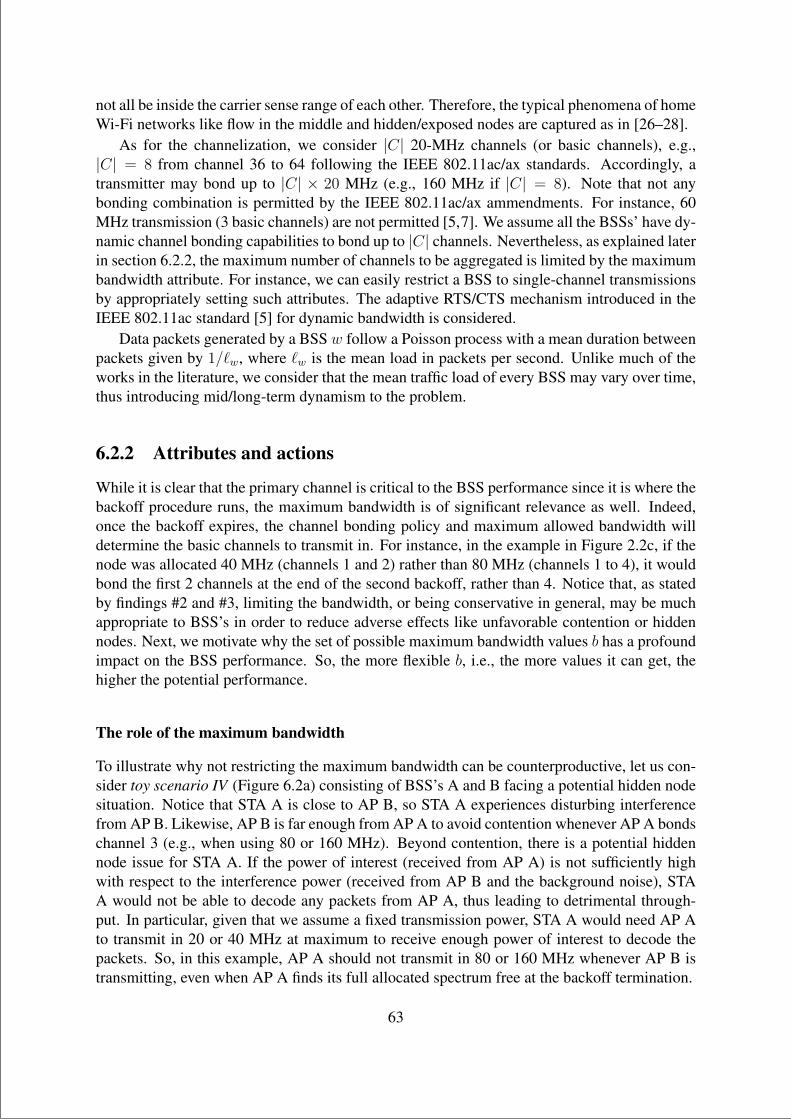
“main” — 2020/11/19 — 10:04 — page 63 — #85

not all be inside the carrier sense range of each other. Therefore, the typical phenomena of homeWi-Fi networks like flow in the middle and hidden/exposed nodes are captured as in [26–28].

As for the channelization, we consider |C| 20-MHz channels (or basic channels), e.g.,|C| = 8 from channel 36 to 64 following the IEEE 802.11ac/ax standards. Accordingly, atransmitter may bond up to |C| × 20 MHz (e.g., 160 MHz if |C| = 8). Note that not anybonding combination is permitted by the IEEE 802.11ac/ax ammendments. For instance, 60MHz transmission (3 basic channels) are not permitted [5,7]. We assume all the BSSs’ have dy-namic channel bonding capabilities to bond up to |C| channels. Nevertheless, as explained laterin section 6.2.2, the maximum number of channels to be aggregated is limited by the maximumbandwidth attribute. For instance, we can easily restrict a BSS to single-channel transmissionsby appropriately setting such attributes. The adaptive RTS/CTS mechanism introduced in theIEEE 802.11ac standard [5] for dynamic bandwidth is considered.

Data packets generated by a BSS w follow a Poisson process with a mean duration betweenpackets given by 1/`w, where `w is the mean load in packets per second. Unlike much of theworks in the literature, we consider that the mean traffic load of every BSS may vary over time,thus introducing mid/long-term dynamism to the problem.

6.2.2 Attributes and actions

While it is clear that the primary channel is critical to the BSS performance since it is where thebackoff procedure runs, the maximum bandwidth is of significant relevance as well. Indeed,once the backoff expires, the channel bonding policy and maximum allowed bandwidth willdetermine the basic channels to transmit in. For instance, in the example in Figure 2.2c, if thenode was allocated 40 MHz (channels 1 and 2) rather than 80 MHz (channels 1 to 4), it wouldbond the first 2 channels at the end of the second backoff, rather than 4. Notice that, as statedby findings #2 and #3, limiting the bandwidth, or being conservative in general, may be muchappropriate to BSS’s in order to reduce adverse effects like unfavorable contention or hiddennodes. Next, we motivate why the set of possible maximum bandwidth values b has a profoundimpact on the BSS performance. So, the more flexible b, i.e., the more values it can get, thehigher the potential performance.

The role of the maximum bandwidth

To illustrate why not restricting the maximum bandwidth can be counterproductive, let us con-sider toy scenario IV (Figure 6.2a) consisting of BSS’s A and B facing a potential hidden nodesituation. Notice that STA A is close to AP B, so STA A experiences disturbing interferencefrom AP B. Likewise, AP B is far enough from AP A to avoid contention whenever AP A bondschannel 3 (e.g., when using 80 or 160 MHz). Beyond contention, there is a potential hiddennode issue for STA A. If the power of interest (received from AP A) is not sufficiently highwith respect to the interference power (received from AP B and the background noise), STAA would not be able to decode any packets from AP A, thus leading to detrimental through-put. In particular, given that we assume a fixed transmission power, STA A would need AP Ato transmit in 20 or 40 MHz at maximum to receive enough power of interest to decode thepackets. So, in this example, AP A should not transmit in 80 or 160 MHz whenever AP B istransmitting, even when AP A finds its full allocated spectrum free at the backoff termination.

63

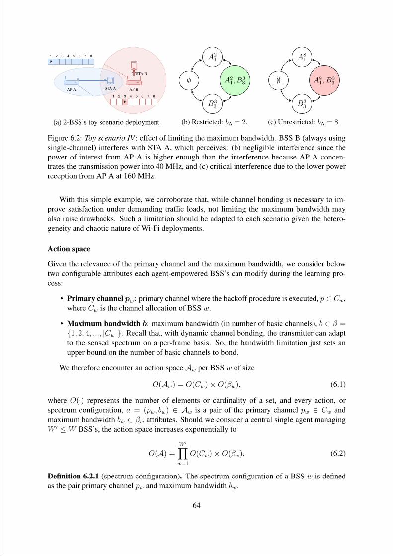
“main” — 2020/11/19 — 10:04 — page 64 — #86

APA STAA APB

STAB

P1 2 3 4 5 6 7 8

P1 2 3 4 5 6 7 8

(a) 2-BSS’s toy scenario deployment.

∅

A21

B33

A21, B

33

(b) Restricted: bA = 2.

∅

A81

B33

A81, B

33

(c) Unrestricted: bA = 8.

Figure 6.2: Toy scenario IV: effect of limiting the maximum bandwidth. BSS B (always usingsingle-channel) interferes with STA A, which perceives: (b) negligible interference since thepower of interest from AP A is higher enough than the interference because AP A concen-trates the transmission power into 40 MHz, and (c) critical interference due to the lower powerreception from AP A at 160 MHz.

With this simple example, we corroborate that, while channel bonding is necessary to im-prove satisfaction under demanding traffic loads, not limiting the maximum bandwidth mayalso raise drawbacks. Such a limitation should be adapted to each scenario given the hetero-geneity and chaotic nature of Wi-Fi deployments.

Action space

Given the relevance of the primary channel and the maximum bandwidth, we consider belowtwo configurable attributes each agent-empowered BSS’s can modify during the learning pro-cess:

• Primary channel pw: primary channel where the backoff procedure is executed, p ∈ Cw,where Cw is the channel allocation of BSS w.

• Maximum bandwidth b: maximum bandwidth (in number of basic channels), b ∈ β =1, 2, 4, ..., |Cw|. Recall that, with dynamic channel bonding, the transmitter can adaptto the sensed spectrum on a per-frame basis. So, the bandwidth limitation just sets anupper bound on the number of basic channels to bond.

We therefore encounter an action space Aw per BSS w of size

O(Aw) = O(Cw)×O(βw), (6.1)

where O(·) represents the number of elements or cardinality of a set, and every action, orspectrum configuration, a = (pw, bw) ∈ Aw is a pair of the primary channel pw ∈ Cw andmaximum bandwidth bw ∈ βw attributes. Should we consider a central single agent managingW ′ ≤ W BSS’s, the action space increases exponentially to

O(A) =W ′∏

w=1

O(Cw)×O(βw). (6.2)

Definition 6.2.1 (spectrum configuration). The spectrum configuration of a BSS w is definedas the pair primary channel pw and maximum bandwidth bw.

64

“main” — 2020/11/19 — 10:04 — page 65 — #87

If we assume that BSS’s have the same attribute spaces C and β, ∀w, then we clearly ob-

serve the exponential growth of the whole action space O(A) =(O(C)×O(β)

)W ′.

6.2.3 Statuses, observations and statesBefore discussing what is an state, which its definition highly depends on the RL framework inuse, let us coin a new concept called system status to depict how the whole WLAN looks likeat time t.

Definition 6.2.2 (system status). The system statusHt is the minimum information we need todescribe the entire WLAN in a given time instant t.

The system statusHt of a static WLAN deployment2 at time t is given by three key parame-ters of each of the W ′ agent-empowered BSS in the WLAN like if we were taking a screenshotof the system: the primary channel pw,t, the maximum bandwidth bw,t, and the quantized meanload `w,t. Formally, a status is defined by the set

Ht = (p1,t, b1,t, `1,t), (p2,t, b2,t, `2,t), ..., (pW ′,t, bW ′,t, `W ′,t). (6.3)

First, notice that we only consider the attributes of the agent-empowered BSS’s since therest of BSS’s are not allowed to modify its configuration; thus, they do not convey any extrainformation for the status. For instance, let us consider a deployment with just a couple ofBSS’s, A and B. Assume A is agent-empowered, whereas B is not, so W ′ = 1 and W = 2. Thesystem information relies just on the configuration of A since B will never change its own. So,the number of system statuses is just the number of possible configurations A can take.

Second, we rely on a quantization L of the mean traffic load ` to discretize its continu-ous domain. Further, notice that the agent cannot modify the load ` by any means since it isapplication-dependent. Naturally, the throughput performance depends on the traffic load, theAP configuration, and the rest of BSS’s configurations and loads.

Definition 6.2.3 (world). The world (or environment) of a particular BSS w is defined as thecombination of configurations and loads of each of the rest BSS’s.

From the point of view of a particular BSS w, the combination of current spectrum con-figurations and loads of the rest BSS’s conform its world or environment, which is determinedas

Iw,t = pw′,t, bw′,t, `w′,t|w′ 6= w. (6.4)

Finally, the amount of possible statuses a certain deployment may have is given by thepossible values each of the status parameters can take,

O(H) =W ′∏

w=1

O(pw)O(bw)O(`w), (6.5)

which raises again exponentially with the number of agents and size of the attributes’ spaces.Assuming all the agent-empowered BSS’s have the same capabilities,

O(H) =(O(p)O(b)O(`)

)W ′. (6.6)

2Static refers to the fixed locations of all the nodes in the WLANs, including APs and STAs.

65

“main” — 2020/11/19 — 10:04 — page 66 — #88

Naturally, most of the time, the agents cannot know the system’s status in a real-time fash-ion. However, they could rely on partial and delayed observations to then infer the most ac-curate state through some discretization function. Besides, since observations are architecture-dependent – given they may be limited to local sensing capabilities or, on the contrary, beshared via a central controller – the states’ definition is also strictly dependent on the RL modelunder consideration.

6.2.4 Problem definitionIn general terms, our goal is to improve the BSS’s performance by maximizing their throughputand minimizing their delay. The key then is to let the BSS’s find (learn) the best actions (p, b),where best depends on the problem formulation itself. For instance, we could assess a max-min approach to maximize the throughput satisfaction experienced by the less favored BSS.Another common aim in network management is to boost the fairness of some performancemetric among contending BSS’s in the WLAN. This thesis does not stick into one problemformulation, but we instead evaluate different performance metrics, including individual andaggregated ones.

In any case, we must define the individual performance metrics of each BSS to assesswhether such metrics tend to improve (i.e., the learning is working) or not. We focus on thethroughput satisfaction ξ and the delay d. First, the throughput satisfaction of a BSS w atiteration t is simply defined as the ratio of throughput Γw,t to generated traffic load `w,t,

ξw,t =Γw,t`w,t

. (6.7)

So, ξw,t ∈ [0, 1],∀w, t. The throughput satisfaction is a commonly used parameter to indicatethe ratio of packets acknowledged to the number of packets generated by a BSS in a given timewindow. Thus, a satisfaction value ξ = 1 indicates that all the traffic has been successfullyreceived at the destination.

Second, the delay is defined as the mean data packet delay, simply computed as the timedifference between a data packet being generated and acknowledged. Unfortunately, the delayis not bounded, which is convenient for guaranteeing most RL algorithms’ convergence. Thus,we propose a bounded delay ratio defined as

δw,t =d∗

dw,t, (6.8)

where dw,t is the mean delay during iteration t, and d∗ is the known minimum achievable delayexperienced when transmitting a single data packet at maximum MCS 11. So, δw,t < 1,∀w, tholds because every BSS will always experience a delay higher than d∗ simply due to the MACinterframes (SIFS, DIFS) and control packets exchange (RTS, CTS, ACK).

Once the two main performance metrics have been defined, we may formulate the rewardfunction R, the philosopher stone of any RL algorithm. In this work, we assess two definitionsof R: only throughput based,

R(ξ) = ξ, (6.9)

and a throughput-delay mix,R(ξ, δ) = ξ · δ, (6.10)

66

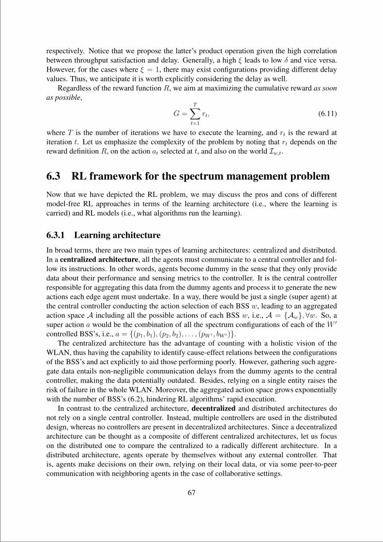
“main” — 2020/11/19 — 10:04 — page 67 — #89

respectively. Notice that we propose the latter’s product operation given the high correlationbetween throughput satisfaction and delay. Generally, a high ξ leads to low δ and vice versa.However, for the cases where ξ = 1, there may exist configurations providing different delayvalues. Thus, we anticipate it is worth explicitly considering the delay as well.

Regardless of the reward function R, we aim at maximizing the cumulative reward as soonas possible,

G =T∑

t=1

rt, (6.11)

where T is the number of iterations we have to execute the learning, and rt is the reward atiteration t. Let us emphasize the complexity of the problem by noting that rt depends on thereward definition R, on the action at selected at t, and also on the world Iw,t.

6.3 RL framework for the spectrum management problemNow that we have depicted the RL problem, we may discuss the pros and cons of differentmodel-free RL approaches in terms of the learning architecture (i.e., where the learning iscarried) and RL models (i.e., what algorithms run the learning).

6.3.1 Learning architectureIn broad terms, there are two main types of learning architectures: centralized and distributed.In a centralized architecture, all the agents must communicate to a central controller and fol-low its instructions. In other words, agents become dummy in the sense that they only providedata about their performance and sensing metrics to the controller. It is the central controllerresponsible for aggregating this data from the dummy agents and process it to generate the newactions each edge agent must undertake. In a way, there would be just a single (super agent) atthe central controller conducting the action selection of each BSS w, leading to an aggregatedaction space A including all the possible actions of each BSS w, i.e., A = Aw,∀w. So, asuper action a would be the combination of all the spectrum configurations of each of the W ′

controlled BSS’s, i.e., a = (p1, b1), (p2, b2), . . . , (pW ′ , bW ′).The centralized architecture has the advantage of counting with a holistic vision of the

WLAN, thus having the capability to identify cause-effect relations between the configurationsof the BSS’s and act explicitly to aid those performing poorly. However, gathering such aggre-gate data entails non-negligible communication delays from the dummy agents to the centralcontroller, making the data potentially outdated. Besides, relying on a single entity raises therisk of failure in the whole WLAN. Moreover, the aggregated action space grows exponentiallywith the number of BSS’s (6.2), hindering RL algorithms’ rapid execution.

In contrast to the centralized architecture, decentralized and distributed architectures donot rely on a single central controller. Instead, multiple controllers are used in the distributeddesign, whereas no controllers are present in decentralized architectures. Since a decentralizedarchitecture can be thought as a composite of different centralized architectures, let us focuson the distributed one to compare the centralized to a radically different architecture. In adistributed architecture, agents operate by themselves without any external controller. Thatis, agents make decisions on their own, relying on their local data, or via some peer-to-peercommunication with neighboring agents in the case of collaborative settings.

67

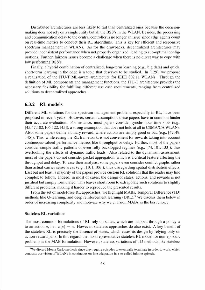
“main” — 2020/11/19 — 10:04 — page 68 — #90

Distributed architectures are less likely to fail than centralized ones because the decision-making does not rely on a single entity but all the BSS’s in the WLAN. Besides, the processingand communication delay to the central controller is no longer an issue since edge agents counton real-time metrics to conduct their RL algorithms. This is key for efficient and responsivespectrum management in WLANs. As for the drawbacks, decentralized architectures mayprovide inconsistent performance when not properly organized, leading to sub-optimal config-urations. Further, fairness issues become a challenge when there is no direct way to cope withlow performing BSS’s.

Finally, a hybrid combination of centralized, long-term learning (e.g., big data) and quick,short-term learning in the edge is a topic that deserves to be studied. In [129], we proposea realization of the ITU-T ML-aware architecture for IEEE 802.11 WLANs. Through thedefinition of ML components and management functions, the ITU-T architecture provides thenecessary flexibility for fulfilling different use case requirements, ranging from centralizedsolutions to decentralized approaches.

6.3.2 RL modelsDifferent ML solutions for the spectrum management problem, especially in RL, have beenproposed in recent years. However, certain assumptions these papers have in common hindertheir accurate evaluation. For instance, most papers consider synchronous time slots (e.g.,[45,47,102,106,122,145]), a strong assumption that does not hold at all in CSMA/CA WLANs.Also, some papers define a binary reward, where actions are simply good or bad (e.g., [47, 49,145]). This, while easing the RL framework, is not convenient for rewards taking into accountcontinuous-valued performance metrics like throughput or delay. Further, most of the papersconsider simple traffic patterns or even fully backlogged regimes (e.g., [74, 101, 133]), thusoverlooking the effects of dynamic traffic loads. Also related to the dynamism assessment,most of the papers do not consider packet aggregation, which is a critical feature affecting thethroughput and delay. To ease their analysis, some papers even consider conflict graphs ratherthan actual carrier sense areas (e.g., [101, 106]), thus disregarding spatial distribution effects.Last but not least, a majority of the papers provide custom RL solutions that the reader may findcomplex to follow. Indeed, in most of cases, the design of states, actions, and rewards is notjustified but simply formulated. This leaves short room to extrapolate such solutions to slightlydifferent problems, making it harder to reproduce the presented results.

From the set of model-free RL approaches, we highlight MABs, Temporal Difference (TD)methods like Q-learning, and deep reinforcement learning (DRL).3 We discuss them below inorder of increasing complexity and motivate why we envision MABs as the best choice.

Stateless RL variations

The most common formulations of RL rely on states, which are mapped through a policy πto an action a, i.e., π(s) = a. However, stateless approaches do also exist. A key benefit ofthe stateless RL is precisely the absence of states, which eases its design by relying only onaction-reward pairs. In this regard, the most representative stateless RL model for non-episodicproblems is the MAB formulation. However, stateless variations of TD methods like stateless

3We discard Monte Carlo methods since they require episodes to eventually terminate in order to work, whichcontrasts our vision of WLANs in continuous on-line adaptation in a so-called infinite episode.

68

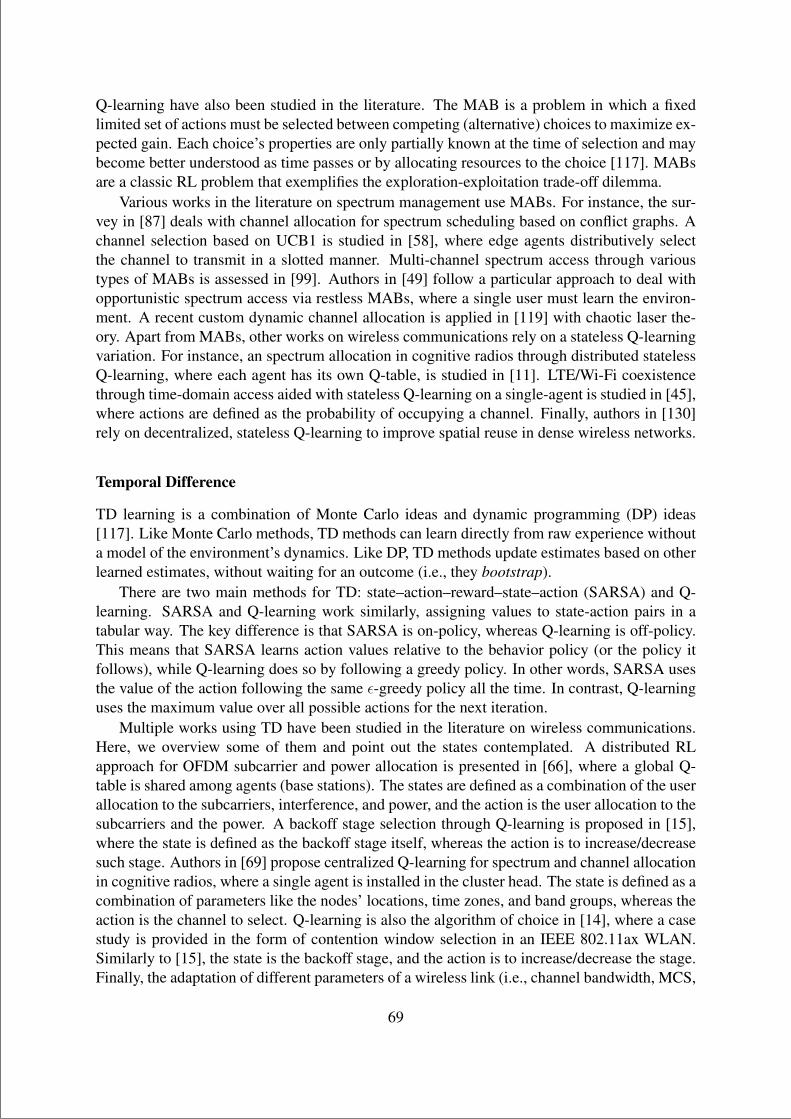
“main” — 2020/11/19 — 10:04 — page 69 — #91

Q-learning have also been studied in the literature. The MAB is a problem in which a fixedlimited set of actions must be selected between competing (alternative) choices to maximize ex-pected gain. Each choice’s properties are only partially known at the time of selection and maybecome better understood as time passes or by allocating resources to the choice [117]. MABsare a classic RL problem that exemplifies the exploration-exploitation trade-off dilemma.

Various works in the literature on spectrum management use MABs. For instance, the sur-vey in [87] deals with channel allocation for spectrum scheduling based on conflict graphs. Achannel selection based on UCB1 is studied in [58], where edge agents distributively selectthe channel to transmit in a slotted manner. Multi-channel spectrum access through varioustypes of MABs is assessed in [99]. Authors in [49] follow a particular approach to deal withopportunistic spectrum access via restless MABs, where a single user must learn the environ-ment. A recent custom dynamic channel allocation is applied in [119] with chaotic laser the-ory. Apart from MABs, other works on wireless communications rely on a stateless Q-learningvariation. For instance, an spectrum allocation in cognitive radios through distributed statelessQ-learning, where each agent has its own Q-table, is studied in [11]. LTE/Wi-Fi coexistencethrough time-domain access aided with stateless Q-learning on a single-agent is studied in [45],where actions are defined as the probability of occupying a channel. Finally, authors in [130]rely on decentralized, stateless Q-learning to improve spatial reuse in dense wireless networks.

Temporal Difference

TD learning is a combination of Monte Carlo ideas and dynamic programming (DP) ideas[117]. Like Monte Carlo methods, TD methods can learn directly from raw experience withouta model of the environment’s dynamics. Like DP, TD methods update estimates based on otherlearned estimates, without waiting for an outcome (i.e., they bootstrap).

There are two main methods for TD: state–action–reward–state–action (SARSA) and Q-learning. SARSA and Q-learning work similarly, assigning values to state-action pairs in atabular way. The key difference is that SARSA is on-policy, whereas Q-learning is off-policy.This means that SARSA learns action values relative to the behavior policy (or the policy itfollows), while Q-learning does so by following a greedy policy. In other words, SARSA usesthe value of the action following the same ε-greedy policy all the time. In contrast, Q-learninguses the maximum value over all possible actions for the next iteration.

Multiple works using TD have been studied in the literature on wireless communications.Here, we overview some of them and point out the states contemplated. A distributed RLapproach for OFDM subcarrier and power allocation is presented in [66], where a global Q-table is shared among agents (base stations). The states are defined as a combination of the userallocation to the subcarriers, interference, and power, and the action is the user allocation to thesubcarriers and the power. A backoff stage selection through Q-learning is proposed in [15],where the state is defined as the backoff stage itself, whereas the action is to increase/decreasesuch stage. Authors in [69] propose centralized Q-learning for spectrum and channel allocationin cognitive radios, where a single agent is installed in the cluster head. The state is defined as acombination of parameters like the nodes’ locations, time zones, and band groups, whereas theaction is the channel to select. Q-learning is also the algorithm of choice in [14], where a casestudy is provided in the form of contention window selection in an IEEE 802.11ax WLAN.Similarly to [15], the state is the backoff stage, and the action is to increase/decrease the stage.Finally, the adaptation of different parameters of a wireless link (i.e., channel bandwidth, MCS,

69

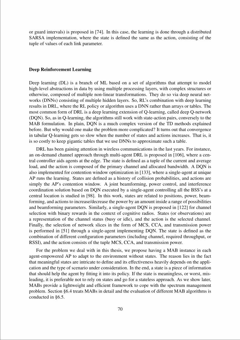
“main” — 2020/11/19 — 10:04 — page 70 — #92

or guard intervals) is proposed in [74]. In this case, the learning is done through a distributedSARSA implementation, where the state is defined the same as the action, consisting of thetuple of values of each link parameter.

Deep Reinforcement Learning

Deep learning (DL) is a branch of ML based on a set of algorithms that attempt to modelhigh-level abstractions in data by using multiple processing layers, with complex structures orotherwise, composed of multiple non-linear transformations. They do so via deep neural net-works (DNNs) consisting of multiple hidden layers. So, RL’s combination with deep learningresults in DRL, where the RL policy or algorithm uses a DNN rather than arrays or tables. Themost common form of DRL is a deep learning extension of Q-learning, called deep Q-network(DQN). So, as in Q-learning, the algorithms still work with state-action pairs, conversely to theMAB formulation. In plain, DQN is a much complex version of the TD methods explainedbefore. But why would one make the problem more complicated? It turns out that convergencein tabular Q-learning gets so slow when the number of states and actions increases. That is, itis so costly to keep gigantic tables that we use DNNs to approximate such a table.

DRL has been gaining attention in wireless communications in the last years. For instance,an on-demand channel approach through multi-agent DRL is proposed in [106], where a cen-tral controller aids agents at the edge. The state is defined as a tuple of the current and averageload, and the action is composed of the primary channel and allocated bandwidth. A DQN isalso implemented for contention window optimization in [133], where a single-agent at uniqueAP runs the learning. States are defined as a history of collision probabilities, and actions aresimply the AP’s contention window. A joint beamforming, power control, and interferencecoordination solution based on DQN executed by a single-agent controlling all the BSS’s at acentral location is studied in [98]. In this work, states are related to positions, power, beam-forming, and actions to increase/decrease the power by an amount inside a range of possibilitiesand beamforming parameters. Similarly, a single-agent DQN is proposed in [122] for channelselection with binary rewards in the context of cognitive radios. States (or observations) area representation of the channel status (busy or idle), and the action is the selected channel.Finally, the selection of network slices in the form of MCS, CCA, and transmission poweris performed in [51] through a single-agent implementing DQN. The state is defined as thecombination of different configuration parameters (including channel, required throughput, orRSSI), and the action consists of the tuple MCS, CCA, and transmission power.

For the problem we deal with in this thesis, we propose having a MAB instance in eachagent-empowered AP to adapt to the environment without states. The reason lies in the factthat meaningful states are intricate to define and its effectiveness heavily depends on the appli-cation and the type of scenario under consideration. In the end, a state is a piece of informationthat should help the agent by fitting it into its policy. If the state is meaningless, or worst, mis-leading, it is preferable not to rely on states and go for a stateless approach. As we show later,MABs provide a lightweight and efficient framework to cope with the spectrum managementproblem. Section §6.4 treats MABs in detail and the evaluation of different MAB algorithms isconducted in §6.5.

70

“main” — 2020/11/19 — 10:04 — page 71 — #93

Proposed RL approach: First, we envision a distributed architecture rather than acentralized one to boost the responsiveness and adaptability in highly dynamic environ-ments. Second, we propose a MAB formulation for the RL problem to speed up thelearning convergence by disregarding states.

6.4 Multi-Armed BanditsIn this thesis, we tackle the spectrum allocation problem in WLANs as a MAB due to itsready-to-use conception for problems facing the exploration-exploitation trade-off. Namely,we would like the agent to learn the best action quickly, but at the same time, we want the agentto perform as good as possible along its quest to find such action.

6.4.1 The MAB problemThe multi-armed bandit problem is a classic RL problem that exemplifies the exploration vs.exploitation dilemma, where no knowledge on the reward probability distribution of each ac-tion is assumed. The typical example to introduce the MAB problem is the gambler who facesmultiple slot machines, each with different probability distributions over the money he/she canget after pulling the slots. Naturally, the gambler wants to get as much money as possible,thus achieving the highest reward in the mid/long-term. So, what strategy should he/she fol-low? That is where the MAB problem arises with its different variations. For instance, a naiveapproach would be to pull each machine slot a lot of times, so the gambler could guess the “au-thentic” reward probability of each slot according to the law of large numbers, and then selectalways the best slot machine. However, such an approach has obvious pitfalls like determininghow many times are enough to discover the “true” reward probability or wasting too many tri-als (or iterations) in a priori lousy machines. Further, in environments where the distribution ofsuch rewards may change due to external actors (as it is the case in WLANs), it would not beviable to get accurate estimates of the reward probability distributions. Simply because fromone iteration to the other, the underlying reward distribution may be completely changed.

Formally, a MAB can be described as a tuple of the set of actions and the reward function< A, R >, where:

• There are K arms (slot machines in the previous example or spectrum management con-figurations in this thesis) with hidden reward probabilities θ1, . . . , θK. A is the set ofactions (or action space), each referring to the interaction with one arm.

• At each time step (or iteration) t, we take an action (or arm) a and observe a reward rtresulting from performing such action.

• We refer to the value of an action a as the expected reward, Q(a) = Eθa [r|a], determinedby the reward distribution θa.

• Finally, the reward function R defines the reward values obtained at any time step t,rt = R(at). For instance, R(at) could be defined in the previous example as the moneyearned in the last slot pull or as the throughput experienced by a BSS when using actionat during the last iteration t.

71

“main” — 2020/11/19 — 10:04 — page 72 — #94

Notice the difference betweenR(at) andQ(at). While rt = R(at) is the actual reward observedwhen applying action at in iteration t (e.g., throughput observed when playing at at iterationt), Q(at) is the expected value of playing at (e.g., mean future throughput when playing atregardless t). In other words, R(at) is a particular outcome of the reward distribution θ(at),whereas Q(at) is a representation (or statistic) of the arm’s value (e.g., mean reward).

The goal is to maximize the cumulative rewardG over a finite number of iterations T (6.11).The simplest action selection rule (or policy π) is to select one of the actions with the highestestimated value, that is, one of the greedy actions, πt = at = arg maxa∈AQt(a). However,greedy selection always exploits current knowledge to maximize the immediate reward, i.e., itdoes not sample the rest of a priori inferior actions. So, what happens if the action that we haveranked as the best is not? There are more sophisticated selection rule alternatives like ε-greedymethods, which force exploration with some probability ε to achieve better knowledge on therewards of the actions in the whole action space. We depict some of the most relevant ones in§6.4.3.

6.4.2 MAB taxonomies

There are different types of MABs. They can be categorized according to three main concepts:the type of reward, the use of contexts, and the temporal horizon.

Reward taxonomy

According to its reward distribution, there are two main classes of MABs: stochastic and adver-sarial. The stochastic MAB is the most common one, and it is completely determined by thedistributions of rewards θ1, . . . , θK of the actions in the action space. In particular, in iterationt, the distribution of the reward observed by a learner that chose action at ∈ A is θa, regard-less of the past rewards and actions. The reward for each action is independent and identicallydistributed (i.i.d). That is, every time an action is chosen, the reward is sampled independentlyfrom this distribution. Both for simplicity and for guaranteeing theoretical convergence in cer-tain MAB algorithms, the reward function is bounded, rt = R(at) ∈ [0, 1], ∀a, t, so normalizedperformance metrics (e.g., throughput satisfaction) are normally used. The main limitation ofstochastic MABs is the difficulty of finding real-world problems that rely on suitable distri-butions. Indeed, rewards can be non-stationary; thus, the reward distribution probability fora given action may change over time. Next, we present adversarial MABs, a paradigmaticexample of non-stationary rewards.

In adversarial MABs, learning is still possible in the sense that the regret can be kept sub-linear. However, selection rules methods must be completely different from the stochastic onessince adversarial rewards can be arbitrary, as if they are chosen by an “omniscient adversary”,so the stochastic assumption on the rewards being generated from a fixed distribution does notlonger hold. In plain, there are no probability distributions to learn whatsoever. Then, what canthe agent do to face such an adversary? The key idea is to introduce noise in the exploration tochoose random actions that the adversary could not expect.

So, what class of MAB suits better the joint spectrum management problem? We anticipatethat the stochastic one. Even though the different actions’ reward distributions are generallycomplex to estimate, no omniscient adversary tells what the rewards will be at every itera-tion. Instead, we have different actors (nodes) that behave according to a certain configuration

72

“main” — 2020/11/19 — 10:04 — page 73 — #95

each. Such configurations determine what the actors will do, resulting in a stochastic setting.Nonetheless, even though the problem is likely to be stochastic, it is so complex that an adver-sarial approach when we assume that no distributions should (or could) be learned may alsobe appropriate to design a fruitful algorithm. Accordingly, we assess in further sections theconvenience of both stochastic and adversarial MABs.

Context taxonomy

While the general MAB formulation does not consider states, contexts may be used to fine-grain the arm selection based not only on the gathered rewards, but also on further observationsabout the world I. Essentially, we may categorize MABs in context-less and contextual MABs.Context-less are the general MAB formulation where no contexts are assumed.

Conversely, in contextual bandits, reward distributions depend on a context, which is fitto the RL algorithm before making a decision. Now, the observed reward rt in each iterationt depends both on the context Ωt and the chosen action at. For instance, assume that an APobserves that a given basic channel, say basic channel 2, is busy most of the time. The derivedcontext would then represent that channel 2 is active. Thus, it is not the same to apply the actioncorresponding to pick primary p = 2 when the context indicates channel 2 is busy rather thanapplying the same action when such channel is idle. Henceforth, it seems that contexts mayaid to the spectrum management problem, especially if we leverage knowledge from previouscontexts (e.g., similar contexts stochastically repeated every day). However, contextual MABsalso pose the challenge of appropriately defining contexts, meaning that a good representationof the world I should be captured in each context.

There are different approaches within the contextual bandit problem. The simplest one,while the most versatile, considers a separate MAB per context (as if each context was a state).Then, the goal is to find the optimal action a∗(Ωt) = π∗(Ωt) per context Ωt.

So, should we go for a contextual bandit approach to tackle the joint spectrum managementproblem? We believe that it is better not to. Essentially, defining contexts may be as complexas defining states. And what would be an appropriate context definition? the current action,Ωt = at? The current reward, Ωt = rt? A mix of the action selected and the reward Ωt =f(at, rt)? A mix including also historical information Ωt = f(at−t′ , . . . , at, rt−t′ , . . . , rt)?Unfortunately, we do not find any definition that suits our multi-agent and non-stationary re-ward problem. The reason lies in the fact that we want to boost the learning speed to raisethe user experience in the short/mid-term. Then, relying on a different MAB per action in acontextual fashion would entail large and potentially unfruitful learning periods.

Temporal taxonomy

The last taxonomy we identify is the temporal one, defined by the duration imposed by theprogrammer to converge to a good solution, which determines the horizon: finite or infinite.Finite-horizon refers to when there is a need to perform (explore and exploit) during a giventime window (e.g., 5 minutes). So, the number of iterations T the agent counts with is finite.Thus, the RL algorithm must try to get the most accumulated reward (6.11) with that ending inmind.

Infinite-horizon, in contrast, poses no time limit to the agent to converge, i.e., T → ∞.As a matter of fact, in many problems, a finite time horizon cannot be easily specified, so the

73

“main” — 2020/11/19 — 10:04 — page 74 — #96

infinite horizon formulation fits more naturally. More importantly, stationary problems withinfinite time horizon lead to optimal stationary strategies, which offer great simplicity.

For the joint spectrum management problem of this thesis, we will rely on finite horizons toassess the myopic nature of the MABs. We call it myopic in the sense that they try to optimizerewards now without any explicit use of forecast information or any direct representation ofdecisions in the future. Meaning we want BSS’s to improve its performance as soon as possible.

Proposed MAB approach: First, we choose to study stochastic rather than adversar-ial MABs because of WLANs’ non-adversarial nature. Second, we adopt the standardcontext-less formulation of MABs given the unfeasibility of defining lightweight mean-ingful context. Third, we study the performance of MABs in finite-horizon experimentsbecause we aim at boosting its learning speed.

6.4.3 MAB exploration strategies

Since any stochastic MAB problem can be seen as an instance of an adversarial problem, wemay apply all the following algorithms regardless of whether contexts are defined or not. Wedepict the different action selection strategies of choice below.

Exploration-first. (Algorithm 2 in the Appendix) The most simple MAB algorithm dedi-cates the first Texp rounds to exploration and the remaining T − Texp rounds to exploitation. Wemay mandate the full exploration of the action space, i.e., Texp = K to explore all the arms,as we do later in the experiments. Notice that in the event of an environment change after theexploration phase, action rewards may drastically change. Exploration-first copes with this is-sue by simply ranking actions according to their last observed reward. So, if the best action initeration t− 1 turns out to be the worst in t, since its reward is updated, the second-best actionin t − 1 is now the best in t and its pick accordingly in t + 1. Consequently, exploration isimplicitly carried when action rewards vary over time.

Epsilon-greedy. (Algorithm 3 in the Appendix) The ε-greedy or (e-greedy) algorithm takesthe best known action with probability 1 − ε, and explores a random action (previously ex-plored or not) with probability ε [125]. The action value Q is estimated, such estimationbeing represented as Q, according to the past experience by averaging the rewards associ-ated with the target action a that we have observed so far (up to the current time step t), i.e.,Qt(a) = 1

Nt(a)

∑tτ=1 rτ1[aτ = a], where 1 is a binary indicator function telling whether the

action a was used in a given iteration, and Nt(a) is the number of times the action a has beenselected so far, i.e., Nt(a) =

∑tτ=1 1[aτ = a]. In an exploring iteration, any action is picked

with same probability, whereas in an exploitation iteration, the best estimated action is picked,i.e., a = argmaxa∈A Qt(a). As for the experiments later presented, we set the original epsilonvalue ε0 = 1 to force exploration. Besides, to avoid inefficient exploration after enough itera-tions, we decrease the parameter ε to reduce the probability of exploring over time as suggestedin [20].

UCB1. (Algorithm 4 in the Appendix) Due to the randomness in e-greedy, we may endup exploring a bad action that we have confirmed in the past. To avoid such inefficient ex-ploration, one approach is to decrease the parameter ε in time (as done in ε-greedy), and theother is to be optimistic about options with high uncertainty and thus to prefer actions for whichwe have not had a confident value estimation yet. The Upper Confidence Bounds (UCB1) al-

74

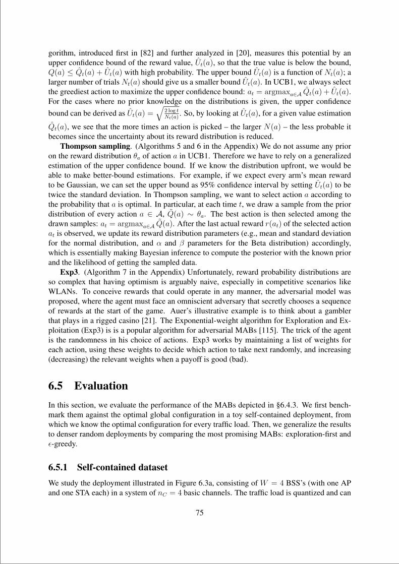
“main” — 2020/11/19 — 10:04 — page 75 — #97

gorithm, introduced first in [82] and further analyzed in [20], measures this potential by anupper confidence bound of the reward value, Ut(a), so that the true value is below the bound,Q(a) ≤ Qt(a) + Ut(a) with high probability. The upper bound Ut(a) is a function of Nt(a); alarger number of trials Nt(a) should give us a smaller bound Ut(a). In UCB1, we always selectthe greediest action to maximize the upper confidence bound: at = argmaxa∈A Qt(a) + Ut(a).For the cases where no prior knowledge on the distributions is given, the upper confidencebound can be derived as Ut(a) =

√2 log tNt(a)

. So, by looking at Ut(a), for a given value estimation

Qt(a), we see that the more times an action is picked – the larger N(a) – the less probable itbecomes since the uncertainty about its reward distribution is reduced.

Thompson sampling. (Algorithms 5 and 6 in the Appendix) We do not assume any prioron the reward distribution θa of action a in UCB1. Therefore we have to rely on a generalizedestimation of the upper confidence bound. If we know the distribution upfront, we would beable to make better-bound estimations. For example, if we expect every arm’s mean rewardto be Gaussian, we can set the upper bound as 95% confidence interval by setting Ut(a) to betwice the standard deviation. In Thompson sampling, we want to select action a according tothe probability that a is optimal. In particular, at each time t, we draw a sample from the priordistribution of every action a ∈ A, Q(a) ∼ θa. The best action is then selected among thedrawn samples: at = argmaxa∈A Q(a). After the last actual reward r(at) of the selected actionat is observed, we update its reward distribution parameters (e.g., mean and standard deviationfor the normal distribution, and α and β parameters for the Beta distribution) accordingly,which is essentially making Bayesian inference to compute the posterior with the known priorand the likelihood of getting the sampled data.

Exp3. (Algorithm 7 in the Appendix) Unfortunately, reward probability distributions areso complex that having optimism is arguably naive, especially in competitive scenarios likeWLANs. To conceive rewards that could operate in any manner, the adversarial model wasproposed, where the agent must face an omniscient adversary that secretly chooses a sequenceof rewards at the start of the game. Auer’s illustrative example is to think about a gamblerthat plays in a rigged casino [21]. The Exponential-weight algorithm for Exploration and Ex-ploitation (Exp3) is is a popular algorithm for adversarial MABs [115]. The trick of the agentis the randomness in his choice of actions. Exp3 works by maintaining a list of weights foreach action, using these weights to decide which action to take next randomly, and increasing(decreasing) the relevant weights when a payoff is good (bad).

6.5 EvaluationIn this section, we evaluate the performance of the MABs depicted in §6.4.3. We first bench-mark them against the optimal global configuration in a toy self-contained deployment, fromwhich we know the optimal configuration for every traffic load. Then, we generalize the resultsto denser random deployments by comparing the most promising MABs: exploration-first andε-greedy.

6.5.1 Self-contained datasetWe study the deployment illustrated in Figure 6.3a, consisting of W = 4 BSS’s (with one APand one STA each) in a system of nC = 4 basic channels. The traffic load is quantized and can

75

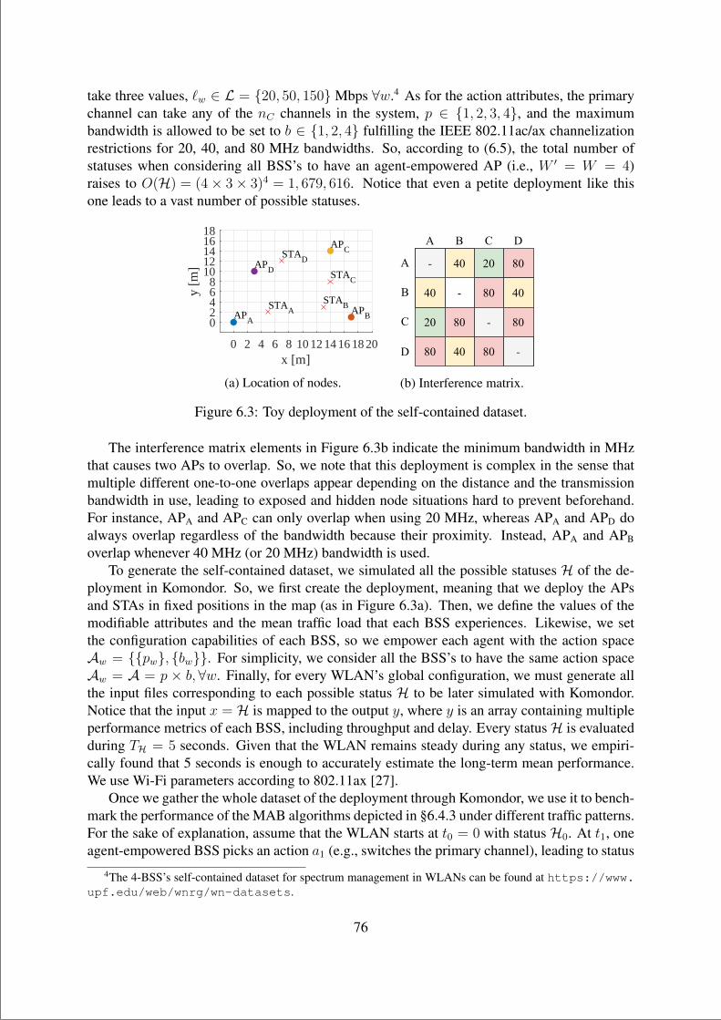
“main” — 2020/11/19 — 10:04 — page 76 — #98

take three values, `w ∈ L = 20, 50, 150Mbps ∀w.4 As for the action attributes, the primarychannel can take any of the nC channels in the system, p ∈ 1, 2, 3, 4, and the maximumbandwidth is allowed to be set to b ∈ 1, 2, 4 fulfilling the IEEE 802.11ac/ax channelizationrestrictions for 20, 40, and 80 MHz bandwidths. So, according to (6.5), the total number ofstatuses when considering all BSS’s to have an agent-empowered AP (i.e., W ′ = W = 4)raises to O(H) = (4× 3× 3)4 = 1, 679, 616. Notice that even a petite deployment like thisone leads to a vast number of possible statuses.

0 2 4 6 8 10 12 14 16 18 20x [m]

02468

1012141618

y [m

]

APA

APB

APC

APD

STAA

STAB

STAC

STAD

(a) Location of nodes.

- 40 20 80

40 - 80 40

20 80 - 80

80 40 80 -

A

B

C

D

A B C D

40

40

-

-

-

(b) Interference matrix.

Figure 6.3: Toy deployment of the self-contained dataset.

The interference matrix elements in Figure 6.3b indicate the minimum bandwidth in MHzthat causes two APs to overlap. So, we note that this deployment is complex in the sense thatmultiple different one-to-one overlaps appear depending on the distance and the transmissionbandwidth in use, leading to exposed and hidden node situations hard to prevent beforehand.For instance, APA and APC can only overlap when using 20 MHz, whereas APA and APD doalways overlap regardless of the bandwidth because their proximity. Instead, APA and APB

overlap whenever 40 MHz (or 20 MHz) bandwidth is used.To generate the self-contained dataset, we simulated all the possible statuses H of the de-

ployment in Komondor. So, we first create the deployment, meaning that we deploy the APsand STAs in fixed positions in the map (as in Figure 6.3a). Then, we define the values of themodifiable attributes and the mean traffic load that each BSS experiences. Likewise, we setthe configuration capabilities of each BSS, so we empower each agent with the action spaceAw = pw, bw. For simplicity, we consider all the BSS’s to have the same action spaceAw = A = p × b,∀w. Finally, for every WLAN’s global configuration, we must generate allthe input files corresponding to each possible status H to be later simulated with Komondor.Notice that the input x = H is mapped to the output y, where y is an array containing multipleperformance metrics of each BSS, including throughput and delay. Every statusH is evaluatedduring TH = 5 seconds. Given that the WLAN remains steady during any status, we empiri-cally found that 5 seconds is enough to accurately estimate the long-term mean performance.We use Wi-Fi parameters according to 802.11ax [27].

Once we gather the whole dataset of the deployment through Komondor, we use it to bench-mark the performance of the MAB algorithms depicted in §6.4.3 under different traffic patterns.For the sake of explanation, assume that the WLAN starts at t0 = 0 with status H0. At t1, oneagent-empowered BSS picks an action a1 (e.g., switches the primary channel), leading to status

4The 4-BSS’s self-contained dataset for spectrum management in WLANs can be found at https://www.upf.edu/web/wnrg/wn-datasets.

76

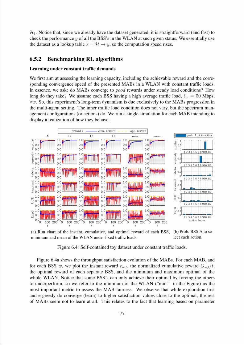
“main” — 2020/11/19 — 10:04 — page 77 — #99

H1. Notice that, since we already have the dataset generated, it is straightforward (and fast) tocheck the performance y of all the BSS’s in the WLAN at such given status. We essentially usethe dataset as a lookup table x = H → y, so the computation speed rises.

6.5.2 Benchmarking RL algorithmsLearning under constant traffic demands

We first aim at assessing the learning capacity, including the achievable reward and the corre-sponding convergence speed of the presented MABs in a WLAN with constant traffic loads.In essence, we ask: do MABs converge to good rewards under steady load conditions? Howlong do they take? We assume each BSS having a high average traffic load, `w = 50 Mbps,∀w. So, this experiment’s long-term dynamism is due exclusively to the MABs progression inthe multi-agent setting. The inner traffic load condition does not vary, but the spectrum man-agement configurations (or actions) do. We run a single simulation for each MAB intending todisplay a realization of how they behave.

0.0

0.5

1.0

0.0

0.5

1.0

0.0

0.5

1.0

0.0

0.5

1.0

0.0

0.5

1.0

0.0

0.5

1.0

0.0

0.5

1.0

0.0

0.5

1.0

0.0

0.5

1.0

0.0

0.5

1.0

0.0

0.5

1.0

0.0

0.5

1.0

0.0

0.5

1.0

0.0

0.5

1.0

0.0

0.5

1.0

0.0

0.5

1.0

0.0

0.5

1.0

0.0

0.5

1.0

0.0

0.5

1.0

0.0

0.5

1.0

0.0

0.5

1.0

0.0

0.5

1.0

0.0

0.5

1.0

0.0

0.5

1.0

0.0

0.5

1.0

0.0

0.5

1.0

0.0

0.5

1.0

0.0

0.5

1.0

0.0

0.5

1.0

0 100 2000.0

0.5

1.0

0 100 2000.0

0.5

1.0

0 100 2000.0

0.5

1.0

0 100 2000.0

0.5

1.0

0 100 2000.0

0.5

1.0

0 100 2000.0

0.5

1.0

(a) Run chart of the instant, cumulative, and optimal reward of each BSS,minimum and mean of the WLAN under fixed traffic loads.

1 2 3 4 5 6 7 8 91011120

0.5

1

1 2 3 4 5 6 7 8 91011120

0.5

1

1 2 3 4 5 6 7 8 91011120

0.5

1

1 2 3 4 5 6 7 8 91011120

0.5

1

1 2 3 4 5 6 7 8 91011120

0.51

1 2 3 4 5 6 7 8 91011120

0.51

(b) Prob. BSS A to se-lect each action.

Figure 6.4: Self-contained toy dataset under constant traffic loads.

Figure 6.4a shows the throughput satisfaction evolution of the MABs. For each MAB, andfor each BSS w, we plot the instant reward rw,t, the normalized cumulative reward Gw,t/t,the optimal reward of each separate BSS, and the minimum and maximum optimal of thewhole WLAN. Notice that some BSS’s can only achieve their optimal by forcing the othersto underperform, so we refer to the minimum of the WLAN (“min.” in the Figure) as themost important metric to assess the MAB fairness. We observe that while exploration-firstand e-greedy do converge (learn) to higher satisfaction values close to the optimal, the restof MABs seem not to learn at all. This relates to the fact that learning based on parameter

77

“main” — 2020/11/19 — 10:04 — page 78 — #100

estimation is fruitless in dynamic and chaotic multi-agent deployments like this. So, it seemspreferable to act quickly with a low-level knowledge of the actions’ rewards. Besides, wefind that win-win relations are established as shown by the minimum and mean convergenceof the whole WLAN. That is, on average, BSS’s tend to benefit from others’ benefits. As forthe learning speed, exploration-first takes approximately a full exploration of the action spacewith erratic rewards to provide a super-steady performance, whereas e-greedy keeps switchingconfigurations throughout the simulation.

Figure 6.4b shows the probability of BSS A (picked as an example) to select each possibleaction. We observe that exploration-first and e-greedy tend to use one single action that behavessufficiently well, so they waste less time in exploring than exploiting. In contrast, the rest ofMABs waste too many iterations exploring the different actions.

Finding #15: In small deployments with constant traffic load, exploration-first and e-greedy (so-called ligthweight MABs) achieve near-optimal rewards after enough explo-ration, showcasing their ability to learn in multi-agent Wi-Fi deployments by establishingwin-win relationships between BSS’s. Further, exploration-first is the only to lead to asuper-steady performance at the cost of experiencing vacillating rewards during the earlyexploration phase.

The usefulness of MAB parameters into the spotlight: why do sophisticated MABs notwork?

From the previous experiments, we concluded that UCB1, Thompson Sampling, and Exp3are not an option for the multi-agent setting of the joint spectrum management problem inWLANs. Here, we delve deep into why, which is tied to the different parameter estimationsthese algorithms must conduct. First, UCB1 cannot profit from computing an estimation ofthe upper confidence bound of any action a. In essence, the action selection relies on the sumof such confidence bound and the estimated value Q(a). Given the non-stationarity of themulti-agent setting, the estimation Q(a) is lousy and may highly vary from one iteration to theother. The algorithm then falls in a loop where most of the actions are selected with similarprobability, thus wasting lots of iterations with low performance and generating even moredynamism to the WLAN.

Second, even though Thompson Sampling is usually known to outperform the rest of thepresented MABs in stationary environments [91], its performance is well below exploration-first and e-greedy under the multi-agent setting. Similarly to UCB1, the reason lies in trying toestimate the parameters (e.g., α and β in the Beta distribution) defining the probability distribu-tion of the reward of each action while assuming that it is constant, or at least, slowly varyingin time, so it would be worth to learn. However, that is not the case at all in the multi-agent set-ting, where from one iteration to the other, the actual probability distribution of any action maycompletely change. So, the gathered knowledge from past iterations can turn entirely worthlessto estimate the new distribution.

To illustrate the low utility of estimating the probability distribution of an agent’s actions ina multi-agent setting, let us consider an elementary example. Assume two single-channel BSS’soverlap, and there are two possible primary channels to pick in the system CA = CB = 1, 2.We call the BSS’s A and B, respectively, and assume they have a constant traffic load. From the

78

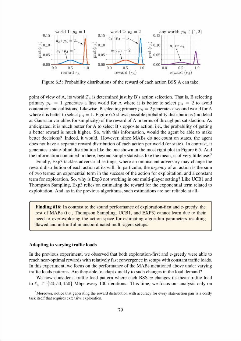
“main” — 2020/11/19 — 10:04 — page 79 — #101

0.0 0.5 1.00.00

0.05

0.10

0.15

0.0 0.5 1.00.00

0.05

0.10

0.15

0.0 0.5 1.00.00

0.05

0.10

0.15

Figure 6.5: Probability distributions of the reward of each action BSS A can take.

point of view of A, its world IA is determined just by B’s action selection. That is, B selectingprimary pB = 1 generates a first world for A where it is better to select pA = 2 to avoidcontention and collisions. Likewise, B selecting primary pB = 2 generates a second world for Awhere it is better to select pA = 1. Figure 6.5 shows possible probability distributions (modeledas Gaussian variables for simplicity) of the reward of A in terms of throughput satisfaction. Asanticipated, it is much better for A to select B’s opposite action, i.e., the probability of gettinga better reward is much higher. So, with this information, would the agent be able to makebetter decisions? Indeed, it would. However, since MABs do not count on states, the agentdoes not have a separate reward distribution of each action per world (or state). In contrast, itgenerates a state-blind distribution like the one shown in the most right plot in Figure 6.5. Andthe information contained in there, beyond simple statistics like the mean, is of very little use.5

Finally, Exp3 tackles adversarial settings, where an omniscient adversary may change thereward distribution of each action at its will. In particular, the urgency of an action is the sumof two terms: an exponential term in the success of the action for exploitation, and a constantterm for exploration. So, why is Exp3 not working in our multi-player setting? Like UCB1 andThompson Sampling, Exp3 relies on estimating the reward for the exponential term related toexploitation. And, as in the previous algorithms, such estimations are not reliable at all.

Finding #16: In contrast to the sound performance of exploration-first and e-greedy, therest of MABs (i.e., Thompson Sampling, UCB1, and EXP3) cannot learn due to theirneed to over-exploring the action space for estimating algorithm parameters resultingflawed and unfruitful in uncoordinated multi-agent setups.

Adapting to varying traffic loads

In the previous experiment, we observed that both exploration-first and e-greedy were able toreach near-optimal rewards with relatively fast convergence in setups with constant traffic loads.In this experiment, we focus on the performance of the MABs mentioned above under varyingtraffic loads patterns. Are they able to adapt quickly to such changes in the load demand?

We now consider a traffic load pattern where each BSS w changes its mean traffic loadto `w ∈ 20, 50, 150 Mbps every 100 iterations. This time, we focus our analysis only on

5Moreover, notice that generating the reward distribution with accuracy for every state-action pair is a costlytask itself that requires extensive exploration.

79

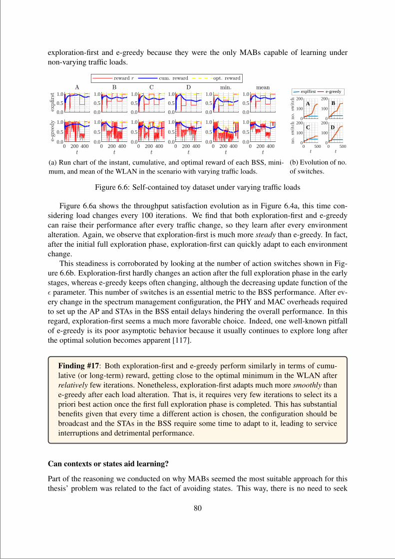
“main” — 2020/11/19 — 10:04 — page 80 — #102

exploration-first and e-greedy because they were the only MABs capable of learning undernon-varying traffic loads.

0.0

0.5

1.0

0.0

0.5

1.0

0.0

0.5

1.0

0.0

0.5

1.0

0.0

0.5

1.0

0.0

0.5

1.0

0 200 4000.0

0.5

1.0

0 200 4000.0

0.5

1.0

0 200 4000.0

0.5

1.0

0 200 4000.0

0.5

1.0

0 200 4000.0

0.5

1.0

0 200 4000.0

0.5

1.0

(a) Run chart of the instant, cumulative, and optimal reward of each BSS, mini-mum, and mean of the WLAN in the scenario with varying traffic loads.

0

100

200

0

100

200

0 5000

100

200

0 5000

100

200

A B

D

explfirst e-greedy

C

(b) Evolution of no.of switches.

Figure 6.6: Self-contained toy dataset under varying traffic loads

Figure 6.6a shows the throughput satisfaction evolution as in Figure 6.4a, this time con-sidering load changes every 100 iterations. We find that both exploration-first and e-greedycan raise their performance after every traffic change, so they learn after every environmentalteration. Again, we observe that exploration-first is much more steady than e-greedy. In fact,after the initial full exploration phase, exploration-first can quickly adapt to each environmentchange.

This steadiness is corroborated by looking at the number of action switches shown in Fig-ure 6.6b. Exploration-first hardly changes an action after the full exploration phase in the earlystages, whereas e-greedy keeps often changing, although the decreasing update function of theε parameter. This number of switches is an essential metric to the BSS performance. After ev-ery change in the spectrum management configuration, the PHY and MAC overheads requiredto set up the AP and STAs in the BSS entail delays hindering the overall performance. In thisregard, exploration-first seems a much more favorable choice. Indeed, one well-known pitfallof e-greedy is its poor asymptotic behavior because it usually continues to explore long afterthe optimal solution becomes apparent [117].

Finding #17: Both exploration-first and e-greedy perform similarly in terms of cumu-lative (or long-term) reward, getting close to the optimal minimum in the WLAN afterrelatively few iterations. Nonetheless, exploration-first adapts much more smoothly thane-greedy after each load alteration. That is, it requires very few iterations to select its apriori best action once the first full exploration phase is completed. This has substantialbenefits given that every time a different action is chosen, the configuration should bebroadcast and the STAs in the BSS require some time to adapt to it, leading to serviceinterruptions and detrimental performance.

Can contexts or states aid learning?

Part of the reasoning we conducted on why MABs seemed the most suitable approach for thisthesis’ problem was related to the fact of avoiding states. This way, there is no need to seek

80

“main” — 2020/11/19 — 10:04 — page 81 — #103

meaningful state definitions, and the learning can be executed more quickly since only actionsand rewards are used to execute the policy.

Nonetheless, in this experiment, we go beyond such qualitative reasoning and provide aquantitative measure on Q-learning performance (relying on states), and contextual MABs (re-lying on contexts). For the sake of boosting the learning speed, given we consider a relativelyshort time-horizon, we define the state s and context Ω the same: as merely the binary through-put satisfaction of the BSS,

s = Ω =

true ξ > 0.95

false otherwise, (6.12)

where ξ is the throughput satisfaction, which we compare against a 0.95 threshold to providea safety margin. Notice that state space S = true, false is small and therefore does not pro-vide much information on the environment. However, other more meaningful state definitionsconsidering parameters like the selected action or spectrum occupancy statistics would expo-nentially increase the size of S and reduce the learning speed dramatically. For instance, if thestate was defined simply as the action, i.e., s = a, the state-action table would be 12x12 giventhe |A| = 12 actions in the action space. Accordingly, 144 state-action elements would exist.So, it would take at least 144 iterations to try each of the pairs once. In contrast, the proposedstate space generates a more manageable state-action table of 2x12.6

Q-learning is a temporal difference algorithm seeking the best action to take given thecurrent state. It is considered off-policy because the Q-learning function learns from actionsoutside the current policy, like taking random actions. The learning rate α or step size deter-mines to what extent newly acquired information overrides old information. A factor α = 0makes the agent learn nothing (exclusively exploiting prior knowledge). In contrast, a factorα = 1 makes the agent consider only the most recent information (ignoring prior knowledge toexplore possibilities). We use a high value of α = 0.7 because the non-stationary of the deploy-ment. The discount factor γ determines the importance of future rewards. A factor γ = 0 willmake the agent myopic (or short-sighted) by only considering current rewards, while a factorapproaching γ → 1 will make it strive for a long-term high reward. We use a relatively smallγ = 0.3 to foster exploitation (for rapid convergence) in front of exploration.

Another way in which agents use partial information gathered from the environment is inthe form of contexts. In plain, contexts can be formulated as states for stateless approaches.That is, a contextual MAB can be instantiated like a particular MAB running separately percontext. The learning is separated from one context to the other so that no information isshared between contexts like it is the case for Q-learning and other state-full approaches. Inthis case, we propose having a separate MAB instance for each of the two contexts defined(true and false).

Figure 6.7 is an extension of Figure 6.4a, this time showing the performance of the proposedQ-learning and contextual MAB. While we observe that both tend to learn, i.e., the individualreward of all BSS’s increases over time, we find unsteadiness with peaks of low (even zero)throughput satisfaction throughout all the iterations. Remarkably, such low throughputs maygenerate service interruptions causing poor user experience. So, we have seen that, by consid-

6From this brief discussion on the size of the state-action space we can conclude that more complex approacheslike DRL do not suit in the scenarios of this thesis. DRL relies on huge state-action spaces and normally takeslong periods to start learning.

81

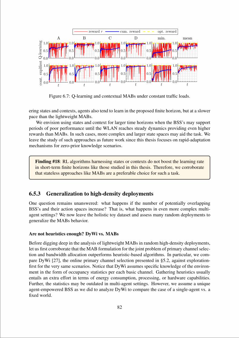
“main” — 2020/11/19 — 10:04 — page 82 — #104

0.0

0.5

1.0

0.0

0.5

1.0

0.0

0.5

1.0

0.0

0.5

1.0

0.0

0.5

1.0

0.0

0.5

1.0

0.0

0.5

1.0

0.0

0.5

1.0

0.0

0.5

1.0

0.0

0.5

1.0

0.0

0.5

1.0

0.0

0.5

1.0

Figure 6.7: Q-learning and contextual MABs under constant traffic loads.

ering states and contexts, agents also tend to learn in the proposed finite horizon, but at a slowerpace than the lightweight MABs.

We envision using states and context for larger time horizons when the BSS’s may supportperiods of poor performance until the WLAN reaches steady dynamics providing even higherrewards than MABs. In such cases, more complex and larger state spaces may aid the task. Weleave the study of such approaches as future work since this thesis focuses on rapid-adaptationmechanisms for zero-prior knowledge scenarios.

Finding #18: RL algorithms harnessing states or contexts do not boost the learning ratein short-term finite horizons like those studied in this thesis. Therefore, we corroboratethat stateless approaches like MABs are a preferable choice for such a task.

6.5.3 Generalization to high-density deploymentsOne question remains unanswered: what happens if the number of potentially overlappingBSS’s and their action spaces increase? That is, what happens in even more complex multi-agent settings? We now leave the holistic toy dataset and assess many random deployments togeneralize the MABs behavior.

Are not heuristics enough? DyWi vs. MABs

Before digging deep in the analysis of lightweight MABs in random high-density deployments,let us first corroborate that the MAB formulation for the joint problem of primary channel selec-tion and bandwidth allocation outperforms heuristic-based algorithms. In particular, we com-pare DyWi [27], the online primary channel selection presented in §5.2, against exploration-first for the very same scenarios. Notice that DyWi assumes specific knowledge of the environ-ment in the form of occupancy statistics per each basic channel. Gathering heuristics usuallyentails an extra effort in terms of energy consumption, processing, or hardware capabilities.Further, the statistics may be outdated in multi-agent settings. However, we assume a uniqueagent-empowered BSS as we did to analyze DyWi to compare the case of a single-agent vs. afixed world.

82

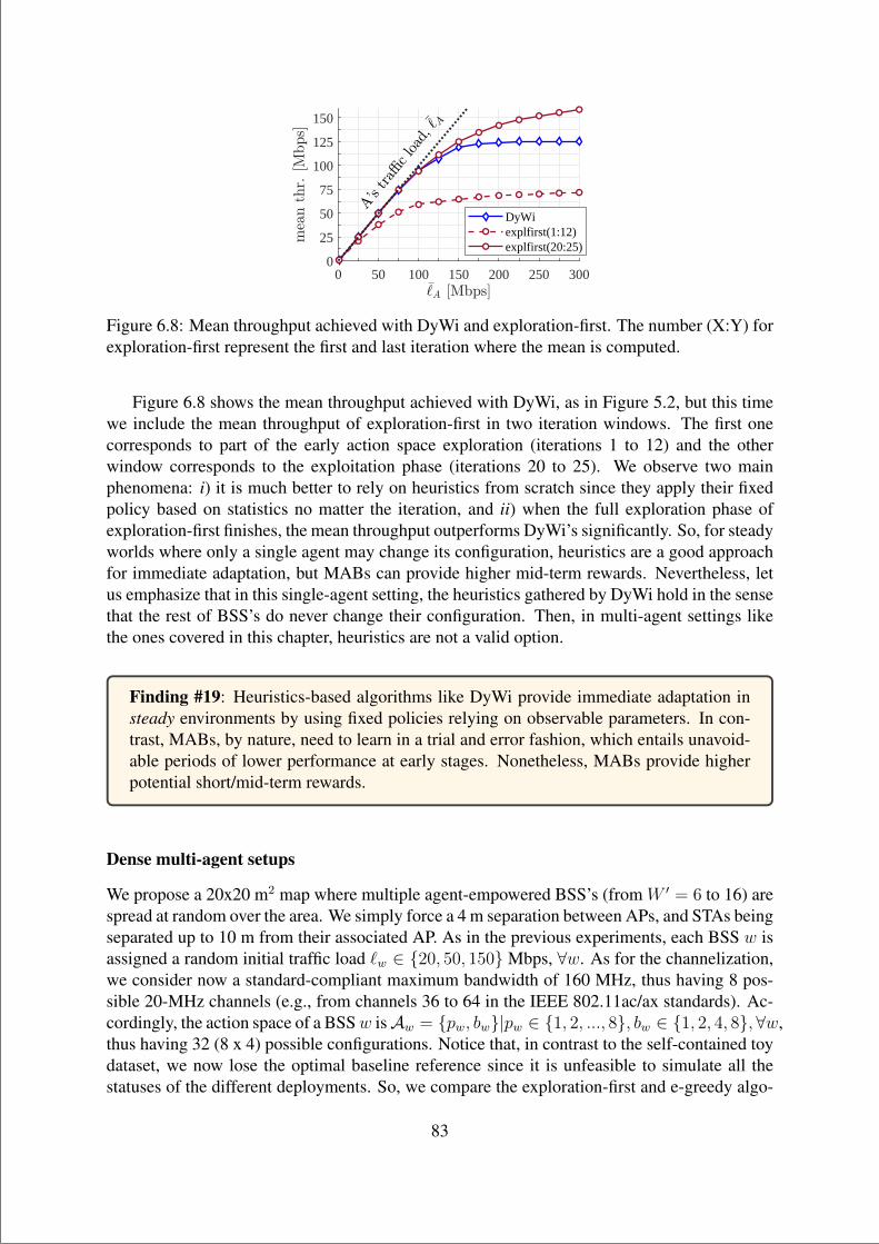
“main” — 2020/11/19 — 10:04 — page 83 — #105

0 50 100 150 200 250 3000

25

50

75

100

125

150

DyWiexplfirst(1:12)explfirst(20:25)

Figure 6.8: Mean throughput achieved with DyWi and exploration-first. The number (X:Y) forexploration-first represent the first and last iteration where the mean is computed.

Figure 6.8 shows the mean throughput achieved with DyWi, as in Figure 5.2, but this timewe include the mean throughput of exploration-first in two iteration windows. The first onecorresponds to part of the early action space exploration (iterations 1 to 12) and the otherwindow corresponds to the exploitation phase (iterations 20 to 25). We observe two mainphenomena: i) it is much better to rely on heuristics from scratch since they apply their fixedpolicy based on statistics no matter the iteration, and ii) when the full exploration phase ofexploration-first finishes, the mean throughput outperforms DyWi’s significantly. So, for steadyworlds where only a single agent may change its configuration, heuristics are a good approachfor immediate adaptation, but MABs can provide higher mid-term rewards. Nevertheless, letus emphasize that in this single-agent setting, the heuristics gathered by DyWi hold in the sensethat the rest of BSS’s do never change their configuration. Then, in multi-agent settings likethe ones covered in this chapter, heuristics are not a valid option.

Finding #19: Heuristics-based algorithms like DyWi provide immediate adaptation insteady environments by using fixed policies relying on observable parameters. In con-trast, MABs, by nature, need to learn in a trial and error fashion, which entails unavoid-able periods of lower performance at early stages. Nonetheless, MABs provide higherpotential short/mid-term rewards.

Dense multi-agent setups

We propose a 20x20 m2 map where multiple agent-empowered BSS’s (from W ′ = 6 to 16) arespread at random over the area. We simply force a 4 m separation between APs, and STAs beingseparated up to 10 m from their associated AP. As in the previous experiments, each BSS w isassigned a random initial traffic load `w ∈ 20, 50, 150Mbps, ∀w. As for the channelization,we consider now a standard-compliant maximum bandwidth of 160 MHz, thus having 8 pos-sible 20-MHz channels (e.g., from channels 36 to 64 in the IEEE 802.11ac/ax standards). Ac-cordingly, the action space of a BSSw isAw = pw, bw|pw ∈ 1, 2, ..., 8, bw ∈ 1, 2, 4, 8,∀w,thus having 32 (8 x 4) possible configurations. Notice that, in contrast to the self-contained toydataset, we now lose the optimal baseline reference since it is unfeasible to simulate all thestatuses of the different deployments. So, we compare the exploration-first and e-greedy algo-

83

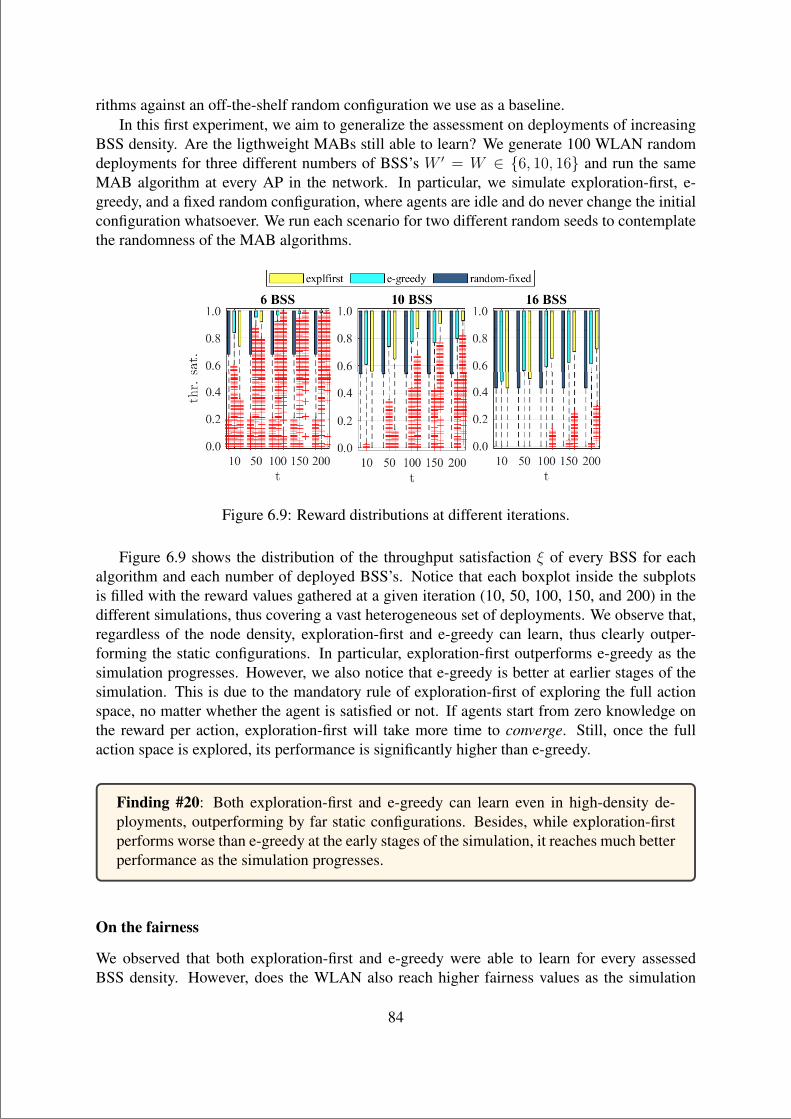
“main” — 2020/11/19 — 10:04 — page 84 — #106

rithms against an off-the-shelf random configuration we use as a baseline.In this first experiment, we aim to generalize the assessment on deployments of increasing

BSS density. Are the ligthweight MABs still able to learn? We generate 100 WLAN randomdeployments for three different numbers of BSS’s W ′ = W ∈ 6, 10, 16 and run the sameMAB algorithm at every AP in the network. In particular, we simulate exploration-first, e-greedy, and a fixed random configuration, where agents are idle and do never change the initialconfiguration whatsoever. We run each scenario for two different random seeds to contemplatethe randomness of the MAB algorithms.

Figure 6.9: Reward distributions at different iterations.

Figure 6.9 shows the distribution of the throughput satisfaction ξ of every BSS for eachalgorithm and each number of deployed BSS’s. Notice that each boxplot inside the subplotsis filled with the reward values gathered at a given iteration (10, 50, 100, 150, and 200) in thedifferent simulations, thus covering a vast heterogeneous set of deployments. We observe that,regardless of the node density, exploration-first and e-greedy can learn, thus clearly outper-forming the static configurations. In particular, exploration-first outperforms e-greedy as thesimulation progresses. However, we also notice that e-greedy is better at earlier stages of thesimulation. This is due to the mandatory rule of exploration-first of exploring the full actionspace, no matter whether the agent is satisfied or not. If agents start from zero knowledge onthe reward per action, exploration-first will take more time to converge. Still, once the fullaction space is explored, its performance is significantly higher than e-greedy.

Finding #20: Both exploration-first and e-greedy can learn even in high-density de-ployments, outperforming by far static configurations. Besides, while exploration-firstperforms worse than e-greedy at the early stages of the simulation, it reaches much betterperformance as the simulation progresses.

On the fairness

We observed that both exploration-first and e-greedy were able to learn for every assessedBSS density. However, does the WLAN also reach higher fairness values as the simulation

84

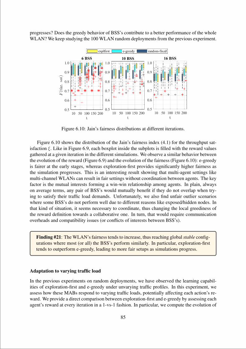
“main” — 2020/11/19 — 10:04 — page 85 — #107

progresses? Does the greedy behavior of BSS’s contribute to a better performance of the wholeWLAN? We keep studying the 100 WLAN random deployments from the previous experiment.

Figure 6.10: Jain’s fairness distributions at different iterations.

Figure 6.10 shows the distribution of the Jain’s fairness index (4.1) for the throughput sat-isfaction ξ. Like in Figure 6.9, each boxplot inside the subplots is filled with the reward valuesgathered at a given iteration in the different simulations. We observe a similar behavior betweenthe evolution of the reward (Figure 6.9) and the evolution of the fairness (Figure 6.10): e-greedyis fairer at the early stages, whereas exploration-first provides significantly higher fairness asthe simulation progresses. This is an interesting result showing that multi-agent settings likemulti-channel WLANs can result in fair settings without coordination between agents. The keyfactor is the mutual interests forming a win-win relationship among agents. In plain, alwayson average terms, any pair of BSS’s would mutually benefit if they do not overlap when try-ing to satisfy their traffic load demands. Unfortunately, we also find unfair outlier scenarioswhere some BSS’s do not perform well due to different reasons like exposed/hidden nodes. Inthat kind of situation, it seems necessary to coordinate, thus changing the local greediness ofthe reward definition towards a collaborative one. In turn, that would require communicationoverheads and compatibility issues (or conflicts of interests between BSS’s).

Finding #21: The WLAN’s fairness tends to increase, thus reaching global stable config-urations where most (or all) the BSS’s perform similarly. In particular, exploration-firsttends to outperform e-greedy, leading to more fair setups as simulations progress.

Adaptation to varying traffic load

In the previous experiments on random deployments, we have observed the learning capabil-ities of exploration-first and e-greedy under unvarying traffic profiles. In this experiment, weassess how these MABs respond to varying traffic loads, potentially affecting each action’s re-ward. We provide a direct comparison between exploration-first and e-greedy by assessing eachagent’s reward at every iteration in a 1-vs-1 fashion. In particular, we compute the evolution of

85

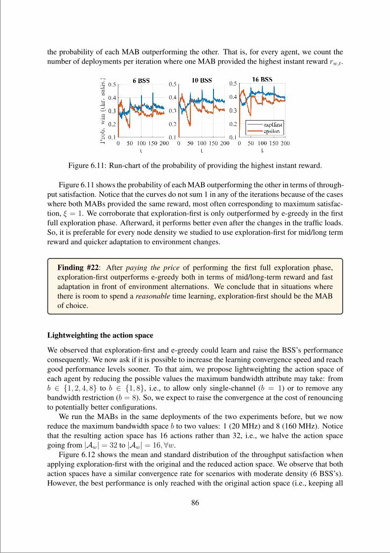
“main” — 2020/11/19 — 10:04 — page 86 — #108

the probability of each MAB outperforming the other. That is, for every agent, we count thenumber of deployments per iteration where one MAB provided the highest instant reward rw,t.

Figure 6.11: Run-chart of the probability of providing the highest instant reward.

Figure 6.11 shows the probability of each MAB outperforming the other in terms of through-put satisfaction. Notice that the curves do not sum 1 in any of the iterations because of the caseswhere both MABs provided the same reward, most often corresponding to maximum satisfac-tion, ξ = 1. We corroborate that exploration-first is only outperformed by e-greedy in the firstfull exploration phase. Afterward, it performs better even after the changes in the traffic loads.So, it is preferable for every node density we studied to use exploration-first for mid/long termreward and quicker adaptation to environment changes.

Finding #22: After paying the price of performing the first full exploration phase,exploration-first outperforms e-greedy both in terms of mid/long-term reward and fastadaptation in front of environment alternations. We conclude that in situations wherethere is room to spend a reasonable time learning, exploration-first should be the MABof choice.

Lightweighting the action space

We observed that exploration-first and e-greedy could learn and raise the BSS’s performanceconsequently. We now ask if it is possible to increase the learning convergence speed and reachgood performance levels sooner. To that aim, we propose lightweighting the action space ofeach agent by reducing the possible values the maximum bandwidth attribute may take: fromb ∈ 1, 2, 4, 8 to b ∈ 1, 8, i.e., to allow only single-channel (b = 1) or to remove anybandwidth restriction (b = 8). So, we expect to raise the convergence at the cost of renouncingto potentially better configurations.

We run the MABs in the same deployments of the two experiments before, but we nowreduce the maximum bandwidth space b to two values: 1 (20 MHz) and 8 (160 MHz). Noticethat the resulting action space has 16 actions rather than 32, i.e., we halve the action spacegoing from |Aw| = 32 to |Aw| = 16,∀w.

Figure 6.12 shows the mean and standard distribution of the throughput satisfaction whenapplying exploration-first with the original and the reduced action space. We observe that bothaction spaces have a similar convergence rate for scenarios with moderate density (6 BSS’s).However, the best performance is only reached with the original action space (i.e., keeping all

86

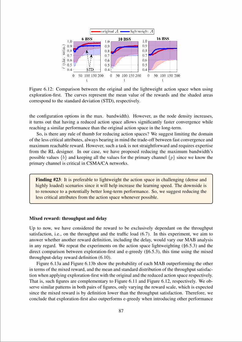
“main” — 2020/11/19 — 10:04 — page 87 — #109

Figure 6.12: Comparison between the original and the lightweight action space when usingexploration-first. The curves represent the mean value of the rewards and the shaded areascorrespond to the standard deviation (STD), respectively.

the configuration options in the max. bandwidth). However, as the node density increases,it turns out that having a reduced action space allows significantly faster convergence whilereaching a similar performance than the original action space in the long-term.

So, is there any rule of thumb for reducing action spaces? We suggest limiting the domainof the less critical attributes, always bearing in mind the trade-off between fast convergence andmaximum reachable reward. However, such a task is not straightforward and requires expertisefrom the RL designer. In our case, we have proposed reducing the maximum bandwidth’spossible values b and keeping all the values for the primary channel p since we know theprimary channel is critical in CSMA/CA networks.

Finding #23: It is preferable to lightweight the action space in challenging (dense andhighly loaded) scenarios since it will help increase the learning speed. The downside isto renounce to a potentially better long-term performance. So, we suggest reducing theless critical attributes from the action space whenever possible.

Mixed reward: throughput and delay

Up to now, we have considered the reward to be exclusively dependant on the throughputsatisfaction, i.e., on the throughput and the traffic load (6.7). In this experiment, we aim toanswer whether another reward definition, including the delay, would vary our MAB analysisin any regard. We repeat the experiments on the action space lightweighting (§6.5.3) and thedirect comparison between exploration-first and e-greedy (§6.5.3), this time using the mixedthroughput-delay reward definition (6.10).

Figure 6.13a and Figure 6.13b show the probability of each MAB outperforming the otherin terms of the mixed reward, and the mean and standard distribution of the throughput satisfac-tion when applying exploration-first with the original and the reduced action space respectively.That is, such figures are complementary to Figure 6.11 and Figure 6.12, respectively. We ob-serve similar patterns in both pairs of figures, only varying the reward scale, which is expectedsince the mixed reward is by definition lower than the throughput satisfaction. Therefore, weconclude that exploration-first also outperforms e-greedy when introducing other performance

87

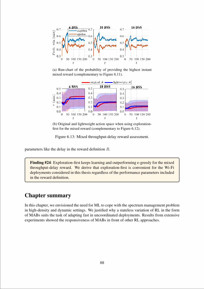
“main” — 2020/11/19 — 10:04 — page 88 — #110

(a) Run-chart of the probability of providing the highest instantmixed reward (complementary to Figure 6.11).

(b) Original and lightweight action space when using exploration-first for the mixed reward (complementary to Figure 6.12).

Figure 6.13: Mixed throughput-delay reward assessment.

parameters like the delay in the reward definition R.

Finding #24: Exploration-first keeps learning and outperforming e-greedy for the mixedthroughput-delay reward. We derive that exploration-first is convenient for the Wi-Fideployments considered in this thesis regardless of the performance parameters includedin the reward definition.

Chapter summaryIn this chapter, we envisioned the need for ML to cope with the spectrum management problemin high-density and dynamic settings. We justified why a stateless variation of RL in the formof MABs suits the task of adapting fast in uncoordinated deployments. Results from extensiveexperiments showed the responsiveness of MABs in front of other RL approaches.

88

“main” — 2020/11/19 — 10:04 — page 89 — #111

Chapter 7

CONCLUDING REMARKS

7.1 Summary

In this thesis, we shed light on the behavior of channel allocation and channel bonding inWLANs, from its essential characteristics to benchmarking its performance on a variety ofdense deployments with different traffic load requirements. To conduct such an in-depth anal-ysis, we have developed different enablers: a CTMN model for channel bonding in spatiallydistributed WLANs, the Komondor wireless network simulator, and the WACA spectrum ana-lyzer. We used the latter to generate a unique dataset simultaneously capturing all the channelsin the 5 GHz Wi-Fi channelization. The dataset contains multiple locations of interest, in-cluding a crowded football match in the Camp Nou stadium. We also covered heuristic-basedapproaches and proposed DyWi, an algorithm for online selection of the primary channel ofa dynamic channel bonding BSS. Finally, we explored the use of ML to better cope with thejoint spectrum management problem and conclude that RL is the approach to follow due to itstrial-and-error black-box conception that disregards the implicit nature or model behind multi-agent WLANs. In this regard, we call into question whether the use of complex RL algorithmsreally helps the quest and derive that stateless algorithms, especially in the form of lightweightMABs, are an efficient solution for rapid adaptation avoiding extensive or meaningless states.

We believe the research carried in this thesis will contribute to the design of novel spectrummanagement techniques for next-generation WLANs. We expect that our findings on channelbonding will help overcome the main challenges imposed by spectrum sharing. Besides, wehope that our reasoning on why stateless RL algorithms in the form of lightweight MABsare an efficient solution for rapid deployment will be useful as well for other techniques likescheduling or transmission power control.

7.2 Future work

There are different research topics to continue exploring concerning spectrum management inWLANs. First and foremost, we envision the use of RL as a key enabler for next-generationWLANs. Thus, we will dig deeper into the analysis of multi-agent settings by considering par-tial and full coordination through other learning architectures that may impose communicationoverheads but also a potentially holistic knowledge of the environment. In this settings, wherewe count with relatively large periods for conducting the learning process, we do believe that

89

“main” — 2020/11/19 — 10:04 — page 90 — #112

the use of more complex state-full RL formulations like DRL can be useful to reach a moreprofound judgment on the WLAN deployment by identifying complex long-terms patterns. Tothat aim, the trade-off between meaningful and condensed states remains an essential venue forresearch.

As for the stateless RL formulation, we believe that the presented lightweight MABs canbe improved in several ways. A mechanism to adapt the iteration duration to the level ofdynamism in the environment is worth to study. In steady environments (e.g., single-agent),short iterations are enough to estimate action rewards. Instead, under high dynamism, iterationsshould be much larger or not used at all. In the latter case, the use of heuristic-based approachescould help to identify good enough actions and pause the MAB exploration. So, designing abackoff mechanism that triggers heuristics or RL instructions depending on the reliability of theestimated action rewards seems promising. Further, the study of asynchronous agents remainsunexplored. While we expect similar behavior to the studied synchronous settings, an in-depthstudy on the matter would aid detecting the main differences and potential pitfalls.

Finally, we observe that the inter-channel correlation detected in the on-the-field tracesplayed a critical role in channel bonding performance. Consequently, simple models relyingjust on occupancy severely underestimate the available gains for channel bonding. Thus, weenvision the design of a trace-driven model for spectrum activity that takes into account inter-channel correlation. We believe such a model will help in building more efficient new spectrummanagement algorithms.

90

“main” — 2020/11/19 — 10:04 — page 91 — #113

Funding

This work has been partially supported by the following grants:

• FI grant from the Generalitat de Catalunya.

• Cisco University Research Program fund, a corporate advised fund of Silicon ValleyCommunity Foundation,Grant number: Project CG No. 890107, Towards DeterministicChannel Access in High-Density WLANs.

• Spanish Ministry of Economy and Competitiveness under the Maria de Maeztu Units ofExcellence Programme (MDM-2015-0502).

• WINDMAL PGC2018-099959-B-I00 (MCIU/AEI/FEDER,UE).

• Catalan Government under grant SGR-2017-1188.

• We appreciate the generosity of Futbol Club Barcelona for letting us take measurementsin the Camp Nou stadium.

91

“main” — 2020/11/19 — 10:04 — page 92 — #114

“main” — 2020/11/19 — 10:04 — page 93 — #115

Bibliography

[1] Devices must be professionally installed when operating in the 5470 – 5725 ghz band.Publication Number: 443999 Rule Parts: 15E.

[2] Rice University Wireless Open Access Research Platform. http://warpproject.org, last accessed January 30, 2020.

[3] Status of project ieee 802.11ax high efficiency wlan (hew). http://www.ieee802.org/11/Reports/tgax_update.htm (accessed July 2017).

[4] IEEE 802.11n enhancements for Higher Throughput, 2009.

[5] IEEE 802.11ac Very High Throughput., 2013.

[6] IEEE 802.11be Extremely High Throughput, 802.11-18/1231r6, 2019.

[7] IEEE P802.11ax/D4.0 High Efficiency WLAN, 2019.

[8] List of WLAN channels. Wikipedia., 2020.

[9] M. Achanta. Method and apparatus for least congested channel scan for wireless accesspoints, Oct. 5 2004. US Patent App. 10/959,446.

[10] T. Adame, M. Carrascosa, and B. Bellalta. The TMB path loss model for 5 GHz indoorWiFi scenarios: On the empirical relationship between RSSI, MCS, and spatial streams.In 2019 Wireless Days (WD), pages 1–8. IEEE, 2019.

[11] A. Ahmed, G. Amel, S. Anis, and M. Abdellatif. Resource allocation for multi-user cog-nitive radio systems using multi-agent q-learning. Procedia Computer Science, 10:46–53, 2012.

[12] R. Akl and A. Arepally. Dynamic channel assignment in IEEE 802.11 networks. InPortable Information Devices, 2007. PORTABLE07. IEEE International Conference on,pages 1–5. IEEE, 2007.

[13] H. Al-Rizzo, M. Haidar, R. Akl, and Y. Chan. Enhanced channel assignment and loaddistribution in IEEE 802.11 WLANs. In Signal Processing and Communications, 2007.ICSPC 2007. IEEE International Conference on, pages 768–771. IEEE, 2007.

[14] R. Ali, Y. A. Qadri, Y. B. Zikria, T. Umer, B.-S. Kim, and S. W. Kim. Q-learning-enabledchannel access in next-generation dense wireless networks for iot-based ehealth systems.EURASIP Journal on Wireless Communications and Networking, 2019(1):1–12, 2019.

93

“main” — 2020/11/19 — 10:04 — page 94 — #116

[15] R. Ali, N. Shahin, Y. B. Zikria, B.-S. Kim, and S. W. Kim. Deep reinforcement learningparadigm for performance optimization of channel observation–based mac protocols indense wlans. IEEE Access, 7:3500–3511, 2018.

[16] M. A. Alsheikh, S. Lin, D. Niyato, and H.-P. Tan. Machine learning in wireless sensornetworks: Algorithms, strategies, and applications. IEEE Communications Surveys &Tutorials, 16(4):1996–2018, 2014.

[17] N. Anand, E. Aryafar, and E. W. Knightly. WARPlab: a flexible framework for rapidphysical layer design. In Proceedings of the 2010 ACM workshop on Wireless of thestudents, by the students, for the students, pages 53–56. ACM, 2010.

[18] M. Y. Arslan, K. Pelechrinis, I. Broustis, S. V. Krishnamurthy, S. Addepalli, and K. Pa-pagiannaki. Auto-configuration of 802.11n WLANs. In Proceedings of the 6th Interna-tional COnference, pages 1–12, 2010.

[19] M. Y. Arslan, K. Pelechrinis, I. Broustis, S. Singh, S. V. Krishnamurthy, S. Addepalli,and K. Papagiannaki. ACORN: An auto-configuration framework for 802.11n WLANs.IEEE/ACM Transactions on Networking (TON), 21(3):896–909, 2013.

[20] P. Auer, N. Cesa-Bianchi, and P. Fischer. Finite-time analysis of the multiarmed banditproblem. Machine learning, 47(2-3):235–256, 2002.

[21] P. Auer, N. Cesa-Bianchi, Y. Freund, and R. E. Schapire. Gambling in a rigged casino:The adversarial multi-armed bandit problem. In Proceedings of IEEE 36th Annual Foun-dations of Computer Science, pages 322–331. IEEE, 1995.

[22] P. Auer, N. Cesa-Bianchi, Y. Freund, and R. E. Schapire. The nonstochastic multiarmedbandit problem. SIAM journal on computing, 32(1):48–77, 2002.

[23] A. Baid and D. Raychaudhuri. Understanding channel selection dynamics in dense Wi-Fi networks. IEEE Communications Magazine, 53(1):110–117, 2015.

[24] S. Barrachina-Munoz, B. Bellalta, and E. Knightly. Wi-Fi all channel analyzer. InThe 14th ACM Workshop on Wireless Network Testbeds, Experimental evaluation &CHaracterization (WiNTECH). Runner-up best-paper award. Runner Up, Best PaperAward. ACM, 2020.

[25] S. Barrachina-Munoz, B. Bellalta, and E. Knightly. Wi-Fi channel bonding: an all-channel system and experimental study from urban hotspots to a sold-out stadium. Sub-mitted to IEEE Transactions on Networking (under major revision), 2020.

[26] S. Barrachina-Munoz, F. Wilhelmi, and B. Bellalta. Dynamic channel bonding inspatially distributed high-density WLANs. IEEE Transactions on Mobile Computing,19(4):821–835, 2019.

[27] S. Barrachina-Munoz, F. Wilhelmi, and B. Bellalta. Online primary channel selectionfor dynamic channel bonding in high-density WLANs. IEEE Wireless CommunicationsLetters, 9(2):258–262, 2019.

94

“main” — 2020/11/19 — 10:04 — page 95 — #117

[28] S. Barrachina-Munoz, F. Wilhelmi, and B. Bellalta. To overlap or not to overlap: en-abling channel bonding in high-density WLANs. Computer Networks, 152:40–53, 2019.

[29] S. Barrachina-Munoz, F. Wilhelmi, I. Selinis, and B. Bellalta. Komondor: A wirelessnetwork simulator for next-generation high-density wlans. In 2019 Wireless Days (WD),pages 1–8. IEEE, 2019.

[30] B. Bellalta. Throughput Analysis in High Density WLANs. IEEE CommunicationsLetters, 21(3):592–595, 2017.

[31] B. Bellalta, A. Checco, A. Zocca, and J. Barcelo. On the interactions between multipleoverlapping wlans using channel bonding. IEEE Transactions on Vehicular Technology,65(2):796–812, 2015.

[32] B. Bellalta, A. Checco, A. Zocca, and J. Barcelo. On the interactions between multipleoverlapping WLANs using channel bonding. IEEE Transactions on Vehicular Technol-ogy, 65(2):796–812, 2016.

[33] B. Bellalta, A. Faridi, J. Barcelo, A. Checco, and P. Chatzimisios. Channel bonding inshort-range WLANs. In European Wireless 2014; 20th European Wireless Conference,pages 1–7. VDE, 2014.

[34] B. Bellalta, A. Zocca, C. Cano, A. Checco, J. Barcelo, and A. Vinel. Throughput analysisin CSMA/CA networks using continuous time Markov networks: a tutorial. In WirelessNetworking for Moving Objects, pages 115–133. Springer, 2014.

[35] G. Bianchi. Performance analysis of the IEEE 802.11 distributed coordination function.IEEE Journal on selected areas in communications, 18(3):535–547, 2000.

[36] S. Biswas, J. Bicket, E. Wong, R. Musaloiu-e, A. Bhartia, and D. Aguayo. Large-scale measurements of wireless network behavior. In Proceedings of the 2015 ACMConference on Special Interest Group on Data Communication, pages 153–165, 2015.

[37] M. Bkassiny, Y. Li, and S. K. Jayaweera. A survey on machine-learning techniques incognitive radios. IEEE Communications Surveys & Tutorials, 15(3):1136–1159, 2012.

[38] R. Boorstyn, A. Kershenbaum, B. Maglaris, and V. Sahin. Throughput analysis in multi-hop CSMA packet radio networks. IEEE Transactions on Communications, 35(3):267–274, 1987.

[39] D. Brelaz. New methods to color the vertices of a graph. Communications of the ACM,22(4):251–256, 1979.

[40] S. H. R. Bukhari, M. H. Rehmani, and S. Siraj. A survey of channel bonding for wire-less networks and guidelines of channel bonding for futuristic cognitive radio sensornetworks. IEEE Communications Surveys & Tutorials, 18(2):924–948, 2016.

[41] G. Buttazzo, C. Di Franco, and M. Marinoni. Design and analysis of target-sensitivereal-time systems. Software: Practice and Experience, 46(9):1181–1200, 2016.

95

“main” — 2020/11/19 — 10:04 — page 96 — #118

[42] X. Chang. Network simulations with opnet. In WSC’99. 1999 Winter Simulation Confer-ence Proceedings.’Simulation-A Bridge to the Future’(Cat. No. 99CH37038), volume 1,pages 307–314. IEEE, 1999.

[43] G. Chen and B. K. Szymanski. Reusing simulation components: cost: a component-oriented discrete event simulator. In Proceedings of the 34th conference on Winter sim-ulation (WSC): exploring new frontiers, pages 776–782. Winter Simulation Conference,2002.

[44] J. K. Chen, G. De Veciana, and T. S. Rappaport. Improved measurement-based fre-quency allocation algorithms for wireless networks. In Global Telecommunications Con-ference, 2007. GLOBECOM’07. IEEE, pages 4790–4795. IEEE, 2007.

[45] Y. Chen, J. Zhao, Q. Zhu, and Y. Liu. Research on unlicensed spectrum access mech-anism based on reinforcement learning in laa/wlan coexisting network. Wireless Net-works, 26(3):1643–1651, 2020.

[46] S. Chieochan, E. Hossain, and J. Diamond. Channel assignment schemes forinfrastructure-based 802.11 WLANs: A survey. IEEE Communications Surveys andTutorials, 12(1), 2010.

[47] L. Cigler and B. Faltings. Decentralized anti-coordination through multi-agent learning.Journal of Artificial Intelligence Research, 47:441–473, 2013.

[48] B. C. Csaji and L. Monostori. Value function based reinforcement learning in changingmarkovian environments. Journal of Machine Learning Research, 9(Aug):1679–1709,2008.

[49] W. Dai, Y. Gai, and B. Krishnamachari. Online learning for multi-channel opportunisticaccess over unknown markovian channels. In 2014 Eleventh Annual IEEE InternationalConference on Sensing, Communication, and Networking (SECON), pages 64–71. IEEE,2014.

[50] S. W. Day and A. Wagstaff. Activity in the wifi bands - an objective approach to estima-tion. In ARMMS Conference. Mass, 2014.

[51] S. De Bast, R. Torrea-Duran, A. Chiumento, S. Pollin, and H. Gacanin. Deep rein-forcement learning for dynamic network slicing in ieee 802.11 networks. In IEEE IN-FOCOM 2019-IEEE Conference on Computer Communications Workshops (INFOCOMWKSHPS), pages 264–269. IEEE, 2019.

[52] L. Deek, E. Garcia-Villegas, E. Belding, S.-J. Lee, and K. Almeroth. The impact ofchannel bonding on 802.11n network management. In Proceedings of the Seventh COn-ference on emerging Networking EXperiments and Technologies, pages 1–12, 2011.

[53] L. Deek, E. Garcia-Villegas, E. Belding, S.-J. Lee, and K. Almeroth. Joint rate and chan-nel width adaptation for 802.11 MIMO wireless networks. In Sensor, Mesh and Ad HocCommunications and Networks (SECON), 2013 10th Annual IEEE Communications So-ciety Conference on, pages 167–175. IEEE, 2013.

96

“main” — 2020/11/19 — 10:04 — page 97 — #119

[54] L. Deek, E. Garcia-Villegas, E. Belding, S.-J. Lee, and K. Almeroth. Intelligent channelbonding in 802.11n WLANs. IEEE Transactions on Mobile Computing, 13(6):1242–1255, 2014.

[55] A. Eisenblatter, H.-F. Geerdes, and I. Siomina. Integrated access point placement andchannel assignment for wireless LANs in an indoor office environment. In World ofWireless, Mobile and Multimedia Networks, 2007. WoWMoM 2007. IEEE InternationalSymposium on a, pages 1–10. IEEE, 2007.

[56] A. Faridi, B. Bellalta, and A. Checco. Analysis of dynamic channel bonding in densenetworks of wlans. IEEE Transactions on Mobile Computing, 16(8):2118–2131, 2016.

[57] L. Farzinvash and M. Kargahi. A scheduling algorithm for execution-instant sensitivereal-time systems. In 2009 15th IEEE International Conference on Embedded and Real-Time Computing Systems and Applications, pages 511–518. IEEE, 2009.

[58] Y. Gai and B. Krishnamachari. Distributed stochastic online learning policies for oppor-tunistic spectrum access. IEEE Transactions on Signal Processing, 62(23):6184–6193,2014.

[59] M. X. Gong, B. Hart, L. Xia, and R. Want. Channel bounding and mac protectionmechanisms for 802.11ac. In 2011 IEEE Global Telecommunications Conference-GLOBECOM 2011, pages 1–5. IEEE, 2011.

[60] M. Haidar, R. Akl, H. Al-Rizzo, and Y. Chan. Channel assignment and load distributionin a power-managed wlan. In Personal, Indoor and Mobile Radio Communications,2007. PIMRC 2007. IEEE 18th International Symposium on, pages 1–5. IEEE, 2007.

[61] S. A. Hanna. A 3-state hypothesis test model for cognitive radio systems. In 2014 IEEEInternational Symposium on Dynamic Spectrum Access Networks (DYSPAN), pages291–302. IEEE, 2014.

[62] S. A. Hanna and J. Sydor. Distributed sensing of spectrum occupancy and interferencein outdoor 2.4 GHz Wi-Fi networks. In 2012 IEEE Global Communications Conference(GLOBECOM), pages 1453–1459. IEEE, 2012.

[63] J. Herzen, R. Merz, and P. Thiran. Distributed spectrum assignment for home WLANs.In 2013 Proceedings Ieee Infocom, pages 1573–1581. IEEE, 2013.

[64] A. Hills. Large-scale wireless LAN design. IEEE Communications Magazine,39(11):98–107, 2001.

[65] M. Hoyhtya, A. Mammela, M. Eskola, M. Matinmikko, J. Kalliovaara, J. Ojaniemi,J. Suutala, R. Ekman, R. Bacchus, and D. Roberson. Spectrum occupancy measure-ments: A survey and use of interference maps. IEEE Communications Surveys & Tuto-rials, 18(4):2386–2414, 2016.

[66] Y. Hu, M. Chen, Z. Yang, M. Chen, and G. Jia. Optimization of resource allocation inmulti-cell ofdm systems: A distributed reinforcement learning approach. In 2020 IEEE31st Annual International Symposium on Personal, Indoor and Mobile Radio Commu-nications, pages 1–6. IEEE.

97

“main” — 2020/11/19 — 10:04 — page 98 — #120

[67] P. Huang, X. Yang, and L. Xiao. Dynamic channel bonding: enabling flexible spectrumaggregation. IEEE Transactions on Mobile Computing, 15(12):3042–3056, 2016.

[68] T. Issariyakul and E. Hossain. Introduction to Network Simulator 2 (NS2). In Introduc-tion to Network Simulator NS2, pages 21–40. Springer, 2012.

[69] S.-J. Jang, C.-H. Han, K.-E. Lee, and S.-J. Yoo. Reinforcement learning-based dynamicband and channel selection in cognitive radio ad-hoc networks. EURASIP Journal onWireless Communications and Networking, 2019(1):131, 2019.

[70] C. Jiang, H. Zhang, Y. Ren, Z. Han, K.-C. Chen, and L. Hanzo. Machine learn-ing paradigms for next-generation wireless networks. IEEE Wireless Communications,24(2):98–105, 2016.

[71] L. Jiao, V. Pla, and F. Y. Li. Analysis on channel bonding/aggregation for multi-channelcognitive radio networks. In Wireless Conference (EW), 2010 European, pages 468–474.IEEE, 2010.

[72] S. Joshi, P. Pawelczak, D. Cabric, and J. Villasenor. When channel bonding is beneficialfor opportunistic spectrum access networks. IEEE Transactions on Wireless Communi-cations, 11(11):3942–3956, 2012.

[73] C. Kai, Y. Liang, T. Huang, and X. Chen. A channel allocation algorithm to maximizeaggregate throughputs in DCB WLANs. arXiv preprint arXiv:1703.03909, 2017.

[74] R. Karmakar, S. Chattopadhyay, and S. Chakraborty. Smartla: Reinforcement learning-based link adaptation for high throughput wireless access networks. Computer Commu-nications, 110:1–25, 2017.

[75] F. Kelly. Reversibility and stochastic networks. Cambridge University Press, 2011.

[76] S. Keranidis, K. Chounos, T. Korakis, I. Koutsopoulos, and L. Tassiulas. Enabling AG-ILE spectrum adaptation in commercial 802.11 WLAN deployments. In Proceedings ofthe 20th annual international conference on Mobile computing and networking, pages295–298. ACM, 2014.

[77] S. Khairy, M. Han, L. X. Cai, Y. Cheng, and Z. Han. A renewal theory based analyticalmodel for multi-channel random access in IEEE 802.11ac/ax. IEEE Transactions onMobile Computing, 2018.

[78] M.-S. Kim, T. Ropitault, S. Lee, and N. Golmie. A throughput study for channel bondingin ieee 802.11ac networks. IEEE Communications Letters, 21(12):2682–2685, 2017.

[79] P. V. Klaine, M. A. Imran, O. Onireti, and R. D. Souza. A survey of machine learningtechniques applied to self-organizing cellular networks. IEEE Communications Surveys& Tutorials, 19(4):2392–2431, 2017.

[80] V. Kone, L. Yang, X. Yang, B. Y. Zhao, and H. Zheng. On the feasibility of effectiveopportunistic spectrum access. In Proceedings of the 10th ACM SIGCOMM conferenceon Internet measurement, pages 151–164, 2010.

98

“main” — 2020/11/19 — 10:04 — page 99 — #121

[81] V. Kone, L. Yang, X. Yang, B. Y. Zhao, and H. Zheng. The effectiveness of opportunis-tic spectrum access: A measurement study. IEEE/ACM Transactions on Networking,20(6):2005–2016, 2012.

[82] T. L. Lai and H. Robbins. Asymptotically efficient adaptive allocation rules. Advancesin applied mathematics, 6(1):4–22, 1985.

[83] R. Laufer and L. Kleinrock. On the capacity of wireless CSMA/CA multihop networks.In 2013 Proceedings IEEE INFOCOM, pages 1312–1320. IEEE, 2013.

[84] J. Lee, W. Kim, S.-J. Lee, D. Jo, J. Ryu, T. Kwon, and Y. Choi. An experimental study onthe capture effect in 802.11a networks. In Proceedings of the second ACM internationalworkshop on Wireless network testbeds, experimental evaluation and characterization,pages 19–26, 2007.

[85] Y. Lee, K. Kim, and Y. Choi. Optimization of AP placement and channel assignmentin wireless LANs. In Local Computer Networks, 2002. Proceedings. LCN 2002. 27thAnnual IEEE Conference on, pages 831–836. IEEE, 2002.

[86] K. K. Leung and B.-J. Kim. Frequency assignment for IEEE 802.11 wireless networks.In Vehicular Technology Conference, 2003. VTC 2003-Fall. 2003 IEEE 58th, volume 3,pages 1422–1426. IEEE, 2003.

[87] F. Li, D. Yu, H. Yang, J. Yu, H. Karl, and X. Cheng. Multi-armed-bandit-based spectrumscheduling algorithms in wireless networks: A survey. IEEE Wireless Communications,27(1):24–30, 2020.

[88] S. C. Liew, C. H. Kai, H. C. Leung, and P. Wong. Back-of-the-envelope computationof throughput distributions in CSMA wireless networks. IEEE Transactions on MobileComputing, 9(9):1319–1331, 2010.

[89] X. Ling and K. L. Yeung. Joint access point placement and channel assignment for802.11 wireless LANs. IEEE Transactions on Wireless Communications, 5(10):2705–2711, 2006.

[90] K. Liu and Q. Zhao. Indexability of restless bandit problems and optimality of whit-tle index for dynamic multichannel access. IEEE Transactions on Information Theory,56(11):5547–5567, 2010.

[91] L. Liu, R. Downe, and J. Reid. Multi-armed bandit strategies for non-stationary rewarddistributions and delayed feedback processes. In CORS conference, 2019.

[92] M. Lopez-Benıtez and F. Casadevall. Modeling and simulation of time-correlation prop-erties of spectrum use in cognitive radio. In 2011 6th International ICST Conferenceon Cognitive Radio Oriented Wireless Networks and Communications (CROWNCOM),pages 326–330, 2011.

[93] N. C. Luong, D. T. Hoang, S. Gong, D. Niyato, P. Wang, Y.-C. Liang, and D. I. Kim. Ap-plications of deep reinforcement learning in communications and networking: A survey.IEEE Communications Surveys & Tutorials, 21(4):3133–3174, 2019.

99

“main” — 2020/11/19 — 10:04 — page 100 — #122

[94] P. Mahonen, J. Riihijarvi, and M. Petrova. Automatic channel allocation for small wire-less local area networks using graph colouring algorithm approach. In Personal, Indoorand Mobile Radio Communications, 2004. PIMRC 2004. 15th IEEE International Sym-posium on, volume 1, pages 536–539. IEEE, 2004.

[95] A. Mishra, S. Banerjee, and W. Arbaugh. Weighted coloring based channel assign-ment for WLANs. ACM SIGMOBILE Mobile Computing and Communications Review,9(3):19–31, 2005.

[96] A. Mishra, V. Brik, S. Banerjee, A. Srinivasan, and W. A. Arbaugh. A client-drivenapproach for channel management in wireless LANs. In Infocom, 2006.

[97] A. Mishra, V. Shrivastava, D. Agrawal, S. Banerjee, and S. Ganguly. Distributed channelmanagement in uncoordinated wireless environments. In Proceedings of the 12th annualinternational conference on Mobile computing and networking, pages 170–181. ACM,2006.

[98] F. B. Mismar, B. L. Evans, and A. Alkhateeb. Deep reinforcement learning for 5g net-works: Joint beamforming, power control, and interference coordination. IEEE Trans-actions on Communications, 68(3):1581–1592, 2019.

[99] T. A. Myrvoll and J. E. Hakegard. Dynamic spectrum access in realistic environmentsusing reinforcement learning. In 2012 International Symposium on Communicationsand Information Technologies (ISCIT), pages 465–470. IEEE, 2012.

[100] A. Nabil, M. J. Abdel-Rahman, and A. B. MacKenzie. Adaptive channel bonding inwireless lans under demand uncertainty. In 2017 IEEE 28th Annual International Sym-posium on Personal, Indoor, and Mobile Radio Communications (PIMRC), pages 1–7.IEEE, 2017.

[101] K. Nakashima, S. Kamiya, K. Ohtsu, K. Yamamoto, T. Nishio, and M. Morikura. Deepreinforcement learning-based channel allocation for wireless lans with graph convolu-tional networks. IEEE Access, 8:31823–31834, 2020.

[102] O. Naparstek and K. Cohen. Deep multi-user reinforcement learning for distributeddynamic spectrum access. IEEE Transactions on Wireless Communications, 18(1):310–323, 2018.

[103] B. Nardelli and E. W. Knightly. Closed-form throughput expressions for CSMA net-works with collisions and hidden terminals. In INFOCOM, 2012 Proceedings IEEE,pages 2309–2317. IEEE, 2012.

[104] M. Park. IEEE 802.11ac: Dynamic bandwidth channel access. In Communications(ICC), 2011 IEEE International Conference on, pages 1–5. IEEE, 2011.

[105] K. Pelechrinis, T. Salonidis, H. Lundgren, and N. Vaidya. Experimental characterizationof 802.11 n link quality at high rates. In Proceedings of the fifth ACM internationalworkshop on Wireless network testbeds, experimental evaluation and characterization,pages 39–46. ACM, 2010.

100

“main” — 2020/11/19 — 10:04 — page 101 — #123

[106] H. Qi, H. Huang, Z. Hu, X. Wen, and Z. Lu. On-demand channel bonding in het-erogeneous wlans: A multi-agent deep reinforcement learning approach. Sensors,20(10):2789, 2020.

[107] M. Rademacher, K. Jonas, and M. Kretschmer. Quantifying the spectrum occupancyin an outdoor 5 GHz WiFi network with directional antennas. In 2018 IEEE WirelessCommunications and Networking Conference (WCNC), pages 1–6. IEEE, 2018.

[108] A. L. Ramaboli, O. E. Falowo, and A. H. Chan. Bandwidth aggregation in heterogeneouswireless networks: A survey of current approaches and issues. Journal of Network andComputer Applications, 35(6):1674–1690, 2012.

[109] A. K. Rathi and A. J. Santiago. The new NETSIM simulation program. Traffic engi-neering & control, 31(5), 1990.

[110] J. Riihijarvi, M. Petrova, and P. Mahonen. Frequency allocation for WLANs using graphcolouring techniques. In Wireless On-demand Network Systems and Services, 2005.WONS 2005. Second Annual Conference on, pages 216–222. IEEE, 2005.

[111] J. Riihijarvi, M. Petrova, P. Mahonen, and J. D. A. Barbosa. Performance evaluation ofautomatic channel assignment mechanism for IEEE 802.11 based on graph colouring.In Personal, Indoor and Mobile Radio Communications, 2006 IEEE 17th InternationalSymposium on, pages 1–5. IEEE, 2006.

[112] G. F. Riley and T. R. Henderson. The ns-3 network simulator. In Modeling and tools fornetwork simulation, pages 15–34. Springer, 2010.

[113] F. Salahdine and H. El Ghazi. A real time spectrum scanning technique based on com-pressive sensing for cognitive radio networks. In 2017 IEEE 8th Annual UbiquitousComputing, Electronics and Mobile Communication Conference (UEMCON), pages506–511. IEEE, 2017.

[114] H. A. B. Salameh, M. Krunz, and D. Manzi. Spectrum bonding and aggregation withguard-band awareness in cognitive radio networks. IEEE Transactions on Mobile Com-puting, 13(3):569–581, 2014.

[115] Y. Seldin, C. Szepesvari, P. Auer, and Y. Abbasi-Yadkori. Evaluation and analysis of theperformance of the exp3 algorithm in stochastic environments. In European Workshopon Reinforcement Learning, pages 103–116, 2013.

[116] S. Subramaniam, H. Reyes, and N. Kaabouch. Spectrum occupancy measurement: Anautocorrelation based scanning technique using USRP. In 2015 IEEE 16th Annual Wire-less and Microwave Technology Conference (WAMICON), pages 1–5. IEEE, 2015.

[117] R. S. Sutton and A. G. Barto. Reinforcement learning: An introduction. MIT press,2018.

[118] T. Taher, R. Attard, A. Riaz, D. Roberson, J. Taylor, K. Zdunek, J. Hallio, R. Ekman,J. Paavola, J. Suutala, et al. Global spectrum observatory network setup and initialfindings. In 2014 9th International Conference on Cognitive Radio Oriented WirelessNetworks and Communications (CROWNCOM), pages 79–88. IEEE, 2014.

101

“main” — 2020/11/19 — 10:04 — page 102 — #124

[119] S. Takeuchi, M. Hasegawa, K. Kanno, A. Uchida, N. Chauvet, and M. Naruse. Dynamicchannel selection in wireless communications via a multi-armed bandit algorithm usinglaser chaos time series. Scientific reports, 10(1):1–7, 2020.

[120] A. Varga and R. Hornig. An overview of the OMNeT++ simulation environment. InProceedings of the 1st international conference on Simulation tools and techniques forcommunications, networks and systems & workshops, page 60. ICST (Institute for Com-puter Sciences, Social-Informatics and Telecommunications Engineering), 2008.

[121] E. G. Villegas, R. V. Ferre, and J. Paradells. Frequency assignments in IEEE 802.11WLANs with efficient spectrum sharing. Wireless Communications and Mobile Com-puting, 9(8):1125–1140, 2009.

[122] S. Wang, H. Liu, P. H. Gomes, and B. Krishnamachari. Deep reinforcement learningfor dynamic multichannel access in wireless networks. IEEE Transactions on CognitiveCommunications and Networking, 4(2):257–265, 2018.

[123] W. Wang, J. Gao, and Y. Bai. Non-contiguous channel bonding via NC-OFDM for usingTV white spaces. In Consumer Electronics, Communications and Networks (CECNet),2013 3rd International Conference on, pages 427–430. IEEE, 2013.

[124] W. Wang, A. Kwasinski, D. Niyato, and Z. Han. A survey on applications of model-free strategy learning in cognitive wireless networks. IEEE Communications Surveys &Tutorials, 18(3):1717–1757, 2016.

[125] C. J. C. H. Watkins. Learning from delayed rewards. 1989.

[126] M. Wellens, J. RiihijaRvi, and P. MaHoNen. Empirical time and frequency domainmodels of spectrum use. Physical Communication, 2(1-2):10–32, 2009.

[127] P. Wertz, M. Sauter, F. Landstorfer, G. Wolfle, and R. Hoppe. Automatic optimizationalgorithms for the planning of wireless local area networks. In Vehicular TechnologyConference, 2004. VTC2004-Fall. 2004 IEEE 60th, volume 4, pages 3010–3014. IEEE,2004.

[128] F. Wilhelmi, S. Barrachina-Munoz, B. Bellalta, C. Cano, A. Jonsson, and G. Neu. Poten-tial and pitfalls of multi-armed bandits for decentralized spatial reuse in wlans. Journalof Network and Computer Applications, 127:26–42, 2019.

[129] F. Wilhelmi, S. Barrachina-Munoz, B. Bellalta, C. Cano, A. Jonsson, and V. Ram. Aflexible machine-learning-aware architecture for future wlans. IEEE CommunicationsMagazine, 58(3):25–31, 2020.

[130] F. Wilhelmi, B. Bellalta, C. Cano, and A. Jonsson. Implications of decentralized q-learning resource allocation in wireless networks. In 2017 ieee 28th annual internationalsymposium on personal, indoor, and mobile radio communications (pimrc), pages 1–5.IEEE, 2017.

[131] F. Wilhelmi, C. Cano, G. Neu, B. Bellalta, A. Jonsson, and S. Barrachina-Munoz. Col-laborative spatial reuse in wireless networks via selfish multi-armed bandits. Ad HocNetworks, 88:129–141, 2019.

102

“main” — 2020/11/19 — 10:04 — page 103 — #125

[132] F. Wilhelmi, M. Carrascosa, C. Cano, A. Jonsson, V. Ram, and B. Bellalta. Usageof network simulators in machine-learning-assisted 5g/6g networks. arXiv preprintarXiv:2005.08281, 2020.

[133] W. Wydmanski and S. Szott. Contention window optimization in ieee 802.11 ax net-works with deep reinforcement learning. arXiv preprint arXiv:2003.01492, 2020.

[134] Y. Xu, J. Wang, Q. Wu, A. Anpalagan, and Y.-D. Yao. Opportunistic spectrum accessin unknown dynamic environment: A game-theoretic stochastic learning solution. IEEEtransactions on wireless communications, 11(4):1380–1391, 2012.

[135] M. Yazid and A. Ksentini. Stochastic modeling of the static and dynamic multichannelaccess methods enabling 40/80/160 MHz channel bonding in the VHT WLANs. IEEECommunications Letters, 23(8):1437–1440, 2019.

[136] S. Yin, D. Chen, Q. Zhang, M. Liu, and S. Li. Mining spectrum usage data: a large-scalespectrum measurement study. IEEE Transactions on Mobile Computing, 11(6):1033–1046, 2012.

[137] M. Yu and H. Luo. An adaptive radio resource management technique for APs inWLANs. In Networks, 2004.(ICON 2004). Proceedings. 12th IEEE International Con-ference on, volume 1, pages 85–91. IEEE, 2004.

[138] M. Yu, H. Luo, and K. K. Leung. A dynamic radio resource management technique formultiple APs in WLANs. IEEE Transactions on Wireless Communications, 5(7):1910–1919, 2006.

[139] X. Yue, C.-F. Wong, and S.-H. G. Chan. Cacao: Distributed client-assisted channelassignment optimization for uncoordinated wlans. IEEE Transactions on Parallel andDistributed Systems, 22(9):1433–1440, 2011.

[140] A. Zappone, M. Di Renzo, and M. Debbah. Wireless networks design in the era of deeplearning: Model-based, ai-based, or both? IEEE Transactions on Communications,67(10):7331–7376, 2019.

[141] Y. Zeng, P. H. Pathak, and P. Mohapatra. A first look at 802.11ac in action: Energyefficiency and interference characterization. In 2014 IFIP Networking Conference, pages1–9. IEEE, 2014.

[142] C. Zhang, P. Patras, and H. Haddadi. Deep learning in mobile and wireless networking:A survey. IEEE Communications Surveys & Tutorials, 21(3):2224–2287, 2019.

[143] W. Zhang, K. S. Kwak, H. Wang, and J. Huh. A practical MAC protocol supporting dis-continuous channel bonding. In Consumer Electronics (ICCE), 2013 IEEE InternationalConference on, pages 510–511. IEEE, 2013.

[144] J. Zheng, Y. Cai, N. Lu, Y. Xu, and X. Shen. Stochastic game-theoretic spectrum accessin distributed and dynamic environment. IEEE transactions on vehicular technology,64(10):4807–4820, 2014.

103

“main” — 2020/11/19 — 10:04 — page 104 — #126

[145] C. Zhong, Z. Lu, M. C. Gursoy, and S. Velipasalar. Actor-critic deep reinforcementlearning for dynamic multichannel access. In 2018 IEEE Global Conference on Signaland Information Processing (GlobalSIP), pages 599–603. IEEE, 2018.

104

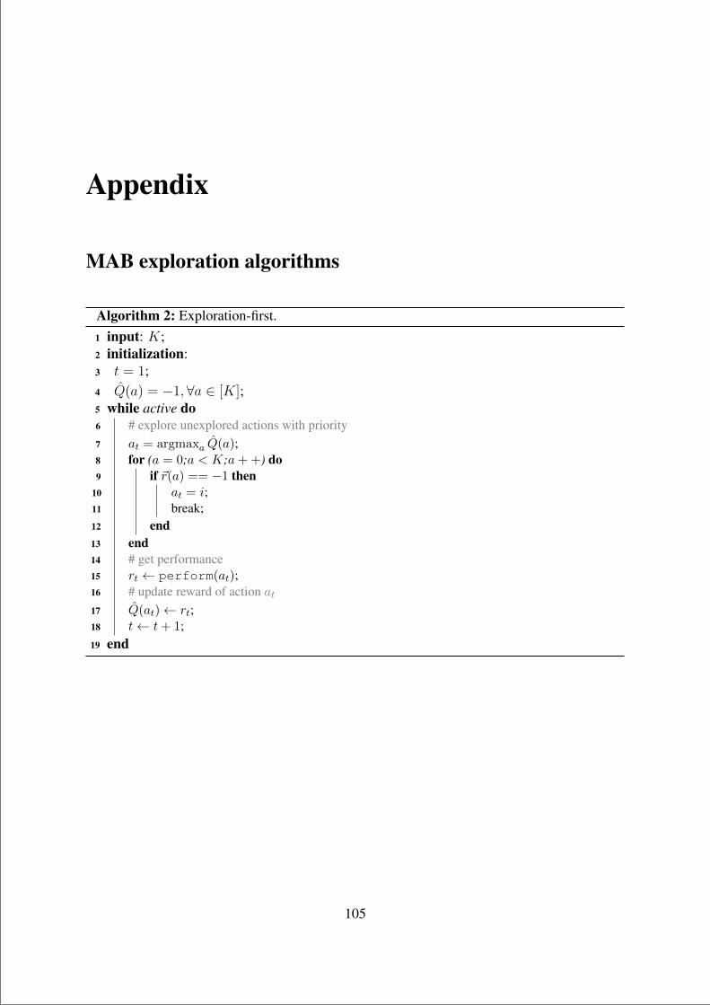
“main” — 2020/11/19 — 10:04 — page 105 — #127

Appendix

MAB exploration algorithms

Algorithm 2: Exploration-first.1 input: K;2 initialization:3 t = 1;4 Q(a) = −1,∀a ∈ [K];5 while active do6 # explore unexplored actions with priority7 at = argmaxa Q(a);8 for (a = 0;a < K;a+ +) do9 if ~r(a) == −1 then

10 at = i;11 break;12 end13 end14 # get performance15 rt ← perform(at);16 # update reward of action at17 Q(at)← rt;18 t← t+ 1;19 end

105

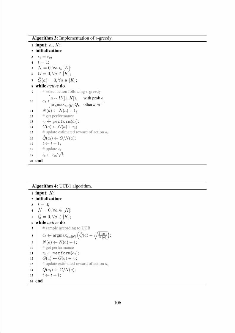
“main” — 2020/11/19 — 10:04 — page 106 — #128

Algorithm 3: Implementation of ε-greedy.1 input: εo, K;2 initialization:3 εt = εo;4 t = 1;5 N = 0, ∀a ∈ [K];6 G = 0, ∀a ∈ [K];7 Q(a) = 0,∀a ∈ [K];8 while active do9 # select action following ε-greedy

10 at

a ∼ U([1,K]), with prob εargmaxa∈[K] Q, otherwise

;

11 N(a)← N(a) + 1;12 # get performance13 rt ← perform(at);14 G(a)← G(a) + rt;15 # update estimated reward of action at16 Q(at)← G/N(a);17 t← t+ 1;18 # update εt19 εt ← εo/

√t;

20 end

Algorithm 4: UCB1 algorithm.1 input: K;2 initialization:3 t = 0;4 N = 0,∀a ∈ [K];5 Q = 0,∀a ∈ [K];6 while active do7 # sample according to UCB

8 at ← argmaxa∈[K]

(Q(a) +

√2 log tN(a)

);

9 N(a)← N(a) + 1;10 # get performance11 rt ← perform(at);12 G(a)← G(a) + rt;13 # update estimated reward of action at14 Q(at)← G/N(a);15 t← t+ 1;16 end

106

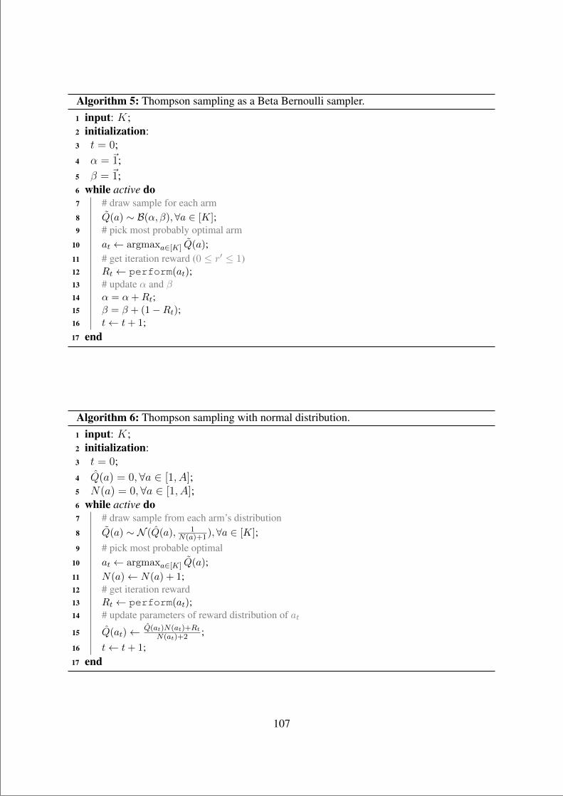
“main” — 2020/11/19 — 10:04 — page 107 — #129

Algorithm 5: Thompson sampling as a Beta Bernoulli sampler.1 input: K;2 initialization:3 t = 0;4 α = ~1;5 β = ~1;6 while active do7 # draw sample for each arm8 Q(a) ∼ B(α, β),∀a ∈ [K];9 # pick most probably optimal arm

10 at ← argmaxa∈[K] Q(a);11 # get iteration reward (0 ≤ r′ ≤ 1)12 Rt ← perform(at);13 # update α and β14 α = α+Rt;15 β = β + (1−Rt);16 t← t+ 1;17 end

Algorithm 6: Thompson sampling with normal distribution.1 input: K;2 initialization:3 t = 0;4 Q(a) = 0,∀a ∈ [1, A];5 N(a) = 0,∀a ∈ [1, A];6 while active do7 # draw sample from each arm’s distribution8 Q(a) ∼ N (Q(a), 1

N(a)+1), ∀a ∈ [K];9 # pick most probable optimal

10 at ← argmaxa∈[K] Q(a);11 N(a)← N(a) + 1;12 # get iteration reward13 Rt ← perform(at);14 # update parameters of reward distribution of at15 Q(at)← Q(at)N(at)+Rt

N(at)+2 ;16 t← t+ 1;17 end

107

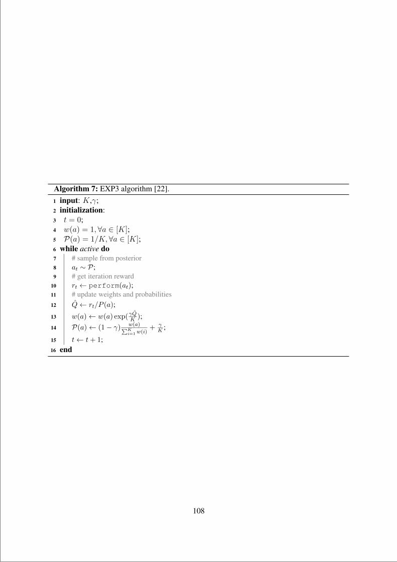
“main” — 2020/11/19 — 10:04 — page 108 — #130

Algorithm 7: EXP3 algorithm [22].1 input: K,γ;2 initialization:3 t = 0;4 w(a) = 1,∀a ∈ [K];5 P(a) = 1/K, ∀a ∈ [K];6 while active do7 # sample from posterior8 at ∼ P;9 # get iteration reward

10 rt ← perform(at);11 # update weights and probabilities12 Q← rt/P (a);

13 w(a)← w(a) exp(γQK );14 P(a)← (1− γ) w(a)∑K

i=1 w(i)+ γ

K ;

15 t← t+ 1;16 end

108

“main” — 2020/11/19 — 10:04 — page 109 — #131

Chapter 8

PUBLICATIONS

The main publications of this thesis, from paper #1 to paper #6, are appended next in theformat of this dissertation.

109

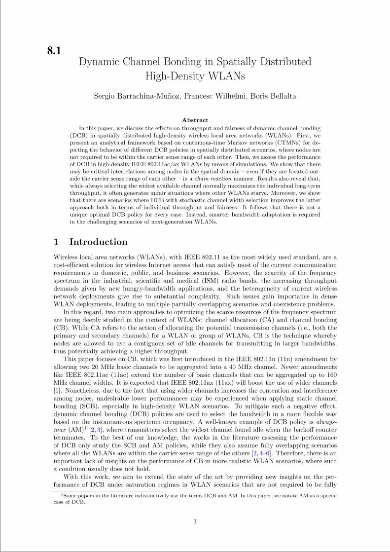
“main” — 2020/11/19 — 10:04 — page 110 — #132

Dynamic Channel Bonding in Spatially Distributed

High-Density WLANs

Sergio Barrachina-Munoz, Francesc Wilhelmi, Boris Bellalta

Abstract

In this paper, we discuss the effects on throughput and fairness of dynamic channel bonding(DCB) in spatially distributed high-density wireless local area networks (WLANs). First, wepresent an analytical framework based on continuous-time Markov networks (CTMNs) for de-picting the behavior of different DCB policies in spatially distributed scenarios, where nodes arenot required to be within the carrier sense range of each other. Then, we assess the performanceof DCB in high-density IEEE 802.11ac/ax WLANs by means of simulations. We show that theremay be critical interrelations among nodes in the spatial domain – even if they are located out-side the carrier sense range of each other – in a chain reaction manner. Results also reveal that,while always selecting the widest available channel normally maximizes the individual long-termthroughput, it often generates unfair situations where other WLANs starve. Moreover, we showthat there are scenarios where DCB with stochastic channel width selection improves the latterapproach both in terms of individual throughput and fairness. It follows that there is not aunique optimal DCB policy for every case. Instead, smarter bandwidth adaptation is requiredin the challenging scenarios of next-generation WLANs.

1 Introduction

Wireless local area networks (WLANs), with IEEE 802.11 as the most widely used standard, are acost-efficient solution for wireless Internet access that can satisfy most of the current communicationrequirements in domestic, public, and business scenarios. However, the scarcity of the frequencyspectrum in the industrial, scientific and medical (ISM) radio bands, the increasing throughputdemands given by new hungry-bandwidth applications, and the heterogeneity of current wirelessnetwork deployments give rise to substantial complexity. Such issues gain importance in denseWLAN deployments, leading to multiple partially overlapping scenarios and coexistence problems.

In this regard, two main approaches to optimizing the scarce resources of the frequency spectrumare being deeply studied in the context of WLANs: channel allocation (CA) and channel bonding(CB). While CA refers to the action of allocating the potential transmission channels (i.e., both theprimary and secondary channels) for a WLAN or group of WLANs, CB is the technique wherebynodes are allowed to use a contiguous set of idle channels for transmitting in larger bandwidths,thus potentially achieving a higher throughput.

This paper focuses on CB, which was first introduced in the IEEE 802.11n (11n) amendment byallowing two 20 MHz basic channels to be aggregated into a 40 MHz channel. Newer amendmentslike IEEE 802.11ac (11ac) extend the number of basic channels that can be aggregated up to 160MHz channel widths. It is expected that IEEE 802.11ax (11ax) will boost the use of wider channels[1]. Nonetheless, due to the fact that using wider channels increases the contention and interferenceamong nodes, undesirable lower performances may be experienced when applying static channelbonding (SCB), especially in high-density WLAN scenarios. To mitigate such a negative effect,dynamic channel bonding (DCB) policies are used to select the bandwidth in a more flexible waybased on the instantaneous spectrum occupancy. A well-known example of DCB policy is always-max (AM)1 [2, 3], where transmitters select the widest channel found idle when the backoff counterterminates. To the best of our knowledge, the works in the literature assessing the performanceof DCB only study the SCB and AM policies, while they also assume fully overlapping scenarioswhere all the WLANs are within the carrier sense range of the others [2, 4–6]. Therefore, there is animportant lack of insights on the performance of CB in more realistic WLAN scenarios, where sucha condition usually does not hold.

With this work, we aim to extend the state of the art by providing new insights on the per-formance of DCB under saturation regimes in WLAN scenarios that are not required to be fully

1Some papers in the literature indistinctively use the terms DCB and AM. In this paper, we notate AM as a specialcase of DCB.

1

8.1

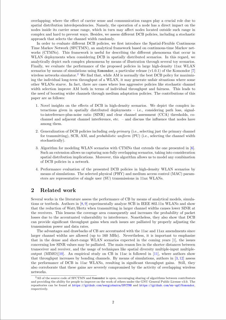
“main” — 2020/11/19 — 10:04 — page 111 — #133

overlapping; where the effect of carrier sense and communication ranges play a crucial role due tospatial distribution interdependencies. Namely, the operation of a node has a direct impact on thenodes inside its carrier sense range, which in turn may affect nodes located outside such range incomplex and hard to prevent ways. Besides, we assess different DCB policies, including a stochasticapproach that selects the channel width randomly.

In order to evaluate different DCB policies, we first introduce the Spatial-Flexible ContinuousTime Markov Network (SFCTMN), an analytical framework based on continuous-time Markov net-works (CTMNs). This framework is useful for describing the different phenomena that occur inWLAN deployments when considering DCB in spatially distributed scenarios. In this regard, weanalytically depict such complex phenomena by means of illustration through several toy scenarios.Finally, we evaluate the performance of the proposed policies in large high-density 11ax WLANscenarios by means of simulations using Komondor, a particular release (v1.0.1) of the Komondor [7]wireless networks simulator.2 We find that, while AM is normally the best DCB policy for maximiz-ing the individual long-term throughput of a WLAN, it may generate unfair situations where someother WLANs starve. In fact, there are cases where less aggressive policies like stochastic channelwidth selection improve AM both in terms of individual throughput and fairness. This leads tothe need of boosting wider channels through medium adaptation policies. The contributions of thispaper are as follows:

1. Novel insights on the effects of DCB in high-density scenarios. We depict the complex in-teractions given in spatially distributed deployments – i.e., considering path loss, signal-to-interference-plus-noise ratio (SINR) and clear channel assessment (CCA) thresholds, co-channel and adjacent channel interference, etc. – and discuss the influence that nodes haveamong them.

2. Generalization of DCB policies including only-primary (i.e., selecting just the primary channelfor transmitting), SCB, AM, and probabilistic uniform (PU) (i.e., selecting the channel widthstochastically).

3. Algorithm for modeling WLAN scenarios with CTMNs that extends the one presented in [6].Such an extension allows us capturing non-fully overlapping scenarios, taking into considerationspatial distribution implications. Moreover, this algorithm allows us to model any combinationof DCB policies in a network.

4. Performance evaluation of the presented DCB policies in high-density WLAN scenarios bymeans of simulations. The selected physical (PHY) and medium access control (MAC) param-eters are representative of single user (SU) transmissions in 11ax WLANs.

2 Related work

Several works in the literature assess the performance of CB by means of analytical models, simula-tions or testbeds. Authors in [8, 9] experimentally analyze SCB in IEEE 802.11n WLANs and showthat the reduction of Watt/Hertz when transmitting in larger channel widths causes lower SINR atthe receivers. This lessens the coverage area consequently and increases the probability of packetlosses due to the accentuated vulnerability to interference. Nonetheless, they also show that DCBcan provide significant throughput gains when such issues are palliated by properly adjusting thetransmission power and data rates.

The advantages and drawbacks of CB are accentuated with the 11ac and 11ax amendments sincelarger channel widths are allowed (up to 160 MHz). Nevertheless, it is important to emphasizethat in the dense and short-range WLAN scenarios expected in the coming years [1], the issuesconcerning low SINR values may be palliated. The main reason lies in the shorter distances betweentransceiver and receiver, and the usage of techniques like spatial diversity multiple-input multiple-output (MIMO)[10]. An empirical study on CB in 11ac is followed in [11], where authors showthat throughput increases by bonding channels. By means of simulations, authors in [3, 12] assessthe performance of DCB in 11ac WLANs, resulting in significant throughput gains. Still, theyalso corroborate that these gains are severely compromised by the activity of overlapping wirelessnetworks.

2All of the source code of SFCTMN and Komondor is open, encouraging sharing of algorithms between contributorsand providing the ability for people to improve on the work of others under the GNU General Public License v3.0. Therepositories can be found at https://github.com/sergiobarra/SFCTMN and https://github.com/wn-upf/Komondor,respectively.

2

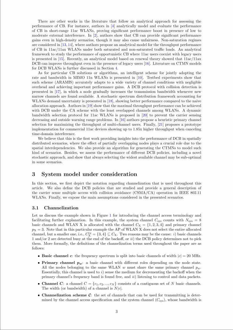
“main” — 2020/11/19 — 10:04 — page 112 — #134

There are other works in the literature that follow an analytical approach for assessing theperformance of CB. For instance, authors in [4] analytically model and evaluate the performanceof CB in short-range 11ac WLANs, proving significant performance boost in presence of low tomoderate external interference. In [2], authors show that CB can provide significant performancegains even in high-density scenarios, though it may also cause unfairness. Non-saturation regimesare considered in [13, 14], where authors propose an analytical model for the throughput performanceof CB in 11ac/11ax WLANs under both saturated and non-saturated traffic loads. An analyticalframework to study the performance of opportunistic CB where 11ac users coexist with legacy usersis presented in [15]. Recently, an analytical model based on renewal theory showed that 11ac/11axDCB can improve throughput even in the presence of legacy users [16]. Literature on CTMN modelsfor DCB WLANs is further discussed in Section 4.

As for particular CB solutions or algorithms, an intelligent scheme for jointly adopting therate and bandwidth in MIMO 11n WLANs is presented in [10]. Testbed experiments show thatsuch scheme (ARAMIS) accurately adapts to a wide variety of channel conditions with negligibleoverhead and achieving important performance gains. A DCB protocol with collision detection ispresented in [17], in which a node gradually increases the transmission bandwidth whenever newnarrow channels are found available. A stochastic spectrum distribution framework accounting forWLANs demand uncertainty is presented in [18], showing better performance compared to the naiveallocation approach. Authors in [19] show that the maximal throughput performance can be achievedwith DCB under the CA scheme with the least overlapped channels among WLANs. A dynamicbandwidth selection protocol for 11ac WLANs is proposed in [20] to prevent the carrier sensingdecreasing and outside warning range problems. In [16] authors propose a heuristic primary channelselection for maximizing the throughput of multi-channel users. Finally, [21] proposes a prototypeimplementation for commercial 11ac devices showing up to 1.85x higher throughput when cancelingtime-domain interference.

We believe that this is the first work providing insights into the performance of DCB in spatiallydistributed scenarios, where the effect of partially overlapping nodes plays a crucial role due to thespatial interdependencies. We also provide an algorithm for generating the CTMNs to model suchkind of scenarios. Besides, we assess the performance of different DCB policies, including a novelstochastic approach, and show that always selecting the widest available channel may be sub-optimalin some scenarios.

3 System model under consideration

In this section, we first depict the notation regarding channelization that is used throughout thisarticle. We also define the DCB policies that are studied and provide a general description ofthe carrier sense multiple access with collision avoidance (CSMA/CA) operation in IEEE 802.11WLANs. Finally, we expose the main assumptions considered in the presented scenarios.

3.1 Channelization

Let us discuss the example shown in Figure 1 for introducing the channel access terminology andfacilitating further explanation. In this example, the system channel Csys counts with Nsys = 8basic channels and WLAN X is allocated with the channel CX = 1, 2, 3, 4 and primary channelpX = 3. Note that in this particular example the AP of WLAN X does not select the entire allocatedchannel, but a smaller one, i.e., Ctx

X = 3, 4 ⊆ CX. Two reasons may be the cause: i) basic channels1 and/or 2 are detected busy at the end of the backoff, or ii) the DCB policy determines not to pickthem. More formally, the definitions of the channelization terms used throughout the paper are asfollows:

Basic channel c: the frequency spectrum is split into basic channels of width |c| = 20 MHz.

Primary channel pw: a basic channel with different roles depending on the node state.All the nodes belonging to the same WLAN w must share the same primary channel pw.Essentially, this channel is used to i) sense the medium for decrementing the backoff when theprimary channel’s frequency band is found free, and ii) listening to control and data packets.

Channel C: a channel C = c1, c2, ..., cN consists of a contiguous set of N basic channels.The width (or bandwidth) of a channel is N |c|.

Channelization scheme C: the set of channels that can be used for transmitting is deter-mined by the channel access specification and the system channel (Csys), whose bandwidth is

3

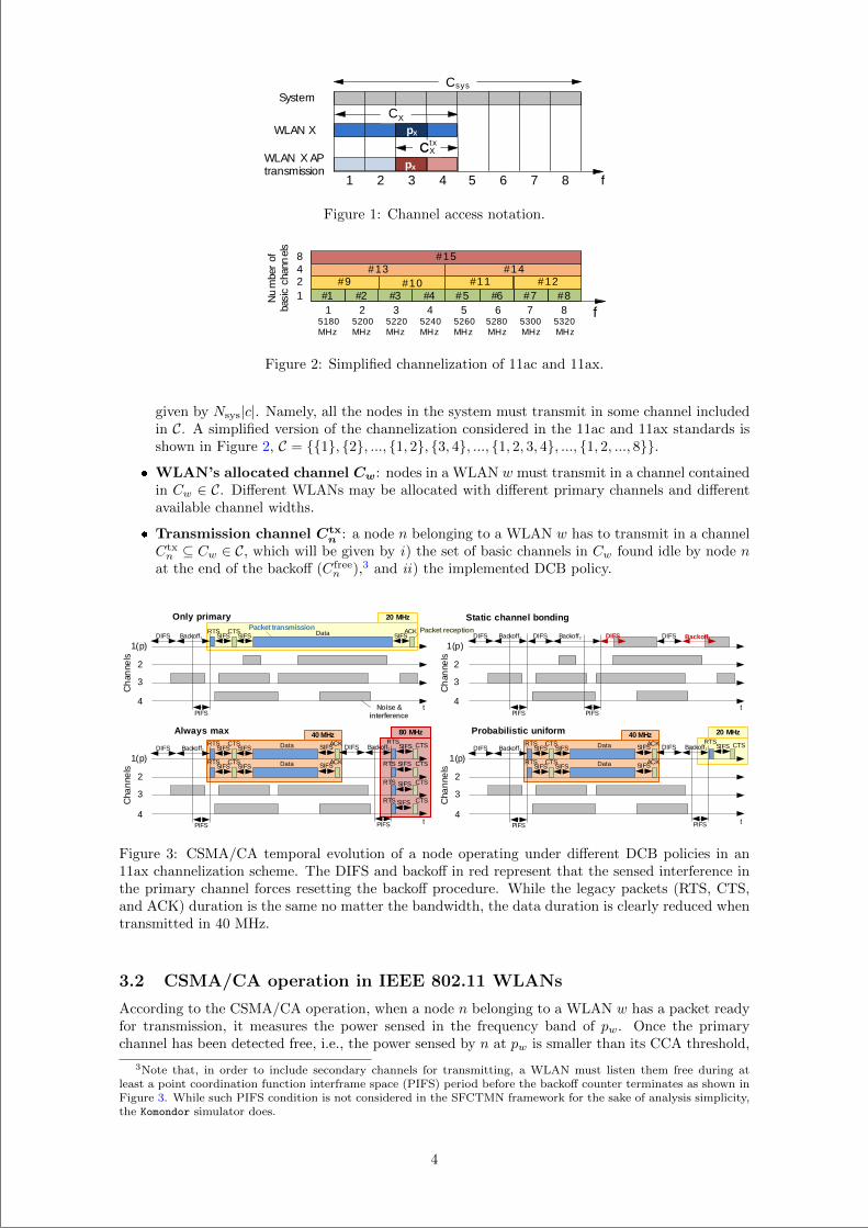
“main” — 2020/11/19 — 10:04 — page 113 — #135

1 2 3 4 5 6 7 8 f

aCsysa

aCXa

aCXa

System

WLAN X

WLAN X AP transmission pX

pX

Ctx

Figure 1: Channel access notation.

1 2 3 4 5 6 7 8 f

8

5180 MHz

5200 MHz

5220MHz

5240 MHz

5260 MHz

5280MHz

5300 MHz

5320 MHz

Nu

mbe

r of

basi

c ch

ann

els

#14#15

#11 #12#8

#9 #10#13

#7#6#5#4#3#2#1

421

Figure 2: Simplified channelization of 11ac and 11ax.

given by Nsys|c|. Namely, all the nodes in the system must transmit in some channel includedin C. A simplified version of the channelization considered in the 11ac and 11ax standards isshown in Figure 2, C = 1, 2, ..., 1, 2, 3, 4, ..., 1, 2, 3, 4, ..., 1, 2, ..., 8.

WLAN’s allocated channel Cw: nodes in a WLAN w must transmit in a channel containedin Cw ∈ C. Different WLANs may be allocated with different primary channels and differentavailable channel widths.

Transmission channel Ctxn : a node n belonging to a WLAN w has to transmit in a channel

Ctxn ⊆ Cw ∈ C, which will be given by i) the set of basic channels in Cw found idle by node n

at the end of the backoff (Cfreen ),3 and ii) the implemented DCB policy.

1(p)

2

3

4

Backoff1DIFS

PIFSt

SIFS Data SIFS

Noise & interference

Ch

anne

ls

Only primary

1(p)

2

3

4

Backoff1DIFS

PIFSt

Ch

anne

ls

Packet receptionPacket transmission

1(p)

2

3

4

Backoff1DIFS

PIFS t

Data SIFS

Cha

nne

ls

Always max

Data SIFS

DIFS Backoff2

RTSSIFS

RTS SIFS

PIFS

RTS

RTS

SIFS

SIFS CTS

CTS

CTS

CTS

40 MHz

20 MHz

80 MHz

Static channel bondingRTS CTS

SIFS

SIFSRTS CTS

SIFS

ACK

ACK

ACKSIFS

RTS CTSSIFS

1(p)

2

3

4

Backoff1DIFS

PIFS t

Data SIFS

Cha

nne

ls

Probabilistic uniform

Data SIFS

DIFS Backoff2

RTSSIFS

PIFS

CTS

40 MHz 20 MHz

SIFSRTS CTS

SIFSACK

ACKSIFS

RTS CTSSIFS

DIFS Backoff2

PIFS

DIFS DIFS Backoff3

Figure 3: CSMA/CA temporal evolution of a node operating under different DCB policies in an11ax channelization scheme. The DIFS and backoff in red represent that the sensed interference inthe primary channel forces resetting the backoff procedure. While the legacy packets (RTS, CTS,and ACK) duration is the same no matter the bandwidth, the data duration is clearly reduced whentransmitted in 40 MHz.

3.2 CSMA/CA operation in IEEE 802.11 WLANs

According to the CSMA/CA operation, when a node n belonging to a WLAN w has a packet readyfor transmission, it measures the power sensed in the frequency band of pw. Once the primarychannel has been detected free, i.e., the power sensed by n at pw is smaller than its CCA threshold,

3Note that, in order to include secondary channels for transmitting, a WLAN must listen them free during atleast a point coordination function interframe space (PIFS) period before the backoff counter terminates as shown inFigure 3. While such PIFS condition is not considered in the SFCTMN framework for the sake of analysis simplicity,the Komondor simulator does.

4

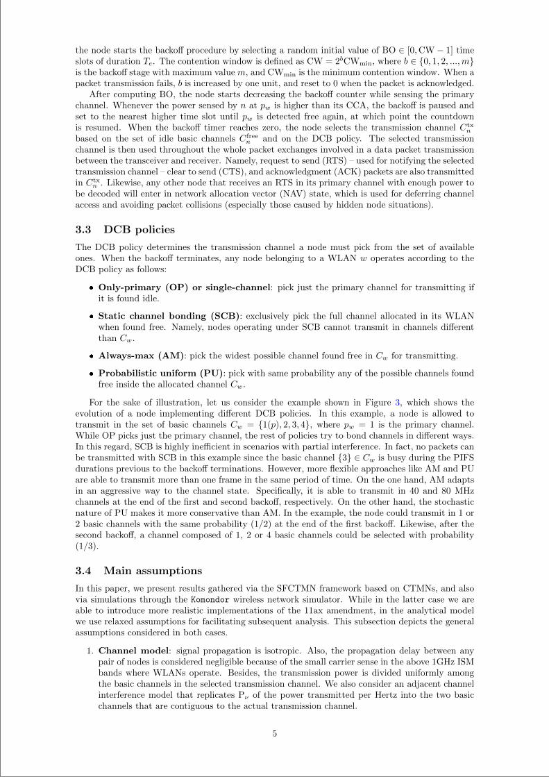
“main” — 2020/11/19 — 10:04 — page 114 — #136

the node starts the backoff procedure by selecting a random initial value of BO ∈ [0,CW− 1] timeslots of duration Te. The contention window is defined as CW = 2bCWmin, where b ∈ 0, 1, 2, ...,mis the backoff stage with maximum value m, and CWmin is the minimum contention window. When apacket transmission fails, b is increased by one unit, and reset to 0 when the packet is acknowledged.

After computing BO, the node starts decreasing the backoff counter while sensing the primarychannel. Whenever the power sensed by n at pw is higher than its CCA, the backoff is paused andset to the nearest higher time slot until pw is detected free again, at which point the countdownis resumed. When the backoff timer reaches zero, the node selects the transmission channel Ctx

n

based on the set of idle basic channels Cfreen and on the DCB policy. The selected transmission

channel is then used throughout the whole packet exchanges involved in a data packet transmissionbetween the transceiver and receiver. Namely, request to send (RTS) – used for notifying the selectedtransmission channel – clear to send (CTS), and acknowledgment (ACK) packets are also transmittedin Ctx

n . Likewise, any other node that receives an RTS in its primary channel with enough power tobe decoded will enter in network allocation vector (NAV) state, which is used for deferring channelaccess and avoiding packet collisions (especially those caused by hidden node situations).

3.3 DCB policies

The DCB policy determines the transmission channel a node must pick from the set of availableones. When the backoff terminates, any node belonging to a WLAN w operates according to theDCB policy as follows:

Only-primary (OP) or single-channel: pick just the primary channel for transmitting ifit is found idle.

Static channel bonding (SCB): exclusively pick the full channel allocated in its WLANwhen found free. Namely, nodes operating under SCB cannot transmit in channels differentthan Cw.

Always-max (AM): pick the widest possible channel found free in Cw for transmitting.

Probabilistic uniform (PU): pick with same probability any of the possible channels foundfree inside the allocated channel Cw.

For the sake of illustration, let us consider the example shown in Figure 3, which shows theevolution of a node implementing different DCB policies. In this example, a node is allowed totransmit in the set of basic channels Cw = 1(p), 2, 3, 4, where pw = 1 is the primary channel.While OP picks just the primary channel, the rest of policies try to bond channels in different ways.In this regard, SCB is highly inefficient in scenarios with partial interference. In fact, no packets canbe transmitted with SCB in this example since the basic channel 3 ∈ Cw is busy during the PIFSdurations previous to the backoff terminations. However, more flexible approaches like AM and PUare able to transmit more than one frame in the same period of time. On the one hand, AM adaptsin an aggressive way to the channel state. Specifically, it is able to transmit in 40 and 80 MHzchannels at the end of the first and second backoff, respectively. On the other hand, the stochasticnature of PU makes it more conservative than AM. In the example, the node could transmit in 1 or2 basic channels with the same probability (1/2) at the end of the first backoff. Likewise, after thesecond backoff, a channel composed of 1, 2 or 4 basic channels could be selected with probability(1/3).

3.4 Main assumptions

In this paper, we present results gathered via the SFCTMN framework based on CTMNs, and alsovia simulations through the Komondor wireless network simulator. While in the latter case we areable to introduce more realistic implementations of the 11ax amendment, in the analytical modelwe use relaxed assumptions for facilitating subsequent analysis. This subsection depicts the generalassumptions considered in both cases.

1. Channel model: signal propagation is isotropic. Also, the propagation delay between anypair of nodes is considered negligible because of the small carrier sense in the above 1GHz ISMbands where WLANs operate. Besides, the transmission power is divided uniformly amongthe basic channels in the selected transmission channel. We also consider an adjacent channelinterference model that replicates Pν of the power transmitted per Hertz into the two basicchannels that are contiguous to the actual transmission channel.

5

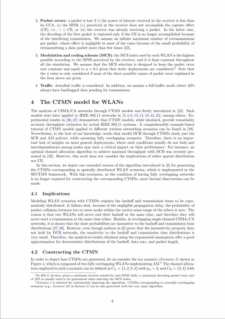
“main” — 2020/11/19 — 10:04 — page 115 — #137

2. Packet errors: a packet is lost if i) the power of interest received at the receiver is less thanits CCA, ii) the SINR (γ) perceived at the receiver does not accomplish the capture effect(CE), i.e., γ < CE, or iii) the receiver was already receiving a packet. In the latter case,the decoding of the first packet is ruptured only if the CE is no longer accomplished becauseof the interfering transmission. We assume an infinite maximum number of retransmissionsper packet, whose effect is negligible in most of the cases because of the small probability ofretransmitting a data packet more than few times [22].

3. Modulation and coding scheme (MCS): the MCS index used by each WLAN is the highestpossible according to the SINR perceived by the receiver, and it is kept constant throughoutall the simulation. We assume that the MCS selection is designed to keep the packet errorrate constant and equal to η = 0.1 given that static deployments are considered.4 Note thatthe η value is only considered if none of the three possible causes of packet error explained inthe item above are given.

4. Traffic: downlink traffic is considered. In addition, we assume a full-buffer mode where APsalways have backlogged data pending for transmission.

4 The CTMN model for WLANs

The analysis of CSMA/CA networks through CTMN models was firstly introduced in [23]. Suchmodels were later applied to IEEE 802.11 networks in [2, 4, 6, 13, 14, 19, 24, 25], among others. Ex-perimental results in [26, 27] demonstrate that CTMN models, while idealized, provide remarkablyaccurate throughput estimates for actual IEEE 802.11 systems. A comprehensible example-basedtutorial of CTMN models applied to different wireless networking scenarios can be found in [28].Nevertheless, to the best of our knowledge, works that model DCB through CTMNs study just theSCB and AM policies, while assuming fully overlapping scenarios. Therefore, there is an impor-tant lack of insights on more general deployments, where such conditions usually do not hold andinterdependencies among nodes may have a critical impact on their performance. For instance, anoptimal channel allocation algorithm to achieve maximal throughput with DCB was recently pre-sented in [29]. However, this work does not consider the implications of either spatial distributionnor CE.

In this section, we depict our extended version of the algorithm introduced in [6] for generatingthe CTMNs corresponding to spatially distributed WLAN scenarios, which is implemented in theSFCTMN framework. With this extension, as the condition of having fully overlapping networksis no longer required for constructing the corresponding CTMNs, more factual observations can bemade.

4.1 Implications

Modeling WLAN scenarios with CTMNs requires the backoff and transmission times to be expo-nentially distributed. It follows that, because of the negligible propagation delay, the probability ofpacket collisions between two or more nodes within the carrier sense range of the others is zero. Thereason is that two WLANs will never end their backoff at the same time, and therefore they willnever start a transmission at the same time either. Besides, in overlapping single-channel CSMA/CAnetworks, it is shown that the state probabilities are insensitive to the backoff and transmission timedistributions [27, 30]. However, even though authors in [6] prove that the insensitivity property doesnot hold for DCB networks, the sensitivity to the backoff and transmission time distributions isvery small. Therefore, the analytical results obtained using the exponential assumption offer a goodapproximation for deterministic distributions of the backoff, data rate, and packet length.

4.2 Constructing the CTMN

In order to depict how CTMNs are generated, let us consider the toy scenario (Scenario I ) shown inFigure 4, which is composed of two fully overlapping WLANs implementing AM.5 The channel alloca-tion employed in such a scenario can be defined as CA = 1, 2, 3, 4 with pA = 2, and CB = 3, 4 with

4In 802.11 devices, given a minimum receiver sensitivity and SINR table, a maximum decoding packet error rateof 10% is usually tried to be guaranteed when selecting the MCS index.

5Scenario I is selected for conveniently depicting the algorithm. CTMNs corresponding to non-fully overlappingscenarios (e.g., Scenario III in Section 5) can be also generated with the very same algorithm.

6

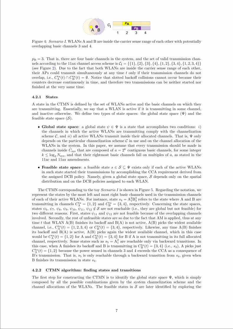
“main” — 2020/11/19 — 10:04 — page 116 — #138

pA

1 2 3 4

CI p

BA B

Figure 4: Scenario I. WLANs A and B are inside the carrier sense range of each other with potentiallyoverlapping basic channels 3 and 4.

pB = 3. That is, there are four basic channels in the system, and the set of valid transmission chan-nels according to the 11ax channel access scheme is CI = 1, 2, 3, 4, 1, 2, 3, 4, 1, 2, 3, 4(see Figure 2). Due to the fact that both WLANs are inside the carrier sense range of each other,their APs could transmit simultaneously at any time t only if their transmission channels do notoverlap, i.e., Ctx

A (t) ∩ CtxB (t) = ∅. Notice that slotted backoff collisions cannot occur because their

counters decrease continuously in time, and therefore two transmissions can be neither started norfinished at the very same time.

4.2.1 States

A state in the CTMN is defined by the set of WLANs active and the basic channels on which theyare transmitting. Essentially, we say that a WLAN is active if it is transmitting in some channel,and inactive otherwise. We define two types of state spaces: the global state space (Ψ) and thefeasible state space (S).

Global state space: a global state ψ ∈ Ψ is a state that accomplishes two conditions: i)the channels in which the active WLANs are transmitting comply with the channelizationscheme C, and ii) all active WLANs transmit inside their allocated channels. That is, Ψ onlydepends on the particular channelization scheme C in use and on the channel allocation of theWLANs in the system. In this paper, we assume that every transmission should be made inchannels inside Csys that are composed of a = 2k contiguous basic channels, for some integerk ≤ log2Nsys, and that their rightmost basic channels fall on multiples of a, as stated in the11ac and 11ax amendments.

Feasible state space: a feasible state s ∈ S ⊆ Ψ exists only if each of the active WLANsin such state started their transmissions by accomplishing the CCA requirement derived fromthe assigned DCB policy. Namely, given a global state space, S depends only on the spatialdistribution and on the DCB policies assigned to each WLAN.

The CTMN corresponding to the toy Scenario I is shown in Figure 5. Regarding the notation, werepresent the states by the most left and most right basic channels used in the transmission channelsof each of their active WLANs. For instance, state s4 = A2

1B43 refers to the state where A and B are

transmitting in channels CtxA = 1, 2 and Ctx

B = 3, 4, respectively. Concerning the state spaces,states ψ6, ψ7, ψ8, ψ9, ψ10, ψ11, ψ12 /∈ S are not reachable (i.e., they are global but not feasible) fortwo different reasons. First, states ψ11 and ψ12 are not feasible because of the overlapping channelsinvolved. Secondly, the rest of unfeasible states are so due to the fact that AM is applied, thus at anytime t that WLAN A(B) finishes its backoff and B(A) is not active, A(B) picks the widest availablechannel, i.e., Ctx

A (t) = 1, 2, 3, 4 or CtxB (t) = 3, 4, respectively. Likewise, any time A(B) finishes

its backoff and B(A) is active, A(B) picks again the widest available channel, which in this casewould be Ctx

A (t) = 1, 2 for A and CtxB (t) = 3, 4 for B if A is not transmitting in its full allocated

channel, respectively. Some states such as s5 = A21 are reachable only via backward transitions. In

this case, when A finishes its backoff and B is transmitting in CtxB (t) = 3, 4 (i.e., s3), A picks just

CtxA (t) = 1, 2 because the power sensed in channels 3 and 4 exceeds the CCA as a consequence of

B’s transmission. That is, s5 is only reachable through a backward transition from s4, given whenB finishes its transmission in state s4.

4.2.2 CTMN algorithm: finding states and transitions

The first step for constructing the CTMN is to identify the global state space Ψ, which is simplycomposed by all the possible combinations given by the system channelization scheme and thechannel allocations of the WLANs. The feasible states in S are later identified by exploring the

7

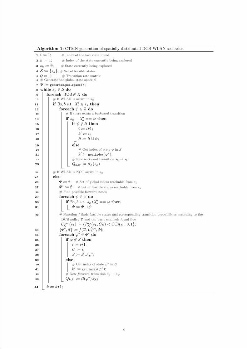
“main” — 2020/11/19 — 10:04 — page 117 — #139

Algorithm 1: CTMN generation of spatially distributed DCB WLAN scenarios.

1 i := 1; .........# Index of the last state found

2 k := 1; ....... # Index of the state currently being explored

3 sk := ∅; ......# State currently being explored

4 S := sk; # Set of feasible states

5 Q := [ ]; ....... # Transition rate matrix6 # Generate the global state space Ψ

7 Ψ := generate psi space() ;8 while sk ∈ S do9 foreach WLAN X do

10 # If WLAN is active in sk

11 if ∃a, b s.t. Xba ∈ sk then12 foreach ψ ∈ Ψ do13 # If there exists a backward transition

14 if sk −Xba == ψ then15 if ψ 6∈ S then16 i := i+1;17 k′ := i;18 S := S ∪ ψ;

19 else20 # Get index of state ψ in S21 k′ := get index(ϕ∗);22 # New backward transition sk → sk′

23 Qk,k′ := µX(sk)

24 # If WLAN is NOT active in sk

25 else26 Φ := ∅; . # Set of global states reachable from sk

27 Φ∗ := ∅; . # Set of feasible states reachable from sk28 # Find possible forward states

29 foreach ψ ∈ Ψ do

30 if ∃a, b s.t. sk+Xba == ψ then

31 Φ := Φ ∪ ψ;

32 # Function f finds feasible states and corresponding transition probabilities according to the

DCB policy D and the basic channels found free

CfreeX (sk) := P rx

X (sk, CX) < CCAX : 0, 1;33 Φ∗, ~α := f(D, Cfree

X , Φ);34 foreach ϕ∗ ∈ Φ∗ do35 if ϕ 6∈ S then36 i := i+1;37 k′ := i;38 S := S ∪ ϕ∗;39 else40 # Get index of state ϕ∗ in S41 k′ := get index(ϕ∗);42 # New forward transition sk → sk′

43 Qk,k′ := ~α(ϕ∗)λX;

44 k := k+1;

8

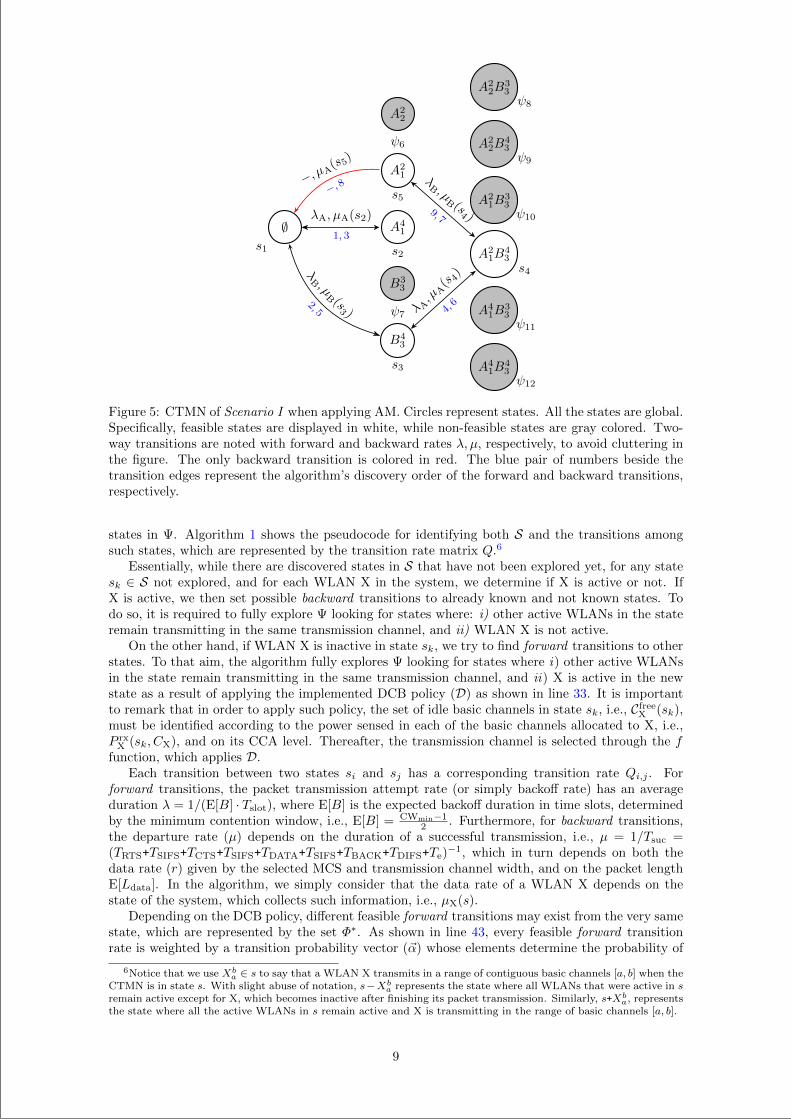
“main” — 2020/11/19 — 10:04 — page 118 — #140

∅s1

A41

s2

A21

s5

A22

ψ6

B33

ψ7

B43

s3

A21B

43s4

A41B

33ψ11

A41B

43ψ12

A21B

33ψ10

A22B

43ψ9

A22B

33ψ8

λA, µA(s2)

1, 3

λB , µ

B (s3 )

2, 5

−, µA(s5)

−, 8

λA, µ

A(s 4

)

4,6

λB , µ

B (s4 )9, 7

Figure 5: CTMN of Scenario I when applying AM. Circles represent states. All the states are global.Specifically, feasible states are displayed in white, while non-feasible states are gray colored. Two-way transitions are noted with forward and backward rates λ, µ, respectively, to avoid cluttering inthe figure. The only backward transition is colored in red. The blue pair of numbers beside thetransition edges represent the algorithm’s discovery order of the forward and backward transitions,respectively.

states in Ψ. Algorithm 1 shows the pseudocode for identifying both S and the transitions amongsuch states, which are represented by the transition rate matrix Q.6

Essentially, while there are discovered states in S that have not been explored yet, for any statesk ∈ S not explored, and for each WLAN X in the system, we determine if X is active or not. IfX is active, we then set possible backward transitions to already known and not known states. Todo so, it is required to fully explore Ψ looking for states where: i) other active WLANs in the stateremain transmitting in the same transmission channel, and ii) WLAN X is not active.

On the other hand, if WLAN X is inactive in state sk, we try to find forward transitions to otherstates. To that aim, the algorithm fully explores Ψ looking for states where i) other active WLANsin the state remain transmitting in the same transmission channel, and ii) X is active in the newstate as a result of applying the implemented DCB policy (D) as shown in line 33. It is importantto remark that in order to apply such policy, the set of idle basic channels in state sk, i.e., Cfree

X (sk),must be identified according to the power sensed in each of the basic channels allocated to X, i.e.,P rx

X (sk, CX), and on its CCA level. Thereafter, the transmission channel is selected through the ffunction, which applies D.

Each transition between two states si and sj has a corresponding transition rate Qi,j . Forforward transitions, the packet transmission attempt rate (or simply backoff rate) has an averageduration λ = 1/(E[B] · Tslot), where E[B] is the expected backoff duration in time slots, determinedby the minimum contention window, i.e., E[B] = CWmin−1

2 . Furthermore, for backward transitions,the departure rate (µ) depends on the duration of a successful transmission, i.e., µ = 1/Tsuc =(TRTS+TSIFS+TCTS+TSIFS+TDATA+TSIFS+TBACK+TDIFS+Te)−1, which in turn depends on both thedata rate (r) given by the selected MCS and transmission channel width, and on the packet lengthE[Ldata]. In the algorithm, we simply consider that the data rate of a WLAN X depends on thestate of the system, which collects such information, i.e., µX(s).

Depending on the DCB policy, different feasible forward transitions may exist from the very samestate, which are represented by the set Φ∗. As shown in line 43, every feasible forward transitionrate is weighted by a transition probability vector (~α) whose elements determine the probability of

6Notice that we use Xba ∈ s to say that a WLAN X transmits in a range of contiguous basic channels [a, b] when the

CTMN is in state s. With slight abuse of notation, s−Xba represents the state where all WLANs that were active in s

remain active except for X, which becomes inactive after finishing its packet transmission. Similarly, s+Xba, represents

the state where all the active WLANs in s remain active and X is transmitting in the range of basic channels [a, b].

9

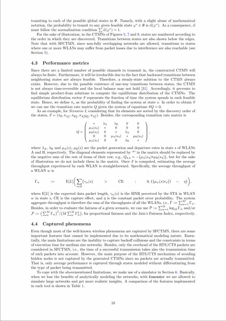
“main” — 2020/11/19 — 10:04 — page 119 — #141

transiting to each of the possible global states in Φ. Namely, with a slight abuse of mathematicalnotation, the probability to transit to any given feasible state ϕ∗ ∈ Φ is ~α(ϕ∗). As a consequence, ~αmust follow the normalization condition

∑~α(ϕ∗) = 1.

For the sake of illustration, in the CTMNs of Figures 5, 7 and 9, states are numbered according tothe order in which they are discovered. Transitions between states are also shown below the edges.Note that with SFCTMN, since non-fully overlapping networks are allowed, transitions to stateswhere one or more WLANs may suffer from packet losses due to interference are also reachable (seeSection 5).

4.3 Performance metrics

Since there are a limited number of possible channels to transmit in, the constructed CTMN willalways be finite. Furthermore, it will be irreducible due to the fact that backward transitions betweenneighboring states are always feasible. Therefore, a steady-state solution to the CTMN alwaysexists. However, due to the possible existence of one-way transitions between states, the CTMNis not always time-reversible and the local balance may not hold [31]. Accordingly, it prevents tofind simple product-from solutions to compute the equilibrium distribution of the CTMNs. Theequilibrium distribution vector ~π represents the fraction of time the system spends in each feasiblestate. Hence, we define πs as the probability of finding the system at state s. In order to obtain ~πwe can use the transition rate matrix Q given the system of equations ~πQ = 0.

As an example, for Scenario I, considering that its elements are sorted by the discovery order ofthe states, ~π = (π∅, πA4

1, πB4

3, πA2

1B43, πA2

1). Besides, the corresponding transition rate matrix is

Q =

∗ λA λB 0 0µA(s2) ∗ 0 0 0µB(s3) 0 ∗ λA 0

0 0 µA(s4) ∗ µB(s4)µA(s5) 0 0 λB ∗

,

where λA, λB and µA(s), µB(s) are the packet generation and departure rates in state s of WLANsA and B, respectively. The diagonal elements represented by ‘*’ in the matrix should be replaced bythe negative sum of the rest of items of their row, e.g., Q4,4 = −

(µA(s4)+µB(s4)

), but for the sake

of illustration we do not include them in the matrix. Once ~π is computed, estimating the averagethroughput experienced by each WLAN is straightforward. Specifically, the average throughput ofa WLAN w is

Γw := E[L]

(∑

s∈Sγw(s) > CE : 0, 1µw(s)πs

(1 − η

)),

where E[L] is the expected data packet length, γw(s) is the SINR perceived by the STA in WLANw in state s, CE is the capture effect, and η is the constant packet error probability. The systemaggregate throughput is therefore the sum of the throughputs of all the WLANs, i.e., Γ :=

∑Mw=1 Γw.

Besides, in order to evaluate the fairness of a given scenario, we can use P :=∑Mw=1 log10 Γw and/or

F :=(∑M

w Γw)2/(M∑Mw Γ2

w

), for proportional fairness and the Jain’s Fairness Index, respectively.

4.4 Captured phenomena

Even though most of the well-known wireless phenomena are captured by SFCTMN, there are someimportant features that cannot be implemented due to its mathematical modeling nature. Essen-tially, the main limitations are the inability to capture backoff collisions and the constraints in termsof execution time for medium size networks. Besides, only the overhead of the RTS/CTS packets areconsidered in SFCTMN, i.e., the time of a successful transmission takes also the transmission timeof such packets into account. However, the main purpose of the RTS/CTS mechanism of avoidinghidden nodes is not captured by the generated CTMNs since no packets are actually transmitted.That is, only average performance is captured through states modeled without differentiating fromthe type of packet being transmitted.

To cope with the abovementioned limitations, we make use of a simulator in Section 6. Basically,when we lose the benefits of analytically modeling the networks, with Komondor we are allowed tosimulate large networks and get more realistic insights. A comparison of the features implementedin each tool is shown in Table 1.

10

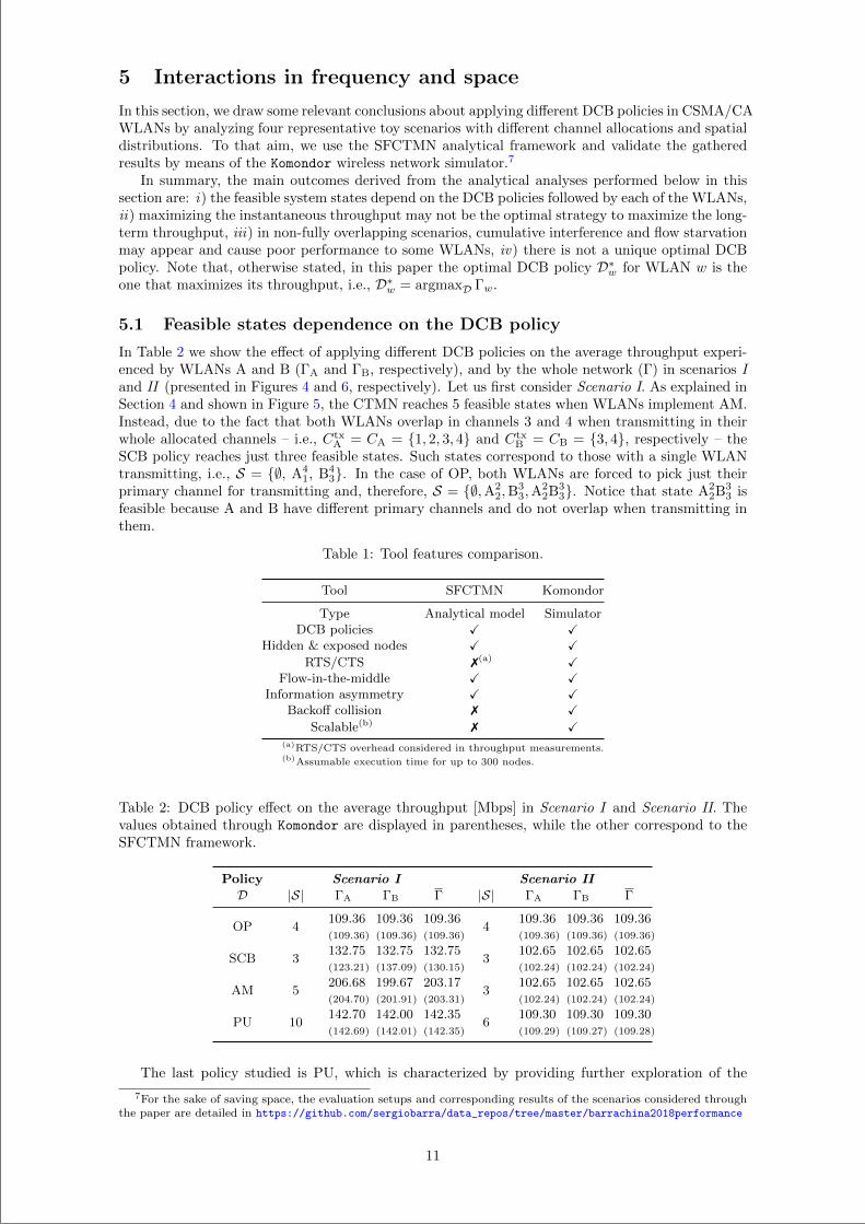
“main” — 2020/11/19 — 10:04 — page 120 — #142

5 Interactions in frequency and space

In this section, we draw some relevant conclusions about applying different DCB policies in CSMA/CAWLANs by analyzing four representative toy scenarios with different channel allocations and spatialdistributions. To that aim, we use the SFCTMN analytical framework and validate the gatheredresults by means of the Komondor wireless network simulator.7

In summary, the main outcomes derived from the analytical analyses performed below in thissection are: i) the feasible system states depend on the DCB policies followed by each of the WLANs,ii) maximizing the instantaneous throughput may not be the optimal strategy to maximize the long-term throughput, iii) in non-fully overlapping scenarios, cumulative interference and flow starvationmay appear and cause poor performance to some WLANs, iv) there is not a unique optimal DCBpolicy. Note that, otherwise stated, in this paper the optimal DCB policy D∗w for WLAN w is theone that maximizes its throughput, i.e., D∗w = argmaxD Γw.

5.1 Feasible states dependence on the DCB policy

In Table 2 we show the effect of applying different DCB policies on the average throughput experi-enced by WLANs A and B (ΓA and ΓB, respectively), and by the whole network (Γ) in scenarios Iand II (presented in Figures 4 and 6, respectively). Let us first consider Scenario I. As explained inSection 4 and shown in Figure 5, the CTMN reaches 5 feasible states when WLANs implement AM.Instead, due to the fact that both WLANs overlap in channels 3 and 4 when transmitting in theirwhole allocated channels – i.e., Ctx

A = CA = 1, 2, 3, 4 and CtxB = CB = 3, 4, respectively – the

SCB policy reaches just three feasible states. Such states correspond to those with a single WLANtransmitting, i.e., S = ∅, A4

1, B43. In the case of OP, both WLANs are forced to pick just their

primary channel for transmitting and, therefore, S = ∅,A22,B

33,A

22B3

3. Notice that state A22B3

3 isfeasible because A and B have different primary channels and do not overlap when transmitting inthem.

Table 1: Tool features comparison.

Tool SFCTMN Komondor

Type Analytical model SimulatorDCB policies X X

Hidden & exposed nodes X XRTS/CTS 7(a) X

Flow-in-the-middle X XInformation asymmetry X X

Backoff collision 7 XScalable(b) 7 X

(a)RTS/CTS overhead considered in throughput measurements.(b)Assumable execution time for up to 300 nodes.

Table 2: DCB policy effect on the average throughput [Mbps] in Scenario I and Scenario II. Thevalues obtained through Komondor are displayed in parentheses, while the other correspond to theSFCTMN framework.

Policy Scenario I Scenario II

D |S| ΓA ΓB Γ |S| ΓA ΓB Γ

OP 4109.36 109.36 109.36

4109.36 109.36 109.36

(109.36) (109.36) (109.36) (109.36) (109.36) (109.36)

SCB 3132.75 132.75 132.75

3102.65 102.65 102.65

(123.21) (137.09) (130.15) (102.24) (102.24) (102.24)

AM 5206.68 199.67 203.17

3102.65 102.65 102.65

(204.70) (201.91) (203.31) (102.24) (102.24) (102.24)

PU 10142.70 142.00 142.35

6109.30 109.30 109.30

(142.69) (142.01) (142.35) (109.29) (109.27) (109.28)

The last policy studied is PU, which is characterized by providing further exploration of the

7For the sake of saving space, the evaluation setups and corresponding results of the scenarios considered throughthe paper are detailed in https://github.com/sergiobarra/data_repos/tree/master/barrachina2018performance

11

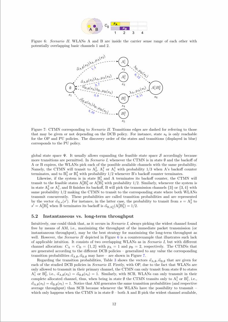
“main” — 2020/11/19 — 10:04 — page 121 — #143

CII

1 2 3 4

pA

pBA B

Figure 6: Scenario II. WLANs A and B are inside the carrier sense range of each other withpotentially overlapping basic channels 1 and 2.

∅s1

A21

s3

A11

s2

B22

s4

B21

s5

A11B

22

s6

~αA,∅(s

2)λA, µA

(s2)

1, 5

~αA,∅(s3)λA, µA(s3)

2, 7~αB,∅(s4)λB, µB(s4)3, 9

~αB,∅ (s5 )λ

B , µB (s5 )4, 10

λB , µ

B (s5 )

6, 12

λA, µA(s5)

8, 11

Figure 7: CTMN corresponding to Scenario II. Transitions edges are dashed for referring to thosethat may be given or not depending on the DCB policy. For instance, state s6 is only reachablefor the OP and PU policies. The discovery order of the states and transitions (displayed in blue)corresponds to the PU policy.

global state space Ψ. It usually allows expanding the feasible state space S accordingly becausemore transitions are permitted. In Scenario I, whenever the CTMN is in state ∅ and the backoff ofA or B expires, the WLANs pick each of the possible available channels with the same probability.Namely, the CTMN will transit to A2

2, A21 or A4

1 with probability 1/3 when A’s backoff counterterminates, and to B3

3 or B43 with probability 1/2 whenever B’s backoff counter terminates.

Likewise, if the system is in state B33 and A terminates its backoff counter, the CTMN will

transit to the feasible states A22B3

3 or A21B3

3 with probability 1/2. Similarly, whenever the system isin state A2

2 or A21, and B finishes its backoff, B will pick the transmission channels 3 or 3, 4 with

same probability 1/2 making the CTMN to transit to the corresponding state where both WLANstransmit concurrently. These probabilities are called transition probabilities and are representedby the vector ~αX,s(s

′). For instance, in the latter case, the probability to transit from s = A22 to

s′ = A22B3

3 when B terminates its backoff is ~αB,A22(A2

2B33) = 1/2.

5.2 Instantaneous vs. long-term throughput

Intuitively, one could think that, as it occurs in Scenario I, always picking the widest channel foundfree by means of AM, i.e., maximizing the throughput of the immediate packet transmission (orinstantaneous throughput), may be the best strategy for maximizing the long-term throughput aswell. However, the Scenario II depicted in Figure 6 is a counterexample that illustrates such lackof applicable intuition. It consists of two overlapping WLANs as in Scenario I, but with differentchannel allocation: CA = CB = 1, 2 with pA = 1 and pB = 2, respectively. The CTMNs thatare generated according to the different DCB policies – generalized to any value the correspondingtransition probabilities ~αA,∅, ~αB,∅ may have – are shown in Figure 7.

Regarding the transition probabilities, Table 3 shows the vectors ~αA,∅, ~αB,∅ that are given foreach of the studied DCB policies in Scenario II. Firstly, with OP, due to the fact that WLANs areonly allowed to transmit in their primary channel, the CTMN can only transit from state ∅ to statesA1

1 or B22, i.e., ~αA,∅(s2) = ~αB,∅(s4) = 1. Similarly, with SCB, WLANs can only transmit in their

complete allocated channel, thus, when being in state ∅ the CTMN transits only to A21 or B2

1, i.e.,~αA,∅(s3) = ~αB,∅(s5) = 1. Notice that AM generates the same transition probabilities (and respectiveaverage throughput) than SCB because whenever the WLANs have the possibility to transmit –which only happens when the CTMN is in state ∅ – both A and B pick the widest channel available,

12

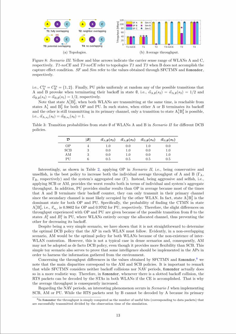
“main” — 2020/11/19 — 10:04 — page 122 — #144

T2: neighbor overlapping

T4: no overlapping

T1: fully overlapping

T3: potential overlapping

(+)

(a) Topologies.

T1-noCE T1 T2 T3-noCE T3 T40

20

40

60

80

100

120

Trh

oguh

put [

Mbp

s] SF ASF BSF C

Sim ASim BSim C

(b) Average throughput.

Figure 8: Scenario III. Yellow and blue arrows indicate the carrier sense range of WLANs A and C,respectively. T1-noCE and T3-noCE refer to topologies T1 and T3 when B does not accomplish thecapture effect condition. SF and Sim refer to the values obtained through SFCTMN and Komondor,respectively.

i.e., CtxA = Ctx

B = 1, 2. Finally, PU picks uniformly at random any of the possible transitions thatA and B provoke when terminating their backoff in state ∅, i.e., ~αA,∅(s2) = ~αA,∅(s3) = 1/2 and~αB,∅(s4) = ~αB,∅(s5) = 1/2, respectively.

Note that state A11B2

2, when both WLANs are transmitting at the same time, is reachable fromstates A1

1 and B22 for both OP and PU. In such states, when either A or B terminates its backoff

and the other is still transmitting in its primary channel, only a transition to state A11B2

2 is possible,i.e., ~αA,s2(s6) = ~αB,s4(s6) = 1.

Table 3: Transition probabilities from state ∅ of WLANs A and B in Scenario II for different DCBpolicies.

D |S| ~αA,∅(s2) ~αA,∅(s3) ~αB,∅(s4) ~αB,∅(s5)

OP 4 1.0 0.0 1.0 0.0SCB 3 0.0 1.0 0.0 1.0AM 3 0.0 1.0 0.0 1.0PU 6 0.5 0.5 0.5 0.5

Interestingly, as shown in Table 2, applying OP in Scenario II, i.e., being conservative andunselfish, is the best policy to increase both the individual average throughput of A and B (ΓA,ΓB, respectively) and the system’s aggregated one (Γ). Instead, being aggressive and selfish, i.e.,applying SCB or AM, provides the worst results both in terms of individual and system’s aggregatethroughput. In addition, PU provides similar results than OP in average because most of the timesthat A and B terminate their backoff counter, they can only transmit in their primary channelsince the secondary channel is most likely occupied by the other WLAN. In fact, state A1

1B22 is the

dominant state for both OP and PU. Specifically, the probability of finding the CTMN in stateA1

1B22, i.e., ~πs6 , is 0.9802 for OP and 0.9702 for PU, respectively. Therefore, the slight differences on

throughput experienced with OP and PU are given because of the possible transition from ∅ to thestates A2

1 and B21 in PU, where WLANs entirely occupy the allocated channel, thus preventing the

other for decreasing its backoff.Despite being a very simple scenario, we have shown that it is not straightforward to determine

the optimal DCB policy that the AP in each WLAN must follow. Evidently, in a non-overlappingscenario, AM would be the optimal policy for both WLANs because of the non-existence of inter-WLAN contention. However, this is not a typical case in dense scenarios and, consequently, AMmay not be adopted as de facto DCB policy, even though it provides more flexibility than SCB. Thissimple toy scenario also serves to prove that some intelligence should be implemented in the APs inorder to harness the information gathered from the environment.

Concerning the throughput differences in the values obtained by SFCTMN and Komondor,8 wenote that the main disparities correspond to the AM and SCB policies. It is important to remarkthat while SFCTMN considers neither backoff collisions nor NAV periods, Komondor actually doesso in a more realistic way. Therefore, in Komondor, whenever there is a slotted backoff collision, theRTS packets can be decoded by the STAs in both WLANs if the CE is accomplished. That is whythe average throughput is consequently increased.

Regarding the NAV periods, an interesting phenomenon occurs in Scenario I when implementingSCB, AM or PU. While the RTS packets sent by B cannot be decoded by A because its primary

8In Komondor the throughput is simply computed as the number of useful bits (corresponding to data packets) thatare successfully transmitted divided by the observation time of the simulation.

13

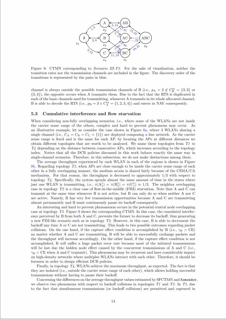
“main” — 2020/11/19 — 10:04 — page 123 — #145

∅s1

B

s3

A

s2

C

s4

AC

s6

AB

s5

BC

s7

ABC

s8

1,4

2, 8

3, 12

5, 14em

pty6, 17empty

7,13

empty

9, 20empty

10, 1

6

11, 19

15, 23

−, 22

18, 2

1

Figure 9: CTMN corresponding to Scenario III-T3. For the sake of visualization, neither thetransition rates nor the transmission channels are included in the figure. The discovery order of thetransitions is represented by the pairs in blue.

channel is always outside the possible transmission channels of B (i.e., pA = 2 /∈ CtxB = 3, 3 or

3, 4), the opposite occurs when A transmits them. Due to the fact that the RTS is duplicated ineach of the basic channels used for transmitting, whenever A transmits in its whole allocated channel,B is able to decode the RTS (i.e., pB = 3 ∈ Ctx

A = 1, 2, 3, 4) and enters in NAV consequently.

5.3 Cumulative interference and flow starvation

When considering non-fully overlapping scenarios, i.e., where some of the WLANs are not insidethe carrier sense range of the others, complex and hard to prevent phenomena may occur. Asan illustrative example, let us consider the case shown in Figure 8a, where 3 WLANs sharing asingle channel (i.e., CA = CB = CC = 1) are deployed composing a line network. As the carriersense range is fixed and is the same for each AP, by locating the APs at different distances weobtain different topologies that are worth to be analyzed. We name these topologies from T1 toT4 depending on the distance between consecutive APs, which increases according to the topologyindex. Notice that all the DCB policies discussed in this work behave exactly the same way insingle-channel scenarios. Therefore, in this subsection, we do not make distinctions among them.

The average throughput experienced by each WLAN in each of the regions is shown in Figure8b. Regarding topology T1, when APs are close enough to be inside the carrier sense range of eachother in a fully overlapping manner, the medium access is shared fairly because of the CSMA/CAmechanism. For that reason, the throughput is decreased to approximately 1/3 with respect totopology T4. Specifically, the system spends almost the same amount of time in the states wherejust one WLAN is transmitting, i.e., π(A1

1) = π(B11) = π(C1

1) ≈ 1/3. The neighbor overlappingcase in topology T2 is a clear case of flow-in-the-middle (FIM) starvation. Note that A and C cantransmit at the same time whenever B is not active, but B can only do so when neither A nor Care active. Namely, B has very few transmission opportunities because A and C are transmittingalmost permanently and B must continuously pause its backoff consequently.

An interesting and hard to prevent phenomenon occurs in the potential central node overlappingcase at topology T3. Figure 9 shows the corresponding CTMN. In this case, the cumulated interfer-ence perceived by B from both A and C, prevents the former to decrease its backoff, thus generatinga new FIM-like scenario such as in topology T2. However, in this case, B is able to decrement thebackoff any time A or C are not transmitting. This leads to two possible outcomes regarding packetcollisions. On the one hand, if the capture effect condition is accomplished by B (i.e., γB > CE)no matter whether A and C are transmitting, B will be able to successfully exchange packets andthe throughput will increase accordingly. On the other hand, if the capture effect condition is notaccomplished, B will suffer a huge packet error rate because most of the initiated transmissionswill be lost due the hidden node effect caused by the concurrent transmissions of A and C (i.e.,γB < CE when A and C transmit). This phenomena may be recurrent and have considerable impacton high-density networks where multiples WLANs interact with each other. Therefore, it should beforeseen in order to design efficient DCB policies.

Finally, in topology T4, WLANs achieve the maximum throughput, as expected. The fact is thatthey are isolated (i.e., outside the carrier sense range of each other), which allows holding successfultransmissions without having to pause their backoff.

Concerning the differences on the average throughput values estimated by SFCTMN and Komondor,we observe two phenomena with respect to backoff collisions in topologies T1 and T3. In T1, dueto the fact that simultaneous transmissions (or backoff collisions) are permitted and captured in

14

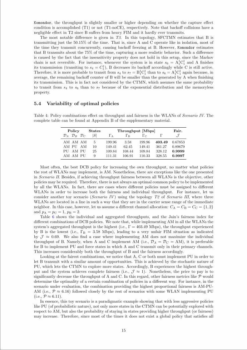
“main” — 2020/11/19 — 10:04 — page 124 — #146

Komondor, the throughput is slightly smaller or higher depending on whether the capture effectcondition is accomplished (T1) or not (T1-noCE), respectively. Note that backoff collisions have anegligible effect in T2 since B suffers from heavy FIM and it hardly ever transmits.

The most notable difference is given in T3. In this topology, SFCTMN estimates that B istransmitting just the 50.15% of the time. That is, since A and C operate like in isolation, most ofthe time they transmit concurrently, causing backoff freezing at B. However, Komondor estimatesthat B transmits about the 75% of the time, capturing a more realistic behavior. Such a differenceis caused by the fact that the insensitivity property does not hold in this setup, since the Markovchain is not reversible. For instance, whenever the system is in state s6 = A1

1C11 and A finishes

its transmission (transiting to s4 = C11 ), B decreases its backoff accordingly while C is still active.

Therefore, it is more probable to transit from s4 to s7 = B11C1

1 than to s6 = A11C1

1 again because, inaverage, the remaining backoff counter of B will be smaller than the generated by A when finishingits transmission. This is in fact not considered by the CTMN, which assumes the same probabilityto transit from s4 to s6 than to s7 because of the exponential distribution and the memorylessproperty.

5.4 Variability of optimal policies

Table 4: Policy combinations effect on throughput and fairness in the WLANs of Scenario IV. Thecomplete table can be found at Appendix B of the supplementary material.

Policy States Throughput [Mbps] Fair.DA DB DC |S| ΓA ΓB ΓC Γ JAM AM AM 5 199.96 3.58 199.96 403.49 0.67853AM PU AM 10 149.41 62.45 149.41 361.27 0.89679PU AM PU 25 109.84 108.44 109.84 328.12 0.9999AM AM PU 9 111.31 106.91 110.33 328.55 0.9997

Most often, the best DCB policy for increasing the own throughput, no matter what policiesthe rest of WLANs may implement, is AM. Nonetheless, there are exceptions like the one presentedin Scenario II. Besides, if achieving throughput fairness between all WLANs is the objective, otherpolicies may be required. Therefore, there is not always an optimal common policy to be implementedby all the WLANs. In fact, there are cases where different policies must be assigned to differentWLANs in order to increase both the fairness and individual throughput. For instance, let usconsider another toy scenario (Scenario IV ) using the topology T2 of Scenario III, where threeWLANs are located in a line in such a way that they are in the carrier sense range of the immediateneighbor. In this case, however, let us assume a different channel allocation: CA = CB = CC = 1, 2and pA = pC = 1, pB = 2.

Table 6 shows the individual and aggregated throughputs, and the Jain’s fairness index fordifferent combinations of DCB policies. We note that, while implementing AM in all the WLANs thesystem’s aggregated throughput is the highest (i.e., Γ = 403.49 Mbps), the throughput experiencedby B is the lowest (i.e., ΓB = 3.58 Mbps), leading to a very unfair FIM situation as indicatedby J ≈ 0.69. We also find a case where implementing AM does not maximize the individualthroughput of B. Namely, when A and C implement AM (i.e., DA = DC = AM), it is preferablefor B to implement PU and force states in which A and C transmit only in their primary channels.This increases considerably both the throughput of B and the fairness accordingly.

Looking at the fairest combinations, we notice that A, C or both must implement PU in order tolet B transmit with a similar amount of opportunities. This is achieved by the stochastic nature ofPU, which lets the CTMN to explore more states. Accordingly, B experiences the highest through-put and the system achieves complete fairness (i.e., J ≈ 1). Nonetheless, the price to pay is tosignificantly decrease the throughput of A and C. In this regard, other fairness metrics like P woulddetermine the optimality of a certain combination of policies in a different way. For instance, in thescenario under evaluation, the combination providing the highest proportional fairness is AM-PU-AM (i.e., P ≈ 6.16) followed closely by the rest of scenarios with some WLAN implementing PU(i.e., P ≈ 6.11).

In essence, this toy scenario is a paradigmatic example showing that with less aggressive policieslike PU (of probabilistic nature), not only more states in the CTMN can be potentially explored withrespect to AM, but also the probability of staying in states providing higher throughput (or fairness)may increase. Therefore, since most of the times it does not exist a global policy that satisfies all

15

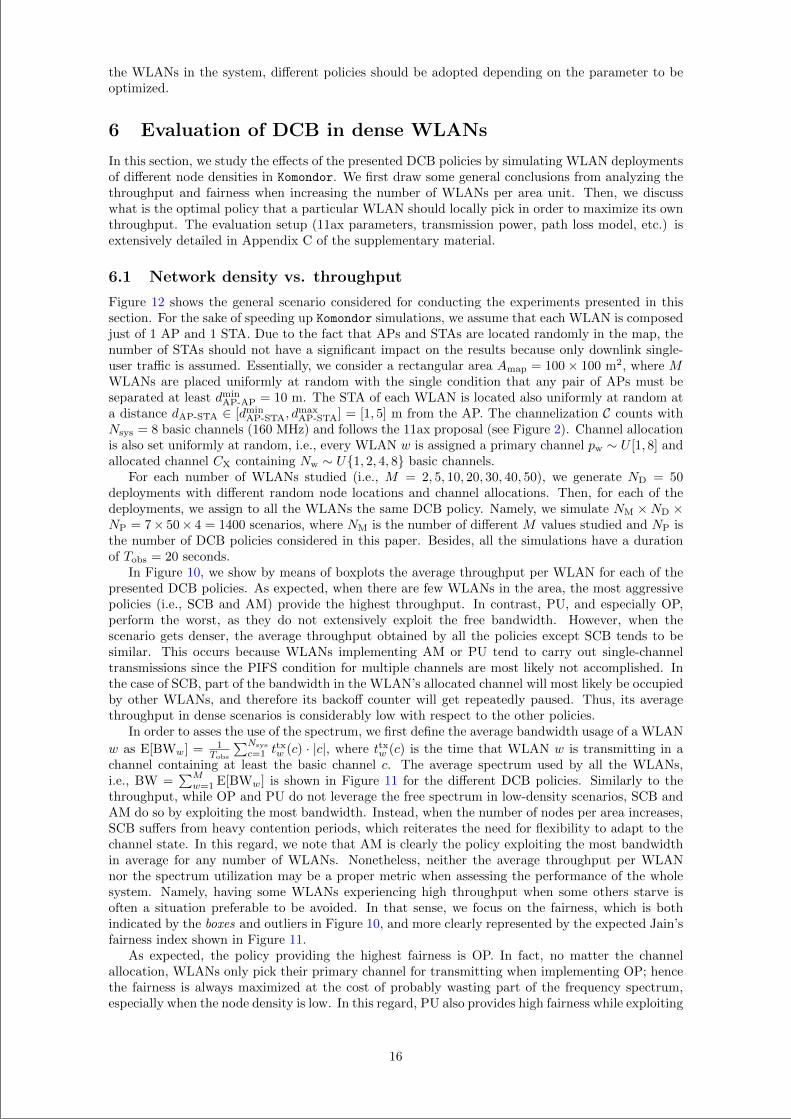
“main” — 2020/11/19 — 10:04 — page 125 — #147

the WLANs in the system, different policies should be adopted depending on the parameter to beoptimized.

6 Evaluation of DCB in dense WLANs

In this section, we study the effects of the presented DCB policies by simulating WLAN deploymentsof different node densities in Komondor. We first draw some general conclusions from analyzing thethroughput and fairness when increasing the number of WLANs per area unit. Then, we discusswhat is the optimal policy that a particular WLAN should locally pick in order to maximize its ownthroughput. The evaluation setup (11ax parameters, transmission power, path loss model, etc.) isextensively detailed in Appendix C of the supplementary material.

6.1 Network density vs. throughput

Figure 12 shows the general scenario considered for conducting the experiments presented in thissection. For the sake of speeding up Komondor simulations, we assume that each WLAN is composedjust of 1 AP and 1 STA. Due to the fact that APs and STAs are located randomly in the map, thenumber of STAs should not have a significant impact on the results because only downlink single-user traffic is assumed. Essentially, we consider a rectangular area Amap = 100× 100 m2, where MWLANs are placed uniformly at random with the single condition that any pair of APs must beseparated at least dmin

AP-AP = 10 m. The STA of each WLAN is located also uniformly at random ata distance dAP-STA ∈ [dmin

AP-STA, dmaxAP-STA] = [1, 5] m from the AP. The channelization C counts with

Nsys = 8 basic channels (160 MHz) and follows the 11ax proposal (see Figure 2). Channel allocationis also set uniformly at random, i.e., every WLAN w is assigned a primary channel pw ∼ U [1, 8] andallocated channel CX containing Nw ∼ U1, 2, 4, 8 basic channels.

For each number of WLANs studied (i.e., M = 2, 5, 10, 20, 30, 40, 50), we generate ND = 50deployments with different random node locations and channel allocations. Then, for each of thedeployments, we assign to all the WLANs the same DCB policy. Namely, we simulate NM ×ND ×NP = 7× 50× 4 = 1400 scenarios, where NM is the number of different M values studied and NP isthe number of DCB policies considered in this paper. Besides, all the simulations have a durationof Tobs = 20 seconds.

In Figure 10, we show by means of boxplots the average throughput per WLAN for each of thepresented DCB policies. As expected, when there are few WLANs in the area, the most aggressivepolicies (i.e., SCB and AM) provide the highest throughput. In contrast, PU, and especially OP,perform the worst, as they do not extensively exploit the free bandwidth. However, when thescenario gets denser, the average throughput obtained by all the policies except SCB tends to besimilar. This occurs because WLANs implementing AM or PU tend to carry out single-channeltransmissions since the PIFS condition for multiple channels are most likely not accomplished. Inthe case of SCB, part of the bandwidth in the WLAN’s allocated channel will most likely be occupiedby other WLANs, and therefore its backoff counter will get repeatedly paused. Thus, its averagethroughput in dense scenarios is considerably low with respect to the other policies.

In order to asses the use of the spectrum, we first define the average bandwidth usage of a WLAN

w as E[BWw] = 1Tobs

∑Nsys

c=1 ttxw (c) · |c|, where ttxw (c) is the time that WLAN w is transmitting in a

channel containing at least the basic channel c. The average spectrum used by all the WLANs,i.e., BW =

∑Mw=1 E[BWw] is shown in Figure 11 for the different DCB policies. Similarly to the

throughput, while OP and PU do not leverage the free spectrum in low-density scenarios, SCB andAM do so by exploiting the most bandwidth. Instead, when the number of nodes per area increases,SCB suffers from heavy contention periods, which reiterates the need for flexibility to adapt to thechannel state. In this regard, we note that AM is clearly the policy exploiting the most bandwidthin average for any number of WLANs. Nonetheless, neither the average throughput per WLANnor the spectrum utilization may be a proper metric when assessing the performance of the wholesystem. Namely, having some WLANs experiencing high throughput when some others starve isoften a situation preferable to be avoided. In that sense, we focus on the fairness, which is bothindicated by the boxes and outliers in Figure 10, and more clearly represented by the expected Jain’sfairness index shown in Figure 11.

As expected, the policy providing the highest fairness is OP. In fact, no matter the channelallocation, WLANs only pick their primary channel for transmitting when implementing OP; hencethe fairness is always maximized at the cost of probably wasting part of the frequency spectrum,especially when the node density is low. In this regard, PU also provides high fairness while exploiting

16

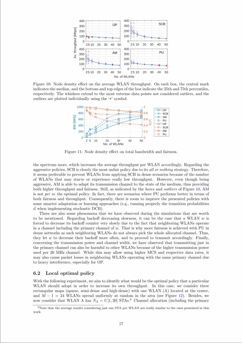
“main” — 2020/11/19 — 10:04 — page 126 — #148

25 10 20 30 40 500

100

200

300

400

Av.

thro

ughp

ut [M

bps]

25 10 20 30 40 500

100

200

300

400

25 10 20 30 40 50No. of WLANs

0

100

200

300

400

25 10 20 30 40 500

100

200

300

400

SCB

PUAM

OP

Figure 10: Node density effect on the average WLAN throughput. On each box, the central markindicates the median, and the bottom and top edges of the box indicate the 25th and 75th percentiles,respectively. The whiskers extend to the most extreme data points not considered outliers, and theoutliers are plotted individually using the ‘+’ symbol.

2 5 10 20 30 40 50No. of WLANs

0

200

400

600

800

1000

BW

[MH

z]

0

0.2

0.4

0.6

0.8

1OPSCBAMPUOPSCBAMPU

Figure 11: Node density effect on total bandwidth and fairness.

the spectrum more, which increases the average throughput per WLAN accordingly. Regarding theaggressive policies, SCB is clearly the most unfair policy due to its all or nothing strategy. Therefore,it seems preferable to prevent WLANs from applying SCB in dense scenarios because of the numberof WLANs that may starve or experience really low throughput. However, even though beingaggressive, AM is able to adapt its transmission channel to the state of the medium, thus providingboth higher throughput and fairness. Still, as indicated by the boxes and outliers of Figure 10, AMis not per se the optimal policy. In fact, there are scenarios where PU performs better in terms ofboth fairness and throughput. Consequently, there is room to improve the presented policies withsome smarter adaptation or learning approaches (e.g., tunning properly the transition probabilities~α when implementing stochastic DCB).

There are also some phenomena that we have observed during the simulations that are worthto be mentioned. Regarding backoff decreasing slowness, it can be the case that a WLAN w isforced to decrease its backoff counter very slowly due to the fact that neighboring WLANs operatein a channel including the primary channel of w. That is why more fairness is achieved with PU indense networks as such neighboring WLANs do not always pick the whole allocated channel. Thus,they let w to decrease their backoff more often, and to proceed to transmit accordingly. Finally,concerning the transmission power and channel width, we have observed that transmitting just inthe primary channel can also be harmful to other WLANs because of the higher transmission powerused per 20 MHz channel. While this may allow using higher MCS and respective data rates, itmay also cause packet losses in neighboring WLANs operating with the same primary channel dueto heavy interference, especially for OP.

6.2 Local optimal policy

With the following experiment, we aim to identify what would be the optimal policy that a particularWLAN should adopt in order to increase its own throughput. In this case, we consider threerectangular maps (sparse, semi-dense and high-dense) with one WLAN (A) located at the center,and M − 1 = 24 WLANs spread uniformly at random in the area (see Figure 12). Besides, wenow consider that WLAN A has NA ∼ U [1, 20] STAs.9 Channel allocation (including the primary

9Note that the average results considering just one STA per WLAN are really similar to the ones presented in thiswork.

17

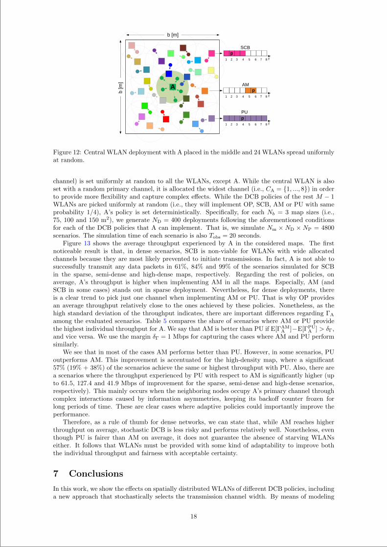
“main” — 2020/11/19 — 10:04 — page 127 — #149

db [m]d

db [m

] d

p1 2 3 4 5 6 7 8 f

p1 2 3 4 5 6 7 8 f

p1 2 3 4 5 6 7 8 f

SCB

AM

PU

A

Figure 12: Central WLAN deployment with A placed in the middle and 24 WLANs spread uniformlyat random.

channel) is set uniformly at random to all the WLANs, except A. While the central WLAN is alsoset with a random primary channel, it is allocated the widest channel (i.e., CA = 1, ..., 8) in orderto provide more flexibility and capture complex effects. While the DCB policies of the rest M − 1WLANs are picked uniformly at random (i.e., they will implement OP, SCB, AM or PU with sameprobability 1/4), A’s policy is set deterministically. Specifically, for each Nb = 3 map sizes (i.e.,75, 100 and 150 m2), we generate ND = 400 deployments following the aforementioned conditionsfor each of the DCB policies that A can implement. That is, we simulate Nm × ND × NP = 4800scenarios. The simulation time of each scenario is also Tobs = 20 seconds.

Figure 13 shows the average throughput experienced by A in the considered maps. The firstnoticeable result is that, in dense scenarios, SCB is non-viable for WLANs with wide allocatedchannels because they are most likely prevented to initiate transmissions. In fact, A is not able tosuccessfully transmit any data packets in 61%, 84% and 99% of the scenarios simulated for SCBin the sparse, semi-dense and high-dense maps, respectively. Regarding the rest of policies, onaverage, A’s throughput is higher when implementing AM in all the maps. Especially, AM (andSCB in some cases) stands out in sparse deployment. Nevertheless, for dense deployments, thereis a clear trend to pick just one channel when implementing AM or PU. That is why OP providesan average throughput relatively close to the ones achieved by these policies. Nonetheless, as thehigh standard deviation of the throughput indicates, there are important differences regarding ΓA

among the evaluated scenarios. Table 5 compares the share of scenarios where AM or PU providethe highest individual throughput for A. We say that AM is better than PU if E[ΓAM

A ]−E[ΓPUA ] > δΓ,

and vice versa. We use the margin δΓ = 1 Mbps for capturing the cases where AM and PU performsimilarly.

We see that in most of the cases AM performs better than PU. However, in some scenarios, PUoutperforms AM. This improvement is accentuated for the high-density map, where a significant57% (19% + 38%) of the scenarios achieve the same or highest throughput with PU. Also, there area scenarios where the throughput experienced by PU with respect to AM is significantly higher (upto 61.5, 127.4 and 41.9 Mbps of improvement for the sparse, semi-dense and high-dense scenarios,respectively). This mainly occurs when the neighboring nodes occupy A’s primary channel throughcomplex interactions caused by information asymmetries, keeping its backoff counter frozen forlong periods of time. These are clear cases where adaptive policies could importantly improve theperformance.

Therefore, as a rule of thumb for dense networks, we can state that, while AM reaches higherthroughput on average, stochastic DCB is less risky and performs relatively well. Nonetheless, eventhough PU is fairer than AM on average, it does not guarantee the absence of starving WLANseither. It follows that WLANs must be provided with some kind of adaptability to improve boththe individual throughput and fairness with acceptable certainty.

7 Conclusions

In this work, we show the effects on spatially distributed WLANs of different DCB policies, includinga new approach that stochastically selects the transmission channel width. By means of modeling

18

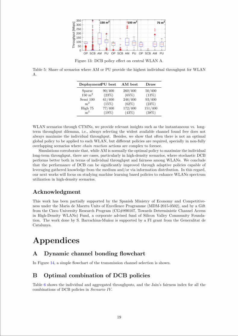
“main” — 2020/11/19 — 10:04 — page 128 — #150

OP SCB AM PU OP SCB AM PU OP SCB AM PU0

50

100

150

200

250

300

350

Thr

ough

put [

Mbp

s] 150 m2 100 m2 75 m2

Figure 13: DCB policy effect on central WLAN A.

Table 5: Share of scenarios where AM or PU provide the highest individual throughput for WLANA.

DeploymentPU best AM best Draw

Sparse150 m2

90/400(23%)

260/400(65%)

50/400(13%)

Semi 100m2

61/400(15%)

246/400(62%)

93/400(23%)

High 75m2

77/400(19%)

172/400(43%)

151/400(38%)

WLAN scenarios through CTMNs, we provide relevant insights such as the instantaneous vs. long-term throughput dilemma, i.e., always selecting the widest available channel found free does notalways maximize the individual throughput. Besides, we show that often there is not an optimalglobal policy to be applied to each WLAN, but different policies are required, specially in non-fullyoverlapping scenarios where chain reaction actions are complex to foresee.

Simulations corroborate that, while AM is normally the optimal policy to maximize the individuallong-term throughput, there are cases, particularly in high-density scenarios, where stochastic DCBperforms better both in terms of individual throughput and fairness among WLANs. We concludethat the performance of DCB can be significantly improved through adaptive policies capable ofleveraging gathered knowledge from the medium and/or via information distribution. In this regard,our next works will focus on studying machine learning based policies to enhance WLANs spectrumutilization in high-density scenarios.

Acknowledgment

This work has been partially supported by the Spanish Ministry of Economy and Competitive-ness under the Maria de Maeztu Units of Excellence Programme (MDM-2015-0502), and by a Giftfrom the Cisco University Research Program (CG#890107, Towards Deterministic Channel Accessin High-Density WLANs) Fund, a corporate advised fund of Silicon Valley Community Founda-tion. The work done by S. Barrachina-Munoz is supported by a FI grant from the Generalitat deCatalunya.

Appendices

A Dynamic channel bonding flowchart

In Figure 14, a simple flowchart of the transmission channel selection is shown.

B Optimal combination of DCB policies

Table 6 shows the individual and aggregated throughputs, and the Jain’s fairness index for all thecombinations of DCB policies in Secnario IV.

19

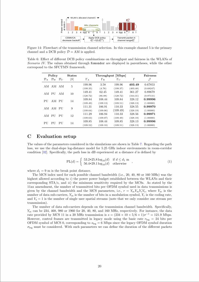
“main” — 2020/11/19 — 10:04 — page 129 — #151

Transmit packet in channel range Ctx

CSMA/CA: decrease backoff

Apply DCB policy:Ctx = f(D,Cfree)

1 f2 3 4 5(p) 6 7 8Pow

er

sens

ed

at n

od

e n

1 f2 3 4 5(p) 6 7 8

Ctx

Idle channels

WLAN’s allocated channel C

Cn Cn Cn

Cn

Figure 14: Flowchart of the transmission channel selection. In this example channel 5 is the primarychannel and a DCB policy D = AM is applied.

Table 6: Effect of different DCB policy combinations on throughput and fairness in the WLANs ofScenario IV. The values obtained through Komondor are displayed in parentheses, while the othercorrespond to the SFCTMN framework.

Policy States Throughput [Mbps] FairnessDA DB DC |S| ΓA ΓB ΓC Γ J

AM AM AM 5199.96 3.58 199.96 403.49 0.67853(199.35) (4.76) (199.37) (403.48) (0.68247)

AM PU AM 10149.41 62.45 149.41 361.27 0.89679(128.72) (86.88) (128.72) (344.31) (0.97131)

PU AM PU 14109.84 108.44 109.84 328.12 0.99996(109.49) (109.13) (109.51) (328.13) (1.00000)

AM AM PU 9111.31 106.91 110.33 328.55 0.99970(109.64) (109.06) (109.49) (328.19) (1.00000)

AM PU PU 12111.29 106.94 110.33 328.56 0.99971(109.63) (109.07) (109.49) (328.18) (1.00000)

PU PU PU 14109.85 108.44 109.85 328.13 0.99996(109.52) (109.10) (109.51) (328.13) (1.00000)

C Evaluation setup

The values of the parameters considered in the simulations are shown in Table 7. Regarding the pathloss, we use the dual-slope log-distance model for 5.25 GHz indoor environments in room-corridorcondition [32]. Specifically, the path loss in dB experienced at a distance d is defined by

PL(d) =

53.2+25.8 log10(d) if d ≤ d1 m56.4+29.1 log10(d) otherwise

, (1)

where d1 = 9 m is the break point distance.The MCS index used for each possible channel bandwidth (i.e., 20, 40, 80 or 160 MHz) was the

highest allowed according to i) the power power budget established between the WLANs and theircorresponding STA/s, and ii) the minimum sensitivity required by the MCSs. As stated by the11ax amendment, the number of transmitted bits per OFDM symbol used in data transmissions isgiven by the channel bandwidth and the MCS parameters, i.e., r = YscYmYcVs, where Ysc is thenumber of data sub-carriers, Ym is the number of bits in a modulation symbol, Yc is the coding rate,and Vs = 1 is the number of single user spatial streams (note that we only consider one stream pertransmission).

The number of data sub-carriers depends on the transmission channel bandwidth. Specifically,Ysc can be 234, 468, 980 or 1960 for 20, 40, 80, and 160 MHz, respectively. For instance, the datarate provided by MCS 11 in a 20 MHz transmission is s = (234× 10× 5/6× 1)σ−1 = 121.9 Mbps.However, control frames are transmitted in legacy mode using the basic rate rleg = 24 bits perOFDM symbol of MCS 0, corresponding to sleg = 6 Mbps since the legacy OFDM symbol durationσleg must be considered. With such parameters we can define the duration of the different packets

20

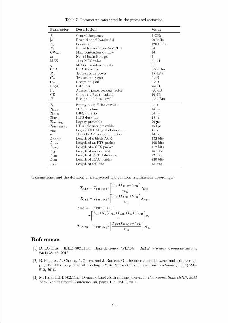
“main” — 2020/11/19 — 10:04 — page 130 — #152

Table 7: Parameters considered in the presented scenarios.

Parameter Description Value

fc Central frequency 5 GHz|c| Basic channel bandwidth 20 MHzLD Frame size 12000 bitsNa No. of frames in an A-MPDU 64CWmin Min. contention window 16m No. of backoff stages 5MCS 11ax MCS index 0 - 11η MCS’s packet error rate 0.1CCA CCA threshold -82 dBmPtx Transmission power 15 dBmGtx Transmitting gain 0 dBGrx Reception gain 0 dBPL(d) Path loss see (1)Pν Adjacent power leakage factor -20 dBCE Capture effect threshold 20 dBN Background noise level -95 dBm

Te Empty backoff slot duration 9 µsTSIFS SIFS duration 16 µsTDIFS DIFS duration 34 µsTPIFS PIFS duration 25 µsTPHY-leg Legacy preamble 20 µsTPHY-HE-SU HE single-user preamble 164 µsσleg Legacy OFDM symbol duration 4 µsσ 11ax OFDM symbol duration 16 µsLBACK Length of a block ACK 432 bitsLRTS Length of an RTS packet 160 bitsLCTS Length of a CTS packet 112 bitsLSF Length of service field 16 bitsLMD Length of MPDU delimiter 32 bitsLMH Length of MAC header 320 bitsLTB Length of tail bits 18 bits

transmissions, and the duration of a successful and collision transmission accordingly:

TRTS = TPHY-leg+

⌈LSF+LRTS+LTB

rleg

⌉σleg,

TCTS = TPHY-leg+

⌈LSF+LCTS+LTB

rleg

⌉σleg,

TDATA = TPHY-HE-SU+

+

⌈LSF+Na(LMD+LMH+LD)+LTB

r

⌉σ,

TBACK = TPHY-leg+

⌈LSF+LBACK+LTB

rleg

⌉σleg.

References

[1] B. Bellalta. IEEE 802.11ax: High-efficiency WLANs. IEEE Wireless Communications,23(1):38–46, 2016.

[2] B. Bellalta, A. Checco, A. Zocca, and J. Barcelo. On the interactions between multiple overlap-ping WLANs using channel bonding. IEEE Transactions on Vehicular Technology, 65(2):796–812, 2016.

[3] M. Park. IEEE 802.11ac: Dynamic bandwidth channel access. In Communications (ICC), 2011IEEE International Conference on, pages 1–5. IEEE, 2011.

21

“main” — 2020/11/19 — 10:04 — page 131 — #153

[4] B. Bellalta, A. Faridi, J. Barcelo, A. Checco, and P. Chatzimisios. Channel bonding in short-range wlans. In European Wireless 2014; 20th European Wireless Conference; Proceedings of,pages 1–7. VDE, 2014.

[5] S. Vasthav, S. Srikanth, and V. Ramaiyan. Performance analysis of an IEEE 802.11ac WLANwith dynamic bandwidth channel access. In Communication (NCC), 2016 Twenty SecondNational Conference on, pages 1–6. IEEE, 2016.

[6] A. Faridi, B. Bellalta, and A. Checco. Analysis of Dynamic Channel Bonding in Dense Networksof WLANs. IEEE Transactions on Mobile Computing, 2016.

[7] Sergio Barrachina-Munoz, Francesc Wilhelmi, Ioannis Selinis, and Boris Bellalta. Komondor:a wireless network simulator for next-generation high-density wlans. In 2019 Wireless Days(WD), pages 1–8. IEEE, 2019.

[8] L. Deek, E. Garcia-Villegas, E. Belding, S. Lee, and K. Almeroth. The impact of channelbonding on 802.11n network management. In Proceedings of the Seventh Conference on emergingNetworking EXperiments and Technologies, page 11. ACM, 2011.

[9] M. Y. Arslan, K. Pelechrinis, I. Broustis, S. V. Krishnamurthy, S. Addepalli, and K. Papagian-naki. Auto-configuration of 802.11n WLANs. In Proceedings of the 6th International Conference,page 27. ACM, 2010.

[10] L. Deek, E. Garcia-Villegas, E. Belding, S. Lee, and K. Almeroth. Joint rate and channel widthadaptation for 802.11 MIMO wireless networks. In Sensor, Mesh and Ad Hoc Communicationsand Networks (SECON), 2013 10th Annual IEEE Communications Society Conference on,pages 167–175. IEEE, 2013.

[11] Y. Zeng, P. Pathak, and P. Mohapatra. A first look at 802.11 ac in action: Energy efficiency andinterference characterization. In Networking Conference, 2014 IFIP, pages 1–9. IEEE, 2014.

[12] M. X. Gong, B. Hart, L. Xia, and R. Want. Channel bounding and MAC protection mechanismsfor 802.11ac. In Global Telecommunications Conference (GLOBECOM 2011), 2011 IEEE, pages1–5. IEEE, 2011.

[13] M. Kim, T. Ropitault, S. Lee, and N. Golmie. A Throughput Study for Channel Bonding inIEEE 802.11ac Networks. IEEE Communications Letters, 2017.

[14] S. Barrachina-Munoz, F. Wilhelmi, and B. Bellalta. To overlap or not to overlap: Enablingchannel bonding in high-density WLANs. Computer Networks, 152:40 – 53, 2019.

[15] M. Han, Sami K., L. X. Cai, and Y. Cheng. Performance Analysis of Opportunistic ChannelBonding in Multi-Channel WLANs. In Global Communications Conference (GLOBECOM),2016 IEEE, pages 1–6. IEEE, 2016.

[16] S. Khairy, M. Han, L. Cai, Y. Cheng, and Z. Han. A renewal theory based analytical model formulti-channel random access in ieee 802.11 ac/ax. IEEE Transactions on Mobile Computing,2018.

[17] P. Huang, X Yang, and L. Xiao. Dynamic channel bonding: enabling flexible spectrum aggre-gation. IEEE Transactions on Mobile Computing, 15(12):3042–3056, 2016.

[18] A. Nabil, M. J. Abdel-Rahman, and A. B. MacKenzie. Adaptive Channel Bonding in WirelessLANs Under Demand Uncertainty. To appear in the Proceedings of the IEEE InternationalSymposium on Personal, Indoor and Mobile Radio Communications (PIMRC), Montreal, QC,Canada, October 2017.

[19] C. Kai, Y. Liang, T. Huang, and X. Chen. A Channel Allocation Algorithm to MaximizeAggregate Throughputs in DCB WLANs. arXiv preprint arXiv:1703.03909, 2017.

[20] Y. Chen, D. Wu, T. Sung, and K. Shih. Dbs: A dynamic bandwidth selection mac protocolfor channel bonding in ieee 802.11 ac wlans. In Wireless Communications and NetworkingConference (WCNC), 2018 IEEE, pages 1–6. IEEE, 2018.

[21] S. Byeon, H. Kwon, Y. Son, C. Yang, and S. Choi. Reconn: Receiver-driven operating chan-nel width adaptation in ieee 802.11ac wlans. In IEEE INFOCOM 2018-IEEE Conference onComputer Communications, pages 1655–1663. IEEE, 2018.

22

“main” — 2020/11/19 — 10:04 — page 132 — #154

[22] P. Chatzimisios, A. Boucouvalas, and V. Vitsas. Performance analysis of IEEE 802.11 DCF inpresence of transmission errors. In Communications, 2004 IEEE International Conference on,volume 7, pages 3854–3858. IEEE, 2004.

[23] R. Boorstyn, A. Kershenbaum, B. Maglaris, and V. Sahin. Throughput analysis in multihopCSMA packet radio networks. IEEE Transactions on Communications, 35(3):267–274, 1987.

[24] G. Bianchi. Performance analysis of the IEEE 802.11 distributed coordination function. IEEEJournal on selected areas in communications, 18(3):535–547, 2000.

[25] B. Bellalta. Throughput Analysis in High Density WLANs. IEEE Communications Letters,21(3):592–595, 2017.

[26] B. Nardelli and E. Knightly. Closed-form throughput expressions for CSMA networks withcollisions and hidden terminals. In INFOCOM, 2012 Proceedings IEEE, pages 2309–2317. IEEE,2012.

[27] S. C. Liew, C. H. Kai, H. C. Leung, and P. Wong. Back-of-the-envelope computation ofthroughput distributions in CSMA wireless networks. IEEE Transactions on Mobile Com-puting, 9(9):1319–1331, 2010.

[28] B. Bellalta, A. Zocca, C. Cano, A. Checco, J. Barcelo, and A. Vinel. Throughput analysis inCSMA/CA networks using continuous time Markov networks: a tutorial. In Wireless Network-ing for Moving Objects, pages 115–133. Springer, 2014.

[29] C. Kai, Y. Liang, T. Huang, and X. Chen. To bond or not to bond: An optimal channelallocation algorithm for flexible dynamic channel bonding in wlans. In Vehicular TechnologyConference (VTC-Fall), 2017 IEEE 86th, pages 1–6. IEEE, 2017.

[30] H. Salameh, M. Krunz, and D. Manzi. Spectrum bonding and aggregation with guard-bandawareness in cognitive radio networks. IEEE Transactions on Mobile Computing, 13(3):569–581,2014.

[31] F Kelly. Reversibility and stochastic networks. Cambridge University Press, 2011.

[32] D. Xu, J. Zhang, X. Gao, P. Zhang, and Y. Wu. Indoor office propagation measurements andpath loss models at 5.25 GHz. In Vehicular Technology Conference, 2007. VTC-2007 Fall. 2007IEEE 66th, pages 844–848. IEEE, 2007.

23

“main” — 2020/11/19 — 10:04 — page 133 — #155

Sergio Barrachina-Munoz is a Ph.D. candidate at Universitat PompeuFabra (UPF). He received his B.Sc. Degree in Telematics Engineering andM.Sc. in Intelligent Interactive Systems in 2015 and 2016, respectively, bothfrom UPF. He joined the Wireless Networking Research Group in 2015, wherehe works under the supervision of Dr. Boris Bellalta. His main researchinterests are focused on machine learning for next-generation WLANs. Sergiois a recipient of a FI grant from the Generalitat de Catalunya.

Francesc Wilhelmi holds a B.Sc. degree in Telematics Engineering fromUniversitat Pompeu Fabra (2015). With the aim of applying new techniquesfor solving many well-known problems in communications, Francesc obtainedhis M.Sc. in Intelligent and Interactive Systems also from UPF in 2016. Heis now a Ph.D. candidate in the Wireless Networking Group at UPF. Themain topics of his PhD Thesis are related to applying reinforcement learningtechniques to spatial reuse in high-density WLANs.

Boris Bellalta is an Associate Professor in the Department of Informa-tion and Communication Technologies (DTIC) at Universitat Pompeu Fabra(UPF). He obtained his degree in Telecommunications Engineering from Uni-versitat Politecnica de Catalunya (UPC) in 2002 and the Ph.D. in Informationand Communication Technologies from UPF in 2007. His research interests arein the area of wireless networks, with emphasis on the design and performanceevaluation of new architectures and protocols. The results from his researchhave been published in more than 100 international journal and conferencepapers. He is currently involved in several international and national researchprojects, including the coordination of the ENTOMATIC FP7 collaborativeproject. At UPF he is giving several courses on networking, queuing theoryand wireless networks. He is co-designer and coordinator of the interuniversity(UPF and UPC) master’s degree in Wireless Communications.

24

“main” — 2020/11/19 — 10:04 — page 134 — #156

To Overlap or not to Overlap: Enabling Channel Bonding in

High-Density WLANs

Sergio Barrachina-Munoz, Francesc Wilhelmi, Boris Bellalta

Abstract

Wireless local area networks (WLANs) are the most popular kind of wireless Internet connectionbecause of their simplicity of deployment and operation. As a result, the number of devices accessingthe Internet through WLANs such as laptops, smartphones, or wearables, is increasing drastically atthe same time that applications’ throughput requirements do. To cope with these challenges, channelbonding (CB) techniques are used for enabling higher data rates by transmitting in wider channels,thus increasing spectrum efficiency. However, important issues like higher potential co-channel andadjacent channel interference arise when bonding channels. This may harm the performance of thecarrier sense multiple access (CSMA) protocol because of recurrent backoff freezing, while makingnodes more sensitive to hidden node effects. In this paper, we address the following point at issue:is it convenient for high-density (HD) WLANs to use wider channels and potentially overlap in thespectrum? First, we highlight key aspects of DCB in toy scenarios through a continuous time Markovnetwork (CTMN) model. Then, by means of extensive simulations covering a wide range of trafficloads and access point (AP) densities, we show that dynamic channel bonding (DCB) – which adaptsthe channel bandwidth on a per-packet transmission – significantly outperforms traditional single-channel on average. Nevertheless, results also corroborate that DCB is more prone to generate unfairsituations where WLANs may starve. Contrary to most of the current thoughts pushing towardsnon-overlapping channels in HD deployments, we highlight the benefits of allocating channels aswider as possible to WLANs altogether with implementing adaptive access policies to cope with theunfairness situations that may appear.

1 Introduction

Although remarkable technological improvements have been achieved in the last decades, wireless localarea networks (WLANs), with IEEE 802.11’s Wi-Fi as the most widely used standard, still face importantchallenges that degrade their performance. Particularly, the frequency spectrum is becoming scarceand inefficient because of the rising number of wireless devices, the characteristically heterogeneous andrandom WLAN deployments, and the raising throughput demands (e.g., some virtual reality applicationsrequire more than 1 Gbps to operate properly [1]). All these circumstances lead to dense or high-dense(HD) scenarios with coexistence issues since WLANs try to selfishly serve their users in non-collaborativedeployments.

As a result, there is a clear need of exploiting the spectrum in a more efficient way by maximizingtransmissions’ bandwidth. One of the most promising techniques to overcome such a challenge is channelbonding (CB). The main idea behind CB is to allow using wider bandwidths in order to transmit athigher transmission rates, increasing the potential throughput accordingly.1 CB for WLANs was firstlyintroduced in the IEEE 802.11n-2009 amendment [2] by letting two separated 20 MHz channels (or basicchannels) get combined into a 40 MHz channel. Later, IEEE 802.11ac-2013 [3] introduced the capabilityof transmitting also in 80 and 160 MHz channels. Future amendments like the IEEE 802.11ax-2019 [4]or EXtreme throughput (XT) [5], which is expected to support up to 320 MHz transmissions, will boostthe use of wider channels. A survey of CB schemes for different types of wireless networks is providedin [6].

There are important drawbacks, however, when it comes to transmitting in wider channels: essentially,the larger the bandwidth used for transmitting, the wider the spectrum suffering from co-channel and

1According to the well-known Shannon-Hartley capacity theorem, the capacity (or raw throughput) of a channel increaseswith the bandwidth.

1

8.2

“main” — 2020/11/19 — 10:04 — page 135 — #157

adjacent channel interference at neighboring nodes. That is, CB may be counterproductive since WLANsnearby are more likely to partially overlap, causing severe performance degradation due to the listen-before-talk nature of the carrier sense multiple access (CSMA) protocol. This effect is further exacerbatedwhen following static channel bonding (SCB) [7]. Besides, the signal-to-interference-plus-noise ratio(SINR) at the receiver decreases for wider channels since the transmission power is spread through thewhole transmission bandwidth (or subcarriers). Accordingly, situations like the hidden node problemare more prone to occur when implementing CB [8].

In this regard, dynamic channel bonding (DCB) allows adapting the selected transmission bandwidthto the channel status right before transmitting. This provides a higher degree of flexibility that improvesthe instantaneous throughput in a simple and efficient way. Then, we can differentiate two approacheswith respect to spectrum management in WLANs: i) fostering transmissions in non-overlapping basicchannels, or ii) enabling faster transmissions in wider channels that may potentially overlap in thespectrum. Alas, in high density (HD) spatially distributed scenarios,2 the complex interrelations amongnodes (located inside or outside the carrier sense range of each other) complicate the task of a prioriestimating the optimal spectrum management approach on a per-WLAN basis.

Significant research has been conducted on the impact of DCB on spatially distributed WLANs’performance under saturation regimes. However, to the best of our knowledge, the effects of unsaturatedtraffic patters, which fit better to real world problems, are still unknown. While saturated regimes offervaluable insights on worst-case scenarios, WLANs are characteristically unsaturated with load patternsthat deeply depend on the application/s being supported. In such scenarios, overlapping approachesseem to be even more convenient since the sensed channels usually remain free during larger periods oftime.

In this paper, we compare the performance of traditional single-channel with channel bonding (in-cluding a stochastic variant) in networks under different traffic load regimes. To do so, we first introducean analytical model to depict the behavior of the aforementioned CB approaches (or policies) in spa-tially distributed WLAN networks. The model is based on continuous time Markov networks (CTMNs)and captures both saturated and unsaturated regimes. Then, by means of simulations, we evaluate theperformance of the CB policies in terms of throughput and delay in toy scenarios and HD WLAN de-ployments. We find that for low individual and neighboring traffic loads single-channel can improve CBin terms of delay since the time to access the channel is reduced. However, in general, DCB significantlyoutperforms traditional single-channel in most of the evaluated scenarios. Nonetheless, DCB is moreprone to cause starvation and hidden nodes, which may lead to unfair scenarios with highly unbalancedperformance among WLANs. Results suggest that future WLANs should be allocated all the availablebandwidth and dynamically adapt to the spectrum.

The remainder of this article is organized as follows. In Section 2, we introduce CB for IEEE 802.11WLANs, present the related work, and define the policies considered in this work. Then, in Section 3we analytically model the interactions of DCB in spatially distributed deployments and point out keyaspects of its performance through toy scenarios. DCB in HD WLANs is assessed in Section 4 by meansof simulations. We conclude with some final remarks at Section 5.

2 Channel bonding

2.1 Channel bonding in IEEE 802.11 WLANs

CB is a technique whereby nodes, i.e., access points (APs) and stations (STAs), are allowed to usecontiguous sets of available basic channels for their transmissions, thus potentially achieving higherthroughput. Namely, by doubling the channel bandwidth, approximately the double data capacity canbe achieved if the modulation coding scheme (MCS) is kept. CB for WLANs was firstly introduced inthe IEEE 802.11n-2009 amendment [2], where high throughput (HT) STAs are allowed to transmit inmore than one 20 MHz channel (or basic channel). Specifically, this amendment allowed bonding up totwo basic channels composing a 40 MHz channel in the 2.4/5 GHz bands. Works in the literature [8–10]show important improvements achieved with CB in IEEE 802.11ac networks when properly adjustingthe transmission power and data rates in WLANs operating at 5 GHz. Note that in the traditional 2.4

2In spatially distributed scenarios, nodes are not necessarily within the carrier sense range of each other. Thus, differentgroups of potentially overlapping WLANs may be given.

2

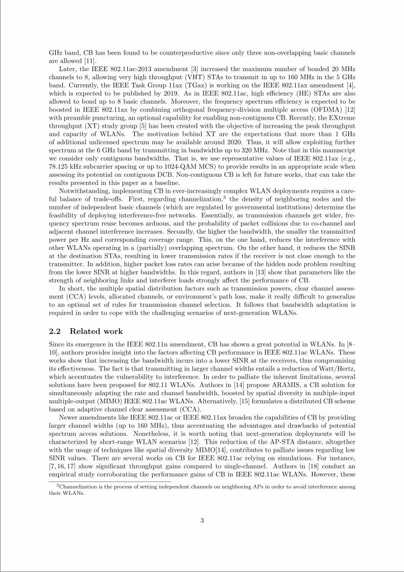
“main” — 2020/11/19 — 10:04 — page 136 — #158

GHz band, CB has been found to be counterproductive since only three non-overlapping basic channelsare allowed [11].

Later, the IEEE 802.11ac-2013 amendment [3] increased the maximum number of bonded 20 MHzchannels to 8, allowing very high throughput (VHT) STAs to transmit in up to 160 MHz in the 5 GHzband. Currently, the IEEE Task Group 11ax (TGax) is working on the IEEE 802.11ax amendment [4],which is expected to be published by 2019. As in IEEE 802.11ac, high efficiency (HE) STAs are alsoallowed to bond up to 8 basic channels. Moreover, the frequency spectrum efficiency is expected to beboosted in IEEE 802.11ax by combining orthogonal frequency-division multiple access (OFDMA) [12]with preamble puncturing, an optional capability for enabling non-contiguous CB. Recently, the EXtremethroughput (XT) study group [5] has been created with the objective of increasing the peak throughputand capacity of WLANs. The motivation behind XT are the expectations that more than 1 GHzof additional unlicensed spectrum may be available around 2020. Thus, it will allow exploiting furtherspectrum at the 6 GHz band by transmitting in bandwidths up to 320 MHz. Note that in this manuscriptwe consider only contiguous bandwidths. That is, we use representative values of IEEE 802.11ax (e.g.,78.125 kHz subcarrier spacing or up to 1024-QAM MCS) to provide results in an appropriate scale whenassessing its potential on contiguous DCB. Non-contiguous CB is left for future works, that can take theresults presented in this paper as a baseline.

Notwithstanding, implementing CB in ever-increasingly complex WLAN deployments requires a care-ful balance of trade-offs. First, regarding channelization,3 the density of neighboring nodes and thenumber of independent basic channels (which are regulated by governmental institutions) determine thefeasibility of deploying interference-free networks. Essentially, as transmission channels get wider, fre-quency spectrum reuse becomes arduous, and the probability of packet collisions due to co-channel andadjacent channel interference increases. Secondly, the higher the bandwidth, the smaller the transmittedpower per Hz and corresponding coverage range. This, on the one hand, reduces the interference withother WLANs operating in a (partially) overlapping spectrum. On the other hand, it reduces the SINRat the destination STAs, resulting in lower transmission rates if the receiver is not close enough to thetransmitter. In addition, higher packet loss rates can arise because of the hidden node problem resultingfrom the lower SINR at higher bandwidths. In this regard, authors in [13] show that parameters like thestrength of neighboring links and interferer loads strongly affect the performance of CB.

In short, the multiple spatial distribution factors such as transmission powers, clear channel assess-ment (CCA) levels, allocated channels, or environment’s path loss, make it really difficult to generalizeto an optimal set of rules for transmission channel selection. It follows that bandwidth adaptation isrequired in order to cope with the challenging scenarios of next-generation WLANs.

2.2 Related work

Since its emergence in the IEEE 802.11n amendment, CB has shown a great potential in WLANs. In [8–10], authors provides insight into the factors affecting CB performance in IEEE 802.11ac WLANs. Theseworks show that increasing the bandwidth incurs into a lower SINR at the receivers, thus compromisingits effectiveness. The fact is that transmitting in larger channel widths entails a reduction of Watt/Hertz,which accentuates the vulnerability to interference. In order to palliate the inherent limitations, severalsolutions have been proposed for 802.11 WLANs. Authors in [14] propose ARAMIS, a CB solution forsimultaneously adapting the rate and channel bandwidth, boosted by spatial diversity in multiple-inputmultiple-output (MIMO) IEEE 802.11ac WLANs. Alternatively, [15] formulates a distributed CB schemebased on adaptive channel clear assessment (CCA).

Newer amendments like IEEE 802.11ac or IEEE 802.11ax broaden the capabilities of CB by providinglarger channel widths (up to 160 MHz), thus accentuating the advantages and drawbacks of potentialspectrum access solutions. Nonetheless, it is worth noting that next-generation deployments will becharacterized by short-range WLAN scenarios [12]. This reduction of the AP-STA distance, altogetherwith the usage of techniques like spatial diversity MIMO[14], contributes to palliate issues regarding lowSINR values. There are several works on CB for IEEE 802.11ac relying on simulations. For instance,[7, 16, 17] show significant throughput gains compared to single-channel. Authors in [18] conduct anempirical study corroborating the performance gains of CB in IEEE 802.11ac WLANs. However, these

3Channelization is the process of setting independent channels on neighboring APs in order to avoid interference amongtheir WLANs.

3

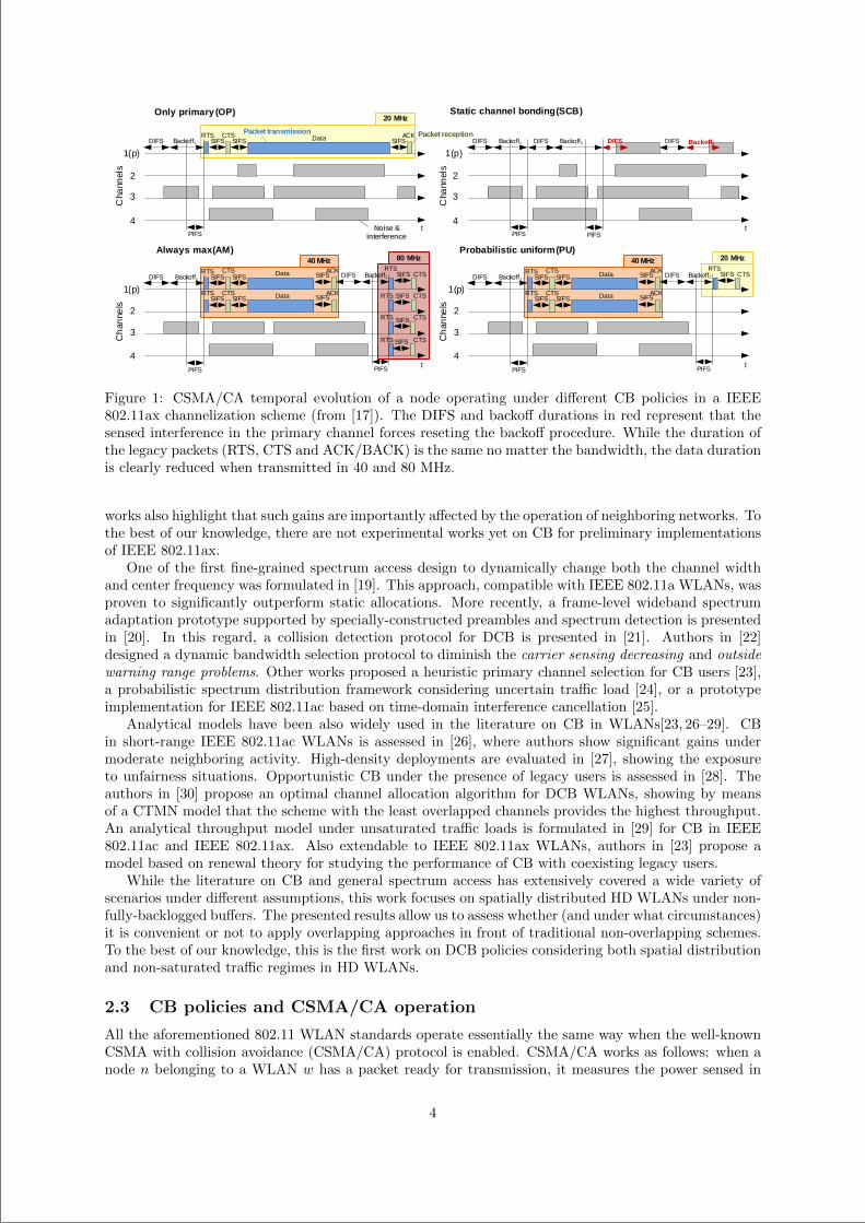
“main” — 2020/11/19 — 10:04 — page 137 — #159

1(p)

2

3

4

Backoff1DIFS

PIFSt

SIFS Data SIFS

Noise & interference

Cha

nnel

sOnly primary (OP)

1(p)

2

3

4

Backoff1DIFS

PIFSt

Cha

nnel

s

Packet receptionPacket transmission

1(p)

2

3

4

Backoff1DIFS

PIFSt

Data SIFS

Ch

anne

ls

Always max (AM)

Data SIFS

DIFS Backoff2

RTSSIFS

RTS SIFS

PIFS

RTS

RTS

SIFS

SIFS CTS

CTS

CTS

CTS

40 MHz

20 MHz

80 MHz

Static channel bonding (SCB)

RTS CTSSIFS

SIFSRTS CTS

SIFS

ACK

ACK

ACKSIFS

RTS CTSSIFS

1(p)

2

3

4

Backoff1DIFS

PIFSt

Data SIFS

Ch

anne

ls

Probabilistic uniform (PU)

Data SIFS

DIFS Backoff2

RTSSIFS

PIFS

CTS

40 MHz 20 MHz

SIFSRTS CTS

SIFSACK

ACKSIFS

RTS CTSSIFS

DIFS Backoff2

PIFS

DIFS DIFS Backoff3

Figure 1: CSMA/CA temporal evolution of a node operating under different CB policies in a IEEE802.11ax channelization scheme (from [17]). The DIFS and backoff durations in red represent that thesensed interference in the primary channel forces reseting the backoff procedure. While the duration ofthe legacy packets (RTS, CTS and ACK/BACK) is the same no matter the bandwidth, the data durationis clearly reduced when transmitted in 40 and 80 MHz.

works also highlight that such gains are importantly affected by the operation of neighboring networks. Tothe best of our knowledge, there are not experimental works yet on CB for preliminary implementationsof IEEE 802.11ax.

One of the first fine-grained spectrum access design to dynamically change both the channel widthand center frequency was formulated in [19]. This approach, compatible with IEEE 802.11a WLANs, wasproven to significantly outperform static allocations. More recently, a frame-level wideband spectrumadaptation prototype supported by specially-constructed preambles and spectrum detection is presentedin [20]. In this regard, a collision detection protocol for DCB is presented in [21]. Authors in [22]designed a dynamic bandwidth selection protocol to diminish the carrier sensing decreasing and outsidewarning range problems. Other works proposed a heuristic primary channel selection for CB users [23],a probabilistic spectrum distribution framework considering uncertain traffic load [24], or a prototypeimplementation for IEEE 802.11ac based on time-domain interference cancellation [25].

Analytical models have been also widely used in the literature on CB in WLANs[23, 26–29]. CBin short-range IEEE 802.11ac WLANs is assessed in [26], where authors show significant gains undermoderate neighboring activity. High-density deployments are evaluated in [27], showing the exposureto unfairness situations. Opportunistic CB under the presence of legacy users is assessed in [28]. Theauthors in [30] propose an optimal channel allocation algorithm for DCB WLANs, showing by meansof a CTMN model that the scheme with the least overlapped channels provides the highest throughput.An analytical throughput model under unsaturated traffic loads is formulated in [29] for CB in IEEE802.11ac and IEEE 802.11ax. Also extendable to IEEE 802.11ax WLANs, authors in [23] propose amodel based on renewal theory for studying the performance of CB with coexisting legacy users.

While the literature on CB and general spectrum access has extensively covered a wide variety ofscenarios under different assumptions, this work focuses on spatially distributed HD WLANs under non-fully-backlogged buffers. The presented results allow us to assess whether (and under what circumstances)it is convenient or not to apply overlapping approaches in front of traditional non-overlapping schemes.To the best of our knowledge, this is the first work on DCB policies considering both spatial distributionand non-saturated traffic regimes in HD WLANs.

2.3 CB policies and CSMA/CA operation

All the aforementioned 802.11 WLAN standards operate essentially the same way when the well-knownCSMA with collision avoidance (CSMA/CA) protocol is enabled. CSMA/CA works as follows: when anode n belonging to a WLAN w has a packet ready for transmission, it measures the power sensed in

4

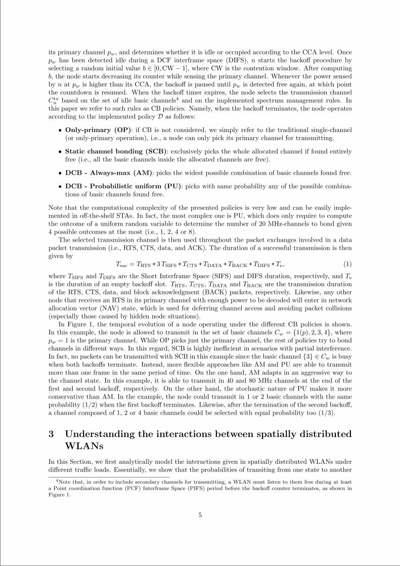
“main” — 2020/11/19 — 10:04 — page 138 — #160

its primary channel pw, and determines whether it is idle or occupied according to the CCA level. Oncepw has been detected idle during a DCF interframe space (DIFS), n starts the backoff procedure byselecting a random initial value b ∈ [0,CW− 1], where CW is the contention window. After computingb, the node starts decreasing its counter while sensing the primary channel. Whenever the power sensedby n at pw is higher than its CCA, the backoff is paused until pw is detected free again, at which pointthe countdown is resumed. When the backoff timer expires, the node selects the transmission channelCtxn based on the set of idle basic channels4 and on the implemented spectrum management rules. In

this paper we refer to such rules as CB policies. Namely, when the backoff terminates, the node operatesaccording to the implemented policy D as follows:

Only-primary (OP): if CB is not considered, we simply refer to the traditional single-channel(or only-primary operation), i.e., a node can only pick its primary channel for transmitting.

Static channel bonding (SCB): exclusively picks the whole allocated channel if found entirelyfree (i.e., all the basic channels inside the allocated channels are free).

DCB - Always-max (AM): picks the widest possible combination of basic channels found free.

DCB - Probabilistic uniform (PU): picks with same probability any of the possible combina-tions of basic channels found free.

Note that the computational complexity of the presented policies is very low and can be easily imple-mented in off-the-shelf STAs. In fact, the most complex one is PU, which does only require to computethe outcome of a uniform random variable to determine the number of 20 MHz-channels to bond given4 possible outcomes at the most (i.e., 1, 2, 4 or 8).

The selected transmission channel is then used throughout the packet exchanges involved in a datapacket transmission (i.e., RTS, CTS, data, and ACK). The duration of a successful transmission is thengiven by

Tsuc = TRTS + 3TSIFS +TCTS +TDATA +TBACK +TDIFS +Te, (1)

where TSIFS and TDIFS are the Short Interframe Space (SIFS) and DIFS duration, respectively, and Te

is the duration of an empty backoff slot. TRTS, TCTS, TDATA and TBACK are the transmission durationof the RTS, CTS, data, and block acknowledgment (BACK) packets, respectively. Likewise, any othernode that receives an RTS in its primary channel with enough power to be decoded will enter in networkallocation vector (NAV) state, which is used for deferring channel access and avoiding packet collisions(especially those caused by hidden node situations).

In Figure 1, the temporal evolution of a node operating under the different CB policies is shown.In this example, the node is allowed to transmit in the set of basic channels Cw = 1(p), 2, 3, 4, wherepw = 1 is the primary channel. While OP picks just the primary channel, the rest of policies try to bondchannels in different ways. In this regard, SCB is highly inefficient in scenarios with partial interference.In fact, no packets can be transmitted with SCB in this example since the basic channel 3 ∈ Cw is busywhen both backoffs terminate. Instead, more flexible approaches like AM and PU are able to transmitmore than one frame in the same period of time. On the one hand, AM adapts in an aggressive way tothe channel state. In this example, it is able to transmit in 40 and 80 MHz channels at the end of thefirst and second backoff, respectively. On the other hand, the stochastic nature of PU makes it moreconservative than AM. In the example, the node could transmit in 1 or 2 basic channels with the sameprobability (1/2) when the first backoff terminates. Likewise, after the termination of the second backoff,a channel composed of 1, 2 or 4 basic channels could be selected with equal probability too (1/3).

3 Understanding the interactions between spatially distributedWLANs

In this Section, we first analytically model the interactions given in spatially distributed WLANs underdifferent traffic loads. Essentially, we show that the probabilities of transiting from one state to another

4Note that, in order to include secondary channels for transmitting, a WLAN must listen to them free during at leasta Point coordination function (PCF) Interframe Space (PIFS) period before the backoff counter terminates, as shown inFigure 1.

5

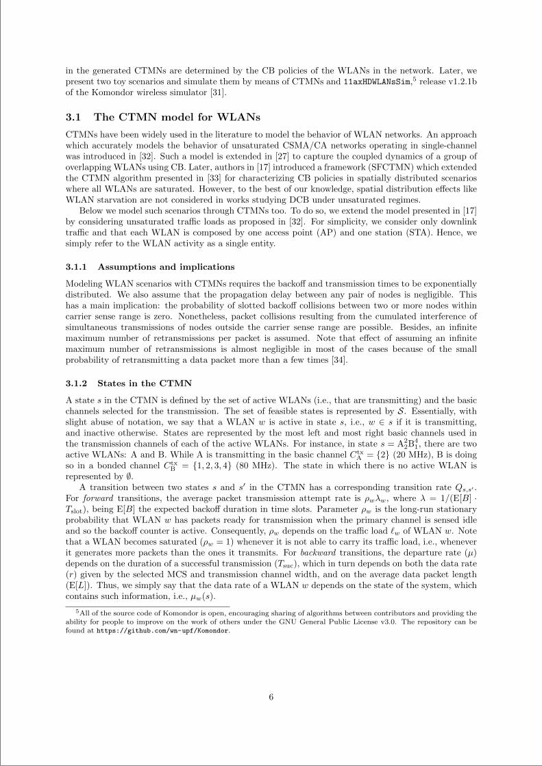
“main” — 2020/11/19 — 10:04 — page 139 — #161

in the generated CTMNs are determined by the CB policies of the WLANs in the network. Later, wepresent two toy scenarios and simulate them by means of CTMNs and 11axHDWLANsSim,5 release v1.2.1bof the Komondor wireless simulator [31].

3.1 The CTMN model for WLANs

CTMNs have been widely used in the literature to model the behavior of WLAN networks. An approachwhich accurately models the behavior of unsaturated CSMA/CA networks operating in single-channelwas introduced in [32]. Such a model is extended in [27] to capture the coupled dynamics of a group ofoverlapping WLANs using CB. Later, authors in [17] introduced a framework (SFCTMN) which extendedthe CTMN algorithm presented in [33] for characterizing CB policies in spatially distributed scenarioswhere all WLANs are saturated. However, to the best of our knowledge, spatial distribution effects likeWLAN starvation are not considered in works studying DCB under unsaturated regimes.

Below we model such scenarios through CTMNs too. To do so, we extend the model presented in [17]by considering unsaturated traffic loads as proposed in [32]. For simplicity, we consider only downlinktraffic and that each WLAN is composed by one access point (AP) and one station (STA). Hence, wesimply refer to the WLAN activity as a single entity.

3.1.1 Assumptions and implications

Modeling WLAN scenarios with CTMNs requires the backoff and transmission times to be exponentiallydistributed. We also assume that the propagation delay between any pair of nodes is negligible. Thishas a main implication: the probability of slotted backoff collisions between two or more nodes withincarrier sense range is zero. Nonetheless, packet collisions resulting from the cumulated interference ofsimultaneous transmissions of nodes outside the carrier sense range are possible. Besides, an infinitemaximum number of retransmissions per packet is assumed. Note that effect of assuming an infinitemaximum number of retransmissions is almost negligible in most of the cases because of the smallprobability of retransmitting a data packet more than a few times [34].

3.1.2 States in the CTMN

A state s in the CTMN is defined by the set of active WLANs (i.e., that are transmitting) and the basicchannels selected for the transmission. The set of feasible states is represented by S. Essentially, withslight abuse of notation, we say that a WLAN w is active in state s, i.e., w ∈ s if it is transmitting,and inactive otherwise. States are represented by the most left and most right basic channels used inthe transmission channels of each of the active WLANs. For instance, in state s = A2

2B41, there are two

active WLANs: A and B. While A is transmitting in the basic channel CtxA = 2 (20 MHz), B is doing

so in a bonded channel CtxB = 1, 2, 3, 4 (80 MHz). The state in which there is no active WLAN is

represented by ∅.A transition between two states s and s′ in the CTMN has a corresponding transition rate Qs,s′ .

For forward transitions, the average packet transmission attempt rate is ρwλw, where λ = 1/(E[B] ·Tslot), being E[B] the expected backoff duration in time slots. Parameter ρw is the long-run stationaryprobability that WLAN w has packets ready for transmission when the primary channel is sensed idleand so the backoff counter is active. Consequently, ρw depends on the traffic load `w of WLAN w. Notethat a WLAN becomes saturated (ρw = 1) whenever it is not able to carry its traffic load, i.e., wheneverit generates more packets than the ones it transmits. For backward transitions, the departure rate (µ)depends on the duration of a successful transmission (Tsuc), which in turn depends on both the data rate(r) given by the selected MCS and transmission channel width, and on the average data packet length(E[L]). Thus, we simply say that the data rate of a WLAN w depends on the state of the system, whichcontains such information, i.e., µw(s).

5All of the source code of Komondor is open, encouraging sharing of algorithms between contributors and providing theability for people to improve on the work of others under the GNU General Public License v3.0. The repository can befound at https://github.com/wn-upf/Komondor.

6

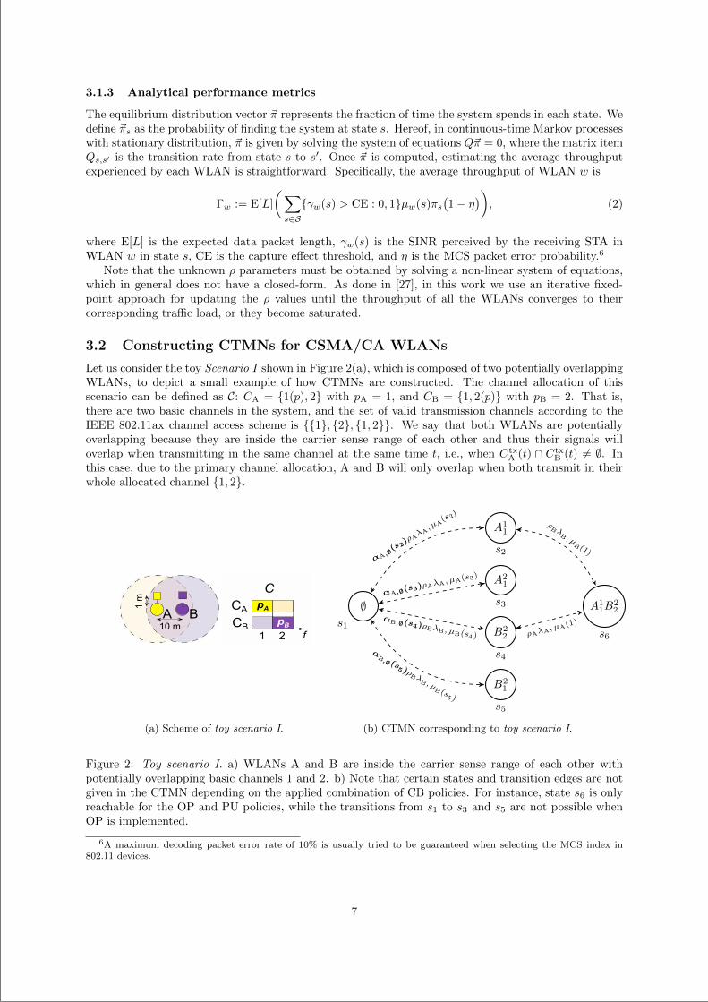
“main” — 2020/11/19 — 10:04 — page 140 — #162

3.1.3 Analytical performance metrics

The equilibrium distribution vector ~π represents the fraction of time the system spends in each state. Wedefine ~πs as the probability of finding the system at state s. Hereof, in continuous-time Markov processeswith stationary distribution, ~π is given by solving the system of equations Q~π = 0, where the matrix itemQs,s′ is the transition rate from state s to s′. Once ~π is computed, estimating the average throughputexperienced by each WLAN is straightforward. Specifically, the average throughput of WLAN w is

Γw := E[L]

(∑

s∈Sγw(s) > CE : 0, 1µw(s)πs

(1− η

)), (2)

where E[L] is the expected data packet length, γw(s) is the SINR perceived by the receiving STA inWLAN w in state s, CE is the capture effect threshold, and η is the MCS packet error probability.6

Note that the unknown ρ parameters must be obtained by solving a non-linear system of equations,which in general does not have a closed-form. As done in [27], in this work we use an iterative fixed-point approach for updating the ρ values until the throughput of all the WLANs converges to theircorresponding traffic load, or they become saturated.

3.2 Constructing CTMNs for CSMA/CA WLANs

Let us consider the toy Scenario I shown in Figure 2(a), which is composed of two potentially overlappingWLANs, to depict a small example of how CTMNs are constructed. The channel allocation of thisscenario can be defined as C: CA = 1(p), 2 with pA = 1, and CB = 1, 2(p) with pB = 2. That is,there are two basic channels in the system, and the set of valid transmission channels according to theIEEE 802.11ax channel access scheme is 1, 2, 1, 2. We say that both WLANs are potentiallyoverlapping because they are inside the carrier sense range of each other and thus their signals willoverlap when transmitting in the same channel at the same time t, i.e., when Ctx

A (t) ∩ CtxB (t) 6= ∅. In

this case, due to the primary channel allocation, A and B will only overlap when both transmit in theirwhole allocated channel 1, 2.

1 2 f

CA

CB

A B

C

10 m

1 m

pB

pA

(a) Scheme of toy scenario I.

∅s1

A21

s3

A11

s2

B22

s4

B21

s5

A11B

22

s6

αA,∅(s2

)ρAλA, µA

(s2)

αA,∅(s3)ρAλA, µA(s3)

αB,∅(s4)ρBλB, µB(s4)

αB,∅ (s

5 )ρBλ

B , µB (s

5 )

ρBλ

B , µB (1)

ρAλA, µA(1)

(b) CTMN corresponding to toy scenario I.

Figure 2: Toy scenario I. a) WLANs A and B are inside the carrier sense range of each other withpotentially overlapping basic channels 1 and 2. b) Note that certain states and transition edges are notgiven in the CTMN depending on the applied combination of CB policies. For instance, state s6 is onlyreachable for the OP and PU policies, while the transitions from s1 to s3 and s5 are not possible whenOP is implemented.

6A maximum decoding packet error rate of 10% is usually tried to be guaranteed when selecting the MCS index in802.11 devices.

7

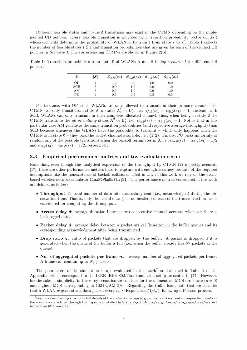
“main” — 2020/11/19 — 10:04 — page 141 — #163

Different feasible states and forward transitions may exist in the CTMN depending on the imple-mented CB policies. Every feasible transition is weighted by a transition probability vector αw,s(s

′)whose elements determine the probability of WLAN w to transit from state s to s′. Table 1 collectsthe number of feasible states (|S|) and transition probabilities that are given for each of the studied CBpolicies in Scenario I. The corresponding CTMNs are shown in Figure 2(b).

Table 1: Transition probabilities from state ∅ of WLANs A and B in toy scenario I for different CBpolicies.

D |S| ~αA,∅(s2) ~αA,∅(s3) ~αB,∅(s4) ~αB,∅(s5)

OP 4 1.0 0.0 1.0 0.0SCB 3 0.0 1.0 0.0 1.0AM 3 0.0 1.0 0.0 1.0PU 6 0.5 0.5 0.5 0.5

For instance, with OP, since WLANs are only allowed to transmit in their primary channel, theCTMN can only transit from state ∅ to states A1

1 or B22, i.e., αA,∅(s2) = αB,∅(s4) = 1. Instead, with

SCB, WLANs can only transmit in their complete allocated channel, thus, when being in state ∅ theCTMN transits to the all or nothing states A2

1 or B21, i.e., αA,∅(s3) = αB,∅(s5) = 1. Notice that in this

particular case AM generates the same transition probabilities (and respective average throughput) thanSCB because whenever the WLANs have the possibility to transmit – which only happens when theCTMN is in state ∅ – they pick the widest channel available, i.e., 1, 2. Finally, PU picks uniformly atrandom any of the possible transitions when the backoff terminates in ∅, i.e., αA,∅(s2) = αA,∅(s3) = 1/2and αB,∅(s4) = αB,∅(s5) = 1/2, respectively.

3.3 Empirical performance metrics and toy evaluation setup

Note that, even though the analytical expression of the throughput by CTMN (2) is pretty accurate[17], there are other performance metrics hard to capture with enough accuracy because of the requiredassumptions like the nonexistence of backoff collisions. That is why in this work we rely on the event-based wireless network simulator 11axHDWLANsSim [31]. The performance metrics considered in this workare defined as follows:

Throughput Γ: total number of data bits successfully sent (i.e., acknowledged) during the ob-servation time. That is, only the useful data (i.e., no headers) of each of the transmitted frames isconsidered for computing the throughput.

Access delay δ: average duration between two consecutive channel accesses whenever there isbacklogged data.

Packet delay d: average delay between a packet arrival (insertion in the buffer queue) and itscorresponding acknowledgment after being transmitted.

Drop ratio ϕ: ratio of packets that are dropped by the buffer. A packet is dropped if it isgenerated when the queue of the buffer is full (i.e., when the buffer already has Nb packets at thequeue).

No. of aggregated packets per frame na: average number of aggregated packets per frame.A frame can contain up to Na packets.

The parameters of the simulation setups evaluated in this work7 are collected in Table 2 of theAppendix, which correspond to the IEEE IEEE 802.11ax simulation setup presented in [17]. However,for the sake of simplicity, in these toy scenarios we consider for the moment no MCS error rate (η = 0)and highest MCS corresponding to 1024-QAM 5/6. Regarding the traffic load, note that we considerthat a WLAN w generates a data packet every tw ∼ Exponential(1/`w), following a Poisson process.

7For the sake of saving space, the full details of the evaluation setups (e.g., nodes positions) and corresponding results ofthe scenarios considered through the paper are detailed in https://github.com/sergiobarra/data_repos/tree/master/

barrachina2018tooverlap.

8

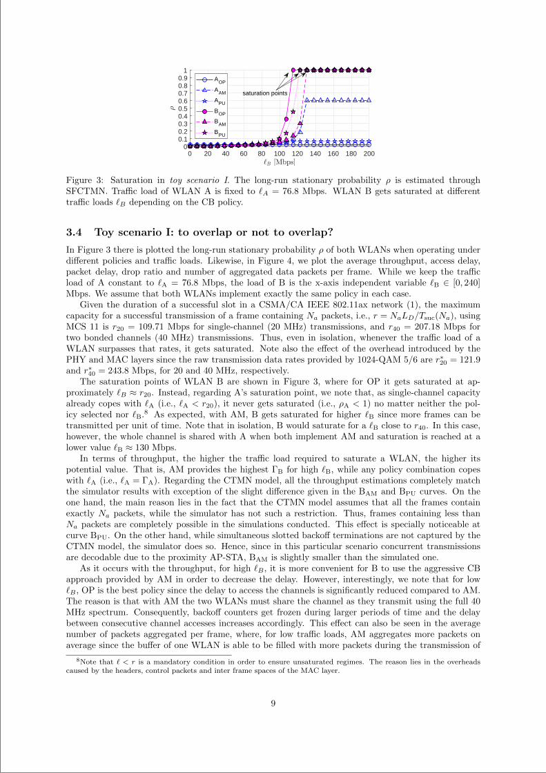
“main” — 2020/11/19 — 10:04 — page 142 — #164

0 20 40 60 80 100 120 140 160 180 2000

0.10.20.30.40.50.60.70.80.9

1AOP

AAM

APU

BOP

BAM

BPU

saturation points

Figure 3: Saturation in toy scenario I. The long-run stationary probability ρ is estimated throughSFCTMN. Traffic load of WLAN A is fixed to `A = 76.8 Mbps. WLAN B gets saturated at differenttraffic loads `B depending on the CB policy.

3.4 Toy scenario I: to overlap or not to overlap?

In Figure 3 there is plotted the long-run stationary probability ρ of both WLANs when operating underdifferent policies and traffic loads. Likewise, in Figure 4, we plot the average throughput, access delay,packet delay, drop ratio and number of aggregated data packets per frame. While we keep the trafficload of A constant to `A = 76.8 Mbps, the load of B is the x-axis independent variable `B ∈ [0, 240]Mbps. We assume that both WLANs implement exactly the same policy in each case.

Given the duration of a successful slot in a CSMA/CA IEEE 802.11ax network (1), the maximumcapacity for a successful transmission of a frame containing Na packets, i.e., r = NaLD/Tsuc(Na), usingMCS 11 is r20 = 109.71 Mbps for single-channel (20 MHz) transmissions, and r40 = 207.18 Mbps fortwo bonded channels (40 MHz) transmissions. Thus, even in isolation, whenever the traffic load of aWLAN surpasses that rates, it gets saturated. Note also the effect of the overhead introduced by thePHY and MAC layers since the raw transmission data rates provided by 1024-QAM 5/6 are r∗20 = 121.9and r∗40 = 243.8 Mbps, for 20 and 40 MHz, respectively.

The saturation points of WLAN B are shown in Figure 3, where for OP it gets saturated at ap-proximately `B ≈ r20. Instead, regarding A’s saturation point, we note that, as single-channel capacityalready copes with `A (i.e., `A < r20), it never gets saturated (i.e., ρA < 1) no matter neither the pol-icy selected nor `B.8 As expected, with AM, B gets saturated for higher `B since more frames can betransmitted per unit of time. Note that in isolation, B would saturate for a `B close to r40. In this case,however, the whole channel is shared with A when both implement AM and saturation is reached at alower value `B ≈ 130 Mbps.

In terms of throughput, the higher the traffic load required to saturate a WLAN, the higher itspotential value. That is, AM provides the highest ΓB for high `B, while any policy combination copeswith `A (i.e., `A = ΓA). Regarding the CTMN model, all the throughput estimations completely matchthe simulator results with exception of the slight difference given in the BAM and BPU curves. On theone hand, the main reason lies in the fact that the CTMN model assumes that all the frames containexactly Na packets, while the simulator has not such a restriction. Thus, frames containing less thanNa packets are completely possible in the simulations conducted. This effect is specially noticeable atcurve BPU. On the other hand, while simultaneous slotted backoff terminations are not captured by theCTMN model, the simulator does so. Hence, since in this particular scenario concurrent transmissionsare decodable due to the proximity AP-STA, BAM is slightly smaller than the simulated one.

As it occurs with the throughput, for high `B , it is more convenient for B to use the aggressive CBapproach provided by AM in order to decrease the delay. However, interestingly, we note that for low`B , OP is the best policy since the delay to access the channels is significantly reduced compared to AM.The reason is that with AM the two WLANs must share the channel as they transmit using the full 40MHz spectrum. Consequently, backoff counters get frozen during larger periods of time and the delaybetween consecutive channel accesses increases accordingly. This effect can also be seen in the averagenumber of packets aggregated per frame, where, for low traffic loads, AM aggregates more packets onaverage since the buffer of one WLAN is able to be filled with more packets during the transmission of

8Note that ` < r is a mandatory condition in order to ensure unsaturated regimes. The reason lies in the overheadscaused by the headers, control packets and inter frame spaces of the MAC layer.

9

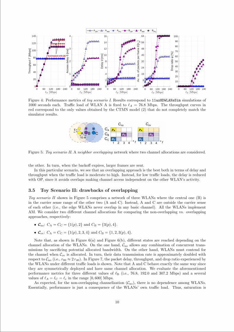
“main” — 2020/11/19 — 10:04 — page 143 — #165

0 60 120 180 2400

1

2

3

4

0 60 120 180 2400

20

40

60

80

100

120

140

0 60 120 180 2400

2

4

6

8

10

12

14

16

Del

ay d

[ms]

0 60 120 180 2400

10

20

30

40

50

60

70

80

90

100

0 60 120 180 2400

8

16

24

32

40

48

56

64

Av.

no.

of p

acke

ts p

er fr

ame

E[n

a]

AOP AAM APU BOP BAM BPU

Estimated with (2)

Figure 4: Performance metrics of toy scenario I. Results correspond to 11axHDWLANsSim simulations of1000 seconds each. Traffic load of WLAN A is fixed to `A = 76.8 Mbps. The throughput curves inred correspond to the only values obtained by the CTMN model (2) that do not completely match thesimulator results.

1 2 f

CB

CC

pBA B C

CA

pC3 4 1 2 f

pB

pA

pC3 4

Cno Cov

pA

10 m

1 m

Figure 5: Toy scenario II. A neighbor overlapping network where two channel allocations are considered.

the other. In turn, when the backoff expires, larger frames are sent.In this particular scenario, we see that an overlapping approach is the best both in terms of delay and

throughput when the traffic load is moderate to high. Instead, for low traffic loads, the delay is reducedwith OP, since it avoids overlaps making channel access independent on the other WLAN’s activity.

3.5 Toy Scenario II: drawbacks of overlapping

Toy scenario II shown in Figure 5 comprises a network of three WLANs where the central one (B) isin the carrier sense range of the other two (A and C). Instead, A and C are outside the carrier senseof each other (i.e., the edge WLANs never overlap in any basic channel). All the WLANs implementAM. We consider two different channel allocations for comparing the non-overlapping vs. overlappingapproaches, respectively:

Cno: CA = CC = 1(p), 2 and CB = 3(p), 4.

Cov: CA = CC = 1(p), 2, 3, 4 and CB = 1, 2, 3(p), 4.

Note that, as shown in Figure 6(a) and Figure 6(b), different states are reached depending on thechannel allocation of the WLANs. On the one hand, Cno allows any combination of concurrent trans-missions by sacrificing potential allocated bandwidth. On the other hand, WLANs must contend forthe channel when Cov is allocated. In turn, their data transmission rate is approximately doubled withrespect to Cno (i.e., r80 ≈ 2 r40). In Figure 7, the packet delay, throughput, and drop ratio experienced bythe WLANs under different traffic loads is shown. Note that A and C behave exactly the same way sincethey are symmetrically deployed and have same channel allocation. We evaluate the aforementionedperformance metrics for three different values of `B (i.e., 76.8, 192.0 and 307.2 Mbps) and a severalvalues of `A = `C = `e in the range [0, 600] Mbps.

As expected, for the non-overlapping channelization (Cno), there is no dependence among WLANs.Essentially, performance is just a consequence of the WLANs’ own traffic load. Thus, saturation is

10

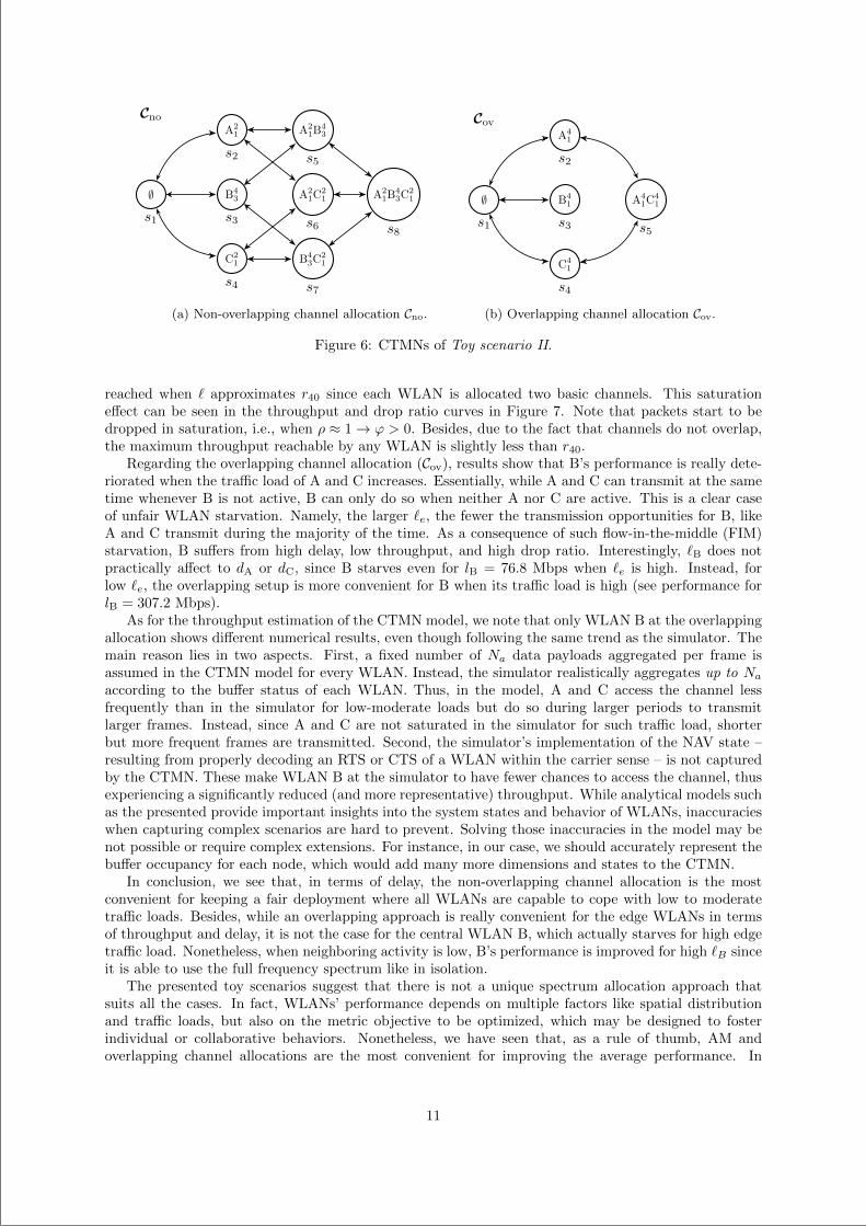
“main” — 2020/11/19 — 10:04 — page 144 — #166

∅s1

B43

s3

A21

s2

C21

s4

A21C2

1

s6

A21B4

3

s5

B43C2

1

s7

A21B4

3C21

s8

Cno

(a) Non-overlapping channel allocation Cno.

∅s1

B41

s3

A41

s2

C41

s4

A41C4

1

s5

Cov

(b) Overlapping channel allocation Cov.

Figure 6: CTMNs of Toy scenario II.

reached when ` approximates r40 since each WLAN is allocated two basic channels. This saturationeffect can be seen in the throughput and drop ratio curves in Figure 7. Note that packets start to bedropped in saturation, i.e., when ρ ≈ 1→ ϕ > 0. Besides, due to the fact that channels do not overlap,the maximum throughput reachable by any WLAN is slightly less than r40.

Regarding the overlapping channel allocation (Cov), results show that B’s performance is really dete-riorated when the traffic load of A and C increases. Essentially, while A and C can transmit at the sametime whenever B is not active, B can only do so when neither A nor C are active. This is a clear caseof unfair WLAN starvation. Namely, the larger `e, the fewer the transmission opportunities for B, likeA and C transmit during the majority of the time. As a consequence of such flow-in-the-middle (FIM)starvation, B suffers from high delay, low throughput, and high drop ratio. Interestingly, `B does notpractically affect to dA or dC, since B starves even for lB = 76.8 Mbps when `e is high. Instead, forlow `e, the overlapping setup is more convenient for B when its traffic load is high (see performance forlB = 307.2 Mbps).

As for the throughput estimation of the CTMN model, we note that only WLAN B at the overlappingallocation shows different numerical results, even though following the same trend as the simulator. Themain reason lies in two aspects. First, a fixed number of Na data payloads aggregated per frame isassumed in the CTMN model for every WLAN. Instead, the simulator realistically aggregates up to Naaccording to the buffer status of each WLAN. Thus, in the model, A and C access the channel lessfrequently than in the simulator for low-moderate loads but do so during larger periods to transmitlarger frames. Instead, since A and C are not saturated in the simulator for such traffic load, shorterbut more frequent frames are transmitted. Second, the simulator’s implementation of the NAV state –resulting from properly decoding an RTS or CTS of a WLAN within the carrier sense – is not capturedby the CTMN. These make WLAN B at the simulator to have fewer chances to access the channel, thusexperiencing a significantly reduced (and more representative) throughput. While analytical models suchas the presented provide important insights into the system states and behavior of WLANs, inaccuracieswhen capturing complex scenarios are hard to prevent. Solving those inaccuracies in the model may benot possible or require complex extensions. For instance, in our case, we should accurately represent thebuffer occupancy for each node, which would add many more dimensions and states to the CTMN.

In conclusion, we see that, in terms of delay, the non-overlapping channel allocation is the mostconvenient for keeping a fair deployment where all WLANs are capable to cope with low to moderatetraffic loads. Besides, while an overlapping approach is really convenient for the edge WLANs in termsof throughput and delay, it is not the case for the central WLAN B, which actually starves for high edgetraffic load. Nonetheless, when neighboring activity is low, B’s performance is improved for high `B sinceit is able to use the full frequency spectrum like in isolation.

The presented toy scenarios suggest that there is not a unique spectrum allocation approach thatsuits all the cases. In fact, WLANs’ performance depends on multiple factors like spatial distributionand traffic loads, but also on the metric objective to be optimized, which may be designed to fosterindividual or collaborative behaviors. Nonetheless, we have seen that, as a rule of thumb, AM andoverlapping channel allocations are the most convenient for improving the average performance. In

11

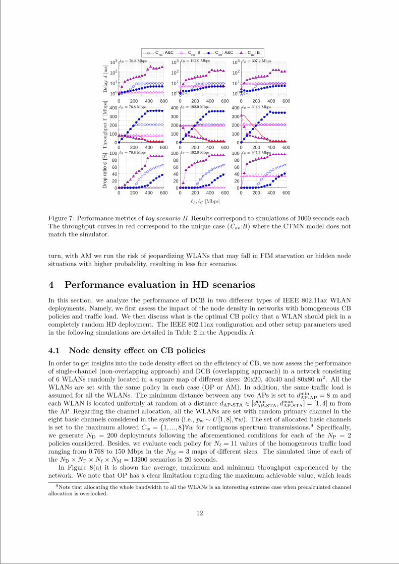
“main” — 2020/11/19 — 10:04 — page 145 — #167

0 200 400 600

100

101

102

103

0 200 400 600

100

101

102

103

0 200 400 600

100

101

102

103

0 200 400 6000

100

200

300

400

0 200 400 6000

100

200

300

400

0 200 400 6000

100

200

300

400

Cno

: A&C Cno

: B Cov

: A&C Cov

: B

0 200 400 6000

20

40

60

80

100

0 200 400 6000

20

40

60

80

100

0 200 400 6000

20

40

60

80

100

Figure 7: Performance metrics of toy scenario II. Results correspond to simulations of 1000 seconds each.The throughput curves in red correspond to the unique case (Cov:B) where the CTMN model does notmatch the simulator.

turn, with AM we run the risk of jeopardizing WLANs that may fall in FIM starvation or hidden nodesituations with higher probability, resulting in less fair scenarios.

4 Performance evaluation in HD scenarios

In this section, we analyze the performance of DCB in two different types of IEEE 802.11ax WLANdeployments. Namely, we first assess the impact of the node density in networks with homogeneous CBpolicies and traffic load. We then discuss what is the optimal CB policy that a WLAN should pick in acompletely random HD deployment. The IEEE 802.11ax configuration and other setup parameters usedin the following simulations are detailed in Table 2 in the Appendix A.

4.1 Node density effect on CB policies

In order to get insights into the node density effect on the efficiency of CB, we now assess the performanceof single-channel (non-overlapping approach) and DCB (overlapping approach) in a network consistingof 6 WLANs randomly located in a square map of different sizes: 20x20, 40x40 and 80x80 m2. All theWLANs are set with the same policy in each case (OP or AM). In addition, the same traffic load isassumed for all the WLANs. The minimum distance between any two APs is set to dmin

AP-AP = 8 m andeach WLAN is located uniformly at random at a distance dAP-STA ∈ [dmin

AP-STA, dmaxAP-STA] = [1, 4] m from

the AP. Regarding the channel allocation, all the WLANs are set with random primary channel in theeight basic channels considered in the system (i.e., pw ∼ U [1, 8],∀w). The set of allocated basic channelsis set to the maximum allowed Cw = 1, ..., 8∀w for contiguous spectrum transmissions.9 Specifically,we generate ND = 200 deployments following the aforementioned conditions for each of the NP = 2policies considered. Besides, we evaluate each policy for N` = 11 values of the homogeneous traffic loadranging from 0.768 to 150 Mbps in the NM = 3 maps of different sizes. The simulated time of each ofthe ND ×NP ×N` ×NM = 13200 scenarios is 20 seconds.

In Figure 8(a) it is shown the average, maximum and minimum throughput experienced by thenetwork. We note that OP has a clear limitation regarding the maximum achievable value, which leads

9Note that allocating the whole bandwidth to all the WLANs is an interesting extreme case when precalculated channelallocation is overlooked.

12

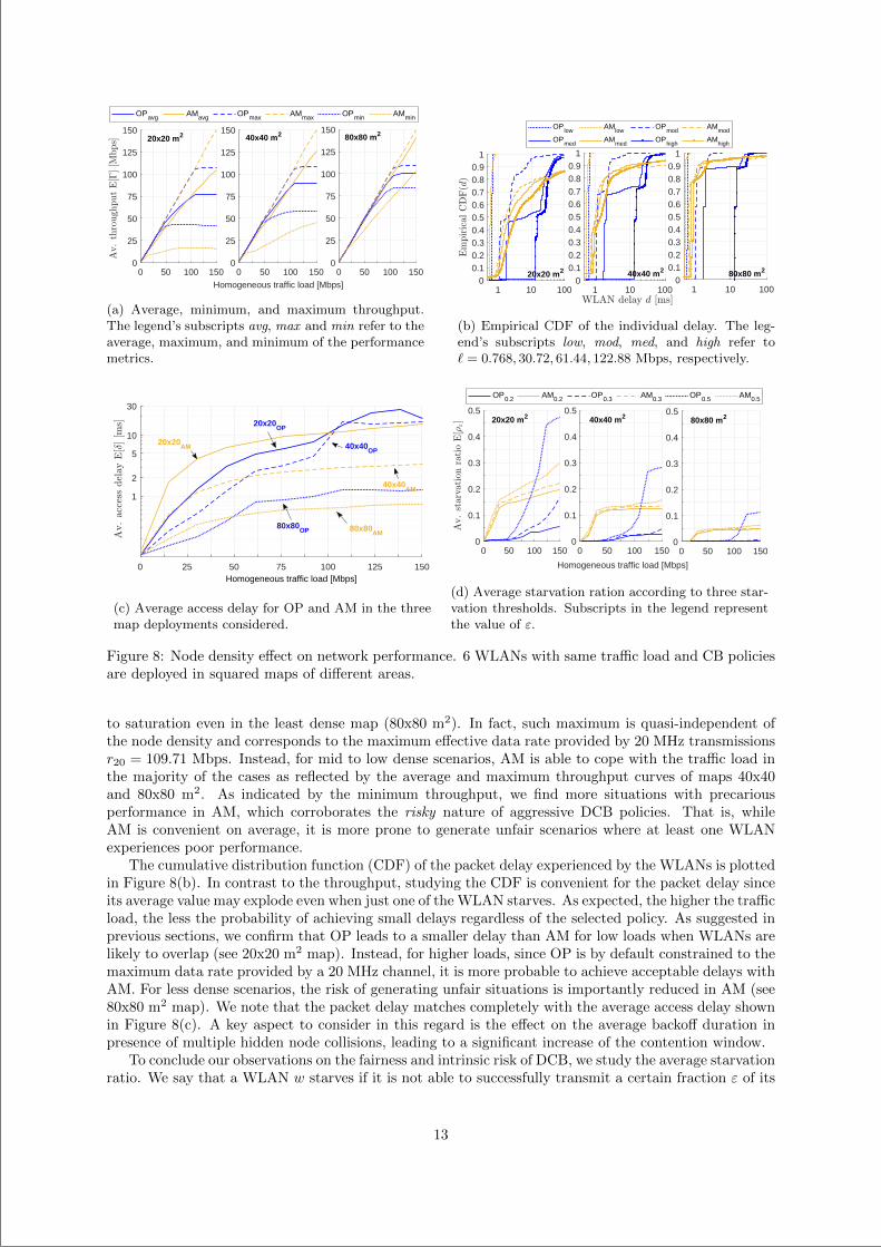
“main” — 2020/11/19 — 10:04 — page 146 — #168

0 50 100 1500

25

50

75

100

125

150

0 50 100 1500

25

50

75

100

125

150

0 50 100 150Homogeneous traffic load [Mbps]

0

25

50

75

100

125

150

OPavg AMavg OPmax AMmax OPmin AMmin

80x80 m240x40 m220x20 m2

(a) Average, minimum, and maximum throughput.The legend’s subscripts avg, max and min refer to theaverage, maximum, and minimum of the performancemetrics.

1 10 1000

0.10.20.30.40.50.60.70.80.9

1

1 10 1000

0.10.20.30.40.50.60.70.80.9

1

1 10 1000

0.10.20.30.40.50.60.70.80.9

1

OPlow

AMlow

OPmod

AMmod

OPmed

AMmed

OPhigh

AMhigh

40x40 m2 80x80 m220x20 m2

(b) Empirical CDF of the individual delay. The leg-end’s subscripts low, mod, med, and high refer to` = 0.768, 30.72, 61.44, 122.88 Mbps, respectively.

0 25 50 75 100 125 150

1

2

5

10

30

80x80AM

20x20AM

20x20OP

40x40AM

80x80OP

40x40OP

Homogeneous traffic load [Mbps]

(c) Average access delay for OP and AM in the threemap deployments considered.

0 50 100 1500

0.1

0.2

0.3

0.4

0.5

0 50 100 150

Homogeneous traffic load [Mbps]

0

0.1

0.2

0.3

0.4

0.5

0 50 100 1500

0.1

0.2

0.3

0.4

0.5

OP0.2 AM0.2 OP0.3 AM0.3 OP0.5 AM0.5

20x20 m2 40x40 m2 80x80 m2

(d) Average starvation ration according to three star-vation thresholds. Subscripts in the legend representthe value of ε.

Figure 8: Node density effect on network performance. 6 WLANs with same traffic load and CB policiesare deployed in squared maps of different areas.

to saturation even in the least dense map (80x80 m2). In fact, such maximum is quasi-independent ofthe node density and corresponds to the maximum effective data rate provided by 20 MHz transmissionsr20 = 109.71 Mbps. Instead, for mid to low dense scenarios, AM is able to cope with the traffic load inthe majority of the cases as reflected by the average and maximum throughput curves of maps 40x40and 80x80 m2. As indicated by the minimum throughput, we find more situations with precariousperformance in AM, which corroborates the risky nature of aggressive DCB policies. That is, whileAM is convenient on average, it is more prone to generate unfair scenarios where at least one WLANexperiences poor performance.

The cumulative distribution function (CDF) of the packet delay experienced by the WLANs is plottedin Figure 8(b). In contrast to the throughput, studying the CDF is convenient for the packet delay sinceits average value may explode even when just one of the WLAN starves. As expected, the higher the trafficload, the less the probability of achieving small delays regardless of the selected policy. As suggested inprevious sections, we confirm that OP leads to a smaller delay than AM for low loads when WLANs arelikely to overlap (see 20x20 m2 map). Instead, for higher loads, since OP is by default constrained to themaximum data rate provided by a 20 MHz channel, it is more probable to achieve acceptable delays withAM. For less dense scenarios, the risk of generating unfair situations is importantly reduced in AM (see80x80 m2 map). We note that the packet delay matches completely with the average access delay shownin Figure 8(c). A key aspect to consider in this regard is the effect on the average backoff duration inpresence of multiple hidden node collisions, leading to a significant increase of the contention window.

To conclude our observations on the fairness and intrinsic risk of DCB, we study the average starvationratio. We say that a WLAN w starves if it is not able to successfully transmit a certain fraction ε of its

13

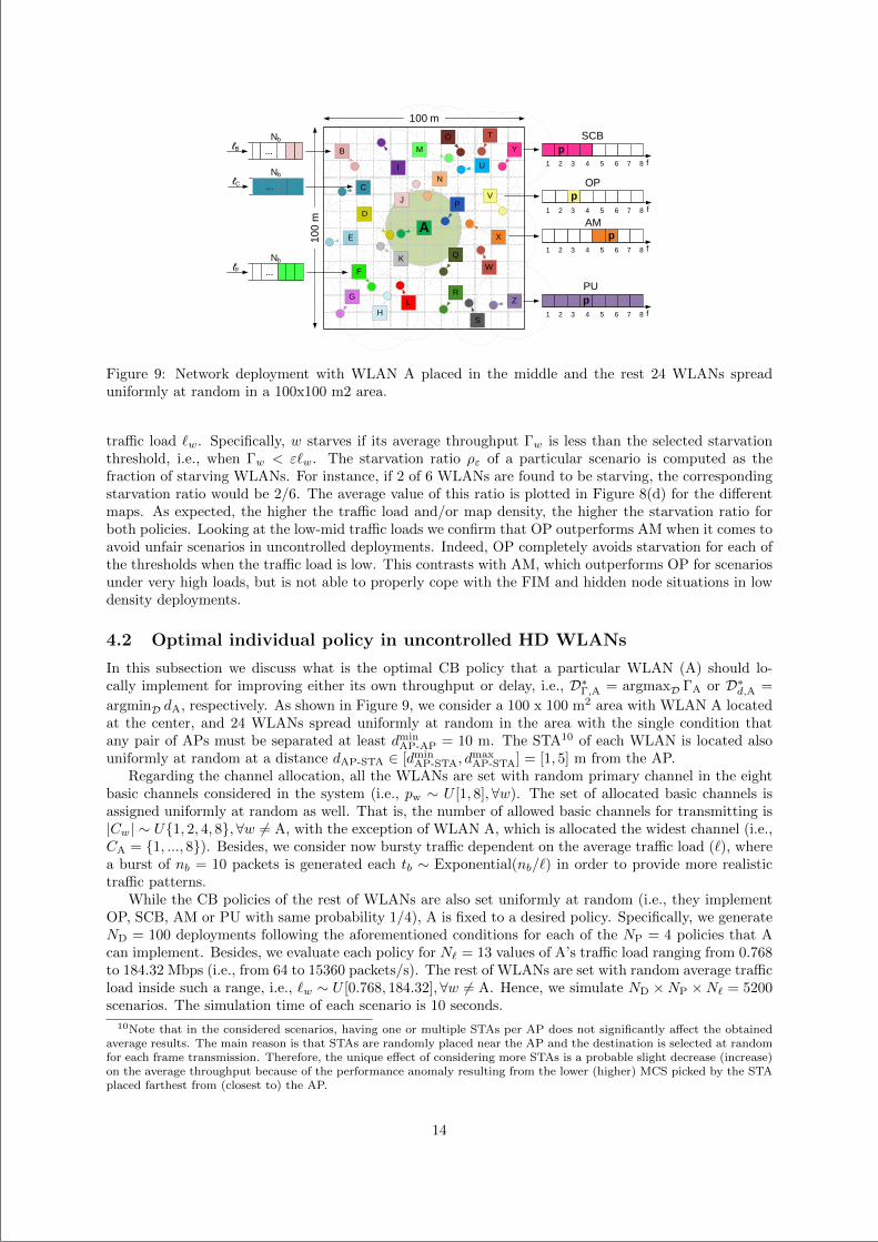
“main” — 2020/11/19 — 10:04 — page 147 — #169

D

F

p1 2 3 4 5 6 7 8 f

p1 2 3 4 5 6 7 8 f

p1 2 3 4 5 6 7 8 f

SCB

AM

PU

d100

md

...

NbℓB

...ℓF

...ℓC

B

V

W

X

Nb

Nb

N

T

H

E

G

I

J

K

L

M

O

P

Q

R

S

U

Z

Y

A

C

d100 md

p1 2 3 4 5 6 7 8 f

OP

Figure 9: Network deployment with WLAN A placed in the middle and the rest 24 WLANs spreaduniformly at random in a 100x100 m2 area.

traffic load `w. Specifically, w starves if its average throughput Γw is less than the selected starvationthreshold, i.e., when Γw < ε`w. The starvation ratio ρε of a particular scenario is computed as thefraction of starving WLANs. For instance, if 2 of 6 WLANs are found to be starving, the correspondingstarvation ratio would be 2/6. The average value of this ratio is plotted in Figure 8(d) for the differentmaps. As expected, the higher the traffic load and/or map density, the higher the starvation ratio forboth policies. Looking at the low-mid traffic loads we confirm that OP outperforms AM when it comes toavoid unfair scenarios in uncontrolled deployments. Indeed, OP completely avoids starvation for each ofthe thresholds when the traffic load is low. This contrasts with AM, which outperforms OP for scenariosunder very high loads, but is not able to properly cope with the FIM and hidden node situations in lowdensity deployments.

4.2 Optimal individual policy in uncontrolled HD WLANs

In this subsection we discuss what is the optimal CB policy that a particular WLAN (A) should lo-cally implement for improving either its own throughput or delay, i.e., D∗Γ,A = argmaxD ΓA or D∗d,A =

argminD dA, respectively. As shown in Figure 9, we consider a 100 x 100 m2 area with WLAN A locatedat the center, and 24 WLANs spread uniformly at random in the area with the single condition thatany pair of APs must be separated at least dmin

AP-AP = 10 m. The STA10 of each WLAN is located alsouniformly at random at a distance dAP-STA ∈ [dmin

AP-STA, dmaxAP-STA] = [1, 5] m from the AP.

Regarding the channel allocation, all the WLANs are set with random primary channel in the eightbasic channels considered in the system (i.e., pw ∼ U [1, 8],∀w). The set of allocated basic channels isassigned uniformly at random as well. That is, the number of allowed basic channels for transmitting is|Cw| ∼ U1, 2, 4, 8,∀w 6= A, with the exception of WLAN A, which is allocated the widest channel (i.e.,CA = 1, ..., 8). Besides, we consider now bursty traffic dependent on the average traffic load (`), wherea burst of nb = 10 packets is generated each tb ∼ Exponential(nb/`) in order to provide more realistictraffic patterns.

While the CB policies of the rest of WLANs are also set uniformly at random (i.e., they implementOP, SCB, AM or PU with same probability 1/4), A is fixed to a desired policy. Specifically, we generateND = 100 deployments following the aforementioned conditions for each of the NP = 4 policies that Acan implement. Besides, we evaluate each policy for N` = 13 values of A’s traffic load ranging from 0.768to 184.32 Mbps (i.e., from 64 to 15360 packets/s). The rest of WLANs are set with random average trafficload inside such a range, i.e., `w ∼ U [0.768, 184.32],∀w 6= A. Hence, we simulate ND ×NP ×N` = 5200scenarios. The simulation time of each scenario is 10 seconds.

10Note that in the considered scenarios, having one or multiple STAs per AP does not significantly affect the obtainedaverage results. The main reason is that STAs are randomly placed near the AP and the destination is selected at randomfor each frame transmission. Therefore, the unique effect of considering more STAs is a probable slight decrease (increase)on the average throughput because of the performance anomaly resulting from the lower (higher) MCS picked by the STAplaced farthest from (closest to) the AP.

14

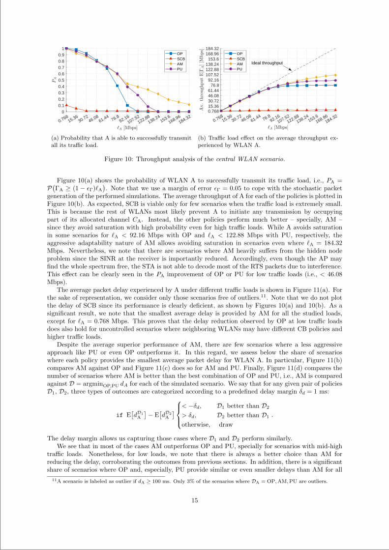
“main” — 2020/11/19 — 10:04 — page 148 — #170

0.76815.36

30.7246.08

61.4476.8

92.16107.52

122.88138.24

153.6168.96

184.320

0.1

0.2

0.3

0.4

0.5

0.6

0.7

0.8

0.9

1OPSCBAMPU

(a) Probability that A is able to successfully transmitall its traffic load.

0.76815.36

30.7246.08

61.4476.8

92.16107.52

122.88138.24

153.6168.96

184.320.76815.3630.7246.0861.44

76.892.16

107.52122.88138.24153.6

168.96184.32

OPSCBAMPU

Ideal throughput

(b) Traffic load effect on the average throughput ex-perienced by WLAN A.

Figure 10: Throughput analysis of the central WLAN scenario.

Figure 10(a) shows the probability of WLAN A to successfully transmit its traffic load, i.e., PA =P(ΓA ≥ (1 − εΓ)`A

). Note that we use a margin of error εΓ = 0.05 to cope with the stochastic packet

generation of the performed simulations. The average throughput of A for each of the policies is plotted inFigure 10(b). As expected, SCB is viable only for few scenarios when the traffic load is extremely small.This is because the rest of WLANs most likely prevent A to initiate any transmission by occupyingpart of its allocated channel CA. Instead, the other policies perform much better – specially, AM –since they avoid saturation with high probability even for high traffic loads. While A avoids saturationin some scenarios for `A < 92.16 Mbps with OP and `A < 122.88 Mbps with PU, respectively, theaggressive adaptability nature of AM allows avoiding saturation in scenarios even where `A = 184.32Mbps. Nevertheless, we note that there are scenarios where AM heavily suffers from the hidden nodeproblem since the SINR at the receiver is importantly reduced. Accordingly, even though the AP mayfind the whole spectrum free, the STA is not able to decode most of the RTS packets due to interference.This effect can be clearly seen in the PA improvement of OP or PU for low traffic loads (i.e., < 46.08Mbps).

The average packet delay experienced by A under different traffic loads is shown in Figure 11(a). Forthe sake of representation, we consider only those scenarios free of outliers.11. Note that we do not plotthe delay of SCB since its performance is clearly deficient, as shown by Figures 10(a) and 10(b). As asignificant result, we note that the smallest average delay is provided by AM for all the studied loads,except for `A = 0.768 Mbps. This proves that the delay reduction observed by OP at low traffic loadsdoes also hold for uncontrolled scenarios where neighboring WLANs may have different CB policies andhigher traffic loads.

Despite the average superior performance of AM, there are few scenarios where a less aggressiveapproach like PU or even OP outperforms it. In this regard, we assess below the share of scenarioswhere each policy provides the smallest average packet delay for WLAN A. In particular, Figure 11(b)compares AM against OP and Figure 11(c) does so for AM and PU. Finally, Figure 11(d) compares thenumber of scenarios where AM is better than the best combination of OP and PU, i.e., AM is comparedagainst D = argminOP,PU dA for each of the simulated scenario. We say that for any given pair of policiesD1, D2, three types of outcomes are categorized according to a predefined delay margin δd = 1 ms:

if E[dD1

A

]− E

[dD2

A

]

< −δd, D1 better than D2

> δd, D2 better than D1

otherwise, draw

.

The delay margin allows us capturing those cases where D1 and D2 perform similarly.We see that in most of the cases AM outperforms OP and PU, specially for scenarios with mid-high

traffic loads. Nonetheless, for low loads, we note that there is always a better choice than AM forreducing the delay, corroborating the outcomes from previous sections. In addition, there is a significantshare of scenarios where OP and, especially, PU provide similar or even smaller delays than AM for all

11A scenario is labeled as outlier if dA ≥ 100 ms. Only 3% of the scenarios where DA = OP,AM,PU are outliers.

15

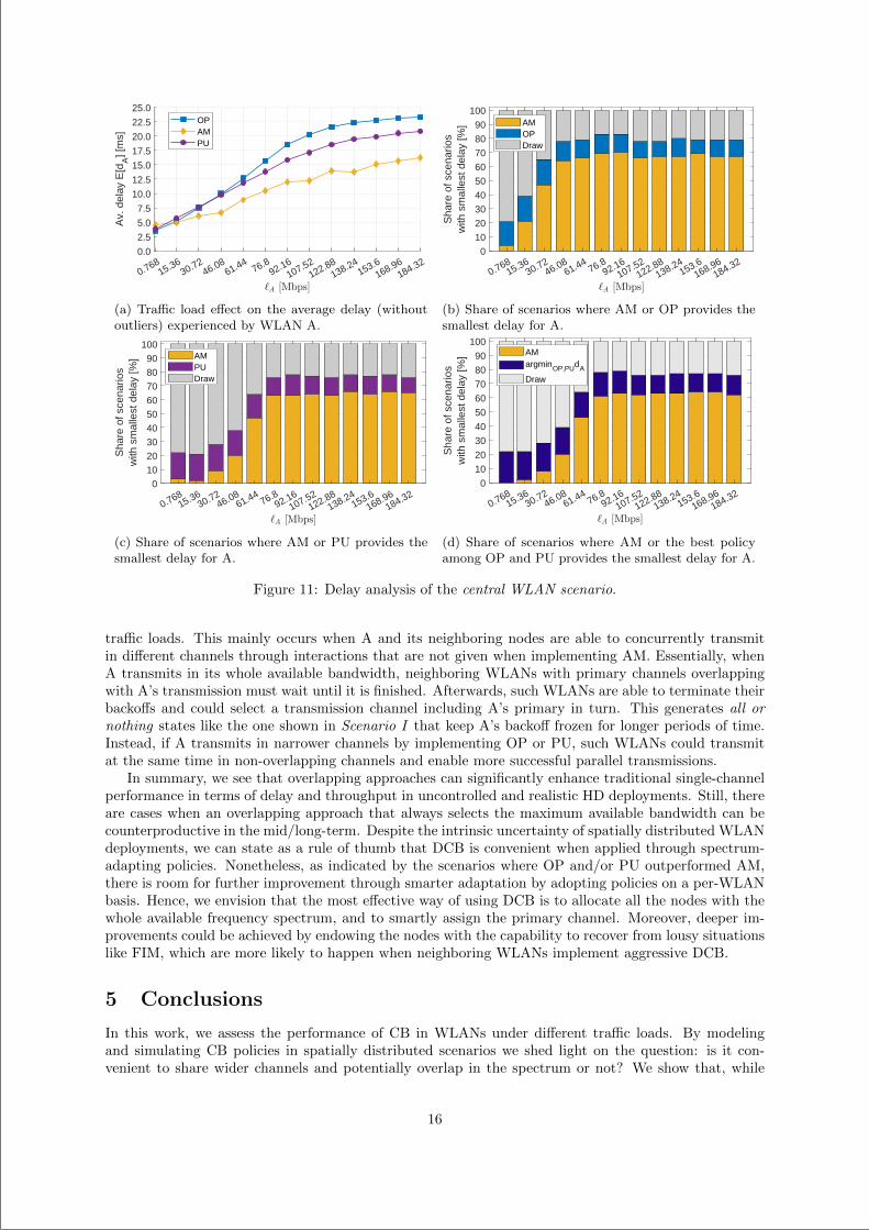
“main” — 2020/11/19 — 10:04 — page 149 — #171

0.76815.36

30.7246.08

61.4476.8

92.16107.52

122.88138.24

153.6168.96

184.320.0

2.5

5.0

7.5

10.0

12.5

15.0

17.5

20.0

22.5

25.0A

v. d

elay

E[d

A] [

ms]

OPAMPU

(a) Traffic load effect on the average delay (withoutoutliers) experienced by WLAN A.

0.76815.36

30.7246.08

61.4476.8

92.16107.52

122.88138.24

153.6168.96

184.320

10

20

30

40

50

60

70

80

90

100

Sha

re o

f sce

nario

sw

ith s

mal

lest

del

ay [%

] AMOPDraw

(b) Share of scenarios where AM or OP provides thesmallest delay for A.

0.76815.36

30.7246.08

61.4476.8

92.16107.52

122.88138.24

153.6168.96

184.320

102030405060708090

100

Sha

re o

f sce

nario

sw

ith s

mal

lest

del

ay [%

] AMPUDraw

(c) Share of scenarios where AM or PU provides thesmallest delay for A.

0.76815.36

30.7246.08

61.4476.8

92.16107.52

122.88138.24

153.6168.96

184.320

10

20

30

40

50

60

70

80

90

100

Sha

re o

f sce

nario

sw

ith s

mal

lest

del

ay [%

] AMargminOP,PUdA

Draw

(d) Share of scenarios where AM or the best policyamong OP and PU provides the smallest delay for A.

Figure 11: Delay analysis of the central WLAN scenario.

traffic loads. This mainly occurs when A and its neighboring nodes are able to concurrently transmitin different channels through interactions that are not given when implementing AM. Essentially, whenA transmits in its whole available bandwidth, neighboring WLANs with primary channels overlappingwith A’s transmission must wait until it is finished. Afterwards, such WLANs are able to terminate theirbackoffs and could select a transmission channel including A’s primary in turn. This generates all ornothing states like the one shown in Scenario I that keep A’s backoff frozen for longer periods of time.Instead, if A transmits in narrower channels by implementing OP or PU, such WLANs could transmitat the same time in non-overlapping channels and enable more successful parallel transmissions.

In summary, we see that overlapping approaches can significantly enhance traditional single-channelperformance in terms of delay and throughput in uncontrolled and realistic HD deployments. Still, thereare cases when an overlapping approach that always selects the maximum available bandwidth can becounterproductive in the mid/long-term. Despite the intrinsic uncertainty of spatially distributed WLANdeployments, we can state as a rule of thumb that DCB is convenient when applied through spectrum-adapting policies. Nonetheless, as indicated by the scenarios where OP and/or PU outperformed AM,there is room for further improvement through smarter adaptation by adopting policies on a per-WLANbasis. Hence, we envision that the most effective way of using DCB is to allocate all the nodes with thewhole available frequency spectrum, and to smartly assign the primary channel. Moreover, deeper im-provements could be achieved by endowing the nodes with the capability to recover from lousy situationslike FIM, which are more likely to happen when neighboring WLANs implement aggressive DCB.

5 Conclusions

In this work, we assess the performance of CB in WLANs under different traffic loads. By modelingand simulating CB policies in spatially distributed scenarios we shed light on the question: is it con-venient to share wider channels and potentially overlap in the spectrum or not? We show that, while

16

“main” — 2020/11/19 — 10:04 — page 150 — #172

the performance of SCB is clearly poor for moderate-high traffic loads, spectrum-adapting DCB cansignificantly outperform the traditional single-channel approach in terms of throughput and delay, evenin high-density deployments. However, we also remark two main outcomes concerning DCB: i) the in-trinsic risk when it comes to generating unfair scenarios as a consequence of the hidden node and FIMsituations, and ii) the exposure to doing more harm than good in terms of delay for low traffic regimes.

In this regard, the intricate nature of uncontrolled WLAN deployments leaves room for furtherimprovements in spectrum efficiency, while prevents designing effective predefined rules. Therefore, ournext work will focus on two aspects: studying machine learning based DCB policies to efficiently adaptto traffic load needs, and jointly combining DCB with adequate primary channel allocation.

Acknowledgment

This work has been partially supported by a Gift from CISCO University Research Program (CG#890107)& Silicon Valley Community Foundation, by the Spanish Ministry of Economy and Competitiveness un-der the Maria de Maeztu Units of Excellence Programme (MDM-2015-0502), and by the Catalan Gov-ernment under grant SGR-2017-1188. The work by S. Barrachina-Munoz is supported by an FI grantfrom the Generalitat de Catalunya.

References

[1] M. Elbamby, C. Perfecto, M. Bennis, and K. Doppler. Toward low-latency and ultra-reliable virtualreality. IEEE Network, 32(2):78–84, 2018.

[2] IEEE 802.11n. Standard for Wireless LAN Medium Access Control (MAC) and Physical Layer(PHY): Enhancements for High Throughput. IEEE, 2009.

[3] I. P802.11ac. Standard for Wireless LAN Medium Access Control (MAC) and Physical Layer(PHY) specifications: Enhancements for Very High Throughput for Operation in Bands below 6GHz. IEEE, 2014.

[4] IEEE 802.11 Task Group AX. Status of Project IEEE 802.11ax High Efficiency WLAN (HEW).http://www.ieee802.org/11/Reports/tgax_update.htm. Accessed: 2018-09-21.

[5] EXtreme Throughput (XT) 802.11. Doc.: IEEE 802.11-18/0789r10, 2018.

[6] S. Bukhari, M. Rehmani, and S. Siraj. A survey of channel bonding for wireless networks andguidelines of channel bonding for futuristic cognitive radio sensor networks. IEEE CommunicationsSurveys & Tutorials, 18(2):924–948, 2016.

[7] M. Park. IEEE 802.11 ac: Dynamic bandwidth channel access. In Communications (ICC), 2011IEEE International Conference on, pages 1–5. IEEE, 2011.

[8] L. Deek, E. Garcia-Villegas, E. Belding, S. Lee, and K. Almeroth. The impact of channel bonding on802.11 n network management. In Proceedings of the Seventh Conference on emerging NetworkingExperiments and Technologies, page 11. ACM, 2011.

[9] M. Arslan, K. Pelechrinis, I. Broustis, S. Krishnamurthy, S. Addepalli, and K. Papagiannaki. Auto-configuration of 802.11n wlans. In Proceedings of the 6th International Conference, page 27. ACM,2010.

[10] M. Arslan, K. Pelechrinis, I. Broustis, S. Krishnamurthy, S. Addepalli, and K. Papagiannaki.ACORN: An auto-configuration framework for 802.11 n WLANs. IEEE/ACM Transactions onNetworking (TON), 21(3):896–909, 2013.

[11] V. Shrivastava, S. Rayanchu, J. Yoonj, and S. Banerjee. 802.11n under the microscope. In Pro-ceedings of the 8th ACM SIGCOMM conference on Internet measurement, pages 105–110. ACM,2008.

17

“main” — 2020/11/19 — 10:04 — page 151 — #173

[12] B. Bellalta. IEEE 802.11ax: High-efficiency WLANs. IEEE Wireless Communications, 23(1):38–46,2016.

[13] L. Deek, E. Garcia-Villegas, E. Belding, S. Lee, and K. Almeroth. Intelligent channel bonding in802.11 n wlans. IEEE Transactions on Mobile Computing, 13(6):1242–1255, 2014.

[14] L. Deek, E. Garcia-Villegas, E. Belding, S. Lee, and K. Almeroth. Joint rate and channel widthadaptation for 802.11 MIMO wireless networks. In Sensor, Mesh and Ad Hoc Communicationsand Networks (SECON), 2013 10th Annual IEEE Communications Society Conference on, pages167–175. IEEE, 2013.

[15] W. Wang, F. Zhang, and Q. Zhang. Managing channel bonding with clear channel assessment in802.11 networks. In Communications (ICC), 2016 IEEE International Conference on, pages 1–6.IEEE, 2016.

[16] M. Gong, B. Hart, L. Xia, and R. Want. Channel bounding and MAC protection mechanisms for802.11ac. In Global Telecommunications Conference (GLOBECOM 2011), 2011 IEEE, pages 1–5.IEEE, 2011.

[17] S. Barrachina-Munoz, F. Wilhelmi, and B. Bellalta. Dynamic Channel Bonding in Spatially Dis-tributed High-Density WLANs. arXiv preprint arXiv:1801.00594, 2018.

[18] Y. Zeng, P. Pathak, and P. Mohapatra. A first look at 802.11ac in action: Energy efficiency andinterference characterization. In Networking Conference, 2014 IFIP, pages 1–9. IEEE, 2014.

[19] S. Yun, Daehyeok Kim, and L. Qiu. Fine-grained spectrum adaptation in wifi networks. In Proceed-ings of the 19th annual international conference on Mobile computing & networking, pages 327–338.ACM, 2013.

[20] W. Wang, Y. Chen, Z. Wang, J. Zhang, K. Wu, and Q. Zhang. Wideband spectrum adaptationwithout coordination. IEEE Transactions on Mobile Computing, 16(1):243–256, 2017.

[21] P. Huang, X. Yang, and L. Xiao. Dynamic channel bonding: enabling flexible spectrum aggregation.IEEE Transactions on Mobile Computing, 15(12):3042–3056, 2016.

[22] Y. Chen, D. Wu, T. Sung, and K. Shih. DBS: A dynamic bandwidth selection MAC protocolfor channel bonding in IEEE 802.11 ac WLANs. In Wireless Communications and NetworkingConference (WCNC), 2018 IEEE, pages 1–6. IEEE, 2018.

[23] S. Khairy, M. Han, L. Cai, Y. Cheng, and Z. Han. A Renewal Theory based Analytical Modelfor Multi-channel Random Access in IEEE 802.11ac/ax. IEEE Transactions on Mobile Computing,2018.

[24] A. Nabil, M. Abdel-Rahman, and A. MacKenzie. Adaptive Channel Bonding in Wireless LANsUnder Demand Uncertainty. To appear in the Proceedings of the IEEE International Symposiumon Personal, Indoor and Mobile Radio Communications (PIMRC), Montreal, QC, Canada, October2017.

[25] S. Byeon, H. Kwon, Y. Son, C. Yang, and S. Choi. RECONN: Receiver-Driven Operating ChannelWidth Adaptation in IEEE 802.11ac WLANs. In IEEE INFOCOM 2018-IEEE Conference onComputer Communications, pages 1655–1663. IEEE, 2018.

[26] B. Bellalta, A. Faridi, J. Barcelo, A. Checco, and P. Chatzimisios. Channel bonding in short-rangeWLANs. In European Wireless 2014; 20th European Wireless Conference; Proceedings of, pages1–7. VDE, 2014.

[27] B. Bellalta, A. Checco, A. Zocca, and J. Barcelo. On the interactions between multiple overlappingWLANs using channel bonding. IEEE Transactions on Vehicular Technology, 65(2):796–812, 2016.

[28] M. Han, Sami K., L. X. Cai, and Y. Cheng. Performance Analysis of Opportunistic ChannelBonding in Multi-Channel WLANs. In Global Communications Conference (GLOBECOM), 2016IEEE, pages 1–6. IEEE, 2016.

18

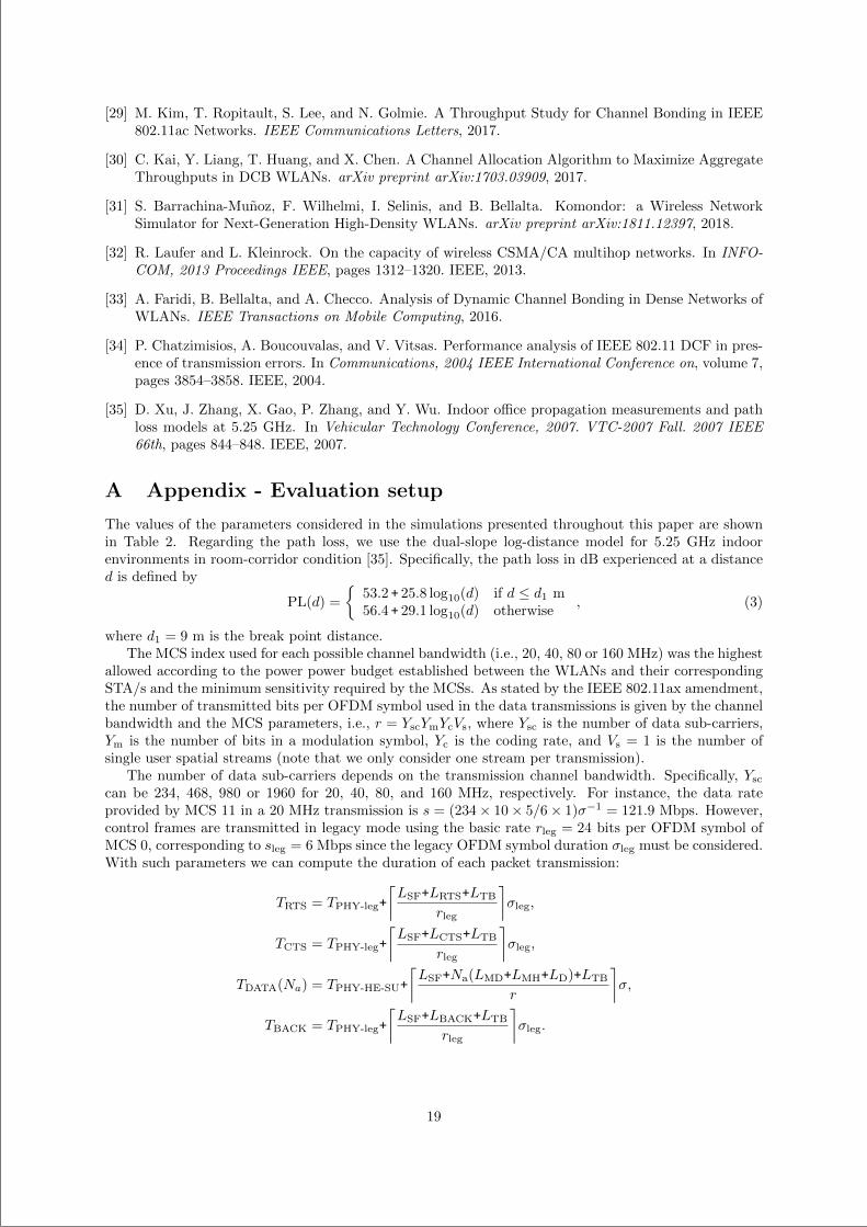
“main” — 2020/11/19 — 10:04 — page 152 — #174

[29] M. Kim, T. Ropitault, S. Lee, and N. Golmie. A Throughput Study for Channel Bonding in IEEE802.11ac Networks. IEEE Communications Letters, 2017.

[30] C. Kai, Y. Liang, T. Huang, and X. Chen. A Channel Allocation Algorithm to Maximize AggregateThroughputs in DCB WLANs. arXiv preprint arXiv:1703.03909, 2017.

[31] S. Barrachina-Munoz, F. Wilhelmi, I. Selinis, and B. Bellalta. Komondor: a Wireless NetworkSimulator for Next-Generation High-Density WLANs. arXiv preprint arXiv:1811.12397, 2018.

[32] R. Laufer and L. Kleinrock. On the capacity of wireless CSMA/CA multihop networks. In INFO-COM, 2013 Proceedings IEEE, pages 1312–1320. IEEE, 2013.

[33] A. Faridi, B. Bellalta, and A. Checco. Analysis of Dynamic Channel Bonding in Dense Networks ofWLANs. IEEE Transactions on Mobile Computing, 2016.

[34] P. Chatzimisios, A. Boucouvalas, and V. Vitsas. Performance analysis of IEEE 802.11 DCF in pres-ence of transmission errors. In Communications, 2004 IEEE International Conference on, volume 7,pages 3854–3858. IEEE, 2004.

[35] D. Xu, J. Zhang, X. Gao, P. Zhang, and Y. Wu. Indoor office propagation measurements and pathloss models at 5.25 GHz. In Vehicular Technology Conference, 2007. VTC-2007 Fall. 2007 IEEE66th, pages 844–848. IEEE, 2007.

A Appendix - Evaluation setup

The values of the parameters considered in the simulations presented throughout this paper are shownin Table 2. Regarding the path loss, we use the dual-slope log-distance model for 5.25 GHz indoorenvironments in room-corridor condition [35]. Specifically, the path loss in dB experienced at a distanced is defined by

PL(d) =

53.2 + 25.8 log10(d) if d ≤ d1 m56.4 + 29.1 log10(d) otherwise

, (3)

where d1 = 9 m is the break point distance.The MCS index used for each possible channel bandwidth (i.e., 20, 40, 80 or 160 MHz) was the highest

allowed according to the power power budget established between the WLANs and their correspondingSTA/s and the minimum sensitivity required by the MCSs. As stated by the IEEE 802.11ax amendment,the number of transmitted bits per OFDM symbol used in the data transmissions is given by the channelbandwidth and the MCS parameters, i.e., r = YscYmYcVs, where Ysc is the number of data sub-carriers,Ym is the number of bits in a modulation symbol, Yc is the coding rate, and Vs = 1 is the number ofsingle user spatial streams (note that we only consider one stream per transmission).

The number of data sub-carriers depends on the transmission channel bandwidth. Specifically, Ysc

can be 234, 468, 980 or 1960 for 20, 40, 80, and 160 MHz, respectively. For instance, the data rateprovided by MCS 11 in a 20 MHz transmission is s = (234× 10× 5/6× 1)σ−1 = 121.9 Mbps. However,control frames are transmitted in legacy mode using the basic rate rleg = 24 bits per OFDM symbol ofMCS 0, corresponding to sleg = 6 Mbps since the legacy OFDM symbol duration σleg must be considered.With such parameters we can compute the duration of each packet transmission:

TRTS = TPHY-leg+

⌈LSF+LRTS+LTB

rleg

⌉σleg,

TCTS = TPHY-leg+

⌈LSF+LCTS+LTB

rleg

⌉σleg,

TDATA(Na) = TPHY-HE-SU+

⌈LSF+Na(LMD+LMH+LD)+LTB

r

⌉σ,

TBACK = TPHY-leg+

⌈LSF+LBACK+LTB

rleg

⌉σleg.

19

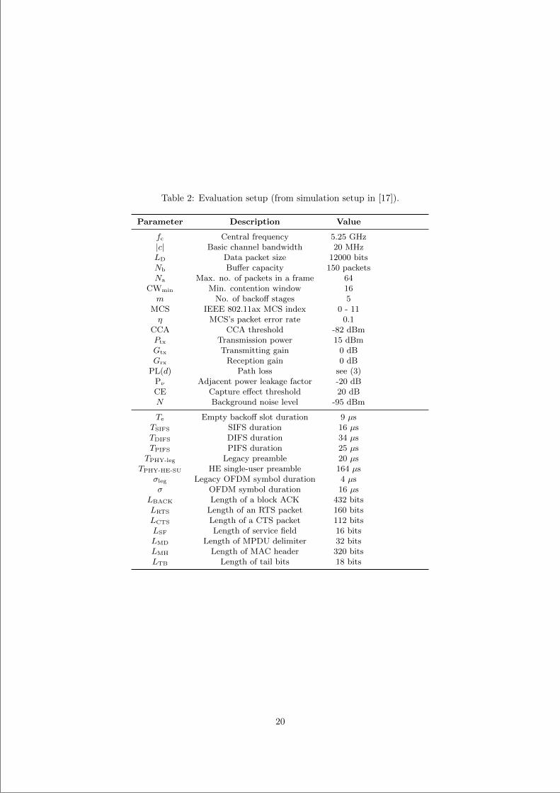
“main” — 2020/11/19 — 10:04 — page 153 — #175

Table 2: Evaluation setup (from simulation setup in [17]).

Parameter Description Value

fc Central frequency 5.25 GHz|c| Basic channel bandwidth 20 MHzLD Data packet size 12000 bitsNb Buffer capacity 150 packetsNa Max. no. of packets in a frame 64

CWmin Min. contention window 16m No. of backoff stages 5

MCS IEEE 802.11ax MCS index 0 - 11η MCS’s packet error rate 0.1

CCA CCA threshold -82 dBmPtx Transmission power 15 dBmGtx Transmitting gain 0 dBGrx Reception gain 0 dB

PL(d) Path loss see (3)Pν Adjacent power leakage factor -20 dBCE Capture effect threshold 20 dBN Background noise level -95 dBm

Te Empty backoff slot duration 9 µsTSIFS SIFS duration 16 µsTDIFS DIFS duration 34 µsTPIFS PIFS duration 25 µsTPHY-leg Legacy preamble 20 µs

TPHY-HE-SU HE single-user preamble 164 µsσleg Legacy OFDM symbol duration 4 µsσ OFDM symbol duration 16 µs

LBACK Length of a block ACK 432 bitsLRTS Length of an RTS packet 160 bitsLCTS Length of a CTS packet 112 bitsLSF Length of service field 16 bitsLMD Length of MPDU delimiter 32 bitsLMH Length of MAC header 320 bitsLTB Length of tail bits 18 bits

20

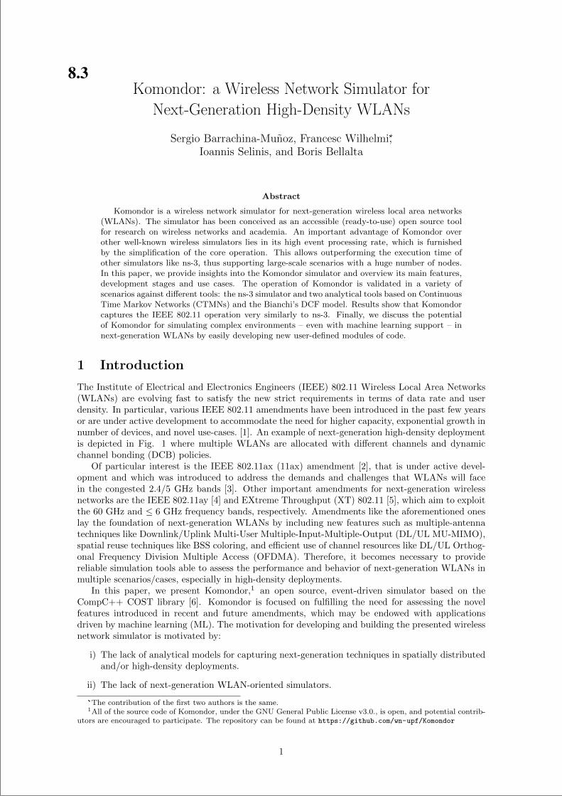
“main” — 2020/11/19 — 10:04 — page 154 — #176

Komondor: a Wireless Network Simulator for

Next-Generation High-Density WLANs

Sergio Barrachina-Munoz, Francesc Wilhelmi*,Ioannis Selinis, and Boris Bellalta

Abstract

Komondor is a wireless network simulator for next-generation wireless local area networks(WLANs). The simulator has been conceived as an accessible (ready-to-use) open source toolfor research on wireless networks and academia. An important advantage of Komondor overother well-known wireless simulators lies in its high event processing rate, which is furnishedby the simplification of the core operation. This allows outperforming the execution time ofother simulators like ns-3, thus supporting large-scale scenarios with a huge number of nodes.In this paper, we provide insights into the Komondor simulator and overview its main features,development stages and use cases. The operation of Komondor is validated in a variety ofscenarios against different tools: the ns-3 simulator and two analytical tools based on ContinuousTime Markov Networks (CTMNs) and the Bianchi’s DCF model. Results show that Komondorcaptures the IEEE 802.11 operation very similarly to ns-3. Finally, we discuss the potentialof Komondor for simulating complex environments – even with machine learning support – innext-generation WLANs by easily developing new user-defined modules of code.

1 Introduction

The Institute of Electrical and Electronics Engineers (IEEE) 802.11 Wireless Local Area Networks(WLANs) are evolving fast to satisfy the new strict requirements in terms of data rate and userdensity. In particular, various IEEE 802.11 amendments have been introduced in the past few yearsor are under active development to accommodate the need for higher capacity, exponential growth innumber of devices, and novel use-cases. [1]. An example of next-generation high-density deploymentis depicted in Fig. 1 where multiple WLANs are allocated with different channels and dynamicchannel bonding (DCB) policies.

Of particular interest is the IEEE 802.11ax (11ax) amendment [2], that is under active devel-opment and which was introduced to address the demands and challenges that WLANs will facein the congested 2.4/5 GHz bands [3]. Other important amendments for next-generation wirelessnetworks are the IEEE 802.11ay [4] and EXtreme Throughput (XT) 802.11 [5], which aim to exploitthe 60 GHz and ≤ 6 GHz frequency bands, respectively. Amendments like the aforementioned oneslay the foundation of next-generation WLANs by including new features such as multiple-antennatechniques like Downlink/Uplink Multi-User Multiple-Input-Multiple-Output (DL/UL MU-MIMO),spatial reuse techniques like BSS coloring, and efficient use of channel resources like DL/UL Orthog-onal Frequency Division Multiple Access (OFDMA). Therefore, it becomes necessary to providereliable simulation tools able to assess the performance and behavior of next-generation WLANs inmultiple scenarios/cases, especially in high-density deployments.

In this paper, we present Komondor,1 an open source, event-driven simulator based on theCompC++ COST library [6]. Komondor is focused on fulfilling the need for assessing the novelfeatures introduced in recent and future amendments, which may be endowed with applicationsdriven by machine learning (ML). The motivation for developing and building the presented wirelessnetwork simulator is motivated by:

i) The lack of analytical models for capturing next-generation techniques in spatially distributedand/or high-density deployments.

ii) The lack of next-generation WLAN-oriented simulators.

*The contribution of the first two authors is the same.1All of the source code of Komondor, under the GNU General Public License v3.0., is open, and potential contrib-

utors are encouraged to participate. The repository can be found at https://github.com/wn-upf/Komondor

1

8.3

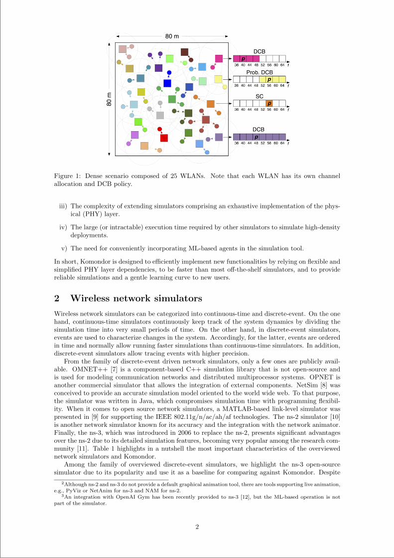
“main” — 2020/11/19 — 10:04 — page 155 — #177

Figure 1: Dense scenario composed of 25 WLANs. Note that each WLAN has its own channelallocation and DCB policy.

iii) The complexity of extending simulators comprising an exhaustive implementation of the phys-ical (PHY) layer.

iv) The large (or intractable) execution time required by other simulators to simulate high-densitydeployments.

v) The need for conveniently incorporating ML-based agents in the simulation tool.

In short, Komondor is designed to efficiently implement new functionalities by relying on flexible andsimplified PHY layer dependencies, to be faster than most off-the-shelf simulators, and to providereliable simulations and a gentle learning curve to new users.

2 Wireless network simulators

Wireless network simulators can be categorized into continuous-time and discrete-event. On the onehand, continuous-time simulators continuously keep track of the system dynamics by dividing thesimulation time into very small periods of time. On the other hand, in discrete-event simulators,events are used to characterize changes in the system. Accordingly, for the latter, events are orderedin time and normally allow running faster simulations than continuous-time simulators. In addition,discrete-event simulators allow tracing events with higher precision.

From the family of discrete-event driven network simulators, only a few ones are publicly avail-able. OMNET++ [7] is a component-based C++ simulation library that is not open-source andis used for modeling communication networks and distributed multiprocessor systems. OPNET isanother commercial simulator that allows the integration of external components. NetSim [8] wasconceived to provide an accurate simulation model oriented to the world wide web. To that purpose,the simulator was written in Java, which compromises simulation time with programming flexibil-ity. When it comes to open source network simulators, a MATLAB-based link-level simulator waspresented in [9] for supporting the IEEE 802.11g/n/ac/ah/af technologies. The ns-2 simulator [10]is another network simulator known for its accuracy and the integration with the network animator.Finally, the ns-3, which was introduced in 2006 to replace the ns-2, presents significant advantagesover the ns-2 due to its detailed simulation features, becoming very popular among the research com-munity [11]. Table 1 highlights in a nutshell the most important characteristics of the overviewednetwork simulators and Komondor.

Among the family of overviewed discrete-event simulators, we highlight the ns-3 open-sourcesimulator due to its popularity and use it as a baseline for comparing against Komondor. Despite

2Although ns-2 and ns-3 do not provide a default graphical animation tool, there are tools supporting live animation,e.g., PyViz or NetAnim for ns-3 and NAM for ns-2.

3An integration with OpenAI Gym has been recently provided to ns-3 [12], but the ML-based operation is notpart of the simulator.

2

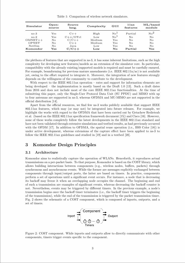
“main” — 2020/11/19 — 10:04 — page 156 — #178

Table 1: Comparison of wireless network simulators.

SimulatorOpen-source

Sourcelang.

Complexity GUI11ax

featuresML/basedmodule

ns-3 Yes C++ High No1 Partial No2

ns-2 Yes C++/OTcl Low No1 No NoOMNET++ No C/C++ Medium Yes No No

OPNET No C++ Medium Yes No NoNetSim No Java Low Yes No No

Komondor Yes C/C++ Low No Partial Yes

the plethora of features that are supported in ns-3, it has some inherent limitations, such as the highcomplexity for developing new features/models as an extension of the simulator core. In particular,compatibility with the already existing/supported models is required and must be carefully ensured.For example, beamforming for previous mature amendments (i.e. IEEE 802.11n/ac) is not availableyet, owing to the effort required to integrate it. Moreover, the integration of new features stronglydepends on the willingness of the community to contribute to the development.

With respect to the IEEE 802.11ax operation – rates and support for information elements arebeing developed – the implementation is mostly based on the Draft 1.0 [13]. Such a draft datesfrom 2016 and does not include most of the core IEEE 802.11ax functionalities. At the time ofsubmitting this paper, only the Single-User Protocol Data Unit (SU PPDU) and MIMO with upto four antennas are supported in ns-3, whereas OFDMA and MU-MIMO are not supported in theofficial distribution [14].

Apart from the official resources, we find few ns-3 works publicly available that support IEEE802.11ax features, which may (or may not) be integrated into future releases. For example, wehighlight the works with regard to the OFDMA that have been carried out by Getachew Redieteabet al. (based on the IEEE 802.11ax specification framework document [15]) and Cisco [16]. However,none of these works completely follow the latest developments in the IEEE 802.11ax standard andhave not been validated through extensive simulations and testbed results, as had previously occurredwith the OFDM [17]. In addition to OFDMA, the spatial reuse operation (i.e., BSS Color [18]) isunder active development, whereas extensions of the capture effect have been applied to ns-3 tofollow the IEEE 802.11ax guidelines and studied in [19] and in a testbed [20].

3 Komondor Design Principles

3.1 Architecture

Komondor aims to realistically capture the operation of WLANs. Henceforth, it reproduces actualtransmissions on a per-packet basis. To that purpose, Komondor is based on the COST library, whichallows building interactions between components (e.g., wireless nodes, buffers, packets) throughsynchronous and asynchronous events. While the former are messages explicitly exchanged betweencomponents through input/output ports, the latter are based on timers. In practice, componentsperform a set of operations until a significant event occurs. For instance, a node that is decreasingits backoff may freeze it when an overlapping node occupies the channel. The beginning and endof such a transmission are examples of significant events, whereas decreasing the backoff counter isnot. Nevertheless, events may be triggered by different timers. In the previous example, a node’stransmission begins once the backoff timer terminates (i.e., the backoff timer triggers the beginningof the transmission), while the end of the transmission is triggered by the packet transmission timer.Fig. 2 shows the schematic of a COST component, which is composed of inports, outports, and aset of timers.

Figure 2: COST component. While inports and outports allow to directly communicate with othercomponents, timers trigger events specific to the component.

3

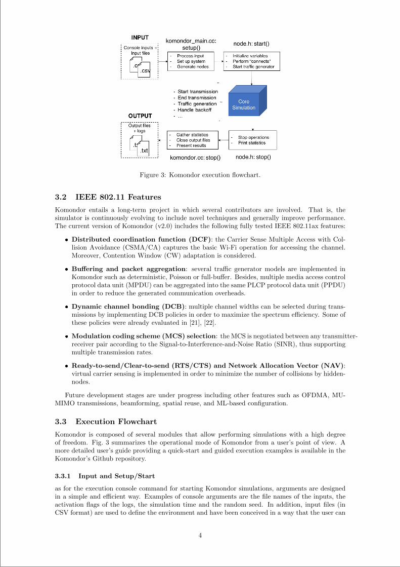
“main” — 2020/11/19 — 10:04 — page 157 — #179

Figure 3: Komondor execution flowchart.

3.2 IEEE 802.11 Features

Komondor entails a long-term project in which several contributors are involved. That is, thesimulator is continuously evolving to include novel techniques and generally improve performance.The current version of Komondor (v2.0) includes the following fully tested IEEE 802.11ax features:

Distributed coordination function (DCF): the Carrier Sense Multiple Access with Col-lision Avoidance (CSMA/CA) captures the basic Wi-Fi operation for accessing the channel.Moreover, Contention Window (CW) adaptation is considered.

Buffering and packet aggregation: several traffic generator models are implemented inKomondor such as deterministic, Poisson or full-buffer. Besides, multiple media access controlprotocol data unit (MPDU) can be aggregated into the same PLCP protocol data unit (PPDU)in order to reduce the generated communication overheads.

Dynamic channel bonding (DCB): multiple channel widths can be selected during trans-missions by implementing DCB policies in order to maximize the spectrum efficiency. Some ofthese policies were already evaluated in [21], [22].

Modulation coding scheme (MCS) selection: the MCS is negotiated between any transmitter-receiver pair according to the Signal-to-Interference-and-Noise Ratio (SINR), thus supportingmultiple transmission rates.

Ready-to-send/Clear-to-send (RTS/CTS) and Network Allocation Vector (NAV):virtual carrier sensing is implemented in order to minimize the number of collisions by hidden-nodes.

Future development stages are under progress including other features such as OFDMA, MU-MIMO transmissions, beamforming, spatial reuse, and ML-based configuration.

3.3 Execution Flowchart

Komondor is composed of several modules that allow performing simulations with a high degreeof freedom. Fig. 3 summarizes the operational mode of Komondor from a user’s point of view. Amore detailed user’s guide providing a quick-start and guided execution examples is available in theKomondor’s Github repository.

3.3.1 Input and Setup/Start

as for the execution console command for starting Komondor simulations, arguments are designedin a simple and efficient way. Examples of console arguments are the file names of the inputs, theactivation flags of the logs, the simulation time and the random seed. In addition, input files (inCSV format) are used to define the environment and have been conceived in a way that the user can

4

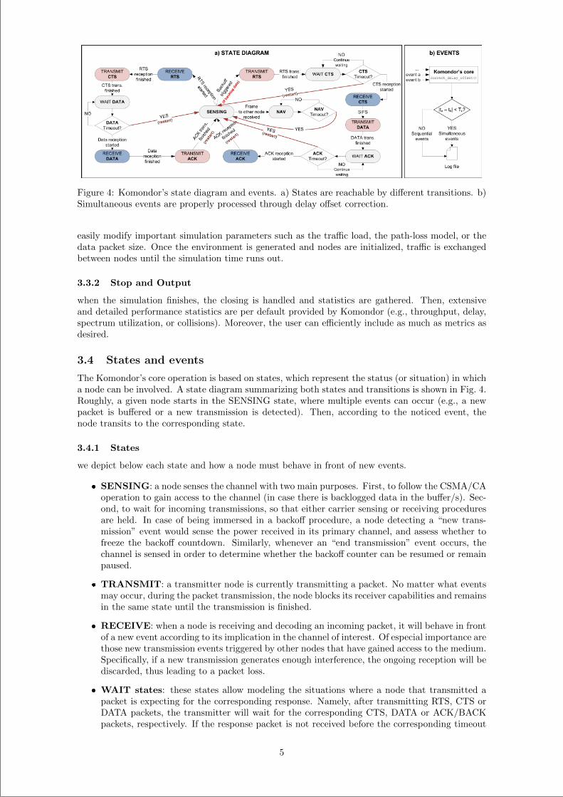
“main” — 2020/11/19 — 10:04 — page 158 — #180

Figure 4: Komondor’s state diagram and events. a) States are reachable by different transitions. b)Simultaneous events are properly processed through delay offset correction.

easily modify important simulation parameters such as the traffic load, the path-loss model, or thedata packet size. Once the environment is generated and nodes are initialized, traffic is exchangedbetween nodes until the simulation time runs out.

3.3.2 Stop and Output

when the simulation finishes, the closing is handled and statistics are gathered. Then, extensiveand detailed performance statistics are per default provided by Komondor (e.g., throughput, delay,spectrum utilization, or collisions). Moreover, the user can efficiently include as much as metrics asdesired.

3.4 States and events

The Komondor’s core operation is based on states, which represent the status (or situation) in whicha node can be involved. A state diagram summarizing both states and transitions is shown in Fig. 4.Roughly, a given node starts in the SENSING state, where multiple events can occur (e.g., a newpacket is buffered or a new transmission is detected). Then, according to the noticed event, thenode transits to the corresponding state.

3.4.1 States

we depict below each state and how a node must behave in front of new events.

SENSING: a node senses the channel with two main purposes. First, to follow the CSMA/CAoperation to gain access to the channel (in case there is backlogged data in the buffer/s). Sec-ond, to wait for incoming transmissions, so that either carrier sensing or receiving proceduresare held. In case of being immersed in a backoff procedure, a node detecting a “new trans-mission” event would sense the power received in its primary channel, and assess whether tofreeze the backoff countdown. Similarly, whenever an “end transmission” event occurs, thechannel is sensed in order to determine whether the backoff counter can be resumed or remainpaused.

TRANSMIT: a transmitter node is currently transmitting a packet. No matter what eventsmay occur, during the packet transmission, the node blocks its receiver capabilities and remainsin the same state until the transmission is finished.

RECEIVE: when a node is receiving and decoding an incoming packet, it will behave in frontof a new event according to its implication in the channel of interest. Of especial importance arethose new transmission events triggered by other nodes that have gained access to the medium.Specifically, if a new transmission generates enough interference, the ongoing reception will bediscarded, thus leading to a packet loss.

WAIT states: these states allow modeling the situations where a node that transmitted apacket is expecting for the corresponding response. Namely, after transmitting RTS, CTS orDATA packets, the transmitter will wait for the corresponding CTS, DATA or ACK/BACKpackets, respectively. If the response packet is not received before the corresponding timeout

5

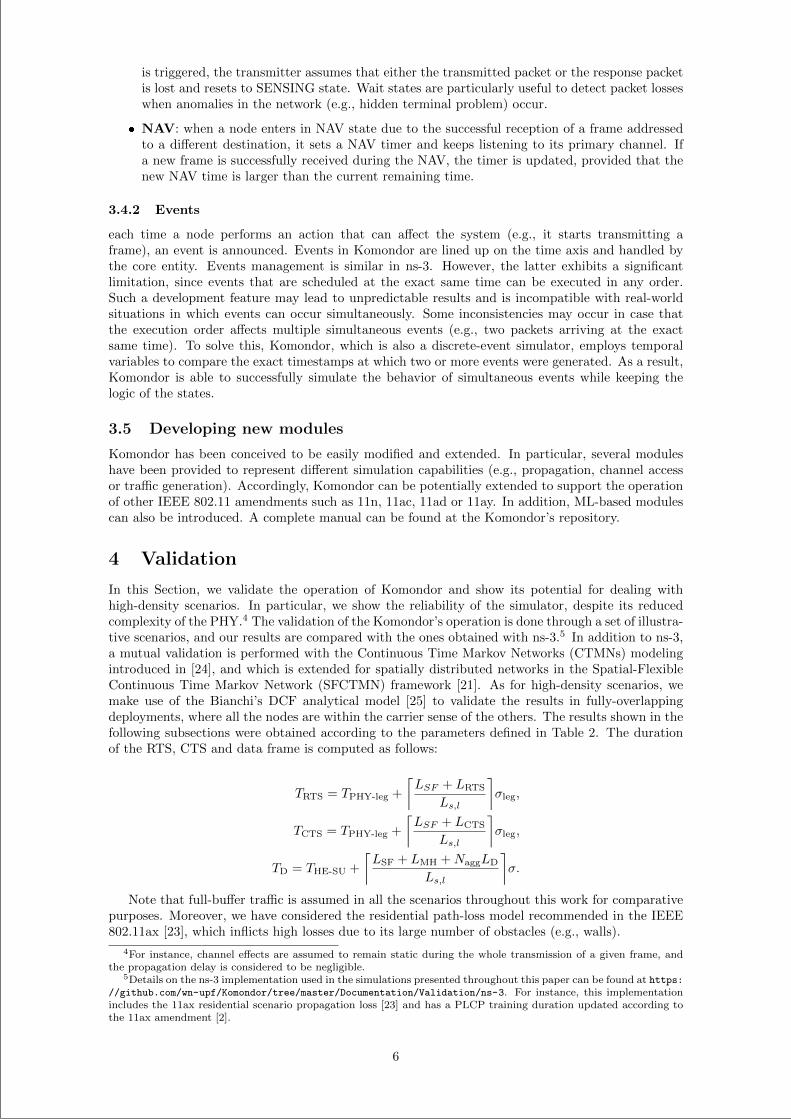
“main” — 2020/11/19 — 10:04 — page 159 — #181

is triggered, the transmitter assumes that either the transmitted packet or the response packetis lost and resets to SENSING state. Wait states are particularly useful to detect packet losseswhen anomalies in the network (e.g., hidden terminal problem) occur.

NAV: when a node enters in NAV state due to the successful reception of a frame addressedto a different destination, it sets a NAV timer and keeps listening to its primary channel. Ifa new frame is successfully received during the NAV, the timer is updated, provided that thenew NAV time is larger than the current remaining time.

3.4.2 Events

each time a node performs an action that can affect the system (e.g., it starts transmitting aframe), an event is announced. Events in Komondor are lined up on the time axis and handled bythe core entity. Events management is similar in ns-3. However, the latter exhibits a significantlimitation, since events that are scheduled at the exact same time can be executed in any order.Such a development feature may lead to unpredictable results and is incompatible with real-worldsituations in which events can occur simultaneously. Some inconsistencies may occur in case thatthe execution order affects multiple simultaneous events (e.g., two packets arriving at the exactsame time). To solve this, Komondor, which is also a discrete-event simulator, employs temporalvariables to compare the exact timestamps at which two or more events were generated. As a result,Komondor is able to successfully simulate the behavior of simultaneous events while keeping thelogic of the states.

3.5 Developing new modules

Komondor has been conceived to be easily modified and extended. In particular, several moduleshave been provided to represent different simulation capabilities (e.g., propagation, channel accessor traffic generation). Accordingly, Komondor can be potentially extended to support the operationof other IEEE 802.11 amendments such as 11n, 11ac, 11ad or 11ay. In addition, ML-based modulescan also be introduced. A complete manual can be found at the Komondor’s repository.

4 Validation

In this Section, we validate the operation of Komondor and show its potential for dealing withhigh-density scenarios. In particular, we show the reliability of the simulator, despite its reducedcomplexity of the PHY.4 The validation of the Komondor’s operation is done through a set of illustra-tive scenarios, and our results are compared with the ones obtained with ns-3.5 In addition to ns-3,a mutual validation is performed with the Continuous Time Markov Networks (CTMNs) modelingintroduced in [24], and which is extended for spatially distributed networks in the Spatial-FlexibleContinuous Time Markov Network (SFCTMN) framework [21]. As for high-density scenarios, wemake use of the Bianchi’s DCF analytical model [25] to validate the results in fully-overlappingdeployments, where all the nodes are within the carrier sense of the others. The results shown in thefollowing subsections were obtained according to the parameters defined in Table 2. The durationof the RTS, CTS and data frame is computed as follows:

TRTS = TPHY-leg +

⌈LSF + LRTS

Ls,l

⌉σleg,

TCTS = TPHY-leg +

⌈LSF + LCTS

Ls,l

⌉σleg,

TD = THE-SU +

⌈LSF + LMH +NaggLD

Ls,l

⌉σ.

Note that full-buffer traffic is assumed in all the scenarios throughout this work for comparativepurposes. Moreover, we have considered the residential path-loss model recommended in the IEEE802.11ax [23], which inflicts high losses due to its large number of obstacles (e.g., walls).

4For instance, channel effects are assumed to remain static during the whole transmission of a given frame, andthe propagation delay is considered to be negligible.

5Details on the ns-3 implementation used in the simulations presented throughout this paper can be found at https://github.com/wn-upf/Komondor/tree/master/Documentation/Validation/ns-3. For instance, this implementationincludes the 11ax residential scenario propagation loss [23] and has a PLCP training duration updated according tothe 11ax amendment [2].

6

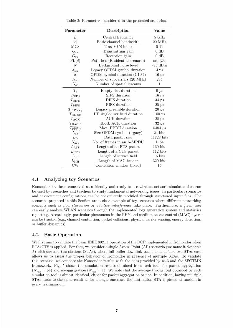
“main” — 2020/11/19 — 10:04 — page 160 — #182

Table 2: Parameters considered in the presented scenarios.

Parameter Description Value

fc Central frequency 5 GHz|c| Basic channel bandwidth 20 MHz

MCS 11ax MCS index 0-11Gtx Transmitting gain 0 dBGrx Reception gain 0 dB

PL(d) Path loss (Residential scenario) see [23]N Background noise level -95 dBmσleg Legacy OFDM symbol duration 4 µsσ OFDM symbol duration (GI-32) 16 µsNsc Number of subcarriers (20 MHz) 234Nss Number of spatial streams 1

Te Empty slot duration 9 µsTSIFS SIFS duration 16 µsTDIFS DIFS duration 34 µsTPIFS PIFS duration 25 µsTPHY-leg Legacy preamble duration 20 µsTHE-SU HE single-user field duration 100 µsTACK ACK duration 28 µsTBACK Block ACK duration 32 µsTmaxPPDU Max. PPDU duration 5484 µsLs,l Size OFDM symbol (legacy) 24 bitsLD Data packet size 11728 bitsNagg No. of frames in an A-MPDU 1, 64LRTS Length of an RTS packet 160 bitsLCTS Length of a CTS packet 112 bitsLSF Length of service field 16 bitsLMH Length of MAC header 320 bitsCW Contention window (fixed) 15

4.1 Analyzing toy Scenarios

Komondor has been conceived as a friendly and ready-to-use wireless network simulator that canbe used by researches and teachers to study fundamental networking issues. In particular, scenariosand environment configurations can be conveniently modified through structured input files. Thescenarios proposed in this Section are a clear example of toy scenarios where different networkingconcepts such as flow starvation or additive interference take place. Furthermore, a given usercan easily analyze WLAN scenarios through the implemented logs generation system and statisticsreporting. Accordingly, particular phenomena in the PHY and medium access control (MAC) layerscan be tracked (e.g., channel contention, packet collisions, physical carrier sensing, energy detection,or buffer dynamics).

4.2 Basic Operation

We first aim to validate the basic IEEE 802.11 operation of the DCF implemented in Komondor whenRTS/CTS is applied. For that, we consider a single Access Point (AP) scenario (we name it Scenario1 ) with one and two stations (STAs), where full-buffer downlink traffic is held. The two-STAs caseallows us to assess the proper behavior of Komondor in presence of multiple STAs. To validatethis scenario, we compare the Komondor results with the ones provided by ns-3 and the SFCTMNframework. Fig. 5 shows the simulation results obtained from each tool, for packet aggregation(Nagg = 64) and no-aggregation (Nagg = 1). We note that the average throughput obtained by eachsimulation tool is almost identical, either for packet aggregation or not. In addition, having multipleSTAs leads to the same result as for a single one since the destination STA is picked at random inevery transmission.

7

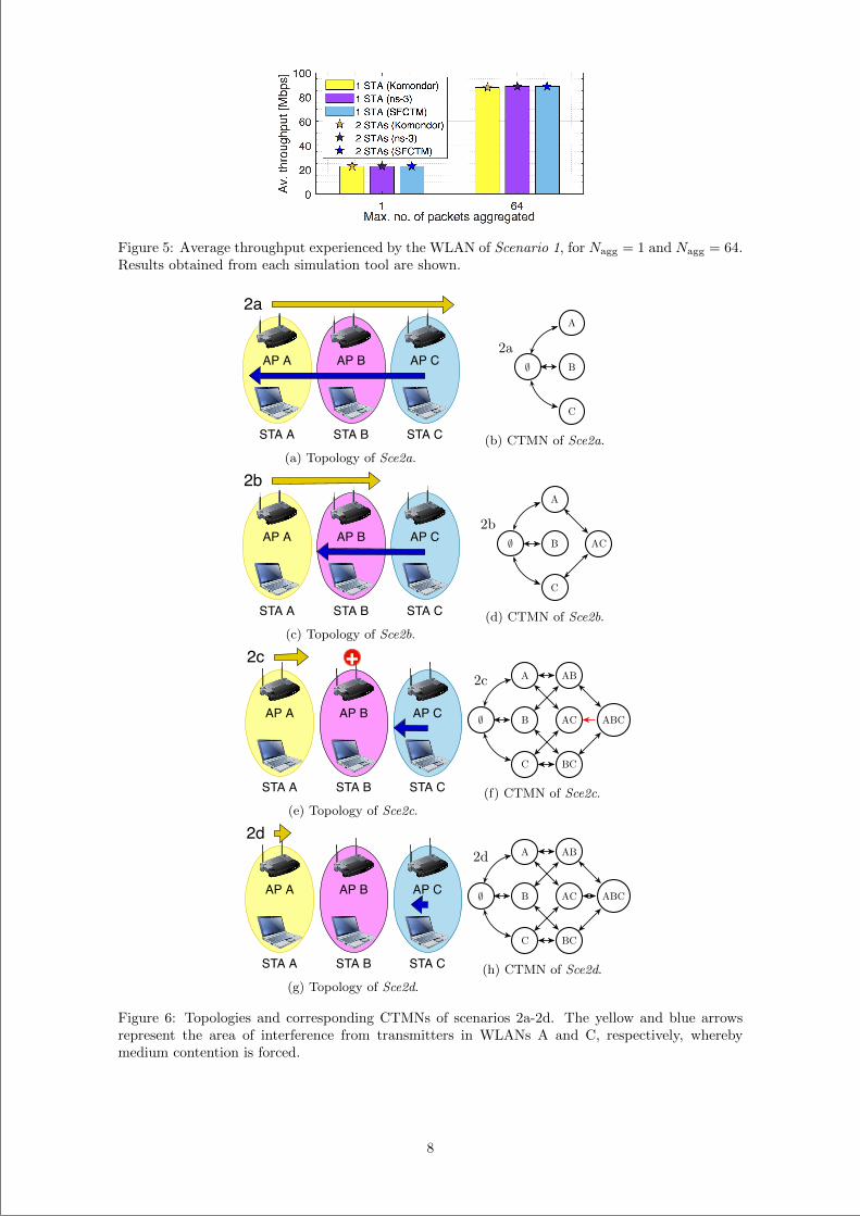
“main” — 2020/11/19 — 10:04 — page 161 — #183

Figure 5: Average throughput experienced by the WLAN of Scenario 1, for Nagg = 1 and Nagg = 64.Results obtained from each simulation tool are shown.

AP A

STA A

AP B AP C

STA B STA C

2a

(a) Topology of Sce2a.

∅2a

B

A

C

(b) CTMN of Sce2a.

AP A

STA A

AP B AP C

STA B STA C

2b

(c) Topology of Sce2b.

∅2b

B

A

C

AC

(d) CTMN of Sce2b.

AP A

STA A

AP B AP C

STA B STA C

2c +

(e) Topology of Sce2c.

∅

2c

B

A

C

AC

AB

BC

ABC

(f) CTMN of Sce2c.

AP A

STA A

AP B AP C

STA B STA C

2d

(g) Topology of Sce2d.

∅

2d

B

A

C

AC

AB

BC

ABC

(h) CTMN of Sce2d.

Figure 6: Topologies and corresponding CTMNs of scenarios 2a-2d. The yellow and blue arrowsrepresent the area of interference from transmitters in WLANs A and C, respectively, wherebymedium contention is forced.

8

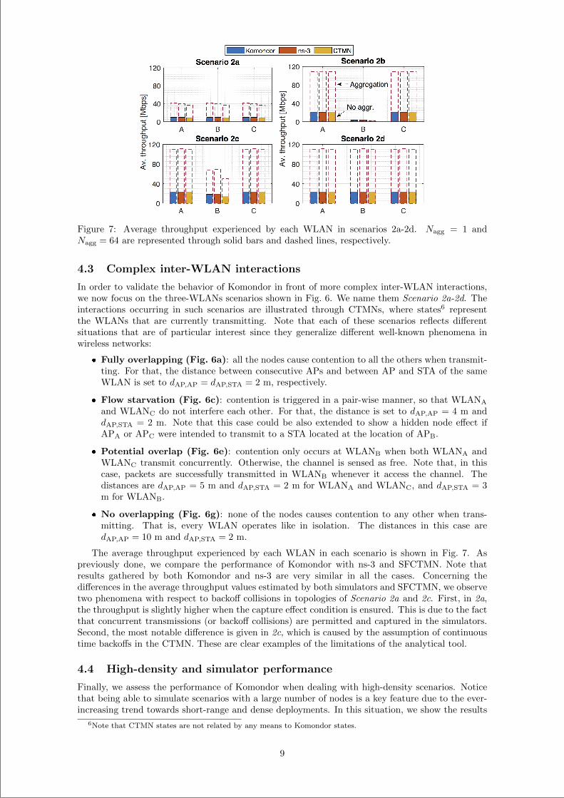
“main” — 2020/11/19 — 10:04 — page 162 — #184

Figure 7: Average throughput experienced by each WLAN in scenarios 2a-2d. Nagg = 1 andNagg = 64 are represented through solid bars and dashed lines, respectively.

4.3 Complex inter-WLAN interactions

In order to validate the behavior of Komondor in front of more complex inter-WLAN interactions,we now focus on the three-WLANs scenarios shown in Fig. 6. We name them Scenario 2a-2d. Theinteractions occurring in such scenarios are illustrated through CTMNs, where states6 representthe WLANs that are currently transmitting. Note that each of these scenarios reflects differentsituations that are of particular interest since they generalize different well-known phenomena inwireless networks:

Fully overlapping (Fig. 6a): all the nodes cause contention to all the others when transmit-ting. For that, the distance between consecutive APs and between AP and STA of the sameWLAN is set to dAP,AP = dAP,STA = 2 m, respectively.

Flow starvation (Fig. 6c): contention is triggered in a pair-wise manner, so that WLANA

and WLANC do not interfere each other. For that, the distance is set to dAP,AP = 4 m anddAP,STA = 2 m. Note that this case could be also extended to show a hidden node effect ifAPA or APC were intended to transmit to a STA located at the location of APB.

Potential overlap (Fig. 6e): contention only occurs at WLANB when both WLANA andWLANC transmit concurrently. Otherwise, the channel is sensed as free. Note that, in thiscase, packets are successfully transmitted in WLANB whenever it access the channel. Thedistances are dAP,AP = 5 m and dAP,STA = 2 m for WLANA and WLANC, and dAP,STA = 3m for WLANB.

No overlapping (Fig. 6g): none of the nodes causes contention to any other when trans-mitting. That is, every WLAN operates like in isolation. The distances in this case aredAP,AP = 10 m and dAP,STA = 2 m.

The average throughput experienced by each WLAN in each scenario is shown in Fig. 7. Aspreviously done, we compare the performance of Komondor with ns-3 and SFCTMN. Note thatresults gathered by both Komondor and ns-3 are very similar in all the cases. Concerning thedifferences in the average throughput values estimated by both simulators and SFCTMN, we observetwo phenomena with respect to backoff collisions in topologies of Scenario 2a and 2c. First, in 2a,the throughput is slightly higher when the capture effect condition is ensured. This is due to the factthat concurrent transmissions (or backoff collisions) are permitted and captured in the simulators.Second, the most notable difference is given in 2c, which is caused by the assumption of continuoustime backoffs in the CTMN. These are clear examples of the limitations of the analytical tool.

4.4 High-density and simulator performance

Finally, we assess the performance of Komondor when dealing with high-density scenarios. Noticethat being able to simulate scenarios with a large number of nodes is a key feature due to the ever-increasing trend towards short-range and dense deployments. In this situation, we show the results

6Note that CTMN states are not related by any means to Komondor states.

9

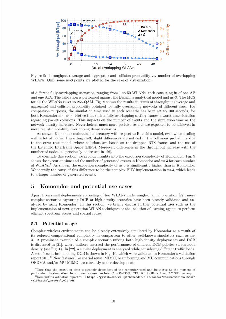
“main” — 2020/11/19 — 10:04 — page 163 — #185

Figure 8: Throughput (average and aggregate) and collision probability vs. number of overlappingWLANs. Only some ns-3 points are plotted for the sake of visualization.

of different fully-overlapping scenarios, ranging from 1 to 50 WLANs, each consisting in of one APand one STA. The validation is performed against the Bianchi’s analytical model and ns-3. The MCSfor all the WLANs is set to 256-QAM. Fig. 8 shows the results in terms of throughput (average andaggregate) and collision probability obtained for fully overlapping networks of different sizes. Forcomparison purposes, the simulation time used in each scenario has been set to 100 seconds, forboth Komondor and ns-3. Notice that such a fully overlapping setting frames a worst-case situationregarding packet collisions. This impacts on the number of events and the simulation time as thenetwork density increases. Nevertheless, much more positive results are expected to be achieved inmore realistic non-fully overlapping dense scenarios.

As shown, Komondor maintains its accuracy with respect to Bianchi’s model, even when dealingwith a lot of nodes. Regarding ns-3, slight differences are noticed in the collisions probability dueto the error rate model, where collisions are based on the dropped RTS frames and the use ofthe Extended Interframe Space (EIFS). Moreover, differences in the throughput increase with thenumber of nodes, as previously addressed in [26].

To conclude this section, we provide insights into the execution complexity of Komondor. Fig. 9shows the execution time and the number of generated events in Komondor and ns-3 for each numberof WLANs.7 As shown, the execution complexity of ns-3 is significantly higher than in Komondor.We identify the cause of this difference to be the complex PHY implementation in ns-3, which leadsto a larger number of generated events.

5 Komondor and potential use cases

Apart from small deployments consisting of few WLANs under single-channel operation [27], morecomplex scenarios capturing DCB or high-density scenarios have been already validated and an-alyzed by using Komondor. In this section, we briefly discuss further potential uses such as theimplementation of next-generation WLAN techniques or the inclusion of learning agents to performefficient spectrum access and spatial reuse.

5.1 Potential usage

Complex wireless environments can be already extensively simulated by Komondor as a result ofits reduced computational complexity in comparison to other well-known simulators such as ns-3. A prominent example of a complex scenario mixing both high-density deployments and DCBis discussed in [21], where authors assessed the performance of different DCB policies versus nodedensity (see Fig. 1). In [22], a similar deployment is analyzed while considering different traffic loads.A set of scenarios including DCB is shown in Fig. 10, which were validated in Komondor’s validationreport v0.1.8 New features like spatial reuse, MIMO, beamforming and MU communications throughOFDMA and/or MU-MIMO are currently under development.

7Note that the execution time is strongly dependent of the computer used and its status at the moment ofperforming the simulation. In our case, we used an Intel Core i5-4300U CPU @ 1.9 GHz x 4 and 7.7 GiB memory.

8Komondor’s validation report v0.1: https://github.com/wn-upf/Komondor/blob/master/Documentation/Other/

validation\_report\_v01.pdf.

10

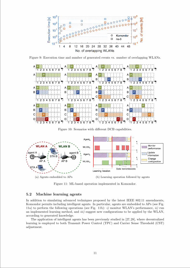
“main” — 2020/11/19 — 10:04 — page 164 — #186

Figure 9: Execution time and number of generated events vs. number of overlapping WLANs.

Figure 10: Scenarios with different DCB capabilities.

agent A agent B

WLAN A WLAN B

AP BAP A

STA B

STA A

(a) Agents embedded to APs (b) Learning operation followed by agents

Figure 11: ML-based operation implemented in Komondor.

5.2 Machine learning agents

In addition to simulating advanced techniques proposed by the latest IEEE 802.11 amendments,Komondor permits including intelligent agents. In particular, agents are embedded to APs (see Fig.11a) to perform the following operations (see Fig. 11b): i) monitor WLAN’s performance, ii) runan implemented learning method, and iii) suggest new configurations to be applied by the WLAN,according to generated knowledge.

The application of intelligent agents has been previously studied in [27,28], where decentralizedlearning is employed to both Transmit Power Control (TPC) and Carrier Sense Threshold (CST)adjustment.

11

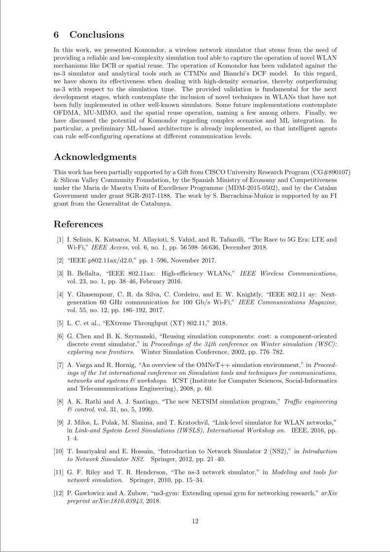
“main” — 2020/11/19 — 10:04 — page 165 — #187

6 Conclusions

In this work, we presented Komondor, a wireless network simulator that stems from the need ofproviding a reliable and low-complexity simulation tool able to capture the operation of novel WLANmechanisms like DCB or spatial reuse. The operation of Komondor has been validated against thens-3 simulator and analytical tools such as CTMNs and Bianchi’s DCF model. In this regard,we have shown its effectiveness when dealing with high-density scenarios, thereby outperformingns-3 with respect to the simulation time. The provided validation is fundamental for the nextdevelopment stages, which contemplate the inclusion of novel techniques in WLANs that have notbeen fully implemented in other well-known simulators. Some future implementations contemplateOFDMA, MU-MIMO, and the spatial reuse operation, naming a few among others. Finally, wehave discussed the potential of Komondor regarding complex scenarios and ML integration. Inparticular, a preliminary ML-based architecture is already implemented, so that intelligent agentscan rule self-configuring operations at different communication levels.

Acknowledgments

This work has been partially supported by a Gift from CISCO University Research Program (CG#890107)& Silicon Valley Community Foundation, by the Spanish Ministry of Economy and Competitivenessunder the Maria de Maeztu Units of Excellence Programme (MDM-2015-0502), and by the CatalanGovernment under grant SGR-2017-1188. The work by S. Barrachina-Munoz is supported by an FIgrant from the Generalitat de Catalunya.

References

[1] I. Selinis, K. Katsaros, M. Allayioti, S. Vahid, and R. Tafazolli, “The Race to 5G Era; LTE andWi-Fi,” IEEE Access, vol. 6, no. 1, pp. 56 598–56 636, December 2018.

[2] “IEEE p802.11ax/d2.0,” pp. 1–596, November 2017.

[3] B. Bellalta, “IEEE 802.11ax: High-efficiency WLANs,” IEEE Wireless Communications,vol. 23, no. 1, pp. 38–46, February 2016.

[4] Y. Ghasempour, C. R. da Silva, C. Cordeiro, and E. W. Knightly, “IEEE 802.11 ay: Next-generation 60 GHz communication for 100 Gb/s Wi-Fi,” IEEE Communications Magazine,vol. 55, no. 12, pp. 186–192, 2017.

[5] L. C. et al., “EXtreme Throughput (XT) 802.11,” 2018.

[6] G. Chen and B. K. Szymanski, “Reusing simulation components: cost: a component-orienteddiscrete event simulator,” in Proceedings of the 34th conference on Winter simulation (WSC):exploring new frontiers. Winter Simulation Conference, 2002, pp. 776–782.

[7] A. Varga and R. Hornig, “An overview of the OMNeT++ simulation environment,” in Proceed-ings of the 1st international conference on Simulation tools and techniques for communications,networks and systems & workshops. ICST (Institute for Computer Sciences, Social-Informaticsand Telecommunications Engineering), 2008, p. 60.

[8] A. K. Rathi and A. J. Santiago, “The new NETSIM simulation program,” Traffic engineering& control, vol. 31, no. 5, 1990.

[9] J. Milos, L. Polak, M. Slanina, and T. Kratochvil, “Link-level simulator for WLAN networks,”in Link-and System Level Simulations (IWSLS), International Workshop on. IEEE, 2016, pp.1–4.

[10] T. Issariyakul and E. Hossain, “Introduction to Network Simulator 2 (NS2),” in Introductionto Network Simulator NS2. Springer, 2012, pp. 21–40.

[11] G. F. Riley and T. R. Henderson, “The ns-3 network simulator,” in Modeling and tools fornetwork simulation. Springer, 2010, pp. 15–34.

[12] P. Gaw lowicz and A. Zubow, “ns3-gym: Extending openai gym for networking research,” arXivpreprint arXiv:1810.03943, 2018.

12

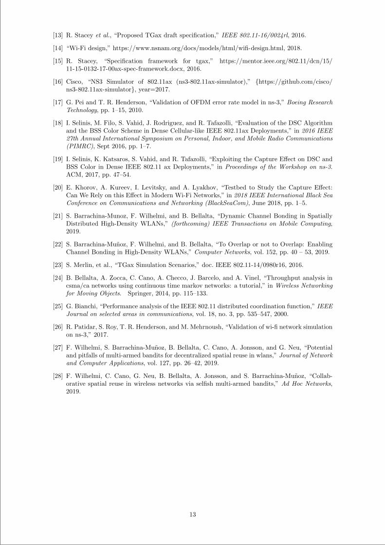
“main” — 2020/11/19 — 10:04 — page 166 — #188

[13] R. Stacey et al., “Proposed TGax draft specification,” IEEE 802.11-16/0024rl, 2016.

[14] “Wi-Fi design,” https://www.nsnam.org/docs/models/html/wifi-design.html, 2018.

[15] R. Stacey, “Specification framework for tgax,” https://mentor.ieee.org/802.11/dcn/15/11-15-0132-17-00ax-spec-framework.docx, 2016.

[16] Cisco, “NS3 Simulator of 802.11ax (ns3-802.11ax-simulator),” https://github.com/cisco/ns3-802.11ax-simulator, year=2017.

[17] G. Pei and T. R. Henderson, “Validation of OFDM error rate model in ns-3,” Boeing ResearchTechnology, pp. 1–15, 2010.

[18] I. Selinis, M. Filo, S. Vahid, J. Rodriguez, and R. Tafazolli, “Evaluation of the DSC Algorithmand the BSS Color Scheme in Dense Cellular-like IEEE 802.11ax Deployments,” in 2016 IEEE27th Annual International Symposium on Personal, Indoor, and Mobile Radio Communications(PIMRC), Sept 2016, pp. 1–7.

[19] I. Selinis, K. Katsaros, S. Vahid, and R. Tafazolli, “Exploiting the Capture Effect on DSC andBSS Color in Dense IEEE 802.11 ax Deployments,” in Proceedings of the Workshop on ns-3.ACM, 2017, pp. 47–54.

[20] E. Khorov, A. Kureev, I. Levitsky, and A. Lyakhov, “Testbed to Study the Capture Effect:Can We Rely on this Effect in Modern Wi-Fi Networks,” in 2018 IEEE International Black SeaConference on Communications and Networking (BlackSeaCom), June 2018, pp. 1–5.

[21] S. Barrachina-Munoz, F. Wilhelmi, and B. Bellalta, “Dynamic Channel Bonding in SpatiallyDistributed High-Density WLANs,” (forthcoming) IEEE Transactions on Mobile Computing,2019.

[22] S. Barrachina-Munoz, F. Wilhelmi, and B. Bellalta, “To Overlap or not to Overlap: EnablingChannel Bonding in High-Density WLANs,” Computer Networks, vol. 152, pp. 40 – 53, 2019.

[23] S. Merlin, et al., “TGax Simulation Scenarios,” doc. IEEE 802.11-14/0980r16, 2016.

[24] B. Bellalta, A. Zocca, C. Cano, A. Checco, J. Barcelo, and A. Vinel, “Throughput analysis incsma/ca networks using continuous time markov networks: a tutorial,” in Wireless Networkingfor Moving Objects. Springer, 2014, pp. 115–133.

[25] G. Bianchi, “Performance analysis of the IEEE 802.11 distributed coordination function,” IEEEJournal on selected areas in communications, vol. 18, no. 3, pp. 535–547, 2000.

[26] R. Patidar, S. Roy, T. R. Henderson, and M. Mehrnoush, “Validation of wi-fi network simulationon ns-3,” 2017.

[27] F. Wilhelmi, S. Barrachina-Munoz, B. Bellalta, C. Cano, A. Jonsson, and G. Neu, “Potentialand pitfalls of multi-armed bandits for decentralized spatial reuse in wlans,” Journal of Networkand Computer Applications, vol. 127, pp. 26–42, 2019.

[28] F. Wilhelmi, C. Cano, G. Neu, B. Bellalta, A. Jonsson, and S. Barrachina-Munoz, “Collab-orative spatial reuse in wireless networks via selfish multi-armed bandits,” Ad Hoc Networks,2019.

13

“main” — 2020/11/19 — 10:04 — page 167 — #189

Online Primary Channel Selection for DynamicChannel Bonding in High-Density WLANs

Sergio Barrachina-Munoz, Francesc Wilhelmi, and Boris Bellalta*

Abstract

In order to dynamically adapt the transmission bandwidth in wireless local area networks(WLANs), dynamic channel bonding (DCB) was introduced in IEEE 802.11n. It has beenextended since then, and it is expected to be a key element in IEEE 802.11ax and futureamendments such as IEEE 802.11be. While DCB is proven to be a compelling mechanism byitself, its performance is deeply tied to the primary channel selection, especially in high-density(HD) deployments, where multiple nodes contend for the spectrum. Traditionally, this primarychannel selection relied on picking the most free one without any further consideration. Inthis paper, in contrast, we propose dynamic-wise (DyWi), a light-weight, decentralized, onlineprimary channel selection algorithm for DCB that improves the expected WLAN throughputby considering not only the occupancy of the target primary channel but also the activityof the secondary channels. Even when assuming important delays due to primary channelswitching, simulation results show a significant improvement both in terms of average delay andthroughput.

1 Introduction

Modern applications like augmented reality, virtual reality, or real-time 8K video are pushing next-generation (nextGen) wireless local area networks (WLANs) to support ever-increasing demandson performance. In addition, the complexity of nextGen high-density (HD) deployments, wherenumerous wireless devices will contend for accessing the medium, hinders even more the task ofachieving high throughput and low latency.

In order to improve the performance of nextGen WLANs, we focus in this work on spectrummanagement techniques. In particular, two well-known techniques have been widely studied in thisregard: channel allocation (CA) and dynamic channel bonding (DCB). CA is the method to assignportions of the spectrum (or channels) to one or multiple WLANs. In contrast, DCB is a techniquewhereby two or more channels are bonded according to their instant occupancy, enabling widerbandwidths per transmission, and thus potentially reaching higher data rates.

Although much has been understood from the works on CA and DCB in the literature, littlehas been assessed with respect to combining CA with DCB altogether in WLANs, particularlyfor high-density (HD) deployments. Nevertheless, while DCB has shown a tremendous potentialto outperform traditional single-channel (SC) [1–3], its performance is severely tied to the CA.Especially, the primary channel selection is critical since it runs the backoff procedure of the carriersense multiple access with collision avoidance (CSMA/CA) protocol. Still, always selecting theleast occupied channel as the primary is no longer appropriate for DCB since potential bonds withadjacent channels should be also considered.

As for works combining CA and DCB for WLANs, we find a distributed algorithm for jointlyallocating channel center frequencies and bandwidths [4], or a centralized approach for maximizingthe network fairness [5]. In addition, a heuristic-based algorithm for primary channel selectionbased on the bonding direction likelihoods was recently presented in [6]. However, such likelihoodsare estimated by assuming a known number of users in each channel, which is normally not feasiblein real deployments. It is worth noticing that the aforementioned works consider fully-backlogged

*All the authors are with the Wireless Networking research group at Universitat Pompeu Fabra, Barcelona, Spain(e-mail: sergio.barrachina, francisco.wilhelmi, boris.bellalta@upf.edu). This work has been partially supported bythe Spanish Ministry of Economy and Competitiveness under the Maria de Maeztu Units of Excellence Programme(MDM-2015-0502), by a Gift from the Cisco University Research Program (CG#890107, Towards DeterministicChannel Access in High-Density WLANs) Fund, a corporate advised fund of Silicon Valley Community Foundation,and by PGC2018-099959-B-I00 (MCIU/AEI/FEDER,UE). The work done by S. Barrachina-Munoz is supported bya FI grant from the Generalitat de Catalunya.

1

8.4

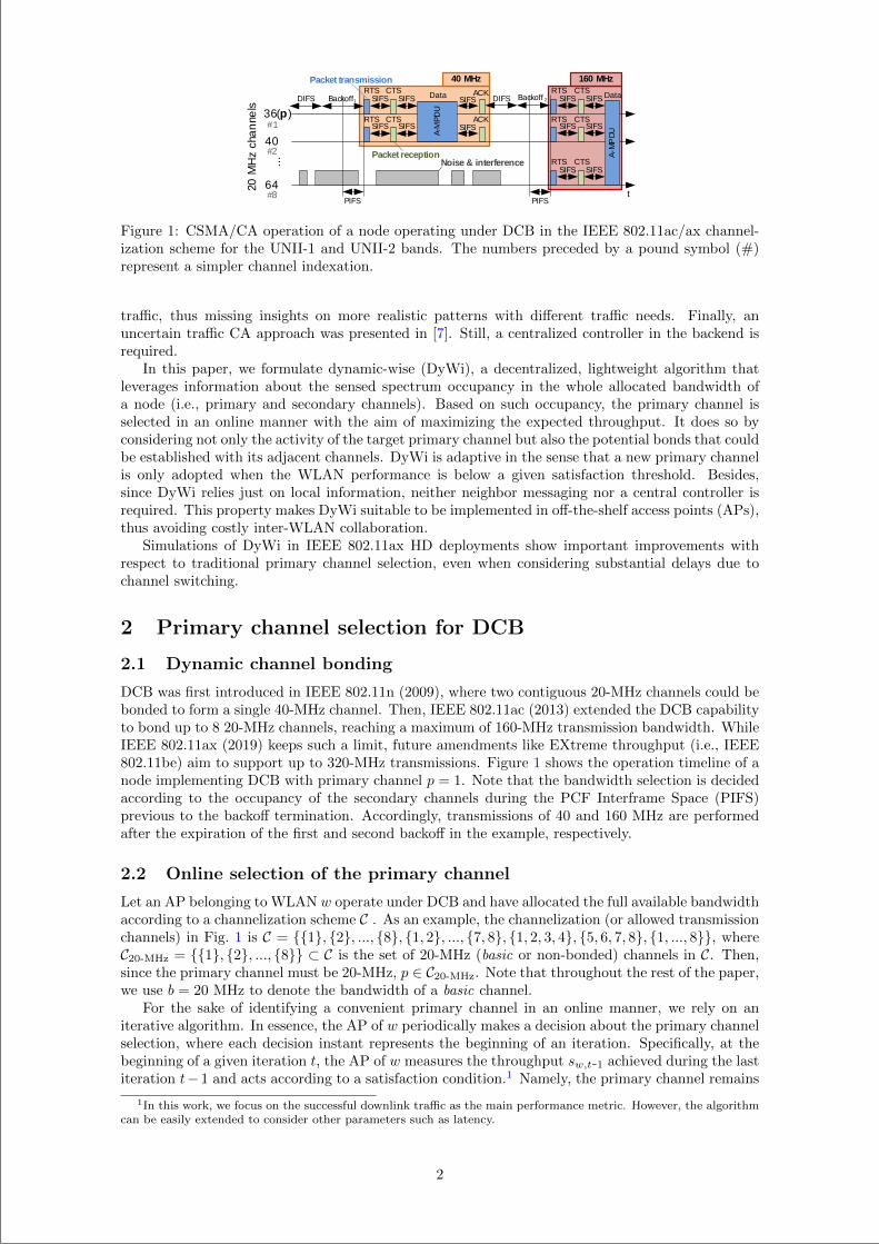
“main” — 2020/11/19 — 10:04 — page 168 — #190

36(p)

40

...

64

Backoff1DIFS

PIFSt

Data SIFS

20 M

Hz

cha

nne

ls

DIFS Backoff 2

RTSSIFS

PIFS

CTS40 MHz 160 MHz

SIFSRTS CTS

SIFSACK

SIFSRTS CTS

SIFS

A-M

PDU

DataSIFS

SIFSACK

SIFSCTS

SIFS

SIFSCTS

SIFS

RTS

RTS

A-M

PD

U

Packet reception

Packet transmission

Noise & interference

#1

#2

#8

Figure 1: CSMA/CA operation of a node operating under DCB in the IEEE 802.11ac/ax channel-ization scheme for the UNII-1 and UNII-2 bands. The numbers preceded by a pound symbol (#)represent a simpler channel indexation.

traffic, thus missing insights on more realistic patterns with different traffic needs. Finally, anuncertain traffic CA approach was presented in [7]. Still, a centralized controller in the backend isrequired.

In this paper, we formulate dynamic-wise (DyWi), a decentralized, lightweight algorithm thatleverages information about the sensed spectrum occupancy in the whole allocated bandwidth ofa node (i.e., primary and secondary channels). Based on such occupancy, the primary channel isselected in an online manner with the aim of maximizing the expected throughput. It does so byconsidering not only the activity of the target primary channel but also the potential bonds that couldbe established with its adjacent channels. DyWi is adaptive in the sense that a new primary channelis only adopted when the WLAN performance is below a given satisfaction threshold. Besides,since DyWi relies just on local information, neither neighbor messaging nor a central controller isrequired. This property makes DyWi suitable to be implemented in off-the-shelf access points (APs),thus avoiding costly inter-WLAN collaboration.

Simulations of DyWi in IEEE 802.11ax HD deployments show important improvements withrespect to traditional primary channel selection, even when considering substantial delays due tochannel switching.

2 Primary channel selection for DCB

2.1 Dynamic channel bonding

DCB was first introduced in IEEE 802.11n (2009), where two contiguous 20-MHz channels could bebonded to form a single 40-MHz channel. Then, IEEE 802.11ac (2013) extended the DCB capabilityto bond up to 8 20-MHz channels, reaching a maximum of 160-MHz transmission bandwidth. WhileIEEE 802.11ax (2019) keeps such a limit, future amendments like EXtreme throughput (i.e., IEEE802.11be) aim to support up to 320-MHz transmissions. Figure 1 shows the operation timeline of anode implementing DCB with primary channel p = 1. Note that the bandwidth selection is decidedaccording to the occupancy of the secondary channels during the PCF Interframe Space (PIFS)previous to the backoff termination. Accordingly, transmissions of 40 and 160 MHz are performedafter the expiration of the first and second backoff in the example, respectively.

2.2 Online selection of the primary channel

Let an AP belonging to WLAN w operate under DCB and have allocated the full available bandwidthaccording to a channelization scheme C . As an example, the channelization (or allowed transmissionchannels) in Fig. 1 is C = 1, 2, ..., 8, 1, 2, ..., 7, 8, 1, 2, 3, 4, 5, 6, 7, 8, 1, ..., 8, whereC20-MHz = 1, 2, ..., 8 ⊂ C is the set of 20-MHz (basic or non-bonded) channels in C. Then,since the primary channel must be 20-MHz, p ∈ C20-MHz. Note that throughout the rest of the paper,we use b = 20 MHz to denote the bandwidth of a basic channel.

For the sake of identifying a convenient primary channel in an online manner, we rely on aniterative algorithm. In essence, the AP of w periodically makes a decision about the primary channelselection, where each decision instant represents the beginning of an iteration. Specifically, at thebeginning of a given iteration t, the AP of w measures the throughput sw,t-1 achieved during the lastiteration t−1 and acts according to a satisfaction condition.1 Namely, the primary channel remains

1In this work, we focus on the successful downlink traffic as the main performance metric. However, the algorithmcan be easily extended to consider other parameters such as latency.

2

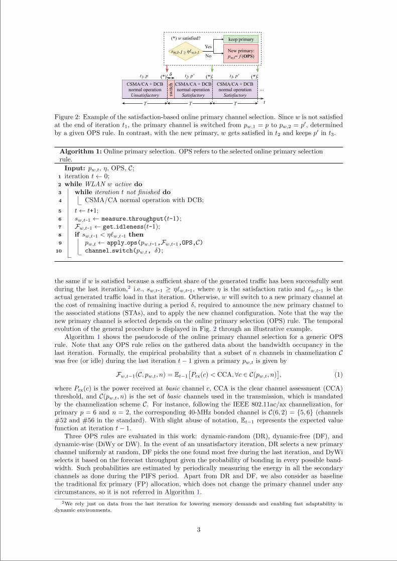
“main” — 2020/11/19 — 10:04 — page 169 — #191

CSMA/CA+DCBnormaloperationSatisfactory

CSMA/CA+DCBnormaloperationSatisfactory

CSMA/CA+DCBnormaloperationUnsatisfactory

sw,t-1≥ηℓw,t-1

(*)wsatisfied?

T

t1,p

T

t2,p'

switch

T

t3,p'

t

keepprimary

No

Yes

...

(*) (*) (*)

Newprimary:pw,t=f(OPS)

Figure 2: Example of the satisfaction-based online primary channel selection. Since w is not satisfiedat the end of iteration t1, the primary channel is switched from pw,1 = p to pw,2 = p′, determinedby a given OPS rule. In contrast, with the new primary, w gets satisfied in t2 and keeps p′ in t3.

Algorithm 1: Online primary selection. OPS refers to the selected online primary selectionrule.

Input: pw,t, η, OPS, C;1 iteration t← 0;2 while WLAN w active do3 while iteration t not finished do4 CSMA/CA normal operation with DCB;

5 t← t+1;6 sw,t-1 ← measure throughput(t-1);7 Fw,t-1 ← get idleness(t-1);8 if sw,t-1 < η`w,t-1 then9 pw,t ← apply ops(pw,t-1,Fw,t-1,OPS,C)

10 channel switch(pw,t, δ);

the same if w is satisfied because a sufficient share of the generated traffic has been successfully sentduring the last iteration,2 i.e., sw,t-1 ≥ η`w,t-1, where η is the satisfaction ratio and `w,t-1 is theactual generated traffic load in that iteration. Otherwise, w will switch to a new primary channel atthe cost of remaining inactive during a period δ, required to announce the new primary channel tothe associated stations (STAs), and to apply the new channel configuration. Note that the way thenew primary channel is selected depends on the online primary selection (OPS) rule. The temporalevolution of the general procedure is displayed in Fig. 2 through an illustrative example.

Algorithm 1 shows the pseudocode of the online primary channel selection for a generic OPSrule. Note that any OPS rule relies on the gathered data about the bandwidth occupancy in thelast iteration. Formally, the empirical probability that a subset of n channels in channelization Cwas free (or idle) during the last iteration t− 1 given a primary pw,t is given by

Fw,t−1(C, pw,t, n) = Et−1[Prx(c) < CCA,∀c ∈ C(pw,t, n)

], (1)

where Prx(c) is the power received at basic channel c, CCA is the clear channel assessment (CCA)threshold, and C(pw,t, n) is the set of basic channels used in the transmission, which is mandatedby the channelization scheme C. For instance, following the IEEE 802.11ac/ax channelization, forprimary p = 6 and n = 2, the corresponding 40-MHz bonded channel is C(6, 2) = 5, 6 (channels#52 and #56 in the standard). With slight abuse of notation, Et−1 represents the expected valuefunction at iteration t− 1.

Three OPS rules are evaluated in this work: dynamic-random (DR), dynamic-free (DF), anddynamic-wise (DiWy or DW). In the event of an unsatisfactory iteration, DR selects a new primarychannel uniformly at random, DF picks the one found most free during the last iteration, and DyWiselects it based on the forecast throughput given the probability of bonding in every possible band-width. Such probabilities are estimated by periodically measuring the energy in all the secondarychannels as done during the PIFS period. Apart from DR and DF, we also consider as baselinethe traditional fix primary (FP) allocation, which does not change the primary channel under anycircumstances, so it is not referred in Algorithm 1.

2We rely just on data from the last iteration for lowering memory demands and enabling fast adaptability indynamic environments.

3

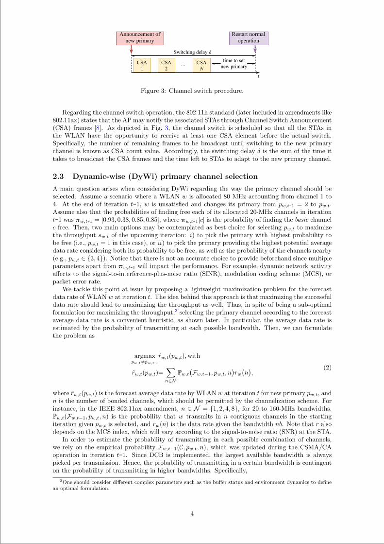
“main” — 2020/11/19 — 10:04 — page 170 — #192

CSA1

timetosetnewprimary

Announcementofnewprimary

Switchingdelay

Restartnormaloperation

t

CSA2

CSAN

...

Figure 3: Channel switch procedure.

Regarding the channel switch operation, the 802.11h standard (later included in amendments like802.11ax) states that the AP may notify the associated STAs through Channel Switch Announcement(CSA) frames [8]. As depicted in Fig. 3, the channel switch is scheduled so that all the STAs inthe WLAN have the opportunity to receive at least one CSA element before the actual switch.Specifically, the number of remaining frames to be broadcast until switching to the new primarychannel is known as CSA count value. Accordingly, the switching delay δ is the sum of the time ittakes to broadcast the CSA frames and the time left to STAs to adapt to the new primary channel.

2.3 Dynamic-wise (DyWi) primary channel selection

A main question arises when considering DyWi regarding the way the primary channel should beselected. Assume a scenario where a WLAN w is allocated 80 MHz accounting from channel 1 to4. At the end of iteration t-1, w is unsatisfied and changes its primary from pw,t-1 = 2 to pw,t.Assume also that the probabilities of finding free each of its allocated 20-MHz channels in iterationt-1 was πw,t-1 = [0.93, 0.38, 0.85, 0.85], where πw,t-1[c] is the probability of finding the basic channelc free. Then, two main options may be contemplated as best choice for selecting pw,t to maximizethe throughput sw,t of the upcoming iteration: i) to pick the primary with highest probability tobe free (i.e., pw,t = 1 in this case), or ii) to pick the primary providing the highest potential averagedata rate considering both its probability to be free, as well as the probability of the channels nearby(e.g., pw,t ∈ 3, 4). Notice that there is not an accurate choice to provide beforehand since multipleparameters apart from πw,t-1 will impact the performance. For example, dynamic network activityaffects to the signal-to-interference-plus-noise ratio (SINR), modulation coding scheme (MCS), orpacket error rate.

We tackle this point at issue by proposing a lightweight maximization problem for the forecastdata rate of WLAN w at iteration t. The idea behind this approach is that maximizing the successfuldata rate should lead to maximizing the throughput as well. Thus, in spite of being a sub-optimalformulation for maximizing the throughput,3 selecting the primary channel according to the forecastaverage data rate is a convenient heuristic, as shown later. In particular, the average data rate isestimated by the probability of transmitting at each possible bandwidth. Then, we can formulatethe problem as

argmaxpw,t 6=pw,t-1

rw,t(pw,t),with

rw,t(pw,t)=∑

n∈NPw,t

(Fw,t−1, pw,t, n

)rw(n),

(2)

where rw,t(pw,t) is the forecast average data rate by WLAN w at iteration t for new primary pw,t, andn is the number of bonded channels, which should be permitted by the channelization scheme. Forinstance, in the IEEE 802.11ax amendment, n ∈ N = 1, 2, 4, 8, for 20 to 160-MHz bandwidths.Pw,t(Fw,t−1, pw,t, n) is the probability that w transmits in n contiguous channels in the startingiteration given pw,t is selected, and rw(n) is the data rate given the bandwidth nb. Note that r alsodepends on the MCS index, which will vary according to the signal-to-noise ratio (SNR) at the STA.

In order to estimate the probability of transmitting in each possible combination of channels,we rely on the empirical probability Fw,t−1(C, pw,t, n), which was updated during the CSMA/CAoperation in iteration t-1. Since DCB is implemented, the largest available bandwidth is alwayspicked per transmission. Hence, the probability of transmitting in a certain bandwidth is contingenton the probability of transmitting in higher bandwidths. Specifically,

3One should consider different complex parameters such as the buffer status and environment dynamics to definean optimal formulation.

4

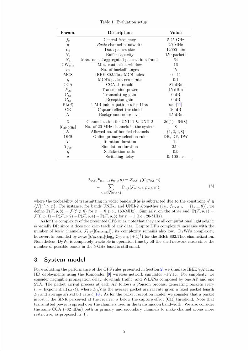
“main” — 2020/11/19 — 10:04 — page 171 — #193

Table 1: Evaluation setup.

Param. Description Value

fc Central frequency 5.25 GHzb Basic channel bandwidth 20 MHzLd Data packet size 12000 bitsNb Buffer capacity 150 packetsNa Max. no. of aggregated packets in a frame 64

CWmin Min. contention window 16m No. of backoff stages 5

MCS IEEE 802.11ax MCS index 0 - 11η MCS’s packet error rate 0.1

CCA CCA threshold -82 dBmPtx Transmission power 15 dBmGtx Transmitting gain 0 dBGrx Reception gain 0 dB

PL(d) TMB indoor path loss for 11ax see [11]CE Capture effect threshold 20 dBN Background noise level -95 dBm

C Channelization for UNII-1 & UNII-2 36(1) - 64(8)|C20-MHz| No. of 20-MHz channels in the system 8N Allowed no. of bonded channels 1, 2, 4, 8

OPS Online primary selection rule DR, DF, DWT Iteration duration 1 sTobs Simulation duration 25 sη Satisfaction ratio 0.9δ Switching delay 0, 100 ms

Pw,t(Fw,t−1, pw,t, n) = Fw,t−1(C, pw,t, n)

−∑

n′∈N|n′>nPw,t(Fw,t−1, pw,t, n

′), (3)

where the probability of transmitting in wider bandwidths is subtracted due to the constraint n′ ∈N |n′ > n. For instance, for bands UNII-1 and UNII-2 altogether (i.e., C20-MHz = 1, ..., 8), wedefine P(F , p, 8) = F(C, p, 8) for n = 8 (i.e., 160-MHz). Similarly, on the other end, P(F , p, 1) =F(C, p, 1)− P(F , p, 2)− P(F , p, 4)− P(F , p, 8) for n = 1 (i.e., 20-MHz).

As for the complexity of the presented OPS rules, note that they are all computational lightweight;especially DR since it does not keep track of any data. Despite DF’s complexity increases with thenumber of basic channels, FDF

(|C20-MHz|

), its complexity remains also low. DyWi’s complexity,

however, is bounded by FDW

(|C20-MHz|(log2 |C20-MHz|+ 1)2

)for the IEEE 802.11ax channelization.

Nonetheless, DyWi is completely tractable in operation time by off-the-shelf network cards since thenumber of possible bonds in the 5-GHz band is still small.

3 System model

For evaluating the performance of the OPS rules presented in Section 2, we simulate IEEE 802.11axHD deployments using the Komondor [9] wireless network simulator v1.2.1c. For simplicity, weconsider negligible propagation delay, downlink traffic, and WLANs composed by one AP and oneSTA. The packet arrival process at each AP follows a Poisson process, generating packets everytn ∼ Exponential

(Ld/¯

), where Ld/¯ is the average packet arrival rate given a fixed packet length

Ld and average arrival bit rate ¯ [10]. As for the packet reception model, we consider that a packetis lost if the SINR perceived at the receiver is below the capture effect (CE) threshold. Note thattransmitted power is spread over the channels used in the transmission bandwidth. We also considerthe same CCA (-82 dBm) both in primary and secondary channels to make channel access morerestrictive, as proposed in [1].

5

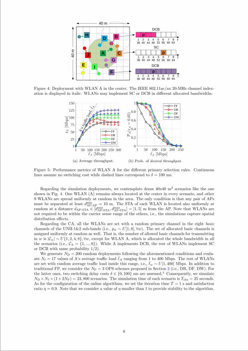
“main” — 2020/11/19 — 10:04 — page 172 — #194

H

GE

J

B

C

F

I

D

A pf

SC

pf

DCB

pf

DCB

d40

md

d40 md

1 2 3 4 5 6 7 836 40 44 48 52 56 60 64

1 2 3 4 5 6 7 836 40 44 48 52 56 60 64

1 2 3 4 5 6 7 836 40 44 48 52 56 60 64

Figure 4: Deployment with WLAN A in the center. The IEEE 802.11ac/ax 20-MHz channel index-ation is displayed in italic. WLANs may implement SC or DCB in different allocated bandwidths.

1 50 100 150 200 250 3001

25

50

75

100

125

150

FPDRDFDW

(a) Average throughput.

1 50 100 150 200 2500

0.2

0.4

0.6

0.8

1FPDRDFDW

(b) Prob. of desired throughput.

Figure 5: Performance metrics of WLAN A for the different primary selection rules. Continuouslines assume no switching cost while dashed lines correspond to δ = 100 ms.

Regarding the simulation deployments, we contemplate dense 40x40 m2 scenarios like the oneshown in Fig. 4. One WLAN (A) remains always located at the center in every scenario, and other9 WLANs are spread uniformly at random in the area. The only condition is that any pair of APsmust be separated at least dmin

AP-AP = 10 m. The STA of each WLAN is located also uniformly atrandom at a distance dAP-STA ∈ [dmin

AP-STA, dmaxAP-STA] = [1, 5] m from the AP. Note that WLANs are

not required to be within the carrier sense range of the others, i.e., the simulations capture spatialdistribution effects.

Regarding the CA, all the WLANs are set with a random primary channel in the eight basicchannels of the UNII-1&2 sub-bands (i.e., pw ∼ U [1, 8],∀w). The set of allocated basic channels isassigned uniformly at random as well. That is, the number of allowed basic channels for transmittingin w is |Cw| ∼ U1, 2, 4, 8,∀w, except for WLAN A, which is allocated the whole bandwidth in allthe scenarios (i.e., CA = 1, ..., 8). While A implements DCB, the rest of WLANs implement SCor DCB with same probability 1/2).

We generate ND = 200 random deployments following the aforementioned conditions and evalu-ate N` = 17 values of A’s average traffic load ¯

A ranging from 1 to 400 Mbps. The rest of WLANsare set with random average traffic load inside this range, i.e., ¯

w ∼ U [1, 400] Mbps. In addition totraditional FP, we consider the NP = 3 OPS schemes proposed in Section 2 (i.e., DR, DF, DW). Forthe latter ones, two switching delay costs δ ∈ 0, 100 ms are assessed.4 Consequently, we simulateND×N`× (1 + 2NP) = 23, 800 scenarios. The simulation time of each scenario is Tobs = 25 seconds.As for the configuration of the online algorithms, we set the iteration time T = 1 s and satisfactionratio η = 0.9. Note that we consider a value of η smaller than 1 to provide stability to the algorithm.

6

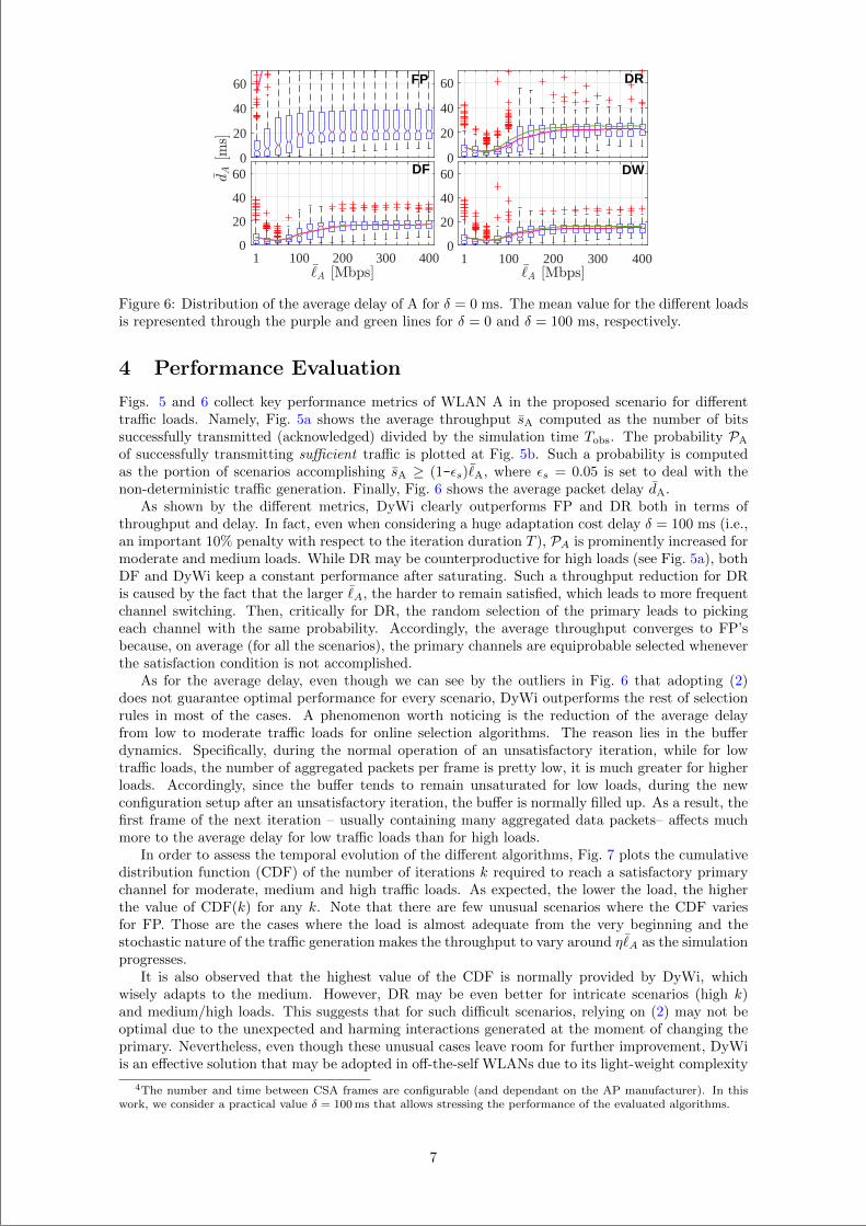
“main” — 2020/11/19 — 10:04 — page 173 — #195

0

20

40

60

0

20

40

60

1 100 200 300 4000

20

40

60

1 100 200 300 4000

20

40

60

FP DR

DWDF

Figure 6: Distribution of the average delay of A for δ = 0 ms. The mean value for the different loadsis represented through the purple and green lines for δ = 0 and δ = 100 ms, respectively.

4 Performance Evaluation

Figs. 5 and 6 collect key performance metrics of WLAN A in the proposed scenario for differenttraffic loads. Namely, Fig. 5a shows the average throughput sA computed as the number of bitssuccessfully transmitted (acknowledged) divided by the simulation time Tobs. The probability PA

of successfully transmitting sufficient traffic is plotted at Fig. 5b. Such a probability is computedas the portion of scenarios accomplishing sA ≥ (1-εs)¯

A, where εs = 0.05 is set to deal with thenon-deterministic traffic generation. Finally, Fig. 6 shows the average packet delay dA.

As shown by the different metrics, DyWi clearly outperforms FP and DR both in terms ofthroughput and delay. In fact, even when considering a huge adaptation cost delay δ = 100 ms (i.e.,an important 10% penalty with respect to the iteration duration T ), PA is prominently increased formoderate and medium loads. While DR may be counterproductive for high loads (see Fig. 5a), bothDF and DyWi keep a constant performance after saturating. Such a throughput reduction for DRis caused by the fact that the larger ¯

A, the harder to remain satisfied, which leads to more frequentchannel switching. Then, critically for DR, the random selection of the primary leads to pickingeach channel with the same probability. Accordingly, the average throughput converges to FP’sbecause, on average (for all the scenarios), the primary channels are equiprobable selected wheneverthe satisfaction condition is not accomplished.

As for the average delay, even though we can see by the outliers in Fig. 6 that adopting (2)does not guarantee optimal performance for every scenario, DyWi outperforms the rest of selectionrules in most of the cases. A phenomenon worth noticing is the reduction of the average delayfrom low to moderate traffic loads for online selection algorithms. The reason lies in the bufferdynamics. Specifically, during the normal operation of an unsatisfactory iteration, while for lowtraffic loads, the number of aggregated packets per frame is pretty low, it is much greater for higherloads. Accordingly, since the buffer tends to remain unsaturated for low loads, during the newconfiguration setup after an unsatisfactory iteration, the buffer is normally filled up. As a result, thefirst frame of the next iteration – usually containing many aggregated data packets– affects muchmore to the average delay for low traffic loads than for high loads.

In order to assess the temporal evolution of the different algorithms, Fig. 7 plots the cumulativedistribution function (CDF) of the number of iterations k required to reach a satisfactory primarychannel for moderate, medium and high traffic loads. As expected, the lower the load, the higherthe value of CDF(k) for any k. Note that there are few unusual scenarios where the CDF variesfor FP. Those are the cases where the load is almost adequate from the very beginning and thestochastic nature of the traffic generation makes the throughput to vary around η ¯

A as the simulationprogresses.

It is also observed that the highest value of the CDF is normally provided by DyWi, whichwisely adapts to the medium. However, DR may be even better for intricate scenarios (high k)and medium/high loads. This suggests that for such difficult scenarios, relying on (2) may not beoptimal due to the unexpected and harming interactions generated at the moment of changing theprimary. Nevertheless, even though these unusual cases leave room for further improvement, DyWiis an effective solution that may be adopted in off-the-self WLANs due to its light-weight complexity

4The number and time between CSA frames are configurable (and dependant on the AP manufacturer). In thiswork, we consider a practical value δ = 100 ms that allows stressing the performance of the evaluated algorithms.

7

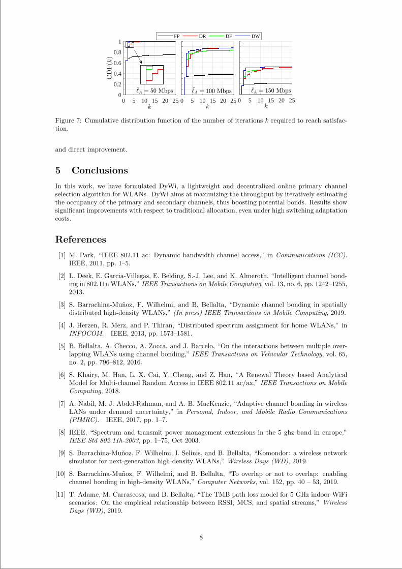
“main” — 2020/11/19 — 10:04 — page 174 — #196

0 5 10 15 20 250

0.2

0.4

0.6

0.8

1

0 5 10 15 20 25 0 5 10 15 20 25

FP DR DF DW

Figure 7: Cumulative distribution function of the number of iterations k required to reach satisfac-tion.

and direct improvement.

5 Conclusions

In this work, we have formulated DyWi, a lightweight and decentralized online primary channelselection algorithm for WLANs. DyWi aims at maximizing the throughput by iteratively estimatingthe occupancy of the primary and secondary channels, thus boosting potential bonds. Results showsignificant improvements with respect to traditional allocation, even under high switching adaptationcosts.

References

[1] M. Park, “IEEE 802.11 ac: Dynamic bandwidth channel access,” in Communications (ICC).IEEE, 2011, pp. 1–5.

[2] L. Deek, E. Garcia-Villegas, E. Belding, S.-J. Lee, and K. Almeroth, “Intelligent channel bond-ing in 802.11n WLANs,” IEEE Transactions on Mobile Computing, vol. 13, no. 6, pp. 1242–1255,2013.

[3] S. Barrachina-Munoz, F. Wilhelmi, and B. Bellalta, “Dynamic channel bonding in spatiallydistributed high-density WLANs,” (In press) IEEE Transactions on Mobile Computing, 2019.

[4] J. Herzen, R. Merz, and P. Thiran, “Distributed spectrum assignment for home WLANs,” inINFOCOM. IEEE, 2013, pp. 1573–1581.

[5] B. Bellalta, A. Checco, A. Zocca, and J. Barcelo, “On the interactions between multiple over-lapping WLANs using channel bonding,” IEEE Transactions on Vehicular Technology, vol. 65,no. 2, pp. 796–812, 2016.

[6] S. Khairy, M. Han, L. X. Cai, Y. Cheng, and Z. Han, “A Renewal Theory based AnalyticalModel for Multi-channel Random Access in IEEE 802.11 ac/ax,” IEEE Transactions on MobileComputing, 2018.

[7] A. Nabil, M. J. Abdel-Rahman, and A. B. MacKenzie, “Adaptive channel bonding in wirelessLANs under demand uncertainty,” in Personal, Indoor, and Mobile Radio Communications(PIMRC). IEEE, 2017, pp. 1–7.

[8] IEEE, “Spectrum and transmit power management extensions in the 5 ghz band in europe,”IEEE Std 802.11h-2003, pp. 1–75, Oct 2003.

[9] S. Barrachina-Munoz, F. Wilhelmi, I. Selinis, and B. Bellalta, “Komondor: a wireless networksimulator for next-generation high-density WLANs,” Wireless Days (WD), 2019.

[10] S. Barrachina-Munoz, F. Wilhelmi, and B. Bellalta, “To overlap or not to overlap: enablingchannel bonding in high-density WLANs,” Computer Networks, vol. 152, pp. 40 – 53, 2019.

[11] T. Adame, M. Carrascosa, and B. Bellalta, “The TMB path loss model for 5 GHz indoor WiFiscenarios: On the empirical relationship between RSSI, MCS, and spatial streams,” WirelessDays (WD), 2019.

8

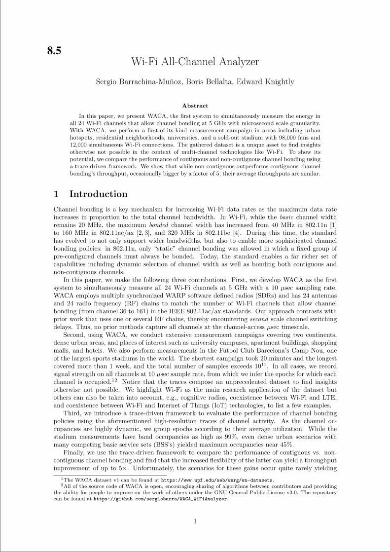
“main” — 2020/11/19 — 10:04 — page 175 — #197

Wi-Fi All-Channel Analyzer

Sergio Barrachina-Munoz, Boris Bellalta, Edward Knightly

Abstract

In this paper, we present WACA, the first system to simultaneously measure the energy inall 24 Wi-Fi channels that allow channel bonding at 5 GHz with microsecond scale granularity.With WACA, we perform a first-of-its-kind measurement campaign in areas including urbanhotspots, residential neighborhoods, universities, and a sold-out stadium with 98,000 fans and12,000 simultaneous Wi-Fi connections. The gathered dataset is a unique asset to find insightsotherwise not possible in the context of multi-channel technologies like Wi-Fi. To show itspotential, we compare the performance of contiguous and non-contiguous channel bonding usinga trace-driven framework. We show that while non-contiguous outperforms contiguous channelbonding’s throughput, occasionally bigger by a factor of 5, their average throughputs are similar.

1 Introduction

Channel bonding is a key mechanism for increasing Wi-Fi data rates as the maximum data rateincreases in proportion to the total channel bandwidth. In Wi-Fi, while the basic channel widthremains 20 MHz, the maximum bonded channel width has increased from 40 MHz in 802.11n [1]to 160 MHz in 802.11ac/ax [2, 3], and 320 MHz in 802.11be [4]. During this time, the standardhas evolved to not only support wider bandwidths, but also to enable more sophisticated channelbonding policies: in 802.11n, only “static” channel bonding was allowed in which a fixed group ofpre-configured channels must always be bonded. Today, the standard enables a far richer set ofcapabilities including dynamic selection of channel width as well as bonding both contiguous andnon-contiguous channels.

In this paper, we make the following three contributions. First, we develop WACA as the firstsystem to simultaneously measure all 24 Wi-Fi channels at 5 GHz with a 10 µsec sampling rate.WACA employs multiple synchronized WARP software defined radios (SDRs) and has 24 antennasand 24 radio frequency (RF) chains to match the number of Wi-Fi channels that allow channelbonding (from channel 36 to 161) in the IEEE 802.11ac/ax standards. Our approach contrasts withprior work that uses one or several RF chains, thereby encountering second scale channel switchingdelays. Thus, no prior methods capture all channels at the channel-access µsec timescale.

Second, using WACA, we conduct extensive measurement campaigns covering two continents,dense urban areas, and places of interest such as university campuses, apartment buildings, shoppingmalls, and hotels. We also perform measurements in the Futbol Club Barcelona’s Camp Nou, oneof the largest sports stadiums in the world. The shortest campaign took 20 minutes and the longestcovered more than 1 week, and the total number of samples exceeds 1011. In all cases, we recordsignal strength on all channels at 10 µsec sample rate, from which we infer the epochs for which eachchannel is occupied.12 Notice that the traces compose an unprecedented dataset to find insightsotherwise not possible. We highlight Wi-Fi as the main research application of the dataset butothers can also be taken into account, e.g., cognitive radios, coexistence between Wi-Fi and LTE,and coexistence between Wi-Fi and Internet of Things (IoT) technologies, to list a few examples.

Third, we introduce a trace-driven framework to evaluate the performance of channel bondingpolicies using the aforementioned high-resolution traces of channel activity. As the channel oc-cupancies are highly dynamic, we group epochs according to their average utilization. While thestadium measurements have band occupancies as high as 99%, even dense urban scenarios withmany competing basic service sets (BSS’s) yielded maximum occupancies near 45%.

Finally, we use the trace-driven framework to compare the performance of contiguous vs. non-contiguous channel bonding and find that the increased flexibility of the latter can yield a throughputimprovement of up to 5×. Unfortunately, the scenarios for these gains occur quite rarely yielding

1The WACA dataset v1 can be found at https://www.upf.edu/web/wnrg/wn-datasets.2All of the source code of WACA is open, encouraging sharing of algorithms between contributors and providing

the ability for people to improve on the work of others under the GNU General Public License v3.0. The repositorycan be found at https://github.com/sergiobarra/WACA_WiFiAnalyzer.

1

8.5

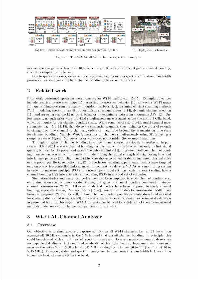
“main” — 2020/11/19 — 10:04 — page 176 — #198

WARP-a

A BFMCD

C WARP-b

A BFMCD

C WARP-c

A BFMCD

C WARP-d

A BFMCD

C WARP-e

A BFMCD

C WARP-f

A BFMCD

C36 40 44 48 52 56 60 64 100

104

108

112

116

120

124

128

132

136

140

144 149

153

157

161

165

38 46 6254 102 110 126118 134 142 151 15942 58

50

WARP-a WARP-b WARP-c WARP-d WARP-e WARP-f

106 122114

138 155

A

B

C

D

RF_A

RF_B

RF_C

RF_D

FMC

FMC-RF-2X245

daughter board

40 MHz80 MHz

160 MHz

20 MHz

stack 1 stack 2

U-NII-1 U-NII-2 U-NII-2-C U-NII-3

(a) IEEE 802.11ac/ax channelization and assignation per RF. (b) Deployment schematic.

Figure 1: The WACA all WiFi channels spectrum analyzer.

modest average gains of less than 10%, which may ultimately favor contiguous channel bonding,since it is simpler to implement.

Due to space constrains, we leave the study of key factors such as spectral correlation, bandwidthprevention, or standard compliant channel bonding policies as future work.

2 Related work

Prior work performed spectrum measurements for Wi-Fi traffic, e.g., [5–15]. Example objectivesinclude creating interference maps [15], assessing interference behavior [16], surveying Wi-Fi usage[10], quantifying spectrum occupancy in outdoor testbeds [5, 6], designing efficient scanning methods[7, 11], modeling spectrum use [8], opportunistic spectrum access [9, 14], dynamic channel selection[17], and assessing real-world network behavior by examining data from thousands APs [12]. Un-fortunately, no such prior work provided simultaneous measurement across the entire 5 GHz band,which we require for our channel bonding study. While some papers do provide multi-channel mea-surements, e.g., [5, 9, 14, 18], they do so via sequential scanning, thus taking on the order of secondsto change from one channel to the next, orders of magnitude beyond the transmission time scalefor channel bonding. Namely, WACA measures all channels simultaneously using SDRs having asampling rate of 10µsec. Moreover, prior work does not consider (for example) stadiums.

Throughput gains of channel bonding have been demonstrated previously in testbeds. In par-ticular, IEEE 802.11n static channel bonding has been shown to be affected not only by link signalquality, but also by the power and rates of neighboring links [19]. Likewise, intelligent channel bond-ing management was shown to benefit from identifying the signal strength of neighboring links andinterference patterns [20]. High bandwidths were shown to be vulnerable to increased thermal noiseor the power per Hertz reduction [21, 22]. Nonetheless, existing experimental results have targetedonly on one or few controlled links at most. In contrast, we develop WACA as a monitoring systemin order to measure multiple BSS’s in various operational settings, which allows tackling how achannel bonding BSS interacts with surrounding BSS’s in a broad set of scenarios.

Simulation studies and analytical models have also been employed to study channel bonding, e.g.,early simulation studies demonstrated throughput gains of channel bonding compared to single-channel transmission [23, 24]. Likewise, analytical models have been proposed to study channelbonding, especially through Markov chains [25, 26]. Analytical models for unsaturated traffic havebeen also proposed [27, 28]. As well, different channel bonding policies were introduced and modeledfor spatially distributed scenarios [29]. However, such work does not have an experimental validationas presented here. In this regard, WACA datasets can be used for validation of the aforementionedmethods under real-world channel occupancies in future work.

3 Wi-Fi All-Channel Analyzer

3.1 Overview

Our objective is to simultaneously capture activity on all Wi-Fi channels, i.e., all 24 basic (nonaggregated) 20 MHz channels in the 5 GHz band that permit channel bonding. In principle, thiscould be achieved with an off-the-shelf spectrum analyzer. However, most spectrum analyzers arenot capable of dealing with the required bandwidth of this objective, i.e., they cannot simultaneouslymeasure the entire Wi-Fi 5-GHz band: 645 MHz ranging from channel 36 to 161 (i.e., from 5170 to5815 MHz). Moreover, wide-band spectrum analyzers that can cover this bandwidth lack resolutionto analyze basic channels within the band.

2

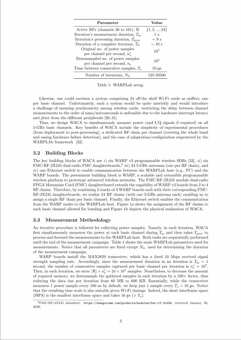
“main” — 2020/11/19 — 10:04 — page 177 — #199

Parameter Value

Active RFs (channels 36 to 161), R 1, 2, ..., 24Iteration’s measurement duration, Tm 1 sIteration’s processing duration, Tproc ∼ 9 sDuration of a complete iteration, Tit ∼ 10 s

Original no. of power samplesper channel per second, n∗s

107

Downsampled no. of power samplesper channel per second, ns

105

Time between consecutive samples, Ts 10 µs

Number of iterations, Nit 125-59500

Table 1: WARPLab setup.

Likewise, one could envision a system comprising 24 off-the shelf Wi-Fi cards as sniffers, oneper basic channel. Unfortunately, such a system would be quite unwieldy and would introducea challenge of ensuring synchronicity among wireless cards: restricting the delay between channelmeasurements to the order of nano/microseconds is unfeasible due to the hardware interrupt latencyand jitter from the different peripherals [30, 31].

Thus, we design WACA to simultaneously measure power (and I/Q signals if required) on all5-GHz basic channels. Key benefits of WACA include the simplicity of experimental procedures(from deployment to post-processing), a dedicated RF chain per channel (covering the whole bandand easing hardware failure detection), and the ease of adaptation/configuration empowered by theWARPLAb framework [32].

3.2 Building Blocks

The key building blocks of WACA are i) six WARP v3 programmable wireless SDRs [33], ii) sixFMC-RF-2X245 dual-radio FMC daughterboards,3 iii) 24 5-GHz antennas (one per RF chain), andiv) one Ethernet switch to enable communication between the WARPLab host (e.g., PC) and theWARP boards. The preeminent building block is WARP, a scalable and extensible programmablewireless platform to prototype advanced wireless networks. The FMC-RF-2X245 module dual-radioFPGA Mezzanine Card (FMC) daughterboard extends the capability of WARP v3 boards from 2 to 4RF chains. Therefore, by combining 2 stacks of 3 WARP boards each with their corresponding FMC-RF-2X245 daughterboards, we realize 24 RF chains (with one 5-GHz antenna each) enabling us toassign a single RF chain per basic channel. Finally, the Ethernet switch enables the communicationfrom the WARP nodes to the WARPLab host. Figure 1a shows the assignment of the RF chains toeach basic channel allowed for bonding and Figure 1b depicts the physical realization of WACA.

3.3 Measurement Methodology

An iterative procedure is followed for collecting power samples. Namely, in each iteration, WACAfirst simultaneously measures the power at each basic channel during Tm and then takes Tproc toprocess and forward the measurements to the WARPLab host. Both tasks are sequentially performeduntil the end of the measurement campaign. Table 1 shows the main WARPLab parameters used formeasurements. Notice that all parameters are fixed except Nit, used for determining the durationof the measurement campaign.

WARP boards install the MAX2829 transceiver, which has a fixed 10 Msps received signalstrength sampling rate. Accordingly, since the measurement duration in an iteration is Tm = 1second, the number of consecutive samples captured per basic channel per iteration is n∗s = 107.Then, in each iteration, we store |R| × n∗s = 24× 107 samples. Nonetheless, to decrease the amountof required memory, we downsample the gathered samples in each iteration by a 100× factor, thusreducing the data size per iteration from 60 MB to 600 KB. Essentially, while the transceivermeasures 1 power sample every 100 ns by default, we keep just 1 sample every Ts = 10 µs. Noticethat the resulting time scale is also suitable given Wi-Fi timings. Indeed, the short interframe space(SIFS) is the smallest interframe space and takes 16 µs (> Ts).

3FMC-RF-2X245 datasheet: https://mangocomm.com/products/modules/fmc-rf-2x245, retrieved January 30,2020.

3

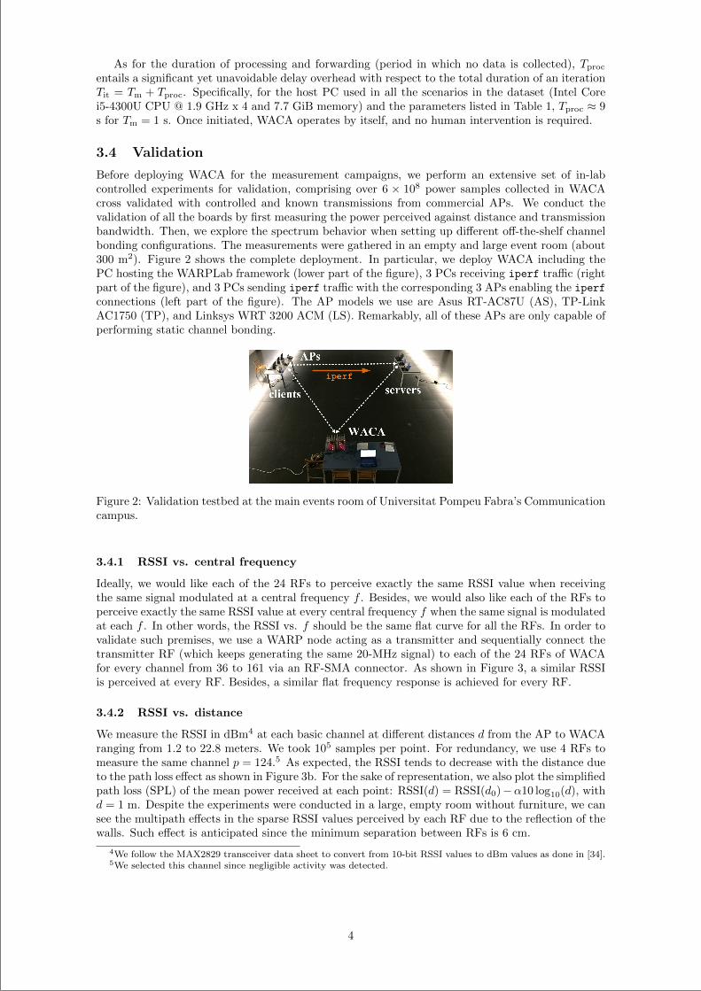
“main” — 2020/11/19 — 10:04 — page 178 — #200

As for the duration of processing and forwarding (period in which no data is collected), Tprocentails a significant yet unavoidable delay overhead with respect to the total duration of an iterationTit = Tm + Tproc. Specifically, for the host PC used in all the scenarios in the dataset (Intel Corei5-4300U CPU @ 1.9 GHz x 4 and 7.7 GiB memory) and the parameters listed in Table 1, Tproc ≈ 9s for Tm = 1 s. Once initiated, WACA operates by itself, and no human intervention is required.

3.4 Validation

Before deploying WACA for the measurement campaigns, we perform an extensive set of in-labcontrolled experiments for validation, comprising over 6 × 108 power samples collected in WACAcross validated with controlled and known transmissions from commercial APs. We conduct thevalidation of all the boards by first measuring the power perceived against distance and transmissionbandwidth. Then, we explore the spectrum behavior when setting up different off-the-shelf channelbonding configurations. The measurements were gathered in an empty and large event room (about300 m2). Figure 2 shows the complete deployment. In particular, we deploy WACA including thePC hosting the WARPLab framework (lower part of the figure), 3 PCs receiving iperf traffic (rightpart of the figure), and 3 PCs sending iperf traffic with the corresponding 3 APs enabling the iperfconnections (left part of the figure). The AP models we use are Asus RT-AC87U (AS), TP-LinkAC1750 (TP), and Linksys WRT 3200 ACM (LS). Remarkably, all of these APs are only capable ofperforming static channel bonding.

Figure 2: Validation testbed at the main events room of Universitat Pompeu Fabra’s Communicationcampus.

3.4.1 RSSI vs. central frequency

Ideally, we would like each of the 24 RFs to perceive exactly the same RSSI value when receivingthe same signal modulated at a central frequency f . Besides, we would also like each of the RFs toperceive exactly the same RSSI value at every central frequency f when the same signal is modulatedat each f . In other words, the RSSI vs. f should be the same flat curve for all the RFs. In order tovalidate such premises, we use a WARP node acting as a transmitter and sequentially connect thetransmitter RF (which keeps generating the same 20-MHz signal) to each of the 24 RFs of WACAfor every channel from 36 to 161 via an RF-SMA connector. As shown in Figure 3, a similar RSSIis perceived at every RF. Besides, a similar flat frequency response is achieved for every RF.

3.4.2 RSSI vs. distance

We measure the RSSI in dBm4 at each basic channel at different distances d from the AP to WACAranging from 1.2 to 22.8 meters. We took 105 samples per point. For redundancy, we use 4 RFs tomeasure the same channel p = 124.5 As expected, the RSSI tends to decrease with the distance dueto the path loss effect as shown in Figure 3b. For the sake of representation, we also plot the simplifiedpath loss (SPL) of the mean power received at each point: RSSI(d) = RSSI(d0)−α10 log10(d), withd = 1 m. Despite the experiments were conducted in a large, empty room without furniture, we cansee the multipath effects in the sparse RSSI values perceived by each RF due to the reflection of thewalls. Such effect is anticipated since the minimum separation between RFs is 6 cm.

4We follow the MAX2829 transceiver data sheet to convert from 10-bit RSSI values to dBm values as done in [34].5We selected this channel since negligible activity was detected.

4

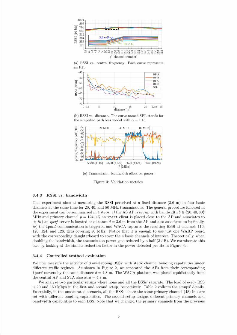
“main” — 2020/11/19 — 10:04 — page 179 — #201

36 40 44 48 52 56 60 64 100

104

108

112

116

120

124

128

132

136

140

144

149

153

157

1610

128256384512640768896

1024

RF e-D

RF c-D

(a) RSSI vs. central frequency. Each curve representsan RF.

0 1.2 5 10 15 20 22.8 25distance [m]

-75

-70

-65

-60

-55

-50

-45R

SSI

[dB

m]

RF-ARF-BRF-CRF-DSPL

(b) RSSI vs. distance. The curve named SPL stands forthe simplified path loss model with α = 1.15.

5580 (#116) 5600 (#120) 5620 (#124) 5640 (#128)-100-95-90-85-80-75-70-65-60-55-50 20 MHz 40 MHz 80 MHz

(c) Transmission bandwidth effect on power.

Figure 3: Validation metrics.

3.4.3 RSSI vs. bandwidth

This experiment aims at measuring the RSSI perceived at a fixed distance (3.6 m) in four basicchannels at the same time for 20, 40, and 80 MHz transmissions. The general procedure followed inthe experiment can be summarized in 4 steps: i) the AS AP is set up with bandwidth b ∈ 20, 40, 80MHz and primary channel p = 124; ii) an iperf client is placed close to the AP and associates toit; iii) an iperf server is located at distance d = 3.6 m from the AP and also associates to it; finally,iv) the iperf communication is triggered and WACA captures the resulting RSSI at channels 116,120, 124, and 128, thus covering 80 MHz. Notice that it is enough to use just one WARP boardwith the corresponding daughterboard to cover the 4 basic channels of interest. Theoretically, whendoubling the bandwidth, the transmission power gets reduced by a half (3 dB). We corroborate thisfact by looking at the similar reduction factor in the power detected per Hz in Figure 3c.

3.4.4 Controlled testbed evaluation

We now measure the activity of 3 overlapping BSSs’ with static channel bonding capabilities underdifferent traffic regimes. As shown in Figure 2, we separated the APs from their correspondingiperf servers by the same distance d = 4.8 m. The WACA platform was placed equidistantly fromthe central AP and STA also at d = 4.8 m.

We analyze two particular setups where none and all the BSSs’ saturate. The load of every BSSis 20 and 150 Mbps in the first and second setup, respectively. Table 2 collects the setups’ details.Essentially, in the unsaturated scenario, all the BSSs’ share the same primary channel (48) but areset with different bonding capabilities. The second setup assigns different primary channels andbandwidth capabilities to each BSS. Note that we changed the primary channels from the previous

5

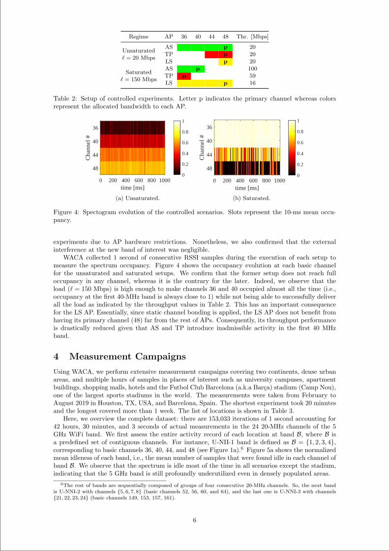
“main” — 2020/11/19 — 10:04 — page 180 — #202

Regime AP 36 40 44 48 Thr. [Mbps]

AS p 20TP p 20

Unsaturated` = 20 Mbps

LS p 20AS p 100TP p 59

Saturated` = 150 Mbps

LS p 16

Table 2: Setup of controlled experiments. Letter p indicates the primary channel whereas colorsrepresent the allocated bandwidth to each AP.

0 200 400 600 800 1000time [ms]

36

40

44

48

Cha

nnel

#

0

0.2

0.4

0.6

0.8

1

(a) Unsaturated.

0 200 400 600 800 1000time [ms]

36

40

44

48

Cha

nnel

#

0

0.2

0.4

0.6

0.8

1

(b) Saturated.

Figure 4: Spectogram evolution of the controlled scenarios. Slots represent the 10-ms mean occu-pancy.

experiments due to AP hardware restrictions. Nonetheless, we also confirmed that the externalinterference at the new band of interest was negligible.

WACA collected 1 second of consecutive RSSI samples during the execution of each setup tomeasure the spectrum occupancy. Figure 4 shows the occupancy evolution at each basic channelfor the unsaturated and saturated setups. We confirm that the former setup does not reach fulloccupancy in any channel, whereas it is the contrary for the later. Indeed, we observe that theload (` = 150 Mbps) is high enough to make channels 36 and 40 occupied almost all the time (i.e.,occupancy at the first 40-MHz band is always close to 1) while not being able to successfully deliverall the load as indicated by the throughput values in Table 2. This has an important consequencefor the LS AP. Essentially, since static channel bonding is applied, the LS AP does not benefit fromhaving its primary channel (48) far from the rest of APs. Consequently, its throughput performanceis drastically reduced given that AS and TP introduce inadmissible activity in the first 40 MHzband.

4 Measurement Campaigns

Using WACA, we perform extensive measurement campaigns covering two continents, dense urbanareas, and multiple hours of samples in places of interest such as university campuses, apartmentbuildings, shopping malls, hotels and the Futbol Club Barcelona (a.k.a Barca) stadium (Camp Nou),one of the largest sports stadiums in the world. The measurements were taken from February toAugust 2019 in Houston, TX, USA, and Barcelona, Spain. The shortest experiment took 20 minutesand the longest covered more than 1 week. The list of locations is shown in Table 3.

Here, we overview the complete dataset: there are 153,033 iterations of 1 second accounting for42 hours, 30 minutes, and 3 seconds of actual measurements in the 24 20-MHz channels of the 5GHz WiFi band. We first assess the entire activity record of each location at band B, where B isa predefined set of contiguous channels. For instance, U-NII-1 band is defined as B = 1, 2, 3, 4,corresponding to basic channels 36, 40, 44, and 48 (see Figure 1a).6 Figure 5a shows the normalizedmean idleness of each band, i.e., the mean number of samples that were found idle in each channel ofband B. We observe that the spectrum is idle most of the time in all scenarios except the stadium,indicating that the 5 GHz band is still profoundly underutilized even in densely populated areas.

6The rest of bands are sequentially composed of groups of four consecutive 20-MHz channels. So, the next bandis U-NNI-2 with channels 5, 6, 7, 8 (basic channels 52, 56, 60, and 64), and the last one is U-NNI-3 with channels21, 22, 23, 24 (basic channels 149, 153, 157, 161).

6

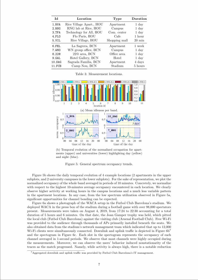
“main” — 2020/11/19 — 10:04 — page 181 — #203

Id Location Type Duration

1 RVA Rice Village Apart., HOU Apartment 1 day2 RNG RNG lab at Rice, HOU Campus 1 day3 TFA Technology for All, HOU Com. center 1 day4 FLO Flo Paris, HOU Cafe 1 hour5 VIL Rice Village, HOU Shopping mall 20 min

6 FEL La Sagrera, BCN Apartment 1 week7 WNO WN group office, BCN Campus 1 day8 22@ 22@ area, BCN Office area 1 day9 GAL Hotel Gallery, BCN Hotel 1 day10 SAG Sagrada Familia, BCN Apartment 4 days11 FCB Camp Nou, BCN Stadium 5 hours

Table 3: Measurement locations.

1 2 3 4 5 6 7 8 9 100.97

0.98

0.99

1.00

110.00.20.40.60.81.0

U-NII-1 U-NNI-2 U-NNI-2C1 U-NNI-2C2 U-NNI-2C3 U-NNI-3

(a) Mean idleness per band.

(b) Temporal evolution of the normalized occupation for apart-ments (upper) and universities (lower) highlighting day (yellow)and night (blue).

Figure 5: General spectrum occupancy trends.

Figure 5b shows the daily temporal evolution of 4 example locations (2 apartments in the uppersubplots, and 2 university campuses in the lower subplots). For the sake of representation, we plot thenormalized occupancy of the whole band averaged in periods of 10 minutes. Concretely, we normalizewith respect to the highest 10-minutes average occupancy encountered in each location. We clearlyobserve higher activity at working hours in the campus locations and a much less variable patternin the apartment locations. In any case, from the low spectrum utilization observed in Figure 5a,significant opportunities for channel bonding can be expected.

Figure 6a shows a photograph of the WACA setup in the Futbol Club Barcelona’s stadium. Wedeployed WACA in the press box of the stadium during a football game with over 98,000 spectatorspresent. Measurements were taken on August 4, 2019, from 17:24 to 22:30 accounting for a totalduration of 5 hours and 6 minutes. On that date, the Joan Gamper trophy was held, which pittedthe local club (Futbol Club Barcelona) against the visiting club (Arsenal Football Club). Free Wi-Fiwas provided to the audience through thousands of APs primarily installed beneath the seats. Wealso obtained data from the stadium’s network management team which indicated that up to 12,000Wi-Fi clients were simultaneously connected. Downlink and uplink traffic is depicted in Figure 6b7

and the spectogram in Figure 6c. Each slot in the spectogram represents the occupancy of eachchannel averaged in 1-second periods. We observe that most channels were highly occupied duringthe measurements. Moreover, we can observe the users’ behavior induced nonstationarity of thetraces as the match progressed. Namely, while activity is always high, there is a notable reduction

7Aggregated downlink and uplink traffic was provided by Futbol Club Barcelona’s IT management.

7

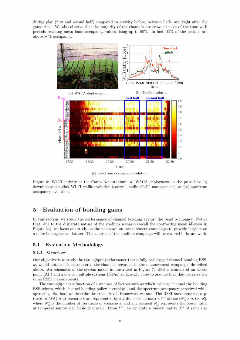
“main” — 2020/11/19 — 10:04 — page 182 — #204

during play (first and second half) compared to activity before, between halfs, and right after thegame time. We also observe that the majority of the channels are crowded most of the time withperiods reaching mean band occupancy values rising up to 99%. In fact, 22% of the periods areabove 80% occupancy.

(a) WACA deployment. (b) Traffic evolution.

17:30 18:30 19:30 20:30 21:30 22:30

3640444852566064

100104108112116120124128132136140144149153157161

chan

nel #

0.0

0.1

0.2

0.3

0.4

0.5

0.6

0.7

0.8

0.9

1.0second halffirst half

(c) Spectrum occupancy evolution.

Figure 6: Wi-Fi activity at the Camp Nou stadium: a) WACA deployment in the press box, b)downlink and uplink Wi-Fi traffic evolution (source: stadium’s IT management), and c) spectrumoccupancy evolution.

5 Evaluation of bonding gains

In this section, we study the performance of channel bonding against the band occupancy. Noticethat, due to the disparate nature of the stadium scenario (recall the contrasting mean idleness inFigure 5a), we focus our study on the non-stadium measurement campaigns to provide insights ona more homogeneous dataset. The analysis of the stadium campaign will be covered in future work.

5.1 Evaluation Methodology

5.1.1 Overview

Our objective is to study the throughput performance that a fully backlogged channel-bonding BSS,w, would obtain if it encountered the channels recorded in the measurement campaigns describedabove. An schematic of the system model is illustrated in Figure 7. BSS w consists of an accesspoint (AP) and a one or multiple stations (STAs) sufficiently close to assume that they perceive thesame RSSI measurements.

The throughput is a function of a number of factors such as which primary channel the bondingBSS selects, which channel bonding policy it employs, and the spectrum occupancy perceived whileoperating. So, here we describe the trace-driven framework we use. The RSSI measurements cap-tured by WACA at scenario s are represented by a 2-dimensional matrix Y s of size (Ns

it×ns)× |R|,where Ns

it is the number of iterations of scenario s, and any element yst,c represents the power valueat temporal sample t in basic channel c. From Y s, we generate a binary matrix Xs of same size

8

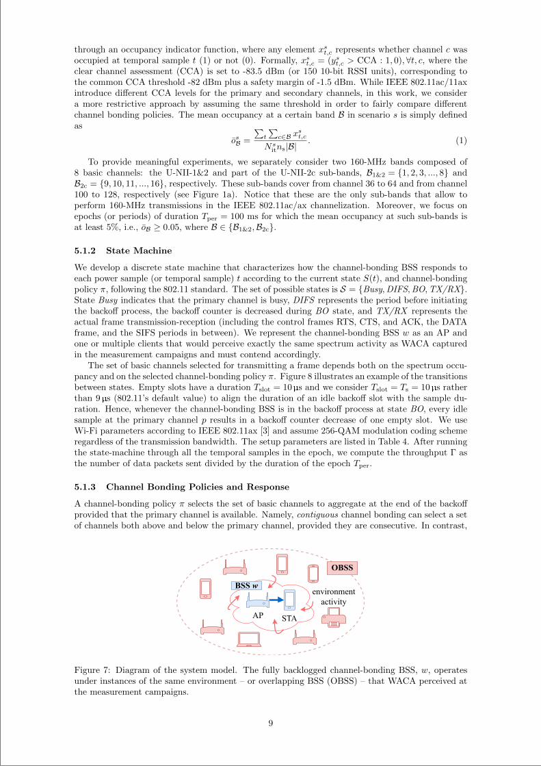
“main” — 2020/11/19 — 10:04 — page 183 — #205

through an occupancy indicator function, where any element xst,c represents whether channel c wasoccupied at temporal sample t (1) or not (0). Formally, xst,c = (yst,c > CCA : 1, 0),∀t, c, where theclear channel assessment (CCA) is set to -83.5 dBm (or 150 10-bit RSSI units), corresponding tothe common CCA threshold -82 dBm plus a safety margin of -1.5 dBm. While IEEE 802.11ac/11axintroduce different CCA levels for the primary and secondary channels, in this work, we considera more restrictive approach by assuming the same threshold in order to fairly compare differentchannel bonding policies. The mean occupancy at a certain band B in scenario s is simply definedas

osB =

∑t

∑c∈B x

st,c

Nsitns|B|

. (1)

To provide meaningful experiments, we separately consider two 160-MHz bands composed of8 basic channels: the U-NII-1&2 and part of the U-NII-2c sub-bands, B1&2 = 1, 2, 3, ..., 8 andB2c = 9, 10, 11, ..., 16, respectively. These sub-bands cover from channel 36 to 64 and from channel100 to 128, respectively (see Figure 1a). Notice that these are the only sub-bands that allow toperform 160-MHz transmissions in the IEEE 802.11ac/ax channelization. Moreover, we focus onepochs (or periods) of duration Tper = 100 ms for which the mean occupancy at such sub-bands isat least 5%, i.e., oB ≥ 0.05, where B ∈ B1&2,B2c.

5.1.2 State Machine

We develop a discrete state machine that characterizes how the channel-bonding BSS responds toeach power sample (or temporal sample) t according to the current state S(t), and channel-bondingpolicy π, following the 802.11 standard. The set of possible states is S = Busy,DIFS,BO,TX/RX.State Busy indicates that the primary channel is busy, DIFS represents the period before initiatingthe backoff process, the backoff counter is decreased during BO state, and TX/RX represents theactual frame transmission-reception (including the control frames RTS, CTS, and ACK, the DATAframe, and the SIFS periods in between). We represent the channel-bonding BSS w as an AP andone or multiple clients that would perceive exactly the same spectrum activity as WACA capturedin the measurement campaigns and must contend accordingly.

The set of basic channels selected for transmitting a frame depends both on the spectrum occu-pancy and on the selected channel-bonding policy π. Figure 8 illustrates an example of the transitionsbetween states. Empty slots have a duration Tslot = 10µs and we consider Tslot = Ts = 10µs ratherthan 9 µs (802.11’s default value) to align the duration of an idle backoff slot with the sample du-ration. Hence, whenever the channel-bonding BSS is in the backoff process at state BO, every idlesample at the primary channel p results in a backoff counter decrease of one empty slot. We useWi-Fi parameters according to IEEE 802.11ax [3] and assume 256-QAM modulation coding schemeregardless of the transmission bandwidth. The setup parameters are listed in Table 4. After runningthe state-machine through all the temporal samples in the epoch, we compute the throughput Γ asthe number of data packets sent divided by the duration of the epoch Tper.

5.1.3 Channel Bonding Policies and Response

A channel-bonding policy π selects the set of basic channels to aggregate at the end of the backoffprovided that the primary channel is available. Namely, contiguous channel bonding can select a setof channels both above and below the primary channel, provided they are consecutive. In contrast,

STAAP

environmentactivity

BSSw

OBSS

Figure 7: Diagram of the system model. The fully backlogged channel-bonding BSS, w, operatesunder instances of the same environment – or overlapping BSS (OBSS) – that WACA perceived atthe measurement campaigns.

9

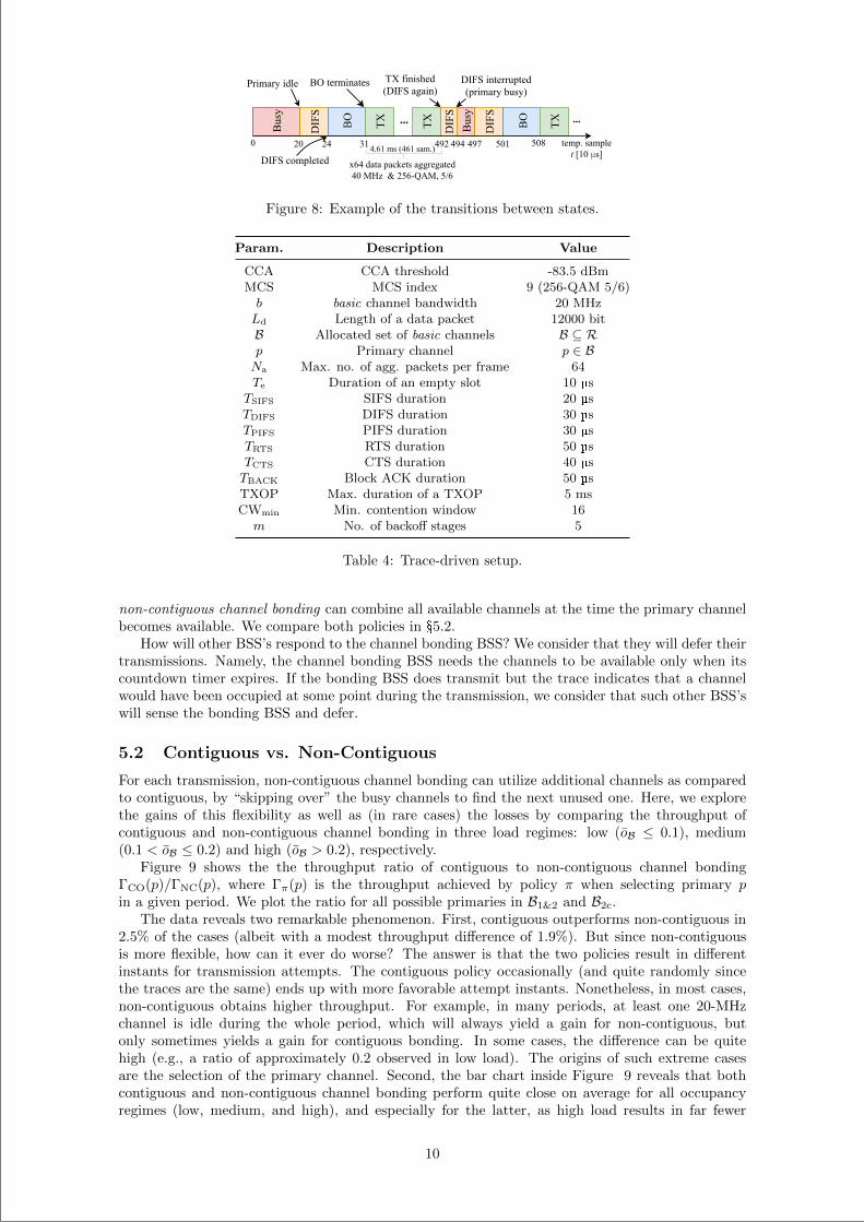
“main” — 2020/11/19 — 10:04 — page 184 — #206

TXBusy

DIFS

BO

TX ...

Busy

DIFS

DIFS

BO

Primaryidle BOterminates TXfinished(DIFSagain)

DIFSinterrupted(primarybusy)

...

temp.samplet[10μs]

TX

0 20 24 31 492

x64datapacketsaggregated40MHz&256-QAM,5/6

494 497 501 5084.61ms(461sam.)

DIFScompleted

Figure 8: Example of the transitions between states.

Param. Description Value

CCA CCA threshold -83.5 dBmMCS MCS index 9 (256-QAM 5/6)b basic channel bandwidth 20 MHzLd Length of a data packet 12000 bitB Allocated set of basic channels B ⊆ Rp Primary channel p ∈ BNa Max. no. of agg. packets per frame 64Te Duration of an empty slot 10 µs

TSIFS SIFS duration 20 µsTDIFS DIFS duration 30 µsTPIFS PIFS duration 30 µsTRTS RTS duration 50 µsTCTS CTS duration 40 µsTBACK Block ACK duration 50 µsTXOP Max. duration of a TXOP 5 msCWmin Min. contention window 16m No. of backoff stages 5

Table 4: Trace-driven setup.

non-contiguous channel bonding can combine all available channels at the time the primary channelbecomes available. We compare both policies in §5.2.

How will other BSS’s respond to the channel bonding BSS? We consider that they will defer theirtransmissions. Namely, the channel bonding BSS needs the channels to be available only when itscountdown timer expires. If the bonding BSS does transmit but the trace indicates that a channelwould have been occupied at some point during the transmission, we consider that such other BSS’swill sense the bonding BSS and defer.

5.2 Contiguous vs. Non-Contiguous

For each transmission, non-contiguous channel bonding can utilize additional channels as comparedto contiguous, by “skipping over” the busy channels to find the next unused one. Here, we explorethe gains of this flexibility as well as (in rare cases) the losses by comparing the throughput ofcontiguous and non-contiguous channel bonding in three load regimes: low (oB ≤ 0.1), medium(0.1 < oB ≤ 0.2) and high (oB > 0.2), respectively.

Figure 9 shows the the throughput ratio of contiguous to non-contiguous channel bondingΓCO(p)/ΓNC(p), where Γπ(p) is the throughput achieved by policy π when selecting primary pin a given period. We plot the ratio for all possible primaries in B1&2 and B2c.

The data reveals two remarkable phenomenon. First, contiguous outperforms non-contiguous in2.5% of the cases (albeit with a modest throughput difference of 1.9%). But since non-contiguousis more flexible, how can it ever do worse? The answer is that the two policies result in differentinstants for transmission attempts. The contiguous policy occasionally (and quite randomly sincethe traces are the same) ends up with more favorable attempt instants. Nonetheless, in most cases,non-contiguous obtains higher throughput. For example, in many periods, at least one 20-MHzchannel is idle during the whole period, which will always yield a gain for non-contiguous, butonly sometimes yields a gain for contiguous bonding. In some cases, the difference can be quitehigh (e.g., a ratio of approximately 0.2 observed in low load). The origins of such extreme casesare the selection of the primary channel. Second, the bar chart inside Figure 9 reveals that bothcontiguous and non-contiguous channel bonding perform quite close on average for all occupancyregimes (low, medium, and high), and especially for the latter, as high load results in far fewer

10

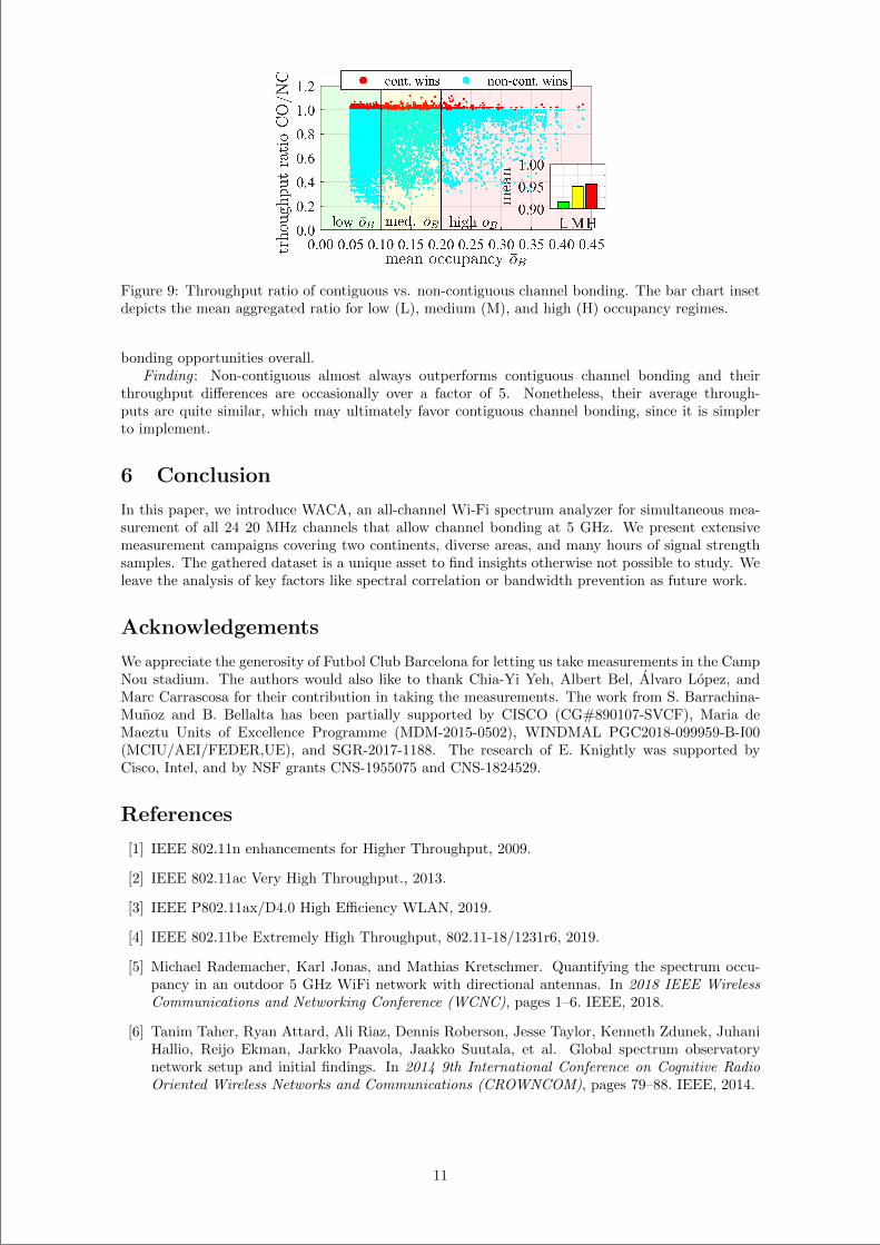
“main” — 2020/11/19 — 10:04 — page 185 — #207

Figure 9: Throughput ratio of contiguous vs. non-contiguous channel bonding. The bar chart insetdepicts the mean aggregated ratio for low (L), medium (M), and high (H) occupancy regimes.

bonding opportunities overall.Finding : Non-contiguous almost always outperforms contiguous channel bonding and their

throughput differences are occasionally over a factor of 5. Nonetheless, their average through-puts are quite similar, which may ultimately favor contiguous channel bonding, since it is simplerto implement.

6 Conclusion

In this paper, we introduce WACA, an all-channel Wi-Fi spectrum analyzer for simultaneous mea-surement of all 24 20 MHz channels that allow channel bonding at 5 GHz. We present extensivemeasurement campaigns covering two continents, diverse areas, and many hours of signal strengthsamples. The gathered dataset is a unique asset to find insights otherwise not possible to study. Weleave the analysis of key factors like spectral correlation or bandwidth prevention as future work.

Acknowledgements

We appreciate the generosity of Futbol Club Barcelona for letting us take measurements in the CampNou stadium. The authors would also like to thank Chia-Yi Yeh, Albert Bel, Alvaro Lopez, andMarc Carrascosa for their contribution in taking the measurements. The work from S. Barrachina-Munoz and B. Bellalta has been partially supported by CISCO (CG#890107-SVCF), Maria deMaeztu Units of Excellence Programme (MDM-2015-0502), WINDMAL PGC2018-099959-B-I00(MCIU/AEI/FEDER,UE), and SGR-2017-1188. The research of E. Knightly was supported byCisco, Intel, and by NSF grants CNS-1955075 and CNS-1824529.

References

[1] IEEE 802.11n enhancements for Higher Throughput, 2009.

[2] IEEE 802.11ac Very High Throughput., 2013.

[3] IEEE P802.11ax/D4.0 High Efficiency WLAN, 2019.

[4] IEEE 802.11be Extremely High Throughput, 802.11-18/1231r6, 2019.

[5] Michael Rademacher, Karl Jonas, and Mathias Kretschmer. Quantifying the spectrum occu-pancy in an outdoor 5 GHz WiFi network with directional antennas. In 2018 IEEE WirelessCommunications and Networking Conference (WCNC), pages 1–6. IEEE, 2018.

[6] Tanim Taher, Ryan Attard, Ali Riaz, Dennis Roberson, Jesse Taylor, Kenneth Zdunek, JuhaniHallio, Reijo Ekman, Jarkko Paavola, Jaakko Suutala, et al. Global spectrum observatorynetwork setup and initial findings. In 2014 9th International Conference on Cognitive RadioOriented Wireless Networks and Communications (CROWNCOM), pages 79–88. IEEE, 2014.

11

“main” — 2020/11/19 — 10:04 — page 186 — #208

[7] Sriram Subramaniam, Hector Reyes, and Naima Kaabouch. Spectrum occupancy measurement:An autocorrelation based scanning technique using USRP. In 2015 IEEE 16th Annual Wirelessand Microwave Technology Conference (WAMICON), pages 1–5. IEEE, 2015.

[8] Matthias Wellens, Janne RiihijaRvi, and Petri MaHoNen. Empirical time and frequency domainmodels of spectrum use. Physical Communication, 2(1-2):10–32, 2009.

[9] Vinod Kone, Lei Yang, Xue Yang, Ben Y Zhao, and Haitao Zheng. The effectiveness of op-portunistic spectrum access: A measurement study. IEEE/ACM Transactions on Networking,20(6):2005–2016, 2012.

[10] Simon W Day and Adrian Wagstaff. Activity in the WiFi bands - An Objective Approach toEstimation. In ARMMS Conference. Mass, 2014.

[11] Fatima Salahdine and Hassan El Ghazi. A real time spectrum scanning technique based oncompressive sensing for cognitive radio networks. In 2017 IEEE 8th Annual Ubiquitous Com-puting, Electronics and Mobile Communication Conference (UEMCON), pages 506–511. IEEE,2017.

[12] Sanjit Biswas, John Bicket, Edmund Wong, Raluca Musaloiu-e, Apurv Bhartia, and DanAguayo. Large-scale measurements of wireless network behavior. In Proceedings of the 2015ACM Conference on Special Interest Group on Data Communication, pages 153–165, 2015.

[13] M. Lopez-Benıtez and F. Casadevall. Modeling and simulation of time-correlation properties ofspectrum use in cognitive radio. In 2011 6th International ICST Conference on Cognitive RadioOriented Wireless Networks and Communications (CROWNCOM), pages 326–330, 2011.

[14] Vinod Kone, Lei Yang, Xue Yang, Ben Y Zhao, and Haitao Zheng. On the feasibility ofeffective opportunistic spectrum access. In Proceedings of the 10th ACM SIGCOMM conferenceon Internet measurement, pages 151–164, 2010.

[15] Marko Hoyhtya, Aarne Mammela, Marina Eskola, Marja Matinmikko, Juha Kalliovaara, JaakkoOjaniemi, Jaakko Suutala, Reijo Ekman, Roger Bacchus, and Dennis Roberson. Spectrumoccupancy measurements: A survey and use of interference maps. IEEE CommunicationsSurveys & Tutorials, 18(4):2386–2414, 2016.

[16] Salim A Hanna and John Sydor. Distributed sensing of spectrum occupancy and interfer-ence in outdoor 2.4 GHz Wi-Fi networks. In 2012 IEEE Global Communications Conference(GLOBECOM), pages 1453–1459. IEEE, 2012.

[17] Salim A Hanna. A 3-state hypothesis test model for cognitive radio systems. In 2014 IEEEInternational Symposium on Dynamic Spectrum Access Networks (DYSPAN), pages 291–302.IEEE, 2014.

[18] Sixing Yin, Dawei Chen, Qian Zhang, Mingyan Liu, and Shufang Li. Mining spectrum usagedata: a large-scale spectrum measurement study. IEEE Transactions on Mobile Computing,11(6):1033–1046, 2012.

[19] Lara Deek, Eduard Garcia-Villegas, Elizabeth Belding, Sung-Ju Lee, and Kevin Almeroth. Theimpact of channel bonding on 802.11n network management. In Proceedings of the SeventhCOnference on emerging Networking EXperiments and Technologies, pages 1–12, 2011.

[20] Lara Deek, Eduard Garcia-Villegas, Elizabeth Belding, Sung-Ju Lee, and Kevin Almeroth.Intelligent channel bonding in 802.11n WLANs. IEEE Transactions on Mobile Computing,13(6):1242–1255, 2014.

[21] Mustafa Y Arslan, Konstantinos Pelechrinis, Ioannis Broustis, Srikanth V Krishnamurthy,Sateesh Addepalli, and Konstantina Papagiannaki. Auto-configuration of 802.11n WLANs.In Proceedings of the 6th International Conference, pages 1–12, 2010.

[22] Mustafa Y Arslan, Konstantinos Pelechrinis, Ioannis Broustis, Shailendra Singh, Srikanth VKrishnamurthy, Sateesh Addepalli, and Konstantina Papagiannaki. ACORN: An auto-configuration framework for 802.11n WLANs. IEEE/ACM Transactions on Networking (TON),21(3):896–909, 2013.

12

“main” — 2020/11/19 — 10:04 — page 187 — #209

[23] Minyoung Park. IEEE 802.11ac: Dynamic bandwidth channel access. In Communications(ICC), 2011 IEEE International Conference on, pages 1–5. IEEE, 2011.

[24] Michelle X Gong, Brian Hart, Liangfu Xia, and Roy Want. Channel bounding and macprotection mechanisms for 802.11ac. In 2011 IEEE Global Telecommunications Conference-GLOBECOM 2011, pages 1–5. IEEE, 2011.

[25] Boris Bellalta, Alessandro Checco, Alessandro Zocca, and Jaume Barcelo. On the interactionsbetween multiple overlapping wlans using channel bonding. IEEE Transactions on VehicularTechnology, 65(2):796–812, 2015.

[26] Mohand Yazid and Adlen Ksentini. Stochastic modeling of the static and dynamic multichan-nel access methods enabling 40/80/160 MHz channel bonding in the VHT WLANs. IEEECommunications Letters, 23(8):1437–1440, 2019.

[27] Mun-Suk Kim, Tanguy Ropitault, Sukyoung Lee, and Nada Golmie. A throughput study forchannel bonding in ieee 802.11ac networks. IEEE Communications Letters, 21(12):2682–2685,2017.

[28] Sergio Barrachina-Munoz, Francesc Wilhelmi, and Boris Bellalta. To overlap or not to overlap:Enabling channel bonding in high-density WLANs. Computer Networks, 152:40–53, 2019.

[29] Sergio Barrachina-Munoz, Francesc Wilhelmi, and Boris Bellalta. Dynamic channel bond-ing in spatially distributed high-density WLANs. IEEE Transactions on Mobile Computing,19(4):821–835, 2020.

[30] Giorgio Buttazzo, Carmelo Di Franco, and Mauro Marinoni. Design and analysis of target-sensitive real-time systems. Software: Practice and Experience, 46(9):1181–1200, 2016.

[31] Leili Farzinvash and Mehdi Kargahi. A scheduling algorithm for execution-instant sensitivereal-time systems. In 2009 15th IEEE International Conference on Embedded and Real-TimeComputing Systems and Applications, pages 511–518. IEEE, 2009.

[32] Narendra Anand, Ehsan Aryafar, and Edward W Knightly. WARPlab: a flexible frameworkfor rapid physical layer design. In Proceedings of the 2010 ACM workshop on Wireless of thestudents, by the students, for the students, pages 53–56. ACM, 2010.

[33] Rice University Wireless Open Access Research Platform. http://warpproject.org, last ac-cessed January 30, 2020.

[34] Seowoo Jang, Kang G Shin, and Saewoong Bahk. Post-CCA and reinforcement learningbased bandwidth adaptation in 802.11ac networks. IEEE Transactions on Mobile Computing,17(2):419–432, 2018.

13

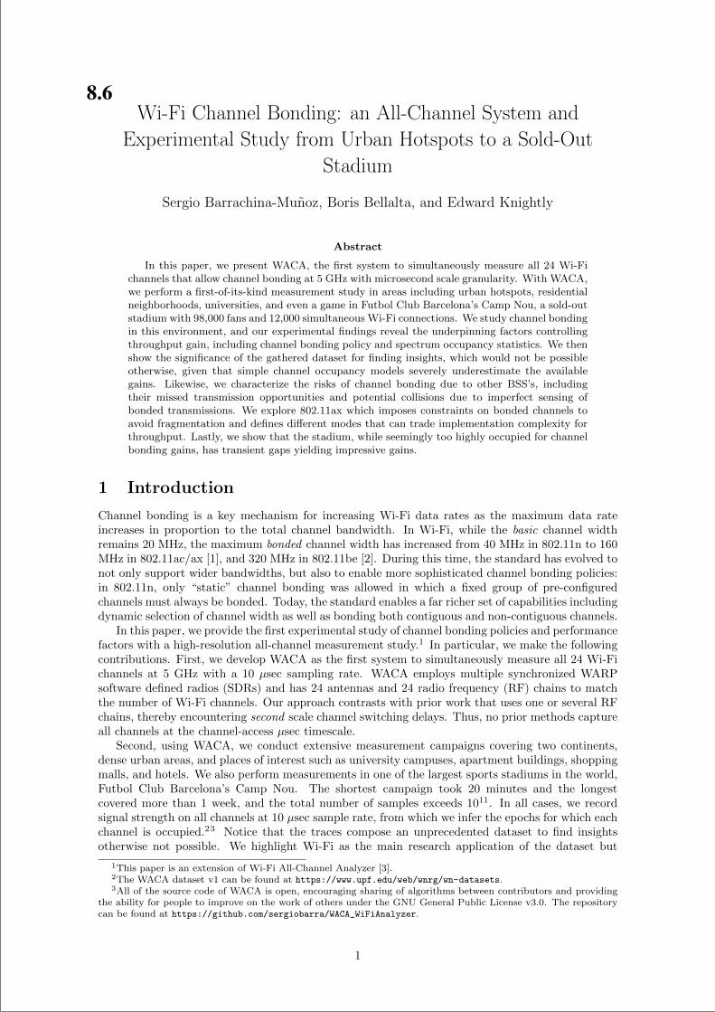
“main” — 2020/11/19 — 10:04 — page 188 — #210

Wi-Fi Channel Bonding: an All-Channel System and

Experimental Study from Urban Hotspots to a Sold-Out

Stadium

Sergio Barrachina-Munoz, Boris Bellalta, and Edward Knightly

Abstract

In this paper, we present WACA, the first system to simultaneously measure all 24 Wi-Fichannels that allow channel bonding at 5 GHz with microsecond scale granularity. With WACA,we perform a first-of-its-kind measurement study in areas including urban hotspots, residentialneighborhoods, universities, and even a game in Futbol Club Barcelona’s Camp Nou, a sold-outstadium with 98,000 fans and 12,000 simultaneous Wi-Fi connections. We study channel bondingin this environment, and our experimental findings reveal the underpinning factors controllingthroughput gain, including channel bonding policy and spectrum occupancy statistics. We thenshow the significance of the gathered dataset for finding insights, which would not be possibleotherwise, given that simple channel occupancy models severely underestimate the availablegains. Likewise, we characterize the risks of channel bonding due to other BSS’s, includingtheir missed transmission opportunities and potential collisions due to imperfect sensing ofbonded transmissions. We explore 802.11ax which imposes constraints on bonded channels toavoid fragmentation and defines different modes that can trade implementation complexity forthroughput. Lastly, we show that the stadium, while seemingly too highly occupied for channelbonding gains, has transient gaps yielding impressive gains.

1 Introduction

Channel bonding is a key mechanism for increasing Wi-Fi data rates as the maximum data rateincreases in proportion to the total channel bandwidth. In Wi-Fi, while the basic channel widthremains 20 MHz, the maximum bonded channel width has increased from 40 MHz in 802.11n to 160MHz in 802.11ac/ax [1], and 320 MHz in 802.11be [2]. During this time, the standard has evolved tonot only support wider bandwidths, but also to enable more sophisticated channel bonding policies:in 802.11n, only “static” channel bonding was allowed in which a fixed group of pre-configuredchannels must always be bonded. Today, the standard enables a far richer set of capabilities includingdynamic selection of channel width as well as bonding both contiguous and non-contiguous channels.

In this paper, we provide the first experimental study of channel bonding policies and performancefactors with a high-resolution all-channel measurement study.1 In particular, we make the followingcontributions. First, we develop WACA as the first system to simultaneously measure all 24 Wi-Fichannels at 5 GHz with a 10 µsec sampling rate. WACA employs multiple synchronized WARPsoftware defined radios (SDRs) and has 24 antennas and 24 radio frequency (RF) chains to matchthe number of Wi-Fi channels. Our approach contrasts with prior work that uses one or several RFchains, thereby encountering second scale channel switching delays. Thus, no prior methods captureall channels at the channel-access µsec timescale.

Second, using WACA, we conduct extensive measurement campaigns covering two continents,dense urban areas, and places of interest such as university campuses, apartment buildings, shoppingmalls, and hotels. We also perform measurements in one of the largest sports stadiums in the world,Futbol Club Barcelona’s Camp Nou. The shortest campaign took 20 minutes and the longestcovered more than 1 week, and the total number of samples exceeds 1011. In all cases, we recordsignal strength on all channels at 10 µsec sample rate, from which we infer the epochs for which eachchannel is occupied.23 Notice that the traces compose an unprecedented dataset to find insightsotherwise not possible. We highlight Wi-Fi as the main research application of the dataset but

1This paper is an extension of Wi-Fi All-Channel Analyzer [3].2The WACA dataset v1 can be found at https://www.upf.edu/web/wnrg/wn-datasets.3All of the source code of WACA is open, encouraging sharing of algorithms between contributors and providing

the ability for people to improve on the work of others under the GNU General Public License v3.0. The repositorycan be found at https://github.com/sergiobarra/WACA_WiFiAnalyzer.

1

8.6

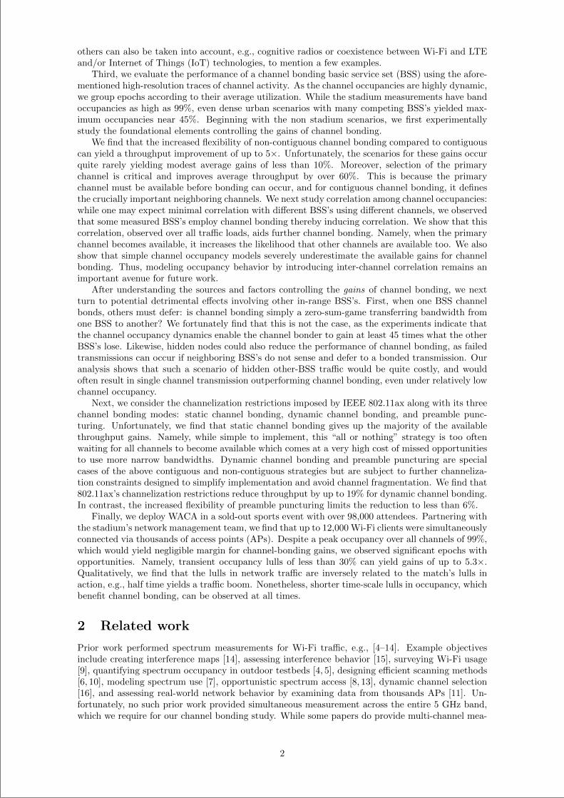
“main” — 2020/11/19 — 10:04 — page 189 — #211

others can also be taken into account, e.g., cognitive radios or coexistence between Wi-Fi and LTEand/or Internet of Things (IoT) technologies, to mention a few examples.

Third, we evaluate the performance of a channel bonding basic service set (BSS) using the afore-mentioned high-resolution traces of channel activity. As the channel occupancies are highly dynamic,we group epochs according to their average utilization. While the stadium measurements have bandoccupancies as high as 99%, even dense urban scenarios with many competing BSS’s yielded max-imum occupancies near 45%. Beginning with the non stadium scenarios, we first experimentallystudy the foundational elements controlling the gains of channel bonding.

We find that the increased flexibility of non-contiguous channel bonding compared to contiguouscan yield a throughput improvement of up to 5×. Unfortunately, the scenarios for these gains occurquite rarely yielding modest average gains of less than 10%. Moreover, selection of the primarychannel is critical and improves average throughput by over 60%. This is because the primarychannel must be available before bonding can occur, and for contiguous channel bonding, it definesthe crucially important neighboring channels. We next study correlation among channel occupancies:while one may expect minimal correlation with different BSS’s using different channels, we observedthat some measured BSS’s employ channel bonding thereby inducing correlation. We show that thiscorrelation, observed over all traffic loads, aids further channel bonding. Namely, when the primarychannel becomes available, it increases the likelihood that other channels are available too. We alsoshow that simple channel occupancy models severely underestimate the available gains for channelbonding. Thus, modeling occupancy behavior by introducing inter-channel correlation remains animportant avenue for future work.

After understanding the sources and factors controlling the gains of channel bonding, we nextturn to potential detrimental effects involving other in-range BSS’s. First, when one BSS channelbonds, others must defer: is channel bonding simply a zero-sum-game transferring bandwidth fromone BSS to another? We fortunately find that this is not the case, as the experiments indicate thatthe channel occupancy dynamics enable the channel bonder to gain at least 45 times what the otherBSS’s lose. Likewise, hidden nodes could also reduce the performance of channel bonding, as failedtransmissions can occur if neighboring BSS’s do not sense and defer to a bonded transmission. Ouranalysis shows that such a scenario of hidden other-BSS traffic would be quite costly, and wouldoften result in single channel transmission outperforming channel bonding, even under relatively lowchannel occupancy.

Next, we consider the channelization restrictions imposed by IEEE 802.11ax along with its threechannel bonding modes: static channel bonding, dynamic channel bonding, and preamble punc-turing. Unfortunately, we find that static channel bonding gives up the majority of the availablethroughput gains. Namely, while simple to implement, this “all or nothing” strategy is too oftenwaiting for all channels to become available which comes at a very high cost of missed opportunitiesto use more narrow bandwidths. Dynamic channel bonding and preamble puncturing are specialcases of the above contiguous and non-contiguous strategies but are subject to further channeliza-tion constraints designed to simplify implementation and avoid channel fragmentation. We find that802.11ax’s channelization restrictions reduce throughput by up to 19% for dynamic channel bonding.In contrast, the increased flexibility of preamble puncturing limits the reduction to less than 6%.

Finally, we deploy WACA in a sold-out sports event with over 98,000 attendees. Partnering withthe stadium’s network management team, we find that up to 12,000 Wi-Fi clients were simultaneouslyconnected via thousands of access points (APs). Despite a peak occupancy over all channels of 99%,which would yield negligible margin for channel-bonding gains, we observed significant epochs withopportunities. Namely, transient occupancy lulls of less than 30% can yield gains of up to 5.3×.Qualitatively, we find that the lulls in network traffic are inversely related to the match’s lulls inaction, e.g., half time yields a traffic boom. Nonetheless, shorter time-scale lulls in occupancy, whichbenefit channel bonding, can be observed at all times.

2 Related work

Prior work performed spectrum measurements for Wi-Fi traffic, e.g., [4–14]. Example objectivesinclude creating interference maps [14], assessing interference behavior [15], surveying Wi-Fi usage[9], quantifying spectrum occupancy in outdoor testbeds [4, 5], designing efficient scanning methods[6, 10], modeling spectrum use [7], opportunistic spectrum access [8, 13], dynamic channel selection[16], and assessing real-world network behavior by examining data from thousands APs [11]. Un-fortunately, no such prior work provided simultaneous measurement across the entire 5 GHz band,which we require for our channel bonding study. While some papers do provide multi-channel mea-

2

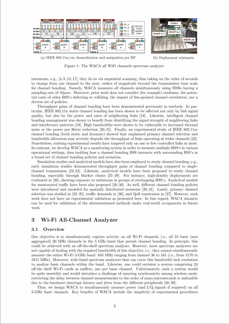
“main” — 2020/11/19 — 10:04 — page 190 — #212

WARP-a

A BFMCD

C WARP-b

A BFMCD

C WARP-c

A BFMCD

C WARP-d

A BFMCD

C WARP-e

A BFMCD

C WARP-f

A BFMCD

C36 40 44 48 52 56 60 64 100

104

108

112

116

120

124

128

132

136

140

144 149

153

157

161

165

38 46 6254 102 110 126118 134 142 151 15942 58

50

WARP-a WARP-b WARP-c WARP-d WARP-e WARP-f

106 122114

138 155

A

B

C

D

RF_A

RF_B

RF_C

RF_D

FMC

FMC-RF-2X245

daughter board

40 MHz80 MHz

160 MHz

20 MHz

stack 1 stack 2

U-NII-1 U-NII-2 U-NII-2-C U-NII-3

(a) IEEE 802.11ac/ax channelization and assignation per RF. (b) Deployment schematic.

Figure 1: The WACA all WiFi channels spectrum analyzer.

surements, e.g., [4, 8, 13, 17], they do so via sequential scanning, thus taking on the order of secondsto change from one channel to the next, orders of magnitude beyond the transmission time scalefor channel bonding. Namely, WACA measures all channels simultaneously using SDRs having asampling rate of 10µsec. Moreover, prior work does not consider (for example) stadiums, the poten-tial costs of other BSS’s deferring or colliding, the impact of fine-grained channel correlation, nor adiverse set of policies.

Throughput gains of channel bonding have been demonstrated previously in testbeds. In par-ticular, IEEE 802.11n static channel bonding has been shown to be affected not only by link signalquality, but also by the power and rates of neighboring links [18]. Likewise, intelligent channelbonding management was shown to benefit from identifying the signal strength of neighboring linksand interference patterns [19]. High bandwidths were shown to be vulnerable to increased thermalnoise or the power per Hertz reduction [20, 21]. Finally, an experimental study of IEEE 802.11acchannel bonding (both static and dynamic) showed that unplanned primary channel selection andbandwidth allocation may severely degrade the throughput of links operating at wider channels [22].Nonetheless, existing experimental results have targeted only on one or few controlled links at most.In contrast, we develop WACA as a monitoring system in order to measure multiple BSS’s in variousoperational settings, thus tackling how a channel bonding BSS interacts with surrounding BSS’s ina broad set of channel bonding policies and scenarios.

Simulation studies and analytical models have also been employed to study channel bonding, e.g.,early simulation studies demonstrated throughput gains of channel bonding compared to single-channel transmission [23, 24]. Likewise, analytical models have been proposed to study channelbonding, especially through Markov chains [25–29]. For instance, high-density deployments areevaluated in [26], showing exposure to unfairness in groups of overlapping BSS’s. Analytical modelsfor unsaturated traffic have been also proposed [28, 30]. As well, different channel bonding policieswere introduced and modeled for spatially distributed scenarios [30, 31]. Lastly, primary channelselection was studied in [32–35], traffic demands in [36], and QoS constraints in [37]. However, suchwork does not have an experimental validation as presented here. In this regard, WACA datasetscan be used for validation of the aforementioned methods under real-world occupancies in futurework.

3 Wi-Fi All-Channel Analyzer

3.1 Overview

Our objective is to simultaneously capture activity on all Wi-Fi channels, i.e., all 24 basic (nonaggregated) 20 MHz channels in the 5 GHz band that permit channel bonding. In principle, thiscould be achieved with an off-the-shelf spectrum analyzer. However, most spectrum analyzers arenot capable of dealing with the required bandwidth of this objective, i.e., they cannot simultaneouslymeasure the entire Wi-Fi 5-GHz band: 645 MHz ranging from channel 36 to 161 (i.e., from 5170 to5815 MHz). Moreover, wide-band spectrum analyzers that can cover this bandwidth lack resolutionto analyze basic channels within the band. Likewise, one could envision a system comprising 24off-the shelf Wi-Fi cards as sniffers, one per basic channel. Unfortunately, such a system wouldbe quite unwieldy and would introduce a challenge of ensuring synchronicity among wireless cards:restricting the delay between channel measurements to the order of nano/microseconds is unfeasibledue to the hardware interrupt latency and jitter from the different peripherals [38, 39].

Thus, we design WACA to simultaneously measure power (and I/Q signals if required) on all5-GHz basic channels. Key benefits of WACA include the simplicity of experimental procedures

3

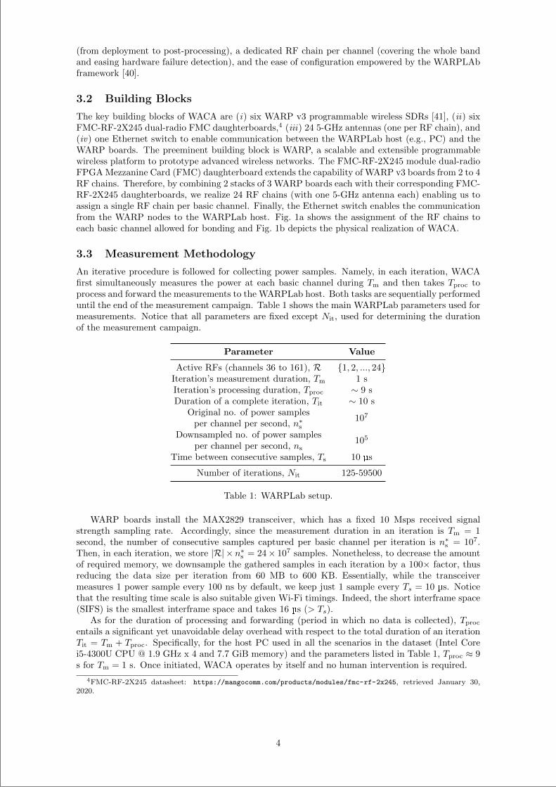
“main” — 2020/11/19 — 10:04 — page 191 — #213

(from deployment to post-processing), a dedicated RF chain per channel (covering the whole bandand easing hardware failure detection), and the ease of configuration empowered by the WARPLAbframework [40].

3.2 Building Blocks

The key building blocks of WACA are (i) six WARP v3 programmable wireless SDRs [41], (ii) sixFMC-RF-2X245 dual-radio FMC daughterboards,4 (iii) 24 5-GHz antennas (one per RF chain), and(iv) one Ethernet switch to enable communication between the WARPLab host (e.g., PC) and theWARP boards. The preeminent building block is WARP, a scalable and extensible programmablewireless platform to prototype advanced wireless networks. The FMC-RF-2X245 module dual-radioFPGA Mezzanine Card (FMC) daughterboard extends the capability of WARP v3 boards from 2 to 4RF chains. Therefore, by combining 2 stacks of 3 WARP boards each with their corresponding FMC-RF-2X245 daughterboards, we realize 24 RF chains (with one 5-GHz antenna each) enabling us toassign a single RF chain per basic channel. Finally, the Ethernet switch enables the communicationfrom the WARP nodes to the WARPLab host. Fig. 1a shows the assignment of the RF chains toeach basic channel allowed for bonding and Fig. 1b depicts the physical realization of WACA.

3.3 Measurement Methodology

An iterative procedure is followed for collecting power samples. Namely, in each iteration, WACAfirst simultaneously measures the power at each basic channel during Tm and then takes Tproc toprocess and forward the measurements to the WARPLab host. Both tasks are sequentially performeduntil the end of the measurement campaign. Table 1 shows the main WARPLab parameters used formeasurements. Notice that all parameters are fixed except Nit, used for determining the durationof the measurement campaign.

Parameter Value

Active RFs (channels 36 to 161), R 1, 2, ..., 24Iteration’s measurement duration, Tm 1 sIteration’s processing duration, Tproc ∼ 9 sDuration of a complete iteration, Tit ∼ 10 s

Original no. of power samplesper channel per second, n∗s

107

Downsampled no. of power samplesper channel per second, ns

105

Time between consecutive samples, Ts 10 µs

Number of iterations, Nit 125-59500

Table 1: WARPLab setup.

WARP boards install the MAX2829 transceiver, which has a fixed 10 Msps received signalstrength sampling rate. Accordingly, since the measurement duration in an iteration is Tm = 1second, the number of consecutive samples captured per basic channel per iteration is n∗s = 107.Then, in each iteration, we store |R| × n∗s = 24× 107 samples. Nonetheless, to decrease the amountof required memory, we downsample the gathered samples in each iteration by a 100× factor, thusreducing the data size per iteration from 60 MB to 600 KB. Essentially, while the transceivermeasures 1 power sample every 100 ns by default, we keep just 1 sample every Ts = 10 µs. Noticethat the resulting time scale is also suitable given Wi-Fi timings. Indeed, the short interframe space(SIFS) is the smallest interframe space and takes 16 µs (> Ts).

As for the duration of processing and forwarding (period in which no data is collected), Tprocentails a significant yet unavoidable delay overhead with respect to the total duration of an iterationTit = Tm + Tproc. Specifically, for the host PC used in all the scenarios in the dataset (Intel Corei5-4300U CPU @ 1.9 GHz x 4 and 7.7 GiB memory) and the parameters listed in Table 1, Tproc ≈ 9s for Tm = 1 s. Once initiated, WACA operates by itself and no human intervention is required.

4FMC-RF-2X245 datasheet: https://mangocomm.com/products/modules/fmc-rf-2x245, retrieved January 30,2020.

4

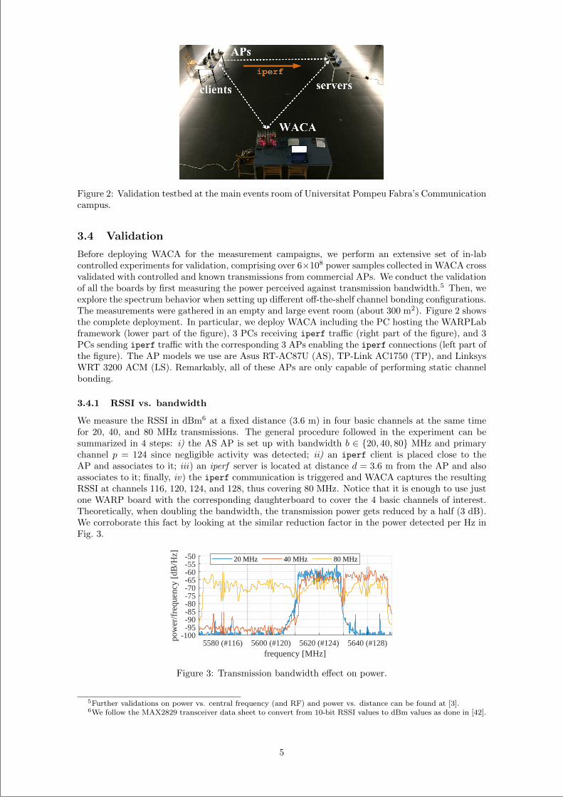
“main” — 2020/11/19 — 10:04 — page 192 — #214

Figure 2: Validation testbed at the main events room of Universitat Pompeu Fabra’s Communicationcampus.

3.4 Validation

Before deploying WACA for the measurement campaigns, we perform an extensive set of in-labcontrolled experiments for validation, comprising over 6×108 power samples collected in WACA crossvalidated with controlled and known transmissions from commercial APs. We conduct the validationof all the boards by first measuring the power perceived against transmission bandwidth.5 Then, weexplore the spectrum behavior when setting up different off-the-shelf channel bonding configurations.The measurements were gathered in an empty and large event room (about 300 m2). Figure 2 showsthe complete deployment. In particular, we deploy WACA including the PC hosting the WARPLabframework (lower part of the figure), 3 PCs receiving iperf traffic (right part of the figure), and 3PCs sending iperf traffic with the corresponding 3 APs enabling the iperf connections (left part ofthe figure). The AP models we use are Asus RT-AC87U (AS), TP-Link AC1750 (TP), and LinksysWRT 3200 ACM (LS). Remarkably, all of these APs are only capable of performing static channelbonding.

3.4.1 RSSI vs. bandwidth

We measure the RSSI in dBm6 at a fixed distance (3.6 m) in four basic channels at the same timefor 20, 40, and 80 MHz transmissions. The general procedure followed in the experiment can besummarized in 4 steps: i) the AS AP is set up with bandwidth b ∈ 20, 40, 80 MHz and primarychannel p = 124 since negligible activity was detected; ii) an iperf client is placed close to theAP and associates to it; iii) an iperf server is located at distance d = 3.6 m from the AP and alsoassociates to it; finally, iv) the iperf communication is triggered and WACA captures the resultingRSSI at channels 116, 120, 124, and 128, thus covering 80 MHz. Notice that it is enough to use justone WARP board with the corresponding daughterboard to cover the 4 basic channels of interest.Theoretically, when doubling the bandwidth, the transmission power gets reduced by a half (3 dB).We corroborate this fact by looking at the similar reduction factor in the power detected per Hz inFig. 3.

5580 (#116) 5600 (#120) 5620 (#124) 5640 (#128)frequency [MHz]

-100-95-90-85-80-75-70-65-60-55-50

pow

er/f

requ

ency

[dB

/Hz]

20 MHz 40 MHz 80 MHz

Figure 3: Transmission bandwidth effect on power.

5Further validations on power vs. central frequency (and RF) and power vs. distance can be found at [3].6We follow the MAX2829 transceiver data sheet to convert from 10-bit RSSI values to dBm values as done in [42].

5

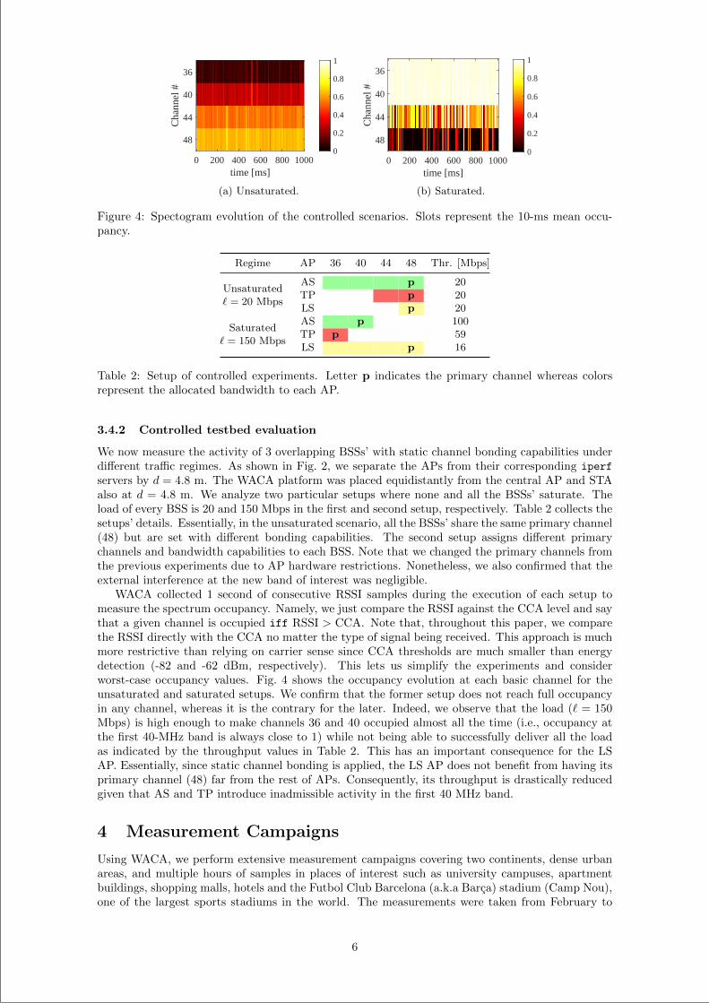
“main” — 2020/11/19 — 10:04 — page 193 — #215

0 200 400 600 800 1000time [ms]

36

40

44

48

Cha

nnel

#

0

0.2

0.4

0.6

0.8

1

(a) Unsaturated.

0 200 400 600 800 1000time [ms]

36

40

44

48

Cha

nnel

#

0

0.2

0.4

0.6

0.8

1

(b) Saturated.

Figure 4: Spectogram evolution of the controlled scenarios. Slots represent the 10-ms mean occu-pancy.

Regime AP 36 40 44 48 Thr. [Mbps]

AS p 20TP p 20

Unsaturated` = 20 Mbps

LS p 20AS p 100TP p 59

Saturated` = 150 Mbps

LS p 16

Table 2: Setup of controlled experiments. Letter p indicates the primary channel whereas colorsrepresent the allocated bandwidth to each AP.

3.4.2 Controlled testbed evaluation

We now measure the activity of 3 overlapping BSSs’ with static channel bonding capabilities underdifferent traffic regimes. As shown in Fig. 2, we separate the APs from their corresponding iperf

servers by d = 4.8 m. The WACA platform was placed equidistantly from the central AP and STAalso at d = 4.8 m. We analyze two particular setups where none and all the BSSs’ saturate. Theload of every BSS is 20 and 150 Mbps in the first and second setup, respectively. Table 2 collects thesetups’ details. Essentially, in the unsaturated scenario, all the BSSs’ share the same primary channel(48) but are set with different bonding capabilities. The second setup assigns different primarychannels and bandwidth capabilities to each BSS. Note that we changed the primary channels fromthe previous experiments due to AP hardware restrictions. Nonetheless, we also confirmed that theexternal interference at the new band of interest was negligible.

WACA collected 1 second of consecutive RSSI samples during the execution of each setup tomeasure the spectrum occupancy. Namely, we just compare the RSSI against the CCA level and saythat a given channel is occupied iff RSSI > CCA. Note that, throughout this paper, we comparethe RSSI directly with the CCA no matter the type of signal being received. This approach is muchmore restrictive than relying on carrier sense since CCA thresholds are much smaller than energydetection (-82 and -62 dBm, respectively). This lets us simplify the experiments and considerworst-case occupancy values. Fig. 4 shows the occupancy evolution at each basic channel for theunsaturated and saturated setups. We confirm that the former setup does not reach full occupancyin any channel, whereas it is the contrary for the later. Indeed, we observe that the load (` = 150Mbps) is high enough to make channels 36 and 40 occupied almost all the time (i.e., occupancy atthe first 40-MHz band is always close to 1) while not being able to successfully deliver all the loadas indicated by the throughput values in Table 2. This has an important consequence for the LSAP. Essentially, since static channel bonding is applied, the LS AP does not benefit from having itsprimary channel (48) far from the rest of APs. Consequently, its throughput is drastically reducedgiven that AS and TP introduce inadmissible activity in the first 40 MHz band.

4 Measurement Campaigns

Using WACA, we perform extensive measurement campaigns covering two continents, dense urbanareas, and multiple hours of samples in places of interest such as university campuses, apartmentbuildings, shopping malls, hotels and the Futbol Club Barcelona (a.k.a Barca) stadium (Camp Nou),one of the largest sports stadiums in the world. The measurements were taken from February to

6

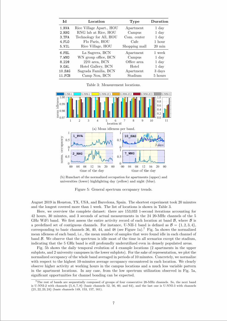
“main” — 2020/11/19 — 10:04 — page 194 — #216

Id Location Type Duration

1 RVA Rice Village Apart., HOU Apartment 1 day2 RNG RNG lab at Rice, HOU Campus 1 day3 TFA Technology for All, HOU Com. center 1 day4 FLO Flo Paris, HOU Cafe 1 hour5 VIL Rice Village, HOU Shopping mall 20 min

6 FEL La Sagrera, BCN Apartment 1 week7 WNO WN group office, BCN Campus 1 day8 22@ 22@ area, BCN Office area 1 day9 GAL Hotel Gallery, BCN Hotel 1 day10 SAG Sagrada Familia, BCN Apartment 3 days11 FCB Camp Nou, BCN Stadium 5 hours

Table 3: Measurement locations.

1 2 3 4 5 6 7 8 9 100.97

0.98

0.99

1.00

110.00.20.40.60.81.0

U-NII-1 U-NNI-2 U-NNI-2C1 U-NNI-2C2 U-NNI-2C3 U-NNI-3

(a) Mean idleness per band.

(b) Runchart of the normalized occupation for apartments (upper) anduniversities (lower) highlighting day (yellow) and night (blue).

Figure 5: General spectrum occupancy trends.

August 2019 in Houston, TX, USA, and Barcelona, Spain. The shortest experiment took 20 minutesand the longest covered more than 1 week. The list of locations is shown in Table 3.

Here, we overview the complete dataset: there are 153,033 1-second iterations accounting for42 hours, 30 minutes, and 3 seconds of actual measurements in the 24 20-MHz channels of the 5GHz WiFi band. We first assess the entire activity record of each location at band B, where B isa predefined set of contiguous channels. For instance, U-NII-1 band is defined as B = 1, 2, 3, 4,corresponding to basic channels 36, 40, 44, and 48 (see Figure 1a).7 Fig. 5a shows the normalizedmean idleness of each band, i.e., the mean number of samples that were found idle in each channel ofband B. We observe that the spectrum is idle most of the time in all scenarios except the stadium,indicating that the 5 GHz band is still profoundly underutilized even in densely populated areas.

Fig. 5b shows the daily temporal evolution of 4 example locations (2 apartments in the uppersubplots, and 2 university campuses in the lower subplots). For the sake of representation, we plot thenormalized occupancy of the whole band averaged in periods of 10 minutes. Concretely, we normalizewith respect to the highest 10-minutes average occupancy encountered in each location. We clearlyobserve higher activity at working hours in the campus locations and a much less variable patternin the apartment locations. In any case, from the low spectrum utilization observed in Fig. 5a,significant opportunities for channel bonding can be expected.

7The rest of bands are sequentially composed of groups of four consecutive 20-MHz channels. So, the next bandis U-NNI-2 with channels 5, 6, 7, 8 (basic channels 52, 56, 60, and 64), and the last one is U-NNI-3 with channels21, 22, 23, 24 (basic channels 149, 153, 157, 161).

7

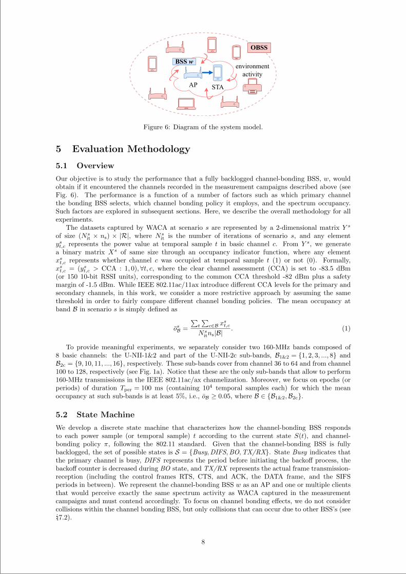
“main” — 2020/11/19 — 10:04 — page 195 — #217

STAAP

environmentactivity

BSSw

OBSS

Figure 6: Diagram of the system model.

5 Evaluation Methodology

5.1 Overview

Our objective is to study the performance that a fully backlogged channel-bonding BSS, w, wouldobtain if it encountered the channels recorded in the measurement campaigns described above (seeFig. 6). The performance is a function of a number of factors such as which primary channelthe bonding BSS selects, which channel bonding policy it employs, and the spectrum occupancy.Such factors are explored in subsequent sections. Here, we describe the overall methodology for allexperiments.

The datasets captured by WACA at scenario s are represented by a 2-dimensional matrix Y s

of size (Nsit × ns) × |R|, where Ns

it is the number of iterations of scenario s, and any elementyst,c represents the power value at temporal sample t in basic channel c. From Y s, we generatea binary matrix Xs of same size through an occupancy indicator function, where any elementxst,c represents whether channel c was occupied at temporal sample t (1) or not (0). Formally,xst,c = (yst,c > CCA : 1, 0),∀t, c, where the clear channel assessment (CCA) is set to -83.5 dBm(or 150 10-bit RSSI units), corresponding to the common CCA threshold -82 dBm plus a safetymargin of -1.5 dBm. While IEEE 802.11ac/11ax introduce different CCA levels for the primary andsecondary channels, in this work, we consider a more restrictive approach by assuming the samethreshold in order to fairly compare different channel bonding policies. The mean occupancy atband B in scenario s is simply defined as

osB =

∑t

∑c∈B x

st,c

Nsitns|B|

. (1)

To provide meaningful experiments, we separately consider two 160-MHz bands composed of8 basic channels: the U-NII-1&2 and part of the U-NII-2c sub-bands, B1&2 = 1, 2, 3, ..., 8 andB2c = 9, 10, 11, ..., 16, respectively. These sub-bands cover from channel 36 to 64 and from channel100 to 128, respectively (see Fig. 1a). Notice that these are the only sub-bands that allow to perform160-MHz transmissions in the IEEE 802.11ac/ax channelization. Moreover, we focus on epochs (orperiods) of duration Tper = 100 ms (containing 104 temporal samples each) for which the meanoccupancy at such sub-bands is at least 5%, i.e., oB ≥ 0.05, where B ∈ B1&2,B2c.

5.2 State Machine

We develop a discrete state machine that characterizes how the channel-bonding BSS respondsto each power sample (or temporal sample) t according to the current state S(t), and channel-bonding policy π, following the 802.11 standard. Given that the channel-bonding BSS is fullybacklogged, the set of possible states is S = Busy,DIFS,BO,TX/RX. State Busy indicates thatthe primary channel is busy, DIFS represents the period before initiating the backoff process, thebackoff counter is decreased during BO state, and TX/RX represents the actual frame transmission-reception (including the control frames RTS, CTS, and ACK, the DATA frame, and the SIFSperiods in between). We represent the channel-bonding BSS w as an AP and one or multiple clientsthat would perceive exactly the same spectrum activity as WACA captured in the measurementcampaigns and must contend accordingly. To focus on channel bonding effects, we do not considercollisions within the channel bonding BSS, but only collisions that can occur due to other BSS’s (see§7.2).

8

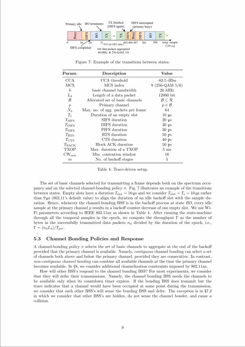
“main” — 2020/11/19 — 10:04 — page 196 — #218

TXBusy

DIFS

BO

TX ...

Busy

DIFS

DIFS

BO

Primaryidle BOterminates TXfinished(DIFSagain)

DIFSinterrupted(primarybusy)

...

temp.samplet[10μs]

TX

0 20 24 31 492

x64datapacketsaggregated40MHz&256-QAM,5/6

494 497 501 5084.61ms(461sam.)

DIFScompleted

Figure 7: Example of the transitions between states.

Param. Description Value

CCA CCA threshold -83.5 dBmMCS MCS index 9 (256-QAM 5/6)b basic channel bandwidth 20 MHzLd Length of a data packet 12000 bitB Allocated set of basic channels B ⊆ Rp Primary channel p ∈ BNa Max. no. of agg. packets per frame 64Te Duration of an empty slot 10 µs

TSIFS SIFS duration 20 µsTDIFS DIFS duration 30 µsTPIFS PIFS duration 30 µsTRTS RTS duration 50 µsTCTS CTS duration 40 µsTBACK Block ACK duration 50 µsTXOP Max. duration of a TXOP 5 msCWmin Min. contention window 16m No. of backoff stages 5

Table 4: Trace-driven setup.

The set of basic channels selected for transmitting a frame depends both on the spectrum occu-pancy and on the selected channel-bonding policy π. Fig. 7 illustrates an example of the transitionsbetween states. Empty slots have a duration Tslot = 10µs and we consider Tslot = Ts = 10µs ratherthan 9 µs (802.11’s default value) to align the duration of an idle backoff slot with the sample du-ration. Hence, whenever the channel-bonding BSS is in the backoff process at state BO, every idlesample at the primary channel p results in a backoff counter decrease of one empty slot. We use Wi-Fi parameters according to IEEE 802.11ax as shown in Table 4. After running the state-machinethrough all the temporal samples in the epoch, we compute the throughput Γ as the number ofbytes in the successfully transmitted data packets nd divided by the duration of the epoch, i.e.,Γ = (ndLd)/Tper.

5.3 Channel Bonding Policies and Response

A channel-bonding policy π selects the set of basic channels to aggregate at the end of the backoffprovided that the primary channel is available. Namely, contiguous channel bonding can select a setof channels both above and below the primary channel, provided they are consecutive. In contrast,non-contiguous channel bonding can combine all available channels at the time the primary channelbecomes available. In §8, we consider additional channelization constraints imposed by 802.11ax.

How will other BSS’s respond to the channel bonding BSS? For most experiments, we considerthat they will defer their transmissions. Namely, the channel bonding BSS needs the channels tobe available only when its countdown timer expires. If the bonding BSS does transmit but thetrace indicates that a channel would have been occupied at some point during the transmission,we consider that such other BSS’s will sense the bonding BSS and defer. The exception is in §7.2in which we consider that other BSS’s are hidden, do not sense the channel bonder, and cause acollision.

9

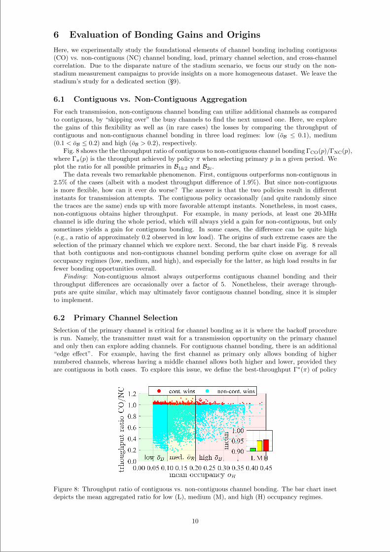
“main” — 2020/11/19 — 10:04 — page 197 — #219

6 Evaluation of Bonding Gains and Origins

Here, we experimentally study the foundational elements of channel bonding including contiguous(CO) vs. non-contiguous (NC) channel bonding, load, primary channel selection, and cross-channelcorrelation. Due to the disparate nature of the stadium scenario, we focus our study on the non-stadium measurement campaigns to provide insights on a more homogeneous dataset. We leave thestadium’s study for a dedicated section (§9).

6.1 Contiguous vs. Non-Contiguous Aggregation

For each transmission, non-contiguous channel bonding can utilize additional channels as comparedto contiguous, by “skipping over” the busy channels to find the next unused one. Here, we explorethe gains of this flexibility as well as (in rare cases) the losses by comparing the throughput ofcontiguous and non-contiguous channel bonding in three load regimes: low (oB ≤ 0.1), medium(0.1 < oB ≤ 0.2) and high (oB > 0.2), respectively.

Fig. 8 shows the the throughput ratio of contiguous to non-contiguous channel bonding ΓCO(p)/ΓNC(p),where Γπ(p) is the throughput achieved by policy π when selecting primary p in a given period. Weplot the ratio for all possible primaries in B1&2 and B2c.

The data reveals two remarkable phenomenon. First, contiguous outperforms non-contiguous in2.5% of the cases (albeit with a modest throughput difference of 1.9%). But since non-contiguousis more flexible, how can it ever do worse? The answer is that the two policies result in differentinstants for transmission attempts. The contiguous policy occasionally (and quite randomly sincethe traces are the same) ends up with more favorable attempt instants. Nonetheless, in most cases,non-contiguous obtains higher throughput. For example, in many periods, at least one 20-MHzchannel is idle during the whole period, which will always yield a gain for non-contiguous, but onlysometimes yields a gain for contiguous bonding. In some cases, the difference can be quite high(e.g., a ratio of approximately 0.2 observed in low load). The origins of such extreme cases are theselection of the primary channel which we explore next. Second, the bar chart inside Fig. 8 revealsthat both contiguous and non-contiguous channel bonding perform quite close on average for alloccupancy regimes (low, medium, and high), and especially for the latter, as high load results in farfewer bonding opportunities overall.

Finding : Non-contiguous almost always outperforms contiguous channel bonding and theirthroughput differences are occasionally over a factor of 5. Nonetheless, their average through-puts are quite similar, which may ultimately favor contiguous channel bonding, since it is simplerto implement.

6.2 Primary Channel Selection

Selection of the primary channel is critical for channel bonding as it is where the backoff procedureis run. Namely, the transmitter must wait for a transmission opportunity on the primary channeland only then can explore adding channels. For contiguous channel bonding, there is an additional“edge effect”. For example, having the first channel as primary only allows bonding of highernumbered channels, whereas having a middle channel allows both higher and lower, provided theyare contiguous in both cases. To explore this issue, we define the best-throughput Γ∗(π) of policy

Figure 8: Throughput ratio of contiguous vs. non-contiguous channel bonding. The bar chart insetdepicts the mean aggregated ratio for low (L), medium (M), and high (H) occupancy regimes.

10

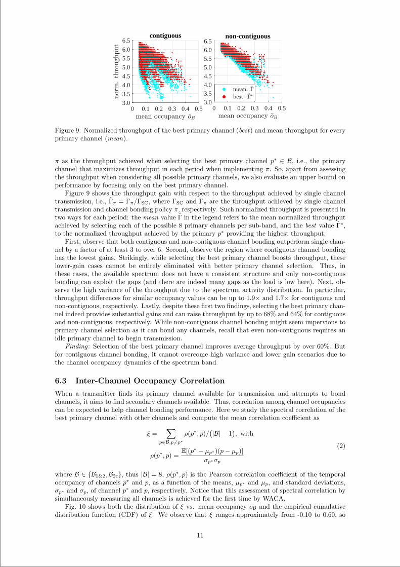
“main” — 2020/11/19 — 10:04 — page 198 — #220

0 0.1 0.2 0.3 0.4 0.53.0

3.5

4.0

4.5

5.0

5.5

6.0

6.5contiguous

0 0.1 0.2 0.3 0.4 0.53.03.54.04.55.05.56.06.5

non-contiguous

Figure 9: Normalized throughput of the best primary channel (best) and mean throughput for everyprimary channel (mean).

π as the throughput achieved when selecting the best primary channel p∗ ∈ B, i.e., the primarychannel that maximizes throughput in each period when implementing π. So, apart from assessingthe throughput when considering all possible primary channels, we also evaluate an upper bound onperformance by focusing only on the best primary channel.

Figure 9 shows the throughput gain with respect to the throughput achieved by single channeltransmission, i.e., Γπ = Γπ/ΓSC, where ΓSC and Γπ are the throughput achieved by single channeltransmission and channel bonding policy π, respectively. Such normalized throughput is presented intwo ways for each period: the mean value Γ in the legend refers to the mean normalized throughputachieved by selecting each of the possible 8 primary channels per sub-band, and the best value Γ∗,to the normalized throughput achieved by the primary p∗ providing the highest throughput.

First, observe that both contiguous and non-contiguous channel bonding outperform single chan-nel by a factor of at least 3 to over 6. Second, observe the region where contiguous channel bondinghas the lowest gains. Strikingly, while selecting the best primary channel boosts throughput, theselower-gain cases cannot be entirely eliminated with better primary channel selection. Thus, inthese cases, the available spectrum does not have a consistent structure and only non-contiguousbonding can exploit the gaps (and there are indeed many gaps as the load is low here). Next, ob-serve the high variance of the throughput due to the spectrum activity distribution. In particular,throughput differences for similar occupancy values can be up to 1.9× and 1.7× for contiguous andnon-contiguous, respectively. Lastly, despite these first two findings, selecting the best primary chan-nel indeed provides substantial gains and can raise throughput by up to 68% and 64% for contiguousand non-contiguous, respectively. While non-contiguous channel bonding might seem impervious toprimary channel selection as it can bond any channels, recall that even non-contiguous requires anidle primary channel to begin transmission.

Finding : Selection of the best primary channel improves average throughput by over 60%. Butfor contiguous channel bonding, it cannot overcome high variance and lower gain scenarios due tothe channel occupancy dynamics of the spectrum band.

6.3 Inter-Channel Occupancy Correlation

When a transmitter finds its primary channel available for transmission and attempts to bondchannels, it aims to find secondary channels available. Thus, correlation among channel occupanciescan be expected to help channel bonding performance. Here we study the spectral correlation of thebest primary channel with other channels and compute the mean correlation coefficient as

ξ =∑

p∈B,p6=p∗ρ(p∗, p)/

(|B| − 1

), with

ρ(p∗, p) =E[(p∗ − µp∗)(p− µp)]

σp∗σp

(2)

where B ∈ B1&2,B2c, thus |B| = 8, ρ(p∗, p) is the Pearson correlation coefficient of the temporaloccupancy of channels p∗ and p, as a function of the means, µp∗ and µp, and standard deviations,σp∗ and σp, of channel p∗ and p, respectively. Notice that this assessment of spectral correlation bysimultaneously measuring all channels is achieved for the first time by WACA.

Fig. 10 shows both the distribution of ξ vs. mean occupancy oB and the empirical cumulativedistribution function (CDF) of ξ. We observe that ξ ranges approximately from -0.10 to 0.60, so

11

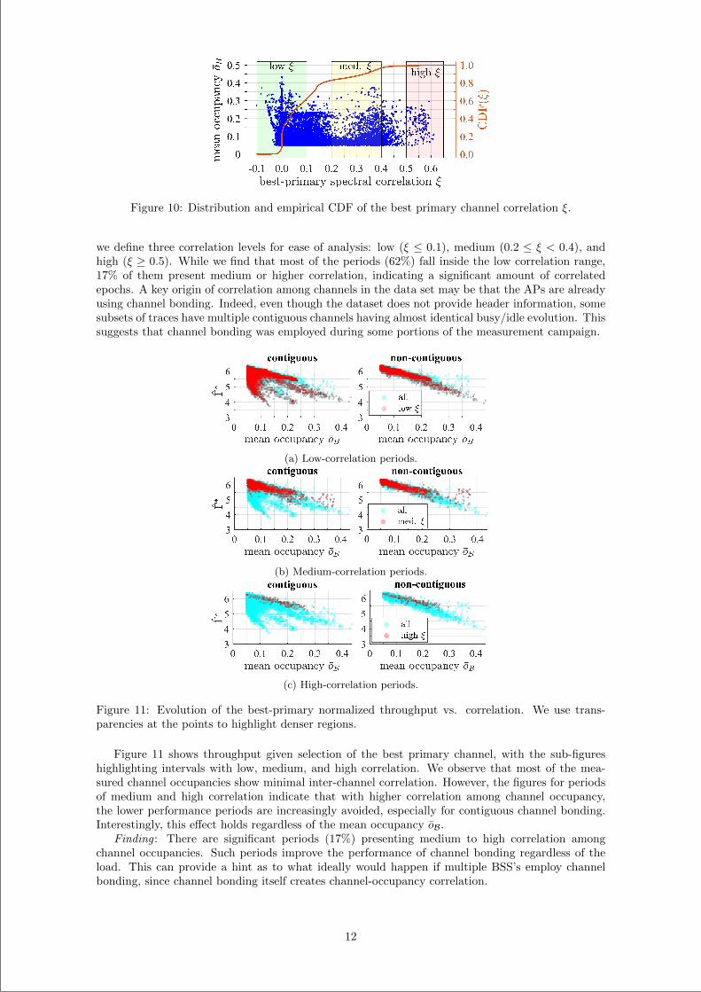
“main” — 2020/11/19 — 10:04 — page 199 — #221

Figure 10: Distribution and empirical CDF of the best primary channel correlation ξ.

we define three correlation levels for ease of analysis: low (ξ ≤ 0.1), medium (0.2 ≤ ξ < 0.4), andhigh (ξ ≥ 0.5). While we find that most of the periods (62%) fall inside the low correlation range,17% of them present medium or higher correlation, indicating a significant amount of correlatedepochs. A key origin of correlation among channels in the data set may be that the APs are alreadyusing channel bonding. Indeed, even though the dataset does not provide header information, somesubsets of traces have multiple contiguous channels having almost identical busy/idle evolution. Thissuggests that channel bonding was employed during some portions of the measurement campaign.

(a) Low-correlation periods.

(b) Medium-correlation periods.

(c) High-correlation periods.

Figure 11: Evolution of the best-primary normalized throughput vs. correlation. We use trans-parencies at the points to highlight denser regions.

Figure 11 shows throughput given selection of the best primary channel, with the sub-figureshighlighting intervals with low, medium, and high correlation. We observe that most of the mea-sured channel occupancies show minimal inter-channel correlation. However, the figures for periodsof medium and high correlation indicate that with higher correlation among channel occupancy,the lower performance periods are increasingly avoided, especially for contiguous channel bonding.Interestingly, this effect holds regardless of the mean occupancy oB.

Finding : There are significant periods (17%) presenting medium to high correlation amongchannel occupancies. Such periods improve the performance of channel bonding regardless of theload. This can provide a hint as to what ideally would happen if multiple BSS’s employ channelbonding, since channel bonding itself creates channel-occupancy correlation.

12

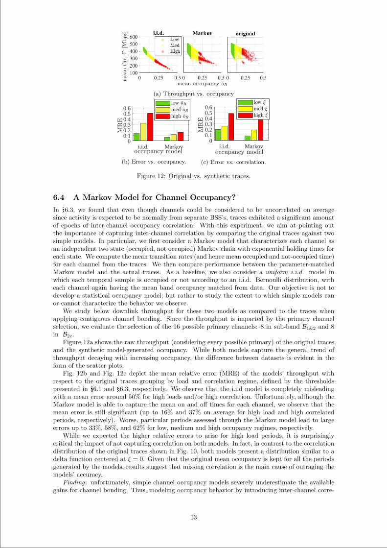
“main” — 2020/11/19 — 10:04 — page 200 — #222

(a) Throughput vs. occupancy

i.i.d. Markov0

0.10.20.30.40.50.6

(b) Error vs. occupancy.

i.i.d. Markov0

0.10.20.30.40.50.6

(c) Error vs. correlation.

Figure 12: Original vs. synthetic traces.

6.4 A Markov Model for Channel Occupancy?

In §6.3, we found that even though channels could be considered to be uncorrelated on averagesince activity is expected to be normally from separate BSS’s, traces exhibited a significant amountof epochs of inter-channel occupancy correlation. With this experiment, we aim at pointing outthe importance of capturing inter-channel correlation by comparing the original traces against twosimple models. In particular, we first consider a Markov model that characterizes each channel asan independent two state (occupied, not occupied) Markov chain with exponential holding times foreach state. We compute the mean transition rates (and hence mean occupied and not-occupied time)for each channel from the traces. We then compare performance between the parameter-matchedMarkov model and the actual traces. As a baseline, we also consider a uniform i.i.d. model inwhich each temporal sample is occupied or not according to an i.i.d. Bernoulli distribution, witheach channel again having the mean band occupancy matched from data. Our objective is not todevelop a statistical occupancy model, but rather to study the extent to which simple models canor cannot characterize the behavior we observe.

We study below downlink throughput for these two models as compared to the traces whenapplying contiguous channel bonding. Since the throughput is impacted by the primary channelselection, we evaluate the selection of the 16 possible primary channels: 8 in sub-band B1&2 and 8in B2c.

Figure 12a shows the raw throughput (considering every possible primary) of the original tracesand the synthetic model-generated occupancy. While both models capture the general trend ofthroughput decaying with increasing occupancy, the difference between datasets is evident in theform of the scatter plots.

Fig. 12b and Fig. 12c depict the mean relative error (MRE) of the models’ throughput withrespect to the original traces grouping by load and correlation regime, defined by the thresholdspresented in §6.1 and §6.3, respectively. We observe that the i.i.d model is completely misleadingwith a mean error around 50% for high loads and/or high correlation. Unfortunately, although theMarkov model is able to capture the mean on and off times for each channel, we observe that themean error is still significant (up to 16% and 37% on average for high load and high correlatedperiods, respectively). Worse, particular periods assessed through the Markov model lead to largeerrors up to 33%, 58%, and 62% for low, medium and high occupancy regimes, respectively.

While we expected the higher relative errors to arise for high load periods, it is surprisinglycritical the impact of not capturing correlation on both models. In fact, in contrast to the correlationdistribution of the original traces shown in Fig. 10, both models present a distribution similar to adelta function centered at ξ = 0. Given that the original mean occupancy is kept for all the periodsgenerated by the models, results suggest that missing correlation is the main cause of outraging themodels’ accuracy.

Finding : unfortunately, simple channel occupancy models severely underestimate the availablegains for channel bonding. Thus, modeling occupancy behavior by introducing inter-channel corre-

13

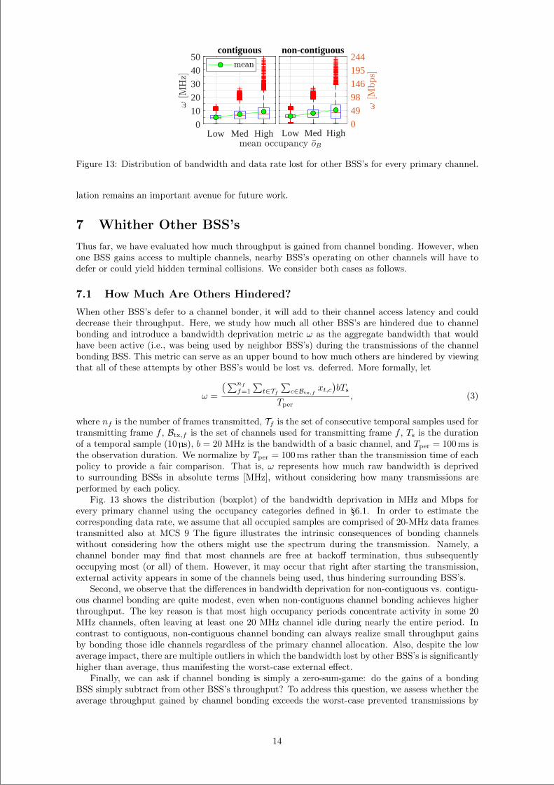
“main” — 2020/11/19 — 10:04 — page 201 — #223

Low Med High0

10

20

30

40

50contiguous

Low Med High0

49

98

146

195

244non-contiguous

Figure 13: Distribution of bandwidth and data rate lost for other BSS’s for every primary channel.

lation remains an important avenue for future work.

7 Whither Other BSS’s

Thus far, we have evaluated how much throughput is gained from channel bonding. However, whenone BSS gains access to multiple channels, nearby BSS’s operating on other channels will have todefer or could yield hidden terminal collisions. We consider both cases as follows.

7.1 How Much Are Others Hindered?

When other BSS’s defer to a channel bonder, it will add to their channel access latency and coulddecrease their throughput. Here, we study how much all other BSS’s are hindered due to channelbonding and introduce a bandwidth deprivation metric ω as the aggregate bandwidth that wouldhave been active (i.e., was being used by neighbor BSS’s) during the transmissions of the channelbonding BSS. This metric can serve as an upper bound to how much others are hindered by viewingthat all of these attempts by other BSS’s would be lost vs. deferred. More formally, let

ω =

(∑nf

f=1

∑t∈Tf

∑c∈Btx,f

xt,c)bTs

Tper, (3)

where nf is the number of frames transmitted, Tf is the set of consecutive temporal samples used fortransmitting frame f , Btx,f is the set of channels used for transmitting frame f , Ts is the durationof a temporal sample (10µs), b = 20 MHz is the bandwidth of a basic channel, and Tper = 100 ms isthe observation duration. We normalize by Tper = 100 ms rather than the transmission time of eachpolicy to provide a fair comparison. That is, ω represents how much raw bandwidth is deprivedto surrounding BSSs in absolute terms [MHz], without considering how many transmissions areperformed by each policy.

Fig. 13 shows the distribution (boxplot) of the bandwidth deprivation in MHz and Mbps forevery primary channel using the occupancy categories defined in §6.1. In order to estimate thecorresponding data rate, we assume that all occupied samples are comprised of 20-MHz data framestransmitted also at MCS 9 The figure illustrates the intrinsic consequences of bonding channelswithout considering how the others might use the spectrum during the transmission. Namely, achannel bonder may find that most channels are free at backoff termination, thus subsequentlyoccupying most (or all) of them. However, it may occur that right after starting the transmission,external activity appears in some of the channels being used, thus hindering surrounding BSS’s.

Second, we observe that the differences in bandwidth deprivation for non-contiguous vs. contigu-ous channel bonding are quite modest, even when non-contiguous channel bonding achieves higherthroughput. The key reason is that most high occupancy periods concentrate activity in some 20MHz channels, often leaving at least one 20 MHz channel idle during nearly the entire period. Incontrast to contiguous, non-contiguous channel bonding can always realize small throughput gainsby bonding those idle channels regardless of the primary channel allocation. Also, despite the lowaverage impact, there are multiple outliers in which the bandwidth lost by other BSS’s is significantlyhigher than average, thus manifesting the worst-case external effect.

Finally, we can ask if channel bonding is simply a zero-sum-game: do the gains of a bondingBSS simply subtract from other BSS’s throughput? To address this question, we assess whether theaverage throughput gained by channel bonding exceeds the worst-case prevented transmissions by

14

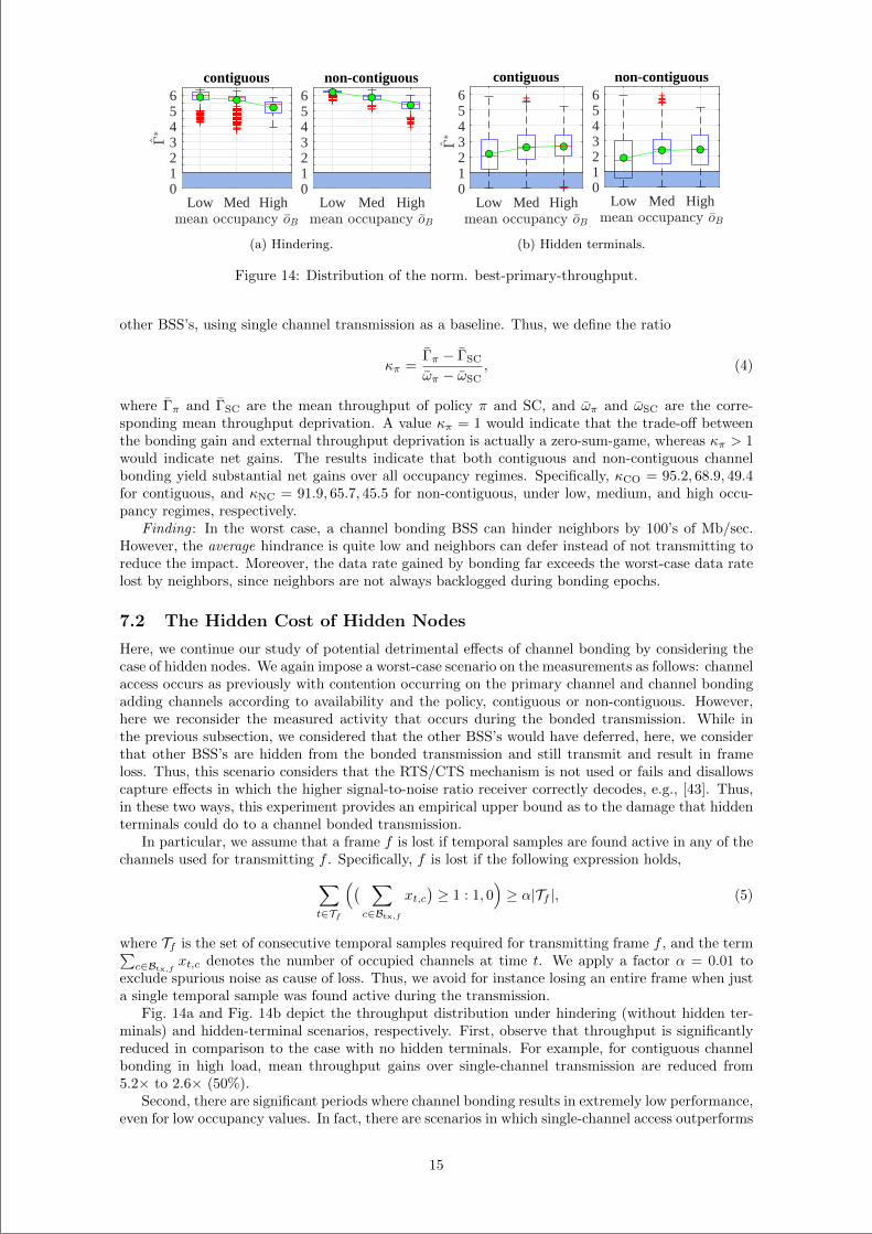
“main” — 2020/11/19 — 10:04 — page 202 — #224

Low Med High0123456

contiguous

Low Med High0123456

non-contiguous

(a) Hindering.

Low Med High0123456

contiguous

Low Med High0123456

non-contiguous

(b) Hidden terminals.

Figure 14: Distribution of the norm. best-primary-throughput.

other BSS’s, using single channel transmission as a baseline. Thus, we define the ratio

κπ =Γπ − ΓSC

ωπ − ωSC, (4)

where Γπ and ΓSC are the mean throughput of policy π and SC, and ωπ and ωSC are the corre-sponding mean throughput deprivation. A value κπ = 1 would indicate that the trade-off betweenthe bonding gain and external throughput deprivation is actually a zero-sum-game, whereas κπ > 1would indicate net gains. The results indicate that both contiguous and non-contiguous channelbonding yield substantial net gains over all occupancy regimes. Specifically, κCO = 95.2, 68.9, 49.4for contiguous, and κNC = 91.9, 65.7, 45.5 for non-contiguous, under low, medium, and high occu-pancy regimes, respectively.

Finding : In the worst case, a channel bonding BSS can hinder neighbors by 100’s of Mb/sec.However, the average hindrance is quite low and neighbors can defer instead of not transmitting toreduce the impact. Moreover, the data rate gained by bonding far exceeds the worst-case data ratelost by neighbors, since neighbors are not always backlogged during bonding epochs.

7.2 The Hidden Cost of Hidden Nodes

Here, we continue our study of potential detrimental effects of channel bonding by considering thecase of hidden nodes. We again impose a worst-case scenario on the measurements as follows: channelaccess occurs as previously with contention occurring on the primary channel and channel bondingadding channels according to availability and the policy, contiguous or non-contiguous. However,here we reconsider the measured activity that occurs during the bonded transmission. While inthe previous subsection, we considered that the other BSS’s would have deferred, here, we considerthat other BSS’s are hidden from the bonded transmission and still transmit and result in frameloss. Thus, this scenario considers that the RTS/CTS mechanism is not used or fails and disallowscapture effects in which the higher signal-to-noise ratio receiver correctly decodes, e.g., [43]. Thus,in these two ways, this experiment provides an empirical upper bound as to the damage that hiddenterminals could do to a channel bonded transmission.

In particular, we assume that a frame f is lost if temporal samples are found active in any of thechannels used for transmitting f . Specifically, f is lost if the following expression holds,

∑

t∈Tf

(( ∑

c∈Btx,f

xt,c)≥ 1 : 1, 0

)≥ α|Tf |, (5)

where Tf is the set of consecutive temporal samples required for transmitting frame f , and the term∑c∈Btx,f

xt,c denotes the number of occupied channels at time t. We apply a factor α = 0.01 toexclude spurious noise as cause of loss. Thus, we avoid for instance losing an entire frame when justa single temporal sample was found active during the transmission.

Fig. 14a and Fig. 14b depict the throughput distribution under hindering (without hidden ter-minals) and hidden-terminal scenarios, respectively. First, observe that throughput is significantlyreduced in comparison to the case with no hidden terminals. For example, for contiguous channelbonding in high load, mean throughput gains over single-channel transmission are reduced from5.2× to 2.6× (50%).

Second, there are significant periods where channel bonding results in extremely low performance,even for low occupancy values. In fact, there are scenarios in which single-channel access outperforms

15

“main” — 2020/11/19 — 10:04 — page 203 — #225

bonding (blue areas where Γ∗ < 1 in the figure). In particular, single channel outperforms contiguouschannel bonding in 18%, 8% and 8% of the cases for low, medium and high occupancy, respectively.Even worse, single channel outperforms non-contiguous channel bonding in 38%, 14%, and 15% ofcases respectively. This illustrates that external traffic patterns may lead to accentuated chances ofincurring collisions, thus impairing the performance of the channel bonder.

Third, due to its more aggressive nature, non-contiguous channel bonding performs slightly worsethan contiguous both in terms of average throughput and how often it is outperformed by singlechannel transmission. This, together with the fact that contiguous performs similarly on average tonon-contiguous without hidden terminals, indicates that gains provided by non-contiguous can berelatively small considering its greater risk and more complex design.

Finally, also in contrast to Fig. 14a, Fig. 14b indicates that the decaying trend of mean normalizedbest-throughput with load when neighbors defer does not hold with hidden terminals. Indeed, weobserve a slight increase of the normalized best-throughput as the occupancy increases as fewerbonding opportunities also diminish the risk of collisions.

Finding : While channel bonding outperforms single-channel transmission in most cases, it isvulnerable to hidden node interference, with non-contiguous channel bonding being impacted themost. To avoid the aforementioned worst-case throughput penalties, nodes can use RTS/CTS,implement capture (to better receive even while a hidden terminal transmission overlaps in time), orincrease channel sensing sensitivity, i.e., reduce the threshold for sensing channel activity to reducethe frequency of hidden terminal transmissions.

8 IEEE 802.11ax Constraints

Here, we consider additional constraints imposed by 802.11ax on channel bonding. Namely, 802.11axdefines three modes of channel bonding, each of which restrict channel bonding to a subset ofchannels [1]. For example, U-NNI-1 and U-NNI-2 restrict channel bonding groups to CB1&2

=1, 2, 3, 4, 5, 6, 7, 8, 1, 2, 3, 4, 5, 6, 7, 8, 1, ..., 8 so that (for example) a 40 MHz bondedchannel that combines channels 2 and 3 is not allowed. Notice that we do not use the IEEE 802.11channel indices (e.g., 36, 40, 44,...) in the example above for ease of exposition. While reducingthroughput when only a single BSS bonds, such restrictions can reduce fragmentation if multipleBSS’s bond. Moreover, such restrictions simplify implementation. Thus, here we study the cost of802.11ax’s channelization restrictions when a single BSS bonds and compare to the non-restrictedcases explored this far.

Static Channel Bonding (SCB): employs a fixed channel width and therefore must alwaysuse the same set of channels. It can be viewed as an“all-or-nothing” policy: for example, if staticchannel bonding uses 8 consecutive basic channels (160 MHz), it must wait until all 8 channels arefree in order to transmit using the entire 160 MHz. Although simple to implement, it is vulnerableto excessive deferral while waiting for all channels to become available.

Dynamic Channel Bonding (DCB): picks the largest available set of contiguous basic chan-nels found free subject to both the primary channel being included and the total set of channelsbeing an allowed set under the restrictions such as above. For example, if channel 4 is selectedas a primary channel, dynamic channel bonding allows bonded transmissions with channels 3, 4,1, 2, 3, 4, or 1, ..., 8, as well as single channel transmission on channel 4. Other combinationssuch as 4, 5 are not permitted.

Preamble Puncturing (PP): allows puncturing wide channels, i.e., aggregating non-contiguous basic channels. Even though the total channel is still subjected to the above chan-nelization constraints, preamble puncturing is more flexible than dynamic channel bonding since itenables non-contiguous channel combinations, provided the primary channel is included [1, 44]. Forexample, a transmission using primary channel 3 could transmit on 60 MHz using channels 1, 3, 4,which would be a punctured subset of 1, 2, 3, 4. Nonetheless, not every combination of puncturedchannels is allowed in the standard. For instance, 1, 3 is not permitted.

Observe that both static and dynamic channel bonding are restricted special cases of contiguouschannel bonding studied previously, whereas preamble puncturing is a restricted special case ofnon-contiguous channel bonding.

Here, we compare the throughput of both the (non-restricted) contiguous and non-contiguouspolices with the three 802.11ax policies, all using selection of the best primary channel. Fig. 15 showsthe resulting 802.11ax throughput normalized to the unrestricted case for the respective category ofcontiguous or non-contiguous.

First, observe that 802.11ax static channel bonding suffers severe throughput degradation com-

16

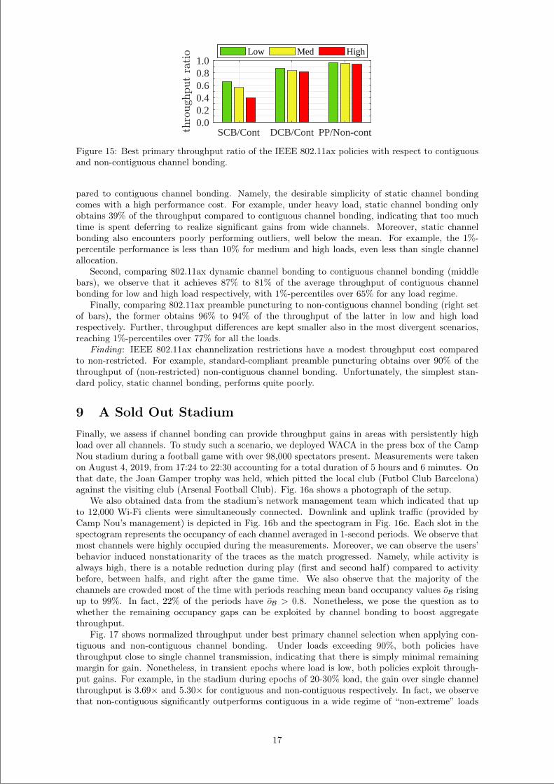
“main” — 2020/11/19 — 10:04 — page 204 — #226

SCB/Cont DCB/Cont PP/Non-cont0.00.20.40.60.81.0

Low Med High

Figure 15: Best primary throughput ratio of the IEEE 802.11ax policies with respect to contiguousand non-contiguous channel bonding.

pared to contiguous channel bonding. Namely, the desirable simplicity of static channel bondingcomes with a high performance cost. For example, under heavy load, static channel bonding onlyobtains 39% of the throughput compared to contiguous channel bonding, indicating that too muchtime is spent deferring to realize significant gains from wide channels. Moreover, static channelbonding also encounters poorly performing outliers, well below the mean. For example, the 1%-percentile performance is less than 10% for medium and high loads, even less than single channelallocation.

Second, comparing 802.11ax dynamic channel bonding to contiguous channel bonding (middlebars), we observe that it achieves 87% to 81% of the average throughput of contiguous channelbonding for low and high load respectively, with 1%-percentiles over 65% for any load regime.

Finally, comparing 802.11ax preamble puncturing to non-contiguous channel bonding (right setof bars), the former obtains 96% to 94% of the throughput of the latter in low and high loadrespectively. Further, throughput differences are kept smaller also in the most divergent scenarios,reaching 1%-percentiles over 77% for all the loads.

Finding : IEEE 802.11ax channelization restrictions have a modest throughput cost comparedto non-restricted. For example, standard-compliant preamble puncturing obtains over 90% of thethroughput of (non-restricted) non-contiguous channel bonding. Unfortunately, the simplest stan-dard policy, static channel bonding, performs quite poorly.

9 A Sold Out Stadium

Finally, we assess if channel bonding can provide throughput gains in areas with persistently highload over all channels. To study such a scenario, we deployed WACA in the press box of the CampNou stadium during a football game with over 98,000 spectators present. Measurements were takenon August 4, 2019, from 17:24 to 22:30 accounting for a total duration of 5 hours and 6 minutes. Onthat date, the Joan Gamper trophy was held, which pitted the local club (Futbol Club Barcelona)against the visiting club (Arsenal Football Club). Fig. 16a shows a photograph of the setup.

We also obtained data from the stadium’s network management team which indicated that upto 12,000 Wi-Fi clients were simultaneously connected. Downlink and uplink traffic (provided byCamp Nou’s management) is depicted in Fig. 16b and the spectogram in Fig. 16c. Each slot in thespectogram represents the occupancy of each channel averaged in 1-second periods. We observe thatmost channels were highly occupied during the measurements. Moreover, we can observe the users’behavior induced nonstationarity of the traces as the match progressed. Namely, while activity isalways high, there is a notable reduction during play (first and second half) compared to activitybefore, between halfs, and right after the game time. We also observe that the majority of thechannels are crowded most of the time with periods reaching mean band occupancy values oB risingup to 99%. In fact, 22% of the periods have oB > 0.8. Nonetheless, we pose the question as towhether the remaining occupancy gaps can be exploited by channel bonding to boost aggregatethroughput.

Fig. 17 shows normalized throughput under best primary channel selection when applying con-tiguous and non-contiguous channel bonding. Under loads exceeding 90%, both policies havethroughput close to single channel transmission, indicating that there is simply minimal remainingmargin for gain. Nonetheless, in transient epochs where load is low, both policies exploit through-put gains. For example, in the stadium during epochs of 20-30% load, the gain over single channelthroughput is 3.69× and 5.30× for contiguous and non-contiguous respectively. In fact, we observethat non-contiguous significantly outperforms contiguous in a wide regime of “non-extreme” loads

17

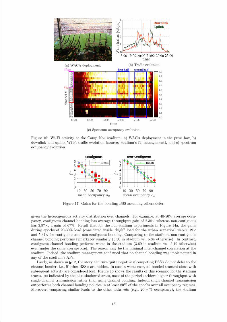
“main” — 2020/11/19 — 10:04 — page 205 — #227

(a) WACA deployment. (b) Traffic evolution.

17:30 18:30 19:30 20:30 21:30 22:30

3640444852566064

100104108112116120124128132136140144149153157161

chan

nel #

0.0

0.1

0.2

0.3

0.4

0.5

0.6

0.7

0.8

0.9

1.0second halffirst half

(c) Spectrum occupancy evolution.

Figure 16: Wi-Fi activity at the Camp Nou stadium: a) WACA deployment in the press box, b)downlink and uplink Wi-Fi traffic evolution (source: stadium’s IT management), and c) spectrumoccupancy evolution.

10 30 50 70 900123456

contiguous

10 30 50 70 900123456

non-contiguous

Figure 17: Gains for the bonding BSS assuming others defer.

given the heterogeneous activity distribution over channels. For example, at 40-50% average occu-pancy, contiguous channel bonding has average throughput gain of 2.38× whereas non-contiguoushas 3.97×, a gain of 67%. Recall that for the non-stadium experiments in Figure 14a, the gainsduring epochs of 20-30% load (considered inside “high” load for the urban scenarios) were 5.19×and 5.34× for contiguous and non-contiguous bonding. Comparing to the stadium, non-contiguouschannel bonding performs remarkably similarly (5.30 in stadium vs. 5.34 otherwise). In contrast,contiguous channel bonding performs worse in the stadium (3.69 in stadium vs. 5.19 otherwise)even under the same average load. The reason may be the minimal inter-channel correlation at thestadium. Indeed, the stadium management confirmed that no channel bonding was implemented inany of the stadium’s APs.

Lastly, as shown in §7.2, the story can turn quite negative if competing BSS’s do not defer to thechannel bonder, i.e., if other BSS’s are hidden. In such a worst case, all bonded transmissions withsubsequent activity are considered lost. Figure 18 shows the results of this scenario for the stadiumtraces. As indicated by the blue shadowed areas, most of the periods achieve higher throughput withsingle channel transmission rather than using channel bonding. Indeed, single channel transmissionoutperforms both channel bonding policies in at least 80% of the epochs over all occupancy regimes.Moreover, comparing similar loads to the other data sets (e.g., 20-30% occupancy), the stadium

18

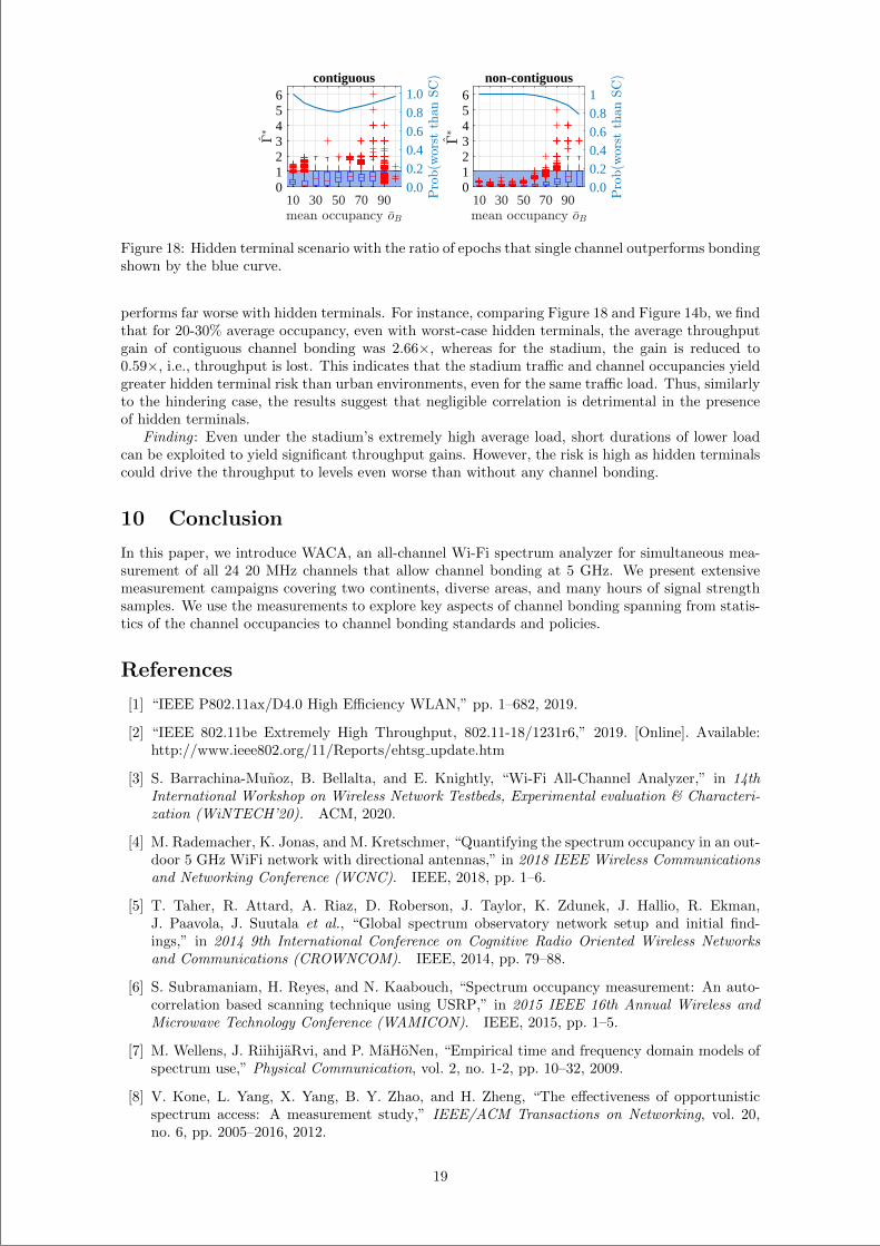
“main” — 2020/11/19 — 10:04 — page 206 — #228

10 30 50 70 900123456

0.00.20.40.60.81.0

contiguous

10 30 50 70 900123456

0.00.20.40.60.81

non-contiguous

Figure 18: Hidden terminal scenario with the ratio of epochs that single channel outperforms bondingshown by the blue curve.

performs far worse with hidden terminals. For instance, comparing Figure 18 and Figure 14b, we findthat for 20-30% average occupancy, even with worst-case hidden terminals, the average throughputgain of contiguous channel bonding was 2.66×, whereas for the stadium, the gain is reduced to0.59×, i.e., throughput is lost. This indicates that the stadium traffic and channel occupancies yieldgreater hidden terminal risk than urban environments, even for the same traffic load. Thus, similarlyto the hindering case, the results suggest that negligible correlation is detrimental in the presenceof hidden terminals.

Finding : Even under the stadium’s extremely high average load, short durations of lower loadcan be exploited to yield significant throughput gains. However, the risk is high as hidden terminalscould drive the throughput to levels even worse than without any channel bonding.

10 Conclusion

In this paper, we introduce WACA, an all-channel Wi-Fi spectrum analyzer for simultaneous mea-surement of all 24 20 MHz channels that allow channel bonding at 5 GHz. We present extensivemeasurement campaigns covering two continents, diverse areas, and many hours of signal strengthsamples. We use the measurements to explore key aspects of channel bonding spanning from statis-tics of the channel occupancies to channel bonding standards and policies.

References

[1] “IEEE P802.11ax/D4.0 High Efficiency WLAN,” pp. 1–682, 2019.

[2] “IEEE 802.11be Extremely High Throughput, 802.11-18/1231r6,” 2019. [Online]. Available:http://www.ieee802.org/11/Reports/ehtsg update.htm

[3] S. Barrachina-Munoz, B. Bellalta, and E. Knightly, “Wi-Fi All-Channel Analyzer,” in 14thInternational Workshop on Wireless Network Testbeds, Experimental evaluation & Characteri-zation (WiNTECH’20). ACM, 2020.

[4] M. Rademacher, K. Jonas, and M. Kretschmer, “Quantifying the spectrum occupancy in an out-door 5 GHz WiFi network with directional antennas,” in 2018 IEEE Wireless Communicationsand Networking Conference (WCNC). IEEE, 2018, pp. 1–6.

[5] T. Taher, R. Attard, A. Riaz, D. Roberson, J. Taylor, K. Zdunek, J. Hallio, R. Ekman,J. Paavola, J. Suutala et al., “Global spectrum observatory network setup and initial find-ings,” in 2014 9th International Conference on Cognitive Radio Oriented Wireless Networksand Communications (CROWNCOM). IEEE, 2014, pp. 79–88.

[6] S. Subramaniam, H. Reyes, and N. Kaabouch, “Spectrum occupancy measurement: An auto-correlation based scanning technique using USRP,” in 2015 IEEE 16th Annual Wireless andMicrowave Technology Conference (WAMICON). IEEE, 2015, pp. 1–5.

[7] M. Wellens, J. RiihijaRvi, and P. MaHoNen, “Empirical time and frequency domain models ofspectrum use,” Physical Communication, vol. 2, no. 1-2, pp. 10–32, 2009.

[8] V. Kone, L. Yang, X. Yang, B. Y. Zhao, and H. Zheng, “The effectiveness of opportunisticspectrum access: A measurement study,” IEEE/ACM Transactions on Networking, vol. 20,no. 6, pp. 2005–2016, 2012.

19

“main” — 2020/11/19 — 10:04 — page 207 — #229

[9] S. W. Day and A. Wagstaff, “Activity in the WiFi bands - An Objective Approach to Estima-tion,” in ARMMS Conference. Mass, 2014.

[10] F. Salahdine and H. El Ghazi, “A real time spectrum scanning technique based on compres-sive sensing for cognitive radio networks,” in 2017 IEEE 8th Annual Ubiquitous Computing,Electronics and Mobile Communication Conference (UEMCON). IEEE, 2017, pp. 506–511.

[11] S. Biswas, J. Bicket, E. Wong, R. Musaloiu-e, A. Bhartia, and D. Aguayo, “Large-scale mea-surements of wireless network behavior,” in Proceedings of the 2015 ACM Conference on SpecialInterest Group on Data Communication, 2015, pp. 153–165.

[12] M. Lopez-Benıtez and F. Casadevall, “Modeling and simulation of time-correlation propertiesof spectrum use in cognitive radio,” in 2011 6th International ICST Conference on CognitiveRadio Oriented Wireless Networks and Communications (CROWNCOM), 2011, pp. 326–330.

[13] V. Kone, L. Yang, X. Yang, B. Y. Zhao, and H. Zheng, “On the feasibility of effective oppor-tunistic spectrum access,” in Proceedings of the 10th ACM SIGCOMM conference on Internetmeasurement, 2010, pp. 151–164.

[14] M. Hoyhtya, A. Mammela, M. Eskola, M. Matinmikko, J. Kalliovaara, J. Ojaniemi, J. Suutala,R. Ekman, R. Bacchus, and D. Roberson, “Spectrum occupancy measurements: A survey anduse of interference maps,” IEEE Communications Surveys & Tutorials, vol. 18, no. 4, pp. 2386–2414, 2016.

[15] S. A. Hanna and J. Sydor, “Distributed sensing of spectrum occupancy and interference in out-door 2.4 GHz Wi-Fi networks,” in Global Communications Conference (GLOBECOM). IEEE,2012, pp. 1453–1459.

[16] S. A. Hanna, “A 3-state hypothesis test model for cognitive radio systems,” in 2014 IEEEInternational Symposium on Dynamic Spectrum Access Networks (DYSPAN). IEEE, 2014,pp. 291–302.

[17] S. Yin, D. Chen, Q. Zhang, M. Liu, and S. Li, “Mining spectrum usage data: a large-scalespectrum measurement study,” IEEE Transactions on Mobile Computing, vol. 11, no. 6, pp.1033–1046, 2012.

[18] L. Deek, E. Garcia-Villegas, E. Belding, S.-J. Lee, and K. Almeroth, “The impact of chan-nel bonding on 802.11n network management,” in Proceedings of the Seventh COnference onemerging Networking EXperiments and Technologies, 2011, pp. 1–12.

[19] L. Deek, E. Garcia-Villegas, E. Belding, S.-J. Lee, and K. Almerot, “Intelligent channel bondingin 802.11n WLANs,” IEEE Transactions on Mobile Computing, vol. 13, no. 6, pp. 1242–1255,2014.

[20] M. Y. Arslan, K. Pelechrinis, I. Broustis, S. V. Krishnamurthy, S. Addepalli, and K. Papa-giannaki, “Auto-configuration of 802.11n WLANs,” in Proceedings of the 6th InternationalCOnference, 2010, pp. 1–12.

[21] M. Y. Arslan, K. Pelechrinis, I. Broustis, S. Singh, S. V. Krishnamurthy, S. Addepalli,and K. Papagiannaki, “ACORN: An auto-configuration framework for 802.11n WLANs,”IEEE/ACM Transactions on Networking (TON), vol. 21, no. 3, pp. 896–909, 2013.

[22] Y. Zeng, P. H. Pathak, and P. Mohapatra, “A first look at 802.11ac in action: Energy efficiencyand interference characterization,” in 2014 IFIP Networking Conference. IEEE, 2014, pp. 1–9.

[23] M. Park, “IEEE 802.11ac: Dynamic bandwidth channel access,” in Communications (ICC),2011 IEEE International Conference on. IEEE, 2011, pp. 1–5.

[24] M. X. Gong, B. Hart, L. Xia, and R. Want, “Channel bounding and mac protection mechanismsfor 802.11ac,” in 2011 IEEE Global Telecommunications Conference-GLOBECOM 2011. IEEE,2011, pp. 1–5.

[25] B. Bellalta, A. Faridi, J. Barcelo, A. Checco, and P. Chatzimisios, “Channel bonding in short-range WLANs,” in European Wireless 2014; 20th European Wireless Conference. VDE, 2014,pp. 1–7.

20

“main” — 2020/11/19 — 10:04 — page 208 — #230

[26] B. Bellalta, A. Checco, A. Zocca, and J. Barcelo, “On the interactions between multiple over-lapping wlans using channel bonding,” IEEE Transactions on Vehicular Technology, vol. 65,no. 2, pp. 796–812, 2015.

[27] A. Faridi, B. Bellalta, and A. Checco, “Analysis of dynamic channel bonding in dense networksof wlans,” IEEE Transactions on Mobile Computing, vol. 16, no. 8, pp. 2118–2131, 2016.

[28] M.-S. Kim, T. Ropitault, S. Lee, and N. Golmie, “A throughput study for channel bonding inieee 802.11ac networks,” IEEE Communications Letters, vol. 21, no. 12, pp. 2682–2685, 2017.

[29] M. Yazid and A. Ksentini, “Stochastic modeling of the static and dynamic multichannel accessmethods enabling 40/80/160 MHz channel bonding in the VHT WLANs,” IEEE Communica-tions Letters, vol. 23, no. 8, pp. 1437–1440, 2019.

[30] S. Barrachina-Munoz, F. Wilhelmi, and B. Bellalta, “To overlap or not to overlap: Enablingchannel bonding in high-density WLANs,” Computer Networks, vol. 152, pp. 40–53, 2019.

[31] S. Barrachina-Munoz, F. Wilhelmi, and B. Bellalta, “Dynamic channel bonding in spatiallydistributed high-density WLANs,” IEEE Transactions on Mobile Computing, vol. 19, no. 4, pp.821–835, 2020.

[32] S. Khairy, M. Han, L. X. Cai, Y. Cheng, and Z. Han, “A renewal theory based analyticalmodel for multi-channel random access in IEEE 802.11ac/ax,” IEEE Transactions on MobileComputing, 2018.

[33] A. Zakrzewska and L. Ho, “Dynamic channel bandwidth use through efficient channel assign-ment in ieee 802.11ac networks,” in 2019 IEEE 90th Vehicular Technology Conference. IEEE,2019, pp. 1–6.

[34] S. Barrachina-Munoz, F. Wilhelmi, and B. Bellalta, “Online primary channel selection fordynamic channel Bonding in high-density WLANs,” IEEE Wireless Communications Letters,vol. 9, no. 2, pp. 258–262, 2020.

[35] Z. Khan and J. J. Lehtomaki, “Interactive trial and error learning method for distributedchannel bonding: model, prototype implementation, and evaluation,” IEEE Transactions onCognitive Communications and Networking, vol. 5, no. 2, pp. 206–223, 2019.

[36] S.-s. Lee, T. Kim, S. Lee, K. Kim, Y. H. Kim, and N. Golmie, “Dynamic channel bondingalgorithm for densely deployed 802.11ac networks,” IEEE Transactions on Communications,vol. 67, no. 12, pp. 8517–8531, 2019.

[37] M. Han, S. Khairy, L. X. Cai, Y. Cheng, and F. Hou, “Capacity analysis of opportunisticchannel bonding over multi-channel WLANs under unsaturated traffic,” IEEE Transactions onCommunications, 2019.

[38] G. Buttazzo, C. Di Franco, and M. Marinoni, “Design and analysis of target-sensitive real-timesystems,” Software: Practice and Experience, vol. 46, no. 9, pp. 1181–1200, 2016.

[39] L. Farzinvash and M. Kargahi, “A scheduling algorithm for execution-instant sensitive real-timesystems,” in 2009 15th IEEE International Conference on Embedded and Real-Time ComputingSystems and Applications. IEEE, 2009, pp. 511–518.

[40] N. Anand, E. Aryafar, and E. W. Knightly, “WARPlab: a flexible framework for rapid physicallayer design,” in Proceedings of the 2010 ACM workshop on Wireless of the students, by thestudents, for the students. ACM, 2010, pp. 53–56.

[41] “Rice University Wireless Open Access Research Platform,” http://warpproject.org, last ac-cessed January 30, 2020.

[42] S. Jang, K. G. Shin, and S. Bahk, “Post-CCA and reinforcement learning based bandwidthadaptation in 802.11ac networks,” IEEE Transactions on Mobile Computing, vol. 17, no. 2, pp.419–432, 2018.

[43] J. Lee, W. Kim, S.-J. Lee, D. Jo, J. Ryu, T. Kwon, and Y. Choi, “An experimental study on thecapture effect in 802.11a networks,” in Proceedings of the second ACM international workshopon Wireless network testbeds, experimental evaluation and characterization, 2007, pp. 19–26.

21

“main” — 2020/11/19 — 10:04 — page 209 — #231

[44] Q. Qu, B. Li, M. Yang, Z. Yan, A. Yang, D.-J. Deng, and K.-C. Chen, “Survey and perfor-mance evaluation of the upcoming next generation WLAN standard - IEEE 802.11ax,” MobileNetworks and Applications, vol. 24, no. 5, pp. 1461–1474, 2019.

Sergio Barrachina-Munoz is a Ph.D. candidate at Universitat PompeuFabra (UPF). He received his B.Sc. in Telematics Engineering and M.Sc.in Intelligent Interactive Systems in 2015 and 2016, respectively, both fromUPF. He joined the Wireless Networking Research Group in 2015 under thesupervision of Dr. Boris Bellalta. His main research interests are focused onmachine learning for next-generation WLANs. Sergio is a recipient of a FIgrant from the Generalitat de Catalunya.

Boris Bellalta is an Associate Professor in the Department of Informa-tion and Communication Technologies (DTIC) at Universitat Pompeu Fabra(UPF). He obtained his Ph.D. in Information and Communication Technolo-gies from UPF in 2007. His research interests are in the area of wirelessnetworks, with emphasis on the design and performance evaluation of newarchitectures and protocols.

Edward Knightly (S’92–M’96–SM’04–F’09) received the B.S. degreefrom Auburn University and the M.S. and Ph.D. degrees from the Universityof California at Berkeley. He is currently the Sheafor-Lindsay Professor andthe Chair of the Department of Electrical and Computer Engineering, RiceUniversity. His research interests are in experimental wireless networking,urban-scale testbeds, 60-GHz, terahertz, and VLC bands, wireless security,and performance evaluation. He is a Sloan Fellow. He was a recipient of theNSF CAREER Award. He received the Best Paper Award from the ACMMobiCom, the ACM MobiHoc, and the IEEE SECON.

22

“main” — 2020/11/19 — 10:04 — page 209 — #232

“main” — 2020/11/19 — 10:04 — page 210 — #233