Embed Size (px)
Citation preview


Series Editor
N. BalakrishnanMcMaster UniversityDepartment of Mathematics and Statistics1280 Main Street WestHamilton, Ontario L8S 4K1Canada
Editorial Advisory Board
Max EngelhardtEG&G Idaho, Inc.Idaho Falls, ID 83415
Harry F. MartzGroup A-1 MS F600Los Alamos National LaboratoryLos Alamos, NM 87545
Gary C. McDonaldNAO Research & Development Center30500 Mound RoadBox 9055Warren, MI 48090-9055
Kazuyuki SuzukiCommunication & Systems Engineering DepartmentUniversity of Electro Communications1-5-1 ChofugaokaChofu-shiTokyo 182Japan
Statistics for Industry and Technology

Advances in Statistical Methodsfor the Health Sciences
Applications to Cancer and AIDS Studies,Genome Sequence Analysis,and Survival Analysis
Jean-Louis AugetN. BalakrishnanMounir MesbahGeert MolenberghsEditors
BirkhauserBoston • Basel • Berlin

Jean-Louis AugetUFR of Pharmaceutical Sciences1 rue Gaston Veil44035 Nantes Cedex 1France
N. BalakrishnanDepartment of Mathematics and StatisticsMcMaster University1280 Main Street WestHamilton, Ontario L8S 4K1Canada
Mounir MesbahLaboratoire de Statistique Theorie et AppliqueeUniversite Pierre et Marie Curie175 rue de Chevaleret75013 ParisFrance
Geert MolenberghsCenter for StatisticsHasselt UniversityAgoralaan–Building D3590 DiepenbeekBelgium
Mathematics Subject Classification: 62K99, 62L05, 62N01, 62N02, 62N03, 62P10, 62P12
Library of Congress Control Number: 2006934773
ISBN-10: 0-8176-4368-0 e-ISBN-10: 0-8176-4542-XISBN-13: 978-0-8176-4368-3 e-ISBN-13: 978-0-8176-4542-7
Printed on acid-free paper.
c©2007 Birkhauser BostonAll rights reserved. This work may not be translated or copied in whole or in part without the written permissionof the publisher (Birkhauser Boston, c/o Springer Science+Business Media LLC, 233 Spring Street, New York,NY 10013, USA), except for brief excerpts in connection with reviews or scholarly analysis. Use in connectionwith any form of information storage and retrieval, electronic adaptation, computer software, or by similar ordissimilar methodology now known or hereafter developed is forbidden.The use in this publication of trade names, trademarks, service marks and similar terms, even if they are notidentified as such, is not to be taken as an expression of opinion as to whether or not they are subject to proprietaryrights.
9 8 7 6 5 4 3 2 1
www.birkhauser.com (Ham)

Contents
Preface xixContributors xxiList of Tables xxixList of Figures xxxv
Part I: Prognostic Studies and General Epidemiology
1 Systematic Review of Multiple Studies of Prognosis:The Feasibility of Obtaining Individual Patient Data 3D. G. Altman, M. Trivella, F. Pezzella, A. L. Harris,and U. Pastorino
1.1 Introduction 31.2 Systematic Review Based on Individual
Patient Data 51.3 A Case Study: Microvessel Density in Non-Small
Cell Lung Cancer 61.3.1 Identifying studies (data sets) and obtaining
the data 71.3.2 Checking the data 91.3.3 MVD measurements 111.3.4 Meta-analysis 12
1.4 Discussion 121.4.1 Systematic review of prognostic studies using
individual patient data 131.4.2 The need for higher-quality prognostic studies 14
References 16
2 On Statistical Approaches for the MultivariableAnalysis of Prognostic Marker Studies 19N. Hollander and W. Sauerbrei
2.1 Introduction 19
v

vi Contents
2.2 Examples: Two Prognostic Studies inBreast Cancer 20
2.3 Statistical Methods 212.3.1 Regression models 212.3.2 Classification and regression trees (CART) 222.3.3 Formation of risk groups 23
2.4 Results in the GBSG-2 Study 232.4.1 Regression models – standard applications 232.4.2 Regression models – the MFP-approach 252.4.3 Summary assessment – implication of the
modelling strategy 252.4.4 Application of classification and regression trees 28
2.5 Formation and Validation of Risk Groups 302.6 Discussion 32References 35
3 Where Next for Evidence Synthesis of Prognostic MarkerStudies? Improving the Quality and Reporting of PrimaryStudies to Facilitate Clinically Relevant Evidence-BasedResults 39R. D. Riley, K. R. Abrams, P. C. Lambert, A. J. Sutton,and D. G. Altman
3.1 Introduction and Aims 403.1.1 Prognostic markers and prognostic marker studies 403.1.2 The need for formal evidence syntheses of
prognostic marker studies 403.1.3 Aims of this chapter 41
3.2 Difficulties of an Evidence Synthesis of PrognosticMarker Studies 423.2.1 Poor and heterogeneous reporting 423.2.2 Poor study design and problems clarifying study
purpose 443.2.3 Little indication of how to implement markers in
clinical practice 453.2.4 Small sample sizes 463.2.5 Publication bias, selective within-study reporting,
and selective analyses 463.2.6 Lack of appreciation or validation of previous
findings 483.3 What Improvements Are Needed in Primary Prognostic
Marker Studies? 493.4 Evidence Synthesis Using Individual Patient Data Rather
than Summary Statistics 51

Contents vii
3.5 Discussion 54References 55
Part II: Pharmacovigilance
4 Sentinel Event Methods for MonitoringUnanticipated Adverse Events 61P. A. Lachenbruch and J. Wittes
4.1 Introduction 614.2 Examples 634.3 Usual Approaches to Monitoring Safety 644.4 Methods for Sentinel Events 66
4.4.1 Constant follow-up time 664.4.2 Censoring at a fixed calendar time 68
4.5 Methods for Sentinel Event Rates 714.6 Bayesian Models 724.7 Summary 73References 74
5 Spontaneous Reporting System Modelling for theEvaluation of Automatic Signal GenerationMethods in Pharmacovigilance 75E. Roux, F. Thiessard, A. Fourrier, B. Begaud,and P. Tubert-Bitter
5.1 Introduction 765.2 Methods 78
5.2.1 Spontaneous reporting system modelling 785.2.2 Exposure to the drug (Ti) 795.2.3 Events’ relative risk (RRij) 795.2.4 Reporting probability (pij) 805.2.5 Data generation process 84
5.3 Application 845.3.1 Values of the model parameters 845.3.2 Application of the empirical Bayes method 86
5.4 Results 865.5 Discussion 885.6 Conclusion 89References 90
Part III: Quality of Life
6 Latent Covariates in Generalized Linear Models:A Rasch Model Approach 95K. B. Christensen

viii Contents
6.1 Introduction 956.2 Generalized Linear Mixed Models 96
6.2.1 Latent regression models 976.3 Interpretation of Parameters 986.4 Generalized Linear Models with a Latent Covariate 98
6.4.1 Model 996.4.2 Interpretation of parameters 996.4.3 Parameter estimation 100
6.5 Example 1016.5.1 Latent covariate 1026.5.2 Job group level effect of the latent covariate 103
6.6 Discussion 104References 105
7 Sequential Analysis of Quality of Life Measurementswith the Mixed Partial Credit Model 109V. Sebille, T. Challa, and M. Mesbah
7.1 Introduction 1107.2 Methods 111
7.2.1 The partial credit model 1117.2.2 Estimation of the parameters 1127.2.3 Sequential analysis 1127.2.4 The Z and V statistics 1127.2.5 Traditional sequential analysis 1137.2.6 Sequential analysis based on partial credit
measurements 1137.2.7 The sequential probability ratio test and
the triangular test 1157.2.8 Simulation design 115
7.3 Results 1167.4 Discussion 1217.5 Conclusion 122Appendix 122References 123
8 A Parametric Degradation Model Used in Reliability,Survival Analysis, and Quality of Life 127M. Nikulin, L. Gerville-Reache, and S. Orazio
8.1 Introduction 1278.2 Degradation Process 1298.3 Estimation Problem 1308.4 Linear MVUE for a 1318.5 Solution of the Optimizatio Problem 132

Contents ix
8.6 Estimation of σ2 and θ0 132References 134
9 Agreement Between Two Ratings with DifferentOrdinal Scales 139S. Natarajan, M. B. McHenry, S. Lipsitz, N. Klar,and S. Lipshultz
9.1 Introduction 1399.2 Notation and Model 1429.3 Examples and Interpretation 1449.4 Discussion 147References 147
Part IV: Survival Analysis
10 The Role of Correlated Frailty Models in Studiesof Human Health, Ageing, and Longevity 151A. Wienke, P. Lichtenstein, K. Czene, and A.I. Yashin
10.1 Introduction 15110.2 Shared Frailty Model 15310.3 Correlated Frailty Model 15510.4 Correlated Gamma Frailty Model 156
10.4.1 Swedish breast cancer twin data 15710.4.2 Parametric and semiparametric models 15810.4.3 Correlated gamma frailty model with
covariates 15910.4.4 Cure-mixture models 160
10.5 Discussion 163References 164
11 Prognostic Factors and Prediction of Residual Survivalfor Hospitalized Elderly Patients 167M. L. Calle, P. Roura, A. Arnau, A. Yanez, and A. Leiva
11.1 Introduction 16711.2 Cohort Description and Follow-Up 16811.3 Multistate Survival Model 171
11.3.1 Predictive process 17311.4 Discussion 176References 177
12 New Models and Methods for Survival Analysis ofExperimental Data 179G. V. Semenchenko, A. I. Yashin, T. E. Johnson,and J. W. Cypser

x Contents
12.1 Introduction 17912.2 Semiparametric Model of Mortality in Heterogeneous
Populations Influenced by Exogenous Interventions 18012.2.1 The heterogeneous mortality model 18012.2.2 Changes in the baseline hazard and frailty
distribution 18112.2.3 Semiparametric representation of the model 18312.2.4 Interpretation of parameters 184
12.3 One Example of the Model Application to the Analysis ofPoststress Survival Data 18712.3.1 Heat shock of different duration applied to
populations of nematodes Caenorhabditis elegans 18712.3.2 Technical details 18812.3.3 Results of fitting the model to the data 188
12.4 Discussion 190References 191
13 Uniform Consistency for Conditional LifetimeDistribution Estimators Under RandomRight-Censorship 195P. Deheuvels and G. Derzko
13.1 Introduction and Results 19513.1.1 Notation and statement of the problem 19513.1.2 Definition of the estimators and uniform
consistency 19813.2 Proofs 203
13.2.1 Construction of the estimators 20313.2.2 A useful auxiliary result 20613.2.3 Concluding comments 208
References 208
14 Sequential Estimation for the SemiparametricAdditive Hazard Model 211L. Bordes and C. Breuils
14.1 Introduction 21114.2 Example and Numerical Study 21314.3 Assumptions and Theoretical Results 21514.4 Technical Tools 220
14.4.1 Complete convergence, Anscombe condition,and exponential inequality 220
14.4.2 Technical results 221References 222

Contents xi
15 Variance Estimation of a Survival Function withDoubly Censored Failure Time Data 225C. Zhu and J. Sun
15.1 Introduction 22515.2 Preliminaries 22715.3 Variance Estimation 228
15.3.1 Simple bootstrap method 22815.3.2 Generalized Greenwood formula 22915.3.3 Imputation methods I and II 230
15.4 Numerical Results 23115.5 Concluding Remarks 233References 234
Part V: Clustering
16 Statistical Models and Artificial Neural Networks:Supervised Classification and Prediction Via Soft Trees 239A. Ciampi and Y. Lechevallier
16.1 Introduction 24016.2 The Prediction Problem: Statistical Models and ANNs 241
16.2.1 Generalized linear models as ANNs 24316.2.2 Generalized additive models as ANNs 24516.2.3 Classification and regression trees as ANNs 246
16.3 Combining Prediction Models: Hierarchy of Experts 24816.4 The Soft Tree 250
16.4.1 General concepts in tree construction 25116.4.2 Constructing a soft tree from data 25216.4.3 An example of data analysis 25316.4.4 An evaluation study 256
16.5 Extending the Soft Tree 25716.6 Conclusions 259References 260
17 Multilevel Clustering for Large Databases 263Y. Lechevallier and A. Ciampi
17.1 Introduction 26317.2 Data Reduction by Kohonen SOMs 265
17.2.1 Kohonen SOMs and PCA initialization 26617.2.2 Binning of the original data matrix using a
Kohonen map 26617.2.3 Dissimilarity for microregimens 268
xii Contents
17.3 Clustering Multilevel Systems 26917.3.1 A two-level statistical model 27017.3.2 Estimating parameters by the EM algorithm 270
17.4 Extracting Dietary Patterns from the NutritionalData 271
References 273
18 Neural Networks: An Application for PredictingSmear Negative Pulmonary Tuberculosis 275A. M. Santos, B. B. Pereira, J. M. Seixas,F. C. Q. Mello, and A. L. Kritski
18.1 Introduction 27618.2 Materials and Methods 277
18.2.1 Data set 27718.2.2 Neural network design 27818.2.3 Data selection for network design 279
18.3 Relevance of Explanatory Variables 28318.4 Results 28318.5 Conclusions 284References 285
19 Assessing Drug Resistance in HIV Infection UsingViral Load Using Segmented Regression 289H. Liang, W.-Y. Tan, and X. Xiong
19.1 Introduction 28919.2 The Model 292
19.2.1 The likelihood function 29419.2.2 The prior distribution 29419.2.3 The posterior distributions 295
19.3 The Gibbs Sampling Procedure 29719.4 Analysis of the ACTG 315 Data 29819.5 Conclusion and Dicussion 301References 303
20 Assessment of Treatment Effects on HIV PathogenesisUnder Treatment By State Space Models 305W.-Y. Tan, P. Zhang, X. Xiong, and P. Flynn
20.1 Introduction 30520.2 A Stochastic Model for HIV Pathogenesis Under
Treatment 30620.2.1 Stochastic differential equations of
state variables 30720.2.2 The probability distribution of state
variables 308

Contents xiii
20.3 A State Space Model for HIV Pathogenesis UnderAntiretroviral Drugs 309
20.4 Estimation of Unknown Parameters and StateVariables 310
20.5 An Illustrative Example 31120.6 Conclusions and Discussion 314References 317
Part VI: Safety and Efficacy Assessment
21 Safety Assessment Versus Efficacy Assessment 323M. A. Foulkes
21.1 Introduction 32321.2 Design Issues 324
21.2.1 Outcomes 32421.2.2 Power 32521.2.3 Population 32621.2.4 Comparison 326
21.3 Analytic Issues 32621.3.1 Compliance 32621.3.2 Missing data 32721.3.3 Confounding 32721.3.4 Bias 32821.3.5 Misclassification 32821.3.6 Multiplicity 328
21.4 Analytic Approaches 32921.5 Inferences 33021.6 Conclusions 330References 332
22 Cancer Clinical Trials with Efficacy and ToxicityEndpoints: A Simulation Study to CompareTwo Nonparametric Methods 335A. Letierce and P. Tubert-Bitter
22.1 Introduction 33622.2 Setting 33722.3 Method for the Simulation Study 34022.4 Results 34222.5 Conclusion 346References 347

xiv Contents
23 Safety Assessment in Pilot Studies WhenZero Events Are Observed 349R. E. Carter and R. F. Woolson
23.1 Introduction 34923.2 Clinical Setting 35023.3 Notation 35123.4 Binomial Setting 35123.5 Geometric Setting 35223.6 Bayesian Credible Interval 35423.7 Clinical Setting: Revisited 35623.8 Summary 357References 357
Part VII: Clinical Designs
24 An Assessment of Up-and-Down Designs andAssociated Estimators in Phase I Trials 361H. K. T. Ng, S. G. Mohanty, and N. Balakrishnan
24.1 Introduction 36124.2 Notation and Designs 362
24.2.1 The biased coin design (BCD) 36324.2.2 The k-in-a-row rule (KROW) 36424.2.3 The Narayana rule (NAR) 36424.2.4 Continual reassessment method (CRM) 364
24.3 Estimation of Maximum Tolerated Dose 36524.4 Simulation Setting 36724.5 Comparison of Estimators 36824.6 Comparison of Designs 369References 385
25 Design of Multicentre Clinical Trials withRandom Enrolment 387V. V. Anisimov and V. V. Fedorov
25.1 Introduction 38725.2 Recruitment Time Analysis 38925.3 Analysis of Variance of the Estimated ECRT 39325.4 Inflation of the Variance Due to Random
Enrolment 39525.5 Solution of the Optimization Problem 39625.6 Conclusions 398Appendix 398References 400

Contents xv
26 Statistical Methods for Combining Clinical TrialPhases II and III 401N. Stallard and S. Todd
26.1 Introduction 40126.2 Background 402
26.2.1 The clinical evaluation programme fornew drugs 402
26.2.2 Combining clinical trial phases II and III 40326.2.3 Background to sequential clinical trials 404
26.3 Methods for Combining Phases II and III 40726.3.1 Two-stage methods 40826.3.2 A multistage group-sequential method 40826.3.3 A multistage adaptive design method 40926.3.4 Example—a multistage trial comparing
three doses of a new drug for thetreatment of Alzheimer’s disease 410
26.4 Discussion and Future Directions 413References 415
27 SCPRT: A Sequential Procedure That GivesAnother Reason to Stop Clinical Trials Early 419X. Xiong, M. Tan, and J. Boyett
27.1 Introduction 42027.2 The SCPRT Procedure 421
27.2.1 Controlling the boundary 42327.2.2 Boundaries in terms of P -values 423
27.3 An Example 42427.4 SCPRT with Unknown Variance 42627.5 Clinical Trials with Survival Data 42827.6 Conclusion 432References 432
Part VIII: Models for the Environment
28 Seasonality Assessment for Biosurveillance Systems 437E. N. Naumova and I. B. MacNeill
28.1 Introduction 43828.1.1 Conceptual framework for seasonality
assessment 43828.2 δ-Method in Application to a Seasonality Model 440
28.2.1 Single-variable case 44028.2.2 Two-variables case 441

xvi Contents
28.2.3 Application to a seasonality model 44228.2.4 Potential model extension 44328.2.5 Additional considerations 444
28.3 Application to Temperature and InfectionIncidence Analysis 446
28.4 Conclusion 449References 450
29 Comparison of Three Convolution Prior SpatialModels for Cancer Incidence 451E.-A. Sauleau, M. Musio, A. Etienne,and A. Buemi
29.1 Introduction 45129.2 Materials and Methods 453
29.2.1 ICAR model 45529.2.2 Distance model based on the exponential
function 45529.2.3 Two-dimensional P-splines model 45629.2.4 Implementation of the models 456
29.3 Results 45629.4 Discussion 459References 463
30 Longitudinal Analysis of Short-Term BronchiolitisAir Pollution Association Using SemiparametricModels 467S. Willems, C. Segala, M. Maidenberg, and M. Mesbah
30.1 Introduction 46730.2 Data 469
30.2.1 Sanitary data 46930.2.2 Environmental data 469
30.3 Methods 47030.3.1 Generalized additive models 47030.3.2 Air pollution time series studies strategy 47130.3.3 Criticism about the use of standard statistical
software to fit GAM to epidemiological timeseries data 474
30.4 Results 47530.4.1 Series of number of hospital consultations:
Results with S-Plus 47530.4.2 Series of number of hospital consultations:
Results with R 48230.4.3 SAS results 483

Contents xvii
30.5 Discussion 484References 486
Part IX: Genomic Analysis
31 Are There Correlated Genomic Substitutions? 491M. Karnoub, P. K. Sen, and F. Seillier-Moiseiwitsch
31.1 Introduction 49131.2 The Probabilistic Model 49231.3 Parameter Estimation 49631.4 New Test Statistic 49731.5 Power Studies 50031.6 Numerical Studies 50131.7 Data Analysis 50431.8 Discussion 507Appendix 31.1 509Appendix 31.2 510References 513
Part X: Animal Health
32 Swiss Federal Veterinary Office RiskAssessments: Advantages and Limitationsof the Qualitative Method 519R. Hauser, E. Breidenbach, and K. D. C. Stark
32.1 Introduction 52032.2 Health Risks from Consumption of Milk and
Dairy Products: An Example of a QualitativeRisk Assessment 52132.2.1 Risk profile 52132.2.2 Hazard identification 52132.2.3 Risk network 52232.2.4 Risk estimation 52332.2.5 Recommendations for random sample planning
and risk managers 52432.3 Advantages and Disadvantages of Qualitative
Risk Assessment 52532.4 Statistics’ Part in Qualitative Risk Assessment 526References 526

xviii Contents
33 Qualitative Risk Analysis in Animal Health:A Methodological Example 527B. Dufour and F. Moutou
33.1 Introduction 52833.2 Global Presentation of the Method 52833.3 Qualitative Appreciation of the Probability of
Each Event 53033.4 Qualitative Risk Appreciation 53133.5 Qualitative Appreciation Examples 53233.6 Discussion 534References 536
Index 539

Preface
Statistical methods have become an increasingly important and integral partof research in health sciences. For this reason, we organized an InternationalConference on Statistics in Health Sciences during June 23–25, 2004, at Univer-site de Nantes, Nantes, France. This conference, with the participation of over200 researchers from numerous countries, was very successful in bringing to-gether experts working on statistical methodology and applications into severaldifferent aspects and problems in health sciences.
This volume comprises a selection of papers that were presented at theconference. All the articles presented here have been peer reviewed and carefullyorganized into 33 chapters. For the convenience of the readers, the volume hasbeen divided into the following parts:
• Prognostic Studies and General Epidemiology
• Pharmacovigilance
• Quality of Life
• Survival Analysis
• Clustering
• Safety and Efficacy Assessment
• Clinical Designs
• Models for the Environment
• Genomic Analysis
• Animal Health
As is evident, these cover a wide range of topics pertaining to statistical methodsin health sciences.
Our sincere thanks go to all the authors who have contributed to this vol-ume, and for their cooperation, patience, and support throughout the course ofthe preparation of the volume. We are also indebted to the referees for helpingus in the evaluation of the manuscripts and in improving the quality of thispublication.
xix

xx Preface
Special thanks are due to Mrs. Debbie Iscoe for the excellent typesettingof the entire volume, and to Mr. Thomas Grasso (Editor, Birhauser, Boston)and Ms. Regina Gorenshteyn (Assistant Editor, Birkhauser, Boston) for theirencouragement and help.
Jean-Louis AugetUniversite de NantesNantes, France
N. BalakrishnanMcMaster UniversityHamilton, Canada
Mounir MesbahUniversite de Pierre et Marie CurieParis, France
Geert MolenberghsHasselt UniversityDiepenbeek, Belgium

Contributors
Abrams, Keith R. Centre for Biostatistics and Genetic Epidemiology, 22-28 Department of Health Sciences, University of Leicester Princess RoadWest, Leicester, [email protected]
Altman, Douglas G. Cancer Research UK Medical Statistics Group Centrefor Statistics in Medicine, Wolfson College Oxford OX2 6UD, [email protected].
Anisimov, Vladimir V. Research Statistics Unit, GlaxoSmithKline NFSP-South, Third Avenue, Harlow Essex CM19 5AW, [email protected]
Arnau, A. Clinical Epidemiology and Research Department, Vic GeneralHospital, 08500 Vic, [email protected]
Balakrishnan, N. Department of Mathematics and Statistics, McMasterUniversity, Hamilton, Ontario, Canada L8S [email protected]
Begaud, B. Universite Victor Segalen, 146 rue Leo Saignat, 33076 BordeausCedex, [email protected]
Bordes, L. Universite de Technologie de Compiegne, LMAC Royallieu, BP525, 60205 Compiegne, [email protected]
Boyett, James St. Jude Children’s Research Hospital, Memphis, TN 38105-2794, [email protected]
Breidenbach, E. Federal Veterinary Office Department of Monitoring, P.O.Box CH-3003, Bern, [email protected]
xxi

xxii Contributors
Breuils, C. Lab. de Math. Nicolas Oresme, Universite de Caen, BP 5186,14032 Caen Cedex, [email protected]
Buemi, Antoine Cancer Registry of Haut-Rhin, Mulhouse, [email protected]
Calle, M. L. Systems Biology Department, Universitat de Vic, 13, Laura St.,E-08500 Vic, [email protected]
Carter, Rickey E. Department of Biostatistics, Bioinformatics and Epidemi-ology, Medical University of South Carolina, Charleston, SC 29425, [email protected]
Challa, Tariku Center for Statistics, Hasselt University, Agoralaan - buildingD, 3590 Diepenbeek, Belgiumtariku [email protected]
Christensen, Karl Bang National Institute of Occupational Health, LersoParkalle 105, 2100 Copenhagen, [email protected]
Ciampi, Antonio Department of Epidemiology and Biostatistics, McGillUniversity, Montreal, Quebec, Canada, H2T [email protected]
Cypser, James W. Institute for Behavioural Genetics, University ofColorado at Boulder, Boulder, CO 80309-0447, USA
Czene, Kamila Department of Medical Epidemiology and Biostatistics,Karolinska Institute, Stockholm, Sweden
Deheuvels, Paul Universite Pierre et Marie Curie, Laboratoire de Statis-tique Theorique et Appliquee, Boıte 158, Bureau 8A25, 175 rue duChevaleret, 75013 Paris, [email protected]
Derzko, Gerard Sanofi-Aventis, 371 rue du Pr Joseph Blayac, 34184 Mont-pellier Cedex 4, [email protected]
Dufour, Barbara UP Maladies contagieuses, Ecole Nationale Veterinaired’Alfort, 7 Avenue du General-de-Gaulle, 94704 Maisons-Alfort Cedex,[email protected]

Contributors xxiii
Etienne, Arnaud Cancer Registry of Haut-Rhin, Mulhouse, [email protected]
Federov, Valerii V. Research Statistics Unit, GlaxoSmithKline, 1250 S.Collegeville Rd., Collegeville, PA 19426-0989, [email protected]
Flynn, Pat Department of Biostatistics, St. Jude Children’s Research Hos-pital, Memphis, TN 38105-2794, USA
Foulkes, Mary A. U.S. Food Drug Administration Center for BiologicsEvaluation and Research, Office of Biostatistics and Epidemiology, 1401Rockville Pike, HFM-210, Rockville, MD 20852, [email protected]
Fourrier, A. Universite Victor Segalen, 146 rue Leo Saignat, 33076Bordeaux Cedex, [email protected]
Gerville-Reache, L. Mathematical Statistics and Its Applications, BP 26,University Victor Segalen Bordeaux 2, 33076 Bordeaux, [email protected]
Harris, Adrian L. Cancer Research UK Oncology Unit, Churchill Hospital,Oxford, UK
Hauser, R. Swiss Federal Veterinary Office (SFVO), Monitoring Schwarzen-burgstrasse 161, CH-3003 Bern, [email protected]
Hollander, N. Institute of Medical Biometry and Medical Informatics,Freiburg, Stefan-Meier Str. 26, 79104 Freiburg, [email protected]
Johnson, Thomas E. Institute for Behavioural Genetics, University ofColorado at Boulder, Boulder, CO 80309, USA
Karnoub, M. Population Genetics, GlaxoSmithKline, 5 Moore Drive, Box13398, Research Triangle Park, NC 27709, [email protected]
Klar, Neil Cancer Care Ontario, Ontario, Canada
Kritski, A. L. Faculty of Medicine and Tuberculosis, Research Unit-IDT-Federal, University of Rio de Janeiro, Rio de Janeiro, Brazil

xxiv Contributors
Lachenbruch, Peter A. FDA/CBER/OBE, 1401 Rockville Pike HFM-215,Rochville, MD 20852, [email protected]
Lambert, Paul C. Centre for Biostatistics and Genetic Epidemiology,Department of Health Sciences, University of Leicester, 22-28 PrincessRoad West, Leicester, [email protected]
Lechevallier, Yves Institut National de Recherche en Informatique et enAutomatique, Rocquencourt 78153, Le Chesnay Cedex, [email protected]
Leiva, A. Clinical Epidemiology and Research Department, Vic General Hos-pital, 08500 Vic, [email protected]
Letierce, Alexia Unite de Recherche Clinique Paris Sud, Hopital Bicetre, 78rue de Ge’eral Leclerc, 94807 Le Kremlin-Bicetre Cedex, [email protected]
Liang, Hua Department of Biostatistics and Computational Biology, Univer-sity of Rochester, Rochester, NY 14642, [email protected]
Lichtenstein, Paul Department of Medical Epidemiology and Biostatistics,Karolinska Institute, Stockholm, Sweden
Lipshultz, Steven Department of Pediatrics, University of Miami School ofMedicine, Miami, FL 33136, USA
Lipsitz, Stuart Department of Biostatistics, Bioinformatics and Epidemiol-ogy, Medical University of South Carolina, Charleston, SC 29425, USA
MacNeill, Ian B. Department of Statistical and Actuarial Sciences, Univer-sity of Western Ontario, London, Ontario, Canada N6G [email protected]
Maidenberg, Manuel Association Respirer, 57 rue de la Convention, 75015Paris, [email protected]
McHenry, M. Brent Department of Biostatistics, Bioinformatics and Epi-demiology, Medical University of South Carolina, Charleston, SC 29425,USA

Contributors xxv
Mello, F. C. Q. Universidade Federal de Rio de Janeiro, TB Unit-HUCFF/UFRJ, Rio de Janiero, Brazil
Mesbah, Mounir Universite Pierre et Marie Curie, Laboratoire de Statis-tique Theorique et Appliquee, Bote 158, Bureau 8A25, 175 rue duChevaleret, 75013 Paris, [email protected]
Mohanty, S. G. Department of Mathematics and Statistics, McMaster Uni-versity, Hamilton, Ontario, Canada L8S [email protected]
Moutou, Francois Unite d’Epidemiologie, AFSSA LERPAZ, BP 67, 94703Maisons-Alfort Cedex, [email protected]
Musio, Monica Department of Mathematics and Informatics, Cagliari Uni-versity, Cagliari, [email protected]
Natarajan, Sundar The Department of Medicine, New York UniversitySchool of Medicine and the VA New York Harbor Healthcare System,New York, NY 10010, [email protected]
Naumova, Elena N. Department of Family Medicine and CommunityHealth, Tufts University School of Medicine, Boston, MA 02111, [email protected]
Ng, H. K. T. Department of Statistical Science, Southern MethodistUniversity, Dallas, TX 75275-0332, [email protected]
Nikulin, M. Mathematical Statistics and Its Applications, BP 26,University Victor Segalen Bordeaux 2, 33076 Bordeaux, [email protected]
Orazio, S. Mathematical Statistics and Its Applications, BP 26,University Victor Segalen Bordeaux 2, 33076 Bordeaux, France
Pastorino, Ugo European Institute of Oncology, Milano, Italy
Pereira, B. B. Post Graduate School of Engineering, Federal University ofRio de Janeiro and Faculty of Medicine and Tuberculosis Research Unit,University of Rio de Janeiro, Rio de Janeiro, [email protected]

xxvi Contributors
Pezzella, Francesco Cancer Research UK Pathology Unit, John RadcliffeHospital, Oxford, UK
Riley, Richard D. Centre for Biostatistics and Genetic Epidemiology, 22-28Department of Health Sciences, University of Leicester, Princess RoadWest, Leicester, [email protected]
Roura, P. Clinical epidemiology and Research Department, Hospital Generalde Vic 1, Francesc Pla St E., 08500 Vic, [email protected]
Roux, E. INSERM U642 (LTSI) Universite Rennes 1 Campus Beaulieu, Bat22, 35042 Rennes, [email protected]
Santos, A. M. Department of Mathematics, Federal University of Maranhao,Maranhao, Brazil [email protected]
Sauerbrei, W. Institute of Medical Biometry, University Hospital Freiburg,Stefan-Meier-Str. 26, 79104 Freiburg, [email protected]
Sauleau, Erik-A. Registre des Cancers du Haut-Rhin, 9 rue du Dr Man-geney, BP 1370, 68070 Mulhouse, [email protected]
Sebille, Veronique Faculte de Pharmacie Lab de Biomathematique-Biostatistique, 1 rue Gaston Veil, 44035 Nantes Cedex 01, [email protected]
Segala, Claire SEPIA-Sante, 18 bis, rue du Calvaire, F-56310 Merland,[email protected]
Seixas, J. M. Signal Processing Laboratory, Federal University of Rio deJaneiro, Rio de Janeiro, Brazil
Seillier-Moiseiwitsch, F. Department of Biostatistics, Bioinformatics andBiomathematics, Georgetown University Medical Center, Washington,DC 20057-1484, [email protected]
Semenchenko, Ganna V. Max Planck Institute for Demographic Research,Konrad Zuze Str. 1, 18057 Rostock, [email protected]

Contributors xxvii
Sen, P. K. Department of Biostatistics, University of North Carolina, ChapelHill, NC 27599-7420, [email protected]
Stallard, Nigel Warwick Medical School, The University of Warwick, Coven-try CV4 7AL, [email protected]
Stark, K. D. C. Swiss Federal Veterinary Office, Department of Monitoring,P.O. Box CH-3003, Bern, [email protected]
Sun, Jianguo Department of Statistics, University of Missouri,Columbia, MI 65211, [email protected]
Sutton, Alex J. Centre for Biostatistics and Genetic Epidemiology, 22-28Department of Health Sciences, University of Leicester, Princess RoadWest, Leicester, [email protected]
Tan, Ming Greenbaum Cancer Center, University of Maryland, Baltimore,MD 21201, [email protected]
Tan, Wai-Yuan Department of Mathematical Sciences, University of Mem-phis, Memphis, TN 38152, [email protected]
Thiessard, F. Universite Victor Segalen, 146 rue Leo Saignat, 33076 Bor-deaux Cedex, [email protected]
Todd, Susan Medical and Pharmaceutical Statistics Research Unit, The Uni-versity of Reading, UK, P.O. Box 240, Earley Gate, Reading RG6 6FN,[email protected]
Trivella, Marialena Cancer Research, UK Medical Statistics Group Centrefor Statistics in Medicine, Wolfson College, Oxford OX2 6UD, UK
Tubert-Bitter, Pascale INSERM Unit 780, Unite de Recherche en Epidemiolo-gie et Biostatistiques, 16 avenue Paul Vaillant Couturier, 94807 VillejuifCedex, [email protected]

xxviii Contributors
Wienke, Andreas Institute of Medical Epidemiology, Biostatistics and In-formatics, Martin-Luther-University Halle-Wittenberg, Halle, [email protected]
Willems, Sylvie Unite de neuropsychologie Faculte de Psychologie et de Sci-ences de l’Education, Universite de Liege, B33 B-4000 Liege, [email protected]
Wittes, Janet Statistics Collaborative, 1625 Massachusetts Ave. NW, Suite600, Washington, DC 20036, [email protected]
Woolson, Robert F. Department of Biostatistics, Bioinformatics and Epi-demiology Medical, University of South Carolina, Charleston, SC 29425,[email protected]
Xiong, Xiaoping Department of Biostatistics, St. Jude Children’s ResearchHospital, Memphis, TN 38105-2794, [email protected]
Yanez, A. Clinical Epidemiology and Research Department, VIC GeneralHospital, 08500 Vic, [email protected]
Yashin, Anatoli I. Demographic Studies, Duke University, Durham, NC27708-0408, [email protected]
Zhang, P. Department of Mathematical Sciences, University of Memphis,Memphis, TN 38152, USA
Zhu, Chao Department of Statistics, University of Missouri, Columbia, MI65211, USA

List of Tables
Table 1.1 Problems encountered with data sets in PILC study 10
Table 2.1 Estimated hazard ratios (HR), AIC, and BIC in Cox mod-els: Results from the univariate Cox model (no adjust-ment), the full model and a selected model obtained bybackward elimination with α = 0.05 (BE(0.05)) assuming(A) a (log-)linear relationship for continuous covariatesand (B) categorising continuous covariates as predefinedin the first analysis of the GBSG-2 study
26
Table 2.2 Selected prognostic markers, AIC, and BIC for differentmodel selection strategies. Included markers marked bydots
27
Table 2.3 Estimated hazard ratios (HR) for prognostic subgroupsderived in the GBSG-2 study by using the selected Coxmodel with categorised covariates (COX) and a modifica-tion of the simple tree displayed in Figure 2.2B (CART*).Validation of the HRs in the Freiburg-DNA study
32
Table 2.4 Summary of important issues for the analysis of singleprognostic marker studies
34
Table 4.1 Posterior probability that the event rate is less than π asa function of various prior distributions
72
Table 5.1 Fuzzy characterization of the variables 82Table 5.2 Average and standard deviation (in brackets), over the
1000 simulated datasets, of the prior parameters of Du-Mouchel’s model, estimated by means of maximum like-lihood
88
Table 6.1 Predictors of the number of absence spells. Results fromPoisson regression with random person effects
102
xxix

xxx Tables
Table 6.2 Results from Poisson regression with random person ef-fects including (i) the observed raw sum score, (ii) esti-mated values for each person, or (iii) latent covariate (cf.(6.6)) as predictors. All analyses are adjusted for effectof gender, age, and job group
103
Table 6.3 Predictors of the number of absence spells. Effect of thelatent covariate skill discretion on job group level
104
Table 7.1 Type I error probability for the sequential probability ra-tio test (SPRT) and the triangular test (TT) (nominalα = β = 0.05). Data are α (standard errors)
117
Table 7.2 Power for the sequential probability ratio test (SPRT)and the triangular test (TT) (nominal α = β = 0.05).Data are 1− β (standard errors)
117
Table 7.3 Average sample number (ASN) and 90th percentile (P90)of the number of patients required to reach a conclusionunder H0 for the sequential probability ratio test (SPRT)and the triangular test (TT) (nominal α = β = 0.05)
118
Table 7.4 Average sample number (ASN) and 90th percentile (P90)of the number of patients required to reach a conclusionunder H1 for the sequential probability ratio test (SPRT)and the triangular test (TT) (nominal α = β = 0.05)
118
Table 7.5 Type I error probability for the sequential probability ra-tio test (SPRT) and the triangular test (TT) for differentamounts of items with one overlapping category (nominalα = β = 0.05). Overlap is the proportion of overlappingcategory. Data are α (standard errors)
119
Table 7.6 Power for the sequential probability ratio test (SPRT)and the triangular test (TT) for different amounts ofitems with one overlapping category (nominal α = β =0.05). Overlap is the proportion of overlapping category.Data are 1− β (standard errors)
119
Table 7.7 Average sample number (ASN) and 90th percentile (P90)of the number of patients required to reach a conclusionunder H0 for the sequential probability ratio test (SPRT)and the triangular test (TT) for different amounts ofitems with one overlapping category (nominal α = β =0.05). Overlap is the proportion of overlapping category.Data are ASN/P90
120

Tables xxxi
Table 7.8 Average sample number (ASN) and 90th percentile (P90)of the number of patients required to reach a conclusionunder H1 for the sequential probability ratio test (SPRT)and the triangular test (TT) for different amounts ofitems with one overlapping category (nominal α = β =0.05). Overlap is the proportion of overlapping category.Data are ASN/P90
120
Table 9.1 (4× 3) table from answers to the two health status ques-tions from the parent questionnaire from the childhoodleukemia study
140
Table 9.2 (4× 5) table from answers to the two health status ques-tions from the 2002 United States National General SocialSurvey (GSS)
141
Table 9.3 (2× 2) table of cell counts at cutpoints j and k 143Table 9.4 (2× 2) table of probabilities at cutpoints j and k 143Table 9.5 Table of six Kappa coefficients at all cutpoints using the
childhood leukemia study. Estimates and 95% confidenceintervals obtained from SAS Proc Freq
145
Table 9.6 (2× 2) table corresponding to κ22 = 0.463 in Table 9.5 145Table 9.7 Table of 12 Kappa coefficients at all cutpoints using the
2002 United States National General Social Survey. Es-timates and 95% confidence intervals obtained from SASProc Freq
146
Table 9.8 (2× 2) table corresponding to κ23 = 0.858 in Table 9.7 146
Table 10.1 Correlated gamma frailty model applied to breast cancerdata
158
Table 10.2 Correlated gamma frailty model with observed covariates 159Table 10.3 Correlated gamma frailty model without and with a cure
fraction162
Table 11.1 Risk coefficient estimates for model 11.1 173
Table 12.1 Lifespan characteristics in the groups of nematodesCaenorhabditis elegans subjected to heat shock of differ-ent duration
187
Table 12.2 Parameter estimates of the semiparametric model of het-erogeneous mortality for groups of nematodes Caenorhab-ditis elegans subjected to heat shock of different duration
189

xxxii Tables
Table 14.1 Nd behavior for various values of d (β0 = 1, censorshiprate: 48%)
214
Table 14.2 N0.5 with respect to β0 215
Table 16.1 Model comparison for Pima Indians data 255Table 16.2 Test set classification error 256Table 16.3 Proportion of time the hard tree test set classification
error (EH) is greater than the soft node test set classifi-cation error (ES)
256
Table 17.1 French center sample 264Table 17.2 Proportion of the six regimens: overall and by center 273
Table 18.1 Composition of the training and testing sets selected 283Table 18.2 Efficiencies of classification 284
Table 19.1 Estimates of the parameters of four subjects 300
Table 20.1 The observed numbers of HIV RNA virus load of an HIV-infected patient
313
Table 20.2 The history of drug treatment 314Table 20.3 The estimate of parameters 315
Table 21.1 Differences that affect the assessments of safety and effi-cacy throughout product/intervention development
331
Table 22.1 Type I error rate estimates for n = 50 and n = 100patients in each group, for the association parameter α =2 and α = 5, obtained from 1000 simulations. LR andST refer to the MULTIN tests for the likelihood ratioordering and the stochastic ordering
343
Table 22.2 Power estimates for the one-sided comparison of treat-ment A versus treatment B, with n = 50 patients in eachgroup, based on 1000 simulations. See Table 22.1 for thecolumn names
344
Table 22.3 Power estimates for the one-sided comparison of treat-ment A versus treatment B, with n = 100 patients ineach group, based on 1000 simulations. See Table 22.1for the column names
345
Table 24.1 Bias and MSE of the estimators under biased-coin designwith N = 15
372

Tables xxxiii
Table 24.2 Bias and MSE of the estimators under biased-coin designwith N = 25
373
Table 24.3 Bias and MSE of the estimators under biased-coin designwith N = 35
374
Table 24.4 Bias and MSE of the estimators under biased-coin designwith N = 50
375
Table 24.5 T-Bias and T-MSE of the estimators under biased-coindesign with N = 15
376
Table 24.6 T-Bias and T-MSE of the estimators under biased-coindesign with N = 25
377
Table 24.7 T-Bias and T-MSE of the estimators under biased-coindesign with N = 35
378
Table 24.8 T-Bias and T-MSE of the estimators under biased-coindesign with N = 50
379
Table 24.9 Ratio of MSE for ISLOG to biased coin design 380Table 24.10 Ratio of T-MSE for ISLOG to biased coin design 380Table 24.11 Ratio of MSE for MMLE to biased coin design 381Table 24.12 Ratio of T-MSE for MMLE to biased coin design 381Table 24.13 Ratio of TE to biased coin design 382Table 24.14 Ratio of TOX to biased coin design 382
Table 26.1 Critical values for the Stallard and Todd (2003) andBauer and Kieser (1999) designs for the galantamine trial
411
Table 26.2 Observed test statistics for the galantamine trial 412
Table 27.1 Boundary coefficient a for given K and ρ 422Table 27.2 OC for the adaptive SCPRT with unknown variance 428
Table 28.1 Characteristics of seasonal curves for ambient tempera-ture and Salmonella cases
448
Table 29.1 Estimation of parameters for the three models 458
Table 30.1 Summary of the introduction of the different pollutants 480
Table 30.2 Summary of the test comparing the model including alinear term and the one with a LOESS function
480
Table 30.3 Summary of the estimates of the final models 482Table 30.4 Summary of the estimates of the final models 483

xxxiv Tables
Table 31.1 Contingency table summarizing the observed characters(either amino acids or nucleotides) at two generic posi-tions
493
Table 31.2 Percentages of statistics falling above given percentiles ofthe χ2-distribution with 4 degrees of freedom. * indi-cates that an entry is farther than 2 S.D.s away from theexpected percentage
502
Table 31.3 Percentages of statistics falling above given percentile ofthe χ2-distribution with 9 degrees of freedom. * indi-cates that an entry is farther than 2 S.D.s away from theexpected percentage
503
Table 31.4 Results of analysis with new statistic and other ap-proaches. Q denotes the proposed statistic. Entries areleft blank when the test statistic does not reach the 0.99significance level. * indicates that the test statistic fallsabove the 99.5 percentile, ** above the 99.9 percentile,and *** outside the support of the reference distribution
504
Table 31.5 Data for positions 12 and 18 507Table 31.6 Data for positions 14 and 19 508
Table 32.1 Expert opinion: Factors with negative effects, probabilityof occurrence, and consequences for the end product
523
Table 32.2 Probability of contamination above threshold limits 525
Table 33.1 Results of the combination of the different qualitative ap-preciations used in the qualitative risk analysis (Nu =Null, N = Negligible, L = Low, M = Moderate, and H =High)
533
Table 33.2 Global and reduced risk appreciation following the conta-mination route by Coxiella burnetii from small domesticruminants [Anonymous (2004)]
535

List of Figures
Figure 2.1 Different risk functions for the effect of age obtained inthe GBSG-2 study: categorised risk function (solid line),linear risk function (dashed line), and fractional polyno-mial (dotted line)
24
Figure 2.2 Classification and regression trees obtained for theGBSG-2 study: (A) no P -value correction and all cut-points allowed (no prespecification) and (B) with P -valuecorrection and prespecification of cutpoints
29
Figure 2.3 Kaplan–Meier estimates of event-free survival probabil-ities for the prognostic subgroups derived from a Coxmodel with categorised covariates (COX) and the simpletree displaced in Figure 2.2B (CART)
31
Figure 3.1 Forest plot for the MYCN overall survival (OS) meta-analysis from the neuroblastoma review including the 45studies that allowed the loge(hazard ratio) and its stan-dard error to be estimated [Riley et al. (2004a)]. N.B.There were 107 other studies which provided MYCN re-sults or IPD in relation to prognosis but not in sufficientdetail to allow the loge(hazard ratio) and its standard er-ror to be obtained; hence, the meta-analysis pooled haz-ard ratio result below must be treated with caution, as itis not possible to include much of the overall evidence inthe evidence synthesis
43
Figure 3.2 Types of prognostic marker studies, as suggested by Alt-man and Lyman (1998)
44
Figure 3.3 Funnel plot of the overall survival loge(hazard ratio) es-timates for MYCN with Begg’s pseudo 95% confidencelimits [Begg and Mazumdar (1994)]
47
Figure 3.4 Key areas where improved research and better statisti-cal practice are needed within primary prognostic markerstudies
50
xxxv

xxxvi Figures
Figure 3.5 Summary of the main problems preventing clinically use-ful meta-analysis of summary statistics extracted frompublished prognostic marker studies
53
Figure 3.6 Summary of the main potential benefits of having individ-ual patient data (IPD) for a meta-analysis of prognosticmarker studies
53
Figure 4.1 Power of the sentinel event test as a function of R, theratio of the mean time between events under the null andalternative hypotheses
69
Figure 5.1 Drug life cycle 79Figure 5.2 Trapezoidal membership function of a fuzzy subset F of
the variable V , and fuzzy membership value for an ob-served value x
81
Figure 5.3 Fuzzy rule base for the reporting probability determina-tion. In each cell of the table are given the conclusionsassociated with a serious event (upper part of the cell)and to a mild event (lower part of the cell). VH is for‘Very high,’ H for ‘High,’ M for ‘Medium,’ L for ‘Low,’and VL for ‘Very low’
83
Figure 5.4 Principle of the fuzzy reasoning implementation and val-ues used for defuzzification
84
Figure 5.5 Sequential data generation process for one (drug i, eventj) couple
85
Figure 5.6 Reporting probabilities (a) and cumulative number of re-ports (b), (c), and (d)
87
Figure 6.1 Overview of the relation between variables in the regres-sion model
99
Figure 7.1 Stopping boundaries based on the triangular test (TT)for α = β = 0.05 with an effect size (ES) of 0.5
116
Figure 11.1 Mean profile of functional status 169Figure 11.2 Mean profile of nutritional status 170Figure 11.3 Multistate model with two intermediate events to de-
scribe all possible paths from admission to death171
Figure 11.4 Multistate model with one intermediate event to describeall possible paths from admission to death
172
Figure 11.5 Predicted residual survival curves for patients two monthsafter admission
175
Figures xxxvii
Figure 11.6 Predicted residual survival curves for patients fourmonths after admission
176
Figure 11.7 Probability of death during the next six months as a func-tion of the time t from admission
177
Figure 12.1 Dependence of survival function for the experimentalgroup on changes in the baseline hazard
185
Figure 12.2 Dependence of survival function for the experimentalgroup on changes in the frailty distribution
186
Figure 12.3 (a) Estimated baseline hazard for the control group ofnematodes compared to the estimates of observed hazardand (b) empirical and modeled conditional survival func-tions for experimental groups of worms (survival func-tion for the control group is approximated by gamma–Gompertz model with parameters α = 4.4e-4 (3e-4; 5e-4),β = 0.42 (0.4; 0.43), σ2 = 0.83 (0.81; 0.85))
189
Figure 15.1 Estimated standard deviations with b = 1 231Figure 15.2 Estimated standard deviations with b = 2 232Figure 15.3 Estimated survival function and 95% confidence bands 233
Figure 16.1 ANN and prediction models 242Figure 16.2 Linear predictor 244Figure 16.3 Additive predictor 246Figure 16.4 Prediction tree and its associated ANN 247Figure 16.5 Alternative architecture: hierarchy of experts 249Figure 16.6 Example of soft tree 251Figure 16.7 Soft tree for Pima Indians data 254Figure 16.8 Hard tree for Pima Indians data 255Figure 16.9 Hard tree for car mileage data 257Figure 16.10 Soft tree for car mileage data 258Figure 16.11 Extended soft tree 258
Figure 17.1 Initialization of PCA 267Figure 17.2 Kohonen map 267Figure 17.3 Relation between center and regimens 269Figure 17.4 The six regimens by Zoom Stars 272
Figure 18.1 Example of cross-validation for k = 10 280Figure 18.2 Relevance for data description using 12 variables 285
Figure 19.1 Viral load data for ACTG 315 study 291

xxxviii Figures
Figure 19.2 Illustrative plot of three segments used to explore viralload trajectory
293
Figure 19.3 Diagnostic plots. Left panel: the number of MCMC iter-ations and posterior means; right panel: the densities ofthe posterior means
299
Figure 19.4 The estimated population mean curve obtained by usingACTG 315 data and Bayesian approach. The observedvalues are indicated by plus
300
Figure 19.5 Profiles of four arbitrarily selected patients for ACTG 315data. The dotted and solid lines are estimated individualand population curves. The observed values are indicatedby the circle signs
301
Figure 20.1 Plots showing the estimated numbers of infectious andnoninfectious virus, and productively HIV-infected CD4T cells per ml of blood
312
Figure 22.1 The five sets of points (X,Y ) on the Q×Q square. Pointsa(X,Y ), a′(X ′, Y ), and a′′(X,Y ′) illustrate the DISCRmethod. They satisfy X ′ > X and Y ′ < Y
339
Figure 23.1 Upper limit of the 100(1 − α)% one-sided confidence in-terval for the true underlying adverse event rate, π, forincreasing sample sizes when zero events of interests areobserved
353
Figure 23.2 Comparisons of upper limit of a 90% Bayesian credibleinterval for values of a and b
355
Figure 24.1 Dose–response curves with parameters a = −6.0, b = 1.0 383Figure 24.2 Dose–response curves with parameters a = −4.5, b = 0.5 383Figure 24.3 Dose–response curves with parameters a = −3.0, b = 0.5 384Figure 24.4 Dose–response curves with parameters a = −6.0, b = 0.5 384Figure 24.5 Dose–response curves with parameters a = −1.5, b = 0.25 385
Figure 25.1 Comparison of recruitment times. n = 160, N = 20.Competitive time: 1 – fixed rates with λ = 2; 2 – gammarates, E[λ] = 2,Var[λ] = 0.5. Balanced time: 3 – fixedrates with λ = 2; 4 – gamma rates, E[λ] = 2,Var[λ] = 0.5
393
Figure 26.1 Group-sequential stopping boundary and sample pathsfor the galantamine trial with efficient score, Z, plottedagainst observed Fisher’s information, V
412

Figures xxxix
Figure 27.1 Sequential test statistic St simulated under H0: μx−μy =0
425
Figure 27.2 Sequential test statistic St simulated under Ha: μx−μy =0.3
426
Figure 27.3 Clinical trial with historical control: survival curves atdifferent looks
431
Figure 28.1 Characteristics of seasonality: Graphical depiction anddefinition for daily time series of exposure (ambient tem-perature) and outcome (disease incidence) variables
439
Figure 28.2 Seasonal curve for ambient temperature in temperate cli-mate of Massachusetts, USA. Solid line is the fitted mean-value function
445
Figure 28.3 Seasonal curve for Salmonella cases in Massachusetts,USA. Solid line is the fitted mean-value function
446
Figure 28.4 Temporal pattern in daily Salmonella cases (Z-axis) withrespect to ambient temperature values in Co (Y -axis) overtime (X-axis)
447
Figure 29.1 Standardized incidence ratios for lung cancer by geo-graphical unit
460
Figure 29.2 Mapping of spatial effects for lung cancer (exponential ofthe values)
461
Figure 30.1 Daily number of hospital consultations for bronchiolitis 476Figure 30.2 Autocorrelations of the daily number of hospital consul-
tations for bronciolitis476
Figure 30.3 Residuals of model (30.14) 478Figure 30.4 Partial autocorrelation of the residuals after introduction
of the time478
Figure 30.5 LOESS function corresponding to the time 479Figure 30.6 LOESS function for the minimal temperature 479Figure 30.7 Comparison between LOESS function and linear term for
pm10A5481
Figure 32.1 The four elements of risk analysis. [Source: OIE, Terres-trial Animal Health Code (2003)]
520
Figure 32.2 Risk network, origin, and identification of hazards indairy product manufacture
522
Figure 32.3 Qualitative assessment of hard cheese. The probability ofcontamination
524

xl Figures
Figure 32.4 Qualitative assessment of yoghurt and curdled milk. Theprobability of contamination
524
Figure 33.1 The components of risk estimation 529Figure 33.2 Presentation of the global chart of the analysis. [From
OIE (2001)]530

Advances in Statistical Methodsfor the Health Sciences

PART I
Prognostic Studies and General Epidemiology

1
Systematic Review of Multiple Studies of
Prognosis: The Feasibility of Obtaining
Individual Patient Data
Douglas G. Altman,1 Marialena Trivella,1 Francesco Pezzella,2
Adrian L. Harris,3 and Ugo Pastorino4
1Cancer Research UK/NHS Centre for Statistics in Medicine, Oxford, UK2Cancer Research UK Pathology Unit, John Radcliffe Hospital, Oxford, UK3Cancer Research UK Oncology Unit, Churchill Hospital, Oxford, UK4Istituto Nazionale Tumori, Milan, Italy
Abstract: Studies of prognosis have received rather little attention by thosecarrying out systematic reviews. Such reviews are increasingly being attemptedbut the poor quality of published ‘primary’ studies leads to serious difficulties.Thus there have been calls for such reviews to be based on individual patientdata (IPD) but such studies are as yet rare.
We consider the advantages of IPD for reviews of prognostic variables anddescribe in detail a systematic review of microvessel density counts as a prog-nostic variable for patients with non-small cell lung cancer. We show that sucha study is feasible, but note that it may not be cost-effective to attempt toobtain all relevant data.
Keywords and phrases: Prognostic markers, systematic review, meta-analysis, individual patient data
1.1 Introduction
Prognostic studies include clinical studies of variables predictive of future eventsas well as epidemiological studies of aetiological risk factors. While they oftenexplore several factors simultaneously, many studies examine the prognosticimportance of a single specified variable, such as a tumour marker. Such studiesare the focus of this paper.
The number of published prognostic studies continues to grow, but unfor-tunately additional studies have often led to more confusion than clarification[Simon and Altman (1994)]. As multiple similar studies accumulate, it becomesincreasingly important to identify and evaluate all of the relevant work in or-
3

4 D. G. Altman et al.
der to develop a more reliable overall assessment [Altman and Lyman (1998)].As with other types of research, all the relevant evidence is best assessed in asystematic review; see Altman (2001) for a systematic identification and struc-tured appraisal of multiple research studies of the same topic. (Such studies areoften called meta-analyses, but we prefer to reserve that term for the statisticalsynthesis of the results of several studies, as discussed below.)
Systematic reviews help both to clarify scientific findings and identify gapsin the literature. At their best, they may also contribute to policy makingand adoption of new clinical practices. Compared with randomised controlledtrials (RCTs) and epidemiological studies of risk factors, studies of prognosishave received rather little attention by those carrying out systematic reviews.Such studies are increasingly being attempted. Although our main emphasis inthis chapter will be on studies of tumour markers, reviews of prognostic studiesare also seen in other medical fields and in other types of research includingepidemiological studies; see Kuijpers et al. (2004), Brocklehurst and French(1998), Ebell, White, and Weismantel (2000), Ray (1998), Sauerbrei, Blettner,and Royston (2001), and Kosmas, Tatsioni, and Ioannidis (2004).
When there are several published studies for a single marker, they frequentlyyield conflicting results. Broadly speaking, the inconsistent findings may be dueto variation in some or all of patient characteristics, laboratory methods, andmethodological quality (including data analysis), as well as chance variation. Itis important to consider carefully the details of each study as misleading resultsfrom individual studies may distort the results of any subsequent meta-analyses.Unfortunately, the generally poor standards of reporting in published articlesseriously impedes efforts to make sense of the literature [Riley et al. (2003)].
The key steps of a systematic review are: (1) define a clear and concise ques-tion, (2) define explicit inclusion and exclusion criteria, (3) identify potentiallyrelevant studies (using a defined search strategy), (4) select eligible studies, (5)appraise methodological quality using standardised criteria, (6) extract infor-mation about methods of each study and its results, (7) analyse and presentresults of all the studies (including, if appropriate, a statistical synthesis usingmeta-analysis and investigation of possible reasons for heterogeneous resultsacross studies), and (8) interpret the combined results; see Selvin et al. (2004).
The specific features of prognostic investigations are such that, howeverdesirable it might be, applying these general principles is not straightforward.Particular concerns include the inability to extract adequate information aboutthe details of how the study was done, inconsistent methods of data analysis(especially relating to cutpoints and adjustment for other variables), inadequatereporting of the results of the study (linked to the specific issues for summarisingsurvival data), and the likelihood of publication bias. This last point shouldnot be underestimated; increasingly systematic reviews are showing a relationbetween sample size and observed effect, strongly suggestive of publication bias.

Systematic Review of Multiple Studies of Prognosis 5
Such an effect has been strongly suggested, for example, in recent reviews ofthymidylate synthase expression in colorectal cancer [see Popat, Matakidou,and Houlston (2004)] and glycosylated haemoglobin and cardiovascular diseasein diabetes mellitus [see Selvin et al. (2004)]. As Simon (2001) wrote: “. . .the literature is probably cluttered with false-positive studies that would nothave been submitted or published if the results had come out differently.” Theconsequence is that published studies will tend to overestimate the prognosticvalue of tumour markers.
The difficulties of carrying out a systematic review using published datahave been widely recognised; see Altman and Lyman (1998), Altman (2001),Riley et al. (2006), Williamson et al. (2002), and Parmar, Torri, and Stew-art (1998). Such problems seriously undermine the key goal of a systematicreview to provide reliable evidence. It is not unusual for systematic reviewersto conclude that a set of prognostic studies was either too diverse or too poorto allow a meaningful meta-analysis. Several authors have noted that reviewsof published studies are of limited value and that instead reviewers should at-tempt to acquire the individual patient data from each study; see Altman andLyman (1998), Altman (2001), Riley et al. (2006), Piedbois and Buyse (2004),and Blettner et al. (1999).
The vast majority of systematic reviews are based on published studies,primarily because of the relative ease with which they can be done (even thoughit is not that easy) [Piedbois and Buyse (2004)]. The alternative of obtainingthe individual patient data (IPD) from multiple studies [Clarke and Stewart(2000), Stewart and Clarke (1995), and Oxman, Clarke, and Stewart (1995)] isin principle far more valuable but also potentially problematic.
We believe that there have been very few IPD systematic reviews of prog-nostic marker studies. Here we consider the issues that arise when carrying outan IPD systematic review, based on our experience of carrying out such a studyin patients with lung cancer. Although it was clear that the IPD approach wasdesirable, we aimed to assess whether such a study was feasible.
1.2 Systematic Review Based on Individual PatientData
The broad reasons in favour of IPD reviews together with the principal benefitsover reviews based on published studies are summarised by Riley et al. (2006).Key advantages include being able to analyse the data in a consistent mannerand reducing (if not eliminating) the effect of publication bias. Noteworthydisadvantages are the considerable resources needed to carry out such a reviewand difficulties encountered in obtaining the data sets, particularly if they werecreated a long time ago.

6 D. G. Altman et al.
The general idea of an IPD systematic review is that the raw data foreach individual are obtained directly from the researchers/data owners irre-spective of whether a particular study has been published. These data arechecked and validated, and ideally are brought up to date (i.e., if extendedfollow up information is available). The data are (re-)analysed centrally by thereview group using consistent statistical methods, including meta-analysis ifappropriate.
IPD meta-analyses have most famously been carried out by the Early BreastCancer Trialists Collaborative Group (1998) when evaluating the impact oftherapies for early breast cancer. Although the IPD approach has been usedincreasingly for reviewing results of RCTs, even here such studies remain ina small minority because of the resources needed. By contrast, there seem tohave been very few attempts to carry out IPD reviews on prognostic studies;see Look et al. (2002).
For IPD reviews of trials, rather than simply asking each group to providetheir data, a recommended approach is to establish a multicentre collaborativeframework; see Stewart and Clarke (1995). Such a partnership, including groupauthorship of the resulting article(s), is more likely to lead to obtaining the rawdata from as many relevant studies as possible.
We note the importance of investing adequate time at the outset in care-fully planning the IPD systematic review, including producing a detailed studyprotocol. Among key issues to be decided are developing strategies to identifystudies, specifying study inclusion criteria, drawing up a careful list of variablesto be requested, developing a simple and flexible data collection procedure, andprespecifying methods of statistical analysis.
1.3 A Case Study: Microvessel Density in Non-SmallCell Lung Cancer
The Prognosis in Lung Cancer (PILC) project was setup as an internationalcooperative group aiming to clarify the area of prognostic factors in lung can-cer. In the first instance, it was decided to examine microvessel density counts(MVD) (a measure of angiogenesis) as a potential prognostic factor in non-smallcell lung cancer (NSCLC); see Trivella et al. (2006).
A pilot study was first carried out to identify published studies. Onlinesearches of Medline and CancerLit databases and a trawl of the referencesincluded in identified publications initially revealed 23 eligible studies inves-tigating MVD as a prognostic factor in NSCLC. The key words used for thesearch were: lung cancer, lung carcinomas, angiogenesis, neovascularisation,and microvessel.

Systematic Review of Multiple Studies of Prognosis 7
As well as meeting some clinical criteria, studies were required to have usedthe median or mean MVD as a cutpoint to define patients with high or lowvascularisation, and to have reported overall survival (%) after at least fiveyears of follow-up. Studies that reported results on partially overlapping setsof data were excluded.
Despite these rather loose criteria only 9 out of the 23 papers (39%) providedsuitable data for inclusion in a meta-analysis. In total, data relating to 1573patients were analysed; 691 classified as high and 882 as low MVD. The Mantel–Haenszel method was used to perform a meta-analysis of the relative risk (RR)from each study. The pooled overall estimate of risk showed a lower risk ofdeath at five years (RR 0.77, 99% CI 0.68 to 0.88; P < 0.001) for patients withlower MVD. However, there was highly significant heterogeneity (variabilitybetween estimates) among the 9 studies.
The PILC steering committee comprised an oncologist, a surgeon, a pathol-ogist, and two statisticians, one of whom worked full time on the project. Thecommittee provided general advice on the project as well as detailed clinicaland pathological expertise. A key objective was to explore the feasibility andpractical difficulties of doing individual patient data (IPD) systematic reviewsin studies of prognosis. In this chapter, we thus focus on the logistic issues asthey provide the greatest challenges and take the majority of the total time ofsuch a project. The findings of the analysis will be presented elsewhere.
In the following sections, we discuss general issues and then describe howwe dealt with these issues in PILC.
1.3.1 Identifying studies (data sets) and obtaining the data
For systematic reviews based on published data, it is generally the aim toinclude as many studies as possible. For IPD systematic reviews, it is naturalto adopt the same philosophy. However, identifying all relevant studies andobtaining the data can be very time-consuming, especially if efforts are madeto obtain unpublished data, so that the goal of including data from all relevantstudies may often be impossible to achieve.
The natural first step is to carry out a careful search of electronic databasesfor relevant studies. It is advisable not to rely only on PubMed; other data-bases may be fruitful. Strategies for searching for prognostic studies have beendescribed by McKibbon et al. (1995). However, in the present context, search-ing needs to be more comprehensive than just searching for published resultsas the aim here is to identify groups who might have relevant data. Thus, forexample, it would be useful also to identify published studies of the comparisonof assays or methods of measuring the marker of interest in patients with thedisease of interest.
Emphasis should be placed on also trying to identify and include as manyunpublished studies as possible, to try to reduce the impact of publication

8 D. G. Altman et al.
bias. Finding unpublished studies is not easy. An unpublished prognostic‘study’ may be merely a set of data sitting on a computer, possibly with littledocumentation. Indeed, their existence may well be nearly forgotten.
Unpublished studies can be identified through a variety of strategies includ-ing asking personal contacts, advertising the project on the Internet, on emaillists, or at conferences, and writing to appropriate departments. It is particu-larly relevant to ask groups who are known to have relevant data if they knowof other groups with similar data.
Once potential collaborators have been identified, the reviewers should pro-vide a detailed protocol of the study as well as any relevant and/or helpfulinformation that may persuade them to participate and offer their data. Theyshould also be made aware of future authorship arrangements and be assuredthat their data contribution will be used in a responsible and confidential man-ner.
Even after groups have agreed to collaborate, there may be some delay inacquiring all the data. It pays to be persistent and polite and when possibleto send regular reminders to those who have failed to respond by the requesteddeadline. An easy-to-use reply form might also increase the response rate. Themultinational approach to such a study may also introduce language difficulties.It is important to establish good relationships and effective ways of communi-cation with each potential collaborator from a very early stage. Occasionalnewsletters may be helpful, reporting on the overall progress of the project.
The few previous IPD studies of prognostic factors seem to have begun witha collaborative network already in place; see Look et al. (2002). For PILC,however, there was no existing group. We believed that relatively few groupsworldwide had studied microvessel density counts in non-small lung cancer, soour intention was to identify all such studies done anywhere and try to obtainindividual patient data from as many research centres as possible, regardlessof whether the studies had been published. Careful searching of the publishedliterature combined with a network of personal contacts revealed a number ofresearch groups around the world working on lung cancer. Also, the projectwas presented at an international conference abroad. A speculative letter wasdrawn up presenting a draft proposal of the project and inviting research groupsto collaborate as well as asking the recipients to forward the letter to anyonethey thought appropriate.
Of the 38 groups initially contacted, 28 (73%) replied positively, but onegroup could not participate due to lack of resources. There was no responsefrom the remaining 10 centres (some of which may not have been reliably iden-tified). The 28 groups that were willing to participate were sent a second letterrequesting their data; 18 (67%) of the centres had appropriate data. Ultimately,17 centres were able to supply the required data within the (very flexible) dead-line, giving data for about 3200 patients. To safeguard the project against pos-

Systematic Review of Multiple Studies of Prognosis 9
sible accusations of irresponsible use of data and to ensure that collaboratorsfelt at ease with the way their data would be treated, at least one investigatorin each group was asked to sign a consent form.
1.3.2 Checking the data
Obtaining individual patient data from each collaborating group opens a newphase of the study. It is essential also to gain a full understanding about howeach study was carried out, including details of methods of measurement andcoding of key variables. These simple steps mask several common difficulties,so that checking all the data sets can be a very slow process.
Even the simplest data checking procedures may reveal inconsistencies thatwould otherwise have gone undetected. For example, a patient coded as alivein one field might by mistake have a date of death entered elsewhere in the dataset and thus they could be misanalysed in a survival analysis. When data areconflicting, it is necessary to seek a resolution from the data owner.
To facilitate data checking in PILC, a ‘Data Characteristics Form’ was sentto each group requesting information on a series of key questions regarding datacollection procedures, criteria for inclusion of patients, and details of the labo-ratory methods used for obtaining the data. The information gathered provedinvaluable for checking and validating the data, and provided an understandingof the structure of each data set. As was expected, however, the standardisationprocess was far from straightforward. Table 1.1 lists some of the most profoundproblems encountered. For data sets that were compiled a long time ago, it willbe hard (at best) to resolve questions about the data, such as contradictoryfields or invalid codes.
Direct communication with the data owners means that it is possible toresolve errors and misunderstandings concerning the collection, coding, andstorage of the data. In fact, this is one of the greatest advantages of IPD meta-analysis over systematic review of only published studies. Also, older data setsmight have been in the meantime updated, so the corrected/updated data canbe used.
A detailed journal was kept of PILC’s daily activity. This exercise, althoughtime consuming, proved invaluable given the complex process of checking mul-tiple data sets over a long period. A key part of the cleaning and preparation ofeach dataset was the implementation of standardised coding of variables com-mon to all PILC data sets, without which sensible analysis would have beenimpossible. Particular issues arose in relation to the MVD measurements, asoutlined in the next section.
After data checking, an ‘Individual Profile’ for each data set was preparedbased on information extracted from the Data Characteristics Forms and in-cluded simple descriptive and basic statistical analysis. These profiles were sent

10 D. G. Altman et al.
Table 1.1: Problems encountered with data sets in PILC study
During visual inspection and basic checking of the data sets
• In a few data sets, for some patients the disease-free survival time waslarger than the total survival.
• In one data set, the sex of the patient was not available and had to bedetermined from the patient’s first name.
• Very often, the survival time had been calculated manually and manyinaccuracies were observed.
• The variable for cancer stage was calculated wrongly on a number ofrecords.
• Numerous live patients had a date of death recorded.
• While dealing with numerical errors, it was discovered that some recordsin question should not have been included in the database in the firstplace. The most common reason was that the patient had not undergonesurgery but only had a biopsy performed.
• Dead patients were coded as “alive” because the cause of death was notrelated to the lung cancer.
• On one occasion whilst enquiring about a numerical mistake, the dataowner discovered that his data were ‘randomised;’ in a sorting attempt inExcel, only half the columns were sorted.
• Different centres use the numbers ‘0’ and ‘9’ in different ways. For in-stance, in some data sets ‘0’ MVD means it is missing whereas in othersit means that no vessels were identified in the slide.
From the individual profiles
• The data distributions were different from what the researchers expected,indicating errors in the data.
• The shapes of the summary Kaplan–Meier curves prompted researchersto recheck their data and correct errors.

Systematic Review of Multiple Studies of Prognosis 11
back to the centres to ensure that all the information had been correctly under-stood and interpreted. As a consequence, some further details were amended.
1.3.3 MVD measurements
Particular issues arose in the PILC study relating to the MVD measurements.Ideally all the studies would have used identical or at least similar laboratorymethods, as even minor differences could affect the quantification. In the eventwhen all data sets used immunohistochemistry for angiogenesis quantification,two main approaches were used and we discovered considerable variability intheir implementation. The Chalkley method uses an eyepiece with 25 randompoints and the pathologist attempts to match as many of the points as possiblewith the vessels on the slide, counting only the matched vessels. The all vesselsmethod requires the pathologist to count all visible stained vessels. For bothmethods, areas showing a concentration of vessels are chosen to be measured,known as ‘hotspots.’ In brief, all vessels is a density method whereas Chalkleyproduces an area estimate.
In addition to there being two counting methods, there was considerablevariation in the methods of preparation of the slides (three staining agents) inthe decision about where to do the counting (choice of ‘hotspots’), the numbersof readings, the numbers of observers, and in the microscope magnificationused. Furthermore, some recorded the mean of several counts whereas othersrecorded the maximum.
Perhaps not surprisingly, therefore, we found that the all vessels counts var-ied considerably across studies, both in terms of the average count and the shapeof the distribution. The Chalkley measurements were rather more consistentacross studies.
Fortunately, three studies had used both methods enabling us to make adirect comparison. Analysis of these data sets showed rather poor agreement.As a result, it was decided that all subsequent data analyses would be performedseparately for Chalkley and all vessels data. Three other data sets were alsoused to develop an empirical correction to convert data recorded as maximumcounts to give estimated mean counts.
With individual patient data and accompanying details of study methodol-ogy, we were able to get far more detailed information than would have beenpossible in a review of only published studies.
To illustrate the value of collecting IPD, 14/17 data sets needed data cor-rections, some of them major. We were able to remove duplicates as severalstudies had been done on overlapping patient groups. Three of the 17 data setshad not previously been published, and for 6 of the remaining 14 we obtainedextended follow-up compared to the data that had been used for the publishedanalyses.
12 D. G. Altman et al.
1.3.4 Meta-analysis
There are several important advantages of IPD when conducting a meta-analysis.All of these were implemented in the PILC study. Thus we were able to carryout a Cox proportional hazards regression analysis for each data set, keeping theMVD measurements as continuous and also adjusting for the same covariates(stage of cancer and age) in each case. The resulting log hazard ratios for MVDcount and standard errors were combined using random effects meta-analysis toget an overall assessment of the prognostic value of MVD counts. All analyseswere performed separately for Chalkley and all vessels MVD counts.
In addition, we were able to explore subgroups in a consistent way; in par-ticular, we examined the prognostic value of MVD within groups defined bystage of cancer. The results of all the analyses are presented elsewhere; seeTrivella et al. (2006).
1.4 Discussion
Prognostic studies are mainly retrospective observational studies. Individuallythey are generally too small, and too poorly designed and analysed to providereliable evidence. As a consequence of the poor quality of research, prognosticmarkers may remain under investigation for many years after initial studieswithout any resolution of the uncertainty. An obvious way forward is to carryout a systematic review and meta-analysis to identify and synthesise the avail-able relevant information.
Carrying out such studies is more of a challenge than for randomised trials,however. Published reports of prognostic studies are often lacking in method-ological reporting, use poorly chosen statistical techniques, and often fail toreport the numerical results that are necessary for inclusion in meta-analysis.There is to date no accepted set of guidelines on how to assess the quality ofsuch studies. In addition, as noted earlier, there are serious concerns about theimpact of publication bias, such that publication is more likely among studiesshowing that a marker has a statistically significant association with prognosis.
Meta-analysis based on published information may thus be difficult or im-possible; see Altman and Lyman (1998) and Riley et al. (2006). Although suchmeta-analyses may sometimes be useful, especially when the study characteris-tics do not vary too much and only the best studies are included, the findingswill rarely be convincing. Some, if not all, of these obstacles may be overcomeby obtaining IPD. For example, the widespread use of dichotomisation of con-tinuous variables reduces power and offers a breeding ground for publicationbias when multiple cutpoints are explored; see Altman et al. (1994). The avail-ability of IPD avoids bias by enabling the original measurements to be used.

Systematic Review of Multiple Studies of Prognosis 13
The IPD approach is perhaps especially useful for studies with time-to-eventdata (for example, prognostic studies) inasmuch as such data are generally notwell summarised in publications; see Riley et al. (2003). Indeed, those system-atic reviews and meta-analyses of RCTs that have been performed using IPDhave largely assessed time-to-event outcomes.
1.4.1 Systematic review of prognostic studies using individualpatient data
Systematic reviews (with meta-analysis) of individual patient data have mainlybeen of randomised trials. Consequently, publications with advice on how toconduct and analyse such studies have concentrated on experiences from RCTs;see Clarke and Stewart (2000) and Stewart and Clarke (1995).
The PILC project was the first known concerted collaborative effort to ob-tain IPD for a prognostic marker from as many centres as possible, with the viewto put them through meta-analysis. The few previous similar efforts have beenlargely restricted to acquiring data from a limited number of centres, perhapsas an existing collaborative group; see Look et al. (2002).
For the PILC project, individual patient data were collected from all con-tributing centres, and unpublished data were sought and included. Methodswere devised to obtain much more detailed information about study methodsthan appeared in publications. The data were carefully checked and standard-ised, and in addition to analysing the data as continuous, a uniform cut-offpoint was adopted. Moreover, all analyses were performed separately for thesingle most contributory factor of variation, the method of MVD counting. Thereliability of MVD measurement techniques, the choice of cut-off points, andthe number of patients and events in each study were major contributing fac-tors to study quality. Finally, random-effects meta-analysis was employed tosynthesize the available data.
Although just a single case study, many of the lessons learnt from PILCwill apply broadly to IPD studies of prognosis in cancer and indeed in othermedical areas. Our experiences accord with what has been written by othersabout IPD studies, and may be summarised as follows
1. Obtaining and combining raw data from prognostic studies is a long,expensive, and rather laborious process, although it offers clear compen-sation in avoiding methodological pitfalls.
2. Identifying unpublished data is difficult and time-consuming.
3. Individual studies are likely to be heterogeneous in terms of measurementmethods (e.g., assays) used.
4. Reported results and publications from participating groups are usuallylacking in detail and laboratory and statistical methods lack consistency.

14 D. G. Altman et al.
5. Data checking and standardisation should be given particular attentionand are inevitably time-consuming.
6. Standardising patient inclusion/exclusion criteria is possible and shouldbe done.
7. Many data sets will benefit from corrected data and extended follow-up.
8. Detailed record keeping is of primary importance.
9. Appropriateness of analyses can be ensured, including maintaining keydata as continuous and applying consistent adjustment for covariates.
10. Variation in the methods of measuring ostensibly the same variable are aserious impediment to clear conclusions – consensus methods should bedeveloped.
The main advantages of collecting IPD in systematic reviews of prognosticstudies are the inclusion of extended follow-up for studies that were published;inclusion of unpublished studies with reduced risk of publication bias; abilityto check the data; standardised data analysis, including correct analysis of con-tinuous variables; analysis based on time-to-event for each patient; and abilityto analyse patient subgroups.
IPD meta-analysis is thus clearly desirable. We have shown that it is fea-sible, but it may not be cost-effective as implemented here. As one of the keyfactors is the number of data sets, an obvious option to consider is to restrictthe study to a smaller number of centres with the larger data sets, and perhapsalso to seek only those studies using consistent laboratory methods. Of course,if not all studies are sought, then the selection of data sets should be madeindependently of the study’s findings. In the future, it may be possible to carryout such studies using high-quality samples stored in tissue banks.
1.4.2 The need for higher-quality prognostic studies
It is encouraging that systematic reviews have expanded into the area of prog-nosis despite the practical difficulties; see Altman (2001). The approach is thebest available in attempting to efficiently utilise published information. How-ever, the quality of a systematic review reflects the quality of the primary stud-ies, and there is ample evidence that primary studies are often poorly reportedand poorly conducted; see Riley et al. (2003, 2006) and Sauerbrei (2005). Intime, we may hope that reporting guidelines for primary prognostic studiesmay lead to better quality published information; see McShane, Altman, andSauerbrei (2005).
Individual patient data undoubtedly provide the best quality of informationfor any systematic review. The great disadvantage is that it is tremendously

Systematic Review of Multiple Studies of Prognosis 15
time-consuming – the whole process can take several years. Also, we note thatit cannot overcome either deficiencies of individual studies or heterogeneity ofmethodological approaches, although such issues will become much clearer inan IPD systematic review. Consideration needs to be given to valid strategiesfor IPD systematic reviews on subsets of studies, perhaps defined by samplesize or methodological features.
Systematic reviews of prognostic studies, whether based on the literatureor on IPD, will generally fail to yield a very clear answer. They will, however,be able to draw attention to the paucity of good-quality evidence and pave theway for higher-quality future research, as in the following example.
From this analysis it becomes evident that further retrospective in-vestigations will not contribute to the solution of the problem andthus are obsolete. There is an obvious need for standardization ofthe assay procedure and the assessment of the specimens as well asfor the initiation of a prospective multicenter trial to provide definiteanswers. [Schmitz-Drager et al. (2000)]
Acknowledgements. This project was supported by a project grant fromImperial Cancer Research Fund (now Cancer Research UK).
We thank the collaborators in all of the PILC centres for providing theirdata and answering many questions about their studies: E. Brambilla, CHUAlbert Michallon, Grenoble, France; A. Cariello, Ospedale Santa Maria delleCroci, Ravenna, Italy; G. Cox, St James’ Hospital, Dublin, Ireland; C. Dazzi,Ospedale Santa Maria delle Croci, Ravenna, Italy; G. Fontanini, University ofPisa, Pisa, Italy; K. Gatter, John Radcliffe Hospital, Oxford, UK; G. Giac-cone, Vrije Universiteit Medical Center, Amsterdam, The Netherlands; A. Gi-atromanolaki, Democritus University of Thrace, Alexandroupolis, Greece; D.Harpole, Duke University Medical Center, Durham, NC, USA; M. Koukourakis,Democritus University of Thrace, Alexandroupolis, Greece; J. Mattern, GermanCancer Research Center, Heidelberg, Germany; M.-B. Moore, Duke UniversityMedical Center, Durham, NC, USA; A. Nicholson, Royal Brompton Hospital,London, UK; K. O’Byrne, St James’ Hospital, Dublin, Ireland; B. Offersen,Aarhus University Hospital, Aarhus, Denmark; P. Paakko, University of Oulu,Oulu, Finland; F. Pasini, University of Verona, Azienda Ospedaliera di Verona,Verona, Italy; G. Pelosi, University of Milan School of Medicine, European In-stitute of Oncology, Milan, Italy ; N. Pendleton, University of Manchester, HopeHospital, Manchester, UK; S. Pilotti, Istituto Nazionale Tumori, Milano, Italy;A. Schor, The Dental School, University of Dundee, Dundee, UK; J. Sikora,National Institute of Tuberculosis, Warsaw, Poland; M. Volm, German CancerResearch Center, Heidelberg, Germany; and Y. Yamazaki, Hokkaido UniversitySchool of Medicine, Kitaku, Sapporo, Japan.

16 D. G. Altman et al.
References
1. Altman, D. G. (2001). Systematic reviews of evaluations of prognosticvariables, British Medical Journal, 323, 224–228.
2. Altman, D. G., Lausen, B., Sauerbrei, W., and Schumacher, M. (1994).Dangers of using “optimal” cutpoints in the evaluation of prognostic fac-tors, Journal of the National Cancer Institute, 86, 829–835.
3. Altman, D. G., and Lyman, G. H. (1998). Methodological challengesin the evaluation of prognostic factors in breast cancer, Breast CancerResearch Treatment, 52, 289–303.
4. Blettner, M., Sauerbrei, W., Schlehofer, B., Scheuchenpflug, T., andFriedenreich, C. (1999). Traditional reviews, meta-analyses and pooledanalyses in epidemiology, International Journal of Epidemiology, 28, 1–9.
5. Brocklehurst, P., and French, R. (1998). The association between ma-ternal HIV infection and perinatal outcome: A systematic review of theliterature and meta-analysis, British Journal of Obstetrics and Gynaecol-ogy, 105, 836–848.
6. Clarke, M. J., and Stewart, L. A. (2000). Obtaining individual patientdata from randomised controlled trials, In Systematic Reviews in HealthCare: Meta-analysis in Context (Eds., M. Egger, G. Davey Smith, andD. G. Altman), pp. 109–121, BMJ Books, London.
7. Early Breast Cancer Trialists’ Collaborative Group (1998). Tamoxifen forearly breast cancer: An overview of the randomised trials, Lancet, 351,1451–1467.
8. Ebell, M. H., White, L. L., and Weismantel, D. (2000). A systematicreview of troponin T and I values as a prognostic tool for patients withchest pain, The Journal of Family Practice, 49, 746–753.
9. Egger, M., and Davey Smith, G. (2004). Principles of and procedures forsystematic reviews, In Systematic Reviews in Health Care. Meta-analysisin Context (Eds., M. Egger, G. Davey Smith and D. G. Altman), pp.23–42, BMJ Books, London.
10. Kosmas, I. P., Tatsioni, A., and Ioannidis, J. P. (2004). Associationof C677T polymorphism in the methylenetetrahydrofolate reductase genewith hypertension in pregnancy and pre-eclampsia: A meta-analysis, Jour-nal of Hypertension, 22, 1655–1662.

Systematic Review of Multiple Studies of Prognosis 17
11. Kuijpers, T., van der Windt, D. A., van der Heijden, G. J., and Bouter,L. M. (2004). Systematic review of prognostic cohort studies on shoulderdisorders, Pain, 109, 420–431.
12. Look, M. P., van Putten W. L., Duffy, M. J., Harbeck, N., Christensen,I. J., Thomassen, C., Kates, R., Spyratos, F., Ferno, M., Eppenberger-Castori, S., Sweep, C. G., Ulm, K., Peyrat, J. P., Martin, P. M., Magdele-nat, H., Brunner, N., Duggan, C., Lisboa, B. W., Bendahl, P. O., Quillien,V., Daver, A., Ricolleau, G., Meijer-van Gelder, M. E., Manders, P., Fi-ets, W. E., Blankenstein, M. A., Boret, P., Romain, S., Daxenbichler, G.,Windbichler, G., Cufer, T., Borstnar, S., Kueng, W., Beex, L. V., Klijn,J. G., O’Higgins, N., Eppenberger, U., Janicke, F., Schmitt, M., andFoekens, J. A. (2002). Pooled analysis of prognostic impact of urokinase-type plasminogen activator and its inhibitor PAI-1 in 8377 breast cancerpatients, Journal of the National Cancer Institute, 94, 116–128.
13. McKibbon, K. A., Walker-Dilks, C., Haynes, R.B., and Wilczynski, N.(1995). Beyond ACP Journal Club: How to harness MEDLINE for prog-nosis problems, ACP Journal Club, 123. A12–A14.
14. McShane, L. M., Altman, D. G., Sauerbrei, W., Taube, S. E., Gion, M.,Clark, G. M. for the Statistics Subcommittee of the NCI/EORTC Work-ing Group on Cancer Diagnostics (2005). Reporting recommendationsfor tumor marker prognostic studies (REMARK), Journal of the NationalCancer Institute, 97, 1180–1184.
15. Oxman, A. D., Clarke, M. J., and Stewart, L. A. (1995). From science topractice. Meta-analyses using individual patient data are needed, Journalof the American Medical Association, 274, 845–846.
16. Parmar, M. K., Torri, V., and Stewart, L. (1998). Extracting summarystatistics to perform meta-analyses of the published literature for survivalendpoints, Statistics in Medicine, 17, 2815–2834.
17. Piedbois, P., and Buyse, M. (2004). Meta-analyses based on abstracteddata: A step in the right direction, but only a first step, Journal of theNational Clinical Oncology, 22, 3839–3841.
18. Popat, S., Matakidou, A., and Houlston, R. S. (2004). Thymidylate syn-thase expression and prognosis in colorectal cancer: A systematic reviewand meta-analysis, Journal of Clinical Oncology, 22, 529–536.
19. Ray, J. G. (1998) Meta-analysis of hyperhomocysteinemia as a risk factorfor venous thromboembolic disease, Archives of Internal Medicine, 158,2101–2106.

18 D. G. Altman et al.
20. Riley, R. D., Abrams, K. R., Sutton, A. J., Lambert, P. C., Jones, D.R., Heney, D., and Burchill, S. A. (2003). Reporting of prognostic mark-ers: Current problems and development of guidelines for evidence-basedpractice in the future, British Journal of Cancer, 88, 1191–1198.
21. Riley, R. D., Abrams, K. R., Lambert, P. C., Sutton, A. J., and Altman,D. G. (2006). Where next for evidence synthesis of prognostic markerstudies? Improving the quality and reporting of primary studies to facil-itate clinically relevant evidence-based results, in this volume.
22. Sauerbrei, W. (2005). Prognostic factors. Confusion caused by bad qual-ity design, analysis and reporting of many studies, Advances in Otorhi-nolaryngology, 62, 184–200.
23. Sauerbrei, W., Blettner, M., and Royston, P. (2001). On alcohol con-sumption and all-case mortality, Journal of Clinical Epidemiology, 54,537–540.
24. Schmitz-Drager, B. J., Goebell, P. J., Ebert, T., and Fradet, Y. (2000).p53 immunohistochemistry as a prognostic marker in bladder cancer.Playground for urology scientists? European Urology, 38, 691–699.
25. Selvin, E., Marinopoulos, S., Berkenblit, G., Rami, T., Brancati, F. L.,Powe, N. R., and Golden, S. H. (2004). Meta-analysis: Glycosylatedhemoglobin and cardiovascular disease in diabetes mellitus, Annals ofInternal Medicine, 141, 421–431.
26. Simon, R. (2001). Evaluating prognostic factor studies, In PrognosticFactors in Cancer (Eds., M. K. Gospodarowicz, D. E. Henson, R. V.P. Hutter, B. O’Sullivan, L. H. Sobin, and C. Wittekind), pp. 49–56,Wiley-Liss, New York.
27. Simon, R., and Altman, D. G. (1994). Statistical aspects of prognosticfactor studies in oncology, British Journal of Cancer, 69, 979–985.
28. Stewart, L. A., and Clarke, M. J. (1995). Practical methodology of meta-analyses (overviews) using updated individual patient data. CochraneWorking Group, Statistics in Medicine, 14, 2057–2079.
29. Trivella, M. H., Altman, D. G., Pezzella, F., Pastorino, U., and Harris,A. L. (2006). Angiogenesis as a prognostic factor in non-small cell lungcarcinoma. A meta-analysis using individual patient data, Submitted forpublication.
30. Williamson, P. R., Smith, C. T., Hutton, J. L., and Marson, A. G. (2002).Aggregate data meta-analysis with time-to-event outcomes, Statistics inMedicine, 21, 3337–3351.

2
On Statistical Approaches for the Multivariable
Analysis of Prognostic Marker Studies
N. Hollander and W. Sauerbrei
Institute of Medical Biometry and Medical Informatics, Freiburg, Germany
Abstract: Various statistical methods to analyse prognostic marker studiesare available and are used in practice. Issues of multivariable model buildingwill be discussed in the framework of regression models and classification andregression trees (CART). It is shown that the choice of one specific statisticalmethod has a strong influence on the results and, therefore, on the interpre-tation of a prognostic marker. Within regression models we compare the fullmodel with models obtained by backward variable selection considering alsotransformations of continuous covariates. We discuss problems caused by theuncritical application of CART and outline advantages of small and simpletrees. Furthermore, we show how to form risk groups with different prognosesand we illustrate the necessity to validate results in an independent study. Dataof two breast cancer studies are used for illustration.
Keywords and phrases: Prognostic markers, model building, regression,trees, validation
2.1 Introduction
The identification and assessment of prognostic markers (also termed as prog-nostic factors) is an important task in clinical research. Studies on prognosticmarkers attempt to determine a prediction of the course of disease for groups ofpatients defined by the values of prognostic markers. In contrast to therapeuticstudies, however, where statistical principles and methods are well developedand generally accepted, this is not the case for the evaluation of prognosticmarkers. Deficiencies in design [see Riley et al. (2006)] and analysis of prog-nostic marker studies (e.g., no proper multivariable analysis) explain to some
19
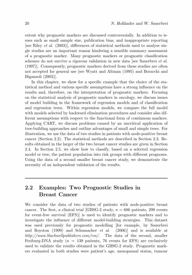
20 N. Hollander and W. Sauerbrei
extent why prognostic markers are discussed controversially. In addition to is-sues such as small sample size, publication bias, and inappropriate reporting[see Riley et al. (2003)], differences of statistical methods used to analyse sin-gle studies are an important reason hindering a sensible summary assessmentof a prognostic marker. Many prognostic markers or prognostic classificationschemes do not survive a rigorous validation in new data [see Sauerbrei et al.(1997)]. Consequently, prognostic markers derived from these studies are oftennot accepted for general use [see Wyatt and Altman (1995) and Boracchi andBiganzoli (2003)].
In this chapter, we show for a specific example that the choice of the sta-tistical method and various specific assumptions have a strong influence on theresults and, therefore, on the interpretation of prognostic markers. Focusingon the statistical analysis of prognostic markers in oncology, we discuss issuesof model building in the framework of regression models and of classificationand regression trees. Within regression models, we compare the full modelwith models selected by backward elimination procedures and consider also dif-ferent assumptions with respect to the functional form of continuous markers.Applying CART, we discuss problems caused by an uncritical application oftree-building approaches and outline advantages of small and simple trees. Forillustration, we use the data of two studies in patients with node-positive breastcancer (Section 2.2). The statistical methods are described in Section 2.3. Re-sults obtained in the larger of the two breast cancer studies are given in Section2.4. In Section 2.5, we show how to classify, based on a selected regressionmodel or tree, the patient population into risk groups with different prognoses.Using the data of a second smaller breast cancer study, we demonstrate thenecessity of an independent validation of the results.
2.2 Examples: Two Prognostic Studies in
Breast Cancer
We consider the data of two studies of patients with node-positive breastcancer. The first, a clinical trial [GBSG-2 study, n = 686 patients, 299 eventsfor event-free survival (EFS)] is used to identify prognostic markers and toinvestigate the influence of different model-building strategies. This datasetwas used previously for prognostic modelling [for example, by Sauerbreiand Royston (1999) and Schumacher et al. (2006)] and is available athttp://www.blackwellpublishers.com/rss/. The data of the second, smallerFreiburg-DNA study (n = 139 patients, 76 events for EFS) are exclusivelyused to validate the results obtained in the GBSG-2 study. Prognostic mark-ers evaluated in both studies were patient’s age, menopausal status, tumour

Multivariable Analysis of Prognostic Marker Studies 21
size, estrogen, and progesterone receptor, tumour grade, and number of in-volved lymph nodes. More details with references are given in Schumacher etal. (2006).
2.3 Statistical Methods
There are several statistical methods to analyse prognostic marker studies. Inthis chapter, we consider regression models and classification and regressiontrees.
2.3.1 Regression models
For survival data, a standard tool to analyse multiple prognostic markers si-multaneously is the Cox proportional hazards regression model. If we denotethe prognostic markers under consideration by X1,X2, . . . ,Xp, then the modelis given by
λ(t|X1,X2, . . . ,Xp) = λ0(t) exp(β1X1 + β2X2 + · · · + βpXp), (2.1)
where λ (t | ·) = limh→0 (1/h)Pr (t ≤ T < t + h | T ≥ t, ·) denotes thehazard function of the event-free or overall survival time random variable Tand λ0(t) is an unspecified baseline hazard. The assumption of a (log-)lineareffect of a continuous prognostic marker Xj (e.g., tumour size) is one of thestandard assumptions in the Cox regression model; here, exp(βj) represents theincrease or decrease in risk if Xj is increased by one unit. If Xj is binary (e.g.,menopausal status), then exp(βj) is simply the hazard ratio (HR) of category 1(e.g., postmenopausal) to the reference category (Xj = 0, e.g., premenopausal).
Continuous markers
Due to this easy interpretation, continuous prognostic markers are often cate-gorised into two or more subgroups. Doing so, in formula (2.1) the correspond-ing prognostic marker is replaced by dummy variables for the different categories(e.g., two dummies for three categories). Then the hazard ratio is estimatedwith respect to one reference category. For more details, see standard text-books by Marubini and Valsecchi (1995) and Therneau and Grambsch (2000).However, the categorisation of a continuous prognostic marker has several dis-advantages such as loss of information [see Royston, Altman, and Sauerbrei(2006)]. On the other hand the assumption of a (log-)linear relationship maybe wrong. As an alternative, Royston and Altman (1994) proposed the frac-tional polynomial (FP) approach which provides more flexibility by allowing

22 N. Hollander and W. Sauerbrei
non-linear relationships of continuous covariates while preserving simplicity ofthe final model to an acceptable degree.
Variable selection
An important aspect in the analysis of prognostic marker studies is the selectionof markers with influence on the outcome. To select relevant covariates in theframework of regression models, variable selection methods such as stepwisemethods or selection based on an information criterion (e.g., Akaike’s AIC) arecommonly applied [see Weissberg (2005)].
In this chapter, we apply backward elimination (BE) using different nom-inal significance levels and compare the results to the full model. We will usethe common significance level α = 0.05 [BE(0.05)], BE with significance levelα = 0.157 [BE(0.157)], which corresponds asymptotically to AIC if selection ofone variable is considered, and α = 0.01 [BE(0.01)] leading to a more stringentselection of markers. Combining the selection of a FP transformation for contin-uous covariates with selection of variables by backward elimination, Sauerbreiand Royston (1999) and Sauerbrei et al. (1999) have extended the FP-approachto a model-building strategy, which is referred to as the multivariable fractionalpolynomial (MFP) approach. This MFP approach also allows the incorpora-tion of basic medical knowledge, that is, the increase or decrease in risk mustbe monotonic. Software is generally available [see Sauerbrei et al. (2006)].
To assess the selected models, we use the Akaike Information Criterion(AIC) and the Bayesian Information Criterion (BIC). The latter depends onsample size and puts more penalty on each covariate in the selected model thanthe AIC. A smaller value of AIC and BIC, respectively, corresponds to a bettermodel.
2.3.2 Classification and regression trees (CART)
Hierarchical trees are a popular approach for nonparametric modelling of therelationship of several potential prognostic markers and a response variable.Briefly, the idea of classification and regression trees (CART) is to constructsubgroups that are internally as homogeneous as possible with respect to theoutcome (here, EFS) and externally as separated as possible. Thus, CART leadsdirectly to prognostic subgroups defined by the selected prognostic markers.This is achieved by a recursive tree-building algorithm. Although the principlesof the approach have been available for a long time, the monograph of Breimanet al. (1984) is often considered as the important “starting point” of tree-basedmethods. Here we will use CART as a synonym for these approaches. Theoriginal version of CART has been modified in various directions, but here weconcentrate on the application to survival data. The log-rank test is used to splitthe data recursively into subgroups. As a stopping rule for the tree-building

Multivariable Analysis of Prognostic Marker Studies 23
process, we use pstop = 0.05 as an upper bound of the minimal p value andnmin = 20 as minimum number of patients in a subgroup. Furthermore, werestricted the possible splits to the range between the 10% and 90% quantilesof the empirical distribution of each continuous marker. Within this range,all splits are considered as potential cutpoints and CART selects the cutpointcorresponding to the minimum p-value pmin of the log-rank test that is usedfor the comparison of the resulting two subgroups. More details with referencesare given in Schumacher et al. (2006).
Because of the well-known problem resulting from multiple testing, it isobvious that the selection of the minimum p-value cannot lead to correct resultsof the log-rank test. To account for this problem, we used a P -value correctionof Lausen and Schumacher (1992).
2.3.3 Formation of risk groups
Quite often, the aim is to develop a prognostic classification scheme. The finalsubgroups obtained in a regression tree are well suited for this task. Dependingon the number of final nodes and their separation, some combination of thesesubgroups to a prognostic subgroup might be indicated, especially if the prog-nosis is comparable. For more complex trees systematic approaches to pruneand amalgamate nodes have been proposed [see Breiman et al. (1984)]. Forsmaller trees, medical knowledge and subjective preferences can be incorporatedto define a prognostic classification scheme [see Sauerbrei et al. (1997)].
For the regression approaches considered in Section 2.3, prognostic sub-groups can be formed by dividing the distribution of the prognostic indexβ1X1 + β2X2 + · · · + βpXp into quartiles.
2.4 Results in the GBSG-2 Study
In this section, we apply the different statistical methods to the data of theGBSG-2 study. Some results will be used to form risk groups in Section 2.5.
2.4.1 Regression models – standard applications
In regression models for the GBSG-2 data, all analyses were adjusted for hor-monal treatment.
Table 2.1 shows results of univariate Cox models as well as the results of thefull model and the model selected by BE(0.05). For continuous covariates, weuse both approaches, assuming either a linear effect (A) or using cutpoints tocategorise the variables (B). Cutpoints were chosen independently from the dataas predefined in the original analysis of the GBSG-2 study; for more details,

24 N. Hollander and W. Sauerbrei
see Schumacher et al. (2006). Results are given in terms of estimated hazardratios (HRs). HRs should be given with confidence intervals, but we haveomitted them for brevity. With BE(0.05), we select with both approaches amodel containing the three markers: tumour grade, number of involved lymphnodes, and progesterone receptor. Using AIC and BIC for model assessment,the two models with categorised covariates fit better than the correspondingmodels based on the assumption of a linear effect of continuous covariates. Forboth approaches, the model selected by BE(0.05) would be preferred to thecorresponding full model due to smaller values of AIC and BIC.
BE(0.01) yields the same model as BE(0.05) when a linear effect is assumed,whereas only two markers (number of lymph nodes, progesterone receptor) wereselected with BE(0.01) for categorised data (Table 2.2). Applying BE(0.157)in the latter situation, age and menopausal status were included in the se-lected model, but both markers were eliminated when assuming a linear effect.However, tumour size is now included. Assessing models by BIC, the smallestmodel would be preferred due to the large penalty term for additional markers;the smallest AIC value was obtained with BE(0.05) for categorised covariates.However, in spite of the better fit, the categorisation can always be criticisedbecause of some degree of arbitrariness and subjectivity concerning the num-ber of cutpoints, the specific cutpoints chosen, and a loss of information [seeRoyston, Altman, and Sauerbrei (2006)].
Age (years)
log−
haza
rd r
atio
25 35 45 55 65 75
−1
0
1
2
3
Figure 2.1: Different risk functions for the effect of age obtained in the GBSG-2study: categorised risk function (solid line), linear risk function (dashed line),and fractional polynomial (dotted line)

Multivariable Analysis of Prognostic Marker Studies 25
2.4.2 Regression models – the MFP-approach
Applying the MFP-approach to the GBSG-2 data with significance level α =0.05, the following markers were selected: number of positive lymph nodes,tumour grade, progesterone receptor, and age, for the latter two a FP transfor-mation was chosen. This model yields an AIC value of 3072.22 corresponding toan improvement of the log-likelihood of 8.7 as compared to the model selectedby BE(0.05) with categorised covariates (Table 2.2). For more details, see Table4 in Sauerbrei and Royston (1999). With the MFP-approach, a highly signif-icant nonlinear effect of age was detected (likelihood ratio test for age givesP < 0.001) with a strong increase in risk for younger patients. Correspondingto the results in Table 2.1, we illustrate in Figure 2.1 that there is hardly anyprognostic effect of age if we assume linearity or after categorising age into thesubgroups based on the predefined cutpoints.
The analysis of the GBSG-2 study has shown that the final regression modelmay strongly depend on the underlying model-building strategy and that stan-dard assumptions such as linearity for continuous covariates may not correspondto the data.
2.4.3 Summary assessment – implication of the modellingstrategy
As shown in Figure 2.1, we observed hardly any effect of age when assuminglinearity or when categorising age using the prespecified cutpoints. However,using a single cutpoint of 40 years the resulting HR (95% confidence inter-val) comparing patients > 40 years, with patients ≤ 40 years in a multivariableregression model is 0.624 (0.424,0.918) indicating, in contrast to scenario B (Ta-ble 2.1), a larger and significant age effect. This simple example demonstratesthat the choice of a specific cutpoint can strongly influence the estimated HRin one single study. This also affects the pooled estimate if such a study isincluded in a meta-analysis.
Furthermore, in meta-analyses based on published data, adjusted estimatesof a specific prognostic marker are often not available for several studies [seeRiley et al. (2006)]. It is not uncommon to calculate a pooled estimate of theHR from all data available, which means that estimated effects from unadjustedanalyses and adjusted analyses are averaged. To illustrate differences betweenresults from adjusted and unadjusted analyses, we have included univariateanalyses for the GBSG-2 data (see Table 2.1). For some variables, unadjustedHRs are much larger giving a very optimistic view on the prognostic value ofthe corresponding marker. In our example, this is more apparent for the modelwith the categorised risk markers. For example, the unadjusted estimated HRfor tumour grades 2 and 3 are 2.369 and 3.056, respectively, as compared topatients with grade 1 tumours. However, adjusting for the other prognostic

26 N. Hollander and W. SauerbreiTab
le2.
1:E
stim
ated
haza
rdra
tios
(HR
),A
IC,
and
BIC
inC
oxm
odel
s.R
esul
tsfr
omth
eun
ivar
iate
Cox
mod
el(n
oad
just
men
t),th
efu
llm
odel
and
ase
lect
edm
odel
obta
ined
byba
ckw
ard
elim
inat
ion
with
α=
0.05
(BE
(0.0
5))
assu
min
g(A
)a
(log
-)lin
ear
rela
tion
ship
for
cont
inuo
usco
vari
ates
and
(B)
cate
gori
sing
cont
inuo
usco
vari
ates
aspr
edefi
ned
inth
efir
stan
alys
isof
the
GB
SG-2
stud
y A:C
ontinuous,
Lin
ear
Effec
t†B
:C
ate
gorise
dM
ark
ers
Univ
ariate
Full
Model
BE
(0.0
5)
Univ
ariate
Full
Model
BE
(0.0
5)
Mark
erH
R#
HR
#H
R#
Cate
gorisa
tion
HR
#H
R#
HR
#
Age
(yea
rs)
1.0
00
0.9
91
–≤
45
11
–46−
60
0.7
90
0.6
72
–>
60
0.9
01
0.6
87
–
Men
opausa
lst
atu
s1.1
66
1.3
10†
–P
re1
1–
–Post
1.1
66
1.3
07
–Tum
our
size
(mm
)1.0
15∗∗
1.0
08∗
–≤
20
1∗∗
1–
21−
30
1.3
54
1.2
40
–>
30
1.7
51
1.3
16
–Tum
our
gra
de
1.5
34∗∗
1.3
21∗∗
1.3
40
11∗∗
11
22.3
69
1.7
23
1.7
09
33.0
56
1.7
46
1.7
77
No.
ofly
mph
nodes
1.0
59∗∗
1.0
51∗∗
1.0
57
1−
31∗∗
1∗∗
14−
92.1
53
1.9
76
2.0
71
≥10
3.9
75
3.5
13
3.6
62
Pro
ges
tero
ne
rece
pto
r(f
mol/
ml)
0.9
97∗∗
0.9
98∗∗
0.9
98
<20
1∗∗
1∗∗
1≥
20
0.4
64
0.5
45
0.5
36
Est
rogen
rece
pto
r(f
mol/
ml)
0.9
99
1.0
00
–<
20
11
–≥
20
0.6
63
0.9
94
–A
IC=
−2lo
gL
+2p
-3120.2
3117.9
-3087.2
3083.6
BIC
=−2
log
L+
log(n
)p-
3146.1
3129.0
-3128.1
3102.1
pN
umbe
rof
cova
riat
esin
the
mod
el,n
deno
tes
effec
tive
sam
ple
size
n=
299.
†E
xcep
tfo
rm
enop
ausa
lsta
tus,
whi
chis
bina
ry;g
rade
code
d1,
2,3.
#H
Rgi
ven
wit
hout
confi
denc
ein
terv
als
for
bett
erill
ustr
atio
non
ly.
*,**
Lik
elih
ood
ratio
test
sign
ifica
ntat
sign
ifica
nce
leve
l*
α=
0.05
and
**α
=0 .
01.

Multivariable Analysis of Prognostic Marker Studies 27
Tab
le2.
2:Se
lect
edpr
ogno
stic
mar
kers
,AIC
,and
BIC
for
diffe
rent
mod
else
lect
ion
stra
tegi
es.
Incl
uded
mar
kers
mar
ked
bydo
ts
A:C
onti
nuou
s,Lin
ear
Effe
ctB
:C
ateg
oris
edM
arke
rsFu
llFu
llM
arke
rM
odel
BE
(0.1
57)
BE
(0.0
5)B
E(0
.01)
Mod
elB
E(0
.157
)B
E(0
.05)
BE
(0.0
1)A
ge•
••
Men
opau
sals
tatu
s•
••
Rum
our
size
••
•R
umou
rgr
ade
••
••
••
•N
o.of
lym
phno
des
••
••
••
••
Pro
gest
eron
ere
cept
or•
••
••
••
•E
stro
gen
rece
ptor
••
AIC
=−
2lo
gL
+2p
3120
.231
16.6
3117
.931
17.9
3087
.230
84.5
3083
.630
85.1
BIC
=−
2lo
gL
+lo
g(n)p
3146
.131
31.4
3129
.031
29.0
3128
.131
14.1
3102
.130
96.2
pN
umbe
rof
cova
riat
esin
the
mod
el,n
deno
tes
effec
tive
sam
ple
size
n=
299.

28 N. Hollander and W. Sauerbrei
markers in the full model, the corresponding estimated HRs reduced to 1.723and 1.746, respectively. In a chapter in this volume Riley et al. (2006) illustratea possible influence of this issue on the result of a meta-analysis by calculatingpooled estimates for adjusted and unadjusted effects of a prognostic marker(MYCN) for neuroblastoma [see Riley et al. (2006)]. As in our analysis, fora single study the estimated HRs from the unadjusted analysis were larger.Consequently, a meta-analysis mixing unadjusted and adjusted risk estimatesfrom the primary studies produces pooled estimates whose interpretation is verydifficult.
2.4.4 Application of classification and regression trees
Using the CART procedure with our choice of specific parameters for the analy-sis of the GBSG-2 data, we obtained the large complex tree displayed on the leftside of Figure 2.2. We start with the whole group of 686 patients (the ‘root’)with 299 observed events corresponding to an event rate of 43.6%. The markerwith the smallest minimum p-value is ‘number of involved lymph nodes’ (inFigure 2.2 denoted as NODES), and the whole group is split at an estimatedcutpoint of 9 positive nodes yielding subgroups of 585 patients with less thanor equal to 9 positive lymph nodes (event rate 38.8%) and a subgroup of 103patients with more than 9 positive nodes (event rate 70.9%). Repeating thisprocedure in the latter smaller subgroup, progesterone receptor (PROGREZ)with cutpoint 23 fmol leads to the smallest minimum p-value and the 103 pa-tients are subdivided into subgroups of 60 and 43 patients, respectively. In thesetwo subgroups, no further splits are possible because of the pstop criterion. Inthe group of 585 patients with maximally 9 positive lymph nodes, again NODESappeared to be the strongest marker with a cutpoint of 3 positive nodes. Inthis left part of the tree, the resulting subgroups are then subdivided by PRO-GREZ; further subdivisions are based on the markers tumour size (TUSIZE),age (AGE), and/or estrogen receptor (ESTREZ). Finally, the tree-building al-gorithm leads to 12 final subgroups, which are illustrated by the boxes in Figure2.2.
This uncritical application of CART has several disadvantages. (i) For con-tinuous markers, the cutpoint is selected from a large set of possible splits.Because of the well-known problem resulting from multiple testing, it is obvi-ous that the selection of the minimum p-value cannot lead to correct results ofthe log-rank test. Ignoring this problem, continuous variables are likely to bechosen for data splitting, even if they have hardly any prognostic effect. Fur-thermore, the tree-building algorithm produces too many splits and ends upwith too many final subgroups. However, this problem can be reduced by usinga corrected p-value pcor instead of the minimum p-value [see Lausen and Schu-macher (1992)]. Additionally, it is questionable whether all selected cutpointsare sensible. In the subgroup of the 103 patients with more than 9 positive

Multivariable Analysis of Prognostic Marker Studies 29
A B
NODES<=9NODES>9
43.6%
686
NODES<=3NODES>3
38.8%
583
PROGREZ<=90PROGREZ>90
31.6%
376
37.9%
240
TUSIZE<=21TUSIZE>21
20.6%
136
12.7%
55
AGE<=44AGE>44
25.9%
81
43.8%
16
ESTREZ<=236ESTREZ>236
21.5%
65
16.0%
50
40.0%
15
PROGREZ<=55PROGREZ>55
51.7%
207
61.5%
117
TUSIZE<=30TUSIZE>30
38.9%
90
ESTREZ<=31ESTREZ>31
32.7%
55
50.0%
14
26.8%
41
AGE<=53AGE>53
48.6%
35
40.9%
22
61.5%
13
PROGREZ<=23PROGREZ>23
70.9%
103
85.0%
60
51.2%
43
NODES<=9
NODES>9
43.6%
686
NODES<=3
NODES>3
38.8%
583
PROGREZ<=100
PROGREZ>100
31.6%
376
36.8%
250
21.4%
126
PROGREZ<=20
PROGREZ>20
51.7%
207
63.2%
87
43.3%
120
PROGREZ<=20
PROGREZ>20
70.9%
103
84.2%
57
54.4%
46
Figure 2.2: Classification and regression trees obtained for the GBSG-2 study:(A) no p-value correction and all cutpoints allowed (no prespecification) and(B) with p-value correction and prespecification of cutpoints
nodes, for example, we obtained for the progesterone receptor a cutpoint of 23fmol. The same value would be obtained when using a corrected instead of theminimum p-value. However, the choice of 23 fmol is somewhat arbitrary andmay not be reproducible or comparable to cutpoints obtained in other studies.In medical studies, cutpoints of 5, 10, or 20 fmol/ml are often used to classifyinto receptor-positive and receptor-negative patients. Thus, another useful re-striction to be implemented in the tree-building process may be the definitionof a set of predefined possible cutpoints. For the progesterone and estrogenreceptors we chose 5, 10, 20, 100, and 300 fmol as possible splits. Definingalso prespecified cutpoints for age and tumour size and using corrected p-valuesof the log-rank test, we obtained the small tree displayed on the right side ofFigure 2.2. NODES with a cutpoint of 9 positive lymph nodes is again used tosplit the complete population. The corrected p-value is still highly significant(pcor < 0.0001) indicating the strong prognostic effect of this marker. Furthersplits are based on NODES with cutpoint 3 and on PROGREZ. In contrastto the first complex tree, we obtained a simple small tree, which is based onthe two important prognostic markers only, with 6 final subgroups. Generally,the interpretation of such simple trees is easier and the chance that results arereproducible is much higher as compared to that from large complex trees.

30 N. Hollander and W. Sauerbrei
2.5 Formation and Validation of Risk Groups
Using the small tree (Figure 2.2B) we form four prognostic subgroups out ofthe six final subgroups:
I: NODES ≤ 3 and PROGREZ > 100.II: NODES ≤ 3 and PROGREZ ≤ 100 or 4 ≤ NODES ≤ 9 and PROGREZ
> 20.III: 4 ≤ NODES ≤ 9 and PROGREZ ≤ 20 or NODES > 9 and PROGREZ
> 20.IV: NODES > 9 and PROGREZ ≤ 20.
The Kaplan–Meier estimates of the event-free survival curves for subgroupsI–IV, which are given in Figure 2.3 under the heading ‘CART,’ show a goodseparation between the selected prognostic subgroups.
Kaplan–Meier estimates of EFS for the prognostic subgroups derived fromthe prognostic index of the Cox regression model selected by BE(0.05) withcategorised variables are displayed in Figure 2.3 as ‘COX.’ Again, we obtaineda clear separation between prognostic subgroups.
Although both approaches use the same two strong prognostic markers theresulting prognostic subgroups need not necessarily contain the same patients.The group with the worst prognosis obtained by COX, for instance, contains180 patients, whereas subgroup IV of CART contains only 57 patients. Further-more, it should be taken into account that we estimated the difference betweenprognostic subgroups with the same data that we used for model building. As aconsequence, the differences between risk groups are most likely overestimatedand results have to be validated in an independent study.
Validation
We attempt to validate the two prognostic classification schemes with the dataof the Freiburg-DNA study that covers the same patient population and prog-nostic markers as the GBSG-2 study. Despite the good agreement, which couldnot be taken for granted in practice, CART is not directly applicable, becauseonly progesterone and estrogen receptor status (positive: > 20 fmol and nega-tive: ≤ 20 fmol) are recorded in the Freiburg-DNA study. Therefore, we modifyCART by replacing the value 100 for PROGREZ by 20. We replace subgroupsI and II by new subgroups I* and II*; the modified classification approach isreferred to as CART*. Except for the adaption for PROGREZ, no further mod-ifications were necessary. However, this good agreement between studies is anexception rather than a rule.

Multivariable Analysis of Prognostic Marker Studies 31
COX
Time (years)
Sur
viva
l pro
babi
lity
0.00
0.25
0.50
0.75
1.00
0 1 2 3 4 5 6 7
I
II
III
IV
CART
Time (years)
Sur
viva
l pro
babi
lity
0.00
0.25
0.50
0.75
1.00
0 1 2 3 4 5 6 7
I
II
III
IV
Figure 2.3: Kaplan–Meier estimates of event-free survival probabilities for theprognostic subgroups derived from a Cox model with categorised covariates(COX) and the simple tree displaced in Figure 2.2B (CART)
Table 2.3 shows the estimated hazard ratios with 95% confidence intervalsfor the prognostic groups derived from the two classification schemes. The HRswere estimated by using dummy variables defining the risk groups and by takingthe group with the best prognosis as reference. To obtain prognostic subgroupsin the Freiburg-DNA study, the definitions and categorisation derived in theGBSG-2 study are used. The results show that there is some shrinkage in theHRs when estimated in the Freiburg DNA study. For several reasons, such asthe baseline category in COX includes only 7.6% of patients in contrast to 35.4%in the baseline category of CART, a comparison of the amount of shrinkage isdifficult. It seems to be that shrinkage is more pronounced in the CART*classification scheme (reduction by 47% in the high-risk group) as comparedwith COX (reduction by 28% in the high-risk group).
To sum up, the assessment of prognostic classification schemes should not beperformed in the same data set that is used for model building and formation ofrisk groups. If no validation data are available, data-splitting as cross-validationor bootstrap resampling methods could be applied to obtain different data setsfor model building and assessment of results.

32 N. Hollander and W. Sauerbrei
Table 2.3: Estimated hazard ratios (HR) for prognostic subgroups derived inthe GBSG-2 study by using the selected Cox model with categorised covariates(COX) and a modification of the simple tree displayed in Figure 2.2B (CART*).Validation of the HRs in the Freiburg-DNA study
GBSG-2 study Freiburg-DNA study†
HR (95% CI) n (percent) HR (95% CI) n (percent)
COXI 1 52 (7.6) 1 33 (23.7)II 2.68 (1.23, 5.83) 218 (31.8) 1.78 (0.73, 4.31) 26 (18.7)III 3.95 (1.83, 8.51) 236 (34.4) 3.52 (1.65, 7.30) 58 (41.7)IV 9.92 (4.62,21.29) 180 (26.2) 7.13 (2.56,17.18) 14 (10.7)
CART*I* 1 243 (35.4) 1 50 (36.0)II* 1.82 (1.34, 2.47) 253 (36.9) 1.99 (1.05, 3.75) 38 (27.3)III 3.48 (2.51, 4.82) 133 (19.4) 3.19 (1.70, 5.97) 33 (23.7)IV 8.20 (5.52,11.98) 57 (8.3) 4.34 (1.85,10.15) 11 (7.9)
† Complete case analysis, observations with missing values deleted.
2.6 Discussion
In this chapter, we presented several statistical methods which are used toanalyse prognostic marker studies. It was shown that results can strongly de-pend on the modelling approach. We demonstrated that a so-called final mul-tivariable regression model is often the result of a more or less extensive model-building process which may involve the categorisation and/or transformation ofmarkers as well as the selection of variables in an automatic or subjective man-ner. Several assumptions are always required. Investigating prognostic markersby means of classification and regression trees, corrected p-values should beapplied to overcome problems caused by multiple testing in continuous mark-ers. Furthermore, the prespecification of cutpoints and the definition of sensiblestopping rules are important to provide interpretable trees.
Considering only 7 potential prognostic markers in our example, we haveshown that standard assumptions of the Cox model may be violated and that acareful multivariable modelling is needed to select relevant markers and to as-sess their effect. Obviously, these problems increase with an increasing numberof potential prognostic markers. Even before the first results of gene expressionstudies were published, the effect of more than 200 potential prognostic mark-ers in breast cancer were controversially discussed, and by 2001 about 1000papers have been published on this issue. Considering only several variables,the ‘full’ model is often not sensible, although its use is postulated in theo-

Multivariable Analysis of Prognostic Marker Studies 33
retical papers or some textbooks [e.g., Harrell (2001)]. One important reasonis that the full model avoids data-dependent modelling providing unbiased pa-rameter estimates and meaningful confidence intervals. On the negative side,it has to be stressed that the choice of variables in the full model is ratherunclear. Generally, a large number of different variables are recorded in a clin-ical trial and also in a clinical cancer registry. Which of these variables belongto the full model? The ‘pro’ to avoid data-dependent modelling leads to the‘con’ that the full model includes some variables with a negligible effect [seeSauerbrei (1999)] and usually assumes linear effects for continuous covariates.However, this assumption may not agree with the dose–response relationship inthe data. Investigating possible nonlinearity with the MFP approach, this wasmost obvious for age in our example. Model building by selection of variablesand functional forms for continuous variables may cause bias of estimates inthe final multivariable regression model. Therefore, the model-building processshould be taken into account when judging the results of a prognostic study;in practice, it is usually neglected. Simplicity should be an important aim ofmodel building [see Sauerbrei (1999)]. This also helps with issues such as sta-bility and reproducibility of the selected model or tree. Bootstrap resamplingmethods may be used to investigate stability of regression models [see Roystonand Sauerbrei (2003)] and to correct for bias caused by model building [seeSchumacher, Hollander, and Sauerbrei (1997) and Hollander, Sauerbrei, andSchumacher (2004)]. Procedures to combine variable selection with shrinkagehave been proposed [see Breiman (1995) and Tibshirani (1997)]. To improvethe predictive ability of trees, stabilising methods based on resampling, such asbagging have been proposed [see Breiman (2001) and Hothorn et al. (2004)].Furthermore, to assess their usefulness, prognostic models should be validatedin independent data [see Simon and Altman (1994) and Altman and Royston(2000)]. Using the classification scheme developed in the GBSG-2 study to formprognostic subgroups in the validation study, we observed some shrinkage withrespect to the separation of the resulting subgroups.
In addition to the statistical approaches described in this chapter, thereare many other modelling approaches available and more statistical issues toconsider for the analysis of a single study. To handle these issues, authors havespecific preferences but general recommendations are currently not available[see Schumacher et al. (2006), Concato, Feinstein, and Holford (1993), Harrell,Lee, and Mark (1996), Pajak et al. (2000), McShane and Simon (2001), andBiganzoli, Borachi, and Marubini (2003)]. A variety of methods is used inreal studies; conflicting results concerning the prognostic relevance of singlemarkers may be caused by the choice and/or the (inadequate) application of aspecific statistical method. In Table 2.4, we have summarised important issuesconcerning the analysis of single studies. In addition to the topics discussedhere, we have also listed a few points requiring more attention in future studies.

34 N. Hollander and W. Sauerbrei
Table 2.4: Summary of important issues for the analysis of single prognosticmarker studies
1. Treatment of Study Population
- Ideally patients without any systemic adjuvant therapy, but unrealistic in many diseases
- Standardisation or randomisation of treatment preferable; adjustment for treatment in the
analysis
2. Model-Building Process
- Multivariable model required to assess the effect of a marker
- Many approaches available; no general agreement concerning preferable strategies
- Our preference is regression models; other approaches can give complementary information
2a. Regression Models
- Problems caused by categorisation of continuous covariates
- Standard assumption of a (log-)linear effect of continuous markers may be wrong
- Variable selection methods sensible to select relevant markers; complexity of the “final”
regression model depends on nominal significance level
- Different variable selection strategies may result in different ”final” regression models
2b. Trees
- Uncritical application of trees can lead to large, unstable, and uninterpretable trees
- p-value correction and prespecification of cutpoints for continuous variables
2c. Other Approaches
- Many methods available, none without problems
3. Formation of Risk Groups
- Different model-building strategies may result in different risk groups
- Avoid too-small risk groups
4. Validation of Results
- Overestimation of effects caused by data-dependent modelling
- Validation of prognostic relevance of markers and models in independent validation study
5. Issues Requiring More Attention in Future Studies
- Stability investigation of selected models
- Combining variable selection with shrinkage
- Differentiation between studies developing a prediction model from studies with main
interest in one specific marker

Multivariable Analysis of Prognostic Marker Studies 35
In general, the evaluation of a prognostic marker requires a summary as-sessment from several studies. For individual studies, it is generally acceptedthat a multivariable analysis is required. Consequently, a pooled estimate fromseveral studies should be based on adjusted estimates from individual studies.Ideally all studies use the same variables for adjustment. This may be possi-ble with individual patient data (IPD) and simple models containing a smallnumber of ‘important’ markers only. For new markers, it is more promisingthat research groups start cooperation when designing new studies with theaim of a prospectively planned pooled analysis, a concept sometimes used inepidemiological research [see Blettner et al. (1999)]. With the current situationof trying to summarise poorly published estimates based on different ways ofanalysis, a reliable assessment of the prognostic value of a marker is nearly im-possible. Many important problems illustrating the difficulties of performing apooled analysis using published studies and the feasibility of obtaining IPD areaddressed in two chapters in this volume by Riley et al. (2006) and Altman etal. (2006).
References
1. Altman, D. G., and Royston, P. (2000). What do we mean by validatinga prognostic model? Statistics in Medicine, 19, 453–473.
2. Altman, D. G., Trivella, M., Pezzella, F., Harris, A. L., and Pastorino, U.(2006). Systematic review of multiple studies of prognosis: The feasibilityof obtaining individual patient data, in this volume.
3. Biganzoli, E., Borachi, P., and Marubini, E. (2003). Biostatistics and tu-mour marker studies in breast cancer: Design, analysis and interpretationissues, The International Journal of Biological Markers, 18, 40–48.
4. Blettner, M., Sauerbrei, W., Schlehofer, B., Scheuchenpflug, T., andFriedenreich, C. (1999). Traditional reviews, meta-analyses and pooledanalyses in epidemiology, International Journal of Epidemiology, 28, 1–9.
5. Boracchi, P., and Biganzoli, E. (2003). Markers of prognosis and responseto treatment: Ready for clinical use in oncology? A biostatistician’s view-point, The International Journal of Biological Markers, 18, 65–69.
6. Breiman, L. (1995). Better subset regression using the nonnegativeGarotte, Technometrics, 37, 373–384.
7. Breiman, L. (2001). Random forests, Machine Learning, 45, 5–32.

36 N. Hollander and W. Sauerbrei
8. Breiman, L., Friedman, J. H., Olsen, R. J., and Stone, C. J. (1984).Classification and Regression Trees, Wadsworth, Monterey, California.
9. Concato, J., Feinstein, A. R., and Holford, T. R. (1993). The risk ofdetermining risk with multivariable models, Annals of Internal Medicine,118, 201–210.
10. Harrell, F. E., Jr. (2001). Regression Modelling Strategies: With Ap-plications to Linear Models, Logistic Regression, and Survival Analysis,Springer-Verlag, New York.
11. Harrell, F. E., Lee, K. L., and Mark, D. B. (1996). Multivariable prog-nostic models: Issues in developing models, evaluating assumptions andaccuracy, and measuring and reducing errors, Statistics in Medicine, 15,361–387.
12. Hollander, N., Sauerbrei, W., and Schumacher, M. (2004). Confidenceintervals for the effect of a prognostic factor after selection of an ‘optimal’cutpoint, Statistics in Medicine, 23, 1701–1713.
13. Hothorn, T., Lausen, B., Benner, A., and Radespiel-Troger, M. (2004).Bagging survival trees, Statistics in Medicine, 23, 77–91.
14. Lausen, B., and Schumacher, M. (1992). Maximally selected rank statis-tics, Biometrics, 48, 73–85.
15. Marubini, E., and Valsecchi, M. G. (1995). Analysing Survival Data fromClinical Trials and Observational Studies, John Wiley & Sons, New York.
16. McShane, L. M., and Simon, R. (2001). Statistical methods for the analy-sis of prognostic factor studies, In Prognostic Factors in Cancer (Eds., M.K. Gospodarowicz, D. E. Henson, R. V. P. Hutter, et al.), 2nd ed., JohnWiley & Sons, Lisbon.
17. Pajak, T. F., Clark, G. M., Sargent, D. J., McShane, L. M., and Ham-mond, M. E. H. (2000). Statistical issues in tumour marker studies,Archives of Pathology and Laboratory Medicine, 124, 1011–1015.
18. Riley, R. D., Abrams, K. R., Lambert, P. C., Sutton, A. J., and Altman,D. G. (2006). Where next for evidence synthesis of prognostic markerstudies? Improving the quality and reporting of primary studies to facil-itate clinically evidence-based results, in this volume.
19. Riley, R. D., Abrams, K. R., Sutton, A. J., Lambert, P. C., Jones, D.R., Heney, D., and Burchill, S. A. (2003). Reporting of prognostic mark-ers: Current problems and development of guidelines for evidence-basedpractice in the future, British Journal of Cancer, 88, 1191–1198.

Multivariable Analysis of Prognostic Marker Studies 37
20. Royston, P., and Altman, D. G. (1994). Regression using fractionalpolynomials of continuous covariates: parsimonious parametric modelling(with discussion), Applied Statistics, 43, 429–467.
21. Royston, P., Altman, D. G., and Sauerbrei, W. (2006). Dichotomizingcontinuous predictors in multiple regression: A bad idea, Statistics inMedicine, 25, 127–141.
22. Royston, P., and Sauerbrei, W. (2003). Stability of multivariable frac-tional polynomial models with selection of variables and transformations:A bootstrap investigation, Statistics in Medicine, 22, 639–659.
23. Sauerbrei, W. (1999). The use of resampling methods to simplify regres-sion models in medical statistics, Applied Statistics, 48, 313–329.
24. Sauerbrei, W., Hubner, K., Schmoor, C., and Schumacher, M. (1997).Validation of existing and development of new prognostic classificationschemes in node negative breast cancer, Breast Cancer Research andTreatment, 42, 149–163.
25. Sauerbrei, W., Meier-Hirmer, C., Benner, A., and Royston, P. (2006).Multivariable regression model building by using fractional polynomials:description of SAS, STATA and R programs, Computational Statistics &Date Analysis, 50, 3464–3485.
26. Sauerbrei, W., and Royston, P. (1999). Building multivariable prognosticand diagnostic models: Transformation of the predictors by using frac-tional polynomials, Journal of the Royal Statistical Society, Series A, 162,71–94.
27. Sauerbrei, W., Royston, P., Bojar, H., Schmoor, C., and Schumacher,M. (1999). Modelling the effects of standard prognostic factors in node-positive breast cancer, British Journal of Cancer, 79, 1752–1760.
28. Schumacher, M., Hollander, N., and Sauerbrei, W. (1997). Resamplingand cross-validation techniques: A tool to reduce bias caused by modelbuilding? Statistics in Medicine, 16, 2813–2827.
29. Schumacher, M., Hollander, N., Schwarzer, G., and Sauerbrei, W. (2006).Prognostic factor studies, In Handbook of Statistics in Clinical Oncology(Eds., J. Crowley and D. P. Ankerst), 2nd ed., pp. 307–351, CRC, BocaRaton, Florida.
30. Simon, R., and Altman, D. G. (1994). Statistical aspects of prognosticfactor studies in oncology. British Journal of Cancer, 69, 979–985.

38 N. Hollander and W. Sauerbrei
31. Therneau, T. M., and Grambsch, P. M. (2000). Modeling Survival Data:Extending the Cox Model, Springer-Verlag, New York.
32. Tibshirani, R. (1997). The lasso method for variable selection in the Coxmodel, Statistics in Medicine, 16, 385–395.
33. Weissberg, S. (2005). Applied Linear Regression, Third ed., John Wiley& Sons, New York.
34. Wyatt, J. C., and Altman, D. (1995). Prognostic models: Clinicallyuseful or quickly forgotten? Commentary, British Medical Journal, 311,1539–1541.

3
Where Next for Evidence Synthesis of Prognostic
Marker Studies? Improving the Quality and
Reporting of Primary Studies to Facilitate
Clinically Relevant Evidence-Based Results
Richard D. Riley,1 Keith R. Abrams,1 Paul C. Lambert,1
Alex J. Sutton,1 and Douglas G. Altman2
1University of Leicester, Princess Road West, Leicester, UK2Wolfson College, Oxford, UK
Abstract: Prognostic markers can help to identify patients with different risksof specific outcomes, facilitate treatment choice, and aid patient counselling.Unfortunately, within any given disease area, the wealth of conflicting and het-erogeneous evidence makes it difficult for the clinician to ascertain the overallevidence about specific markers and how to use them in practice. The ap-plication of formal methods (e.g., a systematic review and meta-analysis) ofobtaining and synthesising evidence is therefore greatly needed in the prognos-tic marker field. However, in this chapter we illustrate and discuss the reasonswhy currently poor standards of design, clinical relevance, and reporting in pri-mary studies limit statistically reliable and clinically relevant evidence-basedresults for prognostic markers. These problems add to those issues for the sta-tistical analysis in primary studies that are discussed in another chapter in thisvolume. To help overcome the problems we highlight guidelines for conductingand reporting primary prognostic research, and we particularly discuss why theavailability of individual patient data would help realise the evidence-based useof prognostic markers in clinical practice.
Keywords and phrases: Meta-analysis, prognosis, predictive marker, indi-vidual patient data, systematic review
39

40 R. D. Riley et al.
3.1 Introduction and Aims
3.1.1 Prognostic markers and prognostic marker studies
Prognostic markers (also called prognostic factors or prognostic variables) areimportant clinical tools as they help to identify patients with different risks ofspecific outcomes (e.g., recurrence of disease) and can thereby facilitate the mostappropriate treatment strategies and aid patient counselling. They can includesimple measures such as age, sex, stage of disease, or size of tumour, but alsomore complex factors such as abnormal levels of proteins or catecholamines,and unusual genetic mutations. In oncology, hundreds of prognostic markerstudies are published each year [see Riley et al. (2003b)] with assessments madeabout the association of one or more markers with overall survival (i.e., whetherpatients were alive or dead at the end of the study) and disease-free survival(i.e., whether patients were alive or had either died or suffered a recurrenceof disease by the end of the study). However, prognostic marker studies arecommon in many other research fields, such as heart disease [Hemingway andMarmot (1999)] and dementia [Mitchell et al. (2004)], and are also used inrelation to many other outcomes such as surgical complications [Carpeggianaet al. (2004)] and arthritis [Deodhar et al. (2003)].
3.1.2 The need for formal evidence syntheses of prognosticmarker studies
Unfortunately, within any given disease area, the results across different pri-mary prognostic marker studies are often inconsistent and contradictory [Si-mon and Altman (1994)]. Across studies, many different markers are assessedin relation to heterogeneous subpopulations, treatments, and outcomes. Fur-thermore, many studies have small numbers of patients and therefore a lowstatistical power of detecting treatment or survival benefits arising out of us-ing prognostic markers. This wealth of conflicting and heterogeneous evidencemakes it difficult for clinicians to ascertain the overall evidence about specificmarkers and, even for those known to be important, how to use them in practice(e.g., to which patients, using which cut-off levels, and applying which treat-ment regimen). Clinicians thus need help in establishing evidence-based resultsand guidelines about prognostic markers. The application of formal methodsof obtaining and synthesising evidence is therefore greatly needed in the prog-nostic marker field, otherwise there will continue to be large uncertainty andsubjective, perhaps inappropriate, use of prognostic markers in practice.
Since about 1990, there has been a growing movement toward evidence-based clinical practice and the formation of evidence-based clinical and public

Where Next for Evidence Synthesis of Prognostic Marker Studies? 41
health policies. The most commonly applied evidence synthesis method is asystematic review, which is a transparent framework for the collection, criticalappraisal, and synthesis of the current evidence from published and (if possible)unpublished studies [Egger, Davey Smith, and Altman (2001)]. If appropriate,a meta-analysis can be performed at the end of a systematic review, whichis a statistical approach that combines the quantitative evidence from all theindividual studies (or the subset of better quality studies) to produce overallevidence-based results [Egger, Davey Smith, and Altman (2001)]. In order tofacilitate a meta-analysis approach, it is common for a summary statistic (e.g.,hazard ratio) of interest to be chosen and extracted, where possible, from eachpublished (and unpublished) study. Alongside the estimate of the summarystatistic chosen, one also requires a measure of the uncertainty about the es-timate obtained [e.g., standard error of the loge(hazard ratio)], so that themeta-analysis can give relatively more weight to those estimates with small un-certainty and, conversely, relatively smaller weight to those estimates with largeuncertainty. A systematic review with meta-analysis is an ideal approach for aformal evidence synthesis of prognostic marker studies. However, we have re-cently demonstrated that a reliable and clinically useful systematic review andmeta-analysis will often not be feasible in this field, especially if one seeks toextract and synthesise summary statistics from published articles [Riley et al.(2003a)]. One major problem is that the primary studies to be synthesised arepoorly reported, in terms of both statistical information (e.g., solely p-valuesare often presented instead of a hazard ratio and confidence interval) and clini-cal information (e.g., treatment used and age of patients is often not reported).This problem restricts the extraction of summary statistics and makes it diffi-cult to perform reliable meta-analyses that determine the clinical importance ofeach marker studied based on the overall evidence [Altman (2001) and Altmanand Lyman (1998)].
3.1.3 Aims of this chapter
Chapter 2 in this volume by Hollander and Sauerbrei (2006) highlights issuesassociated with an appropriate statistical analysis within primary prognosticstudies. It is shown that different analysis strategies can give different resultsconcerning the effect of a factor. However, good research and appropriate sta-tistical practice is required throughout the whole study, not just at the analysisstage, and so the first aim for this chapter is to highlight further areas whereimprovements are needed within primary research of prognostic markers. Oursecond aim is to emphasise why there is a need, alongside improvements in theprimary studies, for individual patient data (IPD) to be commonly made avail-able from each study to help those performing meta-analysis; the practicalitiesof actually realising the IPD approach are assessed by Altman et al. (2006),Chapter 1 in this volume.

42 R. D. Riley et al.
3.2 Difficulties of an Evidence Synthesis of
Prognostic Marker Studies
3.2.1 Poor and heterogeneous reporting
We recently performed a large-scale systematic review of prognostic tumourmarkers in neuroblastoma and used it as an empirical investigation of the fea-sibility of producing evidence-based results of prognostic marker studies fromthe published literature [Riley et al. (2003a)]. The review identified 260 prog-nostic studies and in these there were 575 different reports where levels of oneof 13 different tumour markers were related to overall survival (OS) or disease-free survival (DFS) by summary statistics or IPD. From each of these reportsan estimate of the loge(hazard ratio) and its variance were sought, but only204 (35.5%) of the reports enabled both these statistics to be obtained. Fur-thermore, the loge(hazard ratio) and its variance were both directly providedon only three occasions in the 575 reports (0.005%); the other 201 estimatesrequired either indirect estimation methods (160 estimates), as suggested byParmar et al. (1998), or used the IPD provided in the published articles tocalculate the estimates directly using Cox regression (41 estimates). IPD wassometimes presented within the published literature because many studies hada small sample size due to the rarity of neuroblastoma disease, however, in gen-eral the availability of IPD from cancer studies is not common [Altman et al.(2006)].
In the neuroblastoma review, we used the estimates extracted to performmeta-analyses for each of the 13 markers considered, for each of OS and DFSwhere possible [Riley et al. (2004a)]. For example, the OS meta-analysis resultfor MYCN, the most commonly studied prognostic marker in neuroblastoma(152 studies in total presented OS results or IPD for MYCN ), is shown in Figure3.1 and it suggests that high levels of MYCN are strongly associated with anincreased risk of death. However, the reliability and clinical interpretability ofthis meta-analysis result is clearly limited because: (i) 107 studies (70.4 %)could not be included in the evidence synthesis because the MYCN results orIPD relating to prognosis were not provided in sufficient detail to allow theloge(hazard ratio) and its standard error to be estimated for OS; and (ii) theresults across studies were heterogeneous in clinical factors assessed, such asstage of disease and age of patients, and in the cut-off level used to dichotomisethe data (Figure 3.1). In particular, the multitude of missing summary statisticsin (i) makes one concerned that the set of available summary statistics does notactually reflect the truth. There is a strong potential for the OS (and similarly

Where Next for Evidence Synthesis of Prognostic Marker Studies? 43
paper = study id number, n = number of patients, u/a = unadjusted or adjusted hazard ratio;
stage = stage of disease; all stages = all of stages 1,2,3,4,and 4s were represented by the n
patients, all ages = ages < 1 year and > 1 year were represented by the n patients, and cut-off
= cut-off level used to dichotomise MYCN into ‘low-risk’ and ‘high-risk’ levels.
Figure 3.1: Forest plot for the MYCN overall survival (OS) meta-analysis fromthe neuroblastoma review including the 45 studies that allowed the loge(hazardratio) and its standard error to be estimated [Riley et al. (2004a)]. N.B. Therewere 107 other studies which provided MYCN results or IPD in relation toprognosis but not in sufficient detail to allow the loge(hazard ratio) and itsstandard error to be obtained; hence, the meta-analysis pooled hazard ratioresult below must be treated with caution, as it is not possible to include muchof the overall evidence in the evidence synthesis

44 R. D. Riley et al.
the DFS) meta-analysis result to be biased if some of the missing summarystatistics were not missing at random, perhaps because of publication bias orother related dissemination biases (see Section 3.2.5) [Riley et al. (2004b)].
The key reporting problems (such as no hazard ratio or confidence interval)that prevented us from obtaining 64.5% of the evidence base in the neuroblas-toma review are presented elsewhere, with guidelines also made for improvedreporting in the future [Riley et al. (2003a)]. To complement this work, wewill now discuss some of the other underlying reasons why primary prognos-tic studies often severely limit a clinically useful meta-analysis of the overallevidence.
3.2.2 Poor study design and problems clarifying study purpose
Altman and Lyman (1998) present suitable criteria that those initiating a pri-mary prognostic study should consider, and they suggest that every effortshould be made to limit potential biases and to emulate the design standardsof a clinical trial. They propose three main study types for assessing specificmarkers (Figure 3.2), based on Simon and Altman (1994). Although PhasesI to III have not yet been universally accepted, at the very least they pro-vide an important starting point for prognostic marker research, particularlyas currently many published primary studies are not properly designed. Forexample, often no justification is made for the sample size used, or whether the
1. Phase I: exploratory studies (hypothesis generating) which seek an associationbetween a prognostic marker and characteristics of disease thought to have prog-nostic importance.
2. Phase II: exploratory studies attempting to use values of a prognostic markerto(a) discriminate between patients at high and low risk of disease progression ordeath; or to(b) indicate which subsets of patients are likely to benefit from therapy.
3. Phase III: confirmatory studies of a priori hypotheses attempting to use valuesof a prognostic marker to(a) discriminate between patients at high and low risk of disease progression ordeath; or to(b) indicate which subsets of patients are likely to benefit from therapy.
Figure 3.2: Types of prognostic marker studies, as suggested by Altman andLyman (1998)
markers, subpopulations, and outcomes assessed were determined prior to thestudy beginning [Simon and Altman (1994)]; furthermore, the characteristics ofpatients assessed in a study may often not be described and thus one may havelittle idea of who the samples of patients selected are. Such problems make one

Where Next for Evidence Synthesis of Prognostic Marker Studies? 45
concerned that the reasons regarding how and what results are published froma study may be subject to bias, which limits their reliability for clinical practice(see Section 3.2.5). The further problem for evidence synthesis is that, due topoor reporting of information across the large majority of studies [Riley et al.(2003a)], it is generally very difficult to differentiate those studies which wereproperly designed from those studies that were poorly designed.
A related problem is distinguishing those primary studies that were origi-nally initiated for the same purpose [Altman and Lyman (1998)]. The majorityof prognostic marker studies have the purpose to establish the association be-tween a single putative marker of interest to some outcome (e.g., OS or DFS),and these were the predominant studies included in the neuroblastoma reviewintroduced previously [Riley et al. (2004a)]. However, there are also somestudies that do not have this primary purpose (e.g., studies to develop or val-idate a classification rule [Sauerbrei et al. (1997)]), yet still report summarystatistics or IPD relating markers to outcome as secondary results. Some meta-analysts may deem that, other things being equal, only those studies that werespecifically designed for the purposes of evaluating one or more markers shouldbe included in the meta-analysis (i.e., those where prognostic marker resultswere the primary endpoint) [Egger et al. (2003)]. Unfortunately, as the orig-inal study aims are rarely specified in a published article, it is often hard toascertain whether prognostic results were a primary or secondary objective. In-deed, a study may have started off with prognostic results as a secondary aimbut then, perhaps after witnessing the results obtained, may have switched theprimary focus of the published study to the prognostic markers.
3.2.3 Little indication of how to implement markers in clinicalpractice
Prognostic markers that can be specifically used to predict the response totherapy or treatment are called predictive markers (or predictive factors or pre-dictive variables). For example, estrogen receptor and progesterone receptorsare predictive markers used to select those breast cancer patients most likelyto respond to hormone therapy [Duffy (2005)]. If the results from prognosticstudies are to be most directly relevant to clinical practice, then as well as be-ing properly designed (see Section 3.2.2), they must also take into account thetreatment or therapeutic strategy involved in order to identify specific predic-tive markers [Windeler (2000)]. Such predictive studies relate to the Phase II(b)and III(b) studies in Figure 3.2 and they should ideally be integrated within anRCT, where the predictive ability of the marker can be assessed in relation tothe treatment groups assessed. Unfortunately, there are few high-quality PhaseII(b) and III(b) studies, and even when they are published it is often difficult toidentify them from most other prognostic studies due to the type of study (e.g.,exploratory – Phase I, confirmatory – Phase III) and the treatment received by

46 R. D. Riley et al.
patients not being reported. It is highly likely that the majority of prognosticstudies in the published literature are actually Phase I or II because, as seenin the neuroblastoma review [Riley et al. (2003a)], they often contain smallnumbers of patients and report a large number of results for a variety of possi-ble markers, and therefore do not seem to be focused on making confirmatoryconclusions for a few markers in relation to specific treatments. Thus, even ifa marker appears to have prognostic value, it will be very difficult to utilise itin clinical practice when there is a lack of identifiable, high-quality studies thatrelate its results to specific treatments. This problem will clearly also limit aclinically relevant evidence synthesis.
3.2.4 Small sample sizes
Small sample sizes is a particular problem for rare diseases, such as neurob-lastoma or other childhood cancers, and leads to individual studies having lowstatistical power. It also leads to a greater number of similar, but ultimatelyslightly different, studies of the same prognostic markers as each research groupreports the results for their own small sample. This in turn leads to hetero-geneity and inconsistency in how and what results were reported, especiallyregarding the adjustment factors used, the characteristics of patients included,and the cut-off levels used to dichotomise the continuous markers into “high-risk” and “low-risk” levels (Figure 3.1). All these problems ultimately limitmeta-analysis conclusions. For example, in the neuroblastoma review, if thehazard ratio was not reported we used indirect estimation methods to obtainan approximate value for the unavailable hazard ratios where possible [Par-mar, Torri, and Stewart (1998)]. Such indirect methods more closely estimatethe true values when the sample size is large, however, in the neuroblastomareview only 196 of 318 reports for which indirect estimation was required in-cluded more than 25 patients. Multiple studies with small sample sizes alsocause the problem of overlapping sets of patients across different studies. Al-though prospective studies are the ideal ones [Altman and Lyman (1998)], mostprognostic studies are retrospective, using information that has already beencollected from stored samples (e.g., in a tumour bank), and so there is a largepotential for different studies to report results for many of the same patients.However, it is practically very difficult to elicit those published studies that usethe same or overlapping sets of patients, and this again weakens meta-analysis[Riley et al. (2003b)].
3.2.5 Publication bias, selective within-study reporting, andselective analyses
For prognostic marker studies, there is likely to be the common problem ofpublication bias, where results that do not generate formal statistically sig-

Where Next for Evidence Synthesis of Prognostic Marker Studies? 47
nificant or clinically valuable findings may not be published. Other relateddissemination bias problems may also exist. For example, within-study selec-tive reporting may occur and in particular nonstatistically significant or neg-ative results may not be reported in as much detail as significant or positiveresults, thus making the extraction of desired summary statistics for meta-analysis more difficult (e.g., ‘p > 0.05’ is often presented) [Hahn, Williamson,and Hutton (2002)]. This may often be a consequence of a reluctance of jour-nals or researchers to report negative findings in detail. Other forms of dis-semination bias may include outcome reporting bias, subgroup reporting bias,and language bias [Egger, Dickersin, and Davey Smith (2001)]. In the meta-analysis of OS estimates for MYCN from the neuroblastoma review, therewas a strong suggestion that dissemination bias may be affecting the results.For instance, consider a plot of all the loge(hazard ratio) estimates for OSagainst their standard error (Figure 3.3). The assumption is that this plotshould form a funnel shape if dissemination bias is not present, as estimatesfrom smaller studies will be more widely spread about the mean effect dueto larger standard errors [Sterne, Egger, and Davey Smith (2001) and Duvaland Tweedie (2000)]. However, the plot is not indicative of a very funnel-like shape, and asymmetry is apparent, with a gap in the bottom right of theplot (Figure 3.3). Furthermore, two statistical tests indicated that dissemina-tion bias was likely to exist assuming that this was the main cause of funnel
logH
R
s.e. of: logHR
logHR
0 .5 1 1.5 2
−2
0
2
4
6
Figure 3.3: Funnel plot of the overall survival loge(hazard ratio) estimates forMYCN with Begg’s pseudo 95% confidence limits [Begg and Mazumdar (1994)]

48 R. D. Riley et al.
plot asymmetry (p < 0.001) [Egger et al. (1997) and Begg and Mazumdar(1994)]. It appears that some studies with less positive results than thoseobtained were missing from the meta-analysis, and this suggests that the trueunderlying pooled loge(hazard ratio) for OS is likely to be somewhat smallerthan the estimated pooled value of 1.70 (equivalent to a hazard ratio of 5.48)[Riley et al. (2004b)].
It is important to note many problems of dissemination bias may also beintroduced during a prognostic study and not just at the final reporting stage.For example, the type of statistical analysis used has an influence on the re-sult which then may influence the dissemination bias [Hollander and Sauerbrei(2006)]. The choice of cut-off level used to dichotomise the marker, and thusdefine a low-risk and a high-risk group of patients, may also be specificallychosen to optimise the difference between groups and produce a result withthe maximum statistical or clinical significance possible [Altman et al. (1994)].The difficulty for meta-analysis is again distinguishing those properly conductedstudies from those where biased choices of cut-off levels, analyses, and sampleswere used. Excluding studies with a small number of patients from the evidencesynthesis may help alleviate the potential problem of bias, as these studies arelikely to be of poorest quality. However, this issue relates to currently unan-swered questions facing meta-analysts about which studies should generally beincluded in a meta-analysis [Egger et al. (2003)].
3.2.6 Lack of appreciation or validation of previous findings
Evidence-based reviews are facilitated when new primary studies specificallybuild on the results of previous studies, thus forming a collective drive towardanswering questions of real clinical importance. For example, when a primarystudy assesses the potential of a new marker, it should do so in relation to thoseother markers previously identified as important and currently used in clinicalpractice. However, in reality many studies only report unadjusted results, andthe adjusted results that are presented across studies are often highly inconsis-tent in the set of adjustment factors used [Riley et al. (2003a)]. For example,of the 17 adjusted hazard ratio estimates for OS and DFS that were obtainedfor MYCN from the neuroblastoma review, only 2 were adjusted for exactlythe same set of factors, and both these were from the same article.
It would appear that a lack of collaboration across research groups com-bined with poorly designed studies (see Section 3.2.2) is causing there to bemany similar but slightly different prognostic studies, with many not buildingon previous findings. Indeed, there may be a deliberate ploy to make a newprimary study slightly different from those previously published in order toincrease the opportunity for ‘new’ findings. Validation of previous findings isconsidered less important, and such studies may have a smaller chance of pub-lication. Unfortunately, this leads to substantial clinical and methodological

Where Next for Evidence Synthesis of Prognostic Marker Studies? 49
heterogeneity across studies. For example, the pooled MYCN meta-analysisresult for OS was based on 45 hazard ratios, of which 6 were adjusted and 39were unadjusted, and these related to at least 7 different cut-off levels, 3 differ-ent age groups, and 5 different stage groups (Figure 3.1). Other factors such astreatment received and how the marker was measured are likely to add furtherheterogeneity problems. This heterogeneity makes it very difficult for cliniciansto interpret or use the MYCN pooled OS result in practice; for instance, whichcut-off level should they use, which patients and treatments should MYCN beused for, and how should MYCN be used alongside other prognostic markers?The meta-analysis cannot provide answers to such questions.
To help try to make the meta-analysis results clearer, it may often be pos-sible to perform separate meta-analysis for different subgroups of estimates. InFigure 3.1, we have pooled the 45 unadjusted and adjusted hazard ratios to-gether in one analysis to obtain a pooled HR of 5.48 (95% CI: 4.30 to 6.97).Alternatively, if we just combine the 39 unadjusted results, then a pooled HRof 6.032 (95% CI: 4.640 to 7.842) is obtained; similarly, if we just combine the6 adjusted results, then a pooled HR of 2.886 (95% CI: 1.823 to 4.569) is ob-tained. The fact that the unadjusted pooled result is substantially larger thanthe adjusted pooled result emphasises the difficulty in interpreting one over-all meta-analysis that synthesises both types of estimates together [Hollanderand Sauerbrei (2005)]. Furthermore, even the interpretation of the separateunadjusted and adjusted subgroup meta-analyses is practically impossible dueto the additional heterogeneity in, amongst many other factors, treatment re-ceived, age of patients, and the cut-off level used across studies. Indeed, itwas impossible to synthesise even two different MYCN unadjusted estimatesthat reflected patients and studies with similar features. The heterogeneityaffecting the MYCN OS dataset therefore demonstrates that even subgroupmeta-analyses may not easily allow clinically relevant evidence-based prognos-tic marker results.
3.3 What Improvements Are Needed in PrimaryPrognostic Marker Studies?
Given the discussion in Section 3.2, there are perhaps four main areas whereimprovements in primary prognostic marker studies are needed: study design,clinical relevance, statistica analysis, and study reporting. The key aspects ofhow each of these areas needs to improve are summarised in Figure 3.4, andthese are based on four previous publications [Riley et al. (2003a), Altman andLyman (1998), Hollander and Sauerbrei (2006), and Windeler (2000)]. Improve-ments in each of these four areas would not only improve the clinical relevance

50 R. D. Riley et al.
and validity of the primary studies themselves, but would also greatly facilitateevidence-based reviews in this field as discussed in Section 3.2.
• Study design – see Altman and Lyman (1998). Improvements need to arisethrough greater consideration of, amongst other things:– Study type (e.g., Phase I, II or III).– Study purpose (e.g., what is the primary objective?).– Sample size (e.g., what is the desired power to detect meaningful differences inoutcome).– Inclusion/exclusion criteria.– Prior hypotheses and the prior specification of which markers and outcomes areto be considered (e.g., in a study protocol).
• Clinical relevance – see Windeler(2000). Primary studies need to produce moreclinically useful results by, amongst other things:– Collaborating across research groups to achieve larger sample sizes and consis-tency in method of measuring the marker, cut-off levels, adjustment factors, andoutcomes assessed.– Building on the results of previous studies, and assessing new markers in relationto those markers and treatments currently used in practice.– Being high-quality, large-scale Phase III studies and relating assessments to spe-cific treatment strategies so that predictive markers can be identified for clinicalpractice.
• Statistical analysis – see Hollander and Sauerbrei (2006). The statistical analy-sis in primary studies should consider:– Multivariable analyses that adjust for standard factors.– Whether a Cox regression model is appropriate.– The analysis and reporting of continuous markers on their original scale (ratherthan using a cut-off level).– Analyses in subgroups only if there is strong justification and if sample size issufficient.– Whether the main assumptions of the model are plausible.– The use of sensitivity analyses for important issues.– The potential issue of overoptimism when the same data are used for modeldevelopment, estimation of parameters, and also model assessment.
• Study reporting - see Riley et al. (2003a). Improved reporting of prognosticmarker studies is greatly needed with regard to, amongst other things:– Reporting the results of all markers and outcomes considered, not just thosestatistically significant (to reduce the threat of publication bias and within-studyselective reporting).– Reporting an effect estimate (e.g., hazard ratio) with confidence interval, ratherthan solely a p-value.– Reporting marker results adjusted for other prognostic factors and treatmentsof recognised and accepted clinical importance.– Making individual patient data available for those performing evidence synthe-sis.
Figure 3.4: Key areas where improved research and better statistical practiceare needed within primary prognostic marker studies

Where Next for Evidence Synthesis of Prognostic Marker Studies? 51
To help achieve improvements in study design, we strongly recommend thoseresearchers initiating and carrying out prognostic studies refer to the study de-sign criteria proposed by Altman and Lyman (1998). In particular, those in-volved in primary studies should decide from the outset whether their study isto be a Phase I, Phase II, or Phase III study (Figure 3.2), and then clearly statethis in the eventual published article. Indeed, there needs to be a general moveaway from Phase I or II studies toward a greater number of large, protocol-driven (preferably prospective), high-quality Phase III studies. Furthermore,in order to identify predictive markers, there is also a need to directly relatemarker assessments to a specific treatment regimen (i.e., more Phase III(b)studies are required). Such a move will inevitably require research groups tocollaborate wherever possible to achieve greater sample sizes; for example, Looket al. (2002) have successfully initiated a multicentre study of prognostic mark-ers within the breast cancer field. To help achieve improvements in the analysisand reporting of results in published studies, we refer to Chapter 2 by Hollanderand Sauerbrei (2006) in this volume and to those reporting guidelines providedby Riley et al. (2003a). In particular, all markers assessed (and not just thosestatistically significant) should be reported, because this would help to reducepublication and other related biases, as would the reporting of prespecifiedhypotheses within a clear and readily available study protocol [Altman andLyman (1998)]. We also recommend that continuous markers should not bedichotomised because, amongst other reasons, this approach discards poten-tially important quantitative information and considerably reduces the powerto detect a real association between the marker and outcome [Altman et al.(1994)]. We encourage researchers to analyse and report results (e.g., hazardratio estimates) of continuous markers on their original continuous scale [Alt-man et al. (1994)]. Furthermore, the most appropriate analysis of continuousprognostic markers may require nonlinear modelling techniques, as highlightedby Sauerbrei et al. (1999).
3.4 Evidence Synthesis Using Individual Patient
Data Rather than Summary Statistics
Meta-analysis of survival studies using summary statistics extracted from thepublished literature can be beneficial [Tudur et al. (2001)], and improved re-porting of literature-based results is therefore clearly important [Riley et al.(2003a)]. However, even if all studies are well-designed and clinically impor-tant Phase III studies, there is increasing evidence that unless IPD is alsomade available from these studies, a clinically useful evidence-based review andmeta-analysis may still be limited because of the differing study characteris-

52 R. D. Riley et al.
tics, statistical analyses, and reporting standards used [Riley et al. (2003a) andHollander and Sauerbrei (2006)]. The main problems limiting meta-analysisof summary statistics from the published literature are shown in Figure 3.5,and improved reporting of summary statistics in primary studies is likely toreduce rather than remove these problems [Riley et al. (2003a)]. For example,even if reporting standards improve, it is highly likely that for some studiesnot all the summary statistics and outcomes desired would be available, and itis perhaps inevitable that there will always be some heterogeneity across stud-ies in cut-off levels, markers assessed, and adjustment factors used. The mainpotential advantages for an IPD evidence synthesis of prognostic marker stud-ies are shown in Figure 3.6. For example, IPD including exact marker levelswould allow data to be reanalysed where cut-off levels, and adjustment factorswere not consistent [Hollander and Sauerbrei (2006)], and would allow contin-uous marker results where originally a cut-off level was used. Furthermore, itmay increase the opportunity to evaluate combinations of markers, which mayproduce more specific and accurate prognostic assessments than the individ-ual markers themselves. Furthermore, Lambert et al. (2002) have shown thatIPD is generally required when investigating patient characteristics as effectmodifiers in a meta-analysis.
We acknowledge that having IPD from every primary study may still notnecessarily solve all the problems for meta-analysis of prognostic studies [Stew-art and Tierney (2002)]. In particular, not all the information required tocalculate the desired estimates will always be available in the IPD; for example,if time of disease recurrence had not been recorded, it would not be possible toassess DFS, and if continuous marker levels are presented as dichotomised, thenone could not choose a consistent cut-off level across studies. Publication biasmay also affect which IPD is available across studies, and indeed what is exactlyreported in the IPD itself. For example, information about some outcomes orpatients may be deliberately omitted if they produce less interesting or contra-dictory findings. The availability of IPD will also not overcome the problemsof poor study design or that the study does not consider clinically relevant is-sues, and there is little benefit of obtaining IPD from previous studies of poorquality. Obtaining IPD is also likely to be more costly and time-consumingthan extracting literature-based results [Altman et al. (2006) and Stewart andTierney (2002)] and there is the potential for the IPD available to simply relateto those studies which were the best reported in the first place. Of course, evenwhen prioritising the IPD approach, the meta-analyst will in practice end upwith a mixture of estimates obtained from IPD and estimates obtained fromsummary statistics; hence, novel meta-analysis methods which take these dif-ferent sources into account are also needed [Steyerberg et al. (2000)]. Thepractical feasibility of actually initiating, obtaining, and synthesising IPD isconsidered in further detail Chapter 1 by Altman et al. (2006) in this volume.

Where Next for Evidence Synthesis of Prognostic Marker Studies? 53
• Missing and poorly reported outcomes and summary statistics across studies,possibly due to within-study selective reporting
• The threat of publication bias, and other related dissemination biases• Direct estimates (e.g., of the hazard ratio) for some studies, only indirect esti-
mates for others• Heterogeneous choice and use of adjustment factors across studies• Heterogeneous and biased choice of cut-off levels across studies• Other heterogeneity across studies in type of statistical analysis used, method of
measuring the markers, treatment the patients received, and stage of disease• Possibly overlapping sets of patients across studies• Difficulty in assessing whether patient characteristics are effect modifiers across
studies• Difficulty in assessing the benefits of a prognostic marker over time and in relation
to time-dependent covariates such as treatment received and stage of disease
Figure 3.5: Summary of the main problems preventing clinically usefulmeta-analysis of summary statistics extracted from published prognosticmarker studies
Availability of IPD from the primary studies has the potential to allowone to:• Obtain estimates for those missing or poorly reported outcomes and summary
statistics across studies; it may thus reduce the problem of selective within-studyreporting
• Obtain more direct estimates (e.g., of the hazard ratio) where previously onlyindirect estimates were available
• Standardise strategy of statistical analysis across studies• Produce more adjusted estimates where previously only unadjusted estimates
were available• Use a (small) consistent set of adjustment factors across studies• Use a consistent cut-off level across studies, or produce continuous marker results
where originally a cut-off level was used (or vice versa)• Assess the benefits of using combinations of markers• Assess specific subgroups of patients across studies (e.g., premenopausal, stage 4
disease), and assess whether patient-level characteristics (such as age and treat-ment) are effect modifiers across studies
• Identify those studies which contain the same or overlapping sets of patients• Assess model assumptions in each study, such as proportional hazards• Assess markers over time and in relation to time-dependent covariates such as
treatment received and stage of disease
Figure 3.6: Summary of the main potential benefits of having individual patientdata (IPD) for a meta-analysis of prognostic marker studies

54 R. D. Riley et al.
3.5 Discussion
In this paper we have identified several areas of primary prognostic markerstudies that need to be improved in order to allow more clinically relevantresults from both the individual studies themselves and also from evidence-based reviews in this field. It is clearly important that the design, clinicalrelevance, and reporting of studies are all collectively improved, and this fol-lows on from the message in another chapter in this volume [Hollander andSauerbrei (2006)] that there is a need to improve and partly standardise thestatistical analysis in primary studies. It only takes one of these four areas tobe poor for the usefulness of the individual study to be limited. For exam-ple, no improvements in study reporting can overcome poor study design orthat the study did not consider those questions of clinical relevance. Guide-lines for the design [Altman and Lyman (1998)], purpose [Altman and Lyman(1998)], analysis [Hollander and Sauerbrei (2006)], and reporting [Riley et al.(2003a)] of prognostic marker studies are clearly very important, and indeednew reporting guidelines have just been considered by McShane et al. (2005).However, there is little evidence to suggest that solely publishing such guide-lines will cause the changes in practice required. Perhaps the most pivotal rolein ensuring the guidelines are adhered to is held by the editors of and reviewersfor clinical journals. Editors can be considered as the ‘gate-keepers’ to pub-lication, and they can therefore enforce standards that an article must meetif it is to be considered for publication. Indeed, some editors ensure certainstandards are met at an early stage through the prospective registration of tri-als with their journal (e.g., The Lancet). However, it may be more difficult totake this approach with prognostic marker studies as there is usually no in-tervention as such and many aspects have already been performed before thestudy is initiated (e.g., tumour samples already taken and stored in a tumourbank).
We have also discussed in this paper the importance of IPD for evidencesynthesis of prognostic marker studies, and highlighted how this has substan-tial benefits over the literature-based approach. Authors of primary studiesare encouraged to make their IPD available for those performing meta-analysis.Other steps toward clinically useful evidence-based results are also needed. Forinstance, the initiation of tumour banks may help as these store patient tumoursamples in a central repository and allow retrospective analyses [Kerr (2003)].This set-up allows new potentially important prognostic markers to be retro-spectively analysed in comparison to the set of markers previously found tobe important. Hence, if IPD were also stored for each study, a patient’s tu-mour sample could be reassessed and the information for the new marker placedalongside the other marker details already available in the IPD. The UKCCSG

Where Next for Evidence Synthesis of Prognostic Marker Studies? 55
have initiated such an approach for storing tumour samples of childhood cancers[Mott, Mann, and Stiller (1997)].
The need for IPD combined with the need for new studies that are prop-erly designed and appropriately targeted suggests that evidence synthesis ofprognostic marker studies may be best achieved through prospectively plannedpooled analyses [Blettner et al. (1999)]. To achieve this, collaborative groupsare required to work toward a number of high quality primary studies with thecollective, long-term aim of pooling together the IPD from each study to formu-late evidence-based results. In this situation, the primary studies themselvescould be developed with a prospective meta-analysis in mind, so that it wouldbe pre-specified which clinical questions to address in the studies and one couldachieve consistency in design, markers assessed, marker measurement, treat-ments received, patients included, outcomes recorded, and method of analysisamongst other pertinent factors. It would also allow authors of primary stud-ies to know right from the beginning that their IPD would be needed, whichshould, one would hope, make them more amenable to recording and main-taining high-quality IPD that they are also willing to make available at theend of their study. Prospectively planned pooled analyses are already used inepidemiological research [Blettner et al. (1999)], and their initiation within theprognostic marker field is something we strongly recommend.
Acknowledgements. Richard Riley is funded by the Department of HealthNCCRCD as a Post-doctoral Research Scientist in Evidence Synthesis.
References
1. Altman, D. G. (2001). Systematic reviews of evaluations of prognosticvariables, BMJ, 323, 224–228.
2. Altman, D. G., Lausen, B., Sauerbrei, W., and Schumacher, M. (1994).Dangers of using “optimal” cutpoints in the evaluation of prognostic fac-tors, Journal of the National Cancer Institute, 86, 829–835.
3. Altman, D. G., and Lyman, G. H. (1998). Methodological challengesin the evaluation of prognostic factors in breast cancer, Breast CancerResearch and Treatment, 52, 289–303.
4. Altman, D. G., Trivella, M., Pezzella, F., Harris, A. L., and Pastorino, U.(2006). Systematic review of multiple studies of prognosis: The feasibilityof obtaining individual patient data, In this volume.
5. Begg, C. B., and Mazumdar, M. (1994). Operating characteristics of arank correlation test for publication bias, Biometrics, 50, 1088–1101.

56 R. D. Riley et al.
6. Blettner, M., Sauerbrei, W., Schlehofer, B., Scheuchenpflug, T., andFriedenreich, C. (1999). Traditional reviews, meta-analyses and pooledanalyses in epidemiology, International Journal of Epidemiology, 28, 1-9.
7. Carpeggiani, C., L’Abbate, A., Landi, P. et al. (2004). Early assess-ment of heart rate variability is predictive of in-hospital death and majorcomplications after acute myocardial infarction, International Journal ofCardiolology, 96, 361–368.
8. Deodhar, A. A., Brabyn, J., Pande, I., Scott, D. L., and Woolf, A. D.(2003). Hand bone densitometry in rheumatoid arthritis, a five year lon-gitudinal study: An outcome measure and a prognostic marker, Annalsof the Rheumatic Disease, 62, 767–770.
9. Duffy, M. J. (2005). Predictive markers in breast and other cancers: Areview, Clinical Chemistry, 51, 494–503.
10. Duval, S., and Tweedie, R. (2000). Trim and fill: A simple funnel-plot-based method of testing and adjusting for publication bias in meta-analysis, Biometrics, 56, 455–463.
11. Egger, M., Davey Smith, G., Schneider, M., and Minder, C. (1997). Biasin meta-analysis detected by a simple, graphical test, BMJ, 315, 629–634.
12. Egger, M., Davey Smith, G., and Altman, D. G. (2001). SystematicReviews in Health Care: Meta-Analysis in Context, BMJ, London.
13. Egger, M., Dickersin, K., and Davey Smith, G. (2001). Problems andlimitations in conducting systematic reviews, In Systematic Reviews inHealth Care: Meta-analysis in Context (Eds., M. Egger, G. Davey Smith,and D. G. Altman), pp. 43–68, BMJ, London.
14. Egger, M., Juni, P., Bartlett, C., Holenstein, F., and Sterne, J. (2003).How important are comprehensive literature searches and the assessmentof trial quality in systematic reviews? Empirical study, Health TechnologyAssessment, 7, 1–76.
15. Hahn, S., Williamson, P. R., and Hutton, J. L. (2002). Investigation ofwithin-study selective reporting in clinical research: Follow-up of appli-cations submitted to a local research ethics committee, Journal of Eval-uation in Clinical Practice, 8, 353–359.
16. Hemingway, H., and Marmot, M. (1999). Evidence based cardiology: Psy-chosocial factors in the aetiology and prognosis of coronary heart disease.Systematic review of prospective cohort studies, BMJ, 318, 1460-1467.

Where Next for Evidence Synthesis of Prognostic Marker Studies? 57
17. Hollander, N., and Sauerbrei, W. (2006). On statistical approaches forthe multivariable analysis of prognostic factor studies, in this volume.
18. Kerr, C. (2003). UK launch “virtual” tumour bank to improve treatmentresearch, Lancet Oncology, 4, 264.
19. Lambert, P. C., Sutton, A. J., Abrams, K. R., and Jones, D. R. (2002). Acomparison of summary patient-level covariates in meta-regression withindividual patient data meta-analysis, Journal of Clinical Epidemiology,55, 86–94.
20. Look, M. P., van Putten, W. L., Duffy, M. J. et al. (2002). Pooledanalysis of prognostic impact of urokinase-type plasminogen activator andits inhibitor PAI-1 in 8377 breast cancer patients, Journal of the NationalCancer Institute, 94, 116–128.
21. McShane, L. M., Altman, D. G., Sauerbrei, W., Taube, S. E., Gion,M., and Clark, G. M. (2005). REporting recommendations for tumorMARKer prognostic studies (REMARK), European Journal of Cancer,41, 1690–1696.
22. Mitchell, S. L., Kiely, D. K., Hamel, M. B., Park, P. S., Morris, J. N., andFries, B. E. (2004). Estimating prognosis for nursing home residents withadvanced dementia, Journal of the American Medical Association, 291,2734–2740.
23. Mott, M. G., Mann, J. R., and Stiller, C. A. (1997). The United Kingdomchildren’s cancer study group–the first 20 years of growth and develop-ment, European Journal Cancer, 33, 1448–1452.
24. Parmar, M. K., Torri, V., and Stewart, L. (1998). Extracting summarystatistics to perform meta-analyses of the published literature for survivalendpoints, Statistics in Medicine, 17, 2815–2834.
25. Riley, R. D., Abrams, K. R., Sutton, A. J. et al. (2003a). Reportingof prognostic markers: Current problems and development of guidelinesfor evidence-based practice in the future, British Journal of Cancer, 88,1191–1198.
26. Riley, R. D., Burchill, S. A., Abrams, K. R. et al. (2003b). A systematicreview and evaluation of the use of tumour markers in paediatric oncology:Ewing’s sarcoma and neuroblastoma, Health Technology Assessment, 7,1–162.
27. Riley, R. D., Heney, D., Jones, D. R. et al. (2004a). A systematic review ofmolecular and biological tumor markers in neuroblastoma, Clinical CancerResearch, 10, 4–12.

58 R. D. Riley et al.
28. Riley, R. D., Sutton, A. J., Abrams, K. R., and Lambert, P. C. (2004b).Sensitivity analyses allowed more appropriate and reliable meta-analysisconclusions for multiple outcomes when missing data was present, Journalof Clinical Epidemiology, 57, 911–924.
29. Sauerbrei, W., Hubner, K., Schmoor, C., and Schumacher, M. (1997).Validation of existing and development of new prognostic classificationschemes in node negative breast cancer, German Breast Cancer StudyGroup, Breast Cancer Res. Treat., 42, 149–163.
30. Sauerbrei, W., Royston, P., Bojar, H., Schmoor, C., and Schumacher,M. (1999). Modelling the effects of standard prognostic factors in node-positive breast cancer. German Breast Cancer Study Group (GBSG),British Journal of Cancer, 79, 1752–1760.
31. Simon, R., and Altman, D. G. (1994). Statistical aspects of prognosticfactor studies in oncology, British Journal of Cancer, 69, 979–985.
32. Sterne, J. A., Egger, M., and Davey Smith, G. (2001). Systematic reviewsin health care: Investigating and dealing with publication and other biasesin meta-analysis, BMJ, 323, 101–105.
33. Stewart, L. A., and Tierney, J. F. (2002). To IPD or not to IPD? Ad-vantages and disadvantages of systematic reviews using individual patientdata, Evaluation and Health Professions, 25, 76–97.
34. Steyerberg, E. W., Eijkemans, M. J., Van Houwelingen, J. C., Lee, K.L., and Habbema, J. D. (2000). Prognostic models based on literatureand individual patient data in logistic regression analysis, Statistics inMedicine, 19, 141–160.
35. Tudur, C., Williamson, P. R., Kahan, S., and Best, L. Y. (2001). Thevalue of the aggregated data approach to meta-analysis with time-to-eventoutcomes, Journal of the Royal Statistical Society, Series A, 164, 357–370.
36. Windeler, J. (2000). Prognosis - What does the clinician associate withthis notion? Statistics in Medicine, 19, 425–430.

PART II
Pharmacovigilance

4
Sentinel Event Methods for Monitoring
Unanticipated Adverse Events
Peter A. Lachenbruch and Janet Wittes
U.S. Food and Drug Administration, Rockville, MD, USAStatistical Collaborative, Washington, DC, USA
Abstract: We propose an approach to monitoring unanticipated adverse eventsin a clinical trial. For a specific type of event, the methods allow the firstoccurrence, the first few occurrences, or an elevated rate to trigger a formalmonitoring plan to identify whether that event occurs more frequently in thetreated than in the control arm. The methods can apply either to rare eventsor to common events not expected to occur at an elevated rate in the treatedgroup. We offer some simple models, emphasizing that, by the very nature ofits rarity, a rare event is quite difficult to monitor.
Keywords and phrases: Safety, data monitoring, sentinel events, group se-quential plans, time to event analyses, progressive censoring
4.1 Introduction
A clinical trial studying a new product, or a new use for an already approvedproduct, aims to assess the product’s safety and efficacy. Available statisticalmethods allow rigorous assessment of efficacy: one specifies null and alternativehypotheses along with an appropriate statistical test. At the end of the trial,one applies the test to the data and ends with a conclusion regarding efficacy.Trials with a Data Safety Monitoring Board (DSMB) that observes the dataover time might adopt a group-sequential interim monitoring plan that allowsearly stopping to declare efficacy with preservation of the Type 1 error rate.Such procedures are well known [see, e.g., Jennison and Turnbull (2000)].
Monitoring safety poses more difficult problems. Although some trials ex-plicitly aim to determine whether a product is safe, the primary aim of mosttrials is to show efficacy, with safety a byproduct of the design. We gener-ally assess efficacy with a single prespecified primary endpoint. For safety, by
61

62 P. A. Lachenbruch and J. Wittes
contrast, multiplicity abounds and important safety issues may not be clearlydefined before the clinical trial begins. Strict safety stopping rules may not ap-ply because a DSMB may wish more flexibility in its decision-making for safetythan for efficacy. We note that the FDA has adopted the term Data MonitoringCommittee (DMC); however, we use DSMB to emphasize the “safety” aspectof the function of these boards. Many different types of events can occur; atthe end of the trial, identifying which, if any, the product under study causes isdaunting both statistically and medically. Even more difficult is the dilemmafor a DSMB observing the data over time: a DSMB that stops a trial earlyfor an observed excess of events may be reacting to chance phenomena; failureto stop may put subjects in the trial at unnecessary risk. This paper proposessentinel event approaches, both classical and Bayesian, for a DSMB to use inmonitoring the safety of a product during a clinical trial. We consider hereconfirmatory (Phase 3) controlled or uncontrolled trials; see FDA Guidance forClinical Trial Sponsors (2006). Uncontrolled Phase 3 trials, although not com-mon in most situations, are sometimes used to study orphan diseases or medicaldevices.
We start with three examples (Section 4.2) to provide the context for themethods. We then present a brief description of usual approaches, both formaland informal, for monitoring specific adverse events (Section 4.3). We proposeto use the first recognition of an unanticipated adverse event as a sentinel alert-ing the DSMB to monitor the trial for this event. Not all such first recognitionswould lead to such monitoring; only those deemed sufficiently worrisome wouldqualify. After the sentinel event, we apply statistical procedures that control theType 1 error rate. This chapter presents some examples of the approach. Forspecific cases, the DSMB should devise a method appropriate to the situation,accounting for such items as the stage of recruitment, the planned follow-uptime, and, of course, the nature of the study and of the sentinel event.
For monitoring in response to a few sentinel events, or a single one (Section4.4), we present methods for trials with a fixed follow-up time for each subjectwhere all events occur in the treated group (Section 4.4.1) and for trials witha common closeout time, that is, follow-up censored on a fixed calendar datewhere events occur in both the treated and control group (Section 4.4.2).
For large trials with many events, we propose using the first recognitionthat the rate of a particular event is higher in the treated arm; this type ofsentinel event is really a sentinel rate (Section 4.5).
We end with a simple Bayesian model (Section 4.6) applied to one of theexamples and some concluding remarks (Section 4.7).

Monitoring Unanticipated Adverse Events 63
4.2 Examples
This section presents three examples. The first shows when a single rare, unan-ticipated adverse event could serve as a sentinel for further monitoring. In thesecond, the sentinel is a small number of unanticipated events of a specific type.The third case provides an example where an increased rate of an adverse eventcould trigger further formal monitoring.
Example 4.2.1 (A single sentinel event.) A death occurred early in thecourse of a clinical trial of a childhood vaccine. The trial was so small thatany death was unexpected. Consequently, the death caused serious concern forthe DSMB; members wanted to be confident that the death did not indicate anunanticipated problem with the vaccine.
Example 4.2.2 (A small number of events comprising the sentinel.)In a clinical trial randomizing subjects to either a new or a control vaccine, threesubjects in about 900 in the new vaccine group and one of 300 in the controlvaccine group experienced a specific serious adverse event. The p-value for thedifference in these rates is 0.6. The FDA was consulted about the findingsand was worried not about the difference between the two rates, but about theoverall event rate itself, because the anticipated serious adverse event rate hadbeen roughly 1 in 10,000, substantially lower than the observed rate of 1/300.
Example 4.2.3 (A sentinel event rate.) The Women’s Health Initiative(WHI) was composed of four trials. Here we discuss the PERT trial(Progesterone–Estrogen Replacement Therapy), the component that studiedthe hypothesis that postmenopausal treatment with estrogen and progesteronereduces the rate of myocardial infarction. This trial, designed to last 12 years,had many endpoints and several major hypotheses. The investigators and theDSMB published their monitoring plan for safety and efficacy [Freedman etal. (1996)]. The investigators anticipated that estrogens would reduce the rateof myocardial infarction, hip fracture, and colorectal cancer, but increase therate of invasive breast cancer, pulmonary embolism, and endometrial cancer.Stroke was a “monitored” endpoint, that is, one that the DSMB was to look atcarefully over the course of the trial, but no a priori hypothesis was establishedconcerning the direction of the effect.
Early in the trial, the DSMB noted a higher incidence of stroke and pul-monary embolism, and a lower rate of breast cancer in the PERT group. Quitesurprisingly and contrary to the primary hypothesis of the study, the PERTgroup also had an early higher incidence of myocardial infarction than theplacebo group. The trends for pulmonary embolism, stroke, and myocardial

64 P. A. Lachenbruch and J. Wittes
infarction continued throughout the trial, and the breast cancer rates becamehigher in the PERT than in the placebo group.
The DSMB of the WHI recommended stopping the PERT trial early becauseinterim results showed:
• An excess of invasive breast cancer on the treated arm. This excess ex-ceeded the prespecified boundary for harm for breast cancer.
• A myocardial infarction rate in the treated arm substantially higher thanin the placebo arm. The monitoring plan for the WHI included anO’Brien–Fleming bound for benefit on myocardial infarction. Becausethe plan had no a priori bound for harm, the observed excess did notcross any prespecified monitoring boundary.
• Accounting for both positive and negative effects on seven monitored end-points, an adverse effect of treatment that was consistent with the pre-specified boundary for overall harm.
The National Heart, Lung, and Blood Institute, the sponsor of the trial,stopped the PERT trial soon after the DSMBs recommendation [Writing Groupfor the Womens Health Initiative Investigators (2002)].
Monitoring the PERT trial was complicated by the fact that the WHI in-cluded an estrogen-alone (ERT) trial, which studied women who had a hysterec-tomy prior to randomization. Early in the course of the study, the DSMB hadobserved more myocardial infarctions in both hormone-treated groups (ERTand PERT) than in their respective placebo groups. In response to these obser-vations, the DSMB requested periodic updates on the overall event rates andbased the decision to continue the study on its best judgment at each meeting.The DSMB could have regarded the excess rate of myocardial infarction as asentinel rate.
4.3 Usual Approaches to Monitoring Safety
Many adverse events that occur during the course of a trial are expected. Somemay be due to the disease itself. Others may be caused by the product understudy, by comorbidities, or by drug interactions. For studies of drugs or biolog-icals, sometimes a particular class of product may be known to cause specificadverse events. Early phase studies should have already elucidated the mecha-nism of action of the drug and its pharmacokinetics, so that common adverseevents attributable to the drug should have already been identified. In Phase 3trials of diseases that are not life-threatening, serious adverse events will usuallyoccur only rarely. In life-threatening disease, adverse experiences that reflect

Monitoring Unanticipated Adverse Events 65
the process of the disease are common, but their rates are expected to be simi-lar in the treated and control groups. Of particular concern are unanticipatedserious or life-threatening events that arise during the course of the trial.
Standard statistical guidelines can specify methods for monitoring antici-pated adverse events. When prior experience provides a background rate, aformal statistical monitoring plan can detect rates in excess of expectation. Forexample, many injected vaccines cause injection site reactions, such as sorenessor redness. Similarly, bleeding is common in trials of antithrombotic agents. Ifhistorical data provide an expected event rate, the investigators can design amonitoring plan to identify an unacceptably high rate. Although it is generallypreferable to assess safety by comparing the event rates by treatment group,sometimes it is also useful to compare the rates within a trial to the rates ex-pected from historical data. A DSMB should know if the rates in the trial inboth the treatment and control arms are meaningfully above expectation. Aswe show below, for very rare events, a few occurrences in the treated group andnone in the control can lead to concern.
For unanticipated events, a DSMB risks reacting to a falsely “discovered”endpoint [Jennison and Turnbull (2000) and Mehrotra and Heyse (2004)], forthe event may have occurred in the treatment arm purely by chance. Therefore,DSMBs typically wish to dampen a rush to judgment about the product or in-tervention. In prevention trials among healthy volunteers or in trials of diseasesor conditions not usually accompanied by many types of serious adverse events(e.g., relief of minor headache pain), one analysis might compare the total num-ber of adverse events to a standard rate known from historical data (a hurdle)or to the comparator (a placebo or active control). The observation that thepatients in the test group had more adverse events than expected or more thanthose in the comparator might be disconcerting.
Trials in diseases with many associated adverse events (e.g., Type 2 dia-betes) may compare only the aggregate of all serious adverse events to thosethat lead to hospitalization or are life-threatening. For diseases in which manyserious adverse events occur over a short time period (e.g., sepsis), such an ap-proach will generally not be useful, for nearly all patients will experience seriousadverse events. Instead, focusing on particular serious adverse events will likelyincrease the specificity of the comparison.
A DSMB that encounters a worrisome excess of adverse events in a Phase3 clinical trial typically responds by monitoring that event more frequently orspending more time discussing it. Sometimes, the DSMB waits until the dif-ference between the number of events in the treated and control group hitssome nominal level of significance. The statisticians often complain that suchan approach is biased, because it includes the event that led to the monitoring,nonrigorous, because it does not preserve the Type 1 error rate, and is woefully

66 P. A. Lachenbruch and J. Wittes
lacking in power. We have rarely seen a DSMB institute a formal plan forsubsequent monitoring of that event.
4.4 Methods for Sentinel Events
Without sufficient data, as in the case of rare events, a plausible statisticalmodel, coupled with reasonable sensitivity analyses, may enlighten the DSMB’sinterpretation of the observations. In this section, we present a number of proce-dures as examples of our approach. The procedures share some simple features.First, they identify a sentinel event. Next, they establish a statistical methodfor monitoring subsequent occurrences of that event. The method must excludeany occurrence of the sentinel event that led to the monitoring. Furthermore,the method should have reasonably high power. It should be statistically unbi-ased, but its Type 1 error rate may be set at a one-sided level higher than theconventional 0.025.
For individual events, we may consider (a) the number of nonevents untilthe kth event or (b) the time until the next (or kth) event. For groups ofpatients in whom the sentinel “event” is an unexpectedly high rate, we can use(c) the event rate in the future patients.
Various statistical models suggest themselves: for individual events the neg-ative binomial model or a binomial sequential probability ratio test is naturalfor problem (a) whereas the exponential or gamma distribution is appropriatefor problem (b). Normal models lend themselves to problem (c).
The remainder of this section deals with two specific examples of the ap-proach. In the first example (Section 4.4.1), all subjects have the same follow-uptime and all events occur in the treated group (or the monitoring is based onlyon the treated group). The second example (Section 4.4.2) provides an ap-proach when the follow-up times differ and we are comparing the occurrencesof the event in the treated group to a historical rate or to the control group.
4.4.1 Constant follow-up time
When all subjects in the trial have the same follow-up time, one can define asentinel event that triggers a monitoring activity but is not itself included inthe monitoring. An example of such a trigger is the occurrence of a single rareevent following administration of the product, where “rare” might be definedas an event that would be expected to occur in less than 1/1500 administra-tions. An important question is whether only patients randomized after thissubject should contribute to the monitoring set. If the DSMB uses the expo-nential distribution to model the distribution of time to event, the exponentialdistribution’s lack of memory allows inclusion of early patients. To keep thestatistical analysis simple, we consider the time to such presumably rare events

Monitoring Unanticipated Adverse Events 67
to be exponentially distributed and then monitor the time to the next event(or next k events). Our first example, the single death in a trial of a childhoodvaccine, provides a case of this type. Here we consider the case in which allevents occur in the treated group.
For trials with a single administration of a drug (or a short-term treatmentperiod), we might count the number of nonevents (i.e., the number of admin-istrations of the drug not followed by an adverse event) until the kth eventoccurs, where k is small. The relevant time is the time from randomization.Thus, the DSMB might consider events within a specific number of days, T ,after administration. The analysis applies only to the people who have had anevent or who have had at least T days of follow-up. In such a case, the tradi-tional significance level of 0.05 seems too stringent. Instead, a safety monitoror DSMB might decide that a probability below 0.1 or 0.2 should lead to morefrequent monitoring or to a pause in the trial for further reflection.
A second statistical model might consider the time until the kth event. As-suming a short period of enrollment, an exponential distribution for time toevent yields a gamma distribution for the time to the kth event. In some cases,only adverse events that occur within T days after the end of therapy are plau-sibly considered. Such a model would lead to a progressively censored sample.Of course, the distribution of time to event should be examined carefully, for acluster of events that occur soon after T may in fact be related to therapy.
To increase power, we might wish to estimate the mean time to an event.For the exponential distribution, this estimated mean time μ = ∑ ti + [N −n] × T/n = V/n, where N is the number of subjects in the treated group, nthe number with an event, and 2V/μ has a χ2(2n) distribution. In situationswhere μ is expected to be large, say 1500 days, an estimate of 500 days wouldbe troubling.
Consider a design with moderately high power at μ0/R, (R < 1), whereR is the ratio of the mean time to event under the hypothesis of “no safetyconcern.” For example, if μ0 = 1500 and T = 30, we might want to test forR = 3 at 80% power and use k = 2 (i.e., the distribution of total time to thesecond event after the sentinel event). Note we count each person’s time fromthe administration of the product, not from the start of the study. One mightuse k = 2 if the event were quite serious and one did not wish to wait long todetermine risk. The critical region would be
2[(t1 + t2) + 30(N − 2)]/1500 ≤ 0.711,
where N is the number of people enrolled after the person with the sentinelevent. For each person with an event, we calculate the time from administrationof the product until the event.
For example, suppose after the sentinel event, two new events occur imme-diately upon administration of the vaccine. That is, both events occur at t = 0.

68 P. A. Lachenbruch and J. Wittes
In this situation, being within the critical region would require that N < 20.Consider, for example, a vaccine study where subjects are recruited over time,perhaps a short time. In order to conclude that the event represents a safety con-cern, this second event after the sentinel event must occur before the 20th personenrolled after the person with the sentinel event receives the vaccine. If the sec-ond event did not occur until N = 30, then V = (t1 + t2) + 30(N − 2) > 840,χ2 ≥ 1680/1500 = 1.12, and we could not conclude that there was a safetyconcern.
The power of this procedure, namely, the probability that 2V/μ < 0.711when = 500, is low:
P
(2V
1500≤ 0.711|μ = 500
)= P (χ2
4 ≤ 2.133) = 0.29.
Achieving high power requires either more than two events or specifying a moreextreme difference. For example, a mean time to the event of 5000 days andR = 10.1 would give power:
P
(2V
5000≤ 0.711|μ = 500
)= P (χ2
4 ≤ 7.11) = 0.87.
This model could reliably detect a large difference from expected mean time toevent with only two events in the treated group and none in the control.
Note that this approach rejects for small, not large, values of V creating atrap for the unwary statistician because most χ2 tests reject for large values ofthe test statistic.
The following curves, see Figure 4.1, show the power of this test for variousratios of mean time to event under the null and the alternative hypothesis when(= 0.05 and 0.10). Here, n is the number of events and 2n the number of degreesof freedom. If the ratio R is very high, or the number of events monitored islarge, this method yields adequate power. For as few as four events, this methodcan detect a ratio of at least five with a power of 0.80.
4.4.2 Censoring at a fixed calendar time
We use a type I censoring model if censoring occurs at a fixed calendar time,rather than after a fixed exposure period. The maximum likelihood estimate ofμ is
μ =∑
ti +∑
Tj
n,
where tj are the event times and Tj are the times of censored observations.Using the observed information, we find
z =μ− μ√
μ2
k
=√
kμ− μ
μ.

Monitoring Unanticipated Adverse Events 69
.2.4
.6.8
1
0 2 4 6 8 10events
Power at R=3Power at R=5Power at R=10
Power for p=0.05
.2.4
.6.8
1
0 2 4 6 8 10events
Power at R=3Power at R=5Power at R=10
Power for p=0.10
Figure 4.1: Power of the sentinel event test as a function of R, the ratio of themean time between events under the null and alternative hypotheses

70 P. A. Lachenbruch and J. Wittes
Because this estimate of μ lacks nice distributional properties, the statistic zrequires large samples for the normal approximation to hold; bootstrappingwould give approximately valid tests.
We can adapt this model to compare two arms of a study. Because 2V/μ isdistributed χ2 with 2n d.f., the quantity
F = (VT /nT )/(VC/nC)
has an F distribution with 2nT and 2nC d.f., where VT and VC are the totalexposure times for the treatment and control arms, and nT and nC are thenumbers on each arm. (If the allocation to the two arms is not 1:1, the expectedmean number of events will differ in proportion to the allocation. For example,if nT = 3nC , we would expect VT to be approximately 3VC when the rates donot differ.)
Generally, tests based on F distributions will have low power unless themeans μT and μC differ considerably or the number of events is moderatelylarge. Even a tenfold difference in means will be difficult to detect with a totalof four events in both arms.
Revisiting our second example in Section 4.3, suppose the DSMB had wantedbe sure that the adverse event rate was below 1/2000 = 0.0005. In this case,the 95% two-tail confidence intervals are (0.0007 to 0.0097) if we observe threeevents per 900 and (0.0008 to 0.0184) if we observe one per 300. Both of theseintervals exclude the 0.0005 target. Each participant received one immuniza-tion and was observed for 21 days. Four events occurred at about 10 days aftervaccination. Thus,
∑ti = 40 so V = 40 + (21 × 896) = 18, 856. The maxi-
mum likelihood estimate, μ = 18, 856/4 = 4714 days to event, is substantiallygreater than 2000. The expected rate was 1/10,000 implying that the mediannumber of days to event would be about 6930. This calculation suggests thatμ is somewhat smaller than the expected 10,000 days but perhaps not smallenough to be of concern. Pooling both vaccine and control groups, the test foran overall mean of 6930 days to event is χ2 = 2×18, 856/6930 = 5.44 (p < 0.71),insufficient evidence to reject a mean of 10,000 days to event for this vaccine.
Recall that nT = 900 and nC = 300, so the two sample test,
F6,2 = [(30 + 21× 897)/900]/[(10 + 21× 299)/300]= [18, 846/900]/[6289/300] = 0.998
gives p < 0.58, which provides no statistical evidence of a difference betweenthe vaccines on the control and new vaccine arms.
The FDA, when informed of the adverse events, became concerned eventhough the rates were the same in the treated and control groups. Becauseof the prior experience with vaccines for this disease, a high rate would have

Monitoring Unanticipated Adverse Events 71
caused concern even if the control had been a placebo. The medical severity ofthe events was sufficient to cause the trial to pause.
4.5 Methods for Sentinel Event Rates
Consider now a large trial with many adverse events. Suppose a DSMB ob-serves an elevated event rate of a specific adverse event. The first observationof such a rate would correspond to the sentinel “event.” In such a case, theDSMB could initiate a monitoring scheme (perhaps a group sequential plan)and modify or halt the trial when the adverse event rate exceeded a given level.Once again, the monitoring scheme would apply only to subjects randomizedafter the observation of the sentinel event (the high event rate, in this case).For a single elevated rate, the result follows directly from the earlier mater-ial. A monitoring scheme might examine outcomes among every 100 patients.Monitoring multiple events for safety may require statistical adjustment to pro-tect against overzealous stopping; the chance of exceeding any one endpointis greater than the chance of exceeding a single specified endpoint. Suppose,for example, in a study of several thousand people, the DSMB met for thefirst time after 200 people in each of the treated and control groups had beenrandomized and imagine that six strokes, five in the treated group and one incontrol, had been reported. The exact two-sided p-value for a five-to-one split is0.21; the exact one-sided p-value is 0.11. Thus, the event, although worrisome,does not reach conventional levels of significance even if we disregard multiplelooks. Nonetheless, a 5:1 split in a very serious adverse event would worry aDSMB. It might then institute an α-spending function approach to apply to thenext patients randomized. It might choose to spend α linearly [i.e., α(t) = αt]or, perhaps, quadratically. An O’Brien–Fleming boundary is often too strin-gent at early times, when it is important to stop administering a bad drug,or at least to inform the investigators and participants of a newly discoveredrisk. The bounds would apply only to the newly randomized participants sothat a new stroke that occurred to the first cohort of 400 participants wouldnot count in the formal monitoring. This approach—defining a boundary dur-ing the course of the study—allows the DSMB to use data from the study togenerate hypotheses and then subsequent data to test them.
The DSMB for the WHI could have instituted such a plan when it firstnoted excess rates of stroke and myocardial infarction in the treated arm.
72 P. A. Lachenbruch and J. Wittes
Table 4.1: Posterior probability that the event rate is less than π as a functionof various prior distributions: 3 events; 897 nonevents
Posterior Probability Rate < πPrior Distribution π
a b Mean s.d. 0.0005 0.001 0.005 0.011 1 0.5 0.289 0.0109 0.0628 0.8271 0.9939
0.1 19.9 0.005 0.015 0.0093 0.0572 0.8234 0.99401 999 0.001 0.001 0.0712 0.2960 0.9959 1.00010 9990 0.001 0.0003 0.0041 0.3002 1 110 19990 0.0005 0.00016 0.2523 0.9742 1 1
4.6 Bayesian Models
When we can view adverse events in a clinical trial as arising from a binomialdistribution, a Bayesian analysis with a beta prior distribution offers a differentapproach to the problem of monitoring safety in response to sentinel events. Weprovide examples of five arbitrarily chosen beta priors to illustrate the impact ofthe prior on the posterior. Assume the parameter p, the adverse event rate, hasa beta distribution with parameters a and b. Recall that the mean and varianceof the beta(a, b) prior are a/(a + b) and ab/[(a + b)2(a + b + 1)], respectively.Returning to our second example, a trial of 900 patients with three events wouldhave a beta posterior distribution with parameters a + 3 and b + 897. The pairof parameters (a, b) = (1, 1), which produces a rather flat prior, requires strongevidence from the data to demonstrate a low posterior event rate.
The prior (a = b = 1) gives very little assurance that the adverse eventrate is 0.0005 or less. No case in Table 4.1, even when the prior has a verylow mean, gives a posterior probability above 0.9 that the adverse event rateis below 0.0005. The above analysis shows that the data at hand provide littleevidence that the adverse event rate is below 0.001.
In summary, for the second example, with 900 observations, neither a clas-sical nor a Bayesian approach provides sufficient statistical evidence to declarethe adverse event rate is below 0.001.

Monitoring Unanticipated Adverse Events 73
4.7 Summary
The statistical issues posed by monitoring for safety differ considerably fromthe issues posed by monitoring for efficacy. In the latter case, prior hypothesesgovern the design of the study and the consequent data monitoring bound-aries. For safety monitoring, however, the hypotheses are often data-driven.We suggest that a DSMB can react to an observed worrisome adverse event byestablishing monitoring procedures in response to a sentinel event.
We have discussed some practical issues in implementing this process. First,we have concentrated on phase 3 studies, however, investigators will study po-tentially high-risk products (e.g., gene therapy) in phase 1 and 2 studies. Al-though these are typically smaller, often single-arm, studies, the ideas regardingsentinel events can be useful for them as well. In particular, the methods thatassess whether a safety standard has been exceeded are relevant. We can applythis same approach to phase 4 single arm studies. In these cases, informationabout specific safety events may be available so the sentinel event has alreadyoccurred and we can establish a monitoring plan.
The level of evidence needed to raise a concern is relevant to both the size(the type I error rate) and the power we select in assessing safety. We usedk = 2 events for our vaccine example with progressive censoring. The firstevent occurred soon after the study started, making our level of concern high.Choosing k in other situations will depend on the severity of the event as well asour prior experience. A sentinel event that occurs after a few participants havebeen exposed may lead us to believe the event rate is higher than anticipatedand so we base our power calculations on that higher rate. For example, if thefirst event occurs on the 10th patient where T = 30 days, then the estimatedmean time to event is (t + 30× 9)/1 = 270 + t < 300 days, but if it occurs afterthe 1000th patient the estimated number of days is (t+999×30)/1 = 29, 970+t.In the first case, we might choose a small value of k because of a concern thatthe mean time to event is much shorter than expected, whereas for the secondwe might choose a substantially larger k because the mean is consistent withour prior experience.
A DSMB or safety monitor should not be bound by purely statistical con-siderations. It may recommend termination of a study when no statisticaldifference in safety can be shown because of the medical implications of anadverse event. The statistical criteria should be an adjunct to the DSMB’sjudgment, not a governor of it. If possible, we suggest the DSMB examine thesafety analyses at the same time as the efficacy analyses; however, if the effi-cacy analyses are spaced widely, such a schedule will not provide satisfactoryassurance for safety.

74 P. A. Lachenbruch and J. Wittes
Statistical stringency is often less crucial for safety than for efficacy analyses.We believe that the traditional significance level of 0.05 is often too stringent.Instead, a safety monitor or DSMB might decide that a probability below 0.1or 0.2 should lead to more frequent monitoring or to a pause in the trial forfurther reflection and analysis.
To recapitulate, efficacy endpoints are frequently assessed by group sequen-tial tests. Because safety endpoints are usually not known at the start of thetrial, formal testing procedures cannot be in place from the onset. Instituting aformal testing procedure that includes the event bringing the problem to atten-tion compromises the size of the statistical test. We suggest starting a formalmonitoring procedure on the basis of a sentinel event. We suggest adopting adefinition of “event” as broad as necessary for the purposes of the monitoring.
Acknowledgements. We thank Susan Ellenberg and Mary Foulkes forthoughtful comments on the manuscript. George Gentile provided useful in-formation on some vaccine issues.
References
1. Benjamini, Y., and Hochberg, Y. (1955). Controlling the false discoveryrate: A new and powerful approach to multiple testing, Journal of theRoyal Statistical Society, Series B, 57, 1289–1300.
2. FDA Guidance for Clinical Trial Sponsors (2006). On the establishmentand operation of clinical trial data monitoring committees.
3. Freedman, L., Anderson, G., Kipnis, V., Prentice, R., Wang, C. Y.,Rossouw, J., Wittes, J., and DeMets, D. (1996). Approaches to moni-toring the results of long-term disease prevention trials: Examples fromthe Womens Health Initiative, Controlled Clinical Trials, 17, 509–525.
4. Jennison, C., and Turnbull, B. (2000). Group Sequential Methods with Ap-plications to Clinical Trials, Chapman & Hall/CRC, Boca Raton, Florida.
5. Mehrotra, D. V., and Heyse, J. F. (2004). Use of the false discovery ratefor evaluating clinical safety data, Statistical Methods in Medical Research,13, 227–238.
6. National Institutes of Health (1998). NIH policy for data and safetymonitoring, Available at: http://grants.nih.gov/grants/guide.
7. Writing Group for the Womens Health Initiative Investigators (2002).Risks and benefits of estrogen plus progestin in healthy postmenopausalwomen, Journal of the American Medical Association, 288, 321–333.
5
Spontaneous Reporting System Modelling for the
Evaluation of Automatic Signal Generation
Methods in Pharmacovigilance
E. Roux,1 F. Thiessard,2 A. Fourrier,3 B. Begaud,3 andP. Tubert-Bitter4
1INSERM U642, Rennes, France2Universite Victor Segalen, Bordeaux, France3INSERM U657, Universite Victor Segalen, Bordeaux, France4INSERM U 780, Villejuif, France
Abstract: Pharmacovigilance aims at detecting adverse effects of marketeddrugs. It is generally based on a Spontaneous Reporting System (SRS) thatconsists of the spontaneous reporting, by health professionals, of events that aresupposed to be adverse effects of marketed drugs. SRS supply huge databases,the human-based exploitation of which cannot be exhaustive. Automated signalgeneration methods have been proposed in the literature but no consensus existsconcerning their efficiency and applicability due to the difficulties in evaluatingthe methods on real data.
The objective is to propose SRS modelling in order to simulate realistic datasets that would permit completion of the methods’ evaluation and comparison.In fact, as the status of the drug–event relationships is known in the simulateddata sets, generated signals can be labelled as “true” or “false.”
The spontaneous reporting is viewed as a Poisson process depending on: thedrug’s exposure frequency, the delay from the drug’s launch, the adverse events’background incidence and seriousness, and the reporting probability. This re-porting probability, quantitatively unknown, is derived from the qualitativeknowledge found in the literature and expressed by experts. This knowledge isrepresented and exploited by means of a set of fuzzy rules.
Then, we show that the SRS modelling permits to evaluate the automaticsignal generation methods proposed within pharmacovigilance and contributeto generate a consensus on drugs’ postmarketing surveillance strategies.
Keywords and phrases: Adverse drug reaction reporting systems, modelling,fuzzy system, computer simulation, data mining, validation studies
75

76 E. Roux et al.
5.1 Introduction
Clinical trials are efficient for identifying the most frequent adverse effects of adrug prior to marketing. However, for obvious reasons, the effects of rare occur-rences cannot be detected. Such effects can be specific to a population subgroupand/or can have a latency longer than the trial duration. The identification ofsuch effects is the scope of pharmacovigilance, whose role includes the post-marketing surveillance of adverse effects based on the spontaneous reporting bythe medical community of adverse events suspected to be related to a medica-tion. The Spontaneous Reporting System (SRS) supplies huge databases with acontinuous flow. For example, in 1997, 35,000 new reports were added quarterlyto the Uppsala Monitoring Centre (UMC) database that gathers the reports of47 countries of the World Health Organization (WHO) Collaborating Programfor International Drug Monitoring [Bate et al. (1998)]. DuMouchel (1999) men-tioned that the Food and Drug Administration (FDA) database contained 1.2million different reports. On 1 January 2000, the Netherlands Pharmacovigi-lance Foundation LAREB contained 26,555 reports concerning 17,330 differentdrug–event combinations [Van Puijenbroek et al. (2002)]. At the end of 2001,the French pharmacovigilance database contained about 200,000 reports refer-ring to about 185,000 different drug–event couples [Thiessard et al. (2003)].Such massive databases preclude human-based exploration. In such a context,pharmacovigilance would benefit from an automatic signal generation methodthat would exploit all the available information.
A good evaluation of the suspicious character of a drug–event couple of thedatabase would be to determine to what extent the observed number of reportsreferring to this couple exceeds the expected number of reports, assuming theindependence between exposure to the drug and the adverse event. Such adirect assessment is not permitted by the SRS. Spontaneous Reporting Systemsare based on the subjective appreciation of the medical community and do notprovide an exhaustive reporting of the adverse effects. At first the adverse eventhas to be diagnosed and next, it has to be judged new and serious enough to bereported [Tubert-Bitter et al. (1998)]. It is impossible to know the proportionof adverse events that is reported. Moreover, the reported events are supposedto be causally related to the prescribed drugs but the simultaneous presenceof an adverse event and of a drug can be coincidental. In other words, notall the adverse effects are reported (and the proportion of reported events isunknown), and the adverse events reported are not all adverse drug reactions.Moreover, the background incidence of the events in the whole population andthe number of patients exposed to the drugs are unknown. This prevents reliablecomputation of an expected number of reports for drug–event couples.

Automatic Signal Generation Methods in Pharmacovigilance 77
A solution proposed in the literature is to use Data Mining (DM) methodsthat only exploit the intrinsic information of the database in order to estimate,for a given couple, the expected number of reports by means of the data relatedto all the other drugs and events. DM methods act as automatic hypothesesgenerators that pharmacovigilance experts then have to confirm or invalidate.All the methods use an association measure that evaluates to what extent drugsand events are statistically related. Decision on the status of the drug–eventrelations can then be made according to a threshold. It is also possible to rankthe drug–event couples from the most to the least suspicious according to thevalues of the measure [DuMouchel (1999)]. Methods essentially differ from oneto the other by the association measure they use. A large variety of measures hasbeen proposed: the Proportional Reporting Ratio (PRR) [Evans, Waller, andDavis (2001)], the Reporting Odds Ratio (ROR) [Van Puijenbroek et al. (2002),Rothman, Lanes, and Sacks (2004), Egberts, Meyboom, and Van Puijenbroek(2002), Van Puijenbroek, Diemont, and Van Grootheest (2003) and Waller et al.(2004)], the Yule’s Q [Van Puijenbroek et al. (2002)], the Sequential ProbabilityRatio Test (SPRT) [Evans (2003)], the statistics based on Poisson or Chi-squaredistributions [Van Puijenbroek et al. (2002)], the Information Component [Bateet al. (1998), Van Puijenbroek et al. (2002), and Gould (2003)], and theEmpirical Bayes Method [DuMouchel (1999) and Gould (2003)]. The formerones are very simple and intuitive disproportionality measures and the two lastones are more complicated Bayesian measures, demanding more statistical andcomputational skills.
Due to the fact that the events’ Relative Risk (RR), the background inci-dence of the events, and the number of patients exposed to the drugs are un-known, the signals generated by the DM methods cannot be labelled as ‘true’ or‘false.’ This prevents us from absolutely evaluating the methods’ performancesin identifying suspicious drug–event couples. So no consensus exists concern-ing the DM method(s) to be used and routine application of such methods inpharmacovigilance is still limited. Van Puijenbroek et al. (2002) circumventedthis difficulty by comparing methods’ results with the results of one of them,considered as the reference one. In this way, methods can be compared in a rel-ative manner. However, it is necessary to approach the absolute performancesof the methods in order to draw conclusions about their efficiency. Moreover, itwould be interesting to study the sensitivity of the methods’ results accordingto the drug and/or event characteristics.
The objective of this paper is to propose a SRS modelling in order to simu-late realistic data. The evaluation of the DM methods could then be completed,as the status of the drug–event relationships and the drug and event character-istics as well are known in the simulated dataset. It is important to obtain dataas realistic as possible in order to be able to derive knowledge of the efficiencyof DM methods with real data.
78 E. Roux et al.
The chapter is organized as follows: the SRS modelling is described in thefirst section. The model takes into account the qualitative knowledge expressedby pharmacovigilance experts and found in the literature, by means of a fuzzyrepresentation of knowledge and a fuzzy inference system. Then, the Applica-tion section proposes a set of simulation parameter values that aims at obtainingrealistic situations within the French pharmacovigilance context. The empiri-cal Bayes method [DuMouchel (1999)] is then described. Generated data aredescribed and results relative to the data mining method are presented in theResults section. The data mining method evaluation is not the main issue tack-led by this paper. It is only presented as an illustration of what informationcan be derived from simulations.
5.2 Methods
5.2.1 Spontaneous reporting system modelling
In the present study, a pharmacovigilance database is simply viewed as a two-entry table: one entry for the events and the other for the drugs. The cellcorresponding to the (drug i, event j) couple contains the cumulated reportsnumber Nij, associated with this couple, that is, the total number of reportsconcerning this couple since the launch of the drug.
The probability distribution of the numbers of reports nij , during a givenperiod Δt, is assumed to be Poisson with a mean report number δij [Tubert(1993) and Tubert et al. (1992)]:
δij = RRijIjTipij, (5.1)
where RRij is the drug–event relative risk of a (drug i, event j) combination.When RRij > 1, the drug exposure increases the probability of event; however,some drug–event associations may still be coincidental. Note that the objectiveof a signal generation method is to identify the couples (drug i, event j) withRRij > 1 – such an identification is a ‘true signal’ – while keeping low theproportion of ‘false signals’ corresponding to the couples with RRij = 1. Ij is thebackground incidence of the event j and Ti the exposure frequency, that is, thenumber of patients exposed to the drug i during the given period Δt. Assumingthat the probability of observing the event without the exposure to the drug iscomparable to the probability to observe the event in the whole population, thatis, the background incidence of the event, the product RRij · Ij ·Ti representsthe expected number of events j associated with the drug i during Δt.
As seen in the Introduction section, cases are not systematically reported.So a reporting probability, pij , completes the Spontaneous Reporting Systemmodelling. No particular constraint is imposed on the definition of Ij in the

Automatic Signal Generation Methods in Pharmacovigilance 79
present version of the SRS modelling. We now describe in detail the otherparameters of the model.
5.2.2 Exposure to the drug (Ti)
The exposure to the drug, Ti, is time dependent and is defined, in our study,by the drug life cycle characterised by the five periods: ‘Launch,’ ‘Growth,’‘Maturity,’ ‘Decline,’ and ‘End of life’ (see Figure 5.1). In the present paper,the only parameter required for defining the whole cycle is the maximal ex-posure, Timax, corresponding to the exposure during the Maturity phase. Ti
is supposed to reach Timax/10 at the end of the Launch period, to reach itsmaximal value after the Growth period, and to decline exponentially after theMaturity phase, so that at ten years, Ti = Timax/2. The bounds of the cyclephases and the exposure values associated with these bounds can be adaptedto different situations and can be different from one drug to another. However,by fixing some values, we choose to limit the number of parameter values thathave to be defined for simulation.
T /10max
maxT
0 1 4 106
Launch Growth Maturity Decline End of life
Exposure(Number of patients)
Time
(years)
maxT /2
Figure 5.1: Drug life cycle
5.2.3 Events’ relative risk (RRij)
A proportion of coincidental drug–event associations that will give ‘false’ reports(i.e., with RRij = 1) is defined. The remaining couples, with RRij > 1, areassociated with ‘true’ reports and are supposed to generate a signal. The sameproportions of couples with RRij = 1 and RRij > 1 are imposed on each datasubset having the same value for Ti, Ij , event seriousness and delay since thedrug’s launch. For each subset, the RRij values are randomly attributed to

80 E. Roux et al.
the drug–event couples. The set of RRij > 1 is assumed to be exponentiallydistributed so that RRij > 1 ⊂ [RRmin, RRmax], with RRmin > 1.
5.2.4 Reporting probability (pij)
The submodel concerning the static and dynamic characteristics of the report-ing probability is the most original point of the present paper. In Tubert (1993),a learning model already attempts to reproduce the changes, over time, of thereporting probability magnitude for a given drug–event couple. However, thetwo major differences with the model of the present paper are: the fact thatin Tubert (1993), the probability of detecting and reporting the event can onlyimprove with time, and the fact that the learning model is a mathematical ex-pression with parameters, the values of which can be quite difficult to determineand interpret for pharmacovigilance experts. In fact, the pharmacovigilance ex-perts have only general and/or qualitative knowledge of pij . In order to obtainrealistic simulated data, this qualitative knowledge has to be exploited and hasto be easily updated if a change occurs in it. Fuzzy set theory and fuzzy logicpermit us to represent such knowledge and to exploit it to perform humanlikedeductive reasoning. So we propose to derive a set of fuzzy rules from the liter-ature and pharmacovigilance experts’ advice. These fuzzy rules represent threebasic intuitions of the experts concerning reporting probability, that have beenconfirmed by quantitative analysis of real data [Tubert-Bitter et al. (1998)]:(1) the more serious the event is, and the more reported it is; (2) the moreunknown the causal relationship between a drug and an event is, the more re-ported the event is; (3) the more recent the drug is, the more reported theevent is. These rules are imposed to distinguish serious and mild events, tocharacterise the delay since the drug launch, and the knowledge of the causalrelationship between a drug and an event. We simply consider the seriousnessof an event as a binary variable with two modalities: serious and mild. Weassume that the more a drug–event couple is reported, the more the medicalcommunity suspects the causal relationship between the drug and the eventand considers it as known. So the knowledge the medical community has on agiven drug–event association is assumed to be characterised by the cumulativenumber of reports, for the considered drug–event couple, since the launch dateof the drug.
Fuzzy coding
The delay from the drug launch, the cumulative number of reports, and thereporting probability are characterized by fuzzy subsets as presented in Figure5.2. The delay since the drug launch is coded according to the five modalitiesthat characterize the drug life cycle presented in Figure 5.1, that is, ‘Launch,’‘Growth,’ ‘Maturity,’ ‘Decline,’ and ‘End of life.’ The fuzzy subsets correspond-

Automatic Signal Generation Methods in Pharmacovigilance 81
ing to these modalities are defined by the values in Table 5.1. The cumulativenumber of reports is partitioned into three fuzzy modalities: ‘Low,’ ‘Medium,’and ‘High,’ corresponding to the intervals [0,5], [0,20], and [5, +∞], respectively.Three modalities correspond to an intuitive partitioning of the variable’s domainand do not demand the definition of an unmanageable number of rules. Eventu-ally the reporting probability is coded with five modalities: ‘Very low,’ ‘Low,’‘Medium,’ ‘High,’ and ‘Very high,’ corresponding to the intervals [0,0.0125],[0,0.025], [0.0125,0.05], [0.025,0.1], and [0.05,0.1], respectively. Note that thereporting probability is assumed to be at most equal to 0.1, according to theliterature; see Tubert et al. (1992) and Weber (1986). The five modalities ofthe reporting probability permit us to define enough rules in order to representthe whole available knowledge. They especially permit a better representationof the gradual knowledge previously cited and expressed as ‘The more [. . .] is,the higher the reporting probability is.’
f (x)VF
0
1Fuzzy subset F
xa b c d
valueMembership
Variable
Figure 5.2: Trapezoidal membership function of a fuzzy subset F of the variableV , and fuzzy membership value for an observed value x
The membership value of an observed value x of a variable V , for the fuzzysubset F , is, due to the trapezoidal shape of the membership functions (ortriangular when b = c, see Figure 5.2):
fVF (x) = max
(min
(x− a
b− a, 1,
d− x
d− c
), 0
). (5.2)
For example, a drug–event couple that has been reported ten times belongsto the modality ‘Medium’ with a membership value equal to 2/3 and to themodality ‘High’ with a membership value equal to 1/3.

82 E. Roux et al.
Table 5.1: Fuzzy characterization of the variables
Variable Fuzzy Subset a b c d
Cumulative Low 0 0 0 5reports number Medium 0 5 5 20
High 5 20 +∞ +∞Delay since Launch 0 0 0 1drug launch Growth 0 1 1 4(years) Maturity 1 4 6 10
Decline 6 10 10 50End of life 10 50 +∞ +∞
Reporting Very low 0 0 0 0.0125probability Low 0 0.0125 0.0125 0.025
Medium 0.0125 0.025 0.025 0.05High 0.025 0.05 0.05 0.1Very High 0.05 0.1 0.1 0.1
Fuzzy rules definition
Given the three basic rules previously stated and the coding of the variables, therule base presented in Figure 5.3 is defined. The fuzzy conclusions associatedwith the cells of the table (Figure 5.3) are chosen to represent the gradualknowledge of the type ‘the more [. . .] is, the higher the reporting probability is.’The exceptions are the rules associated to the fuzzy subset ‘Launch,’ for whichthe reporting probability is ‘Very high’ (or ‘High’ for mild events) whateverthe cumulative number of reports is. This is justified by the fact that duringthe ‘Launch’ period, the potential causal relationship between the drug andan observed event is a priori unknown. Another exception is the increase ofthe reporting probability when moving up from the ‘Launch’ to the ‘Growth’period and while keeping with a ‘Low’ cumulative number of reports. Thisincrease of the reporting probability is supposed to model, before the ‘maturity’period of the drug, a learning phase during which the medical community andpharmacovigilance experts are more focused on the new drug–event couples,before the true status of the drug–event relationships is known; see Tubert(1993).
Rules activation
The fuzzy implication and the generalised modus ponens operator are the min-imum (min) operator [Bouchon-Meunier and Marsala (2003)]. For instance,consider the rule (R) ‘IF the event is mild AND IF the cumulative number

Automatic Signal Generation Methods in Pharmacovigilance 83
The more known,the less reported
Launch
Growth
Maturity
Decline
End of life
Low Medium HighD
rug
life
cycl
e pe
riod
sCumulative number of reports
VHH
VHVH
VHH
HM
ML
LVL
ML
HM
VHH
VHH
VHH
HM
ML
LVL
VLVL
The
mor
e re
cent
,th
e m
ore
repo
rted
Figure 5.3: Fuzzy rule base for the reporting probability determination. In eachcell of the table are given the conclusions associated with a serious event (upperpart of the cell) and to a mild event (lower part of the cell). VH is for ‘Veryhigh,’ H for ‘High,’ M for ‘Medium,’ L for ‘Low’ and VL for ‘Very low’
of reports is Low AND IF the delay since the drug launch corresponds to theLaunch period, THEN the reporting probability is High.’ Now consider, for agiven drug–event couple, the observations Nobs and Dobs for the total numberof reports and the delay since the drug launch, respectively. Nobs and Dobs are‘fuzzified’ according to Eq. (5.2); that is, the membership values fN
Low(Nobs )and fdelay
Launch(Dobs) are computed. Then the rule (R) is fired; that is, the fuzzyconclusion CR(Nobs , Dobs ) is computed as follows
CR(Nobs ,Dobs )
= minx∈[0.025,0.1]
(fpij
High(x),min(fN
Low(Nobs), fdelayLaunch(Dobs )
)). (5.3)
The principle for obtaining the fuzzy conclusion is also presented graphicallyin Figure 5.4. Note that several rules can lead to the same conclusion. So thesefuzzy conclusions are aggregated with the maximum operator.
At this stage, the conclusion is still fuzzy and cannot be exploited directlyby Eq. (5.1). It has to be “defuzzified.” This operation is realised by theHeight Method (HM) [Eklund, Kallin, and Riissanen (2000)], using the followingexpression
pij =∑K
k=1 μk × pk∑Kk=1 μk
,

84 E. Roux et al.
f (D ) conclusionFuzzy
N D
DN p
"High""Low" "Launch"
μ
0
1 1 1
0 0
LowN
obs obs
ijk
k
f (N )obs
Launchdelay
obs
p
Figure 5.4: Principle of the fuzzy reasoning implementation and values used fordefuzzification
where K is the number of fuzzy subsets characterizing pij , that is, five in thepresent model (cf. Table 5.1). pk is the mean of the maxima of the membershipfunction associated with the kth fuzzy subset of pij and μk is the minimum ofthe membership values of the conditions of the rule [cf. Eq. (5.3) and Figure5.4].
This defuzzification method does not requires defining the membership func-tions for all the values of pij but only determining the intervals of the fuzzysubset that correspond to the maxima of the membership functions. Such adefuzzification method is simple and fast. Moreover, it permits us to reach theextreme values of pij (i.e., 0 and 0.1), unlike the centre of gravity method, forexample.
5.2.5 Data generation process
The model of the SRS described above can be used to generate simulated dataassociated with virtual drugs and events. Given a set of parameter values chosenfor simulation, data are generated sequentially with respect to the proceduredescribed in Figure 5.5. A total duration of the reporting process, correspondingto the maximal delay since the drug launch we want to consider, must bedefined. The period Δt between two successive generations has to be chosentoo. As a new drug can be launched during the generation process, it is possibleto have, at the same time, drugs with different delays since launch.
5.3 Application
5.3.1 Values of the model parameters
In the present study, ten years of the Spontaneous Reporting System were sim-ulated, with a generation period of six months. We considered 150 virtual drugsand 100 virtual adverse events. The maximal exposures to the drugs over theten-year period, Ti max, were three million, 300,000 and 30,000, each value being

Automatic Signal Generation Methods in Pharmacovigilance 85
ijRR RRij
t+ tΔ
T (t)i ΔT (t+ t)i
Poisson
model
Fuzzy
IjjI
Seriousness
N (t)ij N (t+ t)ij
Seriousness
Δ
model
p (t)ij
n (t)ij
t
t
Figure 5.5: Sequential data generation process for one (drug i, event j) couple
associated with one third of the drugs. For each maximal exposure value, fivedrugs were launched each year during the ten year reporting process, leading toten different delays since launch, from one to ten years. Background incidencesof adverse events, Ij, were 1/50,000 and 1/10,000, each associated with onehalf of the events. For each value of background incidence, half of the eventswere considered as serious and the remaining ones as mild. This repartitioncorresponds approximately to the one in the French pharmacovigilance data-base, where 46% of the events are labelled serious [Thiessard et al. (2003)]. Tenpercent of the drug–event couples were associated with a relative risk, RRij , inthe interval [1.2, 10]. The remaining couples (90%) had a relative risk equal to1. In fact, the results provided by DuMouchel’s method [DuMouchel (1999)] onthe FDA database (this method is described in the next section) tend to showthat about 1/10 of dependent drug–event couples are present in the database,even if DuMouchel himself does not go so far concerning the interpretation ofhis results. In our simulated datasets, this repartition was imposed to each datasubset having the same value for Ti max, Ij, event seriousness, and delay sincethe drug launch. Simulations have been performed with the R language andenvironment.

86 E. Roux et al.
5.3.2 Application of the empirical Bayes method
In order to illustrate the kind of information we can derive from the simulateddata, we apply the empirical Bayes method proposed by DuMouchel (1999). Inthis method, the distribution of the number of reports is assumed to be Poisson,with an expectation μij for the (drug i, event j) couple. Then DuMouchelconsiders the rate
λij =μij
ni. ·n.j
N
,
where ni. and n.j are the total report numbers for the drug i and for the eventj, respectively. N is the total report number in the database and (ni.n.j)/Nis the expected report number for the (drug i, event j) couple, assuming theindependence between the rows and the columns in the dataset. Large values– larger than 1 – of λij indicate that the couple (i, j) is more reported thanexpected. Then a prior mixture of two gamma distributions is assumed for λij :
λija priori∼ P · Γ1(α1, β1) + (1− P ) · Γ2(α2, β2),
where P is the weight of the component Γ1(α1, β1) in the mixture. A priordistribution with five parameters is quite flexible to model the data. The ‘empir-ical’ character of the method comes from the estimation of the prior distributionparameters θ = P,α1, β1, α2, β2, by means of maximum likelihood estimationfrom the data. The posterior distribution is a mixture of two gamma distribu-tions too. It is then possible to obtain the exact posterior mean of λij , denotedEBAMij . DuMouchel proposes using this value [in fact, DuMouchel uses thegeometric mean derived from log2(λij)] to rank the drug–event couples. Theproper objective of the present study is not the method description and eval-uation but the SRS modelling. We refer to the following articles for a moredetailed description of the method [see Bate et al. (1998), DuMouchel (1999),and Gould (2003)].
5.4 Results
One thousand data sets have been generated. Figure 5.6 shows the reportingprobability and the cumulative number of reports in three different cases andas a function of the time. On average, 10,502 (standard deviation, SD = 35)drug–event combinations have been reported at least once. Two thousand (SD= 37) drug-event couples have been reported only once, 1181 (SD = 29) twice,770 (SD = 25) three times, and 6551 (SD = 23) at least four times. Thesenumbers correspond to 19.0%, 11.3%, 7.3%, and 62.4% of the reported couples,respectively. The average maximal report number for a drug–event couple was

Automatic Signal Generation Methods in Pharmacovigilance 87
537 (SD = 19). The average number of ‘true associations,’ that is, the numberof couples whose relative risk exceeds one, was 1182 (SD = 10) and correspondsto 11.3% of the reported couples.
Ti
T i
T i I j
I j
I j
RR ij
RR ij
RR ij
=3M
=30000
=300000
=1/10000
=1/50000
Serious event
Mild event
Mild event=1/100000
=10
=6.67
=5.46
p ijR
epor
ting
prob
abili
tyN
ij
Nij
Nij
Cum
ulat
ive
repo
rts
num
ber
0 2 4 6 8 100
5
10
15
20
25
Time (years)
d)
0 2 4 6 8 100
1
2
3
Time (years)
c)
0 2 4 6 8 100
100
200
300
400
500
600
Time (years)
b)
0 2 4 6 8 100
0.025
0.05
0.075
0.1
Time (years)
a)
Figure 5.6: Reporting probabilities (a) and cumulative number of reports (b),(c), and (d)
For each of the generated data sets, DuMouchel’s method has been applied.Table 5.2 shows the prior parameters of the mixture model, obtained by meansof maximum likelihood estimation. These results can be interpreted as follows.A proportion of P = 0.096 (9.6%) of the drug–event combinations is associatedwith λij values that stem from a gamma distribution with a mean superior toone (α1/β1 = 2.8). The remaining couples (1− P = 0.904) are associated withvalues of λij that stem from a gamma distribution with a mean of 0.86 (< 1).So P = 0.096 can be compared to the 11.3% of the drug–event couples withRRij > 1, that is, the proportion of the drug–event combinations that have tobe identified by a signal generation method.

88 E. Roux et al.
Table 5.2: Average and standard deviation (in brackets), over the 1000 sim-ulated datasets, of the prior parameters of DuMouchel’s model, estimated bymeans of maximum likelihood
θ 1st MixtureComponent
2nd MixtureComponent
Mean Variance Mean Varianceα1 β1 α2 β2 P α1
β1
α1(β1)
2α2β2
α2(β2)
2
5.188(0.466)
1.820(0.134)
146.687(59.028)
171.098(69.711)
0.0964(0.0038)
2.847(0.065)
1.571(0.096)
0.858(0.004)
0.006(0.002)
The knowledge of the ‘true’ status of the drug–event associations, in termsof relative risk, allows us to label the signals generated by the data miningmethods as ‘true’ or ‘false.’ As DuMouchel proposes to rank the drug-eventcouples by means of the values of the empirical Bayes measure of association,without defining a threshold, it seems appropriate to evaluate the method bymeans of the percentage of the false positive signals among a predefined numberof the most highly ranked couples. For 100, 200, and 500 of the most highlyranked drug–event combinations, the empirical Bayes method provides 0.0%,0.3%, and 4.0% of false positive signals, respectively. If a threshold is pro-posed to generate signals, then method performances can be studied in termsof sensitivity, specificity, and the like.
5.5 Discussion
The aim of this paper is to obtain realistic simulated data sets in order to evalu-ate data mining methods, and not to reproduce the reporting process associatedwith a real drug–event combination. Consequently, we discuss model validityat the data set scale. However, the difficulties encountered for the data miningmethod evaluation prevent us from easily validating the SRS modelling too.Nevertheless, qualitative validation can be performed. In fact, the changes ofthe reporting probability follow the expected ones, described in the literatureand by experts (Figure 5.6). In Figure 5.6 we notice the increase of the proba-bility during the first year after the drug launch, corresponding to the ‘learningphase,’ except for frequent drug–event associations with serious events that aresupposed to be known very quickly and whose reporting probabilities remainhigh in the long term.
The estimation of the prior parameters of the mixture model of DuMouchel(Table 5.2) shows that the prior probability associated with the mixture compo-

Automatic Signal Generation Methods in Pharmacovigilance 89
nent with a mean exceeding one and the prior expectations of the two models’components (0.0964, 2.847, and 0.858, respectively), are of the same order asthe ones found by DuMouchel with real data (0.0969, 3.509, and 0.7699, respec-tively).
An effort should be made to make the distributions of the marginal numbers(i.e., ni. and n.j) comparable to the real ones for a size-comparable subsetof the real pharmacovigilance database. Firstly, these numbers are exploitedby the data mining methods to determine the expected numbers of reports.Secondly, to study the distributions of these numbers is, to our knowledge,the only manner to quantitatively evaluate the SRS model. In the presentpaper, the repartition of the numbers of the drug–event couples according tothe report numbers seems to be realistic even if the very low numbers of reportsare less represented in the simulated data sets than in the real ones. In fact,in the Dutch database used by Van Puijenbroek et al. (2002), the proportionsof combinations with one, two, three, and four or more reports were 68,4%,14.2%, 6.2%, and 11.2%, respectively. On the other hand, the FDA databaseused by DuMouchel (1999) contained 35.5% of drug–event couples with onereport. So the features of real databases vary from one country to another and,when performing stratification of the databases according to sex, age, and soon, from one stratum to another. This creates the need to go further into thequantitative evaluation of the model of secondary importance. However, theinfluence of the values of each model parameter on the methods’ results shouldbe further investigated in order to contextualize the methods’ performances andto study the robustness of the results.
Some SRS features have not been taken into account in the previously de-scribed model. The most important one is the drug interactions, that is, thefact that some events can be caused by the simultaneous exposure to two ormore drugs and not by the drugs taken alone. DuMouchel proposes a methodto identify the associations between an event and more than one drug by meansof the ‘all-two-factor’ model [DuMouchel and Pregibon (2001)]. In order toevaluate such a method, it seems necessary to model drugs’ interactions in thesimulated data sets.
5.6 Conclusion
This paper proposes a model of the SRS that permits us to generate realisticdata and to perform the quantitative evaluation of the data mining methodsproposed for pharmacovigilance. Although the quantitative validation of themodel needs further investigations that are difficult to realize, the qualitativeknowledge exploited by the model, especially in order to determine realistic

90 E. Roux et al.
values for the reporting probability, is accepted by pharmacovigilance experts.Fuzzy set theory and fuzzy logic are not only interesting for modelling qual-itative knowledge but also to actualise this knowledge by pharmacovigilanceexperts themselves. They contribute to make the model adjustable and in-telligible for the experts and to make the simulated data interpretable. SoSpontaneous Reporting System modelling participates in knowledge discoveryon the SRS itself and is of particular interest for pharmacovigilance experts. Byattempting to reproduce the reporting process of a specific drug–event couple ofthe real database, for which exposure to the drug over the time and the event’sincidence and seriousness are known, it would be possible to approximate theunobservable features of the couple, and especially the event relative risk. SRSmodelling permits not only the evaluation of data mining methods but alsothe support of pharmacovigilance experts in defining and testing surveillancestrategies. Surveillance strategies of databases are sequential and much in-formation can be derived from the evolution of the report numbers over time[Bate et al. (1998) and Gould (2003)]. As the data generation process in thepresent study is sequential, the evaluation of surveillance strategies includingtime consideration is straightforward.
Acknowledgements. This work has been carried out at the Biostatistics andEpidemiology Unit (U 472) of the French Institute of Health and Medical Re-search (INSERM). It has been supported by the INSERM within the engineershosting program.
References
1. Bate, A., Lindquist, M., Edwards, I. R., Olsson, S., Orre, R., Lansner,A., and De Freitas, R. M. (1998). A Bayesian neural network methodfor adverse drug reaction signal generation, European Journal of ClinicalPharmacology, 54, 315–321.
2. Bouchon-Meunier, B., and Marsala, C. (2003). Methodes de raison-nement, In Logique floue, principes, aide a la decision, Hermes Science,London, England.
3. DuMouchel, W. (1999). Bayesian data mining in large frequency tables,with an application to the FDA spontaneous reporting system, The Amer-ican Statistician, 53, 177–190.
4. DuMouchel, W., and Pregibon, D. (2001). Empirical Bayes screeningfor multi-item associations, In Proceedings of 7th ACM SIGKDD Inter-

Automatic Signal Generation Methods in Pharmacovigilance 91
national Conference on Knowledge Discovery and Data Mining (KDD2001), San Francisco, California, USA.
5. Egberts, A. C. G., Meyboom, R. H. B., and Van Puijenbroek, E. P. (2002).Use of measure of disproportionality in pharmacovigilance – three Dutchexamples, Drug Safety, 25, 453–458.
6. Eklund, P., Kallin, L., and Riissanen, T. (2000). Fuzzy systems, Report,pp. 27–32, Umea University.
7. Evans, S. (2003). Sequential probability ratio tests applied to publichealth problems, Controlled Clinical Trials, 24, 67S.
8. Evans, S. J., Waller, P. C., and Davis, S. (2001). Use of proportionalreporting ratios (PRRs) for signal generation from spontaneous adversedrug reaction reports, Pharmacoepidemiology and Drug Safety, 10, 483–486.
9. Gould, A. L. (2003). Practical pharmacovigilance analysis strategies,Pharmacoepidemiology and Drug Safety, 12, 559–574.
10. Rothman, K. J., Lanes, S., and Sacks, S. T. (2004). The reporting oddsratio and its advantages over the proportional reporting ratio, Pharma-coepidemiology and Drug Safety, 13, 519–523.
11. Thiessard, F., Miremont-Salame, G., Fourrier, A., Haramburu, F.,Auriche, P., Kreft-Jais, C., Tubert-Bitter, P., Roux, E., and Begaud,B. (2003). Description of the French pharmacovigilance system: Reportsfrom 1985 to 2001, In Proceedings of 19th International Conference onPharmacoepidemiology and 1st International Conference on TherapeuticRisk Management, pp. 22–24, Philadelphia, Pennsylvania, USA.
12. Tubert, P. (1993). Modelling in pharmacovigilance, In MethodologicalApproaches in Pharmacoepidemiology (Eds., ARME-P). pp. 151–156, El-sevier Science Publishers B.V., Amsterdam, The Netherlands.
13. Tubert, P., Begaud, B., Pere, J.-C., Haramburu, F., and Lellouch, J.(1992). Power and weakness of spontaneous reporting: A probabilisticapproach, Journal of Clinical Epidemiology, 45, 283–286.
14. Tubert-Bitter, P., Haramburu, F., Begaud, B., Chaslerie, A., Abraham,E., and Hagry, C. (1998). Spontaneous reporting of adverse drug reac-tions: Who reports and what? Pharmacoepidemiology and Drug Safety,7, 323–329.

92 E. Roux et al.
15. Van Puijenbroek, E. P., Bate, A., Leufkens, H., Lindquist, M., Orre, R.and Egberts, A. C. G. (2002). A comparaison of measures of dispropor-tionality for signal detection in spontaneous reporting systems for adversedrug reaction, Pharmacoepidemiology and Drug Safety, 11, 3–10.
16. Van Puijenbroek, E. P., Diemont, W. L. and Van Grootheest, K. (2003).Application of quantitative signal detection in the Dutch spontaneousreporting system for adverse drug reactions, Drug Safety, 26, 293–301.
17. Waller, P., Van Puijenbroek, E., Egberts, A. and Evans, S. (2004). The re-porting odds ratio versus the proportional reporting ratio: ‘deuce’, Phar-macoepidemiology and Drug Safety, 13, 525–526.
18. Weber, J. C. P. (1986). Mathematical models in adverse drug reactionassessment, In Iatrogenic Diseases (Eds., P. F. Arcy, and J. P. Griffin),Oxford University Press, London, England.

PART III
Quality of Life

6
Latent Covariates in Generalized Linear Models:
A Rasch Model Approach
Karl Bang Christensen
National Institute of Occupational Health, DenmarkUniversity of Copenhagen, Copenhagen, Denmark
Abstract: Study of multivariate data in situations where a variable of interestis unobservable (latent) and only measured indirectly is widely applied. Itemresponse models are powerful tools for measurement and have been extendedto incorporate latent structure. The (log-linear) Rasch model is a simple itemresponse model where tests of fit and item parameter estimation can take placewithout assumptions about the distribution of the latent variable. Inclusionof a latent variable as predictor in standard regression models such as logisticor Poisson regression models is discussed, and a study of the relation betweenpsychosocial work environment and absence from work is used to illustrate andmotivate the results.
Keywords and phrases: Rasch models, latent regression, generalized linearmodels, measurement error, random effects
6.1 Introduction
In many applied research situations, many of the variables of interest are un-observable (latent) and are only measured indirectly using indicators. Therationale behind the construction of a psychometric scale using item responsetheory [van der Linden and Hambleton (1997)] is to provide a translation ofmanifest variables (item responses) to an underlying latent variable with valueson the real line, that is, translation from a discrete scale to an interval scale. In-ference about the latent variable should thus not uncritically be based directlyon observed item responses or the observed raw sum score.
This is important when considering a latent covariate, indirectly measuredusing categorical items, because a standard approach would be to include thesum of the observed item responses (the raw sum score) in a regression model,
95

96 K. B. Christensen
thus ignoring the measurement error. The literature on measurement errormodels is large, but deals mostly with linear measurement error models. Mea-surement error models have been applied in different research areas to modelerrors-in-variables problems, incorporating error in the response as well as inthe covariates.
This chapter provides a view on Rasch models within a GLM context. Avery general description of this can be found in De Boeck and Wilson (2004)with focus on modelling latent variables as outcome in regression models, usingobserved item responses. Here it is examined how a latent covariate can be in-cluded in a generalized linear model when the latent covariate is measured usingeither a Rasch model [Rasch (1960) and Fischer and Molenaar (1995)] or a moregeneral log-linear Rasch model [Kelderman (1984,1992)]. Section 6.2 describesan extension of generalized linear models with subject-level random effects andshows how a linear regression model with a latent variable as outcome (a la-tent regression model) can be formulated as a generalized linear mixed model.The interpretation of regression parameters in the presence of random effects isdiscussed in Section 6.3. The results are motivated by an occupational healthexample where observed covariates (gender, age, and education) and a latentcovariate (skill discretion) is included in a Poisson regression analysis of absencerates (Section 6.5).
6.2 Generalized Linear Mixed Models
Generalized linear models [Nelder and Wedderburn (1972) and McCullagh andNelder (1989)] are a class of regression models that includes normal, logistic,and Poisson regression models.
Consider a sample of subjects j = 1, . . . , N and let y1, . . . , yN denote theobserved values of the outcome variable. It is assumed that the distribution ofyj is a one-parameter exponential family:
p(yj|ηj) = exp(yjηj − b(yj , ηj) + c(yj)) (j = 1, . . . , N), (6.1)
where η1, . . . , ηN are parameters called linear predictors and the bs and cs areconstants. Let Xj denote the vector of observed covariates for the jth subject(the jth row in the design matrix). Exponential families such as (6.1) are thebasis of generalized linear models by assuming the linear structure
ηj = Xjβ (j = 1, . . . , N). (6.2)
The distribution of the ys is determined by the Xs and the βs. Thesewill often be of interest because they have a straightforward interpretation (for

Latent Covariates in Generalized Linear Models 97
example, as difference in means in normal regression model parameters and asthe log of odds-ratios in logistic regression models). For Poisson and logisticregression models the predictor can be extended with residual variation; thatis,
ηj = Xjβ + εj, εj ∼ N(0, σ2) (j = 1, . . . , N) (6.3)
The result is a simple generalized linear mixed model (the term simple is used toindicate that only subject-level random effects are introduced). The residual εj
can be interpreted as over dispersion, for example, from unobserved covariates.Let θ1, . . . , θN denote the values of the latent covariate of interest. In what
follows, it is assumed that the latent covariate is measured using a Rasch model[Rasch (1960) and Fischer and Molenaar (1995)] or a log-linear Rasch model[Kelderman (1984)] with known item parameters. Whether such a model fitsthe data should of course be examined carefully, and the approaches discussedin what follows have little merit if a (log-linear) Rasch model does not fit thedata.
6.2.1 Latent regression models
When the values θ1, . . . , θN of the latent covariate have been measured using a(log-linear) Rasch model where the item parameters are known, the distributionof the raw scores t1, . . . , tN comes from a one-parameter exponential family[Christensen et al. (2004)], and the generalized linear mixed model given bythe structure
θj = Zjδ + ξj ξj ∼ N(0, ω2) (j = 1, . . . , N) (6.4)
is called a latent regression model. Since the pioneering work of Andersen andMadsen (1977), models of this kind have been discussed by many authors for di-chotomous Rasch models [Zwinderman (1991), Hoijtink (1995), Kamata (2001),and Maier (2001)], polytomous Rasch models [Anderson (1994), Zwinderman(1997), and Christensen et al. (2004)], and more general dichotomous itemresponse theory models [Janssen et al. (2000) and Fox and Glas (2001)].
Latent regression models are a powerful tool for comparing groups withrespect to the value of a latent variable. Inference based on the observed rawscores t1, . . . , tN has been shown to yield invalid results [Embretson (1996)] andstatistics based on estimated values θ1, . . . , θN for each person can yield biasedresults [Hoijtink and Boomsma (1996)].
It should be noted that, although there is no mathematical difference inthe way the variables θ and η are used in the regression models, they are infact fundamentally different. In the latent regression model, θ is the variableof interest and the use of the observed raw sum score t is a technical detail. In

98 K. B. Christensen
the regression model for the observed outcome, the outcome variable y is thevariable of interest and the introduction of the predictor η is a technical detail.
6.3 Interpretation of Parameters
The inclusion of random effects changes the interpretation of the parametersβ because the predictor η is a stochastic variable. Interpretation of regressionparameters in the presence of random effects has been discussed for logisticregression models by Larsen et al. (2000), and for latent regression models byChristensen et al. (2004) focusing on the advantages of reporting of the randomeffect as the median of the absolute difference.
Here Poisson regression models with subject-level random effects (the regres-sion models used in the example in Section 6.5) are considered. In a Poissonregression model, (6.1) is p(yj|ηj) = exp(yjηj − exp(ηj) − log(yj !)), and theparameter β1, say, in (6.2) can be interpreted as the logarithm of the rate ratiobetween two groups of subjects.
In the presence of random effects, for example, (6.3), differences betweensubjects on the link scale are stochastic variables. For two randomly chosensubjects who have the same value of all fixed effects covariates (i.e., Xj1 = Xj2),the median is
med(|ηj1 − ηj2 |) =√
2σ2med(χ21) 0.954 · σ (6.5)
because ηj1−ηj2 is normally distributed with mean zero and variance 2σ2. Themedian (6.5) is a measure of heterogeneity on the same scale as the contrasts. Inthe example in Section 6.5, where the number of absence days is studied using aPoisson regression model, (6.5) is the logarithm of the ratio between the largestand smallest number of absence days for two randomly chosen subjects in thesame group (i.e., with the same value of the covariates).
6.4 Generalized Linear Models with a LatentCovariate
Assuming for all j = 1, . . . , N that yj and tj are conditionally independentgiven ηj and θj , the joint distribution of (yj, tj) is a two-dimensional exponen-tial family, and the model described in the following is the result of imposinga simpler structure on the variables (θj , ηj), for j = 1, . . . , N and includingresidual correlation.

Latent Covariates in Generalized Linear Models 99
ξ
ε
Z
X
t
y
θ
η
Figure 6.1: Overview of the relation between variables in the regression model
This section describes a one-dimensional regression model for the observedoutcome variable y using the raw sum score t and the known item parametersto model the relation between η and θ. The interpretation of the parameters isdiscussed and a two-stage estimation algorithm is proposed.
6.4.1 Model
The latent covariate θ can be included in a regression model for the observedoutcomes by inserting the θs in (6.3), that is, by imposing the structure(
ηj
θj
)=
(Xjβ + γθj + εj
Zjδ + ξj
) (εj
ξj
)∼ N(0,Σ) Σ =
(σ2 00 ω2
)(6.6)
for j = 1, . . . , N . This extension is a very simple structural equation model[Bollen (1989)] formulated for the variables (η, θ); an example of the structuralrelationship between variables imposed by this model is shown in Figure 6.1.
The standard approach would be to include the observed raw sum scoresin (6.3), that is, ηj = Xjβ + tjγ + εj, εj ∼ N(0, σ2) for j = 1, . . . , N , therebyindirectly postulating a relation between the responses yj and values θj of thelatent covariate. Because the raw sum score is not on an interval scale, anothermodel is required and a better approach would be to include estimated values,ηj = Xjβ + γθj + εj , ε ∼ N(0, σ2) for j = 1, . . . , N , but two subjects with thesame raw sum score do not have exactly the same value of the latent covariate,and this approach will ignore estimation error. The model (6.6) on the otherhand takes variation into account by using θ as a random effect.
6.4.2 Interpretation of parameters
For two subjects j1 and j2, mean values can be compared using the difference
ηj1 − ηj2 = (Xj1 −Xj2)β + γ(θj1 − θj2) + (εj1 − εj2) (6.7)

100 K. B. Christensen
on the η-scale. If the random effects (εj1 and εj2) are disregarded, the para-meters β and γ are differences on this scale: β1, say, is the difference betweensubjects for whom X1j1 = X1j2 + 1 and Xij1 = Xij2, for i = 1 and θj1 = θj2,and γ is the difference between subjects for whom θj1 = θj2 +1, and Xj1 = Xj2 .
When the random effects are included, the difference (6.7) is a stochasticvariable, and this changes the interpretation of the parameters β and γ. Thedifference between subjects for whom X1j1 = X1j2 + 1 and Xij1 = Xij2 , fori = 1 and θj1 = θj2 is normally distributed with mean β1 and variance 2σ2.The difference between subjects for whom θj1 = θj2 + 1, and Xj1 = Xj2 isnormally distributed with mean γ and variance 2σ2.
When a linear structure is imposed on the latent covariate, θj can be re-placed by Xjδ + ξj in (6.7) yielding
ηj1 − ηj2 = (Xj1 −Xj2)β + (Xj1 −Xj2)γδ + γ(ξj1 − ξj2) + (εj1 − εj2)(6.8)
and the difference between subjects for whom X1j1 = X1j2 +1 and Xij1 = Xij2 ,for i = 1 and Xj1 = Xj2 is normally distributed with mean β1 and variance2γ2ω2 + 2σ2. If X1j1 = X1j2 + 1, X1j1 = X1j2 + 1 and Xij1 = Xij2 , Xij1 = Xij2 ,for i = 1 the mean of the difference is β1 + γδ1. This has special implicationswhen a covariate influences both η and θ: the effect on the outcome y is dividedinto a direct effect, and a indirect (or mediated) effect through the effect on thelatent covariate θ (cf. Figure 6.1).
6.4.3 Parameter estimation
The joint probabilities specified by (6.6) are
Pr(yj , tj) =∫ ∫
p(yj|Xjβ + γ(Xjδ + ξj) + εj)
× q(tj |Xjδ + ξj)φω2(ξj)φσ2(εj) (6.9)
where φω2 is the density function of the normal distribution with mean zeroand variance ω2. This yields the log-likelihood function
l(β, γ, δ, σ2, ω2) =N∑
j=1
log(Pr(yj, tj)). (6.10)
This log-likelihood function can be maximized using PROC NLMIXED inSAS. This procedure uses an adaptive Gaussian quadrature, found to be oneof the best methods in a comparison of several different integrated likelihoodapproximations [Pinheiro and Bates (1995)].
Realistic starting values for the parameters β, δ, and γ will decrease com-puting time greatly and these could be obtained by (i) numerical solution of

Latent Covariates in Generalized Linear Models 101
the fixed effects model (given by η = Xβ + γθ and θ = Xδ); (ii) solving thescore equations
U(β, δ, γ) =N∑
j=1
Xj(yj − E(yj |Xjβ + Xjγδ)) +N∑
j=1
Xj(tj − E(tj |Xjδ)) = 0,
because this leads to consistent estimates even though the correlation structureis ignored [Liang and Zeger (1986)]; or (iii) by using the following adaptation ofthe Iterative Weighted Least Squares (IWLS) algorithm [see Nelder and Wed-derburn (1972) and McCullagh and Nelder (1989)]. Estimates of the parametersβ, δ, and γ yield a vector θ = Xδ of predicted θ-values and thereby also a vec-tor η = Xβ + γθ of predicted η-values. Because the mean and variance inone-parameter exponential families are uniquely determined by the parameterpredictors η and θ this yields estimates of the mean vectors and variance–covariance matrices for y and t. Starting values for the parameters β, γ, and δcan be obtained by iteratively solving the equations
(X|θ)′V (y)−1(X|θ)(
βγ
)= (X|θ)V (y)−1y∗
X ′V (t)−1Xδ = X ′V (y)−1t∗,
where y∗ = (y − E(y))V (y)−1 and t∗ = (t − E(t))V (t)−1 are updated in eachstep. This algorithm is very fast and works in many situations, but will notalways converge when the fixed effects model is not identified.
6.5 Example
In 1997, the Danish National Institute of Occupational Health conducted astudy of the psychosocial work environment in a random sample of 4000 peoplefrom a general population between 20 and 60 years (response rate = 62%).The data collection yielded responses from a total of 1858 people who wereemployed. In this example, the subsample of people employed in offices, trade,and industry, who had complete item responses, are considered (504 employeesin all: 268 office workers, 99 trade workers, and 137 workers in industry). Theresearch question concerns how differences in sickness absence rates can beattributed to the observed covariates: gender, age, job group, and education[no education, skilled, vocational education (three years), higher education]and to the latent covariate skill discretion.
Let Yj denote the number of sickness absence spells for person j. Table6.1 shows estimated parameters from a Poisson regression model with randomperson effects (ηj = Xjβ + εj).

102 K. B. Christensen
Table 6.1: Predictors of the number of absence spells. Results from Poissonregression with random person effects
Estimate 95% CI p
Gender (being a woman) 0.247 ( 0.008, 0.487) 0.043Age (10 years) −0.134 (−0.229,−0.038) 0.006Trade workers 0 — —Office workers 0.202 (−0.083, 0.487) 0.164σ 0.645 ( 0.530, 0.759) —
The number of sickness absence spells is seen to differ among job groups, in-dustry workers having 41% more sickness absence spells than trade workers[exp(0.347) = 1.41] and it is also apparent that there is substantial variationbetween persons. The median (6.5) is 0.954 · 0.645 = 0.615 and thus the ratiobetween largest and smallest number of absence days for two randomly chosensubjects with the same value of the covariates is exp(0.618) = 1.850.
6.5.1 Latent covariate
Three items were used to measure skill discretion (Does your job require you totake the initiative? Do you have the possibility of learning new things throughyour work? Can you use your skills or expertise in your work? Responses:To a large extent, To some extent, Somewhat, Not very much, To a very smallextent). The answer categories were scored 0, 1, 2, 3, 4, and total scores tj takingvalues 0, 1, . . . , 12 were computed. The Rasch model was found to fit adequatelyto the data and based on this model a value θj of the latent covariate can beestimated for each person.
Three Poisson regression models are compared introducing skill discretionin the model by: (i) including the raw scores ηj = Xjβ+γ(i)tj +εj, (ii) includingestimated values for each person ηj = Xjβ + γ(ii)θj + εj , or (iii) by the model(6.6)
ηj = Xjβ + γ(iii)θj + εj
θj = δ0 + ξj.
The estimated effects γ(i), γ(ii), γ(iii) of skill discretion on the number of sicknessabsence spells in these three models are shown in Table 6.2
The model (6.6) discloses a substantial reduction and is the only model todisclose a significant effect. The parameters γ(ii) and γ(iii) are immediatelycomparable because they are on the same scale.

Latent Covariates in Generalized Linear Models 103
Table 6.2: Results from Poisson regression with random person effects including(i) the observed raw sum score, (ii) estimated values for each person, or (iii)latent covariate (cf. (6.6)) as predictors. All analyses are adjusted for effect ofgender, age, and job group
Estimate 95% CI p
γ(i) −0.051 (−0.106, 0.004) 0.064γ(ii) −0.087 (−0.187, 0.013) 0.088γ(iii) −0.213 (−0.423,−0.003) 0.046
The parameter γ quantifies the effect of a one-point increase on the latentscale, cf. (6.7), the proposed model estimates that this effect is a reductionof absence rates by 19.2% (exp(−0.213) = 0.808), whereas the predicted ef-fect based on estimated θjs is a reduction by 8.3%, presumably because themeasurement error inherent in the estimates is not taken into account.
6.5.2 Job group level effect of the latent covariate
Next, a more general model incorporating job group levels of skill discretion isconsidered
ηj = Xjβ + γ(iii)θj + εj
θj = Zjδ + ξj.
This structural equation model [Bollen (1989)] for the variables θ, η yieldsa better description of the distribution of the latent variable in the population,and a latent regression model that fits better [Christensen and Kreiner (2004)].The estimated parameters are shown in Table 6.3.
In this model, the difference between office workers and trade workers is
ηoffice − ηtrade = βoffice + γδoffice = 0.183 + 0.135 · 0.206= 0.183 + 0.028 = 0.211;
this difference is of the same magnitude as the one in Table 6.1, but the effecton sickness absence is divided into a direct effect, and a indirect (or mediated)effect through the effect on the latent covariate: 0.028/0.211 = 13.3% of thisjob group difference is explained by differences in skill discretion.

104 K. B. Christensen
Table 6.3: Predictors of the number of absence spells. Effect of the latentcovariate skill discretion on job group level
Parameter Estimate S.E.βwoman 0.205 0.122βage −0.140 0.048βtrade 0 —βoffice 0.183 0.145βindustry 0.315 0.166γ −0.135 0.063δtrade 0 —δoffice −0.206 0.156δindustry −0.144 0.175σ 0.629 —ω 1.044 —
6.6 Discussion
A simple approach to including a latent variable indirectly measured throughitem responses in a generalized linear model was discussed here. Many otherlatent variable models have been proposed; see, for example, Muthen (1984,1989), Rabe-Hesketh, Skrondal, and Pickles (2004), Skrondal and Rabe-Hesketh(2003), and Fox and Glas (2001, 2002). A special feature of the approach usedhere is that the separation between measurement models and structural modelsinherent in the Rasch model is used by inserting known item parameters inthe distribution of the raw sum score. This distribution then comes from aone-parameter exponential family and (6.4) yields a generalized linear mixedmodel. This situation is approximated when consistent conditional maximumlikelihood estimates of item parameters are used. The consequences of this two-stage estimation procedure have been studied: the procedure yields consistentestimates of regression parameters, but standard errors are too small, and thisproblem is constant over sample sizes but gets smaller if the number of itemsis increased, that is, with increased measurement precision [Christensen et al.(2004)].
Because this approach is based on the distribution of the total score and notthe distribution of single item responses, the framework is easily expanded to

Latent Covariates in Generalized Linear Models 105
measurement using log-linear Rasch models [Kelderman (1984) and Christensenet al. (2004)]. Complex relationships between variables (e.g., local dependencestructures) can thus be included [Kreiner and Christensen (2002, 2004)]. Theuse of generalized linear models allows for standard interpretation (e.g., therate ratios in the example). When consistent conditional maximum likelihoodestimates of item parameters are inserted, the distribution of the raw sum scoret is a one-parameter exponential family and a model including both latentvariables and Poisson distributed variables is straightforward.
Most applications of random effect models require specialized standalonesoftware, e.g., HLM [Raudenbush et al. (2000), MLwiN [Goldstein et al. (1998)]and Mplus [Muthen and Muthen (1998)], an exception being gllamm [Rabe-Hesketh, Pickles, and Skrondal (2001)] implemented in Stata. The approachesdiscussed here are implemented in SAS [Christensen and Bjorner (2003)].
References
1. Andersen, E. B. (1994). Latent regression analysis, Research Report 106,Department of Statistics, University of Copenhagen, Denmark.
2. Andersen, E. B., and Madsen, M. (1977). Estimating the parameters ofthe latent population distribution, Psychometrika, 42, 357–374.
3. Bollen, K. A. (1989). Structural Equations with Latent Variables, JohnWiley & Sons, New York.
4. Christensen, K. B., and Bjorner, J. B. (2003). SAS macros for Raschbased latent variable modelling, Technical Report 03/13, Department ofBiostatistics, University of Copenhagen, Denmarkhttp://pubhealth.ku.dk/bs/publikationer.
5. Christensen, K. B., Bjorner, J. B., Kreiner, S., and Petersen, J. H. (2004).Latent regression in loglinear Rasch models, Communications in Statistics—Theory and Methods, 33, 1295–1313.
6. Christensen, K. B., and Kreiner, S. (2004). Testing the fit of latent re-gression models, Communications in Statistics—Theory and Methods, 33,1341–1356.
7. De Boeck, P., and Wilson, M. (2004). Explanatory Item Response Mod-els. A Generalized Linear and Nonlinear Approach, Springer-Verlag, NewYork.

106 K. B. Christensen
8. Embretson, S. E. (1996). Item response theory models and spurious in-teraction effects in factorial ANOVA designs, Applied Psychological Mea-surement, 20, 201–212.
9. Fischer, G. H., and Molenaar, I. W. (1995). Rasch Models—Foundations,Recent Developments, and Applications, Springer-Verlag, New York.
10. Fox, J. P., and Glas, C. A. W. (2001). Bayesian estimation of a multilevelIRT model using Gibbs sampling, Psychometrika, 66, 271–288.
11. Fox, J. P., and Glas, C. A. W. (2002). Modeling Measurement Error ina Structural Multilevel Model, pp. 245–269, Lawrence Erlbaum, Hillsdale,NJ.
12. Fox, J. P., and Glas, C. A. W. (2003). Bayesian modeling of measurementerror in predictor variables using item response theory, Psychometrika, 68,169–191.
13. Goldstein, H., Rasbash, J., Plewis, I., Draper, D., Browne, W., Yang,M., Woodhouse, G., and Healy, M. (1998). A User’s Guide to mlwin,Multilevel Models Project, Institute of Education, University of London,England.
14. Hoijtink, H. (1995). Linear and repeated measures models for the Personparameters, In Rasch Models—Foundations, Recent Developments, andApplications (Eds., G. H. Fischer, and I. W. Molenaar), pp. 203–214,Springer-Verlag, New York.
15. Hoijtink, H., and Boomsma, A. (1996). Statistical inference based onlatent ability estimates, Psychometrika, 61, 313–330.
16. Janssen, R., Tuerlinckx, F., Meulders, M., and De Boeck, P. (2000). Ahierarchial IRT model for criterion-referenced measurement, Journal ofEducational and Behavioral Statistics, 25, 285–306.
17. Kamata, A. (2001). Item analysis by the hierarchial generalized linearmodel, Journal of Educational Measurement, 38, 79–93.
18. Kelderman, H. (1984). Loglinear Rasch model tests, Psychometrika, 49,223–245.
19. Kelderman, H. (1992). Computing maximum likelihood estimates of log-linear models from marginal sums with special attention to loglinear itemresponse theory, Psychometrika, 57, 437–450.
20. Kreiner, S., and Christensen, K. B. (2002). Graphical Rasch Models, pp.187–203, Kluwer Academic, Dordrecht, The Netherlands.

Latent Covariates in Generalized Linear Models 107
21. Kreiner, S., and Christensen, K. B. (2004). Analysis of local dependenceand multidimensionality in graphical loglinear rasch models, Communi-cations in Statistics—Theory and Methods, 33, 1239–1276.
22. Larsen, K., Petersen, J. H., Budtz-Jørgensen, H., and Endahl, L. (2000).Interpreting parameters in the logistic regression model with random ef-fects, Biometrics, 56, 909–914.
23. Liang K. Y., and Zeger, S. (1986). Longitudinal data analysis using gen-eralized linear models, Biometrika, 73, 13–22.
24. Maier, K. S. (2001). A Rasch hierarchial measurement model, Journal ofEducational and Behavioral Statistics, 26, 307–330.
25. McCullagh, P., and Nelder, J. A. (1989). Generalized Linear Models,Second edition, Chapman and Hall, London, England.
26. Muthen, B. (1984). A general structural equation model with dichoto-mous, ordered categorical, and continous latent variable indicators, Psy-chometrika, 49, 115–132.
27. Muthen, B. (1989). Latent variable modeling in heterogenous popula-tions, Psychometrika, 54, 557–585.
28. Muthen, L. K., and Muthen, B. (1998). Mplus: The ComprehensiveModelling Program for Applied Researchers, Users Manual, Muthen &Muthen, Los Angeles.
29. Nelder, J. A., and Wedderburn, R. W. M. (1972). Generalized linearmodels, Journal of the Royal Statistical Society, Series A, 135, 370–384.
30. Pinheiro, J. C., and Bates, D. M. (1995). Approximations to the log-likelihood function in the nonlinear mixed-effects model, Journal of Com-putational and Graphical Statistics, 4, 12–35.
31. Rabe-Hesketh, S., Pickles, A., and Skrondal, A. (2001). Gllamm manual,Technical Report 2001/01, Department of Biostatistics and Computing,Institute of Psychiatry, King’s College, London,http://www.iop.kcl.ac.uk/IoP/Departments/ BioComp/programs/gllamm.html.
32. Rabe-Hesketh, S., Skrondal, A., and Pickles, A. (2004). Generalised mul-tilevel structural equation modelling, Psychometrika, 69, 183–206.
33. Rasch, G. (1960). Probabilistic Models for Some Intelligence and Attain-ment Tests, Danish National Institute for Educational Research, Copen-hagen, Denmark; Expanded edition, University of Chicago Press, Chicago,1980.

108 K. B. Christensen
34. Raudenbush, S. W., Bryk, A. S., Cheong, Y. F., and Congdon, Jr., R. T.(2000). HLM 5. Hierarchical Linear and Nonlinear Modeling, ScientificSoftware International, Inc., Lincolnwood, IL.
35. Skrondal, A., and Rabe-Hesketh, S. (2003). Multilevel logistic regressionfor polytomous data and rankings, Psychometrika, 68, 267–287.
36. van der Linden, W. J., and Hambleton, R. K. (Eds.) (1997). Handbookof Modern Item Response Theory, Springer-Verlag, New York.
37. Zwinderman, A. H. (1991). A generalized Rasch model for manifest pre-dictors, Psychometrika, 56, 589–600.
38. Zwinderman, A. H. (1997). Response models with manifest predictors, InHandbook of Modern Item Response Theory (Eds., W. J. van der Linden,and R. K. Hambelton), pp. 245–258, Springer-Verlag, New York.

7
Sequential Analysis of Quality of Life
Measurements with the Mixed Partial Credit
Model
Veronique Sebille,1 Tariku Challa,2 and Mounir Mesbah3
1 Universite de Nantes, Nantes, France2 Limburgs Universitair Centrum, Diepenbeek, Belgium3 Universite Pierre et Marie Curie Paris VI, Paris, France
Abstract: Early stopping of clinical trials either in the case of beneficial ordeleterious effect of treatment on quality of life (QoL) is an important issue.QoL is usually evaluated using self-assessment questionnaires and responses tothe items are combined into scores assumed to be normally distributed (whichis rarely the case). An alternative is to use item response theory (IRT) modelssuch as the partial credit model (PCM) for polytomous items which takes intoaccount the categorical nature of the items.
Sequential analysis and mixed partial credit models were combined in thecontext of phase II noncomparative trials. The statistical properties of thesequential probability ratio test (SPRT) and of the triangular test (TT) werecompared using mixed PCM and traditional average scores methods (ASM) bymeans of simulations.
The type I error of the sequential tests was correctly maintained for bothmethods, the mixed PCM being more conservative than the ASM. Althoughremaining a bit underpowered, the mixed PCM displayed higher power than theASM for both sequential tests. Both methods allowed substantial reductions inaverage sample numbers as compared with fixed sample designs. Overlappingof item category particularly affected the ASM by inflating the type I errorand power. The use of IRT models in sequential analysis of QoL endpoints ispromising and should provide a more powerful method to detect therapeuticeffects than the traditional ASM.
Keywords and phrases: Quality of life, item response theory, partial creditmodel, mixed models, sequential tests, clinical trials
109

110 V. Sebille, T. Challa, and M. Mesbah
7.1 Introduction
Many clinical trials attempt to measure health-related quality of life (QoL)which refers to ‘the extent to which one’s usual or expected physical, emotionaland social well-being are affected by a medical condition or its treatment’ [Cellaand Bonomi (1995) and Fairclough (2002)]. QoL endpoints, reflecting the pa-tient’s perception of his or her well-being and satisfaction with therapy, areimportant health outcomes to consider. However, each domain of health canhave several components (e.g., symptoms, ability to function, disability) andtranslating these various domains of health into quantitative values to measurequality of life is a complex task, drawing from the field of psychometrics, biosta-tistics, and clinical decision theory. In clinical trials in which specific therapeuticinterventions are being studied, QoL is usually evaluated using self-assessmentquestionnaires that consist of a set of questions called items, which are oftenpolytomous and frequently combined to give scores for scales or subscales. Thecommon practice is to work on average scores that are generally assumed to benormally distributed. However, these average scores are rarely normally dis-tributed and usually do not satisfy a number of basic measurement propertiesincluding sufficiency, unidimensionality, or reliability. Moreover, these scoresare often used as a reduction of a larger amount of data without introducingclearly the mechanism of such reduction in the likelihood.
Item response theory (IRT), which was first mostly developed in educa-tional testing, takes into account the multiplicity and categorical nature ofthe items by introducing an underlying response model [Fisher and Molenaar(1995)] relating those items to a latent parameter having the nice property tobe interpreted as the true individual QoL. In this framework, the probabilityof response of a patient on an item depends upon two different parameters:the ‘ability level’ of the person (which reflects his or her current QoL) and the‘difficulty’ of the item (which reflects somehow the capacity of that specific itemin discriminating between good and bad QoL).
QoL endpoints are often studied in noncomparative phase II trials, whichare commonly designed to evaluate therapeutic efficacy as well as further inves-tigation of the side-effects and potential risks associated with therapy. Earlystopping of clinical trials either in the case of beneficial or deleterious effect ofthe treatment on QoL is an important matter [Cannistra (2004)]. Several earlytermination procedures, allowing for repeated statistical analyses on accumu-lating data and for stopping a trial as soon as the information is sufficient toconclude, have been developed over the last few decades [Jennison and Turn-bull (1999) and Whitehead (1997)]. Although sequential methodology is oftenused in clinical trials, IRT modelling, as a tool for scientific measurement, isnot quite well established in the clinical trial framework despite a number of

Sequential Analysis of Quality of Life with the Mixed PCM 111
advantages offered by IRT to analyse clinical trial data [Holman et al. (2003a)].Moreover, it has been suggested that IRT modelling offers a more accurate mea-surement of health status and thus should be more powerful to detect treatmenteffects [McHorney et al. (1997) and Kosinski et al. (2003)]. Hence, IRT mod-elling could be an interesting alternative to traditional sequential analysis ofQoL endpoints based only on average scores. In fact, the benefit of combin-ing sequential analysis and IRT methodologies using mixed Rasch models forbinary items has already been studied [Sebille and Mesbah (2006)] and seemsvery promising. However, because QoL is much more often assessed in clinicaltrials using scales with polytomous items, our previous work was extended tomixed partial credit modelling for polytomous items in the context of phaseII noncomparative trials. We performed sequential analysis of QoL endpoints(obtained from the observed data) using mixed partial credit models and wecompared the use of such IRT modelling methods with the traditional use ofaverage scores methods.
7.2 Methods
7.2.1 The partial credit model
The partial credit model is an IRT model that allows for the analysis of re-sponses to ordinal items [Masters (1982)]. The model considers one parameter(called the item difficulty parameter) per positive response to each item. Letthe ordinal categories be represented by scores 0, 1, . . .,m. Under the partialcredit model, the probability that the ith patient with health status (QoL)level θi will respond (Xij) in category k rather than any other category on itemj, given the item difficulty parameters vector βj = (βj0 , βj1, . . . , βjm ), whereβj0 = 0 is given by:
P (Xij = k/θi, βj) = f (Xij/θi;βj) =exp
(k∑
l=0
(θi − βjl))
m∑c=0
exp(
c∑l=0
(θi − βjl)) .
Where k = 0, 1, 2, . . .,m, and m is the number of categories minus one, j =1, 2, . . ., J , and J is the number of items in the questionnaire, i = 1, 2, . . ., N ,and N is the number of patients.
The parameter βjl can be thought of as an item step difficulty to respondin category l rather than in category l − 1. That is, βjl is the health status,as measured by the latent trait, one would require to expect a 50–50 chanceof responding in category l rather than in category l − 1. The item difficulty

112 V. Sebille, T. Challa, and M. Mesbah
parameter values can take any order and the possible reverse order of thesethresholds leads to the phenomenon of overlapping. For well-constructed items,the thresholds are ordered. This implies that some grouping of categories mightbe required in the case of overlapping.
7.2.2 Estimation of the parameters
Several methods are available for estimating the parameters (the θs and βs)in the partial credit model [Hamon and Mesbah (2002)] including: joint maxi-mum likelihood (JML), conditional maximum likelihood (CML), and marginalmaximum likelihood (MML). The MML is used when the partial credit modelis interpreted as a mixed model with θ as a random effect having distributionh(θ, ζ) with unknown parameters ζ. The distribution h is often assumed to be-long to some family distribution (often Gaussian) and its parameters are jointlyestimated with the item parameters. The MML estimators for the item parame-ters are asymptotically efficient [Thissen (1982)]. Furthermore, because MMLdoes not presume existence of a sufficient statistic (unlike other methods), it isapplicable to virtually any type of IRT model.
7.2.3 Sequential analysis
The ethical desirability of terminating a trial that shows an early therapeuticadvantage or disadvantage is the primary motivation for the use of sequentialanalysis. In a sequential trial the decision to stop admission to the trial dependson the nature of the evidence accumulated thus far. In this section we shalldiscuss the methodological aspect of sequential analysis performed either underthe partial credit mixed model or under the average scores approach on QoLdata.
7.2.4 The Z and V statistics
Two sample statistics play an important role in the investigation of a parameterof interest, say ϕ, and are fundamental to sequential trials [Whitehead (1997)].One is a cumulative measure of the advantage of a therapy and is called theefficient score (Z) and the other indicates the amount of information about ϕcontained in Z and is called Fisher information (V ). Both can be calculated atany stage of a clinical trial; V will increase as the trial progresses. The formof the efficient score Z for a parameter of interest and of Fisher information Vcan be derived from an appropriate likelihood function.
The model being used to describe the behaviour of the data is assumedto be known, apart from the value of the parameter of interest and the otherparameters φ are treated as nuisances and in particular the likelihood of ϕ andφ based on the data will be known. The maximum likelihood estimates of the

Sequential Analysis of Quality of Life with the Mixed PCM 113
nuisance parameters at a given value of ϕ are used in order to derive the Z andV statistics that are needed for sequential analysis. The log-likelihood will bedenoted by l(ϕ, φ) and the maximum likelihood estimate of φ at a given valueof ϕ by φ(ϕ). The consistency of φ(ϕ) implies that in large samples l(ϕ, φ(ϕ))will provide a good approximation to l(ϕ, φ)with the advantage that it dependsonly on ϕ. This property guarantees that an expansion in the power of ϕ canbe made. From the Taylor expansion of l(ϕ, φ(ϕ)) about (0, φ(0)) it can beshown that
Z = lϕ(0, φ(0))
V = −lϕϕ(0, φ(0)) +
lϕφ(0, φ(0))
′
lφφ(0, φ(0))−1
lϕφ(0, φ(0))),
where the subscripts indicate the derivatives of the log-likelihood with respectto ϕ, φ, or both ϕ and φ. For small ϕ and large samples, Z is assumed tohave a normal distribution with mean ϕV and variance V . More details onthe theoretical background of the two statistics can be found in well-knownreferences [Whitehead (1997) and Jennison and Turnbull (1999)].
7.2.5 Traditional sequential analysis
In the traditional framework of sequential analysis [Wald (1947), Whitehead(1997), and Jennison and Turnbull (1999)], θi is assumed to be observed (notto be a latent value) and the observed score Si is used as a ‘surrogate’ of thetrue latent trait θi. This leads to the classical framework of sequential analy-sis. For N patients, a normal distribution of the observed scores is assumed:S1, S2, . . . , SN ∼ N(μ, σ). Let μ0 be the mean score before treatment, the hy-potheses of interest after receiving treatment can be expressed as: H0: μ = μ0
versus H1: μ > μ0. Let ϕ = (μ− μ0)/σ; the above hypotheses can be rewrittenas H0: ϕ = 0 versus H1: ϕ > 0. The statistics Z and V depending on theobserved scores S, say Z(S) and V (S), can then be derived as previously de-scribed using the log-likelihood of ϕ and σ based on the N observations. Moredetails can be found elsewhere [Whitehead (1997)].
7.2.6 Sequential analysis based on partial credit measurements
We shall now focus on the latent case, that is, the case where θi is unobserved.Thus, the likelihood will be different, because the likelihood is traditionally afunction of the observations, not of the unobserved variables.
The derivation of the Z and V statistics using the partial credit model isless straightforward. The response of a patient Xij (i = 1, . . ., N) to each itemj (j = 1, . . ., J) depends, under the partial credit model, on two parameters:the latent trait θi and the item difficulty parameters βj = (βj0, βj1, . . . , βjm).We assumed a normal distribution g(θi) for the latent trait θi with mean μ and

114 V. Sebille, T. Challa, and M. Mesbah
variance σ2, and the item difficulty parameters βj to be known. The hypothesesof interest can be written as H0: μ = μ0 versus H1: μ > μ0.
Let f (Xij/θi;βj) =exp(
k
l=0(θi−βjl))
m
c=0exp(
c
l=0
(θi−βjl)).
The joint distribution of the responses, Xi, of the ith subject with latenttrait θi, assuming local independence of the items, is given by
f(Xi, θi) =J∏
j=1
f(Xij/θi) g(θi).
Thus, the marginal contribution of the ith subject to the likelihood is
f(Xi, .) =∫ J∏
j=1
f(Xij/θi) g(θi) dθi.
Therefore, the likelihood, assuming patients are independent, is given by
L(θ1, θ2, . . . , θN ;μ, σ (μ)) =N∏
i=1
∫ J∏j=1
f(Xij/θi) g(θi) dθi.
Substituting the actual distributions of f and g under the partial credit model,we obtain the following likelihood.
L (θ1, θ2, . . . , θN , μ, σ (μ))
=N∏
i=1
∫ J∏j=1
⎧⎪⎪⎪⎨⎪⎪⎪⎩exp(
k∑l=0
(θi − βjl))
m∑c=0
exp(c∑
l=0
(θi − βjl))∗
exp(−12
(θi−μ
σ
)2)
σ√
2πdθi
⎫⎪⎪⎪⎬⎪⎪⎪⎭.
Once we have the likelihood, the procedure for finding the Z and the V sta-tistics can be used. This time, the statistics Z and V will depend on X, theresponses to the items, which contain all the information on the items andwill be denoted Z(X) and V (X). Estimation of Z(X) and V (X) was doneby maximising the marginal likelihood, obtained from integrating out the ran-dom effects. Numerical integration methods had to be used because it was notpossible to provide an analytical solution. We used the well-known adaptiveGauss–Hermite quadrature to obtain numerical approximations [Pinheiro andBates (1995)].

Sequential Analysis of Quality of Life with the Mixed PCM 115
7.2.7 The sequential probability ratio test and thetriangular test
The statistics Z and V were denoted Z(S) and V (S) in the case of traditionalsequential analysis based on sufficient scores and Z(X) and V (X) in the case ofa joint sequential and partial credit analysis based directly on observed items.However, for ease of the general presentation of the tests we shall use the no-tations Z and V here. The sequential probability ratio test (SPRT) and thetriangular test (TT) use a sequential plan defined by two perpendicular axes,the horizontal axis corresponds to Fisher’s information V , and the vertical axiscorresponds to the efficient score Z which represents the benefit as comparedwith H0. The TT appears in Figure 7.1. For a one-sided test, the boundariesof the test delineate a continuation region (situated between these lines), fromthe regions of nonrejection of H0 (situated beneath the bottom line) and ofrejection of H0 (situated above the top line). The boundaries depend on thestatistical hypotheses (values of the expected treatment benefit, α and β) andon the number of subjects included between two analyses. They can be adaptedat each analysis when this number varies from one analysis to the other, us-ing the ‘Christmas tree’ correction [Siegmund (1979)]. The expressions of theboundaries for one-sided tests [Sebille and Bellissant (2001)] are given in the ap-pendix. At each analysis, the values of the two statistics Z and V are computedand Z is plotted against V , thus forming a sample path as the trial goes on.The trial is continued as long as the sample path remains in the continuationregion. A conclusion is reached as soon as the sample path crosses one of theboundaries of the test: nonrejection of H0 if the sample path crosses the lowerboundary, and rejection of H0 if it crosses the upper boundary.
7.2.8 Simulation design
We simulated 1000 noncomparative clinical trials with patient’s item responsesgenerated according to a partial credit model. The latent trait θi was assumedto follow a normal distribution with mean μ and variance σ2 = 1 and thetrial we considered involved the comparison of the two hypotheses: H0: μ =μ0 = 0 against H1: μ > 0. We considered a QoL questionnaire with tenitems and four ordinal categories. The items were first assumed to be wellconstructed, meaning that there was no overlapping in the categories of theitems and hence the thresholds (item difficulty parameters) of the items wereordered. We sampled the item difficulty parameters from a uniform distributionranging from −3 to 3 in an increasing order according to the categories. Thestatistical properties of the SPRT and of the TT were studied in the setting ofone-sided noncomparative trials. We studied the type I error (α), power (1−β),average sample number (ASN), and 90th percentile (P90) of the number ofpatients required to reach a conclusion using simulations. The sequential tests

116 V. Sebille, T. Challa, and M. Mesbah
30Rejection of H0
20
Z s
tati
stic
10Continuation region
0
Non rejection of H0
- 10
- 20
0 50 100 150
V statistic
Figure 7.1: Stopping boundaries based on the triangular test (TT) forα = β = 0.05 with an effect size (ES) of 0.5
were compared with the traditional method using the SPRT or TT based onthe averages of patient’s scores. We investigated different expected effect sizes[(μ− μ0)/σ = μ, ranging from 0.4 to 0.6], sequential analyses were performedevery 20 included patients with working significance level 0.05, and power 0.95.
We also investigated the impact of overlapping category items on the prop-erties of the sequential tests using either the partial credit model or the averagescores approach. Items with overlapping categories usually require removal orcollapsing of categories in order to improve the validity of the scale. We consid-ered the case of none, 20%, 30%, 40%, and 50% of items with one overlappingat the third category and sequential analyses were performed using the samedesign as before with an effect size of 0.5.
7.3 Results
Table 7.1 summarises the type I error rate of the SPRT and TT for differentvalues of the effect size using either the partial credit model or the averagescores method. The significance levels achieved by the SPRT and TT werefound to be lower than the working significance level, both under the partialcredit model and the average scores approach. In particular, the SPRT underthe partial credit model for all effect sizes was found to have lower type I error

Sequential Analysis of Quality of Life with the Mixed PCM 117
probability than the average scores method and hence appeared to be moreconservative. Moreover, the type I error seemed to decrease as the effect sizeincreased for both SPRT and TT, especially under the partial credit model.
Table 7.1: Type I error probability for the sequential probability ratio test(SPRT) and the triangular test (TT) (nominal α = β = 0.05). Data are α(standard errors)
Effect SizePartial Credit Model Average Scores Method
SPRT TT SPRT TT0.4 0.026 (0.005) 0.035 (0.006) 0.039 (0.006) 0.038 (0.006)0.5 0.014 (0.004) 0.030 (0.005) 0.038 (0.006) 0.043 (0.006)0.6 0.008 (0.003) 0.023 (0.005) 0.033 (0.006) 0.043 (0.006)
Table 7.2 shows the power achieved by the SPRT and TT for differentvalues of the effect size using either the partial credit model or the averagescores method. The power remained more accurate under the partial creditmodel as compared with the average scores approach, especially for the SPRT.
Table 7.2: Power for the sequential probability ratio test (SPRT) and the tri-angular test (TT) (nominal α = β = 0.05). Data are 1− β (standard errors)
Effect SizePartial Credit Model Average Scores Method
SPRT TT SPRT TT0.4 0.941 (0.007) 0.928 (0.008) 0.920 (0.009) 0.917 (0.009)0.5 0.922 (0.008) 0.905 (0.009) 0.909 (0.009) 0.897 (0.010)0.6 0.935 (0.008) 0.881 (0.010) 0.926 (0.008) 0.905 (0.009)
Table 7.3 summarises the ASN and P90 of the number of patients requiredto reach a conclusion under H0 for the SPRT and TT for different values of theeffect size using either the partial credit model or the average scores method.We also computed for comparison purposes the approximate number of patientsrequired by a single-stage design (SSD) using IRT modelling from the resultspublished in a recent paper [Holman et al. (2003a)]. As expected, the ASN andP90 all decreased as the expected effect sizes increased whatever the methodused. The ASN and P90 under H0 were always much smaller for both methodsbased either on the average scores approach or the partial credit model than forthe SSD for whatever values of effect size considered. The decreases in the ASNwere a bit larger for the average scores method as compared with the partialcredit model: −70% and −66% on average, respectively.

118 V. Sebille, T. Challa, and M. Mesbah
Table 7.3: Average sample number (ASN) and 90th percentile (P90) of thenumber of patients required to reach a conclusion under H0 for the sequentialprobability ratio test (SPRT) and the triangular test (TT) (nominal α = β =0.05)
Effect SizeSSD – IRT* Partial Credit Model Average Scores Method
SPRT TT SPRT TT0.4 125 46.3/80 47.9/80 37.9/80 41.1 /600.5 100 33.6 60 33.3/60 27.8/40 28.0 /400.6 80 26.7/40 25.8/40 24.0/40 23.1 /40
*Approximate number of subjects required in a single-stage design (SSD) usingIRT modelling. Data are ASN/P90.
Tables 7.4 summarises the ASN and P90 of the number of patients requiredto reach a conclusion under H1 for the SPRT and TT for different values of theeffect size using either the partial credit model or the average scores method.The approximate number of patients required by a single-stage design usingIRT modelling was also computed. The same kind of behaviour was observedfor both methods with a reduction in sample size for the average scores methodand the partial credit model as compared with the SSD of −67% and −58% onaverage, respectively, the ASN being a bit larger under H1 as compared withwhat was observed under H0.
Table 7.4: Average sample number (ASN) and 90th percentile (P90) of thenumber of patients required to reach a conclusion under H1 for the sequentialprobability ratio test (SPRT) and the triangular test (TT) (nominal α = β =0.05)
Effect SizeSSD – IRT* Partial Credit Model Average Scores Method
SPRT TT SPRT TT0.4 125 58.1/100 56.0/80 44.1/80 46.5 /800.5 100 42.2/80 39.5/60 32.5/60 32.3 /400.6 80 36.8/60 30.0/40 26.4/40 24.5 /40
*Approximate number of subjects required in a single-stage design (SSD) usingIRT modelling. Data are ASN/P90.
Table 7.5 shows the type I error rate of the SPRT and TT for differentamounts of items with one overlapping category in the scale using either thepartial credit model or the average scores method. The type I error probabilitiesof both sequential procedures under the partial credit model appeared to be

Sequential Analysis of Quality of Life with the Mixed PCM 119
unaffected by the amount of items with one overlapping category and werealways lower than the working significance level (0.05). In contrast, underthe average scores method, the type I error probabilities of both sequentialprocedures increased as more items with one overlapping category appeared inthe scale.
Table 7.5: Type I error probability for the sequential probability ratio test(SPRT) and the triangular test (TT) for different amounts of items with oneoverlapping category (nominal α = β = 0.05). Overlap is the proportion ofoverlapping category. Data are α (standard errors)
OverlapPartial Credit Model Average Scores Method
SPRT TT SPRT TT0 0.014 (0.004) 0.030 (0.005) 0.038 (0.006) 0.043 (0.006)20 0.010 (0.003) 0.028 (0.005) 0.062 (0.008) 0.052 (0.007)30 0.013 (0.004) 0.036 (0.006) 0.101 (0.010) 0.108 (0.010)40 0.012 (0.003) 0.025 (0.005) 0.116 (0.010) 0.141 (0.011)50 0.012 (0.003) 0.028 (0.005) 0.167 (0.012) 0.172 (0.012)
Table 7.6 shows the power achieved by the SPRT and TT for differentamounts of items with one overlapping category in the scale using either thepartial credit model or the average scores method. The power achieved bythe SPRT and TT under the partial credit model appeared to be unaffectedby the amount of items with one overlapping category, the TT being moreunderpowered, however, than the SPRT. In contrast, under the average scoresmethod, the power achieved by the sequential procedures increased as moreitems with one overlapping category appeared in the scale.
Table 7.6: Power for the sequential probability ratio test (SPRT) and the tri-angular test (TT) for different amounts of items with one overlapping category(nominal α = β = 0.05). Overlap is the proportion of overlapping category.Data are 1− β (standard errors)
OverlapPartial Credit Model Average Scores Method
SPRT TT SPRT TT0 0.922 (0.008) 0.905 (0.009) 0.909 (0.009) 0.897 (0.010)20 0.931 (0.008) 0.898 (0.010) 0.941 (0.007) 0.936 (0.008)30 0.917 (0.009) 0.892 (0.010) 0.964 (0.006) 0.964 (0.006)40 0.929 (0.008) 0.892 (0.010) 0.972 (0.005) 0.971 (0.005)50 0.931 (0.008) 0.903 (0.009) 0.982 (0.004) 0.978 (0.005)

120 V. Sebille, T. Challa, and M. Mesbah
Tables 7.7 and 7.8 summarise the ASN and P90 of the number of patientsrequired to reach a conclusion under H0 and H1 for the SPRT and TT fordifferent amounts of items with one overlapping category in the scale usingeither the partial credit model or the average scores method. The ASN andP90 of the number of patients required to reach a conclusion for the SPRT andTT under the partial credit model appeared to be unaffected by the amount ofthe item with one overlapping category. Furthermore, the influence of the itemcategory overlapping was only slight when using the average scores approach;the ASN appeared to increase or decrease as more items with one overlappingcategory were used under H0 and H1, respectively.
Table 7.7: Average sample number (ASN) and 90th percentile (P90) of thenumber of patients required to reach a conclusion under H0 for the sequentialprobability ratio test (SPRT) and the triangular test (TT) for different amountsof items with one overlapping category (nominal α = β = 0.05). Overlap is theproportion of overlapping category. Data are ASN/P90
OverlapPartial Credit Model Average Scores Method
SPRT TT SPRT TT0 33.6/60 33.3/60 27.8/40 28.0/4020 32.7/60 32.3/60 29.5/60 29.9/4030 32.8/60 32.1/60 31.9/60 30.9/4040 33.2/60 33.0/60 35.2/60 33.4/6050 32.8/60 32.6/60 35.7/60 33.8/60
Table 7.8: Average sample number (ASN) and 90th percentile (P90) of thenumber of patients required to reach a conclusion under H1 for the sequentialprobability ratio test (SPRT) and the triangular test (TT) for different amountsof items with one overlapping category (nominal α = β = 0.05). Overlap is theproportion of overlapping category. Data are ASN/P90
OverlapPartial Credit Model Average Scores Method
SPRT TT SPRT TT0 42.2/80 39.5/60 32.5/60 32.3/4020 44.3/80 40.0/60 31.1/60 31.4/4030 41.5/80 36.4/60 27.4/40 28.5/4040 45.6/80 40.2/60 28.2/40 29.5/4050 44.5/80 39.8/60 26.4/40 28.2/40

Sequential Analysis of Quality of Life with the Mixed PCM 121
7.4 Discussion
We evaluated the benefit of combining sequential analysis and IRT methodolo-gies in the context of phase II noncomparative clinical trials using QoL end-points. We studied and compared the statistical properties of the SPRT andof the TT using either a mixed partial credit model or the traditional averagescores method. Simulation studies showed that: (i) the type I error α was cor-rectly maintained but seemed to be lower for the mixed partial credit model ascompared with the average scores method; (ii) both methods seemed to be abit underpowered, especially the average scores method, the power being higherwhen using the mixed partial credit model; (iii) as expected using sequentialanalysis, both methods allowed substantial reductions in ASNs as comparedwith the SSD; and (iv) overlapping of item category particularly affected theaverage score method by inflating the type I error and power.
The observed difference between the mixed partial credit model and the av-erage scores method with respect to the statistical properties of the sequentialprocedures might be partly explained by the plausibility of the distributionalassumption of the Z and V statistics. From the results of normality assessment(Kolmogorov–Smirnov test) under H0, the normality assumption for the Z sta-tistic was found to hold more often under the mixed partial credit model ascompared with the traditional average scores method. Moreover, the estima-tion of Z was always lower when it was performed using the mixed partial creditmodel (Z (X)) as compared with the average scores method (Z (S), p < 0.01,for all cases), which might explain why partial credit modelling methods seemedto be more conservative than the average scores method in terms of significancelevel. Furthermore, the variance of Z was always lower when the estimationwas performed using the Partial Credit modelling method as compared with theaverage scores method suggesting that the estimator of Z using mixed partialcredit modelling might be more efficient.
Several limitations to our study are worth being mentioned. The itemsconsidered were assumed studied and the difficulty parameters were assumedknown before designing the sequential analysis. The motivation for this as-sumption was the existence of calibrated item banks from which items for aspecific study can be obtained [Holman et al. (2003b)]. A two-stage [Andersen(1977)] estimation embedded in the sequential analysis can be performed byfirst estimating the item difficulty parameters from the data and then estimat-ing the Z and V statistics. However, because often few patients are involved inphase II trials, the data might be insufficient to satisfactorily estimate the itemdifficulty parameters and hence will make this approach difficult and furtherwork is needed.

122 V. Sebille, T. Challa, and M. Mesbah
The impact of item overlapping which might often occur in practice seemedto be quite important for the average scores method as compared with mixedpartial credit modelling and further investigations (different amounts of over-lapping in scales including different numbers of items) are needed. Moreover,evaluating the impact on the statistical properties of the sequential tests ofthe amount of missing data (often encountered in practice) and missing datamechanisms (missing completely at random, missing at random, non ignorablemissing data) and studying the statistical properties of other group sequentialmethods could also be investigated such as spending functions [Lan and DeMets (1983)], and Bayesian sequential methods [Grossman et al. (1994)], forinstance. Finally, these combined methodologies (IRT modelling and sequentialprocedures) are currently being developed in the context of comparative clini-cal trials (phase III trials) which frequently include QoL endpoint assessmentswhen comparing one therapeutic strategy against another (work in progress).
7.5 Conclusion
Item response theory usually provides more accurate assessment of health statusas compared with summation methods [McHorney et al. (1997) and Kosinskiet al. (2003)]. Sequential analysis taking into account the specific nature ofQoL data seems to give more accurate results with respect to the statisticalproperties of the sequential procedures and might provide a more powerfulmethod to detect therapeutic effects than the traditional summation method.
The use of IRT methods in the context of sequential analysis of QoL end-points is promising and combining both methods to evaluate the effect of dif-ferent therapeutic strategies on QoL endpoints is appropriate and correct bothfrom the measurement point of view and from the plausibility of response dis-tributional assumption.
Appendix
Stopping boundaries for the one-sided SPRT and TT
The stopping boundaries, allowing us to detect an effect size (ES) with workingsignificance level α and power 1− β (with β = α), are:
Z = −a+ bV (lower boundary) and Z = a+ bV (upper boundary) for theone-sided SPRT,

Sequential Analysis of Quality of Life with the Mixed PCM 123
Z = −a + 3cV (lower boundary) and Z = a + cV (upper boundary) forthe one-sided TT,
with a = a′ − 0.583√
I , b = 12 · ES, c = 1
4 · ES, and I = Vi − Vi−1 whereVi is the information available at inspection i (V0 = 0) for both tests, anda′ = (1/ES) log[(1−α)/α] for the one-sided SPRT, and a′ = (2/ES) log(1/2α)for the one-sided TT.
The correction 0.583√
I is used to adjust for the discrete monitoring of thedata [Siegmund (1979)]. When β = α, a corrected value of the effect size ESmust be used to compute the equations of the boundaries. In this case, theboundaries of the tests are computed from an exact formula.
References
1. Andersen, E. B. (1977). Estimating the parameters of the latent popula-tion distribution, Psychometrika, 42, 357–374.
2. Cannistra, S. A. (2004). The ethics of early stopping rules: Who is pro-tecting whom? Journal of Clinical Oncology, 22, 1542–1545.
3. Cella, D. F., and Bonomi, A. E. (1995). Measuring quality of life: 1995update, Oncology, 9, 47–60.
4. Fairclough, D. L. (2002). Design and Analysis of Quality of Life Studiesin Clinical Trial, Chapman and Hall/CRC, Boca Raton, Florida.
5. Fisher, G. H., and Molenaar, I. W. (1995). Rasch Models, Foundations,Recent Developments, and Applications, Springer-Verlag, New York.
6. Grossman, J., Parmar, M. K., Spiegelhalter, D. J., and Freedman, L. S.(1994). A unified method for monitoring and analysing controlled trials,Statistics in Medicine, 13, 1815–1826.
7. Hamon, A., and Mesbah, M. (2002). Questionnaire reliability under theRasch model, In Statistical Methods for Quality of Life Studies: Design,Measurements and Analysis (Eds., M. Mesbah, B. F.Cole, and M. L. T.Lee), Kluwer, Amsterdam, The Netherlands.
8. Holman, R., Glas, C. A., and de Haan, R. J. (2003a). Power analysisin randomized clinical trials based on item response theory, ControlledClinical Trials, 24, 390–410.

124 V. Sebille, T. Challa, and M. Mesbah
9. Holman, R., Lindeboom, R., Glas, C. A. W., Vermeulen M., and de Haan,R. J. (2003b). Constructing an item bank using item response theory: TheAMC linear disability score project, Health Services Outcome ResearchMethods, 4, 19–33.
10. Jennison, C., and Turnbull, B. W. (1999). Group Sequential Methods withApplications to Clinical Trials, Chapman and Hall/CRC, Boca Raton,Florida.
11. Kosinski, M., Bjorner, J. B., Ware, J. E. Jr, Batenhorst, A., and CadyR. K. (2003). The responsiveness of headache impact scales scored using‘classical’ and ‘modern’ psychometric methods: A re-analysis of threeclinical trials, Quality of Life Research, 12, 903-912.
12. Lan, K. K. G., and De Mets, D. L. (1983). Discrete sequential boundariesfor clinical trials, Biometrika, 70, 659–663.
13. Masters, G. N. (1982). A Rasch model for partial credit scoring, Psy-chometrika, 47, 149–174.
14. McHorney, C. A., Haley, S. M., and Ware, J.E. Jr. (1997). Evaluationof the MOS SF-36 Physical Functioning Scale (PF-10): II. Comparisonof relative precision using Likert and Rasch scoring methods, Journal ofClinical Epidemiology, 50, 451–461.
15. Pinheiro, J. C., and Bates, D. M. (1995). Approximations to the log-likelihood function in the nonlinear mixed-effects model, Journal of Com-putational and Graphical Statistics, 4, 12–35.
16. Sebille, V., and Bellissant, E. (2001). Comparison of the two-sided singletriangular test to the double triangular test, Controlled Clinical Trials,22, 503–514.
17. Sebille, V., and Mesbah, M. (2006). Sequential Analysis of Quality of LifeRasch Measurements, In Probability, Statistics and Modelling in PublicHealth, (Eds., M. Nikulin, D. Commenges, and C. Huber) Springer-Verlag,New York.
18. Siegmund, D. (1979). Corrected diffusion approximations in certain ran-dom walk problems, Advances in Applied Probability, 11, 701–719.
19. Thissen, D. (1982). Marginal maximum likelihood estimation for the one-parameter logistic model, Psychometrika, 47, 175–186.
20. Wald, A. (1947). Sequential Analysis, John Wiley & Sons, New York.

Sequential Analysis of Quality of Life with the Mixed PCM 125
21. Whitehead, J. (1997). The Design and Analysis of Sequential ClinicalTrials, Second edition, John Wiley & Sons, Chichester, U.K.

8
A Parametric Degradation Model Used in
Reliability, Survival Analysis, and Quality of Life
M. Nikulin, L. Gerville-Reache, and S. Orazio
Universite Victor Segalen Bordeaux 2, Bordeaux, France
Abstract: A parametric degradation model based on the Wiener process isstudied. The best unbiased estimators are constructed for the parameters ofthis model.
Keywords and phrases: Accelerated life, conjoint model, degradation process,failure time, longevity, MVUE, nuisance parameter, path model, reliability,quality of life, soft failure, survival analysis, traumatic failure, unbiased estima-tor
8.1 Introduction
Degradation and failure time data in reliability, bioreliability, biology, and med-ical statistics are usually used to estimate the survival or the intensity functions.Degradation data are obtained when quantities characterizing degradation ofindividuals during a course of disease are measured. It is the information usedin addition to censored failure time data. This paper deals with the modelingand simultaneous analysis of failure time data and degradation. Traditionalfailure time analysis methods for estimating component reliability record onlythe time to failure (for units that fail) or the running time (for units that do notfail). In life testing of highly reliable components, there will be few or no fail-ures, making reliability assessment difficult. Degradation data can, particularlyin applications in which few or no failures are expected, provide considerablymore reliability information than would be available from traditional censoredfailure time data.
Linear degradation models were used by Suzuki, Maki, and Yokogawa (1993)to model the increase in a resistance measurement over time and by Tseng,Hamada, and Chiao (1994) for modeling lumen output from fluorescent light
127

128 M. Nikulin, L. Gerville-Reache, and S. Orazio
bulbs over time. Nelson (1990) and Meeker and Escobar (1998) described manydifferent applications and models for accelerated degradation and described Ar-rhenius analysis for data involving a destructive testing. Lu and Meeker (1993)use the convex degradation model for the growth rate of fatigue cracks. Con-cave degradation models are used by Carey and Koenig (1991) and Meeker andLuvalle (1995) to describe degradation of components in electronic circuits.A few years later, Meeker and Escobar (1998) proposed using the so-calledpath models. This approach is very interesting and it often gives good results.See also, Lawless (2003), Bagdonavicius and Nikulin (2001, 2002, 2004), andDuchesne (2004). More examples can be found in Meeker and Escobar (1998).The next important step in the development of degradation models was doneby Doksum and Hoyland (1992), Singpurwalla (1995), and Whitemore (1995)when they proposed the model based on the Wiener process; see also Doksumand Normand (1995, 1996), Kahle and Wendt (2005), and Lehmann (2004).Later, Wendt and Kahle (2004), Singpurwalla (1997), Singpurwalla and Youn-gren (1998), Bagdonavicius and Nikulin (2002), and Harlamov (2004) studiedmodels based on Gamma, Levy and other processes. Influence of covariateson degradation is also modelled by Bagdonavicius and Nikulin (2001, 2002) toestimate reliability when the environment is dynamic. Couallier (2004) com-pared the parametric and semiparametric estimates in the model described byBagdonavicius and Nikulin (2001). The semiparametric analysis of several newdegradation and failure time regression models without and with covariates isdescribed by Bagdonavicius et al. (2002a,b), Bagdonavicius and Nikulin (2002),and Bagdonavicius, Haghighi, and Nikulin (2005). Levuliene (2002) consid-ered semiparametric estimates and goodness-of-fit tests for tire wear analy-sis. Barberger-Gateau et al. (2004) proposed the so-called conjoint accelerateddegradation model to analyze the impact of dementia and sex on disablement inthe elderly, to verify that a hierarchical relationship exists between the conceptsof activities daily living, instrumental activities of daily living and mobility, andto use this model to study the evolution of disability; see also Barberger-Gateauet al. (2006). For more about the applications of degradation and acceleratedlife models in biology, demography, medicine, biophysics, and sports, one mayrefer to Antonov et al. (2004), Bellamy (1995), Bohm et al. (2005), Ellis etal. (2005), Gail et al. (2005), Guyatt et al. (1985), Felson et al. (1998, 1987),Stucki and Simon (2005), and Younger et al. (2005).
We shall consider here a simple parametric degradation model for which wecan describe a good estimation procedure in the sense that we shall constructthe best estimators for the parameters of the considered model.

A Parametric Degradation Model 129
8.2 Degradation Process
To describe the degradation, we shall use a simple degradation model based ona diffusion degradation process X(t), whose parameters can be estimated usingits values in the moments t1, t2, . . . , tn.
We call a failure of an individual natural or soft if the degradation processattains a critical level.
Other failures (death, for example, one of them) are called traumatic. Trau-matic failures may be of various modes; see, for example, Bagdonavicius,Haghighi, and Nikulin (2005). It is interesting to consider models when theintensities of traumatic failures of different modes depend on degradation. Asa rule, these intensities are increasing functions of degradation process X(t).
Using the degradation process, we can also consider a continuous time multi-state illness–death model in terms of a semi-Markovian process, when competingrisk between a disease, described in terms of degradation process, and the deathare assumed.
Here we consider the estimation problem for the parameters of a simpledegradation process X(t), which is of interest in applications in biomedicalresearch, such as sports medicine and public health.
Suppose we observe on the set T = t1, t2, . . . , tn ⊂ [0, T ] a random process
X(t) = expa(θ; t) exp
σW (t)− σ2t
2
, (8.1)
where W (t) is the standard Wiener process on [0,∞). Here, the unknownfunction a(θ; t) to be estimated belongs to the given parametric set L andunknown σ > 0 is the nuisance parameter. Clearly,
EX(t) = exp a(θ, t) .
We have to estimate the function a(·, ·) based on observations X(t), t ∈ T . Itis convenient to deal with another process
Z(t) = ln X(t) = a(θ; t)− σ2t
2+ σW (t).
We set
Z∗(t) = lnX(t) +σ2t
2= a(θ; t) + σW (t) = Z(t) +
σ2t
2.
We suppose that the set L is a linear set
L = sp ϕ0, ϕ1, . . . , ϕm ,
where the system ϕ0, ϕ1, . . . , ϕm is a basis of L.

130 M. Nikulin, L. Gerville-Reache, and S. Orazio
We assume that
ϕ0(t) = ct (8.2)
for some appropriately chosen constant c. Thus,
a(θ; t) =m∑
j=0
θjϕj(t), where θ = (θ0, θ1, . . . , θm).
It is clear that we are free in the selection of the basis ϕ0, ϕ1, . . . , ϕm.
8.3 Estimation Problem
To begin, suppose that σ is known and we have to estimate the unknown pa-rameter θ from the observations Z∗(t), t ∈ T . As the risk function we take thequadratic function
R(a, a) = En∑
k=1
(a(tj)− a(tj))2 . (8.3)
We construct a convenient linear unbiased estimator a for a. We assume thata ∈ L,
a(θ; t) =m∑
j=0
θjϕj(t).
Denote by IR the space of functions defined on T with the inner product
(ϕ,ψ) =n∑
j=1
ϕ(tj)ψ(tj),
and the norm||ϕ|| =
√(ϕ,ϕ).
We also consider another Hilbert structure on IR which is defined by the rela-tions
(ϕ,ψ)W =n∑
i,j=1
ϕ(ti)ψ(tj)ti ∧ tj ,
||ϕ||W =√
(ϕ,ϕ)W .
It is easy to see that
(ϕ,ψ)W = E
⎧⎨⎩n∑
j=1
ϕ(tj)W (tj)n∑
i=1
ϕ(ti)W (ti)
⎫⎬⎭

A Parametric Degradation Model 131
and
||ϕ||2W = E
⎛⎝ n∑j=1
ϕ(tj)W (tj)
⎞⎠2
.
We suppose that the system ϕ0, . . . , ϕm is an orthonormal basis of L inthe space IR with inner product (·, ·):
(ϕk, ϕr) = δkr.
We obtain from (8.3)
R(a, a) = Em∑
j=0
(θk − θk
)2.
8.4 Linear MVUE for a
We now want to construct the best linear unbiased estimator θk for θk for allk = 0, 1, . . . ,m; see, for example, Voinov and Nikulin (1993). It is clear that
θk =n∑
j=1
ψk(tj)Z∗(tj), (8.4)
where the function ψk satisfies the relation
(ψk, ϕr) = δkr. (8.5)
In this case,
E(θk − θk
)2= σ2E
⎛⎝ n∑j=1
ψk(tj)W (tj)
⎞⎠2
= σ2||ψk||W . (8.6)
So we have to minimize (8.6) under the condition (8.5).

132 M. Nikulin, L. Gerville-Reache, and S. Orazio
8.5 Solution of the Optimization Problem
Denote by L⊥ the orthogonal complement to L in the space IR with the innerproduct (·, ·). It is easy to see that
ψk = ϕk − ϕk
for an element ϕk ∈ L⊥. So it follows from (8.4) that the element ϕk is definedby
||ϕk − ϕk||W = infϕ∈L⊥
||ϕk − ϕ||W .
Thus, we haveϕk = PW
(L⊥
)ϕk.
Here we denote by PW
(L⊥
)the orthoprojector in the space IR with the inner
product (·, ·)W onto the subspace L⊥. It is clear that if the system
ξ1, . . . , ξd , d = n−m− 1,
is an orthonormal basis of L⊥ in the space IR with the inner product (·, ·)W ;then for any ϕ ∈ IR
PW
(L⊥
)ϕ =
d∑j=1
(ϕ, ξj) ξj,
So,
ϕk = PW
(L⊥
)ϕk =
d∑j=1
(ϕk, ξj) ξj.
8.6 Estimation of σ2 and θ0
Suppose we construct estimators θ1, . . . , θm. It follows from (8.3) and (8.5) thatfor k = 0 the estimator
θk = (Z∗, ψk) = (Z,ψk)
does not depend on σ.Actually, σ is unknown. To estimate it, we consider the random variables
Yj = (Z, ξj) = σ (W, ξj) , j = 1, . . . , d.

A Parametric Degradation Model 133
It is clear thatEYi = 0, EYiYj = σ (ξi, ξj)W = σδij .
Y1, . . . , Yd is the sequence of i.i.d. random variables and Yj ∈ N(0, σ2); sowe may take as estimator for σ2
σ2 =1
d− 1
d∑j=1
(Yj − Y
)2, Y =
1d
d∑j=1
Yj
and take as estimator for θ0 the statistic
θ0 = (Z,ψ0) +σ2c
2, where c is as defined in (8.2).
It is clear thatθ0 = θ0 +
c
2(σ2 − σ2
).
Now let Xj(t), j = 1, . . . , N be independent copies of the process X(t), t ∈ T :
Xj(t) = expa(θ; t) exp
σWj(t)−σ2t
2
.
We denote by σ2j the unbiased estimator for σ2 that is constructed on the process
Xj :
σ2j =
1d− 1
d∑k=1
(ln Xj , ξk)2 −
(1d
d∑k=1
(ln Xj , ξk)
)2
.
We consider a new estimator for σ2 as
σ2 =1N
N∑k=1
σ2k.
In the same way, we consider estimators
θk =1N
N∑k=1
θjk (k = 1, . . . ,m),
where we denote by θjk the best unbiased estimator for θk, based on the process
Xj . Thus,
θk = θk +1N
N∑k=1
U jk .
Here, for k = 0, . . . ,m, we denote
U jk =
σ
N
N∑k=1
(Wj , ψk) .

134 M. Nikulin, L. Gerville-Reache, and S. Orazio
The estimator θ0 is defined by the relation
θ0 =1N
N∑k=1
θj0,
where
θj0 =
1N
N∑k=1
(ln Xj , ψ0) +σ2c
2.
So
θj0 = θ0 +
c
2(σ2 − σ2
)+
1N
N∑k=1
U j0 .
Suppose N →∞, n→∞. It is then clear that in this case
√N
(θN − θ
)→ N(0,Σ).
Here θN =(θ0, . . . , θm
), θ = (θ0, . . . , θm), and Σ is the covariance matrix of
Gaussian vector(U j
0 , . . . , U jm
), which does not depend on j.
Acknowledgements. The authors wish to thank V. Solev, V. Bagdonavicius,and V. Couallier for valuable comments and suggestions.
References
1. Antonov, V., Huber, C., Nikulin, M., and Polischook, V. (2004). Longevity,Aging and Degradation Models, Politechique University, Saint Petersburg.
2. Bagdonavicius, V., Bikelis, A., Kazakevicius, A., and Nikulin, M. (2002a).Non-parametric estimation from simultaneous degradation and failuredata, Comptes Rendus, Academie des Sciences de Paris, 335, 183–188.
3. Bagdonavicius V., Bikelis, A., Kazakevicius, V., and Nikulin, M. (2002b).Estimation from simultanuous degradation and failure time data, In Math-ematical Statistic and Its Applications, 29 pp, Universite VictorSegalen Bordeaux 2, France.
4. Bagdonavicius V., Haghighi, F., and Nikulin M. (2005). Statistical analy-sis of general degradation path model and failure time data with multiplefailure modes, Communications in Statistics—Theory and Methods, 34,1643–1662.

A Parametric Degradation Model 135
5. Bagdonavicius, V., and Nikulin, M. (2001). Estimation in degradationmodels with explanatory variables, Lifetime Data Analysis, 7, 85–103.
6. Bagdonavicius V., and Nikulin M. (2002). Accelerated Life Models: Mod-eling and Statistical Analysis, Chapman & Hall, Boca Raton, Florida.
7. Bagdonavicius, V., and Nikulin, M. (2004). Semiparametric analysis ofdegradation and failure time data with covariate, In Parametric and Semi-parametric Models with Applications to Reliability, Survival Analysis, andQuality of Life (Eds., M. Nikulin, N. Balakrishnan, M. Mesbah, and N.Limnios), pp. 41–65, Birkhauser, Boston.
8. Barberger-Gateau P., Zdorova-Cheminade, O., Nikulin, M., and Bagdon-avicius, V. (2004). The conjoint accelerated degradation model and sta-tisticsal analysis of the impact of dementia and sex on the disablementin the elderly for survival and longitudinal data measured with noise,Preprint 01O4, IFR Sante Publique, Universite Victor Segalen Bordeaux2, Bordeaux, France.
9. Barberger-Gateau, P., Bagdonavicius, V., Nikulin, M., and Zodorova-Cheminade, O. (2006). The impact of dementia and sex on disablementin the elderly, In Probability, Statistics, and Modelling in Public Health,(Eds., M. Nikulin, D. Commenges, and C. Huber), pp. 37–52, Springer-Verlag, New York.
10. Bellamy, N. (1995). WOMAC Ostheoarthritis Index: A User’s Guide,London, Ontario, Canada.
11. Bohm, B. B., Aigner, T., Roy, B., Brodie, T. A., Blobel, C. P., andBurkhardt, H. (2005). Homeostatic effects of the metalloproteinase disin-tegrin ADAM15 in degenerative cartilage remodeling, Arthritis & Rheuma-tism, 52, 1100–1109.
12. Carey, M., and Koenig, R. (1991). Reliability assessment based on accel-erated degradation: A case study, IEEE Transactions on Reliability, 40,499–506.
13. Couallier, V. (2004). Comparison of parametric and semi-parametric injoint models with covariables and traumatic censoring, In Parametric andSemiparametric Models with Applications to Reliability, Survival Analysis,and Quality of Life (Eds., M. Nikulin, N. Balakrishnan, M. Mesbah, andN. Limnios), pp. 81–99, Birkhauser, Boston.
14. Doksum, K. A., and Hoyland, A. (1992). Models for variable-stress accel-erated life testing experiment based on Wiener processes and the inverseGaussian distribution, Technometrics, 34, 74–82.

136 M. Nikulin, L. Gerville-Reache, and S. Orazio
15. Doksum, K. A., and Normand, S.-L. T. (1995). Gaussian models fordegradation processes - Part I: Methods for the analysis of biomarkerdata, Lifetime Data Analysis, 1, 131–144.
16. Doksum K. A., and Normand S.-L. T. (1996). Models for degradationprocesses and event times based on Gaussian processes, In Lifetime Data:Models in Reliability and Survival Analysis, pp. 85–91, Kluwer, Dordrecht,The Netherlands.
17. Duchesne, T. (2004). Regression models for lifetime given the usage his-tory, In Abstracts of MMR’2004, Santa Fe, California.
18. Ellis, W. C., Mahlooji, M., and Matis, J. H. (2005). Models for estimatingparameters of neutral detergent fiber digestion by ruminal microorganism,Journal of Animal Science, 83, 1591–1601.
19. Felson, D., Couropmitree, N., Chaisson, C, Hannan, M, Zhang, Y., McAlindon, T., La Valley, M., Levy, D., and Myers R. (1998). Evidencefor a mendelin gene in a segregation analysis of generalized radiographicosteoarthrisis, Arthritis & Rheumatism, 41, 1064–1071.
20. Felson, D., Naimark, A., Anderson, J., Kazis, L., Castelli, W., and Meenan,R. (1987). The prevalence of knee osteoarthrisis in the elderly. The Fram-ingham Osteoarthrisis Study, Arthritis & Rheumatism, 30, 914–918.
21. Gail, D., Nancy, E., Robert, L., Michael, G., Matthew, B., and Stephen,C. (2000). Effectiveness of manual physical therapy and exercise in os-teoarthritis of the knee, Annals of Internal Medecine, 132, 173–181.
22. Guyatt, G., Sullivan, M., Thompson, P., Fallen, E., Pugsley, S., and Tay-lor D. (1985). The 6-minute walk: A new measure of exercise capacity inpatients with chronic heart failure, Canadian Medical Association Jour-nal, 132, 919–923.
23. Harlamov, B. (2004). Inverse gamma-process as a model of wear, InLongevity, Aging and Degradation Models in Reliability, Health, Medicineand Biology, volume 2 (Eds., V. Antonov, C. Huber, M. Nikulin, and V.Politschook), pp. 180–190, St. Petersburg State Politechnical University,Saint Petersburg, Russia.
24. Kahle, W., and Wendt, H. (2005). Statistical analysis of some paramet-ric degradation models, In Probability, Statistics and Modelling in PublicHealth (Eds. M. Nikulin, D. Commenges and C. Huber), pp. 266–279,Springer-Verlag, New York.
25. Lawless, J. (2003). Statistical Models and Methods for Lifetime Data,Second edition, John Wiley & Sons, Hoboken, New Jersey.

A Parametric Degradation Model 137
26. Lehmann, A. (2004). On a degradation-failure models for repairableitems, In Parametric and Semiparametric Models with Applications to Re-liability, Survival Analysis, and Quality of Life (Eds., M. Nikulin, N. Bal-akrishnan, M. Mesbah and N. Limnios), pp. 65–80, Birkhauser, Boston.
27. Levuliene, R. (2002). Semiparametric estimates and goodness-of-fit testsfor tire wear and failure time data, Nonlinear Analysis: Modelling andControl, 7, 61–95.
28. Lu, C., and Meeker, W.(1993). Using degradation measures to estimatea time-to-failure distribution, Technometrics, 35, 161–174.
29. Meeker, W., and Escobar, L. (1998). Statistical Methods for ReliabilityData, John Wiley & Sons, New York.
30. Meeker, W., Escobar, L., and Lu, C. (1998). Accelerated degradationtests: Modeling and analysis, Technometrics, 40, 89–99.
31. Meeker, W., and Luvalle, M. (1995). An accelerated life test model basedon reliability kinetics, Technometrics, 37, 133–146.
32. Nelson, W. (1990). Accelerated Testing: Statistical Models, Test Plans,and Data Analysis, John Wiley & Sons, New York.
33. Sandmark, H., and Vingard, E. (1999). Sport and risk for severe os-teoartrosis of the knee, Scandinavian Journal of Medicine & Science inSports, 9 279–284.
34. Singpurwalla, N. (1995). Survival in dynamic environnements, StatisticalScience, l, 86–103.
35. Singpurwalla, N. (1997). Gamma processes and their generalizations:An overview, In Engineering Probabilistic Design and Maintenance forFlood Protection (Eds., R. Cook, M. Mendel, and H. Vrijling), pp. 67–73,Kluwer, Dordrecht, The Netherlands.
36. Singpurwalla, N., and Youngren, M. (1998). Multivariate distributionsinduced by dynamic environments, Scandinavian Journal of Statistics,20, 251–261.
37. Stucki, J. W., and Simon, H. U. (2005). Journal of Theoretical Biology,4, 123–131.
38. Suzuki, K., Maki, K., and Yokogawa, K. (1993). An analysis of degra-dation data of a carbon film and properties of the estimators, In Statis-tical Sciences and Data Analysis (Eds., K. Matusita, M. L. Puri, and T.Hayakawa), VSP, Utrecht, The Netherlands.

138 M. Nikulin, L. Gerville-Reache, and S. Orazio
39. Tseng, S., Hamada, M., and Chiao, H. (1994). Using degradation datafrom a fractional experiment to improve fluorescent lamp reliability, Re-search Report RR-94-05, University of Waterloo, Waterloo, Canada.
40. Voinov, V., and Nikulin, M. (1993). Unbiased Estimators and Their Ap-plications, Volume 1: Univariate Case, Kluwer, Dordrecht, The Nether-lands.
41. Wendt, H., and Kahle, W. (2004). On parametric estimation for a position-dependent marking of a doubly stochastic Poisson process, In Paramet-ric and Semiparametric Models with Applications to Reliability, SurvivalAnalysis, and Quality of Life (Eds. M. Nikulin, N. Balakrishnan, M.Mesbah, and N. Limnios), pp. 473–486, Birkhauser, Boston.
42. Whitmore, G. A. (1995). Estimating degradation by a Wiener diffusionprocess subject to measurement error, Lifetime Data Analysis, 1, 307–319.
43. Whitmore, G. A., Crowder, M. I., and Lawless, J. F. (1998). Failureinference from a marker process based on bivariate model, Lifetime DataAnalysis, 4, 229–251.
44. Whitmore, G. A., and Schenkelberg, F. (1997). Modelling accelerateddegradation data using Wiener diffusion with a time scale transformation,Lifetime Data Analysis, 3, 27–45.
45. Younger, J. M., Fan, C. T., Chen, L., Rosser, M. F., Patterson, C., andCyr, D. M. (2005). Cystic fibrosis transmembrane conductance as a modelsubstrate to study endoplasmic reticulum protein quality control in mam-malian cells, Methods in Molecular Biology, 301, 293–303.

9
Agreement Between Two Ratings with Different
Ordinal Scales
Sundar Natarajan,1 M. Brent McHenry,2 Stuart Lipsitz,2
Neil Klar,3 and Steven Lipshultz4
1New York University School of Medicine and the VA New York HarborHealthcare System, New York, NY, USA2Medical University of South Carolina, Charleston, SC, USA3Cancer Care Ontario, ON, Canada4University of Miami School of Medicine, Miami, FL, USA
Abstract: Agreement studies, where several observers may be rating the samesubject for some characteristic measured on an ordinal scale, provide importantinformation. The weighted Kappa coefficient is a popular measure of agreementfor ordinal ratings. However, in some studies, the raters use scales with differentnumbers of categories. For example, a patient quality of life questionnaire mayask ‘How do you feel today?’ with possible answers ranging from 1 (worst) to7 (best). At the same visit, the doctor reports his impression of the patient’shealth status as very poor, poor, fair, good, or very good. The weighted Kappacoefficient is not applicable here because the two scales have a different numberof categories. In this paper, we discuss Kappa coefficients to measure agreementbetween such ratings. In particular, with R categories of one rating, and Ccategories of another, by dichotomizing the two ratings at all possible cutpoints,there are (R−1)(C−1) possible (2×2) tables. For each of these (2×2) tables, weestimate the Kappa coefficient for dichotomous ratings. The largest estimatedKappa coefficients suggest the cutpoints for the two ratings where agreementis the highest and where categories can be combined for further analysis.
Keywords and phrases: Measure of agreement, Kappa coefficient, ordinaldata
9.1 Introduction
Studies of agreement are common in medical research [Kraemer et al. (2002)].For example, in order to evaluate a child’s health in a study of childhood asthma,both parents may be asked to rate the child’s symptoms. In order to assessthe reliability of a new quality of life measure, a cancer patient may be askedthe same or similar general health questions at the beginning and end of a
139

140 S. Natarajan et al.
questionnaire. The data from such studies give two ratings (e.g., answers toquestions) on the same subject. The goal of these studies is to determine howwell the ratings agree and to quantify their agreement as a way to assess thevalidity of measurement. Typically in these agreement studies, the ratingson the same subject are measured on an ordinal scale with equal numbers ofcategories. In certain circumstances, for example, during the development phaseof an instrument, the two ratings on the same subject may not be on the samescale.
Two examples are presented in this paper. The first example is from theparent questionnaire from a study of childhood leukemia [Hinkle et al. (2004)].One parent is asked questions about the child’s health. In this data set, thereare 84 parent surveys, one for each child. At the beginning of the surveyquestionnaire, a parent is asked, ‘In general, compared to a year ago how wouldyou rate your child’s health? Much better, Somewhat better, About the same,or Worse.’ At the end of the survey questionnaire, the subject’s parents areasked ‘Compared to others of your child’s age and sex, how would you ratehis/her overall health? Better, About the same, or Worse.’ Thus, the answer tothe first question is on a four-point scale: 1—Much better; 2—Somewhat better;3—About the same; 4—Worse; and the answer to the second question is on athree-point scale: 1—Better; 2—About the same; 3—Worse. The differencebetween the two questions is that the second question has one less possiblelevel than the first question; in particular, answers 1 (=Much better) and 2(=Somewhat better) of the first question should correspond to answer 1 (=Better) of question 2. If respondents were thinking of the two questions inidentical fashion, then we would expect that all subjects who give answer 3 toquestion 1 would give answer 2 to question 2; similarly, all subjects who giveanswer 4 to question 1 would give answer 3 to question 2. Finally, we wouldexpect all subjects who give answer 1 or 2 to question 1 would give answer 1 toquestion 2. However, when we look at the data in Table 9.1, we see that this isnot entirely the case.
Table 9.1: (4 × 3) table from answers to the two health status questions fromthe parent questionnaire from the childhood leukemia study
Better About the Same Worse TotalMuch better 6 27 1 34Somewhat better 2 22 3 27About the same 1 9 10 20Worse 1 1 1 3Total 10 59 15 84

Agreement Between Two Ratings with Different Ordinal Scales 141
The second example is from the 2002 United States National General SocialSurvey [Smith (2003) and Davis and Smith (1992)], which has the basic pur-pose of gathering data on contemporary American society in order to monitorand explain trends and constants in attitudes, behaviours, and attributes. Tobe eligible for the survey, a subject had to be 18 years or older. In this dataset, there are 1524 subjects. The survey has over 700 questions. At the begin-ning of the survey questionnaire, a subject is asked, ‘Would you say your ownhealth, in general, is Excellent, Good, Fair, or Poor?’ At the end of the surveyquestionnaire, the subject is asked ‘Would you say that in general your healthis Excellent, Very Good, Good, Fair, or Poor?’ Thus, the answer to the firstquestion is on a four-point scale: 1—Excellent; 2—Good; 3—Fair; 4—Poor;and the answer to the second question is on a five-point scale: 1—Excellent;2—Very Good; 3—Good; 4—Fair; 5—Poor. The difference between the twoquestions is that the subject has one more possible level (Very Good) for thesecond question. If the subjects are thinking of the two questions in identicalfashion, then we would expect that all subjects who give answer 1 to question 1would give answer 1 to question 2; similarly, all subjects who give answer 3 toquestion 1 would give answer 4 to question 2; and all subjects who give answer4 to question 1 would give answer 5 to question 2. Finally, we would expect allsubjects who give answer 2 to question 1 would give answers 2 or 3 to question2. However, when we examine the data in Table 9.2, we note that this is notentirely the case.
Table 9.2: (4 × 5) table from answers to the two health status questions fromthe 2002 United States National General Social Survey (GSS)
Excellent Very Good Good Fair Worse TotalExcellent 435 69 10 2 0 516Good 18 273 394 14 2 701Fair 0 8 40 190 3 241Worse 0 1 0 13 52 66Total 453 351 444 219 57 1524
When evaluating these data, it is important to determine how well theanswers to these two questions agree, but, because they are on different scales,and the resulting contingency table is not ‘square,’ the popular measures ofagreement (i.e., Kappa or weighted Kappa) cannot be used. For two nominalratings, Kraemer (1992) proposed a matrix of Kappa coefficients, in which adiagonal element of the matrix is the Kappa coefficient for a particular categoryrelative to all other categories combined. By looking at the matrix, one can seewhere agreement is the highest, and where and if it is appropriate to combine

142 S. Natarajan et al.
categories for further analysis. In this paper, we propose an analogous analysisfor ordinal data. In particular, we propose dichotomizing the two ratings ateach cutpoint on the ordinal scale, and then examining the Kappa coefficient ateach of the possible cutpoints. In the second example, in which the first rating(question) has four levels, we dichotomize at three cutpoints: 1 versus ≥ 2; ≤ 2versus ≥ 3; and ≤ 3 versus 4. Similarly, for the second rating, we dichotomizeat four cutpoints: 1 versus ≥ 2; ≤ 2 versus ≥ 3; ≤ 3 versus ≥ 4; and ≤ 4 versus5. There are 12 (3× 4) possible (2× 2) tables formed by looking at all possiblecutpoints, and thus 12 possible Kappa coefficients. In general, if there are Rrows and C columns, there are (R− 1)(C − 1) possible (2× 2) tables and thus(R− 1)(C − 1) Kappa coefficients.
This research was motivated by the agreement problem that arose in theParent Questionnaire in the childhood leukemia study described in Table 9.1(Example 1) and is further characterized using the health status questions fromthe National General Social Survey in Table 9.2 (Example 2). In Section 9.2, weintroduce some notation and briefly outline the rationale behind the formationof the Kappa coefficients. Section 9.3 contains analyses of these examples.
9.2 Notation and Model
In an agreement study, subject i (i = 1, . . . , n) has two ratings. The n subjectsare assumed to be independent. The first rating on subject i can take on Rordered levels, and is denoted by the random variable Yi1. The second rating onsubject i can take on C ordered levels, and is denoted by the random variableYi2. In general, R = C. In the first example, R = 3 and C = 4 and in the secondexample, R = 4 and C = 5. The joint distribution of (Yi1, Yi2) is multinomialwith probabilities
pjk = Pr[Yi1 = j, Yi2 = k] (9.1)
for j = 1, . . . , R and k = 1, . . . , C. Let njk be the number of subjects in whichthe first rating is level j and the second rating is level k, that is, the number ofsubjects with Yi1 = j and Yi2 = k. Considering all n independent subjects, thejoint distribution of the data is multinomial [Bishop et al. (1975)]
f(n11, . . . , nRC |p11, . . . , pRC) =n!
n11! · · ·nRC !pn1111 · · · pnRC
RC . (9.2)
Because the ratings are ordinal, cumulative random variables are often used[McCullagh (1980)]. Suppose, for the first rating, we form the cumulative ran-dom variables Uij = 1 if Yi1 ≤ j; 2 if Yi1 > j, j = 1, . . . , R − 1, and, for thesecond rating, we form the cumulative random variables Tik = 1 if Yi2 ≤ k; 2if Yi2 > k, k = 1, . . . , C − 1. Looking at all possible combinations of (Uij , Tik),

Agreement Between Two Ratings with Different Ordinal Scales 143
we can form (R− 1)(C − 1) possible (2× 2) tables. The goal of this paper is toexamine all these (2 × 2) tables, and identify where agreement is the highest,which will tell us where categories can be combined for further analysis.
For a given j and k, suppose we let n11jk be the number of subjects withYi1 ≤ j (Uij = 1) and Yi2 ≤ k (Tik = 1); n12jk be the number of subjects withYi1 ≤ j (Uij = 1) and Yi2 > k (Tik = 2); n21jk be the number of subjects withYi1 > j (Uij = 2) and Yi2 ≤ k (Tik = 1); n22jk be the number of subjects withYi1 > j (Uij = 2) and Yi2 > k (Tik = 2). Then, we can form the (2 × 2) tablegiven in Table 9.3.
Table 9.3: (2× 2) table of cell counts at cutpoints j and k
Rating 2Y i2≤ k Y i2> k Total
Rating 1 Y i1≤ j n11jk n12jk n1+jk
Y i1> j n21jk n22jk n2+jk
Total n+1jk n+2jk n
The probabilities for Table 9.3 are p11jk = Pr[Yi1 ≤ j, Yi2 ≤ k]; p12jk =Pr[Yi1 ≤ j, Yi2 > k]; p21jk = Pr[Yi1 > j, Yi2 ≤ k]; p22jk = Pr[Yi1 > j, Yi2 > k],and can be displayed in a (2× 2) table as given in Table 9.4.
Table 9.4: (2× 2) table of probabilities at cutpoints j and k
Rating 2Y i2≤ k Y i2> k Total
Rating 1 Y i1 ≤ j p11jk p12jk p1+jk
Y i1> j p21jk p22jk p2+jk
Total p+1jk p+2jk 1
The Kappa coefficient [Cohen (1960)] κjk, that is, the observed probabilityof agreement corrected for the agreement based on chance, for the (2× 2) tablein Table 9.4 is
κjk =pagree,jk − pchance,jk
1− pchance,jk, (9.3)
where pagree,jk is the probability that the two ratings agree,
pagree,jk = p11jk + p22jk, (9.4)
and pchance,jk is the probability that two ratings agree if they are independent,
pchance,jk = p1+jkp+1jk + p2+jkp+2jk. (9.5)

144 S. Natarajan et al.
Then, putting (9.4) and (9.5) in (9.3), we have
κjk =p11jk + p22jk − (p1+jkp+1jk + p2+jkp+2jk)
1− (p1+jkp+1jk + p2+jkp+2jk).
Using the underlying multinomial distribution in Eq. (9.2), one can show thatthe maximum likelihood estimate (MLE) of the probability putjk is
putjk =nutjk
n,
for u, t = 1, 2. Given these probability estimates, the MLE of κjk is
κjk =(n11jk + n22jk)/n− (n1+jkn+1jk + n2+jkn+2jk)/n2
1− (n1+jkn+1jk + n2+jkn+2jk)/n2.
Even though the (R − 1)(C − 1) κjks are correlated, a confidence interval ora consistent estimate of the standard error of κjk can be obtained by usingstandard methods for (2× 2) tables [Klar et al. (2002), Lee and Tu (1994) andFleiss (1981)]. Assessing these κjks, we see where agreement is the highest andutilize this knowledge to find cutpoints at which the two questions have thehighest agreement.
9.3 Examples and Interpretation
The parent questionnaire from the study of childhood leukemia [Hinkle et al.(2004)] provides data for the first example. At the beginning of the question-naire, a parent is asked, ‘In general, compared to a year ago, how would yourate your child’s health? Much better, somewhat better, about the same, orworse.’ At the end of the survey questionnaire, the subject’s parents are asked‘Compared to others of your child’s age and sex, how would you rate his/heroverall health? Better, about the same, or worse.’ The joint distributions ofthe paired responses from the two questions are depicted in Table 9.1. Withrating 1 having 4 levels and rating 2 having 3 levels, there are 6 (= 3 × 2)possible (2 × 2) tables formed by looking at all possible cutpoints, and thus 6possible Kappa coefficients. The goal is to look at all of these (2×2) tables andKappa coefficients, and see where agreement is the highest to identify cutpointsat which the two questions have the highest agreement.
Table 9.5 gives the estimates of the 6 different Kappa coefficients, and 95%confidence intervals obtained from a SAS macro developed for this method. Wenote from Table 9.5 that the highest agreement occurs (κ = 0.463) when thefirst question is dichotomized at ≤ 2 (much better or somewhat better) versus≥ 3 (about the same or worse), and the second question is dichotomized at ≤ 2

Agreement Between Two Ratings with Different Ordinal Scales 145
(better or about the same) versus 3 (worse). Table 9.6 gives the (2 × 2) tablethat corresponds to this Kappa of 0.463. Using the cutpoints where agreementis highest, we can decide on where we can combine the data for further analysis.
Table 9.5: Table of six Kappa coefficients at all cutpoints using the childhoodleukemia study. Estimates and 95% confidence intervals obtained from SASProc Freq
1 versus ≥ 2 ≤ 2 versus 3
1 versus ≥ 20.109 0.215
(−0.058,0.276) (0.086,0.344)
≤ 2 versus ≥ 30.026 0.463
(−0.059,0.111) (0.245,0.681)
≤ 3 versus 4−0.018 0.055
(−0.066,0.030) (−0.136,0.246)
Table 9.6: (2× 2) table corresponding to κ22 = 0.463 in Table 9.5
Question 2Better orabout thesame
Worse Total
Question 1 Muchbetter orsomewhatbetter
57 4 61
Aboutthe sameor worse
12 11 23
Total 69 15 84
The questionnaire from the 2002 United States National General SocialSurvey [Smith (2003) and Davis and Smith (1992)] provides the data for oursecond example. At the beginning of the survey, a subject is asked, ‘Wouldyou say your own health, in general, is Excellent, Good, Fair, or Poor?’ At theend of the survey questionnaire, the subject is asked ‘Would you say that ingeneral your health is Excellent, Very Good, Good, Fair, or Poor?’ The jointdistributions of the paired responses from the two questions are depicted inTable 9.2. With rating 1 having 4 levels and rating 2 having 5 levels, there are

146 S. Natarajan et al.
12 (= 3× 4) possible (2× 2) tables formed by looking at all possible cutpoints,and thus 12 possible Kappa coefficients. The goal is to assess all of these (2×2)tables and Kappa coefficients, and identify where agreement is the highest. Thiswill tell us the cutpoints at which the categories can be combined.
Table 9.7 gives the estimates of the 12 different Kappa coefficients, and 95%confidence intervals. We see from Table 9.7 that the highest agreement occurs(κ = 0.858) when the first question is dichotomized at ≤ 2 (excellent or good)versus ≥ 3 (fair or worse), and the second question is dichotomized at ≤ 3(excellent, very good, or good) versus ≥ 4 (fair or worse). Table 9.8 gives the(2 × 2) table that corresponds to this Kappa of 0.858. Using the cutpointswhere agreement is highest, we can decide on where we can combine the datafor further analysis.
Table 9.7: Table of 12 Kappa coefficients at all cutpoints using the 2002 UnitedStates National General Social Survey. Estimates and 95% confidence intervalsobtained from SAS Proc Freq
1 versus ≥ 2 ≤ 2 versus ≥ 3 ≤ 3 versus ≥ 4 ≤ 4 versus 5
1 versus ≥ 20.851 0.598 0.199 0.039
(0.822,0.879) (0.561,0.635) (0.174,0.224) (0.029,0.049)
≤ 2 versus ≥ 30.193 0.415 0.858 0.255
(0.169,0.217) (0.376,0.454) (0.825,0.891) (0.199,0.311)
≤ 3 versus 40.038 0.094 0.334 0.839
(0.028,0.047) (0.071,0.116) (0.271,0.396) (0.768,0.910)
Table 9.8: (2× 2) table corresponding to κ23 = 0.858 in Table 9.7
Question 2ExcellentVeryGood orGood
Fair orPoor
Total
Question 1 Excellent or Good 1199 18 1217Fair or Poor 49 258 307Total 1248 276 1524

Agreement Between Two Ratings with Different Ordinal Scales 147
9.4 Discussion
This chapter compares the degree of agreement between two different ratingsconsisting of different ordinal scales. This comparison is illustrated using ques-tions that are routinely asked in a clinical setting. Using a matrix of Kappacoefficients we describe a method to identify cutpoints where agreement is high-est and where categories can be combined for further analysis.
The method described in this paper may be applied in various settings whensurvey data are collected using different ordinal scales. For the situation whendata of this type are elicited, we provide a formal method for further analy-sis. Two examples were provided where this method is relevant. A confidenceinterval or a consistent estimate of the standard error of κjk can be obtainedby using standard methods. Assessing the estimated Kappa statistics to findthe location where the agreement is the highest is helpful to find cutpoints atwhich the two questions have the highest agreement, and also can be useful inplanning future agreement studies.
SAS macros are available upon request from the authors.
References
1. Bishop, Y. M. M., Fienberg, S. E., and Holland, P. W. (1975). DiscreteMultivariate Analysis: Theory and Practice, MIT Press, Cambridge, MA.
2. Cohen, J. (1960). A coefficient of agreement for nominal scales, Educa-tional and Psychological Measurement, 20, 37–46.
3. Davis, J. A., and Smith, T.W. (1992). The NORC General Social Survey:A User’s Guide, Sage, Newbury Park, CA.
4. Fleiss, J. L. (1981). Statistical Methods for Rates and Proportions, Secondedition, John Wiley & Sons, New York.
5. Hinkle, A. S., Proukou, C., French, C. A., Kozlowski, A. M., Constine,L. S., Lipsitz, S. R., Miller, T. L., and Lipshultz, S. E. (2004). A clinic-based, comprehensive care model for studying late effects in long-termsurvivors of pediatric illnesses, Pediatrics, 113, 1141–1145.
6. Klar, N., Lipsitz, S. R., Parzen, M., and Leong, T. (2002). An exactbootstrap confidence interval for Kappa in small samples, Journal of theRoyal Statistical Society, Series D, 51, 467–478.

148 S. Natarajan et al.
7. Kraemer, H. C., Periyakoil, V. S., and Noda, A. (2002). Kappa coefficientsin medical research, Statistics in Medicine, 21, 2109–2129.
8. Kraemer, H. C. (1992). Measurement of reliability for categorical data inmedical research, Statistical Methods in Medical Research, 183–199.
9. Lee, J. J., and Tu, Z. N. (1994). A better confidence interval for Kappa:On measuring agreement between two raters with binary outcomes,Journal of Computational and Graphical Statistics, 3, 301–321.
10. McCullagh, P. (1980). Regression models for ordinal data, Journal of theRoyal Statistical Society, Series B, 42, 109–142.
11. Smith, T. W. (2003). A Generation of Data: The General Social Survey,1972-2002, NORC, Chicago, IL.

PART IV
Survival Analysis

10
The Role of Correlated Frailty Models in Studies
of Human Health, Ageing, and Longevity
Andreas Wienke,1 Paul Lichtenstein,2 Kamila Czene,2 andAnatoli I. Yashin3
1Martin-Luther-University Halle-Wittenberg, Halle, Germany2Karolinska Institute, Stockholm, Sweden3Duke University, Durham, NC, USA
Abstract: Frailty models are becoming more and more popular in multivari-ate survival analysis. Shared frailty models in particular are often used despitetheir limitations. To overcome their disadvantages, numerous correlated frailtymodels were established during the last decade. In this study, we present dif-ferent variants and extensions of the bivariate correlated gamma frailty modelwith special focus on the analysis of bivariate breast cancer onset data fromthe Swedish Twin Registry. Points of discussion are parametric versus semi-parametric approaches, the inclusion of observed covariates, dependence of thefrailty distribution on observed covariates, and a possible cure fraction.
Keywords and phrases: Multivariate survival analysis, shared frailty model,correlated frailty model, twins, breast cancer
10.1 Introduction
Models based on the hazard function have dominated survival analysis sincethe proportional hazards model was suggested in the seminal paper by Cox(1972). At least in part, this model is so popular because of the ease with whichtechnical difficulties such as censoring and truncation are handled. This is dueto the appealing interpretation of the hazard function as a risk that changesover time. Naturally, the concept allows the entering of covariates to describetheir influence and to model different levels of risk for different subgroups.However, in general it is impossible to include all relevant risk factors, perhapsbecause we have no information on individual values, which is often the casein demography. Furthermore, we may not know all relevant risk factors or itis impossible to measure them without great financial costs, something thatis common in medical, epidemiological, and biological studies. The neglect of
151

152 A. Wienke et al.
covariates leads to (unobserved) heterogeneity. That is, the population consistsof individuals with different risks.
This chapter focuses on frailty models, which is a specific area in survivalanalysis. The notion of frailty provides a convenient way of introducing unob-served heterogeneity and associations into models for survival data. A frailtymodel is a random effects model for time-to-event data, where the random ef-fect (the frailty) acts multiplicatively on the baseline hazard function. It canbe used for univariate (independent) lifetimes, that is, to describe the influenceof unobserved covariates in a proportional hazards model (heterogeneity). Theunivariate frailty model was introduced by Vaupel et al. (1979). Here, thevariability of lifetimes is formulated as arising from two different sources: first,natural variability, which is included in the baseline hazard function; second,unobserved heterogeneity modelled as frailty. There are advantages in sepa-rating these two sources of variability: unobserved heterogeneity can give analternative interpretation of some results such as crossing-over or levelling-offeffects of hazard functions.
Frailty models have been used frequently for modelling dependence in mul-tivariate time-to-event data; see, for example, Clayton (1978), Yashin et al.(1995), Hougaard (2000), and Wienke et al. (2002). The dependence usuallyarises because individuals in the same group (family, litter, study center) arerelated to each other or because of the multiple recurrence of an event for thesame individual. The traditional proportional hazards model cannot be appliedto these cases. A possible solution to this problem is the use of conditional pro-portional hazards given the frailty. The random effect explains the dependencein the sense that had we known the frailty, the events would have been inde-pendent. In other words, the lifetimes are conditionally independent given thefrailty. We assume that, given unobserved frailty, the hazard for each survivaltime follows a proportional hazards model, with the frailty variable and thecovariate effect acting multiplicatively on the baseline hazard. Consequently,specifications of the baseline hazard (in the case of parametric models) anddistributional assumptions about the frailty are necessary.
The most common frailty distribution is the gamma distribution. It has beenwidely applied as a mixture distribution. From a computational and analyticalpoint of view, the gamma distribution fits well into the proportional hazardsframework, because it facilitates closed-form expressions of survival, density,and hazard functions. This is due to the simplicity of the Laplace transform,which allows for the use of traditional maximum likelihood procedures in pa-rameter estimation. Note that no biological reason exists which would preferthe use of one frailty distribution over another. Nearly all arguments in favorof or against a distribution are mathematically based. In a very recent publi-cation, Abbring and van den Berg (2003) proved that the frailty distributionamong the survivors at a specific time t converges to a gamma distribution

The Role of Correlated Frailty Models 153
under some regularity assumptions, which speaks in favor of this distribution.We will use the gamma distribution in the present paper as well but would liketo point out that the concept of correlated frailty is not limited to this frailtydistribution. A useful generalization of the gamma distribution can be foundin Peng et al. (1998). Furthermore, to keep the model as simple as possible,we restrict our analysis to bivariate lifetime models with single spell data.
The chapter is organized as follows. In Sections 10.2 and 10.3, we introducethe shared frailty and the correlated frailty model, respectively. In Section10.4, we describe the correlated gamma frailty model in detail. Section 10.4.1deals with the Swedish breast cancer twin data used as an illustrative example.Sections 10.4.2, 10.4.3, and 10.4.4 consider different variants and extensions ofthe correlated gamma frailty model. The chapter ends with a discussion inSection 10.5.
10.2 Shared Frailty Model
A shared frailty model in survival analysis is defined as follows. Suppose thereare n clusters and that the ith cluster has ni individuals and is associated withan unobserved random effect (frailty) Zi (1 ≤ i ≤ n). Conditional on frailtiesZi, the survival times are assumed to be independent and their hazard functionsto be of the form
λ(t, Zi) = Ziλ0j(t),
where t denotes age or time and λ0j , (j = 1, . . . , ni) is the baseline hazardfunction for the jth failure. The frailties Zi are assumed to be identically andindependently distributed random variables with a common density functionf(z, θ), where θ is the parameter of the frailty distribution. A semiparametricshared frailty model is a model where the baseline hazard functions λ0j are leftunspecified. Observed covariates will be introduced into the model later.
For simplicity, we restrict our treatment of frailty models to the bivariatecase (ni = 2), because extensions to the multivariate case are straightforward.The assumption of a shared frailty model is that both individuals in a pairshare the same frailty Zi, and this is why the model is called the shared frailtymodel. It was introduced by Clayton (1978) (who did not use the notion of“frailty”) and extensively studied by Hougaard (2000). The two lifetimes areassumed to be conditionally independent with respect to the shared (common)frailty. We derive the quantities based on this conditional formulation below.In the following, we will use Z as a shorthand for all Zi.
Conditionally on Z, the hazard function of an individual in a pair is ofthe form Zλ0j(t), where the value of Z is common to both individuals in the

154 A. Wienke et al.
pair, and thus is the cause for dependence between lifetimes within pairs. In-dependence of the lifetimes corresponds to a degenerate frailty distribution (novariability in Z). In all other cases, the dependence is positive. It is assumedthat there is independence between different pairs. The conditional bivariatesurvival function is of the form
S(t1, t2|Z) = S01(t1)ZS02(t2)Z = e−Z(Λ01(t1)+Λ02(t2)), (10.1)
where Λ0j(t) =∫ t0 λ0j(s) ds (j = 1, 2), and S0j(t) = e−Λ0j (t) are the cumulative
baseline hazard and survival functions of the marginal distributions. Averaging(10.1) with respect to Z produces the marginal bivariate survival function
S(t1, t2) = ES(t1, t2|Z) = ES01(t1)ZS02(t2)Z
= Ee−Z(Λ01(t1)+Λ02(t2)) = L(Λ01(t1) + Λ02(t2)),
where L denotes the Laplace transform of Z. Thus, the bivariate survival func-tion is expressed as the Laplace transform of the frailty distribution, evaluatedat the cumulative baseline hazard.
The standard assumption about the frailty distribution is that it is a gammadistribution with mean 1 and variance σ2. In this case, we get
S(t1, t2) = L(Λ01(t1) + Λ02(t2))
= (1 + σ2(Λ01(t1) + Λ02(t2)))−1/σ2
= (S1(t1)−σ2+ S2(t2)−σ2 − 1)−1/σ2
.
The notion of shared frailty is different from the definition of individualfrailty introduced by Vaupel et al. (1979) in his analysis of univariate durationdata. This difference has gone largely unrecognized, perhaps because of thesuperficial similarity of the individual hazards in the two approaches. Thefrailty in the bivariate shared frailty model is only a part of the individualfrailty, capturing only the components of frailty that both individuals share.
Asymptotic properties of the nonparametric maximum likelihood estimatesin the shared gamma frailty model are well established. Murphy shows consis-tency [Murphy (1994)] and asymptotic normality [Murphy (1995)] in the modelwithout observed covariates.
Shared frailty models explain correlations within groups or for recurrentevents facing the same individual. However, this approach does have limita-tions. First, it forces unobserved factors to be the same within the group, whichis not generally acceptable. For example, it is inappropriate to assume that bothpartners in a twin pair share all of their unobserved risk factors. Second, thedependence between survival times within the group is based on their marginaldistributions. To see this, when covariates are present in a proportional haz-ards model with a gamma distributed frailty, the dependence parameter and

The Role of Correlated Frailty Models 155
the population heterogeneity are confounded, implying that the multivariatedistribution of the lifetimes can be identified from the marginal distributions ofthese lifetimes. Elbers and Ridder (1982) show that this problem applies to anyunivariate frailty distribution with a finite mean. Third, in most cases, sharedfrailty will only induce a positive association within the group. However, thereare some situations in which survival times for subjects within the same clusterare negatively associated.
To avoid these limitations, correlated frailty models are being developedfor the analysis of multivariate failure time data; see, for example, Yashin andIachine (1994), Pickles and Crouchley (1994), Xue and Brookmeyer (1996),Petersen (1998), and Wienke et al. (2003a,b), in which associated random vari-ables are used to characterize the frailty effect for each cluster. In twin pairs,for example, one random variable is assigned to twin one and another to twintwo, so that they are no longer constrained to have a common frailty. These twovariables are associated and jointly distributed, and so, knowing one of themdoes not automatically imply the other. As a consequence, correlated frailtymodels provide not only variance parameters of the frailties as in shared frailtymodels, but they also contain additional parameters for modelling the correla-tion between frailties in each group. Also, these variables may be negativelyassociated, which would then induce a negative association between survivaltimes.
10.3 Correlated Frailty Model
Consider some bivariate observations such as the lifetimes of twins, or age atonset of a disease in spouses, and so on. In the correlated frailty model, thefrailty of each individual in a pair is defined by a measure of relative risk, thatis, exactly as it was defined in the univariate case. For two individuals in apair, frailties are not necessarily the same, as they are in the shared frailtymodel. We are assuming that the frailties are acting multiplicatively on thebaseline hazard function and that the observations in the pairs are conditionallyindependent, given the frailties. Hence, the hazard of individual j (j = 1, 2) inpair i (i = 1, . . . , n) has the form
λ(t, Zij) = Zijλ0j(t), (10.2)
where λ0j are some baseline functions and Zij are unobserved (random) effectsor frailties. Bivariate correlated frailty models are characterized by the jointdistribution of a two-dimensional vector of frailties (Zi1, Zi2).
In order to derive a marginal likelihood function, the assumption of con-ditional independence of life spans given frailty is always used. Let δij be a

156 A. Wienke et al.
censoring indicator for an individual j (j = 1, 2) in pair i (i = 1, . . . , n). In-dicator δij is 1 if the individual has experienced the event of interest, and 0otherwise. The contribution of the jth individual in the ith pair of the condi-tional likelihood is given by
L(tij, δij |Zij) =(Zijλ0j(tij)
)δijeZijΛ0j(tij), (10.3)
where tij stands for the lifetime or the censoring time of the individual andΛ0j(t) is the cumulative baseline hazard function. Then, assuming the condi-tional independence of life spans given frailty and integrating out the randomeffects, we obtain the marginal likelihood function as
L(t, δ) =n∏
i=1
∫ ∫R+×R+
(zi1λ01(ti1)
)δi1ezi1Λ01(ti1)
∗(zi2λ02(ti2)
)δi2ezi2Λ02(ti2)fZ(zi1, zi2) dzi1 dzi2,
where t = (t1, . . . , tn), ti = (ti1, ti2), δ = (δ1, . . . , δn), δi = (δi1, δi2), and fZ(·, ·)is the p.d.f. of the corresponding frailty distribution.
10.4 Correlated Gamma Frailty Model
This model was introduced by Yashin and Iachine (1994) and Pickles andCrouchley (1994) and applied to related lifetimes in many different settings;see, for example, Yashin et al. (1995), Yashin and Iachine (1997), Petersen(1998), Wienke et al. (2001, 2003b), and Zdravkovic et al. (2002). Apply-ing the Laplace transform of the gamma distributed random variables, we canderive the unconditional model as
S(t1, t2) = S1(t1)1−(σ1/σ2)ρS2(t2)1−(σ2/σ1)ρ(S1(t1)−σ21 + S2(t2)−σ2
2 − 1)−(ρ/σ1σ2).(10.4)
Here and in the following sections, S is used as a generic symbol for a survivalfunction. In the following, we apply different variants of the correlated gammafrailty model to Swedish breast cancer twin data. Because of the symmetricstructure of the twin data, we use the simplification S(t) = S1(t) = S2(t) andσ2 = σ2
1 = σ22.
Parner (1998) proved consistency and asymptotic normality of the nonpara-metric maximum likelihood estimator in the multivariate correlated gamma-frailty model with observed covariates.

The Role of Correlated Frailty Models 157
10.4.1 Swedish breast cancer twin data
First established in the late 1950s to study the importance of smoking andalcohol consumption on cancer and cardiovascular diseases whilst controlling forgenetic propensity to disease, the Swedish Twin Registry has today developedinto a unique source. Since its establishment, the registry has been expandedand updated on several occasions, and the focus has similarly broadened tomost common complex diseases.
The present analysis is restricted to the so-called old cohort (born 1886–1925) because of small numbers of breast cancer in the younger cohorts. Thedata set was created by merging the Swedish Twin Registry with the SwedishCancer Registry maintained by the National Board of Health and Welfare.
The church registers from all parishes of the relevant time period were man-ually checked to identify all twin births. Between 1959 and 1961, to all twins aquestionnaire was sent which included a question about phenotypic similaritiesto assess the zygosity: ‘Were you as children as alike as two peas in a pod?’When both partners agreed, they were defined as MZ twins. This zygosity clas-sification was compared with laboratory methods (serological markers). Themisclassification rate for this method was very low.
The event under study is the onset of breast cancer. If a woman did notdevelop breast cancer or she died during the follow-up, the corresponding ob-servation is censored.
In order to adjust for year at birth, a variable for different birth periods wascreated. This variable was divided into three categories, 1886–1905, 1906–1915,and 1916–1925. The period between 1886 and 1905 served as the referencecategory. Information on dates about childbirth was obtained by means oflinkage with the Swedish Multi Generation Register. This register containsinformation on all Swedish residents born on or after 1932 who did not die before1961. The variable age at first birth was divided into four groups: youngerthan 25 years (reference category), 25 up to 30 years, 30 years and older and nochildren. The last category also contains all women with no information aboutchildbirth, especially all women from the older birth cohorts, who gave birthbefore 1932.
The data set contains records of 5904 female twin pairs with both partnersbeing alive in 1959–1961. Individuals were followed up from 1959–1961 to 31December 2001. The final sample contained, therefore, 4056 MZ and 7752 DZfemales, respectively, with 774 observed breast cancer cases.
For a comprehensive description of the Swedish Twin Registry database,with a focus on the recent data collection efforts and a review of the principalfindings that have come from the Registry, see Lichtenstein et al. (2002).

158 A. Wienke et al.
10.4.2 Parametric and semiparametric models
In most applications of frailty models, a parametric approach is used, whichmeans that the baseline hazard function is specified up to a finite-dimensionalparameter. The main advantage of multivariate frailty models without covari-ates when compared with univariate models without covariates is that it ispossible to relax the parametric assumption about the baseline hazard in asimilar way as with the Cox regression model. In semiparametric frailty mod-els, no parametric assumption about the form of the baseline hazard function isnecessary. We deal with both a parametric and a semiparametric approach. Inthe parametric approach, we use a Gompertz and a Weibull model, respectively:
λ0(t) = aebt, λ0(t) = abtb−1.
In the semiparametric model the univariate marginal survival is left unspec-ified. The data is right censored and left truncated which has to be includedinto the likelihood. The results of the maximum likelihood parameter estima-tion procedure are given in Table 10.1.
Table 10.1: Correlated gamma frailty model applied to breast cancer data
Model Gompertz Weibull Semi-parametrica 3.90e−7 (2.17e−7) 5.20e-16 (1.07e−15) —b 0.151 (0.011) 7.627 (0.507) —σ 6.930 (0.427) 5.046 (0.400) 7.403 (1.364)ρMZ 0.131 (0.041) 0.157 (0.050) 0.126 (0.041)ρDZ 0.116 (0.030) 0.139 (0.037) 0.111 (0.031)
In all cases, the estimates of correlation coefficients of frailty for MZ twins(ρMZ) tend to be slightly higher than for DZ twins (ρDZ). Higher correlationsin MZ twins compared to DZ twins indicate the influence of genetic factorsin susceptibility to breast cancer. However, the difference between the twocorrelations is not significant. Heterogeneity (σ2) seems to be huge. Anotherimportant aspect is the similarity of the results in parametric and semiparamet-ric analysis. The estimates are close to each other. Using the semiparametricanalysis as a standard, the Gompertz parameterization shows advantage (esti-mates are closer to the estimates of the semiparametric analysis) compared tothe Weibull parameterization.
It is necessary to keep in mind that the parameter ρ describes the corre-lation between the frailties in a pair and not the correlation of the respectivelifetimes. Lindeboom and van den Berg (1994) analyzed the relation of correla-tion between frailties and between lifetimes. They derived explicit expressions

The Role of Correlated Frailty Models 159
for the correlation between the survival times and examined the properties ofthis correlation in the special case of a constant baseline hazard function.
10.4.3 Correlated gamma frailty model with covariates
One reason for the popularity of frailty models is that (observed) covariatescan be easily included in the model. We demonstrate the use of the correlatedgamma frailty model with covariates [Yashin and Iachine (1997)] by applyingthe model on the Swedish breast cancer twin data described above. We analyzethe influence of birth cohort and age at first birth on the risk to develop breastcancer. The model takes into account the dependence of lifespans of relatives(twins). This approach enables the combined analysis of bivariate data on timeto onset and observed covariates; and furthermore, to account for unobservedheterogeneity and to deal with censored observations. The model results from(10.2) and the unconditional bivariate survival function is given by
S(t1, t2|X1,X2) = S(t1|X1)1−ρS(t2|X2)1−ρ(S(t1|X1)−σ2
+ S(t2|X2)−σ2 − 1)−(ρ/σ2),
where S(t|X) denotes the marginal univariate survival function and X1 and X2
denote the vectors of observed covariates. We used a Gompertz model
S(t|X) =(1 + σ2 a
b(ebt − 1)eβX
)−(1/σ2).
Here, β1 and β2 describe the effect of the birth cohort 1906–1915 and 1916–1925 compared to the birth cohort 1886–1905. The younger birth cohorts show
Table 10.2: Correlated gamma frailty model with observed covariates
Model Without Covariates With Covariates Dispersion Frailtya 3.90e-7 (2.17e-7) 3.30e-11 ( — ) 4.20e-11 ( — )b 0.151 (0.011) 0.201 (0.022) 0.196 (0.018)σ 6.930 (0.427) 8.235 (0.655) 8.286 (0.553)ρMZ 0.131 (0.041) 0.115 (0.038) 0.126 (0.040)ρDZ 0.116 (0.030) 0.093 (0.029) 0.099 (0.031)β1 2.016 (0.403) 1.845 (0.360)β2 3.160 (0.533) 2.984 (0.465)β3 0.769 (0.388) 0.899 (0.368)β4 0.260 (0.389) 0.359 (0.365)β5 0.324 (0.387) 0.310 (0.314)γ −0.202 (0.092)

160 A. Wienke et al.
a significant higher risk (β1 = 2.016, β2 = 3.160) to breast cancer. The para-meters β3, β4, and β5 show the effect of age at first birth. Women giving birthat age between 25-30 show a significant increased risk (β3 = 0.769) comparedto women giving first birth at age before 25, whereas the risk for women givingbirth at older ages (30 years and older) is slightly less increased (β4 = 0.260).The risk for nulliparous women (including women from the older birth cohortswith births before 1932) is also increased (β5 = 0.324). Table 10.2 shows thatthe inclusion of observed covariates into the model has only small effects onthe estimates of the bivariate frailty distribution, σ2, ρMZ , and ρDZ . Interest-ingly, the variance estimate of the frailty (σ2) increases slightly after includingobserved covariates. This is the opposite of what we expected, because theobserved covariates should account for at least a part of the unobserved hetero-geneity in the model without observed covariates. This indicates the existenceof important covariates that are not included in our model. A more detailedexample of a correlated gamma frailty model with observed covariates appliedto coronary heart disease can be found in Zdravkovic et al. (2004).
Traditionally, analysis of failure times using a frailty model deals with iden-tically distributed frailties. However, such a homogeneous assumption aboutfrailties could sometimes be suspect. For modelling heterogeneity in frailties,a dispersion frailty model can be used. This model was suggested by Wasselland Moeschberger (1993) and allows for different heterogeneity (variance of thefrailty) in the study population depending on the value of observed covariatesas
σ(X) = σeγX .
Here, γ is an additional parameter to be estimated. It indicates whether thereis heterogeneity in the frailties (γ = 0) or not (γ = 0). This model was appliedto the Swedish breast cancer twin data and the results are given in the lastcolumn in Table 10.2. The parameter γ allowing for different frailty variancesof women giving births at different ages is significantly far from zero. In theconcrete situation above, nulliparous women show a slightly lower heterogeneityin frailty than the other women.
10.4.4 Cure-mixture models
A bivariate cure-mixture approach for modelling familiar association in diseaseswas established by Chatterjee and Shih (2001). For a pair of individuals
Yj =
1 : if the jth individual is susceptible0 : otherwise,
(10.5)
let Tj denote the age at onset for the jth individual when Yj = 1 (j = 1, 2). Inthat case, the likelihood function is of the form

The Role of Correlated Frailty Models 161
L(t1, t2, δ1, δ2)= δ1δ2φ11St1,t2(t1, t2)
+ δ1(1− δ2)(φ11St1(t1, t2) + φ10St1(t1)
)+ (1− δ1)δ2
(φ11St2(t1, t2) + φ01St2(t2)
)+ (1− δ1)(1− δ2)
(φ11S(t1, t2) + φ10S(t1) + φ01S(t2) + φ00
).
Here the following notations are used: φ11 = P(Y1 = 1, Y2 = 1), φ10 = P(Y1 =1, Y2 = 0), φ01 = P(Y1 = 0, Y2 = 1), and φ00 = P(Y1 = 0, Y2 = 0). Chat-terjee and Shih (2001) applied three different copulas in their approach: theshared gamma frailty model (Clayton’s model), Frank’s copula, and Hougaard’sshared positive stable frailty model. Their model was extended by Wienke etal. (2003a), who substituted the shared gamma frailty model by the correlatedgamma frailty model. A parametric model with a Gompertz baseline hazardwas used. The likelihood function of a right-censored lifetime data is given by
L(t1, t2, δ1, δ2)= δ1δ2φ11St1,t2(t1, t2) + δ1(1− δ2)(φ11St1(t1, t2) + φ10St1(t1))
+ (1− δ1)δ2(φ11St2(t1, t2) + φ01St2(t2)) + (1− δ1)(1 − δ2)(φ11S(t1, t2)+ φ10S(t1) + φ01S(t2) + φ00).
The model was applied to the Swedish breast cancer twin data and results aregiven in Table 10.3.
We consider two different cure models. In the first case, it is assumed thatthe susceptible status of the individuals in a pair is independent of the other;that is, P(Y1 = p1, Y2 = p2) = P(Y1 = p1)P(Y2 = p2) with p1, p2 ∈ 0, 1. Thecure fraction is given by the univariate probability φ = P(Y1 = 1) = P(Y2 = 1),which results in φ11 = φ2, φ10 = φ01 = φ(1− φ), φ00 = (1− φ)2. In the secondcase, which is an extension of the first one, the restriction of independencebetween the susceptibility status of the two partners in a pair is relaxed andsubstituted by the weaker constraints φ10 = φ01, φ11 + φ10 + φ01 + φ00 = 1.When comparing the likelihoods, it turns out that the cure model with anindependent susceptible status of the twin partners shows a nonsignificantlybetter fit than the model without a cure fraction (χ2
1 = 1.69, p = 0.19). Themore complicated cure model without an independence assumption between thesusceptible status of the twin partners shows no improvement compared to thecure model assuming independence (χ2
1 = 0.86, p = 0.35). Interestingly, theestimate of the size of a susceptible fraction (due to breast cancer) with 0.213(0.105) is closed to the estimate 0.22 (0.0093) in the parametric model found byChatterjee and Shih (2001) in a study population that is completely different.

162 A. Wienke et al.
Table 10.3: Correlated gamma frailty model without and with a cure fraction
Without Cure Fraction With Cure Fraction1 With Cure Fraction2
Parameter Estimates (std) Estimates (std) Estimates (std)a 3.90e−7 (2.17e−7) 3.05e−6 (3.04e−6) 1.40e−6 (1.99e−6)b 0.151 (0.011) 0.139 (0.013) 0.144 (0.011)σ 6.930 (0.427) 2.592 (1.092) 3.920 (1.566)ρMZ 0.131 (0.041) 0.918 (0.694) 1.000 ( — )ρDZ 0.116 (0.030) 0.843 (0.676) 0.940 (0.274)φ11 1.000 ( — ) 0.045 ( — ) 0.076 (0.087)φ10 0.000 ( — ) 0.168 ( — ) 0.310 (0.342)φ00 0.000 ( — ) 0.619 ( — ) 0.304 (0.769)φ 1.000 ( — ) 0.213 (0.105) 0.3863 ( — )
1constrained by φ11 = φ2, φ10 = φ01 = φ(1− φ), φ00 = (1− φ)2.2constrained by φ10 = φ01, φ11 + φ10 + φ01 + φ00 = 1.3calculated by φ = φ11 + φ10.
The strong increase of the correlation estimates ρMZ and ρDZ after allowingfor a cure fraction makes sense because in the model without a cure fractionthe correlation is measured in all twin pairs, whereas in the model with a curefraction the correlation is only measured in susceptible individuals. This is alsothe reason for the decline in the frailty variance σ2.
The results of this study are slightly different from the numbers obtained inWienke et al. (2003a) because the study population used in the present analysiscontains a few more twin pairs with longer follow-up.
Multivariate cure models suffer from the same inherent identifiability prob-lem with the right-censored observations as univariate cure models. For suchobservations, the event under study has not occurred either because the personis insusceptible or the person is susceptible, but follow-up did not last longenough to observe the event. The identifiability problem grows with increasingcensoring, but is less of a problem with parametric modelling of the baselinehazard. In cure models with fixed censoring times (caused by ending the study),censoring is no longer noninformative even if censoring times and the survivaltimes are independent. The proportion of censored observations contains im-portant information about parameters in the model. For example, in the (usualideal) case of no censoring, φ = 1.

The Role of Correlated Frailty Models 163
10.5 Discussion
Frailty models are becoming increasingly popular in multivariate survival analy-sis. We discuss the advantages and limitations of the commonly used sharedfrailty model. To overcome the disadvantages of shared frailty models, corre-lated frailty models as an extension were established during the last decade. Inthe present study, we examine correlated gamma frailty models in detail.
First, the relation between parametric and semiparametric correlatedgamma frailty models is analysed. A parametric approach means that thebaseline hazard function is specified up to a finite-dimensional parameter, forexample, by a Gompertz or Weibull distribution. The main advantage of multi-variate frailty models without covariates when compared with univariate frailtymodels without covariates is that it is possible to relax the parametric assump-tion about the baseline hazard similar to the Cox model, which means theunivariate baseline hazard functions are left unspecified. The analysis of theSwedish breast cancer twin data shows the similarity of the results in paramet-ric and semiparametric analysis, which supports the use of parametric models,because they are easier to handle than semiparametric models.
Second, observed covariates can be easily included in the model. This canbe done in the same natural way as in the proportional hazards model byCox (1972). We demonstrate the use of the correlated gamma frailty modelwith observed covariates by analyzing the influence of birth cohort and ageat first birth on risk to develop breast cancer. The model takes into accountthe dependence of event times of relatives (twins). This approach enables thecombined analysis of bivariate data on time to onset and observed covariates,and also to account for unobserved heterogeneity.
Third, the often-used assumption of identically distributed frailties can berelaxed by introducing a dispersion frailty model, which allows for heterogeneityin the frailty distribution of the study population. Here, the variance of thefrailty depends on observed covariates.
Fourth, correlated frailty models can be easily extended to include a curefraction to overcome the often unstated assumption that everybody in the studypopulation is susceptible to the event under study and will eventually experi-ence this event if the follow-up is sufficiently long. These models extend theunderstanding of time-to-event data by allowing for the formulation of moreaccurate and informative conclusions. These conclusions are otherwise unob-tainable from an analysis which fails to account for a cured or insusceptiblefraction of the population. If a cured component is not present, the analysisreduces to standard approaches of survival analysis.
All model variants allow us to deal with censored and truncated data in asimple way. The advantages of these models are illustrated by application to

164 A. Wienke et al.
Swedish breast cancer twin data. We conclude that the concept of correlatedfrailty provides a useful tool to model multivariate time-to-event data. Thisconcept is open for further extensions in various directions. One promisingexample of research is the use of correlated log-normal frailty models, wherethe frailties are assumed to be log-normally distributed [Locatelli et al. (2004)].The log-normal model is much more flexible than the gamma model, becauseit is not based on the additive composition of the two frailties. On the otherhand, the log-normal distribution does not allow an explicit representation ofthe likelihood function, which requires more sophisticated estimation strategies.
References
1. Abbring, J., and van den Berg, G. J. (2003). The unobserved hetero-geneity distribution in duration analysis, Working Paper, Free UniversityAmsterdam, The Netherlands.
2. Chatterjee, N., and Shih, J. (2001). A bivariate cure-mixture approachfor modeling familial association in diseases, Biometrics, 57, 779–786.
3. Clayton, D. (1978). A model for association in bivariate life tables andits application in epidemiological studies of familial tendency in chronicdisease incidence, Biometrika, 65, 141–151.
4. Cox, D. R. (1972). Regression models and life-tables, Journal of the RoyalStatistical Society, Series B, 34, 187–220.
5. Elbers, C., and Ridder, G. (1982). True and spurious duration depen-dence: The identifiability of the proportional hazard model, Review ofEconomic Studies, XLIX, 403–409.
6. Hougaard, P. (2000) Analysis of Multivariate Survival Data, Springer-Verlag, New York.
7. Lichtenstein, P., de Faire, U., Floderus, B., Svartengren, M., Svedberg,P., and Pedersen, N. L. (2002). The Swedish Twin Registry: a unique re-source for clinical, epidemiological and genetic studies, Journal of InternalMedicine, 252, 184–205.
8. Locatelli, I., Lichtenstein, P., and Yashin, A. I. (2004). The heritabilityof breast cancer: A Bayesian correlated frailty model applied to Swedishtwins data, Twin Research, 7, 182–191.

The Role of Correlated Frailty Models 165
9. Lindeboom, M., and van den Berg, G. J. (1994). Heterogeneity in modelsfor bivariate survival: the importance of the mixing distribution, Journalof the Royal Statistical Society, Series B, 56, 49–60.
10. Murphy, S. A. (1994). Consistency in a proportional hazards modelsincorporating a random effect, The Annals of Statistics, 22, 712–731.
11. Murphy, S. A. (1995). Asymptotic theory for the frailty model, TheAnnals of Statistics, 23, 182–198.
12. Parner, E. (1998). Asymptotic theory for the correlated gamma-frailtymodel, The Annals of Statistics, 26, 183–214.
13. Peng, Y., Dear, K. B. G., and Denham, J. W. (1998). A generalized Fmixture model for cure rate estimation, Statistics in Medicine, 17, 813–830.
14. Petersen, J. H. (1998). An additive frailty model for correlated lifetimes,Biometrics, 54, 646–661.
15. Pickles, A., and Crouchley, R. (1994). Generalizations and applications offrailty models for survival and event data, Statistical Methods in MedicalResearch, 3, 263–278.
16. Vaupel, J. W., Manton, K. G., and Stallard, E. (1979). The impact of het-erogeneity in individual frailty on the dynamics of mortality, Demography,16, 439–454.
17. Wassell, J. T., and Moeschberger, M. L. (1993). A bivariate survivalmodel with modified gamma frailty for assessing the impact of interven-tions, Statistics in Medicine, 12, 241–248.
18. Wienke, A., Holm, N., Skytthe, A. and Yashin A. I. (2001). The heritabil-ity of mortality due to heart diseases: A correlated frailty model appliedto Danish twins, Twin Research, 4, 266–274.
19. Wienke, A., Christensen, K., Skytthe, A., and Yashin, A. I. (2002). Ge-netic analysis of cause of death in a mixture model with bivariate lifetimedata, Statistical Modelling, 2, 89–102.
20. Wienke, A., Lichtenstein, P., and Yashin, A. I. (2003a). A bivariate frailtymodel with a cure fraction for modeling familial correlations in diseases,Biometrics, 59, 1178–1183.
21. Wienke, A., Holm, N., Christensen, K., Skytthe, A., Vaupel, J., andYashin, A. I. (2003b). The heritability of cause-specific mortality: Acorrelated gamma-frailty model applied to mortality due to respiratory

166 A. Wienke et al.
diseases in Danish twins born 1870–1930, Statistics in Medicine, 22, 3873–3887.
22. Xue, X., and Brookmeyer, R. (1996). Bivariate frailty model for theanalysis of multivariate survival time, Lifetime Data Analysis, 2, 277–290.
23. Yashin, A. I., and Iachine, I. A. (1994). Environment determines 50%of variability in individual frailty: Results from Danish twin study, InPopulation Studies of Aging, 10, Odense University, Research Report.
24. Yashin, A. I., and Iachine, I. A. (1997). How frailty models can be usedfor evaluating longevity limits: Taking advantage of an interdisciplinaryapproach, Demography, 34, 31–48.
25. Yashin, A. I., Vaupel, J. W. and Iachine, I. A. (1995). Correlated indi-vidual frailty: an advantageous approach to survival analysis of bivariatedata, Mathematical Population Studies, 5, 145–159.
26. Zdravkovic, S., Wienke, A., Pedersen, N. L., Marenberg, M. E., Yashin,A. I., and de Faire, U. (2002). Heritability of death from coronary heartdisease: A 36 years follow-up of 20,966 Swedish twins, Journal of InternalMedicine, 252, 247–254.
27. Zdravkovic, S., Wienke, A., Pedersen, N. L., Marenberg, M. E., Yashin,A. I., and de Faire, U. (2004). Genetic influences on CHD-death and theimpact of known risk factors: Comparison of two frailty models, BehaviorGenetics, 34, 585–591.

11
Prognostic Factors and Prediction of Residual
Survival for Hospitalized Elderly Patients
M. L. Calle,1 P. Roura,2 A. Arnau,2 A. Yanez,2 and A. Leiva2
1Universitat de Vic, Catalonia, Spain2Vic General Hospital, Catalonia, Spain
Abstract: The aim of this study, corresponding to a research project on func-tional decline and mortality of frail elderly patients, is to build a predictivesurvival process that takes into account the functional and nutritional evolu-tion of the patients over time. We deal with both survival data and repeatedmeasures, but the usual statistical methods for the joint analysis of longitudi-nal and survival data are not appropriate in this case. As an alternative, weuse the multistate survival model approach to evaluate the association betweenmortality and the recovery, or not, of normal functional and nutritional levels.Once the model is estimated and the prognostic factors of mortality identified, apredictive process is computed that allows predictions to be made of a patient’ssurvival based on his or her history at a given time. This provides a more exactestimate of the prognosis for each group of patients that may be very helpfulto clinicians in the making of decisions.
Keywords and phrases: Survival analysis, longitudinal data, predictiveprocess, prognostic factors
11.1 Introduction
In any medical specialty, the regular measurement of health and quality oflife indicators is known to be an effective tool that allows the perception ofthe function and patients’ capacities to be incorporated into clinical decisions.This is particularly relevant in geriatrics, where evaluations of impairment anddisability play a fundamental clinical role.
The goal of this work, which corresponds to a research project on the func-tional decline and mortality of frail elderly patients, is to build a predictiveprocess that includes the functional and nutritional evolution of the patients
167

168 M. L. Calle et al.
over time as prognostic factors of mortality. The data set includes survival timesand repeated observations (the functional and nutritional levels of the patientsat each visit) and their analysis requires a specific statistical methodology. Theproblem is that most available methods for the joint analysis of longitudinaland survival data, such as those used by Faucett and Thomas (1996), Wulfsohnand Tsiatis (1997), and Henderson, Diggle, and Dobson (2000), are not appro-priate for our data. The reasons are, firstly, that these methods do not allow forthe use of multivariate markers and, secondly, that due to the mortality of thepatients, for many of them we have fewer than three measurements, insufficientfor the proper use of the mixed model.
As an alternative, we propose to focus our analysis on two clinically relevantaspects of the health progression: whether the normal levels of functional andnutritional status are recovered, and the speed of recovery of these normal levels.We use a multistate survival model to evaluate the association of these twoaspects with mortality. Once the model is estimated and the prognostic factorsof mortality identified, we can obtain a predictive process of a patient’s survivalbased on his or her history at a given time. These predictive probabilities arecomputed as described in Klein, Keiding, and Copelan (1994) and Klein andMoeschberger (1998, pp. 289–294).
The paper is organized as follows: In Section 11.2, we describe the cohortstudy and the follow-up process. In Section 11.3, we propose specific multi-state models for the analysis of our data set. The resulting predictive processis developed in Section 11.3.1. A concluding discussion appears in Section 11.4.
11.2 Cohort Description and Follow-Up
For many elderly patients, an acute medical illness requiring hospitalizationis followed by a progressive decline, resulting in high rates of mortality in thispopulation during the year following discharge. However, few prognostic indiceshave focused on predicting posthospital mortality in older patients. In orderto know more about this question, we analyze a cohort of frail elderly patientsolder than 75, who have had an acute disease and that, after being treated inan acute care unit, were admitted to the geriatric rehabilitation unit.
A multidimensional geriatric assessment was performed at baseline visit in-cluding information on demographics (age, sex, education, living site prior toadmission and after discharge, etc.); cognitive, functional (measured by Barthelindex), and nutritional (measured by Mini nutritional assessment) status; pres-ence of depression; co-morbidity; and quality of life level. For any patient,information for all assessments was collected either from the patient himselfor herself (when cognitive performance was intact) or from a knowledgeableinformant.

Prognostic Factors in Geriatry 169
It is a well-known clinical fact that, in this kind of cohort, the status ofpatients at admission is not enough for an accurate prognosis to be made.Instead, the evolution of their functional and nutritional status, especially in thefirst weeks after admission, might be very informative of the future mortality ofthese patients. For this reason, we planned a one-year prospective longitudinalfollow-up. The patients were visited on admission to the geriatric unit and ataround 1, 3, and 6 months after admission. Of course, not all patients were ableto attend all 4 visits because of mortality during the follow-up. In addition tothis, information on mortality up to 12 months after admission was obtainedthrough telephone interviews.
The cohort included 165 patients with an average age of 83.3 years old(standard deviation of 5.1 years) and 31.5% were male. The average lengthof stay in the acute care unit was 15.2 days (SD 8.1) and 32% had a good orvery good perception of his quality of life before the acute episode of illness.At 6 months, accumulated mortality was 29.1% (CI 0.95: 22.2–36.7) and themortality accumulated at 12 months was 36.4 (CI 0.95: 29.0–44.2).
0
20
40
60
80
100
Pre
adm
issio
n
Adm
issio
n
1m
onth
3 m
onth
6 m
onth
31
5058
64 74
Figure 11.1: Mean profile of functional status
The functional status of the patients was measured with the so-called Barthelindex which consists of a questionnaire dealing with daily activities (bowels andbladder continence, grooming, toilet use, feeding, transfers, mobility, dressing,and stairs). In addition to information collected at baseline, 1, 3, and 6 months,for this index the investigators estimated retrospectively the patient functionalstatus 15 days before admission to the acute care unit (called preadmission

170 M. L. Calle et al.
assessment). Barthel index rules between 0 and 100 and a Barthel index lowerthan 50 indicates the patient is functionally dependent, whereas a Barthel indexhigher than 50 is considered to be normal for this kind of cohort. Figure 11.1represents the mean profile of the functional status of this cohort. Most of thepatients enter the rehabilitation unit with very low Barthel indexes but after acertain time some of them improve, with functional capacity reaching normalBarthel levels.
The nutritional status of patients was measured at each visit with the mininutritional assessment (MNA) test. This assessment tool can be used to iden-tify patients at risk of malnutrition. It is composed of 18 questions grouped in4 categories: anthropometric assessment (weight, height, and weight loss), gen-eral assessment (lifestyle, medication, and mobility), dietary assessment (foodand fluid intake and autonomy of feeding), and subjective assessment (self-perception of health and nutrition). A total score lower than 20 indicates arisk of malnutrition and a score higher than 20 can be considered as a normalnutritional level for this cohort. In Figure 11.2, we present the mean profile forthe nutritional status of this cohort. As before, most patients enter the unitat risk of malnutrition but after a certain time the nutritional status of somepatients improves.
12
14
16
18
20
22
24
Admissio
n
1 m
onth
3 m
onth
6 m
onth
16,3
18
21,321,8
Figure 11.2: Mean profile of nutritional status

Prognostic Factors in Geriatry 171
11.3 Multistate Survival Model
As explained in the introduction, the available methods for jointly analyzinglongitudinal and survival data using mixed-effect models are not appropriate inthis study. As an alternative approach, we focus our analysis on two importantaspects of the patients’ evolution. These two aspects are whether the normallevels of functional and nutritional status are recovered and the speed at whichthis recovery occurs. We use a multistate survival model approach to evaluatethe association of these two aspects with mortality.
We consider two intermediate events defined as follows. We use E1 to denotethe event of a patient’s recovery of normal functional levels and, in a similarway, E2 denotes the event of a patient’s recovery of normal nutritional levels.All possible paths for a patient who enters the rehabilitation unit are describedin the multistate model represented in Figure 11.3. There are three survivaltimes involved in this model: the survival time of interest, denoted by T , whichis the elapsed time from admission to death; the elapsed time from admissionto the occurrence of event E1, which is denoted by TB ; and the elapsed timefrom admission to the occurrence of event E2, which is denoted by TN .
Figure 11.3: Multistate model with two intermediate events to describe allpossible paths from admission to death
We use Z to denote all fixed covariates measured at admission and definetwo time-dependent covariates as B(t) = 1TB ≤ t and N(t) = 1TN ≤ twhich are indicators of whether the normal functional and nutritional levelshave been achieved at time t.
The multistate model in Figure 11.3 can be analyzed under the proportionalhazards assumption with three Cox models [Cox (1972)]: a Cox model for the

172 M. L. Calle et al.
survival time T with B(t) and N(t) as time-dependent covariates
λT (t|Z,B(t), N(t)) = λT0(t) expβT Z + γT B(t) + θT N(t);
a Cox model for TB , the time to normal functional levels, with N(t) as time-dependent covariate
λB(t|Z,N(t)) = λB0(t) expβBZ + θBN(t);
and a Cox model for TN given B(t) as time-dependent covariate
λN (t|Z,B(t)) = λN0(t) expβNZ + γNB(t).
When fitting the first model, the result we obtained indicated that theparameter γ in (11.1) was not significatively different from zero; that is, timeTB to normal functional levels turned out to be not significant. Thus, our initialmultistate model can be simplified as shown in Figure 11.4.
Figure 11.4: Multistate model with one intermediate event to describe all pos-sible paths from admission to death
This new multistate model can be analyzed with only two Cox models: aCox model for the survival time T with N(t) as time-dependent covariate
λT (t|Z,N(t)) = λT0(t) expβT Z + θT N(t), (11.1)
and a Cox model for TN
λN (t|Z) = λN0(t) expβNZ. (11.2)
The three hazard functions defined in the new multistate model (Figure11.4) are obtained from models (11.1) and (11.2) as follows.
λ1(t) = λT (t|Z,N(t) = 1) = λT0(t) expβT Z + θT (11.3)λ2(t) = λT (t|Z,N(t) = 0) = λT0(t) expβT Z (11.4)λ3(t) = λN (t|Z) = λN0(t) expβNZ. (11.5)

Prognostic Factors in Geriatry 173
The best fit for the model (11.1) shows that there are three fixed covariatesassociated with mortality: gender, nutritional status at admission, and func-tional status before the onset of the acute disease. The results are presented inTable 11.1. They show that at the moment of admission the risk of mortalityof a man is approximately three times that for a woman and that patients withlow nutritional levels at admission and with low functional levels before the on-set of the acute disease have a higher risk of mortality. This fit also shows thatthe time taken to regain normal nutritional levels is associated with mortality.
Table 11.1: Risk coefficient estimates for model 11.1
coef exp(coef) exp(−coef) p
Gender β1T = −1.1083 0.330 3.03 0.000029Barthel (pre-admission) β2T = −0.0142 0.986 1.01 0.003800MNA (admission) β3T = −0.0741 0.929 1.08 0.027000N(t) θT = −0.9963 0.369 2.71 0.015000
11.3.1 Predictive process
The results in Table 11.1 are useful in describing the effect of the fixed covariateson survival, but if our interest is rather in how the process of recovering normalnutritional levels influences the prognosis for a patient, it is more useful tocompute what is called the predictive process. The predictive process is definedas the probability of death before time u given that the patient is alive at timet and given the history of this patient at time t:
π(u, t) = P [t < T ≤ u|H(t)]. (11.6)
In our study, we have two possible histories:
H1(t) = T > t, TN ≤ t = T > t, N(t) = 1
andH2(t) = T > t, TN > t = T > t, N(t) = 0 .
The first one, H1, corresponds to a patient who recovered normal nutritionallevels before time t and the second one, H2, to a patient whose nutritional levelscontinued to be lower than normal at time t.
The predictive process can be obtained in a closed form for both possiblehistories, H1 and H2, and will be denoted by π1(u, t) and π2(u, t), respectively.

174 M. L. Calle et al.
The probability π1(u, t) of death before time u for a patient who at time t isalive and has recovered normal nutritional levels can be obtained by integratingthe conditional density over all possible death times between t and u:
π1(u, t) = P [t < T ≤ u|H1(t)] = P [t < T ≤ u|T > t,N(t) = 1]
=∫ u
t
f1(s)S1(t)
ds =∫ u
t
S1(s)λ1(s)S1(t)
ds
=∫ u
texp−(H1(s)−H1(t))λ1(s) ds.
This expression can be estimated with the estimated risk factors obtained fromfitting model (11.1) and using expression (11.3):
π1(u, t) ≈∑
t<ti≤u
exp− exp
(βT Z + θT
) (ΛT0(ti)− ΛT0(t)
)× exp
(βT Z + θT
)λT0(ti),
where ΛT0(t) is Breslow’s estimate of the cumulative baseline hazard functioncorresponding to model (11.1).
The probability π2(u, t) of death before time u for a patient who at time tis alive and has not yet recovered normal nutritional levels can be obtained byconsidering two possibilities: that the patient dies at time s or that the patientrecovers normal nutritional levels at time s and then dies between s and u:
π2(u, t) = P [t < T ≤ u|H2(t)] =∫ u
t
(f2(s)S2(t)
+f3(s)S3(t)
π1(u, s))
ds
=∫ u
t(exp−(H2(s)−H2(t))λ2(s)
+ exp−(H3(s)−H3(t))λ3(s)π1(u, s)) ds.
To approximate this expression, we use the estimated risk factors obtained fromfitting models (11.1) and (11.2) and using the relationship between λ2 and λT
when N(t) = 0 given in expression (11.4) and the relationship between λ3 andλN given in expression (11.5):
π2(u, t) ≈∑
t<ti≤u
(exp
− exp
(βT Z
)(ΛT0(ti)− ΛT0(t)
)exp
(βT Z
)λT0(ti)
× exp− exp
(βNZ
) (ΛN0(ti)− ΛN0(t)
)× exp
(βNZ
)λN0(ti)π1(u, ti)
),

Prognostic Factors in Geriatry 175
where ΛT0(t) and ΛN0(t) are Breslow’s estimates of the cumulative baselinehazard function of T and TN corresponding to models (11.1) and (11.2), re-spectively.
The predictive process depends on the time t at which the history is knownand the point s at which we wish to make a prediction. By fixing or varying ad-equately the values of t and s, we can obtain different insights into the problem.In Figure 11.5, we show the predictive process when fixing t = 2 and varyings. This corresponds to the predicted residual survival times for patients twomonths after admission. It is clear that gender is an important risk factor withwomen having a higher predicted survival time than men. Also, recovering ornot normal nutritional levels during the first two months appears to be a riskfactor, though not a very strong one; that is, the survival curves for womenin both categories are very similar as are the survival curves for men in bothcategories.
2101801501209060
1,1
1,0
,9
,8
,7
,6
male- MNA<20
male- MNA>=20
female- MNA<20
female- MNA>=20
days from admission (t)
Figure 11.5: Predicted residual survival curves for patients two months afteradmission
Now we computed the predictive process with t = 4 and varying s. Thisgives the residual survival curves four months after being admitted (Figure11.6). Here we note that the differences between patients who recovered andthose who did not, have increased. In particular, though gender is still animportant risk factor, now women who did not recover MNA during the firstfour months after admission have a similar predicted survival time to men whodid recover. What these two pictures show is that the recovery, or not, of normal
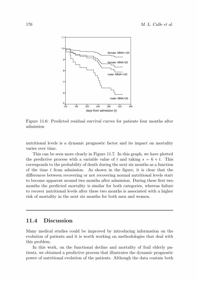
176 M. L. Calle et al.
360320280240200160120
1,1
1,0
,9
,8
,7
,6
,5
female- MNA<20
female- MNA>=20
male- MNA>=20
male- MNA<20
days from admission (t)
Figure 11.6: Predicted residual survival curves for patients four months afteradmission
nutritional levels is a dynamic prognostic factor and its impact on mortalityvaries over time.
This can be seen more clearly in Figure 11.7. In this graph, we have plottedthe predictive process with a variable value of t and taking s = 6 + t. Thiscorresponds to the probability of death during the next six months as a functionof the time t from admission. As shown in the figure, it is clear that thedifferences between recovering or not recovering normal nutritional levels startto become apparent around two months after admission. During these first twomonths the predicted mortality is similar for both categories, whereas failureto recover nutritional levels after these two months is associated with a higherrisk of mortality in the next six months for both men and women.
11.4 Discussion
Many medical studies could be improved by introducing information on theevolution of patients and it is worth working on methodologies that deal withthis problem.
In this work, on the functional decline and mortality of frail elderly pa-tients, we obtained a predictive process that illustrates the dynamic prognosticpower of nutritional evolution of the patients. Although the data contain both

Prognostic Factors in Geriatry 177
1801501209060300
,5
,4
,3
,2
,1
0,0
male- MNA<20
male- MNA>=20
female- MNA<20
female- MNA>=20
days from admission (t)
Figure 11.7: Probability of death during the next six months as a function ofthe time t from admission
survival and repeated observations, the available methods for the joint analysisof longitudinal and survival data were not appropriate in this case and, as analternative we propose a multistate survival model. We observed that the re-covery of normal nutritional levels during the first two months is critical. Thismethodology gives the clinicians a dynamic tool for prediction.
Acknowledgements. The data analyzed correspond to a research project onfunctional decline and mortality of frail patients. Dr. Espaulella from Hospitalde la Santa Creu de Vic is the main researcher and the project received finan-cial support in 2002 from the Academia de ciencies mediques de Catalunya ide Balears (a regional academic and scientific association). The authors haveprovided methodological support to the researchers. We gratefully acknowledgethe comments and opinions we have received from the doctors and nurses atthe Hospital de la Santa Creu de Vic, which have helped and encouraged us inthe study and implementation of this methodology.
References
1. Cox, D. R. (1972). Regression models and life-tables (with discussion),Journal of the Royal Statistical Society, Series B, 34, 187–220.

178 M. L. Calle et al.
2. Faucett, C. L., and Thomas, D. C. (1996). Simultaneously modeling cen-sored survival data and repeatedly measured covariates: A Gibbs sam-pling approach, Statistical Methods in Medical Research, 15, 1663–1686.
3. Henderson, R., Diggle, P., and Dobson, A. (2000). Joint modeling oflongitudinal measurements and event time data, Biostatistics, 3, 33–50.
4. Klein, J. P., Keiding, N., and Copelan, E. A. (1994). Plotting summarypredictions in multistate survival models. Probability of relapse and deathin remission for bone marrow transplanted percents, Statistics in Medi-cine, 12, 2315–2332.
5. Klein, J. P., and Moeschberger, M. L. (1998). Survival Analysis. Tech-niques for Censored and Truncated Data, Springer-Verlag, Inc, New York.
6. Wulfsohn, M. S., and Tsiatis, A. A. (1997). A joint model for survivaland longitudinal data measured with error, Biometrics, 53, 330–339.

12
New Models and Methods for Survival Analysis of
Experimental Data
Ganna V. Semenchenko,1 Anatoli I. Yashin,2 Thomas E. Johnson,3
and James W. Cypser3
1Max Planck Institute for Demographic Research, Rostock, Germany2Duke University, Durham, NC, USA3University of Colorado at Boulder, Boulder, CO, USA
Abstract: We propose an approach for analysis of survivorship data fromobservational and/or experimental studies that allows comparison of survivalin the control and several experimental groups. Our approach is based on themodel of heterogeneous mortality (frailty model), and we also assume that thedifference between survivals for the control and experimental groups is in boththe frailty distribution and baseline hazard. We explore the variety of survivalpatterns that can be captured by different specifications of the proposed modeland illustrate the approach with an example of the model application to theanalysis of data from stress-experiment with nematodes Caenorhabditis elegans.We show that the proposed model gives a good fit to the data and helps toadvance our understanding of biological phenomena as they appear at bothindividual and population levels.
Keywords and phrases: Frailty model, hormesis, longevity, survival analysis
12.1 Introduction
The Gompertz model [Gompertz (1825)] is very often used to analyze survivalin the experiments on laboratory animals. Parameters of this model are asso-ciated with the rate of aging and initial mortality, but these associations arebiologically unjustified. It is well documented that mortality rates for humans[Manton and Stallard (1984) and Strehler and Mildvan (1960)] as well as forlaboratory animals [Carey et al. (1992), Curtsinger et al. (1992), and Fukuiet al. (1996)] decelerate at advanced ages and deviate from the Gompertzlaw. It is also discussed, that only for inbred populations in highly controlledhomogeneous will the environments mortality rate follow the Gompertz curve
179

180 G. V. Semenchenko et al.
[Economos (1985), Sacher (1966), and Vaupel et al. (1979)]. Still, the theoreti-cal challenge is to understand how different effects of environmental conditionsor the application of treatment to the experimental group combine to producedifferent survival patterns [Boxenbaum et al. (1988), Lithgow et al. (1995),and Yakovlev et al. (1993)].
The notion of heterogeneity, as applied to a description of stochastic processes,first appeared in connection with an analysis of demographic processes [Keyfitzand Littman (1979)]. The authors drew attention to the fact that applica-tion of treatment produces different effects on homogeneous and heterogeneouspopulations. In a homogeneous population, the reduction in death rate andextension of lifespan are equal: a drop of one percent in the death rate is equiv-alent to an increase of one percent in the expectation of life. In a heterogeneouspopulation, the reduction and extension can be very different. Thus, neglect ofheterogeneity can lead to an overestimation of healthcare improvement.
In a homogeneous population, risk of dying is the same for all individuals ofthe given age. Due to this, population characteristics such as average lifespan,hazard, or survival function are true for every member of the population. In aheterogeneous population, such a generalization can be misleading.
In the model proposed in this chapter, the heterogeneity assumption meansthat the population consists of individuals with different susceptibility to death.This characteristic, which is also called frailty, influences the individual’s risk ofdying. Although lifespan is registered in most observational and experimentalstudies, aiming to investigate influences of different treatments on survival, it isoften difficult to detect or measure an individual’s frailty. The model of hetero-geneous mortality [Vaupel et al. (1979)] allows us to take into account hiddenheterogeneity of the population for survival analysis because of the assumptionabout probability distribution of an unobserved random variable—frailty. Wepropose an approach for analysis of survivorship data that allows comparisonof survival in the control and several experimental groups.
12.2 Semiparametric Model of Mortality inHeterogeneous Populations Influenced
by Exogenous Interventions
12.2.1 The heterogeneous mortality model
Let T and Z be the life span and the heterogeneity (frailty) variable such thatthe conditional hazard of death given Z is Zμ0 (x), where μ0 (x) is the baselinehazard, which corresponds to the risk of dying for the individual whose frailty

New Models and Methods for Survival Analysis of Experimental Data 181
is equal to 1. This means that the baseline hazard can only be observed in ahomogeneous population, which is comprised of identical individuals.
Let us assume that Z is a gamma-distributed random variable (Z ∼ G (k, λ))with mean 1 and variance σ2; that is, k = λ, and σ2 = 1/λ.
Let H (x) =∫ x0 μ0 (u) du be the cumulative baseline hazard. Then for the
observed mortality μ (x), one can write [Vaupel et al. (1979)]
μ (x) =μ0 (x)
1 + σ2H (x). (12.1)
The marginal survival function S (x), can be presented as follows.
S (x) =(
1 +1λ
H (x))−k
=(1 + σ2H (x)
)−(1/σ2). (12.2)
For a homogeneous population, σ2 = 0, the expression (12.1) transformsinto μ (x) = μ0 (x). It is easy to show, using the L’Hopital rule, that S (x) →exp (−H (x)) = S0 (x), for σ2 → 0 in (12.2), which corresponds to mortalityand survival functions for a homogeneous population.
12.2.2 Changes in the baseline hazard and frailty distribution
In our further calculations, we followed the methodology suggested by Yashinet al. (1996). Such a methodology was also used for the analysis of data fromstress experiments with Drosophila melanogaster [Semenchenko et al. (2004a)]and for investigation of influences of different stressors and antistressors on thesurvival of transgenic mice HER-2/neu [Semenchenko et al. (2004b)].
Let us consider two identical heterogeneous populations whose chances ofsurvival correspond to the proportional hazards model [Eqs. (12.1) and (12.2)],and assume that the initial frailties are gamma-distributed with means 1 andvariances σ2
1 , σ22 , respectively.
The first population—the control group—experiences standard living condi-tions without any interventions, and the second—experimental group—is sub-jected to some treatment at the age interval [x0, x
∗]. At the age x∗, the treat-ment is over.
To compare the survival functions after age x∗ in the experimental and inthe control group let us assume that in the control group, the baseline hazardμ01 (x) does not change and in the experimental cohort the baseline hazardμ02 (x) increases or decreases at the interval [x0, x
∗]. After age x∗, it can berepresented as follows: μ02 (x) = μ0 (x) + f (x). Note that if f (x) ≡ 0, thebaseline hazard is on the level of the control group. A negative f (x) manifestsa decrease of the baseline hazard during the treatment, and a positive f (x)represents an increase of the baseline hazard compared to the control group.

182 G. V. Semenchenko et al.
Changes in the baseline hazard can serve as a characteristic of changes in theintensity of occurrence of intracellular damages caused by treatment [Michalskiet al. (2001)]. If the intensity of damage occurrence decreases, the baselinehazard also decreases. An increase of the intensity of damage occurrence leadsto an increase of the baseline hazard. Thus, we can consider a beneficial effectof the treatment as a decrease of the baseline hazard, whereas a detrimentaleffect of the treatment is characterized by an increase of the baseline hazard.Because changes in the baseline hazard can be persistent, progressive, or evenregressive, it is appropriate to consider them as a function of age when thetreatment is over (f (x) for x ≥ x∗).
It follows from (12.2) that the marginal survival functions Si (x), i = 1, 2,for those who survived age x∗ in both control and experimental groups are
Si (x) =
(1 +
1λ∗
i
H∗i (x)
)−ki
, i = 1, 2, (12.3)
where λ∗i = (1/σ2
i ) + Hi(x∗), Hi(x∗) =∫ x∗0 μ0i(u)du, H∗
1 (x) =∫ xx∗ μ0(u)du,
H∗2 (x) =
∫ xx∗ μ0(u)du + F (x), F (x) =
∫ xx∗ f(u)du, ki = 1/σ2
i , i = 1, 2.Let us assume that under normal living conditions an individual’s suscep-
tibility to death does not change during her life and that any exogenous inter-vention can increase or decrease an individual’s frailty. Note that in the controlpopulation the “natural” selection process does not change the shape parame-ter k1 = 1/σ2
1 of the frailty distribution. If the application of treatment doesnot influence an individual’s frailty, this parameter also does not change in theexperimental cohort; that is, k2 = 1/σ2
2 .Let us assume that σ2
1 = σ22 = σ2 and that the application of a treatment
can also change the shape parameter of the frailty distribution by a factor γ;that is, k2 = 1/γσ2. So, for the survival in the control cohort after age x∗, onecan write:
S1 (x) =(
1 +k1
λ1σ2H1 (x)
)−k1
=(1 + m1σ
2H1 (x))−(1/σ2)
. (12.4)
Then the survival in the experimental cohort (x > x∗) can be presented asfollows.
S2 (x) =(1 + m2γσ2H2 (x)
)−(1/γσ2). (12.5)
In (12.4) and (12.5), m1 and m2 denote the mean values of frailty distribution atage x∗ in the control and in the experimental populations, respectively. Factor γshows the presence of changes in the frailty distribution that are not associatedwith changes of average frailty in the population during the treatment.
Changes in individual frailty characterize the ability of an organism toswitch on new mechanisms of defense or repair in order to withstand harm-ful effects of treatment or to repair lesions that occurred due to treatment

New Models and Methods for Survival Analysis of Experimental Data 183
[Yashin et al. (2002)]. Thus, the beneficial effect of the applied treatment canbe due to a decrease of the average frailty of the population. This means thatindividual characteristics of every cohort member were improved and individ-ual susceptibility to death was reduced. The detrimental effect produced bytreatment can result in increased average frailty of the population. However,the application of treatment can produce different effects on different membersof a heterogeneous population. Robust individuals can become more robust,and weak individuals can become more weak after the treatment, and this re-sults in an increase of population heterogeneity. If the treatment is beneficialfor weak individuals and detrimental for robust ones, the population becomesmore homogeneous.
12.2.3 Semiparametric representation of the model
Additional assumptions about the parametric form of the baseline hazard inboth control and experimental groups are needed in representations (12.4) and(12.5), as well as (12.2). Because it is impossible to observe the baseline hazardin a heterogeneous population, any assumption about its parametric form isbiologically unjustified and should be avoided in an analysis of valuable exper-imental data.
It follows from (12.4) and from the definition of F (x) that
H2 (x) =S1 (x)−σ2 − 1
σ2m1+ F (x) . (12.6)
Replacing H∗2 (x) in (12.5) with (12.6), we obtain the following equation for the
survival S2 (x), (x > x∗) in the experimental group.
S2 (x) =(1 + rγ
(S1 (x)−σ2 − 1
)+ m1rγσ2F (x)
)−(1/γσ2), (12.7)
where r = m∗2/m
∗1, the ratio of mean values of the frailty distributions in ex-
perimental and control groups.Assuming that an increase or decrease of the baseline hazard after the ap-
plication of treatment can vary nonlinearly with age, in our calculations we usef (x) = aeβ(x−x∗). Denoting α = am∗
1, Eq. (12.7) can be rewritten as
S2 (x) =(
1 + rγ(S1 (x)−σ2 − 1
)+ γrσ2 α
β
(eβx − 1
))−(1/γσ2)
. (12.8)
We call this representation semiparametric because the survival function inthe experimental group (12.8) contains S1 (x), the observed survival functionin the control group. However, parametric approximations of S1 (x) [Thatcheret al. (1998)] can be used as well as nonparametric ones [Kaplan and Meier(1958)].

184 G. V. Semenchenko et al.
12.2.4 Interpretation of parameters
In the framework of this model several treatment groups can be considered andcompared to one control group. The model (12.8) has four unknown parametersα, β, r, γ that are specific to each experimental group and its treatment and oneparameter σ2 that is common to all groups, the frailty variance in the controlcohort.
Parameter σ2 indicates the presence of hidden heterogeneity in the con-trol population. When values of σ2 are close to zero, the control populationcan be considered as homogeneous; large values of σ2 characterize the controlpopulation as highly heterogeneous.
Dependences of the survival function in the experimental group on changesof the model’s parameters are presented in Figures 12.1 and 12.2.
Effects of changes in the baseline hazard, controlled by parameters α andβ, are presented in Figure 12.1. If β = 0 in the additive part of hazard for thetreatment group f(x) = a exp(βx), changes in parameter α reflect permanent(constant) decrease or increase of the baseline hazard (Figure 12.1a), producingrectangularization or derectangularization of the survival curve (Figure 12.1b),respectively, depending on whether α is greater or less than zero. It can alsobe seen that permanent decrease or increase of the baseline hazard does notinfluence the “tail” of the survival curve.
Parameter β describes the amplification or disappearance of the α-effect,according to whether β is greater or less than zero. For each effect a small valueof α was fixed. Absolute values of negative β characterize the rate at which thebaseline hazard in the experimental group returns to the level of the controlgroup (Figure 12.1c). Different patterns of survival curves, corresponding tothe changes in parameter β < 0, for increased or decreased baseline hazard arepresented in Figure 12.1d. It can be seen that these changes do not influencethe “tail” of the survival function, as in the case of constant changes of thebaseline hazard.
Positive values of β characterize an amplification of effects, produced by thetreatment, during the life (Figure 12.1e). Amplified with age increase of thebaseline hazard shifts the survival curve to the left along the age axis (com-pared to the control group), and amplified with age decrease shifts it to theright along the age axis (Figure 12.1f). In both cases the tail of the sur-vival curve moves in the same direction. The shifts produced are not paral-lel; they resemble rotation around the initial level of increased or decreasedsurvival.
Changes produced by the treatment on the frailty distribution and corre-sponding survival functions are presented in Figure 12.2. An increase or de-crease in the mean of the frailty distribution (Figure 12.2a) produces a nearlyparallel shift of the survival curve along the age axis with respective lengthen-ing/shortening of its tail (Figure 12.2b). Parameter r < 1 shows an increase

New Models and Methods for Survival Analysis of Experimental Data 185
0 50 100 150 200 250 30010
−5
10−4
10−3
10−2
10−1
100
101
102
decrease ofthe baseline hazardα=−.003*i, β=0
increase ofthe baseline hazardα=+.005*i, β=0
control groupi=1i=2i=3
Age
μ0(x
)
(a)0 50 100 150 200 250 300
0
0.1
0.2
0.3
0.4
0.5
0.6
0.7
0.8
0.9
1
decrease ofthe baseline hazardα=−.003*i, β=0
increase ofthe baseline hazardα=+.005*i, β=0
control groupi=1i=2i=3
Surv
ival
funct
ion
Age
(b)
0 50 100 150 200 250 30010
−8
10−6
10−4
10−2
100
102
vanishingdecreaseof the baseline hazardα=−.01, β=−.01*i
vanishingincreaseof the baseline hazardα=+.01, β=−.01*i
control groupi=1i=2i=3
Age
μ0(x
)
(c)0 50 100 150 200 250 300
0
0.1
0.2
0.3
0.4
0.5
0.6
0.7
0.8
0.9
1
vanishingdecreaseof the baseline hazardα=−.01, β=−.01*i
vanishingincreaseof the baseline hazardα=+.01, β=−.01*i
control groupi=1i=2i=3
Surv
ival
funct
ion
Age
(d)
0 50 100 150 200 250 30010
−6
10−4
10−2
100
102
104
amplifieddecrease of thebaseline hazardα=−.001, β=+.005*i
amplifiedincrease of thebaseline hazardα=+.001, β=+.01*i
control groupi=1i=2i=3
Age
μ0(x
)
(e)0 50 100 150 200 250 300
0
0.1
0.2
0.3
0.4
0.5
0.6
0.7
0.8
0.9
1
amplifieddecrease of thebaseline hazardα=−.001, β=+.005*i
amplifiedincrease of thebaseline hazardα=+.001, β=+.01*i
control groupi=1i=2i=3
Surv
ival
funct
ion
Age
(f)
Figure 12.1: Dependence of survival function for the experimental group onchanges in the baseline hazard
in the average robustness, whereas r > 1 indicates an accumulation of frailindividuals in the population subjected to the treatment.
Parameter γ = 1 characterizes changes in frailty variance in the experimen-tal groups compared to the control cohort (Figure 12.2c). A decrease in varianceof the frailty distribution (γ < 1) indicates that the experimental group becameless heterogeneous, and an increase in frailty variance (γ > 1) corresponds to an

186 G. V. Semenchenko et al.
0 0.5 1 1.5 2 2.5 3 3.5 40
0.5
1
1.5
2
2.5
frailty
control groupr=0.4r=0.6r=0.8r=1.5r=2r=2.5
(a)
0 50 100 150 200 250 3000
0.1
0.2
0.3
0.4
0.5
0.6
0.7
0.8
0.9
1
decrease ofthe average frailtyr=1−.2*i
increase ofthe average frailtyr=1+.5*i
control groupi=1i=2i=3
Surv
ival
funct
ion
Age
(b)
0 0.5 1 1.5 2 2.5 30
0.5
1
1.5
2
2.5
frailty
control groupγ=0.1γ=0.4γ=0.7γ=1.3γ=1.6γ=1.9
(c)
0 50 100 150 200 250 3000
0.1
0.2
0.3
0.4
0.5
0.6
0.7
0.8
0.9
1
increase ofthe frailty varianceγ=1+.3*i
decrease ofthe frailty varianceγ=1−.3*i
control groupi=1i=2i=3Surv
ival
funct
ion
Age
(d)
Figure 12.2: Dependence of survival function for the experimental group onchanges in the frailty distribution
increase of heterogeneity of the experimental population after the applicationof a treatment. It can be seen in Figure 12.2d that changes in population het-erogeneity mostly influence the tail of the survival function. The population,which is more heterogeneous, comprises more individuals with high chances ofsurvival to advanced ages.
By fixing some parameters on the level of the control group, it is possible toconsider a different specification of the proposed model. Thus, if the applicationof treatment does not influence survival of the experimental group, the controland experimental populations remain identical. The following combination ofparameter values α = 0, r = 1, γ = 1 corresponds to such a case. If the onlyeffect produced by the treatment is a change in the mean value of the frailtydistribution, parameter r = 1 and all others are fixed on the level of the controlgroup. If the only difference between the control and experimental cohortsis in their heterogeneity, the combination γ = 1, α = 0, r = 1 will describethis situation. In much the same way, changes in the baseline hazard can bedescribed by the following combination of parameter values; α = 0, β = 0,r = 1, γ = 1.
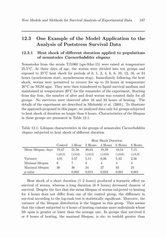
New Models and Methods for Survival Analysis of Experimental Data 187
12.3 One Example of the Model Application to the
Analysis of Poststress Survival Data
12.3.1 Heat shock of different duration applied to populationsof nematodes Caenorhabditis elegans
Nematodes from the strain TJ1060 (spe-9;fer-15) were raised at temperature25.5C. At three days of age, the worms were divided into ten groups andexposed to 35C heat shock for periods of 0, 1, 2, 4, 6, 8, 10, 12, 16, or 24hours (synchronous start, asynchronous stop). Immediately following the heatshock, worms were permitted to recover for up to 24 hours at temperature20C on NGM agar. They were then transferred to liquid survival medium andmaintained at temperature 20C for the remainder of the experiment. Startingfrom day four, the number of alive and dead worms was counted daily for allgroups. No survivors were observed after 16 and 24 hours of heating. Thedetails of the experiment are described in Michalski et al. (2001). To illustratethe approach proposed in this paper, we analyzed data only for groups subjectedto heat shock of duration no longer than 8 hours. Characteristics of the lifespanin these groups are presented in Table 12.1.
Table 12.1: Lifespan characteristics in the groups of nematodes Caenorhabditiselegans subjected to heat shock of different duration
Heat Shock DurationControl 1 Hour 2 Hours 4 Hours 6 Hours 8 Hours
Mean lifespan, days 19,47 21,58 20,64 18,58 10,54 7,15(±0,5) (±0,6) (±0,5) (±0,6) (±0,6) (±0,3)
Variance 4,91 5,57 5,11 6,06 5,42 2,56Minimal lifespan 6 7 6 4 4 4Maximal lifespan 36 36 34 27 33 25p-value 0,002 0,015 0,023 0,001 0,001
Heat shock of a short duration (1–2 hours) produced a hormetic effect onsurvival of worms, whereas a long duration (6–8 hours) decreased chances ofsurvival. Despite the fact that the mean lifespan of worms subjected to heatingfor 4 hours does not differ from one of the control group, the difference insurvival according to the log-rank test is statistically significant. Moreover, thevariance of the lifespan distribution is the biggest in this group. This meansthat the cohort subjected to 4 hours of heating contains more individuals whoselife span is greater or lower than the average one. In groups that survived 6or 8 hours of heating, the maximal lifespan, is six- to tenfold greater than

188 G. V. Semenchenko et al.
the average lifespan. This bears evidence of heterogeneity in reaction to theproposed treatment.
12.3.2 Technical details
To obtain the estimates of the model parameters, the observations of life spansin all treatment groups were used simultaneously. The maximum likelihoodapproach was implemented and parameters were estimated using a nonlinearoptimization procedure [Fletcher (1987)]. Because the structure of the datacorresponds to the number of dead and alive nematodes during discrete timeperiods, the log-likelihood function is derived from the binomial distribution,where binomial probabilities depend on model parameters:
LogLik =∑j
(mj ln(qj) + (nj −mj) ln(1− qj)),
where mj is the number of deaths on day j of life, and nj is the number ofindividuals that were alive on day j − 1. Values qj are related to survivalfunctions for the experimental groups by the relationship
qj = 1− S (j + 1)S (j)
.
Confidence intervals for the parameter estimates were calculated using thebootstrap method [Davison and Hinkley (1997)].
12.3.3 Results of fitting the model to the data
In order to describe effects produced by treatments on frailty distribution andbaseline hazard, several specifications of the heterogeneous mortality modelwere considered. The first one deals with effects such as increase of averagerobustness or accumulation of frail individuals in the population. In the second,changes in mean frailty are accompanied by changes in the baseline hazard. Thethird takes into account the opportunity of changes in population heterogeneityduring the treatment in addition to changes in the baseline hazard and meanvalues of the frailty distribution. All models are nested, so respective hypotheseswere tested using the likelihood ratio statistics. It turned out that the thirdspecification of the model fits the data better than the others (p < 0.01).
Parameter estimates of this specification are presented in Table 12.2. Usingthe estimate of frailty variance (parameter σ2 in Table 12.2), Eq. (12.1) allowsus to estimate the conditional baseline hazard for the control group, which ispresented in Figure 12.3a. It can be seen that the baseline hazard deviates fromthe Gompertz law at advanced ages.
In order to explore predictive abilities of the the model, parameter estima-tion procedure was conducted in two stages, and first for the groups subjected

New Models and Methods for Survival Analysis of Experimental Data 189
Table 12.2: Parameter estimates of the semiparametric model of heterogeneousmortality for groups of nematodes Caenorhabditis elegans subjected to heatshock of different duration
Heat Shock DurationParameter 1 Hour 2 Hours 4 Hours 6 Hours 8 Hoursα× 10−1 0,3 0,2 0,4 5,4 7,1
(0,25; 0,32) (0,19; 0,22) (0,38; 0,41) (5,22; 5,47) (7,05; 7,13)
β × 10−1 −0,9 −0,3 −0,8 1 3,9(−1;−0, 88) (−0, 32;−0, 27) (−0, 9;−0, 72) (0,92; 1,11) (3,86; 4,07)
r × 10−1 3,6 4,5 6,3 2 1,6(3,45; 3,62) (4,36; 4,54) (6,16; 6,32) (1,97; 2,08) (1,52; 1,63)
γ 0,31 0,40 0,87 1,40 1,31(0,28; 0,33) (0,37; 0,41) (0,85; 0,9) (1,38; 1,44) (1,3; 1,33)
σ2 Common for all groups 0,28 (0,27; 0,29)
5 10 15 20 25 30 3510
−4
10−3
10−2
10−1
100
101
estimated baseline haz.approximated control haz.empirical control haz.
Age (days)
μ(x
)
5 10 15 20 25 30 350
0.1
0.2
0.3
0.4
0.5
0.6
0.7
0.8
0.9
1control emp.control mod.1 hr heat. emp.1 hr heat. mod.2 hrs heat. emp.2 hrs heat. mod.4 hrs heat. emp.4 hrs heat. mod.6 hrs heat. emp.6 hrs heat. mod.8 hrs heat. emp.8 hrs heat. mod.
Surv
ival
funct
ion
Age (days)
(a) (b)
Figure 12.3: (a) Estimated baseline hazard for the control group of nematodescompared to the estimates of observed hazard and (b) empirical and modeledconditional survival functions for experimental groups of worms (survival func-tion for the control group is approximated by gamma–Gompertz model withparameters α = 4.4e-4 (3e-4; 5e-4), β = 0.42 (0.4; 0.43), σ2 = 0.83 (0.81; 0.85))
to heating during 1, 4, and 8 hours. According to the proposed model, an in-crease in survival after 1 hour of heating (Table 12.1 and Figure 12.3b) is dueto a decrease of the average frailty, despite the fact that it was accompaniedby an increase of the baseline hazard before the age of about 17 days and adecrease of the population heterogeneity.

190 G. V. Semenchenko et al.
The effect of incomplete hormesis (the intersection of survival curves inthe control and experimental groups), which was observed after four hours ofheating, was caused by greater increase of the baseline hazard at young ages,accompanied by decrease of the average frailty and heterogeneity (both wereless than in the first group).
The group subjected to eight hours of heating became the least frail and themost heterogeneous, however, long duration of heating not only increased thebaseline hazard but also the rate of its amplification with age. A combinationof these effects determined a concave pattern of survival function and its long“tail” in this group (Table 12.1 and Figure 12.3b).
Proceeding from these results, we assumed that after two and six hours ofheating the mean values and variances of the frailty distributions, as well asbaseline hazards, are in the intervals between the values, which characterizerespective effects in the groups that survived heat shock during one, four, andeight hours. As the next step, we conducted parameter estimation for all groupssimultaneously, and the results (Table 12.2) confirmed the assumption that thebaseline hazard increases with an increase of the heat shock duration. Heatshock of short duration (one and two hours) made the population of nematodesless frail on average and less heterogeneous. With an increase of heat shock du-ration up to four hours, average frailty and its variance increased but remainedless then in the control group. Further increase of heat shock duration (six andeight hours) decreased average frailty but increased heterogeneity of experimen-tal populations compared to the control group. The fact that the estimate ofthe frailty variance for the group survived six hours of heating is greater thanone for the group subjected to heat shock during eight hours, gives evidencethat the longer duration of heating would lead to decrease of heterogeneity ofthe population of worms.
12.4 Discussion
The main reason for attempts to investigate influences of toxic substances onsurvival [Boxenbaum et al. (1988) and Neafsey et al. (1988)] was to explain thedeviations of the hazard function from the Gompertz curve under assumptionthat “The Law” holds for mortality in the absence of treatment.
Further development of studies of survival under or after stress using math-ematical models [Butov et al. (2001), Yakovlev et al. (1993), and Yashin et al.(2001)] helped to bind some biological and physiological mechanisms to popula-tion mortality. However, those models did not take into account heterogeneityin response to applied treatment.
The Cox regression model [Cox (1972)], which is also widely used in medicaland biological studies, is a method of choice in the case of observed covariates.

New Models and Methods for Survival Analysis of Experimental Data 191
When it is impossible to observe covariates, the specification for the two-sampleproblem allows us to estimate relative risk of death in the treatment groupcompared to the control population.
Application of a frailty model in the case of unobserved covariates is moreappropriate [Vaupel et al. (1979)]. Still this approach requires additional as-sumptions for the parametric form of a baseline hazard [Michalski et al. (2001)].These assumptions are biologically unjustified because of the impossibility ofobserving the baseline hazard in the heterogeneous population, and they alsomake the model unidentifiable from the viewpoint that the frailty variance de-pends on the choice of the baseline hazard. The semiparametric representationof the heterogeneous mortality model allows us to avoid unjustified assump-tions and makes the model identifiable. Moreover, such a representation makesit possible to estimate the baseline hazard for the control group, knowing thevariance of frailty distribution.
The main distinctive feature of our model in comparison to other gammafrailty models [Klein (1992), Michalski et al. (2001), Nielsen et al. (1992), andVaupel et al. (1979)] is that we assume that treatment influences parametersof both frailty distribution and baseline hazard.
Changes in frailty distribution under stressful experimental conditions firstwere discussed and studied by modeling discrete frailty classes [Yashin et al.(2002)]. This model is based on the assumption that a population consists ofthree subpopulations of individuals: weak, normal, and robust. Stressful exper-imental conditions can influence an individual’s frailty and change proportionof members in each subpopulation. If applied treatment is detrimental, robustindividuals become normal, normal ones become weak, and weak individualsdie. The hormetic effect is caused by an increase in robustness of individuals.If application of treatment is beneficial, weak individuals become normal, nor-mal ones become robust. When some individuals from a normal subpopulationbecome weak and at the same time other normal individuals become robust,the effect of incomplete hormesis is observed. We incorporated this elegantidea into our semiparametric model of heterogeneous mortality assuming con-tinuous distribution for the frailty variable. We believe that the applicationof sophisticated mathematical models advances our understanding of biologicalphenomena as they appear at both individual and population levels.
References
1. Boxenbaum, H., Neafsey, P., and Fournier, D. (1988). Hormesis, Gom-pertz functions and risk assessment, Drug Metabolism Reviews, 19, 195–229.

192 G. V. Semenchenko et al.
2. Butov, A., Johnson, T., Cypser, J., Sannikov, I., Volkov, M., Sehl, M., andYashin, A. (2001). Hormesis and debilitation effects in stress experimentsusing the nematode worm Caenorhabditis elegans: the model of balancebetween cell damage and hsp levels, Experimental Gerontology, 37, 57–66.
3. Carey, J., Liedo, P., Orozco, D., and Vaupel, J. (1992). Slowing of mor-tality rates at older ages in large medfly cohorts, Science, 258, 457–461.
4. Cox, D. (1972). Regression models and life-tables (with discussion), Jour-nal of the Royal Statistical Society, Series B, 34, 187–220.
5. Curtsinger, J., Fukui, H., Townsend, D., and Vaupel, J. (1992). Demogra-phy of genotypes: Failure of the limited life-span paradigm in drosophilamelanogaster, Science, 258, 461–463.
6. Davison, A. C., and Hinkley, D. V. (1997). Bootstrap Methods and TheirApplication, Cambridge University Press, Cambridge, England.
7. Economos, A. (1985). Rate of aging, rate of dying and non-Gompertzianmortality, Encore Gerontology, 31, 106–111.
8. Fletcher, R. (1987). Practical Methods of Optimization, Second edition,John Wiley & Sons, New York.
9. Fukui, H., Ackert, L., and Curtsinger, J. (1996). Deceleration of age-specific mortality rates in Drosophila melanogaster, Experimental Geron-tology, 31, 517–531.
10. Gompertz, B. (1825). On the nature of the function expressive of the lawof human mortality, and on the new mode of determining the values oflife contingencies, Philosophical Transaction, The Royal Society, London,115, 513–585.
11. Kaplan, E., and Meier, P. (1958). Nonparametric estimation from incom-plete observation, Journal of the American Statistical Association, 53,457–481.
12. Keyfitz, N., and Littman, G. (1979). Mortality in a heterogeneous popu-lation, Population Studies, 33, 333–342.
13. Klein, J. P. (1992). Semiparametric estimation of random effects usingthe cox model based on the em algorithm, Biometrics, 48, 795–806.
14. Lithgow, G., White, T., Melov, S., and Johnson, T. (1995). Thermo-tolerance and extended life span confered by single-gene mutations andinduced by thermal stress, Proceedings of the National Academy of ScienceUSA, 92, 7540–7544.

New Models and Methods for Survival Analysis of Experimental Data 193
15. Manton, K., and Stallard, E. (1984). Recent Trends in the MortalityAnalysis, Academic, Orlando, Florida.
16. Michalski, A. I., Johnson, T. E., Cypser, J. R., and Yashin, A. I. (2001).Heating stress patterns in Caenorhabditis elegans longevity and survivor-ship, Biogerontology, 2, 35–44.
17. Neafsey, P. J., Boxenbaum, H., Ciraulo, D. A., and Fournier, D. J. (1988).A gompertz age-specific mortality rate model for aging, hormesis andtoxicity: Single dose studies, Drug Metabolism Reviews, 19), 369–401.
18. Nielsen, G., Gill, R., Andersen, P., and Sørensen, T. (1992). A countingprocess approach to maximum likelihood estimation in frailty models,Scandinavian Journal of Statistics, 19, 25–43.
19. Sacher, G. (1966). The Gompertz transformation in the study of theinjury-mortality relationship: Application to late radiation effects andageing, In Radiation and Ageing. Proceedings of a Colloquium held inSemmering, Austria, pp. 411–441, Taylor and Francis, London.
20. Semenchenko, G. V., Khazaeli, A. A., Curtsinger, J. W., and Yashin,A. I. (2004a). Stress resistance declines with age: Analysis of data fromsurvival experiment with Drosophila melanogaster, Biogerontology, 5, 17–30.
21. Semenchenko, A., Anisimov, V., and Yashin, A. (2004b). Stressors andantistressors: How do they influence survival in HER-2/neu transgenicmice? Experimental Gerontology, 39, 1499–1511.
22. Strehler, B., and Mildvan, A. (1960). General theory of mortality andaging, Science, 132, 14–21.
23. Thatcher, A., Kanisto, V., and Vaupel, J. (1998). The force of mortalityat ages 80 to 120, In Monographs on Population Aging, Volume 5, OdenseUniversity press, Odense, Denmark.
24. Vaupel, J., Manton, K., and Stallard, E. (1979). The impact of hetero-geneity in individual frailty on the dynamics of mortality, Demography,16, 439–454.
25. Yakovlev, A., Tsodikov, A., and Bass, L. (1993). A stochastic model ofhormesis, Mathematical Biosciences, 116, 197–219.
26. Yashin, A., Andreev, K., Curtsinger, J., and Vaupel, J. (1996). Death-after-stress-data in the analysis of heterogeneous mortality, In Transac-tions of Symposium in Applied Statistics (Ed., G. Christensen), pp. 24–32.

194 G. V. Semenchenko et al.
27. Yashin, A., Cypser, J., Johnson, T., Michalski, A., Boyko, S., andNovoseltsev, V. (2001). Ageing and survival after different doses of heatshock: the results of analysis of data from stress experiments with thenematode worm Caenorhabditis elegans, Mechanisms of Ageing and De-velopment, 122, 1477–1495.
28. Yashin, A., Cypser, J., Johnson, T., Michalski, A., Boyko, S., andNovoseltsev, V. (2002). Heat shock changes the heterogeneity distributionin populations of Caenorhabditis elegans: does it tell us anything aboutthe biological mechanism of stress response? The Journals of Gerontology,Series A, 57, B83–B92.

13
Uniform Consistency for Conditional Lifetime
Distribution Estimators Under Random
Right-Censorship
Paul Deheuvels and Gerard Derzko
Universite Pierre et Marie Curie—Paris VI, Paris, FranceSanofi-Aventis, Montpellier, France
Abstract: We define nonparametric kernel-type estimators of the conditionaldistribution of a lifetime, in a random censorship framework. We show thatthese estimators have closed-form expressions, and establish their strong uni-form consistency under minimal assumptions.
Keywords and phrases: Nonparametric estimation, lifetime distributions,regression estimation, kernel estimation, empirical processes, functional esti-mation, weak laws, laws of large numbers
13.1 Introduction and Results
13.1.1 Notation and statement of the problem
The present work is concerned with the estimation of a conditional lifetimedistribution under random censorship from the right. The model we consider isbased upon a sequence of observations (Xn, Yn, Un), n = 1, 2, . . ., of a randomvector (X,Y,U), where X denotes a positive lifetime of interest, Y a positivecensoring time, and U a concomitant variable whose influence on the distribu-tions of X and Y is to be assessed. Throughout, we will assume that X and Yare conditionally mutually independent, given U . The observed data set is givenby the triplets (Zi, δi, Ui), i = 1, . . . , n, where (Zi := Xi∧Yi, δi := 1IXi≤Yi, Ui),for i = 1, . . . , n, constitutes a random sample of independent and identicallydistributed copies of (Z := X ∧ Y, δ := 1IX≤Y , U). Our aim is to estimatethe conditional distribution function F (x|u) = P(X ≤ x|U = u) [respectively,G(y|u) = P(Y ≤ y|U = u)], provided that this last expression is meaningful.
195

196 P. Deheuvels and G. Derzko
We start by giving some notation and assumptions that are needed for theforthcoming definition of our estimators.
We mention that, in the uncensored case, corresponding to the limiting de-generate case where Y = ∞ with probability 1, our estimators reduce to thatgiven by Stute (1986) for conditional empirical distribution functions. Thelatter estimators turn out to be a special version of the Nadaraya-Watson non-parametric regression estimator [see Nadaraya (1964, 1989), Watson (1964),Hardle (1990), Einmahl and Mason (2000), Deheuvels and Mason (2004), andthe references therein]. In the case where U is independent of (X,Y ), our esti-mators yield, as a special case, the usual product-limit estimator due to Kaplanand Meier (1958), for which there is a huge literature [see, e.g., Burke, Csorgo,and Horvath (1981, 1988), Deheuvels and Einmahl (2000), Foldes, Rejto, andWinter (1981), Gill (1980), Stute (1995), and the references therein].
Unless otherwise specified, the (possibly defective) distribution functionswe will consider will be assumed to be right-continuous, and of the generalform Ψ(t) = Ψ+(t) = P(R ≤ t ∩ E) = limε↓0 Ψ(t + ε). At times, we willmake use of the left-continuous version of Ψ, denoted by Ψ−(t) = P(R <t ∩ E) = limε↓0 Ψ(t− ε). Below, we will always assume that the distributionfunctions F (x) = P(X ≤ x) and G(y) = P(Y ≤ y), of X and Y , respectively,are continuous, so that F (x) = F±(x), G(y) = G±(y), and F±(0) = G±(0) = 0.This assumption entails that the distribution function H(z) = P(Z ≤ z) =1 − (1 − F (z))(1 −G(z)) of Z is continuous, and such that H(0) = 0. In thisframework, with probability 1 for each n ≥ 1, the order statistics 0 < Z1,n <· · · < Zn,n of Z1, . . . , Zn are distinct and positive. Unless otherwise specified,we will work on the event of probability 1 on which this property holds. Thereexists therefore (on the latter event) a rank sequence r1,n, . . . , rn,n, definedas the unique permutation of 1, . . . , n such that
Zi,n = Zri,n for i = 1, . . . , n. (13.1)
In the sequel, we will set accordingly
δi:n = δri,n and Ui:n = Uri,n for i = 1, . . . , n. (13.2)
We stress the fact that the Ui:n for 1 ≤ i ≤ n are not to be confused with theorder statistics of U1, . . . , Un, which will not be used here. The latter should bedenoted, in agreement with the notation above, by U1,n ≤ · · · ≤ Un,n.
The conditioning random variable U will be assumed to have a measurabledensity κ(u) on R, and, therefore, a continuous distribution function K(u) =∫(−∞,x] κ(u)du. We are specifically interested in conditioning on U = u when
u varies in a specified bounded interval I := [A,B] of R. We will assume, fortechnical purposes, the existence of a larger interval J := [A′, B′] ⊃ I, suchthat −∞ < A′ < B < B′ < ∞, and κ(·) is continuous and positive (and thus,

Conditional Lifetime Distribution Estimators 197
bounded away from 0) on J . Our primary concern is to estimate F (x|u) whenu varies in I. To give a precise meaning to this last expression, we assumefurther that (X,U) and (Y,U) have joint densities on R
+ × R, denoted byf(x, u) and g(y, u), respectively. Moreover, we assume that f(x, u) and g(y, u)are continuous on R
+× J . This allows us to set, for each u ∈ J and x, y ∈ R+,
F (x|u) = P(X ≤ x|U = u) =1
κ(u)
∫ x
0f(x, u)dx, (13.3)
G(y|u) = P(Y ≤ y|U = u) =1
κ(u)
∫ y
0g(y, u)dy, (13.4)
κ(u) =∫ ∞
0f(x, u)dx =
∫ ∞
0g(y, u)dy. (13.5)
We note for further use that our assumptions on κ(·), f(·, ·), and g(·, ·), imply,via (13.3)–(13.5), that F (·|·) and G(·|·) are both continuous on R
+× J . In thisframework, we will make use of the following distribution functions, where, asusual, we set Z = X ∧ Y and δ = 1IX≤Y . We set, for each u ∈ J and z ∈ R
+,
H(0)(z|u) = P(Z ≤ z, δ = 0|U = u) =∫
(0,z](1− F−(t|u)) dG(t|u)
=1
κ(u)
∫(0,z]
(1− F−(t|u)) g(t, u)dt, (13.6)
H(1)(z|u) = P(Z ≤ z, δ = 1|U = u) =∫
(0,z](1−G−(t|u)) dF (t|u)
=1
κ(u)
∫(0,z]
(1−G−(t|u)) f(t, u)dt, (13.7)
andH(z|u) = P(Z ≤ z|U = u) = 1− (1− F (t|u))(1 −G(t|u))
= H(0)(z|u) + H(1)(z|u). (13.8)
Even though the continuity of F (·|·) and G(·|·) implies that, in (13.6)–(13.8),F (t|u) = F±(t|u) and G(t|u) = G±(t|u) over (t, u) ∈ R
+ × J , it is of interestto use the above formulations in anticipation of the empirical versions of theseequations given later on [see, e.g., (13.30)–(13.32) in the sequel]. We keep inmind that, under the previous assumptions, (13.6)–(13.8) jointly imply thatH(·|·), H(0)(·|·), and H(1)(·|·) are continuous on R
+ × J .For each u ∈ J , let ωX(u) = supt : F (t|u) < 1, ωY (u) = supt : G(t|u) <
1, and ωZ(u) = ωX(u) ∧ ωY (u) = supt : H(t|u) < 1 denote the upper end-points of the conditional distributions of X, Y , and Z, respectively, given thatU = u. A direct consequence of (13.6)–(13.7) is that, for each specified u ∈ J ,

198 P. Deheuvels and G. Derzko
F (t|u) and G(t|u) are uniquely defined for t ∈ [0, ωZ(u)) as the right-continuousjoint solutions of the differential system
dF (t|u) =dH(1)(t|u)
1−G−(t|u)and dG(t|u) =
dH(0)(t|u)1− F−(t|u)
, (13.9)
or, equivalently, via (13.8),
dF (t|u)1− F−(t|u)
=dH(1)(t|u)
1−H−(t|u)and
dG(t|u)1−G−(t|u)
=dH(0)(t|u)
1−H−(t|u), (13.10)
subject to the boundary conditions
F−(0|u) = G−(0|u) = 0. (13.11)
Among other consequences, the fact that the above equations do not make sensewhen t > ωZ(u) illustrates the property that our data set does not carry anydetailed information on F (t|u) and G(t|u) for t > ωZ(u). We will thereforerestrict our interest to the values of t ∈ [0, C], where C denotes a specifiedconstant, fulfilling, uniformly over u ∈ I,
0 < C < ωZ(u). (13.12)
By continuity of H(·|·) on R+ × I, we infer from (13.12) the existence of a
constant γ = γ(C, I) ∈ (0, 12) such that
1− 2γ := supu∈I
H(C|u) < 1. (13.13)
In the next section, we will describe a class of nonparametric estimators Fn,a(x|u)of F (x|u) [respectively, Gn,a(y|u) of G(y|u)] depending upon a smoothing factora > 0. We will establish their uniform consistency over (x, u) ∈ [0, C]× I, viz.,by showing, in Theorem 13.1.2 that, under suitable conditions imposed upona = an, we have, almost surely as n→∞,
sup0≤x≤C
supu∈I|Fn,a(x|u)− F (x|u)| → 0, (13.14)
andsup
0≤y≤Csupu∈I|Gn,a(x|u)−G(x|u)| → 0. (13.15)
13.1.2 Definition of the estimators and uniform consistency
With the aim of estimating F (x|u) and G(y|u), we start by introducing a generalkernel K(·), defined as a right-continuous function fulfilling the conditions (K.1–3) below.

Conditional Lifetime Distribution Estimators 199
(K.1) The total variation ‖dK‖ :=∫
R|dK(t)| of K on R is bounded;
(K.2)∫
RK(t)dt = 1;
(K.3) There exists an M <∞ such that K(t) = 0 for |t| ≥M/2.
We consider further two sequences of positive constants a′n : n ≥ 1 anda′′n : n ≥ 1, such that
0 < a′n ≤ a′′n for each n ≥ 1, (13.16)
na′n/ log n→∞ and a′′n → 0. (13.17)
We set, for each n ≥ 1, An = [a′n, a′′n]. The estimators that will be introducedin this section will be indexed by a positive bandwidth a > 0. In practice, oneneeds to select this factor in a way that is appropriate to the data set [see, e.g.,Deheuvels and Mason (2004)]. This question, for the estimators, which will beintroduced below, will be considered elsewhere. In this chapter, we will limitourselves to show, in Theorem 13.1.2, that the uniform strong consistency ofour estimators will hold independently of the choice of a ∈ An. Our estimatorsof F (x|u) and G(y|u) are defined as follows.
First, we introduce a kernel density estimator of κ(u) [refer to Parzen (1962)and Rosenblatt (1958)], defined, for each choice of u ∈ R, n ≥ 1, and of thebandwidth a > 0, by
κn,a(u) =1na
n∑i=1
K(u− Ui
a
). (13.18)
Second, we introduce, for each n ≥ 1 and a > 0, an array of random (andpossibly negative) weights Wi,n,a(u) : 1 ≤ i ≤ n, by setting, for 1 ≤ i ≤ n,
Wi,n,a(u) =K(
u−Uia
)∑n
j=1 K(
u−Uj
a
) =1
κn,a(u)
1na
K(u− Ui
a
), (13.19)
when κn,a(u) = 0, and
Wi,n,a(u) =1n
, (13.20)

200 P. Deheuvels and G. Derzko
when κn,a(u) = 0. We then set
Hn,a(z|u) =n∑
i=1
Wi,n,a(u)1IZi≤z =
∑ni=1 1IZi≤zK
(u−Ui
a
)∑n
i=1 K(
u−Uia
)=
1κn,a(u)
n∑i=1
1IZi≤z 1
naK(u− Ui
a
)=:
Rn,a(z|u)κn,a(u)
, (13.21)
H(0)n,a(z|u) =
n∑i=1
Wi,n,a(u)1IZi≤z(1− δi) =
∑ni=1 1IZi≤z(1− δi)K
(u−Ui
a
)∑n
i=1 K(
u−Uia
)=
1κn,a(u)
n∑i=1
1IZi≤z(1− δi) 1
naK(u− Ui
a
)=:
R(0)n,a(z|u)κn,a(u)
,
(13.22)
H(1)n,a(z|u) =
n∑i=1
Wi,n,a(u)1IZi≤zδi =
∑ni=1 1IZi≤zδiK
(u−Ui
a
)∑n
i=1 K(
u−Uia
)=
1κn,a(u)
n∑i=1
1IZi≤zδ)
1na
K(u− Ui
a
)=:
R(1)n,a(z|u)κn,a(u)
, (13.23)
whenever κn,a(u) = 0, and
Hn,a(z|u) =n∑
i=1
Wi,n,a(u)1IZi≤z =1n
n∑i=1
1IZi≤z, (13.24)
H(0)n,a(z|u) =
n∑i=1
Wi,n,a(u)1IZi≤z(1− δi) =1n
n∑i=1
1IZi≤z(1− δi), (13.25)
H(1)n,a(z|u) =
n∑i=1
Wi,n,a(u)1IZi≤zδi =1n
n∑i=1
1IZi≤zδi, (13.26)
when κn,a(u) = 0.The following proposition turns out to follow, either directly [for (13.27)–
(13.28) below], or after some routine adaptations of the proofs [for (13.29)below], from Corollary 1 and Theorem 3 of Einmahl and Mason (2005), and sothe corresponding details are omitted.

Conditional Lifetime Distribution Estimators 201
Proposition 13.1.1 Under the assumptions above, we have, almost surely
supa∈An
supu∈I|κn,a(u)− κ(u)| = o(1), (13.27)
supa∈An
supu∈I
supz∈R+
|Hn,a(z|u) −H(z|u)| = o(1), (13.28)
and, for = 0, 1,sup
a∈An
supu∈I
supz∈R+
|H()n,a(z|u) −H(z|u)| = o(1). (13.29)
In view of these preliminary results, it becomes very logical to define our esti-mators of F (x|u) and G(y|u), denoted, respectively, by Fn,a(x|u) and Gn,a(y|u),as the joint solutions, whenever they exist, of the differential system obtained bythe formal replacements in (13.9)–(13.11) of H(0)(t|u), H(1)(t|u), and H(t|u),respectively, by their empirical counterparts H
(0)n,a(t|u), H
(1)n,a(t|u), and Hn,a(t|u),
as defined in (13.21)–(13.26). By so doing, we are led to the differential system
dFn,a(t|u) =dH
(1)n,a(t|u)
1−Gn,a−(t|u)and dGn,a(t|u) =
dH(0)n,a(t|u)
1− Fn,a−(t|u), (13.30)
or, equivalently (see, e.g., Remark 13.1.1),
dFn,a(t|u)1− Fn,a−(t|u)
=dH
(1)n,a(t|u)
1−Hn,a−(t|u)and
dGn,a(t|u)1−Gn,a−(t|u)
=dH
(0)n,a(t|u)
1−Hn,a−(t|u),
(13.31)subject to the boundary conditions
Fn,a−(0|u) = Gn,a−(0|u) = 0. (13.32)
It turns out, rather surprisingly, that the solutions of the differential system(13.30)–(13.32) have simple closed-form expressions in terms of the randomweights Wi,n,a(u) : 1 ≤ i ≤ n, and ranks ri,n : 1 ≤ i ≤ n, as defined in (13.1)and (13.19)–(13.20). These are given as follows. For notational convenience,we define below a sequence of ranked random weights wi,n,a(u) : 1 ≤ i ≤ n.Recalling the definition (13.2) of Ui:n : 1 ≤ i ≤ n, we set, for u ∈ R, a > 0,and 1 ≤ i ≤ n,
wi,n,a(u) = Wri,n,n,a(u) =K(
u−Ui:na
)∑n
j=1 K(
u−Uj:n
a
) =1
κn,a(u)
1na
K(u− Ui:n
a
),
(13.33)
whenever κn,a(u) = 0, and
wi,n,a(u) = Wri,n,n,a(u) =1n
, (13.34)

202 P. Deheuvels and G. Derzko
when κn,a(u) = 0. Next, recalling the definitions (13.21)–(13.24), of Hn,a(z|u),and (13.33)–(13.34), of wi,n,a(u), we introduce a random index, defined, for eachu ∈ R, a > 0, and n ≥ 1 by
Nn,a(u) = min
i ∈ 1, . . . , n :i∑
j=1
wj,n,a(u) = 1
= min
i ∈ 1, . . . , n : Hn,a(Zi,n|u) = 1
. (13.35)
Because of the fact [obvious, via (13.21)–(13.24)] that Hn,a(Zn,n|u) = 1, theindex Nn,a(u) ∈ 1, . . . , n always exists. The following simple lemma gives auseful limiting property of this statistic.
Lemma 13.1.1 Under the assumptions above, we have, almost surely for all nsufficiently large,
infa∈An
infu∈I
ZNn,a(u),n ≥ C. (13.36)
Proof. In view of (13.35), it is enough to show that the inequality
supa∈An
supu∈I
Hn,a(C|u) < 1
holds ultimately in n → ∞ with probability 1. This, however, is a directconsequence of (13.12)–(13.13), when combined with (13.28).
We are now ready to state the first main result of this chapter, givingexplicit closed-form expressions for the solutions Fn,a(x|u) and Gn,a(y|u) of thedifferential system (13.30)–(13.32). In the statement of the theorem, we use theconventions that
∑∅(·) = 0 and
∏∅(·) = 1.
Theorem 13.1.1 For each u ∈ R, n ≥ 1, and a > 0, the solutions Fn,a(x|u)and Gn,a(y|u) of the differential system (13.30)–(13.31), subject to the boundaryconditions (13.32), are uniquely defined over t ∈ [0, ZNn,a(u),n), and coincide onthis interval with the functions defined on R
+ by
Fn,a(t|u) = 1−∏
i:Zi,n≤t
1−∑ij=1 wj,n,a(u)
1−∑i−1
j=1 wj,n,a(u)
δi:n
when t < ZNn,a(u),n,
= 1 when t ≥ ZNn,a(u),n, (13.37)
and
Gn,a(t|u) = 1−∏
i:Zi,n≤t
1−∑ij=1 wj,n,a(u)
1−∑i−1j=1 wj,n,a(u)
1−δi:n
when t < ZNn,a(u),n,
= 1 when t ≥ ZNn,a(u),n. (13.38)

Conditional Lifetime Distribution Estimators 203
The proof of Theorem 13.1.1 is postponed until Section 13.2.
Remark 13.1.1 (1) It is obvious from the definition (13.25) of Nn,a(u) thatFn,a(·|·) and Gn,a(·|·) are properly defined by (13.37)–(13.38), and fulfill
Hn,a(t|u) = 1−(1− Fn,a(t|u)
)(1−Gn,a(t|u)
)for t < ZNn,a(u),n. (13.39)
On the other hand, the equality on the left-hand side of (13.39) may not betrue for some t ≥ ZNn,a(u),n. If that is the case, we see that the equivalencebetween the differential systems (13.30) and (13.31) fails to hold in the interval[ZNn,a(u),n,∞).
(2) As a consequence of (1), there exists almost surely an n0 = n0(C, I) suchthat, for all n ≥ n0, (13.39) holds uniformly over t ∈ [0, C], u ∈ I, and a ∈ An,with Fn,a(t|u) < 1 and Gn,a(t|u) < 1 being properly defined by (13.37)–(13.38).We will make a repeated implicit use of this observation in the remainder ofthis chapter.
Our second theorem gives a general uniform consistency result of our esti-mators.
Theorem 13.1.2 Under the assumptions above, we have, almost surely
supa∈An
supu∈I
supx∈[0,C]
|Fn,a(x|u)− F (x|u)| = o(1), (13.40)
andsup
a∈An
supu∈I
supx∈[0,C]
|Gn,a(y|u)−G(y|u)| = o(1). (13.41)
The proof of Theorem 13.1.2 will be given in Section 13.2. The study ofrates of consistency for these estimators will be investigated elsewhere.
13.2 Proofs
13.2.1 Construction of the estimators
In the present subsection, we give a proof of Theorem 13.1.1, together withadditional details on the construction of our estimators. We recall that thedistribution function H(z) = P(Z ≤ z) = 1 − (1 − F (z))(1 −G(z)) is continu-ous, and that the order statistics Z1,n, . . . , Zn,n of Z1, . . . , Zn are almost surelydistinct and fulfilling
0 < Z1,n < · · · < Zn,n. (13.42)

204 P. Deheuvels and G. Derzko
For convenience, we will set, in the sequel,
Z0,n = 0 and Zn+1,n =∞. (13.43)
The strict inequalities in (13.42) allow us to define, on the event where (13.42)holds, a unique permutation r1,n, . . . , rn,n of 1, . . . , n, such that, for i =1, . . . , n,
Zr1,n = Zi,n. (13.44)
In view of (13.42)–(13.44), we set, for i = 1, . . . , n,
δi:n = δri,n . (13.45)
Let now π1:n, . . . , πn:n be any sequence of (possibly negative) weights fulfillingπ1:n + · · ·+ πn:n = 1, and set
nπ = min
i ∈ 1, . . . , n :i∑
j=1
πj:n = 1
. (13.46)
Keeping in mind that 1 ≤ nπ ≤ n, we set further
H(0)n;π(z) =
∑j:Zj,n≤z
πj:n(1− δj:n), (13.47)
andH(1)
n;π(z) =∑
j:Zj,n≤z
πj:nδj:n. (13.48)
Throughout, we make use of the convention that∑
∅(·) = 0. In particular,in (13.51)–(13.52) below, we set
∑0j=1 πj:n = 0. We next define Fn;π(z) and
Gn;π(z) for z ∈ R+ as follows.
– When∑nπ
i=1 δi = 0, we set, for all z ∈ R+,
Fn;π(z) = 0 and Gn;π(z) = H(0)n;π(z). (13.49)
– When∑nπ
i=1(1− δi) = 0, we set, for all z ∈ R+,
Fn;π(z) = H(1)n;π(z), and Gn;π(z) = 0. (13.50)
– When 0 <∑nπ
i=1 δi < nπ, we set
Fn;π(z) =
⎧⎪⎪⎨⎪⎪⎩1−
∏i:Zi,n≤z
1−∑ij=1 πj:n
1−∑i−1j=1 πj:n
δi:n
for z < Znπ,n,
1 for z ≥ Znπ,n.
(13.51)
Gn;π(z) =
⎧⎪⎪⎨⎪⎪⎩1−
∏i:Zi,n≤z
1−∑i
j=1 πj:n
1−∑i−1
j=1 πj:n
1−δi:n
for z < Znπ,n,
1 for z ≥ Znπ,n.
(13.52)

Conditional Lifetime Distribution Estimators 205
Theorem 13.2.1 The differential system
dGn(z) =dH(0)
n;π(z)1−Fn−(z)
, and dFn(z) =dH(1)
n;π(z)1− Gn−(z)
. (13.53)
with limit conditionsFn−(0) = Gn−(0) = 0, (13.54)
has a pair of right-continuous solutions, uniquely defined on [0, Znπ ,n) byFn(z) = Fn;π(z) and Gn(z) = Gn;π(z).
Proof. We will limit ourselves to the case where nπ = n. The proof of thetheorem when 1 ≤ nπ < n turns out to follow from simple modifications of ourarguments, and the details will be therefore omitted. Set Sn = δ1 + · · ·+ δn.
– When Sn = 0, we infer from (13.51)–(13.52) that Fn;π(z) = 0 for all z < Zn,n,whereas, for i = 0, . . . , n and Zi,n ≤ z < Zi+1,n,
Gn;π(z) =i∑
j=1
πj:n =i∑
j=1
πj:n(1− δj:n) = H(0)n;π(z).
It is now straightforward that the so-defined Fn;π(z) and Gn;π(z) are solutionson [0, Zn,n) of the differential system (13.53). The arguments are very similarwhen Sn = n and shall be omitted.
– We now turn to the only remaining case where 0 < s := Sn < 1, and definea sequence of indices 1 ≤ j1 < · · · < js ≤ n in such a way that δi:n = 1 iffi ∈ j1, . . . , js. Obviously, for Zjm−1,n ≤ z < Zjm,n,
1−Fn;π(z) = 1−Fn;π(Zjm−1,n), (13.55)
whereas, for z = Zjm,n,
1−Fn;π(Zjm,n) =
1−Fn;π(Zjm−1,n) 1−∑jm
i=1 πi:n
1−∑jm−1i=1 πi:n
= Fn;π(Zjm−1,n) +
1−Fn;π(Zjm−1,n)
πjm:n
1−∑jm−1i=1 πi:n
.
Now, we use the observation that1−Fn;π(Zjm−1,n)
1− Gn;π(Zjm−1,n)
= 1−
jm−1∑i=1
πi:n,
so that
Fn;π(Zjm,n) = Fn;π(Zjm−1,n) +πjm:n
1− Gn;π(Zjm−1,n)
1−∑jm−1
i=1 πi:n
1−∑jm−1i=1 πi:n
= Fn;π(Zjm−1,n) +
dHn;π(1)(Zjm,n)
1− Gn;π(Zjm−1,n).

206 P. Deheuvels and G. Derzko
This, in turn, suffices to show that Fn;π satisfies the differential system (13.53)on (Zjm−1,n, Zjm,n]. By combining this property with a straightforward induc-tion, and a similar argument for Gn;π, we readily conclude the proof of Theorem13.2.1.
Proof of Theorem 13.1.1. It suffices to apply Theorem 13.2.1 in the par-ticular case where the weights are given by πi:n = wi,n,a(u) for 1 ≤ i ≤ n.
13.2.2 A useful auxiliary result
In this section, we will show that the proof of Theorem 13.1.2 turns out to be asimple consequence of Proposition 13.1.1, when combined with a useful auxiliaryresult of independent interest, stated in Proposition 13.2.1. Consider, in general,two pairs of right-continuous distribution functions F and G, = 1, 2. Set, forz ∈ R and = 1, 2,
H(0) (z) =
∫(0,z]
(1−F−(t)
)dG(t), (13.56)
H(1) (z) =
∫(0,z]
(1− G−(t)
)dF(t), (13.57)
H(z) = 1−(1−F(z)
)(1− G(z)
)= H(0)
(z) +H(1) (z). (13.58)
We have the following proposition.
Proposition 13.2.1 Let c > 0 and θ > 0 be such that, for = 0, 1,
sup0≤t≤c
|H()1 (t)−H()
2 (t)| ≤ θ. (13.59)
Assume further that, for some 0 < ρ < 1,
H1(c) ∨H2(c) ≤ ρ < 1. (13.60)
Then, we have
sup0≤x≤c
|F1(x)−F2(x)| ≤ 4θ(1− ρ)2
. (13.61)
Proof. Under (13.59), we infer from (13.58) the inequalities
sup0≤t≤c
|H1±(t)−H2±(t)|
≤ sup0≤t≤c
|H(0)1 (t)−H(0)
2 (t)|+ sup0≤t≤c
|H(1)1 (t)−H(1)
2 (t)| ≤ 2θ. (13.62)

Conditional Lifetime Distribution Estimators 207
Moreover, we infer from (13.60) and (13.58) that, uniformly over 0 ≤ t ≤ c, and = 0, 1,
0 ≤ H()1±(t) ∨H()
2±(t) ≤ H1(t) ∨H2(t) ≤ ρ < 1. (13.63)
Observe that, for = 1, 2, F(t) and G(t) are joint solutions over t ∈ [0, c] ofthe differential system
dF(t)1−F−(t)
=dH(1)
(t)1−H−(t)
anddG(t)
1− G−(t)=
dH(0) (t)
1−H−(t), (13.64)
subject to the boundary conditions
F−(0) = G−(0) = 0. (13.65)
Thus, making use of (13.64) and integrating by parts, we may write, for 0 ≤x ≤ c,
Δ(x) :=− log
(1−F1(x)
)−
− log
(1−F2(x)
)=
∫(0,x]
dF1(t)1−F1−(t)
−
∫(0,x]
dF2(t)1−F2−(t)
=
∫(0,x]
dH(1)1 (t)
1−H1−(t)
−
∫(0,x]
dH(1)2 (t)
1−H2−(t)
=∫
(0,x]
(1−H2−(t)
)−
(1−H1−(t)
)(1−H2−(t)
)(1−H1−(t)
) dH(1)
1 (t)
+∫
(0,x]
11−H2−(t)
dH(1)
1 (t)−H(1)2 (t)
=
∫(0,x]
H1−(t)−H2−(t)(1−H2−(t)
)(1−H1−(t)
)dH(1)1 (t) +
H(1)1 (x)−H(1)
2 (x)1−H2−(x)
−∫
(0,x]
H(1)
1 (t)−H(1)2 (t)
dH2(t)(1−H2−(t)
)2
.
This, in turn, readily implies, via (13.62) and (13.63), that
sup0≤x≤c
|Δ(x)| ≤ 2θ(1− ρ)2
+θ
1− ρ+
θ
(1− ρ)2≤ 4θ
(1− ρ)2. (13.66)
Next, we infer from Taylor’s formula that, for each choice of 0 ≤ u ≤ v < 1,there exists a w ∈ [u, v] for which
− log(1− v)−
− log(1− u)
=
v − u
1− w> v − u.

208 P. Deheuvels and G. Derzko
We have, therefore, for any 0 ≤ u, v ≤ 1,
|v − u| ≤∣∣− log(1− v)
−
− log(1− u)
∣∣,so that we infer readily (13.61) from (13.66), by setting u = F1(x) and v = F2(x)in this last inequality.
Proof of Theorem 13.1.2. It is a straightforward consequence of Proposi-tions 13.1.1 and 13.2.1, in combination with Theorem 13.1.2.
13.2.3 Concluding comments
The well-known results [see, e.g., Deheuvels and Mason (2004) and the refer-ences therein] concerning the consistency of Nadaraya–Watson regression esti-mators (which are obtained as a special case of our estimators, as mentioned inSection 13.1), show readily that the conditions of our theorems are sharp.
References
1. Burke, M. D., Csorgo, S., and Horvath, L. (1981). Strong approximationsof some biometric estimates under random censorship, Z. Wahrsch. Verw.Gebiete, 56, 87–112.
2. Burke, M. D., Csorgo, S., and Horvath, L. (1988). A correction to and animprovement of strong approximations of some biometric estimates underrandom censorship, Probability Theory and Related Fields, 56, 87–112.
3. Deheuvels, P., and Einmahl, J. H. J. (2000). Functional limit laws forthe increments of Kaplan-Meier product-limit processes and applications,The Annals of Statistics, 28, 1301–1335.
4. Deheuvels, P., and Mason, D. M. (2004). General asymptotic confidencebands based on kernel-type function estimators, Statistical Inference forStochastic Processes, 7, 225–277.
5. Einmahl, U., and Mason, D. M. (2000). An empirical approach to theuniform consistency of kernel-type function estimators, Journal of Theo-retical Probability, 13, 1–37.
6. Einmahl, U., and Mason, D. M. (2005). Uniform in bandwidth consis-tency of kernel-type function estimators, Annals of Probability, 33, 1380–1403.

Conditional Lifetime Distribution Estimators 209
7. Foldes, A., Rejto, L., and Winter, B. B. (1981). A LIL type result for theproduct-limit estimator, Z. Wahrsch. Verw. Gebiete, 56, 75–86.
8. Gill, R. D. (1980). Censoring and Stochastic Integrals, MathematischCentrum Tracts, Amsterdam, The Netherlands.
9. Hardle, W. (1990). Applied Nonparametric Regression, Cambridge Uni-versity Press, Cambridge.
10. Kaplan, E. L., and Meier, P. (1958). Nonparametric estimation for in-complete observations, Journal of the American Statistical Association,53, 457–481.
11. Nadaraya, E. A. (1964). On estimating regression, Theory of Probabilityand Its Applications, 9, 141–142.
12. Nadaraya, E. A. (1989). Nonparametric Estimation of Probability Densi-ties and Regression Curves, Kluwer, Dordrecht, The Netherlands.
13. Watson, G. S. (1964). Smooth regression analysis, Sankhya, Series A, 26,359–372.
14. Stute, W. (1986). On almost sure convergence of conditional empiricaldistribution functions, The Annals of Statistics, 14, 891–901.
15. Stute, W. (1995). The central limit theorem under random censorship,The Annals of Statistics, 23, 86–107.

14
Sequential Estimation for the Semiparametric
Additive Hazard Model
L. Bordes and C. Breuils
University of Technology of Compiegne, LMAC, Compiegne, FranceUniversity of Metz, LMAM, Metz, France
Abstract: In this chapter, we investigate the asymptotic behavior of the se-quential version of the regression parameter estimator for the additive hazardmodel. We mainly establish that the Lin and Ying (1994) nonsequential esti-mator is strongly consistent (in the sense of complete convergence) and thatthis estimator, indexed by any regular sequence (sequential estimator), has thesame asymptotic behavior as the nonsequential estimator. An example of afixed-width confidence-type sequential estimator is illustrated by simulations.
Keywords and phrases: Semiparametric additive hazard model, sequentialestimation, right-censored survival data, complete convergence
14.1 Introduction
In semiparametric survival studies, Cox’s (1972) proportional hazards model(PHM) is certainly the most popular among lifetime regression models. How-ever, several studies [see, for example, Huffer and McKeague (1991)] showedthat the hazard rate proportionality assumption is not satisfied and it is there-fore necessary to use alternative models. The additive hazards regression model[Cox and Oakes (1984)], studied by Lin and Ying (1994), like the PHM, allowseasy interpretation of the covariates effect. Formally, the hazard rate functionλ(t;Z) of a duration T , given a covariate process Z, is defined at time t ∈ R
+,by
λ(t;Z) = λ0(t) + βT0 Z(t), (14.1)
where λ0 is a baseline hazard rate function (a nuisance parameter in this study)and β0 ∈ R
p a vector of regression parameters.
211

212 L. Bordes and C. Breuils
In many studies, the cost of the study is linked to the total duration ofthe experiments or to the number of experiments. This is the reason why weneed to propose an earlier stop of the study without deteriorating the qualityof the estimators [see Lai (2001) for a recent overview on sequential trials].This naturally leads us to define stopping rules (i.e., criteria), which once theyare satisfied, lead to estimators having some prespecified properties. In thischapter, we consider sequential versions of the Lin and Ying (1994) regressionestimator.
Let T be the failure time of interest, Z be a covariate vector (that possiblydepends on time t), and C be a censoring time that is conditionally independentof T given Z. We are given data on X = min(T,C), δ = I(T ≤ C) (where I(·) isthe set characteristic function), and also on covariates Z ≡ Z(s); s ≤ X. Theproblem is to account for the covariate effect by assuming that the conditionalhazard function of T given Z follows model (14.1). Suppose we are given nsuch independent observations (X1, δ1, Z1), . . . , (Xn, δn, Zn). For simplicity weshall assume that the covariate processes are real-valued. Lin and Ying (1994)proposed to estimate β0 by βn, solving Un(βn, τ) = 0, where
Un(β, t) =1n
n∑i=1
∫ t
0(Zi(s)− En(s)) (dNi(s)− Yi(s)βZi(s)ds),
with τ the (deterministic) upper bound of the time interval of study, and
Ni(s) = I(Xi ≤ s, δi = 1), Yi(s) = I(Xi ≥ s),
Z(k)n (s) =
1n
n∑i=1
Zki (s)Yi(s), k ∈ 0, . . . , 3, En = Z
(1)n /Z
(0)n .
From the linearity of Un with respect to β, the estimator of β0 has an explicitform
βn ≡ βn(τ) = I−1n (τ)×Θn(τ),
whereIn(τ) =
∫ τ
0
(Z
(2)n (s)− Z
(1)n (s)En(s)
)ds
and
Θn(τ) =1n
n∑i=1
∫ τ
0(Zi(s)− En(s)) dNi(s).
It is also interesting to note that βn = arg maxβ∈R Cn(β, τ), where Cn(β, τ) =βΘn(τ)−β2In(τ)/2 is concave (at least asymptotically) and twice continuouslydifferentiable with respect to β. Let us recall that a random sequence of integers(Tn)n≥1 is regular if there exists a deterministic sequence of integers (tn)n≥1 suchthat (i) tn → +∞ as n→ +∞, and (ii) Tn/tn → 1 in probability, as n→ +∞.

Sequential Additive Hazard Regression 213
Lin and Ying (1994) proved that√
n(βn − β0) is asymptotically Gaussianwith zero mean and covariance σ2
0(τ) consistently estimated by σ2n(τ) = I−2
n (τ)Vn(τ),where
Vn(τ) =1n
n∑i=1
∫ τ
0(Zi(s)− En(s))2 dNi(s).
In Section 14.3, we introduce general assumptions for which we prove the fol-lowing results.
(A) βn converges completely (see Section 14.4.1) to β0, as n→ +∞;
(B) For any regular sequence (Tn)n≥1,√
n(βn − β0) and√
Tn(βTn − β0) havethe same asymptotic behavior;
(C) σ2Tn
(τ) is a consistent estimator of σ20(τ).
14.2 Example and Numerical Study
One of the most popular sequential estimators arises from fixing the length ofa α-level confidence set [see, for example, Ghosh et al. (1997)] leading to aregular sequence (Nd)d>0 of stopping rules defined by
Nd = infn ≥ n0;n ≥ σ2n(τ)u2
α/d2, (14.2)
where uα is the quantile of order 1− α/2 of a standard Gaussian distribution,n0 an initial sample size, 2d > 0 an upper bound of the length of the asymptoticconfidence set, and σ2
n = max(σ2n, εn), where (εn)n≥1 is a sequence of real num-
bers decreasing to 0. One can show [see, for example, Ghosh et al. (1997) andBreuils (2003)] that such a sequence is regular with respect to the deterministicsequence (nd)d>0, where
nd = infn ≥ n0;n ≥ σ20(τ)u2
α/d2. (14.3)
Note that here, asymptotics must be understood in the sense that d → 0+;that is, the smaller the length of the confidence set is, the more accurate is theestimator. Under assumptions given in the next section, we obtain:
(i) βNdconverges in probability to β0, as d→ 0+;
(ii)√
Nd(βNd−β0) converges in distribution to N (0, σ2
0(τ)), as d→ 0+, whereN (μ, σ2) denotes a Gaussian distribution with mean μ and variance σ2;
(iii) σ2Nd
(τ) converges in probability to σ20(τ), as d→ 0+.

214 L. Bordes and C. Breuils
Moreover, by assuming that the whole data are identically distributed, we provethat
(iv)√
Nd −√
nd is asymptotically Gaussian, as d→ 0+.
Now, we provide some results obtained by Monte Carlo simulations, takinga Weibull law for both baseline hazard rate and censorship laws. The covariatesare supposed to be time independent and uniformly distributed on [0, 1].
Table 14.1: Nd behavior for various values of d (β0 = 1, censorship rate: 48%)
d EM.(βNd)(StD.) EM.(Nd)(StD.) M.1 M.2 C.I.
1 0.90(0.34) 95(33) 5.97 6.43 910.9 0.97(0.29) 126(35) 6.41 8.17 870.8 0.99(0.25) 164(39) 6.71 8.60 930.7 0.95(0.19) 203(45) 6.39 6.70 900.6 0.98(0.15) 283(42) 6.56 6.06 920.5 0.99(0.13) 415(47) 6.71 6.64 940.4 1.00(0.11) 641(69) 6.65 7.51 920.3 0.99(0.07) 1149(90) 6.72 6.15 970.2 1.00(0.05) 2585(138) 6.65 6.64 94
0.15 1.00(0.04) 4575(181) 6.69 5.71 97
The given results are Empirical Means (EM.), Standard Deviations (StD.)of estimators from 100 simulations. In Table 14.1, we study the sequential rulebehavior as d is positively decreasing to 0. We can observe that the requiredsample size is increasing. This study affords two ways to estimate the asymp-totic variance: M.2 is the variance of the
√Nd(βNd
− β0) (which cannot becomputed for real data) and M.1 is the mean of estimated variances, whichseems more stable as d varies. The last column “C.I.” gives the percentage(based on 100 simulations) of coverage of the confidence interval. We can seethe behavior of N0.5 when β0 decreases (d = 0.5) in Table 14.2. The requiredsample sizes decrease, which is explained by the fact that the theoretical risksare closer to λ0 as β0 goes to 0. The column “Cens. (%)” indicates the censoringpercentages.

Sequential Additive Hazard Regression 215
Table 14.2: N0.5 with respect to β0
β0 EM.(βN0.5)(StD.) EM.(N0.5)(StD.) M.1 M.2 Cens. (%) C.I.5 5.01(0.13) 5013(201) 81.11 85.92 12.7 954 3.99(0.12) 3345(146) 54.03 48.25 15.8 943 3.00(0.12) 2034(120) 33.00 28.96 20.9 982 2.01(0.13) 1069(80) 17.33 19.07 29.9 92
1.5 1.49(0.15) 701(77) 11.35 14.20 37.5 921 1.02(0.11) 413(48) 6.68 4.73 48.6 98
0.5 0.49(0.12) 190(35) 3.04 2.77 65.3 930 0(0.09) 24(17) 0.29 0.29 93.5 100
14.3 Assumptions and Theoretical Results
We consider the following assumptions.
A1. There exist deterministic functions γi defined on [0, τ ], satisfying
∀k ∈ 0, . . . , 3, sups∈[0,τ ]
∣∣∣EZ(k)n (s)− γk(s)
∣∣∣→ 0, as n→ +∞,
with γ0 bounded away from 0 on [0, τ ],
0 < I0(τ) =∫ τ
0(γ2(s)− e1(s)γ1(s))ds < +∞
and
0 < V0(τ) =∫ τ
0λ0(s)(γ2(s)− e1(s)γ1(s))ds
+ β0
∫ τ
0(γ3(s)− 2e1(s)γ2(s) + e2
1(s)γ1(s))ds < +∞,
where ei = γi/γ0 for i = 1, 2;
A2. τ is positive real number such that∫ τ0 λ0(s)ds < +∞;
A3. Zi(t); t ∈ [0, τ ]i≥1 has bounded variations (uniformly in i ≥ 1); that is,there exists 0 < B <∞ such that
∀i ≥ 1,∫ τ
0|Zi(ds)| ≤ B;

216 L. Bordes and C. Breuils
A4. The random triples (Ti, Ci, Zi(·)) are identically distributed.
Note that the first assumption in A1 is automatically fulfilled if A4 is true be-cause in this case, we have equality between EZ
(k)n (s) and γk(s) for all s ∈ [0, τ ].
The last assumptions in A1 ensure a nondegenerate asymptotic distribution for√n(βn − β0). Assumption A2 specifies that the probability to observe a fail-
ure near the upper bound of the interval of study is large enough. A3 is anassumption that is met in practical survival analysis studies and A4 is purelya technical assumption. Our main result is then as follows.
Theorem 14.3.1 Under A1–A3, we have results (A), (B), and (C) of Section14.1. If A4 is also satisfied, and if Nd and nd are defined by (14.2) and (14.3),respectively, then
√Nd −
√nd is asymptotically Gaussian with zero mean.
Proof. For all n ≥ 1, the map β → Cn(τ, β) we introduced in Section 14.1,defined on a bounded open subset B ⊂ R containing β0, is twice continuouslydifferentiable and concave (for n large enough; see C1 and C2 below). We alsodenote by Un(τ, β) and In(τ) = In(β, τ) the first- and second-order derivativesof Cn with respect to β. By Theorems 2.1, 2.2, and 2.3 in Bordes and Breuils(2006), we need to prove Condition C1–C4 below (under A1–A3), and C5 if A4is also satisfied:
C1. |In(τ)− EIn(τ)| c−→ 0, and |Vn(τ)− EVn(τ)| c−→ 0, as n→∞;
C2. EIn(τ)−→I0(τ) > 0 and EVn(τ)−→V0(τ), as n→∞;
C3. (Un(β0))n≥1 converges completely to 0, as n→∞;
C4. For all regular sequences of integer-valued random variables (Tn)n≥1, wehave √
TnUTn(β0)D−→ N (0,V0(τ)), as n→∞;
C5. For all regular sequences of integer-valued random variables (Tn)n≥1, wehave√
Tn
(VTn(βTn)− V0(τ)ITn(βTn)− I0(τ)
)D−→ N (0,Γ0(τ)) , as n→∞. (14.4)
First note that C4 with Tn = n follows directly from Lin and Ying (1994),and C2 is straightforward under A1. The main part of this proof consists inshowing C1, C3, C4, and C5. Let us recall [see, for example, Andersen et al.(1993)] that processes Mi, defined for t ∈ [0, τ ] by
Mi(t) = Ni(t)−∫ t
0Yi(s)(λ0(s) + β0Zi(s))ds,
are martingales with respect to the natural filtration.

Sequential Additive Hazard Regression 217
Proof of C3: First note that for β = β0, Un(β0, ·) is a martingale, becausewe have
Un(β0, t) =1n
n∑i=1
∫ t
0(Zi(s)− En(s)) dMi(s).
Because by A3 covariates Zi are uniformly bounded by a constant B, we have
|ΔUn(β0, t)| ≤1n
n∑i=1
∣∣∣∣Δ ∫ t
0(Zi(s)− En(s)) dNi(s)
∣∣∣∣≤ 1
n
n∑i=1
|Zi(Xi)− En(Xi)|ΔNi(t) ≤2Bn
,
and, using A2 and A3 there exists a constant K such that
| 〈Un(β0, ·)〉 (t)| ≤K
n.
Then, applying Proposition 14.4.3, we get the complete convergence of thesequence (supt∈[0,τ ] |Un(β0, t)|)n≥1 to 0.
Proof of C1: For t in [0, τ ], we write
In(t)− EIn(t) =∫ t
0
(Z
(2)n (s)− EZ
(2)n (s)
)ds
+∫ t
0
(E
(Z
(1)n (s)En(s)
)− Z
(1)n (s)En(s)
)ds,
whose complete convergence can then be easily deduced from Lemma 14.4.1.For Vn, straightforward calculations lead to
Vn(t)− EVn(t) =1n
n∑i=1
∫ t
0(Zi(s)− En(s))2 dMi(s) (14.5)
+∫ t
0
(H(1)
n (s)− EH(1)n (s)
)λ0(s)ds (14.6)
+ β0
∫ t
0
(H(2)
n (s)− EH(2)n (s)
)ds, (14.7)
where
H(1)n (s) = Z
(2)n (s)− Z
(1)n (s)En(s)
andH(2)
n (s) = Z(3)n (s)− 2En(s)Z(2)
n (s) + Z(1)n (s)(En(s))2.

218 L. Bordes and C. Breuils
Again Lemma 14.4.1 allows us to prove the uniform complete convergence ofH
(k)n − EH
(k)n to 0 on [0, τ ] for k = 1, 2; then, using A2, we get the complete
convergence of (14.6) and (14.7) to 0. Following the proof of C3, we finallyshow that (14.5) converges completely to 0.
Proof of C4: Let us define Un on [0, τ ] by
√nUn(β0, t) =
1√n
n∑i=1
∫ t
0(Zi(s)− e1(s)) dMi(s).
Lemma 14.3.1 (√
nUn(β0, ·)) and (√
nUn(β0, ·)) are completely asymptoticallyequivalent.
Proof. First note that for t ∈ [0, τ ], we have
Bn(t) =√
n(Un(β0, t)− Un(β0, t)) =1√n
n∑i=1
∫ t
0(En(s)− e1(s)) dMi(s),
and, as in the proof of C3, we check that the assumptions of Proposition 14.4.3are fulfilled. Indeed, Bn(·) is a martingale, such that ΔBn(·) is a O(n−1/2), andwe have
P(〈Bn〉 (t) > n−1/4
)= P
(∫ t
0(En(s)− e1(s))
2 1n
n∑i=1
d < Mi > (s) > n−1/4
)
≤ P
(sup
s∈[0,τ ]|En(s)− e1(s)| > Bn−1/8
).
We then use Lemma 14.4.1(ii) to obtain the second assumption of Proposi-tion 14.4.3 and to complete the proof of the result.
Lemma 14.3.2 For t ∈ [0, τ ], (√
nUn(β0, t))n≥1 satisfies the Anscombe condi-tion (see Section 14.4.1).
Proof. For t in [0, τ ] and k an integer, we have∣∣∣√n + k Un+k(β0, t)−√
n Un(β0, t)∣∣∣
≤∣∣∣∣ 1√
n + k− 1√
n
∣∣∣∣∣∣∣∣∣
n∑i=1
∫ t
0(Zi(s)− e1(s)) dMi(s)
∣∣∣∣∣ (14.8)
+1√
n + k
∣∣∣∣∣n+k∑
i=n+1
∫ t
0(Zi(s)− e1(s)) dMi(s)
∣∣∣∣∣ . (14.9)

Sequential Additive Hazard Regression 219
By applying the Rebolledo theorem to (14.8) and the Kolmogorov inequalityto (14.9), we show that the Anscombe condition is fulfilled and the lemma isproved [for details of such a proof see Bordes and Breuils (2006)].
To achieve the proof of C4, we use a result by Breuils (2003) [see alsoBordes and Breuils (2006)]. By the Rebolledo theorem, it is easy to see that(√
nUn(β0, ·)) and (√
nUn(β0, ·)) have the same asymptotic Gaussian distribu-tion. Therefore, both Lemmas 14.3.1 and 14.3.2 allow us to apply Proposition14.4.1 which proves C4.
Proof of C5. Here we assume that A1–A4 are satisfied; in this case, theprimary assumption in A1 is satisfied because EZ
(k)n = γk for 0 ≤ k ≤ 3. In the
sequel, we use the oc(1) notation to specify that a “remaining term” convergescompletely to 0. Straightforward but lengthy calculations allow us to show,using Lemma 14.4.1 repeatedly, that for t ∈ [0, τ ] we have
Zn(t) =√
n
(In(t)− I0(t)Vn(t)− V0(t)
)= Zn(t) + oc(1),
with
Zn(t) =
( ∑2i=0
∫ t0 ki(s)W
(i)n (s)ds∑3
i=0
∫ t0 hi(s)W
(i)n (s)ds +
∑6i=4
∫ t0 hi(s)dW
(i)n (s)
),
where for 0 ≤ k ≤ 3, W(k)n (t) =
√n(Z(k)
n (t)− γk(t)), and
W (k)n (t) = n−1/2
n∑i=1
∫ t
0(Zi(s))k−4dMi(s)
for 4 ≤ k ≤ 6. Functions hi and ki are defined by
h0 = λ0e21 + 2β0e1e2 − 2β0e
31, h1 = 3β0e
21 − 2β0e2 − 2e1λ0,
h2 = λ0 − 2β0e1, h3 = β0, h4 = e21, h5 = −2e1, h6 = 1,
and k0 = e21, k1 = −2e1, k2 = 1.
Let us define on [0, τ ], the R7-valued process Wn = (W (0)
n , . . . ,W(6)n )T . By
A4 and the definition of the W(i)n s, we can see that
Wn =1√n
n∑i=1
Wn,i,
where the Wn,is are independent and identically distributed processes. Becausewe proved that Zn(τ) is asymptotically completely equivalent to Zn(τ), an R
2-valued linear functional of Wn(·), it follows that Zn(τ) is a sum of centered,independent, and identically distributed random variables with finite variance

220 L. Bordes and C. Breuils
under A2–A3. By the classical central limit theorem, Zn(τ) has an asymptoticcentered Gaussian distribution with a variance–covariance matrix Γ0(τ). More-over, Zn(τ) satisfies the Anscombe condition (as a sum of centered indepen-dent and identically distributed random vectors with finite variance–covariancematrix), and so by Proposition 14.4.1, Condition C5 is fulfilled and, hence,Theorem 14.3.1 is proved.
14.4 Technical Tools
14.4.1 Complete convergence, Anscombe condition, andexponential inequality
First we recall that a sequence (Xn)n≥1 of real-valued random variables con-verges completely to a random variable X (denoted by Xn
c−→ X) if for allε > 0 we have ∑
n≥1
P (|Xn −X| > ε) < +∞.
Two sequences (Xn)n≥1 and (Yn)n≥1 of real-valued random variables are com-pletely asymptotically equivalent if their difference converges completely to 0.
We say that (Xn)n≥1 satisfies the Anscombe condition or is uniformly con-tinuous in probability, if for all ε > 0 there exists an integer n0 ≥ 1 and a realnumber δ > 0 such that
P
(max
0≤k≤δn|Xn+k −Xn| > ε
)< ε, ∀n ≥ n0.
Proposition 14.4.1 Let (Xn)n≥1 and (Yn)n≥1 be two asymptotically completelyequivalent sequences. If (Xn)n≥1 satisfies the Anscombe condition, and (Tn)n≥1
is a regular sequence, thenYTn − Ytn
P−→ 0.
Moreover, if (Xn)n≥1 converges to X in distribution, (YTn)n≥1 converges to Xin distribution too.
Proof. See Breuils (2003) or Bordes and Breuils (2006).
We consider (Ω,A, P ) a probability space. For ω ∈ Ω, we define
Fn,ω = fn(ω, t) = (fn,1(ω, t), . . . , fn,n(ω, t)), t ∈ [0, τ ] ,
a subset of Rn corresponding to a triangular array of processes. We focus our
interest on the random element defined by
Δn(ω) = supt∈[0,τ ]
|Sn(ω, t)− ESn(·, t)| , ω ∈ Ω,

Sequential Additive Hazard Regression 221
where Sn(ω, t) =∑n
i=1 fn,i(ω, t). We write Fn,ω =(F
(1)n,ω, . . . , F
(n)n,ω
), the enve-
lope of Fn,ω, and it satisfies |fn,i(ω, t)| ≤ F(i)n,ω for all t ∈ [0, τ ] and 1 ≤ i ≤ n;
we write δn(ω) = |Fn,ω|2, where | · |2 denotes the Euclidean norm in Rn.
Proposition 14.4.2 Let Fn,ω be a subset of Rn. We assume that (i) δn(ω) =
O(n−1/2) uniformly in ω ∈ Ω, and (ii) Fn,ω is Euclidean [see Pollard (1990)].Then, there exist constants 0 < c1 ≤ 5 and c2 > 0 such that
1. P (Δn ≥ ε) ≤ c1 exp(−c2nε2), for all n ≥ 1,
2. Δnc−→ 0, as n→∞.
Proof. Follows from Pollard (1990, Chapter 7); see Breuils (2003) and Bordesand Breuils (2064).
Proposition 14.4.3 Let (Mn)n≥1 be a sequence of local martingales, locallyuniformly integrable, with value 0 at 0. We suppose that for n ≥ 1, we have
supt∈[0,τ ]
|ΔMn(t)| ≤ c√n
,
where c > 0. If we have∑n≥1
P(⟨
Mn
⟩(τ) ≥ n−1/4
)< +∞,
then (supt∈[0,τ ] |Mn(t)|)n≥1
converges completely to 0.
Proof. Follows from a result by Shorack and Wellner (1986, p. 900); seeBreuils (2003) and Bordes and Breuils (2006).
14.4.2 Technical results
Lemma 14.4.1 Under A1–A3, we have:(i) There exist real numbers c > 0, d > 0, and an integer n0 ≥ 1, such that
for all ε > 0, 0 ≤ k ≤ 3, and n ≥ n0:
P
(sup
s∈[0,τ ]
∣∣∣Z(k)n (s)− γk(s)
∣∣∣ > ε
)≤ c exp(−dnε2);
moreover, both sups∈[0,τ ]
∣∣∣Z(k)n (s)− EZ
(k)n (s)
∣∣∣ and sups∈[0,τ ]
∣∣∣Z(k)n (s)− γk(s)
∣∣∣converge completely to 0;
(ii) There exist real numbers c′ > 0, d′ > 0, and an integer n′0 ≥ 1, such
that for all ε > 0, and n ≥ n′0:
P
(sup
s∈[0,τ ]|En(s)− e1(s)| > ε
)≤ c′ exp(−d′nε2).

222 L. Bordes and C. Breuils
Proof. Let us prove (i). By the triangular inequality applied to Z(k)n (s) −
γk(s) and A1, it is enough to prove the result for sups∈[0,τ ] |Z(k)n (s)−EZ
(k)n (s)|.
Moreover, we prove that the family Fnω defined by
Fnω = (fn,1(ω, t), . . . , fn,n(ω, t)), t ∈ [0, τ ] ,
for i ∈ 1, . . . , n, fn,i(ω, t) = n−1Yi(t)Zki (t), is Euclidean by arguments similar
to those of Bilias et al. (1997). This family has an envelope Fn,ω with anEuclidean norm less than Cn−1/2 (with C > 0) and thus satisfies assumptionsof Proposition 14.4.2 giving constants ck and dk. Finally, we take c = max ck
and d = min dk. The last two results of (i) follow immediately.Result (ii) is straightforward by using the triangular inequality with result
(i) and the fact that, by A1 and A3, 1/γ0 and En are, respectively, bounded.
References
1. Andersen, P. K., Borgan, O., Gill, R. D., and Keiding, N. (1993). Statis-tical Models Based on Counting Processes, Springer-Verlag, New York.
2. Bilias, Y., Gu, M., and Ying, Z. (1997). Towards a general asymptotictheory for Cox model with staggered entry, The Annals of Statistics, 25,662–682.
3. Bordes, L., and Breuils, C. (2006). Sequential estimation for semipara-metric models with application to the proportional hazards model, Jour-nal of Statistical Planning and Inference, in press.
4. Breuils, C. (2003). Analyse de Durees de Vie : Analyse Sequentielle duModele des Risques Proportionnels et Tests d’homogeneite, Ph.D. Dis-sertation (in French) University of Compiegne, D1484.(downloadable at http://tel.ccsd.cnrs.fr).
5. Cox, D. R. (1972). Regression models with life-tables (with Discussion),Journal of the Royal Statistical Society, Series B, 34, 187–220.
6. Cox, D. R., and Oakes, D. (1984). Analysis of Survival Data, Chapman& Hall, London, U.K.
7. Ghosh, M., Mukhopadhay, N., and Sen, P. K. (1997). Sequential Estima-tion, John Wiley & Sons, New York.
8. Huffer, F. W., and McKeague, I. W. (1991). Weighted least square esti-mation for Aalen’s additive risk model, Journal of the American StatisticalAssociation, 86, 114–129.

Sequential Additive Hazard Regression 223
9. Lai, T. L. (2001). Sequential analysis: Some classical problems and newchallenges (with Discussion), Statistica Sinica, 11, 303–408.
10. Lin, D. Y., and Ying, Z. (1994). Semiparametric analysis for the additiverisk model, Biometrika, 81, 61–71.
11. Pollard, D. (1990). Empirical Processes: Theory and Applications, NSF-CBMS Regional Conference Series in Probability and Statistics, 2.
12. Shorack, G. R., and Wellner, J. A. (1986). Empirical Processes withApplications to Statistics, John Wiley & Sons, New York.

15
Variance Estimation of a Survival Function with
Doubly Censored Failure Time Data
Chao Zhu and Jianguo Sun
University of Missouri, Columbia, MO, USA
Abstract: Doubly censored failure time data often occur in epidemiological ordisease progression studies. In this situation, several authors have investigatedthe problem of estimating a survival function and proposed methods for theproblem. However, there appears to be no existing research studying varianceestimation of an estimated survival function. This chapter discusses pointwiseestimation of variances of an estimated survival function and several methodsare presented. The evaluation and comparison of the methods are conductedusing numerical studies and a set of real doubly censored failure time data. Theresults suggest that the proposed methods work well under practical situations.
Keywords and phrases: AIDS incubation time, disease progression studies,pointwise estimation of variance, survival function
15.1 Introduction
Doubly censored failure time data arise in many studies of disease progressionthat involve two events, an initial event and an end event such as disease onsetand subsequent death [De Gruttola and Lagakos (1989) and Sun (2004)]. Bydoubly censored data, we mean that the survival time of interest is defined asthe elapsed time between the initial and end events and observations on theoccurrences of both events can be either right- or interval-censored [Finkelstein(1986), Kalbfleisch and Prentice (2002), and Sun (2005)]. If the initial event canbe exactly observed, we then have right- or interval-censored failure time datadepending on observations on the end event. This chapter discusses pointwiseestimation of variances of the estimated survival function and several methodsare presented.
225

226 C. Zhu and J. Sun
An example of doubly censored data that motivated this research occursin the analysis of follow-up studies of patients who have been or are at riskof being infected by the Type-1 human immunodeficiency virus (HIV-1) andthus are also at risk of developing the acquired immune deficiency syndrome(AIDS). In this case, one variable of great interest is AIDS incubation time [DeGruttola and Lagakos (1989)], the survival time of interest defined as the timefrom HIV-1 infection (initial event) to the diagnosis of AIDS (end event). TheHIV-1 infection time is often interval-censored partly due to the recruitment ofHIV-1 positive patients into the studies and the fact that the infection timesof these patients can usually only be determined retrospectively to lie in someintervals. In the meantime, observations on the diagnosis of AIDS could beright- or interval-censored too.
A number of authors have considered the analysis of doubly censored failuretime data. For example, De Gruttola and Lagakos (1989) and Gomez andCalle (1999) proposed some algorithms for estimation of the survival function.Goggins et al. (1999), Pan (2001), and Sun et al. (1999) investigated regressionanalysis of doubly censored data under the proportional hazards model andSun (2001a) developed a nonparametric test for survival comparison based ondoubly censored data. However, there does not seem to be research discussingvariance estimation of estimated survival functions except that one sometimessuggests using the Fisher information matrix. It is well known that the Fisherinformation matrix approach could usually work only for the case with a finitenumber of parameters and it does not seem to provide a reasonable choice in thepresence of interval censoring [Goodall et al. (2004)]. In the following, severalmethods are presented and studied for the pointwise estimation of variances ofestimated survival functions. More references on doubly censored data can befound in Sun (2004).
The remainder of the chapter is organized as follows. Section 15.2 introducessome notation and assumptions that will be used throughout the chapter andalso gives a brief review of variance estimation of survival functions with right-censored data. In Section 15.3, four approaches are presented for pointwisevariance estimation of estimated survival functions when only doubly censoreddata are available. The first two are generalizations of methods given in Sun(2001b) for interval-censored failure time data. For evaluation and comparisonof the proposed methods, simulation studies are conducted and their resultsare reported in Section 15.4, which indicate that they work well under realisticsituations. Also in Section 15.4, we apply the methods to the AIDS examplethat motivated this study and some concluding remarks are given in Section15.5.

Variance Estimation with Doubly Censored Data 227
15.2 Preliminaries
Consider a survival study in which there are n independent subjects and eachexperiences two related events, initial and end events. Let Xi and Ti > 0represent the time to the initial event (HIV infection time in the case of AIDS)and the time to the end event (diagnosis of AIDS), respectively, for i = 1, . . . , n.The random variable Si = Ti −Xi corresponds to the survival time of interest(AIDS incubation time). Assume that 1, 2, . . . , k + 1 is the possible rangeof Xi, Ti and Si, i = 1, . . . , n, for a simple presentation. That is, we assumethat all of the random variables are discrete and there are only finite possiblefailure time points, which is often the case when data arise from clinical trialsor longitudinal studies. A more practical way would be to assume that Xi, Ti,and Si belong to a set of times whose indices are from 1, 2, . . . , k + 1. In thiscase, the following proposed methods can be developed in the same way. Whenthe underlying variable is continuous, the approach here also applies if observeddata are discrete. In this case, k + 1 represents infinity.
For each subject, suppose that intervals Ai = [ai1, ai2] and Ii = [ai3, ai4] areobserved to which Xi and Ti belong, respectively, where aij ∈ 1, 2, . . . , k + 1and ai1 ≤ ai2 ≤ ai3 ≤ ai4, i = 1, . . . , n and j = 1, 2, 3, 4. That is, we haveinterval-censored data on the Xis and Tis and observed data on the Sis aredoubly censored and have the form (Ai, Ii); i = 1, . . . , n. If ai1 = ai2, i =1, . . . , n, then the occurrence of the initial event is exactly observed and we havethe usual interval-censored data for the Sis [Finkelstein (1986) and Sun (2005)].Furthermore, if ai3 = ai4 or ai4 = k + 1 for all subjects, we then observe right-censored failure time data [Kalbfleisch and Prentice (2002)]. Let v1 < · · · < vr
denote the possible mass points for the Xis and u1 < · · · < um < um+1 = k + 1the possible mass points for the Sis. Define αi
lj = I(ai1 ≤ vl ≤ ai2, ai3 ≤ vl +uj ≤ ai4), wl = Pr(Xi = vl), and fj = Pr(Si = uj), l = 1, . . . , r, j = 1, . . . ,m.Then the full likelihood function L can be written as
L(w′ls, f
′js) =
n∏i=1
r∑l=1
m+1∑j=1
αiljwlfj .
Let H(x) = PrXi ≤ x and S(t) = PrSi > t denote the cumulative dis-tribution function of the Xis and the survival function of the Sis, respectively.Also let S(t) and H(x) denote the joint nonparametric maximum likelihoodestimators of S and H, which have no closed forms and can be obtained by, forexample, the self-consistency algorithm of De Gruttola and Lagakos (1989). Inthe following, our main interest focuses on the problem of estimating the point-wise variances of S(t). As did other authors [De Gruttola and Lagakos (1989),Sun (2004), Gomez and Calle (1999), Goggins et al. (1999), Pan (2001), Sun

228 C. Zhu and J. Sun
et al. (1999), and Sun (2001b)], we will assume that Xi and Si are independent.Also we will assume that the censoring mechanisms yielding the Ais and Iis areindependent of the failure variables Xis and Sis.
Note that for right-censored data, S(t) has a closed form and is given by
SKM(t) =∏
j|uj≤t
nj − dj
nj,
the so-called Kaplan–Meier estimator [Kalbfleisch and Prentice (2002)], wheredj = # i; ai3 − ai1 = ai4 − ai1 = uj, the failure numbers at uj, and nj = #i; ai3 − ai1 ≥ uj, the risk numbers at u−
j . In this case, the most commonlyused variance estimator of SKM(t) is given by the so-called Greenwood formula[Kalbfleisch and Prentice (2002)]
VG(t) = S2KM(t)
∑j|uj≤t
dj
nj(nj − dj).
Corresponding to the Greenwood formula, which tends to underestimate thevariance, Simon and Lee (1982) and Zhao (1996) suggested using, respectively,
VSL(uj) =S2
KM(uj)1 − SKM(uj)(nj − cj)
and
VZ(uj) =S2
KM(uj)1− SKM(uj)(nj − dj)
for the variance estimation of S at uj, where cj = # i; ai3 − ai1 = uj, thenumber of tied observations at uj .
15.3 Variance Estimation
This section presents four methods for pointwise variance estimation of S(t).The first one is conceptually simple and based on the bootstrap approach [Efron(1981)], but may be computationally intensive. In contrast, the other three usethe imputation approach [Pan (2001) and Wei and Tanner (1991)] and arecomputationally simpler than the first one.
15.3.1 Simple bootstrap method
Let M be a prespecified integer. For each l (1 ≤ l ≤ M), let (A(l)1 , I
(l)1 ), . . . ,
(A(l)n , I
(l)n ) be an independent sample of size n drawn with replacement from the

Variance Estimation with Doubly Censored Data 229
observation set (Ai, Ii) and S(l)(t) denote the maximum likelihood estimatorof S(t) based on (A(l)
1 , I(l)1 ), . . . , (A(l)
n , I(l)n ). Then for given t, one can estimate
the variance of S(t) by the sample variance
VB(t) =1
M − 1
M∑l=1
[S(l)(t)− S(t)]2 ,
where
S(t) =∑M
l=1 S(l)(t)M
.
15.3.2 Generalized Greenwood formula
Let M be a prespecified integer as before. For each l (1 ≤ l ≤ M), first wedraw a right-censored survival sample of size n using the following algorithm.
Step 1. Let X(l)i ; i = 1, . . . , n be an independent sample of size n such that
X(l)i is drawn from the conditional probability function
hi(x) = PrX(l)i = x =
H(x)− H(x−)H(ai2)− H(ai1−)
, x ∈ [ai1, ai2]
given Xi ∈ [ai1, ai2], i = 1, . . . , n.
Step 2. For the given X(l)i s, let (S(l)
i , δ(l)i ); i = 1, . . . , n be an independent
right-censored number of size n such that if ai4 = k + 1, let S(l)i = ai3 − X
(l)i
and δ(l)i = 0 and if ai4 < k + 1, let S
(l)i be a random sample drawn from the
conditional survival probability function
fi(s) = PrS(l)i = s =
S(s−)− S(s)
S((ai3 −X(l)i )−)− S(ai4 −X
(l)i )
s ∈ [ai3 −X(l)i , ai4 −X
(l)i ]
and δ(l)i = 1, i = 1, . . . , n, where δ
(l)i is the censoring indicator.
Let d(l)j and n
(l)j denote the failure and risk numbers dj and nj defined above,
but based on the data set (S(l)i , δ
(l)i ); i = 1, . . . , n, and S
(l)KM(t) and V
(l)G (t)
the Kaplan–Meier estimator of S and the Greenwood estimator VG also basedon the data set (S(l)
i , δ(l)i ); i = 1, . . . , n, respectively, l = 1, . . . ,M . Then the
variance of S(t) can be estimated by
VGG(t) =1M
M∑l=1
V(l)G (t) +
(1 +
1M
) ∑Ml=1S
(l)KM (t)− SKM(t)2
M − 1,

230 C. Zhu and J. Sun
where
SKM(t) =∑M
l=1 S(l)KM(t)
M.
It is easy to see that if right-censored data are available, the proposed estimateVGG reduces to the Greenwood formula VG.
15.3.3 Imputation methods I and II
For given l and the generated data set (S(l)i , δ
(l)i ); i = 1, . . . , n, by using the
notation given above, let
V(l)SL(uj) =
S(l)2KM(uj)1 − S
(l)KM(uj)
(n(l)j − c
(l)j )
and
V(l)Z (uj) =
S(l)2KM(uj)1 − S
(l)KM(uj)
(n(l)j − d
(l)j )
,
where as cj , c(l)j denotes the number of tied observations at uj, l = 1, . . . ,M ,
j = 1, . . . ,m. Then following VSL and VZ , we can also estimate the variance ofS(uj) by
VGSL(uj) =1M
M∑l=1
V(l)SL(uj) +
(1 +
1M
) ∑Ml=1S
(l)KM(uj)− SKM(uj)2
M − 1
or
VGZ(uj) =1M
M∑l=1
V(l)Z (uj) +
(1 +
1M
) ∑Ml=1 S
(l)KM (uj)− SKM(uj)2
M − 1,
which will be referred to as imputation I and imputation II.As mentioned above, the simple bootstrap method is clearly conceptually
simpler than other three methods, but it is computationally more demandingthan the others. This is because the former requires estimation of the survivalfunction based on doubly censored data, which could be really slow. In contrast,the other methods only need the estimation with right-censored data, whichdoes not need iterations. In both the simulation and the example below, theself-consistency algorithm proposed by De Gruttola and Lagakos (1989) wasused for the estimation with doubly censored data. To apply the above methods,one needs to choose M and our simulation experience suggests that M = 30seems large enough for all situations considered. Of course, for a particularexample, one may want to try different values of M to obtain stable varianceestimation.

Variance Estimation with Doubly Censored Data 231
Survival Time
Sta
ndar
d D
evia
tion
2 4 6 8 10 12 14
0.0
0.02
0.04
0.06
0.08
Sample standard deviationsSimple bootstrapGeneralized Greenwood formulaImputation IImputation II
Figure 15.1: Estimated standard deviations with b = 1
15.4 Numerical Results
We conducted a simulation study to investigate the performance of the proposedvariance estimators. In the study, we assumed that a failure could occur only at1, 2, . . . , 20 and infinity; that is, k = 20. In the simulation, the failure time Si
of interest was assumed to follow an exponential distribution with the hazardλ0. To generate doubly censored data, we first generated the initial event timeXi from the uniform distribution U1, 2, . . . , a; given this value of Xi, ai1 andai2 were generated by subtracting from Xi (for ai1) and adding to Xi (for ai2)two random numbers generated from the uniform distribution U0, 1, . . . , b,respectively, where a and b are some integers. For the Tis, we assumed thatright-censored data are available and defined Ti = Xi+Si with a common right-censoring time point 20. The results reported below are based on the samplesize n = 100, M = 30, a = 8, and 300 replications.
Figure 15.1 shows the sample means of the estimated standard deviationsgiven by four methods presented in the previous section with b = 1 and λ0 =1/12, which corresponds to roughly 30% right-censoring on the Sis. For com-parison, the sample standard deviations based on estimated survival functionsare also calculated and included in the figure. It can be seen that all esti-mates are close to each other except at the tail, where there exists relativelyless information about the survival time of interest. As expected, while ap-proaching the tail, the estimates given by the bootstrap, imputation I and IIstart to overestimate the variances, and the generalized Greenwood formulaunderestimates.

232 C. Zhu and J. Sun
Survival Time
Sta
ndar
d D
evia
tion
2 4 6 8 10 12 14
0.0
0.02
0.04
0.06
0.08
Sample standard deviationsSimple bootstrapGeneralized Greenwood formulaImputation IImputation II
Figure 15.2: Estimated standard deviations with b = 2
Figure 15.2 displays the same estimates as Figure 15.1 except with b = 2 andgives similar conclusions to Figure 15.1. We also considered other set-ups andobtained similar results. In summary, the results suggest that all four methodsseem to work reasonably well and give similar variance estimates except at thetail. In particular, the simple bootstrap method seems little better than theother three without considering computational effort. Also, it should be notedthat the simple bootstrap method may need relatively large M to obtain stableestimates compared to the other three methods.
To illustrate the proposed methods, we applied them to a set of doublycensored data from an AIDS study on hemophiliacs [De Gruttola and Lagakos(1989), Goggins et al. (1999), and Sun et al. (1999)]. The original studyconsisted of individuals with Type A or B hemophilia who were at risk for HIV-1 infection through the contaminated blood factor they received during theirtreatment. The subjects were classified into two groups, lightly and heavilytreated groups, according to the amount of blood. The data include observedintervals for HIV infection and AIDS diagnosis times, respectively, and one ofthe objectives was to compare the AIDS incubation distributions between thetwo groups. For illustration, here we will focus on observed data from thesubjects in the heavily treated group.
Figure 15.3 presents the estimated survival function for AIDS incubationtime along with the estimated 95% confidence bands given by the simple boot-strap method and generalized Greenwood formula. The confidence bands basedon imputations I and II were also obtained and are similar to those shown inFigure 15.3 except at the tail as seen in Figures 15.1 and 15.2, and so wereomitted. To check the dependence of the results on M , we tried a number ofvalues of M including 10, 20, 30, 50, 100, and 200. It seems that the estimated

Variance Estimation with Doubly Censored Data 233
AIDS Incubation Time
Sur
viva
l Fun
ctio
n
2 4 6 8 10 12 14
0.0
0.2
0.4
0.6
0.8
1.0
Estimated survival function95% CB from simple bootstrap95% CB from generalized Greenwood formula
Figure 15.3: Estimated survival function and 95% confidence bands
standard deviations by the generalized Greenwood formula and imputation Iand II are quite stable when M is close to 30. In contrast, the results givenby the simple bootstrap method are still changing for large M although thechange is somewhat mild. Note that the dependence of the results on M couldalso depend on the sample size.
15.5 Concluding Remarks
This chapter discussed variance estimation of estimated survival functions fordoubly censored data and four methods were presented for the problem. Amongthem, the simple bootstrap method seems little better than the others, but itrequires more computational effort and larger M than the others. The threeapproaches based on imputation tend to give very close estimates except atthe tail, where the generalized Greenwood formula tends to underestimate thevariance. In contrast, imputations I and II tend to overestimate the varianceat the tail. The bootstrap method and generalized Greenwood formula aregeneralizations of the methods given in Sun (2001b) for interval-censored failuretime data.
For simplicity, the discussion was confined to discrete situations, which isthe case for many clinical and epidemiological studies with periodic follow-ups. In these situations, subjects under study are usually given or assignedprespecified finite numbers of clinical visit or observation times although actualvisit or observation times may differ from subject to subject. This includes the

234 C. Zhu and J. Sun
situation where the underlying variable is continuous, but observed data appearon a discrete scale as is the case in the example discussed in Section 15.4. Itis straightforward to generalize the presented methods to situations where allconcerned variables are continuous with doubly censored data.
Throughout this chapter, we assumed that there are no covariates. Forregression analysis, several methods have been proposed under the proportionalhazards model [Goggins et al. (1999), Pan (2001), and Sun et al. (1999)] andall proposed methods focused on estimation of regression parameters. In otherwords, no research or method exists for variance estimation of baseline hazard orsurvival function. It would be useful to generalize the methods proposed aboveto regression situations. This is needed, for example, if one wants survivalprediction. The same is true for truncated and doubly censored failure timedata, which often occur in cohort or longitudinal studies [Turnbull (1976)].
Acknowledgements. The research of the second author was supported inpart by a grant from the U.S. National Institutes of Health.
References
1. De Gruttola, V. G., and Lagakos, S. W. (1989). Analysis of doubly-censored survival data, with application to AIDS, Biometrics, 45, 1–11.
2. Efron, B. (1981). Censored data and the bootstrap, Journal of the Amer-ican Statistical Association, 76, 312–331.
3. Finkelstein, D. M. (1986). A proportional hazards model for interval-censored failure time data, Biometrics, 42, 845–854.
4. Goggins, W. B., Finkelstein, D. M., and Zaslavsky, A. M. (1999). Apply-ing the Cox proportional hazards model for analysis of latency data withinterval censoring, Statistics in Medicine, 18, 2737–2747.
5. Gomez, G., and Calle, M. L. (1999). Nonparametric estimation withdoubly censored data, Journal of Applied Statistics, 26, 45–58.
6. Goodall, R. L., Dunn, D. T., and Babiker, A. G. (2004). Interval-censoredsurvival time data: Confidence intervals for the non-parametric survivorfunction, Statistics in Medicine, 23, 1131–1145.
7. Kalbfleisch, J. D., and Prentice, R. L. (2002). The Statistical Analysis ofFailure Time Data, Second edition, John Wiley & Sons, New York.

Variance Estimation with Doubly Censored Data 235
8. Pan, W. (2001). A multiple imputation approach to regression analysisfor doubly censored data with application to AIDS studies, Biometrics,57, 1245–1250.
9. Simon, R., and Lee, Y. J. (1982). Nonparametric confidence limits for sur-vival probabilities and median survival time, Cancer Treatment Reports,66, 37–42.
10. Sun, J. (2001a). Nonparametric test for doubly interval-censored failuretime data, Lifetime Data Analysis, 7, 363–375.
11. Sun, J. (2001b). Variance estimation of a survival function for interval-censored survival data, Statistics in Medicine, 20, 1249–1257.
12. Sun, J. (2004). Statistical analysis of doubly interval-censored failuretime data, In Handbook of Statistics – 23: Advances in Survival Analysis(Eds., N. Balakrishnan and C. R. Rao), pp. 105–122, North-Holland,Amsterdam, The Netherlands.
13. Sun J. (2005). Interval censoring, In Encyclopedia of Biostatistics, Secondedition, pp. 2603–2609, John Wiley & Sons, New York.
14. Sun, J., Liao, Q., and Pagano, M. (1999). Regression analysis of doublycensored failure time data with applications to AIDS studies, Biometrics,55, 909–914.
15. Turnbull, B. W. (1976). The empirical distribution function with arbitrar-ily grouped censored and truncated data, Journal of the Royal StatisticalSociety, Series B, 38, 290–295.
16. Wei, G. C. G., and Tanner, M. A. (1991). Applications of multiple impu-tation to the analysis of censored regression data, Biometrics, 47, 1297–1309.
17. Zhao, G. (1996). The homogenetic estimate for the variance of survivalrate, Statistics in Medicine, 15, 51–60.

PART V
Clustering

16
Statistical Models and Artificial Neural Networks:
Supervised Classification and Prediction Via Soft
Trees
Antonio Ciampi and Yves Lechevallier
McGill University, Montreal, QC, CanadaINRIA-Rocquencourt, Le Chesnay, France
Abstract: It is well known that any statistical model for supervised or unsu-pervised classification can be realized as a neural network. This discussion isdevoted to supervised classification and therefore the essential framework is thefamily of feedforward nets.
Ciampi and Lechevallier have studied two- and three-hidden-layer feed-forward neural nets that are equivalent to trees, characterized by neurons with“hard” thresholds. Softening the thresholds has led to more general models.Also, neural nets that realize additive models have been studied, as well as net-works of networks that represent a “mixed” classifier (predictor) consisting ofa tree component and an additive component. Various “dependent” variableshave been studied, including the case of censored survival times.
A new development has recently been proposed: the soft tree. A soft tree canbe represented as a particular type of hierarchy of experts. This representationcan be shown to be equivalent to that of Ciampi and Lechevallier. However,it leads to an appealing interpretation, to other possible generalizations andto a new approach to training. Soft trees for classification and prediction of acontinuous variable will be presented. Comparisons between conventional trees(trees with hard thresholds) and soft trees will be discussed and it will be shownthat the soft trees achieve better predictions than the hard tree.
Keywords and phrases: Prediction trees, probabilistic nodes, hierarchy ofexperts
239

240 A. Ciampi and Y. Lechevallier
16.1 Introduction
The task of learning from data has been the object of two independent but con-verging traditions: machine learning, which emphasizes algorithmic approaches,and statistical modeling, which emphasizes choice of a model for the probabilitydistribution of the observed data. From the point of view of statistical learn-ing theory, the well-known distinction between supervised and unsupervisedlearning corresponds to the problems of conditional and unconditional densityestimation, respectively.
Traditional parametric modeling uses data to search for an optimal value ofa parameter that varies within a space of specified dimension. Complex data,such as those encountered in contemporary data analysis can seldom be fullystudied by this traditional approach. Statistical learning theory [Hastie, Tibshi-rani, and Friedman (2001)] aims to extract information from complex data bya new, flexible approach known as adaptive modeling. Typically, dictionaries—that is, “super-families” of models of unspecified dimension—replace parametricmodels. And model searches are conducted within dictionaries relying on vari-ous heuristics, often inspired by simple cognitive strategies. Although the goalof statistical learning remains the modeling of a probability distribution, theapproach becomes increasingly algorithmic. Also, the goal of finding a globaloptimum is often reduced to the search for a suboptimal but meaningful solutionsuch as a reasonably stable local optimum.
In this chapter, we are concerned with supervised learning and, in particular,with the prediction problem. The aim is to construct from data the regressionfunction E[y|x], which is the expectation of the variable to predict y giventhe vector of predictors x. Two common examples of regression functions areordinary linear regression, in which y is a continuous variable and E[y|x] isassumed linear in the x; and generalized linear regression, in which linearityis assumed for a monotone transformation of E[y|x], as in logistic and Poissonregressions. In the statistical modeling tradition, variable selection algorithmsfor multivariable regression may be considered as the ancestors of adaptivemodeling in supervised learning.
Much of contemporary research in statistical supervised learning focuses onapproaches shared with machine learning, such as trees and, to a lesser extent,feedforward Artificial Neural Networks (ANN). Neural networks appear particu-larly attractive because they are universal approximators [Hornik, Stinchcombe,and White (1989)]. However, this very desirable property is of little use in prac-tice. Indeed, before training an ANN, one needs to choose its architecture. Thisis not done by use of mathematical results, but rather by trial and error and re-liance on past experience. This lack of mathematical definition may well be oneof the main reasons why ANNs have been to date less attractive to statisticians.

Statistical Models and Artificial Neural Networks 241
Indeed, statisticians have directed their attention to the sampling properties ofANNs and to some training algorithms for simple architectures [Venable andRipley (2002)], but not so much to the design of innovative architectures.
On the other hand, owing to the universal approximation property, anystatistical model can be realized as an ANN. Therefore, one can use a statis-tical model that produces reasonably good predictions as the basis on whichto build the architecture of an ANN. Once trained, this ANN should producepredictions at least as good as the original statistical model. In the last fewyears, we have pursued this theme in the context of supervised learning [Ciampiand Lechevallier (1995a,b, 1997, 2000, 2001), Ciampi and Zhang (2002), andCiampi, Couturier, and Li (2002)]. In this chapter, we present some of theresults obtained in the endeavor. In Section 16.2, we state more formally thecorrespondence between statistical models and ANNs. We also demonstratethe realization of linear, generalized linear, and tree-shaped prediction modelsas specific ANN architectures. Furthermore, we show how these specific archi-tectures can be made more flexible and to produce indeed ANNs which shouldbe at least as good as the original ones. In Section 16.3, we introduce a sim-ple approach to the design of an ANN that has statistical models as buildingblocks, and explore its advantages and shortcomings. A subtler approach tocombining models, developed in Section 16.4, is based on the notion of hierar-chy of experts. In Section 16.5, we propose a new architecture, the soft tree,which can be seen as a special case of hierarchy of experts, but one that canbe constructed directly from data. This constructive approach is extended inSection 16.5 to a more general hierarchy of experts. Section 16.6 contains a fewconcluding remarks.
16.2 The Prediction Problem: Statistical Modelsand ANNs
For the purpose of this work, the prediction problem can be formulated asfollows. Suppose we have obtained a data matrix D = [Y |X], whose columnsrepresent measurements on n randomly sampled units of the variable y andof the vector of predictors x. Assume a statistical model for the conditionaldistribution of y given x as
y|x ∼ f(y; θ(x), φ),
where θ is a parameter that can be influenced by x, and φ is a possibly infinite-dimensional parameter that does not depend on x and may be considered as anuisance parameter. Often, we have θ(x) = μ(x), the expected value of y givenx. The task is to estimate from D a functional form for θ(x), θ(x).

242 A. Ciampi and Y. Lechevallier
The ANN modeling approach to the prediction problem is summarized inFigure 16.1. The “input” data vector x enters the ANN through the input layerand then flows through the inner layers towards the output layer. Each unitor (artificial neuron) transforms an input into an output through a specifiedfunction, known as the activation function of the neuron. Neurons are disposedin layers. Usually the neurons of a layer share the same activation function.The first layer is the input layer; its neurons receive as input one of the com-ponents of x and the output repeats the input (identity activation function).Each neuron in the inner layers is connected to some or all of those in theimmediately preceding layer; the lines in the figure represent the connections.The input of each inner layer neuron is a linear combination of the outputs ofthe neurons directly connected to it. The coefficients of the linear combinationare called connection weights and have to be determined from the data. Theycan be considered as constituting a high-dimensional vector parameter w . Itshould be noted here that, from the point of view of the classical statisticalmodeler, trained to strive for parsimony of parameterization and interpretabil-ity of parameters, the role of w as “parameter” is highly unusual: the ANNdoes not appear parsimonious, but rather overparameterized. The activationfunction of the inner layers’ neurons is usually a sigmoid function (e.g., the lo-gistic function). At the output of the outer layer neurons (in Figure 16.1, thereis only one), one reads the output out(x|w), which represents the prediction.The activation function of the neurons of the outer layer depends on the specificproblem.
In the training phase, connection weights are determined from data. Ingeneral, the optimal weights vector parameter w is determined by maximizing
ANN
Statistical Model:
θ (x) = out (x)
.
.
.
x → out (x)
.
.
.
w
Figure 16.1: ANN and prediction models

Statistical Models and Artificial Neural Networks 243
a “cost function” c(Y, out(X|w)). Backpropagation is the most popular maxi-mization algorithm: it has an intuitive appeal in terms of learning theory, butit is by no means the only way to approach the maximization problem.
It is natural to identify out(x) with θ(x), and, when training is completed,out(x|w) with θ(x). Although the choice of the cost function can be dictated bya number of pragmatic considerations, a statistically natural one is to identifythe cost function with the deviance, that is, the negative of twice the log-likelihood of the data. It is clear that with these choices, the neural networkfamily is simply a highly flexible model family and ANN training is just oneapproach to likelihood maximization.
We shall now see how some familiar statistical models can be representedas ANNs.
16.2.1 Generalized linear models as ANNs
Consider the generalized linear model family:
f(y|x) = f(y|θ(x)), (16.1)η(μ(x)) = η(θ(x)) = βx, (16.2)
where η is the link function and f is a density of the exponential family [Mc-Cullagh and Nelder (1989)]. For ease of notation, we do not explicitly indicatethe dispersion parameter, inasmuch as it does not play a role in the estimationof the regression coefficients.
Several useful regression models are included in this general definition: onesimply has to specify the link and the density f . For example, the normallinear regression model corresponds to the choice of the identity link and of anormal density. Two other examples, particularly useful in health statistics,are the logistic regression model, with the logit link function and the binomialdistribution, and the Poisson regression model, with the logarithmic link andPoisson distribution. The Poisson regression model can be easily adapted totreat censored survival data when the survival time is assumed to be exponen-tially distributed.
Figure 16.2 represents the generalized linear model as an ANN.The architecture consists of one inner layer, with identity activation function
for its neurons; the weights of the connections from the input to the inner layerare fixed and equal, for example, all equal to 1; and the output neuron hasan activation function equal to the inverse of the link function. Clearly, theonly weights to learn are those of the connections between the inner layer andthe output neuron, so that w is identified with β, the vector of the regressioncoefficients. In particular, for ordinary linear regression we have
out(x|β) − θ(x) = μ(x) = βx, (16.3)

244 A. Ciampi and Y. Lechevallier
.
.
.
x → μ
ANN
or
Statistical Model:
μ = β x logit μ = β xor
Figure 16.2: Linear predictor
and for logistic regression we have
out(x|β) = θ(x) = μ(x) = p(x) =eβx
1 + eβx. (16.4)
A likelihood-based cost function is then
c(Y, out(X,β)) = −2 log L = −2n∑
i=1
log f(yi|out(xi|β)). (16.5)
Thus it can be seen that from an ANN perspective, the choice of the densityfunction and of the link function corresponds to the choice of the cost functionand of the activation function of the output neuron, respectively.
As long as we wish to limit ourselves to fitting generalized linear models,the correspondence we have outlined amounts to nothing more than a formalremark; in particular, backpropagation is not especially useful in this situation,as there are simple and powerful algorithms to learn the parameters, whichrequire no iterations for the linear model and generally few iterations for thegeneralized linear models. However, suppose we want to allow little deviationsfrom linearity. Then we can use logistic thresholds in the inner layer, allowvariable connection weights between the input and the inner layer, but choosean initialization of these weights so that the logistic activation functions behavevirtually as identity functions at the first step of the training. Also, at initializa-tion, the weights of the connections of the inner layer with the output layer canbe taken as the regression coefficients of the regression estimated by the appro-priate statistical procedure. During training, these initial weights may changevery little or not at all, in which case the linear model is consistent with the

Statistical Models and Artificial Neural Networks 245
data, or they may change substantially, indicating that the linear assumptionis not valid. Therefore, the data will decide whether a deviation from the linearmodel is warranted. We stress, however, that if such deviation is warranted,it will be of a particular nature: the final model will be linear in some logistictransformation of the original predictors. Therefore, it will still be “close” to alinear model, in the sense that it will be a simple case of additive model.
Another way to enlarge the generalized linear model ANN (GLM-ANN) isto add a second hidden layer, initialize the training process so that the newANN is indistinguishable from the GLM-ANN, and then let the data determinewhether the generalization is warranted. In principle, the result can be anyANN with one hidden layer. The “linear” initialization underlies the approachdeveloped in Ciampi and Zhang (2002) for training an ANN. It has a number ofadvantages on the standard random initialization, at least when the variable topredict is a binary variable. In this case, training is achieved in a shorter timethan with random initialization and the predictive accuracy is not inferior tothat obtained by the more costly initialization; furthermore, one demonstrablyimproves the predictive accuracy of the “initial” linear regression model. Asimilar approach was developed in Ciampi and Lechevallier (2000, 2001) forcensored survival data, using the formal equivalence of censored exponentialregression with a Poisson model referred to above.
16.2.2 Generalized additive models as ANNs
Generalized additive models are an extension of the generalized linear modelthat has proved very useful in a variety of applications [Hastie and Tibshi-rani (1990)]. The linear assumption in Eq. (16.2) is replaced by the additiveassumption
η(μ(x)) = θ(x) =∑
gi(xi), (16.6)
where the gs are arbitrary continuous functions, to be determined from the datathrough flexible modeling.
An ANN, as shown in Figure 16.3, can also represent the most generaladditive model. Here, instead of having an inner layer of neurons, we have aninner layer of ANNs; in other words, the architecture is that of a network ofnetworks.
Each component xi of the predictor vector x serves as input to a standardANN whose internal connection weights have to be learned from the data. Theoutput of the ith inner layer ANN is denoted by gi(xi); because of the universalapproximation property of ANNs, the form of this function is totally flexible.The outputs of the inner layer ANNs flow towards the output of the networkof networks, with fixed, equal connection weights. As for the linear case, theform of the activation function of the output neuron and the choice of thecost function determine the type of additive model. The output functions for

246 A. Ciampi and Y. Lechevallier
.
.
.
x1 →
μ
ANN
x2 →
xk →
x
g1 (x1)
g2 (x2)
gk (xk)
Statistical Model: μ = gi (xi) logit μ = gi (xi)or
Figure 16.3: Additive predictor
ordinary and for logistic additive regression are, respectively,
out(x|β) = θ(x) = μ(x) =n∑
i=1
βxi (16.7)
and
out(x|β) = θ(x) = μ(x) = p(x) =e∑
gi(xi)
1 + e∑
gi(xi). (16.8)
The ANN for additive modeling can be enlarged, in a manner similar to thatdiscussed at the end of the previous section. We can, for instance, add anotherinner layer between the layer of networks and the output layer, initialize it ina way that it is indistinguishable from the additive model ANN, and then letthe data determine departures from the initial model.
16.2.3 Classification and regression trees as ANNs
Tree-structured prediction is becoming increasingly popular in a vast domainof applications. A prediction tree is a graph such as the one shown in Figure16.4, with which the following statistical model is associated.
μ(x) = μ1I [x1 > a1] I [x1 > a2] + μ2I [x1 > a1] I [x1 ≤ a2] + μ3I [x1 ≤ a2] .(16.9)
Here I[x ∈ A] is the characteristic function of the set A; that is, I[x ∈ A](x)is 1 if x is in A and 0 otherwise. Also this model has an ANN representation,which was proposed in Ciampi and Lechevallier (1995b, 1997) and Ciampi andZhang (2002) and is shown in Figure 16.4.
This ANN has two inner layers, with activation functions I[x ≤ 0]. Thefirst inner layer has as many neurons as there are inner nodes in the tree: it

Statistical Models and Artificial Neural Networks 247
creates the questions at the nodes, in the sense that each neuron has output1 or 0 depending on whether the question defining the branching has answeryes or no. The second inner layer has as many neurons as there are leavesand the output of each neuron is 1 or 0 depending on whether the subjectwith predictor x is assigned to the corresponding leaf. The output layer simplyrealizes Equation (16.9).
Tree
x1 >a1
x2 >a2 μ 3
μ 2μ 1
Statistical Model:μ = μ 1 I[x1 > a1] I[x 2 > a2]
+ μ 2 I[x1 > a1] I[x 2 ≤ a2]+ μ 3 I[x1 ≤ a1]
ANN
x1
a1
x2
const
μ
μ 3
μ 2
μ 1
a2+1/2+1/2
-1
-1/2
+1/2
Figure 16.4: Prediction tree and its associated ANN
As in Section 16.2.1, the main interest of the correspondence between treeand ANN is that it can be used to train a neural net that can in fact im-prove on the tree. The problem with the description of Figure 16.4(b) is thatwe have “hard thresholds” as activation functions for the inner layer neurons,which makes optimization hard and impossible with techniques based on dif-ferentiation of the activation function, such as backpropagation. However, byappropriate choice of the initial conditions, one can replace hard thresholdswith very steep soft thresholds without changing the numerical value of thecost function at initialization. As training proceeds, the weights may evolve sothat the activation functions become quite far from the initial steep threshold,in which case the indication given by the data is that a tree model can be im-proved upon. Our experience shows that this behavior is observed in practicalapplications and that substantial improvement on the tree may result [Ciampiand Lechevallier (1995b, 1997) and Ciampi and Zhang (2002)]. Unfortunately,when thresholds become soft, the interpretation of the model is not clear. How-ever, it is possible to interpret the output of the neurons of the first inner layer:if we still consider an inner layer neuron as corresponding to a node in the tree,then the output of such a neuron is between 0 and 1; it is close to 1 if the input

248 A. Ciampi and Y. Lechevallier
is large and close to 0 if it is small. It is suggestive to interpret this output as aprobabilistic answer to the question defining the node, which could be restatedas, “Is x1 large?” For instance, if x1 is very large or very small for a subject,then that subject goes left or right; for “intermediate” values of x1, the subjectgoes to the left with the probability given by the output of the neuron andto the right with complementary probability. We are implicitly assuming thatthere is a latent binary variable, taking values 1 for “large” and 0 for “small,”for which x1 is an indicator.
We will see later that this interpretation can be developed more fully butonly after we propose an alternative representation of the tree as an ANN.
16.3 Combining Prediction Models: Hierarchy ofExperts
We have seen that an additive model can be represented as a network with aninner layer consisting of networks. There is, however, the important restrictionthat each neuron of the input layer, corresponding to a one-dimensional compo-nent of x, is connected to only one of the inner networks. What if we drop thisrestriction and allow full connectivity between the outer and the inner layer?We proposed this in Ciampi and Lechevallier (2000), and suggested that eachinner network might represent a statistical model; for example, we might havetwo inner networks, one representing a linear model, and the other a tree. Theoutput of the whole network would then appropriately weight the two modelsand suggest whether a tree or a linear model is more consistent with the data.Again, our experience shows that, when the data warrant it, the ANN basedon the combination of two statistical models does better than the individualmodels themselves and the associated ANNs [Ciampi and Lechevallier (2000)].
Although the idea of a network of networks has proved useful in the directform proposed in Ciampi and Lechevallier (2000), we have recently pursued aninteresting alternative to the development of a network of networks: we canarrange several networks in a hierarchical structure called hierarchy of experts[Jordan and Jacobs (1994)]. Figure 16.5 represents such a structure.
At the core of the graph, there is a tree structure. However, data flow fromthe leaves to the root of the tree. The leaves of the tree, represented by darklyfilled squares, are neural networks, receiving input x. Each node, representedas usual by a circle, is a neuron with sigmoid activation function, receivinginput from its children and sending its output towards its parent node. Next toeach branch there is a neural network, represented by a lightly filled box andknown as a gating network or, more briefly, gater. A gater also receives x asinput, and outputs a number p between 0 and 1. The role of the gater is to

Statistical Models and Artificial Neural Networks 249
x↑
x↑
x↑
x↑
μ = out (x)
↑
Level 1Experts
Level 2Experts
Level 3Expert
gater
← xgater
x →
gater
← x
Figure 16.5: Alternative architecture: hierarchy of experts
weight the outputs of the children with its own output. Conventionally the leftbranch receives weight p and the right branch receives weight 1−p. Then theseweighted outputs serve as input to the parent node. The output of the rootnode is the output of the whole system.
The name of this architecture is explained by the following suggestive in-terpretation. A leaf of the tree represent a “first-level” expert, who looks atthe data and makes a prediction. This prediction is examined by a “second-level” expert, who also examines the data but only to decide how to weightthe predictions of the first-level experts. Second-level experts submit their ownpredictions, based on the weighted predictions of their subordinates, to third-level experts; and so on, until a “super expert,” represented by the root of thetree, makes the final prediction.
The idea of mixing ANNs based on statistical models can easily be realizedwith the hierarchy of experts architecture. For example, one can place classicalstatistical models at the leaves, and use as gaters networks with constant output:this will be equivalent to the network of networks architecture discussed at thebeginning of this section. More generally, using linear or additive ANNs asgaters allows greater flexibility, because models are weighted by weights thatmay depend on the predictors.
Hierarchy of experts has great flexibility and can be used to mimic a widevariety of situations. One such situation is the following: leaf networks represent“experts” working with different sets of variables: for example, one expert mightmake a tentative diagnosis based on standard blood tests, another on genetictests, yet another on an X-ray examination, and so on. Then the role of a “superexpert” is to combine these different points of view and, based on the totality

250 A. Ciampi and Y. Lechevallier
of the information, to weight the partial diagnoses and issue a comprehensiveone.
In spite of many impressive features, the hierarchy of experts remains anarchitecture, that is, a structure that should be designed a priori before usingthe data for learning the weights of its components. This is a limitation thatwe are attempting to overcome by developing algorithms that can constructa hierarchy of experts directly from data. The key idea at the root of thisdevelopment is the soft tree.
16.4 The Soft Tree
In Section 16.2.3, we have discussed an ANN architecture based on a tree; wealso pointed out that during training, the resulting predictor may differ quitemarkedly from the original tree structure and may indeed lose the advantage ofinterpretability. The hierarchy of the experts offers an alternative approach tothe design of a network based on a tree, which remains interpretable even if thedata suggest departures from the original tree structure. Indeed, a hard treecan be easily represented as a hierarchy of experts with very specific features.The expert at the leaves should be imagined as making the same prediction forall subjects, regardless of the values of the predictor variables x; in other words,the outputs of the leaf networks do not depend on the input. Furthermore, eachgater should be thought of as a hard threshold on a single variable, characteristicof the corresponding node. In terms of the expert interpretation, the superexpert simply chooses one of the predictions of its subordinate experts, anddoes so on the basis of just one variable.
As in Section 16.2.3, one can replace hard thresholds with soft thresholds,initialize all the gaters so that at the beginning of the learning process they be-have as hard thresholds, and then train the networks while allowing departuresfrom the hard thresholds. The resulting structure is a tree with soft nodes, or,for brevity, a soft tree. It is represented in Figure 16.6.
The process for creating such a structure may be entirely constructive: thedata are used a first time to determine the hard tree structure on which to basethe architecture of hierarchy of experts, and a second time to soften the hardthresholds, if warranted to improve prediction. It could be easily implementedas an algorithm. However, we have developed a more efficient alternative ap-proach, which determines recursively both the variable at each node and thegater associated with it. The details of the algorithms to predict a binary re-sponse are discussed in Ciampi, Couturier, and Li (2002). In what follows, weoutline the main ideas.

Statistical Models and Artificial Neural Networks 251
StatisticalModel:
μ = μ 1 g1[x1 > a1] g2[x 2 > a2]+ μ 2 g1[x1 > a1] (1-g2[x 2 > a2])+ μ 3 (1-g1[x1 > a1])
μ 3
μ 2μ 1
a1
g1(x1 )
a2
g2(x2 )
gk= logistic((xk-ak)/σk)
Figure 16.6: Example of soft tree
16.4.1 General concepts in tree construction
The construction algorithm proposed in Ciampi, Couturier, and Li (2002) restson some intuitive concepts that are simple generalizations of their counterpartsfor a tree with ordinary hard thresholds [see Hornik, Stinchcombe, and White(1989)]; we will refer to the latter as a hard tree. Consider first a simple binarysplit with a soft threshold based on the variable x1, say: thus a subject goesto the left branch with probability g(x1) and to the right branch with comple-mentary probability 1 − g(x1). The trivial tree consisting of the root node isonly a statistical model corresponding to the hypothesis that the distributionof y|x does not depend on x. The tree with the two nodes of the split is alsoa statistical model, according to which the distribution of y|x is a mixture ofdistributions of the form
f(y|x) = g(x1)f1(y) + (1− g(x1))f2(y). (16.10)
We define the information content of the split as the Likelihood Ratio Statistic(LRS) for comparing these two models. This definition is easily generalized toa tree of general structure T . In fact, we can construct an LRS for comparingthe root node model with the model associated with the leaves of T , that is, aformula for the conditional density that generalizes (16.10) in a direct way
f(y|x) =L∑
l=1
Gl(x)fl(y), (16.11)
where fl(y) denotes the probability density associated with the th leaf, the sumis over the L leaves of T , and the coefficient of f(y)s is obtained from basicproperties of probability, as a product of “soft threshold” functions g(x) and

252 A. Ciampi and Y. Lechevallier
of complements of such functions associated with the nodes that are ancestorsof the th leaf. Thus the information content of a tree is
IC(T : Root|data) = LRS(T : Root|data). (16.12)
Other concepts used in (soft) tree-growing are Information Gain (IG) and In-formation Loss (IL). If T∗ is a rooted subtree of T (a subtree containing theroot node), then the IG of T with respect to T∗ and the IL of T∗ with respectto T are
IG(T : T ∗ |data) = LRS(T : T ∗ |data) = IC(T |data)− IC(T ∗ |data)
and
IL(T∗ : T |data) = LRS(T∗ : T |data) = IC(T ∗ |data)− IC(T |data).
Given a tree T , we define the best one-split augmentation of T as the treeobtained from T by adding to one split one leaf such that the augmented treehas the highest information gain with respect to T .
16.4.2 Constructing a soft tree from data
We can now write the general outline of our soft tree construction algorithm:
GENERAL ALGORITHM:1. FIX admissibility conditions and selection rules (AIC or BIC )2. STEP 0: INITIALIZE:Estimate the parameter for the trivial tree T0=Root. . . . . . . . . . . . . . . . . . ..3. STEP k :ENLARGE TREE BY 1 SPLITFind best 1-split augmentation of Tk
4. UPDATE: Tk ← T k+1
5. If IG(T∗ : T ) is small enoughTHEN STOPELSE, GO TO 3.
In order to perform STEP k, we need to repeatedly estimate the parametersof the soft tree Tk and of all its one-split augmentations. The parameters ofa soft tree describe the constant leaf predictors; on the other hand, there arealso parameters describing the soft nodes. If we model the gater at a node bya logistic function
fk(x) =eak+bkx
1 + eak+bkx,

Statistical Models and Artificial Neural Networks 253
we have two parameters to estimate for each node: ak and bk. If L is the numberof leaves and we have K parameters per leaf, we have a total of (2 + K)L − 2parameters, or 3L − 2 for K = 1, the case of a single continuous or binaryresponse variable.
We estimate the parameters by an EM-type algorithm, described below.Indeed, the actual likelihood of a soft tree of a given structure is rather hard towrite down and maximize directly. On the other hand, it is easy to “complete”the data and to write a “complete data” likelihood, based on the following idea.Suppose that there is an unobserved binary variable at each node k, such thatζk = 1 means “go left” and ζk = 0 means “go right.” Then we can complete theobserved data by adding hypothetical values of ζk so that the soft tree becomesa hard tree: when this is done, the task of writing and maximizing the likelihoodis trivial or, at least, reducible to a well-known one.
EM ALGORITHM FOR ESTIMATING THE PARAMETERS OFA SOFT TREE1. INITIALIZE:Assign initial values to all parameters θ (0)
2. E-STEP:Calculate E[ζk | y;θ (r)] and substitute this to ζk in the completelikelihood3. M-STEP:Maximize complete likelihood to obtain θ (r+1)
4. UPDATE: θ (r) ← θ (r+1)
5. IF update parameters are “close enough” to old parameter,THEN STOPELSE GO TO 2
The algorithms of tree construction and parameter estimation are quitegeneral in the form presented here, however, several technical difficulties had tobe overcome in practice. Different types of response variable present differentproblems. We now have a stable algorithm for the case of binary and continuousresponses. An improved version of this approach, which can handle continuous,binary and multinomial responses, is now under development and the resultsseem promising.
16.4.3 An example of data analysis
We summarize here the results of the construction of a soft tree predictor froma well-known data set in the public domain: the Pima Indians Diabetes data[Venable and Ripley (2002)]. Data are available on 532 subjects of Pima Indian

254 A. Ciampi and Y. Lechevallier
heritage, all females and of age 21 or older, living near Phoenix, Arizona. Thegoal is to predict a binary variable that indicates the presence of Type II di-abetes (WHO definition), from the following predictors: number of pregnan-cies (npreg), plasma glucose concentration (Glu), diastolic blood pressure (bp),triceps skin fold thickness (skin), body mass index (BMI), diabetes pedigreefunction (Ped), and age. Figure 16.7 shows a soft tree constructed from thesedata according to the algorithm outlined in Section 16.4.2.
80.9134.3
21.848.5
42.7227.0
Glu
3.033.8
11.648.4
17.140
high low
Ageold young BMI
high low
BMIhigh low
Pedhigh low
177532
Leaf 1p = 0.94
Leaf 3p = 0.002
Leaf 4p = 0.38
Leaf 5p = 0.01
Leaf 2p = 0.69
Leaf 6p = 0.01
Cut point: 31.5
BMI
0
0.5
1
10 30 50 70
Ped
0
0.5
1
0 1 2
Cut point: 0.46
BMI
0
0.5
1
10 30 50 70
Cut point: 36.9
Age
0
0.5
1
20 70
Cut point: 26.9
Glu
0
0.5
1
50 150
Cut point: 130.7
Figure 16.7: Soft tree for Pima Indians data
Notice that the soft nodes vary in degree of “softness,” as shown by thegater functions at the nodes: for instance, the first node, determined by plasmaglucose concentration is very soft, and the lowest node based on BMI is nearlyhard. For purpose of comparison, we also constructed a hard tree from thesame data, shown in Figure 16.8.
Is one model clearly better than the other? Model comparison is summa-rized in Table 16.1, which contains four common cross-validated measures ofpredictive accuracy [Harrell (2002)] for the soft and the hard trees: deviance,area under the receiving operator characteristic (ROC) curve, Brier’s score, andmisclassification error. Except for the Brier’s score, which is the same for thetwo predictors, the measures reveal a clear advantage of the soft tree.

Statistical Models and Artificial Neural Networks 255
5360
65105
15102
Glu
324
018
43111
Age
Age BMI
177532
65129
118189
59343
43129
Leaf 1(0.88)
Leaf 3(0.13)
Leaf 4(0.39)
Leaf 5(0.0)
Leaf 2(0.59)
Leaf 6(0.15)
1112
Leaf 6(0.01)
16214
Glu
BMI
≤ 165.5 > 165.5
>23.5 ≤ 23.5
> 28.5 ≤ 28.5
>26.4 ≤ 26.4 >30.9 ≤ 30.9
> 127.5 ≤ 127.5
Figure 16.8: Hard tree for Pima Indians data
Table 16.1: Model comparison for Pima Indians data
Soft tree Hard treeDeviance 448.23 453.67Area under the ROC curve 86.54 85.81Brier’s score 0.14 0.14Misclassification error 19.55% 21.05%

256 A. Ciampi and Y. Lechevallier
1. Split at random the data into a learning set and a test set (10% of thedata).2. Build two predictors, hard and soft tree, on the black learning set.3. On the test set, compare the accuracy of the two predictorsRepeat the random splitting 100 times.
Table 16.2: Test set classification error
Soft tree Hard treeMean Std Mean Std p-values
Breast cancer 3.998 2.499 5.31 2.715 < 0.0001Pima Indian 22.86 5.58 26.12 5.797 < 0.0001Heart disease 22.37 7.429 33.73 7.803 < 0.0001Liver disease 37.74 7.556 50.63 8.634 < 0.0001Diabetes 2 15.68 5.34 14.62 5.47 0.0007Prostate cancer 36.92 6.92 39.19 6.65 0.0013
16.4.4 An evaluation study
The analysis of the Pima Indian data is part of an evaluation study presentedin Ciampi and Couturier (2002). We chose six public domain data sets witha binary response: breast cancer, Pima Indian, heart disease, liver disease,diabetes 2, and prostate cancer. By the following resampling approach, wecompared soft and hard trees on these data.
The results are summarized in Tables 16.2 and 16.3, in which the comparisonis based on the classification error. Clearly, as could be expected, the soft treeperforms statistically better than the hard tree.
Table 16.3: Proportion of time the hard tree test set classification error (EH)is greater than the soft node test set classification error (ES)
EH > ES(%) EH >= ES(%)Breast cancer 58 84Pima Indian 69 77Heart disease 82 86Liver disease 86 93Diabetes 2 3 78Prostate cancer 54 66

Statistical Models and Artificial Neural Networks 257
The results of the comparisons based on other measures of predictive accu-racy point in the same direction, and are not shown here.
16.5 Extending the Soft Tree
The soft tree model can be easily extended in order to increase predictive accu-racy while sacrificing as little as possible of interpretability and parsimony. Theidea is suggested by the hierarchy of expert paradigm, and on the other handby some generalized tree-growing algorithms for trees with hard nodes [Ciampi(1991), Chaudhuri et al. (1995), and Chipman, George, and McCulloch (2002)].One can replace the constant predictor at the leaves by a (generalized) linearpredictor, that is, a regression equation. The algorithm outlined in Section16.4.2 has to be modified by allowing at each split some simple form of stepwisevariable selection.
Although we are still in the process of developing stable algorithms, wewill present here some new results. We have analyzed another public domaindata set, the car mileage data [Venable and Ripley (2002)]. These data containcity-cycle fuel consumption in miles per gallon, to be predicted in terms of thefollowing predictors: cylinders, displacement, horsepower, weight, acceleration,model year. Hard, soft, and extended soft trees were constructed from thesedata. They are shown in Figures 16.9–16.11.
The cross-validated prediction mean square error was calculated for each ofthe predictors, obtaining 11.64 for the hard tree, 10.23 for the soft tree, and9.68 for the extended soft tree. Clearly, at least for these data, the extended
Displacement
Horsepower
Model
Year
< -0.04 ≥ -0.04
Weight
Horsepower
< 0.59 ≥ 0.59< -0.89 ≥ -0.89
< 0.41 ≥0.41< 0.68 ≥0.68
< -0.8 ≥-0.8
CV-PMSE = 11.64
μ = 0.81 μ = 1.64
μ = 0.42 μ = - 0.15
μ = - 0.51 μ = - 1.14
^ ^
^Model
Year
μ = 0.82^
^^
^
Figure 16.9: Hard tree for car mileage data

258 A. Ciampi and Y. Lechevallier
Displacement
Horsepower
Model
Year
Weight
Horsepower
Model
Year
CV-PMSE = 10.23
μ = 0.62^
μ = 1.38^ μ = 2.53^
μ = -0.04^ μ = 0.57^
μ = -0.53^ μ = -1.14^
1
0 1-1 2
1
0 1-1 2
1
0 1-1 2
1
0 1-1 2
1
0 1-1 2
1
0 1-1 2
Figure 16.10: Soft tree for car mileage data
Cylinders
WeightMpg = 0.70 – 0.86 Weight
+ 0.39 Model Year+ 1.03 cylinders – 0.15 Horsepower
Mpg = – 0.4 – 0.42 Weight+ 0.21 Model Year CV-PMSE = 9.68
x↑
x↑
Mpg = 2.51
x↑
gater← x
gater← x
1
0 1-1 2
1
0 1-1 2
Figure 16.11: Extended soft tree

Statistical Models and Artificial Neural Networks 259
soft tree appears to be superior and the soft tree better than the hard tree. Anempirical evaluation study based on several publicly available data sets is underway.
16.6 Conclusions
We have summarized some work and presented some new results based onthe interplay of statistical modeling and artificial neural networks. The simpleremark that ANNs and statistical models are equivalent opens up new directionsof methodological development. Statistical models can be used to advantage fordesigning ANNs and initializing ANN training algorithms. On the other hand,ANN thinking may suggest new statistical modeling approaches. Indeed, newadaptive modeling approaches such as the soft tree begin to emerge; they canbe seen as true “hybrids” of statistical models and ANNs.
ANNs and statistical models share the same goal, learning from data. Butthis goal is pursued with different emphasis: ANNs privilege predictive ac-curacy, whereas statistical modeling privileges interpretability and parsimony.The approach we have been developing aims at striking a compromise betweenthe two principal aims. The soft tree, which we have discussed in some detail,is a primary example: it aims to be nearly as accurate as an ANN and nearlyas interpretable/parsimonious as a statistical model. After a first successfulattempt, the basic soft tree model has been extended to increase predictive ac-curacy while sacrificing as little as possible of interpretability and parsimony.This has been done, as we have shown, by replacing the constant predictor atthe leaves of the soft tree by a regression equation. We are currently workingat refining the present algorithm. Careful evaluation is also in progress. Softtrees for more complex response variables are under development (survival time,longitudinal response, etc.).
The process we have outlined can be extended much further. One possiblegoal could be the construction of a more general hierarchy of experts from data.Gating networks, which are for now of the simplest kind, can also be made alittle more complex, while remaining interpretable. For instance, a simple gatecould be one that responds to “total number of symptoms or features” out ofa specified list. This and other ideas will be explored in future research.

260 A. Ciampi and Y. Lechevallier
References
1. Chaudhuri, P., Lo W.-D., Loh, W.-Y., and Yang, C.-C. (1995). General-ized regression trees, Statistica Sinica, 5, 641–666.
2. Chipman, H., George, E., and McCulloch, R. (2002). Bayesian treedmodels, Machine Learning, 48, 299–320.
3. Ciampi, A. (1991), Generalized regression trees, Computational Statistics& Data Analysis, 12, 57–78.
4. Ciampi, A., Couturier, A., and Li, S. (2002). Prediction trees with softnodes for binary outcomes, Statistics in Medicine, 21, 1145–1165.
5. Ciampi, A. and Lechevallier Y. (1995a). Reseaux de neurones et modelesstatistiques, La revue de Modulad, 15, 27–46.
6. Ciampi, A., and Lechevallier, Y. (1995b). Designing neural networks fromstatistical models: A new approach to data exploration, In Proceedingsof the 1st International Conference on Knowledge Discovery and DataMining, pp. 45–50, AAAI Press, Menlo Park, California.
7. Ciampi, A., and Lechevallier Y. (1997). Statistical models as buildingblocks of neural networks, Communication in Statistics, 26, 991–1009.
8. Ciampi, A., and Lechevallier, Y. (2000). Constructing artificial neuralnetworks for censored survival data from statistical models, In Data Analy-sis, Classification and Related Methods (Eds., H. Kiers, J.-P. Rasson, P.Groenen, and M. Schader), pp. 223–228, Springer-Verlag, New York.
9. Ciampi, A., and Lechevallier, Y. (2001). Training an artificial neural net-work predictor from censored survival data, In 10th International Sympo-sium on Applied Stochastic Models and Data Analysis (Eds., G. Govaerts,J. Janssen, and N. Limnios), Vol. 1, pp. 332–337, Universite de Technolo-gie de Compiegne, France.
10. Ciampi, A., and Zhang F. (2002). A new approach to training back-propagation artificial neural networks: Empirical evaluation on ten datasets from clinical studies, Statistics in Medicine, 21, 1309–1330.
11. Hastie, T. J., and Tibshirani, R. J. (1990). Generalized Additive Models,Chapman and Hall, New York.

Statistical Models and Artificial Neural Networks 261
12. Hastie, T., Tibshirani, R., and Friedman, J. H. (2001). The Elementsof Statistical Learning: Data Mining, Inference and Prediction, Springer-Verlag, New York.
13. Harrell, F. E., Jr. (2002). Regression Modeling Strategies, Springer-Verlag, New York.
14. Hornik, K., Stinchcombe, M., and White H. (1989). Multilayer feedfor-ward networks are universal approximators, Neural Networks, 2, 359–366.
15. Jordan, M. I., and Jacobs, R. A. (1994). Hierarchical mixtures of expertsand the EM algorithm, Neural Computation, 6, 181–214.
16. McCullagh, P., and Nelder, J. (1989). Generalized Linear Models, Secondedition, Chapman and Hall, London, U.K.
17. Venable, W. N., and Ripley, B. D. (2002). Modern Applied Statistics withS, Fourth edition, Springer-Verlag, New York.

17
Multilevel Clustering for Large Databases
Yves Lechevallier and Antonio Ciampi
INRIA-Rocquencourt, Le Chesnay, FranceMcGill University, Montreal, QC, Canada
Abstract: Standard clustering methods do not handle truly large data setsand fail to take into account multilevel data structures. This work outlinesan approach to clustering that integrates the Kohonen Self-Organizing Map(SOM) with other clustering methods. Moreover, in order to take into accountmultilevel structures, a statistical model is proposed, in which a mixture ofdistributions may have mixing coefficients depending on higher-level variables.Thus, in a first step, the SOM provides a substantial data reduction, whereby avariety of ascending and divisive clustering algorithms becomes accessible. As asecond step, statistical modeling provides both a direct means to treat multilevelstructures and a framework for model-based clustering. The interplay of thesetwo steps is illustrated on an example of nutritional data from a multicenterstudy on nutrition and cancer, known as EPIC.
Keywords and phrases: Clustering, classification on very large databases,data reduction
17.1 Introduction
Appropriate use of a clustering algorithm is often a useful first step in extractingknowledge from a data base. Clustering, in fact, leads to a classification, thatis, the identification of homogeneous and distinct subgroups in data [Gordon(1981) and Bock (1993)], where the definition of homogeneous and distinctdepends on the particular algorithm used: this is indeed a simple structure,which, in the absence of a priori knowledge about the multidimensional shapeof the data, may be a reasonable starting point towards the discovery of richer,more complex structures.
In spite of the great wealth of clustering algorithms, the rapid accumulationof large databases of increasing complexity poses a number of new problemsthat traditional algorithms are not equipped to address. One important feature
263

264 Y. Lechevallier and A. Ciampi
Table 17.1: French center sample
Center Number FrequencyIle-de-France 1201 24.75
Nord-Pas-de-Calais 452 9.32Alsace-Lorraine 478 9.85Rhone-Alpes 1018 20.98
Languedoc-Roussillon 625 12.88Aquitaine 443 9.13
Bretagne-Pays-de-Loire 635 13.09
of modern data collection is the ever-increasing size of a typical database: itis not so unusual to work with data bases containing from a few thousandto a few million individuals and hundreds or thousands of variables. Now,most clustering algorithms of the traditional type are severely limited as to thenumber of individuals they can comfortably handle (from a few hundred to afew thousand). Another related feature is the multilevel nature of the data:typically a database may be obtained from a multicountry, multicenter study,so that individuals are nested into centers which are nested into countries. Thisis an example of an elementary known structure in the data that should not beignored when attempting to discover new unknown structures.
This work arises from the participation of one of its authors in the EPICproject. EPIC is a multicenter prospective cohort study designed to investigatethe effect of dietary, metabolic, and other lifestyle factors on the risk of cancer.The study started in 1990 and now includes 23 centers from ten Europeancountries. By now, dietary data are available on almost 500,000 subjects. Herewe initiate a new methodological development towards the discovery of dietarypatterns in the EPIC database. We look for general dietary patterns, but takinginto account, at the same time, geographical and socioeconomic variation dueto country and centers.
For simplicity, we consider only data from a subsample of the EPIC popu-lation consisting of 4852 French women distributed in seven centers.
Also, we limit ourselves to an analysis of data from a 24-hour recall question-naire concerning intake of 16 food groups. Thus, we will only discuss clusteringfor two-level systems: subjects (first level) and center (second level), in ourcase.
The approach we propose is based on two key ideas:
(1) A preliminary data reduction using a Kohonen Self-Organizing Map (SOM)is performed. As a result, the individual measurements are replaced bythe means of the individual measurements over a relatively small number

Multilevel Clustering for Large Databases 265
of microregimens corresponding to Kohonen neurons. The microregimenscan now be treated as new cases and the means of the original variablesover microregimens as new variables. This reduced data set is now smallenough to be treated by classical clustering algorithms. A further ad-vantage of the Kohonen reduction is that the vector of means over themicroregimens can safely be treated as multivariate normal, owing to thecentral limit theorem. This is a key property, in particular, because itpermits the definition of an appropriate dissimilarity measure betweenmicroregimens.
(2) The multilevel feature of the problem is treated by a statistical modelthat assumes a mixture of distributions, each distribution representing,in our example, a regimen or dietary pattern. Although more complexdependencies can be modeled, here we will assume that the centers onlyaffect the mixing coefficients, and not the parameters of the distributions.Thus we look for general dietary patterns assuming that centers differfrom each other only in the distribution of the local population across thegeneral dietary patterns.
Although the idea of a preliminary Kohonen reduction followed by the ap-plication of a classical clustering algorithm is not entirely new [Murthag (1995),Ambroise et al. (2000) and Thiria et al. (1997)], this work differs from previousattempts in several respects, the most important of which are:
(a) The Kohonen chart is trained by an initialization based on principal com-ponent analysis;
(b) The choice of clustering algorithm is guided by the multilevel aspect ofthe problem at hand;
(c) The clustering algorithm is based on a statistical model.
Thus this work continues the authors research program which aims to de-velop data analytic strategies integrating KDDM and classical data analysismethods [Ciampi and Lechevallier (1995, 1997)].
17.2 Data Reduction by Kohonen SOMs
We consider p measurements performed on n subjects grouped in C classes,Gc, c = 1, . . . , C. We denote these measurements by (G(i), x(i)), i = 1, . . . , n,where for the ith subject G(i) denotes the class (the center, in our example),and x(i) the p-vector of measurements (the 16 food-group intake variables); or,in matrix form, D = [G|X].

266 Y. Lechevallier and A. Ciampi
In this section we describe the first step of the proposed approach, whichconsists in reducing the n × p matrix X to a m × p matrix, m n. To dothis, we first pass the data matrix X through a Kohonen SOM consisting ofm units (neurons) disposed in a rectangular sheet with connections along twoperpendicular axis.
17.2.1 Kohonen SOMs and PCA initialization
We recall that in a Kohonen SOM the neurons of the rectangular sheet areassociated with a grid of prototypes in the p-dimensional space which representsthe row-vectors of the data matrix: the sheet is supposed to represent the gridwith a minimum distortion, so that a SOM can be seen as a nonlinear versionof classical data reduction techniques such as a Principal Component Analysis(PCA). In order to specify a SOM, one needs to specify initial values of thesheet’s connection weights and of the position of the prototypes. Then, thedata points are repeatedly sent through the SOM, each passage causing anupdate of both the connection weights and the position of the prototypes, thatis, an alteration of both the sheet in two-dimensional space and the grid inp-dimensional space. Normally, this process converges, in that the changes ateach passage become negligible.
In the original approach, initial weights were chosen at random; however,as the efficacy of the algorithms crucially depends on the initialization, mucheffort has been devoted to improving this first step. The distinguishing featureof our construction consists in designing the sheet with the help of the resultsof PCA performed on X. It is advantageous to choose the dimensions of thegrid, a and b (m = ab), such that
a
b=√
λ1√λ2
,
where λ1 and λ2 denote the first and second eigenvalues of the PCA; see Fig-ure 17.1. Also, the initial connection weights and position of the prototypes areobtained from the two first eigenvectors of the PCA. The details are describedin Elemento (1999), where it is also shown that PCA initialization presentssubstantial practical advantages over several alternative approaches.
17.2.2 Binning of the original data matrix using aKohonen map
As a result of the training process, the SOM associates with each subject aunique neuron–prototype pair, which we shall refer to as a microregimen. Eachmicroregimen, Br, r = 1, . . . ,m, can be considered as a bin in which similarindividuals are grouped. We shall denote by nr the number of subjects in Br
and by nr,c the number of subjects in Br ∩ Gc. Also, let xr and x(c)r denote

Multilevel Clustering for Large Databases 267
Figure 17.1: Initialization by PCA
Figure 17.2: Kohonen map

268 Y. Lechevallier and A. Ciampi
the vectors of the means of x(i) taken over Br and over Br ∩Gc, respectively.Figure 17.2 gives a graphical representation of the bins [Hebrail and Debregeas(1998)]: in each bin, the dot is proportional to bin size and the graph is a profileof the input variables.
Already at this stage, an exploratory analysis of the two-way table nr,c;r = 1, . . . ,m, c = 1, . . . , C, would be instructive: for example, CorrespondenceAnalysis (CA) of the table, ordering its rows and columns according to the factorscores and eventually clustering rows and columns, is likely to shed some lighton the relationship between centers and microregimens.
Our goal, however, is to look for macroregimens, (dietary patterns in ourexample), by clustering microregimens. To proceed further, we assume herethat the expected value of x and its variance–covariance matrix may depend onthe microregimens but not on the centers. It follows that if nr,c is large enough,then, by the central limit theorem, x
(c)r is approximately multivariate normal
Np(μr, (1/nr,c)/Σr), and the maximum likelihood estimates of μr and Σr are
xr =1nr
∑i∈Br
x(i) and Vr =1nr
∑i∈Br
(x(i) − xr)T (x(i) − xr).
17.2.3 Dissimilarity for microregimens
From these considerations, a natural definition for a dissimilarity between twobins Br and Bs follows. This is the Likelihood Ratio Statistic (LRS) comparingthe hypothesis that x
(c)r and x
(c)s have different distributions with the hypothesis
that they have the same distribution; viz.,
d(Br, Bs) = 2C∑
s=1
log
⎧⎨⎩ Np(x(c)r |xr,
1nr,c
Vr)Np(x(c)s |xs,
1ns,c
Vs)
Np(x(c)r |xr∪s,
1nr,c
Vr∪s)Np(x(c)s |xr∪s,
1ns,c
Vr∪s)
⎫⎬⎭ , (17.1)
where Np(.|μ,Σ) is the density function of a multivariate normal Np(μ,Σr) and
xr∪s =nrxr + nsxs
nr + ns(17.2)
and
Vr∪s =1
nr + ns[nrVr + nsVs + nrns(xr − xs)(xr − xs)T ]. (17.3)

Multilevel Clustering for Large Databases 269
Figure 17.3: Relation between center and regimens
17.3 Clustering Multilevel Systems
Although the dissimilarity of Eqs. (17.1) and (17.2) is very natural in our con-text, some other ones can be usefully defined, such as those proposed in thesymbolic data analysis literature [Bock and Diday (1999)]. Once the choice ofdissimilarity has been made, several standard algorithms can be applied to thebins. Because the number of bins (m n) may be chosen to be relativelysmall, a panoply of ascending approaches becomes accessible. Moreover, sev-eral dissimilarity-based divisive approaches are available. Among these, someconceptual clustering algorithms [Chavent (1998)] seem particularly promisingas the one used in this work; see the next section, for example.
Suppose now that a clustering algorithm has been deployed. As a result, them microregimens are grouped to produce k m macroregimens. Furthermore,the two-way table mi,c; i = 1, . . . , k, c = 1, . . . , C obtained by crossing centerswith macroregimens can be analyzed by CA as outlined in the previous section.Finally, proportions of subjects following different regimens in each center wouldusefully summarize local characteristics, and a description of the clusters wouldgive insight on the nature of the macroregimens found in the general population.

270 Y. Lechevallier and A. Ciampi
17.3.1 A two-level statistical model
A statistical model may now be proposed. This can be useful for efficientlyextracting information from the data, as it suggests a family of model-basedclustering algorithms that explicitly account for the multi-level structure ofthe data. For a two-level system, we suppose that the reduced data vectorx
(c)r has as distribution a mixture of k multivariate normal distributions, each
corresponding to a macroregimen, or dietary pattern in our example. Thus thedensity can be written as
f(x(c)r ) =
k∑i=1
αi(Gc)Np(x(c)r |μi,Δi). (17.4)
A more complex model would include dependence of the μs and the Δs on c.The interest of such a model is limited, although it could eventually be usedto check the adequacy of the one we propose. The simpler model is of greaterinterest, especially for our dietary data example, because it allows identifica-tion of general patterns that are to be found in all centers albeit in differentproportions. For instance, we may expect that the Mediterranean diet is notan exclusive characteristic of Mediterranean regions; although more frequentlyencountered in these regions, it can be chosen as a way of eating normally,perhaps for health reasons, by people living in all areas of France, and indeed,of Europe.
It is easy to see how this two-level model can be generalized to three- andmultilevel systems by introducing, for example, a country level and treatingcenters-within-country by random effects. This, however, will not be pursuedhere.
17.3.2 Estimating parameters by the EM algorithm
In many situations, a reasonable description of the data is amply sufficient.Then the statistical model of (17.3) serves as useful guidance, but the ex-ploratory approach outlined above is all that is needed: indeed, it producesboth a reasonable guess for the number of clusters and rough estimates ofmeans, variance–covariance matrices, and mixing coefficients. On the otherhand, when more precise estimates are desired, these rough ones can be usedto initialize an iterative algorithm for maximum likelihood estimation. Here, aswe are dealing with a mixture model, the EM algorithm seems an appropriatechoice, with the dependence of the mixing coefficients on the center introducingonly a minor additional complication.
The EM is applied as follows.(a) The complete data are
(x
(c)r , ρ(r)
), where ρ(r) is the (actually unknown)
regimen to which the rth microregimen belongs;

Multilevel Clustering for Large Databases 271
(b) The log-likelihood of the complete data is
l = log L =C∑
c=1
m∑r=1
k∑i=1
log[α(t)i (Gc) +Np(x(c)
r |μi,1
nr,cΔi)].
(c) At step t, let
p(t)(c|i, x(c)r ) =
α(t)i (Gc)Np(x
(c)r |μt
i,1
nr,cΔt
i)∑kj=1 α
(t)j (Gc)Np(x
(c)r |μt
j,1
nr,cΔt
j).
Then the iterative equations from the EM approach can be shown to be
μ(t)i =
1n
C∑c=1
m∑r=1
p(t−1)(c|i, x(c)r ))x(c)
r ,
Δ(t)i =
1n
C∑c=1
m∑r=1
p(t−1)(c|i,m(r,c))(x(c)r )− μ
(t−1)i )T (x(c)
r )− μ(t−1)i ),
p(t)(c|i, x(c)r ) =
1nc
m∑s=1
p(t−1)(c|i, x(c)s )) .
17.4 Extracting Dietary Patterns from theNutritional Data
We return now to the subset of the EPIC database describing dietary habits of4852 French women. Figure 17.2 summarizes the Kohonen SOM analysis of thedata based on a 10× 10 sheet. Because one bin is empty, 99 distinct regimenswere identified. Both a standard ascending algorithm [Murthag (1995)] and aconceptual clustering algorithm [Chavent (1998)] applied to the microregimens,suggest four, six, or nine classes or dietary patterns. The results of the six-classanalysis are summarized in Figure 17.4 which shows the first factorial plane ofthe CA representing the relationship between centers and dietary pattern; Fig-ure 17.4, which shows the Zoom Star graphs [Noirhomme-Fraiture and Rouard(1998)] of the eight most discriminating variables describing dietary patterns;and Table 17.4 which gives a rough estimate of the proportions of subjectsfollowing the six dietary patterns, overall and by center.
An example of interpretation is as follows: regimen 1 is characterized by highconsumption of meat and vegetables; regimen 2 by high soup and low vegetableconsumption; regimen 3 by high fish and low meat consumption (respectively,13% and 3% of the total weight of food intake); regimen 4 by high meat and
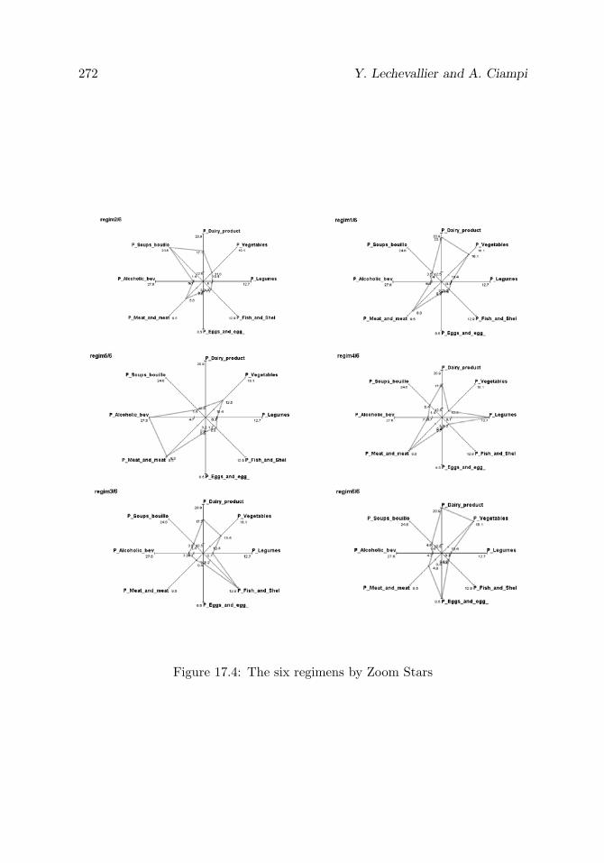
272 Y. Lechevallier and A. Ciampi
Figure 17.4: The six regimens by Zoom Stars

Multilevel Clustering for Large Databases 273
Table 17.2: Proportion of the six regimens: overall and by center
Regimens Overall Alsace Aquitaine Bretagne Ile-de Languedoc Nord -Pas Rhone-Lorraine Loire -France -Roussillon -de-Calais -Alpes
regim 1 0,56 0,58 0,59 0,49 0,58 0,54 0,46 0,61regim 2 0,19 0,18 0,18 0,20 0,14 0,21 0,28 0,18regim 3 0,08 0,08 0,07 0,12 0,09 0,08 0,08 0,06regim 4 0,03 0,02 0,04 0,03 0,03 0,04 0,02 0,03regim 5 0,10 0,10 0,08 0,11 0,10 0,08 0,13 0,09regim 6 0,04 0,04 0,04 0,05 0,05 0,04 0,03 0,04
low fish consumption; regimen 5 by high alcohol and meat consumption; andregimen 6 by high consumption of dairy products, eggs, and vegetables and lowconsumption of fish, alcoholic beverage, and vegetables. Also, the Nord-Pas-de-Calais region is positively associated with regimens 2 and 5 and negativelywith regimen 1; similarly, there is a positive association of Bretagne-Pays-de-Loire with regimen 3 and a negative association with regimen 1; and finally,Rhone-Alpes is positively associated with regimen 1.
Acknowledgements. We wish to thank Dr. F. Clavel for having shared theFrench data with us, and Dr. E. Riboli for general assistance in becomingfamiliar with EPIC.
References
1. Ambroise, C., Seze, G., Badran, F., and Thiria, S. (2000). Hierarchicalclustering of self-organizing maps for cloud classification, Neurocomputing,30, 47–52.
2. Bock, H. H. (1993). Classification and clustering: Problems for the future,In New Approaches in Classification and Data Analysis (Eds., E. Diday,Y. Lechevallier, M. Schader, P. Bertrand, and B. Burtschy), pp. 3–24,Springer-Verlag, Heidelberg.
3. Bock, H. H., and Diday, E. (Eds.) (1999). Analysis of symbolic data,exploratory methods for extracting statistical information from complexdata, In Studies in Classification, Data Analysis and Knowledge Organi-zation, Springer-Verlag, Heidelberg.
4. Chavent, M. (1998). A monothetic clustering algorithm, Pattern Recog-nition Letters, 19, 989–996.
5. Ciampi, A., and Lechevallier, Y. (1995). Designing neural networks fromstatistical models: A new approach to data exploration, In Proceedings

274 Y. Lechevallier and A. Ciampi
of the First International Conference on Knowledge Discovery and DataMining, pp. 45–50, AAAI Press, Menlo Park, California.
6. Ciampi, A., and Lechevallier, Y. (1997). Statistical models as buildingblocks of neural networks, Communications in Statistics, 26, 991–1009.
7. Elemento, O. (1999). Apport de l’analyse en composantes principalespour l’initialisation et la validation de cartes de Kohonen, In SeptiemesJournees de la Societe Francophone de Classification, Nancy, France.
8. Gordon, A. D. (1981). Classification: Methods for the Exploratory Analy-sis of Multivariate Data, Chapman & Hall, London, UK.
9. Hebrail, G., and Debregeas, A. (1998). Interactive interpretation of Ko-honen maps applied to curves, In Proceedings of the Fourth Interna-tional Conference on Knowledge Discovery and Data Mining, pp. 179–183,AAAI press, Menlo Park, California.
10. Murthag, F. (1995). Interpreting the Kohonen self-organizing feature mapusing contiguity-constrained clustering, Pattern Recognition Letters, 16,399–408.
11. Noirhomme-Fraiture, M., and Rouard, M. (1998). Representation of sub-populations and correlation with Zoom Star, In Proceedings of NNTS’98,Sorrento, Italy.
12. Thiria, S., Lechevallier, Y., Gascuel, O., and Canu, S. (1997). Statistiqueet Methodes Neuronales, Dunod, Paris.

18
Neural Networks: An Application for Predicting
Smear Negative Pulmonary Tuberculosis
A. M. Santos,1 B. B. Pereira,2 J. M. Seixas,2 F. C. Q. Mello,2
and A. L. Kritski2
1Federal University of Maranhao, Maranhao, Brazil2Federal University of Rio de Janeiro, Rio de Janeiro, Brazil
Abstract: Smear negative pulmonary tuberculosis (SNPT) accounts for 30%of pulmonary tuberculosis (PT) cases reported yearly. Rapid and accurate diag-nosis of SNPT could provide lower morbidity and mortality, and case detectionat a less contagious status. The main objective of this work is to evaluate aprediction model for diagnosis of SNPT, useful for outpatients who are attendedin settings with limited resources. The data used for developing the proposedmodels werecomprised of 136 patients from health care units. They were re-ferred to the University Hospital in Rio de Janeiro, Brazil, from March 2001to September 2002, with clinical–radiological suspicion of SNPT. Only symp-toms and physical signs were used for constructing the neural network (NN)modelling, which was able to correctly classify 77% of patients from a test sam-ple. The achievements of the NN model suggest that mathematical modelling,developed for classifying SNPT cases could be a useful tool for optimizing ap-plication of more expensive tests, and to avoid costs of unnecessary anti-PTtreatment. In addition, the main features extracted by the neural model areshown to agree with current analysis from experts in the field.
Keywords and phrases: Neural networks, cross-validation, clustering, tuber-culosis, medical diagnosis
275

276 A. M. Santos et al.
18.1 Introduction
Tuberculosis is a serious public health problem and it is estimated by the WorldHealth Organization (WHO) that approximately 1.8 billion individuals are in-fected by Mycobacterium tuberculosis [WHO (2002)]. In Brazil, approximately35 to 45 million individuals are currently infected by this disease.
Sputum smear and Mycobacterium tuberculosis culture have been advo-cated as valuable tools for diagnosis of pulmonary tuberculosis. However, thesputum smear staining lacks sensitivity, and culture confirmation requires sev-eral weeks; few tuberculosis-control programmes in low-income countries haveaccess to facilities that allow culture performance in their primary-care diag-nostic.
Approximately 20% to 50% of patients with pulmonary tuberculosis aresmear negative, and 10% of these patients are culture negative. However, thesesmear-negative cases pose a relevant public health hazard due to their trans-mission rate of Mycobacterium tuberculosis of 17% among exposed individuals[Sarmiento et al. (2003)].
Much attention has recently been paid to the problem of smear negativepulmonary tuberculosis (SNPT) particularly due to the HIV epidemic, becausethe co-infection increases the risks of tuberculosis atypical presentation andassociated morbidity and mortality. Quite appropriately, the discussion regard-ing SNPT has focused on low-income countries, home of the vast majority ofindividuals with tuberculosis and HIV infection and where the availability ofculture diagnostics is limited. So, rapid and accurate diagnosis of SNPT couldprovide lower morbidity and mortality, and case detection at a less contagiousstatus [Long (2001)].
Diagnosis of SNPT is usually based upon clinical presentation and radiolog-ical indicators that present a limited accuracy. In this context, there is a needfor new approaches for the diagnosis of SNPT. For clinical use, these new toolsshould be used under routine conditions in the health care units.
In the medical literature, several statistical models have been suggestedfor pulmonary tuberculosis diagnostics. El-Solh et al. (1999) established amodel for identification of PT using neural networks. Mello et al. (2006) usemultivariate logistic regression and classification trees to predict the patient’sprobability of PT. Santos (2003) uses neural networks and classification treesto identify patients with clinical–radiological suspicion of SNPT.

Smear Negative Pulmonary Tuberculosis 277
Statistical models can be used for prediction of infection or of the disease.They also can be used to simulate epidemic situations providing clues for pre-ventive interventions. If formulated in a systematic way and implemented withhigh-qualified data, these models can be representative of the clinical problemunder evaluation and could be useful for physicians in their clinical regularpractice, as well as for public health policy administration [Kritski and Ruffino-Netto (2000)].
In this work, we use artificial neural network for developing and evaluat-ing a prediction model for diagnosing SNPT, useful for patients attended inhealth care units within areas of limited resources. In addition, we analyze theinformation that is extracted by the model and compare it to expert analysisfor diagnosis. This analysis aims at helping doctors to understand the way themodel works and to make them more confident in its practical application.
The chapter is arranged as follows. Section 18.2 describes the methods usedin this work and specifically describes the networks used. This section alsodescribes the data set in the study as well as the selection criteria for boththe training and testing sets used for developing the artificial neural modeland testing its generalization capacity. In Section 18.3, the methodology usedto identify the relevant variables is presented. Results and conclusions arepresented in Sections 18.4 and 18.5, respectively.
18.2 Materials and Methods
In this section, we first describe the data set used for artificial neural networkdesign. In Section 18.2.2, the topology of the artificial neural networks used inthis work is defined. Clustering techniques were applied for splitting the dataset into a training and testing sets and this is described in Section 18.2.3. Thesection concludes with a study of the relevance of the explanatory variables thatfeed into networks.
18.2.1 Data set
The data set refers to 136 patients who agreed to participate in the study. Theywere referred to Hospital Clementino Fraga Filho, a University Hospital of Fed-eral University of Rio de Janeiro, Brazil, from March, 2001 to September, 2002,with clinical–radiological suspicion of SNPT. The data consisted of informationfrom anamnesis interview and included demographic and risk factors typicallyknown for tuberculosis diagnosis.

278 A. M. Santos et al.
These patients were under suspicion of active pulmonary tuberculosis, pre-senting negative smear. Forty-three percent of these patients actually showedPT in activity.
Firstly, 26 clinical variables were considered for model development. Theseincluded: age, cough, sputum, sweat, fever, weight loss, chest pain, shudder,dyspnea, diabetes, alcoholism, and others. In the sequence, the data set wasdescribed using just 12 or 8 clinical variables. Those variables were selected byexperts active in tuberculosis research.
18.2.2 Neural network design
In this work, we use a multilayer feedforward architecture with a backpropa-gation algorithm [Haykin (1999)]. The network has three layers and each layerreceives inputs only from its preceding layer. Adjacent layers are fully con-nected, that is, every neuron in a layer is connected to every neuron in anadjacent layer.
Several factors are important in a network design for pattern classificationproblems. These include the network architecture as well as the training metho-dology used. All the networks investigated in this study used a single hiddenlayer. It has been shown that neural networks of this type can handle themajority of problems [Hornik (1991)].
As already mentioned, from 26 to 8 input variables were fed into the networkinput nodes, which correspond to the patients’ clinical variables. Variables werenormalized by the following transformation:
x∗i =
xi − x
max(xi − x), i = 1, 2, . . . , 136, (18.1)
where xi is the original variable and x its arithmetic mean. Variable norma-lization is required for matching input variation with the dynamic range ofactivation function of the neurons. In our case, a hyperbolic tangent was chosenas the function for activating all neurons.
The binary variables were codified as −1 or 1, where −1 represents theabsence of the observed attribute and 1 the presence of the attribute. Thequalitative variables with three categories were codified as −1 (absence of ob-served attribute), 1 (presence of the observed attribute) and 0 (ignored).
The network has a single output neuron, with training targets defined as 1if the patient is with active PT and −1 otherwise.

Smear Negative Pulmonary Tuberculosis 279
It is known that parsimonious models with few hidden neurons are prefe-rable, because they tend to show better generalization ability, reducing the over-fitting problem. The number of neurons in the hidden layer was defined throughexperimentation. Networks having three and four hidden neurons proved towork well for this problem.
The performance of the neural network (NN) was evaluated through theclassification for the testing set, which is referred to here as accuracy. Otherdescriptive statistics were also used to evaluate the performance of NN in study,they are: sensitivity and specificity, because those measured are of general use inmedicine. Sensitivity of the neural model will tell us how the model is classifyingthe patients with PT in activity, and the specificity will tell how the model isclassifying patients without PT in activity.
We will use the notation (i − h − o) to refer to a neural network with iinputs, h hidden neurons and o neurons in the output layer.
18.2.3 Data selection for network design
Building the training and testing sets is one of the main tasks in designingan artificial neural network, especially in practical situations where statisticalrestrictions are present.
Both training and testing sets should be constituted from the available dataset. In practical applications, the amount of available data for model deve-lopment may be small. In such a situation, the training and testing sets shouldbe carefully selected, so that representative samples of the problem are obtained.
At first, the original data were randomly divided into the training and tes-ting sets. Given the statistical limitations of the available data, a division inthe form of 80% of the patients for the training set and 20% for the testing setwould be preferable. With this strategy, model development was made varyingthe number of hidden neurons. It was observed that some neural networksexhibited poor performance. This was due to poor statistical representation ofthe training set with respect to patterns belonging to the testing set. If anyregion of the domain of the input of the network does not have an appropriatenumber of patterns included in the training set, this region will not be learnedefficiently and, consequently, patterns in the testing set that belong to regionwill be probably classified erroneously [Alencar (2003)].
Efficient alternatives for data selection are cross-validation [Stone (1974)]and cluster analysis [Morrison (1990)].

280 A. M. Santos et al.
Cross validation
Cross-validation has been successful in neural network designs. For this, theoriginal data set D is divided randomly into k mutually exclusive subsets Dv,v = 1, . . . , k. The subsets should be the most homogeneous possible and thenumber of cases of each subset should be approximately the same. Frequently,k is taken to be ten and the division of the data into k subsets is through thek-fold cross-validation method.
After the division of the original data D, as showed in Figure 18.1, theneural networks are trained, using as training set D−Dv (the cases that belongto D but not to Dv) and as test set Dv. In Figure 18.1, the first subset is thetesting set, and the others form the training set. Next, the second subset is thetesting set and the others as training set, and so on. We can observe that eachsubset enters the training set as well as the testing set.
Figure 18.1: Example of cross-validation for k = 10
In this study, the data set was split into six subsets, containing approxi-mately the same number of patterns. Four of the six subsets were used fortraining of the NN, and the remaining ones were used for testing the generali-zation capacity of the classifier. This procedure was repeated until all possiblecombinations of the six subsets were used for training the NN. In total, 15 dif-ferent training and testing subsets were formed. Each training subset comprisedon an average 92 patterns, and the testing subset 44.
Cluster analysis
Cluster analysis is a technique used to detect the existence of clusters in givendata. This grouping process can be seen as an unsupervised learning technique.
Generally speaking, cluster analysis methods are of two types: (a) Parti-tioning methods: algorithms that divide the data set into k clusters, wherethe integer k needs to be specified by the user; (b) Hierarchical methods: algo-rithms yielding an entire hierarchy of clusterings of the data set. Agglomerative

Smear Negative Pulmonary Tuberculosis 281
methods start by forming local clusters from each object in the data set andthen successively merge clusters until only one large cluster remains that is thewhole set of data. Divisive methods start by considering the whole data set asone cluster, and then split up clusters until each object is separate.
To avoid the possibility of some regions not being represented, training andtesting sets were also obtained data clustering. Firstly, for obtaining the groups,we used the agglomerative hierarchical method. The hierarchical methods donot present an intuitive indicator for the number of clusters present in the dataset. An alternative is the construction of the dendrogram, which is a tree whoseleaves are data objects, and branches can be seen as the identified clusters[Morrison (1990)].
The dendrogram was constructed using Ward’s method [Kaufman andRousseeuw (1990)]. In the first step, the patterns were grouped according tothe 26 explanatory variables. Analyzing the dendrogram, three main clusterswere identified. Restricting the data space to 12 or 8 explanatory variables,three main clusters were also identified.
An artificial neural network method was also used to obtain homogeneousgroups. This method is the modified ART (adaptive resonance theory) archi-tecture, presented by Vassali, Seixas, and Caloba (2002). This method is basedessentially on the Kohonen layer and competitive learning [Haykin (1999)].
In the modified ART, each neuron of such a layer has assigned to it a vectorof synaptic weights with unitary norm. The classification of an input vector xis performed by the neuron that exhibits the smallest distance (according to theEuclidean metric) to this vector, among all neurons, provided that this distanceis smaller than a predefined radius r0. This neuron becomes the winner andwill be the only neuron to be trained, according to the equation
wn+1 = (1 − η)wn + ηx, (18.2)
where η is the learning coefficient and w is the weight vector.The distance between an incoming vector and a given weight vector can be
obtained by computing the inner product between these two vectors as
< x,w >= 1− d(x,w)2
2 . (18.3)
This is possible because vectors are normalized (|x| = |w| = 1). Vector nor-malization is performed by adding one more element to each original vector, sothat this extra component provides the information concerning the norm of theoriginal vector.
It should be clear that this operation is equivalent to a clustering procedure,where each neuron is assigned to a cluster. In fact, after a number of trainingsteps, it is expected that the weight vector assigned with a neuron will convergeto the centroid of the corresponding cluster [Vassali, Seixas, and Caloba (2002)].

282 A. M. Santos et al.
An interesting feature that has been added to this network was the vigilanceradius r0, which can impose a limited region for the neuron’s action. Geometri-cally, it is equivalent to imposing a maximum volume on each cluster, so that anincoming vector that does not exhibit similarity to any of the existing neuronswill not be classified. During the training phase, whenever this happens, a newneuron is created, and its corresponding weight vector is the incoming vectoritself. If this happens during the production phase, the incoming vector cannotbe assigned to any class and it is declared to be unknown [Vassali, Seixas, andCaloba (2002)].
In the sequence, the modified ART method was applied. Initially, the normof each vector of explanatory variables xi was made unitary. Considering p ex-planatory variables, the normalization component, denoted as xip+1, was addedas
xip+1 = (M −p∑
j=1
x2ij)
1/2, i = 1, 2, . . . , 136, (18.4)
where
M = max ||xi||. (18.5)
So, the normalized data vector became
xi =1√M
(xi1, xi2, · · · , xip+1)′, i = 1, 2, . . . , 136. (18.6)
The modified ART method requests a vigilance radius for each cluster to beformed. To obtain the vigilance radius, we calculated the Euclidean distancebetween the patterns in the data set. The choice for this radius was based on themore frequent distance. As result of this, three clusters were again recognizedin the data set, despite describing the input space with 26, 12, or 8 exploratoryvariables.
Although both clustering methods under investigation pointed out threeclusters in the data set, they were not the same. In this case, the training setwas obtained by randomly selecting 75% of the patients in each cluster and 25%of patients was selected to form the testing set.
After having formed the training and the testing sets from both the cluste-ring and cross-validation approaches, we trained several NN and evaluated theirperformance. The data sets that exhibited the best performance were chosento form the final model. Table 18.1 presents these data sets. We can observethat amount of patients with PT in activity (PT+) and without PT (PT−) isdifferent in the considered data sets.
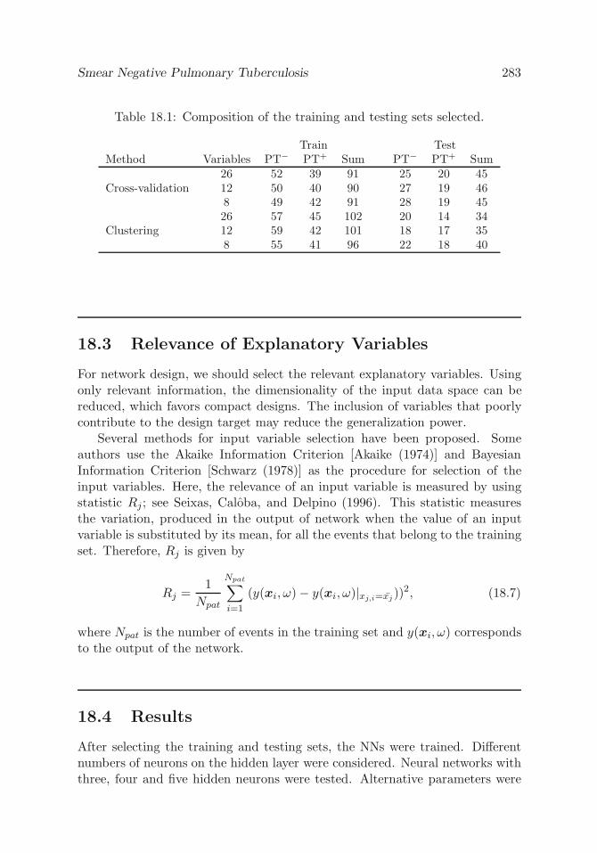
Smear Negative Pulmonary Tuberculosis 283
Table 18.1: Composition of the training and testing sets selected.
Train TestMethod Variables PT− PT+ Sum PT− PT+ Sum
26 52 39 91 25 20 45Cross-validation 12 50 40 90 27 19 46
8 49 42 91 28 19 4526 57 45 102 20 14 34
Clustering 12 59 42 101 18 17 358 55 41 96 22 18 40
18.3 Relevance of Explanatory Variables
For network design, we should select the relevant explanatory variables. Usingonly relevant information, the dimensionality of the input data space can bereduced, which favors compact designs. The inclusion of variables that poorlycontribute to the design target may reduce the generalization power.
Several methods for input variable selection have been proposed. Someauthors use the Akaike Information Criterion [Akaike (1974)] and BayesianInformation Criterion [Schwarz (1978)] as the procedure for selection of theinput variables. Here, the relevance of an input variable is measured by usingstatistic Rj ; see Seixas, Caloba, and Delpino (1996). This statistic measuresthe variation, produced in the output of network when the value of an inputvariable is substituted by its mean, for all the events that belong to the trainingset. Therefore, Rj is given by
Rj =1
Npat
Npat∑i=1
(y(xi, ω)− y(xi, ω)|xj,i=xj))2, (18.7)
where Npat is the number of events in the training set and y(xi, ω) correspondsto the output of the network.
18.4 Results
After selecting the training and testing sets, the NNs were trained. Differentnumbers of neurons on the hidden layer were considered. Neural networks withthree, four and five hidden neurons were tested. Alternative parameters were

284 A. M. Santos et al.
used (learning rate, momentum, and number of iterations) of the backpropaga-tion algorithm. The NNs with the smallest classification errors in the test setwere selected.
According to Table 18.2, the NN with 12 input variables presented thelargest accuracy (77%), as well as the largest specificity (83%). However, theneural network developed with the training set obtained by cross-validationpossessed the largest sensitivity (84%); that is, this network better classifiesthe individuals with active PT.
Table 18.2: Classification efficiencies
Cross Validation ClusteringAccuracy Specificity Sensitivity Accuracy Specificity Sensitivity
Networks (%) (%) (%) (%) (%) (%)
(26-4-1) 71 76 65 71 65 79(12-4-1) 72 63 84 77 83 71(8-4-1) 71 68 76 70 61 82
To identify the relevant variables, considering the neural network with thelargest accuracy, the relevance of each variable was computed. For this, Eq.(18.7), defined in Section 18.3, was used.
According to Figure 18.2, the neural network identified 11 relevant variablesfor the problem under study, except the variable extrapulmonary tuberculosis.
18.5 Conclusions
The proposed NN model suggests that mathematical modelling, for classifyingSNPT cases, could be a useful tool for optimizing utilization of more expensivetests, and to avoid costs of unnecessary anti-PT treatment. Besides, the neuralmodel was able to identify the important variables for the problem under study,as described by experts of the field.
In the case under study, the sample size was one of the main limitations fordesign network. We used cross-validation and clustering methods to overcomethis limitation of NN model development. These techniques made it possible toidentify a training set that could allow good response generalization for testingset.
The neural network model achieved good classification performance, exhibit-ing sensitivity from 71 to 82% and specificity from 60 to 83%. However, onlysymptoms and physical signs were used for constructing the neural network.
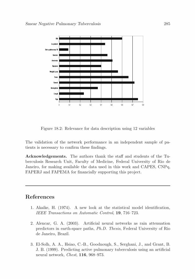
Smear Negative Pulmonary Tuberculosis 285
Figure 18.2: Relevance for data description using 12 variables
The validation of the network performance in an independent sample of pa-tients is necessary to confirm these findings.
Acknowledgements. The authors thank the staff and students of the Tu-berculosis Research Unit, Faculty of Medicine, Federal University of Rio deJaneiro, for making available the data used in this work and CAPES, CNPq,FAPERJ and FAPEMA for financially supporting this project.
References
1. Akaike, H. (1974). A new look at the statistical model identification,IEEE Transactions on Automatic Control, 19, 716–723.
2. Alencar, G. A. (2003). Artificial neural networks as rain attenuationpredictors in earth-space paths, Ph.D. Thesis, Federal University of Riode Janeiro, Brazil.
3. El-Solh, A. A., Hsiao, C.-B., Goodnough, S., Serghani, J., and Grant, B.J. B. (1999). Predicting active pulmonary tuberculosis using an artificialneural network, Chest, 116, 968–973.

286 A. M. Santos et al.
4. Haykin, S. (1999). Neural Networks: A Comparative Foundation, Prentice-Hall, Upper Saddle River, New Jersey.
5. Hornik, K. (1991). Approximation capabilities of multilayer feedforwardnetworks, Neural Networks, 4, 251-257.
6. Kaufman, L., and Rousseeuw, P. (1990). Finding Groups in Data, JohnWiley & Sons, New York.
7. Kritski, A. L., and Ruffino-Netto, A. (2000). Health sector reform inBrazil: Impact on tuberculosis control, International Journal of Tubercu-losis and Lung Disease, 4, 622–626.
8. Long, R. (2001). Smear-negative pulmonary tuberculosis in industrializedcountries, Chest, 120(2), 330–334.
9. Mello, F. C, Bastos, L. G, Soares, S. L, Rezende, V. M, Conde, M. B,Chaisson, R. E, Kritski, A. L, Ruffino-Netto, A., and Werneck, G. L.(2006). Predicting smear negative pulmonary tuberculosis with classifi-cation trees and logistic regression: a cross-sectional study, BMC PublicHealth, 6.
10. Morrison, D. F. (1990). Multivariate Statistical Methods, Third edition,McGraw-Hill, New York.
11. Santos, A. M. (2003). Neural networks and classification trees: an applica-tion for predicting smear negative pulmonary tuberculosis, Ph.D. Thesis,Federal University of Rio de Janeiro, Brazil.
12. Sarmiento, O., Weigle, K., Alexander, J., Weber, D. J., and Miller, W.(2003). Assessment by meta-analysis of PCR for diagnosis of smear-negative pulmonary tuberculosis, Journal of Clinical Microbiology, 41,3233-3240.
13. Schwarz, G. (1978). Estimating the dimension of a model, Annals ofStatistics, 6, 461–464.
14. Seixas, J. M., Caloba, L. P., and Delpino, I. (1996). Relevance criteriafor variable selection in classifier designs, In International Conference onEngineering Applications of Neural Networks, 451–454.
15. Stone, M. (1974). Cross-validatory choice and assessment of statisticalpredictions, Journal of the Royal Statistical Society, Series B, 36, 111–147.

Smear Negative Pulmonary Tuberculosis 287
16. Vassali, M. R., Seixas, J. M. d., and Caloba, L. P. (2002). A neural particlediscriminator based on a modified art architecture, In Proceedings of the2002 IEEE International Symposium on Circuits and Systems, Volume 2,121–124.
17. WHO (2002). Stop TB, annual report 2001.

19
Assessing Drug Resistance in HIV Infection Using
Viral Load Using Segmented Regression
Hua Liang,1 Wai-Yuan Tan,2 and Xiaoping Xiong3
1University of Rochester Medical Center, Rochester, NY, USA2The University of Memphis, Memphis, TN, USA3St. Jude Children’s Research Hospital, Memphis, TN, USA
Abstract: In this chapter, we have assessed the time to development of drugresistance in HIV-infected individuals treated with antiviral drugs by usinglongitudinal viral load HIV-1 counts. Through log-transformed data of HIVvirus counts over time, we have assumed a linear changing-point model and de-veloped procedures to estimate the unknown parameters by using the Bayesianapproach. We have applied the method and procedure to the data generated bythe ACTG 315 involving treatment by the drug combination (3TC, AZT, andRitonavir). Our analysis showed that the mean time to the first changing point(i.e., the time the macrophage and long-lived cells began to release HIV parti-cles) was around 15 days whereas the time to development of drug resistance byHIV was around 75 days. The Bayesian HPD intervals for these changing pointsare given by (8.7, 21.3) and (42, 108), respectively. This analysis indicated thatif we use the combination of three drugs involving two NRTI inhibitors (3TCand AZT) and one PI inhibitor (Ritonavir) to treat HIV-infected individuals,in about two and half months, it would be beneficial to change drugs to avoidthe problem of drug resistance.
Keywords and phrases: AIDS clinical trial, Gibbs sampler, HIV dynamics,longitudinal data, random change points, nonlinear mixed-effects models
19.1 Introduction
It has been well documented that plasma HIV RNA level (viral load) is a veryeffective predictor for clinical outcomes in HIV-infected individuals [Saag etal. (1996) and Mellors et al. (1995, 1996)], and has thus become a primarysurrogate marker in most AIDS clinical trials. To assess the effects of drugs andalso to monitor the progression of the disease in HIV-infected individuals treated
289

290 H. Liang, W.-Y. Tan, and X. Xiong
with anti-retroviral drugs, it appears necessary to study the HIV dynamicsduring treatment through HIV viral loads and how the dynamics are related tothe changing numbers of HIV virus load over time.
To illustrate the basic HIV dynamics in HIV-infected individuals, consideran HIV-infected individual treated with highly active antiretroviral therapy(HAART) involving two nucleoside reverse transcriptase inhibitors (NRTI) suchas 3TC and AZT and one protease inhibitor (PI) such as Ritonavir. Then, ithas been shown that within the first week, the total number of HIV counts perml of blood can be approximated by an exponential function. It follows that inthe first week, the log of the HIV virus load decreases linearly and sharply withlarge negative slope [Ho et al. (1995), Wei et al. (1995), and Tan (2000, Chap-ter 8)]. After the first week, however, the picture is very different and showsmultiphases of decline and increase. In log scale, within the first two to threemonths after the first week, the picture is again linear but the curve is very flatdue presumably to the release of HIV by macrophage and other long-lived cellsfrom the lymph nodes [Perelson et al. (1997) and Tan (2000, Chapter 8)]; atsome point between the third and eighth months, for some individuals the virusload increases sharply, reaching the level before treatment, due presumably tothe development of drug resistance of HIV to the drugs. By using a compre-hensive stochastic model of HIV pathogenesis involving flow of HIV from thelymph nodes and development of drug resistance, Tan (2000, Chapter 8) hasdemonstrated through computer simulation how these changes and outcomesare predicted by the model. To illustrate these points, we give in Figure 19.1a scatter plot of viral load (in log10 scale) at different treatment times froman AIDS clinical study conducted by the AIDS Clinical Trials Group (ACTG315). In this study, 48 HIV-1 infected patients were treated with potent antivi-ral therapy consisting of Ritonavir, 3TC, and AZT [see Lederman et al. (1998)and Wu et al. (1999) for more details on this study]. Viral load was monitoredsimultaneously at treatment days 0, 2, 7, 10, 14, 28, 56, 84, 168, and 336.
From Figure 19.1, we observe that the viral load of most patients declinesrapidly within the first two weeks with large negative slope; after two weeks,however, the trend of decline decreases and becomes flat. At about ten weeks,the viral loads rebound mostly upward to the end of treatment. From this,it is logical to assume that the effect of treatment can be divided into threestages: rapid decline, slow decline, and rebound. We are interested in therate of decline/rebound and the time of changing points. From the biologicalperspective, one may link the time of the first changing point as the time whenthe macrophage or other long-lived HIV-infected cells from lymphoid tissuesrelease free HIV to the blood; one may link the second time of changing pointas the time when HIV has developed resistance to the drugs. These time pointshave important clinical implications because this is the time to change drugs toavoid the problem of drug resistance.

Assessing Drug Resistance in HIV Infection 291
0 50 100 150 200 250 300
23
45
6
ACTG 315 Data
Days
Log1
0 RN
A (c
opies
/mL)
Figure 19.1: Viral load data for ACTG 315 study
For better understanding of the HIV pathogenesis and for better treatmentmanagement and care of AIDS patients, it is important to identify when thepatients’ viral load or CD4 cell counts decline, and when to change the decliningtrend, and rebound. For assessing HIV infection, Lange et al. (1992) considereda fully Bayesian analysis of CD4 cell counts. Kiuchi et al. (1995) used a similarapproach to examine change points in the series of T4 counts prior to AIDS.Putter et al. (2002) and Han et al. (2002) have considered a population HIVdynamic model using the Bayesian approach. But none of these studies hasever attempted to estimate the time to drug resistance. By using data fromthe clinical trial ACTG 315, in this chapter we develop a Bayesian procedureto estimate the time of these changing points.
In this chapter, we propose a three-segment model with random changepoint to describe viral load trajectory data. We are concerned with the decline/rebound rates and the location of changing points. This chapter is organizedas follows. In Section 19.2, we propose the model structure, prior distrib-utions and conditional posterior distributions. In Section 19.3, we describethe multilevel Gibbs sampling procedures to estimate the unknown parame-ters and the times of changing points. In Section 19.4, we present the analysis

292 H. Liang, W.-Y. Tan, and X. Xiong
and results for the ACTG 315 data by using the models and methods givenin previous sections. Finally, in Section 19.5, we present some conclusions anddiscussions.
19.2 The Model
For monitoring the disease progression in HIV-infected individuals, the dataare usually the number of RNA virus copies over different time points. Asillustrated in Section 19.1, in log scale these data sets are best described by apiecewise linear model with at most two unknown changing points. The firstchanging point is the time at which some HIV are released by macrophageor other long-lived cells from the lymphoid tissues [Perelson et al. (1997)].The second changing point is the time at which the HIV in the HIV-infectedindividual develops resistance to the drugs. For those individuals in which theHIV has not yet developed resistance to the drugs, the log of the RNA viruscopies per ml then showed a two-segment linear curve with one changing point;the first linear segment is a sharp linear declining curve with large negative slopeshowing a rapid decline of the HIV numbers due to the inhibition effect of thedrugs whereas the second linear segment is a less rapid linearly declining curvewith small negative slope due to additional new release of HIV of macrophagefrom lymphoid tissues [Perelson et al. (1997)]. When the HIV in the HIV-infected individual has developed drug resistance, then one would expect athree-piece linear model with two changing points; the third linear segment isa linear ascending curve with positive slope and the second changing point isthe time when the HIV develops resistance to the drugs. A typical picturedescribing this situation is shown in Figure 19.2.
To describe the model, suppose that there are n HIV-infected individualstreated by the same drug combination. For the ith individual, let tLi andtRi denote the time of the first and second changing points, respectively. As-suming a mixed model to account for the variation between individuals, thentLi, i = 1, . . . , n is a random sample from an unknown density with meantL and tRi, i = 1, . . . , n is a random sample from an unknown density withmean tR. It is generally believed that tL occurs at about two weeks [Perelsonet al. (1997)] and tR occurs some time between the third and eleventh months[Tan (2000, Chapter 8)]. For the ith individual, the three linear segments areseparated by tLi and tRi. For this individual, the first line segment is η0i + η1it,showing a rapid decline in log(RNA) after treatment. The second line segmentis η2i + η3it, showing a less rapid decline after some unknown time point tLi
due to the release of HIV from macrophage or other long-lived cells from thelymphoid tissues. The third segment is η4i + η5it, showing an increase of the

Assessing Drug Resistance in HIV Infection 293
0 20 40 60 80 100
23
45
6
x
1st segment
2nd segment
3rd segment
Figure 19.2: Illustrative plot of three segments used to explore viral load tra-jectory
log(RNA) after some unknown time point tRi, because of the drug resistance.Notice that the first two segments agree at tLi, whereas the last two segmentsagree at tRi. Denote by Δ1i = η3i − η1i and Δ2i = η5i − η3i. Then, by comb-ing these three line segments we can express the piecewise linear model by thefollowing equation:
yij = η0i + η1itij + Δ1i(tij − tLi)+ + Δ2i(tij − tRi)+ + εij , (19.1)
where s+ = max(s, 0) and εij is the random measurement error for measuringyij.
It is assumed that the εijs are independently distributed normal randomvariables with means 0 and variance σ2
i , independently of ηri, r = 0, 1,Δui, u =1, 2, tLi, tRi for all i = 1, . . . , n. That is, εij ∼ N(0, σ2
i ), independently distrib-uted of the random variables η0i, η1i, Δ1i, Δ2i, tLi, and tRi for all i = 1, . . . , n.
In the above model, because of variation between individuals, the ηji, j =0, 1 and the Δri, r = 1, 2 are random variables. As in Wu et al. (1999), weuse a mixed-effects model to account for variation between individuals. Also,following Lange et al. (1992) and Kiuchi et al. (1995), we will model thesevariables by using first-order linear equations:
η0i = α0 + β0i,

294 H. Liang, W.-Y. Tan, and X. Xiong
η1i = α1 + β1i,
Δ1i = α2 + β2i,
Δ2i = α3 + β3i,
In the above equations, the αs denote population effects, and the βs individualeffects to account for variations between individuals. Let βi = (β0i, β1i, β2i, β3i)T.As in Lange et al. (1992) and Kiuchi et al. (1995), we assume that the βisare independently and identically distributed as a Gaussian vector with mean0 and unknown covariance matrix V, that is, βi ∼ N(0,V), independently.
19.2.1 The likelihood function
In the above model, the tLR,i = (tLi, tRi)T,βi are random variables. Theunknown parameters are α = (α0, α1, α2, α3)T,V, σ2
i . Let β denote thecollection of all βi, σ2 the collection of all σ2
i , and tLR the collection of alltLR,i = (tLi, tRi)T. Let N(y|μ, σ2) denote the density of a normal distributionwith mean μ and variance σ2, and let y = (yij , i = 1, . . . , n, j = 1, . . . , ni)T.Then the conditional likelihood given (α,β, tLR) is
L(y|α,β, tLR) =n∏
i=1
mi∏j=1
N(yij|μij , σ2i ),
where μij is the right-hand side of (19.1) apart from εij .Let p(tLR,i) denote the probability density function of tLR,i. Then the joint
density of y,β, tLR given the parameters α,V,σ2 is
P(y,β, tLR|α,V,σ2) =n∏
i=1
mi∏j=1
N(yij |μij, σ2i )
n∏i=1
N(βi|0,V)p(tLR,i).
In the above distribution, p(tLR,i) is a density of discrete random variables.To specify this density, we assume that the tLis are independently distributedof the tRis. Because we have very little information about tLi except thatthe expected value of tLi probably occurs at about two weeks [Perelson et al.(1997)], we assume that the tLi is a discrete uniform random variable on theset 8, 9, . . . , 18; similarly, because we have no information about tRi exceptthat the plots of the data seemed to suggest that its expected value probablyoccurs between 60 and 90 days, we assume that tRi is a discrete uniform randomvariable on the set 60, 65, . . . , 90.
19.2.2 The prior distribution
For the prior distribution of the parameters α,σ2,V, we assume that a priorithese parameters are independently distributed of one another. As in Lange

Assessing Drug Resistance in HIV Infection 295
et al. (1992), we assume that α is a normal vector with prior mean μα andprior covariance matrix Dα. For specifying these hyperparameters, we willadopt an empirical Bayes approach by using some data to estimate its values;for details, see Section 19.4. For the prior distribution of σ2
i s, it is assumed thatthe σ2
i s are independently and identically distributed as an inverted gammadistribution IG(λ1, λ2) with λ1 = 10 and λ2 = 0.06. For the prior distributionof V, we assume that the V is distributed as an inverted Wishart randommatrix. Denote by S ∼ W (Σ, f) that the symmetric random matrix S isdistributed as a Wishart distribution with matrix Σ and degrees of freedom f .Then, V−1 ∼W ((ρΓ)−1, ρ). In Γ, the left upper 2×2 submatrix is initiated bythe covariance matrix of random term from modeling (19.9); the right-bottom2×2 submatrix is an identity matrix and the other elements are zeros. We alsotake ρ = 2.
Let N(α|μα,Dα) denote the density of α, IG(z|f1, f2) the density of aninverted Gamma distribution with parameters (f1, f2), and W (V−1|(ρΓ)−1, ρ)the density of V−1. Using the above prior distributions, the joint density ofy,α,β, tLR,σ2,V is
P(y,α,β, tLR,σ2,V)
=n∏
i=1
mi∏j=1
N(yij|μij , σ2i )N(α|μα,Dα)
n∏i=1
N(βi|0,V)
×n∏
i=1
IG(σ2i |λ1, λ2)
n∏i=1
p(tLR,i)W (V−1|(ρΓ)−1, ρ). (19.2)
19.2.3 The posterior distributions
From the joint density given in Eq. (19.2), one may readily derive the conditionalposterior distributions of the parameters and the conditional distributions ofβi, tLR,i. For this purpose, we introduce the following notations: Xij =1, tij , (tij − tLi)+, (tij − tRi)+, Xi = (XT
i1, . . . ,XTimi
)T, εi = (εi1, . . . , εimi)T,
yi = (yi1, . . . , yimi)T. Then, (19.1) can be described as
yij = Xij(α + βi) + εij or yi = Xiα + Xiβi + εi.
Then, with εi = yi − (Xiα + Xiβi),
L(y|α,β, tLR,σ2) ∝ exp
−
n∑i=1
εiTεi
2σ2i
.
By direct calculation, one can readily derive the posterior distributions of theparameters. For implementing the Gibbs sampling method to estimate the un-known parameters and βi, tLR,i, we summarize these distributions as follows.

296 H. Liang, W.-Y. Tan, and X. Xiong
(a) Denote rα,i = yi − Xiβi. Then the conditional posterior distribution ofα given y, tLR,β,V,σ2 is a Gaussian random vector with means α andcovariance matrix Σα, where
α =
(n∑
i=1
XTi Xi
σ2i
+ D−1α
)−1 ( n∑i=1
XTi rα,i
σ2i
+ D−1α μα
)and
Σα =
(n∑
i=1
XTi Xi
σ2i
+ D−1α
)−1
.
That is,
α|y, tLR,β,V,σ2 ∼ N(α, Σα). (19.3)
(b) Denote rβ,i = yi −Xiα. Then,
βi|y, tLR,V,α,σ2 ∼ N(βi, Σβ), (19.4)
where
βi =
(XT
i Xi
σ2i
+ V−1
)−1 (XT
i rβ,i
σ2i
+ V−1μα
)and
Σβ =
(XT
i Xi
σ2i
+ V−1
)−1
.
(c) Denote rσ2,i = yi −Xiα−Xiβi. Then,
σ2i |yi,α,βi,V, tLR ∼ IG
λ1 +
mi
2,
(1λ2
+12rT
σ2,irσ2,i
)−1
. (19.5)
(d) Denote ai = α + βi − μα. Then,
V−1|α,βi,σ, tL, tR ∼W
⎧⎨⎩(
n∑i=1
aiaiT + ρΓ
)−1
, n + ρ
⎫⎬⎭ . (19.6)
(e) Denote the exponent in the expression∏mi
j=1 N(yij|μij , σ2i ) from
L(y|α,β, tLR) as G. Then, the conditional distribution of tLi giveny, tR,α,βi,σ
2,V is
tLi|y, tRi,α,βi,σ2,V ∼ exp−G(tLi)p(tLi)∑
tLkexp−G(tLk)p(tLk)
. (19.7)
(f) In the exactly same way as (e), we obtain the conditional distribution of tRi
given y, tL,α,βi,σ2,V as
tRi|y, tLi,α,βi,σ2,V ∼ exp−G(tLi)p(tRi)∑
tLkexp−G(tRk)p(tRk)
. (19.8)

Assessing Drug Resistance in HIV Infection 297
19.3 The Gibbs Sampling Procedure
In the Bayesian approach, one derives the Bayesian estimates via the posteriormeans and derives the HPD intervals of the parameters from the marginalposterior distributions. With the conditional posterior distributions given byEqs. (19.3) to (19.8), one may generate random samples from the marginaldistributions via the multi-level Gibbs sampling method. General theories ofthese procedures are given by Sheppard (1994), Liu and Chen (1998), andKitagawa (1998). Detailed procedures and their proofs are given in Chapter 3of Tan (2002). This is an iterative algorithm by sampling from the conditionaldistributions alternatively and sequentially with updated parameter values. Atconvergence, this then gives samples from the marginal distributions. For themodel here, each cycle in this algorithm loops through the following steps.
Step 1. Starting with initial values Θα0 = (σ−2
0 ,β0,V0, tL0, tR0)T, one draws asample from the density fα(α|y,Θα
0 ) given by (19.3). Denote the samplevalue of α by α1.
Step 2. With Θβ0 = (σ−2
0 ,α1,V0, tL0, tR0)T, one draws a sample from thedensity fβ(βi|y,Θβ
0 ) given by (19.4). Denote the sample value of βi byβi1, i = 1, . . . , n, and let β1 = βi, i = 1, . . . , nT.
Step 3. With Θσ2
0 = (α1,β1,V0, tL0, tR0)T, one draws a sample of σ2i from
the density fσ(σ2i |y,Θσ2
0 ) given by (19.5). Denote the sample value of σ2i
by σi1, i = 1, . . . , n, and let σ1 = σi1, i = 1, . . . , nT.
Step 4. With Θ(V )0 = (σ1,α1,β1, tL0, tR0)T, one draws a sample of V from
the density fV (V−1|y,Θ(V )0 ) given by (19.6). Denote the sample value of
V by V1.
Step 5. With Θ(L)0 = (σ1,α1,β1, tR0)T, one draws a sample of tLi from the
density fL(tLi|y,Θ(L)0 ) given by (19.7). Denote the sample value of tLi
by tLi,1, and let tL1 = tLi,1, i = 1, . . . , nT.
Step 6. With Θ(R)0 = (σ1,α1,β1, tL1)T, one draws a sample of tRi from the
density fR(tRi|y,Θ(R)0 ) given by (19.8). Denote the sample value of tRi
by tRi,1, and let tR1 = tRi,1, i = 1, . . . , nT.
Step 7. With Θα0 in Step 1 replaced by Θα
0 = (σ−21 ,β1,V1, tL1, tR1)T, repeat
the above cycle until convergence is reached.

298 H. Liang, W.-Y. Tan, and X. Xiong
As shown in Chapter 3 of Tan (2002), at convergence one generates a sampleof size one from the marginal distribution of each parameter and of tL, tRrespectively. By repeating the above procedure, one generates a random sampleof size m from the marginal posterior distribution for each parameter and fortL, tR, respectively. Then one may compute the sample means and the samplevariances and covariances for these parameters. These estimates are optimalin the sense that under the squared loss function, the posterior mean valuesminimize the Bayesian risk function.
19.4 Analysis of the ACTG 315 Data
Using data from the ACTG 315 clinical trial on HAART, in this section we willderive a full Bayesian analysis to estimate the times to changing points and todrug resistance. In this analysis, we will adopt an empirical Bayesian approachto estimate the prior means and prior variances of the parameters α. Becausethe first change point generally occurs in about two weeks, we use the first twoweek’s data to conduct linear mixed effects modelling via
yij = η0i + η1itij + εij . (19.9)
The estimated values of α0 and α1 given here are taken as the means of ourprior distributions of α0 and α1. The prior distribution of α2 and α3 are bothassumed to be N(•|0, 1). The covariance matrix of α0 and α1 obtained from(19.9) is taken as the left-upper submatrix of D. The random estimated valuesare taken as the prior distributions of β0i and β1i.
With the posterior distributions given in Section 19.2 and with the Gibbssampling procedure in Section 19.3, one can readily develop a full Bayesiananalysis to estimate the relevant parameters and the times to changing points.To implement the MCMC sampling scheme, we follow the method proposed byRaftery and Lewis (1992). The procedure works as follows. After an initialnumber of 1000 burn-in iterations, every tenth MCMC sample is retained fromthe next 200,000 samples. Thus, we obtain 20,000 samples of targeted posteriordistributions of the unknown parameters. The stability of the posterior meansis checked informally by examining the graphics of the runs. Figure 19.3 showsthe number of MCMC iterations and convergence diagnostics.
Figure 19.4 shows us a population trend of the viral load trajectory withη1 = −0.12(0.005), η3 = −0.011(0.006), and η5 = 0.003(0.003), tL = 15, andtR = 75. Denote the time period from entry time to 15 days as the first stage,and the time period from 15 days to 75 days as the second stage. Figure 19.4then implies that the decline rate at the beginning stage is about ten times that

Assessing Drug Resistance in HIV Infection 299
0 5000 10000 15000 20000
−0.
20−
0.16
−0.
12
iteration
eta1
−0.130 −0.125 −0.120 −0.115 −0.110
020
4060
80
eta1
dens
ity
0 5000 10000 15000 20000
−0.
20−
0.10
0.00
iteration
eta3
−0.05 −0.04 −0.03 −0.02 −0.01 0.00 0.01
010
2030
4050
eta3
dens
ity
0 5000 10000 15000 20000
−0.
15−
0.05
0.05
iteration
eta5
0.00 0.01 0.02 0.03 0.04 0.05
010
2030
4050
eta5
dens
ity
Figure 19.3: Diagnostic plots. Left panel: the number of MCMC iterations andposterior means; right panel: the densities of the posterior means
of the decline rate of the second stage. After 75 days, the viral load trajectoryslightly rebounds.
To characterize the patterns of viral dynamics, we select four subjects andexamine the trajectories of their viral load. Given in Table 19.1 are the estimatesof the parameters for these four subjects. Given in Figure 19.5 are the plotsof fitted values for these four subjects based on the three-segment model andthe Bayesian approach. These results indicate that the individual estimates ofη1, tL, and tR are quite similar to the corresponding ones of the populationestimates respectively. However, the individual estimates of η3 and η5 variedwidely so that the individual estimates may be totally different from the onesof the population. Figure 19.5 shows that the viral load trajectory of patient10 is comparable to that of the population but with a stronger rebound in

300 H. Liang, W.-Y. Tan, and X. Xiong
the later stage; but the patterns of viral load trajectory in subjects 8 and 20are very different from that of the population in that in the second segment,their viral loads continued declining (patient 8) or flat (patient 20) insteadof a rebound as in the population pattern, suggesting that drug resistance inthese patients had not yet been developed. Figure 19.5 also shows a largedifference between individual viral load trajectory in patient 48 and that fromthe population; for this patient, the viral loads rapidly declined in the firststage, then rapidly rebounded in the second segment, and kept flatly reboundin the third segment to the end of the treatment. These results indicate that forthe clinicians to manage treatment and care of AIDS patients, it is necessary tostudy the viral load trajectory of each individual. Because the HIV pathogenesisis a stochastic dynamic process, this calls for individual-based models to assesseffects of treatment and drug resistance.
Figure 19.4: The estimated population mean curve obtained by using ACTG315 data and Bayesian approach. The observed values are indicated by plus
Table 19.1: Estimates of the parameters of four subjects
ID η0 η1 η3 η5 tL tR8 4.947 −0.12 −0.003 −0.005 14 75
10 5.38 −0.112 −0.017 0.009 15 7630 4.741 −0.118 −0.019 0 15 7648 4.838 −0.144 0.032 0.002 14 76

Assessing Drug Resistance in HIV Infection 301
Figure 19.5: Profiles of four arbitrarily selected patients for ACTG 315 data.The dotted and solid lines are estimated individual and population curves. Theobserved values are indicated by the circle signs
19.5 Conclusion and Discussion
To treat HIV-infected individuals with antiretroviral drugs, a major obstacle isthe development of drug resistance. In order to avoid the problem of drug resis-tance, it is therefore of considerable interest to estimate the time at which someresistance to the drugs have developed by the HIV. To answer this question,we have developed here a full Bayesian approach by assuming a three-segmentlinear model with two unknown changing points for the log of RNA viral load.In this model, the first changing point is the time when the macrophage orother long-lived cells release HIV to the blood from lymph nodes [Perelson etal. (1997)]; the second changing point is the time when the HIV develops resis-tance to the drugs [Tan (2000, Chapter 8)]. This statistical model is motivated

302 H. Liang, W.-Y. Tan, and X. Xiong
and dictated by the dynamic models of HIV pathogenesis under treatment andby the observed and simulated data on HIV pathogenesis [Perelson et al. (1997)and Tan (2000, Chapter 8)]. The Bayesian approach is useful because it canincorporate prior information from an empirical study or other related or pre-vious studies. This is important because current clinical data are not enoughto identify all viral dynamic parameters.
In this chapter, we have applied the above Bayesian procedure to analyzethe ACTG 315 data. These data treated patients with HAART involving 3TCand AZT (NRTI) and ritonavir (PI). For each patient, the data gave RNA viralload per ml of blood at different time points after treatment. Using this dataand the log transformation, we have estimated the expected time to the firstchanging point as 15 days after treatment and the time to development of drugresistance as 75 days after treatment. The Bayesian HPD intervals for thesechanging points are (8.7, 21.3) and (42, 108), respectively. For the three-linesegments, the estimates of the slope are −0.12, −0.011, and 0.003, respectively.The variances of these estimates are 0.005, 0.006, and 0.003 respectively. Fromthese estimates, it is clear that most patients have very much the same slopefor the first segment; but the opposite is true for the other two segments.Observing the log plots of RNA load, one may explain this by noting: (i) forsome patients, the second segment is very short or hardly noticeable, whereasfor other patients, the second segment is long. (ii) Although drug resistancehave developed in some patients (about 21 patients), in other patients drugresistance had not developed or was hardly noticeable. Thus, for the secondand third segments, there is considerable variation among individuals.
We have estimated the time to drug resistance by using a Bayesian approach,however, in treating HIV-infected individuals with antiretroviral drugs, manyimportant problems cannot be answered by this or any other statistical model.In particular, to monitor the disease progression, to assess efficacy of the drugs,and to search for optimal treatment protocols, it is important to estimate effectsof different drugs and how these effects are affected by many risk factors suchas CD4 T cell counts and CD8 T cell counts; also it is important to estimatethe numbers of infectious as well as noninfectious virus loads. Because thedrug efficacy depends on pharmacokinetics and the bioavailability of the drugs,it is also of considerable interest to study how the pharmaco-kinetics affectseffects of treatment and drug resistance. Because the HIV pathogenesis is astochastic dynamic process, this calls for stochastic dynamic models and statespace models. Using the ACTG 315 data, we are currently developing stochasticdynamic models and state space models to answer these questions.
Acknowledgements. Liang’s research was partially supported by grants fromthe National Institute of Allergy and Infectious Diseases (R01 AI062247 andR01 AI059773). Xiong’s research was partially supported by the AmericanLebanese Syrian Associated Charities (ALSAC).

Assessing Drug Resistance in HIV Infection 303
References
1. Han, C., Chaloner, K., and Perelson, A. S. (2002). Bayesian analysis of apopulation HIV dynamic model, In Case Studies in Bayesian Statistics,Volume 6, Springer-Verlag, New York.
2. Ho, D. D., Neumann, A. U., Perelson, A. S., Chen, W., Leonard, J.M., and Makowitz, M. (1995). Rapid turnover of plasma virus and CD4lymphocytes in HIV-1 infection, Nature, 373, 123–126.
3. Kitagawa, G. (1998). A self organizing state space model, Journal of theAmerican Statistical Association, 93, 1203–1215.
4. Kiuchi, A. S., Hartigan, J. A., Holford, T. R., Rubinstein, P., and Stevens,C. E. (1995). Change points in the series of T4 counts prior to AIDS,Biometrics, 51, 236–248.
5. Lange, N., Carlin, B. P., and Gelfand, A. E. (1992). Hierarchical Bayesmodels for the progression of HIV infection using longitudinal CD4 T-cellnumbers (with discussion), Journal of the American Statistical Associa-tion, 87, 615–632.
6. Lederman, M.M., Connick, E., Landay, A., Kuritzkes, D. R., SpritzlerJ, St Clair, M., Kotzin, B. L., Fox, L., Chiozzi, M. H., Leonard, J. M.,Rousseau, F., Wade, M., D’Arc Roe, J., Martinez, A., and Kessier, H.(1998). Immunological responses associated with 12 weeks of combina-tion antiretroviral therapy consisting of Zidovudine, Lamivudine, and Ri-tonavir: Results of AIDS clinical trial group protocol 315, Journal ofInfectious Diseases, 178, 70–79.
7. Liu, J. S., and Chen, R. (1998). Sequential Monte Carlo method fordynamic systems, Journal of the American Statistical Association, 93,1032–1044.
8. Mellors, J. W., Kingsley, L. A., and Rinaldo, C. R. (1995). Quantitationof HIV-1 RNA in plasma predicts outcome after seroconversion, Annalsof Internal Medicine, 122, 573–579.
9. Mellors, J. W., Rinaldo, C. R., and Gupta, P. (1996). Prognosis in HIV-1 infection predicted by the quantity of virus in plasma, Science, 272,1167–1170.
10. Perelson, A. S., Essunger, O., Cao, Y. Z., Vesanen, M., Hurley, A., Sak-sela, K., Markowitz, M., and Ho, D. D. (1997). Decay characteristics

304 H. Liang, W.-Y. Tan, and X. Xiong
of HIV infected compartments during combination therapy, Nature, 387,188–191.
11. Putter, H., Heisterkamp, S. H., Lange, J. M. A., and De Wolf, F. (2002).A Bayesian approach to parameter estimation in HIV dynamical models,Statistics in Medicine, 21, 2199–2214.
12. Raftery, A. E., and Lewis, S. (1992). How many iterations in the Gibbssample? In Bayesian Statistics – 4 (Eds., J. Bernardo, J. Berger, A.Dawid, and A. Smith), pp. 763–773, Oxford University Press, Oxford,UK.
13. Saag, M. S., Holodniy, M., Kuritzkes, D. R., O’Brien, W. A., Coombs,R., Poscher, M. E., Jacobsen, D. M., Shaw, G. M., Richman, D. D., andVolberding, P. A. (1996). HIV viral load markers in clinical practice,Nature Medicine, 2, 625–629.
14. Shephard, N. (1994). Partial non-Gaussian state space model, Biometrika,81, 115–131.
15. Tan, W. Y. (2000). Stochastic Modeling of AIDS Epidemiology and HIVPathogenesis, World Scientific, River Edge, New Jersey.
16. Tan, W. Y. (2002). Stochastic Models with Applications to Genetics,Cancers, AIDS and Other Biomedical Systems, World Scientific, RiverEdge, New Jersey.
17. Wei, X., Ghosh, S. K., Taylor, M. E., Johnson, V. A., Emini, E. A.,Deutsch, P., Lifson, J. D., Bonhoeffer, S., Nowak, M. A., Hahn, B. H.,Saag, M. S., and Shaw, G. M. (1995). Viral dynamics in human immun-odeficiency virus type 1 infection, Nature, 373: 117-122.
18. Wu, H., and Ding, A. (1999). Population HIV-1 dynamics in vivo: Ap-plicable models and inferential tools for virological data from AIDS clinicaltrials, Biometrics, 55, 410–418.
19. Wu, H., Kuritzkes, D. R., and McClernon, D. R. (1999). Characteriza-tion of viral dynamics in human immunodeficiency virus type 1-infectedpatients treated with combination antiretroviral therapy: Relationshipsto host factors, cellular restoration and virological endpoints, Journal ofInfectious Diseases, 179, 799–807.

20
Assessment of Treatment Effects on HIV
Pathogenesis Under Treatment By
State Space Models
Wai-Yuan Tan,1 Ping Zhang,1 Xiaoping Xiong,2 and Pat Flynn2
1The University of Memphis, Memphis, TN, USA2St. Jude Children’s Research Hospital, Memphis, TN, USA
Abstract: In this chapter, we have developed a method to estimate the ef-ficiency of the drugs and the numbers of infectious and noninfectious HIV inHIV-infected individuals treated with antiretroviral drugs. As an illustration,we have applied the method to some clinical and laboratory data of an AIDSpatient treated with various antiviral drugs. For this individual, the estimatesshow that the HAART protocol has effectively controlled the number of in-fectious HIV virus to below 400/ml copies although the total number of HIVcopies was very high in some intervals.
Keywords and phrases: Productively infected CD4(+) T cells, numbers of in-fectious and noninfectious HIV, multilevel Gibbs sampling method, observationmodel, stochastic equation
20.1 Introduction
To control HIV, recently important progress has been made through the com-bination of three drugs: two of nucleoside reverse transcriptase inhibitors (NR-TIs) such as AZT and 3TC with a nonnucleoside reverse transcriptase inhibitor(NNRTI) such as efavirenz or a protease inhibitor (PI) such as indinavir, re-ferred to as the Highly Active Anti-Retroviral Therapy (HAART); see Bajariaet al. (2002). However, many recent studies on HAART have indicated thatthis treatment protocol, despite its effectiveness, is still far from perfect andlife-long treatment is required [Betts et al. (2001), Chun et al. (1999), Garciaet al. (1999), and Pitcher et al. (1999)]. For monitoring HIV progression un-der treatment by antiviral drugs and to alert for possible development of drug
305
306 W.-Y. Tan et al.
resistance, it is therefore important to estimate the relative effects of NRTIs,NNRTIs, and PIs, as well as the numbers of infectious HIV virus and noninfec-tious HIV viruses over time. To date, methods for estimating these parametersand state variables are nonexistent. By applying the state space model and themultilevel Gibbs sampling procedures, the objective here is to develop efficientprocedures to estimate these parameters and the state variables as well as otherunknown parameters.
In Section 20.2, we will describe how to derive a stochastic model forHIV pathogenesis in HIV-infected individuals under treatment by antiretroviraldrugs. In Section 20.3, we will derive a state space model for HIV pathogenesisin HIV-infected individuals under treatment by antiretroviral drugs by usingdata from the observed RNA virus counts over time. In Section 20.4, we willdevelop a general procedure via the multilevel Gibbs sampling method to es-timate the unknown parameters and the state variables. As an application ofour models, in Section 20.5 we will apply the results to the data of a patientfrom St. Jude Children’s Research Hospital treated by various antiviral drugs.
20.2 A Stochastic Model for HIV PathogenesisUnder Treatment
To assess effects of different drugs and to estimate relevant state variables, inthis section we will extend the Perelson et al. (1996) model into a more complexstochastic dynamic model for HIV pathogenesis in HIV-infected individualstreated with antiretroviral drugs including HAART. Under this model, free HIVviruses infect actively dividing CD4(+) T cells to generate productively infectedCD4(+) T cells (denoted by TP cells). At the death of a TP cell, a large number(N(t)) of free HIV is generated, which will further infect other CD4(+) T cells.[Because N(t) is very large, we will assume N(t) as a deterministic function of t.]As in Perelson et al. (1996), we will ignore latently HIV-infected CD4(+) T cellsbecause the contribution to HIV of these cells is very small. Because differentdrugs and drug combinations are used over different time periods in practicalsituations, we partition the time interval into nonoverlapping subintervals andfollow Perelson et al. (1996) to assume that the number of uninfected CD4(+)
T cells is a constant in each subinterval. This is justified by the observationsthat before the start of the treatment, the HIV pathogenesis is at a steady-statecondition and that the uninfected CD4 T cells have a relatively long lifespan;see Cohen et al. (1998).
To derive the stochastic model, consider the situation in which an HIV-infected individual is treated by antiretroviral drugs including HAART. Let V0
and V1 denote noninfectious and infectious HIV, respectively. Let V0(t), V1(t)

Assessing Treatment of HIV by State Space Models 307
denote the numbers of V0 HIV and V1 HIV per ml of blood at time t and TP (t)the number of productively HIV-infected CD4(+) T cells (TP cells) at time tper ml of blood. Then we are entertaining a three-dimensional Markov processX∼
(t) = TP (t), V0(t), V1(t)′with continuous time Ω = [0,∞) and with discrete
state space S = (i, j, k), i, j, k = 0, 1, . . . ,∞. For this stochastic process, thetraditional approach is too complicated to be of much use. Hence, we proposehere an alternative approach by using stochastic differential equations.
20.2.1 Stochastic differential equations of state variables
To derive stochastic equations for the state variables, we define the followingstochastic variables.
DP (t) = Number of deaths of TP cells per ml of blood during[t, t +t);
DV i(t) = Number of free Vi HIV per ml of blood that have lostinfectivity, or die, or have been removed during [t, t +t), i = 0, 1;
F (t) = Number of V1 per ml of blood that have lost through infec-tion of CD4(+) T cells during [t, t +t). This is the number of V1
HIV per ml that have entered the CD4(+) T cells but whose viralRNA have not yet been converted to viral DNA;
F1(t) = Number of productively infected CD4(+) T cells (TP cells)per ml generated by the infection of actively dividing CD4(+) T cellsby free HIV during [t, t +t);
Rj(t) = Number of noninfectious free HIV per ml of blood (i.e., V0)generated by the death of the jth TP cell during [t, t +t) undertreatment by PI inhibitors.
To specify the probability distribution of these variables, let μT (t) and μV i(t)denote the death rate of TP cells and the rate by which free Vi HIV are beingremoved, die, or have lost infectivity at time t, respectively. Let k(t) be theHIV infection rate of CD4(+) T cells in the absence of NRTIs and NNRTIs, andlet kT (t) = k(t)T (t), where T (t) is the number of uninfected CD4(+) T cells perml of blood at time t. Denote by ξR(t) the probability that the RNA→ DNAprocess is blocked by the NRTIs and/or NNRTIs at time t inside the uninfectedCD4(+) T cells and let ξP (t) denote the probability that free HIV released inthe blood at time t by the death of a productively infected T cell in the bloodis noninfectious. Then the conditional probability distribution of the aboverandom variables given the state variables is given by:
• [F (t),DV 1(t)] | V1(t) ∼ Multinomial[V1(t); kT (t)Δt, μV 1(t)Δt];

308 W.-Y. Tan et al.
• F1(t) | F (t) ∼ Binomial[c(t)F (t)]; [1 − ξR(t)], where [c(t)F (t)] is thelargest integer ≤ c(t)F (t) and where c(t) is the proportion of activatedCD4 T cells at time t among all uninfected CD4 T cells;
• DP (t) | TP (t) ∼ Binomial [TP (t);μT (t)Δt];
• Rj(t), j = 1, . . . ,DP (t) | DP (t) > 0 ∼ Binomial [N(t); ξP (t)] indepen-dently (Rj(t) = 0 if DP (t) = 0.);
• DV 0(t) | V0(t) ∼ Binomial [V0(t);μV 0(t)Δt].
Given X(t), conditionally DP (t), [F (t),DV 1(t)],DV 0(t) are independentlydistributed from one another; given F (t), conditionally F1(t) is independentlydistributed from other variables.
By the conservation law and by using these distribution results, we ob-tain the following stochastic differential equations for TP (t), Vj(t), j = 0, 1,respectively.
dTP (t) = TP (t + Δt)− TP (t) = F1(t)−DP (t) = c(t)kT (t)[1 − ξR(t)]V1(t)− TP (t)μT (t)Δt + ε1(t)Δt, (20.1)
dV0(t) = V0(t + Δt)− V0(t) =DP (t)∑j=1
Rj(t)−DV 0(t) = R(t)−DV 0(t)
= N(t)ξP (t)TP (t)μT (t)− μV 0(t)V0(t)Δt + ε3(t)Δt, (20.2)
dV1(t) = V1(t + Δt)− V1(t) =DP (t)∑j=1
[N(t)−Rj(t)]− F (t)−DV 1(t)
= N(t)[1− ξP (t)]μT (t)TP (t)− kT (t)V1(t)− μV 1(t)V1(t)Δt ++ ε3(t)Δt. (20.3)
In Eqs. (20.1) to (20.3), the random noises εj(t)Δt, j = 1, 2, 3 are derivedby subtracting the conditional mean values from the random variables, respec-tively, and have expectation zero. It can easily be shown that these randomnoises are uncorrelated with the state variables TP (t) and Vj(t),= 0, 1; further-more, one may also assume that the random noises εj(t) are uncorrelated withthe random noises εl(τ) for all j and l if t = τ .
20.2.2 The probability distribution of state variables
Let Θ be the collection of all parameters. Letting Δt ∼ 1 correspond to asmall interval such as 0.1 day, then the state variables are X = X∼ (t), t =
0, 1, . . . , tM, where tM is the termination time of the study. For implementingthe multilevel Gibbs sampling procedure, we define the unobserved state vari-ables U∼
(t) = F (t),DP (t), R(t) and let U = U∼ (t), t = 0, 1, . . . , tM − 1. By

Assessing Treatment of HIV by State Space Models 309
using the above distribution results, we obtain the conditional density of U∼(t)
given X∼(t) as
PU∼ (t)|X∼ (t) = C1(t)[μT (t)]DP (t)[1− μT (t)]TP (t)−DP (t)[kT (t)]F (t)
× [1− kT (t)]V1(t)−F (t)[ξP (t)]R(t)[1− ξR(t)]DP (t)N−R(t) ,
(20.4)
where C1(t) =(V1(t)
F (t)
)(TP (t)DP (t)
)(NDP (t)R(t)
)and R(t) = 0 if DP (t) = 0.
The conditional density of X∼(t + 1) given U∼ (t),X∼
(t) is
PX∼ (t + 1)|U∼ (t),X∼(t) =
([c(t)F (t)]
A1(t)
)[ξR(t)]A2(t)[1− ξR(t)]A1(t)
×(
V0(t)B1(t)
)[μV0(t)]
B1(t)[1− μV0(t)]V0(t)−B1(t)
×(
V1(t)− F (t)B2(t)
)[
μV1(t)1− kT (t)
]B2(t)
× [1− μV1(t)1− kT (t)
]V1(t)−F (t)−B2(t), (20.5)
where
A1(t) = TP (t + 1)− TP (t) + DP (t), A2(t) = [c(t)F (t)] −A1(t)
and
B1(t) = V0(t)−V0(t+1)+R(t), B2(t) = V1(t)−V1(t+1)+NDP (t)−R(t)−F (t).
The joint density of X ,U given Θ is
PX,U |Θ = PX∼ (0)|ΘtM∏t=1
PX∼ (t)|U∼ (t− 1),X∼(t− 1)
× PU∼ (t− 1)|X∼ (t− 1). (20.6)
20.3 A State Space Model For HIV PathogenesisUnder Antiretroviral Drugs
Based on the observed number of RNA virus counts over time, in this sectionwe develop a state space model for the HIV pathogenesis under treatment by

310 W.-Y. Tan et al.
antiretroviral drugs including HAART. For this state space model, the statevariables are X∼
(t) = TP (t), Vj(t), j = 0, 1. Thus the stochastic system
model is represented by the stochastic Eqs. (20.1) to (20.6) given above forthese variables. The observation model is given by the statistical model basedon the observed number of RNA virus copies per ml of blood over time.
To derive the observation model, let yj be the observed total number of HIVRNA virus load at time tj, j = 1, . . . , n. Then the conditional mean of yj givenV (tj) = V0(tj)+V1(tj) and the conditional variance of yj given V (tj) are V (tj)and σ2V (tj), respectively [Tan and Xiang (1998) and Tan (2000, Chapter 3)],where σ2 > 0. Let ej = (yj −V (tj))/
√V (tj). Following Tan and Xiang (1998),
we assume that the ejs are independently distributed as normal variables withmeans 0 and variance σ2. From this, the observation model is given by
yj = V (tj) + ej
√V (tj), j = 1, . . . , n, (20.7)
where ej ∼ N(0, σ2), j = 1, . . . , n, independently.Let Y = yj, j = 1, . . . , n and
fY yj |X(tj) = 2π V (tj)σ21/2 exp− 12V (tj)σ2
[yj − V (tj)]2. (20.8)
Then the joint density of X ,U ,Y given Θ is
PX ,U ,Y |Θ = PX∼ (0)|Θn∏
j=1
fY Y (j)|V (tj)tj∏
t=tj−1+1
PU∼ (t−1)|X∼ (t−1)
× PX∼ (t)|X∼ (t− 1), U∼(t− 1). (20.9)
20.4 Estimation of Unknown Parameters and State
Variables
As in Tan (2000, Chapter 8), one may assume c(t) = c,N(t) = N,μT (t) =μT , μVi(t) = μV , i = 0, 1. To estimate the time-dependent parameters ξR(t),ξP (t), kT (t), we partition the time interval [0, tM ) into k nonoverlapping subin-tervals Lj = [sj−1, sj), j = 1, . . . , k with (s0 = 0, sk = tM ) and assume theseparameters as constants in each subinterval. Now, we will use least squaresmethods to estimate Θ1 = c,N and use the multilevel Gibbs sampling methodto estimate Θ2 = μT , μV , σ2, ξR(t), ξP (t), kT (t), t = 1, . . . , k, and then iteratebetween these two procedures until convergence. The least squares method isdescribed in Tan and Wu (1998) by using some statistical packages from IMS.

Assessing Treatment of HIV by State Space Models 311
The multilevel Gibbs sampling procedures are given in Tan (2002, Chapter 9)and Tan, Zhang, and Xiong (2004). The proof of convergence of these pro-cedures is available from Tan (2002, Chapter 3) and Tan, Zhang, and Xiong(2004).
Let PΘ2 be the prior density of the parameters Θ2. For i = 1, . . . , k andr = 1, 2, let
R(i) =si∑
j=si−1+1
R(j), DP (i) =si∑
j=si−1+1
DP (j),
F (i) =si∑
j=si−1+1
F (j), TP (i) =si∑
j=si−1+1
TP (j),
Vl(i) =si∑
j=si−1+1
Vl(j), l = 0, 1, Ar(i) =si∑
j=si−1+1
Ar(j),
Br(i) =si∑
j=si−1+1
Br(j), Cr(i) =si∑
j=si−1+1
Cr(j), r = 1, 2.
By using the densities given above, the conditional density of Θ2 givenY ,X ,U ,Θ1 is
PΘ2|X,U ,Y ,Θ1
∝ PΘμDPT (1−μT )TP−DP μB
V (1−μV )V−Bn∏
j=1
[ξR(j)]A2(j)
× [1− ξR(j)]A1(j)[ξP (j)]R(j)[1− ξP (j)]NDP (j)−R(j)
×(
kT (j)1− μV
)F (j) (1− kT (j)
1− μV
)V1(j)−F (j)−B2(j)
, (20.10)
where
DP =k∑
j=1
DP (j), TP =k∑
j=1
TP (j), V =1∑
r=0
k∑j=1
Vr(j), B =2∑
r=1
k∑j=1
Br(j).
Equation (20.10) will be used to generate Θ2 given X,U ,Y ,Θ1 in the mul-tilevel Gibbs sampling procedures.
20.5 An Illustrative Example
In this section, we apply the above method to a patient from St. Jude Children’sHospital treated by various drugs including HAART. This patient is a perinatal

312 W.-Y. Tan et al.
AIDS treated by various anti-retroviral drugs. For this patient, the observedRNA virus copies per ml blood over time since HIV infection are given in Table20.1. The history of drug treatment is given in Table 20.2. To analyze datafrom this patient, we partition the time period into k subintervals Li as given inTable 20.3 and assume ξR(t) = ξR(i), ξP (t) = ξP (i), kT (t) = kT (i) for t ∈ Li.
Using the procedures in Section 20.4, we have developed a Fortran pro-gram to compute the estimates of the unknown parameters and the statevariables. Applying this program to the data in Table 20.1, the estimatesof μT , μV , c,N are μT = 0.0490 ± 1.9819 × 10⁻², μV = 0.3014 ± 0.1336 ×10⁻², σ2 = 5.0500±0.9514, c = 0.03±0.4426×10⁻² , N = 2, 000±0.3987. Theestimates of the time-dependent parameters ξR(i), ξP (i), kT (i), i = 1, . . . , kare given in Table 20.3. The estimates of the numbers of the infectious HIVand noninfectious HIV per ml of blood over time and the number of TP cells perml of blood over time are all plotted in Figure 20.1. Given in the third columnin Table 20.1 are the predicted total numbers of HIV by using the model andthe jackknife procedure of Efron (1982).
(a) Infectious Virus
Time(Days) since HIV Infection
Est
imat
ed N
umbe
r (c
opie
s/m
l)
0 200 400 600 800 1000
050
000
1500
00
(b) Non-Infectious Virus
Time(Days) since HIV Infection
Est
imat
ed N
umbe
r (c
opie
s/m
l)
0 200 400 600 800 1000
050
000
1500
0025
0000
(c) Productively HIV-infected CD4 T Cells
Time(Days) since HIV Infection
Est
imat
ed N
umbe
r (c
ells
/ml)
0 200 400 600 800 1000
020
040
060
080
010
00
Figure 20.1: Plots showing the estimated numbers of infectious and noninfec-tious virus, and productively HIV-infected CD4 T cells per ml of blood

Assessing Treatment of HIV by State Space Models 313
Table 20.1: The observed numbers of HIV RNA virus load of an HIV-infectedpatient
Days RNA Predicted Predicted InfectiousSince Copies/ml RNA Copies/ml RNA Copies/ml
HIV Infection ± Std Error ± Std Error80 150000 149104±58003 149104±5800388 160000 167419±68292 167419±6829292 210000 208541±170760 4659±411493 120000 116406±137000 2032±249095 110000 111653±7433 1931±129599 43000 43647±21277 9202±5024120 1200 1364±2806 54±253179 950 615±1461 92±313204 ≤400 532±1493 18±232232 20000 20109±9440 1418±720248 14000 14026±7412 743±398260 36000 36286±17361 5037±2390291 ≤400 467±1272 39±269331 ≤400 551±1254 31±186353 ≤400 528±1455 19±164437 34000 33805±18528 5068±2839465 4400 4383±2672 332±214527 ≤400 517±1349 24±142592 4100 3938±2807 575±370671 12000 12088±6343 1110±618746 3300 3389±2208 391±271774 5700 5799±3098 854±483802 ≤400 487±1471 29±176894 ≤400 758±1591 56±185984 1600 1897±1920 279±3641073 1100 1354±1956 169±367
(1) The predicted numbers by using the model as given in Table 20.1 arevery close to the observed numbers. This indicates that the fitting of the databy the model is extremely good; for more details, see Zhang (2004, Chapter 2).
(2) It appears that the estimates of μT , μV are consistent with the esti-mates of Ho et al. (1995), indicating that both the productively HIV-infectedCD4 T cells and the HIV are short lived. Similarly, the estimate of N is con-sistent with the estimate given by Tan and Wu (1998) and the estimate of c isclose to the observation by Phillips (1996).

314 W.-Y. Tan et al.
Table 20.2: The history of drug treatment
Days Partition Drug Treatment Inhibitor[0, 49) Zidovudine NRTI[49, 91) No Drugs No Inhibitor[91, 98) Ritonavir PR Inhibitor[98, 122) Ritonavir, Lamivudine NRTIs + PI
Zidovudine[122, 414) Ritonavir, Lamivudine, Zidovudine NRTIs + PI
Trimethoprim-sulfamethoxazole[414, 668) Nelfinavir, Lamivudine, Zidovudine NRTIs + PI
Trimethoprim-sulfamethoxazole[668, 773) Nelfinavir, Lamivudine, Zidovudine NRTIs + PI[773, 1100) Didanosine, Efavirenz, Stavudine NRTIs + NNRTI
(3) From Figure 20.1 (a), we observe that in most time periods after 440 dayssince HIV infection, the number of infectious HIV is very small. Apparently,the HAART protocols (i.e., the combination of two NRTIs and one PI) havesuccessfully suppressed HIV reproduction. From the estimates of ξR(t), ξP (t)in Table 20.3, it is observed that at least one of the drugs worked very wellwhen HAART was applied. This may help explain why the HAART protocolis very effective in suppressing HIV replication.
(4) From the estimates of infectious HIV virus copies as given in Table 20.1and Figure 20.1(a), we observe that the drug combination involving two NRTIs(Didanosine and Starvudine) and one NNRTI (Efavirenz) is at least as efficientas the three drug combinations in HAART involving two NRTIs (Lamivudineand Zidovudine) and one PI (Ritonavir or Nelfinavir) in suppressing HIV repli-cation. This suggests that controlling HIV infection of CD4 T cells by HIV maybe of primary importance.
20.6 Conclusions and Discussion
In this chapter, we have developed a state space model for the HIV pathogenesisunder treatment by HAART based on data of RNA HIV virus copies over time.This is an individual-based model applicable to cases when the observed RNAHIV virus copies are available over time. Because different individuals havedifferent genetic backgrounds, it is expected that different drugs and different

Assessing Treatment of HIV by State Space Models 315
Table 20.3: The estimate of parameters
Periods Estimate Estimate EstimateDays of ξP (t) of ξR(t) of kT (t)
After Infection ± Std Error ± Std Error ± Std Error
[0, 49) 0.01 0.845 2.85E-02± 6.0064E-04 ±4.1930E-03 ±5.8051E-04
[49, 91) 0.0 0.0 5.101E-03±0.0 ±1.1166E-02 ±1.7281E-04
[91, 98) 0.9775 0.0 6.05E-02±5.4589E-04 ±1.2851E-02 ±9.6712E-04
[98, 102) 0.5 0.9998 6.67E-01±4.0100E-03 ±1.2023E-03 ±2.1950E-03
[102, 122) 0.865 0.9885 1.5E-01±0.3496 ±0.3225 ±6.8427E-02
[122, 188) 0.7535 0.9975 5.8152E-02±0.3341 ±0.3901 ±2.7205E-02
[188, 226) 0.806 0.9971 1.985E-01±0.3573 ±0.4263 ±9.9543E-02
[226, 236) 0.915 0.856 2.15E-02±0.4316 ±0.3164 ±1.0879E-02
[236, 251) 0.935 0.8985 3.95E-02±0.4411 ±0.3363 ±2.0148E-02
[251, 284) 0.8245 0.81 8.652E-02±0.3886 ±0.2907 ±4.2733E-02
[284, 311) 0.7505 0.9975 1.251E-01±0.3539 ±0.4543 ±6.2958E-02
[311, 337) 0.81 0.9975 1.51E-01±0.4041 ±0.4820 ±8.3933E-02
[337, 414) 0.845 0.997 1.935E-01±0.4266 ±0.4831 ±0.1101
[414, 444) 0.8085 0.8112 7.7E-02±0.4084 ±0.3092 ±4.1171E-02
[444, 465) 0.9 0.9975 5.7455E-02±0.4544 ±0.4857 ±3.1137E-02
[465, 528) 0.85 0.9973 1.9358E-01±0.4291 ±0.4847 ±0.1098
[528, 668) 0.804 0.985 1.45E-01±0.4069 ±0.4066 ±8.5151E-02
[668, 679) 0.7945 0.956 0.395±0.4015 ±0.4375 ±0.2017
[679, 773) 0.845 0.9865 8.5295E-02±0.4270 ±0.4698 ±4.7300E-02
[773, 786) 0.805 0.9785 7.286E-02±0.4074 ±0.3630 ±4.3805E-02
[786, 894) 0.845 0.997 1.756E-01±0.4270 ±0.4836 ±9.9170E-02
[894, 1100] 0.765 0.9885 7.55E-02±0.3873 ±0.4679 ±4.2816E-02

316 W.-Y. Tan et al.
treatment regimens are usually applied to different patients. This makes theindividual-based model extremely useful and appropriate.
To monitor HIV progression in HIV-infected individuals treated by HAARTor other protocols, it is important to estimate the number of infectious HIV andnoninfectious HIV. In this chapter, by using the state space model, we have de-veloped procedures to estimate both the unknown parameters and the numbersof infectious HIV virus and noninfectious HIV virus per ml of blood. We haveapplied these procedures to the data of a patient treated with various antivi-ral drugs and HAART at St. Jude Children’s Research Hospital in Memphis,TN. For this patient, in most time periods the HAART treatment appearedto have controlled the number of infectious HIV to the undetectable level veryeffectively. Besides these results, we also make the following observations.
(1) We have provided here some examples indicating that in monitoring thedisease status, using the total number of HIV to measure the success or failureof the drugs is very misleading and may be erroneous. For example, at 232, 248,and 260 days since HIV infection, the total number of observed HIV copies perml of blood are 20,000, 14,000, and 36,000, respectively. However, most of theHIV are noninfectious and the estimated number of infectious HIV are 1418,743, and 5307 copies per ml of blood, respectively, indicating the effectivenessof the treatment. These results suggest that for clinical applications and forproviding guidelines for medical doctors to follow, it is important to estimateboth the numbers of infectious HIV and noninfectious HIV.
(2) It has been reported in the literature that when the drugs are stopped, in3 to 14 days the number of HIV rebounds, reaching the level before treatment;see Chun et al. (1999). We have obtained here similar results. For example,during the period [49, 91) when the treatment had been stopped, both the num-ber of productively HIV-infected CD4(+) T cells (i.e., TP cells) and infectiousHIV (i.e., V1) copies are very high, reaching the highest number in a few days(200,000 copies HIV per ml of blood). However, our estimates also indicatedthat when the HAART treatment was reintroduced, in a few days the totalnumber of HIV copies was reduced significantly whereas the number of infec-tious HIV had reduced to below 1931 copies per ml of blood by day 95 sinceHIV infection. This result provides some clues and justification of the use of astructural on and off HAART protocol as discussed in Bajaria et al. (2002).
(3) The estimates of ξP (t), ξR(t) indicate that in most time periods, atleast one type of drug has efficiency over 94%; thus although one might beanticipating possible problems such as drug resistance of HIV to one of thedrugs and noncompliance by the patient due to high side-effects of the drugs,the HAART can still successfully control the HIV infection, suggesting theusefulness of the combination therapy.
(4) The successful suppression of HIV replication by the drug combina-tion (Didanosine, Stavudine, and Efavirenz) suggests that one may replace the

Assessing Treatment of HIV by State Space Models 317
protease inhibitors Ritonavir and Nelfinavir by the NNRTI drug Efavirenz. Thishas important clinical implications because the PIs Ritonavir and Nelfinavirhave serious side-effects and toxicity for most patients.
To validate the model, we have used the jackknife procedure as given inEfron (1982) to derive the predicted value of each observation. This proceduredeletes one observation each time and uses the remaining data (i.e., the datawith the observation in question being deleted) and the model to derive the pre-dicted value of the observed numbers of RNA HIV copies. The results are givenin the third column of Table 20.1. These results indicated that the predictednumbers are very close to the observed ones.
Although the models and the methods developed here are useful to estimatethe unknown parameters and state variables and to monitor the HIV dynamicsunder HAART, some further research is needed to address some importantissues regarding the methods. Specifically, we need to do more research toanswer the following questions.
(1) In this chapter, we have partitioned the time period into nonoverlappingsubperiods and assume that the parameters ξR(t), ξP (t), kT (t) are constantsin each subperiod. This partition is dictated by the treatment regimens and bythe assumption that the number of noninfected CD4(+) T cells is a constant ineach subperiod. In order for the latter assumption to prevail, the subperiodscannot be too long and more subperiods are needed in intervals where thenumber of HIV changes wildly. In our future research, we will examine theimpact of this partitioning and look for optimal ways of selecting a partition.
(2) In many practical problems, it is important to assess the impact of manyrisk variables such as CD4 T cell counts over time and CD8 T cell counts overtime. We have not addressed these problems here.
In this chapter, we have proposed a state space model based on RNA HIVcopies over time. To make the procedures here widely applicable and useful, weneed to develop user-friendly software for the computation. Also, we need toapply the model and methods to some data of the structural on-and-off HAARTprotocol as described in Bajaria et al. (2002); this will be our future researchwork.
References
1. Bajaria, S. H., Webb, G., Cloyd, M., and Kirschner, D. E. (2002). Dy-namics of naive and memory CD4+ T lymphocytes in HIV-1 disease pro-gression, JAIDS, 30, 41–58.
2. Betts, M. R., Ambrozak, D. R., and Douek, D. C. (2001). Analysis oftotal human immunodeficiency virus (HIV)-specific CD4(+) and CD8(+)

318 W.-Y. Tan et al.
T-cell responses: Relationship to viral load in untreated HIV infection,Journal of Virology, 75, 11983–11991.
3. Chun, T-W., Davey, R. T., and Engel, D. (1999). Re-emergence of HIVafter stopping therapy, Nature, 401, 874–875.
4. Cohen, O., Weissman, D. and Fauci, A. S. (1998). The immunopathpge-nesis of HIV infection, In Fundamental Immunology, Fourth edition (Ed.,W.E. Paul), Chapter 44, pp. 1511–1534, Lippincott-Raven, Philadelphia.
5. Dybul, M., Chun T-W., and Yoder, C. (2001). Short-cycle structural in-termittent treatment of chronic HIV infection with highly active antiretro-viral therapy: Effects on virologic, immunologic, and toxicity parameters,Proceedings of the National Academy of Sciences USA 98, 15161–15166.
6. Efron, B. (1982). The Jacknife, the Bootstrap and Other ResamplingPlans, SIAM, Philadelphia.
7. Garcia, P., Plana, M., and Vidal, C. (1999). Dynamics of viral loadrebound and immunological changes after stopping effective antiretroviraltherapy, AIDS, 13, F79–86.
8. Ho, D. D., Neumann, A. U., and Perelson, A. S. (1995). Rapid turnoverof plasma virus and CD4 lymphocytes in HIV-1 infection, Nature, 373,123–126.
9. Perelson, A. S., Neumann, A. U., and Markowitz, M. (1996). HIV-1dynamics in vivo: Virion clearance rate, infected cell life-span,and viralgeneration time, Science, 271, 1582–1586.
10. Phillips, A. N. (1996). Reduction of HIV concentration during acuteinfection: Independence from a specific immune response, Science, 271,497–499.
11. Pitcher, C. J., Quittner, C., and Peterson, D. M. (1999). HIV-1 specificCD4(+) T cells are detectable in most individuals with active HIV-1 in-fection, but decline with prolonged viral suppression, Nature Medicine, 5,518–525.
12. Tan, W. Y. (2000). Stochastic Modeling of AIDS Epidemiology and HIVPathogenesis, World Scientific, River Edge, New Jersey.
13. Tan, W. Y. (2002). Stochastic Models With Applications to Genetics,Cancers, AIDS and Other Biomedical Systems, World Scientific, RiverEdge, New Jersey.

Assessing Treatment of HIV by State Space Models 319
14. Tan, W. Y., and Wu, H. (1998). Stochastic modeling of the dynamic ofCD4(+) T cell infection by HIV and some Monte Carlo studies, Mathe-matical Bioscience, 147, 173–205.
15. Tan, W. Y., and Xiang, Z. H. (1998). State space models for the HIVepidemic with variable infection in homosexual populations by state spacemodels, Journal of Statistical Planning and Inference, 78, 71–87.
16. Tan, W. Y., Zhang, P., and Xiong, X. (2004). A state space model for HIVpathogenesis under anti-viral drugs and applications, In Deterministic andStochastic Models of AIDS Epidemic and HIV with Interventions (Eds.,W. Y. Tan and H. Wu), Chapter 14 World Scientific, River Edge, NewJersey.
17. Zhang, P. (2004). Stochastic modeling of HIV pathogenesis under ther-apy and AIDS vaccination, Ph.D. Thesis, Department of MathematicalSciences, The University of Memphis, Memphis, Tennessee.

PART VI
Safety and Efficacy Assessment

21
Safety Assessment Versus Efficacy Assessment
Mary A. Foulkes
Center for Biologics Evaluations and Research, FDA, Rockville, MD, USA
Abstract: Many statistical methods have been developed that focus primarilyon efficacy. Safety evaluation frequently involves many additional considera-tions. Randomized controlled trials, especially later phase 3 trials, are infre-quently designed based on safety outcomes. Most of these trials are designedbased on efficacy outcomes, and therefore have limited power to detect impor-tant differences in safety outcomes. Recently, there have been calls to designtrials with sufficient power to address known safety concerns. When preventiontrials introduce an experimental preventive intervention (e.g., a vaccine) to anotherwise healthy (although at-risk) population, safety considerations can sub-stantially affect the benefit:risk ratio and thus the utility and acceptability ofthe intervention. Observation of safety outcomes is often less controlled thanfor efficacy outcomes, particularly for safety concerns that emerge during thecourse of the trial. When either safety or efficacy outcomes are missing, spe-cific assumptions are required for analysis (e.g., missing completely at random,MCAR), but often these assumptions may not apply. The statistical meth-ods that rely on these assumptions have largely been developed with a focuson efficacy outcomes. Illustrative examples, including meta-analyses, will bepresented and the underdeveloped areas highlighted.
Keywords and phrases: Patient safety, clinical evaluations
21.1 Introduction
Most clinical trials are designed with a focus on efficacy assessment. Recently,there have been calls for longer-term safety studies with large placebo groups todetermine the natural rate of a particular disease, and for larger vaccine trialswith the capability of estimating rates of rare adverse events (AEs) [Ellenberget al. (2004)]. Usually, safety and efficacy are evaluated separately within the
323

324 M. A. Foulkes
same subjects, and then at benefit:risk ratio assessed. Counterterrorism pre-paredness, however, has opened the possibilities of evaluation of safety of ther-apeutics or preventive interventions (as demonstrated in more than one animalspecies, as well as in humans), and regulatory decisions made without definitiveefficacy evaluations in humans, for example, for post exposure treatments forsoman gas exposure [Couzin (2003)]. This puts the careful evaluation of safetyinto sharper focus. Prospective safety evaluation based on studies that arelarge enough, long enough, and detailed enough present different experimentaldesign, analysis, and inference issues than do efficacy evaluations. Differences(some subtle and some not so subtle) and the opportunities for novel approachesto the evaluation of safety and evaluation of efficacy will be examined.
21.2 Design Issues
21.2.1 Outcomes
In order to arrive at inferences and conclusions that are reproducible, inter-pretable, and generalizable, precise definitions of terms, including processes bywhich the data may be obtained, are critical to acquiring information on out-comes in a reproducible fashion. Experimental or observational study design,either early in product/intervention development or later in general use, re-quires the specific definition of an outcome of interest. Efficacy outcomes are,by design, defined a priori with specific methods of measurement, observed ona planned schedule (e.g., monthly), and capable of being observed on everysubject regardless of experimental treatment. Safety outcomes are often not.
AE reporting (particularly outside of a controlled trial, e.g., passive post-marketing surveillance) relies on medical/clinical personnel to observe, recog-nize and report suspected AEs. The occurrence of adverse events is activelyqueried in a controlled trial at follow-up visits, which occurred on an establishedschedule. By contrast, passive spontaneous AE reports are recorded often with-out any coding conventions, on an irregular, undefined schedule, notoriouslyincomplete in their detail and application of rigorous, a priori definitions. Soan overall evaluation of all available safety data needs to take into account thecontext of the AE report, and address both the information that is availableand that which is not. Unexpected safety issues often emerge during the courseof a controlled trial, and require analyses that are necessarily data-driven. Themore forethought and predefined analyses the better, for example, “Decide be-fore looking at the data on order [rules of intensity grade] based on certaintyof diagnosis and anticipated adverse experience” [Chuang-Stein et al. (1992)].Adjudication of safety outcomes rarely involves the process of oversight thatprimary efficacy outcomes adjudication committee reviews provide [Jovanovic,

Safety Assessment Versus Efficacy Assessment 325
Algra, and van Gijn (2004) and Walter et al. (1997)], except in those caseswhere the safety outcome is the primary outcome [Bombardier et al. (2000)and Wingard et al. (2000)].
Safety and efficacy cannot, in some cases, be completely separated andevaluated based on disjoint sets of variables. The same instrument can measureboth safety and efficacy, for example, in psychopharmacological trials [Benderet al. (2004)].
21.2.2 Power
Comparisons for each individual data item lack power for the safety compar-isons of interest. Clinical trials, for example, are designed to provide sufficientpower to address a primary hypothesis, most frequently the primary efficacyhypothesis. This establishes the overall sample size, but it may not be adequateto address safety issues that emerge during the conduct of a trial or later. Rarereactions, reactions with delayed onset, or reactions in specific subpopulationsare all difficult to detect, and difficult to assess associations with exposure to aspecific medical intervention or product. The sample size needed to detect dif-ferences between treatment groups in background rates of anticipated adverseevents, such as differences in rates of torsade de pointe arrhythmias in cardiacpatients, are not necessarily considered. If the safety question of interest de-pends upon having sufficient power to detect a rare event, the approximatesample sizes needed as a function of that event rate are shown in this table:
Sample SizeRate ofEvent
80%Power
90%Power
0.01 160 2300.001 1,600 2,3000.0001 16,000 23,000
With smallpox vaccine, for example, for every million people immunized,there would be anexpected one to two deaths and 15 life-threatening compli-cations, and about 60 less serious events (such as encephalitis) [Fauci (2003)].These represent event rates considerably smaller than 0.0001, and would requirevery large trials to detect.
If, however, the safety question of interest were whether a particular ad-verse event rate increased with chronic exposure, the issue of power and samplesize also involves duration of follow-up. O’Neill (1995) presented an examplethat, with 1000 subjects exposed to a drug and followed for six months and 20%of those followed for an additional six months (with an expected gastrointestinal

326 M. A. Foulkes
bleeding rate of 1% in a six month period), the power was insufficient to detecta sixfold increase in that rate of gastrointestinal bleeding.
21.2.3 Population
Efficacy trial enrollment may be purposefully restricted to those at highest risk,to improve efficiency and demonstrate an effect. However, to the extent thatthe trial enrollees do not reflect the ultimate target population, unanticipatedsafety issues may emerge when a new intervention or product is introducedto a less restrictive population. Safety issues might not be uniform across allpopulation subgroups, for example, across age groups or gender. The diversityof the population initially studied, which will necessarily be constrained by thesize of the studies, may limit the detection of some safety issues until effectsare observable in a more diverse population.
21.2.4 Comparison
A strength of the experimental design in controlled trials is the appropriatecomparison group for the efficacy assessment. The appropriate comparisongroup for safety assessments is not always well defined, or even known. Inrandomized trials, there may be no placebo or untreated group, which would insome cases be the appropriate comparison group. In observational studies, itmay be difficult to determine whether the noncases (those without the adverseevent) were exposed to the intervention or product.
21.3 Analytic Issues
21.3.1 Compliance
Compliance may be more of a concern in evaluation of safety data, where it maybe difficult to attribute an adverse event occurring to a noncompliant subject.Comparisons of efficacy outcomes relying (at least initially) on “intention-to-treat” analysis (ITT) may be less directly dependent on individual compliance[Institute of Medicine Committee on Data Standards for Patient Safety (2003)].Safety analyses can sometimes focus on “as treated” subgroups of subjects,for example, subjects who received one, two, or three doses, which destroysthe randomized comparison groups and, as with all postbaseline characteristicsubgroups, may introduce bias. Safety evaluations are performed with cautionand the concern is more with minimizing risk than maximizing benefits, withfalse negative conclusions than with false positives, that is, with type II errorthan with type I error.

Safety Assessment Versus Efficacy Assessment 327
21.3.2 Missing data
A second analytic issue relates to missing data for either efficacy or safety evalu-ations. The set of subjects included in a safety evaluation may differ from thoseincluded in the efficacy evaluation. The measurements needed for safety maynot be recorded because they never were taken (e.g., no tests of an organ sys-tem because there was no suspicion of an effect on that system), because theywere considered optional, or for other reasons. Thus, it may not be possibleto distinguish those truly missing responses from responses implying no safetyconcern. Efforts in controlled trials to minimize the amount of missing primaryefficacy outcome data frequently cannot be applied to emerging safety concerns.The mechanisms of missingness may be very different for safety outcomes thanfor efficacy outcomes [Touloumi et al. (2002) and Mertens (1993)]. Missingessential information often cannot be anticipated, for example, a spontaneousreport of a case of suspected drug-induced pancreatitis that fails to includewhether the subject was alcoholic or was examined for gallstones, two of themost common causes of acute pancreatitis. The distinction between character-istics of safety and efficacy outcomes can be minimal, as in the case where theprimary efficacy outcomes and major safety outcomes are the same, for exam-ple, myocardial infarction. Alternatively, that distinction can be considerable,particularly when the full range of safety outcomes that should optimally becaptured is not known at the beginning of the trial and the efficacy outcome istotal mortality with potential missingness minimized by input from a nationaldeath registry.
Clinical trials of interventions with relatively well-known safety profiles, forexample, the third or fourth drug developed in a class, have obvious domainsfor careful follow-up. For example, studies of antiplatelet agents such as ticlopi-dine will capture detailed data on hematological response variables, and studiesof antiretroviral drugs will evaluate evidence of lipodystrophy. For such a pri-ori treatment group comparisons, the usual testing and estimation approachesapply. However, a new agent without historical background will not have aclear direction for attention to safety outcomes. Analytic assumptions aboutmissingness may not be as viable for missing safety outcomes and for missingvalues of the primary efficacy outcome and validating missingness assumptionswould be difficult at best.
21.3.3 Confounding
Safety and efficacy evaluations are limited by the information available on con-founding factors, for example, concomitant medications, intercurrent illnesses,and chronic conditions. Concomitant medications are not easily recorded out-side controlled trials, particularly information on over-the-counter (OTC) med-ications, which are often taken without input from healthcare professionals.

328 M. A. Foulkes
Other confounding factors, such as access to care, may differentially affect safetyand efficacy evaluations.
21.3.4 Bias
Biases can both over- and underestimate the relative risk of AEs after exposureto an intervention or product, and can be a particular problem in unblindedtrials. Unlike the primary efficacy outcome, adverse event data are often cap-tured passively, in an open-ended fashion, without structured and timely pro-cedures (e.g., diagnostic work-up), and without clear, uniformly applied, andobjective definitions. Information bias or diagnostic suspicion bias could occurif the treatment groups were differentially monitored or ascertained with re-spect to completeness of safety outcome data. Safety responses are often basedon subject recall, or on the depth of the interviewers’ prompting. Informationobtained from computerized records, or queries prompted equally from all treat-ment groups could ameliorate potential information biases. Lastly, publicationbias may affect safety evaluations even more than efficacy evaluations.
21.3.5 Misclassification
Individuals not familiar with the specific definition of an outcome might pro-vide inaccurate information and might confuse the outcome in the informa-tion reported. For example, anaphylaxis might be recorded as syncope. Thus,an uncritical review and analysis of the reported outcomes might ignore someoutcomes due to misclassification. Even in a well-designed clinical trial suchmisclassification can lead to biased estimates [O’Neill (1995)].
21.3.6 Multiplicity
Evaluations of either efficacy or safety involve large numbers of comparisons thatmay then identify either real differences, or chance findings. There are multipledimensions of concern, multiple outcomes, and possibly multiple comparisongroups. A single study may simultaneously evaluate multiple outcomes, forexample, EKG and clinical lab data, or liver enzymes, nausea, and jaundice.Occasionally, there is the need for a “no treatment” (or placebo) comparison aswell as an active comparator, in order to provide estimates addressing differentrisk:benefit questions. Multiple comparisons also occur in assessing drug–druginteractions where either efficacy or safety evaluations may differ by drug–drugcombinations. Adverse reactions to an intervention may not be distinguishablefrom events in the natural course of the disease under study, or the targetstudy population may have extensive comorbidities so that the cause of theevent is unclear. A variety of comparisons may help distinguish the causal fromthe coincidental effects, but the strongest experimental design, the randomized

Safety Assessment Versus Efficacy Assessment 329
controlled trial, provides the context in which adverse event rates elevated overbackground rates could be detected.
21.4 Analytic Approaches
The analyses of missing data, and particularly the assumptions about the mech-anism of missingness, have been extensively addressed in the statistical litera-ture [Little and Rubin (1987) and Laird (1988)]. Designations such as missingcompletely at random (MCAR), missing at random (MAR), and missing notat random (MNAR) may apply differently to efficacy outcomes than to safetyoutcomes even for the same subject. Some analytic approaches utilize covari-ates related to missing (e.g., distance from residence to clinic) or to reasons fordiscontinuation of therapy (tolerance, toxicity, drug–drug interactions, etc.).Analytic approaches can contribute to and advance the identification of poten-tial safety problems that might not rapidly come to light with less sensitivemethods. In evaluating either efficacy or safety, the sensitivity of estimatesand hypothesis tests to assumptions and to methods of estimation should beexamined.
A common analytic approach is to compare the incidence of each med-ical/clinical outcome or to compare the mean changes from baseline values[Peace (1987)]. Hypothesis testing and confidence interval estimation for treat-ment group differences or for evaluating prespecified adverse events of specificconcern are frequent analyses; however, safety issues often emerge during thecourse of a study or a series of studies. The characterization of the availablesafety data for purposes of regulatory decisions can be called an integratedsummary of safety (ISS) [FDA Reviewer Guidance (2005)]. In addition to theguidance offered by regulatory agencies, a variety of statistical approaches tosummarizing the safety data has been published [Enas and Goldstein (1995)and Chuang-Stein and Le (2001)]. Various approaches to modeling should beexplored for the potential to contribute to both safety and efficacy evaluations,for example, pattern-mixture models [Fitzmaurice, Laird, and Shneyer (2001)],and latent dropout class models [Roy (2003)].
One measure that clinicians may find more immediately useful than relativeor absolute risk estimates are the estimates of the number of patients needto treat (NNT), which is the reciprocal of the absolute risk reduction for thetreatment. With respect to safety concerns, the metric is the number needed toharm (NNH). These may provide clinicians and patients with information formaking therapeutic choices. These measures do have limitations, as they mayhave wide confidence intervals, apply only to the limited conditions or eligibilityof the source trial, depend on the subject’s risk at baseline, and be based onthe specific period of observations of the source trial [Altman (1998)].
330 M. A. Foulkes
Meta-analyses are often employed to evaluate either efficacy or safety. Thedifficulties and limitations of meta-analyses to evaluate safety are well demon-strated in Shekelle et al. (2003). They summarized adverse events (psychi-atric symptoms, autonomic symptoms, upper-gastrointestinal symptoms, andheart palpitations) in 52 controlled trials, and concluded that subjects receiv-ing ephedra or ephedrine for either weight loss or athletic performance, com-pared to controls, were at two to three times the risk of those adverse events.Given the size of the trials, they could not exclude that more serious adverseevents may have occurred at rates less than one per thousand. They reportedheterogeneity among the athletic performance trials, but did not observe het-erogeneity among the weight loss trials. In another example of meta-analysesof a safety outcome, Freeman, Zehenbauer, and Buchman (2003) reported ameta-analysis of the risk of clinically significant bleeding with anticoagulanttherapies. Publication bias, restrictive enrollment, and duration of observa-tion within the trials were all discussed as limitations to both of these meta-analyses.
21.5 Inferences
Analytic results are used to make a range of inferences for personal decisions,and for public health policy and regulatory actions. Recognition of the dif-ferences between efficacy and safety evaluations (summarized in Table 21.1)should be part of each of these decisions or actions. Two limits on inferencesparticularly affect safety evaluations, and have been extensively addressed inboth the statistical and the clinical literatures. These are, first, distinguishingcausal from coincidental events, and interpreting zero safety events, that is, anabsence of evidence [Altman and Bland (1995)].
21.6 Conclusions
Evaluation of efficacy and safety may be based on the same data sources, thesame study designs, the same subjects, and sometimes even similar outcomedefinitions. The careful evaluation of efficacy and safety, however, requiresan understanding of the data to inform the respective analytic assumptionsand inferences. Recognizing the limits in the available safety information canprovide insights into the additional investigations needed to further characterizea safety profile, highlight inadequately assessed areas of concern, and specificsafety outcome definitions, and can also suggest improvements in study designs,

Safety Assessment Versus Efficacy Assessment 331
conduct, and analytic approaches that serve each of the goals of efficacy andsafety evaluation.
Table 21.1: Differences that affect the assessments of safety and efficacythroughout product/intervention development
Safety Efficacy
DesignA priori defined outcomes Few All critical outcomesPrimary outcome parameter Rarely Almost alwaysScheduled or spontaneousobservations
Scheduled evaluations, e.g.,toxicity, others spontaneous
According to design sched-ule
Experimental design Observational/randomized,controlled
Randomized, controlled
Long-term observation Rarely Duration by designElicitation of outcome Uncertain quality of data,
often insufficient detailAs designed, and stafftrained
Power Often not addressed To detect a specified differ-ence
Adequate sample size Limited By designPreferably assessed in popu-lation
More broadly defined, possi-bly healthier population
More narrowly defined, pos-sibly more serious diseasepatients, e.g., trial eligibility
Comparison group Occasionally Often by designAnalytic IssuesAdjudication of events Unusual, unless a specific
safety outcome is the pri-mary outcome
Often adjudication of pri-mary efficacy outcome
Benefit:risk considerations Minimize risk Maximize benefitsMultiplicity Often ignored More clearly recognized and
addressed in analytic plansInterim monitoring plan Rarely OftenMechanism of action Little known; in any body
system; often at low inci-dence
Usually well characterized
Completeness of follow-up Not often known QuantifiableAnalytic ApproachesMechanisms of missingness Often unclear Often unclear, analytic as-
sumptions include MCAR,MAR, or MNAR
Clinical summary measures Number needed to harm(NNH)
Number needed to treat(NNT)
Summaries Often descriptive Inferential

332 M. A. Foulkes
References
1. Altman, D. G. (1998). Confidence intervals for the number needed totreat, British Medical Journal. 317, 1309–1312.
2. Altman, D. G., and Bland, J. M. (1995). Statistics notes: Absence ofevidence is not evidence of absence, British Medical Journal, 311, 485.
3. Bender, S., Grohmann, R., Engel, R. R., Degner, D., Dittmann-Balcar,A., and Ruther, E. (2004). Severe adverse drug reactions in psychiatricinpatients treated with neuroleptics, Pharmacopsychiatry, 37, S46–S53.
4. Bombardier, C., Laine, L., Reicin, A., Shapiro, D., Burgos-Vargas, R.,Davis, B., Day, R., Ferraz, M. B., Hawkey, C. J., and Hochberg, M. C.(2000). Comparison of upper gastrointestinal toxicity of Rofecoxib andNaproxen in patients with rheumatoid arthritis, New England Journal ofMedicine, 343, 1520–1528.
5. Chuang-Stein, C., and Le, V. (2001). Recent advancements in the analysisand presentation of safety data, Drug Information Journal, 35, 377–397.
6. Chuang-Stein, C., Mohberg, N. R., and Musselman, D. M. (1992). Orga-nization and analysis of safety data using a multivariate approach, Sta-tistics in Medicine, 11, 1075–1089.
7. Couzin, J. (2003). Clinical trials: New rule triggers debate over best wayto test drugs, Science, 299, 1651–1653.
8. Ellenberg, S. S., Foulkes, M. A., Midthun, K., and Goldenthal, K. L.(2004). Evaluation of new vaccines: How much safety data? In press.
9. Enas, G. G., and Goldstein, D. J. (1995). Defining, monitoring and com-bining safety information in clinical trials, Statistics in Medicine, 14,1099–1111.
10. Fauci, A. S. (2003). Bioterrorism: A Clear and Present Danger, Rand,Santa Monica, California.
11. FDA Reviewer Guidance (2005). Conducting a clinical safety review of anew product application and preparing a report on the review,http://www.fda.gov/CDER/GUIDANCE/3580fnl.pdf.
12. Fitzmaurice, G. M., Laird, N. M., and Shneyer, L. (2001). An alternativeparameterization of the general linear mixture model for longitudinal datawith non-ignorable drop-outs, Statistics in Medicine, 20, 1009–1021.

Safety Assessment Versus Efficacy Assessment 333
13. Freeman, B. D., Zehnbauer, B. A., and Buchman, T. G. (2003). A meta-analysis of controlled trials of anticoagulant therapies in patients withsepsis, Shock, 20, 5–9.
14. Institute of Medicine Committee on Data Standards for Patient Safety(2003). In Patient Safety: Achieving a New Standard of Care, NationalAcademic, Washington, DC.
15. Jovanovic, D. R., Algra, A., and van Gijn, J. (2004). Classification ofoutcomes events in Dutch TIA trial: prognostic value of accepted andrejected events, Current Medical Research Opinion, 20, 255–258.
16. Laird, N. M. (1988). Missing data in longitudinal studies, Statistics inMedicine, 7, 305–315.
17. Little, R. J. A., and Rubin, D. B. (1987). Statistical Analysis with MissingData, John Wiley & Sons, New York.
18. Mertens, T. E. (1993). Estimating the effects of misclassification, Lancet,342, 418–421.
19. O’Neill, R. T. (1995). Statistical concepts in the planning and evalu-ation of drug safety from clinical trials in drug development: Issues ofinternational harmonization, Statistics in Medicine, 14, 117–127.
20. Peace, K. E. (1987). Design, monitoring, and analysis issues relative toadverse events, Drug Informatics Journal, 21, 21–28.
21. Roy, J. (2003). Modeling longitudinal data with nonignorable dropoutsusing a latent dropout class model, Biometrics, 59, 829–836.
22. Shekelle, P. G., Hardy, M. L., Morton, S. C., Maglione, M., Mojica, W. A.,Suttorp, M. J., Rhodes, S. L., Jungvig, L., and Gagne, J. (2003). Efficacyand safety of Ephedra and Ephedrine for weight loss and athletic perfor-mance: A meta-analysis, Journal of the American Medical Association,289, 1537–1545.
23. Touloumi, G., Pocock, S. J., Babiker, A. G., and Darbyshire, J. H. (2002).Impact of missing data due to selective dropouts in cohort studies andclinical trials, Epidemiology, 13, 347–355.
24. Walter, S. D., Cook, D. J., Guyatt, G. H., and King, D. (1997). Out-come assessment for clinical trials: How many adjudicators do we need?Controlled Clinical Trials, 18, 27–42.

334 M. A. Foulkes
25. Wingard, J. R., White, M. H., Anaissie, E., Raffalli, J., Goodman, J., andArrieta, A. (2000). A double-blind comparative trial evaluating the safetyof liposomal amphotericin B versus amphotericin B lipid complex in theempirical treatment of febrile neutropenia. L Amph/ABLC CollaborativeStudy Group, Clinical Infectious Diseases, 31, 1155–1163.

22
Cancer Clinical Trials with Efficacy and Toxicity
Endpoints: A Simulation Study to Compare Two
Nonparametric Methods
Alexia Letierce and Pascale Tubert-Bitter
Hoptial Bicetre, Le Kremlin-Bicetre, France INSERM, Villejuif, France
Abstract: Few methods for cancer clinical trials have been proposed in thepast decade to evaluate treatments on the basis of joint efficacy and toxicityendpoints. The primary goal of a new cancer treatment is to improve efficacy.Because of the antagonist relationship between efficacy and toxicity, a criticalquestion is to achieve this improvement without increasing unacceptably therisk of a severe toxicity. In this paper, two methods due to Letierce et al.(2003) and Tubert-Bitter et al. (2005) are compared in a simulation study.They are both nonparametric and, besides the joint approach of efficacy andtoxicity, they consider the cumulative doses at which efficacy and toxicity occur,with the idea that it is better for the patient to attain efficacy at a small doseand to experience toxicity, if it happens, at the highest dose possible. Thesemethods are detailed in the same framework. For the simulation study, thetwo true correlated doses at which efficacy and toxicity occur are generatedfrom a Clayton model with Weibull marginal distributions. A fixed censoringvalue is considered, corresponding to the total dose of drug received at theend of the trial by the patients. Treatment groups of size 50 and 100 patientswere simulated with 50%, 65%, and 80% of efficacy and 20%, 35%, and 50%of toxicity. Two values for the correlation of the variables were considered.One thousand simulations were run to estimate the type I error rate and thepower of the tests. A few features were observed depending on the sample size,the correlation of the variables, and whether the difference between the twosimulated treatments concerned efficacy, toxicity, or both.
Keywords and phrases: Cancer, clinical trials, efficacy, toxicity, nonpara-metrics, Clayton model
335

336 A. Letierce and P. Tubert-Bitter
22.1 Introduction
In cancer treatment, physicians seek complete remission or at least the reduc-tion of the tumour mass by a significant amount. To this end, they need toemploy efficacious drugs in large dosage. Improvements in the control of thetoxic effects of the cancer therapies have been realized, such as the introductionof haematopoietic growth factors in chemotherapy to reduce haematologicaltoxicity or the better control of radiation administration in radiotherapy. Yet,the use of larger doses of therapeutics can cause damage to many organs, some-times very serious and even lethal. In addition, these toxicities can affect thecourse of the treatment and as a result prevent efficacy. In this context, thequestion of a global evaluation of treatments, taking into account both of theseantagonist effects, efficacy and toxicity, becomes critical.
In the past decade, few methods have been proposed for phase III clinicaltrials to address the question of a joint analysis of the treatments. Severalapproaches can be found, and they correspond to different testing hypothe-ses defining the superiority of a treatment in a multidimensional space. Somemethods for one-sided comparisons are based on the derivation of reasonabletrade-offs between efficacy and toxicity. Jennison and Turnbull (1993) havedeveloped a parametric method based on the definition of an “indifference re-gion” to analyse one treatment. Two continuous variables measuring efficacyand toxicity are assumed to have a bivariate normal distribution with meanµ = (µ1, µ2). Assuming that high values of µ1 and µ2 are preferable, two para-meters εj and ∆j (εj < ∆j , j = 1, 2) are a priori defined for each variable, todivide the axis into three parts: µj > ∆j, where the treatment is acceptable,µj < εj, where the treatment is unacceptable, and between εj and ∆j, a regionof indifference. The intersection of the two axes forms nine parts from whichseveral acceptance or rejection regions can be derived to obtain more or lessdemanding decision rules, depending on the context of the treatment. Bloch,Lai, and Tubert-Bitter (2001) have proposed a test for the comparison of twotreatments A and B, derived from the difference of the vector means of theconsidered variables, removing the normality assumption. A is preferable to Bif one of the univariate differences is strictly positive and the other one is largerthan a prespecified quantity, to ensure that the benefit on one endpoint is notobtained at the detriment of the other one. The test is derived with a bootstrapprocedure [Efron and Tibshirani (1993)]. Thall and Cheng (1999) have deriveda method specifically for the comparison of cancer treatments. It is based on thedefinition of “target-points” that constitute clinically meaningful improvementsover the null hypothesis of “no difference between the two treatments.” Thesepoints are elicited by the physicians and are expressed in terms of either binaryendpoints or continuous measures, possibly censored. The rejection region is

Cancer Clinical Trials with Efficacy and Toxicity Endpoints 337
obtained by a numerical procedure, assuming that some proper transformationof the two-dimensional difference follows a normal bivariate distribution. Allthese methods are either parametric, based on the normality of some variables,or they require some parameters to be fixed a priori. These parameters are athreshold of efficacy to attain or a threshold of toxicity not to exceed, or targetpoints.
Two recent methods, by Letierce et al. (2003, denoted below by MULTIN)and by Tubert-Bitter et al. (2005, denoted below by DISCR), are the focusof attention here. These methods derive nonparametric tests to compare twotreatments with both efficacy and toxicity binary endpoints. They additionallytake into account the cumulative doses of treatment received by the patient,that respectively achieve efficacy and toxicity, with the idea that it is preferablethat the patient experiences efficacy at a small dose of treatment and suffersfrom toxicity at the largest possible dose, and at best, not at all. If toxicityoccurs near the end of the treatment, one can hope the patient will avoid atoo serious damage and will be able to continue the treatment till the end,which increases the chance of response. Parametric bivariate models on thedoses, with the possibility of censoring, could be fitted but they do not solvethe crucial issue of formulating the alternative hypothesis of the superiority ofone treatment over another one in a clinical trial. Concerning this matter, onlythe nonparametric methods MULTIN and DISCR have been proposed in theliterature. The other common point of these two latter methods is that they arenot based on the specification of any trade-off between the antagonist effects,and consequently, they do not require the definition of any parameter before theanalysis. A simulation study is reported in this chapter to compare them. Thetwo approaches are presented in the same framework in Section 22.2, followedby the description of the simulation method in Section 22.3. Then the resultsare reported in Section 22.4 and some concluding remarks are given in Section22.5.
22.2 Setting
The two methods MULTIN and DISCR deal with binary endpoints, one forefficacy and one for toxicity. They both add another consideration, that is,which one of the antagonist effects occurs first. Let us introduce the commonframework. Consider a patient involved in a clinical trial; he is followed for acertain period of time, planned by the protocol, and receives either the newtreatment A or the standard treatment B. Define for each patient two positiverandom variables X∗ and Y ∗, respectively, corresponding to the cumulativedoses of treatment required to achieve toxicity and efficacy (usually expressed

338 A. Letierce and P. Tubert-Bitter
in mg/m2). Time-to-event variables can be used as well. The variables X∗ andY ∗ are censored at the total dose of treatment if the corresponding effects arenot attained at the end of the treatment. Denoting by Q (Q > 0) the total doseof treatment received by the patient at the end of the trial, the observationsare X = min(X∗, Q) and Y = min(Y ∗, Q). Two binary variables T and E arealso defined to denote if toxicity and efficacy are attained (respectively, T = 1,E = 1) or not (respectively, T = 0, E = 0). Notice that T = 1 and E = 1 are,respectively, equivalent to X = X∗ ≤ Q and to Y = Y ∗ ≤ Q.
Considering the plane (X∗, Y ∗) with the origin O(0, 0), the dose Q delimitsa square in the first quadrant (OX∗, OY ∗). Different situations are possible forthe couple (X∗, Y ∗) depending on whether X∗ and/or Y ∗ are lower than Q, andon their sequence: (i) X∗ > Q and Y ∗ > Q: the necessary doses of treatmentto attain toxicity and efficacy are not reached; (ii) X = X∗ ≤ Q and Y ∗ > Q:only the dose causing toxicity is attained; (iii) X∗ > Q and Y = Y ∗ ≤ Q: thedose achieving efficacy is attained without causing toxicity; (iv) X∗ ≤ Y ∗ ≤ Q:the doses achieving efficacy and toxicity are both attained, the dose up totoxicity being smaller than the dose up to efficacy; (v) Y ∗ < X∗ ≤ Q: thedoses achieving efficacy and toxicity are attained, with the efficacy obtained atfirst. In terms of observed values (X,Y, T,E), as plotted in Figure 22.1, thecorresponding five parts are: (i′) X = Y = Q, T = 0, E = 0; (ii′) X ≤ Q,Y = Q, T = 1, E = 0; (iii′) X = Q, Y ≤ Q, T = 0, E = 1; (iv′) X ≤ Y ≤ Q,T = 1, E = 1; (v′) Y < X ≤ Q, T = 1, E = 1. The best outcome is thesituation (iii′) when efficacy is attained without toxicity. Between (iv′) and (v′)for which the patient experiences both efficacy and toxicity, (v′) is preferablebecause efficacy is attained at a lower dose than toxicity. For (i′) and (ii′),efficacy is not reached and the worst outcome is the situation (ii′) where thepatient experiences toxicity.
The methods compared in this paper share a common approach in thesense that they are based on the division of the plane into these five parts.In MULTIN, by Letierce et al. (2003), two tests on the multinomial reparti-tion of the patients into the five parts are applied. An order of the parts hasto be defined first, from the worst outcome, to the best. This is done in thefollowing way: (ii′) ≺ (i′) ≺ (iv′) ≺ (v′) ≺ (iii′). Let us now renumber theseordered parts from category 1 to category 5. The authors justify the positionof category 2, for which E = 0 and T = 0 by the fact that efficacy is the mainaim in cancer trials. The two multinomial parameters pA = (pA1, pA2, . . ., pA5)and pB = (pB1, pB2, . . ., pB5) of the probabilities of the five categories for treat-ments A and B (with
∑5i=1 pAi =
∑5i=1 pBi = 1) are compared with likelihood
ratio tests that were derived by Dykstra, Kochar, and Robertson (1995). Thenull hypothesis is H0 : pA = pB and two alternative one-sided hypotheses cor-responding to two stochastic orderings are considered. The first alternativehypothesis is the likelihood ratio ordering [Dykstra, Kochar, and Robertson

Cancer Clinical Trials with Efficacy and Toxicity Endpoints 339
Figure 22.1: The five sets of points (X,Y ) on the Q×Q square. Points a(X,Y ),a′(X ′, Y ), and a′′(X,Y ′) illustrate the DISCR method. They satisfy X ′ > Xand Y ′ < Y
(1995)], denoted by LR, and the second is the stochastic ordering [Lehmann(1955)], denoted by ST . The superiority of pA over pB for the LR orderingis defined as the ratio pAi/pBi is nondecreasing in i, for i in 1, 2, . . ., 5. Thesuperiority of pA over pB for the ST ordering is defined as follows: for all jin 1, . . ., 4, ∑j
i=1 pAi ≤∑j
i=1 pBi with∑5
i=1 pAi =∑5
i=1 pBi = 1. The com-putation of these tests requires the estimation of isotonic regressions and thecalculation of coefficients involved in the asymptotic distribution of the test sta-tistic under the null hypothesis. Indeed, the asymptotic distribution under H0
is a mixture of chi-squared distributions, called a chi-bar squared distribution[Robertson, Wright, and Dykstra (1988)]. The authors performed a simulationstudy [Letierce et al. (2003)] to estimate the type I error rate and the power ofthe two tests, in comparison with the usual tests used to compare multinomialdistributions (the Wilcoxon test and a scored t-test).
The method DISCR by Tubert-Bitter et al. (2005) consists of the construc-tion of an “effectiveness region” in the plane of the observed values (X,Y ) foreach treatment A and B. This region is determined by a discrimination al-gorithm that allows us to separate points of two types with a monotone stepfunction [Bloch and Silvermann (1997)]. The authors propose a statistic S thatis a sum of two components. The first term is the proportion of efficaciousoutcomes for which there is no toxicity or for which toxicity occurs at a greaterdose than efficacy, that is, points falling in parts (iii′) and (v′) (Figure 22.1).The second term of S concerns the other outcomes, belonging to parts (i′), (ii′),

340 A. Letierce and P. Tubert-Bitter
and (iv′) that form a set denoted D. For these points, there may be efficacy,but at a larger dose than toxicity. The algorithm is run on them to discrimi-nate between outcomes for which E = 1 and outcomes for which E = 0 withan increasing function, with points E = 1 supposed to lie under the discrimi-nant function, and points E = 0 supposed to lie above it. The monotonicityof the discrimination procedure is required to follow certain constraints: if agiven point a = (X,Y ), such as the one plotted in Figure 22.1, is included inthe effectiveness region, any point a′ = (X ′, Y ) with X ′ > X should also beincluded because it reflects a better outcome (the dose up to toxicity is largerfor a′ than for a; i.e., the patient tolerates the treatment better). Similarly,any point a′′ = (X,Y ′) with Y ′ < Y should be included in the effectivenessregion because efficacy occurs at a lower dose for a′′ than for a. The secondterm of the statistic S is the proportion of efficacious outcomes in the set D,weighted by the area between the diagonal of the square and the discriminantfunction. The statistic S lies between 0 and 1, S = 0 if there is no efficacy,S = 1 if efficacy is attained for every patient, and it increases with the numberof efficacious outcomes. The computations of the difference between the twogroups A and B, SA–SB , and of the P -values of the test require us to computethe step monotone discrimination function and to run a bootstrap testing pro-cedure [Efron and Tibshirani (1993)]. The authors showed in their simulationstudy that the type I error rate of their test was well controlled and that itspower was greater than the power of the usual normal test used to compareproportions of efficacious outcomes.
22.3 Method for the Simulation Study
Couples (X∗, Y ∗) of random variables were generated from a Clayton copulamodel with marginal Weibull distributions according to an algorithm based onthe one proposed by Marshall and Olkin (1988). Copula models [Genest andMac Kay (1986)] allow us to handle multivariate distributions by consideringthe marginal variables. Denoting by SX∗,Y ∗ the bivariate survival function ofX∗ and Y ∗, and by SX∗ and SY ∗ the marginal survival functions, a copula Csatisfies:
SX∗,Y ∗ (x, y) = C (SX∗ (x) , SY ∗ (y)) .
Some copulas Cα, called Archimedean copulas, are generated by a function ϕα
satisfying some properties [Genest and Mac Kay (1986)] so that Cα(u, v) =ϕ−1
α (ϕα (u) + ϕα (v)) for (u, v) in [0, 1]. α is an association parameter: thegreater α is, the stronger is the association between X∗ and Y ∗. The Claytoncopula is an Archimedean copula, for which ϕα (t) = t1−α − 1 (α > 1) andCα (u, v) =
(u1−α + v1−α − 1
)1/(1−α).
Cancer Clinical Trials with Efficacy and Toxicity Endpoints 341
The algorithm by Marshall and Olkin was turned out to handle survivalfunctions instead of distribution functions. It uses the relation
SX∗,Y ∗ (x, y) =∫
SX∗ (x)w SY ∗ (y)wdW (w); (22.1)
that is, SX∗,Y ∗ is the Laplace transform L(s) = EW (exp(−sw)) of a variable Wtaken at the point s = − log(SX∗)− log(SY ∗).
In a Clayton model, the inverse function of ϕα, ϕ−1α (s) = (1 + s)1/(1−α),
is the Laplace transform L of a Gamma distribution with parameter A =1/(α − 1). Then, the procedure to generate a random couple (X∗, Y ∗) involvesthe three following stages.
• Firstly, a variable W is generated from a Γ(A, 1) distribution, whose den-sity function is defined by f(w) = [1/Γ(A)]e−wwA−1 for w > 0;
• Secondly, two independent random variables U and V are generated fromthe uniform distribution on [0; 1];
• And thirdly, U and V are transformed using W and the inverse functionsS−1
X∗ and S−1Y ∗ of SX∗ and SY ∗ , to obtain the random variables X∗ and Y ∗.
Two-parameter Weibull variables (γj ,βj)j=1,2, where γj is the scale and βj isthe shape of the distribution, were chosen for the marginal distributions becausethe Weibull model is flexible enough to describe different situations.
To obtain variables X and Y , a constant Q was fixed, representing thetotal dose of treatment received by the patient and planned in the protocol,assuming that it is the same for every patient. The observations were thenX = min(X∗, Q), Y = min(Y ∗, Q), and the binary variables T = 0/1 andE = 0/1 defined as previously. Independent realizations were generated andgathered to form two samples of equal size n = 50 and n = 100 figuring thetreatment groups. Observations were classified into categories 1 to 5 to run thetests for the LR ordering and the ST ordering in MULTIN. The test statisticS in DISCR was calculated directly from the observations (X,Y,E, T ).
Two values for α were explored: α = 2 and α = 5. The total dose Q wasfixed at 0.8. Both β1 and β2 were fixed at 6; γ1 and γ2 were made variable so asto obtain different marginal percentages of efficacy and toxicity. Configurationswith 80%, 65%, and 50% of efficacy and 20%, 35%, and 50% of toxicity wereconsidered. Nine treatments were labelled by juxtaposing the percentage of effi-cacy “Exx” and the percentage of toxicity “Eyy” in the following: “Exx Tyy.”Each configuration was generated 1000 times. The two tests of MULTIN werecomputed in SPlus and DISCR was computed in Fortran.
Tests were run for one-sided alternative hypotheses and with a nominaltype I error equal to 0.05. Each treatment was compared to itself in order toestimate the type I error rate, and it was compared to each treatment having

342 A. Letierce and P. Tubert-Bitter
less or equal efficacy and more or equal toxicity (not equal at the same time).Another configuration in which there is a gain of at least 15% in efficacy anda loss in safety of 15% between treatments A and B was considered: the sixfollowing comparisons were performed, between A = E80T35 and B = E65T20or B = E50T20, A = E80T50 and B = E65T35 or B = E50T35, A = E65T35,and B = E50T20 and A = E65T50 and B = E50T35 with the one-sidedalternative hypothesis “A is better than B.”
22.4 Results
The type I error estimates are reported in Table 22.1 for the two sizes of treat-ment group. For 1000 simulations, the 95% probability interval of the type Ierror rate is [0.036;0.064]. Estimates for S are always in this interval, whateverthe sample size and the value of the association parameter α. Estimates for thetests of MULTIN are less satisfactory, as LR has sometimes too high a type Ierror rate and ST is sometimes conservative.
Results for the power estimates are reported in Tables 22.2 and 22.3, respec-tively, for n = 50 and n = 100 patients in each group. As expected, a higherpower is always observed for the greater sample size for all the tests. The powerof the three tests is generally greater for α = 5 than for α = 2; there are only afew exceptions among the 33 comparisons run for each sample size, that ratherhappens for ST . When the difference between the two compared treatmentsonly concerns toxicity, the power of DISCR is less than the power of MULTIN,and this is much more marked for a difference of 30% in toxicity, as the powerestimates of the MULTIN tests are near 100%. This situation is caused by thefact that DISCR was constructed to compare efficacies, with a penalty for too-toxic treatments. When the difference between the two compared treatmentsonly concerns efficacy, ST has a lower power than the other two tests, whichhave almost similar powers, for both sample sizes. For a given treatment ExxTyy, the power for the comparison with treatments Exx′ Tyy′ (in the list ofcompared treatments) always increases with the percentage of toxicity Tyy′,for a given percentage of efficacy Exx′. For the extreme comparisons, that is,between treatments with very different percentages of efficacy and toxicity, thepowers are excellent, near to 100%, even if the powers of the MULTIN testsrise more rapidly when the difference becomes more pronounced. Concerningthe comparisons between a treatment Exx Tyy and treatments Exx′ Tyy′ withxx′ < xx and yy′ = yy − 15, the powers are comparable for the three tests foreach sample size and each value of α, but there is a slight superiority of thepower of DISCR.
These results are consistent with what the authors found in their respectivepapers even though the simulations were not conducted in the same way. For

Cancer Clinical Trials with Efficacy and Toxicity Endpoints 343
Table 22.1: Type I error rate estimates for n = 50 and n = 100 patients ineach group, for the association parameter α = 2 and α = 5, obtained from 1000simulations. LR and ST refer to the MULTIN tests for the likelihood ratioordering and the stochastic ordering
α = 2 α = 5DISCR LR ST DISCR LR ST
n = 50E80 T20 0.055 0.052 0.036 0.052 0.055 0.035E80 T35 0.041 0.049 0.021 0.042 0.044 0.045E80 T50 0.052 0.060 0.039 0.046 0.051 0.053E65 T20 0.054 0.063 0.020 0.055 0.053 0.036E65 T35 0.037 0.051 0.028 0.054 0.048 0.041E65 T50 0.047 0.064 0.049 0.052 0.053 0.038E50 T20 0.062 0.059 0.036 0.059 0.053 0.032E50 T35 0.052 0.066 0.065 0.053 0.048 0.030E50 T50 0.063 0.050 0.056 0.049 0.054 0.042n = 100E80 T20 0.049 0.051 0.040 0.055 0.056 0.048E80 T35 0.050 0.060 0.056 0.048 0.060 0.061E80 T50 0.053 0.049 0.043 0.047 0.047 0.048E65 T20 0.038 0.066 0.060 0.047 0.054 0.038E65 T35 0.053 0.054 0.047 0.048 0.041 0.033E65 T50 0.041 0.044 0.048 0.055 0.079 0.038E50 T20 0.062 0.044 0.028 0.053 0.060 0.034E50 T35 0.056 0.058 0.036 0.044 0.065 0.039E50 T50 0.049 0.075 0.031 0.053 0.059 0.052

344 A. Letierce and P. Tubert-Bitter
Table 22.2: Power estimates for the one-sided comparison of treatment A versustreatment B, with n = 50 patients in each group, based on 1000 simulations.See Table 22.1 for the column names
α = 2 α = 5A B DISCR LR ST DISCR LR ST
E80 T20 E80 T35 0.118 0.302 0.246 0.099 0.342 0.301E80 T50 0.153 0.801 0.794 0.121 0.849 0.875E65 T20 0.537 0.536 0.311 0.565 0.555 0.387E65 T35 0.696 0.844 0.621 0.717 0.894 0.764E65 T50 0.797 0.980 0.944 0.848 0.998 0.995E50 T20 0.941 0.939 0.805 0.968 0.971 0.885E50 T35 0.980 0.992 0.943 0.995 1 0.992E50 T50 0.986 0.999 0.994 0.999 1 1
E80 T35 E80 T50 0.076 0.283 0.238 0.077 0.329 0.343E65 T20 0.380 0.361 0.387 0.437 0.403 0.415E65 T35 0.553 0.541 0.326 0.600 0.603 0.431E65 T50 0.668 0.832 0.634 0.752 0.943 0.879E50 T20 0.885 0.890 0.850 0.930 0.914 0.847E50 T35 0.946 0.946 0.832 0.977 0.987 0.929E50 T50 0.970 0.994 0.959 0.996 1 0.997
E80 T50 E65 T35 0.451 0.392 0.396 0.496 0.441 0.412E65 T50 0.580 0.569 0.382 0.682 0.731 0.559E50 T35 0.923 0.910 0.864 0.967 0.956 0.880E50 T50 0.964 0.951 0.879 0.993 0.998 0.970
E65 T20 E65 T35 0.102 0.304 0.273 0.100 0.340 0.305E65 T50 0.182 0.725 0.812 0.201 0.876 0.905E50 T20 0.443 0.464 0.242 0.504 0.504 0.304E50 T35 0.605 0.784 0.590 0.700 0.898 0.785E50 T50 0.729 0.968 0.945 0.844 1 0.999
E65 T35 E65 T50 0.102 0.294 0.274 0.120 0.417 0.399E50 T20 0.304 0.290 0.397 0.386 0.342 0.331E50 T35 0.458 0.461 0.314 0.574 0.602 0.389E50 T50 0.586 0.774 0.636 0.759 0.969 0.891
E65 T50 E50 T35 0.333 0.295 0.366 0.387 0.344 0.301E50 T50 0.474 0.466 0.350 0.609 0.708 0.478
E50 T20 E50 T35 0.114 0.309 0.323 0.137 0.397 0.334E50 T50 0.204 0.741 0.862 0.295 0.936 0.933
E50 T35 E50 T50 0.107 0.281 0.307 0.137 0.463 0.407

Cancer Clinical Trials with Efficacy and Toxicity Endpoints 345
Table 22.3: Power estimates for the one-sided comparison of treatment A versustreatment B, with n = 100 patients in each group, based on 1000 simulations.See Table 22.1 for the column names
α = 2 α = 5A B DISCR LR ST DISCR LR ST
E80 T20 E80 T35 0.125 0.520 0.525 0.121 0.508 0.574E80 T50 0.187 0.973 0.988 0.211 0.997 0.997E65 T20 0.806 0.774 0.581 0.817 0.809 0.649E65 T35 0.916 0.992 0.945 0.918 0.995 0.985E65 T50 0.971 1 1 0.980 1 1E50 T20 1 1 0.994 1 1 0.995E50 T35 0.999 1 1 1 1 1E50 T50 1 1 1 1 1 1
E80 T35 E80 T50 0.094 0.495 0.468 0.126 0.593 0.608E65 T20 0.627 0.645 0.748 0.681 0.674 0.738E65 T35 0.810 0.786 0.612 0.861 0.869 0.718E65 T50 0.902 0.984 0.954 0.951 0.996 0.996E50 T20 0.993 0.996 0.996 1 0.997 0.990E50 T35 0.999 0.998 0.991 1 1 0.999E50 T50 0.999 1 1 1 1 1
E80 T50 E65 T35 0.694 0.620 0.688 0.724 0.677 0.639E65 T50 0.837 0.816 0.712 0.882 0.923 0.802E50 T35 0.997 0.994 0.991 0.998 0.999 0.995E50 T50 0.999 0.999 0.996 1 1 1
E65 T20 E65 T35 0.126 0.467 0.576 0.120 0.576 0.639E65 T50 0.251 0.950 0.985 0.307 0.994 0.996E50 T20 0.683 0.669 0.506 0.759 0.759 0.557E50 T35 0.869 0.966 0.919 0.922 0.997 0.981E50 T50 0.945 1 0.999 0.982 1 1
E65 T35 E65 T50 0.112 0.425 0.481 0.146 0.668 0.649E50 T20 0.488 0.491 0.697 0.565 0.575 0.641E50 T35 0.707 0.697 0.546 0.829 0.883 0.655E50 T50 0.838 0.970 0.929 0.948 1 0.998
E65 T50 E50 T35 0.519 0.506 0.633 0.639 0.578 0.563E50 T50 0.711 0.697 0.571 0.833 0.925 0.853
E50 T20 E50 T35 0.134 0.486 0.571 0.169 0.622 0.654E50 T50 0.281 0.959 0.993 0.413 0.999 0.999
E50 T35 E50 T50 0.136 0.439 0.494 0.200 0.724 0.770

346 A. Letierce and P. Tubert-Bitter
MULTIN, the authors generated directly random multinomial variables for thefrequencies of the categories, without considering any underlying distributionsfor the doses. For DISCR, the model for the random generation of the vari-ables was a trivariate logistic distribution, as the total dose received by thepatient was also considered as a random variable, instead of a fixed censoringas simulated in this paper.
22.5 Conclusion
The two compared methods MULTIN and DISCR both take into account thecumulative doses of treatment at which efficacy and toxicity occur. They areboth completely nonparametric and they do not need to fix a priori thresh-olds for the differences of efficacy and toxicity as it is necessary for the othermethods [Bloch, Lai, and Tubert-Bitter (2001) and Thall and Cheng (1999)].They have been developed in the context of cancer trials where efficacy is theprimary goal, as it is reflected in MULTIN by the order of category 2, and inDISCR by the definition of the statistic S itself. The simulation study showsdifferent behaviours of these methods depending on whether the simulated dif-ference between the two treatments concerns efficacy, toxicity, or both. It iscaused by the definition of the statistic S that rather focuses on efficacy andtreats toxicity as a nuisance effect (what it is exactly). Nevertheless, they haveexcellent powers to detect differences in all the clear-cut cases. In addition,these methods proved to perform better than the other classical methods usedin their respective domains, that is, comparison of multinomial distributions forMULTIN and comparison of proportions for DISCR, so that the computationalwork they require, identical for both, seems to be worth the while. In conclu-sion, DISCR is not appropriate to compare treatments for which the differenceonly concerns toxicity but in other cases, the two methods are comparable toanalyse treatments with binary endpoints and dose-related effects.
Concerning the two approaches, some points are worth mentioning. WithMULTIN, it is possible to deal with more than one toxicity by creating one ormore further categories. If one considers two toxicities T1 and T2 in a cancertrial, defined by binary variables, and one does not want to give more impor-tance to one or another, the worst category would be T1 = 1, T2 = 1, E = 0,and additional categories would be defined from the occurrence of T1, or T2, orboth, and eventually their sequence. With DISCR, it does not seem possible tohandle two toxicities without choosing one or both to define the variable X∗.A reasonable choice of X∗ could be the dose up to the first toxicity, whateverthe type. The same problem arises when many efficacious assessments haveto be taken into account. Thanks to the great adaptability of the definition

Cancer Clinical Trials with Efficacy and Toxicity Endpoints 347
of the categories in MULTIN, the tests LR and ST can be applied whateverthe binary variables, not necessarily antagonist outcomes, whereas for DISCR,variables X∗ and Y ∗ have to reflect antagonist effects (X∗ not desirable, Y ∗
highly desirable). For the two methods, when the two compared treatmentsdo not involve the same drug, X∗ and Y ∗ can be defined in a rank scale asopposed to a dose scale. Otherwise, an appropriate alternative is to expressthem in terms of duration of the treatment that makes it possible to apply themethods to treatments composed of several drugs.
References
1. Bloch, D. A., Lai, T. L., and Tubert-Bitter, P. (2001). One-sided tests inclinical trials with multiple endpoints, Biometrics, 57, 1039–1047.
2. Bloch, D. A., and Silverman, B. W. (1997). Monotone discriminant func-tions and their applications in rhumatology, Journal of the American Sta-tistical Association, 92, 144–153.
3. Dykstra, R., Kochar, S., and Robertson, T. (1995). Inference for likeli-hood ratio ordering in the two-sample problem, Journal of the AmericanStatistical Association, 90, 1034–1040.
4. Efron, B., and Tibshirani, R. J. (1993). An Introduction to the Bootstrap,Chapman & Hall, San Francisco.
5. Genest, C., and Mac Kay, J. (1986). The joy of copulas: Bivariate distri-butions with uniform marginals, The American Statistician, 40, 280–283.
6. Jennison, C., and Turnbull, B. W. (1993). Group sequential tests forbivariate response: Interim analyses of clinical trials with both efficacyand safety endpoints, Biometrics, 49, 741–752.
7. Lehmann, E. (1955). Ordered families of distributions, Annals of Mathe-matical Statistics, 26, 399–404.
8. Letierce, A., Tubert-Bitter, P., Maccario, J., and Kramar, A. (2003).Two treatment comparison based on joint toxicity and efficacy orderedalternatives in cancer trials, Statistics in Medicine, 22, 859–868.
9. Marshall, A. W., and Olkin, I. (1988). Families of multivariate distribu-tions, Journal of the American Statistical Association, 83, 834–841.
10. Robertson, T., Wright, F. T., and Dykstra, R. L. (1988). Order-RestrictedStatistical Inferences, John Wiley & Sons, New York.

348 A. Letierce and P. Tubert-Bitter
11. Thall, P., and Cheng, S.-C. (1999). Treatment comparisons based on two-dimensional safety and efficacy alternatives in oncology trials, Biometrics,55, 746–753.
12. Tubert-Bitter, P., Bloch, D. A., Letierce, A., and Kramar, A. (2005). Anonparametric comparison of the effectiveness of treatments: A multivari-ate toxicity-penalized approach, Journal of Biopharmaceutical Statistics,15, 129-142.

23
Safety Assessment in Pilot Studies When Zero
Events Are Observed
Rickey E. Carter and Robert F. Woolson
Medical University of South Carolina, Charleston, SC, USA
Abstract: Pilot studies in clinical research settings frequently focus on esti-mating the frequency of occurrence of certain adverse events. When zero suchevents are observed, the question of legitimate inference on the true event ratearises. The relationship between binomial and geometric distributions’ confi-dence intervals yields two useful graphical displays and interpretations for theevent rate inference in this circumstance. The interval is also closely related tothe Bayesian credible interval when the prior distribution for the event rate isuniform. In addition, the simple algebraic expression for the confidence boundis seen to be useful in the context of planning studies.
Keywords and phrases: Bayesian credible interval, binomial distribution,geometric distribution, confidence interval, pilot study
23.1 Introduction
Statisticians collaborating in clinical research settings often assist in the plan-ning and analysis of pilot studies. Although pilot studies may vary in the fun-damental objectives, many are designed to explore the safety profile of a drugor a procedure [Spilker (1991) and Friedman, Furberg, and DeMets (1998)].Often before applying a new therapy to large groups of patients, a small non-comparative study is used to estimate the safety profile of the therapy usingrelatively few patients. This type of investigation is typically encountered inthe authors’ experiences as collaborating biostatisticians at our General Clini-cal Research Center, and to a more limited extent, through our NIDA ClinicalTrial Network Regional Research Training Center.
In these settings, a relatively common interest is in deriving knowledge froma pilot investigation in which there are no occurrences of the adverse event
349

350 R. E. Carter and R. F. Woolson
under study. This is often the case because initial pilot studies will typicallyfocus on rather major categories of adverse events such as death, respiratoryfailure, major hemorrhage, and so forth. For example, if a synthetic heparin-likeproduct is under investigation for its ability to prevent occlusion of the arteries,then a major adverse event to be monitored would be major hemorrhage. Ifinitial studies fail to rule out a high probability of major hemorrhagic events,then the product, at that dose regimen, likely will not proceed further to moreintensive study. On the other hand, if no hemorrhages are observed in the pilot,how optimistic can one be about the true hemorrhage rate?
Louis (1981) describes a similar clinical setting in the context of diagnostictesting. He notes that many diagnostic tests have relatively small false negativerates (i.e., the likelihood a diseased person will test negative for the disease),and when studying the test among only a few diseased persons, the studymay yield zero negative test results. He cautions that this sample result maygenerate a false sense of optimism for the actual false negative rate. Accordingly,confidence intervals should be reported to reflect the uncertainty accompanyingthe findings. Of course, a major ingredient in the calculations is the sample size,n, upon which the observation of zero false negatives is made.
In this chapter, we focus on a somewhat different, but related, context. Inparticular, we utilize the pilot clinical study as our motivation, and examine theinferences (primarily via confidence intervals) that one can make in the settingwhen no events are observed. We consider three apparently distinct approaches,but as it turns out, all three approaches are mathematically related under therealization of zero events. Interesting reminders of relationships between somebasic distributions emerge. The development includes graphical representationof one-sided confidence intervals, which may be useful to clinical researchersand to biostatisticians collaborating in such clinical research settings. Finally,it is noted that one rather simple algebraic expression underlies the resultinginference, and this expression arises from several different viewpoints.
23.2 Clinical Setting
When a novel therapeutic intervention is in development, a pilot clinical studyin humans is typically undertaken. In many settings, these pilot studies may bein the formal clinical trial context of phase I and phase II trials, and in others,it may be to explore the intervention in a more limited way [Spilker (1991)].
For many such circumstances there is a specific adverse event that is definedto be critical in determining whether the treatment regimen moves forward foradditional testing. If the treatment regimen results in an unacceptably highadverse event rate, then the treatment regimen might not be considered for

Pilot Study Safety Analysis 351
additional testing. One of the major goals of an initial pilot study would be toestimate the adverse event rate that may result from the therapy.
To narrow the setting further, there are numerous clinical instances whereinthe initial expectation is that the therapy has an extremely low chance of elic-iting the particular adverse event, and the aim of the pilot study is to attemptto rule out the levels of adverse event rates that do not seem tenable on thebasis of the resulting observations in the pilot study.
The situation of particular interest is then one in which no adverse eventsare realized in a pilot study, and inferences are to be made using this finding.As will be seen in the following sections, there are several statistical approachesapplicable when a pilot study yields the finding of zero events, and in the contextof confidence intervals, it will be seen that these findings have interpretationswith important clinical points of view.
23.3 Notation
For ease of presentation, assume the pilot study will involve n independentpatients for which the probability of the adverse event of interest is π, where0 < π < 1. In the next two sections, two designs are considered. The first isthe typical binomial setting in which the number of patients is fixed in advance.The second is one in which the number of participants increases until the firstadverse event of interest is observed. The second setting is, of course, the typicalgeometric distribution setting. In each case, a 100(1− α)% confidence intervalis to be generated for π.
23.4 Binomial Setting
One design common in pilot studies is to select n patients and observe thenumber of adverse events in this sample. Denote X as the number of patientssampled who experience the adverse event of interest. Then,
P (X = x) =
(nx
)πx(1− π)n−x , x = 0, 1, . . . , n .
Denote πu as the upper limit of the exact one-sided 100(1−α)% confidenceinterval for the unknown proportion, π [Clopper and Pearson (1934)]. Then πu
is the value such thatx∑
j=0
(nj
)πj
u(1− πu)n−j = α . (23.1)

352 R. E. Carter and R. F. Woolson
When zero events are realized, Eq. (23.1) reduces to
(1− πu)n = α .
Accordingly, the upper limit of a one-sided 100(1−α)% confidence interval forπ is
πu = 1− α1/n. (23.2)
The resulting 100(1−α)% one-sided confidence interval is (0, 1−α1/n). Graph-ically, one can represent this interval on a plot of π against n as illustrated inFigure 23.1 for α = 0.05, 0.10, and 0.25. Values of π below 1 − α1/n repre-sent the values of π consistent (at the 1−α level of confidence) with observingzero events. This display makes evident the point of clinical concern, viz.,with smaller sample sizes a realization of no adverse events is consistent withmany potential rates. Some rates may be high enough to be of concern beforeproceeding to the next stages of clinical investigation.
In a similar manner, one can look at the values of π above 1 − α1/n in thegraph. Schoenfeld (1980) discussed statistical inference for pilot studies andargued that many clinical researchers design pilot studies asking, “What valuesof π have at least a (1 − α) chance of generating at least one adverse event?”By reflecting on this question a moment and on the preceding confidence in-terval development, it can be seen that the area in the graph above 1 − α1/n
would correspond to the values of π with the chance less than or equal to α ofgenerating zero events; therefore, they are the values of π with probability of1−α or more of seeing at least one adverse event. Hence, this single graph hasan important clinical interpretation from both perspectives.
23.5 Geometric Setting
Another reasonable approach to designing a pilot study in this environment isto sample patients until the first adverse event is realized, and in this way itis the number of patients studied that is the random variable. Denoting Y asthe number of patients studied until the first adverse event, then following theusual geometric distribution, we have
P (Y = y) = π(1− π)y−1 ; y = 1, 2, . . . .
Now in the context of observing no adverse events, suppose n trials wereconducted sequentially and no adverse events were observed. Hence, if oneabruptly stopped at this point, one can conclude that n + 1 or more trialsare required to observe the first adverse event. Accordingly, what values of πcorrespond to a 100(1 − α)% confidence interval?

Pilot Study Safety Analysis 353
Figure 23.1: Upper limit of the 100(1 − α)% one-sided confidence interval forthe true underlying adverse event rate, π, for increasing sample sizes when zeroevents of interests are observed
In this situation, the 100(1−α)% confidence interval will be the set of valuesof π that have greater than or equal to α chance of requiring n + 1 or moretrials to get to the first adverse event. Putting this in probability terms, onehas
P (Y ≥ n + 1) =∞∑
y=n+1
π(1 − π)y−1 ,
or, in terms of α∞∑
y=n+1
π(1− π)y−1 ≥ α . (23.3)
The preceding expression can be evaluated for each n; however, some algebraicwork on the left-hand side of (23.3) yields
∞∑y=n+1
π(1− π)y−1 = (1− π)n[
∞∑j=1
π(1− π)j−1
]= (1− π)n · 1= (1− π)n .
Accordingly, following (23.3) the upper limit of the 100(1 − α)% confidenceinterval for π is ∞∑
y=n+1
πu(1− πu)y = (1− πu)n = α ,

354 R. E. Carter and R. F. Woolson
which yieldsπu = 1− α1/n .
This is identical to (23.2); hence, the 100(1 − α)% confidence interval is thesame with either formulation when zero adverse events are observed in the ntrials.
23.6 Bayesian Credible Interval
A Bayesian approach to the statistical inference with zero events is particularlyuseful, even with a noninformative (i.e., uniform) prior is considered. Oneimmediate advantage of considering a Bayesian approach is the incorporation ofprior information into the estimation of πu. In particular, the beta distributiondescribing the posterior distribution is
f(π|x) =Γ(n + a + b)
Γ(x + a)Γ(n− x + b)πx+a−1(1− π)n−x+b−1 . (23.4)
When zero events are observed, the 100(1− α)% Bayesian credible interval forπ using an uniform prior (a = b = 1) is (0, πu), where πu such that
1− α =πu∫0
Γ(n + 2)Γ(1)Γ(n + 1)
(1− π)ndπ ,
or simply in terms of πu,πu = 1− α1/(n+1) .
Thus, utilizing a Bayesian approach to estimating the upper limit of the 100(1−α)% confidence (or credible) interval reduces the upper limit by a factor of(1−α1/(n+1))/(1−α1/n). Louis (1981) presents this interval as πu = 1−α1/n, aresult consistent with the Clopper–Pearson upper limit derived above; however,our calculations show the credible interval to be slightly different. In some pilotstudies, reasonable estimates of the adverse event rate may be available, andincorporating this information in terms of a and b in Eq. (23.4) yields increasedprecision for estimating π, the unknown adverse event in the population understudy.
Winkler, Smith, and Fryback (2002) and Thall and Simon (1994) have con-sidered various prior distributions when utilizing Bayesian approaches to relatedproblems. Indeed, one could argue that other values of a and b besides 1 wouldform a more appropriate prior distribution for π. When zero events are realizedand terms are regrouped, Eq. (23.4) reduces to
f(π|x = 0) =Γ(a + (n + b))Γ(a)Γ(n + b)
πa−1(1 − π)n+b−1 , (23.5)

Pilot Study Safety Analysis 355
Figure 23.2: Comparisons of upper limit of a 90% Bayesian credible interval forvalues of a and b
which is beta(a,n + b). Therefore, the upper limit, πu, of the (1−α)% credibleinterval satisfying
1− α =πu∫0
Γ(a + (n + b))Γ(a)Γ(n + b)
πa−1(1− π)n+b−1
can be easily obtained from the cumulative distribution of the beta distribution.Figure 23.2 illustrates the effect the selection of a and b have on the upper limitof the 90% Bayesian credible interval in relationship to the Clopper–Pearsoninterval. For small sample sizes, the effect of a and b is more dramatic. Inparticular, if a = 1 and b = 10, 90% of the prior beta distribution is concentratedbelow p = .206. Thus, a result of observing zero adverse events is highlyconsistent with this prior information and would lead to great efficiency in trialdesign. However, we caution that more conservative values of a and b, such asa = b = 1, should be considered in early phase testing in which limited priorinformation may be available.

356 R. E. Carter and R. F. Woolson
23.7 Clinical Setting: Revisited
One of the major items prompting this work was interest in summarizing safetyfindings from noncomparative pilot studies in which no adverse events (of aspecific type) are observed. As Louis (1981) observed, the clinical observa-tion of zero false negatives in the context of diagnostic testing may generateunreasonable optimism regarding the rate, particularly for smaller sample sizes.
A similar situation does arise in pilot studies, wherein the number of patientsstudied is typically small and zero observed events may not be an uncommonresult. From the perspective of the collaborating biostatistician, it is critical tobe able to reflect the uncertainty in the findings, and in most instances offerguidance regarding the interpretation. As seen in the preceding sections, aunifying expression that emerges from the zero adverse events setting is
π = 1− α1/n , (23.6)
and in this setting, this expression is interpretable as follows.
1. The upper limit of the 100(1− α)% one-sided confidence interval for π
2. The lower limit for π such that all values of π above it have at least (1−α)probability of yielding 1 or more adverse events in n trials
3. The approximate upper limit of the 100(1−α)% one-sided Bayesian cred-ible interval for π under a uniform (0, 1) prior distribution for π
Furthermore, one can consider using (23.6) in other clinically importantmanners. For instance, an investigator may be planning a pilot study and wantto know how large it would need to be to infer with 100(1−α)% confidence thatthe true rate did not exceed a prespecified π, say π0, given that zero adverseevents were observed. Using (23.6), it follows that
n =lnα
ln(1− π0). (23.7)
Hence, the expression 1 − α1/n has a pivotal place in the statistical inter-pretation of clinical pilot studies in which zero adverse events are observed. Itis an upper limit of a confidence interval, a Bayesian prediction interval, andcan be easily inverted to address questions of sample size. To illustrate theexpression’s utility, consider the following example that originated as a part ofroutine collaboration.
Our Neonatal Intensive Care Unit often treats premature infant births withsurfactant to stimulate lung tissue and prevent respiratory failure that couldresult in death. Once a vial of surfactant is opened, it must be stored in
Pilot Study Safety Analysis 357
controlled conditions and discharged after 12 hours. Because regular adminis-tration of surfactant is delivered on 12 hour intervals, it would be desirable toextend the viability period beyond 12 hours. The question of interest is, “Howlong is a safe period for storage?” In this setting, in vitro examination of thedrug could be used to identify drug samples that have become contaminatedas a surrogate endpoint for infection in the premature infant, a likely adverseexperience resulting from prolonged storage of the drug. It is desirable to ruleout storage conditions not consistent with the general risk of infection, sayπ0 = 0.05, before considering more conclusive testing or treatment of humansubjects. Therefore, using Eq. (23.7), we would calculate that 45 vials wouldneed to be contaminant free after a period of prolonged storage to be confident,at the α = 0.10 level, that the prolonged storage conditions would be consistentwith a contamination risk less than or equal to 0.05. This screening procedurecould be replicated at more stringent significance levels to arrive at one or twoviable storage conditions that would undergo additional study.
23.8 Summary
In clinical pilot studies, it is common to explore the adverse event profile ofa new regimen. In this note, we illustrate how a simple expression has mul-tiple useful clinical interpretations for the generation of confidence intervalswhen zero events are observed. Settings of fixed and variable sample sizes yieldequivalent confidence interval inference in this specialized scenario. This hasimplications as a practical finding for the interpretation of clinical trial safetydata, and offering clinicians advice on the range of adverse event rates that canbe thought to be consistent with the observation of zero events. The presentedformula offers more flexibility than the “rule of 3” approximation [Lewis (1981)]because it allows for the specification of significance levels other than α = 0.05.The ability to choose the significance level might be important when designingor interpreting preliminary data obtained from a pilot study.
Acknowledgements. This work was partially supported by the National In-stitute of Health grants DA013727 and RR01070.
References
1. Clopper, C. J., and Pearson, E. S. (1934). The use of confidence or fiduciallimits illustrated in the case of the binomial, Biometrika, 26, 406–413.

358 R. E. Carter and R. F. Woolson
2. Friedman, L. M., Furberg, C., and DeMets, D. L. (1998). Fundamentalsof Clinical Trials, Springer-Verlag, New York.
3. Lewis, J. A. (1981). Cost-marketing surveillance – How many patients?,Trends in Pharmacological Sciences, 2, 93–94.
4. Louis, T. A. (1981). Confidence intervals for a binomial parameter afterobserving no successes, The American Statistician, 35, 154.
5. Schoenfeld, D. (1980). Statistical considerations for pilot studies, Inter-national Journal of Radiation Oncology, Biology, Physics, 6, 371–374.
6. Spilker, B. (1991). Guide to Clinical Trials, Raven, New York.
7. Thall, P. F., and Simon, R. M. (1994). Practical Bayesian guidelines forphase IIB clinical trials, Biometrics, 50, 337–349.
8. Winkler, R. L., Smith, J. E., and Fryback, D. G. (2002). The role ofinformative priors in zero-numerator problems: Being conservative versusbeing candid, The American Statistician, 56, 1–4.

PART VII
Clinical Designs

24
An Assessment of Up-and-Down Designs and
Associated Estimators in Phase I Trials
H. K. T. Ng,1 S. G. Mohanty,2 and N. Balakrishnan2
1Southern Methodist University, Dallas, TX, USA2McMaster University, Hamilton, ON, Canada
Abstract: In this article, we consider some up-and-down designs that are dis-cussed in Ivanova et al. (2003) for estimating the maximum tolerated dose(MTD) in phase I trials: the biased coin design, k-in-a-row rule, Narayana rule,and continual reassessment method (CRM). A large-scale Monte Carlo simula-tion study, which is substantially more extensive than Ivanova et al. (2003), isconducted to examine the performance of these five designs for different samplesizes and underlying dose–response curves. For the estimation of MTD, we pro-pose a modified maximum likelihood estimator (MMLE) in addition to those inIvanova et al. (2003). The selection of different dose–response curves and theirparameters allows us to evaluate the robustness features of the designs as wellas the performance of the estimators. The results obtained, in addition to re-vealing that the new estimator performs better than others in many situations,enable us to make recommendations on designs.
Keywords and phrases: Clinical trials, sequential adaptive designs, maxi-mum tolerated dose, isotonic regression estimators, maximum likelihood esti-mator, robustness, Monte Carlo simulations
24.1 Introduction
In a phase I clinical trial, researchers study a new drug or treatment to de-termine a safe dose level for humans and also the highest dose that can betolerated. The standard phase I design is a dose escalation trial in which suc-cessive patients are given successively higher doses of the treatment until someof the patients experience unacceptable side effects. In most phase I trials, thepatients in the trial are assigned sequentially to various dose levels of a drugone at a time, starting at the lowest dose. If unacceptable side effects are not
361

362 H. K. T. Ng, S. G. Mohanty, and N. Balakrishnan
seen in the first patient, the next patient gets a higher dose. This continuesuntil a dose level is reached that is too toxic, then the next patient gets a lowerdose. The goal here is to estimate a dose, usually referred to as the maximumtolerated dose (MTD), which has a prescribed probability, Γ, of toxicity.
For ethical consideration so as to avoid patients being assigned to highertoxic dose levels and for possible improvement of efficiency in estimation byallowing more patients to be assigned to dose levels closer to MTD, it hasbeen seen that up-and-down designs, being sequential and adaptive, are quitesuitable.
Based on simulation results, Ivanova et al. (2003) have compared four up-and-down designs, viz., the biased coin design, k-in-a-row rule, Narayana rule,and continual reassessment method (CRM), by considering three estimators,viz., the empirical mean, isotonic regression estimator, and maximum likelihoodestimator. For the purpose of simulation, they have used only logistic responsemodels with different sets of parameters. In all three scenarios, the MTD iswithin the selected dose levels. In this chapter, we have carried out a veryextensive examination of the same problem, by inclusion of a proposed modifiedmaximum likelihood estimator (MMLE), by adding to the list of norms forcomparison the mean squared error of the estimates of the probability at targetdose (T-MSE) which is same as MTD [Stylianou et al. (2003)] and two more tothe list of target doses (viz., Γ = 0.15 and 0.5), and by considering more responsemodels, particularly ones such that the target dose is outside the selected doselevels for checking the robustness of a design. The MMLE proposed here isa modification of the MLE by means of isotonization and hence is expectedto be an improvement over MLE; the simulation results do support this. InSection 24.2, we define the notation and the start-up rule that is used priorto the primary design and describe all designs. Section 24.3 is devoted toputting forth all estimators. The formulation for Monte Carlo simulation isdealt with in Section 24.4. The comparisons of estimators and the designsincluding conclusions are presented in Sections 24.5 and 24.6, respectively.
24.2 Notation and Designs
The following notation will be used throughout this paper.

An Assessment in Phase I Trials 363
K Number of dose levelsN Total number of subjectsµ The maximum tolerated dose (MTD), the tar-
get doseY 1, 0 depending on whether the outcome is
toxicΓ Pr(Y = 1|µ)dj , j = 1, 2, . . . ,K The set of ordered dose levelsY (n), n = 1, 2, . . . , N Outcome for the nth subject (1 or 0)D(n), n = 1, 2, . . . , N Dose assignment for the nth subjectQ(dj), j = 1, 2, . . . ,K Pr(Y = 1|dj), assumed to be a nondecreasing
function of dosesXj(n) Number of toxic response at dose dj including
the nth patientNj(n) Number of assignments to dose dj including
the nth patienth The maximum index such that Nh(n) > 0
(h ≤ k)
Let Q(dj , n) denote Xj(n)/Nj(n), which is an estimate of Q(dj) for j =1, . . . , h in which the nth subject is included.
A start-up rule is used before the primary design to bring the starting pointof the primary design closer to the target. The start-up rule proposed by Storer(1989), and modified by Korn et al. (1994), which is employed in Ivanova et al.(2003), is described below.
Start-up rule: Given Γ, let k be the closest integer solution of Γ = 1−0.51/k .Beginning at the lowest dose level, treat k subjects and go to the next higherdose level if no toxicity in the group is observed. Stop as soon as the firsttoxicity is observed, go to the next lower level and start the primary design.We note that k = 1, 2, 3, 4 for Γ = 0.5, 0.2, 0.2, 0.15, respectively, are the choiceswe have used.
In this study, the primary design is taken as one of the following five up-and-down designs. To describe the designs, let us assume that the nth subjectis assigned to dose level dj , j = 1, . . . ,K.
24.2.1 The biased coin design (BCD)
The biased coin design is a randomized design introduced by Durham andFlournoy (1994). For Γ ≤ 0.5, the biased coin design assigns the next subjectto
(i) Dose level max(d1, dj−1) if Y (n) = 1; that is, toxicity is observed in theprevious subject;

364 H. K. T. Ng, S. G. Mohanty, and N. Balakrishnan
(ii) Dose level min(dK , dj+1) with probability Γ/(1 − Γ) and dose level dj withprobability 1− [Γ/(1− Γ)], if Y (n) = 0.
24.2.2 The k-in-a-row rule (KROW)
The k-in-a-row design was introduced by Gezmu (1996) which can target anyΓ = 1− (0.5)1/k , where k is a positive integer. The k-in-a-row rule assigns thenext subject to
(i) Dose level max(d1, dj−1) if Y (n) = 1;(ii) Dose level min(dK , dj+1) if Y (n) = Y (n − 1) = · · · = Y (n − k + 1) = 0;
that is, no toxicity is observed in the k most recent subjects receivingdose dj ;
(iii) Dose level dj otherwise.
Note that selection of Γ is dependent on positive integer k.
24.2.3 The Narayana rule (NAR)
The Narayana rule was introduced by Narayana (1953) for Γ = 0.5. This hasbeen modified in Ivanova et al. (2003) in order to consider any Γ. The Narayanarule assigns the next subject to
(i) Dose level max(d1, dj−1) if Q(dj , n) > Γ and if there is at least one toxicityamong the k most recent responses on the current dose level;
(ii) Dose level min(dK , dj+1) if Q(dj , n) < Γ and if there are no toxicitiesamong the k most recent responses on the current dose level;
(iii) Dose level dj otherwise.
Note that the rule uses the information on Q through its estimate at everystage.
24.2.4 Continual reassessment method (CRM)
A Bayesian design for a phase I clinical trial, the continual reassessment method,was proposed by O’Quigley, Pepe, and Fisher (1990). The restricted CRM sug-gested by Faries (1994) and Korn et al. (1994) is to avoid a rapid escalation ofthe dose by prohibiting any skipping of a dose level. For a more comprehensivereview on CRM, one may refer to Crowley (2001).
We choose a simple one-parameter dose–response model as the workingmodel for the CRM
Pr(Y = 1|dj , a) = αadj
,

An Assessment in Phase I Trials 365
where (α1, α2, α3, . . . , α11) = (0.05, 0.1, 0.15, 0.2, 0.25, 0.3, 0.35, 0.4, 0.45, 0.55,0.7). This is the same as given in Ivanova et al. (2003).
The prior distribution of a is set to be g(a) = exp(−a), and is updatedusing the Bayes theorem as data become available. Assume that n patientshave been assigned so far and the nth subject was allocated to level dj , j =1, 2, . . . ,K. After observing the response of the nth patient, we have the dataΩn = (D(1), Y (1)), . . . , (D(n), Y (n)) and the likelihood function is
LΩn(a) =n∏
j=1
[Pr(Y = 1|D(j), a)]Y (j) [1− Pr(Y = 1|D(j), a)]1−Y (j) .
The posterior density of a given LΩn(a) can be computed as
f(a|LΩn) =LΩn(a)g(a)∫∞
0 LΩn(u)g(u)du,
and the posterior mean is
an = E(a|Ωn) =∫ ∞
0af(a|Ωn)da.
The dose–response probabilities can be updated as Pr(Y = 1|dj , an). Ac-cording to the restricted CRM, the (n + 1)th patient is assigned to one of thedose levels di such that |Pr(Y = 1|di, an)− Γ|, i = j − 1, j, j + 1, is minimized.
24.3 Estimation of Maximum Tolerated Dose
Several estimators of the MTD have been studied by Stylianou and Flournoy(2002) which are also considered in Ivanova et al. (2003). In this section, areview of these estimators will be given and a modified maximum likelihoodestimator will be proposed. Note that if all the subjects are assigned to thestart-up stage, then we will estimate µ by the highest dose without toxicity.This will be so for each estimator described below.
• The Empirical Mean Estimator (EME):A simple nonparametric estimator of µ is the mean of the dose assignmentsdistribution, called the empirical mean estimator. It is given by [see, forexample, Stylianou and Flournoy (2002)]
µ1 =1
N − r + 2
N+1∑i=r
D(i),
where r is the first subject in the design stage. Note that the (N + 1)thdose assignment is included in the estimate.

366 H. K. T. Ng, S. G. Mohanty, and N. Balakrishnan
• The Isotonic Regression Estimator (IS):Estimate Q(dj) by Q(dj) = Q(dj , N) = Xj(N)/Nj(N) for j = 1, . . . , h.
Estimators based on isotonic regression [see Robertson et al. (1988)]can be used here. Because Q(d1), Q(d2), . . . , Q(dh) may not be isotonic,therefore, the pool adjacent violators algorithm (PAVA) [see Barlow et al.(1972)] is used to adjust Qs to obtain Q∗(d1) ≤ Q∗(d2) ≤ · · · ≤ Q∗(dh).We can use linear interpolation to get the estimator
µ2(linear) = dm +Γ− Q∗(dm)
Q∗(dm+1)− Q∗(dm)(dm+1 − dm),
or use logistic type interpolation to get the estimator
µ2(logit) = dm +logit(Γ) − logit[Q∗(dm)]
logit[Q∗(dm+1)]− logit[Q∗(dm)](dm+1 − dm),
where Q∗(dm) < Γ ≤ Q∗(dm+1) and logit(Z) = log[Z/(1 − Z)].
Based on linear interpolation, we propose the estimator (ISLIN) :
µ2a =
⎧⎪⎨⎪⎩d1, if Γ < Q∗(d1),dh, if Γ > Q∗(dh),µ2(linear), otherwise.
Note that µ2a is equivalent to the modified isotonic estimator (MIE) dis-cussed in Stylianou and Flournoy (2002).
As the logit function is undefined when Q∗(dm) = 0 or Q∗(dm+1) = 1, wewill use the following estimator (ISLOG):
µ2b =
⎧⎪⎪⎪⎪⎪⎪⎨⎪⎪⎪⎪⎪⎪⎩
d1, if Γ < Q∗(d1),dh, if Γ > Q∗(dh),µ2(linear), if Q∗(dm) < Γ ≤ Q∗(dm+1), Q∗(dm) = 0
or Q∗(dm+1) = 1,µ2(logit), otherwise.
• Maximum Likelihood Estimator (MLE):Consider the two-parameter logistic model for dose-toxicity function
Q(dj , a, b) =exp(a + bdj)
1 + exp(a + bdj), j = 1, 2, . . . ,K.
The data are augmented by adding two observations so that the fittedprobability shrinks towards Γ by Clogg’s correction [Clogg et al. (1991)].

An Assessment in Phase I Trials 367
The Clogg’s correction ensures the existence of the MLE of a and b. Wedenote the resulting Qs after Clogg’s correction by Qc(d1), Qc(d2), . . . ,Qc(dh). In other words, the MLEs of a and b are computed based onQc(d1), Qc(d2), . . ., Qc(dh). Then the MLE of µ is given by
µ3 =
⎧⎨⎩d1 if µ′
3 < d1,dK if µ′
3 > dK ,µ′
3 otherwise,
where µ′3 =
(log(
Γ1−Γ
)− a
)/b.
• Modified Maximum Likelihood Estimator (MMLE):Here, because Qc(d1), Qc(d2), . . . , Qc(dh) may not be isotonic, we suggestapplying the PAVA before computing the MLE of a and b, that is, computethe MLE based on Q∗
c(d1) ≤ Q∗c(d2) ≤ · · · ≤ Q∗
c(dh). The resulting MLEsare, say a∗ and b∗:
µ4 =
⎧⎨⎩d1, if µ′
4 < d1,dK , if µ′
4 > dK ,µ′
4, otherwise,
where µ′4 =
(log(
Γ1−Γ
)− a∗
)/b∗.
24.4 Simulation Setting
For the simulation study, we consider the following dose–response curves byassuming the probability of toxicity at dose dj is given by the relationship:
Q(dj , a, b) = H(a + bdj), j = 1, 2, . . . ,K,
where H(·) is a monotone function that is twice differentiable. The followingmodels are used in the simulation study.
• Logistic:
H(x) =exp(x)
1 + exp(x).
• Extreme-value:H(x) = 1− exp [exp(x)] .
• Probit:
H(x) =1√2π
∫ x
−∞exp
(−u2
2
)du.

368 H. K. T. Ng, S. G. Mohanty, and N. Balakrishnan
• Generalized Logistic:
H(x) =[
exp(x)1 + exp(x)
]α, α > 0.
In the simulation study, we use [1] a = −6.0, b = 1.0, [2] a = −4.5, b = 0.5, [3]a = −3.0, b = 0.5, [4] a = −6.0, b = 0.5, [5] a = −1.5, b = 0.25, and α = 2.0 forthe generalized logistic curves. The choice of parameters in [1], [2], and [3] willplace the target dose level within the selected range of dose levels, and those in[4] and [5] will, respectively, tend to shift them to the right and left within theselected range.
We consider the situation with K = 11 dose levels with dj = j, j =1, 2, . . . , 11 and target toxicity Γ = 0.15, 0.2, 0.3, 0.5, giving rise to k = 4, 3, 2, 1,respectively. Different sample sizes (N = 15, 25, 35, and 50) are consideredin the simulation study. In each scenario (crossover of dose–response curve,sample size, and target toxicity), we simulated M = 10000 samples in order toobtain the estimates for comparison.
It is important to mention here that for each configuration of the parameter(a, b), the four dose–response curves listed above provide a reasonable degree ofvariation (see Figures 24.1 to 24.5) thus allowing us to evaluate the performanceof the designs and estimators under a more flexible response setting. Moreover,our selection of the three groups of the parameter (a, b) as described above helpus to examine the robustness features.
24.5 Comparison of Estimators
We use the following criteria for comparison.
• Bias (BIAS) and Mean Squared Error (MSE):We compare the five estimators based on the bias and mean squared errorwhich are computed as
Bias =1M
M∑i=1
µ(i) − µ, MSE =1M
M∑i=1
(µ(i) − µ)2,
where µi, i = 1, . . . ,M , are the resulting estimates of µ in each simulation.
• Bias (T-BIAS) and Mean Squared Error (T-MSE) of Probability of Tox-icity at Target Dose:In a phase I trial, it is important to estimate the probability of toxicity atthe target dose which is an estimate of Γ and see how close it is to Γ [see

An Assessment in Phase I Trials 369
Stylianou et al. (2003)]. Therefore, in addition to the previous criterion,we may use the following bias and mean squared error as measures,
T-Bias =1M
M∑i=1
[Q(µ(i), a, b)− Γ
],
T-MSE =1M
M∑i=1
[Q(µ(i), a, b)− Γ
]2,
where Q(µ(i), a, b) is the probability of toxicity at µ(i) based on the dose–response curve (assume that we know the underlying dose–response curve)in each simulation.
The average BIAS and MSE and the average T-Bias and T-MSE (aver-aged over the four dose–response curves given earlier) of each estimator for thefive parameter configurations [1] to [5] are presented in Tables 24.1 to 24.8,respectively. These results are based on the BCD only. However, we are notpresenting results for other designs, because they manifest similar patterns asfar as the comparison of estimators is concerned.
From these results, we observe that the isotonic regression estimator basedon the logistic interpolation is, in most cases, better than the one based on thelinear interpolation. It is also observed that the MMLE is consistently betterthan the MLE. Moreover, in most cases, the MMLE has better performancethan the other estimators in terms of MSE and T-MSE, whereas ISLOG per-forms better than the MMLE in some scenarios. In addition, our simulationresults (not presented here) have revealed that the superiority of MMLE ismaintained even when the underlying model is not logistic. Because of theseobservations, we will use ISLOG and MMLE for comparison of designs.
24.6 Comparison of Designs
We compare the five designs based on the measures described below.
• Mean Squared Error (MSE):Because of our observation in Section 24.5 that among the five estimatorsISLOG and MMLE have better performance in general, we will use MSEof ISLOG and MMLE for comparison.
• Mean Squared Error of Probability of toxicity at target dose (T-MSE):Another natural measure by which the designs can be compared is T-MSEas it measures the closeness of Γ to the probability of toxicity evaluatedfrom the dose–response curve. Hence, it is appropriate to consider T-MSEof ISLOG and MMLE.

370 H. K. T. Ng, S. G. Mohanty, and N. Balakrishnan
• Average Squared Targeting Error (TE):The main aim of these designs is to assign most subjects to dose levelsclose to the target level. A measure for the closeness is the average squaredtargeting error as given by
1N − r + 1
N∑i=r
[D(i)− µ]2,
where r is the first subject in the design stage. We then take the averageof these values over the simulation runs. If we do not go into the designstage (all subjects are in the start-up stage), this quantity will be set to0 and, therefore, will not be taken into account.
• Average Proportion of Toxic Responses (TOX):For ethical reasons, it is important to have as few toxic responses aspossible. Thus, for comparison of designs, one may calculate averageproportion of toxic responses as given by
1N − r + 1
N∑i=r
Y (i),
where r is the first subject in the design stage. We then take the averageof these values over the simulation runs. If we do not go into the designstage (all subjects are in the start-up stage), this quantity will be set to0 and, therefore, will not be taken into account.
For the purpose of comparison, we divided the dose–response curves consid-ered in the simulation study into three groups by the location of the true MTD:(1) within the selected dose levels ([1] a = −6.0, b = 1.0; [2] a = −4.5, b = 0.5;[3] a = −3.0, b = 0.5); (2) shifted to the right within the selected dose levels ([4]a = −6.0, b = 0.5); and (3) shifted to the left within the selected dose levels ([5]a = −1.5, b = 0.25). Because the BCD is the design most commonly referred toin the literature, we calculate the ratio of a comparison measure of the BCD tothat of every other design, and use the average value of this ratio as an overallmeasure. These values are presented in Tables 24.9 to 24.14. A value less than1 means the BCD is a better design.
From Tables 24.9 to 24.12, we can see that for the group of dose–responsecurves wherein the true MTD are within the selected dose levels, NAR is abetter design in terms of MSE and BCD is a better design in terms of T-MSE.This additional information, which was not observed earlier, will be of interestif T-MSE is of primary concern.
KROW performs better in most scenarios for the group of dose–responsecurves wherein the true MTD are to the right of the selected dose levels and

An Assessment in Phase I Trials 371
BCD is better in most scenarios for the group of dose–response curves whereinthe true MTD are on the left of the selected dose levels.
The purpose of an up-and-down design is to have trials close to µ. From thispoint of view, the efficacy of a design is reflected by comparison of TE (Table24.13). We can see that CRM targets Γ better than the others, for Γ = 0.15, 0.2,and 0.3 except when Γ = 0.3 and the true MTD is shifted to the left within theselected dose levels. For Γ = 0.5, NAR performs better in most cases but CRMis comparable.
It is well known that the KROW and CRM tend to overdose patients. Thiscan be seen from the measure TOX in Table 24.14. In terms of TOX, it isclear that BCD gives the lowest average proportion of toxic responses and theaverage proportion of toxic responses of NAR are higher than those of BCD butlower than those of KROW and CRM. In situations where avoiding overdoseis the primary concern of the experimenter, for example, when patients whoare treated at a dose level above the MTD are expected to have serious healthproblems or side effects, BCD will be the best choice for phase I trials eventhough it will suffer from a loss in efficiency in the estimation of MTD. Butif avoiding overdose is not a predominant concern, we suggest the use of NARbecause it performs well (based on the criteria considered) and has a relativelylower average proportion of toxic responses compared to other designs.
Overall, if we compare the designs from the estimation point of view, CRMoutperforms the other designs in general for small values of Γ (Γ = 0.15 and0.2). However, its performance becomes worse for larger values of Γ (Γ = 0.3and 0.5) even though it has comparatively a higher average proportion of toxicresponses in these cases. In these cases when Γ = 0.3 and 0.5, NAR is observedto be a better design to use. Thus, when one is particularly interested in thecase of Γ = 0.5 (ED50, for example), it is observed that the CRM is undesirableon two counts: one, that the performance is poor in general under the differentcriteria considered and second, that it has a higher average proportion of toxicresponses. In this case, NAR seems to be the best design to use on both grounds.
Finally, Γ and N will usually be known in advance and so the tables pre-sented here can serve as a guideline for selecting a suitable design. For example,if Γ = 0.15 and N = 35, CRM should be used; if its toxicity measure is consid-ered to be too high, NAR should be selected.
Our observation that CRM performs better but rapidly escalates assignmentof subjects to highly toxic doses is in agreement with Ivanova et al. (2003).However, differing from their conclusion, we find KROW to be not as efficientas CRM or NAR.
An important point to keep in mind is that although the conclusions ofIvanova et al. (2003) are based only on the logistic model, our study is notmodel specific. In addition, we have included MMLE as an estimator and

372 H. K. T. Ng, S. G. Mohanty, and N. Balakrishnan
T-MSE as a criterion for comparison of designs, and therefore have addedstrength to our conclusions for practical applications.
Acknowledgements. We would like to thank the two referees for their com-ments and suggestions which resulted in a much improved version of themanuscript.
Table 24.1: Bias and MSE of the estimators under biased-coin design withN = 15
Γ = 0.15 Γ = 0.2 Γ = 0.3 Γ = 0.5
Estimator Bias MSE Bias MSE Bias MSE Bias MSE
[1] EME -1.148 1.807 -0.858 1.356 -0.528 0.988 -0.219 0.362ISLIN -1.087 1.570 -0.576 0.786 -0.185 0.632 0.004 0.418ISLOG -1.087 1.569 -0.575 0.783 -0.179 0.625 0.005 0.417MLE -1.094 1.604 -0.584 0.902 -0.273 0.819 -0.101 0.393
MMLE -1.077 1.536 -0.546 0.747 -0.232 0.639 -0.119 0.380
[2] EME -2.907 9.550 -2.652 8.124 -1.686 4.712 -1.014 2.125ISLIN -2.826 9.039 -2.460 7.082 -1.322 3.162 -0.366 1.272ISLOG -2.825 9.032 -2.459 7.073 -1.319 3.146 -0.364 1.270MLE -2.860 9.258 -2.534 7.630 -1.511 4.541 -0.318 1.619
MMLE -2.825 9.023 -2.458 7.098 -1.348 3.297 -0.348 1.365
[3] EME -0.841 1.667 -0.940 1.900 -0.381 0.552 -0.647 1.299ISLIN -0.675 1.386 -0.593 1.391 -0.033 0.578 -0.098 1.190ISLOG -0.668 1.377 -0.583 1.373 0.002 0.571 -0.097 1.189MLE -0.718 1.430 -0.705 1.675 -0.101 0.451 -0.242 1.369
MMLE -0.648 1.320 -0.573 1.344 -0.082 0.407 -0.281 1.198
[4] EME -5.586 32.405 -5.198 28.095 -3.399 12.900 -2.336 6.543ISLIN -5.562 32.122 -5.163 27.674 -3.292 11.899 -1.761 4.333ISLOG -5.562 32.122 -5.163 27.673 -3.292 11.896 -1.760 4.332MLE -5.575 32.282 -5.188 28.006 -3.350 12.763 -1.758 5.048
MMLE -5.563 32.128 -5.167 27.728 -3.278 11.837 -1.693 4.154
[5] EME 0.960 1.914 -0.960 1.732 -0.684 1.410 -0.198 0.538ISLIN 0.931 1.705 -0.623 1.081 -0.275 0.914 0.068 0.955ISLOG 0.943 1.720 -0.620 1.073 -0.265 0.901 0.069 0.954MLE 0.983 1.866 -0.660 1.274 -0.401 1.256 -0.127 0.834
MMLE 0.999 1.847 -0.588 1.030 -0.320 0.929 -0.106 0.731
EME: Empirical Mean Estimator, ISLIN: Isotonic Regression Estimator with Linear Inter-polation, ISLIN: Isotonic Regression Estimator with Logistic Interpolation, MLE: MaximumLikelihood Estimator, MMLE: Modified Maximum Likelihood Estimator.
[1] a = −6.0, b = 1.0, [2] a = −4.5, b = 0.5, [3] a = −3.0, b = 0.5, [4] a = −6.0, b = 0.5,
[5] a = −1.5, b = 0.25.

An Assessment in Phase I Trials 373
Table 24.2: Bias and MSE of the estimators under biased-coin design withN = 25
Γ = 0.15 Γ = 0.2 Γ = 0.3 Γ = 0.5
Estimator Bias MSE Bias MSE Bias MSE Bias MSE
[1] EME -0.536 1.059 -0.477 0.815 -0.365 0.508 -0.123 0.182ISLIN -0.196 0.657 -0.155 0.495 -0.064 0.343 0.010 0.249ISLOG -0.188 0.647 -0.132 0.485 -0.032 0.338 0.011 0.247MLE -0.182 0.742 -0.184 0.550 -0.158 0.322 -0.095 0.196
MMLE -0.139 0.597 -0.149 0.429 -0.152 0.293 -0.104 0.195
[2] EME -1.321 3.531 -1.193 3.353 -1.014 2.444 -0.649 0.964ISLIN -1.002 2.415 -0.691 2.034 -0.339 1.336 -0.103 0.735ISLOG -0.995 2.391 -0.677 2.001 -0.313 1.313 -0.102 0.734MLE -1.095 3.029 -0.848 2.977 -0.515 2.016 -0.123 0.724
MMLE -0.978 2.387 -0.692 2.045 -0.445 1.440 -0.183 0.707
[3] EME -0.511 1.259 -0.606 1.294 -0.483 0.826 -0.380 0.661ISLIN -0.192 1.076 -0.202 1.047 -0.041 0.780 0.047 0.876ISLOG -0.165 1.063 -0.166 1.030 -0.005 0.772 0.047 0.874MLE -0.255 1.216 -0.308 1.233 -0.155 0.681 -0.139 0.722
MMLE -0.135 1.002 -0.186 0.946 -0.129 0.592 -0.179 0.670
[4] EME -3.050 10.845 -2.155 6.602 -1.808 4.750 -1.953 4.519ISLIN -2.924 9.835 -1.920 5.096 -1.186 2.636 -1.414 2.872ISLOG -2.924 9.830 -1.918 5.084 -1.175 2.608 -1.413 2.870MLE -2.969 10.383 -1.994 6.132 -1.268 3.942 -1.359 2.906
MMLE -2.917 9.820 -1.888 5.025 -1.152 2.675 -1.353 2.746
[5] EME 1.009 1.918 -0.561 1.081 -0.457 0.753 -0.076 0.339ISLIN 0.896 1.549 -0.186 0.716 -0.073 0.545 0.085 0.746ISLOG 0.918 1.571 -0.157 0.701 -0.040 0.539 0.085 0.743MLE 0.967 1.793 -0.230 0.827 -0.167 0.533 -0.080 0.525
MMLE 0.958 1.656 -0.164 0.632 -0.152 0.461 -0.066 0.481
EME: Empirical Mean Estimator, ISLIN: Isotonic Regression Estimator with Linear Inter-polation, ISLIN: Isotonic Regression Estimator with Logistic Interpolation, MLE: MaximumLikelihood Estimator, MMLE: Modified Maximum Likelihood Estimator.
[1] a = −6.0, b = 1.0, [2] a = −4.5, b = 0.5, [3] a = −3.0, b = 0.5, [4] a = −6.0, b = 0.5,
[5] a = −1.5, b = 0.25.

374 H. K. T. Ng, S. G. Mohanty, and N. Balakrishnan
Table 24.3: Bias and MSE of the estimators under biased-coin design withN = 35
Γ = 0.15 Γ = 0.2 Γ = 0.3 Γ = 0.5
Estimator Bias MSE Bias MSE Bias MSE Bias MSE
[1] EME -0.475 0.737 -0.414 0.555 -0.308 0.337 -0.089 0.121ISLIN -0.161 0.429 -0.108 0.328 -0.059 0.234 0.005 0.170ISLOG -0.124 0.419 -0.059 0.322 -0.016 0.230 0.006 0.167MLE -0.131 0.455 -0.108 0.302 -0.118 0.197 -0.079 0.139
MMLE -0.095 0.350 -0.092 0.254 -0.115 0.188 -0.085 0.139
[2] EME -1.046 2.708 -0.931 2.279 -0.750 1.490 -0.515 0.624ISLIN -0.547 1.641 -0.339 1.334 -0.123 0.908 -0.068 0.527ISLOG -0.523 1.603 -0.300 1.303 -0.088 0.895 -0.067 0.524MLE -0.657 2.344 -0.464 1.846 -0.264 1.041 -0.089 0.478
MMLE -0.508 1.581 -0.366 1.278 -0.255 0.864 -0.141 0.457
[3] EME -0.421 0.938 -0.486 0.945 -0.620 1.199 -0.264 0.429ISLIN -0.106 0.854 -0.107 0.842 -0.113 0.977 0.046 0.660ISLOG -0.059 0.846 -0.058 0.832 -0.081 0.966 0.046 0.656MLE -0.143 0.899 -0.163 0.833 -0.265 1.049 -0.112 0.482
MMLE -0.044 0.742 -0.088 0.687 -0.209 0.839 -0.138 0.459
[4] EME -1.898 5.443 -1.531 4.093 -1.424 2.977 -1.852 4.019ISLIN -1.604 3.926 -0.981 2.297 -0.704 1.293 -1.345 2.613ISLOG -1.599 3.901 -0.965 2.259 -0.681 1.264 -1.344 2.611MLE -1.706 5.057 -1.070 3.548 -0.691 1.666 -1.309 2.652
MMLE -1.578 3.872 -0.942 2.293 -0.681 1.345 -1.307 2.537
[5] EME 1.030 1.899 -0.482 0.768 -0.375 0.504 -0.022 0.242ISLIN 0.868 1.446 -0.120 0.516 -0.052 0.394 0.069 0.566ISLOG 0.892 1.465 -0.071 0.506 -0.012 0.389 0.069 0.562MLE 0.949 1.710 -0.127 0.504 -0.116 0.328 -0.063 0.370
MMLE 0.936 1.559 -0.092 0.413 -0.109 0.302 -0.049 0.348
EME: Empirical Mean Estimator, ISLIN: Isotonic Regression Estimator with Linear Inter-polation, ISLIN: Isotonic Regression Estimator with Logistic Interpolation, MLE: MaximumLikelihood Estimator, MMLE: Modified Maximum Likelihood Estimator.
[1] a = −6.0, b = 1.0, [2] a = −4.5, b = 0.5, [3] a = −3.0, b = 0.5, [4] a = −6.0, b = 0.5,
[5] a = −1.5, b = 0.25.

An Assessment in Phase I Trials 375
Table 24.4: Bias and MSE of the estimators under biased-coin design withN = 50
Γ = 0.15 Γ = 0.2 Γ = 0.3 Γ = 0.5
Estimator Bias MSE Bias MSE Bias MSE Bias MSE
[1] EME -0.431 0.516 -0.374 0.383 -0.272 0.228 -0.064 0.081ISLIN -0.130 0.285 -0.093 0.225 -0.058 0.154 0.002 0.115ISLOG -0.068 0.276 -0.030 0.218 -0.010 0.150 0.003 0.111MLE -0.068 0.253 -0.062 0.174 -0.084 0.126 -0.063 0.101
MMLE -0.048 0.209 -0.054 0.161 -0.080 0.122 -0.067 0.101
[2] EME -0.820 1.849 -0.733 1.477 -0.568 0.897 -0.429 0.430ISLIN -0.280 1.104 -0.175 0.893 -0.065 0.635 -0.059 0.373ISLOG -0.227 1.074 -0.123 0.875 -0.030 0.626 -0.059 0.369MLE -0.338 1.425 -0.238 0.942 -0.162 0.570 -0.076 0.316
MMLE -0.245 0.978 -0.201 0.747 -0.168 0.526 -0.120 0.304
[3] EME -0.341 0.676 -0.409 0.665 -0.927 2.099 -0.190 0.286ISLIN -0.070 0.679 -0.083 0.656 -0.448 1.434 0.023 0.479ISLOG -0.011 0.675 -0.030 0.647 -0.433 1.412 0.022 0.475MLE -0.063 0.623 -0.091 0.546 -0.654 2.043 -0.091 0.357
MMLE 0.008 0.540 -0.044 0.481 -0.502 1.466 -0.109 0.344
[4] EME -1.264 3.269 -1.167 2.480 -1.216 2.059 -1.798 3.783ISLIN -0.647 1.668 -0.474 1.073 -0.553 0.913 -1.309 2.508ISLOG -0.616 1.625 -0.434 1.035 -0.529 0.892 -1.308 2.507MLE -0.723 2.646 -0.498 1.495 -0.491 0.915 -1.289 2.547
MMLE -0.610 1.636 -0.463 1.055 -0.521 0.892 -1.289 2.476
[5] EME 1.047 1.883 -0.416 0.521 -0.317 0.345 0.017 0.175ISLIN 0.840 1.364 -0.090 0.369 -0.054 0.276 0.045 0.431ISLOG 0.865 1.377 -0.031 0.360 -0.012 0.271 0.045 0.427MLE 0.926 1.610 -0.065 0.301 -0.078 0.216 -0.050 0.275
MMLE 0.905 1.438 -0.045 0.267 -0.072 0.205 -0.038 0.264
EME: Empirical Mean Estimator, ISLIN: Isotonic Regression Estimator with Linear Inter-polation, ISLIN: Isotonic Regression Estimator with Logistic Interpolation, MLE: MaximumLikelihood Estimator, MMLE: Modified Maximum Likelihood Estimator.
[1] a = −6.0, b = 1.0, [2] a = −4.5, b = 0.5, [3] a = −3.0, b = 0.5, [4] a = −6.0, b = 0.5,
[5] a = −1.5, b = 0.25.

376 H. K. T. Ng, S. G. Mohanty, and N. Balakrishnan
Table 24.5: T-Bias and T-MSE of the estimators under biased-coin design withN = 15
Γ = 0.15 Γ = 0.2 Γ = 0.3 Γ = 0.5Estimator T-Bias T-MSE T-Bias T-MSE T-Bias T-MSE T-Bias T-MSE
[1] EME -0.102 0.012 -0.099 0.016 -0.078 0.032 -0.060 0.027ISLIN -0.100 0.012 -0.074 0.012 -0.013 0.030 0.000 0.030ISLOG -0.100 0.012 -0.074 0.012 -0.012 0.030 0.001 0.030MLE -0.101 0.012 -0.072 0.012 -0.027 0.030 -0.030 0.029
MMLE -0.100 0.012 -0.071 0.012 -0.025 0.029 -0.035 0.029[2] EME -0.118 0.015 -0.150 0.024 -0.144 0.031 -0.137 0.038
ISLIN -0.117 0.015 -0.145 0.023 -0.122 0.025 -0.048 0.026ISLOG -0.117 0.015 -0.145 0.023 -0.122 0.025 -0.047 0.026MLE -0.118 0.015 -0.146 0.023 -0.129 0.027 -0.037 0.028
MMLE -0.117 0.015 -0.145 0.023 -0.124 0.025 -0.044 0.027[3] EME -0.048 0.006 -0.066 0.010 -0.041 0.007 -0.091 0.026
ISLIN -0.039 0.006 -0.039 0.009 0.003 0.009 -0.012 0.024ISLOG -0.039 0.006 -0.038 0.009 0.008 0.009 -0.012 0.024MLE -0.042 0.005 -0.045 0.009 -0.006 0.007 -0.033 0.026
MMLE -0.038 0.005 -0.037 0.009 -0.004 0.006 -0.040 0.024[4] EME -0.142 0.020 -0.187 0.035 -0.245 0.062 -0.299 0.099
ISLIN -0.141 0.020 -0.186 0.035 -0.243 0.061 -0.235 0.070ISLOG -0.141 0.020 -0.186 0.035 -0.243 0.061 -0.235 0.070MLE -0.141 0.020 -0.186 0.035 -0.243 0.061 -0.228 0.068
MMLE -0.141 0.020 -0.186 0.035 -0.243 0.061 -0.227 0.067[5] EME 0.098 0.018 -0.089 0.014 -0.083 0.027 -0.029 0.012
ISLIN 0.094 0.017 -0.059 0.011 -0.023 0.025 0.010 0.020ISLOG 0.095 0.017 -0.059 0.011 -0.021 0.025 0.010 0.020MLE 0.100 0.019 -0.060 0.011 -0.037 0.026 -0.019 0.017
MMLE 0.102 0.019 -0.056 0.011 -0.031 0.024 -0.016 0.016
EME: Empirical Mean Estimator, ISLIN: Isotonic Regression Estimator with Linear Inter-polation, ISLIN: Isotonic Regression Estimator with Logistic Interpolation, MLE: MaximumLikelihood Estimator, MMLE: Modified Maximum Likelihood Estimator.
[1] a = −6.0, b = 1.0, [2] a = −4.5, b = 0.5, [3] a = −3.0, b = 0.5, [4] a = −6.0, b = 0.5,[5] a = −1.5, b = 0.25.
T-Bias: Bias of probability of toxicity at target dose; T-MSE: MSE of probability of toxicity
at target dose.

An Assessment in Phase I Trials 377
Table 24.6: T-Bias and T-MSE of the estimators under biased-coin design withN = 25
Γ = 0.15 Γ = 0.2 Γ = 0.3 Γ = 0.5Estimator T-Bias T-MSE T-Bias T-MSE T-Bias T-MSE T-Bias T-MSE
[1] EME -0.033 0.014 -0.048 0.015 -0.063 0.019 -0.036 0.015ISLIN 0.005 0.015 -0.001 0.016 0.001 0.019 0.002 0.019ISLOG 0.006 0.015 0.003 0.016 0.009 0.020 0.002 0.019MLE 0.010 0.015 -0.006 0.014 -0.024 0.016 -0.029 0.016
MMLE 0.012 0.015 -0.004 0.014 -0.024 0.015 -0.032 0.016[2] EME -0.061 0.008 -0.068 0.014 -0.091 0.021 -0.092 0.019
ISLIN -0.050 0.007 -0.036 0.012 -0.023 0.017 -0.013 0.016ISLOG -0.050 0.007 -0.035 0.012 -0.020 0.017 -0.013 0.016MLE -0.051 0.007 -0.041 0.013 -0.037 0.018 -0.018 0.015
MMLE -0.049 0.007 -0.036 0.012 -0.035 0.017 -0.026 0.015[3] EME -0.024 0.007 -0.041 0.009 -0.050 0.010 -0.055 0.014
ISLIN 0.000 0.008 -0.003 0.010 0.005 0.013 0.006 0.018ISLOG 0.002 0.008 0.000 0.010 0.010 0.013 0.006 0.018MLE -0.002 0.007 -0.011 0.010 -0.010 0.010 -0.021 0.015
MMLE 0.004 0.007 -0.003 0.009 -0.008 0.009 -0.027 0.014[4] EME -0.120 0.015 -0.128 0.019 -0.162 0.033 -0.265 0.078
ISLIN -0.118 0.015 -0.122 0.018 -0.114 0.023 -0.199 0.052ISLOG -0.118 0.015 -0.122 0.018 -0.113 0.023 -0.198 0.052MLE -0.118 0.015 -0.122 0.018 -0.111 0.024 -0.189 0.049
MMLE -0.118 0.015 -0.120 0.018 -0.109 0.023 -0.190 0.049[5] EME 0.102 0.018 -0.047 0.013 -0.062 0.017 -0.011 0.008
ISLIN 0.088 0.014 -0.002 0.014 0.002 0.018 0.011 0.015ISLOG 0.090 0.015 0.002 0.014 0.008 0.018 0.011 0.015MLE 0.097 0.018 -0.006 0.013 -0.016 0.015 -0.013 0.011
MMLE 0.095 0.016 -0.002 0.012 -0.015 0.014 -0.011 0.010
EME: Empirical Mean Estimator, ISLIN: Isotonic Regression Estimator with Linear Inter-polation, ISLIN: Isotonic Regression Estimator with Logistic Interpolation, MLE: MaximumLikelihood Estimator, MMLE: Modified Maximum Likelihood Estimator.
[1] a = −6.0, b = 1.0, [2] a = −4.5, b = 0.5, [3] a = −3.0, b = 0.5, [4] a = −6.0, b = 0.5,[5] a = −1.5, b = 0.25.
T-Bias: Bias of probability of toxicity at target dose; T-MSE: MSE of probability of toxicity
at target dose.

378 H. K. T. Ng, S. G. Mohanty, and N. Balakrishnan
Table 24.7: T-Bias and T-MSE of the estimators under biased-coin design withN = 35
Γ = 0.15 Γ = 0.2 Γ = 0.3 Γ = 0.5Estimator T-Bias T-MSE T-Bias T-MSE T-Bias T-MSE T-Bias T-MSE
[1] EME -0.038 0.009 -0.049 0.011 -0.059 0.014 -0.026 0.010ISLIN -0.001 0.010 -0.002 0.011 -0.003 0.014 0.001 0.014ISLOG 0.004 0.010 0.008 0.012 0.008 0.014 0.001 0.013MLE 0.003 0.009 -0.004 0.009 -0.020 0.011 -0.025 0.012
MMLE 0.005 0.008 -0.003 0.009 -0.019 0.010 -0.027 0.012[2] EME -0.047 0.008 -0.057 0.011 -0.072 0.015 -0.075 0.013
ISLIN -0.020 0.007 -0.012 0.011 -0.002 0.014 -0.009 0.012ISLOG -0.019 0.007 -0.008 0.011 0.002 0.014 -0.009 0.012MLE -0.022 0.007 -0.019 0.010 -0.019 0.013 -0.013 0.011
MMLE -0.018 0.007 -0.016 0.010 -0.020 0.012 -0.021 0.010[3] EME -0.022 0.005 -0.034 0.007 -0.062 0.014 -0.039 0.009
ISLIN 0.004 0.007 0.003 0.009 -0.001 0.015 0.006 0.014ISLOG 0.008 0.007 0.008 0.009 0.003 0.015 0.006 0.014MLE 0.002 0.006 -0.002 0.007 -0.018 0.013 -0.017 0.010
MMLE 0.008 0.006 0.003 0.007 -0.015 0.012 -0.021 0.010[4] EME -0.090 0.010 -0.096 0.014 -0.139 0.025 -0.256 0.073
ISLIN -0.082 0.009 -0.065 0.011 -0.073 0.014 -0.191 0.049ISLOG -0.082 0.009 -0.064 0.011 -0.071 0.014 -0.191 0.048MLE -0.083 0.009 -0.063 0.011 -0.066 0.015 -0.185 0.047
MMLE -0.081 0.009 -0.061 0.011 -0.068 0.014 -0.186 0.047[5] EME 0.103 0.018 -0.045 0.010 -0.055 0.012 -0.003 0.006
ISLIN 0.083 0.013 0.001 0.011 0.002 0.014 0.009 0.012ISLOG 0.086 0.013 0.008 0.011 0.010 0.014 0.009 0.012MLE 0.094 0.017 -0.001 0.009 -0.012 0.010 -0.010 0.008
MMLE 0.091 0.014 0.002 0.009 -0.011 0.010 -0.008 0.008
EME: Empirical Mean Estimator, ISLIN: Isotonic Regression Estimator with Linear Inter-polation, ISLIN: Isotonic Regression Estimator with Logistic Interpolation, MLE: MaximumLikelihood Estimator, MMLE: Modified Maximum Likelihood Estimator.
[1] a = −6.0, b = 1.0, [2] a = −4.5, b = 0.5, [3] a = −3.0, b = 0.5, [4] a = −6.0, b = 0.5,[5] a = −1.5, b = 0.25.
T-Bias: Bias of probability of toxicity at target dose; T-MSE: MSE of probability of toxicity
at target dose.

An Assessment in Phase I Trials 379
Table 24.8: T-Bias and T-MSE of the estimators under biased-coin design withN = 50
Γ = 0.15 Γ = 0.2 Γ = 0.3 Γ = 0.5Estimator T-Bias T-MSE T-Bias T-MSE T-Bias T-MSE T-Bias T-MSE
[1] EME -0.042 0.006 -0.051 0.008 -0.056 0.010 -0.020 0.007ISLIN -0.005 0.006 -0.005 0.008 -0.007 0.009 0.000 0.010ISLOG 0.006 0.007 0.008 0.008 0.006 0.009 0.001 0.009MLE 0.003 0.005 -0.001 0.006 -0.014 0.007 -0.020 0.009
MMLE 0.005 0.005 0.000 0.006 -0.014 0.007 -0.021 0.009[2] EME -0.040 0.006 -0.049 0.008 -0.058 0.010 -0.063 0.009
ISLIN -0.005 0.006 -0.003 0.008 0.001 0.010 -0.008 0.009ISLOG -0.001 0.006 0.003 0.008 0.005 0.010 -0.008 0.008MLE -0.007 0.006 -0.009 0.007 -0.012 0.008 -0.012 0.007
MMLE -0.004 0.005 -0.007 0.006 -0.014 0.008 -0.018 0.007[3] EME -0.019 0.004 -0.031 0.005 -0.087 0.021 -0.028 0.006
ISLIN 0.004 0.005 0.002 0.007 -0.036 0.018 0.003 0.010ISLOG 0.009 0.006 0.008 0.007 -0.034 0.018 0.003 0.010MLE 0.005 0.004 0.001 0.005 -0.052 0.020 -0.014 0.008
MMLE 0.010 0.004 0.004 0.005 -0.042 0.018 -0.017 0.007[4] EME -0.061 0.007 -0.081 0.010 -0.127 0.021 -0.251 0.070
ISLIN -0.030 0.006 -0.031 0.007 -0.060 0.011 -0.187 0.047ISLOG -0.028 0.006 -0.028 0.007 -0.057 0.011 -0.186 0.047MLE -0.028 0.006 -0.029 0.007 -0.051 0.011 -0.183 0.046
MMLE -0.027 0.006 -0.030 0.007 -0.055 0.011 -0.184 0.046[5] EME 0.105 0.018 -0.044 0.007 -0.049 0.009 0.003 0.004
ISLIN 0.079 0.012 0.000 0.008 -0.002 0.009 0.006 0.009ISLOG 0.082 0.012 0.008 0.008 0.006 0.010 0.006 0.009MLE 0.090 0.015 0.002 0.006 -0.008 0.007 -0.008 0.006
MMLE 0.087 0.013 0.004 0.006 -0.007 0.007 -0.007 0.006
EME: Empirical Mean Estimator, ISLIN: Isotonic Regression Estimator with Linear Inter-polation, ISLIN: Isotonic Regression Estimator with Logistic Interpolation, MLE: MaximumLikelihood Estimator, MMLE: Modified Maximum Likelihood Estimator.
[1] a = −6.0, b = 1.0, [2] a = −4.5, b = 0.5, [3] a = −3.0, b = 0.5, [4] a = −6.0, b = 0.5,[5] a = −1.5, b = 0.25.
T-Bias: Bias of probability of toxicity at target dose; T-MSE: MSE of probability of toxicity
at target dose.

380 H. K. T. Ng, S. G. Mohanty, and N. Balakrishnan
Tab
le24
.9:
Rat
ioof
MSE
for
ISLO
Gto
Bia
sed
coin
desi
gn
Wit
hin
Sele
cte
dD
ose
Levels
Rig
ht
ofSele
cte
dD
ose
Levels
Left
ofSele
cte
dD
ose
Levels
ΓD
esi
gns
N=
15
N=
25
N=
35
N=
50
N=
15
N=
25
N=
35
N=
50
N=
15
N=
25
N=
35
N=
50
0.1
5K
RO
W1.1
50.8
80.8
10.9
81.0
31.4
41.9
51.7
80.5
40.6
10.7
20.8
0N
AR
1.6
71.3
21.1
71.1
61.0
21.2
91.6
31.6
50.7
80.8
20.8
90.9
0C
RM
1.0
31.1
81.3
71.4
60.9
70.8
01.8
51.8
70.8
01.0
01.0
61.0
60.2
KR
OW
1.3
20.9
61.0
31.1
71.0
61.9
72.0
41.5
70.5
30.6
30.7
80.8
7N
AR
1.2
31.0
81.0
61.1
81.0
41.5
31.6
91.4
70.7
90.8
60.9
51.0
0C
RM
1.2
81.2
51.3
71.4
21.1
81.2
61.9
11.4
71.0
21.1
11.2
61.4
10.3
KR
OW
1.3
30.9
61.0
31.1
01.1
72.1
11.5
51.2
80.6
50.7
50.8
90.9
3N
AR
1.2
11.1
01.1
81.2
51.1
01.5
31.3
31.2
80.9
51.0
51.1
01.0
9C
RM
1.1
81.1
01.1
71.1
60.7
81.7
01.0
10.8
60.9
91.1
51.3
51.5
50.5
KR
OW
1.0
11.0
01.0
01.0
21.0
10.9
81.0
00.9
90.9
90.9
90.9
91.0
0N
AR
1.0
51.1
81.2
21.2
40.8
60.9
81.0
41.0
41.1
91.2
71.2
71.2
8C
RM
0.7
20.7
30.7
20.6
71.1
50.7
80.7
20.6
90.8
90.9
91.0
40.9
4
KR
OW
:k-in-a
-row
rule
,N
AR
:N
ara
yana
rule
,C
RM
:C
onti
nualR
eass
ess
ment
Model.
Tab
le24
.10:
Rat
ioof
T-M
SEfo
rIS
LO
Gto
bias
edco
inde
sign
Wit
hin
Sele
cte
dD
ose
Levels
Rig
ht
ofSele
cte
dD
ose
Levels
Left
ofSele
cte
dD
ose
Levels
ΓD
esi
gns
N=
15
N=
25
N=
35
N=
50
N=
15
N=
25
N=
35
N=
50
N=
15
N=
25
N=
35
N=
50
0.1
5K
RO
W0.8
00.3
20.4
00.7
01.0
11.0
30.8
40.9
60.4
40.5
40.6
70.7
6N
AR
0.6
80.8
10.7
40.8
71.0
11.0
50.9
11.0
00.7
20.7
80.8
60.8
7C
RM
1.0
30.8
91.0
71.4
50.9
90.9
31.4
01.4
51.0
21.0
01.0
91.2
70.2
KR
OW
0.8
80.5
20.6
30.8
31.0
21.2
21.0
81.1
20.4
60.5
70.7
30.8
5N
AR
0.9
50.7
00.8
01.0
11.0
11.1
71.1
01.1
30.7
40.8
20.9
20.9
9C
RM
1.0
50.9
01.2
81.5
21.0
51.0
91.5
11.4
20.9
61.0
61.3
11.5
20.3
KR
OW
0.9
80.7
80.9
41.0
71.0
61.5
91.3
31.2
10.6
10.7
30.8
80.9
4N
AR
1.0
20.9
71.1
11.1
91.0
31.3
11.2
21.2
10.9
41.0
41.0
91.0
8C
RM
0.9
11.0
51.2
81.3
40.9
31.5
21.1
10.9
90.9
01.1
41.4
01.6
70.5
KR
OW
1.0
01.0
01.0
01.0
11.0
10.9
91.0
00.9
90.9
91.0
01.0
01.0
0N
AR
1.0
51.1
51.1
91.2
10.8
70.9
91.0
41.0
41.1
61.2
21.2
31.2
4C
RM
0.7
70.7
80.7
90.7
61.1
20.8
40.7
80.7
50.8
91.0
01.0
60.9
7
KR
OW
:k-in-a
-row
rule
,N
AR
:N
ara
yana
rule
,C
RM
:C
onti
nualR
eass
ess
ment
Model.

An Assessment in Phase I Trials 381
Tab
le24
.11:
Rat
ioof
MSE
for
MM
LE
tobi
ased
coin
desi
gn
Wit
hin
Sele
cte
dD
ose
Levels
Rig
ht
ofSele
cte
dD
ose
Levels
Left
ofSele
cte
dD
ose
Levels
ΓD
esi
gns
N=
15
N=
25
N=
35
N=
50
N=
15
N=
25
N=
35
N=
50
N=
15
N=
25
N=
35
N=
50
0.1
5K
RO
W1.2
01.2
31.1
61.1
01.0
31.4
62.2
12.1
60.6
60.6
80.7
50.7
7N
AR
2.3
11.6
91.4
21.2
61.0
11.3
01.7
41.8
40.8
70.8
80.9
30.9
2C
RM
1.0
21.1
91.3
71.3
10.9
70.7
31.6
31.7
21.0
11.0
31.0
41.0
40.2
KR
OW
1.3
91.3
31.3
61.3
01.0
61.9
62.0
21.9
30.6
80.6
90.7
50.7
8N
AR
1.2
91.2
81.2
41.2
41.0
31.5
41.7
11.5
70.8
80.9
00.9
50.9
7C
RM
1.2
11.3
41.4
11.2
41.1
71.0
51.9
11.5
31.0
31.0
41.1
01.1
30.3
KR
OW
1.4
41.2
91.3
21.2
41.1
71.8
71.9
11.8
00.7
50.7
90.8
20.7
9N
AR
1.2
61.2
11.2
21.1
71.1
11.5
31.4
71.3
60.9
50.9
80.9
90.9
5C
RM
1.3
21.2
71.2
71.0
80.7
92.0
61.3
71.0
70.9
81.0
51.0
20.9
60.5
KR
OW
1.0
11.0
01.0
01.0
11.0
20.9
91.0
01.0
00.9
91.0
40.9
90.9
9N
AR
1.0
00.9
91.0
21.0
50.8
60.9
41.0
31.0
70.9
30.9
10.9
00.9
0C
RM
1.0
10.9
30.8
50.7
61.5
10.8
90.8
00.7
71.1
91.1
01.0
20.8
8
KR
OW
:k-in-a
-row
rule
,N
AR
:N
ara
yana
rule
,C
RM
:C
onti
nualR
eass
ess
ment
Model.
Tab
le24
.12:
Rat
ioof
T-M
SEfo
rM
MLE
tobi
ased
coin
desi
gn
Wit
hin
Sele
cte
dD
ose
Levels
Rig
ht
ofSele
cte
dD
ose
Levels
Left
ofSele
cte
dD
ose
Levels
ΓD
esi
gns
N=
15
N=
25
N=
35
N=
50
N=
15
N=
25
N=
35
N=
50
N=
15
N=
25
N=
35
N=
50
0.1
5K
RO
W0.9
00.5
00.6
00.7
21.0
11.0
60.9
31.1
10.5
80.6
30.7
10.7
4N
AR
0.9
31.1
50.9
00.9
11.0
01.0
60.9
81.0
90.8
30.8
60.9
30.9
1C
RM
1.0
21.0
11.0
81.2
30.9
90.9
21.2
71.3
81.0
01.0
11.0
31.0
70.2
KR
OW
0.9
80.7
60.8
10.8
61.0
21.2
11.0
81.2
30.6
10.6
40.7
00.7
4N
AR
1.0
20.8
90.9
51.0
41.0
11.1
61.1
21.1
40.8
40.8
80.9
30.9
5C
RM
1.0
21.0
31.2
41.2
11.0
51.0
31.4
91.3
40.9
70.9
81.1
01.1
50.3
KR
OW
1.0
91.0
31.1
31.1
01.0
61.4
41.5
61.5
50.7
10.7
60.7
90.7
6N
AR
1.0
61.0
51.1
01.0
81.0
31.2
81.3
01.2
40.9
30.9
60.9
80.9
4C
RM
1.0
31.1
21.2
01.0
60.9
41.7
01.2
81.0
70.9
01.0
01.0
10.9
80.5
KR
OW
1.0
01.0
00.9
91.0
01.0
11.0
01.0
01.0
00.9
91.0
40.9
91.0
0N
AR
1.0
10.9
81.0
01.0
30.8
90.9
51.0
31.0
70.9
30.9
10.9
00.8
9C
RM
1.0
10.9
20.8
50.7
71.3
90.9
00.8
30.8
01.1
71.1
01.0
10.8
8
KR
OW
:k-in-a
-row
rule
,N
AR
:N
ara
yana
rule
,C
RM
:C
onti
nualR
eass
ess
ment
Model.

382 H. K. T. Ng, S. G. Mohanty, and N. Balakrishnan
Tab
le24
.13:
Rat
ioof
TE
tobi
ased
coin
desi
gn
Wit
hin
Sele
cte
dD
ose
Levels
Rig
ht
ofSele
cte
dD
ose
Levels
Left
ofSele
cte
dD
ose
Levels
ΓD
esi
gns
N=
15
N=
25
N=
35
N=
50
N=
15
N=
25
N=
35
N=
50
N=
15
N=
25
N=
35
N=
50
0.1
5K
RO
W1.1
91.1
10.9
60.8
91.1
41.1
71.4
11.4
30.7
40.7
10.7
10.7
2N
AR
1.0
71.0
91.0
61.1
01.0
71.0
91.2
11.2
90.9
30.9
51.0
01.0
6C
RM
1.2
41.2
01.2
31.3
21.1
31.1
71.5
01.6
21.0
41.0
51.0
71.1
60.2
KR
OW
1.2
41.1
01.0
10.9
81.1
51.2
21.4
41.4
70.7
50.7
20.7
30.7
4N
AR
1.1
11.1
21.1
41.2
01.0
61.1
11.2
41.3
30.9
71.0
21.0
81.1
5C
RM
1.3
11.1
71.2
41.3
51.1
71.2
51.5
81.6
61.0
21.0
51.1
21.2
40.3
KR
OW
1.1
71.1
11.0
91.0
81.0
81.2
81.3
41.3
70.8
30.8
20.8
30.8
4N
AR
1.1
01.1
41.1
91.2
61.0
41.1
51.2
11.2
91.0
11.0
91.1
61.2
4C
RM
1.1
61.1
11.2
21.3
31.1
11.4
11.5
61.6
90.9
81.0
11.0
81.2
00.5
KR
OW
1.0
01.0
01.0
01.0
01.0
01.0
01.0
01.0
01.0
01.0
01.0
01.0
0N
AR
1.0
41.1
11.1
91.2
70.9
71.0
51.1
11.1
81.0
71.1
61.2
21.2
9C
RM
0.8
50.9
51.0
61.1
71.1
11.2
11.3
11.3
61.0
51.1
01.1
41.2
2
KR
OW
:k-in-a
-row
rule
,N
AR
:N
ara
yana
rule
,C
RM
:C
onti
nualR
eass
ess
ment
Model.
Tab
le24
.14:
Rat
ioof
TO
Xto
bias
edco
inde
sign
Wit
hin
Sele
cte
dD
ose
Levels
Rig
ht
ofSele
cte
dD
ose
Levels
Left
ofSele
cte
dD
ose
Levels
ΓD
esi
gns
N=
15
N=
25
N=
35
N=
50
N=
15
N=
25
N=
35
N=
50
N=
15
N=
25
N=
35
N=
50
0.1
5K
RO
W0.3
20.5
20.4
60.4
70.3
40.2
90.3
20.5
10.7
90.7
60.7
60.7
6N
AR
0.5
00.7
30.6
60.7
00.5
00.5
90.5
30.6
70.9
30.9
60.9
81.0
1C
RM
0.4
60.6
10.6
60.7
70.6
50.4
90.4
10.7
40.9
30.9
40.9
61.0
10.2
KR
OW
0.4
30.5
70.5
50.5
50.4
10.5
00.5
90.6
20.7
90.7
70.7
70.7
8N
AR
0.7
00.7
50.7
50.7
90.6
30.6
80.7
20.7
50.9
50.9
71.0
01.0
2C
RM
0.4
50.6
00.6
90.7
90.5
30.5
20.6
80.7
60.8
60.8
90.9
40.9
90.3
KR
OW
0.7
60.7
10.7
20.7
30.8
00.7
50.7
80.8
10.8
30.8
30.8
40.8
4N
AR
0.8
80.8
60.8
80.9
01.0
90.8
70.8
50.8
50.9
60.9
91.0
11.0
3C
RM
0.6
40.6
40.7
40.8
11.1
10.7
50.7
60.7
90.8
20.8
50.8
90.9
40.5
KR
OW
1.0
01.0
01.0
01.0
00.9
91.0
01.0
01.0
01.0
01.0
01.0
01.0
0N
AR
1.0
31.0
21.0
01.0
01.0
20.9
40.9
20.9
01.0
41.0
41.0
31.0
3C
RM
0.6
80.7
60.8
10.8
60.8
90.8
60.8
60.8
60.8
10.8
50.8
80.9
1
KR
OW
:k-in-a
-row
rule
,N
AR
:N
ara
yana
rule
,C
RM
:C
onti
nualR
eass
ess
ment
Model.

An Assessment in Phase I Trials 383
Figure 24.1: Dose–response curves with parameters a = −6.0, b = 1.0
Figure 24.2: Dose–response curves with parameters a = −4.5, b = 0.5

384 H. K. T. Ng, S. G. Mohanty, and N. Balakrishnan
Figure 24.3: Dose–response curves with parameters a = −3.0, b = 0.5
Figure 24.4: Dose–response curves with parameters a = −6.0, b = 0.5

An Assessment in Phase I Trials 385
Figure 24.5: Dose–response curves with parameters a = −1.5, b = 0.25
References
1. Barlow, R. E., Bartholomew, D. J., Bremner, J. M., and Brunk, H. D.(1972). Statistical Inference under Order Restrictions, John Wiley &Sons, New York.
2. Clogg, C. C., Rubin, D. B., Schenker, N., Schultz, B., and Weidman, L.(1991). Multiple imputation of industry and occupation codes in cen-sus public-use samples using Bayesian logistic regression, Journal of theAmerican Statistical Association, 86, 68–78.
3. Crowley, J. (2001). Handbook of Statistics in Clinical Oncology, MarcelDekker, New York.
4. Durham, S. D., and Flournoy, N. (1994). Random walks for quantileestimation, In Statistical Decision Theory and Related Topics V (Eds., S.S. Gupta and J. O. Berger), pp. 467–476, Springer-Verlag, New York.
5. Durham, S. D., and Flournoy, N. (1995). Up-and-down designs I. Station-ary treatment distributions, In Adaptive Designs (Eds., N. Flournoy andW. F. Rosenberger), pp. 139–157, Institute of Mathematical Statistics,Hayward, California.

386 H. K. T. Ng, S. G. Mohanty, and N. Balakrishnan
6. Durham, S. D., Flournoy, N., and Rosenberger, W. F. (1997). A randomwalk rule for phase I clinical trials, Biometrics, 53, 745–760.
7. Faries, D. (1994). Practical modifications of the continual reassessmentmethod for phase I cancer clinical trials. Journal of BiopharmaceuticalStatistics, 4, 147–164.
8. Gezmu, M. (1996). The geometric up-and-down design for allocatingdosage levels, Ph.D. Dissertation, American University, Washington, DC.
9. Ivanova, A., Montazer-Haghighi, A., Mohanty, S. G., and Durham, S. D.(2003). Improved up-and-down designs for phase I trails, Statistics inMedicine, 22, 69–82.
10. Korn, E. L., Midthune, D., Chen, T. T., Rubinstein, L. V., Christian, M.C., and Simon, R. M. (1994). A comparison of two phase I trial designs,Statistics in Medicine, 13, 1799–1806.
11. Narayana, T. V. (1953). Sequential procedures in the probit analysis,Ph.D. Dissertation, University of North Carolina, Chapel Hill, NC.
12. O’Quigley, J., Pepe, M., and Fisher, L. (1990). Continual reassessmentmethod: a practical design for phase I clinical trials in cancer, Biometrics,46, 33–48.
13. Robertson, T., Wright, F. T., and Dykstra, R. L. (1988). Order RestrictedStatistical Inference, John Wiley & Sons, New York.
14. Storer, B. E. (1989). Design and analysis of phase I clinical trials, Bio-metrics, 45, 925–937.
15. Stylianou, M., and Flournoy, N. (2002). Dose finding using the biased coinup-and-down design and isotonic regression, Biometrics, 58, 171–177.
16. Stylianou, M., Proschan, M., and Flournoy, N. (2003). Estimating theprobability of toxicity at the target dose following an up-and-down design,Statistics in Medicine, 22, 535–543.

25
Design of Multicentre Clinical Trials with Random
Enrolment
Vladimir V. Anisimov and Valerii V. Fedorov
GlaxoSmithKline, New Frontiers Science Park (South), Harlow, Essex, UKGlaxoSmithKline, Upper Providence R&D Laboratory, RI, USA
Abstract: This chapter is devoted to the investigation of multicentre clinicaltrials with random enrolment, where the patients enter the centres at randomaccording to doubly stochastic Poisson processes. We consider two-arm trialsand use a random-effects model to describe treatment responses. The timeneeded to complete the trial (recruitment time) and the variance of the estima-tor of the Expected Combined Response to Treatment (ECRT) are investigatedfor different enrolment scenarios, and closed-form expressions and asymptoticformulae are derived. Possible delays in initiating centres and dropouts of pa-tients are also taken into account. The developed results lead to rather simpleapproximate formulae which can be used to design a trial.
Keywords and phrases: Multicentre clinical trial, combined response totreatment, random enrolment, recruitment time, optimization
25.1 Introduction
A large clinical trial usually involves multiple centres. The analysis of multi-centre clinical trials includes several key variables such as the recruitment time,the variance of the estimated ECRT, and the risk function, which includes pos-sible costs for treatments, cost of enrolment, centre initiation, advertisementexpenses, and so on, and potential revenue loss due to delay of the trial.
For the sake of simplicity, we consider the case with only two treatments.When treatments and centres are fixed effects, a combined response to treat-ment as the measure of the treatment effect difference was introduced in Dra-galin et al. (2002). In Fedorov, Jones, and Rockhold (2002), this definition wasextended to the case of the random-effects model for the treatment effects witha fixed number of patients per centre. Because at the design stage the number
387

388 V. V. Anisimov and V. V. Fedorov
of patients that actually will be enrolled at each centre is not known and can beviewed as a random variable, these results were extended by Anisimov, Fedorov,and Jones (2003) to the case where the patients arrive at centres according toPoisson processes with fixed rates. However, with many centres (several hun-dred) and a large number of descriptors for these centres, it is expedient tomodel enrolment rates as a sample from some population. In this chapter, weextend the results of Anisimov, Fedorov, and Jones (2003) to the case whenthe patients arrive at different centres according to doubly stochastic Poissonprocesses with gamma or arbitrary distributed rates.
One problem in designing a multicentre trial can be formulated as follows:find the optimal numbers of centres and patients minimizing a risk functiongiven the restrictions on the variance of the estimator of ECRT.
Assume that we plan to recruit in total n patients at N medical centres.Consider the following costs: Ci, the cost of initiating and running the ithcentre; ck, the cost of treating the kth patient; and R, the potential revenueloss per time unit due to the late market entering. Here, Ci and ck are randomvariables with known expectations C = E[Ci] and c = E[ck]. Denote byTe(n,N) the recruitment time (the time needed to enrol all n patients at Ncentres) under some enrolment strategy e. The linear loss function can bedefined as follows,
L(n,N) =N∑
i=1
Ci +n∑
k=1
ck + RTe(n,N).
The risk function is
L(n,N) = E[L(n,N)] = CN + cn + RE[Te(n,N)]. (25.1)
If nij is the number of patients actually recruited in centre i on treatmentj, then n =
∑i,j nij. Let ζ2(nij) be the variance of the estimator of ECRT
for the enrolment nij. At the design stage, we do not know the values nij.Assume that they are random and consider the averaged by distribution of nijvariance ζ2(n,N) = E[ζ2(nij)] given n and N .
The simplest design optimization problem is: find the values n∗ and N∗
such that
n∗, N∗ = arg minn,N
L(n,N) given that ζ2(n,N) ≤ v2, (25.2)
where v is some specified small value.Alternatively, we can consider the minimization of the risk function given
the condition P(ζ2(nij) ≤ v2), or the minimization of a certain quantile ofa loss function P(L(n,N) > L∗) given the restrictions on the variance of theestimator of the ECRT.

Multicentre Clinical Trials 389
The solution of the optimization problem includes several stages. Firstly,we analyze the recruitment time which is one of the key decision variables atthe planning stage of a multicentre trial. Secondly, we analyze the variance ofthe estimator of the ECRT under different enrolment scenarios and derive thefirst-order approximation formulae which are simple and intuitively transparent.Finally, we solve the optimization problem.
25.2 Recruitment Time Analysis
We assume that the patients arrive at centre i according to a doubly stochasticPoisson process [or Cox process; see Kovalenko, Kuznetsov, and Shurenkov(1996, p. 141)], with random rate λi, where λi are sampled from a populationwith a gamma or arbitrary distribution. In addition, there can be dropouts ofpatients and random delays in initiating the centres. At this stage, we studyonly the recruitment time and do not investigate different schemes for how thepatients at each centre can be allocated to the treatments.
Consider the following three enrolment policies.
(1) A competitive policy means stopping when the total number of enrolledpatients reaches a prescribed level n. In this case, the recruitment timeT1(n,N) is called a competitive time.
(2) A balanced enrolment policy means waiting until the number of patientsin every centre reaches some fixed value n0 = n/N . The recruitment timeT2(n,N) is called a balanced time.
(3) A restricted enrolment policy means that every centre has to enrol atleast n∗ patients and cannot enrol more than n∗ patients, where n∗ andn∗ are given threshold levels. The recruitment time T3(n,N) in this caseis called a restricted time.
Note that the balanced policy leads to trials with minimal variance of theestimator of the ECRT [Fedorov, Jones, and Rockhold (2002)], but the recruit-ment time in this case can be too large.
Let ni(t) be the number of recruited patients at centre i at time t andn(t) =
∑Ni=1 ni(t) be the total number of patients recruited at time t at all N
centres.If the rates λi are fixed, then ni(t) is a Poisson process with rate λi and n(t)
is a Poisson process with rate λN , where λ =∑N
i=1 λi/N . Denote by Ga(α, β)a random variable which has a gamma distribution with p.d.f. p(x, α, β) =e−βxβαxα−1/Γ(α), where α and β are the shape and rate parameters, respec-tively, and Γ(α) is a gamma function. T1(n,N) is the time of the nth event

390 V. V. Anisimov and V. V. Fedorov
for the Poisson process n(t) and it has a gamma distribution with parametersα = n and β =
∑i λi = λN . Thus,
T1 = E[T1(n,N)] = n/λN, S21 = Var[T1(n,N)] = n/(λN)2.
The result [Johnson, Kotz, and Balakrishnan (1994, p. 340)] on the normalapproximation of a standardized gamma distribution implies that for any fixedN as n→∞, the variable (T1(n,N)− T1)/S1 converges in distribution to thestandard normal random variable N (0, 1).
Consider now the case when the rates λi are sampled from a gamma dis-tribution with parameters (αλ, βλ), and denote by T1 = T1(n,N) a competitivetime. Recalling that for a given collection λi the time T1 has a gamma dis-tribution with parameters α = n and β =
∑i λi, one may conclude that T1 is
gamma distributed with parameters α = n and β = Ga(αλN,βλ), where therate parameter is random. Integrating by the distribution of β, one may verifythat T1 has a Pearson Type VI distribution with p.d.f. [Johnson, Kotz, andBalakrishnan (1994, p. 381)]
p(x | n,N,αλ, βλ) =1
B(n, αλN)xn−1βαλN
λ
(x + βλ)n+αλN, x ≥ 0, (25.3)
where B(i, a) is a beta function. From (25.3), we can conclude that forαλN > 2,
T1 = E[T1] =βλn
αλN − 1, S2
1 = Var[T1] =β2
λn(n + αλN − 1)(αλN − 1)2(αλN − 2)
. (25.4)
Consider the asymptotic properties of T1. Denote convergence in probabilityby the symbol P−→. It is known [Johnson, Kotz, and Balakrishnan (1994, p. 17)]that the normal distribution is the limiting distribution for all Pearson types.Using the asymptotic properties of a gamma distribution, one can prove thatas n→∞ and N →∞, T1/T1
P−→ 1, and the variable (T1− T1)/S1 convergesin distribution to N (0, 1).
The condition that both N → ∞ and n → ∞ is necessary and sufficient.Note that in the case of deterministic rates, we need only the condition n→∞;see Anisimov, Fedorov, and Jones (2003).
Limit theorems for doubly stochastic Poisson processes are studied by Sny-der and Miller (1991). Note that our result does not follow from Theorem 7.2.2.of Snyder and Miller (1991) because, in our case, the value βλn/αλN , whichplays the role of t of Snyder and Miller (1991), may not tend to infinity.
Consider now a general case when the rates λi are sampled from a populationwith arbitrary distribution. In this case, the moment and distribution functionsof T1 in general cannot be calculated in closed form. Thus, we provide anasymptotic analysis. Assume that λi have finite second moments and denoteE[λi] = λ, Var[λi] = σ2. Suppose that λ > 0, σ2 ≥ 0.

Multicentre Clinical Trials 391
Theorem 25.2.1 If n → ∞ and N → ∞, then λNT1/nP−→ 1, and the
variable αn,N (T1−n/λN) converges in distribution to N (0, 1), where αn,N =λ2Nn−1(λ2/n + σ2/N)−1/2.
The proof is given in Appendix A.1. Note that this result includes in par-ticular the cases when σ2 = 0 (the rates are fixed) and when the rates have agamma distribution.
The results of Theorem 25.2.1 can be extended to a practical case wherethere are r groups of centres of different types (quick or slow recruitment, forexample). Assume that the kth group contains Nk centres and the recruitmentrates for this group are sampled from a population with arbitrary distributionwith mean ak ≥ 0 and variance σ2
k ≥ 0. Let N → ∞, Nk/N → gk ≥ 0,k = 1, . . . , r. Denote λ =
∑rk=1 gkak, σ2 =
∑rk=1 gkσ
2k, AN =
∑rk=1 akNk, and
assume that λ > 0, σ2 > 0.
Theorem 25.2.2 As n→∞ and N →∞, λNT1/nP−→ 1, and the variable
αn,N (T1 − n/AN ) converges in distribution to N (0, 1),
The proof follows along the same lines and is therefore omitted.Consider now trials with delays and dropouts. Assume that λi satisfy condi-
tions of Theorem 25.2.1. Suppose that each patient stays in the trial only withprobability p > 0, and with probability 1 − p the patient leaves the trial. Inaddition, allow for a random delay τi in initiating centre i, where the variablesτi are sampled from a population with mean m ≥ 0 and variance b2 ≥ 0. Forsimplicity, let τi be bounded by some constant Cτ . Denote a competitive timeas above by T1. Set
Mn,N = m + n/(pλN), βn,N = pλ2N√
N/√
σ2n2 + λ2p2b2N2 + λ2nN.
Theorem 25.2.3 If n→∞, N →∞, and lim Mn,N > Cτ , then T1/Mn,NP−→
1 and βn,N (T1 −Mn,N ) converges in distribution to N (0, 1).
The proof is given in Appendix A.2.These results can be also extended to the case where there are different
groups of centres.The analysis of other enrolment characteristics such as the cumulative ar-
rival process, the total cost of enrolment, and so on, can be provided as well.Consider, as an example, n(t), the total number of patients enrolled at all cen-tres up to time t. Suppose that the conditions of Theorem 25.2.1 (or Theorem25.2.2) are satisfied. Assume for simplicity that there are no delays (m = 0)and dropouts appear with probability 1− p. Consider the normalized processγN (t) = (n(t)− pλtN)/
√N, t > 0.

392 V. V. Anisimov and V. V. Fedorov
Lemma 25.2.1 As N →∞, the process γN (t) converges (in the sense of weak
convergence in Skorokhod space) to the process γ0(t) = pσξt+√
λp w(t), wherew(t) is a standard Wiener process, E[w(t)] = 0, Var[w(t)] = t, ξ is independentof w(t), and has a normal distribution with parameters (0, 1).
The proof is given in Appendix A.3.This implies that for modelling n(t), we can use the approximation n(t) ≈
pλtN +√
N(pσt ξ +
√pλw(t)
).
Consider now a balanced time T2(n,N). Suppose first that the rates λi arefixed and λi ≡ λ. Let t
(i)k be the time of arrival of the kth patient at the ith
centre. Then t(i)k has a gamma distribution with parameters (k, λ), and for any
x > 0,
P(T2(n,N) ≤ x) = P( maxi=1,...,N
t(i)n0≤ x) = P(Ga(n0, λ) ≤ x)N .
Consider the case when the rates λi are random and sampled from a gammapopulation with parameters (αλ, βλ). In this case, t
(i)k is a doubly stochastic
random variable of the form t(i)k = Ga(k,Ga(αλ, βλ)). Denote γ(k, αλ, βλ) =
Ga(k,Ga(αλ, βλ)). Then for any x > 0,
P(T2(n,N) ≤ x) = P( maxi=1,...,N
t(i)n0≤ x) = P(γ(n0, αλ, βλ) ≤ x)N , (25.5)
where γ(n0, αλ, βλ) according to (25.3) has a Pearson Type VI distribution withp.d.f. p(x) = xn0−1βαλ
λ B(n0, αλ)−1(x + βλ)−(n+αλ), x ≥ 0.Equation (25.5) can be written in a convenient form suitable for computation
P(T2(n,N) ≤ x) = I(n0, αλ,
x
βλ + x
)N, x > 0, (25.6)
where I(i, αλ, x) = B(i, αλ, x)/B(i, αλ), and B(i, αλ, x) is the incomplete betafunction:
B(i, αλ, x) =∫ x
0ti−1(1− t)αλ−1dt, 0 ≤ x ≤ 1.
In fact, by definition, I(i, αλ, x) is a distribution function of a beta ran-dom variable beta(i, αλ) with parameters (i, αλ). Now we can use a repre-sentation [Johnson, Kotz, and Balakrishnan (1995, p. 248)]: γ(i, αλ, βλ) =βλbeta(i, αλ)(1− beta(i, αλ))−1, which implies (25.6).
Let us compare enrolment policies. Assume that n0 = n/N and n∗ < n0 <n∗. Then stochastically T1(n,N) < T3(n,N) < T2(n,N), which means, for anyt > 0,
P(T1(n,N) > t) < P(T3(n,N) > t) < P(T2(n,N) > t), (25.7)
and E[T1(n,N)] < E[T3(n,N)] < E[T2(n,N)], respectively. Numerical calcu-lations show that a balanced time is essentially larger than a competitive time

Multicentre Clinical Trials 393
Figure 25.1: Comparison of recruitment times. n = 160, N = 20. Competitivetime: 1 – fixed rates with λ = 2; 2 – gamma rates, E[λ] = 2,Var[λ] = 0.5.Balanced time: 3 – fixed rates with λ = 2; 4 – gamma rates, E[λ] = 2,Var[λ] =0.5
and the variation in rates essentially inflates the recruitment time (see Figure25.1).
For restricted recruitment time, we cannot write a closed-form solution, butit follows from (25.7) that in some sense the restricted time is somewhere be-tween competitive and balanced times and it essentially depends on the thresh-old levels n∗ and n∗.
25.3 Analysis of Variance of the Estimated ECRT
Consider a clinical trial in which n patients are enrolled at N centres. Denote bynij the number of patients on treatment j in centre i, i = 1, 2, . . . , N ; j = 1, 2.Let ni = ni1 + ni2 be the total number of patients in centre i. The problemis how to combine the treatment responses at different centres to a combinedresponse to treatment. Different approaches are considered in Dragalin et al.(2002), Fedorov, Jones, and Rockhold (2002), Gallo (2000), and Senn (1997,2000), for example. Following Fedorov, Jones, and Rockhold (2002), we use arandom-effects model: a response given by patient k on treatment j in centre iis
yijk = μij + εijk, (25.8)

394 V. V. Anisimov and V. V. Fedorov
where often εijk are assumed to be independent and normally distributed,E[εijk] = 0 and Var[εijk] ≡ σ2. The variables εijk describe the within-centrevariability. The centre mean vector μi = [μi1, μi2] is assumed to be sampledfrom the bivariate normal distribution N (μ,V ), where μ = [μ1, μ2] and V forconvenience is presented in the form V = σ2Λ. The treatment effect differenceat centre i is δi = μi1 − μi2, and the ECRT is defined as follows: δ = ECRT =∑N
i=1 E[δi]/N = μ1 − μ2.Let yij. =
∑nij
k=1 yijk/nij if nij > 0, and 0 otherwise, i = 1, . . . , N , j = 1, 2,and yi = [yi1., yi2.]. Given N and nij, the best linear unbiased estimator ofμ [see Fedorov, Jones, and Rockhold (2002)] is
μ =
N∑
i=1
Wi
−1 N∑i=1
Wiyi, (25.9)
where, if all nij > 0, Wi = (Λ + M−1i )−1, and Mi is a diagonal matrix with
entries ni1, ni2. If in the ith centre there are no patients on treatment j′ (i.e.,nij′ = 0), where j′ = 1 or 2, then formula (25.9) still applies, but now for j = j′
the (j, j)th entry of the matrix Wi is (Λjj + 1/nij)−1 and all other entries arezeros.
The estimator of the ECRT is δ = μ = μ1 − μ2, where = [1,−1].In Fedorov, Jones, and Rockhold (2002), the following formula for the vari-
ance of δ is derived: for given nij ,
ζ2[nij] = Var[δ | nij] = σ2
N∑i=1
Wi
−1
. (25.10)
As nij are random values due to random enrolment, then the averagedvariance [Anisimov, Fedorov, and Jones (2003)] is
ζ2(n,N) = Var[δ] = σ2E
[N∑
i=1
Wi
−1]. (25.11)
In particular, if the trial is completely balanced (in each centre nij = n/2N),then
ζ2(n,N) =4σ2
n+
s2
N, (25.12)
where σ2 = Var[εijk] (within-centre variability) and s2 = V (between-centre variability).

Multicentre Clinical Trials 395
25.4 Inflation of the Variance Due to Random
Enrolment
The expressions in (25.10) and (25.11) have quite a complicated form. We givesimpler approximate formulae which can be used at the design stage and forsolving the optimization problem. The results of simulation show that theseformulae work very well for a very wide range of parameters.
The type of approximation essentially depends on the relationship betweenσ2 and s2. Let us consider the case when s2 is relatively small compared toσ2, as is often seen in practical situations. If the patients are equally allocatedbetween treatments, it was shown by Anisimov, Fedorov, and Jones (2003) thatthe first-order approximation of the variance in (25.10) is
ζ2[nij] ≈4σ2
n+
s2
n2
N∑i=1
n2i =
4σ2
n+
s2
N(1 + ω2
n), (25.13)
where ω2n =
[∑Ni=1(ni − n)2
]/(n2N), n =
∑Ni=1 ni/N = n/N. The averaged
variance is
ζ2(n,N) ≈ 4σ2
n+
s2
n2
N∑i=1
E[n2i ] =
4σ2
n+
s2
N(1 + E[ω2
n]). (25.14)
The computation of the right-hand side of (25.14) depends on the type ofenrolment model we study. Consider the competitive enrolment policy. Assumefirst that the rates λi are fixed. Denote pi = λi/ΛN , i = 1, 2, . . . , N, whereΛN =
∑Ni=1 λi. Given n, the vector ni, i = 1, . . . , N has a multinomial
distribution with parameters (n, p1, . . . , pN ), and ni has a binomial distributionwith parameters (n, pi), Thus, E[n2
i ] = n(n − 1)p2i + npi and we can represent
(25.14) up to the terms of order O(1/nN) in the form
ζ2(n,N) ≈ 4σ2
n+
s2
N
(N
n+ N
N∑i=1
p2i
)=
4σ2
n+
s2
N
(1 +
N
n+ ω2
λ
), (25.15)
where ω2λ =
[∑Ni=1(λi − λ)2
]/(λ2N). In particular, if λi ≡ λ (stochastically
balanced case), then ω2λ = 0.
If the rates λi are random, then in (25.15) we need to take E[ω2λ]. Thus, if
λi are sampled from some population with arbitrary distribution, then at largeN , E[ω2
λ] ≈ ω2λ = Var[λ]/(E[λ])2, and at large n and N ,
ζ2(n,N) ≈ 4σ2
n+
s2
N
(1 +
N
n+ ω2
λ
). (25.16)

396 V. V. Anisimov and V. V. Fedorov
If λi are sampled from a gamma distribution with parameters (αλ, βλ), wecan calculate exactly the expectation on the right-hand side in (25.15). In thiscase pi = Ga(αλ, βλ)−1(Ga(αλ, βλ)+Ga((N−1)αλ , βλ)), where Ga(αλ, βλ) andGa((N − 1)αλ, βλ) are independent. Thus, pi has a standard beta distributionwith parameters (αλ, (N −1)αλ). As E[p2
i ] = (αλ +1)/(N(αλN +1)) [Johnson,Kotz, and Balakrishnan (1995, p. 217)], we get
ω2λ = (N − 1)/(αλN + 1). (25.17)
Therefore, if the rates vary (which is always true in practical situations), thevariance is larger compared to the stochastically balanced case where λi ≡ λ.
The following table summarizes the results on the inflation of the variance.
Model Enrolment VarianceFixed effects Deterministic, balanced 4σ2
n
Random effects Deterministic, balanced 4σ2
n + s2
N
Random effects Poisson, equal rates 4σ2
n + s2
N
(1 + N
n
)Random effects Varying rates 4σ2
n + s2
N
(1 + N
n + E[ω2λ])
These results show that the additional sources of variability add extra termsand increase the variance of the estimator of ECRT. Thus, using the traditionalapproach may lead to underpowered studies.
These results are supported by a simulation study showing that for a verywide range of scenarios at large enough n ≥ 200 and N ≥ 20, the first-orderapproximation (25.12) is a very close lower boundary for the variance of theestimator of the ECRT. The models with varying and gamma rates have a largervariance and the expansions (25.15) and (25.17) improve the approximations.
25.5 Solution of the Optimization Problem
Consider only the case when s2 is smaller than σ2 as this is often seen inpractical situations. Let us study a competitive enrolment policy which is themost common one. Assume first that λi are sampled from a gamma distributionwith parameters (αλ, βλ). According to (25.4), E[T1(n,N)] = βλn/(αλN − 1)and the risk function (25.1) can be written in the form L(n,N) = CN + cn +βλRn/(αλN − 1). To find an approximate solution, we use (25.16) with ω2
λ inthe form (25.17). Thus, the optimization problem (25.2) can be written in thefollowing form. Find
n∗, N∗ = arg minn,N
L(n,N) given that4σ2 + s2
n+
(αλ + 1)s2
αλN + 1≤ v2. (25.18)

Multicentre Clinical Trials 397
To solve the problem (25.18) in closed form, we replace L(n,N) by theexpression L∗(n,N) = CN + cn + βλRn/(αλN + 1), which is asymptoticallyequivalent at large N . Now the optimization problem up to some constants isequivalent to problem (27) of Fedorov, Jones, and Rockhold (2002) [see alsoproblems (6.2) and (6.3) of Anisimov, Fedorov, and Jones (2003)]. Solving itin the same way, we get
N∗ =(αλ + 1)s2
αλv2+
1v2
√4σ2 + s2
Cαλ
√c(αλ + 1)s2 + βλRv2,
n∗ =4σ2 + s2
v2 − (αλ+1)s2
αλN∗+1
. (25.19)
Using these formulae we can calculate the variance ζ2(n∗, N∗) and the powerof the optimal trial, respectively.
If λi are sampled from a population with a general distribution and N islarge enough, then according to Theorem 25.2.1 we can use the approximationE[T1(n,N)] ≈ n/λN and the expression (25.16) for the variance. In this casethe optimization problem has the form: find
n∗, N∗ = arg minn,N
CN + cn +
Rn
λN
given that
4σ2 + s2
n+
(1 + ω2λ)s2
N≤ v2. (25.20)
According to Fedorov, Jones, and Rockhold (2002) and Anisimov, Fedorov,and Jones (2003), a solution of (25.20) has the form
N∗ =(1 + ω2
λ)s2
v2+
1v2
√4σ2 + s2
C
√(1 + ω2
λ)cs2 + Rv2/λ, n∗ =4σ2 + s2
v2 − (1+ω2λ)s2
N∗
.
Consider now a problem of minimization of a certain quantileP(L(n,N) > L∗) of the loss function L(n,N) given that ζ2(n,N) ≤ v2.
According to Theorems 25.2.1–25.2.3, we can use a normal approximationfor T1(n,N) in the form T1(n,N) ≈ An,N + Bn,NN (0, 1) for a very wide rangeof enrolment models, where the values An,N and An,N are calculated in closedform. For the sake of simplicity, assume that all other costs are nonrandom andCi ≡ C, ci ≡ c. Then the problem of minimization of P(L(n,N) > L∗), wherefor T1(n,N) we use a normal approximation, is equivalent to the problem ofminimization of the expression (CN + cn + RAn,N − L∗)/RBn,N .
For example, under the conditions of Theorem 25.2.3, An,N = Mn,N , Bn,N =β−1
n,N , and the optimization problem has the form: find
n∗, N∗ = arg minn,N
βn,N (CN + cn + RMn,N − L∗)
given that4σ2 + s2
n+
(1 + ω2λ)s2
N≤ v2. (25.21)

398 V. V. Anisimov and V. V. Fedorov
This problem can be easily solved numerically for any given values of theparameters.
25.6 Conclusions
We consider a multicentre trial under quite general and practical assumptionstaking into account random enrolment. The developed results lead to simpleapproximate formulae which can be used at the design and planning stages ofmulticentre clinical trials. These results prove that random enrolment increasesthe mean and the variance of the recruitment time and the variance of theestimated ECRT and decreases the power of the trial. To achieve the necessarypower, we need to increase the number of centres N , as well as the number ofpatients n.
These facts should be taken into account at the design and planning stagesof multicentre clinical trials because the use of the traditional approach maylead to underpowered studies.
Appendix
A.1 Proof of Theorem 25.2.1
We use the following representation (in the sense of the equality of distribu-tions): T1 = Ga(n,ΛN ) = Ga(n, 1)/ΛN , where ΛN =
∑i λi. As λi are indepen-
dent, we can apply the Law of Large Numbers: as N → ∞, ΛN/λNP−→ 1.
Thus, as n→∞, N →∞, λNT1(n,N)/n = (Ga(n, 1)/n)× (ΛN /λN)−1 P−→ 1.Furthermore, if σ > 0,
αn,N (T1(n,N)− n/λN) =
(cn1
Ga(n, 1) − n√n
+ cn2ΛN − λN
σ√
N
)λN
ΛN, (A.1)
where cn1 = αn,N√
n/λN, cn2 = αn,N nσN−3/2/λ2, and c2n1 + c2
n2 = 1. Notingthat the variables (Ga(n, 1)−n)/
√n and (ΛN−αN)
/(σ√
N) are independentand, for large n and N , are both asymptotically standard normally distributed,we prove that the right-hand side of (A.1) is asymptotically standard normallydistributed.

Multicentre Clinical Trials 399
A.2 Proof of Theorem 25.2.3
Denote by Πλ(t) a Poisson process with parameter λ. Let χi = χ(τi ≤ t) be theindicator of the event τi ≤ t; that is, χi = 1 if τi ≤ t, and χi = 0 otherwise.Denote QN (t) = p
∑Ni=1 λi(t−τi)χi, ΛN =
∑i λi. We can write representations
n(t) =N∑
i=1
Πpλi((t− τi)χi) = Π1(QN (t)),
P(T1(n,N) ≤ t) = P(Ga(n, 1) ≤ QN (t)). (A.2)
If t > Cτ , then for all i, χi = 1 and QN (t) = p∑N
i=1 λi(t− τi). Therefore,
P(T1(n,N) ≤ t) = P
(Ga(n, 1) + p
∑Ni=1 λiτi
pΛN≤ t
). (A.3)
Under the conditions of Theorem 25.2.3 we can apply the Law of LargeNumbers: as n→∞, N →∞,
ΛN
/Nλ
P−→ 1,
(Ga(n, 1) + p
N∑i=1
λiτi
)/(n + pλmN) P−→ 1.
These relationships imply that T1(n,N)/Mn,NP−→ 1. Furthermore, using (A.2)
we can write a relationship P(βn,N (T1(n,N)−Mn,N ) ≤ z) = P(ζn,NqN ≤ z),where
ζn,N = βn,N
(Ga(n, 1) + p
N∑i=1
λi(τi −Mn,N)
)/(pλN), qN = λN
/ΛN . (A.4)
One can calculate that E[ζn,N ] = 0, Var[ζn,N ] = 1 and under conditions ofTheorem 25.2.3, as n→∞, N →∞, the variable ζn,N converges in distribution
to N (0, 1). As qNP−→ 1, this implies the statement of Theorem 25.2.3.
A.3 Proof of Lemma 25.2.1
Using the property that as N → ∞, the random variable (ΛN − λN)/√
N
converges in distribution to N (0, σ2), we can write for any t > 0 the followingrelationship for the characteristic function of the process ζN (t): as N →∞,
E[expiθζN(t)
]= E
[exp
pΛN t(eiθ/
√N − 1)− iθpλt
√N
]≈ E
[exp
iθpt(ΛN − λN)/
√N − ptθ2ΛN/2N
]→ E
[exp−(p2σ2t2 + pλt)θ2/2
],

400 V. V. Anisimov and V. V. Fedorov
where i = +√−1. Thus, for any t > 0, ζN (t) converges in distribution to
the variable ζ0(t) = pσξt +√
pλw(t). As the process ζN (t) has conditionallyindependent increments, we can prove in the same way that the incrementsof ζN (t) weakly converge to the increments of ζ0(t) and also check the weakcompactness in Skorokhod space.
References
1. Anisimov, V., Fedorov, V., and Jones, B. (2003). Optimization of clinicaltrials with random enrollment, GSK BDS Technical Report, 2003–03.
2. Dragalin, V., Fedorov, V., Jones, B., and Rockhold, F. (2002). Estimationof the combined response to treatment in multicentre trials, Journal ofBiopharmaceutical Statistics, 11, 275–295.
3. Fedorov, V., Jones, B., and Rockhold, F. (2002). The design and analysisof multicentre trials in the random effects setting, GSK BDS TechnicalReport, 2002–03.
4. Gallo, P. P. (2000). Center-weighting issues in multicenter clinical trials,Journal of Biopharmaceutical Statistics, 10, 145-163.
5. Johnson, N. L., Kotz, S., and Balakrishnan, N. (1994). Continuous Uni-variate Distributions, Vol. 1, Second edition, John Wiley & Sons, NewYork.
6. Johnson, N. L., Kotz, S., and Balakrishnan, N. (1995). Continuous Uni-variate Distributions, Vol. 2, Second edition, John Wiley & Sons, NewYork.
7. Kovalenko, I. N., Kuznetsov, N. Yu., and Shurenkov, V. M. (1996). Mod-els of random processes, In A Handbook for Mathematicians and Engi-neers, CRC Press, Boca Raton, Florida.
8. Senn, S. (1997). Statistical Issues in Drug Development, John Wiley &Sons, Chichester, U.K.
9. Senn, S. (2000). The many modes of meta, Drug Information Journal,34, 535-549.
10. Snyder, D., and Miller, M. (1991). Random Point Processes in Time andSpace, Second edition, Springer-Verlag, New York.

26
Statistical Methods for Combining Clinical Trial
Phases II And III
Nigel Stallard and Susan Todd
The University of Warwick, Coventry, UKThe University of Reading, Reading, UK
Abstract: This chapter reviews recently developed methodology for designsthat combine clinical trial phases II and III in a single trial. The designsenable both selection of the best of a number of experimental treatments andcomparison of this treatment with a control treatment, and allow the trial to bestopped early if the best experimental treatment is insufficiently promising or isclearly superior to the control. The stopping rules are constructed to preservethe overall type I error rate for the trial. Two-stage designs are reviewed brieflyand two multistage methods based, respectively, on the adaptive and group-sequential approaches are described in detail. The latter are illustrated by atrial to compare three doses of a new drug for the treatment of Alzheimer’sdisease.
Keywords and phrases: Adaptive designs, phase II/III trials, select and testdesigns, sequential clinical trials, treatment selection
26.1 Introduction
In the statistical design of clinical trials to evaluate new drugs, an area ofconsiderable interest is the combination of clinical trial phases II and III into asingle trial, because this allows the drug development process to be accelerated.Trial design methods with this aim have been proposed by Thall et al. (1988,1989), Schaid et al. (1990), Bauer and Kieser (1999), Stallard and Todd (2003),Royston et al. (2003), and Inoue et al. (2002). Their approaches extendthe sequential design of clinical trials where two or more interim analyses areconducted as data accumulate through the course of the trial. In essence,the new methods use one or more of the earlier interim analyses to replacethe phase II trial. A single trial is thus conducted which allows selection of
401

402 N. Stallard and S. Todd
one or more of the experimental treatments, as would usually take place in aphase II trial, as well as the comparison of the selected treatment(s) with thecontrol treatment as in a phase III trial. With the exception of Royston et al.(2003) and Inoue et al. (2002), all of the cited papers focus on the constructionof frequentist designs in which the overall type I error rate allowing for thetreatment selection is controlled. These two papers, however, address a slightlydifferent problem in the combination of phases II and III: that of the use ofa definitive endpoint in the final ‘phase III’ analysis and a surrogate endpointin the interim ‘phase II’ analysis. Royston et al. (2003) propose a frequentistsolution to this problem, whereas Inoue et al. (2002) adopt a Bayesian method.Although the use of surrogate endpoints is considered briefly in the Discussionsection, most of this chapter is concerned with frequentist methods that allowfor treatment selection based on the use of the same endpoint throughout. Thechapter provides a review of such methods, illustrating the advantages thattheir use might bring and highlighting when they are most appropriate. Anexample of a clinical trial to compare several dose levels of galantamine for thetreatment of Alzheimer’s disease is used to illustrate and compare the newermethods and future directions and challenges in this field are discussed.
Following this introductory section, we give an overview of the clinical test-ing process for a new drug in Section 26.2, explaining the roles played by phaseII and phase III clinical trials. The advantages and limitations associated withthe combination of phases II and III are then discussed. As several of themethods described rely on statistical methodology for sequential clinical trialscomparing a single experimental treatment with a control treatment, a briefsummary of this area is given in Section 26.2. The main description of themethods combining phases II and III is given in Section 26.3, together withthe illustrative example. We end with a discussion of the methodology andremaining challenges in Section 26.4.
26.2 Background
26.2.1 The clinical evaluation programme for new drugs
The programme of clinical evaluation of a new drug prior to application toregulatory authorities for registration can be divided into three phases. PhaseI clinical trials are small-scale trials in which the first exposure to humans ofthe new drug is carefully assessed. The focus is on the safety of the drug,and the subjects will often be healthy volunteers. A control group may beincluded to maintain blindness, but formal comparison between treated andcontrol groups is unusual. A number of doses of the new drug are generallyused, with the aim of determining the maximum tolerated dose; the highest

Combining Clinical Trial Phases II and III 403
dose that can be administered without causing an unacceptably high level of sideeffects.
Phase II clinical trials are both the first trials conducted in the target pa-tient population and the first in which treatment efficacy is assessed. They areusually conducted using a control group and double-blind randomization. Al-though a maximum tolerated dose will have been determined by phase I trials,phase II may include a number of doses, dosing patterns, or formulations. Themain purpose of these trials is to act as screens to decide which new drugs areworthy of further evaluation in phase III trials. The trials are relatively small-scale, with sample sizes of a few hundred or less, to avoid large commitmentof resources. In order to minimize trial duration, a short-term or surrogateendpoint can be primarily considered.
The aim of phase III trials is to provide definitive evidence of the efficacy andsafety of a drug for regulatory approval. These are large-scale trials conductedin the target patient population, requiring several hundred or more patients.The large sample size, and hence the high cost and long duration of such trialsmeans that a single dose level is compared with a control treatment, whichmay be a placebo or a standard therapy in a double-blind randomised trial.The primary endpoint is chosen to reflect the clinical setting. This is oftenan endpoint, such as survival, obtained after long-term follow-up. To provideconfirmatory evidence of treatment efficacy, regulatory authorities generallyrequire two phase III trials.
26.2.2 Combining clinical trial phases II and III
Approaches that allow the clinical testing programme to be completed morequickly or with fewer patients without any compromise in the level of evidenceprovided are appealing to companies acting in the competitive field of drugdevelopment. Such approaches are also of benefit to society if effective drugscan be made available more quickly as indicated in Section 112 of the US FDAModernization Act of 1997 on Expediting Study and Approval of Fast TrackDrugs. One movement towards accelerated drug development that has beenvery successful over the last few decades is the application of sequential meth-ods in phase III clinical trials comparing a single experimental treatment witha control. This approach allows analysis of accumulating data to be conductedduring the course of a trial, with the trial being stopped as soon as sufficient evi-dence has been observed to conclude that the experimental treatment is superiorto the control, or that the experimental treatment is insufficiently superior tomake continuation of the trial worthwhile. Overviews of sequential clinical trialmethods are given by Whitehead (1997) and Jennison and Turnbull (2000).
Of more recent interest, with the same aim of accelerating the drug testingprocess, has been the possibility of designs that combine the usually distinctphases of development. The range of methods for combining phases II and

404 N. Stallard and S. Todd
III that have been proposed are described in detail and compared in Section26.3 below. We first consider the situations in which combination of the twophases is and is not possible and desirable. We may consider three distinctcases. The first is that in which phases II and III involve efficacy evaluationin different patient populations. This is common in cancer trials, for example,when patients are often enrolled in phase II trials only after the failure of first-line therapy. In this case, it seems reasonable to consider phases II and IIIseparately, and there is very little scope for combining them. The second caseis that in which the patient populations for phases II and III are the same,but a different primary endpoint is used in the two phases. For example, itis common to use a rapidly observable endpoint in a phase II trial, with long-term survival considered in phase III. In this case, there might be some scope forcombining phases II and III, but existing methods would have to be extended.This extension is an area of current research. In the third case, in which thesame patient population and endpoint are used for phases II and III, a combinedtrial seems both suitable and desirable. For the remainder of the chapter, itwill be this case that is considered.
If two separate phase III trials are required, we suggest that the first couldbe conducted using a combined phase II/III approach as discussed here andthe second conducted comparing the chosen experimental treatment with thecontrol treatment using a more conventional phase III design.
26.2.3 Background to sequential clinical trials
Several of the methods for clinical trials that combine phases II and III arebased on extensions of sequential methods for trials that compare a single ex-perimental treatment group with a control group. This section describes twosuch methods, the group-sequential method and the adaptive design approach,introducing the key underlying concepts and some notation and terminologythat will be used in the description of the combined phase II/phase III designs,in Section 26.3.
In a sequential trial to compare a single experimental group with a controlgroup, a test statistic giving some measure of treatment difference is comparedwith a stopping boundary at a series of interim analyses. The trial stops assoon as the stopping boundary is reached, or after some maximum number, n,of interim analyses. Let θ be a measure of the treatment difference, with θ > 0,θ = 0, and θ < 0 corresponding, respectively, to superiority, equality, and inferi-ority of the experimental treatment to the control. The aim of the trial is to testthe null hypothesis H0 : θ = 0 in favour of the one-sided alternative hypothesisθ > 0. Whitehead (1997) proposes use of the efficient score for θ as a test statis-tic, which may be compared with stopping limits that depend on the observedFisher’s information at the interim analysis. The efficient score and observed in-formation at the jth interim analysis will be denoted by Zj and Vj, respectively.

Combining Clinical Trial Phases II and III 405
Forms for θ and the corresponding Zj and Vj for a number of settings aregiven by Whitehead (1997). In the case of normal data, for example, he takesθ to be the standardised difference in means. If the experimental and controlgroups have, respectively, nE and nC observations and observed means xE andxC , and the sum of the squares of all observations (taken over both groups) isQ, then Z and V are given by
Z = nEnC(xE − xC)/nE + nCD (26.1)
andV = nEnC/(nE + nC)− Z2/2nE + nC, (26.2)
where D = Q/(nE + nC) − (nE xE + nC xC)2/(nE + nC)21/2. In this case,under H0, when the expected value of Z is zero, if nE = nC , V is approximatelyequal to nC/2.
It can be shown that in a wide range of settings, asymptotically, for largesample sizes and small θ, Z1 ∼ N(θV1, V1), and the increment in efficient scoreat the jth interim analysis, Zj−Zj−1, is independent of Zj−1, with Zj−Zj−1 ∼N(θ(Vj −Vj−1), (Vj −Vj−1)) [Scharfstein et al. (1987)]. In the group sequentialmethod at the jth interim analysis, j = 1, . . . , n, Zj are compared with stoppinglimits, lj and uj. If Zj ≥ uj , the trial will be stopped with H0 rejected in favourof the one-sided alternative, θ > 0. If Zj ≤ lj, the trial will be stopped withoutrejection of H0. If lj < Zj < uj, the trial continues to the (j + 1)th interimanalysis, with ln = un so that the trial must stop at the nth interim analysis ifnot before.
The values of lj and uj , j = 1, . . . , n, may be chosen so as to satisfy somespecified α-spending function as introduced by Lan and DeMets (1983). Usingthe approach proposed by Stallard and Facey (1995) for asymmetric tests thatmay stop for futility with overall one-sided type I error rate α/2, two increasingfunctions, α∗
U : [0, 1] → [0, α/2], with α∗U (0) = 0 and α∗
U (1) = α/2, and α∗L :
[0, 1]→ [0, 1−α/2], with α∗L(0) = 0 and α∗
L(1) = 1−α/2, are specified. Stoppinglimits are then constructed so as to satisfy
Pr(stop and reject H0 at or before look j | H0) = α∗U (tj) (26.3)
and
Pr(stop and do not reject H0 at or before look j | H0) = α∗L(tj), (26.4)
with tj = Vj/Vmax, where Vmax is the planned value of Vn.The values of lj and uj , to give a test to satisfy (26.3) and (26.4), can be
obtained via a recursive numerical integration technique based on the asymp-totic distribution of Z first described by Armitage et al. (1969). Further detailsare given by Jennison and Turnbull (2000). A numerical search may be used

406 N. Stallard and S. Todd
to find Vmax so that the procedure has the required power under some specifiedalternative hypothesis.
Bauer and Kohne (1994) present the adaptive design approach that allowsfor more design modification than the group-sequential method. Consideringa two-stage sequential trial, they propose that the evidence of a treatmentdifference at the jth stage of the trial for j = 1, 2, is summarised by a one-sidedp-value, pj, for the test of the null hypothesis, H0 : θ = 0, where, as above,θ is some measure of treatment difference. The evidence from the two stagesis then combined via the product of the p-values, p1p2. Suppose that the trialstops at the first interim analysis with rejection of H0 if p1 ≤ α1 and withoutrejection of H0 if p1 ≥ α0, for some α1 and α0. Bauer and Kohne show that inorder to achieve overall one-sided type I error rate α/2, a critical value of cα/2 =(α/2−α1)/(log α0− log α1) must then be used for the product of p-values at thesecond stage. The only assumption is that p1 and p2 are independent and havea U [0, 1] distribution under H0. This is generally satisfied by the fact that thep-values are based on observations from different groups of patients. In contrastto the group-sequential approach, this means that considerable flexibility in themodification of the sequential design can be allowed without affecting the typeI error rate.
Wassmer (1999) describes how the Bauer and Kohne procedure can be ex-tended to allow more than two stages. Suppose that at the jth stage forj = 1, . . . , n, the product of p-values p1 × · · · × pj is calculated and com-pared with a critical value cα(j) , with the trial being stopped and H0 rejectedif p1 × · · · × pj ≤ cα(j) , and being stopped for futility if pj ≥ α
(j)0 , for some
choice of cα(j) , j = 1, . . . , n, and α(j)0 , j = 1, . . . , n − 1. Wassmer shows that
the probability of stopping and rejecting the null hypothesis at the jth interimanalysis is equal to Pj , given recursively by
Pj = cα(j)
j∑k=1
(k−1∏i=1
log(α(j−i)0 )
)(Yk −Xk), (26.5)
where Xk =∑j−k−1
i=1 (1/(j − k + 1− i)!) logj−k+1−i((cα(i)
∏j−k−1l=i+1 α
(l)0 )/cα(j−k)
)×(Pi/cα(i)) and Yk = logj−k
((∏j−k−1
i=1 α(i)0 )/cα(j−k)
)/(j − k)! with logi(x) de-
noting (log(x))i, cα(0) = 1 and∑b
i=a xi = 0 and∏b
i=a xi = 1 if a > b.Values of α
(j)0 and cα(j) , j = 1, . . . , n, may be constructed so that the test
satisfies (26.3) and (26.4) for some specified spending function, provided theseare such that the cα(j) values are decreasing. At the first interim analysis, theprobabilities under the null hypothesis of stopping and rejecting or not rejectingH0 are, respectively, P1 = cα(1) and 1− α
(1)0 , so that these can be set equal to
α∗U (t1) and α∗
L(t1), respectively. At the jth interim analysis, the probabilityunder H0 of stopping for futility given that the trial has not stopped earlier is

Combining Clinical Trial Phases II and III 407
1−α(j)0 . If the values of cα(h) and α
(h)0 , for h = 1, . . . , j− 1, have been obtained
so that the test satisfies (26.3) and (26.4) for earlier looks, the probabilityof not having stopped before the jth look is 1 − α∗
U (tj−1) − α∗L(tj−1). The
probability of stopping at the jth look and not rejecting H0 is thus equal to(1 − α
(j)0 )(1 − α∗
U (tj−1) − α∗L(tj−1)). To satisfy (26.3) and (26.4), this must
be equal to α∗L(tj) − α∗
L(tj−1), so that α(j)0 = (1 − α∗
U (tj−1) − α∗L(tj))/(1 −
α∗U (tj−1)− α∗
L(tj−1)). It is also desired that the probability of stopping at thejth interim analysis and rejecting H0 is equal to α∗
U (tj) − α∗U (tj−1). A value
of cα(j) to achieve this can be found from (26.5) with Pj set equal to α∗U (tj)−
α∗U (tj−1).
As in the two-stage design, the only requirement for (26.3) and (26.4) tobe satisfied, and hence for the preservation of the overall type I error rate, isthat p1, . . . , pn follow independent uniform distributions under H0. This allowsconsiderable design flexibility. Indeed, in principle at least, H0 may be changedfrom one interim analysis to the next to provide a final test of the intersectionof the null hypotheses considered, though the practical value of such a strategymight be questioned.
26.3 Methods for Combining Phases II and III
As indicated in Section 26.1 above, one of the aims of a phase II clinical trial isto compare competing treatments, which may be the same drug administered atdifferent doses or with different treatment regimens, or different drugs, in termsof their efficacy to choose the most effective. The aim of a phase III clinicaltrial is to compare a single treatment with a control treatment with the hope ofobtaining definitive evidence of a treatment effect. An approach to combiningphases II and III into a single trial must thus focus on both selecting the best ofa number of treatments and comparing this with the control treatment. In viewof this dual nature, the designs for combining phases II and III are sometimesknown as ‘select and test’ designs.
In detail, we suppose k competing experimental treatments, which we willdenote by T1, . . . , Tk, are to be compared with each other and with a controltreatment, T0. Let θi be a measure of the superiority of treatment Ti rela-tive to T0, with θi > 0, θi = 0, and θi < 0 corresponding, respectively, tosuperiority, equality, and inferiority of Ti. The aims of the combined phaseII/III trial are to both select the best experimental treatment and to test theglobal null hypothesis H0 : θ1 = · · · = θk = 0, with controlled type I errorrate.

408 N. Stallard and S. Todd
26.3.1 Two-stage methods
Methods for combining phases II and III were proposed by Thall et al. (1988)and Schaid et al. (1990). Both papers propose trials conducted in two stages,with a single interim analysis at the end of the first stage, at which the trialwill be stopped if results are insufficiently promising. In the first stage, pa-tients are randomized between a number of experimental treatments and acontrol treatment, with the aim of selecting the best treatment or treatmentsfor continuation to the second stage. The final analysis is performed at the endof the second stage, and uses data from both the second and the first stages forthose treatments continuing to the end of the trial.
Thall et al. (1988, 1989) proposed a method for trials with a binary endpointin which, providing the trial has not been stopped, only the best treatmentfrom the first look continues with the control treatment to the second stage.The overall type I error rate, given the critical values at the two analyses maybe obtained through the use of a normal approximation if a control group isincluded in the first stage [Thall et al. (1988)] or by binomial calculations ifthere is no control group [Thall et al. (1989)]. A numerical search can thusbe used to obtain the critical value at the final analysis given that at the firststage, and the latter can be chosen to minimize the required sample size subjectto a specification of the power of the trial.
Schaid et al. (1990) propose a method for trials with a survival endpoint.Their method allows any number of the experimental treatments to continueto the second stage along with the control. The overall type I error rate ismaintained by imposing a Bonferroni correction as if no experimental armscould be dropped, leading to a design that is more flexible than that suggestedby Thall et al. (1988), but is generally conservative.
26.3.2 A multistage group-sequential method
More recently proposed methods for combining phase II and phase III clinicaltrials build on sequential clinical trial methodology to allow trials that may beconducted in more than two stages. The frequentist properties of the test canbe specified via spending functions as in (26.3) and (26.4), where now the testis of the global null hypothesis, with rejection of this in the one-sided directionthat some experimental treatment is superior to the control.
Stallard and Todd (2003) proposed a method based on the group-sequentialapproach described in Section 26.2. It is assumed that randomization is initiallyto the k experimental treatments and the control. At the first interim analysisthe best of the experimental treatments is selected, and, if the trial does not stopat this point, further randomization is between the control and this treatmentonly. The trial then proceeds with a series of interim analyses comparing thistreatment with the control. The combination of evidence from the different

Combining Clinical Trial Phases II and III 409
stages in the trial is achieved through the calculation of efficient score statisticsfor θ1, . . . , θk.
Suppose that at the first interim analysis, the efficient score and observedFisher’s information for θi are, respectively, Zi,1 and Vi,1, i = 1, . . . , k. Ifthe sample size for each treatment arm is the same, it is often reasonable toassume that V1,1 = · · · = Vk,1. Because an approximate maximum likelihoodestimate of θi is given by Zi,1/Vi,1, the best treatment is the one with the largestvalue of Zi,1. Let S = arg maxZi,1, that is, the value of i for which Zi,1 islargest, so that the selected treatment is TS . A test of the global null hypothesiscan be based on the observed value of ZS,1. Based on the assumption thatV1,1 = · · · = Vk,1, Stallard and Todd (2003) derive the density of ZS,1. As onlyTS and T0 continue beyond the first stage of the trial, data from subsequentstages can be summarized by the statistics ZS,j and VS,j. As in the case ofa trial with a single experimental treatment, the increment ZS,j − ZS,j−1 isasymptotically N(θS(VS,j −VS,j−1), (VS,j −VS,j−1)) and independent of ZS,j−1.The joint density of ZS,1, . . . , ZS,k can thus be obtained from the density ofZS,1 using recursive numerical integration in a similar way to that described byArmitage et al. (1969) and Jennison and Turnbull (2000) to give a stoppingboundary that satisfies (26.3) and (26.4) for specified spending functions.
26.3.3 A multistage adaptive design method
An alternative approach to the design of a trial combining phases II and IIIhas been proposed by Bauer and Kieser (1999). They use the adaptive designapproach described in Section 26.2 above. Although they describe a two-stagemethod, the approach of Wassmer can be used to extend their approach to amultistage setting. In general, at the jth stage, patients are randomized be-tween the control treatment and some subset τj of T1, . . . , Tk. Although theflexibility of the adaptive design approach allows τj to be chosen in any way,typically τ1 would be taken to be T1, . . . , Tk and τj ⊆ τj−1 for j > 1, so thatrandomization is initially to all treatments, with ineffective treatments droppedthrough the course of the trial and no dropped treatment reinstated. At the jthstage a p-value, pj, is calculated as a test of the global null hypothesis based onthe new data from that stage and the product of p-values up to and includingthat stage is compared with appropriate critical values to decide whether thetrial should be stopped. To preserve the overall type I error rate, the p-valuemust allow for the multiple comparison of several experimental treatments witha control. Bauer and Kieser (1999) give a brief discussion of alternative meth-ods including a simple Bonferroni correction. Using this approach, at the jthstage, one-sided p-values would be obtained for the comparison of each of thetreatments in τj with the control. The smallest of these p-values, correspond-ing to the treatment most superior to the control, would then be multiplied bythe number of treatments, that is, |τj |, to correct for the multiple comparisons,
410 N. Stallard and S. Todd
to give pj. The product p1 × · · · × pj is then compared with cα(j) , and pj iscompared with α
(j)0 as described above to give a test with overall error rates as
specified by the spending functions (26.3) and (26.4).
26.3.4 Example—a multistage trial comparing three doses of anew drug for the treatment of Alzheimer’s disease
Stallard and Todd (2003) illustrate their method with the example of a clinicaltrial to assess the effectiveness of galantamine for the treatment of Alzheimer’sdisease. Patients were randomized to receive the placebo or galantamine at adose of 18 mg/day, 24 mg/day, or 36 mg/day.
The original trial was conducted as three simultaneous group-sequentialtriangular tests [see Whitehead (1997, Section 3.7) for details of the triangulartest], each one comparing a single dose of galantamine with the placebo control.Comparison was in terms of the cognitive portion of the Alzheimer’s diseaseassessment scale (ADAS) score, which was assumed to be normally distributed.Sample size calculations indicated that a maximum of 100 patients on eachtreatment arm would be needed, and it was planned to conduct interim analyseswhen results were available from groups of 20 patients on each arm, so thata maximum of five interim analyses was anticipated. Using the result thatthe observed Fisher’s information, V , is approximately equal to half of thenumber of patients per group, this corresponds to V increasing by 10 eachlook.
As an alternative to the three simultaneous triangular tests that take noaccount of the multiple comparisons, the selection of the best galantaminedose and comparison of this with the control treatment could be conductedusing either of the methods described in Section 26.3 above, as illustratedin the remainder of this section. To give a test with similar properties tothat actually used, the combined phase II/III test may be designed to sat-isfy (26.3) and (26.4) with spending functions corresponding to the triangulartest. The form of the spending functions is given by Whitehead (1997). Fora test with overall one-sided type I error rate of 0.025 and five equally spacedinterim analyses planned, we get (α∗
U (0.2), α∗U (0.4), α∗
U (0.6), α∗U (0.8), α∗
U (1)) =(0.001, 0.010, 0.019, 0.024, 0.025) and (α∗
L(0.2), α∗L(0.4), α∗
L(0.6), α∗L(0.8), α∗
L(1))= (0.185, 0.733, 0.933, 0.973, 0.975). The critical values for the product of p-values, cα(j) , j = 1, . . . , 5, obtained from Eq. (26.5) with these spending func-tion values are not decreasing, so that critical values satisfying these spendingfunctions cannot be found using (26.5). In particular, because cα(1) = α∗
U (0.2),the small value of the spending function for the upper boundary at this firstlook results in cα(1) < cα(2) . Stopping boundaries were instead obtained usinga slight modification of the triangular test spending function, with the valuesgiven in the second and third columns of Table 26.1.

Combining Clinical Trial Phases II and III 411
Table 26.1: Critical values for the Stallard and Todd (2003) and Bauer andKieser (1999) designs for the galantamine trial
Look Spending Functions Stallard and Todd Bauer and Kieser(j) α∗
L(tj) α∗U (tj) Critical Values Critical Values
lj uj α(j)0 cα(j)
1 0.2 0.002 -0.461 10.1 0.800 0.0022 0.7 0.01 4.01 12.0 0.373 0.001343 0.9 0.02 8.32 13.4 0.310 0.0006914 0.97 0.024 14.2 16.0 0.125 0.0002105 0.975 0.025 18.1 18.1 . 0.000140
The critical values for ZS,j, lj, and uj obtained using the approach of Stal-lard and Todd (2003) are given in Table 26.1. The values are calculated assum-ing that for each of the three comparisons with control, the observed Fisher’sinformation, V , increases by 10 at each interim analysis. Also given in Table26.1 are the critical values for the products of p-values, α0(j) and cα(j) , forj = 1, . . . , 5. The boundary values for the Stallard and Todd approach are alsoplotted against V in Figure 26.1. The figure shows the roughly triangular shapeof the continuation region bounded by the stopping boundaries. The continua-tion region is similar in shape to the triangular tests of Whitehead (1997), butis moved upwards due to the selection of the best treatment at the first interimanalysis.
Table 26.2 gives a summary of the comparison of each dose with the placeboat the first two interim analyses. The values of the efficient score, Z, andobserved Fisher’s information, V , for each comparison are obtained from ex-pressions (26.1) and (26.2), so that Z represents the cumulative evidence of adifference between the dose group and placebo based on all of the data accu-mulated thus far in the trial. The p-values for the first interim analysis aregiven by pi,1 = 1− Φ(Zi,1/Vi,1), i = 1, . . . , 3, and so correspond to an analysisbased on the asymptotic normality of the efficient score statistics Zi,1. Becausethe full data for the trial were unavailable, the p-values that would be obtainedfrom a similar analysis of the data from the new patients at the second interimanalysis have been approximated by pi,2 = 1 − Φ((Zi,2 − Zi,1)/(Vi,2 − Vi,1)),i = 1, . . . , 3, because the values of Zi and Vi for the new patients’ data arelikely to be similar to the increments (Zi,2 − Zi,1) and (Vi,2 − Vi,1).
It can be seen that the values of observed Fisher’s information, V , are closeto the expected values of 10 at the first interim analysis and 20 at the secondinterim analysis. The values of the efficient score, Z, at the first interim analysisare plotted against the values of V in Figure 26.1. At this interim analysis, the24 mg/day dose appears the best, so that this dose is considered for continuation

412 N. Stallard and S. Todd
Table 26.2: Observed test statistics for the galantamine trial
Comparison Look 1 Look 2Zi,1 Vi,1 pi,1 Zi,2 Vi,2 pi,2
18 mg/day vs. placebo 4.28 11.79 0.1063 4.29 20.61 0.498724 mg/day vs. placebo 7.89 10.82 0.0082 13.78 19.58 0.023336 mg/day vs. placebo 4.64 11.01 0.0810 8.39 20.30 0.1093
along with the control in the Stallard and Todd (2003) design. As the value ofZ for the comparison of this dose with the control is between l1 and u1 givenin Table 26.1, the trial continues to the second interim analysis. At the secondlook, the value of Z for the comparison of the 24 mg/day dose with the placebois 13.78. This value is also plotted in Figure 26.1. As it exceeds the value foru2 given in Table 26.1, using the Stallard and Todd design, the trial would bestopped at this point and it would be concluded that the 24 mg/day dose issuperior to the control.
V
Z
0 10 20 30 40 50
05
1015
20
18 mg/day vs placebo
24 mg/day vs placebo
36 mg/day vs placebo
Figure 26.1: Group-sequential stopping boundary and sample paths for thegalantamine trial with efficient score, Z, plotted against observed Fisher’s in-formation, V

Combining Clinical Trial Phases II and III 413
With the Bauer and Kieser (1999) approach, the critical values are obtainedexactly as in the case of comparison of a single experimental treatment withcontrol. The correction for the use of multiple doses must be made in calculationof the p-values that are compared with those critical values. At the first stagethere are three comparisons with control. A simple Bonferroni correction thususes, as the p-value for the test of the global null hypothesis, the smallest ofthe three p-values observed and multiplies this by three. This gives a p1 of3 × 0.0082 = 0.0246. As this is larger than cα(1) and smaller than α
(1)0 from
Table 26.1, the trial continues. With the Bauer and Kieser (1999) approach,any number of doses may continue to the second stage. We therefore illustratehow the trial would proceed in two different cases. In the first, as in the Stallardand Todd design, only the 24 mg/day dose proceeds to the second stage alongwith the placebo. In the second case, both the 18 and 24 mg/day doses continueto the second stage. This case might correspond to a situation in which thelowest effective dose is sought and it was considered that there was insufficientevidence from the first stage alone to reject the 18 mg/day dose.
In the first case, the p-value for comparison of the 24 mg/day dose with thecontrol at the second stage does not need correcting for multiple comparisonsas only one comparison is conducted at this interim analysis. The productof p-values is thus equal to 0.0246 × 0.0233 = 0.000573. In the second case,again applying a Bonferroni correction, now to allow for the two comparisonsconducted at the second interim analysis, the product of p-values is equal to0.0246×2×0.0233 = 0.001146. In both cases, the product of p-values is smallerthan cα(2) from Table 26.1, so that, as in the Stallard and Todd design, the trialwould be stopped at this point.
26.4 Discussion and Future Directions
This chapter has provided a review of recent research work on designs for clin-ical trials that combine phases II and III, focusing in particular on the mul-tistage approach of Stallard and Todd (2003) and the approach of Bauer andKieser (1999) that may be extended to a multistage method using the tech-nique proposed by Wassmer (1999). Although both the Stallard and Todd andthe Bauer and Kieser methods achieve similar aims and may lead to the sameconclusion, the underlying statistical methodology is different. The Stallardand Todd method is based on the group-sequential approach. This means thatthe number of experimental treatments that will be compared with the controltreatment at each stage must be specified in advance. As formulated by Stallardand Todd, only a single experimental treatment is allowed to continue beyondthe first interim analysis. This is in contrast to the Bauer and Kieser approach,

414 N. Stallard and S. Todd
which is based on the adaptive design approach of Bauer and Kohne (1994) andallows a great amount of flexibility in the design, including the possibility tocontinue with any number of experimental treatments at any stage. Althoughthe adaptive designs have been criticized for a lack of power compared withthe group-sequential approach due to the fact that the product of p-values usedas a test statistic is not a sufficient statistic for the parameter of interest [seeJennison and Turnbull (2003) and Tsiatis and Mehta (2003)], the differencein power may be very small in practice [Kelly et al. (2005)]. A more severepractical problem may be the fact that for the adaptive design approach, thep-values are based on the separate data sets observed at each interim analysis.When the test used to construct the p-values is based on an asymptotic result,this may hold poorly in these small samples, leading to inaccurate type I errorrates.
A feature of both multistage methods described above is that they formallytest the global null hypothesis that all experimental treatments are of identi-cal efficacy as the control. Rejection of the null hypothesis thus indicates thatsome experimental treatment is superior to the control, but does not give in-formation on individual treatment comparisons. As an example, suppose thattwo experimental treatments are compared with a control using the Bauer andKieser design, and that at the first interim analysis T1 is superior to T0 and T2
is inferior. Suppose that the trial continues with both treatments and that atthe second interim analysis, based on the new data, T2 is superior to T0 and T1
is inferior. The corrected p-values from the two stages may be such that theglobal null hypothesis can be rejected based on the p-value product withoutrejection of either H01 : θ1 = 0 or H02 : θ2 = 0. The restriction in the Stallardand Todd approach that only the best experimental treatment from the firststage continues to subsequent stages means that the evidence against the nullhypothesis from the different stages arises from comparison of the same exper-imental treatment with the control, so that this problem does not arise. In theStallard and Todd design, the need to specify in advance the rule for decidingwhich treatments are to be used in the different stages might also be seen as anadvantage by the regulatory authorities, who do not always look favourably onunplanned design modification.
Although, as reported above, great advances have been made recently in themethodology available for combined phase II/III clinical trials, this remains anarea of active research. One outstanding challenge is the question of analysisafter such a trial. Another is the use of information on a surrogate endpointearly in the trial as discussed by, for example, D’Agostino (2000), Zhang etal. (1997), and Shih et al. (2003). Whilst some work on the use of surro-gate endpoints in the setting of combined phase II/phase III clinical trials hasbeen undertaken [see, for example, Todd and Stallard (2005) and Stallard andTodd (2005)], some difficulties remain. The optimal design of trials of this sort,

Combining Clinical Trial Phases II and III 415
particularly the division of resources between assessment of several experimen-tal treatments early in the trial and the more detailed comparison of a singleexperimental treatment with a control later in the trial, is also an area in whichmore work is needed.
Acknowledgements. The authors are grateful to Gernot Wassmer for assis-tance with implementation of the multistage adaptive design approach, to ananonymous referee for helpful comments on the chapter, and to Professor Augetand the organising committee of the International Conference on Statistics inHealth Sciences for the opportunity to present this work. Some of the work re-ported here was developed at a workshop organised by the authors in Readingin March 2004. The authors are grateful to the UK Engineering and Physi-cal Sciences Research Council for funding the workshop and to participants fortheir input.
References
1. Armitage, P., McPherson, C. K., and Rowe, B. C. (1969). Repeatedsignificance tests on accumulating data, Journal of the Royal StatisticalSociety, Series A, 132, 235–244.
2. Bauer P., and Kieser M. (1999). Combining different phases in the devel-opment of medical treatments within a single trial, Statistics in Medicine,18, 1833–1848.
3. Bauer, P., and Kohne, K. (1994). Evaluation of experiments with adaptiveinterim analyses, Biometrics, 51, 1315–1324.
4. D’Agostino, R. B. (2000). Controlling alpha in a clinical trial: the casefor secondary endpoints, Statistics in Medicine, 19, 763–766.
5. Inoue, L. Y. T., Thall, P. F., and Berry, D. A. (2002). Seamlessly expand-ing a randomized phase II trial to phase III, Biometrics, 58, 823–831.
6. Jennison, C., and Turnbull, B. W. (2000). Group Sequential Methods withApplications to Clinical Trials, Chapman & Hall, London.
7. Jennison, C., and Turnbull, B. W. (2003). Mid-course sample size modi-fication in clinical trials based on the observed treatment effect, Statisticsin Medicine, 22, 971–993.
8. Kelly, P. J., Sooriyarachchi, M. R., Stallard, N., and Todd, S. (2005). Apractical comparison of group-sequential and adaptive designs, Journal ofBiopharmaceutical Statistics, 15, 719–738.

416 N. Stallard and S. Todd
9. Lan, K. K. G., and DeMets, D. L. (1983). Discrete sequential boundariesfor clinical trials, Biometrika, 70, 659–663.
10. Royston, P., Parmar, M. K. B., and Qian, W. (2003). Novel designs formulti-arm clinical trials with survival outcomes with an application inovarian cancer, Statistics in Medicine, 22, 2239–2256.
11. Schaid, D. J., Wieand, S., and Therneau, T. M. (1990). Optimal two-stagescreening designs for survival comparisons, Biometrika, 77, 507–513.
12. Scharfstein, D. O., Tsiatis, A. A., and Robins, J. M. (1987) Semipara-metric efficiency and its implication on the design and analysis of group-sequential studies. Journal of the American Statistical Association, 92,1342-1350.
13. Shih, W. J., Ouyang, P., Quan, H., Lin, Y., Michiels, B., and Bijnens,L. (2003). Controlling type I error rate for fast track drug developmentprogrammes, Statistics in Medicine, 22, 665–675.
14. Stallard, N., and Facey, K. M. (1996). Comparison of the spending func-tion method and the Christmas tree correction for group sequential trials,Journal of Biopharmaceutical Statistics, 6, 361–373.
15. Stallard, N., and Todd, S. (2003). Sequential designs for phase III clinicaltrials incorporating treatment selection, Statistics in Medicine, 22, 689–703.
16. Stallard, N., and Todd, S. (2005). Point estimates and confidence regionsfor sequential trials involving selection, Journal of Statistical Planningand Inference, 135, 402–419.
17. Thall, P. F., Simon, R., and Ellenberg, S. S. (1988). A two-stage design forchoosing among several experimental treatments and a control in clinicaltrials, Biometrics, 45, 537–547.
18. Thall, P. F., Simon, R., and Ellenberg, S. S. (1989). Two-stage selectionand testing designs for comparative clinical trials, Biometrika, 75, 303–310.
19. Todd, S., and Stallard, N. (2005). A new clinical trial design combiningphases II and III: Sequential designs with treatment selection and a changeof endpoint, Drug Information Journal, 39, 109–118.
20. Tsiatis, A. A., and Mehta, C. (2003). On the inefficiency of the adaptivedesign for monitoring clinical trials, Biometrika, 90, 367–378.

Combining Clinical Trial Phases II and III 417
21. Wassmer, G. (1999). Multistage adaptive test procedures based on Fisher’sproduct criterion, Biometrical Journal, 41, 279–293.
22. Whitehead, J. (1997). The Design and Analysis of Sequential ClinicalTrials, John Wiley & Sons, Chichester, UK.
23. Zhang, J., Quan, H., Ng, J., and Stepanavage, M. E. (1997). Some statis-tical methods for multiple endpoints in clinical trials, Controlled ClinicalTrials, 18, 204–221.

27
SCPRT: A Sequential Procedure That Gives
Another Reason to Stop Clinical Trials Early
Xiaoping Xiong,1 Ming Tan,2 and James Boyett1
1St. Jude Children’s Research Hospital, Memphis, TN, USA2University of Maryland, Baltimore, MD, USA
Abstract: A sequential clinical trial is designed with given significance leveland power to detect a certain difference in the parameter of interest and thetrial will be stopped early when data collected at an early stage of the trialhave produced enough, in one sense or another, evidence for the conclusion ofthe hypotheses. Different sequential test designs are available for a same re-quirement of significance level and power. On the other hand, a same set ofobserved data can be interpreted as outcomes of different sequential designswith the same significance level and power. Therefore for same observed data,the conclusion of a test may be significant by one sequential design but in-significant by another sequential test design. This phenomenon may lead to thequestion of whether applying sequential test design to clinical trials is ratio-nal. Withstanding this challenge, the sequential conditional probability ratiotest (SCPRT) offers a special feature such that a conclusion made at an earlystopping is unlikely to be reversed if the trial were not stopped but continuedto the planned end. The SCPRT gives a sound reason to stop a trial early;that is, if the trial were not stopped as it should, then adding more data andcontinuing the trial by the planned end would not change the conclusion. Withan SCPRT procedure, a sequential clinical trial is designed not only with givensignificance level and power, but also with a given probability of discordancewhich controls the chance that conclusion at an early stage would differ fromthat at the final stage of the trial. In particular, the SCPRT procedure basedon Brownian motion on information time is simple to use and can be appliedto clinical trials with different endpoints and different distributions.
Keywords and phrases: Sequential analysis, hypothesis testing
419

420 X. Xiong, M. Tan, and J. Boyett
27.1 Introduction
Whether we realize it or not, clinical trials are experiments with human subjectsand hence there is a conflict between the scientific merits of clinical trials andthe ethical concerns on the trials in terms of sample sizes. The scientific meritsof clinical trials require larger sample sizes for more reliable results, whereas theethical concerns in clinical trials demand that fewer patients should be exposedto the inferior treatment. In addition, the scientific merits also conflict withthe efficiency of clinical trials in light of the many potential research initiativescompeting for clinical trials, whereas the number of patients and resourcesavailable for clinical trials is very limited. The sequential clinical trials providea better solution to balance these conflicts, by which fewer patients will beexposed to the inferior treatment, the test is more efficient with smaller expectedsample sizes, and investigators can monitor data at early stages of a trial.Motivated by improving the efficiency of sampling for inspection of ammunitionproduction in World War II, Wald (1947) proposed the first sequential procedureas the sequential probability ratio test (SPRT) in the United States in 1943, andindependently in the same year, Bernard (1946) proposed a similar sequentialprocedure as the problem of gambler’s ruin in the United Kingdom. Since then,the sequential test procedures have been widely applied in industry, economics,business, and other fields. The application of sequential designs to clinicaltrials, although started in early 1950, did not sail smoothly through the clinicaltrial community. This is because some properties of sequential procedures areunappealing to clinical investigators. The past decades witnessed many authors’efforts to improve sequential designs to make them more suitable for clinicaltrials: for example, the sequential medical plans by Bross (1952) and Armitage(1957), the truncated SPRT by Anderson (1960), the uniformly most powerful(UMP) sequential test by Alling (1966), the direct method by Aroian (1968),the repeated significance tests by Armitage et al. (1969), the modified UMPsequential test by Breslow (1970), the Pocock boundaries by Pocock (1977), theO & F boundaries by O’Brien and Fleming (1979), the stochastic curtailing byLan et al. (1982), the triangular sequential design by Whitehead and Stratton(1983), the spending function by Lan and DeMets (1983), and the repeatedconfidence interval approach by Jennison and Turnbull (1989). A recent bookby Jennison and Turnbull (2000) summarizes various group-sequential methodsand applications to clinical trials. The sequential procedure offers an advantagewith smaller sample size on average as compared with the fixed sample test.However, the enthusiasm for sequential procedures by clinical trial investigatorscould have been discouraged by concerns such as, “Is the conclusion reliable?”when the trial was stopped early and the conclusion was drawn from a smallersample, or, “Would the conclusion be reversed if the trial were not stopped and

SCPRT: Another Reason to Stop Clinical Trials Early 421
had got more samples?” On the other hand, although the sequential trial isexpected to stop with a smaller sample size, it may end up with a substantiallylarger sample size than that of the fixed sample size test. The bottom line isthat medical investigators are conservative and would be hesitant to use thesequential procedure if they do not feel confident about it. Consequently, thequestion is, what should be the ideal sequential test procedures for clinicaltrials? In our opinion, at least, an ideal sequential test procedure should beconsistent in conclusions at different interim and final looks, and for which theefficiency of the test should be judged not only by the expected sample size butalso by the maximum sample size.
27.2 The SCPRT Procedure
The Sequential Conditional Probability Ratio Test (SCPRT) procedure wasproposed by Xiong (1993, 1995), based on one of the results in Xiong (1991).The special properties of SCPRT are that the (maximum) sample size of thesequential test is not larger than that of the (reference) fixed sample size test,and that the probability of discordance as a design parameter can be controlledto any small level, where the discordance is the disagreement between the con-clusion reached by the sequential test and that by the fixed sample test at thefinal stage or the planned end. The SCPRT is derived using the ratio of max-imum conditional likelihoods which are conditioned on the future value of thetest statistic at the final stage. The likelihood ratio is the ratio of maximumlikelihood that the test statistic at the final stage will end at the rejection regionto the maximum likelihood that this test statistic will end at the acceptanceregion. The SCPRT procedures have been developed so far for several distrib-utions such as binomial, normal, exponential, Poisson, Gamma, and Brownianmotion in a technical report [Xiong (1993)] and published papers [Xiong (1995)and Xiong et al. (2003)]. In this paper, we sketch the basic concepts of SCPRTusing the example of SCPRT for Brownian motion on information time for thosewho are mainly interested in clinical trial applications, and details of this pro-cedure can be found in Xiong et al. (2003). For Brownian motion St ∼ N(δt, t)on information time [0, 1] to test hypotheses H0 : δ ≤ 0 versus Ha : δ > 0 withsignificance level α, the ratio of maximum conditional likelihoods is defined as
LR(t, St|zα) =maxs>zα f(St|S1 = s)maxs≤zα f(St|S1 = s)
, (27.1)
where St is the test statistic at current information time t; S1 is the St atfuture information time t = 1; f(St|S1) is the likelihood of St given S1; zα
(upper α-quantile of standard normal distribution) is the cutoff value for S1.

422 X. Xiong, M. Tan, and J. Boyett
By taking the log of LR in (27.1), the stopping rule is defined as
log(LR(tk, Stk |zα)) > a or log(LR(tk, Stk |zα)) < −b, (27.2)
where a and b are positive numbers. Applications can be greatly simplified byletting a = b which produces symmetric sequential boundaries. Derived fromequations in (27.2) with a = b, the upper and lower boundaries for Stk are,respectively,
ak = zαtk +√
2atk(1− tk) and bk = zαtk −√
2atk(1− tk), (27.3)
where (t1, . . . , tK) are the information times specified by investigators for theinterim and final analyses. If the hypotheses are H0 : δ ≥ 0 versus Ha : δ < 0,then the upper and lower boundaries should be
ak = −zαtk +√
2atk(1− tk) and bk = −zαtk −√
2atk(1− tk). (27.4)
The a in the above equations is called the boundary coefficient, and can bedetermined through the probability of discordance using Table 27.1. If investi-gators of a clinical trial are interested in only one side of the boundaries (e.g.,the upper boundaries), then the other side of the boundaries (e.g., the lowerboundaries) can be deleted. For the design after deletion, the power function(including its two special values, the significance level, and the power for de-tecting the given alternative) change very little if a small ρmax was chosen forthe design before deletion (e.g., ρmax = 0.0054). The ρmax for the design afterdeletion is about half of that for the design before deletion.
Table 27.1: Boundary coefficient a for given K and ρ
For any K Boundary Coefficient aρ ρmax K = 2 K = 3 K = 4 K = 5 K = 6
0.005 0.0012 3.315 3.895 4.227 4.459 4.6360.01 0.0025 2.699 3.271 3.595 3.819 3.9870.02 0.0054 2.109 2.645 2.953 3.166 3.3270.03 0.0084 1.769 2.285 2.583 2.789 2.9450.04 0.0116 1.532 2.031 2.320 2.521 2.6720.05 0.0149 1.353 1.835 2.118 2.313 2.4600.06 0.0183 1.209 1.678 1.951 2.142 2.2870.08 0.0256 0.987 1.431 1.693 1.876 2.0150.10 0.0331 0.821 1.243 1.494 1.669 1.803

SCPRT: Another Reason to Stop Clinical Trials Early 423
27.2.1 Controlling the boundary
The only undetermined parameter in Eqs. (27.3) and (27.4) is the bound-ary coefficient a which controls the width of the continuation region betweenthe upper and lower boundaries: the smaller the a, the narrower the regionis. For a sequential design, it is critical to choose an appropriate a, whichcan be determined intuitively through using the probability of discordance de-fined as follows. Let D be the event that the sequential test and the non-sequential test at the final stage reach different conclusions on sequentiallycollected data. The probability of discordance Pδ(D) depends on δ, and ismaximized at δ = zα. The maximum probability of discordance is defined asρmax = maxδ Pδ(D), and the maximum conditional probability of discordanceis defined as ρ = maxs P (D|S1 = s). The relationships among a and ρmax andρ are given in Table 27.1, in which K is the total number of interim looks andthe final look. The principle for choosing an appropriate a is that the designshould be as efficient as possible, while keeping the significance level and powerof the sequential test about the same as that of the fixed sample size test at thefinal stage. The smaller the a, the larger are ρ and ρmax, and the smaller is theexpected sample size. Because a smaller ρmax is desirable and a larger expectedsample size is undesirable, one has to choose the a by balancing the two oppositedesirabilities in accordance with the very utility in the clinical trial. In general,we recommend to choose an a that produces ρ = 0.02 or ρmax = 0.0054, whichimplies that on average there are 5.4 cases of reversing conclusion in 1000 trialsusing this design under the most unfavorable scenario (δ = zα).
27.2.2 Boundaries in terms of P -values
For practical convenience, users may prefer sequential boundaries in terms ofthe (nominal) critical P -values, and accordingly the sequential test statistic interms of the (nominal) observed P -value. At information time tk, the varianceof test statistic St is Var(Stk) = tk; then the upper and lower boundaries canbe standardized by ak, bk/
√Var(Stk) = zα
√tk ±
√2a(1 − tk). For testing hy-
potheses H0 : δ ≤ 0 versus Ha : δ > 0, the (nominal) critical P -values (criticalsignificance levels) are
Pak=1−Φ
(zα
√tk+
√2a(1−tk)
)and Pbk
=1−Φ(
zα
√tk−
√2a(1−tk)
)(27.5)
for the upper and lower boundaries, respectively. The test statistic Sk canbe standardized as Stk/
√Var(Stk) = Stk/
√tk. Hence, the (nominal) observed
P -value at stage k is
PSk= 1− Φ
(Stk/√
tk). (27.6)

424 X. Xiong, M. Tan, and J. Boyett
The trial should be stopped if the observed P -value ≤ critical P -value on theupper boundary, or ≥ critical P -value on the lower boundary. If the hypothesesare H0 : δ ≥ 0 versus Ha : δ < 0, then the critical P -values are
Pak= Φ
(−zα
√tk +
√2a(1− tk)
)and Pbk
= Φ(−zα
√tk −
√2a(1 − tk)
)(27.7)
for the upper and lower boundaries, respectively; and the observed P -value atstage k is
PSk= Φ
(Stk/√
tk). (27.8)
The trial should be stopped if the observed P -value ≥ critical P -value on theupper boundary, or ≤ critical P -value on the lower boundary. The observedP -value in (27.6) or (27.8) at stage k is actually same as the P -value (of one-sided test) for the regular nonsequential test applied to the data up to stage k,which is available from regular analysis of updated data using SAS, SPlus, orother statistical packages.
27.3 An Example
Assume the Xis are normally distributed with mean μx and variance σ2x = 1,
and the Yis are normally distributed with mean μy and variance σ2y = 1.52. To
test H0 : μx ≤ μy versus Ha : μx > μy, with significance level α = 0.05 andpower 1 − β = 0.8 for detecting an alternative δ = μx − μy = 0.3, the samplesizes for a nonsequential test are calculated as m = mx = my = 224. Forthe sequential test, assume the interim and final looks are planned when 25%,50%, 75%, and 100% of the data are collected; hence the information times are(0.25, 0.5, 0.75, 1) and sample sizes are (56, 112, 168, 224) for those looks. Thetest statistic is
Stk = nk(Xnk− Ynk
)/√
m(σ2x + σ2
y), (27.9)
where tk = nk/m for k = 1, . . . , 4. Assume ρ = 0.02; then a = 2.953and ρmax = 0.0054 from Table 27.1. The SCPRT upper and lower bound-aries are (1.4635, 2.0375, 2.2860, 1.6449) and (−0.6411,−0.3927, 0.1813, 1.6449)by Eq. (27.3). The critical P -values are (0.0017, 0.002, 0.0042, 0.05) for theupper boundary and (0.9001, 0.7107, 0.4171, 0.05) for the lower boundary byEq. (27.5).

SCPRT: Another Reason to Stop Clinical Trials Early 425
SCPRT boundaries for Brownian motion on [0,1]
Information time: t
Tes
t sta
tistic
: S_t
0 0.25 0.5 0.75 1
−1
01
23
4
Figure 27.1: Sequential test statistic St simulated under H0: μx − μy = 0
Under H0 assuming μx = μy = 0, we simulated 224 Xis and 224 Yis,from which the test statistic St was a process on information time interval[0, 1] emulating a Brownian motion, as shown in Figure 27.1. On the fourinterim and final looks, (St1 , . . . , St4) = (−0.2083,−0.7161,−0.3262,−0.4142)and the observed P -values = (0.6615, 0.8444, 0.6468, 0.6606). The observedP -value is greater than the critical P -value of the lower boundary at k = 2(i.e., 0.8444 > 0.7107) and hence the trial should be stopped with sample sizen2 = 112 and a conclusion of not significant. As shown in Figure 27.1, the teststatistic St exited the lower boundary at t2 = 0.5, and if the trial did not stopas it should at t2 = 0.5 but continued to the planned end, then the test statisticat t4 = 1 would fall in the acceptance region and the conclusion would still bethe same as not significant.
Under Ha assuming μx = 0.4 and μy = 0, a simulation similar to theabove leads to a process of test statistic St as plotted in Figure 27.2. On thefour looks (St1 , . . . , St4) = (0.8004, 2.3843, 2.6519, 3.3241) and the observed P -values = (0.0547, 0.0004, 0.0011, 0.0004). The observed P -value is smaller thanthe critical P -value of the upper boundary at k = 2 (i.e., 0.0004 < 0.002) and

426 X. Xiong, M. Tan, and J. Boyett
SCPRT boundaries for Brownian motion on [0,1]
Information time: t
Tes
t sta
tistic
: S_t
0 0.25 0.5 0.75 1
−1
01
23
4
Figure 27.2: Sequential test statistic St simulated under Ha: μx − μy = 0.3
hence the trial should be stopped with sample size n2 = 112 and conclusionof significant. As shown in Figure 27.2, the test statistic St exited the upperboundary at t2 = 0.5, and if the trial did not stop as it should at t2 = 0.5 butcontinued to the planned end, then the test statistic at t4 = 1 would fall in therejection region and the conclusion would still be the same as significant.
27.4 SCPRT with Unknown Variance
In the statistical design of clinical trials, the variance σ2 has to be assumedknown for calculating the sample size and the test statistic. However, in reality,the variance is usually unknown and its estimate σ2 is used for the samplesize calculation, which leads to a loss of power. In the table below, for anonsequential test designed with significance level α = 0.05 and power 1− β =0.8, the actual (overall) power is calculated for different n which is the samplesize for σ2. For example, the actual power is 0.74 instead of 0.8 when n = 10.

SCPRT: Another Reason to Stop Clinical Trials Early 427
Sample size for σ2: n 10 20 30 40 80 100Overall power: E(1 − β) 0.74 0.772 0.781 0.786 0.793 0.795
For a clinical trial design in which σ2 instead of σ2 was used for calculatingsample size, in order to reach a targeted overall power 1− β, the loss of powercan be compensated by using a nominal power 1−β∗ which is a solution of theequation,
1− β = (1− β∗)− φ(zβ∗)4(n − 1)
(zα + zβ∗) + (zα + zβ∗)2zβ∗
.
For significance level α = 0.05 and the targeted power 1−β = 0.80, the nominalpower 1 − β∗ is calculated for different n in the table below. For example, forn = 10, 1 − β∗ = 0.867 which is substantially larger than the targeted power1− β = 0.8.
n for σ2 10 20 30 40 80 100Nominal power 1− β∗ 0.867 0.831 0.82 0.815 0.807 0.806
We now give a nonsequential test procedure that guarantees significancelevel and power for any unknown true σ2. Assume σ2 is estimated by σ2 withsample size n = 20 and then this σ2 is used to calculate the sample size m∗
(an estimate of m∗) for a design of a test with significance level α = 0.05 andtargeted power 1−β∗ = 0.831 (corresponding to n = 20 in the table above). Theconditional power for this test given σ2 is 1− β∗ which is random and unknown(because it depends on the random σ2 and the unknown σ2). However, theoverall power for this procedure (that includes estimating σ2, calculating thesample size of the test using σ2, and carrying out a test with sample size m∗)is E(1 − β∗) = 0.80(= 1− β) for any unknown true σ2.
Based on the nonsequential test procedure above, we then develop an adap-tive SCPRT procedure for which the significance level and power of a sequentialtest procedure can be retained for any true variance. This procedure was builton the property that the SCPRT is a sequential test in accordance with conclu-sions of the nonsequential test with the same significance and power. At eachlook k, σ2 is reestimated as σ2
k, and by which the final sample size (unknownm) is reestimated as mk. Then the SCPRT boundaries are recalculated usingthe updated estimate of final sample size mk. The upper quantile of t distribu-tion, tα(n− 1), is used (instead of zα for the standard normal distribution) forcalculating the boundaries. Ultimately, the adaptive SCPRT design keeps thepower of the test for any unknown true σ2. For example, to test hypotheses ofμ0 = 0 versus μa = 0.5 with significance level α = 0.05 and power 1− β = 0.8,the operating characteristics (OC) for the adaptive SCPRT (t-test) are given inTable 27.2, in which different scenarios are assumed for the unknown true vari-ance σ2 (= 1, 16, 64) and the maximum conditional probability of discordanceρ (= 0.005, 0.02).

428 X. Xiong, M. Tan, and J. Boyett
Table 27.2: OC for the adaptive SCPRT with unknown variance
Fixed Sample Size Test Adaptive SPCRT with Unknown σ2
True with Known σ2 t-Test; Nominal α = 0.04σ2 Sample Size m ρ α 1− β Eμ0N EμaN
1 25 0.005 0.051 0.802 22.2 24.60.02 0.053 0.802 20.8 23.5
16 396 0.005 0.045 0.797 353 3910.02 0.050 0.790 323 367
64 1583 0.005 0.047 0.796 1416 15700.02 0.053 0.790 1296 1470
27.5 Clinical Trials with Survival Data
In this section, we apply SCPRT procedures to clinical trials for comparing twosurvival curves (treatment and control). There are two scenarios for this typeof sequential procedures. The first scenario is for regular clinical trials in whichenrollments for the treatment group and control group are both prospective,and synchronize in proportion of total enrollments at each stage. The secondscenario is for the clinical trials with historical controls, in which the enrollmentof the control group had been completed before the start of the clinical trial,whereas the treatment group is prospectively and sequentially enrolled. Forthis scenario, the comparison at each stage is between the partially enrolledtreatment group and the whole control group.
Assume observations for the treatment group are Xis with hazard rate λx,and observations for control group are Yis with hazard rate λy. The hypothesesof interest are H0 : r ≤ 1 versus Ha : r > 1, where r = λy/λx. Let mx andmy be sample sizes for the treatment and control groups, respectively. Letπ = mx/(mx + my) and 1 − π = my/(mx + my) be proportions of pooledpatients for the two groups. Let a be the length of the enrollment period andf be the length of the followup period in the clinical trial, and a and f arethe same for both groups. Assume Gx(t) and Gy(t) are survival functions forXi and Yi, respectively. Let A = (1/6)Gx(f) + 4Gx(0.5a + f) + Gx(a + f)and B = (1/6)Gy(f) + 4Gy(0.5a + f) + Gy(a + f), as in Collett (2003).Suppose we want to test the hypothesis with significance level α and power1 − β for detecting alternative ra. For the first scenario of sequential design,

SCPRT: Another Reason to Stop Clinical Trials Early 429
the proportion π should have been given, by which the (maximum) sample sizeof the control group is
my =(zα + zβ)2
π[1−B − π(A−B)](log ra)2, (27.10)
and the sample size of the treatment group is mx = myπ/(1−π). For the secondscenario of sequential design, the sample size of control group my should havebeen given; then the proportion π is calculated as the solution of Eq. (27.10),and by which the sample size of the treatment group is mx = myπ/(1− π).
In a uniform way, we describe how to calculate the sequential test statisticfor the two scenarios of sequential designs. Assume distinct event times τ1 <τ2 < · · · < τj < · · · across two groups, where the event time is defined as thelength of time from the accrual to the event for a patient. At time τj, let dx
j bethe number of events in the treatment group and dy
j the number of events in thecontrol group. Let nx
j and nyj be the numbers of patients at risk just before time
τj for the two groups. Consequently, dj = dxj + dy
j is the total number of eventsat time τj among a total of nj = nx
j + nyj patients just before τj. At the kth
look of the sequential clinical trial, let τ∗(k) be the calendar time, and by whicha log-rank score is defined as Uk =
∑j(d
xjτ∗(k) − ex
jτ∗(k)), where dxjτ∗(k), ex
jτ∗(k),nx
jτ∗(k), djτ∗(k), and njτ∗(k) are those as dxj , ex
j , nxj , dj , and nj but calculated
from the data up to calendar time τ∗(k). The variance of Uk is Vk =∑
j vxjτ∗(k),
where vxjτ∗(k) = nx
jτ∗(k)nyjdjτ∗(k)(njτ∗(k)−djτ∗(k))/n2
jτ∗(k)(njτ∗(k)−1). We define
the sequential test statistic as Stk = Uk/V∗K
1/2 for k = 1, . . . ,K − 1, whereV ∗
K = (zα + zβ)/ln(ra)2 is the projected final variance; tk = Vk/V∗K is the
projected information time. At the final stage K, the true variance VK is usedinstead of V ∗
K , and so tK = 1 and StK = UK/V1/2K . For sequential procedures
with survival data, the information time tk cannot be specified in advance, butcan be calculated from Vk with data up to the stage k, where the kth look isdesigned according to the calendar time or the number of patients enrolled sincethe start of the clinical trial. At stage k, the SCPRT boundaries for Stk can becalculated by (27.3) with information time tk and boundary coefficient a whichwas determined from the prespecified probability of discordance ρ and the totalnumber of looks K. For practical convenience, one does not need to calculateStks. The observed P -value PSk
is available as the P -value from regular survival(nonsequential) test applying to the data up to stage k, for which the criticalP -values Pak
and Pbkare available by (27.5) or (27.7) with tk = Vk/V
∗K . If at
some stage k for the first time, PSkis less than or equal to Pak
, or greater thanor equal to Pbk
, then the trial will be stopped. We illustrate here the SCPRTprocedure for the design and analysis of clinical trials with survival data usinga simulation example below.

430 X. Xiong, M. Tan, and J. Boyett
Example: Assume Xis are distributed with Exponential(μx) with hazardλx = 1/μx for the treatment group, and assume Yis are distributed withExponential(μy) with hazard λy = 1/μy for the control group. Suppose hy-potheses H0 : r ≤ 1 versus Ha : r > 1 are to be tested with α = 0.05 andpower 1 − β = 0.8 for detecting ra = 1.6 for r (= λy/λx = μx/μy). Assumethe length of the accrual period in clinical trial is a = 4 years, and assume thelength of the follow-up period is f = 1 year. Assume interim and final looksare planned at calendar time (2, 3, 4, 5) years from the start of the clinical trial.For sample size calculation, assume μy = 5 years and thus under Ha we haveμx = 8 years. Hence Gy(t) = e−0.2t and Gx(t) = e−0.125t, by which A = 0.6945and B = 0.5636 are calculated. For the first scenario of sequential design (i.e.,for regular clinical trials with prospective enrollment for both treatment andcontrol groups), assume π = 0.5 (sample sizes of two groups are equal), thenmy = mx = 151 by Eq. (27.10). For the second scenario of sequential de-sign (for the clinical trials with historical controls), assume the sample size forcontrols is my = 170, then the proportion for treatment group π = 0.5843 iscalculated by (27.10), and hence mx = 140.
We now simulate data for the second sequential design scenario, for whichsample sizes mx = 140 and my = 170. With interim and final looks at 2, 3, 4,and 5 years, the information times (t1, . . . , t4) = (0.3889, 0.6264, 0.8725, 1) arecalculated from simulated data. The SCPRT upper boundary (a1, . . . , a4) =(0.5451, 0.1453,−0.6244,−1.6449) and lower boundary (b1, . . . , b4) = (−1.8243,−2.2060, −2.2457,−1.6449) by Eq. (27.4), for which the boundary coefficienta = 2.953 from Table 27.1 for a specified ρ = 0.02 (ρmax = 0.0054) andK = 4. The sequential test statistic at the four stages is (St1 , . . . , St4) =(−1.0476,−2.2299,−2.6425,−3.0113). The clinical trial should stop at the sec-ond stage because the test statistic crosses the boundaries for the first time at(St2 = −2.2299 ≤ −2.2060 = b2). The decision made at the second stage is inaccordance with that made at the planned end if the study were not stopped,that is, both rejecting H0. In terms of nominal P -values for practical conve-nience, the critical P -values are (Pa1 , . . . , Pa4) = (0.809, 0.573, 0.252, 0.05) forupper boundaries (for acceptance of H0), and are (Pb1 , . . . , Pb4) = (0.0017,0.0027, 0.0081, 0.05) for lower boundaries (for rejection of H0), calculatedby (27.7). The observed P -values are (PS1 , . . . , PS4) = (0.0465, 0.0024, 0.0023,0.0013), calculated by (27.8).

SCPRT: Another Reason to Stop Clinical Trials Early 431
0 1 2 3 4 5
0.0
0.2
0.4
0.6
0.8
1.0
Years on study
Sur
viva
l pro
babi
lity
Historical controlTreatment
Treatment: 1st look at year 2
0 1 2 3 4 5
0.0
0.2
0.4
0.6
0.8
1.0
Years on study
Sur
viva
l pro
babi
lity
Historical controlTreatment
Treatment: 2nd look at year 3
0 1 2 3 4 5
0.0
0.2
0.4
0.6
0.8
1.0
Years on study
Sur
viva
l pro
babi
lity
Historical controlTreatment
Treatment: 3rd look at year 4
0 1 2 3 4 5
0.0
0.2
0.4
0.6
0.8
1.0
Years on study
Sur
viva
l pro
babi
lity
Historical controlTreatment
Treatment: 4th look at year 5
Figure 27.3: Clinical trial with historical control: survival curves at differentlooks

432 X. Xiong, M. Tan, and J. Boyett
27.6 Conclusion
Ethical consideration and availability of patients are major concerns for sta-tistical designs of clinical trials. Sequential procedures lessen the conflict be-tween the scientific merits and the ethical concerns of clinical trials in termsof sample sizes, and improve the efficiency of clinical trials by having smallerexpected sample sizes. However, medical investigators are hesitant to apply se-quential procedures for designing studies because some properties of sequentialprocedures are not suitable for this application. SCPRT procedures meet thechallenge by providing properties useful in clinical trials, especially one thatprovides a sound reason (from a scientific point of view) to stop a trial early: ifthe trial were not stopped as it should, then adding more data and continuingthe trial until the planned end would not change the conclusion. A sequentialclinical trial by SCPRT is designed not only with given significance level andpower, but also with a given probability of discordance. The SCPRT procedurebased on Brownian motion on information time is simple to use, and in par-ticular is appropriate for clinical trials that compare two populations for whichdistributions are not normal. The distribution of the observed difference be-tween two groups usually approximates the normal distribution well even whensample sizes are small, and thus meets the application condition for the SCPRTprocedure based on Brownian motion on information time. Computer softwarefor implementing the designs described in this paper is available from the Website www.stjuderesearch.org/depts/biostats.
Acknowledgements. The research work was supported in part by CA 21765and by the American Lebanese Syrian Associated Charities, the fund raisingarm of St. Jude Children’s Research Hospital, both in Memphis, Tennessee,USA.
References
1. Anderson, T. W. (1960). A modification of the sequential probabilityratio test to reduce the sample size, Annals of Mathematical Statistics,31, 165–197.
2. Alling, D. M. (1966). Closed sequential tests for binomial probabilities,Biometrika, 53, 73–84.
3. Armitage, P. (1957). Restricted sequential procedure, Biometrika, 44,9–26.

SCPRT: Another Reason to Stop Clinical Trials Early 433
4. Armitage, P., McPherson, C. K., and Rowe, B. C. (1969). Repeatedsignificance tests on accumulating data, Journal of the Royal StatisticalSociety, Series A, 132, 235–244.
5. Aroian, L. A. (1968). Sequential analysis, direct method, Technometrics,10, 125–132.
6. Bernard, G. A. (1946). Sequential tests in industrial statistics, Journalof the Royal Statistical Society, 8 (1), Suppl. 1–21.
7. Breslow, N. (1970). Sequential modification of the UMP test for binomialprobabilities, Journal of the American Statistical Association, 65, 639–648.
8. Bross, I. (1952). Sequential medical plans, Biometrics, 8, 188–205.
9. Collett, D. (2003). Modeling Survival Data in Medical Research, 2ndedition, Chapman & Hall/CRC, London.
10. Jennison, C., and Turnbull, B. W. (1989). Interim analyses: The repeatedconfidence interval approach (with discussion), Journal of the Royal Sta-tistical Society, Series B, 51, 305–361.
11. Jennison, C., and Turnbull, B. W. (2000). Group Sequential Methods withApplications to Clinical Trials, Chapman & Hall/CRC, New York.
12. Lan, K. K. G., Simon, R., and Halperin, M. (1982). Stochastically cur-tailed tests in long-term clinical trials, Sequential Analysis, 1, 207–219.
13. Lan, K. K. G., and DeMets, D. L. (1983). Discrete sequential boundariesfor clinical trials, Biometrika, 70, 659-663.
14. O’Brien, P. C., and Fleming, T. R. (1979). A multiple testing procedurefor clinical trials, Biometrics, 35, 549–556.
15. Pocock, S. J. (1977). Group sequential methods in the design and analysisof clinical trials, Biometrika, 64, 191–199.
16. Wald, A. (1947). Sequential Analysis, John Wiley & Sons, New York.
17. Whitehead, J., and Stratton, I. (1983). Group sequential clinical trialswith triangular continuation regions, Biometrics, 39, 227–236.
18. Xiong, X. (1991). Sequential analysis for hypergeometric distribution,Ph.D. Dissertation, Department of Statistics, Purdue University,W. Lafayette, Indiana.

434 X. Xiong, M. Tan, and J. Boyett
19. Xiong, X. (1993). Principle of generalized conditional PLR sequential testand its applications, Technical Report 93-15, Department of Statistics,Purdue University, W. Lafayette, Indiana.
20. Xiong, X. (1995). A class of sequential conditional probability ratio tests,Journal of the American Statistical Association, 90, 1463–1473.
21. Xiong, X., Tan, M., and Boyett, J. (2003). Sequential conditional prob-ability ratio tests for normalized test statistic on information time, Bio-metrics, 59, 624–631.

PART VIII
Models for the Environment

28
Seasonality Assessment for Biosurveillance
Systems
Elena N. Naumova and Ian B. MacNeill
Tufts University School of Medicine, Boston, MA, USAUniversity of Western Ontario, London, ON, Canada
Abstract: Biosurveillance systems for infectious diseases typically deal withnonlinear time series. This nonlinearity is due to the non-Gaussian and non-stationary nature of an outcome process. Infectious diseases (ID), waterborneand foodborne enteric infections in particular, are typically characterized by asequence of sudden outbreaks, which are often followed by long low endemic lev-els. Multiple outbreaks occurring within a relatively short time interval form aseasonal pattern typical for a specific pathogen in a given population. Seasonalvariability in the probability of exposure combined with a partial immunity toa pathogen adds to the complexity of seasonal patterns. Although seasonalvariation is a well-known phenomenon in the epidemiology of enteric infections,simple analytical tools for examination, evaluation, and comparison of seasonalpatterns are limited. This obstacle also limits analysis of factors associatedwith seasonal variations. The objectives of this paper are to outline the notionof seasonality, to define characteristics of seasonality, and to demonstrate toolsfor assessing seasonal patterns and the effects of environmental factors on suchpatterns. To demonstrate these techniques, we conducted a comparative studyof seasonality in Salmonella cases as reported by the state surveillance system inrelation to seasonality in ambient temperature, and found that the incidence inSalmonella infection peaked two weeks after a peak in temperature. The resultssuggest that ambient temperature can be a potential predictor of Salmonellainfections at a seasonal scale.
Keywords and phrases: Seasonality, δ-method, ambient temperature,Salmonella infection, biosurveillance
437
438 E. N. Naumova and I. B. MacNeill
28.1 Introduction
We define “disease seasonality” as systematic periodic fluctuations within thecourse of a year that can be characterized by the magnitude, timing, and dura-tion of a seasonal increase. Variations in seasonal characteristics in temporal,spatial, or demographic contexts provide important clues to factors influenc-ing disease occurrence. We consider stability in seasonality, expressed by somemeasure of variation in the above-mentioned characteristics of a seasonal pat-tern, as an indicator of synchronization in disease incidence by environmentaland/or social processes. Meteorological factors, and ambient temperature inparticular, appear to be critically linked to seasonal patterns of disease. Recentstudies indicate that meteorological disturbances may influence the emergenceand proliferation of water- or foodborne pathogens. It is quite plausible thatseasonal fluctuation in ambient temperature might affect the timing and in-tensity of infectious outbreaks. Therefore, we examined seasonal patterns inboth infections and temperature time series and then compared characteristicsof seasonality.
28.1.1 Conceptual framework for seasonality assessment
This synchronization in disease incidence and environmental factors can beviewed as a special case when multiple time series exhibit common periodicities[MacNeill (1977)]. The conceptual format for measuring the temporal relationbetween seasonal patterns in environmental temperatures and disease incidenceis shown in Figure 28.1. Considering two characteristics of seasonality: themagnitude and the timing of a seasonal peak, we define a set of measures.The measures related to timing are (1) the position of the maximum point onthe seasonal curve of exposure (i.e., temperature) or disease incidence, (2) theposition of the minimum point on the seasonal curve of exposure or diseaseincidence, and (3) the lag, which is the difference between time of exposuremaximum and time of disease incidence maximum. The magnitude relatedmeasures are (1) maximum value on the seasonal curve of exposure or incidenceof disease, (2) minimum value on the seasonal curve of exposure or incidenceof disease, (3) the amplitude, which is the difference between maximum andminimum values on the seasonal curve for exposure or incidence of disease, and(4) the relative intensity, which is the ratio of maximum value and minimumvalue on the seasonal curve. Thus, the task of measuring the temporal relationbetween seasonal patterns is translated to the problem of estimating the lagand associations among measures of timing and intensity.
This concept is easy to express via Model 1 as follows.
Y (t) = γ cos(2πωt + ψ) + e(t), (28.1)

Seasonality Assessment for Biosurveillance Systems 439
Figure 28.1: Characteristics of seasonality: Graphical depiction and definitionfor daily time series of exposure (ambient temperature) and outcome (diseaseincidence) variables
where Y (t) is a time series, the periodic component has a frequency of ω, anamplitude of γ, and a phase angle of ψ, and e(t), t = 1, 2, . . ., n is an i.i.d.sequence of random variables with E[e(t)] = 0 and Var[e(t)] = σ2. From auser standpoint, this model offers the highly desirable property of being easyto interpret. The model describes a seasonal curve by a cosine function withsymmetric rise and fall over a period of a full year. The locations of two pointsat which this seasonal curve peaks and has the lowest value can be determinedusing a shift, or phase angle parameter, ψ. This parameter reflects the timingof the peak relative to the origin. For convenience, an origin can be set at thebeginning of a calendar year, January 1. So, if ψ = 0, there is no shift of a peakrelative to the origin. If ψ = π, the peak shifts to the summer, that is, to the182nd day. If π < ψ < 2π, there is a shift toward fall; or if ψ < π, there is ashift toward spring. The parameter can be used for seasonality comparison andcan be expressed in days. The amplitude of fluctuations between two extremepoints is controlled via a parameter γ; if γ = 0, there is no seasonal increase.
This Model 1 is equivalent to Model 2:
Y (t) = β1 sin(2πωt) + β2 cos(2πωt) + e(t), (28.2)

440 E. N. Naumova and I. B. MacNeill
which is more convenient to fit by least squares, a procedure available in muchcommercial statistical software. Below we demonstrate an approach that allowsus to combine the ease of fitting Model 2 and the simplicity and elegance ofinterpretation of Model 1, by using the δ-method.
28.2 δ-Method in Application to a Seasonality Model
This methodology, whose origin is remote, enables one to obtain a workableapproximation to the mean, variances, and covariances of a function of randomvariables whose means and variances are either known or for which there existconsistent estimators.
28.2.1 Single-variable case
Let X be a random variable with E(X) = μ and Var(X) = σ2. Also letX1,X2,. . . , Xn, be a sequence of i.i.d. random variables each with the samedistribution as X. If Xn = n−1 ∑n
i=1 Xi, then E(Xn) = μ and σ2Xn
= σ2/n.Hence, Xn → μ as n → ∞, where convergence is in each of: probability, a.e.,and mean square. Now let f () be a function of one variable that may beexpanded in Taylor’s series; that is,
f (x) = f (x0) + (x− x0)f ′ (x0) +(x− x0)2
2!f ′′(x0) + · · · .
In consequence of the above,
Yn = f(Xn
)= f (μ) +
(Xn − μ
)f ′ (μ) + O
(1n
).
Because Xn → μ, f(Xn
)→ f (μ), and f ′
(Xn
)→ f ′ (μ),
f(Xn
)− f (μ)
=(Xn − μ
) [f ′(Xn)−
f ′(Xn)− f ′ (μ)
]+ O
(1n
)=
(Xn − μ
)f ′(Xn)−
(Xn − μ
)f ′(Xn)− f ′ (μ)
+ O
(1n
)=
(Xn − μ
)f ′(Xn) + O
(1n
).
Therefore, E [Yn − f (μ)]2 = E[Xn − μ
]2 f ′
(Xn
)2+ O
(1
n1/2
). That is
σ2Yn
= σ2Xn
f ′ (Xn
)2+ O
(1
n1/2
),

Seasonality Assessment for Biosurveillance Systems 441
where σ2 may be estimated consistently by σ2 = n−1 ∑ni=1
(Xi − Xn
)2. Thus,
for large samples: E [Yn] ∼= f ′(Xn
)and σ2
Yn∼=
f ′
(Xn
)2(σ2
Xn/n).
28.2.2 Two-variables case
Let f (·, ·) be a function of two random variables X and Y , whose means (μx
and μy), variances (σ2xand σ2
y), and covariance (σxy) are known. Consider thefirst few terms in the Taylor’s series expansion of f (·, ·):
f (X,Y ) = f (μx, μy) + (X − μx)∂f
∂X
∣∣∣∣μx,μy
+ (Y − μy)∂f
∂Y
∣∣∣∣μx,μy
+12(X − μx)2
∂2f
∂X2
∣∣∣∣∣μx,μy
+12(Y − μy)2
∂2f
∂Y 2
∣∣∣∣∣μx,μy
+ (X − μx)(Y − μy)∂2f
∂X∂Y
∣∣∣∣∣μx,μy
+ · · · .
Then, by neglecting higher-order terms in the expansion, one can obtain a largesample approximation to E [f (X,Y )] as follows.
E [f (X,Y )] ∼= f (μx, μy) +σ2
x
2∂2f
∂X2
∣∣∣∣∣μx,μy
+σ2
y
2∂2f
∂Y 2
∣∣∣∣∣μx,μy
+ σxy∂2f
∂X∂Y
∣∣∣∣∣μx,μy
.
Similarly, a large sample approximation to the variance of f (X,Y ) can beobtained as follows.
Var [f (X,Y )] ∼= σ2x
(∂f
∂X
∣∣∣∣μx,μy
)2
+ σ2y
(∂f
∂Y
∣∣∣∣μx,μy
)2
+ 2σxy
(∂f
∂X
∂f
∂Y
∣∣∣∣μx,μy
).
Now we consider large sample results. Let X1n and X2n be two sequences of ran-dom variables with Var(X1n) = n−1σ11, Var(X2n) = n−1σ22, andCov(X1n,X2n) = n−1σ12. The estimators for the parameters are denoted byμjn and σjkn, j, k = 1, 2. These estimators are assumed to be consistent. Then
Yn = f (μ1n, μ2n) + (μ1n − μ1)∂f
∂μ1
∣∣∣∣μ1n,μ2n
+ (μ2n − μ2)∂f
∂μ2
∣∣∣∣μ1n,μ2n
+12
(μ1n − μ1)2 ∂2f
∂μ21
∣∣∣∣∣μ1n,μ2n
+12
(μ2n − μ2)2 ∂2f
∂μ22
∣∣∣∣∣μ1n,μ2n
+ (μ1n − μ1) (μ2n − μ2)∂2f
∂μ1∂μ2
∣∣∣∣∣μ1n,μ2n
+ · · · .

442 E. N. Naumova and I. B. MacNeill
Because E (μjn − μj)→ 0, j = 1, 2, and σjkn = (1/n)σjk j, k = 1,2, E [Yn] ∼=f (μ1n, μ2n), then
σ2Yn∼= σ11n
(∂f
∂μ1
∣∣∣∣μ1n,μ2n
)2
+ σ22n
(∂f
∂μ2
∣∣∣∣μ1n,μ2n
)2
+ 2σ12n
(∂f
∂μ1
∣∣∣∣μ1n,μ2n
)(∂f
∂μ2
∣∣∣∣μ1n,μ2n
).
More generally, it can be shown that
E [f (X1,X2, . . . ,Xk)]
∼= f (μx1, μx2 , . . . , μxk) +
12
k∑i=1
k∑j=1
σxixj
∂2f
∂Xi∂Xj
∣∣∣∣∣μx1 ,μx2 ,...,μxk
and
Var [f (X1,X2, . . . ,Xk)] ∼=k∑
i=1
k∑j=1
σxixj
⎛⎝ ∂f
∂Xi
∂f
∂Xj
∣∣∣∣∣μx1 ,μx2 ,...,μxk
⎞⎠.
28.2.3 Application to a seasonality model
Now by using the δ-method we demonstrate how we can relate parameters oftwo models: Model 1 and Model 2. Consider a time series Y (t), t = 1, 2, . . ., nand the traditional model for seasonality, Model 2:
Y (t) = β1 sin(2πωt) + β2 cos(2πωt) + e(t),
where e(t), t = 1, 2, . . ., n is an i.i.d. sequence of random variables withE[e(t)] = 0 and Var[e(t)] = σ2. Note that cos(2πωt + ψ) = cos(2πωt) cos(ψ) −sin(2πωt) sin(ψ).
If β1 = −γ sin ψ and β2 = γ cos ψ, then γ cos(2πωt + ψ) = β1 sin(2πωt) +β1 cos(2πωt).
Also, β1/β2 = − sin(ψ)/ cos(ψ) = − tan(ψ) and γ2 = β21 + β2
2 . Therefore,γ = a(β2
1 + β22)1/2, where a = −1 when β2 < 0 and a = 1 otherwise; and
ψ = − arctan(β1/β2) with π2 < ψ < π
2 . It may be noted that a change of signof gamma results in a phase shift of ±π. Also,
∂γ
∂β1= aβ1/(β2
1 + β22)1/2,
∂γ
∂β2= aβ2/(β2
1 + β22)1/2,
∂ψ
∂β1= −β2/(β2
1 + β22),
∂ψ
∂β2= β1/(β2
1 + β22).
To fit the Model 2 by OLS, we let Y ′ = Y (1), Y (2), . . . , Y (n) be the vectorof observations; e′ = e(1), e(2), . . . , e(n) be the vector of noise variables; β′ =

Seasonality Assessment for Biosurveillance Systems 443
β1, β2 be the vector of parameters; and X be the design matrix where Xk1 =sin(ωk) and Xk2 = cos(ωk), k = 1, 2, . . ., n. Then for Y = Xβ + e, the leastsquares estimators are β = (X ′X)−1X ′Y , and the variance–covariance matrixis Cov(β) = σ2(X ′X)−1. If Y = Xβ, then we denote the vector of residualsby e = Y − Y . The unknown variance may be consistently estimated by σ2 =n−1e′e. Because OLS estimators of the parameters of Model 2 are consistent,we have consistent estimators for β1, β2, and σ2.
Models 1 and 2 are equivalent, therefore we can fit Model 2 to obtain theestimates for the amplitude and phase parameters by applying the δ-method.Thus, we have E[β′] = E[(β1, β2)]→ (β1, β2) = β′ and
Cov(β) = σ2(X ′X)−1 =
(σ2
β1σβ1β2
σβ1β2 σ2β1
)≈ σ2(X ′X)−1.
For the amplitude γ = f(β1, β2) = (β21 + β2
2)1/2, the estimates are
γ = f(β1, β2) = (β21 + β2
2)1/2
andVar(γ) = (σ2
β1β2
1 + σ2β2
β22 + 2σβ1β2β1β2)/(β2
1 + β22).
The phase angle estimate is ψ = − arctan(β1/β2) and corresponding vari-ance estimate is
Var(ψ) = (σ2β1
β22 + σ2
β2β2
1 − 2σβ1β2 β1β2)/(β21 + β2
2)2.
28.2.4 Potential model extension
Model 2 can be extended to a more general Model 3 for seasonality as
Y (t) = β0 + β1 sin(2πωt) + β2 cos(2πωt) + β3 sin(4πωt) + β2 cos(4πωt) + e(t),(28.3)
where ω is the frequency of the seasonal component and 2ω is its first harmonic.The vector form of the model uses the following notation.
Y ′ = Y (1), Y (2), . . . , Y (n);
e′ = e(1), e(2), . . . , e(n);
β′ = β0, β1, β2, β3, β4;
and the (n× 5) design matrix X has as kth row
1, sin(2πωt), cos(2πωt), sin(4πωt), cos(4πωt).

444 E. N. Naumova and I. B. MacNeill
Model 3 can now be rewritten as described above with an alternative Model4 as
Y (t) = β0 + γ1 cos(2πωt + ψ1) + γ2 cos(4πωt + ψ2) + e(t). (28.4)
The relations between the parameters of Models 3 and 4 are as follows: γ21 =
β21 + β2
2 ; ψ1 = − arctan(β1/β2); γ22 = β2
3 + β24 ;ψ2 = − arctan(β3/β4) and
β1 = −γ1 sin(ψ1); β2 = γ1 cos(ψ1); β3 = −γ2 sin(ψ2); β4 = γ2 cos(ψ2). Theestimation for β0 is the same for each of Models 3 and 4. The partial derivativesare those given in Models 1 and 2, but it should be noted that many of thederivatives are zero; that is,
∂γ1
∂β0=
∂γ1
∂β3=
∂γ1
∂β4=
∂γ2
∂β0=
∂γ2
∂β3=
∂γ2
∂β4= 0,
∂ψ1
∂β0=
∂ψ1
∂β3=
∂ψ1
∂β4=
∂ψ2
∂β0=
∂ψ2
∂β3=
∂ψ2
∂β4= 0,
and∂β0
∂βi= 0, i = 1, . . ., 4; also
∂β0
∂β0= 1.
This simplifies the computation of the standard error estimates for(β0, γ1, ψ1, γ2, ψ2). Thus, we have the following estimates for Model 4 basedon the fit for Model 3:
β0 = β0; γ1 = (β21 + β2
2)1/2; γ2 = (β23 + β2
4)1/2;ψ1 = − arctan(β1/β2); ψ2 = − arctan(β3/β4).
To obtain the estimates of the standard errors of the parametersΩ = (β0, γ1, ψ1, γ2, ψ2), we denote the matrix of partial derivatives of the Model4 parameters with respect to Model 3 by ∂Ω
∂β
∣∣∣β. Then
Cov(Ω) ∼=(
∂Ω∂β
∣∣∣∣β
)′(σ2(X ′X)−1)
(∂Ω∂β
∣∣∣∣β
).
28.2.5 Additional considerations
Here we intend to apply the proposed method for assessing seasonality in infec-tious diseases that typically have one annual peak and are measured by count-ing cases occurring over prespecified time periods (e.g., days, weeks, months).Therefore, two main aspects of the method of implementation should be dis-cussed: the underlying distribution of the case counting process and the or-thogonality of the design matrix.

Seasonality Assessment for Biosurveillance Systems 445
It is plausible to assume a Poisson process for a rare event such as a caseof infection in a large closed population that satisfies a requirement of non-negativity in a time series of counts. Suppose the mean-value function for aPoisson process follows Model 2 or 3. Then the process will have as its tthcomponent a Poisson variate with parameter λ(t). Unless λ(t) = λ for all t, theprocess will not have constant variance. In a case of nonconstant variance, theOLS parameters will be biased. To reduce this bias, we will use an iterativeweighted least squares approach implemented via standard statistical softwarefor a generalized Poisson regression.
Figure 28.2: Seasonal curve for ambient temperature in temperate climate ofMassachusetts, USA. Solid line is the fitted mean-value function
When fitting a trigonometric polynomial to a set of data, it is helpful if thecolumns of the design matrix X are orthogonal. Suppose that a time periodconsists of n equal subintervals of length 1/n, and the data are collected atthe end of each time subinterval. For a one-year study period, a year is atime period of one unit in length divided into 365 subunits, that is, days, eachof 1/365th of the unit. For the proposed Model 1, the frequency ω equals 1,meaning that in one full cycle per unit of time (year) the first harmonic hastwice this frequency, or there are two full cycles per year. Then the designmatrix X will have columns that are orthogonal and X ′X will be a diagonalmatrix.

446 E. N. Naumova and I. B. MacNeill
28.3 Application to Temperature and InfectionIncidence Analysis
To examine the relations between seasonal patterns in ambient temperature anddisease incidence, we study time series of daily mean temperature and countsof Salmonella that have been established over the last decade in Massachusetts,USA. Ten years of temperature daily observations and Salmonella counts, su-perimposed for ease of seasonality visualization are shown in Figures 28.2 and28.3. Figure 28.4 demonstrates daily counts of Salmonella with respect to thecorresponding temperature values. As we can see, there are apparent increasesin Salmonella cases in warm summer months, as well as respective increases invariability in these time periods. A daily rate of Salmonella is 0.78 cases per1,000,000 population.
Our first step was to describe the seasonal pattern in temperature and in-fections over the last decade. We used a generalized linear model (GLM) with a
Figure 28.3: Seasonal curve for salmonella cases in Massachusetts, USA. Solidline is the fitted mean-value function

Seasonality Assessment for Biosurveillance Systems 447
Figure 28.4: Temporal pattern in daily Salmonella cases (Z-axis) with respectto ambient temperature values in Co (Y -axis) over time (X-axis)
Gaussian distribution for the outcome when the variable of interest is ambienttemperature,
Y (t) = β0 + β1 sin(2πωt) + β2 cos(2πωt) + e(t), (28.5)
and a Poisson distribution if the studied outcome is daily disease counts,
log(E[Y (t)]) = β0 + β1 sin(2πωt) + β2 cos(2πωt) + e(t). (28.6)
In both cases, β0 is an intercept that estimates a baseline of a seasonal pattern.With t as time, expressed in days for a time series of length N (t = 1, 2, . . ., N ,where N is the number of days in a time series), we set ω = 1/365 to properlyexpress the annual cycle. The expβ0 for the Poisson regression reflects amean daily disease count over a study period. We estimated the mean-valuefunction using Models 5 and 6, as well as using the estimates of the amplitudeand phase angle, and obtained the exact same plot (Figures 28.2 and 28.4).
Now, using the estimates of the amplitude and the phase angle, the proposedcharacteristics of seasonality can be expressed as follows.
1. The average maximum value on the seasonal curve of exposure, maxY (t)= β0 + γ, or incidence of disease, maxY (t) = expβ0 + γ;
2. The average minimum value on the seasonal curve of exposure, minY (t)= β0 − γ, or incidence of disease, minY (t) = expβ0 − γ;

448 E. N. Naumova and I. B. MacNeill
3. The average intensity, the difference between maximum and minimumvalues on the seasonal curve for exposure, I = 2γ, or incidence of disease,I = expβ0 + γ − expβ0 − γ;
4. The average relative intensity, the ratio of maximum value and minimumvalue on the seasonal curve, for exposure, IR = (β2
0 − γ2)/(β0 − γ )2, orincidence of disease, IR = exp2γ;
5. The average peak timing (in days), a position of the maximum point onthe seasonal curve of exposure or disease incidence, P = 365(1−ψ/π)/2;
6. The average lag, PE−PD, the difference between peak timing of exposure,PE , and peak timing of disease incidence, PE .
The results of fitting Model 2, as well as the estimated amplitude and phaseangle parameters are shown in Table 28.1. We used S-Plus glm-function to fitthe models. S-Plus codes for estimation of seasonality parameters are availableon request. Suggested models demonstrate that a seasonal component explained83% of variability in daily temperature and 23% in counts of Salmonella infec-tions. The Salmonella infections peaked two weeks after a peak in temperature.
Table 28.1: Characteristics of seasonal curves for ambient temperature andSalmonella cases
Temperature DiseaseParameters ParametersValue (Std.error) Value (Std.error)
Intercept—β0 58.971 (0.1213) 1.377 (0.0086)sin(2*π*time/365)—β1 −9.187 (0.1716) −0.3111 (0.0117)cos(2*π*time/365)—β2 −21.093 (0.1715) −0.4331 (0.0118)
Null variance (df = 3652) 1163591 8967Residual variance (df = 3650) 196222 6871% variance explained 83% 23%
Amplitude—γ 22.9698 0.5412Phase angle—ψ −0.4071 −0.6489Relative intensity—IR 2.2760 2.9519Peak timing—P 206.1 220.2
Next, we hypothesized that temporality in ambient temperature will deter-mine, in part, the timing and magnitude of peaks and we explored associationsbetween seasonal characteristics in disease and temperature. Specifically, weasked the question, “Do the timing and/or intensity of a seasonal peak in am-bient temperature predict the timing and/or intensity of the seasonal peak for

Seasonality Assessment for Biosurveillance Systems 449
an enteric infection?” In order to answer this question, we examined seasonalcharacteristics in ambient temperature and Salmonella infections in the mannerdescribed above for each year separately and then examined the synchronizationof seasonal patterns in temperature and Salmonella counts. A few interestingobservations are: moderate association exists between relative intensities fortemperature and Salmonella cases (ρ = 0.648), and negative correlation existsbetween average minimum values for temperature and average maximum val-ues for Salmonella infections (ρ = −0.806). These results suggest that ambienttemperature can be a potential predictor of Salmonella infections at a seasonalscale.
28.4 Conclusion
An ability to provide estimates for seasonality characteristics as a set of para-meters was the main objective in developing the presented models. The pre-sented set of analytical tools allows for comprehensive, systematic, and detailedexamination of a seasonal pattern in daily time series of continuous and dis-crete outcomes. The application indicates the promise of these techniques toproduce sensible and intuitively appearing functional relationships. The sug-gested conceptual structure permits the description of seasonal patterns andtheir comparison. In fitting a GLM with a cosine function for a seasonal curvewe assumed that a pattern described by a cosine curve has a symmetric riseand fall, and a cosine curve with a period of a full year has a point at whichit peaks and a point with the lowest value. We demonstrated an approach, inwhich we combine the ease of fitting one model with the simplicity and eleganceof interpretation of another one, by using the δ-method. We also demonstratedthat the proposed technique could be extended to a more general case, for ex-ample, when two seasonal peaks can be identified. Clearly, further experiencein using these techniques and some theoretical work are required. It is impor-tant to compare the performance of models with well-documented statisticaltechniques for seasonality evaluation, to expand visual presentation of mod-eling results, and to provide step-by-step instructions for implementing thesestatistical procedures in practical settings for public health professionals. Thepresented models and parameter estimation procedures allow for a straightfor-ward interpretation, are easy to perform using commercial statistical software,and are valuable tools for investigating seasonal patterns in biosurveillance.
One methodological aspect of this exercise deserves special comment. Thevast majority of epidemiological studies that have examined the seasonality ofdiseases used crude quarterly or monthly aggregate data which prevent a fullydetailed, accurate, or comprehensive analysis of a seasonal pattern and may

450 E. N. Naumova and I. B. MacNeill
even be misleading [da Silva Lopes (1999)]. Examination of weekly rates sub-stantially improves the evaluation of seasonal curves when compared to monthlydata, but a systematic approach to the issue of week standardization has oftenbeen lacking. The use of daily time series enabled us to detect significant differ-ences in the seasonal peaks of infections, which would have been lost in a studythat used monthly cumulative information. The effective use of the presentedmethods requires data collected over a long period with sufficient frequency.An efficient surveillance system has similar requirements. The vast majority ofcontinuously monitored surveillance systems collect data on a daily basis andfocus on the use of daily time series.
Acknowledgements. We wish to thank Drs. Jeffrey Griffiths and AndreyEgorov for their thoughtful suggestions, and Drs. Alfred DeMaria and BelaMatyas and the Massachusetts Department of Public Health for providing uswith surveillance data. We would also like to thank the USA EPA, the NationalInstitute of Allergy and Infectious Diseases, and the National Institute of En-vironmental Health Sciences that provided funding through the SubcontractAgreement, AI43415, and ES013171 grants, respectively.
References
1. MacNeill, I. B. (1977). A test of whether several time series share commonperiodicities, Biometrika, 64, 495–508.
2. da Silva Lopes, A. C. B. (1999). Spurious deterministic seasonality andautocorrelation corrections with quarterly data: Further Monte Carlo re-sults, Empir Econ., 24, 341–359.

29
Comparison of Three Convolution Prior Spatial
Models for Cancer Incidence
Erik-A. Sauleau,1 Monica Musio,2 Arnaud Etienne,1
and Antoine Buemi1
1Cancer Registry of Haut-Rhin, Mulhouse, France2University of Cagliari, Cagliari, Italy
Abstract: Generalized linear models with a Poisson distribution are often usedto model cancer registry data stratified by sex, age, year, and little geographicalunits. We compare three different approaches which take into account possiblespatial correlation among neighbouring units, using lung cancer incidence data.Inference is fully Bayesian and uses Markov chain Monte Carlo techniques.Comparison between models is based on the Deviance Information Criterion(DIC).
Keywords: Bayesian hierarchical spatial model, conditional autoregressivemodel, distance model, P-splines, cancer registry, incidence, lung cancer
29.1 Introduction
The cancer registries collect data for calculation of incidence and survival ofdifferent sites of cancer. Among influential factors, age and sex are collected.Environmental factors are also important but they are not gathered by theregistries. To take into account the cumulative effect of such unobserved co-variates, a spatial effect is added in the models: each case in the cancer registryis geographically located by his address, reported to the geographical unit itbelongs to, and eventually located by the geographical coordinates of its cen-troid, that is, the centre of the geographical unit, derived mathematically andweighted to approximate a sort of ‘centre of gravity.’ This location is used as aproxy for environmental exposure. During the last ten years, spatial modellinghas become a topic of great interest. Many atlases of diseases or publicationsbefore the year 1990 have represented by some geographical unit the maximumlikelihood estimate of relative risks under Poisson assumption. If O is the num-ber of observed cases and E the expected cases (both are cases for incidence
451

452 E.-A. Sauleau et al.
or deaths for mortality), these estimates are O/E, which correspond to thestandardized incidence ratio (SIR) or to the standardized mortality ratio. Sucha model ignores the correlation between geographical units: the outcome in aunit is more similar to the outcome of a proximate unit than the outcome of anarbitrary unit. Different kinds of methods have been developed for taking intoaccount this correlation. Non-Gaussian spatial data are frequently modelled us-ing generalized linear mixed models, with location-specific random effect. Thecorrelation between units can be taken into account in a joint way or in a con-ditional way. The conditional way uses a singular precision matrix whereas thejoint approach models the variance–covariance matrix. The joint modelling canbe considered as a first step of kriging modelling [Diggle, Tawn, and Moyeed(1998)]. The spatial effect is normally distributed with mean μ and variance–covariance σ2V . For example, in an exponential model, the element vij of theV matrix is given by exp[−(dij/ρ)], where dij is the Euclidian distance betweentwo units and ρ is a given random “attenuation” factor. On the other hand,the conditional way yields conditional autoregressive models [Besag, York, andMollie (1991) and Mollie (1996)] whose expansion is a multivariate normal. Aparticular form of this model is a pure autocorrelation model, which is namedthe intrinsic conditional autoregressive (ICAR) model. In this model, the forceof the autocorrelation is maximum, measured by a so-called adjacency matrix,an indicator matrix of direct neighbourhood (i.e., geographical units sharinga boundary). The conditional spatial effect φ is then a normal with a meanwhich is the mean of the spatial effect around each unit and the variance isproportional to the number of neighbours ni of each unit (all neighbours of iconstituting the set ∂). This can then be written as
φi|φ−i ∼ N
(∑j∈∂ φj
ni,
z
ni
). (29.1)
The only parameter to be estimated is a variance parameter z. A nonspatiallystructured exchangeable normal distribution θi ∼ N [0, (1/τθ)] is often added tothe autocorrelation part and represents an heterogeneity part, which is aimedto distribute spatially some residual variability. A particular model is called the‘convolution prior’ [Besag, York, and Mollie (1991)], a sum of this heterogeneityterm and an ICAR component.
The goal of all the previous models is to take into account the outcomeof neighbours for each geographical unit. Beside these distance and adjacencymodels, there is an interesting other series of smoothing functions, such as two-dimensional P-splines. The spatial effect is now an unknown surface which canbe approximated by the tensor product of two one-dimensional B-splines [Langand Brezger (2004)]. B-splines provide a useful tool for fitting complicatedmodels with smooth components. In general, if u+ defines the positive part ofa function u (equal to u if u is positive and 0 otherwise), a smoothing B-spline

Three Convolution Prior Spatial Models 453
of degree l for a variable x is a linear combination of 1, x, x2, . . . , xl, (x−κ1)l+,. . . , (x−κK)l+ [Ruppert, Wand, and Carroll (2003)]. The K points κ are pointsequally spaced between the minimal value of x and its maximal and are calledknots. If the centroid of the geographical units has coordinates (x, y), thenthe smoothing surface is defined by f(x, y) =
∑m ∑m πijBi(x)Bj(y), whereBi and Bj are B-splines and π are the coefficients of the linear combinationsof B-splines. In a Bayesian framework, the most commonly used priors on πare based on the four nearest neighbours [Lang and Brezger (2004)] and arespecified in first-order random walks:
πij ∼ N
(14(π(i−1)j + π(i+1)j + πi(j−1) + πi(j+1)
),
1τπ
). (29.2)
These methods of disease mapping are useful for cancer registries only if theyfulfill some conditions. Geographical units highlighted with a particular highor low risk must have internal plausibility (relation between cancer and knownexposure, relative constancy over time, etc.) and also external (spatial patternof contiguous regions). The smoothing proposed by these methods should besufficient for a public health utilization which cannot focus on several isolatedgeographical units.
Our aim is to compare, using a lung cancer incidence data set from the reg-istry of the Haut-Rhin department in France, three “convolution prior” mod-els: the first with an ICAR model, the second with a joint exponential-distancemodel, and the third with two-dimensional P-splines. In all these three models,an heterogeneity part is added and modelled as an exchangeable normal. Ourapproach is fully Bayesian with Markov chains and Monte Carlo inference. Theexample of lung cancer is chosen because of the high incidence in the popu-lation of this site and its known epidemiology; see, for example, Hill, Millar,and Connelly (2003) and Janssen-Heijnen and Coebergh (2003). Among its riskfactors, the main one is tobacco habits and of less importance is atmosphericor occupational exposure (asbestos, nickel, etc.). This cancer is a male one (1female for 5 males) but the incidence for female grows for 35–44 age categoriesbecause of new smoking habits. A peak of incidence is reached about 70 yearsold. This location of cancer is threefold more frequent in cities than in ruralzones.
29.2 Material and Methods
The data are from the cancer registry of the Haut-Rhin. The Haut-Rhin depart-ment is located in the north-east of France sharing a boundary with Germanyand Switzerland. It has 3525 km2 and 707,555 inhabitants (in 1999) in a very

454 E.-A. Sauleau et al.
dense irregular lattice of 377 municipalities (‘communes’) which are our geo-graphical units. The largest distance between two geographical units is about95 kms. We extract the counts of lung cancer by age, sex, year of diagnosis andgeographical unit. The age is categorized into nine groups: the interval [0–44years], the 5-year intervals [45–49], . . . , [75–79], and the interval [80 and more].Our data are available and validated between 1988 and 1999 (renumbered as1 to 12). The total number of cases is 3415, unequally split between 2903 formales and 513 for females. The temporal evolution of numbers of cases is dif-ferent between sexes. For males, the number of cases is 218 in 1988 and 230 in1999 with little variations between 231 and 247 in the interval (except 281 casesin 1996). For females, the number is 20 in 1988 and 62 in 1998 with increasingfrom 26 to 52 in the interval. The population at risk during these 12 years is8,240,000 with 4,200,000 females. By geographical unit, this population variesfrom about 55 to about 110,000 (from 25 to 56,000 for female) by year. Due tocovariates, the data set consists of counts of cases distributed in 81,432 cells.
Following Clayton and Kaldor (1987), we assume that the number of ob-served cases O follows a Poisson distribution: O|. ∼ P (E.eμ.), where E denotesthe number of cases expected and μ is a linear combination of covariate effects(the symbol ‘.’ stands for all these covariates). Hence, we build the differentmodels with outcome Osati (the counts of cases) and as covariates: sex s (1 or2), age category a (a ∈ [1 − A] where A = 9), year of diagnosis t (t ∈ [1 − T ]where T = 12), and geographical units i (i ∈ [1 − N ] where N = 377). Popu-lation counts are known by age, sex, and geographical unit for 1990 and 1999(national census). We use the 1990 population for 1988, 1989, 1990, and 1991.The population of 1999 is used for 1998 and 1999. A linear interpolation onthe years 1993 and 1996 is used for 1992 to 1994 and for 1995 to 1997. If wedenote by R the population counts, we then get the estimation for Rsati. Forthe calculation of expected counts E, Esati = pRsati, where p estimates a globalrisk by
p =∑2 ∑A ∑T∑N Osati∑2 ∑A ∑T∑N Rsati
.
The modelling of the spatial effect, say Ψ, takes the form of a sort of ‘con-volution prior’ as it associates a factor θ for heterogeneity and a factor φ forcorrelation, and will yield three different hierarchical main models, just differingon the specification of φ. The first level of the hierarchy, for all three models,is the Poisson level for observed cases in geographical unit i, for sex s, age a,and time t:
Osati ∼ P (Esatieμsati) where μsati = α + βs + γa + δt + Ψi. (29.3)

Three Convolution Prior Spatial Models 455
29.2.1 ICAR model
In the second level of the hierarchy, priors are assigned to the parameters ofμ. For the constant α, we choose a noninformative uniform prior. The ageeffect γa has vague normal prior with 0 mean and a certain common precisionτγ . Due to the different evolution in incidence between genders, we choose tomodel βs + δt as a random slope for linear time trend: βs× t with vague normalprior on βs: βs|τβ ∼ N [0, (1/τβ)]. In the spatial effect, Ψi = θi + φi, the θisare exchangeable normals for heterogeneity with 0-mean and τθ precision. Themain spatial effect φ is an ICAR model with a precision λ which is 1/z withthe notation of Eq. (29.1).
The precisions on βs, γa, and θ, τβ, τγ , and τθ, are supposed to be vaguegamma distributions Γ(0.01, 0.01). The relative contribution of autocorrelationeffect φ with respect to the totally spatial effect is about 0.30 [Bernardinelli,Clayton, and Montomoli (1995)] and thus the priors on the autocorrelation partand the heterogeneity part have to be calibrated. It seems that a good procedureis to divide τθ by 2m, where m is the mean number of neighbours of eachgeographical unit. Thus, the λ prior is gamma distributed but its parameters arethe parameters for the τθ divided by 10 because the mean number of neighboursof the geographical units in our region of interest is 5.5.
In what follows, this model is referred to as M-ICAR. The specifications ofthe second and third models are the same as the M-ICAR except for the mainspatial effect of the correlation φ and its priors.
29.2.2 Distance model based on the exponential function
Here φ is modelled as a multivariate normal distribution with 0 mean and aprecision matrix Ω. We choose to parametrize elements of Ω rather than touse a Wishart distribution, which is the conjugate prior distribution for theinverse covariance matrix in a multinormal distribution [Gelman et al. (1995)],because our focus is on spatial structure. Thus, we write Ω = (1/σ2)V −1, wherean element of the matrix V is vij = exp[−(dij/ρ)] with the same notation asbefore. The prior on 1/σ2 is a vague gamma Γ(0.01, 0.01) and the prior onρ is a uniform prior. The bounds of this uniform are chosen with respect tothe bounds of the expected correlation between two units (element of the Vmatrix) at a given distance d∗ apart. Because v = exp[−(d/ρ)], for vmin andvmax, ρmin and ρmax are, respectively, −[(log(vmax))/d∗] and −[(log(vmin))/d∗].For a correlation between 0.001 and 0.8 at a distance of 20,000 metres, theprior of ρ is a uniform (0.00001, 0.0005) (rounded values). In what follows, thismodel is referred to as M-EXP.

456 E.-A. Sauleau et al.
29.2.3 Two-dimensional P-splines model
In the third model (which will be referred to as M-SMOOTH), φ is modelledas two-dimensional P-splines, based on the coordinates of the centroid of eachgeographical unit. We use cubic B-splines and 15 knots. The priors for thecoefficients of the P-splines are two-dimensional first-order random walks ofprecision τπ [see Eq. (29.2)]. This precision is supposed to be vague gammadistribution Γ(0.01, 0.01).
29.2.4 Implementation of the models
The number of parameters to be estimated is quite big (for example, we have2NAT + 2N + A + 7 parameters in the M-ICAR model). Clearly, computationvia numerical integration is not feasible and instead we use Gibbs sampling.The models are implemented in WinBUGS [Spiegelhalter et al. (2003)] for thefirst two models and in BayesX [Brezger, Kneib, and Lang (2005)] for the thirdone. The length of the burn-in phase is based on the plots of correlations andtraces of iterations for all the parameters. Then, the simulations for estimationare about tenfold longer than the burn-in.
The adequacy of models is assessed by the deviance information criterion(DIC) [Spiegelhalter et al. (2002)] which is the sum of the posterior mean ofthe deviance and the effective number of parameters of the model. The smallerthe DIC, the better is the fit of the model. Following Knorr-Held and Besag(1998), we present spatial effect as the exponential of the effect which can definean ‘adjusted relative risk’ in a Poisson model such as (29.3).
29.3 Results
The values of the DIC are 18,112, 18,086, and 17,848, respectively, for theM-ICAR, M-EXP, and the M-SMOOTH models, and the effective number ofparameters are, respectively, 102, 77, and 66. Selection based on the DICsuggests that the M-SMOOTH model has to be preferred. Table 29.1 showssummary statistics of the posterior distribution of the fixed parameters in thethree models. The constant α has very different values according to the threemodels: a strong negative value in the M-ICAR and M-EXP models and apositive value in M-SMOOTH. Whatever the model is, posterior distributionsfor βs are nearly the same. The means are about 0.06 for females and −0.14 formales. This means that, in an exponential scale, a linear time trend for womenhas a 0.1 slope (credibility interval of 0.08 and 0.12) and for men a −0.06 slope(interval also). The estimates of the γa are different between M-ICAR andM-EXP on the one hand and M-SMOOTH. The M-ICAR and M-EXP models

Three Convolution Prior Spatial Models 457
exhibit an age effect increasing (in mean from −0.7 to 0.7) with maxima for 60–69 years categories and then decreasing to −0.2 for the oldest age category. TheM-SMOOTH model shows about the same range of effect but with a constantlow risk for the two youngest categories of age, then a higher steady state in 50–79 years categories (about 0), and then a peak for the oldest category (0.8). Theattenuation factor ρ of the M-EXP model exhibits a narrow credible interval butits distribution is very near to the upper bound of the prior uniform distribution.The M-ICAR yields the more precise value for heterogeneity (the strongest ofthe three different estimates for τθ), but with a coefficient of variation morethan 1 contrary to the M-EXP. A contrario, the M-EXP model gives a poorvalue for 1/σ2, compared to the value of λ and the precision τε in the P-splines.
Gathering the data over the 12 years, the age categories, and genders, theSIRs are from 0 (in 54 geographical units) to 4.3, without any clear spatialstructure (Figure 29.1). Figure 29.2 represents the mapping of the exponentialof ‘main’ spatial effects (Figures 29.2a,b,c) and the exponential of the het-erogeneity components (Figures 29.2d,e,f) for the three models. For all threemodels, the heterogeneity part is the same in terms of spatial position (severaldispersed geographical units with high residual heterogeneity) but also in val-ues: the mean is 1.0 for all the geographical units, with a maximum at 1.2 or1.3 and a minimum at 0.9 (all values in term of exponential effect). The maineffect is 1.0 in mean (with a maximum at 1.2 and a minimum at 0.8). The mapsfor M-EXP and M-SMOOTH seem to be smoother than that for M-ICAR. TheM-ICAR exhibits three subregions with high risk but one is along the east-ern boundary and the other corresponding to two of the cities in the region.The M-SMOOTH highlights the same two central subregions (more markedlythan M-ICAR) but also another one along the western boundary. The M-EXPshows an identical pattern to M-ICAR. At the nominal level of 95%, no ge-ographical unit exhibits a ‘significant’ spatial effect either with the M-ICARmodel or with the M-SMOOTH (all credible intervals include 0). With theM-SMOOTH model and at the level of 80%, the units in a subregion alongthe eastern boundary have low risk and all the units in the central subregionconstitute a contiguous set of units with higher risks. But credible intervals forthe effect in the units along the western boundary all include 0.
For the three models, iterations required more memory than we had, so wehad to access the disk as virtual memory, a process that dramatically sloweddown the computation. This problem was stronger with the M-ICAR and M-EXP models in WinBUGS. Very globally, burn-in phase of 5000 iterations is thenorm and estimations on 50,000 further iterations are enough for estimations(little less in WinBUGS). The times for achieving 1000 simulations are 7200seconds for M-ICAR, 12,000 for M-EXP, and 1500 seconds for M-SMOOTH.

458 E.-A. Sauleau et al.
Table 29.1: Estimation of parameters for the three models
Parameter Model Mean Sd p2.5 Median p97.5Fixed Effects
α M-ICAR -5.68 0.199 -6.10 -5.67 -5.31M-EXP -5.59 0.898 -6.61 -6.03 -3.86M-SMOOTH 0.182 0.142 -0.0988 0.180 0.472
β1 M-ICAR 0.0632 0.00469 0.0540 0.0634 0.0726M-EXP 0.0633 0.00489 0.0537 0.0634 0.0728M-SMOOTH 0.0614 0.00534 0.0521 0.0614 0.0711
β2 M-ICAR -0.140 0.00797 -0.156 -0.140 -0.124M-EXP -0.140 0.00812 -0.156 -0.140 -0.125M-SMOOTH -0.156 0.00810 -0.172 -0.156 -0.140
γ1 M-ICAR -0.770 0.206 -1.14 -0.780 -0.319M-EXP -0.847 0.223 -1.27 -0.859 -0.385M-SMOOTH -0.386 0.148 -0.657 -0.383 -0.118
γ2 M-ICAR -0.514 0.204 -0.874 -0.525 -0.0614M-EXP -0.591 0.220 -1.01 -0.603 -0.129M-SMOOTH -0.378 0.150 -0.686 -0.374 -0.0951
γ3 M-ICAR -0.121 0.201 -0.473 -0.132 0.332M-EXP -0.197 0.217 -0.600 -0.212 0.262M-SMOOTH 0.0854 0.145 -0.206 0.0870 0.370
γ4 M-ICAR 0.321 0.199 -0.0237 0.310 0.772M-EXP 0.245 0.216 -0.150 0.228 0.702M-SMOOTH -0.0542 0.128 -0.325 -0.0515 0.213
γ5 M-ICAR 0.750 0.198 0.406 0.731 1.20M-EXP 0.668 0.214 0.280 0.649 1.12M-SMOOTH -0.00276 0.125 -0.274 -0.000132 0.265
γ6 M-ICAR 0.759 0.197 0.421 0.747 1.21M-EXP 0.681 0.214 0.294 0.663 1.13M-SMOOTH -0.00965 0.118 -0.281 -0.00702 0.258
γ7 M-ICAR 0.443 0.198 0.0996 0.431 0.893M-EXP 0.366 0.215 -0.0238 0.349 0.823M-SMOOTH -0.00346 0.118 -0.275 -0.000830 0.264
γ8 M-ICAR 0.00913 0.200 -0.338 -0.00446 0.461M-EXP -0.0670 0.217 -0.463 -0.0823 0.388M-SMOOTH -0.0694 0.128 -0.341 -0.0668 0.198
γ9 M-ICAR -0.211 0.202 -0.566 -0.223 0.242M-EXP -0.288 0.218 -0.695 -0.304 0.171M-SMOOTH 0.805 0.199 0.465 0.811 1.111
ρ M-EXP 3.42E-4 9.26E-5 1.54E-4 3.50E-4 4.89E-4Precisions of the Spatial Effects
τθ M-ICAR 53.1 70.5 17.1 37.6 184M-EXP 46.4 36.2 16.5 36.0 142M-SMOOTH 44.7 80.2 18.7 48.7 215
λ M-ICAR 44.9 57.5 8.00 28.2 1991
σ2 M-EXP 7.05 8.81 0.328 3.04 32.1τε M-SMOOTH 24.3 31.6 8.73 29.7 276

Three Convolution Prior Spatial Models 459
29.4 Discussion
Comparing with the mapping of the crude SIRs (Figure 29.1), maps of the maineffect of the three spatial models are smoother—less with the M-ICAR model—with obvious spatial similarity between neighbouring geographical units (Figure29.2). All three models exhibit a very global weak heterogeneity component butin some of the geographical units strong values remain. Furthermore, accord-ing to our three models there is little main spatial effect also. In fact the maineffect in value is clearly the age effect for the M-ICAR and the M-EXP models.The main effect in the M-SMOOTH is the overall risk (constant α), but othereffects also play a role (which is quite diffuse). For this model, the age effectdoes not have a classical form (with an incidence peak about 70 years). For allthree models, the sex–time effect are the same and coherent with the publishedpapers; see, for example, Janssen-Heijnen and Coebergh (2003). The modelsidentify two central subregions with high risk. M-ICAR identifies another sub-region along the eastern boundary, and M-SMOOTH another subregion alongthe western boundary and also a subregion along the eastern boundary withlow risk. An edge effect cannot be kept off although it seems to be too massive.The lack of difference between M-ICAR and M-EXP is a little surprising asthe region has geographical units with very different sizes and shapes, and sodifferences are expected when the models rely on distance between units ratherthan on adjacency. This is perhaps due to a very weak spatial effect and somedifferences will arise if the spatial effect is stronger. Finally, the best modelaccording to the DIC is the M-SMOOTH.
When the disease mapping is for descriptive purposes, the user needs toknow first how important is the effect drawn on her maps and if it is accurateto model disease risk with spatial model and autocorrelation. A first step canbe made with a simple Potthoff–Whittinghill’s test [Potthoff and Whittinghill(1966)] to investigate if risks are homogeneous in the study region. Then in asecond step a Moran’s I statistic [Moran (1948)] can be used to test if risks arespatially related in the study region. Because distributions of these statisticsare difficult to derive, it is possible to use a bootstrap approach for estimatingtheir distributions [Gomez-Rubio, Ferrandiz, and Lopez (2003)].
A main problem occurring with count data with several covariates is that thedata have many zero counts. Furthermore, the models contain a large numberof parameters with high correlations. The consequences of these facts are un-ambiguous. MCMC samplers need a large amount of iterations for convergenceand the mixing can be very poor. Different solutions can then be found. It ispossible to aggregate the data in both time and space to some level that repre-sents an equilibrium between the sparseness of cases and the spatial or temporalinformation of the data. However, this point is difficult to find without any prior

460 E.-A. Sauleau et al.
Figure 29.1: Standardized incidence ratios for lung cancer by geographical unit

Three Convolution Prior Spatial Models 461
(a) M-ICAR, ICAR(λ) (b) M-EXP, MV N(0, Ω) (c) M-SMOOTH, 2D-splines
(d) M-ICAR, θ (e) M-EXP, θ (f) M-SMOOTH, θ
Figure 29.2: Mapping of spatial effects for lung cancer (exponential of thevalues)

462 E.-A. Sauleau et al.
knowledge. Another solution is the reparametrization of the models: for exam-ple, by centering (in the M-EXP model) or by considering no further the spatialeffects θ and φ but θ + φ and φ [Waller et al. (1997)]. And finally, changingthe sampler can improve mixing of parameters. For our three different models,we use two different software: WinBUGS which allows to choose the algorithmin relation to the models and BayesX which implements a block updating algo-rithm [Rue (2001) and Knorr-Held and Rue (2002)]. In WinBUGS, the mostefficient algorithms, among those open to choice, are the rejection sampling forthe M-ICAR and the slice sampling for the M-EXP. Considering the time spentby convergence, it seems that the best algorithm is the block-update but it isdifficult to compare M-ICAR and M-EXP algorithms because a considerableamount of computation time for M-EXP is spent on the inversion at each stepof the variance matrix (the algorithm has N3 complexity). For M-ICAR, it hasbeen shown [Haran, Hodges, and Carlin (2003)] that a structured MCMC, aclass of block-update MCMC algorithms using different size blocks, to whichthe one of BayesX belongs, with or without reparametrization, improves themixing and sometimes the number of effective samples generated by a secondof time. All these considerations tend to suggest that block-update MCMC isthe more accurate algorithm (BayesX can also be used for the M-ICAR model).
In the M-EXP model, the choice of prior on ρ is very subjective and a sensi-tivity analysis should be conducted on this choice. The convolution prior model,like the M-ICAR model, is highly sensitive to the prior specification [MacNab(2003)] and also needs a sensitivity analysis on the choice of λ and τθ. Differentvalues for the parameters of τθ, for example, Γ(0.001, 0.001) and Γ(1, 1), canbe used. The precision λ of the ICAR is then adapted with respect to thesenew values. For priors on all the precisions in our models (which only concernnormal distributions), we chose to use proper conjugate priors and our priorsare Γ(G,G). When G→ 0, we get an improper posterior distribution and thuswe set G to the ‘reasonable’ value 0.01. According to Gelman (2004), it couldbe possible to use other priors for precision or for the standard deviation ofnormal distribution. For example, we could choose as a noninformative prioran uniform distribution on a wide positive range or, if a more informative priorwere desired, a distribution of the positive t-family which has a better behaviournear 0 than inverse-Γ, for example, a positive-Cauchy distribution.
In our models, we take into account the age at the diagnosis and the yearat the diagnosis. Nevertheless, there is a growing literature about the cohort ofbirth effect and so we have to model this effect as well. For example, Schmid,and Held (2004), in a binomial model, use random walks and Gaussian randomMarkov fields for age, time, cohort with interaction space–time or space–cohort.Lagazio, Dreassi, and Biggeri (2001) use a conditional autoregressive prior forcohort effect (adjacent cohorts of a cohort c are the cohort c − 1 and c + 1),whereas Lagazio, Biggeri, and Dreassi (2003) use random walks prior for main

Three Convolution Prior Spatial Models 463
age, period, and cohort effects and some interactions space–time and space–cohort.
Another way to address the problem of disease mapping is by using partitionmodels. These models stay in the strict definition of mapping whereas they splitthe region of study in a series of a priori unknown subregions with homogeneousrisks as cluster analysis does. But no formal test for clustering is allowed withthese methods. For example, Knorr-Held and Rasser (2000) and Giudici, Knorr-Held, and Rasser (2000), for taking into account some categorical covariates,model log-risk in each subregion as a normal distribution. The method used inthese two articles is related to that of Schlattmann and Bohning (1993) who usemixture models. Denison and Holmes (2001) make use of Voronoi tessellationfor building subregions.
The cancer registries have to produce incidence data for each site of cancer,taking into account (or not) several covariates. The M-SMOOTH model isthe fastest one to converge whereas M-EXP can take one day. Furthermore,M-SMOOTH seems to be less sensitive to prior choice than M-EXP and M-ICAR and so sensitivity analysis can be reduced (but not cancelled). Globally,our results agree with those of a recent paper [Best, Richardson, and Thomson(2005)], which includes M-EXP and M-ICAR models but not the M-SMOOTH.This chapter concludes that the exponential model (M-EXP) does not performwell. Its issues are based on simulation study. Beyond these results are somepublic health consequences, which have to rely on an accurate smoothing. Forexample, the descriptions of subregions are not so strictly defined for the M-ICAR model as compared to those for the M-SMOOTH model. Finally, themodel using a spatial smoothing with Bayesian P-splines seems to be the moreaccurate model among all those we have tested.
Acknowledgements. The authors are grateful to Avner Bar-Hen and MarcColonna for valuable comments on a draft of this chapter, and to the reviewerswhose comments have improved its clarity.
References
1. Bernardinelli, L., Clayton, D., and Montomoli, C. (1995). Bayesian esti-mates of disease maps: How important are priors? Statistics in Medicine,14, 2411–3241.
2. Besag, J., York, J., and Mollie, A. (1991). Bayesian image restoration,with two applications in spatial statistics (with discussion), Annals of theInstitute of Statistical Mathematics, 43, 1–59.

464 E.-A. Sauleau et al.
3. Best, N., Richardson, S., and Thomson, A. (2005). A comparison ofBayesian spatial models for disease mapping, Statistical Methods in Med-ical Research, 14, 35–59.
4. Brezger, A., Kneib, T., and Lang, S. (2005). BayesX, Version 1.4, Avail-able at http://www.stat.uni-muenchen.de/˜lang/bayesx.
5. Clayton, D., and Kaldor, J. (1987). Empirical Bayes estimates of age-standardized relative risks for use of disease mapping, Biometrics, 43,671–681.
6. Denison, D. G. T., and Holmes. C. C. (2001). Bayesian partitioning forestimating disease risk, Biometrics, 57, 143–149.
7. Diggle, P. J., Tawn, J. A., and Moyeed, R. A. (1998). Model-based geo-statistics, Applied Statistics, 47, 299–350.
8. Gelman, A. (2004). Prior distributions for variance parameters in hierar-chical models, June 2004, Available athttp://www.stat.columbia.edu/˜gelman/research/unpublished/.
9. Gelman, A., Carlin, J., Stern, H., and Rubin, D. (1995). Bayesian DataAnalysis, Chapman & Hall, London.
10. Giudici, P., Knorr-Held, L., and Rasser, G. (2000). Modelling categoricalcovariates in Bayesian disease mapping by partition structures, Statisticsin Medicine, 19, 2579–2593.
11. Gomez-Rubio, V., Ferrandiz, J., and Lopez, A. (2003). Detecting clus-ters of diseases with R, In Proceedings of the Third International Work-shop on Distributed Statistical Computing (Eds., F. Leisch K. Hornik andA. Zeileis), Vienna, Austria.
12. Haran, M., Hodges, J. S., and Carlin, B. P. (2003). Accelerating com-putation in Markov random field models for spatial data via structuredMCMC, Journal of Computational and Graphical Statistics, 12, 249–264.
13. Hill, G., Millar, W., and Connelly, J. (2003). “The great debate” 1:Smoking, lung cancer, and cancer epidemiology, Canadian Bulletin ofMedical History, 20, 367–386.
14. Janssen-Heijnen, M. L. and Coebergh, J. W. (2003). The changing epi-demiology of lung cancer in Europe, Lung Cancer, 41, 245–258.
15. Knorr-Held, L., and Besag, J. (1998). Modelling risk from a disease intime and space, Statistics in Medicine, 17, 2045–2060.

Three Convolution Prior Spatial Models 465
16. Knorr-Held, L., and Rasser, G. (2000). Bayesian detection of clusters anddiscontinuities in disease maps, Biometrics, 56, 13–21.
17. Knorr-Held, L., and Rue, H. (2002). On block updating in Markov ran-dom field models for disease mapping, Scandinavian Journal of Statistics,29, 597–614.
18. Lagazio, C., Biggeri, A., and Dreassi, E. (2003). Age-period-cohort mod-els and disease mapping, Environmetrics, 14, 475–490.
19. Lagazio, C., Dreassi, E., and Biggeri, A. (2001). A hierarchical Bayesianmodel for space-time variation of disease risk, Statistical Modelling, 1,17–29.
20. Lang, S. and Brezger, A. (2004). Bayesian P-splines, Journal of Compu-tational and Graphical Statistics, 13, 183–212.
21. MacNab, Y. C. (2003). Hierarchical Bayesian modeling of spatially cor-related health service outcome and utilization rates, Biometrics, 59, 305–316.
22. Mollie, A. (1996). Bayesian mapping of disease, In Markov Chain MonteCarlo in Practice (Eds., W. R. Gilks, S. Richardson, and J. C. Wakefield),pp. 359–379, Chapman and Hall, New York.
23. Moran, P. A. (1948). The interpretation of statistical maps, Journal ofthe Royal Statistical Society, Series B, 10, 243–251.
24. Potthoff, R. F., and Whittinghill, M. (1966). Testing for homogeneity:II. The Poisson distribution, Biometrika, 53, 183–190.
25. Rue, H. (2001). Fast sampling of Gaussian Markov random fields withapplications, Journal of the Royal Statistical Society, Series B, 63, 325–338.
26. Ruppert, D., Wand, M. P., and Carroll, R. J. (2003). SemiparametricRegression, Cambridge University Press, Cambridge, UK.
27. Schlattmann, P., and Bohning, D. (1993). Mixture models and diseasemapping, Statistics in Medicine, 12, 1943–1950.
28. Schmid, V., and Held, L. (2004). Bayesian extrapolation of space-timetrends in cancer registry data, Biometrics, 60, 1034–1042.
29. Spiegelhalter, D. J., Best, N., Carlin, B. P., and Van der Linde, A. (2002).Bayesian measures of model complexity and fit (with discussion), Journalof the Royal Statistical Society, Series B, 64, 583–639.

466 E.-A. Sauleau et al.
30. Spiegelhalter, D. J., Thomas, A., Best, N., and Lunn, D. (2003). Win-BUGS Version 1.4 User Manual, Institute of Public Health, Cambridge,U.K.
31. Waller, L. A., Carlin, B. P., Xia, H., and Gelfand, A. E. (1997). Hierar-chical spatio-temporal mapping of disease rates, Journal of the AmericanStatistical Association, 92, 607–617.

30
Longitudinal Analysis of Short-Term Bronchiolitis
Air Pollution Association Using Semiparametric
Models
Sylvie Willems,1 Claire Segala,1 Manuel Maidenberg,2 andMounir Mesbah3
1SEPIA-SANTE, Melrand, France2RESPIRER, Paris, France3LSTA, Universite de Pierre et Marie Curie, Paris, France
Abstract: The first aim of this work is to clearly present a very popular semi-parametric methodology often used to estimate the association between deathor hospital counting data and pollution data and to estimate short-term effectsof ambient air pollution on infant bronchiolitis hospital consultations. Infantbronchiolitis is a frequent infectious disease caused by a virus, the syncethialrespiratory virus (RSV). Normally, contact with this virus is responsible fora cold, but in infant and in some circumstances, especially at the beginningof winter, the virus can be responsible for a severe respiratory disease whichcan lead to numerous hospital consultations and hospitalizations. A criticalcomparison of its practical application using S-Plus, R, or SAS Proc Gam isperformed. It appears that more work is needed to get a satisfactory implemen-tation of the Schwartz method in SAS with similar results to those in S-Plus orR.
Keywords and phrases: GAM model, air pollution, semiparametric models
30.1 Introduction
Time series studies of air pollution and health estimating associations betweenday-to-day variations in air pollution concentrations and day-to-day variationsin adverse health outcomes have been widely used since the 1980s and have mo-tivated reassessment of air quality standards in the United States and Europe.
In the last ten years, many advances have been made in the statistical mod-eling of air pollution time series studies. Standard regression methods usedinitially have been replaced by semiparametric approaches. Use of generalized
467

468 S. Willems et al.
additive models [GAMs; Hastie and Tibshirani (1990)] became popular in themid-1990s. In a recent issue of American Journal of Epidemiology, Dominiciet al. (2002) discuss the fact that the gam default convergence criteria definedin S-Plus version 3.4, (and, to a lesser degree in SAS) were not sufficientlyrigorous for these analyses; the result was an overestimation of the effect ofair pollution on health. More recently, in a issue of Epidemiology, Ramsay etal. (2003) point out that S-Plus and SAS GAM functions use a computationalapproximation which, in the presence of a large correlation between the nonlin-ear functions included in the model (called concurvity), can underestimate thestandard errors of the relative rates. The community of air pollution researchersis now faced with the obligation of repeating analyses that have used the GAMfunction in S-Plus and considering further methodological issues [Health EffectInstitute (2003)]. Researchers over the past decade have found other ways to fitGAM. Penalized regression splines (P-Splines) using R software are an exampleof a technique with similar characteristics to smoothing splines, that requiresmuch less computation for standard errors. From 1997 to 2001, daily means ofenvironmental variables including pollution data and meteorological data weregathered. In order to evaluate the impact of the GAM problems, data areanalyzed using different methods:
– GAM using LOESS functions and the default convergence parameters(using S-Plus and SAS software)
– GAM using more stringent convergence parameters than the default set-ting (in S-Plus) and GAM using P-Splines (in R)
The aim of this work is to estimate short-term effects of PM10 on infantbronchiolitis hospital consultations. Infant bronchiolitis is a frequent infectiousdisease caused by a virus, the syncethial respiratory virus (RSV). Normally,contact with this virus is responsible for a cold, but in infants and in some cir-cumstances, especially at the beginning of winter, the virus can be responsiblefor a severe respiratory disease which leads to numerous hospital consultationsand hospitalizations. The bronchiolitis and environmental data are first pre-sented in Section 30.2. Secondly, the methods used are detailed. GAMs aredescribed in Section 30.3.1. The particular strategy applied in the case of airpollution time series studies is then expounded (Section 30.3.2). Next, in Sec-tion 30.3.3, criticism about the use of standard statistical software to fit GAMis displayed. Results of the bronchiolitis study are finally presented in Section30.4.

Analysis of Short-Term Bronchiolitis Air Pollution 469
30.2 Data
The study consists of a longitudinal data analysis based on ecological sanitaryand environmental data.
30.2.1 Sanitary data
For 43 hospitals of the Paris region, the number of hospital consultations havebeen provided by the ERBUS (“Epidemiologie et Recueil des Bronchiolites enUrgence pour Surveillance”) network for the period between 1997 and 2000,[Thelot et al. (1998)], given a standardized definition. Bronchiolitis is definedas respiratory dyspnea and/or sibilants and wheezing for an infant of less than3 years old during the supervision period. Particularly, the counts are availablefor the period between the 15th of October and the 15th of January for eachyear. In 1999–2000, some hospitals momentarily stopped the data collection.To avoid missing values problems, only the 34 hospitals that provided completedata were retained for the study.
30.2.2 Environmental data
From 1997 to 2001, daily means of PM10 (particles with an aerometric diameterless than 10 microg) and meteorological data were gathered. Air pollutants wereroutinely measured at the stations of the AIRPARIF network. We retainedPM10 data from the nine urban background monitoring sites representativeof ambient air pollution in the geographical area (greater Paris). The dailyaverage (SE) during the study period was 24.2 (10.4) micro/m3. Weather datacorresponding to Paris and its outer suburbs were provided by Meteo France.Twelve covariates were transmitted for the period beginning 01/01/1996 andfinishing 12/31/2000. Five of them were chosen using the results of a previouslyperformed principal components analysis [Tual (2003)]. The idea was to retainthe covariates that carry the most information about the principal components.The weather factors retained for this study are the daily minimal temperature,the relative humidity, the daily precipitation, the daily average wind strength,and the pressure at sea level.

470 S. Willems et al.
30.3 Methods
30.3.1 Generalized additive models
GAMs [Hastie and Tibshirani (1990) and Xiang (2002)] assume that the meanof the dependent variable depends on an additive predictor through a nonlinearfunction. Let Y be a response random variable and X = (X1, . . . ,Xp) be aset of predictor variables. The standard linear regression model assumes theexpected value of Y has a linear form and can be written as
E(Y |X) = f(X1, . . . ,Xp) = β0 + β1X1 + · · ·+ βpXp. (30.1)
The additive model generalizes the linear model by modeling the expected valueof Y as
E(Y |X) = f(X1, . . . ,Xp) = s0 + s1(X1) + · · ·+ sp(Xp), (30.2)
where si(X), i = 1, . . . , p are smooth functions. These functions are not given aparametric form but instead are estimated in a nonparametric fashion. GAMsextend traditional linear models in another way, viz., by allowing for a linkbetween f(X1, . . . ,Xp) and the expected value of Y . Hence, GAMs consist of arandom component, an additive component, and a link function relating thesetwo components. The response Y , the random component, is assumed to havea density in the exponential family
fY (y; θ;φ) = exp
yθ − b(θ)a(φ)
+ c(y;φ)
, (30.3)
where θ is called the natural parameter and φ the scale parameter. The additivecomponent is the quantity η defined as
η = s0 + s1(X1) + · · · + sp(Xp), (30.4)
where si(X), i = 1, . . . , p, are smooth functions. Finally, the relationship be-tween the mean E(Y |X) of the response variable Y and η is defined by a linkfunction g(E(Y |X)) = η.
Scatterplot smoothing functions, commonly referred to as smoothers, arecentral to GAMs. A smoother is a mathematical technique for approximat-ing an observed variable Y by a smooth function of one (or several) indepen-dent variables(s). Some examples of commonly used smoothers are smoothingsplines, regression splines, LOESS functions (locally estimated polynomial re-gression), and kernel smoothers. These methods are nonparametric becausethey make no parametric assumption about the shape of the function being

Analysis of Short-Term Bronchiolitis Air Pollution 471
estimated. Each smoother has a parameter that determines how smooth theresulting function will be. For the LOESS function, that parameter is calledthe span. For smoothing splines and natural splines, the degree of smoothingcan be specified through the degrees of freedom parameter. In general, theamount of smoothing selected will have more impact than the type of smootherchosen. Further information about smooth functions can be found in Hastieand Tibshirani (1990).
GAMs have the advantage that they allow greater flexibility than the tradi-tional parametric modeling tools. They relax the usual parametric assumptionand enable us to uncover hidden structure in the relationship between the in-dependent variables and the dependent variable. The link amounts to allowingfor an alternative distribution for the underlying random variation besides justthe normal distribution. GAMs can therefore be applied to a much wider rangeof data analysis problems. In particular, they are widely used for air pollutiontime series studies.
30.3.2 Air pollution time series studies strategy
A time series analysis of air pollution and health raises distributional and mod-eling issues. On any given day, only a small portion of the population consultsor is hospitalized. This number is a count, which suggests that a Poisson processis the underlying mechanism being modeled.
Analysis of the health effects of air pollution must account for other time-varying factors that may affect health outcomes to avoid taking the effectsof such factors for pollution effects. Indeed, the basic issue in modeling isto control properly potential confounding. Many variables show systematicvariation in time. Because any two variables that show a long-term trend mustbe correlated, searches for correlations that are more likely to be causal mustexclude these trends. A second common attribute of many variables that evolveover time is seasonality. These variations would be present even if these factorswere not causally related, and will induce correlations among them. Again, tofocus on possibly causal associations, it is necessary to remove these patterns.A final systematic component that may bias time series regressions involvescalendar-specific days such as day of week or holiday effects.
After season and trend, weather terms are the most important covariatesto enter the model. The variables will be there to carry information about theeffects of short-term variations in weather on health effect. The effects of allthe explanatory variables may be immediate, or may occur with some lag.
Repeated measurements are likely to be dependent. In the case where twoobservations closer together in time are more alike than two randomly chosenobservations, this is referred to as serial correlation. If the serial correlation inthe outcome is due to omitted covariates or imperfectly controlled for covariates,serial correlation will be observed in the residuals of the model. Autoregressive

472 S. Willems et al.
models represent efficient schemes to take the serial correlation into account.Consequently, it is essential to take into account time effects and serial
correlation to identify and estimate the short-term relation between pollutionand health events without bias. The model building is done, in accordance withthe methodology developed by Schwartz et al. (1996), including step by step:long-term variations (trend), medium-term variations (seasonality), short-termvariations (calendar-specific days, weather factors), short-term relations withthe different pollutants, and autoregressive terms if necessary.
Note that, because of the high correlations between the pollutants, multi-pollutant models are seldom considered.
During the model-building process, diagnostics plots are used to evaluatethe success of the approach. First, a plot of the residuals versus time canoften identify long wavelength patterns that remain. These patterns shoulddisappear as one goes along. Secondly, a plot of the predicted outcome overtime can also be quite useful. The comparison of the graph of the predictedseries and the graph of the initial series allows us to judge the quality of themodel. Finally, a graph of the partial autocorrelation of the residuals of themodel is very important. The sum of the autocorrelations should be as nearto 0 as possible and, ideally, at the end of the analysis, the autocorrelationfunction of the residuals should be a white noise. In the case of morbidity, theautocorrelation is also due to intrinsic factors and is more difficult to suppress.Sometimes, an important residual autocorrelation remains on the first lag. Itis, however, necessary to obtain a white noise beyond the ten first lags as wellas a reduction of the autocorrelation on the first lags.
Let Y be the response variable studied, date, the covariate representing thetime (in days), and X1, . . . ,Xk, the different weather factors. Note pol is thepollutant considered, J1 = I(Sunday), J6 = I(Friday), . . . , F = I(official holi-day), V = I(holidays), where I is the indicator function. Let X = (date,X1, . . . ,Xk, pol, J1, . . . , J6, F, V ) be the set of all the covariates. Note lospdate
(date) isthe LOESS function for date with a span equal to spdate, and for 1 ≤ i ≤ k,lospi(Xi) is the LOESS function for the weather factor i and a span equal to spi.Let losppol
(pol) be the LOESS function corresponding to the pollutant (with aspan equal to sppol) and verifying
losppol(pol) = βpol + f(pol), (30.5)
with f(pol), a nonlinear function of the pollutant, and β0, β11,. . . , β16, β2, β3,and β, the parameters of the model. The model can be written as
logE(Y |X) = β0 + lospdate(date) + β11J1 + · · ·+ β16J6 + β2F
+ β3V + losppol(pol) +
∑1≤i≤k
lospi(Xi) = a. (30.6)

Analysis of Short-Term Bronchiolitis Air Pollution 473
A model differing from the preceding one by the fact that the effect of thepollutant is linear is also interesting. This model has the form
logE(Y |X) =β0 + lospdate(date) + β11J1 + · · ·+ β16J6 + β2F
+ β3V + βpol +∑
1≤i≤k
lospi(Xi) = b. (30.7)
Because (30.5), models (30.6) and (30.7) are nested and because the distributionused is the Poisson distribution, a χ2-test can be performed to compare them.Indeed, the deviance corresponding to a Poisson distribution is given by
2∑
i
yi(log(
yi
μi)− (yi − μi)
.
The difference of the deviances in models (30.6) and (30.7) has, therefore, thefollowing form.
S = 2∑
i
yif(pol)− (exp(a)− exp(b)) . (30.8)
The statistic S follows a chi-square distribution. If the two models are notsignificantly different, model (30.7) will be preferred for ease of interpretation.
At this step, some autocorrelation terms can be introduced in the model if itis necessary. Let AR1, . . . , ARj , be these terms. The final model then becomes
logE(Y |X) = β0 + lospdate(date) + β11J1 + · · ·+ β16J6 + β2F
+ β3V + βpol +∑
1≤i≤k
lospi(Xi) +∑
1≤l≤j
ARl.(30.9)
The pollutant parameter can now be interpreted. Indeed, for pol = 1, model(30.9) becomes
logE(Y |X)|pol = 1 = β0 + lospdate(date) + β11J1 + · · ·+ β16J6
+ β2F + β3V + β +∑
1≤i≤k
lospi(Xi) +∑
1≤l≤j
ARl.
(30.10)
Similarly, for pol = 0, model (30.9) can be written as
logE(Y |X)|pol = 0 = β0 + lospdate(date) + β11J1 + · · · + β16J6
+ β2F + β3V +∑
1≤i≤k
lospi(Xi) +∑
1≤l≤j
ARl.(30.11)
By subtracting (30.10) and (30.11), the following equation is obtained,
logE(Y |X)|pol = 1 − logE(Y |X)|pol = 0 = β, (30.12)

474 S. Willems et al.
which can be rewritten as
log
[E(Y |X)|pol = 1][E(Y |X)|pol = 0]
= β. (30.13)
The exponential of the parameter β can therefore be interpreted as the relativerisk of the variable Y for an increase of one unity of the value of the pollutant.
Note that another strategy could be adopted. The autocorrelation termscould be inserted in the model before comparing the LOESS function of thepollutant to a linear effect of this pollutant. In this work, it was chosen to addthe autocorrelation terms at the end. Autocorrelation terms are introducedonly for taking the serial correlation into account.
30.3.3 Criticism about the use of standard statistical softwareto fit GAM to epidemiological time series data
Recently, major concern has been raised about the numerical accuracy of theestimates of pollutant effect obtained by fitting GAM. Ramsay et al. (2003)and Dominici et al. (2002) identified important critical points in the analysis ofepidemiological time series using commercial statistical software that fits GAMby a backfitting algorithm. Two criticisms have been made specifically. First,the default convergence criteria of the backfitting algorithm defined in S-Plus(and, to a lesser degree, in SAS) are too lax to assure convergence and lead toupwards biased estimates of pollutant effect. Secondly, the estimated standarderrors obtained by fitting GAM in S-Plus or SAS are biased.
As demonstrated in Section 30.3.1, the GAM is a generalization of linearregression. Most of the familiar diagnosis tests for fitting linear regression mod-els have analogues to fitting GAMs. One important exception to this rule isconcurvity, the nonparametric analogue of multicollinearity. Multicollinearityis present in the data if some subset of the regressors is highly correlated.It leads to highly unstable and highly correlated parameter estimates associ-ated with the multicollinear variables. Concurvity is a nonparametric exten-sion of this concept. Concurvity occurs when a function s(Xi) of one of thevariables, say Xp, can be approximated by a linear combination of functionss(X1), . . . , s(Xp−1) of the other variables. As is the case for linear regression, theparameter estimates of a fitted GAM are highly unstable if there is concurvityin the data. If data exhibit relevant a degree of concurvity, the convergence ofthe backfitting algorithm can be very slow [Biggeri et al. (2002)]. Dominici etal. (2002) showed that when a smooth function for time and a smooth functionfor weather are included in the model, the greater the degree of concurvity, thegreater is the overestimation of the pollutant effect.
At present, S-Plus and SAS provide no diagnostic tools for assessing theimpact of concurvity on a fitted GAM. The inability of the GAMs to detect

Analysis of Short-Term Bronchiolitis Air Pollution 475
concurvity can lead to misleading statistical inferences, notably an overstate-ment of the significance of the association between air pollution and healthstatus. Because of the way variances are estimated in the S-Plus and SASGAM functions, the variance estimates do not reflect the instability of the pa-rameter estimates. The variance estimates produced by the GAM functionwill be biased downwards in the case of concurvity. Indeed, both statisticalsoftwaresprovide an approximation of the variance–covariance matrix, whichtakes into account only the linear component of the variable that was fit with asmooth function. That leads to confidence intervals on linear parameters beingtoo narrow and in misleading P -values for hypothesis tests based on varianceestimates, resulting in an inflated type I error.
Some solutions to these problems have been suggested [Samet et al. (2003)].It was first proposed to replace GAM functions with those using stricter con-vergence criteria. That was suggested to correct the GAM convergence prob-lem while acknowledging that the problem with standard error estimates wasnot addressed. Secondly, it could be interesting to use alternative modelingapproaches to GAM fitted by A backfitting algorithm. The use of generalizedlinear models (GLMs) with natural cubic splines, using approximately the samedegrees of freedom as were used in the original GAMs or the use of GAM withpenalized regression spline fitted by the direct method in R software, whichcorrectly computes the variance–covariance matrix, are two solutions. Thesesolutions were suggested for correcting problems with the standard errors.
In the case of the bronchiolitis study, it was decided to evaluate the sensi-tivity of the results by fitting: firstly, GAM by the backfitting algorithm usingS-Plus with default or stringent convergence criteria and secondly, GAM by thedirect method implemented in R 1.6.2 software. A comparison between S-Plusand SAS results has also been performed.
30.4 Results
The different programs used to produce results here can be obtained from theauthors on request. An example is presented for S-Plus, and a comparison withR and SAS is discussed.
30.4.1 Series of number of hospital consultations: Results withS-Plus
This section deals with the model-building process of the daily number of hospi-tal consultations for infant bronchiolitis for the period between 1997 and 2000,using the S-Plus method.

476 S. Willems et al.
For each model tested, a graphical validation step consisting of examinationof the graph of the residual, and/or the autocorrelation, and/or the partialautocorrelation of its residuals and the graph of the LOESS function for thenew introduced variable is performed. Due to the large number of these models,only a few representative graphs will be presented here.
Long term and seasonal variations
Figure 30.1 displays the daily number of hospital consultations for infant bron-chiolitis in the 34 hospitals considered for this study. The series shows clearlysome seasonal variations. A peak can be observed each winter.
Index
nbco
ns9
0 100 200 300 400
5010
015
020
025
030
0
Figure 30.1: Daily number of hospital consultations for bronchiolitis
Figure 30.2: Autocorrelations of the daily number of hospital consultations forbronchiolitis

Analysis of Short-Term Bronchiolitis Air Pollution 477
The autocorrelation of the number of hospital consultations is given in Fig-ure 30.2. The interval around 0 represents the 95% confidence interval of thetest of the null hypothesis “null autocorrelation.” This graph shows that someserial correlation is present in the data. The autocorrelation on the first lag isvery high.
Long-term and seasonal variations are first modeled by introducing the timein the model. A LOESS function is used as a smoothing function. By lookingat the different validation graphs, a span equal to 0.15 is retained. Figures30.3 and 30.4 show, respectively, the graph of the residuals of the model andthe graph of partial autocorrelation of these residuals. After adjustment forthe trend and seasonal variations, the partial autocorrelation of the residualsdecreases considerably on the first lag and is low on the last lags. Some lagsare, however, still significantly different from 0.
Figure 30.5 displays the LOESS function corresponding to the time. Itrepresents the part of the logarithm of the number of hospital consultationsexplained by this covariate. The seasonal variations of the daily number of hos-pital consultations can be clearly observed. Indeed, the four peaks are presenton this graph.
At this step, the model can be written as
logE(nb|X) = β0 + lo0.15(date), (30.14)
with nb as the number of hospital consultations in the 34 hospitals retained forthe study.
Short-term variations
The next step consists in modeling the short-term variations by introducing thevariables corresponding to the days of the week (six binary variables J1,. . . ,J6,with Sunday as reference), official holidays (binary variable: F), and holidays(binary variable: V). After each introduction, the graphs of partial autocorre-lation of the residuals of the model and the part of the logarithm of the numberof consultations explained by each covariate were produced and evaluated. Themodel obtained after this step can then be written as
logE(nb|X) = β0 + lo0.15(date) + β11J1 + · · · + β16J6 + β2F + β3V. (30.15)
After taking these covariates into account, the partial autocorrelation of theresiduals becomes null on the last lags.
Introduction of the weather factors
All five weather factors could be introduced in the model. The minimal tem-perature is the first included in the model. It was decided to choose the lag for

478 S. Willems et al.
Index
gam
t0.1
5$re
sidu
als
0 100 200 300 400
-0.4
-0.2
0.0
0.2
0.4
0.6
Figure 30.3: Residuals of model (30.14)
Figure 30.4: Partial autocorrelation of the residuals after introduction of thetime
this covariate using the “AIC-criterion” and to keep the same lag for the otherweather factors. The minimal temperature at lag 1 is retained. Let tmin1 bethis variable. As for the covariate representing the time, a LOESS function isused to model the effect of minimal temperature at lag 1. A span equal to 0.8is retained by looking at the validation graphs. Then, successively, the rela-tive humidity, the daily precipitation, the wind strength, and the atmosphericpressure were taken into consideration. As for the minimal temperature, the ex-amination of the validation graphs allows us to choose the span value. The final

Analysis of Short-Term Bronchiolitis Air Pollution 479
date
lo(d
ate,
spa
n =
0.1
5)
13800 14000 14200 14400 14600 14800 15000
-1.0
-0.5
0.0
0.5
Figure 30.5: LOESS function corresponding to the time
tmin1
lo(t
min
1, s
pan
= 0
.8)
-5 0 5 10 15
0.0
0.02
0.04
0.06
Figure 30.6: LOESS function for the minimal temperature
model at this step is
logE(nb|X) = β0 + lo0.15(date) + β11J1 + · · · + β16J6 + β2F
+ β3V + lo0.8(tmin1) + lo0.6(humrel1) + lo0.7(precipit1)+ lo0.7(forcvent1) + lo0.9(pressmer1).
(30.16)

480 S. Willems et al.
Short-term relations with air pollution
For PM10, two indicators were analyzed. Let pm10A1 be the average of thepollutant concentration over 2 days (the day considered and the previous day)and pm10A5 be the average of the pollutant concentration over 6 days (the dayconsidered and the 5 previous days). Only one of these indicators is includedin the model at a time. A LOESS function with a span value equal to 0.7 isused to model the pollutant effect [Le Tertre (2003)]. If the introduction of thepollutant is pertinent, the model is compared, as explained in Section 30.3.2,to a model presenting a linear effect of this pollutant.
Table 30.1 displays summary of the p-values corresponding to the introduc-tion of PM10.
Table 30.1: Summary of the introduction of the different pollutants
Pollutant pm10A1 pm10A5p-value 0.0626 1.3736 ∗ 10−6
The introduction of the average over 6 days is significant and a new model isobtained as
logE(nb|X) = A + lo0.7pm10A5. (30.17)
The model containing a linear trend of the pollutant is equivalent to the oneincluding a LOESS function. Table 30.4.1 displays a summary of the p-valuescorresponding to the test of the null hypothesis, “Model with linear term isequivalent to model with LOESS function.”
Table 30.2: Summary of the test comparingthe model including a linear term and the onewith a LOESS function
Pollutant pm10A5p-value 0.1639
The pollutant for which the linear term is retained is the particle matterless than 10 μm in aerodynamic diameter. These models can then be writtenas
logE(nb|X) = A + βpm10A5. (30.18)

Analysis of Short-Term Bronchiolitis Air Pollution 481
For the particle matter less than 10 μm in aerodynamic diameter, a com-parison between the LOESS function and the linear term is shown inFigure 30.7.
Figure 30.7: Comparison between LOESS function and linear term for pm10A5
A lot of serial correlation remains on the first lag. Some autoregressiveterms are therefore introduced in the model. After looking at the validationgraphs, it was decided to introduce three autoregressive terms in the model.Hence, the final model has the following form.
logE(nb|X) = A + βpm10A5 +∑
1≤l≤4
ARl. (30.19)
The graph of the partial autocorrelation of the residuals of these final modelsis produced. A graph of partial autocorrelation very close to a white noise canbe observed. A graphical comparison between the series and the predictivevalues for the final model shows us that this model is good.
It has been shown in Section 30.3.2 that the exponential of the parameter βcan be interpreted as the relative risk of the number of hospital consultationsfor an increase of one unity of the value of the pollutant. Table 30.3 displaysthe estimate of the parameter β, its standard error, the corresponding t-value,the relative risk for an increase of 10 unities of the pollutant, and its confidenceinterval.
The model-building process was repeated using more stringent convergenceparameters than the default setting. Results obtained were exactly the same.

482 S. Willems et al.
Table 30.3: Summary of the estimates of the final models
Model β Standard t-Value Relative CI(−) CI(+)Error Risk
pm10A5 0.0083 0.0013 6.2506 1.0863 1.0585 1.1149
30.4.2 Series of number of hospital consultations: Resultswith R
Models obtained in the previous section are rebuilt using R software. LOESSfunctions are replaced by penalized splines with a number of knots k anda smoothing parameter λ instead of a span parameter. The model-buildingprocess under R is not done from the beginning. Concerning the specific daysand the weather factors, for an easier comparison with S-Plus results, the co-variates retained in Section 30.4.1 will be used here. Hence, the five weatherfactors will be used at lag 1. Moreover, only one pollutant, the particle mat-ter less than 10 μm in aerodynamic diameter, for which the relation hospitalconsultations–pollutant has been expressed in relative risk (in Section 30.4.1)is considered.
A model without any pollutant is built first. Spline functions are used tomodel the effect of the time and of the weather factors. By looking at thevalidation graphs, the selected model is
logE(nb|X)= β0 + s40&5.8∗104(date) + β11J1 + · · ·+ β16J6 + β2F + β3V
+s5&5.1∗1011(tmin1) + s8&5.6∗104(humrel1) + s6&2.3∗105(precipit1)+s5&1∗106(forcvent1) + s5&8∗106(pressmer1), (30.20)
with s40&5.8∗104(date) being a penalized spline of the time using a number ofknots k equal to 40 and a smoothing parameter λ equal to 5.8∗104. The graphof the partial autocorrelation of the residuals of this model was produced andexamined. Only for very few lags, is the partial autocorrelation significativelydifferent from 0.
The next step is the introduction of the pollutant. Particle matter less than10 μm improves the model significantly (p-values are 3.6085 ∗ 10−5) .
The penalized splines corresponding to this pollutant were examined. Thenumber of hospital consultations increases with the pollutants. Because thisfunction is almost a perfect line, the model including a linear term for thepollutant is preferred to the one including a nonparametric function of the

Analysis of Short-Term Bronchiolitis Air Pollution 483
same pollutant. This new model is
logE(nb|X)= β0 + s40&5.8∗104(date) + β11J1 + · · · + β16J6 + β2F + β3V
+ s5&5.1∗1011(tmin1) + s8&5.6∗104(humrel1) + s6&2.3∗105(precipit1)+ s5&1∗106(forcvent1) + s5&8∗106(pressmer1) + βpm10A5. (30.21)
The graph of the partial autocorrelation of the residuals of the final modelwas produced. Almost a white noise can be observed. Therefore, it was decidednot to introduce autoregressive terms in this case.
Again, the exponential of the parameter β can be interpreted as the relativerisk of the number of consultations for an increase of one unity of the value ofthe pollutant. Table 30.4 displays the estimate of the parameter β, its standarderror, the t-value, the relative risk for an increase of 10 unities of the pollutant,and its confidence interval.
Table 30.4: Summary of the estimates of the final models
Model β Standard t-Value Relative CI(−) CI(+)Error Risk
pm10 (30.21) 0.0043 0.0010 4.159 1.0441 1.0231 1.0655
Using p-splines with R, the estimate of the increase in consultations droppedto 4.4 percent per 10 mg/m3 increase in PM10 with a standard error of 0.0010,compared with 8.6 percent (se: 0.0013) using LOESS with S-Plus.
30.4.3 SAS results
As in S-Plus, proc GAM in SAS allows us to fit GAMs using LOESS functions.However, the smoothing parameter differs from S-Plus. Instead of a “spanparameter,” the LOESS function needs a “DF parameter.” An option allowsus to ask the value of the smoothing parameter to be selected by generalizedcross-validation. The default method in SAS uses DF = 4 for each smoothfunction. It is also permitted to choose a particular DF for each function. Thislast method is equivalent to playing with the spans in S-Plus.
In order to compare S-Plus and SAS software, the models obtained usingS-Plus have also been implemented in SAS. They are first programmed using,for each LOESS function, the DF value given in the S-Plus output. The LOESSfunctions corresponding to the different covariates of the model can be obtained.They appear, more or less, to be the ones obtained using S-Plus.
The use of SAS software to apply this method on the bronchiolitis datahas some disadvantages. First, SAS looks for functions with values of DF as

484 S. Willems et al.
close as possible to the values asked. That leads to smooth functions differentfrom those asked. For instance, the obtained graph does not show, as expected,the four peaks corresponding to the seasonal variations of the daily number ofhospital consultations. Secondly, it takes longer than S-Plus. Indeed, for thebronchiolitis data, a program runs several hours in SAS whereas it is almostinstantaneous in S-Plus. Finally, the validation graphs used to construct themodel step by step are not provided in the options of the GAM-procedure inSAS. They can be obtained more easily in S-Plus.
An interesting challenge could be building a SAS macro that allows SAS pro-cedures (GAM and others, such as Arima and Graphs) to perform the Schwartzmethod.
30.5 Discussion
Numerous time series studies have linked levels of particulate air pollution todaily mortality and cardiorespiratory hospitalizations. However, the study ofthe specific role of air pollution as a risk factor for specific respiratory disease isnot usual. This study, conducted in Paris during four successive winters, foundthat prevailing levels of PM10 had measurable short-term effects on hospitalconsultations for an infectious disease in infants, bronchiolitis.
Generalized additive models (GAMs) with smoothing splines were used forthis purpose and models are presented in detail in this paper. Because of thecritical points identified in the analysis of epidemiological time series usingcommercial statistical software which fits GAMs by a backfitting algorithm, asensibility analysis was performed using S-Plus, R, and SAS software.
The model-building process was done in accordance with the method pro-posed by Schwartz, controlling for weather, season, and other longer-term time-varying factors to minimize confounding the effect estimates for the air pollu-tant. Models were first constructed using LOESS functions in the GAM functionS-Plus. PM10 (particle matter less than 10 μm) present an effect that can beexpressed in terms of a relative risk of hospital consultation for an increase ofa certain amount of the pollutant concentration. An increase of 10 μg/m3 ofthe particle matter less than 10 μm raises the risk of hospital consultation forbronchiolitis of 8.6% [95% CI is (5.9; 11.5)]. Because it was raised that thedefault convergence criteria of the backfitting algorithm would be too lax toassure convergence, the model-building process was repeated using more strin-gent convergence parameters than the default setting; results obtained wereidentical.
The models obtained in S-Plus were then rebuilt using R software. LOESSfunctions were replaced by penalized splines. An increase of 10 μg/m3 of the

Analysis of Short-Term Bronchiolitis Air Pollution 485
particle matter less than 10 μm raises this risk of only 4.4% [95% CI (2.3; 6.6)].S-Plus provides no diagnosis tools for assessing the impact of concurvity on afitted GAM. S-Plus version 3.4 leads to an overstatement of the significanceof the association between air pollution and health status. Moreover, S-Plusprovides an approximation of the variance–covariance matrix, which takes intoaccount only the linear component of the variable fitted with a smooth function.That would lead to confidence intervals on linear parameters being too narrow.As was expected, the relative risks obtained using S-Plus are higher than theones obtained with R. However, with this data set, confidence intervals aroundthe estimate are similar (and even a little larger) in S-Plus than in R.
The model-building process is easier to implement in S-Plus than in R.Indeed, using the LOESS function in S-Plus, values must be chosen for thespan of each covariate for which the effect is modeled using a smooth function.Using penalized splines in R, values for two parameters (k and λ) have to beselected for each covariate. Therefore, for ease of comparison, we first build themodels using S-Plus before working with R.
Using GAM in SAS is more difficult. Indeed, the validation graphs used toconstruct the model step by step are not provided in the options of the GAMprocedure in SAS. Creating SAS macros for an application of the Schwartzmethod will be of interest. However, in the case of the bronchiolitis data, SASsoftware does not seem to be very appropriate because of the time necessary torun the different programs. Moreover, implementation in SAS presents moreproblems than in S-Plus.
The methodological issues in time series analysis of air pollution epidemiol-ogy are important as the air pollution effect is small and possibly confounded byvarying factors that are correlated with pollution exposures. The potential forincorrect standard errors in GAMs was known [Hastie and Tibshirani (1990)],but the new methods had not been implemented in widely used software, andtherefore have not reached epidemiologists. Actually, the S-Plus default con-vergence parameters have already been revised in the new S-Plus version andrevisions of GAM software implementation, to enable “exact” calculations ofthe standard errors are underway.
Our work has permitted us to show that the pollutants would have a short-term incidence on infant bronchiolitis and to confirm the overestimation of therisks by the implementation of GAMs in S-Plus, version 3.4.
Acknowledgements. This study was supported by Conseil Scientifique del’ANTADIR. The authors are grateful to Delegation a l’Information Medicaleet a L’Epidemiologie, AP-HP, Paris who provided ERBUS data.

486 S. Willems et al.
References
1. Biggeri, A., Baccini, M., Accetta, G., and Lagazio C. (2002). Estimates ofshort-term effects of air pollutants in Italy, Epidemiologia e Prevenzione,26, 203–205 (in Italian).
2. Dominici, F., McDermott, A., Zeger, S. L., and Samet, J. (2002). On theuse of generalized additive models in times-series studies of air pollutionand health, American Journal of Epidemiology, 156, 193.
3. Hastie, T. J. and Tibshirani, R. J. (1990). Generalized Additive Models,Chapman & Hall, London.
4. Health Effects Institute, (2003). Revised Analyses of Time-Series Studiesof Air Pollution and Health, Boston, Massachusetts.
5. Le Tertre, A. (2003). Personal Communication, INVS, Paris.
6. Ramsay, T. O., Burnett, R. T., and Krewski, D. (2003). The effect ofconcurvity in generalized additive models linking mortality to ambientparticulate matter, Epidemiology, 14, 18–23.
7. Samet, J. M., Dominici, F., McDermott, A., and Zeger, S. L. (2003).New problems for an old design: Time series analyses of air pollution andhealth, Epidemiology, 14, 11–17.
8. SAS Stat Documentation (2001). Chapter 4: The GAM Procedure Re-lease 8.1.
9. Schwartz, J., Spix, C., Touloumi, G., Bacharova, L., Barumamdzadeh, T.,Le Tertre, A., Piekarski, T., Leon, A. P., Ponka, A., Rossi, G., Saez, M.,Schouten, J. P. (1996). Methodological issues in studies of air pollutionand daily counts of deaths or hospital admissions, Journal of Epidemiologyand Community Health, 50 (Sup. 1), S3–S11.
10. Thelot, B., Benichou, J. J., Cheron, G., Chevalier, B., Begue, P., andBourrillon, A. (1998). Surveillance epidemiologique hospitaliere de labronchiolite du nourisson par le reseau ERBUS, Revue d’Epidemiologieet de Sante Publique, 46, 277–288.
11. Tual, S. (2003). Rapport de stage, Etude de l’impact des facteurs en-vironnementaux exterieurs et des facteurs de susceptibilite individuelledans la survenue d’affections respiratoires et cardio-vasculaires, Rapportde stage, IUT Statitisque et Informatique de Vannes, Vannes, France.

Analysis of Short-Term Bronchiolitis Air Pollution 487
12. Xiang, D. (2002). Fitting generalized additive models with the GAM pro-cedure, In Statistics, Data Analysis, and Data Mining, SUGI Proceeding.

PART IX
Genomic Analysis
31
Are There Correlated Genomic Substitutions?
M. Karnoub,1 P. K. Sen,2 and F. Seillier-Moiseiwitsch3
1GlaxoSmithKline, Research Triangle Park, NC, USA2University of North Carolina at Chapel Hill, Chapel Hill, NC, USA3Georgetown University, Washington, DC, USA
Abstract: Evidence shows that mutations along some genomes do not alloccur independently. This paper introduces statistical methodology for testingthe assumption of independence of the substitution processes acting at twodifferent positions. We consider specific pairs of sites along a genome of interest.For each pair, we focus on the distribution of double mutations away fromthe consensus (i.e., the most frequent configuration) conditioning on the totalnumber of sequences and on the consensus pair. The resulting test statistic isapplicable to general contingency tables that have an arbitrary number of rowsand columns.
Keywords and phrases: Contingency table, genomic sequences, indepen-dence, statistical test
31.1 Introduction
For genomic sequences, the probabilistic model underlying analytical methodsrelies, more often than not, on the assumption that positions undergo indepen-dent mutation processes. For example, in phylogenetic reconstruction, manypopular models for the substitutions at a single position stem from the re-versible continuous-time time-homogeneous Markov chain model by imposingvarious constraints on the rate parameters [Tavare (1986) and Rodrıgues et al.(1990)]. The assumption of independence can be relaxed in a number of ways.For instance, Felsenstein and Churchill (1996) consider a hidden Markov modelfor the assignment of substitution rates at different positions, which results incorrelated rates and implies that, once these rates are fixed, positions undergoindependent mutation processes. Violation of the assumption of independenceleads to the overestimation of genetic distances and therefore to erroneous phy-logenetic reconstructions [Seillier-Moiseiwitsch et al. (1998)]. It is, therefore,
491

492 M. Karnoub, P. K. Sen, and F. Seillier-Moiseiwitsch
critical to assess whether this assumption holds. The methodology introducedin this paper can serve to check this assumption. It is suitable for contingencytables with an arbitrary number of rows and columns. A statistical test for 2×2tables or for the total number of double mutations in a contingency table ofarbitrary dimension was published in Karnoub, Seillier-Moiseiwitsch, and Sen(1999).
Here, we are concerned with detecting correlated substitutions. Via the con-sensus character (either amino acid or nucleotide depending on the nature ofthe data) at a position we can identify changes at that position. Consequently,to locate the correlated changes at different positions, we need to conditionon the joint consensus. Other techniques [Korber et al. (1993) and Bickel etal. (1996)] do not take this consensus into account and thus test for indepen-dence between positions rather than independence of substitutions. In thesepapers, departures from independence can be caused by correlations between aconsensus and a change; this type of correlation is not of interest in our case.Furthermore, these tests are not suitable for situations where a strong consensusis expected [Karnoub (1997)].
The outline of this chapter is as follows. In Section 31.2, we describe theprobabilistic model underlying the contingency tables. Parameter estimates arederived in Section 31.3. We present a χ2-type test in Section 31.4. A powerstudy is described in Section 31.5. In Section 31.6, we summarize the resultsof some simulations. We close this chapter with a data analysis (Section 31.7)and a brief discussion (Section 31.8).
31.2 The Probabilistic Model
In some contexts, it is justifiable to treat sequences as independent, at least asa first assumption. In the case of sequences from the immunodeficiency virus(HIV), for instance, replication cycles are short (e.g., 1 to 2 days) and each cycleyields a number of substitutions (1 to 10). When sequences are sampled fromdifferent individuals, hundreds of rounds of replication are likely to separateany two viruses, with each position having had many opportunities to mutate.Furthermore, functionality of the resulting proteins drives survival/fitness ofthe organism. Functionality depends on structure, and thus dictates whether aposition is allowed to mutate and whether substitutions at one position work inconcert with events at other positions. Hence, structural constraints and highturn-over rates overwhelm ancestral relationships.
Consider a specific pair of sites along the sequences of interest, say positionsI and J . At position I, over all sequences, the characters (amino acids ornucleotides) are AI1, AI2, . . . , AIc, whereas at position J they are AJ1, AJ2, . . . ,

Are There Correlated Genomic Substitutions? 493
Table 31.1: Contingency table summarizing the observed characters (eitheramino acids or nucleotides) at two generic positions
P o s i t i o n I
AI1 AI2 . . . AIc TotalAJ1 n11, p11 n12 . . . n1c n1.
consensus p12 p1c p1.
AJ2 n21 n22 . . . n2c n2.
p21 p22 p2c p2.
P o s i t i o n J...
......
. . ....
...AJr nr1 nr2 . . . nrc nr.
pr1 pr2 prc pr.
Total n.1 n.2 . . . n.c np.1 p.2 p.c
AJr. The indices c and r run to at most 4 for nucleotides and at most 20for amino acids. Table 31.1 gives the observed counts for all possible pairs ofcharacters at these positions. By convention, the (1, 1)-cell contains the numberof sequences with the consensus configuration. Observed counts are denoted bynij and the corresponding random variables by Nij . Let Nij be the number ofsequences with AIi at position I and AJj at position J , and pij the probabilityof having this configuration. Any sequence in the first row or the first columnbut not in the (1, 1)-cell sustained a single mutation away from the consensus.All sequences outside the first row and column had two mutations. The totalnumber of observed sequences is represented by N and its realization by n.
The interest here is in investigating whether departures from the consensuscharacters at two positions are correlated. Clearly, the identification of sub-stitutions relies on the identification of the consensus pair. This is essentiallyour reasoning behind conditioning on the consensus cell. In addition, there aretwo statistical arguments in favor of conditioning on N11. First, the data arepresented in a usually large r × c contingency table (with r and c between 2and 20) with many empty and low-frequency cells. Hence, the exact test con-ditional on fixed marginals has little power. To gain power, the table needsto be reduced. To this end, we use the consensus cell as it does not containinformation on the correlation between mutations. The consensus being datadependent, conditioning on this consensus affects the table structure and theprobability model. Second, the size of N11 affects the power of the test: itsorder of magnitude is different from those of other entries (see Tables 31.5 and31.6). Conditioning on N11, again, improves power.

494 M. Karnoub, P. K. Sen, and F. Seillier-Moiseiwitsch
It is argued [Karnoub (1997)] that the familiar Fisher’s exact test basedon the hypergeometric law or its large-sample (normal) approximation are notjustifiable in the present context. Indeed, conditioning on the marginal totalsis not an option because we do not have any knowledge about the total numberof mutations with a specific character at any one of the positions. We could,however, remove the conditioning by taking the expected values and variancesover all possible marginals. Because the asymptotic distribution of the condi-tional test statistic does not depend on these, we would still retain the normaldistribution as the unconditional distribution of the test statistic. But, we needto deal with the fact that we know the consensus and the number of sequenceswith this consensus. The maximality of N11 and its being fixed to n11 are noteasily handled in such a setup. We therefore develop a test where we conditionon the total sample size and on the fact that we know that the (1, 1) cell ismaximal and equal to n11.
The standard distributions associated with cell counts in contingency tablesare: the Poisson model obtained with a sampling plan that has no restrictionson the total sample size, the multinomial model with a fixed total sample size,and independent multinomial distributions for the rows with fixed row totalsor independent multinomial distributions for the columns with fixed columntotals [Bishop, Fienberg, and Holland (1975)]. For these sampling models,the marginal totals are sufficient statistics for testing the independence of twofactors. Furthermore, under the assumption of independence of the factors, themaximum-likelihood estimates under the above sampling processes exist, areunique, and, if none of the marginals is 0, they are equal. In fact, when thetotal sample size is fixed, the multinomial and Poisson schemes are equivalent[Bishop, Fienberg, and Holland (1975)]. The Poisson model is usually preferredwhen the events are rare; that is, the cell counts are small. In view of the natureof our data, we adopt this model here.
The assumptions are:
1. The cell counts Nij are mutually independent and have a Poisson distri-bution with means λij,
P (Nij = nij) =e−λij λ
nij
ij
nij !, 1 ≤ i ≤ r, 1 ≤ j ≤ c .
2. λ11 λij for all (i, j) = (1, 1) and the λijs are all greater than 5, prefer-ably greater than 10.
Let λ =∑(i,j)
λij . The two hypotheses of interest are
• The null hypothesis H0: λij = λαi βj for all (i, j),∑i
αi = 1,∑j
βj = 1.

Are There Correlated Genomic Substitutions? 495
• The alternative hypothesis H1: the cell counts are not restricted in anyway.
Let N∗ = N −N11, n∗ = n− n11 and let λ∗ = λ− λ11. We derive the jointdistribution of the cell counts, given the fixed (1, 1)-cell count n11 and the fixedtotal sample size n. First,
P (N11 = n11, N12 = n12, . . . , Nrc = nrc |N11 = n11) = e−λ∗
∏(i,j)=(1,1)
λnij
ij∏(i,j)=(1,1)
nij !.
As for the distribution of N∗ given the fixed (1, 1)-cell count n11,
P (N∗ = n∗ |N11 = n11) =P (N∗ = n∗, N11 = n11)
P (N11 = n11)= e−λ∗ λn∗∗
n∗ !.
Therefore,
P (N12 = n12, . . . , Nrc = nrc |N11 = n11 , N = n)
=
⎧⎨⎩P (N12 = n12, . . . , Nrc = nrc |N11 = n11)
P (N = n |N11 = n11)if n11 + . . . + nrc = n
0 otherwise .
Now, P (N = n |N11 = n11) = P (N∗ = n∗ |N11 = n11) . If λ11 λij for all(i, j) = (1, 1) and λij > 5 (cf. Appendix 31.1), then
P (N12 = n12, . . . , Nrc = nrc , N11 maximum |N11 = n11)≈ P (N12 = n12, . . . , Nrc = nrc |N11 = n11) ,
P (N∗ = n∗ , N11 maximum |N11 = n11) ≈ P (N∗ = n∗ |N11 = n11)
P (N12 = n12, . . . , Nrc = nrc |N11 = n11, N11 maximum , N = n)
≈ n∗n12 !n21 ! . . . nrc !
(λ12
λ∗
)n12(
λ21
λ∗
)n21
. . .
(λrc
λ∗
)nrc
.
This is thus an ((r × c)− 1)-multinomial distribution with parameters n∗ andλij/λ∗, 1 ≤ i ≤ r, 1 ≤ j ≤ c. The expected values, variances, and covariancesof the cell counts under this conditional model are
E (Nij |N11 = n11, N11 maximum , N∗ = n∗) ≈ n∗λij
λ∗
Var(Nij |N11 = n11, N11 maximum , N∗ = n∗) ≈ n∗λij
λ∗
(1− λij
λ∗
)Cov(Nij , Nkl |N11 = n11, N11 maximum , N∗ = n∗) ≈ −n∗
λij
λ∗λkl
λ∗.

496 M. Karnoub, P. K. Sen, and F. Seillier-Moiseiwitsch
31.3 Parameter Estimation
Under H0,
P (N11 = n11, . . . , Nrc = nrc |N11 = n11, N11 maximum, N = n)
≈ n∗n12!n21! . . . nrc!
(α1 β2
1− α1 β1
)n12(
α2 β1
1− α1 β1
)n21
. . .
(αr βc
1− α1 β1
)nrc
.
This conditional law is a function of the (r + c− 2) parameters αi and βj ,1 ≤ i ≤ r − 1, 1 ≤ j ≤ c − 1. As there are (r × c − 2) degrees of freedom,non-estimability of the parameters is not a issue. However, to comply with theconstraints imposed by fixing N11 = n11 and N = n, we estimate Θ = α1 β1
from the marginal distribution of N11 and utilize Θ in the log-likelihood for αi
and βj , 1 ≤ i ≤ r − 1 , 1 ≤ j ≤ c− 1.The marginal distribution of N11 given n is, under H0,
P (N11 = n11 |N = n) =n !
n11 ! (n− n11) !(α1 β1)
n11 (1− α1 β1)n∗ .
Because (∂2L0(Θ))/∂Θ2 = −(n11/Θ2) − (n∗/((1 − Θ)2)) < 0 , the maximumlikelihood estimate of Θ based on this marginal law is Θ = n11/n .
To simplify computations, we keep the log-likelihood as a function of all αsand βs and maximize it with respect to the constraints
αr = 1− ∑1 ≤ i ≤ r−1
αi , βc = 1− ∑1 ≤ j ≤ c−1
βj and Θ = Θ .
Maximizing the log-likelihood is the same as minimizing
f (αi, βj , 1 ≤ i ≤ r, 1 ≤ j ≤ c)
= − (n1. − n11) log α1 −∑i =1
ni. log αi − (n.1 − n11) log β1 −∑j = 1
n.j log βj
subject to the constraints
g1 (αi, βj , 1 ≤ i ≤ r, 1 ≤ j ≤ c) = α1 + α2 + · · · + αr − 1 = 0g2 (αi, βj , 1 ≤ i ≤ r, 1 ≤ j ≤ c) = β1 + β2 + · · ·+ βc − 1 = 0g3 (αi, βj , 1 ≤ i ≤ r, 1 ≤ j ≤ c) = α1 β1 − Θ = 0 .
Now represent the gradient of a function h by ∇h and define
g (αi, βj , 1 ≤ i ≤ r, 1 ≤ j ≤ c) =
⎡⎢⎣ g1 (αi, βj)g2 (αi, βj)g3 (αi, βj)
⎤⎥⎦ .

Are There Correlated Genomic Substitutions? 497
The first-order necessary condition for finding a point at which f (αi, βj) attainsits minimum is that there exists a vector μτ = (μ1, μ2, μ3) such that
∇f τ + μτ∇gτ = 0
[Luenberger (1984)]. Because
∇f τ =[−n1. − n11
α1−n2.
α2· · · −nr.
αr−n.1 − n11
β1−n.2
β2· · · −n.c
βc
]
and ∇gτ =
⎡⎢⎣ 1 1 · · · 1 0 0 · · · 00 0 · · · 0 1 1 · · · 1β1 0 · · · 0 α1 0 · · · 0
⎤⎥⎦3×(r+c)
,
this condition is equivalent to
n1. − n11
α1= μ1 + μ3 β1 (1)
n2.
α2= μ1 (2) · · · nr.
αr= μ1 (r)
n.1 − n11
β1= μ2 + μ3 α1 (r + 1)
n.2
β2= μ2 (r + 2) · · · n.c
βc= μ2 (r + c)
(2) · · · (r) =⇒ n2. + · · · + nr. = μ1 (α2 + · · · + αr)⇐⇒ μ1 =n− n1.
1− α1
(r + 2) · · · (r + c) =⇒ n.2 + · · · + n.c = μ2 (β2 + · · · + βr)⇐⇒ μ2 =n− n.1
1− β1
(1) =⇒ μ3 = Θ−1 (n1. − n11 − μ1 α1)(1) and (r + 1) =⇒ n1. − n.1 = μ1 α1 − μ2 β1
⇐⇒ (n− n.1) α12 + (n.1 − n1.) α1 − Θ (n− n1.) = 0
=⇒ α1 =12
⎧⎨⎩1− n− n1.
n− n.1+
(1− n− n1.
n− n.1
)2
+ 4 Θn− n1.
n− n.1
1/2⎫⎬⎭ ,
the other solution to the quadratic equation being negative. From Eqs. (2) to(r + c), we obtain
αi =ni.
μ1=
ni. (1− α1)n− n1.
2 ≤ i ≤ r
β1 =Θα1
and βj =n.j
μ2=
n.j
(1− β1
)n− n.1
2 ≤ j ≤ c .
31.4 New Test Statistic
The proposed test statistic focuses on the inner-cell counts, that is, Nij for2 ≤ i ≤ r and 2 ≤ j ≤ c . It combines the standardized inner-cell counts Nij .

498 M. Karnoub, P. K. Sen, and F. Seillier-Moiseiwitsch
The component statistics of interest therefore are
Zij =1
n1/2
(Nij − n αi βj
)2 ≤ i ≤ r and 2 ≤ j ≤ c .
In order to study their large sample properties, we consider the classical stan-dardized variables
Zij =1
n1/2
(Nij − n
λij
λ
)i = 1, . . . r, j = 1, . . . c.
Under H0,
Zij =1
n1/2(Nij − n αi βj) .
Note that
Zij =1
n1/2
(Nij − n αi βj − n αi βj + n αi βj
)=
1n1/2
(Nij − n αi βj)− n1/2 αi βj + n1/2 αi βj
= Zij + n1/2 αi βj − n1/2 ni. n.j
(n− n1.) (n− n.1)(1− α1)
(1− β1
).
In Appendix 31.2, we linearize α1, β1, and (ni. n.j)/((n − n1.) (n − n.1)) for2 ≤ i ≤ r, 2 ≤ j ≤ c. These results lead to
Zij = Zij +2αi βj
α1 + β1 − 2α1 β1Z11
− αi βj β1
α1 + β1 − 2α1 β1
(Z1. −
1− α1
1− β1Z.1
)+
αi βj α1 (1− β1)(1− α1) (α1 + β1 − 2α1 β1)
(Z1. −
1− α1
1− β1Z.1
)− βj Zi. − αi Z.j −
αi βj
1− α1Z1. −
αi βj
1− β1Z.1 + Op
(n−1/2
)= Zij + κij
11 Z11 + κij1. Z1. + κij
.1 Z.1 + κiji. Zi. + κij
.j Z.j + Op
(n−1/2
),
where
κij11 =
2αi βj
α1 + β1 − 2α1 β1, κij
1. = − 2αi βj β1
α1 + β1 − 2α1 β1
κij.1 = − 2αi βj α1
α1 + β1 − 2α1 β1, κij
i. = −βj and κij.j = −αi .
With Zτ = [Z11 Z12 · · · Z1c Z21 Z22 · · · Z2c · · · Zr1 Zr2 · · · Zrc]1×rc ,
Zij = C(ij)τ Z + op (1) 2 ≤ i ≤ r , 2 ≤ j ≤ c,

Are There Correlated Genomic Substitutions? 499
where C(ij)τ =[Cij
11 Cij12 · · · Cij
1c Cij21 Cij
22 · · · Cij2c · · · Cij
r1 Cijr2 · · · Cij
rc
]1×rc
with all entries being 0 except
Cij11 =
2αi βj (1− α1 − β1)α1 + β1 − 2α1 β1
, Cij1k = − 2αi βj β1
α1 + β1 − 2α1 β1k = 1, j,
Cij1j = − 2αi βj β1
α1 + β1 − 2α1 β1− αi , Cij
i1 = − 2αi βj α1
α1 + β1 − 2α1 β1− βj ,
Ciju1 = − 2αi βj α1
α1 + β1 − 2α1 β1u = 1, i , Cij
ij = 1− βj − αi,
Cijuj = −αi u = 1, i, Cij
ik = −βj k = 1, j.
Let Pτ =[
α1 β1 α1 β2 · · · α1 βc · · · αr β1 αr β2 · · · αr βc
]and DP
be the diagonal matrix with the entries of P as elements. Then Var0 (Z) =DP −PPτ .
Consider Zτ =[Z22 · · · Z2c · · · Zr2 · · · Zrc
]1×(r−1)(c−1)
. The variance–
covariance matrix under H0 of Z, namely, Var0
(Z), has diagonal elements
Var0
(Zij
)and off-diagonal elements Cov0
(Zij , Zkl
)for 2 ≤ i, k ≤ r , 2 ≤
j, l ≤ c and (i, j) = (k, l):
Var0(Zij
)≈ C(ij)τ Var0 (Z) C(ij)
Cov0
(Zij , Zkl
)≈ C(ij)τ Var0 (Z) C(kl) .
The matrix
Var0
(Z)≈
⎡⎢⎢⎢⎢⎣C(22)τ
C(23)τ
...C(rc)τ
⎤⎥⎥⎥⎥⎦ (DP −PPτ )[
C(22) C(23) · · · C(rc)]
has rank at most (r − 1) (c− 1), which is the number of independent parame-ters, and has a generalized inverse.
In summary, the new test statistic is
ZτVar0
(Z)−
Z,
whereVar0
(Z)−
stands for the generalized inverse of Var0
(Z). The vari-
ance estimate Var0
(Z)
is obtained by substituting the parameter estimates αi
and βj for αi and βj , respectively. This statistic follows a χ2-distribution with(r − 1) (c− 1) degrees of freedom [Sen and Singer (1993, Theorem 3.4.7)].

500 M. Karnoub, P. K. Sen, and F. Seillier-Moiseiwitsch
31.5 Power Studies
To study the power of the test, we need to assess the behavior of the teststatistic under a small departure from the null hypothesis. Consider the localPitman alternatives.
H1: the cell counts are independent and λ−1 λij = αi βj + n−1/2 γij with∑i
γij =∑j
γij = 0 .
Recall that Zij = n−1/2(Nij − n αi βj
), i = 2, . . . r, and j = 2, . . . c . Rewrite
this as
Zij =1√n
(Nij − n
λij
λ
)−√
n
(αi βj −
λij
λ
)=
1√n
(Nij − n
λij
λ
)−√
n
(ni. n.j
(n− n1.) (n− n.1)(1− α1)(1 − β1)−
λij
λ
).
We use the results from the previous sections to linearize this expression. Hence,
E1
(Zij
)= E1
1√n
(Nij − n
λij
λ
)−√
n
(ni. n.j
(n− n1.) (n− n.1)(1− α1)(1− β1)−
λij
λ
)= E1
(−√
n αi βj + κij11 Z11 + κij
1. Z1. + κij.1 Z.1 + κij
i. Zi. + κij.j Z.j
)+√
nλij
λ+ O
(n−1/2
)= γij + κij
11 E1
(1
n1/2(N11 − n α1 β1)
)+ O
(n−1/2
)= γij +
κij11√n
E1
(N11 − n
λ11
λ− n α1 β1 + n
λ11
λ
)+ O
(n−1/2
)= γij + κij
11 γ11 + O(n−1/2
)= γij +
2αi βj
α1 + β1 − 2α1 β1γ11 + O
(n−1/2
).
Let E1
(Z)≡
[γij +
2αi βj
α1 + β1 − 2α1 β1γ11
](r−1) (c−1)×1
≡ Γ + Δ, where
Γ = [γij ](r−1) (c−1)×1 and Δ =2αi βj
α1 + β1 − 2α1 β1γ11 [1](r−1) (c−1)×1.

Are There Correlated Genomic Substitutions? 501
Var1
(Z)≈
⎡⎢⎢⎢⎢⎣C(22)τ
C(23)τ
...C(rc)
τ
⎤⎥⎥⎥⎥⎦ Var1 (Z)[
C(22) C(23) · · · C(rc)]
≈
⎡⎢⎢⎢⎢⎣C(22)τ
C(23)τ
...C(rc)τ
⎤⎥⎥⎥⎥⎦ Var0 (Z)[
C(22) C(23) · · · C(rc)]
.
Then, by Theorem 3.4.7 in Sen and Singer (1993),
Q = ZτVar0 (Z)− Z ∼ χ2rank(Var0(Z))
((E1
(Z))τ
Var0 (Z)−(E1
(Z)))
and the test statistic
Q = Zτ Var0 (Z)− Z ∼ χ2rank(Var0(Z))
((E1
(Z))τ
Var0 (Z)−(E1
(Z)))
by Slutsky’s theorem because Q/Q converges to 1 in probability. If
Γτ (Var0 (Z))− Δ = 0,
the noncentrality parameter will be increased. As the noncentrality parameterbecomes larger, the distribution of the test statistics shifts to the right, and theprobability that it is greater than a specific value goes to 1, which implies thatthe power of the test converges to 1.
31.6 Numerical Studies
We present in Tables 31.2 and 31.3 the results of simulations that supportthe methodological work developed in the previous sections. For a specificsample size and combination of row and column probabilities, a total of 1000replications was performed. Each simulation proceeds as follows. Given therow and column probability vectors, a contingency table is generated underindependence of positions and the multinomial model. The test statistic is thencomputed under the conditional model. The numbers of such statistics fallingabove the 90th, 95th, and 99th percentiles of the relevant χ2-square distributionare entered in the table. It is evident from these tables that the proposed teststatistic converges quickly to its asymptotic distribution.

502 M. Karnoub, P. K. Sen, and F. Seillier-Moiseiwitsch
Table 31.2: Percentages of statistics falling above given percentiles of the χ2-distribution with 4 degrees of freedom. * indicates that an entry is farther than2 S.D.s away from the expected percentage
Sample Row Probabilities Column Probabilities 90 95 99200 0.80 0.10 0.10 0.80 0.10 0.10 11.8 5.5 2.1 *
0.70 0.20 0.10 0.70 0.20 0.10 9.6 5.2 1.50.70 0.20 0.10 0.60 0.20 0.20 9.9 5.3 1.10.60 0.20 0.20 0.60 0.20 0.20 9.1 4.5 0.90.50 0.25 0.25 0.50 0.25 0.25 10.0 5.2 1.20.40 0.30 0.30 0.40 0.30 0.30 8.0 4.0 1.4
600 0.80 0.10 0.10 0.80 0.10 0.10 10.1 4.8 1.20.70 0.20 0.10 0.70 0.20 0.10 10.5 6.1 1.50.70 0.20 0.10 0.60 0.20 0.20 9.0 4.8 0.90.60 0.20 0.20 0.60 0.20 0.20 11.1 5.0 0.90.50 0.25 0.25 0.50 0.25 0.25 9.3 3.9 0.70.40 0.30 0.30 0.40 0.30 0.30 9.9 5.3 0.8
1000 0.80 0.10 0.10 0.80 0.10 0.10 9.6 4.0 0.60.70 0.20 0.10 0.70 0.20 0.10 9.7 4.6 1.10.70 0.20 0.10 0.60 0.20 0.20 11.0 6.0 1.6 *0.60 0.20 0.20 0.60 0.20 0.20 12.9 * 6.4 1.40.50 0.25 0.25 0.50 0.25 0.25 10.9 5.5 1.40.40 0.30 0.30 0.40 0.30 0.30 10.9 5.3 1.2

Are There Correlated Genomic Substitutions? 503
Table 31.3: Percentages of statistics falling above given percentile of the χ2-distribution with 9 degrees of freedom. * indicates that an entry is farther than2 S.D.s away from the expected percentage
Sample Row Probabilities Column Probabilities 90 95 99200 0.70 0.10 0.10 0.10 0.70 0.10 0.10 0.10 11.2 6.6 * 2.2 *
0.60 0.20 0.10 0.10 0.60 0.20 0.10 0.10 11.1 5.4 2.1 *0.40 0.30 0.20 0.10 0.40 0.30 0.20 0.10 9.1 4.7 0.9
400 0.70 0.10 0.10 0.10 0.70 0.10 0.10 0.10 9.7 5.1 1.00.60 0.20 0.10 0.10 0.60 0.20 0.10 0.10 10.2 6.0 1.10.40 0.30 0.20 0.10 0.40 0.30 0.20 0.10 8.9 4.3 1.0
600 0.70 0.10 0.10 0.10 0.70 0.10 0.10 0.10 10.5 5.6 1.8 *0.60 0.20 0.10 0.10 0.60 0.20 0.10 0.10 9.0 5.2 0.80.40 0.30 0.20 0.10 0.40 0.30 0.20 0.10 11.0 4.4 0.8
800 0.70 0.10 0.10 0.10 0.70 0.10 0.10 0.10 10.5 5.9 1.20.60 0.20 0.10 0.10 0.60 0.20 0.10 0.10 10.7 5.3 1.00.40 0.30 0.20 0.10 0.40 0.30 0.20 0.10 9.7 4.3 1.5
1000 0.70 0.10 0.10 0.10 0.70 0.10 0.10 0.10 9.9 5.5 1.40.60 0.20 0.10 0.10 0.60 0.20 0.10 0.10 11.0 5.8 1.10.40 0.30 0.20 0.10 0.40 0.30 0.20 0.10 8.6 4.9 0.8

504 M. Karnoub, P. K. Sen, and F. Seillier-Moiseiwitsch
Table 31.4: Results of analysis with new statistic and other approaches. Qdenotes the proposed statistic. Entries are left blank when the test statisticdoes not reach the 0.99 significance level. * indicates that the test statistic fallsabove the 99.5 percentile, ** above the 99.9 percentile, and *** outside thesupport of the reference distribution
Positions Q M G K
9, 11 20.34 *** 0.05 ** 0.03 0.04 **11, 13 9.30 * 0.07 ** 0.07 ***11, 27 12.76 * 0.0312, 18 9.82 *14, 16 85.42 *** 0.11 *** 0.11 *** 0.15 ***14, 20 59.31 *** 0.03 ** 0.10 *** 0.04 **19, 20 83.24 *** 0.02 ** 0.08 *** 0.08 ***29, 32 31.53 *** 0.05 ** 0.08 ** 0.05 **32, 34 37.79 *** 0.06 ** 0.06 ***
31.7 Data Analysis
The human immunodeficiency virus (HIV) genome evolves rapidly. Indeed,frequent recombination between RNA strands and the high error rate of thereverse transcriptase enzyme give rise to many viral variants. Some of theserandom changes are advantageous to the virus as they confer a survival advan-tage. Furthermore, a potentially deleterious mutation at one position may berescued by a mutation at another position, maintaining the structure of theresulting protein and thus virus viability. These double mutations then becomefixed in some subpopulations.
From the Los Alamos database, we have selected 450 amino-acid sequencesspanning the V3 loop of the envelope gene env . These sequences belong tothe so-called clade B, a phylogenetic grouping that comprises North American,Western European, Brazilian, and Thai strains. All have the biological propertyof not inducing syncitia. We sampled a single sequence from an individual, andto ensure that epidemiological linkage is unlikely we only consider sequencesthat exhibit at least five different nucleotides in pairwise comparisons.
To take into account possible epidemiological linkages among study sub-jects as well as the underlying phylogenetic relationships among sequences, wegenerate the reference distribution on the basis of simulated sequences. Inthe absence of information on suitable models for within-individual evolution,we resort to a simple evolutionary model, which we now describe. From the

Are There Correlated Genomic Substitutions? 505
sequence data, for each position, we estimate the amino-acid frequencies. Inview of structural constraints that block the occurrence of some characters atspecific positions, we do not pool the estimates for different sites into overallestimates. We take the observed frequencies as substitution rates. For HIV,this is reasonable as the observed frequencies reflect both structural constraintsand immune selection pressures. The event of a mutation at a specific site is atwo-step process. First, whether the position undergoes a change is governed bythe overall mutation rate. For HIV sequences, this is the error rate for reversetranscriptase, that is, 0.0005 per site per replication [Preston, Poiesz, and Loeb(1988)]. Next, in the case of mutation, the specific substitution is randomlyselected according to the following transition matrix,
time i + 1C NC1 NC2 NC3
C M Mp1 Mp2 Mp3
time i NC1 Mp1 M Mp2 Mp3
NC2 Mp2 Mp1 M Mp3
NC3 Mp3 Mp1 Mp2 M
where C denotes the consensus character and NCi a nonconsensus character.M stands for the probability of change (M = 1 −M) and pi for the observedfrequency of change from C to NCi.
The simulation starts with the consensus sequence as seed. It is subjectedto the mutation process a random number of times. This random numberrepresents the number of replications before transmission, and is set between100 and 2400. Indeed, for HIV, mutations occur at the time of replication, andthe replication rate is approximately 240 times per year. The original sequencethus gives rise to offspring sequences. In the present application, this branchingprocess mimics HIV transmission: no offspring with probability 0.20 and 1 to5 offspring with probability 0.16 each [Blower and McLean (1994)]. The tree isgrown by repeating this process many times (with the output sequences fromthe previous generation as seeds). We obtain a total of 150,000 sequences. Wesample without replacement as many sequences as there are in the original dataset. Sampling is not restricted to the tips of the simulated phylogenetic tree: allgenerated sequences are candidates for selection. From the sampled sequenceswe compute the test statistic. The sampling procedure is performed a largenumber of times (here 100,000) to build up a reference distribution.
The results of our analysis appear in Table 31.4. For the sake of comparison,we also analyzed our data with methodologies that purport to identify corre-lated mutations (Table 31.4). To detect covariation among mutations, Korberet al. (1993) utilized an information-theoretic measure computed on the wholedata set. Let i denote a position along the genome and a an amino acid appear-ing at that position. If pi(a) represents the frequency of appearance of amino
506 M. Karnoub, P. K. Sen, and F. Seillier-Moiseiwitsch
acid a at position i, the mutual information is defined as
M(i, j) = H(i) + H(j)−H(i, j),
where H(i) denotes the Shannon entropy at position i
H(i) = −∑ai
pi(ai) log pi(ai)
with ai referring to amino acids appearing at position i, and H(i, j) generalizesthis concept to two positions
H(i, j) = −∑ai,bj
pij(ai, bj) log pij(ai, bj) .
M(i, j) takes its minimum value of 0 when either there is no variation or thepositions i and j vary independently. It attains its maximum when the samepairings always occur. To focus on the covariability of a specific pair of residues,define Ki,j(a, b) as the M(i, j) statistic obtained by replacing the 20-letter al-phabet at site i by a, a (i.e., a and not a) and at site j by b, b. Finally,
K(i, j) = maxa,b
Kij(a, b) (31.1)
is reportedly suited to identify linked mutations [Bickel et al. (1996)].To obtain the reference distribution for the statistics M(i, j), the amino
acids at each position are permuted independently. A large number B (here100,000) of pseudo-data sets are created. From each of these pseudo-data sets,the statistics are computed for all pairs of positions. The number bij of pseudo-statistics for the pair (i, j) that exceeds the observed M(i, j) is computed forall (i, j), which leads to the observed significance level (bij + 1)/(B + 1). Whenbij = 0, the observed significance is thus (B + 1)−1. Similarly for K(i, j).
Bickel et al. (1996) also used the statistic developed by Goodman andKruskal (1979):
G(i, j) =12
∑a
pij(a,max) +∑
b
pij(max, b)− pi(max)− pj(max)
/
1− 12(pi(max) + pj(max))
, (31.2)
where
pij(a,max) = maxb
pij(a, b), pij(max, b) = maxa
pij(a, b)
pi(max) = maxa
pi(a) .

Are There Correlated Genomic Substitutions? 507
Table 31.5: Data for positions 12 and 18
R S K G Q W E AI 312 26 39 29 14 1 2 1V 9 4 1 3 2 0 0 1K 1 0 0 0 0 0 0 0T 0 0 1 0 0 0 0 0L 1 0 0 0 1 0 0 0M 1 0 0 0 0 0 0 0F 1 0 0 0 0 0 0 0
G(i, j) represents the relative reduction in the probability of guessing incorrectlythe amino acid at site j associated with the knowledge of the residue at site i andvice versa. If the two positions are not associated G(i, j) = 0 . The referencedistribution of G(i, j) is generated through the process described above.
31.8 Discussion
With respect to sequence variation, independence has three facets:
• Independence between different sequences
• Independence between positions along a sequence
• Independence of mutations along sequences
This work focuses on the third issue whereas the papers by Korber et al. (1993)and Bickel et al. (1996) deal with the second issue. It is clear from the abovedata analysis that these issues are distinct. Indeed, although there is a greatdeal of agreement between the approaches (Table 31.4), some pairs turn up sta-tistically significant at the chosen threshold but not at the other. For instance,only the statistic Q is highly significant for the pair (12, 28) (Table 31.5). Thereverse situation occurs for (14, 19) and (16, 20) (Table 31.6). In the case of(12, 28), the cell with entry 4 drives the significance of the Q statistic. Forthe other two pairs, the 0 cells along the first row or the first column influencegreatly the M , G, and K statistics but are excluded from consideration in theQ statistic (the latter focuses on the inner-table cells).
An alternative explanation for the lack of statistical significance of the Qstatistic for the pairs (14, 19) and (16, 20) is the manner in which the ref-erence distributions for the different statistics were generated. The reference

508 M. Karnoub, P. K. Sen, and F. Seillier-Moiseiwitsch
Table 31.6: Data for positions 14 and 19
A V T S R G NI 256 7 14 3 0 0 0M 82 5 6 4 1 0 0V 8 0 3 1 0 0 1L 38 1 7 2 0 1 0F 2 0 2 0 1 0 0Y 0 1 0 0 0 0 0T 2 0 0 0 0 0 0K 0 1 0 0 0 0 0D 1 0 0 0 0 0 0
distribution for the Q statistic explicitly takes into account the phylogeneticrelationships among the analyzed sequences. This ensures that only pairingsthat occur at several branch tips are declared significant. Otherwise, a chanceevent that is propagated down a single branch could be found significant. Infact, when a parametric bootstrap procedure is utilized to create the referencedistribution (which assumes that the sequences are unrelated), many more pairsare identified than when the phylogenetic approach is adopted (data not shown).
Recall that the proposed methodology is based on the assumption that theprobability of the (1,1) cell frequency being greater than all the others is closeto 1. In the sequence data we have scrutinized this assumption holds for allpairs of positions but a few. Such an assumption is not tenable when thetrue probability of the (1, 1) cell is not substantially larger than the others.This situation is usually due to a single highly polymorphic position. Then,it appears that the sample is made up of at least two subpopulations. Eachsubpopulation should be considered separately.
Yet we need to consider the possibility that the basic assumption is notjustified. In this context, we note that it is possible to write the conditionaldistribution of the cell counts given the (1, 1) cell without assuming anythingabout maximality. This conditional distribution of the cell counts given N11
should be used to obtain the MLEs or similar estimators of the parameters αsand βs. Moreover, estimates of the conditional (given N11) means and variancescan be obtained following the same procedures as here. This would give us aparallel test statistic, that would be asymptotically χ2-distributed. This test,however, does incorporate the information contained in the marginal distribu-tion of N11 in the estimation of the parameters. Therefore, the power of thistest would be different and might not be as good as the one we obtained earlierwhere the information in the marginal distribution of N11 was incorporated.

Are There Correlated Genomic Substitutions? 509
In the absence of reliable information about the underlying evolutionaryprocess the simple model, on which the simulation is based, is best. The ref-erence distribution then takes into account an array of possible phylogeneticrelationships as generated by this model. The simulation starts with the con-sensus sequence. However, the ancestral sequence could also be used. Ourresults indicate that this modification leaves the inferences unchanged.
The test procedure introduced in this paper was constructed for the spe-cific purpose of detecting correlated substitutions. However, it is more widelyapplicable. For example, it may be used in the investigation of gene or pro-tein networks. There, one wants to assess whether genes or proteins are jointlyupregulated or downregulated under specific conditions in a microarray or pro-teomic experiment.
Acknowledgements. This research was funded in part by the National Sci-ence Foundation (DMS-9305588), the American Foundation for AIDS Research(70428-15-RF), and the National Institutes of Health (R29-GM49804, AI47068and P30-HD37260).
Appendix 31.1
P (N11 maximum) ≈ 1.
P (N11 maximum)= P (Nij < N11 ∀ (i, j) = (1, 1))= E P (Nij < N11 ∀ (i, j) = (1, 1) |N11)= E P (N12 < N11 |N11)× P (N21 < N11 |N11)× P (N21 < N11 |N11)=
∏(i,j)=(1,1)
EP
(√Nij <
√N11 |N11
)=
∏(i,j)=(1,1)
EP
2(√
Nij −√
λij
)< 2
(√N11 −
√λ11 −
√λij +
√λ11
)|N11
=
∏(i,j)=(1,1)
E Wij ,
where
Wij = P2(√
Nij −√
λij
)< 2
(√N11 −
√λ11 −
√λij +
√λ11
)|N11
.

510 M. Karnoub, P. K. Sen, and F. Seillier-Moiseiwitsch
Each of these conditional probabilities Wij are bounded and can be approxi-mated by a random variable based on Anscombe’s Poisson-normal approxima-tion [Anscombe (1948)]. Hence, the product W12 W21 W22 can be approximatedfor a given N11 = n11 by∏
(i,j)=(1,1)
PN (0, 1) < 2
(√n11 −
√λ11 +
(√λ11 −
√λij
)).
Now,√
N11 −√
λ11 is bounded in probability and λ11 λij for all (i, j) =(1, 1). Therefore, with probability tending to 1, the above product is closeto 1. Because W12, W21, W22 are bounded random variables, convergence inprobability implies convergence in the first mean and∏
(i,j)=(1,1)
E Wij −→ 1,
which is what we set out to prove.
Appendix 31.2
ni. n.j
(n− n1.) (n− n.1)=
(ni./n) (n.j/n)(1− n1.
n
) (1− n.1
n
)= f
(ni.
n,
n.j
n,n1.
n,
n.1
n
).
We linearize f = f
(ni.
n,
n.j
n,
n1.
n,
n.1
n
)around (αi, βj , α1, β1) .
∂f
∂ ni.n
|(ni.
n,
n.j
n,n1.
n,
n.1
n
)= (αi, βj , α1, β1)
=βj
(1− α1) (1− β1),
∂f
∂n.j
n
|(ni.
n,
n.j
n,n1.
n,
n.1
n
)= (αi, βj , α1, β1)
=αi
(1− α1) (1− β1),
∂f
∂ n1.n
|(ni.
n,
n.j
n,n1.
n,
n.1
n
)= (αi, βj , α1, β1)
=αi βj
(1− α1)2 (1− β1)
,
∂f
∂ n.1n
|(ni.
n,
n.j
n,n1.
n,
n.1
n
)= (αi, βj , α1, β1)
=αi βj
(1− α1) (1− β1)2 .

Are There Correlated Genomic Substitutions? 511
f =αi βj
(1− α1) (1− β1)+
βj
(1− α1) (1− β1)
(ni.
n− αi
)+
αi
(1− α1) (1− β1)
(n.j
n− βj
)+
αi βj
(1− α1)2 (1− β1)
(n1.
n− α1
)+
αi βj
(1− α1) (1− β1)2
(n.1
n− β1
)+ op
∥∥∥∥(ni.
n,
n.j
n,n1.
n,
n.1
n
)− (αi, βj , α1, β1)
∥∥∥∥ .
α1 = α1
(x, Θ
)=
12
⎧⎨⎩1− n− n1.
n− n.1+
√(1− n− n1.
n− n.1
)2
+ 4 Θn− n1.
n− n.1
⎫⎬⎭=
12
⎧⎨⎩1− 1− (n1./n)1− (n.1/n)
+
√(1− 1− (n1./n)
1− (n.1/n)
)2
+ 4 Θ1− (n1./n)1− (n.1/n)
⎫⎬⎭=
12
x +
√x2 + 4 Θ (1− x)
with x = 1− 1− (n1./n)1− (n.1/n)
. Expand α1 around(x, Θ
)=
(1− 1− α1
1− β1, Θ
):
α1 =12
⎧⎨⎩(
1− 1− α1
1− β1
)+
√(1− 1− α1
1− β1
)2
+ 4Θ(
1−(
1− 1− α1
1− β1
))⎫⎬⎭︸ ︷︷ ︸α1
+∂α1
(x, Θ
)∂x
|(x,Θ
)=
(1− 1−α1
1−β1,Θ
) (x−
(1− 1− α1
1− β1
))
+∂α1
(x, Θ
)∂Θ
|(x,Θ
)=
(1− 1−α1
1−β1,Θ
) (Θ−Θ
)︸ ︷︷ ︸
1n
(N11−n α1 β1)
+ op
∥∥∥∥(x, Θ)−
(1− 1− α1
1− β1,Θ
)∥∥∥∥= α1 +
∂α1
(x, Θ
)∂x
|(x,Θ
)=
(1− 1−α1
1−β1,Θ
) (1− α1
1− β1− 1− (n1./n)
1− (n.1/n)
)
+∂α1
(x, Θ
)∂Θ
|(x,Θ
)=
(1− 1−α1
1−β1,Θ
) 1n1/2
Z11
+ op
∥∥∥∥(x, Θ)−
(1− 1− α1
1− β1,Θ
)∥∥∥∥ .

512 M. Karnoub, P. K. Sen, and F. Seillier-Moiseiwitsch
∂α1
(x, Θ
)∂x
|(x,Θ
)=
(1− 1−α1
1−β1,Θ
) =12
⎧⎨⎩1 +α1 − β1 − 2α1 β1 (1− β1)√
(α1 + β1 − 2α1 β1)2
⎫⎬⎭=
α1 − 2α1 β1 + α1 β12
α1 + β1 − 2α1 β1
because α1 + β1 − 2α1 β1 ≥ 0
and∂α1
(x, Θ
)∂Θ
|(x,Θ
)=
(1− 1−α1
1−β1,Θ
) =1− α1
α1 + β1 − 2α1 β1.
Therefore,
α1 = α1
+
(α1 − 2α1 β1 + α1 β1
2
α1 + β1 − 2α1 β1
) (1− α1
1− β1− 1− (n1./n)
1− (n.1/n)
)+
(1− α1
α1 + β1 − 2α1 β1
)1
n1/2Z11
+ op
∥∥∥∥(1− 1− (n1./n)1− (n.1/n)
, Θ)−
(1− 1− α1
1− β1,Θ
)∥∥∥∥ .
Linearizing1− (n1./n)1− (n.1/n)
around1− α1
1− β1,
1− (n1./n)1− (n.1/n)
=1− α1
1− β1− 1
1− β1
(n1.
n− α1
)+
1− α1
(1− β1)2
(n.1
n− β1
)+ op
∥∥∥∥(n1.
n,
n.1
n
)− (α1, β1)
∥∥∥∥=
1− α1
1− β1− 1
1− β1
1n1/2
Z1. +1− α1
(1− β1)2
1n1/2
Z.1
+ op
∥∥∥∥(n1.
n,
n.1
n
)− (α1, β1)
∥∥∥∥ .
Hence,
α1 = α1 +
(α1 − 2α1 β1 + α1 β1
2
α1 + β1 − 2α1 β1
) (1
1− β1
1n1/2
Z1. −1− α1
(1− β1)2
1n1/2
Z.1
)
+(
1− α1
α1 + β1 − 2α1 β1
)1
n1/2Z11 + op
∥∥∥∥(n1.
n,
n.1
n
)− (α1, β1)
∥∥∥∥+ op
∥∥∥∥(1− 1− (n1./n)1− (n.1/n)
, Θ)−
(1− 1− α1
1− β1,Θ
)∥∥∥∥ .

Are There Correlated Genomic Substitutions? 513
Similarly, linearize β1 = β1
(α1, Θ
)=
Θα1
around(α1, Θ
)= (α1,Θ).
β1 = β1
(α1, Θ
)= β1 +
∂β1
(α1, Θ
)∂Θ
|(α1,Θ
)=(α1,Θ)
(Θ−Θ
)+
∂β1
(α1, Θ
)∂α1
|(α1,Θ
)=(α1,Θ)
(α1 − α1) + op
∥∥∥(α1, Θ)− (α1,Θ)
∥∥∥= β1 +
1n1/2 α1
Z11 −Θ
α12
(α1 − α1) + op
∥∥∥(α1, Θ)− (α1,Θ)
∥∥∥= β1 +
1n1/2 α1
Z11 −Θ
α12
(α1 − 2α1 β1 + α1 β1
2
α1 + β1 − 2α1 β1
)
×(
11− β1
1n1/2
Z1. −1− α1
(1− β1)2
1n1/2
Z.1
)
+(
1− α1
α1 + β1 − 2α1 β1
)1
n1/2Z11 + op
∥∥∥∥(n1.
n,
n.1
n
)− (α1, β1)
∥∥∥∥+ op
∥∥∥∥(1− 1− (n1./n)1− (n.1/n)
, Θ)−
(1− 1− α1
1− β1,Θ
)∥∥∥∥+ op
∥∥∥(α1, Θ)− (α1,Θ)
∥∥∥ .
References
1. Anscombe, F. G. (1948). The transformation of Poisson, binomial andnegative binomial data, Biometrika, 35, 246–254.
2. Bickel, P., Cosman, P., Olshen, R., Spector, P., Rodrigo, A., and Mullins,J. (1996). Covariability of V3 loop amino acids, AIDS Research andHuman Retroviruses, 12, 1401–1411.
3. Bishop, Y., Fienberg, S., and Holland, P. (1975). Discrete MultivariateAnalysis: Theory and Practice, MIT Press, Cambridge, Massachusetts.
4. Blower, S. M., and McLean, A. R. (1994). Prophylactic vaccines, riskbehavior change, and the probability of eradicating HIV in San Francisco,Science, 265, 1451–54.
5. Felsenstein, J., and Churchill, G. (1996). A hidden Markov approach tovariation among sites in rate of evolution, Molecular Biology and Evolu-tion, 13, 93–104.

514 M. Karnoub, P. K. Sen, and F. Seillier-Moiseiwitsch
6. Goodman, L., and Kruskal, W. (1979). Measures of Association for CrossClassifications, Springer, New York.
7. Karnoub, M. (1997) Understanding Dependencies among Mutations alongthe HIV Genome, Ph.D. Thesis, Department of Biostatistics, Universityof North Carolina at Chapel Hill.
8. Karnoub, M., Seillier-Moiseiwitsch, F., and Sen, P.K. (1999). A condi-tional approach to the detection of correlated mutations, In Statistics inMolecular Biology and Genetics (Ed., F. Seillier-Moiseiwitsch), LectureNotes Series, 13, pp. 221–235, Institute of Mathematical Statistics andAmerican Mathematical Society.
9. Korber, B. T. M., Farber, R. M., Wolpert, D. H., and Lapedes, A. S.(1993). Covariation of mutations in the V3 loop of the human immunod-eficiency virus type 1 envelope protein: An information-theoretic analysis,Proceedings of the National Academy of Sciences U.S.A., 90, 7176–80.
10. Luenberger, D. (1984). Linear and Non-Linear Pogramming, Second Edi-tion, Wiley and Sons, New York.
11. Miedema, F., Meyaard, L., Koot, M., Klein, M. R., Roos, M. T. L.,Groenink, M., Fouchier, R. A. M., Van’t Wout, A. B., Tersmette, M.,Schellekens, P. T. A., and Schuitemaker, H. (1994). Changing virus-hostinteractions in the course of HIV-1 infection, Immunological Reviews, 140,35–71.
12. Preston, B. D., Poiesz, B. J., and Loeb, L. A. (1988). Fidelity of HIV-1reverse transcriptase, Science, 242, 1168–71.
13. Rodrıgues, F., Oliver, J. L., Marın, A., and Medina, J. R. (1990). Thegeneral stochastic model of nucleotide substitution, Journal of TheoreticalBiology, 142, 485–501.
14. Seillier-Moiseiwitsch, F., Margolin, B. H., and Swanstrom, R. (1994). Ge-netic variability of the human immunodeficiency virus: Statistical andbiological issues, Annual Review of Genetics, 28, 559–596.
15. Seillier-Moiseiwitsch, F., Pinheiro, H., Karnoub, M., and Sen, P. K.(1998). Novel methodology for quantifying genomic heterogeneity, InProceedings of the Joint Statistical Meetings, Anaheim, California, Au-gust 1997.
16. Sen, P. K., and Singer, J. M. (1993). Large Sample Methods in Statistics:An Introduction with Applications, Chapman and Hall, New York.

Are There Correlated Genomic Substitutions? 515
17. Tavare, S. (1986). Some probabilistic and statistical problems in theanalysis of DNA sequences, Lectures on Mathematics in the Life Sciences,17, 57–86.

PART X
Animal Health

32
Swiss Federal Veterinary Office Risk Assessments:
Advantages and Limitations of The Qualitative
Method
R. Hauser, E. Breidenbach, and K. D. C. Stark
Swiss Federal Veterinary Office, Bern, Switerland
Abstract: The Swiss Federal Veterinary Office (SFVO) applies risk analysismethods in the fields of animal disease control and food safety. Analysis resultsare used to formulate import regulations for animals and goods, to check theeffectiveness of control measures, and to set up monitoring programmes foranimal diseases and food contamination. The assessment of the potential healthrisks to the population from consuming milk and dairy products contaminatedwith zoonotic agents is used to demonstrate the steps and the advantages of aqualitative risk assessment. The probability of contamination occurring in rawmilk, retail milk, and 12 milk products was investigated. The products posingthe greatest risk were raw milk and fresh and soft cheeses whereas the risk frompasteurised milk, cream, butter, and hard cheese was seen to be negligible.Based on these results, the first risk-based monitoring of milk products wasintroduced in Switzerland in 2002. The initial phase of a risk analysis is aqualitative process. Often, while the risk network is being established, it isrealised that the required data are unavailable or that data quality is insufficient.Qualitative evaluation of expert opinion is easier than quantitative evaluation.However, assigning risks to qualitative categories is done subjectively and thereis no standardised method. Usually the information provided by qualitativeassessments is adequate for risk managers for decision making. Managementmeasures in public health are often ‘yes’ or ‘no’ decisions. Risk communicationbetween risk managers and stakeholders is simplified when the results of aqualitative assessment are available.
Keywords and phrases: Qualitative risk assessment, milk contamination,risk-based monitoring
519

520 R. Hauser, E. Breidenbach, and K. D. C. Stark
32.1 Introduction
The Swiss Federal Veterinary Office (SFVO) is responsible for monitoring thehealth and welfare of animals in Switzerland and protecting the public from dis-eases transmitted by animals or through animal products. Risk analysis meth-ods are used in the fields of disease control and food safety in accordance withinternational standards laid out by the Office International des Epizooties (OIE)[Anonymous (2003)] and in the FAO/WHO’s Codex Alimentarius [Anonymous(2001)].
Figure 32.1: The four elements of risk analysis. [Source: OIE, Terrestrial Ani-mal Health Code (2003)]
In accordance with international standards, risk analyses at the FVO arestructured into four elements: Hazard Identification, Risk Assessment, RiskManagement, and Risk Communication.
Hazard Identification involves identifying pathogenic agents that could poten-tially produce adverse consequences within the use of a defined commodity.
Risk Management is the process of deciding and implementing measures toachieve the appropriate level of protection, taking into account scientific andother legitimate factors. The effects of the implemented measures are moni-tored.
Risk Communication is an important part of a successful risk analysis. It in-volves the exchange of information and opinions concerning the risk. Risk com-munication is part of the responsibility of risk management with comprehensionof all participants and communication specialists.
During the Risk Assessment, current information is collected, documented, andassessed according to scientific criteria by means of literature research and ex-pert opinion. Existing knowledge gaps, limitations, and uncertainties are trans-parently documented. The risk consists of the probability that the undesired

Swiss Federal Veterinary Office Risk Assessments 521
events might happen and the extent of the possible harm. For a qualitative riskanalysis, the result is described in words.
Analysis results are used to formulate import regulations for animals andgoods, to check the effectiveness of control measures, and to set up monitoringprograms for animal diseases and food contamination. Information gained fromliterature searches and expert opinion is evaluated according to establishedscientific criteria. Gaps in data, limitations on its use, and uncertainties areidentified and documented. Risk is then assessed on the basis of structuredinformation and is expressed in terms of the likelihood of an adverse eventoccurring and the magnitude of the consequences. Results are usually given inreport form (qualitative risk analysis).
32.2 Health Risks from Consumption of Milk andDairy Products: An Example of a Qualitative
Risk Assessment
An analysis of the potential health risks to the population from consuming milkand dairy products is used here to demonstrate the steps involved in qualitativerisk analysis and the advantages of the method.
32.2.1 Risk profile
After inspections by the European Union’s Food and Veterinary Office inSwitzerland, it was recognised that a program of risk-based monitoring of man-ufactured milk and dairy products, supported by official random sampling, wasrequired to ensure products were fit for export to the EU. In co-operation withrisk managers, risk analysts drew up a risk profile establishing the reason forthe assessment, identifying the hazards to be investigated, the tolerance values,and a detailed questionnaire. The likelihood of high levels of contaminationoccurring in raw milk, retail milk, and 12 milk product groups leading to rejec-tion of the products (contamination above tolerance values or above thresholdlimits) was investigated.
32.2.2 Hazard identification
Hazard identification is an important part of a risk assessment in which allpotential hazards are identified including those that will not actually be studied,in this case Listeria monocytogenes, Salmonella spp., Staphylococcus aureus andits toxins, Escherichia coli, Bacillus cereus and its toxins, and Aflatoxin M1. Noassessment was made of the risk from campylobacter, Yersinia enterocolitica,

522 R. Hauser, E. Breidenbach, and K. D. C. Stark
Vibrio cholerae, and Central European encephalitis. They were assessed to benot relevant for milk products (no or extremely rare evidence). Cattle, goats,and sheep have been officially declared free of Mycobacterium bovis and Brucellaspp. so no assessment was made for these pathogens.
32.2.3 Risk network
After all the potential hazards and their origins were identified, a risk networkfor milk and dairy products was drawn up, as shown in Figure 32.2.
Figure 32.2: Risk network, origin, and identification of hazards in dairy productmanufacture
The chain of primary production, manufacturing, and sale of milk and dairyproducts was divided into four stages. Animal health, water, feed, animal hous-ing, milking hygiene and staff hygiene are all factors that influence the qualityof raw milk during primary milk production. Refrigeration and hygiene arecrucial during transport. Each manufacturing process used for dairy productshas an influence on any potential hazards. During storage and distribution topoints of sale, quality is influenced by staff and equipment hygiene.
Potential factors that could have a negative effect on the quality of the endproduct were identified in the risk network. Expert opinion was obtained toassess the probability of occurrence for each factor and the consequences for theend product. The probability of occurrence was defined as less than 1%, lessthan 10%, less than 25%, and more than 50%. The consequences were classifiedqualitatively as ‘negligible,’ ‘low,’ ‘medium,’ and ‘high’ (see Table 32.1).
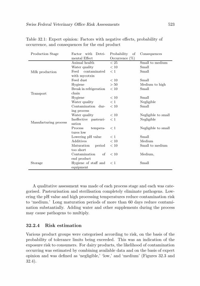
Swiss Federal Veterinary Office Risk Assessments 523
Table 32.1: Expert opinion: Factors with negative effects, probability ofoccurrence, and consequences for the end product
Production Stage Factor with Detri-mental Effect
Probability ofOccurrence (%)
Consequences
Milk production
Animal health < 25 Small to mediumWater quality < 10 SmallFeed contaminatedwith mycotxin
< 1 Small
Feed dust < 10 SmallHygiene > 50 Medium to high
Transport
Break in refrigerationchain
< 10 Small
Hygiene < 10 SmallWater quality < 1 Negligible
Manufacturing process
Contamination dur-ing process
< 10 Small
Water quality < 10 Negligible to smallIneffective pasteuri-sation
< 1 Negligible
Process tempera-tures low
< 1 Negligible to small
Lowering pH value < 1 SmallAdditives < 10 MediumMaturation periodtoo short
< 10 Small to medium
Contamination ofend product
< 10 Medium,
Storage Hygiene of staff andequipment
< 1 Small
A qualitative assessment was made of each process stage and each was cate-gorised. Pasteurisation and sterilisation completely eliminate pathogens. Low-ering the pH value and high processing temperatures reduce contamination riskto ‘medium.’ Long maturation periods of more than 60 days reduce contami-nation substantially. Adding water and other supplements during the processmay cause pathogens to multiply.
32.2.4 Risk estimation
Various product groups were categorised according to risk, on the basis of theprobability of tolerance limits being exceeded. This was an indication of theexposure risk to consumers. For dairy products, the likelihood of contaminationoccurring was estimated by combining available data and on the basis of expertopinion and was defined as ‘negligible,’ ‘low,’ and ‘medium’ (Figures 32.3 and32.4).
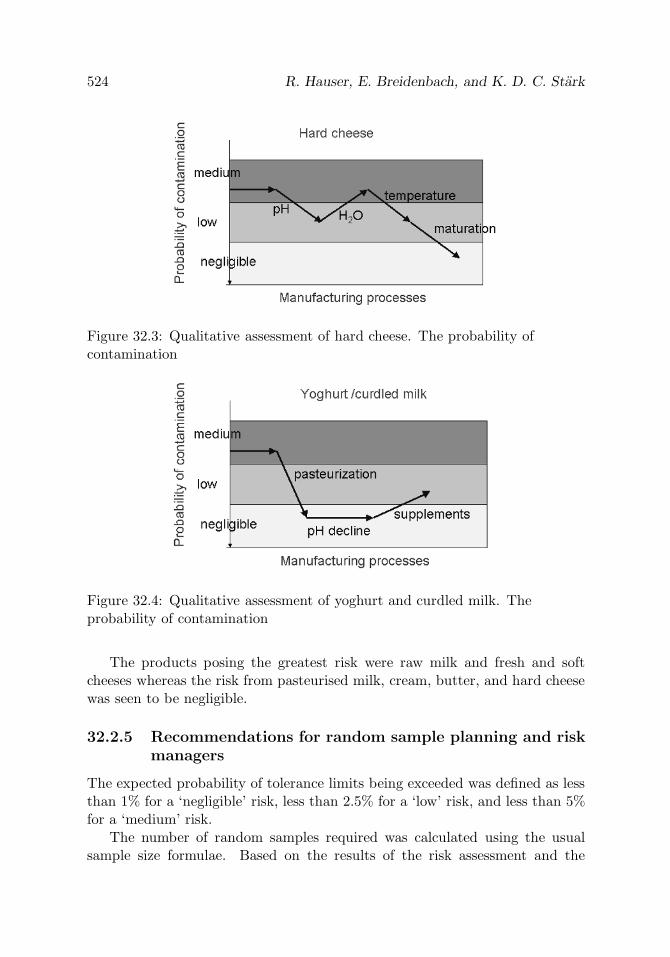
524 R. Hauser, E. Breidenbach, and K. D. C. Stark
Figure 32.3: Qualitative assessment of hard cheese. The probability ofcontamination
Figure 32.4: Qualitative assessment of yoghurt and curdled milk. Theprobability of contamination
The products posing the greatest risk were raw milk and fresh and softcheeses whereas the risk from pasteurised milk, cream, butter, and hard cheesewas seen to be negligible.
32.2.5 Recommendations for random sample planning and riskmanagers
The expected probability of tolerance limits being exceeded was defined as lessthan 1% for a ‘negligible’ risk, less than 2.5% for a ‘low’ risk, and less than 5%for a ‘medium’ risk.
The number of random samples required was calculated using the usualsample size formulae. Based on the results of the risk assessment and the

Swiss Federal Veterinary Office Risk Assessments 525
experience of the authorities, the first risk-based monitoring of end productswas introduced throughout Switzerland in the autumn of 2002.
Table 32.2: Probability of contamination above threshold limits
Risk Category Probability ofContaminationover ThresholdLimits (%)
Milk Product
Negligible < 1 Pasteurized milk,cream, butter,hard cheese
Low < 2.5 Yogurt, dessert,semi-hard cheese
Medium < 5 Fresh cheese, creamycheese, raw milk
32.3 Advantages and Disadvantages of Qualitative
Risk Assessment
Establishing a risk profile and characterising the hazards in the initial phase ofa risk analysis is a qualitative process. A risk network is indispensable to boththe qualitative and quantitative methods. Often, while the network is beingestablished, it is seen that the required data are unavailable or data qualityis insufficient. Qualitative evaluation of expert opinion is much easier thanquantitative evaluation.
Drawing up a qualitative risk assessment to determine whether there is infact a risk is the first requirement before proceeding with a quantitative risk as-sessment. If data of sufficiently high quality are available, models can be createdand all risk paths can be quantitatively assessed. In practice, risk assessmentsare comprehensive projects that can keep whole institutes and organisations oc-cupied for years. The qualitative assessment of health hazards in milk and dairyproducts described in this chapter was completed in less than seven months.
In qualitative risk assessments, the risk can be described in terms such as‘negligible,’ ‘low,’ ‘medium,’ and ‘high.’ However, assigning risks to qualitativecategories is done subjectively and there is no standardised method. The tran-sition between ‘negligible’ and ‘non-negligible’ is defined subjectively by riskmanagers. International standards could be reached by a broad discussion of

526 R. Hauser, E. Breidenbach, and K. D. C. Stark
terminology leading to more meaningful risk assessments and improved accep-tance of the method.
Usually the information provided by qualitative assessments is adequate forrisk managers for decision making. In most cases, management measures aregeneral in nature and concern import requirements, monitoring and controlregulations, or require ‘yes’ or ‘no’ decisions. Often, measures will either beimplemented or not, irrespective of the fine shades of risk.
Risk communication between risk managers and stakeholder groups is sim-plified when the results of a qualitative assessment are available. No specialmathematical knowledge is needed to determine the risk paths and to evaluatethe data. Complex quantitative models such as dose–effect relationships, sim-ulations, and the like, are usually hard to understand and may be difficult tocommunicate. They may be perceived as ‘black-box’ approaches.
32.4 Statistics’ Part in Qualitative Risk Assessment
Qualitative risk assessments make use of descriptive statistical evaluations.Probability calculus is used to estimate prevalent risks, their development andthe effect of risk reduction measures. It is difficult, if not impossible, to comparerisk assessments made in different countries or by different analysts because cat-egorisations are subjective. Statistical methods could help standardise assess-ments and make comparison possible. Statistics’ role is to provide high-qualitydata resulting in more accurate risk assessments. Inaccuracies are possible in allassessments because of data gaps and variability. High-quality data compensatefor lack of knowledge and increase the accuracy of assessments. Well-plannedand evaluated studies are needed to obtain such data. Corresponding data fromdifferent studies may be combined by means of a meta-analysis.
References
1. Anonymous (2001). Definitions of risk analysis terms related to foodsafety, In Codex Alimentarius Commission Procedural Manual, 12th edi-tion, pp. 43–44, Joint FAO/WHO food standards programme, Food andAgriculture Organization of the United Nations/World Health Organiza-tion, Rome.
2. Anonymous (2003). Import risk analysis, In Office International des Epi-zooties. Terrestrial Animal Health Code, Section 1.3, Paris, France.

33
Qualitative Risk Analysis in Animal Health: A
Methodological Example
Barbara Dufour and Francois Moutou
Ecole nationale veterinaire d’Alfort, Maisons-Alfort, FranceAFSSA Lerpaz, Maisons-Alfort, France
Abstract: Risk analysis can be performed following either a quantitative ora qualitative approach. Both methodologies are linked to the same theoreticalrules. Once the potential hazard has been identified, the qualitative risk assess-ment is carried out by combining the probabilities of occurrences of the events(emission and exposition) in the presence of a hazard, and its consequences.The probability of an event can be evaluated by combining the probabilities ofthe different parameters.
Within the frame of global expertise, the necessity of realizing collegial riskevaluations, sometimes when only few data are available and within a shortamount of time, leads us to work on a standardised method for a qualitativeapproach.
The process of global qualitative risk appreciation is completed by addingsupport to the rationalisation of the estimation step. It has been proposed thateach parameter be evaluated with the help of all available information and thatan evaluation of the probability of occurrence of each of these can be realizedindividually to yield a given level of probability (null, negligible, low, moderate,high) or an interval between two levels (for example: ‘negligible to low’).
The combination of probabilities and of intervals was carried out using atable that was tested and evaluated through the following risk assessment: qual-itative risk evaluations of the transmission of Q fever to humans in France.
Both the advantages and the limitation of this approach are also presented.
Keywords and phrases: Risk analysis, qualitative methodology, Q fever
527

528 B. Dufour and F. Moutou
33.1 Introduction
Risk analysis has undergone rapid development in the whole field of food safetyand within a few years become a priority for scientists and decision makers whosee in this new tool a way to improve the rationale of their decisions, particularlyin animal health expertise.
It is now recognised that risk estimation can be performed following eitherquantitative or qualitative methodology. Quantitative risk analysis must be fu-eled by data that are not always available, either easily or rapidly. At the sametime, risk analysis needs to be organised around more or less complex models inorder to estimate the variables’ distributions and occurrence probabilities [Sut-moller and Wrathall (1997) and Gale et al. (1998)]. The field of quantitativerisk analysis is indeed a rich research domain for scientists. On the other hand,few publications have presented investigations using the qualitative approach,although this may be seen as easier to perform in the absence of some of thebasic data. The qualitative approach is nevertheless used by managers [Pharo(2002)] and by expert working groups [Anonymous (2002, 2003, 2004)], espe-cially when time is lacking for a full quantitative analysis or when crude data aremissing.
It thus seemed that a methodological approach to quantitative risk analysiscould be of some interest. This chapter presents the method used within thecollegial scientific expertise of the French food safety agency (AFSSA, Agencefrancaise de securite sanitaire des aliments), following and adapting the workof Zepeda-Sein (1998).
33.2 Global Presentation of the Method
The method to appreciate a risk, as proposed by the Animal World HealthOrganisation (OIE, Paris), consists of the following five steps [Ahl et al. (1993)and OIE (2001)]: (i) hazard identification; (ii) appreciation of the emission (theprobability of emission from the source); (iii) appreciation of the exposition (theprobability of exposition to the hazard); (iv) appreciation of the consequences(occurrence and severity combined); and (v) estimation of the risk (the combi-nation of the probabilities of occurrence of the emission and of the expositionwith its consequences).
Each of the parameters, like emission, exposition, and consequences, maythemselves be complex and can be subdivided into simpler elements, each ofwhich contributes to their global occurrence.

Qualitative Risk Analysis in Animal Health 529
As an example to illustrate this, the meanings of these parameters in thefield of animal health are presented as follows. The parameter ‘emission’ islinked to and depends on the sources of virulent materials, the cycle of excre-tion by the infected animals, as well as the prevalence of the disease in thespecies of concern. The parameter ‘exposition’ depends on the characteristicsof the exposed populations (density, distribution, sensitivity, etc.) and on thedifferent possible routes of contamination (airborne, foodborne, etc.). The pa-rameter ‘consequences’ takes into account the sanitary (severity of the disease,morbidity, and lethality rates) and economical costs of the possible outbreak(loss of production, loss of markets, direct slaughtering and destruction of ani-mals) aspects.
For each parameter, the list of all the elements to be taken into account iscompleted, following the timing and the chronology of the more pertinent eventtree, specifically built for the item of concern. Each of these elements is firstdescribed; then the available information and data are collected and analysedthrough the process, to result in an estimation value.
The parameters can be characterized following three modalities: (i) by avalue: this kind of quantitative analysis is said to be ‘punctual’ or ‘determin-istic;’ (ii) by a law of probability : this kind of quantitative analysis is said tobe ‘probabilistic’ or ‘stochastic;’ (iii) by a qualitative appreciation for which aquantification process will not be used, but instead the level of each parameterwill be assessed using descriptive scales or qualifications
Risk can then be evaluated by combining probabilities of each parameterfollowing the rules presented in Figure 33.1. In the case of a quantitative riskappreciation, the laws of probabilities show how to combine the probabilitiesof each parameter. This chapter proposes a rationalized approach to deal withqualitative risk appreciation (Figure 33.2).
Figure 33.1: The components of risk estimation

530 B. Dufour and F. Moutou
Figure 33.2: Presentation of the global chart of the analysis. [From OIE (2001).]
33.3 Qualitative Appreciation of the Probability
of Each Event
The global process of qualitative risk appreciation was completed with the helpof the estimation rationalisation adapted from the work of Zepeda-Sein (1998).This author proposes that each of the parameters (emission, exposition, andconsequences) can be analysed by using all the available information and thatan evaluation of the occurrence probability of each of them can be realisedseparately to obtain a certain level of probability [five qualifications are thenfixed to qualify the occurrence probability of each parameter: null (Nu: theoccurrence of the event is not possible); negligible (N: the occurrence of the eventcould only be possible under exceptional circumstances); low (L: the occurrenceof the event is not very high, but is possible under some circumstance); moderate(M: the occurrence of the event is clearly possible); or high (H: the occurrenceof the event is high)] or within a given interval (for instance: between negligibleto low).
After each event has been evaluated separately from the others following aqualitative process, the final qualitative appreciation of each parameter is madeglobally, by combining its event qualifications. The process must be strongly

Qualitative Risk Analysis in Animal Health 531
argued and some specific weight can be given to specific events, following thecharacteristics of each disease. For instance, for the exposition parameter, theevent ‘contamination route’ may or may not be a determinant compared to‘populations of concern,’ and its qualification will depend on this.
33.4 Qualitative Risk Appreciation
The combination of the probabilities of two given parameters, as proposed byZepeda-Sein (1998) has been adapted by Dufour et al. (2003) and then used bydifferent working groups organised within the context of the expert specialisedgroups of the French food safety agency (AFSSA). The method was developed,then tested on different subjects [Anonymous (2003) and Anonymous (2004)],and underwent different adjustments before being validated through an expertconsensus of the Animal Health Committee of the French food safety agency in2004.
For example, the working group on bat rabies and the risk of its transmissionplayed a major role in the realisation and adaptation of this method. Here, theuse of the qualitative approach allowed the expert group to characterise therisk of transmission of bat rabies to human beings in France when data onthe prevalence of rabies within bat colonies was lacking, making impossibleany quantitative analysis [Anonymous (2003)]. However, at the end of thisqualitative analysis, the combination table rules were judged to be too severe,quite probably leading to an overestimation of the risk.
Therefore, new adaptations were introduced to take into account the im-precision of some data, the real subjectivity of the evaluation of the differentprobabilities which are used, and mainly the fact that the combination of twoprobabilities should result in a lower probability than each of the two originalprobabilities (as when following this quantitative example: 10−4×10−4 = 10−8),which had not been the case in the bat rabies document.
To take this last point into account, the qualification combination rulesadopted are as follows.
• Two probabilities with the same qualification combined together give thequalification just below (low × low = negligible),
• Two adjacent probabilities give the lower interval of the lower originalprobability (low × moderate = negligible to low),
• Two probabilities neither adjacent nor opposed give the lower probability(low × high = low),

532 B. Dufour and F. Moutou
• Two opposite probabilities give the higher interval of the lowest probabil-ity (negligible × high = negligible to low),
• The combination of probabilities can also be performed by combining oneor two interval(s). Table 33.1 shows all these possible combinations.
Using this method, the combination of two ‘negligible’ qualifications shouldlogically lead to ‘null.’ However, AFSSA experts estimated that this qualifica-tion should be reserved to describe an impossible event, so they decided to useinstead the ‘null to negligible’ interval for all the lowest probability situations.
The combination of these different probabilities for each parameter leadsto the probability of occurrence of a hazard, which is therefore also presentedusing the same five qualifications as seen before (null, negligible, low, moderate,or high) or with the intermediate intervals.
The following remarks are to be taken into account: (i) Table 33.1 givesresults that are close to results which could have been obtained through aquantitative analysis, if quantitative data had been available. The multiplica-tion of two probabilities gives a probability lower than each of the two originalprobabilities; (ii) Table 33.1 gives relative information as opposed to absoluteinformation between the different rows and columns; (iii) the combination ofmore than two parameters leads to the question of the ordering of the combi-nation. With three parameters, N, M, and H for instance (N × H) × M givesN to L, whereas N × (H × M) yields N. To overcome this difficulty, it is heresuggested to return to the event tree and to combine the parameters in thesame order every time.
33.5 Qualitative Appreciation Examples
This qualitative approach, after being developed within different workinggroups, has recently been used by the specialised experts committee on AnimalHealth of the French food safety agency for an evaluation of Q fever transmis-sion from ruminants to man in France [Anonymous (2004)].
The prevalence of Q fever in domestic ruminants in France is not known.Various surveys, with protocols that are both quite different and difficult tocompare, suggested a global serological prevalence somewhere between 5% and85%, which is not useful in a quantitative evaluation.
Three populations were defined with respect to their degree of risk exposi-tion: people living closely to possibly infected animals, the ‘rural’ populationthat could be exposed to airborne contamination, and the global, usually urban,population.

Qualitative Risk Analysis in Animal Health 533
Tab
le33
.1:
Res
ults
ofth
eco
mbi
nation
ofth
edi
ffere
ntqu
alitat
ive
appr
ecia
tion
sus
edin
the
qual
itat
ive
risk
anal
ysis
(Nu
=N
ull,
N=
Neg
ligib
le,L
=Low
,M
=M
oder
ate,
and
H=
Hig
h)
Nu
Nu
toN
NN
toL
LL
toM
MM
toH
HN
uN
uN
uN
uN
uN
uN
uN
uN
uN
uN
uto
NN
uN
uto
NN
uto
NN
uto
NN
uto
NN
uto
NN
NN
NN
uN
uto
NN
uto
NN
uto
NN
uto
NN
NN
Nto
LN
toL
Nu
Nu
toN
Nu
toN
Nu
toN
NN
NN
toL
LL
Nu
Nu
toN
Nu
toN
NN
NN
toL
LL
Lto
MN
uN
uto
NN
NN
Nto
LL
LL
MN
uN
NN
Nto
LL
LL
Lto
MM
toH
Nu
NN
Nto
LL
LL
Lto
MM
HN
uN
Nto
LL
LL
Lto
MM
M

534 B. Dufour and F. Moutou
The qualitative method used by the working group led to the followingpoints: (i) the risk for the global population, that is, without any known extrarisk factor (no pregnancy, valvulopathy, nor immunodepression) could be qual-ified as very low (‘null to negligible’); (ii) globally, the level of risk was higherfor populations with extra risk factors, which means that a specific therapyand/or treatment will be of great importance in these subpopulations. Indeed,the global risk is lowered from ‘negligible to low’ to ‘null to negligible’ after atherapeutic risk reduction for these subpopulations; (iii) the risk linked to theconsumption of contaminated foodstuffs (such as raw milk or milk productsfrom raw milk) was, as a whole, ‘null to negligible’ except for the populationswith extra risk factors, in which it was ‘negligible;’ (iv) exposure through theairborne route or through close contacts with contaminated animals were thehighest risks, so the persons in close contact with infected animals or ‘rural per-sons’ were the ones facing the greatest risk; (v) Table 33.2 presents the details ofone of the tables obtained in the case of contamination through direct contactswith domestic ruminants issued from the AFSSA report [Anonymous (2004)].Recommendations could then be established following this risk assessment.
33.6 Discussion
The qualitative approach presented here was built to answer the needs of ex-pert committees of the French food safety agency, who have the obligation toevaluate, within short delays, risks linked to animal health in order to provideadvice to risk managers, in this case the Central Veterinary Office (Directiongenerale de l’alimentation) of the ministry in charge of agriculture. With thisbackground, two items are of specific concern: the method had to be simple,understandable, and easily accessible, both to the experts and to the man-agers; and it should not overevaluate the risk too much. For the first point,Zepeda-Sein methodology was preferred to semi-quantitative approaches, whoseappropriation and understanding by users are more delicate. To prevent anyover-estimation of the risk, the combination tables were redrawn from the ex-perience gained in the bat rabies working group [Anonymous (2003)].
The experience of the different AFSSA working groups that have used themethod show that the qualitative approach is simpler than the quantitativeone and thus open to a wider audience. The experts of these different workinggroups had no difficulties familiarizing themselves with the method. Anothermajor advantage is to be much less time consuming, and it thus represents areal possibility when there is little time to answer and when the decision behindthe assessment is urgent.
This process requires a detailed and organised study of all the parametersthat must be taken into account in the decision, including those for which the

Qualitative Risk Analysis in Animal Health 535
Tab
le33
.2:
Glo
bal
and
redu
ced
risk
appr
ecia
tion
follo
win
gth
eco
ntam
inat
ion
rout
eby
Cox
iella
burn
etii
from
smal
ldo
mes
tic
rum
inan
ts[A
nony
mou
s(2
004)
]
Pro
bab
ility
ofin
fect
ion
occ
urr
ence
Clo
seC
onta
ctPop
u-
lati
on(M
odera
te)
a
Rura
lPop
ula
tion
(Modera
te)
aG
lobal
Pop
ula
tion
(Low)
a
With
extr
ari
sks*
Witho
utex
tra
risk
With
extr
ari
sks
Witho
utex
tra
risk
With
extr
ari
sks
Witho
utex
tra
risk
Con
sequen
ces
Glo
bal
(Hig
h)b
Mod
erat
eto
high
(Neg
ligib
leto
low)b
Low
(Hig
h)b
Mod
erat
eto
high
(Low
)b
Low
tom
oder
ate
(Hig
h)b
Mod
erat
e(L
ow)b
Low
Red
uced
(Low
tom
oder
ate)
b
Mod
erat
e
(Nul
lto
negl
igib
le)b
Low
(Low
tom
oder
ate)
b
Mod
erat
e
(Nul
lto
negl
igib
le)b
Low
(Low
tom
oder
ate)
b
Low
(Nul
lto
negl
igib
le)b
Neg
ligib
le
*A
reco
nsid
ered
asex
tra
risk
s:pr
egna
ncy,
valv
ulop
athi
es,an
dim
mun
odep
ress
ion
Qua
lifica
tion
sbe
twee
nbr
acke
tsar
efo
rth
eco
rres
pond
ing
row
and
colu
mn
estim
atio
ns

536 B. Dufour and F. Moutou
lack of available data does not allow quantitative analysis to be carried out.This is why the construction of an event tree is so important.
Moreover, the approach points to the data used to obtain the estimation:the whole method is built on the quality of the information used and on thequality of the arguments followed to qualify the parameters. It is then quiteeasy to judge the pertinence of the analysis and to discuss its results followingthe quality of the data used to fuel the process. This is quite helpful to preventspending too much time discussing software, algorithms or distribution laws inthe case of quantitative or even semi-quantitative approaches. These discussionsmay lead one to forget that the real questions are at the data level, not in thecomputation.
However, the weakness of the qualitative process lies in the important partof subjectivity that is present in it. The attribution of the retained levels ofprobability (null, negligible, low, moderate, high probabilities) can be seen asarbitrary and thus questionable. A way to decrease the arbitrary part of anindividual estimation is to make this process a collective one, by using an expertgroup to discuss its different steps. In this case, it is important that the expertshave a good apprehension of the different proposed probability levels.
It is also necessary to make the process as transparent as possible; for ex-ample, the documentation on which the argumentation is built and which leadsto each of the qualifications used must be presented in detail.
The quantitative method seems, at a first glance, more rigorous and lessarbitrary. It also presents the advantage of permitting a sensitivity analysisof the estimation, compared to the incertitude of the hypothesis. However,this process can be very long and is only possible in a very few situations,as it requires much quantitative information quite often difficult to obtain.When major data are lacking, the evaluators will use hypotheses, which, evenif presented with figures, are also arbitrary.
Acknowledgements. The authors are pleased to acknowledge all the col-leagues that contributed their participation to the ‘bat rabies’ and ‘Q fever’working groups of the animal health committee of AFSSA. Jayne Ireland iswarmly thanked for improving our English. The authors also thank Anne-MarieHattenberger as well as the two referees who helped improve a first version ofthe manuscript.
References
1. Ahl, A. S., Acree, J. A., Gipson, P. S., Mc Dowell, R. M., Miller, L., andMcElvaine M. D. (1993). Standardisation of nomenclature for animal

Qualitative Risk Analysis in Animal Health 537
health risk analysis, Revue scientifique et technique (International Officeof Epizootics), 12, 1045–1053.
2. Anonymous (2002). Rapport sur le botulisme d’origine aviaire et bovine,Rapport realise par un groupe de travail du Comite d’experts specialisesante animale de l’Agence francaise de securite sanitaire des aliments, 82p.
3. Anonymous (2003). Rapport sur la rage des Chiropteres en Francemetropolitaine, realise par un groupe de travail du Comite d’expertspecialise “sante animale” de l’Agence francaise de securite sanitaire desaliments, AFSSA, Maisons-Alfort.
4. Anonymous (2004). Rapport sur l’evaluation des risques pour la santepublique et des outils de gestion des risques en elevage des ruminants,realise par un groupe de travail du Comite d’expert specialise “ santeanimale ” de l’Agence francaise de securite sanitaire des aliments, AFSSA,Maisons-Alfort.
5. Dufour, B., Moutou, F., and Hattenberger A. M. (2003). Qualitative andcollegial risk analysis method: An example: Bats rabies transmission toman in France, In Proceedings of ISVEE 10th (Ed., S. Urcelay), pp. 1–4,ISVEE, Vina del Mar, Chile, November 16–21, 2004.
6. Gale, P., Young, C., Stanfield, G., and Oakes, D. (1998). Development ofa risk assessment for BSE in the aquatic environment, Journal of AppliedMicrobiology, 84, 467–477.
7. Office international des epizooties (2001). Code zoosanitaire interna-tional: mammiferes, oiseaux et abeilles, 10eme edition, OIE, Paris.
8. Pharo, H. J. (2002). Foot-and-mouth disease: An assessment of the risksfacing New Zealand, New Zealand Veterinary Journal, 50, 46–55.
9. Sutmoller, P., and Wrathall, A. E. (1997). A quantitative assessmentof the risk of transmission of foot-and-mouth disease, bluetongue andvesicular stomatis by embryo transfer in cattle, Preventive VeterinaryMedicine, 32, 111–132.
10. Zepeda-Sein, C. (1998). Methodes d’evaluation des risques zoosanitaireslors des echanges internationaux, In Seminaire sur la securite zoosani-taire des echanges dans les Caraıbes, 9-11 decembre 1997, Port of Spain,(Trinidad and Tobago), pp. 2–17, OIE, Paris.

Index
Accelerated life 127Adaptive designs 401Adverse drug reaction reporting
systems 75AIDS clinical trial 289AIDS incubation time 225Air pollution 467Ambient temperature 437
Bayesian credible interval 349Bayesian hierarchical spatial model 451Binomial distribution 349Biosurveillance 437Breast cancer 151
Cancer 335Cancer registry 451Classification on very large
databases 263Clayton model 335Clinical evaluations 323Clinical trials 109, 335, 361Clustering 263, 289Combined response to treatment 387Complete convergence 211Computer simulation 75Conditional autoregressive model 451Confidence interval 349Conjoint model 127Contingency table 491Correlated frailty model 151Cross-validation 275
δ-Method 437Data mining 75Data monitoring 61Data reduction 263Degradation process 127Disease progression studies 225Distance model 451
Efficacy 335Empirical processes 195
Failure time 127Frailty model 179Functional estimation 195Fuzzy system 75
GAM model 467Generalized linear models 95Genomic sequences 491Geometric distribution 349Gibbs sampler 289Group sequential plans 61
Hierarchy of experts 239HIV dynamics 289Hormesis 179Hypothesis testing 419
Incidence 451Independence 491Individual patient data 3, 39Isotonic regression estimators 361Item response theory 109
Kappa coefficient 139Kernel estimation 195
Latent regression 95Laws of large numbers 195Lifetime distributions 195Longevity 127, 179Longitudinal data 167, 289Lung cancer 451
Maximum likelihood estimator 361Maximum tolerated dose 361Measure of agreement 139Measurement error 95Medical diagnosis 275
539

540 Index
Meta-analysis 3, 39Milk contamination 519Mixed models 109Model building 19Modelling 75Monte Carlo simulations 361Multicentre clinical trial 387Multilevel Gibbs sampling method 305Multivariate survival analysis 151MVUE 127
Neural networks 275Nonlinear mixed-effects 289Nonparametric estimation 195Nonparametrics 335Nuisance parameter 127Numbers of infectious and
noninfectious HIV 305
Observation model 305Optimization 387Ordinal data 139
Partial credit model 109Path model 127Patient safety 323Phase II/III trials 401Pilot study 349Pointwise estimation of variance 225Prediction trees 239Predictive marker 39Predictive process 167Probabilistic nodes 239Productively infected CD4(+) T cells 305Prognosis 39Prognostic factors 167Prognostic markers 3, 19Progressive censoring 61P-splines 451
Q fever 539Qualitative methodology 539Qualitative risk assessment 519Quality of life 109, 127
Random change points 289Random effects 95
Random enrolment 387Rasch models 95Recruitment time 387Regression 19Regression estimation 195Reliability 127Right-censored survival data 211Risk analysis 539Risk-based monitoring 519Robustness 361
Safety 61Salmonella infection 437Seasonality 437Select and test designs 401Semiparametric additive hazard
model 211Semiparametric models 467Sentinel events 61Sequential adaptive designs 361Sequential analysis 419Sequential clinical trials 401Sequential estimation 211Sequential tests 109Shared frailty model 151Soft failure 127Statistical test 491Stochastic equation 305Survival analysis 127, 167, 179Survival function 225Systematic review 3, 39
Time to event analyses 61Toxicity 335Traumatic failure 127Treatment selection 401Trees 19Tuberculosis 275Twins 151
Unbiased estimator 127
Validation 19Validation studies 75
Weak laws 195