Inferring Latent Brand Dependencies

72Journal of Marketing ResearchVol. XXXVII (February 2000), 72–87

*Ulf Böckenholt is Professor of Psychology, University of Illinois,Urbana-Champaign (e-mail: [email protected]). William R. Dillon isHerman W. Lay Professor of Marketing and Professor of Statistics, CoxSchool of Business, Southern Methodist University (e-mail: [email protected]). This research was supported by a grant from the NationalScience Foundation (SR-9730197). The authors thank Soumen Mukherjeefor assisting with the simulation experiments. To interact with colleagueson specific articles in this issue, see “Feedback” on the JMR Web site atwww.ama.org/pubs/jmr.

ULF BÖCKENHOLT and WILLIAM R. DILLON*

In this article, the authors develop a class of models to reconstructbrand-transition probabilities when individual brand purchase sequenceinformation is not available. The authors introduce two general modelforms by assuming different underlying mechanisms for individual het-erogeneity in brand switching. The first model form captures individualheterogeneity by a latent class structure. The second model form cap-tures individual heterogeneity by postulating that the brand-choice prob-abilities follow a Dirichlet distribution, which yields the popular Dirichletmultinomial formulation. Monte Carlo simulations are performed with aview toward assessing whether individual transition probabilities can becaptured from knowledge of only aggregated brand choices. Results indi-cate that the proposed method can indeed capture individual brand-tran-sition probabilities under several different conditions. An empirical appli-cation illustrates how these models can be used to provide importantinformation on individual brand transitions and the role of marketing-

related covariates.

Inferring Latent Brand Dependencies

Stochastic models of choice date back to the late 1950sand Luce’s (1959) choice axiom, which set into motion abody of brand choice models strongly influenced by the pi-oneering work of Bass (1969, 1974) and Ehrenberg (1972).The development of models to estimate the sources of brandmarket-share gains and losses, including retention and can-nibalization, continues to be of interest to marketing man-agers and scientists alike (see, e.g., Böckenholt and Dillon1997; Dillon and Gupta 1996). And the need to understandmarket-share changes, the whys and hows, has led to thewidespread use of stochastic brand-choice models for de-scribing the purchase behavior of individual consumers overtime. Beginning with models that assumed no state depend-ency in observed choices and only choice heterogeneity,various functional forms have been developed to account forthe influence of prior purchases on current-period choice de-cisions. Models that relax the assumption of zero-orderchoice behavior and recognize the potential of state depend-ency and heterogeneity have recently appeared (Erdem1996). Keane (1997), for example, finds evidence for truestate dependency in the choice process, even after control-

ling for a rich heterogeneity structure (see also Allenby andLenk 1994).

Although models that can investigate the extent to whichstate dependence or heterogeneity or both affect brandchoices are now available, the calibration of such models re-quires that information is available on individual brand pur-chases over time, and it is for this reason that panel scannerdata has proved so useful. However, much of the data rele-vant to understanding market-share changes available tomarketing managers come in aggregated form, which repre-sents the sum or aggregation of all brand purchases of indi-viduals, and as such give only a brand’s incidence or volumeshare at particular points in time. Store scanner data, for ex-ample, give store sales, which are the aggregation of allhouseholds’ brand choices within specific stores, duringspecific weeks. Although direct information on individualtransitions is lost in the aggregation process, in this articlewe show that it is possible to recover this information fromthe dependencies between the marginal distributions of theaggregated data.

Dependencies in aggregated brand-choice or market-share data can arise in several different ways depending onthe nature of the sampling and the study design. For exam-ple, brand dependencies over time may arise when the samegroup of individuals is observed in each time period. In thiscase, we would assume that the brand choices of each indi-vidual are correlated across time as a result of similarity,substitution, or variety-seeking effects, and such dependen-cies would be present even after aggregation. This type ofobservation is also likely to arise in cross-sectional studiesin which survey respondents are asked to provide informa-

Latent Brand Dependencies 73

1We discuss this problem setting further in our closing remarks.

tion retrospectively on which brands they purchased, say, ontheir last shopping trip and the quantity purchased of eachbrand; then, after some intervention—for example, a newproduct or concept introduction—respondents are asked toprovide the same information but this time for their nextshopping trip. Brand dependencies between aggregatedmarginal distributions can arise even when different groupsof individuals are observed over time, provided these indi-viduals are exchangeable in the sense that they follow thesame brand-choice process over time (see, e.g., Hawkes[1969], who considers the problem of estimating electoralswings on the basis of aggregate voting data). Frequently,store or market-sales data are consistent with this type ofdata structure.1

Contribution

The problem of inferring transition probabilities from ag-gregate data has a long tradition in marketing, starting withwork by Telser (1963) and Massy, Montgomery, andMorrison (1970), and has been of interest in other fields aswell, especially political science, sociology (see King1997), and econometrics (see Lee, Judge, and Zellner 1970).We contribute to this line of research in several ways. First,we develop an easily implemented full-information maxi-mum-likelihood (FIML) approach for estimating latentbrand dependencies when information on the exact se-quence of brand choices at the individual level is not avail-able. Second, the FIML approach can in principle accom-modate brand dependencies generated in either of the twoways described previously and as such can be used with sur-vey data or store scanner data. Third, the proposed approachexplicitly accounts for individual preference differences un-der different modeling assumptions. In particular, ourframework allows for the possibility that some segmentsmay exhibit brand dependencies whereas others may exhibitindependence in their brand choices. Fourth, the proposedapproach facilitates testing probabilistic choice models thatassume brand choices to be independent across time periods.

Organization

The article is organized as follows. We begin with a for-mal description of the latent brand-choice dependency prob-lem. There we develop the necessary notation and provide aframework for the proposed approach. Next, an individual-level representation is introduced. Individual differences aremodeled with mixture distributions. Two general modelforms are discussed. How to incorporate brand- and person-specific covariates, as well as the use of the model to predictconditional share losses and gains, is discussed in this sec-tion. The following section describes Monte Carlo simula-tions designed to investigate the ability of the proposed ap-proach to recover known (i.e., population) brand-switchingprobabilities generated under a variety of conditions.Simulation results are then presented and discussed. Thepenultimate section focuses on data collected in a producttesting study and demonstrates how the proposed approachcan provide important information on the character of brandswitching and the role of marketing-related covariates whenexact brand purchase sequences are not available. We close 2This requirement is typically satisfied in (quasi) experimental settings.

However, the proposed approach must be modified when data are collectedin observational studies, because in this case the number of trials (e.g., pur-chase incidences) may vary from one time period to the next. This issuewill be developed further in our closing remarks.

with a discussion of how the proposed approach can in prin-ciple be extended to other application settings.

MODELING LATENT BRAND SWITCHING

The Inference Problem

Let r(i)j,t – 1 denote the observed number of choices of brand

j (j = 1, …, a) at time point t – 1. The superscript i (i = 1, …,n) refers to the unit of analysis, which in our case is eitheran individual who makes multiple choices at time point t – 1or a group of individuals/households in which each groupmember makes a single choice. The number of times brandk (k = 1, …, b) is selected at time point t is denoted by r(i)

k,t,and Σa

j = 1r(i)j,t – 1 = Σb

k = 1r(i)k,t = r(i). In the following develop-

ment, we assume that the number of choices is the sameacross the time periods but the number of choices can varyfor each unit.2 Although the information provided by eachunit i can be used straightforwardly to compute the changein the volume share for each brand, this information is, how-ever, less satisfactory if interest centers on estimating thesources of gains and losses for any of the brands, because noinformation is provided on the exact sequence of brandspurchased. One approach for answering this question is toassume that brand choices are independent. In this case,transition probabilities are equal to the marginal brand-choice probabilities at time point t. However, in most appli-cations, the independence assumption lacks plausibility,with the result that sources of gains and losses are misinter-preted. In the next section, we present a general approachthat facilitates an accurate representation of brand-switchingprobabilities without imposing a priori some presumedstructure on brand switching.

Model Development

To investigate dependencies between the frequency vec-tors r(i)

t – 1 = (r(i)l,t – 1, ..., r(i)

a,t – 1)′ and rt(i) = (r(i)

l,t, ..., r(i)b,t)′, we in-

troduce the binomial thinning operator ° (Cox and Isham1980; McKenzie 1988). Let r be a discrete random variabledefined on the nonnegative integers and hg be a sequence ofi.i.d. binary random variables independent of r, such thatPr(hg = 1) = 1 – Pr(hg = 0) = α, where α ∈ [0,1]. Then thebinomial thinning operation is defined as

where B(α;r) is a binomial random variable based on r trialsand probability of success α. By applying the binomial thin-ning operation to the frequency vector r(i)

t – 1 and suppressingthe superscript (i) for the moment, we can decompose the el-ements of rt – 1 into their contributions to rt by

where Σbk = 1 αjk = 1 for all j. Note that in our context αjk rep-

resents the transition probability from brand j to brand k.

( ) ( ; ),, ,2 1

1

αr B rk t jk j t

j

a

= −=∑

( ) ( ; ),11

α αo r h B rg

g

r

= ==

∑

74 JOURNAL OF MARKETING RESEARCH, FEBRUARY 2000

If the conditional distribution of rt – 1 given r is multino-mial with probability vector pt – 1 = (p1,t – 1, …, pa,t – 1)′, theconditional distribution of rt given r is also multinomialwith probability vector pt = (p1,t, …, pb,t)′. In the next sec-tion, we discuss the application of the binomial thinning ap-proach to determine the latent brand-switching patterns, firstfor the case of two brands (a = b = 2) and then for the gen-eral case in which a,b > 2.

The conditional distribution of brand choices. In thecase of two brands, the number of times each brand ischosen at time t can be represented in terms of the num-ber of times each brand was chosen at time t – 1 asfollows:

Because the conditional distribution of rkt(k = 1,2) given(r1,t – 1, r2,t – 1) is a convolution of two binomial distribu-tions, we obtain

Equation 4 has been studied by Wicksell (1916), Aitkin andGonith (1935), and Plackett (1977). We note that the condi-tional mean of Equation 4,

is linear in r1, t – 1. Clearly, rt and rt – 1 are independent if andonly if α1k = α2k.

For general a and b, the conditional distribution of rktgiven the observed values of rt – 1 is a convolution of a bi-nomial distributions:

When rt and rt – 1 are independent, α1k = … = αak = pk,t,and Equation 6 simplifies to the binomial distribution,where

It is instructive to derive the mean and covariance structureof Equation 6. The conditional expectation of rt given rt – 1is obtained as

where A is an (a × b) matrix of transition probabilities withelements αjk; that is, A1 = 1, and 1 is a unit vector. Similarly,the conditional variances and covariances are

r r A rt t t− −= ′1 18( ) ( | ) ,ε

( ) Pr( |,rk t7 rrt k t k t k tr

k tr rr

rr p pk t k t−

−= =

−1 1) Pr( ) ( ) ., , , ,, ,

( ) Pr( | )

( ) .

,,

... ,

,

rr

uk t tj t

jj

a

u u u r

jku

jkr u

a k t

j j t j

11

1

6

1

1 2

1

−−

=+ + + =

−

=

−

∏∑−α α

r

5( ) ( ,ε k tr || , ) ( ) ,, , ,r r r rt t k k k t1 1 2 1 2 1 2 1 1− − −= + −α α α

( ) Pr( |,4 rk t tr −−

− −

= − −

−

−

−−

− −

∑

1 1 2

2

2

1 1 2 1 1 2

1 2

1 1

1

1

1

1 1 2 1) ( ) ( )

( )

( ).

, ,

,, ,

α α

αα

α αα α

kr

kr

k

k

rt

u

t

kt

k k

k k

u

t t

k t ru

rr u

( )

( ) ( ) .

, , ,

, , ,

3

1 1

1 11 1 1 21 2 1

2 11 1 1 21 2 1

α α

α α

o o

o o

r r r

r r r

t t t

t t t

= +

= − + −

− −

− −

Model Forms: Accounting for Individual Differences withMixture Distributions

So far, we assumed that individual differences are notpresent in the choice data. Because this assumption is un-likely to be met in practice, we discuss two general ap-proaches to incorporating heterogeneity in brand-choicemodels. The first accounts for heterogeneity in consumerpurchase behavior by grouping consumers into homoge-neous segments. The second assumes that brand-choiceprobabilities are distributed across consumers according tothe Dirichlet distribution.

Latent class models. According to a latent class (LC) rep-resentation, individuals belong to different segments that areexhaustive and mutually exclusive. Each of the segments s(s = 1, …, S) is characterized by its set of brand-choice prob-abilities pt – 1|s at time point t – 1 and transition probabilitiesαjk|s (j = 1, …, a; k = 1, …, b). The relative size of segments is denoted by πs, (0 < πs ≤ 1 and Σsπs = 1). Latent classmodels have been used frequently in accounting for individ-ual heterogeneity in the context of market segmentation (seeWedel and Kamakura 1998).

On the basis of these specifications, the conditional dis-tribution of rk,t given the observed values of rt – 1 can bewritten as a finite mixture of summated binomial distribu-tions:

Equation 11 simplifies to a finite mixture of binomial distri-butions when rt and rt – 1 are conditionally independent givenclass membership s with α1k|s = … = αak|s = pk,t|s, that is,

To distinguish Equation 11 from Equation 12, we refer toEquation 11 as the LC conditional dependence (LC-CD)model and to Equation 12 as the LC conditional independ-ence (LC-CI) model.

Dirichlet multinomial models. The Dirichlet multinomial(DM) models specify that the individual choice probabilityvectors pt – 1 and pt are Dirichlet distributed with parametervectors θθt – 1 and θθt, respectively. Consequently, the pur-chase-frequency vectors rt – 1 and rt follow DM distribu-tions. Similarly, it is assumed that the transition-probabilityvectors ααj vary from person to person according to a Dirich-let distribution with parameter vector ζζj = (ζj1, …, ζjb)′ (j =1, …, a).

( ) Pr( | ) Pr( ), , ,12 1r r

rr pk t t k t k t s

s

r − = =

∑ π kk t s

rk t s

r rk t k tp, | , |, ,( ) .1 − −

( ) Pr( | )

( ) .

,,

...

|

|

,

,

11

1

11

11 2

1

rr

uk t t s

s

j t

jj

a

u u u r

jk su

jk sr u

a k t

j

j t j

r −−

=+ + + =

−

=

−

∑ ∏∑−

π α

α

rk t t jk

j

a

jk j t

k t k

r r

r r

and

c

−=

−= −∑1

1

19 1

10

( ) ( | ) ( )

( ) (

, ,

, *,

ν α α

tt t jk j k

j

a

j tr| ) .* ,r −=

−= −∑1

1

1α α


Setting �j = θj,t – 1 = Σbk = 1 �jk, we can write the conditional

distribution of rk,t given the observed values of rt – 1 as aconvolution of a beta-binomial distributions:

An independence version of Equation 13 is obtained byexpressing ζjk as a product of the marginal θj,t – 1 and θk,tparameters:

where θ = Σjθj,t – 1 = Σkθk,t. In the following, we refer toEquation 13 as the DM dependence (DM-D) model and toEquation 14 as the DM independence (DM-I) model.

Likelihood functions and covariates. Assuming randomsampling of n respondents, we specify the general likelihoodfunction for the LC and DM models as

If the choice frequencies at t – 1 and t are independent, thelikelihood function of the LC-CI model can be simplifiedbecause both Pr(r(i)

t – 1;r (i)) and Pr(r(i)t ;r (i)) follow finite-mix-

ture multinomial distributions:

where c(i) is a person-specific constant.The likelihood functions of the other models are more

complex because they involve convolutions of multinomialor DM distributions. For the computation of these convolu-tions, we consider r(i)

t – 1 and rt(i) marginal frequencies of an

(a × b) frequency table and determine the set of all possiblecell frequencies denoted by rjk

(il) (j =1, ..., a; k = 1, ..., b; l =1, ..., di) that satisfy both Σk rjk

(il) = r(i)j,t – 1 and Σj rjk

(il) = r(i)k,t. The

complete enumeration of the frequencies rjk(il) is accom-

plished through a modified version of Saunders’s (1984) al-gorithm. Then the likelihood function of the LC-CD modelcan be written as

Because the set of individual-level cell frequencies rjk(il) can

be obtained before the maximization of the likelihood func-tion, differences in computational time between the LC-CImodel and the LC-CD model are relatively minor.

The same approach is applied for the DM-D model. Inthis case, the likelihood function is

,( ) ( )

( ), | |( ) .

irj t

ijki

LC CDi

n

s

s

Si

d

j t sj

a

jk sr

k

b

L c p −−

= = =−

= =∏ ∑ ∑ ∏ ∏= 1

1 1 1

11 1

17 π αll

l

=−= =

−∏ ∑L c pLC CIi

i

n

s

s

S

j t srj( ) ( ), |π

1 1

116 ,,( )

,( )

, | ,ti

k ti

j

a

k t sr

k

b

p−

= =∏ ∏1

1 1

= ( ) ( )− −=

∏L r r r r rti i

ti

ti i

i

n

( ) Pr ; Pr | ; .( ) ( ) ( ) ( ) ( )1 1

1

15

= −jk

j t k t( ) ,, ,ςθ θ

θ114

k t tj t

jj

a

u u u r

j

jk j jk

jk j j jk j t

a k t

rr

u

u r

,,

...

,

,

( ) Pr( | )

( )

( ) ( )

( ) (

13 11

1

1

1 2

=

−+ − +

−−

=+ + + =

−

∏∑r

ΓΓ Γ

Γ Γςς ς ς

ς ς ς −−+ −

u

rj

j j t

)

( ).

,Γ ς 1

The likelihood function for the DM-I model is also given byEquation 18, and the additional constraint is provided byEquation 14.

Because it is straightforward to differentiate the log-like-lihood functions with respect to the model parameters, weomit the partial derivatives. However, it is worth noting thatthe multinomial probabilities are estimated by the weightedmean of the observed frequencies:

Similarly, under the LC models, we obtain

No analytical solution can be obtained for the class-specifictransition probabilities (αjk|s; j = 1, …, a; k = 1, …, b) or theDM parameters. For all four models, the parameters are es-timated by a quasi-Newton method that approximates theinverse Hessian according to the Broyden–Fletcher–Goldfarb–Shanno update (see Gill, Murray, and Wright1981). Computations were carried out in Gauss, Version 3(1995).

Covariates for LC models. When covariates are availableand respondent heterogeneity is captured by introducingLCs, different model specifications are possible, dependingon how the covariates are incorporated and which parame-ters are explicitly allowed to vary across LCs and brands.For example, covariates can be parameterized to allowbrand-specific effects, which may or may not vary acrossLCs, or the model may include only brand-specific con-stants (i.e., intercepts), which vary across LCs, and nobrand-specific effects of the covariates. For example, wecan parameterize the segment-specific choice probabilities,pj,t – 1|s, through a logistic link function as

where zj,t – 1|s is expressed as a linear function of the brands’covariate values at t – 1, xj,t – 1 = (x1j,t – 1, …, xpj,t – 1),

( ) ,, |( )

,( )22 1 0 1z j t s j

sj t

s− −= + ′δ x d

( )exp( )

exp( ),, |

, |

, |

21 11

1 1

pz

zj t sj t s

qa

q t s−

−

= −=

Σ

( ) ˆ ˆ20 sπ ppr

r

pr

r

jt sin

jti

in i

s

s j t s

s

in

k ti

in i

|

( )

( )

, |,

( )

( )ˆ ˆ .

=

=

=

=

−= −

=

∑

∑

ΣΣ

ΣΣ

1

1

11 1

1

π

( )

( )

,,

( )

( )

( ) ˆ

ˆ .

=

=

−= −

=

=

=

1

1

11 1

1

19 jtin

jti

in i

k tin

k ti

in i

pr

r

pr

r

ΣΣ

ΣΣ

(( ) DM Di

niL c−

=∏=

1

18 ll

l

l

)( )

( )

( )

( )

( ).

=

==

∑

∏∏

+

+

1

11

d

i

jki

jk

jkk

b

j

a

i

r

r

ΓΓ

Γ

Γ

θθ

ς

ς


3Note that the brand similarity structure underlying the transition proba-bility matrices can be investigated by use of tree-based models (Novak1993) or related techniques.

and δδ(s) = (δ1(s), ..., δp

(s))′. For identifiability reasons, Σjδ(s)0j

=0. Note that in this particular parameterization, we assumesegment-specific brand intercept and covariate effects.Additional details about estimating and incorporating co-variates into the model specification are provided in the con-text of the application that follows.

Logistic link functions are also used for relating the seg-ment-specific probabilities, πs, and transition probabilities,αjk|s, to the covariates. Typically, covariates for the class-specific probabilities are demographic variables (see Daytonand Macready 1988; Dillon, Kumar, and de Borrero 1993).In contrast, covariates for the transition probabilities are dif-ferences (or ratios) between the brand-specific covariatevalues measured at time points t – 1 and t.

Covariates for DM models. To account for the influenceof covariates on brand choice, the Dirichlet parameters θθt – 1and ζζjk can be reparameterized as follows:

(23) θj,t – 1 = exp(β0 + x′j,t – 1ββ)

and

(24) ζjk = exp[γ0 + (xk,t – xj,t – 1)′γγ],

where xk,t = (x1k,t, …, xpk,t)′ denotes the vector of p covari-ate values for the kth brand at time point t.

Model Predictions

By explicitly allowing for heterogeneity in brand switch-ing, the LC-CD and DM-D models are better suited to yieldan accurate and informative representation of choice behav-ior than are their independence versions. Equally important,and as demonstrated in the application section, the transitionprobabilities estimated under either model provide useful in-formation about brand-switching behavior though the dataare aggregated.3 The transition probabilities assume addi-tional importance because of their role in predicting condi-tional share losses and gains.

Under the LC-CD model, the conditional expectation of rtgiven rt – 1 is obtained as

where As is segment’s s matrix of transition probabilitieswith elements αjk|s, and πs|rt – 1

are posterior probabilitiesgiven the brand choices at t – 1:

Thus, the conditional brand means at time point t are aweighted linear function of the brand means at time pointt – 1. When the transition matrix reduces to the independ-ence structure, the model predicts that the conditional brandmeans (within a segment) are equal to each other.

The conditional variance of rk,t is derived as

( ) .|, |

, |

,

,r = = −

′ = ′ = − ′−

−

−26 1 1

1 1 11

1

1π

π

πs

s ja

j t s

sS

s ja

j t st

rj t

rj t

p

p

Π

Σ Π

( ) ( | ) ,| s= ′− −−∑25 1 11ε πr r A rt t s r

s

tt

and ααk|s is the kth column vector of As. It is straightforwardto show that the conditional variance is, as expected, largestunder the LC-CI model form and decreases the more the tran-sition probabilities deviate from the independence structure.

Similar results are obtained for the DM model. Here theconditional brand mean vector is given by a linear functionof the brand means at t – 1:

where C is a matrix of transition probabilities with elementscjk = ζjk/θj,t – 1. Under independence the conditional brandmeans are predicted to be equal to each other. Finally, theconditional variance is obtained by

Note again that the conditional variance is largest under theDM-I model form.

DESIGN OF MONTE CARLO SIMULATIONS

Factors Manipulated

We designed a series of Monte Carlo sampling experi-ments to investigate the performance of the proposed mod-eling approach. In Table 1 we present the factors included inthe sampling experiments and the levels manipulated. Abrief discussion of each factor follows.

Number of respondents. For the LC models the number ofrespondents was set at 200 and 400, and each segment con-

,( ) ( | )k t t jkr c=−29 12ν r

jj

aj t j t j t

j t

r r

=

− − −

−∑ +

+1

1 1 1

11, , ,

,

( ).

θθ

( ) ( | ) ,t t t= ′− −28 1 1ε r r C r

( ) ( | ), =−27 1ν πrk t t sr || | | ,

| | | |

( )

( ) ,

r

r ra a

t

t t

s

jk s jk s

j

a

j t

ss s

s t k s k s

r−

− −

∑ ∑

∑

−

+ ′ −[ ]=

−

′′ < ′′

′′ − ′ ′′

1

1 1

11

1

12

α α

π π r

Table 1FACTORS/LEVELS INCLUDED IN SIMULATION STUDY

Factor LC Model DM Model

Number of respondents 200 50400 200

400

Number of choices 4 48 8

Number of parameters 9 929 2567

Heterogeneitya NA Heterogeneous (2)NA Homogeneous (10)

Structure Conditional independence IndependenceConditional dependency Dependency

aThe degree of respondent heterogeneity was manipulated by varying thepolarization index φ. For homogeneous samples θ = 10; for heterogeneoussamples θ = 2.


4There is no reason to believe that varying the number of respondents persegment will influence relative performance.

sists of equal number of respondents.4 For the DM modelthe number of respondents was set at three levels: 50, 200,and 400. The 50 sample size condition was included specif-ically to examine the behavior of the DM model under smallsample sizes. Consistent with standard theory on statisticalinference, we expect that the performance of both modelforms will improve in the presence of larger sample sizes.

Number of choices. The number of choices refers to thetotal number of purchases that a respondent makes within aspecified period. Selecting levels for this factor should beinfluenced by the purchase cycle periodicity. In our study,we decided to use two levels, four and eight, that are repre-sentative of the total number of purchases that we found inour empirical data sets. Because increasing the number ofchoices provides more information (the number of choicesis analogous to replications), we expect performance of themodels to improve when the number of choices increases.

Number of parameters. The number of parameters esti-mated is determined by the number of brands in the case ofthe DM models and by the number of brands and the num-ber of LCs in the case of the LC models. In the LC modelsimulations, we manipulated both the number of brands andthe number of LCs, varying these two factors together toproduce three levels: (1) two brands/two classes (9 parame-ters), (2) three brands/three classes (29 parameters), and (3)four brands/four classes (67 parameters). In the DM modelsimulations, the number of brands was set at either three orfive, consistent with the typical number of brands examinedin applications of stochastic models of brand choice (seeZufryden 1986) and the typical size of evoked sets (Urbanand Hauser 1993). All else being equal, we expect that, withmore parameters to estimate, the performance of the modelswill deteriorate, consistent with standard theory on statisti-cal inference.

Heterogeneity. For the DM model, the degree of respon-dent heterogeneity was manipulated by varying the polar-ization index, φ = 1/(θ + 1). The degree of respondent ho-mogeneity was varied by defining the two levels θ = 2 andθ = 10; the first condition yields relatively heterogeneoussamples, whereas the second condition results in relativelyhomogeneous samples.

Structure. In this study we define structure in terms of twoelements: (1) the closeness of the parameter population val-ues to their boundary values and (2) the dependency ofbrand choice—in other words, the influence of brand choiceat time t – 1 on brand choice at time t. Choice data were gen-erated from two types of brand-switching populations. In thefirst, prior brand purchases at time t – 1 had a relatively largeinfluence on brand purchases at time t, and in the second,brand purchases at time t – 1 had no influence on brand pur-chase at time t, which is consistent with the independenceassumption.

In LC simulations we focused closely on the extremity ofparameter population values and the resulting effects on rel-ative performance. Data were generated under brand-choiceindependence and dependence. However, in those cellscharacterized by brand-choice independence, population pa-rameter values were less extreme. In addition, we also in-vestigated several more complex structures for which spe-

5As we discussed previously, if no brand-choice dependencies exist, theproposed models will yield transition probabilities that are consistent withan independence structure.

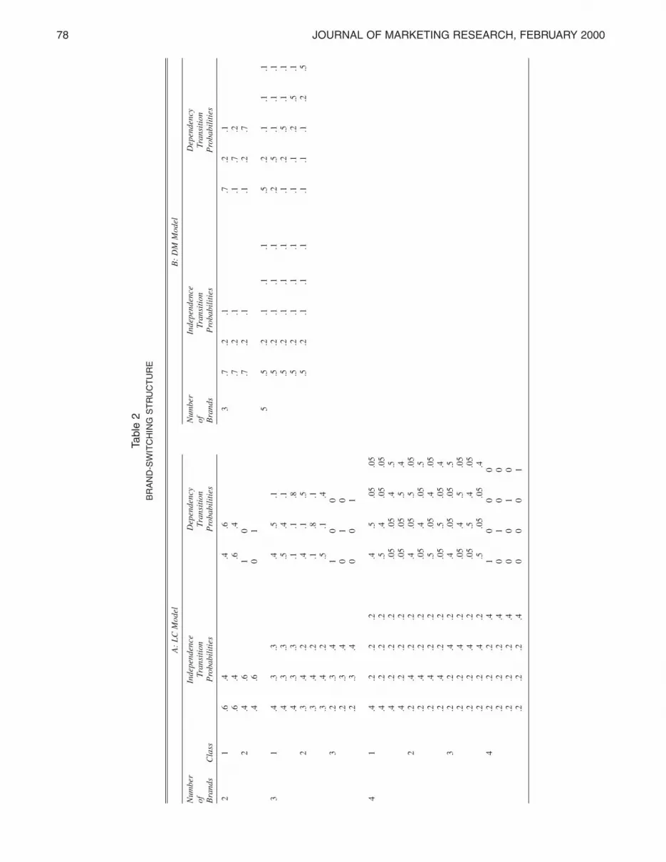
cific subsets of brands had relatively strong dependency ofbrand choice. Included in these more complex structures isthe now well-known “mover–stayer” model; in this contextmovers are analogous to brand switchers and stayers areanalogous to brand-loyal consumers, whose probability ofbuying the same brand is equal to one. The mover–stayerrepresentation yields a restrictive and extreme model form.Table 2, Part A, provides a description of the populationtransition probabilities used in these simulations.

Table 2, Part B, provides a description of the transitionprobabilities used in the DM model simulations. Notice thatin the DM simulations we did not vary the extremity of pa-rameter population values, keeping them constant from cellto cell. Recent work by Collins and colleagues (1993) sug-gests that, all else the same, model performance should im-prove in the presence of less extreme structures. Thus, ingeneral, we would expect better parameter recovery underbrand-choice independence, as opposed to structures forwhich the pattern of brand switching yields parameters thathave extreme population values, as in the case of themover–stayer representation. However, the proposed mod-els were developed specifically to capture brand-choice de-pendencies, if they exist, so we look to these extreme struc-tures as a good test of the efficacy of the proposed models.

Implementation and Performance Measures

For the LC model simulations, the design has four factorsgenerating 3 × 23 = 24 cells. For the DM model simulations,the design has five factors generating 3 × 24 = 48 cells. Foreach cell, 50 replications were completed. In all cases, we fitthe LC-CD and DM-D models to the generated data evenwhen the data exhibit no brand dependencies, which con-forms to an independence structure.5

The comparative evaluative performance measures focusattention on parameter recovery. The accuracy of the param-eter estimates is evaluated by assessing relative performanceon two criterion measures: (1) the average absolute percent-age bias (%BIAS), defined as the average of the ratio of theabsolute difference between the parameter estimates and thepopulation parameter values divided by the population pa-rameter value, and (2) the root mean square error (RMSE)between the population and estimated value of a parameter.Performance measures were computed for all relevant pa-rameters: (1) initial probabilities, (2) transition probabilities,(3) polarization index (DM model only), and (4) %HITS(LC model only), which is defined as the percentage of re-spondents that are classified into their true segments on thebasis of the estimated segment membership.

SIMULATION RESULTS

LC Model

Mean %BIAS effects under each factor level are pre-sented in Table 3, Part A. In general, parameter recovery ofboth the population initial and transition probabilities wasquite good; for the initial probabilities, the largest %BIASeffect obtained was 3.9%, whereas for the transition proba-bilities, %BIAS effects ranged (in absolute value) from a


Tabl

e 2

BR

AN

D-S

WIT

CH

ING

ST

RU

CT

UR

E

A:

LC

Mod

elB

: D

M M

odel

Num

ber

Inde

pend

ence

D

epen

denc

y N

umbe

rIn

depe

nden

ce

Dep

ende

ncy

of

Tran

siti

on

Tran

siti

on

of

Tran

siti

on

Tran

siti

onB

rand

s C

lass

P

roba

bili

ties

P

roba

bili

ties

B

rand

s P

roba

bili

ties

P

roba

bili

ties

21

.6.4

.4.6

3.7

.2.1

.7.2

.1.6

.4.6

.4.7

.2.1

.1.7

.22

.4.6

10

.7.2

.1.1

.2.7

.4.6

01

5.5

.2.1

.1.1

.5.2

.1.1

.13

1.4

.3.3

.4.5

.1.5

.2.1

.1.1

.2.5

.1.1

.1.4

.3.3

.5.4

.1.5

.2.1

.1.1

.1.2

.5.1

.1.4

.3.3

.1.1

.8.5

.2.1

.1.1

.1.1

.2.5

.12

.3.4

.2.4

.1.5

.5.2

.1.1

.1.1

.1.1

.2.5

.3.4

.2.1

.8.1

.3.4

.2.5

.1.4

3.2

.3.4

10

0.2

.3.4

01

0.2

.3.4

00

1

41

.4.2

.2.2

.4.5

.05

.05

.4.2

.2.2

.5.4

.05

.05

.4.2

.2.2

.05

.05

.4.5

.4.2

.2.2

.05

.05

.5.4

2.2

.4.2

.2.4

.05

.5.0

5.2

.4.2

.2.0

5.4

.05

.5.2

.4.2

.2.5

.05

.4.0

5.2

.4.2

.2.0

5.5

.05

.43

.2.2

.4.2

.4.0

5.0

5.5

.2.2

.4.2

.05

.4.5

.05

.2.2

.4.2

.05

.5.4

.05

.2.2

.4.2

.5.0

5.0

5.4

4.2

.2.2

.41

00

0.2

.2.2

.40

10

0.2

.2.2

.40

01

0.2

.2.2

.40

00

1


Table 3MEAN PERFORMANCE: %BIAS AND %HITS

A: LC Model B: DM Model

Initial Transition % Initial TransitionProbabilities Probabilities Hits Probabilities Probabilities Polarization

Number of respondents50 NAa NA NA 1.64 7.01 16.98

200 1.95 8.16 90.02 .88 5.69 13.58400 1.21 7.07 91.76 .44 4.48 10.86

Number of choices4 1.91 8.52 89.52 1.26 6.53 17.518 1.25 6.71 92.26 .71 4.93 10.11

Number of parameters9 1.30 3.48 95.23 .56 5.01 12.04

25 NA NA NA 1.41 6.54 15.5629 1.29 9.13 89.31 NA NA NA67 2.15 10.24 88.11 NA NA NA

StructureDependent 1.79 8.00 90.67 .86 5.09 13.76Independent 1.37 7.23 91.11 1.11 6.36 13.85

HeterogeneityHeterogeneous NA NA NA 1.22 5.75 8.95Homogeneous NA NA NA .75 5.71 18.66

aNA = not applicable to this model.

6Percentage differences were not included for segments in which the de-sign called for population values to be set at zero (this occurs in the courseof testing the models’ ability to capture the mover–stayer structures), be-cause the denominator is by definition zero.

low of approximately 2.5% to a high of almost 12.5%.6Again, no systematic bias in algebraic sign was found in es-timating these parameters. Performance was generallypoorer (relatively) as the number of parameters increased(cells characterized by more segments and more brands) andthe number of observations decreased, though increasing thesample size from 200 to 400 did not yield relatively largegains in precision. With respect to capturing segment mem-bership, the model did extremely well—in over 50% of thecells the %HIT rate exceeded 90%.

The RMSE performance measures were analyzed byanalyses of variance (ANOVAs) for main effects of the fourfactors and for first-order interaction effects. An effect sizewas considered statistically large if it was significant at orbelow the .01 alpha level and had an ω2 greater than 5%.The following summarizes important findings:

•Initial probabilities: There were three statistically large effectscorresponding to (1) the number of respondents, (2) the num-ber of choices, and (3) the number of parameters estimated.None of the first-order interaction effects was statisticallylarge. Least significant difference (LSD) tests showed that pa-rameter recovery improved with larger sample sizes, fewer pa-rameters, and more choices.

•Transition probabilities: All four main effects were statisticallylarge. The LSD tests showed that parameter recovery improvedwith larger sample sizes, more choices, and fewer parameters,which is consistent with standard theory on statistical infer-ence. It is also apparent that parameter recovery improvedwhen the parameter population values were not close to theboundary values of 0 and 1 in cells characterized by brand-choice dependencies. One statistically large first-order interac-tion effect between number of choices and structure imposed

was found. A plot of this interaction effect showed that differ-ences in performance due to structure (i.e., brand-choice de-pendence versus brand-choice independence) dissipates in thepresence of larger numbers of choices, that is, when more ob-servations on an individual’s choices are available.

•%HITS: There are two statistically large main effects corre-sponding to (1) the number of parameters and (2) the numberof choices. The LSD tests showed that the ability to recoversegment membership deteriorates when the number of parame-ters increases (i.e., more segments and brands) but improveswhen more observations are available for an individual. Thenumber of respondents did not significantly affect this per-formance measure.

The simulation results are consistent with the work ofCollins and colleagues (1993) in that parameter recovery de-teriorated when parameter population values approachedtheir boundary values. Perhaps the most important result,however, is the general ability of the LC model to recoverpopulation parameter values in the presence of structuredand extreme patterns of brand switching. In Table 4 we pres-ent parameter estimates for Cell 9 of the Monte Carlo de-sign, which had the largest %BIAS effects. Although theseparameter estimates are the poorest in a relative sense, wedo not believe that such biases would be judged alarmingfrom a practical viewpoint. Furthermore, the model did re-markably well in capturing the mover–stayer parameteriza-tion, which demonstrates that our approach can identify het-erogeneous transition probabilities solely on the basis ofmarginal distributions.

DM Model

Mean %BIAS effects under each factor level are pre-sented in Table 3, Part B. In the case of initial probabilities,the %BIAS effects were, from a practical viewpoint, negli-gible across all cells in the design: in half the cells the%BIAS effects were less than 1%. Recovery of the transi-tion probabilities was also extremely good: %BIAS effects


Table 4LC MODEL: CELL 9a

Population Structure Estimated (Mean) Structure

Numberof Initial Transition Initial Transition %Brands Class Probabilities Matrix Probabilities Matrix HITS

4 1 .6 .2 .1 .1 .4 .5 .05 .05 .606 .193 .093 .118 .382 .496 .049 .073 86.5.5 .4 .05 .05 .481 .418 .064 .037.05 .05 .4 .5 .037 .062 .380 .521.05 .05 .5 .4 .064 .052 .538 .346

2 .2 .25 .15 .40 .4 .05 .5 .05 .203 .236 .146 .415 .386 .065 .496 .053.05 .4 .05 .5 .055 .388 .056 .501.5 .05 .4 .05 .529 .039 .394 .038.05 .5 .4 .05 .034 .519 .036 .414

3 .1 .4 .25 .25 .4 .05 .05 .5 .106 .393 .255 .246 .413 .501 .040 .046.05 .4 .5 .05 .043 .415 .486 .056.05 .5 .4 .05 .055 .075 .416 .454.5 .05 .05 .4 .490 .390 .064 .056

4 .25 .25 .25 .25 1 0 0 0 .233 .258 .248 .264 .989 .005 .005 .0010 1 0 0 .000 .990 .004 .0060 0 1 0 .003 .010 .986 .0010 0 0 1 .001 .005 .001 .997

aCell 9 description: 200 respondents, 4 choices, 67 parameters.

ranged from a low of a little more than 1% to a high of10.4%. No systematic pattern in algebraic sign was found.Not surprisingly, the largest absolute %BIAS effects werefound in cells with small sample sizes (50). However, evenin these cells the ability of the model to capture populationinitial and transition probabilities was quite good: the largest%BIAS effect was less than 4%. In the case of the polariza-tion index, the results were relatively not as good. Relativelypoor performance was found in cells characterized by ho-mogeneous samples. There was also a clear tendency for thepolarization index to overestimate the degree of respondenthomogeneity systematically in samples that were relativelyhomogeneous. In the presence of relatively heterogeneoussamples, recovery of the true polarization index was gener-ally much better, typically less than 10%. We revisit this is-sue subsequently.

The RMSE performance measures were analyzed byANOVAs for main effects of the five factors and first-orderinteraction effects. The following summarizes importantfindings:

•Initial probabilities: There were two statistically large effectscorresponding to (1) the number of respondents and (2) thenumber of choices. None of the first-order interaction effectswas statistically large. The LSD tests showed that parameter re-covery improves, as expected, with larger sample sizes andwith more choices. These results are consistent with those ob-tained under the LC model.

•Transition probabilities: There are three statistically large maineffects corresponding to (1) the number of respondents, (2) thenumber of parameters estimated, and (3) the structure imposed.The LSD tests showed that, as expected, parameter recoverydeteriorates with smaller sample sizes, with more parameters toestimate, and under independence of brand-choice sequences,which corresponds to the more restrictive structure being in-vestigated. Several first-order interaction effects were statisti-cally large. All the significantly large interaction effects in-cluded the number of respondents factor. A plot of theseinteraction effects pointed to the small sample size (50) condi-tion; for example, in the case of the number of choices, with

sample size equal to 50, more observations resulted in rela-tively better performance, whereas with sample sizes of 200 or400, this was not the case. Respondent heterogeneity improvedmodel performance with a small sample size (50), whereas withlarger sample sizes (200 or 400), respondent homogeneity im-proved model performance.

•Polarization: There were four statistically large main effectscorresponding to (1) the number of respondents, (2) the num-ber of choices, (3) the number of parameters estimated, and (4)the degree of heterogeneity. The LSD tests showed that param-eter recovery improves for larger sample sizes—again, as ex-pected—with more choices and in the presence of relativelyheterogeneous as opposed to homogeneous samples and dete-riorates as the number of parameters increases. In general,mean comparisons show that in relatively homogeneous sam-ples, the polarization index is systematically overestimated; inother words, the estimates of the polarization index consis-tently indicate that the sample is more homogeneous than it ac-tually is.

Overall, the DM model could recover parameter valuesremarkably well. Perhaps what is most encouraging is theability of the DM model to recover population values withsmall sample sizes. The results demonstrated that even forsamples as small as 50 the DM model did a good job of re-covering population parameter values, except it did not cap-ture the polarization index in the presence of relatively ho-mogeneous samples; furthermore, the results suggest thatthe relative gains in parameter recovery from larger samplesizes is modest, from a practical viewpoint. For example, in-creasing sample size from 50 to 200, a fourfold increase, re-duces the average %BIAS by 1.3%; increasing sample sizefrom 50 to 400, an eightfold increase, reduces the average%BIAS by 2.5%. Because the %BIAS effects are not largein absolute value, such small gains in precision would notseem to compensate for the increase in sample size. We alsofound that the DM model systematically overestimated thedegree of respondent homogeneity in relatively homoge-neous samples. Although this finding was not expected, itsuggests that there is a strong small-sample bias when


7Also excluded from the final sample were respondents who purchaseda single brand. The transition probabilities of these individuals are not la-tent but instead can be determined unambiguously from the past-four-weekand after-trial consumption batteries.

Dirichlet parameters are estimated by maximum likelihoodmethods.

PILOT APPLICATION

This application is based on a survey conducted for papertowels. The study focused on jumbo paper towels, whichdominate this category. The study was commissioned in themid-1990s to investigate the effects of launching a re-designed private label (PL) and specifically the effects of thelaunch on categorywide brand choice and brand percep-tions. The redesigned PL was intended to compete againstthe national brands on the strength and absorbency dimen-sions and to be priced more closely to the national brands.

Background

Before exposure to the redesigned PL, respondents (retro-spectively) provided information on rolls of paper towelsbought in the past four weeks, rolls of each brand of papertowel bought in the past four weeks, brand usually bought,brands of paper towels they would consider buying, averageprice paid or expected for each brand bought or considered,ratings on a set of performance-related attributes, and a de-mographic battery. Respondents were then exposed to theredesigned PL through a concept storyboard and were givenone roll of the new PL to use over the next two weeks.Before respondents left, follow-up interviews were sched-uled. In the follow-up interview, respondents were remindedof the suggested retail selling price of the redesigned PL andwere asked to indicate which brands of paper towels theywould buy during the next four-week period and how manyrolls of each brand they would buy during the next four-week period, assuming that they would purchase the samequantity as in the past four weeks, and to provide perform-ance-related attribute ratings for the redesigned PL onceagain.

Respondents mentioned a total of nine brands in the sur-vey, and the top five brands accounted for slightly morethan 79% of the total volume purchased; we restrict our at-tention to these five brands and eliminate respondents whopurchased any of the other brands.7 Our final sample con-sisted of 315 respondents. The average purchase rate for thissample was approximately 3.6 rolls of paper towels perfour-week period. Table 5 provides summary descriptivestatistics.

8The CAIC is defined as CAIC = –2LM + QM (ln n + 1), where LM de-notes the log-likelihood associated with model M, QM is the number of pa-rameters fit under model M, and n gives the number of observations.

The Inference Problem

Figure 1 provides a simple illustration of the problem weface in this particular study. For discussion purposes, con-sider three prototypical respondents and, for the moment,just three brands that have been labeled simply as A, B, andPL. Notice from Table 5 that Individual 1 purchased a totalof six packages of paper totals over the past four weeks, sothat, r(1)

A,t – 1 = 4, r(1)B,t – 1 = 1, and r(1)

PL,t – 1 = 1. After the in-home product trial, we find that the six selections are reallo-cated as r(1)

A,t = 1, r(1)B,t = 2, and r(1)

PL,t = 3. Although the infor-mation provided by each individual can be usedstraightforwardly to compute the change in the volumeshare for each brand, this information is, however, less sat-isfactory if interest centers on estimating the sources ofgains and losses for the new private label. Take, for exam-ple, Individual 1. Although it is clear that the PL has gainedshare after the in-home product trial (1/6 = .167 versus 3/6 =.50 ), it is not clear from where exactly this sales gain iscoming. As we indicated previously, one approach for an-swering this question is to assume that brand choices are in-dependent. In this case, transition probabilities are equal tothe marginal brand choice probabilities at time point t.However, as we show subsequently, the independence as-sumption does not adequately characterize the brand transi-tions in this study.

Baseline Models: No Covariates

We begin by fitting several baseline models that do not in-corporate any of the available covariates. The goal of theanalyses is to determine the number of LCs and to seewhether the data exhibit strong brand dependencies. Table 6provides summary goodness-of-fit information for ninebaseline models. We evaluate the goodness-of-fit of themodels on the basis of several criteria. When one hypothe-sis is nested within another, differences between the likeli-hood-ratio (LR) statistics are computed to assess the statis-tical significance of the denigration in fit that results fromthe additional constraints imposed by the more restrictivehypothesis. When deciding how many LCs to retain we relyon two fit measures. The first is a Monte Carlo method sug-gested by Aitkin, Anderson, and Hinde (1981), which in-volves performing an α = .05 test for the null hypothesis ofs classes versus the alternative, (s + 1) classes. The secondmeasure chooses the number of LCs on the basis of mini-mizing Bozdogan’s (1987) consistent Akaike’s informationcriterion (CAIC).8 For comparisons of nonnested models,

Table 5DESCRIPTIVE STATISTICS

Before Number Volume After Number Volume Average MeanBrand of Rolls Share % of Rolls Share % Price ($) Strength Absorbing

PL 258 22.99 210 18.72 .79 5.11 5.45Bounty 276 24.60 317 28.25 .95 6.25 6.65Brawny 236 21.03 221 19.70 .90 5.75 6.13Scott 209 18.63 243 21.66 .92 6.05 5.98Viva 143 12.75 131 11.68 .89 5.66 5.78Total 1122 1122


Past Four Weeks After In-Home Trial

Brand Brand

Individual A B PL A B PL1 4 1 1 1 2 32 3 1 1 1 1 33 1 4 3 3 4 1¥ ¥ ¥ ¥ ¥ ¥ ¥

¥ ¥ ¥ ¥ ¥ ¥ ¥

¥ ¥ ¥ ¥ ¥ ¥ ¥

n ¥ ¥ ¥ ¥ ¥ ¥

Individual 1 Individual 2 Individual 3

After After After

Past A B PL Past A B PL Past A B PL

A ? ? ? 4 A ? ? ? 3 A ? ? ? 1

B ? ? ? 1 B ? ? ? 1 B ? ? ? 4

PL ? ? ? 1 PL ? ? ? 1 PL ? ? ? 3

1 2 3 1 1 3 3 4 1

Figure 1THE LATENT INFERENCE PROBLEM

that is, models that are not proper subsets of one another, theCAIC statistic can provide a useful heuristic for determiningthe better model. We also assess how well each model re-produces the observed choice data. This is accomplished byusing the conditional expectation formulas (see Equations25 and 28) to compute the expected brand frequencies afterin-home trial and then computing the disaggregated total ab-solute error (TAE).9

To assess the predictive validity of each model, we ran-domly selected 25% of the sample (approximately 80 house-holds) as a holdout sample that purchased a total of 265 rollsof paper towels. Each model was recalibrated on the re-maining (training) sample. The parameter estimates ob-tained from the training sample were then used to computethe expected brand frequencies for members of the holdoutsample and the corresponding TAE.

Fit and predictive accuracy. On the basis of all the good-ness-of-fit measures shown in Table 6, we select model M4b,which fits three latent classes, as the best-fitting baselinemodel. Across all models, it yields the lowest CAIC, and wecannot accept the hypothesis that model M4c, which adds an

additional LC, fits any better from an LR perspective. Mostimportant, note that model M4b places no restrictions on thebrand transitions, so that there are 74 parameters to estimate:3 – 1 = 2 LC size parameters and 3 × [(5 × 5) – 1] brand-intercept parameters. This model also fits the after-trialbrand frequencies very well. The TAE for this model is 79.4,which is based on a total sample volume of 1122 rolls andrepresents a percentage error of approximately 7.1%. Fi-nally, in terms of predictive validity, this model does verywell, yielding a percentage (holdout sample) error of ap-proximately 8.1%.

Why not a simpler model? It is clear from the informationprovided in Table 6 that, in general, models that allow de-pendency as opposed to independence in brand choice pro-vide much better fits. All the goodness-of-fit heuristics areconsistent in this regard. For any given number of LCs, theCAIC for a model that allows for brand dependencies is al-ways lower than its independence counterpart, and in allcases the difference is rather large. Also striking is the im-provement in predictive accuracy that comes about from ex-plicitly modeling brand dependencies. Notice that, for theDM model forms, allowing brand dependencies reduces theTAE from 335.3 to 119.8, an improvement of more than64%, that is, (335.3 – 119.8)/335.3. For the LC modelforms, the improvement in predictive accuracy is as dra-

9The TAE is defined as

TAE = ΣiΣj|r (i)jt – ε(r (i)

jt |r (i)t – 1)|.


Table 6FIT HEURISTICS AND TAE: BASELINE AND COMPETING MODELS

Test ofMixture Switching Number Number Log- s Versus s + 1 Total Holdout

Model Distribution Structure of Classes of Parameters Likelihood Classes CAIC TAE TAE

Baseline modelsM1 DM Independence 1 10 –2275.31 NA 4620 335.3 79.7M2 DM Dependence 1 30 –1912.11 NA 4025 119.8 25.9M3a LC Independence 2 17 –2259.12 Reject 4633 278.1 68.3M3b LC Independence 3 26 –2213.98 Reject 4604 251.6 60.7M3c LC Independence 4 35 –2158.49 Accept 4553 227.7 57.8M3d LC Independence 5 44 –2152.23 Reject 4602 219.1 49.6M4a LC Dependence 2 49 –1905.67 Reject 4142 87.5 25.7M4b LC Dependence 3 74 –1705.55 Accept 3911 79.4 21.4M4c LC Dependence 4 99 –1689.17 Reject 4047 75.8 20.9

Covariate modelsC1 LC Dependence 3 88 –1611.6 NA 3817 59.7 15.4C2 LC Dependence 3 84 –1671.01 NA 3949 72.3 19.2C3 LC Dependence 3 92 –1595.91 NA 3813 55.1 14.9

matic. For example, incorporating brand dependencies inthe three-class model yields an improvement of (251.6 –79.4)/251.6, or more than 68%. Comparison for the otherLC models with different numbers of classes yields similarresults and conclusions. The same general pattern of com-parative performance is found in the holdout sample as well.

Competing Models

We now examine several competing models that explaindependency in brand choice by incorporating the availablecovariates in model M4b. For purposes of this analysis andfor confidentiality reasons, we focus on only three covari-ates: (1) strength and absorbency ratings (hereafter referredto as SAR),10 (2) price paid, and (3) number of children liv-ing at home. Table 5, introduced previously, provides aver-age price paid for each brand along with the mean ratings foreach brand obtained from combining (averaging) those at-tribute ratings that are strength and absorbency related.11

Two of the covariates, price and SAR, are treated as brandcovariates. The remaining covariate, number of children liv-ing at home, is treated as a person-specific covariate. All thecompeting models discussed herein involve identical para-meterizations with respect to the covariates but differ as tothe number of covariates included. Three sets of parameterscan be distinguished. The first set captures the influence ofthe brand covariates on the past four weeks of brand choices(i.e., t – 1 marginal frequencies). The second set captures theinfluence of the covariates on the transition probabilities.The third set captures the effects of the person-specific co-variate, number of children living at home, which was codedin terms of four possible categories: 0 children, 1 child, 2children, or 3+ children. The person-specific covariate is hy-pothesized to influence the probability that an individualcomes from a specific LC. In total there are S × 28 (= 4 +

10The SAR covariate was formed from a factor model that included allof the performance related attributes.

11Strength and absorbency ratings were collected on a one-to-seven–point excellent-to-poor scale.

2 + 20 + 2) brand-intercept and slope parameters and (S – 1)× 4 person-specific parameters to estimate.

Different competing models are evaluated depending onthe number of covariates included. Model C1 includes bothbrand covariates but not the person-specific covariate,model C2 includes the person-specific covariate but not anyof the brand covariates, and model C3 includes all the avail-able covariates.

Fit and predictive accuracy. Summary fit information foreach of these competing models is shown in Table 6. Interms of the difference LR test statistics, all the competingmodels fit better than model M4b, the best-fitting baselinemodel without covariates. On the basis of the CAIC statis-tic, we select models C1 and C3 over any of the baselinemodels without covariates, and model C3 is superior tomodel C1. Notice that according to the CAIC statistic weconclude that model C2, which includes only person-spe-cific covariates, does not provide a better fit than modelM4b, which includes no covariates. In terms of fitting thebrand-choice data, all the competing models provide someimprovement over baseline model M4b. For example, undermodel C3, which includes all covariates, the TAE reduces to55.1, which represents a percentage error of less than 5%.Compared with model M4b, this represents an improvementof slightly more than 30%. Consistent with the other fitheuristics, there is less of a difference between the baselinemodel M4b and competing model C2 in terms of predictiveaccuracy—compared with model M4b, model C2 yields animprovement in TAE of less than 9%. The same pattern ofcomparative performance among these competing models ispresent in the holdout sample as well. Model C3 yields apercentage error in the holdout sample of only 5.6%, which,compared with model M4b, represents a 30.2% improve-ment. Similarly, there is far less difference between modelsM4b and C2.

Segment results. In Table 7 we present covariate parame-ter estimates obtained under model C3, and in Table 8 wepresent the segment-level transition probabilities. A briefdescription of each segment follows.


Table 7MODEL C3: COVARIATE PARAMETER ESTIMATES

Segment

1 2 3Covariate Price Absorbency Value

PricePast four weeks –4.17 –.31 –3.79

(–15.11)a (–.71) (–5.51)After trialb –5.22 –.26 –3.25

(–16.43) (–.44) (–3.11)SAR

Past four weeks .31 2.98 2.58(.97) (7.33) (6.31)

After trial .57 4.83 1.37(1.01) (10.11) (1.98)

Number of childrenChild = 1 —c 1.41 1.07

(2.56) (2.11)Child = 2 — –.32 –.11

(–3.01) (–1.01)Child = 3+ — –4.11 –.98

(–6.41) (–1.31)Size 23.41% 41.05% 35.54%

Brand SharesPL

Past four weeks 36.83 7.43 30.82After trial 11.32 17.18 25.79

BountyPast four weeks 10.77 36.33 20.37After trial 16.10 35.36 27.71

BrawnyPast four weeks 19.32 31.80 10.42After trial 20.79 23.03 14.88

ScottPast four weeks 27.81 13.73 18.27After trial 43.86 13.63 16.27

VivaPast four weeks 5.27 10.71 20.12After trial 7.90 10.79 15.34

Segment profileAverage price .75 1.03 .79After-trial average SAR 4.31d 6.83e 5.43d

Number of children 2.7 .9 2.0Revenue gain/loss Loss Gain Loss

at-values are in parentheses.bThe after-trial slope parameters give the effects of each covariate on the

transition probabilities.cSegment 1 is the reference group for comparing person-specific covari-

ate parameter estimates.dChange in SAR not statistically significant.eChange in SAR statistically significant.

•Segment 1 (23.41%) is, in general, extremely price sensitive;notice that both price slope parameters are highly significant,whereas the SAR slope parameter estimates suggest thatstrength and absorbency perceptions are not influential in de-termining brand choice, either before or after exposure to thenew PL brand. Price has a strong influence on the transitionprobabilities, which accounts in part for the PL’s loss of sharein this segment. The probability of belonging to Segment 1 in-creases if a consumer lives in a household with three or morechildren. The transition probabilities shown in Table 8 indicatethat the redesigned PL is particularly vulnerable in this seg-ment, losing almost half its share, and Scott is the big winner.Compared with the other brands, its repeat purchase probabilityis low, which contributes to a net revenue loss in this segment.

•Segment 2 (41.05%), the largest segment, is not price sensitive,but values strength and absorbency; notice that both SAR slopeparameters are statistically significant and both price slope pa-rameters are not. Bounty and Brawny are the dominant playersin this segment (see Table 7), which is consistent with the posi-tioning of these brands in the marketplace. Repeat purchaseprobabilities (see Table 8) are relatively high for all brands inthis segment, which suggests that this segment is characterizedby a high degree of brand dependencies. In this segment thebrand-intercept parameters associated with choosing the samebrand were all statistically significant, which provides addi-tional support for this contention. Thus, all else the same, con-sumers who value strength and absorbency tend to be loyal, orat least less likely to switch. This may also suggest that there arereturns from carving out a positioning on an important attribute.The PL achieves its largest share gain in this segment (7.43 to17.18 share points), primarily at the expense of Brawny, whichcontributes to a net revenue gain in this segment.

•Segment 3 (35.54%) shows moderate price sensitivity and sen-sitivity to strength and absorbency. Price and SAR both havesignificant influence on the past four weeks of brand choices.However, it appears that price has a stronger impact on the tran-sition probabilities than does SAR. This accounts for the PL’sloss of share in this segment, even though its strength and ab-sorbency ratings improve. Having one child living at home in-creases the probability of belonging to this segment. The brand-share estimates shown in Table 7 suggest that the PL brandloses share, which contributes to a net loss in revenue in thissegment. After in-home trial, the PL share decreases, from30.84 to 25.79 share points, and the loss goes primarily toBounty and Brawny.

Segment predictive accuracy. In Table 8 we also presentthe percentage error in predicting brand frequencies for eachof these segments. To evaluate the percentage errors, wefirst use Equation 25 to compute the segment-level condi-tional expectations. Next we computed the TAE for eachsegment. Finally, to compute the percentage error we usedthe posterior probabilities to compute a weighted average ofthe volume (i.e., number of rolls) in each segment. In termsof percentage error, we see that this model does particularlywell in Segments 1 and 2 and slightly poorer in Segment 3,the segment exhibiting fewer brand dependencies. Noteonce again, however, that in terms of overall TAE (as wellas segment-level TAE) this model does considerably betterthan the DM-D model and much better than any model thatdoes not allow for brand dependencies.

Covariate effects. We now examine what happens to tran-sition probabilities of the redesigned PL by varying its priceand its SAR. For price we investigated four levels: $.75,$.80, $.83, and $.87; and for SAR we investigated three lev-els corresponding to low (one standard deviation below themean), moderate (mean rating), and high (one standard de-viation above the mean). We consider the effects of the co-variates on the probability of purchasing the PL after in-home trial. Two competitors, Brawny and Bounty, aresingled out for discussion purposes.

Figure 2 shows results. Notice first that the price slopesare relatively steep in Segments 1 and 2, which indicatesthat as price increases from $.78 to the anticipated $.87 thereis a precipitous decrease in the ability of the PL brand to re-tain its previous customers. In contrast the price slope inSegment 2 is relatively flat. This result is rather disconcert-ing, because it suggests that PL repeat purchasers continueto be price sensitive. Visual inspection of the price slopes


Table 8MODEL C3: SEGMENT-LEVEL TRANSITION PROBABILITIES

Size PercentageSegment (%) TAE Error Brand PL Bounty Brawny Scott Viva

1 23.41 3.9 PL .2076 .1009 .1835 .4489 .0591Bounty .0192 .9555 .0091 .0110 .0052Brawny .0995 .0495 .6382 .1706 .0422

Scott .0456 .0394 .0382 .8518 .0250Viva .0520 .0091 .1045 .0443 .7901

2 41.05 3.7 PL .8687 .0278 .0555 .0444 .0036Bounty .1100 .8689 .0137 .0063 .0011Brawny .1807 .1121 .6797 .0100 .0175

Scott .0411 .0010 .0091 .9213 .0275Viva .0394 .0008 .0356 .0099 .9143

3 35.54 6.9 PL .4412 .1699 .1900 .0983 .1006Bounty .0523 .9307 .0099 .0007 .0064Brawny .2110 .0577 .6789 .0199 .0325

Scott .3299 .0345 .0445 .4999 .0912Viva .1445 .1134 .0466 .1933 .5022

Transition Probabilities:

Figure 2COVARIATE EFFECTS

A: Price

PL–PL

0

.2

.4

.6

.8

1

$.75 $.80 $.83 $.87

Price

S1

S2

S3

Brawny–PL

$.75 $.80 $.83 $.87

Bounty–PL

$.75 $.80 $.83 $.87

PL– PL

Low Moderate High

SAR

S1

S2

S3

Brawny–PL

Low Moderate High

SAR

Bounty–PL

Low Moderate High

SAR

Tra

nsi

tio

n P

rob

abili

ty

0

.2

.4

.6

.8

1

Tra

nsi

tio

n P

rob

abili

ty

0

.2

.4

.6

.8

1

Tra

nsi

tio

n P

rob

abili

ty

0

.2

.4

.6

.8

1

Tra

nsi

tio

n P

rob

abili

ty

0

.2

.4

.6

.8

1

Tra

nsi

tio

n P

rob

abili

ty

0

.2

.4

.6

.8

1

Tra

nsi

tio

n P

rob

abili

ty

Price Price

B: SAR

also suggests that the PL brand might consider a slightlylower price, for example, $.83, instead of at the proposed$.87; this is supported by the (crude) point elasticities aswell.

The SAR results also show some interesting relation-ships. Relatively high SAR are important in retaining PL

customers in Segments 1 and 3. For these segments the SARslopes are relatively steep, which suggests that, at the pro-posed price of $.87, it is imperative that the improvedstrength and absorbency of the redesigned PL be perceived.It is also true that higher SAR results in the redesigned PLbrand drawing share from Brawny; this is true in all seg-


ments but is more prominent in Segment 3. As we indicatedpreviously, the evidence suggests that the redesigned PLwill not draw from Bounty. The SAR slopes reflect this aswell. Bounty appears to be a strong brand and will not pres-ent a major source of draw for the redesigned PL.

CONCLUDING REMARKS

The primary purpose of this research was to present amodeling framework that can help brand managers betterunderstand choice data when it is impossible, or at least im-practical, to collect data on the exact sequence of brandchoice. To that end, we discussed two general model forms,both of which can capture heterogeneity in brand-transitionprobabilities and can accommodate brand- and person-spe-cific covariates. Overall, we expected the LC-CD model tofit better than the DM-D model, because it is more flexiblein describing segment-specific variability in the transitionprobabilities. However, because of its parsimonious struc-ture, the LC-DM is likely to be more stable in small samples.

We reported results of a modest Monte Carlo simulation,which showed that the proposed approach can indeed cap-ture transition probabilities under several different condi-tions. We also provided a real-life application of our pro-posed modeling approach for the paper towel category. Wefound that consumers could be classified into three latentsegments with very different transition probabilities, reac-tions to the redesigned PL, and profiles. Equally important,the final model yielded share estimates consistent with priorexpectations.

Other applications of our approach are also of interest. Asmentioned in the introduction, it is desirable to reconstructbrand-switching behavior on the basis of aggregate marketdata. Consider, for example, a sample of stores for which weobserve sales data at two adjacent time points. By treatingthe store as unit of analysis, we can apply the methods pre-sented here to estimate the transition probabilities underly-ing the households’ brand-choice data. Some care may beneeded to model spatial dependencies among the stores, butwith an appropriate selection of covariates that account foreffects of spatial variation and autocorrelation, these modi-fications are minor (King 1997). Finally, we note that theLC-CI and DM-I are not restricted to the analysis of brand-transition data but may prove useful in any application thatinvolves the reconstruction of joint distributions on the ba-sis of marginal distributions (Putler, Kalyanam, and Hodges1996).

Extensions

Although the proposed LC-CD and DM-D models prom-ise to be useful in different settings, there are at least two ex-tensions that we are currently exploring. The first extensionallows for dependencies among purchase vectors observedat more than two time points, and the second allows for thepossibility that the total number of brand purchases mayvary from one time period to the next.

The first extension can be approached by again applyingthe binomial thinning operator. Specifically, with the use ofthe binomial thinning operator it is straightforward to derivea (nonstationary) first-order Markov process that captureslatent brand switching over time with

k t jkt j t

j

r r −=∑= 1

1

30 , ,( ) α o

for t = 1, …, T. Note that the transition probabilities are al-lowed to be time dependent. For two time periods, Equation30 reduces to the approach presented in this article.

The second extension is of interest when the total numberof choices is a random variable whose values vary from onetime period to the next. In this case,

where Σbk = 1 αjkt ≤ 1, and ik,t is a nonnegative discrete ran-

dom variable representing the number of purchases at t thatare not predictable from brand purchases at t – 1.

The intent of these extensions is to enhance the general-izability of the basic modeling approach. However, it is im-portant to note that this outlook for further research does notdistract from the proposed LC-CD and DM-D model formsproviding a general approach to the problem of inferring la-tent brand switching in a heterogeneous population.

REFERENCES

Aitkin, A.C. and H.T. Gonith (1935), “On Fourfold Sampling withand Without Replacement,” Proceedings of the Royal Society ofEdinburgh, 55, 114–25.

Aitkin, M., D. Anderson, and J. Hinde (1981), “Statistical Model-ing of Data on Teaching Styles,” Journal of the Royal StatisticalSociety, A144, 419–61.

Allenby, G.M. and P.J. Lenk (1994), “Modeling Household Pur-chase Behavior with Logistic Normal Regression,” Journal ofthe American Statistical Association, 89 (December), 1218–31.

Bass, Frank M. (1969), “A New Product Growth Model for Con-sumer Durables,” Management Science, 15 (January), 215–27.

——— (1974), “The Theory of Stochastic Preference and BrandSwitching,” Journal of Marketing Research, 11 (February),1–20.

Böckenholt, Ulf and William R. Dillon (1997), “Some New Meth-ods for an Old Problem: Modeling Preference Changes andCompetitive Market Structures in Pretest Market Data,” Journalof Marketing Research, 35 (February), 130–42.

Bozdogan, H. (1987), “Model Selection and Akaike’s InformationCriterion (AIC): The General Theory and Its Analytical Exten-sions,” Psychometrika, 52 (1), 345–70.

Collins, Linda M., Penny L. Fidler, Stuart E. Wugalter, and JeffreyD. Long (1993), “Goodness-of-Fit Testing for Latent ClassModels,” Multivariate Behavioral Research, 28 (3), 375–89.

Cox, D.R. and V. Isham (1980), Point Processes. London: Chap-man & Hall.

Dayton, C.M. and G.B. Macready (1988), “Concomitant-VariableLatent Class Models,” Journal of the American Statistical Asso-ciation, 83 (March), 173–8.

Dillon, William R. and Sunil Gupta (1996), “A Segment-LevelModel of Category Volume and Brand Choice,” Marketing Sci-ence, 15 (1), 38–59.

———, Ajith Kumar, and Melinda Smith de Borrero (1993),“Capturing Individual Differences in Paired Comparisons: AnExtended BTL Model Incorporating Descriptor Variables,”Journal of Marketing Research, 30 (February) 42–51.

Ehrenberg, Andrew S.C. (1972), Repeat Buying. Amsterdam:North Holland Publishing Company.

Erdem, T. (1996), “A Dynamic Analysis of Market Structure Basedon Panel Data,” Marketing Science, 15 (4), 359–78.

Gauss (1995), System and Graphics Manual, Version 3. Kent, WA:Aptech Systems Inc.

Gill, P.E., W. Murray, and M.H. Wright (1981), Practical Opti-mization. New York: Academic Press.

Hawkes, A.G. (1969), “An Approach to the Analysis of ElectoralSwing,” Journal of the Royal Statistical Society, 31, 68–79.

k t jkt j t

j

k tr r i−=∑= +1

1

31 , , ,( ) ,α o


Keane, Michael P. (1997), “Modeling Heterogeneity and State De-pendence in Consumer Choice Behavior,” Journal of Businessand Economic Statistics, 15 (July), 310–26.

King, Gary (1997), A Solution to the Ecological Inference Prob-lem. Princeton, NJ: Princeton University Press.

Lee, T.E., G.G. Judge, and A. Zellner (1970), Estimating the Para-meters of the Markov Probability Model from Aggregate TimeSeries Data. Amsterdam: North-Holland.

Luce, Duncan R. (1959), Individual Choice. New York: John Wi-ley & Sons.

Massy, W.F., D.B. Montgomery, and D.G. Morrison (1970), Sto-chastic Models of Buying Behavior. Cambridge, MA: MITPress.

McKenzie, Ed (1988), “Some ARMA Models for Dependent Se-quences of Poisson Counts,” Advances in Applied Probability,20 (December), 822–35.

Novak, Thomas P. (1993), “Log-Linear Trees: Models of MarketStructure in Brand Switching Data,” Journal of Marketing Re-search, 30 (August), 267–87.

Plackett, R.L. (1977), “The Marginal Totals of a 2 × 2 Table,” Bio-metrika, 64 (April), 37–42.

Putler, Daniel S., Kirthi Kalyanam, and James S. Hodges (1996),“A Bayesian Approach for Estimating Target Market Potentialwith Limited Geodemographic Informations,” Journal of Mar-keting Research, 33 (May), 134–49.

Saunders, Ian W. (1984), “Enumeration of R × C Tables with Re-peated Row Totals,” Applied Statistics, 33 (3), 340–52.

Telser, L.G. (1963), “Least-Squares Estimates of Transition Proba-bilities,” in Measurement in Economics, C.F. Christ et al., eds.Stanford, CA: Stanford University Press, 270–93.

Urban, Glen L. and John R. Hauser (1993), Design and Marketingof New Products, 2d ed. Englewood Cliffs, NJ: Prentice-Hall.

Wedel, Michel and Wagner A. Kamakura (1998), Market Segmen-tation: Conceptual and Methodological Foundations. Boston:Kluwer Academic Publishers.

Wicksell, S.D. (1916), “Some Theorems in the Theory of Probabil-ity, with Special Reference to their Importance in the Theory ofHomograde Correlation,” Aktuarieföreningens Tidskrift, 165–213.

Zufryden, Fred S. (1986), “Multibrand Transition Probabilities asa Function of Explanatory Variables: Estimation by a Least-Squares-Based Approach,” Journal of Marketing Research, 23(May), 177–83.

Documents

Inferring Latent Brand Dependencies