Latin Hypercube Sampling and the Identification of the Foreclosure Contagion Threshold

1

Latin Hypercube Sampling and the Identification of

the Foreclosure Contagion Threshold

by

Marshall Gangel

Virginia Modeling, Analysis, and Simulation Center (VMASC)

Old Dominion University

Norfolk, VA 23529

[email protected]

Michael J. Seiler*

Professor and Robert M. Stanton Chair of Real Estate and Economic Development


2154 Constant Hall

Norfolk, VA 23529-0223

[email protected]

757.683.3505 phone

757.683.3258 fax

and

Andrew J. Collins

Virginia Modeling, Analysis, and Simulation Center (VMASC)


Norfolk, VA 23529

[email protected]

Published in the Journal of Behavioral Finance

May 31, 2011

* Contact author

2



Over the last several years, the U.S. economy has experienced a significant recession brought on

by the collapse of the residential real estate market. During this downturn, the number of real

estate foreclosures has risen drastically. Recent studies have empirically demonstrated a

reduction in real estate values due to neighboring foreclosures, termed the foreclosure contagion

effect. The foreclosure contagion effect impacts healthy neighboring properties that surround the

foreclosed property as a function of both time and distance.

We mathematically specify a precise equation that identifies the foreclosure contagion

threshold – the boundary that separates surviving markets from those that crash. Then, using a

new technique to our field known as Latin Hypercube Sampling, we presents the results of a

large scale sensitivity analysis to find that beyond the foreclosure discount and disposition time

variables, the percentage of adjustable rate mortgages (ARMs) and the foreclosure distance

discount distance weight are the two secondary most contributing causes to a market collapse.

Keywords: emergent behavior, foreclosure contagion threshold, agent-based models, Latin

hypercube sampling.

3



Introduction

The real estate market has a significant role in the nation‟s financial systems as evidenced during

the ongoing financial crisis. Lending practices allowed high risk individuals to obtain mortgages

they could not afford. The result was a surge in foreclosures causing great instability within the

overall financial system which quickly turned global. While a handful of studies have measured

the magnitude of the foreclosure contagion effect, only Gangel, Seiler, and Collins (2011) have

used Agent-based Modeling and Simulation (ABMS) to measure how mortgage foreclosure

contagion can impact an overall marketplace. While their study focused on two key inputs,

foreclosure discount and disposition time, they failed to mathematically specify the contagion

threshold between surviving and failing markets. Without this equation, it is difficult for

policymakers to identify points where it is necessary to intervene and restore financial stability in

the system.

The second purpose of this study is to perform a sensitivity analysis on the numerous remaining

variables included in their model. Specifically, this study seeks to identify, through the use of

Latin Hypercube Sampling (LHS) – a technique newer before used in finance or real estate – the

sensitivity of additional variables on the potential collapse of the real estate market, and thus on

the overall financial markets.

In addition to successfully specifying the key equation to identify the foreclosure contagion

threshold, we are also able to identify the variables “foreclosure discount distance weight” (the

4

weight given to the foreclosed property based on its proximity to the subject property) and “loan

type” (adjustable rate versus fixed rate mortgages) as the next most significant contributors to a

market collapse. This finding is important because if policymakers are striving to lower the

negative impact of foreclosures, they should begin by streamlining the foreclosure process. In a

preventative sense moving forward, policymakers should also be wary of the percentage of

ARMs present in the market as an indicator of eminent collapse. These two variables are in the

direct control of policymakers, whereas foreclosure discount and foreclosure distance discount

weight are not.

Literature Review

Foreclosures within the real estate market occur when the borrower can no longer fulfill the

mortgage contract and eventually defaults. A legal process then begins which allows the creditor,

typically a bank, to gain possession of the property and then sell it to a third party. The money

received from the sale is applied to the remaining balance on the original loan. The foreclosure

process is extremely detrimental for all entities involved. Foreclosures directly cause financial

loss, personal credit decline, and property devaluation. Until recently, the most negative effects

of foreclosure were assumed to solely impact the parties directly involved with the foreclosed

properties. Although foreclosures were perceived to cause some devaluation to nearby

properties, research to define and quantify the contagion wasn‟t pursued until recently

(Immergluck and Smith, 2006).

Recent research has demonstrated that the negative effects of foreclosure are not felt solely by

the involved entities, but are also experienced by real estate properties that are located within

5

proximity to foreclosure events. This externalization of the negative consequences of foreclosure

events is known as the contagion effect. The effect is contagious because foreclosures are shown

to decrease neighboring property values which may lead to additional foreclosures. The negative

effects of foreclosed properties also spills over as a result of increased crime (Immergluck and

Smith, 2006). Harding, Rosenblatt, and Yao (2009) state the contagion effect is caused by

several factors. First, foreclosed properties are eventually listed for sale along with the other

properties that are listed in the traditional fashion. Therefore, foreclosures add to the supply of

properties that are contending for buyers, resulting in excess supply and thus lower property

values. The second factor involves the typical loss of value due to neglect, vandalism, and

abandonment, which can be observed from visual inspection of the premises of the foreclosure

property and its neighbors.

(insert Exhibit 1 here)

The datasets used in extant research are geographically focused within a single Metropolitan

Statistical Area (MSA). Exhibit 1 displays the MSAs, time period examined, and findings of the

major studies in foreclosure contagion research. Each study chose a different MSA for different

reasons. Rogers and Winter (2009) selected St. Louis because they felt its real estate market and

foreclosure activity were minimally impacted by the country‟s housing bubble. They support

this argument by comparing the rise of property values in St. Louis against other areas of the

country. They observed a smaller increase in value which indicates St. Louis property values are

driven by local economic factors and not the drastic increase that most American cities

6

experienced. Intuitively, a dataset with as few external factors as possible will produce results

with a higher confidence.

Lin, Rosenblatt, and Yao (2009) use data from Chicago for two primary reasons. First, Chicago

was used as a dataset in earlier studies. This promotes the comparison of their results with the

results of earlier research efforts. Second, they chose the city of Chicago because it possessed

one of the highest foreclosure rates in the country. In general, a dataset that contains a greater

number of occurrences of the phenomena to be studied should provide more thorough results

than a dataset with fewer occurrences.

Harding, Rosenblatt, and Yao (2009) select their multiple geographic datasets by reviewing the

accuracy of the data. Their initial dataset consisted of the entire nation. They reduced their

dataset to 37 MSAs by selecting the zip codes that contained the data with the highest integrity.

Finally, they reduced their dataset to seven MSAs. The final seven MSAs were the MSAs that

the authors felt could best be controlled for local market conditions.

Immergluck and Smith (2006) and Schuetz, Been, and Ellen (2008) do not directly state why

they chose Chicago and New York, respectively, as their sources of data. Immergluck and Smith

(2006) may have chosen Chicago for reasons similar to Lin, Rosenblatt, and Yao (2009).

Schuetz, Been, and Ellen (2008) may have chosen New York because of their familiarity with

the data due to their geographic collocation with the city.

7

The literature hypothesizes that the negative contagion effect of foreclosures is a function of time

and distance from a foreclosed property. Immergluck and Smith (2006) was the premier study in

quantifying the contagion effect of foreclosures. Their research only studied the contagion effect

of foreclosures as a function of distance. This negative effect decreases as the distance between

the foreclosure and the neighboring properties increases. The research following this initial

study has included foreclosure time along with distance. The foreclosure time theory

hypothesizes a foreclosure event will have the greatest negative contagion effect on the value of

properties that immediately surround the foreclosure, at the point in time when the foreclosure

initially occurs. With the exception of Immergluck and Smith (2006), the literature hypothesizes

that the negative contagion effect of a foreclosure event on its neighboring properties‟ values will

decrease as time and distance increases from the foreclosure event.

When measuring the strength of the foreclosure contagion effect, the Lin, Rosenblatt, and Yao

(2009) results demonstrate a significantly higher value than the other authors. Rogers and

Winter (2009) comment on this discrepancy, but are not able to explain it. Such a discrepancy

indicates that the contagion effect of foreclosures could change based on variables not examined

by the current research or that the contagion effect is not fully understood. Schuetz, Been, and

Ellen (2008) find negative coefficients, but they do not convert these figures into percentages.

ABM Background

Agent-based Modeling and Simulation (ABMS) is a relatively new technique in the world of

quantitative analysis. ABMS has been developed over the last couple of decades to study

problems that can be described as Complex Adaptive Systems (CAS). CAS are typically

8

composed of individual entities that follow a set of rules. The aggregate actions of the entities

directly impact the posture of a system. The behavior of the system, which is determined by the

complex aggregation of many entities, is referred to as emergent behavior. The goal of ABMS is

to understand how entity or agent level actions impact the emergent behavior of the entire system

in which the agents exist (North and Macal, 2007; Miller and Page, 2007).

ABMS provides a unique approach that differs from the traditional analytical techniques.

Techniques such as system dynamics make assumptions to represent collective effects of a

system or subsystem. The resulting model of a systems dynamics model is usually constructed as

a set of assumptions which dynamically interact for a given amount of time. Although the

ABMS modeling process includes its own assumptions, the strength of this technique is the

capability of agent level behavior and rules. This bottom up modeling approach enables ABMS

to explore system level emergent behavior through the implementation of individual agent rules

and behaviors (Gilbert, 2008).

Agents are the key element to ABMS. An agent is defined as a decision-maker within the

model. Agents typically follow a predefined list of rules or behaviors that is determined by the

individuals constructing the model during development. The agent behaviors are usually

dependent on the environment in which the agent resides (North and Macal, 2007).

One of the first observations of Complex Adaptive Behavior was made by Adam Smith (1776) in

his writing “The Wealth of Nations”. Smith noted that individuals in a society act with self-

centered motives without considering the impact of their decisions on society. The collective

9

decisions of all the agents create global actions that benefit society but cannot be traced to a

single agent‟s decision. He referred to this principle as the Invisible Hand. Smith‟s Invisible

Hand also illustrates the theme of emergence. Emergent behavior is the global behavior of a

system which is determined by the aggregate actions of many agents. Some actions of some

agents may have a greater impact on the emergent behavior than other actions or agents, but a

single agent cannot manipulate the outcome of the system (North and Macal, 2007).

Although emergence and CAS were first observed hundreds of years ago, ABMS techniques

were recently developed. The recent emergence of ABMS is due to two factors: an increased

need for the technique and the capability to build ABMS. The world has always contained

complexity, but the need to understand complex systems has increased drastically in recent

decades. The fields of social sciences, biology, and business are three fields that contain

substantial complexities. Subsequently, these fields are implementing ABMS to analyze

complex systems (North and Macal, 2007). Secondly, ABMS development was possible due to

the advances in computational techniques in the field of computer science. Techniques such as

object oriented programming have enabled analysis to simulate complex systems. ABMS would

not be possible without the combination of complex problems and computational techniques

(North and Macal, 2007). AMBS does not replace or supersede other analytical techniques;

instead, it complements the robust set of tools that are used by researchers. ABMS should

continue to build its reputation as an analytic technique as individuals demonstrate how it can be

utilized to study the complex world in which we live.

Latin Hypercube Sampling (LHS) Methodology

10

When performing system wide sensitivity analysis, one must consider each combination of the

sampled input variable values. However, this could result in a large number of combinations.

For example, if there were six input variables under consideration and each was sampled for 50

values, then there would be approximately 16 billion combinations to consider. In a stochastic

simulation, each input variable combination would need to be run several times for statistical

significance, thus the total number of runs required to achieve this analysis would be impractical.

Latin Hypercube Sampling (LHS) offers a way to look at the total variation of input variables

without having to conduct a large numbers of runs. By sampling the input variables in a certain

way, LHS produces results similar to looking at all combination of input variables, but with only

a fraction of the runs. The process of LHS was developed by McKay, Beckman, & Conover

(1979). LHS was originally designed for use within the sensitivity analysis of computer

simulations and was developed around the same time that Agent-based modeling was first being

developed as a subject (Schelling, 1969). Though both methods were developed during a similar

time-frame, they have rarely been applied together. The advantage of the LHS approach to

sampling is that similar results1 are achieved as those from a simple random sample, but LHS

requires a much smaller sample size to achieve this. Given that each sample run requires

additional time and computing power, this is a very practical benefit. The method of using LHS

described below assumes the input variables have a continuous distribution, but the approach can

easily be adapted to the discrete distribution case as well.

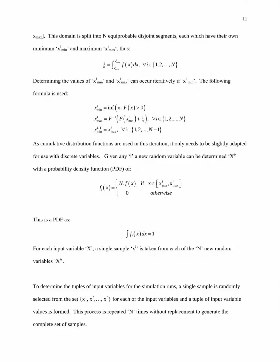
Given that „k‟ input variables are of interest, and „N‟ samples are required, LHS is achieved as

follows. Each input variable „X‟ is given a probability density function „f(X)‟ and a domain [xmin,

1 By similar results, we mean that both methods produce a similar distribution of the output variables.

11

xmax]. This domain is split into N equiprobable disjoint segments, each which have their own

minimum „ximin‟ and maximum „x

imax„, thus:

max

min

1 , 1,2, ,i

i

x

Nx

f x dx i N

Determining the values of „ximin‟ and „x

imax„ can occur iteratively if „x

1min‟. The following

formula is used:

1

min

1 1max min

1

min max

inf : 0

, 1,2,...,

, 1,2,..., 1

i i

N

i i

x x F x

x F F x i N

x x i N

As cumulative distribution functions are used in this iteration, it only needs to be slightly adapted

for use with discrete variables. Given any „i‟ a new random variable can be determined „Xi‟

with a probability density function (PDF) of:

min max. if x x ,x

0

i i

i

N f xf x

otherwise

This is a PDF as:

1if x dx

For each input variable „X‟, a single sample „xi‟ is taken from each of the „N‟ new random

variables „Xi‟.

To determine the tuples of input variables for the simulation runs, a single sample is randomly

selected from the set {x1, x

2,…, x

n} for each of the input variables and a tuple of input variable

values is formed. This process is repeated „N‟ times without replacement to generate the

complete set of samples.

12

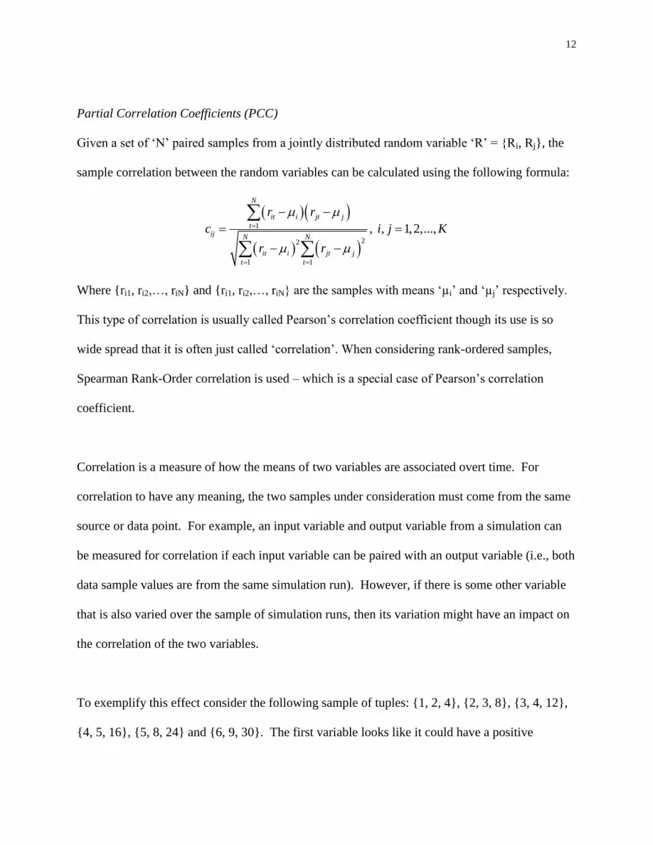
Partial Correlation Coefficients (PCC)

Given a set of „N‟ paired samples from a jointly distributed random variable „R‟ = {Ri, Rj}, the

sample correlation between the random variables can be calculated using the following formula:

1

22

1 1

, , 1,2,...,

N

it i jt j

tij N N

it i jt j

t t

r r

c i j K

r r

Where {ri1, ri2,…, riN} and {ri1, ri2,…, riN} are the samples with means „µi‟ and „µj‟ respectively.

This type of correlation is usually called Pearson‟s correlation coefficient though its use is so

wide spread that it is often just called „correlation‟. When considering rank-ordered samples,

Spearman Rank-Order correlation is used – which is a special case of Pearson‟s correlation

coefficient.

Correlation is a measure of how the means of two variables are associated overt time. For

correlation to have any meaning, the two samples under consideration must come from the same

source or data point. For example, an input variable and output variable from a simulation can

be measured for correlation if each input variable can be paired with an output variable (i.e., both

data sample values are from the same simulation run). However, if there is some other variable

that is also varied over the sample of simulation runs, then its variation might have an impact on

the correlation of the two variables.

To exemplify this effect consider the following sample of tuples: {1, 2, 4}, {2, 3, 8}, {3, 4, 12},

{4, 5, 16}, {5, 8, 24} and {6, 9, 30}. The first variable looks like it could have a positive

13

relationship with the second variable but so does the third variable; to what extent does the first

variable have a relationship with the second becomes difficult to determine because of the

influence from the third variable.

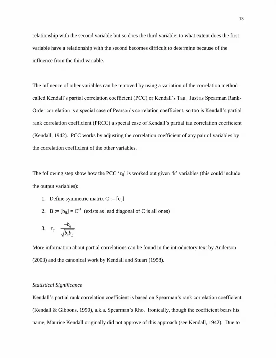
The influence of other variables can be removed by using a variation of the correlation method

called Kendall‟s partial correlation coefficient (PCC) or Kendall‟s Tau. Just as Spearman Rank-

Order correlation is a special case of Pearson‟s correlation coefficient, so too is Kendall‟s partial

rank correlation coefficient (PRCC) a special case of Kendall‟s partial tau correlation coefficient

(Kendall, 1942). PCC works by adjusting the correlation coefficient of any pair of variables by

the correlation coefficient of the other variables.

The following step show how the PCC „ij‟ is worked out given „k‟ variables (this could include

the output variables):

1. Define symmetric matrix C := [cij]

2. B := [bij] = C-1

(exists as lead diagonal of C is all ones)

3. ij

ij

ii jj

b

b b

More information about partial correlations can be found in the introductory text by Anderson

(2003) and the canonical work by Kendall and Stuart (1958).

Statistical Significance

Kendall‟s partial rank correlation coefficient is based on Spearman‟s rank correlation coefficient

(Kendall & Gibbons, 1990), a.k.a. Spearman‟s Rho. Ironically, though the coefficient bears his

name, Maurice Kendall originally did not approve of this approach (see Kendall, 1942). Due to

14

the complicated nature of the distribution of Kendall‟s partial rank correlation coefficient, it has

either been ignored as a method or approximated (Nelson & Yang, 1988). Thus a common

hypothesis test approximation is to use the same statistics as for Spearman‟s rho (Kendall &

Gibbons, 1990; Blower & Dowlatabadi, 1994; Anderson, 2003; Marino et al., 2008). If the null

hypothesis is that there is non-significant partial correlation (i.e., rrank = 0) then the following

statistic can be used:

21

2

ij

ij

ij

t

n

The degrees of freedom, Student‟s t-distribution statistic, are „n -2‟. An underlying assumption

of this approximate test is that variables are normally distributed. There are several approaches

that could be employed to remove this normality assumption, such as Fisher‟s transformation

(Fisher, 1915), but considering this test is already an approximation, the approach was deemed

an unnecessary complication.

Results

Recall that it is not the purpose of the current investigation to build an ABM to replicate the

residential real estate market. Instead, our first goal is to mathematically specify the boundary

between healthy and crashing markets in terms of the tradeoff between foreclosure discount and

disposition time. Using the ABM model of Gangel, Seiler, and Collins (2011), we then perform

LHS analysis to identify the relative strengths of additional deterministic variables not

investigated in their model.

Foreclosure Threshold Identification

15


Foreclosure discount and disposition time are the two variables selected for foreclosure threshold

analysis. Exhibit 2 demonstrates a sample of the results of the single variable analysis with a

discrete step of -0.005 for the foreclosure discount. Each line on the exhibit represents the

average of 30 simulation runs with the same foreclosure discount value. The results of the

parametric analysis of the foreclosure discount demonstrate that the impact of the foreclosure

discount has an inverse macro level impact on average property values. This behavior can be

considered emergent because the temporary effect of the foreclosure discount of individual

foreclosures creates a lasting impact on the value of the entire market. For relatively weak

contagion effects, the market continues to gain value as time increases. But as the contagion

discount becomes stronger, the growth of the average value of the entire market decreases,

reaches a maximum, and then (in some simulations) declines. The only differences between the

runs are random numbers with previously discussed underlying distributions generated by the

computer. Once this behavior was observed at a particular foreclosure discount, it was observed

for all configurations that were executed with larger foreclosure discount values. Once the

crashing threshold was crossed, the contagion effect of foreclosures was too strong for the

market to retain its value. The market‟s foreclosures create a positive feedback loop that causes

extreme devaluation of surrounding property values which, in turn, causes additional

foreclosures. This cycle continues until the entire market loses all value.

The second variable that was examined by using parametric analysis was disposition time.

Disposition time represents the amount of time that a property remains foreclosed on the market.

16

Unlike the contagion effect of foreclosures, which cannot be controlled, the amount of time that

foreclosures are on the market is usually dictated by processes mandated by state-specific laws

(Seiler et al., 2011). Because the market is impacted by the amount of time foreclosures are left

to linger on the market, the contagion effect of foreclosures can be mitigated with the

introduction of new policy.

As seen in Panel B of Exhibit 2, similar to the foreclosure discount variable, the disposition time

also has a substantial impact on the average property value of the entire market. This behavior

can be considered an emergent behavior because it was not directly implemented in the model.

Foreclosures have a temporary negative impact on their neighbors‟ value while they are present.

When a foreclosed property is resold, it can no longer directly impact its neighbors‟ values.

Indirectly, however, there is a legacy or hangover effect that persists. The contagion effect of

foreclosures can have a lasting impact if a property is sold while in the presence of foreclosed

properties. Given this principle, the results from the above figure are logical. Markets with

longer disposition times are exposed to larger number of foreclosures, on average. Therefore,

the contagion effect can have a large negative impact on the entire market.

The single variable parametric analysis was executed numerous times with different values set

for foreclosure discount and disposition time variables. In all configurations, the crashing

market phenomenon was observed, but it occurred at different combinations of the two

foreclosure variables. For example, the crashing threshold occurred at a foreclosure discount of -

5.8% when the disposition time was set at a value of 8 months. When the disposition time was

set at a value of 7 months, the crashing threshold occurred at a foreclosure discount of -6.6%.

17

Once the analysis of the results revealed that the disposition time and foreclosure discount

variables share an interdependent effect on the average property value metric, multiple variable

parametric analyses were initiated to understand the relationship between the two variables.

Various combinations of the two variables were then executed in an attempt to establish a

relationship between them by inspecting the impact on the average property value metric over

numerous simulation runs. Before the simulation runs could be executed, a primary variable and

benchmark needed to be selected. The crashing threshold was established as the benchmark for

this analysis. A market with an equal probability of succeeding or failing is recognizable and

constant for any configuration of the model. The primary variable would serve as a pseudo

independent variable during the multiple variable parametric analysis. Once the value of the

primary variable was set, the second variable would be adjusted until the desired benchmark, or

crashing threshold, was observed in the output data. The disposition time variable was selected

as the primary variable because it has a limited number of discrete values that it can possess,

while the foreclosure discount variable is a continuous variable with unlimited values. In theory,

a foreclosure discount value exists for each disposition time value which subsequently produces

a crashing threshold, but not vice versa.

Thousands of combinations were executed to produce enough data to establish a relationship

between the foreclosure discount and disposition time variables. The disposition time variable

was set between 1 and 14 months with a discrete step of 1 month. For each value of disposition

time, the model was executed with numerous values for the foreclosure discount variable until

the crashing threshold was found. If the simulation runs produced all successful markets, the

18

foreclosure discount was set to values with greater negative intensity. If the simulation runs

produced all crashing markets, the foreclosure discount was set with values with lesser negative

intensities. Once the crashing threshold was bounded, the discrete step of the foreclosure

discount was reduced until the crashing threshold result was obtained. Exhibit 3 represents a

sample of the simulation runs produced by the multiple variable parametric analyses. Each point

represents a unique combination between foreclosure discount and disposition time. The y axis

represents values of foreclosure discount, and the x axis represents values of disposition time.

Each point or combination was executed thirty times to produce enough output data to identify

the crashing threshold.

(insert Exhibit 3 and 4 here)

The multiple variable parametric analysis reveals that the relationship between the disposition

time and foreclosure discount variables follow the below equation:

Exhibit 4 graphically represents the above equation. Each point represents a unique combination

of the two variables that result in a crashing threshold where half of the simulation runs produce

a successful market and the other half produce a market crash. Any combination of the two

variables found above the curve produces an unsuccessful or crashing market, whereas

combinations below the curve results in a successful market. This emergent behavior suggests

that the contagion effect of foreclosures can be mitigated by controlling the amount of time that

19

foreclosures are allowed to remain on the market. Furthermore, the relationship between these

two variables may follow a mathematical function. This relationship was not programmed into

the model, but resulted from other rules and functions that were previously described.

Latin Hypercube Sampling and Partial (Rank) Correlation Coefficients

Sensitivity analysis is split into two components: the sampling of input variables and the

determination of effects of this variation. We use the approached of Blower & Dowlatabadi

(1994) and Marino et al. (2008). This involves using LHS for the input variable sampling and

Partial Correlation Coefficients (PCC) / Partial Rank Correlation Coefficients to determine its

impact.


LHS

To properly sample the possible input variables, certain assumptions about their underlying

distributions have to be made. Exhibit 5 shows the list of variables that where considered for the

sensitivity analysis. The first two variables, disposition time and foreclosure discount, have

already been varied in previous runs. The first new input variable is the Foreclosure Distance

Discount Weight. The simulation model currently assumes that the appraised value of a property

is equally affected by the amount of time that local foreclosed properties have been foreclosed

and the distance that these properties are from the property of interest. This would correspond to

an input value of 0.5. In the sensitivity analysis, if this variable was assigned a weight of 0, then

only the amount of time that a local property has been foreclosed would have any affect.

20

Conversely, if the input variable is 1, then only the distance of the foreclosed properties would be

under consideration.

The input variable Foreclosure Effect Radius indicates the maximum distance that a foreclosed

property will have on the appraisal of other properties. At present, the current radius sweep is 10

homes in any direction2. The Loan Type variable indicates the fraction of mortgages which are

fixed rate. Appraisal Time indicates the amount of time that passes before each property is

appraised. Currently, the simulation appraises each property at each time-step, which is one

month.

Each of the input variables was given a probability distribution from which 50 samples could be

selected. The simplest possible probability distributions were chosen for each input variable,

given the information available. Within Bayesian statistics, the uniform distribution is used

when there is no information about the underlying distribution of the variable of interest. When

possible, we use the uniform distribution for both discrete and continuous case.

In the case of Foreclosure Discount, the literature suggests that foreclosures could have

approximately a 1% (Immergluck & Smith, 2006) or a 10% (Rogers & Winter, 2009) effect on

the appraisals of surrounding properties. A Chi-squared distribution was chosen here because it

is the simplest continuous positive distribution that only requires one parameter, the mean, as an

input. As it was not clear which mean value to use, two sets of sensitivity analysis simulation

runs were conducted. One with Foreclosure Discount mean of 1% and one with a mean of 10%.

2 Using a torous grid environment, this means that up to 351 homes are considered each time an appraisal id

performed.

21

The Poisson distribution was chosen for Foreclosure Effect Radius and Appraisal Time because

it was the simplest positive discrete distribution that only requires one parameter. In the case of

Appraisal Time, an adjusted version of the Poisson distribution was chosen to remove the chance

that a time of zero was sampled. Once each input variable was sampled 50 times, the samples

were combined to form the inputs to 50 different simulation runs. Each run was repeated 30

times due to the stochastic nature of the simulation, and the results were then averaged from

these 30 runs. With the results collected from the LHS simulation runs, various types of analysis

can now be conducted on them. As with the previous results, only the final average property

price is considered for analysis.

Simulation runs with 1% average foreclosure discount

The first set of LHS simulation results considers an average of the Foreclosure Discount of 1%.

With such a low discount, none of the simulations saw a property market crash. As there are no

property crashes to consider, the average property price is used as the dependent variable.


Regression

Exhibit 6 shows the coefficients from standard multivariate linear regression. As the table

indicates, all independent variables, except Appraisal Time, have a significant impact on the final

average property values. The Adjusted R-squared value is 0.715, which implies that

approximately 72% of all variation in the average property values could be accredited to these

variables. Each of the 30 x 50 simulation runs is considered separately for this analysis, and as

22

such, it is expected that some of the remaining variation is due to the differences within the 30

simulation runs for a particular input variable set. Once each input variable is sampled 50 times,

the samples are combined to form the inputs to 50 different simulation runs. Each run is then

repeated 30 times due to the stochastic nature of the simulation. Finally, the results are then

averaged from these 30 runs.

The coefficient from the Foreclosure Distance Discount Weight variable indicates that the

greater the effect that the distance of a foreclosure has on the appraisal of local properties, the

lower the average property price will be. The Foreclosure Distance Discount Weight represents

the relative weight of a foreclosure distance as opposed to disposition time on a local appraisal.

A foreclosed property‟s distance remains constant for the duration that the foreclosure property

is on the market, where as the effect of disposition time declines within the simulation during the

time that the property is foreclosed. Thus, it is not surprising that foreclosure distance will have

a more negative effect on the prices of surrounding properties which is reflected within the

regression coefficient.

Partial Correlation Coefficient

We now focus on the relative strengths of the individual additional variables used in the model.

Analysis of the LHS can be done by looking at the Kendal‟s Partial Rank Correlation Coefficient

(PRCC) and Kendall‟s Partial Tau Correlation Coefficient (PCC) (Kendall & Gibbons, 1990).

The reason for using Partial Correlation Coefficients for a given variable, as opposed to standard

Pearson Correlation Coefficient, is that the variation from the other input variables is removed

23

from the correlation value. The removal of this external variation from other variables is

important within the analysis of a LHS sample as all the variables change at once.

Exhibit 6 shows the partial correlation values of different input variables. The partial correlated

values are on the same scale as the normal correlated values ranging from -1 to +1. The only

variable that has a significant non-zero correlation is Foreclosure Distance Discount Weight.

Recall that the Foreclosure Distance Discount Weight measures how much more an impact the

distance of a foreclosed property has on the pricing of the subject property relative to the impact

of recent foreclosures (time). The mechanism of the model can explain this correlation between

Foreclosure Distance Discount Weight and average housing prices. Simply put, the distance the

subject property is from a foreclosed property remains constant over time, whereas the

„recentness‟ of a foreclosure decreases with time, and therefore, will have less impact.

Because we include both discrete and continuous representations of our variables, the preferred

use of a ranked or non-ranked approach to the partial correlation analysis can be debated. For

completeness, we also report the Partial Rank Correlation Coefficients. The figures are very

similar to the results from the partial correlation coefficient. The only exception is the additional

significance of the loan type variable.

Simulation runs with 10% average foreclosure discount

The previous set of result contained no simulation runs where the property market actually

crashed. There was no property market crashes because the distribution of each of the input

variables were conservative estimates. To induce property market crashes within the simulation

24

results, more extreme input variables are required. Foreclosure Discount was again selected as

the influencing input variable to achieve this task because the previous results showed a very

high negative deterministic relationship with average house price. The previous discussed

results were generated using an average Foreclosure Discount of 1%. To achieve the more

extreme results presented in the right half of Exhibit 6, an average foreclosure discount of 10% is

used to be consistent with the upper range found in the literature (Immergluck & Smith, 2006).

All other input variables retain their previous value ranges.

The new output from the LHS is analyzed in a similar fashion to the previous set of results. The

difference between these analyses is that a new dependent variable is used. Instead of using the

average property price as the dependent variable, a binary indicator of whether or not the market

crashed is used. If the market did not crash, the dependent variable has a value of one, and if the

market did crash, then the dependent variable takes a value of zero. As the dependent variable is

binary, logistic regression analysis is used instead of traditional linear regression.

The results are very similar to the results seen in the previous analysis in terms of significance of

the input variables. In the regression, all the independent variables are significant, whereas the

partial correlation indicates that only two are significant: foreclosure distance discount weight

and loan type. A positive correlation between loan type and market crashes indicates that the

greater the percentage of fixed rate properties there are in the marketplace, the less likely the

market is going to crash.

Conclusions

25

The purpose of this study is to identify the equation specifying the boundary or threshold

between markets that do and do not crash based on foreclosure discount and disposition time.

After a series of analyses, we were able to specify this relationship with precision. We then

introduced a new methodology to the field, Latin Hypercube Sampling, that allows for a

sensitivity analysis to be conducted when traditionally, the number of combinations is too

numerous for mainstream computational techniques to handle. We find that beyond the two

major contributors: foreclosure discount and disposition time, the foreclosure distance discount

weight and loan type are the two most significant determinants of unstable real estate markets.

This study is helpful to policymakers in that it gives them a better understanding of just how

much stress a real estate market can take before it collapses. Moreover, by conducting the LHS

analysis, we further provide policymakers with suggestions on where to begin when trying to

stem the tide of a mortgage foreclosure contagion.

26

References

Anderson, T.W., 2003, “An Introduction to Multivariate Statistical Analysis,” 3rd ed., Wiley-

Interscience.

Blower, S.M. & H. Dowlatabadi, 1994, “Sensitivity and uncertainty analysis of complex-models

of disease transmission - an HIV model, as an example,” International Statistical Review, 62(2),

229-243.

Gangel, M., M. Seiler, and A. Collins, 2011, “Exploring the Foreclosure Contagion Effect Using

Agent-Based Modeling,” Journal of Real Estate Finance and Economics, forthcoming.

Gilbert, N., 2008, “Agent-Based Models”, in Series: Quantitative Applications in the Social

Sciences, SAGE Publications.

Fisher, R.A., 1915, “Frequency Distribution of the Values of the Correlation Coefficient in

Samples from an Indefinitely Large Population,” Biometrika, 10(4), 507-521.

Harding, J., E. Rosenblatt, and V. Yao, 2009, “The Contagion Effect of Foreclosed Properties,”

Journal of Urban Economics, 66(3), 164-178.

Immergluck, D., and G. Smith, 2006, “The External Costs of Foreclosures: The Impact of

Single-Family Mortgage Foreclosures on Property Values,” Housing Policy Debate, 17(1), 57-

79.

Kendall, M., 1942, “Partial Rank Correlation,” Biometrika, 32, 277-283.

Kendall, M., & J. Gibbons, 1990, “Rank Correlation Methods,” 5th ed., Charles Griffin and

Company.

Kendall, M., & A. Stuart, 1958, “The Advanced Theory of Statistics,” Charles Griffin and

Company.

Lin, Z., E. Rosenblatt, and V. Yao, 2009, “Spillover Effects of Foreclosures on Neighborhood

Property Values,” Journal of Real Estate Finance and Economics, 38(4), 387-407.

Marino, S., I. Hogue, C. Ray, and D. Kirschner, 2008, “A Methodology for Performing Global

Uncertainty and Sensitivity Analysis in Systems Biology. Journal of Theoretical Biology,

254(1), 178-196.

McKay, M., R. Beckman, & W. Conover, 1979, “A Comparison of Three Methods for Selecting

Values of Input Variables in the Analysis of Output from a Computer Code,” Technometrics,

21(2), 239-245.

Miller. J., and S. Page, 2007, “Complex Adaptive Systems: An Introduction to Computational

Models of Social Life,” Illustrated edition. Princeton University Press.

27

Nelson, P. & S. Yang, 1988, “Some Properties of Kendall's Partial Rank Correlation

Coefficient,” Statistics & Probability Letters, 6(3), 147-150.

North, M., and C. Macal, 2007, “Managing Business Complexity: Discovering Strategic

Solutions with Agent-Based Modeling and Simulation”, Oxford University Press.

Rogers, W., and W. Winter, 2009, “The Impact of Foreclosures on Neighboring Housing Sales,”

Journal of Real Estate Research, 31(4), 455-479.

Schelling, T., 1969, “Models of Segregation,” American Economic Review, 59(2), 488-493.

Schuetz, J., V. Been, and I. Ellen, 2008, “Neighborhood Effects of Concentrated Mortgage

Foreclosures,” Journal of Housing Economics, 17(4), 306-319.

Seiler, M., V. Seiler, M. Lane, and D. Harrison, 2011,“Fear, Shame, and Guilt: Economic and

Behavioral Motivations for Strategic Default,” working paper, Old Dominion University.

Smith, A., 1776, “The Wealth of Nations,” later published as “An Inquiry into the Nature and

Causes of the Wealth of Nations,” Edwin Cannan, ed., 1904. Library of Economics and Liberty.

28

Exhibit 1: Summary of the Foreclosure Contagion Literature

Author Location Date Range

Studied Distant Bins Time Bins Max

Contagion (%)

Rogers and Winter St. Louis, Missouri 1998 - 2007 0-200, 300-400, and

500-600 yards 0-6, 7-12, 13-18, and

19-24 months -1.4

Lin, Rosenblatt, and Yao Chicago, Illinois 1990 - 2006 0-20 km with 25 bins 0-2, 3-5, and 6-10 years -8.7

Harding, Rosenblatt, and Yao

Altanta, Georgia Charlotte, North Carolina

Columbus, Ohio Las Vegas, Nevada

Los Angeles, California Memphis, Tennessee

St. Louis, Missouri

1990 - 2007 0-300, 300-500, 500-1000, and 1000-2000

feet 0-2 years with 13 bins -1

Immergluck and Smith Chicago, Illinois

1997-1999 0-0.125 and 0.125-

0.25 miles 0-2 years -0.09

Schuetz, Been, and Ellen New York, New York 2000-2005 0-250, 250-1000 feet 0-18 and 18+ months NA

29

Exhibit 2. Disposition Time and Foreclosure Discount versus Home Prices

Panel A: Relationship between Foreclosure Discount and Home Prices over Time

Panel B. Relationship between Disposition Time and Home Prices

$0

$200,000

$400,000

$600,000

$800,000

$1,000,000

$1,200,000

$1,400,000

1

55

10

9

16

3

21

7

27

1

32

5

37

9

43

3

48

7

54

1

59

5

64

9

70

3

75

7

81

1

86

5

91

9

97

3

Ave

rage

Pro

pe

rty

Val

ue

Months

-0.1

-0.095

-0.09

-0.085

-0.08

-0.075

-0.07

-0.065

-0.06

-0.055

-0.05

-0.045

$0

$200,000

$400,000

$600,000

$800,000

$1,000,000

$1,200,000

1

49

97

14

5

19

3

24

1

28

9

33

7

38

5

43

3

48

1

52

9

57

7

62

5

67

3

72

1

76

9

81

7

86

5

91

3

96

1

Ave

rage

Pro

pe

rty

Val

ue

Months

Example of Parametric Analysis of Foreclosure Time

3

4

5

6

7

8

9

10

11

12

30

Exhibit 3. Defining the Threshold Line between Foreclosure Discount and

Disposition Time

0

0.02

0.04

0.06

0.08

0.1

0.12

0.14

0 2 4 6 8 10 12 14

Fore

clo

sure

Dis

cou

nt

Disposition Time

31

Exhibit 4. Specifying the Equation of the Foreclosure Contagion Threshold

y = 0.4737x-1.001

0

0.1

0.2

0.3

0.4

0.5

0.6

0 2 4 6 8 10 12 14 16

Fore

clo

sure

Dis

cou

nt

Disposition Time

32

Exhibit 5: Assumed distributions Variable used for the Latin Hypercube Sampling

Variable Distribution Parameters

Disposition Time Uniformed (Discrete) 1-12 (months)

Foreclosure Discount Chi-squared Mean: 1% & 10%

Foreclosure Distance Discount

Weight

Uniformed

(Continuous)

0-1

Foreclosure Effect Radius Poisson distribution Mean: 50 (10 house at

size 5)

Loan Type Uniformed (continuous) 0-1 (fraction of FRM)

Appraisal Time Poisson distribution

(adjusted) Mean: 1 (month)

33

Exhibit 6: Regression, Partial Correlation Coefficients, and Partial Rank Correlation Coefficients for Foreclosure Discounts of

1% and 10% The dependent variable in the “Foreclosure Discount = 1%” regression is average ending property value. The dependent variable in the “Foreclosure Discount =

10%” regression is a dummy variable equal to 1 if the market did not crash, and equal to 0 if the market did crash. Disposition time is the number of months the

property is allowed to linger on the market. Foreclosure discount is the amount by which the property decreases due to foreclosure. Foreclosure Distance

Discount Weight refers to the relationship between how close the neighboring foreclosure is to the subject property and how great is its negative impact.

Foreclosure Effect Radius indicates the maximum distance that a foreclosed property can be away from the subject property and still have an impact. Loan Type

indicates the fraction of mortgages which are fixed rate. Appraisal Time indicates the amount of time that passes before each property is appraised.

Foreclosure Discount = 1% Foreclosure Discount = 10%

Traditional

Regression

PCC

PRCC

Logistic

Regression PCC

PRCC

Intercept 4,740,000**

104**

Disposition Time -26,800**

-3.80**

Foreclosure Discount -25,100,000**

-212**

Foreclosure Distance Discount Weight -526,000**

-0.613* -0.551* -59.8** -0.562* -0.452*

Foreclosure Effect Radius -2,290**

-0.187 -0.211 -0.261** -0.245 -0.265

Loan Type -89,800*

-0.125 -0.529* 21.0** 0.409** 0.332**

Appraisal Time 1,400

0.010 0.137 1.27** 0.126 0.103

R2 0.715

Negelkerke R2

0.903

Cox & Snell R2

0.591

* Significance at 95%; ** Significance at 99%

Documents

Latin Hypercube Sampling and the Identification of the Foreclosure Contagion Threshold