Embed Size (px)
Citation preview
SLAC–PUB–17142August, 2017
Lectures on the Theory of the Weak Interaction
Michael E. Peskin1
SLAC, Stanford University, Menlo Park, CA 94025, USA
ABSTRACT
I review aspects of the theory of the weak interaction in a set of lecturesoriginally presented at the 2016 CERN-JINR European School of ParticlePhysics. The topics discussed are: (1) the experimental basis of the V –Astructure of the weak interaction; (2) precision electroweak measurementsat the Z resonance; (3) the Goldstone Boson Equivalence Theorem; (4)the Standard Model theory of the Higgs boson; (5) the future program ofprecision study of the Higgs boson.
Lectures presented at the CERN-JINREuropean School of Particle Physics
Skeikampen, Norway, June 15-28, 2016
1Work supported by the US Department of Energy, contract DE–AC02–76SF00515.

2
Contents
1 Introduction 1
2 Formalism of the Standard Model 2
2.1 Gauge boson interactions . . . . . . . . . . . . . . . . . . . . . . . . . 2
2.2 Massless fermions . . . . . . . . . . . . . . . . . . . . . . . . . . . . . 6
3 Tests of the V –A Interaction 8
3.1 Polarization in β decay . . . . . . . . . . . . . . . . . . . . . . . . . . 9
3.2 Muon decay . . . . . . . . . . . . . . . . . . . . . . . . . . . . . . . . 10
3.3 Pion decay . . . . . . . . . . . . . . . . . . . . . . . . . . . . . . . . . 12
3.4 Neutrino deep inelastic scattering . . . . . . . . . . . . . . . . . . . . 13
3.5 e+e− annihilation at high energy . . . . . . . . . . . . . . . . . . . . . 16
4 Precision electroweak measurements at the Z resonance 20
4.1 Properties of the Z boson in the Standard Model . . . . . . . . . . . 22
4.2 Measurements of the Z properties . . . . . . . . . . . . . . . . . . . . 23
4.3 Constraints on oblique radiative corrections . . . . . . . . . . . . . . 33
5 The Goldstone Boson Equivalence Theorem 37
5.1 Questions about W and Z bosons at high energy . . . . . . . . . . . 39
5.2 W polarization in top quark decay . . . . . . . . . . . . . . . . . . . 41
5.3 High energy behavior in e+e− → W+W− . . . . . . . . . . . . . . . . 43
5.4 Parametrizing corrections to the Yang-Mills vertex . . . . . . . . . . 47
5.5 W parton distributions . . . . . . . . . . . . . . . . . . . . . . . . . . 49
6 The Standard Model theory of Higgs boson decays 53
6.1 Decay modes of the Higgs boson . . . . . . . . . . . . . . . . . . . . . 54
6.2 Study of the Higgs boson at the LHC . . . . . . . . . . . . . . . . . . 62
3
7 Precision measurements of the Higgs boson properties 67
7.1 The mystery of electroweak symmetry breaking . . . . . . . . . . . . 69
7.2 Expectations for the Higgs boson in theories beyond the Standard Model 72
7.3 The Decoupling Theorem . . . . . . . . . . . . . . . . . . . . . . . . . 75
7.4 Effects on the Higgs boson couplings from models of new physics . . . 76
7.5 Measurement of the Higgs boson properties at e+e− colliders . . . . . 81
8 Conclusions 87
4
1 Introduction
Today, all eyes in particle physics are on the Higgs boson. This particle has beencentral to the structure of our theory of weak interactions ever since Weinberg andSalam first wrote down what we now call the Standard Model of this interaction in1967 [1,2]. As our understanding of particle physics developed over the followingdecades. what lagged behind was our knowledge of this particle and its interactions.Increasingly, the remaining mysteries of particle physics became centered on thisparticle and the Higgs field of which it is a part.
In 2012, the Higgs boson was finally discovered by the ATLAS and CMS exper-iments at the LHC [3,4]. Finally, we have the opportunity to study this particle indetail and to learn some of its secrets by direct observation. Many students at thissummer school, and many others around the world, are involved in this endeavor. Soit is worthwhile to review the theory of the Higgs boson and the broader theory ofweak interactions in which it is embedded. That is the purpose of these lectures.
To learn where we are going, it is important to understand thoroughly where wehave been. For this reason, the first half of this lecture series is devoted to historicaltopics. In Section 2, I review the basic formulae of the Standard Model and set upmy notation. An important property of the Standard Model is that, unexpectedlyat first sight, charge-changing weak interactions couple only to left-handed-polarizedfermions. This structure, called the V –A interaction, is the reason that we need theHiggs field in the first place. In Section 3, I review the most convincing experimentaltests of V –A. Section 4 reviews the precision measurements on the weak interactionmade possible by the e+e− experiments of the 1990’s at the Z resonance. Theseexperiments confirmed the basic structure of the Standard Model and made the Higgsfield a necessity.
One aspect of the Higgs field that is subtle and difficult to understand but verypowerful it is application is the influence of the Higgs field on the high-energy dy-namics of vector bosons W and Z. Section 5 is devoted to this topic. The physicsof W and Z bosons at high energy is full of seemingly mysterious enhancementsand cancellations. The rule that explains these is the connection to the Higgs fieldthrough a result called the Goldstone Boson Equivalence Theorem, first enunciatedby Cornwall, Levin, and Tiktopoulos and Vayonakis [5,6]. In Section 5, I explainthis theorem and illustrate the way it controls the energy-dependence of a number ofinteresting high-energy processes.
In Sections 6 and 7, I turn to the study of the Higgs boson itself. Section 6 isdevoted to the Standard Model theory of the Higgs boson. I will review the generalproperties of the Higgs boson and explain in some details its expected pattern of decaymodels. Section 7 is devoted to the remaining mysteries of the Higgs boson and thepossibility of their elucidation through a future program of precision measurements.
1
2 Formalism of the Standard Model
To begin, I write the formalism of the Standard Model (SM) in a form convenientfor the analysis given these lectures. The formalism of the SM is standard materialfor students of particle physics, so I assume that you have seen this before. It isexplained more carefully in many textbooks (for example, [7,8]).
2.1 Gauge boson interactions
The SM is a gauge theory based on the symmetry group SU(2)× U(1). A gaugetheory includes interactions mediated by vector bosons, one boson for each generatorof the gauge symmetry G. The coupling of spin 0 and spin 1
2particles to these vector
bosons is highly restricted by the requirements of gauge symmetry. The interactionsof these fermions and scalars with one another is much less restricted, subject onlyto the constraints of the symmetry G as a global symmetry. Thus, the theory offermions and vector bosons is extremely tight, while the introduction of a scalar fieldsuch as the Higgs field introduces a large number of new and somewhat uncontrolledinteraction terms.
The SM contains 4 vector bosons corresponding to the 3 generators of SU(2) and1 generator of U(1). I will call these
Aaµ , Bµ , (1)
with a = 1, 2, 3. These couple to fermion and scalar fields only through the replace-ment of the derivatives by covariant derivative
∂µ → Dµ = (∂µ − igAaµta) , (2)
where ta is the generator of G in the representation to which the fermions or scalarsare assigned. For the SM, fermion and scalar fields are assign SU(2), or weak isospin,quantum numbers 0 or 1
2and a U(1), or hypercharge, quantum number Y . The
covariant derivative is then written more explicitly as
Dµ = ∂µ − igAaµta − ig′BµY , (3)
with
ta = 0 for I = 0 , ta =σa
2for I =
1
2. (4)
This formalism makes precise predictions for the coupling of the weak interactionvector bosons to quarks and leptons, and to the Higgs field. To obtain the massesof the vector bosons, we need to make one more postulate: The Higgs field obtainsa nonzero value in the ground state of nature, the vacuum state, thus spontaneously
2
breaking the SU(2)× U(1) symmetry. This postulate is physically very nontrivial. Iwill discuss its foundation and implications in some detail in Section 7. However, fornow, I will consider this a known aspect of the SM.
We assign the Higgs field ϕ the SU(2) × U(1) quantum numbers I = 12, Y = 1
2.
The Higgs field is thus a spinor in isospin space, a 2-component complex-valued vectorof fields
ϕ =(ϕ+
ϕ0
)(5)
The action of an SU(2)× U(1) transformation on this field is
ϕ→ exp[iαaσa
2+ iβ
1
2](ϕ+
ϕ0
). (6)
If ϕ obtains a nonzero vacuum value, we can rotate this by an SU(2) symmetrytransformation into the form
〈ϕ〉 =1√2
(0v
). (7)
where v is a nonzero value with the dimensions of GeV. Once 〈ϕ〉 is in this form, anySU(2)× U(1) transformation will disturb it, except for the particular direction
α3 = β , (8)
which corresponds to a U(1) symmetry generated by Q = (I3 + Y ). We say thatthe SU(2) × U(1) symmetry generated by (Ia, Y ) is spontaneously broken, leavingunbroken only the U(1) subgroup generated by Q.
This already gives us enough information to work out the mass spectrum of thevector bosons. The kinetic energy term for ϕ in the SM Lagrangian is
L =∣∣∣∣Dµϕ
∣∣∣∣2 (9)
Replacing ϕ by its vacuum value (7), this becomes
L =1
2( 0 v ) (g
σa
2Aaµ + g′
1
2Bµ)2
(0v
). (10)
Multiplying this out and taking the matrix element, we find, from the σ1 and σ2
termsg2v2
8
[(A1
µ)2 + (A2µ)2], (11)
and, from the remaining terms
v2
8
(−gA3
µ + g′Bµ
)2
(12)
3
So, three linear combinations of the vector fields obtain mass by virtue of the sponta-neous symmetry breaking. This is the mechanism of mass generation called the Higgsmechanism [9–11]. The mass eigenstates are
W± = (A1 ∓ iA2)/√
2 m2W = g2v2/4
Z = (gA3 − g′B)/√g2 + g′2 m2
Z = (g2 + g′2)v2/4
A = (g′A3 + gB)/√g2 + g′2 m2
A = 0 (13)
As we will see more clearly in a moment, the massless boson A is associated withthe unbroken gauge symmetry Q. The combination of local gauge symmetry andthe Higgs mechanism is the only known way to give mass to a vector boson that isconsistent with Lorentz invariance and the positivity of the theory.
The linear combinations in (13) motivate the definition of the weak mixing angleθw, defined by
cos θw ≡ cw = g/√g2 + g′2
sin θw ≡ sw = g′/√g2 + g′2 . (14)
The factors cw, sw will appear throughout the formulae that appear in these lectures.For reference, the value of the weak mixing angle turns out to be such that
s2w ≈ 0.231 (15)
I will describe the measurement of sw in some detail in Section 3.
An important relation that follows from (13), (14) is
mW = mZ cw . (16)
This is a nontrivial consequence of the quantum number assignments for the Higgsfield, and the statement that the masses of W and Z come only from the vacuumvalue of ϕ. Using the Particle Data Group values for the masses [12] and the value(15), we find
80.385 GeV ≈ 91.188 GeV · 0.877 = 79.965 GeV . (17)
so this prediction works well already at the leading order. We will see in Section 3that, when radiative corrections are included, the relation (16) is satisfied to betterthan 1 part per mil.
Once we have the mass eigenstates of the vector bosons, the couplings of quarksand leptons to these bosons can be worked out from the expresssion (3) for thecovariant derivative. The terms in (3) involving A1
µ and A2µ appear only for I = 1
2
particles and can be recast as
−i g√2
(W+µ σ
+ +W−µ σ−) , (18)
4
The W bosons couple only to SU(2) doublets, with universal strength g.
The terms with A3µ and Bµ can similarly be recast in terms of Zµ and Aµ,
−igA3µ − ig′BµY = −i
√g2 + g′2
[cw(cwZµ + swAµ)I3 + sw(−swZµ + cwAµ)
]= −i
√g2 + g′2
[swcwAµ(I3 + Y ) + Zµ(c2wI
3 − s2wY )]
= −i√g2 + g′2
[swcwAµ(I3 + Y ) + Zµ(I3 − s2w(I3 + Y )
]. (19)
We now see explicitly that the massless gauge boson Aµ couples to Q = (I3 + Y ), aswe had anticipated. Its coupling constant is
e = swcw√g2 + g′2 =
gg′√g2 + g′2
. (20)
We can then identify this boson with the photon and the coupling constant e withthe strength of electric charge. The quantity Q is the (numerical) electric charge ofeach given fermion or boson species. The expression (19) then simplifies to
−ieAµQ− ie
swcsZµQZ , (21)
where the Z charge isQZ = (I3 − s2wQ) . (22)
To complete the specification of the SM, we assign the SU(2) × U(1) quantumnumbers to the quarks and leptons in each generation. As I will explain below, eachquark or lepton is build up from fields of left- and right-handed chirality, associatedwith massless left- and right-handed particles and massless right- and left-handedantiparticles. For the applications developed in Sections 3–5, it will almost alwaysbe appropriate to ignore the masses of quarks and leptons, so these quantum numberassignments will apply literally. The generation of masses for quarks and leptons ispart of the physics of the Higgs field, which we will discuss beginning in Section 6.
In the SM, the left-handed fields are assigned I = 12, and the right-handed fields
are assigned I = 0. It is not so easy to understand how these assignments come downfrom fundamental theory. They are requred by experiment, as I will explain in laterin this section.
With this understanding, we can assign quantum numbers to the quarks andleptons as
νL : I3 = +1
2, Y = −1
2, Q = 0 νR : I3 = 0, Y = 0, Q = 0
eL : I3 = −1
2, Y = −1
2, Q = −1 eR : I3 = 0, Y = −1, Q = −1
5
uL : I3 = +1
2, Y =
1
6, Q =
2
3uR : I3 = 0, Y =
2
3, Q =
2
3
dL : I3 = +1
2, Y =
1
6, Q = −1
3dR : I3 = 0, Y = −1
3, Q = −1
3(23)
The νL and eL, and the uL and dL, belong to the same SU(2) multiplet, so they mustbe assigned the same hypercharge Y . Note that (23) gives the correct electric chargeassignments for all quarks and leptons. The νR do not couple to the SM gauge fieldsand will play no role in the results reviewed in these lectures.
2.2 Massless fermions
The idea that massless fermions can be separated into left- and right-handedcomponents will play a major role throughout these lectures. In this sentence, Iintroduce some notation that makes it especially easy to apply this idea.
To begin, write the the 4-component Dirac spinor and the Dirac matrices as
Ψ =(ψLψR
)γµ =
(0 σµ
σµ 0
), (24)
withσµ = (1, ~σ)µ σµ = (1,−~σ)µ . (25)
In this representation, the vector current takes the form
jµ = ΨγµΨ = ψ†LσµψL + ψ†Rσ
µψR (26)
and splits neatly into pieces that involve only the L or R fields. The L and R fields aremixed by the fermion mass term. In circumstances in which we can ignore the fermionmasses, the L and R fermion numbers are separately conserved. We can treat ψL andψR as completely independent species and assign them different quantum numbers,as we have already in (23). The label L, R is called chirality. For massless fermions,the chirality of the fields and the helicity of the particles are identical. For massivefermions, there is a change of basis from the chirality states to the helicity eigenstates.
The spinors for massless fermions are very simple. In the basis (24), we can writethese spinors as
U(p) =(uLuR
)V (p) =
(vRvL
). (27)
For massless fermions, where the helicity and chirality states are identical, the spinorsfor a fermion with left-haned spin have uR = 0 and the spinors for an antifermion withright-handed spin have vL = 0; the opposite is true for a right-handed fermion and
6
a left-handed antifermion. The nonzero spinor compoments for a massless fermion ofenergy E take the form
uL(p) =√
2E ξL vR(p) =√
2E ξL
uR(p) =√
2E ξR vL(p) =√
2E ξR (28)
where ξR is the spin-up and ξL is the spin-down 2-component spinor along thedirection of motion. For example, for a fermion or antifermion moving in the 3direction,
ξL =(
01
)ξR =
(10
). (29)
Spinors for other directions are obtained by rotating these according to the usualformulae for spin 1
2. The reversal for antifermions can be thought of by viewing right-
handed (for example) antifermions as holes in the Dirac sea of left-handed fermions.For a massive fermion moving in the 3 direction, with
pµ = (E, 0, 0, p)µ , (30)
the solutions to the Dirac equation are
UL(p) =(√
E + p ξL√E − p ξL
)VR(p) =
( √E + p ξL
−√E − p ξL
)UR(p) =
(√E − p ξR√E + p ξR
)VL(p) =
( √E − p ξR
−√E + p ξR
), (31)
with ξL, ξR given by (29). These formulae go over to (28) in the zero mass limit.
The matrix elements for creation or annihilation of a massless fermion pair willappear very often in these lectures. For annihilation of a fermion pair colliding alongthe 3 axis,
〈0| jµ∣∣∣e−Le+R⟩ = v†Rσ
µuL
=√
2E (−1 0 ) (1,−σ1,−σ2,−σ3)√
2E(
01
), (32)
Note that I have rotated the e+ spinor appropriately by 180◦. This gives
〈0| jµ∣∣∣e−Le+R⟩ = 2E (0, 1,−i, 0)µ . (33)
It is illuminating to write this as
〈0| jµ∣∣∣e−Le+R⟩ = 2
√2E εµ− , (34)
where
εµ+ =1√2
(0, 1,+i, 0)µ εµ− =1√2
(0, 1,−i, 0)µ (35)
7
are the vectors of J3 = ±1 along the 3 axis. The total spin angular momentum ofthe annihilating fermions (J = 1) is transfered to the current and, eventually, to thefinal state.
More generally, we find
〈0| jµ∣∣∣e−Re+L⟩ = 2
√2E εµ+
〈0| jµ∣∣∣e−Le+R⟩ = 2
√2E εµ−⟨
e−Re+L
∣∣∣ jµ |0〉 = 2√
2E ε∗µ+⟨e−Le
+R
∣∣∣ jµ |0〉 = 2√
2E ε∗µ− . (36)
For an annihilation process such as e−Le+R → µ−Lµ
+R with annihilation by a current
and creation by another current, the spinors appear as
(u†LσµvR)(v†RσµuL) = 2 (2E)2 ε′∗− · ε− . (37)
To evaluate this, rotate the ε− vector for the muons into the muon direction. If themuons come off at polar angle θ, this gives
ε′∗− =1√2
(0, cos θ,−i,− sin θ) . (38)
Then (37) becomes2(2E)2 ε′∗− · ε− = s(1 + cos θ) = −2u , (39)
in terms of the usual kinematic invariants s, t, u. Another way to write this is
|(u†LσµvR)(v†RσµuL)|2 = 4 (2pe− · pµ+)(2pe+ · pµ−) . (40)
Similarly, for e−Le+R → µ−Rµ
+L ,
|(u†RσµvL)(v†RσµuL)|2 = 4 (2pe+ · pµ+)(2pe− · pµ−) . (41)
It is a nice exercise to check these answers using the usual trace theorems. The tracetheorems are more automatic, but the helicity formalism gives more physical insight.
3 Tests of the V –A Interaction
The property that the W boson only couples to fermions of left-handed chiralityis a crucial property of the SM. It is responsible for many of the surprising featuresof the weak interactions, both the most attractive and the most puzzling ones. Itis therefore important to understand that this feature is extremely well supportedexperimentally. In this section, I review the most convincing experimental tests ofthis property.
8
3.1 Polarization in β decay
The first applications discussed in this section involve exchange of W bosons atlow energy. In this limit, we can simplify the W propagator to a pointlike interaction
−iq2 −m2
W
→ i
m2W
. (42)
In this limit, the W exchange can be represented by the product of currents
∆L =g2
2m2W
J+µ J−µ , (43)
where
J+µ = ν†eLσµeL + u†LσµdL + · · ·J−µ = e†LσµνeL + d†LσµuL + · · · . (44)
Here and henceforth in these lectures, I replace the label ψ with a label that gives theflavor quantum numbers of the field. In (44), I write explicitly the terms associatedwith the first generation quarks and leptons; the omitted terms are those for thehigher generations. I ignore Cabibbo mixing, a reasonable approximation for thetopics discussed in these lectures. I will also ignore the masses of the neutrinos.
The theory (43) is called the V –A interaction, since
u†LσµdL = Uγµ
1− γ5
2D , (45)
the difference of a vector and an axial vector current. The coefficient in (43) isconventionally represented by the Fermi constant GF ,
g2
2m2W
=4GF√
2. (46)
This interaction has maximal parity violation in charge-changing weak interactions.
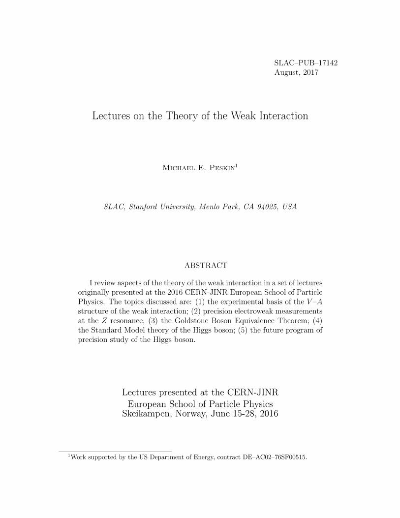
The simplest consequence of V –A is that electrons emitted in β decay should bepreferentially left-handed polarized. Since the energies of electrons in β decay are oforder 1 MeV, it is typically not a good approximation to ignore the electron mass.However, since in V –A the electron is produced in the L chirality eigenstate, we canwork out the polarization from the relative magnitude of the uL terms in the left- andright-handed helicity massive spinors given in (31). The electron polarization, in theleft-handed sense, is then given by
Pol(e−) =(√E + p)2 − (
√E − p)2
(√E + p)2 + (
√E − p)2
=p
E=v
c. (47)
A data compilation is shown in Fig. 1 [13]. Careful experiments both at high and lowelectron energies verify the regularity (47).
9
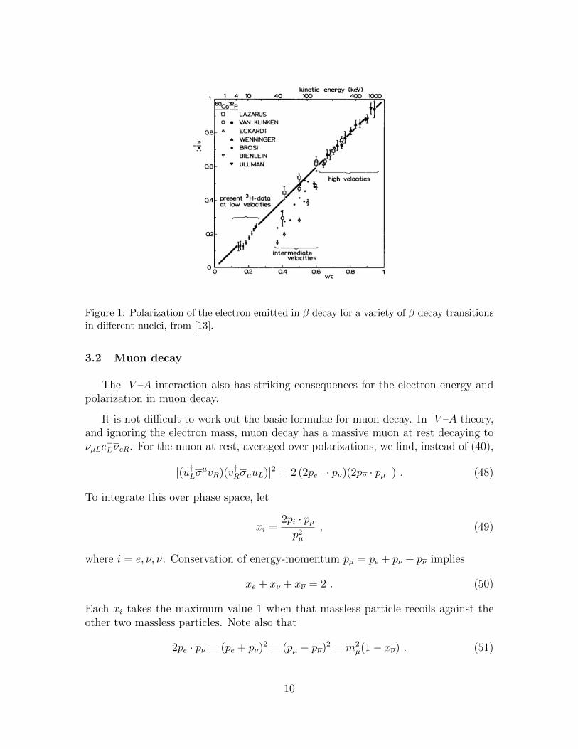
Figure 1: Polarization of the electron emitted in β decay for a variety of β decay transitionsin different nuclei, from [13].
3.2 Muon decay
The V –A interaction also has striking consequences for the electron energy andpolarization in muon decay.
It is not difficult to work out the basic formulae for muon decay. In V –A theory,and ignoring the electron mass, muon decay has a massive muon at rest decaying toνµLe
−LνeR. For the muon at rest, averaged over polarizations, we find, instead of (40),
|(u†LσµvR)(v†RσµuL)|2 = 2 (2pe− · pν)(2pν · pµ−) . (48)
To integrate this over phase space, let
xi =2pi · pµp2µ
, (49)
where i = e, ν, ν. Conservation of energy-momentum pµ = pe + pν + pν implies
xe + xν + xν = 2 . (50)
Each xi takes the maximum value 1 when that massless particle recoils against theother two massless particles. Note also that
2pe · pν = (pe + pν)2 = (pµ − pν)2 = m2
µ(1− xν) . (51)
10
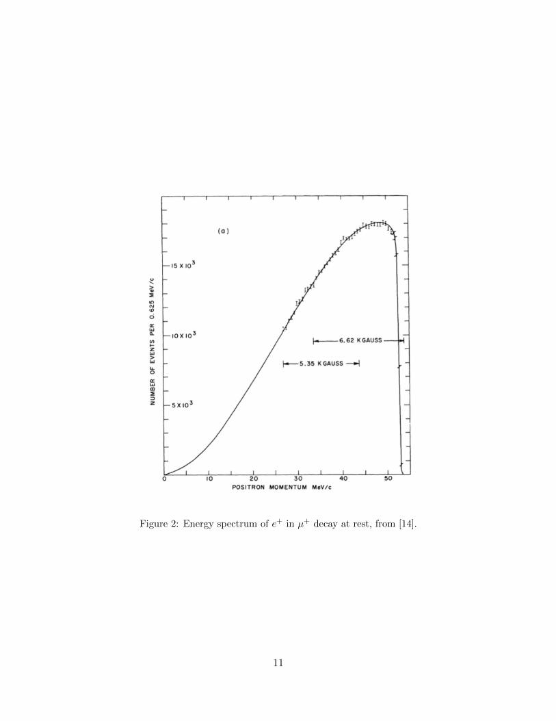
Figure 2: Energy spectrum of e+ in µ+ decay at rest, from [14].
11
Three-body phase space takes a simple form in the xi variables,
∫dΠ3 =
m2µ
128π3
∫dxedxν . (52)
Assembling the pieces, the muon decay rate is predicted to be
Γ =1
2mµ
(4GF√
2
)2 m2µ
128π3
∫dxedxν 2m4
µxν(1− xν) . (53)
The integral over xν is ∫ 1
1−xedxν xν(1− xν) =
1
2x2e −
1
3x3e . (54)
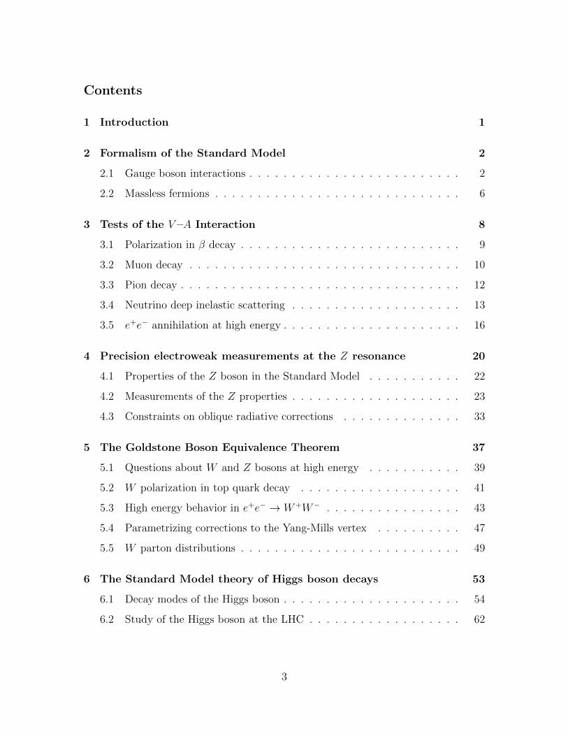
Then finally we find for the electron energy distribution
dΓ
dxe=G2Fm
5µ
16π3
(x2e2− x3e
3
). (55)
This shape of this distribution is quite characteristic, with a double zero at Ee = 0and zero slope at the endpoint at Ee = mµ/2. Both effects are slightly rounded byradiative corrections, but, with these taken into account, the prediction agrees withthe measured spectrum to high precision, as shown in Fig. 2 [14].
3.3 Pion decay
Charged pion decay is mediated by the V –A interaction
4GF√2
(d†LσµuL)
(ν†eLσµeL + 통LσµµL
)(56)
At first sight, it might seem that the π+ must decay equally often to e+ and µ+.Experimentally, almost all pion decays are to µ+. Can this be reconciled with V –A?
The pion matrix element is
〈0| d†LσµuL∣∣∣π+(p)
⟩= −i1
2Fπp
µ , (57)
where Fπ is the pion decay constant, equal to 135 MeV. The matrix element of (56)then evaluates to
4GF√2· (− i
2Fπ) pµU †νLσµV`+ . (58)
The pion is at rest, sopµσµ = mπ · 1 . (59)
12
The neutrino is (essentially) massless and therefore must be left-handed. The pionhas spin 0, so angular momentum requires that the `+ is also left-handed. But, from(31), the lepton spinor is then
VL =(√
E − p ξR×
)(60)
The matrix element (58) reduces to
i4GF√
2· (1
2Fπ)
√2Eνmπ
√E` − p` . (61)
Two-body kinematics gives Eν = pν = p` = (m2π−m2
`)/2mπ. Then (E`−p`) = m2`/m
2π.
Phase space includes the factor 2p`/mπ, which brings another factor of (E` − p`).Finally we find
Γ(π+ → `+ν) =G2Fm
3πF
2π
8π
m2`
m2π
(1− m2`
m2π
)2 . (62)
The overall factor m2`/m
2π comes from the matrix element (60). Angular momen-
tum conservation requires the `+ to have the wrong helicity with respect to V –A,accounting for this suppression factor.
The result (62) leads to the ratio of branching fractions
BR(π+ → e+νe)
BR(π+ → µ+νµ)=m2e
m2µ
(m2π −m2
e
m2π −m2
µ
)2
= 1.28× 10⁻⁴ , (63)
in good agreement with the observed value 1.23× 10⁻⁴.
3.4 Neutrino deep inelastic scattering
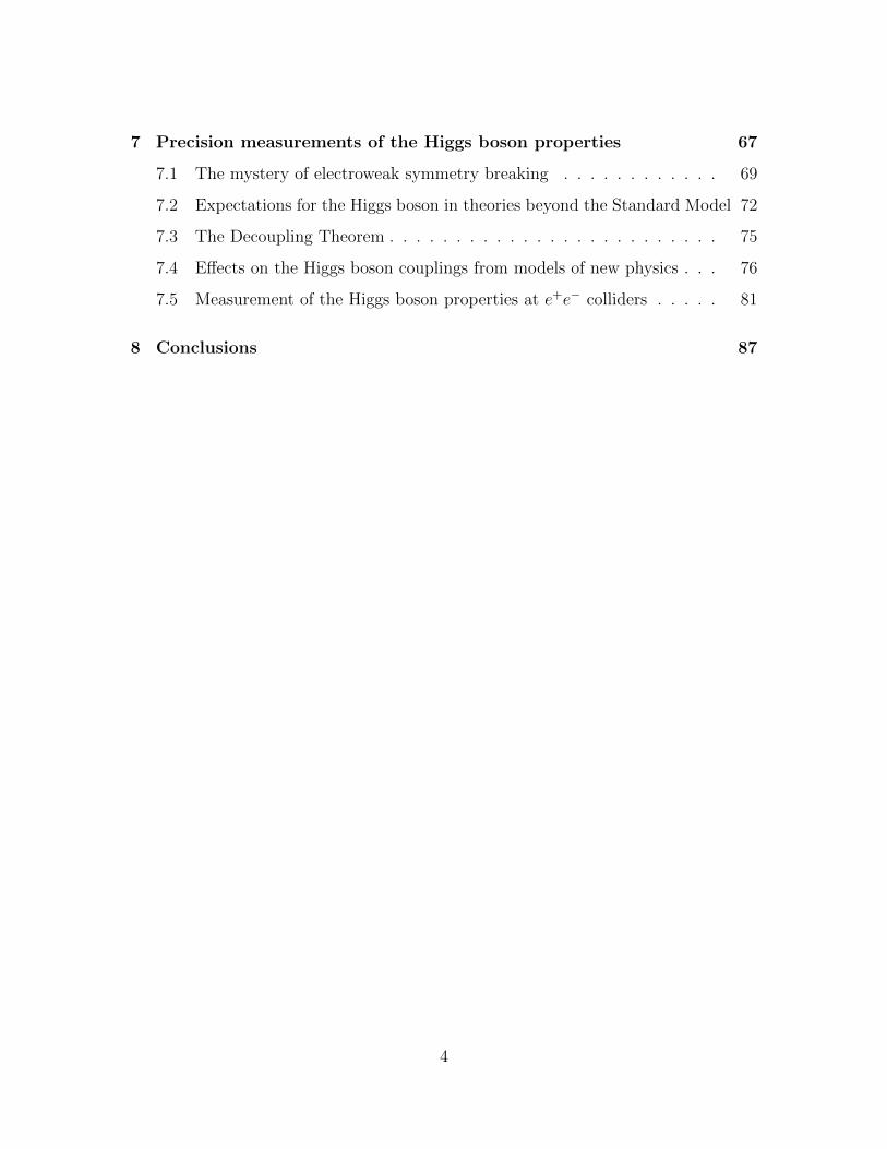
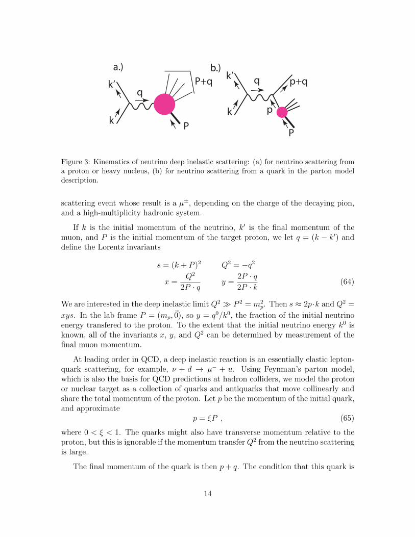
The helicity structure of the V –A interaction is also seen in the energy distri-butions in deep inelastic neutrino scattering. For electrons, deep inelastic scatteringis the scattering from a proton or nuclear target in which the momentum transfer islarge and the target is disrupted to a high mass hadronic state. The kinematics isshown in Fig. 3(a). In the leading order of QCD, deep inelastic scattering is describedby the scattering for the electron from a single quark in the parton distribution ofthe target. This kinematics is shown in Fig. 3(b).
Neutrino deep inelastic scattering experiments are done in the following way: Onefirst creates a high-energy pion beam by scattering protons from a target. Thenthe pions are allowed to decay, producing a beam of neutrinos and muons. Thebeam is made to pass through a long path length of absorber to remove the muonsand residual pions and other hadrons. Finally, the neutrinos are allowed to interactwith a large-volume detector. A charged-current neutrino reaction then leads to a
13
k
k’q
P
P+q
k
k’ q
P
p+qa.) b.)
p
Figure 3: Kinematics of neutrino deep inelastic scattering: (a) for neutrino scattering froma proton or heavy nucleus, (b) for neutrino scattering from a quark in the parton modeldescription.
scattering event whose result is a µ±, depending on the charge of the decaying pion,and a high-multiplicity hadronic system.
If k is the initial momentum of the neutrino, k′ is the final momentum of themuon, and P is the initial momentum of the target proton, we let q = (k − k′) anddefine the Lorentz invariants
s = (k + P )2 Q2 = −q2
x =Q2
2P · qy =
2P · q2P · k
(64)
We are interested in the deep inelastic limit Q2 � P 2 = m2p. Then s ≈ 2p·k and Q2 =
xys. In the lab frame P = (mp,~0), so y = q0/k0, the fraction of the initial neutrinoenergy transfered to the proton. To the extent that the initial neutrino energy k0 isknown, all of the invariants x, y, and Q2 can be determined by measurement of thefinal muon momentum.
At leading order in QCD, a deep inelastic reaction is an essentially elastic lepton-quark scattering, for example, ν + d → µ− + u. Using Feynman’s parton model,which is also the basis for QCD predictions at hadron colliders, we model the protonor nuclear target as a collection of quarks and antiquarks that move collinearly andshare the total momentum of the proton. Let p be the momentum of the initial quark,and approximate
p = ξP , (65)
where 0 < ξ < 1. The quarks might also have transverse momentum relative to theproton, but this is ignorable if the momentum transfer Q2 from the neutrino scatteringis large.
The final momentum of the quark is then p+ q. The condition that this quark is
14
on-shell is0 = (p+ q)2 = 2p · q + q2 = 2ξP · q −Q2 . (66)
Then
ξ =Q2
2P · q= x . (67)
This is a remarkable result, also due to Feynman: To the leading order in QCD, deepinelastic scattering events at a given value of the invariant x arise from scatteringfrom quarks or antiquarks in the proton with momentum fraction ξ = x.
We can now evaluate the kinematic invariants for a neutrino-quark scatteringevent. I call these s, t, u to distinguish them from the invariants of neutrino-protonscattering. First,
s = (p+ k)2 = 2p · k = 2ξP · k = x s . (68)
The momentum transfer can be evaluated from the lepton side, so
t = q2 = −Q2 . (69)
Finally, for scattering of approximately massless particles, s+ t+ u = 0, so
u = xs−Q2 = xs(1− y) . (70)
The aspect of the deep inelastic scattering cross section that is most importantfor the subject of this lecture is the distribution in y. To begin, consider the deepinelastic scattering of a νµ. The quark-level reaction is
ν + d→ µ− + u (71)
In the V –A theory, the ν and the d must be left-handed. Similarly to (41),
|(u†L(µ−)σµuL(ν))(u†L(u)σµuL(d))|2 = 4 (2pµ− · pu)(2pν · pd) = 4s2 . (72)
On the other hand, antineutrino scattering from a quark, which proceeds by thereaction
ν + u→ µ+ + d , (73)
is, in V –A theory, the scattering of a right-handed ν and a left-handed u. Then
|(v†R(µ−)σµvR(ν))(u†L(u)σµuL(d))|2 = 4 (2pµ+ · pu)(2pν · pd) = 4u2 . (74)
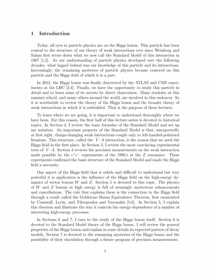
Inserting (68), (70), we see that the dependence of the deep inelastics scatteringcross section on y should be
dσ
dy(νp→ µ−X) ∼ s2 ∼ 1
dσ
dy(νp→ µ+X) ∼ u2 ∼ (1− y)2 . (75)
15
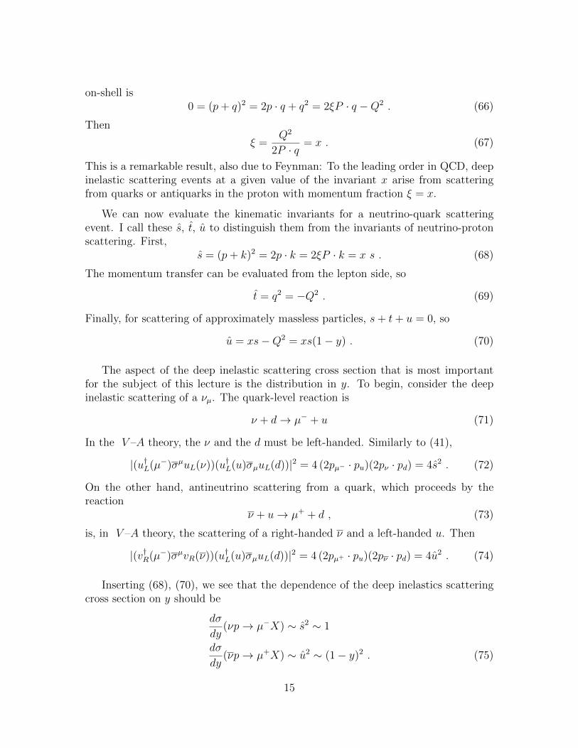
Figure 4: Dependence on the variable y of the cross sections for neutrino and antineutrinoscattering on an iron target, from [15].
These results, which I have derived for a proton target, hold for any nuclear targetunder the assumption that we consider only scattering from quarks and not fromantiquarks. For scattering from antiquarks, the dependence on y is reversed, with a(1−y)2 dependence for neutrino scattering. The experimental result, from the CDHSexperiment, a CERN neutrino experiment of the1980’s, is shown in Fig. 4 [15]. They distribution for neutrino scattering is indeed almost flat, and that for antineutrinoscattering is close to (1− y)2. The deviations from these ideal results are consistentwith arising from the antiquark content of the proton and neutron.
The same regularity can be seen in collider physics. For example, the StandardModel predicts that, in quark-antiquark annihilation to a W boson,
dσ
d cos θ(du→ W− → µ−ν) ∼ u2 ∼ (1 + cos θ)2
dσ
d cos θ(ud→ W+ → µ+ν) ∼ t2 ∼ (1− cos θ)2 , (76)
and these distributions are well verified at the LHC [16,17].
3.5 e+e− annihilation at high energy
The angular distributions in annihilation through the neutral current are morecomplex, first, because of photon-Z interference, and, second, because the weak neu-tral current couples to both left- and right-handed quarks and leptons.
16
To write formulae for the cross sections in e+e− annihilation to a fermion pair, itis simplest to begin with the cross sections for polarized initial and final states. Usingthe same principles for evaluating spinor products as before, it is not difficult to workthese out. The general form of the differential cross sections is
dσ
d cos θ(e−Le
+R → fLfR) =
πα2
2s|s FLL(s)|2 (1 + cos θ)2
dσ
d cos θ(e−Re
+L → fLfR) =
πα2
2s|s FRL(s)|2 (1− cos θ)2
dσ
d cos θ(e−Le
+R → fRfL) =
πα2
2s|s FLR(s)|2 (1− cos θ)2
dσ
d cos θ(e−Re
+L → fRfL) =
πα2
2s|s FRR(s)|2 (1 + cos θ)2 . (77)
The form factors FIJ(s) reflect photonγ–Z interference, with the pγ charges Q andthe Z charges QZ in (22). Using the subscript f to denote the flavor and chirality ofthe fermion,
FLL(s) =Qf
s+
(1/2− s2w)(I3f − s2wQf )
swcw
1
s−m2Z
FRL(s) =Qf
s+
(−s2w)(−s2wQf )
swcw
1
s−m2Z
FLR(s) =Qf
s+
1/2− s2w)(I3f − s2wQf )
swcw
1
s−m2Z
FRR(s) =Qf
s+
(−s2w)(−s2wQf )
swcw
1
s−m2Z
. (78)
The total cross sections predicted from these formulae for e+e− → hadrons, e+e− →µ+µ−, and e+e− → τ+τ− are shown in Fig. 5 and compared to data from the DELPHIexperiment at the CERN e+e− collider LEP. The resonance at the center of massenergy of 91 GeV is of course the Z boson.
Notice that, for s > m2Z , we have constructive interference in the LL and RR
polarization states and destructive interference for RL and LR. Then in an experimentwith unpolarized beams (as in the program of e+e− experiments at LEP), the LL andRR modes should dominate and produce a positive forward-backward asymmetry inthe angular distribution. This behavior is actually seen in the data. Figure 6 showsthe forward-backward asymmetry in e+e− → µ+µ− and e+e− → τ+τ− measured bythe DELPHI experiment at LEP [18]. The solid line is the prediction of the SM.
It is interesting to explore the high-energy limits of the expressions (78). Beginwith FRL(s), corresponding to e−Re
+L → fLfR. In the limit s � m2
Z and insertingQ = I3f + Y , this becomes
FRL →s2wc
2w(I3f + Yf )− s2wI3f + s4w(I3f + Yf )
s2wc2w s
17
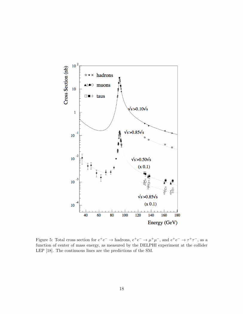
Figure 5: Total cross section for e+e− → hadrons, e+e− → µ+µ−, and e+e− → τ+τ−, as afunction of center of mass energy, as measured by the DELPHI experiment at the colliderLEP [18]. The continuous lines are the predictions of the SM.
18
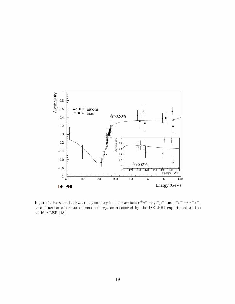
Figure 6: Forward-backward asymmetry in the reactions e+e− → µ+µ− and e+e− → τ+τ−,as a function of center of mass energy, as measured by the DELPHI experiment at thecollider LEP [18]. .
19
=s2wYfs2wc
2w s
=1
e2
(g′2YeRYf
s
). (79)
The expression in parentheses is exactly the amplitude for s-channel exchange of theU(1) boson B in the situation in which the original SU(2)×U(1) symmetry was notspontaneously broken. So we see that the full gauge symmetry is restored at highenergies.
Here is the same analysis for FLL(s):
FRL →s2wc
2w(I3f + Yf ) + (1/2− s2w)(I3f − s2w(I3f + Yf ))
s2wc2w s
=(1/2)c2wI
3f + (1/2)s2wYf
s2wc2w s
=1
e2
(g2I3eLI3fs
+g′2YeRYf
s
). (80)
Now the result is a coherent sum of A3 and B exchanges in the s-channel. Again,this is the result expected in a theory of unbroken SU(2)× U(1).
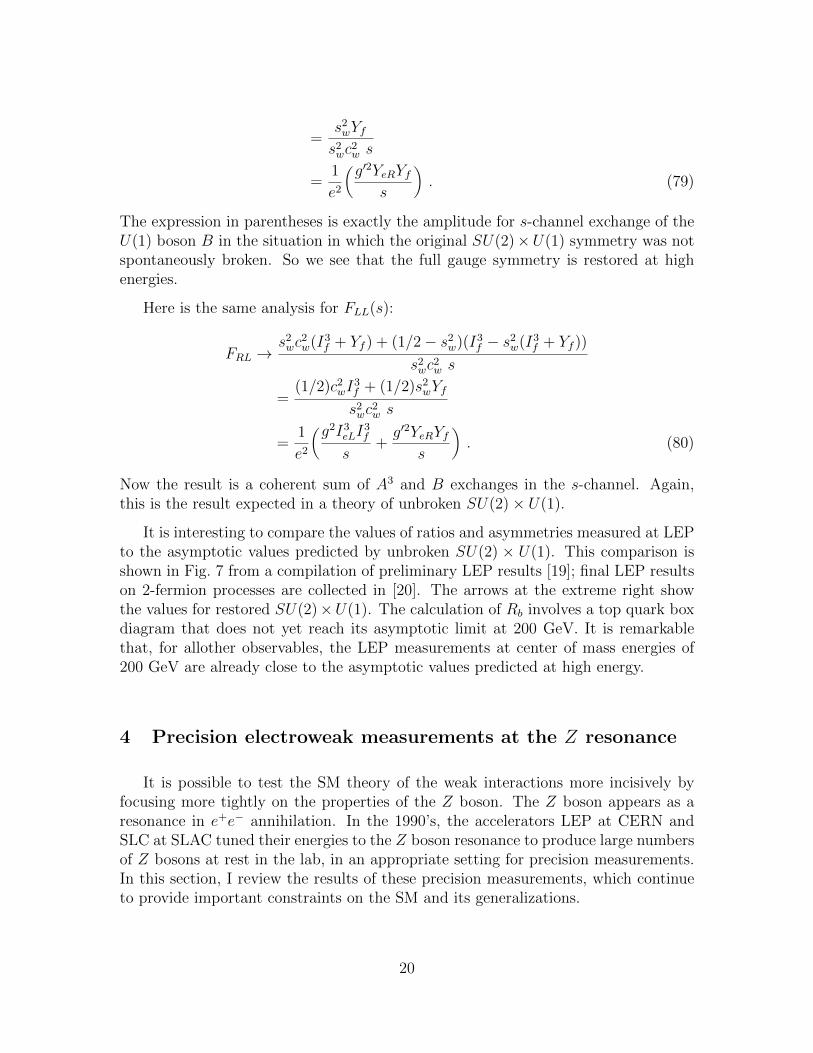
It is interesting to compare the values of ratios and asymmetries measured at LEPto the asymptotic values predicted by unbroken SU(2) × U(1). This comparison isshown in Fig. 7 from a compilation of preliminary LEP results [19]; final LEP resultson 2-fermion processes are collected in [20]. The arrows at the extreme right showthe values for restored SU(2)×U(1). The calculation of Rb involves a top quark boxdiagram that does not yet reach its asymptotic limit at 200 GeV. It is remarkablethat, for allother observables, the LEP measurements at center of mass energies of200 GeV are already close to the asymptotic values predicted at high energy.
4 Precision electroweak measurements at the Z resonance
It is possible to test the SM theory of the weak interactions more incisively byfocusing more tightly on the properties of the Z boson. The Z boson appears as aresonance in e+e− annihilation. In the 1990’s, the accelerators LEP at CERN andSLC at SLAC tuned their energies to the Z boson resonance to produce large numbersof Z bosons at rest in the lab, in an appropriate setting for precision measurements.In this section, I review the results of these precision measurements, which continueto provide important constraints on the SM and its generalizations.
20
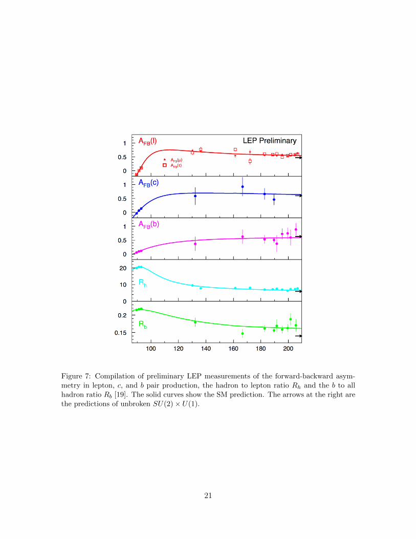
Figure 7: Compilation of preliminary LEP measurements of the forward-backward asym-metry in lepton, c, and b pair production, the hadron to lepton ratio Rh and the b to allhadron ratio Rb [19]. The solid curves show the SM prediction. The arrows at the right arethe predictions of unbroken SU(2)× U(1).
21
4.1 Properties of the Z boson in the Standard Model
My discussion will be based on the leading order matrix elements for Z decay tofLfR and fRfL. It is straightforward to work these out based on the spinor matrixelements computed in Section 2.2. The leading order matrix element for Z decay tofLfR is
M(Z → fLfR) = ig
cwQZf u
†Lσ
µvR εZµ , (81)
withQZ = I3 − s2wQ , (82)
as in (22). Using (36) for the spinor matrix element, this becomes
M = ig
cw
√2mZε
∗− · εZ . (83)
Square this and average over the direction of the fermion, or, equivalently, averageover three orthogonal directions for the Z polarization vector. The result is
⟨|M|2
⟩=
2
3
g2
c2wQ2Zfm
2Z . (84)
Then, since
Γ(Z → fLfR) =1
2mZ
1
8π
⟨|M|2
⟩, (85)
we findΓ(Z → fLfR) =
αwmZ
6c2wQ2ZfNf , (86)
where
αw =g2
4π(87)
and
Nf ={
1 lepton3(1 + αs/π + · · ·) quark
(88)
accounts the number of color states and the QCD correction. The same formula holdsfor the Z width to fRfL.
To evaluate this formula, we need values of the weak interaction coupling con-stants. The electromagnetic coupling α is famously close to 1/137. However, inquantum field theory, α is a running coupling constant that becomes larger at smallldistanct scales. At a scale of Q = mZ , α(Q) = 1/129. Later in the lecture, I willdefend a value of the weak mixing angle
s2w = 0.231 . (89)
22
Then the SU(2) and U(1) couplings take the values
αw =g2
4π=
1
29.8α′ =
g′2
4π=
1
99.1(90)
It is interesting to compare these values to other fundamental SM couplings taken atthe same scale Q = mZ ,
αs =1
8.5αt =
y2t4π
=1
12.7. (91)
All of these SM couplings are roughly of the same order of magnitude.
Using (89) or (90), we can tabulate the values of the Z couplings to left- andright-handed fermions,
species QZL QZR Sf Afν +1
2- 0.250 1.00
e −12
+ s2w +s2W 0.126 0.15u +1
2− 2
3s2w −2
3s2W 0.143 0.67
d −12
+ 13s2w +1
3s2W 0.185 0.94
(92)
In this table, the quantities evalated numerically are
Sf = Q2ZL +Q2
ZR Af =Q2ZL −Q2
ZR
Q2ZL +Q2
ZR
. (93)
The quantity Sf gives the contribution of the species f to the total decay rate ofthe Z boson. The quantity Af gives the polarization asymmetry for f , that is, thepreponderance of fL over fR, in Z decays,
4.2 Measurements of the Z properties
It is possible to measure many of the total rates and polarization asymmetriesfor individual species in a very direct way through experiments on the Z resonance.This subject is reviewed in great detail in the report [22]. Values of the Z observablesgiven below are taken from this reference unless it is stated otherwise.
The Sf are tested by the measurement of the Z resonance width and its branchingratios. Using (86), we find for the total width of the Z
ΓZ =αwmZ
6c2w
[3 · 0.25 + 3 · 0.126
+2 · (3.1) · 0.144 + 3 · (3.1) · 0.185]. (94)
23
The four terms denote the contributions from 3 generations of ν, e, u, and d, minusthe top quark, which is too heavy to appear in Z decays. The numerical predictionis
ΓZ = 2.49 GeV (95)
The separate terms in (94) give the branching ratios
BR(νeνe) = 6.7% BR(e+e−) = 3.3%
BR(uu) = 11.9% BR(dd) = 15.3% (96)
The measured value of the total width, whose extraction I will discuss in a moment,is
ΓZ = 2.4952± 0.0023 GeV . (97)
This is in very good agreement with (95), with accuracy such that a valid comparisonwith theory requires the inclusion of electroweak radiative corrections, with typicallyare of order 1%. The measurements of branching ratios and polarization asymmetrythat I review later in this section are also of sub-% accuracy. At the end of this sec-tion, I will present a more complete comparison of theory and experiment, includingradiative corrections to the theoretical predictions.
To begin our review of the experimental measurements, we should discuss themeasurement of the Z resonance mass and width in more detail. Ideally, the Z is aBreit-Wigner resonance, with cross section shape
σ ∼∣∣∣∣ 1
s−m2Z + imZΓZ
∣∣∣∣2 . (98)
At first sight, it seems that we can simply read off the Z mass as the maximum of theresonance and the width as the observed width at half maximum. However, we musttake into account that the resonance is distorted by initial-state radiation. As theelectron and positron collide and annihilate into a Z, they can radiate hard collinearphotons. Because of this, the resonance is pushed over to higher energies, an effectthat shifts the peak and creates a long tail on above the resonance. The magnitudeof the photon radiation is given by the parameter
β =2α
π(log
s
m2e
− 1) = 0.108 at s = m2Z (99)
In addition, since the Z is narrow, the effect of this radiation is magnified, since evena relatively soft photon can push the center of mass energy off of the resonance. Thesize of the correction can be roughly estimated as
−β · logmZ
ΓZ= 40% . (100)
24
To make a proper accounting of this effect, we need to include arbitrary numbersof radiated collinear photons. Fadin and Kuraev introduced the idea of viewing theradiated photons and the final annihilating electron as partons in the electron in thesame way that quarks and gluons are treated as partons in the proton [21]. For theproton, the parton distribution is generated by non-perturbative effects, but for theelectron the parton distributions are generated only by QED, so that they can becalculated as a function of α. The result for the parton distribution of the electronin the electron, to order α, is
fe(z, s) =β
2(1− z)β/2−1(1 +
3
8β)− 1
4β(1 + z) + · · · , (101)
where z is the momentum fraction of the original electron carried into the e+e−
annihilation to a Z boson. The cross section for producing a Z boson would thenbe a convolution of the Breit-Wigner cross section (98) with the parton distribution(101) and the corresponding distribution for the positron. For the LEP experiments,this theory was extended to include two orders of subleading logarithms and finitecorrections of order α2 [23].
The experimental aspects of the measurement of the Z resonance lineshape werealso very challenging; see Section 2.2 of [22]. Careful control was needed for point-to-point normalization errors across the Z resonance. The absolute energy of the LEPring was calibrated using resonant depolarization of a single electron beam and thencorrected for two-beam effects. This calibration was found to depend on the seasonand the time of day. Some contributing effects were the changes in the size of theLEP tunnel due to the annual change in the water level in Lake Geneva and currentsurges in the LEP magnets due to the passage to the TGV leaving Geneva for Paris.
Some final results for the resonance line shape measurement are shown in Figs. 8,9. The first of these figures shows the measurements by the OPAL experiment over theresonance and the detaied agreement of the shape between theory and experiment [24].The second shows the combination of the resonance height and width measurementsfrom the four LEP experiments ALEPH, DELPHI, L3, and OPAL [22]. In this figure,the lower curve is the radiatively corrected result; the higher curve is the inferredBreit-Wigner distribution excluding the effects of radiative corrections.
The measurement of branching ratios is more straightforward. It is necessaryonly to collect Z decay events and sort them into categories. The various types ofleptonic and hadronic decay modes have very different, characteristic forms. Typicalevents are shown in Fig. 10 for hadronic, e+e−, µ+µ−, and τ+τ− decays [25]. Themajor backgrounds are from Bhabha scattering and 2-photon events. These do notresemble Z decay events and are rather straightforwardly separated. Nonresonante+e− annihilations are also a small effect, generally providing backgrounds at onlythe level of parts per mil. An exception is the Z decay to τ+τ−, which can be fakedby hadronic e+e− annihilations with radiation to provide a background level of a few
25
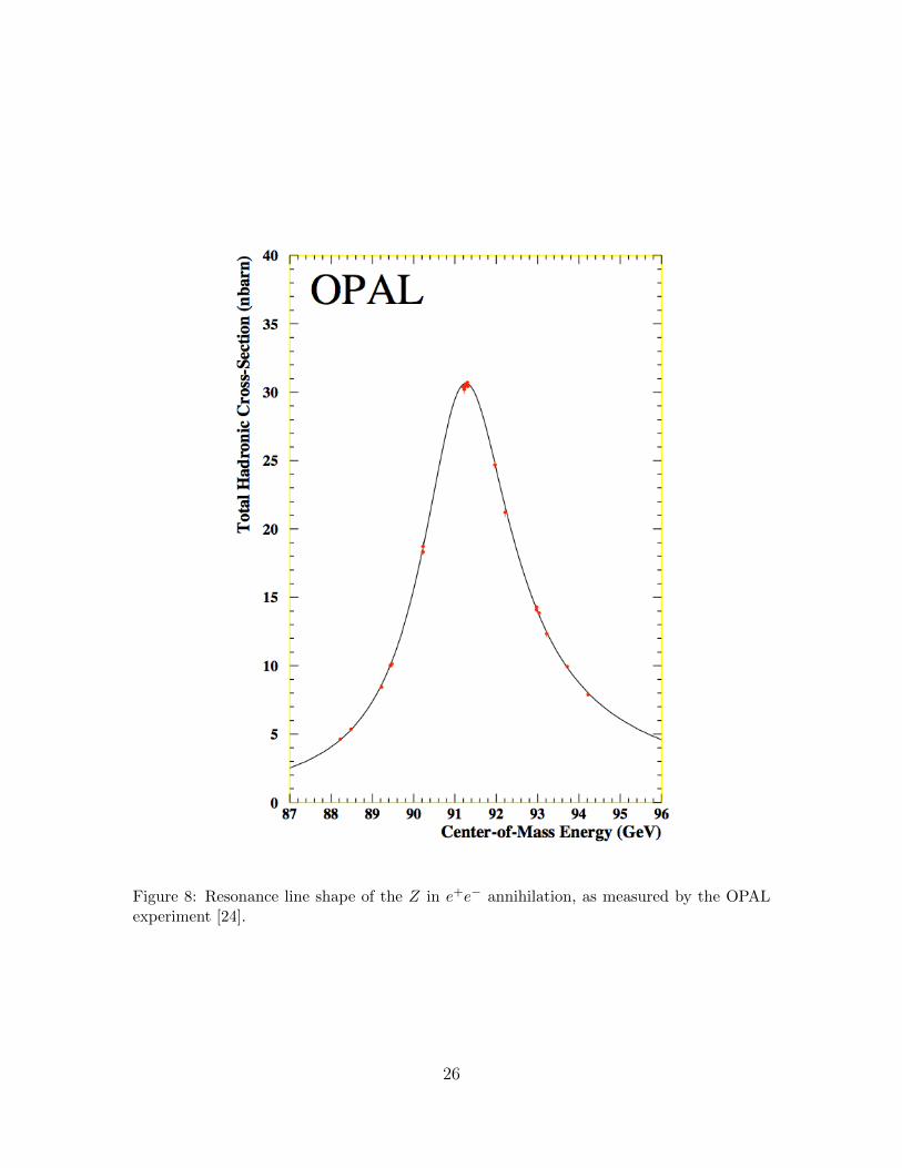
Figure 8: Resonance line shape of the Z in e+e− annihilation, as measured by the OPALexperiment [24].
26
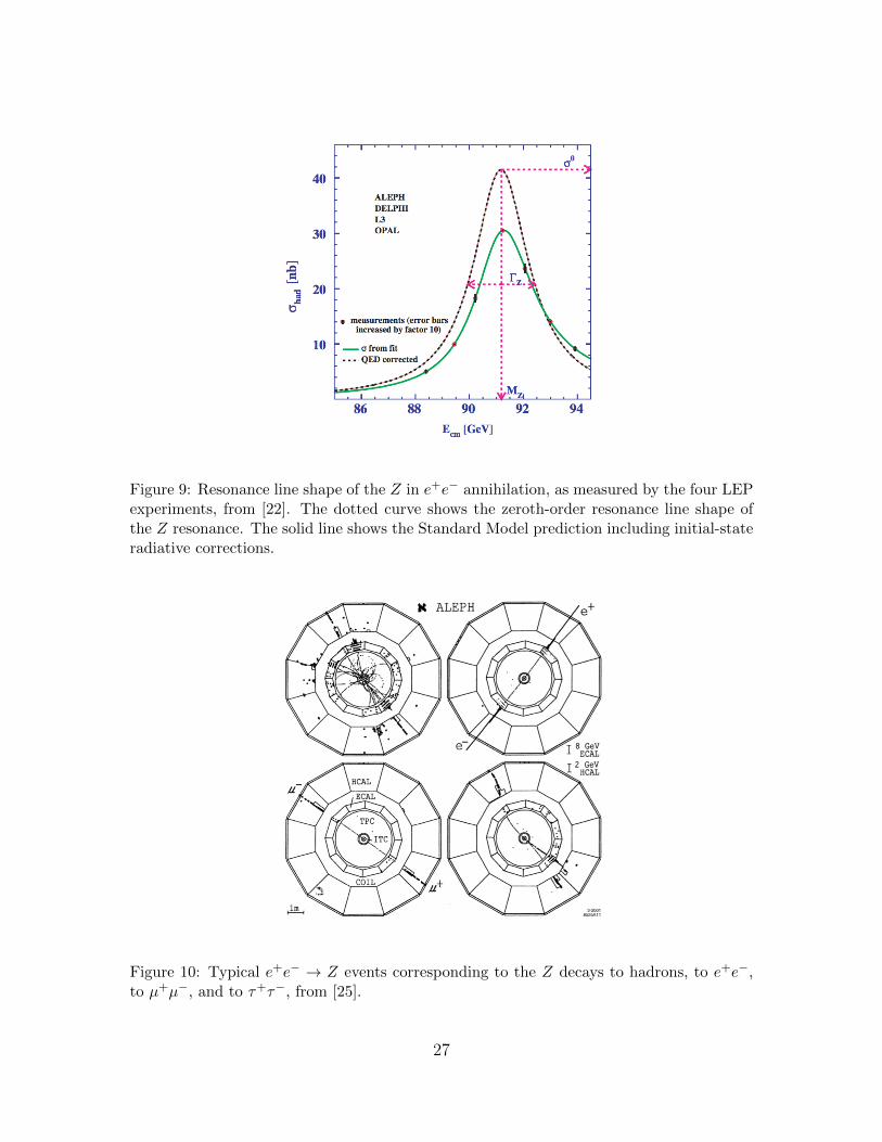
Figure 9: Resonance line shape of the Z in e+e− annihilation, as measured by the four LEPexperiments, from [22]. The dotted curve shows the zeroth-order resonance line shape ofthe Z resonance. The solid line shows the Standard Model prediction including initial-stateradiative corrections.
Figure 10: Typical e+e− → Z events corresponding to the Z decays to hadrons, to e+e−,to µ+µ−, and to τ+τ−, from [25].
27
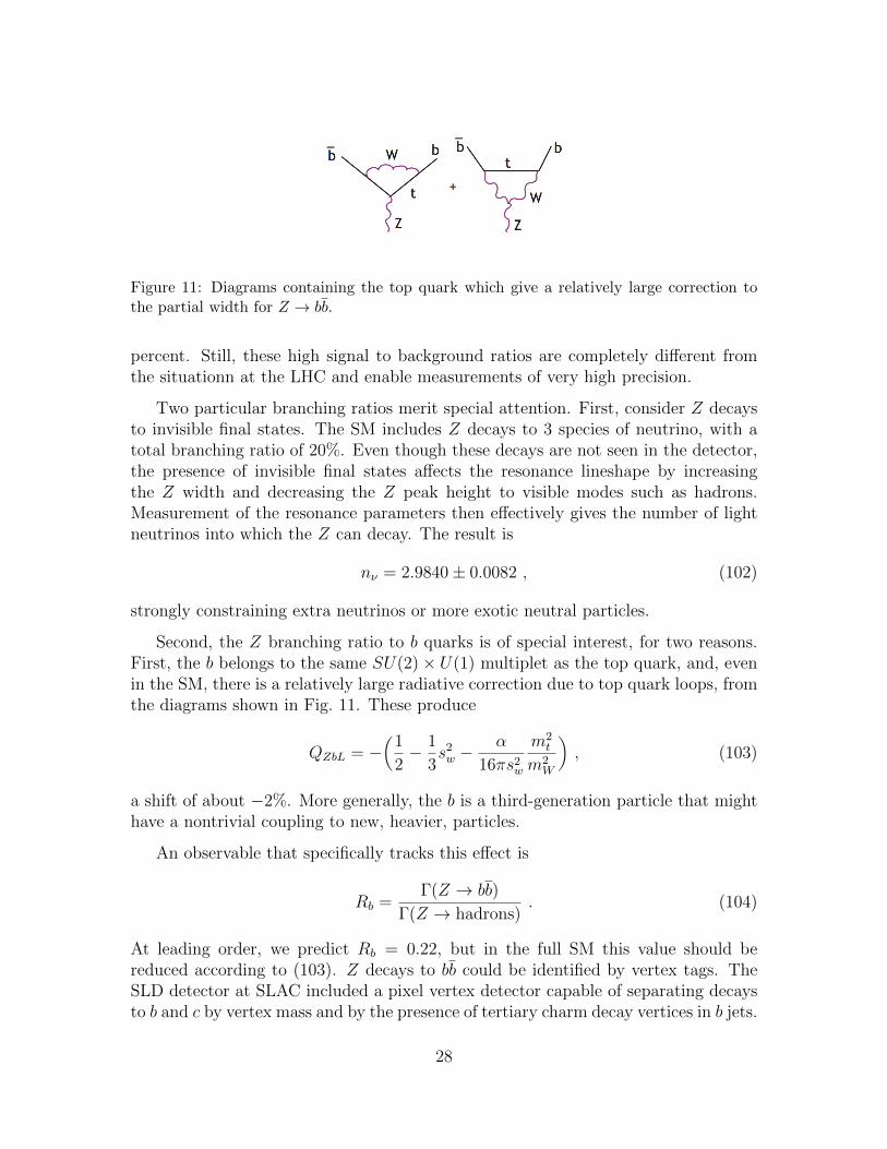
Figure 11: Diagrams containing the top quark which give a relatively large correction tothe partial width for Z → bb.
percent. Still, these high signal to background ratios are completely different fromthe situationn at the LHC and enable measurements of very high precision.
Two particular branching ratios merit special attention. First, consider Z decaysto invisible final states. The SM includes Z decays to 3 species of neutrino, with atotal branching ratio of 20%. Even though these decays are not seen in the detector,the presence of invisible final states affects the resonance lineshape by increasingthe Z width and decreasing the Z peak height to visible modes such as hadrons.Measurement of the resonance parameters then effectively gives the number of lightneutrinos into which the Z can decay. The result is
nν = 2.9840± 0.0082 , (102)
strongly constraining extra neutrinos or more exotic neutral particles.
Second, the Z branching ratio to b quarks is of special interest, for two reasons.First, the b belongs to the same SU(2)× U(1) multiplet as the top quark, and, evenin the SM, there is a relatively large radiative correction due to top quark loops, fromthe diagrams shown in Fig. 11. These produce
QZbL = −(
1
2− 1
3s2w −
α
16πs2w
m2t
m2W
), (103)
a shift of about −2%. More generally, the b is a third-generation particle that mighthave a nontrivial coupling to new, heavier, particles.
An observable that specifically tracks this effect is
Rb =Γ(Z → bb)
Γ(Z → hadrons). (104)
At leading order, we predict Rb = 0.22, but in the full SM this value should bereduced according to (103). Z decays to bb could be identified by vertex tags. TheSLD detector at SLAC included a pixel vertex detector capable of separating decaysto b and c by vertex mass and by the presence of tertiary charm decay vertices in b jets.
28
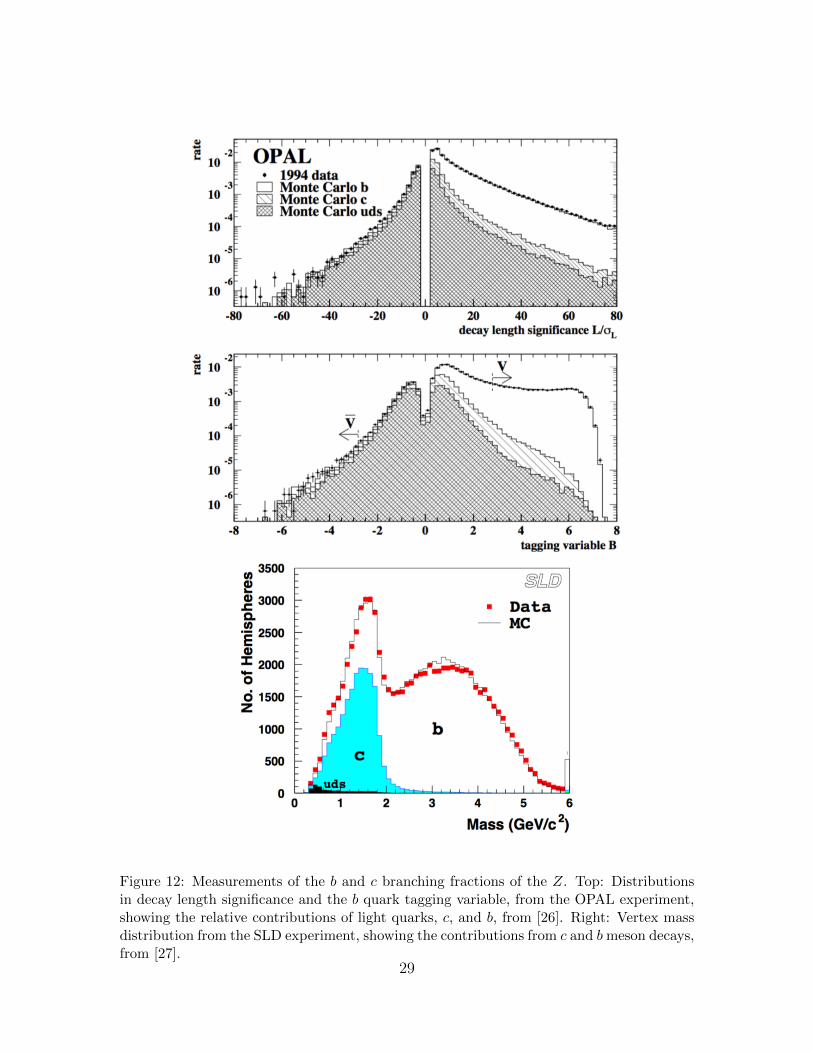
Figure 12: Measurements of the b and c branching fractions of the Z. Top: Distributionsin decay length significance and the b quark tagging variable, from the OPAL experiment,showing the relative contributions of light quarks, c, and b, from [26]. Right: Vertex massdistribution from the SLD experiment, showing the contributions from c and bmeson decays,from [27].
29
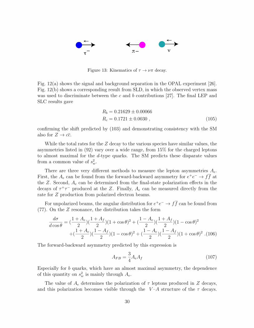
Figure 13: Kinematics of τ → νπ decay.
Fig. 12(a) shows the signal and background separation in the OPAL experiment [26].Fig. 12(b) shows a corresponding result from SLD, in which the observed vertex masswas used to discriminate between the c and b contributions [27]. The final LEP andSLC results gave
Rb = 0.21629± 0.00066
Rc = 0.1721± 0.0030 , (105)
confirming the shift predicted by (103) and demonstrating consistency with the SMalso for Z → cc.
While the total rates for the Z decay to the various species have similar values, theasymmetries listed in (92) vary over a wide range, from 15% for the charged leptonsto almost maximal for the d-type quarks. The SM predicts these disparate valuesfrom a common value of s2w.
There are three very different methods to measure the lepton asymmetries Ae.First, the Ae can be found from the forward-backward asymmetry for e+e− → ff atthe Z. Second, Ae can be determined from the final-state polarization effects in thedecays of τ+τ− produced at the Z. Finally, Ae can be measured directly from therate for Z production from polarized electron beams.
For unpolarized beams, the angular distribution for e+e− → ff can be found from(77). On the Z resonance, the distribution takes the form
dσ
d cos θ= (
1 + Ae2
)(1 + Af
2)(1 + cos θ)2 + (
1− Ae2
)(1 + Af
2)(1− cos θ)2
+(1 + Ae
2)(
1− Af2
)(1− cos θ)2 + (1− Ae
2)(
1− Af2
)(1 + cos θ)2 .(106)
The forward-backward asymmetry predicted by this expression is
AFB =3
4AeAf (107)
Especially for b quarks, which have an almost maximal asymmetry, the dependenceof this quantity on s2w is mainly through Ae.
The value of Ae determines the polarization of τ leptons produced in Z decays,and this polarization becomes visible through the V –A structure of the τ decays.
30
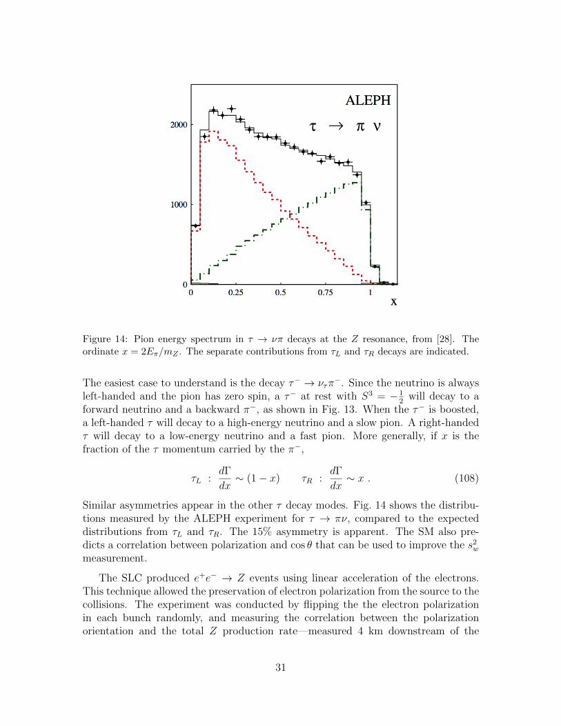
Figure 14: Pion energy spectrum in τ → νπ decays at the Z resonance, from [28]. Theordinate x = 2Eπ/mZ . The separate contributions from τL and τR decays are indicated.
The easiest case to understand is the decay τ− → ντπ−. Since the neutrino is always
left-handed and the pion has zero spin, a τ− at rest with S3 = −12
will decay to aforward neutrino and a backward π−, as shown in Fig. 13. When the τ− is boosted,a left-handed τ will decay to a high-energy neutrino and a slow pion. A right-handedτ will decay to a low-energy neutrino and a fast pion. More generally, if x is thefraction of the τ momentum carried by the π−,
τL :dΓ
dx∼ (1− x) τR :
dΓ
dx∼ x . (108)
Similar asymmetries appear in the other τ decay modes. Fig. 14 shows the distribu-tions measured by the ALEPH experiment for τ → πν, compared to the expecteddistributions from τL and τR. The 15% asymmetry is apparent. The SM also pre-dicts a correlation between polarization and cos θ that can be used to improve the s2wmeasurement.
The SLC produced e+e− → Z events using linear acceleration of the electrons.This technique allowed the preservation of electron polarization from the source to thecollisions. The experiment was conducted by flipping the the electron polarizationin each bunch randomly, and measuring the correlation between the polarizationorientation and the total Z production rate—measured 4 km downstream of the
31
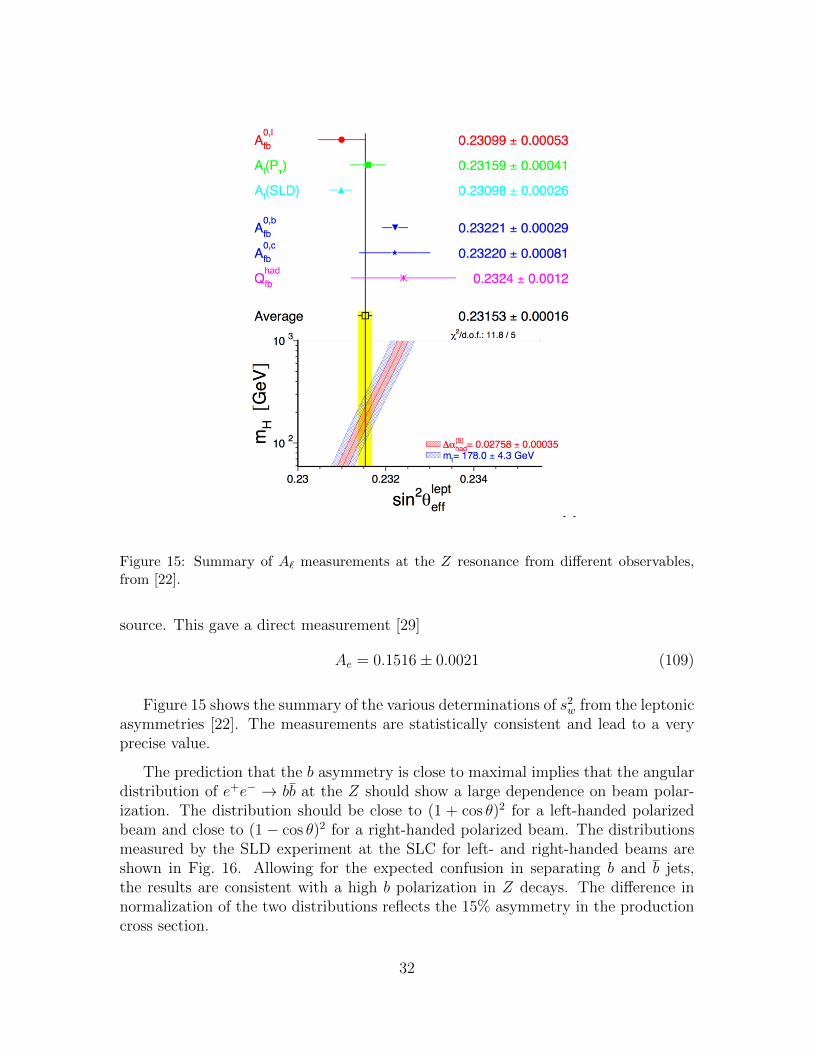
Figure 15: Summary of A` measurements at the Z resonance from different observables,from [22].
source. This gave a direct measurement [29]
Ae = 0.1516± 0.0021 (109)
Figure 15 shows the summary of the various determinations of s2w from the leptonicasymmetries [22]. The measurements are statistically consistent and lead to a veryprecise value.
The prediction that the b asymmetry is close to maximal implies that the angulardistribution of e+e− → bb at the Z should show a large dependence on beam polar-ization. The distribution should be close to (1 + cos θ)2 for a left-handed polarizedbeam and close to (1− cos θ)2 for a right-handed polarized beam. The distributionsmeasured by the SLD experiment at the SLC for left- and right-handed beams areshown in Fig. 16. Allowing for the expected confusion in separating b and b jets,the results are consistent with a high b polarization in Z decays. The difference innormalization of the two distributions reflects the 15% asymmetry in the productioncross section.
32
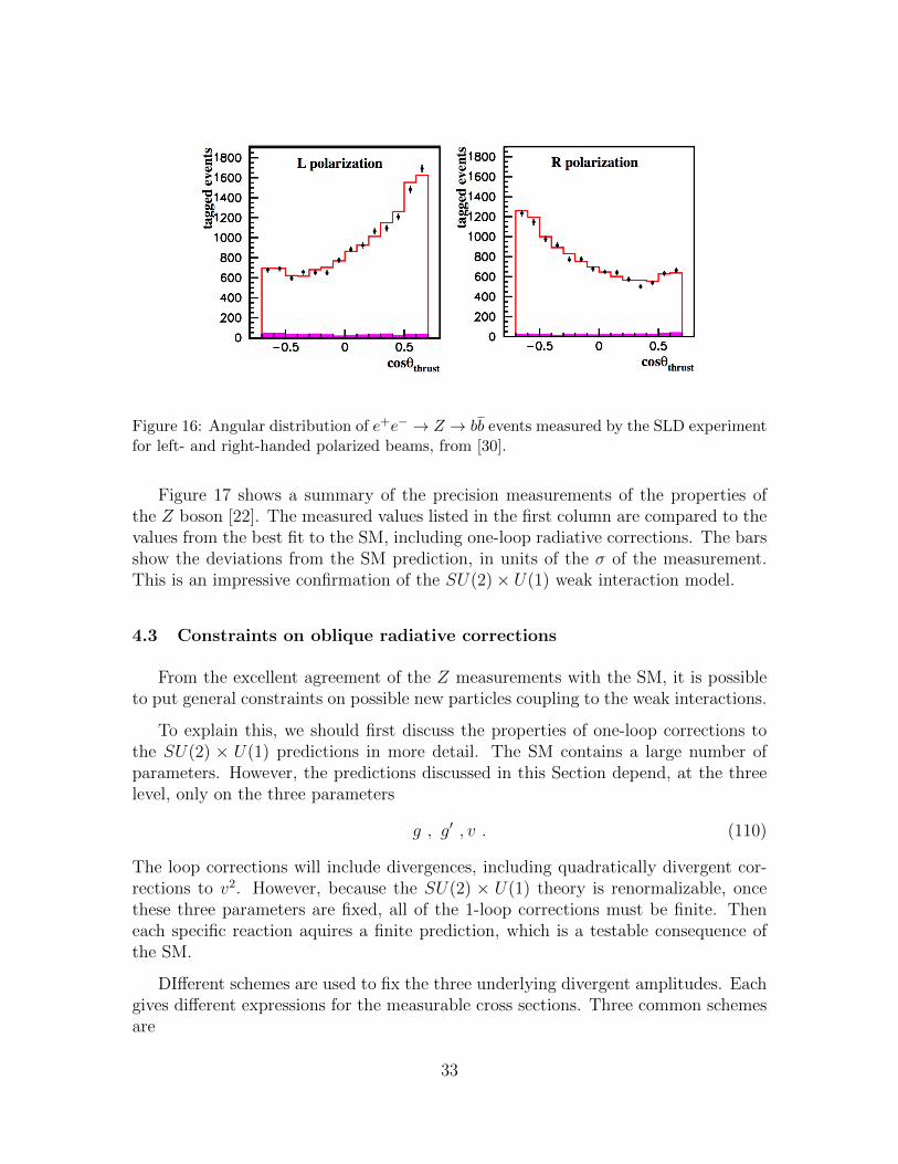
Figure 16: Angular distribution of e+e− → Z → bb events measured by the SLD experimentfor left- and right-handed polarized beams, from [30].
Figure 17 shows a summary of the precision measurements of the properties ofthe Z boson [22]. The measured values listed in the first column are compared to thevalues from the best fit to the SM, including one-loop radiative corrections. The barsshow the deviations from the SM prediction, in units of the σ of the measurement.This is an impressive confirmation of the SU(2)× U(1) weak interaction model.
4.3 Constraints on oblique radiative corrections
From the excellent agreement of the Z measurements with the SM, it is possibleto put general constraints on possible new particles coupling to the weak interactions.
To explain this, we should first discuss the properties of one-loop corrections tothe SU(2) × U(1) predictions in more detail. The SM contains a large number ofparameters. However, the predictions discussed in this Section depend, at the threelevel, only on the three parameters
g , g′ , v . (110)
The loop corrections will include divergences, including quadratically divergent cor-rections to v2. However, because the SU(2) × U(1) theory is renormalizable, oncethese three parameters are fixed, all of the 1-loop corrections must be finite. Theneach specific reaction aquires a finite prediction, which is a testable consequence ofthe SM.
DIfferent schemes are used to fix the three underlying divergent amplitudes. Eachgives different expressions for the measurable cross sections. Three common schemesare
33
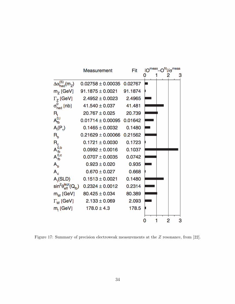
Figure 17: Summary of precision electroweak measurements at the Z resonance, from [22].
34
• applying MS subtraction, as in QCD
• fixing α(mZ), mZ , mW to their measured values (Marciano-Sirlin scheme) [32]
• fixing α(mZ), mZ , GF to their measured values (on shell Z scheme)
In the MS scheme, used by the Particle Data Group, the MS parameters g, g′, andv are unphysical but can be defined as the values that give the best fit to the corpusof SM measurements [31].
The various schemes for renormalizing the SU(2) × U(1) model lead to differentdefinitions of s2w that are found in the literature. In the Marciano-Sirlin scheme, wedefine θw by
cw ≡ mW/mZ . (111)
This leads tos2w = 0.22290± 0.00008 . (112)
We will see in Section 4 that the relation (111) is often needed to insure the correctbehavior in high-energy reactions of W and Z, so it is useful that this relation isinsured at the tree level. Thus, the Marciano-Sirlin definition of θw is the mostcommon one used in event generators for LHC. However, one should note that thevalue (112) is significantly different from the value (89) that best represents the sizesof the Z cross sections and asymmetries.
In the on-shell Z scheme, θw is defined by
sin22θw = (2cwsw)2 ≡ 4πα(mZ)√2GFm2
Z
, (113)
leading tos2w = 0.231079± 0.000036 . (114)
This defintion gives at tree level a value that is much closer to (89). All three valuesof sin2 θw lead to the same predictions for the relation of observables to observablesafter the (scheme-dependent) finite 1-loop corrections are included.
One particular class of radiative corrections is especially simple to analyze. Ifnew particles have no direct coupling to light fermions, they can apprear in radiativecorrections to the Z observables only through vector boson vacuum polarization am-plitudes. Effects of this type are called oblique radiative corrections. These effectscan be analyzed in a quite general way.
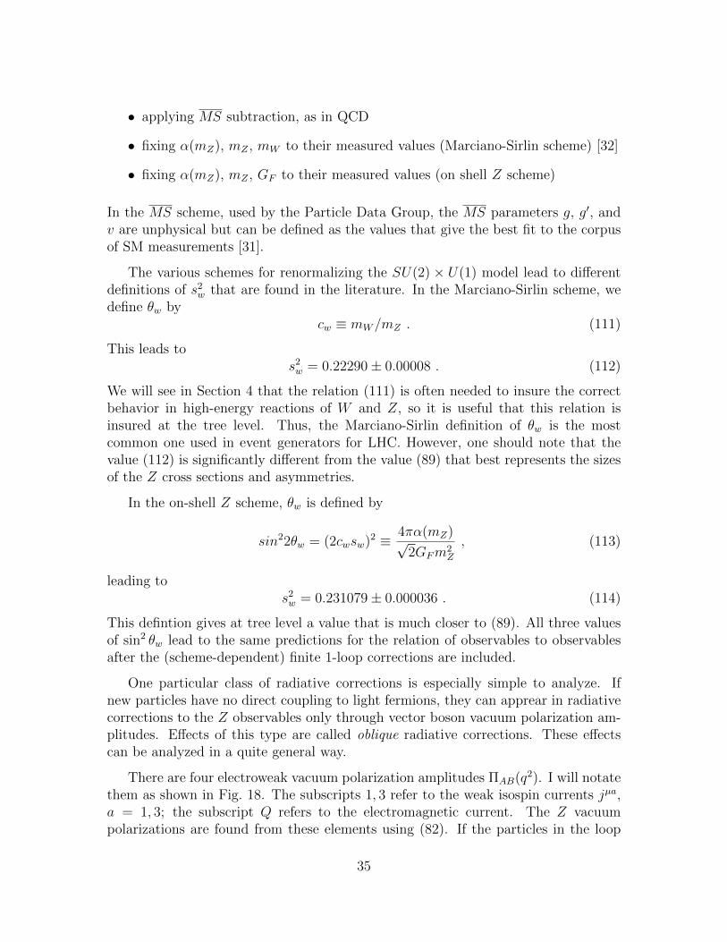
There are four electroweak vacuum polarization amplitudes ΠAB(q2). I will notatethem as shown in Fig. 18. The subscripts 1, 3 refer to the weak isospin currents jµa,a = 1, 3; the subscript Q refers to the electromagnetic current. The Z vacuumpolarizations are found from these elements using (82). If the particles in the loop
35
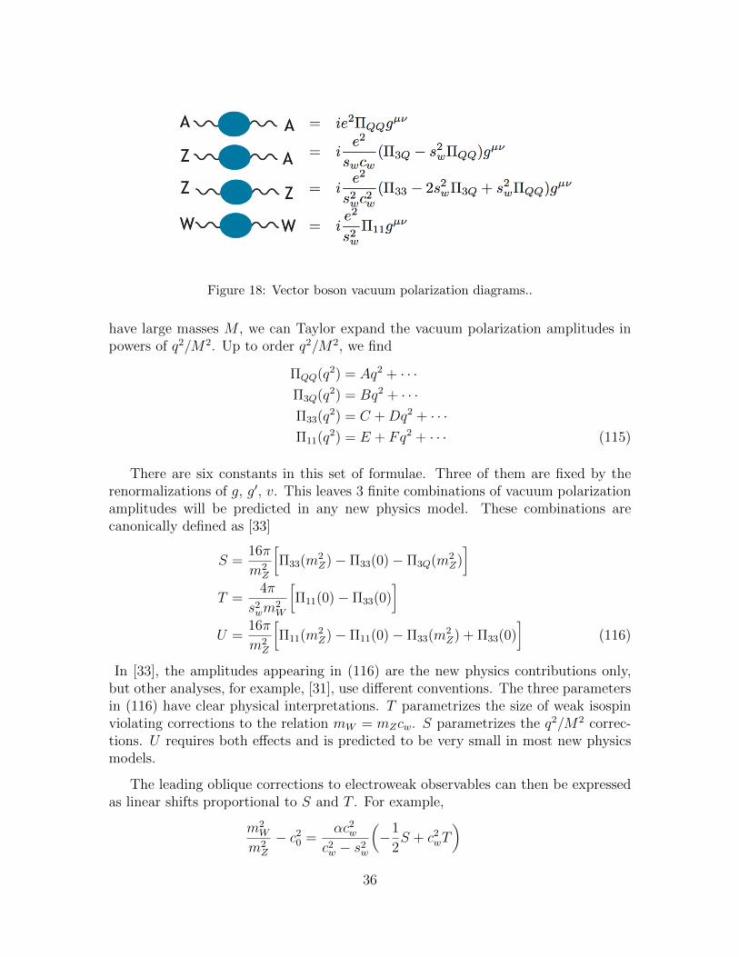
Figure 18: Vector boson vacuum polarization diagrams..
have large masses M , we can Taylor expand the vacuum polarization amplitudes inpowers of q2/M2. Up to order q2/M2, we find
ΠQQ(q2) = Aq2 + · · ·Π3Q(q2) = Bq2 + · · ·Π33(q
2) = C +Dq2 + · · ·Π11(q
2) = E + Fq2 + · · · (115)
There are six constants in this set of formulae. Three of them are fixed by therenormalizations of g, g′, v. This leaves 3 finite combinations of vacuum polarizationamplitudes will be predicted in any new physics model. These combinations arecanonically defined as [33]
S =16π
m2Z
[Π33(m
2Z)− Π33(0)− Π3Q(m2
Z)]
T =4π
s2wm2W
[Π11(0)− Π33(0)
]U =
16π
m2Z
[Π11(m
2Z)− Π11(0)− Π33(m
2Z) + Π33(0)
](116)
In [33], the amplitudes appearing in (116) are the new physics contributions only,but other analyses, for example, [31], use different conventions. The three parametersin (116) have clear physical interpretations. T parametrizes the size of weak isospinviolating corrections to the relation mW = mZcw. S parametrizes the q2/M2 correc-tions. U requires both effects and is predicted to be very small in most new physicsmodels.
The leading oblique corrections to electroweak observables can then be expressedas linear shifts proportional to S and T . For example,
m2W
m2Z
− c20 =αc2w
c2w − s2w
(−1
2S + c2wT
)
36
s2∗ − s20 =α
c2w − s2w
(−1
2
1
4S − s2wc2wT
), (117)
where s0, c0 are the values of sw and cw in the on-shell Z scheme and s∗ is the valueof sw used to evaluate the Z asymmetries Af . By fitting to the formulae such as(117), we can obtain general constraints that can be applied to a large class of newphysics models.
Some guidance about the expected sizes of S and T is given by the result for onenew heavy electroweak doublet,
S =1
6πT =
|m2U −m2
D|m2Z
. (118)
A complete heavy fourth generation gives S = 0.2. The effects of the SM top quarkand Higgs boson can also be expressed approximately in the S, T framework,
top : S =1
6πlog
m2t
m2Z
T =3
16πs2wc2w
m2t
m2Z
Higgs : S =1
12πlog
m2h
m2Z
T = − 3
16πc2wlog
m2h
m2Z
(119)
The appearance of corrections proportional to m2t/m
2Z , which we have already seen
in (103), will be explained in Section 5.
Figure 19 shows the progress of the S, T fit with our improved understanding ofthe SM. Figure 19(a) reflects the situation in 1991, before the discovery of the topquark [33]. The two vertical lines to the left are predictions of the SM with a varyingtop quark mass. Values of mt in the range of 170–180 GeV are highly favored by theprecision electroweak data. The measurement of S, even without the value of mt,strongly constrained the “technicolor” models of electroweak symmetry breaking. (Iwill describe these models at the end of Section 7.2.) Figure 19(b) shows the S, T fitin 2008. The solid curve shows the predictions of the SM with a variable Higgs bosonmass. Values of the Higgs mass close to 100 GeV are strongly favored. Figure 19(c)shows the current S, T fit [34]. The fit is in good agreement with the SM with thenow-measured values of mt and mh. It also is in substantial tension with the presenceof a fourth generation of quarks and leptons.
5 The Goldstone Boson Equivalence Theorem
In this section, I will describe the properties of the weak interactions at energiesmuch greater than mW and mZ . Some new conceptual issues appear here. Theseaffect the energy-dependence of W and Z boson reactions at high energy and the
37
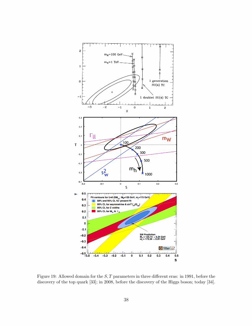
Figure 19: Allowed domain for the S, T parameters in three different eras: in 1991, before thediscovery of the top quark [33]; in 2008, before the discovery of the Higgs boson; today [34].
38
parametrization of possible effects of new physics. I will introduce a way of thinkingthat can be used as a skeleton key for understanding these issues, called the GoldstoneBoson Equivalence Theorem.
5.1 Questions about W and Z bosons at high energy
To begin this discussion, I wil raise a question, one that turns out to be one ofthe more difficult questions to answer about spontaneously broken gauge theories.
In its rest frame, with pµ = (m, 0, 0, 0)µ, a massive vector boson has 3 polarizationstates, corresponding to the 3 orthogonal spacelike vectors
εµ+ =1√2
(0, 1,+i, 0)µ
εµ0 = (0, 0, 0, 1)µ
εµ− =1√2
(0, 1,−i, 0)µ . (120)
These vectors represent the states of the vector boson with definite angular momen-tum J3 = +1, 0,−1.
Now boost along the 3 axis to high energy, pµ = (E, 0, 0, p)µ. The boosts of thepolarization vectors in (120) are
εµ+ =1√2
(0, 1,+i, 0)µ
εµ0 = (p
m, 0, 0,
E
m)µ
εµ− =1√2
(0, 1,−i, 0)µ . (121)
The transverse polarization vectors ε+, ε− are left unchanged by the boost. However,for the longitudinal polarization vector ε0, the components grow without bound. Atvery high energy
εµ0 →pµ
m. (122)
Another way to understand this is to recall that the polarization sum for a massivevector boson is written covariantly as
∑i
εµi ενj = −
(gµν − pµpν
m2
). (123)
In the rest frame of the vector boson, this is the projection onto the 3 spacelikepolarization vectors. For a highly boosted vector boson, however, the second term in
39
parentheses in this expression has matrix elements that grow large in the same wayas (122).
This potentially leads to very large contributions to amplitudes for high-energyvector bosons, even threatening violation of unitarity. An example of this problem isfound in the production of a pair of massive vector bosons in e+e− annihilation. Theamplitude for production of a pair of scalar bosons in QED is
iM(e+e− → φ+φ−) = −ie2
s(2E)
√2ε− · (k− − k+) , (124)
where k+, k− are the scalar particle momenta. In e+e− → W+W−, we might expectthat this formula generalizes to
iM(e+e− → φ+φ−) = ie2
s(2E)
√2ε− · (k+ − k−) ε∗(k+) · ε∗(k−) . (125)
where ε(k+), ε(k−) are the W+ and W− polarization vectors. For longitudinallypolarized W bosons, this extra factor becomes
k+ · k−m2W
=s− 2m2
W
2m2W
(126)
at high energy. This growth of the production amplitude really would violate unitar-ity.
This raises the question: Are the enhancements due to ε0 ∼ p/m at high energyactually present? Do these enhancements appear always, sometimes, or never?
The answer to this question is given by the Goldstone Boson Equivalence Theorem(GBET) of Cornwall, Levin, and Tiktopoulos and Vayonakis [5,6].
When a W boson or other gauge boson acquires mass through the Higgs mech-anism, this boson must also acquire a longitudinal polarization state that does notexist for a massless gauge boson. The extra degree of freedom is obtained from thesymmetry-breaking Higgs field, for which a Goldstone boson is gauged away. Whenthe W is at rest, it is not so clear which polarization state came from the Higgsfield. However, for a highly boosted W boson, there is a clear distinction betweenthe transverse and longitudinal polarization states. The GBET states, in the limit ofhigh energy, the couplings of the longitudinal polarization state are precisely those ofthe original Goldstone boson,
M(X → Y +W+0 (p)) =M(X → Y + π+(p)) (1 +O(
mW
EW)) (127)
The proof is too technical to give here. Some special cases are analyzed in Chapter21 of [7]. A very elegant and complete proof, which accounts for radiative corrections
40
and includes the possibility of multiple boosted vector bosons, has been given byChanowitz and Gaillard in [35]. Both arguments rely in an essential way on theunderlying gauge invariance of the theory.
In the rest of this section, I will present three examples that illustrate the variousaspects of this theorem.
5.2 W polarization in top quark decay
The first application is the theory of the polarization of the W boson emitted intop quark decay, t→ bW+.
It is straightforward to compute the rates for top quark decay to polarized Wbosons. These rates follow directly from the form of the V –A coupling. The matrixelement is
iM = ig√2u†L(b) σµ uL(t) ε∗µ . (128)
In evauating this matrix element, I will ignore the b quark mass, a very good approx-imation. I will use coordinates in which the t quark is at rest, with spin orientationgiven by a 2-component spinor ξ, and the W+ is emitted in the 3 direction. The bquark is left-handed and moves in the −3 direction. Then the spinors are
uL(b) =√
2Eb
(−10
)uL(t) =
√mtξ . (129)
For a W+− ,
σ · ε∗− =1√2
(σ1 + iσ2) =√
2σ+ (130)
and so the amplitude is
iM = ig√
2mtEbξ2 . (131)
with, from 2-body kinematics, Eb = (m2t −m2
w)/2mt. For a W++ , the sigma matrix
structure is proportional to σ− and the amplitude vanishes. For a W+0 ,
σ · ε∗0 = −p+ Eσ3
mW
(132)
and the amplitude is
iM = ig√
2mtEbmt
mW
ξ1 . (133)
Squaring these matrix elements, averaging over the t spin direction, and integratingover phase space, we find
Γ(t→ bW+− ) =
αw8mt(1−
m2W
m2t
)2
41
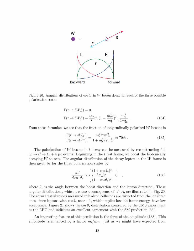
Figure 20: Angular distributions of cos θ∗ in W boson decay for each of the three possiblepolarization states.
Γ(t→ bW++ ) = 0
Γ(t→ bW+0 ) =
αw8mt(1−
m2W
m2t
)2 · m2t
2m2W
. (134)
From these formulae, we see that the fraction of longitudinally polarized W bosons is
Γ(t→ bW+0 )
Γ(t→ bW+)=
m2t/2m
2W
1 +m2t/2m
2W
≈ 70% . (135)
The polarization of W bosons in t decay can be measured by reconstructing fullpp→ tt→ `ν + 4 jet events. Beginning in the t rest frame, we boost the leptonicallydecaying W to rest. The angular distribution of the decay lepton in the W frame isthen given by for the three polarization states by
dΓ
d cos θ∗∼
(1 + cos θ∗)
2 +sin2 θ∗/2 0(1− cosθ∗)2 −
, (136)
where θ∗ is the angle between the boost direction and the lepton direction. Theseangular distributions, which are also a consequence of V –A, are illustrated in Fig. 20.The actual distributions measured in hadron collisions are distorted from the idealizedones, since leptons with cos θ∗ near −1, which implies low lab-frame energy, have lowacceptance. Figure 21 shows the cos θ∗ distribution measured by the CMS experimentat the LHC and indicates an excellent agreement with the SM prediction [36].
An interesting feature of this prediction is the form of the amplitude (133). Thisamplitude is enhanced by a factor mt/mW , just as we might have expected from
42
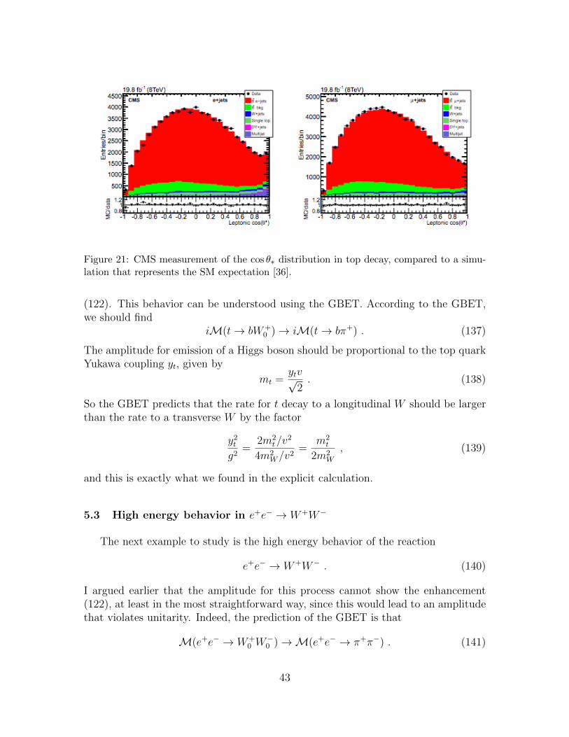
Figure 21: CMS measurement of the cos θ∗ distribution in top decay, compared to a simu-lation that represents the SM expectation [36].
(122). This behavior can be understood using the GBET. According to the GBET,we should find
iM(t→ bW+0 )→ iM(t→ bπ+) . (137)
The amplitude for emission of a Higgs boson should be proportional to the top quarkYukawa coupling yt, given by
mt =ytv√
2. (138)
So the GBET predicts that the rate for t decay to a longitudinal W should be largerthan the rate to a transverse W by the factor
y2tg2
=2m2
t/v2
4m2W/v
2=
m2t
2m2W
, (139)
and this is exactly what we found in the explicit calculation.
5.3 High energy behavior in e+e− → W+W−
The next example to study is the high energy behavior of the reaction
e+e− → W+W− . (140)
I argued earlier that the amplitude for this process cannot show the enhancement(122), at least in the most straightforward way, since this would lead to an amplitudethat violates unitarity. Indeed, the prediction of the GBET is that
M(e+e− → W+0 W
−0 )→M(e+e− → π+π−) . (141)
43
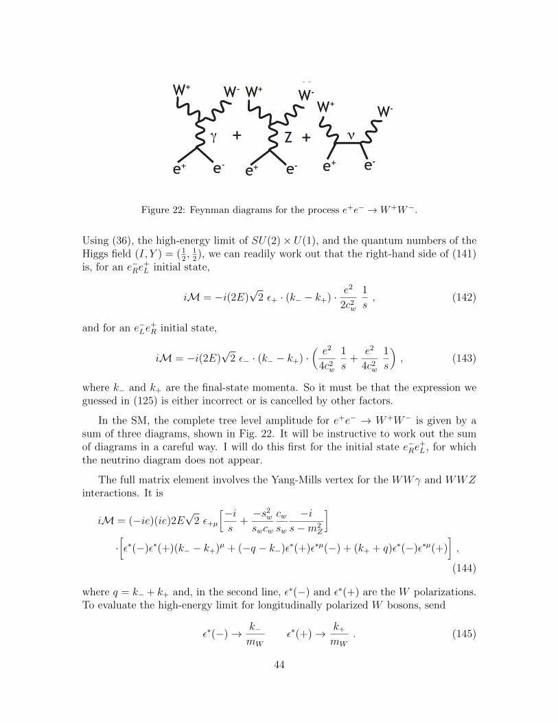
Figure 22: Feynman diagrams for the process e+e− →W+W−.
Using (36), the high-energy limit of SU(2)× U(1), and the quantum numbers of theHiggs field (I, Y ) = (1
2, 12), we can readily work out that the right-hand side of (141)
is, for an e−Re+L initial state,
iM = −i(2E)√
2 ε+ · (k− − k+) · e2
2c2w
1
s, (142)
and for an e−Le+R initial state,
iM = −i(2E)√
2 ε− · (k− − k+) ·(e2
4c2w
1
s+
e2
4c2w
1
s
), (143)
where k− and k+ are the final-state momenta. So it must be that the expression weguessed in (125) is either incorrect or is cancelled by other factors.
In the SM, the complete tree level amplitude for e+e− → W+W− is given by asum of three diagrams, shown in Fig. 22. It will be instructive to work out the sumof diagrams in a careful way. I will do this first for the initial state e−Re
+L , for which
the neutrino diagram does not appear.
The full matrix element involves the Yang-Mills vertex for the WWγ and WWZinteractions. It is
iM = (−ie)(ie)2E√
2 ε+µ
[−is
+−s2wswcw
cwsw
−is−m2
Z
]·[ε∗(−)ε∗(+)(k− − k+)µ + (−q − k−)ε∗(+)ε∗µ(−) + (k+ + q)ε∗(−)ε∗µ(+)
],
(144)
where q = k− + k+ and, in the second line, ε∗(−) and ε∗(+) are the W polarizations.To evaluate the high-energy limit for longitudinally polarized W bosons, send
ε∗(−)→ k−mW
ε∗(+)→ k+mW
. (145)
44
Then the second term in brackets becomes
1
m2W
[k−k+(k− − k+)µ − 2k−k+k
µ− + 2k+k−k
µ+
]
= −k−k+m2W
(k− − k+)µ = −s− 2m2W
2m2W
(k− − k+)µ . (146)
This expression has the enhancement (126). However, there is a nice cancellation inthe first term in brackets, [−i
s− −is−m2
Z
]=
i m2Z
s(s−m2Z)
. (147)
Assembling the pieces and using m2W = m2
Zc2w, we find
iM = ie2 2E√
2 ε+µ(k− − k+)µ(− s− 2m2
W
2c2ws(s−m2Z)
), (148)
which indeed agrees with (142) in the high energy limit.
For the e−Le+R case, the γ and Z diagrams do not cancel, and so the neutrino
diagram is needed. The first two diagrams contribute
iM = (−ie)(ie)2E√
2 ε+µ
[−is
+(1/2− s2w)
swcw
cwsw
−is−m2
Z
]·[ε∗(−)ε∗(+)(k− − k+)µ + (−q − k−)ε∗(+)ε∗µ(−) + (k+ + q)ε∗(−)ε∗µ(+)
],
(149)
After the reductions just described, there is a term in the high-energy behavior thatdoes not cancel,
iM = ie2 2E√
2 ε−µ(k− − k+)µ[
1
2s2W s
](− s
2m2W
)
=ie2
4s2w2E√
2 ε−µ(k− − k+)µ1
m2W
. (150)
We must add to this the neutrino diagram, which contributes
iM = (ig√2
)2 vR(p)† σ · ε∗(+)iσ · (p− k−)
(p− k−)2σ · ε∗(−) uL(p) . (151)
Substituting ε∗(−)→ k−/mW , the second half of this formula becomes
iσ · (p− k−)
(p− k−)2σ · k−
mW
u(p) . (152)
45
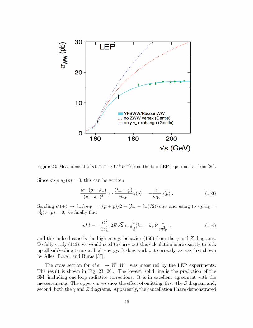
Figure 23: Measurement of σ(e+e− →W+W−) from the four LEP experimenta, from [20].
Since σ · p uL(p) = 0, this can be written
iσ · (p− k−)
(p− k−)2σ · (k− − p)
mW
u(p) = − i
m2W
u(p) . (153)
Sending ε∗(+) → k+/mW = ((p + p)/2 + (k+ − k−)/2)/mW and using (σ · p)uL =v†R(σ · p) = 0, we finally find
iM = − ie2
2s2w2E√
2 ε−µ1
2(k− − k+)µ
1
m2W
, (154)
and this indeed cancels the high-energy behavior (150) from the γ and Z diagrams.To fully verify (143), we would need to carry out this calculation more exactly to pickup all subleading terms at high energy. It does work out correctly, as was first shownby Alles, Boyer, and Buras [37].
The cross section for e+e− → W+W− was measured by the LEP experiments.The result is shown in Fig. 23 [20]. The lowest, solid line is the prediction of theSM, including one-loop radiative corrections. It is in excellent agreement with themeasurements. The upper curves show the effect of omitting, first, the Z diagram and,second, both the γ and Z diagrams. Apparently, the cancellation I have demonstrated
46
here is important not only at very high energy but even in the qualitative behaviorof the cross section quite close to threshold.
5.4 Parametrizing corrections to the Yang-Mills vertex
The cancellation described in the previous section clearly requires the precisestructure of the Yang-Mills vertex that couples three vector bosons. Before the LEPmeasurements, when the gauge boson nature of the W and Z was less clear, theoristssuggested that the WWγ and WWZ vertices might be modified form the Yang-Millsform, and that such modifications could be tested by measurements of W reactionsat high energy.
The most general Lorentz-invariant, CP conserving WWγ vertex in which thephoton couples to a conserved current has the form [38]
∆L = e[ig1AAµ(W−νW+µν −W+
ν W−µν) + iκAAµνW
−µW+ν
+iλA1
m2W
W−λµW
+µνAνλ]. (155)
In this formula, for each vector field, Vµν = (∂µVν − ∂νVµ). We can write a similargeneralization of the SM WWZ vertex, with parameters g1Z , κZ , λZ and overallcoupling ecw/sw. The choice
g1γ = g1Z = κA = κZ = 1 λA = λZ = 0 (156)
gives the SM coupling. If we relax the assumption of CP conservation, several moreterms can be added.
It was quickly realized that any changes to the SM vertex produce extra contri-butions to the W production amplitudes that are enhanced by the factor s/m2
W . Inview of the discussion earlier in this section, this is no surprise. If the additionalterms violate the gauge invariance of the theory, the GBET will not be valid, and thecancellations it requires will not need to occur. However, this idea would seem to bealready excluded by the strong evidence from the precision electroweak measurementsthat the W and Z are the vector bosons of a gauge theory.
Still, there is a way to modify the WWγ and WWZ vertices in a way that isconsistent with gauge invariance. It is certainly possible that there exist new heavyparticles that couple to the gauge bosons of the SM. The quantum effects of theseparticles can be described as a modification of the SM Lagrangian by the addition ofnew gauge-invariant operators. This approach to the parametrizatoin f new physicseffects has become known as Effective Field Theory (EFT). The SM already containsthe most general SU(2)×U(1)-invariant operators up to dimension 4, but new physicsat high energy can add higher-dimension operators, beginning with dimension 6.
47
There are many dimension 6 operators that can be added to the SM. Even for1 generation of fermions, there are 84 independent dimension 6 operators, of which59 are baryon-number and CP-conserving [39]. The theory of these operators has acomplexity that I do not have room to explain here. It is possible to make manydifferent choices for the basis of these operators, using the fact that combinations ofthese operators are set to zero by the SM equations of motion. The theory of EFTmodifications of the SM is reviewed in [40] and, in rather more detail, in [41]. I willgive only a simple example here.
Consider, then, adding to the SM the dimension-6 operators
∆L =cT2v2
ΦµΦµ +4gg′
m2W
ΦaW aµνB
µν +g3c3Wm2W
εabcW aµνW
bνρW
cρµ , (157)
where, in this formula, W aµν and Bµν are the SU(2) and U(1) field strengths and Φµ,
Φa are bilinears in the Higgs field,
Φµ = ϕ†Dµϕ− (Dµϕ)†ϕ Φa = ϕ†σa
2ϕ . (158)
It can be shown that these shift the parameters of the WWγ and WWZ couplingsto
g1Z = 1 +[
cT2(c2w − s2w)
− 8s2wcWB
c2w(c2w − s2w)
]κA = 1− 4cWB
λA = −6g2c3W (159)
The parameter g1A = 1 is not shifted; this is the electric charge of the W boson. Theremaining two parameters obey
κZ = g1Z −s2wc2w
(κA − 1) λZ = λA . (160)
It can be shown that the relations (160) are maintained for any set of dimension-6perturbations of the SM. They may be modified by dimension-8 operators.
Dimension-6 operators also contribute to the S and T parameters discussed at theend of the previous section. From the perturbation (157),
αS = 32s2wcWB
αT = cT (161)
Given that EFT is based on gauge-invariant Lagrangian, this formalism for pa-rametrizing new physics can be worked out explicitly in great detail. QCD and
48
electroweak radiative corrections can be included. The higher-dimension operators inthe EFT must of course be renormalized according to some scheme, and the detailedformulae will depend on the scheme.
A dimension-6 operator has a coefficient with the units of (GeV)−2. Thus, theeffects of such operators are suppressed by one factor of s/M2, where M is thenmass scale of new particles. Contributions from dimension-8 operators suppressedby (s/M2)2, and similarly for operators of still higher dimension. So, an analysisthat puts constraints on dimension-6 operators, ignoring the effects of dimension-8operators is properly valid only when s/M2 � 1.
As a corollary to this point, I call your attention to a Devil’s bargain that arisesfrequently in tests of the structure of W and Z vertices at hadron colliders. In ppcollisions, the parton center of mass energy s varies over a wide range. There is alwaysa region of phase space where s becomes extremely large. This is the region that hasthe greatest sensitivity to higher-dimension operators. It is tempting to apply eventselections that emphasize this region to obtain the strongest possible limits.
However, this is exactly the region where operators of dimension 8 and highermight also be important. In many models, these give negative contribution. Then aparametrization that uses only dimension-6 operators leads to limits on their coeffi-cients that are stronger than the limits that would be obtained in a more completetheory.
The question of how to interpret limits on dimension-6 EFT coefficients is nowhotly debated in the literature. My personal position is on one extreme, that onlyanalyses in which s/M2 � 1 for all events included in the analysis should be trusted.The authors of [42] advocate for a much more aggressive approach. Experimenterswho quote such limits should study this issue carefully.
On the other hand, the SM itself makes precise predictions in all regions of s.Your first priority should be to discover a deviation from these predictions. If you areable to demonstrate a substantial deviation from the SM predictions in any region ofphase space, we can all have fun quarreling about the interpretation of this result.
5.5 W parton distributions
As a final topic in this section, I will discuss a situation in which the GBETmight be expected to apply, but it does not. This is involves processes in which a Wboson is radiated from a quark or lepton with small transverse momentum relative tothe fermion direction. In QCD, the collinear radiation of gluons from initial quarks isessential is creating the observed quark and gluon parton distributions. In Section 4.2,we saw that collinear radiation of photons from initial electrons and positrons is alsoan important effect that makes qualitative changes in the Z resonance line shape. In
49
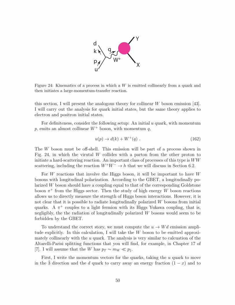
k q
pX
Y
W+
u
d
Figure 24: Kinematics of a process in which a W is emitted collinearly from a quark andthen initiates a large-momentum-transfer reaction.
this section, I will present the analogous theory for collinear W boson emission [43].I will carry out the analysis for quark initial states, but the same theory applies toelectron and positron initial states.
For definiteness, consider the following setup: An initial u quark, with momentump, emits an almost collinear W+ boson, with momentum q,
u(p)→ d(k) +W+(q) . (162)
The W boson must be off-shell. This emission will be part of a process shown inFig. 24, in which the virutal W collides with a parton from the other proton toinitiate a hard-scattering reaction. An important class of processes of this type is WWscattering, including the reaction W+W− → h that we will discuss in Section 6.2.
For W reactions that involve the Higgs boson, it will be important to have Wbosons with longitudinal polarization. According to the GBET, a longitudinally po-larized W boson should have a coupling equal to that of the corresponding Goldstoneboson π+ from the Higgs sector. Then the study of high energy W boson reactionsallows us to directly measure the strength of Higgs boson interactions. However, it isnot clear that it is possible to radiate longitudinally polarized W bosons from initialquarks. A π+ couples to a light fermion with its Higgs Yukawa coupling, that is,negligibly, the the radiation of longitudinally polarized W bosons would seem to beforbidden by the GBET.
To understand the correct story, we must compute the u → Wd emission ampli-tude explicitly. In this calculation, I will take the W boson to be emitted approxi-mately collinearly with the u quark. The analysis is very similar to calcuation of theAltarelli-Parisi splitting functions that you will find, for example, in Chapter 17 of[7]. I will assume that the W has pT ∼ mW � p‖.
First, I write the momentum vectors for the quarks, taking the u quark to movein the 3 direction and the d quark to carry away an energy fraction (1 − x) and to
50
have a small transverse momentum,
p = (E, 0, 0, E)
k = ((1− z)E,−pT , 0, (1− z)E − p2T2(1− z)E
) . (163)
The momentum k is on-shell to order p2T . The W momentum vector is then deter-mined by momentum conservation
q = (zE, pT , 0, zE +p2T
2(1− z)E) . (164)
The denominator of the W propagator is then
q2 −m2W = −p2T −
z
(1− z)p2T −m2
W = −(p2T
1− z+m2
W ) . (165)
Next, we compute the matrix elements for W emission
iM = ig u†L(k) σ · ε∗W uL(p) (166)
to first order in (pT ,mW ). The explicit form of the spinors is
uL(k) =√
2(1− z)E(pT/2(1− z)
1
)uL(p) =
√2E
(01
). (167)
The W polarization vectors are
ε∗µ± = (0, 1,∓i,−pT/zE)µ/√
2 (168)
for the transverse polarizations, and
ε∗µ0 = (q, pT , 0, zE)µ/mW (169)
for the longitudinal polarization state. In this formula
q = [(zE)2 −m2W ]1/2 = zE − m2
W
2zE(170)
Then
σ · ε∗+ =1√2
(−pT/zE 02 pT/zE
)σ · ε∗− =
1√2
(−pT/zE 20 pT/zE
)σ · ε∗0 =
1
mW
(q + zE pTpT q − zE
)(171)
51
With these ingredients, it is straightfoward to work out the matrix elements for thethree W polarization states,
iM(u→ dW+) = ig ·
√
1− z pT/z +√1− z pT/z(1− z) −−√
1− z mW/√
2z 0
. (172)
We can convert these expressions to cross sections for complete W -induced pro-cesses. The cross section for a process uX → dY , in the approximation in which theW is almost on shell, is given by
σ =1
2s
∫ d3k
(2π)32k
∫dΠY (2π)4δ(4)(p+ pX − k − pY )∣∣∣∣M(u→ dW+)
1
q2 −m2W
M(W+X → Y )∣∣∣∣2 (173)
In the collinear kinematics, with s = zs
1
2s
∫ d3k
(2π)32k=
1
2s/z
∫ dzEd2pT16π3E(1− z)
=1
2s
∫ dzdp2Tπ
16π3
z
(1− z)(174)
Then, also using (165), (173) simplifies to
σ =∫dz∫ dp2T
(4π)2z
(1− z)|M(u→ dW+)|2 1
p2T/(1− z) +m2W )2
· 1
2s
∫dΠY (2π)4δ(4)(q + pX − pY )|M(W+X → Y )|2 (175)
The last line of (175) is σ(W+(q) +X → Y ). Then (175) has the form of a partonmodel cross section
σ(uX → dY ) =∫dzfW←u(z) σ(W+X → Y ) (176)
where fW←u(z) is the parton distribution for a W boson in the u quark,
fW←u(z) =∫ dp2T
(4π)2z
(1− z)
(1− z)2
(p2T + (1− z)m2W )2|M(u→ dW+)|2 . (177)
We can evaluate this parton distribution for each W polarization state by using theformula (172). The result is
fW−(z) =α2
4π
∫ dp2T p2T
(p2T + (1− z)m2W )2
1
z
fW+(z) =α2
4π
∫ dp2T p2T
(p2T + (1− z)m2W )2
(1− z)2
z
fW0(z) =α2
8π
∫ dp2T m2W
(p2T + (1− z)m2W )2
(1− z)2
z(178)
52
For the transverse polarizations, we find a resut very similar to the Altarelli-Parisisplitting function for collinear gluon emission,
fWT (z) =αw4π
1 + (1− z)2
z· log
Q2
m2W
, (179)
where Q2 is the upper limit of the p2T integral, which is set by the momentum transferin the hard reaction.
For the longitudinal W polarization, the story is different. The integral over pTis convergent, so that the pT is restricted to the region pT ∼ mW . In this regime, aswe see explicitly, longitudinal W bosons can be produced with coupling strength g.Apparently, in this process, the error term in the GBET is actually O(mW/pT ), whichis consistent with (127) but, still, larger than we might expect. The reduction of thelongitudinal W boson to a Higgs boson then is not accurate in the region pT ∼ mW ,though it does apply—and cuts off the amplitude—when pT � mW .
When we perform the convergent integral over pT , we find that the parton distri-bution for W0 is substantial [43],
fW0(z) =αw8π
1− zz
. (180)
Then the proton does contain longitudinal W bosons, which can induce Higgs sectorreactions when this proton collides with another proton at high energy. The collinearlongitudinal W bosons have pT ∼ mW but not higher, a kinematic feature that canbe used to suppress backgrounds from reactions involving transversely-polarized Wbosons.
6 The Standard Model theory of Higgs boson decays
There remains one heavy particle of the SM that we have not yet discussed,the Higgs boson. The Higgs boson has a central role in the structure of the weakinteractions. Its field is the agent that breaks the SU(2) × U(1) symmetry andgenerates the masses of all quarks, leptons, and vector bosons. This at the same timeforms a unified picture of the electroweak interactions as we have studied them so farand also points to new mysteries whose explanations are still to be found.
The best way to enter a discussion of the Higgs boson is to understand thoroughlythe predictions for the properties of this particle given by the SM. The Higgs sectorinvolves one more parameter of the SM beyond those we have discussed already, theHiggs field self-coupling λ. However, this coupling is fixed by the measurement of the
53
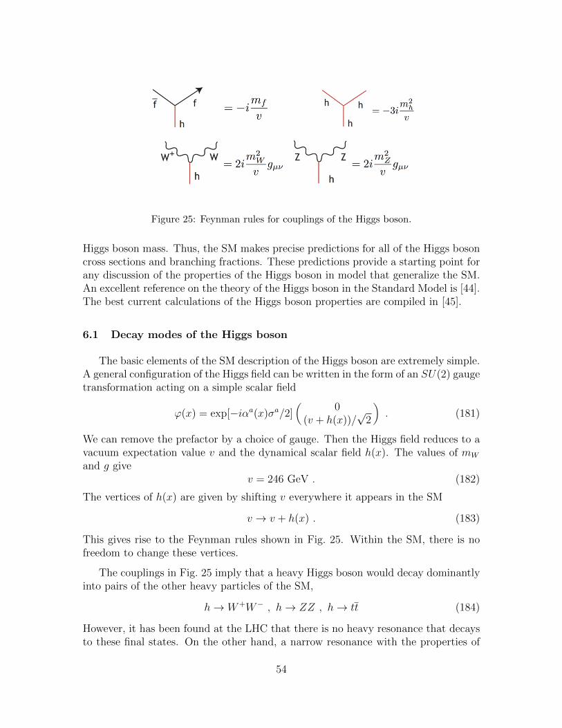
Figure 25: Feynman rules for couplings of the Higgs boson.
Higgs boson mass. Thus, the SM makes precise predictions for all of the Higgs bosoncross sections and branching fractions. These predictions provide a starting point forany discussion of the properties of the Higgs boson in model that generalize the SM.An excellent reference on the theory of the Higgs boson in the Standard Model is [44].The best current calculations of the Higgs boson properties are compiled in [45].
6.1 Decay modes of the Higgs boson
The basic elements of the SM description of the Higgs boson are extremely simple.A general configuration of the Higgs field can be written in the form of an SU(2) gaugetransformation acting on a simple scalar field
ϕ(x) = exp[−iαa(x)σa/2](
0(v + h(x))/
√2
). (181)
We can remove the prefactor by a choice of gauge. Then the Higgs field reduces to avacuum expectation value v and the dynamical scalar field h(x). The values of mW
and g givev = 246 GeV . (182)
The vertices of h(x) are given by shifting v everywhere it appears in the SM
v → v + h(x) . (183)
This gives rise to the Feynman rules shown in Fig. 25. Within the SM, there is nofreedom to change these vertices.
The couplings in Fig. 25 imply that a heavy Higgs boson would decay dominantlyinto pairs of the other heavy particles of the SM,
h→ W+W− , h→ ZZ , h→ tt (184)
However, it has been found at the LHC that there is no heavy resonance that decaysto these final states. On the other hand, a narrow resonance with the properties of
54
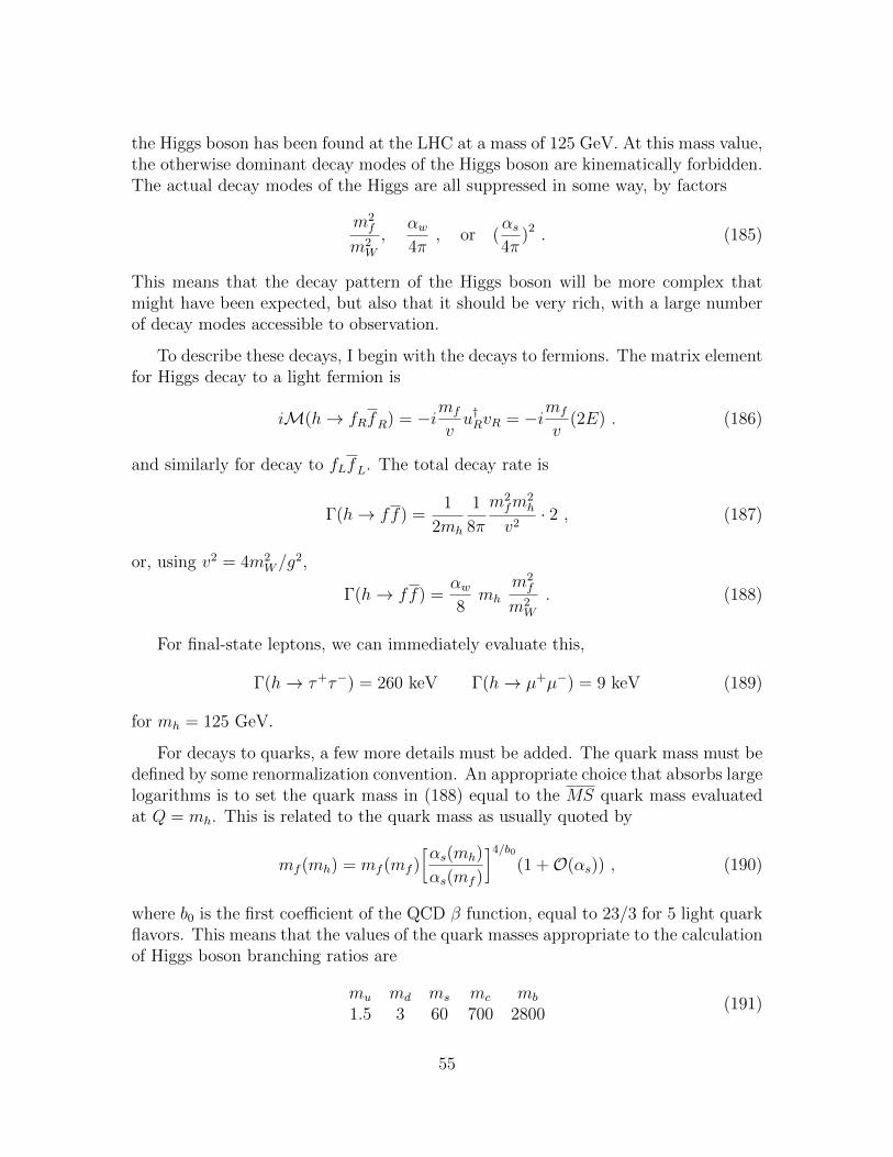
the Higgs boson has been found at the LHC at a mass of 125 GeV. At this mass value,the otherwise dominant decay modes of the Higgs boson are kinematically forbidden.The actual decay modes of the Higgs are all suppressed in some way, by factors
m2f
m2W
,αw4π
, or (αs4π
)2 . (185)
This means that the decay pattern of the Higgs boson will be more complex thatmight have been expected, but also that it should be very rich, with a large numberof decay modes accessible to observation.
To describe these decays, I begin with the decays to fermions. The matrix elementfor Higgs decay to a light fermion is
iM(h→ fRfR) = −imf
vu†RvR = −imf
v(2E) . (186)
and similarly for decay to fLfL. The total decay rate is
Γ(h→ ff) =1
2mh
1
8π
m2fm
2h
v2· 2 , (187)
or, using v2 = 4m2W/g
2,
Γ(h→ ff) =αw8mh
m2f
m2W
. (188)
For final-state leptons, we can immediately evaluate this,
Γ(h→ τ+τ−) = 260 keV Γ(h→ µ+µ−) = 9 keV (189)
for mh = 125 GeV.
For decays to quarks, a few more details must be added. The quark mass must bedefined by some renormalization convention. An appropriate choice that absorbs largelogarithms is to set the quark mass in (188) equal to the MS quark mass evaluatedat Q = mh. This is related to the quark mass as usually quoted by
mf (mh) = mf (mf )[αs(mh)
αs(mf )
]4/b0(1 +O(αs)) , (190)
where b0 is the first coefficient of the QCD β function, equal to 23/3 for 5 light quarkflavors. This means that the values of the quark masses appropriate to the calculationof Higgs boson branching ratios are
mu md ms mc mb
1.5 3 60 700 2800(191)
55
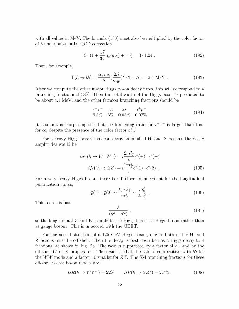
with all values in MeV. The formula (188) must also be multiplied by the color factorof 3 and a substantial QCD correction
3 · (1 +17
3παs(mh) + · · ·) = 3 · 1.24 . (192)
Then, for example,
Γ(h→ bb) =αwmh
8(
2.8
mW
)2 · 3 · 1.24 = 2.4 MeV . (193)
After we compute the other major Higgs boson decay rates, this will correspond to abranching fractionn of 58%. Then the total width of the Higgs boson is predicted tobe about 4.1 MeV, and the other fermion branching fractions should be
τ+τ− cc ss µ+µ−
6.3% 3% 0.03% 0.02%(194)
It is somewhat surprising the that the branching ratio for τ+τ− is larger than thatfor cc, despite the presence of the color factor of 3.
For a heavy Higgs boson that can decay to on-shell W and Z bosons, the decayamplitudes would be
iM(h→ W+W−) = i2m2
W
vε∗(+) · ε∗(−)
iM(h→ ZZ) = i2m2
Z
vε∗(1) · ε∗(2) . (195)
For a very heavy Higgs boson, there is a further enhancement for the longitudinalpolarization states,
ε∗0(1) · ε∗0(2) ∼ k1 · k2m2Z
∼ m2h
2m2Z
. (196)
This factor is justλ
(g2 + g′2). (197)
so the longitudinal Z and W couple to the Higgs boson as Higgs boson rather thanas gauge bosons. This is in accord with the GBET.
For the actual situation of a 125 GeV Higgs boson, one or both of the W andZ bosons must be off-shell. Then the decay is best described as a Higgs decay to 4fermions, as shown in Fig. 26. The rate is suppressed by a factor of αw and by theoff-shell W or Z propagator. The result is that the rate is competitive with bb forthe WW mode and a factor 10 smaller for ZZ. The SM branching fractions for theseoff-shell vector boson modes are
BR(h→ WW ∗) = 22% BR(h→ ZZ∗) = 2.7% . (198)
56
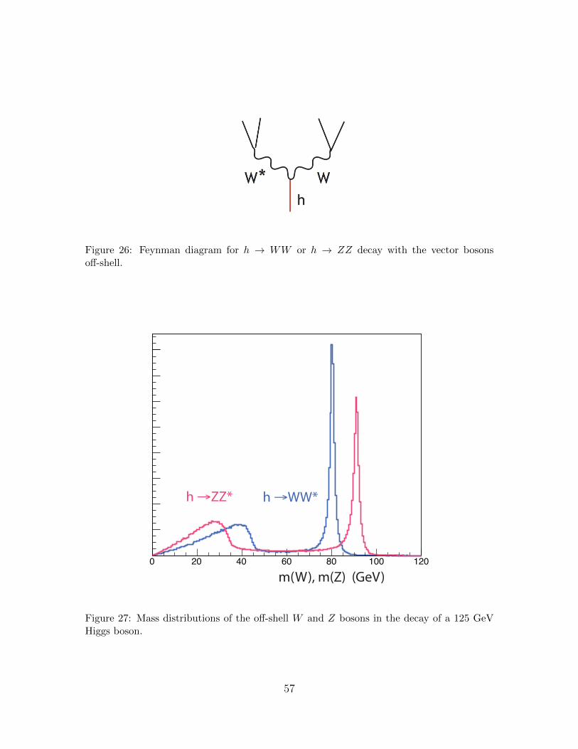
Figure 26: Feynman diagram for h → WW or h → ZZ decay with the vector bosonsoff-shell.
0 20 40 60 80 100 120
m(W), m(Z) (GeV)
h →WW*h →ZZ*
Figure 27: Mass distributions of the off-shell W and Z bosons in the decay of a 125 GeVHiggs boson.
57
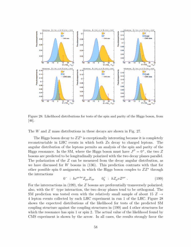
Figure 28: Likelihood distributions for tests of the spin and parity of the Higgs boson, from[46].
The W and Z mass distributions in these decays are shown in Fig. 27.
The Higgs boson decay to ZZ∗ is exceptionally interesting because it is completelyreconstructable in LHC events in which both Zs decay to charged leptons. Theangular distribution of the leptons permits an analysis of the spin and parity of theHiggs resonance. In the SM, where the Higgs boson must have JP = 0+, the two Zbosons are predicted to be longitudinally polarized with the two decay planes parallel.The polarization of the Z can be measured from the decay angular distribution, aswe have discussed for W bosons in (136). This prediction contrasts with that forother possible spin 0 assigments, in which the Higgs boson couples to ZZ∗ throughthe interactions
0− : hεµνλσZµνZλσ 0+h : hZµνZ
µν . (199)
For the intereractions in (199), the Z bosons are preferentially transversely polarized;also, with the 0− type interaction, the two decay planes tend to be orthogonal. TheSM prediction was tested even with the relatively small sample of about 15 Z →4 lepton events collected by each LHC experiment in run 1 of the LHC. Figure 28shows the expectred distributions of the likelihood for tests of the predicted SMcoupling structure against the coupling structures in (199) and 4 other structures forwhich the resonance has spin 1 or spin 2. The actual value of the likelihood found byCMS experiment is shown by the arrow. In all cases, the results strongly favor the
58
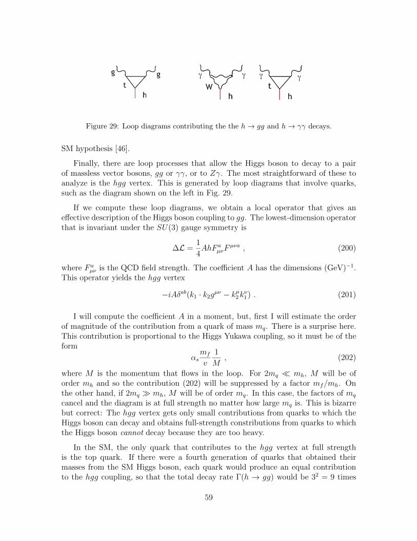
Figure 29: Loop diagrams contributing the the h→ gg and h→ γγ decays.
SM hypothesis [46].
Finally, there are loop processes that allow the Higgs boson to decay to a pairof massless vector bosons, gg or γγ, or to Zγ. The most straightforward of these toanalyze is the hgg vertex. This is generated by loop diagrams that involve quarks,such as the diagram shown on the left in Fig. 29.
If we compute these loop diagrams, we obtain a local operator that gives aneffective description of the Higgs boson coupling to gg. The lowest-dimension operatorthat is invariant under the SU(3) gauge symmetry is
∆L =1
4AhF a
µνFµνa , (200)
where F aµν is the QCD field strength. The coefficient A has the dimensions (GeV)−1.
This operator yields the hgg vertex
−iAδab(k1 · k2gµν − kµ2kν1) . (201)
I will compute the coefficient A in a moment, but, first I will estimate the orderof magnitude of the contribution from a quark of mass mq. There is a surprise here.This contribution is proportional to the Higgs Yukawa coupling, so it must be of theform
αsmf
v
1
M, (202)
where M is the momentum that flows in the loop. For 2mq � mh, M will be oforder mh and so the contribution (202) will be suppressed by a factor mf/mh. Onthe other hand, if 2mq � mh, M will be of order mq. In this case, the factors of mq
cancel and the diagram is at full strength no matter how large mq is. This is bizarrebut correct: The hgg vertex gets only small contributions from quarks to which theHiggs boson can decay and obtains full-strength constributions from quarks to whichthe Higgs boson cannot decay because they are too heavy.
In the SM, the only quark that contributes to the hgg vertex at full strengthis the top quark. If there were a fourth generation of quarks that obtained theirmasses from the SM Higgs boson, each quark would produce an equal contributionto the hgg coupling, so that the total decay rate Γ(h → gg) would be 32 = 9 times
59
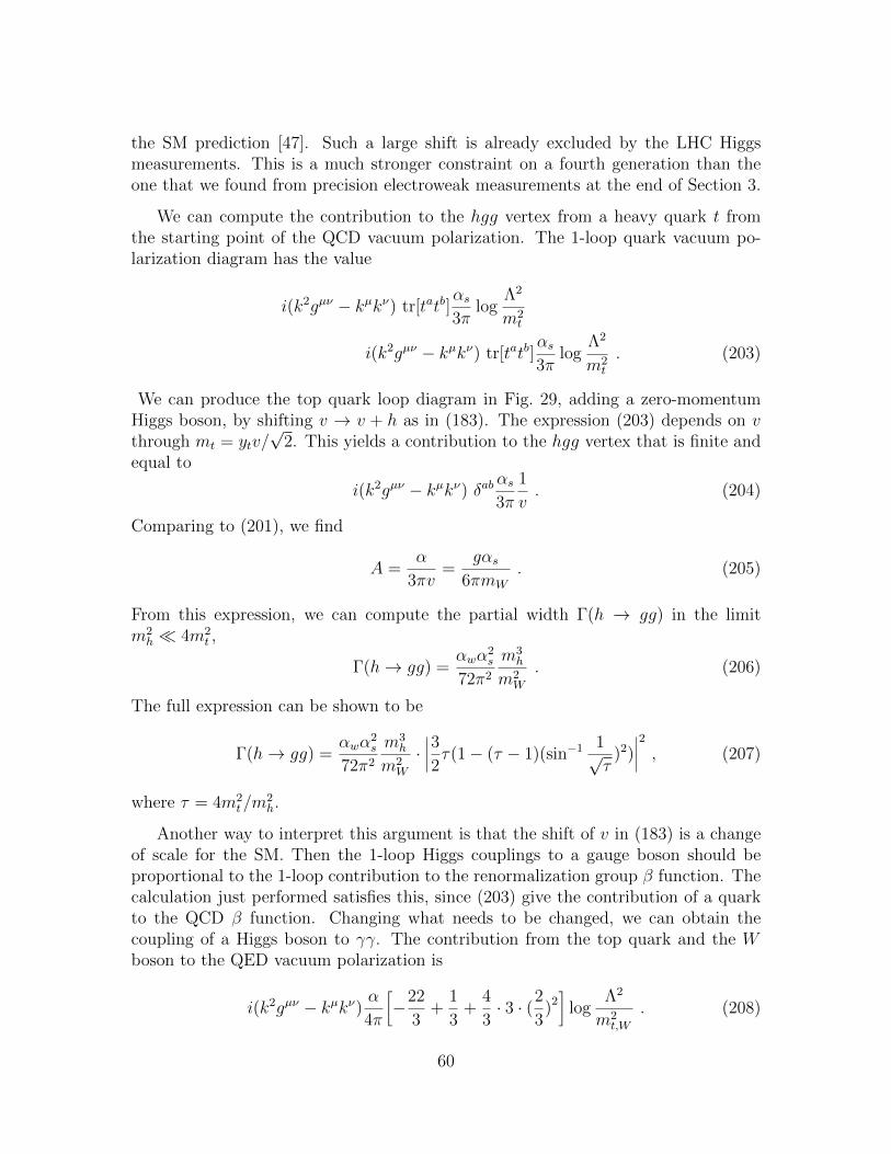
the SM prediction [47]. Such a large shift is already excluded by the LHC Higgsmeasurements. This is a much stronger constraint on a fourth generation than theone that we found from precision electroweak measurements at the end of Section 3.
We can compute the contribution to the hgg vertex from a heavy quark t fromthe starting point of the QCD vacuum polarization. The 1-loop quark vacuum po-larization diagram has the value
i(k2gµν − kµkν) tr[tatb]αs3π
logΛ2
m2t
i(k2gµν − kµkν) tr[tatb]αs3π
logΛ2
m2t
. (203)
We can produce the top quark loop diagram in Fig. 29, adding a zero-momentumHiggs boson, by shifting v → v + h as in (183). The expression (203) depends on vthrough mt = ytv/
√2. This yields a contribution to the hgg vertex that is finite and
equal to
i(k2gµν − kµkν) δabαs3π
1
v. (204)
Comparing to (201), we find
A =α
3πv=
gαs6πmW
. (205)
From this expression, we can compute the partial width Γ(h → gg) in the limitm2h � 4m2
t ,
Γ(h→ gg) =αwα
2s
72π2
m3h
m2W
. (206)
The full expression can be shown to be
Γ(h→ gg) =αwα
2s
72π2
m3h
m2W
·∣∣∣∣32τ(1− (τ − 1)(sin−1
1√τ
)2)∣∣∣∣2 , (207)
where τ = 4m2t/m
2h.
Another way to interpret this argument is that the shift of v in (183) is a changeof scale for the SM. Then the 1-loop Higgs couplings to a gauge boson should beproportional to the 1-loop contribution to the renormalization group β function. Thecalculation just performed satisfies this, since (203) give the contribution of a quarkto the QCD β function. Changing what needs to be changed, we can obtain thecoupling of a Higgs boson to γγ. The contribution from the top quark and the Wboson to the QED vacuum polarization is
i(k2gµν − kµkν) α4π
[−22
3+
1
3+
4
3· 3 · (2
3)2]
logΛ2
m2t,W
. (208)
60
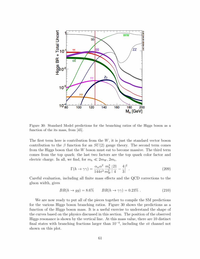
Figure 30: Standard Model predictions for the branching ratios of the Higgs boson as afunction of the its mass, from [45].
The first term here is contribution from the W , it is just the standard vector bosoncontribution to the β function for an SU(2) gauge theory. The second term comesfrom the Higgs boson that the W boson must eat to become massive. The third termcomes from the top quark; the last two factors are the top quark color factor andelectric charge. In all, we find, for mh � 2mW , 2mt,
Γ(h→ γγ) =αwα
2
144π2
m3h
m2W
∣∣∣∣21
4− 4
3
∣∣∣∣2 . (209)
Careful evaluation, including all finite mass effects and the QCD corrections to thegluon width, gives
BR(h→ gg) = 8.6% BR(h→ γγ) = 0.23% . (210)
We are now ready to put all of the pieces together to compile the SM predictionsfor the various Higgs boson branching ratios. Figure 30 shows the predictions as afunction of the Higgs boson mass. It is a useful exercise to understand the shape ofthe curves based on the physics discussed in this section. The position of the observedHiggs resonance is shown by the vertical line. At this mass value, there are 10 distinctfinal states with branching fractions larger than 10−4, including the ss channel notshown on this plot.
61
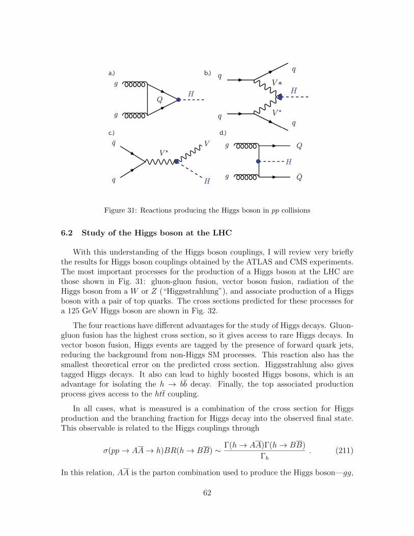
a.) b.)
c.) d.)
Figure 31: Reactions producing the Higgs boson in pp collisions
6.2 Study of the Higgs boson at the LHC
With this understanding of the Higgs boson couplings, I will review very brieflythe results for Higgs boson couplings obtained by the ATLAS and CMS experiments.The most important processes for the production of a Higgs boson at the LHC arethose shown in Fig. 31: gluon-gluon fusion, vector boson fusion, radiation of theHiggs boson from a W or Z (“Higgsstrahlung”), and associate production of a Higgsboson with a pair of top quarks. The cross sections predicted for these processes fora 125 GeV Higgs boson are shown in Fig. 32.
The four reactions have different advantages for the study of Higgs decays. Gluon-gluon fusion has the highest cross section, so it gives access to rare Higgs decays. Invector boson fusion, Higgs events are tagged by the presence of forward quark jets,reducing the background from non-Higgs SM processes. This reaction also has thesmallest theoretical error on the predicted cross section. Higgsstrahlung also givestagged Higgs decays. It also can lead to highly boosted Higgs bosons, which is anadvantage for isolating the h → bb decay. Finally, the top associated productionprocess gives access to the htt coupling.
In all cases, what is measured is a combination of the cross section for Higgsproduction and the branching fraction for Higgs decay into the observed final state.This observable is related to the Higgs couplings through
σ(pp→ AA→ h)BR(h→ BB) ∼ Γ(h→ AA)Γ(h→ BB)
Γh. (211)
In this relation, AA is the parton combination used to produce the Higgs boson—gg,
62
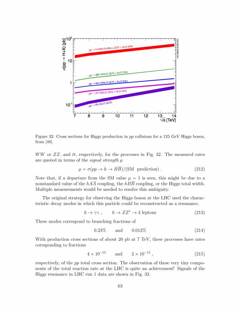
Figure 32: Cross sections for Higgs production in pp collisions for a 125 GeV Higgs boson,from [48].
WW or ZZ, and tt, respectively, for the processes in Fig. 32. The measured ratesare quoted in terms of the signal strength µ
µ = σ(pp→ h→ BB)/(SM prediction) . (212)
Note that, if a departure from the SM value µ = 1 is seen, this might be due to anonstandard value of the hAA coupling, the hBB coupling, or the Higgs total width.Multiple measurements would be needed to resolve this ambiguity.
The original strategy for observing the Higgs boson at the LHC used the charac-teristic decay modes in which this particle could be reconstructed as a resonance.
h→ γγ , h→ ZZ∗ → 4 leptons (213)
These modes correspond to branching fractions of
0.23% and 0.012% (214)
With production cross sections of about 20 pb at 7 TeV, these processes have ratescoresponding to fractions
4× 10⁻¹³ and 2× 10⁻¹⁴ , (215)
respectively, of the pp total cross section. The observation of these very tiny compo-nents of the total reaction rate at the LHC is quite an achievement! Signals of theHiggs resonance in LHC run 1 data are shown in Fig. 33.
63
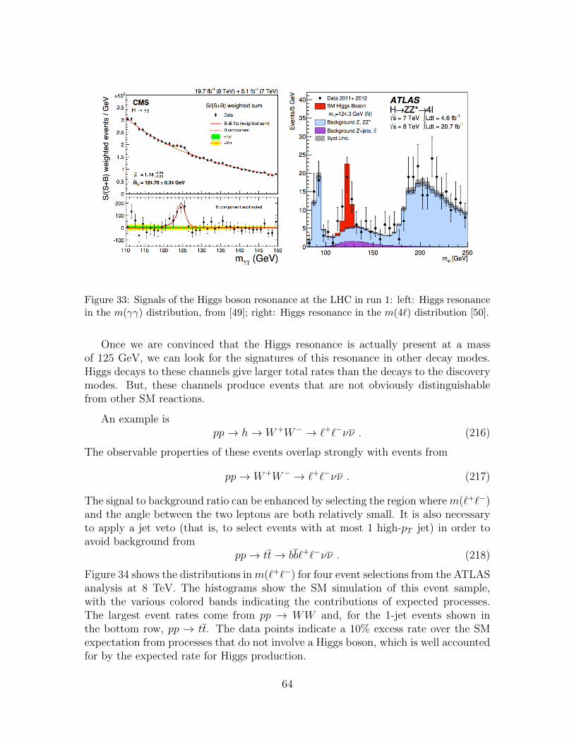
Figure 33: Signals of the Higgs boson resonance at the LHC in run 1: left: Higgs resonancein the m(γγ) distribution, from [49]; right: Higgs resonance in the m(4`) distribution [50].
Once we are convinced that the Higgs resonance is actually present at a massof 125 GeV, we can look for the signatures of this resonance in other decay modes.Higgs decays to these channels give larger total rates than the decays to the discoverymodes. But, these channels produce events that are not obviously distinguishablefrom other SM reactions.
An example ispp→ h→ W+W− → `+`−νν . (216)
The observable properties of these events overlap strongly with events from
pp→ W+W− → `+`−νν . (217)
The signal to background ratio can be enhanced by selecting the region wherem(`+`−)and the angle between the two leptons are both relatively small. It is also necessaryto apply a jet veto (that is, to select events with at most 1 high-pT jet) in order toavoid background from
pp→ tt→ bb`+`−νν . (218)
Figure 34 shows the distributions inm(`+`−) for four event selections from the ATLASanalysis at 8 TeV. The histograms show the SM simulation of this event sample,with the various colored bands indicating the contributions of expected processes.The largest event rates come from pp → WW and, for the 1-jet events shown inthe bottom row, pp → tt. The data points indicate a 10% excess rate over the SMexpectation from processes that do not involve a Higgs boson, which is well accountedfor by the expected rate for Higgs production.
64
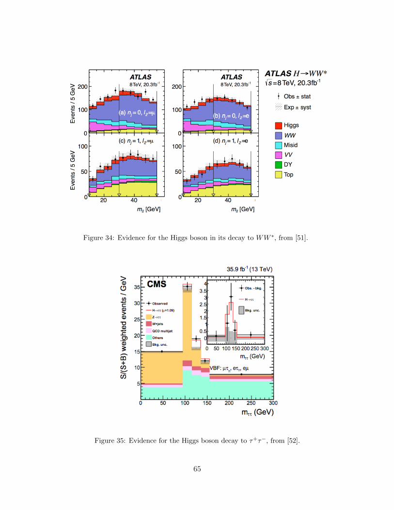
Figure 34: Evidence for the Higgs boson in its decay to WW ∗, from [51].
Figure 35: Evidence for the Higgs boson decay to τ+τ−, from [52].
65
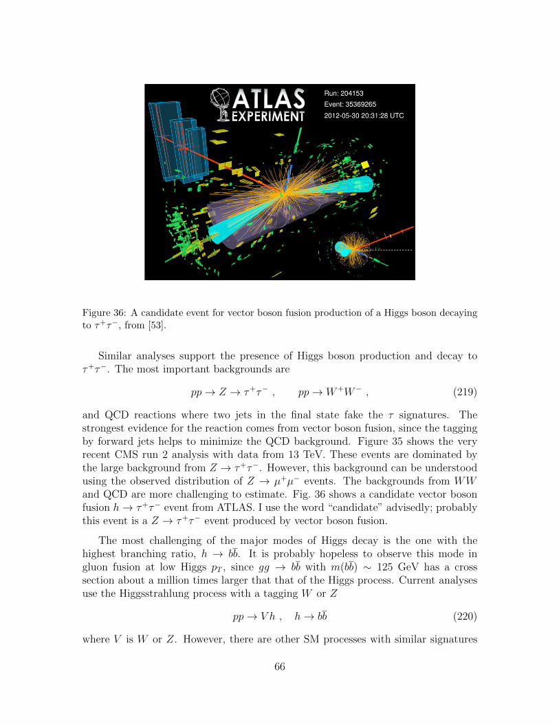
Figure 36: A candidate event for vector boson fusion production of a Higgs boson decayingto τ+τ−, from [53].
Similar analyses support the presence of Higgs boson production and decay toτ+τ−. The most important backgrounds are
pp→ Z → τ+τ− , pp→ W+W− , (219)
and QCD reactions where two jets in the final state fake the τ signatures. Thestrongest evidence for the reaction comes from vector boson fusion, since the taggingby forward jets helps to minimize the QCD background. Figure 35 shows the veryrecent CMS run 2 analysis with data from 13 TeV. These events are dominated bythe large background from Z → τ+τ−. However, this background can be understoodusing the observed distribution of Z → µ+µ− events. The backgrounds from WWand QCD are more challenging to estimate. Fig. 36 shows a candidate vector bosonfusion h→ τ+τ− event from ATLAS. I use the word “candidate” advisedly; probablythis event is a Z → τ+τ− event produced by vector boson fusion.
The most challenging of the major modes of Higgs decay is the one with thehighest branching ratio, h → bb. It is probably hopeless to observe this mode ingluon fusion at low Higgs pT , since gg → bb with m(bb) ∼ 125 GeV has a crosssection about a million times larger that that of the Higgs process. Current analysesuse the Higgsstrahlung process with a tagging W or Z
pp→ V h , h→ bb (220)
where V is W or Z. However, there are other SM processes with similar signatures
66
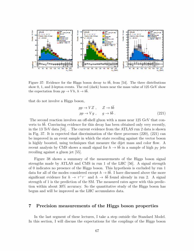
Figure 37: Evidence for the Higgs boson decay to bb, from [54]. The three distributionsshow 0, 1, and 2-lepton events. The red (dark) boxes near the mass value of 125 GeV showthe expectation from pp→ V h, h→ bb.
that do not involve a Higgs boson,
pp→ V Z , Z → bb
pp→ V g , g → bb . (221)
The second reaction involves an off-shell gluon with a mass near 125 GeV that con-verts to bb. Convincing evidence for this decay has been obtained only very recently,in the 13 TeV data [54]. . The current evidence from the ATLAS run 2 data is shownin Fig. 37. It is expected that discrimination of the three processes (220), (221) canbe improved in an event sample in which the state recoiling against the vector bosonis highly boosted, using techniques that measure the dijet mass and color flow. Arecent analysis by CMS shows a small signal for h → bb in a sample of high pT jetsrecoiling against a gluon jet [55].
Figure 38 shows a summary of the measurements of the Higgs boson signalstrengths made by ATLAS and CMS in run 1 of the LHC [56]. A signal strengthof 0 indicates no presence of the Higgs boson. This hypothesis is excluded by run 1data for all of the modes considered except h→ bb. I have discussed above the moresignificant evidence for h → τ+τ− and h → bb found already in run 2. A signalstrength of 1 is the prediction of the SM. The measured rates agree with this predic-tion within about 30% accuracy. So the quantitative study of the Higgs boson hasbegun and will be improved as the LHC accumulates data.
7 Precision measurements of the Higgs boson properties
In the last segment of these lectures, I take a step outside the Standard Model.In this section, I will discuss the expectations for the couplings of the Higgs boson
67
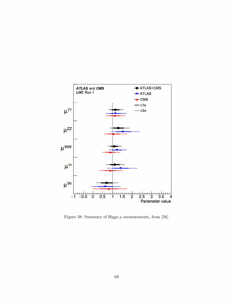
Figure 38: Summary of Higgs µ measurements, from [56].
68

in theories beyond the Standard Model. This is an interesting story that motivatesa dedicated experimental campaign to measure the couplings of the Higgs bosonwith high precision. First, though, I will explain why I believe there must be newinteractions of physics waiting to be discovered.
7.1 The mystery of electroweak symmetry breaking
I have shown in the previous lectures that the SM of weak interactions is anextremely successful theory in its own domain. It is not a complete theory of nature,but we can supplement it by adding gravity, quantum chromodynamics (QCD) as thetheory of the strong interactions, and some model of dark matter and dark energy. Itis also not difficult to add neutrino masses to the model, either by introducing threegenerations of right-handed neutrinos or by adding lepton-number-violating Majoranamass terms. Each of these additions accounts for some set of observed phenomenathat is outside the range of topics considered in these lectures.
But this is not enough. A key part of the explanation for the structure of the weakinteractions and the generation of masses for quarks, leptons, and gauge bosons is thespontaneous symmetry breaking of SU(2)× U(1) and the generation of the Yukawacouplings that link the symmetry-breaking Higgs field to the quarks and leptons.The structure that I have described leads immedately to questions about all of theseingredients:
• Why just quarks and leptons? What is the origin of the quantum numberassignments (I, Y ) for the matter particles seen in nature?
• What explains the spectrum of quark and lepton masses? The SM gives therelation
mf =yfv√
2, (222)
where v is the Higgs field vacuum expectation value. But the yf are renor-malized parameters that cannot be predicted with the Standard Model. Thepresence of nonzero CKM angles—and, with neutrinos, PMNS angles—addsfurther difficulty to this problem.
• What is the origin of the Higgs field? Is there only one such field, or are theremultiplets of scalar fields with different quantum numbers? The SM makes theminimal choice of one Higgs multiplet. Is this necessary?
• Why is SU(2)× U(1) spontaneously broken? The shape of the Higgs potentialenergy function is an input for which the SM gives no explanation.
This last question merits more discussion. Here is the explanation for electroweaksymmetry breaking given in the SM: The model instructs us to write the most general
69
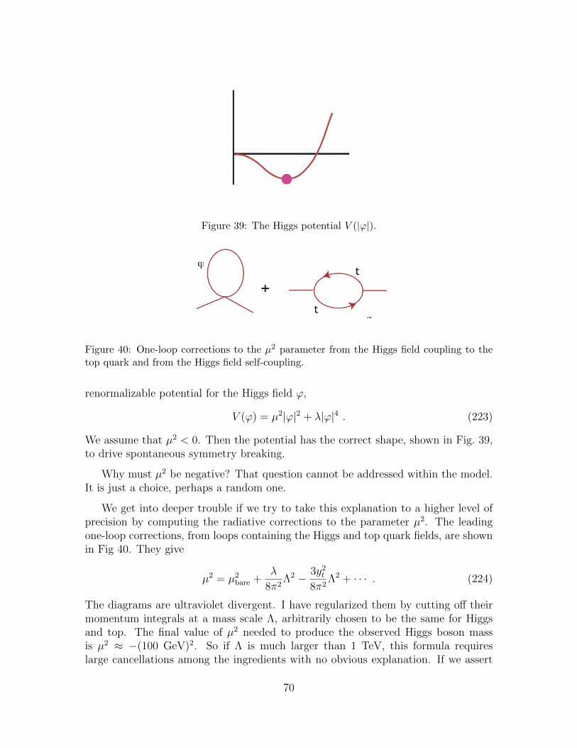
Figure 39: The Higgs potential V (|ϕ|).
Figure 40: One-loop corrections to the µ2 parameter from the Higgs field coupling to thetop quark and from the Higgs field self-coupling.
renormalizable potential for the Higgs field ϕ,
V (ϕ) = µ2|ϕ|2 + λ|ϕ|4 . (223)
We assume that µ2 < 0. Then the potential has the correct shape, shown in Fig. 39,to drive spontaneous symmetry breaking.
Why must µ2 be negative? That question cannot be addressed within the model.It is just a choice, perhaps a random one.
We get into deeper trouble if we try to take this explanation to a higher level ofprecision by computing the radiative corrections to the parameter µ2. The leadingone-loop corrections, from loops containing the Higgs and top quark fields, are shownin Fig 40. They give
µ2 = µ2bare +
λ
8π2Λ2 − 3y2t
8π2Λ2 + · · · . (224)
The diagrams are ultraviolet divergent. I have regularized them by cutting off theirmomentum integrals at a mass scale Λ, arbitrarily chosen to be the same for Higgsand top. The final value of µ2 needed to produce the observed Higgs boson massis µ2 ≈ −(100 GeV)2. So if Λ is much larger than 1 TeV, this formula requireslarge cancellations among the ingredients with no obvious explanation. If we assert
70
that the SM is correct up to the Planck scale, the first 33 significant figures mustcancel. It is also apparent that the right-hand side contains both positive and negativecontributions, so it is not obvious without invoking a much deeper explanation whythe final answer after the cancellation should turn out to be negative.
The simplest resolution of this set of problems would be that there are new par-ticles, not yet known to us, that generate additional diagrams contributing to thecalculation of µ2. If these particles have masses of TeV size, they might cancel thedivergences seen in (224) and—in the best case—leave over a calculable answer forµ2. However, we have not yet been able to discover these particles in high-energyexperiments.
The general problem of the uncalculability of the parameter µ2 is not new to high-energy physics. It is encountered in all systems in which a symmetry is spontaneouslybroken. Condensed matter physics gives many examples.
The most direct analogy to the Higgs theory comes in the phenomenon of su-perconductivity seen in most metals at cryogenic temperatures. The original paperson the Higgs mechanism by Englert and Brout, Higgs, and Guralnik, Hagen, andKibble [9–11] all used the analogy to superconductivity to motivate their arguments.However, they used only a piece of the complete theory. Supercondutivity was dis-covered in 1911 by Kamerlingh Onnes and was quickly seen to be associated with asharp phase transition [57]. However, the explanation for this phase transition wasnot understood for another 45 years.
In 1950, Landau and Ginzburg proposed a phenomenological theory of supercon-ductivity based on a scalar field with the potential (223) [58]. They assumed thatthe parameter µ2 would be a function of temperature, taking negative values belowthe phase transition temperature TC . Coupling this theory to electromagnetism, theyfound that the photon acquires a mass by the Higgs mechanism and that the scalarfields in the vacuum can transmit electric current frictionlessly. This theory turnedout to be extremely successful in explaing many aspect of superconductivity, includ-ing the Meissner effect in which superconductors repel magnetic flux, the existenceof Type I and Type II superconductors, and the systematics of the destruction ofsuperconductivity by high currents or high magnetic fields.
However, this theory could not address the most important problem of why su-perconductivity occured in the first place. The answer to that question waited until1957, when Bardeen, Cooper, and Schrieffer discovered the mechanism that causeselectrons in a metal to pair up into bound states and form a boson condensate withthe properties of the Landau-Ginzburg scalar field [59].
In our understanding of the phase transition to symmetry breaking of SU(2) ×U(1), we are now at the Landau-Ginzburg stage.
In the case of superconductivity, physicists knew that there must be a deeper
71
explanation that had to be given in terms of the interactions of elecrons and atoms.For the symmetry-breaking of the weak interactions, any analogous explanation mustinvolve new elementary particles outside the SM. We do not know what these particlesare. We only know that we have not discovered them yet.
7.2 Expectations for the Higgs boson in theories beyond the StandardModel
Even if we cannot discover new heavy particles responsible for the Higgs potentialenergy, we can hope to find clues to the nature of these new particles and interactionsby looking more deeply into the properties of the Higgs boson itself. In the previouslecture, I emphasized that the SM makes precise predictions for the couplings of theHiggs boson to all particles of the SM in terms of the measured masses of thoseparticles. Any deviation from these predictions must indicate the presence of newinteractions beyond the SM. In this and the next two sections, I will trace out theexpectations for corrections to the Higgs properties in different classes of models ofnew physics.
To begin, I will present two sets of expectations for the properties of new physicsmodels. The first is guidance from the concept that these models should solve theproblem of the calculability of the Higgs potential. The second comes from a con-straint that is well-satisfied in the precision electroweak measurements.
I have already explained that the parameter µ2 in the Higgs potential cannotbe computed within the SM. To construct a model in which µ2 can be computed,that model must satisfy some special properties. In particular, some structure in thetheory msut require the cancellation of quadratically divergent Feynman diagramswhich would otherwise add large, arbitrary terms to the final result for µ2.
There are two strategies to achieve this. The first is to include in the model asymmetry that forbids the appearance of the
µ2|ϕ|2 (225)
term in the Lagrangian. It is not so obvious how to construct such a symmetry, sincethe operator (225) seems to be conpletely neutral. It would be forbidden in a scale-invariant theory, but in quantum field theory scale invariance is usually explicitlybroken by the running of coupling constants. Two schemes that do forbid such asterm are supersymmetry, the spacetime symmetry that links fermions and bosons,and the identification of ϕ with a Goldstone boson of some spontaneous symmetrybreaking at a very high mass scale. The computation of the Higgs potential in modelsof supersymmetry is reviewed in [60,61]. The computation of the Higgs potential inmodels in which the Higgs boson is a Goldstone boson is reviewed in [62,63]. Thereare also other proposed generalizations of the SM Higgs sector in which the Higgspotential is not calculable.
72
One of the properties of mass generaion in the SM is the relation mW = mZcw,as we saw in (16). This property can be derived from a symmetry of the Higgspotential assumed in the SM. Since the relation works so well, it is suggested thatgeneralizations of the SM Higgs sector should also have this property.
The origin of the relation (16) can be seen as follows: Look at the form of thevector boson mass matrix acting on the original SU(2)× U(1) fields,
m2 =
g2
g2
g2 −gg′−gg′ g′2
on
A1
A2
A3
B
. (226)
The form of the matrix is dictated by the requirement that the matrix have a zeroeigenvalue, associated with the massless photon, and that the part of the matrix act-ing on the SU(2) fields (A1, A2, A3) should be symmetric among these fields. Therequirement for the latter statement is that the theory contains an SO(3) transfor-mation that rotates the SU(2) gauge fields into one another and is unbroken evenwhen the SU(2) gauge symmetry is spontaeously broken. This extra transformationis called custodial symmetry [64].
Custodial symmetry is an accidental property of the SM Higgs potential. If wewrite
ϕ =1√2
(ϕ1 + iϕ2
ϕ0 + iϕ3
)(227)
the Higgs potential depends only on the combination
|ϕ|2 = (ϕ0)2 + (ϕ1)2 + (ϕ2)2 + (ϕ3)2 . (228)
A vacuum expectation value for ϕ0 preserves the SO(3) symmetry that acts on(ϕ1, ϕ2, ϕ3). From this observation, we understand why the SM satisfies (16).
There are many generalizatios of the SM Higgs theory that also satisfy this con-dition. For example, we could introduce two or more scalar field multiplets with(I, Y ) = (1
2, 12). In the most general case, a different Higgs boson can be used to give
mass to the charged leptons, d quarks, and u quarks, by writing the Higgs Yukawainteractions as
L = −yeL† · ϕ1eR − ydQ† · ϕ2dR − yuQ†aεabϕ†3buR + h.c.. (229)
In this equation, L is the left-handed lepton doublet, Q is the doublet of left-handedquarks, and all three Higgs multiplets have I = 1
2, Y = 1
2. The three Higgs fields
should have a potential that aligns their vacuum expectation values so that the U(1)symmetry giving electromagnetism remains unbroken. This structure can be extendedto three generations by replacing the three Yukawa couplings by three 3×3 matrices.
73
The resulting theory shares with the Standard Model the property that, after a changeof variables, the Higgs couplings are all CP even and flavor diagonal.
It can be shown that the Yukawa coupling with a complex conjugated field φ†3is inconsistent with supersymmetry. Then, in models of supersymmetry, we mustintroduce at least two Higgs double fields, one with I = 1
2, Y = +1
2, to give mass to
the d quarks and leptons, and a different field with I = 12, Y = −1
2, to give mass to
the u quarks.
More complex Higgs field multiplets are also possible. Georgi and Machacek founda way to preserve custodial symmetry with Higgs bosons in higher representations,corresponding to spin I under the weak interaction SU(2) symmetry [65,66]. Forexample, for I = 1, we could introduce a 3× 3 matrix of fields
X =
χ0∗ ξ+ χ++
−χ+∗ ξ0 χ+
χ++∗ −ξ+∗ χ0
, (230)
in which the rows are SU(2) triplets and the columns have Y = −1, 0, 1, respectively.The potential for this field can be arranged to have SU(2)× SU(2) symmetry and aminimum at
〈X〉 = V · 13 (231)
that preserves the diagonal SU(2) as a global symmetry. We need at least one I = 12
Higgs multiplet to give mass to the quarks and leptons, but we can supplement thiswith additional Higgs fields with any value of I.
The criterion of custodial symmetry also provides guidance in constructing mod-els of composite Higgs bosons that satisfy current phenomenological constraints. Toprovide examples of such models, let me begin by describing the Technicolor modelintroduced in 1978 by Weinberg and Susskind [67,68]. These authors introduced acopy of QCD with two massless techni-quark flavors (U,D), and with a strong in-teraction mass scale corresponding to a techni-ρ meson mass at 2 TeV. This modelhas SU(2) × SU(2) chiral symmetry, analogous to that in the known strong inter-actions. Just as happens there, the theory should have a spontaneous breaking ofthis symmetry to a diagonal SU(2) symmetry, dynamically generating masses forthe techni-quarks and creating three techni-pions as Goldstone bosons. The diagonalSU(2) symmetry remains unbroken, and this plays the role of the custodial symme-try. If this model is coupled to the SU(2) × U(1) gauge symmetry of the SM, theW and Z bosons eat the Goldstone techni-pions and acquire mass through the Higgsmechanism. The W and Z masses obey (16), with
mW =gFπ
2, (232)
where Fπ is the analogue of the pion decay constant in the technicolor interactions. Weobtain the observed W and Z masses for Fπ = 246 GeV, the Higgs field expectation
74
value in the SM. In this model, the Higgs boson would be a spin zero, isoscalar boundstate of the U and D quarks and their antiquarks.
The Weinberg-Susskind technicolor model is now excluded. The model predicts aHiggs boson mass at about 1 TeV, and also too large an S parameter to be consis-tent with precision electroweak measurements. However, it points the way to moresophisticated models that also build the Higgs boson as a composite state.
An example is given by the following scenario, which uses the strong interactionchiral symmetry breaking in a different way: Introduce new QCD-like strong interac-tions at a mass scale of 10 TeV, with 4 associated quarks in real, rather than complex,representations of the gauge group. This theory has a chiral symmetry SU(4), whichis spontaneously broken to SO(4) when the quarks dynamically acquire mass. SU(4)has 15 generators, and SO(4) has 6, so the symmetry-breaking creates 15 − 6 = 9Goldstone bosons. We might take two of the four quarks to transform as a doubletunder the weak interaction SU(2) and the other two to be weak interaction singletsthat form a doublet under another SU(2). Then the Goldstone boson multiplet willcontain 4 bosons that transform as (1
2, 12) under this SU(2) × SU(2). We can iden-
tify this multiplet with the Higgs boson doublet. This scenario realizes the idea ofthe Higgs doublet as a set of Goldstone bosons that, by Goldstone’s theorem, staymassless while the strong interaction chiral symmetry is broken. In a set of modelscalled Little Higgs, it is possible to perturb the strong interaction theory to producea nonzero, calculable Higgs potential [69,70].
7.3 The Decoupling Theorem
Through the strategies described in the previous section, it is possible to buildmany models of the Higgs field that are more complex than the SM and yet compatiblewith all current experimental constraints. One’s first instinct is that these modelswill lead to wildly different predictions for the properties of the Higgs boson thatare easily distinguished experimentally. However, this is not correct. To distinguishmodels of the Higgs sector, it is necessary to make detailed measurements reaching arelatively high degree of precision. This is a consequence of the Decoupline Theorem,enunciated by Howard Haber in [71].
The Decoupling Theorem states: If the spectrum of the Higgs sector containsone Higgs boson of mass mh, with all other Higgs particles having masses at leastM , then the influence of these particles on the properties of the light Higgs boson isproportional to
m2h/M
2 . (233)
If the Higgs sector contains additional particles, but these particles have masses of1 TeV, they shift the properties of the known Higgs boson by corrections to the Higgscouplings at the percent level.
75
The proof of this theorem is quite straightforward. It uses the viewpoint of effec-tive Lagrangians described in Section 5.4. As I have explained above, once we havemeasured the mass of the Higgs boson, the parameters of the SM relevant to theHiggs field are fixed, and the SM makes precise predictions for the Higgs couplings.On the other hand, I have also explained that the SM Lagrangian is the most generalrenormalizable Lagrangian with the known quark and lepton fields and the gaugesymmetry SU(3)×SU(2)×U(1). So, in an effective Lagrangian description, any per-turbation of the Higgs couplings away from the SM predictions must be associatedwith operators of dimension 6. These operators have dimensionalful coefficients. Ifthey are generated by particles of mass M , their coeffcients will be of order 1/M2.
This situation is challenging but not hopeless. It implies that the current levelof agreement of the Higgs boson properties with the predictions of the SM—to 20-30%, as described in the previous section—is absolutely to be expected no matterhow complex the Higgs sector might be. But, it offers the opportunity that, withmeasurements of higher precision, an picture of the Higgs boson entirely differentfrom that of the SM might be revealed.
7.4 Effects on the Higgs boson couplings from models of new physics
To amplify this discussion of the effects of new physics on the SM Higgs couplings,I will now review some specific examples of those effects.
To begin, consider models with two Higgs scalar doublets. I remind you that su-persymmetric models necessarily contain these effects, since supersymmetry requirestwo different Higgs doublets ϕu, ϕd to give mass to the u and d quarks.
In a model with two Higgs doublets, there are a total of 8 Higgs degrees of freedom.When the Higgs fields acquire vacuum expectation values, 3 of these bosons are eatenby W and Z when these particles obtain mass through the Higgs mechanism. Theremaining physical Higgs particles include two CP-even neutral Higgs bosons h0 andH0, a neutral pseudoscalar bosons A0, and a pair of charged Higgs bosons H±. Mostof the parameter space for such particles to have masses below 200 GeV has beenexcluded by searches at the LHC [72,73].
In general, these particles correspond to mixtures of the fields in the originaltwo Higgs doublets. The mixing angle that defines the CP-even mass eigenstates iscalled α. For the CP-odd states, one mixture gives the eaten Goldstone bosons andorthogonal combination gives the physical boson mass eigenstates. The mixing anglethat defines these linear combinations is called β, with
tan β = 〈ϕu〉 / 〈ϕd〉 . (234)
The properties of the observed Higgs boson are then predicted to be modified as a
76
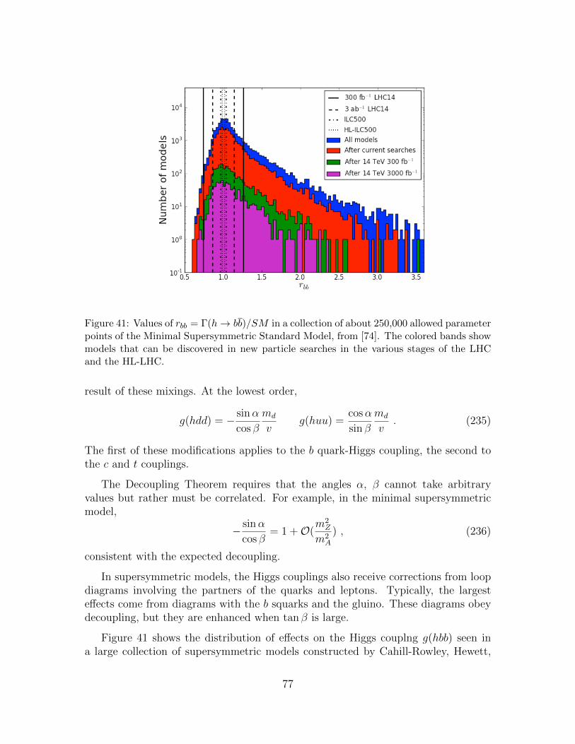
Figure 41: Values of rbb = Γ(h→ bb)/SM in a collection of about 250,000 allowed parameterpoints of the Minimal Supersymmetric Standard Model, from [74]. The colored bands showmodels that can be discovered in new particle searches in the various stages of the LHCand the HL-LHC.
result of these mixings. At the lowest order,
g(hdd) = − sinα
cos β
md
vg(huu) =
cosα
sin β
md
v. (235)
The first of these modifications applies to the b quark-Higgs coupling, the second tothe c and t couplings.
The Decoupling Theorem requires that the angles α, β cannot take arbitraryvalues but rather must be correlated. For example, in the minimal supersymmetricmodel,
− sinα
cos β= 1 +O(
m2Z
m2A
) , (236)
consistent with the expected decoupling.
In supersymmetric models, the Higgs couplings also receive corrections from loopdiagrams involving the partners of the quarks and leptons. Typically, the largesteffects come from diagrams with the b squarks and the gluino. These diagrams obeydecoupling, but they are enhanced when tan β is large.
Figure 41 shows the distribution of effects on the Higgs couplng g(hbb) seen ina large collection of supersymmetric models constructed by Cahill-Rowley, Hewett,
77
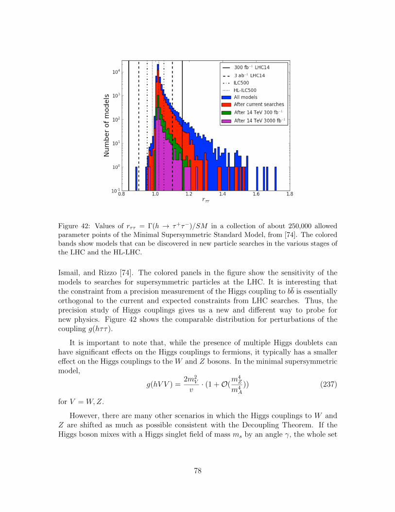
Figure 42: Values of rττ = Γ(h → τ+τ−)/SM in a collection of about 250,000 allowedparameter points of the Minimal Supersymmetric Standard Model, from [74]. The coloredbands show models that can be discovered in new particle searches in the various stages ofthe LHC and the HL-LHC.
Ismail, and Rizzo [74]. The colored panels in the figure show the sensitivity of themodels to searches for supersymmetric particles at the LHC. It is interesting thatthe constraint from a precision measurement of the Higgs coupling to bb is essentiallyorthogonal to the current and expected constraints from LHC searches. Thus, theprecision study of Higgs couplings gives us a new and different way to probe fornew physics. Figure 42 shows the comparable distribution for perturbations of thecoupling g(hττ).
It is important to note that, while the presence of multiple Higgs doublets canhave significant effects on the Higgs couplings to fermions, it typically has a smallereffect on the Higgs couplings to the W and Z bosons. In the minimal supersymmetricmodel,
g(hV V ) =2m2
V
v· (1 +O(
m4Z
m4A
)) (237)
for V = W,Z.
However, there are many other scenarios in which the Higgs couplings to W andZ are shifted as much as possible consistent with the Decoupling Theorem. If theHiggs boson mixes with a Higgs singlet field of mass ms by an angle γ, the whole set
78
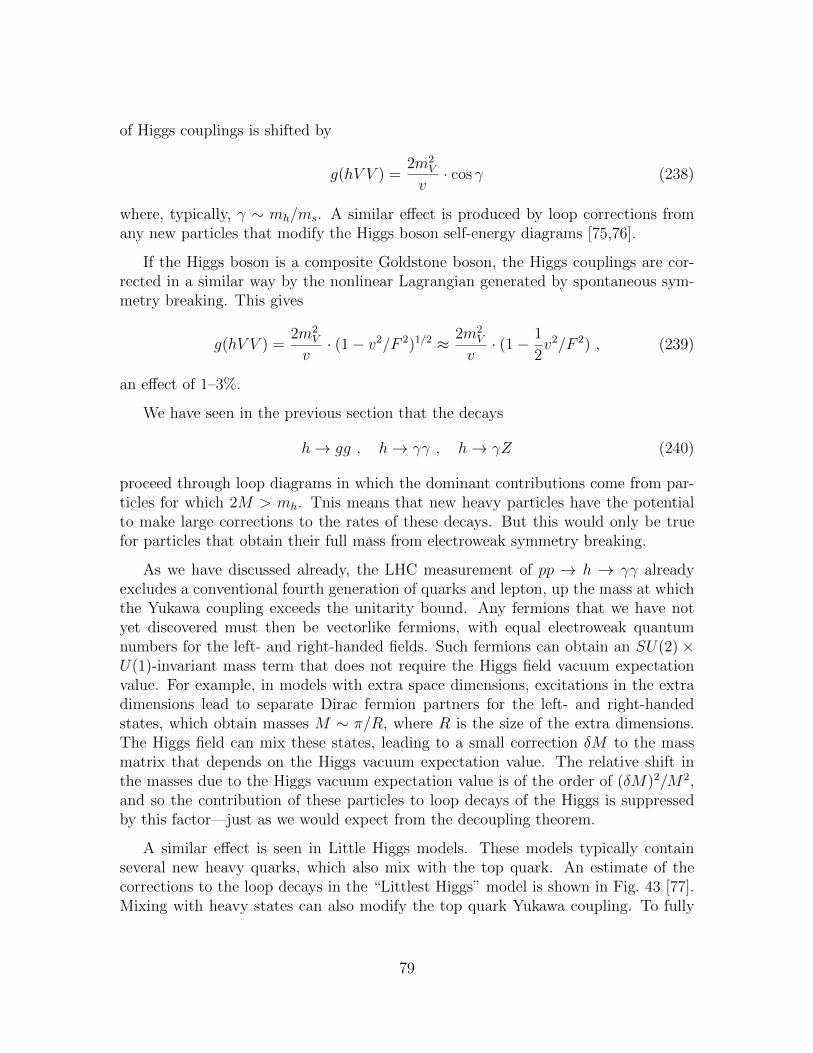
of Higgs couplings is shifted by
g(hV V ) =2m2
V
v· cos γ (238)
where, typically, γ ∼ mh/ms. A similar effect is produced by loop corrections fromany new particles that modify the Higgs boson self-energy diagrams [75,76].
If the Higgs boson is a composite Goldstone boson, the Higgs couplings are cor-rected in a similar way by the nonlinear Lagrangian generated by spontaneous sym-metry breaking. This gives
g(hV V ) =2m2
V
v· (1− v2/F 2)1/2 ≈ 2m2
V
v· (1− 1
2v2/F 2) , (239)
an effect of 1–3%.
We have seen in the previous section that the decays
h→ gg , h→ γγ , h→ γZ (240)
proceed through loop diagrams in which the dominant contributions come from par-ticles for which 2M > mh. Tnis means that new heavy particles have the potentialto make large corrections to the rates of these decays. But this would only be truefor particles that obtain their full mass from electroweak symmetry breaking.
As we have discussed already, the LHC measurement of pp → h → γγ alreadyexcludes a conventional fourth generation of quarks and lepton, up the mass at whichthe Yukawa coupling exceeds the unitarity bound. Any fermions that we have notyet discovered must then be vectorlike fermions, with equal electroweak quantumnumbers for the left- and right-handed fields. Such fermions can obtain an SU(2)×U(1)-invariant mass term that does not require the Higgs field vacuum expectationvalue. For example, in models with extra space dimensions, excitations in the extradimensions lead to separate Dirac fermion partners for the left- and right-handedstates, which obtain masses M ∼ π/R, where R is the size of the extra dimensions.The Higgs field can mix these states, leading to a small correction δM to the massmatrix that depends on the Higgs vacuum expectation value. The relative shift inthe masses due to the Higgs vacuum expectation value is of the order of (δM)2/M2,and so the contribution of these particles to loop decays of the Higgs is suppressedby this factor—just as we would expect from the decoupling theorem.
A similar effect is seen in Little Higgs models. These models typically containseveral new heavy quarks, which also mix with the top quark. An estimate of thecorrections to the loop decays in the “Littlest Higgs” model is shown in Fig. 43 [77].Mixing with heavy states can also modify the top quark Yukawa coupling. To fully
79
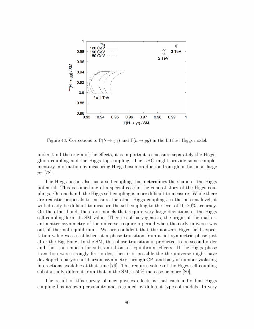
Figure 43: Corrections to Γ(h→ γγ) and Γ(h→ gg) in the Littlest Higgs model.
understand the origin of the effects, it is important to measure separately the Higgs-gluon coupling and the Higgs-top coupling. The LHC might provide some comple-mentary information by measuring Higgs boson production from gluon fusion at largepT [78].
The Higgs boson also has a self-coupling that determines the shape of the Higgspotential. This is something of a special case in the general story of the Higgs cou-plings. On one hand, the Higgs self-coupling is more difficult to measure. While thereare realistic proposals to measure the other Higgs couplings to the percent level, itwill already be difficult to measure the self-coupling to the level of 10–20% accuracy.On the other hand, there are models that require very large deviations of the Higgsself-coupling form its SM value. Theories of baryogenesis, the origin of the matter-antimatter asymmetry of the universe, require a period when the early universe wasout of thermal equilibrium. We are confident that the nonzero Higgs field expec-tation value was established at a phase transition from a hot symmetric phase justafter the Big Bang. In the SM, this phase transition is predicted to be second-orderand thus too smooth for substantial out-of-equilibrium effects. If the Higgs phasetransition were strongly first-order, then it is possible the the universe might havedeveloped a baryon-antibaryon asymmetry through CP- and baryon number violatinginteractions available at that time [79]. This requires values of the Higgs self-couplingsubstantially different from that in the SM, a 50% increase or more [80].
The result of this survey of new physics effects is that each individual Higgscoupling has its own personality and is guided by different types of models. In very
80
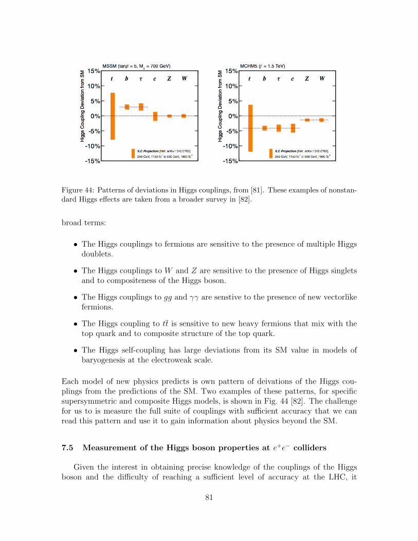
Figure 44: Patterns of deviations in Higgs couplings, from [81]. These examples of nonstan-dard Higgs effects are taken from a broader survey in [82].
broad terms:
• The Higgs couplings to fermions are sensitive to the presence of multiple Higgsdoublets.
• The Higgs couplings to W and Z are sensitive to the presence of Higgs singletsand to compositeness of the Higgs boson.
• The Higgs couplings to gg and γγ are senstive to the presence of new vectorlikefermions.
• The Higgs coupling to tt is sensitive to new heavy fermions that mix with thetop quark and to composite structure of the top quark.
• The Higgs self-coupling has large deviations from its SM value in models ofbaryogenesis at the electroweak scale.
Each model of new physics predicts is own pattern of deivations of the Higgs cou-plings from the predictions of the SM. Two examples of these patterns, for specificsupersymmetric and composite Higgs models, is shown in Fig. 44 [82]. The challengefor us to is measure the full suite of couplings with sufficient accuracy that we canread this pattern and use it to gain information about physics beyond the SM.
7.5 Measurement of the Higgs boson properties at e+e− colliders
Given the interest in obtaining precise knowledge of the couplings of the Higgsboson and the difficulty of reaching a sufficient level of accuracy at the LHC, it
81
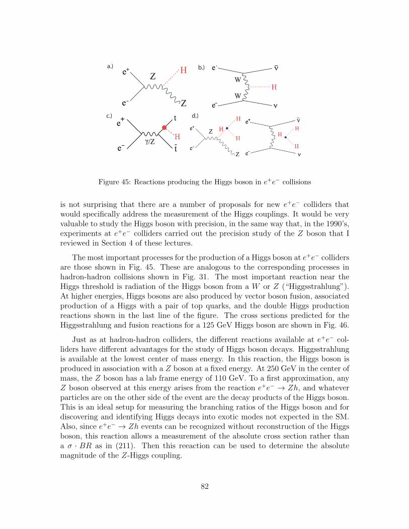
a.) b.)
c.) d.)
Figure 45: Reactions producing the Higgs boson in e+e− collisions
is not surprising that there are a number of proposals for new e+e− colliders thatwould specifically address the measurement of the Higgs couplings. It would be veryvaluable to study the Higgs boson with precision, in the same way that, in the 1990’s,experiments at e+e− colliders carried out the precision study of the Z boson that Ireviewed in Section 4 of these lectures.
The most important processes for the production of a Higgs boson at e+e− collidersare those shown in Fig. 45. These are analogous to the corresponding processes inhadron-hadron collisions shown in Fig. 31. The most important reaction near theHiggs threshold is radiation of the Higgs boson from a W or Z (“Higgsstrahlung”).At higher energies, Higgs bosons are also produced by vector boson fusion, associatedproduction of a Higgs with a pair of top quarks, and the double Higgs productionreactions shown in the last line of the figure. The cross sections predicted for theHiggsstrahlung and fusion reactions for a 125 GeV Higgs boson are shown in Fig. 46.
Just as at hadron-hadron colliders, the different reactions available at e+e− col-liders have different advantages for the study of Higgs boson decays. Higgsstrahlungis available at the lowest center of mass energy. In this reaction, the Higgs boson isproduced in association with a Z boson at a fixed energy. At 250 GeV in the center ofmass, the Z boson has a lab frame energy of 110 GeV. To a first approximation, anyZ boson observed at this energy arises from the reaction e+e− → Zh, and whateverparticles are on the other side of the event are the decay products of the Higgs boson.This is an ideal setup for measuring the branching ratios of the Higgs boson and fordiscovering and identifying Higgs decays into exotic modes not expected in the SM.Also, since e+e− → Zh events can be recognized without reconstruction of the Higgsboson, this reaction allows a measurement of the absolute cross section rather thana σ · BR as in (211). Then this reeaction can be used to determine the absolutemagnitude of the Z-Higgs coupling.
82
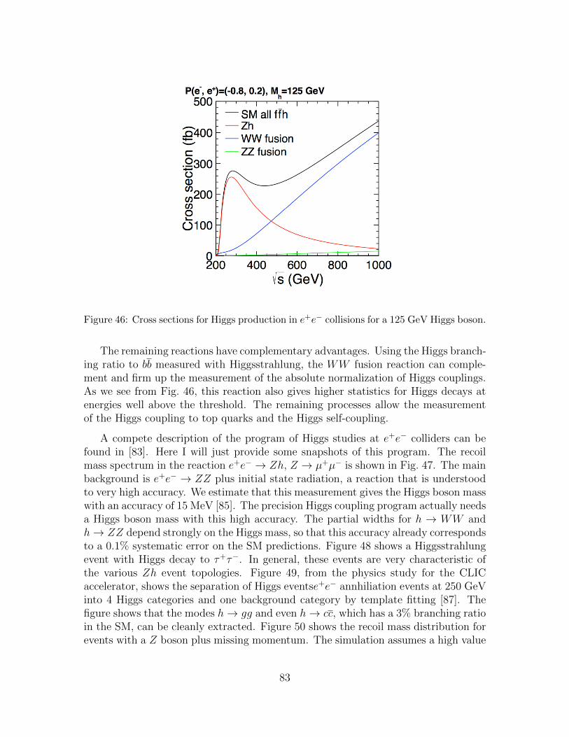
Figure 46: Cross sections for Higgs production in e+e− collisions for a 125 GeV Higgs boson.
The remaining reactions have complementary advantages. Using the Higgs branch-ing ratio to bb measured with Higgsstrahlung, the WW fusion reaction can comple-ment and firm up the measurement of the absolute normalization of Higgs couplings.As we see from Fig. 46, this reaction also gives higher statistics for Higgs decays atenergies well above the threshold. The remaining processes allow the measurementof the Higgs coupling to top quarks and the Higgs self-coupling.
A compete description of the program of Higgs studies at e+e− colliders can befound in [83]. Here I will just provide some snapshots of this program. The recoilmass spectrum in the reaction e+e− → Zh, Z → µ+µ− is shown in Fig. 47. The mainbackground is e+e− → ZZ plus initial state radiation, a reaction that is understoodto very high accuracy. We estimate that this measurement gives the Higgs boson masswith an accuracy of 15 MeV [85]. The precision Higgs coupling program actually needsa Higgs boson mass with this high accuracy. The partial widths for h → WW andh→ ZZ depend strongly on the Higgs mass, so that this accuracy already correspondsto a 0.1% systematic error on the SM predictions. Figure 48 shows a Higgsstrahlungevent with Higgs decay to τ+τ−. In general, these events are very characteristic ofthe various Zh event topologies. Figure 49, from the physics study for the CLICaccelerator, shows the separation of Higgs eventse+e− annhiliation events at 250 GeVinto 4 Higgs categories and one background category by template fitting [87]. Thefigure shows that the modes h→ gg and even h→ cc, which has a 3% branching ratioin the SM, can be cleanly extracted. Figure 50 shows the recoil mass distribution forevents with a Z boson plus missing momentum. The simulation assumes a high value
83
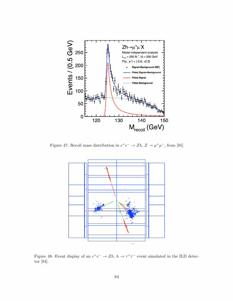
Figure 47: Recoil mass distribution in e+e− → Zh, Z → µ+µ−, from [85]
Figure 48: Event display of an e+e− → Zh, h → τ+τ− event simulated in the ILD detec-tor [84].
84
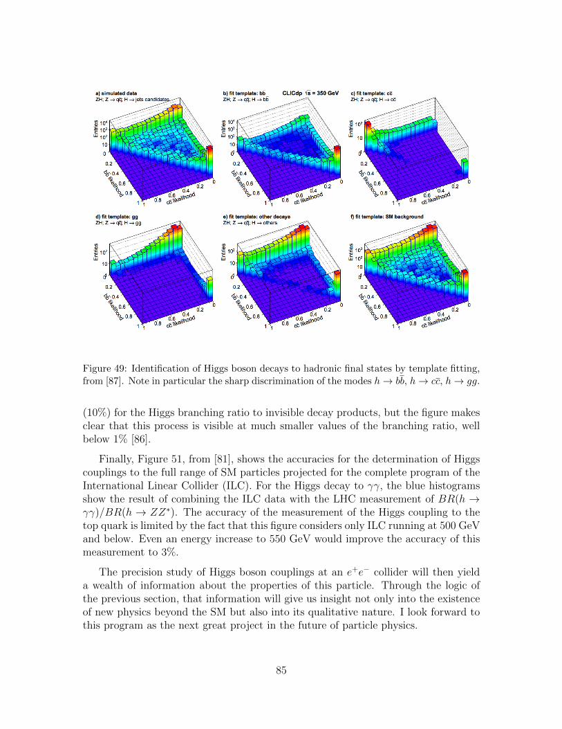
Figure 49: Identification of Higgs boson decays to hadronic final states by template fitting,from [87]. Note in particular the sharp discrimination of the modes h→ bb, h→ cc, h→ gg.
(10%) for the Higgs branching ratio to invisible decay products, but the figure makesclear that this process is visible at much smaller values of the branching ratio, wellbelow 1% [86].
Finally, Figure 51, from [81], shows the accuracies for the determination of Higgscouplings to the full range of SM particles projected for the complete program of theInternational Linear Collider (ILC). For the Higgs decay to γγ, the blue histogramsshow the result of combining the ILC data with the LHC measurement of BR(h →γγ)/BR(h → ZZ∗). The accuracy of the measurement of the Higgs coupling to thetop quark is limited by the fact that this figure considers only ILC running at 500 GeVand below. Even an energy increase to 550 GeV would improve the accuracy of thismeasurement to 3%.
The precision study of Higgs boson couplings at an e+e− collider will then yielda wealth of information about the properties of this particle. Through the logic ofthe previous section, that information will give us insight not only into the existenceof new physics beyond the SM but also into its qualitative nature. I look forward tothis program as the next great project in the future of particle physics.
85
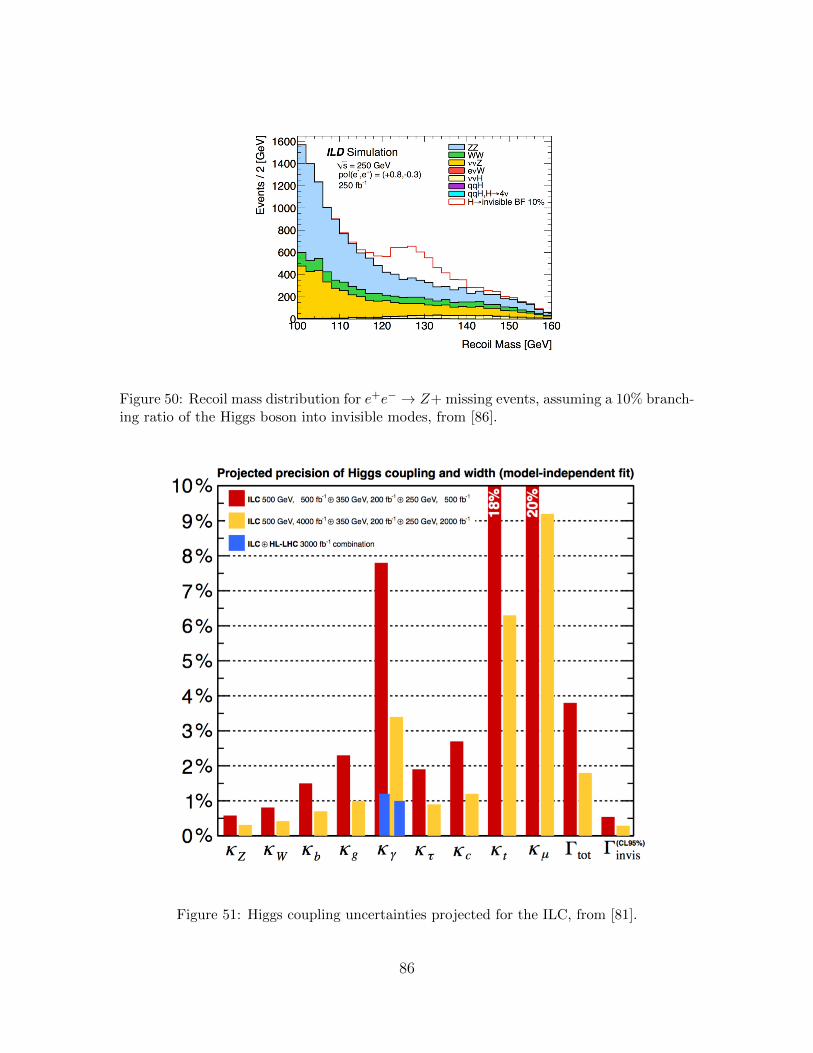
Figure 50: Recoil mass distribution for e+e− → Z+ missing events, assuming a 10% branch-ing ratio of the Higgs boson into invisible modes, from [86].
Figure 51: Higgs coupling uncertainties projected for the ILC, from [81].
86
8 Conclusions
In these lectures, I have developed the theory of the weak interaction from itsexperimental foundations in the V –A effective theory, through the precision studyof SU(2) × U(1) couplings at the Z resonance, to the present and future study ofthe couplings of the Higgs boson. We have learned much about this fundamentalinteraction of nature, but there is much more that we need to learn, and that wecan learn from future experiments. The study of the weak interaction is not a closedsubject but one that still contains tantalizing questions and promises to open newchapters in our exploration of particle physics.
References
[1] S. Weinberg, Phys. Rev. Lett. 19, 1264 (1967).
[2] A. Salam, in Procededings of the 8th Nobel Symposium: Elementary ParticleTheory, N. Svartholm, ed. (Almqvist and Wiksell, 1968).
[3] G. Aad et al. [ATLAS Collaboration], Phys. Lett. B 716, 1 (2012)[arXiv:1207.7214 [hep-ex]].
[4] S. Chatrchyan et al. [CMS Collaboration], Phys. Lett. B 716, 30 (2012)[arXiv:1207.7235 [hep-ex]].
[5] J. M. Cornwall, D. N. Levin and G. Tiktopoulos, Phys. Rev. D 10, 1145 (1974)Erratum: [Phys. Rev. D 11, 972 (1975)].
[6] C. E. Vayonakis, Lett. Nuovo Cim. 17, 383 (1976).
[7] M. E. Peskin and D. V. Schroeder, An Introduction to Quantum Field Theory’.(Westview Press, 1995).
[8] M. D. Schwartz, Quantum Field Theory and the Standard Model. (CambridgeUniversity Press, 2013).
[9] F. Englert and R. Brout, Phys. Rev. Lett. 13, 321 (1964).
[10] P. W. Higgs, Phys. Lett. 12, 132 (1964), Phys. Rev. Lett. 13, 508 (1964).
[11] G. S. Guralnik, C. R. Hagen and T. W. B. Kibble, Phys. Rev. Lett. 13, 585(1964).
[12] C. Patrignani et al. (Particle Data Group), Chin. Phys. C 40, 100001 (2016).
87
[13] F. W. J. Koks and J. Van Klinken, Nucl. Phys. A 272, 61 (1976).
[14] M. Bardon, P. Norton, J. Peoples, A. M. Sachs and J. Lee-Franzini, Phys. Rev.Lett. 14, 449 (1965).
[15] J. G. H. de Groot et al., Z. Phys. C 1, 143 (1979).
[16] G. Aad et al. [ATLAS Collaboration], Phys. Lett. B 701, 31 (2011)[arXiv:1103.2929 [hep-ex]].
[17] S. Chatrchyan et al. [CMS Collaboration], JHEP 1104, 050 (2011)[arXiv:1103.3470 [hep-ex]].
[18] P. Abreu et al. [DELPHI Collaboration], Eur. Phys. J. C 11, 383 (1999).
[19] I am grateful to Michael Hildreth for assembling this compilation of preliminaryLEP 2 data.
[20] S. Schael et al. [ALEPH and DELPHI and L3 and OPAL and LEP ElectroweakCollaborations], Phys. Rept. 532, 119 (2013) [arXiv:1302.3415 [hep-ex]].
[21] E. A. Kuraev and V. S. Fadin, Sov. J. Nucl. Phys. 41, 466 (1985) [Yad. Fiz. 41,733 (1985)].
[22] S. Schael et al. [ALEPH and DELPHI and L3 and OPAL and SLD Collaborationsand LEP Electroweak Working Group and SLD Electroweak Group and SLDHeavy Flavour Group], Phys. Rept. 427, 257 (2006) [hep-ex/0509008].
[23] O. Nicrosini and L. Trentadue, Nucl. Phys. B 318, 1 (1989).
[24] G. Abbiendi et al. [OPAL Collaboration], Eur. Phys. J. C 19, 587 (2001) [hep-ex/0012018]. I thank Toshinori Mori for the use of this figure.
[25] D. Decamp et al. [ALEPH Collaboration], Z. Phys. C 48, 365 (1990).
[26] R. Akers et al. [OPAL Collaboration], Z. Phys. C 65, 17 (1995).
[27] K. Abe et al. [SLD Collaboration], Phys. Rev. Lett. 80, 660 (1998) [hep-ex/9708015]. Phys. Rev. Lett. 94, 091801 (2005) [hep-ex/0410042].
[28] A. Heister et al. [ALEPH Collaboration], Eur. Phys. J. C 20, 401 (2001) [hep-ex/0104038].
[29] K. Abe et al. [SLD Collaboration], Phys. Rev. Lett. 86, 1162 (2001) [hep-ex/0010015].
[30] K. Abe et al. [SLD Collaboration], Phys. Rev. Lett. 81, 942 (1998).
88
[31] J. Erler and A. Freitas, in [12]
[32] W. J. Marciano and A. Sirlin, Phys. Rev. D 29, 945 (1984) Erratum: [Phys.Rev. D 31, 213 (1985)].
[33] M. E. Peskin and T. Takeuchi, Phys. Rev. Lett. 65, 964 (1990), Phys. Rev. D46, 381 (1992).
[34] M. Baak et al. [Gfitter Group], Eur. Phys. J. C 74, 3046 (2014) [arXiv:1407.3792[hep-ph]].
[35] M. S. Chanowitz and M. K. Gaillard, Nucl. Phys. B 261, 379 (1985).
[36] V. Khachatryan et al. [CMS Collaboration], Phys. Lett. B 762, 512 (2016)[arXiv:1605.09047 [hep-ex]].
[37] W. Alles, C. Boyer and A. J. Buras, Nucl. Phys. B 119, 125 (1977).
[38] K. Hagiwara, R. D. Peccei, D. Zeppenfeld and K. Hikasa, Nucl. Phys. B 282,253 (1987).
[39] B. Grzadkowski, M. Iskrzynski, M. Misiak and J. Rosiek, JHEP 1010, 085 (2010)[arXiv:1008.4884 [hep-ph]].
[40] S. Willenbrock and C. Zhang, Ann. Rev. Nucl. Part. Sci. 64, 83 (2014)[arXiv:1401.0470 [hep-ph]].
[41] B. Henning, X. Lu and H. Murayama, JHEP 1601, 023 (2016) [arXiv:1412.1837[hep-ph]].
[42] A. Falkowski, M. Gonzalez-Alonso, A. Greljo, D. Marzocca and M. Son,arXiv:1609.06312 [hep-ph].
[43] S. Dawson, Nucl. Phys. B 249, 42 (1985).
[44] J. F. Gunion, H. E. Haber, G. L. Kane and S. Dawson, The Higgs Hunter’sGuide. (Westview Press, 2000).
[45] S. Heinemeyer et al. [LHC Higgs Cross Section Working Group], Handbook ofLHC Higgs Cross Sections: 3. Higgs Properties, arXiv:1307.1347 [hep-ph].
[46] CMS Collaboration, CMS-PAS-HIG-13-002 (2013).
[47] M. I. Vysotsky, arXiv:1312.0474 [hep-ph].
[48] M. Carena, C. Grojean, M. Kado, and V. Sharma, in K. A. Olive et al. (ParticleData Group), Chin. Phys. C38, 090001 (2014).
89
[49] V. Khachatryan et al. [CMS Collaboration], Eur. Phys. J. C 74, no. 10, 3076(2014) [arXiv:1407.0558 [hep-ex]].
[50] G. Aad et al. [ATLAS Collaboration], Phys. Lett. B 726, 88 (2013) Erratum:[Phys. Lett. B 734, 406 (2014)] [arXiv:1307.1427 [hep-ex]].
[51] G. Aad et al. [ATLAS Collaboration], Phys. Rev. D 92, 012006 (2015)[arXiv:1412.2641 [hep-ex]].
[52] A. M. Sirunyan et al. [CMS Collaboration], arXiv:1708.00373 [hep-ex].
[53] ATLAS Collaboration, ATLAS-CONF-2013-108 (2013).
[54] M. Aaboud et al. [ATLAS Collaboration], arXiv:1708.03299 [hep-ex].
[55] CMS Collaboration, CMS-PAS-HIG-17-010 (2017).
[56] M. Carena, C. Grojean, M. Kado, and V. Sharma, in C. Patrignani et al. (ParticleData Group), Chin. Phys. C40, 100001 (2016).
[57] H. K. Onnes, Commun. Phys. Lab. Univ. Leiden. 12, 120 (1911).
[58] V. L. Ginzburg and L. D. Landau, Zh. Eksp. Teor. Fiz. 20, 1064 (1950).
[59] J. Bardeen, L. N. Cooper and J. R. Schrieffer, Phys. Rev. 108, 1175 (1957).
[60] S. P. Martin, in Perspectives on Supersymmetry, G. L. Kane, ed. (World Scien-tific, 1998) [hep-ph/9709356].
[61] M. E. Peskin, in Exploring New Frontiers Using Collider and Neutrinos(TASI 2006), S. Dawson and R. Mohapatra, eds. (World Scientific, 2008)[arXiv:0801.1928 [hep-ph]].
[62] R. Contino, Y. Nomura and A. Pomarol, Nucl. Phys. B 671, 148 (2003) [hep-ph/0306259].
[63] T. Gherghetta, in Physics of the Large and the Small (TASI 09), C. Csaki andS. Dodelson, eds. (World Scientific, 2011) [arXiv:1008.2570 [hep-ph]].
[64] P. Sikivie, L. Susskind, M. B. Voloshin and V. I. Zakharov, Nucl. Phys. B 173,189 (1980).
[65] H. Georgi and M. Machacek, Nucl. Phys. B 262, 463 (1985).
[66] H. E. Logan and V. Rentala, Phys. Rev. D 92, no. 7, 075011 (2015)[arXiv:1502.01275 [hep-ph]].
[67] S. Weinberg, Phys. Rev. D 19, 1277 (1979).
90
[68] L. Susskind, Phys. Rev. D 20, 2619 (1979).
[69] N. Arkani-Hamed, A. G. Cohen, E. Katz and A. E. Nelson, JHEP 0207, 034(2002) [hep-ph/0206021].
[70] M. Schmaltz and D. Tucker-Smith, Ann. Rev. Nucl. Part. Sci. 55, 229 (2005)[hep-ph/0502182].
[71] H. E. Haber, in Electroweak Symmetry Breaking, F. Csikor and G. Pocsik, eds.(World Scientific, 1995) [hep-ph/9501320].
[72] R. K. Dewanjee [CMS Collaboration], PoS DIS 2016, 100 (2016).
[73] ATLAS Collaboration, ATLAS-CONF-2017-050 (2017).
[74] M. Cahill-Rowley, J. Hewett, A. Ismail and T. Rizzo, Phys. Rev. D 90, 095017(2014) [arXiv:1407.7021 [hep-ph]].
[75] V. Barger, T. Han, P. Langacker, B. McElrath and P. Zerwas, Phys. Rev. D 67,115001 (2003) [hep-ph/0301097].
[76] N. Craig, C. Englert and M. McCullough, Phys. Rev. Lett. 111, 121803 (2013)[arXiv:1305.5251 [hep-ph]].
[77] T. Han, H. E. Logan, B. McElrath and L. T. Wang, Phys. Lett. B 563, 191(2003) Erratum: [Phys. Lett. B 603, 257 (2004)] [hep-ph/0302188].
[78] C. Grojean, E. Salvioni, M. Schlaffer and A. Weiler, JHEP 1405, 022 (2014)[arXiv:1312.3317 [hep-ph]].
[79] D. E. Morrissey and M. J. Ramsey-Musolf, New J. Phys. 14, 125003 (2012)[arXiv:1206.2942 [hep-ph]].
[80] A. Noble and M. Perelstein, Phys. Rev. D 78, 063518 (2008) [arXiv:0711.3018[hep-ph]]
[81] K. Fujii et al., arXiv:1506.05992 [hep-ex].
[82] S. Kanemura, K. Tsumura, K. Yagyu and H. Yokoya, Phys. Rev. D 90, 075001(2014) [arXiv:1406.3294 [hep-ph]].
[83] H. Baer et al., The International Linear Collider Technical Design Report - Vol-ume 2: Physics, arXiv:1306.6352 [hep-ph].
[84] I thank Manqi Ruan for the use of this figure.
[85] J. Yan, S. Watanuki, K. Fujii, A. Ishikawa, D. Jeans, J. Strube, J. Tian andH. Yamamoto, Phys. Rev. D 94, 113002 (2016) [arXiv:1604.07524 [hep-ex]].
91

[86] J. Tian and K. Fujii, Nucl. Part. Phys. Proc. 273-275, 826 (2016).
[87] H. Abramowicz et al., Eur. Phys. J. C 77, no. 7, 475 (2017) [arXiv:1608.07538[hep-ex]].
92


![Lectures and essays [microform]](https://img.pdfslide.net/doc/110x75/6333fdffa6138719eb0adf7d/lectures-and-essays-microform.jpg)


