Limit and Shakedown Analysis Using a General Purpose Finite Element Code

M. Staat, M. Heitzer Institute for Safety Research and Reactor Technology,

Forschungszentmm Jtilich GmbH, D-52425 Jlilich, Germany

Abstract

Limit and shakedown theorems are exact theories of classical plasticity for the direct computation of safety factors or of the load carrying capac­ity under constant and varying loads. They are implemented in a general purpose FEM code in a way capable of large-scale analysis. The method deviates from the current approach in several aspects: No load history is used, the field quantities are not calculated, and the solution is ob­tained from a mathematical optimization problem. The approach needs considerably less input data and computer time than incremental plastic analyses.

l INTRODUCTION

Finite Element Method (FEM) is greatly accepted as prime numerical method for computation of field quantities such as stress or deformation in engineering structures and passive components. Todays computing capacities and postpro­cessing quality give fairly complete knowledge of these field quantities to the engineer with high accuracy for complex structures, loading, and constitutive equations. However, it is not always this knowledge what the engineer is look­ing for. The chief objective of engineering design is the assessment of the load carrying capacity or of the life time of a structure.

Comparison of stress or displacement to allowable values yields the de­sired answer if the material is brittle or if displacemems at critical points are restricted. If the load carrying capacity is governed by fracture mechanics there are various postprocessors to derive the relevant measures like e.g. J-integral from the computed FE-fields. But simple stress analysis tells the engineer little to nothing about structural safety if failure is of the ductile type. The situa­tion is most obvious from the fact that residual stresses have no influence on the collapse load in a monotone loading programme, provided they do not sig­nificantly alter the geometry of the structure (this excludes buckling from our

522

discussion) or the yield surface of its material. This property is known from the theory of limit analysis and is supported by numerous experiments, the most striking one being the classica1 two-span beam investigated in [7]. It is impossible to derive this fact from the discussion of the computed stress field.

Practically, residual stresses in metallic structures are hardly known and difficult to avoid. They are introduced in steel structures by the production process: rolling, cold straightening, flame cutting, welding, and cold forming. Additional residual stress may be caused by foundation setting or incidentaJ overloading. In pressure vessels and piping there are usually thermal stresses with the consequence that all design codes require the engineer to make a dis­tinction into primary and secondary stress (i.e. respectively, load and displace­ment controlled stress). This distinction has to be made by the analyst on the FEM input, because it cannot be read from the stress output.

It is obvious, that rational design must take ductility into account for struc­tures made of ductile material. Additional reasons are given by the possible occurence of high local stresses, which do not present a problem if ductile flow leads to stress redistribution. Several examples demonstrate the opportunities offered by relaxing the restrictive conditions imposed by elasticity.

In this contribution it is shown, how the design process for ductile mate­rials may be integrated into a general purpose FEM code within the classical theory of plasticity. The code PERMAS was chosen, because it is sufficiently open to the user allowing to implement limit and shakedown analysis, which means a radical departure from current FEM concepts and solution steps, with­out any need of support by the PERMAS developers [9]. To the knowledge of the authors it is the first implementation of its kind.

2 PLASTIC FAILURE CONCEPTS

The reasons why the simple stress calculation tells so little about ductile col­lapse of an (internally) statically undetermined structure is, that the redundancy of the structure is reduced by local (contained) flow connected with stress re­distribution until a statically determined state is reached. Only then has stress a simple meaning for the further displacement towards collapse. Note in passing, that the statically determined state removes any residual stress, the dependence on the load path, and also the influence of the details of the constitutive equa­tions on the value of the limit load.

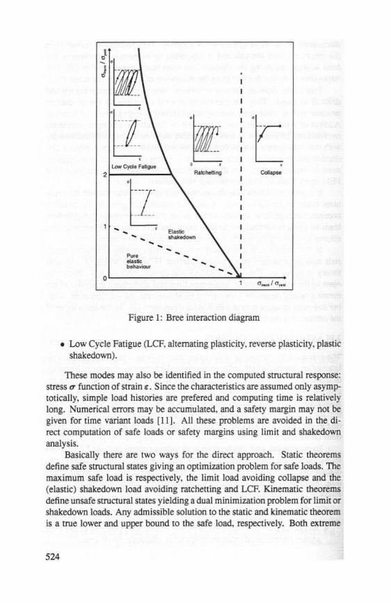
To understand what can be done with todays general purpose FEM codes let us discuss the plastic structural behaviour iconized in the so-called Bree­diagram for a thin walled tube. This is a map giving regions of different struc­tural response in the space of thermal and mechanical loads (internal pressure). Possible failure modes are:

• Collapse at ultimate load (limit load).

• Ratchetting i.e. accumulation of plastic deformation over successive load cycles (incremental collapse, progressive plasticity, cyclic creep).

2

0

Low Cycle Fati!Jie

1£ . -- --.. ( .. .. .. .. Pure elaslc behaviou.r

..

·~ •t 0

Ratchetting Collapse

Bastic shakedown .. .. .. .. ..

Figure 1: Bree interaction diagram

• Low Cycle Fatigue (LCF, alternating plasticity, reverse plasticity, plastic shakedown).

These modes may also be identified in the computed structural response: stress u function of strain e. Since the characteristics are assumed only asymp­totically, simple load histories are prefered and computing time is relatively long. Numerical errors may be accumulated, and a safety margin may not be given for time variant loads [11]. All these problems are avoided in the di­rect computation of safe loads or safety margins using limit and shakedown analysis.

Basically there are two ways for the direct approach. Static theorems define safe structural states giving an optimization problem for safe loads. The maximum safe load is respectively, the limit load avoiding collapse and the (elastic) shakedown load avoiding ratchetting and LCF. Kinematic theorems define unsafe structural states yielding a dual minimization problem for limit or shakedown loads. Any admissible solution to the static and kinematic theorem is a true lower and upper bound to the safe load, respectively. Both extreme

524

values are exact solutions, because there is no duality gap. The static approach is used, which is on the safe side for admissible solutions and is numerically more convenient. This report is restricted to ideal plasticity, emphasizing that extension to linear or bounded kinematic hardening is available [ 14].

Static limit load theorem: An elasto-plastic structure will not collapse under monotone loads if it is in static equilibrium and if the yield function is nowhere violated. The limit load is the maximum safe load.

For a load increasing with load factor {3 the above necessary conditions for a safe state of system n with traction boundary an~ (with outer normal n) and yield function ~ under body forces {Jb and surface loads {Jp read

divu = {Jb inn

0' n = {J p on an~

~ (u) :5 0 inn.

(1)

(2)

(3)

The limit load factor fJ1 = max {3 is a safety factor. This leads to the mathe­matical optimization problem formulated in static quantities (stress u )

max {3

such that (s.t.) restrictions (1)- (3) hold. (4)

Static shakedown theorem: An elasto-plastic structure will not fail with macro­scopic plasticity under time variant loads if it is in static equilibrium, if the yield function is nowhere and at no instance violated, and if all plastic deformations fade away, i.e. lim €P = 0 . The shakedown load is the maximum safe load.

t- oo There is only a difference between pure elastic behaviour and elastic

shakedown if the plastic part of the load history is known, because in the latter case the material becomes eventually elastic. Fig. 1 shows that there is no ben­efit for the thin tube under internal pressure alone. But with thermal stresses the shakedown region may increase the usefull operating by more than a factor two.

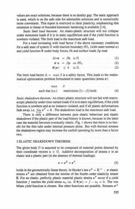
3 ELASTIC SHAKEDOWN THEOREM

The given body n is assumed to be composed of material points denoted by their coordinate vectors x E n. Additive decomposition of strains e in an elastic and a plastic part (in the absence of thermalloadings)

(5)

holds in the geometrically linear theory. In Hooke's law eE = E-1 u elastic strains eE are obtained from the inverse of the fourth-<>rder elasticity tensor E. For an elastic, perfectly plastic material plastic strains eP occur if a yield function f reaches the yield stress o-0 , i.e. if <P( u ) = f - o-0 = 0. The von Mises yield func~ion is chosen. But other functions are possible. Stresses u A

525

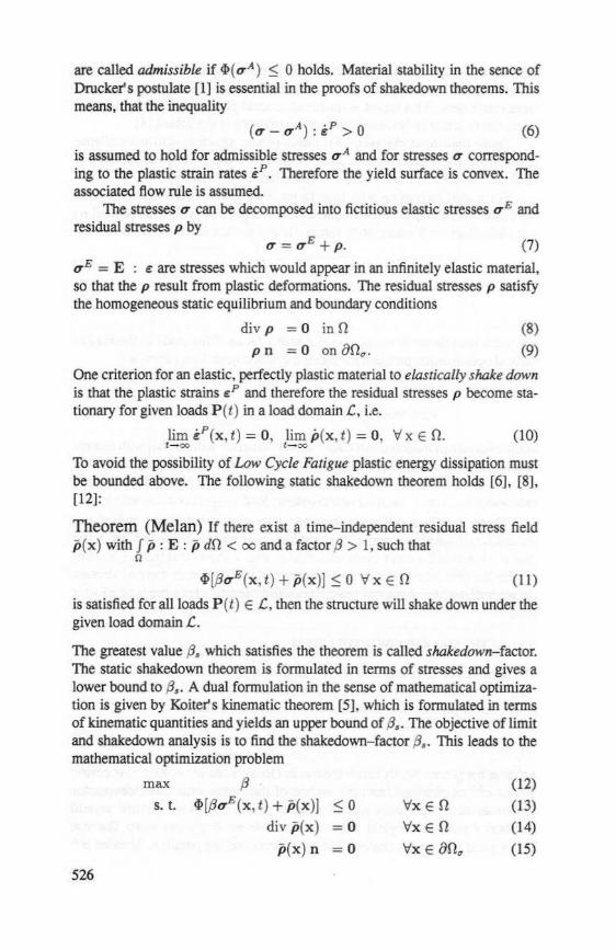
are called admissible if 11>( erA) ::; 0 holds. Material stability in the sence of Drucker' s postulate [ 1) is essential in the proofs of shakedown theorems. This means, that the inequality

(6)

is assumed to hold for admissible stresses erA and for stresses er correspond­ing to the plastic strain rates eP. Therefore the yield surface is convex. The associated flow rule is assumed.

The stresses er can be decomposed into fictitious elastic stresses erE and residual stresses p by

(7) erE = E : e are stresses which would appear in an infinitely elastic material, so that the p result from plastic deformations. The residual stresses p satisfy the homogeneous static equilibrium and boundary conditions

div p = 0 inn (8)

p n = 0 on anu. (9)

One criterion for an elastic, perfectly plastic material to elastically shake down is that the plastic strains eP and therefore the residual stresses p become sta­tionary for given loads P(t) in a load domain C, i.e.

lim ep(x, t) = 0, lim p(x , t) = 0, V X En. (10) t- oo t-oo

To avoid the possibility of Low Cycle Fatigue plastic energy dissipation must be bounded above. The following static shakedown theorem holds [6), [8), [12):

Theorem (Melan) If there exist a time-independent residual stress field p(x) with f p: E : p dO< oo and a factor {3 > l, such that

0

ll>[.BerE(x, t) + p(x )J :5 0 V X E n (11)

is satisfied for all loads P ( t) E C, then the structure will shake down under the given load domain C.

The greatest value {3. which satisfies the theorem is called shakedown-factor. The static shakedown theorem is formulated in terms of stresses and gives a lower bound to {3 •. A dual formulation in the sense of mathematical optimiza­tion is given by Koiter's kinematic theorem [5), which is formulated in terms of kinematic quantities and yields an upper bound of .B •. The objective of limit and shakedown analysis is to find the shakedown- factor ,8, . This leads to the mathematical optimization problem

max .B (12)

s. t. II> [.BerE(x , t) + p(x)J $0 VxEn (1 3)

div p(x ) =0 Vx E n (14)

p(x ) n =0 Vx E 80u (15)

526

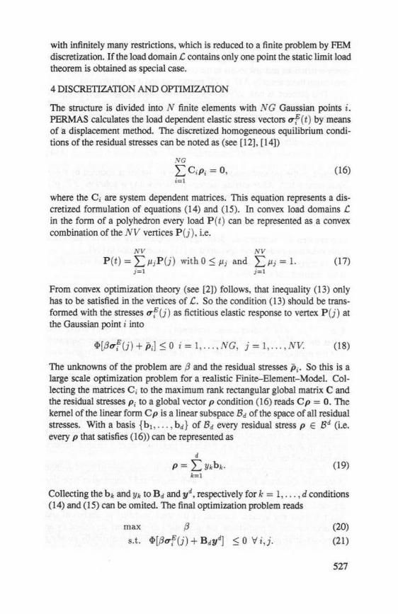
with infinitely many restrictions, which is reduced to a finite problem by FEM discretization. If the load domain .C contains only one point the static limit load theorem is obtained as special case.

4 DISCRETIZATION AND OPTIMIZATION

The structure is divided into N finite elements with NG Gaussian points i. PERMAS calculates the load dependent elastic stress vectors u f(t) by means of a displacement method. The discretized homogeneous equilibrium condi­tions of the residual stresses can be noted as (see [12], [14])

.VG

l::C;p; = 0, (16) i=l

where the C; are system dependent matrices. This equation represents a dis­cretized formulation of equations (14) and (15). In convex load domains .C in the form of a polyhedron every load P (t) can be represented as a convex combination of the NV vertices P (j), i.e.

NV NV P(t) = L ~L;P(j) withO ~ ~L; and L ILi = 1. (17)

j = l i= l

From convex optimization theory (see [2]) follows, that inequality (13) only has to be satisfied in the vertices of .C. So the condition (1 3) should be trans­formed with the stresses u f(j) as fictitious elastic response to vertex P (j) at the Gaussian point i into

<I>[,Buf(j) + i>;) ~ 0 i = 1, ... , NG, j = 1, .. . , N V. (18)

The unknowns of the problem are {3 and the residual stresses i>;. So this is a large scale optimization problem for a realistic Finite-Element-Model. Col­lecting the matrices C ; to the maximum rank rectangular global matrix C and the residual stresses P; to a global vector p condition (16) reads Cp = 0. The kernel of the linear form Cp is a linear subs pace Bd of the space of all residual stresses. With a basis {b" . . . , bd} of Bd every residual stress p E Bd (i.e. every p that satisfies (16)) can be represented as

(19)

Collecting the bk and Yk to B d and y d, respectively fork = 1, .. . , d conditions (14) and (15) can be omited. The final optimization problem reads

max {3

s.t. <I>[/3u f(j) + B dy d] ~ 0 V i, j.

(20)

(21)

527

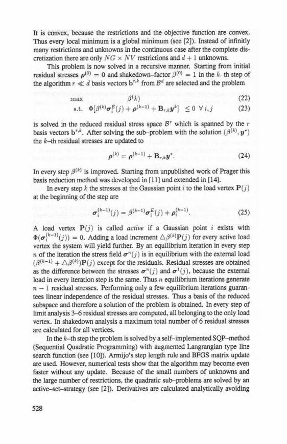
It is convex, because the restrictions and the objective function are convex. Thus every local minimum is a global minimum (see [2]). Instead of infinitly many restrictions and unknowns in the continuous case after the complete dis­cretization there are only NG x N V restrictions and d + 1 unknowns.

This problem is now solved in a recursive manner. Starting from initial residual stresses p<0> = 0 and shakedown-factor pco) = 1 in the k-th step of the algorithm r ~ d basis vectors b '·Jc from Bd are selected and the problem

max (3< k) (22)

s.t. 4>[f3Ckl cr f(j) + p<Jc-t) + B r,JcYk ] $ 0 V i,j (23)

is solved in the reduced residual stress space B' which is spanned by the r basis vectors b '•Jc. After solving the sub-problem with the solution (f3(Jc), y·) the k-th residual stresses are updated to

(24)

In every step f3(k) is improved. Starting from unpublished work of Prager this basis reduction method was developed in [11] und extended in [14].

In every step k the stresses at the Gaussian point i to the load vertex P (j) at the beginning of the step are

(Jc-1 )( ") _ f3(Jc- 1) E( ·) + (k-1) CT; J - CT; J Pi . (25)

A load vertex P (j) is called active if a Gaussian point i exists with 4>( cr~Jc-t)(j)) = 0. Adding a load increment .6.j3Cklp (j) for every active load vertex the system will yield further. By an equilibrium iteration in every step n of the iteration the stress field ern (j) is in equilibrium with the external load (f3<Jc-I) + .6.f3<"l)P (j) except for the residuals. Residual stresses are obtained as the difference between the stresses crn(j) and cr1(j), because the external load in every iteration step is the same. Thus n equilibrium iterations generate n - 1 residual stresses. Performing only a few equilibrium iterations guaran­tees linear independence of the residual stresses. Thus a basis of the reduced subs pace and therefore a solution of the problem is obtained. In every step of limit analysis 3-6 residual stresses are computed, all belonging to the only load vertex. In shakedown analysis a maximum total number of 6 residual stresses are calculated for all vertices.

In the k- th step the problem is solved by a self-implemented SQP- method (Sequential Quadratic Programming) with augmented Langrangian type line search function (see [10]). Armijo' s step length rule and BFGS matrix update are used. However, numerical tests show that the algorithm may become even faster without any update. Because of the small numbers of unknowns and the large number of restrictions, the quadratic sub-problems are solved by an active-set-strategy (see [2]). Derivatives are calculated analytically avoiding

528

automatic differentiation methods. All computations were performed on the same machine using version IV ofPERMAS (9].

5EXAMPLES

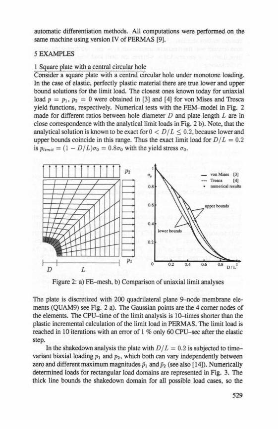
1 Square plate with a central circular hole Consider a square plate with a central circular hole under monotone loading. In the case of elastic, perfectly plastic material there are true lower and upper bound solutions for the limit load. The closest ones known today for uniaxial load p = P~> p2 = 0 were obtained in [3] and [4] for von Mises and Tresca yield functions, respectively. Numerical tests with the FEM-model in Fig. 2 made for different ratios between hole diameter D and plate length L are in close correspondence with the analytical limit loads in Fig. 2 b). Note, that the analytical solution is known to be exact for 0 < D I L ~ 0. 2, because lower and upper bounds coincide in this range. Thus the exact limit load forD I L = 0.2 is Plimit = ( 1 - D I L }cro = 0.8cro with the yield stress cro.

P2 a, von~s (3] -- Tresca (4]

0.8 . numerical results

0.6 upper bol!llds

0.4

0.2

0 0.2 0.4 D L

Figure 2: a) FE-mesh, b) Comparison ofuniaxiallimit analyses

The plate is discretized with 200 quadrilateral plane 9-node membrane ele­ments (QUAM9) see Fig. 2 a). The Gaussian points are the 4 corner nodes of the elements. The CPU- time of the limit analysis is 1 0-times shorter than the plastic incremental calculation of the limit load in PERMAS. The limit load is reached in 10 iterations with an error of 1 o/o only 60 CPU-sec after the elastic step.

In the shakedown analysis the plate with D I L = 0.2 is subjected to time­variant biaxial loading Pt and P2 . which both can vary independently between zero and different maximum magnitudes p1 and P2 (see also [14]). Numerically determined loads for rectangular load domains are represented in Fig. 3. The thick line bounds the shakedown domain for all possible load cases, so the

529

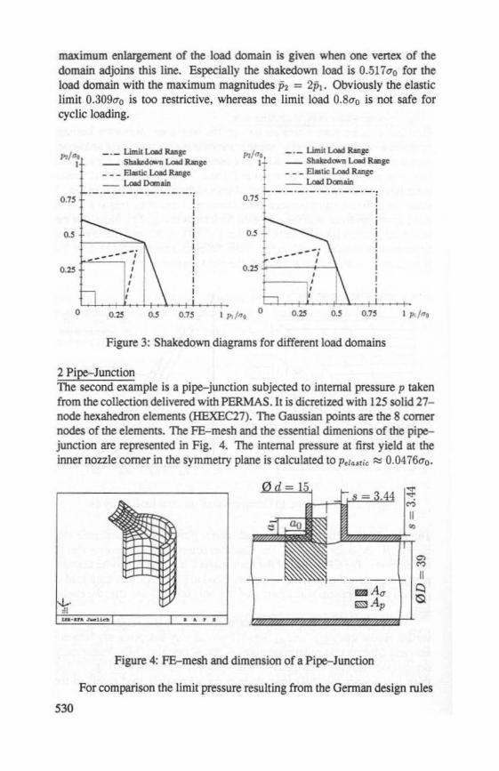
maximum enlaxgement of the load domain is given when one vertex of the domain adjoins this line. Especially the shakedown load is 0.517 u0 for the load domain with the maximum magnitudes fi2 = 2p1 • Obviously the elastic limit 0.309u0 is too restrictive, whereas the limit load 0.8u0 is not safe for cyclic loading.

P!/a• --- Limit Loed Ranae 1 - Shakedown Loed R.mge

_ _ _ Elastic Loed Range

- Loed D<Xnain ·-·-·-·-·-·-·- ·-·-··

0~ I

I

o.s

0.25

0.25 O.S 0.1S

P!/t7t, - · - Umit Loed Range 1- - Shakedown Loed Range

___ Elastic Loed Range _ Load Danain

·-·-·-·- ·- ·- ·-·-·-·· 0.7S 1

o.s

I 1--------., I

I I

I Pl/"e 0 0.25

I

O.S 0.1S

Figure 3: Shakedown diagrams for different load domains

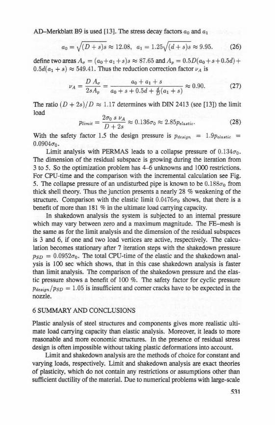
2 Pipe-Junction The second example is a pipe-junction subjected to internal pressure p taken from the collection delivered with PERMAS.It is dicretized with 125 solid 27-node hexahedron elements (HEXEC27). The Gaussian points are the 8 corner nodes of the elements. The FE- mesh and the essential dimenions of the pipe­junction are represented in Fig. 4. The internal pressure at first yield at the inner nozzle corner in the symmetry plane is calculated to Peto,tic ::::::: 0.0476uo.

I. A p •

Figure 4: FE-mesh and dimension of a Pipe-Junction

For comparison the limit pressure resulting from the German design rules

530

AD-Merkblatt B9 is used [13]. The stress decay factors ao and a1

a0 = j(D + s)s::::: 12.08, a1 = 1.25j(d + s)s::::: 9.95. (26)

definetwoareasA" = (ao+at +s)s ::::: 87.65 andAp = 0.5D(ao+s+0.5d)+ 0.5d( a1 + s) ::::: 549.41. Thus the reduction correction factor 11 A is

_ D A" _ ao + a1 + s ~ 0 90 IIA- - d ~ ' .

2sAp a0 + s + 0.5d + 0 (at + s) (27)

The ratio ( D + 2s) / D ::::: 1.17 determines with DIN 2413 (see [ 13]) the limit load

2ao s 11 A • Plimit = D +

25 ;:::;;: 0.136ao;:::;;: 2.85Pelastic · (28)

With the safety factor 1.5 the design pressure is Pdesign = 1.9Pela&tic = 0.0904ao.

Limit analysis with PERMAS leads to a collapse pressure of 0.134a0 •

The dimension of the residual subspace is growing during the iteration from 3 to 5. So the optimization problem has 4-6 unknowns and 1000 restrictions. For CPU-time and the comparison with the incremental calculation see Fig. 5. The collapse pressure of an undisturbed pipe is known to be 0.188ao from thick shell theory. Thus the junction presents a nearly 28 % weakening of the structure. Comparison with the elastic limit 0.0476ao shows, that there is a benefit of more than 181 %in the ultimate load carrying capacity.

In shakedown analysis the system is subjected to an internal pressure which may vary between zero and a maximum magnitude. The FE-mesh is the same as for the limit analysis and the dimension of the residual subs paces is 3 and 6, if one and two load vertices are active, respectively. The calcu­lation becomes stationary after 7 iteration steps with the shakedown pressure Psn = 0.0952ao. The total CPU-time of the elastic and the shakedown anal­ysis is 100 sec which shows, that in this case shakedown analysis is faster than limit analysis. The comparison of the shakedown pressure and the elas­tic pressure shows a benefit of 100 %. The safety factor for cyclic pressure Pde&ign/Psn = 1.05 is insufficient and corner cracks have to be expected in the nozzle.

6 SUMMARY AND CONCLUSIONS

Plastic analysis of steel structures and components gives more realistic ulti­mate load carrying capacity than elastic analysis. Moreover, it leads to more reasonable and more economic structures. In the presence of residual stress design is often impossible without taking plastic deformations into account.

Limit and shakedown analysis are the methods of choice for constant and varying loads, respectively. Limit and shakedown analysis are exact theories of plasticity, which do not contain any restrictions or assumptions other than sufficient ductility of the material. Due to numerical problems with large-scale

531

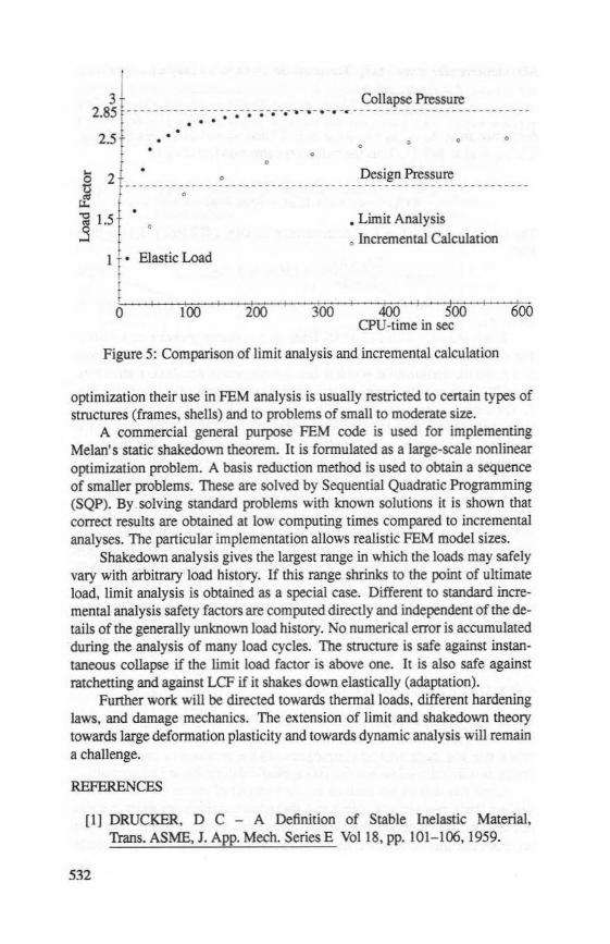
3 j Collapse Pressure 2.85 --- - --- - - -- ----.--.- . - ; -.--.- --- -- .. ... ....... - -- --- -------- ... ---- ----- ...... ... . . . 2.5 •

g 2

tf ~ 1.5 .3

0

Elastic Load

100 2oo

0

0

Design Pressure

• Limit Analysis o Incremental Calculation

300 400 5oo CPU-time in sec

Figure 5: Comparison of limit analysis and incremental calculation

0

6oo

optimization their use in FEM analysis is usually restricted to certain types of structures (frames, shells) and to problems of small to moderate size.

A commercial general purpose FEM code is used for implementing Melan' s static shakedown theorem. It is formulated as a large-scale nonlinear optimization problem. A basis reduction method is used to obtain a sequence of smaller problems. These are solved by Sequential Quadratic Programming (SQP). By solving standard problems with known solutions it is shown that correct results are obtained at low computing times compared to incremental analyses. The particular implementation allows realistic FEM model sizes.

Shakedown analysis gives the largest range in which the loads may safely vary with arbitrary load history. If this range shrinks to the point of ultimate load, limit analysis is obtained as a special case. Different to standard incre­mental analysis safety factors are computed directly and independent of the de­tails of the generally unknown load history. No numerical error is accumulated during the analysis of many load cycles. The structure is safe against instan­taneous collapse if the limit load factor is above one. It is also safe against ratchetting and against LCF if it shakes down elastically (adaptation).

Further work will be directed towards thermal loads, different hardening laws, and damage mechanics. The extension of limit and shakedown theory towards large deformation plasticity and towards dynamic analysis will remain a challenge.

REFERENCES

[1] DRUCKER, D C - A Definition of Stable Inelastic Material, Trans. ASME, J. App. Mech. Series E Vol18, pp. 101- 106, 1959.

532

[2] FLETCHER, R - Practical Methods of Optimization, John Wiley & Sons, New York, 1987.

[3] GAYDON, FA and McCRUM, A W- A theoretical investigation of the yield- point loading of a square plate with a central circular hole, J. Mech. Phys. Solids, Vo12, pp. 156--169, 1954.

[4] GAYDON, FA and McCRUM, A W-On the yield-point loading of a square plate with concentric circular hole, J. Mech. Phys. Solids, Vol 2, pp. 170-176, 1954.

[5] KOITER, W T - General theorems for elastic-plastic solids, Progress in Solid Mechanics, Ed Sneddon, I N and Hill, R, North­Holland Publishing Company, Amsterdam, 1960.

[6] KONIG, J A - Shakedown of Elastic- Plastic Structures, Elsevier and PWN, Amsterdam and Warszawa, 1987.

[7] MAIER- LEIBNITZ - Beitrage zur Frage der Tragfahigkeit einfacher und durchlaufender Balkentrager aus Baustahl St 37 und aus Holz, Die Bautechnik, Vol6, pp. 11- 14 and 27-31, 1928.

[8] MELAN, E - Theorie statisch unbestirnmter Systeme aus ideal-plas­tischem Baustoff, Sitzungsbericht der Osterreichiscben Akademie der Wissenschaften der Mathematisch- Naturwissenschaftlichen Klasse IIa, Vol 145,pp. 195-218, 1936.

[9] PERMAS IV- User's Reference Manual, INTES Publicati~n No. 202, 207,208,404,405, Stuttgart, 1985 - 1988.

[1 0] SCHITTKOWSKI, K- The Nonlinear Programming Method of Wilson, Han and Powell with Augmented Lagrangian Type Line Search Func­tion, Numer. Math., Vo138, pp. 83-114, 1981.

[ll] SHEN, W - Trag1ast- und Anpassungsanalyse von Konstruktionen aus elastisch, ideal platischem Material, Thesis University of Stuttgart, 1986.

[12] STEIN, E and ZHANG, G and MAHNKEN, R - Shakedown analysis for perfectly plastic and kinematic hardening materials, Progress in computational analysis of inelastic structures, Ed Stein, E, Springer, Wien, 1993.

[13] WAGNER, W - Festigkeitsberechnungen im Apparate- und Rohrlei­tungsbau, Vogel Buchverlag, Wiirzburg, 1991.

[14] ZHANG, G- Einspielen und dessen numerische Behandlung von Fla­chentragwerken aus ideal plastischem bzw. kinematisch verfestigendem Material, Thesis University of Hannover, 1991.

533