1616 P St. NW Washington, DC 20036 202-328-5000 www.rff.org

August 2009 � RFF DP 09-33

Lose Some, Save Some: Obesity, Automobile Demand, and Gasoline Consumption in the United States

Shan jun L i , Yan yan L iu , and Jun j i e Zhang

DIS

CU

SSIO

N P

APE

R

Lose Some, Save Some: Obesity, Automobile Demand, and

Gasoline Consumption in the U.S.

Shanjun Li, Yanyan Liu, and Junjie Zhang⇤

Abstract

This paper examines the unexplored link between the prevalence of overweight

and obesity and vehicle demand in the United States. Exploring annual sales data of

new passenger vehicles at the model level in 48 U.S. counties from 1999 to 2005, we

find that a 10 percentage point increase in the rate of overweight and obesity reduces

the average MPG of new vehicles demanded by 2.5 percent: an effect that requires a

30 cent increase in gasoline prices to counteract. Our findings suggest that policies

to reduce overweight and obesity can have additional benefits for energy security

and the environment.

⇤We thank Arie Beresteanu, Avi Goldfarb, Hanan Jacoby, Martin Smith, Kenneth Train, and Chris Tim-

mins for their helpful comments. Financial support from Micro-Incentives Research Center at Duke Uni-

versity is gratefully acknowledged. Affiliations: Shanjun Li, Resources for the Future, li@rff.org; Yanyan

Liu, Postdoctoral Fellow, IFPRI, Washington DC, y.liu@cgiar.org; Junjie Zhang, Assistant Professor of En-

vironmental Economics, University of California - San Diego, junjiezhang@ucsd.edu.

1 IntroductionDo people who are overweight or obese tend to buy larger and less fuel-efficient vehi-

cles? If so, how significant is its implication on the fuel economy of vehicle fleet and

gasoline consumption in the United States? We address these questions using a unique

data set of annual sales of new passenger vehicles at the model level in 48 U.S. coun-

ties from 1999 to 2005. Our empirical analysis shows that the prevalence of overweight

and obesity has a sizable effect on the fuel economy of new vehicles demanded. A 10

percentage point increase in the rate of overweight and obesity among the population

reduces the average miles per gallon (MPG) of new vehicles demanded by 2.5 percent:

an effect that requires a 30 cent increase in gasoline prices to counteract.1

Figure 1: Shares of Overweight, Obesity, and Light Trucks in the U.S. 1960-2006

Note: The overweight and obesity rates are for 20-74 years old adults.The middle line depicts the percentage of light trucks (including passengervans, SUVs and pickup trucks) among all passenger vehicles in stock. Therates of overweight and obesity are from U.S. National Center for HealthStatistics (2009) while data on vehicle stock are from U.S. Bureau of Trans-portation Statistics (2009).

1A 10 percentage point increase in the overweight and obesity rate could be realized in about 12 years

should the recent U.S. trend continue. For example, the rate of overweight and obesity in the population

increased from 52 to 62 percent from 1995 to 2006.

1

The increasing prevalence of overweight and obesity is one of the most serious health

issues in the United States. As depicted in Figure 1, the obesity rate among adults 20-

74 years of age reached 34 percent during 2003-2006 up from 13 percent during 1960-

1962 while the rate of overweight and obesity increased from 45 to 67 percent over the

same period. According to Wang and Beydoun (2007), the prevalence of overweight and

obesity has been climbing at an alarming rate of 0.3-0.8 percentage point each year over

the past three decades. If the rate continues to grow at the current pace, 75 percent of

U.S. adults will be overweight or obese by 2015.

It is a well-established fact that overweight and obesity are associated with a number

of medical conditions, most of which are costly to treat.2 Sturm (2002) shows that obese

individuals cost 36 percent more in inpatient and outpatient spending and 77 percent

more in medications than individuals with normal weight and concludes that obesity

outranks both smoking and drinking in its adverse health effects. The costs of over-

weight and obesity include both direct costs such as medical expenditures and indirect

costs that are related to morbidity and mortality. Wolf and Colditz (1998) estimate that

the total U.S. obesity costs, including both direct and indirect costs, amounted to $99

billion in 1995, with 52 percent being direct costs. A more recent study by Finkelstein et

al. (2004) finds that the medical cost of overweight and obesity accounted for 9.1 percent

of total U.S. medical expenditures in 1998 and reached $78.5 billion, half of which were

through financially-distressed Medicare and Medicaid systems. Because of the signifi-

cant health and economic consequences from overweight and obesity, many have called

for making weight control a national priority.3

2These conditions include elevated cholesterol levels, depression, musculoskeletal disorders, gallblad-

der disease, nonalcoholic fatty liver disease, and several cancers (Kortt et al. (1998), Ogden et al. (2007)).3For example, the Office of Surgeon General issued a report in 2001 titled “The Surgeon General’s Call

to Action to Prevent and Decrease Overweight and Obesity”. In addition to detailing the economic and

health consequences from overweight and obesity, the report provides many policy suggestions at both

local and national levels.

2

During the same period, a seemingly unrelated but equally significant trend is the

dramatic increase in the number of large passenger vehicles on American roads. As

shown in Figure 1, the percentage of light trucks including passenger vans, SUVs, and

pickup trucks among all passenger vehicles in stock increased from about 16 percent in

early 1970’s to more than 40 percent in recent years. Largely due to this trend, motor

gasoline consumption in the United Stated increased by 38 percent from 6.6 million bar-

rels a day in 1981 to more than 9 million barrels a day in 2007. In recent years, passenger

vehicles have accounted for more than 40 percent of total U.S. oil consumption. As a

result of increasing motor gasoline consumption, U.S. is more and more dependent on

foreign oil: the proportion of imports in total petroleum products has reached 60 percent

in recent years. The concerns for oil price volatility and energy security arise because a

large portion of U.S. oil imports are from areas that are politically unstable. Moreover,

the combustion of gasoline in automobiles imposes many environmental problems and

contributes to global warming.4 While producing an estimated 60 to 70 percent of to-

tal urban air pollution, motor gasoline combustion accounts for about 20 percent of the

annual U.S. emissions of carbon dioxide, the predominant greenhouse gas that causes

global warming.

Both the increasing prevalence of obesity and the growing energy consumption have

become important public policy issues in the U.S. in recent years. Although these two

have been almost always discussed as separate issues, several recent studies have demon-

strated the link between the two based on the fact of physics that fuel consumption

per unit of distance traveled increases with the weight of cargo/passengers in trans-

portation. Based on this relationship between weight transported and fuel efficiency,

Dannenberg et al. (2004) find that the weight gain among U.S. consumers during 1990s

increased jet fuel consumption by 2.4 percent in 2000. Both Jacobson and McLay (2006)

4See Parry, Harrington, and Walls (2007) for a comprehensive review of externalities associated with

vehicle usage and gasoline consumption as well as discussions on policy instruments.

3

and Jacobson and King (2009) quantify the effect of overweight and obesity on gasoline

consumption due to the fact that heavier passengers reduce fuel efficiency of a vehicle.

The latter finds that the weight gain among Americans from 1960s contributed to 0.8

percent of the gasoline consumption by passenger vehicles in 2005.

The aforementioned papers examine how fuel efficiency in travel is affected by pas-

sengers’ weight after transportation choices being made (i.e., the ex-post effect). Our

paper focuses on a different and as our findings suggest, a more significant channel

whereby consumers choose different transportation tools in response to changes in their

weights. In particular, we examine how the demand for passenger vehicles is affected

by the increasing rate of overweight and obesity. Our findings suggest that consumers

demand larger and less fuel-efficient vehicles, presumably to accommodate their heav-

ier bodies. Moreover, obesity exhibits much stronger effects than overweight on vehicle

demand. Our simulation results show that had the prevalence of overweight and obe-

sity stayed at the level in 1981 (about 20 percentage points lower than that in 2005), the

average MPG of new vehicles demanded in 2005 would have been about 4.6 percent

higher, everything else being equal. The improved fuel efficiency implies total gasoline

savings of about 138 million barrels and reduction in CO2 emissions of 58 million tons

over the lifetime of these vehicles.5

With volatile gasoline prices and growing concerns about climate change and local

air quality, political support for curbing U.S. fuel consumption has increased dramat-

ically in recent years. A suite of policy instruments such as more stringent Corporate

Average Fuel Economy (CAFE) standards, consumer tax incentives for adopting alter-

native fuel vehicles, and government support for developing fuel-efficient technologies

5Assumptions about vehicle lifetime and vehicle miles traveled are presented in Section 4.3. In addi-

tion to environmental problems and climate change associated with increased gasoline consumption due

to more and more large vehicles being used, recent empirical evidences have shown that a vehicle fleet

with more large vehicles such as SUVs and pickup trucks can have more traffic fatalities and hence reduce

overall traffic safety (White (2004) and Li (2008)).

4

have been adopted. Our findings suggest that the progress achieved through these poli-

cies could be reversed by the increasing prevalent of overweight and obesity. On the

other hand, our findings also imply that overall benefits from local and national pro-

grams aimed to reduce overweight and obesity are larger than what has been previously

thought once energy and environmental benefits are taken into account.

The remainder of this paper is organized as follows. Section 2 discusses the back-

ground of our study and describes our data. Section 3 discusses the empirical strategy.

Section 4 present estimation results and caveats of our analysis. Section 5 conducts fur-

ther robustness checks. Section 6 concludes.

2 Background and DataWe first briefly discuss the trends in the U.S. auto industry and then present data sets

used in our study.

2.1 Background

The U.S. auto industry witnessed dramatic changes during the past three decades, one of

which is the increasing popularity of large vehicles such as SUVs. As depicted by the left

panel of Figure 2, the market share of new light trucks over total new light-duty vehicles

grew from 17 percent to about 50 percent from 1981 to 2007.6 The majority of the increase

in light truck sales was accounted for by SUVs, whose share rose from 1.3 percent to

almost 30 percent during the period. After two decades of constant growth, the market

share of light trucks started to stabilize from 2002 largely due to the significant run-up

in gasoline prices.

The right panel of Figure 2 plots the average MPG of new light-duty vehicles sold in

each year from 1981 to 2007. The fuel economy of all new vehicles, shown by the line

in the middle, increased to its peak in 1987 following two oil crisis and the enactment

6Light-duty vehicles are those vehicles that EPA classifies as cars or light trucks (SUVs, vans, and

pickup trucks with less than 8500 pounds gross vehicle weight).

5

Figure 2: Market Shares by Vehicle Type and Fuel Economy 1981-2007

Note: To smooth the trend, the data points in the graph are three-year moving averagesthat are tabulated at the midpoint of each three consecutive years. Data source: Light-DutyAutomotive Technology and Fuel Economy Trends: 1975 Through 2008 by EPA.

of CAFE standards in 1970’s. It then continuously declined until the reversal of this

long-term trend in 2005. Since light trucks are on average less fuel efficient than cars

(by about 6 MPGs among those sold), the increase in the market share of light trucks

is an important factor behind the decline in fuel economy of new vehicles. Moreover,

even within the same segment (car or light truck), vehicles have become larger and

less fuel efficient from late 1980’s to early 2000’s. For example, according to the EPA’s

classifications, the fraction of small cars in the car segment increased from 51 percent

in 1981 to 65 percent in 1987 and then dropped to 44 percent in 2007 while the fraction

of median-sized cars and that of large cars both show an opposite trend. The top and

bottom lines in the right panel of Figure 2 present similar temporal patterns for the fuel

economy of each of the two vehicle segments.

It is important to note that more advanced and fuel-efficient vehicle technologies

have been constantly developed over time. These technologies include more efficient

engines, better transmission designs, and better matching of the engine and transmis-

sion. That means that in the absence of these technologies, the average fuel economy of

new vehicles would have been much lower and the effect of more and more large vehi-

6

cles on fuel economy would have been more pronounced. To understand the importance

of these technologies on fuel economy, it is useful to look at an alternative fuel-efficiency

measure, “Ton-MPG”, which takes vehicle weight into consideration. This measure is

defined as a vehicle’s MPG multiplied by its inertia weight (i.e., vehicle weight with

standard equipment plus 300 pounds) in tons.7 From 1981 to 2007, the average Ton-

MPG for new cars increased from 33.1 to 42.8 while that for new light trucks increased

from 33.0 to 42.1. Typically, Ton-MPG for both vehicle types increased at a rate of about

one to two percent a year over this period according to EPA.

2.2 Data

Several data sets are used in our study. The first data set, collected from the annual issues

of Automotive News Market Data Book, containing characteristics and total sales of

virtually all new vehicle models available in the U.S. from 1999 to 2005. Vehicle models

with U.S. sales less than 10,000 units are excluded. These models account for less than

1 percent of total new vehicle sales. Table 1 reports summary statistics for the 1,287

models in this data set. Price is the manufacturer suggested retail prices (MSRP). Size,

equal to the product of vehicle length and width, measures the “footprint” of a vehicle.

Miles per gallon (MPG) is the weighted harmonic mean of city MPG and highway MPG

based on the formula provided by the EPA to measure the fuel economy of the vehicle:

MPG = 10.55/city MPG+0.45/highway MPG.8

The second data set, purchased from R. L. Polk & Company, contains total annual

registrations of each new vehicle model in each of the 48 U.S. counties from 1999 to

7Intuitively, an increase in vehicle’s MPG at constant weight should be considered as an improvement

in fuel-efficiency. Similarly, an increase in a vehicle’s weight while holding MPG constant should also be

considered as an improvement.8Alternatively, the arithmetic mean can be used on Gallon per Mile (GPM, equals 1/MPG) to capture

the gallon used per mile by a vehicle traveling on both highway and local roads: GPM = 0.55 city GPM +

0.45 highway GPM. The arithmetic mean directly applied to MPG, however, does not provide the correct

measure of vehicle fuel efficiency.

7

Table 1: New Vehicle Characteristics 1999-2005

Mean Median S. D. Min MaxQuantity (’000) 89.7 56.0 108.5 10.0 939.5Price (in ’000 $) 25.65 22.98 11.42 9.05 90.62Size(in ’0000 inch2) 1.359 1.341 0.169 0.935 1.835MPG 22.37 22.25 4.85 13.19 55.59

Note: Data are from various issues of Automotive NewsMarket Data Book (1999-2005) and the EPA’s fuel economydatabase. The number of observations is 1,287.

2005. These counties are within 20 MSAs that are studied in Li, Timmins, and von Hae-

fen (2008).9 These 20 MSAs are from all nine U.S. Census divisions and exhibit large

variations in total population and average household demographics. They are well rep-

resentative of national data in terms of vehicle fleet characteristics and household demo-

graphics. Although there are 160 counties in these MSAs, data on the rate of overweight

and obesity are only available in large counties. Our study focuses on 48 counties that

have at least 50,000 households. This implies that rural counties are under-represented

in our data. Nonetheless, the correlation coefficient between vehicle sales in these coun-

ties and national sales is 0.914 (comparing to 0.94 between model sales in the 20 MSAs

and national sales). In total, there are 61,776 (1287*48) observations of vehicle sales.

The fuel cost of driving is measured by dollars per mile (DPM = gasoline price/MPG).

We collect annual gasoline prices for each MSA from 1999 to 2005 from the American

Chamber of Commerce Research Association (ACCRA) data base. During this period,

we observe large variations in gasoline prices both across years and MSAs. The average

annual gasoline price is $1.66, with a minimum of $1.09 observed in Atlanta in 1998 and

9These 20 MSAs are: Albany-Schenectady-Troy, NY; Atlanta, GA; Cleveland-Akron, OH; Denver-

Boulder-Greeley, CO; Des Moines, IA; Hartford, CT; Houston-Galveston-Brazoria, TX; Lancaster, PA;

Las Vegas, NV-AZ; Madison, WI; Miami-Fort Lauderdale, FL; Milwaukee-Racine, WI; Nashville, TN;

Phoenix-Mesa, AZ; St. Louis, MO-IL; San Antonio, TX; San Diego, CA; San Francisco-Oakland-San Jose,

CA; Seattle-Tacoma-Bremerton, WA; Syracuse, NY.

8

a maximum of $2.62 in San Francisco in 2005. We assume that the gasoline price is the

same in counties within an MSA. We collect median household income at the county

level from Small Area Income and Poverty Estimates of U.S. Census Bureau. From 2000

Census and annual American Community Survey, we also collect several county-level

demographic variables including total population, average household size, the propor-

tion of households with children under 18 years old, and average driving time to work.

The overweight and obesity information are obtained from the National Health and

Nutrition Examination Survey Data published by National Center for Health Statistics

(NCHS) at Centers for Disease Control and Prevention (CDC). The survey is conducted

at the individual level. The rates of overweight and obesity at the 48 counties under

study are obtained based on individual observations. The range of overweight and

obesity is determined by Body Mass Index (BMI) or Quetelet index. BMI is calculated

based on a person’s weight (W ) and hight (H) following the formula: BMI = W/H2. An

adult is considered overweight if he/she has a BMI between 25 and 29.9, and considered

obese if the BMI is 30 or higher. For children and teens, BMI ranges are age and gender-

specific in order to account for normal differences in body fat between genders and

across ages. Although BMI does not measure body fat directly, it has been shown to be

a convenient and reliable indicator of obesity (Garrow and Webster (1985)). However,

it is worth noting that BMI is not a perfect measure of weight partly because it ignores

heterogeneity due to age, gender, and athleticity for adults.

Table 2 presents correlation coefficients among several variables of interest as well as

their summary statistics based on data at the county level. There are in total 336 (48*7)

county-level observations. The average MPG and size of new vehicles in each county

are weighted by vehicles sales in the county. The market share of new vehicles is equal

to total new vehicle sales over the number of households in the county. The correlation

coefficients in columns 2 to 6 show some interesting patterns. The rate of overweight

and obesity is negatively correlated with median household income and the average

9

Table 2: Correlation Matrix and Summary Statistics

(1) (2) (3) (4) (5) Mean S.D.Rate of overweight and obesity (1) 1.000 0.553 0.066Gasoline price (2) 0.103 1.000 1.764 0.320Median household income (3) -0.415 0.101 1.000 5.564 1.160Average new vehicle MPG (4) -0.156 0.459 0.068 1.000 22.473 0.877Average new vehicle size (5) 0.411 -0.090 -0.239 -0.827 1.000 1.385 0.037New vehicle market share (6) -0.048 -0.272 0.227 -0.266 0.090 0.132 0.029

Note: Variables are at the county level. The number of observations is 336. Columns 2-6 showcorrelation coefficients and the last two columns are the means and standard deviations.

MPG of new vehicles in the county, and is positively correlated with the average size

of new vehicles. The gasoline price is positively correlated with the average MPG of

new vehicles and negatively correlated with the market share of new vehicles. There are

larger variations in the rate of overweight and obesity in both temporal and geographic

dimensions. For example, the average rate of overweight and obesity increased from

0.516 to 0.581 during the seven year period. In 2005, the lowest rate was 0.406 in San

Francisco, CA while the highest was 0.72 in Galveston, TX.

Figure 3: Overweight and Obesity, Vehicle Size, and MPG in 48 Counties in 2005

The left panel of Figure 3 plots the average size of new vehicles against the rate of

10

overweight and obesity while the right panel plots the average MPG against the rate

of overweight and obesity in the 48 counties in 2005. The plots clearly show a posi-

tive correlation between the average vehicle size and the prevalence of overweight and

obesity and a negative correlation between the average MPG and the prevalence of over-

weight and obesity. The goal of our empirical model is to determine if a higher rate of

overweight and obesity results in stronger demand for large and fuel-inefficient vehicles

and to further quantify the relationship.

3 Estimation StrategyOur empirical model is a linear model transformed from a multinomial logit model. To

describe the empirical model, let m index markets (i.e., counties), and j index vehicle

models. We assume that that consumers have total J vehicle models plus an outside

good (indexed by 0) to choose from in a give year. With the time index suppressed, we

estimate the following equation:

ln(smj/sm0) = xj↵ + xmj� + ⇠j + ⌫mj, (1)

where smj and sm0 are the market shares of model j and the outside good, respectively.

xj is a vector of product attributes such as vehicle price (MSRPs) and vehicle size that

do not vary across market. To save notation, xmj includes market demographics (such

as gasoline price and the rate of overweight and obesity) as well as the interaction terms

between product attributes and market demographics (such as dollars per mile and the

interaction term between the rate of overweight and obesity with vehicle size). ⇠j is the

unobserved product attribute such as presentation/appearance, quality or prestige of

a vehicle. It can also include promotions such as marketing campaign or consumption

trend at the national level. ⌫mj includes unobserved market-varying demographics that

affect consumers’ vehicle choices and are not controlled for.

This linear model is a transformation of a multinomial logit model as shown in Berry

(1994) and exhibits the following two important features. First, the transformed model

11

is parsimonious: it only has product attributes (including price) of a single product j

as explanatory variables. Nevertheless, the presence of sm0 in the equation allows at-

tributes of other products to affect the market share of product j.10 This contrasts with a

linear demand model where the dependent variable is the quantity of a product and the

regressors include prices of all competing products. Second, although the underlying

multinomial model starts with individual utility maximization, the transformed model

can be estimated based on market-level sales data in a linear framework.

We now discuss the implications of the unobserved product attribute ⇠j and local un-

observables ⌫mj on estimation. Controlling for the unobserved product attribute ⇠j is one

of the focal points of previous studies on automobile demand based on aggregate sales

data (Berry, Levinsohn, and Pakes (1995) ). Since the unobserved product attribute may

affect vehicle price, ignoring it could render vehicle price endogenous and cause price

elasticities of demand to be under-estimated. The identification assumption commonly

employed in the literature is that observed product attributes xj are uncorrelated with

the unobserved product attribute ⇠j . Therefore, attributes of the competing products

can be used as instruments for vehicle price of a given product. However, the identifi-

cation assumption could be violated if there are unobserved national promotions (could

be treated as unobserved product attributes) that are correlated with product attributes.

For example, there were strong marketing efforts for SUVs by automakers in late 1990’s

and early 2000’s. These promotions unobserved to the researchers enter ⇠j and are also

correlated with product attributes such as vehicle size and type. Taking advantage of

the fact that we have sales data in multiple markets, we use product (i.e., model-year)

fixed effects to control for unobserved product attributes (or national promotions). With

10Another way to see this point is to recognize that the market share of product j in a multinomial logit

model is:

smj =xj↵ + xmj� + ⇠j + ⌫mj

1 +PJ

h=1(xh↵ + xmh� + ⇠h + ⌫mh). (2)

12

product fixed effects, the above model can be written as:

ln(smj/sm0) = �j + xmj� + ⌫mj, (3)

where product dummy, �j , subsumes market-invariant product attributes xj as well as

the unobserved product attribute ⇠j .

The second challenge before taking equation (3) to the data lies in the market-level

unobservable ⌫mj , which may include local unobservables that affect consumer pref-

erences. The possible correlation between local unobservables and observed market-

level characteristics such as gasoline price or the rate of overweight and obesity would

cause the observed variables to be endogenous. For example, in hilly areas or areas

with snow, consumers may have stronger preference for four-wheel drive and hence

SUVs and pickup trucks because four-wheel drive is more common among these vehi-

cles than cars. If these unobserved conditions are also correlated with the rate of over-

weight and obesity, the interaction term between vehicle size and the rate of overweight

and obesity will be endogenous. In order to control for the effect of local unobservables

on vehicle preference, we include county dummies interacting with vehicle category

dummies. That is, we allow consumer preferences for a certain vehicle category to be

different across counties.

To understand the effect of ignoring unobservables on parameter estimates as well

as if interaction terms between county dummies and vehicle category dummies are ad-

equate controls for local unobservables, we carry out various robustness checks. Our

robustness analyses suggest that local unobservables tend to attenuate the effect of over-

weight and obesity. Moreover, we find that the effect of overweight and obesity is quite

robust to how both product unobservables and local unobservables are controlled for.

4 Estimation ResultsTables 3 and 4 present parameter estimates as well as the estimates for implied elas-

ticities from six different model specifications. We first discuss the results for the first

13

specification which we believe, provides the most credible results. We then present the

results from other specifications and discuss the significance of our findings as well as

two caveats of our analysis.

4.1 Results from the Preferred Model

Specification 1 includes most control variables among the six specifications as shown

in Table 3. In addition to the first six variables shown in the table, we include four

demographic variables as well as their interactions with MPG and vehicle size. These

four demographic variables are total population in logarithm, average household size,

the proportion of households with children under 18 years old, and average driving

time to work. The parameter estimates for these four variables as well as the eight

interaction terms, available from authors, are not reported for the sake of brevity.11 In

the regression, product dummies are used to control for unobserved product attributes

as well as national level trends or promotions. We include county dummies to control

for county-level unobservables (such as the availability of public transportation) that

could affect consumers’ choice margin of whether to purchase a new vehicle. We also

include interaction terms between county dummies and 11 vehicle segment dummies

to control for county-level unobservables that affect consumer preference for different

types of vehicles.

The overweight and obesity rate (OR) in the regressions is the percentage of peo-

ple who are either overweight or obese in the population. The first two variables are

used to capture the effect of overweight and obesity on vehicle demand. The parameter

estimates imply that the partial effect of the rate of overweight and obesity on vehicle

market share is: @smj

@OR = (�8.601 + 6.317 ⇤ vehicle size)smj(1 � smj). The partial effect is

11Because these variables are not available in all counties in 2000 to 2004 American Community Sur-

vey, we interpolate the values in between assuming geometric growth based on data from 2000 Census

and 2005 American Community Survey. The results are virtually the same using the interpolation with

arithmetic growth.

14

positive only for vehicles whose size is larger than 1.36 (’0000 inch2), which is about 55

percentile in the vehicle size distribution among all 1,287 vehicles in the data. Moreover,

the partial effect of overweight and obesity on vehicle demand is stronger for larger

vehicles.

Based on the parameter estimates on the third and fourth variables, the partial effect

of gasoline price on vehicle market share is: @smj

@Gas price = (1.494�26.993/MPG)smj(1�smj).

This implies that an increase in gasoline price would increase the demand for vehicles

with MPG larger than 18.07 while reducing the demand for less fuel-efficient vehicles.

Moreover, the more fuel-efficient a vehicle is, the larger the demand increase would be

with an increase in gasoline price. The coefficient estimate on Log(price)/log(MHI) for

specification 1 suggests that the own-price elasticity for product j is �5.528log(MHI)(1 � smj).

The price elasticity estimates for all 1,287 vehicle models range from -2.40 to -4.68 with

the average being -3.39. The identification of the above partial effect relies not only on

cross-sectional and temporal variations in vehicle demand due to differences in the de-

mographic variables (i.e., the rate of overweight and obesity, gasoline price, and income)

but also on cross-model variations arising from the fact that vehicle demand responds

to changes in demographic variables differently across vehicles with different attributes

(i.e., size, MPG, or price).

The parameter estimates suggest that as overweight and obesity become more preva-

lent, vehicles demanded will become larger and as a result, less fuel-efficient on average.

The effects of an gasoline price increase on vehicle demand are opposite. In order to

measure the magnitude of these effects, we simulate several elasticities and their stan-

dard errors, which are presented in panel 2 of Tables 3. The elasticity of MPG with

respect to the rate of overweight and obesity being -0.139 in 2005 suggests that a one-

percent increase in the rate of overweight and obesity would reduce the average MPG

of new vehicles demanded in 2005 by 0.139 percent. The elasticity of MPG with respect

to gasoline price is estimated at 0.191 in 2005. The elasticities of vehicle size to both

15

variables of interests are also presented.

Although we are not aware of any existing studies that we can compare to in terms

of the effect of overweight and obesity on vehicle demand, there are several recent stud-

ies that provide the elasticity of average MPG to gasoline price. The elasticity estimate

based on our preferred specification is 0.191 in 2005. Small and Van Dender (2007) ob-

tain an estimate of 0.21 from 1997-2001 using U.S. state level panel data on vehicle fuel

efficiency and gasoline prices. Li, Timmins, and von Haefen (2008) estimate the elastic-

ity of the average MPG of new vehicles with respect to the gasoline price in 2005 to be

0.204 using a similar data set to ours but a different empirical framework.

4.2 Robustness Checks

In the first specification, we include interaction terms between county dummies and 11

vehicle segment dummies to control for local unobservables that may be correlated with

observable demographics such as the rate of overweight and obesity or gasoline price.

If local unobservables affect consumers’ preferences on continuous vehicle characteris-

tics such as vehicle size and MPG, we should include interaction terms between county

dummies with these characteristics in the regression. However, doing so would elimi-

nate crucial cross-county variations in the rate of overweight and obesity and especially

gasoline price so that precise estimates on the effect of overweight and obesity as well

as that of gasoline price cannot be obtained.12

To understand how local unobservables affects the parameter estimates, we conduct

the following two estimations. In specification 2, we include interaction terms between

county dummies with 3 vehicle type dummies (i.e., using a coarser categorization than

vehicle segments) while in specification 3, no interaction terms between county dum-

12Due to the lack of gasoline price data at the county level, we use same gasoline price for counties

within the same MSA. Because cross-MSA variations in gasoline prices, largely due to differences in state

and local gasoline taxes and transportation costs, are fairly stable over time, county dummies would

subsume most of the cross-sectional variations in gasoline price.

16

mies and vehicle category dummies are included. Comparing the results across the

three specifications, we can see that all elasticity estimates (in absolute values) are simi-

lar across specifications with those from the first specification being slightly larger. This

suggests that local unobservables that are controlled for by the interaction terms be-

tween vehicle category dummies and county dummies have little effect on our model

estimates and if ignored, tends to bias the effect of the rate of overweight and obesity

and that of gasoline price on vehicle demand toward zero. To the extent that local un-

observables are not fully controlled for by interactions terms between county dummies

and vehicle segment dummies (e.g., a even finer categorization is needed), we expect

that the elasticity estimates from the first specification provide close lower bounds for

the true effects.

It is worth pointing out that our empirical strategy controls for time-varying un-

observables at the national level through product dummies. It also controls for time-

invariant components of county-level unobservables through interaction terms of county

dummies and vehicle category dummies. We cannot, however, rule out the possibility

of time-varying components of local unobservables co-varying with the observed vari-

ables and affecting vehicle demand at the same time, although such variables are not

easy to conceive. To investigate the potential effect of time-varying local unobservables

on estimation results, we conduct three additional regressions where some of observed

time-varying variables are omitted. The results of these three specifications are reported

in Table 4. Specification 4 does not include median household income and its inter-

action with vehicle price in the regression. The elasticity estimates of overweight and

obesity rate become only slightly smaller in magnitude while those of gasoline price

decrease more visibly. As high-income households are more likely to buy large and

less fuel-efficient vehicles and median household income is negatively correlated with

the rate of overweight and obesity, the effects of overweight and obesity will be under-

estimated with income levels not being controlled for. Conversely, median household

17

income is positively correlated with gasoline price, therefore, the increased demand for

fuel-efficient vehicles due to a higher gasoline price would be dampened by higher in-

come. However, when income levels are not controlled for, the effect of gasoline price

on vehicle fuel efficiency will be under-estimated. In specification 5, we also omit the

addition 12 variables related to county demographics. Again, the elasticity estimates

only change slightly compared to those from specification 1. Specification 6 excludes

variables related to gasoline price in addition to those omitted in specification 5. The

elasticity of MPG to overweight and obesity rate is estimated at -0.150 compared to -

0.139. Our results from these three specifications show that the elasticity estimates with

respect to overweight and obesity are very close to those from the first specification

where more time-varying variables are included. This supports that time-varying com-

ponents of local unobservables that are correlated with overweight and obesity and at

the same time affect vehicle demand, if exist at all, may not significantly compromise

key results on the effect of overweight and obesity.

Our previous analysis combines overweight and obesity together. It is interesting

to see if they affect vehicle demand differently. Table 5 presents estimation results for

three specifications where we separate overweight and obesity. These three specifica-

tions correspond to those in Table 3 where different categorizations of vehicle dummies

are used. The first two parameters capture the effect of obesity on vehicle demand while

the next two capture the effect of overweight. In all three specifications, the parameters

suggest that obesity and overweight have qualitatively same effect on vehicle demand:

an increase in either of them reduces the demand for small vehicles but increases the

demand for large vehicles.

The results in all three specification also show that obesity exhibits larger effects on

vehicle demand than overweight. This can be easily seen based on elasticity estimates

presented in panel 2 of the table. Moreover, since the average overweight rate was 36.1

percent while the average obesity rate was 22.6 percent in 2005, this implies that even if

18

the MPG elasticity to obesity and that to overweight were the same, the effect of obesity

on the fuel economy of vehicles demanded would be about 60 percent larger than that

of overweight. Similar to findings from Table 3, the elasticity estimates are close across

three specifications.

4.3 Discussion and Caveats

Our simulation results based on parameter estimates show that the average MPG of

new vehicles demanded would have been 2.5 percent lower (22.42 instead of 22.99) in

2005 with a 10 percentage points increase in the rate of overweight and obesity from

0.587. This increase in overweight and obesity rate could be realized in about 12 years

following the trend since 1995. In order to counteract this decrease in the average MPG,

a 30 cents increase in gasoline price (e.g., through a higher gasoline tax) over the av-

erage price of $2.32 per gallon in 2005 is needed. Interestingly, obesity has a stronger

effect on the fuel economy of vehicles demanded. A 10 percentage points increase in

the obesity rate over that in 2005 (holding the overweight rate constant) would have

increased the average MPG of new vehicles demanded by 3.4 percent, which needs a 41

cents increase in gasoline price to counteract. Meanwhile, the effect of a 10 percentage

points increase in the overweight rate (holding the obesity rate constant) on the average

MPG is about 1.6 percent in 2005. Many studies have shown that increasing the gaso-

line tax is a more effective way to reduce gasoline consumption than tightening CAFE

standards.13 Moreover, the average 41 cents gasoline tax in the U.S. is lower than the

optimal level in relation to externalities associated with gasoline usage (Parry and Small

(2005)). However, increasing gasoline taxes has been a politically difficult policy to pass.

Our simulation results suggest that if the rate of overweight and obesity in 2005 had

stayed at the 1981 level (20 percentage points lower), the average MPG of new vehicles

demanded would have been 24.04 instead of 22.99. This implies about 4.6 percent saving

13See for example, National Research Council (2002); Congressional Budget Office (2003); West and

Williams (2005); and Bento, Goulder, Jacobsen, and von Haefen (2008).

19

in gasoline consumption over vehicles’ lifetime holding vehicle usage constant. Assum-

ing the annual average vehicle-miles-traveled to be 12,000 and annual new vehicle sales

to be 17 millions, the total gasoline saving over 15 years for these vehicles is about 138

million barrels and the reduction in CO2 emissions is about 58 million tons.14 Our results

show that the effect of overweight and obesity on gasoline consumption through vehicle

choices is much larger than the ex-post effect (i.e, through the effect on fuel efficiency

conditioning on vehicle choices) by Jacobson and McLay (2006) and Jacobson and King

(2009) as discussed in the introduction. Taking these results together, we consider our

empirical estimate on the effect of overweight and obesity on vehicle fuel economy and

gasoline consumption to be quantitatively significant.

Two caveats regarding our analysis are worth mentioning. The first one is related to

the undesirable feature of a logit model, independence of irrelevant alternatives (IIA).

This property suggests unreasonable uniform substitution patterns across products. Both

a nested logit model and to a larger extent, a random coefficient logit model allow for

more reasonable cross-product substitutions than a logit model. As a logit model, a

nested logit model can also be estimated in a linear framework following Berry (1994).

We estimate a nested model with various nesting structures, all of which are rejected

when product fixed effects are included. However, as we show in the next section, the

usage of product fixed effects to control for unobserved product attributes is crucial to

the identification of our empirical model.

Although a random coefficient logit model does not suffer from the IIA property, the

estimation cannot be carried out in a linear framework and is very computationally in-

tensive. The method to estimate a random coefficient model with aggregated sales data

such as ours is a simulated Generalized Method of Moments (GMM) with a nested con-

14We find that although there is a small positive effect of overweight and obesity on the total number of

new vehicles demanded, the effect is not statistically significant from zero. Improved fuel economy often

increases vehicle usage, which is called rebound effect. A recent study by Small and Van Dender (2007)

estimates that the short-run and long-run rebound effects are 2.2% and 10.7% during 1997-2001.

20

traction mapping developed by Berry et al. (1995). The contraction mapping recovers

a vector with length being equal to the number of products that consumers can choose

from (about 184 on average in our case). The larger the choice set is, the more compu-

tationally intensive the contraction mapping is. More importantly, it has to be done for

each market in each year (48*7 times) for each parameter iteration. In addition, that fact

that the objective function may have many local optima adds to computational burden.

Although a full random coefficient model can provide significant gain in doing welfare

analysis coupled with a supply side, it may not provide much benefit for our analysis

where we are mainly interested in the average partial effects of explanatory variables.

Beresteanu and Li (2008) estimate a random coefficient multinomial logit model based

on an aggregate vehicle sales data in 22 MSAs from 1999 to 2006 augmented with a

household survey data. It provides an estimate of 0.169 for the elasticity of average

MPG to gasoline price in 2005, comparing to 0.191 from our preferred model. We take

comfort from the fact that our estimate from a logit model is close to those from a ran-

dom coefficient multinomial logit model as well as other models that do not suffer from

the IIA property as discussed in Section 4.1.

The second caveat of our analysis is that we focus on the effect of overweight and

obesity on vehicle demand rather than the equilibrium effect. Estimating the equilib-

rium effect necessitates the analysis of demand and supply sides simultaneously. Al-

though the supply side is out of scope of our study, it is worth mentioning the following

two important and counteracting factors in the supply side. First, given the positive

correlation between overweight and the demand for large and less fuel-efficient ve-

hicles, automakers are likely to increase the prices of those vehicles with an increase

in the rate of overweight and obesity. The higher prices of large vehicles will in turn

dampen the demand effect of overweight and obesity on fleet fuel economy in equilib-

rium. The changes in prices and their subsequent effects on vehicle demand depend

on both across-firm competition and within-firm competition given the fact that all au-

21

tomarkers produce multiple products. The second factor in the supply side is the effect

of overweight and obesity on automakers’s product mix decisions which are inherently

dynamic. Recognizing the demand effect of overweight and obesity, automakers are

likely to introduce more large models into the market when overweight and obesity

become more prevalent. This, opposite to the first factor, will exacerbate the static de-

mand effect that we analyze. The decision of product choice should be more important

than the first factor, especially in the long run. Nevertheless, it can be more challenging

to model. In addition to the dynamic nature of product choice decisions, several facts

about the auto industry should be considered: the industry consists of several big play-

ers that act strategically; each of them produces multiple products; and products are

differentiated.

5 Further Robustness AnalysisTo further check the robustness of our findings to model specifications, we estimate two

additional specifications where we do not use product dummies to control for unob-

served product attributes and national level promotions. In the first specification, we

include brand dummies where a brand is defined by the model name. There are in total

330 brands in the data with the vast majority of the brands appearing in multiple peri-

ods. Vehicle models under the same name are sold in many year with minor changes

(e.g., changes in small features and cosmetics) being done almost every year and major

changes (e.g., changes on powertrain system and chassis) being done every 3-10 years in

most cases. Although brand dummies can control for time-invariant unobserved prod-

uct attributes, they cannot control for time-varying unobserved product attributes such

as those associated with model changes. These time-varying components are likely to be

correlated with vehicle prices and would cause vehicle price variable to be endogenous.

We use instrumental variable method to deal with the price endogeneity problem by

invoking the assumption that time-varying unobserved product attributes are not cor-

22

related with observed product attributes. Following the literature, we use the attributes

of the competing products as instruments for vehicle price of a given product. Specifi-

cally, we use the averages of vehicle size, horsepower, and MPG of the other products

produced by the same firm, and the average attributes of products of the same type

produced by other firms. We also include the number of products of the same type pro-

duced by the same firm and that by all the other firms. The first stage regression shows

that the instruments have good explanatory power for vehicle price.

Columns 2 to 5 in Table 6 present the results from both OLS and 2SLS with brand

dummies in both regressions. We include interaction terms between county dummies

and 11 segment dummies to control for local unobservables and interactions terms be-

tween year dummies and 11 segment dummies to control for time-varying unobserv-

ables at the national level such as promotions or trends. All the coefficient estimates

have the expected signs in both regressions. With the instruments, the estimate of price

coefficient changes from -3.473 to -4.553, comparing to the estimate of -5.528 in the pre-

ferred model where product dummies are used as shown in Table 3. The coefficient esti-

mates on other variables only change slightly from OLS to 2SLS. Comparing the results

from 2SLS to those from our preferred model shown in Table 3, the effects of overweight

and obesity on the average MPG and size of vehicles demanded become smaller in mag-

nitude while the effects of gasoline price on MPG and vehicle size become slightly larger

in magnitude. This may arise from the possibility that time-varying unobserved prod-

uct attributes (e.g., due to model changes over time) are correlated with vehicle size and

fuel efficiency.

In the second specification, we do not include either brand dummies or product

dummies. Therefore, both time-invariant and time-varying unobserved product at-

tributes are not controlled for. To deal with the problem of price endogeneity, we use

a commonly used assumption in the automobile demand literature following Berry et

al. (1995)) that unobserved product attributes are not correlated with observed prod-

23

uct attributes. This assumption is likely to be stronger than the one used in the first

specification that the time-varying component of unobserved product attributes are not

correlated with observed product attributes. We use the same instrumental variables for

the price variable as in the first specification. The coefficient estimate on the price vari-

able changes from -2.289 in OLS to -1.618 in 2SLS, both of which are far from -5.528 in

the preferred model. The coefficient estimate being -1.618 implies that the average price

elasticity is only -0.99 among all products and that half of the products have inelastic de-

mand, which are not consistent with profit-maximizing pricing decisions by firms with

market power. These results suggest that the exogeneity assumption used to construct

instruments could be violated. The elasticity estimates with respect to overweight and

obesity are slightly larger in magnitude than those from the preferred model while the

elasticity estimates with respected to gasoline price are much smaller than those from

the preferred model.

These robustness analysis shows the importance of using product dummies to con-

trol for unobserved product attributes and in turn the benefit of having data from multi-

ple markets. Consistent with the findings in previous analysis, the effects of overweight

and obesity on the average MPG and size of vehicles demanded are quite robust to

model specifications.

6 ConclusionDuring the past several decades, the prevalence of overweight and obesity in the U.S.

has been increasing at an alarming rate. Meanwhile, motor gasoline consumption and

petroleum import have also been growing, partly due to the fact that American drivers

have been buying larger and less fuel-efficient vehicles. This paper examines the un-

explored link between these two trends and finds that new vehicles demanded by con-

sumers are less fuel-efficient on average as the rate of overweight and obesity goes up.

Our results show that if the prevalence of overweight and obesity has stayed at the 1981

24

level, the average fuel economy of new vehicles demanded would have been about 4.6

percent higher than that observed in 2005, ceteris paribus. We find that a 10 percentage

point increase in the obesity rate from the 2005 level would decrease the average MPG

of new vehicles demanded by 3.4 percent, more than twice as large as the effect of over-

weight.

The effect of overweight and obesity on vehicle fuel economy in the long run has po-

tentially important implications for policies aiming to address U.S. energy security and

environmental problems associated with gasoline consumption. Without taking into

consideration the growth trend of overweight and obesity and its impact on vehicle de-

mand, long-term government interventions are likely to miss the intended policy goals

in reducing gasoline consumption and CO2 emissions. Moreover, our findings imply

that local and national policies that aim to prevent and decrease overweight and obesity

could provide, in addition to the savings in health care costs, extra benefits in energy

saving and environmental protection.

25

ReferencesBento, A., L. Goulder, M. Jacobsen, and R. von Haefen, “Distributional and efficiency

impacts of increased U.S. gasoline taxes.” American Economic Review, forthcoming.

Beresteanu, Arie and Shanjun Li, “Gasoline Price, Government Support, and the De-

mand for Hybrid Vehicles,” 2008. Working Paper.

Berry, S., “Estimating Discrete Choice Models of Product Differentiation,” RAND Journal

of Economics, 1994, 25 (2), 242–262.

, J. Levinsohn, and A. Pakes, “Automobile Prices in Market Equilibrium,” Economet-

rica, July 1995, 63, 841–890.

Congressional Budget Office, The Economic Costs of Fuel Economy Standards Versus a

Gasoline Tax, Washington, DC: Congress of the United States, 2003.

Dannenberg, A., D. Burton, and R. Jackson, “Economic and environmental costs of

obesity, the impact on airlines,” American Journal of Preventive Medicine, 2004, 27, 264–

264.

Finkelstein, E. A., I. C. Fiebelkorn, and G. Wang, “State-level estimates of annual med-

ical expenditures attributable to obesity,” Obesity Research, 2004, 12 (1), 18–24.

Garrow, J. S. and J. Webster, “Quetelet’s index (W/H2) as a measure of fatness,” Inter-

national Journal of Obesity, 1985, 9 (2), 147–53.

Jacobson, S. and D. King, “Measuring the potential for automobile fuel savings in the

US: the impact of obesity,” Transportation Research, 2009, 14, 6–13.

and L. McLay, “The Economic Impact of Obesity on Automobile Fuel Consumption,”

The Engineering Economist, 2006, 51 (4), 307–323.

Kortt, M. A., P. C. Langley, and E. R. Cox, “A review of cost-of-illness studies on obe-

sity,” Clinical Therapeutics, 1998, 20 (4), 772–9.

26

Li, S., C. Timmins, and R. von Haefen, “How Do Gasoline Prices Affect Fleet Fuel

Economy,” American Economic Journal: Economic Policy, 2009, 1 (2), 1–29.

Li, Shanjun, “Traffic Safety and Vehicle Choice: Quantifying the Arms Race on Ameri-

can Roads,” 2008. Working Paper.

National Research Council, Effectiveness and Impact of Corporate Average Fuel Economy

(CAFE) Standards, National Academy Press, 2002.

Ogden, C. L., S. Z. Yanovski, M. D. Carroll, and K. M. Flegal, “The epidemiology of

obesity,” Gastroenterology, 2007, 132 (6), 2087–102.

Parry, I., W. Harrington, and M. Walls, “Automobile Externalities and Policies,” Journal

of Economic Literature, 2007, pp. 374–400.

Parry, W. and K. Small, “Does Britain or the United States Have the Right Gasoline

Tax?,” American Economic Review, 2005, 95 (4), 1276–1289.

Small, K. and K. Van Dender, “Fuel Efficiency and Motor Vehicle Travel: The Declining

Rebound Effect,” Energy Journal, 2007, (1), 25–51.

Sturm, R., “The effects of obesity, smoking, and drinking on medical problems and

costs,” Health Affairs, 2002, 21 (2), 245–53.

U.S. Bureau of Transportation Statistics, National Transportation Statistics, U.S. Depart-

ment of Transportation, 2009.

U.S. National Center for Health Statistics, Health, United States, 2008, Hyattsville, MD:

Department of Health and Human Services Publication No. 2009-1232, 2009.

Wang, Y. and M. Beydoun, “The Obesity Epidemic In the United States– Gender, Age,

Socioeconomic, Racial/Ethnic, and Geographic Characteristics: A Systematic Review

and Meta-Regression Analysis,” Epidemiology Review, 2007, 29, 6–28.

27

West, S. and R. Williams, “The Cost of Reducing Gasoline Consumption,” American

Economic Review, 2005, (2), 294–299.

White, M., “The ‘arms race’ on American Roads: The Effect of SUV’s and Pickup Trucks

on Traffic Safety,” Journal of Law and Economics, 2004, XLVII (2), 333–356.

Wolf, A. M. and G. A. Colditz, “Current estimates of the economic cost of obesity in the

United States,” Obesity Research, 1998, 6 (2), 97–106.

28

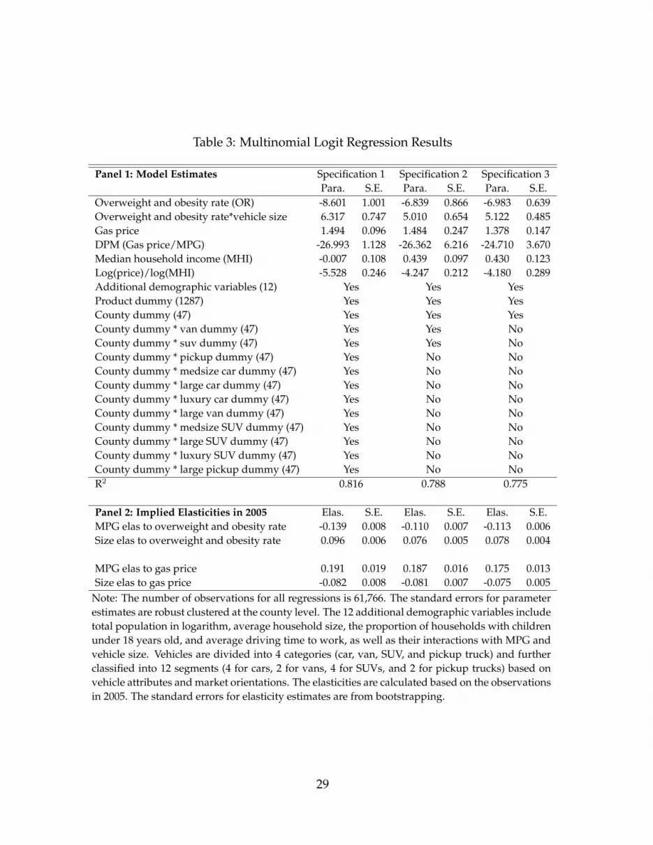
Table 3: Multinomial Logit Regression Results

Panel 1: Model Estimates Specification 1 Specification 2 Specification 3Para. S.E. Para. S.E. Para. S.E.

Overweight and obesity rate (OR) -8.601 1.001 -6.839 0.866 -6.983 0.639Overweight and obesity rate*vehicle size 6.317 0.747 5.010 0.654 5.122 0.485Gas price 1.494 0.096 1.484 0.247 1.378 0.147DPM (Gas price/MPG) -26.993 1.128 -26.362 6.216 -24.710 3.670Median household income (MHI) -0.007 0.108 0.439 0.097 0.430 0.123Log(price)/log(MHI) -5.528 0.246 -4.247 0.212 -4.180 0.289Additional demographic variables (12) Yes Yes YesProduct dummy (1287) Yes Yes YesCounty dummy (47) Yes Yes YesCounty dummy * van dummy (47) Yes Yes NoCounty dummy * suv dummy (47) Yes Yes NoCounty dummy * pickup dummy (47) Yes No NoCounty dummy * medsize car dummy (47) Yes No NoCounty dummy * large car dummy (47) Yes No NoCounty dummy * luxury car dummy (47) Yes No NoCounty dummy * large van dummy (47) Yes No NoCounty dummy * medsize SUV dummy (47) Yes No NoCounty dummy * large SUV dummy (47) Yes No NoCounty dummy * luxury SUV dummy (47) Yes No NoCounty dummy * large pickup dummy (47) Yes No NoR2 0.816 0.788 0.775

Panel 2: Implied Elasticities in 2005 Elas. S.E. Elas. S.E. Elas. S.E.MPG elas to overweight and obesity rate -0.139 0.008 -0.110 0.007 -0.113 0.006Size elas to overweight and obesity rate 0.096 0.006 0.076 0.005 0.078 0.004

MPG elas to gas price 0.191 0.019 0.187 0.016 0.175 0.013Size elas to gas price -0.082 0.008 -0.081 0.007 -0.075 0.005

Note: The number of observations for all regressions is 61,766. The standard errors for parameterestimates are robust clustered at the county level. The 12 additional demographic variables includetotal population in logarithm, average household size, the proportion of households with childrenunder 18 years old, and average driving time to work, as well as their interactions with MPG andvehicle size. Vehicles are divided into 4 categories (car, van, SUV, and pickup truck) and furtherclassified into 12 segments (4 for cars, 2 for vans, 4 for SUVs, and 2 for pickup trucks) based onvehicle attributes and market orientations. The elasticities are calculated based on the observationsin 2005. The standard errors for elasticity estimates are from bootstrapping.

29

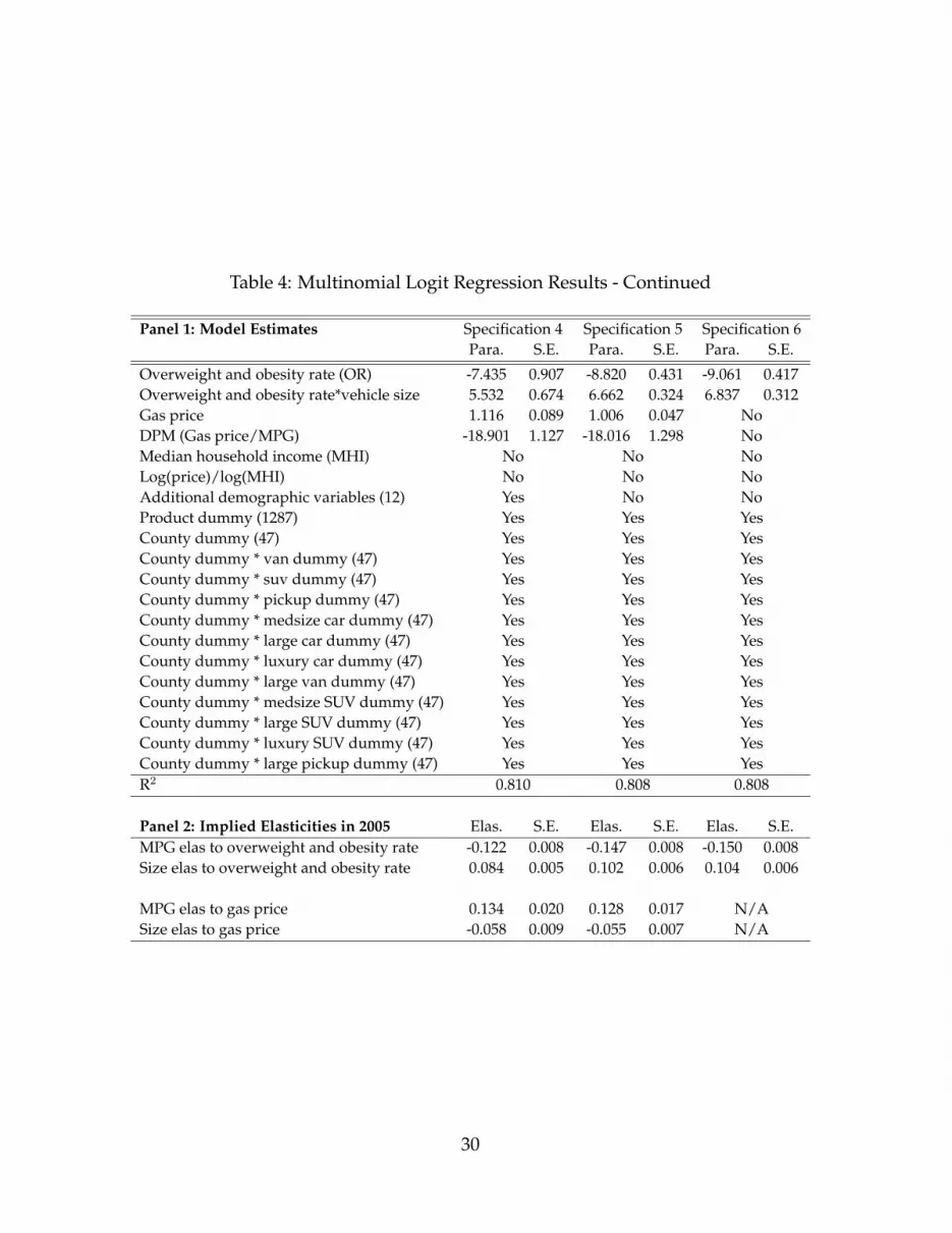
Table 4: Multinomial Logit Regression Results - Continued

Panel 1: Model Estimates Specification 4 Specification 5 Specification 6Para. S.E. Para. S.E. Para. S.E.

Overweight and obesity rate (OR) -7.435 0.907 -8.820 0.431 -9.061 0.417Overweight and obesity rate*vehicle size 5.532 0.674 6.662 0.324 6.837 0.312Gas price 1.116 0.089 1.006 0.047 NoDPM (Gas price/MPG) -18.901 1.127 -18.016 1.298 NoMedian household income (MHI) No No NoLog(price)/log(MHI) No No NoAdditional demographic variables (12) Yes No NoProduct dummy (1287) Yes Yes YesCounty dummy (47) Yes Yes YesCounty dummy * van dummy (47) Yes Yes YesCounty dummy * suv dummy (47) Yes Yes YesCounty dummy * pickup dummy (47) Yes Yes YesCounty dummy * medsize car dummy (47) Yes Yes YesCounty dummy * large car dummy (47) Yes Yes YesCounty dummy * luxury car dummy (47) Yes Yes YesCounty dummy * large van dummy (47) Yes Yes YesCounty dummy * medsize SUV dummy (47) Yes Yes YesCounty dummy * large SUV dummy (47) Yes Yes YesCounty dummy * luxury SUV dummy (47) Yes Yes YesCounty dummy * large pickup dummy (47) Yes Yes YesR2 0.810 0.808 0.808

Panel 2: Implied Elasticities in 2005 Elas. S.E. Elas. S.E. Elas. S.E.MPG elas to overweight and obesity rate -0.122 0.008 -0.147 0.008 -0.150 0.008Size elas to overweight and obesity rate 0.084 0.005 0.102 0.006 0.104 0.006

MPG elas to gas price 0.134 0.020 0.128 0.017 N/ASize elas to gas price -0.058 0.009 -0.055 0.007 N/A

30

Table 5: Multinomial Logit Regressions: Separating Obesity and Overweight

Panel 1: Model Estimates Specification 1 Specification 2 Specification 3Para. S.E. Para. S.E. Para. S.E.

Obesity rate -11.367 1.106 -8.924 0.888 -8.844 0.687Obesity rate*vehicle size 8.396 0.822 6.589 0.659 6.519 0.506Overweight rate -5.492 0.100 -3.921 0.880 -4.168 0.691Overweight rate*vehicle size 3.998 1.124 2.829 0.671 3.028 0.531Gas price 1.463 0.106 1.473 0.242 1.367 0.147DPM (Gas price/MPG) -26.327 0.254 -26.095 6.038 -24.469 3.588Median household income (MHI) -0.033 0.829 0.414 0.094 0.413 0.120Log(price)/log(MHI) -5.649 0.623 -4.364 0.216 -4.264 0.295Additional demographic variables (12) Yes Yes YesProduct dummy (1287) Yes Yes YesCounty dummy (47) Yes Yes YesCounty dummy * van dummy (47) Yes Yes NoCounty dummy * suv dummy (47) Yes Yes NoCounty dummy * pickup dummy (47) Yes No NoCounty dummy * medsize car dummy (47) Yes No NoCounty dummy * large car dummy (47) Yes No NoCounty dummy * luxury car dummy (47) Yes No NoCounty dummy * large van dummy (47) Yes No NoCounty dummy * medsize SUV dummy (47) Yes No NoCounty dummy * large SUV dummy (47) Yes No NoCounty dummy * luxury SUV dummy (47) Yes No NoCounty dummy * large pickup dummy (47) Yes No NoR2 0.812 0.783 0.770

Panel 2: Implied Elasticities in 2005 Elas. S.E. Elas. S.E. Elas. S.E.MPG elas to obesity rate -0.070 0.004 -0.055 0.003 -0.054 0.003Size elas to obesity rate 0.049 0.003 0.038 0.002 0.038 0.002

MPG elas to overweight rate -0.055 0.006 -0.039 0.005 -0.041 0.005Size elas to overweight rate 0.038 0.004 0.027 0.004 0.029 0.004

MPG elas to gas price 0.187 0.019 0.185 0.005 0.173 0.014Size elas to gas price -0.080 0.008 -0.080 0.003 -0.075 0.006

31

Table 6: Multinomial Logit Regressions without Product Dummies

Panel 1: Model Estimates With Brand Dummy No Brand DummyOLS 2SLS OLS 2SLS

Para. S.E. Para. S.E. Para. S.E. Para. S.E.OR -6.551 1.045 -6.741 1.045 -10.264 0.541 -10.250 0.576OR*vehicle size 4.803 0.779 4.967 0.777 7.535 0.417 7.465 0.445Gas price 2.162 0.094 2.317 0.122 1.134 0.056 1.045 0.090DPM (Gas price/MPG) -41.205 0.565 -43.982 1.371 -23.009 1.170 -20.439 1.346MHI 0.682 0.097 0.311 0.215 0.874 0.102 1.043 0.172Log(price)/log(MHI) -3.473 0.112 -4.553 0.513 -2.289 0.068 -1.618 0.262Vehicle size 9.134 1.115 8.762 1.125 -1.650 0.540 -0.974 0.471Horsepower 0.356 0.006 0.420 0.031 0.511 0.018 0.357 0.028Demographic variables (12) Yes Yes Yes YesBrand dummy (330) Yes Yes No NoR2 0.746 0.746 0.263 0.256

Panel 2: Implied Elasticities Elas. S.E. Elas. S.E. Elas. S.E. Elas. S.E.MPG elas to OR -0.092 0.007 -0.095 0.008 -0.144 0.010 -0.143 0.012Size elas to OR 0.072 0.006 0.075 0.006 0.114 0.008 0.113 0.010

MPG elas to gas price 0.189 0.011 0.202 0.012 0.105 0.032 0.094 0.034Size elas to gas price -0.090 0.005 -0.096 0.006 -0.051 0.015 -0.045 0.016

Note: A brand is defined according to the name of a vehicle model (e.g., Ford Taurus) while a productis a brand-year observation (e.g., a 1999 Ford Taurus). In all regressions, there are county dummies(47) interacting with segment dummies (11) as well as year dummies (6) interacting with segmentdummies (11). We control for the endogeneity of vehicle price due to unobserved product attributesusing the observed attributes of other competing products in 2SLS.

32