Low Dimensional Model Development Using Double Proper Orthogonal Decomposition and System Identification

American Institute of Aeronautics and Astronautics

1

Low Dimensional Model Development using Double Proper

Orthogonal Decomposition and System Identification

Stefan Siegel*, Kelly Cohen

†, Jürgen Seidel

‡, Selin Aradag

§, and Thomas McLaughlin

**

Department of Aeronautics, United States Air Force Academy, CO, 80840

For feedback control of complex spatio-temporally evolving flow fields, it is imperative to use a global flow

model for both flow state estimation, as well as controller development. It is important that this model

correctly presents not just the natural, unforced flow state, but also the interaction of actuators with the flow

for both open and closed loop situations. It is difficult and in some cases impossible to develop such a model

with the traditional POD-Galerkin approach. This is due to the fact that the truncation of the mode set leads

to structural instabilities. Furthermore, boundary conditions for time dependent actuation are often difficult

to implement. Lastly, the presence of turbulence in higher Reynolds number flow fields leads to severe

problems in the projection.

For these reasons, a new approach to low dimensional modeling is introduced in this paper. An extension to

POD, the so called Double POD decomposition, is employed to facilitate derivation of POD modes for

transient flow fields. These modes can correctly span a large number of flow conditions, caused by changes in

actuation, Reynolds number or other parameters of technical interest. Next, the original data is projected

onto the truncated DPOD mode set, leading to a set of mode amplitudes. The final step in model development

used nonlinear system identification techniques, in particular, the ANN-ARX method (Artificial Neural

Network – Auto Regressive eXternal Input) is employed to develop a numerical model of the temporal

evolution of the flow. This resulting model can correctly capture open loop transient flow behavior for a

parameter space large enough for controller development, and is inherently stable even for hydro

dynamically unstable flow fields.

I. Introduction

ne of the main purposes of flow control is the improvement of aerodynamic characteristics of air vehicles and

munitions enabling augmented mission performance. In general, flow control can be characterized to be passive

or active, the latter of which may employ open or closed loop control of the flow1. Traditionally, active open

loop control schemes have been developed in a trial-and-error fashion: A given actuation was employed to the flow,

and then a determination was made if the effect was detrimental or beneficial in terms of the desired outcome based

on measurements of bulk flow parameters2-5

. This approach, however, does not work well for closed loop control,

where a control algorithm needs to be derived based on a dynamic description of the flow behavior. Without a flow

model, no systematic controller development can be done. This dynamic flow model has been elusive for most flows

of technical interest, mostly due to the fact that the governing Navier Stokes equations are nonlinear and cannot be

solved in closed form for these problems. Thus, the lack of accurate dynamic flow models is one of the biggest

impediments that feedback flow control is facing. Nonetheless, a variety of attempts to derive low dimensional

models of various types has been made.

A common method used to substantially reduce the order of the model is Proper Orthogonal Decomposition

(POD). This method, as detailed in Holmes, Lumley, and Berkooz6, is an optimal approach in that it will capture the

largest amount of the flow energy in the fewest modes of any decomposition of the flow. The two dimensional POD

method was used to identify the characteristic features, or modes, of a cylinder wake as demonstrated by Noack,

Tadmor, and Morzynski7. A common approach referred to as the method of “snapshots” introduced by Sirovich

8 is

employed to generate the basis functions of the POD modes from flow-field information obtained using either

experiments or numerical simulations. Cohen, Siegel, McLaughlin and Gillies9 and Siegel, Cohen and McLaughlin

10

* Visiting Researcher, Department of Aeronautics, USAF Academy, and AIAA Senior Member.

† Associate Professor, Department of Aerospace Engineering and Engineering Mechanics, Univ. of Cincinnati, and

AIAA Associate Fellow. ‡ Visiting Researcher, Department of Aeronautics, USAF Academy, and AIAA Senior Member.

§ Visiting Researcher, Department of Aeronautics, USAF Academy, and AIAA Member.

** Director of Research, Department of Aeronautics, USAF Academy, and AIAA Associate Fellow.

O

4th Flow Control Conference<br>23 - 26 June 2008, Seattle, Washington

AIAA 2008-4193

This material is declared a work of the U.S. Government and is not subject to copyright protection in the United States.

Dow

nloa

ded

by U

NIV

ER

SIT

Y O

F C

INC

INN

AT

I on

Nov

embe

r 24

, 201

4 | h

ttp://

arc.

aiaa

.org

| D

OI:

10.

2514

/6.2

008-

4193


2

have shown that using a low dimensional model, developed by Gillies1, the model of the cylinder wake flow can be

successfully controlled using a relatively simple linear control approach based on the most dominant mode only.

Recently, Siegel, Cohen, Seidel and McLaughlin11

developed an extension to the POD approach, referred to as

„Double Proper Orthogonal Decomposition‟ (DPOD), in which shift modes have been added to account for the

changes in the flow due to transient forcing.

For low-dimensional control schemes to be implemented, a real-time estimation of the modes present in the

wake is necessary, since it is not possible to measure them directly, especially in real-time. Velocity field data,

provided from either simulation or experiment, is fed into the DPOD procedure. The time histories of the temporal

coefficients of the DPOD model are determined by mapping the unforced flow onto the spatial Eigenfunctions using

a least squares technique. Sensor measurements may take the form of wake velocity measurements, as in this effort,

or, for an application, can be based on surface-mounted pressure measurements or shear stress sensors. Then, the

estimation of the low-dimensional states is provided using a nonlinear system identification approach12

with

Artificial Neural Networks (ANN) and ARX models13-14

. The controller acts on the flow state estimates in order to

determine the actuator displacement (Figure 1 shows the overall setup of the model development process). The goal

of this effort is to develop a flow model that correctly predicts unforced, open loop forced and closed-loop

controlled flow behavior and thus can be used for controller development and testing.

In this paper, we demonstrate this DPOD-ANN-ARX model development approach shown in for a D-shaped

cylinder wake subject to transients in Reynolds number as well as blowing and suction open loop forcing input.

The following section details the simulation methodology, followed by a description of the DPOD

decomposition and the ANN-ARX system identification method. We then present a comparison of the flow fields

obtained from the CFD simulation to that predicted by the DPOD-ANN-ARX model. This comparison is performed

not just for the data that was used for model development, but also for validation data at different Reynolds numbers

and forcing conditions.

II. Computational Methodology

For the scope of this work, a D-shaped two-dimensional bluff body geometry was chosen as a generic wake flow

developing a von Karman vortex street. The geometry is a semi ellipse with an aspect ratio of 35:2. This geometry

was chosen to provide room for actuator implementation in future wind tunnel studies. The reference length for

Reynolds and Strouhal numbers is the base height, H. The fundamental target Reynolds number based on H was

Figure 1. Flow Chart of DPOD-ANN-ARX Modelling process

Dow

nloa

ded

by U

NIV

ER

SIT

Y O

F C

INC

INN

AT

I on

Nov

embe

r 24

, 201

4 | h

ttp://

arc.

aiaa

.org

| D

OI:

10.

2514

/6.2

008-

4193


3

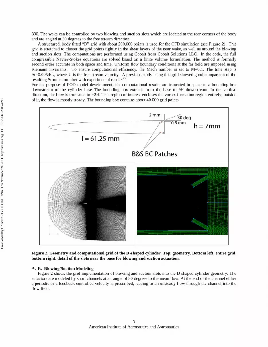
300. The wake can be controlled by two blowing and suction slots which are located at the rear corners of the body

and are angled at 30 degrees to the free stream direction.

A structured, body fitted “D” grid with about 200,000 points is used for the CFD simulation (see Figure 2). This

grid is stretched to cluster the grid points tightly in the shear layers of the near wake, as well as around the blowing

and suction slots. The computations are performed using Cobalt from Cobalt Solutions LLC. In the code, the full

compressible Navier-Stokes equations are solved based on a finite volume formulation. The method is formally

second order accurate in both space and time. Uniform flow boundary conditions at the far field are imposed using

Riemann invariants. To ensure computational efficiency, the Mach number is set to M=0.1. The time step is

t=0.005d/U, where U is the free stream velocity. A previous study using this grid showed good comparison of the

resulting Strouhal number with experimental results25

.

For the purpose of POD model development, the computational results are truncated in space to a bounding box

downstream of the cylinder base The bounding box extends from the base to 9H downstream. In the vertical

direction, the flow is truncated to ±2H. This region of interest encloses the vortex formation region entirely; outside

of it, the flow is mostly steady. The bounding box contains about 40 000 grid points.

Figure 2. Geometry and computational grid of the D-shaped cylinder. Top, geometry. Bottom left, entire grid,

bottom right, detail of the slots near the base for blowing and suction actuation.

A. B. Blowing/Suction Modeling

Figure 2 shows the grid implementation of blowing and suction slots into the D shaped cylinder geometry. The

actuators are modeled by short channels at an angle of 30 degrees to the mean flow. At the end of the channel either

a periodic or a feedback controlled velocity is prescribed, leading to an unsteady flow through the channel into the

flow field.

Dow

nloa

ded

by U

NIV

ER

SIT

Y O

F C

INC

INN

AT

I on

Nov

embe

r 24

, 201

4 | h

ttp://

arc.

aiaa

.org

| D

OI:

10.

2514

/6.2

008-

4193


4

Figure 3. Instantaneous snapshots of vorticity during a blowing and suction cycle at the same forcing phase.

Left, 12.5% of the freestream velocity, right, 100% of the freestream velocity.

Figure 4. Transient lift (green, bottom trace) and drag (blue, top trace) forces for different actuation levels;

top left: 12.5% of the freestream velocity, top right: 25%, bottom left: 75% and bottom right: 100% of the

freestream velocity.

Figure 4 demonstrates the effect of periodic open loop blowing and suction. The forcing frequency is equal to the

natural shedding frequency, while the peak velocity during a sinusoidal blowing and suction cycle is 12.5%, 25%,

75% or 100% of the freestream velocity, respectively. The top and bottom slot were operated 180 degrees out of

Dow

nloa

ded

by U

NIV

ER

SIT

Y O

F C

INC

INN

AT

I on

Nov

embe

r 24

, 201

4 | h

ttp://

arc.

aiaa

.org

| D

OI:

10.

2514

/6.2

008-

4193


5

phase for all investigations. The plots show isocontours of vorticity, demonstrating the local effect of the forcing.

The blowing and suction velocity is not large enough for the resulting jet to penetrate the boundary layer in either

case. However, with the higher forcing velocity more vorticity is injected into the boundary layer, effectively cutting

off the forming vortices. Additionally, the vorticity ejected from the slots then merges with the vortices of the

Kármán vortex street.

As can be seen in the transient lift and drag force plots shown in Figure 4, the higher velocity forcing creates a

transient behavior that is quite different in that there is significant overshoot before the wake settles into a phase

locked state. This is a result of the vorticity ejected from the blowing and suction slot merging with the vortex street,

an effect that is not existent for smaller velocities. The open loop investigations used blowing and suction peak

velocities down to 3% of the freestream velocity. However, for values smaller than about 10%, the transient settling

times increased considerably. This indicates a loss of control authority, and the 10% threshold was determined to be

the minimum desirable actuation amplitude for the subsequent closed loop controlled simulations.

For the development of a low dimensional model that covers a range of flow parameters, a decision needs to be

made how large this parameter range should be and which parameters are to be varied. To achieve a model valid

both for a range of Reynolds numbers as well as different forcing amplitudes and frequencies, the simulation

parameters summarized in Table 1 were used.

Type Re Start Re End f /f0 U / U∞ Phase

Transient Reynolds number 300 150 - - -

Transient Reynolds number 300 450 - - -

Transient Blowing and Suction 300 - 0.9 0.75 0

Transient Blowing and Suction 300 - 1 0.75 0






Table 1. Neural Network training data sets

This set of parameters leads to a Reynolds number range of 150 to 450, as well as forcing amplitudes from 12.5 to

75 percent of the free stream velocity. For all Reynolds numbers the unforced wake flow exhibits vortex shedding,

while for all forcing conditions the flow field will achieve lock-in. However, the formation length of the shedding

varies due to the Reynolds number changes. Similarly, the frequency and intensity of the vortex shedding changes as

a function of the forcing input.

Figure 5. Entire training data set inputs

Dow

nloa

ded

by U

NIV

ER

SIT

Y O

F C

INC

INN

AT

I on

Nov

embe

r 24

, 201

4 | h

ttp://

arc.

aiaa

.org

| D

OI:

10.

2514

/6.2

008-

4193


6

The forcing inputs of the entire data ensemble used for model development is shown in Figure 5. Two transients in

Reynolds number are followed by a total of seven transients in open loop forcing, one of which (f/f0=0.95;

U/U∞=0.75) is shown in greater detail in Figure 6.

Figure 6. Open loop forcing inputs f/fn =0.95; U/Uinf = 0.75

III. Double Proper Orthogonal Decomposition (DPOD) Modeling

POD is an efficient means to reduce spatially highly complex flow fields by representing them by a small number of

spatial modes and their temporal coefficients7.

1

( , , ) ( ) ( , )K

k k

k

u x y t a t x y (1)

Equation 1 shows this decomposition, where a flow quantity u is represented by the spatial modes k(x,y) and

temporal coefficients ak(t). While this decomposition is well suited to time periodic flow fields, it faces problems

for transient flows (see Siegel et al.19

). Different additions to the basic POD procedure have been proposed, most

notably the addition of a shift mode as introduced independently by Noack, Afanasiev, Morzynski and Thiele20

as

well as Siegel, Cohen and McLaughlin.10

This shift mode originally only addressed changes to the mean flow, but

this concept has been extended recently by Siegel, Cohen, Seidel and McLaughlin11

to adjust the fluctuating modes

of transient flows as well. This modified POD procedure, referred to as Double POD (DPOD) procedure, provides

shift modes for all physical modes of a transient flow field. In Equation (2), the index i refers to the physical modes

of the original POD procedure, while the index j identifies the shift mode order. Figure 7 shows the normalized

kinetic energy of the DPOD modes used in this investigation. The mean flow mode M1,1 contains most of the

energy, followed by the unsteady von Kármán modes, M2,1 and M3,1,.

( ) ( )

, ,

1 1

( , , ) ( ) ( , ).J K

i i

j k j k

j k

u x y t t x y

(2)

Reference is made to all modes with index k larger than 1 as shift modes, since they modify a given physical

mode (index j=1) to match a new flow state due to transient effects. This may be due to effects of forcing, changes in

Reynolds number, feedback or open loop control or similar events. Thus, in the truncated DPOD mode ensemble for

each physical mode, one or more shift modes may be retained based on inspection of energy content or spatial

structure of the mode. For further details on the DPOD procedure refer to Siegel et al.11

.

The results from this DPOD decomposition for the data set described in the previous paragraph are show in

Figure 7 in terms of the mode energy and Figure 8 showing the spatial modes of the streamwise velocity component.

Figure 7 illustrates the importance of the shift modes, where especially for higher modes (i=4 and i=5) the shift

modes contain similar energy as the main modes.

Dow

nloa

ded

by U

NIV

ER

SIT

Y O

F C

INC

INN

AT

I on

Nov

embe

r 24

, 201

4 | h

ttp://

arc.

aiaa

.org

| D

OI:

10.

2514

/6.2

008-

4193


7

Figure 7. DPOD Mode Energy

The mode energy can also be used to make decisions on truncation of the model, where for the purpose of controller

development three main modes were kept, which physically represent the mean flow (mode i=1) as well as the mode

pair representing the von Kàrmàn vortex shedding (i=2 and i=3). Since the energy for shift modes of index j=3 and

higher drops off steeply, only the physical modes and one shift mode were retained. This leads to a 3 x 2 mode

ensemble as shown in Figure 8. Inspection of these modes demonstrates the purpose of the shift modes: All of them

are representative of a wake that is longer in the mean flow (mode 1,2), and exhibit vortex shedding further

downstream (modes 2,2 and modes 3,2). This feature allows the DPOD mode ensemble to correctly model all flow

states incurred both due to Reynolds number and open loop forcing effects.

Using this DPOD procedure, accurate transient spatial mode sets have been developed. The next step towards a

dynamic model, which represents the temporal behaviour of the unsteady forced wake, is derived from the time

coefficients obtained from the DPOD procedure. The low dimensional model that represents the time-dependent

coefficients of the POD is then derived using a non-linear system identification approach based on artificial neural

networks (ANN).

IV. ANN-ARX System Identification

System identification of a cylinder wake can be accomplished with a linear ARX model,

)t(e)q(D

1)t(f

)q(D

)q(Bq)t(a

11

1d

, (3)

where a(t) is the state vector representing the POD mode amplitudes aj(t) shown in Eqn.(1). f(t) describes the

external input, which in the current effort is the vertical displacement of the cylinder and e(t) is the white noise

vector. For the above case, B and D are matrix polynomials in q-1

.

The time delay operator is defined as

)dt(a)t(aq d, (4)

where d is a multiple of the sampling period. The parameter matrix, θ, and the regression vector, φ(t), are

respectively defined as

θ = [dij bij]T

(5)

φ(t) = [a(t-1),…,a(t-n), f(t-d),…..,f(t-d-m)]T (6)

As can be seen in Equation (6), the vector φ(t) is comprised of past states and past inputs.

Dow

nloa

ded

by U

NIV

ER

SIT

Y O

F C

INC

INN

AT

I on

Nov

embe

r 24

, 201

4 | h

ttp://

arc.

aiaa

.org

| D

OI:

10.

2514

/6.2

008-

4193


8

The ARX predictor14

may then be written as

1 1( | ) ( ) ( ) [1 ( )] ( )

( ) .

d

T

a t q B q f t D q a t

t (7)

Figure 8. DPOD Spatial Modes

Eqn. (7) represents an algebraic relationship between the prediction, given on the left hand side, and past inputs and

states, summarized by φ(t). The parameter matrix, θ, is determined during the estimation process. The main

advantage of the ARX predictor is that it is always stable, even when the dynamic plant (the flow field in this case)

being estimated is unstable. This feature is of utmost importance when modelling an unstable system such as the

absolutely unstable cylinder wake flow.

Dow

nloa

ded

by U

NIV

ER

SIT

Y O

F C

INC

INN

AT

I on

Nov

embe

r 24

, 201

4 | h

ttp://

arc.

aiaa

.org

| D

OI:

10.

2514

/6.2

008-

4193


9

The main drawback of this approach is that it is limited to modelling of linear systems which, as described above, is

insufficient for modelling of unstable limit cycles. A general representation of nonlinear system identification, based

on a hybrid ANN-ARX approach13

, may be written as

)t(e]),t([g)|t(a , (8)

where θ is the matrix containing the weights of the ANN that are estimated by a back propagation algorithm using a

training data set13

, and g is the nonlinear mapping realized by the feed-forward structure of the ANN.

The ANN-ARX predictor can then be expressed as

( | ) [ ( ), ]a t g t . (9)

The basic methodology to design an ARX-ANN plant for dynamic modelling of the DPOD mode amplitudes is

presented in Figure 1. The ANN-ARX algorithms used in this effort are a modification of the toolbox developed by

Nørgaard et al.13

. The modification extends the toolbox for use in simulations, as opposed to one step prediction, of

MIMO (multi-input, multi-output) systems. After the DPOD mode amplitudes were obtained from the CFD data as

described in the previous section, a single hidden layer ANN-ARX architecture is selected. The training set

comprised input-output data obtained from CFD simulations. The model is validated for off-design cases and if the

estimation error is unacceptable, then the ANN architecture is modified. This cycle was repeated until estimation

errors were acceptable for all off-design cases.

Figure 9. Neural Network Topology

The ANN-ARX predictor is inherently stable because, although the modelling approach is nonlinear, the algebraic

relationship between the prediction and past states and inputs is preserved. This is extremely important when dealing

with nonlinear systems represented by PDEs like the Navier Stokes equations, since the stability problems are more

Dow

nloa

ded

by U

NIV

ER

SIT

Y O

F C

INC

INN

AT

I on

Nov

embe

r 24

, 201

4 | h

ttp://

arc.

aiaa

.org

| D

OI:

10.

2514

/6.2

008-

4193


10

severe than in linear systems. The ANN-ARX approach is an ideal choice when the system to be modelled is

deterministic and the signal to noise ratio (SNR) of the data is good13

.

The choice of the specific artificial neural network (ANN) architecture was based on two main design criteria.

The first concerns the number of hidden layers. This was selected as one, i.e. a single hidden layer, since it is the

simplest form that allows for a universal approximator 26 and its effectiveness for system identification problems has

been shown by Nørgaard et al.13

. The second decision concerns the number of nodes. If the number of nodes in the

hidden layer is small, the resulting error is unacceptable. As the number of nodes is increased, the error is reduced at

the cost of computational complexity until a number of nodes is reached beyond which no further improvement in

error is observed. In this effort a parameter study was conducted to find the optimal number of nodes.

A schematic representation of the neural network topology is shown in Figure 9. This network structure allows

for the selection of the number of time delays for each mode, the number of skipped time steps between the time

delay inputs, and the number of hidden layer neurons. Thus, the complexity and size of the network can be adjusted

both to the temporal dynamics of the mode amplitudes by selecting the time history parameters of number of time

delay inputs and delay between these inputs. The number of hidden layer neurons is usually dependent on the

nonlinear properties of the mode amplitudes to be modelled.

While Figure 9 shows a simplified example with few neurons and inputs for clarity, the actual parameters used for

the model are summarized in Table 2. The overall network features 126 neurons in the hidden layer, which model a

total of 2x3 = 6 DPOD mode amplitudes, while the network has two external inputs, i.e. Reynolds number and

forcing velocity.

Input Number of Past

Inputs or Outputs

to Neural Net

Delay between

Inputs

Total Time

History

Reynolds Number 2 Rx 10 20

Actuator Position 4 Yx 5 20

Mode 1,1 1 Ax1,1 12 1

Mode 2,1 3 Ax2,1 8 24

Mode 3,1 3 Ax3,1 8 24

Mode 1,2 1 Ax1,2 12 12

Mode 2,2 1 Ax2,2 12 12

Mode 3,2 1 Ax3,2 12 12

Table 2. Neural Network Parameters

V. CFD simulation results compared to Model output

Here we compare results for the open loop forced wake flow CFD simulations, to model output from the DPOD-

ANN-ARX model for different transients in forcing as well as Reynolds numbers. This is done using the first time

steps of a data set as initial conditions, and then simulating the flow behavior for the entire data set using only the

Reynolds number and forcing signal as inputs. The first comparison is done for the training data ensemble shown in

Figure 5, which was used for development of the dynamic model. This comparison shown in Figure 10 demonstrates

that the DPOD-ANN-ARX provides a numerically stable model for the open loop controlled wake flow that is able

to span a range of Reynolds number and actuation conditions. While due to plotting limitations only the amplitude

envelope match between model and CFD simulation can be observed, a zoomed in detail covering the first 100

shedding cycles is shown in Figure 11. This plot shows good agreement between model and simulation for the two

Reynolds number transients. Using any other low dimensional modeling technique, this has not been shown so far.

Dow

nloa

ded

by U

NIV

ER

SIT

Y O

F C

INC

INN

AT

I on

Nov

embe

r 24

, 201

4 | h

ttp://

arc.

aiaa

.org

| D

OI:

10.

2514

/6.2

008-

4193


11

Figure 10. Comparison mode amplitudes from CFD simulation (blue line) to mode amplitudes from DPOD-

ANN-ARX model (red line) for the entire training data set with inputs as shown in Figure 5.

While a reasonable match between model and simulation for the training data is important, the more important

test of model performance is to compare the model against the simulation for a data set that was not used for model

development, which is commonly referred to as a validation data set. This comparison is shown in Figure 12 and

Figure 13 for a transient change in Reynolds number and a transient change in actuation, using different parameters

for the flow conditions than were used for the model development. The good agreement between model and

simulation demonstrates that the model is not only a point design valid for the data used for its construction, but

rather spans the parameter range in between the design points as well, i.e. Reynolds numbers in the range from 150-

450 as well as forcing amplitudes between 0.125 to 0.75 percent of the free stream velocity, as well as forcing

frequencies between 90 and 100 percent of the natural frequency.

Dow

nloa

ded

by U

NIV

ER

SIT

Y O

F C

INC

INN

AT

I on

Nov

embe

r 24

, 201

4 | h

ttp://

arc.

aiaa

.org

| D

OI:

10.

2514

/6.2

008-

4193


12


ANN-ARX model (red line) for the first 100 training data cycles with inputs as shown in Figure 5.

Dow

nloa

ded

by U

NIV

ER

SIT

Y O

F C

INC

INN

AT

I on

Nov

embe

r 24

, 201

4 | h

ttp://

arc.

aiaa

.org

| D

OI:

10.

2514

/6.2

008-

4193


13


ANN-ARX model (red line) for a transient change in Reynolds number from 300 to 250 and back, a data set

which was NOT used for training the network but just for the validation simulation shown.

Dow

nloa

ded

by U

NIV

ER

SIT

Y O

F C

INC

INN

AT

I on

Nov

embe

r 24

, 201

4 | h

ttp://

arc.

aiaa

.org

| D

OI:

10.

2514

/6.2

008-

4193


14


ANN-ARX model (red line) for transient forcing at 95% of the natural frequency with 75% of the free stream

velocity peak velocity, a data set which was NOT used for training the network but just for the validation

simulation shown.

VI. Discussion and Outlook

While the agreement between model and simulation is acceptable, there are noticeable discrepancies especially

for the shift modes j=2, whose dynamic behavior is more complex than that of the main modes. In order to model

these correctly, it is necessary to increase the number of neurons for these modes. Doing this, however, also requires

Dow

nloa

ded

by U

NIV

ER

SIT

Y O

F C

INC

INN

AT

I on

Nov

embe

r 24

, 201

4 | h

ttp://

arc.

aiaa

.org

| D

OI:

10.

2514

/6.2

008-

4193


15

additional training data in order to properly train the now larger network that features more degrees of freedom. As

we did not have more training data available within the scope of this paper, we plan to perform additional open loop

forced CFD simulations in the future in order to be able to train a larger network for the shift modes for better

estimation accuracy. Later, the open-loop model can be used as a basis for development of a closed-loop controller

and this controller will be validated using high resolution simulations.

VII. Conclusion

We introduce an extension to the POD procedure, DPOD, which is capable of deriving mode ensembles that are

valid for a range of different flow conditions, in the present for a range of Reynolds numbers as well as open loop

forcing frequencies and amplitudes. Using the DPOD derived mode amplitudes as input for a nonlinear system

identification procedure, the ANN-ARX technique, we are able to develop a low dimensional dynamic model that is

capable of correctly modeling the dynamic flow behavior for a range of training parameters, not just the individual

data sets used for its derivation. This DPOD-ANN-ARX is thus suitable for deriving low dimensional models that

correctly model global flow behavior and thus are useful for closed loop controller development.

VIII. Acknowledgments

We would like to thank Mr. Casey Fagley for training the neural networks presented in this work. The authors

thank Lt. Col. Scott Wells (AFOSR), and Dr. James Myatt (AFRL) for their support and assistance. The authors

acknowledge the assistance of Dr. Jim Forsythe of Cobalt Solutions, LLC.

References 1 E. A. Gillies, “Low-dimensional control of the circular cylinder wake”, Journal of Fluid Mechanics, vol. 371, pp.157-178,

1998. 2 G. Koopmann, “The vortex wakes of vibrating cylinders at low Reynolds numbers”, Journal of Fluid Mechanics, vol. 28, part

3, pp. 501-512, 1967. 3 D. S. Park, D. M. Ladd, and E. W. Hendricks, “Feedback control of a global mode in spatially developing flows”, Physics

Letters A, vol. 182, pp. 244- 248, 1993. 4 K. Roussopoulos., “Feedback control of vortex shedding at low Reynolds numbers”, Journal of Fluid Mechanics, vol. 248, pp.

267-296, 1993. 5 C. H. K. Williamson, “Vortex dynamics in the cylinder wake”, Annu. Rev. Fluid Mech, vol. 8, pp. 477-539, 1996. 6 P. Holmes, J. L. Lumley, and G. Berkooz, Turbulence, Coherent Structures, Dynamical Systems and Symmetry. Cambridge:

Cambridge University Press, 1996, ch. 3. 7 B. R. Noack, G. Tadmor, and M. Morzynski, "Low-dimensional models for feedback flow control. Part I: Empirical Galerkin

models", presented at the 2nd AIAA Flow Control Conference, Portland, Oregon, 28 Jun - 1 Jul 2004, AIAA Paper 2004-

2408. 8 L. Sirovich, “Turbulence and the dynamics of coherent structures Part I: Coherent structures”, Quarterly of Applied

Mathematics, vol. 45, no., 3, pp.561-571, 1987. 9 K. Cohen, S. Siegel, T. McLaughlin, and E. Gillies, “Feedback control of a cylinder wake low-dimensional model”, AIAA

Journal, vol. 41, no. 7, pp. 1389-1391, July 2003. 10 S. Siegel, K. Cohen and T. McLaughlin., "Numerical simulations of a feedback controlled circular cylinder wake", AIAA

Journal, vol. 44, no. 6, pp.1266-1276, June 2006. 11 S. Siegel., K. Cohen., J. Seidel and T. McLaughlin, “State estimation of transient flow fields using double proper orthogonal

decomposition (DPOD)”, presented at the International Conference on Active Flow Control, Berlin, Germany, September 27-

29, 2006. 12 Nelles, O., Nonlinear System Identification, Springer-Verlag, Berlin, Germany, 2001, Chap. 11. 13 Nørgaard, M., Ravn., O., Poulsen, N.K., and Hansen, L.K., Neural Networks for Modeling and Control of Dynamic Systems,

3rd printing, Springer-Verlag, London, U.K., 2003, Chap. 2. 14 Ljung, L., System Identification: Theory for the User, 2nd Edition, Prentice Hall, Upper Saddle, NJ, USA, 1999, Chap.4. 15 Cobalt CFD, Cobalt Solutions, LLC, Available: http://www.cobaltcfd.com. 16 H. Oertel, Jr.., “Wakes behind blunt bodies”, Annual Review of Fluid Mechanics, vol. 22, pp. 539-564, 1990. 17 R. L. Panton, Incompressible Flow. 2nd Edition, New York: John Wiley & Sons, 1996. 18 C. Min and H. Choi, “Suboptimal feedback control of vortex shedding at low Reynolds numbers”, J Fluid Mechanics, vol.

401, pp.123-156, 1999. 19 Siegel, S., Cohen, K., Seidel, J., McLaughlin, T., 'Short Time Proper Orthogonal Decomposition for State Estimation of

Transient Flow Fields', 43rd AIAA Aerospace Sciences Meeting, Reno, AIAA2005-0296, 2005 20 B. R. Noack, K. Afanasiev, M. Morzynski and F. Thiele “A hierarchy of low dimensional models for the transient and post-

transient cylinder wake”, J. Fluid Mechanics, vol. 497, pp. 335–363, 2003.

Dow

nloa

ded

by U

NIV

ER

SIT

Y O

F C

INC

INN

AT

I on

Nov

embe

r 24

, 201

4 | h

ttp://

arc.

aiaa

.org

| D

OI:

10.

2514

/6.2

008-

4193

http://www.aiaa.org/author/index.hfm?view=3&screen=20&loadview=-1&lumeetingid=977&cfp=cfp

http://www.cobaltcfd.com/


16

21 O. Stalnov, V. Palei, I. Fono, K. Cohen, and A. Seifert, "Experimental validation of sensor placement for control of a "D"

shaped cylinder wake", presented at the 35th AIAA Fluid Dynamics Conference and Exhibit, Toronto, Canada, June 6-9, 2005,

AIAA Paper 2005-5260. 22 Cohen, K., Siegel, S., Seidel, J., and McLaughlin, T., “Low dimensional modeling, estimation and control of a cylinder wake”,

Invited lecture at Invited Session organized by Dr. James Myatt of AFRL/VA called "Order Reduction and Control for

Aerodynamics", 45th IEEE Conference on Decision and Control, San Diego, 13-15 December 2006. 23 Y. Shin, K. Cohen, S. Siegel, J. Seidel, and T. McLaughlin, “Neural network estimator for closed-loop control of a cylinder

wake”, Presented at the AIAA Guidance, Navigation, and Control Conference and Exhibit, Keystone, Colorado, 21 - 24 Aug

2006, AIAA Paper 2006-6428. 24 K. Cohen, S. Siegel, J. Seidel, and T. McLaughlin, “ "Reduced order modeling for closed-loop control of three dimensional

wakes", Presented as an Invited lecture at the 3rd AIAA Flow Control Conference, San Francisco, California, 5 - 8 June 2006,

AIAA Paper 2006-3356. 25Stefan Siegel , Kelly Cohen , Jürgen Seidel , Thomas McLaughlin , 'Two Dimensional Simulations Of A Feedback Controlled

D-Cylinder Wake', AIAA Fluid Dynamics Conf Toronto, ON, CA, AIAA 2005-5019, 2005 26 Cybenko, G., 'Neural Networks in Computational Science and Engineering', IEEE Computational Science and Engineering

Dow

nloa

ded

by U

NIV

ER

SIT

Y O

F C

INC

INN

AT

I on

Nov

embe

r 24

, 201

4 | h

ttp://

arc.

aiaa

.org

| D

OI:

10.

2514

/6.2

008-

4193

http://www.aiaa.org/author/index.hfm?view=3&screen=20&loadview=-1&lumeetingid=977&cfp=cfp

Documents

Low Dimensional Model Development Using Double Proper Orthogonal Decomposition and System Identification